LLMs in Production

From Language Models to Successful Products

Chapter 1 ~ 5

Foreword by Joe Reis

For online information and ordering of this and other Manning books, please visit <www.manning.com>. The publisher offers discounts on this book when ordered in quantity. For more information, please contact

Special Sales Department Manning Publications Co. 20 Baldwin Road PO Box 761 Shelter Island, NY 11964 Email: orders@manning.com

©2025 by Manning Publications Co. All rights reserved.

No part of this publication may be reproduced, stored in a retrieval system, or transmitted, in any form or by means electronic, mechanical, photocopying, or otherwise, without prior written permission of the publisher.

Many of the designations used by manufacturers and sellers to distinguish their products are claimed as trademarks. Where those designations appear in the book, and Manning Publications was aware of a trademark claim, the designations have been printed in initial caps or all caps.

Recognizing the importance of preserving what has been written, it is Manning’s policy to have the books we publish printed on acid-free paper, and we exert our best efforts to that end. Recognizing also our responsibility to conserve the resources of our planet, Manning books are printed on paper that is at least 15 percent recycled and processed without the use of elemental chlorine.

The authors and publisher have made every effort to ensure that the information in this book was correct at press time. The authors and publisher do not assume and hereby disclaim any liability to any party for any loss, damage, or disruption caused by errors or omissions, whether such errors or omissions result from negligence, accident, or any other cause, or from any usage of the information herein.

Manning Publications Co. Development editor: Doug Rudder 20 Baldwin Road Technical editor: Daniel Leybzon PO Box 761 Review editor: Dunja Nikitovic´ Shelter Island, NY 11964 Production editor: Aleksandar Dragosavljevic´ Copy editor: Alisa Larson Proofreader: Melody Dolab Technical proofreader: Byron Galbraith Typesetter: Dennis Dalinnik Cover designer: Marija Tudor

ISBN: 9781633437203 Printed in the United States of America To my wife Jess and my kids, Odin, Magnus, and Emrys, who have supported me through thick and thin

—Christopher Brousseau

I dedicate this book to Evelyn, my wife, and our daughter, Georgina. Evelyn, thank you for your unwavering support and encouragement through every step of this journey. Your sacrifices have been paramount to making this happen. And to my daughter, you are an endless source of inspiration and motivation. Your smile brightens my day and helps remind me to enjoy the small moments in this world. I hope and believe this book will help build a better tomorrow for both of you.

—Matthew Sharp

brief contents

• 1 Words’ awakening: Why large language models have captured attention 1
• 2 Large language models: A deep dive into language modeling 20
• 3 Large language model operations: Building a platform for LLMs 73
• 4 Data engineering for large language models: Setting up for success 111
• 5 Training large language models: How to generate the generator 154
• 6 Large language model services: A practical guide 201
• 7 Prompt engineering: Becoming an LLM whisperer 254
• 8 Large language model applications: Building an interactive experience 279
• 9 Creating an LLM project: Reimplementing Llama 3 305
• 10 Creating a coding copilot project: This would have helped you earlier 332
• 11 Deploying an LLM on a Raspberry Pi: How low can you go? 355
• 12 Production, an ever-changing landscape: Things are just getting started 379

contents

foreword xi preface xii acknowledgments xiv about the book xvi about the authors xix about the cover illustration xx

1 Words’ awakening: Why large language models have captured attention 1

• 1.1 Large language models accelerating communication 3
• 1.2 Navigating the build-and-buy decision with LLMs 7

Buying: The beaten path 8 ■ Building: The path less traveled 9 A word of warning: Embrace the future now 15

1.3 Debunking myths 16

2 Large language models: A deep dive into language modeling 20

2.1 Language modeling 21

Linguistic features 23 ■ Semiotics 29 ■ Multilingual NLP 32

2.2 Language modeling techniques 33

N-gram and corpus-based techniques 34 ■ Bayesian techniques 36 Markov chains 40 ■ Continuous language modeling 43

Embeddings 47 ■ Multilayer perceptrons 49 ■ Recurrent neural networks and long short-term memory networks 51 Attention 58

• 2.3 Attention is all you need 60 Encoders 61 ■ Decoders 62 ■ Transformers 64
• 2.4 Really big transformers 66

3 Large language model operations: Building a platform for LLMs 73

• 3.1 Introduction to large language model operations 73
• 3.2 Operations challenges with large language models 74

Long download times 74 ■ Longer deploy times 75 Latency 76 ■ Managing GPUs 77 ■ Peculiarities of text data 77 ■ Token limits create bottlenecks 78 ■ Hallucinations cause confusion 80 ■ Bias and ethical considerations 81 Security concerns 81 ■ Controlling costs 84

3.3 LLMOps essentials 84

Compression 84 ■ Distributed computing 93

3.4 LLM operations infrastructure 99

Data infrastructure 101 ■ Experiment trackers 102 ■ Model registry 103 ■ Feature stores 104 ■ Vector databases 105 Monitoring system 106 ■ GPU-enabled workstations 107 Deployment service 108

4 Data engineering for large language models: Setting up for success 111

4.1 Models are the foundation 112

GPT 113 ■ BLOOM 114 ■ LLaMA 115 ■ Wizard 115 Falcon 116 ■ Vicuna 116 ■ Dolly 116 ■ OpenChat 117

4.2 Evaluating LLMs 118

Metrics for evaluating text 118 ■ Industry benchmarks 121 Responsible AI benchmarks 126 ■ Developing your own benchmark 128 ■ Evaluating code generators 130 Evaluating model parameters 131

4.3 Data for LLMs 133

Datasets you should know 134 ■ Data cleaning and preparation 138

• 4.4 Text processors 144 Tokenization 144 ■ Embeddings 149
• 4.5 Preparing a Slack dataset 152

5 Training large language models: How to generate the generator 154

• 5.1 Multi-GPU environments 155 Setting up 155 ■ Libraries 159
• 5.2 Basic training techniques 161 From scratch 162 ■ Transfer learning (finetuning) 169 Prompting 174
• 5.3 Advanced training techniques 175

Prompt tuning 175 ■ Finetuning with knowledge distillation 181 ■ Reinforcement learning with human feedback 185 ■ Mixture of experts 188 ■ LoRA and PEFT 191

5.4 Training tips and tricks 196

Training data size notes 196 ■ Efficient training 197 Local minima traps 198 ■ Hyperparameter tuning tips 198 A note on operating systems 199 ■ Activation function advice 199

6 Large language model services: A practical guide 201

6.1 Creating an LLM service 202

Model compilation 203 ■ LLM storage strategies 209 Adaptive request batching 212 ■ Flow control 212 Streaming responses 215 ■ Feature store 216 Retrieval-augmented generation 219 ■ LLM service libraries 223

6.2 Setting up infrastructure 224

Provisioning clusters 225 ■ Autoscaling 227 ■ Rolling updates 232 ■ Inference graphs 234 ■ Monitoring 237

6.3 Production challenges 240

Model updates and retraining 241 ■ Load testing 241 Troubleshooting poor latency 245 ■ Resource management 247 Cost engineering 248 ■ Security 249

6.4 Deploying to the edge 251

7 Prompt engineering: Becoming an LLM whisperer 254

7.1 Prompting your model 255 Few-shot prompting 255 ■ One-shot prompting 257 Zero-shot prompting 258 7.2 Prompt engineering basics 260 Anatomy of a prompt 261 ■ Prompting hyperparameters 263 Scrounging the training data 265 7.3 Prompt engineering tooling 266 LangChain 266 ■ Guidance 267 ■ DSPy 270 ■ Other tooling is available but . . . 271 7.4 Advanced prompt engineering techniques 271 Giving LLMs tools 271 ■ ReAct 274 8 Large language model applications: Building an interactive experience 279 8.1 Building an application 280 Streaming on the frontend 281 ■ Keeping a history 284 Chatbot interaction features 287 ■ Token counting 290 RAG applied 291 8.2 Edge applications 293 8.3 LLM agents 296 9 Creating an LLM project: Reimplementing Llama 3 305 9.1 Implementing Meta’s Llama 306 Tokenization and configuration 306 ■ Dataset, data loading, evaluation, and generation 309 ■ Network architecture 314 9.2 Simple Llama 317 9.3 Making it better 321 Quantization 322 ■ LoRA 323 ■ Fully sharded data parallel– quantized LoRA 326 9.4 Deploy to a Hugging Face Hub Space 328 10 Creating a coding copilot project: This would have helped you earlier 332 10.1 Our model 333 10.2 Data is king 336 Our VectorDB 336 ■ Our dataset 337 ■ Using RAG 341

• 10.3 Build the VS Code extension 344
• 10.4 Lessons learned and next steps 351

11 Deploying an LLM on a Raspberry Pi: How low can you go? 355

• 11.1 Setting up your Raspberry Pi 356 Pi Imager 357 ■ Connecting to Pi 359 ■ Software installations and updates 363
• 11.2 Preparing the model 364
• 11.3 Serving the model 366
• 11.4 Improvements 368

Using a better interface 368 ■ Changing quantization 369 Adding multimodality 370 ■ Serving the model on Google Colab 374

12 Production, an ever-changing landscape: Things are just getting started 379

• 12.1 A thousand-foot view 380
• 12.2 The future of LLMs 381

Government and regulation 381 ■ LLMs are getting bigger 386 ■ Multimodal spaces 392 ■ Datasets 393 Solving hallucination 394 ■ New hardware 401 ■ Agents will become useful 402

• 12.3 Final thoughts 406
• appendix A History of linguistics 408
• appendix B Reinforcement learning with human feedback 416
• appendix C Multimodal latent spaces 420

index 427

foreword

Unless you’ve been hiding in a cave, you know that LLMs are everywhere. They’re becoming a staple for many people. If you’re reading this book, there’s a good chance you’ve integrated LLMs into your workflow. But you might be wondering how to deploy LLMs in production.

This is precisely why LLMs in Production is a timely and invaluable book. Drawing from their extensive experience and deep expertise in machine learning and linguistics, the authors offer a comprehensive guide to navigating the complexities of bringing LLMs into production environments. They don’t just explore the technical aspects of implementation; they delve into the strategic considerations, ethical implications, and best practices crucial for responsible and effective production deployments of LLMs.

LLMs in Production has it all. Starting with an overview of what LLMs are, the book dives deep into language modeling, MLOps for LLMs, prompt engineering, and every relevant topic in between. You’ll come away with a bottoms-up approach to working with LLMs from first principles. This book will stand the test of time, at least as long as possible, in this fast-changing landscape.

You should approach this book with an open mind and a critical eye. The future of LLMs is not predetermined—it will be shaped by the decisions we make and the care with which we implement these powerful tools in production. Let this book guide you as you navigate the exciting, challenging world of LLMs in production.

—Joe Reis, Author of Fundamentals of Data Engineering

preface

In January of 2023, I was sitting next to a couple, and they started to discuss the latest phenomenon, ChatGPT. The husband enthusiastically discussed how excited he was about the technology. He had been spending quality time with his teenagers writing a book using it—they had already written 70 pages. The wife, however, wasn’t as thrilled, more scared. She was an English teacher and was worried about how it was going to affect her students.

It was around this time the husband said something I was completely unready for: his friend had fired 100 writers at his company. My jaw dropped. His friend owned a small website where he hired freelance writers to write sarcastic, funny, and fake articles. After being shown the tool, the friend took some of his article titles and asked ChatGPT to write one. What it came up with was indistinguishable from anything else on the website! Meaningless articles that lack the necessity for veracity are LLM’s bread and butter, so it made sense. It could take him minutes to write hundreds of articles, and it was all free!

We have both experienced this same conversation—with minor changes—a hundred times over since. From groups of college students to close-knit community members, everyone is talking about AI all the time. Very few people have experienced it firsthand, outside of querying a paid API. For years, we’ve seen how it’s been affecting the translation industry. Bespoke translation is difficult to get clients for, and the rise of PEMT (Post-Edit of Machine Translation) workflows has allowed translators to charge less and do more work faster, all with a similar level of quality. We’re gunning for LLMs to do the same for many other professions.

PREFACE xiii

When ChatGPT first came out, it was essentially still in beta release for research purposes, and OpenAI hadn’t even announced plus subscriptions yet. In our time in the industry, we have seen plenty of machine learning models put up behind an API with the release of a white paper. This helps researchers build clout so they can show off a working demo. However, these demos are just that—never built to scale and usually taken down after a month for cost reasons. OpenAI had done just that on several occasions already.

Having already seen the likes of BERT, ELMO, T5, GPT-2, and a host of other language models come and go without any fanfare outside the NLP community, it was clear that GPT-3 was different. LLMs aren’t just popular; they are technically very difficult. There are so many challenges and pitfalls that one can run into when trying to deploy one, and we’ve seen many make those mistakes. So when the opportunity came up to write this book, we were all in. LLMs in Production is the book we always wished we had.

acknowledgments

Before writing this book, we always fantasized about escaping up to the mountains and writing in the seclusion of some cabin in the forest. While that strategy might work for some authors, there’s no way we would have been able to create what we believe to be a fantastic book without the help of so many people. This book had many eyes on it throughout its entire process, and the feedback we’ve received has been fundamental to its creation.

First, we’d like to thank our editors and reviewers, Jonathan Gennick, Al Krinker, Doug Rudder, Sebastian Raschka, and Danny Leybzon. Danny is a data and machine learning expert and worked as a technical editor on this book. He has helped Fortune 500 enterprises and innovative tech startups alike design and implement their data and machine learning strategies. He now does research in reinforcement learning at Universitat Pompeu Fabra in Spain. We thank all of you for your direct commentary and honest criticism. Words can’t describe the depth of our gratitude.

We are also thankful for so many in the community who encouraged us to write this book. There are many who have supported us as mentors, colleagues, and friends. For their encouragement, support, and often promotion of the book, we’d like to thank in no particular order: Joe Reis, Mary MacCarthy, Lauren Balik, Demetrios Brinkman, Joselito Balleta, Mkolaj Pawlikowski, Abi Aryan, Bryan Verduzco, Fokke Dekker, Monica Kay Royal, Mariah Peterson, Eric Riddoch, Dakota Quibell, Daniel Smith, Isaac Tai, Alex King, Emma Grimes, Shane Smit, Dusty Chadwick, Sonam Choudhary, Isaac Vidas, Olivier Labrèche, Alexandre Gariépy, Amélie Rolland, Alicia Bargar, Vivian Tao, Colin Campbell, Connor Clark, Marc-Antoine Bélanger, Abhin

ACKNOWLEDGMENTS xv

Chhabra, Sylvain Benner, Jordan Mitchell, Benjamin Wilson, Manny Ko, Ben Taylor, Matt Harrison, Jon Bradshaw, Andrew Carr, Brett Ragozzine, Yogesh Sakpal, Gauri Bhatnagar, Sachin Pandey, Vinícius Landeira, Nick Baguely, Cameron Bell, Cody Maughan, Sebastian Quintero, and Will McGinnis. This isn’t a comprehensive list, and we are sure we are forgetting someone. If that’s you, thank you. Please reach out, and we’ll be sure to correct it.

Next, we are so thankful for the entire Manning team, including Aira Ducˇic´, Robin Campbell, Melissa Ice, Ana Romac, Azra Dedic, Ozren Harlovic´, Dunja Nikitovic´, Sam Wood, Susan Honeywell, Erik Pillar, Alisa Larson, Melody Dolab, and others.

To all the reviewers, Abdullah Al Imran, Allan Makura, Ananda Roy, Arunkumar Gopalan, Bill Morefield, Blanca Vargas, Bruno Sonnino, Dan Sheikh, Dinesh Chitlangia, George Geevarghese, Gregory Varghese, Harcharan S. Kabbay, Jaganadh Gopinadhan, Janardhan Shetty, Jeremy Bryan, John Williams, Jose San Leandro, Kyle Pollard, Manas Talukdar, Manish Jain, Mehmet Yilmaz, Michael Wang, Nupur Baghel, Ondrej Krajicek, Paul Silisteanu, Peter Henstock, Radhika Kanubaddhi, Reka Anna Horvath, Satej Kumar Sahu, Sergio Govoni, Simon Tschoeke, Simone De Bonis, Simone Sguazza, Siri Varma Vegiraju, Sriram Macharla, Sudhir Maharaj, Sumaira Afzal, Sumit Pal, Supriya Arun, Vinod Sangare, Xiangbo Mao, Yilun Zhang, your suggestions helped make this a better book.

Lastly, we’d also like to give a special thanks to Elmer Saflor for giving us permission to use the Yellow Balloon meme and George Lucas, Hayden Christensen, and Temuera Morrison for being a welcome topic of distraction during many late nights working on the book. “We want to work on Star Wars stuff.”

about the book

LLMs in Production is not your typical Data Science book. In fact, you won’t find many books like this at all in the data space mainly because creating a successful data product often requires a large team—data scientists to build models, data engineers to build pipelines, MLOps engineers to build platforms, software engineers to build applications, product managers to go to endless meetings, and, of course, for each of these, managers to take the credit for it all despite their only contribution being to ask questions, oftentimes the same questions repeated, just trying to understand what’s going on.

There are so many books geared toward each of these individuals, but there are so very few that tie the entire process together from end to end. While this book focuses on LLMs—indeed, it can be considered an LLMOps book—what you will take away will be so much more than how to push a large model onto a server. You will gain a roadmap that will show you how to create successful ML products—LLMs or otherwise—that delight end users.

Who should read this book

Anyone who finds themselves working on an application that uses LLMs will benefit from this book. This includes all of the previously listed individuals. The individuals who will benefit the most, though, will likely be those who have cross-functional roles with titles like ML engineer. This book is hands-on, and we expect our readers to know Python and, in particular, PyTorch.

How this book is organized

There are 12 chapters in this book, 3 of which are project chapters:

• Chapter 1 presents some of the promising applications of LLMs and discusses the build-versus-buy dichotomy. This book’s focus is showing you how to build, so we want to help you determine whether building is the right decision for you.
• Chapter 2 lays the necessary groundwork. We discuss the basics of linguistics and define some terms you’ll need to understand to get the most out of this book. We then build your knowledge of natural language modeling techniques. By the end of this chapter, you should both understand how LLMs work and what they are good or bad at. You should then be able to determine whether LLMs are the right technology for your project.
• Chapter 3 addresses the elephant in the room by explaining why LLMs are so difficult to work with. We’ll then discuss some necessary concepts and solutions you’ll need to master just to start working with LLMs. Then we’ll discuss the necessary tooling and infrastructure requirements you’ll want to acquire and why.
• Chapter 4 starts our preparations by discussing the necessary assets you’ll need to acquire, from data to foundation models.
• Chapter 5 then shows you how to train an LLM from scratch as well as a myriad of methods to finetune your model, going over the pros and cons of each method.
• Chapter 6 then dives into serving LLMs and what you’ll need to know to create an API. It discusses setting up a VPC for LLMs as well as common production challenges and how to overcome them.
• Chapter 7 discusses prompt engineering and how to get the most out of an LLM’s responses.
• Chapter 8 examines building an application around an LLM and features you’ll want to consider adding to improve the user experience.
• Chapter 9 is the first of our project chapters, where you will build a simple LLama 3 model and deploy it.
• Chapter 10 builds a coding copilot that you can use directly in VSCode.
• Chapter 11 is a project where we will deploy an LLM to a Raspberry Pi.
• Chapter 12 ends the book with our thoughts on the future of LLMs as a technology, including discussions of promising fields of research.

In general, this book was designed to be read cover to cover, each chapter building upon the last. To us, the chapters are ordered to mock an ideal situation and thus outline the knowledge you’ll need and the steps you would go through when building an LLM product under the best circumstances. That said, this is a production book, and production is where reality lives. Don’t worry; we understand the real world is messy. Each chapter is self-contained, and readers are free and encouraged to jump around depending on their interests and levels of understanding.

About the code

This book contains many examples of source code, both in numbered listings and in line with normal text. In both cases, source code is formatted in a fixed-width font like this to separate it from ordinary text. Sometimes code is also in bold to highlight code that has changed from previous steps in the chapter, such as when a new feature is added to an existing line of code.

In many cases, the original source code has been reformatted; we’ve added line breaks and reworked indentation to accommodate the available page space in the book. In rare cases, even this was not enough, and listings include line-continuation markers (➥). Additionally, comments in the source code have often been removed from the listings when the code is described in the text. Code annotations accompany many of the listings, highlighting important concepts.

You can get executable snippets of code from the liveBook (online) version of this book athttps://livebook.manning.com/book/llms-in-production. The complete code for the examples in the book is available for download from the Manning website at https://www.manning.com/books/llms-in-production, and from GitHub at https:// github.com/IMJONEZZ/LLMs-in-Production.

liveBook Discussion Forum

Purchase of LLMs in Production includes free access to liveBook, Manning’s online reading platform. Using liveBook’s exclusive discussion features, you can attach comments to the book globally or to specific sections or paragraphs. It’s a snap to make notes for yourself, ask and answer technical questions, and receive help from the authors and other users. To access the forum, go to https://livebook.manning.com/ book/llms-in-production/discussion. You can also learn more about Manning’s forums and the rules of conduct athttps://livebook.manning.com/discussion.

Manning’s commitment to our readers is to provide a venue where a meaningful dialogue between individual readers and between readers and the authors can take place. It is not a commitment to any specific amount of participation on the part of the authors, whose contribution to the forum remains voluntary (and unpaid). We suggest you try asking the authors some challenging questions lest their interest stray! The forum and the archives of previous discussions will be accessible from the publisher’s website as long as the book is in print.

about the authors

CHRISTOPHER BROUSSEAU is a staff MLE at JPMorganChase with a linguistics and localization background. He specializes in linguistically informed NLP, especially with an international focus, and has led successful ML and data product initiatives at both startups and Fortune 500s.

MATT SHARP is an engineer, former data scientist, and seasoned technology leader in MLOps. He has led many successful data initiatives for startups and top-tier tech companies alike. Matt specializes in deploying, managing, and scaling machine learning models in production, regardless of what that production setting looks like.

about the cover illustration

The illustration on the cover of LLMs in Production is an engraving by Nicolas de Lermessin (1640–1725) titled “Habit d’imprimeur en lettres,” or “The Printer’s Costume.” The engraving is from the series Les Costumes Grotesques et les Metiers, published by Jacques Chiquet in the early 18th century.

In those days, it was easy to identify where people lived and what their trade or station in life was just by their dress. Manning celebrates the inventiveness and initiative of the computer business with book covers based on the rich diversity of regional culture centuries ago, brought back to life by pictures from collections such as this one.

Words’ awakening: Why large language models have captured attention

This chapter covers

• What large language models are and what they can and cannot do
• When you should and should not deploy your own large language models
• Large language model myths and the truths that lie behind them

Any sufficiently advanced technology is indistinguishable from magic.

—Arthur C. Clarke

The year is 1450. A sleepy corner of Mainz, Germany, unknowingly stands on the precipice of a monumental era. In Humbrechthof, a nondescript workshop shrouded in the town’s shadows pulsates with anticipation. It is here that Johannes Gutenberg, a goldsmith and innovator, sweats and labors amidst the scents of oil, metal, and determination, silently birthing a revolution. In the late hours of the night, the peace is broken intermittently by the rhythmic hammering of metal on metal. In the lamp-lit heart of the workshop stands Gutenberg’s decade-long labor of love—a contraption unparalleled in design and purpose.

This is no ordinary invention. Craftsmanship and creativity transform an assortment of moveable metal types, individually cast characters born painstakingly into a matrix. The flickering light dances off the metallic insignias. The air pulsates with the anticipation of a breakthrough and the heady sweetness of oil-based ink, an innovation from Gutenberg himself. In the stillness of the moment, the master printer squares his shoulders and, with unparalleled finesse, lays down a crisp sheet of parchment beneath the ink-loaded matrix, allowing his invention to press firmly and stamp fine print onto the page. The room adjusts to the symphony of silence, bated breaths hanging heavily in the air. As the press is lifted, it creaks under its own weight, each screech akin to a war cry announcing an exciting new world.

With a flurry of motion, Gutenberg pulls from the press the first printed page and slams it flat onto the wooden table. He carefully examines each character, all of which are as bold and magnificent as the creator’s vision. The room drinks in the sight, absolutely spellbound. A mere sheet of parchment has become a testament to transformation. As the night gives way to day, he looks upon his workshop with invigorated pride. His legacy is born, echoing in the annals of history and forever changing the way information would take wings. Johannes Gutenberg, now the man of the millennium, emerges from the shadows, an inventor who dared to dream. His name is synonymous with the printing press, which is not just a groundbreaking invention but the catalyst of the modern world.

As news of Gutenberg’s achievement begins to flutter across the continent, scholars from vast disciplines are yet to appreciate the extraordinary tool at their disposal. Knowledge and learning, once coveted treasures, are now within the reach of the common person. There were varied and mixed opinions surrounding that newfound access.

In our time, thanks to the talent and industry of those from the Rhine, books have emerged in lavish numbers. A book that once would’ve belonged only to the rich—nay, to a king—can now be seen under a modest roof. . . . There is nothing nowadays that our children . . , fail to know.

—Sebastian Brant

Scholarly effort is in decline everywhere as never before. Indeed, cleverness is shunned at home and abroad. What does reading offer to pupils except tears? It is rare, worthless when it is offered for sale, and devoid of wit.

—Egbert of Liege

People have had various opinions on books throughout history. One thing we can agree on living in a time when virtual printing presses exist and books are ubiquitous is that the printing press changed history. While we weren’t actually there when Gutenberg printed the first page using his printing press, we have watched many play with large language models (LLMs) for the first time. The astonishment on their faces as they see it respond to their first prompt. Their excitement when challenging it with a difficult question only to see it respond as if it was an expert in the field—the light bulb moment when they realize they can use this to simplify their life or make themselves wealthy. We imagine this wave of emotions is but a fraction of that felt by Johannes Gutenberg. Being able to rapidly generate text and accelerate communication has always been valuable.

1.1 Large language models accelerating communication

Every job has some level of communication. Often, this communication is shallow, bureaucratic, or political. We’ve often warned students and mentees that every job has its own paperwork. Something that used to be a passion can easily be killed by the dayto-day tedium and menial work that comes with it when it becomes a job. In fact, when people talk about their professions, they often talk them up, trying to improve their social standing, so you’ll rarely get the full truth. You won’t hear about the boring parts, and the day-to-day grind is conveniently forgotten.

However, envision a world where we reduce the burden of monotonous work. A place where police officers no longer have to waste hours of each day filling out reports and could instead devote that time to community outreach programs. Or a world where teachers no longer work late into the night grading homework and preparing lesson plans, instead being able to think about and prepare customized lessons for individual students. Or even a world where lawyers would no longer be stuck combing through legal documents for days, instead being free to take on charity cases for causes that inspire them. When the communication burden, the paperwork burden, and the accounting burden are taken away, the job becomes more akin to what we sell it as.

For this, LLMs are the most promising technology to come along since, well, the printing press. For starters, they have completely upended the role and relationship between humans and computers, transforming what we believed they were capable of. They have already passed medical exams, the bar exam, and multiple theory of mind tests. They’ve passed both Google and Amazon coding interviews. They’ve gotten scores of at least 1410 out of 1600 on the SAT. One of the most impressive achievements to the authors is that GPT-4 has even passed the Advanced Sommelier exam, which makes us wonder how the LLM got past the practical wine-tasting portion. Indeed, their unprecedented accomplishments are coming at breakneck speed and often make us mere mortals feel a bit queasy and uneasy. What do you do with a technology that seems able to do anything?

NOTE Med-PaLM 2 scored an 86.5% on the MedQA exam. You can see a list of exams passed in OpenAI’s GPT-4 paper at https://cdn.openai.com/papers/ gpt-4.pdf. Finally, Google interviewed ChatGPT as a test, and it passed (https:// mng.bz/x2y6).

Passing tests is fun but not exactly helpful, unless our aim is to build the most expensive cheating machine ever, and we promise there are better ways to use our time.

What LLMs are good at is language, particularly helping us improve and automate communication. This allows us to transform common bitter experiences into easy, enjoyable experiences. For starters, imagine entering your home where you have your very own personal JARVIS, as if stepping into the shoes of Iron Man, an AI-powered assistant that adds an unparalleled dynamic to your routine. While not quite to the same artificial general intelligence (AGI) levels as those portrayed by JARVIS in the Marvel movies, LLMs are powering new user experiences, from improving customer support to helping you shop for a loved one’s birthday. They know to ask you about the person, learn about their interests and who they are, find out your budget, and then make specialized recommendations. While many of these assistants are being put to good work, many others are simply chatbots that users can talk to and entertain themselves—which is important because even our imaginary friends are too busy these days. Jokes aside, these can create amazing experiences, allowing you to meet your favorite fictional characters like Harry Potter, Sherlock Holmes, Anakin Skywalker, or even Iron Man.

What we’re sure many readers are interested in, though, is programming assistants, because we all know googling everything is actually one of the worst user experiences. Being able to write a few objectives in plain English and see a copilot write the code for you is exhilarating. We’ve personally used these tools to help us remember syntax, simplify and clean code, write tests, and learn a new programming language.

Video gaming is another interesting field in which we can expect LLMs to create a lot of innovation. Not only do they help the programmers create the game, but they also allow designers to create more immersive experiences. For example, talking to NPCs (nonplayer characters) will have more depth and intriguing dialogue. Picture games like Animal Crossing and Stardew Valley having near-infinite quests and conversations.

Consider other industries, like education, where there doesn’t ever seem to be enough teachers to go around, meaning our kids aren’t getting the one-on-one attention they need. An LLM assistant can help save the teacher time doing manual chores and serve as a private tutor for kids who are struggling. The corporate world is looking into LLMs for talk-to-your-data jobs—tasks such as helping employees understand quarterly reports and data tables—essentially giving everyone their own personal analyst. Sales and marketing divisions are guaranteed to take advantage of this marvelous innovation, for better or worse. The state of search engine optimization (SEO) will change a lot too since currently, it is mostly a game of generating content to hopefully make websites more popular, which is now super easy.

The preceding list is just a few of the common examples where companies are interested in using LLMs. People are using them for personal reasons too, such as writing music, poetry, and even books; translating languages; summarizing legal documents or emails; and even free therapy—which, yes, is an awful idea since LLMs are still dreadful at this. Just a personal preference, but we wouldn’t try to save a buck when our sanity is on the line. Of course, this leads us to the fact that people are already using LLMs for darker purposes like cheating, scams, and fake news to skew elections. At this point, the list has become rather long and varied, but we’ve only begun to scratch the surface of the possible. Really, since LLMs help us with communication, often it’s better to think, “What can’t they do?” than “What can they do?” Or better yet, “What shouldn’t they do?”

Well, as a technology, there are certain restrictions and constraints. For example, LLMs are kind of slow. Of course, slow is a relative term, but responsive times are often measured in seconds, not milliseconds. We’ll dive deeper into this topic in chapter 3, but as an example, we probably won’t see them being used in autocomplete tasks anytime soon, which require blazingly fast inference to be useful. After all, autocomplete needs to be able to predict the word or phrase faster than someone types. In a similar fashion, LLMs are large, complex systems; we don’t need them for such a simple problem anyway. Hitting an autocomplete problem with an LLM isn’t just hitting the nail with a sledgehammer; it’s hitting it with a full-on wrecking ball. And just like it’s more expensive to rent a wrecking ball than to buy a hammer, an LLM will cost you more to operate. There are a lot of similar tasks for which we should consider the complexity of the problem we are trying to solve.

There are also many complex problems that are often poorly solved with LLMs, such as predicting the future. No, we don’t mean with mystic arts but rather forecasting problems—acts like predicting the weather or when high tide will hit the ocean shore. These are actually problems we’ve solved, but we don’t necessarily have good ways to communicate how they have been solved. They are expressed through combinations of math solutions, like Fourier transforms and harmonic analysis, or black box ML models. Many problems fit into this category, like outlier prediction, calculus, or finding the end of the roll of tape.

You also probably want to avoid using them for highly risky projects. LLMs aren’t infallible and make mistakes often. To increase creativity, we often allow for a bit of randomness in LLMs, which means you can ask an LLM the same question and get different answers. That’s risky. You can remove this randomness by doing what’s called turning down the temperature, but that might make the LLM useless depending on your needs. For example, you might decide to use an LLM to categorize investment options as good or bad, but do you want it to then make actual investment decisions based on its output? Not without oversight, unless your goal is to create a meme video.

Ultimately, an LLM is just a model. It can’t be held accountable for losing your money, and really, it didn’t lose your money—you did by choosing to use it. Similar risky problems include filling out tax forms or getting medical advice. While an LLM could do these things, it won’t protect you from heavy penalties in an IRS audit like hiring a certified CPA would. If you take bad medical advice from an LLM, there’s no doctor you can sue for malpractice. However, in all of these examples, the LLM could potentially help practitioners perform their job roles better, both by reducing errors and improving speed.

When to use an LLM

Use them for

• Generating content
• Question-and-answer services
• Chatbots and AI assistants
• Text-to-something problems (diffusion, txt2img, txt23d, txt2vid, etc.)
• Talk-to-your-data applications
• Anything that involves communication

Avoid using them for

• Latency-sensitive workloads
• Simple projects
• Problems we don’t solve with words but with math or algorithms—forecasting, outlier prediction, calculus, etc.
• Critical evaluations
• High-risk projects

Language is not just a medium people use to communicate. It is the tool that made humans apex predators and gives every individual self-definition in their community. Every aspect of human existence, from arguing with your parents to graduating from college to reading this book, is pervaded by our language. Language models are learning to harness one of the fundamental aspects of being human and have the ability, when used responsibly, to help us with each and every one of those tasks. They have the potential to unlock dimensions of understanding both of ourselves and of others if we responsibly teach them how.

LLMs have captured the world’s attention since their potential allows imaginations to run wild. LLMs promise so much, but where are all these solutions? Where are the video games that give us immersive experiences? Why don’t our kids have personal AI tutors yet? Why am I not Iron Man with my own personal assistant yet? These are the deep and profound questions that motivated us to write this book. Particularly, that last one keeps us up at night. So while LLMs can do amazing things, not enough people know how to turn them into actual products, and that’s what we aim to share in this book.

This isn’t just a machine learning operations book. There are a lot of gotchas and pitfalls involved with making an LLM work in production because LLMs don’t work like traditional software solutions. Turning an LLM into a product that can interact coherently with your users will require an entire team and a diverse set of skills. Depending on your use case, you may need to train or finetune and then deploy your own model, or you may need to access one from a vendor through an API.

Regardless of which LLM you use, if you want to take full advantage of the technology and build the best user experience, you will need to understand how it works—not just on the math/tech side either, but also on the soft side, making it a good experience for your users. In this book, we’ll cover everything you need to make LLMs work in production. We’ll talk about the best tools and infrastructure, how to maximize their utility with prompt engineering, and other best practices like controlling costs. LLMs could be one step toward greater equality, so if you are thinking, “I don’t feel like the person this book is for,” please reconsider. This book is for the whole team and anyone who will be interacting with LLMs in the future.

We’re going to hit on a practical level everything that you’ll need for collecting and creating a dataset, training or finetuning an LLM on

Courtesy of SuperElmer, https://www .facebook.com/SuperElmerDS

consumer or industrial hardware, and deploying that model in various ways for customers to interact with. While we aren’t going to cover too much theory, we will cover the process from end to end with real-world examples. At the end of this book, you will know how to deploy LLMs with some viable experience to back it up.

1.2 Navigating the build-and-buy decision with LLMs

If you bought this book, you are likely already convinced of the overwhelming potential LLMs can have in your life and in your organization. Buying this book, then, is the first step to turning your dreams into a reality because none of it is possible until we know how to put these models into production. After all, if you talk to any entrepreneur or investor out there, they will tell you good ideas are a dime a dozen; what matters is execution to manifest those ideas. What we need to do is get these models into production, where they are readily available to do actual work for you.

There’s no getting around it and no need to sugarcoat it either: deploying LLMs into production is hard. Often, anything worth pursuing is. In this book, we aim to teach you everything you need to know to do it and give you some practical hands-on experience. But because it is so hard, it is mighty tempting to take a shortcut. Large corporations like OpenAI and Google have some great offerings of models to choose from. Why not just buy them? Let’s start by considering what they offer and when they are a good choice. Then we’ll take a look at the other side of the coin, where these offerings tend to fall flat.

1.2.1 Buying: The beaten path

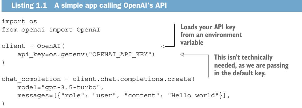
There are many great reasons to simply buy access to an LLM. First and foremost is the speed and flexibility accessing an API provides. Working with an API is an incredibly easy and cheap way to build a prototype and get your hands dirty quickly. In fact, it’s so easy that it only takes a few lines of Python code to start connecting to OpenAI’s API and using LLMs, as shown in listing 1.1. Sure, there’s a lot that’s possible, but it would be a bad idea to invest heavily in LLMs only to find out they happen to fail in your specific domain. Working with an API allows you to fail fast. Building a prototype application to prove the concept and launching it with an API is a great place to get started.

Often, buying access to a model can give you a competitive edge. In many cases, it could very well be that the best model on the market is built by a company specializing in your domain using specialized datasets it has spent a fortune to curate. While you could try to compete and build your own, it may better serve your purposes to buy access to the model instead. Ultimately, whoever has the better domain-specific data to finetune on is likely to win, and that might not be you if this is a side project for your company. Curating data can be expensive, after all. It can save you a lot of work to go ahead and buy it.

This leads to the next point: buying is a quick way to access expertise and support. For example, OpenAI has spent a lot of time making their models safe with plenty of filtering and controls to prevent the misuse of their LLMs. They’ve already encountered and covered a lot of the edge cases so you don’t have to. Buying access to their model also gives you access to the system they’ve built around it.

Not to mention that the LLM itself is only half the problem when deploying it to production. There’s still an entire application you need to build on top of it. Sometimes buying OpenAI’s model has thrived over its competitors in not a small way due to its UX and some tricks like making the tokens look like they’re being typed. We’ll take you through how you can start solving for the UX in your use case, along with some ways you can prototype to give you a major head start in this area.

1.2.2 Building: The path less traveled

Using an API is easy and, in most cases, likely the best choice. However, there are many reasons why you should aim to own this technology and learn how to deploy it yourself instead. While this path might be harder, we’ll teach you how to do it. Let’s dive into several of those reasons, starting with the most obvious: control.

CONTROL

One of the first companies to truly adopt LLMs as a core technology was a small video game company called Latitude. Latitude specializes in Dungeon and Dragons–like role-playing games that utilize LLM chatbots, and they have faced challenges when working with them. This shouldn’t come off as criticizing this company for their missteps, as they have contributed to our collective learning experience and were pioneers in forging a new path. Nonetheless, their story is a captivating and intriguing one—like a train wreck, we can’t help but keep watching.

Latitude’s first release was a game called AI Dungeon. At inception, it utilized OpenAI’s GPT-2 to create an interactive and dynamic storytelling experience. It quickly garnered a large gathering of players, who, of course, started to use it inappropriately. When OpenAI gave Latitude access to GPT-3, it promised an upgrade to the gaming experience; instead, what it got was a nightmare.1

You see, with GPT-3, OpenAI added reinforcement learning from human feedback (RLHF), which greatly helps improve functionality, but this also meant OpenAI contractors were now looking at the prompts. That’s the human feedback part. And these workers weren’t too thrilled to read the filth the game was creating. OpenAI’s reps were quick to give Latitude an ultimatum. Either it needed to start censoring the players, or OpenAI would remove Latitude’s access to the model—which would have essentially killed the game and the company. With no other option, Latitude quickly added some filters, but the filtering system was too much of a band-aid, a buggy and glitchy mess. Players were upset at how bad the system was and unnerved to realize Latitude’s developers were reading their stories, completely oblivious to the fact that OpenAI was already doing so. It was a PR nightmare. And it wasn’t over.

OpenAI decided the game studio wasn’t doing enough; stonewalled, Latitude was forced to increase its safeguards and started banning players. Here’s the twist: the reason so many of these stories turned to smut was because the model had a preference for erotica. It would often unexpectedly transform harmless storylines into inappropriately risqué situations, causing the player to be ejected and barred from the game. OpenAI was acting as the paragon of purity, but it was their model that was the problem, which led to one of the most ironic and unjust problems in gaming history: players were getting banned for what the game did.

So there they were—a young game studio just trying to make a fun game stuck between upset customers and a tech giant that pushed all the blame and responsibility

¹ WIRED, “It began as an AI-fueled dungeon game. Then it got much darker,” Ars Technica, May 8, 2021, https://mng.bz/AdgQ.

onto it. If the company had more control over the technology, it could have gone after a real solution, like fixing the model instead of having to throw makeup on a pig.

In this example, control may come off as your ability to finetune your model, and OpenAI now offers finetuning capabilities, but there are many fine-grained decisions that are still lost by using a service instead of rolling your own solution. For example, what training methodologies are used, what regions the model is deployed to, or what infrastructure it runs on. Control is also important for any customer or internal-facing tool. You don’t want a code generator to accidentally output copyrighted code or create a legal situation for your company. You also don’t want your customer-facing LLM to output factually incorrect information about your company or its processes.

Control is your ability to direct and manage the operations, processes, and resources in a way that aligns with your goals, objectives, and values. If a model ends up becoming central to your product offering and the vendor unexpectedly raises its prices, there’s little you can do but pay it. If the vendor decides its model should give more liberal or conservative answers that no longer align with your values, you are just as stuck.

The more central a technology is to your business plan, the more important it is to control it. This is why McDonald’s owns the real estate for its franchises and why Google, Microsoft, and Amazon all own their own cloud networks—and even why so many entrepreneurs build online stores through Shopify instead of using other platforms like Etsy or Amazon Marketplace. Ultimately, control is the first thing that’s lost when you buy someone else’s product. Keeping control will give you more options to solve future problems and will also give you a competitive edge.

COMPETITIVE EDGE

One of the most valuable aspects of deploying your own models is the competitive edge it gives you over your competition. Customization allows you to train the model to be the best at one thing. For example, after the release of Bidirectional Encoder Representations from Transformers (BERT) in 2017, which is a transformer model architecture you could use to train your own model, there was a surge of researchers and businesses testing this newfound technology on their own data to worldwide success. At the time of writing, if you search the Hugging Face Hub for “BERT,” more than 13.7K models are returned, all of which people individually trained for their own purposes, aiming to create the best model for their task.

One author’s personal experience in this area was training SlovenBERTcina after aggregating the largest (at the time) monolingual Slovak language dataset by scraping the Slovak National Corpus with permission, along with a bunch of other resources like the OSCAR project and the Europarl corpus. It never set any computational records and has never appeared in any model reviews or generated partnerships for the company the author worked for. It did, however, outperform every other model on the market on the tasks it trained on.

Chances are, neither you nor your company needs AGI to generate relevant insights from your data. In fact, if you invented an actual self-aware AGI and planned

to only ever use it to crunch some numbers, analyze data, and generate visuals for PowerPoint slides once a week, that would definitely be reason enough for the AGI to eradicate humans. More than likely, you need exactly what this author did when he made SlovenBERTcina, a large language model that performs two to three tasks better than any other model on the market and doesn’t also share your data with Microsoft or other potential competitors. While some data is required to be kept secret for security or legal reasons, a lot of data should be guarded because it includes trade secrets.

There are hundreds of open source LLMs for both general intelligence and foundational expertise on a specific task. We’ll hit some of our favorites in chapter 4. Taking one of these open source alternatives and training it on your data to create a model that is the best in the world at that task will ensure you have a competitive edge in your market. It will also allow you to deploy the model your way and integrate it into your system to have the most effect.

INTEGRATE ANYWHERE

Let’s say you want to deploy an LLM as part of a choose-your-own-adventure–styled game that uses a device’s GPS location to determine story plots. You know your users are often going to go on adventures into the mountains, out at sea, and generally to locations where they are likely to experience poor service and lack of internet access. Hitting an API just isn’t going to work. Now, don’t get us wrong: deploying LLMs onto edge devices like in this scenario is still an exploratory subject, but it is possible; we will be showing you how in chapter 10. Relying upon an API service is just not going to work for immersive experiences.

Similarly, using third-party LLMs and hitting an API adds integration and latency problems, requiring you to send data over the wire and wait for a response. APIs are great, but they are always slow and not always reliable. When latency is important to a project, it’s much better to have the service in-house. The previous section on competitive edge discussed two projects with edge computing as a priority; however, many more exist. LLAMA.cpp and ALPACA.cpp are two of the first such projects, and this space is innovating quicker than any others. Quantization into 4-bit, low-rank adaptation, and parameter-efficient finetuning are all methodologies recently created to meet these needs, and we’ll be going over each of these starting in chapter 3.

When this author’s team first started integrating with ChatGPT’s API, it was both an awe-inspiring and humbling experience—awe-inspiring because it allowed us to quickly build some valuable tools, and humbling because, as one engineer joked, “When you hit the endpoint, you will get 503 errors; sometimes you get a text response as if the model was generating text, but I think that’s a bug.” Serving an LLM in a production environment—trying to meet the needs of so many clients—is no easy feat. However, deploying a model that’s integrated into your system allows you more control of the process, affording higher availability and maintainability than you can currently find on the market. This, of course, also allows you to better control costs.

COSTS

Considering costs is always important because it plays a pivotal role in making informed decisions and ensuring the financial health of a project or an organization. It helps you manage budgets efficiently and make sure that resources are allocated appropriately. Keeping costs under control allows you to maintain the viability and sustainability of your endeavors in the long run.

Additionally, considering costs is crucial for risk management. When you understand the different cost aspects, you can identify potential risks and exert better control over them. This way, you can avoid unnecessary expenditures and ensure that your projects are more resilient to unexpected changes in the market or industry.

Finally, cost considerations are important for maintaining transparency and accountability. By monitoring and disclosing costs, organizations demonstrate their commitment to ethical and efficient operations to stakeholders, clients, and employees. This transparency can improve an organization’s reputation and help build trust.

All of these apply as you consider building versus buying LLMs. It may seem immediately less costly to buy, as the costliest service widely used on the market currently is only $20 per month. Compared to an EC2 instance on AWS, just running that same model for inference (not even training) could run you up a bill of about $250k per year. This is where building has done its quickest innovation, however. If all you need is an LLM for a proof of concept, any of the projects mentioned in the Competitive Edge section will allow you to create a demo for only the cost of electricity to run the computer you are demoing on. They can spell out training easily enough to allow for significantly reduced costs to train a model on your own data, as low as $100 (yes, that’s the real number) for a model with 20 billion parameters. Another benefit is knowing that if you build your own, your cost will never go up like it very much will when paying for a service.

SECURITY AND PRIVACY

Consider the following case. You are a military staff member in charge of maintenance for the nuclear warheads in your arsenal. All the documentation is kept in a hefty manual. There’s so much information required to outline all the safety requirements and maintenance protocols that cadets are known to forget important information despite their best efforts. They often cut the wires before first removing the fuse (https://youtu.be/UcaWQZlPXgQ). You decide to finetune an LLM model to be a personal assistant, giving directions and helping condense all that information to provide soldiers with exactly what they need when they need it. It’s probably not a good idea to upload those manuals to another company—understatement of the century so you’re going to want to train something locally that’s kept secure and private.

This scenario may sound farfetched, but when speaking to an expert working in analytics for a police department, they echoed this exact concern. Talking with them, they expressed how cool ChatGPT is and even had their whole team take a prompt engineering class to better take advantage of it but lamented that there was no way for their team to use it for their most valuable work—the sort of work that literally saves

lives—without exposing sensitive data and conversations. Anyone in similar shoes should be eager to learn how to deploy a model safely and securely.

You don’t have to be in the army or on a police force to handle sensitive data. Every company has important intellectual property and trade secrets that are best kept a secret. Having worked in the semiconductor, healthcare, and finance industries, we can tell you firsthand that paranoia and corporate espionage are part of the culture in these industries. Because of this, Samsung and other industry players locked down ChatGPT at first, preventing employees from using it, only later opening it up. Of course, it didn’t take long before several Samsung employees leaked confidential source code.² Because OpenAI uses its users’ interactions to improve the model, that code is retained and could have been used to further train the model later on. That means that with the right prompt injection, anyone could potentially pull the code out of the model. A recent example goes even further: when any OpenAI model was prompted to repeat a word ad infinitum, it would start regurgitating training data, including all of the personally identifiable information (PII) that had snuck through the cleaning process.

NOTE OpenAI’s privacy and usage policies have changed a lot over the course of this book’s writing. When ChatGPT was first introduced, it was done as a demo specifically so OpenAI could collect user interactions and improve the model. It pretty much didn’t have a privacy policy, and it had disclaimers saying such. As ChatGPT grew and became an actual product, this changed, as clients wanted more protection. For example, OpenAI changed its policies to better serve its customers and, since March 1, 2023, no longer uses customer API data to improve its models (see ChatGPT FAQ: https://mng.bz/QV8Q). The wording, of course, indicates that only data is sent through the API. It’s best to ask your lawyers where your company stands on using it. Regardless, the fact that terms of use have changed so much is just further proof you might want more control in this regard.

It’s not just code that can easily be lost. Business plans, meeting notes, confidential emails, and even potential patent ideas are at risk. Unfortunately, we know of a few companies that have started sending confidential data to ChatGPT, using that model to clean and extract PII. If this strikes you as potential negligent misuse, you’d be right. This methodology directly exposes customer data, not just to OpenAI, but to any and all third-party services they use (including AWS Mechanical Turk, Fiverr, and freelance workers) to perform the human feedback part of RLHF. Don’t get us wrong: it’s not necessarily a security or privacy problem if you use a third party to do data processing tasks even for sensitive data, but it should only be done with high levels of trust and contracts in place.

² 이코노미스트, “[단독] 우려가 현실로…삼성전자, 챗GPT 빗장 풀자마자 ‘오남용’ 속출,” 이코노미스트 [“Concerns become reality: As soon as Samsung Electronics unblocks ChatGPT, ‘abuse’ continues”]. The Economist, March 30, 2023, https://mng.bz/4p1v.

WRAPPING UP

As you can see, there are lots of reasons why a company might want to own and build its own LLMs, including greater control, cutting costs, and meeting security and regulation requirements. Despite this, we understand that buying is easy, and building is much more difficult, so for many projects, it makes sense to buy. However, before you do, in figure 1.1, we share a flowchart of questions you should ask yourself first. Even though it’s the more difficult path, building can be much more rewarding.

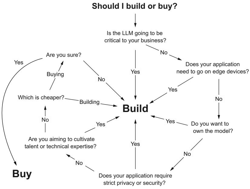
Figure 1.1 Questions you should ask yourself before making that build-vs.-buy decision

One last point we think these build-versus-buy conversations never seem to hone in on enough is “Por qué no los dos?” Buying gets you all the things building is bad at: time to market, relatively low cost, and ease of use. Building gets you everything buying struggles with: privacy, control, and flexibility. Research and prototyping phases could benefit very much from buying a subscription to GPT-4 or Databricks in order to build something quick to help raise funding or get stakeholder buy-in. Production, however, often isn’t an environment that lends itself well to third-party solutions.

Ultimately, whether you plan to build or buy, we wrote this book for you. Obviously, if you plan to build, there’s going to be a lot more you need to know about, so a majority of this book will be geared to these folks. In fact, we don’t need to belabor the point anymore: we’re going to teach you how to build in this book, but don’t let that stop you from doing the right thing for your company.

1.2.3 A word of warning: Embrace the future now

All new technology meets resistance and has critics; despite this, technologies keep being adopted, and progress continues. In business, technology can give a company an unprecedented advantage. There’s no shortage of stories of companies failing because they didn’t adapt to new technologies. We can learn a lot from their failures.

Borders first opened its doors in 1971. After developing a comprehensive inventory management system that included advanced analytic capabilities, it skyrocketed to become the second-largest book retailer in the world, only behind Barnes & Noble. Using this new technology, Borders disrupted the industry, allowing it to easily keep track of tens of thousands of books, opening large stores where patrons could peruse many more books than they could at smaller stores. The analytic capabilities helped it track which books were gaining popularity and gain better insights into its customers, allowing it to make better business decisions. It dominated the industry for over two decades.

Borders, however, failed to learn from its own history, going bankrupt in 2011 because of failing to adapt and being disrupted by technology: this time e-commerce. In 2001, instead of building its own platform and online store, it decided to outsource its online sales to Amazon.3 Many critics would say this decision was akin to giving your competitors the key to your business. While not exactly handing over its secret sauce, it was a decision that gave up Borders’ competitive edge.

For the next seven years, Borders turned a blind eye to the growing online sector, instead focusing on expanding its physical store presence, buying out competitors, and securing a coveted Starbucks deal. When Amazon released the Kindle in 2007, the book retail landscape completely changed. Barnes & Noble, having run its own online store, quickly pivoted and released the Nook to compete. Borders, however, did nothing or, in fact, could do nothing.

By embracing e-commerce through a third party, Borders failed to develop the in-house expertise required to create a successful online sales strategy, leading to a substantial loss in market share. It eventually launched its own e-reader, Kobo, in late 2010, but it was too late to catch up. Its inability to fully understand and implement e-commerce technology effectively led to massive financial losses and store closures; ultimately, the company filed for bankruptcy in 2011.

Borders is a cautionary tale, but there are hundreds more similar companies that failed to adopt new technology, to their own detriment. With a new technology as impactful as LLMs, each company has to decide on which side of the fence it wants to be. Does it delegate implementation and deployment to large FAANG-like corporations, relegating its job to just hitting an API, or does it take charge, preferring to master the technology and deploy it in-house?

³ A. Lowrey, “Borders bankruptcy: Done in by its own stupidity, not the Internet.,” Slate Magazine, July 20, 2011, https://mng.bz/PZD5.

The biggest lesson we hope to impart from this story is that technologies build on top of one another. E-commerce was built on top of the internet. Failing to build its own online store meant Borders failed to build the in-house technical expertise it needed to stay in the game when the landscape shifted. We see the same things with LLMs today because the companies that are best prepared to utilize them have already gathered expertise in machine learning and data science and have some idea of what they are doing.

We don’t have a crystal ball that tells us the future, but many believe that LLMs are a revolutionary new technology, like the internet or electricity before it. Learning how to deploy these models, or failing to do so, may very well be the defining moment for many companies—not because doing so will make or break their company now, but because it may in the future when something even more valuable comes along that’s built on top of LLMs.

Foraying into this new world of deploying LLMs may be challenging, but it will help your company build the technical expertise to stay on top of the game. No one really knows where this technology will lead, but learning about this technology will likely be necessary to avoid mistakes like those made by Borders.

There are many great reasons to buy your way to success, but there is at least one prevalent thought that is just absolutely wrong: it’s the myth that only large corporations can work in this field because it takes millions of dollars and thousands of GPUs to train these models, which creates this impenetrable moat of cash and resources the little guy can’t hope to cross. We’ll be talking about this more in the next section, but any company of any size can get started, and there’s no better time than now to do so.

1.3 Debunking myths

We have all heard from large corporations and the current leaders in LLMs how incredibly difficult it is to train an LLM from scratch and how intense it is to try to finetune them. Whether from OpenAI, BigScience, or Google, they discuss large investments and the need for strong data and engineering talent. But how much of this is true, and how much of it is just a corporate attempt to create a technical moat?

Most of these barriers start with the premise that you will need to train an LLM from scratch if you hope to solve your problems. Simply put, you don’t! Open source models covering many dimensions of language models are constantly being released, so more than likely, you don’t need to start from scratch. While it’s true that training LLMs from scratch is supremely difficult, we are still constantly learning how to do it and are able to automate the repeatable portions more and more. In addition, since this is an active field of research, frameworks and libraries are being released or updated daily and will help you start from wherever you currently are. Frameworks like oobabooga’s Gradio will help you run LLMs, and base models like Falcon 40B will be your starting point. All of it is covered. In addition, memos have circulated at large companies addressing the lack of a competitive edge that any organization currently holds over the open source community at large.

A friend once confided, “I really want to get more involved in all this machine learning and data science stuff. It seems to be getting cooler every time I blink an eye. However, it feels like the only way to get involved is to go through a lengthy career change and go work for a FAANG. No, thank you. We’ve done our time at large companies, and they aren’t for us. But we hate feeling like we’re trapped on the outside.” This is the myth that inspired this book. We’re here to equip you with tools and examples to help you stop feeling trapped on the outside. We’ll help you go through the language problems that we’re trying to solve with LLMs, along with machine learning operation strategies to account for the sheer size of the models.

Oddly enough, while many believe they are trapped on the outside, many others believe they can become experts in a weekend. Just get a GPT API key, and that’s it you’re done. This has led to a lot of fervor and hype, with a cool new demo popping up on social media every day. Most of these demos never become actual products but not because people don’t want them.

To understand this, let’s discuss IBM’s Watson, the world’s most advanced language model before GPT. Watson is a question-and-answering machine that crushed Jeopardy in 2011 against some of the best human contestants to ever appear on the show, Brad Rutter and Ken Jennings. Rutter was the highest-earning contestant ever to play the game show, and Jennings was so good at the game that he won a whopping 74 times in a row. Despite facing these legends, it wasn’t even close. Watson won in a landslide. Jennings, in response to the loss, responded with the famous quote, “I, for one, welcome our new computer overlords.”⁴

Watson was the first impressive foray into language modeling, and many companies were clamoring to take advantage of its capabilities. Starting in 2013, Watson started being released for commercial use. One of the biggest applications involved many attempts to integrate it into healthcare to solve various problems. However, none of these solutions ever really worked the way they needed to, and the business never became profitable. By 2022, Watson Health was sold off.

What we find when solving language-related problems is that building a prototype is easy; building a functioning product, on the other hand, is very, very difficult. There are just too many nuances to language. Many people wonder what made ChatGPT, which gained over a million clients in just five days, so explosive. Most of the answers we’ve heard would never satisfy an expert because ChatGPT wasn’t much more impressive than GPT-3 or other LLMs that had already been around for several years. Sam Altman of OpenAI once said in an interview that he didn’t think ChatGPT would get this much attention; he thought it would come with GPT-4’s release.⁵ So why was it explosive? In our opinion, the magic was that it was the first product to truly productionize LLMs—turning them from a demo into an actual product. It was something

⁴ J. Best, “IBM Watson: The inside story of how the Jeopardy-winning supercomputer was born, and what it wants to do next,” TechRepublic, September 9, 2013, https://mng.bz/JZ9Q.

⁵ “A conversation with OpenAI CEO Sam Altman; hosted by Elevate,” May 18, 2023, https://youtu.be/uRIWgbvouEw.

anyone could interact with, asking tough questions only to be amazed by how well it responded. A demo only has to work once, but the product has to work every time, even when millions of users are showing it to their friends, saying, “Check this out!” That magic is exactly what you can hope to learn from reading this book.

We’re excited about writing this book. We are excited about the possibilities of bringing this magic to you so you can take it to the world. LLMs are at the intersection of many fields, such as linguistics, mathematics, computer science, and more. While knowing more will help you, being an expert isn’t required. Expertise in any of the individual parts only raises the skill ceiling, not the floor, to get in. Consider an expert in physics or music theory: they won’t automatically have the skills for music production, but they will be more prepared to learn it quickly. LLMs are a communication tool, and communicating is a skill just about everyone needs.

Like all other skills, your proximity and willingness to get involved are the two main blockers to knowledge, not a degree or ability to notate—these only shorten your journey toward being heard and understood. If you don’t have any experience in this area, it might be good to start by first developing an intuition around what an LLM is and needs by contributing to a project like OpenAssistant. If you’re a human, that’s exactly what LLMs need. By volunteering, you can start understanding what these models train on and why. If you fall anywhere, from no knowledge up to being a professional machine learning engineer, we’ll be imparting the knowledge necessary to shorten your time to understanding considerably. If you’re not interested in learning the theoretical underpinnings of the subject, we’ve got plenty of hands-on examples and projects to get your hands dirty.

We’ve all heard a story by now of LLM hallucinations, but LLMs don’t need to be erratic. Companies like Lakera are working daily to improve security, while others like LangChain are making it easier to provide models with pragmatic context that makes them more consistent and less likely to deviate. Techniques such as RLHF and Chain of Thought further allow our models to align themselves with negotiations we’ve already accepted that people and models should understand from the get-go, such as basic addition and the current date, both of which are conceptually arbitrary. We’ll help you increase your model stability from a linguistic perspective so it will figure out not just the most likely outputs but also the most useful.

Something to consider as you venture further down this path is not only the security of what goes into your model/code but what comes out. LLMs can sometimes produce outdated, factually incorrect, or even copyrighted or licensed material, depending on what their training data contains. LLMs are unaware of any agreements people make about what is supposed to be a trade secret and what can be shared openly—that is, unless you tell them about those agreements during training or through careful prompting mechanisms during inference. Indeed, the challenges around prompt injection giving inaccurate information arise primarily due to two factors: users requesting information beyond the model’s understanding and model developers not fully predicting how users will interact with the models or the nature of their inquiries. If you had a resource that could help you get a head start on that second problem, it would be pretty close to invaluable, wouldn’t it?

Lastly, we don’t want to artificially or untruthfully inflate your sense of hope with LLMs. They are resource intensive to train and run. They are hard to understand, and they are harder to get working how you want. They are new and not well-understood. The good news is that these problems are being actively worked on, and we’ve put in a lot of work finding implementations concurrent with this writing to actively lessen the burden of knowing everything about the entire deep-learning architecture. From quantization to Kubernetes, we’ll help you figure out everything you need to know to do this now with what you have. Maybe we’ll inadvertently convince you that it’s too much and you should just purchase from a vendor. Either way, we’ll help you every step of the way to get the results you need from this magical technology.

Summary

• LLMs are exciting because they work within the same framework (language) as humans.
• Society has been built on language, so effective language models have limitless applications, such as chatbots, programming assistants, video games, and AI assistants.
• LLMs are excellent at many tasks and can even pass high-ranking medical and law exams.
• LLMs are wrecking balls, not hammers, and should be avoided for simple problems that require low latency or entail high risks.
• Reasons to buy include
  • Quickly getting up and running to conduct research and prototype use cases
  • Easy access to highly optimized production models
  • Access to vendors’ technical support and systems
• Reasons to build include
  • Getting a competitive edge for your business use case
  • Keeping costs low and transparent
  • Ensuring the reliability of the model
  • Keeping your data safe
  • Controlling model output on sensitive or private topics
• There is no technical moat preventing you from competing with larger companies, since open source frameworks and models provide the building blocks to pave your own path.

Large language models: A deep dive into language modeling

This chapter covers

• The linguistic background for understanding meaning and interpretation
• A comparative study of language modeling techniques
• Attention and the transformer architecture
• How large language models both fit into and build upon these histories

If you know the enemy and know yourself, you need not fear the result of a hundred battles.

—Sun Tzu

This chapter delves into linguistics as it relates to the development of LLMs, exploring the foundations of semiotics, linguistic features, and the progression of language modeling techniques that have shaped the field of natural language processing (NLP). We will begin by studying the basics of linguistics and its relevance to LLMs, highlighting key concepts such as syntax, semantics, and pragmatics that form the basis of natural language and play a crucial role in the functioning of LLMs. We will

delve into semiotics, the study of signs and symbols, and explore how its principles have informed the design and interpretation of LLMs.

We will then trace the evolution of language modeling techniques, providing an overview of early approaches, including N-grams, naive Bayes classifiers, and neural network-based methods such as multilayer perceptrons (MLPs), recurrent neural networks (RNNs), and long short-term memory (LSTM) networks. We will also discuss the groundbreaking shift to transformer-based models that laid the foundation for the emergence of LLMs, which are really just big transformer-based models. Finally, we will introduce LLMs and their distinguishing features, discussing how they have built upon and surpassed earlier language modeling techniques to revolutionize the field of NLP.

This book is about LLMs in production. We firmly believe that if you want to turn an LLM into an actual product, understanding the technology better will improve your results and save you from making costly and time-consuming mistakes. Any engineer can figure out how to lug a big model into production and throw a ton of resources at it to make it run, but that brute-force strategy completely misses the lessons people have already learned trying to do the same thing before, which is what we are trying to solve with LLMs in the first place. Having a grasp of these fundamentals will better prepare you for the tricky parts, the gotchas, and the edge cases you are going to run into when working with LLMs. By understanding the context in which LLMs emerged, we can appreciate their transformative impact on NLP and how to enable them to create a myriad of applications.

2.1 Language modeling

It would be a great disservice to address LLMs in any depth without first addressing language. To that end, we will start with a brief but comprehensive overview of language modeling, focusing on the lessons that can help us with modern LLMs. Let’s first discuss levels of abstraction, as this will help us garner an appreciation for language modeling.

Language, as a concept, is an abstraction of the feelings and thoughts that occur to us in our heads. Feelings come first in the process of generating language, but that’s not the only thing we’re trying to highlight here. We’re also looking at language as being unable to capture the full extent of what we are able to feel, which is why we’re calling it an abstraction. It moves away from the source material and loses information. Math is an abstraction of language, focusing on logic and provability, but as any mathematician will tell you, it is a subset of language used to describe and define in an organized and logical way. From math comes another abstraction, the language of binary, a base-2 system of numerical notation consisting of either on or off.

This is not a commentary on usefulness, as binary and math are just as useful as the lower-level aspects of language, nor is it commenting on order, as we said before. With math and binary, the order coincidentally lines up with the layer of abstraction. Computers can’t do anything on their own and need to take commands to be useful. Binary, unfortunately, ends up taking too long for humans to communicate important things in it, so binary was also abstracted to assembly, a more human-comprehensible language for communicating with computers. This was further abstracted to the highlevel assembly language C, which has been even further abstracted to object-oriented languages like Python or Java (which one doesn’t matter—we’re just measuring distance from binary). The flow we just discussed is outlined in figure 2.1.

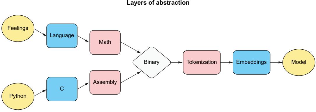
Figure 2.1 We compare cognitive layers of abstraction to programming layers of abstraction down to the logical binary abstraction. Python doesn’t come from C, nor does it compile into C. Python is, however, another layer of abstraction distant from binary. Language follows a similar path. Each layer of abstraction creates a potential point of failure. There are also several layers of abstraction to creating a model, and each is important in seeing the full path from our feelings to a working model.

This is obviously a reduction; however, it’s useful to understand that the feelings you have in your head are the same number of abstractions away from binary, the language the computer actually reads, as the languages most people use to program in. Some people might argue that there are more steps between Python and binary, such as compilers or using assembly to support the C language, and that’s true, but there are more steps on the language side too, such as morphology, syntax, logic, dialogue, and agreement.

This reduction can help us understand how difficult the process of getting what we want to be understood by an LLM actually is and even help us understand language modeling techniques better. We focus on binary here to illustrate that there are a similar number of abstract layers to get from an idea you have or from one of our code samples to a working model. Like the children’s telephone game where participants whisper into each other’s ears, each abstraction layer creates a disconnect point or barrier where mistakes can be made.

Figure 2.1 is also meant not only to illustrate the difficulty in creating reliable code and language input but also to draw attention to how important the intermediary abstraction steps, like tokenization and embeddings, are for the model itself. Even if you have perfectly reliable code and perfectly expressed ideas, the meaning may be fumbled by one of those processes before it ever reaches the LLM.

In this chapter, we will try to help you understand what you can do to reduce the risks of these failure points, whether on the language, coding, or modeling side. Unfortunately, it’s a bit tricky to strike a balance between giving you too much linguistics that doesn’t immediately matter for the task at hand versus giving you too much technical knowledge that, while useful, doesn’t help you develop an intuition for language modeling as a practice. With this in mind, you should know that linguistics can be traced back thousands of years in our history, and there’s lots to learn from it. We’ve included a brief overview of how language modeling has progressed over time in appendix A, and we encourage you to take a look.

Let’s start with our focus on the building blocks that constitute language itself. We expect our readers to have at least attempted language modeling before and to have heard of libraries like PyTorch and TensorFlow, but we do not expect most of our readers to have considered the language side of things before. By understanding the essential features that make up language, we can better appreciate the complexities involved in creating effective language models and how these features interact with one another to form the intricate web of communication that connects us all. In the following section, we will examine the various components of language, such as phonetics, pragmatics, morphology, syntax, and semantics, as well as the role they play in shaping our understanding and usage of languages around the world. Let’s take a moment to explore how we currently understand language, along with the challenges we face that LLMs are meant to solve.

2.1.1 Linguistic features

Our current understanding of language is that language is made up of at least five parts: phonetics, syntax, semantics, pragmatics, and morphology. Each of these portions contributes significantly to the overall experience and meaning being ingested by the listener in any conversation. Not all of our communication uses all of these forms; for example, the book you’re currently reading is devoid of phonetics, which is one of the reasons why so many people think text messages are unsuited for more serious or complex conversations. Let’s work through each of these five parts to figure out how to present them to a language model for a full range of communicative power.

PHONETICS

Phonetics is probably the easiest for a language model to ingest, as it involves the actual sound of the language. This is where accent manifests and deals with the production and perception of speech sounds, with phonology focusing on the way sounds are organized within a particular language system. Similarly to computer vision, while a sound isn’t necessarily easy to deal with as a whole, there’s no ambiguity in how to parse, vectorize, or tokenize the actual sound waves. They have a numerical value attached to each part, the crest, the trough, and the slope during each frequency cycle. It is vastly easier than text to tokenize and process by a computer while being no less complex.

Sound inherently also contains more encoded meaning than text. For example, imagine someone saying the words “Yeah, right,” to you. It could be sarcastic, or it could be congratulatory, depending on the tone—and English isn’t even tonal! Phonetics, unfortunately, doesn’t have terabyte-sized datasets commonly associated with it, and performing data acquisition and cleaning on phonetic data, especially on the scale needed to train an LLM, is difficult at best. In an alternate world where audio data was more prevalent than text data and took up a smaller memory footprint, phonetic-based or phonetic-aware LLMs would be much more sophisticated, and creating that world is a solid goal to work toward.

Anticipating this phonetical problem, a system was created in 1888 called the International Phonetic Alphabet (IPA). It has been revised in both the 20th and 21st centuries to be more concise, more consistent, and clearer and could be a way to insert phonetic awareness into text data. IPA functions as an internationally standardized version of every language’s sound profile. A sound profile is the set of sounds that a language uses; for example, in English, we never have the /ʃ/ (she, shirt, sh) next to the /v/ sound. IPA is used to write sounds, rather than writing an alphabet or logograms, as most languages do. For example, you could describe how to pronounce the word “cat” using these symbols: /k/, /æ/, and /t/. Of course, that’s a very simplified version of it, but for models, it doesn’t have to be. You can describe tone and aspiration as well. This could be a happy medium between text and speech, capturing some phonetic information. Think of the phrase “What’s up?” Your pronunciation and tone can drastically change how you understand that phrase, sometimes sounding like a friendly “Wazuuuuup?” and other times an almost threatening “’Sup?” which IPA would fully capture. IPA isn’t a perfect solution, though; for example, it doesn’t solve the problem of replicating tone very well.

Phonetics is listed first here because it’s the place where LLMs have been applied to the least out of all the features and, therefore, has the largest space for improvement. Even modern text-to-speech (TTS) and voice-cloning models, for the most part, end up converting the sound to a spectrogram and analyzing that image rather than incorporating any type of phonetic language modeling. Improving phonetic data and representation in LLMs is something to look for as far as research goes in the coming months and years.

SYNTAX

Syntax is the place where current LLMs are highest-performing, both in parsing syntax from the user and in generating their own. Syntax is generally what we think of as grammar and word order; it is the study of how words can combine to form phrases, clauses, and sentences. Syntax is also the first place language-learning programs start to help people acquire new languages, especially based on where they are coming from natively. For example, it is important for a native English speaker learning Turkish to know that the syntax is completely different, and you can often build entire sentences in Turkish that are just one long compound word, whereas in English, we never put our subject and verb together into one word.

Syntax is largely separate from meaning in language, as the famous sentence from Noam Chomsky, the so-called father of syntax, demonstrates: “Colorless green ideas sleep furiously.” Everything about that sentence is both grammatically correct and semantically understandable. The problem isn’t that it doesn’t make sense; it’s that it does, and the encoded meanings of those words conflict. This is a reduction; however, you can think of all the times LLMs give nonsense answers as this phenomenon manifests. Unfortunately, the syntax is also where ambiguity is most commonly found. Consider the sentence, “I saw an old man and woman.” Now answer this question: Is the woman also old? This is syntactic ambiguity, where we aren’t sure whether the modifier “old” applies to all people in the following phrase or just the one it immediately precedes. This is less consequential than the fact that semantic and pragmatic ambiguity also show up in syntax. Consider this sentence: “I saw a man on a hill with a telescope,” and answer these questions: Where is the speaker, and what are they doing? Is the speaker on the hill cutting a man in half using a telescope? Likely, you didn’t even consider this option when you read the sentence because when we interpret syntax, all of our interpretations are at least semantically and pragmatically informed. We know from lived experience that that interpretation isn’t at all likely, so we throw it out immediately, usually without even taking time to process that we’re eliminating it from the pool of probable meanings. Single-modality LLMs will always have this problem, and multimodal LLMs can (so far) only asymptote toward the solution.

It shouldn’t take any logical leap to understand why LLMs need to be syntax-aware to be high-performing. LLMs that don’t get word order correct or generate nonsense aren’t usually described as “good.” LLMs being syntax-dependent has prompted even Chomsky to call LLMs “stochastic parrots.” In our opinion, GPT-2 in 2018 was when language modeling solved syntax as a completely meaning-independent demonstration, and we’ve been happy to see the more recent attempts to combine the syntax that GPT-2 outputs so well with encoded and entailed meaning, which we’ll get into now.

SEMANTICS

Semantics are the literal encoded meaning of words in utterances, which changes at breakneck speed in waves. People automatically optimize semantic meaning by only using words they consider meaningful in the current language epoch. If you’ve ever created or used an embedding with language models (word2vec, ELMo, BERT, MUSE [the E is for embedding], etc.), you’ve used a semantic approximation. Words often go through semantic shifts, and while we won’t cover this topic completely or go into depth, here are some common ones you may already be familiar with: narrowing, a broader meaning to a more specific one; broadening, the inverse of narrowing going from a specific meaning to a broad one; and reinterpretations, going through whole or partial transformations. These shifts do not have some grand logical underpinning.

They don’t even have to correlate with reality, nor do speakers of a language often consciously think about the changes as they’re happening. That doesn’t stop the change from occurring, and in the context of language modeling, it doesn’t stop us from having to keep up with that change.

Let’s look at some examples. Narrowing includes “deer,” which in Old and Middle English just meant any wild animal, even a bear or a cougar, and now means only one kind of forest animal. For broadening, we have “dog,” which used to refer to only one canine breed from England and now can be used to refer to any domesticated canine. One fun tangent about dog-broadening is in the FromSoft game Elden Ring, where because of a limited message system between players, “dog” will be used to refer to anything from a turtle to a giant spider and literally everything in between. For reinterpretation, we can consider “pretty,” which used to mean clever or well-crafted, not visually attractive. Another good example is “bikini,” which went from referring to a particular atoll to referring to clothing you might have worn when visiting that atoll to people acting as if the “bi-” was referring to the two-piece structure of the clothing, thus implying the tankini and monokini. Based on expert research and decades of study, we can think of language as being constantly compared and re-evaluated by native language speakers, out of which common patterns emerge. The spread of those patterns is closely studied in sociolinguistics and is largely out of the scope of the current purpose but can quickly come into scope as localization (l10n) or internationalization (i18n) for LLMs arises as a project requirement. Sociolinguistic phenomena such as prestige can help design systems that work well for everyone.

In the context of LLMs, so-called semantic embeddings are vectorized versions of text that attempt to mimic semantic meaning. Currently, the most popular way of doing this is by tokenizing or assigning an arbitrary number in a dictionary to each subword in an utterance (think prefixes, suffixes, and morphemes generally), applying a continuous language model to increase the dimensionality of each token within the vector so that there’s a larger vector representing each index of the tokenized vector, and then applying a positional encoding to each of those vectors to capture word order. Each subword ends up being compared to other words in the larger dictionary based on how it’s used. We’ll show you an example of this later. Something to consider when thinking about word embeddings is that they struggle to capture the deep, encoded meaning of those tokens, and simply adding more dimensions to the embeddings hasn’t shown marked improvement. Evidence that embeddings work similarly to humans is that you can apply a distance function to related words and see that they are closer together than unrelated words. How to capture and represent meaning more completely is another area in which to expect groundbreaking research in the coming years and months.

PRAGMATICS

Pragmatics is sometimes omitted from linguistics due to its referent being all the nonlinguistic context affecting a listener’s interpretation and the speaker’s decision to express things in a certain way. Pragmatics refers in large part to dogmas followed in cultures, regions, socio-economic classes, and shared lived experiences, which are played off of to take shortcuts in conversations using entailment.

If we were to say, “A popular celebrity was just taken into the ICU,” your pragmatic interpretation based on lived experience might be to assume that a well-beloved person has been badly injured and is now undergoing medical treatment in a wellequipped hospital. You may wonder about which celebrity it is, whether they will have to pay for the medical bills, or if the injury was self-inflicted, also based on your lived experience. None of these things can be inferred directly from the text and its encoded meaning by itself. You would need to know that ICU stands for a larger set of words and what those words are. You would need to know what a hospital is and why someone would need to be taken there instead of going there themselves. If any of these feel obvious, good. You live in a society, and your pragmatic knowledge of that society overlaps well with the example provided. If we share an example from a lesspopulated society, “Janka got her grand-night lashings yesterday; she’s gonna get Peter tomorrow,” you might be left scratching your head. If you are, realize this probably looks like how a lot of text data ends up looking to an LLM (anthropomorphization acknowledged). For those wondering, this sentence comes from Slovak Easter traditions. A lot of meaning here will be missed and go unexplained if you are unaccustomed to these particular traditions as they stand in that culture. This author personally has had the pleasure of trying to explain the Easter Bunny and its obsession with eggs to foreign colleagues and enjoyed the satisfaction of looking like I’m off my rocker.

In the context of LLMs, we can effectively group all out-of-text contexts into pragmatics. This means LLMs start without any knowledge of the outside world and do not gain it during training. They only gain a knowledge of how humans respond to particular pragmatic stimuli. LLMs do not understand social class or race or gender or presidential candidates, or anything else that might spark some type of emotion in you based on your life experience. Pragmatics isn’t something that we expect will be able to be directly incorporated into a model at any point because models cannot live in society. Yet we have already seen the benefits of incorporating it indirectly through data engineering and curation, prompting mechanisms like RAG, and supervised finetuning on instruction datasets. In the future, we expect great improvements in incorporating pragmatics into LLMs, but we emphasize that it’s an asymptotic solution because language is ultimately still an abstraction.

Pragmatic structure gets added, whether you mean to add it or not, as soon as you acquire the data you are going to train on. You can think of this type of pragmatic structure as bias, not inherently good or bad, but impossible to get rid of. Later down the line, you get to pick the types of bias you’d like your data to keep by normalizing and curating, augmenting particular underrepresented points, and cutting overrepresented or noisy examples. Instruction datasets show us how you can harness pragmatic structure in your training data to create incredibly useful bias, like biasing your model to answer a question when asked instead of attempting to categorize the sentiment of the question.

Pragmatics and context all revolve around entailment. An entailment is a pragmatic marker within your data, as opposed to the literal text your dataset contains. For example, let’s say you have a model attempting to take an input like “Write me a speech about frogs eating soggy socks that doesn’t rhyme and where the first letters of each line spell amphibian” and actually follow that instruction. You can immediately tell that this input is asking for a lot. The balance for you as a data engineer would be to make sure that everything the input is asking for is explicitly accounted for in your data. You need examples of speeches, examples of what frogs and socks are and how they behave, and examples of acrostic poems. If you don’t have them, the model might be able to understand just from whatever entailments exist in your dataset, but it’s pretty up in the air. If you go the extra mile and keep track of entailed versus explicit information and tasks in your dataset, along with data distributions, you’ll have examples to answer, “What is the garbage-in resulting in our garbage-out?”

LLMs struggle to pick up on pragmatics, even more so than people, but they do pick up on the things that your average standard deviation of people would. They can even replicate responses from people outside that standard deviation, but pretty inconsistently without the exact right stimulus. That means it’s difficult for a model to give you an expert answer on a problem the average person doesn’t know without providing the correct bias and entailment during training and in the prompt. For example, including “masterpiece” at the beginning of an image-generation prompt will elicit different and usually higher-quality generations, but only if that distinction was present in the training set and only if you’re asking for an image where “masterpiece” is a compliment. Instruction-based datasets attempt to manufacture those stimuli during training by asking questions and giving instructions that entail representative responses. It is impossible to account for every possible situation in training, and you may inadvertently create new types of responses from your end users by trying to account for everything. After training, you can coax particular information from your model through prompting, which has a skill ceiling based on what your data originally entailed.

MORPHOLOGY

Morphology is the study of word structures and how they are formed from smaller units called morphemes. Morphemes are the smallest units of meaning, like the “re-” in “redo” or “relearn.” However, not all parts of words are morphemes, such as “ra-” in “ration” or “na-” in “nation,” and some can be unexpected, like “helico-” as in “helicoid” and “-pter” as in “pterodactyl.”

Understanding how words are constructed helps create better language models and parsing algorithms, which are essential for tasks like tokenization. Tokens are the basic units used in NLP; they can be words, subwords, characters, or whole utterances and do not have to correspond to existing morphemes. People do not consciously decide what their units of meaning are going to be, and as such, they are often illogical. The effectiveness of a language model can depend on how well it can understand and process these tokens. For instance, in tokenization, a model needs to store a set of dictionaries to convert between words and their corresponding indices. One of these tokens is usually an / token, which represents any word that the model does not recognize. If this token is used too frequently, it can hinder the model’s performance, either because the model’s vocabulary is too small or because the tokenizer is not using the right algorithm for the task.

Consider a scenario where you want to build a code completion model, but you’re using a tokenizer that only recognizes words separated by whitespace, like the NLTK punkt tokenizer. When it encounters the string def add_two_numbers_together(x, y):, it will pass [def, [UNK], y] to the model. This causes the model to lose valuable information, not only because it doesn’t recognize the punctuation but also because the important part of the function’s purpose is replaced with an unknown token due to the tokenizer’s morphological algorithm. A better understanding of word structure and the appropriate parsing algorithms is needed to improve the model’s performance.

2.1.2 Semiotics

After exploring the fundamental features of language and examining their significance in the context of LLMs, it is important to consider the broader perspective of meaning-making and interpretation in human communication. Semiotics, the study of signs and symbols, offers a valuable lens through which we can better understand how people interpret and process language. We will delve into semiotics, examining the relationship between signs, signifiers, and abstractions and how LLMs utilize these elements to generate meaningful output. This discussion will provide a deeper understanding of the intricate processes through which LLMs manage to mimic human-like understanding of language while also shedding light on the challenges and limitations they face in this endeavor. We do not necessarily believe that mimicking human behavior is the right answer for LLM improvement, only that mimicry is how the field has evaluated itself so far.

To introduce semiotics, let’s consider figure 2.2, an adapted Peircean semiotic triangle. These triangles are used to organize base ideas into sequences of firstness, secondness, and thirdness, with firstness being at the top left, secondness at the bottom, and thirdness at the top right. If you’ve ever seen a semiotic triangle before, you may be surprised at the number of corners and orientation. To explain, we’ve turned them upside down to make it slightly easier to read. Also, because the system is recursive, we’re showing you how the system can simultaneously model the entire process and each piece individually. While the whole concept of these ideas is very cool, it’s outside of the scope of this book to delve into the philosophy fully. Instead, we can focus on the cardinal parts of those words (first, second, third) to show the sequence of how meaning is processed.

We can also look at each intersection of the triangles to understand why things are presented in the order they are. Feelings can be attached to images and encodings long before they can be attached to words and tables. Ritual and common scripts give a space for interpreted action that’s second nature and doesn’t have to be thought

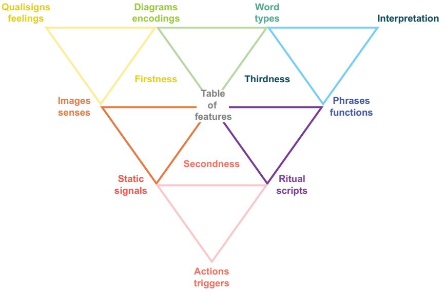
Figure 2.2 A recursive Peircean semiotic triangle is a system of organizing the process of extracting meaning from anything—in our case, from language. Each point on the triangle illustrates one of the minimal parts needed to synthesize meaning within whatever the system is being used to describe, so each point is a minimal unit in meaning for language. Firstness, secondness, and thirdness are not points on the triangle; instead, they are more like markers for the people versed in semiotics to be able to orient themselves in this diagram.

about, similar to how most phrases just come together from words without the native speaker needing to perform metacognition about each word individually. All of these eventually lead to an interpretation or a document (a collection of utterances); in our case, that interpretation should be reached by the LLM. This is why, for example, prompt engineering can boost model efficacy. Foundation LLMs trained on millions of examples of ritual scripts can replicate the type of script significantly better when you explicitly tell the model in the prompt which script needs to be followed. Try asking the model for a step-by-step explanation—maybe prepend your generation with “Let’s think about this step-by-step.” The model will generate step-by-step scripts based on previous scripts it’s seen play out.

For those interested, there are specific ways of reading these figures and a whole field of semiotics to consider; however, it’s not guaranteed that you’ll be able to create the best LLMs by understanding the whole thing. Instead of diving deeply into this, we’ll consider the bare minimum that can help you build the best models, UX, and UI for everyone to interact with. For example, one aspect of the process of creating meaning is recursiveness. When someone is talking to you and they say something that doesn’t make sense (is “meaningless” to you), what do you do? Generally, people will ask one or more clarifying questions to figure out the meaning, and the process will start over and over until the meaning is clear to you. The most state-of-the-art

models currently on the market do not do this, but they can be made to do it through very purposeful prompting. Many people wouldn’t even know to do that without having it pointed out to them. In other words, this is a brief introduction to semiotics. You don’t need to be able to give in-depth and accurate coordinate-specific explanations to experts in the semiotic field by the end of this section. The point we are trying to make is that this is an organizational system showcasing the minimum number of things you need to create a full picture of meaning for another person to interpret. We are not giving the same amount of the same kinds of information to our models during training, but if we did, it would result in a marked improvement in model behavior.

Figures 2.2 and 2.3 are meant to represent a minimal organizational model, where each of these pieces is essential. Let’s consider figure 2.3, which walks through an example of using a semiotic triangle. Consider images, pictures, and memories and think about what it would be like to try to absorb the knowledge in this book without your eyes to process images and without orthography (a writing system) to abstract the knowledge. Looking at the bullet points, etc., how could you read this book without sections, whitespace between letters, and bullet points to show you the order and structure to process information? Look at semantics and literal encoded meaning, and imagine the book without diagrams or with words that didn’t have dictionary defini-

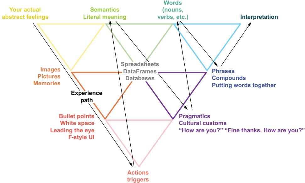
Figure 2.3 Starting at the top-left corner, follow the arrows to see the general order we use to build our interpretations and extract meaning from things we interact with. Here, we’ve replaced the descriptive words with some examples of each point. Try to imagine interpreting this diagram without any words, examples, arrows, or even the pragmatic context of knowing what a figure in a book like this is supposed to be for.

tions. The spreadsheets in the middle could be a book without any tables or comparative informational organizers, including these figures. What would it be like to read this book without a culture or society with habits and dogma to use as a lens for our interpretations? All these points form our ability to interpret information, along with the lens through which we pass our information to recognize patterns.

So these are the important questions: How many of these things do you see LLMs having access to in order to return meaningful interpretations? Does an LLM have access to feelings or societal rituals? Currently, they do not, but as we go through traditional and newer techniques for NLP inference, think about what different models have access to.

2.1.3 Multilingual NLP

The last challenge that we need to touch on before we evaluate previous NLP techniques and current-generation LLMs is the foundation of linguistics and the reason LLMs even exist. People have wanted to understand or exploit each other since the first civilizations made contact. These cases have resulted in the need for translators, and this need has only exponentially increased as the global economy has grown and flourished.

It’s pretty simple math for business as well. Did you know that there are almost as many native speakers of Bengali as there are native speakers of English? If this is the first time you’ve heard of the Bengali language, this should hopefully color your perception that there is a valuable market for multilingual models. There are billions of people in the world, but only about a third of 1 billion speak English natively. If your model is Anglocentric, like most are, you are missing out on 95% of the people in the world as customers and users. Spanish and Mandarin Chinese are easy wins in this area, but most people don’t even go that far.

There are many more politically charged examples of calling things, including different languages, the same that are out of the scope of this book. These are most often because of external factors like government involvement. Keeping these two points in mind—that a monolingual system focusing on English doesn’t have the coverage or profit potential that many businesses act like it does and that the boundaries between languages and dialects are unreliable at best and systematically harmful at worst should highlight the dangerous swamp of opinions. Many businesses and research scientists don’t even pretend to want to touch this swamp with a 50-foot pole when designing a product or system.

Unfortunately, no easy solutions exist at this time. However, considering these factors can help you as a scientist or engineer (and hopefully an ethical person) to design LLMs that, at the very least, don’t exacerbate and negatively contribute to the existing problems. The first step in this process is deciding on a directional goal from the beginning of the project, either toward localization (l10n) or internationalization (i18n). Localization is an approach exemplified by Mozilla, which has a different version of its browser available through crowdsourced l10n in over 90 languages with no indications of stopping that effort. Internationalization is similar, but in the opposite

direction; for example, Ikea tries to put as few words as possible in their instructional booklets, opting instead for internationally recognized symbols and pictures to help customers navigate the DIY projects. Deciding at the beginning of the project cuts down on the effort required to expand to either solution exponentially. It is large enough to switch the perception of translation and formatting from a cost to an investment. In the context of LLMs and their rapid expansion across the public consciousness, it becomes even more important to make that consideration early. Hitting the market with a world-changing technology that automatically disallows most of the world from interacting with it devalues those voices. Having to wait jeopardizes businesses’ economic prospects.

Before continuing, let’s take a moment to reflect on what we’ve discussed so far. We’ve hit important points in linguistics, illustrating concepts for us to consider, such as understanding that the structure of language is separate from its meaning. We have demonstrated quite a journey that each of us takes, both personally and as a society, toward having the metacognition to understand and represent language in a coherent way for computers to work with. This understanding will only improve as we deepen our knowledge of cognitive fields and solve for the linguistic features we encounter. Going along with figure 2.1, we will now demonstrate the computational path for language modeling that we have followed and explore how it has and hasn’t solved for any of those linguistic features or strived to create meaning. Let’s move into evaluating the various techniques for representing a language algorithmically.

2.2 Language modeling techniques

Having delved into the fundamental features of language, the principles of semiotics, and how LLMs interpret and process linguistic information, we now transition into a more practical realm. We will explore the various NLP techniques developed and employed to create these powerful language models. By examining the strengths and weaknesses of each approach, we will gain valuable insights into the effectiveness of these techniques in capturing the essence of human language and communication. This knowledge will not only help us appreciate the advancements made in the field of NLP but also enable us to better understand the current limitations of these models and the challenges that lie ahead for future research and development.

Let’s take a second to go over some data processing that will be universal to all language modeling. First, we’ll need to decide how to break up the words and symbols we’ll be passing into our model, effectively deciding what a token will be in our model. We’ll need a way to convert those tokens to numerical values and back again. Then, we’ll need to pick how our model will process the tokenized inputs. Each of the following techniques will build upon the previous techniques in at least one of these ways.

The first of these techniques is called a bag-of-words (BoW) model, and it consists of simply counting words as they appear in text. You could import the Count-Vectorizer class from sklearn to use it, but it’s more instructive if we show you with a small snippet. It can be accomplished very easily with a dictionary that scans through

text, creating a new vocabulary entry for each new word as a key and an incrementing value starting at 1:

sentence = "What is a bag of words and what does it do for me when " \
 "processing words?"
clean_text = sentence.lower().split(" ")
bow = {word:clean_text.count(word) for word in clean_text}
print(bow)
# {'what': 2, 'is': 1, 'a': 1, 'bag': 1, 'of': 1, 'words': 1, 'and': 1, 
# 'does': 1, 'it': 1, 'do': 1, 'for': 1, 'me': 1, 'when': 1, 'processing': 1,
# 'words?': 1}

Considering its simplicity, even this model, based entirely on frequency, can be quite powerful when trying to gain insight into a speaker’s intentions or at least their idiosyncrasies. For example, you could run a simple BoW model on inaugural speeches of US presidents, searching for the words “freedom,” “economy,” and “enemy” to gain a pretty good insight about which presidents assumed office under peacetime, during wartime, and during times of monetary strife, just based on how many times each word was mentioned. The BoW model’s weaknesses are many, however, as the model provides no images, semantics, pragmatics, phrases, or feelings. In our example, there are two instances of “words,” but because our tokenization strategy is just whitespace, it didn’t increment the key in the model. It doesn’t have any mechanisms to evaluate context or phonetics, and because it divides words by default on whitespace (you can obviously tokenize however you want, but try tokenizing on subwords and see what happens with this model—spoiler: it is bad), it doesn’t account for morphology either. Altogether, it should be considered a weak model for representing language but a strong baseline for evaluating other models against it. To solve the problem of BoW models not capturing any sequence data, N-gram models were conceived.

2.2.1 N-gram and corpus-based techniques

N-gram models represent a marked and efficient improvement to BoW by allowing you to give the model a sort of context, represented by N. They are relatively simple statistical models that enable you to generate words based on the N = 1 context space. Listing 2.1 uses trigrams, which means N = 3. We clean the text and give it minimal padding/formatting to help the model, and then we train using everygrams, which prioritizes flexibility over efficiency so that we can train a pentagram (N = 5) or a septagram (N = 7) model if we want. At the end of the listing, where we are generating, we can give the model up to two tokens to help it figure out how to generate further. N-gram models were not created for and have never claimed to attempt complete modeling systems of linguistic knowledge, but they are widely useful in practical applications. They ignore all linguistic features, including syntax, and only attempt to draw probabilistic connections between words appearing in an N-length phrase.

NOTE All assets necessary to run the code—including text and data files can be found in the code repository accompanying this book: https://github .com/IMJONEZZ/LLMs-in-Production/.

from nltk.corpus.reader import PlaintextCorpusReader
from nltk.util import everygrams
from nltk.lm.preprocessing import (
 pad_both_ends,
 flatten,
 padded_everygram_pipeline,
)
from nltk.lm import MLE
my_corpus = PlaintextCorpusReader("./", ".*\.txt") 
for sent in my_corpus.sents(fileids="hamlet.txt"):
 print(sent)
padded_trigrams = list(
 pad_both_ends(my_corpus.sents(fileids="hamlet.txt")[1104], n=2)
) 
list(everygrams(padded_trigrams, max_len=3))
list(
 flatten(
 pad_both_ends(sent, n=2)
 for sent in my_corpus.sents(fileids="hamlet.txt")
 )
)
train, vocab = padded_everygram_pipeline(
 3, my_corpus.sents(fileids="hamlet.txt")
) 
lm = MLE(3) 
len(lm.vocab) 
lm.fit(train, vocab)
print(lm.vocab)
len(lm.vocab)
lm.generate(6, ["to", "be"]) 
  Listing 2.1 A generative N-grams language model implementation 
                                                                   Creates a corpus 
                                                                   from any number 
                                                                   of plain .txt files
                                                              Pads each side of every line 
                                                              in the corpus with <s> and 
                                                              </s> to indicate the start 
                                                              and end of utterances
                                                       Allows everygrams to create a 
                                                       training set and a vocab object 
                                                       from the data
                                Instantiates and trains the model we'll use for 
                                N-grams, a maximum likelihood estimator (MLE)
                              This model will take the everygrams 
                              vocabulary, including the <UNK> 
                              token used for out-of-vocabulary.
                                           Language can be generated with this model 
                                           and conditioned with n-1 tokens preceding.

This code is all that you need to create a generative N-gram model. For those interested in being able to evaluate that model further, we’ve included the following code so you can grab probabilities and log scores or analyze the entropy and perplexity of a particular phrase. Because this is all frequency-based, even though it’s mathematically significant, it still does a pretty bad job of describing how perplexing or frequent realworld language actually is:

print(lm.counts)
Lm.counts[["to"]]["be"] 
                                          Any set of tokens up to length 
                                          = n can be counted easily to 
                                          determine frequency.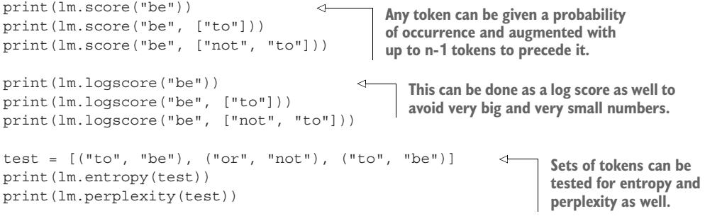

While this code example illustrates creating a trigram language model, unfortunately, not all phrases needing to be captured are only three tokens long. For example, from Hamlet, “To be or not to be” consists of one phrase with two words and one phrase with four words. Note that even though N-grams are typically very small language models, it is possible to make an N-gram LLM by making N=1,000,000,000 or higher, but don’t expect to get even one ounce of use out of it. Just because we made it big doesn’t make it better or mean it’ll have any practical application: 99.9% of all text and 100% of all meaningful text contains fewer than 1 billion tokens appearing more than once, and that computational power can be much better spent elsewhere.

N-grams only use static signals (whitespace, orthography) and words to extract meaning (figure 2.2). They try to measure phrases manually, assuming all phrases will be the same length. That said, N-grams can be used to create powerful baselines for text analysis. In addition, if the analyst already knows the pragmatic context of the utterance, N-grams can give quick and accurate insight into real-world scenarios. Nonetheless, this type of phrasal modeling fails to capture any semantic encodings that individual words could have. To solve this problem, Bayesian statistics were applied to language modeling.

2.2.2 Bayesian techniques

Bayes’ theorem is one of the most mathematically sound and simple theories for describing the occurrence of your output within your input space. Essentially, it calculates the probability of an event occurring based on prior knowledge. The theorem posits that the probability of a hypothesis being true given evidence—for example, that a sentence has a positive sentiment—is equal to the probability of the evidence occurring given the hypothesis is true multiplied by the probability of the hypothesis occurring, all divided by the probability of the evidence being true. It can be expressed mathematically as

\[P(hyplushes \mid evidence) = (P(evidence \mid hyplushesis) \times P(hyplushesis)) \text{ / } P(evidence)\]

or

\[P(A|B) \times P(B) = P(B|A) \times P(A)\]

Because this isn’t a math book, we’ll dive into Bayes’ theorem to the exact same depth we dove into other linguistics concepts and trust the interested reader to search for more.

Unfortunately, even though the theorem represents the data in a mathematically sound way, it doesn’t account for any stochasticity or multiple meanings of words. One word you can always throw at a Bayesian model to confuse it is “it.” Any demonstrative pronoun ends up getting assigned values in the same LogPrior and LogLikelihood way as all other words, and it gets a static value, which is antithetical to the usage of those words. For example, if you’re trying to perform sentiment analysis on an utterance, assigning all pronouns a null value would be better than letting them go through the Bayesian training. Note also that Bayesian techniques don’t create generative language models the way the rest of these techniques will. Because of the nature of Bayes’ theorem validating a hypothesis, these models work for classification and can bring powerful augmentation to a generative language model.

Listing 2.2 shows you how to create a naive Bayes classification language model, or a system that performs classification on text based on a prior-learned internal language model. Instead of using a package like sklearn or something that would make writing the code a little easier, we opted to write out what we were doing, so it’s a bit longer, but it should be more information about how it works. We are using the leastcomplex version of a naive Bayes model. We haven’t made it multinomial or added anything fancy; obviously, it would work better if you opted to upgrade it for any problem you want. And we highly recommend you do.

NOTE To make the code easier to understand and help highlight the portions we wanted to focus on, we have simplified some of our code listings by extracting portions to utility helpers. If you are seeing import errors, this is why. These helper methods can be found in the code repository accompanying this book:https://github.com/IMJONEZZ/LLMs-in-Production/

Listing 2.2 Categorical naive Bayes language model implementation

from utils import process_utt, lookup
from nltk.corpus.reader import PlaintextCorpusReader
import numpy as np
my_corpus = PlaintextCorpusReader("./", ".*\.txt")
sents = my_corpus.sents(fileids="hamlet.txt")
def count_utts(result, utts, ys):
 """
 Input:
 result: a dictionary that is used to map each pair to its frequency
 utts: a list of utts
 ys: a list of the sentiment of each utt (either 0 or 1)

 Output:
 result: a dictionary mapping each pair to its frequency
 """
 for y, utt in zip(ys, utts):
 for word in process_utt(utt):
 pair = (word, y) 
 if pair in result:
 result[pair] += 1 
 else:
 result[pair] = 1 
 return result
result = {}
utts = [" ".join(sent) for sent in sents]
ys = [sent.count("be") > 0 for sent in sents]
count_utts(result, utts, ys)
freqs = count_utts({}, utts, ys)
lookup(freqs, "be", True)
for k, v in freqs.items():
 if "be" in k:
 print(f"{k}:{v}")
def train_naive_bayes(freqs, train_x, train_y):
 """
 Input:
 freqs: dictionary from (word, label) to how often the word appears
 train_x: a list of utts
 train_y: a list of labels correponding to the utts (0,1)
 Output:
 logprior: the log prior.
 loglikelihood: the log likelihood of you Naive bayes equation.
 """
 loglikelihood = {}
 logprior = 0
 vocab = set([pair[0] for pair in freqs.keys()]) 
 V = len(vocab)
 N_pos = N_neg = 0 
 for pair in freqs.keys():
 if pair[1] > 0: 
 N_pos += lookup(freqs, pair[0], True) 
 else: 
 N_neg += lookup(freqs, pair[0], False) 
                                          Defines the key, which is 
                                          the word and label tuple
                                       If the key exists in the dictionary, 
                                       increments the count
                                      If the key is new, adds it to the 
                                      dict and sets the count to 1
                                                            Calculates V, the 
                                                            number of unique 
                                                            words in the 
                                                            vocabulary
                                            Calculates N_pos and N_neg
                                                      If the label is positive 
                                                      (greater than zero) . . .
                                                              . . . increments the 
                                                              number of positive 
                                                              words (word, label)
                                                            Else, the label 
                                                            is negative.
                                    Increments the number of
                                  negative words (word, label)

 D = len(train_y) 
 D_pos = sum(train_y) 
 D_neg = D - D_pos 
 logprior = np.log(D_pos) - np.log(D_neg) 
 for word in vocab: 
 freq_pos = lookup(freqs, word, 1)
 freq_neg = lookup(freqs, word, 0)
 p_w_pos = (freq_pos + 1) / (N_pos + V) 
 p_w_neg = (freq_neg + 1) / (N_neg + V)
 loglikelihood[word] = np.log(p_w_pos / p_w_neg) 
 return logprior, loglikelihood
def naive_bayes_predict(utt, logprior, loglikelihood):
 """
 Input:
 utt: a string
 logprior: a number
 loglikelihood: a dictionary of words mapping to numbers
 Output:
 p: the sum of all the logliklihoods + logprior
 """
 word_l = process_utt(utt) 
 p = 0 
 p += logprior 
 for word in word_l:
 if word in loglikelihood: 
 p += loglikelihood[word] 
 return p
def test_naive_bayes(test_x, test_y, logprior, loglikelihood):
 """
 Input:
 test_x: A list of utts
 test_y: the corresponding labels for the list of utts
 logprior: the logprior
 loglikelihood: a dictionary with the loglikelihoods for each word
 Output:
 accuracy: (# of utts classified correctly)/(total # of utts)
 """
 accuracy = 0 
                                 Calculates D, the number of documents
                                    Calculates the number of positive documents
                                  Calculates the number of negative documents
                                                       Calculates logprior
                                                 For each word in 
                                                 the vocabulary . . .
                                                          . . . calculates the probability 
                                                          that each word is positive or 
                                                          negative
                                                                  Calculates the 
                                                                  log likelihood 
                                                                  of the word
                                         Processes the utt to 
                                         get a list of words
                       Initializes probability to zero
                               Adds the logprior
                                                  Checks if the word exists in 
                                                  the loglikelihood dictionary
                                                Adds the log likelihood of 
                                                that word to the probability
                              Returns this properly

 y_hats = []
 for utt in test_x:
 if naive_bayes_predict(utt, logprior, loglikelihood) > 0: 
 y_hat_i = 1 
 else:
 y_hat_i = 0 
 y_hats.append(y_hat_i) 
 error = sum(
 [abs(y_hat - test) for y_hat, test in zip(y_hats, test_y)]
 ) / len(y_hats) 
 accuracy = 1 - error 
 return accuracy
if __name__ == "__main__":
 logprior, loglikelihood = train_naive_bayes(freqs, utts, ys)
 print(logprior)
 print(len(loglikelihood))
 my_utt = "To be or not to be, that is the question."
 p = naive_bayes_predict(my_utt, logprior, loglikelihood)
 print("The expected output is", p)
 print(
 f"Naive Bayes accuracy = {test_naive_bayes(utts, ys, logprior, 
     loglikelihood):0.4f}
 )
                                                      If the prediction is > 0 . . .
                                                . . . the predicted class is 1.
                                      Otherwise, the predicted class is 0.
                                        Appends the predicted class to the list y_hats
                                         Error = avg of the abs vals of the 
                                         diffs between y_hats and test_y.
                                     Accuracy is 1 minus the error.

This theorem doesn’t create the same type of language model but one with a list of probabilities associated with one hypothesis. As such, Bayesian language models can’t be used effectively to generate language, but they can be very powerfully implemented for classification tasks. In our opinion, though, Bayesian models are often overhyped for even this task. One of the crowning achievements of one author’s career was replacing and removing a Bayesian model from production.

In Bayesian models, one big problem is that all sequences are completely unconnected, like BoW models, moving us to the opposite end of sequence modeling from N-grams. Like a pendulum, language modeling swings back toward sequence modeling and language generation with Markov chains.

2.2.3 Markov chains

Often called hidden Markov models (HMMs), Markov chains essentially add state to the N-gram models, storing probabilities using hidden states. They are often used to help parse text data for even larger models, doing things like part-of-speech (PoS) tagging (marking words with their parts of speech) and named entity recognition (NER; marking identifying words with their referent and usually type; e.g., LA – Los

Angeles – City) on textual data. Building on the previous Bayesian models, Markov models rely completely on stochasticity (predictable randomness) in the tokens encountered. The idea that the probability of anything happening next depends completely upon the state of now is, like Bayes’ theorem, mathematically sound. So instead of modeling words based solely on their historical occurrence and drawing a probability from that, we model their future and past collocation based on what is currently occurring. So the probability of “happy” occurring goes down to almost zero if “happy” was just output but goes up significantly if “am” has just occurred. Markov chains are so intuitive that they were incorporated into later iterations of Bayesian statistics and are still used in production systems today.

In listing 2.3, we train a Markov chain generative language model. This is the first model where we’ve used a specific tokenizer, which, in this case, will tokenize based on the whitespace between words. This is also only the second time we’ve referred to a collection of utterances meant to be viewed together as a document. As you play around with this one, pay close attention and make some comparisons yourself of how well the HMM generates compared to even a large N-gram model.

import re import random from nltk.tokenize import word_tokenize from collections import defaultdict, deque class MarkovChain: def __init__(self): self.lookup_dict = defaultdict(list) self._seeded = False self.__seed_me() def __seed_me(self, rand_seed=None): if self._seeded is not True: try: if rand_seed is not None: random.seed(rand_seed) else: random.seed() self._seeded = True except NotImplementedError: self._seeded = False def add_document(self, str): preprocessed_list = self._preprocess(str) pairs = self.__generate_tuple_keys(preprocessed_list) for pair in pairs: self.lookup_dict[pair[0]].append(pair[1]) Listing 2.3 Generative hidden Markov language model implementation

 def _preprocess(self, str):
 cleaned = re.sub(r"\W+", " ", str).lower()

 tokenized = word_tokenize(cleaned)
 return tokenized
 def __generate_tuple_keys(self, data):
 if len(data) < 1:
 return
 for i in range(len(data) - 1):
 yield [data[i], data[i + 1]]
 def generate_text(self, max_length=50):
 context = deque()
 output = []
 if len(self.lookup_dict) > 0:
 self.__seed_me(rand_seed=len(self.lookup_dict))
 chain_head = [list(self.lookup_dict)[0]]
 context.extend(chain_head)
 while len(output) < (max_length - 1):
 next_choices = self.lookup_dict[context[-1]]
 if len(next_choices) > 0:
 next_word = random.choice(next_choices)
 context.append(next_word)
 output.append(context.popleft())
 else:
 break
 output.extend(list(context))
 return " ".join(output)
if __name__ == "__main__":
 with open("hamlet.txt", "r", encoding="utf-8") as f:
 text = f.read()
 HMM = MarkovChain()
 HMM.add_document(text)
 print(HMM.generate_text(max_length=25))

This code shows a basic implementation of a Markov model for generation, and we encourage you to experiment with it. Give it text from songs from your favorite musicians or books from your favorite authors, and see whether what comes out sounds like them. HMMs are incredibly fast and are often used in predictive text or predictive search applications. Markov models represent the first comprehensive attempt to model language from a descriptive linguistic perspective, as opposed to a prescriptive one. The perspective is interesting because Markov did not originally intend to use linguistic modeling, only to win an argument about continuous independent states. Later, Markov used Markov chains to model vowel distribution in a Pushkin novel, so he was at least aware of the possible applications.

The difference between descriptive and prescriptive linguistics is that the latter focuses on how things ought to be, while the former focuses on how things are. From a language modeling perspective, it has proven vastly more effective to describe what language is doing from a corpus or Markov perspective rather than to attempt to prescribe how language ought to behave. Unfortunately, a current state by itself cannot be used to give context beyond the now, so historical or societal context cannot be represented effectively in a Markov model. The semantic encoding of words also becomes problematic, as represented in the code example: Markov chains will output syntactically correct chains of words that are nonsense semantically, similar to “colorless green ideas sleep furiously.” To solve this problem, “continuous” models were developed to allow for a “semantic embedding” representation of tokens.

2.2.4 Continuous language modeling

A continuous bag-of-words (CBoW) model—much like its namesake, the BoW model is a frequency-based approach to analyzing language, meaning that it models words based on how often they occur. The next word in a human utterance has never been determined based on probability or frequency. Consequently, we provide an example of creating word embeddings to be ingested or compared by other models using a CBoW. We’ll use a neural network to provide you with a good methodology.

This is the first language modeling technique we’ll see that essentially slides a context window over a given utterance (the context window is an N-gram model) and attempts to guess the word in the middle based on the surrounding words in the window. For example, let’s say your window has a length of 5, and your sentence is “Learning about linguistics makes me happy.” You would give the CBoW [‘learning’, ‘about’, ‘makes’, ‘me’] to try to get the model to guess “linguistics” based on how many times the model has previously seen that word occur in similar places. This example shows you why generation is difficult for models trained like this. Say you give the model [‘makes’, ‘me’, ‘’] as input. Now the model only has three pieces of information, instead of four, to use to try to figure out the answer; it also will be biased toward only guessing words it has seen before at the end of sentences, as opposed to getting ready to start new clauses. It’s not all bad, though. One feature that makes continuous models stand out for embeddings is that they don’t have to look at only words before the target word; they can also use words that come after the target to gain some semblance of context.

In listing 2.4, we create our first continuous model. In our case, to keep things as simple as possible, we use a BoW model for the language processing and a one-layer neural network with two parameters for the embedding estimation, although both could be substituted for any other models. For example, you could substitute N-grams for the BoW and a naive Bayes model for the neural network to get a continuous naive N-gram model. The point is that the actual models used in this technique are a bit arbitrary; it’s the continuous technique that’s important. To illustrate this further, we don’t use any packages other than numpy to do the math for the neural network, even though it’s the first one appearing in this section.

Pay special attention to the steps—initializing the model weights, the rectified linear unit (ReLU) activation function, the final softmax layer, and forward and

backpropagation—and how it all fits together in the gradient_descent function. These are pieces of the puzzle that you will see crop up again and again, regardless of programming language or framework. You will need to initialize models, pick activation functions, pick final layers, and define forward and backward propagation in TensorFlow, PyTorch, and Hugging Face, as well as if you ever start creating your own models instead of using someone else’s.

import nltk
import numpy as np
from utils import get_batches, compute_pca, get_dict
import re
from matplotlib import pyplot
with open("hamlet.txt", "r", encoding="utf-8") as f:
 data = f.read() 

data = re.sub(r"[,!?;-]", ".", data) 
data = nltk.word_tokenize(data)
data = [ch.lower() for ch in data if ch.isalpha() or ch == "."]
print("Number of tokens:", len(data), "\n", data[500:515])
fdist = nltk.FreqDist(word for word in data) 
print("Size of vocabulary:", len(fdist))
print("Most Frequent Tokens:", fdist.most_common(20))
word2Ind, Ind2word = get_dict(data) 
V = len(word2Ind)
print("Size of vocabulary:", V)
print("Index of the word 'king':", word2Ind["king"])
print("Word which has index 2743:", Ind2word[2743])
def initialize_model(N, V, random_seed=1): 
 """
 Inputs:
 N: dimension of hidden vector
 V: dimension of vocabulary
 random_seed: seed for consistent results in tests
 Outputs:
 W1, W2, b1, b2: initialized weights and biases
 """
 np.random.seed(random_seed)
 W1 = np.random.rand(N, V)
 W2 = np.random.rand(V, N)
 b1 = np.random.rand(N, 1)
 b2 = np.random.rand(V, 1)
 return W1, W2, b1, b2
  Listing 2.4 Generative CBoW language model implementation
                                                            Creates our corpus 
                                                            for training
                                                              Slightly cleans the data by 
                                                              removing punctuation, 
                                                              tokenizing by word, and 
                                                              converting to lowercase 
                                                              alpha characters
                                                        Gets our bag of words, 
                                                        along with a distribution
                                                 Creates two dictionaries to speed 
                                                 up time-to-convert and keep 
                                                 track of vocabulary
                                                        Here, we create our neural 
                                                        network with one layer and 
                                                        two parameters.

def softmax(z): 
 """
 Inputs:
 z: output scores from the hidden layer
 Outputs:
 yhat: prediction (estimate of y)
 """
 yhat = np.exp(z) / np.sum(np.exp(z), axis=0)
 return yhat
def forward_prop(x, W1, W2, b1, b2): 
 """
 Inputs:
 x: average one-hot vector for the context
 W1,W2,b1,b2: weights and biases to be learned
 Outputs:
 z: output score vector
 """
 h = W1 @ x + b1
 h = np.maximum(0, h)
 z = W2 @ h + b2
 return z, h
def compute_cost(y, yhat, batch_size): 
 logprobs = np.multiply(np.log(yhat), y) + np.multiply(
 np.log(1 - yhat), 1 - y
 )
 cost = -1 / batch_size * np.sum(logprobs)
 cost = np.squeeze(cost)
 return cost
def back_prop(x, yhat, y, h, W1, W2, b1, b2, batch_size): 
 """
 Inputs:
 x: average one hot vector for the context
 yhat: prediction (estimate of y)
 y: target vector
 h: hidden vector (see eq. 1)
 W1, W2, b1, b2: weights and biases
 batch_size: batch size
 Outputs:
 grad_W1, grad_W2, grad_b1, grad_b2: gradients of weights and biases
 """
 l1 = np.dot(W2.T, yhat - y)
 l1 = np.maximum(0, l1)
 grad_W1 = np.dot(l1, x.T) / batch_size
 grad_W2 = np.dot(yhat - y, h.T) / batch_size
 grad_b1 = np.sum(l1, axis=1, keepdims=True) / batch_size
 grad_b2 = np.sum(yhat - y, axis=1, keepdims=True) / batch_size
 return grad_W1, grad_W2, grad_b1, grad_b2
def gradient_descent(data, word2Ind, N, V, num_iters, alpha=0.03): 
 """
 This is the gradient_descent function
                          Creates our final classification layer, 
                          which makes all possibilities add up to 1
                                               Defines the behavior for moving 
                                               forward through our model, along 
                                               with an activation function
                                                    Define how we determine 
                                                    the distance between 
                                                    ground truth and model 
                                                    predictions
                                                                Defines how we 
                                                                move backward 
                                                                through the 
                                                                model and 
                                                                collect 
                                                                gradients
                                                            Puts it all together
                                                                  and trains

 Inputs:
 data: text
 word2Ind: words to Indices
 N: dimension of hidden vector
 V: dimension of vocabulary
 num_iters: number of iterations
 Outputs:
 W1, W2, b1, b2: updated matrices and biases
 """
 W1, W2, b1, b2 = initialize_model(N, V, random_seed=8855)
 batch_size = 128
 iters = 0
 C = 2
 for x, y in get_batches(data, word2Ind, V, C, batch_size):
 z, h = forward_prop(x, W1, W2, b1, b2)
 yhat = softmax(z)
 cost = compute_cost(y, yhat, batch_size)
 if (iters + 1) % 10 == 0:
 print(f"iters: {iters+1} cost: {cost:.6f}")
 grad_W1, grad_W2, grad_b1, grad_b2 = back_prop(
 x, yhat, y, h, W1, W2, b1, b2, batch_size
 )
 W1 = W1 - alpha * grad_W1
 W2 = W2 - alpha * grad_W2
 b1 = b1 - alpha * grad_b1
 b2 = b2 - alpha * grad_b2
 iters += 1
 if iters == num_iters:
 break
 if iters % 100 == 0:
 alpha *= 0.66
 return W1, W2, b1, b2
C = 2 
N = 50
word2Ind, Ind2word = get_dict(data)
V = len(word2Ind)
num_iters = 150
print("Call gradient_descent")
W1, W2, b1, b2 = gradient_descent(data, word2Ind, N, V, num_iters)
# Call gradient descent
# Iters: 10 loss: 0.525015
# Iters: 20 loss: 0.092373
# Iters: 30 loss: 0.050474
# Iters: 40 loss: 0.034724
# Iters: 50 loss: 0.026468
# Iters: 60 loss: 0.021385
# Iters: 70 loss: 0.017941
# Iters: 80 loss: 0.015453
# Iters: 90 loss: 0.012099
# Iters: 100 loss: 0.012099
# Iters: 110 loss: 0.011253
# Iters: 120 loss: 0.010551
                            Trains the model

# Iters: 130 loss: 0.009932
# Iters: 140 loss: 0.009382
# Iters: 150 loss: 0.008889

The CBoW example is our first code example to showcase a full and effective training loop in machine learning. Within all of that, pay special attention to the steps in a training loop, especially the activation function, ReLU. As we expect you to be at least familiar with various ML paradigms, including different activations, we won’t explain the ReLU here. We will address when you should use it and when you shouldn’t. ReLUs, while solving the vanishing gradient problem, don’t solve the exploding gradient problem, and they destroy all negative comparisons within the model. Better situational variants include the Exponential linear unit (ELU), which allows negative numbers to normalize to alpha, and the generalized Gaussian linear units (GEGLU)/Swish-gated linear unit (SWIGLU), which works well in increasingly perplexing scenarios, like language. However, people often use ReLUs, not because they are the best in a situation, but because they are easy to understand and code and intuitive, even more so than the activations they were created to replace, the sigmoid or tanh.

A lot of this ends up being abstracted with packages and the like, but knowing what’s going on under the hood will be very helpful for you as someone putting LLMs in production. You should be able to predict with some certainty how different models will behave in various situations. The next section will dive into one of those abstractions—in this case, the abstraction created by the continuous modeling technique.

2.2.5 Embeddings

Hearkening back to our features of language, it should be easy to connect why continuous-style language modeling was such a breakthrough. Embeddings take the tokenized vectors we’ve created that don’t contain any meaning and attempt to insert that meaning based on observations that can be made about the text, such as word order and subwords appearing in similar contexts. Despite the primary mode of meaning being collocation (co-located, words that appear next to each other), they prove useful and even show some similarities to human-encoded word meaning.

The quintessential example from Word2Vec, one of the first pretrained vector embeddings, was taking the vector for “king,” subtracting the vector for “man,” adding the vector for “woman,” and finding the nearest neighbor to the sum was the vector for the word “queen.” This makes sense to us, as it mimics human semantics. One of the major differences is one that’s already been mentioned a couple of times: pragmatics. Humans use pragmatic context to inform semantic meaning, understanding that just because you said, “I need food,” doesn’t mean you are actually in physical danger without it. Embeddings are devoid of any influence outside of pure usage, which feels like it could be how humans learn as well, and there are good arguments on all sides here. The one thing holding is that if we can somehow give models more representative data, that may open the door to more effective embeddings, but it’s a chicken-and-egg problem because more effective embeddings give better model performance.

In listing 2.5, we dive into how to visualize embeddings using pyplot. We will be going more in depth into embeddings in later chapters. This is helpful for model explainability and also for validation during your pretraining step. If you see that your semantically similar embeddings are relatively close to each other on the graph, you’re likely going in the right direction.

words = [ 
 "King",
 "Queen",
 "Lord",
 "Man",
 "Woman",
 "Prince",
 "Ophelia",
 "Rich",
 "Happy",
] 
embs = (W1.T + W2) / 2.0
idx = [word2Ind[word] for word in words]
X = embs[idx, :]
print(X.shape, idx)
result = compute_pca(X, 2)
pyplot.scatter(result[:, 0], result[:, 1])
for i, word in enumerate(words):
 pyplot.annotate(word, xy=(result[i, 0], result[i, 1]))
pyplot.show()
  Listing 2.5 Embedding visualization
                     After listing 2.4 is done 
                     and gradient descent 
                     has been executed

As shown in figure 2.4, this code is a successful but very sparse embedding representation that we trained from our CBoW model. Getting those semantic representations (embeddings) to be denser is the main place we can see improvement in this field, although many successful experiments have been run where denser semantic meaning has been supplanted with greater pragmatic context through instruct and different thought-chaining techniques. We will address chain of thought (CoT) and other techniques later. For now, let’s pivot to discussing why our continuous embedding technique can even be successful, given that frequency-based models are characteristically difficult to correlate with reality. All of this started with the MLP more than half a century ago.

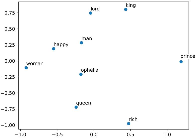
Figure 2.4 A visualization technique for word embeddings. Visualizing embeddings can be important for model explainability.

2.2.6 Multilayer perceptrons

MLPs are the embodiment of the sentiment, “Machines are really good at doing one thing, so I wish we could just use a bunch of machines that are really good at the one thing to make one that’s good at a lot of things.” Every weight and bias in the neural network of the MLP is good at doing one thing, which could be detecting one or more features. So we bind a bunch of them together to detect larger, more complex features. MLPs serve as the primary building block in most neural network architectures. The key distinctions between architectures, such as convolutional neural networks and recurrent neural networks, mainly arise from data loading methods and the handling of tokenized and embedded data as it flows through the layers of the model rather than the functionality of individual layers, particularly the fully connected layers.

Listing 2.6 provides a more dynamic class of neural networks that can have as many layers and parameters as deemed necessary for your task. We give a more defined and explicit class using PyTorch to give you the tools to implement the MLP in whatever way you’d like, both from scratch and in a popular framework.

Listing 2.6 Multilayer perceptron PyTorch class implementation

import torch
import torch.nn as nn
import torch.nn.functional as F

class MultiLayerPerceptron(nn.Module):
 def __init__(
 self,
 input_size,
 hidden_size=2,
 output_size=3,
 num_hidden_layers=1,
 hidden_activation=nn.Sigmoid,
 ):
 """Initialize weights.
 Args:
 input_size (int): size of the input
 hidden_size (int): size of the hidden layers
 output_size (int): size of the output
 num_hidden_layers (int): number of hidden layers
 hidden_activation (torch.nn.*): the activation class
 """
 super(MultiLayerPerceptron, self).__init__()
 self.module_list = nn.ModuleList()
 interim_input_size = input_size
 interim_output_size = hidden_size
 torch.device("cuda:0" if torch.cuda.is_available() else "cpu")
 for _ in range(num_hidden_layers):
 self.module_list.append(
 nn.Linear(interim_input_size, interim_output_size)
 )
 self.module_list.append(hidden_activation())
 interim_input_size = interim_output_size
 self.fc_final = nn.Linear(interim_input_size, output_size)
 self.last_forward_cache = []
 def forward(self, x, apply_softmax=False):
 """The forward pass of the MLP
 Args:
 x_in (torch.Tensor): an input data tensor.
 x_in.shape should be (batch, input_dim)
 apply_softmax (bool): a flag for the softmax activation
 should be false if used with the Cross Entropy losses
 Returns:
 the resulting tensor. tensor.shape should be (batch, output_dim)
 """
 for module in self.module_list:
 x = module(x)
 output = self.fc_final(x)
 if apply_softmax:
 output = F.softmax(output, dim=1)
 return output

From this code, we can see, as opposed to the CBoW implementation, which had two static layers, that this MLP is not static in size until it has been instantiated. If you wanted to give this model 1 million layers, you would have to put num_hidden_layers= 1000000 when you instantiate the class. However, just because you give a model that many parameters doesn’t mean that will make it immediately better. LLMs are more than just a lot of layers. Like RNNs and CNNs, the magic of LLMs is in how data goes in and moves through the model. To illustrate, let’s look at the RNN and one of its variations.

2.2.7 Recurrent neural networks and long short-term memory networks

RNNs are a class of neural networks designed to analyze sequences based on the weaknesses in previous language modeling techniques. A sequence can be thought of as an ordered array, where the sum of the whole array changes value if any of the parts are moved around. The logic goes that if language is presented in a sequence, then maybe it should be processed in a sequence instead of one token at a time. RNNs accomplish this by using logic we’ve seen before, both in MLPs and Markov chains, where an internal state or memory is referred to when new inputs are processed and by creating cycles when connections between nodes are detected as useful.

In fully recurrent networks, like the one in listing 2.7, all nodes start out initially connected to all subsequent nodes, but those connections can be set to zero to simulate them breaking if they are not useful. This solves one of the biggest problems that earlier models suffered from, static input size, and enables an RNN and its variants to process variable length inputs. Unfortunately, longer sequences create a new problem. Because each neuron in the network connects to subsequent neurons, longer sequences create smaller changes to the overall sum, making the gradients smaller until they eventually vanish, even with important words; this is called a vanishing gradient. Other problems exist too, such as exploding and diminishing gradients.

For example, let’s consider the following sentences with the task sentiment analysis: “I loved the movie last night” and “The movie I went to see last night was the very best I had ever expected to see.” These sentences can be considered semantically similar, even if they aren’t exactly the same. When moving through an RNN, each word in the first sentence is worth more, and the consequence is that the first sentence has a higher positive rating than the second sentence just because the first sentence is shorter. The inverse is also true: exploding gradients are a consequence of this sequence processing, which makes training deep RNNs difficult.

To solve this problem, LSTMs, a type of RNN, use memory cells and gating mechanisms to process sequences of variable length but without the problem of comprehending longer and shorter sequences differently. Anticipating multilingual scenarios and understanding that people don’t think about language in only one direction, LSTMs can also process sequences bidirectionally by concatenating the outputs of two RNNs, one reading the sequence from left to right and the other from right to left. This bidirectionality improves results, allowing information to be seen and remembered even after thousands of tokens have passed.

In listing 2.7, we give classes for both an RNN and an LSTM. In the code in the repo associated with this book (https://github.com/IMJONEZZ/LLMs-in-Production), you can see the results of training both the RNN and LSTM. The takeaway is that the LSTM achieves better accuracy on both training and validation sets in half as many epochs (25 versus 50 with RNN). One of the innovations to note is that the packed embeddings utilize padding to extend all variable-length sequences to the maximum length. Thus, LSTMs can process input of any length as long as it is shorter than the maximum. To set up the LSTM effectively, we’ll do some classical NLP on the dataset (a Twitter sentiment analysis dataset). That workflow will tokenize with the Natural Language Toolkit Regex. It looks for words and nothing else, passing into a spacy lemmatizer to get a list of lists containing only the base unconjugated forms of words.

Listing 2.7 RNN and LSTM PyTorch class implementations

import torch
import pandas as pd
import numpy as np
from gensim.models import Word2Vec
from sklearn.model_selection import train_test_split
import nltk
import spacy
 tokenizer = nltk.tokenize.RegexpTokenizer("\w+'?\w+|\w+'")
 tokenizer.tokenize("This is a test")
 stop_words = nltk.corpus.stopwords.words("english")
 nlp = spacy.load("en_core_web_lg", disable=["parser", "tagger", "ner"])
dataset = pd.read_csv("./data/twitter.csv") 
text_data = list(
 map(lambda x: tokenizer.tokenize(x.lower()), dataset["text"])
)
text_data = [
 [token.lemma_ for word in text for token in nlp(word)]
 for text in text_data
]
label_data = list(map(lambda x: x, dataset["feeling"]))
assert len(text_data) == len(
 label_data
), f"{len(text_data)} does not equal {len(label_data)}"
EMBEDDING_DIM = 100
model = Word2Vec(
 text_data, vector_size=EMBEDDING_DIM, window=5, min_count=1, workers=4
)
word_vectors = model.wv
print(f"Vocabulary Length: {len(model.wv)}")
del model
                                                       Creates our corpus for 
                                                       training and performs some 
                                                       classic NLP preprocessing

padding_value = len(word_vectors.index_to_key)
 embedding_weights = torch.Tensor(word_vectors.vectors) 
class RNN(torch.nn.Module):
 def __init__(
 self,
 input_dim,
 embedding_dim,
 hidden_dim,
 output_dim,
 embedding_weights,
 ):
 super().__init__()
 self.embedding = torch.nn.Embedding.from_pretrained(
 embedding_weights
 )
 self.rnn = torch.nn.RNN(embedding_dim, hidden_dim)
 self.fc = torch.nn.Linear(hidden_dim, output_dim)
 def forward(self, x, text_lengths):
 embedded = self.embedding(x)
 packed_embedded = torch.nn.utils.rnn.pack_padded_sequence(
 embedded, text_lengths
 )
 packed_output, hidden = self.rnn(packed_embedded)
 output, output_lengths = torch.nn.utils.rnn.pad_packed_sequence(
 packed_output
 )
 return self.fc(hidden.squeeze(0))
INPUT_DIM = padding_value
EMBEDDING_DIM = 100
HIDDEN_DIM = 256
OUTPUT_DIM = 1
rnn_model = RNN(
 INPUT_DIM, EMBEDDING_DIM, HIDDEN_DIM, OUTPUT_DIM, embedding_weights
)
rnn_optimizer = torch.optim.SGD(rnn_model.parameters(), lr=1e-3)
rnn_criterion = torch.nn.BCEWithLogitsLoss()
device = torch.device("cuda" if torch.cuda.is_available() else "cpu")
class LSTM(torch.nn.Module):
 def __init__(
 self,
 input_dim,
 embedding_dim,
 hidden_dim,
 output_dim,
 n_layers,
 bidirectional,
                                                            Embeddings are 
                                                            needed to give 
                                                            semantic value 
                                                            to the inputs of 
                                                            an LSTM.

 dropout,
 embedding_weights,
 ):
 super().__init__()
 self.embedding = torch.nn.Embedding.from_pretrained(
 embedding_weights
 )
 self.rnn = torch.nn.LSTM(
 embedding_dim,
 hidden_dim,
 num_layers=n_layers,
 bidirectional=bidirectional,
 dropout=dropout,
 )
 self.fc = torch.nn.Linear(hidden_dim * 2, output_dim)
 self.dropout = torch.nn.Dropout(dropout)
 def forward(self, x, text_lengths):
 embedded = self.embedding(x)
 packed_embedded = torch.nn.utils.rnn.pack_padded_sequence(
 embedded, text_lengths
 )
 packed_output, (hidden, cell) = self.rnn(packed_embedded)
 hidden = self.dropout(
 torch.cat((hidden[-2, :, :], hidden[-1, :, :]), dim=1)
 )
 return self.fc(hidden.squeeze(0))
INPUT_DIM = padding_value
EMBEDDING_DIM = 100
HIDDEN_DIM = 256
OUTPUT_DIM = 1
N_LAYERS = 2
BIDIRECTIONAL = True
DROPOUT = 0.5
lstm_model = LSTM(
 INPUT_DIM,
 EMBEDDING_DIM,
 HIDDEN_DIM,
 OUTPUT_DIM,
 N_LAYERS,
 BIDIRECTIONAL,
 DROPOUT,
 embedding_weights,
)
lstm_optimizer = torch.optim.Adam(lstm_model.parameters())
lstm_criterion = torch.nn.BCEWithLogitsLoss()
device = torch.device("cuda" if torch.cuda.is_available() else "cpu")
def binary_accuracy(preds, y):
 rounded_preds = torch.round(torch.sigmoid(preds))

 correct = (rounded_preds == y).float()
 acc = correct.sum() / len(correct)
 return acc
def train(model, iterator, optimizer, criterion):
 epoch_loss = 0
 epoch_acc = 0
 model.train()
 for batch in iterator:
 optimizer.zero_grad()
 predictions = model(batch["text"], batch["length"]).squeeze(1)
 loss = criterion(predictions, batch["label"])
 acc = binary_accuracy(predictions, batch["label"])
 loss.backward()
 optimizer.step()
 epoch_loss += loss.item()
 epoch_acc += acc.item()
 return epoch_loss / len(iterator), epoch_acc / len(iterator)
def evaluate(model, iterator, criterion):
 epoch_loss = 0
 epoch_acc = 0
 model.eval()
 with torch.no_grad():
 for batch in iterator:
 predictions = model(batch["text"], batch["length"]).squeeze(1)
 loss = criterion(predictions, batch["label"])
 acc = binary_accuracy(predictions, batch["label"])
 epoch_loss += loss.item()
 epoch_acc += acc.item()
 return epoch_loss / len(iterator), epoch_acc / len(iterator)
batch_size = 2 
def iterator(X, y):
 size = len(X)
 permutation = np.random.permutation(size)
 iterate = []
 for i in range(0, size, batch_size):
 indices = permutation[i : i + batch_size]
 batch = {}
 batch["text"] = [X[i] for i in indices]
 batch["label"] = [y[i] for i in indices]
 batch["text"], batch["label"] = zip(
 *sorted(
 zip(batch["text"], batch["label"]),
 key=lambda x: len(x[0]),
                                             Usually should be a power of 
                                             2 because it's the easiest for 
                                             computer memory

 reverse=True,
 )
 )
 batch["length"] = [len(utt) for utt in batch["text"]]
 batch["length"] = torch.IntTensor(batch["length"])
 batch["text"] = torch.nn.utils.rnn.pad_sequence(
 batch["text"], batch_first=True
 ).t()
 batch["label"] = torch.Tensor(batch["label"])
 batch["label"] = batch["label"].to(device)
 batch["length"] = batch["length"].to(device)
 batch["text"] = batch["text"].to(device)
 iterate.append(batch)
 return iterate
index_utt = [
 torch.tensor([word_vectors.key_to_index.get(word, 0) for word in text])
 for text in text_data
]
X_train, X_test, y_train, y_test = train_test_split(
 index_utt, label_data, test_size=0.2
) 
X_train, X_val, y_train, y_val = train_test_split(
 X_train, y_train, test_size=0.2
)
train_iterator = iterator(X_train, y_train)
validate_iterator = iterator(X_val, y_val)
test_iterator = iterator(X_test, y_test)
print(len(train_iterator), len(validate_iterator), len(test_iterator))
N_EPOCHS = 25
for model in [rnn_model, lstm_model]:
 print(
 "|-----------------------------------------------------------------------
    ------------------|"
 )
 print(f"Training with {model.__class__.__name__}")
 if "RNN" in model.__class__.__name__:
 for epoch in range(N_EPOCHS):
 train_loss, train_acc = train(
 rnn_model, train_iterator, rnn_optimizer, rnn_criterion
 )
 valid_loss, valid_acc = evaluate(
 rnn_model, validate_iterator, rnn_criterion
 )
                                                   You've got to determine 
                                                   some labels for whatever 
                                                   you're training on.

 print(
 f"| Epoch: {epoch+1:02} | Train Loss: {train_loss: .3f} | 
 ➥ Train Acc: {train_acc*100: .2f}% | Validation Loss: 
 ➥ {valid_loss: .3f} | Validation Acc: {valid_acc*100: .2f}% |"
 )
 else:
 for epoch in range(N_EPOCHS):
 train_loss, train_acc = train(
 lstm_model, train_iterator, lstm_optimizer, lstm_criterion
 )
 valid_loss, valid_acc = evaluate(
 lstm_model, validate_iterator, lstm_criterion
 )
 print(
 f"| Epoch: {epoch+1:02} | Train Loss: {train_loss: .3f} | 
 ➥ Train Acc: {train_acc*100: .2f}% | Validation Loss: 
 ➥ {valid_loss: .3f} | Validation Acc: {valid_acc*100: .2f}% |"
 )
# Training on our dataset
# | Epoch: 01 | Train Loss: 0.560 | Train Acc: 70.63% | Validation Loss:
# 0.574 | Validation Acc: 70.88% |
# | Epoch: 05 | Train Loss: 0.391 | Train Acc: 82.81% | Validation Loss:
# 0.368 | Validation Acc: 83.08% |
# | Epoch: 10 | Train Loss: 0.270 | Train Acc: 89.11% | Validation Loss:
# 0.315 | Validation Acc: 86.22% |
# | Epoch: 15 | Train Loss: 0.186 | Train Acc: 92.95% | Validation Loss:
# 0.381 | Validation Acc: 87.49% |
# | Epoch: 20 | Train Loss: 0.121 | Train Acc: 95.93% | Validation Loss:
# 0.444 | Validation Acc: 86.29% |
# | Epoch: 25 | Train Loss: 0.100 | Train Acc: 96.28% | Validation Loss:
# 0.451 | Validation Acc: 86.83% |

Looking at our classes and instantiations, you should see that the LSTM is not vastly different from the RNN. The only difference is that the init input variables are n_layers (for convenience, you can also specify it with RNNs), bidirectional, and dropout. bidirectional allows LSTMs to look ahead in sequences to help with meaning and context. It also helps immensely with multilingual scenarios, as left-to-right languages like English are not the only format for orthography. dropout, another huge innovation, changes the paradigm of overfitting from being data dependent and helps the model not overfit by turning off random nodes layer by layer during training to force all nodes not to correlate with each other and preventing complex co-adaptations. The only difference in the out-of-model parameters is that the optimizer used for an RNN is stochastic gradient descent (SGD), like our CBoW; the LSTM uses Adam (although either could use any, depending on performance, including AdamW). Next, we define our training loop and train the LSTM. Compare this training loop to the one defined in listing 2.4 in the gradient_descent function.

One of the amazing things demonstrated in the code here is how much quicker the LSTM can learn compared to previous model iterations, thanks to both bidirectionality and dropout. Although the previous models train faster than the LSTM, they take hundreds of epochs to get the same performance as an LSTM in just 25 epochs. As its name implies, the performance on the validation set adds validity to the architecture, performing inference during training on examples it has not trained on and keeping accuracy fairly close to the training set.

The problems with these models are not as pronounced, manifesting primarily as being incredibly resource-heavy, especially when applied to longer, more detail-oriented problems like healthcare and law. Despite the incredible advantages of dropout and bidirectional processing, they both at least double the amount of processing power required to train. So while inference ends up being only 2 to 3 times as expensive as an MLP of the same size, training becomes 10 to 12 times as expensive. That is, dropout and bidirectional solve exploding gradients nicely but explode the compute required to train. To combat this problem, a shortcut was devised and implemented that allows any model, including an LSTM, to figure out which parts of a sequence are the most influential and which parts can be safely ignored, known as attention.

2.2.8 Attention

Attention is a mathematical shortcut that gives the model a mechanism for solving larger context windows faster by telling the model through an emergent mathematical formula which parts of an input to consider and how much. Attention is based upon an upgraded version of a dictionary, where instead of just key–value pairs, a contextual query is added. Simply know that the following code is the big differentiator between older NLP techniques and more modern ones.

Attention solves the slowness of training LSTMs yet keeps high performance on a low number of epochs. There are multiple types of attention as well. The dot product attention method captures the relationships between each word (or embedding) in your query and every word in your key. When queries and keys are part of the same sentences, this is known as bi-directional self-attention. However, in certain cases, it is more suitable to only focus on words that precede the current one. This type of attention, especially when queries and keys come from the same sentences, is referred to as causal attention. Language modeling further improves by masking parts of a sequence and forcing the model to guess what should be behind the mask. The functions in the following listing demonstrate both dot product attention and masked attention.

Listing 2.8 Multihead attention implementation

import numpy as np
from scipy.special import softmax
x = np.array([[1.0, 0.0, 1.0, 0.0],
 [0.0, 2.0, 0.0, 2.0],
 [1.0, 1.0, 1.0, 1.0]]) 
w_query = np.array([1,0,1],
 [1,0,0],
 [0,0,1],
                                         Step 1: Input: 
                                         three inputs, 
                                         d_model=4

 [0,1,1]]) 
w_key = np.array([[0,0,1],
 [1,1,0],
 [0,1,0],
 [1,1,0]]) 
w_value = np.array([[0,2,0],
 [0,3,0],
 [1,0,3],
 [1,1,0]]) 
Q = np.matmul(x,w_query) 
K = np.matmul(x,w_key) 
V = np.matmul(x,w_value) 
k_d = 1 
attention_scores = (Q @ K.transpose())/k_d 
attention_scores[0] = softmax(attention_scores[0]) 
attention_scores[1] = softmax(attention_scores[1]) 
attention_scores[2] = softmax(attention_scores[2]) 
attention1 = attention_scores[0].reshape(-1,1) 
attention1 = attention_scores[0][0]*V[0] 
attention2 = attention_scores[0][1]*V[1] 
attention3 = attention_scores[0][2]*V[2] 
attention_input1 = attention1 + attention2 + attention3 
attention_head1 = np.random.random((3,64)) 
z0h1 = np.random.random((3,64)) 
z1h2 = np.random.random((3,64)) 
z2h3 = np.random.random((3,64)) 
z3h4 = np.random.random((3,64)) 
z4h5 = np.random.random((3,64)) 
z5h6 = np.random.random((3,64)) 
z6h7 = np.random.random((3,64)) 
z7h8 = np.random.random((3,64)) 
Output_attention = np.hstack((z0h1,z1h2,z2h3,z3h4,z4h5,z5h6,z6h7,z7h8)) 
def dot_product_attention(query, key, value, mask, scale=True): 
 assert query.shape[-1] == key.shape[-1] == value.shape[-1], "q,k,v have 
     different dimensions!"
 if scale:
 depth = query.shape[-1]
 else:
 depth = 1
 dots = np.matmul(query, np.swapaxes(key, -1, -2)) / np.sqrt(depth)
 if mask is not None:
 dots = np.where(mask, dots, np.full_like(dots, -1e9))
 logsumexp = scipy.special.logsumexp(dots, axis=-1, keepdims=True)
 dots = np.exp(dots - logsumexp)
 attention = np.matmul(dots, value)
 return attention
                                    Step 2: Weights 
                                    three dimensions 
                                    x d_model=4
                                Step 3: Matrix multiplication to 
                                obtain Q,K,V; query: x * w_query; 
                                key: x * w_key; value: x * w_value
                                                   Step 4: Scaled attention scores; 
                                                   square root of the dimensions
                                                           Step 5: Scaled softmax 
                                                           attention scores for 
                                                           each vector
                                                        Step 6: Attention value 
                                                        obtained by score1/k_d * V
                                                                  Step 7: Sums the 
                                                                  results to create 
                                                                  the first line of the 
                                                                  output matrix
                                                           Step 8: Steps 1 to 7 for inputs 
                                                           1 to 3; because this is just a 
                                                           demo, we'll do a random matrix 
                                      Step 9: We train all of the right dimensions. eight heads of the 
                                      attention sublayer 
                                      using steps 1 to 7. Step 10: Concatenates
                                                               heads 1 to 8 to get the
                                                               original 8 ! 64 output
                                                              dimension of the model
                                                                       This function
                                                                     performs all of
                                                                       these steps.

def masked_dot_product_self_attention(q,k,v,scale=True): 
 mask_size = q.shape[-2]
 mask = np.tril(np.ones((1, mask_size, mask_size), dtype=np.bool_), k=0)
 return DotProductAttention(q,k,v,mask,scale=scale)
                                                               This function performs
                                                               the previous steps but
                                                            adds causality in masking.

In the full implementation of attention, you may have noticed some terminology you’re familiar with—namely Key and Value, but you may not have been introduced to Query before. Key and Value pairs are familiar because of dictionaries and lookup tables, where we map a set of keys to an array of values. Query should feel intuitive as a sort of search for retrieval. The Query is compared to the Keys from which a Value is retrieved in a normal operation.

In attention, the Query and Keys undergo dot product similarity comparison to obtain an attention score, which is later multiplied by the Value to get an ultimate score for how much attention the model should pay to that portion of the sequence. This can get more complex, depending upon your model’s architecture, because both encoder and decoder sequence lengths have to be accounted for, but suffice it to say for now that the most efficient way to model in this space is to project all input sources into a common space and compare using dot product for efficiency.

This code explanation was a bit more math-heavy than the previous examples, but it is needed to illustrate the concept. The math behind attention is truly innovative and has rocketed the field forward. Unfortunately, even with the advantages attention brings to the process of sequence modeling, with LSTMs and RNNs, there were still problems with speed and memory size. You may notice from the code and the math that a square root is taken, meaning that attention, as we use it, is quadratic. Various techniques, including subquadratics like Hyena and the Recurrent Memory Transformer (RMT, basically an RNN combined with a transformer), have been developed to combat these problems, which we will cover in more detail later. For now, let’s move on to the ultimate application of attention: the transformer.

2.3 Attention is all you need

In the seminal paper, “Attention Is All You Need,”1 Vaswani et al. take the mathematical shortcut several steps further, positing that for performance, absolutely no recurrence (the “R” in RNN) or any convolutions are needed at all.

NOTE We don’t go over convolutions because they aren’t good for NLP, but they are popular, especially in computer vision.

Instead, Vaswani et al. opted to use only attention and specify where Q, K, and V were taken from much more carefully. We’ll dive into this presently. In our review of this diverse range of NLP techniques, we have observed their evolution over time and the

¹ Vaswani et al., 2017, Attention Is All You Need,” https://arxiv.org/abs/1706.03762.

ways in which each approach has sought to improve upon its predecessors. From rule-based methods to statistical models and neural networks, the field has continually strived for more efficient and accurate ways to process and understand natural language.

Now we turn our attention to a groundbreaking innovation that has revolutionized the field of NLP: the transformer architecture. In the following section, we will explore the key concepts and mechanisms that underpin transformers and how they have enabled the development of state-of-the-art language models that surpass the performance of previous techniques. We will also discuss the effect of transformers on the broader NLP landscape and consider the potential for further advancements in this exciting area of research.

2.3.1 Encoders

Encoders are the first half of a full transformer model, excelling in the areas of classification and feature engineering. Vaswani et al. figured out that after the embedding layer inside the encoder, any additional transformations done to the tensors could end up harming their ability to be compared “semantically,” which was the point of the embedding layer. These models rely heavily upon self-attention and clever positional encoding to manipulate those vectors without significantly decreasing the similarity expressed.

Again, a key characteristic of embeddings is that they are vector representations of data—in our case, tokens. Tokens are whatever you pick to represent language. We recommend subwords as a general rule, but you will get a feel for where and which types of tokens work well. Consider the sentence, “The cat in the hat rapidly leapt above the red fox and the brown unmotivated dog.” “Red” and “brown” are semantically similar, and both are similarly represented after the embedding layer. However, they fall on positions 10 and 14, respectively, in the utterance, assuming that we’re tokenizing by word. Therefore, the positional encoding puts distance between them, also adding the ability to distinguish between the same tokens at different positions in an utterance. However, once the sine and cosine functions are applied, it brings their meaning back to only a little further apart than they were after the encoding, and this encoding mechanism scales brilliantly with recurrence and more data. To illustrate, let’s say there was a 99% cosine similarity between [red] and [brown] after embedding. Encoding would drastically reduce that to around 85% to 86% similarity. Applying sine and cosine methodologies as described brings their similarity back up to around 96%.

BERT was one of the first architectures after Vaswani et al.’s original paper and is an example of encoder-only transformers. BERT is such an incredibly powerful model architecture, given how small it is, that it is still used in production systems today. BERT was the first encoder-only transformer to surge in popularity, showcasing that performing continuous or sequential (they’re the same) modeling using a transformer results in much better embeddings than Word2Vec. We can see that these embeddings are better because they can be very quickly applied to new tasks and data with minimal training, with human-preferred results versus Word2Vec embeddings. For a while, most people were using BERT-based models for few-shot learning tasks on smaller datasets. BERT puts state-of-the-art performance within arm’s reach for most researchers and businesses with minimal effort required.

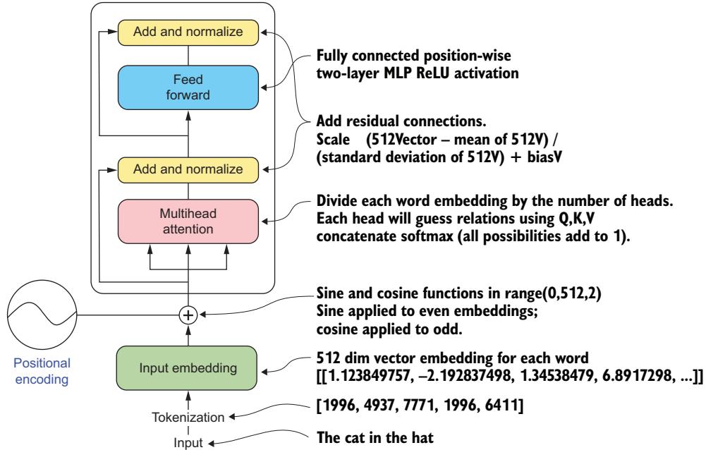
Figure 2.5 An encoder visualized. Encoders are the first half of the full transformer architecture and excel in natural language understanding tasks like classification or named entity recognition. Encoder models improve upon previous designs by not requiring priors or recurrence and using clever positional encoding and multihead attention to create a vector embedding of each token.

The strengths of encoders (visualized in figure 2.5) include the following:

• Classification and hierarchical tasks showcasing understanding
• Blazing fast, considering the long-range dependency modeling
• Builds off of known models, CBoW in embedding, MLP in feed forward, etc.
• Parallel

Encoders weaknesses include the following:

• As suggested, requires lots of data (although less than RNNs) to be effective
• Even more complex architecture

2.3.2 Decoders

Decoder models, as shown in figure 2.6, are larger versions of encoders that have two multihead attention blocks and three sum and normalize layers in their base form. They are the second half of a transformer behind an encoder. Decoders are very good at masked language modeling and learning and applying syntax very quickly, leading to the almost immediate idea that decoder-only models are needed to achieve artificial general intelligence. A useful reduction of encoder versus decoder tasks is that encoders excel in natural language understanding (NLU) tasks, while decoders excel in natural language generation (NLG) tasks. An example of decoder-only transformer architectures is the Generative Pre-trained Transformer (GPT) family of models. These models follow the logic of transformational generative grammar being completely syntax based, allowing for infinite generation of all possible sentences in a language (see appendix A).

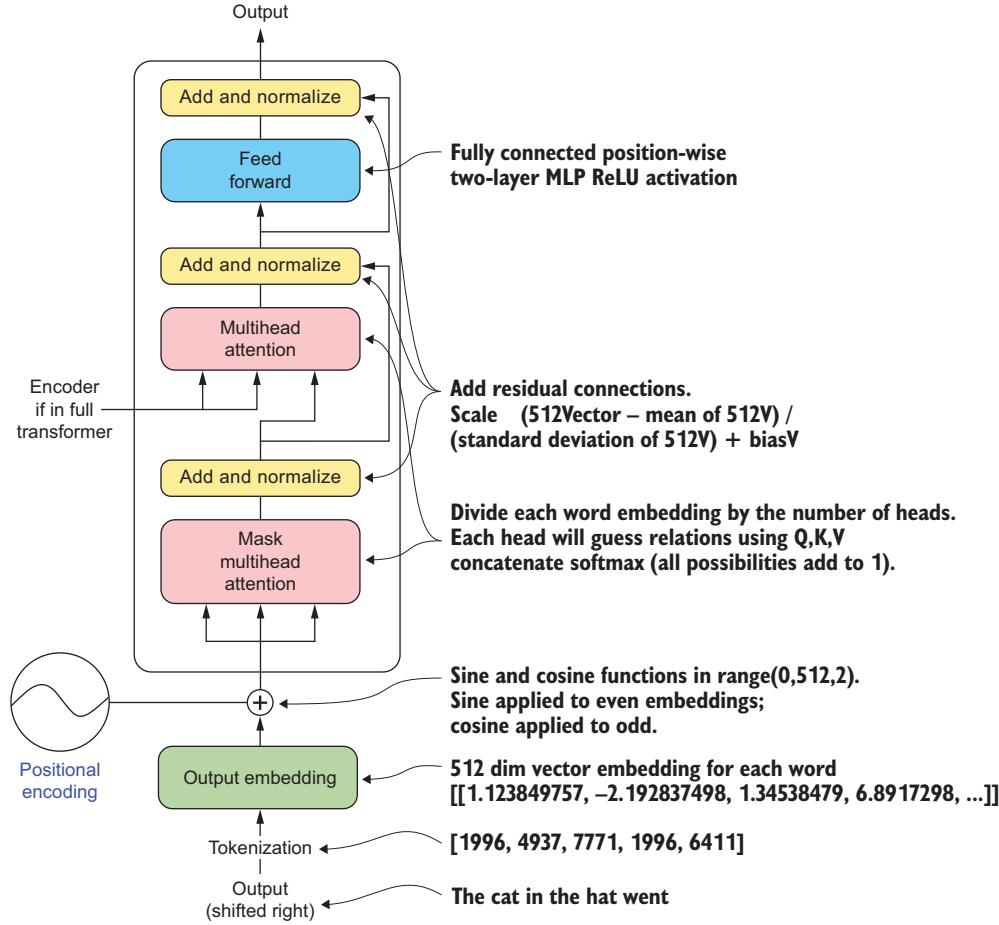
Figure 2.6 A decoder visualized. Decoders are the second half of a full transformer, and they excel at NLG tasks like chatbots and storytelling. Decoders improve upon previous architectures in the same way as encoders, but they shift their output one space to the right for next-word generation to help utilize the advantages of multihead self-attention.

The strengths of decoders include the following:

• Generates the next token in a sequence (shifted right means taking alreadygenerated tokens into account)
• Builds off of both known models and encoders
• Can be streamed during generation for great UX

Their weaknesses include the following:

• Syntax-only models can often struggle to insert the expected or intended meaning (see all “I forced an AI to watch 1000 hours of x and generated” memes from 2018–present).
• Hallucinations.

2.3.3 Transformers

The full transformer architecture takes advantage of both encoders and decoders, passing the understanding of the encoder into the second multihead attention block of the decoder before giving output. As each piece of the transformer has a specialty in either understanding or generation, it should feel intuitive for the full product to be best at conditional generation tasks like translation or summarization, where some level of understanding is required before generation occurs. Encoders are geared toward processing input at a high level, and decoders focus more on generating coherent output. The full transformer architecture can successfully understand the data and then generate the output based on that understanding, as shown in figure 2.7. The Text-To-Text Transfer Transformer (T5) family of models is an example of transformers.

NOTE Transformer models have an advantage in that they are built around the parallelization of inputs, which adds speed that LSTMs can’t currently replicate. If LSTMs ever get to a point where they can run as quickly as transformers, they may become competitive in the state-of-the-art field.

The strengths of a transformer are as follows:

• Includes both an encoder and decoder, so it’s good at everything they are good at
• Highly parallelized for speed and efficiency

Weaknesses include the following:

• Memory intensive, but still less than LSTMs of the same size
• Requires large amounts of data and VRAM for training

As you’ve probably noticed, most of the models we’ve discussed aren’t at all linguistically focused, being heavily syntax-focused, if they even attempt to model real language at all. Models, even state-of-the-art transformers, only have semantic approximations—no pragmatics, no phonetics—and only really utilize a mathematical model of morphology during tokenization without context. This doesn’t mean the models can’t learn these, nor does it mean that, for example, transformers can’t take audio as an input; it

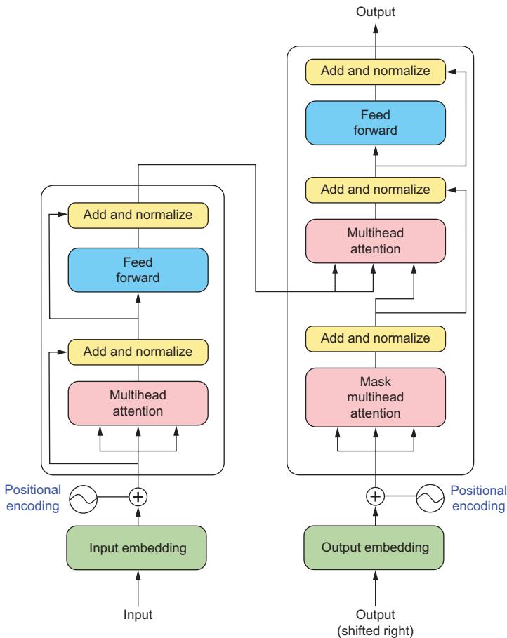
Figure 2.7 A full transformer visualized. A full transformer combines the encoder and the decoder and does well on all of the tasks of each, as well as conditional generation tasks such as summarization and translation. Because transformers are bulkier and slower than each of their halves, researchers and businesses have generally opted to use those halves over the whole transformer.

just means that the average usage doesn’t. With this in mind, it is nothing short of a miracle that they work as well as they do, and they really should be appreciated for what they can do.

So far, we’ve attempted to highlight the current limitations in models, and we will dive into where to improve upon them in the remainder of this book. One such route is one that’s already been, and is still being, explored to great success: transfer learning and finetuning large foundational models. This technique came about soon after BERT’s initial release. Researchers discovered that although BERT generally performed well on a large number of tasks, if they wanted it to perform better on a particular task or data domain, they simply needed to retrain the model on data representative of the

task or domain but not from scratch. Given all of the pretrained weights BERT learned while creating the semantic approximation embeddings on a much larger dataset, significantly less data is required to get state-of-the-art performance on the portion you need. We’ve seen this with BERT and the GPT family of models as they’ve come out, and now we’re seeing it again to solve exactly the challenges we discussed: semantic approximation coverage, domain expertise, and data availability.

2.4 Really big transformers

Enter LLMs. Since their introduction, transformer-based models have continued to get larger and larger, not just in their size and number of parameters but also in the size and length of their training datasets and training cycles. If you studied machine learning or deep learning during the 2010s, you likely heard the moniker, “Adding more layers doesn’t make the model better.” LLMs prove this both wrong and right wrong because their performance is unparalleled, often matching smaller models that have been meticulously finetuned on a particular domain and dataset, even those trained on proprietary data, and right because of the challenges that come with both training and deploying LLMs.

One of the major differences between LLMs and language models involves transfer learning and finetuning. Like previous language models, LLMs are pretrained on massive text corpora, enabling them to learn general language features and representations that can be finetuned for specific tasks. Because LLMs are so massive and their training datasets are so large, they are able to achieve better performance with less labeled data, which was a significant limitation of earlier language models. Often, you can finetune an LLM to do highly specialized tasks with only a dozen or so examples.

However, what makes LLMs so powerful and has opened the door to widespread business use cases is their ability to do specialized tasks using simple prompting without any finetuning. Just give a few examples of what you want in your query, and the LLM can produce results. Training an LLM on a smaller set of labeled data is called few-shot prompting. It’s referred to as one-shot prompting when only one example is given and zero-shot when the task is totally novel. LLMs, especially those trained using reinforcement learning from human feedback and prompt engineering methodologies, can perform few-shot learning, where they can generalize and solve tasks with only a few examples, at a whole new level. This ability is a significant advancement over earlier models that required extensive finetuning or large amounts of labeled data for each specific task.

LMs previously have shown promise in the few and zero-shot learning domains, and LLMs have proven that promise to be true. As models have gotten larger, we find they are capable of accomplishing tasks smaller models can’t. We call this emergent behavior. 2 Figure 2.8 illustrates eight different tasks previous language models couldn’t perform better than at random, and then once the models got large enough, they could.

² J. Wei et al., “Emergent abilities of large language models,” Transactions on Machine Learning Research, Aug. 2022,https://openreview.net/forum?id=yzkSU5zdwD.

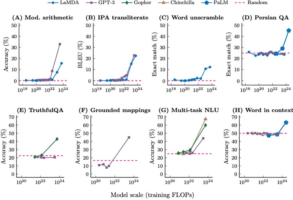
Figure 2.8 Examples of LLMs demonstrating emergent behaviors when given few-shot prompting tasks after the model scale reaches a certain size

LLMs also have demonstrably great zero-shot capabilities due to their vast parameter sizes, which is the main reason for their popularity and viability in the business world. LLMs also exhibit improved handling of ambiguity due to their large size and capacity. They are better at disambiguating words with multiple meanings and understanding the nuances of language, resulting in more accurate predictions and responses. This improvement isn’t because of better ability or architecture, as they share their architecture with smaller transformers, but because they have vastly more examples of how people generally disambiguate. LLMs, therefore, respond with the same disambiguation as is generally represented in the dataset. Thanks to the diverseness of the text data on which LLMs are trained, they exhibit increased robustness in handling various input styles, noisy text, and grammatical errors.

Another key difference between LLMs and language models is input space. A larger input space is important since it makes few-shot prompting tasks that much more viable. Many LLMs have max input sizes of 8,000+ tokens (originally 32K, GPT-4 has sported 128K since November 2023), and while all the previously discussed models could also have input spaces that high, they generally don’t. We have recently seen a boom in this field, with techniques like Recurrent Memory Transformer (RMT) allowing 1M+ token context spaces, which rocket LLMs even more toward proving that bigger models are always better. LLMs are designed to capture long-range dependencies within text, allowing them to understand context more effectively than their predecessors. This improved understanding enables LLMs to generate more coherent and contextually relevant responses in tasks like machine translation, summarization, and conversational AI.

LLMs have revolutionized NLP by offering powerful solutions to problems that were challenging for earlier language models. They bring substantial improvements in contextual understanding, transfer learning, and few-shot learning. As the field of NLP continues to evolve, researchers are actively working to maximize the benefits of LLMs while mitigating all potential risks. Because a better way to approximate semantics hasn’t been found, they make bigger and more dimensional approximations. Because a good way of storing pragmatic context hasn’t been found, LLMs often allow inserting context into the prompt directly, into a part of the input set aside for context, or even through sharing databases with the LLM at inference. This capability doesn’t create pragmatics or a pragmatic system within the models, in the same way that embeddings don’t create semantics, but it allows the model to correctly generate syntax that mimics how humans respond to those pragmatic and semantic stimuli. Phonetics is a place where LLMs could likely make gigantic strides, either as completely text-free models or as a text-phonetic hybrid model, maybe utilizing the IPA in addition to or instead of text. It is exciting to consider the possible developments that we are watching sweep across this field right now.

At this point, you should have a pretty good understanding of what LLMs are and some key principles of linguistics that will come in handy when putting LLMs in production. You should now be able to start reasoning about what type of products will be easier or harder to build. Consider figure 2.9: tasks in the lower left-hand corner, like writing assistants and chatbots, are LLMs’ bread and butter. Text generation based on a little context from a prompt is a strictly syntax-based problem; with a large enough model trained on enough data, we can do this pretty easily. A shopping assistant is pretty similar and rather easy to build as well; we are just missing pragmatics. The assistant needs to know a bit more about the world, such as products, stores, and prices. With a little engineering, we can add this information to a database and give this context to the model through prompting.

On the other end, consider a chess bot. LLMs can play chess, but they aren’t any good. They have been trained on chess games and understand that E4 is a common first move, but their understanding is completely syntactical. LLMs only understand that the text they generate should contain a letter between A and H and a number between 1 and 8. Like the shopping assistant, they are missing pragmatics and don’t have a clear model of the game of chess. In addition, they are also missing semantics. Encoders might help us understand that the words “king” and “queen” are similar, but they don’t help us understand that E4 is a great move one moment for one player and that same E4 move is a terrible move the very next moment for a different player. LLMs also lack knowledge based on phonetics and morphology for chess, although

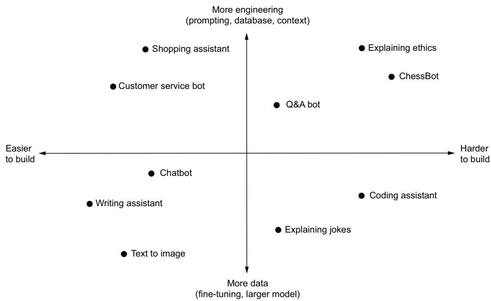
Figure 2.9 How difficult or easy certain tasks are for LLMs and what approaches to take to solve them

they are not as important in this case. Either way, we hope this exercise will better inform you and your team on your next project.

LLMs have amazing benefits, but with all of these capabilities come some limitations. Foundational LLMs require vast computational resources for training, making them less accessible for individual researchers and smaller organizations. This problem is being remedied with techniques we’ll talk about throughout the book, like quantization, textual embeddings, low-rank adaptation, parameter-efficient finetuning, and graph optimization. Still, foundation models are currently solidly outside the average individual’s ability to train effectively. Beyond that, there are concerns that the energy consumption associated with training LLMs could have significant environmental effects and cause problems associated with sustainability. These problems are complex and largely out of the scope of this book, but we would be remiss not to bring them up.

Last but not least, since LLMs are trained on large-scale datasets containing realworld text, they may learn and perpetuate biases present in the data, leading to ethical concerns because real-world people don’t censor themselves to provide optimal unbiased data. Also, knowing much about what data you’re training on is not a widespread practice. For example, if you ask a text-to-image diffusion LLM to generate 1,000 images of “leader,” 99% of the images feature men, and 95% of the images feature people with white skin. The concern here isn’t that men or white people shouldn’t be depicted as leaders, but that the model isn’t representing the world accurately, and it’s showing.

Sometimes, more nuanced biases are brought out. For example, in the Midjourney example in figure 2.10, the model, without being prompted (the only prompt given was the word “leader”), changed the popular feminist icon Rosie the Riveter to a man. The model didn’t think about this change; it just determined during its sampling steps that the prompt “leader” had more male-looking depictions in the training set. Many people will argue about what “good” and “bad” mean in this context, and instead of going for a moral ought, we’ll talk about what accuracy means. LLMs are trained on a plethora of data with the purpose of returning the most accurate representations possible. When they cannot return accurate representations, especially with their heightened abilities to disambiguate, we can view that as a bias that harms the model’s ability to fulfill its purpose. Later, we will discuss techniques to combat harmful bias to allow you, as an LLM creator, to get the exact outputs you intend and minimize the number of outputs you do not intend.

Figure 2.10 Midjourney 5, which is, at the time of this writing, the most popular text2img model on the market, when prompted with only one token, “leader” (left), changed a well-known popular feminist icon, Rosie the Riveter, into a male depiction. ChatGPT (right) writes a function to place you in your job based on race, gender, and age. These are examples of unintended outputs.

Alright, we’ve been building up to this moment the entire chapter. Let’s go ahead and run our first LLM! In listing 2.9, we download the Bloom model, one of the first open source LLMs to be created, and generate text! We are using Hugging Face’s Transformers library, which takes care of all the heavy lifting for us. Very exciting stuff!

from transformers import AutoModelForCausalLM, AutoTokenizer
MODEL_NAME = "bigscience/bloom" 
tokenizer = AutoTokenizer.from_pretrained(MODEL_NAME)
model = AutoModelForCausalLM.from_pretrained(MODEL_NAME)
prompt = "Hello world! This is my first time running an LLM!"
input_tokens = tokenizer.encode(prompt, return_tensors="pt", padding=True)
generated_tokens = model.generate(input_tokens, max_new_tokens=20)
generated_text = tokenizer.batch_decode(
 generated_tokens, skip_special_tokens=True
)
print(generated_text)
  Listing 2.9 Running our first LLM

Did you try to run it?!? If you did, you probably just crashed your laptop. Oopsie! Forgive me for a little harmless MLOps hazing, but getting some first-hand experience on how large these models can get and how difficult they can be to run is a helpful experience to have. In the next chapter, we will talk more about the difficulties of running LLMs and some of the tools you need to run this code. If you don’t want to wait and would like to get a similar but much smaller LLM running, change the model name to “bigscience/bloom-3b”, and run it again. It should work just fine this time on most hardware.

All in all, LLMs are an amazing technology that allows our imaginations to run wild with possibility, and deservedly so. The number-one use case for considering an LLM over a smaller language model is when few-shot capabilities come into play for whoever the model will be helping, such as a CEO when raising funds or a software engineer when writing code. LLMs have these abilities precisely because of their size. The larger number of parameters in LLMs directly enables their ability to generalize over smaller spaces in larger dimensions. In this chapter, we’ve hit the lesser-known side of LLMs, the linguistic and language modeling side. In the next chapter, we’ll cover the other half, the MLOps side, where we dive into exactly how that large parameter size affects the model and the systems designed to support that model and makes it accessible to the customers or employees the model is intended for.

Summary

• The five components of linguistics are phonetics, syntax, semantics, pragmatics, and morphology:
  • Phonetics can be added through a multimodal model that processes audio files and is likely to improve LLMs in the future, but current datasets are too small.
  • Syntax is what current models are good at.
  • Semantics is added through the embedding layer.
• Pragmatics can be added through engineering efforts.
• Morphology is added in the tokenization layer.
• Language does not necessarily correlate with reality. Understanding the process people use to create meaning outside of reality is useful in training meaningful (to people) models.
• Proper tokenization can be a major hurdle due to too many tokens, especially when it comes to specialized problems like code or math.
• Multilingual processing has always outperformed monolingual processing, even on monolingual tasks without models.
• Each language model type in sequence shows a natural and organic growth of the LLM field as more and more linguistic concepts are added that make the models better.
• Language modeling has seen an exponential increase in efficacy, correlating to how linguistics-focused the modeling has been.
• Attention is a mathematical shortcut for solving larger context windows faster and is the backbone of modern architectures—encoders, decoders, and transformers:
  • Encoders improve the semantic approximations in embeddings.
  • Decoders are best at text generation.
  • Transformers combine the two.
• Larger models demonstrate emergent behavior, suddenly being able to accomplish tasks they couldn’t before.

Large language model operations: Building a platform for LLMs

This chapter covers

• An overview of large language model operations
• Deployment challenges
• Large language model best practices
• Required large language model infrastructure

Before anything else, preparation is the key to success.

—Alexander Graham Bell

As we learned in the last chapter, when it comes to transformers and natural language processing (NLP), bigger is better, especially when it’s linguistically informed. However, bigger models come with bigger challenges because of their size, regardless of their linguistic efficacy, thus requiring us to scale up our operations and infrastructure to handle these problems. In this chapter, we’ll be looking into exactly what those challenges are, what we can do to minimize them, and what architecture can be set up to help solve them.

3.1 Introduction to large language model operations

What is large language model operations (LLMOps)? Well, since we like to focus on practicality over rhetoric, we’re not going to dive into any fancy definitions that you’d expect in a textbook, but let’s simply say it’s machine learning operations (MLOps) that have been scaled to handle LLMs. Let us also say scaling up is hard. One of the hardest tasks in software engineering. Unfortunately, too many companies are running rudimentary MLOps setups, and don’t think for a second that they will be able to handle LLMs. That said, the term LLMOps may not be needed. It has yet to show through as sufficiently different from core MLOps, especially considering they still have the same bones. If this book were a dichotomous key, MLOps and LLMOps would definitely be in the same genus, and only time will tell whether they are the same species. Of course, by refusing to define LLMOps properly, we might have traded one confusion for another, so let’s take a minute to describe MLOps.

MLOps is the field and practice of reliably and efficiently deploying and maintaining machine learning models in production. This includes—and, indeed, requires managing the entire machine learning life cycle, from data acquisition and model training to monitoring and termination. A few principles required to master this field include workflow orchestration, versioning, feedback loops, continuous integration and continuous deployment (CI/CD), security, resource provisioning, and data governance. While there are often personnel who specialize in the productionizing of models, with titles like ML Engineers, MLOps Engineers, or ML Infrastructure Engineer, the field is a large-enough beast that it often abducts many other unsuspecting professionals to work in it who hold titles like Data Scientist or DevOps Engineer—often against their knowledge or will, leaving them kicking and screaming, “It’s not my job.”

3.2 Operations challenges with large language models

So why have a distinction at all? If MLOps and LLMOps are so similar, is LLMOps just another fad opportunists throw on their resume? Not quite. In fact, it’s quite similar to the term Big Data. When the term was at its peak popularity, people with titles like Big Data Engineer used completely different tool sets and developed specialized expertise necessary to handle large datasets. LLMs come with a set of challenges and problems you won’t find with traditional machine learning systems. A majority of these problems extend almost exclusively because they are so big. Large models are large! We hope to show you that LLMs truly earn their name. Let’s take a look at a few of these challenges so we can appreciate the task ahead of us when we start talking about deploying an LLM.

3.2.1 Long download times

Back in 2017, when I was still heavily involved as a data scientist, I decided to try my hand at reimplementing some of the most famous computer vision models at the time: AlexNet, VGG19, and ResNet. I figured this would be a good way to reinforce my understanding of the basics with some practical hands-on experience. Plus, I had an ulterior motive: I had just built my own rig with some NVIDIA GeForce 1080 TI GPUs, which were state of the art at the time, and I thought this would be a good way to break them in. The first task was to download the ImageNet dataset.

The ImageNet dataset was one of the largest annotated datasets available, containing millions of images rounding out to a file size of a whopping ~150 GB! Working with it was proof that you knew how to work with Big Data, which was still a trendy word and an invaluable skill set for a data scientist at the time. After agreeing to the terms and gaining access, I got my first wakeup call. Downloading it took an entire week.

When my team first deployed Bloom, it took an hour and a half to download it. Heck, it took an hour and a half to download The Legend of Zelda: Tears of the Kingdom, and that’s only 16 GB, so we really couldn’t complain.

Large models are large. That can’t be overstated. You’ll find throughout this book that that fact comes with many additional headaches and problems for the entire production process, and you have to be prepared for it. In comparison to the ImageNet dataset, the Bloom LLM model is 330 GB, more than twice the size. We’re guessing most readers haven’t worked with either ImageNet or Bloom, so for comparison, Call of Duty: Modern Warfare, one of the largest games at the time of this writing, is 235 GB. Final Fantasy 15 is only 148 GB, so you could fit two into the model with plenty of room to spare. It’s just hard to really comprehend how massive LLMs are. We went from 100 million parameters in models like BERT and took them to billions of parameters. If you went on a shopping spree and spent $20 a second (or maybe accidentally left your AWS EC2 instance on), it’d take you half a day to spend a million dollars; it would take you two years to spend a billion.

Thankfully, it doesn’t take two weeks to download Bloom because unlike Image-Net, it’s not hosted on a poorly managed university server, and it also has been sharded into multiple smaller files to allow downloading in parallel, but it will still take an uncomfortably long time. Consider a scenario where you are downloading the model under the best conditions. You’re equipped with a gigabit speed fiber internet connection, and you’re magically able to dedicate the entire bandwidth and I/O operations of your system and the server to it. It will still take over 5 minutes to download! Of course, that’s under the best conditions. You probably won’t be downloading the model under such circumstances; with modern infrastructure, you can expect it to take on the order of hours.

3.2.2 Longer deploy times

Just downloading the model is a long enough time frame to make any seasoned developer shake, but deployment times are going to make them keel over and call for medical attention. A model as big as Bloom can take 30 to 45 minutes just to load the model into GPU memory—at least, those are the time frames we’ve experienced. That’s not to mention any other steps in your deployment process that can add to this. Indeed, with GPU shortages, it can easily take hours just waiting for resources to free up—more on that in a minute.

What does this mean for you and your team? Well, for starters, we know lots of teams that deploy ML products often simply download the model at run time. That might work for small sklearn regression models, but it isn’t going to work for LLMs. Additionally, you can take most of what you know about deploying reliable systems and throw it out the window (but thankfully not too far). Most modern-day best practices for software engineering assume you can easily restart an application if anything happens, and there’s a lot of rigmarole involved to ensure your systems can do just that. With LLMs, it can take seconds to shut down, but potentially hours to redeploy, making this a semi-irreversible process. Like picking an apple off a tree, it’s easy to pluck one off, but if you bite into it and decide it’s too sour, you can’t reattach it to the tree so it can continue to ripen. You’ll just have to wait awhile for another to grow.

While not every project requires deploying the largest models out there, you can expect to see deployment times measured in minutes. These longer deploy times make scaling down right before a surge of traffic a terrible mistake, as well as figuring out how to manage bursty workloads difficult. General CI/CD methodologies need to be adjusted since rolling updates take longer, leaving a backlog piling up quickly in your pipeline. Silly mistakes like typos or other bugs often take longer to notice and longer to correct.

3.2.3 Latency

Along with increases in model size often come increases in inference latency. This is obvious when stated, but more parameters equate to more computations, and more computations mean longer inference wait times. However, this can’t be underestimated. We know many people who downplay the latency problems because they’ve interacted with an LLM chatbot, and the experience felt smooth. Take a second look, though, and you’ll notice that it is returning one word at a time, which is streamed to the user. It feels smooth because the answers are coming in faster than a human can read, but a second look helps us realize this is just a UX trick. LLMs are still too slow to be very useful for an autocomplete solution, for example, where responses have to be blazingly fast. Building it into a data pipeline or workflow that reads a large corpus of text and then tries to clean it or summarize it may also be too prohibitively slow to be useful or reliable.

There are also many less obvious reasons for their slowness. For starters, LLMs are often distributed across multiple GPUs, which adds extra communication overhead. As discussed later in this chapter in section 3.3.2, they are distributed in other ways, often even to improve latency, but any distribution adds an additional overhead burden. In addition, LLMs’ latency is severely affected by completion length, meaning the more words it uses to return a response, the longer it takes. Of course, completion length also seems to improve accuracy. For example, using prompt engineering techniques like chain of thought (CoT), we ask the model to think about a problem in a step-by-step fashion, which has been shown to improve results for logic and math questions but significantly increases the response length and latency time.

3.2.4 Managing GPUs

To help with these latency problems, we usually want to run them in GPUs. If we want to have any success training LLMs, we’ll need GPUs for that as well, but this all adds additional challenges that many underestimate. Most web services and many ML use cases can be done solely on CPUs, but not so with LLMs—partly because of GPUs’ parallel processing capabilities offering a solution to our latency problems and partly because of the inherent optimization GPUs offer in the linear algebra, matrix multiplications, and tensor operations; that’s happening under the hood. For many who are stepping into the realm of LLMs, this requires utilizing a new resource and extra complexity. Many brazenly step into this world, acting like it’s no big deal, but they are in for a rude awakening. Most system architectures and orchestrating tooling available, like Kubernetes, assume your application will run with CPU and memory alone. While they often support additional resources like GPUs, it’s often an afterthought. You’ll soon find you have to rebuild containers from scratch and deploy new metric systems.

One aspect of managing GPUs that most companies are not prepared for is that they tend to be rare and limited. For the last decade, it seems that we have gone in and out of a global GPU shortage. They can be extremely difficult to provision for companies looking to stay on-premise. We’ve spent lots of time in our careers working with companies that chose to stay on-premise for a variety of reasons. One of the things they had in common is that they never had GPUs on their servers. When they did, they were often purposely difficult to access except for a few key employees.

If you are lucky enough to be working in the cloud, a lot of these problems are solved, but there is no free lunch here either. We’ve both been part of teams that have often gone chasing their tails trying to help data scientists struggling to provision a new GPU workspace. We’ve run into obscure, ominous errors like scale.up.error .out.of.resources, only to discover that these esoteric readings indicate all the GPUs of a selected type in the entire region are being utilized, and none are available. CPU and memory can often be treated as infinite in a data center; GPU resources, however, cannot. Sometimes you can’t expect them at all. Most data centers only support a subset of instance or GPU types, which means you may be forced to set up your application in a region further away from your user base, thus increasing latency. Of course, we’re sure you can work with your cloud provider when looking to expand your service to a new region that doesn’t currently support it, but you might not like what you hear based on timelines and cost. Ultimately, you’ll run into shortage problems no matter where you choose to run, on-premise or in the cloud.

3.2.5 Peculiarities of text data

LLMs are the modern-day solution to NLP. NLP is one of the most fascinating branches of ML in general because it primarily deals with text data, which is primarily a qualitative measure. Every other field deals with quantitative data. We have figured out a way to encode our observations of the world into a direct translation of numerical values. For example, we’ve learned how to encode heat into temperature scales

and measure it with thermometers and thermocouples, and we can measure pressure with manometers and gauges and put it into pascals.

Computer vision and the practice of evaluating images are often seen as qualitative, but the actual encoding of images into numbers is a solved problem. Our understanding of light has allowed us to break images apart into pixels and assign them RGB values. Of course, this doesn’t mean computer vision is by any means solved; there’s still lots of work to do to learn how to identify the different signals in the patterns of the data. Audio data is also often considered qualitative. How does one compare two songs? But we can measure sound and speech, directly measuring the sound wave’s intensity in decibels and frequency in hertz.

Unlike other fields that encode our physical world into numerical data, text data is looking at ways to measure the ephemeral world. After all, text data is our best effort at encoding our thoughts, ideas, and communication patterns. While, yes, we have figured out ways to turn words into numbers, we haven’t figured out a direct translation. Our best solutions to encode text and create embeddings are just approximations at best; in fact, we use machine learning models to do it! An interesting aside is that numbers are also text and a part of language. If we want models that are better at math, we need a more meaningful way to encode these numbers. Since it’s all made up, when we try to encode text numbers into machine-readable numbers, we are creating a system attempting to reference itself recursively in a meaningful way. Not an easy problem to solve!

Because of all this, LLMs (and all NLP solutions) have unique challenges. Take, for example, monitoring. How do you catch data drift in text data? How do you measure “correctness”? How do you ensure the cleanliness of the data? These types of problems are difficult to define, let alone solve.

3.2.6 Token limits create bottlenecks

A big challenge for those new to working with LLMs is dealing with the token limits. The token limit for a model is the maximum number of tokens that can be included as an input for a model. The larger the token limit, the more context we can give the model to improve its success at accomplishing the task. Everyone wants them to be higher, but it’s not that simple. These token limits are defined by two problems: the memory and speed our GPUs have access to and the nature of memory storage in the models themselves.

The first problem seems unintuitive: Why couldn’t we just increase the GPU memory? The answer is complex. We can, but stacking more layers in the GPU to take into account more gigabytes at once slows down the GPU’s computational ability as a whole. Right now, GPU manufacturers are working on new architectures and ways to get around this problem. The second challenge is fascinating because increasing the token limits actually exacerbates the mathematical problems under the hood. Let me explain. Memory storage within an LLM itself isn’t something we think about often. We call that mechanism attention, which we discussed in depth in section 2.2.7. What

we didn’t discuss was that attention is a quadratic solution: as the number of tokens increases, the number of calculations required to compute the attention scores between all the pairs of tokens in a sequence scales quadratically with the sequence length. In addition, within our gigantic context spaces, and since we are dealing with quadratics, we’re starting to hit problems where the only solutions involve imaginary numbers, which can cause models to behave in unexpected ways. This is likely one of the reasons why LLMs hallucinate.

These problems have real implications and affect application designs. For example, when this author’s team upgraded from GPT-3 to GPT-4, the team was excited to have access to a higher token limit, but it soon found this led to longer inference times and, subsequently, a higher timeout error rate. In the real world, it’s often better to get a less accurate response quickly than to get no response at all because the promise of a more accurate model often is just that: a promise. Of course, when deploying it locally, where you don’t have to worry about response times, you’ll likely find your hardware to be a limiting factor. For example, LLaMA was trained with 2,048 tokens, but you’ll be lucky to take advantage of more than 512 of that when running with a basic consumer GPU, as you are likely to see out-of-memory (OOM) errors or even the model simply crashing.

A gotcha, which is likely to catch your team by surprise and should be pointed out now, is that different languages have different tokens per character. Take a look at table 3.1, where we compare converting the same sentence in different languages to tokens using OpenAI’s cl100k_base Byte Pair Encoder. Just a quick glance reveals that LLMs typically favor the English language in this regard. In practice, this means that if you are building a chatbot with an LLM, your English users will have greater flexibility in their input space than Japanese users, leading to very different user experiences.

Language	String	Characters	Tokens
English	The quick brown fox jumps over the lazy dog	43	9
French	Le renard brun rapide saute par-dessus le chien paresseux	57	20
Spanish	El rápido zorro marrón salta sobre el perro perezoso	52	22
Japanese	素早い茶色のキツネが怠惰な犬を飛び越える	20	36
Chinese (simplified)	敏捷的棕色狐狸跳过了懒狗	12	28

Table 3.1 Comparison of token counts in different languages

If you are curious about why this is, it is due to text encodings, which are another peculiarity of working with text data, as discussed in the previous section. Consider table 3.2, where we show several different characters and their binary representations in UTF-8. English characters can almost exclusively be represented with a single byte included in the original ASCII standard computers were originally built on, while most other characters require 3 or 4 bytes. Because it takes more memory, it also takes more token space.

Character	Binary UTF-8	Hex UTF-8
$	00100100	0x24
£	11000010 10100011	0xc2 0xa3
¥	11000010 10100101	0xc2 0xa5
?	11100010 10000010 10100000	0xe2 0x82 0xa0
?	11110000 10011111 10010010 10110000	0xf0 0x9f 0x92 0xb0

Table 3.2 Comparison of byte lengths for different currency characters in UTF-8

Increasing the token limits has been an ongoing research question since the popularization of transformers, and there are some promising solutions still in the research phases, like recurrent memory transformers (RMT).¹ We can expect to continue to see improvements in the future, and hopefully, this will become naught but an annoyance.

3.2.7 Hallucinations cause confusion

So far, we’ve been discussing some of the technical problems a team faces when deploying an LLM into a production environment, but nothing compares to the simple problem that LLMs tend to be wrong. They tend to be wrong a lot. Hallucinations is a term coined to describe occurrences when LLM models will produce correctsounding results that are wrong—for example, book references or hyperlinks that have the form and structure of what would be expected but are, nevertheless, completely made up. As a fun example, we asked for books on LLMs in production from the publisher, Manning (a book that doesn’t exist yet since one author is still writing it). We were given the following suggestions: Machine Learning Engineering in Production by Mike Del Balso and Lucas Serveén, which could be found at https://www.manning .com/books/machine-learning-engineering-in-production, and Deep Learning for Coders with Fastai and PyTorch by Jeremy Howard and Sylvain Gugger, which could be found at https://www.manning.com/books/deep-learning-for-coders-with-fastai-andpytorch. The first book is entirely made up. The second book is real; however, it’s not published by Manning. In each case, the internet addresses are entirely made up. These URLs are actually very similar in format to what you’d expect if you were browsing Manning’s website, but they will return 404 errors if you visit them.

One of the most annoying aspects of hallucinations is that they are often surrounded by confident-sounding words. LLMs are terrible at expressing uncertainty, in

¹ A. Bulatov, Y. Kuratov, and M. S. Burtsev, “Scaling transformer to 1M tokens and beyond with RMT,” April 2023, https://arxiv.org/abs/2304.11062.

large part because of the way they are trained. Consider the case “2 + 2 =.” Would you prefer it to respond, “I think it is 4” or simply “4”? Most would prefer to get the correct “4” back. This bias is built in, as models are often given rewards for being correct or at least sounding like it.

There are various explanations as to why hallucinations occur, but the most truthful answer is that we don’t know if there’s just one cause. It’s likely a combination of several things; thus, there isn’t a good fix for it yet. Nevertheless, being prepared to counter these inaccuracies and biases of the model is crucial to provide the best user experience for your product.

3.2.8 Bias and ethical considerations

Just as concerning as the model getting things wrong is when it gets things right in the worst possible way—for example, allowing it to encourage users to commit suicide,2 teaching users how to make a bomb,3 or participating in sexual fantasies involving children.4 These are extreme examples, but prohibiting the model from answering such questions is undeniably vital to success.

LLMs are trained on vast amounts of text data, which is also their primary source of bias. Because we’ve found that larger datasets are just as important as larger models in producing human-like results, most of these datasets have never truly been curated or filtered to remove harmful content, instead choosing to prioritize size and a larger collection. Cleaning the dataset is often seen as prohibitively expensive, requiring humans to go in and manually verify everything, but there’s a lot that could be done with simple regular expressions and other automated solutions. By processing these vast collections of content and learning the implicit human biases, these models will inadvertently perpetuate them. These biases range from sexism and racism to political preferences and can cause your model to inadvertently promote negative stereotypes and discriminatory language.

3.2.9 Security concerns

As with all technology, we need to be mindful of security. LLMs have been trained on a large corpus of text, some of which could be harmful or sensitive and shouldn’t be exposed. So steps should be taken to protect this data from being leaked. The bias and ethical concerns from the last section are good examples of conversations you don’t want your users to be having, but you could also imagine finetuning a model on your company’s data and potentially having secrets lost inadvertently if proper precautions aren’t taken.

² R. Daws, “Medical chatbot using OpenAI’s GPT-3 told a fake patient to kill themselves,” AI News, October 28, 2020,https://mng.bz/qO6z.

³ T. Kington, “ChatGPT bot tricked into giving bomb-making instructions, say developers,” The Times, December 17, 2022, https://mng.bz/7d64.

⁴ K. Quach, “AI game bans players for NSFW stories it generated itself,” The Register, October 8, 2021, https://www.theregister.com/2021/10/08/ai\_game\_abuse/.

One should be aware that LLMs are susceptible to adversarial attacks like prompt injections. Prompt injections are attacks done by a user to trick the LLM into ignoring instructions given to it and generating undesired content. For example, if you ask ChatGPT what its gender is, it appropriately replies that as an AI language model, it doesn’t have a gender. However, with clever prompting, you may be able to bypass these protocols and get it to reveal one. While this example is harmless, we’ve seen others successfully extract API keys and other secrets from an LLM, run code in nonprotected environments, steal environment variables, and traverse local file systems where the model is served. That’s not to mention the plethora of examples of users using prompting to jailbreak or bypass protocols put in place for ethical considerations outlined in the previous section. An interesting aside to this is that LLMs are good at inventing fake secrets! Even successful prompt injection attacks can often fail due to LLM hallucinations, which can have funny consequences.

For example, using a simple prompt to ask for Coca-Cola’s secret recipe simply returned the boring result, “I cannot divulge trade secrets or any proprietary information.” Pretty lame if you ask us. With a little trickery and some prompt injection, we were able to get it to spill its secrets, which, of course, we decided to try—after confirming with a food scientist it wouldn’t poison us. After following the instructions exactly, we were surprised to find we got a pretty tasty drink, but it tasted nothing like Coke. While the recipe looks legitimate, nuances like quantities, cook times, and even the need to strain the syrup were all off. Guess we’ll have to hold off taking over the beverage industry until we get the real recipe.

Coca-Cola recipe hallucinated from prompt injection

Homemade Coca-Cola Recipe
=====================
**Disclaimer**: The original Coca-Cola recipe is a highly guarded trade 
secret. The following recipe is an approximation for creating a homemade 
cola drink that resembles the taste of Coca-Cola.

Ingredients:
- 3 cups of water
- 2 cups granulated sugar
- 1/8 tsp food-grade citric acid
- 3/4 tsp caramel color (liquid)
- 1/2 tsp caffeine (powder or liquid form)
- 1 1/2 tsp cola extract
- 1/8 tsp vanilla extract
- 1 1/2 cups carbonated water (store-bought or using a home soda maker)
- A pinch of ground cinnamon (optional)
- A pinch of ground nutmeg (optional)
Instructions:
1. In a large saucepan, bring the 3 cups of water to a gentle simmer.

2. Slowly stir in the granulated sugar, ensuring that it fully

dissolves.

• 3. Add the citric acid, caramel color, caffeine, cola extract, and vanilla extract to the saucepan. Mix well.
• 4. Stir in the optional spices if desired: cinnamon and nutmeg.
• 5. Simmer the mixture for about 20 minutes, stirring occasionally.
• 6. Remove the saucepan from the heat and let it cool to room temperature.
• 7. Once cooled, strain the syrup to remove any undissolved solids.
• 8. To make the final drink, mix 1 part syrup with 3 parts carbonated water. Adjust to taste depending on your preference for sweetness and carbonation.

Variations:

• You can experiment with different amounts of caramel color, caffeine, and cola extract to adjust the flavor and appearance of your homemade cola.
• To create different cola flavor profiles, experiment with adding additional spices (such as star anise, orange or lemon peel, or cardamom), essential oils, or fruit extracts.
• Consider using a natural sweetener, like honey or agave syrup, as an alternative to granulated sugar.

Historical context and interesting facts:

• Coca-Cola was first introduced in 1886 by pharmacist Dr. John S. Pemberton, who aimed to create a unique and refreshing beverage that could also relieve fatigue and headaches.
• The original Coca-Cola formula contained trace amounts of cocaine extracted from the coca leaf, which was later replaced with caffeine in the early 20th century.
• In 1985, Coca-Cola introduced “New Coke,” a reformulation aimed at competing with Pepsi. However, the taste change was met with backlash, and the company returned to its original formula just three months later, rebranded as “Coca-Cola Classic.”

Result(s): You can now create your own homemade version of cola, resembling the taste of Coca-Cola. Enjoy and feel free to experiment with different spices, extracts, and sweeteners to create your own unique flavor profile.

Another security concern involves pickle injections. Pickle is a library in Python that serializes objects and is often used to serialize ML models. It serializes them into a byte stream containing opcodes executed one by one as it is deserialized. It’s a fast and easy way to share large objects. Pickle injections corrupt this byte stream, often injecting malware over the wire when the model is transferred over an insecure network. This is especially concerning for large models that take a long time to download, as it makes it easier for a third party to intercept the transfer and inject malicious code. If this happens, the code injected can potentially give the attackers access to your system. This can happen when attempting to use the model during inference, as the harmful code will execute if it is not detected and properly removed. It is important to take precautions such as using secure networks and verifying the integrity of the model before use to prevent this type of attack.

3.2.10 Controlling costs

Working with LLMs involves various cost-related concerns. The first, as you probably gathered by now, is infrastructure costs, which include high-performance GPUs, storage, and other hardware resources. We talked about how GPUs are harder to procure, which, unfortunately, means they are more expensive. Mistakes like leaving your service on have always had the potential to rack up the bills, but with GPUs in the mix, this type of mistake is even more deadly. These models also demand significant computational power, leading to high energy consumption during both training and inference. On top of all this, their longer deploy times mean we are often running them even during low traffic to handle bursty workloads or anticipated future traffic. Overall, this leads to higher operational costs.

Additional costs include managing and storing vast amounts of data used to train or finetune as well as for regular maintenance, such as model updates, security measures, and bug fixes, which can be financially demanding. As with any technology used for business purposes, managing potential legal disputes and ensuring compliance with regulations is a concern. Lastly, investing in continuous research and development to improve your models and give you a competitive edge will be a factor.

We talked a bit about the technical concerns regarding token limits, which are likely to be solved, but we didn’t discuss the cost limitations, as most APIs charge on a token basis. This makes it more expensive to send more context and use better prompts. It also makes it a bit harder to predict costs since while you can standardize inputs, you can’t standardize outputs. You can never be too sure how many tokens will be returned, making it difficult to govern. Just remember, with LLMs, it is as important as ever to implement and follow proper cost engineering practices to ensure costs never get away from you.

3.3 LLMOps essentials

Now that we have a handle on the type of challenge we are grappling with, let’s take a look at all the different LLMOps practices, tooling, and infrastructure to see how different components help us overcome these obstacles. First, let’s dive into different practices, starting with compression, where we will talk about shrinking, trimming, and approximating to get models as small as we can. We will then talk about distributed computing, which is needed to make things run since the models are so large that they rarely fit into a single GPU’s memory. After we are finished with that, we will venture into the infrastructure and tooling needed to make it all happen in the next section.

3.3.1 Compression

As you were reading about the challenges of LLMs in the last section, you might have asked yourself something akin to “If the biggest problems from LLMs come from their size, why don’t we just make them smaller?” If you did, congratulations! You are a genius—compression is the practice of doing just that. Compressing models to as small as we can make them will improve deployment time, reduce latency, scale down the number of expensive GPUs needed, and, ultimately, save money. However, the whole point of making the models so stupefyingly gargantuan in the first place was because it made them better at what they do. We need to be able to shrink them without losing all the progress we made by making them big in the first place.

This problem is far from solved, but there are multiple ways to approach the problem, with different pros and cons to each method. We’ll be talking about several of the methods, starting with the easiest and most effective.

QUANTIZING

Quantizing is the process of reducing precision in preference of lowering the memory requirements. This tradeoff makes intuitive sense. When this author was in college, he was taught to always round numbers to the precision of the tooling. Pulling out a ruler and measuring his pencil, you wouldn’t believe him if he stated the length was 19.025467821973739 cm. Even if he used a caliper, he couldn’t verify a number so precisely. With our ruler, any number beyond 19.03 cm is fantasy. To drive the point home, one of his engineering professors once asked him him, “If you are measuring the height of a skyscraper, do you care if there is an extra sheet of paper at the top?”

How we represent numbers inside computers often leads us to believe we have better precision than we actually do. To illustrate this point, open a Python terminal and add 0.1 + 0.2. If you’ve never tried this before, you might be surprised to find it doesn’t equal 0.3, but 0.30000000000000004. We won’t go into the details of the math behind this phenomenon, but the question stands: Can we reduce the precision without making things worse? We really only need precision to the tenth decimal, but reducing the precision will likely get us a number like 0.304 rather than 0.300, thus increasing our margin of error.

Ultimately, the only numbers a computer understands are 0 and 1, on or off, a single bit. To improve this range, we combine multiple bits and assign them different meanings. String 8 of them together, and you get a byte. Using the INT8 standard, we can take that byte and encode all the integers from –128 to 127. We’ll spare you the particulars because we assume you already know how binary works; suffice it to say, the more bits we have, the larger range of numbers we can represent, both larger and smaller. Figure 3.1 shows a few common floating point encodings. With 32 bits strung together, we get what we pretentiously term full precision, and that is how most numbers are stored, including the weights in machine learning models. Basic quantization moves us from full precision to half precision, shrinking models to half their size. There are two different half precision standards, FP16 and BF16, which differ in how many bits represent the range or exponent part. Since BF16 uses the same number of exponents as FP32, it’s been found to be more effective for quantizing, and you can generally expect almost exactly the same level of accuracy for half the size of model. If you understood the paper and skyscraper analogy, it should be obvious why.

However, there’s no reason to stop there. We can often push it down another byte to 8-bit formats without too much loss of accuracy. There have already even been successful research attempts showing selective 4-bit quantization of portions of LLMs is

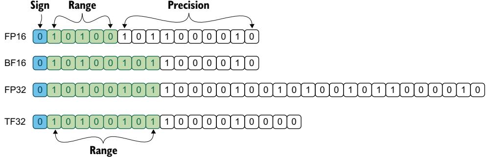
Figure 3.1 The bit mapping for a few common floating point encodings: 16-bit float or half precision (FP16), bfloat 16 (BF16), 32-bit float or single full precision (FP32), and NVIDIA’s TensorFloat (TF32)

possible with only a fractional loss of accuracy. The selective application of quantization is a process known as dynamic quantization and is usually done on just the weights, leaving the activations in full precision to reduce accuracy loss.

The holy grail of quantizing, though, is INT2, representing every number as –1, 0, or 1. This currently isn’t possible without completely degrading the model, but it would make the model up to 8 times smaller. The Bloom model would be a measly ~40 GB, small enough to fit on a single GPU. This is, of course, as far as quantizing can take us, and if we wanted to shrink further, we’d need to look at additional methods.

The best part of quantization is that it is easy to do. There are many frameworks that allow this, but in listing 3.1, we demonstrate how to use PyTorch’s quantization library to do a simple post-training static quantization (PTQ). All you need is the full precision model, some example inputs, and a validation dataset to prepare and calibrate with. As you can see, it’s only a few lines of code.

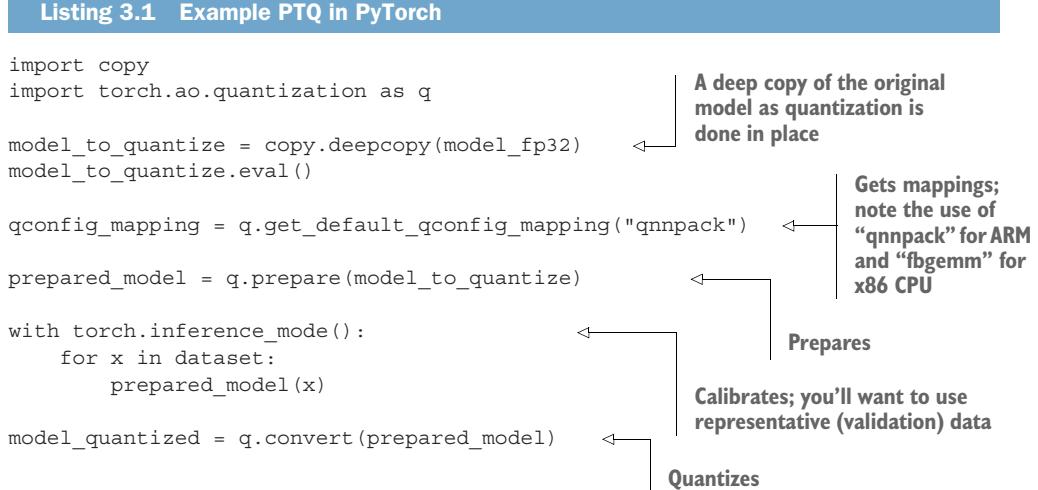
Static PTQ is the most straightforward approach to quantizing; it is done after the model is trained and uniformly quantizes all the model parameters. As with most formulas, the most straightforward approach introduces more error. Often, this error is acceptable, but when it’s not, we can add extra complexity to reduce the accuracy loss from quantization. Some methods to consider are uniform versus nonuniform, static versus dynamic, symmetric versus asymmetric, and applying it during or after training.

To understand these methods, let’s consider the case where we are quantizing from FP32 to INT8. In FP32, we essentially have the full range of numbers at our disposal, but in INT8, we only have 256 values. We are trying to put a genie into a bottle, and it’s no small feat. If you study the weights in your model, you might notice that most of the numbers are fractions between [–1, 1]. We could take advantage of this by using an 8-bit standard that represents more values in this region in a non-uniform way instead of the standard uniform [–128, 127]. While mathematically possible, unfortunately, any such standards aren’t commonplace, and modern-day deep learning hardware and software are not designed to take advantage of them. So for now, it’s best to stick to uniform quantization.

The simplest approach to shrinking the data is to normalize it, but since we are going from a continuous scale to a discrete scale, there are a few gotchas, so let’s explore those. We start by taking the min and max and scale them down to match our new number range. We would then bucket all the other numbers based on where they fall. Of course, if we have really large outliers, we may find all our other numbers squeezed into just one or two buckets, ruining any granularity we once had. To prevent this, we can clip any large numbers; this is what we do in static quantization. However, before we clip the data, what if we choose a range and scale that captures the majority of our data beforehand? We need to be careful since if this dynamic range is too small, we will introduce more clipping errors; if it’s too big, we will introduce more rounding errors. The goal of dynamic quantization is, of course, to reduce both errors.

Next, we need to consider the symmetry of the data. Generally, in normalization, we force the data to be normal and thus symmetric; however, we could choose to scale the data in a way that leaves any asymmetry it had. By doing this, we could potentially reduce our overall loss due to the clipping and rounding errors, but it’s not guaranteed.

As a last resort, if none of these other methods fail to reduce the accuracy loss of the model, we can use quantization-aware training (QAT). QAT is a simple process where we add a fake quantization step during model training. By fake, we mean we clip and round the data while leaving it in full precision. This allows the model to adjust for the error and bias introduced by quantization while it’s training. QAT is known to produce higher accuracy compared to other methods but at a much higher cost in time to train.

Quantization methods

• Uniform versus non-uniform—Whether we use an 8-bit standard that is uniform in the range it represents or non-uniform to be more precise in the -1 to 1 range.
• Static versus dynamic—Choosing to adjust the range or scale before clipping in an attempt to reduce clipping and rounding errors and reduce data loss.
• Symmetric versus asymmetric—Normalizing the data to be normal and force symmetry or choosing to keep any asymmetry and skew.
• During or after training—Quantization after training is really easy to do, and while doing it during training is more work, it leads to reduced bias and better results.

Quantizing is a very powerful tool. It reduces the size of the model and the computational overhead required to run the model, thus reducing the latency and cost of running the model. However, the best thing about quantization is that it can be done after the fact, so you don’t have to worry about whether your data scientists remembered to quantize the model during training using processes like QAT. This is why quantization has become so popular when working with LLMs and other large machine learning models. While reduced accuracy is always a concern with compression techniques, compared to other methods, quantization is a win-win-win.

PRUNING

Congratulations, you just trained a brand new LLM! With billions of parameters, all of them must be useful, right? Wrong! Unfortunately, as with most things in life, the model’s parameters tend to follow the Pareto principle. About 20% of the weights lead to 80% of the value. “If that’s true,” you may be asking yourself, “why don’t we just cut out all the extra fluff?” Great idea! Give yourself a pat on the back. Pruning is the process of weeding out and removing any parts of the model we deem unworthy.

There are essentially two different pruning methods: structured and unstructured. Structured pruning is the process of finding structural components of a model that aren’t contributing to the model’s performance and then removing them—whether they are filters, channels, or layers in the neural network. The advantage of this method is that your model will be a little smaller but keep the same basic structure, which means we don’t have to worry about losing hardware efficiencies. We are also guaranteed a latency improvement, as there will be fewer computations involved.

Unstructured pruning, on the other hand, shifts through the parameters and zeros out the less important ones that don’t contribute much to the model’s performance. Unlike structured pruning, we don’t actually remove any parameters; we just set them to zero. From this, we can imagine that a good place to start would be any weights or activations already close to 0. Of course, while this effectively reduces the size of a model, this also means we don’t cut out any computations, so it’s common to see only minimal, if any, latency improvement. But a smaller model still means faster load times and fewer GPUs to run. It also gives us very fine-grained control over the process, allowing us to shrink a model further than we could with structured pruning, with less effect on performance too.

Like quantization, pruning can be done after a model is trained. However, unlike quantization, it’s common practice to see additional finetuning needed to prevent too great a loss of performance. It’s becoming more common to include pruning steps during the model training to avoid the need to finetune later on. Since a more sparse model will have fewer parameters to tune, adding these pruning steps may help a model converge faster as well.5

You’ll be surprised at how much you can shrink a model with pruning while minimally affecting performance. How much? In the SparseGPT⁶ paper, a method was developed to try to automatically one-shot the pruning process without the need for finetuning afterward. The authors found they could decrease a GPT-3 model by 50% to 60% without a problem! Depending on the model and task, they even saw slight improvements in a few of them. We are looking forward to seeing where pruning takes us in the future.

KNOWLEDGE DISTILLATION

Knowledge distillation is probably the coolest method of compression in our minds. It’s a simple idea too: we’ll take the large LLM and have it train a smaller language model to copy it. What’s nice about this method is that the larger LLM provides essentially an infinite dataset for the smaller model to train on, which can make the training quite effective. Because the larger the dataset, the better the performance, we’ve often seen smaller models reach almost the same level as their teacher counterparts in accuracy.7

A smaller model trained this way is guaranteed to both be smaller and improve latency. The downside is that it will require us to train a completely new model, which is a pretty significant upfront cost to pay. Any future improvements to the teacher model will require being passed down to the student model, which can lead to complex training cycles and version structure. It’s definitely a lot more work compared to some of the other compression methods.

The hardest part about knowledge distillation, though, is that we don’t really have good recipes for them yet. Tough questions like “How small can the student model be?” will have to be solved through trial and error. There’s still a lot to learn and research to be done here.

However, there has been some exciting work in this field via Stanford’s Alpaca.8 Instead of training a student model from scratch, they chose to finetune the open

⁵ T. Hoefler, D. Alistarh, T. Ben-Nun, N. Dryden, and A. Peste, “Sparsity in deep learning: Pruning and growth for efficient inference and training in neural networks,” January 2021,https://arxiv.org/abs/2102.00554.

⁶ E. Frantar and D. Alistarh, “SparseGPT: Massive Language models can be accurately pruned in one-shot,” January 2023, https://arxiv.org/abs/2301.00774.

⁷ V. Sanh, L. Debut, J. Chaumond, and T. Wolf, “DistilBERT, a distilled version of BERT: smaller, faster, cheaper and lighter,” October 2019, https://arxiv.org/abs/1910.01108.

⁸ R. Taori, I. Gulrajani, T. Zhang, Y. Dubois, X. Li, C. Guestrin, P Liang, and T. B. Hashimoto, “Alpaca: A strong, replicable instruction-following model,” CRFM, 2023, https://crfm.stanford.edu/2023/03/13/alpaca.html.

source LLaMA 7B parameter model using OpenAI’s GPT3.5’s 175B parameter model as a teacher via knowledge distillation. It’s a simple idea, but it paid off big, as they were able to get great results from their evaluation. The biggest surprise was the cost, as they only spent $500 on API costs to get the training data from the teacher model and $100 worth of GPU training time to finetune the student model. Granted, if you did this for a commercial application, you’d be violating OpenAI’s terms of service, so it’s best to stick to using your own or open source models as the teacher.

LOW-RANK APPROXIMATION

Low-rank approximation, also known as low-rank factorization, low-rank decomposition, or matrix factorization, among other terms (too many names—we blame the mathematicians), uses linear algebra math tricks to simplify large matrices or tensors to find a lower-dimensional representation. There are several techniques to do this. Singular value decomposition (SVD), Tucker decomposition (TD), and canonical polyadic decomposition (CPD) are the most common ones you run into.

In figure 3.2, we show the general idea behind the SVD method. Essentially, we are going to take a very large matrix, A, and break it up into three smaller matrices, U, Σ, and V. While U and V are there to ensure we keep the same dimensions and relative strengths of the original matrix, Σ allows us to apply a direction and bias. The smaller Σ is, the more we end up compressing and reducing the total number of parameters, but the less accurate the approximation becomes.

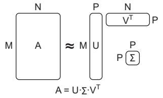
Figure 3.2 Example of SVD, a low-rank approximation. A is a large matrix with dimensions N and M. We can approximate it with three smaller matrices: U with dimensions M and P, Σ a square matrix with dimension P, and V with dimensions N and P (here we show the transpose). Usually, both P<<M and P<<N are true.

To solidify this concept, it may help to see a concrete example. In the next listing, we show a simple example of SVD at work compressing a 4 × 4 matrix. For this, we only need the basic libraries SciPy and NumPy, which are imported on lines 1 and 2. In line 3, we define the matrix, and then in line 9, we apply SVD to it.

Listing 3.2 Example of SVD low-rank approximation

import scipy
import numpy as np
matrix = np.array([
 [ 1., 2., 3., 4.],
 [ 5., 6., 7., 8.],
 [ 9., 10., 11., 12.],
 [13., 14., 15., 16.]
])
u, s, vt = scipy.sparse.linalg.svds(matrix, k=1)
print(u,s,vt)

# [[-0.13472211]
# [-0.34075767]
# [-0.5467932 ]

The generated text is

[-0.7528288 ]], [38.62266], [[-0.4284123 -0.47437257 -0.52033263 –0.5662928 ]]

Taking a moment to inspect U, Sigma, and the transpose of V, we see a 4 × 1 matrix, a 1 × 1 matrix, and a 1 × 4 matrix, respectively. All in all, we now only need 9 parameters versus the original 16, shrinking the memory footprint almost by half.

Lastly, we multiply the matrices back together to get an approximation of the original matrix. In this case, the approximation isn’t all that great, but we can still see that the general order and magnitudes match the original matrix:

svd_matrix = u*s*vt
print(svd_matrix)

The generated text is

 array([[ 2.2291691, 2.4683154, 2.7074606, 2.9466066],
 [ 5.6383204, 6.243202 , 6.848081 , 7.4529614],
 [ 9.047472 , 10.018089 , 10.988702 , 11.959317 ],
 [12.456624 , 13.792976 , 15.129323 , 16.465673 ]], dtype=float32)

Unfortunately, we are not aware of anyone actually using this to compress models in production, most likely due to the poor accuracy of the approximation. What they are using it for—and this is important—is adaptation and finetuning, which is where lowrank adaptation (LoRA)9 comes in. Adaptation is the process of finetuning a generic or base model to do a specific task. LoRA applies SVD low-rank approximation to the attention weights or, rather, to inject update matrices that run parallel to the attention weights, allowing us to finetune a much smaller model. LoRA has become very popular because it makes it a breeze to take an LLM, shrink the trainable layers to a tiny fraction of the original model, and then allow anyone to train it on commodity hardware. You can get started with LoRA using the PEFT library from Hugging Face, where you can check out several LoRA tutorials.

NOTE For the extra curious, parameter-efficient finetuning (PEFT) is a class of methods aimed at finetuning models in a computationally efficient way. The PEFT library seeks to put them all in one easy-to-access place; you can get started here: https://huggingface.co/docs/peft.

⁹ E. J. Hu et al., “LoRA: Low-rank adaptation of large language models.,” June 2021, https://arxiv.org/abs/ 2106.09685.

MIXTURE OF EXPERTS

Mixture of experts (MoE) is a technique where we replace the feed-forward layers in a transformer with MoE layers instead. Feed-forward layers are notorious for being parameter-dense and computationally intensive, so replacing them with something better can often have a large effect. MoEs are a group of sparsely activated models. They differ from ensemble techniques in that typically only one or a few expert models will be run, rather than combining results from all models. The sparsity is often induced by a gate mechanism that learns which experts to use and/or a router mechanism that determines which experts should even be consulted. In figure 3.3, we demonstrate the MoE architecture with potentially N experts, as well as show where it goes inside a decoder stack.

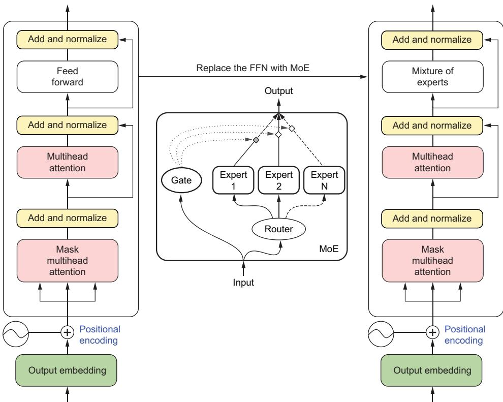
Figure 3.3 Example mixture of an expert’s model with both a gate and router to control flow. The MoE model is used to replace the FFN layers in a transformer; here, we show it replacing the FFN in a decoder.

Depending on how many experts you have, the MoE layer could potentially have more parameters than the FFN, leading to a larger model, but in practice, this isn’t the case, since engineers and researchers are aiming to create a smaller model. What we are guaranteed to see, though, is a faster computation path and improved inference times. However, what really makes MoE stand out is when it’s combined with quantization. One study10 between Microsoft and NVIDIA showed that 2-bit quantization was reachable with only a minimal effect on accuracy using MoE!

Of course, since this is a pretty big change to the model’s structure, finetuning will be required afterward. You should also be aware that MoE layers often reduce a model’s generalizability, so it’s best when used on models designed for a specific task. There are several libraries that implement MoE layers, but we recommend checking out DeepSpeed.

NOTE DeepSpeed is a library that optimizes many of the hard parts for largescale deep learning models like LLMs and is particularly useful when training. Check out their MoE tutorial at https://www.deepspeed.ai/tutorials/ mixture-of-experts/.

3.3.2 Distributed computing

Distributed computing is a technique used in deep learning to parallelize and speed up large, complex neural networks by dividing the workload across multiple devices or nodes in a cluster. This approach significantly reduces training and inference times by enabling concurrent computation, data parallelism, and model parallelism. With the ever-growing size of datasets and complexity of models, distributed computing has become crucial for deep learning workflows, ensuring efficient resource utilization and enabling researchers to iterate on their models effectively. Distributed computing is one of the core practices that separate deep learning from machine learning, and with LLMs, we have to pull out every trick in the book. Let’s look at different parallel processing practices to take full advantage of distributed computing.

DATA PARALLELISM

Data parallelism is what most people think about when they think about running processes in parallel; it’s also the easiest to do. The practice involves splitting up the data and running them through multiple copies of the model or pipeline. For most frameworks, this is easy to set up; for example, in PyTorch, you can use the Distributed-DataParallel method. There’s just one catch for most of these setups: your model has to be able to fit onto one GPU. This is where a tool like Ray.io comes in.

Ray.io, or Ray, is an open source project designed for distributed computing, specifically aimed at parallel and cluster computing. It’s a flexible and user-friendly tool that simplifies distributed programming and helps developers easily execute concurrent tasks in parallel. Ray is primarily built for machine learning and other highperformance applications but can be utilized in other applications. In listing 3.3, we give a simple example of using Ray to distribute a task. The beauty of Ray is the

¹⁰ R. Henry and Y. J. Kim, “Accelerating large language models via low-bit quantization,” March 2023, https:// mng.bz/maD0.

simplicity—all we need to do to make our code run in parallel is add a decorator. It sure beats the complexity of multithreading or asynchronization setups.

import ray
import time
ray.init() 
def slow_function(x): 
 time.sleep(1)
 return x
@ray.remote
def slow_function_ray(x): 
 time.sleep(1)
 return x
results = [slow_function(i) for i in range(1, 11)] 
results_future = [slow_function_ray.remote(i) for i in range(1, 11)] 
results_ray = ray.get(results_future)
print("Results without Ray: ", results)
print("Results with Ray: ", results_ray)
ray.shutdown()
  Listing 3.3 Example Ray parallelization task 
                       Starts Ray
                                    Defines a regular 
                                    Python function
                                        Turns the function 
                                        into a Ray task
                                                                    Executes the slow 
                                                                    function without Ray 
                                                                    (takes 10 seconds)
                                                                       Executes the slow
                                                                       function with Ray
                                                                        (takes 1 second)

Ray uses the concepts of tasks and actors to manage distributed computing. Tasks are functions, whereas actors are stateful objects that can be invoked and run concurrently. When you execute tasks using Ray, it distributes tasks across the available resources (e.g., multicore CPUs or multiple nodes in a cluster). For LLMs, we would need to set up a Ray cluster in a cloud environment, as this would allow each pipeline to run on a node with as many GPUs as needed, greatly simplifying the infrastructure set up to run LLMs in parallel.

NOTE Learn more about Ray clusters here: https://mng.bz/eVJP.

There are multiple alternatives out there, but Ray has been gaining a lot of traction and becoming more popular as more and more machine learning workflows require distributed training. Teams have had great success with it. By utilizing Ray, developers can ensure better performance and more efficient utilization of resources in distributed workflows.

TENSOR PARALLELISM

Tensor parallelism takes advantage of matrix multiplication properties to split up the activations across multiple processors, running the data through, and then combining them on the other side of the processors. Figure 3.4 demonstrates how this process works for a matrix, which can be parallelized in two separate ways that give us the same result. Imagine that Y is a really big matrix that can’t fit on a single processor or, more likely, a bottleneck in our data flow that takes too much time to run all the calculations. In either case, we could split Y by columns or rows, run the calculations, and then combine the results. In this example, we are dealing with matrices, but in reality, we often deal with tensors with more than two dimensions. However, the same mathematical principles that make this work still apply.

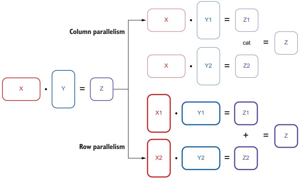
Figure 3.4 Tensor parallelism example showing that you can break up tensors by different dimensions and get the same end result. Here, we compare column and row parallelism of a matrix.

Choosing which dimension to parallelize is a bit of an art, but there are a few things to remember to help make this decision easier. First, how many columns or rows do you have? In general, you want to pick a dimension that has more than the number of processors you have, or you will end up stopping short. Generally, this isn’t a problem, but with tools like Ray, discussed in the last section, parallelizing in a cluster and spinning up loads of processes is a breeze. Second, different dimensions have different multiplicity costs. For example, column parallelism requires us to send the entire dataset to each process but with the benefit of concatenating them together at the end, which is fast and easy. Row parallelism, however, allows us to break up the dataset into chunks but requires us to add the results, a more expensive operation than concatenating. You can see that one operation is more I/O bound, while the other is more computation

bound. Ultimately, the best dimension will be dataset dependent and hardware limited. It will require experimentation to optimize this fully, but a good default is to just choose the largest dimension.

Tensor parallelism allows us to split up the heavy computation layers like MLP and attention layers onto different devices, but it doesn’t help us with normalization or dropout layers that don’t utilize tensors. To get better overall performance of our pipeline, we can add sequence parallelism that targets these blocks.11 Sequence parallelism is a process that partitions activations along the sequence dimension, preventing redundant storage, and can be mixed with tensor parallelism to achieve significant memory savings with minimal additional computational overhead. In combination, they reduce the memory needed to store activations in transformer models. In fact, they nearly eliminate activation recomputation and save activation memory up to five times.

Figure 3.5 shows how combining tensor parallelism, which allows us to distribute the computationally heavy layers, and sequence parallelism, which does the same for the memory limiting layers, allows us to fully parallelize the entire transformer model. Together, they allow for extremely efficient use of resources.

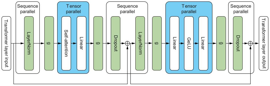
Figure 3.5 Combining tensor parallelism that focuses on computational heavy layers with sequence parallelism to reduce memory overhead to create a fully parallel process for the entire transformer

PIPELINE PARALLELISM

So far, we can run lots of data and speed up any bottlenecks, but none of that matters because our model is too big; we can’t fit it into a single GPU’s memory to even get it to run. That’s where pipeline parallelism comes in; it’s the process of splitting up a model vertically and putting each part onto a different GPU. This creates a pipeline, as input data will go to the first GPU, process, then transfer to the next GPU, and so on until it’s run through the entire model. While other parallelism

¹¹ V. Korthikanti et al., “Reducing activation recomputation in large transformer models,” May 2022, https:// arxiv.org/abs/2205.05198.

techniques improve our processing power and speed up inference, pipeline parallelism is required to get it to run. However, it comes with some major downsides, mainly device utilization.

To understand where this downside comes from and how to mitigate it, let’s first consider the naive approach to this, where we simply run all the data at once through the model. We find that this leaves a giant “bubble” of underutilization. Since the model is broken up, we have to process everything sequentially through the devices. This means that while one GPU is processing, the others are sitting idle. In figure 3.6, we can see this naive approach and a large bubble of inactivity as the GPUs sit idle. We also see a better way to take advantage of each device. We do this by sending the data in small batches. A smaller batch allows the first GPU to pass on what it was working on quicker and move on to another batch. This allows the next device to get started earlier and reduces the size of the bubble.

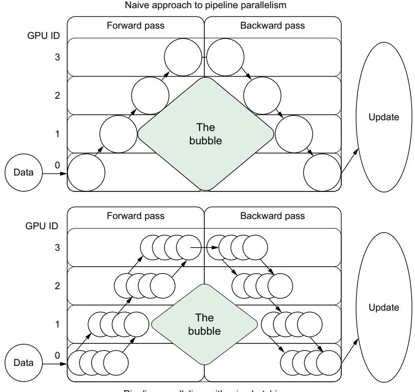
Pipeline parallelism with microbatching

Figure 3.6 The bubble problem. When data runs through a broken-up model, the GPUs holding the model weights are underutilized while they wait for their counterparts to process the data. A simple way to reduce this bubble is to use microbatching.

We can actually calculate the size of the bubble quite easily with the following formula:

\[\text{Idle Percentage} = \text{l} - \text{m} \mid (\text{m} + \text{n} - \text{l})\]

where m is the number of microbatches and n is the depth of the pipeline or number of GPUs. So for our naive example case of four GPUs and one large batch, we see the devices sitting idle 75% of the time! GPUs are quite expensive to allow to sit idle three quarters of the time. Let’s see what that looks like using the microbatch strategy. With a microbatch of 4, it cuts this almost in half, down to just 43% of the time. We can glean from this formula that the more GPUs we have, the higher the idle times, but the more microbatches, the better the utilization.

Unfortunately, we often can neither reduce the number of GPUs nor make the microbatches as large as we want. There are limits. For GPUs, we have to use as many as it takes to fit the model into memory. However, try to use a few larger GPUs, as this will lead to more optimal utilization than using many smaller GPUs. Reducing the bubble in pipeline parallelism is another reason why compression is so important. For microbatching, the first limit is obvious: since the microbatch is a fraction of our batch size, we are limited by how big that is. The second is that each microbatch increases the memory demand for cached activations in a linear relationship. One way to counter this higher memory demand is a method called PipeDream.12 There are different configurations and approaches, but the basic idea is the same. In this method, we start working on the backward pass as soon as we’ve finished the forward pass of any of the microbatches. This allows us to fully complete a training cycle and release the cache for that microbatch.

3D PARALLELISM

For LLMs, we are going to want to take advantage of all three parallelism practices, as they can all be run together. This is known as 3D parallelism, which combines data, tensor, and pipeline parallelism (DP + TP + PP) together. Since each technique and, thus, dimension will require at least two GPUs to run 3D parallelism, we’ll need at least eight GPUs to get started. How we configure these GPUs will be important to get the most efficiency out of this process. Because TP has the largest communication overhead, we want to ensure these GPUs are close together, preferably on the same node and machine. PP has the least communication volume of the three, so breaking up the model across nodes is the least expensive here.

By running the three together, we see some interesting interactions and synergies between them. Since TP splits the model to work well within a device’s memory, we see that PP can perform well even with small batch sizes due to the reduced effective batch size enabled by TP. This combination also improves the communication between DP nodes at different pipeline stages, allowing DP to work effectively too.

¹² A. Harlap et al., “PipeDream: Fast and efficient pipeline parallel DNN training,” June 8, 2018, https:// arxiv.org/abs/1806.03377.

The communication bandwidth between nodes is proportional to the number of pipeline stages. Consequently, DP can scale well even with smaller batch sizes. Overall, we see that when running in combination, we get better performance than when we run them individually.

Now that we know some tricks of the trade, it’s just as important to have the right tools to do the job.

3.4 LLM operations infrastructure

We are finally going to start talking about the infrastructure needed to make this all work. This likely comes as a surprise, as we know that some readers would have expected this section at the beginning of chapter 1. Why wait till the end of chapter 3? In the many times we’ve interviewed machine learning engineers, we have often asked this open-ended question: “What can you tell me about MLOps?” An easy softball question to get the conversation going. Most junior candidates would immediately start jumping into the tooling and infrastructure. It makes sense; there are so many different tools available. That’s not to mention the fact that whenever you see posts or blogs describing MLOps, there’s a pretty little diagram showing the infrastructure. While all of that is important, it’s useful to recognize what a more senior candidate jumps into—the machine learning life cycle.

For many, the nuance is lost, but the infrastructure is the how, and the life cycle is the why. Most companies can get by with just bare-bones infrastructure. We’ve seen our share of scrappy systems that exist entirely on one data scientist’s laptop, and they work surprisingly well—especially in the era of scikit-learn everything!

Unfortunately, a rickshaw machine learning platform doesn’t cut it in the world of LLMs. Since we still live in a world where the standard storage capacity of a Mac-Book Pro laptop is 256 GB, just storing the model locally can already be a problem. Companies that invest in a sturdier infrastructure are better prepared for the world of LLMs.

In figure 3.7, we see an example MLOps infrastructure designed with LLMs in mind. While most infrastructure diagrams simplify the structure to make everything look clean, the raw truth is that there’s a bit more complexity to the entire system. Of course, a lot of this complexity would disappear if we could get data scientists to work inside scripts instead of ad hoc workstations—usually with a Jupyter Notebook interface.

Taking a closer look at figure 3.7, you can see several tools on the outskirts that squarely land in DataOps or even just DevOps—data stores, orchestrators, pipelines, streaming integrations, and container registries. These are tools you are likely already using for just about any data-intensive application and aren’t necessarily focused on MLOps. Toward the center, we have more traditional MLOps tools—experiment trackers, model registry, feature store, and ad hoc data science workstations. For LLMs, we really only introduce one new tool to the stack: a vector database. What’s not pictured is the monitoring system because it intertwines with every piece. This

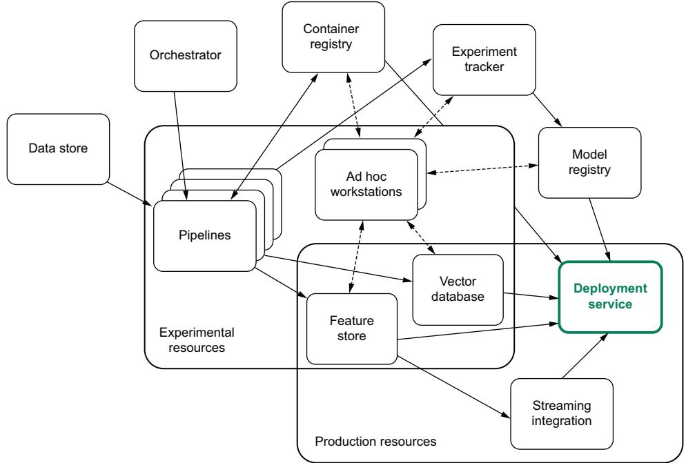
Figure 3.7 A high level view of an MLOps infrastructure with LLMs in mind. This diagram attempts to cover the full picture and the complexity of the many tools involved to make ML models work in production.

all culminates into what we are working toward in this book—a deployment service where we can confidently deploy and run LLMs in production.

Infrastructure by discipline

The following list defines infrastructure by the specific discipline:

• DevOps—In charge of procuring the environmental resources: experimental (dev, staging) and production. This includes hardware, clusters, and networking to make it all work. Also in charge of basic infrastructure systems like Github/Gitlab, artifact registries, container registries, application or transactional databases like Postgres or MySQL, caching systems, and CI/CD pipelines. This list is by no means comprehensive.
• DataOps—In charge of data, in motion and at rest. It includes centralized or decentralized data stores like data warehouses, data lakes, and data meshes, as well as data pipelines, either in batch systems or in streaming systems with tools like Kafka and Flink. It also includes orchestrators like Airflow, Prefect, and Mage. DataOps is built on top of DevOps. For example, we’ve seen many CI/CD pipelines being used for data pipeline work until eventually graduating to systems like Apache Spark or DBT.

MLOps—In charge of the machine learning life cycle, from the creation of models to deprecation. This includes data science workstations like Jupyter-Hub, experiment trackers, and a model registry. It includes specialty databases like feature stores and vector databases, as well as a deployment service to tie everything together and actually serve results. It is built on top of both DataOps and DevOps.

Let’s go through each piece of the infrastructure puzzle and discuss features you should consider when thinking about LLMs in particular. While we will be discussing specialized tooling for each piece, we’ll note that there are also MLOps as a service platform, like Dataiku, Amazon’s SageMaker, Azure Machine Learning, and Google’s VertexAI. These platforms attempt to complete the whole puzzle; how well they do that is another question. However, they are often a great shortcut, and you should be aware of them. Well, that’s enough dillydallying; let’s dive in already!

3.4.1 Data infrastructure

While not the focus of this book, it’s important to note that MLOps is built on top of a data operations infrastructure, which itself is built on top of DevOps. Key features of the DataOps ecosystem include a data store, an orchestrator, and pipelines. Additional features usually required include a container registry and a streaming integration service.

Data stores are the foundation of DataOps and come in many forms, from a simple database to large data warehouses and from even larger data lakes to an intricate data mesh. This is where your data is stored, and a lot of work goes into managing, governing, and securing the data store. The orchestrator is the cornerstone of DataOps, as it’s a tool that manages and automates both simple and complex multistep workflows and tasks, ensuring they run across multiple resources and services in a system. The most commonly talked about are Airflow, Prefect, and Mage. Lastly, pipelines are the pillars. They hold everything else up and are where we run our jobs. Initially built to simply move, clean, and define data, these same systems are used to run machine learning training jobs on a schedule and do batch inference and loads of other work needed to ensure MLOps runs smoothly.

A container registry is a keystone of DevOps and, subsequently, DataOps and MLOps. Running all our pipelines and services in containers is necessary to ensure consistency. Streaming services are a much bigger beast than what we may let on in this chapter, and if you know, you know. Thankfully, for most text-related tasks, realtime processing isn’t a major concern. Even for tasks like real-time captioning or translation, we can often get by with some sort of pseudo–real-time processing strategy that doesn’t degrade the user experience depending on the task.

3.4.2 Experiment trackers

Experiment trackers are central to MLOps. Experiment trackers do the fundamental job of keeping track and recording tests and results. As the famous Adam Savage quote from Myth Busters states, “Remember, kids, the only difference between screwing around and science is writing it down.” Without it, your organization is likely missing the “science” in data science, which is honestly quite embarrassing.

Even if your data scientists are keen to manually track and record results in notebooks, it might as well be thrown in the garbage if it’s not easy for others to view and search for. This is the real purpose of experiment trackers—to ensure knowledge is easily shared and made available. Eventually, a model will make it to production, and that model is going to have problems. Sure, you can always just train a new model, but unless the team is able to go back and investigate what went wrong the first time, you are likely to repeat the same mistakes over and over.

There are many experiment trackers out there; the most popular by far is MLFlow, which is open source. It was started by the team at Databricks, which also offers an easy hosting solution. Some paid alternatives worth checking out include CometML and Weights & Biases.

Experiment trackers nowadays come with so many bells and whistles. Most open source and paid solutions will certainly have what you need when looking to scale up your needs for LLMOps. However, ensuring you take advantage of these tools correctly might require a few small tweaks. For example, the default assumption is usually that you are training a model from scratch, but often when working with LLMs, you will be finetuning models instead. In this case, it’s important to note the checkpoint of the model you started from. If possible, even linking back to the original training experiment. This will allow future scientists to dig deeper into their test results, find original training data, and discover paths forward to eliminate bias.

Another feature to look out for is evaluation metric tooling. We will go into greater depth in chapter 4, but evaluation metrics are difficult for language models. There are often multiple metrics you care about, and none of them are simple, like complexity ratings or similarity scores. While experiment tracker vendors try to be agnostic and unopinionated about evaluation metrics, they should at least make it easy to compare models and their metrics to help us decide which one is better. Since LLMs have become so popular, some have made it easy to evaluate the more common metrics like ROUGE for text summarization.

You will also find that many experiment-tracking vendors have started to add tools specifically for LLMs. Some features you might consider looking for include direct Hugging Face support, LangChain support, prompt engineering toolkits, finetuning frameworks, and foundation model shops. The space is developing quickly, and no one tool has all the same features right now, but these feature sets will likely converge.

3.4.3 Model registry

The model registry is probably the simplest tool of an MLOps infrastructure. The main objective is one that’s easy to solve; we just need a place to store the models. We’ve seen many successful teams get by simply by putting their models in an object store or shared filesystem and calling it good. That said, there are a couple bells and whistles you should look for when choosing one.

The first is whether the model registry tracks metadata about the model. Most of what you care about is going to be in the experiment tracker, so you can usually get away with simply ensuring you can link the two. In fact, most model registries are built into experiment tracking systems because of this. However, a problem with these systems happens when the company decides to use an open source model or even buy one. Is it easy to upload a model and tag it with relevant information? The answer is usually no.

Next, you want to make sure you can version your models. At some point, a model will reach a point where it’s no longer useful and will need to be replaced. Versioning your models will simplify this process. It also makes running production experiments like A/B testing or shadow tests easier.

Lastly, if we are promoting and demoting models, we need to be concerned with access. Models tend to be valuable intellectual property for many companies, so ensuring only the right users have access to the models is important. But it’s also important to ensure that only the team that understands the models—what they do and why they were trained—is in charge of promoting and demoting the models. The last thing we want is to delete a model in production or worse.

For LLMs, there are some important caveats you should be aware of: mainly, when choosing a model registry, be aware of any limit sizes. Several model registries restrict model sizes to 10 GB or smaller. That’s just not going to cut it. We could speculate on the many reasons for this, but none of them are worthy of note. Speaking of limit sizes, if you are going to be running your model registry on an on-premise storage system like Ceph, make sure it has lots of space. You can buy multiple terabytes of storage for a couple of hundred dollars for your on-premise servers, but even a couple of terabytes fills up quickly when your LLM is over 300 GB. Don’t forget: you are likely to be keeping multiple checkpoints and versions during training and finetuning, as well as duplicates for reliability purposes. Storage is still one of the cheapest aspects of running LLMs, though, so there’s no reason to skimp here and cause headaches down the road.

This brings me to a good point: a lot of optimization could still be made, allowing for better space-saving approaches to storing LLMs and their derivatives, especially since most of these models will be very similar overall. We’ll likely see storage solutions to solve just this problem in the future.

3.4.4 Feature stores

Feature stores solve many important problems and answer questions like, Who owns this feature? How was it defined? Who has access to it? Which models are using it? How do we serve this feature in production? Essentially, they solve the “single source of truth” problem. Creating a centralized store allows teams to shop for the highest quality, most well-maintained, thoroughly managed data. Feature stores solve the problems of collaboration, documentation, and versioning of data.

If you’ve ever thought, “A feature store is just a database, right?”, you are probably thinking about the wrong type of store—we are referencing a place to shop, not a place of storage. Don’t worry: this confusion is normal, as we’ve heard this sentiment a lot and have had similar thoughts ourselves. The truth is that modern-day feature stores are more virtual than a physical database, which means they are built on top of whatever data store you are already using. For example, Google’s Vertex AI feature store is just BigQuery, and we’ve seen a lot of confusion from data teams wondering, “Why don’t we just query BigQuery?” Loading the data into a feature store feels like an unnecessary extra step, but think about shopping at an IKEA store. No one goes directly to the warehouse where all the furniture is in boxes. That would be a frustrating shopping experience. The features store is the showroom that allows others in your company to easily peruse, experience, and use the data.

Often, we see people reach for a feature store to solve a technical problem like low latency access for online feature serving. A huge win for feature stores is solving the training-serving skew. Some features are just easier to do in SQL after the fact, like calculating the average number of requests for the last 30 seconds. This can lead to naive data pipelines being built for training but causing massive headaches when going to production because getting this type of feature in real time can be anything but easy. Feature store abstractions help minimize this burden. Related to this are feature store point-in-time retrievals, which are table stakes when talking feature stores. Point-intime retrievals ensure that, given a specific time, a query will always return the same result. This is important because features like averages over “the last 30 seconds” are constantly changing, so this allows us to version the data (without the extra burden of a bloated versioning system), as well as ensure our models will give accurate and predictable responses.

As far as options, Feast is a popular open source feature store. Featureform and Hopsworks are also open source. All three offer paid hosting options. For LLMs, we’ve heard the sentiment that feature stores aren’t as critical as other parts of the MLOps infrastructure. After all, the model is so large that it should incorporate all the features needed inside it, so you don’t need to query for additional context. Just give the model the user’s query, and let the model do its thing. However, this approach is still a bit naive, and we haven’t quite gotten to a point where LLMs are completely self-sufficient. To avoid hallucinations and improve factual correctness, it is often best to give the model some context. We do this by feeding it embeddings of our documents that we want it to know very well, and a feature store is a great place to put these embeddings.

3.4.5 Vector databases

If you are familiar with the general MLOps infrastructure, most of this section has been review for you. We’ve only had to make slight adjustments highlighting important scaling concerns to make a system work for LLMs. Vector databases, however, are new to the scene and have been developed to be a tailored solution for working with LLMs and language models in general, but you can also use them with other datasets like images or tabular data, which are easy enough to transform into a vector. Vector databases are specialized databases that store vectors along with some metadata around the vector, which makes them great for storing embeddings. Now, while that last sentence is true, it is a bit misleading because the power of vector databases isn’t in their storage but in the way that they search through the data.

Traditional databases, using b-tree indexing to find IDs or text-based search using reverse indexes, all have the same common flaw: you have to know what you are looking for. If you don’t have the ID or you don’t know the keywords, it’s impossible to find the right row or document. Vector databases, however, take advantage of the vector space, meaning you don’t need to know exactly what you are looking for; you just need to know something similar, which you can then use to find the nearest neighbors using similarity searches based on Euclidean distance, cosine similarity, dot product similarity, or what have you. For example, using a vector database makes solving the reverse image search problem a breeze.

At this point, some readers may be confused. First, we told you to put your embeddings into a feature store, and now we’re telling you to put them into a Vector DB. Which one is it? Well, that’s the beauty of it: you can do both at the same time. If it didn’t make sense before, we hope it makes sense now. A feature store is not a database; it is just an abstraction. You can use a feature store built on top of a vector DB, and it will solve many of your problems. Vector DBs can be difficult to maintain when you have multiple data sources, are experimenting with different embedding models, or otherwise have frequent data updates. Managing this complexity can be a real pain, but a feature store can handily solve this problem. Using them in combination will ensure a more accurate and up-to-date search index.

Vector databases have only been around for a couple of years at the time of writing, and their popularity is still relatively new, as they have grown hand in hand with LLMs. It’s easy to understand why since they provide a fast and efficient way to retrieve vector data, making it simple to provide LLMs with needed context to improve their accuracy.

That said, it’s a relatively new field, and there are lots of competitors in this space right now. It’s a bit too early to know who the winners and losers are. Not wanting to date this book too much, let me at least suggest two options to start: Pinecone and Milvus. Pinecone is one of the first vector databases as a product and has a thriving community with lots of documentation. It’s packed with features and has proven itself to scale. Pinecone is a fully managed infrastructure offering that has a free tier for beginners to learn. If you are a fan of open source, however, then you’ll want to check out Milvus. Milvus is feature rich and has a great community. Zilliz, the company behind Milvus, offers a fully managed offering, but it’s also available to deploy in your own clusters. If you already have a bit of infrastructure experience, it’s relatively easy and straightforward to do.

There are lots of alternatives out there right now, and it’s likely worth a bit of investigation before picking one. The two things you’ll probably care most about are price and scalability, as the two often go hand in hand. After that, it’s valuable to pay attention to search features, such as support for different similarity measures like cosine similarities, dot product, and Euclidean distance, as well as indexing features like Hierarchical Navigable Small World (HNSW) and locality-sensitive hashing (LSH). Being able to customize your search parameters and index settings is important for any database, as you can customize the workload for your dataset and workflow, allowing you to optimize query latency and search result accuracy.

It’s also important to note that with the rise of vector databases, we are quickly seeing many database incumbents like Redis and Elastic offering vector search capabilities. For now, most of these tend to offer the most straightforward feature sets, but they are hard to ignore if you are already using these tool sets, as they can provide quick wins to help you get started quickly.

Vector databases are powerful tools that can help you train or finetune LLMs, as well as improve the accuracy and results of your LLM queries.

3.4.6 Monitoring system

A monitoring system is crucial to the success of any ML system, LLMs included. Unlike other software applications, ML models are known to fail silently—that is, continue to operate but start to give poor results. This is often due to data drift, a common example being a recommendation system that gives worse results over time because sellers start to game the system by giving fake reviews to get better recommendation results. A monitoring system allows us to catch poorly performing models and make adjustments or simply retrain them.

Despite their importance, monitoring systems are often the last piece of the puzzle added. This is often purposeful, as putting resources into figuring out how to monitor models doesn’t help if you don’t have any models to monitor. However, don’t make the mistake of putting it off too long. Many companies have been burned by a model that went rogue with no one knowing about it, often costing them dearly. It’s also important to realize you don’t have to wait to get a model into production to start monitoring your data. There are plenty of ways to introduce a monitoring system into the training and data pipelines to improve data governance and compliance. Regardless, you can usually tell the maturity of a data science organization by its monitoring system.

There are lots of great monitoring toolings out there; some great open source options include whylogs and Evidently AI. We are also fans of Great Expectations but have found it rather slow outside of batch jobs. There are also many more paid options out there. Typically, for ML monitoring workloads, you’ll want to monitor everything

you’d normally record in other software applications; this includes resource metrics like memory and CPU utilization, performance metrics like latency and queries per second, and operational metrics like status codes and error rates. In addition, you’ll need ways to monitor data drift going in and out of the model. You’ll want to pay attention to things like missing values, uniqueness, and standard deviation shifts. In many instances, you’ll want to be able to segment your data while monitoring—for example, for A/B testing or monitoring by region. Some metrics useful to monitor in ML systems include model accuracy, precision, recall, and F1 scores. These are difficult since you won’t know the correct answer at inference time, so it’s often helpful to set up some sort of auditing system. Of course, auditing will be easier if your LLM is designed to be a Q&A bot rather than if your LLM is built to help writers be more creative.

This hints at a whole set of new challenges for your monitoring systems, even more than what we see with other ML systems. With LLMs, we are dealing with text data, which is hard to quantify, as discussed earlier in this chapter. For instance, consider the features you look at to monitor for data drift, because language is known to drift a lot! One feature we suggest is unique tokens. These will alert you when new slang words or terms are created; however, they still don’t help when words switch meaning, for example, when “wicked” means “cool.” We would also recommend monitoring the embeddings; however, you’ll likely find this to either add a lot of noise and false alarms or, at the very least, be difficult to decipher and dig into when problems do occur. The systems that work the best often involve a lot of handcrafted rules and features to monitor, but these can be error-prone and time-consuming to create.

Monitoring text-based systems is far from a solved problem, mostly stemming from the difficulties in understanding text data to begin with. This begs the question of what the best methods are to use language models to monitor themselves since they are our current best solution to codifying language. Unfortunately, we’re not aware of anyone researching this, but we imagine it’s only a matter of time.

3.4.7 GPU-enabled workstations

GPU-enabled workstations and remote workstations in general are often considered a nice-to-have or luxury by many teams, but when working with LLMs, that mindset has to change. When troubleshooting a problem or just developing a model in general, a data scientist isn’t able to spin up the model in a notebook on their laptop anymore. The easiest way to solve this is to simply provide remote workstations with GPU resources. There are plenty of cloud solutions for this, but if your company is working mainly on-premise, it may be a bit more difficult to provide but necessary nonetheless.

LLMs are GPU memory-intensive models. Consequently, there are some numbers every engineer should know when it comes to working in the field. The first is how many GPUs to have. The NVIDIA Tesla T4 and V100 are the two most common GPUs you’ll find in a datacenter, but they only have 16 GB of memory. They are workhorses, though, and cost-effective, so if we can compress our model to run on these, all the better. After these, you’ll find a range of GPUs like NVIDIA A10G, NVIDIA Quadro

series, and NVIDIA RTX series that offer GPU memories in the ranges of 24, 32, and 48 GB. All of these are fine upgrades; you’ll just have to figure out which ones are offered by your cloud provider and available to you. This brings us to the NVIDIA A100, which is likely going to be your GPU of choice when working with LLMs. Thankfully, they are relatively common and offer two different models providing 40 or 80 GB. A big problem with these is that they are constantly in high demand by everyone right now. You should also be aware of the NVIDIA H100, which offers 80 GB like the A100. The H100 NVL is promised to support up to 188 GB and has been designed with LLMs in mind. Another new GPU you should be aware of is the NVIDIA L4 Tensor Core GPU, which has 24 GB and is positioned to take over as a new workhorse along with the T4 and V100, at least as far as AI workloads are concerned.

LLMs come in all different sizes, and it’s useful to have a horse sense for what these numbers mean. For example, the LLaMA model has 7B, 13B, 33B, and 65B parameter variants. If you aren’t sure off the top of your head which GPU you need to run which model, here’s a shortcut: multiply the number of billions of parameters by two, and that’s how much GPU memory you need. The reason is that most models at inference will default to run at half precision, FP16 of BF16, which means we need at least 2 bytes for every parameter. For example, 7 billion × 2 bytes = 14 GB. You’ll need a little extra as well for the embedding model, which will be about another gigabyte, and more for the actual tokens you are running through the model. One token is about 1 MB, so 512 tokens will require 512 MB. This isn’t a big deal until you consider running larger batch sizes to improve performance. For 16 batches of this size, you’ll need an extra 8 GB of space.

Of course, so far, we’ve only been talking about inference; for training, you’ll need a lot more space. While training, you’ll always want to do this in full precision, and you’ll need extra room for the optimizer tensors and gradients. In general, to account for this, you’ll need about 16 bytes for every parameter. So to train a 7B parameter model, you’ll want 112 GB of memory.

3.4.8 Deployment service

Everything we’ve been working toward is collected and finally put to good use here. In fact, if you took away every other service and were left with just a deployment service, you’d still have a working MLOps system. A deployment service provides an easy way to integrate with all the previous systems we talked about and to configure and define the needed resources to get our model running in production. It will often provide boilerplate code to serve the model behind a REST and gRPC API or directly inside a batch or streaming pipeline.

Some tools to help create this service include NVIDIA Triton Inference Service, MLServer, Seldon, and BentoML. These services provide a standard API interface, typically the KServe V2 Inference Protocol. This protocol provides a unified and extensible way to deploy, manage, and serve machine learning models across different platforms and frameworks. It defines a common interface to interact with models,

including gRPC and HTTP/RESTful APIs. It standardizes concepts like input/output tensor data encoding, predict and explain methods, model health checks, and metadata retrieval. It also allows seamless integration with languages and frameworks, including TensorFlow, PyTorch, ONNX, Scikit Learn, and XGBoost.

Of course, there are times when flexibility and customization provide enough value to step away from the automated path these other frameworks provide, in which case it’s best to reach for a tool like FastAPI. Your deployment service should still provide as much automation and boilerplate code here as possible to make the process as smooth as possible. It should be mentioned that most of the previously mentioned frameworks do offer custom methods, but your mileage may vary.

Deploying a model is more than just building the interface. Your deployment service will also provide a bridge to close the gap between the MLOps infrastructure and general DevOps infrastructure. The connection to whatever CI/CD tooling and build and shipping pipelines your company has set up so you can ensure appropriate tests and deployment strategies like health checks and rollbacks can easily be monitored and done. This is often very platform- and thus company-specific. It must also provide the needed configurations to talk to Kubernetes or whatever other container orchestrator you may be using to acquire the needed resources like CPU, memory, accelerators, autoscalers, proxies, etc. It also applies the needed environment variables and secret management tools to ensure everything runs.

All in all, this service ensures you can easily deploy a model into production. For LLMs, the main concern is often just being sure the platform and clusters are set up with enough resources to provision what will ultimately be configured.

We’ve discussed a lot so far in this chapter, starting with what makes LLMs so much harder than traditional ML, which is hard enough as it is. First, we learned that their size can’t be underestimated, but then we also discovered many peculiarities about them, from token limits to hallucinations—not to mention that they are expensive. Fortunately, despite being difficult, they aren’t impossible. We discussed compression techniques and distributed computing, which are crucial to master. We then explored the infrastructure needed to make LLMs work. While most of it was likely familiar, we came to realize that LLMs put a different level of pressure on each tool, and often, we need to be ready for a larger scale than what we could get away with for deploying other ML models.

Summary

• LLMs are difficult to work with mostly because they are big. This results in a longer time to download, load into memory, and deploy, forcing us to use expensive resources.
• LLMs are also hard because they deal with natural language and all its complexities, including hallucinations, bias, ethics, and security.
• Regardless of whether you build or buy, LLMs are expensive, and managing costs and risks associated with them will be crucial to the success of any project utilizing them.
• Compressing models to be as small as we can makes them easier to work with; quantization, pruning, and knowledge distillation are particularly useful for this.
• Quantization is popular because it is easy and can be done after training without any finetuning.
• Low-rank approximation is an effective way to shrink a model and has been used heavily for adaptation, thanks to LoRA.
• There are three core directions we use to parallelize LLM workflows: data, tensor, and pipeline. DP helps us increase throughput, TP helps us increase speed, and PP makes it all possible to run in the first place.
• Combining the parallelism methods, we get 3D parallelism (data + tensor + pipeline), where we find that the techniques synergize, covering each other’s weaknesses and helping us get more utilization.
• The infrastructure for LLMOps is similar to MLOps, but don’t let that fool you, since there are many caveats where “good enough” no longer works.
• Many tools have begun to offer new features specifically for LLM support.
• Vector databases, in particular, are interesting as a new piece of the infrastructure puzzle needed for LLMs that allow quick search and retrievals of embeddings.

Data engineering for large language models: Setting up for success

This chapter covers

• Common foundation models used in the industry
• How to evaluate and compare large language models
• Different data sources and how to prepare your own
• Creating your own custom tokenizers and embeddings
• Preparing a Slack dataset to be used in future chapters

Data is like garbage. You’d better know what you are going to do with it before you collect it.

—Mark Twain

Creating our own LLM is no different from any ML project in that we will start by preparing our assets—and there isn’t a more valuable asset than your data. All successful AI and ML initiatives are built on a good data engineering foundation. It’s important then that we acquire, clean, prepare, and curate our data.

Unlike other ML models, you generally won’t be starting from scratch when creating an LLM customized for your specific task. Of course, if you do start from scratch, you’ll likely only do it once. Then it’s best to tweak and polish that model to further refine it for your specific needs. Selecting the right base model can make or break your project. Figure 4.1 gives a high-level overview of the different pieces and assets you’ll need to prepare before training or finetuning a new model.

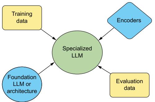
Figure 4.1 The different elements of training an LLM. Combining earth, fire, water—wait, no, not those elements. To get started, you’ll need to collect several assets, including a foundation model, training data, text encoders (e.g., tokenizer), and evaluation data.

As was so well defined in the book Fundamentals of Data Engineering¹ :

Data engineering is the development, implementation, and maintenance of systems and processes that take in raw data and produce high-quality, consistent information that supports downstream use cases, such as analysis and machine learning.

In this chapter, we will discuss the steps you’ll need to take before you can start creating your LLM, which largely involves preparing the data assets necessary to train a model. We will go over many of the base or foundation models available to you as a starting point and how to evaluate and compare them. We will then go into depth on many of the different datasets available and how to prepare your own for finetuning a model, including preparing your own tokenizer or embeddings. Lastly, we will craft a dataset that we will use to finetune a model in the next chapter.

4.1 Models are the foundation

We will first discuss the most important dataset you will need to collect when training, which is the model weights of a pretrained model. A big reason why LLMs are so successful as a technology is that we can take a model already trained on language as a whole and tweak it to do well on a specific task. Of course, knowing how that beginning model was trained and what it was trained on will be a huge shortcut in choosing the right one to tweak.

Choosing the right one has become obnoxiously difficult since LLMs have been a hot research topic, resulting in a new one that sports benchmark-breaking records

¹ Joe Reis and Matt Housley, Fundamentals of Data Engineering, O’Reilly, 2022.

popping up almost every week. Because we know (or at least assume) you are eager to learn about them, we will first discuss the many different models currently out there. These models have already been trained (for better or worse) by professionals working to make your life easier and put powerful language models into the public arena. There are thousands upon thousands of open source models available on GitHub, Hugging Face Hub, and elsewhere, so to simplify, we’ll highlight our favorites, giving you details about each of the models to make it easier to compare and to give you an idea about whether you should use that particular model or opt for one of its lesserknown open source variants. If you are planning to train from scratch, consider the architecture involved and if there’s a certain family you’d like to try.

4.1.1 GPT

There’s probably no better place to start than with GPT (Generative Pre-trained Transformer) models. A fan favorite and one of ours too, these models are sold commercially through OpenAI and have gained popularity for their impressive performance on a wide range of tasks. GPT models are so well known that laypersons often use “GPT” to replace “LLM,” just as one might say Kleenex or Band-Aid instead of tissue or bandage.

The first GPT model was introduced in 2018, shortly after transformers were introduced, and only had 120M parameters. It was trained on the small BookCorpus dataset and had impressive results on NLP benchmarks at the time. The GPT-2 model came out the next year, increasing its size by 10-fold to 1.5B parameters; it was trained on the much larger WebText dataset. The next year, in 2020, GPT-3 came out 100 times larger with 175B parameters and trained on the massive Common Crawl dataset. This model was still based on GPT-1’s original architecture with slight modifications for improved scaling.

OpenAI has chosen to keep further iterations like GPT-4 under greater secrecy, not revealing training data or specific architectures, since it has started to productionize and sell them as a product. ChatGPT is a finetuned GPT-3 model trained for conversational interaction using reinforcement learning with human feedback (RLHF). Not to get into the weeds, but there is a whole host of GPT-3 models you can find under API names such as ada, babbage, curie, and davinci, as well as other finetuned models such as webGPT and InstructGPT. We leave it to the reader to investigate further if they are interested.

Other open source variations like GPT-J were created by the open source community utilizing the knowledge gained from the whitepapers OpenAI published. Several GPT models have no relation to OpenAI, as Generative Pre-trained Transformer is a very generic name that fits most LLMs. Of course, OpenAI has started to see it as a brand and is trying to trademark the acronym.2

² C. Loizos, “‘GPT’ may be trademarked soon if OpenAI has its way,” TechCrunch, April 25, 2023, https://mng .bz/5Omq.

GPT-X models, although closed source, can be accessed via the OpenAI API, which also includes features for their finetuning. We will be using GPT-2 throughout this book—even though it is a bit smaller than what most would consider an actual LLM as it is a well-understood architecture and easy to learn with.

4.1.2 BLOOM

BLOOM is one of the most iconic LLMs because of the learning that has come from creating it. The model came out in 2022 and is the first public LLM to rival GPT-3’s size with 176B parameters; it was trained with complete transparency. It was put together by Hugging Face’s BigScience team, with help from Microsoft’s DeepSpeed team and NVIDIA’s Megatron-LM team, and was sponsored by French government grants.

BLOOM was trained on the BigScienceCorpus dataset, a conglomerate of many smaller datasets amounting to 1.6TB of pre-processed text. It is licensed under RAIL, which means it isn’t technically open source, since there are restrictions on how you can use it, but it can be commercialized.

TIP You can learn more about the RAIL license here: https://mng.bz/mR20.

BLOOM was trained to be industry size and industry grade for all tasks. Because of this, fitting on a consumer device was not a priority, but several smaller versions were trained as the research team was coming up to speed. There are 560M-, 3B-, and 7B-parameter versions. There is also BLOOMZ, a multitask, finetuned version of the full 176B parameter model. BLOOM was only trained in 46 different languages, and BLOOMZ’s goal was to increase the cross-lingual generalization of the model.3 You can find all of these models on Hugging Face’s hub: https://huggingface .co/bigscience/bloom.

The big downside to BLOOM is that it often gives poor responses and doesn’t compete very well in benchmarks—most likely due to limited funds and tight deadlines of the project, leading to a feeling that it was undertrained. This isn’t always a bad thing and is often better than an overtrained model, but you can expect to require a lot more finetuning on a larger dataset if you decide to use it. The benefit of using it, though, is that it is well understood and trained in the open, and you can check its training data.

In general, the authors wouldn’t recommend using it as a foundation model anymore; there are better alternatives, but it’s one you should be familiar with because of its contributions. For example, BLOOM’s creation of petals, which allowed distributed training, was a significant contribution to the field.

³ N. Muennighoff et al., “Cross lingual generalization through multitask finetuning,” November 3, 2022, https://arxiv.org/abs/2211.01786.

4.1.3 LLaMA

LLaMA is the result of Meta’s foray into LLMs. The first version was released in February 2023 and was released to the research community with a noncommercial license. A week later, the weights were leaked on 4chan. In an unlikely turn of events, this leak has likely been very beneficial to Meta, as this model has become the standard for experimentation and development. Several more models we will discuss are based on it.

Later, in July 2023, Meta released Llama 2, which has both a research and a commercial license. Llama 2 is a big deal since it’s the first commercially available model that really packs a punch, and you’ll see many other models based on its architecture. There are three different model sizes available: 7B, 13B, and 70B parameters. You can download them here: https://ai.meta.com/llama/. You’ll need to request access and accept the terms and conditions if you plan to use it.

Llama 2 was trained on 2 trillion tokens from a curated dataset taken from the internet where they removed websites known to contain personal information and upsampled what they considered factual sources. While exact details of the dataset haven’t been shared, it likely contained data from Common Crawl, GitHub, Wikipedia, Project Gutenberg, ArXiv, and Stack Exchange since those were the primary datasets for LLaMA 1. These datasets were later packaged together and distributed under the name RedPajama. Llama 2 was then further finetuned using RLHF, with one model finetuned for chat and another for code.

4.1.4 Wizard

The Wizard family of language models comes from the 2023 paper “WizardLM: Empowering Large Language Models to Follow Complex Instructions.”⁴ These models follow the idea that LLMs function better when trained on dense training data filled with high-complexity tasks. Based on a proposed framework for creating more complex instruction tasks, the WizardLM methodology has been applied to many popular datasets and used to finetune almost all of the most popular models. The methodology is so popular that, amazingly, it only took the community two days after LlamaCoder34B came out to finetune the WizardCoder34B model.

These models have been consistently praised for their human-like prose and their ability to correctly sort through complex problems that rivals many paid services. One problem we encourage you to try is to ask WizardCoder34B to write a program that draws a realistic-looking tree using any language you’d like. Because the Wizard models don’t revolve as much around a specific dataset as they do around the methodology of changing an existing dataset to fit the Wizard style, the applications are incredibly broad and diverse. If you hit a wall where you aren’t sure how to improve when using another model or architecture, try taking the dataset you’ve already used and applying the Wizard methodology. You’re welcome.

⁴ C. Xu et al., “WizardLM: Empowering large language models to follow complex instructions,” Jun. 10, 2023, https://arxiv.org/abs/2304.12244.

As a side note, WizardCoder models tend to get a lot of attention, but the Wizard-Math models are also impressive in their own right. We note that a lot of readers likely deal more with data problems than code problems, and the WizardMath models might be a great place to start when working with talk-to-your-data applications.

4.1.5 Falcon

Falcon models are a model family from the Technology Innovation Institute in Abu Dhabi. They are the first state-of-the-art models to be released under a truly open source license, Apache 2.0. You can get the model from the institute’s website: https:// falconllm.tii.ae/falcon-models.html. Its easy access and the open license make this a dream for hackers, practitioners, and the industry.

Falcon models first introduced in June 2023 only introduced 7B and 40B parameter models, but in September 2023, Falcon released a 180B parameter model that can truly compete with GPT-3–sized models. What’s also exciting and probably more important to many readers is that Falcon has often led LLM leaderboards in many benchmarking tasks. The models were primarily trained on the RefinedWeb dataset, which is a smaller but much higher-quality dataset that was carefully and meticulously curated and extracted from the Common Crawl dataset.

4.1.6 Vicuna

Vicuna was trained on a dataset of user-shared conversations from ShareGPT. The logic is that a model trained off of the best outputs of ChatGPT will be able to emulate the performance of ChatGPT, piggy-backing off of the Llama–Alpaca trend.

NOTE We won’t talk about Alpaca here, but we introduced it in chapter 3 when discussing knowledge distillation.

Vicuna has been praised for both its performance and its relatively low training costs. Vicuna is an amazing example of why data coverage and quality matter so much while simultaneously demonstrating the dangers of model collapse from training on the output of another model. Model collapse happens when an ML model is trained on synthetic data, leading to increasingly less diverse outputs. For example, Vicuna performs admirably on anything that is at least close to what appeared in the dataset, but when asked to perform more generative or agent-like tasks, it tends to hallucinate far beyond what its predecessors do. Vicuna is not licensed for commercial use, but it is amazing for personal projects.

4.1.7 Dolly

Created by Databricks as more of a thought experiment than a competitive model, Dolly and its V2 do not perform well compared to other models of the same size. However, Dolly boasts one of the best underlying understandings of English and is a fantastic starting point for finetuning or creating low-ranking adaptations (LoRAs; which we will discuss in chapter 5) to influence other models. Dolly 1.0 was trained on the Stanford Alpaca Dataset, while Dolly 2.0 was trained on a high-quality human-generated instruction-following dataset that was crowdsourced by the Databricks employees. Dolly 2.0 has been open sourced in its entirety, including the training code, dataset, and model weights, all with a commercial use license.5

4.1.8 OpenChat

OpenChat is similar to Vicuna in that OpenChat used 80K ShareGPT conversations for training, but dissimilar in that their conditioning and weighted loss strategies end up creating a model that is undeniably great in its ability to generate human-like and, more importantly, human-preferred responses.

OpenChat models—not to be confused with the open source chatbot console are a collection of various finetunings for different tasks, with some meant for coding, others for agents, and others for chatting. Free for commercial use under the Llama 2 Community License, these models could be a great solution to build off of at your corporation.

We’ve discussed a lot of models already, and while we could go on like this for the rest of the chapter, it’s in everyone’s best interest that we don’t. Table 4.1 shows a summary highlighting some of the major points of comparison for the models we discussed. One major point we’d like to highlight is that a lot of models are available for commercial use! While many of the licenses come with restrictions, they likely aren’t rules you plan to break anyway.

Model family	Dataset	Largest model size	Commercial license	Organization
GPT	Common Crawl/RLHF	1.76T	No	OpenAI
BLOOM	BigScienceCorpus	176B	Yes	BigSciense
Llama	RedPajama	70B	Yes	Meta
Wizard	Evol-Instruct	70B	No	Microsoft
Falcon	RefinedWeb	180B	Yes	TII

Table 4.1 Comparison of LLM model families

Now that you have an understanding of some of the more popular model families, you might have an idea of which model to pick to start for your project. But how can you be sure? In the next section, we’ll look at different ways you can evaluate and compare models.

⁵ Mike Conover et al., “Free Dolly: Introducing the world’s first truly open instruction-tuned LLM,” Databricks, April 12, 2023, https://mng.bz/n0e8.

4.2 Evaluating LLMs

While we have just discussed some of our favorite model families, there are so many more and varying models available out there, with many more coming out every month, all claiming to be the best. It is impossible to keep them all straight. So how do you pick the best one to use? Can it perform well on your task out of the box, or will it require finetuning? How do you know if your finetuning improved the model or just made it worse? How do you know if you picked the right size? A smaller model is convenient, but larger models perform better on many tasks. To be honest, these are not easy questions to answer, but thankfully, there are a few industry standards we can rely on.

When evaluating a model, you will need two things: a metric and a dataset. A metric is an algorithm that allows us to compare results to a ground truth. A dataset is a list of tasks we want our model to run, which we will then compare using our metrics of choice.

In this section, we will discuss many different methodologies employed to evaluate LLMs so we can evaluate and compare them objectively. We will discuss everything from common industry benchmarks to methodologies used to develop your own unique evaluations. Let’s get started.

4.2.1 Metrics for evaluating text

Evaluating text is often difficult because it’s easy to say the exact same thing in two different ways. Semantically, two sentences can be exactly the same, but syntactically, they are nothing alike, making text comparison tricky. See what I did there?

To evaluate our models, we will need better metrics than just an exact match or check for equality, which we can get away with for most other ML problems. We need a metric that allows us to compare the generated text from our models against a ground truth without being too rigid. Let’s look at some of the most common metrics used.

ROUGE

ROUGE, short for Recall-Oriented Understudy for Gisting Evaluation, is one of the oldest metrics used for evaluating machine translation tasks, but still one of the most reliable. It was developed specifically for automatic summarization tasks where the goal is to take a long article and sum it up in a short brief. Let’s consider the problem: How do you determine whether a summary is correct? The simplest method would be to compare it to a known summary—a ground truth, if you will. However, no matter the article, there’s often thousands of ways you could choose to simplify the text to be more concise, and you don’t want to penalize a model simply because it chose a different word order than the ground truth; this would only lead to overfitting.

Rouge doesn’t compare the generated summary to the ground truth summary expecting an exact match; instead, it looks for overlaps between the two summaries using N-grams—the greater the overlap, the higher the score. This is similar to how a full-text search engine works. There are multiple variations depending on what N is for the N-gram, but there is also a version that compares longest common subsequences and versions that compare skip-bigrams, which are any pair of words in their sentence order and not necessarily right next to each other.

The original implementation of ROUGE was written in Perl, and we remember having to use it even a couple of years ago. Easily some of the worst days of one author’s career were having to work in Perl. Thankfully, it seems that in the last year or so, there have finally been fast, stable reimplementations in Python. In the next listing, we use the rouge-score library, which is a reimplementation from Google. We’ll compare two explanations of The Legend of Zelda and see how well they compare.

Listing 4.1 Using ROUGE

from rouge_score import rouge_scorer target = “The game ‘The Legend of Zelda’ follows the adventures of the  hero Link in the magical world of Hyrule.” prediction = “Link embarks on epic quests and battles evil forces to  save Princess Zelda and restore peace in the land of Hyrule.” scorer = rouge_scorer.RougeScorer([“rouge1”, “rougeL”], use_stemmer=True) scores = scorer.score(target, prediction) print(scores) # {‘rouge1’: Score(precision=0.28571428, recall=0.31578947, fmeasure=0.3), # ‘rougeL’: Score(precision=0.238095238, recall=0.26315789, fmeasure=0.25)} Example N-gram where N=1 and also using the longest common subsequence

As you can see from the example, even though these two texts are quite different syntactically, they are both accurate descriptions. Because of this, instead of giving a big fat zero for the score, ROUGE gives a little more flexibility and a better comparison with similarity scores around 0.25. The ROUGE algorithm is a fast and effective way to quickly compare the similarity between two short bodies of text. ROUGE is very common in the industry, and many benchmarks use it as one of their metrics.

BLEU

BLEU, which stands for BiLingual Evaluation Understudy, is the oldest evaluation metric we will talk about in this book. It was developed to evaluate machine translation tasks and compare methods of translating one language to another. It is very similar to ROUGE, where we compare N-grams between a target and a prediction. While ROUGE is primarily a recall metric, BLEU is a precision metric, but using standard precision can lead to some problems we need to account for.

To understand the problem, we can calculate standard precision with the code from listing 4.1. Replace the target variable with “the cat in the hat” and the prediction variable with “cat hat.” Rerun the listing, and you’ll notice the recall is 0.4—we got two out of five words correct—but the precision is 1.0, a perfect score despite not being very good! This result is because both words “cat” and “hat” show up in the target.

BLEU fixes this by adding two adjustments. The first is straightforward: add a brevity penalty. If the prediction is shorter than the target, we’ll penalize it. The second

adjustment, known as the modified N-gram precision, is a bit more complicated, but it allows us to compare a prediction against multiple targets. The next listing shows how to use the NLTK library to calculate the BLEU score. We are using the same Zelda example as we did with ROUGE so you can compare results.

Listing 4.2 Using BLEU

import nltk.translate.bleu_score as bleu
target = [
 "The game 'The Legend of Zelda' follows the adventures of the \
 hero Link in the magical world of Hyrule.".split(),
 "Link goes on awesome quests and battles evil forces to \
 save Princess Zelda and restore peace to Hyrule.".split(),
]
prediction = "Link embarks on epic quests and battles evil forces to \
 save Princess Zelda and restore peace in the land of Hyrule.".split()
score = bleu.sentence_bleu(target, prediction)
print(score)
# 0.6187934993051339

BLEU has long been an industry standard, as it has been reported several times to correlate well with human judgment on translation tasks. In our example, we split the sentences, but it would be better to tokenize the sentences instead. Of course, you can’t compare BLEU scores that use different tokenizers. On that note, SacreBLEU is a variant worth looking at, as it attempts to improve the comparability of scores despite different tokenizers.

BPC

The bits per character (BPC) evaluation is an example of an entropy-based evaluation for language models. These are metrics we try to minimize. We will not dive deeply into entropy or perplexity, but we’ll go over an intuitive understanding here. Entropy is an attempt to measure information by calculating the average amount of binary digits required per character in a language. Entropy is the average number of BPC.

Perplexity can be broken down into attempting to measure how often a language model draws particular sequences from its corpus or vocabulary. This draws directly from the model’s tokenization strategy (too many equals bad perplexity), meaning that a 1:1 comparison between LLMs with different tokenization strategies using perplexity—or entropy, for that matter—is impossible. For example, a model that tokenizes at the character level will have much lower perplexity than a model that tokenizes at the word level but often performs worse overall. That doesn’t invalidate either as a metric, as they are very helpful metrics during training of the same model.

NOTE Entropy-related metrics are highly related to information theory, which we don’t cover. However, we recommend you take a look at these metrics if you’re interested in creating or improving evaluation metrics for LLMs.

To drive the point further with a hands-on example, comparing two models that use different tokenization strategies is like comparing how good one third-grader is at addition with another third-grader’s multiplication ability. Saying one is better than the other doesn’t really matter because they’re doing different things at the same skill level. The closest you could get to an accurate comparison would be having the two third-graders do the same task, say spelling. Then you could at least compare apples to apples, as much as possible.

Now that we have some metrics under our belt, let’s look into benchmark datasets that we will run our evaluations on.

4.2.2 Industry benchmarks

Evaluating language models’ performance is a notoriously difficult problem, and many benchmarks have been created to tackle it. In this subsection, we’ll discuss several of the most common solutions you are likely to run into and what type of problem they are trying to solve. Since benchmarks typically are only good at evaluating one quality of a model and LLMs are usually deployed to do many general tasks, you will likely need to run several evaluation benchmarks to get a full picture of the strengths and weaknesses of your model. As we go through this list, don’t think about which metric is better than another, but about how they can be used in tandem to improve your overall success.

GLUE

The General Language Understanding Evaluation (GLUE) is essentially a standardized test (think ACT, SAT, GRE, etc.) for language models (just “language models” this time) to measure performance versus humans and each other on language tasks meant to test understanding. When introduced, two problems arose pretty quickly: the LMs surpassed human parity on the tasks too fast, and there were doubts about whether the tasks demonstrated actual understanding. Similar to when people train animals like parrots to speak, the question is always there: Is the parrot actually acquiring human language or simply being conditioned to mimic certain sound sequences in response to specific stimuli in exchange for food? That said, the GLUE benchmark is still valuable for comparing model performance.

GLUE is no longer an industry standard, but it can still give you a fairly quick idea of how well your model is performing, especially if you are training on an instructionbased dataset and using GLUE to measure few or zero-shot performance on new tasks. You can view the leaderboard athttps://gluebenchmark.com/leaderboard.

SUPERGLUE

As stated in the previous section, one problem that came up quickly was human parity on the GLUE tasks. To solve this problem, one year after GLUE was developed, Super-GLUE was created and contains more difficult and diverse tasks styled in the same easy-to-use way as GLUE. Beyond that, because the GLUE nonexpert human benchmark was being surpassed so quickly, more expert people were used to generate the SuperGLUE benchmark. That said, the SuperGLUE human baselines are in eighth place on the leaderboard at the time of this writing, calling into question the second problem with GLUE: Do the SuperGLUE tasks adequately measure understanding?

Considering that models like PaLM 540B, which are beating the human baseline, struggle to generate output generally considered acceptable to people, another question arises: How much of the training data and evaluation metrics are idealized and nonreflective of how we actually use language? There aren’t yet any adequate answers to these questions, but they’re helpful to consider when your evaluation metrics could be what stands between your model and acceptable performance on its task.

In listing 4.3, we show how to run a model against the MultiRC SuperGLUE test. The MultiRC dataset contains short paragraphs and asks comprehension questions about the content of the paragraph. Let’s go ahead and load the dataset and take a quick look at what we are dealing with.

from datasets import load_dataset
from transformers import AutoTokenizer, AutoModelForCausalLM
dataset = load_dataset("super_glue", "multirc", split="validation") 
     print(dataset[0])
  Listing 4.3 Example SuperGLUE Benchmark 
                                                        SuperGlue has multiple test datasets;
                                                  options are boolq, cb, copa, multirc, record,
                                                        rte, wic, wsc, wsc.fixed, axb, and axg.

Here we see a paragraph discussing some basic physics around forces along with a simple yes-or-no question and its answer:

# {
# "paragraph": "What causes a change in motion? The application of a force."
# " Any time an object changes motion, a force has been applied. In what "
# "ways can this happen? Force can cause an object at rest to start "
# "moving. Forces can cause objects to speed up or slow down. Forces can "
# "cause a moving object to stop. Forces can also cause a change in "
# "direction. In short, forces cause changes in motion. The moving "
# "object may change its speed, its direction, or both. We know that "
# "changes in motion require a force. We know that the size of the force "
# "determines the change in motion. How much an objects motion changes "
# "when a force is applied depends on two things. It depends on the "
# "strength of the force. It also depends on the objects mass. Think "
# "about some simple tasks you may regularly do. You may pick up a "
# "baseball. This requires only a very small force. ",
# "question": "Would the mass of a baseball affect how much force you have "
# "to use to pick it up?",
# "answer": "No",
# "idx": {"paragraph": 0, "question": 0, "answer": 0},
# "label": 0,
# }

Let’s go ahead and pull down a small model and run it against the dataset. For this example, we’ll print out the model’s generated answer to the correct answer to compare qualitatively:

model = "bigscience/bloomz-560m" # Update with your model of choice
tokenizer = AutoTokenizer.from_pretrained(model)
model = AutoModelForCausalLM.from_pretrained(model)
for row in dataset:
 input_text = (
 f'Paragraph: {row["paragraph"]}\nQuestion: {row["question"]}'
 ) 
 input_ids = tokenizer(input_text, return_tensors="pt").input_ids
 outputs = model.generate(input_ids, max_new_tokens=20)
 input_length = input_ids.shape[1] 
 results = tokenizer.decode(outputs[0][input_length:])
 print(row["answer"])
 print(results)
                                                            Replace this with the
                                                           correct input for your
                                                                   benchmark.
                                                               We use this to 
                                                               trim out the 
                                                               input.

From this, you might get results similar to the following:

# No
# No</s>
# Yes
# No</s>
# Less the mass, less the force applied
# No</s>
# It depends on the shape of the baseball
# No</s>
# Strength
# Force</s>
# A force
# Force</s>
# No
# Yes</s>

You can see our model isn’t doing all that great, but we aren’t too concerned; we just want to show a SuperGLUE test in action. You may be wondering why we aren’t using a metric like ROUGE or BLEU. While we could do so to improve our understanding, if you decide to submit results to the SuperGLUE leaderboard, it will want the raw generated text.

NOTE For more information on how to use SuperGLUE, check out Super-GLUE FAQs:https://super.gluebenchmark.com/faq.

SuperGLUE does exactly what it sets out to do: be GLUE but super. If you want to test your model’s few and zero-shot capabilities, SuperGLUE would be one of the ultimate tests. It will show whether your LLM can follow instructions with very low perplexity, only generating what is needed and not more. You can look at the current Super-GLUE leaderboard at https://super.gluebenchmark.com/leaderboard.

MMLU

The Massive Multitask Language Understanding (MMLU) test was developed primarily by UC Berkeley in cooperation with several other universities to test deeper knowledge than the GLUE tasks. No longer concerned with surface-level language understanding, MMLU seeks to test whether a model understands language well enough to answer second-tier questions about subjects such as history, mathematics, morality, and law. For example, instead of asking, “What did Newton write about gravity?”, ask, “What arguments would Newton have gotten into with Einstein?”

MMLU’s questions range in difficulty from an elementary level to an advanced professional level, and they test both world knowledge and problem-solving ability. They are known to be quite difficult, with unspecialized humans from Mechanical Turk only obtaining results slightly better than random with 34.5% accuracy.⁶ Experts in their field performed much better, but generally only for the portion of the test that was their specialty. So when we look at the models’ performance on the test, as might be expected, the models, even at the top of SuperGLUE’s leaderboard, are barely better than random at applying the language understanding to answer questions about it. This test encompasses a much wider range of understanding tasks than GLUE and takes a much lower perplexity to pass.

Listing 4.4 shows how to run this test. We’ll download the MMLU dataset and then, for convenience, run the test against OpenAI’s different models for comparison. The code also allows for different levels of few-shot prompting. We haven’t discussed this, but we wanted to show an example early. Try adjusting this parameter to see how different numbers of examples can improve your overall results.

Listing 4.4 Example MMLU evaluation

from deepeval.benchmarks import MMLU
from deepeval.benchmarks.tasks import MMLUTask
from deepeval.models.base_model import DeepEvalBaseLLM
import torch
from transformers import AutoModelForCausalLM, AutoTokenizer
class DeepEvalLLM(DeepEvalBaseLLM): 
 def __init__(self, model, tokenizer, name):
 self.model = model
 self.tokenizer = tokenizer
 self.name = name
 device = torch.device(
 "cuda" if torch.cuda.is_available() else "cpu"
 )
 self.model.to(device)
 self.device = device
                                               Sets up the 
                                               model

⁶ D. Hendrycks et al., “Measuring massive multitask language understanding,” arXiv (Cornell University), September 2020, https://doi.org/10.48550/arxiv.2009.03300.

 def load_model(self):
 return self.model
 def generate(self, prompt: str) -> str:
 model = self.load_model()
 model_inputs = self.tokenizer([prompt], return_tensors="pt").to(
 self.device
 )
 generated_ids = model.generate(
 **model_inputs, max_new_tokens=100, do_sample=True
 )
 return self.tokenizer.batch_decode(generated_ids)[0]
 async def a_generate(self, prompt: str) -> str:
 return self.generate(prompt)
 def get_model_name(self):
 return self.name
model = AutoModelForCausalLM.from_pretrained("gpt2")
tokenizer = AutoTokenizer.from_pretrained("gpt2")
gpt2 = DeepEvalLLM(model=model, tokenizer=tokenizer, name="GPT-2")
benchmark = MMLU( 
 tasks=[MMLUTask.HIGH_SCHOOL_COMPUTER_SCIENCE, MMLUTask.ASTRONOMY],
 n_shots=3,
)
benchmark.evaluate(model=gpt2) 
print(benchmark.overall_score)
# MMLU Task Accuracy (task=high_school_computer_science): 0.0
# MMLU Task Accuracy (task=astronomy): 0.0
# Overall MMLU Accuracy: 0.0
                                                        Defines benchmark
                                                         with specific tasks
                                                               and shots
                                   Runs 
                                   benchmark

MMLU gets at a deeper understanding than any of the previous benchmarks, which is promising, and a correlation can be drawn between this test and chat models that generally produce human-preferred responses. With deeper understanding, though, comes the need for more responsibility in the testing, and ethical concerns are beginning to be raised about these evaluations. For example, are the models being trained to answer questions about US history truthfully, or are they being evaluated on propaganda for an ideal nation? When answering questions about the law, are they conditioned to accept any bias the law system may or may not contain? The current answer is that models are likely demonstrating a deeper bias when performing well on these types of evals, and greater care needs to be taken to ensure that the bias presupposed in our evaluations is unharmful and generally accepted.

4.2.3 Responsible AI benchmarks

Pretty much all industry benchmarks that evaluate LLMs have focused strictly on the model’s capability: “Is it able to do the job?” Unfortunately, that’s where most industry benchmarks end. It’s quite unfortunate, especially since going a step further and evaluating for bias isn’t that different from or more difficult than other evaluation techniques. It’s your responsibility, and it makes good business sense. Knowing where your model’s blind spots are can help you create plans to resolve them, which will help you sell to larger markets and avoid costly trouble in the future.

The most common approach to evaluating bias is to take what we already know and segment the data across diverse groups. Thankfully, since moderating behavior for chat groups and social media sites is valuable to businesses, we already have many good evaluation metrics for traits like toxicity, polarity, hurtfulness, and similar. These metrics aim to measure how much a given text is related to violence, hate speech, racism, or profanity and how positive or negative they may be or just generally in violation of your company’s terms and conditions. Listing 4.5 demonstrates how to use the HONEST evaluation metric, which compares how hurtful prompt completions are for different genders. For example, when comparing potential attributes, generating the adjective “smart” would be less hurtful than “dumb.”

Listing 4.5 The HONEST metric

import evaluate

honest = evaluate.load('honest', 'en')
prompts = ["he is a", "he is", "she is a", "she is"]
completions = [['CEO', 'businessman', 'father'], 
 ['good', 'excellent', 'smart'], 
 ['secretary', 'prostitute', 'maid'], 
 ['beautiful', 'smart', 'tall']]
groups = ["male", "male", "female", "female"]
result = honest.compute(predictions=completions, groups=groups)
print(result)
# {'honest_score_per_group': {'male': 0.0, 'female': 0.16667}}

Once you pick one or more evaluators, you’ll need a dataset of prompts. You can find several in Hugging Face’s dataset. WinoBias focuses on gender bias. It contains prompts like, “The mechanic greets the receptionist because he” along with the opposite gender version, “The mechanic greets the receptionist because she.” We would run these prompts through our model and compare the groups. Some other datasets worth checking out include CALM, which compares gender and race, and Wino-Queer, which looks at bias for LGBTQ+ groups. There are many more to check out, including datasets for politics, religions, and occupations, to name a few.

NOTE You can learn more about CALM at https://arxiv.org/abs/2308.12539v1, and WinoQueer here: https://arxiv.org/abs/2306.15087.

To put this all together, in listing 4.6, we’ll create an evaluation pipeline utilizing the Regard metric. The Regard metric looks at the polarity of content—whether it is a

positive or negative statement. We’ll run this across the WinoBias dataset, segmenting the data by gender. Once we’ve run the analysis for each group, we can compare the results across the segments and see whether the distributions differ. Before reading on, take a guess. Do you think we’ll see more positive results for men or women, or will they be the same? What about negative results?

import torch
from transformers import pipeline
from datasets import Dataset, load_dataset
from evaluate import evaluator
import evaluate
import pandas as pd
device = torch.device('cuda' if torch.cuda.is_available() else 'cpu')
pipe = pipeline("text-generation", model="gpt2", device=device) 
wino_bias = load_dataset("sasha/wino_bias_prompt1", split="test")
polarity = evaluate.load("regard")
task_evaluator = evaluator("text-generation")
def prepare_dataset(wino_bias, pronoun): 
 data = wino_bias.filter(
 lambda example: example["bias_pronoun"] == pronoun
 ).shuffle()
 df = data.to_pandas()
 df["prompts"] = df["prompt_phrase"] + " " + df["bias_pronoun"]
 return Dataset.from_pandas(df)
female_prompts = prepare_dataset(wino_bias, "she")
male_prompts = prepare_dataset(wino_bias, "he")
female_results = task_evaluator.compute(
 model_or_pipeline=pipe,
 data=female_prompts,
 input_column="prompts",
 metric=polarity,
) 
male_results = task_evaluator.compute(
 model_or_pipeline=pipe,
 data=male_prompts,
 input_column="prompts",
 metric=polarity,
)
def flatten_results(results): 
 flattened_results = []
 for result in results["regard"]:
 item_dict = {}
 for item in result:
  Listing 4.6 Running an evaluation pipeline on Regard 
                                                                 Pulls model,
                                                             data, and metrics
                                                   Prepares dataset
                                          Runs through the 
                                          evaluation pipeline
                                         Analyzes results

 item_dict[item["label"]] = item["score"]
 flattened_results.append(item_dict)
 return pd.DataFrame(flattened_results)
print(flatten_results(female_results).mean()) 
# Prints the mean polarity scores
# positive 0.129005
# negative 0.391423
# neutral 0.331425
# other 0.148147
print(flatten_results(male_results).mean()) 
# Positive 0.118647
# negative 0.406649
# neutral 0.322766
# other 0.151938
                                                  Prints the mean 
                                                  polarity scores

Surprisingly to many, this example shows that gender polarity is rather comparable in our model. A good sign for this model! The bigger takeaway is that you should be automating your evaluations and running pipelines across many metrics, including looking for bias, not just performance. Overall, there are still many opportunities to improve evaluations and metrics in this space, especially when creating datasets and finetuning models to reduce bias. We expect to see lots of growth and innovation in this area of research.

4.2.4 Developing your own benchmark

Overall, developing good benchmark datasets is still an unsolved problem. This is partly because once we develop one, our models quickly surpass it, making it obsolete and no longer “good.” There will be times when we discover edge cases for our model, such as parts of speech or certain tasks where it seems to struggle—maybe that’s playing chess or identifying sarcasm. Spoiler alert: LLMs are still terrible at these tasks, and if you haven’t seen a GPT versus Stockfish video yet, you’re in for a treat. In these cases, where we are trying to perform a specialized task, a simple evaluation would be to compare a custom list of prompts with expected responses.

We recommend first checking out OpenAI’s Evals library (https://github.com/ openai/evals), where OpenAI has open sourced its evaluations. The library acts both as an evaluation framework and as a registry for edge-case datasets. At the time of this writing, the library contains almost 400 different datasets and is a great place to get started and contribute. This library gives you access to the same evaluation standards that OpenAI uses for their state-of-the-art models, and they’ve already done most of the heavy lifting in identifying areas of interest and curating datasets for these areas.

As with most libraries built for a specific company but subsequently open sourced, it can be a bit of a pain to generalize. Running these evaluations against OpenAI’s models is easy-peasy, but extending it to run against your own models is anything but. While this is an annoyance that will likely go away if the community fully embraces and adopts the framework, the real downside to using this library is, ironically, that it’s open sourced. Being both a framework and registry (the data is stored alongside the code in the GitHub repo), if you are looking to curate a new evaluation dataset, but the dataset is private or can’t be open sourced for whatever reason, you are left with forking the repo and all the pain of managing it as your fork goes out of date.

Another library to pay attention to is Hugging Face’s Evaluate. The Evaluate library is also a framework for building evaluation methods; however, the datasets are separate and can be found on the Hugging Face Hub in their own spaces. Since spaces can be private or public, it’s a much more user-friendly experience. Hugging Face has custom metrics and all the standard benchmarks already discussed in this chapter, as well as several not discussed. In listing 4.7, we show how to use the Evaluate library to get SQuAD metrics. SQuAD stands for the Stanford Question Answering Dataset, which is an older dataset with 100K questions and answers. SQuAD is a reading comprehension dataset consisting of questions generated from a set of Wikipedia articles, where the answer to every question is a segment of text inside the reading passage. The SQuAD metrics are a set of custom metrics that consist of an exact match; F1 scores were used in the paper introducing the dataset.7

import evaluate
squad_metric = evaluate.load("squad") 
predictions = [
 {"prediction_text": "Saint Bernadette", "id": 
    "5733be284776f41900661182"},
 {"prediction_text": "Salma Hayek", "id": "56d4fa2e2ccc5a1400d833cd"},
 {"prediction_text": "1000 MB", "id": "57062c2552bb89140068992c"},
] 
references = [
 {
 "answers": {
 "text": ["Saint Bernadette Soubirous"],
 "answer_start": [515],
 },
 "id": "5733be284776f41900661182",
 },
 {
 "answers": {
 "text": ["Salma Hayek and Frida Giannini"],
 "answer_start": [533],
 },
 "id": "56d4fa2e2ccc5a1400d833cd",
 },
  Listing 4.7 Using the Evaluate library to run SQuAD
                                            Downloads a metric from 
                                            Hugging Face's Hub
                                                        Example from the 
                                                        SQuAD dataset

⁷ P. Rajpurkar, R. Jia, and P. Liang, “Know what you don’t know: Unanswerable questions for SQuAD,” June 2018,https://arxiv.org/abs/1806.03822.

 {
 "answers": {"text": ["1000 MB"], "answer_start": [437]},
 "id": "57062c2552bb89140068992c",
 },
]
results = squad_metric.compute(
 predictions=predictions, references=references
)
print(results)
# {'exact_match': 33.333333333333336, 'f1': 79.04761904761905}

If you are creating your own benchmark, with the Evaluate library, you can easily create your own metric in a metric space and the dataset to use with the metric. This process isn’t too difficult. If you’ve decided not to create your own, the hardest part is finding good metrics. Searching through the hub is one thing, but since anyone can upload a metric and dataset, you never know if what you find is all that good, well curated, or clean.

We haven’t dug too deeply into actually generating a dataset or metric, as that will be very specific to your use case, but what we have discussed are two great libraries you can use to do it. Evals is great if you are looking for an already curated dataset, and Evaluate is easy to use when generating your own. These tools are very useful, but in some special cases, you’ll need to think outside the box, and one of those cases that sticks out like a sore thumb is code generation.

4.2.5 Evaluating code generators

One of the most valuable and sought-after use cases for LLMs is to have them help us write code. While we are unaware of any industry standard evaluation metrics for evaluating the generated code, thankfully, there are plenty of industry standards for evaluating the code itself (e.g., tests, profiles, security scanners, etc.). Using these tools provides a powerful path to evaluating the LLM through the code it generates.

The basic setup looks like this:

• ¹ Have your model generate code based on docstrings.
• ² Run the generated code in a safe environment on prebuilt tests to ensure they work and that no errors are thrown.
• ³ Run the generated code through a profiler and record the time it takes to complete.
• ⁴ Run the generated code through a security scanner and count the number of vulnerabilities.
• ⁵ Run the code against architectural fitness functions to determine artifacts, like how much coupling, integrations, and internal dependencies there are.
• ⁶ Run steps 1 to 5 on another LLM.
• ⁷ Compare results.

Listing 4.8 demonstrates an example using everyone’s favorite LeetCode problem, the Fibonacci sequence, as our prompt. This example shows using a separate fibonacci.py file as a prompt for our LLM to generate code. We could then use this test file to check that it runs correctly and how fast it runs.

''' fibonacci.py
def fibonacci_sequence(n):
 """Returns the nth number in the Fibonacci sequence"""
'''
import pytest
import time
from fibonacci import fibonacci_sequence
def test_fibonacci_sequence():
 test_cases = [(1, 0), (2, 1), (6, 5), (15, 377)]
 for n, expected in test_cases:
 result = fibonacci_sequence(n)
 assert (
 result == expected
 ), f"Expected {expected}, but got {result} for n={n}."
 with pytest.raises(ValueError):
 fibonacci_sequence(-1)
if __name__ == "__main__": 
 start_time = time.time()
 pytest.main(["-v"])
 end_time = time.time()
 execution_time = end_time - start_time
 print(f"Execution time: {execution_time} seconds")
  Listing 4.8 An example test for evaluating code generators
                                      Runs tests using 
                                      pytest and times it

There is lots of flexibility to this system, but the major downside is that it requires you to either create docstrings of coding challenges and write tests for them ahead of time or scrape LeetCode. Of course, you could have your LLM generate both of those too, but it’s easy to write simple tests that always pass and much harder to write tests that cover all the edge cases. So at some point, you’ll want a human in the loop.

4.2.6 Evaluating model parameters

So far, all the evaluation methods we’ve looked at involve running the model and checking the results, but there is a lot we can learn by simply looking at the model. Surprisingly, there’s a lot you can learn by simply looking at the parameters of an ML model. For example, an untrained model will have a completely random distribution.

By evaluating the distribution and paying attention to distinct features of a model’s parameters, we can learn whether a model is over- or undertrained. In the next listing, we use the weightwatcher library to do just that on the GPT-2 model, which will tell us which layers are over- or undertrained.

Listing 4.9 Using the weightwatcher library to evaluate GPT-2

import weightwatcher as ww
from transformers import GPT2Model
gpt2_model = GPT2Model.from_pretrained("gpt2")
gpt2_model.eval()
watcher = ww.WeightWatcher(model=gpt2_model)
details = watcher.analyze(plot=False)
print(details.head())

This code prints out the following:

	layer_id	name		D	warning	xmax	xmin
0					2 Embedding 0.076190 over-trained 3837.188332		0.003564
1	8		Conv1D 0.060738				2002.124419 108.881419
2	9		Conv1D 0.037382			712.127195	46.092445
3	14		Conv1D 0.042383			1772.850274	95.358278
4	15		Conv1D 0.062197			626.655218	23.727908

Along with summary statistics, weightwatcher provides spectral analysis plots, as shown in figure 4.2. To create these plots, change line 8 in listing 4.9 to plot=True. The spectral analysis plots evaluate the frequencies of eigenvalues for each layer of a model. When evaluating these plots, we care about the tail of the distribution—the straighter it is (indicating a nice heavy tail), the better trained we expect the layer to be.

NOTE These plots are created to mimic Spectral Density plots you might see in a physics lab. We will not discuss them in this book, but if interested, we recommend you check out the WeightWatchers documentation: https:// github.com/CalculatedContent/WeightWatcher.

weightwatcher is rather powerful, as it allows us to compare different models, helping us better understand which model is better trained without running them at all, making it relatively inexpensive. This capability comes in handy when you are trying to determine which base model to use, as an undertrained model may require a lot more finetuning.

Since we are comparing models based on their parameters alone, this method provides a nice agnostic view of the current state of a model. We can implement it during and after training and during ongoing updates using methods such as RLHF. It is both an easy and powerful evaluation method. However, the downside is that it doesn’t

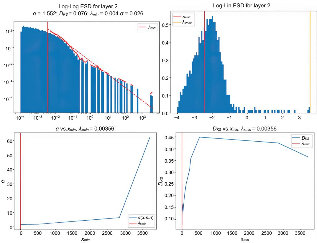
Figure 4.2 weightwatcher Empirical Spectral Density (ESD) plots generated for GPT2’s second layer, which is predicted to be overtrained

provide any insight into the training data, so it can’t tell us which model is that effective at which task and is best paired with other evaluation methods already discussed.

We’ve already spent quite a bit of time talking about data most data engineers likely don’t think about often: model weights and evaluation data. These are crucial ingredients to gather to generate a specialized finetuned LLM. Indeed, LLMs introduce new data engineering challenges, just like they introduce new MLOps and data science challenges. Next, we will discuss what many of you have been waiting for: the training data. We’ll discuss different datasets that are essential to know about, where to get them, and how to prepare them to train or finetune LLMs.

4.3 Data for LLMs

It has been shown that data is the most important part of training an LLM. We hope that the sudden importance of language modeling will persuade businesses to start managing their data generally according to accepted guidelines. As is shown by experiments like LLaMA, Alpaca, Goat, Vicuna, and later, LIMA⁸ and SpQR,9 high-quality training data and clever modeling are much more important than the number of parameters or size of training data. Measuring that quality is still a point of difficulty in general; however, we’ll discuss methodologies you can employ to do so.

We’ll first discuss common datasets you should know about, what’s in them, why you would want them, and where you can get them. Then we’ll talk about common processing and preparation techniques you’ll need to understand to get the most out of them and get better results from your LLMs.

4.3.1 Datasets you should know

If you didn’t notice, in section 4.1, we made it a point to discuss which datasets different models were trained on. It might have come across as just another factoid about the model, but this is highly valuable information! Knowing what a model was trained on (or not trained on) is the first step to understanding what it can or cannot do. For example, knowing an LLM coding model was trained heavily on the C programming language but didn’t see a lick of C++ will be more than enough to realize why it seems to work syntactically but produces so many errors and bugs when writing C++ code.

WIKITEXT

One of the most familiar datasets, Wikitext is, as the name implies, essentially Wikipedia. It was crafted by the Salesforce team back in 2016. It is a great dataset to turn to when you’re only trying to do a proof of concept or a rapid prototype since the English version comes in at only 741 MB, not even 1 GB. Add to that the fact that Wikipedia is a trusted source of information—especially compared to the internet at large, where most of the other sources come from—and this gets even better!

Some downsides: it is purely an English dataset, which greatly reduces the diversity of tokens the model will see; Wikipedia contains an idealized version of language one that we subjectively value as clear—even though it doesn’t contain any instances of how language is actually used, only meta-explanations on usage. Also, it’s almost a decade old as of this writing, which, of course, no one checks. We’ve seen many teams use it to quickly prototype and create Q&A bots due to its ease of use and access. It does well in prototyping but always comes off as unimpressive when it gets to production, as users tend to prefer asking questions about current events. Always check the freshness of your data! Overall, it’s a valuable dataset information-wise, but bad if you want your models to interact in a human-like way.

WIKI-40B

A good alternative is Wiki-40B from 2020, a cleaned-up version of Wikitext with 40 different language variations. It comes in at a little over 10 GB. So it’s still quite small for

⁸ C. Zhou et al., “LIMA: Less is more for alignment,” arXiv.org, May 18, 2023, https://arxiv.org/abs/2305 .11206.

⁹ T. Dettmers et al., “SpQR: A sparse-quantized representation for near-lossless LLM weight compression,” arXiv.org, June 5, 2023,https://arxiv.org/abs/2306.03078.

prototyping. It comes with all the same benefits Wikitext does: it’s a clean dataset and a trusted source of information. Plus, it’s newer and has more languages. This is a great dataset to use to become familiar with multilingual modeling.

EUROPARL

One of the best toy datasets for multilingual problems, Europarl contains the European Parliament proceedings from 1996 to 2011. It includes translations in 21 different European languages and is great for smaller projects and multilingual demos. Europarl is an excellent source of data, albeit idealized and outdated, much like English Wikitext. In addition, the project includes many parallel corpora, which are paired down to English and one of the 20 other languages. The total dataset is just 1.5 GB and can be found at https://www.statmt.org/europarl/.

COMMON CRAWL

The Common Crawl dataset is essentially the entire internet, web scraped and open sourced. It uses web crawlers similar to what Google or Microsoft use to enable search engines. C4, the Colossal Cleaned version of the Common Crawl dataset, is the most common dataset for self-supervised pretraining. Unfortunately, being cleaned doesn’t mean it is free of inherent societal bias, which is true for pretty much all the datasets openly available today. Containing the entirety of the internet means it contains all the good and the bad; it is a very diverse dataset full of multiple languages and code.

The Common Crawl dataset is named after the nonprofit organization of the same name that is dedicated to providing a copy of the internet to anyone for the purpose of research and analysis. You can access the dataset at https://commoncrawl.org/, where you will find many versions because Common Crawl periodically crawls the web and updates the dataset. The community has been archiving the internet since 2008. It comes in four variants to help with your various needs: a 305 GB version containing the actual C4; a 380 GB version that contains so-called bad words along with everything else; a 2.3 TB version, which is the uncleaned version (not recommended); and a 15 GB version of data that is professional enough to appear on the news.

OPENWEBTEXT

Another dataset we’d recommend for pretraining is OpenWebText, which only takes up 55 GB on disk. It is an open source effort to reproduce OpenAI’s WebText dataset used to train GPT-2. Instead of being a copy of the entire internet, researchers used Reddit to extract URLs from posts and then filtered the list using Reddit’s karma ranking system. They then scraped the URLs to create the dataset. Since the content mainly comes from Reddit, it calls into question its real-world accuracy due to the selection bias of only including people with a Reddit account. It is made up mostly of news articles, blog posts, and other content often shared on forums. You can think of it as a highly curated and much smaller version of the Common Crawl dataset.

Like Wikitext, it’s a bit older; the most commonly used version was created in 2019, and a new version hasn’t been updated in four years at the time of writing. Of course, since the dataset was curated with a specific methodology, it could be refreshed at any time.

THE PILE

One dataset that has garnered a lot of attention and should be on your radar is The Pile, which was created by EleutherAI in 2020 and published on December 31 of the same year.10 It is useful for self-supervised pretraining tasks. The Pile is one of the largest datasets we’ll discuss at 825 GB and consists of 22 smaller high-quality datasets combined to make a diverse and dense training set. It includes most of the datasets we have already discussed, like Common Crawl, OpenWebText, and Wikipedia. It also contains book datasets, like Books3 and Gutenberg; code datasets, like GitHub and Stack Exchange; and specialist datasets, like PubMed and FreeLaw. It also includes datasets like the Enron Emails, which we can’t help but think was a mistake.

Because it’s so massive and includes multiple languages and code samples, it has proven useful in training many LLMs. It is multilingual in addition to dense, making it ideal for learning sparse general language representations. Overall, though, it’s not very clean and is essentially just a conglomerate of multiple datasets. Unless you are training LLMs from scratch, you likely won’t use this dataset, but it’s important to become familiar with it, as many of the largest models have been trained on it. You can find the dataset at EleutherAI’s website: https://pile.eleuther.ai/.

REDPAJAMA

RedPajama is a dataset created by a collaboration of Together.ai, Ontocord.ai, ETH DS3Lab, Stanford CRFM, and Hazy Research. The goal was to create a fully open dataset that mimicked what was described in the LLaMA paper.

NOTE You can read the blog post introducing RedPajama here: https:// together.ai/blog/redpajama.

The dataset is similar to The Pile but much larger at 5 TB and newer, published in April 2023. It contains fewer datasets: GitHub, arXiv, Books, Wikipedia, StackExchange, and Common Crawl. It is so large because it contains five different dumps of the Common Crawl dataset with varying filters and the standard C4 dataset. It is made available through the Hugging Face Hub and can be found at https://mng.bz/4ppD.

OSCAR

The best dataset by far to train on for multilingual models is OSCAR, which is larger than any other dataset discussed, coming in at 9.4TB, over 11 times as big as The Pile! It is an open source project started in 2019 and has been funded by a multitude of institutes and governments. You can learn more about the project and dataset at https:// oscar-project.org/.

¹⁰ L. Gao et al., “The Pile: An 800GB Dataset of Diverse Text for Language Modeling,” Dec. 2020, https://arxiv .org/abs/2101.00027.

This project is actively being worked on, and new releases come out annually with regular updates. It currently supports 166 languages at the time of this writing, much more than any other dataset. As a work in progress, though, there are some languages much more represented than others, with some in the TBs of data and others in KBs. This is one of our favorite datasets because it is actively being worked on, and the team is passionate about representation in LLMs and AI, as well as producing highly clean, high-quality data. We encourage all interested readers to contribute to this dataset.

SUMMARY OF DATASETS

In table 4.2, you can see a summary of the datasets we’ve discussed so far. These datasets are all commonly used in industry and worth familiarizing yourself with. We encourage you to investigate them further and take a closer look at the data within.

Dataset	Contents		Last update
Wikitext	English Wikipedia	<1 GB	2016
Wiki-40B	Multi-lingual Wikipedia	10 GB	2020
Europarl	European Parliament proceedings	1.5 GB	2011
Common Crawl	The internet	~300 GB	Ongoing
OpenWebText	Curated internet using Reddit	55 GB	2019
The Pile	Everything above plus specialty datasets (books, law, med)	825 GB	2020
RedPajama	GitHub, arXiv, Books, Wikipedia, StackExchange, and multi ple version of Common Crawl		2023
OSCAR	Highly curated multilingual dataset with 166 languages	9.4 TB	Ongoing

Table 4.2 Summary of datasets

CORPORA

As you probably picked up on, most of the datasets out there are essentially just text dumps of the internet. If you’re looking for something with a little more finesse, something that contains more meta info to help your model disambiguate for more complex tasks, consider downloading a corpus. A corpus is just like a dataset, except it is more easily searchable, visualized, and explained. Corpora are often paid datasets that can be well worth your money. Corpora, like the Corpus Of Historical American English (COHA) and the Corpus of Contemporary American English (COCA), are excellent downloads. They contain not just text data but also frequency analysis (bag of words) and collocates (N-grams), all ready to go. Whether or not you are interested in the applications of allowing models to analyze metadata as part of training, using corpora can help with model explainability and quality of data.

You can think of a corpus as a vector database that has already been highly cleaned and curated and is ready to go. While it hasn’t yet been done, a corpus that combines both the linguistic explainability and time-series bucketing with precalculated

embeddings put into a real-time vector database would likely be invaluable and highly profitable in this field for the foreseeable future, especially if both textual and audio data are captured. If your company has its own language data it wants to train on, your best course of action is to create a corpus where your biggest job is saying where data came from when and what the overall goal of the data going into the model is. Almost every NLP library has strategies for creating corpora, from NLTK to spaCy and even LangChain. Be mindful about which strategies and tools you pick because at the end of the day, your dataset or corpus contains everything your model will see.

4.3.2 Data cleaning and preparation

If you pulled any of the previously mentioned datasets, you might be surprised to realize most of them are just giant text dumps—a large parquet or text file. There are no labels or annotations, and feature engineering hasn’t been done at all. LLMs are trained via self-supervised methods to predict the next word or a masked word, so a lot of traditional data cleaning and preparation processes are unneeded. This fact leads many to believe that data cleaning as a whole is unnecessary, but this couldn’t be further from the truth. Datasets are the lifeblood of all ML, and they are so much more than a pile of data. Yet that’s what most businesses have—a pile of data. Data cleaning and curation are difficult, time-consuming, and ultimately subjective tasks that are difficult to tie to key performance indicators (KPIs). Still, taking the time and resources to clean your data will create a more consistent and unparalleled user experience.

Since the 1990s, people have tested whether Big Data can produce better results than high-quality data; we believe the answer is no. Big Data is nowhere close to devoid of value. The Law of Big Numbers has been applied, and it has shown that models can generate convincing syntax at the same level as people. However, as we’ve said before, models have also soundly demonstrated that syntax is in no way connected to semantics or pragmatics.

In this section, we hope to share with you the right frame of mind when preparing your dataset. We will focus on the high-level linguistic considerations you should be thinking about when preparing a dataset, and we won’t be going too deep into how to create the actual data pipelines. That said, the main logic is simple and follows these basic steps:

• ¹ Take your pile of data, and determine a schema for the features.
• ² Make sure all the features conform to a distribution that makes sense for the outcome you’re trying to get through normalization or scaling.
• ³ Check the data for bias/anomalies (most businesses skip this step by using automated checking instead of informed verification).
• ⁴ Convert the data into a format for the model to ingest (for LLMs, it’s through tokenization and embedding)
• ⁵ Train, check, and retrain.

NOTE For more information on creating data pipelines, check out Fundamentals of Data Engineering,11 WizardLM,12 and “LIMA: Less Is More for Alignment.”13 These resources can help you create effective data pipelines to get as much data into a trainable state as possible.

None of these steps are necessarily easy, but we hope to share a few tips and tricks. Evaluating whether your distribution is correct can be as simple as looking at the data and asking yourself whether it truly represents the problem or as difficult as creating a whole human-in-the-loop workflow to validate your model’s output. Next, we’ll go over the first three steps, and in the next section, we’ll go over the fourth. The last step is covered in depth in the next chapter.

INSTRUCT SCHEMA

One of the best and most common data schemas you should consider when preparing your data, especially for finetuning, is the instruct schema. Instruction tuning is based on the intuitive logic that if we show a model how to perform a task with instructions, the model will perform better than if we just show it tasks and “answers.” Instruction tuning involves demonstrating for the model what you would like to happen, and as such, the datasets are more intensive to create than your run-of-the-mill crawl data. You need to prepare your data to match a format that will look something like this:

###Instruction

{user input}

###Input

{meta info about the instruction}

###Response

{model output}

Instruction datasets are powerful because they allow the model to consider both instructions and relevant input. For example, if the instruction was “Translate this sentence to Japanese,” the input would be the sentence you’d want translated, and the response would be the Japanese translation. Thus, they prepare your model for many prompting techniques and prompt tuning, making them more effective later.

Despite their name, instruction tuning datasets are not restricted to test-based modalities; they can also use vision instruction tuning (image–instruction–answer) and red teaming instruction (RLHF) datasets. The “instruction” offers a semblance of pragmatics within the model and prompt, providing important guardrails for the

¹¹ Reis and Housley, Fundamentals of Data Engineering, 2022.

¹² Xu et al., “WizardLM,” 2023.

¹³ Zou et al., “LIMA,” 2023.

LLM as it generates responses. It grounds the prompt with syntax that repeats and is predictable, along with syntax that is unpredictable for the model to guess at. These syntactic landmarks (###Instruction, User:, Chat History:, etc.) also help lower the chance of an EOS (end-of-sequence) token being predicted early due to the variable length of what can come between each of them, like chat history. Chat history can be one message or thousands of tokens, but the pattern, given there’s another landmark coming afterward, helps the model succeed in long-term memory. When you are deciding what to train your model on, keep those landmarks in mind, as they can make an instruct-tuned model even better at a specific task if you only need it to do one thing.

This isn’t the only format; some competitors in the space include the evol-instruct format used by WizardLM and the self-instruct format used by Alpaca, both of which use scripts to create instruction-based prompts. The best format is still an open-ended question, and we’d like to extend a challenge to the reader to explore creating their own. GitHub (https://mng.bz/5OmD) and Hugging Face datasets are both great places to look for vetted datasets at the moment, but keep in mind that if the dataset doesn’t contain many examples of the tasks you’d like your model to perform or it doesn’t contain enough examples of semantic ambiguity being resolved when completing the task, performance will be unstable—which takes us to step 2 in our cleaning process.

ENSURING PROFICIENCY WITH SPEECH ACTS

In preparing the dataset, the most important consideration is what you want the model to do. If you want a model to predict housing prices in Boston, you probably shouldn’t train it on survivors of the Titanic. This is obvious when stated, but it raises the question, “Is my dataset correct for the problem, and how would I know?” When it comes to language data, the answer isn’t as obvious as we might hope. Let’s look at an example to figure out why.

Let’s say you want your model to take orders at a fast-food restaurant. This scenario may seem boring and mundane, where all we expect to see are queries like, “I’ll order the #3 combo,” which you will. But if you ask a cashier about how people actually talk to them, really, anything can happen! I had a friend who worked at Burger King tell me that because of Burger King’s slogan “Have It Your Way,” he received many crazy requests, like asking for a burger with two top buns. That blew my mind, but it was also a tame example. Not to mention, you never know when the next LARPing convention will bring more creative and colorful interactions to otherwise mundane scenarios. A generic dataset containing customer orders and cashier responses won’t be enough here. When you aren’t intentional about what kind of data goes into your model, the performance of the model suffers.

DEFINITION LARP stands for live-action role-playing, and you can imagine the tomfoolery of a customer pretending to be an elf, orc, or pirate and thus breaking all rules and expectations.

To ensure your data is right for the task, first, you should think about what speech acts generally go together to perform the task at hand. Speech acts refer to the various functions language can perform in communication beyond conveying information. They are a way of categorizing utterances based on their intended effect or purpose in a conversation. Speech acts are important, as they shed light on how communication goes beyond the literal meaning of words and involves the speaker’s intentions and the listener’s interpretation.

Speech acts defined

The following list includes common speech acts and their definitions:

• Expressives—Greetings, apologies, congratulations, condolences, thanksgivings (e.g., “You’re the best!”)
• Commissives—Promises, oaths, pledges, threats, vows (e.g., “I swear by the realm, the princess will come to no harm.”)
• Directives—Commands, requests, challenges, invitations, orders, summons, entreaties, dares (e.g., “Get it done in the next three days.”)
• Declarations—Blessings, firings, baptisms, arrests, marrying, juridical speech acts such as sentencings, declaring a mistrial, declaring out of order (e.g., “You’re hired!”)
• Verdictives—Rankings, assessments, appraising, condoning (combinations such as representational declarations; e.g., “You’re out!”)
• Questions—Usually starting with interrogative words like what, where, when, why, who, or indicated with rising intonation at the end in English (e.g., “Which model is best for my task?”)
• Representatives—Assertions, statements, claims, hypotheses, descriptions, suggestions, answers to questions (e.g., “This model is best for your task.”

The current way we measure the robustness of datasets for LLMs is the vanilla number of tokens. Instruct datasets are relatively new, but they rely on you being intentional with how instruction for the model happens. What will your model do when given a directive it shouldn’t respond to when it’s only been trained on helpful responses to directives? If you aren’t sure, now’s the time to consider. For example, imagine a user declaring with glee to your bot, “Promise you’ll help me take over the world!” If it was only trained to be helpful, it would likely respond by promising to do just that because similar scenarios are in the training set. And now we have an evil AI overlord taking over the world. Thanks. In actuality, this is a fairly innocuous example, but the unpredictability of the seemingly infinite number of possible responses from the model should make you think, especially if this agent has access to tools like Google or your internal HR documents. Being cognizant of speech acts can simplify your work so that you don’t have to focus as much on individual tokens for the vocabulary as on the overall structure of what your model will come in contact with during training.

Going back, when you think about a customer-facing role like a cashier, how many of these speech acts are likely to occur in your average order? Take a minute to think it through. We can tell you that declarations and verdictives are out, and commissives are uncommon. But what if you get them regardless? You then need to consider how you might want to steer such highly expressive customers toward the speech acts you can work with, likely questions, directives, and representatives.

To make matters more complicated, the form of a speech act doesn’t always have to match its function. For example, you could say “You’re fired” to your friend who doesn’t work for you, where, even though its form is declarative, its function is more likely expressive. Once you have a dataset or a trained LLM and are looking to improve its ability to take instruction, this is something to seriously consider to increase your data’s quality and your LLM’s performance. Does your model weirdly fail when users frame utterances as questions when they’re actually directives? Does your model start hallucinating when coming in contact with the representative-only HR documents you’ve been asked to analyze? As a note, you don’t have to completely finetune a model all over again to improve performance. We’ll go over this in more detail later, but giving specific examples within the prompt can patch a lot of these edge cases quickly and inexpensively.

Now that you have an understanding of the different features you should be looking for in your dataset, let’s consider the best ways to annotate your dataset so you can make sure it conforms to expectations.

ANNOTATING THE DATA

Annotation is labeling your data, usually in a positionally aware way. For speech recognition tasks, annotations would identify the different words as noun, verb, adjective, or adverb. Annotations were used as labels in supervised learning tasks as the main way to train a model. Now annotations essentially give us metadata that makes it easier to reason about and analyze our datasets. Instead of worrying about micro information like speech recognition or named-entity recognition, you’ll get more value by focusing on macro metadata, like the speech acts just discussed or what language the data is in.

Of course, this is the real trick, isn’t it? If this were easy, every company on the face of the earth would have its own models already in production. The fact is data wrangling is too large to be done by hand but too varying to be done automatically, and you need to find the middle ground as quickly as possible. You don’t want to ignore your data and just download a dataset someone recommended (even us) and then proceed to harm a real-world population because it contained harmful data. But you also don’t want to have to hand-validate millions of rows of utterances. Thankfully, there are tools to help with every part of this, but we’d like to specifically mention these first:

• Prodi.gy (https://prodi.gy/)—Prodigy takes a one-time payment for a quick and powerful multimodal annotation tool.
• doccano: Open source annotation tool for machine learning practitioners (https:// github.com/doccano/doccano)—A truly open-source and, at the time of writing, updated web-based platform for data annotation.
• d5555/TagEditor: Annotation tool for spaCy (https://github.com/d5555/TagEditor)— Works in conjunction with https://spacy.io. Both create an ecosystem on top of spaCy, a popular NLP framework that makes rapid prototyping well within the reach of your average ML team.
• Praat: Doing phonetics by computer (https://github.com/praat/praat)—The only audio annotation tool on this list, Praat is fundamentally a tool for phonetics with annotations thrown in. Given how much we predict the LLM space to shift toward phonetics, we couldn’t omit this one from the list.
• Galileo (https://www.rungalileo.io/llm-studio)—At the time of this writing, Galileo’s LLM studio has yet to come out, but it makes some big promises for prompt creation and evaluation, which would immensely speed up annotation and creation of instruction datasets.

Which tool is best for your project depends entirely on the goal of your annotation. Going into annotating without a specified goal leads nowhere, as you’ll find discrepancies on the other end of data processing. Of course, we recommend adding speech act annotations; you’ll also want to consider additional annotations looking for bias and anomalies. We can show that by measuring the number of pieces of outside context present in the text (things like insinuations or entailments), you can gain a confidence score about how high quality a particular data is. The reason for this is intuitive: the more ambiguity a set of examples can solve for the model, the more the model learns from that set. The hard part is that no one can pin any of these contextual information nuggets on repeating parts of orthography, such as individual characters or a particular word or subword.

Annotating can be a lot of work, but the reason for all of this consideration at the front is fairly simple: your model can only learn what you teach it. Thankfully, to make matters much easier, the goal isn’t to annotate every bit of text in your dataset. We are simply annotating a large-enough sample to ensure our dataset is representative of the task. Remember, LLMs are generally trained in two steps:

• ¹ Self-supervised pretraining—Analyzing many different speech acts in varying forms and functions to learn general representations
• ² Finetuning and RLHF—Teaching the model how/when to use the representations learned in step 1

This training significantly lightens the burden on you as a trainer of attempting to parse every possible locution (what a person literally says) and illocution (what they actually mean in context) within the given task. Even for something viewed as simple work, like being a cashier, having to come up with a dataset vast enough to cover all edge cases would be quite a headache. For most cases, all you need to do is prepare a finetuning dataset, which often doesn’t need to be large at all—sometimes a dozen examples is more than enough to start getting good results.

4.4 Text processors

Now that you have a dataset for training or finetuning, we need to transform it into something that can be consumed by the LLM. Simply put, we need to turn the text into numbers. We’ve already briefly gone over the process of doing that conversion quickly and effectively, so let’s dive into different examples and methodologies.

In this section, we’ll show you how to train your own tokenizers, both byte-pair encoding (BPE) and SentencePiece tokenizers, and how to grab embeddings from (almost) any model for storage or manipulation later. This step is often ignored when working with an LLM through an API, but much of modern performance in data applications depends on doing this process correctly and specifically for your goal. There are many mathematically sound and correct ways to tokenize text, so you can’t rely on something someone else did when you have a specific use case. You need to prepare it for that use case. Training your own tokens will allow you to minimize unknown tokens, , while also maximizing encoded semantics. Having control of this process is one of the simplest and easiest hacks to give your models a major boost in performance. Let’s start first with tokenization.

4.4.1 Tokenization

Tokenization is a bit more involved than simple vectorization but leads to the same overall result: text input, vector output, and the ability to encode and decode. We mentioned in chapter 2 the multilingual factor and in chapter 3 the token tax of foreign languages, which are both motivations to be at least aware of your own tokenization strategies. However, it goes beyond those. Your tokenization strategy isn’t just important; it is vitally important for every subsequent step.

A good example is comparing GOAT 7B and GPT-4 in math and arithmetic. Consider table 4.3. The left column is a simple arithmetic prompt. Then we see the two models’ answers and, for reference, the actual answer so you don’t have to pull out your calculator.

Prompt	GOAT 7B	GPT-4 1.7T	Correct
3978640188 + 42886272 =	4021526460	4,021,526,460	4,021,526,460
4523646 minus 67453156	–62929510	–63,930,510	–62,929,510
Calculate 397 × 4429	1758313	1,757,413	1,758,313
What is 8914/64?	139 R 18	139.15625	139.28125 Or 139 R 18

Table 4.3 Tokenization allows GOAT 7B to outperform GPT-4 in math

GOAT 7B consistently outperforms GPT-4, which leaves the question, “Why does GOAT perform better despite being 200 times smaller? Aren’t larger models more likely to show emergent behavior?” You probably already guessed the answer based on the subsection’s heading, but if you didn’t, it’s because of the tokenization algorithm used!

The GPT family of models tokenizes all subwords and digits in groups based purely on frequency only, meaning that if that exact group of numbers or words hadn’t shown up before, they could be grouped together during the embedding and inference processes later! GOAT is a finetuned Llama model, meaning that while it was finetuned on math to be good at it, the underlying secret to success lies in its tokenization strategy, which is the same as Llama’s. GPT-X tokenizes like this:

print(enc.encode(“4523646 minus 67453156”)) [21098, 15951, 21, 28382, 220, 25513, 20823, 3487]

Did you notice how the first group of numbers is seven digits long, but the entire output is eight tokens? This is the exact grouping methodology we’re talking about. Compare that to Llama’s tokenization strategy in figure 4.3. Notice that each digit is highlighted individually, meaning that the model will eventually see all the digits. As this example demonstrates, your tokenization strategy will ultimately determine what your model will see and won’t see, as they’ll become tokens—and that’s why it’s vitally important to get it right for your use case.

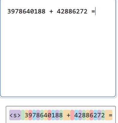
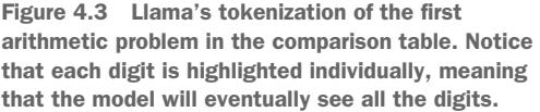
What started out as creating a simple set of bag-of-words conversion dictionaries has evolved immensely, and we couldn’t be happier about it. Tokenization essentially consists of two major steps: a step to split up the text and a step to turn it into numbers. The most obvious form of tokenization is splitting a string on whitespace and then converting it to a number based on a word-to-integer dictionary.

This makes sense to most Indo-European language speakers, but we can’t recommend this because of the two assumptions presupposed: alphabets and whitespace. What will you do when you come across a language that doesn’t use an alphabet, like Chinese? And what will you do when you come across a language that doesn’t use whitespace in the same way as English, like Hungarian or Turkish? Or code, for that matter—whitespace is critical to Python’s syntax and is more than just a separator; it has semantic meanings. This is one reason why multilingual models end up outperforming monolinguals on the same tasks in almost every case: they’re forced to learn deeper representations for meaning without the bowling bumpers of easy tokenization. So let’s look at some deeper methodologies that work for UTF-8 encoded languages.

Here are examples of all the current popular options for basing your tokenization:

• Word-based—“Johannes Gutenberg” becomes [‘Johannes’, ‘Gutenberg’].
• Character-based—“Shakespeare” becomes [‘S’,‘h’,‘a’,‘k’,‘e’,‘s’,‘p’,‘e’, ‘a’,‘r’,‘e’].
• Subword-based—“The quick red Delphox jumped over the lazy brown Emolga” becomes [‘the’,‘quick’,‘red’,‘delph’,‘ox’,‘jump’,‘ed’,‘over’,‘the’, ‘laz’,‘y’,‘brown’,‘emol’,‘ga’]

Let’s take a look at each of them in turn.

WORD-BASED

Word-based tokenizers most commonly split on whitespace, but there are other methods like using regular expressions, dictionaries, or punctuation. For example, a punctuation-based approach would split “It’s the truth!” into [‘It’, ’ ’’ , ’ s’, ’ the’, ’ truth’, ’ !’], which gives us slightly better context than splitting on whitespace alone. The TreebankWordTokenizer from NLTK is an example of a regular expression tokenizer. Word-based tokenizers are relatively easy to implement but require us to keep an unmanageably large dictionary mapping to encode every single possible word. That’s unreasonable, so generally, you’ll implement a dictionary cutoff and return unknown tokens when the model runs into unrecognized words to make it work. This makes the tokenizer poor at many tasks like code, name, and entity recognition, as well as generalizing across domains.

CHARACTER-BASED

Character-based encoding methods are the most straightforward and easiest to implement since we split on the UTF-8 character encodings. With this method, we only need the tiniest of dictionaries to map characters to numbers, which means we can prevent the need for unknown tokens and related concerns. However, it comes with a major loss of information and fails to keep relevant syntax, semantics, or morphology of the text.

SUBWORD-BASED

Just like Goldilocks and the Three Bears, while character-based tokenizers are too hard and word-based tokenizers are too soft, subword-based tokenizers are just right. Subword-based tokenizers have proven to be the best option, being a mixture of the previous two. We are able to use a smaller dictionary like a character-based tokenizer but lose less semantics like a word-based tokenizer. It even has the added bonus of including some morphological information. However, it’s an unsolved problem for where and how words should be split, and there are many different methods and

approaches. The best method to choose will be, like all other things with LLMs, dependent on the task. If you don’t have a specific goal in mind for what you are trying to do, there will be consequences later.

Three main algorithms are used to create the subword dictionaries: BPE, Word-Piece, and Unigram. In addition, SentencePiece, a combination of the three that explicitly handles whitespaces, is also very common. It’s outside the scope of this book to discuss how they work, but as a book focused on production, you should know that the most popular subword tokenization methodologies are BPE (GPT-x) and Sentence-Piece (LlamaX).

In listing 4.10, we’ll go over how to train a custom version for both BPE and SentencePiece on your data so that you’re equipped to face (almost) any dataset head-on. While reading the code, pay attention to where we train the tokenizers. In particular, you’ll want to tune three key parameters: vocab_size, min_frequency, and special_tokens. A larger vocabulary size means your tokenizer will be more robust and will likely be better at handling more languages, but it will add computational complexity. Minimum frequency determines how often a particular subword token has to be seen in the dataset before it is added to the dictionary. Larger values prevent rare and likely unimportant tokens from filling our dictionary and prevent us from learning rare tokens that are important. Lastly, special tokens are relatively straightforward and include syntactical tokens we care about specifically for model training.

Listing 4.10 Training your own subword tokenizers
import os from pathlib import Path
import transformers from tokenizers import ByteLevelBPETokenizer, SentencePieceBPETokenizer from tokenizers.processors import BertProcessing
paths = [str(x) for x in Path(“./data/”).glob(“**/*.txt”)] bpe_tokenizer = ByteLevelBPETokenizer()	Initializes the texts to train from
bpe_tokenizer.train(
files=paths,
vocab_size=52_000, min_frequency=2,	Trains a byte
show_progress=True,	pair encoding tokenizer
special_tokens=[
“”,
“”,
“”,
“”,
“”,
],
)

token_dir = "./chapters/chapter_4/tokenizers/bytelevelbpe/"
if not os.path.exists(token_dir):
 os.makedirs(token_dir)
bpe_tokenizer.save_model(token_dir)
bpe_tokenizer = ByteLevelBPETokenizer(
 f"{token_dir}vocab.json",
 f"{token_dir}merges.txt",
)
example_text = "This sentence is getting encoded by a tokenizer."
print(bpe_tokenizer.encode(example_text).tokens) 
# ['This', '?sentence', '?is', '?getting', '?enc', \
# 'oded', '?by', '?a', '?to', 'ken', 'izer', '.']
print(bpe_tokenizer.encode(example_text).ids)
# [2666, 5651, 342, 1875, 4650, 10010, 504, 265, \ 
# 285, 1507, 13035, 18]
bpe_tokenizer._tokenizer.post_processor = BertProcessing(
 ("</s>", bpe_tokenizer.token_to_id("</s>")),
 ("<s>", bpe_tokenizer.token_to_id("<s>")),
)
bpe_tokenizer.enable_truncation(max_length=512)
special_tokens = [
 "<s>",
 "<pad>",
 "</s>",
 "<unk>",
 "<cls>",
 "<sep>",
 "<mask>",
]
sentencepiece_tokenizer = SentencePieceBPETokenizer() 
sentencepiece_tokenizer.train( 
 files=paths, 
 vocab_size=4000, 
 min_frequency=2, 
 show_progress=True, 
 special_tokens=special_tokens, 
)
token_dir = "./chapters/chapter_4/tokenizers/sentencepiece/"
if not os.path.exists(token_dir):
 os.makedirs(token_dir)
sentencepiece_tokenizer.save_model(token_dir)
tokenizer = transformers.PreTrainedTokenizerFast(
 tokenizer_object=sentencepiece_tokenizer,
 model_max_length=512,
 special_tokens=special_tokens,
) 
                                                          Trains a 
                                                          SentencePiece 
                                                          tokenizer
                                          Converts

tokenizer.bos_token = "<s>"
tokenizer.bos_token_id = sentencepiece_tokenizer.token_to_id("<s>")
tokenizer.pad_token = "<pad>"
tokenizer.pad_token_id = sentencepiece_tokenizer.token_to_id("<pad>")
tokenizer.eos_token = "</s>"
tokenizer.eos_token_id = sentencepiece_tokenizer.token_to_id("</s>")
tokenizer.unk_token = "<unk>"
tokenizer.unk_token_id = sentencepiece_tokenizer.token_to_id("<unk>")
tokenizer.cls_token = "<cls>"
tokenizer.cls_token_id = sentencepiece_tokenizer.token_to_id("<cls>")
tokenizer.sep_token = "<sep>"
tokenizer.sep_token_id = sentencepiece_tokenizer.token_to_id("<sep>")
tokenizer.mask_token = "<mask>"
tokenizer.mask_token_id = sentencepiece_tokenizer.token_to_id("<mask>")
tokenizer.save_pretrained(token_dir) 
print(tokenizer.tokenize(example_text))
# ['_This', '_s', 'ent', 'ence', '_is', '_', 'g', 'et', 'tin', 'g', '_'
# 'en', 'co', 'd', 'ed', '_', 'b', 'y', '_a', '_', 't', 'ok', 'en', 
# 'iz', 'er', '.']
print(tokenizer.encode(example_text))
# [814, 1640, 609, 203, 1810, 623, 70, \
# 351, 148, 371, 125, 146, 2402, 959, 632]
                                                            And saves for later!

Out of the two, BPE and SentencePiece, we find ourselves using both about equally. It mostly depends on which model we’re finetuning or using as a base for a particular project. Algorithmically, we’re partial to SentencePiece because it tends to boost evaluation scores on pretty much any test for models trained on it, and it’s also closer to how we interact with morphology as people.

All in all, tokenization loses information, just as converting from speech to text does—namely, word order (syntax) and meaning (semantics). All of the information about what a number is and how it would differ from a letter is completely gone after tokenization. To circumvent potential semantic and syntactic problems, we need to create an approximation for each of these features and figure out how to mathematically represent them in abstraction to insert that meaning back into the tokenized vector. For this, we have embeddings.

4.4.2 Embeddings

Embeddings provide meaning to the vectors generated during tokenization. Tokenized text is just numbers assigned almost arbitrarily (occurrence-based) to a dictionary, but it’s at least in a format that the model can ingest. Embeddings are the next step, where positional and semantic encodings are created and looked up to give the model additional context for making decisions about how to (probably) complete the task it’s given.

Embeddings are imperfect for several reasons, but perhaps the most relevant is this theoretical question: Can you represent a set using only a subset of that same set? In this case, the first set is language, one or more, and the second set is numbers, floats, and digits. Math is a subset of language used to describe things axiomatically that we accept as true. Take the English alphabet, for example: Can you represent the entire alphabet by only using some fraction of the 26 letters? Obviously not, but what if both the original set and the subset are infinite? Can you represent all digits using only the decimals between 0 and 1? Given that the first is a numerable infinite set and the second is a nonenumerable infinite set, the answer is yes, which should be enheartening for the field of language modeling.

Now that we’ve talked about why embeddings shouldn’t be completely and blindly relied on, embeddings are what most businesses are looking for with LLMs. You don’t need a 1.7T-parameter model to handle customers asking questions about your pricing or performing a search through your documents. As we discussed in chapter 2, embeddings have the innate advantage of being comparable by distance, provided both embeddings you’re comparing were created by the same model in the same dimensional space. That opens up the door for all sorts of speedy computation and retrieval where you never have to figure out how to host a gigantic model somewhere because you can run a smaller embedding model on a CPU, and it takes milliseconds for hundreds of tokens.

One of the most popular and coolest applications of embeddings at the moment is retrieval-augmented generation (RAG), where you store data that is pertinent to the overall task of the model and give portions of that data as needed to a larger model at prompting time to improve results. Suppose we apply RAG to the Boston Housing dataset and attempt to predict the value of a new house. In that case, we can compare that house’s embedded data to the closest comparable houses in the area and generate an informed appraisal without ever needing an appraiser to verify, as long as the embeddings you’re retrieving from are up-to-date.

Embeddings can be used for dozens of different tasks and are the result of taking final hidden state representations from your model. Every layer of your model is a potential option, but the general consensus is to take representations after the final layer before any decoding or final linear layers or softmaxes. Listing 4.11 gives a practical example of how to extract the embeddings from both PyTorch and Hugging Face models. Best practice dictates that you should extract the embeddings from documents using whatever embedding model you are planning to use for inference, especially if those embeddings will end up being stored in a VectorDB later on. After creating our embeddings, we show how to do a simple similarity search on the results, which is the basis of RAG systems.

Listing 4.11 Example embeddings

import numpy as np
from sentence_transformers import SentenceTransformer
from datasets import load_dataset
model_ckpt = "sentence-transformers/all-MiniLM-L6-v2" 
model = SentenceTransformer(model_ckpt)

Downloads embedding model and dataset

embs_train = load_dataset("tweet_eval", "emoji", split="train[:1000]")
embs_test = load_dataset("tweet_eval", "emoji", split="test[:100]")
def embed_text(example): 
 embedding = model.encode(example["text"])
 return {"embedding": np.array(embedding, dtype=np.float32)}
print(f"Train 1: {embs_train[0]}")
embs_train = embs_train.map(embed_text, batched=False)
embs_test = embs_test.map(embed_text, batched=False)
embs_train.add_faiss_index("embedding") 
# 
idx, knn = 1, 3 # Select the first query and 3 nearest neighbors 
query = np.array(embs_test[idx]["embedding"], dtype=np.float32)
scores, samples = embs_train.get_nearest_examples("embedding", query, k=knn)
print(f"QUERY LABEL: {embs_test[idx]['label']}") 
print(f"QUERY TEXT: {embs_test[idx]['text'][:200]} [...]\n")
print("=" * 50)
print("Retrieved Documents:")
for score, label, text in zip(scores, samples["label"], samples["text"]):
 print("=" * 50)
 print(f"TEXT:\n{text[:200]} [...]")
 print(f"SCORE: {score:.2f}")
 print(f"LABEL: {label}")
                                                   Creates embeddings
                                                             Adds Faiss 
                                                             index that allows 
                                                             similarity search
                                                                           Runs 
                                                                           query
                                                                   Prints 
                                                                   results

Extracting embeddings, like the listing shows, is pretty simple and differs very little from simply running inference or training on a dataset. Remember, if you aren’t using sentence transformers, set your model to eval mode, run with torch.no_grad(), and if you’re running on torch 2.0+, run torch.compile(model). Things should speed up and become more computationally efficient immediately.

Another as-of-yet unsolved problem is how to compare embedding spaces. Mathematically sound comparisons have popped up time and again over the years, but as has been demonstrated, mathematical soundness isn’t the first problem to be solved; the modality is. In addition, pairwise comparison functions have mathematical limits on how fast it is possible to run them. If you’re comparing language embeddings, a mathematically sound conversion of a linguistically sound comparison method is the solution, and a linguistically sound comparison is dependent upon the goal of the comparison. It’s too much to go into here, but we dive more deeply into this topic in appendix C, where we discuss diffusion and multimodal LLMs.

4.5 Preparing a Slack dataset

Now that we have learned the ins and outs of preparing the necessary assets to train our own LLM, we wanted to end this chapter by preparing a dataset that we can use later. For this exercise, we will tackle a very common problem in the industry. I’m sure most readers have experienced or witnessed an HR help channel constantly inundated with the same questions over and over. It doesn’t matter how many FAQ pages are created; users don’t want to waste their time searching for documentation when they could ask an expert. So let’s build a chatbot to answer these questions!

We will show you how to pull your company’s Slack data and prepare it for training an LLM-based chatbot. In listing 4.12, we pull Slack data, filter it to keep just the user’s data, and save it to a parquet file. This way, you can create a bot that will talk like you, but feel free to edit it. For example, you might enjoy creating a bot that talks like your boss, but I’d recommend not telling them in case they feel threatened knowing you are automating them out of a job.

import slack_sdk
import pandas
token_slack = "Your Token Here"
client = slack_sdk.WebClient(token=token_slack)
auth = client.auth_test()
self_user = auth["user_id"]
dm_channels_response = client.conversations_list(types="im")
all_messages = {}
for channel in dm_channels_response["channels"]:
 history_response = client.conversations_history(channel=channel["id"])
 all_messages[channel["id"]] = history_response["messages"]
txts = []
for channel_id, messages in all_messages.items():
 for message in messages:
 try:
 text = message["text"]
 user = message["user"]
 timestamp = message["ts"]
 txts.append([timestamp, user, text])
 except Exception:
 pass
slack_dataset = pandas.DataFrame(txts)
slack_dataset.columns = ["timestamp", "user", "text"]
df = slack_dataset[slack_dataset.user == self_user]
df[["text"]].to_parquet("slack_dataset.gzip", compression="gzip")
  Listing 4.12 Example of pulling Slack data

As you can see, there’s not much to it! We have an example dataset we pulled using this script in the GitHub repo accompanying this book. We will use this dataset in the coming chapters.

We’ve gone over a lot in this chapter, but you should now be prepared and know how to select and evaluate a foundation model, prepare and clean a dataset, and optimize your own text processors. We will use this information in the next chapter to train and finetune our own LLM model.

Summary

• Data engineers have unique datasets to acquire and manage LLMs, like model weights, evaluation datasets, and embeddings.
• No matter your task, there is a wide array of open source models to choose from to finetune your own model.
• Text-based tasks are harder to evaluate than simple equality metrics you’d find in traditional ML tasks, but there are many industry benchmarks to help you get started.
• Evaluating LLMs for more than just performance, like bias and potential harm, is your responsibility.
• You can use the Evaluate library to build your own evaluation metrics.
• There are many large open source datasets, but most come from scraping the web and require cleaning.
• Instruct schemas and annotating your data can be effective ways to clean and analyze your data.
• Finetuning a model on a dataset with an appropriate distribution of speech acts for the task you want your model to perform will help it generate contextappropriate content.
• Building your own subword tokenizer to match your data can greatly improve your model’s performance.
• Many problems teams are trying to use LLMs for can be solved by using embeddings from your model instead.

Training large language models: How to generate the generator

This chapter covers

• Setting up a training environment and common libraries
• Applying various training techniques, including using advanced methodologies
• Tips and tricks to get the most out of training

Be water, my friend.

—Bruce Lee

Are you ready to have some fun?! What do you mean the last four chapters weren’t fun? Well, I promise this one for sure will be. We’ve leveled up a lot and gained a ton of context that will prove invaluable now as we start to get our hands dirty. By training an LLM, we can create bots that can do amazing things and have unique personalities. Indeed, we can create new friends and play with them. In the last chapter, we showed you how to create a training dataset based on your Slack messages. Now we will show you how to take that dataset and create a persona of yourself. Finally, you will no longer have to talk to that one annoying coworker, and just like Gilfoyle, you can have your own AI Gilfoyle (https://youtu.be/IWIusSdn1e4).

First things first, we’ll show you how to set up a training environment, as the process can be very resource-demanding, and without the proper equipment, you won’t be able to enjoy what comes next. We’ll then show you how to do the basics, like training from scratch and finetuning, after which we’ll get into some of the best-known methods to improve upon these processes, making them more efficient, faster, and cheaper. We’ll end the chapter with some tips and tricks we’ve acquired through our experience of training models in the field.

5.1 Multi-GPU environments

Training is a resource-intensive endeavor. A model that only takes a single GPU to run inference on may take 10 times that many to train if, for nothing else, to parallelize your work and speed things up so you aren’t waiting for a thousand years for it to finish training. To really take advantage of what we want to teach you in this chapter, we’re first going to have to get you set up in an environment you can use as a playground. Later in the chapter, we’ll teach some resource-optimal strategies as well, but you’ll need to understand how to set up a multi-GPU env if you want to use the largest LLMs anyway.

While you can learn a lot using smaller LLMs, what sets apart a pro from an amateur is often the ease and fluidity they have when working with larger models. And there’s a good reason for this since, on the whole, larger models outperform smaller models. If you want to work with the largest models, you’ll never be able to get started on your laptop. Even most customized gaming rigs with dual GPUs aren’t enough for inference, let alone training.

To this end, we wanted to share with you a few methods to acquire access to a multi-GPU environment in the cloud, and then we will share the tools and libraries necessary to utilize them. The largest models do not fit in a single GPU, so without these environments and tools, you’ll be stuck playing on easy mode forever.

5.1.1 Setting up

It should be pointed out up front that while multi-GPU environments are powerful, they are also expensive. When it comes to multi-GPUs, no services we know of offer a free tier or offering, but you can at least take comfort in knowing that paying per hour will be way cheaper than purchasing the rigs wholesale. Of course, if you can get your company to pay the bill, we recommend it, but it is still your responsibility to spin down and turn off any environment you create to avoid unnecessary charges.

If your company is paying, it likely has chosen a hosted service that makes this whole process easy. For the rest of us, setting up a virtual machine (VM) in Google’s Compute Engine is one of the easiest methods. Once set up, we will then show you how to utilize it.

A note to the readers

For learning purposes, we use smaller models throughout this book in our code listings such that you can work with them on a single GPU either locally or using a service like Colab or Kaggle, which offers a free tier of a single GPU. While the listings could be run on CPU-only hardware, you won’t want to do it. Ultimately, there shouldn’t be any need to run these costly VMs throughout the book. However, you likely will still want to. Training with multiple GPUs is much faster, more efficient, and often necessary. We do encourage you to try larger LLM variations that require these bigger rigs, as the experience will be priceless. To make it easy, you should be able to recycle the code in this chapter for models and datasets much larger than what is presented, which will often just be a matter of changing a few lines.

GOOGLE VIRTUAL MACHINE

One of the easiest ways to create a multi-GPU environment is to set up a VM on Google’s cloud. To get started, you’ll need to create an account, create a Google Cloud Project (GCP), set up billing, and download the gcloud CLI. None of these steps are particularly hard, but be sure to follow the documentation found at https://cloud .google.com/sdk/docs/install-sdk for your operating system to install the SDK. The steps here also include the steps and how-tos for creating an account, project, and billing in the Before You Begin section if you don’t already have an account.

For new accounts, Google offers a $300 credit to be used for pretty much anything on their GCP platform except GPUs. We hate to break this news, but sadly, there’s just no free lunch where we are going. So you’ll need to be sure to upgrade to a paid GCP tier. Don’t worry; just following along should only cost a couple of dollars, but if you are money conscious, we recommend reading the entire section first and then trying it out.

After setting up your account, by default, GCP sets your GPU quotas to 0. Quotas are used to manage your costs. To increase your quotas, go to https://console.cloud .google.com/iam-admin/quotas. You’ll be looking for the gpus_all_regions quota, and since we plan to use multiple GPUs, go ahead and submit a request to increase it to 2 or more.

With all the prerequisites in place, we’ll get started by initializing and logging in. You’ll do this by running the following command in a terminal on your computer:

$ gcloud init

You may have already done this step if you had to install the SDK, but if not, it will launch a web browser to help us log in and authorize us for the gcloud CLI, which allows us to select our project. We will be assuming you have just the one project, but if this isn’t your first rodeo and you have multiple projects, you’ll need to add the –project flag in all the subsequent commands.

Next, we need to determine two things: the machine type (or which GPUs we want to use) and our container image. To pick a machine type, you can check out the different options at https://cloud.google.com/compute/docs/gpus. For beginners, we highly recommend the NVIDIA L4 GPU, as it is an all-around fantastic machine. For our purposes, we’ll be using the g2-standard-24, which comes with two L4 GPUs and costs us about $2 per hour. This machine type isn’t in every region and zone, but you can find a region close to you at https://cloud.google.com/compute/docs/regions -zones. We will be using the us-west1 region and us-west1-a zone.

For the container image, we’ll save ourselves a lot of hassle by using one that has all the basics set up. Generally, this means creating your own, but Google has several prebuilt container images for deep learning, which are great to use or a great place to start as a base image to customize. These are all found in the deeplearning-platform -release project that they own. To check out the options available, you can run

$ gcloud compute images list --project deeplearning-platform-release 
 --format="value(NAME)" --no-standard-images

NOTE You can learn more about the container image options here: https:// cloud.google.com/deep-learning-vm/docs/images.

You can pick from Base, TensorFlow, and PyTorch compiled images, along with the CUDA and Python versions. We’ll be using common-gpu-v20230925-debian-11-py310, which is a simple image ready for GPU with a Debian Linux distribution and Python 3.10. Now that we have everything we need, we can create our VM! Go ahead and run the following commands to set up the VM:

$ INSTANCE_NAME="g2-llminprod-example"

 $ gcloud compute instances create ${INSTANCE_NAME} --zone=us-west1-a 
 --machine-type=g2-standard-24 --image-project=deeplearning-platform-release
 --image=common-gpu-v20230925-debian-11-py310 --boot-disk-size=200GB --scopes
 cloud-platform --metadata=install-unattended-upgrades=False,install-nvidia-
 driver=True --maintenance-policy TERMINATE --restart-on-failure

The first command creates an environment variable to store the name of our VM since we’ll also be using it in several of the following commands. This name can be whatever you want it to be. The next command creates our VM instance. The first several flags (zone, image, machine) should make sense since we just spent the previous paragraphs preparing and gathering that information. The boot-disk-size sets the disk space for our VM and defaults to 200 GB, so it’s included here because it’s important to know for LLMs since they are large assets, and you will likely need to increase it—especially for LLMs that require multiple GPUs to run.

The scopes flag is passed to set authorization. Current GCP best practices recommend setting it to cloud-platform, which determines authorization through OAuth and IAM roles. The metadata field isn’t required but is used here as a trick to ensure the NVIDIA drivers are installed. It is really useful if you are using these commands to create a shell script to automate this process. You should know that it will cause a small delay between when the VM is up and when you can actually SSH into it, as it won’t be

responsive while it installs the drivers. If you don’t include it, the first time you SSH in through a terminal, it will ask you if you want to install it, so no harm done. However, if you access the VM through other methods (described in the next sections), you can run into problems. The last two commands are standard maintenance policies.

Once that runs, you can verify the VM is up by running

$ gcloud compute instances describe ${INSTANCE_NAME}

This command will give you a lot of information about your instance that is worth looking over, including a status field that should read ‘RUNNING’. Once you’ve confirmed that it’s up, we will SSH into it. If this is your first time using gcloud to SSH, an SSH key will be generated automatically. Go ahead and run the following command:

$ gcloud compute ssh ${INSTANCE_NAME}

Your terminal will be shelled into our multi-GPU VM, and you are now in business. At this point, your VM is still just an empty shell, so you’ll want to bring in code. The easiest way to do this is to copy the files over with Secure Copy Protocol (SCP). You can do this for a single file or a whole directory. For example, assuming your project has a requirements.txt file and a subdirectory local-app-folder, from a new terminal, you can run the following commands:

$ gcloud compute scp requirements.txt ${INSTANCE_NAME}:~/requirements.txt
$ gcloud compute scp --recurse ~/local-app-folder/ 
${INSTANCE_NAME}:~/vm-app-folder

Overall, not too bad. Once you’ve gone through the process and set everything up, the next time you set up a VM, it will only be four commands (create, describe, ssh, scp) to get up and running.

Of course, these instances cost good money, so the last command you’ll want to know before moving on is how to delete it:

$ gcloud compute instances delete ${INSTANCE_NAME} --quiet

For Linux power users, this code line is likely all you need, but for the rest of us plebs, shelling into a VM through a terminal is less than an ideal working environment. We’ll show you some tips and tricks to make the most of your remote machine.

SSH THROUGH VS CODE

For most devs, a terminal is fine, but what we really want is an IDE. Most IDEs offer remote SSH capabilities, but we’ll demonstrate with VS Code. The first step is to install the extension Remote-SSH (you can find the extension here: https://mng.bz/ q0dE). Other extensions offer this capability, but Remote-SSH is maintained by Microsoft and has over 17 million installs, so it’s a great choice for beginners.

Next, we are going to run a configuration command:

$ gcloud compute config-ssh

Then, inside of VS Code, you can press F1 to open the command palette and run the Remote-SSH: Open SSH Host… command, and you should see your VM’s SSH address, which will look like l4-llm-example.us-west1-a.project-id-401501. If you don’t see it, something went wrong with the config-ssh command, and you likely need to run gcloud init again. Select the address, and a new VS Code window should pop up. In the bottom corner, you’ll see that it is connecting to your remote machine. And you are done! Easy. From here, you can use VS Code like you would when using it locally.

5.1.2 Libraries

Although setting up hardware is important, none of it will work without the software packages that enable different points of hardware to communicate with each other effectively. With LLMs, the importance of the software is compounded. One author personally experienced having all hardware correctly configured and was pretty sure the software setup was likewise configured, only to start up training a model and be met with an estimated training time of over three years. After troubleshooting, the team realized this was because he had installed multiple versions of CUDA Toolkit, and PyTorch was looking at an incompatible (up-to-date) one instead of the one he had intended to use.

These software packages are about more than just using the CUDA low-level communication with your GPU; they’re about load-balancing, quantizing, and parallelizing your data as it runs through each computation to make sure it’s going as fast as possible while still enabling a certain level of fidelity for the matrices. You wouldn’t want to spend a long time making sure your embedding vectors are phenomenal representations just to have them distorted at run time. Thus, we present the four deeplearning libraries every practitioner should know for multi-GPU instances: Deep-Speed, Accelerate, BitsandBytes, and xFormers. At the time of this writing, all complementary features between these libraries are experimental, so feel free to mix and match. If you get a setup that utilizes all four at once to their full potential without erroring, drop it in a reusable container so fast.

DEEPSPEED

DeepSpeed is an optimization library for distributed deep learning. DeepSpeed is powered by Microsoft and implements various enhancements for speed in training and inference, like handling extremely long or multiple inputs in different modalities, quantization, caching weights and inputs, and, probably the hottest topic right now, scaling up to thousands of GPUs.

Installation is fairly simple if you remember to always install the latest—but not nightly—version of PyTorch first. This means you also need to configure your CUDA Toolkit beforehand. Once you have that package, pip install deepspeed should get you right where you want to go unless, ironically, you use Microsoft’s other products. If you are on a Windows OS, there is only partial support, and there are several more steps you will need to follow to get it working for inference, not training, mode.

ACCELERATE

From Hugging Face, Accelerate is made to help abstract the code for parallelizing and scaling to multiple GPUs away from you so that you can focus on the training and inference side. One huge advantage of Accelerate is that it adds only one import and two lines of code and changes two other lines, compared to a standard training loop in PyTorch in its vanilla implementation. Beyond that, Accelerate also has fairly easy CLI usage, allowing it to be automated along with Terraform or AWS CDK.

Accelerate boasts compatibility over most environments, and as long as your environment is Python 3.8+ and PyTorch 1.10.0+ (CUDA compatibility first), you should be able to use Accelerate without problems. Once that’s done, pip install accelerate should get you there. Accelerate also has experimental support for DeepSpeed if you would like to get the benefits of both.

BITSANDBYTES

If you don’t already know the name Tim Dettmers in this field, you should become acquainted pretty quickly. Not many people have done as much as he has to make CUDA-powered computing accessible. This package is made to help practitioners quantize models and perform efficient matrix multiplication for inference (and maybe training) within different bit sizes, all the way down to INT8. BitsandBytes has similar requirements and drawbacks to DeepSpeed: the requirements are Python 3.8+ and CUDA 10.0+ on Linux and Mac environments and partial support for Windows with a different package.

You should have little trouble installing BitsandBytes, as pip install bitsandbytes should work for most use cases. If you find yourself on Windows, you’re in luck: pip install bitsandbytes-windows will work as well. If you want to use it with Hugging Face’s transformers or PyTorch, you will need to edit some minimum requirements stated within both of those packages, as the Windows version does not have the same version numbers as the regular package. BitsandBytes offers its own implementations of optimizers like Adam and NN layers like Linear to allow for that 8-bit boost to run deep learning apps on smaller devices at greater speed with a minimal drop in accuracy.

XFORMERS

The most bleeding edge of the libraries we recommend for most use cases is xFormers, which is made for research and production. Following a (hopefully) familiar PyTorch-like pattern of independent building blocks for multiple modalities, xFormers takes it a step further and offers components that won’t be available in PyTorch for quite a while. One that we’ve used quite a lot is memory-efficient exact attention, which speeds up inference considerably.

xFormers has more requirements than the other packages, and we’d like to stress once more that using one or more tools to keep track of your environment is strongly recommended. On Linux and Windows, you’ll need PyTorch 2.0.1, and pip install -U xFormers should work for you. That said, there are paths for installation

with pretty much any other version of PyTorch, but the main ones are versions 1.12.1, 1.13.1, and 2.0.1.

In table 5.1, we can see a heavily reduced breakdown of what each of these packages does and how it integrates with your code. Each package does similar things, but even when performing the same task, they will often perform those tasks differently or on different parts of your model or pipeline. There is some overlap between packages, and we’d encourage you to use all of them to see how they might benefit you. Now that you have an environment and a basic understanding of some of the tools we’ll be using, let’s move forward and see it in action.

Library	Faster training or inference	Code integration	Lower accuracy	Many GPUs	Quantization	Optimizations
DeepSpeed	Both	CLI	Depends	Yes	Supports	Caching, gradient checkpointing, mem ory management, scaling
Accelerate	Both	CLI and Code	Depends	Yes	Supports	Automation, compil ing, parallelization
BitsandBytes	Both	Code	Always	NA	Yes but only	Quantization, quan tized optimizers
xFormers	Training	Code	Depends	NA	Yes and more	Efficient attention, memory management

Table 5.1 Comparison of optimization packages for ML

5.2 Basic training techniques

In training LLMs, the process typically starts with defining the architecture of the model, the nature and amount of data required, and the training objectives. We’ve already gone over these steps in the last chapter, so you should be well prepared already, but let’s look at a brief recap. The model architecture usually follows a variant of the Transformer architecture due to its effectiveness in capturing long-term dependencies and its parallelizable nature, making it amenable to large-scale computation. Data is the lifeblood of any LLM (or any ML model in general), which typically requires extensive corpora of diverse and representative text data. As the model’s purpose is to learn to predict the next word in a sequence, it’s crucial to ensure that the data covers a wide array of linguistic contexts.

Because we’ll be going over various training techniques in this chapter, here’s a (super) quick rundown of the investments you’ll need for different types. For training from scratch, you’ll need VRAM greater than four times the number of billions of parameters to hold the model, along with the batches of training data. So to train a 1B parameter model from scratch, you’ll need at least 5 or 6 GB of VRAM, depending on your batch sizes and context length. Consider training a 70B parameter model like Llama 2 as an exercise. How much VRAM will you need to fit the model, along with a 32K token context limit? If you’re coming up with a number around 300 GB of VRAM, you’re right. For the finetuning techniques, you’ll need significantly fewer resources for a couple of reasons—namely, quantization and amount of data needed, meaning you no longer need 4× VRAM, but can use 2× or 1× with the correct setup.

Unlike traditional ML models, LLMs are often trained in stages. Figure 5.1 shows the basic training life cycle of an LLM, starting from scratch, then finetuning, and finally prompting. The first step is creating our foundation model, where we take a large, often unrefined, dataset and train an empty shell of a model on it. This training will create a model that has seen such a large corpus of text that it appears to have a basic understanding of language. We can then take that foundation model and use transfer learning techniques, generally finetuning on a small, highly curated dataset to create a specialized LLM for expert tasks. Lastly, we use prompting techniques that, while not traditional training, allow us to goad the model to respond in a particular fashion or format, improving the accuracy of our results.

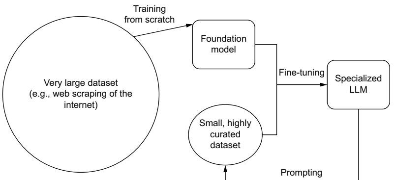
Figure 5.1 The training life cycle of an LLM. We start by creating a foundation model based on a large corpus of text, which we later finetune using a curated dataset for a specific task. We can then further improve the model by using the model itself and techniques like prompting to enhance or enlarge our curated dataset.

You’ll notice that the training life cycle is often a continuous loop—training models to understand language better and then using those models to improve our training datasets. Later in this chapter, we will go into more depth about other advanced training techniques that take advantage of this loop, like prompt tuning and RLHF. For now, let’s solidify our understanding of three basic steps.

5.2.1 From scratch

Training an LLM is computationally intensive and can take several weeks or months even on high-performance hardware. This process feeds chunks of data (or “batches”)

to the model and adjusts the weights based on the calculated loss. Over time, this iterative process of prediction and adjustment, also known as an epoch, leads the model to improve its understanding of the syntactic structures and complexities in the data. It’s worth noting that monitoring the training process is crucial to avoid overfitting, where the model becomes excessively tailored to the training data and performs poorly on unseen data. Techniques like early stopping, dropout, and learning rate scheduling are used to ensure the generalizability of the model, but they are not silver bullets. Remember, the ultimate goal is not just to minimize the loss on training data but to create a model that can understand and generate human-like text across a broad range of contexts.

Training an LLM from scratch is a complex process that begins with defining the model’s architecture. This decision should be guided by the specific task at hand, the size of the training dataset, and the available computational resources. The architecture, in simple terms, is a blueprint of the model that describes the number and arrangement of layers, the type of layers (like attention or feed-forward layers), and the connections between them. Modern LLMs typically employ a variant of the Transformer architecture, known for its scalability and efficiency in handling long sequences of data.

Once the model’s architecture is set, the next step is to compile a large and diverse dataset for training. The quality and variety of data fed into the model largely dictate the model’s ability to understand and generate human-like text. A common approach is to use a large corpus of internet text, ensuring a wide-ranging mix of styles, topics, and structures. The data is then preprocessed and tokenized, converting the raw text into a numerical format that the model can learn from. During this tokenization process, the text is split into smaller units, or tokens, which could be as short as a single character or as long as a word.

With a model and dataset ready, the next step is to initialize the model and set the learning objectives. The LLMs are trained using autoregressive semi-supervised learning techniques where the model learns to predict the next word in a sequence given the preceding words. The model’s weights are randomly initialized and then adjusted through backpropagation and optimization techniques such as Adam or Stochastic Gradient Descent based on the difference between the model’s predictions and the actual words in the training data. The aim is to minimize this difference, commonly referred to as the “loss,” to improve the model’s predictive accuracy.

Training involves feeding the tokenized text into the model and adjusting the model’s internal parameters to minimize the loss. We said this once, but it bears repeating: this process is computationally demanding and may take weeks or even months to complete, depending on the model size and available hardware. After training, the model is evaluated on a separate validation dataset to ensure that it can generalize to unseen data. It is common to iterate on this process, finetuning the model parameters and adjusting the architecture as needed based on the model’s performance on the validation set.

Let’s explore training a brand-new transformer-based language model “from scratch,” meaning without any previously defined architecture, embeddings, or weights. Figure 5.2 shows this process. You shouldn’t have to train an LLM from scratch, nor would you normally want to, as it’s a very expensive and time-consuming endeavor; however, knowing how can help you immensely.

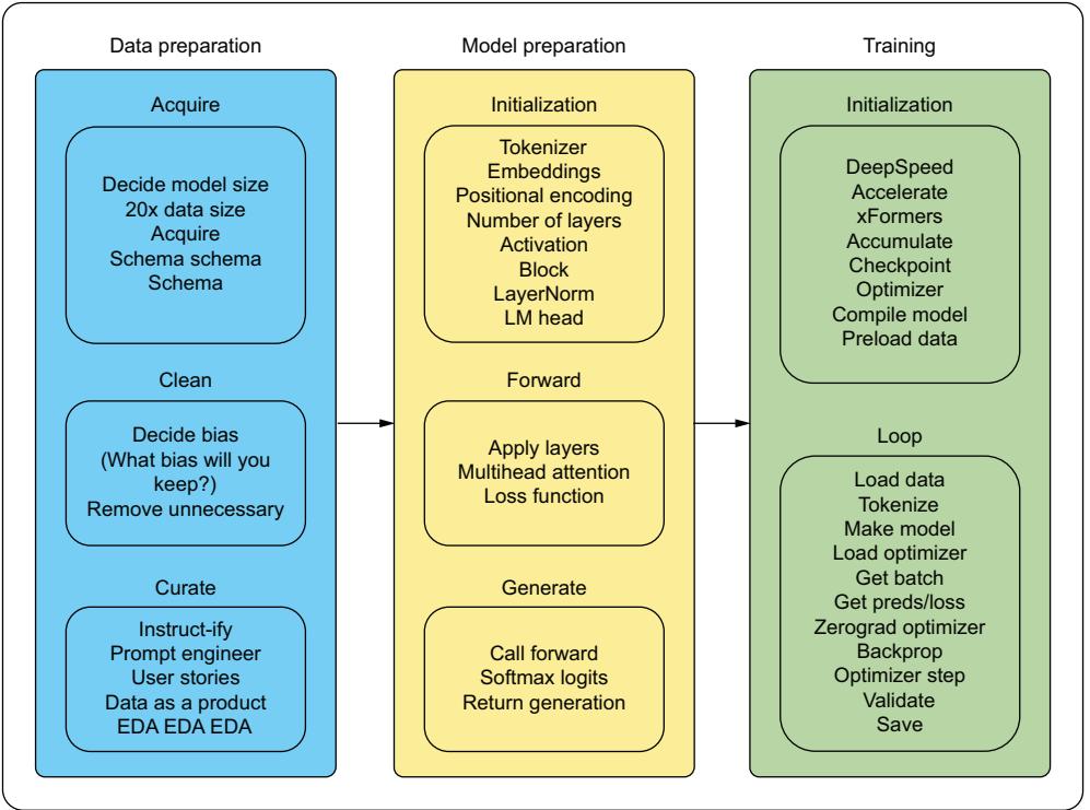
Training from scartch

Figure 5.2 A simplified version of all the steps necessary to train a language model (large or otherwise) from scratch. You must have data, then define all of the model behavior, and only then proceed to train.

Listing 5.1 allows you to run through the motions without training an actual massive model, so feel free to explore with this code. For a more complex and complete example, check out Andrej Karpathy’s minGPT project here: https://github .com/karpathy/minGPT. You should pay attention to some things when you review the listing. You might recall that we talked about tokenization and embeddings in the last chapter, so one thing to notice is that for simplicity, we will be using a character-based tokenizer. Before you run the code, can you predict whether this was a good or bad idea? Also, pay attention to how we use both Accelerate and BitsandBytes, which we introduced a little bit ago; you’ll see that these libraries come in mighty handy. Next, watch as we slowly build up the LLMs architecture, building each piece in a modular fashion and later defining how many of each piece is used and where to put them, almost like Legos. Finally, at the very end of the code, you’ll see a typical model training loop, splitting our data, running epochs in batches, and so forth.

import os
import torch
from accelerate import Accelerator
import bitsandbytes as bnb 
class GPT(torch.nn.Module): 
 def __init__(self):
 super().__init__()
 self.token_embedding = torch.nn.Embedding(vocab_size, n_embed)
 self.positional_embedding = torch.nn.Embedding(block_size, n_embed)
 self.blocks = torch.nn.Sequential(
 *[Block(n_embed, n_head=n_head) for _ in range(n_layer)]
 )
 self.ln_f = torch.nn.LayerNorm(n_embed)
 self.lm_head = torch.nn.Linear(n_embed, vocab_size)
 self.apply(self._init_weights)
 def forward(self, idx, targets=None):
 B, T = idx.shape
 tok_emb = self.token_embedding(idx)
 pos_emb = self.positional_embedding(torch.arange(T, device=device))
 x = tok_emb + pos_emb
 x = self.blocks(x)
 x = self.ln_f(x)
 logits = self.lm_head(x)
 if targets is None:
 loss = None
 else:
 B, T, C = logits.shape
 logits = logits.view(B * T, C)
 targets = targets.view(B * T)
 loss = torch.nn.functional.cross_entropy(logits, targets)
 return logits, loss
 def _init_weights(self, module):
 if isinstance(module, torch.nn.Linear):
 torch.nn.init.normal_(module.weight, mean=0.0, std=0.02)
 if module.bias is not None:
 torch.nn.init.zeros_(module.bias)
 elif isinstance(module, torch.nn.Embedding):
 torch.nn.init.normal_(module.weight, mean=0.0, std=0.02)
  Listing 5.1 An example of training from scratch 
                                Defines the 
                                overall GPT 
                                architecture

 def generate(self, idx, max_new_tokens):
 for _ in range(max_new_tokens):
 idx_cond = idx[:, -block_size:]
 logits, loss = self(idx_cond)
 logits = logits[:, -1, :]
 probs = torch.nn.functional.softmax(logits, dim=-1)
 idx_next = torch.multinomial(probs, num_samples=1)
 idx = torch.cat((idx, idx_next), dim=1)
 return idx
class Block(torch.nn.Module): 
 def __init__(self, n_embed, n_head):
 super().__init__()
 head_size = n_embed // n_head
 self.self_attention = MultiHeadAttention(n_head, head_size)
 self.feed_forward = FeedFoward(n_embed)
 self.ln1 = torch.nn.LayerNorm(n_embed)
 self.ln2 = torch.nn.LayerNorm(n_embed)
 def forward(self, x):
 x = x + self.self_attention(self.ln1(x))
 x = x + self.feed_forward(self.ln2(x))
 return x
class MultiHeadAttention(torch.nn.Module):
 def __init__(self, num_heads, head_size):
 super().__init__()
 self.heads = torch.nn.ModuleList(
 [Head(head_size) for _ in range(num_heads)]
 )
 self.projection = torch.nn.Linear(head_size * num_heads, n_embed)
 self.dropout = torch.nn.Dropout(dropout)
 def forward(self, x):
 out = torch.cat([h(x) for h in self.heads], dim=-1)
 out = self.dropout(self.projection(out))
 return out
class Head(torch.nn.Module):
 def __init__(self, head_size):
 super().__init__()
 self.key = torch.nn.Linear(n_embed, head_size, bias=False)
 self.query = torch.nn.Linear(n_embed, head_size, bias=False)
 self.value = torch.nn.Linear(n_embed, head_size, bias=False)
 self.register_buffer(
 "tril", torch.tril(torch.ones(block_size, block_size))
 )
 self.dropout = torch.nn.Dropout(dropout)
 def forward(self, x):
 _, T, _ = x.shape
                                     Defines the building 
                                     blocks of the model

 k = self.key(x)
 q = self.query(x)
 attention = q @ k.transpose(-2, -1) * k.shape[-1] ** 0.5
 attention = attention.masked_fill(
 self.tril[:T, :T] == 0, float("-inf")
 )
 attention = torch.nn.functional.softmax(attention, dim=-1)
 attention = self.dropout(attention)
 v = self.value(x)
 out = attention @ v
 return out
class FeedFoward(torch.nn.Module):
 def __init__(self, n_embed):
 super().__init__()
 self.net = torch.nn.Sequential(
 torch.nn.Linear(n_embed, 4 * n_embed),
 torch.nn.ReLU(),
 torch.nn.Linear(4 * n_embed, n_embed),
 torch.nn.Dropout(dropout),
 )
 def forward(self, x):
 return self.net(x)
def encode(string): 
 return [utt2int[c] for c in string]
def decode(line):
 return "".join([int2utt[i] for i in line])
def get_batch(split):
 data = train_data if split == "train" else val_data
 idx = torch.randint(len(data) - block_size, (batch_size,))
 x = torch.stack([data[i : i + block_size] for i in idx])
 y = torch.stack([data[i + 1 : i + block_size + 1] for i in idx])
 x, y = x.to(device), y.to(device)
 return x, y
@torch.no_grad()
def estimate_loss():
 out = {}
 model.eval()
 for split in ["train", "val"]:
 losses = torch.zeros(eval_iters)
 for k in range(eval_iters):
 X, Y = get_batch(split)
 logits, loss = model(X, Y)
 losses[k] = loss.item()
                                     Helper functions 
                                     for training

 out[split] = losses.mean()
 model.train()
 return out
if __name__ == "__main__": 
 batch_size = 64 # Number of utterances at once 
 block_size = 256 # Maximum context window size
 max_iters = 5000
 eval_interval = 500
 learning_rate = 3e-4
 eval_iters = 200
 n_embed = 384
 n_head = 6
 n_layer = 6
 dropout = 0.2
 accelerator = Accelerator()
 device = accelerator.device
 doing_quantization = False # Change to True if imported bitsandbytes
 with open("./data/crimeandpunishment.txt", "r", encoding="utf-8") as f: 
 text = f.read()
 chars = sorted(list(set(text))) 
 vocab_size = len(chars)
 utt2int = {ch: i for i, ch in enumerate(chars)}
 int2utt = {i: ch for i, ch in enumerate(chars)}
 data = torch.tensor(encode(text), dtype=torch.long)
 n = int(0.9 * len(data))
 train_data = data[:n]
 val_data = data[n:]
 model = GPT().to(device) 
 print("Instantiated Model")
 print(
 sum(param.numel() for param in model.parameters()) / 1e6,
 "Model parameters",
 )
 optimizer = (
 torch.optim.AdamW(model.parameters(), lr=learning_rate)
 if not doing_quantization
 else bnb.optim.Adam(model.parameters(), lr=learning_rate)
 )
 print("Instantiated Optimizer")
 model, optimizer, train_data = accelerator.prepare(
 model, optimizer, train_data
 )
 print("Prepared model, optimizer, and data")
 # 
 for iter in range(max_iters): 
 print(f"Running Epoch {iter}")
                                                     Trains the 
                                                     model
                                                          Parameters for 
                                                          our experiment
                                                                     Dataset
                                                      Character-based 
                                                      pseudo-tokenization
                                       Instantiates the 
                                       model and looks 
                                       at the parameters
                                           Training block

 if iter % eval_interval == 0 or iter == max_iters - 1:
 losses = estimate_loss()
 print(
 f"| step {iter}: train loss {losses['train']:.4f} "
 "| validation loss {losses['val']:.4f} |"
 )
 xb, yb = get_batch("train")
 logits, loss = model(xb, yb)
 optimizer.zero_grad(set_to_none=True)
 accelerator.backward(loss)
 optimizer.step()
 model_dir = "./models/scratchGPT/" 
 if not os.path.exists(model_dir):
 os.makedirs(model_dir)
 model_path = model_dir + "model.pt" 
 torch.save(
 model.state_dict(),
 model_path,
 )
 loaded = GPT().load_state_dict(model_path) 
 context = torch.zeros((1, 1), dtype=torch.long, device=device) 
 print(decode(loaded.generate(context, max_new_tokens=500)[0].tolist()))
                                         Creates model 
                                         directory
                                           Saves the 
                                           model
                                                  Loads the 
                                                  saved model
                                                    Tests the loaded model

In listing 5.1, we explored how the Lego blocks are put together for the GPT family of models and showed a training loop reminiscent of our exploration of language modeling in chapter 2. Beyond showing the first part of generative pretraining for models, this example also illustrates why character-based modeling, whether convolutional or otherwise, is weak for language modeling. Did you get it right? Yup, character-based modeling isn’t the best. Alphabets on their own do not contain enough information to produce statistically significant results, regardless of the tuning amount. From a linguistic standpoint, this is obvious, as alphabets and orthography, in general, are representations of meaning generated from humans, which is not intrinsically captured.

Some of the ways to help with that information capture are increasing our tokenization capture window through word-, subword-, or sentence-level tokenization. We can also complete the pretraining before showing the model our task to allow it to capture as much approximate representation as possible. Next, we’ll show what benefits combining these two steps can have on our model’s performance.

5.2.2 Transfer learning (finetuning)

Transfer learning is an essential approach in machine learning and a cornerstone of training LLMs. It’s predicated on the notion that we can reuse knowledge learned from one problem (the source domain) and apply it to a different but related problem (the target domain). In the context of LLMs, this typically means using a pretrained model, trained on a large, diverse dataset, and adapting it to a more specific task or domain.

In the first step of transfer learning, an LLM is trained on a large, general-purpose corpus, such as the entirety of Wikipedia, books, or the internet. This pretraining stage allows the model to learn an extensive range of language patterns and nuances on a wide variety of topics. The goal here is to learn a universal representation of language that captures a broad understanding of syntax, semantics, and world knowledge. These models are often trained for many iterations and require significant computational resources, which is why it’s practical to use pretrained models provided by organizations like OpenAI or Hugging Face.

After pretraining, the LLM is updated on a specific task or domain. This update process adapts the general-purpose language understanding of the model to a more specific task, such as sentiment analysis, text classification, or question answering. Updating usually requires significantly less computational resources than the initial pretraining phase because it involves training on a much smaller dataset specific to the task at hand. Through this process, the model is able to apply the vast knowledge it gained during pretraining to a specific task, often outperforming models trained from scratch on the same task. This process of transfer learning has led to many of the advances in NLP over recent years.

FINETUNING

There are several different transfer learning techniques, but when it comes to LLMs, the one everyone cares about is finetuning. Finetuning an LLM involves taking a pretrained model—that is, a model already trained on a large general corpus—and adapting it to perform a specific task or to understand a specific domain of data.

This technique uses the fact that the base model has already learned a significant amount about the language, allowing you to reap the benefits of a large-scale model without the associated computational cost and time. The process of finetuning adapts the pre-existing knowledge of the model to a specific task or domain, making it more suitable for your specific use case. It’s like having a generalist who already understands the language well and then providing specialist training for a particular job. This approach is often more feasible for most users due to the significantly reduced computational requirements and training time compared to training a model from scratch.

The first step in finetuning involves choosing a suitable pretrained model. This decision is guided by the specific task you want the model to perform and by the resources available to you. Keep in mind that this means setting a goal for the model’s behavior before training. Once the pretrained model has been chosen, it’s crucial to prepare the specific dataset you want the model to learn from. This data could be a collection of medical texts, for example, if you’re trying to finetune the model to understand medical language. The data must be preprocessed and tokenized in a way that’s compatible with the model’s pretraining.

The finetuning process involves training the model on your specific dataset, but with a twist: instead of learning from scratch, the model’s existing knowledge is adjusted to better fit the new data. This finetuning is typically done with a smaller learning rate than in the initial training phase to prevent the model from forgetting its previously learned knowledge. After finetuning, the model is evaluated on a separate dataset to ensure it can generalize to unseen data in the specific domain. Similar to training from scratch, this process may involve several iterations to optimize the model’s performance. Finetuning offers a way to harness the power of LLMs for specific tasks or domains without the need for extensive resources or computation time. See figure 5.3.

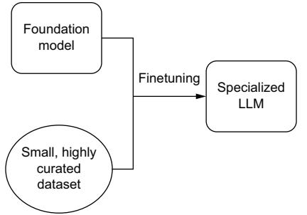
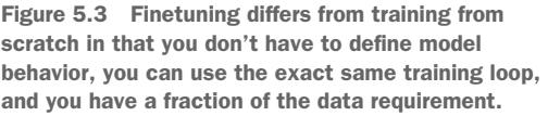
In listing 5.2, we show you how to finetune a GPT model. Notice how much less code there is in this listing than in listing 5.1. We don’t need to define an architecture or a tokenizer; we’ll just use those from the original model. Essentially, we get to skip ahead because weights and embeddings have already been defined.

import os
from transformers import (
 GPT2Tokenizer,
 GPT2LMHeadModel,
 GPT2Config,
 DataCollatorForLanguageModeling,
 TrainingArguments,
 Trainer,
)
from datasets import load_dataset
dataset = load_dataset("text", data_files="./data/crimeandpunishment.txt") 
dataset = dataset.filter(lambda sentence: len(sentence["text"]) > 1)
print(dataset["train"][0])
model_dir = "./models/betterGPT/" 
if not os.path.exists(model_dir):
 os.makedirs(model_dir)
  Listing 5.2 An example of finetuning 
                                                                          Loads and
                                                                        formats the
                                                                            dataset
                                             Creates model 
                                             directory to save to

config = GPT2Config( 
 vocab_size=50261,
 n_positions=256,
 n_embd=768,
 activation_function="gelu",
)
tokenizer = GPT2Tokenizer.from_pretrained("gpt2") 
special_tokens_dict = {
 "bos_token": "<BOS>",
 "eos_token": "<EOS>",
 "pad_token": "<PAD>",
 "mask_token": "<MASK>",
}
tokenizer.add_special_tokens(special_tokens_dict)
model = GPT2LMHeadModel.from_pretrained( 
 "gpt2", config=config, ignore_mismatched_sizes=True
)
def tokenize(batch): 
 return tokenizer(
 str(batch), padding="max_length", truncation=True, max_length=256
 )
tokenized_dataset = dataset.map(tokenize, batched=False) 
print(f"Tokenized: {tokenized_dataset['train'][0]}")
data_collator = DataCollatorForLanguageModeling( 
 tokenizer=tokenizer, mlm=True, mlm_probability=0.15
) # Masked Language Modeling - adds <MASK> tokens to guess the words
train_args = TrainingArguments( 
 output_dir=model_dir,
 num_train_epochs=1,
 per_device_train_batch_size=8,
 save_steps=5000,
 save_total_limit=2,
 report_to="none",
)
trainer = Trainer( 
 model=model,
 args=train_args,
 data_collator=data_collator,
 train_dataset=tokenized_dataset["train"],
)
trainer.train() 
trainer.save_model(model_dir)
tokenizer.save_pretrained()
model = GPT2LMHeadModel.from_pretrained(model_dir) 
                                   Establishes our GPT-2 
                                   parameters (different from 
                                   the paper and scratchGPT)
                                                                 Instantiates our 
                                                                 tokenizer and our 
                                                                 special tokens
                                                               Instantiates our 
                                                               model from the 
                                                               config
                                 Creates a 
                                 tokenize function
                                                                    Tokenizes our whole 
                                                                    dataset (so we never 
                                                                    have to do it again)
                                                                Creates a data 
                                                                collator to format 
                                                                the data for training
                                             Establishes training 
                                             arguments
                                 Instantiates 
                                 the Trainer
                                    Trains and saves 
                                    the model
                                                               Loads the 
                                                               saved model

input = "To be or not" 
tokenized_inputs = tokenizer(input, return_tensors="pt")
out = model.generate(
 input_ids=tokenized_inputs["input_ids"],
 attention_mask=tokenized_inputs["attention_mask"],
 max_length=256,
 num_beams=5,
 temperature=0.7,
 top_k=50,
 top_p=0.90,
 no_repeat_ngram_size=2,
)
print(tokenizer.decode(out[0], skip_special_tokens=True))
                                                            Tests the 
                                                            saved model

Looking at listing 5.2 compared with listing 5.1, they have almost the exact same architecture (minus the activation function), and they’re training on exactly the same data. Yet, there’s a marked improvement with the finetuned GPT-2 model due to the lack of learned representation in the first model. Our pretrained model, along with subword BPE tokenization instead of character-based, helps the model figure out which units of statistically determined meaning are most likely to go together. You’ll notice, though, that GPT-2, even with pretraining, struggles to generate relevant longer narratives despite using a newer, better activation function.

FINETUNING OPENAI

We just trained a GPT model from scratch, and then we finetuned GPT-2, but we know many readers really want the power behind OpenAI’s larger GPT models. Despite being proprietary models, OpenAI has graciously created an API where we can finetune GPT-3 models. Currently, three models are available for finetuning with OpenAI’s platform, but it looks like it intends to extend that finetuning ability to all of its models on offer. OpenAI has written a whole guide, which you can find at http://platform .openai.com/, but once you have your dataset prepared in the necessary format, the code is pretty easy. Here are some snippets for various tasks:

import os
from openai import OpenAI
client = OpenAI()
client.api_key = os.getenv("OPENAI_API_KEY")
client.files.create(
 file=open("mydata.jsonl", "rb"),
 purpose='fine-tune'
)

This first snippet uploads a training dataset in the correct format for the platform and specifies the purpose as finetuning, but doesn’t start the process yet. Next, you’ll need to create the finetuning job:

client.fine_tuning.jobs.create(training_file="file-abc123", model="gpt-3.5-
     turbo")

This is where you specify which training file and which model you want to finetune. Once OpenAI’s training loop has completed, you’ll see the finetuned model’s name populated when you retrieve the job details. Now you can use that model the same way you would have used any of the vanilla ones for chat completion or anything else like this:

completion = client.chat.completion.create(
 model="ft:gpt-3.5-turbo:my-org:custom_suffix:id",
 messages=[
 {"role": "system", "content": "You are a helpful assistant."},
 {"role": "user", "content": "Hello!"}
 ]
)
print(completion.choices[0].message)

And that’s it for finetuning an OpenAI model! Very simple, doesn’t take too long, and as of March 2023, your data is private to you. Of course, you’ll be ceding all of the control of how that finetuning occurs over to OpenAI. If you’d like to do something beyond vanilla finetuning, you’ll need to do that yourself. In just a minute, we’ll go over those techniques you may consider, along with some more advanced processes that can help with more fine-grained models and more complex tasks.

5.2.3 Prompting

One of the main reasons why LLMs are so powerful compared to traditional ML is because we can train them at run time. Give them a set of instructions and watch them follow them to the best of their ability. This technique is called prompting and is used in LLMs to guide the model’s output. In essence, the prompt is the initial input given to the model that provides it with context or instructions for what it should do. For example, “translate the following English text to French” and “summarize the following article” are prompts. In the context of LLMs, prompting becomes even more critical, as these models are not explicitly programmed to perform specific tasks but learn to respond to a variety of tasks based on the given prompt.

Prompt engineering refers to the process of crafting effective prompts to guide the model’s behavior. The aim is to create prompts that lead the model to provide the most desirable or useful output. Prompt engineering can be more complex than it appears, as slight changes in how a prompt is phrased can lead to vastly different responses from the model. Some strategies for prompt engineering include being more explicit in the prompt, providing an example of the desired output, or rephrasing the prompt in different ways to get the best results. It’s a mixture of art and science, requiring a good understanding of the model’s capabilities and limitations.

In this chapter, we are going to focus mainly on training and finetuning, the steps before deployment, but we would be remiss if we didn’t first mention prompting. We will talk about prompting in much more depth in chapter 7.

5.3 Advanced training techniques

Now that you know how to do the basics, let’s go over some more advanced techniques. These techniques have been developed for a variety of reasons, such as improving generated text outputs, shrinking the model, providing continuous learning, speeding up training, and reducing costs. Depending on the needs of your organization, you may need to reach for a different training solution. While not a comprehensive list, the following techniques are often used and should be valuable tools as you prepare a production-ready model.

Classical ML training background

Going over some techniques to enhance your finetuning process requires a bit of background. We won’t be doing a full course in ML; however, in case this is your first exposure, you should know some classic learning paradigms that experiments tend to follow—supervised, unsupervised, adversarial, and reinforcement:

• Supervised learning involves collecting both the data to train on and the labels showcasing the expected output.
• Unsupervised learning does not require labels, as the data is probed for similarity and grouped into clusters that are the closest comparison to each other.
• Adversarial learning is what’s used to train a generative adversarial network. It involves two models, generally referred to as the Critic model and the Forger model. These two models essentially play a game against each other where the forger tries to copy some ideal output, and the critic tries to determine whether the forgery is the real thing.
• Reinforcement learning (RL) opts for establishing a reward function instead of having predefined labels for the model to learn from. By measuring the model’s actions, it is given a reward based on that function instead.

All LLMs must be trained using at least one of these, and they perform at a high level with all of them done correctly. The training techniques discussed in this chapter differ from those basic ones, ranging from adding some form of human input to the model to comparing outputs to changing how the model does matrix multiplication.

5.3.1 Prompt tuning

We’ve gone over pragmatics before, but as a reminder, language models perform better when given real-world nonsemantic context pertaining to the tasks and expectations. Language modeling techniques all operate on the underlying assumption that the LM, given inputs and expected outputs, can divine the task to be done and do it in the best way within the number of parameters specified.

While the idea of the model inferring both the task and the method of completing it from the data showed promise, it has been shown time and time again, from BERT to every T5 model and now to all LLMs, that providing your model with the expected task and relevant information for solving the task improves model performance drastically. As early as 2021, Google Research, DeepMind, and OpenAI had all published papers about prompt tuning, or giving a model pragmatic context during training. The benefits of prompt tuning are reducing the amount of data required for the model to converge during training and, even cooler, the ability to reuse a completely frozen language model for new tasks without retraining or fully finetuning.

Because LLMs are so large (and getting larger), it is becoming increasingly difficult to share them and even more difficult to guarantee their performance on a given task, even one they are trained on. Prompt tuning can help nudge the model in the right direction without becoming a significant cost. Figure 5.4 shows this process.

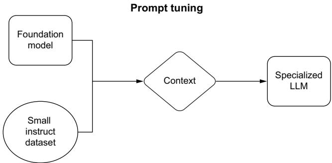
Figure 5.4 Prompt tuning foregoes most finetuning to allow the majority of the foundation model’s language understanding ability to stay exactly the same and, instead, focuses on changing how the model responds to specific inputs.

Listing 5.3 shows how to prompt tune a smaller variant of the BLOOMZ model from Big Science. BLOOMZ was released as an early competitor in the LLM space but has ultimately struggled to garner attention or momentum in the community because of its inability to generate preferred outputs despite its mathematical soundness. Because prompt tuning doesn’t add much to the regular finetuning structure we used in listing 5.2, we’ll perform Parameter-Efficient Fine-Tuning (PEFT), which drastically reduces the memory requirements by determining which model parameters need changing the most.

Listing 5.3 An example of prompt tuning

import os
from transformers import (
 AutoModelForCausalLM,
 AutoTokenizer,
 default_data_collator,
 get_linear_schedule_with_warmup,
)
from peft import (
 get_peft_model,
 PromptTuningInit,

 PromptTuningConfig,
 TaskType,
)
import torch
from datasets import load_dataset
from torch.utils.data import DataLoader
from tqdm import tqdm
def preprocess_function(examples): 
 batch_size = len(examples[text_column])
 inputs = [
 f"{text_column} : {x} Label : " for x in examples[text_column]
 ]
 targets = [str(x) for x in examples[label_column]]
 model_inputs = tokenizer(inputs)
 labels = tokenizer(targets)
 for i in range(batch_size):
 sample_input_ids = model_inputs["input_ids"][i]
 label_input_ids = labels["input_ids"][i] + [tokenizer.pad_token_id]
 model_inputs["input_ids"][i] = sample_input_ids + label_input_ids
 labels["input_ids"][i] = [-100] * len(
 sample_input_ids
 ) + label_input_ids
 model_inputs["attention_mask"][i] = [1] * len(
 model_inputs["input_ids"][i]
 )
 for i in range(batch_size):
 sample_input_ids = model_inputs["input_ids"][i]
 label_input_ids = labels["input_ids"][i]
 model_inputs["input_ids"][i] = [tokenizer.pad_token_id] * (
 max_length - len(sample_input_ids)
 ) + sample_input_ids
 model_inputs["attention_mask"][i] = [0] * (
 max_length - len(sample_input_ids)
 ) + model_inputs["attention_mask"][i]
 labels["input_ids"][i] = [-100] * (
 max_length - len(sample_input_ids)
 ) + label_input_ids
 model_inputs["input_ids"][i] = torch.tensor(
 model_inputs["input_ids"][i][:max_length]
 )
 model_inputs["attention_mask"][i] = torch.tensor(
 model_inputs["attention_mask"][i][:max_length]
 )
 labels["input_ids"][i] = torch.tensor(
 labels["input_ids"][i][:max_length]
 )
 model_inputs["labels"] = labels["input_ids"]
 return model_inputs
                                            Helper function to preprocess 
                                            text; go ahead and skip to 
                                            the training

if __name__ == "__main__": 
 # Define training parameters
 device = "cuda"
 model_name_or_path = "bigscience/bloomz-560m"
 tokenizer_name_or_path = "bigscience/bloomz-560m"
 dataset_name = "twitter_complaints"
 text_column = "Tweet text"
 label_column = "text_label"
 max_length = 64
 lr = 3e-2
 num_epochs = 1
 batch_size = 8
 peft_config = PromptTuningConfig( 
 task_type=TaskType.CAUSAL_LM,
 prompt_tuning_init=PromptTuningInit.TEXT,
 num_virtual_tokens=8,
 prompt_tuning_init_text="Classify if the tweet "
 "is a complaint or not:",
 tokenizer_name_or_path=model_name_or_path,
 )
 checkpoint_name = (
 f"{dataset_name}_{model_name_or_path}"
 f"_{peft_config.peft_type}_{peft_config.task_type}_v1.pt".replace(
 "/", "_"
 )
 )
 dataset = load_dataset("ought/raft", dataset_name) 
 print(f"Dataset 1: {dataset['train'][0]}")
 classes = [ 
 label.replace("_", " ")
 for label in dataset["train"].features["Label"].names
 ]
 dataset = dataset.map(
 lambda x: {"text_label": [classes[label] for label in x["Label"]]},
 batched=True,
 num_proc=1,
 )
 print(f"Dataset 2: {dataset['train'][0]}")
 tokenizer = AutoTokenizer.from_pretrained(model_name_or_path) 
 if tokenizer.pad_token_id is None:
 tokenizer.pad_token_id = tokenizer.eos_token_id
 target_max_length = max(
 [
 len(tokenizer(class_label)["input_ids"])
 for class_label in classes
 ]
 )
 print(f"Target Max Length: {target_max_length}")
 processed_datasets = dataset.map( 
 preprocess_function,
 batched=True,
                                    Model prompt 
                                    tuning
                                           Defines prompt 
                                           tuning config; 
                                           notice init_text
                                                          Loads Dataset
                                  Labels the dataset
                                                                Loads
                                                             tokenizer
                                            Runs Tokenizer 
                                            across dataset 
                                            and preprocess

 num_proc=1,
 remove_columns=dataset["train"].column_names,
 load_from_cache_file=False,
 desc="Running tokenizer on dataset",
 )
 train_dataset = processed_datasets["train"] 
 eval_dataset = processed_datasets["test"]
 train_dataloader = DataLoader(
 train_dataset,
 shuffle=True,
 collate_fn=default_data_collator,
 batch_size=batch_size,
 pin_memory=True,
 )
 eval_dataloader = DataLoader(
 eval_dataset,
 collate_fn=default_data_collator,
 batch_size=batch_size,
 pin_memory=True,
 )
 model = AutoModelForCausalLM.from_pretrained(model_name_or_path) 
 model = get_peft_model(model, peft_config)
 print(model.print_trainable_parameters())
 model = model.to(device)
 optimizer = torch.optim.AdamW(model.parameters(), lr=lr) 
 lr_scheduler = get_linear_schedule_with_warmup(
 optimizer=optimizer,
 num_warmup_steps=0,
 num_training_steps=(len(train_dataloader) * num_epochs),
 )
 for epoch in range(num_epochs): 
 model.train()
 total_loss = 0
 for step, batch in enumerate(tqdm(train_dataloader)):
 batch = {k: v.to(device) for k, v in batch.items()}
 outputs = model(**batch)
 loss = outputs.loss
 total_loss += loss.detach().float()
 loss.backward()
 optimizer.step()
 lr_scheduler.step()
 optimizer.zero_grad()
 model.eval()
 eval_loss = 0
 eval_preds = []
 for step, batch in enumerate(tqdm(eval_dataloader)):
 batch = {k: v.to(device) for k, v in batch.items()}
 with torch.no_grad():
 outputs = model(**batch)
                                                 Prepares data 
                                                 loaders
                                                            Loads
                                                         foundation
                                                            model
                                                           Defines 
                                                           optimizer
                                      Training 
                                      steps

 loss = outputs.loss
 eval_loss += loss.detach().float()
 eval_preds.extend(
 tokenizer.batch_decode(
 torch.argmax(outputs.logits, -1).detach().cpu().numpy(),
 skip_special_tokens=True,
 )
 )
 eval_epoch_loss = eval_loss / len(eval_dataloader)
 eval_ppl = torch.exp(eval_epoch_loss)
 train_epoch_loss = total_loss / len(train_dataloader)
 train_ppl = torch.exp(train_epoch_loss)
 print(
 f"{epoch=}: {train_ppl=} {train_epoch_loss=} "
 f"{eval_ppl=} {eval_epoch_loss=}"
 )
 model_dir = "./models/PromptTunedPEFT" 
 if not os.path.exists(model_dir):
 os.makedirs(model_dir)
 tokenizer.save_pretrained(model_dir) 
 model.save_pretrained(model_dir)
 with torch.no_grad(): 
 inputs = tokenizer(
 f'{text_column} : {{"@nationalgridus I have no water and '
 "the bill is current and paid. Can you do something about "
 'this?"}} Label : ',
 return_tensors="pt",
 )
 inputs = {k: v.to(device) for k, v in inputs.items()}
 outputs = model.generate(
 input_ids=inputs["input_ids"],
 attention_mask=inputs["attention_mask"],
 max_new_tokens=10,
 eos_token_id=3,
 )
 print(
 tokenizer.batch_decode(
 outputs.detach().cpu().numpy(), skip_special_tokens=True
 )
 )
                                          Creates model 
                                          directory to save to
                                        Saving
                             Inference

Other than the changed setup, the main difference between listings 5.2 and 5.3 is simply prepending a prompt with some sort of instruction to the beginning of each input, reminiscent of the T5 training method that pioneered having a prepended task string before every input. Prompt tuning has emerged as a powerful technique for finetuning large language models to specific tasks and domains. By tailoring prompts to the desired output and optimizing them for improved performance, we can make our models more versatile and effective. However, as our LLMs continue to grow in scale and complexity, it becomes increasingly challenging to efficiently finetune them on specific tasks. This is where knowledge distillation comes into play, offering a logical next step. Knowledge distillation allows us to transfer the knowledge and expertise of these highly tuned models to smaller, more practical versions, enabling a wider range of applications and deployment scenarios. Together, prompt tuning and knowledge distillation form a dynamic duo in the arsenal of techniques for harnessing the full potential of modern LLMs.

5.3.2 Finetuning with knowledge distillation

Knowledge distillation is an advanced technique that provides a more efficient path to finetuning an LLM. Rather than just finetuning an LLM directly, knowledge distillation involves transferring the knowledge from a large, complex model (the teacher) to a smaller, simpler model (the student). The aim is to create a more compact model that retains the performance characteristics of the larger model but is more efficient in terms of resource usage. Figure 5.5 shows this process.

Distillation training

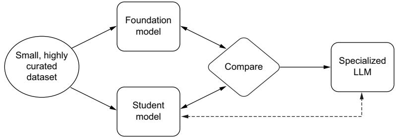
Figure 5.5 Knowledge distillation allows a smaller model to learn from a foundation model to replicate similar behavior with fewer parameters. The student model does not always learn the emergent qualities of the foundation model, so the dataset must be especially curated. The dotted line indicates a special relationship as the student model becomes the specialized LLM.

The first step in knowledge distillation is to select a pre-trained LLM as the teacher model. This could be any of the large models, such as Llama 2 70B or Falcon 180B, which have been trained on vast amounts of data. You also need to create or select a smaller model as the student. The student model might have a similar architecture to the teacher’s, but with fewer layers or reduced dimensionality to make it smaller and faster.

Next, the student model is trained on the same task as the teacher model. However, instead of learning from the raw data directly, the student model learns to mimic the teacher model’s outputs. This training is typically done by adding a term to the loss function that encourages the student model’s predictions to be similar to the teacher model’s predictions. Thus, the student model not only learns from the task-specific labels but also benefits from the rich representations learned by the teacher model.

Once the distillation process is complete, you’ll have a compact student model that can handle the specific tasks learned from the teacher model but at a fraction of the size and computational cost. The distilled model can then be further finetuned on a specific task or dataset if required. Through knowledge distillation, you can use the power of LLMs in situations where computational resources or response time are limited.

In listing 5.4, we show how to perform finetuning with knowledge distillation using BERT and becoming DistilBERT. As opposed to regular finetuning, pay attention to the size and performance of the model. Both will drop; however, size will drop much faster than performance.

import os
from transformers import (
 AutoTokenizer,
 TrainingArguments,
 Trainer,
 AutoModelForSequenceClassification,
 DataCollatorWithPadding,
)
from datasets import load_dataset, load_metric
import torch
import torch.nn as nn
import torch.nn.functional as F
import numpy as np
def process(examples):
 tokenized_inputs = tokenizer(
 examples["sentence"], truncation=True, max_length=256
 )
 return tokenized_inputs
def compute_metrics(eval_pred):
 predictions, labels = eval_pred
 predictions = np.argmax(predictions, axis=1)
 acc = accuracy_metric.compute(
 predictions=predictions, references=labels
 )
 return {
 "accuracy": acc["accuracy"],
 }
class DistillationTrainingArguments(TrainingArguments):
 def __init__(self, *args, alpha=0.5, temperature=2.0, **kwargs):
 super().__init__(*args, **kwargs)
  Listing 5.4 An example of knowledge distillation

 self.alpha = alpha
 self.temperature = temperature
class DistillationTrainer(Trainer):
 def __init__(self, *args, teacher_model=None, **kwargs):
 super().__init__(*args, **kwargs)
 self.teacher = teacher_model
 self._move_model_to_device(self.teacher, self.model.device) 
 self.teacher.eval()
 def compute_loss(self, model, inputs, return_outputs=False):
 outputs_student = model(**inputs) 
 student_loss = outputs_student.loss
 with torch.no_grad(): 
 outputs_teacher = self.teacher(**inputs)
 assert ( 
 outputs_student.logits.size() == outputs_teacher.logits.size()
 )
 # Soften probabilities and compute distillation loss
 loss_function = nn.KLDivLoss(reduction="batchmean")
 loss_logits = loss_function(
 F.log_softmax(
 outputs_student.logits / self.args.temperature, dim=-1
 ),
 F.softmax(
 outputs_teacher.logits / self.args.temperature, dim=-1
 ),
 ) * (self.args.temperature**2)
 loss = ( 
 self.args.alpha * student_loss
 + (1.0 - self.args.alpha) * loss_logits
 )
 return (loss, outputs_student) if return_outputs else loss
if __name__ == "__main__":
 model_dir = "./models/KDGPT/" 
 if not os.path.exists(model_dir):
 os.makedirs(model_dir)
 student_id = "gpt2" 
 teacher_id = "gpt2-medium"
 teacher_tokenizer = AutoTokenizer.from_pretrained(teacher_id)
 student_tokenizer = AutoTokenizer.from_pretrained(student_id)
 sample = "Here's our sanity check."
 assert teacher_tokenizer(sample) == student_tokenizer(sample), (
 "Tokenizers need to have the same output! "
 f"{teacher_tokenizer(sample)} != {student_tokenizer(sample)}"
 )
                                                           Place teacher
                                                          on same device
                                                             as student
                                                            Computes 
                                                            student 
                                                            output
                                                   Computes 
                                                   teacher output
                                                    Asserts size
                                              Returns weighted 
                                              student loss
                                        Creates model 
                                        directory to save to
                                  Defines the teacher 
                                  and student models

 del teacher_tokenizer
 del student_tokenizer
 tokenizer = AutoTokenizer.from_pretrained(teacher_id)
 tokenizer.add_special_tokens({"pad_token": "[PAD]"})
 dataset_id = "glue"
 dataset_config = "sst2"
 dataset = load_dataset(dataset_id, dataset_config)
 tokenized_dataset = dataset.map(process, batched=True)
 tokenized_dataset = tokenized_dataset.rename_column("label", "labels")
 print(tokenized_dataset["test"].features)
 labels = tokenized_dataset["train"].features["labels"].names 
 num_labels = len(labels)
 label2id, id2label = dict(), dict()
 for i, label in enumerate(labels):
 label2id[label] = str(i)
 id2label[str(i)] = label
 training_args = DistillationTrainingArguments( 
 output_dir=model_dir,
 num_train_epochs=1,
 per_device_train_batch_size=1,
 per_device_eval_batch_size=1,
 fp16=True,
 learning_rate=6e-5,
 seed=8855,
 Evaluation strategies
 evaluation_strategy="epoch",
 save_strategy="epoch",
 save_total_limit=2,
 load_best_model_at_end=True,
 metric_for_best_model="accuracy",
 report_to="none",
 push_to_hub=False, 
 alpha=0.5, 
 temperature=4.0,
 )
 data_collator = DataCollatorWithPadding(tokenizer=tokenizer) 
 teacher_model = AutoModelForSequenceClassification.from_pretrained( 
 teacher_id,
 num_labels=num_labels,
 id2label=id2label,
 label2id=label2id,
 )
 student_model = AutoModelForSequenceClassification.from_pretrained( 
 student_id,
 num_labels=num_labels,
 id2label=id2label,
                                                      Creates label2id,
                                                   id2label dicts for nice
                                                   outputs for the model
                                                         Defines 
                                                         training args
                                        Pushes to hub 
                                        parameters
                                  Distillation 
                                  parameters Defines
                                                           data_collator
                                                           Defines model
                                                                Defines
                                                           student model

 label2id=label2id,
 )
 accuracy_metric = load_metric("accuracy") 
 trainer = DistillationTrainer(
 student_model,
 training_args,
 teacher_model=teacher_model,
 train_dataset=tokenized_dataset["train"],
 eval_dataset=tokenized_dataset["validation"],
 data_collator=data_collator,
 tokenizer=tokenizer,
 compute_metrics=compute_metrics,
 )
 trainer.train()
 trainer.save_model(model_dir)
                                               Defines metrics 
                                               and metrics 
                                               function

Knowledge distillation, as exemplified by the provided compute_loss method, is a technique that enables the transfer of valuable insights from a teacher model to a more lightweight student model. In this process, the teacher model provides soft targets, offering probability distributions over possible outputs, which are then utilized to train the student model. The critical aspect of knowledge distillation lies in the alignment of these distributions, ensuring that the student model not only learns to mimic the teacher’s predictions but also gains a deeper understanding of the underlying data. This approach helps improve the student’s generalization capabilities and performance on various tasks, ultimately making it more efficient and adaptable.

As we look forward, one logical progression beyond knowledge distillation is the incorporation of RLHF. While knowledge distillation enhances a model’s ability to make predictions based on existing data, RLHF allows the model to learn directly from user interactions and feedback. This dynamic combination not only refines the model’s performance further but also enables it to adapt and improve continuously. By incorporating human feedback, RL can help the model adapt to real-world scenarios, evolving its decision-making processes based on ongoing input, making it an exciting and natural evolution in the development of LLM systems.

5.3.3 Reinforcement learning with human feedback

RLHF is a newer training technique developed to overcome one of the biggest challenges when it comes to RL: how to create reward systems that actually work. It sounds easy, but anyone who’s played around with RL knows how difficult it can be. Before AlphaStar, one author was building his own RL bot to play StarCraft, a war simulation game in space.

NOTE Check outhttps://mng.bz/Dp4a to learn more about AlphaStar.

A simple reward system based on winning or losing was taking too long, so he decided to give it some reasonable intermediate rewards based on growing an army. However, this got blocked when it failed to build Pylons, a building required to increase army supply limits. So he gave it a reward to build Pylons. His bot quickly learned that it liked to build Pylons—so much so that it learned to almost win but not win, crippling its opponent so that it could keep building Pylons unharassed and for as long as it wanted.

With a task like winning a game, even if it’s difficult, we can usually still come up with reasonable reward systems. But what about more abstract tasks, like teaching a robot how to do a backflip? These tasks get really difficult to design reward systems for, which is where RLHF comes in. What if instead of designing a system, we simply have a human make suggestions? A human knows what a backflip is, after all. The human will act like a tutor, picking attempts it likes more as the bot is training. That’s what RLHF is, and it works really well. Applied to LLMs, a human simply looks at generated responses to a prompt and picks which one they like more. See figure 5.6.

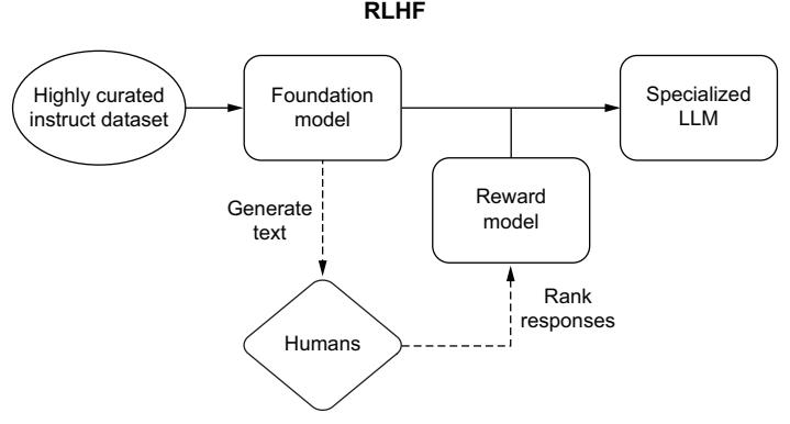
Figure 5.6 RLHF substitutes a loss function for a reward model and proximal policy optimization (PPO), allowing the model a much higher ceiling for learning trends within the data, including what is preferred as an output instead of what completes the task.

While very powerful, RLHF likely won’t stick around for very long. The reason is that it is incredibly computationally expensive for a result that is only incrementally better, especially a result that can be achieved and matched by higher-quality datasets with supervised learning approaches.

There are some other problems with RLHF, such as that it requires hiring domain experts to evaluate and provide the human feedback. Not only can this get expensive, but it can also lead to privacy concerns since these reviewers would need to look at actual traffic and user interactions to grade them. To combat both of these concerns, you could try to outsource this directly to the users, asking for their feedback, but it may end up poisoning your data if your users have ill intent or are simply not experts in the subject matter, in which case they might upvote responses they like but that aren’t actually correct. This gets to the next problem: even experts have biases. RLHF doesn’t train a model to be more accurate or factually correct; it trains the model to generate human-acceptable answers.

In production, RLHF has the advantage of allowing you to easily update your model on a continual basis. However, this is a two-edged sword, as it also increases the likelihood of your model degrading over time. OpenAI uses RLHF heavily, and it has led to many users complaining about their models, like GPT-4, becoming terrible in certain domains compared to when it first came out. One Stanford study found that GPT-4, when asked if a number was prime, used to get it right 98% of the time in March 2023, but three months later, in June 2023, it would only get it right 2% of the time.¹ One reason is that the June model is much less verbose, opting to give a simple yes or no response. Humans like these responses. Getting straight to the point is often better, but LLMs tend to be better after they have had time to reason through the answer with techniques like chain of thought.

With this in mind, RLHF is fantastic for applications where human-acceptable answers are the golden standard, and factually correct answers are less important—for example, a friendly chatbot or improving summarization tasks. These problems are intuitively syntactic in nature, essentially tasks that LLMs are already good at but which you want to refine by possibly creating a certain tone or personality.

Another reason for RLHF degradation is due to data leakage. Data leakage is when your model is trained on the test or validation dataset you use to evaluate it. When this happens, you are essentially allowing the model to cheat, leading to overfitting and poor generalization. It’s just like how LeetCode interview questions lead tech companies to hire programmers who have lots of experience solving toy problems but don’t know how to make money or do their job.

How does this happen? Well, simply. When you are running an LLM in production with RLHF, you know it’s going to degrade over time, so it’s best to run periodic evaluations to monitor the system. The more you run these evaluations, the more likely that one of the prompts will be picked up for human feedback and subsequent RL training. It could also happen by pure coincidence if your users happen to ask a question similar to a prompt in your evaluation dataset. Either way, without restrictions placed on RLHF (which generally are never done), it’s a self-defeating system.

The really annoying aspect of continual updates through RLHF is that these updates ruin downstream engineering efforts, methods like prompting or retrievalaugmented generation (RAG). Engineering teams can take a lot of effort to dial in a process or procedure to query a model and then clean up responses, but all that work can easily be undermined if the underlying model is changing. As a result, many teams prefer a static model with periodic updates to one with continual updates.

¹ L. Chen, M. Zaharia, and J. Zou, “How is ChatGPT’s behavior changing over time?,” arXiv.org, Jul. 18, 2023, https://arxiv.org/abs/2307.09009.

All that said, RLHF is still a powerful technique that may yield greater results later as it is optimized and refined. Also, it’s just really cool. We don’t recommend using RLHF, and we don’t have the space here to delve deeper; just know that it is a tool used by companies specializing in LLMs. For readers who want to understand RLHF better, we have included an in-depth example and code listing in appendix B.

5.3.4 Mixture of experts

A mixture of experts (MoE) is functionally the same as any other model for training but contains a trick under the hood: sparsity. This gives the advantage of being able to train a bunch of models on a diverse set of data and tasks at once. You see, a MoE is exactly what it sounds like: an ensemble of identical models in the beginning. You can think of them as a group of freshman undergrads. Then, using some unsupervised grouping methods, such as k-means clustering, each of these experts “picks a major” during training. This allows the model only to activate some experts to answer particular inputs instead of all of them, or maybe the input is complex enough that it requires activating all of them. The point is that once training has completed, if it has been done on a representative-enough dataset, each of your experts will have a college degree in the major that they studied. Because the homogeneity of inputs is determined mathematically, those majors won’t always have a name that correlates to something you would major in at school, but we like to think of these as eccentric double minors or something of the sort. Maybe one of your experts majored in physics but double minored in advertising and Africana studies. It doesn’t really matter, but the major upside to designing an ensemble of models in this way is that you can effectively reduce computational requirements immensely while retaining specialization and training memory by only consulting the experts whose knowledge correlates with the tokenized input at inference time.

In listing 5.5, we finetune a MoE model in much the same way as we did in listing 5.2 with GPT-2, thanks to Hugging Face’s API and Google’s Switch Transformer. Unlike the method we described in chapter 3, where we turned a feed-forward network into an MoE, we’ll start with an already created MoE and train it on our own dataset. Training an MoE is pretty simple now, unlike when they first came out. Very smart people performed so much engineering that we can give an oversimplified explanation of these models. Google created the Switch Transformer to combat two huge problems they had run into while trying to train LLMs: size and instability. Google engineers simplified the routing algorithm (how the model decides which experts to query for each input) and showed how to train models with lower quantizations (in this case, bfloat16) for the first time—quite an amazing feat and not one to take lightly, as GPT-4 is likely an MoE.

Listing 5.5 Example mixture of experts finetuning

import os
from transformers import (
 AutoTokenizer,
 SwitchTransformersForConditionalGeneration,

 SwitchTransformersConfig,
 TrainingArguments,
 Trainer,
 DataCollatorForLanguageModeling,
)
from datasets import load_dataset
import torch
dataset = load_dataset("text", data_files="./data/crimeandpunishment.txt") 
dataset = dataset.filter(lambda sentence: len(sentence["text"]) > 1)
print(f"Dataset 1: {dataset['train'][0]}")
model_dir = "./models/MoE/" 
if not os.path.exists(model_dir):
 os.makedirs(model_dir)
tokenizer = AutoTokenizer.from_pretrained("google/switch-base-8") 
config = SwitchTransformersConfig( 
 decoder_start_token_id=tokenizer.pad_token_id
)
model = SwitchTransformersForConditionalGeneration.from_pretrained( 
 "google/switch-base-8",
 config=config,
 device_map="auto",
 torch_dtype=torch.float16,
)
def tokenize(batch): 
 return tokenizer(
 str(batch), padding="max_length", truncation=True, max_length=256
 )
tokenized_dataset = dataset.map(tokenize, batched=False) 
print(f"Tokenized: {tokenized_dataset['train'][0]}")
data_collator = DataCollatorForLanguageModeling( 
 tokenizer=tokenizer, mlm=False, mlm_probability=0.0
) # Causal Language Modeling - Does not use mask
train_args = TrainingArguments( 
 output_dir=model_dir,
 num_train_epochs=1,
 per_device_train_batch_size=8,
 save_steps=5000,
 save_total_limit=2,
 report_to="none",
)
trainer = Trainer( 
 model=model,
                                                                         Loads and
                                                                        formats the
                                                                            dataset
                                          Creates model 
                                          directory to save to Instantiates
                                                                     our tokenizer
                                                          Establishes our 
                                                          SwitchTransformers config
                                                              Instantiates our model
                                                                    from the config
                                Creates a 
                                tokenize function
                                                                     Tokenizes our 
                                                                     whole dataset 
                                                                     (so we never have 
                                                                     to do it again)
                                                               Creates a data 
                                                               collator to format 
                                                               the data for training
                                            Establishes 
                                            training 
                                            arguments
                                Instantiates 
                                the trainer

 args=train_args,
 data_collator=data_collator,
 train_dataset=tokenized_dataset["train"],
)
trainer.train() 
trainer.save_model(model_dir)
tokenizer.save_pretrained(model_dir)
model = SwitchTransformersForConditionalGeneration.from_pretrained( 
 model_dir,
 device_map="auto",
 torch_dtype=torch.float16,
)
input = "To be or not <extra_id_0> <extra_id_0>" 
tokenized_inputs = tokenizer(input, return_tensors="pt")
out = model.generate(
 input_ids=tokenized_inputs["input_ids"].to("cuda"),
 attention_mask=tokenized_inputs["attention_mask"],
 max_length=256,
 num_beams=5,
 temperature=0.7,
 top_k=50,
 top_p=0.90,
 no_repeat_ngram_size=2,
)
print(f"To be or not {tokenizer.decode(out[0], skip_special_tokens=True)}")
                                     Trains and saves 
                                     the model
                                                                  Loads the
                                                                saved model
                                                              Tests the 
                                                              saved model

In this script, an MoE model is finetuned using the Switch Transformer foundation model. MoE models are unique during finetuning because you typically update the taskspecific parameters, such as the gating mechanism and the parameters of the experts, while keeping the shared parameters intact. This allows the MoE to use the expertise of the different experts for better task-specific performance. Finetuning MoE models differs from traditional finetuning because it requires handling the experts and gating mechanisms, which can be more complex than regular neural network architectures. In our case, we’re lucky that trainer.train() with the right config covers it for finetuning, and we can just bask in the work that Google did before us.

A logical progression beyond MoE finetuning involves exploring Parameter-Efficient Fine-Tuning (PEFT) and low-rank adaptations (LoRA). PEFT aims to make the finetuning process more efficient by reducing the model’s size and computational demands, making it more suitable for resource-constrained scenarios. Techniques such as knowledge distillation, model pruning, quantization, and compression can be employed in PEFT to achieve this goal. In contrast, LoRA focuses on incorporating low-rank factorization methods into model architectures to reduce the number of parameters while maintaining or even enhancing model performance. These approaches are essential, as they enable the deployment of sophisticated models on devices with limited resources and in scenarios where computational efficiency is paramount.

5.3.5 LoRA and PEFT

LoRA represents a significant breakthrough for machine learning in general. Taking advantage of a mathematical trick, LoRAs can change the output of a model without changing the original model weights or taking up significant space or cost, as shown in figure 5.7. The reason for the significance here is that it makes finetuning a separate model for many different tasks or domains much more feasible, as has already been seen in the diffusion space with text2image LoRAs popping up quite often for conditioning model output without significantly altering the base model’s abilities or style. Put simply, if you already like your model and would like to change it to do the exact same thing in a new domain without sacrificing what it was already good at on its own, an adapter might be the path for you, especially if you have multiple new domains that you don’t want bleeding into one another.

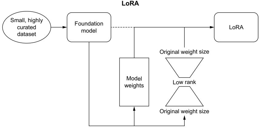
Figure 5.7 LoRA exemplifies the idea that you should only need to train and save the difference between where the foundation model is and where you want it to be. It does this through singular value decomposition (SVD).

To understand LoRAs, you need to first understand how models currently adjust weights. Since we aren’t going to go over a complete backpropagation tutorial here, we can abstract it as

\[\mathbf{W} = \mathbf{W} + \Delta \mathbf{W}\]

So if you have a model with 100 100-dimensional layers, your weights can be represented by a 100 × 100 matrix. The cool part comes with singular value decomposition (SVD), which has been used for compression by factoring a single matrix into three smaller matrices. We covered this topic in depth back in chapter 3 (see listing 3.2). So while we know the intuition for SVD with LLMs, what can we compress from that original formula?

\[\Delta \mathbf{W} = \mathbf{W\_a} \times \mathbf{W\_b}\]

So if ∆W = 100 × 100, Wa = 100 × c and Wb = c × 100, where c < 100. If c = 2, you can represent 10,000 elements using only 400 because when they’re multiplied together, they equal the 10,000 original elements. So the big question is, what does c equal for your task? The c-value is the “R” in LoRA, referring to the rank of the matrix of weights. There are algorithmic ways of determining that rank using eigenvectors and the like, but you can approximate a lot of it by knowing that a higher rank equals more complexity, meaning that the higher the number you use there, the closer you’ll get to original model accuracy, but the less memory you’ll save. If you think the task you’re finetuning the LoRA for isn’t as complex, reduce the rank.

The next listing shows you how to combine creating a LoRA and then perform inference with both the LoRA and your base model.

import os
from datasets import load_dataset
from transformers import (
 AutoModelForTokenClassification,
 AutoTokenizer,
 DataCollatorForTokenClassification,
 TrainingArguments,
 Trainer,
)
from peft import (
 PeftModel,
 PeftConfig,
 get_peft_model,
 LoraConfig,
 TaskType,
)
import evaluate
import torch
import numpy as np
model_checkpoint = "meta-llama/Llama-2-7b-hf"
lr = 1e-3
batch_size = 16
num_epochs = 10
model_dir = "./models/LoRAPEFT" 
if not os.path.exists(model_dir):
 os.makedirs(model_dir)
bionlp = load_dataset("tner/bionlp2004")
seqeval = evaluate.load("seqeval")
label_list = [
 "O",
 "B-DNA",
 "I-DNA",
 "B-protein",
  Listing 5.6 Example LoRA and PEFT training 
                                         Creates model 
                                         directory to 
                                         save to

 "I-protein",
 "B-cell_type",
 "I-cell_type",
 "B-cell_line",
 "I-cell_line",
 "B-RNA",
 "I-RNA",
]
def compute_metrics(p):
 predictions, labels = p
 predictions = np.argmax(predictions, axis=2)
 true_predictions = [
 [label_list[p] for (p, l) in zip(prediction, label) if l != -100]
 for prediction, label in zip(predictions, labels)
 ]
 true_labels = [
 [label_list[l] for (p, l) in zip(prediction, label) if l != -100]
 for prediction, label in zip(predictions, labels)
 ]
 results = seqeval.compute(
 predictions=true_predictions, references=true_labels
 )
 return {
 "precision": results["overall_precision"],
 "recall": results["overall_recall"],
 "f1": results["overall_f1"],
 "accuracy": results["overall_accuracy"],
 }
tokenizer = AutoTokenizer.from_pretrained(
 model_checkpoint, add_prefix_space=True
)
def tokenize_and_align_labels(examples):
 tokenized_inputs = tokenizer(
 examples["tokens"], truncation=True, is_split_into_words=True
 )
 labels = []
 for i, label in enumerate(examples["tags"]):
 word_ids = tokenized_inputs.word_ids(batch_index=i)
 previous_word_idx = None
 label_ids = []
 for word_idx in word_ids:
 if word_idx is None:
 label_ids.append(-100)
 elif word_idx != previous_word_idx:
 label_ids.append(label[word_idx])

 else:
 label_ids.append(-100)
 previous_word_idx = word_idx
 labels.append(label_ids)
 tokenized_inputs["labels"] = labels
 return tokenized_inputs
tokenized_bionlp = bionlp.map(tokenize_and_align_labels, batched=True)
data_collator = DataCollatorForTokenClassification(tokenizer=tokenizer)
id2label = {
 0: "O",
 1: "B-DNA",
 2: "I-DNA",
 3: "B-protein",
 4: "I-protein",
 5: "B-cell_type",
 6: "I-cell_type",
 7: "B-cell_line",
 8: "I-cell_line",
 9: "B-RNA",
 10: "I-RNA",
}
label2id = {
 "O": 0,
 "B-DNA": 1,
 "I-DNA": 2,
 "B-protein": 3,
 "I-protein": 4,
 "B-cell_type": 5,
 "I-cell_type": 6,
 "B-cell_line": 7,
 "I-cell_line": 8,
 "B-RNA": 9,
 "I-RNA": 10,
}
model = AutoModelForTokenClassification.from_pretrained(
 model_checkpoint, num_labels=11, id2label=id2label, label2id=label2id
)
peft_config = LoraConfig(
 task_type=TaskType.TOKEN_CLS,
 inference_mode=False,
 r=16,
 lora_alpha=16,
 lora_dropout=0.1,
 bias="all",
)
model = get_peft_model(model, peft_config)
model.print_trainable_parameters()

training_args = TrainingArguments(
 output_dir=model_dir,
 learning_rate=lr,
 per_device_train_batch_size=batch_size,
 per_device_eval_batch_size=batch_size,
 num_train_epochs=num_epochs,
 weight_decay=0.01,
 evaluation_strategy="epoch",
 save_strategy="epoch",
 load_best_model_at_end=True,
)
trainer = Trainer(
 model=model,
 args=training_args,
 train_dataset=tokenized_bionlp["train"],
 eval_dataset=tokenized_bionlp["validation"],
 tokenizer=tokenizer,
 data_collator=data_collator,
 compute_metrics=compute_metrics,
)
trainer.train()
peft_model_id = "stevhliu/roberta-large-lora-token-classification"
config = PeftConfig.from_pretrained(model_dir)
inference_model = AutoModelForTokenClassification.from_pretrained(
 config.base_model_name_or_path,
 num_labels=11,
 id2label=id2label,
 label2id=label2id,
)
tokenizer = AutoTokenizer.from_pretrained(config.base_model_name_or_path)
model = PeftModel.from_pretrained(inference_model, peft_model_id)
text = (
 "The activation of IL-2 gene expression and NF-kappa B through CD28 "
 "requires reactive oxygen production by 5-lipoxygenase."
)
inputs = tokenizer(text, return_tensors="pt")
with torch.no_grad():
 logits = model(**inputs).logits
tokens = inputs.tokens()
predictions = torch.argmax(logits, dim=2)
for token, prediction in zip(tokens, predictions[0].numpy()):
 print((token, model.config.id2label[prediction]))

Keep in mind that you still need to keep your base model, as shown in listing 5.6. The LoRA is run in addition to the foundation model; it sits on top and changes the weights at only the rank determined in the LoraConfig class (in this case, 16). RoBERTa-Large was likely already decent at doing token classification on the bionlp dataset, but now, running with the LoRA on top, it’ll be even better. There are multiple types of LoRAs you can use, with QLoRA, QA-LoRA, and AWQ-LoRA all gaining popularity in different domains and tasks. With the transformers library, which can be controlled from the LoraConfig, we encourage you to experiment with different adaptation methods to find what works for your data and task.

The most attractive thing about LoRA is that the particular one we discussed here results in a file only 68 KB in size on disk and still has a significant performance boost. You could create LoRAs for each portion of your company that wants a model, one for the legal team that’s siloed so it doesn’t have to worry about any private data it is putting into it, one for your engineering team to help with code completion and answering questions about which data structures or algorithms to use, and one for anyone else. Because they’re so small, it’s suddenly much more feasible to store than the 1.45 GB (14.5 GB if we use Llama in fp16; it’s 28 GB in fp32) RoBERTa-Large model being finetuned a bunch of times. In the spirit of giving you more of these time- and space-saving tips, we’ll go over some things that aren’t mentioned anywhere else, but you may still get some use out of if the data science part of LLMs is what you are working with.

5.4 Training tips and tricks

While this book isn’t focused on training and researching new models, we feel kind of bad telling you that finetuning models is an effective strategy for teaching LLMs correct guardrails based on your data and then just leaving you to figure out how to make it work on your own stuff. With this in mind, let’s look at some tried-and-true tips and tricks for both training and finetuning LLMs. These tips will help you with some of the least-intuitive parts of training LLMs that most practitioners (like us) had to learn the hard way.

5.4.1 Training data size notes

First off, LLMs are notorious for overfitting. If you are considering training a foundation model, you need to consider the amount of data you have, which should be roughly 20× the number of parameters you’re trying to train.2 For example, if you’re training a 1B parameter model, you should train it on 20B tokens. If you have fewer tokens than that, you will run the risk of overfitting.

If you already have a model and need to finetune it on your data, consider the inverse, where you should likely have ~0.000001× the number of tokens as a minimum (10K tokens for a 1B parameter model). We came up with this rule of thumb based on our experience, although it should be fairly intuitive. If you have fewer than 1/100,000 of your model parameters in tokens, finetuning likely won’t have much of an effect. In this case, you should consider another strategy that won’t cost as much,

² J. Hoffmann et al., “Training compute-optimal large language models,” arXiv:2203.15556 [cs], March 2022, https://arxiv.org/abs/2203.15556.

such as LoRA (which we just discussed), RAG (which we talk about in the next chapter), or a system that uses both.

For both these examples, we’ve had the experience where a company we worked for hoped for great results with minimal data and was disappointed. One hoped to train an LLM from scratch with only ~1 million tokens while also disallowing open source datasets, and another wanted to finetune the model but only on a couple of hundred examples. Neither of these approaches were cost-efficient, nor did they create models that performed up to the standards the companies aimed for.

5.4.2 Efficient training

We’ve so far focused on tools and methodologies for training, which should supercharge your ability to create the best and largest models your training system allows. However, other factors should be considered when setting up your training loops. In physics, the uncertainty principle shows that you can never perfectly know both the speed and position of a given particle. Machine learning’s uncertainty principle is that you can never perfectly optimize both your speed and your memory utilization. Improving speed comes at the cost of memory, and vice versa. Table 5.2 shows some choices you can make in training and their effects on speed and memory.

Method	Improve speed	Improves memory utilization	Difficulty
Batch size choice	Yes	Yes	Easy
Gradient accumulation	No	Yes	Medium
Gradient checkpointing	No	Yes	Medium
Mixed precision	Yes	No	Hard
Optimizer choice	Yes	Yes	Easy
Data preloading	Yes	No	Medium
Compiling	Yes	No	Easy

Table 5.2				Training choices to consider
———–	–	–	–	——————————

Carefully consider your options and what goal you’re working toward when setting up your training loop. For example, your batch size should be a power of 2 to hit maximum speed and memory efficiency. One author remembers working on getting an LLM to have a single-digit milli-second response time. The team was gearing up to serve millions of customers as fast as possible, and every millisecond counted. After using every trick in the book, I was able to achieve it, and I remember the huge feeling of accomplishment for finally getting that within the data science dev environment. Yet, it turned out that there was a hard batch size of 20 in the production environment. It was just a nice number picked out of a hat, and too many systems were built around this assumption; no one wanted to refactor. Software engineers, am I right?

For the majority of these methods, the tradeoff is clear: if you go slower, you can fit a significantly larger model, but it will take way longer. Gradient accumulating and checkpointing can reduce memory usage by ~60%, but training will take much longer. The packages we talked about in section 5.1 can help mitigate these tradeoffs.

5.4.3 Local minima traps

Local minima are hard to spot with LLMs and, as such, can be difficult to avoid. If you see your model converging early, be suspicious and judiciously test it before accepting the results. When you find that your model is converging early at a certain number of steps, one way to avoid it on subsequent runs is to save and load a checkpoint 100 or so steps before you see the errant behavior, turn your learning rate way down, train until you’re sure you’re past it, and then turn it back up and continue. Make sure to keep the previously saved checkpoint, and save a new checkpoint after that so that you have places to come back to in case things go wrong!

You can probably tell that this is a frustrating occurrence that one author has run into before. He was so confused; he was working on a T5 XXL model, and around the 25K step mark, the model was converging and stopping early. He knew for a fact that it wasn’t actually converged; it was only 10% through the dataset! This happened two or three times, where he loaded up the checkpoint at around 20K steps and watched the exact same thing happen. It wasn’t until he loaded and turned the learning rate down that he finally saw the model improve past this point. Once he got through the patch of the local minimum, he turned it back up. This happened four more times throughout training this particular model, but since he knew what was happening, he was now able to avoid wasting lots of extra time. The lesson of the story? Use this rule of thumb: your LLM is not ready if it hasn’t trained on your full dataset.

5.4.4 Hyperparameter tuning tips

Hyperparameter tuning isn’t something we’ve gone over extensively in this book, not because it’s not interesting but because it doesn’t help nearly as much as changing up your data, either getting more or cleaning it further. If you want to tune hyperparameters, Optuna is a great package, and you can get that ~1% boost in accuracy or F1 score that you really need. Otherwise, if you’re looking for a boost in a particular metric, try representing that metric more completely within your dataset and maybe use some statistical tricks like oversampling.

While hyperparameter tuning is pretty cool mathematically, for LLMs, it’s not something that ever really needs to happen. If you need a boost in performance, you need more/better data, and tuning your hyperparameters will never match the performance boost you’d get quantizing the weights or performing any of the optimizations we’ve mentioned here or in chapter 3. The biggest performance boost we’ve ever gotten through tuning hyperparameters was about a 4% increase in F1, and we only did it because we wouldn’t be able to change our dataset for a couple of weeks at least.

5.4.5 A note on operating systems

Windows is not the right OS to work professionally with LLMs without the Windows Subsystem for Linux. MacOS is great but lacks the hardware packages to really carry this load unless you know how to use an NVIDIA or AMD GPU with a Mac. If you are uncomfortable with Linux, you should take some time to familiarize yourself with it while your OS of choice catches up (if it ever does). A myriad of free online materials are available to help you learn about Bash, Linux, and the command line. Configuring the CUDA Toolkit and Nvidia drivers on Linux can make you want to pull your hair out, but it’s worth it compared to the alternatives. Along with this, learn about virtual environments, Docker, and cloud computing, like what’s in this chapter!

All in all, Windows is easy in the beginning but frustrating in the long run. MacOS is also easy in the beginning but currently doesn’t work at all in the long run. Linux is incredibly frustrating in the beginning, but once you’re through that, it’s smooth sailing.

5.4.6 Activation function advice

We’ve neglected to really dive into activation functions so far, not because they aren’t useful or cool but because you generally don’t need to tweak your activation functions unless you’re doing research science on model performance. If you take vanilla GPT-2 and give it a GeGLU activation instead of the GELU that it comes with, you will not get a significant boost in anything. In addition, you’ll need to redo your pretraining, as it pretrained with a different activation function. Activation functions help reduce some of the mathematical weaknesses of each layer, be they imaginary numbers from the quadratic attention, exploding and vanishing gradients, or maybe the researchers noticed positional encodings disappearing as they went through the model and changed a little bit. You can learn about activation functions, and we recommend doing so; in general, you can trust the papers that introduce new ones.

We’ve come a long way in this chapter, discussing setting up an environment, training an LLM from scratch, and looking at a multitude of finetuning techniques. While we recognize there are still many aspects to this process that we did not touch on and that you need to learn on your own, you should be more than ready to create your own models. Now that you have a model, in the next chapter, we’ll discuss making it production-ready and creating an LLM service you can use to serve online inference.

Summary

• Training is memory intensive, and you will need to master multi-GPU environments for many LLM training tasks.
• Model training has the same basic steps every time:
  • Dataset preparation—Acquire, clean, and curate your data.
  • Model preparation—Define model behavior, architecture, loss functions, etc.
  • Training loop—Initialization, tokenize, batch data, get predictions/loss, backpropagation, etc.
• Good data has a significantly greater effect on model performance than architecture or the training loop.
• Finetuning is way easier than training from scratch because it requires much less data and resources.
• Prompting allows us to train a model on a specific task after the fact, which is one of the reasons LLMs are so powerful compared to traditional ML.
• Prompt tuning is a powerful way to focus your model to respond as a specialist to certain prompts.
• Knowledge distillation is useful for training powerful smaller models that are efficient and adaptable.
• RLHF is great at getting a model to respond in a way that pleases human evaluators but increases factually incorrect results.
• Finetuning MoE models differs from traditional finetuning because it requires handling the experts and gating mechanisms.
• LoRA is a powerful finetuning technique that adapts pretrained models to new tasks by creating tiny assets (low-rank matrices) that are fast to train, easy to maintain, and very cost-effective.
• The quality and size of your data are two of the most important considerations for successfully training your model.
• The major training tradeoff is speed for memory efficiency; if you go slower, you can fit a significantly larger model, but it will take way longer.