Regression Modeling Strategies

Chapter 10 ~ 20

Author

Frank E. Harrell, Jr.

Chapter 10 Binary Logistic Regression

10.1 Model

Binary responses are commonly studied in many fields. Examples include ¹ the presence or absence of a particular disease, death during surgery, or a consumer purchasing a product. Often one wishes to study how a set of predictor variables X is related to a dichotomous response variable Y . The predictors may describe such quantities as treatment assignment, dosage, risk factors, and calendar time.

For convenience we define the response to be Y = 0 or 1, with Y = 1 denoting the occurrence of the event of interest. Often a dichotomous outcome can be studied by calculating certain proportions, for example, the proportion of deaths among females and the proportion among males. However, in many situations, there are multiple descriptors, or one or more of the descriptors are continuous. Without a statistical model, studying patterns such as the relationship between age and occurrence of a disease, for example, would require the creation of arbitrary age groups to allow estimation of disease prevalence as a function of age.

Letting X denote the vector of predictors {X1, X2,…,Xk}, a first attempt at modeling the response might use the ordinary linear regression model

\[E\{Y|X\} = X\beta,\tag{10.1}\]

since the expectation of a binary variable Y is Prob{Y = 1}. However, such a model by definition cannot fit the data over the whole range of the predictors since a purely linear model E{Y |X} = Prob{Y = 1|X} = XΛ can allow Prob{Y = 1} to exceed 1 or fall below 0. The statistical model that is generally preferred for the analysis of binary responses is instead the binary logistic regression model, stated in terms of the probability that Y = 1 given X, the values of the predictors:

^© Springer International Publishing Switzerland 2015

F.E. Harrell, Jr., Regression Modeling Strategies, Springer Series

in Statistics, DOI 10.1007/978-3-319-19425-7 10

\[\text{Prob}\{Y=1|X\} = [1 + \exp(-X\beta)]^{-1}.\tag{10.2}\]

As before, XΛ stands for Λ⁰ + Λ1X¹ + Λ2X² + … + ΛkXk. The binary logistic regression model was developed primarily by Cox129 and Walker and Duncan. ² 647 The regression parameters Λ are estimated by the method of maximum likelihood (see below).

The function

\[P = [1 + \exp(-x)]^{-1} \tag{10.3}\]

is called the logistic function. This function is plotted in Figure 10.1 for x varying from ×4 to +4. This function has an unlimited range for x while P is restricted to range from 0 to 1.

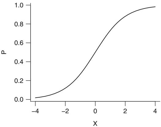
Fig. 10.1 Logistic function

For future derivations it is useful to express x in terms of P. Solving the equation above for x by using

\[1 - P = \exp(-x) / [1 + \exp(-x)]\tag{10.4}\]

yields the inverse of the logistic function:

x = log[P/(1 × P)] = log[odds that Y = 1 occurs] = logit{Y = 1}. (10.5)

Other methods that have been used to analyze binary response data include the probit model, which writes P in terms of the cumulative normal distribution, and discriminant analysis. Probit regression, although assuming a similar shape to the logistic function for the regression relationship between XΛ and Prob{Y = 1}, involves more cumbersome calculations, and there is no natural interpretation of its regression parameters. In the past, discriminant analysis has been the predominant method since it is the simplest computationally. However, it makes more assumptions than logistic re-³ gression. The model used in discriminant analysis is stated in terms of the

distribution of X given the outcome group Y , even though one is seldom interested in the distribution of the predictors per se. The discriminant model has to be inverted using Bayes’ rule to derive the quantity of primary interest, Prob{Y = 1}. By contrast, the logistic model is a direct probability model since it is stated in terms of Prob{Y = 1|X}. Since the distribution of a binary random variable Y is completely defined by the true probability that Y = 1 and since the model makes no assumption about the distribution of the predictors, the logistic model makes no distributional assumptions whatsoever.

10.1.1 Model Assumptions and Interpretation of Parameters

Since the logistic model is a direct probability model, its only assumptions relate to the form of the regression equation. Regression assumptions are verifiable, unlike the assumption of multivariate normality made by discriminant analysis. The logistic model assumptions are most easily understood by transforming Prob{Y = 1} to make a model that is linear in XΛ:

\[\begin{split} \log \text{fit} \{ Y = 1 | X \} &= \text{logit}(P) = \log[P/(1 - P)] \\ &= X\beta, \end{split} \tag{10.6}\]

where P = Prob{Y = 1|X}. Thus the model is a linear regression model in the log odds that Y = 1 since logit(P) is a weighted sum of the Xs. If all effects are additive (i.e., no interactions are present), the model assumes that for every predictor Xj,

\[\begin{split} \text{logit} \{ Y = 1 | X \} &= \beta\_0 + \beta\_1 X\_1 + \dots + \beta\_j X\_j + \dots + \beta\_k X\_k \\ &= \beta\_j X\_j + C, \end{split} \tag{10.7}\]

where if all other factors are held constant, C is a constant given by

\[C = \beta\_0 + \beta\_1 X\_1 + \dots + \beta\_{j-1} X\_{j-1} + \beta\_{j+1} X\_{j+1} + \dots + \beta\_k X\_k. \tag{10.8}\]

The parameter Λ^j is then the change in the log odds per unit change in X^j if X^j represents a single factor that is linear and does not interact with other factors and if all other factors are held constant. Instead of writing this relationship in terms of log odds, it could just as easily be written in terms of the odds that Y = 1:

\[\text{odds}\{Y=1|X\} = \exp(X\beta),\tag{10.9}\]

and if all factors other than X^j are held constant,

\[\text{odds}\{Y=1|X\} = \exp(\beta\_j X\_j + C) = \exp(\beta\_j X\_j)\exp(C). \tag{10.10}\]

The regression parameters can also be written in terms of odds ratios. The odds that Y = 1 when X^j is increased by d, divided by the odds at X^j is

\[\begin{split} \frac{\text{odds}\{Y=1|X\_1, X\_2, \dots, X\_j+d, \dots, X\_k\}}{\text{odds}\{Y=1|X\_1, X\_2, \dots, X\_j, \dots, X\_k\}}\\ &= \frac{\exp[\beta\_j(X\_j+d)]\exp(C)}{[\exp(\beta\_j X\_j)\exp(C)]}\\ &= \exp[\beta\_j X\_j + \beta\_j d - \beta\_j X\_j] = \exp(\beta\_j d). \end{split} \tag{10.11}\]

Thus the effect of increasing X^j by d is to increase the odds that Y = 1 by a factor of exp(Λjd), or to increase the log odds that Y = 1 by an increment of Λjd. In general, the ratio of the odds of response for an individual with predictor variable values X′ compared with an individual with predictors X is

\[\begin{split} X^\*: X \text{ odds ratio} &= \exp(X^\*\beta) / \exp(X\beta) \\ &= \exp[(X^\* - X)\beta]. \end{split} \tag{10.12}\]

Now consider some special cases of the logistic multiple regression model. If there is only one predictor X and that predictor is binary, the model can be written

\[\begin{aligned} \text{logit}\{Y=1|X=0\} &= \beta\_0\\ \text{logit}\{Y=1|X=1\} &= \beta\_0 + \beta\_1. \end{aligned} \tag{10.13}\]

Here Λ⁰ is the log odds of Y = 1 when X = 0. By subtracting the two equations above, it can be seen that Λ¹ is the difference in the log odds when X = 1 as compared with X = 0, which is equivalent to the log of the ratio of the odds when X = 1 compared with the odds when X = 0. The quantity exp(Λ1) is the odds ratio for X = 1 compared with X = 0. Letting ^P⁰ = Prob{^Y = 1|^X = 0} and ^P¹ = Prob{^Y = 1|^X = 1}, the regression parameters are interpreted by

\[\begin{split} \beta\_0 &= \text{logit}(P^0) = \log[P^0/(1-P^0)] \\ \beta\_1 &= \text{logit}(P^1) - \text{logit}(P^0) \\ &= \log[P^1/(1-P^1)] - \log[P^0/(1-P^0)] \\ &= \log\{[P^1/(1-P^1)]/[P^0/(1-P^0)]\}. \end{split} \tag{10.14}\]

Since there are only two quantities to model and two free parameters, there is no way that this two-sample model can’t fit; the model in this case is essentially fitting two cell proportions. Similarly, if there are g × 1 dummy indicator Xs representing g groups, the ANOVA-type logistic model must always fit.

If there is one continuous predictor X, the model is

\[\text{logit}\{Y=1|X\}=\beta\_0+\beta\_1X,\tag{10.15}\]

and without further modification (e.g., taking log transformation of the predictor), the model assumes a straight line in the log odds, or that an increase in X by one unit increases the odds by a factor of exp(Λ1).

Now consider the simplest analysis of covariance model in which there are two treatments (indicated by X¹ = 0 or 1) and one continuous covariable (X2). The simplest logistic model for this setup is

\[\text{logit}\{Y=1|X\} = \beta\_0 + \beta\_1 X\_1 + \beta\_2 X\_2,\tag{10.16}\]

which can be written also as

\[\begin{aligned} \text{logit}\{Y=1|X\_1=0, X\_2\} &= \beta\_0 + \beta\_2 X\_2\\ \text{logit}\{Y=1|X\_1=1, X\_2\} &= \beta\_0 + \beta\_1 + \beta\_2 X\_2. \end{aligned} \tag{10.17}\]

The X¹ =1: X¹ = 0 odds ratio is exp(Λ1), independent of X2. The odds ratio for a one-unit increase in X² is exp(Λ2), independent of X1.

This model, with no term for a possible interaction between treatment and covariable, assumes that for each treatment the relationship between X² and log odds is linear, and that the lines have equal slope; that is, they are parallel. Assuming linearity in X2, the only way that this model can fail is for the two slopes to differ. Thus, the only assumptions that need verification are linearity and lack of interaction between X¹ and X2.

To adapt the model to allow or test for interaction, we write

\[\text{logit}\{Y=1|X\} = \beta\_0 + \beta\_1 X\_1 + \beta\_2 X\_2 + \beta\_3 X\_3,\tag{10.18}\]

where the derived variable X³ is defined to be X1X2. The test for lack of interaction (equal slopes) is H⁰ : Λ³ = 0. The model can be amplified as

\[\begin{aligned} \text{logit}\{Y=1|X\_1=0, X\_2\} &= \beta\_0 + \beta\_2 X\_2\\ \text{logit}\{Y=1|X\_1=1, X\_2\} &= \beta\_0 + \beta\_1 + \beta\_2 X\_2 + \beta\_3 X\_2\\ &= \beta\_0' + \beta\_2' X\_2, \end{aligned} \tag{10.19}\]

Without Risk Factor			With Risk Factor
Probability	Odds		Odds Probability
.2	.25	.5	.33
.5	1	2	.67
.8	4	8	.89
.9	9	18	.95
.98	49	98	.99

Table 10.1 Effect of an odds ratio of two on various risks

where Λ∗ ⁰ = Λ⁰ +Λ¹ and Λ^∗ ² = Λ² +Λ3. The model with interaction is therefore equivalent to fitting two separate logistic models with X² as the only predictor, one model for each treatment group. Here the X¹ =1: X¹ = 0 odds ratio is exp(Λ¹ + Λ3X2).

10.1.2 Odds Ratio, Risk Ratio, and Risk Difference

As discussed above, the logistic model quantifies the effect of a predictor in terms of an odds ratio or log odds ratio. An odds ratio is a natural description of an effect in a probability model since an odds ratio can be constant. For example, suppose that a given risk factor doubles the odds of disease. Table 10.1 shows the effect of the risk factor for various levels of initial risk.

Since odds have an unlimited range, any positive odds ratio will still yield a valid probability. If one attempted to describe an effect by a risk ratio, the effect can only occur over a limited range of risk (probability). For example, a risk ratio of 2 can only apply to risks below .5; above that point the risk ratio must diminish. (Risk ratios are similar to odds ratios if the risk is small.) Risk differences have the same difficulty; the risk difference cannot be constant and must depend on the initial risk. Odds ratios, on the other hand, can describe an effect over the entire range of risk. An odds ratio can, for example, describe the effect of a treatment independently of covariables affecting risk. Figure 10.2 depicts the relationship between risk of a subject without the risk factor and the increase in risk for a variety of relative increases (odds ratios). It demonstrates how absolute risk increase is a function of the baseline risk. Risk increase will also be a function of factors that interact with the risk factor, that is, factors that modify its relative effect. Once a model is developed for estimating Prob{Y = 1|X}, this model can easily be used to estimate the absolute risk increase as a function of baseline risk factors as well as interacting factors. Let X¹ be a binary risk factor and let A = {X2,…,Xp} be the other factors (which for convenience we assume do not interact with X1). Then the estimate of Prob{Y = 1|X¹ = 1, A} × Prob{Y = 1|X¹ = 0, A} is

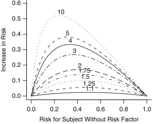
Fig. 10.2 Absolute benefit as a function of risk of the event in a control subject and the relative effect (odds ratio) of the risk factor. The odds ratios are given for each curve.

Table 10.2 Example binary response data

Females	Age: 37 39 39 42 47 48 48 52 53 55 56 57 58 58 60 64 65 68 68 70
	Response:	0	0	0	0	0	0	1	0	0	0	0	0	0	1	0	0	1	1	1	1
Males	Age: 34 38 40 40 41 43 43 43 44 46 47 48 48 50 50 52 55 60 61 61
	Response:	1	1	0	0	0	1	1	1	0	0	1	1	1	0	1	1	1	1	1	1

\[\begin{split} \frac{1}{1 + \exp - [\hat{\beta}\_0 + \hat{\beta}\_1 + \hat{\beta}\_2 X\_2 + \dots + \hat{\beta}\_p X\_p]} \\ - \frac{1}{1 + \exp - [\hat{\beta}\_0 + \hat{\beta}\_2 X\_2 + \dots + \hat{\beta}\_p X\_p]} \\ = \frac{1}{1 + (\frac{1 - \hat{R}}{\hat{R}}) \exp(-\hat{\beta}\_1)} - \hat{R}, \end{split} \tag{10.20}\]

where ^R^ˆ is the estimate of the baseline risk, Prob{^Y = 1|X¹ = 0}. The risk difference estimate can be plotted against Rˆ or against levels of variables in A to display absolute risk increase against overall risk (Figure 10.2) or against specific subject characteristics. ⁴

10.1.3 Detailed Example

Consider the data in Table 10.2. A graph of the data, along with a fitted logistic model (described later), appears in Figure 10.3. The graph also displays proportions of responses obtained by stratifying the data by sex and age group (< 45, 45 × 54, ← 55). The age points on the abscissa for these groups are the overall mean ages in the three age intervals (40.2, 49.1, and 61.1, respectively).

require(rms)

getHdata ( sex.age.response)
d − sex.age.response
dd − datadist (d); options (datadist = ' dd ' )
f − lrm(response ← sex + age , data=d)
fasr − f # Save for later
w − function (...)
  with(d, {
    m − sex== ' male '
    f − sex== ' female '
    lpoints(age [f], response [f], pch=1)
    lpoints(age [m], response [m], pch=2)
    af − cut2(age , c(45,55), levels.mean =TRUE)
    prop − tapply (response , list(af, sex), mean ,
                     na.rm=TRUE)
    agem − as.numeric (row.names (prop))
    lpoints(agem , prop[, ' female ' ],
             pch=4, cex=1.3, col= ' green ' )
    lpoints(agem , prop[, ' male ' ],
             pch=5, cex=1.3, col= ' green ' )
    x − rep(62, 4); y − seq(.25 , .1, length =4)
    lpoints (x, y, pch=c(1, 2, 4, 5),
             col=rep(c( ' blue ' , ' green ' ),each=2))
    ltext(x+5, y,
           c( ' F Observed ' , ' M Observed ' ,
              ' F Proportion ' , ' M Proportion ' ), cex=.8)
  } ) # Figure 10.3
plot(Predict (f, age=seq (34, 70, length =200), sex , fun=plogis ),
     ylab= ' Pr[response ] ' , ylim=c(-.02 , 1.02), addpanel =w)
ltx − function (fit) latex(fit , inline=TRUE , columns =54,
                              file= ' ' , after= ' $ . ' , digits =3,
         size= ' Ssize ' , before= ' $X\\hat{\\beta}= ' )
ltx(f)

^XΛ^ˆ ⁼ ^×9.84 + 3.49[male] + 0.158 age.

Descriptive statistics for assessing the association between sex and response, age group and response, and age group and response stratified by sex are found below. Corresponding fitted logistic models, with sex coded as 0 = female, 1 = male are also given. Models were fitted first with sex as the only predictor, then with age as the (continuous) predictor, then with sex and age simultaneously. First consider the relationship between sex and response, ignoring the effect of age.

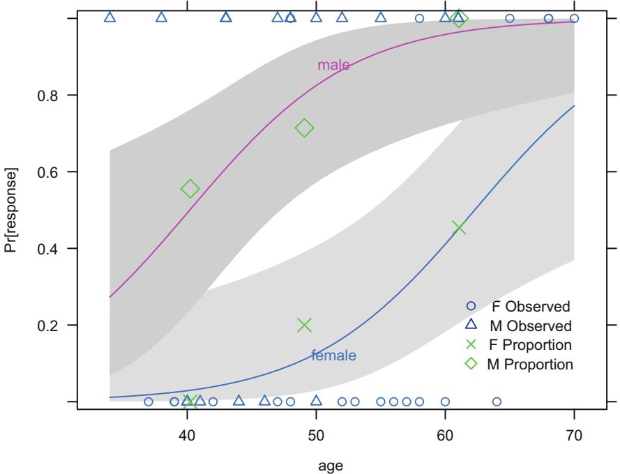
Fig. 10.3 Data, subgroup proportions, and fitted logistic model, with 0.95 pointwise confidence bands

sex	response
Frequency Row Pct	0	1	Total	Odds/Log
F	14 70.00	6 30.00	20	6/14=.429 -.847
M	6 30.00	14 70.00	20	14/6=2.33 .847
Total	20	20	40
		M:F odds ratio = (14/6)/(6/14)		= 5.44, log=1.695
Statistics for sex ∼ response

	Statistic		d.f. Value	P
σ2	Likelihood Ratio σ2 Parameter Estimate Std Err Wald σ2		1 6.400 0.011 1 6.583 0.010	P
χ0 χ1	×0.8473 1.6946	0.4880 0.6901	3.0152	6.0305 0.0141

Note that the estimate of Λ0, Λˆ⁰ is the log odds for females and that Λˆ¹ is the log odds (M:F) ratio. Λˆ⁰ + Λˆ¹ = .847, the log odds for males. The likelihood ratio test for H⁰ : no effect of sex on probability of response is obtained as follows.

Log likelihood (χ1	= 0) : ×27.727
Log likelihood (max)	: ×24.435
LR σ2(H0 : χ1 = 0)	: ×2(×27.727 × ×24.435) = 6.584.

(Note the agreement of the LR β² with the contingency table likelihood ratio β2, and compare 6.584 with the Wald statistic 6.03.)

Next, consider the relationship between age and response, ignoring sex.

age	response
Frequency
Row Pct	0	1	Total	Odds/Log
<45	8	5	13	5/8=.625
	61.5	38.4		-.47
45-54	6	6	12	6/6=1
	50.0	50.0		0
55+	6	9	15	9/6=1.5
	40.0	60.0		.405
Total	20	20	40
55+ : <45 odds ratio = (9/6)/(5/8)				= 2.4, log=.875

Parameter Estimate Std Err Wald σ² P

χ0	×2.7338	1.8375	2.2134 0.1368
χ1	0.0540	0.0358	2.2763 0.1314

The estimate of Λ¹ is in rough agreement with that obtained from the frequency table. The 55+ : < 45 log odds ratio is .875, and since the respective mean ages in the 55+ and <45 age groups are 61.1 and 40.2, an estimate of the log odds ratio increase per year is .875/(61.1 × 40.2) = .875/20.9 = .042.

The likelihood ratio test for H⁰ : no association between age and response is obtained as follows.

Log likelihood (χ¹ = 0) : ×27.727 Log likelihood (max) : ×26.511 LR ^σ²(H⁰ : ^χ¹ = 0) : ^×2(×27.⁷²⁷ × ×26.511) = 2.432.

(Compare 2.432 with the Wald statistic 2.28.)

Next we consider the simultaneous association of age and sex with response.

sex=F
——-

age Frequency	response
Row Pct	0	1	Total
<45	4 100.0	0 0.0	4
45-54	4 80.0	1 20.0	5
55+	6 54.6	5 45.4	11
Total	14	6	20

sex=M

age Frequency	response
Row Pct	0	1	Total
<45	4 44.4	5 55.6	9
45-54	2 28.6	5 71.4	7
55+	0 0.0	4 100.0	4
Total	6	14	20

A logistic model for relating sex and age simultaneously to response is given below.

Parameter Estimate Std Err Wald σ² P

χ0	×9.8429	3.6758	7.1706 0.0074
χ1 (sex)	3.4898	1.1992	8.4693 0.0036
χ2 (age)	0.1581	0.0616	6.5756 0.0103

Likelihood ratio tests are obtained from the information below.

= 0) : ×27.727
: ×19.458
: ×26.511
: ×24.435
: ×2(×27.727 × ×19.458) = 16.538
: ×2(×26.511 × ×19.458) = 14.106
: ×2(×24.435 × ×19.458) = 9.954.

The 14.1 should be compared with the Wald statistic of 8.47, and 9.954 should be compared with 6.58. The fitted logistic model is plotted separately for females and males in Figure 10.3. The fitted model is

\[\text{logit}\{\text{Response} = 1|\text{sex}, \text{age}\} = -9.84 + 3.49 \times \text{sex} + .158 \times \text{age}, \quad (10.21)\]

where as before sex = 0 for females, 1 for males. For example, for a 40-yearold female, the predicted logit is ×9.84 + .158(40) = ×3.52. The predicted probability of a response is 1/[1 + exp(3.52)] = .029. For a 40-year-old male, the predicted logit is ×9.84 + 3.49 + .158(40) = ×.03, with a probability of .492.

10.1.4 Design Formulations

The logistic multiple regression model can incorporate the same designs as can ordinary linear regression. An analysis of variance (ANOVA) model for a treatment with k levels can be formulated with k × 1 dummy variables. This logistic model is equivalent to a 2 ≤ k contingency table. An analysis of covariance logistic model is simply an ANOVA model augmented with covariables used for adjustment.

One unique design that is interesting to consider in the context of logistic models is a simultaneous comparison of multiple factors between two groups. Suppose, for example, that in a randomized trial with two treatments one wished to test whether any of 10 baseline characteristics are mal-distributed between the two groups. If the 10 factors are continuous, one could perform a two-sample Wilcoxon–Mann–Whitney test or a t-test for each factor (if each is normally distributed). However, this procedure would result in multiple comparison problems and would also not be able to detect the combined effect of small differences across all the factors. A better procedure would be a multivariate test. The Hotelling T ² test is designed for just this situation. It is a k-variable extension of the one-variable unpaired t-test. The T ² test, like discriminant analysis, assumes multivariate normality of the k factors. This assumption is especially tenuous when some of the factors are polytomous. A better alternative is the global test of no regression from the logistic model. This test is valid because it can be shown that H⁰ : mean X is the same for both groups (= H⁰ : mean X does not depend on group = H⁰ : mean X| group = constant) is true if and only if H⁰ : Prob{group|X} = constant. Thus k factors can be tested simultaneously for differences between the two groups using the binary logistic model, which has far fewer assumptions than does the Hotelling T ² test. The logistic global test of no regression (with k d.f.) would be expected to have greater power if there is non-normality. Since the logistic model makes no assumption regarding the distribution of the descriptor variables, it can easily test for simultaneous group differences involving a mixture of continuous, binary, and nominal variables. In observational studies, such models for treatment received or exposure (propensity score models) hold great promise for adjusting for confounding.117, 380, 526, 530, 531 ⁵

O’Brien479 has developed a general test for comparing group 1 with group 2 for a single measurement. His test detects location and scale differences by fitting a logistic model for Prob{Group 2} using ^X and ^X² as predictors.

For a randomized study where adjustment for confounding is seldom necessary, adjusting for covariables using a binary logistic model results in increases in standard errors of regression coefficients.527 This is the opposite of what happens in linear regression where there is an unknown variance parameter that is estimated using the residual squared error. Fortunately, adjusting for covariables using logistic regression, by accounting for subject heterogeneity, will result in larger regression coefficients even for a randomized treatment variable. The increase in estimated regression coefficients more than offsets the increase in standard error284, 285, 527, 588.

10.2 Estimation

10.2.1 Maximum Likelihood Estimates

The parameters in the logistic regression model are estimated using the maximum likelihood (ML) method. The method is based on the same principles as the one-sample proportion example described in Section 9.1. The difference is that the general logistic model is not a single sample or a two-sample problem. The probability of response for the ith subject depends on a particular set of predictors Xi, and in fact the list of predictors may not be the same for any two subjects. Denoting the response and probability of response of the ith subject by Yⁱ and Pi, respectively, the model states that

\[P\_i = \text{Prob}\{Y\_i = 1 | X\_i\} = \left[1 + \exp(-X\_i\beta)\right]^{-1}.\tag{10.22}\]

The likelihood of an observed response Yⁱ given predictors Xⁱ and the unknown parameters Λ is

\[P\_i^{Y\_i}[1 - P\_i]^{1 - Y\_i}.\tag{10.23}\]

The joint likelihood of all responses Y1, Y2,…,Yⁿ is the product of these likelihoods for i = 1,…,n. The likelihood and log likelihood functions are rewritten by using the definition of Pⁱ above to allow them to be recognized as a function of the unknown parameters Λ. Except in simple special cases (such as the k-sample problem in which all Xs are dummy variables), the ML estimates (MLE) of Λ cannot be written explicitly. The Newton–Raphson method described in Section 9.4 is usually used to solve iteratively for the list of values Λ that maximize the log likelihood. The MLEs are denoted by Λˆ. The inverse of the estimated observed information matrix is taken as the estimate of the variance–covariance matrix of Λˆ.

Under H⁰ : Λ¹ = Λ² = … = Λ^k = 0, the intercept parameter Λ⁰ can be estimated explicitly and the log likelihood under this global null hypothesis can be computed explicitly. Under the global null hypothesis, Pⁱ = P = [1 + exp(×Λ0)]−¹ and the MLE of ^P is ^P^ˆ ⁼ s/n where ^s is the number of responses and n is the sample size. The MLE of Λ⁰ is Λˆ⁰ = logit(Pˆ). The log 6 likelihood under this null hypothesis is

\[\begin{aligned} &s\,\log(\hat{P}) + (n-s)\log(1-\hat{P})\\ &=\quad s\,\log(s/n) + (n-s)\log[(n-s)/n] \\ &=s\,\log s + (n-s)\log(n-s) - n\log(n). \end{aligned} \tag{10.24}\]

10.2.2 Estimation of Odds Ratios and Probabilities

Once Λ is estimated, one can estimate any log odds, odds, or odds ratios. The MLE of the X^j +1: X^j log odds ratio is Λˆ^j , and the estimate of the X^j + d : X^j log odds ratio is Λˆjd, all other predictors remaining constant (assuming the absence of interactions and nonlinearities involving Xj). For large enough samples, the MLEs are normally distributed with variances that are consistently estimated from the estimated variance–covariance matrix. Letting z denote the 1×σ/2 critical value of the standard normal distribution, a two-sided 1 × σ confidence interval for the log odds ratio for a one-unit increase in ^X^j is [Λˆ^j ^× zs, ^Λˆ^j ⁺ zs], where ^s is the estimated standard error of Λˆ^j . (Note that for σ = .05, i.e., for a 95% confidence interval, z = 1.96.)

A theorem in statistics states that the MLE of a function of a parameter is that same function of the MLE of the parameter. Thus the MLE of the ^X^j +1: ^X^j odds ratio is exp(Λˆ^j ). Also, if a 1 ^× ^σ confidence interval of a parameter Λ is [c, d] and f(u) is a one-to-one function, a 1 × σ confidence interval of f(Λ) is [f(c), f(d)]. Thus a 1×σ confidence interval for the X^j +1 : ^X^j odds ratio is exp[Λˆ^j ^±zs]. Note that while the confidence interval for ^Λ^j is symmetric about Λˆj, the confidence interval for exp(Λ^j ) is not. By the same theorem just used, the MLE of Pⁱ = Prob{Yⁱ = 1|Xi} is

\[\hat{P}\_i = [1 + \exp(-X\_i \hat{\beta})]^{-1}.\tag{10.25}\]

A confidence interval for Pⁱ could be derived by computing the standard error of Pˆi, yielding a symmetric confidence interval. However, such an interval would have the disadvantage that its endpoints could fall below zero or exceed one. A better approach uses the fact that for large samples XΛˆ is approximately normally distributed. An estimate of the variance of XΛˆ in matrix notation is XVX^∗ where V is the estimated variance–covariance matrix of Λˆ (see Equation 9.51). This variance is the sum of all variances and covariances of Λˆ weighted by squares and products of the predictors. The estimated standard error of XΛˆ, s, is the square root of this variance estimate. A 1 × σ confidence interval for Pⁱ is then ⁷

\[\left\{1+\exp[-(X\_i\hat{\beta}\pm zs)]\right\}^{-1}.\tag{10.26}\]

10.2.3 Minimum Sample Size Requirement

Suppose there were no covariates, so that the only parameter in the model is the intercept. What is the sample size required to allow the estimate of the intercept to be precise enough so that the predicted probability is within 0.1 of the true probability with 0.95 confidence, when the true intercept is in the neighborhood of zero? The answer is n=96. What if there were one covariate, and it was binary with a prevalence of ¹ ² ? One would need 96 subjects with X = 0 and 96 with X = 1 to have an upper bound on the margin of error for estimating Prob{^Y = 1|^X ⁼ ^x} not exceed 0.1 for either value of ^x^a.

Now consider a very simple single continuous predictor case in which X has a normal distribution with mean zero and standard deviation τ, with the true Prob{^Y = 1|^X ⁼ ^x} = [1 + exp(×x)]−¹. The expected number of events is ⁿ 2 ^b. The following simulation answers the question “What should n be so that the expected maximum absolute error (over ^x ^≥ [×1.5, ¹.5]) in ^P^ˆ is less than χ?”

sigmas − c(.5 , .75 , 1, 1.25 , 1.5 , 1.75 , 2, 2.5 , 3, 4)
ns − seq(25, 300, by=25)
nsim − 1000
xs − seq(-1.5 , 1.5 , length =200)
pactual − plogis (xs)
dn − list(sigma =format (sigmas ), n=format (ns))
maxerr − N1 − array (NA , c(length (sigmas ), length (ns)), dn)
require(rms)
i − 0
for(s in sigmas ) {
  i − i+1
  j − 0
  for(n in ns) {

^a The general formula for the sample size required to achieve a margin of error of ϵ in estimating a true probability of β at the 0.95 confidence level is n = ( ¹.⁹⁶ ^δ )² ^∼β(1×β). Set β = ¹ ² (intercept=0) for the worst case.

^b The R code can easily be modified for other event frequencies, or the minimum of the number of events and non-events for a dataset at hand can be compared with ⁿ 2 in this simulation. An average maximum absolute error of 0.05 corresponds roughly to a half-width of the 0.95 confidence interval of 0.1.

j − j+1
    n1 − maxe − 0
    for(k in 1:nsim) {
      x − rnorm (n, 0, s)
      P − plogis (x)
      y − ifelse (runif (n) ≤ P, 1, 0)
      n1 − n1 + sum(y)
      beta − lrm.fit(x, y)$coefficients
      phat − plogis (beta [1] + beta [2] * xs)
      maxe − maxe + max(abs(phat - pactual))
    }
    n1 − n1/nsim
    maxe − maxe/nsim
    maxerr [i,j] − maxe
    N1[i,j] − n1
  }
}
xrange − range (xs)
simerr − llist (N1 , maxerr , sigmas , ns , nsim , xrange )
maxe − reShape( maxerr )
# Figure 10.4
xYplot (maxerr ← n, groups = sigma , data=maxe ,
       ylab= expression( paste( ' Average Maximum ' ,
            abs(hat(P) - P))),
       type= ' l ' , lty=rep(1:2, 5), label.curve =FALSE ,
       abline =list (h=c(.15 , .1 , .05), col=gray (.85 )))
Key(.8 , .68 , other =list (cex=.7 ,
                title = expression(←←←←←←←←←←←sigma )))

10.3 Test Statistics

The likelihood ratio, score, and Wald statistics discussed earlier can be used to test any hypothesis in the logistic model. The likelihood ratio test is generally preferred. When true parameters are near the null values all three statistics usually agree. The Wald test has a significant drawback when the true parameter value is very far from the null value. In such case the standard error estimate becomes too large. As Λˆ^j increases from 0, the Wald test statistic for H⁰ : Λ^j = 0 becomes larger, but after a certain point it becomes smaller. The statistic will eventually drop to zero if Λˆ^j becomes infinite.278 Infinite estimates can occur in the logistic model especially when there is a binary predictor whose mean is near 0 or 1. Wald statistics are especially problematic in this case. For example, if 10 out of 20 males had a disease and 5 out of 5 females had the disease, the female : male odds ratio is infinite and so is the logistic regression coefficient for sex. If such a situation occurs, the likelihood ratio or score statistic should be used instead of the Wald statistic.

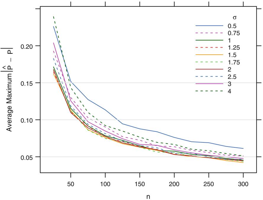
Fig. 10.4 Simulated expected maximum error in estimating probabilities for x ̸ [×1.5, 1.5] with a single normally distributed X with mean zero

For k-sample (ANOVA-type) logistic models, logistic model statistics are equivalent to contingency table β² statistics. As exemplified in the logistic model relating sex to response described previously, the global likelihood ratio statistic for all dummy variables in a k-sample model is identical to the contingency table (k-sample binomial) likelihood ratio β² statistic. The score statistic for this same situation turns out to be identical to the k × 1 degrees of freedom Pearson ^β² for a ^k ^≤ 2 table.

As mentioned in Section 2.6, it can be dangerous to interpret individual parameters, make pairwise treatment comparisons, or test linearity if the overall test of association for a factor represented by multiple parameters is insignificant.

10.4 Residuals

Several types of residuals can be computed for binary logistic model fits. Many of these residuals are used to examine the influence of individual observations on the fit. The partial residual can be used for directly assessing how each ⁸ predictor should be transformed. For the ith observation, the partial residual for the jth element of X is defined by

\[r\_{ij} = \hat{\beta}\_j X\_{ij} + \frac{Y\_i - \hat{P}\_i}{\hat{P}\_i (1 - \hat{P}\_i)},\tag{10.27}\]

where Xij is the value of the jth variable in the ith observation, Yⁱ is the corresponding value of the response, and Pˆⁱ is the predicted probability that Yⁱ = 1. A smooth plot (using, e.g., loess) of Xij against rij will provide an estimate of how X^j should be transformed, adjusting for the other Xs (using their current transformations). Typically one tentatively models X^j linearly and checks the smoothed plot for linearity. A U-shaped relationship in this plot, for example, indicates that a squared term or spline function needs to ⁹ be added for X^j . This approach does assume additivity of predictors.

10.5 Assessment of Model Fit

As the logistic regression model makes no distributional assumptions, only the assumptions of linearity and additivity need to be verified (in addition to the usual assumptions about independence of observations and inclusion of important covariables). In ordinary linear regression there is no global test for lack of model fit unless there are replicate observations at various settings of X. This is because ordinary regression entails estimation of a separate variance parameter τ². In logistic regression there are global tests for goodness of fit. Unfortunately, some of the most frequently used ones are inappropriate. For example, it is common to see a deviance test of goodness of fit based on the “residual”log likelihood, with P-values obtained from a β² distribution with n × p d.f. This P-value is inappropriate since the deviance does not have an asymptotic β² distribution, due to the facts that the number of parameters estimated is increasing at the same rate as n and the expected cell frequencies are far below five (by definition).

Hosmer and Lemeshow304 have developed a commonly used test for goodness of fit for binary logistic models based on grouping into deciles of predicted probability and performing an ordinary β² test for the mean predicted probability against the observed fraction of events (using 8 d.f. to account for evaluating fit on the model development sample). The Hosmer–Lemeshow test is dependent on the choice of how predictions are grouped303 and it is not clear that the choice of the number of groups should be independent of n. Hosmer et al.303 have compared a number of global goodness of fit tests for binary logistic regression. They concluded that the simple unweighted sum of squares test of Copas124 as modified by le Cessie and van Houwelingen387 is as good as any. They used a normal Z-test for the sum of squared errors (n≤B, where B is the Brier index in Equation 10.35). This test takes into account the fact that one cannot obtain a β² distribution for the sum of squares. It also takes into account the estimation of Λ. It is not yet clear for which types of lack of fit this test has reasonable power. Returning to the external validation case where uncertainty of Λ does not need to be accounted for, Stallard584 has further documented the lack of power of the original Hosmer-Lemeshow test and found more power with a logarithmic scoring rule (deviance test) and a β² test that, unlike the simple unweighted sum of squares test, weights each squared error by dividing it by ^Pˆi(1×Pˆi). A scaled ^β² distribution seemed to provide the best approximation to the null distribution of the test statistics.

More power for detecting lack of fit is expected to be obtained from testing specific alternatives to the model. In the model

\[\text{logit}\{Y=1|X\} = \beta\_0 + \beta\_1 X\_1 + \beta\_2 X\_2,\tag{10.28}\]

where X¹ is binary and X² is continuous, one needs to verify that the log odds is related to X¹ and X² according to Figure 10.5.

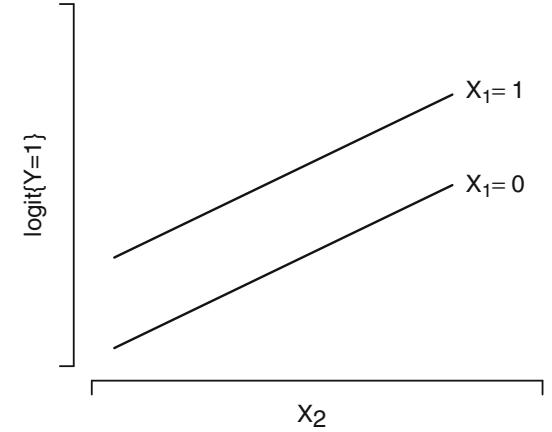
Fig. 10.5 Logistic regression assumptions for one binary and one continuous predictor

The simplest method for validating that the data are consistent with the no-interaction linear model involves stratifying the sample by X¹ and quantile groups (e.g., deciles) of X2. 265 Within each stratum the proportion of responses ^P^ˆ is computed and the log odds calculated from log[P /^ˆ (1 ^× ^Pˆ)]. The number of quantile groups should be such that there are at least 20 (and perhaps many more) subjects in each X1≤X² group. Otherwise, probabilities cannot be estimated precisely enough to allow trends to be seen above “noise” in the data. Since at least 3 X² groups must be formed to allow assessment of linearity, the total sample size must be at least 2 ≤ 3 ≤ 20 = 120 for this method to work at all.

Figure 10.6 demonstrates this method for a large sample size of 3504 subjects stratified by sex and deciles of age. Linearity is apparent for males while there is evidence for slight interaction between age and sex since the age trend for females appears curved.

getHdata( acath )
acath $sex − factor (acath $sex , 0:1, c( ' male ' , ' female ' ))
dd − datadist( acath ); options(datadist= ' dd ' )
f − lrm(sigdz ← rcs(age , 4) * sex , data =acath )

w − function(...)
  with( acath , {
    plsmo (age , sigdz , group =sex , fun=qlogis , lty= ' dotted ' ,
           add=TRUE , grid=TRUE)
    af − cut2 (age , g=10, levels.mean = TRUE)
    prop − qlogis (tapply (sigdz , list (af , sex), mean ,
                             na.rm =TRUE ))
    agem − as.numeric(row.names( prop ))
    lpoints(agem , prop[, ' female ' ], pch=4, col= ' green ' )
    lpoints(agem , prop[, ' male ' ], pch=2, col= ' green ' )
  } ) # Figure 10.6
plot( Predict(f, age , sex), ylim =c(-2 ,4), addpanel=w,
     label.curve = list (offset =unit (0.5 , ' cm ' )))

The subgrouping method requires relatively large sample sizes and does not use continuous factors effectively. The ordering of values is not used at all between intervals, and the estimate of the relationship for a continuous variable has little resolution. Also, the method of grouping chosen (e.g., deciles vs. quintiles vs. rounding) can alter the shape of the plot.

In this dataset with only two variables, it is efficient to use a nonparametric smoother for age, separately for males and females. Nonparametric smoothers, such as loess111 used here, work well for binary response variables (see Section 2.4.7); the logit transformation is made on the smoothed ¹⁰ probability estimates. The smoothed estimates are shown in Figure 10.6.

When there are several predictors, the restricted cubic spline function is better for estimating the true relationship between X² and logit{Y = 1} for continuous variables without assuming linearity. By fitting a model containing X² expanded into k×1 terms, where k is the number of knots, one can obtain an estimate of the transformation of X² as discussed in Section 2.4:

\[\begin{split} \text{logit}\{Y=1|X\} &= \hat{\beta}\_0 + \hat{\beta}\_1 X\_1 + \hat{\beta}\_2 X\_2 + \hat{\beta}\_3 X\_2' + \hat{\beta}\_4 X\_2''\\ &= \hat{\beta}\_0 + \hat{\beta}\_1 X\_1 + f(X\_2), \end{split} \tag{10.29}\]

where X^∗ ² and X∗∗ ² are constructed spline variables (when k = 4). Plotting the estimated spline function f(X2) versus X² will estimate how the effect of X² should be modeled. If the sample is sufficiently large, the spline function can be fitted separately for X¹ = 0 and X¹ = 1, allowing detection of even unusual interaction patterns. A formal test of linearity in X² is obtained by testing H⁰ : Λ³ = Λ⁴ = 0.

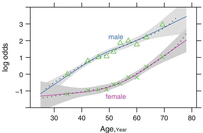
Fig. 10.6 Logit proportions of significant coronary artery disease by sex and deciles of age for n=3504 patients, with spline fits (smooth curves). Spline fits are for k = 4 knots at age= 36, 48, 56, and 68 years, and interaction between age and sex is allowed. Shaded bands are pointwise 0.95 confidence limits for predicted log odds. Smooth nonparametric estimates are shown as dotted curves. Data courtesy of the Duke Cardiovascular Disease Databank.

For testing interaction between X¹ and X2, a product term (e.g., X1X2) can be added to the model and its coefficient tested. A more general simultaneous test of linearity and lack of interaction for a two-variable model in which one variable is binary (or is assumed linear) is obtained by fitting the model

\[\begin{aligned} \text{logit}\{Y=1|X\} &= \beta\_0 + \beta\_1 X\_1 + \beta\_2 X\_2 + \beta\_3 X\_2' + \beta\_4 X\_2''\\ &+ \beta\_5 X\_1 X\_2 + \beta\_6 X\_1 X\_2' + \beta\_7 X\_1 X\_2'' \end{aligned} \tag{10.30}\]

and testing H⁰ : Λ³ = … = Λ⁷ = 0. This formulation allows the shape of the X² effect to be completely different for each level of X1. There is virtually no departure from linearity and additivity that cannot be detected from this expanded model formulation. The most computationally efficient test for lack of fit is the score test (e.g., X¹ and X² are forced into a tentative model and the remaining variables are candidates). Figure 10.6 also depicts a fitted spline logistic model with k = 4, allowing for general interaction between age and sex as parameterized above. The fitted function, after expanding the restricted cubic spline function for simplicity (see Equation 2.27), is given above. Note the good agreement between the empirical estimates of log odds and the spline fits and nonparametric estimates in this large dataset.

An analysis of log likelihood for this model and various sub-models is found in Table 10.3. The β² for global tests is corrected for the intercept and the degrees of freedom does not include the intercept.

Model / Hypothesis	Likelihood d.f.		P	Formula
	Ratio σ2
a: sex, age (linear, no interaction)	766.0	2
b: sex, age, age ∼ sex	768.2	3
c: sex, spline in age	769.4	4
d: sex, spline in age, interaction	782.5	7
H0 : no age ∼ sex interaction	2.2	1	.14	(b × a)
given linearity
H0 : age linear no interaction	3.4	2	.18	(c × a)
H0 : age linear, no interaction	16.6	5	.005	(d × a)
H0 : age linear, product form	14.4	4	.006	(d × b)
interaction
H0 : no interaction, allowing for	13.1	3	.004	(d × c)
nonlinearity in age

Table 10.3 LR σ² tests for coronary artery disease risk

Table 10.4 AIC on σ² scale by number of knots

k	β2 Model	AIC
0	99.23	97.23
3	112.69	108.69
4	121.30	115.30
5	123.51	115.51
6	124.41	114.51

This analysis confirms the first impression from the graph, namely, that age ≤ sex interaction is present but it is not of the form of a simple product between age and sex (change in slope). In the context of a linear age effect, there is no significant product interaction effect (P = .14). Without allowing for interaction, there is no significant nonlinear effect of age (P = .18). However, the general test of lack of fit with 5 d.f. indicates a significant departure from the linear additive model (P = .005).

In Figure 10.7, data from 2332 patients who underwent cardiac catheterization at Duke University Medical Center and were found to have significant (← 75%) diameter narrowing of at least one major coronary artery were analyzed (the dataset is available from the Web site). The relationship between the time from the onset of symptoms of coronary artery disease (e.g., angina, myocardial infarction) to the probability that the patient has severe (threevessel disease or left main disease—tvdlm) coronary disease was of interest. There were 1129 patients with tvdlm. A logistic model was used with the duration of symptoms appearing as a restricted cubic spline function with k = 3, 4, 5, and 6 equally spaced knots in terms of quantiles between .05 and .95. The best fit for the number of parameters was chosen using Akaike’s information criterion (AIC), computed in Table 10.4 as the model likelihood ratio β² minus twice the number of parameters in the model aside from the intercept. The linear model is denoted k = 0.

dz − subset (acath , sigdz ==1)
dd − datadist(dz)

f − lrm(tvdlm ← rcs(cad.dur , 5), data =dz)
w − function(...)
  with (dz , {
    plsmo(cad.dur , tvdlm , fun= qlogis , add=TRUE ,
           grid=TRUE , lty= ' dotted ' )
    x − cut2(cad.dur , g=15, levels.mean = TRUE)
    prop − qlogis (tapply (tvdlm , x, mean , na.rm =TRUE ))
    xm − as.numeric( names (prop))
    lpoints(xm , prop , pch=2, col= ' green ' )
  } ) # Figure 10.7
plot( Predict(f, cad.dur), addpanel=w)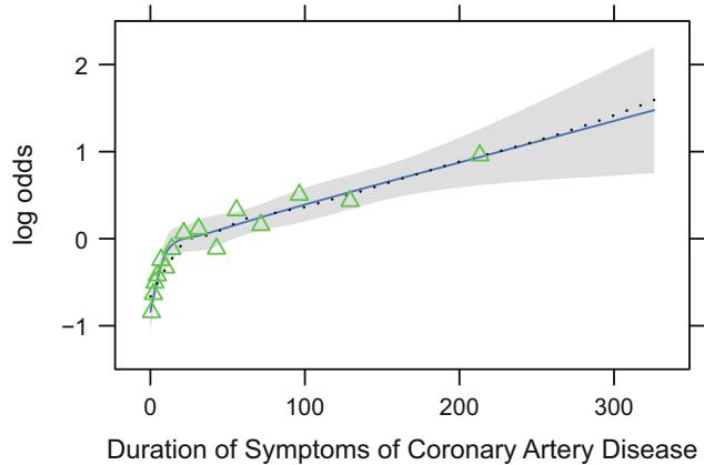

Fig. 10.7 Estimated relationship between duration of symptoms and the log odds of severe coronary artery disease for k = 5. Knots are marked with arrows. Solid line is spline fit; dotted line is a nonparametric loess estimate.

Figure 10.7 displays the spline fit for k = 5. The triangles represent subgroup estimates obtained by dividing the sample into groups of 150 patients. For example, the leftmost triangle represents the logit of the proportion of tvdlm in the 150 patients with the shortest duration of symptoms, versus the mean duration in that group. A Wald test of linearity, with 3 d.f., showed highly significant nonlinearity (β²= 23.92 with 3 d.f.). The plot of the spline transformation suggests a log transformation, and when log (duration of symptoms in months + 1) was fitted in a logistic model, the log likelihood of the model (119.33 with 1 d.f.) was virtually as good as the spline model (123.51 with 4 d.f.); the corresponding Akaike information criteria (on the β² scale) are 117.33 and 115.51. To check for adequacy in the log transformation, a five-knot restricted cubic spline function was fitted to log10(months + 1), as displayed in Figure 10.8. There is some evidence for lack of fit on the right, but the Wald β² for testing linearity yields P = .27.

f − lrm(tvdlm ← log10 ( cad.dur + 1), data=dz)
w − function(...)
  with (dz , {
    x − cut2(cad.dur , m =150, levels.mean = TRUE)
    prop − tapply (tvdlm , x, mean , na.rm =TRUE)
    xm − as.numeric( names (prop))
    lpoints(xm , prop , pch=2, col= ' green ' )
  } )
# Figure 10.8
plot( Predict(f, cad.dur , fun=plogis ), ylab= ' P ' ,
     ylim =c(.2 , .8), addpanel=w)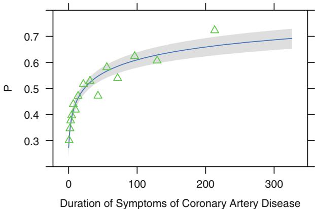

Fig. 10.8 Fitted linear logistic model in log10(duration + 1), with subgroup estimates using groups of 150 patients. Fitted equation is logit(tvdlm) = ×.9809 + .7122 log10(months + 1).

If the model contains two continuous predictors, they may both be expanded with spline functions in order to test linearity or to describe nonlinear relationships. Testing interaction is more difficult here. If X¹ is continuous, one might temporarily group X¹ into quantile groups. Consider the subset of 2258 (1490 with disease) of the 3504 patients used in Figure 10.6 who have serum cholesterol measured. A logistic model for predicting significant coronary disease was fitted with age in tertiles (modeled with two dummy variables), sex, age ≤ sex interaction, four-knot restricted cubic spline in cholesterol, and age tertile ≤ cholesterol interaction. Except for the sex adjustment this model is equivalent to fitting three separate spline functions in cholesterol, one for each age tertile. The fitted model is shown in Figure 10.9 for cholesterol and age tertile against logit of significant disease. Significant age ≤ cholesterol interaction is apparent from the figure and is suggested by the Wald β² statistic (10.03) that follows. Note that the test for linearity of the interaction with respect to cholesterol is very insignificant (β² = 2.40 on 4 d.f.), but we retain it for now. The fitted function is

acath − transform(acath ,
                    cholesterol = choleste ,
                    age.tertile = cut2 (age ,g=3),
                    sx = as.integer ( acath $sex) - 1)
# sx for loess , need to code as numeric
dd − datadist( acath ); options(datadist= ' dd ' )
# First model stratifies age into tertiles to get more
# empirical estimates of age x cholesterol interaction
f − lrm(sigdz ← age.tertile *(sex + rcs( cholesterol ,4)),
         data=acath )
print (f, latex =TRUE)

Logistic Regression Model

lrm(formula = sigdz ~ age.tertile * (sex + rcs(cholesterol, 4)), data = acath)

Frequencies of Missing Values Due to Each Variable

	sigdz age.tertile	sex	cholesterol
0	0	0	1246

		Model Likelihood			Discrimination		Rank Discrim.
		Ratio Test			Indexes		Indexes
Obs	2258	β2 LR	533.52	R2	0.291	C	0.780
0	768	d.f.	14	g	1.316	Dxy	0.560
1	1490	β2) Pr(>	< 0.0001	gr	3.729	α	0.562
α log L max αρ	2≤10−8			gp	0.252	Γa	0.251
				Brier	0.173

	Coef	S.E.	Wald Z	Pr(> Z )
Intercept	-0.4155	1.0987	-0.38	0.7053
age.tertile=[49,58)	0.8781	1.7337	0.51	0.6125
age.tertile=[58,82]	4.7861	1.8143	2.64	0.0083
sex=female	-1.6123	0.1751	-9.21	< 0.0001
cholesterol	0.0029	0.0060	0.48	0.6347
cholesterol’	0.0384	0.0242	1.59	0.1126
cholesterol”	-0.1148	0.0768	-1.49	0.1350
age.tertile=[49,58) * sex=female	-0.7900	0.2537	-3.11	0.0018
age.tertile=[58,82] * sex=female	-0.4530	0.2978	-1.52	0.1283
age.tertile=[49,58) * cholesterol	0.0011	0.0095	0.11	0.9093

	Coef	S.E.	Wald Z	Pr(> Z )
age.tertile=[58,82] * cholesterol	-0.0158	0.0099	-1.59	0.1111
age.tertile=[49,58) * cholesterol’	-0.0183	0.0365	-0.50	0.6162
age.tertile=[58,82] * cholesterol’	0.0127	0.0406	0.31	0.7550
age.tertile=[49,58) * cholesterol”	0.0582	0.1140	0.51	0.6095
age.tertile=[58,82] * cholesterol”	-0.0092	0.1301	-0.07	0.9436

ltx(f)

^XΛ^ˆ ⁼ ^×0.415 + 0.878[age.tertile ^≥ [49, 58)] + 4.79[age.tertile ^≥ [58, 82]] ^× ¹.61[female] + 0.00287cholesterol + 1.52≤10−6(cholesterol ^× 160)³ ⁺ × 4.53≤ ¹⁰−6(cholesterol ^× 208)³ ⁺ + 3.⁴⁴ ^≤ ¹⁰−6(cholesterol ^× 243)³ ⁺ ^× ⁴.²⁸ ^≤ ¹⁰−⁷ (cholesterol×319)³ ⁺+[female][×0.79[age.tertile ≥ [49, 58)]×0.453[age.tertile ≥ [58, 82]]]+[age.tertile ^≥ [49, 58)][0.00108cholesterol×7.23≤10−⁷(cholesterol^× 160)³ ⁺ + 2.3≤10−⁶(cholesterol ^× 208)³ ⁺ ^× ¹.84≤10−⁶(cholesterol ^× 243)³ ⁺ + ².69≤10−⁷(cholesterol ^× 319)³ ⁺] + [age.tertile ≥ [58, 82]][×0.0158cholesterol+ ⁵≤10−⁷(cholesterol ^× 160)³ ⁺ ^× ³.64≤10−⁷(cholesterol ^× 208)³ ⁺ ^× ⁵.15≤10−⁷ (cholesterol ^× 243)³ ⁺ + 3.78≤10−⁷(cholesterol ^× 319)³ ⁺].

# Table 10.5:
latex (anova (f), file= ' ' , size= ' smaller ' ,
       caption= ' Crudely categorizing age into tertiles ' ,
       label = ' tab:anova-tertiles ' )

yl − c(-1 ,5)
plot( Predict(f, cholesterol , age.tertile ),
     adj.subtitle =FALSE , ylim=yl) # Figure 10.9

Table 10.5		Crudely categorizing age into tertiles
————	–	—————————————-	–	–	–

	σ2	d.f.	P
age.tertile (Factor+Higher Order Factors)	120.74		10 < 0.0001
All Interactions	21.87	8	0.0052
sex (Factor+Higher Order Factors)	329.54		3 < 0.0001
All Interactions	9.78	2	0.0075
cholesterol (Factor+Higher Order Factors)	93.75		9 < 0.0001
All Interactions	10.03	6	0.1235
Nonlinear (Factor+Higher Order Factors)	9.96	6	0.1263
age.tertile ∼ sex (Factor+Higher Order Factors)	9.78	2	0.0075
age.tertile ∼ cholesterol (Factor+Higher Order Factors)	10.03	6	0.1235
Nonlinear	2.62	4	0.6237
Nonlinear Interaction : f(A,B) vs. AB	2.62	4	0.6237
TOTAL NONLINEAR	9.96	6	0.1263
TOTAL INTERACTION	21.87	8	0.0052
TOTAL NONLINEAR + INTERACTION	29.67	10	0.0010
TOTAL	410.75		14 < 0.0001

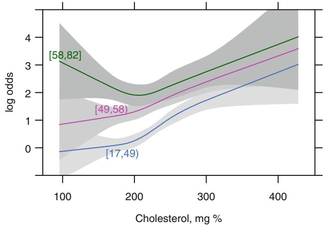
Fig. 10.9 Log odds of significant coronary artery disease modeling age with two dummy variables

Before fitting a parametric model that allows interaction between age and cholesterol, let us use the local regression model of Cleveland et al.96 discussed in Section 2.4.7. This nonparametric smoothing method is not meant to handle binary Y , but it can still provide useful graphical displays in the binary case. Figure 10.10 depicts the fit from a local regression model predicting Y = 1 = significant coronary artery disease. Predictors are sex (modeled parametrically with a dummy variable), age, and cholesterol, the last two fitted nonparametrically. The effect of not explicitly modeling a probability is seen in the figure, as the predicted probabilities exceeded 1. Because of this we do not take the logit transformation but leave the predicted values in raw form. However, the overall shape is in agreement with Figure 10.10.

# Re-do model with continuous age
f − loess (sigdz ← age * (sx + cholesterol ), data=acath ,
           parametric ="sx", drop.square ="sx")
ages − seq(25, 75, length =40)
chols − seq(100, 400, length =40)
g − expand.grid (cholesterol= chols , age=ages , sx=0)
# drop sex dimension of grid since held to 1 value
p − drop( predict(f, g))
p[p < 0.001] − 0.001
p[p > 0.999] − 0.999
zl − c(-3 , 6) # Figure 10.10
wireframe( qlogis (p) ← cholesterol *age ,
          xlab=list(rot =30), ylab=list(rot=-40),
          zlab=list(label= ' log odds ' , rot=90), zlim=zl ,
          scales = list(arrows = FALSE), data=g)

Chapter 2 discussed linear splines, which can be used to construct linear spline surfaces by adding all cross-products of the linear variables and spline terms in the model. With a sufficient number of knots for each predictor, the linear spline surface can fit a wide variety of patterns. However, it requires a large number of parameters to be estimated. For the age–sex–cholesterol example, a linear spline surface is fitted for age and cholesterol, and a sex ≤ age spline interaction is also allowed. Figure 10.11 shows a fit that placed knots at quartiles of the two continuous variablesc. The algebraic form of the fitted model is shown below.

f − lrm(sigdz ← lsp(age ,c(46 ,52 ,59)) *
          (sex + lsp(cholesterol ,c(196 ,224 ,259))) ,
          data=acath )
ltx(f)

XΛˆ = ×1.83 + 0.0232 age + 0.0759(age × 46)+ × 0.0025(age × 52)+ +
2.27(age×59)++3.02[female]×0.0177cholesterol+0.114(cholesterol×196)+×
0.131(cholesterol×224)+ + 0.0651(cholesterol×259)+ +[female][×0.112 age+
0.0852 (age × 46)+ × 0.0302 (age × 52)+ + 0.176 (age × 59)+] + age
[0.000577 cholesterol × 0.00286 (cholesterol × 196)+ + 0.00382 (cholesterol ×
224)+ × 0.00205 (cholesterol × 259)+] + (age × 46)+[×0.000936 cholesterol +
0.00643(cholesterol×196)+×0.0115(cholesterol×224)++0.00756(cholesterol×
259)+] + (age × 52)+[0.000433 cholesterol × 0.0037 (cholesterol × 196)+ +
0.00815 (cholesterol × 224)+ × 0.00715 (cholesterol × 259)+] + (age × 59)+
[×0.0124cholesterol+0.015(cholesterol×196)+×0.0067(cholesterol×224)+ +
0.00752 (cholesterol × 259)+].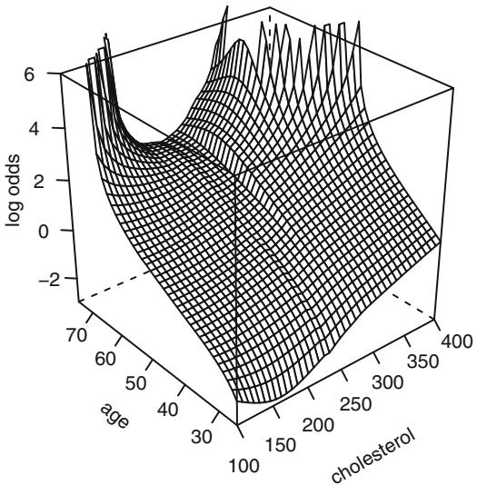

Fig. 10.10 Local regression fit for the logit of the probability of significant coronary disease vs. age and cholesterol for males, based on the loess function.

^c In the wireframe plots that follow, predictions for cholesterol–age combinations for which fewer than 5 exterior points exist are not shown, so as to not extrapolate to regions not supported by at least five points beyond the data perimeter.

latex (anova (f), caption= ’ Linear spline surface ’ , file= ’ ’ , size= ’ smaller ’ , label= ’ tab:anova-lsp ’ ) # Table 10.6

perim − with(acath ,
               perimeter( cholesterol , age , xinc =20, n=5))
zl − c(-2 , 4) # Figure 10.11
bplot ( Predict(f, cholesterol , age , np =40), perim =perim ,
      lfun =wireframe , zlim=zl , adj.subtitle = FALSE )

Table 10.6				Linear spline surface
————	–	–	–	———————–

	σ2	d.f.	P
age (Factor+Higher Order Factors)	164.17		24 < 0.0001
All Interactions	42.28	20	0.0025
Nonlinear (Factor+Higher Order Factors)	25.21	18	0.1192
sex (Factor+Higher Order Factors)	343.80		5 < 0.0001
All Interactions	23.90	4	0.0001
cholesterol (Factor+Higher Order Factors)	100.13		20 < 0.0001
All Interactions	16.27	16	0.4341
Nonlinear (Factor+Higher Order Factors)	16.35	15	0.3595
age ∼ sex (Factor+Higher Order Factors)	23.90	4	0.0001
Nonlinear	12.97	3	0.0047
Nonlinear Interaction : f(A,B) vs. AB	12.97	3	0.0047
age ∼ cholesterol (Factor+Higher Order Factors)	16.27	16	0.4341
Nonlinear	11.45	15	0.7204
Nonlinear Interaction : f(A,B) vs. AB	11.45	15	0.7204
f(A,B) vs. Af(B) + Bg(A)	9.38	9	0.4033
Nonlinear Interaction in age vs. Af(B)	9.99	12	0.6167
Nonlinear Interaction in cholesterol vs. Bg(A)	10.75	12	0.5503
TOTAL NONLINEAR	33.22	24	0.0995
TOTAL INTERACTION	42.28	20	0.0025
TOTAL NONLINEAR + INTERACTION	49.03	26	0.0041
TOTAL	449.26		29 < 0.0001

Chapter 2 also discussed a tensor spline extension of the restricted cubic spline model to fit a smooth function of two predictors, f(X1, X2). Since this function allows for general interaction between X¹ and X2, the twovariable cubic spline is a powerful tool for displaying and testing interaction, assuming the sample size warrants estimating 2(^k ^× 1) + (^k ^× 1)² parameters for a rectangular grid of k ≤ k knots. Unlike the linear spline surface, the cubic surface is smooth. It also requires fewer parameters in most situations. The general cubic model with k = 4 (ignoring the sex effect here) is

\[\begin{aligned} \beta\_0 &+ \beta\_1 X\_1 + \beta\_2 X\_1' + \beta\_3 X\_1'' + \beta\_4 X\_2 + \beta\_5 X\_2' + \beta\_6 X\_2'' + \beta\_7 X\_1 X\_2 \\ &+ \quad \beta\_8 X\_1 X\_2' + \beta\_9 X\_1 X\_2'' + \beta\_{10} X\_1' X\_2 + \beta\_{11} X\_1' X\_2' \\ &+ \quad \quad + \beta\_{12} X\_1' X\_2'' + \beta\_{13} X\_1'' X\_2 + \beta\_{14} X\_1'' X\_2' + \beta\_{15} X\_1'' X\_2'', \end{aligned} \tag{10.31}\]

where X∗ 1, X∗∗ ¹ , X^∗ ², and X∗∗ ² are restricted cubic spline component variables for X¹ and X² for k = 4. A general test of interaction with 9 d.f. is H⁰ : Λ⁷ = … = Λ¹⁵ = 0. A test of adequacy of a simple product form interaction is H⁰ : Λ⁸ = … = Λ¹⁵ = 0 with 8 d.f. A 13 d.f. test of linearity and additivity is H⁰ : Λ² = Λ³ = Λ⁵ = Λ⁶ = Λ⁷ = Λ⁸ = Λ⁹ = Λ¹⁰ = Λ¹¹ = Λ¹² = Λ¹³ = Λ¹⁴ = Λ¹⁵ =0.

Figure 10.12 depicts the fit of this model. There is excellent agreement with Figures 10.9 and 10.11, including an increased (but probably insignificant) risk with low cholesterol for age ← 57.

f − lrm(sigdz ← rcs(age ,4)*(sex + rcs(cholesterol ,4)),
         data=acath , tol=1 e-11)
ltx(f)

^XΛ^ˆ ⁼ ^×6.41 + 0.166age ^× ⁰.00067(age ^× 36)³ ⁺ + 0.00543(age ^× 48)³ ⁺ × ⁰.00727(age×56)³ ⁺ + 0.00251(age×68)³ ⁺ + 2.87[female]+ 0.00979cholesterol+ ¹.⁹⁶ ^≤ ¹⁰−⁶(cholesterol ^× 160)³ ⁺ ^× ⁷.¹⁶ ^≤ ¹⁰−⁶(cholesterol ^× 208)³ ⁺ + 6.35 ≤ ¹⁰−⁶(cholesterol×243)³ +×1.16≤10−⁶(cholesterol×319)³ ⁺+[female][×0.109age+ ⁷.52≤10−⁵(age×36)³ ++0.00015(age×48)³ +×0.00045(age×56)³ ⁺+0.000225(age× 68)³ ⁺] + age[×0.00028cholesterol + 2.68≤10−⁹(cholesterol ^× 160)³ ⁺ + 3.03≤ ¹⁰−⁸(cholesterol ^× 208)³ ⁺ ^× ⁴.⁹⁹ ^≤ ¹⁰−⁸(cholesterol ^× 243)³ ⁺ + 1.⁶⁹ ^≤ ¹⁰−⁸ (cholesterol ^× 319)³ +] + age^∗ [0.00341cholesterol ^× ⁴.⁰² ^≤ ¹⁰−⁷(cholesterol ^× 160)³ ++9.71≤10−⁷(cholesterol×208)³ +×5.79≤10−⁷(cholesterol×243)³ ⁺+8.79≤ ¹⁰−⁹(cholesterol×319)³ ⁺]+ age∗∗[×0.029cholesterol+ 3.04≤10−⁶(cholesterol^×

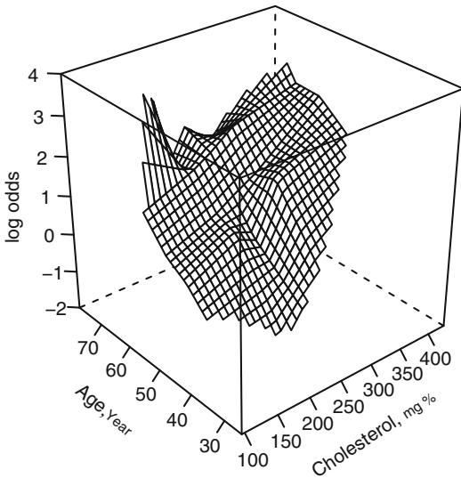
Fig. 10.11 Linear spline surface for males, with knots for age at 46, 52, 59 and knots for cholesterol at 196, 224, and 259 (quartiles).

160)³ ⁺ ^× ⁷.34≤10−6(cholesterol ^× 208)³ ⁺ + 4.36≤10−6(cholesterol ^× 243)³ + × ⁵.82≤10−8(cholesterol ^× 319)³ ⁺].

latex (anova (f), caption= ' Cubic spline surface ' , file= ' ' ,
       size= ' smaller ' , label= ' tab:anova-rcs ' ) #Table 10.7

# Figure 10.12:
bplot ( Predict(f, cholesterol , age , np =40), perim =perim ,
      lfun =wireframe , zlim=zl , adj.subtitle = FALSE )

Table 10.7				Cubic spline surface
————	–	–	–	———————-

	σ2	d.f.	P
age (Factor+Higher Order Factors)	165.23		15 < 0.0001
All Interactions	37.32	12	0.0002
Nonlinear (Factor+Higher Order Factors)	21.01	10	0.0210
sex (Factor+Higher Order Factors)	343.67		4 < 0.0001
All Interactions	23.31		3 < 0.0001
cholesterol (Factor+Higher Order Factors)	97.50		12 < 0.0001
All Interactions	12.95	9	0.1649
Nonlinear (Factor+Higher Order Factors)	13.62	8	0.0923
age ∼ sex (Factor+Higher Order Factors)	23.31		3 < 0.0001
Nonlinear	13.37	2	0.0013
Nonlinear Interaction : f(A,B) vs. AB	13.37	2	0.0013
age ∼ cholesterol (Factor+Higher Order Factors)	12.95	9	0.1649
Nonlinear	7.27	8	0.5078
Nonlinear Interaction : f(A,B) vs. AB	7.27	8	0.5078
f(A,B) vs. Af(B) + Bg(A)	5.41	4	0.2480
Nonlinear Interaction in age vs. Af(B)	6.44	6	0.3753
Nonlinear Interaction in cholesterol vs. Bg(A)	6.27	6	0.3931
TOTAL NONLINEAR	29.22	14	0.0097
TOTAL INTERACTION	37.32	12	0.0002
TOTAL NONLINEAR + INTERACTION	45.41	16	0.0001
TOTAL	450.88		19 < 0.0001

Statistics for testing age ≤ cholesterol components of this fit are above. None of the nonlinear interaction components is significant, but we again retain them.

The general interaction model can be restricted to be of the form

\[f(X\_1, X\_2) = f\_1(X\_1) + f\_2(X\_2) + X\_1 g\_2(X\_2) + X\_2 g\_1(X\_1) \tag{10.32}\]

by removing the parameters Λ11, Λ12, Λ14, and Λ¹⁵ from the model. The previous table of Wald statistics included a test of adequacy of this reduced form (β² = 5.41 on 4 d.f., P = .248). The resulting fit is in Figure 10.13.

f − lrm(sigdz ← sex*rcs(age ,4) + rcs(cholesterol ,4) +
          rcs(age ,4) %ia% rcs(cholesterol ,4), data =acath )
latex (anova (f), file= ' ' , size= ' smaller ' ,
      caption= ' Singly nonlinear cubic spline surface ' ,
      label = ' tab:anova-ria ' ) #Table 10.8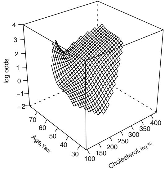

Fig. 10.12 Restricted cubic spline surface in two variables, each with k = 4 knots

		Table 10.8		Singly nonlinear cubic spline surface
–	–	————	–	—————————————	–	–	–

	σ2	d.f.	P
sex (Factor+Higher Order Factors)	343.42		4 < 0.0001
All Interactions	24.05		3 < 0.0001
age (Factor+Higher Order Factors)	169.35		11 < 0.0001
All Interactions	34.80		8 < 0.0001
Nonlinear (Factor+Higher Order Factors)	16.55	6	0.0111
cholesterol (Factor+Higher Order Factors)	93.62		8 < 0.0001
All Interactions	10.83	5	0.0548
Nonlinear (Factor+Higher Order Factors)	10.87	4	0.0281
age ∼ cholesterol (Factor+Higher Order Factors)	10.83	5	0.0548
Nonlinear	3.12	4	0.5372
Nonlinear Interaction : f(A,B) vs. AB	3.12	4	0.5372
Nonlinear Interaction in age vs. Af(B)	1.60	2	0.4496
Nonlinear Interaction in cholesterol vs. Bg(A)	1.64	2	0.4400
sex ∼ age (Factor+Higher Order Factors)	24.05		3 < 0.0001
Nonlinear	13.58	2	0.0011
Nonlinear Interaction : f(A,B) vs. AB	13.58	2	0.0011
TOTAL NONLINEAR	27.89	10	0.0019
TOTAL INTERACTION	34.80		8 < 0.0001
TOTAL NONLINEAR + INTERACTION	45.45		12 < 0.0001
TOTAL	453.10		15 < 0.0001

# Figure 10.13:
bplot ( Predict(f, cholesterol , age , np =40), perim =perim ,
      lfun =wireframe , zlim=zl , adj.subtitle = FALSE )
ltx(f)

Table 10.9 Linear interaction surface

	σ2	d.f. P
age (Factor+Higher Order Factors)	167.83	7 < 0.0001
All Interactions	31.03	4 < 0.0001
Nonlinear (Factor+Higher Order Factors)	14.58	4 0.0057
sex (Factor+Higher Order Factors)	345.88	4 < 0.0001
All Interactions	22.30	3 0.0001
cholesterol (Factor+Higher Order Factors)	89.37	4 < 0.0001
All Interactions	7.99	1 0.0047
Nonlinear	10.65	2 0.0049
age ∼ cholesterol (Factor+Higher Order Factors)	7.99	1 0.0047
age ∼ sex (Factor+Higher Order Factors)	22.30	3 0.0001
Nonlinear	12.06	2 0.0024
Nonlinear Interaction : f(A,B) vs. AB	12.06	2 0.0024
TOTAL NONLINEAR	25.72	6 0.0003
TOTAL INTERACTION	31.03	4 < 0.0001
TOTAL NONLINEAR + INTERACTION	43.59	8 < 0.0001
TOTAL	452.75	11 < 0.0001

^XΛ^ˆ ⁼ ^×7.2+2.96[female]+0.164age+7.23≤10−⁵(age×36)³ ⁺ ×0.000106(age× 48)³ ⁺ ^× ¹.63≤10−⁵(age ^× 56)³ ⁺ + 4.99≤10−⁵(age ^× 68)³ ⁺ + 0.0148cholesterol + ¹.²¹ ^≤ ¹⁰−⁶(cholesterol ^× 160)³ ⁺ ^× ⁵.⁵ ^≤ ¹⁰−⁶(cholesterol ^× 208)³ ⁺ + 5.5 ≤ ¹⁰−⁶(cholesterol ^× 243)³ ⁺ ^× ¹.21≤10−⁶(cholesterol ^× 319)³ ⁺ + age[×0.00029 cholesterol+ 9.28≤10−⁹(cholesterol×160)³ ⁺ + 1.7≤10−⁸(cholesterol×208)³ ⁺ × ⁴.43≤10−⁸(cholesterol×243)³ ++1.79≤10−⁸(cholesterol×319)³ ⁺]+cholesterol[2.3≤ ¹⁰−⁷(age ^× 36)³ ⁺ + 4.21≤10−⁷(age ^× 48)³ ⁺ ^× ¹.31≤10−⁶(age ^× 56)³ ⁺ + 6.64≤ ¹⁰−⁷(age×68)³ +]+[female][×0.111age+8.03≤10−⁵(age×36)³ ⁺+0.000135(age× 48)³ ⁺ ^× ⁰.00044(age ^× 56)³ ⁺ + 0.000224(age ^× 68)³ ⁺].

The fit is similar to the former one except that the climb in risk for lowcholesterol older subjects is less pronounced. The test for nonlinear interaction is now more concentrated (P = .54 with 4 d.f.). Figure 10.14 accordingly depicts a fit that allows age and cholesterol to have nonlinear main effects, but restricts the interaction to be a product between (untransformed) age and cholesterol. The function agrees substantially with the previous fit.

f − lrm(sigdz ← rcs(age ,4)*sex + rcs(cholesterol ,4) +
          age %ia% cholesterol , data=acath)
latex(anova (f), caption= ' Linear interaction surface ' , file= ' ' ,
      size= ' smaller ' , label= ' tab:anova-lia ' ) #Table 10.9

# Figure 10.14:
bplot ( Predict(f, cholesterol , age , np =40), perim =perim ,
      lfun =wireframe , zlim=zl , adj.subtitle = FALSE )
f.linia − f # save linear interaction fit for later
ltx(f)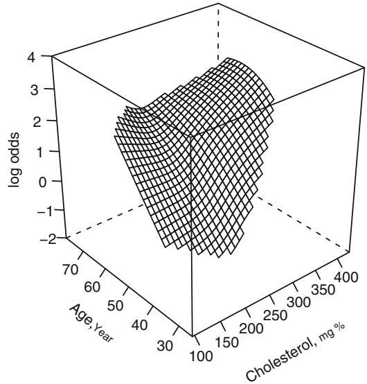

Fig. 10.13 Restricted cubic spline fit with age ∼ spline(cholesterol) and cholesterol ∼ spline(age)

^XΛ^ˆ ⁼ ^×7.36+0.182age×5.18≤10−⁵(age×36)³ ++8.45≤10−⁵(age×48)³ ⁺×2.91≤ ¹⁰−⁶(age ^× 56)³ ⁺ ^× ².99≤10−⁵(age ^× 68)³ ⁺ + 2.8[female] + 0.0139cholesterol + ¹.⁷⁶ ^≤ ¹⁰−⁶(cholesterol ^× 160)³ ⁺ ^× ⁴.⁸⁸ ^≤ ¹⁰−⁶(cholesterol ^× 208)³ ⁺ + 3.45 ≤ ¹⁰−⁶(cholesterol ^× 243)³ ⁺ ^× ³.26≤10−⁷(cholesterol ^× 319)³ ⁺ × 0.00034 age ≤ cholesterol + [female][×0.107age + 7.71≤10−⁵(age ^× 36)³ ⁺ + 0.000115(age × 48)³ ⁺ ^× ⁰.000398(age ^× 56)³ ⁺ + 0.000205(age ^× 68)³ ⁺].

The Wald test for age ^≤ cholesterol interaction yields ^β² = 7.99 with 1 d.f., P = .005. These analyses favor the nonlinear model with simple product interaction in Figure 10.14 as best representing the relationships among cholesterol, age, and probability of prognostically severe coronary artery disease. A nomogram depicting this model is shown in Figure 10.21.

Using this simple product interaction model, Figure 10.15 displays predicted cholesterol effects at the mean age within each age tertile. Substantial agreement with Figure 10.9 is apparent.

# Make estimates of cholesterol effects for mean age in
# tertiles corresponding to initial analysis
mean.age −
  with( acath ,
       as.vector( tapply (age , age.tertile , mean , na.rm=TRUE)))
plot( Predict(f, cholesterol , age=round (mean.age ,2),
              sex="male"),
     adj.subtitle =FALSE , ylim=yl) #3 curves , Figure 10.15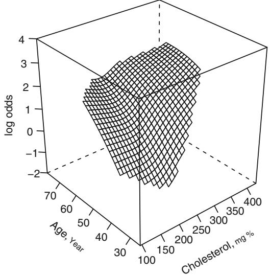

Fig. 10.14 Spline fit with nonlinear effects of cholesterol and age and a simple product interaction

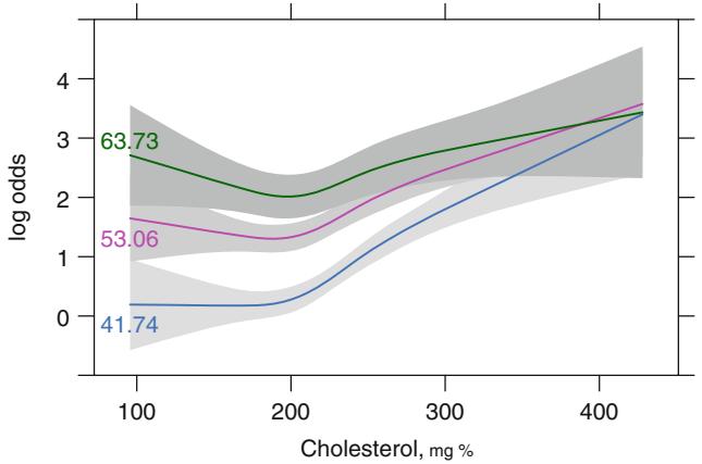
Fig. 10.15 Predictions from linear interaction model with mean age in tertiles indicated.

The partial residuals discussed in Section 10.4 can be used to check logistic model fit (although it may be difficult to deal with interactions). As an example, reconsider the “duration of symptoms” fit in Figure 10.7. Figure 10.16 displays “loess smoothed” and raw partial residuals for the original and log-transformed variable. The latter provides a more linear relationship, especially where the data are most dense.

Method	Choice	Assumes	Uses Ordering	Low	Good
	Required	Additivity	of X	Variance	Resolution
					on X
Stratification	Intervals
Smoother on X1	Bandwidth		x	x	x
stratifying on X2			(not on X2)	(if min. strat.)	(X1)
Smooth partial	Bandwidth	x	x	x	x
residual plot
Spline model	Knots	x	x	x	x
for all Xs

Table 10.10 Merits of Methods for Checking Logistic Model Assumptions

f − lrm(tvdlm ← cad.dur , data=dz , x=TRUE , y= TRUE)
resid (f, " partial", pl=" loess ", xlim=c(0 ,250), ylim=c(-3 ,3))
scat1d (dz$ cad.dur)
log.cad.dur − log10 (dz$ cad.dur + 1)
f − lrm(tvdlm ← log.cad.dur , data =dz , x=TRUE , y= TRUE)
resid (f, " partial", pl=" loess", ylim =c(-3 ,3))
scat1d ( log.cad.dur ) # Figure 10.16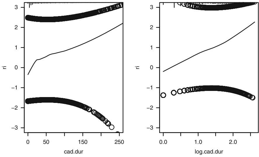

Fig. 10.16 Partial residuals for duration and log10(duration+1). Data density shown at top of each plot.

Table 10.10 summarizes the relative merits of stratification, nonparametric smoothers, and regression splines for determining or checking binary logistic model fits.

10.6 Collinearity

The variance inflation factors (VIFs) discussed in Section 4.6 can apply to any regression fit.147, 654 These VIFs allow the analyst to isolate which variable(s) are responsible for highly correlated parameter estimates. Recall that, in general, collinearity is not a large problem compared with nonlinearity and overfitting.

10.7 Overly Influential Observations

Pregibon511 developed a number of regression diagnostics that apply to the family of regression models of which logistic regression is a member. Influence statistics based on the “leave-out-one”method use an approximation to avoid having to refit the model n times for n observations. This approximation uses the fit and covariance matrix at the last iteration and assumes that the “weights” in the weighted least squares fit can be kept constant, yielding a computationally feasible one-step estimate of the leave-out-one regression coefficients.

Hosmer and Lemeshow [305, pp. 149–170] discuss many diagnostics for logistic regression and show how the final fit can be used in any least squares program that provides diagnostics. A new dependent variable to be used in that way is

\[Z\_i = X\hat{\beta} + \frac{Y\_i - \hat{P}\_i}{V\_i},\tag{10.33}\]

where ^Vⁱ ⁼ ^Pˆi(1×Pˆi), and ^Pˆⁱ = [1+ exp ^×XΛˆ] ⁻¹ is the predicted probability that Yⁱ = 1. The Vi, i = 1, 2,…,n are used as weights in an ordinary weighted least squares fit of X against Z. This least squares fit will provide regression coefficients identical to b. The new standard errors will be off from the actual logistic model ones by a constant.

As discussed in Section 4.9, the standardized change in the regression coefficients upon leaving out each observation in turn (DFBETAS) is one of the most useful diagnostics, as these can pinpoint which observations are influential on each part of the model. After carefully modeling predictor transformations, there should be no lack of fit due to improper transformations. However, as the white blood count example in Section 4.9 indicates, it is commonly the case that extreme predictor values can still have too much influence on the estimates of coefficients involving that predictor.

In the age–sex–response example of Section 10.1.3, both DFBETAS and DFFITS identified the same influential observations. The observation given by age = 48 sex = female response = 1 was influential for both age and sex, while the observation age = 34 sex = male response = 1 was influential for age and the observation age = 50 sex = male response = 0 was influential for sex. It can readily be seen from Figure 10.3 that these points do not fit the overall trends in the data. However, as these data were simulated from a

		Females		Males
	DFBETAS		DFFITS	DFBETAS			DFFITS
Intercept	Age	Sex		Intercept	Age	Sex
0.0	0.0	0.0	0	0.5	-0.5	-0.2	2
0.0	0.0	0.0	0	0.2	-0.3	0.0	1
0.0	0.0	0.0	0	-0.1	0.1	0.0	-1
0.0	0.0	0.0	0	-0.1	0.1	0.0	-1
-0.1	0.1	0.1	0	-0.1	0.1	-0.1	-1
-0.1	0.1	0.1	0	0.0	0.0	0.1	0
0.7	-0.7	-0.8	3	0.0	0.0	0.1	0
-0.1	0.1	0.1	0	0.0	0.0	0.1	0
-0.1	0.1	0.1	0	0.0	0.0	-0.2	-1
-0.1	0.1	0.1	0	0.1	-0.1	-0.2	-1
-0.1	0.1	0.1	0	0.0	0.0	0.1	0
-0.1	0.0	0.1	0	-0.1	0.1	0.1	0
-0.1	0.0	0.1	0	-0.1	0.1	0.1	0
0.1	0.0	-0.2	1	0.3	-0.3	-0.4	-2
0.0	0.0	0.1	-1	-0.1	0.1	0.1	0
0.1	-0.2	0.0	-1	-0.1	0.1	0.1	0
-0.1	0.2	0.0	1	-0.1	0.1	0.1	0
-0.2	0.2	0.0	1	0.0	0.0	0.0	0
-0.2	0.2	0.0	1	0.0	0.0	0.0	0
-0.2	0.2	0.1	1	0.0	0.0	0.0	0

Table 10.11 Example influence statistics

population model that is truly linear in age and additive in age and sex, the apparent influential observations are just random occurrences. It is unwise to assume that in real data all points will agree with overall trends. Removal of such points would bias the results, making the model apparently more ¹¹ predictive than it will be prospectively. See Table 10.11.

f − update (fasr , x=TRUE , y= TRUE) which.influence (f, .4) # Table 10.11

10.8 Quantifying Predictive Ability

The test statistics discussed above allow one to test whether a factor or set of factors is related to the response. If the sample is sufficiently large, a factor that grades risk from .01 to .02 may be a significant risk factor. However, that factor is not very useful in predicting the response for an individual subject. There is controversy regarding the appropriateness of R² from ordinary least squares in this setting.136, 424 The generalized R² ^N index of Nagelkerke471 ¹² and Cragg and Uhler137, Maddala431, and Magee432 described in Section 9.8.3 can be useful for quantifying the predictive strength of a model:

10.8 Quantifying Predictive Ability 257

\[R\_\mathrm{N}^2 = \frac{1 - \exp(-\mathrm{LR}/n)}{1 - \exp(-L^0/n)},\tag{10.34}\]

where LR is the global log likelihood ratio statistic for testing the importance of all ^p predictors in the model and ^L⁰ is the ^×2 log likelihood for the null model. 13

Tjur613 coined the term “coefficient of discrimination” D, defined as the average Pˆ when Y = 1 minus the average Pˆ when Y = 0, and showed how it ties in with sum of squares–based R² measures. D has many advantages as an index of predictive powerd.

Linnet416 advocates quadratic and logarithmic probability scoring rules for measuring predictive performance for probability models. Linnet shows how to bootstrap such measures to get bias-corrected estimates and how to use bootstrapping to compare two correlated scores. The quadratic scoring rule is Brier’s score, frequently used in judging meteorologic forecasts30, 73:

\[B = \frac{1}{n} \sum\_{i=1}^{n} (\hat{P}\_i - Y\_i)^2,\tag{10.35}\]

where Pˆⁱ is the predicted probability and Yⁱ the corresponding observed response for the ith observation. ¹⁴

A unitless index of the strength of the rank correlation between predicted probability of response and actual response is a more interpretable measure of the fitted model’s predictive discrimination. One such index is the probability of concordance, c, between predicted probability and response. The c index, which is derived from the Wilcoxon–Mann–Whitney two-sample rank test, is computed by taking all possible pairs of subjects such that one subject responded and the other did not. The index is the proportion of such pairs with the responder having a higher predicted probability of response than the nonresponder.

Bamber39 and Hanley and McNeil255 have shown that c is identical to a widely used measure of diagnostic discrimination, the area under a “receiver operating characteristic”(ROC) curve. A value of c of .5 indicates random predictions, and a value of 1 indicates perfect prediction (i.e., perfect separation of responders and nonresponders). A model having c greater than roughly .8 has some utility in predicting the responses of individual subjects. The concordance index is also related to another widely used index, Somers’ Dxy rank correlation579 between predicted probabilities and observed responses, by the identity

\[D\_{xy} = 2(c - .5). \tag{10.36}\]

Dxy is the difference between concordance and discordance probabilities. When Dxy = 0, the model is making random predictions. When Dxy = 1,

^d Note that D and B (below) and other indexes not related to c (below) do not work well in case-control studies because of their reliance on absolute probability estimates.

the predictions are perfectly discriminating. These rank-based indexes have 15 the advantage of being insensitive to the prevalence of positive responses.

A commonly used measure of predictive ability for binary logistic models is the fraction of correctly classified responses. Here one chooses a cutoff on the predicted probability of a positive response and then predicts that a response will be positive if the predicted probability exceeds this cutoff. There are a number of reasons why this measure should be avoided.

1. It’s highly dependent on the cutpoint chosen for a “positive” prediction.
1. You can add a highly significant variable to the model and have the percentage classified correctly actually decrease. Classification error is a very insensitive and statistically inefficient measure264, 633 since if the threshold for “positive” is, say 0.75, a prediction of 0.99 rates the same as one of 0.751.
1. It gets away from the purpose of fitting a logistic model. A logistic model is a model for the probability of an event, not a model for the occurrence of the event. For example, suppose that the event we are predicting is the probability of being struck by lightning. Without having any data, we would predict that you won’t get struck by lightning. However, you might develop an interesting model that discovers real risk factors that yield probabilities of being struck that range from 0.000000001 to 0.001.
1. If you make a classification rule from a probability model, you are being presumptuous. Suppose that a model is developed to assist physicians in diagnosing a disease. Physicians sometimes profess to desiring a binary decision model, but if given a probability they will rightfully apply different thresholds for treating different patients or for ordering other diagnostic tests. Even though the age of the patient may be a strong predictor of the probability of disease, the physician will often use a lower threshold of disease likelihood for treating a young patient. This usage is above and beyond how age affects the likelihood.
1. If a disease were present in only 0.02 of the population, one could be 0.98 accurate in diagnosing the disease by ruling that everyone is disease–free, i.e., by avoiding predictors. The proportion classified correctly fails to take the difficulty of the task into account.
1. van Houwelingen and le Cessie633 demonstrated a peculiar property that occurs when you try to obtain an honest estimate of classification error using cross-validation. The cross-validated error rate corrects the apparent error rate only if the predicted probability is exactly 1/2 or is 1/2±1/(2n). The cross-validation estimate of optimism is “zero for n even and negligibly small for n odd.” Better measures of error rate such as the Brier score and logarithmic scoring rule do not have this problem. They also have the nice property of being maximized when the predicted probabilities are the population probabilities.416 ¹⁶ .

10.9 Validating the Fitted Model

The major cause of unreliable models is overfitting the data. The methods described in Section 5.3 can be used to assess the accuracy of models fairly. If a sample has been held out and never used to study associations with the response, indexes of predictive accuracy can now be estimated using that sample. More efficient is cross-validation, and bootstrapping is the most efficient validation procedure. As discussed earlier, bootstrapping does not require holding out any data, since all aspects of model development (stepwise variable selection, tests of linearity, estimation of coefficients, etc.) are revalidated on samples taken with replacement from the whole sample.

Cox130 proposed and Harrell and Lee267 and Miller et al.457 further developed the idea of fitting a new binary logistic model to a new sample to estimate the relationship between the predicted probability and the observed outcome in that sample. This fit provides a simple calibration equation that can be used to quantify unreliability (lack of calibration) and to calibrate the predictions for future use. This logistic calibration also leads to indexes of unreliability (U), discrimination (D), and overall quality (Q = D × U) which are derived from likelihood ratio tests267. Q is a logarithmic scoring rule, which can be compared with Brier’s index (Equation 10.35). See [633] for many more ideas.

With bootstrapping we do not have a separate validation sample for assessing calibration, but we can estimate the overoptimism in assuming that the final model needs no calibration, that is, it has overall intercept=0 and slope=1. As discussed in Section 5.3, refitting the model

\[P\_c = \text{Prob}\{Y = 1 | X\hat{\beta}\} = [1 + \exp - (\gamma\_0 + \gamma\_1 X \hat{\beta})]^{-1} \tag{10.37}\]

(where P^c denotes the calibrated probability and the original predicted probability is ^P^ˆ = [1 + exp(×XΛˆ)]−¹) in the original sample will always result in α = (α0, α1) = (0, 1), since a logistic model will always “fit” the training sample when assessed overall. We thus estimate α by using Efron’s172 method to estimate the overoptimism in (0, 1) to obtain bias-corrected estimates of the true calibration. Simulations have shown this method produces an efficient estimate of α. 259

More stringent calibration checks can be made by running separate calibrations for different covariate levels. Smooth nonparametric curves described in Section 10.11 are more flexible than the linear-logit calibration method just described.

A good set of indexes to estimate for summarizing a model validation is the c or Dxy indexes and measures of calibration. In addition, the overoptimism in the indexes may be reported to quantify the amount of overfitting present. The estimate of α can be used to draw a calibration curve by plotting Pˆ on the ^x-axis and ^Pˆ^c = [1 + exp ^×(α⁰ ⁺ ^α1L)]−¹ on the ^y-axis, where ^L ⁼ logit(Pˆ).130, 267 An easily interpreted index of unreliability, Emax, follows immediately from this calibration model:

\[E\_{\max}(a,b) = \max\_{a \le \hat{P} \le b} |\hat{P} - \hat{P}\_c|,\tag{10.38}\]

the maximum error in predicted probabilities over the range ^a ⁻ ^P^ˆ ⁻ ^b. In some cases, we would compute the maximum absolute difference in predicted and calibrated probabilities over the entire interval, that is, use Emax(0, 1). The null hypothesis H⁰ : Emax(0, 1) = 0 can easily be tested by testing H⁰ : α⁰ = 0, α¹ = 1 as above. Since Emax does not weight the discrepancies by the actual distribution of predictions, it may be preferable to compute the average absolute discrepancy over the actual distribution of predictions (or to use a mean squared error, incorporating the same calibration function).

If stepwise variable selection is being done, a matrix depicting which factors are selected at each bootstrap sample will shed light on how arbitrary is the selection of “significant” factors. See Section 5.3 for reasons to compare full and stepwise model fits.

As an example using bootstrapping to validate the calibration and discrimination of a model, consider the data in Section 10.1.3. Using 150 samples with replacement, we first validate the additive model with age and sex forced into every model. The optimism-corrected discrimination and calibration statistics produced by validate (see Section 10.11) are in the table below.

d − sex.age.response
dd − datadist(d); options(datadist= ' dd ' )
f − lrm(response ← sex + age , data =d, x=TRUE , y= TRUE)
set.seed (3) # for reproducibility
v1 − validate(f, B =150)

latex (v1 ,

caption= ' Bootstrap Validation , 2 Predictors Without
Stepdown ' , digits =2, size= ' Ssize ' , file= ' ' )

Index		Original Training	Test	Optimism Corrected
	Sample	Sample	Sample		Index
Dxy	0.70	0.70	0.67	0.04	0.66 150
R2	0.45	0.48	0.43	0.05	0.40 150
Intercept	0.00	0.00	0.01	×0.01	0.01 150
Slope	1.00	1.00	0.91	0.09	0.91 150
Emax	0.00	0.00	0.02	0.02	0.02 150
D	0.39	0.44	0.36	0.07	0.32 150
U	×0.05	×0.05	0.04	×0.09	0.04 150
Q	0.44	0.49	0.32	0.16	0.28 150
B	0.16	0.15	0.18	×0.03	0.19 150
g	2.10	2.49	1.97	0.52	1.58 150
gp	0.35	0.35	0.34	0.01	0.34 150

Bootstrap Validation, 2 Predictors Without Stepdown

Now we incorporate variable selection. The variables selected in the first 10 bootstrap replications are shown below. The apparent Somers’ Dxy is 0.7, and the bias-corrected Dxy is 0.66. The slope shrinkage factor is 0.91. The maximum absolute error in predicted probability is estimated to be 0.02.

We next allow for step-down variable selection at each resample. For illustration purposes only, we use a suboptimal stopping rule based on significance of individual variables at the σ = 0.10 level. Of the 150 repetitions, both age and sex were selected in 137, and neither variable was selected in 3 samples. The validation statistics are in the table below.

v2 − validate(f, B=150, bw=TRUE , rule= ’ p ’ , sls=.1 , type = ’ individual ’ )

latex(v2,

caption= ' Bootstrap Validation , 2 Predictors with Stepdown ' ,
digits =2, B=15, file= ' ' , size= ' Ssize ' )

Index		Original Training	Test	Optimism Corrected	n
	Sample	Sample	Sample		Index
Dxy	0.70	0.70	0.64	0.07	0.63 150
R2	0.45	0.49	0.41	0.09	0.37 150
Intercept	0.00	0.00	×0.04	0.04	×0.04 150
Slope	1.00	1.00	0.84	0.16	0.84 150
Emax	0.00	0.00	0.05	0.05	0.05 150
D	0.39	0.45	0.34	0.11	0.28 150
U	×0.05	×0.05	0.06	×0.11	0.06 150
Q	0.44	0.50	0.28	0.22	0.22 150
B	0.16	0.14	0.18	×0.04	0.20 150
g	2.10	2.60	1.88	0.72	1.38 150
gp	0.35	0.35	0.33	0.02	0.33 150

Bootstrap Validation, 2 Predictors with Stepdown

Factors Retained in Backwards Elimination First 15 Resamples

	sex age
•	•
•	•
•	•
•	•
•	•
•	•
•	•
•	•
•	•
•	•
•	•
•	•
•	•
•	•
•

Frequencies of Numbers of Factors Retained

\[\begin{array}{c|ccc}\hline 0 & 1 & 2\\ \hline 3 & 10 & 137\\ \hline \end{array}\]

The apparent Somers’ Dxy is 0.7 for the original stepwise model (which actually retained both age and sex), and the bias-corrected Dxy is 0.63, slightly worse than the more correct model which forced in both variables. The calibration was also slightly worse as reflected in the slope correction factor estimate of 0.84 versus 0.91.

Next, five additional candidate variables are considered. These variables are random uniform variables, x1,…,x5 on the [0, 1] interval, and have no association with the response.

set.seed (133)
n − nrow(d)
x1 − runif (n)
x2 − runif (n)
x3 − runif (n)
x4 − runif (n)
x5 − runif (n)
f − lrm(response ← age + sex + x1 + x2 + x3 + x4 + x5 ,
           data=d, x=TRUE , y= TRUE)
v3 − validate(f, B=150, bw=TRUE ,
                rule= ' p ' , sls=.1 , type = ' individual ' )

k − attr (v3 , ' kept ' )
# Compute number of x1-x5 selected
nx − apply (k[ ,3:7], 1, sum)
# Get selections of age and sex
v − colnames(k)
as − apply (k[ ,1:2], 1,

function(x) paste(v[1:2][ x], collapse= ' , ' ))
table (paste (as , ' ' , nx , ' Xs ' ))

		0	Xs			1	Xs		age	2	Xs	age,	sex	0	Xs
age,	sex	1	50 Xs	age,	sex	2	3 Xs	age,	sex	3	1 Xs	age,	sex	4	34 Xs
			17				11				7				1
	sex	0	Xs		sex	1	Xs
			12				3

latex (v3 ,

caption= ' Bootstrap Validation with 5 Noise Variables and
Stepdown ' , digits =2, B=15, size = ' Ssize ' , file= ' ' )

Index		Original Training	Test	Optimism Corrected	n
	Sample	Sample	Sample		Index
Dxy	0.70	0.47	0.38	0.09	0.60 139
R2	0.45	0.34	0.23	0.11	0.34 139
Intercept	0.00	0.00	0.03	×0.03	0.03 139
Slope	1.00	1.00	0.78	0.22	0.78 139
Emax	0.00	0.00	0.06	0.06	0.06 139
D	0.39	0.31	0.18	0.13	0.26 139
U	×0.05	×0.05	0.07	×0.12	0.07 139
Q	0.44	0.36	0.11	0.25	0.19 139
B	0.16	0.17	0.22	×0.04	0.20 139
g	2.10	1.81	1.06	0.75	1.36 139
gp	0.35	0.23	0.19	0.04	0.31 139

Bootstrap Validation with 5 Noise Variables and Stepdown

Factors Retained in Backwards Elimination

First 15 Resamples
	age sex x1 x2 x3 x4 x5
•	•		•	•	•	•
•	•	•				•

•	•

•	•				•	•
•	•	•


•	•
•	•
•	•		•

•	•			•

Frequencies of Numbers of Factors Retained 0 1 2 3 4 56 50 15 37 18 11 7 1

Using step-down variable selection with the same stopping rule as before, the “final” model on the original sample correctly deleted x1,…,x5. Of the 150 bootstrap repetitions, 11 samples yielded a singularity or non-convergence either in the full-model fit or after step-down variable selection. Of the 139 successful repetitions, the frequencies of the number of factors selected, as well as the frequency of variable combinations selected, are shown above. Validation statistics are also shown above.

Figure 10.17 depicts the calibration (reliability) curves for the three strategies using the corrected intercept and slope estimates in the above tables as ^α⁰ and ^α1, and the logistic calibration model ^P^c = [1 + exp ^×(α⁰ ⁺ ^α1L)]−¹, where P^c is the “actual” or calibrated probability, L is logit(Pˆ), and Pˆ is the predicted probability. The shape of the calibration curves (driven by slopes < 1) is typical of overfitting—low predicted probabilities are too low and high predicted probabilities are too high. Predictions near the overall prevalence of the outcome tend to be calibrated even when overfitting is present.

g − function(v) v[c( ' Intercept ' , ' Slope ' ), ' index.corrected ' ]
k − rbind (g(v1), g(v2), g(v3))
co − c(2,5,4,1)
plot (0, 0, ylim =c(0,1), xlim=c(0,1),
     xlab=" Predicted Probability",
     ylab=" Estimated Actual Probability ", type ="n")
legend (.45 ,.35 ,c("age , sex", "age , sex stepdown",
                  "age , sex , x1-x5 ", "ideal "),
       lty=1, col=co , cex=.8 , bty="n")
probs − seq(0, 1, length =200); L − qlogis (probs )
for(i in 1:3) {
  P − plogis (k[i, ' Intercept ' ] + k[i, ' Slope ' ] * L)
  lines ( probs , P, col=co[i], lwd=1)
}
abline (a=0, b=1, col=co[4], lwd =1) # Figure 10.17

“Honest” calibration curves may also be estimated using nonparametric smoothers in conjunction with bootstrapping and cross-validation (see Section 10.11).

10.10 Describing the Fitted Model

Once the proper variables have been modeled and all model assumptions have been met, the analyst needs to present and interpret the fitted model. There are at least three ways to proceed. The coefficients in the model may be interpreted. For each variable, the change in log odds for a sensible change in the variable value (e.g., interquartile range) may be computed. Also, the odds

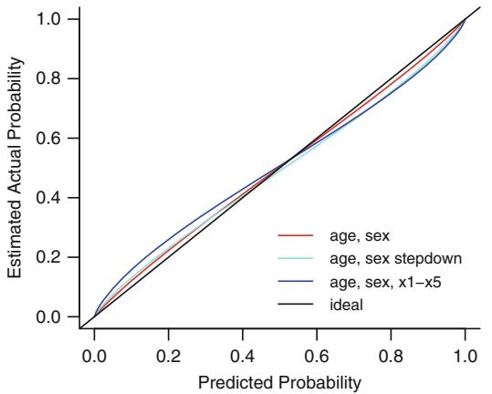
Fig. 10.17 Estimated logistic calibration (reliability) curves obtained by bootstrapping three modeling strategies.

Table 10.12 Effects Response : sigdz

		Low High ρ	Effect	S.E.		Lower 0.95 Upper 0.95
age	46	59 13	0.90629 0.18381		0.546030	1.26650
Odds Ratio	46	59 13	2.47510		1.726400	3.54860
cholesterol	196	259 63		0.75479 0.13642	0.487410	1.02220
Odds Ratio	196	259 63	2.12720		1.628100	2.77920
sex — female:male	1	2	-2.42970 0.14839		-2.720600	-2.13890
Odds Ratio	1	2	0.08806		0.065837	0.11778

ratio or factor by which the odds increases for a certain change in a predictor, holding all other predictors constant, may be displayed. Table 10.12 contains such summary statistics for the linear age ≤ cholesterol interaction surface fit described in Section 10.5.

s − summary(f.linia) # Table 10.12
latex (s, file= ' ' , size= ' Ssize ' ,
      label = ' tab:lrm-cholxage-confbar ' )

plot(s) # Figure 10.18

The outer quartiles of age are 46 and 59 years, so the “half-sample” odds ratio for age is 2.47, with 0.95 confidence interval [1.63, 3.74] when sex is male and cholesterol is set to its median. The effect of increasing cholesterol from 196 (its lower quartile) to 259 (its upper quartile) is to increase the log odds by 0.79 or to increase the odds by a factor of 2.21. Since there are interactions allowed between age and sex and between age and cholesterol, each odds ratio in the above table depends on the setting of at least one other factor. The

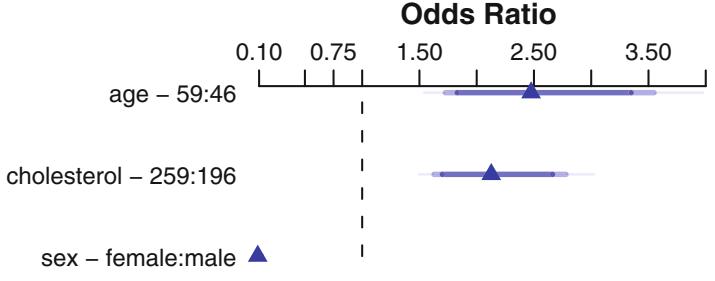
Adjusted to:age=52 sex=male cholesterol=224.5

Fig. 10.18 Odds ratios and confidence bars, using quartiles of age and cholesterol for assessing their effects on the odds of coronary disease

results are shown graphically in Figure 10.18. The shaded confidence bars show various levels of confidence and do not pin the analyst down to, say, the 0.95 level.

For those used to thinking in terms of odds or log odds, the preceding description may be sufficient. Many prefer instead to interpret the model in terms of predicted probabilities instead of odds. If the model contains only a single predictor (even if several spline terms are required to represent that predictor), one may simply plot the predictor against the predicted response. Such a plot is shown in Figure 10.19 which depicts the fitted relationship between age of diagnosis and the probability of acute bacterial meningitis (ABM) as opposed to acute viral meningitis (AVM), based on an analysis of 422 cases from Duke University Medical Center.580 The data may be found on the web site. A linear spline function with knots at 1, 2, and 22 years was used to model this relationship.

When the model contains more than one predictor, one may graph the predictor against log odds, and barring interactions, the shape of this relationship will be independent of the level of the other predictors. When displaying the model on what is usually a more interpretable scale, the probability scale, a difficulty arises in that unlike log odds the relationship between one predictor and the probability of response depends on the levels of all other factors. For example, in the model

\[\text{Prob}\{Y=1|X\} = \{1 + \exp[-(\beta\_0 + \beta\_1 X\_1 + \beta\_2 X\_2)]\}^{-1} \tag{10.39}\]

there is no way to factor out X¹ when examining the relationship between X² and the probability of a response. For the two-predictor case one can plot X² versus predicted probability for each level of X1. When it is uncertain whether to include an interaction in this model, consider presenting graphs for two models (with and without interaction terms included) as was done in [658].

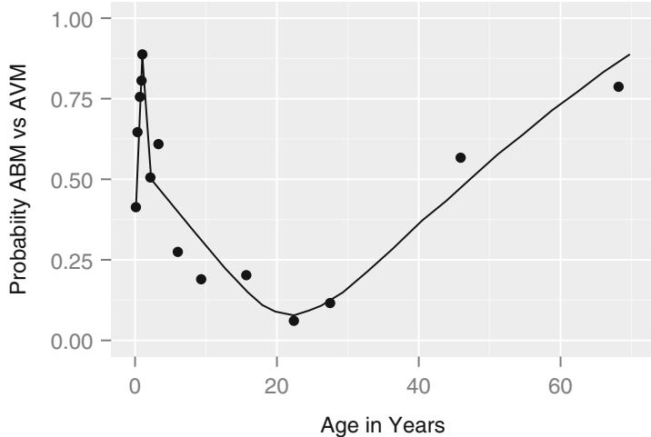
Fig. 10.19 Linear spline fit for probability of bacterial versus viral meningitis as a function of age at onset580. Points are simple proportions by age quantile groups.

When three factors are present, one could draw a separate graph for each level of X3, a separate curve on each graph for each level of X1, and vary X² on the x-axis. Instead of this, or if more than three factors are present, a good way to display the results may be to plot “adjusted probability estimates” as a function of one predictor, adjusting all other factors to constants such as the mean. For example, one could display a graph relating serum cholesterol to probability of myocardial infarction or death, holding age constant at 55, sex at 1 (male), and systolic blood pressure at 120 mmHg.

The final method for displaying the relationship between several predictors and probability of response is to construct a nomogram.40, 254 A nomogram not only sheds light on how the effect of one predictor on the probability of response depends on the levels of other factors, but it allows one to quickly estimate the probability of response for individual subjects. The nomogram in Figure 10.20 allows one to predict the probability of acute bacterial meningitis (given the patient has either viral or bacterial meningitis) using the same sample as in Figure 10.19. Here there are four continuous predictor values, none of which are linearly related to log odds of bacterial meningitis: age at admission (expressed as a linear spline function), month of admission (expressed as |month×8|), cerebrospinal fluid glucose/blood glucose ratio (linear effect truncated at .6; that is, the effect is the glucose ratio if it is − .6, and .6 if it exceeded .6), and the cube root of the total number of polymorphonuclear leukocytes in the cerebrospinal fluid. ¹⁷

The model associated with Figure 10.14 is depicted in what could be called a “precision nomogram” in Figure 10.21. Discrete cholesterol levels were required because of the interaction between two continuous variables.

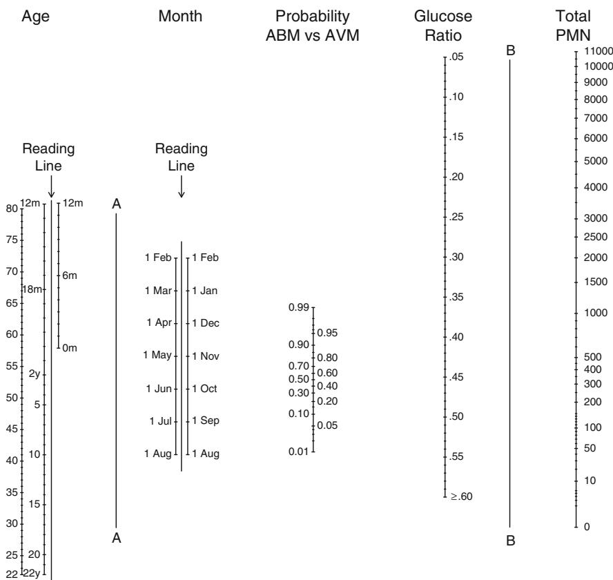
Fig. 10.20 Nomogram for estimating probability of bacterial (ABM) versus viral (AVM) meningitis. Step 1, place ruler on reading lines for patient’s age and month of presentation and mark intersection with line A; step 2, place ruler on values for glucose ratio and total polymorphonuclear leukocyte (PMN) count in cerebrospinal fluid and mark intersection with line B; step 3, use ruler to join marks on lines A and B, then read off the probability of ABM versus AVM.580

# Draw a nomogram that shows examples of confidence intervals
nom nomogram( f.linia , cholesterol =seq (150, 400, by=50), −
interact= list(age=seq(30, 70, by =10)),
lp.at =seq(-2 , 3.5 , by=.5),
conf.int= TRUE , conf.lp=“all”,
fun=function(x)1/(1+ exp(-x)), # or plogis
funlabel=“Probability of CAD”,
fun.at =c(seq(.1 , .9 , by=.1), .95 , .99)
) # Figure 10.21
plot (nom , col.grid = gray (c(0.8 , 0.95)),
varname.label =FALSE , ia.space =1, xfrac =.46 , lmgp=.2)

10.11 R Functions

The general R statistical modeling functions96 described in Section 6.2 work with the author’s lrm function for fitting binary and ordinal logistic regression models. lrm has several options for doing penalized maximum likelihood estimation, with special treatment of categorical predictors so as to shrink all estimates (including the reference cell) to the mean. The following exam- 18 ple fits a logistic model containing predictors age, blood.pressure, and sex, with age fitted with a smooth five-knot restricted cubic spline function and a different shape of the age relationship for males and females.

fit − lrm(death ← blood.pressure + sex * rcs(age ,5))
anova (fit)
plot( Predict(fit , age , sex ))

The pentrace function makes it easy to check the effects of a sequence of penalties. The following code fits an unpenalized model and plots the AIC and Schwarz BIC for a variety of penalties so that approximately the best cross-validating model can be chosen (and so we can learn how the penalty relates to the effective degrees of freedom). Here we elect to only penalize the nonlinear or non-additive parts of the model.

f − lrm(death ← rcs(age ,5)*treatment + lsp(sbp ,c (120,140)) ,
          x=TRUE , y= TRUE)
plot( pentrace(f,
               penalty= list( nonlinear =seq(.25 ,10, by=.25 ))) )

See Sections 9.8.1 and 9.10 for more information. ¹⁹

The residuals function for lrm and the which.influence function can be used to check predictor transformations as well as to analyze overly influential observations in binary logistic regression. See Figure 10.16 for one application. The residuals function will also perform the unweighted sum of squares test for global goodness of fit described in Section 10.5.

The validate function when used on an object created by lrm does resampling validation of a logistic regression model, with or without backward step-down variable deletion. It provides bias-corrected Somers’ Dxy rank correlation, R² ^N index, the intercept and slope of an overall logistic calibration equation, the maximum absolute difference in predicted and calibrated probabilities ^Emax, the discrimination index ^D [(model L.R. ^β² ^× 1)/n], the unreliability index U = (difference in ×2 log likelihood between uncalibrated XΛ and XΛ with overall intercept and slope calibrated to test sample)/n, and the overall quality index Q = D × U. 267 The “corrected” slope can be thought of as a shrinkage factor that takes overfitting into account. See predab.resample in Section 6.2 for the list of resampling methods.

The calibrate function produces bootstrapped or cross-validated calibration curves for logistic and linear models. The “apparent”calibration accuracy is estimated using a nonparametric smoother relating predicted probabilities

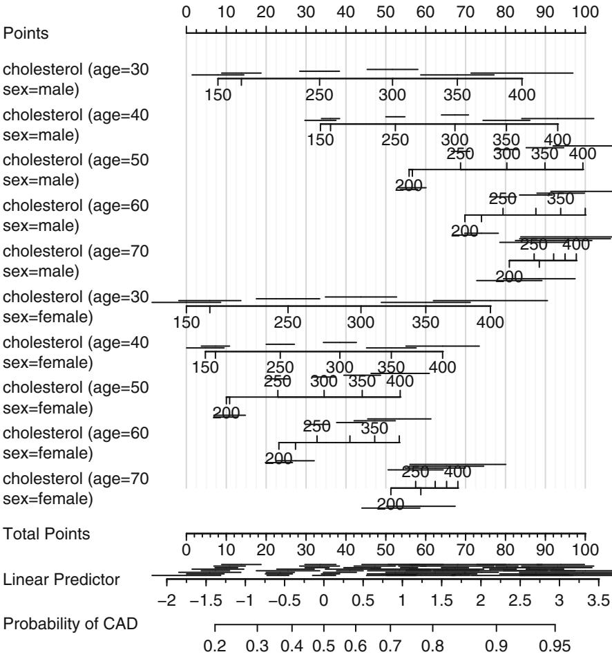
Fig. 10.21 Nomogram relating age, sex, and cholesterol to the log odds and to the probability of significant coronary artery disease. Select one axis corresponding to sex and to age ̸ {30, 40, 50, 60, 70}. There is linear interaction between age and sex and between age and cholesterol. 0.70 and 0.90 confidence intervals are shown (0.90 in gray). Note that for the “Linear Predictor” scale there are various lengths of confidence intervals near the same value of Xχˆ, demonstrating that the standard error of Xχˆ depends on the individual X values. Also note that confidence intervals corresponding to smaller patient groups (e.g., females) are wider.

to observed binary outcomes. The nonparametric estimate is evaluated at a sequence of predicted probability levels. Then the distances from the 45^≤ line are compared with the differences when the current model is evaluated back on the whole sample (or omitted sample for cross-validation). The differences in the differences are estimates of overoptimism. After averaging over many replications, the predicted-value-specific differences are then subtracted from the apparent differences and an adjusted calibration curve is obtained. Unlike validate, calibrate does not assume a linear logistic calibration. For an example, see the end of Chapter 11. calibrate will print the mean absolute calibration error, the 0.9 quantile of the absolute error, and the mean squared error, all over the observed distribution of predicted values.

The val.prob function is used to compute measures of discrimination and calibration of predicted probabilities for a separate sample from the one used to derive the probability estimates. Thus val.prob is used in external validation and data-splitting. The function computes similar indexes as validate plus the Brier score and a statistic for testing for unreliability or H⁰ : α⁰ = 0, α¹ = 1.

In the following example, a logistic model is fitted on 100 observations simulated from the actual model given by

\[\text{Prob}\{Y=1|X\_1, X\_2, X\_3\} = \left[1 + \exp[-(-1 + 2X\_1)]\right]^{-1},\tag{10.40}\]

where X¹ is a random uniform [0, 1] variable. Hence X² and X³ are irrelevant. After fitting a linear additive model in X1, X2, and X3, the coefficients are used to predict Prob{Y = 1} on a separate sample of 100 observations.

set.seed (13)
n − 200
x1 − runif (n)
x2 − runif (n)
x3 − runif (n)
logit − 2*(x1-.5 )
P − 1/(1+exp(-logit ))
y − ifelse (runif (n) ≤ P, 1, 0)
d − data.frame (x1 , x2 , x3 , y)
f − lrm(y ← x1 + x2 + x3 , subset =1:100)
phat − predict(f, d [101:200 ,], type= ' fitted ' )
# Figure 10.22
v − val.prob(phat , y [101:200] , m=20, cex=.5)

The output is shown in Figure 10.22.

The R built-in function glm, a very general modeling function, can fit binary logistic models. The response variable must be coded 0/1 for glm to work. Glm is a slight modification of the built-in glm function in the rms package that allows fits to use rms methods. This facilitates Poisson and several other types of regression analysis.

10.12 Further Reading

1 See [590] for modeling strategies specific to binary logistic regression.
2 See [632] for a nice review of logistic modeling. Agresti6 is an excellent source for categorical Y in general.
3 Not only does discriminant analysis assume the same regression model as logistic regression, but it also assumes that the predictors are each normally distributed and that jointly the predictors have a multivariate normal distribution. These assumptions are unlikely to be met in practice, especially when

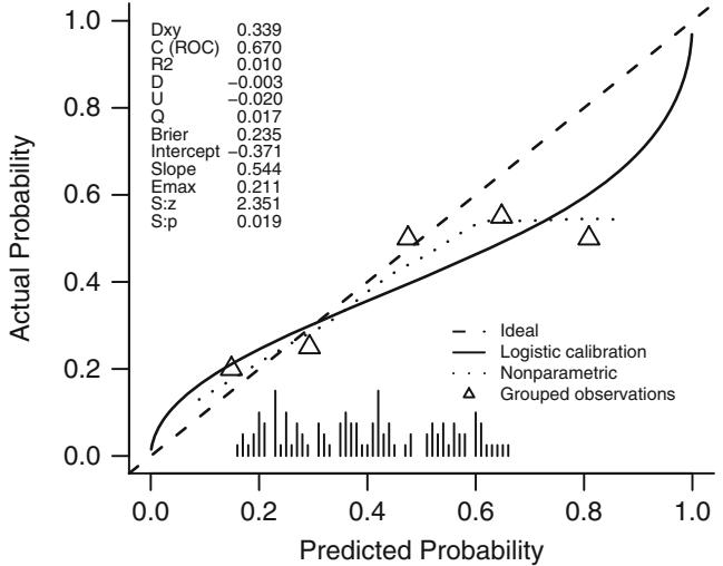
Fig. 10.22 Validation of a logistic model in a test sample of size n = 100. The calibrated risk distribution (histogram of logistic-calibrated probabilities) is shown.

one of the predictors is a discrete variable such as sex group. When discriminant analysis assumptions are violated, logistic regression yields more accurate estimates.251,514 Even when discriminant analysis is optimal (i.e., when all its assumptions are satisfied) logistic regression is virtually as accurate as the discriminant model.264

4 See [573] for a review of measures of effect for binary outcomes.
5 Cepedaet al.95 found that propensity adjustment is better than covariate adjustment with logistic models when the number of events per variable is less than 8.
6 Pregibon512 developed a modification of the log likelihood function that when maximized results in a fit that is resistant to overly influential and outlying observations.
7 See Hosmer and Lemeshow306 for methods of testing for a difference in the observed event proportion and the predicted event probability (average of predicted probabilities) for a group of heterogeneous subjects.
8 See Hosmer and Lemeshow,305 Kay and Little,341 and Collett [115, Chap. 5]. Landwehr et al.373 proposed the partial residual (see also Fowlkes199).
9 See Berk and Booth51 for other partial-like residuals.
10 See [341] for an example comparing a smoothing method with a parametric logistic model fit.
11 See Collett [115, Chap. 5] and Pregibon512 for more information about influence statistics. Pregibon’s resistant estimator of χ handles overly influential groups of observations and allows one to estimate the weight that an observation contributed to the fit after making the fit robust. Observations receiving low weight are partially ignored but are not deleted.
12 Buyse86 showed that in the case of a single categorical predictor, the ordinary R² has a ready interpretation in terms of variance explained for binary responses. Menard454 studied various indexes for binary logistic regression. He criticized R² ^N for being too dependent on the proportion of observations with Y = 1. Hu et al.309 further studied the properties of variance-based R² measures for binary responses. Tjur613 has a nice discussion discrimination graphics

and sum of squares–based R² measures for binary logistic regression, as well as a good discussion of “separation” and infinite regression coefficients. Sums of squares are approximated various ways.

13 Very little work has been done on developing adjusted R² measures in logistic regression and other non-linear model setups. Liao and McGee406 developed one adjusted R² measure for binary logistic regression, but it uses simulation to adjust for the bias of overfitting. One might as well use the bootstrap to adjust any of the indexes discussed in this section.
14 [123, 633] have more pertinent discussion of probability accuracy scores.
15 Copas121 demonstrated how ROC areas can be misleading when applied to different responses having greatly different prevalences. He proposed another approach, the logit rank plot. Newsom473 is an excellent reference on Dxy. Newson474 developed several generalizations to Dxy including a stratified version, and discussed the jackknife variance estimator for them. ROC areas are not very useful for comparing two models118,493 (but see490).
16 Gneiting and Raftery219 have an excellent review of proper scoring rules. Hand253 contains much information about assessing classification accuracy. Mittlb¨ock and Schemper461 have an excellent review of indexes of explained variation for binary logistic models. See also Korn and Simon366 and Zheng and Agresti.684.
17 Pryor et al.515 presented nomograms for a 10-variable logistic model. One of the variables was sex, which interacted with some of the other variables. Evaluation of predicted probabilities was simplified by the construction of separate nomograms for females and males. Seven terms for discrete predictors were collapsed into one weighted point score axis in the nomograms, and age by risk factor interactions were captured by having four age scales.
18 Moons et al.462 presents a case study in penalized binary logistic regression modeling.
19 The rcspline.plot function in the Hmisc R package does not allow for interactions as does lrm, but it can provide detailed output for checking spline fits. This function plots the estimated spline regression and confidence limits, placing summary statistics on the graph. If there are no adjustment variables, rcspline.plot can also plot two alternative estimates of the regression function: proportions or logit proportions on grouped data, and a nonparametric estimate. The nonparametric regression estimate is based on smoothing the binary responses and taking the logit transformation of the smoothed estimates, if desired. The smoothing uses the “super smoother” of Friedman207 implemented in the R function supsmu.

10.13 Problems

1. Consider the age–sex–response example in Section 10.1.3. This dataset is available from the text’s web site in the Datasets area.
- 1. Duplicate the analyses done in Section 10.1.3.
- 1. For the model containing both age and sex, test H⁰ : logit response is linear in age versus H^a : logit response is quadratic in age. Use the best test statistic.
- 1. Using a Wald test, test H⁰ : no age ≤ sex interaction. Interpret all parameters in the model.
1. Plot the estimated logit response as a function of age and sex, with and without fitting an interaction term.
1. Perform a likelihood ratio test of H⁰ : the model containing only age and sex is adequate versus H^a : model is inadequate. Here, “inadequate” may mean nonlinearity (quadratic) in age or presence of an interaction.
1. Assuming no interaction is present, test H⁰ : model is linear in age versus H^a : model is nonlinear in age. Allow “nonlinear” to be more general than quadratic. (Hint: use a restricted cubic spline function with knots at age=39, 45, 55, 64 years.)
1. Plot age against the estimated spline transformation of age (the transformation that would make age fit linearly). You can set the sex and intercept terms to anything you choose. Also plot Prob{response = 1 | age, sex} from this fitted restricted cubic spline logistic model.
1. Consider a binary logistic regression model using the following predictors: age (years), sex, race (white, African-American, Hispanic, Oriental, other), blood pressure (mmHg). The fitted model is given by

logit Prob[^Y = 1|X] = ^XΛ^ˆ ⁼ ^×1.36 + .03(race = African-American) × .04(race = hispanic) + .05(race = oriental) × .06(race = other) ⁺ .07|blood pressure ^× ¹¹⁰^| ⁺ .3(sex = male) ^× .1age + .002age² ⁺ (sex = male)[.05age ^× .003age²].

1. Compute the predicted logit (log odds) that Y = 1 for a 50-year-old female Hispanic with a blood pressure of 90 mmHg. Also compute the odds that Y = 1 (Prob[Y = 1]/Prob[Y = 0]) and the estimated probability that Y = 1.
1. Estimate odds ratios for each nonwhite race compared with the reference group (white), holding all other predictors constant. Why can you estimate the relative effect of race for all types of subjects without specifying their characteristics?
1. Compute the odds ratio for a blood pressure of 120 mmHg compared with a blood pressure of 105, holding age first to 30 years and then to 40 years.
1. Compute the odds ratio for a blood pressure of 120 mmHg compared with a blood pressure of 105, all other variables held to unspecified constants. Why is this relative effect meaningful without knowing the subject’s age, race, or sex?
1. Compute the estimated risk difference in changing blood pressure from 105 mmHg to 120 mmHg, first for age = 30 then for age = 40, for a white female. Why does the risk difference depend on age?
1. Compute the relative odds for males compared with females, for age = 50 and other variables held constant.
1. Same as the previous question but for females : males instead of males : females.
1. Compute the odds ratio resulting from increasing age from 50 to 55 for males, and then for females, other variables held constant. What is wrong with the following question: What is the relative effect of changing age by one year?

Chapter 11 Case Study in Binary Logistic Regression, Model Selection and Approximation: Predicting Cause of Death

11.1 Overview

This chapter contains a case study on developing, describing, and validating a binary logistic regression model. In addition, the following methods are exemplified:

1. Data reduction using incomplete linear and nonlinear principal components
1. Use of AIC to choose from five modeling variations, deciding which is best for the number of parameters
1. Model simplification using stepwise variable selection and approximation of the full model
1. The relationship between the degree of approximation and the degree of predictive discrimination loss
1. Bootstrap validation that includes penalization for model uncertainty (variable selection) and that demonstrates a loss of predictive discrimination over the full model even when compensating for overfitting the full model.

The data reduction and pre-transformation methods used here were discussed in more detail in Chapter 8. Single imputation will be used because of the limited quantity of missing data.

11.2 Background

Consider the randomized trial of estrogen for treatment of prostate cancer87 described in Chapter 8. In this trial, larger doses of estrogen reduced the effect of prostate cancer but at the cost of increased risk of cardiovascular death.

^© Springer International Publishing Switzerland 2015 F.E. Harrell, Jr., Regression Modeling Strategies, Springer Series in Statistics, DOI 10.1007/978-3-319-19425-7 11

Kay340 did a formal analysis of the competing risks for cancer, cardiovascular, and other deaths. It can also be quite informative to study how treatment and baseline variables relate to the cause of death for those patients who died.376 We subset the original dataset of those patients dying from prostate cancer (n = 130), heart or vascular disease (n = 96), or cerebrovascular disease (n = 31). Our goal is to predict cardiovascular–cerebrovascular death (cvd, n = 127) given the patient died from either cvd or prostate cancer. Of interest is whether the time to death has an effect on the cause of death, and whether the importance of certain variables depends on the time of death.

11.3 Data Transformations and Single Imputation

In R, first obtain the desired subset of the data and do some preliminary calculations such as combining an infrequent category with the next category, and dichotomizing ekg for use in ordinary principal components (PCs).

require(rms)

getHdata(prostate)
prostate −
  within (prostate , {
    levels (ekg)[levels (ekg) %in%
                 c ( ' old MI ' , ' recent MI ' )] − ' MI '
    ekg.norm − 1*(ekg %in% c( ' normal ' , ' benign ' ))
    levels (ekg) − abbreviate( levels (ekg))
    pfn − as.numeric (pf)
    levels (pf) − levels (pf)[c(1,2,3 ,3)]
    cvd − status %in% c("dead - heart or vascular",
                           "dead - cerebrovascular ")
    rxn = as.numeric (rx) })
# Use transcan to compute optimal pre-transformations
ptrans − # See Figure 8.3
  transcan(← sz + sg + ap + sbp + dbp +
            age + wt + hg + ekg + pf + bm + hx + dtime + rx ,
            imputed=TRUE , transformed =TRUE ,
            data=prostate , pl= FALSE , pr= FALSE )
# Use transcan single imputations
imp − impute (ptrans , data=prostate , list.out= TRUE)

Imputed missing values with the following frequencies and stored them in variables with their original names: sz sg age wt ekg 5 11 1 2 8

NAvars − all.vars(← sz + sg + age + wt + ekg)
for(x in NAvars ) prostate [[x]] − imp[[x]]
subset − prostate$ status %in% c("dead - heart or vascular",

"dead - cerebrovascular "," dead - prostatic ca")
trans − ptrans $ transformed[ subset ,]
psub − prostate[ subset ,]

11.4 Regression on Original Variables, Principal Components and Pretransformations

We first examine the performance of data reduction in predicting the cause of death, similar to what we did for survival time in Section 8.6. The first analyses assess how well PCs (on raw and transformed variables) predict the cause of death.

There are 127 cvds. We use the 15:1 rule of thumb discussed on P. 72 to justify using the first 8 PCs. ap is log-transformed because of its extreme distribution.

# Function to compute the first k PCs
ipc − function (x, k=1, ...)
  princomp (x, ... , cor=TRUE)$scores [,1:k]
# Compute the first 8 PCs on raw variables then on
# transformed ones
pc8 − ipc(← sz + sg + log(ap) + sbp + dbp + age +
           wt + hg + ekg.norm + pfn + bm + hx + rxn + dtime ,
           data=psub , k=8)
f8 − lrm(cvd ← pc8 , data=psub)
pc8t − ipc(trans , k=8)
f8t − lrm(cvd ← pc8t , data=psub)
# Fit binary logistic model on original variables
f − lrm(cvd ← sz + sg + log(ap) + sbp + dbp + age +
         wt + hg + ekg + pf + bm + hx + rx + dtime , data=psub)
# Expand continuous variables using splines
g − lrm(cvd ← rcs(sz ,4) + rcs(sg ,4) + rcs(log(ap),4) +
         rcs(sbp ,4) + rcs(dbp ,4) + rcs(age ,4) + rcs(wt ,4) +
         rcs(hg ,4) + ekg + pf + bm + hx + rx + rcs(dtime ,4),
         data=psub)
# Fit binary logistic model on individual transformed var.
h − lrm(cvd ← trans , data=psub)

The five approaches to modeling the outcome are compared using AIC (where smaller is better).

c(f8=AIC(f8), f8t=AIC(f8t), f=AIC(f), g=AIC(g), h=AIC(h))

f8 f8t f g h 257.6573 254.5172 255.8545 263.8413 254.5317

Based on AIC, the more traditional model fitted to the raw data and assuming linearity for all the continuous predictors has only a slight chance of producing worse cross-validated predictive accuracy than other methods. The chances are also good that effect estimates from this simple model will have competitive mean squared errors.

11.5 Description of Fitted Model

Here we describe the simple all-linear full model. Summary statistics and a Wald-ANOVA table are below, followed by partial effects plots with pointwise confidence bands, and odds ratios over default ranges of predictors.

print (f, latex =TRUE)

Logistic Regression Model

lrm(formula = cvd ~ sz + sg + log(ap) + sbp + dbp + age + wt + hg + ekg + pf + bm + hx + rx + dtime, data = psub)

			Model Likelihood		Discrimination		Rank Discrim.
		Ratio Test		Indexes		Indexes
Obs	257	β2 LR	144.39	R2	0.573	C	0.893
FALSE	130	d.f.	21	g	2.688	Dxy	0.786
TRUE	127	β2) Pr(>	< 0.0001	gr	14.701	α	0.787
α log L max αρ	6≤10−11			gp	0.394	Γa	0.395
				Brier	0.133

	Coef	S.E.	Wald Z	Pr(> Z )
Intercept	-4.5130	3.2210	-1.40	0.1612
sz	-0.0640	0.0168	-3.80	0.0001
sg	-0.2967	0.1149	-2.58	0.0098
ap	-0.3927	0.1411	-2.78	0.0054
sbp	-0.0572	0.0890	-0.64	0.5201
dbp	0.3917	0.1629	2.40	0.0162
age	0.0926	0.0286	3.23	0.0012
wt	-0.0177	0.0140	-1.26	0.2069
hg	0.0860	0.0925	0.93	0.3524
ekg=bngn	1.0781	0.8793	1.23	0.2202
ekg=rd&ec	-0.1929	0.6318	-0.31	0.7601
ekg=hbocd	-1.3679	0.8279	-1.65	0.0985
ekg=hrts	0.4365	0.4582	0.95	0.3407
ekg=MI	0.3039	0.5618	0.54	0.5886
pf=in bed < 50% daytime	0.9604	0.6956	1.38	0.1673
pf=in bed > 50% daytime	-2.3232	1.2464	-1.86	0.0623
bm	0.1456	0.5067	0.29	0.7738
hx	1.0913	0.3782	2.89	0.0039

	Coef	S.E.	Wald Z	Pr(> Z )
rx=0.2 mg estrogen	-0.3022	0.4908	-0.62	0.5381
rx=1.0 mg estrogen	0.7526	0.5272	1.43	0.1534
rx=5.0 mg estrogen	0.6868	0.5043	1.36	0.1733
dtime	-0.0136	0.0107	-1.27	0.2040

an − anova (f)

latex (an , file = ' ' , table.env= FALSE)

	β2	d.f.	P
sz	14.42	1	0.0001
sg	6.67	1	0.0098
ap	7.74	1	0.0054
sbp	0.41	1	0.5201
dbp	5.78	1	0.0162
age	10.45	1	0.0012
wt	1.59	1	0.2069
hg	0.86	1	0.3524
ekg	6.76	5	0.2391
pf	5.52	2	0.0632
bm	0.08	1	0.7738
hx	8.33	1	0.0039
rx	5.72	3	0.1260
dtime	1.61	1	0.2040
TOTAL 66.87		21	< 0.0001

plot(an) # Figure 11.1
s − f$stats
gamma.hat − (s[ ' Model L.R. ' ] - s[ ' d.f. ' ])/s[ ' Model L.R. ' ]
dd − datadist( psub ); options(datadist= ' dd ' )

ggplot ( Predict(f), sepdiscrete= ' vertical ' , vnames = ' names ' ,
        rdata =psub ,
        histSpike.opts = list(frac= function(f) .1*f/max(f) ))
        # Figure 11.2

plot( summary(f), log= TRUE) # Figure 11.3

The van Houwelingen–Le Cessie heuristic shrinkage estimate (Equation 4.3) is ˆα = 0.85, indicating that this model will validate on new data about 15% worse than on this dataset.

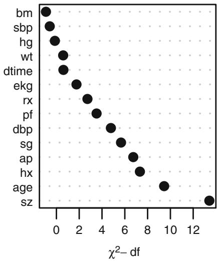
Fig. 11.1 Ranking of apparent importance of predictors of cause of death

11.6 Backwards Step-Down

Now use fast backward step-down (with total residual AIC as the stopping rule) to identify the variables that explain the bulk of the cause of death. Later validation will take this screening of variables into account.The greatly reduced model results in a simple nomogram.

fastbw (f)

Deleted Chi-Sq d.f. P Residual d.f. P AIC
ekg 6.76 5 0.2391 6.76 5 0.2391 -3.24
bm 0.09 1 0.7639 6.85 6 0.3349 -5.15
hg 0.38 1 0.5378 7.23 7 0.4053 -6.77
sbp 0.48 1 0.4881 7.71 8 0.4622 -8.29
wt 1.11 1 0.2932 8.82 9 0.4544 -9.18
dtime 1.47 1 0.2253 10.29 10 0.4158 -9.71
rx 5.65 3 0.1302 15.93 13 0.2528 -10.07
pf 4.78 2 0.0915 20.71 15 0.1462 -9.29
sg 4.28 1 0.0385 25.00 16 0.0698 -7.00
dbp 5.84 1 0.0157 30.83 17 0.0209 -3.17
Approximate Estimates after Deleting Factors
           Coef S.E. Wald Z P
Intercept -3.74986 1.82887 -2.050 0.0403286
sz -0.04862 0.01532 -3.174 0.0015013
ap -0.40694 0.11117 -3.660 0.0002518
age 0.06000 0.02562 2.342 0.0191701
hx 0.86969 0.34339 2.533 0.0113198
Factors in Final Model
[1] sz ap age hx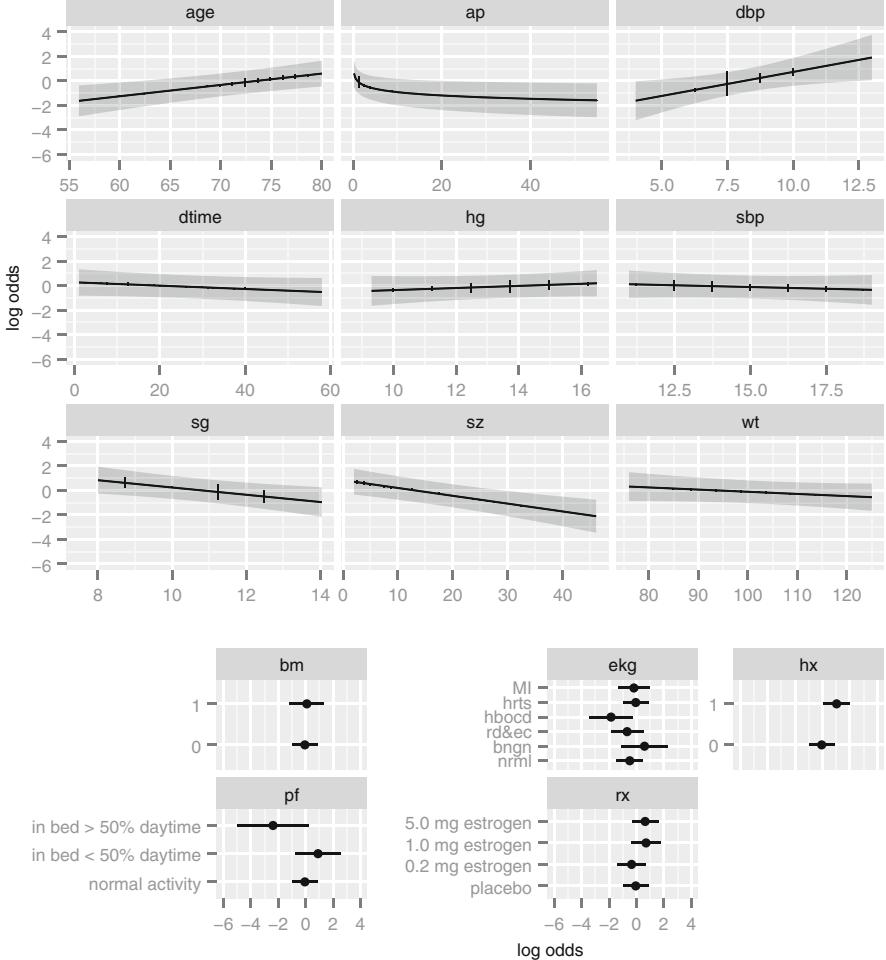

Fig. 11.2 Partial effects (log odds scale) in full model for cause of death, along with vertical line segments showing the raw data distribution of predictors

fred − lrm(cvd ← sz + log(ap) + age + hx , data =psub) latex (fred , file= ’ ’ )

\[\text{Prob}\{\text{cvd}\} = \frac{1}{1 + \exp(-X\beta)}, \quad \text{where}\]

XΛˆ = ×5.009276 × 0.05510121 sz × 0.509185 log(ap) + 0.0788052 age + 1.070601 hx

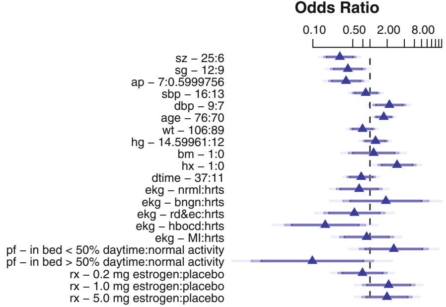
Fig. 11.3 Interquartile-range odds ratios for continuous predictors and simple odds ratios for categorical predictors. Numbers at left are upper quartile : lower quartile or current group : reference group. The bars represent 0.9, 0.95, 0.99 confidence limits. The intervals are drawn on the log odds ratio scale and labeled on the odds ratio scale. Ranges are on the original scale.

nom − nomogram(fred , ap=c(.1 , .5 , 1, 5, 10, 50),
                  fun=plogis , funlabel="Probability ",
                  fun.at =c(.01 ,.05 ,.1 ,.25 ,.5 ,.75 ,.9 ,.95 ,.99 ))
plot (nom , xfrac =.45) # Figure 11.4

It is readily seen from this model that patients with a history of heart disease, and patients with less extensive prostate cancer are those more likely to die from cvd rather than from cancer. But beware that it is easy to overinterpret findings when using unpenalized estimation, and confidence intervals are too narrow. Let us use the bootstrap to study the uncertainty in the selection of variables and to penalize for this uncertainty when estimating predictive performance of the model. The variables selected in the first 20 bootstrap resamples are shown, making it obvious that the set of “significant” variables, i.e., the final model, is somewhat arbitrary.

f − update (f, x=TRUE , y= TRUE)
v − validate(f, B=200, bw= TRUE)

latex (v, B=20, digits =3)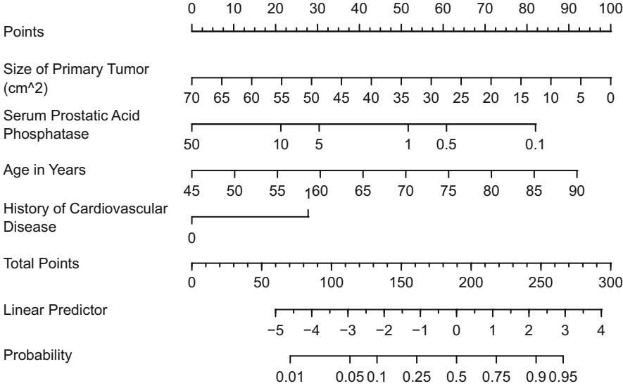

Fig. 11.4 Nomogram calculating Xχˆ and Pˆ for cvd as the cause of death, using the step-down model. For each predictor, read the points assigned on the 0–100 scale and add these points. Read the result on the Total Points scale and then read the corresponding predictions below it.

Index	Original Training		Test	Optimism Corrected	n
	Sample	Sample	Sample		Index
Dxy	0.682	0.713	0.643	0.071	0.611 200
R2	0.439	0.481	0.393	0.088	0.351 200
Intercept	0.000	0.000	×0.006	0.006	×0.006 200
Slope	1.000	1.000	0.811	0.189	0.811 200
Emax	0.000	0.000	0.048	0.048	0.048 200
D	0.395	0.449	0.346	0.102	0.293 200
U	×0.008	×0.008	0.018	×0.026	0.018 200
Q	0.403	0.456	0.329	0.128	0.275 200
B	0.162	0.151	0.174	×0.022	0.184 200
g	1.932	2.213	1.756	0.457	1.475 200
gp	0.341	0.355	0.320	0.035	0.306 200

											sz sg ap sbp dbp age wt hg ekg pf bm hx rx dtime
	•		•	•
•		•		•	•	•	•		•	•
•		•							•	•
•		•
•	•			•			•
	•								•
•		•							•	•	•
•		•			•	•
•		•			•
•	•								•
•		•			•				•
•		•			•				•
•		•		•					•
•		•		•	•
•	•			•	•		•	•	•	•
		•		•	•				•
•	•	•		•	•				•
•		•
•	•				•			•
	•								•

Factors Retained in Backwards Elimination First 20 Resamples

Frequencies of Numbers of Factors Retained 1 2 3 4 5 6 7 8 9 11 12 6 39 47 61 19 10 8 4 2 3 1

The slope shrinkage (ˆα) is a bit lower than was estimated above. There is drop-off in all indexes. The estimated likely future predictive discrimination of the model as measured by Somers’ Dxy fell from 0.682 to 0.611. The latter estimate is the one that should be claimed when describing model performance.

A nearly unbiased estimate of future calibration of the stepwise-derived model is given below.

cal − calibrate(f, B =200, bw= TRUE)
plot(cal) # Figure 11.5

The amount of overfitting seen in Figure 11.5 is consistent with the indexes produced by the validate function.

For comparison, consider a bootstrap validation of the full model without using variable selection.

vfull − validate(f, B =200)
latex ( vfull , digits =3)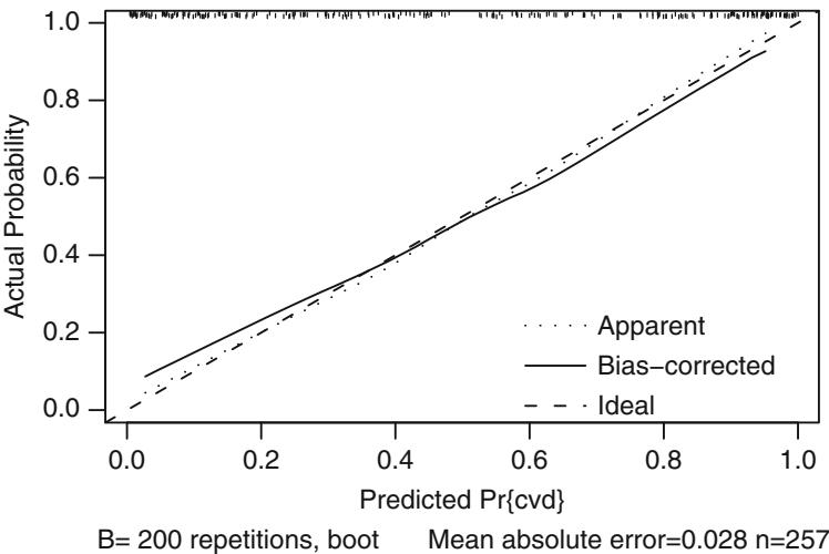

Fig. 11.5 Bootstrap overfitting–corrected calibration curve estimate for the backwards step-down cause of death logistic model, along with a rug plot showing the distribution of predicted risks. The smooth nonparametric calibration estimator (loess) is used.

Index		Original Training	Test	Optimism Corrected	n
	Sample	Sample	Sample		Index
Dxy	0.786	0.833	0.738	0.095	0.691 200
R2	0.573	0.641	0.501	0.140	0.433 200
Intercept	0.000	0.000	×0.013	0.013	×0.013 200
Slope	1.000	1.000	0.690	0.310	0.690 200
Emax	0.000	0.000	0.085	0.085	0.085 200
D	0.558	0.653	0.468	0.185	0.373 200
U	×0.008	×0.008	0.051	×0.058	0.051 200
Q	0.566	0.661	0.417	0.244	0.322 200
B	0.133	0.115	0.150	×0.035	0.168 200
g	2.688	3.464	2.355	1.108	1.579 200
gp	0.394	0.416	0.366	0.050	0.344 200

Compared to the validation of the full model, the step-down model has less optimism, but it started with a smaller Dxy due to loss of information from removing moderately important variables. The improvement in optimism was not enough to offset the effect of eliminating variables. If shrinkage were used with the full model, it would have better calibration and discrimination than the reduced model, since shrinkage does not diminish Dxy. Thus stepwise variable selection failed at delivering excellent predictive discrimination.

Finally, compare previous results with a bootstrap validation of a stepdown model using a better significance level for a variable to stay in the

model (σ = 0.5,589) and using individual approximate Wald tests rather than tests combining all deleted variables.

v5 − validate(f, bw= TRUE , sls=0.5 , type= ’ individual ’ , B=200)

			Backwards Step - down		-	Original	Model
Deleted	Chi-Sq	d.f.	P	Residual	d.f.	P	AIC
ekg	6.76	5	0.2391	6.76	5	0.2391	-3.24
bm	0.09	1	0.7639	6.85	6	0.3349	-5.15
hg	0.38	1	0.5378	7.23	7	0.4053	-6.77
sbp	0.48	1	0.4881	7.71	8	0.4622	-8.29
wt	1.11	1	0.2932	8.82	9	0.4544	-9.18
dtime	1.47	1	0.2253	10.29	10	0.4158	-9.71
rx	5.65	3	0.1302	15.93	13	0.2528	-10.07

Approximate		Estimates	after	Deleting	Factors

				Coef	S.E.	Wald Z	P
Intercept				-4.86308	2.67292	-1.819	0.068852
sz				-0.05063	0.01581	-3.202	0.001366
sg				-0.28038	0.11014	-2.546	0.010903
ap				-0.24838	0.12369	-2.008	0.044629
dbp				0.28288	0.13036	2.170	0.030008
age				0.08502	0.02690	3.161	0.001572
pf=in bed	< 50%	daytime		0.81151	0.66376	1.223	0.221485
pf=in bed	> 50%	daytime		-2.19885	1.21212	-1.814	0.069670
hx				0.87834	0.35203	2.495	0.012592

Factors	in Final	Model

1 sz	sg ap	dbp	age pf	hx

latex (v5 , digits =3, B=0)

Index		Original Training	Test	Optimism Corrected	n
	Sample	Sample	Sample		Index
Dxy	0.739	0.801	0.716	0.085	0.654 200
R2	0.517	0.598	0.481	0.117	0.400 200
Intercept	0.000	0.000	×0.008	0.008	×0.008 200
Slope	1.000	1.000	0.745	0.255	0.745 200
Emax	0.000	0.000	0.067	0.067	0.067 200
D	0.486	0.593	0.444	0.149	0.337 200
U	×0.008	×0.008	0.033	×0.040	0.033 200
Q	0.494	0.601	0.411	0.190	0.304 200
B	0.147	0.125	0.156	×0.030	0.177 200
g	2.351	2.958	2.175	0.784	1.567 200
gp	0.372	0.401	0.358	0.043	0.330 200

The performance statistics are midway between the full model and the smaller stepwise model.

11.7 Model Approximation

Frequently a better approach than stepwise variable selection is to approximate the full model, using its estimates of precision, as discussed in Section 5.5. Stepwise variable selection as well as regression trees are useful for making the approximations, and the sacrifice in predictive accuracy is always apparent.

We begin by computing the “gold standard” linear predictor from the full model fit (R² = 1.0), then running backwards step-down OLS regression to approximate it.

lp − predict(f) # Compute linear predictor from full model
# Insert sigma=1 as otherwise sigma=0 will cause problems
a − ols(lp ← sz + sg + log(ap) + sbp + dbp + age + wt +
         hg + ekg + pf + bm + hx + rx + dtime , sigma =1,
         data=psub)
# Specify silly stopping criterion to remove all variables
s − fastbw (a, aics =10000)
betas − s$Coefficients # matrix , rows= iterations
X − cbind (1, f$x) # design matrix
# Compute the series of approximations to lp
ap − X %*% t(betas )
# For each approx. compute approximation R−2 and ratio of
# likelihood ratio chi-square for approximate model to that
# of original model
m − ncol(ap) - 1 # all but intercept-only model
r2 − frac − numeric(m)
fullchisq − f$stats[ ' Model L.R. ' ]
for(i in 1:m) {
  lpa − ap[,i]
  r2[i] − cor(lpa , lp)−2
  fapprox − lrm(cvd ← lpa , data =psub )
  frac[i] − fapprox$ stats[ ' Model L.R. ' ] / fullchisq
  } # Figure 11.6:
plot (r2 , frac , type= ' b ' ,
     xlab= expression( paste ( ' Approximation ' , R−2)),
     ylab= expression( paste ( ' Fraction of ' ,
         chi−2, ' Preserved ' )))
abline (h=.95 , col=gray (.83 )); abline (v=.95 , col=gray (.83 ))
abline (a=0, b=1, col=gray (.83))

After 6 deletions, slightly more than 0.05 of both the LR β² and the approximation R² are lost (see Figure 11.6). Therefore we take as our approximate model the one that removed 6 predictors. The equation for this model is below, and its nomogram is in Figure 11.7.

fapprox − ols(lp ← sz + sg + log(ap) + age + ekg + pf + hx +
                rx , data =psub)
fapprox$ stats [ ' R2 ' ] # as a check

R2 0.9453396

latex (fapprox , file= ’ ’ )

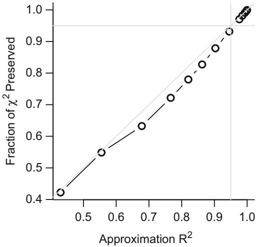
Fig. 11.6 Fraction of explainable variation (full model LR σ²) in cvd that was explained by approximate models, along with approximation accuracy (x–axis)

\[\mathcal{E}(\text{lp}) = X\beta,\quad\text{where}\]

Xβˆ = −2.868303 − 0.06233241 sz − 0.3157901 sg − 0.3834479 log(ap) + 0.09089393 age +1.396922[bngn] + 0.06275034[rd&ec] − 1.24892[hbocd] + 0.6511938[hrts] +0.3236771[MI] +1.116028[in bed < 50% daytime] − 2.436734[in bed > 50% daytime] +1.05316 hx −0.3888534[0.2 mg estrogen] + 0.6920495[1.0 mg estrogen] +0.7834498[5.0 mg estrogen]

and [c] = 1 if subject is in group c, 0 otherwise.

nom − nomogram( fapprox , ap=c(.1 , .5 , 1, 5, 10, 20, 30, 40),
                 fun=plogis , funlabel="Probability ",
                 lp.at =(-5):4,
            fun.lp.at= qlogis (c(.01 ,.05 ,.25 ,.5 ,.75 ,.95 ,.99 )))
plot (nom , xfrac =.45) # Figure 11.7

11.7 Model Approximation 289

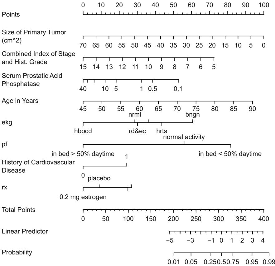
Fig. 11.7 Nomogram for predicting the probability of cvd based on the approximate model

Chapter 12 Logistic Model Case Study 2: Survival of Titanic Passengers

This case study demonstrates the development of a binary logistic regression model to describe patterns of survival in passengers on the Titanic, based on passenger age, sex, ticket class, and the number of family members accompanying each passenger. Nonparametric regression is also used. Since many of the passengers had missing ages, multiple imputation is used so that the complete information on the other variables can be efficiently utilized. Titanic passenger data were gathered by many researchers. Primary references are the Encyclopedia Titanica at www.encyclopedia-titanica.org and Eaton and Haas.169 Titanic survival patterns have been analyzed previously151, 296, 571 but without incorporation of individual passenger ages. Thomas Cason while a University of Virginia student compiled and interpreted the data from the World Wide Web. One thousand three hundred nine of the passengers are represented in the dataset, which is available from this text’s Web site under the name titanic3. An early analysis of Titanic data may be found in Bron75.

12.1 Descriptive Statistics

First we obtain basic descriptive statistics on key variables.

require(rms)

getHdata(titanic3) # get dataset from web site
# List of names of variables to analyze
v − c ( ' pclass ' , ' survived ' , ' age ' , ' sex ' , ' sibsp ' , ' parch ' )
t3 − titanic3[, v]
units (t3$age) − ' years '
latex ( describe(t3), file= ' ' )

6 Variables 1309 Observations
pclass n missing unique 1309 0 3
1st (323, 25%), 2nd (277, 21%), 3rd (709, 54%)
survived : Survived n missing unique Info Sum Mean 1309 0 2 0.71 500 0.382
age : Age [years]
n missing unique Info Mean .05 .10 .25 .50 .75 .90 .95 1046 263 98 1 29.88 5 14 21 28 39 50 57
lowest : 0.1667 0.3333 0.4167 0.6667 0.7500 highest: 70.5000 71.0000 74.0000 76.0000 80.0000
sex n missing unique 1309 0 2 female (466, 36%), male (843, 64%)
sibsp : Number of Siblings/Spouses Aboard n missing unique Info Mean 1309 0 7 0.67 0.4989
0 1 2 3 458 Frequency 891 319 42 20 22 6 9 % 68 24 3 2 2 0 1
parch : Number of Parents/Children Aboard n missing unique Info Mean 1309 0 8 0.55 0.385
0 1 234569 Frequency 1002 170 113 86622 % 77 13 9 1 0 0 0 0

Next, we obtain access to the needed variables and observations, and save data distribution characteristics for plotting and for computing predictor effects. There are not many passengers having more than 3 siblings or spouses or more than 3 children, so we truncate two variables at 3 for the purpose of estimating stratified survival probabilities.

dd − datadist(t3)
# describe distributions of variables to rms
options(datadist= ' dd ' )
s − summary(survived ← age + sex + pclass +
             cut2(sibsp ,0:3) + cut2( parch ,0:3), data=t3)
plot(s, main= ' ' , subtitles= FALSE) # Figure 12.1

Note the large number of missing ages. Also note the strong effects of sex and passenger class on the probability of surviving. The age effect does not appear to be very strong, because as we show later, much of the effect is restricted to

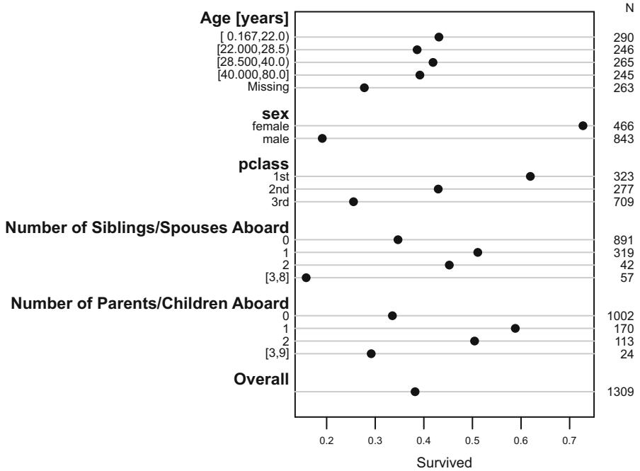
Fig. 12.1 Univariable summaries of Titanic survival

age < 21 years for one of the sexes. The effects of the last two variables are unclear as the estimated proportions are not monotonic in the values of these descriptors. Although some of the cell sizes are small, we can show four-way empirical relationships with the fraction of surviving passengers by creating four cells for sibsp ≤ parch combinations and by creating two age groups. We suppress proportions based on fewer than 25 passengers in a cell. Results are shown in Figure 12.2.

tn − transform (t3 ,
  agec = ifelse (age < 21, ' child ' , ' adult ' ),
  sibsp = ifelse (sibsp == 0, ' no sib/sp ' , ' sib/sp ' ),
  parch = ifelse (parch == 0, ' no par/child ' , ' par/child ' ))
g − function(y) if( length (y) < 25) NA else mean(y)
s − with (tn , summarize( survived ,
            llist (agec , sex , pclass , sibsp , parch ), g))
# llist , summarize in Hmisc package
# Figure 12.2:
ggplot (subset (s, agec != ' NA ' ),
  aes(x=survived , y=pclass , shape =sex)) +
  geom_point () + facet_grid ( agec ← sibsp * parch ) +
  xlab( ' Proportion Surviving ' ) + ylab( ' Passenger Class ' ) +
  scale_x_continuous ( breaks =c(0, .5 , 1))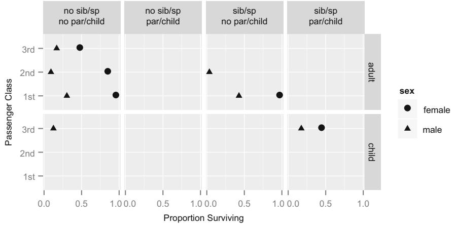

Fig. 12.2 Multi-way summary of Titanic survival

Note that none of the effects of sibsp or parch for common passenger groups appear strong on an absolute risk scale.

12.2 Exploring Trends with Nonparametric Regression

As described in Section 2.4.7, the loess smoother has excellent performance when the response is binary, as long as outlier detection is turned off. Here we use a ggplot2 add-on function histSpikeg in the Hmisc package to obtain and plot the loess fit and age distribution. histSpikeg uses the “no iteration” option for the R lowess function when the response is binary.

# Figure 12.3
b − scale_size_discrete ( range =c(.1 , .85))
yl − ylab(NULL)
p1 − ggplot (t3 , aes(x=age , y= survived )) +
      histSpikeg(survived ← age , lowess =TRUE , data=t3) +
      ylim (0,1) + yl
p2 − ggplot (t3 , aes(x=age , y=survived , color =sex)) +
      histSpikeg(survived ← age + sex , lowess =TRUE ,
                  data=t3) + ylim (0,1) + yl
p3 − ggplot (t3 , aes(x=age , y=survived , size =pclass )) +
      histSpikeg(survived ← age + pclass , lowess =TRUE ,
                  data=t3) + b + ylim (0,1) + yl
p4 − ggplot (t3 , aes(x=age , y=survived , color =sex ,
       size=pclass )) +
      histSpikeg(survived ← age + sex + pclass ,
                  lowess =TRUE , data=t3) +
      b + ylim (0,1) + yl
gridExtra :: grid.arrange (p1 , p2 , p3 , p4 , ncol =2) # combine 4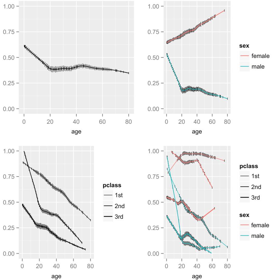

Fig. 12.3 Nonparametric regression (loess) estimates of the relationship between age and the probability of surviving the Titanic, with tick marks depicting the age distribution. The top left panel shows unstratified estimates of the probability of survival. Other panels show nonparametric estimates by various stratifications.

Figure 12.3 shows much of the story of passenger survival patterns. “Women and children first” seems to be true except for women in third class. It is interesting that there is no real cutoff for who is considered a child. For men, the younger the greater chance of surviving. The interpretation of the effects of the “number of relatives”-type variables will be more difficult, as their definitions are a function of age. Figure 12.4 shows these relationships.

# Figure 12.4
top − theme ( legend.position = ' top ' )
p1 − ggplot (t3 , aes(x=age , y=survived , color =cut2( sibsp ,
       0:2))) + stat_plsmo () + b + ylim (0,1) + yl + top +
      scale_color_discrete ( name= ' siblings/spouses ' )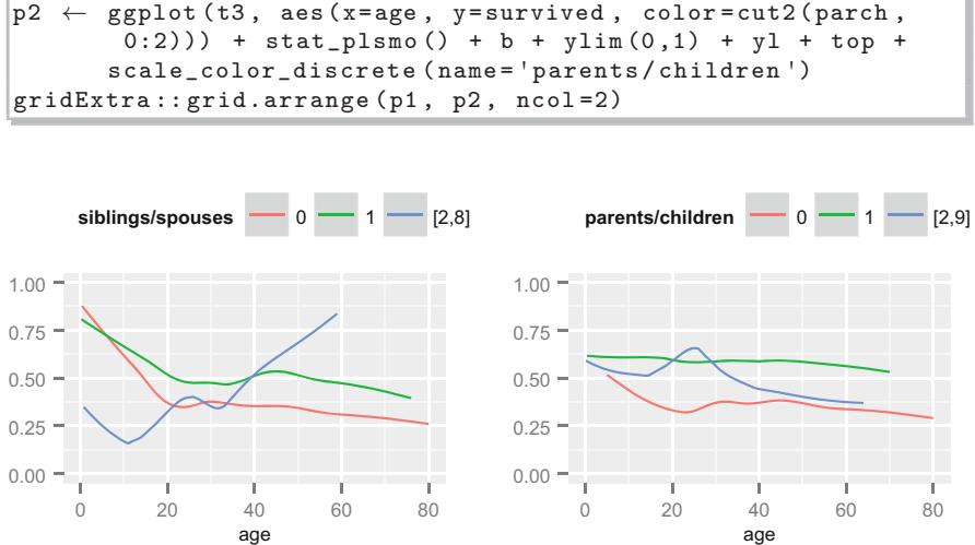

Fig. 12.4 Relationship between age and survival stratified by the number of siblings or spouses on board (left panel) or by the number of parents or children of the passenger on board (right panel).

12.3 Binary Logistic Model With Casewise Deletion of Missing Values

What follows is the standard analysis based on eliminating observations having any missing data. We develop an initial somewhat saturated logistic model, allowing for a flexible nonlinear age effect that can differ in shape for all six sex ≤ class strata. The sibsp and parch variables do not have sufficiently dispersed distributions to allow for us to model them nonlinearly. Also, there are too few passengers with nonzero values of these two variables in sex ≤ pclass ≤ age strata to allow us to model complex interactions involving them. The meaning of these variables does depend on the passenger’s age, so we consider only age interactions involving sibsp and parch.

f1 − lrm(survived ← sex*pclass *rcs(age ,5) +
           rcs(age ,5)*(sibsp + parch ), data =t3) # Table 12.1
latex (anova (f1), file= ' ' , label= ' titanic-anova3 ' ,
      size= ' small ' )

Three-way interactions are clearly insignificant (P = 0.4) in Table 12.1. So is parch (P = 0.6 for testing the combined main effect + interaction effects for parch, i.e., whether parch is important for any age). These effects would be deleted in almost all bootstrap resamples had we bootstrapped a variable selection procedure using σ = 0.1 for retention of terms, so we can safely ignore these terms for future steps. The model not containing those terms

Table 12.1 Wald Statistics for survived
——————————————–

	σ2	d.f.	P
sex (Factor+Higher Order Factors)	187.15		15 < 0.0001
All Interactions	59.74		14 < 0.0001
pclass (Factor+Higher Order Factors)	100.10		20 < 0.0001
All Interactions	46.51	18	0.0003
age (Factor+Higher Order Factors)	56.20	32	0.0052
All Interactions	34.57	28	0.1826
Nonlinear (Factor+Higher Order Factors)	28.66	24	0.2331
sibsp (Factor+Higher Order Factors)	19.67	5	0.0014
All Interactions	12.13	4	0.0164
parch (Factor+Higher Order Factors)	3.51	5	0.6217
All Interactions	3.51	4	0.4761
sex ∼ pclass (Factor+Higher Order Factors)	42.43		10 < 0.0001
sex ∼ age (Factor+Higher Order Factors)	15.89	12	0.1962
Nonlinear (Factor+Higher Order Factors)	14.47	9	0.1066
Nonlinear Interaction : f(A,B) vs. AB	4.17	3	0.2441
pclass ∼ age (Factor+Higher Order Factors)	13.47	16	0.6385
Nonlinear (Factor+Higher Order Factors)	12.92	12	0.3749
Nonlinear Interaction : f(A,B) vs. AB	6.88	6	0.3324
age ∼ sibsp (Factor+Higher Order Factors)	12.13	4	0.0164
Nonlinear	1.76	3	0.6235
Nonlinear Interaction : f(A,B) vs. AB	1.76	3	0.6235
age ∼ parch (Factor+Higher Order Factors)	3.51	4	0.4761
Nonlinear	1.80	3	0.6147
Nonlinear Interaction : f(A,B) vs. AB	1.80	3	0.6147
sex ∼ pclass ∼ age (Factor+Higher Order Factors)	8.34	8	0.4006
Nonlinear	7.74	6	0.2581
TOTAL NONLINEAR	28.66	24	0.2331
TOTAL INTERACTION	75.61		30 < 0.0001
TOTAL NONLINEAR + INTERACTION	79.49		33 < 0.0001
TOTAL	241.93		39 < 0.0001

is fitted below. The ^2 in the model formula means to expand the terms in parentheses to include all main effects and second-order interactions.

f − lrm(survived ← (sex + pclass + rcs(age ,5))−2 +
         rcs(age ,5)*sibsp , data=t3)
print (f, latex =TRUE)

Logistic Regression Model

lrm(formula = survived ~ (sex + pclass + rcs(age, 5))^2 + rcs(age, 5) * sibsp, data = t3)

Frequencies of Missing Values Due to Each Variable

survived	sex	pclass	age	sibsp
0	0	0	263	0

		Model Likelihood		Discrimination		Rank Discrim.
		Ratio Test		Indexes		Indexes
Obs 1046	β2 LR	553.87	R2	0.555	C	0.878
0 619	d.f.	26	g	2.427	Dxy	0.756
1 427	β2) Pr(>	< 0.0001	gr	11.325	α	0.758
α log L 6≤10−6 max αρ			gp	0.365	Γa	0.366
			Brier	0.130

	Coef	S.E.	Wald Z	Pr(> Z )
Intercept	3.3075	1.8427	1.79	0.0727
sex=male	-1.1478	1.0878	-1.06	0.2914
pclass=2nd	6.7309	3.9617	1.70	0.0893
pclass=3rd	-1.6437	1.8299	-0.90	0.3691
age	0.0886	0.1346	0.66	0.5102
age’	-0.7410	0.6513	-1.14	0.2552
age”	4.9264	4.0047	1.23	0.2186
age”’	-6.6129	5.4100	-1.22	0.2216
sibsp	-1.0446	0.3441	-3.04	0.0024
sex=male * pclass=2nd	-0.7682	0.7083	-1.08	0.2781
sex=male * pclass=3rd	2.1520	0.6214	3.46	0.0005
sex=male * age	-0.2191	0.0722	-3.04	0.0024
sex=male * age’	1.0842	0.3886	2.79	0.0053
sex=male * age”	-6.5578	2.6511	-2.47	0.0134
sex=male * age”’	8.3716	3.8532	2.17	0.0298
pclass=2nd * age	-0.5446	0.2653	-2.05	0.0401
pclass=3rd * age	-0.1634	0.1308	-1.25	0.2118
pclass=2nd * age’	1.9156	1.0189	1.88	0.0601
pclass=3rd * age’	0.8205	0.6091	1.35	0.1780
pclass=2nd * age”	-8.9545	5.5027	-1.63	0.1037
pclass=3rd * age”	-5.4276	3.6475	-1.49	0.1367
pclass=2nd * age”’	9.3926	6.9559	1.35	0.1769
pclass=3rd * age”’	7.5403	4.8519	1.55	0.1202
age * sibsp	0.0357	0.0340	1.05	0.2933
age’ * sibsp	-0.0467	0.2213	-0.21	0.8330
age” * sibsp	0.5574	1.6680	0.33	0.7382
age”’ * sibsp	-1.1937	2.5711	-0.46	0.6425

latex (anova (f),file= ’ ’ ,label= ’ titanic-anova2 ’ ,size= ’ small ’ ) #12.2

This is a very powerful model (ROC area = c = 0.88); the survival patterns are easy to detect. The Wald ANOVA in Table 12.2 indicates especially strong sex and pclass effects (β² = 199 and 109, respectively). There is a very strong

Table 12.2 Wald Statistics for survived

	σ2	d.f.	P
sex (Factor+Higher Order Factors)	199.42		7 < 0.0001
All Interactions	56.14		6 < 0.0001
pclass (Factor+Higher Order Factors)	108.73		12 < 0.0001
All Interactions	42.83		10 < 0.0001
age (Factor+Higher Order Factors)	47.04	20	0.0006
All Interactions	24.51	16	0.0789
Nonlinear (Factor+Higher Order Factors)	22.72	15	0.0902
sibsp (Factor+Higher Order Factors)	19.95	5	0.0013
All Interactions	10.99	4	0.0267
sex ∼ pclass (Factor+Higher Order Factors)	35.40		2 < 0.0001
sex ∼ age (Factor+Higher Order Factors)	10.08	4	0.0391
Nonlinear	8.17	3	0.0426
Nonlinear Interaction : f(A,B) vs. AB	8.17	3	0.0426
pclass ∼ age (Factor+Higher Order Factors)	6.86	8	0.5516
Nonlinear	6.11	6	0.4113
Nonlinear Interaction : f(A,B) vs. AB	6.11	6	0.4113
age ∼ sibsp (Factor+Higher Order Factors)	10.99	4	0.0267
Nonlinear	1.81	3	0.6134
Nonlinear Interaction : f(A,B) vs. AB	1.81	3	0.6134
TOTAL NONLINEAR	22.72	15	0.0902
TOTAL INTERACTION	67.58		18 < 0.0001
TOTAL NONLINEAR + INTERACTION	70.68		21 < 0.0001
TOTAL	253.18		26 < 0.0001

sex ≤ pclass interaction and a strong age ≤ sibsp interaction, considering the strength of sibsp overall.

Let us examine the shapes of predictor effects. With so many interactions in the model we need to obtain predicted values at least for all combinations of sex and pclass. For sibsp we consider only two of its possible values.

p − Predict(f, age , sex , pclass , sibsp =0, fun=plogis )
ggplot (p) # Fig. 12.5

Note the agreement between the lower right-hand panel of Figure 12.3 with Figure 12.5. This results from our use of similar flexibility in the parametric and nonparametric approaches (and similar effective degrees of freedom). The estimated effect of sibsp as a function of age is shown in Figure 12.6.

ggplot ( Predict(f, sibsp , age=c(10,15,20 ,50), conf.int= FALSE ))
## Figure 12.6

Note that children having many siblings apparently had lower survival. Married adults had slightly higher survival than unmarried ones.

There will never be another Titanic, so we do not need to validate the model for prospective use. But we use the bootstrap to validate the model anyway, in an effort to detect whether it is overfitting the data. We do not penalize the calculations that follow for having examined the effect of parch or

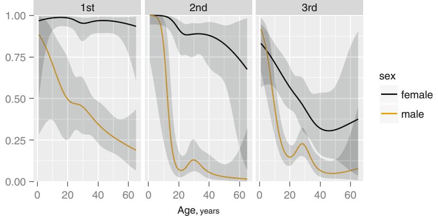
Fig. 12.5 Effects of predictors on probability of survival of Titanic passengers, estimated for zero siblings or spouses

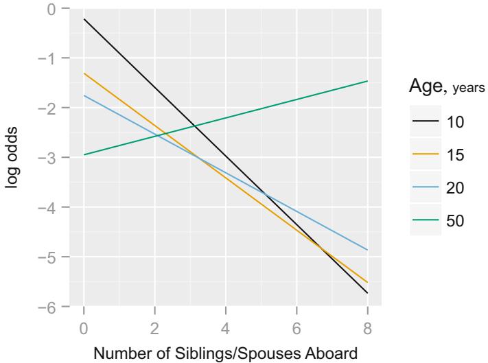
Fig. 12.6 Effect of number of siblings and spouses on the log odds of surviving, for third class males

for testing three-way interactions, in the belief that these tests would replicate well.

f − update (f, x=TRUE , y= TRUE)
# x=TRUE , y= TRUE adds raw data to fit object so can bootstrap
set.seed (131) # so can replicate re-samples
latex ( validate(f, B=200), digits =2, size = ' Ssize ' )

Index	Original Training		Test	Optimism Corrected
	Sample	Sample	Sample		Index
Dxy	0.76	0.77	0.74	0.03	0.72 200
R2	0.55	0.58	0.53	0.05	0.50 200
Intercept	0.00	0.00	×0.08	0.08	×0.08 200
Slope	1.00	1.00	0.87	0.13	0.87 200
Emax	0.00	0.00	0.05	0.05	0.05 200
D	0.53	0.56	0.50	0.06	0.46 200
U	0.00	0.00	0.01	×0.01	0.01 200
Q	0.53	0.56	0.49	0.07	0.46 200
B	0.13	0.13	0.13	×0.01	0.14 200
g	2.43	2.75	2.37	0.37	2.05 200
gp	0.37	0.37	0.35	0.02	0.35 200

n=1046 Mean absolute error=0.009 Mean squared error=0.00012
0.9 Quantile of absolute error =0.017

The output of validate indicates minor overfitting. Overfitting would have been worse had the risk factors not been so strong. The closeness of the calibration curve to the 45^≤ line in Figure 12.7 demonstrates excellent validation on an absolute probability scale. But the extent of missing data casts some doubt on the validity of this model, and on the efficiency of its parameter estimates.

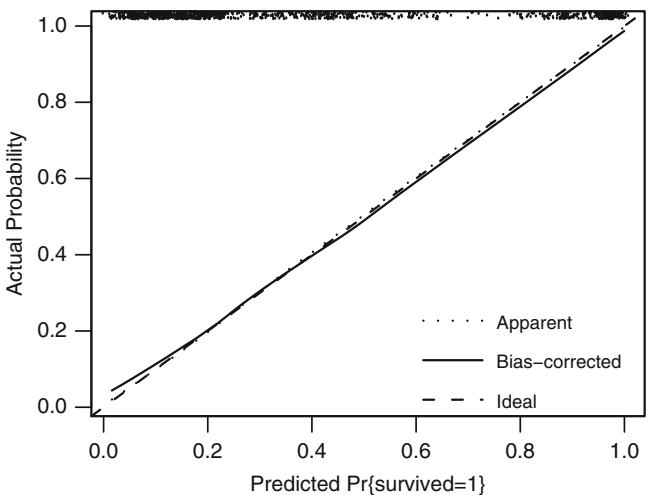
Fig. 12.7 Bootstrap overfitting-corrected loess nonparametric calibration curve for casewise deletion model

12.4 Examining Missing Data Patterns

The first step to dealing with missing data is understanding the patterns of missing values. To do this we use the Hmisc library’s naclus and naplot functions, and the recursive partitioning library of Atkinson and Therneau. Below naclus tells us which variables tend to be missing on the same persons, and it computes the proportion of missing values for each variable. The rpart function derives a tree to predict which types of passengers tended to have age missing.

na.patterns − naclus ( titanic3)
require( rpart ) # Recursive partitioning package
who.na − rpart (is.na(age) ← sex + pclass + survived +
                 sibsp + parch , data=titanic3 , minbucket =15)
naplot (na.patterns , ' na per var ' )
plot(who.na , margin =.1); text(who.na ) # Figure 12.8
plot( na.patterns )

We see in Figure 12.8 that age tends to be missing on the same passengers as the body bag identifier, and that it is missing in only 0.09 of first or second class passengers. The category of passengers having the highest fraction of missing ages is third class passengers having no parents or children on board. Below we use Hmisc’s summary.formula function to plot simple descriptive statistics on the fraction of missing ages, stratified by other variables. We see that without adjusting for other variables, age is slightly more missing on nonsurviving passengers.

plot( summary( is.na (age) ← sex + pclass + survived +
             sibsp + parch , data=t3)) # Figure 12.9

Let us derive a logistic model to predict missingness of age, to see if the survival bias maintains after adjustment for the other variables.

m − lrm(is.na(age) ← sex * pclass + survived + sibsp + parch ,
         data=t3)
print(m, latex=TRUE , needspace = ' 2in ' )

Logistic Regression Model

lrm(formula = is.na(age) ~ sex * pclass + survived + sibsp + parch, data = t3)

			Model Likelihood		Discrimination		Rank Discrim.
			Ratio Test		Indexes		Indexes
Obs	1309	β2 LR	114.99	R2	0.133	C	0.703
FALSE	1046	d.f.	8	g	1.015	Dxy	0.406
TRUE	263	β2) Pr(>	< 0.0001	gr	2.759	α	0.452
α log L max αρ	5≤10−6			gp	0.126	Γa	0.131
				Brier	0.148

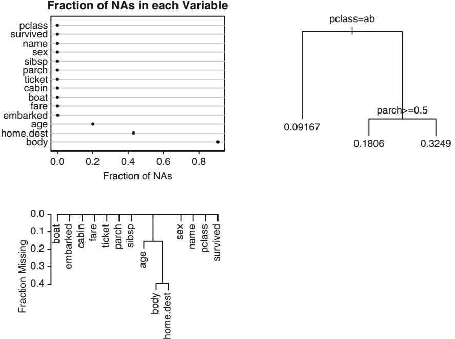
Fig. 12.8 Patterns of missing data. Upper left panel shows the fraction of observations missing on each predictor. Lower panel depicts a hierarchical cluster analysis of missingness combinations. The similarity measure shown on the Y -axis is the fraction of observations for which both variables are missing. Right panel shows the result of recursive partitioning for predicting is.na(age). The rpart function found only strong patterns according to passenger class.

	Coef	S.E.	Wald Z	Pr(> Z )
Intercept	-2.2030	0.3641	-6.05	< 0.0001
sex=male	0.6440	0.3953	1.63	0.1033
pclass=2nd	-1.0079	0.6658	-1.51	0.1300
pclass=3rd	1.6124	0.3596	4.48	< 0.0001
survived	-0.1806	0.1828	-0.99	0.3232
sibsp	0.0435	0.0737	0.59	0.5548
parch	-0.3526	0.1253	-2.81	0.0049
sex=male * pclass=2nd	0.1347	0.7545	0.18	0.8583
sex=male * pclass=3rd	-0.8563	0.4214	-2.03	0.0422

latex (anova (m), file= ' ' , label= ' titanic-anova.na ' )
    # Table 12.3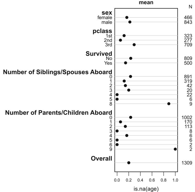

Fig. 12.9 Univariable descriptions of proportion of passengers with missing age

Fortunately, after controlling for other variables, Table 12.3 provides evidence that nonsurviving passengers are no more likely to have age missing. The only important predictors of missingness are pclass and parch (the more parents or children the passenger has on board, the less likely age was to be missing).

12.5 Multiple Imputation

Multiple imputation is expected to reduce bias in estimates as well as to provide an estimate of the variance–covariance matrix of Λˆ penalized for imputation. With multiple imputation, survival status can be used to impute missing ages, so the age relationship will not be as attenuated as with single conditional mean imputation. aregImpute The following uses the Hmisc package aregImpute function to do predictive mean matching, using van Buuren’s “Type 1” matching [85, Section 3.4.2] in conjunction with bootstrapping to incorporate all uncertainties, in the context of smooth additive imputation

	β2	d.f.	P
sex (Factor+Higher Order Factors)	5.61	3	0.1324
All Interactions	5.58	2	0.0614
pclass (Factor+Higher Order Factors)	68.43	4	< 0.0001
All Interactions	5.58	2	0.0614
survived	0.98	1	0.3232
sibsp	0.35	1	0.5548
parch	7.92	1	0.0049
sex ≤ pclass (Factor+Higher Order Factors)	5.58	2	0.0614
TOTAL	82.90	8	< 0.0001

Table 12.3 Wald Statistics for is.na(age)

models. Sampling of donors is handled by distance weighting to yield better distributions of imputed values. By default, aregImpute does not transform age when it is being predicted from the other variables. Four knots are used to transform age when used to impute other variables (not needed here as no other missings were present in the variables of interest). Since the fraction of observations with missing age is ²⁶³ ¹³⁰⁹ = 0.2 we use 20 imputations.

set.seed (17) # so can reproduce random aspects
mi − aregImpute(← age + sex + pclass +
                 sibsp + parch + survived ,
                 data =t3 , n.impute =20, nk=4, pr= FALSE)

Multiple Imputation using Bootstrap and PMM
aregImpute( formula = ◦age + sex + pclass + sibsp + parch + survived ,
   data = t3, n.impute = 20, nk = 4, pr = FALSE)
n: 1309 p: 6 Imputations: 20 nk: 4
Number of NAs:
    age sex pclass sibsp parch survived
    263 0 0 0 0 0
       type d.f.
age s 1
sex c 1
pclass c 2
sibsp s 2
parch s 2
survived l 1
Transformation of Target Variables Forced to be Linear
R-squares for Predicting Non- Missing Values for Each Variable
Using Last Imputations of Predictors
 age
0.295

#	Print	the	first		10		imputations	for	the	first
#	having		missing		age
	mi$imputed$age [1:10,					1:10]

	[,1]	[,2]	[,3]	[,4]	[,5]	[,6]	[,7]	[,8]	[,9]	[,10]
16	40	49	24	29	60.0	58	64	36	50	61
38	33	45	40	49	80.0	2	38	38	36	53
41	29	24	19	31	40.0	60	64	42	30	65
47	40	42	29	48	36.0	46	64	30	38	42
60	52	40	22	31	38.0	22	19	24	40	33
70	16	14	23	23	18.0	24	19	27	59	23
71	30	62	57	30	42.0	31	64	40	40	63
75	43	23	36	61	45.5	58	64	27	24	50
81	44	57	47	31	45.0	30	64	62	39	67
107	52	18	24	62	32.5	38	64	47	19	23

	plot(mi)
Ecdf (t3$age , add=TRUE , col= ’ gray ’ , lwd=2,

	subtitles= FALSE)#Fig. 12.10

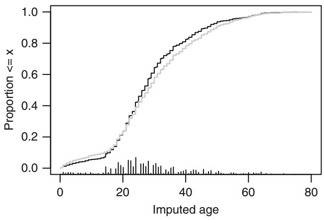
Fig. 12.10 Distributions of imputed and actual ages for the Titanic dataset. Imputed values are in black and actual ages in gray.

We now fit logistic models for five completed datasets. The fit.mult.impute function fits five models and examines the within– and between–imputation variances to compute an imputation-corrected variance–covariance matrix that is stored in the fit object f.mi. fit.mult.impute will also average the five Λˆ vectors, storing the result in f.mi$coefficients. The function also prints the ratio of imputation-corrected variances to average ordinary variances.

f.mi − fit.mult.impute (
  survived ← (sex + pclass + rcs(age ,5))−2 +
  rcs(age ,5)*sibsp ,

Table 12.4		Wald Statistics for survived
————	–	——————————	–	–

	σ2	d.f.	P
sex (Factor+Higher Order Factors)	240.42		7 < 0.0001
All Interactions	54.56		6 < 0.0001
pclass (Factor+Higher Order Factors)	114.21		12 < 0.0001
All Interactions	36.43	10	0.0001
age (Factor+Higher Order Factors)	50.37	20	0.0002
All Interactions	25.88	16	0.0557
Nonlinear (Factor+Higher Order Factors)	24.21	15	0.0616
sibsp (Factor+Higher Order Factors)	24.22	5	0.0002
All Interactions	12.86	4	0.0120
sex ∼ pclass (Factor+Higher Order Factors)	30.99		2 < 0.0001
sex ∼ age (Factor+Higher Order Factors)	11.38	4	0.0226
Nonlinear	8.15	3	0.0430
Nonlinear Interaction : f(A,B) vs. AB	8.15	3	0.0430
pclass ∼ age (Factor+Higher Order Factors)	5.30	8	0.7246
Nonlinear	4.63	6	0.5918
Nonlinear Interaction : f(A,B) vs. AB	4.63	6	0.5918
age ∼ sibsp (Factor+Higher Order Factors)	12.86	4	0.0120
Nonlinear	1.84	3	0.6058
Nonlinear Interaction : f(A,B) vs. AB	1.84	3	0.6058
TOTAL NONLINEAR	24.21	15	0.0616
TOTAL INTERACTION	67.12		18 < 0.0001
TOTAL NONLINEAR + INTERACTION	70.99		21 < 0.0001
TOTAL	298.78		26 < 0.0001

lrm , mi , data =t3 , pr=FALSE )
latex (anova (f.mi), file= ' ' , label= ' titanic-anova.mi ' ,
       size= ' small ' ) # Table 12.4

The Wald β² for age is reduced by accounting for imputation but is increased (by a lesser amount) by using patterns of association with survival status to impute missing age. The Wald tests are all adjusted for multiple imputation. Now examine the fitted age relationship using multiple imputation vs. casewise deletion.

p1 − Predict(f, age , pclass , sex , sibsp =0, fun=plogis )
p2 − Predict(f.mi , age , pclass , sex , sibsp =0, fun=plogis )
p − rbind ( ' Casewise Deletion ' =p1 , ' Multiple Imputation ' =p2)
ggplot (p, groups = ' sex ' , ylab= ' Probability of Surviving ' )
# Figure 12.11

12.6 Summarizing the Fitted Model

In this section we depict the model fitted using multiple imputation, by computing odds ratios and by showing various predicted values. For age, the odds ratio for an increase from 1 year old to 30 years old is computed, instead of the default odds ratio based on outer quartiles of age. The estimated odds

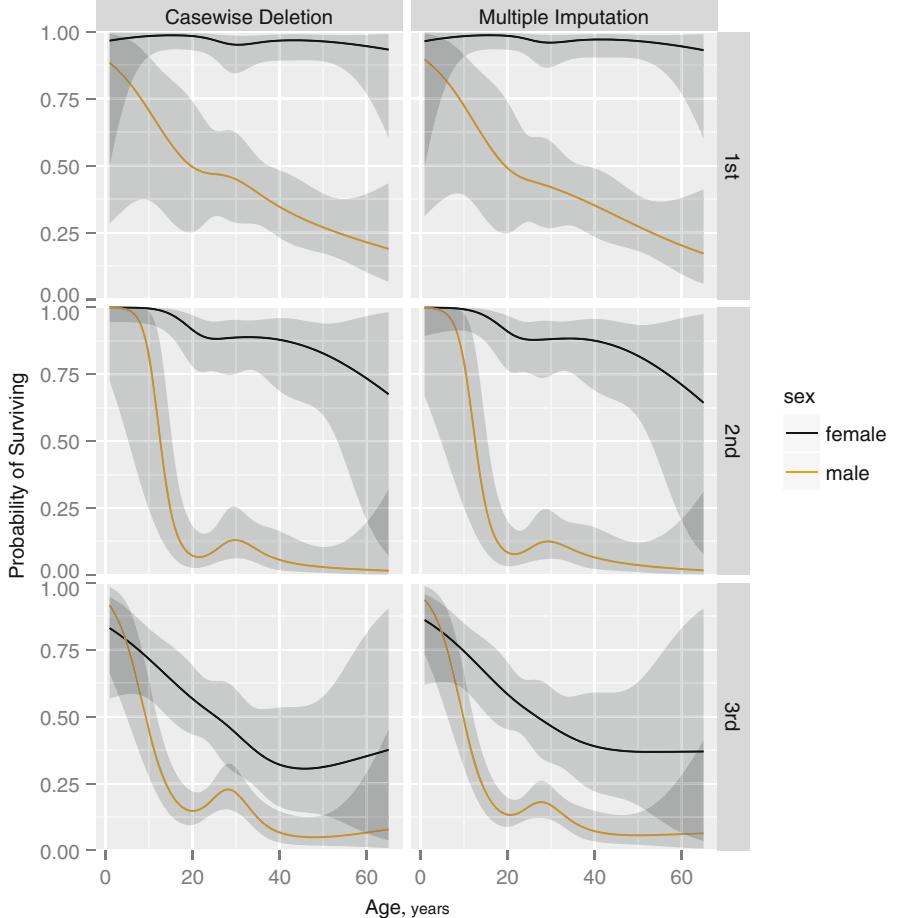
Fig. 12.11 Predicted probability of survival for males from fit using casewise deletion again (top) and multiple random draw imputation (bottom). Both sets of predictions are for sibsp=0.

ratios are very dependent on the levels of interacting factors, so Figure 12.12 depicts only one of many patterns.

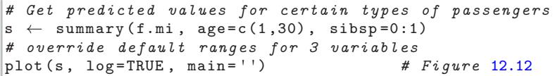
Now compute estimated probabilities of survival for a variety of settings of the predictors.

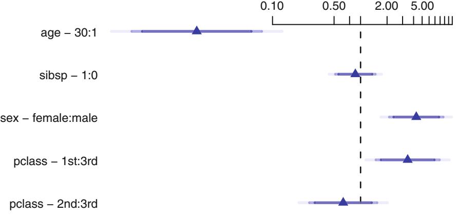
Adjusted to:sex=male pclass=3rd age=28 sibsp=0

Fig. 12.12 Odds ratios for some predictor settings

phat − predict(f.mi ,
                combos −
         expand.grid (age=c(2,21 ,50), sex= levels (t3$sex),
                     pclass =levels (t3$pclass ),
                     sibsp =0), type= ' fitted ' )
# Can also use Predict(f.mi , age=c(2,21 ,50), sex , pclass ,
# sibsp=0, fun=plogis)$ yhat
options( digits =1)
data.frame( combos , phat)

	age	sex	pclass	sibsp	phat
1	2	female	1st	0	0.97
2	21	female	1st	0	0.98
3	50	female	1st	0	0.97
4	2	male	1st	0	0.88
5	21	male	1st	0	0.48
6	50	male	1st	0	0.27
7	2	female	2nd	0	1.00
8	21	female	2nd	0	0.90
9	50	female	2nd	0	0.82
10	2	male	2nd	0	1.00
11	21	male	2nd	0	0.08
12	50	male	2nd	0	0.04
13	2	female	3rd	0	0.85
14	21	female	3rd	0	0.57
15	50	female	3rd	0	0.37
16	2	male	3rd	0	0.91
17	21	male	3rd	0	0.13
18	50	male	3rd	0	0.06

options( digits =5)

We can also get predicted values by creating an R function that will evaluate the model on demand.

pred.logit − Function( f.mi)
# Note: if don ' t define sibsp to pred.logit , defaults to 0
# normally just type the function name to see its body
latex (pred.logit , file= ' ' , type= ' Sinput ' , size= ' small ' ,
       width.cutoff =49)
pred.logit − function ( sex = "male " , pcl as s = "3rd " ,
    age = 28, sibsp = 0)
{
    3.2427671 × 0.95431809 ` ( s ex == "male " ) + 5 . 4 0 8 6 5 0 5 `
         ( p c l a s s == "2nd " ) × 1.3378623 ` ( p c l a s s ==
         "3rd ") + 0.091162649 ` age × 0.00031204327 `
        pmax ( age × 6, 0)−3 + 0.0021750413 ` pmax ( age ×
         21, 0)−3 × 0.0027627032 ` pmax ( age × 27, 0)−3 +
         0.0009805137 ` pmax ( age × 36, 0)−3 × 8.0808484e×05 `
        pmax ( age × 55.8 , 0)−3 × 1.1567976 ` sibsp +
         ( s ex == "male " ) ` ( ×0.46061284 ` ( p c l a s s ==
             "2nd ") + 2.0406523 ` ( p c l a s s == "3 rd " ) ) +
         ( s ex == "male " ) ` ( ×0.22469066 ` age + 0.00043708296 `
             pmax ( age × 6, 0)−3 × 0.0026505136 ` pmax ( age ×
             21, 0)−3 + 0.0031201404 ` pmax ( age × 27,
             0 )−3 × 0.00097923749 ` pmax ( age × 36,
             0 )−3 + 7.2527708e×05 ` pmax ( age × 55.8 ,
             0 )− 3 ) + ( p c l a s s == "2nd " ) ` ( ×0.46144083 `
         age + 0.00070194849 ` pmax ( age × 6, 0)−3 ×
         0.0034726662 ` pmax ( age × 21, 0)−3 + 0.0035255387 `
        pmax ( age × 27, 0)−3 × 0.0007900891 ` pmax ( age ×
         36, 0)−3 + 3.5268151e×05 ` pmax ( age × 55.8 ,
         0 )− 3 ) + ( p c l a s s == "3 rd ") ` ( ×0.17513289 `
         age + 0.00035283358 ` pmax ( age × 6, 0)−3 ×
         0.0023049372 ` pmax ( age × 21, 0)−3 + 0.0028978962 `
        pmax ( age × 27, 0)−3 × 0.00105145 ` pmax ( age ×
         36, 0)−3 + 0.00010565735 ` pmax ( age × 55.8 ,
         0 )− 3) + sibsp ` (0.040830773 ` age × 1.5627772e×05 `
        pmax ( age × 6, 0)−3 + 0.00012790256 ` pmax ( age ×
         21, 0)−3 × 0.00025039385 ` pmax ( age × 27,
         0 )−3 + 0.00017871701 ` pmax ( age × 36, 0)−3 ×
         4.0597949e×05 ` pmax ( age × 55.8 , 0)− 3 )
}

# Run the newly created function
plogis ( pred.logit (age=c(2,21 ,50), sex= ' male ' , pclass = ' 3rd ' ))

1 0.914817 0.132640 0.056248

A nomogram could be used to obtain predicted values manually, but this is not feasible when so many interaction terms are present.

Chapter 13 Ordinal Logistic Regression

13.1 Background

Many medical and epidemiologic studies incorporate an ordinal response variable. In some cases an ordinal response Y represents levels of a standard measurement scale such as severity of pain (none, mild, moderate, severe). In other cases, ordinal responses are constructed by specifying a hierarchy of separate endpoints. For example, clinicians may specify an ordering of the severity of several component events and assign patients to the worst event present from among none, heart attack, disabling stroke, and death. Still another use of ordinal response methods is the application of rank-based methods to continuous responses so as to obtain robust inferences. For example, the proportional odds model described later allows for a continuous Y and is really a generalization of the Wilcoxon–Mann–Whitney rank test. Thus the semiparametric proportional odds model is a direct competitor of ordinary linear models.

There are many variations of logistic models used for predicting an ordinal response variable Y . All of them have the advantage that they do not assume a spacing between levels of Y . In other words, the same regression coefficients and P-values result from an analysis of a response variable having levels 0, 1, 2 when the levels are recoded 0, 1, 20. Thus ordinal models use only the rankordering of values of Y .

In this chapter we consider two of the most popular ordinal logistic models, the proportional odds (PO) form of an ordinal logistic model647 and the forward continuation ratio (CR) ordinal logistic model.190 Chapter 15 deals with a wider variety of ordinal models with emphasis on analysis of continuous Y . ¹

^© Springer International Publishing Switzerland 2015 F.E. Harrell, Jr., Regression Modeling Strategies, Springer Series in Statistics, DOI 10.1007/978-3-319-19425-7 13

13.2 Ordinality Assumption

A basic assumption of all commonly used ordinal regression models is that the response variable behaves in an ordinal fashion with respect to each predictor. Assuming that a predictor X is linearly related to the log odds of some appropriate event, a simple way to check for ordinality is to plot the mean of X stratified by levels of Y . These means should be in a consistent order. If for many of the Xs, two adjacent categories of Y do not distinguish the means, that is evidence that those levels of Y should be pooled.

One can also estimate the mean or expected value of X|Y = j (E(X|Y = j)) given that the ordinal model assumptions hold. This is a useful tool for checking those assumptions, at least in an unadjusted fashion. For simplicity, assume that X is discrete, and let Pjx = Pr(Y = j|X = x) be the probability that Y = j given X = x that is dictated from the model being fitted, with X being the only predictor in the model. Then

\[\Pr(X=x|Y=j) = \Pr(Y=j|X=x)\Pr(X=x)/\Pr(Y=j)\]

\[E(X|Y=j) = \sum\_{x} x P\_{jx} \Pr(X=x)/\Pr(Y=j),\tag{13.1}\]

and the expectation can be estimated by

\[ \hat{E}(X|Y=j) = \sum\_{x} x \hat{P}\_{jx} f\_x / g\_j,\tag{13.2} \]

where Pˆjx denotes the estimate of Pjx from the fitted one-predictor model (for inner values of Y in the PO models, these probabilities are differences between terms given by Equation 13.4 below), f^x is the frequency of X = x in the sample of size n, and g^j is the frequency of Y = j in the sample. This estimate can be computed conveniently without grouping the data by X. For n subjects let the n values of X be x1, x2,…,xn. Then

\[ \hat{E}(X|Y=j) = \sum\_{i=1}^{n} x\_i \hat{P}\_{jx\_i} / g\_j. \tag{13.3} \]

Note that if one were to compute differences between conditional means of X and the conditional means of X given PO, and if furthermore the means were conditioned on Y ← j instead of Y = j, the result would be proportional to means of score residuals defined later in Equation 13.6.

13.3 Proportional Odds Model

13.3.1 Model

The most commonly used ordinal logistic model was described in Walker and Duncan647 and later called the proportional odds (PO) model by Mc-Cullagh.449 The PO model is best stated as follows, for a response variable having levels 0, 1, 2,…,k:

\[\Pr[Y \ge j | X] = \frac{1}{1 + \exp[- (\alpha\_j + X\beta)]},\tag{13.4}\]

where j = 1, 2,…,k. Some authors write the model in terms of Y − j. Our formulation makes the model coefficients consistent with the binary logistic model. There are k intercepts (σs). For fixed j, the model is an ordinary logistic model for the event Y ← j. By using a common vector of regression coefficients Λ connecting probabilities for varying j, the PO model allows for parsimonious modeling of the distribution of Y . ²

There is a nice connection between the PO model and the Wilcoxon– Mann–Whitney two-sample test: when there is a single predictor X¹ that is binary, the numerator of the score test for testing H⁰ : Λ¹ = 0 is proportional to the two-sample test statistic [664, pp. 2258–2259].

13.3.2 Assumptions and Interpretation of Parameters

There is an implicit assumption in the PO model that the regression coefficients (Λ) are independent of j, the cutoff level for Y . One could say that there is no X ≤Y interaction if PO holds. For a specific Y -cutoff j, the model has the same assumptions as the binary logistic model (Section 10.1.1). That is, the model in its simplest form assumes the log odds that Y ← j is linearly related to each X and that there is no interaction between the Xs.

In designing clinical studies, one sometimes hears the statement that an ordinal outcome should be avoided since statistical tests of patterns of those outcomes are hard to interpret. In fact, one interprets effects in the PO model using ordinary odds ratios. The difference is that a single odds ratio is assumed to apply equally to all events Y ← j, j = 1, 2,…,k. If linearity and additivity hold, the X^m +1: X^m odds ratio for Y ← j is exp(Λm), whatever the cutoff j.

The proportional hazards assumption is frequently violated, just as the assumptions of normality of residuals with equal variance in ordinary regression are frequently violated, but the PO model can still be useful and powerful in this situation. As stated by Senn and Julious564,

Clearly, the dependence of the proportional odds model on the assumption of proportionality can be over-stressed. Suppose that two different statisticians would cut the same three-point scale at different cut points. It is hard to see how anybody who could accept either dichotomy could object to the compromise answer produced by the proportional odds model.

Sometimes it helps in interpreting the model to estimate the mean Y as a function of one or more predictors, even though this assumes a spacing for 3 the Y -levels.

13.3.3 Estimation

The PO model is fitted using MLE on a somewhat complex likelihood function that is dependent on differences in logistic model probabilities. The estimation process forces the σs to be in descending order.

13.3.4 Residuals

Schoenfeld residuals557 are very effective233 in checking the proportional hazards assumption in the Cox132 survival model. For the PO model one could analogously compute each subject’s contribution to the first derivative of the log likelihood function with respect to Λm, average them separately by levels of Y , and examine trends in the residual plots as in Section 20.6.2. A few examples have shown that such plots are usually hard to interpret. Easily interpreted score residual plots for the PO model can be constructed, however, by using the fitted PO model to predict a series of binary events Y ← j, j = 1, 2,…,k, using the corresponding predicted probabilities

\[\hat{P}\_{ij} = \frac{1}{1 + \exp[- (\hat{\alpha}\_j + X\_i \hat{\beta})]},\tag{13.5}\]

where Xⁱ stands for a vector of predictors for subject i. Then, after forming an indicator variable for the event currently being predicted ([Yⁱ ← j]), one computes the score (first derivative) components Uim from an ordinary binary logistic model:

\[U\_{im} = X\_{im}([Y\_i \ge j] - \hat{P}\_{ij}),\tag{13.6}\]

for the subject i and predictor m. Then, for each column of U, plot the mean ^U¯·^m and confidence limits, with ^Y (i.e., ^j) on the ^x-axis. For each predictor the trend against j should be flat if PO holds. ^aIn binary logistic regression, partial residuals are very useful as they allow the analyst to fit linear effects

^a If ^χ^ˆ were derived from separate binary fits, all ^U¯·^m ^∈ 0.

for all the predictors but then to nonparametrically estimate the true transformation that each predictor requires (Section 10.4). The partial residual is defined as follows, for the ith subject and mth predictor variable.115, 373

\[r\_{im} = \hat{\beta}\_m X\_{im} + \frac{Y\_i - \hat{P}\_i}{\hat{P}\_i (1 - \hat{P}\_i)},\tag{13.7}\]

where

\[\hat{P}\_i = \frac{1}{1 + \exp[- (\alpha + X\_i \hat{\beta})]}. \tag{13.8}\]

A smoothed plot (e.g., using the moving linear regression algorithm in loess111) of Xim against rim provides a nonparametric estimate of how X^m relates to the log relative odds that Y = 1|Xm. For ordinal Y , we just need to compute binary model partial residuals for all cutoffs j:

\[r\_{im} = \hat{\beta}\_m X\_{im} + \frac{[Y\_i \ge j] - \hat{P}\_{ij}}{\hat{P}\_{ij}(1 - \hat{P}\_{ij})},\tag{13.9}\]

then to make a plot for each m showing smoothed partial residual curves for all j, looking for similar shapes and slopes for a given predictor for all j. Each curve provides an estimate of how X^m relates to the relative log odds that Y ← j. Since partial residuals allow examination of predictor transformations (linearity) while simultaneously allowing examination of PO (parallelism), partial residual plots are generally preferred over score residual plots for ordinal models.

Li and Shepherd402 have a residual for ordinal models that serves for the entire range of Y without the need to consider cutoffs. Their residual is useful for checking functional form of predictors but not the proportional odds assumption.

13.3.5 Assessment of Model Fit

Peterson and Harrell502 developed score and likelihood ratio tests for testing the PO assumption. The score test is used in the SAS PROC LOGISTIC, 540 but its extreme anti-conservatism in many cases can make it unreliable.502 ⁴

For determining whether the PO assumption is likely to be satisfied for each predictor separately, there are several graphics that are useful. One is the graph comparing means of X|Y with and without assuming PO, as described in Section 13.2 (see Figure 14.2 for an example). Another is the simple method of stratifying on each predictor and computing the logits of all proportions of the form Y ← j, j = 1, 2,…,k. When proportional odds holds, the differences in logits between different values of j should be the same at all levels of X, because the model dictates that logit(Y ← j|X) × logit(Y ← i|X) = σ^j × σi, for any constant X. An example of this is in Figure 13.1.

require( Hmisc )

getHdata(support)
sfdm − as.integer(support$ sfdm2) - 1
sf − function(y)
  c ( ' Y ≡ 1 ' =qlogis (mean(y ≡ 1)), ' Y ≡ 2 ' =qlogis (mean(y ≡ 2)),
    ' Y ≡ 3 ' =qlogis (mean(y ≡ 3)))
s − summary( sfdm ← adlsc + sex + age + meanbp , fun=sf ,
              data= support)
plot(s, which =1:3, pch=1:3, xlab= ' logit ' , vnames = ' names ' ,
     main= ' ' , width.factor =1.5) # Figure 13.1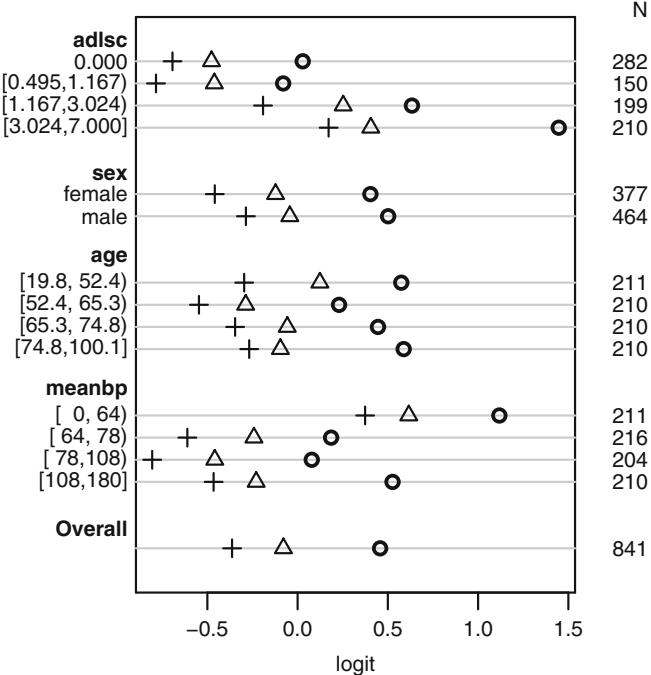

Fig. 13.1 Checking PO assumption separately for a series of predictors. The circle, triangle, and plus sign correspond to Y ≡ 1, 2, 3, respectively. PO is checked by examining the vertical constancy of distances between any two of these three symbols. Response variable is the severe functional disability scale sfdm2 from the 1000-patient SUPPORT dataset, with the last two categories combined because of low frequency of coma/intubation.

When Y is continuous or almost continuous and X is discrete, the PO model assumes that the logit of the cumulative distribution function of Y is parallel across categories of X. The corresponding, more rigid, assumptions of the ordinary linear model (here, parametric ANOVA) are parallelism and linearity if the normal inverse cumulative distribution function across categories of X. As an example consider the web site’s diabetes dataset, where we consider the distribution of log glycohemoglobin across subjects’ body frames.

getHdata(diabetes)
a − Ecdf(← log(glyhb), group=frame , fun=qnorm ,
       xlab= ' log(HbA1c) ' , label.curves =FALSE , data=diabetes ,
       ylab= expression( paste(Phi−-1 , (F[n](x ))))) # Fig. 13.2
b − Ecdf(← log(glyhb), group=frame , fun= qlogis ,
           xlab= ' log(HbA1c) ' , label.curves = list(keys= ' lines ' ),
           data=diabetes , ylab= expression( logit (F[n](x ))))
print (a, more=TRUE , split =c(1,1,2 ,1))
print (b, split =c(2,1,2 ,1))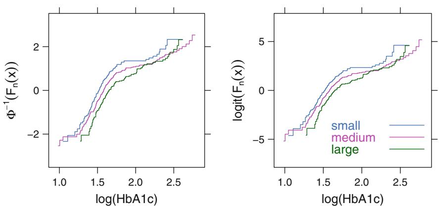

Fig. 13.2 Transformed empirical cumulative distribution functions stratified by body frame in the diabetes dataset. Left panel: checking all assumptions of the parametric ANOVA. Right panel: checking all assumptions of the PO model (here, Kruskal–Wallis test).

One could conclude the right panel of Figure 13.2 displays more parallelism than the left panel displays linearity, so the assumptions of the PO model are better satisfied than the assumptions of the ordinary linear model.

Chapter 14 has many examples of graphics for assessing fit of PO models. Regarding assessment of linearity and additivity assumptions, splines, partial residual plots, and interaction tests are among the best tools. Fagerland and Hosmer182 have a good review of goodness-of-fit tests for the PO model.

13.3.6 Quantifying Predictive Ability

The R² ^N coefficient is really computed from the model LR β² (β² added to a model containing only the k intercept parameters) to describe the model’s predictive power. The Somers’ Dxy rank correlation between XΛˆ and Y is an easily interpreted measure of predictive discrimination. Since it is a rank measure, it does not matter which intercept σ is used in the calculation. The probability of concordance, c, is also a useful measure. Here one takes all possible pairs of subjects having differing Y values and computes the fraction of such pairs for which the values of XΛˆ are in the same direction as the two Y values. c could be called a generalized ROC area in this setting. As before, Dxy = 2(c × 0.5). Note that Dxy, c, and the Brier score B can easily be computed for various dichotomizations of Y , to investigate predictive ability in more detail.

13.3.7 Describing the Fitted Model

As discussed in Section 5.1, models are best described by computing predicted values or differences in predicted values. For PO models there are four and sometimes five types of relevant predictions:

1. logit[Y ← j|X], i.e., the linear predictor
1. Prob[Y ← j|X]
1. Prob[Y = j|X]
1. Quantiles of ^Y ^|^X (e.g., the median^b)
1. E(Y |X) if Y is interval scaled.

For the first two quantities above a good default choice for j is the middle category. Partial effect plots are as simple to draw for PO models as they are for binary logistic models. Other useful graphics, as before, are odds ratio charts and nomograms. For the latter, an axis displaying the predicted mean makes the model more interpretable, under scaling assumptions on Y .

13.3.8 Validating the Fitted Model

The PO model is validated much the same way as the binary logistic model (see Section 10.9). For estimating an overfitting-corrected calibration curve (Section 10.11) one estimates Pr(Y ← j|X) using one j at a time.

^b If Y does not have very many levels, the median will be a discontinuous function of X and may not be satisfactory.

13.3.9 R Functions

The rms package’s lrm and orm functions fit the PO model directly, assuming that the levels of the response variable (e.g., the levels of a factor variable) are listed in the proper order. lrm is intended to be used for the case where the number of unique values of Y are less than a few dozen whereas orm handles the continuous Y case efficiently, as well as allowing for links other than the logit. See Chapter 15 for more information.

If the response is numeric, lrm assumes the numeric codes properly order the responses. If it is a character vector and is not a factor, lrm assumes the correct ordering is alphabetic. Of course ordered variables in R are appropriate response variables for ordinal regression. The predict function (predict.lrm) can compute all the quantities listed in Section 13.3.7 except for quantiles.

The R functions popower and posamsize (in the Hmisc package) compute power and sample size estimates for ordinal responses using the proportional odds model.

The function plot.xmean.ordinaly in rms computes and graphs the quantities described in Section 13.2. It plots simple Y -stratified means overlaid with ^Eˆ(X|^Y ⁼ ^j), with ^j on the ^x-axis. The ^Eˆs are computed for both PO and continuation ratio ordinal logistic models. The Hmisc package’s summary.formula function is also useful for assessing the PO assumption (Figure 13.1). Generic rms functions such as validate, calibrate, and nomogram work with PO model fits from lrm as long as the analyst specifies which intercept(s) to use. rms has a special function generator Mean for constructing an easy-to-use function for getting the predicted mean Y from a PO model. This is handy with plot and nomogram. If the fit has been run through the bootcov function, it is easy to use the Predict function to estimate bootstrap confidence limits for predicted means.

13.4 Continuation Ratio Model

13.4.1 Model

Unlike the PO model, which is based on cumulative probabilities, the continuation ratio (CR) model is based on conditional probabilities. The (forward) CR model31, 52, 190 is stated as follows for Y = 0,…,k.

\[\Pr(Y=j|Y\geq j,X) = \frac{1}{1+\exp[- (\theta\_j + X\gamma)]}\]

\[\begin{split} \text{logit}(Y=0|Y\geq 0,X) &= \text{logit}(Y=0|X) \\ &= \theta\_0 + X\gamma \end{split} \tag{13.10}\]

\[\text{logit}(Y=1|Y\ge 1, X) = \theta\_1 + X\gamma\]

\[\dots\]

\[\text{logit}(Y=k-1|Y\ge k-1, X) = \theta\_{k-1} + X\gamma.\]

The CR model has been said to be likely to fit ordinal responses when subjects have to “pass through” one category to get to the next. The CR model is a discrete version of the Cox proportional hazards model. The discrete hazard function is defined as Pr(Y = j|Y ← j).

13.4.2 Assumptions and Interpretation of Parameters

The CR model assumes that the vector of regression coefficients, α, is the same regardless of which conditional probability is being computed.

One could say that there is no X≤ condition interaction if the CR model holds. For a specific condition Y ← j, the model has the same assumptions as the binary logistic model (Section 10.1.1). That is, the model in its simplest form assumes that the log odds that Y = j conditional on Y ← j is linearly related to each X and that there is no interaction between the Xs.

A single odds ratio is assumed to apply equally to all conditions Y ← j, j = 0, 1, 2,…,k × 1. If linearity and additivity hold, the X^m +1: X^m odds ratio for Y = j is exp(Λm), whatever the conditioning event Y ← j.

To compute Pr(Y > 0|X) from the CR model, one only needs to take one minus Pr(Y = 0|X). To compute other unconditional probabilities from the CR model, one must multiply the conditional probabilities. For example, Pr(Y > 1|X) = Pr(Y > 1|X, Y ← 1) ≤ Pr(Y ← 1|X) = [1 × Pr(Y = 1|Y ← 1, X)][1×Pr(Y = 0|X)] = [1×1/(1+ exp[×(γ¹ +Xα)])][1×1/(1+ exp[×(γ⁰ + Xα)])].

13.4.3 Estimation

Armstrong and Sloan31 and Berridge and Whitehead52 showed how the CR model can be fitted using an ordinary binary logistic model likelihood function, after certain rows of the X matrix are duplicated and a new binary Y vector is constructed. For each subject, one constructs separate records by considering successive conditions Y ← 0, Y ← 1,…,Y ← k × 1 for a response variable with values 0, 1,…,k. The binary response for each applicable condition or “cohort” is set to 1 if the subject failed at the current “cohort” or “risk set,” that is, if Y = j where the cohort being considered is Y ← j. The constructed cohort variable is carried along with the new X and Y . This variable is considered to be categorical and its coefficients are fitted by adding k ×1 dummy variables to the binary logistic model. For ease of computation, the CR model is restated as follows, with the first cohort used as the reference cell.

\[\Pr(Y = j | Y \ge j, X) = \frac{1}{1 + \exp[- (\alpha + \theta\_j + X\gamma)]}.\tag{13.11}\]

Here σ is an overall intercept, γ⁰ ̸ 0, and γ1,…, γk−¹ are increments from σ.

13.4.4 Residuals

To check CR model assumptions, binary logistic model partial residuals are again valuable. We separately fit a sequence of binary logistic models using a series of binary events and the corresponding applicable (increasingly small) subsets of subjects, and plot smoothed partial residuals against X for all of the binary events. Parallelism in these plots indicates that the CR model’s constant α assumptions are satisfied.

13.4.5 Assessment of Model Fit

The partial residual plots just described are very useful for checking the constant slope assumption of the CR model. The next section shows how to test this assumption formally. Linearity can be assessed visually using the smoothed partial residual plot, and interactions between predictors can be tested as usual.

13.4.6 Extended CR Model

The PO model has been extended by Peterson and Harrell502 to allow for unequal slopes for some or all of the Xs for some or all levels of Y . This partial PO model requires specialized software. The CR model can be extended more easily. In R notation, the ordinary CR model is specified as ⁵

y ← cohort + X1 + X2 + X3 + …

with cohort denoting a polytomous variable. The CR model can be extended to allow for some or all of the Λs to change with the cohort or Y -cutoff. 31 Suppose that non-constant slope is allowed for X1 and X2. The R notation for the extended model would be

y ← cohort *(X1 + X2) + X3

The extended CR model is a discrete version of the Cox survival model with time-dependent covariables.

There is nothing about the CR model that makes it fit a given dataset better than other ordinal models such as the PO model. The real benefit of the CR model is that using standard binary logistic model software one can flexibly specify how the equal-slopes assumption can be relaxed.

13.4.7 Role of Penalization in Extended CR Model

As demonstrated in the upcoming case study, penalized MLE is invaluable in allowing the model to be extended into an unequal-slopes model insofar as the information content in the data will support. Faraway186 has demonstrated how all data-driven steps of the modeling process increase the real variance in “final” parameter estimates, when one estimates variances without assuming that the final model was prespecified. For ordinal regression modeling, the most important modeling steps are (1) choice of predictor variables, (2) selecting or modeling predictor transformations, and (3) allowance for unequal slopes across Y -cutoffs (i.e., non-PO or non-CR). Regarding Steps (2) and (3) one is tempted to rely on graphical methods such as residual plots to make detours in the strategy, but it is very difficult to estimate variances or to properly penalize assessments of predictive accuracy for subjective modeling decisions. Regarding (1), shrinkage has been proven to work better than stepwise variable selection when one is attempting to build a main-effects model. Choosing a shrinkage factor is a well-defined, smooth, and often a unique process as opposed to binary decisions on whether variables are “in” or “out” of the model. Likewise, instead of using arbitrary subjective (residual plots) or objective (β² due to cohort ^≤ covariable interactions, i.e., non-constant covariable effects), shrinkage can systematically allow model enhancements insofar as the information content in the data will support, through the use of differential penalization. Shrinkage is a solution to the dilemma faced when the analyst attempts to choose between a parsimonious model and a more complex one that fits the data. Penalization does not require the analyst to make a binary decision, and it is a process that can be validated using the bootstrap.

13.4.8 Validating the Fitted Model

Validation of statistical indexes such as Dxy and model calibration is done using techniques discussed previously, except that certain problems must be addressed. First, when using the bootstrap, the resampling must take into account the existence of multiple records per subject that were created to use the binary logistic likelihood trick. That is, sampling should be done with replacement from subjects rather than records. Second, the analyst must isolate which event to predict. This is because when observations are expanded in order to use a binary logistic likelihood function to fit the CR model, several different events are being predicted simultaneously. Somers’ Dxy could be computed by relating Xαˆ (ignoring intercepts) to the ordinal Y , but other indexes are not defined so easily. The simplest approach here would be to validate a single prediction for Pr(Y = j|Y ← j, X), for example. The simplest event to predict is Pr(Y = 0|X), as this would just require subsetting on all observations in the first cohort level in the validation sample. It would also be easy to validate any one of the later conditional probabilities. The validation functions described in the next section allow for such subsetting, as well as handling the cluster sampling. Specialized calculations would be needed to validate an unconditional probability such as Pr(Y ← 2|X).

13.4.9 R Functions

The cr.setup function in rms returns a list of vectors useful in constructing a dataset used to trick a binary logistic function such as lrm into fitting CR models. The subs vector in this list contains observation numbers in the original data, some of which are repeated. Here is an example.

u − cr.setup(Y) # Y=original ordinal response
attach (mydata [u$subs ,]) # mydata is the original dataset
                       # mydata[i,] subscripts input data ,
                       # using duplicate values of i for
                       # repeats
y − u$y # constructed binary responses
cohort − u$cohort # cohort or risk set categories
f − lrm(y ← cohort *age + sex)

Since the lrm and pentrace functions have the capability to penalize different parts of the model by different amounts, they are valuable for fitting extended CR models in which the cohort ≤ predictor interactions are allowed to be only as important as the information content in the data will support. Simple main effects can be unpenalized or slightly penalized as desired.

The validate and calibrate functions for lrm allow specification of subject identifiers when using the bootstrap, so the samples can be constructed with replacement from the original subjects. In other words, cluster sampling is done from the expanded records. This is handled internally by the predab.resample function. These functions also allow one to specify a subset of the records to use in the validation, which makes it especially easy to validate the part of the model used to predict Pr(Y = 0|X).

The plot.xmean.ordinaly function is useful for checking the CR assumption for single predictors, as described earlier. ⁶

13.5 Further Reading

1 See5,25,26,31,32,52,63,64,113,126,240,245,276,354,449,502,561,664,679 for some excellent background references, applications, and extensions to the ordinal models.663 and428 demonstrate how to model ordinal outcomes with repeated measurements within subject using random effects in Bayesian models. The first to develop an ordinal regression model were Aitchison and Silvey8.
2 Some analysts feel that combining categories improves the performance of test statistics when fitting PO models when sample sizes are small and cells are sparse. Murad et al.469 demonstrated that this causes more problems, because it results in overly conservative Wald tests.
3 Anderson and Philips [26, p. 29] proposed methods for constructing properly spaced response values given a fitted PO model.
4 The simplest demonstration of this is to consider a model in which there is a single predictor that is totally independent of a nine-level response Y , so PO must hold. A PO model is fitted in SAS using:

DATA test;
DO i=1 to 50;
     y=FLOOR(RANUNI(151)*9);
     x=RANNOR(5);
     OUTPUT;
     END;
PROC LOGISTIC; MODEL y=x;

The score test for PO was σ² = 56 on 7 d.f., P < 0.0001. This problem results from some small cell sizes in the distribution of Y . 502 The P-value for testing the regression effect for X was 0.76.

5 The R glmnetcr package by Kellie Archer provides a different way to fit continuation ratio models.
6 Bender and Benner48 have some examples using the precursor of the rms package for fitting and assessing the goodness of fit of ordinal logistic regression models.

13.6 Problems

Test for the association between disease group and total hospital cost in SUPPORT, without imputing any missing costs (exclude the one patient having zero cost).

1. Use the Kruskal–Wallis rank test.
1. Use the proportional odds ordinal logistic model generalization of the Wilcoxon–Mann–Whitney Kruskal–Wallis Spearman test. Group total cost into 20 quantile groups so that only 19 intercepts will need to be in the model, not one less than the number of subjects (this would have taken the program too long to fit the model). Use the likelihood ratio β² for this and later steps.
1. Use a binary logistic model to test for association between disease group and whether total cost exceeds the median of total cost. In other words, group total cost into two quantile groups and use this binary variable as the response. What is wrong with this approach?
4. Instead of using only two cost groups, group cost into 3, 4, 5, 6, 8, 10, and 12 quantile groups. Describe the relationship between the number of intervals used to approximate the continuous response variable and the efficiency of the analysis. How many intervals of total cost, assuming that the ordering of the different intervals is used in the analysis, are required to avoid losing significant information in this continuous variable?
1. If you were selecting one of the rank-based tests for testing the association between disease and cost, which of any of the tests considered would you choose?
1. Why do all of the tests you did have the same number of degrees of freedom for the hypothesis of no association between dzgroup and totcst?
1. What is the advantage of a rank-based test over a parametric test based on log(cost)?
1. Show that for a two-sample problem, the numerator of the score test for comparing the two groups using a proportional odds model is exactly the numerator of the Wilcoxon-Mann-Whitney two-sample rank-sum test.

Chapter 14 Case Study in Ordinal Regression, Data Reduction, and Penalization

This case study is taken from Harrell et al.272 which described a World Health Organization study439 in which vital signs and a large number of clinical signs and symptoms were used to develop a predictive model for an ordinal response. This response consists of laboratory assessments of diagnosis and severity of illness related to pneumonia, meningitis, and sepsis. Much of the modeling strategy given in Chapter 4 was used to develop the model, with additional emphasis on penalized maximum likelihood estimation (Section 9.10). The following laboratory data are used in the response: cerebrospinal fluid (CSF) culture from a lumbar puncture (LP), blood culture (BC), arterial oxygen saturation (SaO2, a measure of lung dysfunction), and chest X-ray (CXR). The sample consisted of 4552 infants aged 90 days or less.

This case study covers these topics:

1. definition of the ordinal response (Section 14.1);
1. scoring and clustering of clinical signs (Section 14.2);
1. testing adequacy of weights specified by subject-matter specialists and assessing the utility of various scoring schemes using a tentative ordinal logistic model (Section 14.3);
1. assessing the basic ordinality assumptions and examining the proportional odds and continuation ratio (PO and CR) assumptions separately for each predictor (Section 14.4);
1. deriving a tentative PO model using cluster scores and regression splines (Section 14.5);
1. using residual plots to check PO, CR, and linearity assumptions (Section 14.6);
1. examining the fit of a CR model (Section 14.7);
1. utilizing an extended CR model to allow some or all of the regression coefficients to vary with cutoffs of the response level as well as to provide formal tests of constant slopes (Section 14.8);

F.E. Harrell, Jr., Regression Modeling Strategies, Springer Series in Statistics, DOI 10.1007/978-3-319-19425-7 14

Outcome	Definition	n	Fraction in Outcome Level
Level			BC, CXR	Not	Random
Y			Indicated	Indicated	Sample
			(n = 2398)	(n = 1979)	(n = 175)
0	None of the below	3551	0.63	0.96	0.91
1	90% ≤ SaO2 < 95%	490	0.17	0.04a	0.05
	or CXR+
2	BC+ or CSF+	511	0.21	0.00b	0.03
	or SaO2 < 90%

Table 14.1 Ordinal Outcome Scale

^a SaO² was measured but CXR was not done

^b Assumed zero since neither BC nor LP were done.

1. using penalized maximum likelihood estimation to improve accuracy (Section 14.9);
1. approximating the full model by a sub-model and drawing a nomogram on the basis of the sub-model (Section 14.10); and
1. validating the ordinal model using the bootstrap (Section 14.11).

14.1 Response Variable

To be a candidate for BC and CXR, an infant had to have a clinical indication for one of the three diseases, according to prespecified criteria in the study protocol (n = 2398). Blood work-up (but not necessarily LP) and CXR was also done on a random sample intended to be 10% of infants having no signs or symptoms suggestive of infection (n = 175). Infants with signs suggestive of meningitis had LP done. All 4552 infants received a full physical exam and standardized pulse oximetry to measure SaO2. The vast majority of infants getting CXR had the X-rays interpreted by three independent radiologists.

The analyses that follow are not corrected for verification bias687 with respect to BC, LP, and CXR, but Section 14.1 has some data describing the extent of the problem, and the problem is reduced by conditioning on a large number of covariates.

Patients were assigned to the worst qualifying outcome category. Table 14.1 shows the definition of the ordinal outcome variable Y and shows the distribution of Y by the lab work-up strategy.

The effect of verification bias is a false negative fraction of 0.03 for Y = 2, from comparing the detection fraction of zero for Y = 2 in the “Not Indicated” group with the observed positive fraction of 0.03 in the random sample that was fully worked up. The extent of verification bias in Y = 1 is 0.05 × 0.04 = 0.01. These biases are ignored in this analysis.

14.2 Variable Clustering

Forty-seven clinical signs were collected for each infant. Most questionnaire items were scored as a single variable using equally spaced codes, with 0 to 3 representing, for example, sign not present, mild, moderate, severe. The resulting list of clinical signs with their abbreviations is given in Table 14.2. The signs are organized into clusters as discussed later.

Table 14.2 Clinical Signs

Cluster Name	Sign	Name	Values
	Abbreviation	of Sign
bul.conv	abb	bulging fontanel	0-1
	convul	hx convulsion	0-1
hydration	abk	sunken fontanel	0-1
	hdi	hx diarrhoea	0-1
	deh	dehydrated	0-2
	stu	skin turgor	0-2
	dcp	digital capillary refill	0-2
drowsy	hcl	less activity	0-1
	qcr	quality of crying	0-2
	csd	drowsy state	0-2
	slpm	sleeping more	0-1
	wake	wakes less easily	0-1
	aro	arousal	0-2
	mvm	amount of movement	0-2
agitated	hcm	crying more	0-1
	slpl	sleeping less	0-1
	con	consolability	0-2
	csa	agitated state	0-1
crying	hcm	crying more	0-1
	hcs	crying less	0-1
	qcr	quality of crying	0-2
	smi2		0-2
		smiling ability ∼ age > 42 days
reffort	nfl	nasal flaring	0-3
	lcw	lower chest in-drawing	0-3
	gru	grunting	0-2
	ccy	central cyanosis	0-1
stop.breath	hap	hx stop breathing	0-1
	apn	apnea	0-1
ausc	whz	wheezing	0-1
	coh	cough heard	0-1
	crs	crepitation	0-2
hxprob	hfb	fast breathing	0-1
	hdb	difficulty breathing	0-1
	hlt	mother report resp. problems	none, chest, other
feeding	hfa	hx abnormal feeding	0-3
	absu	sucking ability	0-2
	afe	drinking ability	0-2
labor	chi	previous child died	0-1
	fde	fever at delivery	0-1
	ldy	days in labor	1-9
	twb	water broke	0-1
abdominal	adb	abdominal distension	0-4
	jau	jaundice	0-1
	omph	omphalitis	0-1
fever.ill	illd	age-adjusted no. days ill
	hfe	hx fever	0-1

pustular	conj	conjunctivitis	0-1
	oto	otoscopy impression	0-2
	puskin	pustular skin rash	0-1

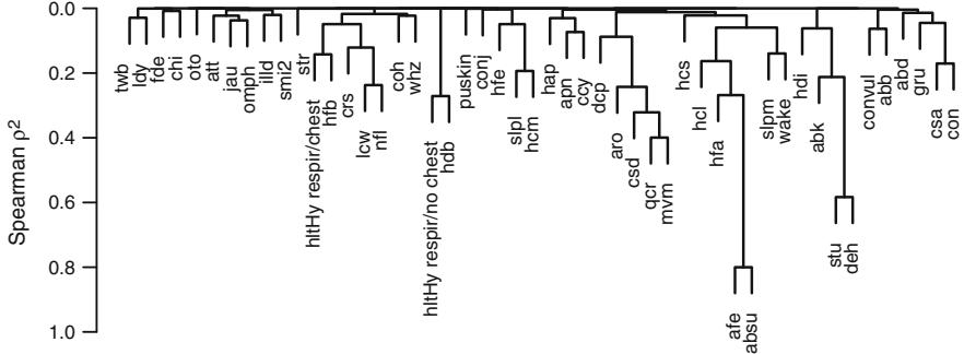
Fig. 14.1 Hierarchical variable clustering using Spearman Λ² as a similarity measure for all pairs of variables. Note that since the hlt variable was nominal, it is represented by two dummy variables here.

Here, hx stands for history, ausc for auscultation, and hxprob for history of problems. Two signs (qcr, hcm) were listed twice since they were later placed into two clusters each.

Next, hierarchical clustering was done using the matrix of squared Spearman rank correlation coefficients as the similarity matrix. The varclus R function was used as follows.

require(rms)

getHdata (ari) # defines ari, Sc, Y, Y.death
vclust −
 varclus(← illd + hlt + slpm + slpl + wake + convul + hfa +
           hfb + hfe + hap + hcl + hcm + hcs + hdi +
           fde + chi + twb + ldy + apn + lcw + nfl +
           str + gru + coh + ccy + jau + omph + csd +
           csa + aro + qcr + con + att + mvm + afe +
           absu + stu + deh + dcp + crs + abb + abk +
           whz + hdb + smi2 + abd + conj + oto + puskin ,
         data=ari)
plot(vclust) # Figure 14.1

The output appears in Figure 14.1. This output served as a starting point for clinicians to use in constructing more meaningful clinical clusters. The clusters in Table 14.2 were the consensus of the clinicians who were the investigators in the WHO study. Prior subject matter knowledge plays a key role at this stage in the analysis.

14.3 Developing Cluster Summary Scores

The clusters listed in Table 14.2 were first scored by the first principal component of transcan-transformed signs, denoted by P C1. Knowing that the resulting weights may be too complex for clinical use, the primary reasons

Cluster	Combined/Ranked Signs in Order of Severity	Weights
bul.conv	abb ≥ convul	0–1
drowsy	hcl, qcr>0, csd>0 ≥ slpm ≥ wake, aro>0, mvm>0	0–5
agitated	hcm, slpl, con=1, csa, con=2	0, 1, 2, 7, 8, 10
reffort	nfl>0, lcw>1, gru=1, gru=2, ccy	0–5
ausc	whz, coh, crs>0	0–3
feeding	hfa=1, hfa=2, hfa=3, absu=1 ≥ afe=1,	0–5
	absu=2 ≥ afe=2
abdominal	jau ≥ abd>0 ≥ omph	0–1

Table 14.3 Clinician Combinations, Rankings, and Scorings of Signs

for analyzing the principal components were to see if some of the clusters could be removed from consideration so that the clinicians would not spend time developing scoring rules for them. Let us “peek” at Y to assist in scoring clusters at this point, but to do so in a very structured way that does not involve the examination of a large number of individual coefficients.

To judge any cluster scoring scheme, we must pick a tentative outcome model. For this purpose we chose the PO model. By using the 14 P C1s corresponding to the 14 clusters, the fitted PO model had a likelihood ratio (LR) β² of 1155 with 14 d.f., and the predictive discrimination of the clusters was quantified by a Somers’ Dxy rank correlation between XΛˆ and Y of 0.596. The following clusters were not statistically important predictors and we assumed that the lack of importance of the P C1s in predicting Y (adjusted for the other P C1s) justified a conclusion that no sign within that cluster was clinically important in predicting Y : hydration, hxprob, pustular, crying, fever.ill, stop.breath, labor. This list was identified using a backward step-down procedure on the full model. The total Wald β² for these seven P C1s was 22.4 (P = 0.002). The reduced model had LR β² = 1133 with 7 d.f., Dxy = 0.591. The bootstrap validation in Section 14.11 penalizes for examining all candidate predictors.

The clinicians were asked to rank the clinical severity of signs within each potentially important cluster. During this step, the clinicians also ranked severity levels of some of the component signs, and some cluster scores were simplified, especially when the signs within a cluster occurred infrequently. The clinicians also assessed whether the severity points or weights should be equally spaced, assigning unequally spaced weights for one cluster (agitated). The resulting rankings and sign combinations are shown in Table 14.3. The signs or sign combinations separated by a comma are treated as separate categories, whereas some signs were unioned (“or”–ed) when the clinicians deemed them equally important. As an example, if an additive cluster score was to be used for drowsy, the scorings would be 0 = none present, 1 = hcl, 2 = qcr>0,3= csd>0 or slpm or wake,4= aro>0,5= mvm>0 and the scores would be added.

Scoring Method	LR	β2 d.f.	AIC
P C1 of each cluster	1133	7	1119
Union of all signs	1045	7	1031
Union of higher categories	1123	7	1109
Hierarchical (worst sign)	1194	7	1180
Additive, equal weights	1155	7	1141
Additive using clinician weights	1183	7	1169
Hierarchical, data-driven weights	1227		25 1177

Table 14.4 Predictive information of various cluster scoring strategies. AIC is on the likelihood ratio σ² scale.

This table reflects some data reduction already (unioning some signs and selection of levels of ordinal signs) but more reduction is needed. Even after signs are ranked within a cluster, there are various ways of assigning the cluster scores. We investigated six methods. We started with the purely statistical approach of using P C¹ to summarize each cluster. Second, all sign combinations within a cluster were unioned to represent a 0/1 cluster score. Third, only sign combinations thought by the clinicians to be severe were unioned, resulting in drowsy=aro>0 or mvm>0, agitated=csa or con=2, reffort=lcw>1 or gru>0 or ccy, ausc=crs>0, and feeding=absu>0 or afe>0. For clusters that are not scored 0/1 in Table 14.3, the fourth summarization method was a hierarchical one that used the weight of the worst applicable category as the cluster score. For example, if aro=1 but mvm=0, drowsy would be scored as 4. The fifth method counted the number of positive signs in the cluster. The sixth method summed the weights of all signs or sign combinations present. Finally, the worst sign combination present was again used as in the second method, but the points assigned to the category were data-driven ones obtained by using extra dummy variables. This provided an assessment of the adequacy of the clinician-specified weights. By comparing rows 4 and 7 in Table 14.4 we see that response data-driven sign weights have a slightly worse AIC, indicating that the number of extra Λ parameters estimated was not justified by the improvement in β². The hierarchical method, using the clinicians’ weights, performed quite well. The only cluster with inadequate clinician weights was ausc—see below. The P C¹ method, without any guidance, performed well, as in268. The only reasons not to use it are that it requires a coefficient for every sign in the cluster and the coefficients are not translatable into simple scores such as 0, 1,….

Representation of clusters by a simple union of selected signs or of all signs is inadequate, but otherwise the choice of methods is not very important in terms of explaining variation in Y . We chose the fourth method, a hierarchical severity point assignment (using weights that were prespecified by the clinicians), for its ease of use and of handling missing component variables (in most cases) and potential for speeding up the clinical exam (examining

to detect more important signs first). Because of what was learned regarding the relationship between ausc and Y , we modified the ausc cluster score by redefining it as ausc=crs>0 (crepitations present). Note that neither the “tweaking” of ausc nor the examination of the seven scoring methods displayed in Table 14.4 is taken into account in the model validation.

14.4 Assessing Ordinality of Y for each X, and Unadjusted Checking of PO and CR Assumptions

Section 13.2 described a graphical method for assessing the ordinality assumption for Y separately with respect to each X, and for assessing PO and CR assumptions individually. Figure 14.2 is an example of such displays. For this dataset we expect strongly nonlinear effects for temp, rr, and hrat, so for those predictors we plot the mean absolute differences from suitable “normal” values as an approximate solution.

Sc − transform (Sc ,
                 ausc = 1 * (ausc == 3),
                 bul.conv = 1 * (bul.conv == ' TRUE ' ),
                 abdominal = 1 * (abdominal == ' TRUE ' ))
plot.xmean.ordinaly (Y ← age + abs(temp-37) + abs( rr-60) +
                     abs(hrat-125) + waz + bul.conv + drowsy +
                     agitated + reffort + ausc + feeding +
                     abdominal , data =Sc , cr=TRUE ,
                     subn= FALSE , cex.points =.65) # Figure 14.2

The plot is shown in Figure 14.2. Y does not seem to operate in an ordinal fashion with respect to age, |rr×60|, or ausc. For the other variables, ordinality holds, and PO holds reasonably well for the other variables. For heart rate, the PO assumption appears to be satisfied perfectly. CR model assumptions appear to be more tenuous than PO assumptions, when one variable at a time is fitted.

14.5 A Tentative Full Proportional Odds Model

Based on what was determined in Section 14.3, the original list of 47 signs was reduced to seven predictors: two unions of signs (bul.conv, abdominal), one single sign (ausc), and four “worst category” point assignments (drowsy, agitated, reffort, feeding). Seven clusters were dropped for the time being because of weak associations with Y . Such a limited use of variable selection reduces the severe problems inherent with that technique.

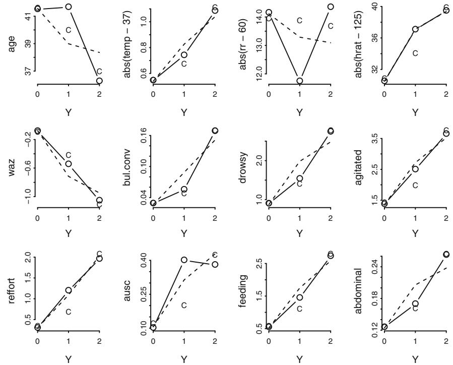
Fig. 14.2 Examination of the ordinality of Y for each predictor by assessing how varying Y relate to the mean X, and whether the trend is monotonic. Solid lines connect the simple stratified means, and dashed lines connect the estimated expected value of X|Y = j given that PO holds. Estimated expected values from the CR model are marked with Cs.

At this point in model development add to the model age and vital signs: temp (temperature), rr (respiratory rate), hrat (heart rate), and waz, weightfor-age Z-score. Since age was expected to modify the interpretation of temp, rr, and hrat, and interactions between continuous variables would be difficult to use in the field, we categorized age into three intervals: 0–6 days (n = 302), 7–59 days (n = 3042), and 60–90 days (n = 1208).^a

cut2 (Sc$age , c(7, 60))
———————————

The new variables temp, rr, hrat, waz were missing in, respectively, n = 13, 11, 147, and 20 infants. Since the three vital sign variables are somewhat correlated with each other, customized single imputation models were developed to impute all the missing values without assuming linearity or even monotonicity of any of the regressions.

^a These age intervals were also found to adequately capture most of the interaction effects.

vsign.trans − transcan(← temp + hrat + rr , data =Sc,
                          imputed=TRUE , pl= FALSE )

Convergence criterion:2.222 0.643 0.191 0.056 0.016
Convergence in 6 iterations
R2 achieved in predicting each variable:
 temp hrat rr
0.168 0.160 0.066
Adjusted R2:
 temp hrat rr
0.167 0.159 0.064

Sc − transform (Sc ,
                 temp = impute (vsign.trans , temp),
                 hrat = impute (vsign.trans , hrat),
                 rr = impute (vsign.trans , rr))

After transcan estimated optimal restricted cubic spline transformations, temp could be predicted with adjusted R² = 0.17 from hrat and rr, hrat could be predicted with adjusted R² = 0.16 from temp and rr, and rr could be predicted with adjusted R² of only 0.06. The first two R², while not large, mean that customized imputations are more efficient than imputing with constants. Imputations on rr were closer to the median rr of 48/minute as compared with the other two vital signs whose imputations have more variation. In a similar manner, waz was imputed using age, birth weight, head circumference, body length, and prematurity (adjusted R² for predicting waz from the others was 0.74). The continuous predictors temp, hrat, rr were not assumed to linearly relate to the log odds that Y ← j. Restricted cubic spline functions with five knots for temp,rr and four knots for hrat,waz were used to model the effects of these variables:

f1 − lrm(Y ← ageg*(rcs( temp ,5)+ rcs(rr ,5)+ rcs(hrat ,4)) +
           rcs(waz ,4) + bul.conv + drowsy + agitated +
           reffort + ausc + feeding + abdominal ,
           data =Sc , x= TRUE , y= TRUE)
# x=TRUE , y= TRUE used by resid() below
print (f1 , latex =TRUE , coefs =5)

Logistic Regression Model

lrm(formula = Y ~ ageg * (rcs(temp, 5) + rcs(rr, 5) + rcs(hrat, 4)) + rcs(waz, 4) + bul.conv + drowsy + agitated + reffort + ausc + feeding + abdominal, data = Sc, x = TRUE, y = TRUE)

			Model Likelihood		Discrimination		Rank Discrim.
			Ratio Test		Indexes		Indexes
Obs	4552	β2 LR	1393.18	R2	0.355	C	0.826
0	3551	d.f.	45	g	1.485	Dxy	0.653
1	490	β2) Pr(>	< 0.0001	gr	4.414	α	0.654
2	511			gp	0.225	Γa	0.240
max	α log L 2≤10−6 αρ			Brier	0.120

	Coef	S.E.	Wald Z	Pr(> Z )
y←1	0.0653	7.6563	0.01	0.9932
y←2	-1.0646	7.6563	-0.14	0.8894
ageg=[ 7,60)	9.5590	9.9071	0.96	0.3346
ageg=[60,90]	29.1376	15.8915	1.83	0.0667
temp	-0.0694	0.2160	-0.32	0.7480

Wald tests of nonlinearity and interaction are shown in Table 14.5.

latex (anova (f1), file= ’ ’ , label= ’ ordinal-anova.f1 ’ , caption= ’ Wald statistics from the proportional odds model ’ , size= ’ smaller ’ ) # Table 14.5

The bottom four lines of the table are the most important. First, there is strong evidence that some associations with Y exist (45 d.f. test) and very strong evidence of nonlinearity in one of the vital signs or in waz (26 d.f. test). There is moderately strong evidence for an interaction effect somewhere in the model (22 d.f. test). We see that the grouped age variable ageg is predictive of Y , but mainly as an effect modifier for rr, and hrat. temp is extremely nonlinear, and rr is moderately so. hrat, a difficult variable to measure reliably in young infants, is perhaps not important enough (β² = 19, 9 d.f.) to keep in the final model.

14.6 Residual Plots

Section 13.3.4 defined binary logistic score residuals for isolating the PO assumption in an ordinal model. For the tentative PO model, score residuals for four of the variables were plotted using

resid (f1 , ’ score.binary ’ , pl=TRUE , which =c(17,18,20,21)) ## Figure 14.3

The result is shown in Figure 14.3. We see strong evidence of non-PO for ausc and moderate evidence for drowsy and bul.conv, in agreement with Figure 14.2.

	σ2	d.f.	P
ageg (Factor+Higher Order Factors)	41.49	24	0.0147
All Interactions	40.48	22	0.0095
temp (Factor+Higher Order Factors)	37.08	12	0.0002
All Interactions	6.77	8	0.5617
Nonlinear (Factor+Higher Order Factors)	31.08	9	0.0003
rr (Factor+Higher Order Factors)	81.16		12 < 0.0001
All Interactions	27.37	8	0.0006
Nonlinear (Factor+Higher Order Factors)	27.36	9	0.0012
hrat (Factor+Higher Order Factors)	19.00	9	0.0252
All Interactions	8.83	6	0.1836
Nonlinear (Factor+Higher Order Factors)	7.35	6	0.2901
waz	35.82		3 < 0.0001
Nonlinear	13.21	2	0.0014
bul.conv	12.16	1	0.0005
drowsy	17.79		1 < 0.0001
agitated	8.25	1	0.0041
reffort	63.39		1 < 0.0001
ausc	105.82		1 < 0.0001
feeding	30.38		1 < 0.0001
abdominal	0.74	1	0.3895
ageg ∼ temp (Factor+Higher Order Factors)	6.77	8	0.5617
Nonlinear	6.40	6	0.3801
Nonlinear Interaction : f(A,B) vs. AB	6.40	6	0.3801
ageg ∼ rr (Factor+Higher Order Factors)	27.37	8	0.0006
Nonlinear	14.85	6	0.0214
Nonlinear Interaction : f(A,B) vs. AB	14.85	6	0.0214
ageg ∼ hrat (Factor+Higher Order Factors)	8.83	6	0.1836
Nonlinear	2.42	4	0.6587
Nonlinear Interaction : f(A,B) vs. AB	2.42	4	0.6587
TOTAL NONLINEAR	78.20		26 < 0.0001
TOTAL INTERACTION	40.48	22	0.0095
TOTAL NONLINEAR + INTERACTION	96.31		32 < 0.0001
TOTAL	1073.78		45 < 0.0001

Table 14.5 Wald statistics from the proportional odds model

Partial residuals computed separately for each Y -cutoff (Section 13.3.4) are the most useful residuals for ordinal models as they simultaneously check linearity, find needed transformations, and check PO. In Figure 14.4, smoothed partial residual plots were obtained for all predictors, after first fitting a simple model in which every predictor was assumed to operate linearly. Interactions were temporarily ignored and age was used as a continuous variable.

f2 − lrm(Y ← age + temp + rr + hrat + waz +
          bul.conv + drowsy + agitated + reffort + ausc +
          feeding + abdominal , data=Sc, x=TRUE , y=TRUE)
resid(f2, ' partial ' , pl=TRUE , label.curves= FALSE) # Figure 14.4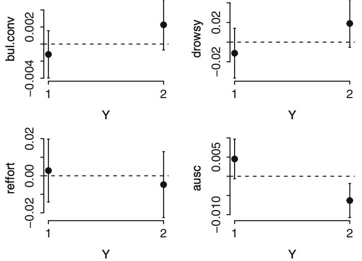

Fig. 14.3 Binary logistic model score residuals for binary events derived from two cutoffs of the ordinal response Y . Note that the mean residuals, marked with closed circles, correspond closely to differences between solid and dashed lines at Y = 1, 2 in Figure 14.2. Score residual assessments for spline-expanded variables such as rr would have required one plot per d.f.

The degree of non-parallelism generally agreed with the degree of non-flatness in Figure 14.3 and with the other score residual plots that were not shown. The partial residuals show that temp is highly nonlinear and that it is much more useful in predicting Y = 2. For the cluster scores, the linearity assumption appears reasonable, except possibly for drowsy. Other nonlinear effects are taken into account using splines as before (except for age, which is categorized).

A model can have significant lack of fit with respect to some of the predictors and still yield quite accurate predictions. To see if that is the case for this PO model, we computed predicted probabilities of Y = 2 for all infants from the model and compared these with predictions from a customized binary logistic model derived to predict Pr(Y = 2). The mean absolute difference in predicted probabilities between the two models is only 0.02, but the 0.90 quantile of that difference is 0.059. For high-risk infants, discrepancies of 0.2 were common. Therefore we elected to consider a different model.

14.7 Graphical Assessment of Fit of CR Model

In order to take a first look at the fit of a CR model, let us consider the two binary events that need to be predicted, and assess linearity and parallelism over Y -cutoffs. Here we fit a sequence of binary fits and then use the plot.lrm.partial function, which assembles partial residuals for a sequence of fits and constructs one graph per predictor.

cr0 − lrm(Y==0 ← age + temp + rr + hrat + waz +
           bul.conv + drowsy + agitated + reffort + ausc +
           feeding + abdominal , data =Sc , x=TRUE , y= TRUE)
# Use the update function to save repeating model right-
# hand side. An indicator variable for Y=1 is the
# response variable below
cr1 − update (cr0 , Y==1 ← ., subset =Y ≡ 1)
plot.lrm.partial (cr0 , cr1 , center =TRUE) # Figure 14.5

The output is in Figure 14.5. There is not much more parallelism here than in Figure 14.4. For the two most important predictors, ausc and rr, there are strongly differing effects for the different events being predicted (e.g., Y = 0 or Y = 1|Y ← 1). As is often the case, there is no one constant Λ model that satisfies assumptions with respect to all predictors simultaneously, especially

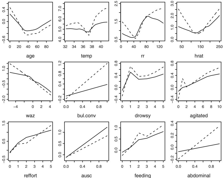
Fig. 14.4 Smoothed partial residuals corresponding to two cutoffs of Y , from a model in which all predictors were assumed to operate linearly and additively. The smoothed curves estimate the actual predictor transformations needed, and parallelism relates to the PO assumption. Solid lines denote Y ≡ 1 while dashed lines denote Y ≡ 2.

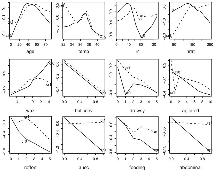
Fig. 14.5 loess smoothed partial residual plots for binary models that are components of an ordinal continuation ratio model. Solid lines correspond to a model for Y = 0, and dotted lines correspond to a model for Y = 1|Y ≡ 1.

when there is evidence for non-ordinality for ausc in Figure 14.2. The CR model will need to be generalized to adequately fit this dataset.

14.8 Extended Continuation Ratio Model

The CR model in its ordinary form has no advantage over the PO model for this dataset. But Section 13.4.6 discussed how the CR model can easily be extended to relax any of its assumptions. First we use the cr.setup function to set up the data for fitting a CR model using the binary logistic trick.

u − cr.setup(Y) Sc.expanded − Sc[u$subs , ] y − u$y cohort − u$cohort

Here the cohort variable has values ‘all’, ‘Y>=1’ corresponding to the conditioning events in Equation 13.10. Once the data frame is expanded to include the different risk cohorts, vectors such as age are lengthened (to 5553 records). Now we fit a fully extended CR model that makes no equal slopes assumptions; that is, the model has to fit Y assuming the covariables are linear and additive. At this point, we omit hrat but add back all variables that were deleted by examining their association with Y . Recall that most of these seven cluster scores were summarized using P C1. Adding back “insignificant” variables will allow us to validate the model fairly using the bootstrap, as well as to obtain confidence intervals that are not falsely narrow.16

full −
  lrm(y ← cohort *(ageg*(rcs(temp ,5) + rcs(rr ,5)) +
      rcs(waz ,4) + bul.conv + drowsy + agitated + reffort +
      ausc + feeding + abdominal + hydration + hxprob +
      pustular + crying + fever.ill + stop.breath + labor),
      data=Sc.expanded , x= TRUE , y= TRUE)
# x=TRUE , y= TRUE are for pentrace , validate , calibrate below
perf − function(fit) { # model performance for Y=0
  pr − predict(fit , type= ' fitted ' )[ cohort == ' all ' ]
  s − round ( somers2(pr , y[ cohort == ' all ' ]), 3)
  pr − 1 - pr # Predict Prob[Y > 0] instead of Prob[Y = 0]
  f − round (c(mean(pr < .05), mean(pr > .25),
                mean (pr > .5)), 2)
  f − paste (f[1], ' , ' , f[2], ' , and ' , f[3], ' . ' , sep= ' ' )
  list(somers =s, fractions=f)
}
perf.unpen − perf(full)
print (full , latex =TRUE , coefs =5)

Logistic Regression Model

lrm(formula = y ~ cohort * (ageg * (rcs(temp, 5) + rcs(rr, 5)) + rcs(waz, 4) + bul.conv + drowsy + agitated + reffort + ausc + feeding + abdominal + hydration + hxprob + pustular + crying + fever.ill + stop.breath + labor), data = Sc.expanded, x = TRUE, y = TRUE)

	Model Likelihood	Discrimination	Rank Discrim.
	Ratio Test	Indexes	Indexes
Obs 5553	β2 LR 1824.33	R2 0.406	C 0.843
0 1512	d.f. 87	g 1.677	Dxy 0.685
1 4041	β2) Pr(> < 0.0001	gr 5.350	α 0.687
α log L 8≤10−7 max αρ		gp 0.269	Γa 0.272
		Brier 0.135

	σ2	P
cohort (Factor+Higher Order Factors) 199.47		44 < 0.0001
All Interactions	172.12	43 < 0.0001
TOTAL	199.47	44 < 0.0001

	Coef	S.E.	Wald Z	Pr(> Z )
Intercept	1.3966	9.0827	0.15	0.8778
cohort=Y←1	1.5077	14.6443	0.10	0.9180
ageg=[ 7,60)	-9.3715	11.4104	-0.82	0.4115
ageg=[60,90]	-26.4502	17.2188	-1.54	0.1245
temp	-0.0049	0.2551	-0.02	0.9846

latex (anova (full , cohort ), file= ' ' , # Table 14.6
  caption= ' Wald statistics for \\co{ cohort } in the CR model ' ,
  size= ' smaller[2] ' , label= ' ordinal-anova.cohort ' )

an − anova (full , india= FALSE , indnl=FALSE )

Table 14.6 Wald statistics for cohort in the CR model

latex (an , file = ' ' , label= ' ordinal-anova.full ' ,
  caption= ' Wald statistics for the continuation ratio model.
   Interactions with \\co{cohort } assess non-proportional
   hazards ' , caption.lot= ' Wald statistics for $Y$ in the
                     continuation ratio model ' ,
      size= ' smaller[2] ' ) # Table 14.7

This model has LR β² = 1824 with 87 d.f. Wald statistics are in Tables 14.6 and 14.7. The global test of the constant slopes assumption in the CR model (test of all interactions involving cohort) has Wald β² = 172 with 43 d.f., P < 0.0001. Consistent with Figure 14.5, the formal tests indicate that ausc is the biggest violator, followed by waz and rr.

14.9 Penalized Estimation

We know that the CR model must be extended to fit these data adequately. If the model is fully extended to allow for all cohort ≤ predictor interactions, we have not gained any precision or power in using an ordinal model over using a polytomous logistic model. Therefore we seek some restrictions on the model’s parameters. The lrm and pentrace functions allow for differing ϵ for shrinking different types of terms in the model. Here we do a grid search to determine the optimum penalty for simple main effect (non-interaction) terms and the penalty for interaction terms, most of which are terms interacting with cohort

σ2 d.f. P cohort 199.47 44 < 0.0001 ageg 48.89 36 0.0742 temp 59.37 24 0.0001 rr 93.77 24 < 0.0001 waz 39.69 6 < 0.0001 bul.conv 10.80 2 0.0045 drowsy 15.19 2 0.0005 agitated 13.55 2 0.0011 reffort 51.85 2 < 0.0001 ausc 109.80 2 < 0.0001 feeding 27.47 2 < 0.0001 abdominal 1.78 2 0.4106 hydration 4.47 2 0.1069 hxprob 6.62 2 0.0364 pustular 3.03 2 0.2194 crying 1.55 2 0.4604 fever.ill 3.63 2 0.1630


















stop.breath 5.34 2 0.0693
labor 5.35 2 0.0690
ageg ∼ temp 8.18 16 0.9432
ageg ∼ rr 38.11 16 0.0015
cohort ∼ ageg 14.88 18 0.6701
cohort ∼ temp 8.77 12 0.7225
cohort ∼ rr 19.67 12 0.0736
cohort ∼ waz 9.04 3 0.0288
cohort ∼ bul.conv 0.33 1 0.5658
0.57 1 0.4489
cohort ∼ drowsy 0.55 1 0.4593
cohort ∼ agitated 2.29 1 0.1298
cohort ∼ reffort 38.11 1 < 0.0001
cohort ∼ ausc 2.48 1 0.1152
cohort ∼ feeding
cohort ∼ abdominal 0.09 1 0.7696
cohort ∼ hydration 0.53 1 0.4682
cohort ∼ hxprob 2.54 1 0.1109
cohort ∼ pustular 2.40 1 0.1210
cohort ∼ crying 0.39 1 0.5310
cohort ∼ fever.ill 3.17 1 0.0749
cohort ∼ stop.breath 2.99 1 0.0839
cohort ∼ labor 0.05 1 0.8309
cohort ∼ ageg ∼ temp 2.22 8 0.9736
cohort ∼ ageg ∼ rr 10.22 8 0.2500
TOTAL NONLINEAR 93.36 40 < 0.0001
TOTAL INTERACTION 203.10 59 < 0.0001
TOTAL NONLINEAR + INTERACTION 257.70 67 < 0.0001
TOTAL 1211.73 87 < 0.0001

Table 14.7 Wald statistics for the continuation ratio model. Interactions with cohort assess non-proportional hazards

to allow for unequal slopes. The following code uses pentrace on the full extended CR model fit to find the optimum penalty factors. All combinations of the simple and interaction ϵs for which the interaction penalty ← the penalty for the simple parameters are examined.

d − options( digits =4)
pentrace(full ,
          list (simple =c(0, .025 ,.05 ,.075 ,.1),
                interaction =c(0,10,50 ,100,125 ,150)))

Best penalty:
simple interaction df
  0.05 125 49.75
simple interaction df aic bic aic.c
 0.000 0 87.00 1650 1074 1648
 0.000 10 60.63 1671 1269 1669
 0.025 10 60.11 1672 1274 1670
 0.050 10 59.80 1672 1276 1670
 0.075 10 59.58 1671 1277 1670
 0.100 10 59.42 1671 1278 1670
 0.000 50 54.64 1671 1309 1670
 0.025 50 54.14 1672 1313 1671
 0.050 50 53.83 1672 1316 1671
 0.075 50 53.62 1672 1317 1671
 0.100 50 53.46 1672 1318 1671
 0.000 100 51.61 1672 1330 1671
 0.025 100 51.11 1673 1334 1672
 0.050 100 50.81 1673 1336 1672
 0.075 100 50.60 1672 1337 1671
 0.100 100 50.44 1672 1338 1671
 0.000 125 50.55 1672 1337 1671
 0.025 125 50.05 1673 1341 1672
 0.050 125 49.75 1673 1343 1672
 0.075 125 49.54 1672 1344 1672
 0.100 125 49.39 1672 1345 1671
 0.000 150 49.65 1672 1343 1671
 0.025 150 49.15 1672 1347 1672
 0.050 150 48.85 1673 1349 1672
 0.075 150 48.64 1672 1350 1671
 0.100 150 48.49 1672 1351 1671

options(d)

We see that shrinkage from 87 d.f. down to 49.75 effective d.f. results in an improvement in β²–scaled AIC of 23. The optimum penalty factors were 0.05 for simple terms and 125 for interaction terms.

Let us now store a penalized version of the full fit, find where the effective d.f. were reduced, and compute β² for each factor in the model. We take the effective d.f. for a collection of model parameters to be the sum of the diagonals of the matrix product defined underneath Gray’s Equation 2.9237 that correspond to those parameters.

full.pen −
  update (full ,
          penalty= list (simple =.05 , interaction =125))
print (full.pen , latex= TRUE , coefs=FALSE)

Logistic Regression Model

lrm(formula = y ~ cohort * (ageg * (rcs(temp, 5) + rcs(rr, 5)) +
    rcs(waz, 4) + bul.conv + drowsy + agitated + reffort + ausc +
    feeding + abdominal + hydration + hxprob + pustular + crying +
    fever.ill + stop.breath + labor), data = Sc.expanded, x = TRUE,
    y = TRUE, penalty = list(simple = 0.05, interaction = 125))

Penalty factors

simple nonlinear interaction nonlinear.interaction 0.05 0.05 125 125

		Model Likelihood		Discrimination			Rank Discrim.
		Ratio Test		Indexes			Indexes
Obs	5553	β2 LR	1772.11	R2	0.392	C	0.840
0	1512	d.f.	49.75	g	1.594	Dxy	0.679
1	4041	β2) Pr(>	< 0.0001	gr	4.924	α	0.681
α log L max αρ	1≤10−7 Penalty		21.48	gp	0.263	Γa	0.269
				Brier	0.136
effective.df (full.pen)

Original and Effective Degrees of Freedom

	Original	Penalized
All	87	49.75
Simple Terms	20	19.98
Interaction or Nonlinear	67	29.77
Nonlinear	40	16.82
Interaction	59	22.57
Nonlinear Interaction	32	9.62

## Compute discrimination for Y=0 vs. Y>0
perf.pen − perf( full.pen) # Figure 14.6
# Exclude interactions and cohort effects from plot
plot(anova ( full.pen ), cex.labels =0.75 , rm.ia =TRUE ,
     rm.other= ' cohort (Factor +Higher Order Factors) ' )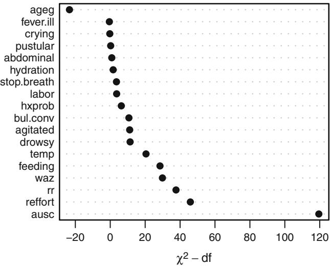

Fig. 14.6 Importance of predictors in full penalized model, as judged by partial Wald σ² minus the predictor d.f. The Wald σ² values for each line in the dot plot include contributions from all higher-order effects. Interaction effects by themselves have been removed as has the cohort effect.

This will be the final model except for the model used in Section 14.10. The model has LR β² = 1772. The output of effective.df shows that noninteraction terms have barely been penalized, and coefficients of interaction terms have been shrunken from 59 d.f. to effectively 22.6 d.f. Predictive discrimination was assessed by computing the Somers’ Dxy rank correlation between XΛˆ and whether Y = 0, in the subset of records for which Y = 0 is what was being predicted. Here Dxy = 0.672, and the ROC area is 0.838 (the unpenalized model had an apparent Dxy = 0.676). To summarize in another way the effectiveness of this model in screening infants for risks of any abnormality, the fraction of infants with predicted probabilities that Y > 0 being < 0.05, > 0.25, and > 0.5 are, respectively, 0.1, 0.28, and 0.14. anova output is plotted in Figure 14.6 to give a snapshot of the importance of the various predictors. The Wald statistics used here are computed on a variance–covariance matrix which is adjusted for penalization (using Gray Equation 2.6237 before it was determined that the sandwich covariance estimator performs less well than the inverse of the penalized information matrix—see p. 211).

The full equation for the fitted model is below. Only the part of the equation used for predicting Pr(Y = 0) is shown, other than an intercept for Y ← 1 that does not apply when Y = 0.

latex (full.pen , which =1:21, file= ’ ’ )

Xχˆ = ×1.337435[Y >= 1] +0.1074525[ageg ̸ [ 7, 60)] + 0.1971287[ageg ̸ [60, 90]] +0.1978706temp + 0.1091831(temp ^× ³⁶.19998)³ ⁺ ^× ².833442(temp ^× 37)³ + +5.07114(temp ^× ³⁷.29999)³ ⁺ ^× ².507527(temp ^× ³⁷.69998)³ + +0.1606456(temp ^× 39)³ + +0.02090741rr ^× ⁶.336873∼10∼5(rr ^× 32)³ ⁺ + 8.405441∼10∼5(rr ^× 42)³ + +6.152416∼10∼5(rr ^× 49)³ ⁺ ^× ⁰.0001018105(rr ^× 59)³ ⁺ + 1.960063∼10∼5(rr ^× 76)³ + ^×0.07589699waz + 0.02508918(waz + 2.9)³ ⁺ ^× ⁰.1185068(waz + 0.75)³ + +0.1225752(waz ^× ⁰.28)³ ⁺ ^× ⁰.02915754(waz ^× ¹.73)³ ⁺ × 0.4418073 bul.conv ×0.08185088 drowsy × 0.05327209 agitated × 0.2304409 reffort ×1.158604 ausc × 0.1599588 feeding × 0.1608684 abdominal ×0.05409718 hydration + 0.08086387 hxprob + 0.007519746 pustular +0.04712091 crying + 0.004298725 fever.ill × 0.3519033 stop.breath +0.06863879 labor +[ageg ̸ [ 7, 60)][6.499592∼10∼⁵ temp ^× ⁰.00279976(temp ^× ³⁶.19998)³ + ^×0.008691166(temp ^× 37)³ ⁺ ^× ⁰.004987871(temp ^× ³⁷.29999)³ + +0.0259236(temp ^× ³⁷.69998)³ ⁺ ^× ⁰.009444801(temp ^× 39)³ +] +[ageg ̸ [60, 90]][0.0001320368temp ^× ⁰.00182639(temp ^× ³⁶.19998)³ + ^×0.01640406(temp ^× 37)³ ⁺ ^× ⁰.0476041(temp ^× ³⁷.29999)³ + +0.09142148(temp ^× ³⁷.69998)³ ⁺ ^× ⁰.02558693(temp ^× 39)³ +] +[ageg ̸ [ 7, 60)][×0.0009437598rr ^× ¹.044673∼10∼6(rr ^× 32)³ + ^×1.670499∼10∼6(rr ^× 42)³ ⁺ ^× ⁵.189082∼10∼6(rr ^× 49)³ ⁺ + 1.428634∼10∼5(rr ^× 59)³ + ^×6.382087∼10∼6(rr ^× 76)³ +] +[ageg ̸ [60, 90]][×0.001920811rr ^× ⁵.52134∼10∼6(rr ^× 32)³ + ^×8.628392∼10∼6(rr ^× 42)³ ⁺ ^× ⁴.147347∼10∼6(rr ^× 49)³ ⁺ + 3.813427∼10∼5(rr ^× 59)³ + ^×1.98372∼10∼5(rr ^× 76)³ +]

where [c] = 1 if subject is in group c, 0 otherwise; (x)⁺ = x if x > 0, 0 otherwise.

Now consider displays of the shapes of effects of the predictors. For the continuous variables temp and rr that interact with age group, we show the effects for all three age groups separately for each Y cutoff. All effects have been centered so that the log odds at the median predictor value is zero when cohort=‘all’, so these plots actually show log odds relative to reference values. The patterns in Figures 14.9 and 14.8 are in agreement with those in Figure 14.5.

yl − c(-3, 1) # put all plots on common y-axis scale
# Plot predictors that interact with another predictor
# Vary ageg over all age groups, then vary temp over its
# default range (10th smallest to 10th largest values in
# data). Make a separate plot for each ' cohort '
# ref.zero centers effects using median x
dd − datadist (Sc.expanded ); dd − datadist (dd, cohort)
options (datadist = ' dd ' )
p1 − Predict(full.pen , temp , ageg , cohort ,
             ref.zero =TRUE , conf.int =FALSE)
p2 − Predict (full.pen , rr, ageg , cohort ,
               ref.zero =TRUE , conf.int =FALSE)
p − rbind(temp=p1, rr=p2) # Figure 14.7:
source(paste( ' http:// biostat.mc.vanderbilt.edu/ wiki/pub/Main ' ,
              ' RConfiguration/graphicsSet.r ' , sep= ' / ' ))
ggplot(p, ← cohort , groups= ' ageg ' , varypred =TRUE ,
       ylim=yl, layout=c(2, 1), legend.position=c(.85 ,.8),
       addlayer =ltheme(width=3, height =3, text=2.5, title =2.5),
       adj.subtitle= FALSE) # ltheme defined with source()

# For each predictor that only interacts with cohort , show
# the differing effects of the predictor for predicting
# Pr(Y=0) and Pr(Y=1 given Y exceeds 0) on the same graph
dd$limits [ ' Adjust to ' , ' cohort ' ] − ' Y ≡ 1 '
v − Cs(waz , bul.conv , drowsy , agitated , reffort , ausc ,
        feeding , abdominal , hydration , hxprob , pustular ,
        crying )
yeq1 − Predict( full.pen , name=v, ref.zero= TRUE)
yl − c(-1.5 , 1.5)
ggplot (yeq1 , ylim =yl, sepdiscrete= ' vertical ' ) # Figure 14.8

dd$limits [ ’ Adjust to ’ , ’ cohort ’ ] − ’ all ’ # original default all − Predict( full.pen , name=v, ref.zero= TRUE) ggplot (all , ylim =yl , sepdiscrete= ’ vertical ’ ) # Figure 14.9

1

14.10 Using Approximations to Simplify the Model

Parsimonious models can be developed by approximating predictions from the model to any desired level of accuracy. Let Lˆ = XΛˆ denote the predicted log odds from the full penalized ordinal model, including multiple records for subjects with Y > 0. Then we can use a variety of techniques to approximate Lˆ from a subset of the predictors (in their raw form). With this approach one can immediately see what is lost over the full model by computing, for example, the mean absolute error in predicting Lˆ. Another advantage to full model approximation is that shrinkage used in computing Lˆ is inherited by any model that predicts Lˆ. In contrast, the usual stepwise methods result in Λˆ that are too large since the final coefficients are estimated as if the model structure were prespecified. 2

CART would be particularly useful as a model approximator as it would result in a prediction tree that would be easy for health workers to use.

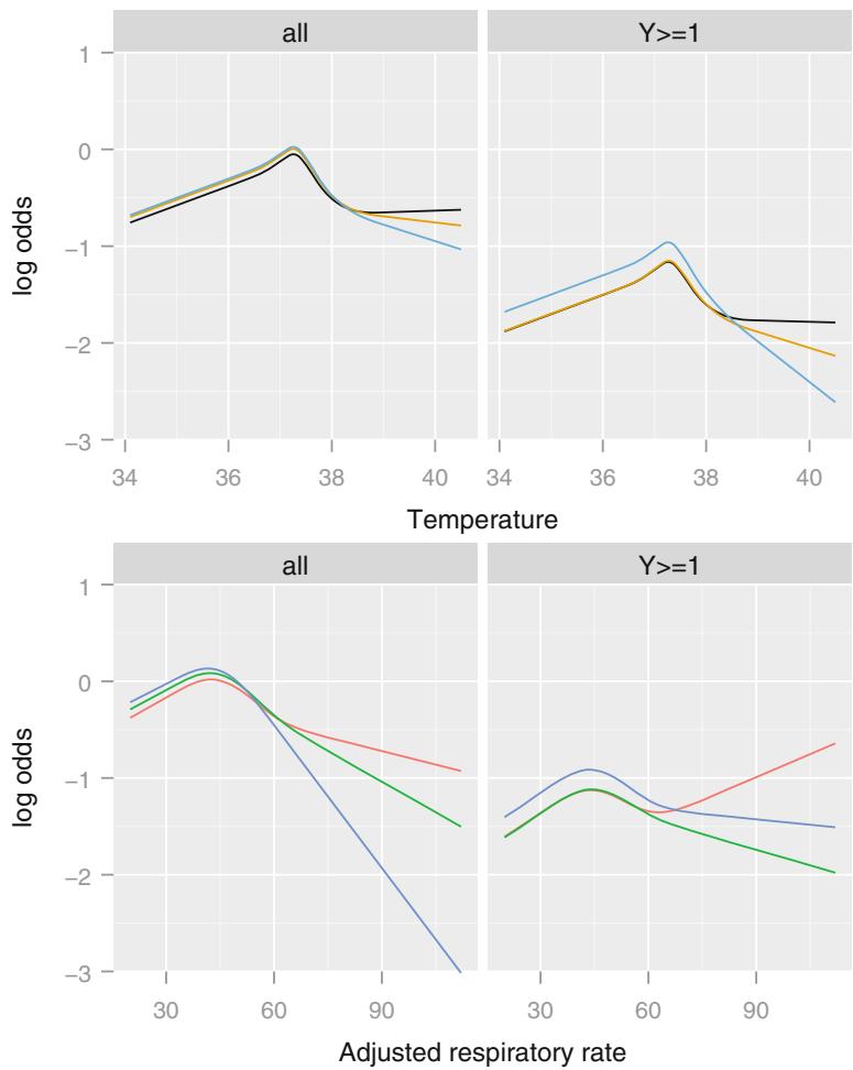
Fig. 14.7 Centered effects of predictors on the log odds, showing the effects of two predictors with interaction effects for the age intervals noted. The title all refers to the prediction of Y = 0|Y ≡ 0, that is, Y = 0. Y>=1 refers to predicting the probability of Y = 1|Y ≡ 1.

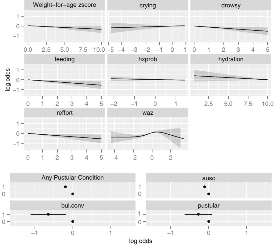
Fig. 14.8 Centered effects of predictors on the log odds, for predicting Y = 1|Y ≡ 1

Unfortunately, a 50-node CART was required to predict ^L^ˆ with an ^R² ^← ⁰.9, and the mean absolute error in the predicted logit was still 0.4. This will happen when the model contains many important continuous variables.

Let’s approximate the full model using its important components, by using a step-down technique predicting Lˆ from all of the component variables using ordinary least squares. In using step-down with the least squares function ols in rms there is a problem when the initial R² = 1.0 as in that case the estimate of τ = 0. This can be circumvented by specifying an arbitrary nonzero value of τ to ols (here 1.0), as we are not using the variance–covariance matrix from ols anyway. Since cohort interacts with the predictors, separate approximations can be developed for each level of Y . For this example we approximate the log odds that Y = 0 using the cohort of patients used for determining Y = 0, that is, Y ← 0 or cohort=‘all’.

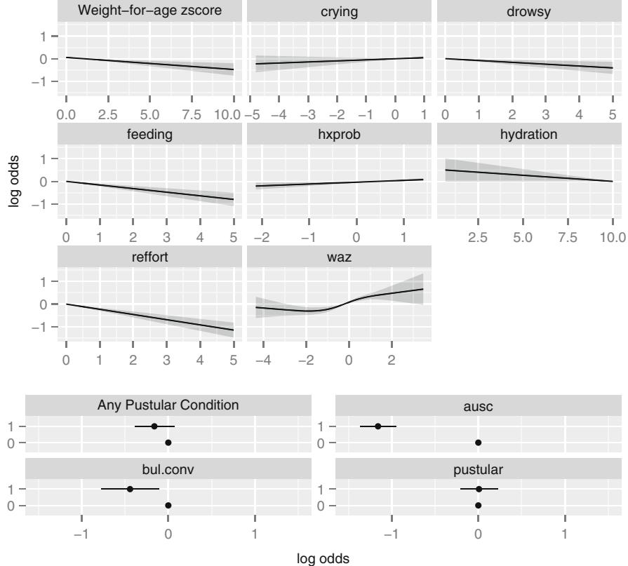
Fig. 14.9 Centered effects of predictors on the log odds, for predicting Y ≡ 1. No plot was made for the fever.ill, stop.breath. or labor cluster scores.

plogit − predict(full.pen)
f − ols(plogit ← ageg*(rcs(temp ,5) + rcs(rr ,5)) +
         rcs(waz ,4) + bul.conv + drowsy + agitated +
         reffort + ausc + feeding + abdominal + hydration +
         hxprob + pustular + crying + fever.ill +
         stop.breath + labor ,
         subset =cohort == ' all ' , data=Sc.expanded , sigma =1)
# Do fast backward stepdown
w − options( width =120)
fastbw (f, aics =1e10)

De leted Chi−Sq d . f . P R e s i d u a l d . f . P AIC R2
ageg ∗ temp 1 .87 8 0 .9848 1 .87 8 0 .9848 −14.13 1.000
ageg 0.05 2 0.9740 1.92 10 0.9969 −18.08 1.000
 pustu lar 0.02 1 0.8778 1.94 11 0.9987 −20.06 1.000
 fev er . i l l 0.08 1 0.7828 2.02 12 0.9994 −21.98 1.000
 crying 9.47 1 0.0021 11.49 13 0.5698 −14.51 0.999
abdominal 12.66 1 0.0004 24.15 14 0.0440 −3.85 0.997
 rr 17.90 4 0.0013 42.05 18 0.0011 6.05 0.995
hydration 13.21 1 0.0003 55.26 19 0.0000 17.26 0.993
 labor 23.48 1 0.0000 78.74 20 0.0000 38.74 0.990
stop . breath 33.40 1 0.0000 112.14 21 0.0000 70.14 0.986
bul . conv 51.53 1 0.0000 163.67 22 0.0000 119.67 0.980
 ag itated 63.66 1 0.0000 227.33 23 0.0000 181.33 0.972
hxprob 84.16 1 0.0000 311.49 24 0.0000 263.49 0.962
drowsy 109.86 1 0.0000 421.35 25 0.0000 371.35 0.948
temp 295 .67 4 0 .0000 717 .01 29 0 .0000 659 .01 0 .911
waz 368 .86 3 0 .0000 1085 .87 32 0 .0000 1021 .87 0 .866
 r e f f o r t 449.83 1 0.0000 1535.70 33 0.0000 1469.70 0.810
ageg ∗ rr 751.19 8 0.0000 2286.90 41 0.0000 2204.90 0.717
ausc 1906.82 1 0.0000 4193.72 42 0.0000 4109.72 0.482
 feed ing 3900.33 1 0.0000 8094.04 43 0.0000 8008.04 0.000
Approximate Estimates a fter Deleting Factors
     Coe f S .E . Wald Z P
[1 ,] 1.617 0.01482 109.1 0
Factors in F ina l Model
None

options(w)
# 1e10 causes all variables to eventually be
# deleted so can see most important ones in order
# Fit an approximation to the full penalized model using
# most important variables
full.approx −
  ols(plogit ← rcs(temp ,5) + ageg *rcs(rr ,5) +
      rcs(waz ,4) + bul.conv + drowsy + reffort +
      ausc + feeding ,
      subset =cohort == ' all ' , data= Sc.expanded )
p − predict(full.approx)
abserr − mean(abs(p - plogit [cohort == ' all ' ]))
Dxy − somers2(p, y[ cohort == ' all ' ])[ ' Dxy ' ]

The approximate model had R² against the full penalized model of 0.972, and the mean absolute error in predicting Lˆ was 0.17. The Dxy rank correlation between the approximate model’s predicted logit and the binary event Y = 0

is 0.665 as compared with the full model’s Dxy = 0.672. See Section 19.5 for an example of computing correct estimates of variance of the parameters in an approximate model.

Next turn to diagramming this model approximation so that all predicted values can be computed without the use of a computer. We draw a type of nomogram that converts each effect in the model to a 0 to 100 scale which is just proportional to the log odds. These points are added across predictors to derive the “Total Points,” which are converted to Lˆ and then to predicted probabilities. For the interaction between rr and ageg, rms’s nomogram function automatically constructs three rr axes—only one is added into the total point score for a given subject. Here we draw a nomogram for predicting the probability that Y > 0, which is 1 × Pr(Y = 0). This probability is derived by negating Λˆ and XΛˆ in the model derived to predict Pr(Y = 0).

f − full.approx
f$coefficients − -f$coefficients
f$linear.predictors − -f$linear.predictors
n − nomogram(f,
               temp =32:41, rr=seq(20 ,120, by=10),
               waz=seq(-1.5 ,2,by=.5),
               fun=plogis , funlabel= ' Pr(Y>0) ' ,
               fun.at =c(.02 ,.05 ,seq(.1 ,.9 ,by=.1),.95 ,.98 ))
# Print n to see point tables
plot (n, lmgp =.2 , cex.axis=.6) # Figure 14.10
newsubject −
  data.frame( ageg= ' [ 0, 7) ' , rr=30, temp =39, waz=0, drowsy =5,
              reffort=2, bul.conv =0, ausc =0, feeding=0)
xb − predict(f, newsubject)

The nomogram is shown in Figure 14.10. As an example in using the nomogram, a six-day-old infant gets approximately 9 points for having a respiration rate of 30/minute, 19 points for having a temperature of 39≤C, 11 points for waz=0, 14 points for drowsy=5, and 15 points for reffort=2. Assuming that bul.conv=ausc=feeding=0, that infant gets 68 total points. This corresponds to ^XΛ^ˆ ⁼ ^×0.68 and a probability of 0.34. ³

14.11 Validating the Model

For the full CR model that was fitted using penalized maximum likelihood estimation (PMLE), we used 200 bootstrap replications to estimate and then to correct for optimism in various statistical indexes: Dxy, generalized R², intercept and slope of a linear re-calibration equation for XΛˆ, the maximum calibration error for Pr(Y = 0) based on the linear-logistic re-calibration (Emax), and the Brier quadratic probability score B. PMLE is used at each of the 200 resamples. During the bootstrap simulations, we sample with

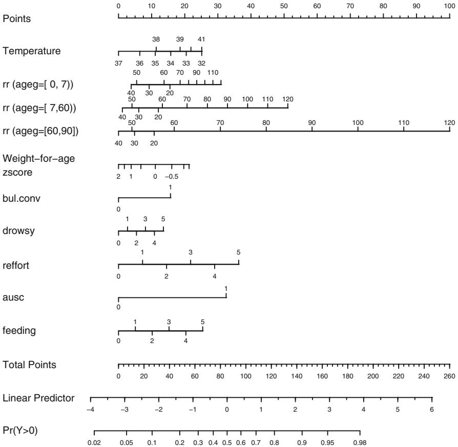
Fig. 14.10 Nomogram for predicting Pr(Y > 0) from the penalized extended CR model, using an approximate model fitted using ordinary least squares (R² = 0.972 against the full model’s predicted logits).

replacement from the patients and not from the 5553 expanded records, hence the specification cluster=u$subs, where u$subs is the vector of sequential patient numbers computed from cr.setup above. To be able to assess predictive accuracy of a single predicted probability, the subset parameter is specified so that Pr(Y = 0) is being assessed even though 5553 observations are used to develop each of the 200 models.

set.seed (1) # so can reproduce results
v − validate( full.pen , B =200, cluster=u$subs ,
                subset =cohort == ' all ' )
latex (v, file= ' ' , digits =2, size = ' smaller ' )

Index	Original Training		Test	Optimism Corrected
	Sample	Sample	Sample		Index
Dxy	0.67	0.68	0.67	0.01	0.66 200
R2	0.38	0.38	0.37	0.01	0.36 200
Intercept	×0.03	×0.03	0.00	×0.03	0.00 200
Slope	1.03	1.03	1.00	0.03	1.00 200
Emax	0.00	0.00	0.00	0.00	0.00 200
D	0.28	0.29	0.28	0.01	0.27 200
U	0.00	0.00	0.00	0.00	0.00 200
Q	0.28	0.29	0.28	0.01	0.27 200
B	0.12	0.12	0.12	0.00	0.12 200
g	1.47	1.50	1.45	0.04	1.42 200
gp	0.22	0.23	0.22	0.00	0.22 200
v round (v, 3) −

We see that for the apparent Dxy = 0.672 and that the optimism from overfitting was estimated to be 0.011 for the PMLE model, so the biascorrected estimate of predictive discrimination is 0.661. The intercept and slope needed to re-calibrate XΛˆ to a 45^≤ line are very near (0, 1). The estimate of the maximum calibration error in predicting Pr(Y = 0) is 0.001, which is quite satisfactory. The corrected Brier score is 0.122.

The simple calibration statistics just listed do not address the issue of whether predicted values from the model are miscalibrated in a nonlinear way, so now we estimate an overfitting-corrected calibration curve nonparametrically.

cal − calibrate( full.pen , B =200, cluster=u$subs ,
                  subset =cohort == ' all ' )
err − plot(cal) # Figure 14.11

n=5553 Mean a b s o l u t e e r r o r =0 .017 Mean squ a r e d e r r o r =0 .00043
0.9 Quantile of absolute error =0.038

The results are shown in Figure 14.11. One can see a slightly nonlinear calibration function estimate, but the overfitting-corrected calibration is excellent everywhere, being only slightly worse than the apparent calibration. The estimated maximum calibration error is 0.044. The excellent validation for both predictive discrimination and calibration are a result of the large sample size, frequency distribution of Y , initial data reduction, and PMLE.

14.12 Summary

Clinically guided variable clustering and item weighting resulted in a great reduction in the number of candidate predictor degrees of freedom and hence increased the true predictive accuracy of the model. Scores summarizing clusters of clinical signs, along with temperature, respiration rate, and weightfor-age after suitable nonlinear transformation and allowance for interactions

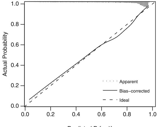
Predicted Pr{y=1}

Fig. 14.11 Bootstrap calibration curve for the full penalized extended CR model. 200 bootstrap repetitions were used in conjunction with the loess smoother.111 Also shown is a “rug plot” to demonstrate how effective this model is in discriminating patients into low- and high-risk groups for Pr(Y = 0) (which corresponds with the derived variable value y = 1 when cohort=‘all’).

with age, are powerful predictors of the ordinal response. Graphical methods are effective for detecting lack of fit in the PO and CR models and for diagramming the final model. Model approximation allowed development of parsimonious clinical prediction tools. Approximate models inherit the shrinkage from the full model. For the ordinal model developed here, substantial shrinkage of the full model was needed.

14.13 Further Reading

1 See Moons et al.462 for another case study in penalized maximum likelihood estimation.
2 The lasso method of Tibshirani608,609 also incorporates shrinkage into variable selection.
3 To see how this compares with predictions using the full model, the extra clinical signs in that model that are not in the approximate model were predicted individually on the basis of Xχˆ from the reduced model along with the signs that are in that model, using ordinary linear regression. The signs not specified when evaluating the approximate model were then set to predicted values based on the values given for the 6-day-old infant above. The resulting Xχˆ for the full model is ×0.81 and the predicted probability is 0.31, as compared with -0.68 and 0.34 quoted above.

14.14 Problems

Develop a proportional odds ordinal logistic model predicting the severity of functional disability (sfdm2) in SUPPORT. The highest level of this variable corresponds to patients dying before the two-month follow-up interviews. Consider this level as the most severe outcome. Consider the following predictors: age, sex, dzgroup, num.co, scoma, race (use all levels), meanbp, hrt, temp, pafi, alb, adlsc. The last variable is the baseline level of functional disability from the “activities of daily living scale.”

1. For the variables adlsc, sex, age, meanbp, and others if you like, make plots of means of predictors stratified by levels of the response, to check for ordinality. On the same plot, show estimates of means assuming the proportional odds relationship between predictors and response holds. Comment on the evidence for ordinality and for proportional odds.
1. To allow for maximum adjustment of baseline functional status, treat this predictor as nominal (after rounding it to the nearest whole number; fractional values are the result of imputation) in remaining steps, so that all dummy variables will be generated. Make a single chart showing proportions of various outcomes stratified (individually) by adlsc, sex, age, meanbp. For continuous predictors use quartiles. You can pass the following function to the summary (summary.formula) function to obtain the proportions of patients having sfdm2 at or worse than each of its possible levels (other than the first level). An easy way to do this is to use the cumcategory function with the Hmisc package’s summary.formula function. cumcategorysummary.formula Print estimates to only two significant digits of precision. Manually check the calculations for the sex variable using table(sex, sfdm2). Then plot all estimates on a single graph using plot(object, which=1:4), where object was created by summary (actually summary.formula). Note: for printing tables you may want to convert sfdm2 to a 0–4 variable so that column headers are short and so that later calculations are simpler. You can use for example:

sfdm − as.integer( sfdm2) - 1

Use an R function such as the following to compute the logits of the cumulative proportions.

sf − function(y)
  c ( ' Y ≡ 1 ' =qlogis (mean(y ≡ 1)),
     ' Y ≡ 2 ' =qlogis (mean(y ≡ 2)),
     ' Y ≡ 3 ' =qlogis (mean(y ≡ 3)),
     ' Y ≡ 4 ' =qlogis (mean(y ≡ 4)))

As the Y = 3 category is rare, it may be even better to omit the Y ← 4 column above, as was done in Section 13.3.9 and Figure 13.1. For each predictor pick two rows of the summary table having reasonable sample sizes, and take the difference between the two rows. Comment on the validity of the proportional odds assumption by assessing how constant the row differences are across columns. Note: constant differences in log odds (logits) mean constant ratios of odds or constant relative effects of the predictor across outcome levels.

Make two plots nonparametrically relating age to all of the cumulative proportions or their logits. You can use commands such as the following (to use the R Hmisc package).

for(i in 1:4)
  plsmo (age , sfdm ≡ i, add=i>1,
         ylim=c(.2 ,.8), ylab = ' Proportion Y ≡ j ' )
for(i in 1:4)
  plsmo (age , sfdm ≡ i, add=i>1, fun=qlogis ,
         ylim=qlogis (c(.2 ,.8)), ylab= ' logit ' )

Comment on the linearity of the age effect (which of the two plots do you use?) and on the proportional odds assumption for age, by assessing parallelism in the second plot.

1. Impute race using the most frequent category and pafi and alb using “normal” values.
1. Fit a model to predict the ordinal response using all predictors. For continuous ones assume a smooth relationship but allow it to be nonlinear. Quantify the ability of the model to discriminate patients in the five outcomes. Do an overall likelihood ratio test for whether any variables are associated with the level of functional disability.
1. Compute partial tests of association for each predictor and a test of nonlinearity for continuous ones. Compute a global test of nonlinearity. Graphically display the ranking of importance of the predictors.
1. Display the shape of how each predictor relates to the log odds of exceeding any level of sfdm2 you choose, setting other predictors to typical values (one value per predictor). By default, Predict will make predictions for the second response category, which is a satisfactory choice here.
1. Use resampling to validate the Somers’ Dxy rank correlation between predicted logit and the ordinal outcome. Also validate the generalized R², and slope shrinkage coefficient, all using a single R command. Comment on the quality (potential “export-ability”) of the model.

Chapter 15 Regression Models for Continuous Y and Case Study in Ordinal Regression

This chapter concerns univariate continuous Y . There are many multivariable models for predicting such response variables, such as

linear models with assumed normal residuals, fitted with ordinary least squares
generalized linear models and other parametric models based on special distributions such as the gamma
generalized additive models (GAMs)277
generalization of GAMs to also nonparametrically transform Y (see Chapter 16)
quantile regression (see Section 15.2)
other robust regression models that, like quantile regression, use an objective different from minimizing the sum of squared errors635
semiparametric models based on the ranks of Y , such as the Cox proportional hazards model (Chapter 20) and the proportional odds ordinal logistic model (Chapters 13 and 14)
cumulative probability models (often called cumulative link models) which are semiparametric models from a wider class of families than the logistic.

Semiparametric models that treat Y as ordinal but not interval-scaled have many advantages including robustness and freedom from all distributional assumptions for Y conditional on any given set of predictors. Advantages are demonstrated in a case study of a cumulative probability ordinal model. Some of the results are compared to quantile regression and OLS. Many of the methods used in the case study also apply to ordinary linear models.

15.1 The Linear Model

The most popular multivariable model for analyzing a univariate continuous Y is the linear model

359

^© Springer International Publishing Switzerland 2015 F.E. Harrell, Jr., Regression Modeling Strategies, Springer Series in Statistics, DOI 10.1007/978-3-319-19425-7 15

360 15 Regression Models for Continuous Y and Case Study in Ordinal Regression

\[E(Y|X) = X\beta,\tag{15.1}\]

where Λ is estimated using ordinary least squares, that is, by solving for Λˆ to minimize “(Yⁱ ^× ^XΛˆ)².

To compute P-values and confidence limits using parametric methods we would have to assume that Y |X is normal with mean XΛ and constant variance τ2a. One could estimate conditional means of Y without any distributional assumptions, but least squares estimators are not robust to outliers or high-leverage points, and the model would be inaccurate in estimating conditional quantiles of Y |X or Prob[Y ← c|X] unless normality of residuals holds. To be accurate in estimating all quantities, the linear model assumes that the Gaussian distribution of Y |X¹ is a simple shift from the distribution of Y |X2.

15.2 Quantile Regression

Quantile regression355, 357 is a different approach to modeling Y . It makes no distributional assumptions other than continuity of Y , while having all the usual right hand side assumptions. Quantile regression provides essentially the same estimates as sample quantiles if there is only an intercept or a categorical predictor in the model. Quantile regression is transformation invariant — pre-transforming Y is not important.

Quantile regression is a natural generalization of sample quantiles. Let ^∂^∂ (y) = ^y(^Γ ^× [y < 0]). The ^Γ ^t^h ” sample quantile is the minimizer ^q of ⁿ ⁱ−¹ ^∂^∂ (yⁱ ^× ^q). For a conditional ^Γ ^t^h quantile of ^Y ^|^X the corresponding quantile regression estimator Λˆ^∂ minimizes “ⁿ ⁱ=1 ∂^∂ (Yⁱ × XΛ).

In non-large samples, quantile regression is not as efficient at estimating quantiles as is ordinary least squares at estimating the mean, if the latter’s assumptions hold.

Koenker’s quantreg package in R356 implements quantile regression, and the rms package’s Rq function provides a front-end that gives rise to various graphics and inference tools.

Using quantile regression, we directly model the median as a function of covariates so that only the XΛ structure need be correct. Other quantiles (e.g., 90^t^h percentile) can be modeled but standard errors will be much larger as it is more difficult to precisely estimate outer quantiles.

^a The latter assumption may be dispensed with if we use a robust Huber–White or bootstrap covariance matrix estimate. Normality may sometimes be dispensed with by using bootstrap confidence intervals.

15.3 Ordinal Regression Models for Continuous Y

A different robust semiparametric regression approach than quantile regression is the cumulative probability ordinal model. Semiparametric models have several advantages over parametric models such as OLS. While quantile regression has no restriction in the parameters when modeling one quantile versus anotherb, ordinal cumulative probability models assume a connection between distributions of Y for different X. Ordinal regression even makes one less assumption than quantile regression about the distribution of Y for a specific X: the distribution need not be continuous.

Applying an increasing 1–1 transformation to Y results in no change to regression coefficient estimates with ordinal regressionc. Regression coefficient estimates are completely robust to extreme Y values^d. Estimates of quantiles of Y from ordinal regression are exactly transformation-preserving, e.g., the estimate of the median of log Y is exactly the log of the estimate of the median Y .

For a general continuous distribution function F(y), an ordinal regression model based on cumulative probabilities may be stated as follows^e. Let the ordered unique values of Y be denoted by y1, y2,…,y^k and let the intercepts associated with y1,…,y^k be σ1, σ2,…, σk, where σ¹ = √ because Prob[Y ← y1] = 1. Let σ^y = σi, i : yⁱ = y. Then

\[\text{Prob}[Y \ge y\_i | X] = F(\alpha\_i + X\beta) = F(\alpha\_{y\_i} + X\beta) \tag{15.2}\]

For the OLS fully parametric case, the model may be restated

\[\text{Prob}[Y \ge y | X] = \text{Prob}[\frac{Y - X\beta}{\sigma} \ge \frac{y - X\beta}{\sigma}] \tag{15.3}\]

\[1 = 1 - \Phi(\frac{y - X\beta}{\sigma}) = \Phi(\frac{-y}{\sigma} + \frac{X\beta}{\sigma}) \tag{15.4}\]

^b Quantile regression allows the estimated value of the 0.5 quantile to be higher than the estimated value of the 0.6 quantile for some values of X. Composite quantile regression690 removes this possibility by forcing all the X coefficients to be the same across multiple quantiles, a restriction not unlike what cumulative probability ordinal models make.

^c For symmetric distributions applying a decreasing transformation will negate the coefficients. For asymmetric distributions (e.g., Gumbel), reversing the order of Y will do more than change signs.

^d Only an estimate of mean Y from these χˆs is non-robust.

^e It is more traditional to state the model in terms of Prob[^Y ^≤ ^y|X] but we use Prob[Y ≡ y|X] so that higher predicted values are associated with higher Y .

Table 15.1 Distribution families used in ordinal cumulative probability models. ρ denotes the Gaussian cumulative distribution function. For the Connection column, P¹ = Prob[Y ≡ y|X1], P² = Prob[Y ≡ y|X2], ∆ = (X² × X1)χ. The connection specifies the only distributional assumption if the model is fitted semiparametrically, i.e, contains an intercept for every unique Y value less one. For parametric models, P¹ must be specified absolutely instead of just requiring a relationship between P¹ and P2. For example, the traditional Gaussian parametric model specifies that Prob[Y ≡ ^y|X]=1 ^× ^ρ( ^y∧X^β ^σ ) = ^ρ( ^∧y+X^β ^σ ).

Distribution	F	Inverse	Link Name	Connection
		(Link Function)
Logistic	[1 + exp(∼y)]∧1	log( y 1∧y )	logit	P2 P1 = exp(∆) 1∧P2 1∧P1
Gaussian	Φ(y)	Φ∧1(y)	probit	P2 = Φ(Φ∧1(P1) + ∆)
Gumbel maximum exp(∼ exp(∼y)) value		log(∼ log(y))	log ∼ log	P2 = P exp(∆) 1
value			log ∼ log	Gumbel minimum 1 ∼ exp(∼ exp(y)) log(∼ log(1 ∼ y)) complementary 1 ∼ P2 = (1 ∼ P1)exp(∆)
Cauchy	π tan∧1(y) + 1 1 2	tan[π(y ∼ 1 2 )]	cauchit

so that to within an additive constant^f σ^y = ⁻^y ^β (intercepts σ are linear in y whereas they are arbitrarily descending in the ordinal model), and τ is absorbed in Λ to put the OLS model into the new notation.

The general ordinal regression model assumes that for fixed X1, X2,

\[F^{-1}(\text{Prob}[Y \ge y | X\_2]) - F^{-1}(\text{Prob}[Y \ge y | X\_1]) \tag{15.5}\]

\[=(X\_2 - X\_1)\beta\tag{15.6}\]

independent of the ^σs (parallelism assumption). If ^F = [1 + exp(×y)]−¹, this is the proportional odds assumption.

Common choices of F, implemented in the R rms orm function, are shown in Table 15.1. The Gumbel maximum value distribution is also called the extreme value type I distribution. This distribution (log × log link) also represents a continuous time proportional hazards model. The hazard ratio when X changes from X¹ to X² is exp(×(X² × X1)Λ).

The mean of Y |X is easily estimated from a fitted cumulative probability ordinal model by computing

\[\sum\_{i=1}^{n} y\_i \widehat{\text{Prob}}[Y=y\_i|X] \tag{15.7}\]

and the ^qth quantile of ^Y ^|^X is ^y such that ^F ⁻¹(1 ^× ^q) ^× ^XΛ^ˆ = ˆσy. g

^f ∂ˆ^y are unchanged if a constant is added to all y.

^g The intercepts have to be shifted to the left one position in solving this equation because the quantile is such that Prob[Y ≤ y] = q whereas the model is stated in terms of Prob[Y ≡ y].

The orm function in the rms package takes advantage of the information matrix being of a sparse tri-band diagonal form for the intercept parameters. This makes the computations efficient even for hundreds of intercepts (i.e., unique values of Y ). orm is made to handle continuous Y .

Ordinal regression has nice properties in addition to those listed above, allowing for

estimation of quantiles as efficiently as quantile regression if the parallel slopes assumptions hold
efficient estimation of mean Y
direct estimation of Prob[Y ← y|X]
arbitrary clumping of values of Y , while still estimating Λ and mean Y efficiently^h
solutions for Λˆ using ordinary Newton-Raphson or other popular optimization techniques
being based on a standard likelihood function, penalized estimation can be straightforward
Wald, score, and likelihood ratio β² tests that are more powerful than tests from quantile regression.

On the last point, if there is a single predictor in the model and it is binary, the score test from the proportional odds model is essentially the Wilcoxon test, and the score test from the Gumbel log-log cumulative probability model is essentially the log-rank test.

15.3.1 Minimum Sample Size Requirement

When Y is continuous and the purpose of an ordinal model includes semiparametric estimation of probabilities or quantiles, the accuracy of estimates is limited even more by the accuracy of estimating the empirical cumulative distribution of Y than by estimating Λ. When Λ = 0, intercept estimates are transformations of the empirical distribution step function. As described in Section 20.3, the sample size must be 184 to estimate the entire distribution of Y with a global margin of error not exceeding 0.1. For estimating the mean of Y , smaller sample sizes may be needed.

^h But it is not sensible to estimate quantiles of Y when there are heavy ties in Y in the area containing the quantile.

15.4 Comparison of Assumptions of Various Models

Quantile regression makes the fewest left-hand-side model assumptions except for the assumption that Y be continuous, but can have less estimator precision than other models and has lower power. To summarize how assumptions of parametric models compare to assumptions of semiparametric ordinal models, consider the ordinary linear model or its special case the equal variance twosample t-test, vs. the probit or logit (proportional odds) ordinal model or their special cases the Van der Waerden (normal-scores) two-sample rank test or the Wilcoxon two-sample test. All the assumptions of the linear model other than independence of residuals are captured in the following, using the more standard Y − y notation:

\[F(y|X) = \text{Prob}[Y \le y|X] = \Phi(\frac{y - X\beta}{\sigma}) \tag{15.8}\]

\[\Phi^{-1}(F(y|X)) = \frac{y - X\beta}{\sigma} \tag{15.9}\]

On the other hand, ordinal models assume the following:

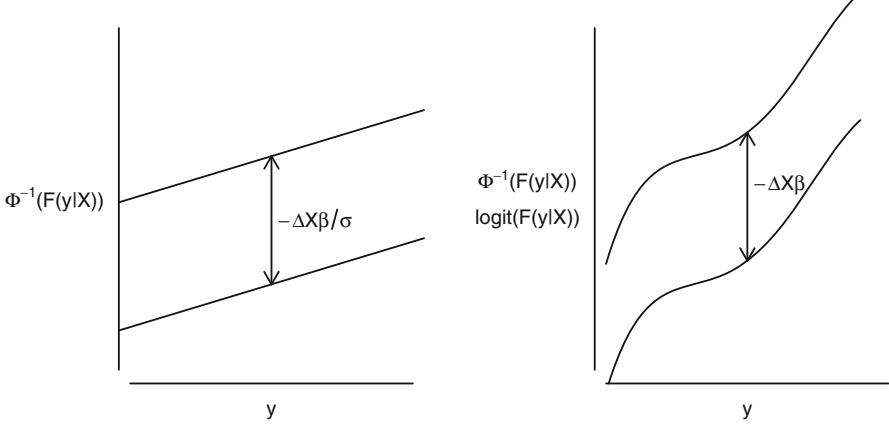
Fig. 15.1 Assumptions of the linear model (left panel) and semiparametric ordinal probit or logit (proportional odds) models (right panel). Ordinal models do not assume any shape for the distribution of Y for a given X; they only assume parallelism. The linear model can relax the parallelism assumption if λ is allowed to vary, but in practice it is difficult to know how to vary it except for the unequal variance two-sample t-test.

\[\text{Prob}[Y \le y | X] = F(g(y) - X\beta),\tag{15.10}\]

where g is unknown and may be discontinuous. This translates to the parallelism assumption in the right panel of Figure 15.1, whereas the linear model makes the additional strong assumption of linearity of normal inverse cumulative distribution function, which arises from the Gaussian distribution assumption.

15.5 Dataset and Descriptive Statistics

Diabetes Mellitus (DM) type II (adult onset diabetes) is strongly associated with obesity. The currently best laboratory test for diabetes measures glycosylated hemoglobin (HbA1c), also called glycated hemoglobin, glycohemoglobin, or hemoglobin A1c. HbA1^c reflects average blood glucose for the preceding 60 to 90 days. HbA1^c > 7.0 is sometimes taken as a positive diagnosis of diabetes even though there are no data to support the use of a threshold.

The goals of this analyses are to better understand effects of body size measurements on risk of DM and to enhance screening for DM. The best way to develop a model for DM screening is not to fit a binary logistic model with HbA1^c > 7 as the response variable. There are at least two reasons for this. First, when the relationship between a measurement and its ultimate clinical impact is smooth, all cutpoints are arbitrary. There is no justification for any putative cut on HbA1c. Second, such an analysis loses information by treating HbA1c=2 the same as HbA1c=6.9, and by treating HbA1c=7.1 as equal to HbA1c=10. Failure to use all available information results in larger standard errors of Λˆ, lower power, and wider confidence bands. It is better to predict continuous HbA1^c using a continuous response model, then use that model to estimate the probability that HbA1^c exceeds any cutoff, or estimate the 0.9 quantile of HbA1c.

The data used here are from the National Health and Nutrition Examination Survey (NHANES) 2009–2010 from the U.S. National Center for Health Statistics/Centers for Disease Control. The original data may be obtained from http://www.cdc.gov/nchs/nhanes.htm 94; the analysis file used here, called nhgh, may be obtained from the DataSets wiki page, along with R code used to download and create the file. Note that CDC coded age ← 80 as 80. We use the subset of subjects with age ← 21 who have neither been diagnosed nor treated for DM. Descriptive statistics are shown below.

require(rms)

getHdata (nhgh)
w − subset(nhgh , age ≡ 21 & dx==0 & tx==0, select=-c(dx,tx))
latex(describe(w), file= ' ' )

	18 Variables	w 4629	Observations
4629 0	seqn : Respondent sequence number n missing unique Info Mean 4629	.05 .10	.25 .50 .75 .90 .95 1 56902 52136 52633 54284 56930 59495 61079 61641
	lowest : 51624 51629 51630 51645 51647 highest: 62152 62153 62155 62157 62158
sex n missing unique 4629 0	2
	male (2259, 49%), female (2370, 51%)
age : Age [years] 4629 0	n missing unique Info Mean 703	.05 .10	.25 .50 .75 .90 .95 1 48.57 23.33 26.08 33.92 46.83 61.83 74.83 80.00
	lowest : 21.00 21.08 21.17 21.25 21.33 highest: 79.67 79.75 79.83 79.92 80.00
re : Race/Ethnicity n missing unique 4629 0	5
Non-Hispanic	Mexican American (832, 18%), Other Hispanic (474, 10%) White (2318, 50%), Non-Hispanic Other Race Including Multi-Racial	(249, 5%)	Black (756, 16%)
income : Family Income n missing unique 4389 240	14
>= 100000 (619, 14%)	[15000,20000) (300, 7%), [20000,25000) (374, 9%) [25000,35000) (535, 12%), [35000,45000) (421, 10%)		[0,5000) (162, 4%), [5000,10000) (216, 5%), [10000,15000) (371, 8%) [45000,55000) (346, 8%), [55000,65000) (257, 6%), [65000,75000) (188, 4%) > 20000 (149, 3%), < 20000 (52, 1%), [75000,100000) (399, 9%)
wt : Weight [kg] 4629 0	n missing unique Info Mean 890	.05 .10	.25 .50 .75 .90 .95 1 80.49 52.44 57.18 66.10 77.70 91.40 106.52 118.00
lowest : 33.2	36.1 37.9 38.5 highest: 184.3 186.9 195.3 196.6 203.0	38.7
ht : Standing Height [cm] 4629 0	n missing unique Info Mean 512 lowest : 123.3 135.4 137.5 139.4 139.8 highest: 199.2 199.3 199.6 201.7 202.7	.05 .10	.25 .50 .75 .90 .95 1 167.5 151.1 154.4 160.1 167.2 175.0 181.0 184.8

bmi : Body Mass Index [kg/m2] n missing unique Info Mean .05 .10 .25 .50 .75 .90 .95 4629 0 1994 1 28.59 20.02 21.35 24.12 27.60 31.88 36.75 40.68
lowest : 13.18 14.59 15.02 15.40 15.49 highest: 61.20 62.81 65.62 71.30 84.87
leg : Upper Leg Length [cm] n missing unique Info Mean .05 .10 .25 .50 .75 .90 .95 4474 155 216 1 38.39 32.0 33.5 36.0 38.4 41.0 43.3 44.6 lowest : 20.4 24.9 25.0 25.1 26.4, highest: 49.0 49.5 49.8 50.0 50.3
arml : Upper Arm Length [cm] n missing unique Info Mean .05 .10 .25 .50 .75 .90 .95 4502 127 156 1 37.01 32.6 33.5 35.0 37.0 39.0 40.6 41.7 lowest : 24.8 27.0 27.5 29.2 29.5, highest: 45.2 45.5 45.6 46.0 47.0
armc : Arm Circumference [cm] n missing unique Info Mean .05 .10 .25 .50 .75 .90 .95 4499 130 290 1 32.87 25.4 26.9 29.5 32.5 35.8 39.1 41.4 lowest : 17.9 19.0 19.3 19.5 19.9, highest: 54.2 54.9 55.3 56.0 61.0
waist : Waist Circumference [cm] n missing unique Info Mean .05 .10 .25 .50 .75 .90 .95 4465 164 716 1 97.62 74.8 78.6 86.9 96.3 107.0 117.8 125.0 lowest : 59.7 60.0 61.5 62.0 62.4 highest: 160.0 160.6 162.2 162.7 168.7
tri : Triceps Skinfold [mm] n missing unique Info Mean .05 .10 .25 .50 .75 .90 .95 4295 334 342 1 18.94 7.2 8.8 12.0 18.0 25.2 31.0 33.8 lowest : 2.6 3.1 3.2 3.3 3.4, highest: 39.6 39.8 40.0 40.2 40.6
sub : Subscapular Skinfold [mm] n missing unique Info Mean .05 .10 .25 .50 .75 .90 .95 3974 655 329 1 20.8 8.60 10.30 14.40 20.30 26.58 32.00 35.00 lowest : 3.8 4.2 4.6 4.8 4.9, highest: 40.0 40.1 40.2 40.3 40.4
gh : Glycohemoglobin [%] n missing unique Info Mean .05 .10 .25 .50 .75 .90 .95 4629 0 63 0.99 5.533 4.8 5.0 5.2 5.5 5.8 6.0 6.3 lowest : 4.0 4.1 4.2 4.3 4.4, highest: 11.9 12.0 12.1 12.3 14.5
albumin : Albumin [g/dL] n missing unique Info Mean .05 .10 .25 .50 .75 .90 .95 4576 53 26 0.99 4.261 3.7 3.9 4.1 4.3 4.5 4.7 4.8 lowest : 2.6 2.7 3.0 3.1 3.2, highest: 4.9 5.0 5.1 5.2 5.3

368 15 Regression Models for Continuous Y and Case Study in Ordinal Regression

bun : Blood urea nitrogen [mg/dL] 4576	53		n missing unique Info Mean .05 .10 .25 .50 .75 .90 .95 50 0.99 13.03 7	8 10 12	15 19	22
lowest :	1 2	3 4	5, highest: 49 53 55 56 63
SCr : Creatinine [mg/dL] 4576 lowest : highest:	53 0.34 5.98	n missing unique Info 167 0.38 6.34	Mean .05 1 0.8887 0.58 0.62 0.72 0.84 0.99 1.14 1.25 0.39 0.40 9.13 10.98 15.66	.10 .25 0.41	.50	.75 .90	.95
dd −	datadist(w);		options(datadist= ’ dd ’ )

15.5.1 Checking Assumptions of OLS and Other Models

First let’s see if gh would make a Gaussian residuals model fit. Use ordinary regression on four key variables to collapse these into one variable (predicted mean from the OLS model). Stratify the predicted means into six quantile groups. Apply the normal inverse cumulative distribution function π−¹ to the empirical cumulative distribution functions (ECDF) of gh using these strata, and check for normality and constant ^τ². The ECDF estimates Prob[^Y ⁻ y|X] but for ordinal modeling we want to state models in terms of Prob[Y ← y|X] so take one minus the ECDF before inverse transforming.

f − ols(gh ← rcs(age ,5) + sex + re + rcs(bmi , 3), data=w)
pgh − fitted(f)
p − function (fun , row , col) {
  f − substitute (fun); g − function (F) eval(f)
  z − Ecdf(← gh, groups =cut2(pgh , g=6),
            fun=function (F) g(1 - F),
            ylab= as.expression(f), xlim=c(4.5, 7.75), data=w,
            label.curve =FALSE)
  print(z, split=c(col , row , 2, 2), more=row < 2 | col < 2)
}
p(log(F/(1-F)), 1, 1)
p(qnorm (F), 1, 2)
p(-log(-log(F)), 2, 1)
p(log(-log(1-F)), 2, 2)
# Get slopes of pgh for some cutoffs of Y
# Use glm complementary log-log link on Prob(Y < cutoff) to
# get log-log link on Prob(Y ≡ cutoff)
r − NULL
for(link in c( ' logit ' , ' probit ' , ' cloglog ' ))
  for(k in c(5, 5.5, 6)) {
    co − coef(glm(gh < k ← pgh , data=w, family =binomial (link)))

r − rbind(r, data.frame (link=link , cutoff=k,
                               slope=round(co[2],2)))
}

print(r, row.names =FALSE)

cutoff	slope
5.0	-3.39
5.5	-4.33
6.0	-5.62
5.0	-1.69
5.5	-2.61
6.0	-3.07
5.0	-3.18
5.5	-2.97
6.0	-2.51

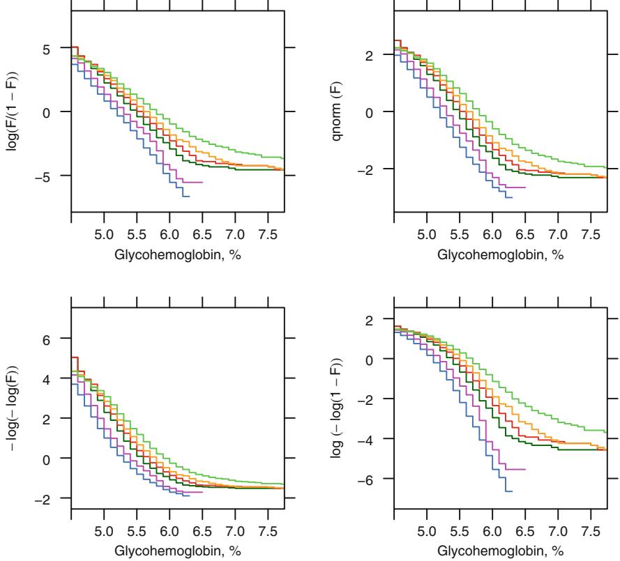
Fig. 15.2 Examination of normality and constant variance assumption, and assumptions for various ordinal models

The upper right curves in Figure 15.2 are not linear, implying that a normal conditional distribution cannot work for ghⁱ There is non-parallelism for the logit model. The other graphs will be used to guide selection of an ordinal model below.

15.6 Ordinal Regression Applied to HbA1^c

In the upper left panel of Figure 15.2, logit inverse curves are not parallel so the proportional odds assumption does not hold when predicting HbA1c. The log-log link yields the highest degree of parallelism and most constant regression coefficients across cutoffs of gh, so we use this link in an ordinal regression model (linearity of the curves is not required).

15.6.1 Checking Fit for Various Models Using Age

Another way to examine model fit is to flexibly fit the single most important predictor (age) using a variety of methods, and compare predictions to sample quantiles and means based on subsets on age. We use overlapping subsets to gain resolution, with each subset composed of those subjects having age within five years of the point being predicted by the models. Here we predict the 0.5, 0.75, and 0.9 quantiles and the mean. For quantiles we can compare to quantile regression (discussed below) and for means we compare to OLS.

ag ← 25:75
lag ← length(ag)
q2 ← q3 ← p90 ← means ← numeric(lag)
for(i in 1:lag) {
  s ← which(abs(w$age - ag[i]) < 5)
  y ← w$gh[s]
  a ← quantile(y, probs =c(.5, .75 , .9))
  q2[i] ← a[1]
  q3[i] ← a[2]
  p90[i] ← a[3]
  means[i] ← mean(y)
}
fams ← c( ' logistic ' , ' probit ' , ' loglog ' , ' cloglog ' )
fe ← function(pred , target) mean(abs(pred$yhat - target))
mod ← gh ◦ rcs(age ,6)
P ← Er ← list()
for(est in c( ' q2 ' , ' q3 ' , ' p90 ' , ' mean ' )) {
  meth ← if(est == ' mean ' ) ' ols ' else ' QR '
  p ← list()
  er ← rep(NA, 5)
  names(er) ← c(fams , meth)
  for(family in fams) {
    h ← orm(mod, family=family, data=w)
    fun ← if(est == ' mean ' ) Mean(h)
    else {
      qu ← Quantile(h)

ⁱ They are not parallel either.

switch(est, q2 = function (x) qu(.5, x),
                   q3 = function (x) qu(.75, x),
                   p90 = function (x) qu(.9, x))
    }
    p[[family]] ← z ← Predict(h, age=ag, fun=fun, conf.int =FALSE)
    er[family] ← fe(z, switch(est, mean=means , q2=q2, q3=q3, p90=p90))
  }
  h ← switch(est,
              mean= ols(mod, data=w),
              q2 = Rq (mod, data=w),
              q3 = Rq (mod, tau=0.75, data=w),
              p90 = Rq (mod, tau=0.90, data=w))
  p[[meth]] ← z ← Predict (h, age=ag, conf.int =FALSE)
  er[meth] ← fe(z, switch(est, mean=means , q2=q2, q3=q3, p90=p90))
  Er[[est]] ← er
  pr ← do.call( ' rbind ' , p)
  pr$est ← est
  P ← rbind.data.frame(P, pr)
}
xyplot(yhat ◦ age | est, groups= .set. , data=P, type= ' l ' , # Figure 15.3
       auto.key =list(x=.75, y=.2 , points =FALSE , lines=TRUE),
       panel=function (..., subscripts) {
         panel.xyplot(..., subscripts=subscripts)
         est ← P$est[subscripts[1]]
         lpoints (ag, switch(est, mean=means , q2=q2, q3=q3, p90=p90),
                  col=gray(.7))
         er ← format(round(Er[[est]],3), nsmall =3)
         ltext(26, 6.15, paste(names(er), collapse = ' \n ' ),
               cex=.7, adj=0)
         ltext(40, 6.15, paste(er , collapse = ' \n ' ),
               cex=.7, adj=1)})

It can be seen in Figure 15.3 that models dedicated to a specific task (quantile regression for quantiles and OLS for means) were best for those tasks. Although the log-log ordinal cumulative probability model did not estimate the median as accurately as some other methods, it does well for the 0.75 and 0.9 quantiles and is the best compromise overall because of its ability to also directly predict the mean as well as quantities such as Prob[HbA1^c > 7|X].

From here on we focus on the log-log ordinal model. Returning to the bottom left of Figure 15.2, let’s look at quantile groups of predicted HbA1^c by OLS and plot predicted distributions of actual HbA1^c against empirical distributions.

w$pghg − cut2(pgh , g=6)
f − orm(gh ← pghg , data=w)
lp − predict (f, newdata =data.frame (pghg=levels(w$pghg)))
ep − ExProb(f) # Exceedance prob. functn. generator in rms
z − ep(lp)
j − order(w$pghg) # puts in order of lp (levels of pghg)
plot(z, xlim=c(4, 7.5), data=w[j,c( ' pghg ' , ' gh ' )]) # Fig. 15.4

Agreement between predicted and observed exceedance probability distributions is excellent in Figure 15.4.

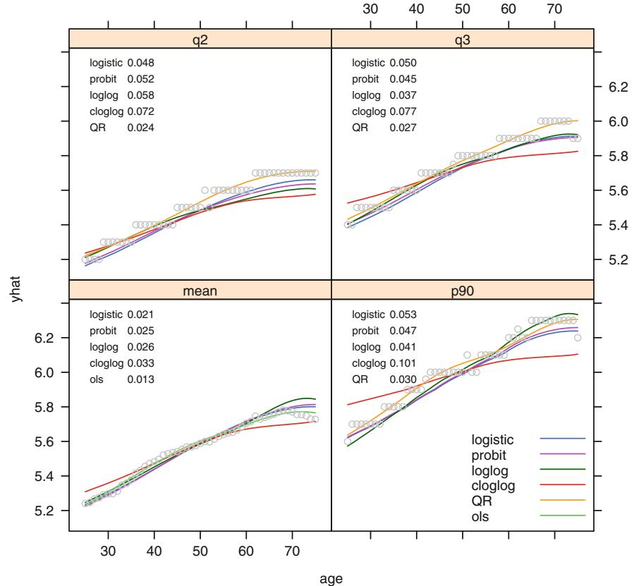
Fig. 15.3 Three estimated quantiles and estimated mean using 6 methods, compared against caliper-matched sample quantiles/means (circles). Numbers are mean absolute differences between predicted and sample quantities using overlapping intervals of age and caliper matching. QR:quantile regression.

To return to the initial look at a linear model with assumed Gaussian residuals, fit a probit ordinal model and compare the estimated intercepts to the linear relationship with gh that is assumed by the normal distribution.

f − orm(gh ← rcs(age ,6), family =probit , data=w)
g − ols(gh ← rcs(age ,6), data=w)
s − g$stats[ ' Sigma ' ]
yu − f$yunique [-1]
r − quantile (w$gh, c(.005 , .995))
alphas − coef(f)[1: num.intercepts(f)]
plot(-yu / s, alphas , type= ' l ' , xlim=rev(- r / s), # Fig. 15.5
   xlab=expression (-y/hat(sigma)), ylab=expression (alpha[y]))

Figure 15.5 depicts a significant departure from the linear form implied by Gaussian residuals (Eq. 15.4).

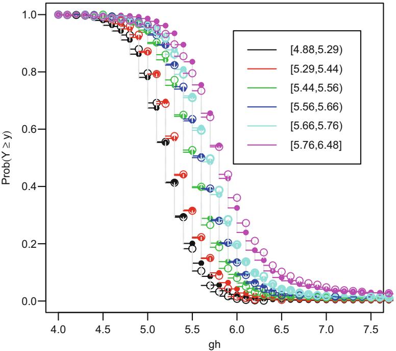
Fig. 15.4 Observed (dashed lines, open circles) and predicted (solid lines, closed circles) exceedance probability distributions from a model using 6-tiles of OLS-predicted HbA1c. Key shows quantile group intervals of predicted mean HbA1c.

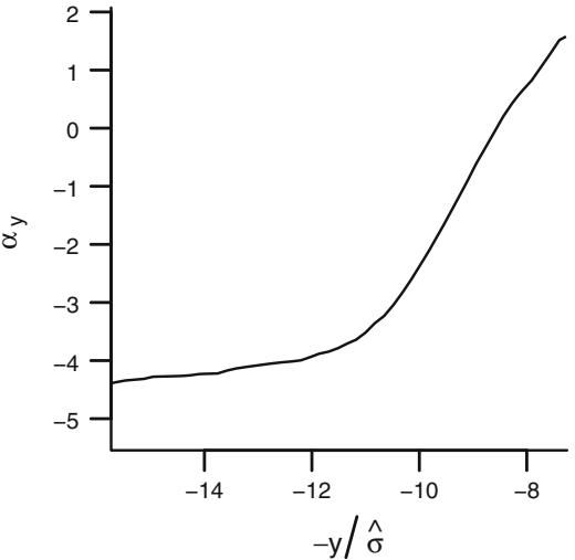
Fig. 15.5 Estimated intercepts from probit model. Linearity would have indicated Gaussian residuals.

15.6.2 Examination of BMI

Body mass index (BMI, weight divided by height2) is commonly used as an obesity measure because it is well correlated with abdominal visceral fat. But it is not obvious that BMI is the correct summary of height and weight for predicting pre-clinical diabetes, and it may be the case that body size measures other than height and weight are better predictors.

Use the log-log ordinal model to check the adequacy of BMI, adjusting for age (without assuming linearity). This can be done by examining the ratio of coefficients of log height and log weight, and also by using AIC to judge whether BMI is an adequate summary of height and weight when compared to nonlinear functions of the logs, and to a tensor spline interaction surface.

f ← orm(gh ◦ rcs(age ,5) + log(ht) + log(wt),
         family=loglog, data=w)
print(f, latex=TRUE)

-log-log Ordinal Regression Model

orm(formula = gh ~ rcs(age, 5) + log(ht) + log(wt), data = w,
    family = loglog)

	Model Likelihood	Discrimination	Rank Discrim.
	Ratio Test	Indexes	Indexes
Obs 4629	β2 LR 1126.94	R2 0.217	∂ 0.486
Unique Y 63	d.f. 6	g 0.627
Y0.5 5.5	β2) Pr(> < 0.0001	gr 1.872
α log L max αρ	β2 Score 1262.81	× 1 Pr(Y ← Y0.5) 2 0.153
1≤10−6	β2) Pr(> < 0.0001

	Coef	S.E.	Wald Z	Pr(> Z )
age	0.0398	0.0055	7.29	< 0.0001
age’	-0.0158	0.0275	-0.57	0.5657
age”	-0.0072	0.0866	-0.08	0.9333
age”’	0.0309	0.1135	0.27	0.7853
ht	-3.0680	0.2789	-11.00	< 0.0001
wt	1.2748	0.0704	18.10	< 0.0001

aic ← NULL
for(mod in list(gh ◦ rcs(age ,5) + rcs(log(bmi),5),
                gh ◦ rcs(age ,5) + rcs(log(ht),5) + rcs(log(wt),5),
                gh ◦ rcs(age ,5) + rcs(log(ht),4) * rcs(log(wt),4)))
  aic ← c(aic, AIC(orm(mod, family=loglog, data=w)))
print(aic)

1 25910.77 25910.17 25906.03

The ratio of the coefficient of log height to the coefficient of log weight is - 2.4, which is between what BMI uses and the more dimensionally reasonable weight / height3. By AIC, a spline interaction surface between height and weight does slightly better than BMI in predicting HbA1c, but a nonlinear function of BMI is barely worse. It will require other body size measures to displace BMI as a predictor.

As an aside, compare this model fit to that from the Cox proportional hazards model. The Cox model uses a conditioning argument to obtain a partial likelihood free of the intercepts σ (and requires a second step to estimate these log discrete hazard components) whereas we are using a full marginal likelihood of the ranks of Y 330.

print(cph(Surv(gh) ◦ rcs(age ,5)	+	log(ht)	+	log(wt),	data=w),
latex=TRUE)

Cox Proportional Hazards Model

cph(formula = Surv(gh) ~ rcs(age, 5) + log(ht)
              + log(wt), data = w)

		Model Tests		Discrimination
				Indexes
Obs	4629	β2 LR	1120.20	R2	0.215
Events	4629	d.f.	6	Dxy	0.359
Center 8.3792		β2) Pr(>	0.0000	g	0.622
		Score	β2 1258.07	gr	1.863
		β2) Pr(>	0.0000

	Coef	S.E.	Wald Z	Pr(> Z )
age	-0.0392	0.0054	-7.24	< 0.0001
age’	0.0148	0.0274	0.54	0.5888
age”	0.0093	0.0862	0.11	0.9144
age”’	-0.0321	0.1131	-0.28	0.7767
ht	3.0477	0.2779	10.97	< 0.0001
wt	-1.2653	0.0701	-18.04	< 0.0001

Close agreement of the two is seen, as expected.

15.6.3 Consideration of All Body Size Measurements

Next we examine all body size measures, and check their redundancies.

v − varclus(← wt + ht + bmi + leg + arml + armc + waist + tri + sub + age + sex + re , data =w) plot(v)

376 15 Regression Models for Continuous Y and Case Study in Ordinal Regression

# Omit wt so it won ' t be removed before bmi
redun (← ht + bmi + leg + arml + armc + waist + tri + sub ,
      data=w, r2=.75)

Redundancy Analysis
redun(formula = ◦ht + bmi + leg + arml + armc + waist + tri +
   sub, data = w, r2 = 0.75)
n: 3853 p: 8 nk: 3
Number of NAs: 776
Frequencies of Missing Values Due to Each Variable
  ht bmi leg arml armc waist tri sub
   0 0 155 127 130 164 334 655
Transformation of target variables forced to be linear
R2 cutoff: 0.75 Type: ordinary
R2 with which each variable can be predicted from all other variables:
  ht bmi leg arml armc waist tri sub
0.829 0.924 0.682 0.748 0.843 0.864 0.531 0.594
Rendundant variables:
bmi ht
Predicted from variables:
leg arml armc waist tri sub
  Variable Deleted R2 R2 after later deletions
1 bmi 0.924 0.909
2 ht 0.792

Six size measures adequately capture the entire set. Height and BMI are removed (Figure 15.6). An advantage of removing height is that it is agedependent due to vertebral compression in the elderly:

f − orm(ht ← rcs(age ,4)*sex , data =w) # Prop. odds model
qu − Quantile(f); med − function(x) qu(.5 , x)
ggplot ( Predict(f, age , sex , fun=med , conf.int = FALSE),
       ylab= ' Predicted Median Height , cm ' )

However, upper leg length has the same declining trend, implying a survival bias or birth year effect.

In preparing to create a multivariable model, degrees of freedom are allocated according to the generalized Spearman ∂²(Figure 15.7)^j .

s − spearman2 (gh ← age + sex + re + wt + leg + arml + armc +
               waist + tri + sub , data =w, p=2)
plot(s)

Parameters will be allocated in descending order of ∂². But note that subscapular skinfold has a large number of NAs and other predictors also have NAs. Suboptimal casewise deletion will be used until the final model is fitted (Figure 15.8).

^j Competition between collinear size measures hurts interpretation of partial tests of association in a saturated additive model.

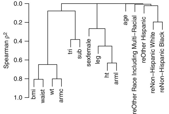
Fig. 15.6 Variable clustering for all potential predictors

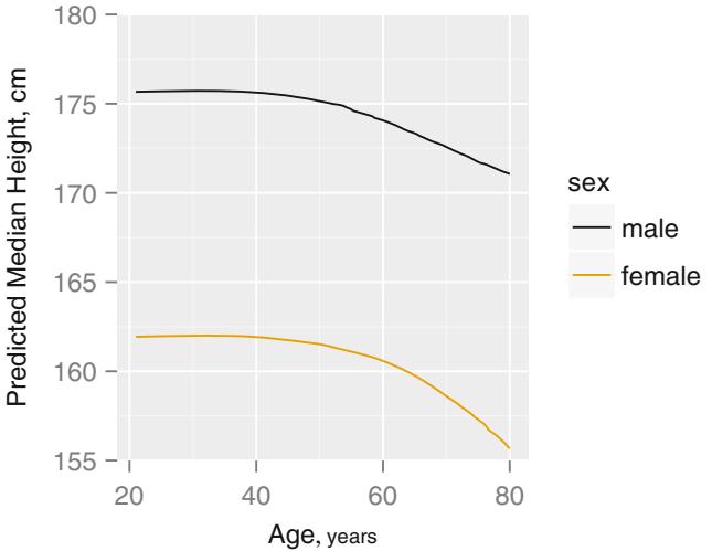
Fig. 15.7 Estimated median height as a smooth function of age, allowing age to interact with sex, from a proportional odds model

Because there are many competing body measures, we use backwards stepdown to arrive at a set of predictors. The bootstrap will be used to penalize predictive ability for variable selection. First the full model is fit using casewise deletion, then we do a composite test to assess whether any of the frequently–missing predictors is important.

f ← orm(gh ◦ rcs(age ,5) + sex + re + rcs(wt ,3) + rcs(leg ,3) + arml +
         rcs(armc ,3) + rcs(waist ,4) + tri + rcs(sub,3),
         family= ' loglog ' , data=w, x=TRUE , y= TRUE)
print(f, latex=TRUE , coefs=FALSE)

378 15 Regression Models for Continuous Y and Case Study in Ordinal Regression

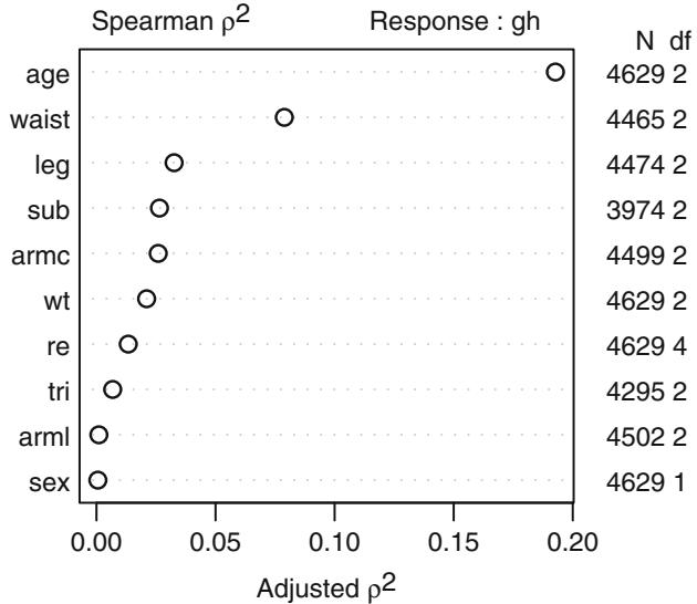
Fig. 15.8 Generalized squared rank correlations

-log-log Ordinal Regression Model

orm(formula = gh ~ rcs(age, 5) + sex + re + rcs(wt, 3) + rcs(leg, 3) + arml + rcs(armc, 3) + rcs(waist, 4) + tri + rcs(sub, 3), data = w, x = TRUE, y = TRUE, family = “loglog”)

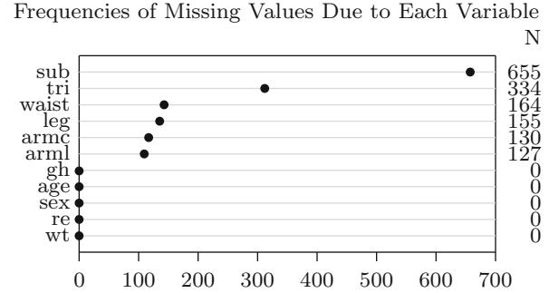
	Model Likelihood	Discrimination	Rank Discrim.
	Ratio Test	Indexes	Indexes
Obs 3853	β2 LR 1180.13	R2 0.265	∂ 0.520
Unique Y 60	d.f. 22	g 0.732
Y0.5 5.5	β2) Pr(> < 0.0001	gr 2.080
α log L max αρ	β2 Score 1298.88	× 1 Pr(Y ← Y0.5) 2 0.172
3≤10−5	β2) Pr(> < 0.0001
## Composite test : lan function(a) latex(a, table.env=FALSE , file= ’ ’ ) ← lan(anova(f, leg, arml , armc , waist , tri, sub))

	β2	d.f.	P
leg	8.30	2	0.0158
Nonlinear	3.32	1	0.0685
arml	0.16	1	0.6924
armc	6.66	2	0.0358
Nonlinear	3.29	1	0.0695
waist	29.40	3	< 0.0001
Nonlinear	4.29	2	0.1171
tri	16.62	1	< 0.0001
sub	40.75	2	< 0.0001
Nonlinear	4.50	1	0.0340
TOTAL NONLINEAR	14.95	5	0.0106
TOTAL	128.29	11	< 0.0001

The model achieves Spearman ∂ = 0.52, the rank correlation between predicted and observed HbA1c.

We show the predicted mean and median HbA1^c as a function of age, adjusting other variables to their median or mode (Figure 15.9). Compare the estimate of the median and 90t^h percentile with that from quantile regression.

M − Mean(f)
qu − Quantile(f)
med − function (x) qu(.5 , x)
p90 − function (x) qu(.9 , x)
fq − Rq(formula(f), data=w)
fq90 − Rq(formula(f), data=w, tau=.9)
pmean − Predict(f, age , fun=M, conf.int = FALSE)
pmed − Predict(f, age , fun=med , conf.int = FALSE)
p90 − Predict(f, age , fun=p90 , conf.int = FALSE)
pmedqr − Predict(fq, age , conf.int = FALSE )
p90qr − Predict(fq90 , age , conf.int= FALSE )
z − rbind ( ' orm mean ' =pmean , ' orm median ' =pmed , ' orm P90 ' =p90 ,
           ' QR median ' =pmedqr , ' QR P90 ' =p90qr )
ggplot (z, groups = ' .set. ' ,
       adj.subtitle =FALSE , legend.label = FALSE )

print (fastbw (f, rule= ’ p ’ ), estimates= FALSE )

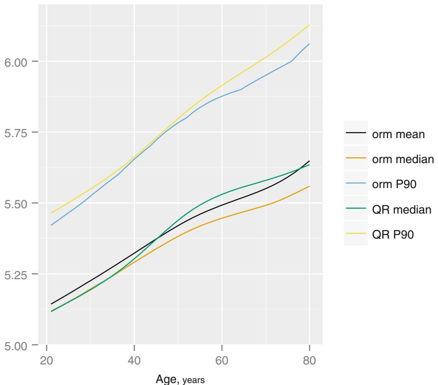
Fig. 15.9 Estimated mean and 0.5 and 0.9 quantiles from the log-log ordinal model using casewise deletion, along with predictions of 0.5 and 0.9 quantiles from quantile regression (QR). Age is varied and other predictors are held constant to medians/ modes.

Deleted arml sex wt armc	Chi-Sq 0.16 0.45 5.72 3.32	d.f. 1 1 2 2	P 0.6924 0.5019 0.0572 0.1897	Residual 0.16 0.61 6.33 9.65	d.f. 1 2 4 6	P 0.6924 0.7381 0.1759 0.1400	AIC -1.84 -3.39 -1.67 -2.35
Factors 1 age	in Final re	Model leg	waist	tri sub
set.seed (13) # so can reproduce results v validate(f, B=100, bw=TRUE , estimates=FALSE , rule= ’ p ’ ) −

Backwards Step - down - Original Model
Deleted Chi-Sq d.f. P Residual d.f. P AIC
arml 0.16 1 0.6924 0.16 1 0.6924 -1.84
sex 0.45 1 0.5019 0.61 2 0.7381 -3.39
wt 5.72 2 0.0572 6.33 4 0.1759 -1.67
armc 3.32 2 0.1897 9.65 6 0.1400 -2.35
Factors in Final Model
[1] age re leg waist tri sub

# Show number of variables selected in first 30 boots latex (v, B=30, file= ’ ’ , size= ’ small ’ )

Index		Original Training	Test	Optimism Corrected
	Sample	Sample	Sample		Index
Λ	0.5225	0.5290	0.5208	0.0083	0.5142 100
R2	0.2712	0.2788	0.2692	0.0095	0.2617 100
Slope	1.0000	1.0000	0.9761	0.0239	0.9761 100
g	1.2276	1.2505	1.2207	0.0298	1.1978 100
Pr(Y ≡ Y0.5) × 1 2	0.2007	0.2050	0.1987	0.0064	0.1943 100

Factors Retained in Backwards Elimination

First 30 Resamples
							age sex re wt leg arml armc waist tri sub
•	•	•	•	•		•	•		•
•		•		•		•	•	•	•
•		•		•		•	•	•	•
•	•	•	•	•		•	•		•
•	•	•	•	•		•	•		•
•		•		•		•	•	•	•
•	•	•	•			•	•		•
•	•	•	•	•		•	•
•		•	•	•		•	•	•	•
•	•	•	•	•		•	•		•
•		•	•			•	•	•	•
•		•		•	•	•	•	•	•
•		•	•	•		•	•	•	•
•		•	•	•		•	•	•	•
•		•		•		•	•	•	•
•		•	•	•		•	•	•	•
•	•	•	•	•		•	•	•	•
•		•		•			•	•	•
•		•	•	•		•	•	•	•
•		•	•	•		•	•	•	•
•		•	•	•		•	•	•	•
•		•	•			•	•	•	•
•		•	•	•		•	•	•	•
•	•	•		•			•		•
•		•		•		•		•	•
•		•	•	•		•	•	•	•
•		•	•			•	•	•	•
• •		• •	• •	• •		• •	• •	• •	• •
•		•		•		•		•	•

382 15 Regression Models for Continuous Y and Case Study in Ordinal Regression

Frequencies of Numbers of Factors Retained

5	6	7	8	9 10
			1 19 29 46 4	1

Next we fit the reduced model, using multiple imputation to impute missing predictors (Figure 15.10).

a ← aregImpute(◦ gh + wt + ht + bmi + leg + arml + armc + waist + tri + sub + age +re, data=w, n.impute =5, pr=FALSE) g ← fit.mult.impute(gh ◦ rcs(age ,5) + re + rcs(leg ,3) + rcs(waist ,4) + tri + rcs(sub,4), orm, a, family=loglog, data=w, pr=FALSE)

print(g, latex=TRUE , needspace= ’ 1.5in ’ )

-log-log Ordinal Regression Model

fit.mult.impute(formula = gh ~ rcs(age, 5) + re + rcs(leg, 3) + rcs(waist, 4) + tri + rcs(sub, 4), fitter = orm, xtrans = a, data = w, pr = FALSE, family = loglog)

	Model Likelihood		Discrimination		Rank Discrim.
	Ratio Test		Indexes		Indexes
Obs 4629	β2 LR	1448.42	R2	0.269	∂ 0.513
Unique Y 63	d.f.	17	g	0.743
Y0.5 5.5	β2) Pr(>	< 0.0001	gr	2.102
α log L max αρ	β2 Score	1569.21	× 1 Pr(Y ← Y0.5)	2 0.173
1≤10−5	β2) Pr(>	< 0.0001

	Coef	S.E.	Wald Z	Pr(> Z )
age	0.0404	0.0055	7.29	< 0.0001
age’	-0.0228	0.0279	-0.82	0.4137
age”	0.0126	0.0876	0.14	0.8857
age”’	0.0424	0.1148	0.37	0.7116
re=Other Hispanic	-0.0766	0.0597	-1.28	0.1992
re=Non-Hispanic White	-0.4121	0.0449	-9.17	< 0.0001
re=Non-Hispanic Black	0.0645	0.0566	1.14	0.2543
re=Other Race Including Multi-Racial	-0.0555	0.0750	-0.74	0.4593
leg	-0.0339	0.0091	-3.73	0.0002
leg’	0.0153	0.0105	1.46	0.1434
waist	0.0073	0.0050	1.47	0.1428
waist’	0.0304	0.0158	1.93	0.0536
waist”	-0.0910	0.0508	-1.79	0.0732
tri	-0.0163	0.0026	-6.28	< 0.0001
sub	-0.0027	0.0097	-0.28	0.7817
sub’	0.0674	0.0289	2.33	0.0198
sub”	-0.1895	0.0922	-2.06	0.0398

an ← anova(g) lan(an)

	β2	d.f.	P
age	692.50	4	< 0.0001
Nonlinear	28.47	3	< 0.0001
re	168.91	4	< 0.0001
leg	24.37	2	< 0.0001
Nonlinear	2.14	1	0.1434
waist	128.31	3	< 0.0001
Nonlinear	4.05	2	0.1318
tri	39.44	1	< 0.0001
sub	39.30	3	< 0.0001
Nonlinear	6.63	2	0.0363
TOTAL NONLINEAR	46.80	8	< 0.0001
TOTAL	1464.24	17	< 0.0001

b ← anova(g, leg, waist , tri, sub)
# Add new lines to the plot with combined effect of 4 size var.
s ← rbind(an, size=b[ ' TOTAL ' , ])
class(s) ← ' anova.rms '
plot(s)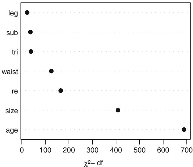

Fig. 15.10 ANOVA for reduced model, after multiple imputation, with addition of a combined effect for four size variables

ggplot(Predict (g), abbrev=TRUE , ylab=NULL) # Figure 15.11

384 15 Regression Models for Continuous Y and Case Study in Ordinal Regression

Compare the estimated age partial effects and confidence intervals with those from a model using casewise deletion, and with bootstrap nonparametric confidence intervals (also with casewise deletion).

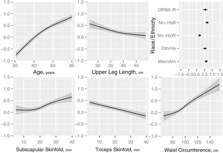
Fig. 15.11 Partial effects (log hazard or log-log cumulative probability scale) of all predictors in reduced model, after multiple imputation

gc − orm(gh ← rcs(age ,5) + re + rcs(leg ,3) +
          rcs(waist ,4) + tri + rcs(sub ,4),
          family =loglog , data=w, x=TRUE , y= TRUE)
gb − bootcov(gc , B =300)

bootclb − Predict(gb, age , boot.type = ' basic ' )
bootclp − Predict(gb, age , boot.type = ' percentile ' )
multimp − Predict(g, age)
plot( Predict(gc , age), addpanel =function (...) {
  with (bootclb , {llines (age , lower , col= ' blue ' )
                   llines (age , upper , col= ' blue ' )})
  with (bootclp , {llines (age , lower , col= ' blue ' , lty=2)
                   llines (age , upper , col= ' blue ' , lty=2)})
  with (multimp , {llines (age , lower , col= ' red ' )
                   llines (age , upper , col= ' red ' )
                   llines (age , yhat , col= ' red ' )} ) },
     col.fill= gray(.9), adj.subtitle = FALSE ) # Figure 15.12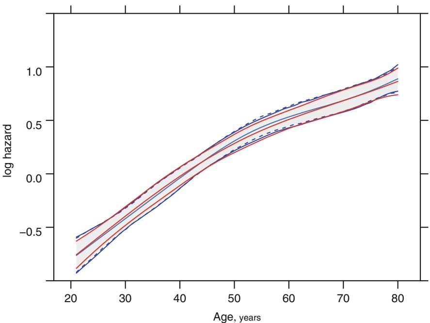

Fig. 15.12 Partial effect for age from multiple imputation (center red line) and casewise deletion (center blue line) with symmetric Wald 0.95 confidence bands using casewise deletion (gray shaded area), basic bootstrap confidence bands using casewise deletion (blue lines), percentile bootstrap confidence bands using casewise deletion (dashed blue lines), and symmetric Wald confidence bands accounting for multiple imputation (red lines).

Figure 15.13 depicts the relationship between various predicted quantities, demonstrating that the ordinal model makes fewer model assumptions that dictate their connections. A Gaussian or log-Gaussian model would have a straight-line relationship between the predicted mean and median.

M − Mean(g)
qu − Quantile(g)
med − function (lp) qu(.5 , lp)
q90 − function (lp) qu(.9 , lp)
lp − predict(g)
lpr − quantile(predict(g), c(.002 , .998), na.rm =TRUE)
lps − seq(lpr[1], lpr[2], length =200)
pmn − M(lps)
pme − med(lps)
p90 − q90(lps)
plot (pmn , pme , # Figure 15.13
     xlab= expression( paste ( ' Predicted Mean ' , HbA["1c"])),
     ylab= ' Median and 0.9 Quantile ' , type= ' l ' ,
     xlim =c(4.75 , 8.0), ylim=c(4.75 , 8.0), bty= ' n ' )
box(col=gray(.8))

386 15 Regression Models for Continuous Y and Case Study in Ordinal Regression

lines (pmn , p90 , col= ' blue ' )
abline (a=0, b=1, col=gray (.8))
text (6.5 , 5.5 , ' Median ' )
text (5.5 , 6.3 , ' 0.9 ' , col= ' blue ' )
nint − 350
scat1d (M(lp), nint=nint)
scat1d (med(lp), side =2, nint=nint )
scat1d (q90(lp), side =4, col= ' blue ' , nint=nint)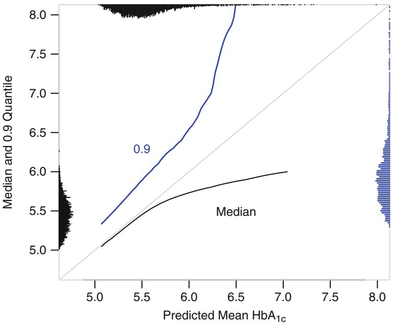

Fig. 15.13 Predicted mean HbA1cvs. predicted median and 0.9 quantile along with their marginal distributions

Finally, let us draw a nomogram that shows the full power of ordinal models, by predicting five quantities of interest.

g − Newlevels(g, list(re= abbreviate( levels (w$re))))
exprob − ExProb (g)
nom −
  nomogram(g, fun= list(Mean=M,
                 ' Median Glycohemoglobin ' = med ,
                 ' 0.9 Quantile ' = q90 ,
                 ' Prob(HbA1c ≡ 6.5) ' =
                      function(x) exprob (x, y=6.5),
                 ' Prob(HbA1c ≡ 7.0) ' =
                      function(x) exprob (x, y=7),
                 ' Prob(HbA1c ≡ 7.5) ' =

function(x) exprob (x, y=7.5)),
fun.at =list (seq(5, 8, by=.5),
c(5,5.25 ,5.5 ,5.75 ,6,6 .25),
c(5.5 ,6,6.5 ,7,8,10,12,14) ,
c(.01 ,.05 ,.1 ,.2 ,.3 ,.4),
c(.01 ,.05 ,.1 ,.2 ,.3 ,.4),
c(.01 ,.05 ,.1 ,.2 ,.3 ,.4 )))
plot (nom , lmgp =.28) 15.14 # Figure

Points	0 10	20 30	40	50 60	70 80	90	100
Age	20 25	30	35 40	45 50	55 60 65	70 75	80
Race/Ethnicity	N−HW	OthH ORIM
Upper Leg Length	55 45	35 30	25 20
Waist Circumference	50 70	90 100	110	120 130	140 150	160	170
Triceps Skinfold	45 35	25 15	5 0
Subscapular Skinfold	15 20 25 10	30 35 40	45
Total Points	0 20 40	60 80	100 120	140 160 180	200 220	240 260	280
Linear Predictor	−1.5	−1 −0.5	0	0.5 1	1.5	2 2.5
Mean	5			5.5	6 6.5	7 7.5 8
Median Glycohemoglobin	5		5.25	5.5	5.75	6 6.25
0.9 Quantile		5.5		6	6.5 7 8 10 12	14
Prob(HbA1c >= 6.5)				0.01 0.05 0.1	0.2	0.3 0.4
Prob(HbA1c >= 7.0)				0.01	0.05 0.1 0.2	0.3 0.4
Prob(HbA1c >= 7.5)				0.01	0.05 0.1	0.2 0.3

Fig. 15.14 Nomogram for predicting median, mean, and 0.9 quantile of glycohemoglobin, along with the estimated probability that HbA1c≡ 6.5, 7, or 7.5, all from the log-log ordinal model

Chapter 16 Transform-Both-Sides Regression

16.1 Background

Fitting multiple regression models by the method of least squares is one of the most commonly used methods in statistics. There are a number of challenges to the use of least squares, even when it is only used for estimation and not inference, including the following.

1. How should continuous predictors be transformed so as to get a good fit?
1. Is it better to transform the response variable? How does one find a good transformation that simplifies the right-hand side of the equation?
1. What if Y needs to be transformed non-monotonically (e.g., |Y × 100|) before it will have any correlation with X?

When one is trying to draw an inference about population effects using confidence limits or hypothesis tests, the most common approach is to assume that the residuals have a normal distribution. This is equivalent to assuming that the conditional distribution of the response Y given the set of predictors X is normal with mean depending on X and variance that is (one hopes) a constant independent of X. The need for a distributional assumption to enable us to draw inferences creates a number of other challenges such as the following.

1. If for the untransformed original scale of the response Y the distribution of the residuals is not normal with constant spread, ordinary methods will not yield correct inferences (e.g., confidence intervals will not have the desired coverage probability and the intervals will need to be asymmetric).
1. Quite often there is a transformation of Y that will yield well-behaving residuals. How do you find this transformation? Can you find a transformation for the Xs at the same time?

3. All classical statistical inferential methods assume that the full model was pre-specified, that is, the model was not modified after examining the data. How does one correct confidence limits, for example, for data-based model and transformation selection?

16.2 Generalized Additive Models

Hastie and Tibshirani275 have developed generalized additive models (GAMs) for a variety of distributions for Y . There are semiparametric GAMs, but most GAMs for continuous Y assume that the conditional distribution of Y is from a specific distribution family. GAMs nicely estimate the transformation each continuous X requires so as to optimize a fitting criterion such as sum of squared errors or log likelihood, subject to the degrees of freedom the analyst desires to spend on each predictor. However, GAMs assume that Y has already been transformed to fit the specified distribution family.

There is excellent software available for fitting a wide variety of GAMs, such as the R packages gam, mgcv, and robustgam.

16.3 Nonparametric Estimation of Y -Transformation

When the model’s left-hand side also needs transformation, either to improve R² or to achieve constant variance of the residuals (which increases the chances of satisfying a normality assumption), there are a few approaches available. One approach is Breiman and Friedman’s alternating conditional expectation (ACE) method.68 ACE simultaneously transforms both Y and each of the Xs so as to maximize the multiple R² between the transformed Y and the transformed Xs. The model is given by

\[g(Y) = f\_1(X\_1) + f\_2(X\_2) + \dots + f\_p(X\_p). \tag{16.1}\]

ACE allows the analyst to impose restrictions on the transformations such as monotonicity. It allows for categorical predictors, whose categories will automatically be given numeric scores. The transformation for Y is allowed to be non-monotonic. One feature of ACE is its ability to estimate the maximal correlation between an X and the response Y . Unlike the ordinary correlation coefficient (which assumes linearity) or Spearman’s rank correlation (which assumes monotonicity), the maximal correlation has the property that it is zero if and only if X and Y are statistically independent. This property holds because ACE allows for non-monotonic transformations of all variables. The “super smoother”(see the S supsmu function) is the basis for the nonparametric estimation of transformations for continuous Xs.

Tibshirani developed a different algorithm for nonparametric additive regression based on least squares, additivity and variance stabilization (AVAS).607 Unlike ACE, AVAS forces g(Y ) to be monotonic. AVAS’s fitting criterion is to maximize R² while forcing the transformation for Y to result in nearly constant variance of residuals. The model specification is the same as for ACE (Equation 16.3).

ACE and AVAS are powerful fitting algorithms, but they can result in overfitting (R² can be greatly inflated when one fits many predictors), and they provide no statistical inferential measures. As discussed earlier, the process of estimating transformations (especially those for Y ) can result in significant variance under-estimation, especially for small sample sizes. The bootstrap can be used to correct the apparent R² (R² app) for overfitting. As before, it estimates the optimism (bias) in R² app and subtracts this optimism from R² app to get a more trustworthy estimate. The bootstrap can also be used to compute confidence limits for all estimated transformations, and confidence limits for estimated predictor effects that take fully into account the uncertainty associated with the transformations. To do this, all steps involved in fitting the additive models must be repeated fresh for each re-sample.

Limited testing has shown that the sample size needs to exceed 100 for ACE and AVAS to provide stable estimates. In small sample sizes the bootstrap bias-corrected estimate of R² will be zero because the sample information did not support simultaneous estimation of all transformations.

16.4 Obtaining Estimates on the Original Scale

A common practice in least squares fitting is to attempt to rectify lack of fit by taking parametric transformations of Y before fitting; the logarithm is the most common transformation.^a If after transformation the model’s residuals have a population median of zero, the inverse transformation of a predicted transformed value estimates the population median of Y given X. This is because unlike means, quantiles are transformation-preserving. Many analysts make the mistake of not reporting which population parameter is being estimated when inverse transforming XΛˆ, and sometimes they even report that the mean is being estimated.

How would one go about estimating the population mean or other parameter on the untransformed scale? If the residuals are assumed to be normally distributed and if log(Y ) is the transformation, the mean of the log-normal distribution, a function of both the mean and the variance of the residuals, can be used to derive the desired quantity. However, if the residuals are not normally distributed, this procedure will not result in the correct estimator.

^a A disadvantage of transform-both-sides regression is this difficulty of interpreting estimates on the original scale. Sometimes the use of a special generalized linear model can allow for a good fit without transforming Y .

Duan165 developed a “smearing” estimator for more nonparametrically obtaining estimates of parameters on the original scale. In the simple one-sample case without predictors in which one has computed ˆγ = “ⁿ ⁱ=1 log(Yi)/n, the residuals from this fitted value are given by ^eⁱ = log(Yi) ^× ^ˆγ. The smearing estimator of the population mean is”exp[ˆγ + ei]/n. In this simple case the result is the ordinary sample mean Y .

The worth of Duan’s smearing estimator is in regression modeling. Suppose that the regression was run on g(Y ) from which estimated values ^gˆ(Yi) = ^XiΛ^ˆ and residuals on the transformed scale ^eⁱ = ˆg(Yi)×XiΛ^ˆ were obtained. Instead of restricting ourselves to estimating the population mean, let W(y1, y2,…,yn) denote any function of a vector of untransformed response values. To estimate the population mean in the homogeneous one-sample case, W is the simple average of all of its arguments. To estimate the population 0.25 quantile, W is the sample 0.25 quantile of y1,…,yn. Then the smearing estimator of the population parameter estimated by W given X is W(g−¹(a + e1), g−¹(a + e2),…,g−¹(a + en)), where g−¹ is the inverse of the g transformation and a = XΛˆ.

When using the AVAS algorithm, the monotonic transformation g is estimated from the data, and the predicted value of ˆg(Y ) is given by Equation 16.3. So we extend the smearing estimator as W(ˆg−¹(a+e1),…, gˆ−¹(a+ en)), where a is the predicted transformed response given X. As ˆg is nonparametric (i.e., a table look-up), the areg.boot function described below computes ˆg−¹ using reverse linear interpolation.

If residuals from ˆg(Y ) are assumed to be symmetrically distributed, their population median is zero and we can estimate the median on the untransformed scale by computing ˆg−¹(XΛˆ). To be safe, areg.boot adds the median residual to XΛˆ when estimating the population median (the median residual can be ignored by specifying statistic=‘fitted’ to functions that operate on objects created by areg.boot).

When quantiles of Y are of major interest, a more direct way to obtain estimates is through the use of quantile regression357. An excellent case study including comparisons with other methods such as Cox regression can be found in Austin et al.38.

16.5 R Functions

The R acepack package’s ace function implements all the features of the ACE algorithm, and its avas function does likewise for AVAS. The bootstrap and smearing capabilities mentioned above are offered for these estimation functions by the areg.boot (“additive regression using the bootstrap”) function in the Hmisc package. Unlike the ace and avas functions, areg.boot uses the R modeling language, making it easier for the analyst to specify the predictor variables and what is assumed about their relationships with the transformed Y . areg.boot also implements a parametric transform-both-sides approach using restricted cubic splines and canonical variates, and offers various estimation options with and without smearing. It can estimate the effect of changing one predictor, holding others constant, using the ordinary bootstrap to estimate the standard deviation of difference in two possibly transformed estimates (for two values of X), assuming normality of such differences. Normality is assumed to avoid generating a large number of bootstrap replications of time-consuming model fits. It would not be very difficult to add nonparametric bootstrap confidence limit capabilities to the software. areg.boot re-samples every aspect of the modeling process it uses, just as Faraway186 did for parametric least squares modeling.

areg.boot implements a variety of methods as shown in the simple example below. The monotone function restricts a variable’s transformation to be monotonic, while the I function restricts it to be linear.

f − areg.boot(Y ← monotone(age) +
              sex + weight + I( blood.pressure ))
plot(f) #show transformations , CLs
Function(f) #generate S functions
             #defining transformations
predict(f) #get predictions , smearing estimates
summary(f) #compute CLs on effects of each X
smearingEst () #generalized smearing estimators
Mean(f) #derive S function to
             #compute smearing mean Y
Quantile(f) #derive function to compute smearing quantile

The methods are best described in a case study.

16.6 Case Study

Consider simulated data where the conditional distribution of Y is log-normal given X, but where transform-both-sides regression methods use unlogged ^Y . Predictor ^X¹ is linearly related to log ^Y , ^X² is related by ^|X² ^× ¹ ² |, and categorical X³ has reference group a effect of zero, group b effect of 0.3, and group c effect of 0.5.

require(rms)

set.seed (7)
n − 400
x1 − runif (n)
x2 − runif (n)
x3 − factor (sample (c( ' a ' , ' b ' , ' c ' ), n, TRUE ))
y − exp(x1 + 2*abs(x2 - .5) + .3*(x3== ' b ' ) + .5*(x3== ' c ' ) +
           .5*rnorm (n))

# For reference fit appropriate OLS model
print (ols(log(y) ← x1 + rcs(x2 , 5) + x3), coefs =FALSE ,
      latex =TRUE)

Linear Regression Model

ols(formula = log(y) ~ x1 + rcs(x2, 5) + x3)

	Model Likelihood			Discrimination
	Ratio Test			Indexes
Obs 400	β2 LR	236.87	R2	0.447
τ 0.4722	d.f.	7	R2 adj	0.437
d.f. 392	β2) Pr(>	0.0000	g	0.482
		Residuals
Min	1Q	Median	3Q	Max
×1.346	×0.3075	×0.0134 0.327 1.527

Now fit the avas model. We use 300 bootstrap repetitions but only plot the first 20 estimates to see clearly how the bootstrap re-estimates of transformations vary. Had we wanted to restrict transformations to be linear, we would have specified the identity function, for example, I(x1).

f − areg.boot(y ← x1 + x2 + x3 , method = ’ avas ’ , B=300)

avas Additive Regression Model
areg.boot(x = y ◦ x1 + x2 + x3, B = 300, method = "avas")
Predictor Types
  type
x1 s
x2 s
x3 c
y type: s
n= 400 p= 3
Apparent R2 on transformed Y scale: 0.444
Bootstrap validated R2 : 0.42
Coefficients of standardized transformations:
   Intercept x1 x2 x3
-3.443111e-16 9.702960e-01 1.224320e+00 9.881150e-01
Residuals on transformed scale:

Min	1Q	Median	3Q	Max
-1.877152e+00	-5.252194e-01	-3.732200e-02	5.339122e-01	2.172680e+00
Mean	S.D.
8.673617e-19	7.420788e-01

Note that the coefficients above do not mean very much as the scale of the transformations is arbitrary. We see that the model was very slightly overfitted (R² dropped from 0.44 to 0.42), and the R² are in agreement with the OLS model fit above.

Next we plot the transformations, 0.95 confidence bands, and a sample of the bootstrap estimates.

plot(f, boot =20) # Figure 16.1

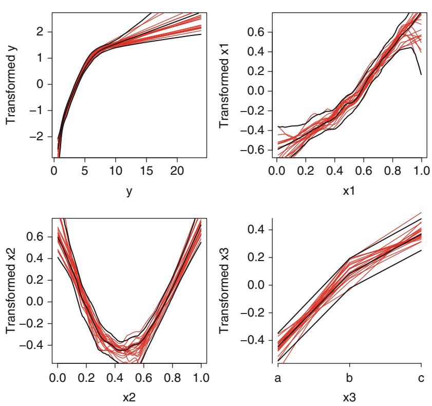
Fig. 16.1 avas transformations: overall estimates, pointwise 0.95 confidence bands, and 20 bootstrap estimates (red lines).

The plot is shown in Figure 16.1. The nonparametrically estimated transformation of x1 is almost linear, and the transformation of x2 is close to |x2×0.5|. We know that the true transformation of y is log(y), so variance stabilization and normality of residuals will be achieved if the estimated y-transformation is close to log(y).

ys − seq(.8 , 20, length =200)
ytrans − Function(f)$y # Function outputs all transforms
plot(log(ys), ytrans (ys), type= ' l ' ) # Figure 16.2
abline (lm(ytrans (ys) ← log(ys)), col=gray (.8))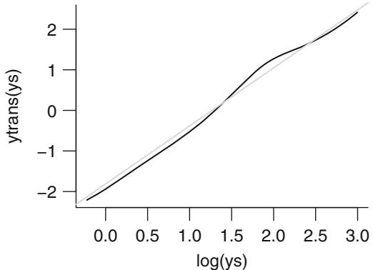

Fig. 16.2 Checking estimated against optimal transformation

Approximate linearity indicates that the estimated transformation is very log-like.^b

Now let us obtain approximate tests of effects of each predictor. summary does this by setting all other predictors to reference values (e.g., medians), and comparing predicted responses for a given level of the predictor X with predictions for the lowest setting of X. The default predicted response for summary is the median, which is used here. Therefore tests are for differences in medians.

summary(f, values =list (x1=c(.2 , .8), x2 =c(.1 , .5)))
summary .areg.boot(object = f, values = list(x1 = c(0.2, 0.8),
   x2 = c(0.1, 0.5)))
Estimates based on 300 resamples
Values to which predictors are set when estimating
effects of other predictors:
      y x1 x2 x3
3.728843 0.500000 0.300000 2.000000

^b Beware that use of a data–derived transformation in an ordinary model, as this will result in standard errors that are too small. This is because model selection is not taken into account.186

Estimates of differences of effects on Median Y (from first X
value), and bootstrap standard errors of these differences.
Settings for X are shown as row headings .
Predictor: x1
x Differences S.E Lower 0.95 Upper 0.95 Z Pr(|Z|)
 0.2 0.000000 NA NA NA NA NA
 0.8 1.546992 0.2099959 1.135408 1.958577 7.366773 1.747491e-13
Predictor: x2
x Differences S.E Lower 0.95 Upper 0.95 Z Pr(|Z|)
 0.1 0.000000 NA NA NA NA NA
 0.5 -1.658961 0.3163361 -2.278968 -1.038953 -5.244298 1.568786e-07
Predictor: x3
x Differences S.E Lower 0.95 Upper 0.95 Z Pr(|Z|)
 a 0.0000000 NA NA NA NA NA
 b 0.8447422 0.1768244 0.4981728 1.191312 4.777295 1.776692e-06
 c 1.3526151 0.2206395 0.9201697 1.785061 6.130431 8.764127e-10

For example, when x1 increases from 0.2 to 0.8 we predict an increase in median y by 1.55 with bootstrap standard error 0.21, when all other predictors are held to constants. Setting them to other constants will yield different estimates of the x1 effect, as the transformation of y is nonlinear.

Next depict the fitted model by plotting predicted values, with x2 varying on the x-axis, and three curves corresponding to three values of x3. x1 is set to 0.5. Figure 16.3 shows estimates of both the median and the mean y.

newdat − expand.grid (x2=seq(.05 , .95 , length =200),
                          x3=c( ' a ' , ' b ' , ' c ' ), x1=.5 ,
                          statistic=c( ' median ' , ' mean ' ))
yhat − c(predict(f, subset (newdat , statistic == ' median ' ),
                     statistic= ' median ' ),
            predict(f, subset (newdat , statistic == ' mean ' ),
                     statistic= ' mean ' ))
newdat −
  upData (newdat ,
          lp = x1 + 2*abs(x2 - .5) + .3*(x3== ' b ' ) +
                .5*(x3== ' c ' ),
          ytrue = ifelse ( statistic == ' median ' , exp(lp),
             exp(lp + 0.5*(0.5−2))), pr= FALSE )

Input object size: 45472 bytes; 4 variables
Added variable lp
Added variable ytrue
Added variable pr

New object size: 69800 bytes; 7 variables

# Use Hmisc function xYplot to produce Figure 16.3
xYplot (yhat ← x2 | statistic , groups =x3 ,
       data=newdat , type= ' l ' , col=1,
       ylab= expression (hat(y)),
       panel = function(...) {

panel.xYplot (…) dat − subset (newdat , statistic ==c( ’ median ’ , ’ mean ’ )[ current.column ()]) for(w in c( ’ a ’ , ’ b ’ , ’ c ’ )) with (subset (dat , x3==w), llines (x2 , ytrue , col= gray(.7), lwd=1.5)) } )

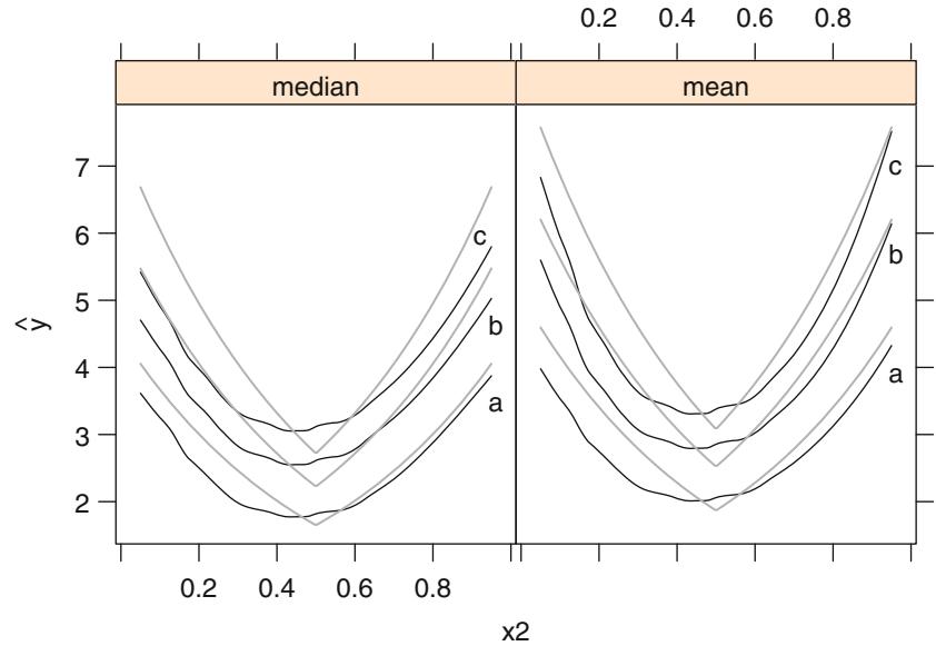
Fig. 16.3 Predicted median (left panel) and mean (right panel) y as a function of x2 and x3. True population values are shown in gray.

Chapter 17 Introduction to Survival Analysis

17.1 Background

Suppose that one wished to study the occurrence of some event in a population of subjects. If the time until the occurrence of the event were unimportant, the event could be analyzed as a binary outcome using the logistic regression model. For example, in analyzing mortality associated with open heart surgery, it may not matter whether a patient dies during the procedure or he dies after being in a coma for two months. For other outcomes, especially those concerned with chronic conditions, the time until the event is important. In a study of emphysema, death at eight years after onset of symptoms is different from death at six months. An analysis that simply counted the number of deaths would be discarding valuable information and sacrificing statistical power.

Survival analysis is used to analyze data in which the time until the event is of interest. The response variable is the time until that event and is often called a failure time, survival time, or event time. Examples of responses ¹ of interest include the time until cardiovascular death, time until death or myocardial infarction, time until failure of a light bulb, time until pregnancy, or time until occurrence of an ECG abnormality during exercise. Bull and Spiegelhalter83 have an excellent overview of survival analysis.

The response, event time, is usually continuous, but survival analysis allows the response to be incompletely determined for some subjects. For example, suppose that after a five-year follow-up study of survival after myocardial infarction a patient is still alive. That patient’s survival time is censored on the right at five years; that is, her survival time is known only to exceed five years. The response value to be used in the analysis is 5+. Censoring can also occur when a subject is lost to follow-up. ²

If no responses are censored, standard regression models for continuous responses could be used to analyze the failure times by writing the expected failure time as a function of one or more predictors, assuming that

399

^© Springer International Publishing Switzerland 2015

F.E. Harrell, Jr., Regression Modeling Strategies, Springer Series in Statistics, DOI 10.1007/978-3-319-19425-7 17

the distribution of failure time is properly specified. However, there are still several reasons for studying failure time using the specialized methods of survival analysis.

1. Time to failure can have an unusual distribution. Failure time is restricted to be positive so it has a skewed distribution and will never be normally distributed.
1. The probability of surviving past a certain time is often more relevant than the expected survival time (and expected survival time may be difficult to estimate if the amount of censoring is large).
1. A function used in survival analysis, the hazard function, helps one to understand the mechanism of failure.308

Survival analysis is used often in industrial life-testing experiments, and it is heavily used in clinical and epidemiologic follow-up studies. Examples include a randomized trial comparing a new drug with placebo for its ability to maintain remission in patients with leukemia, and an observational study of prognostic factors in coronary heart disease. In the latter example subjects may well be followed for varying lengths of time, as they may enter the study over a period of many years.

When regression models are used for survival analysis, all the advantages of these models can be brought to bear in analyzing failure times. Multiple, independent prognostic factors can be analyzed simultaneously and treatment differences can be assessed while adjusting for heterogeneity and imbalances in baseline characteristics. Also, patterns in outcome over time can be predicted for individual subjects.

Even in a simple well-designed experiment, survival modeling can allow one to do the following in addition to making simple comparisons.

1. Test for and describe interactions with treatment. Subgroup analyses can easily generate spurious results and they do not consider interacting factors in a dose-response manner. Once interactions are modeled, relative treatment benefits can be estimated (e.g., hazard ratios), and analyses can be done to determine if some patients are too sick or too well to have even a relative benefit.
1. Understand prognostic factors (strength and shape).
1. Model absolute effect of treatment. First, a model for the probability of surviving past time t is developed. Then differences in survival probabilities for patients on treatments A and B can be estimated. The differences will be due primarily to sickness (overall risk) of the patient and to treatment interactions.
1. Understand time course of treatment effect. The period of maximum effect or period of any substantial effect can be estimated from a plot of relative effects of treatment over time.
1. Gain power for testing treatment effects.
1. Adjust for imbalances in treatment allocation in non-randomized studies.

17.2 Censoring, Delayed Entry, and Truncation

Responses may be left–censored and interval–censored besides being right– censored. Interval–censoring is present, for example, when a measuring device functions only for a certain range of the response; measurements outside that range are censored at an end of the scale of the device. Interval–censoring also occurs when the presence of a medical condition is assessed during periodic exams. When the condition is present, the time until the condition developed is only known to be between the current and the previous exam. Left–censoring means that an event is known to have occurred before a certain time. In addition, left–truncation and delayed entry are common. Nomenclature is confus- 3 ing as many authors refer to delayed entry as left–truncation. Left–truncation really means that an unknown subset of subjects failed before a certain time and the subjects didn’t get into the study. For example, one might study the survival patterns of patients who were admitted to a tertiary care hospital. Patients who didn’t survive long enough to be referred to the hospital compose the left-truncated group, and interesting questions such as the optimum timing of admission to the hospital cannot be answered from the data set.

Delayed entry occurs in follow-up studies when subjects are exposed to the risk of interest only after varying periods of survival. For example, in a study of occupational exposure to a toxic compound, researchers may be interested in comparing life length of employees with life expectancy in the general population. A subject must live until the beginning of employment before exposure is possible; that is, death cannot be observed before employment. The start of follow-up is delayed until the start of employment and it may be right–censored when follow-up ends. In some studies, a researcher may want to assume that for the purpose of modeling the shape of the hazard function, time zero is the day of diagnosis of disease, while patients enter the study at various times since diagnosis. Delayed entry occurs for patients who don’t enter the study until some time after their diagnosis. Patients who die before study entry are left-truncated. Note that the choice of time origin is very important.53, 83, 112, 133

Heart transplant studies have been analyzed by considering time zero to be the time of enrollment in the study. Pre-transplant survival is right–censored at the time of transplant. Transplant survival experience is based on delayed entry into the “risk set” to recognize that a transplant patient is not at risk of dying from transplant failure until after a donor heart is found. In other words, survival experience is not credited to transplant surgery until the day of transplant. Comparisons of transplant experience with medical treatment suffer from “waiting time bias” if transplant survival begins on the day of transplant instead of using delayed entry.209, 438, 570

There are several planned mechanisms by which a response is right– censored. Fixed type I censoring occurs when a study is planned to end after two years of follow-up, or when a measuring device will only measure responses up to a certain limit. There the responses are observed only if they

fall below a fixed value C. In type II censoring, a study ends when there is a pre-specified number of events. If, for example, 100 mice are followed until 50 die, the censoring time is not known in advance.

We are concerned primarily with random type I right-censoring in which each subject’s event time is observed only if the event occurs before a certain time, but the censoring time can vary between subjects. Whatever the cause of censoring, we assume that the censoring is non-informative about the event; that is, the censoring is caused by something that is independent of the impending failure. Censoring is non-informative when it is caused by planned termination of follow-up or by a subject moving out of town for reasons unrelated to the risk of the event. If subjects are removed from follow-up because of a worsening condition, the informative censoring will result in biased estimates and inaccurate statistical inference about the survival experience. For example, if a patient’s response is censored because of an adverse effect of a drug or noncompliance to the drug, a serious bias can result if patients with adverse experiences or noncompliance are also at higher risk of suffering the outcome. In such studies, efficacy can only be assessed fairly using the intention to treat principle: all events should be attributed to the treatment ⁴ assigned even if the subject is later removed from that treatment.

17.3 Notation, Survival, and Hazard Functions

In survival analysis we use T to denote the response variable, as the response is usually the time until an event. Instead of defining the statistical model for the response T in terms of the expected failure time, it is advantageous to define it in terms of the survival function, S(t), given by

\[S(t) = \text{Prob}\{T > t\} = 1 - F(t),\tag{17.1}\]

where F(t) is the cumulative distribution function for T . If the event is death, S(t) is the probability that death occurs after time t, that is, the probability that the subject will survive at least until time t. S(t) is always 1 at t = 0; all subjects survive at least to time zero. The survival function must be non-increasing as t increases. An example of a survival function is shown in Figure 17.1. In that example subjects are at very high risk of the event in the early period so that the S(t) drops sharply. The risk is low for 0.1 − t − 0.6, so S(t) is somewhat flat. After t = .6 the risk again increases, so S(t) drops more quickly. Figure 17.2 depicts the cumulative hazard function corresponding to the survival function in Figure 17.1. This function is denoted by ∆(t). It describes the accumulated risk up until time t, and as is shown later, is the negative of the log of the survival function. ∆(t) is non-decreasing as t increases; that is, the accumulated risk increases or remains the same. Another important function is the hazard function, ϵ(t), also called the force

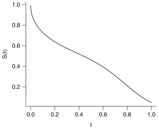
Fig. 17.1 Survival function

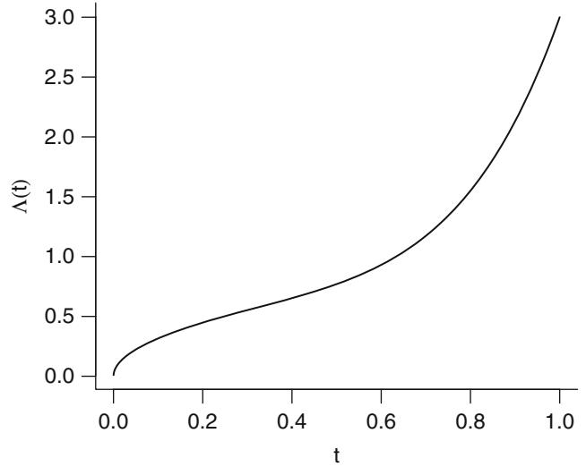
Fig. 17.2 Cumulative hazard function

of mortality, or instantaneous event (death, failure) rate. The hazard at time t is related to the probability that the event will occur in a small interval around t, given that the event has not occurred before time t. By studying the event rate at a given time conditional on the event not having occurred by

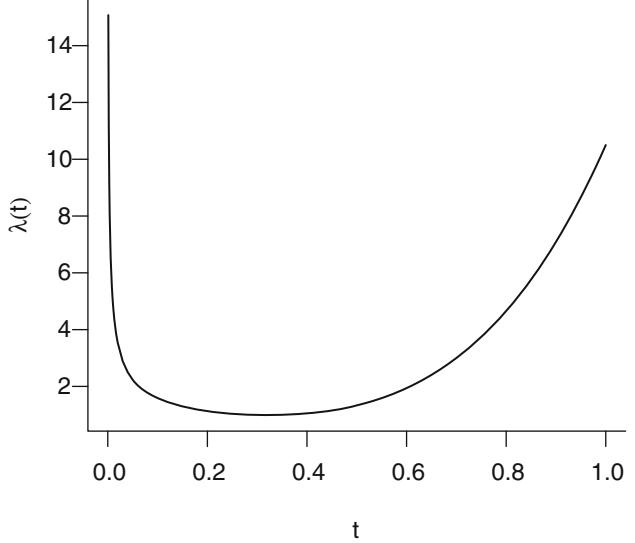
Fig. 17.3 Hazard function

that time, one can learn about the mechanisms and forces of risk over time. Figure 17.3 depicts the hazard function corresponding to S(t) in Figure 17.1 and to ∆(t) in Figure 17.2. Notice that the hazard function allows one to more easily determine the phases of increased risk than looking for sudden drops in S(t) or ∆(t).

The hazard function is defined formally by

\[\lambda(t) = \lim\_{u \to 0} \frac{\text{Prob}\{t < T \le t + u | T > t\}}{u},\tag{17.2}\]

which using the law of conditional probability becomes

\[\begin{split} \lambda(t) &= \lim\_{u \to 0} \frac{\text{Prob}\{t < T \le t + u\} / \text{Prob}\{T > t\}}{u} \\ &= \lim\_{u \to 0} \frac{[F(t + u) - F(t)]/u}{S(t)} \\ &= \frac{\partial F(t) / \partial t}{S(t)} \\ &= \frac{f(t)}{S(t)}, \end{split} \tag{17.3}\]

where f(t) is the probability density function of T evaluated at t, the derivative or slope of the cumulative distribution function 1 × S(t). Since

\[\frac{\partial \log S(t)}{\partial t} = \frac{\partial S(t)/\partial t}{S(t)} = -\frac{f(t)}{S(t)},\tag{17.4}\]

the hazard function can also be expressed as

\[ \lambda(t) = -\frac{\partial \log S(t)}{\partial t},\tag{17.5} \]

the negative of the slope of the log of the survival function. Working backwards, the integral of ϵ(t) is:

\[\int\_0^t \lambda(v)dv = -\log S(t). \tag{17.6}\]

The integral or area under ϵ(t) is defined to be ∆(t), the cumulative hazard function. Therefore

\[A(t) = -\log S(t),\tag{17.7}\]

\[S(t) = \exp[-A(t)].\tag{17.8}\]

So knowing any one of the functions S(t), ∆(t), or ϵ(t) allows one to derive the other two functions. The three functions are different ways of describing the same distribution.

One property of ∆(t) is that the expected value of ∆(T ) is unity, since if T ≈ S(t), the density of T is ϵ(t)S(t) and

\[\begin{split} E[A(T)] &= \int\_0^\infty A(t)\lambda(t) \exp(-A(t))dt \\ &= \int\_0^\infty u \exp(-u) du \\ &= 1. \end{split} \tag{17.9}\]

Now consider properties of the distribution of T . The population qth quantile (100qth percentile), Tq, is the time by which a fraction q of the subjects will fail. It is the value t such that S(t)=1 × q; that is

\[T\_q = S^{-1}(1-q).\tag{17.10}\]

The median life length is the time by which half the subjects will fail, obtained by setting S(t)=0.5:

\[T\_{0.5} = S^{-1}(0.5). \tag{17.11}\]

The qth quantile of T can also be computed by setting exp[×∆(t)] = 1 × q, giving

\[\begin{aligned} T\_q &= \Lambda^{-1} [-\log(1-q)] \quad \text{and as a special case,} \\ T\_{.5} &= \Lambda^{-1} (\log 2). \end{aligned} \tag{17.12}\]

The mean or expected value of T (the expected failure time) is the area under the survival function for t ranging from 0 to √:

\[ \mu = \int\_0^\infty S(v)dv.\tag{17.13} \]

Irwin has defined mean restricted life (see [334,335]), which is the area under S(t) up to a fixed time (usually chosen to be a point at which there is still adequate follow-up information).

The random variable T denotes a random failure time from the survival distribution S(t). We need additional notation for the response and censoring information for the ith subject. Let Tⁱ denote the response for the ith subject. This response is the time until the event of interest, and it may be censored if the subject is not followed long enough for the event to be observed. Let Cⁱ denote the censoring time for the ith subject, and define the event indicator as

\[e\_i = 1 \quad \text{if the event was observed} \quad (T\_i \le C\_i),\]

\[= 0 \quad \text{if the response was censored} \quad (T\_i > C\_i). \tag{17.14}\]

The observed response is

\[Y\_i = \min(T\_i, C\_i),\tag{17.15}\]

which is the time that occurred first: the failure time or the censoring time. The pair of values (Yi, ei) contains all the response information for most purposes (i.e., the potential censoring time Cⁱ is not usually of interest if the event occurred before Ci).

Figure 17.4 demonstrates this notation. The line segments start at study entry (survival time t = 0).

A useful property of the cumulative hazard function can be derived as follows. Let z be any cutoff time and consider the expected value of ∆ evaluated at the earlier of the cutoff time or the actual failure time.

\[\begin{split} E[A(\min(T, z))] &= E[A(T)[T \le z] + A(z)[T > z]] \\ &= E[A(T)[T \le z]] + A(z)S(z). \end{split} \tag{17.16}\]

The first term in the right–hand side is

\[\int\_{0}^{\infty} A(t)[t \le z] \lambda(t) \exp(-A(t)) dt\]

\[\int\_{0}^{z} A(t) \lambda(t) \exp(-A(t)) dt \tag{17.17}\]

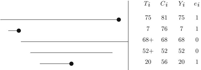
Termination of Study

Fig. 17.4 Some censored data. Circles denote events.

\[\begin{aligned} &= -[u \exp(-u) + \exp(-u)]|\_0^{A(z)}, \\ &= 1 - S(z)[A(z) + 1]. \end{aligned}\]

Adding Λ(z)S(z) results in

\[E[A(\min(T, z))] = 1 - S(z) = F(z). \tag{17.18}\]

It follows that “ⁿ ⁱ=1 Λ(min(Ti, z)) estimates the expected number of failures occurring before time z among the n subjects. ⁵

17.4 Homogeneous Failure Time Distributions

In this section we assume that each subject in the sample has the same distribution of the random variable T that represents the time until the event. In particular, there are no covariables that describe differences between subjects in the distribution of T . As before we use S(t), λ(t), and Λ(t) to denote, respectively, the survival, hazard, and cumulative hazard functions.

The form of the true population survival distribution function S(t) is almost always unknown, and many distributional forms have been used for describing failure time data. We consider first the two most popular parametric survival distributions: the exponential and Weibull distributions. The exponential distribution is a very simple one in which the hazard function is constant; that is, λ(t) = λ . The cumulative hazard and survival functions are then

\[\begin{aligned} A(t) &= \lambda t \quad \text{and} \\ S(t) &= \exp(-A(t)) = \exp(-\lambda t). \end{aligned} \tag{17.19}\]

The median life length is Λ−¹(log 2) or

\[T\_{0.5} = \log(2) / \lambda. \tag{17.20}\]

The time by which 1/2 of the subjects will have failed is then proportional to the reciprocal of the constant hazard rate λ . This is true also of the expected or mean life length, which is 1/λ.

The exponential distribution is one of the few distributions for which a closed-form solution exists for the estimator of its parameter when censoring is present. This estimator is a function of the number of events and the total person-years of exposure. Methods based on person-years in fact implicitly assume an exponential distribution. The exponential distribution is often used to model events that occur “at random in time.”323 It has the property that the future lifetime of a subject is the same, no matter how “old” it is, or

\[\text{Prob}\{T > t\_0 + t | T > t\_0\} = \text{Prob}\{T > t\}.\tag{17.21}\]

This “ageless” property also makes the exponential distribution a poor choice for modeling human survival except over short time periods.

The Weibull distribution is a generalization of the exponential distribution. Its hazard, cumulative hazard, and survival functions are given by

\[\begin{aligned} \lambda(t) &= \alpha \gamma t^{\gamma - 1} \\ A(t) &= \alpha t^{\gamma} \\ S(t) &= \exp(-\alpha t^{\gamma}) .\end{aligned} \tag{17.22}\]

The Weibull distribution with γ = 1 is an exponential distribution (with constant hazard). When γ > 1, its hazard is increasing with t, and when γ < 1 its hazard is decreasing. Figure 17.5 depicts some of the shapes of the hazard function that are possible. If T has a Weibull distribution, the median of T is

\[T\_{0.5} = [(\log 2)/\alpha]^{1/\gamma}.\tag{17.23}\]

There are many other traditional parametric survival distributions, some of which have hazards that are “bathtub shaped” as in Figure 17.3. 243, 323 The restricted cubic spline function described in Section 2.4.5 is an alternative basis for λ(t).286, 287 This function family allows for any shape of smooth λ(t) since the number of knots can be increased as needed, subject to the number of events in the sample. Nonlinear terms in the spline function can be tested to assess linearity of hazard (Rayleigh-ness) or constant hazard ⁶ (exponentiality).

The restricted cubic spline hazard model with k knots is

\[ \lambda\_k(t) = a + bt + \sum\_{j=1}^{k-2} \gamma\_j w\_j(t), \tag{17.24} \]

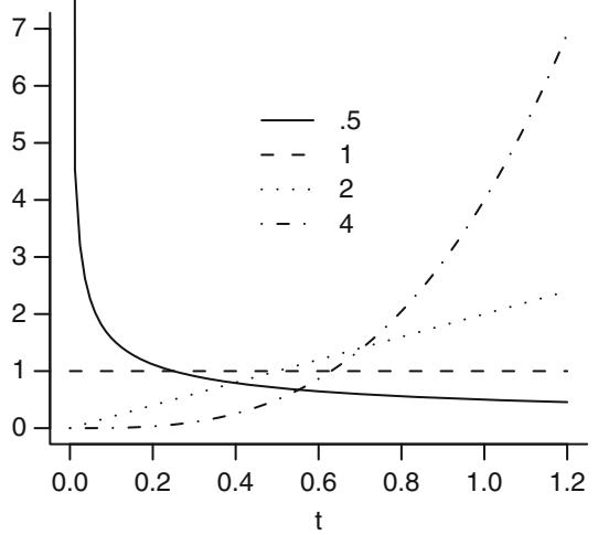
Fig. 17.5 Some Weibull hazard functions with ∂ = 1 and various values of θ.

where the w^j (t) are the restricted cubic spline terms of Equation 2.25. There terms are cubic terms in t. A set of knots v1,…,v^k is selected from the quantiles of the uncensored failure times (see Section 2.4.5 and [286]).

The cumulative hazard function for this model is

\[A(t) = at + \frac{1}{2}t^2 + \frac{1}{4} \times \text{ quartic terms in t.}\tag{17.25}\]

Standard maximum likelihood theory is used to obtain estimates of the k unknown parameters to derive, for example, smooth estimates of λ(t) with confidence bands. The flexible estimates of S(t) using this method are as efficient as Kaplan–Meier estimates, but they are smooth and can be used as a basis for modeling predictor variables. The spline hazard model is particularly useful for fitting steeply falling and gently rising hazard functions that are characteristic of high-risk medical procedures.

17.5 Nonparametric Estimation of S and Λ

17.5.1 Kaplan–Meier Estimator

As the true form of the survival distribution is seldom known, it is useful to estimate the distribution without making any assumptions. For many analyses, this may be the last step, while in others this step helps one select a statistical model for more in-depth analyses. When no event times are censored, a nonparametric estimator of S(t) is 1×Fn(t) where Fn(t) is the usual

	Day No. Subjects Deaths Censored			Cumulative
	At Risk			Survival
12	100	1	0	99/100 = .99
30	99	2	1	97/99 ≤ 99/100 = .97
60	96	0	3	96/96 ≤ .97 = .97
72	93	3	0	90/93 ≤ .97 = .94

Table 17.1 Kaplan-Meier computations

empirical cumulative distribution function based on the observed failure times T1,…,Tn. Let Sn(t) denote this empirical survival function. Sn(t) is given by the fraction of observed failure times that exceed t:

\[S\_n(t) = \text{[number of } T\_i > t]/n. \tag{17.26}\]

When censoring is present, S(t) can be estimated (at least for t up until the end of follow-up) by the Kaplan–Meier333 product-limit estimator. This method is based on conditional probabilities. For example, suppose that every subject has been followed for 39 days or has died within 39 days so that the proportion of subjects surviving at least 39 days can be computed. After 39 days, some subjects may be lost to follow-up besides those removed from follow-up because of death within 39 days. The proportion of those still followed 39 days who survive day 40 is computed. The probability of surviving 40 days from study entry equals the probability of surviving day 40 after living 39 days, multiplied by the chance of surviving 39 days.

The life table in Table 17.1 demonstrates the method in more detail. We suppose that 100 subjects enter the study and none die or are lost before day 12.

Times in a life table should be measured as precisely as possible. If the event being analyzed is death, the failure time should usually be specified to the nearest day. We assume that deaths occur on the day indicated and that being censored on a certain day implies the subject survived through the end of that day. The data used in computing Kaplan–Meier estimates consist of (Yi, ei), i = 1, 2,…,n using notation defined previously. Primary data collected to derive (Yi, ei) usually consist of entry date, event date (if subject failed), and censoring date (if subject did not fail). Instead, the entry date, date of event/censoring, and event/censoring indicator eⁱ may be specified.

The Kaplan–Meier estimator is called the product-limit estimator because it is the limiting case of actuarial survival estimates as the time periods shrink so that an entry is made for each failure time. An entry need not be in the table for censoring times (when no failures occur at that time) as long as the number of subjects censored is subtracted from the next number

Table 17.2 Summaries used in Kaplan-Meier computations

i ti	ni	di	(ni × di)/ni
1 1	7	1	6/7
2 3	6	2	4/6
3 9	2	1	1/2

at risk. Kaplan–Meier estimates are preferred to actuarial estimates because they provide more resolution and make fewer assumptions. In constructing a yearly actuarial life table, for example, it is traditionally assumed that subjects censored between two years were followed 0.5 years.

The product-limit estimator is a nonparametric maximum likelihood estimator [331, pp. 10–13]. The formula for the Kaplan–Meier product-limit estimator of S(t) is as follows. Let k denote the number of failures in the sample and let t1, t2,…,t^k denote the unique event times (ordered for ease of calculation). Let dⁱ denote the number of failures at tⁱ and nⁱ be the number of subjects at risk at time ti; that is, nⁱ = number of failure/censoring times ← tⁱ . The estimator is then

\[S\_{\rm KM}(t) = \prod\_{i: t\_i \le t} (1 - d\_i/n\_i). \tag{17.27}\]

The Kaplan–Meier estimator of Λ(t) is ΛKM(t) = × log SKM(t). An estimate of quantile q of failure time is S−¹ KM(1 × q), if follow-up is long enough so that SKM(t) drops as low as 1×q. If the last subject followed failed so that SKM(t) drops to zero, the expected failure time can be estimated by computing the area under the Kaplan–Meier curve.

To demonstrate computation of SKM(t), imagine a sample of failure times given by

\[1 \quad 3 \quad 3 \quad 6^+ \quad 8^+ \quad 9 \quad 10^+,\]

where + denotes a censored time. The quantities needed to compute SKM are in Table 17.2. Thus

\[\begin{aligned} S\_{\text{KM}}(t) &= 1, \quad 0 \le t < 1 \\ &= 6/7 = .85, \quad 1 \le t < 3 \\ &= (6/7)(4/6) = .57, \quad 3 \le t < 9 \\ &= (6/7)(4/6)(1/2) = .29, \quad 9 \le t < 10. \end{aligned} \tag{17.28}\]

Note that the estimate of S(t) is undefined for t > 10 since not all subjects have failed by t = 10 but no follow-up extends beyond t = 10. A graph of the Kaplan–Meier estimate is found in Figure 17.6.

tt − c(1,3,3,6,8,9,10)
stat − c(1,1,1,0,0,1,0)
S − Surv (tt , stat )
survplot( npsurv (S ← 1), conf="bands ", n.risk =TRUE ,
         xlab= expression (t))
survplot( npsurv (S ← 1, type=" fleming-harrington ",
                  conf.int= FALSE), add=TRUE , lty=3)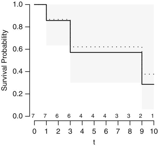

Fig. 17.6 Kaplan–Meier product–limit estimator with 0.95 confidence bands. The Altschuler–Nelson–Aalen–Fleming–Harrington estimator is depicted with the dotted lines.

The variance of SKM(t) can be estimated using Greenwood’s formula [331, p. 14], and using normality of SKM(t) in large samples this variance can be used to derive a confidence interval for S(t). A better method is to derive an asymmetric confidence interval for S(t) based on a symmetric interval for log Λ(t). This latter method ensures that a confidence limit does not exceed one or fall below zero, and is more accurate since log ΛKM(t) is more normally distributed than SKM(t). Once a confidence interval, say [a, b] is determined for log Λ(t), the confidence interval for S(t) is computed by [exp{× exp(b)}, exp{× exp(a)}]. The formula for an estimate of the variance of interest is [331, p. 15]:

\[\text{Var}\{\log A\_{\text{KM}}(t)\} = \frac{\sum\_{i:t\_i \le t} d\_i / [n\_i(n\_i - d\_i)]}{\{\sum\_{i:t\_i \le t} \log[(n\_i - d\_i)/n\_i]\}^2}. \tag{17.29}\]

Letting s denote the square root of this variance estimate, an approximate 1 × α confidence interval for log Λ(t) is given by log ΛKM(t) ± zs , where z is the 1×α/2 standard normal critical value. After simplification, the confidence interval for S(t) becomes

\[S\_{\rm KM}(t)^{\rm exp(\pm z\,\kappa)}.\tag{17.30}\]

Even though the log Λ basis for confidence limits has theoretical advantages, on the log × log scale the estimate of S(t) has the greatest instability where much information is available: when S(t) falls just below 1.0. For that reason, the recommended default confidence limits are on the Λ(t) scale using

\[\text{Var}\{A\_{\text{KM}}(t)\} = \sum\_{i:t\_i \le t} \frac{d\_i}{[n\_i(n\_i - d\_i)]}.\tag{17.31}\]

Letting s denote its square root, an approximate 1×α confidence interval for S(t) is given by

\[\exp(\pm zs)S\_{\rm KM}(t),\tag{17.32}\]

truncated to [0, 1]. ⁷

17.5.2 Altschuler–Nelson Estimator

Altschuler19, Nelson472, Aalen1 and Fleming and Harrington196 proposed estimators of Λ(t) or of S(t) based on an estimator of Λ(t):

\[ \hat{A}(t) = \sum\_{i: t\_i \le t} \frac{d\_i}{n\_i} \]

\[ S\_A(t) = \exp(-\hat{A}(t)).\tag{17.33} \]

SΛ(t) has advantages over SKM(t). First, “ⁿ ⁱ=1 ^Λˆ(Yi) =”ⁿ ⁱ=1 eⁱ [605, Appendix 3]. In other words, the estimator gives the correct expected number of events. Second, there is a wealth of asymptotic theory based on the Altschuler–Nelson estimator.196

See Figure 17.6 for an example of the SΛ(t) estimator. This estimator has the same variance as SKM(t) for large enough samples. ⁸

17.6 Analysis of Multiple Endpoints

Clinical studies frequently assess multiple endpoints. A cancer clinical trial may, for example, involve recurrence of disease and death, whereas a cardiovascular trial may involve nonfatal myocardial infarction and death. Endpoints may be combined, and the new event (e.g., time until infarction or death) may be analyzed with any of the tools of survival analysis because only the usual censoring mechanism is used. Sometimes the various endpoints may need separate study, however, because they may have different risk factors.

When the multiple endpoints represent multiple causes of a terminating event (e.g., death), Prentice et al. have developed standard methods for analyzing cause-specific hazards513 [331, pp. 163–178]. Their methods allow each cause of failure to be analyzed separately, censoring on the other causes. They do not assume any mechanism for cause removal nor make any assumptions regarding the interrelation among causes of failure. However, analyses of competing events using data where some causes of failure are removed in a different way from the original dataset will give rise to different inferences.

When the multiple endpoints represent a mixture of fatal and nonfatal outcomes, the analysis may be more complex. The same is true when one wishes to jointly study an event-time endpoint and a repeated measurement.

17.6.1 Competing Risks

When events are independent, each event may also be analyzed separately by censoring on all other events as well as censoring on loss to follow-up. This will yield an unbiased estimate of an easily interpreted cause-specific λ(t) or S(t) because censoring is non-informative [331, pp. 168–169]. One minus SKM(t) computed in this manner will correctly estimate the probability of failing from the event in the absence of other events. Even when the competing events are not independent, the cause-specific hazard model may lead to valid results, but the resulting model does not allow one to estimate risks conditional on removal of one or more causes of the event. See Kay340 for a nice example of competing risks analysis when a treatment reduces the risk of death from ¹⁰ one cause but increases the risk of death from another cause.

Larson and Dinse376 have an interesting approach that jointly models the time until (any) failure and the failure type. For r failure types, they use an r-category polytomous logistic model to predict the probability of failing from each cause. They assume that censoring is unrelated to cause of event.

17.6.2 Competing Dependent Risks

In many medical and epidemiologic studies one is interested in analyzing multiple causes of death. If the goal is to estimate cause-specific failure probabilities, treating subjects dying from extraneous causes as censored and then computing the ordinary Kaplan–Meier estimate results in biased (high) survival estimates212, 225. If cause m is of interest, the cause-specific hazard

function is defined as

\[\lambda\_m(t) = \lim\_{u \to 0} \frac{\Pr\{\text{fail from cause } m \text{ in } [t, t+u) | \text{alive at } t\}}{u}. \tag{17.34}\]

The cumulative incidence function or probability of failure from cause m by time t is given by

\[F\_m(t) = \int\_0^t \lambda\_m(u) S(u) du,\tag{17.35}\]

where S(u) is the probability of surviving (ignoring cause of death), which equals exp[^× & ^u 0 ( “λm(x))dx] [212]; [444, Chapter 10]; [102,408]. As previously mentioned, 1×Fm(t) = exp[^× & ^t ⁰ λm(u)du] only if failures due to other causes are eliminated and if the cause-specific hazard of interest remains unchanged in doing so.212

Again letting t1, t2,…,t^k denote the unique ordered failure times, a nonparametric estimate of Fm(t) is given by

\[\hat{F}\_m(t) = \sum\_{i: t\_i \le t} \frac{d\_{mi}}{n\_i} S\_{\text{KM}}(t\_{i-1}),\tag{17.36}\]

where dmi is the number of failures of type m at time tⁱ and nⁱ is the number of subjects at risk of failure at ti.

Pepe and others494, 496, 497 showed how to use a combination of Kaplan– Meier estimators to derive an estimator of the probability of being free of event 1 by time t given event 2 has not occurred by time t (see also [349]). Let T¹ and T² denote, respectively, the times until events 1 and 2. Let S1(t) and S2(t) denote, respectively, the two survival functions. Let us suppose that event 1 is not a terminating event (e.g., is not death) and that even after event 1 subjects are followed to ascertain occurrences of event 2. The probability that T¹ > t given T² > t is

\[\text{Prob}\{T\_1 > t | T\_2 > t\} = \frac{\text{Prob}\{T\_1 > t \text{ and } T\_2 > t\}}{\text{Prob}\{T\_2 > t\}}\]

\[= \frac{S\_{12}(t)}{S\_2(t)},\tag{17.37}\]

where S12(t) is the survival function for min(T1, T2), the earlier of the two events. Since S12(t) does not involve any informative censoring (assuming as always that loss to follow-up is non-informative), S¹² may be estimated by the Kaplan–Meier estimator SKM¹² (or by SΛ). For the type of event 1 we have discussed above, S² can also be estimated without bias by SKM² . Thus we estimate, for example, the probability that a subject still alive at time t will be free of myocardial infarction as of time t by SKM¹² /SKM2.

Another quantity that can easily be computed from ordinary survival estimates is S2(t) × S12(t) = [1 × S12(t)] × [1 × S2(t)], which is the probability that event 1 occurs by time t and that event 2 has not occurred by time t.

The ratio estimate above is used to estimate the survival function for one event given that another has not occurred. Another function of interest is the crude survival function which is a marginal distribution; that is, it is the probability that T¹ > t whether or not event 2 occurs:362

\[\begin{aligned} S\_c(t) &= 1 - F\_1(t) \\ F\_1(t) &= \text{Prob}\{T\_1 \le t\}, \end{aligned} \tag{17.38}\]

where F1(t) is the crude incidence function defined previously. Note that the T¹ − t implies that the occurrence of event 1 is part of the probability being computed. If event 2 is a terminating event so that some subjects can never suffer event 1, the crude survival function for T¹ will never drop to zero. The crude survival function can be interpreted as the survival distribution of W where ^W ⁼ ^T¹ if ^T¹ < T² and ^W ⁼ ^√ otherwise.362 ¹¹

17.6.3 State Transitions and Multiple Types of Nonfatal Events

In many studies there is one final, absorbing state (death, all causes) and multiple live states. The live states may represent different health states or phases of a disease. For example, subjects may be completely free of cancer, have an isolated tumor, metastasize to a distant organ, and die. Unlike this example, the live states need not have a definite ordering. One may be interested in estimating transition probabilities, for example, the probability πij (t1, t2) that an individual in state i at time t¹ is in state j after an additional time t2. Strauss and Shavelle596 have developed an extended Kaplan–Meier estimator for this situation. Let Sⁱ KM (t|t1) denote the ordinary Kaplan–Meier estimate of the probability of not dying before time t (ignoring distinctions between multiple live states) for a cohort of subjects beginning follow-up at time t¹ in state i. This is an estimate of the probability of surviving an additional t time units (in any live state) given that the subject was alive and in state i at time t1. Strauss and Shavelle’s estimator is given by

\[ \pi\_{ij}(t\_1, t\_2) = \frac{n\_{ij}(t\_1, t\_2)}{n\_i(t\_1, t\_2)} S\_{KM}^i(t\_2 | t\_1), \tag{17.39} \]

where ni(t1, t2) is the number of subjects in live state i at time t¹ who are alive and uncensored t² time units later, and nij (t1, t2) is the number of such ¹² subjects in state j t² time units beyond t1.

17.6.4 Joint Analysis of Time and Severity of an Event

In some studies, an endpoint is given more weight if it occurs earlier or if it is more severe clinically, or both. For example, the event of interest may be myocardial infarction, which may be of any severity from minimal damage to the left ventricle to a fatal infarction. Berridge and Whitehead52 have provided a promising model for the analysis of such endpoints. Their method assumes that the severity of endpoints which do occur is measured on an ordinal categorical scale and that severity is assessed at the time of the event. Berridge and Whitehead’s example was time until first headache, with severity of headaches graded on an ordinal scale. They proposed a joint hazard of an individual who responds with ordered category j:

\[ \lambda\_j(t) = \lambda(t)\pi\_j(t),\tag{17.40} \]

where λ(t) is the hazard for the failure time and π^j (t) is the probability of an individual having event severity j given she fails at time t. Note that a shift in the distribution of response severity is allowed as the time until the event increases. ¹³

17.6.5 Analysis of Multiple Events

It is common to choose as an endpoint in a clinical trial an event that can recur. Examples include myocardial infarction, gastric ulcer, pregnancy, and infection. Using only the time until the first event can result in a loss of statistical information and power.^a There are specialized multivariate survival models (whose assumptions are extremely difficult to verify) for handling this setup, but in many cases a simpler approach will be efficient.

The simpler approach involves modeling the marginal distribution of the time until each event.407, 495 Here one forms one record per subject per event, and the survival time is the time to the first event for the first record, or is the time from the previous event to the next event for all later records. This approach yields consistent estimates of distribution parameters as long as the marginal distributions are correctly specified.655 One can allow the number of previous events to influence the hazard function of another event by modeling this count as a covariable.

The multiple events within subject are not independent, so variance estimates must be corrected for intracluster correlation. The clustered sandwich covariance matrix estimator described in Section 9.5 and in [407] will provide

^a An exception to this is the case in which once an event occurs for the first time, that event is likely to recur multiple times for any patient. Then the latter occurrences are redundant.

consistent estimates of variances and covariances even if the events are dependent. Lin407 also discussed how this method can easily be used to model 14 multiple events of differing types.

17.7 R Functions

The event.chart function of Lee et al.394 will draw a variety of charts for displaying raw survival time data, for both single and multiple events per subject. Relationships with covariables can also be displayed. The event.history function of Dubin et al.166 draws an event history graph for right-censored survival data, including time-dependent covariate status. These function are in the Hmisc package.

The analyses described in this chapter can be viewed as special cases of the Cox proportional hazards model.132 The programs for Cox model analyses described in Section 20.13 can be used to obtain the results described here, as long as there is at least one stratification factor in the model. There are, however, several R functions that are pertinent to the homogeneous or stratified case. The R function survfit, and its particular renditions of the print, plot, lines, and points generic functions (all part of the survival package written by Terry Therneau), will compute, print, and plot Kaplan–Meier and Nelson survival estimates. Confidence intervals for S(t) may be based on S,Λ, or log Λ. The rms package’s front-end to the survival package’s survfit function is npsurv for “nonparametric survival”. It and other functions described in later chapters use Therneau’s Surv function to combine the response variable and event indicator into a single R”survival time” object. In its simplest form, use Surv(y, event), where y is the failure/right–censoring time and event is the event/censoring indicator, usually coded T/F, 0 = censored 1 = event or 1 = censored 2 = event. If the event status variable has other coding (e.g., 3 means death), use Surv(y, s==3). To handle interval time-dependent covariables, or to use Andersen and Gill’s counting process formulation of the Cox model,23 use the notation Surv(tstart, tstop, status). The counting process notation allows subjects to enter and leave risk sets at random. For each time interval for each subject, the interval is made up of tstart< t −tstop. For time-dependent stratification, there is an optional origin argument to Surv that indicates the hazard shape time origin at the time of crossover to a new stratum. A type argument is used to handle left– and interval– censoring, especially for parametric survival models. Possible values of type are “right”,“left”,“interval”,“counting”,“interval2”,“mstate”.

The Surv expression will usually be used inside another function, but it is fine to save the result of Surv in another object and to use this object in the particular fitting function.

npsurv is invoked by the following, with default parameter settings indicated.

require(rms)
units (y) − "Month "
# Default is "Day" - used for axis labels , etc.
npsurv (Surv(y, event) ← svar1 + svar2 + ... , data , subset ,
       type =c(" kaplan-meier ", "fleming-harrington ", "fh2"),
       error =c(" greenwood", "tsiatis"), se.fit =TRUE ,
       conf.int =.95 ,
       conf.type =c("log"," log-log"," plain ","none"), ...)

If there are no stratification variables (svar1, . . . ), omit them. To print a table of estimates, use

f − npsurv (...)
print (f) # print brief summary of f
summary(f, times , censored= FALSE) # in survival

For failure times stored in days, use

f − npsurv (Surv(futime , event) ← sex)
summary(f, seq(30, 180, by =30))

to print monthly estimates.

There is a plot method To plot the object returned by survfit and npsurv. This invokes plot.survfit.

Objects created by npsurv can be passed to the more comprehensive plotting function survplot (here, actually survplot.npsurv) for other options that include automatic curve labeling and showing the number of subjects at risk at selected times. See Figure 17.6 for an example. Stratified estimates, with four treatments distinguished by line type and curve labels, could be drawn by

units (y) − "Year"
f − npsurv (Surv(y, stat) ← treatment)
survplot(f, ylab=" Fraction Pain-Free")

The groupkm in rms computes and optionally plots SKM(u) or log ΛKM(u) (if loglog=TRUE) for fixed u with automatic stratification on a continuous predictor x. As in cut2 (Section 6.2) you can specify the number of subjects per interval (default is m=50), the number of quantile groups (g), or the actual cutpoints (cuts). groupkm plots the survival or log–log survival estimate against mean x in each x interval.

The bootkm function in the Hmisc package bootstraps Kaplan–Meier survival estimates or Kaplan–Meier estimates of quantiles of the survival time distribution. It is easy to use bootkm to compute, for example, a nonparametric confidence interval for the ratio of median survival times for two groups.

See the Web site for a list of functions from other users for nonparametric estimation of S(t) with left–, right–, and interval–censored data. The adaptive linear spline log-hazard fitting function heft361 is freely available.

17.8 Further Reading

1 Some excellent general references for survival analysis are [57, 83, 114, 133, 154, 197, 282, 308, 331, 350, 382, 392, 444, 484, 574, 604]. Govindarajulu et al.229 have a nice review of frailty models in survival analysis, for handling clustered timeto-event data.
2 See Goldman,220 Bull and Spiegelhalter,83, Lee et al.394, and Dubin et al.166 for ways to construct descriptive graphs depicting right–censored data.
3 Some useful references for left–truncation are [83,112,244,524]. Mandel435 carefully described the difference between censoring and truncation.
4 See [384, p. 164] for some ideas for detecting informative censoring. Bilker and Wang54 discuss right–truncation and contrast it with right–censoring.
5 Arjas29 has applications based on properties of the cumulative hazard function. 6 Kooperberg et al.361,594 have an adaptive method for fitting hazard functions using linear splines in the log hazard. Binquet et al.56 studied a related approach
using quadratic splines. Mudholkar et al.466 presented a generalized Weibull model allowing for a variety of hazard shapes.
7 Hollander et al.299 provide a nonparametric simultaneous confidence band for S(t), surprisingly using likelihood ratio methods. Miller459 showed that if the parametric form of S(t) is known to be Weibull with known shape parameter (an unlikely scenario), the Kaplan–Meier estimator is very inefficient (i.e., has high variance) when compared with the parametric maximum likelihood estimator. See [666] for a discussion of how the efficiency of Kaplan–Meier estimators can be improved by interpolation as opposed to piecewise flat step functions. That paper also discusses a variety of other estimators, some of which are significantly more efficient than Kaplan–Meier.
8 See [112,244,438,570,614,619] for methods of estimating S or δ in the presence of left–truncation. See Turnbull616 for nonparametric estimation of S(t) with left–, right–, and interval–censoring, and Kooperberg and Clarkson360 for a flexible parametric approach to modeling that allows for interval–censoring. Lindsey and Ryan413 have a nice tutorial on the analysis of interval–censored data.
9 Hogan and Laird297,298 developed methods for dealing with mixtures of fatal and nonfatal outcomes, including some ideas for handling outcome-related dropouts on the repeated measurements. See also Finkelstein and Schoenfeld.193 The 30 April 1997 issue of Statistics in Medicine (Vol. 16) is devoted to methods for analyzing multiple endpoints as well as designing multiple endpoint studies. The papers in that issue are invaluable, as is Therneau and Hamilton606 and Therneau and Grambsch.604 Huang and Wang311 presented a joint model for recurrent events and a terminating event, addressing such issues as the frequency of recurrent events by the time of the terminating event.
10 See Lunn and McNeil429 and Marubini and Valsecchi [444, Chapter 10] for practical approaches to analyzing competing risks using ordinary Cox proportional hazards models. A nice overview of competing risks with comparisons of various approaches is found in Tai et al.599, Geskus214, and Koller et al.358. Bryant and Dignam78 developed a semiparametric procedure in which competing risks are adjusted for nonparametrically while a parametric cumulative incidence function is used for the event of interest, to gain precision. Fine and Gray192 developed methods for analyzing competing risks by estimating subdistribution functions. Nishikawa et al.478 developed some novel approaches to competing risk analysis involving time to adverse drug events competing with time to withdrawal from therapy. They also dealt with different severities of events in an interesting way. Putter et al.517 has a nice tutorial on competing risks, multi-state models, and associated R software. Fiocco et al.194 developed

an approach to avoid the problems caused by having to estimate a large number of regression coefficients in multi-state models. Ambrogi et al.22 provide clinically useful estimates from competing risks analyses.

11 Jiang, Chappell, and Fine322 present methods for estimating the distribution of event times of nonfatal events in the presence of terminating events such as death.
12 Shen and Thall568 have developed a flexible parametric approach to multi-state survival analysis.
13 Lancar et al.372 developed a method for analyzing repeated events of varying severities.
14 Lawless and Nadeau384 have a very good description of models dealing with recurrent events. They use the notion of the cumulative mean function, which is the expected number of events experienced by a subject by a certain time. Lawless383 contrasts this approach with other approaches. See Aalen et al.3 for a nice example in which multivariate failure times (time to failure of fillings in multiple teeth per subject) are analyzed. Francis and Fuller204 developed a graphical device for depicting complex event history data. Therneau and Hamilton606 have very informative comparisons of various methods for modeling multiple events, showing the importance of whether the analyst starts the clock over after each event. Kelly and Lim343 have another very useful paper comparing various methods for analyzing recurrent events. Wang and Chang650 demonstrated the difficulty of using Kaplan–Meier estimates for recurrence time data.

17.9 Problems

1. Make a rough drawing of a hazard function from birth for a man who develops significant coronary artery disease at age 50 and undergoes coronary artery bypass surgery at age 55.
1. Define in words the relationship between the hazard function and the survival function.
1. In a study of the life expectancy of light bulbs as a function of the bulb’s wattage, 100 bulbs of various wattage ratings were tested until each had failed. What is wrong with using the product-moment linear correlation test to test whether wattage is associated with life length concerning (a) distributional assumptions and (b) other assumptions?
1. A placebo-controlled study is undertaken to ascertain whether a new drug decreases mortality. During the study, some subjects are withdrawn because of moderate to severe side effects. Assessment of side effects and withdrawal of patients is done on a blinded basis. What statistical technique can be used to obtain an unbiased treatment comparison of survival times? State at least one efficacy endpoint that can be analyzed unbiasedly.
1. Consider long-term follow-up of patients in the support dataset. What proportion of the patients have censored survival times? Does this imply that one cannot make accurate estimates of chances of survival? Make a histogram or empirical distribution function estimate of the censored followup times. What is the typical follow-up duration for a patient in the study

who has survived so far? What is the typical survival time for patients who have died? Taking censoring into account, what is the median survival time from the Kaplan–Meier estimate of the overall survival function? Estimate the median graphically or using any other sensible method.

1. Plot Kaplan–Meier survival function estimates stratified by dzclass. Estimate the median survival time and the first quartile of time until death for each of the four disease classes.
1. Repeat Problem 6 except for tertiles of meanbp.
1. The commonly used log-rank test for comparing survival times between groups of patients is a special case of the test of association between the grouping variable and survival time in a Cox proportional hazards regression model. Depending on how one handles tied failure times, the log-rank χ² statistic exactly equals the score χ² statistic from the Cox model, and the likelihood ratio and Wald χ² test statistics are also appropriate. To obtain global score or LR χ² tests and P-values you can use a statement as the following, where cph is in the rms package. It is similar to the survival package’s coxph function.

cph(Survobject ← predictor)

Here Survobject is a survival time object created by the Surv function. Obtain the log-rank (score) χ² statistic, degrees of freedom, and P-value for testing for differences in survival time between levels of dzclass. Interpret this test, referring to the graph you produced in Problem 6 if needed.

Do preliminary analyses of survival time using the Mayo Clinic primary biliary cirrhosis dataset described in Section 8.9. Make graphs of Altschuler– Nelson or Kaplan–Meier survival estimates stratified separately by a few categorical predictors and by categorized versions of one or two continuous predictors. Estimate median failure time for the various strata. You may want to suppress confidence bands when showing multiple strata on one graph. See [361] for parametric fits to the survival and hazard function for this dataset.

Chapter 18 Parametric Survival Models

18.1 Homogeneous Models (No Predictors)

The nonparametric estimator of S(t) is a very good descriptive statistic for displaying survival data. For many purposes, however, one may want to make more assumptions to allow the data to be modeled in more detail. By specifying a functional form for S(t) and estimating any unknown parameters in this function, one can

1. easily compute selected quantiles of the survival distribution;
1. estimate (usually by extrapolation) the expected failure time;
1. derive a concise equation and smooth function for estimating S(t), Λ(t), and λ(t); and
1. estimate S(t) more precisely than SKM(t) or SΛ(t) if the parametric form is correctly specified.

18.1.1 Specific Models

Parametric modeling requires choosing one or more distributions. The Weibull and exponential distributions were discussed in Chapter 18. Other commonly used survival distributions are obtained by transforming T and using a standard distribution. The log transformation is most commonly employed. The log-normal distribution specifies that log(T ) has a normal distribution with mean ^µ and variance ^σ². Stated another way, log(^T ) ^≈ ^µ ⁺ σϵ, where ^ϵ has a standard normal distribution. Then S(t)=1 × Φ((log(t) × µ)/σ), where Φ is the standard normal cumulative distribution function. The loglogistic distribution is given by ^S(t) = [1 + exp(×(log(t) ^× ^µ)/σ)]−¹. Here log(^T ) ^≈ ^µ+σϵ where ^ϵ follows a logistic distribution [1+exp(×u)]−¹. The log

423

F.E. Harrell, Jr., Regression Modeling Strategies, Springer Series

in Statistics, DOI 10.1007/978-3-319-19425-7 18

extreme value distribution is given by S(t) = exp[× exp((log(t) × µ)/σ)], and log(T ) ≈ µ + σϵ, where ϵ ≈ 1 × exp[× exp(u)].

The generalized gamma and generalized F distributions provide a richer variety of distribution and hazard functions127, 128. Spline hazard models286, 287, 361 are other excellent alternatives.

18.1.2 Estimation

Maximum likelihood (ML) estimation is used to estimate the unknown parameters of S(t). The general method presented in Chapter 9 must be augmented, however, to allow for censored failure times. The basic idea is as follows. Again let T be a random variable representing time until the event, Tⁱ be the (possibly censored) failure time for the ith observation, and Yⁱ denote the observed failure or censoring time min(Ti, Ci), where Cⁱ is the censoring time. If Yⁱ is uncensored, observation i contributes a factor to the likelihood equal to the density function for T evaluated at Yi, f(Yi). If Yⁱ instead represents a censored time so that Tⁱ = Y ⁺ ⁱ , it is only known that Tⁱ exceeds Yi. The contribution to the likelihood function is the probability that Tⁱ > Cⁱ (equal to Prob{Tⁱ > Yi}). This probability is S(Yi). The joint likelihood over all observations i = 1, 2,…,n is

\[L = \prod\_{i:Y\_i \text{ uncensored}}^n f(Y\_i) \prod\_{i:Y\_i \text{ censored}}^n S(Y\_i). \tag{18.1}\]

There is one more component to L: the distribution of censoring times if these are not fixed in advance. Recall that we assume that censoring is noninformative, that is, it is independent of the risk of the event. This independence implies that the likelihood component of the censoring distribution simply multiplies L and that the censoring distribution contains little information about the survival distribution. In addition, the censoring distribution may be very difficult to specify. For these reasons we can maximize L separately to estimate parameters of S(t) and ignore the censoring distribution.

Recalling that f(t) = λ(t)S(t) and Λ(t) = × log S(t), the log likelihood can be written as

\[\log L = \sum\_{i:Y\_i \text{ unencosored}}^n \log \lambda(Y\_i) - \sum\_{i=1}^n A(Y\_i). \tag{18.2}\]

All observations then contribute an amount to the log likelihood equal to the negative of the cumulative hazard evaluated at the failure/censoring time. In addition, uncensored observations contribute an amount equal to the log of the hazard function evaluated at the time of failure. Once L or log L is specified, the general ML methods outlined earlier can be used without change in most situations. The principal difference is that censored observations contribute less information to the statistical inference than uncensored observations. For distributions such as the log-normal that are written only in terms of S(t), it may be easier to write the likelihood in terms of S(t) and f(t).

As an example, we turn to the exponential distribution, for which log L has a simple form that can be maximized explicitly. Recall that for this distribution λ(t) = λ and Λ(t) = λt. Therefore,

\[\log L = \sum\_{i:Y\_i \text{ uncensored}}^{n} \log \lambda - \sum\_{i=1}^{n} \lambda Y\_i. \tag{18.3}\]

Letting n^u denote the number of uncensored event times,

\[\log L = n\_u \log \lambda - \sum\_{i=1}^{n} \lambda Y\_i. \tag{18.4}\]

Letting w denote the sum of all failure/censoring times (“person years of exposure”):

\[w = \sum\_{i=1}^{n} Y\_i,\tag{18.5}\]

the derivatives of log L are given by

\[\frac{\partial \log L}{\partial \lambda} = n\_u / \lambda - w\]

\[\frac{\partial^2 \log L}{\partial \lambda^2} = -n\_u / \lambda^2. \tag{18.6}\]

Equating the derivative of log L to zero implies that the MLE of λ is

\[ \hat{\lambda} = n\_u / w \tag{18.7} \]

or the number of failures per person-years of exposure. By inserting the MLE of λ into the formula for the second derivative we obtain the observed estimated information, w²/nu. The estimated variance of λˆ is thus nu/w² and the standard error is n ¹/² ^u /w. The precision of the estimate depends primarily on nu.

Recall that the expected life length µ is 1/λ for the exponential distribution. The MLE of µ is w/n^u and its estimated variance is w²/n³ ^u. The MLE of ^S(t), ^Sˆ(t), is exp(×λˆt), and the estimated variance of log(Λˆ(t)) is simply 1/nu.

As an example, consider the sample listed previously,

\[1 \quad 3 \quad 3 \quad 6^+ \quad 8^+ \quad 9 \quad 10^+ \dots\]

Here n^u = 4 and w = 40, so the MLE of λ is 0.1 failure per person-period. The estimated standard error is 2/40 = 0.05. Estimated expected life length is 10 units with a standard error of 5 units. Estimated median failure time is log(2)/0.1=6.931. The estimated survival function is exp(×0.1t), which at t = 1, 3, 9, 10 yields 0.90, 0.74, 0.41, and 0.37, which can be compared to the product limit estimates listed earlier (0.85, 0.57, 0.29, 0.29).

Now consider the Weibull distribution. The log likelihood function is

\[\log L = \sum\_{i:Y\_i \text{ uncenored}}^n \log[\alpha \gamma Y\_i^{\gamma - 1}] - \sum\_{i=1}^n \alpha Y\_i^{\gamma}. \tag{18.8}\]

Although log L can be simplified somewhat, it cannot be solved explicitly for α and γ. An iterative method such as the Newton–Raphson method is used to compute the MLEs of α and γ. Once these estimates are obtained, the estimated variance–covariance matrix and other derived quantities such as Sˆ(t) can be obtained in the usual manner.

For the dataset used in the exponential fit, the Weibull fit follows.

\[\begin{aligned} \hat{\alpha} &= 0.0728\\ \hat{\gamma} &= 1.164\\ \hat{S}(t) &= \exp(-0.0728t^{1.164})\\ \hat{S}^{-1}(0.5) &= [(\log 2)/\hat{\alpha}]^{1/\hat{\gamma}} = 6.935 \text{ (estimated median)}. \end{aligned} \tag{18.9}\]

This fit is very close to the exponential fit since ˆγ is near 1.0. Note that the two medians are almost equal. The predicted survival probabilities for the Weibull model for t = 1, 3, 9, 10 are, respectively, 0.93, 0.77, 0.39, 0.35.

Sometimes a formal test can be made to assess the fit of the proposed parametric survival distribution. For the data just analyzed, a formal test of exponentiality versus a Weibull alternative is obtained by testing H⁰ : γ = 1 in the Weibull model. A score test yielded χ² = 0.14 with 1 d.f., p = 0.7, showing little evidence for non-exponentiality (note that the sample size is too small for this test to have any power).

18.1.3 Assessment of Model Fit

The fit of the hypothesized survival distribution can often be checked easily using graphical methods. Nonparametric estimates of S(t) and Λ(t) are primary tools for this purpose. For example, the Weibull distribution ^S(t) = exp(×αt^γ) can be rewritten by taking logarithms twice:

\[ \log[-\log S(t)] = \log A(t) = \log \alpha + \gamma(\log t). \tag{18.10} \]

The fit of a Weibull model can be assessed by plotting log Λˆ(t) versus log t and checking whether the curve is approximately linear. Also, the plotted curve provides approximate estimates of α (the antilog of the intercept) and γ (the slope). Since an exponential distribution is a special case of a Weibull distribution when γ = 1, exponentially distributed data will tend to have a graph that is linear with a slope of 1.

For any assumed distribution S(t), a graphical assessment of goodness of fit can be made by plotting S−1[SΛ(t)] or S−1[SKM(t)] against t and checking for linearity. For log distributions, S specifies the distribution of log(T ), so we plot against log t. For a log-normal distribution we thus plot Φ−1[SΛ(t)] against log t, where Φ−¹ is the inverse of the standard normal cumulative distribution function. For a log-logistic distribution we plot logit[SΛ(t)] versus log t. For an extreme value distribution we use log × log plots as with the Weibull distribution. Parametric model fits can also be checked by plotting the fitted Sˆ(t) and SΛ(t) against t on the same graph.

18.2 Parametric Proportional Hazards Models

In this section we present one way to generalize the survival model to a survival regression model. In other words, we allow the sample to be heterogeneous by adding predictor variables X = {X1, X2,…,Xk}. As with other regression models, X can represent a mixture of binary, polytomous, continuous, spline-expanded, and even ordinal predictors (if the categories are scored to satisfy the linearity assumption). Before discussing ways in which the regression part of a survival model might be specified, first recall how regression effects have been modeled in other settings. In multiple linear regression, the regression effect Xβ = β⁰ + β1X¹ + β2X² + … + βkX^k can be thought of as an increment in the expected value of the response Y . In binary logistic regression, Xβ specifies the log odds that Y = 1, or exp(Xβ) multiplies the odds that Y = 1.

18.2.1 Model

The most widely used survival regression specification is to allow the hazard function λ(t) to be multiplied by exp(Xβ). The survival model is thus generalized from a hazard function λ(t) for the failure time T to a hazard function λ(t) exp(Xβ) for the failure time given the predictors X:

\[ \lambda(t|X) = \lambda(t) \exp(X\beta). \tag{18.11} \]

This regression formulation is called the proportional hazards (PH) model. The λ(t) part of λ(t|X) is sometimes called an underlying hazard function or a hazard function for a standard subject, which is a subject with Xβ = 0. Any parametric hazard function can be used for λ(t), and as we show later, λ(t) can be left completely unspecified without sacrificing the ability to estimate β, by the use of Cox’s semi-parametric PH model.132 Depending on whether the underlying hazard function λ(t) has a constant scale parameter, Xβ may or may not include an intercept β0. The term exp(Xβ) can be called a relative hazard function and in many cases it is the function of primary interest as it describes the (relative) effects of the predictors.

The PH model can also be written in terms of the cumulative hazard and survival functions:

\[\begin{aligned} A(t|X) &= A(t) \exp(X\beta) \\ S(t|X) &= \exp[-A(t)\exp(X\beta)] = \exp[-A(t)]^{\exp(X\beta)}.\end{aligned} \tag{18.12}\]

Λ(t) is an “underlying” cumulative hazard function. S(t|X), the probability of surviving past time t given the values of the predictors X, can also be written as

\[S(t|X) = S(t)^{\exp(X\beta)},\tag{18.13}\]

where S(t) is the “underlying” survival distribution, exp(×Λ(t)). The effect of the predictors is to multiply the hazard and cumulative hazard functions by a factor exp(Xβ), or equivalently to raise the survival function to a power equal to exp(Xβ).

18.2.2 Model Assumptions and Interpretation of Parameters

In the general regression notation of Section 2.2, the log hazard or log cumulative hazard can be used as the property of the response T evaluated at time t that allows distributional and regression parts to be isolated and checked. The PH model can be linearized with respect to Xβ using the following identities.

\[\begin{aligned} \log \lambda(t|X) &= \log \lambda(t) + X\beta\\ \log A(t|X) &= \log A(t) + X\beta. \end{aligned} \tag{18.14}\]

No matter which of the three model statements are used, there are certain assumptions in a parametric PH survival model. These assumptions are listed below.

The true form of the underlying functions (λ, Λ, and S) should be specified correctly.

2. The relationship between the predictors and log hazard or log cumulative hazard should be linear in its simplest form. In the absence of interaction terms, the predictors should also operate additively.
1. The way in which the predictors affect the distribution of the response should be by multiplying the hazard or cumulative hazard by exp(Xβ) or equivalently by adding Xβ to the log hazard or log cumulative hazard at each t. The effect of the predictors is assumed to be the same at all values of t since log λ(t) can be separated from Xβ. In other words, the PH assumption implies no t by predictor interaction.

The regression coefficient for X^j , β^j , is the increase in log hazard or log cumulative hazard at any fixed point in time if X^j is increased by one unit and all other predictors are held constant. This can be written formally as

\[\beta\_j = \log \lambda(t|X\_1, X\_2, \dots, X\_j + 1, X\_{j+1}, \dots, X\_k) - \log \lambda(t|X\_1, \dots, X\_j, \dots, X\_k), \tag{18.15}\]

which is equivalent to the log of the ratio of the hazards at time t. The regression coefficient can just as easily be written in terms of a ratio of hazards at time t. The ratio of hazards at X^j + d versus Xj, all other factors held constant, is exp(βjd). Thus the effect of increasing X^j by d is to increase the hazard of the event by a factor of exp(βjd) at all points in time, assuming X^j is linearly related to log λ(t). In general, the ratio of hazards for an individual with predictor variable values X′ compared to an individual with predictors X is

\[\begin{split} X^\*: X \text{ hazard ratio} &= [\lambda(t) \exp(X^\* \beta)] / [\lambda(t) \exp(X \beta)] \\ &= \exp(X^\* \beta) / \exp(X \beta) = \exp[(X^\* - X)\beta]. \end{split} \tag{18.16}\]

If there is only one predictor X¹ and that predictor is binary, the PH model can be written

\[ \begin{aligned} \lambda(t|X\_1=0) &= \lambda(t) \\ \lambda(t|X\_1=1) &= \lambda(t) \exp(\beta\_1). \end{aligned} \tag{18.17} \]

Here exp(β1) is the X¹ =1: X¹ = 0 hazard ratio. This simple case has no regression assumption but assumes PH and a form for λ(t). If the single predictor X¹ is continuous, the model becomes

\[ \lambda(t|X\_1) = \lambda(t) \exp(\beta\_1 X). \tag{18.18} \]

Without further modification (such as taking a transformation of the predictor), the model assumes a straight line in the log hazard or that for all t, an increase in X by one unit increases the hazard by a factor of exp(β1).

As in logistic regression, much more general regression specifications can be made, including interaction effects. Unlike logistic regression, however, a model containing, say age, sex, and age ≤ sex interaction is not equivalent to fitting two separate models. This is because even though males and females are allowed to have unequal age slopes, both sexes are assumed to have the

Subject	5-Year	Difference	Mortality
	Survival		Ratio (T/C)
	C T
1	0.98 0.99	0.01	0.01/0.02 = 0.5
2	0.80 0.89	0.09	0.11/0.2 = 0.55
3	0.25 0.50	0.25	0.5/0.75 = 0.67

Table 18.1 Mortality differences and ratios when hazard ratio is 0.5

underlying hazard function proportional to λ(t) (i.e., the PH assumption holds for sex in addition to age).

18.2.3 Hazard Ratio, Risk Ratio, and Risk Difference

Other ways of modeling predictors can also be specified besides a multiplicative effect on the hazard. For example, one could postulate that the effect of a predictor is to add to the hazard of failure instead of to multiply it by a factor. The effect of a predictor could also be described in terms of a mortality ratio (relative risk), risk difference, odds ratio, or increase in expected failure time. However, just as an odds ratio is a natural way to describe an effect on a binary response, a hazard ratio is often a natural way to describe an effect on survival time. One reason is that a hazard ratio can be constant.

Table 18.1 provides treated (T) to control (C) survival (mortality) differences and mortality ratios for three hypothetical types of subjects. We suppose that subjects 1, 2, and 3 have increasingly worse prognostic factors. For example, the age at baseline of the subjects might be 30, 50, and 70 years, respectively. We assume that the treatment affects the hazard by a constant multiple of 0.5 (i.e., PH is in effect and the constant hazard ratio is 0.5). Note that S^T = S⁰.⁵ ^C . Notice that the mortality difference and ratio depend on the survival of the control subject. A control subject having “good” predictor values will leave little room for an improved prognosis from the treatment.

The hazard ratio is a basis for describing the mechanism of an effect. In the above example, it is reasonable that the treatment affect each subject by lowering her hazard of death by a factor of 2, even though less sick subjects have a low mortality difference. Hazard ratios also lead to good statistical tests for differences in survival patterns and to predictive models. Once the model is developed, however, survival differences may better capture the impact of a risk factor. Absolute survival differences rather than relative differences (hazard ratios) also relate more closely to statistical power. For example, even if the effect of a treatment is to halve the hazard rate, a population where the control survival is 0.99 will require a much larger sample than will a population where the control survival is 0.3.

Figure 18.1 depicts the relationship between survival S(t) of a control subject at any time t, relative reduction in hazard (h), and difference in survival ^S(t) ^× ^S(t)h. This figure demonstrates that absolute clinical benefit

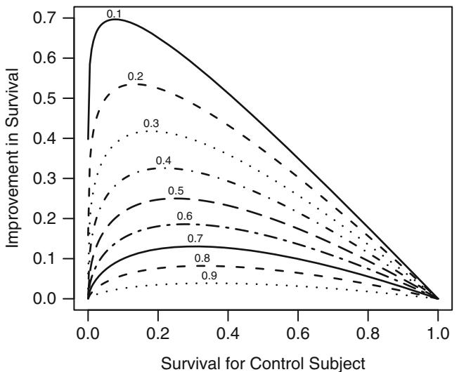
Fig. 18.1 Absolute clinical benefit as a function of survival in a control subject and the relative benefit (hazard ratio). The hazard ratios are given for each curve.

is primarily a function of the baseline risk of a subject. Clinical benefit will also be a function of factors that interact with treatment, that is, factors that modify the relative benefit of treatment. Once a model is developed for estimating S(t|X), this model can be used to estimate absolute benefit as a function of baseline risk factors as well as factors that interact with a treatment. Let X¹ be a binary treatment indicator and let A = {X2,…,Xp} be the other factors (which for convenience we assume do not interact with X1). Then the estimate of S(t|X¹ = 0, A) × S(t|X¹ = 1, A) can be plotted against S(t|X¹ = 0) or against levels of variables in A to display absolute benefit versus overall risk or specific subject characteristics. ¹

18.2.4 Specific Models

Let Xβ denote the linear combination of predictors excluding an intercept term. Using the PH formulation, an exponential survival regression model218 can be stated as

\[\begin{aligned} \lambda(t|X) &= \lambda \exp(X\beta) \\ S(t|X) &= \exp[-\lambda t \exp(X\beta)] = \exp(-\lambda t)^{\exp(X\beta)}. \end{aligned} \tag{18.19}\]

The parameter λ can be thought of as the antilog of an intercept term since the model could be written λ(t|X) = exp[(log λ) + Xβ]. The effect of X on the expected or median failure time is as follows.

\[\begin{aligned} E\{T|X\} &= 1/[\lambda \exp(X\beta)]\\ T\_{0.5}|X &= (\log 2)/[\lambda \exp(X\beta)]. \end{aligned} \tag{18.20}\]

The exponential regression model can be written in another form that is more numerically stable by replacing the λ parameter with an intercept term in Xβ, specifically λ = exp(β0). After redefining Xβ to include β0, λ can be dropped in all the above formulas.

The Weibull regression model is defined by one of the following functions (assuming that Xβ does not contain an intercept).

\[\begin{split} \lambda(t|X) &= \alpha \gamma t^{\gamma - 1} \exp(X\beta) \\ A(t|X) &= \alpha t^{\gamma} \exp(X\beta) \\ S(t|X) &= \exp[-\alpha t^{\gamma} \exp(X\beta)] \\ &= [\exp(-\alpha t^{\gamma})]^{\exp(X\beta)}. \end{split} \tag{18.21}\]

Note that the parameter α in the homogeneous Weibull model has been replaced with α exp(Xβ). The median survival time is given by

\[|T\_{0.5}|X = \{\log 2 / [\alpha \exp(X\beta)]\}^{1/\gamma}.\tag{18.22}\]

As with the exponential model, the parameter α could be dropped (and replaced with exp(β0)) if an intercept β⁰ is added to Xβ.

For numerical reasons it is sometimes advantageous to write the Weibull PH model as

\[S(t|X) = \exp(-A(t|X)),\tag{18.23}\]

where

\[A(t|X) = \exp(\gamma \log t + X\beta). \tag{18.24}\]

18.2.5 Estimation

The parameters in λ and β are estimated by maximizing a log likelihood function constructed in the same manner as described in Section 18.1. The only difference is the insertion of exp(Xiβ) in the likelihood function:

18.2 Parametric Proportional Hazards Models 433

\[\log L = \sum\_{i:Y\_i \text{ unencoored}}^n \log[\lambda(Y\_i)\exp(X\_i\beta)] - \sum\_{i=1}^n \Lambda(Y\_i)\exp(X\_i\beta). \tag{18.25}\]

Once βˆ, the MLE of β, is computed along with the large-sample standard error estimates, hazard ratio estimates and their confidence intervals can readily be computed. Letting s denote the estimated standard error of βˆ^j , a 1 × α confidence interval for the X^j +1 : X^j hazard ratio is given by exp[βˆ^j ^± zs], where ^z is the 1 ^× ^α/2 critical value for the standard normal distribution.

Once the parameters of the underlying hazard function are estimated, the MLE of ^λ(t), ^λˆ(t), can be derived. The MLE of ^λ(t|X), the hazard as a function of t and X, is given by

\[ \hat{\lambda}(t|X) = \hat{\lambda}(t) \exp(X\hat{\beta}).\tag{18.26} \]

The MLE of Λ(t), Λˆ(t), can be derived from the integral of λˆ(t) with respect to t. Then the MLE of S(t|X) can be derived:

\[\hat{S}(t|X) = \exp[-\hat{A}(t)\exp(X\hat{\beta})].\tag{18.27}\]

For the Weibull model, we denote the MLEs of the hazard parameters α and γ by ˆα and ˆγ. The MLE of λ(t|X), Λ(t|X), and S(t|X) for this model are

\[\begin{aligned} \hat{\lambda}(t|X) &= \hat{\alpha}\hat{\gamma}t^{\hat{\gamma}-1} \exp(X\hat{\beta}) \\ \hat{A}(t|X) &= \hat{\alpha}t^{\hat{\gamma}} \exp(X\hat{\beta}) \\ \hat{S}(t|X) &= \exp[-\hat{A}(t|X)]. \end{aligned} \tag{18.28}\]

Confidence intervals for S(t|X) are best derived using general matrix notation to obtain an estimate ^s of the standard error of log[λˆ(t|X)] from the estimated information matrix of all hazard and regression parameters. A confidence interval for Sˆ will be of the form

\[ \hat{S}(t|X)^{\exp(\pm z \cdot s)}.\tag{18.29} \]

The MLEs of β and of the hazard shape parameters lead directly to MLEs of the expected and median life length. For the Weibull model the MLE of the median life length given X is

\[ \hat{T}\_{0.5}|X = \{\log 2 / [\hat{\alpha} \exp(X\hat{\beta})] \}^{1/\hat{\gamma}}.\tag{18.30} \]

For the exponential model, the MLE of the expected life length for a subject having predictor values X is given by

\[ \triangle(T|X) = [\hat{\lambda} \exp(X\hat{\beta})]^{-1},\tag{18.31} \]

where λˆ is the MLE of λ.

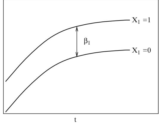
Fig. 18.2 PH model with one binary predictor. Y -axis is log Φ(t) or log δ(t). For log δ(t), the curves must be non-decreasing. For log Φ(t), they may be any shape.

18.2.6 Assessment of Model Fit

Three assumptions of the parametric PH model were listed in Section 18.2.2. We now lay out in more detail what relationships need to be satisfied. We first assume a PH model with a single binary predictor X1. For a general underlying hazard function λ(t), all assumptions of the model are displayed in Figure 18.2. In this case, the assumptions are PH and a shape for λ(t).

If λ(t) is Weibull, the two curves will be linear if log t is plotted instead of t on the x-axis. Note also that if there is no association between X and survival (β¹ = 0), estimates of the two curves will be close and will intertwine due to random variability. In this case, PH is not an issue.

If the single predictor is continuous, the relationships in Figures 18.3 and 18.4 must hold. Here linearity is assumed (unless otherwise specified) besides PH and the form of λ(t). In Figure 18.3, the curves must be parallel for any choices of times t¹ and t² as well as each individual curve being linear. Also, the difference between ordinates needs to conform to the assumed distribution. This difference is log[λ(t2)/λ(t1)] or log[Λ(t2)/Λ(t1)].

Figure 18.4 highlights the PH assumption. The relationship between the two curves must hold for any two values c and d of X1. The shape of the function for a given value of X¹ must conform to the assumed λ(t). For a Weibull model, the functions should each be linear in log t.

When there are multiple predictors, the PH assumption can be displayed in a way similar to Figures 18.2 and 18.4 but with the population additionally cross-classified by levels of the other predictors besides X1. If there is one binary predictor X¹ and one continuous predictor X2, the relationship in

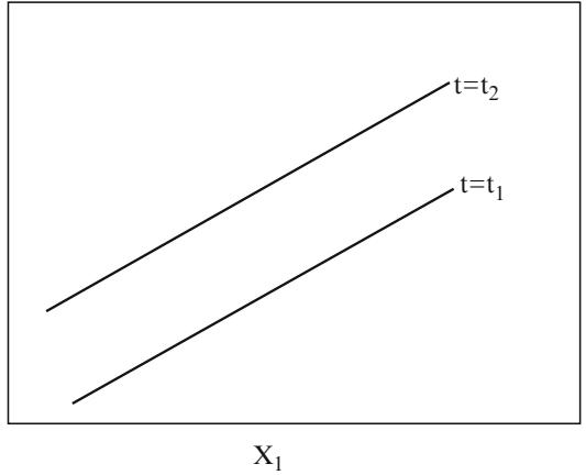
Fig. 18.3 PH model with one continuous predictor. Y -axis is log Φ(t) or log δ(t); for log δ(t), drawn for t² > t1. The slope of each line is χ1.

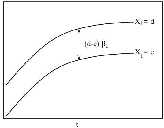
Fig. 18.4 PH model with one continuous predictor. Y -axis is log Φ(t) or log δ(t). For log Φ, the functions need not be monotonic.

Figure 18.5 must hold at each time t if linearity is assumed for X² and there is no interaction between X¹ and X2. Methods for verifying the regression assumptions (e.g., splines and residuals) and the PH assumption are covered in detail under the Cox PH model in Chapter 20.

The method for verifying the assumed shape of S(t) in Section 18.1.3 is also useful when there are a limited number of categorical predictors. To validate a Weibull PH model one can stratify on X and plot log ΛKM(t|X stratum) against log t. This graph simultaneously assesses PH in addition to shape assumptions—all curves should be parallel as well as straight. Straight but nonparallel (non-PH) curves indicate that a series of Weibull models with differing γ parameters will fit.

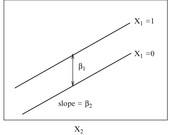
Fig. 18.5 Regression assumptions, linear additive PH or AFT model with two predictors. For PH, Y -axis is log Φ(t) or log δ(t) for a fixed t. For AFT, Y -axis is log(T).

18.3 Accelerated Failure Time Models

18.3.1 Model

Besides modeling the effect of predictors by a multiplicative effect on the hazard function, other regression effects can be specified. The accelerated failure time (AFT) model is commonly used; it specifies that the predictors act multiplicatively on the failure time or additively on the log failure time. The effect of a predictor is to alter the rate at which a subject proceeds along the time axis (i.e., to accelerate the time to failure [331, pp. 33–35]). The ² model is

\[S(t|X) = \psi((\log(t) - X\beta)/\sigma),\tag{18.32}\]

where ψ is any standardized survival distribution function. The parameter σ is called the scale parameter. The model can also be stated as (log(T )×Xβ)/σ ≈ ψ or log(T ) = Xβ + σϵ, where ϵ is a random variable from the distribution ψ. Sometimes the untransformed T is used in place of log(T ). When the log form is used, the models are said to be log-normal, log-logistic, and so on.

The exponential and Weibull are the only two distributions that can de-³ scribe either a PH or an AFT model.

18.3.2 Model Assumptions and Interpretation of Parameters

The log λ or log Λ transformation of the PH model has the following equivalent for AFT models.

18.3 Accelerated Failure Time Models 437

\[ \psi^{-1}[S(t|X)] = (\log(t) - X\beta)/\sigma. \tag{18.33} \]

Letting as before ϵ denote a random variable from the distribution S, the model is also

\[ \log(T) = X\beta + \sigma \epsilon.\tag{18.34} \]

So the property of the response T of interest for regression modeling is log(T ). In the absence of censoring, we could check the model by plotting an X against log ^T and checking that the residuals log(^T ) ^× ^Xβ^ˆ are distributed as ψ to within a scale factor.

The assumptions of the AFT model are thus the following.

1. The true form of ψ (the distributional family) is correctly specified.
1. In the absence of nonlinear and interaction terms, each X^j affects log(T ) or ^ψ−¹[S(t|X)] linearly.
1. Implicit in these assumptions is that σ is a constant independent of X.

A one-unit change in X^j is then most simply understood as a β^j change in the log of the failure time. The one-unit change in X^j increases the failure time by a factor of exp(β^j ).

The median survival time is obtained by solving ψ((log(t)× Xβ)/σ)=0.5 giving

\[|T\_{0.5}|X = \exp[X\beta + \sigma\psi^{-1}(0.5)]\tag{18.35}\]

18.3.3 Specific Models

Common choices for the distribution function ψ in Equation 18.32 are the extreme value distribution ψ(u) = exp(× exp(u)), the logistic distribution ^ψ(u) = [1 + exp(u)]−¹, and the normal distribution ^ψ(u)=1 ^× ^Φ(u). The AFT model equivalent of the Weibull model is obtained by using the extreme value distribution, negating β, and replacing γ with 1/σ in Equation 18.24:

\[S(t|X) = \exp[-\exp((\log(t) - X\beta)/\sigma)]\]

\[T\_{0.5}|X = [\log(2)]^\sigma \exp(X\beta). \tag{18.36}\]

The exponential model is obtained by restricting σ = 1 in the extreme value distribution.

The log-normal regression model is

\[S(t|X) = 1 - \Phi((\log(t) - X\beta)/\sigma),\tag{18.37}\]

and the log-logistic model is

\[S(t|X) = \left[1 + \exp((\log(t) - X\beta)/\sigma)\right]^{-1}.\tag{18.38}\]

The t distribution allows for more flexibility by varying the degrees of freedom. Figure 18.6 depicts possible hazard functions for the log t distribution for varying σ and degrees of freedom. However, this distribution does not have a late increasing hazard phase typical of human survival.

require(rms)

haz − survreg.auxinfo$t$hazard
times − c(seq(0, .25 , length =100), seq(.26 , 2, length =150))
high − c(6, 1.5, 1.5, 1.75)
low − c(0, 0, 0, .25)
dfs − c(1, 2, 3, 5, 7, 15, 500)
cols − rep(1, 7)
ltys − 1:7
i − 0
for(scale in c(.25 , .6, 1, 2)) {
  i − i+1
  plot(0, 0, xlim=c(0,2), ylim=c(low [i], high[i]),
    xlab=expression (t), ylab=expression (lambda (t)), type="n")
  col − 1.09
  j − 0
  for(df in dfs) {
    j − j+1
    ## Divide by t to get hazard for log t distribution
    lines(times ,
          haz(log(times), 0, c(log(scale), df))/times ,
          col=cols[j], lty= ltys[j])
    if(i==1) text(1.7, .23 + haz(log (1.7), 0,
         c(log(scale),df))/1.7, format (df))
  }
  title(paste("Scale:", format(scale)))
} # Figure 18.6

All three of these parametric survival models have median survival time T0.5|X = exp(Xβ).

18.3.4 Estimation

Maximum likelihood estimation is used much the same as in Section 18.2.5. Care must be taken in the choice of initial values; iterative methods are especially prone to problems in choosing the initial ˆσ. Estimation works better if σ is parameterized as exp(δ). Once β and σ (exp(δ)) are estimated, MLEs of secondary parameters such as survival probabilities and medians can readily be obtained:

\[ \begin{aligned} \hat{S}(t|X) &= \psi( (\log(t) - X\hat{\beta}) / \hat{\sigma} ) \\ \hat{T}\_{0.5}|X &= \exp[X\hat{\beta} + \hat{\sigma}\psi^{-1}(0.5)]. \end{aligned} \tag{18.39} \]

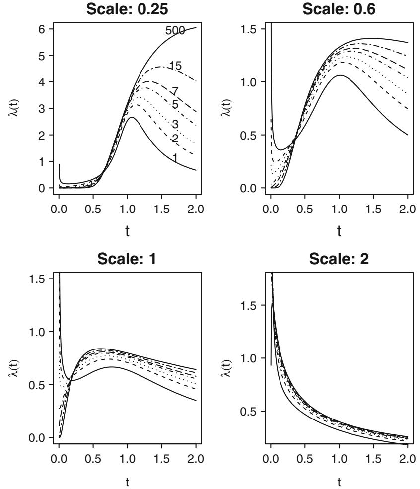
Fig. 18.6 log(T) distribution for λ = 0.25, 0.6, 1, 2 and for degrees of freedom 1, 2, 3, 5, 7, 15, 500 (almost log-normal). The top left plot has degrees of freedom written in the plot.

For normal and logistic distributions, Tˆ ⁰.5|^X = exp(Xβˆ). The MLE of the effect on log(T ) of increasing X^j by d units is βˆ ^jd if X^j is linear and additive.

The delta (statistical differential) method can be used to compute an estimate of the variance of ^f = [log(t) ^× ^Xβˆ]/σˆ. Let (βˆ, ^ˆδ) denote the estimated parameters, and let Vˆ denote the estimated covariance matrix for these parameter estimates. Let F denote the vector of derivatives of f with respect to (β0, ^β1,…, ^βp, ^δ); that is, ^F = [×1, ^×X1, ^×X2,…, ^×Xp, ^×(log(t) ^× ^Xβˆ)]/σˆ. The variance of f is then approximately

\[\text{Var}(f) = F\hat{V}F'.\tag{18.40}\]

Letting s be the square root of the variance estimate and z1−α/² be the normal critical value, a 1 × α confidence limit for S(t|X) is

\[ \psi((\log(t) - X\hat{\beta})/\hat{\sigma} \pm z\_{1-\alpha/2} \times s). \tag{18.41} \]

18.3.5 Residuals

For an AFT model, standardized residuals are simply

\[r = (\log(T) - X\hat{\beta})/\sigma.\tag{18.42}\]

⁴ When T is right-censored, r is right-censored. Censoring must be taken into account, for example, by displaying Kaplan–Meier estimates based on groups of residuals rather than showing individual residuals. The residuals can be used to check for lack of fit as described in the next section. Note that examining individual uncensored residuals is not appropriate, as their distribution is conditional on Tⁱ < Ci, where Cⁱ is the censoring time.

Cox and Snell134 proposed a type of general residuals that also work for censored data. Using their method on the cumulative probability scale results in the probability integral transformation. If the probability of failure before time t given X is S(t|X), F(T |X)=1 × S(T |X) has a uniform [0, 1] distribution, where T is a subject’s actual failure time. When T is right-censored, so is 1 ^× ^S(^T ^|X). Substituting ^S^ˆ for ^S results in an approximate uniform [0, 1] distribution for any value of X. One minus the Kaplan–Meier estimate of 1 ^× ^Sˆ(^T ^|X) (using combined data for all ^X) is compared against a 45^≤ line to check for goodness of fit. A more stringent assessment is obtained by repeating this process while stratifying on X.

18.3.6 Assessment of Model Fit

For a single binary predictor, all assumptions of the AFT model are depicted in Figure 18.7. That figure also shows the assumptions for any two values of a single continuous predictor that behaves linearly. For a single continuous predictor, the relationships in Figure 18.8 must hold for any two follow-up times. The regression assumptions are isolated in Figure 18.5.

To verify the fit of a log-logistic model with age as the only predictor, one could stratify by quartiles of age and check for linearity and parallelism of the four logit SΛ(t) or SKM(t) curves over increasing t as in Figure 18.7, which stresses the distributional assumption (no T by X interaction and linearity vs. log(t)). To stress the linear regression assumption while checking for absence of time interactions (part of the distributional assumptions), one could make

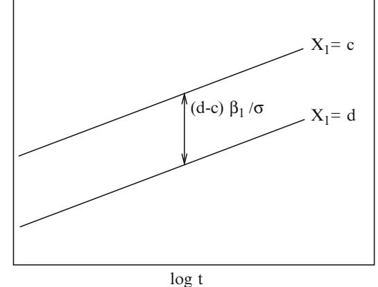
Fig. 18.7 AFT model with one predictor. ^Y -axis is ^α∧¹[S(t|X)] = (log(t) ^× ^Xχ)/λ. Drawn for d>c. The slope of the lines is λ∧¹.

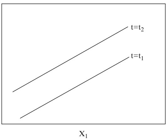
Fig. 18.8 AFT model with one continuous predictor. ^Y -axis is ^α∧¹[S(t|X)] = (log(t) × Xχ)/λ. Drawn for t² > t1. The slope of each line is χ1/λ and the difference between the lines is log(t2/t1)/λ.

a plot like Figure 18.8. For each decile of age, the logit transformation of the 1-, 3-, and 5-year survival estimates for that decile would be plotted against the mean age in the decile. This checks for linearity and constancy of the age effect over time. Regression splines will be a more effective method for checking linearity and determining transformations. This is demonstrated in Chapter 20 with the Cox model, but identical methods apply here.

As an example, consider data from Kalbfleisch and Prentice [331, pp. 1–2], who present data from Pike508 on the time from exposure to the carcinogen DMBA to mortality from vaginal cancer in rats. The rats are divided into two groups on the basis of a pre-treatment regime. Survival times in days (with censored times marked ⁺) are found in Table 18.2.

Group 1	143	164 188 188 190 192 206 209		213	216
	220		227 230 234 246 265 304 216+ 244+
Group 2	142	156 163 198 205 232 232 233		233	233

	233	239 240 261 280 280 296 296		323	204+
	344+

Table 18.2 Rat vaginal cancer data from Pike508

getHdata (kprats)
kprats$group ← factor(kprats$ group , 0:1, c( ' Group 1 ' , ' Group 2 ' ))
dd ← datadist (kprats ); options (datadist ="dd")
S ← with(kprats , Surv(t, death))
f ← npsurv(S ◦ group , type="fleming", data=kprats)
survplot (f, n.risk=TRUE , conf= ' none ' , # Figure 18.9
          label.curves =list(keys= ' lines ' ), levels.only =TRUE)
title(sub=" Nonparametric estimates ", adj =0, cex=.7)
# Check fits of Weibull, log-logistic, log-normal
xl ← c(4.8 , 5.9)
survplot (f, loglog=TRUE , logt= TRUE , conf="none", xlim=xl ,
          label.curves =list(keys= ' lines ' ), levels.only =TRUE)
title(sub="Weibull (extreme value)", adj =0, cex=.7)
survplot (f, fun=function (y)log(y/(1-y)), ylab="logit S(t)",
         logt=TRUE , conf=" none", xlim=xl ,
          label.curves =list(keys= ' lines ' ), levels.only =TRUE)
title(sub=" Log-logistic ", adj =0, cex=.7)
survplot (f, fun=qnorm , ylab="Inverse Normal S(t)",
         logt=TRUE , conf="none",
         xlim=xl , cex.label =.7 ,
          label.curves =list(keys= ' lines ' ), levels.only =TRUE)
title(sub=" Log-normal ", adj =0, cex=.7)

The top left plot in Figure 18.9 displays nonparametric survival estimates for the two groups, with the number of rats “at risk” at each 30-day mark written above the x-axis. The remaining three plots are for checking assumptions of three models. None of the parametric models presented will completely allow for such a long period with no deaths. Neither will any allow for the early crossing of survival curves. Log-normal and log-logistic models yield very similar results due to the similarity in shapes between ^Φ(z) and [1 + exp(×z)]−¹ for non-extreme z. All three transformations show good parallelism after the early crossing. The log-logistic and log-normal transformations are slightly more linear. The fitted models are:

fw − psm(S ← group , data=kprats , dist= ' weibull ' )
fl − psm(S ← group , data=kprats , dist= ' loglogistic ' ,
           y=TRUE)
fn − psm(S ← group , data=kprats , dist= ' lognormal ' )
latex (fw , fi= ' ' )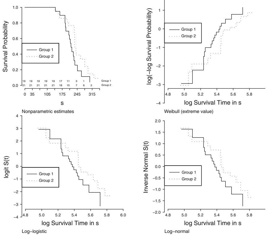

Fig. 18.9 Altschuler–Nelson–Fleming–Harrington nonparametric survival estimates for rats treated with DMBA,508 along with various transformations of the estimates for checking distributional assumptions of three parametric survival models.

\[\begin{aligned} \text{Prob}\{T \ge t\} &= \exp[-\exp(\frac{\log(t) - X\beta}{0.1832976})] \text{ where} \\\\ X\hat{\beta} &= \\ 5.450859 \\ &+ 0.131983 [\text{Group 2}] \end{aligned}\]

and [c] = 1 if subject is in group c, 0 otherwise.

latex (fl , fi= ’ ’ )

Model	Group 2:1	Median Survival Time
	Failure Time Ratio Group 1		Group 2
Extreme Value (Weibull)	1.14	217	248
Log-logistic	1.11	217	241
Log-normal	1.10	217	238

Table 18.3 Group effects from three survival models

\[\text{Prob}\{T \ge t\} = [1 + \exp(\frac{\log(t) - X\beta}{0.1159753})]^{-1} \quad \text{where} \beta\]

Xχˆ = 5.375675 +0.1051005[Group 2]

and [c] = 1 if subject is in group c, 0 otherwise.

latex (fn , fi= ’ ’ )

\[\text{Prob}\{T \ge t\} = 1 - \Phi(\frac{\log(t) - X\beta}{0.2100184}) \text{ where}\]

Xχˆ = 5.375328 +0.0930606[Group 2]

and [c] = 1 if subject is in group c, 0 otherwise.

The estimated failure time ratios and median failure times for the two groups are given in Table 18.3. For example, the effect of going from Group 1 to Group 2 is to increase log failure time by 0.132 for the extreme value model, giving a Group 2:1 failure time ratio of exp(0.132) = 1.14. This ratio is also the ratio of median survival times. We choose the log-logistic model for its simpler form. The fitted survival curves are plotted with the nonparametric estimates in Figure 18.10. Excellent agreement is seen, except for 150 to 180 days for Group 2. The standard error of the regression coefficient for group in the log-logistic model is 0.0636 giving a Wald χ² for group differences of (.105/.0636)² = 2.73, P = 0.1.

survplot(f, conf.int= FALSE , # Figure 18.10
          levels.only= TRUE , label.curves = list(keys= ' lines ' ))
survplot (fl , add=TRUE , label.curves = FALSE , conf.int= FALSE)

The Weibull PH form of the fitted extreme value model, using Equation 18.24, is

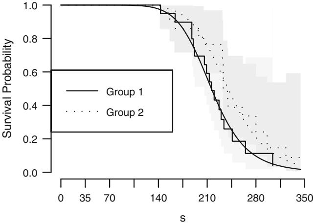
Fig. 18.10 Agreement between fitted log-logistic model and nonparametric survival estimates for rat vaginal cancer data.

\[\begin{aligned} \text{Prob}\{T \ge t\} &= \exp\{-t^{5.456} \exp(X\hat{\beta})\} \text{ where } \\\\ X\hat{\beta} &= \\ &-29.74 \\ &-0.72 \text{[Group 2]} \end{aligned}\]

and [c] = 1 if subject is in group c, 0 otherwise.

A sensitive graphical verification of the distributional assumptions of the AFT model is obtained by plotting the estimated survival distribution of standardized residuals (Equation 18.3.5), censored identically to the way T is censored. This distribution is plotted along with the theoretical distribution ψ. The assessment may be made more stringent by stratifying the residuals by important subject characteristics and plotting separate survival function estimates; they should all have the same standardized distribution (e.g., same σ).

r − resid (fl , ' cens ' )
survplot( npsurv (r ← group , data=kprats ),
          conf= ' none ' , xlab= ' Residual ' ,
          label.curves = list(keys= ' lines ' ), levels.only= TRUE)
survplot( npsurv (r ← 1), conf= ' none ' , add=TRUE , col= ' red ' )
lines (r, lwd=1, col= ' blue ' ) # Figure 18.11

As an example, Figure 18.11 shows the Kaplan–Meier estimate of the distribution of residuals, Kaplan–Meier estimates stratified by group, and the assumed log-logistic distribution. ⁵

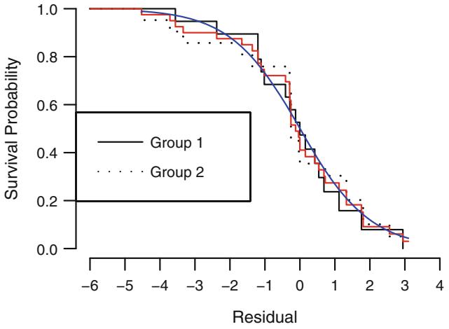
Fig. 18.11 Kaplan–Meier estimates of distribution of standardized censored residuals from the log-logistic model, along with the assumed standard log-logistic distribution (dashed curve). The step functions in red is the estimated distribution of all residuals, and the step functions in black are the estimated distributions of residuals stratified by group, as indicated. The blue curve is the assumed log-logistic distribution.

Section 19.2 has a more in-depth example of this approach.

18.3.7 Validating the Fitted Model

AFT models may be validated for both calibration and discrimination accuracy using the same methods that are presented for the Cox model in Section 20.11. The methods discussed there for checking calibration are based on choosing a single follow-up time. Checking the distributional assumptions of the parametric model is also a check of calibration accuracy in a sense. Another indirect calibration assessment may be obtained from a set of Cox–Snell residuals (Section 18.3.5) or by using ordinary residuals as just described. A higher resolution indirect calibration assessment based on plotting individual uncensored failure times is available when the theoretical censoring times for those observations are known. Let C denote a subject’s censoring time and F the cumulative distribution of a failure time T . The expected value of F(T |X) is 0.5 when T is an actual failure time random variable. The expected value for an event time that is observed because it is uncensored is the expected value of F(T |T − C, X)=0.5F(C|X). A smooth plot (using, say, loess) of ^F(^T ^|X) ^× ⁰.5F(C|X) against ^Xβ^ˆ should be a flat line through ^y = 0 if the model is well calibrated. A smooth plot of 2F(^T ^|X)/F(C|X) against ^Xβ^ˆ (or anything else) should be a flat line through y = 1. This method assumes that the model is calibrated well enough that we can substitute 1 ^× ^Sˆ(C|X) for F(C|X).

18.4 Buckley–James Regression Model

Buckley and James81 developed a method for estimating regression coefficients using least squares after imputing censored residuals. Their method does not assume a distribution for survival time or the residuals, but is aimed at estimating expected survival time or expected log survival time given predictor variables. This method has been generalized to allow for smooth nonlinear effects and interactions in the S bj function in the rms package, written by Stare and Harrell585.

18.5 Design Formulations

Various designs can be formulated with survival regression models just as with other regression models. By constructing the proper dummy variables, ANOVA and ANOCOVA models can easily be specified for testing differences in survival time between multiple treatments. Interactions and complex nonlinear effects may also be modeled.

18.6 Test Statistics

As discussed previously, likelihood ratio, score, and Wald statistics can be derived from the maximum likelihood analysis, and the choice of test statistic depends on the circumstance and on computational convenience.

18.7 Quantifying Predictive Ability

See Section 20.10 for a generalized measure of concordance between predicted and observed survival time (or probability of survival) for right-censored data.

18.8 Time-Dependent Covariates

Time-dependent covariates (predictors) requires special likelihood functions and add significant complexity to analyses in exchange for greater versatility and enhanced predictive discrimination604. Nicolaie et al.477 and D’Agostino et al.145 provide useful static covariate approaches to modeling time-dependent predictors using landmark analysis.

18.9 R Functions

Therneau’s survreg function (part of his survival package) can fit regression models in the AFT family with left–, right–, or interval–censoring. The time variable can be untransformed or log-transformed (the default). Distributions supported are extreme value (Weibull and exponential), normal, logistic, and Student-t. The version of survreg in rms that fits parametric survival models in the same framework as lrm, ols, and cph is called psm. psm works with print, coef, formula, specs, summary, anova, predict, Predict, fastbw, latex, nomogram, validate, calibrate, survest, and survplot functions for obtaining and plotting predicted survival probabilities. The dist argument to psm can be “exponential”, “extreme”, “gaussian”, “logistic”, “loglogistic”, “lognormal”, “t”, or “weibull”. To fit a model with no covariables, use the command

psm(Surv(d.time , event) ← 1)

To restate a Weibull or exponential model in PH form, use the pphsm function. An example of how many of the functions are used is found below.

units (d.time ) − "Year"
f − psm(Surv(d.time ,cdeath ) ← lsp(age ,65) *sex)
# default is Weibull
anova (f)
summary(f) # summarize effects with delta log T
latex (f) # typeset math. form of fitted model
survest(f, times =1) # 1y survival est. for all subjects
survest(f, expand.grid (sex=" female ", age=30:80) , times =1:2)
# 1y, 2y survival estimates vs. age , for females
survest(f, data.frame(sex=" female ",age=50))
# survival curve for an individual subject
survplot (f, sex=NA , age =50, n.risk =T)
# survival curves for each sex, adjusting age to 50
f.ph − pphsm (f) # convert from AFT to PH
summary( f.ph) # summarize with hazard ratios
                    # instead of changes in log(T)

Special functions work with objects created by psm to create S functions that contain the analytic form for predicted survival probabilities (Survival), hazard functions (Hazard), quantiles of survival time (Quantile), and mean or expected survival time (Mean). Once the S functions are constructed, they can be used in a variety of contexts. The survplot and survest functions have a special argument for psm fits: what. The default is what=“survival” to estimate or plot survival probabilities. Specifying what=“hazard” will plot hazard functions. Predict also has a special argument for psm fits: time. Specifying a single value for time results in survival probability for that time being plotted instead of Xβˆ. Examples of many of the functions appear below, with the output of the survplot command shown in Figure 18.12.

med − Quantile(fl)
meant − Mean(fl)

18.9 R Functions 449

haz − Hazard (fl)
surv − Survival(fl)
latex (surv , file= ' ' , type= ' Sinput ' )

surv − function ( times = NULL , lp = NULL ,
                   parms = -2.15437773933124 )
{
    1/(1 + exp((logb(times ) - lp)/exp(parms )))
}

# Plot estimated hazard functions and add median
# survival times to graph
survplot (fl , group , what="hazard ") # Figure 18.12
# Compute median survival time
m − med(lp=predict(fl ,
           data.frame( group=levels (kprats $group ))))
m

1 2 216.0857 240.0328

med(lp=range (fl$ linear.predictors ))

[1] 216.0857 240.0328

m − format (m, digits =3)
text (68, .02 , paste ("Group 1 median : ", m[1], "\n",
                     "Group 2 median : ", m[2], sep=""))
# Compute survival probability at 210 days
xbeta − predict(fl ,
                  data.frame( group =c(" Group 1","Group 2")))
surv (210, xbeta )

1 2 0.5612718 0.7599776

The S object called survreg.distributions in Therneau’s survival package and the object survreg.auxinfo in the rms package have detailed information for extreme-value, logistic, normal, and t distributions. For each distribution, components include the deviance function, an algorithm for obtaining starting parameter estimates, a LATEX representation of the survival function, and S functions defining the survival, hazard, quantile functions, and basic survival inverse function (which could have been used in Figure 18.9). See Figure 18.6 for examples. rms’s val.surv function is useful for indirect external validation of parametric models using Cox–Snell residuals and other approaches of Section 18.3.7. The plot method for an object created by val.surv makes it easy to stratify all computations by a variable of interest to more stringently validate the fit with respect to that variable.

rms’s bj function fits the Buckley–James model for right-censored responses.

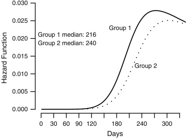
Fig. 18.12 Estimated hazard functions for log-logistic fit to rat vaginal cancer data, along with median survival times.

Kooperberg et al.’s adaptive linear spline log-hazard model360, 361, 594 has been implemented in the S function hare. Their procedure searches for secondorder interactions involving predictors (and linear splines of them) and linear splines in follow-up time (allowing for non-proportional hazards). hare is also used to estimate calibration curves for parametric survival models (rms function calibrate) as it is for Cox models.

18.10 Further Reading

1 Wellek657 developed a test statistic for a specified maximum survival difference after relating this difference to a hazard ratio.
2 Hougaard308 compared accelerated failure time models with proportional hazard models.
3 Gore et al.226 discuss how an AFT model (the log-logistic model) gives rise to varying hazard ratios.
4 See Hillis293 for other types of residuals and plots that use them.
5 See Gore et al.226 and Lawless382 for other methods of checking assumptions for AFT models. Lawless is an excellent text for in-depth discussion of parametric survival modeling. Kwong and Hutton369 present other methods of choosing parametric survival models, and discuss the robustness of estimates when fitting an incorrectly chosen accelerated failure time model.

18.11 Problems

For the failure times (in days)

133⁺ 6⁺ 7⁺

compute MLEs of the following parameters of an exponential distribution by hand: λ, µ, T0.5, and S(3 days). Compute 0.95 confidence limits for λ and S(3), basing the latter on log[Λ(t)].

For the same data in Problem 1, compute MLEs of parameters of a Weibull distribution. Also compute the MLEs of S(3) and T0.5.

Chapter 19 Case Study in Parametric Survival Modeling and Model Approximation

Consider the random sample of 1000 patients from the SUPPORT study,352 described in Section 3.12. In this case study we develop a parametric survival time model (accelerated failure time model) for time until death for the acute disease subset of SUPPORT (acute respiratory failure, multiple organ system failure, coma). We eliminate the chronic disease categories because the shapes of the survival curves are different between acute and chronic disease categories. To fit both acute and chronic disease classes would require a log-normal model with σ parameter that is disease-specific.

Patients had to survive until day 3 of the study to qualify. The baseline physiologic variables were measured during day 3.

19.1 Descriptive Statistics

First we create a variable acute to flag the categories of interest, and print univariable descriptive statistics for the data subset.

require(rms)

getHdata(support) # Get data frame from web site
acute − support$dzclass %in% c( ' ARF/MOSF ' , ' Coma ' )
latex ( describe(support[ acute ,]), file= ' ' )

35 Variables 537 Observations
age : Age n missing unique Info Mean .05 .10 .25 .50 .75 .90 .95 537 0 529 1 60.7 28.49 35.22 47.93 63.67 74.49 81.54 85.56 lowest : 18.04 18.41 19.76 20.30 20.31 highest: 91.62 91.82 91.93 92.74 95.51
death : Death at any time up to NDI date:31DEC94 n missing unique Info Sum Mean 537 0 2 0.67 356 0.6629
sex n missing unique 537 0 2
female (251, 47%), male (286, 53%)
hospdead : Death in Hospital n missing unique Info Sum Mean 537 0 2 0.7 201 0.3743
slos : Days from Study Entry to Discharge n missing unique Info Mean .05 .10 .25 .50 .75 .90 .95 537 0 85 1 23.44 4.0 5.0 9.0 15.0 27.0 47.4 68.2 lowest : 3 4 5 6 7, highest: 145 164 202 236 241
d.time : Days of Follow-Up n missing unique Info Mean .05 .10 .25 .50 .75 .90 .95 537 0 340 1 446.1 4 6 16 182 724 1421 1742 lowest : 3 4 5 6 7, highest: 1977 1979 1982 2011 2022
dzgroup n missing unique 537 0 3 ARF/MOSF w/Sepsis (391, 73%), Coma (60, 11%), MOSF w/Malig (86, 16%)
dzclass n missing unique 537 0 2 ARF/MOSF (477, 89%), Coma (60, 11%)
num.co : number of comorbidities n missing unique Info Mean 537 0 7 0.93 1.525 0 1 2 3 4 56 Frequency 111 196 133 51 31 10 5
% 21 36 25 9 6 2 1

support[acute, ]

edu : Years of Education n missing unique Info Mean .05 .10 .25 .50 .75 .90 .95 411 126 22 0.96 12.03 7 8 10 12 14 16 17 lowest : 0 1 2 3 4, highest: 17 18 19 20 22 income n missing unique 335 202 4 under $11k (158, 47%), $11-$25k (79, 24%), $25-$50k (63, 19%) >$50k (35, 10%) scoma : SUPPORT Coma Score based on Glasgow D3 n missing unique Info Mean .05 .10 .25 .50 .75 .90 .95 537 0 11 0.82 19.24 0 0 0 0 37 55 100 0 9 26 37 41 44 55 61 89 94 100 Frequency 301 50 44 19 17 43 11 6 8 6 32 % 56 9 8 4 3 8 2 1 1 1 6 charges : Hospital Charges n missing unique Info Mean .05 .10 .25 .50 .75 .90 .95 517 20 516 1 86652 11075 15180 27389 51079 100904 205562 283411 lowest : 3448 4432 4574 5555 5849 highest: 504660 538323 543761 706577 740010 totcst : Total RCC cost n missing unique Info Mean .05 .10 .25 .50 .75 .90 .95 471 66 471 1 46360 6359 8449 15412 29308 57028 108927 141569 lowest : 0 2071 2522 3191 3325 highest: 269057 269131 338955 357919 390460 totmcst : Total micro-cost n missing unique Info Mean .05 .10 .25 .50 .75 .90 .95 331 206 328 1 39022 6131 8283 14415 26323 54102 87495 111920 lowest : 0 1562 2478 2626 3421 highest: 144234 154709 198047 234876 271467 avtisst : Average TISS, Days 3–25 n missing unique Info Mean .05 .10 .25 .50 .75 .90 .95 536 1 205 1 29.83 12.46 14.50 19.62 28.00 39.00 47.17 50.37 lowest : 4.000 5.667 8.000 9.000 9.500 highest: 58.500 59.000 60.000 61.000 64.000 race n missing unique 535 2 5 white black asian other hispanic Frequency 417 84 4 8 22 % 78 16 1 1 4

456 19 Parametric Survival Modeling and Model Approximation meanbp : Mean Arterial Blood Pressure Day 3 n missing unique Info Mean .05 .10 .25 .50 .75 .90 .95 537 0 109 1 83.28 41.8 49.0 59.0 73.0 111.0 124.4 135.0 lowest : 0 20 27 30 32, highest: 155 158 161 162 180 wblc : White Blood Cell Count Day 3 n missing unique Info Mean .05 .10 .25 .50 .75 .90 .95 532 5 241 1 14.1 0.8999 4.5000 7.9749 12.3984 18.1992 25.1891 30.1873 lowest : 0.05000 0.06999 0.09999 0.14999 0.19998 highest: 51.39844 58.19531 61.19531 79.39062 100.00000 hrt : Heart Rate Day 3 n missing unique Info Mean .05 .10 .25 .50 .75 .90 .95 537 0 111 1 105 51 60 75 111 126 140 155 lowest : 0 11 30 36 40, highest: 189 193 199 232 300 resp : Respiration Rate Day 3 n missing unique Info Mean .05 .10 .25 .50 .75 .90 .95 537 0 45 1 23.72 8 10 12 24 32 39 40 lowest : 0 4 6 7 8, highest: 48 49 52 60 64 temp : Temperature (celcius) Day 3 n missing unique Info Mean .05 .10 .25 .50 .75 .90 .95 537 0 61 1 37.52 35.50 35.80 36.40 37.80 38.50 39.09 39.50 lowest : 32.50 34.00 34.09 34.90 35.00 highest: 40.20 40.59 40.90 41.00 41.20 pafi : PaO2/(.01*FiO2) Day 3 n missing unique Info Mean .05 .10 .25 .50 .75 .90 .95 500 37 357 1 227.2 86.99 105.08 137.88 202.56 290.00 390.49 433.31 lowest : 45.00 48.00 53.33 54.00 55.00 highest: 574.00 595.12 640.00 680.00 869.38 alb : Serum Albumin Day 3 n missing unique Info Mean .05 .10 .25 .50 .75 .90 .95 346 191 34 1 2.668 1.700 1.900 2.225 2.600 3.100 3.400 3.800 lowest : 1.100 1.200 1.300 1.400 1.500 highest: 4.100 4.199 4.500 4.699 4.800 bili : Bilirubin Day 3 n missing unique Info Mean .05 .10 .25 .50 .75 .90 .95 386 151 88 1 2.678 0.3000 0.4000 0.6000 0.8999 2.0000 6.5996 13.1743 lowest : 0.09999 0.19998 0.29999 0.39996 0.50000 highest: 22.59766 30.00000 31.50000 35.00000 39.29688 crea : Serum creatinine Day 3 n missing unique Info Mean .05 .10 .25 .50 .75 .90 .95 537 0 84 1 2.232 0.6000 0.7000 0.8999 1.3999 2.5996 5.2395 7.3197 lowest : 0.3 0.4 0.5 0.6 0.7, highest: 10.4 10.6 11.2 11.6 11.8

sod : Serum sodium Day 3 n missing unique Info Mean .05 .10 .25 .50 .75 .90 .95
537 0 38 1 138.1 129 131 134 137 142 147 150
lowest : 118 120 121 126 127, highest: 156 157 158 168 175
ph : Serum pH (arterial) Day 3 n missing unique Info Mean .05 .10 .25 .50 .75 .90 .95 500 37 49 1 7.416 7.270 7.319 7.380 7.420 7.470 7.510 7.529
lowest : 6.960 6.989 7.069 7.119 7.130 highest: 7.560 7.569 7.590 7.600 7.659
glucose : Glucose Day 3 n missing unique Info Mean .05 .10 .25 .50 .75 .90 .95 297 240 179 1 167.7 76.0 89.0 106.0 141.0 200.0 292.4 347.2 lowest : 30 42 52 55 68, highest: 446 468 492 576 598

bun : BUN Day 3 n missing unique Info Mean .05 .10 .25 .50 .75 .90 .95 304 233 100 1 38.91 8.00 11.00 16.75 30.00 56.00 79.70 100.70 lowest : 1 3 4 5 6, highest: 123 124 125 128 146
urine : Urine Output Day 3 n missing unique Info Mean .05 .10 .25 .50 .75 .90 .95 303 234 262 1 2095 20.3 364.0 1156.5 1870.0 2795.0 4008.6 4817.5
lowest : 0 5 8 15 20, highest: 6865 6920 7360 7560 7750
adlp : ADL Patient Day 3 n missing unique Info Mean 104 433 8 0.87 1.577 0 1234567
Frequency 51 19 7 6 4 7 8 2 % 49 18 7 6 4 7 8 2
adls : ADL Surrogate Day 3 n missing unique Info Mean 392 145 8 0.89 1.86
0 1 2 3 4 5 6 7 Frequency 185 68 22 18 17 20 39 23 % 47 17 6 5 4 5 10 6
sfdm2 n missing unique 468 69 5
no(M2 and SIP pres) (134, 29%), adl>=4 (>=5 if sur) (78, 17%) SIP>=30 (30, 6%), Coma or Intub (5, 1%), <2 mo. follow-up (221, 47%)

458 19 Parametric Survival Modeling and Model Approximation adlsc : Imputed ADL Calibrated to Surrogate n missing unique Info Mean .05 .10 .25 .50 .75 .90 .95 537 0 144 0.96 2.119 0.000 0.000 0.000 1.839 3.375 6.000 6.000 lowest : 0.0000 0.4948 0.4948 1.0000 1.1667 highest: 5.7832 6.0000 6.3398 6.4658 7.0000

Next, patterns of missing data are displayed.

plot(naclus ( support[acute ,])) # Figure 19.1

The Hmisc varclus function is used to quantify and depict associations between predictors, allowing for general nonmonotonic relationships. This is done by using Hoeffding’s D as a similarity measure for all possible pairs of predictors instead of the default similarity, Spearman’s ρ.

ac − support[acute ,]
ac$dzgroup − ac$dzgroup [drop=TRUE] # Remove unused levels
label(ac$dzgroup ) − ' Disease Group '
attach(ac)
vc − varclus(← age + sex + dzgroup + num.co + edu + income +
             scoma + race + meanbp + wblc + hrt + resp +
             temp + pafi + alb + bili + crea + sod + ph +
             glucose + bun + urine + adlsc , sim= ' hoeffding ' )
plot(vc) # Figure 19.2

19.2 Checking Adequacy of Log-Normal Accelerated Failure Time Model

Let us check whether a parametric survival time model will fit the data, with respect to the key prognostic factors. First, Kaplan–Meier estimates stratified by disease group are computed, and plotted after inverse normal transformation, against log t. Parallelism and linearity indicate goodness of fit to the log normal distribution for disease group. Then a more stringent assessment is made by fitting an initial model and computing right-censored residuals. These residuals, after dividing by ˆσ, should all have a normal distribution if the model holds. We compute Kaplan–Meier estimates of the distribution of the residuals and overlay the estimated survival distribution with the theoretical Gaussian one. This is done overall, and then to get more stringent assessments of fit, residuals are stratified by key predictors and plots are produced that contain multiple Kaplan–Meier curves along with a single theoretical normal curve. All curves should hover about the normal distribution. To gauge the natural variability of stratified residual distribution estimates, the residuals are also stratified by a random number that has no bearing on the goodness of fit.

dd − datadist(ac) # describe distributions of variables to rms

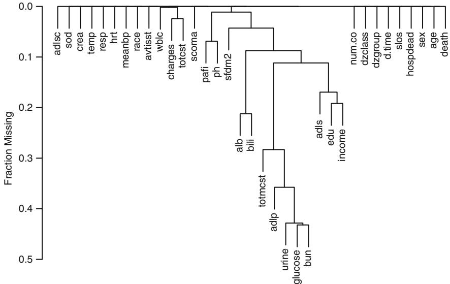
Fig. 19.1 Cluster analysis showing which predictors tend to be missing on the same patients

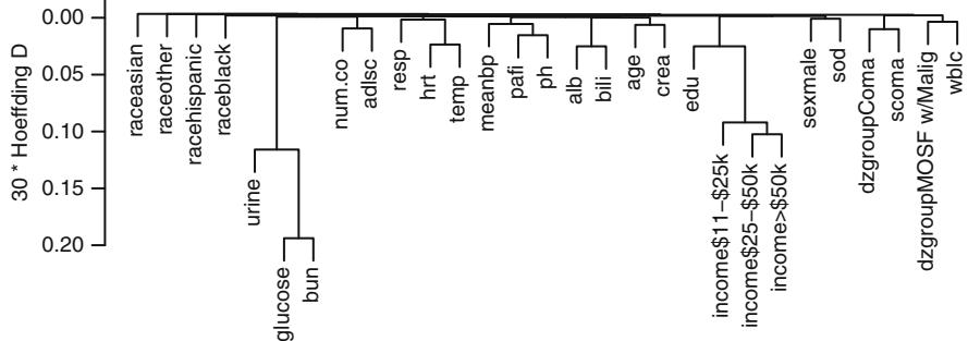
Fig. 19.2 Hierarchical clustering of potential predictors using Hoeffding D as a similarity measure. Categorical predictors are automatically expanded into dummy variables.

options(datadist= ' dd ' )
# Generate right-censored survival time variable
years − d.time /365.25
units (years ) − ' Year '
S − Surv(years , death)
# Show normal inverse Kaplan-Meier estimates
# stratified by dzgroup
survplot( npsurv (S ← dzgroup), conf= ' none ' ,
         fun=qnorm , logt=TRUE) # Figure 19.3

f − psm(S ← dzgroup + rcs(age ,5) + rcs( meanbp ,5),
         dist= ' lognormal ' , y=TRUE)
r − resid(f)
survplot (r, dzgroup , label.curve =FALSE)
survplot (r, age , label.curve =FALSE)
survplot (r, meanbp , label.curve =FALSE)
random − runif(length(age)); label(random) − ' Random Number '
survplot (r, random , label.curve =FALSE) # Fig. 19.4

Now remove from consideration predictors that are missing in more than 0.2 of patients. Many of these were collected only for the second half of SUP-PORT. Of those variables to be included in the model, find which ones have enough potential predictive power to justify allowing for nonlinear relationships or multiple categories, which spend more d.f. For each variable compute Spearman ρ² based on multiple linear regression of rank(x), rank(x)², and the

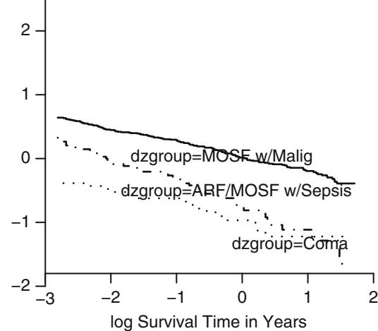
Fig. 19.3 ρ∧¹(SKM(t)) stratified by dzgroup. Linearity and semi-parallelism indicate a reasonable fit to the log-normal accelerated failure time model with respect to one predictor.

survival time, truncating survival time at the shortest follow-up for survivors (356 days; see Section 4.1).

shortest.follow.up − min(d.time [death ==0], na.rm =TRUE)
d.timet − pmin(d.time , shortest.follow.up )
w − spearman2(d.timet ← age + num.co + scoma + meanbp +
             hrt + resp + temp + crea + sod + adlsc +
             wblc + pafi + ph + dzgroup + race , p=2)
plot(w, main= ' ' ) # Figure 19.5

A better approach is to use the complete information in the failure and censoring times by computing Somers’ Dxy rank correlation allowing for censoring.

w − rcorrcens (S ← age + num.co + scoma + meanbp + hrt + resp +
              temp + crea + sod + adlsc + wblc + pafi + ph +
              dzgroup + race)
plot(w, main= ' ' ) # Figure 19.6

Remaining missing values are imputed using the “most normal” values, a procedure found to work adequately for this particular study. Race is imputed using the modal category.

# Compute number of missing values per variable
sapply (llist (age ,num.co , scoma , meanbp ,hrt ,resp ,temp ,crea ,sod ,
               adlsc ,wblc ,pafi ,ph), function(x) sum( is.na(x)))
  age num.co scoma meanbp hrt resp temp crea sod adlsc
    0000000000
 wblc pafi ph
    5 37 37
                Residual
Survival Probability
     −3.0 −2.0 −1.0 0.0 0.5 1.0 1.5 2.0
  0.0
  0.2
  0.4
  0.6
  0.8
  1.0
              Disease Group
                                                       Residual
                                      Survival Probability
                                           −3.0 −2.0 −1.0 0.0 0.5 1.0 1.5 2.0
                                        0.0
                                        0.2
                                        0.4
                                        0.6
                                        0.8
                                        1.0
                                                        Age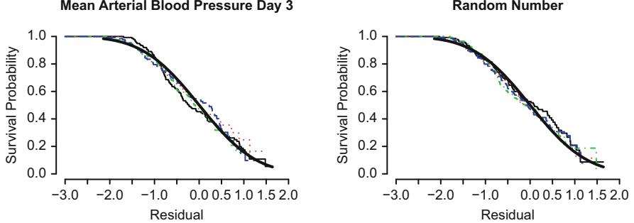

Fig. 19.4 Kaplan-Meier estimates of distributions of normalized, right-censored residuals from the fitted log-normal survival model. Residuals are stratified by important variables in the model (by quartiles of continuous variables), plus a random variable to depict the natural variability (in the lower right plot). Theoretical standard Gaussian distributions of residuals are shown with a thick solid line.

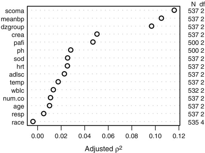
Fig. 19.5 Generalized Spearman Λ² rank correlation between predictors and truncated survival time

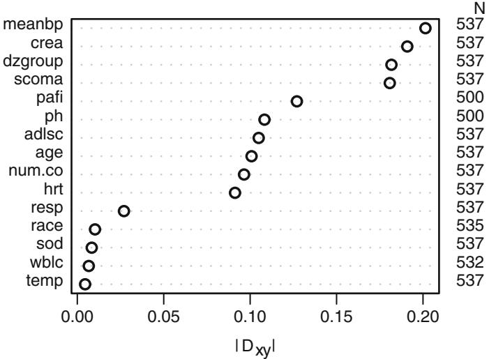
Fig. 19.6 Somers’ Dxy rank correlation between predictors and original survival time. For dzgroup or race, the correlation coefficient is the maximum correlation from using a dummy variable to represent the most frequent or one to represent the second most frequent category.’,scap=‘Somers’ Dxy rank correlation between predictors and original survival time

# Can also do naplot(naclus(support[ acute ,]))
# Can also use the Hmisc naclus and naplot functions
# Impute missing values with normal or modal values
wblc.i − impute (wblc , 9)
pafi.i − impute (pafi , 333.3)
ph.i − impute (ph , 7.4)
race2 − race
levels (race2 ) − list(white= ' white ' ,other =levels (race )[-1])
race2 [is.na (race2 )] − ' white '
dd − datadist (dd , wblc.i , pafi.i , ph.i , race2 )

Now that missing values have been imputed, a formal multivariable redundancy analysis can be undertaken. The Hmisc package’s redun function goes farther than the varclus pairwise correlation approach and allows for nonmonotonic transformations in predicting each predictor from all the others.

redun(← crea + age + sex + dzgroup + num.co + scoma + adlsc +
      race2 + meanbp + hrt + resp + temp + sod + wblc.i +
      pafi.i + ph.i , nk=4)

Redundancy Analysis
redun(formula = ◦crea + age + sex + dzgroup + num.co + scoma +
   adlsc + race2 + meanbp + hrt + resp + temp + sod + wblc.i +
   pafi.i + ph.i, nk = 4)
n: 537 p: 16 nk: 4
Number of NAs: 0
Transformation of target variables forced to be linear
R2 cutoff: 0.9 Type: ordinary
R2 with which each variable can be predicted from all other variables:
   crea age sex dzgroup num.co scoma adlsc race2 meanbp
  0.133 0.246 0.132 0.451 0.147 0.418 0.153 0.151 0.178
   hrt resp temp sod wblc.i pafi.i ph.i
  0.258 0.131 0.197 0.135 0.093 0.143 0.171
No redundant variables

Now turn to a more efficient approach for gauging the potential of each predictor, one that makes maximal use of failure time and censored data is to all continuous variables to have a maximum number of knots in a log-normal survival model. This approach must use imputation to have an adequate sample size. A semi-saturated main effects additive log-normal model is fitted. It is necessary to limit restricted cubic splines to 4 knots, force scoma to be linear, and to omit ph.i in order to avoid a singular covariance matrix in the fit.

k − 4 f − psm(S ← rcs(age ,k)+sex+dzgroup+pol( num.co ,2)+ scoma+ pol(adlsc ,2)+ race+rcs(meanbp ,k)+ rcs(hrt ,k)+

464 19 Parametric Survival Modeling and Model Approximation

rcs(resp ,k)+rcs(temp ,k)+rcs(crea ,3)+ rcs(sod ,k)+ rcs(wblc.i ,k)+rcs(pafi.i ,k), dist= ’ lognormal ’ ) plot(anova (f)) # Figure 19.7

Figure 19.7 properly blinds the analyst to the form of effects (tests of linearity). Next fit a log-normal survival model with number of parameters corresponding to nonlinear effects determined from the partial χ² tests in Figure 19.7. For the most promising predictors, five knots can be allocated, as there are fewer singularity problems once less promising predictors are simplified.

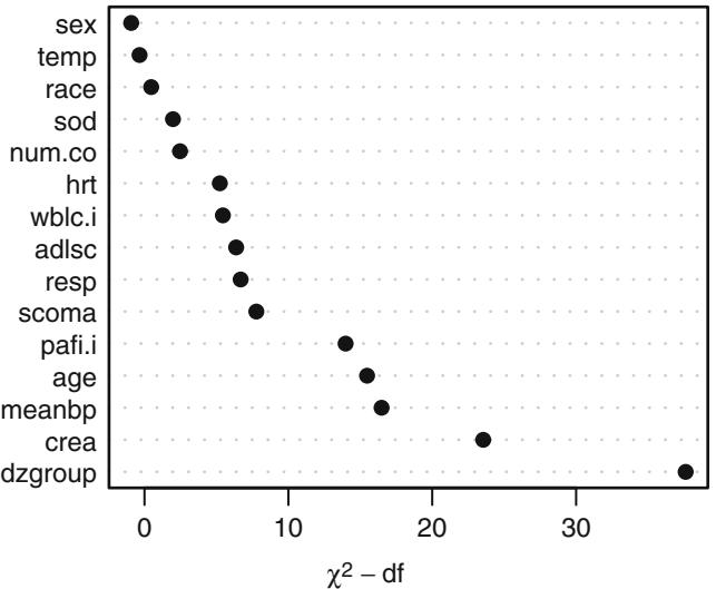
Fig. 19.7 Partial σ² statistics for association of each predictor with response from saturated main effects model, penalized for d.f.

f − psm(S ← rcs(age ,5)+ sex+ dzgroup+ num.co +
               scoma +pol( adlsc ,2)+ race2+rcs(meanbp ,5)+
               rcs(hrt ,3)+ rcs(resp ,3)+ temp+
               rcs(crea ,4)+ sod+rcs(wblc.i ,3)+ rcs(pafi.i ,4),
          dist= ' lognormal ' )
print (f, latex =TRUE , coefs=FALSE)

Parametric Survival Model: Log Normal Distribution

psm(formula = S ~ rcs(age, 5) + sex + dzgroup + num.co + scoma + pol(adlsc, 2) + race2 + rcs(meanbp, 5) + rcs(hrt, 3) + rcs(resp, 3) + temp + rcs(crea, 4) + sod + rcs(wblc.i, 3) + rcs(pafi.i, 4), dist = “lognormal”)

		Model Likelihood		Discrimination
		Ratio Test		Indexes
	Obs 537	χ2 LR	236.83	R2	0.594
	Events 356	d.f.	30	Dxy	0.485
	σ 2.230782	χ2) Pr(>	< 0.0001	g	0.033
				gr	1.959

a anova (f) −

Table 19.1 Wald Statistics for S

	χ2	d.f.	P
age	15.99	4	0.0030
Nonlinear	0.23	3	0.9722
sex	0.11	1	0.7354
dzgroup	45.69	2	< 0.0001
num.co	4.99	1	0.0255
scoma	10.58	1	0.0011
adlsc	8.28	2	0.0159
Nonlinear	3.31	1	0.0691
race2	1.26	1	0.2624
meanbp	27.62	4	< 0.0001
Nonlinear	10.51	3	0.0147
hrt	11.83	2	0.0027
Nonlinear	1.04	1	0.3090
resp	11.10	2	0.0039
Nonlinear	8.56	1	0.0034
temp	0.39	1	0.5308
crea	33.63	3	< 0.0001
Nonlinear	21.27	2	< 0.0001
sod	0.08	1	0.7792
wblc.i	5.47	2	0.0649
Nonlinear	5.46	1	0.0195
pafi.i	15.37	3	0.0015
Nonlinear	6.97	2	0.0307
TOTAL NONLINEAR	60.48	14	< 0.0001
TOTAL	261.47	30	< 0.0001

19.3 Summarizing the Fitted Model

First let’s plot the shape of the effect of each predictor on log survival time. All effects are centered so that they can be placed on a common scale. This allows the relative strength of various predictors to be judged. Then Wald χ² statistics, penalized for d.f., are plotted in descending order. Next, relative effects of varying predictors over reasonable ranges (survival time ratios varying continuous predictors from the first to the third quartile) are charted.

ggplot ( Predict(f, ref.zero= TRUE), vnames = ' names ' ,
        sepdiscrete = ' vertical ' , anova =a) # Figure 19.8

latex (a, file= ' ' ,label= ' tab:support-anovat ' ) # Table 19.1

plot(a) # Figure 19.9

options( digits =3) plot( summary(f), log=TRUE , main= ’ ’ ) # Figure 19.10

19.4 Internal Validation of the Fitted Model Using the Bootstrap

Let us decide whether there was significant overfitting during the development of this model, using the bootstrap.

# First add data to model fit so bootstrap can re-sample
# from the data
g − update (f, x=TRUE , y= TRUE)
set.seed (717)
latex ( validate(g, B=300), digits =2, size = ' Ssize ' )

Index		Original Training	Test	Optimism Corrected	n
	Sample	Sample	Sample		Index
Dxy	0.49	0.51	0.46	0.05	0.43 300
R2	0.59	0.66	0.54	0.12	0.47 300
Intercept	0.00	0.00	×0.05	0.05	×0.05 300
Slope	1.00	1.00	0.90	0.10	0.90 300
D	0.48	0.55	0.42	0.13	0.35 300
U	0.00	0.00	×0.01	0.01	×0.01 300
Q	0.48	0.56	0.43	0.12	0.36 300
g	1.96	2.05	1.87	0.19	1.77 300

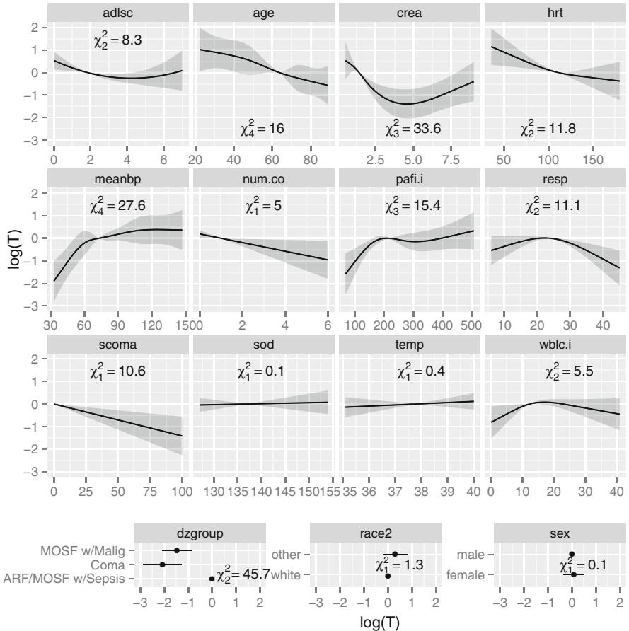
Fig. 19.8 Effect of each predictor on log survival time. Predicted values have been centered so that predictions at predictor reference values are zero. Pointwise 0.95 confidence bands are also shown. As all y-axes have the same scale, it is easy to see which predictors are strongest.

Judging from Dxy and R² there is a moderate amount of overfitting. The slope shrinkage factor (0.9) is not troublesome, however. An almost unbiased estimate of future predictive discrimination on similar patients is given by the corrected Dxy of 0.43. This index equals the difference between the probability of concordance and the probability of discordance of pairs of predicted survival times and pairs of observed survival times, accounting for censoring.

Next, a bootstrap overfitting-corrected calibration curve is estimated. Patients are stratified by the predicted probability of surviving one year, such that there are at least 60 patients in each group.

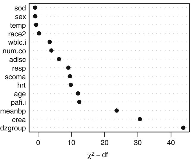
Fig. 19.9 Contribution of variables in predicting survival time in log-normal model

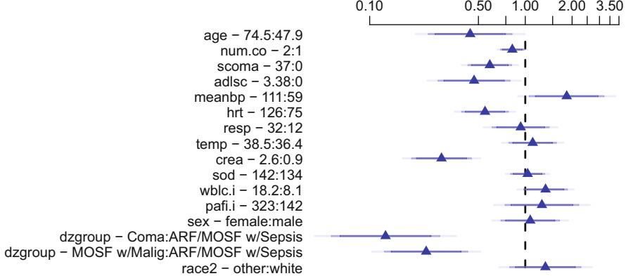
Fig. 19.10 Estimated survival time ratios for default settings of predictors. For example, when age changes from its lower quartile to the upper quartile (47.9y to 74.5y), median survival time decreases by more than half. Different shaded areas of bars indicate different confidence levels (.9, 0.95, 0.99).

set.seed (717)
cal − calibrate (g, u=1, B =300)
plot (cal , subtitles= FALSE)
cal − calibrate(g, cmethod= ' KM ' , u=1, m=60, B=120, pr= FALSE)
plot (cal , add=TRUE ) # Figure 19.11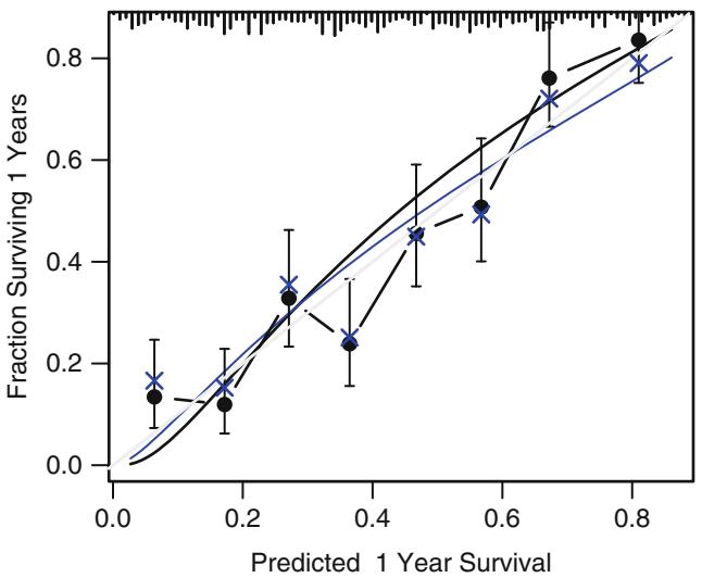

Fig. 19.11 Bootstrap validation of calibration curve. Dots represent apparent calibration accuracy; ∼ are bootstrap estimates corrected for overfitting, based on binning predicted survival probabilities and computing Kaplan-Meier estimates. Black curve is the estimated observed relationship using hare and the blue curve is the overfitting-corrected hare estimate. The gray-scale line depicts the ideal relationship.

19.5 Approximating the Full Model

The fitted log-normal model is perhaps too complex for routine use and for routine data collection. Let us develop a simplified model that can predict the predicted values of the full model with high accuracy (R² = 0.967). The simplification is done using a fast backward step-down against the full model predicted values.

Z − predict(f) # X* beta hat
a − ols(Z ← rcs(age ,5)+ sex+ dzgroup+ num.co +
             scoma +pol( adlsc ,2)+ race2+
             rcs(meanbp ,5)+ rcs(hrt ,3)+ rcs(resp ,3)+
             temp+rcs( crea ,4)+sod+rcs(wblc.i ,3)+
             rcs(pafi.i ,4), sigma =1)
# sigma=1 is used to prevent sigma hat from being zero when
# R2=1.0 since we start out by approximating Z with all
# component variables
fastbw (a, aics =10000) # fast backward stepdown

Deleted	Chi-Sq	d.f.	P	Residual	d.f.	P	AIC	R2
sod	0.43	1	0.512	0.43	1	0.5117	-1.57	1.000
sex	0.57	1	0.451	1.00	2	0.6073	-3.00	0.999
temp	2.20	1	0.138	3.20	3	0.3621	-2.80	0.998
race2	6.81	1	0.009	10.01	4	0.0402	2.01	0.994
wblc.i	29.52	2	0.000	39.53	6	0.0000	27.53	0.976

num.co 30.84 1 0.000 70.36 7 0.0000 56.36 0.957
resp 54.18 2 0.000 124.55 9 0.0000 106.55 0.924
adlsc 52.46 2 0.000 177.00 11 0.0000 155.00 0.892
pafi.i 66.78 3 0.000 243.79 14 0.0000 215.79 0.851
scoma 78.07 1 0.000 321.86 15 0.0000 291.86 0.803
hrt 83.17 2 0.000 405.02 17 0.0000 371.02 0.752
age 68.08 4 0.000 473.10 21 0.0000 431.10 0.710
crea 314.47 3 0.000 787.57 24 0.0000 739.57 0.517
meanbp 403.04 4 0.000 1190.61 28 0.0000 1134.61 0.270
dzgroup 441.28 2 0.000 1631.89 30 0.0000 1571.89 0.000
Approximate Estimates after Deleting Factors
       Coef S.E. Wald Z P
[1,] -0.5928 0.04315 -13.74 0
Factors in Final Model
None

f.approx − ols(Z ← dzgroup + rcs( meanbp ,5) + rcs(crea ,4) +
                 rcs(age ,5) + rcs(hrt ,3) + scoma +
                 rcs(pafi.i ,4) + pol( adlsc ,2)+
                 rcs(resp ,3), x= TRUE)
f.approx$ stats

	537.000	n Model L.R. 1688.225	d.f. 23.000	R2 0.957	g 1.915	Sigma 0.370
–	———	——————————–	—————-	————-	————	—————-	–

We can estimate the variance–covariance matrix of the coefficients of the reduced model using Equation 5.2 in Section 5.5.2. The computations below result in a covariance matrix that does not include elements related to the scale parameter. In the code x is the matrix T in Section 5.5.2.

V − vcov(f, regcoef.only = TRUE) # var(full model)
X − cbind ( Intercept =1, g$x) # full model design
x − cbind ( Intercept =1, f.approx $x) # approx. model design
w − solve (t(x) %*% x, t(x)) %*% X # contrast matrix
v − w %*% V %*% t(w)

Let’s compare the variance estimates (diagonals of v) with variance estimates from a reduced model that is fitted against the actual outcomes.

f.sub − psm(S ← dzgroup + rcs(meanbp ,5) + rcs(crea ,4) + rcs(age ,5) + rcs(hrt ,3) + scoma + rcs(pafi.i ,4) + pol(adlsc ,2)+ rcs(resp ,3), dist= ’ lognormal ’ )

diag(v)/diag(vcov(f.sub , regcoef.only=TRUE))

Intercept	dzgroup=Coma	dzgroup=MOSF w/Malig
0.981	0.979	0.979
meanbp	meanbp ’	meanbp ’ ’
0.977	0.979	0.979
meanbp ’’’	crea	crea ’
0.979	0.979	0.979
crea ’ ’	age	age ’
0.979	0.982	0.981
age ’ ’	age ’’’	hrt
0.981	0.980	0.978

hrt ’	scoma	pafi.i
0.976	0.979	0.980
pafi.i ’	pafi.i ’ ’	adlsc
0.980	0.980	0.981
adlsc−2	resp	resp ’
0.981	0.978	0.977

r − diag (v)/ diag(vcov( f.sub , regcoef.only = TRUE ))
r[c( which.min(r), which.max(r))]

hrt ’ age 0.976 0.982

The estimated variances from the reduced model are actually slightly smaller than those that would have been obtained from stepwise variable selection in this case, had variable selection used a stopping rule that resulted in the same set of variables being selected. Now let us compute Wald statistics for the reduced model.

f.approx$var − v
latex (anova (f.approx , test= ' Chisq ' , ss=FALSE ), file= ' ' ,
       label = ' tab:support-anovaa ' )

The results are shown in Table 19.2. Note the similarity of the statistics to those found in the table for the full model. This would not be the case had deleted variables been very collinear with retained variables.

The equation for the simplified model follows. The model is also depicted graphically in Figure 19.12. The nomogram allows one to calculate mean and median survival time. Survival probabilities could have easily been added as additional axes.

# Typeset mathematical form of approximate model
latex (f.approx , file= ' ' )

\[\mathcal{E}(\mathbf{Z}) = X\boldsymbol{\beta}, \text{ where}\]

Xβˆ =

−2.51
−1.94[Coma] − 1.75[MOSF w/Malig]
+0.068meanbp − 3.08∼10∧5(meanbp − 41.8)3
                                          + + 7.9∼10∧5(meanbp − 61)3
                                                                      +
−4.91∼10∧5(meanbp − 73)3
                          + + 2.61∼10∧6(meanbp − 109)3
                                                       + − 1.7∼10∧6(meanbp − 135)3
                                                                                    +
−0.553crea − 0.229(crea − 0.6)3
                             + + 0.45(crea − 1.1)3
                                                + − 0.233(crea − 1.94)3
                                                                     +
+0.0131(crea − 7.32)3
                   +
−0.0165age − 1.13∼10∧5(age − 28.5)3
                                   + + 4.05∼10∧5(age − 49.5)3
                                                             +
−2.15∼10∧5(age − 63.7)3
                       + − 2.68∼10∧5(age − 72.7)3
                                                 + + 1.9∼10∧5(age − 85.6)3
                                                                          +
−0.0136hrt + 6.09∼10∧7(hrt − 60)3
                                 + − 1.68∼10∧6(hrt − 111)3
                                                          + + 1.07∼10∧6(hrt − 140)3
                                                                                   +
−0.0135 scoma
+0.0161pafi.i − 4.77∼10∧7(pafi.i − 88)3
                                     + + 9.11∼10∧7(pafi.i − 167)3
                                                                +

	χ2	d.f.	P
dzgroup	55.94	2	< 0.0001
meanbp	29.87	4	< 0.0001
Nonlinear	9.84	3	0.0200
crea	39.04	3	< 0.0001
Nonlinear	24.37	2	< 0.0001
age	18.12	4	0.0012
Nonlinear	0.34	3	0.9517
hrt	9.87	2	0.0072
Nonlinear	0.40	1	0.5289
scoma	9.85	1	0.0017
pafi.i	14.01	3	0.0029
Nonlinear	6.66	2	0.0357
adlsc	9.71	2	0.0078
Nonlinear	2.87	1	0.0904
resp	9.65	2	0.0080
Nonlinear	7.13	1	0.0076
TOTAL NONLINEAR	58.08	13	< 0.0001
TOTAL	252.32	23	< 0.0001

Table 19.2 Wald Statistics for Z

⁻5.02∼10^∧⁷(pafi.ⁱ ⁻ 276)³ ⁺ + 6.76∼10^∧⁸(pafi.ⁱ ⁻ 426)³ ⁺ ⁻ ⁰.369 adlsc + 0.0409 adlsc² +0.0394resp ⁻ ⁹.11∼10^∧⁵(resp ⁻ 10)³ ⁺ + 0.000176(resp ⁻ 24)³ ⁺ ⁻ ⁸.5∼10^∧⁵(resp ⁻ 39)³ +

and [c] = 1 if subject is in group c, 0 otherwise; (x)⁺ = x if x > 0, 0 otherwise.

# Derive S functions that express mean and quantiles
# of survival time for specific linear predictors
# analytically
expected.surv − Mean(f)
quantile.surv − Quantile(f)
latex (expected.surv , file= ' ' , type= ' Sinput ' )

expected.surv − function (lp = NULL ,
                             parms = 0 .802352037606488 )
{
    names (parms ) − NULL
    exp(lp + exp(2 * parms )/2)
}

latex (quantile.surv , file= ’ ’ , type= ’ Sinput ’ )

quantile.surv − function (q = 0.5 , lp = NULL ,
                            parms = 0 .802352037606488 )

19.6 Problems 473

{
    names (parms ) − NULL
    f − function (lp, q, parms ) lp + exp(parms ) * qnorm (q)
    names (q) − format (q)
    drop (exp(outer (lp, q, FUN = f, parms = parms )))
}

median.surv − function(x) quantile.surv (lp=x)

# Improve variable labels for the nomogram
f.approx − Newlabels (f.approx , c( ' Disease Group ' ,
           ' Mean Arterial BP ' , ' Creatinine ' , ' Age ' , ' Heart Rate ' ,
           ' SUPPORT Coma Score ' , ' PaO2/(.01*FiO2) ' , ' ADL ' ,
           ' Resp. Rate ' ))
nom −
  nomogram (f.approx ,
            pafi.i=c(0, 50, 100, 200, 300, 500, 600, 700, 800,
                      900),
            fun=list( ' Median Survival Time ' =median.surv ,
                      ' Mean Survival Time ' =expected.surv),
            fun.at=c(.1,.25 ,.5 ,1,2,5,10,20,40))
plot(nom , cex.var =1, cex.axis =.75 , lmgp=.25)
# Figure 19.12

19.6 Problems

Analyze the Mayo Clinic PBC dataset.

1. Graphically assess whether Weibull (extreme value), exponential, loglogistic, or log-normal distributions will fit the data, using a few apparently important stratification factors.
1. For the best fitting parametric model from among the four examined, fit a model containing several sensible covariables, both categorical and continuous. Do a Wald test for whether each factor in the model has an association with survival time, and a likelihood ratio test for the simultaneous contribution of all predictors. For classification factors having more than two levels, be sure that the Wald test has the appropriate degrees of freedom. For continuous factors, verify or relax linearity assumptions. If using a Weibull model, test whether a simpler exponential model would be appropriate. Interpret all estimated coefficients in the model. Write the full survival model in mathematical form. Generate a predicted survival curve for a patient with a given set of characteristics.

See [361] for an analysis of this dataset using linear splines in time and in the covariables.

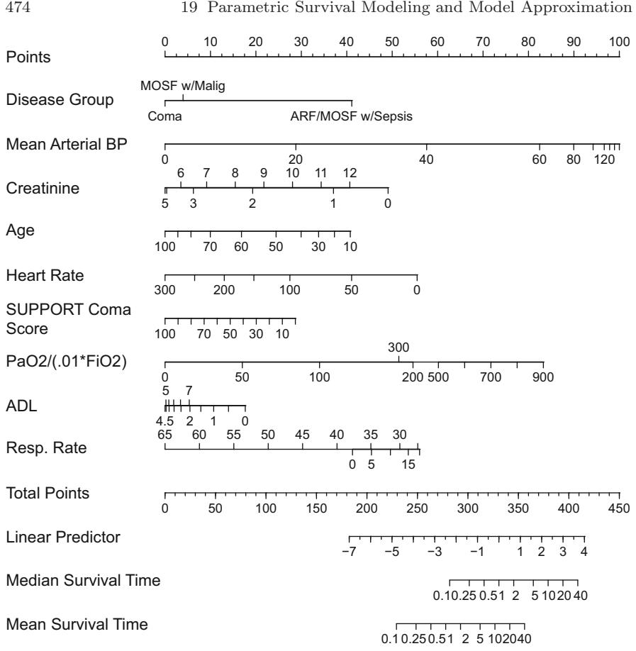
Fig. 19.12 Nomogram for predicting median and mean survival time, based on approximation of full model

Chapter 20 Cox Proportional Hazards Regression Model

20.1 Model

20.1.1 Preliminaries

The Cox proportional hazards model132 is the most popular model for the analysis of survival data. It is a semiparametric model; it makes a parametric ¹ assumption concerning the effect of the predictors on the hazard function, but makes no assumption regarding the nature of the hazard function λ(t) itself. The Cox PH model assumes that predictors act multiplicatively on the hazard function but does not assume that the hazard function is constant (i.e., exponential model), Weibull, or any other particular form. The regression portion of the model is fully parametric; that is, the regressors are linearly related to log hazard or log cumulative hazard. In many situations, either the form of the true hazard function is unknown or it is complex, so the Cox model has definite advantages. Also, one is usually more interested in the effects of the predictors than in the shape of λ(t), and the Cox approach allows the analyst to essentially ignore λ(t), which is often not of primary interest.

The Cox PH model uses only the rank ordering of the failure and censoring times and thus is less affected by outliers in the failure times than fully parametric methods. The model contains as a special case the popular logrank test for comparing survival of two groups. For estimating and testing regression coefficients, the Cox model is as efficient as parametric models (e.g., Weibull model with PH) even when all assumptions of the parametric model are satisfied.171

When a parametric model’s assumptions are not true (e.g., when a Weibull model is used and the population is not from a Weibull survival distribution so that the choice of model is incorrect), the Cox analysis is more efficient

F.E. Harrell, Jr., Regression Modeling Strategies, Springer Series in Statistics, DOI 10.1007/978-3-319-19425-7 20

than the parametric analysis. As shown below, diagnostics for checking Cox model assumptions are very well developed.

20.1.2 Model Definition

The Cox PH model is most often stated in terms of the hazard function:

\[ \lambda(t|X) = \lambda(t) \exp(X\beta). \tag{20.1} \]

We do not include an intercept parameter in Xβ here. Note that this is identical to the parametric PH model stated earlier. There is an important difference, however, in that now we do not assume any specific shape for λ(t). For the moment, we are not even interested in estimating λ(t). The reason for this departure from the fully parametric approach is due to an ingenious conditional argument by Cox.132 Cox argued that when the PH model holds, information about λ(t) is not very useful in estimating the parameters of primary interest, β. By special conditioning in formulating the log likelihood function, Cox showed how to derive a valid estimate of β that does not require estimation of λ(t) as λ(t) dropped out of the new likelihood function. Cox’s derivation focuses on using the information in the data that relates to the relative hazard function exp(Xβ).

20.1.3 Estimation of β

Cox’s derivation of an estimator of β can be loosely described as follows. Let t¹ < t² <…< t^k represent the unique ordered failure times in the sample of n subjects; assume for now that there are no tied failure times (tied censoring times are allowed) so that k = n. Consider the set of individuals at risk of failing an instant before failure time ti. This set of individuals is called the risk set at time ti, and we use Rⁱ to denote this risk set. Rⁱ is the set of subjects j such that the subject had not failed or been censored by time ti; that is, the risk set Rⁱ includes subjects with failure/censoring time Y^j ← ti.

The conditional probability that individual i is the one that failed at ti, given that the subjects in the set Rⁱ are at risk of failing, and given further that exactly one failure occurs at ti, is

\[\begin{aligned} \text{Prob\{subject \ i fails at } t\_i | R\_i \text{ and one failure at } t\_i \} &= \\ \hline \text{Prob\{subject \ i fails at } t\_i | R\_i \text{\}} \\ \text{Prob\{\ one failure at } t\_i | R\_i \text{\}} \end{aligned} \tag{20.2}\]

using the rules of conditional probability. This conditional probability equals

\[\frac{\lambda(t\_i)\exp(X\_i\beta)}{\sum\_{j\in R\_i}\lambda(t\_i)\exp(X\_j\beta)} = \frac{\exp(X\_i\beta)}{\sum\_{j\in R\_i}\exp(X\_j\beta)} = \frac{\exp(X\_i\beta)}{\sum\_{Y\_j\geq t\_i}\exp(X\_j\beta)}\tag{20.3}\]

independent of λ(t). To understand this likelihood, consider a special case where the predictors have no effect; that is, β =0[93, pp. 48–49]. Then exp(Xiβ) = exp(Xjβ) = 1 and Prob{subject i is the subject that failed at ti|Rⁱ and one failure occurred at ti} is 1/nⁱ where nⁱ is the number of subjects at risk at time ti.

By arguing that these conditional probabilities are themselves conditionally independent across the different failure times, a total likelihood can be computed by multiplying these individual likelihoods over all failure times. Cox termed this a partial likelihood for β:

\[L(\beta) = \prod\_{Y\_i \text{ unconsored}} \frac{\exp(X\_i \beta)}{\sum\_{Y\_j \ge Y\_i} \exp(X\_j \beta)}.\tag{20.4}\]

The log partial likelihood is

\[\log L(\beta) = \sum\_{Y\_i \text{ unconsored}} \{X\_i \beta - \log[\sum\_{Y\_j \ge Y\_i} \exp(X\_j \beta)]\}.\tag{20.5}\]

Cox and others have shown that this partial log likelihood can be treated as an ordinary log likelihood to derive valid (partial) MLEs of β. Note that this log likelihood is unaffected by the addition of a constant to any or all of the Xs. This is consistent with the fact that an intercept term is unnecessary and cannot be estimated since the Cox model is a model for the relative hazard and does not directly estimate the underlying hazard λ(t).

When there are tied failure times in the sample, the true partial log likelihood function involves permutations so it can be time-consuming to compute. When the number of ties is not large, Breslow70 has derived a satisfactory approximate log likelihood function. The formula given above, when applied without modification to samples containing ties, actually uses Breslow’s approximation. If there are ties so that k<n and t1,…,t^k denote the unique failure times as we originally intended, Breslow’s approximation is written as

\[\log L(\beta) = \sum\_{i=1}^{k} \{ S\_i \beta - d\_i \log \left[ \sum\_{Y\_j \ge t\_i} \exp(X\_j \beta) \right] \},\tag{20.6}\]

where Sⁱ = ” ^j∈Dⁱ ^Xj, ^Dⁱ is the set of indexes ^j for subjects failing at time ti, and dⁱ is the number of failures at ti.

Efron171 derived another approximation to the true likelihood that is significantly more accurate than the Breslow approximation and often yields estimates that are very close to those from the more cumbersome permutation likelihood:288

\[\begin{split} \log L(\beta) &= \sum\_{i=1}^{k} \{ S\_i \beta - \sum\_{j=1}^{d\_i} \log \left[ \sum\_{Y\_j \ge t\_i} \exp(X\_j \beta) \right] \\ &- \frac{j-1}{d\_i} \sum\_{l \in D\_i} \exp(X\_l \beta) \} . \end{split} \tag{20.7}\]

In the special case when all tied failure times are from subjects with identical Xiβ, the Efron approximation yields the exact (permutation) marginal likelihood (Therneau, personal communication, 1993).

Kalbfleisch and Prentice330 showed that Cox’s partial likelihood, in the absence of predictors that are functions of time, is a marginal distribution of the ranks of the failure/censoring times.

See Therneau and Grambsch604 and Huang and Harrington310 for descriptions of penalized partial likelihood estimation methods for improving mean squared error of estimates of β in a similar fashion to what was discussed in Section 9.10.

20.1.4 Model Assumptions and Interpretation of Parameters

The Cox PH regression model has the same assumptions as the parametric PH model except that no assumption is made regarding the shape of the underlying hazard or survival functions λ(t) and S(t). The Cox PH model assumes, in its most basic form, linearity and additivity of the predictors with respect to log hazard or log cumulative hazard. It also assumes the PH assumption of no time by predictor interactions; that is, the predictors have the same effect on the hazard function at all values of t. The relative hazard function exp(Xβ) is constant through time and the survival functions for subjects with different values of X are powers of each other. If, for example, the hazard of death at time t for treated patients is half that of control patients at time t, this same hazard ratio is in effect at any other time point. In other words, treated patients have a consistently better hazard of death over all follow-up time.

The regression parameters are interpreted the same as in the parametric PH model. The only difference is the absence of hazard shape parameters in the model, since the hazard shape is not estimated in the Cox partial likelihood procedure.

20.1.5 Example

Consider again the rat vaginal cancer data from Section 18.3.6. Figure 20.1 displays the nonparametric survival estimates for the two groups along with estimates derived from the Cox model (by a method discussed later).

require(rms)

group − c(rep( ' Group 1 ' ,19),rep( ' Group 2 ' ,21))
group − factor (group)
dd − datadist( group ); options(datadist= ' dd ' )
days −
  c(143 ,164,188 ,188,190 ,192,206 ,209,213 ,216 ,220,227 ,230,
    234,246 ,265,304,216 ,244,142 ,156,163 ,198,205,232 ,232,
    233 ,233 ,233,233 ,239 ,240 ,261 ,280 ,280 ,296,296 ,323 ,204 ,344)
death − rep(1,40)
death [c(18,19,39,40)] − 0
units (days) − ' Day '
df − data.frame(days , death , group)
S − Surv(days , death)
f − npsurv (S ← group , type= ' fleming ' )
for(meth in c( ' exact ' , ' breslow ' , ' efron ' )) {
  g − cph(S ← group , method =meth , surv=TRUE , x=TRUE , y= TRUE)
  # print(g) to see results
}
f.exp − psm(S ← group , dist= ' exponential ' )
fw − psm(S ← group , dist= ' weibull ' )
phform − pphsm (fw)

co − gray(c(0, .8))
survplot (f, lty=c(1, 1), lwd=c(1, 3), col=co,
          label.curves=FALSE , conf= ' none ' )
survplot (g, lty=c(3, 3), lwd=c(1, 3), col=co, # Efron approx.
          add=TRUE , label.curves=FALSE , conf.type = ' none ' )
legend (c(2, 160), c(.38 , .54),
       c( ' Nonparametric Estimates ' , ' Cox-Breslow Estimates ' ),
       lty=c(1, 3), cex=.8, bty= ' n ' )
legend (c(2, 160), c(.18 , .34), cex=.8,
       c( ' Group 1 ' , ' Group 2 ' ), lwd=c(1,3), col=co, bty= ' n ' )

The predicted survival curves from the fitted Cox model are in good agreement with the nonparametric estimates, again verifying the PH assumption for these data. The estimates of the group effect from a Cox model (using the exact likelihood since there are ties, along with both Efron’s and Breslow’s approximations) as well as from a Weibull model and an exponential model are shown in Table 20.1. The exponential model, with its constant hazard, cannot accommodate the long early period with no failures. The group predictor was coded as X¹ = 0 and X¹ = 1 for Groups 1 and 2, respectively. For this example, the Breslow likelihood approximation resulted in βˆ closer to that from maximizing the exact likelihood. Note how the group effect (47% reduction in hazard of death by the exact Cox model) is underestimated by the exponential model (9% reduction in hazard). The hazard ratio from the Weibull fit agrees with the Cox fit.

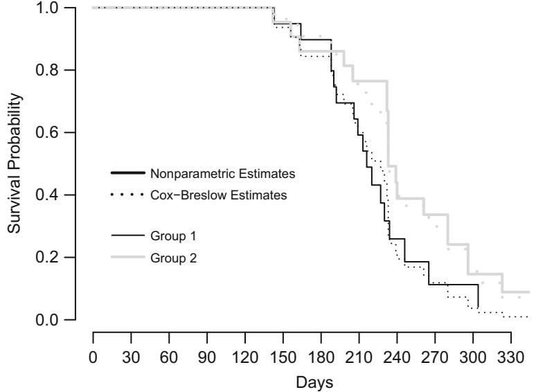
Fig. 20.1 Altschuler–Nelson–Fleming–Harrington nonparametric survival estimates and Cox-Breslow estimates for rat data508

Table 20.1 Group effects using three versions of the partial likelihood and three parametric models

Model	Group Regression	S.E.	Wald	Group 2:1
	Coefficient			P-Value Hazard Ratio
Cox (Exact)	×0.629	0.361	0.08	0.533
Cox (Efron)	×0.569	0.347	0.10	0.566
Cox (Breslow)	×0.596	0.348	0.09	0.551
Exponential	×0.093	0.334	0.78	0.911
Weibull (AFT)	0.132	0.061	0.03	–
Weibull (PH)	×0.721	–	–	0.486

20.1.6 Design Formulations

Designs are no different for the Cox PH model than for other models except for one minor distinction. Since the Cox model does not have an intercept parameter, the group omitted from X in an ANOVA model will go into the underlying hazard function. As an example, consider a three-group model for treatments A, B, and C. We use the two dummy variables

X¹ = 1 if treatment is A, 0 otherwise, and X² = 1 if treatment is B, 0 otherwise.

The parameter β¹ is the A : C log hazard ratio or difference in hazards at any time t between treatment A and treatment C. β² is the B : C log hazard ratio (exp(β2) is the B : C hazard ratio, etc.). Since there is no intercept parameter, there is no direct estimate of the hazard function for treatment C or any other treatment; only relative hazards are modeled.

As with all regression models, a Wald, score, or likelihood ratio test for differences between any treatments is conducted by testing H⁰ : β¹ = β² = 0 with 2 d.f.

20.1.7 Extending the Model by Stratification

A unique feature of the Cox PH model is its ability to adjust for factors that are not modeled. Such factors usually take the form of polytomous stratification factors that either are too difficult to model or do not satisfy the PH assumption. For example, a subject’s occupation or clinical study site may take on dozens of levels and the sample size may not be large enough to model this nominal variable with dozens of dummy variables. Also, one may know that a certain predictor (either a polytomous one or a continuous one that is grouped) may not satisfy PH and it may be too complex to model the hazard ratio for that predictor as a function of time.

The idea behind the stratified Cox PH model is to allow the form of the underlying hazard function to vary across levels of the stratification factors. A stratified Cox analysis ranks the failure times separately within strata. Suppose that there are b strata indexed by j = 1, 2,…,b. Let C denote the stratum identification. For example, C = 1 or 2 may stand for the female and male strata, respectively. The stratified PH model is

\[ \lambda(t|X, C=j) = \lambda\_j(t) \exp(X\beta), \quad \text{or}\]

\[ S(t|X, C=j) = S\_j(t)^{\exp(X\beta)}.\tag{20.8} \]

Here λ^j (t) and S^j (t) are, respectively, the underlying hazard and survival functions for the jth stratum. The model does not assume any connection between the shapes of these functions for different strata.

In this stratified analysis, the data are stratified by C but, by default, a common vector of regression coefficients is fitted across strata. These common regression coefficients can be thought of as “pooled” estimates. For example, a Cox model with age as a (modeled) predictor and sex as a stratification variable essentially estimates the common slope of age by pooling information about the age effect over the two sexes. The effect of age is adjusted by sex differences, but no assumption is made about how sex affects survival. There is no PH assumption for sex. Levels of the stratification factor C can represent multiple stratification factors that are cross-classified. Since these factors are not modeled, no assumption is made regarding interactions among them.

At first glance it appears that stratification causes a loss of efficiency. However, in most cases the loss is small as long as the number of strata is not too large with regard to the total number of events. A stratum that contains no events contributes no information to the analysis, so such a situation should be avoided if possible.

The stratified or “pooled” Cox model is fitted by formulating a separate log likelihood function for each stratum, but with each log likelihood having a common β vector. If different strata are made up of independent subjects, the strata are independent and the likelihood functions are multiplied together to form a joint likelihood over strata. Log likelihood functions are thus added over strata. This total log likelihood function is maximized once to derive a pooled or stratified estimate of β and to make an inference about β. No inference can be made about the stratification factors. They are merely “adjusted for.”

Stratification is useful for checking the PH and linearity assumptions for one or more predictors. Predicted Cox survival curves (Section 20.2) can be derived by modeling the predictors in the usual way, and then stratified survival curves can be estimated by using those predictors as stratification factors. Other factors for which PH is assumed can be modeled in both instances. By comparing the modeled versus stratified survival estimates, a graphical check of the assumptions can be made. Figure 20.1 demonstrates this method although there are no other factors being adjusted for and stratified Cox estimates are KM estimates. The stratified survival estimates are derived by stratifying the dataset to obtain a separate underlying survival curve for each stratum, while pooling information across strata to estimate coefficients of factors that are modeled.

Besides allowing a factor to be adjusted for without modeling its effect, a stratified Cox PH model can also allow a modeled factor to interact with strata.143, 180, 603 For the age–sex example, consider the following model with X¹ denoting age and C = 1, 2 denoting females and males, respectively.

\[\begin{aligned} \lambda(t|X\_1, C=1) &= \lambda\_1(t) \exp(\beta\_1 X\_1) \\ \lambda(t|X\_1, C=2) &= \lambda\_2(t) \exp(\beta\_1 X\_1 + \beta\_2 X\_1) . \end{aligned} \tag{20.9}\]

This model can be simplified to

\[ \lambda(t|X\_1, C=j) = \lambda\_j(t) \exp(\beta\_1 X\_1 + \beta\_2 X\_2) \tag{20.10} \]

if X² is a product interaction term equal to 0 for females and X¹ for males. The β² parameter quantifies the interaction between age and sex: it is the difference in the age slope between males and females. Thus the interaction between age and sex can be quantified and tested, even though the effect of sex is not modeled!

The stratified Cox model is commonly used to adjust for hospital differences in a multicenter randomized trial. With this method, one can allow for differences in outcome between q hospitals without estimating q × 1 parameters. Treatment ≤ hospital interactions can be tested efficiently without computational problems by estimating only the treatment main effect, after stratifying on hospital. The score statistic (with q × 1 d.f.) for testing q × 1 treatment ^≤ hospital interaction terms is then computed (“residual ^χ2” in a stepwise procedure with treatment ≤ hospital terms as candidate predictors).

The stratified Cox model turns out to be a generalization of the conditional logistic model for analyzing matched set (e.g., case-control) data.71 Each stratum represents a set, and the number of “failures” in the set is the number of “cases”in that set. For r : 1 matching (r may vary across sets), the Breslow70 likelihood may be used to fit the conditional logistic model exactly. For r : m matching, an exact Cox likelihood must be computed.

20.2 Estimation of Survival Probability and Secondary Parameters

As discussed above, once a partial log likelihood function is derived, it is used as if it were an ordinary log likelihood function to estimate β, estimate standard errors of β, obtain confidence limits, and make statistical tests. Point and interval estimates of hazard ratios are obtained in the same fashion as with parametric PH models discussed earlier.

The Cox model and parametric survival models differ markedly in how one estimates S(t|X). Since the Cox model does not depend on a choice of the underlying survival function S(t), fitting a Cox model does not result directly in an estimate of S(t|X). However, several authors have derived secondary estimates of S(t|X). One method is the discrete hazard model of Kalbfleisch and Prentice [331, pp. 36–37, 84–87]. Their estimator has two advantages: it is an extension of the Kaplan–Meier estimator and is identical to SKM if the estimated value of β happened to be zero or there are no covariables being modeled; and it is not affected by the choice of what constitutes a “standard” subject having the underlying survival function S(t). In other words, it would not matter whether the standard subject is one having age equal to the mean age in the sample or the median age in the sample; the estimate of S(t|X) as a function of X = age would be the same (this is also true of another estimator which follows).

Let t1, t2,…,t^k denote the unique failure times in the sample. The discrete hazard model assumes that the probability of failure is greater than zero only at observed failure times. The probability of failure at time t^j given that the subject has not failed before that time is also the hazard of failure at time t^j since the model is discrete. The hazard at t^j for the standard subject is written λ^j . Letting α^j = 1 × λ^j , the underlying survival function can be written

484 20 Cox Proportional Hazards Regression Model

\[S(t\_i) = \prod\_{j=0}^{i-1} \alpha\_j, i = 1, 2, \dots, k \quad (\alpha\_0 = 1). \tag{20.11}\]

A separate equation can be solved using the Newton–Raphson method to estimate each α^j . If there is only one failure at time ti, there is a closed-form solution for the maximum likelihood estimate of αi, ai, letting j denote the subject who failed at ti. βˆ denotes the partial MLE of β.

\[\hat{\alpha}\_i = \left[1 - \exp(X\_j \hat{\beta})\right] \sum\_{Y\_m \ge Y\_j} \exp(X\_m \hat{\beta}) ]^{\exp(-X\_j \hat{\beta})}.\tag{20.12}\]

If βˆ = 0, this formula reduces to a conditional probability component of the product-limit estimator, 1 × (1/number at risk).

The estimator of the underlying survival function is

\[\hat{S}(t) = \prod\_{j:t\_j \le t} \hat{\alpha}\_j,\tag{20.13}\]

and the estimate of the probability of survival past time t for a subject with predictor values X is

\[ \hat{S}(t|X) = \hat{S}(t)^{\exp(X\beta)}.\tag{20.14} \]

When the model is stratified, estimation of the α^j and S is carried out separately within each stratum once βˆ is obtained by pooling over strata. The stratified survival function estimates can be thought of as stratified Kaplan– Meier estimates adjusted for X, with the adjustment made by assuming PH and linearity. As mentioned previously, these stratified adjusted survival estimates are useful for checking model assumptions and for providing a simple way to incorporate factors that violate PH.

The stratified estimates are also useful in themselves as descriptive statistics without making assumptions about a major factor. For example, in a study from Califf et al.88 to compare medical therapy with coronary artery bypass grafting (CABG), the model was stratified by treatment but adjusted for a variety of baseline characteristics by modeling. These adjusted survival estimates do not assume a form for the effect of surgery. Figure 20.2 displays unadjusted (Kaplan–Meier) and adjusted survival curves, with baseline predictors adjusted to their mean levels in the combined sample. Notice that valid adjusted survival estimates are obtained even though the curves cross (i.e., PH is violated for the treatment variable). These curves are essentially product limit estimates with respect to treatment and Cox PH estimates with respect to the baseline descriptor variables.

The Kalbfleisch–Prentice discrete underlying hazard model estimates of the α^j are one minus estimates of the hazard function at the discrete failure times. However, these estimated hazard functions are usually too “noisy” to be useful unless the sample size is very large or the failure times have been grouped (say by rounding).

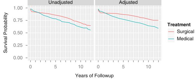
Fig. 20.2 Unadjusted (Kaplan–Meier) and adjusted (Cox–Kalbfleisch–Prentice) estimates of survival. Left, Kaplan–Meier estimates for patients treated medically and surgically at Duke University Medical Center from November 1969 through December 1984. These survival curves are not adjusted for baseline prognostic factors. Right, survival curves for patients treated medically or surgically after adjusting for all known important baseline prognostic characteristics.88

Just as Kalbfleisch and Prentice have generalized the Kaplan–Meier estimator to allow for covariables, Breslow70 has generalized the Altschuler– Nelson–Aalen–Fleming–Harrington estimator to allow for covariables. Using the notation in Section 20.1.3, Breslow’s estimate is derived through an estimate of the cumulative hazard function:

\[\hat{A}(t) = \sum\_{i:t\_i < t} \frac{d\_i}{\sum\_{Y\_i \ge t\_i} \exp(X\_i \hat{\beta})}. \tag{20.15}\]

For any X, the estimates of Λ and S are

\[ \begin{aligned} \hat{A}(t|X) &= \hat{A}(t) \exp(X\hat{\beta}) \\ \hat{S}(t|X) &= \exp[-\hat{A}(t)\exp(X\hat{\beta})]. \end{aligned} \tag{20.16} \]

More asymptotic theory has been derived from the Breslow estimator than for the Kalbfleisch–Prentice estimator. Another advantage of the Breslow estimator is that it does not require iterative computations for dⁱ > 1. Lawless [382, p. 362] states that the two survival function estimators differ little except in the right-hand tail when all dis are unity. Like the Kalbfleisch– Prentice estimator, the Breslow estimator is invariant under different choices of “standard subjects” for the underlying survival S(t). ²

Somewhat complex formulas are available for computing confidence limits of ^Sˆ(t|X).615 ³

20.3 Sample Size Considerations

One way of estimating the minimum sample size for a Cox model analysis aimed at estimating survival probabilities is to consider the simplest case where there are no covariates. Thus the problem reduces to using the Kaplan-Meier estimate to estimate S(t). Let’s further simplify things to assume there is no censoring. Then the Kaplan-Meier estimate is just one minus the empirical cumulative distribution function. By the Dvoretzky-Kiefer-Wolfowitz inequality, the maximum absolute error in an empirical distribution function estimate of the true continuous distribution function is less than or equal to ^ϵ with probability of at least 1 ^× ²e−2nϵ² . For the probability to be at least 0.95, n = 184. Thus in the case of no censoring, one needs 184 subjects to estimate the survival curve to within a margin of error of 0.1 everywhere. To estimate the subject-specific survival curves (S(t|X)) will require greater sample sizes, as will having censored data. It is a fair approximation to think of 184 as the needed number of subjects suffering the event or being censored “late.”

Turning to estimation of a hazard ratio for a single binary predictor X that has equal numbers of X = 0 and X = 1, if the total sample size is n and the number of events in the two categories are respectively e⁰ and e1, the variance of the log hazard ratio is approximately v = ¹ ^e⁰ ⁺ ¹ ^e¹ . Letting z denote the 1 × α/2 standard normal critical value, the multiplicative margin of error (MMOE) with confidence 1 × α is given by exp(z ∞v). To achieve a MMOE of 1.2 in estimating e^β^ˆ with equal numbers of events in the two groups and α = 0.05 requires a total of 462 events.

20.4 Test Statistics

Wald, score, and likelihood ratio statistics are useful and valid for drawing inferences about β in the Cox model. The score test deserves special mention here. If there is a single binary predictor in the model that describes two groups, the score test for assessing the importance of the binary predictor is virtually identical to the Mantel–Haenszel log-rank test for comparing the two groups. If the analysis is stratified for other (nonmodeled) factors, the score test from a stratified Cox model is equivalent to the corresponding stratified log-rank test. Of course, the likelihood ratio or Wald tests could also be used in this situation, and in fact the likelihood ratio test may be better than the score test (i.e., type I errors by treating the likelihood ratio test statistic as having a χ² distribution may be more accurate than using the log-rank statistic).

The Cox model can be thought of as a generalization of the log-rank procedure since it allows one to test continuous predictors, perform simultaneous tests of various predictors, and adjust for other continuous factors without grouping them. Although a stratified log-rank test does not make assumptions regarding the effect of the adjustment (stratifying) factors, it makes the same assumption (i.e., PH) as the Cox model regarding the treatment effect for the statistical test of no difference in survival between groups.

20.5 Residuals

Therneau et al.605 discussed four types of residuals from the Cox model: martingale, score, Schoenfeld, and deviance. The first three have been proven to be very useful, as indicated in Table 20.2. 4

Residual	Purposes
	Martingale Assessing adequacy of a hypothesized predictor
	transformation. Graphing an estimate of a
	predictor transformation (Section 20.6.1).
Score	Detecting overly influential observations
	(Section 20.9). Robust estimate of
	βˆ 9.5).410 covariance matrix of (Section
	Schoenfeld Testing PH assumption (Section 20.6.2).
	Graphing estimate of hazard ratio function
	(Section 20.6.2).

Table 20.2 Types of residuals for the Cox model

20.6 Assessment of Model Fit

As stated before, the Cox model makes the same assumptions as the parametric PH model except that it does not assume a given shape for λ(t) or S(t). Because the Cox PH model is so widely used, methods of assessing its fit are dealt with in more detail than was done with the parametric PH models.

20.6.1 Regression Assumptions

Regression assumptions (linearity, additivity) for the PH model are displayed in Figures 18.3 and 18.5. As mentioned earlier, the regression assumptions can be verified by stratifying by ^X and examining log ^Λˆ(t|X) or log[ΛKM(t|X)] estimates as a function of X at fixed time t. However, as was pointed out in logistic regression, the stratification method is prone to problems of high variability of estimates. The sample size must be moderately large before estimates are precise enough to observe trends through the “noise.” If one wished to divide the sample by quintiles of age and 15 events were thought to be needed in each stratum to derive a reliable estimate of log[ΛKM(2 years)], there would need to be 75 events in the entire sample. If the Kaplan–Meier estimates were needed to be adjusted for another factor that was binary, twice as many events would be needed to allow the sample to be stratified by that factor.

Figure 20.3 displays Kaplan–Meier three-year log cumulative hazard estimates stratified by sex and decile of age. The simulated sample consists of 2000 hypothetical subjects (389 of whom had events), with 1174 males (146 deaths) and 826 females (243 deaths). The sample was drawn from a population with a known survival distribution that is exponential with hazard function

\[ \lambda(t|X\_1, X\_2) = .02 \exp[.8X\_1 + .04(X\_2 - 50)],\tag{20.17} \]

where X¹ represents the sex group (0 = male, 1 = female) and X² age in years, and censoring is uniform. Thus for this population PH, linearity, and additivity hold. Notice the amount of variability and wide confidence limits in the stratified nonparametric survival estimates.

n − 2000
set.seed (3)
age − 50 + 12 * rnorm (n)
label (age) − ' Age '
sex − factor (1 + (runif (n) ≤ .4), 1:2, c( ' Male ' , ' Female ' ))
cens − 15 * runif (n)
h − .02 * exp(.04 * (age - 50) + .8 * (sex == ' Female ' ))
ft − -log(runif (n)) / h
e − ifelse (ft ≤ cens , 1, 0)
print (table (e))

e
  0 1
1611 389

ft − pmin(ft, cens)
units(ft) − ' Year '
Srv − Surv(ft, e)
age.dec − cut2(age , g=10, levels.mean =TRUE)
label(age.dec) − ' Age '
dd − datadist (age , sex , age.dec ); options (datadist = ' dd ' )
f.np − cph(Srv ← strat(age.dec ) + strat(sex), surv=TRUE)
# surv=TRUE speeds up computations, and confidence limits when
# there are no covariables are still accurate.
p − Predict(f.np , age.dec , sex , time=3, loglog=TRUE)
# Treat age.dec as a numeric variable (means within deciles)
p$age.dec − as.numeric ( as.character(p$age.dec ))
ggplot (p, ylim=c(-5, -.5 ))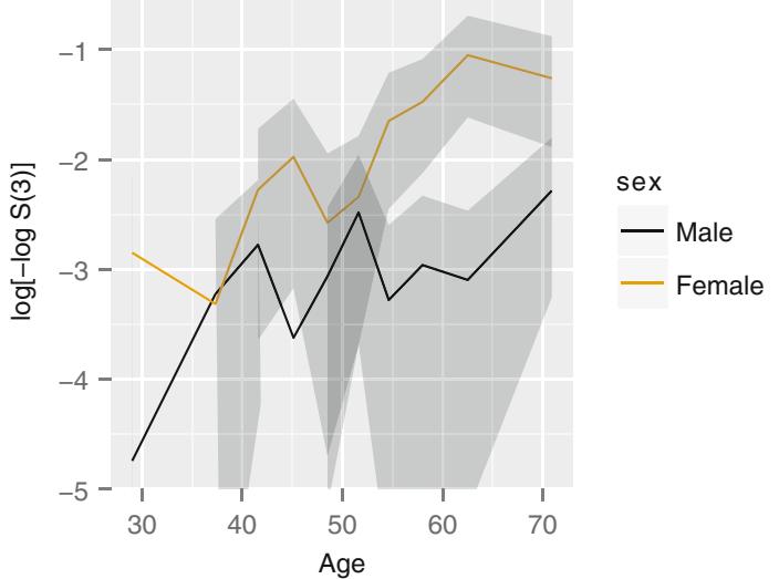

Fig. 20.3 Kaplan–Meier log δ estimates by sex and deciles of age, with 0.95 confidence limits. Solid line is for males, dashed line for females.

As with the logistic model and other regression models, the restricted cubic spline function is an excellent tool for modeling the regression relationship with very few assumptions. A four-knot spline Cox PH model in two variables (X1, X2) that assumes linearity in X¹ and no X¹ ≤ X² interaction is given by

\[\begin{split} \lambda(t|X) &= \lambda(t) \exp(\beta\_1 X\_1 + \beta\_2 X\_2 + \beta\_3 X\_2' + \beta\_4 X\_2''), \\ &= \lambda(t) \exp(\beta\_1 X\_1 + f(X\_2)), \end{split} \tag{20.18}\]

where X^∗ ² and X∗∗ ² are spline component variables as described earlier and f(X2) is the spline function or spline transformation of X² given by

\[f(X\_2) = \beta\_2 X\_2 + \beta\_3 X\_2' + \beta\_4 X\_2''.\tag{20.19}\]

In linear form the Cox model without assuming linearity in X² is

\[ \log \lambda(t|X) = \log \lambda(t) + \beta\_1 X\_1 + f(X\_2). \tag{20.20} \]

By computing partial MLEs of β2, β3, and β4, one obtains the estimated transformation of X² that yields linearity in log hazard or log cumulative hazard.

A similar model that does not assume PH in X¹ is the Cox model stratified on X1. Letting the stratification factor be C = X1, this model is

490 20 Cox Proportional Hazards Regression Model

\[\begin{split} \log \lambda(t|X\_2, C=j) &= \log \lambda\_j(t) + \beta\_1 X\_2 + \beta\_2 X\_2' + \beta\_3 X\_2'' \\ &= \log \lambda\_j(t) + f(X\_2). \end{split} \tag{20.21}\]

This model does assume no X¹ ≤ X² interaction.

Figure 20.4 displays the estimated spline function relating age and sex to log[Λ(3)] in the simulated dataset, using the additive model stratified on sex.

f.noia − cph(Srv ← rcs(age ,4) + strat (sex), x=TRUE , y= TRUE)
# Get accurate C.L. for any age by specifying x= TRUE y=TRUE
# Note: for evaluating shape of regression , we would not
# ordinarily bother to get 3-year survival probabilities -
# would just use X * beta
# We do so here to use same scale as nonparametric estimates
w − latex (f.noia , inline = TRUE , digits =3)
latex (anova (f.noia ), table.env= FALSE , file= ' ' )

	χ2	d.f.	P
age	72.33	3	< 0.0001
Nonlinear	0.69	2	0.7067
TOTAL	72.33	3	< 0.0001

p − Predict( f.noia , age , sex , time =3, loglog =TRUE)
ggplot (p, ylim =c(-5 , -.5 ))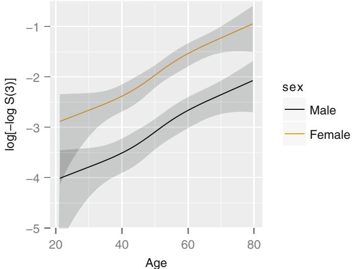

Fig. 20.4 Cox PH model stratified on sex, using spline function for age, no interaction. 0.95 confidence limits also shown. Solid line is for males, dashed line is for females.

A formal test of the linearity assumption of the Cox PH model in the above example is obtained by testing H⁰ : β² = β³ = 0. The χ² statistic with 2 d.f. is 0.69, P = 0.7. The fitted equation, after simplifying the restricted cubic spline to simpler (unrestricted) form, is ^Xβ^ˆ ⁼ ^×1.46 + 0.0255age + ².59≤10−5(age×30.3)³ ^×0.000101(age×45.1)³ ⁺ + 9.73≤10−5(age×54.6)³ + × ².²² ^≤ ¹⁰−5(age ^× ⁶⁹.6)³ ⁺. Notice that the spline estimates are closer to the true linear relationships than were the Kaplan–Meier estimates, and the confidence limits are much tighter. The spline estimates impose a smoothness on the relationship and also use more information from the data by treating age as a continuous ordered variable. Also, unlike the stratified Kaplan–Meier estimates, the modeled estimates can make the assumption of no age ≤ sex interaction. When this assumption is true, modeling effectively boosts the sample size in estimating a common function for age across both sex groups. Of course, this assumption can be tested and interactions can be modeled if necessary.

A Cox model that still does not assume PH for X¹ = C but which allows for an X¹ ≤ X² interaction is

\[\begin{split} \log \lambda(t|X\_2, C=j) &= \log \lambda\_j(t) + \beta\_1 X\_2 + \beta\_2 X\_2' + \beta\_3 X\_2'' \\ &+ \beta\_4 X\_1 X\_2 + \beta\_5 X\_1 X\_2' \\ &+ \beta\_6 X\_1 X\_2''. \end{split} \tag{20.22}\]

This model allows the relationship between X² and log hazard to be a smooth nonlinear function and the shape of the X² effect to be completely different for each level of X¹ if X¹ is dichotomous. Figure 20.5 displays a fit of this model at t = 3 years for the simulated dataset.

f.ia − cph(Srv ← rcs(age ,4) * strat (sex), x=TRUE , y=TRUE ,
             surv=TRUE)
w − latex (f.ia , inline = TRUE , digits =3)
latex (anova (f.ia), table.env= FALSE , file= ' ' )

	χ2	d.f.	P
age (Factor+Higher Order Factors)	72.82	6	< 0.0001
All Interactions	1.05	3	0.7886
Nonlinear (Factor+Higher Order Factors)	1.80	4	0.7728
age ≤ sex (Factor+Higher Order Factors)	1.05	3	0.7886
Nonlinear	1.05	2	0.5911
Nonlinear Interaction : f(A,B) vs. AB	1.05	2	0.5911
TOTAL NONLINEAR	1.80	4	0.7728
TOTAL NONLINEAR + INTERACTION	1.80	5	0.8763
TOTAL	72.82	6	< 0.0001

p − Predict(f.ia , age , sex , time =3, loglog =TRUE ) ggplot (p, ylim =c(-5 , -.5 ))

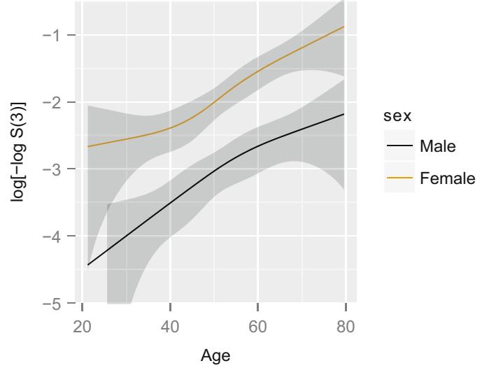
Fig. 20.5 Cox PH model stratified on sex, with interaction between age spline and sex. 0.95 confidence limits are also shown. Solid line is for males, dashed line for females.

The fitted equation is ^Xβ^ˆ ⁼ ^×1.8+0.0493age×2.15≤10−⁶(age×30.3)³ ⁺ × ².82≤10−⁵(age×45.1)³ ++5.18≤10−⁵(age×54.6)³ +×2.15≤10−⁵(age×69.6)³ ⁺+ [Female][×0.0366age + 4.²⁹ ^≤ ¹⁰−⁵(age ^× ³⁰.3)³ ⁺ ^× ⁰.00011(age ^× ⁴⁵.1)³ ⁺ + ⁶.74≤10−⁵(age×54.6)³ ⁺ ^×2.32≤10−⁷(age×69.6)³ ⁺]. The test for interaction yielded χ² = 1.05 with 3 d.f., P = 0.8. The simultaneous test for linearity and additivity yielded χ² = 1.8 with 5 d.f., P = 0.9. Note that allowing the model to be very flexible (not assuming linearity in age, additivity between age and sex, and PH for sex) still resulted in estimated regression functions that are very close to the true functions. However, confidence limits in this unrestricted model are much wider.

Figure 20.6 displays the estimated relationship between left ventricular ejection fraction (LVEF) and log hazard ratio for cardiovascular death in a sample of patients with significant coronary artery disease. The relationship is estimated using three knots placed at quantiles 0.05, 0.5, and 0.95 of LVEF. Here there is significant nonlinearity (Wald χ² = 9.6 with 1 d.f.). The graphs leads to a transformation of LVEF that better satisfies the linearity assumption: min(LVEF, 0.5). This transformation has the best log likelihood “for the money” as judged by the Akaike information criterion (AIC = ×2 log L.R. ×2≤ no. parameters = 127). The AICs for 3, 4, 5, and 6-knot spline fits were, respectively, 126, 124, 122, and 120.

Had the suggested transformation been more complicated than a truncation, a tentative transformation could have been checked for adequacy by expanding the new transformed variable into a new spline function and testing it for linearity.

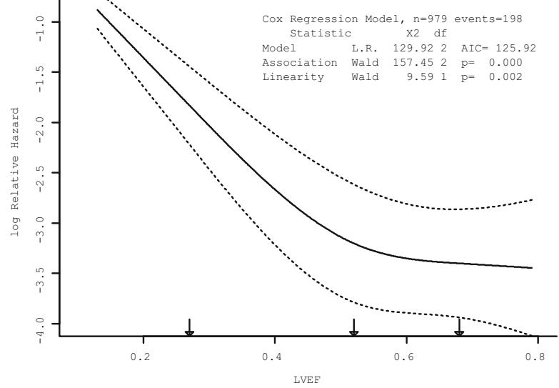
Fig. 20.6 Restricted cubic spline estimate of relationship between LVEF and relative log hazard from a sample of 979 patients and 198 cardiovascular deaths. Data from the Duke Cardiovascular Disease Databank.

Other methods based on smoothed residual plots are also valuable tools for selecting predictor transformations. Therneau et al.605 describe residuals based on martingale theory that can estimate transformations of any number of predictors omitted from a Cox model fit, after adjusting for other variables included in the fit. Figure 20.7 used various smoothing methods on the points (LVEF, residual). First, the R loess function96 was used to obtain a smoothed scatterplot fit and approximate 0.95 confidence bars. Second, an ⁵ ordinary least squares model, representing LVEF as a restricted cubic spline with five default knots, was fitted. Ideally, both fits should have used weighted regression as the residuals do not have equal variance. Predicted values from this fit along with 0.95 confidence limits are shown. The loess and splinelinear regression agree extremely well. Third, Cleveland’s lowess scatterplot smoother111 was used on the martingale residuals against LVEF. The suggested transformation from all three is very similar to that of Figure 20.6. For smaller sample sizes, the raw residuals should also be displayed. There is one vector of martingale residuals that is plotted against all of the predictors. When correlations among predictors are mild, plots of estimated predictor transformations without adjustment for other predictors (i.e., marginal transformations) may be useful. Martingale residuals may be obtained quickly by fixing βˆ = 0 for all predictors. Then smoothed plots of predictor against residual may be made for all predictors. Table 20.3 summarizes some of the

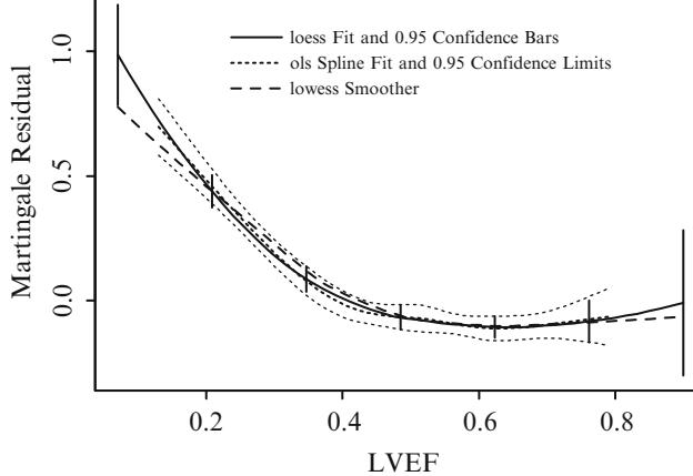
Fig. 20.7 Three smoothed estimates relating martingale residuals605 to LVEF.

Purpose	Method
Estimate transformation for	βˆ Force 1 = 0 and compute
a single variable	residuals from the null regression
Check linearity assumption for	βˆ Compute 1 and compute
a single variable	residuals from the linear regression
Estimate marginal	βˆ βˆ Force 1,, p = 0 and compute
transformations for p	variables residuals from the global null model
Estimate transformation for	βˆ Estimate p × 1 βs, forcing i = 0
variable i adjusted for other	Compute residuals from mixed
p × 1 variables	global/null model

Table 20.3 Uses of martingale residuals for estimating predictor transformations

⁶ ways martingale residuals may be used. See section 10.5 for more information on checking the regression assumptions. The methods for examining interaction surfaces described there apply without modification to the Cox model (except that the nonparametric regression surface does not apply because of censoring).

20.6.2 Proportional Hazards Assumption

Even though assessment of fit of the regression part of the Cox PH model corresponds with other regression models such as the logistic model, the Cox model has its own distributional assumption in need of validation. Here, of course, the distributional assumption is not as stringent as with other survival models, but we do need to validate how the survival or hazard functions for various subjects are connected. There are many graphical and analytical methods of verifying the PH assumption. Two of the methods have already been discussed: a graphical examination of parallelism of log Λ plots, and a comparison of stratified with unstratified models (as in Figure 20.1). Muenz467 suggested a simple modification that will make nonproportional hazards more apparent: plot ΛKM¹ (t)/ΛKM² (t) against t and check for flatness. The points on this curve can be passed through a smoother. One can also plot differences in log(× log S(t)) against t. 143 Arjas29 developed a graphical method based on plotting the estimated cumulative hazard versus the cumulative number of events in a stratum as t progresses.

There are other methods for assessing whether PH holds that may be more direct. Gore et al.,226 Harrell and Lee,266 and Kay340 (see also Anderson and Senthilselvan27) describe a method for allowing the log hazard ratio (Cox regression coefficient) for a predictor to be a function of time by fitting specially stratified Cox models. Their method assumes that the predictor being examined for PH already satisfies the linear regression assumption. Followup time is stratified into intervals and a separate model is fitted to compute the regression coefficient within each interval, assuming that the effect of the predictor is constant only within that small interval. It is recommended that intervals be constructed so that there is roughly an equal number of events in each. The number of intervals should allow at least 10 or 20 events per interval.

The interval-specific log hazard ratio is estimated by excluding all subjects with event/censoring time before the start of the interval and censoring all events that occur after the end of the interval. This process is repeated for all desired time intervals. By plotting the log hazard ratio and its confidence limits versus the interval, one can assess the importance of a predictor as a function of follow-up time and learn how to model non-PH using more complicated models containing predictor by time interactions. If the hazard ratio is approximately constant within broad time intervals, the time stratification method can be used for fitting and testing the predictor ≤ time interaction [266, p. 827]; [98].

Consider as an example the rat vaginal cancer data used in Figures 18.9, 18.10, and 20.1. Recall that the PH assumption appeared to be satisfied for the two groups although Figure 18.9 demonstrated some non-Weibullness. Figure 20.8 contains a Λ ratio plot.467

f − cph(S ← strat (group), surv=TRUE)
# For both strata , eval. S(t) at combined set of death times
times − sort(unique (days[death == 1]))
est − survest(f, data.frame( group =levels (group )),
                  times= times , conf.type=" none")$surv
cumhaz − - log(est)
plot( times , cumhaz [2,] / cumhaz [1,], xlab="Days",
     ylab=" Cumulative Hazard Ratio", type ="s")
abline (h=1, col=gray (.80 ))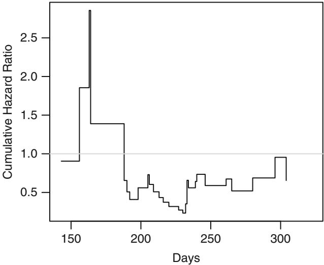

Fig. 20.8 Estimate of δ2/δ¹ based on × log of Altschuler–Nelson–Fleming– Harrington nonparametric survival estimates.

Table 20.4 Interval-specific group effects from rat data by artificial censoring

Time	Observations Deaths Log Hazard Standard
Interval			Ratio	Error
[0, 209)	40	12	×0.47	0.59
[209, 234)	27	12	×0.72	0.58
234 +	14	12	×0.50	0.64

|–|

The number of observations is declining over time because computations in each interval were based on animals followed at least to the start of that interval. The overall Cox regression coefficient was ×0.57 with a standard error of 0.35. There does not appear to be any trend in the hazard ratio over time, indicating a constant hazard ratio or proportional hazards (Table 20.4).

Now consider the Veterans Administration Lung Cancer dataset [331, pp. 60, 223–4]. Log Λ plots indicated that the four cell types did not satisfy PH. To simplify the problem, omit patients with “large” cell type and let the binary predictor be 1 if the cell type is “squamous” and 0 if it is “small” or “adeno.” We are assessing whether survival patterns for the two groups “squamous” versus “small” or “adeno” have PH. Interval-specific estimates of the squamous : small,adeno log hazard ratios (using Efron’s likelihood) are found in Table 20.5. Times are in days.

Time	Observations Deaths Log Hazard Standard
Interval			Ratio	Error
[0, 21)	110	26	×0.46	0.47
[21, 52)	84	26	×0.90	0.50
[52, 118)	59	26	×1.35	0.50
118 +	28	26	×1.04	0.45

Table 20.5 Interval-specific effects of squamous cell cancer in VA lung cancer data

Table 20.6 Interval-specific effects of performance status in VA lung cancer data

Time	Observations Deaths Log Hazard Standard
Interval			Ratio	Error
[0, 19]	137	27	×0.053	0.010
[19, 49)	112	26	×0.047	0.009
[49, 99)	85	27	×0.036	0.012
99 +	28	26	×0.012	0.014

getHdata( valung )
with(valung , {
  hazard.ratio.plot (1 * ( cell == ' Squamous ' ), Surv(t, dead),
                      e=25, subset =cell != ' Large ' ,
                      pr=TRUE , pl= FALSE)
  hazard.ratio.plot (1 * kps , Surv(t, dead), e=25,
                      pr=TRUE , pl= FALSE ) })

There is evidence of a trend of a decreasing hazard ratio over time which is consistent with the observation that squamous cell patients had equal or worse survival in the early period but decidedly better survival in the late phase.

From the same dataset now examine the PH assumption for Karnofsky performance status using data from all subjects, if the linearity assumption is satisfied. Interval-specific regression coefficients for this predictor are given in Table 20.6. There is good evidence that the importance of performance status is decreasing over time and that it is not a prognostic factor after roughly 99 days. In other words, once a patient survives 99 days, the performance status does not contain much information concerning whether the patient will survive 120 days. This non-PH would be more difficult to detect from Kaplan– Meier plots stratified on performance status unless performance status was stratified carefully. ⁷

Figure 20.9 displays a log hazard ratio plot for a larger dataset in which more time strata can be formed. In 3299 patients with coronary artery disease, 827 suffered cardiovascular death or nonfatal myocardial infarction. Time

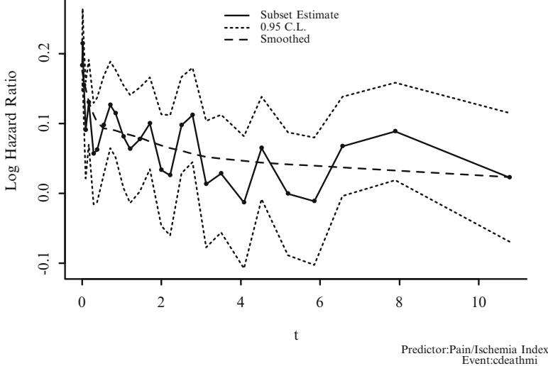
Fig. 20.9 Stratified hazard ratios for pain/ischemia index over time. Data from the Duke Cardiovascular Disease Databank.

was stratified into intervals containing approximately 30 events, and within each interval the Cox regression coefficient for an index of anginal pain and ischemia was estimated. The pain/ischemia index, one component of which is unstable angina, is seen to have a strong effect for only six months. After that, survivors have stabilized and knowledge of the angina status in the previous six months is not informative.

Another method for graphically assessing the log hazard ratio over time is based on Schoenfeld’s partial residuals503, 557 with respect to each predictor in the fitted model. The residual is the contribution of the first derivative of the log likelihood function with respect to the predictor’s regression coefficient, computed separately at each risk set or unique failure time. In Figure 20.10 the “loess-smoothed”96 (with approximate 0.95 confidence bars) and “supersmoothed”207 relationship between the residual and unique failure time is shown for the same data as Figure 20.9. For smaller n, the raw residuals should also be displayed to convey the proper sense of variability. The agreement with the pattern in Figure 20.9 is evident.

Pettitt and Bin Daud503 suggest scaling the partial residuals by the information matrix components. They also propose a score test for PH based on the Schoenfeld residuals. Grambsch and Therneau233 found that the Pettitt– Bin Daud standardization is sometimes misleading in that non-PH in one variable may cause the residual plot for another variable to display non-PH. The Grambsch–Therneau weighted residual solves this problem and also yields a residual that is on the same scale as the log relative hazard ratio. Their residual is

\[ \beta + dR\hat{V}, \tag{20.23} \]

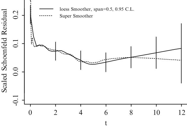
Fig. 20.10 Smoothed weighted233 Schoenfeld557 residuals for the same data in Figure 20.9. Test for PH based on the correlation (Λ) between the individual weighted Schoenfeld residuals and the rank of failure time yielded Λ = ×0.23, z = ×6.73, P = ² ^∼ ¹⁰∧¹¹.

where d is the total number of events, R is the n ≤ p matrix of Schoenfeld residuals, and Vˆ is the estimated covariance matrix for βˆ. This new residual can also be the basis for tests for PH, by correlating a user-specified function of unique failure times with the weighted residuals. ⁸

The residual plot is computationally very attractive since the score residual components are byproducts of Cox maximum likelihood estimation. Another attractive feature is the lack of need to categorize the time axis. Unless approximate confidence intervals are derived from smoothing techniques, a lack of confidence intervals from most software is one disadvantage of the method.

Formal tests for PH can be based on time-stratified Cox regression estimates.27, 266 Alternatively, more complex (and probably more efficient) formal tests for PH can be derived by specifying a form for the time by predictor interaction (using what is called a time-dependent covariable in the Cox model) and testing coefficients of such interactions for significance. The obsolete Version 5 SAS PHGLM procedure used a computationally fast procedure based on an approximate score statistic that tests for linear correlation between the rank order of the failure times in the sample and Schoenfeld’s partial residuals.258, 266 This test is available in R (for both weighted and unweighted ¹⁰ residuals) using Therneau’s cox.zph function in the survival package. For the results in Figure 20.10, the test for PH is highly significant (correlation coefficient = ×0.23, normal deviate z = ×6.73). Since there is only one regression parameter, the weighted residuals are a constant multiple of the unweighted ones, and have the same correlation coefficient. ¹¹

Table 20.7	Time-specific hazard ratio estimates of squamous cell cancer effect in VA
lung cancer data, by fitting two Weibull distributions with unequal shape parameters

t	log Hazard
	Ratio
10	×0.36
36	×0.64
83.5	×0.83
200	×1.02

Another method for checking the PH assumption which is especially applicable to a polytomous predictor involves taking ratios of parametrically estimated hazard functions estimated separately for each level of the predictor. For example, suppose that a risk factor X is either present (X = 1) or absent (X = 0), and suppose that separate Weibull distributions adequately fit the survival pattern of each group. If there are no other predictors to adjust for, define the hazard function for X = 0 as αγt ^γ−¹ and the hazard for X = 1 as δθt ^θ−¹. The X =1: X = 0 hazard ratio is

\[\frac{\alpha \gamma t^{\gamma - 1}}{\delta \theta t^{\theta - 1}} = \frac{\alpha \gamma}{\delta \theta} t^{\gamma - \theta}. \tag{20.24}\]

The hazard ratio is constant if the two Weibull shape parameters (γ and θ) are equal. These Weibull parameters can be estimated separately and a Wald test statistic of H⁰ : γ = θ can be computed by dividing the square of their difference by the sum of the squares of their estimated standard errors, or ¹² better by a likelihood ratio test. A plot of the estimate of the hazard ratio above as a function of t may also be informative.

In the VA lung cancer data, the MLEs of the Weibull shape parameters for squamous cell cancer is 0.77 and for the combined small + adeno is 0.99. Estimates of the reciprocals of these parameters, provided by some software packages, are 1.293 and 1.012 with respective standard errors of 0.183 and 0.0912. A Wald test for differences in these reciprocals provides a rough test for a difference in the shape estimates. The Wald χ² is 1.89 with 1 d.f. indicating slight evidence for non-PH.

The fitted Weibull hazard function for squamous cell cancer is .0167t 0.23 and for adeno + small is 0.0144t ⁻0.⁰¹. The estimated hazard ratio is then 1.16t ⁻0.²² and the log hazard ratio is 0.¹⁴⁸ ^× ⁰.22 log ^t. By evaluating this Weibull log hazard ratio at interval midpoints (arbitrarily using t = 200 for the last (open) interval) we obtain log hazard ratios that are in good agreement with those obtained by time-stratifying the Cox model (Table 20.5) as shown in Table 20.7.

There are many methods of assessing PH using time-dependent covariables in the Cox model.226, 583 Gray237, 238 mentions a flexible and efficient method of estimating the hazard ratio function using time-dependent covariables that are X ≤ spline term interactions. Gray’s method uses B-splines and

requires one to maximize a penalized log-likelihood function. Verweij and van Houwelingen641 developed a more nonparametric version of this approach. Hess289 uses simple restricted cubic splines to model the time-dependent covariable effects (see also [4, 287, 398, 498]). Suppose that k = 4 knots are used and that a covariable X is already transformed correctly. The model is

\[\log \lambda(t|X) = \log \lambda(t) + \beta\_1 X + \beta\_2 Xt + \beta\_3 Xt' + \beta\_4 Xt'',\tag{20.25}\]

where t ∗ , t∗∗ are constructed spline variables (Equation 2.25). The X +1: X log hazard ratio function is estimated by

\[ \hat{\beta}\_1 + \hat{\beta}\_2 t + \hat{\beta}\_3 t' + \hat{\beta}\_4 t''. \tag{20.26} \]

This method can be generalized to allow for simultaneous estimation of the shape of the X effect and X ≤ t interaction using spline surfaces in (X, t) instead of (X1, X2) (Section 2.7.2). ¹³

Table 20.8 summarizes many facets of verifying assumptions for PH models. The trade-offs of the various methods for assessing proportional hazards are given in Table 20.9. ¹⁴

20.7 What to Do When PH Fails

When a factor violates the PH assumption and a test of association is not needed, the factor can be adjusted for through stratification as mentioned earlier. This is especially attractive if the factor is categorical. For continuous predictors, one may want to stratify into quantile groups. The continuous version of the predictor can still be adjusted for as a covariable to account for any residual linearity within strata.

When a test of significance is needed and the P-value is impressive, the “principle of conservatism” could be invoked, as the P-value would likely have been more impressive had the factor been modeled correctly. Predicted survival probabilities using this approach will be erroneous in certain time intervals.

An efficient test of association can be done using time-dependent covariables [444, pp. 208–217]. For example, in the model

\[ \lambda(t|X) = \lambda\_0(t) \exp(\beta\_1 X + \beta\_2 X \times \log(t+1))\tag{20.27} \]

one tests H⁰ : β¹ = β² = 0 with 2 d.f. This is similar to the approach used by [72]. Stratification on time intervals can also be used:27, 226, 266

\[ \lambda(t|X) = \lambda\_0(t) \exp(\beta\_1 X + \beta\_2 X \times [t > c]). \tag{20.28} \]

Variables	Assumptions	Verification
Response Variable T Time Until Event	Shape of Φ(t X) for fixed X as t ∪ Cox: none Weibull: tθ	Shape of SKM(t)
Interaction Between X and T	Proportional hazards—effect of X does not depend on T (e.g., treatment effect is con stant over time)	• Categorical X: check parallelism of strati fied log[× log S(t)] plots as t ∪ • Muenz467 cum. hazard ra tio plots • Arjas29 cum. hazard plots • Check agreement of strati fied and modeled estimates • Hazard ratio plots • Smoothed Schoenfeld resid ual plots and correlation test (time vs. residual) • Test time-dependent co variable such as X ∼log(t+ 1) • Ratio of parametrically es timated Φ(t)
Individual Predictors X	Shape of Φ(t X) for fixed t as X ∪ Linear: log Φ(t X) = log Φ(t) + χX Nonlinear: log Φ(t X) = log Φ(t) + f(X)	• k-level ordinal X : linear term + k × 2 dummy vari ables • Continuous X: polynom ials, spline functions, smoothed martingale residual plots
Interaction Between X1 and X2	Additive effects: effect of X1 on log Φ is independent of X2 and vice versa	Test nonadditive terms (e.g., products)

Table 20.8 Assumptions of the Proportional Hazards Model

If this step-function model holds, and if a sufficient number of subjects have late follow-up, you can also fit a model for early outcomes and a separate one for late outcomes using interval-specific censoring as discussed in Section 20.6.2. The dual model approach provides easy to interpret models, assuming that proportional hazards is satisfied within each interval.

Kronborg and Aaby367 and Dabrowska et al.143 provide tests for differences in Λ(t) at specific t based on stratified PH models. These can also be used to test for treatment effects when PH is violated for treatment but not for adjustment variables. Differences in mean restricted life length (differences in areas under survival curves up to a fixed finite time) can also be useful for comparing therapies when PH fails.335

Method	Requires	Requires	Computa-	Yields	Yields	Requires	Must Choose
	Grouping	Grouping	tional	Formal	Estimate of	Fitting 2	Smoothing
	X	t	Efficiency	Test	λ2(t)/λ1(t)	Models	Parameter
log[− log], Muenz, Arjas plots	x		x			x
Dabrowska log Λˆ difference plots	x		x	x		x
Stratified vs. Modeled Estimates	x		x			x
Hazard ratio plot		x		?	x	x	?
Schoenfeld residual plot			x		x		x
Schoenfeld residual correlation test			x	x
Fit time dependent covariables				x	x
Ratio of parametric estimates of λ(t)	x		x	x	x	x

Table 20.9 Comparison of methods for checking the proportional hazards assumption and for allowing for non-proportional hazards

Parametric models that assume an effect other than PH, for example, the log-logistic model,226 can be used to allow a predictor to have a constantly increasing or decreasing effect over time. If one predictor satisfies PH but another does not, this approach will not work. ¹⁵

20.8 Collinearity

See Section 4.6 for the general approach using variance inflation factors.

20.9 Overly Influential Observations

Therneau et al.605 describe the use of score residuals for assessing influence in Cox and related regression models. They show that the infinitesimal jackknife estimate of the influence of observation i on β equals V s∗ , where V is the estimated variance–covariance matrix of the p regression estimates b and s = (si1, si2,…,sip) is the vector of score residuals for the p regression coefficients for the ith observation. Let Sn∼^p denote the matrix of score residuals over all observations. Then an approximation to the unstandardized change in b (DFBETA) is SV . Standardizing by the standard errors of b found from the diagonals of V , e = (V11, V22,…,Vpp)1/2, yields

\[\text{DFBETAS} = SV \text{ Diag}(e)^{-1},\tag{20.29}\]

where Diag(e) is a diagonal matrix containing the estimated standard errors.

As discussed in Section 20.13, identification of overly influential observations is facilitated by printing, for each predictor, the list of observations containing DFBETAS > u for any parameter associated with that predictor. The choice of cutoff u depends on the sample size among other things. A typical choice might be u = 0.2 indicating a change in a regression coefficient of 0.2 standard errors.

20.10 Quantifying Predictive Ability

To obtain a unitless measure of predictive ability for a Cox PH model we can use the R index described in Section 9.8.3, which is the square root of the fraction of log likelihood explained by the model of the log likelihood that could be explained by a perfect model, penalized for the complexity of the model. The lowest (best) possible ×2 log likelihood for the Cox model is zero, which occurs when the predictors can perfectly rank order the survival times. Therefore, as was the case with the logistic model, the quantity L′ from Section 9.8.3 is zero and an R index that is penalized for the number of parameters in the model is given by

\[R^2 = (\text{LR} - 2p)/L^0,\tag{20.30}\]

where ^p is the number of parameters estimated and ^L⁰ is the ^×2 log likelihood when β is restricted to be zero (i.e., there are no predictors in the model). R will be near one for a perfectly predictive model and near zero for a model that does not discriminate between short and long survival times. The R index does not take into account any stratification factors. If stratification factors are present, R will be near one if survival times can be perfectly ranked within strata even though there is overlap between strata.

Schemper546 and Korn and Simon365 have reported that R² is too sensitive to the distribution of censoring times and have suggested alternatives based on the distance between estimated Cox survival probabilities (using predictors) and Kaplan–Meier estimates (ignoring predictors). Kent and O’Quigley345 also report problems with R² and suggest a more complex measure. Schemper548 investigated the Maddala–Magee431, 432 index R² LR described in Section 9.8.3, applied to Cox regression:

\[\begin{split} R\_{\text{LR}}^2 &= 1 - \exp(-\text{LR}/n) \\ &= 1 - \omega^{2/n}, \end{split} \tag{20.31}\]

where ω is the null model likelihood divided by the fitted model likelihood.

For many situations, R² LR performed as well as Schemper’s more complex measure546, 549 and hence it is preferred because of its ease of calculation (assuming that PH holds). Ironically, Schemper548 demonstrated that the n in the formula for this index is the total number of observations, not the number of events (but see O’Quigley, Xu, and Stare481). To make the R² index have a maximum value of 1.0, we use the Nagelkerke471 R² ^N discussed in Section 9.8.3. ¹⁶

An easily interpretable index of discrimination for survival models is derived from Kendall’s τ and Somers’ Dxy rank correlation,579 the Gehan– Wilcoxon statistic for comparing two samples for survival differences, and the Brown–Hollander–Korwar nonparametric test of association for censored data.76, 170, 262, 268 This index, c, is a generalization of the area under the ROC curve discussed under the logistic model, in that it applies to a continuous response variable that can be censored. The c index is the proportion of all pairs of subjects whose survival time can be ordered such that the subject with the higher predicted survival is the one who survived longer. Two subjects’ survival times cannot be ordered if both subjects are censored or if one has failed and the follow-up time of the other is less than the failure time of the first. The c index is a probability of concordance between predicted and observed survival, with c = 0.5 for random predictions and c = 1 for a perfectly discriminating model. The c index is mildly affected by the amount of censoring. Dxy is obtained from 2(c × 0.5). While c (and Dxy) is a good measure of pure discrimination ability of a single model, it is not sensitive enough to allow multiple models to be compared447. ¹⁷

Since high hazard means short survival time, when the linear predictor Xβˆ from a Cox model is compared with observed survival time, Dxy will be negative. Some analysts may want to negate reported values of Dxy.

20.11 Validating the Fitted Model

Separate bootstrap or cross-validation assessments can be made for calibration and discrimination of Cox model survival and log relative hazard esti-18 mates.

20.11.1 Validation of Model Calibration

One approach to validation of the calibration of predictions is to obtain unbiased estimates of the difference between Cox predicted and Kaplan–Meier survival estimates at a fixed time u. Here is one sequence of steps.

1. Obtain cutpoints (e.g., deciles) of predicted survival at time u so as to have a given number of subjects (e.g., 50) in each interval of predicted survival. These cutpoints are based on the distribution of ^Sˆ(u|X) in the whole sample for the”final”model (for data-splitting, instead use the model developed in the training sample). Let k denote the number of intervals used.
1. Compute the average ^Sˆ(u|X) in each interval.
1. Compare this with the Kaplan–Meier survival estimates at time u, stratified by intervals of ^Sˆ(u|X). Let the differences be denoted by ^d ⁼ (d1,…,dk).
1. Use bootstrapping or cross-validation to estimate the overoptimism in d and then to correct d to get a more fair assessment of these differences. For each repetition, repeat any stepwise variable selection or stagewise significance testing using the same stopping rules as were used to derive the “final”model. No more than B = 200 replications are needed to obtain accurate estimates.
1. If desired, the bias-corrected d can be added to the original stratified Kaplan–Meier estimates to obtain a bias-corrected calibration curve.

However, any statistical method that uses binning of continuous variables (here, the predicted risk), is arbitrary and has lower precision than smooth estimates that allow for interpolation. A far better approach to estimating calibration curves for survival models is to use the flexible adaptive hazard regression approach of Kooperberg et al.361 as discussed on P. 450. Their method does not assume linearity or proportional hazards. Hazard regression can be used to estimate the relationship between (suitably transformed) predicted survival probabilities and observed outcomes, i.e., to derive a calibration curve. The bootstrap is used to de-bias the estimates to correct for overfitting, allowing estimation of the likely future calibration performance of the fitted model.

As an example, consider a dataset of 20 random uniformly distributed predictors for a sample of size 200. Let the failure time be another random

uniform variable that is independent of all the predictors, and censor half of the failure times at random. Due to fitting 20 predictors to 100 events, there will apparently be fair agreement between predicted and observed survival over all strata (smooth black curve from hazard regression in Figure 20.11). However, the bias-corrected calibration (blue curve from hazard regression) gives a more truthful answer: examining the Xs across levels of predicted survival demonstrate that predicted and observed survival are weekly related, in more agreement with how the data were generated. For the more arbitrary Kaplan-Meier approach, we divide the observations into quintiles of predicted 0.5-year survival, so that there are 40 observations per stratum.

n − 200
p − 20
set.seed (6)
xx − matrix (rnorm (n * p), nrow=n, ncol=p)
y − runif (n)
units (y) − "Year"
e − c(rep(0, n / 2), rep(1, n / 2))
f − cph(Surv(y, e) ← xx , x=TRUE , y=TRUE ,
           time.inc =.5 , surv=TRUE)
cal − calibrate (f, u=.5 , B =200)

Using Cox survival estimates at 0.5 Years

plot (cal , ylim =c(.4 , 1), subtitles= FALSE )
calkm − calibrate (f, u=.5 , m=40, cmethod= ' KM ' , B=200)

Using Cox survival estimates at 0.5 Years

plot( calkm , add= TRUE) # Figure 20.11

20.11.2 Validation of Discrimination and Other Statistical Indexes

Here bootstrapping and cross-validation are used as for logistic models (Section 10.9). We can obtain bootstrap bias-corrected estimates of c or equivalently Dxy. To instead obtain a measure of relative calibration or slope shrinkage, we can bootstrap the apparent estimate of γ = 1 in the model

\[ \lambda(t|X) = \lambda(t) \exp(\gamma Xb). \tag{20.32} \]

Besides being a measure of calibration in itself, the bootstrap estimate of γ also leads to an unreliability index U which measures how far the model maximum log likelihood (which allows for an overall slope correction) is from the log likelihood evaluated at”frozen”regression coefficients (γ = 1) (see [267] and Section 10.9).

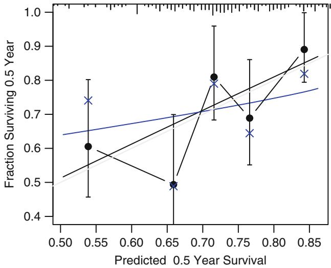
Fig. 20.11 Calibration of random predictions using Efron’s bootstrap with B = 200 resamples. Dataset has n = 200, 100 uncensored observations, 20 random predictors, model σ² ²⁰ = 19. The smooth black line is the apparent calibration estimated by adaptive linear spline hazard regression361, and the blue line is the bootstrap bias– (overfitting–) corrected calibration curve estimated also by hazard regression. The gray scale line is the line of identity representing perfect calibration. Black dots represent apparent calibration accuracy obtained by stratifying into intervals of predicted 0.5y survival containing 40 events per interval and plotting the mean predicted value within the interval against the stratum’s Kaplan-Meier estimate. The blue ∼ represent bootstrap bias-corrected Kaplan-Meier estimates.

\[U = \frac{\text{LR}(\hat{\gamma}Xb) - \text{LR}(Xb)}{L^0},\tag{20.33}\]

where ^L⁰ is the ^×2 log likelihood for the null model (Section 9.8.3). Similarly, a discrimination index ^D267 can be derived from the ^×2 log likelihood at the shrunken linear predictor, penalized for estimating one parameter (γ) (see also [633, p. 1318] and [123]):

\[D = \frac{\text{LR}(\hat{\gamma}Xb) - 1}{L^0}.\tag{20.34}\]

D is the same as R² discussed above when p = 1 (indicating only one reestimated parameter, γ), the penalized proportion of explainable log likelihood that was explained by the model. Because of the remark of Schemper,546 all of these indexes may unfortunately be functions of the censoring pattern.

An index of overall quality that penalizes discrimination for unreliability is

\[Q = D - U = \frac{\text{LR}(Xb) - 1}{L^0}.\tag{20.35}\]

Q is a normalized and penalized ×2 log likelihood that is evaluated at the uncorrected linear predictor.

For the random predictions used in Figure 20.11, the bootstrap estimates with B = 200 resamples are found in Table 20.10.

latex ( validate(f,	B=200),	digits =3, file = ’ ’ ,	caption= ’ ’ ,
table.env=TRUE ,		label= ’ tab:cox-val-random ’ )

Table 20.10 Bootstrap validation of a Cox model with random predictors

	Index Original Training		Test		Optimism Corrected n
	Sample	Sample	Sample		Index
Dxy	0.213	0.335	0.147	0.188	0.025 200
R2	0.092	0.191	0.042	0.150	×0.058 200
Slope	1.000	1.000	0.389	0.611	0.389 200
D	0.021	0.048	0.009	0.039	×0.019 200
U	×0.002	×0.002	0.028	×0.031	0.028 200
Q	0.023	0.050	×0.020	0.070	×0.047 200
g	0.516	0.878	0.339	0.539	×0.023 200

It can be seen that the apparent correlation (Dxy = ×0.21) does not hold up after correcting for overfitting (Dxy = ×0.02). Also, the slope shrinkage (0.39) indicates extreme overfitting.

See [633, Section 6] and [640] and Section 18.3.7 for still more useful methods for validating the Cox model.

20.12 Describing the Fitted Model

As with logistic modeling, once a Cox PH model has been fitted and all its assumptions verified, the final model needs to be presented and interpreted. The fastest way to describe the model is to interpret each effect in it. For each predictor the change in log hazard per desired units of change in the predictor value may be computed, or the antilog of this quantity, exp(β^j ≤ change in X^j ), may be used to estimate the hazard ratio holding all other factors constant. When X^j is a nonlinear factor, changes in predicted Xβ for sensible values of X^j such as quartiles can be used as described in Section 10.10. Of course for nonmodeled stratification factors, this method is of no help. Figure 20.12 depicts a way to display estimated surgical : medical hazard ratios in the presence of a significant treatment by disease severity interaction and a secular trend in the benefit of surgical therapy (treatment by year of diagnosis interaction).

Often, the use of predicted survival probabilities may make the model more interpretable. If the effect of only one factor is being displayed and

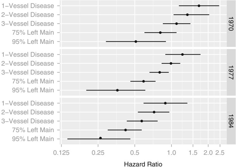
Fig. 20.12 A display of an interaction between treatment and extent of disease, and between treatment and calendar year of start of treatment. Comparison of medical and surgical average hazard ratios for patients treated in 1970, 1977, and 1984 according to coronary disease severity. Circles represent point estimates; bars represent 0.95 confidence limits of hazard ratios. Ratios less than 1.0 indicate that coronary bypass surgery is more effective.88

that factor is polytomous or predictions are made for specific levels, survival curves (with or without adjustment for other factors not shown) can be drawn for each level of the predictor of interest, with follow-up time on the x-axis. Figure 20.2 demonstrated this for a factor which was a stratification factor. Figure 20.13 extends this by displaying survival estimates stratified by treatment but adjusted to various levels of two modeled factors, one of which, year of diagnosis, interacted with treatment.

When a continuous predictor is of interest, it is usually more informative to display that factor on the x-axis with estimated survival at one or more time points on the y-axis. When the model contains only one predictor, even if that predictor is represented by multiple terms such as a spline expansion, one may simply plot that factor against the predicted survival. Figure 20.14 depicts the relationship between treadmill exercise score, which is a weighted linear combination of several predictors in a Cox model, and the probability of surviving five years.

When displaying the effect of a single factor after adjusting for multiple predictors which are not displayed, care only need be taken for the values to which the predictors are adjusted (e.g., grand means). When instead the desire is to display the effect of multiple predictors simultaneously, an important continuous predictor can be displayed on the x-axis while separate p − Predict(f.ia , age , sex , time =3)

curves or graphs are made for levels of other factors. Figure 20.15, which corresponds to the logΛ plots in Figure 20.5, displays the joint effects of age and sex on the three-year survival probability. Age is modeled with a cubic spline function, and the model includes terms for an age ≤ sex interaction.

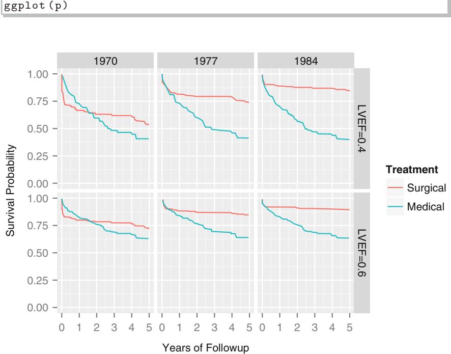
Fig. 20.13 Cox–Kalbfleisch–Prentice survival estimates stratifying on treatment and adjusting for several predictors, showing a secular trend in the efficacy of coronary artery bypass surgery. Estimates are for patients with left main disease and normal (LVEF=0.6) or impaired (LVEF=0.4) ventricular function.516

Besides making graphs of survival probabilities estimated for given levels of the predictors, nomograms have some utility in specifying a fitted Cox model. A nomogram can be used to compute Xβˆ, the estimated log hazard for a subject with a set of predictor values X relative to the “standard” subject. The central line in the nomogram will be on this linear scale unlike the logistic model nomograms given in Section 10.10 which further transformed Xβˆ into [1 + exp(×Xβˆ)]−¹. Alternatively, the central line could be on the nonlinear exp(Xβˆ) hazard ratio scale or survival at fixed t. ¹⁹

A graph of the estimated underlying survival function Sˆ(t) as a function of t can be coupled with the nomogram used to compute Xβˆ. The survival for a specific subject, ^Sˆ(t|X) is obtained from ^Sˆ(t)exp(Xβˆ). Alternatively, one could graph ^Sˆ(t)exp(Xβˆ) for various values of ^Xβ^ˆ (e.g., ^Xβ^ˆ ⁼ ^×2, ^×1, ⁰, ¹, 2)

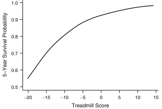
Fig. 20.14 Cox model predictions with respect to a continuous variable. X-axis shows the range of the treadmill score seen in clinical practice and Y -axis shows the corresponding five-year survival probability predicted by the Cox regression model for the 2842 study patients.440

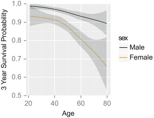
Fig. 20.15 Survival estimates for model stratified on sex, with interaction.

so that the desired survival curve could be read directly, at least to the nearest tabulated Xβˆ. For estimating survival at a fixed time, say two years, one only need to provide the constant Sˆ(t). The nomogram could even be adapted to include a nonlinear scale Sˆ(2)exp(Xβˆ) to allow direct computation of two-year survival.

20.13 R Functions

Harrell’s cpower, spower, and ciapower (in the Hmisc package) perform power calculations for Cox tests in follow-up studies. cpower computes power for a two-sample Cox (log-rank) test with random patient entry over a fixed duration and a given length of minimum follow-up. The expected number of events in each group is estimated by assuming exponential survival. cpower uses a slight modification of the method of Schoenfeld558 (see [501]). Separate specification of noncompliance in the active treatment arm and “drop-in” from the control arm into the active arm are allowed, using the method of Lachin and Foulkes.370 The ciapower function computes power of the Cox interaction test in a 2 ^≤ 2 setup using the method of Peterson and George.501 It does not take noncompliance into account. The spower function simulates power for two-sample tests (the log-rank test by default) allowing for very complex conditions such as continuously varying treatment effect and noncompliance probabilities.

The rms package cph function is a slight modification of the coxph function written by Terry Therneau (in his survival package to work in the rms framework. cph computes MLEs of Cox and stratified Cox PH models, overall score and likelihood ratio χ² statistics for the model, martingale residuals, the linear predictor (Xβˆ centered to have mean 0), and collinearity diagnostics. Efron, Breslow, and exact partial likelihoods are supported (although the exact likelihood is very computationally intensive if ties are frequent). The function also fits the Andersen–Gill23 generalization of the Cox PH model. This model allows for predictor values to change over time in the form of step functions as well as allowing time-dependent stratification (subjects can jump to different hazard function shapes). The Andersen–Gill formulation allows multiple events per subject and permits subjects to move in and out of risk at any desired time points. The latter feature allows time zero to have a more general definition. (See Section 9.5 for methods of adjusting the variance– covariance matrix of βˆ for dependence in the events per subject.) The printing function corresponding to cph prints the Nagelkerke index R² ^N described in Section 20.10, and has a latex option for better output. cph works in conjunction with the generic functions such as specs, predict, summary, anova, fastbw, which.influence, latex, residuals, coef, nomogram, and Predict described in Section 20.13, the same as the logistic regression function lrm does. For the purpose of plotting predicted survival at a single time, Predict has an additional argument time for plotting cph fits. It also has an argument loglog which if TRUE causes instead log-log survival to be plotted on the y-axis. cph has all the arguments described in Section 20.13 and some that are specific to it.

Similar to functions for psm, there are Survival, Quantile, and Mean functions which create other R functions to evaluate survival probabilities and perform other calculations, based on a cph fit with surv=TRUE. These functions, unlike all the others, allow polygon (linear interpolation) estimation of survival probabilities, quantiles, and mean survival time as an option. Quantile is the only automatic way for obtaining survival quantiles with cph. Quantile estimates will be missing when the survival curve does not extend long enough. Likewise, survival estimates will be missing for t > maximum follow-up time, when the last event time is censored. Mean computes the mean survival time if the last failure time in each stratum is uncensored. Otherwise, Mean may be used to compute restricted mean lifetime using a user-specified truncation point.334 Quantile and Mean are especially useful with plot and nomogram. Survival is useful with nomogram.

The R program below demonstrates how several cph-related functions work well with the nomogram function. Here predicted three-year survival probabilities and median survival time (when defined) are displayed against age and sex from the previously simulated dataset. The fact that a nonlinear effect interacts with a stratified factor is taken into account.

surv − Survival( f.ia)
surv.f − function(lp) surv (3, lp , stratum= ' sex=Female ' )
surv.m − function(lp) surv (3, lp , stratum= ' sex=Male ' )
quant − Quantile( f.ia)
med.f − function(lp) quant (.5 , lp , stratum= ' sex=Female ' )
med.m − function(lp) quant (.5 , lp , stratum= ' sex=Male ' )
at.surv − c(.01 , .05 , seq(.1 ,.9 ,by=.1), .95 , .98 , .99 , .999)
at.med − c(0, .5 , 1, 1.5 , seq(2, 14, by =2))
n − nomogram(f.ia , fun= list(surv.m , surv.f , med.m , med.f),
          funlabel=c( ' S(3 | Male) ' , ' S(3 | Female ) ' ,
                      ' Median (Male) ' , ' Median (Female ) ' ),
          fun.at =list (c(.8 ,.9 ,.95 ,.98 ,.99),
                       c(.1 ,.3 ,.5 ,.7 ,.8 ,.9 ,.95 ,.98),
                       c(8,10,12), c(1,2,4,8 ,12)))
plot(n, col.grid=FALSE , lmgp=.2)
latex (f.ia , file= ' ' , digits =3)

\[\text{Prob}\{T \ge t \mid \text{sex} = i\} = S\_i(t)^{e^{X\beta}}, \quad \text{where}\]

Xβˆ =

×1.8 +0.0493age ^× ².15≤10−⁶ (age ^× ³⁰.3)³ ⁺ ^× ².82≤10−⁵ (age ^× ⁴⁵.1)³ + +5.18≤10−⁵ (age ^× ⁵⁴.6)³ ⁺ ^× ².15≤10−⁵ (age ^× ⁶⁹.6)³ + +[Female][×0.0366age + 4.29≤10−⁵ (age ^× ³⁰.3)³ ⁺ ^× ⁰.00011(age ^× ⁴⁵.1)³ + +6.74≤10−⁵ (age ^× ⁵⁴.6)³ ⁺ ^× ².32≤10−⁷ (age ^× ⁶⁹.6)³ +]

and [c] = 1 if subject is in group c, 0 otherwise; (x)⁺ = x if x > 0, 0 otherwise.

20.13 R Functions 515

	t SMale(t)	SF emale(t)
0	1.000	1.000
1	0.993	0.902
2	0.984	0.825
3	0.975	0.725
4	0.967	0.648
5	0.956	0.576
6	0.947	0.520
7	0.938	0.481
8	0.928	0.432
9	0.920	0.395
10	0.909	0.358
11	0.904	0.314
12	0.892	0.268
13	0.886	0.223
14	0.877	0.203

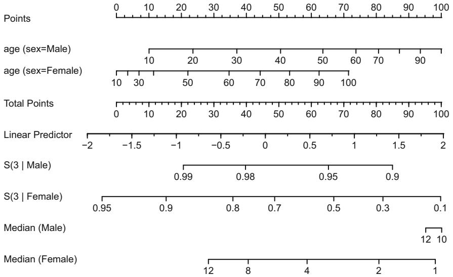
Fig. 20.16 Nomogram from a fitted stratified Cox model that allowed for interaction between age and sex, and nonlinearity in age. The axis for median survival time is truncated on the left where the median is beyond the last follow-up time.

rcspline.plot (lvef ,	d.time ,	event =cdeath ,	nk=3)
———————–	———-	—————–	——-

The corresponding smoothed martingale residual plot for LVEF in Figure 20.7 was created with

cox − cph(Surv(d.time , cdeath) ← lvef , iter.max =0)
res − resid(cox)
g ← loess(res ← lvef)
plot(g, coverage =0.95 , confidence =7, xlab="LVEF",
     ylab="Martingale Residual ")
g − ols(res ← rcs(lvef ,5))
plot(g, lvef=NA, add=T, lty =2)
lines(lowess (lvef , res , iter=0), lty =3)
legend (.3, 1.15 , c("loess Fit and 0.95 Confidence Bars",
                    "ols Spline Fit and 0.95 Confidence Limits",
                    "lowess Smoother "), lty =1:3, bty="n")

Because we desired residuals with respect to the omitted predictor LVEF, the parameter iter.max=0 had to be given to make cph stop the estimation process at the starting parameter estimates (default of zero). The effect of this is to ignore the predictors when computing the residuals; that is, to compute residuals from a flat line rather than the usual residuals from a fitted straight line.

The residuals function is a slight modification of Therneau’s residuals. coxph function to obtain martingale, Schoenfeld, score, deviance residuals, or approximate DFBETA or DFBETAS. Since martingale residuals are always stored by cph (assuming there are covariables present), residuals merely has to pick them off the fit object and reinsert rows that were deleted due to missing values. For other residuals, you must have stored the design matrix and Surv object with the fit by using …, x=TRUE, y=TRUE. Storing the design matrix with x=TRUE ensures that the same transformation parameters (e.g., knots) are used in evaluating the model as were used in fitting it. To use residuals you can use the abbreviation resid. See the help file for residuals for an example of how martingale residuals may be used to quickly plot univariable (unadjusted) relationships for several predictors.

Figure 20.10, which used smoothed scaled Schoenfeld partial residuals557 to estimate the form of a predictor’s log hazard ratio over time, was made with

Srv − Surv(dm.time ,cdeathmi )
cox − cph(Srv ← pi, x=T, y=T)
cox.zph (cox , "rank") # Test for PH for each column of X
res − resid(cox , "scaledsch ")
time − as.numeric (names(res))
# Use dimnames(res)[[1]] if more than one predictor
f − loess(res ← time , span=0.50)
plot(f, coverage =0.95 , confidence =7, xlab="t",
     ylab="Scaled Schoenfeld Residual ", ylim=c(-.1 ,.25))
lines(supsmu(time , res),lty=2)
legend (1.1,.21 ,c("loess Smoother with span=0.50 and 0.95 C.L.",
                 "Super Smoother "), lty =1:2, bty="n")

The computation and plotting of scaled Schoenfeld residuals could have been done automatically in this case by using the single command plot(cox.zph (cox)), although cox.zph defaults to plotting against the Kaplan–Meier transformation of follow-up time.

The hazard.ratio.plot function in rms repeatedly estimates Cox regression coefficients and confidence limits within time intervals. The log hazard ratios are plotted against the mean failure/censoring time within the interval. Figure 20.9 was created with

hazard.ratio.plot (pi, S) # S was Surv(dm.time , …)

If you have multiple degree of freedom factors, you may want to score them into linear predictors before using hazard.ratio.plot. The predict function with argument type=“terms” will produce a matrix with one column per factor to do this (Section 20.13).

Therneau’s cox.zph function implements Harrell’s Schoenfeld residual correlation test for PH. This function also stores results that can easily be passed to a plotting method for cox.zph to automatically plot smoothed residuals that estimate the effect of each predictor over time.

Therneau has also written an R function survdiff that compares two or more survival curves using the G × ρ family of rank tests (Harrington and Fleming273).

The rcorr.cens function in the Hmisc library computes the c index and the corresponding generalization of Somers’ Dxy rank correlation for a censored response variable. rcorr.cens also works for uncensored and binary responses (see ROC area in Section 10.8), although its use of all possible pairings makes it slow for this purpose. The survival package’s survConcordance has an ex- ²⁰ tremely fast algorithm for the c index and a fairly accurate estimator of its standard error.

The calibrate function for cph constructs a bootstrap or cross-validation optimism-corrected calibration curve for a single time point by resampling the differences between average Cox predicted survival and Kaplan–Meier estimates (see Section 20.11.1). But more precise is calibrate’s default method based on adaptive semiparametric regression discussed in the same section. Figure 20.11 is an example.

The validate function for cph fits validates several statistics describing Cox model fits—slope shrinkage, R² ^N, D, U, Q, and Dxy. The val.surv function can also be of use in externally validating a Cox model using the methods presented in Section 18.3.7.

20.14 Further Reading

1 Good general texts for the Cox PH model include Cox and Oakes,133 Kalbfleisch and Prentice,331 Lawless,382 Collett,114 Marubini and Valsecchi,444 and Klein and Moeschberger.350 Therneau and Grambsch604 describe the many ways the standard Cox model may be extended.
2 Cupples et al.141 and Marubini and Valsecchi [444, pp. 201–206] present good description of various methods of computing “adjusted survival curves.”
3 See Altman and Andersen15 for simpler approximate formulas. Cheng et al.103 derived methods for obtaining pointwise and simultaneous confidence bands for

S(t) for future subjects, and Henderson282 has a comprehensive discussion of the use of Cox models to estimate survival time for individual subjects.

4 Aalen2 and Valsecchi et al.625 discuss other residuals useful in graphically checking survival model assumptions. Le´on and Tsai400 derived residuals for estimating covariate transformations that are different from martingale residuals.
5 [411] has other methods for generating confidence intervals for martingale residual plots.
6 Lin et al.411 describe other methods of checking transformations using cumulative martingale residuals.
7 A parametric analysis of the VA dataset using linear splines and incorporating X ∼ t interactions is found in [361].
8 Winnett and Sasieni671 show how to use scaled Schoenfeld residuals in an iterative fashion to actually model effects that are not in proportional hazards.
9 See [233, 503] for some methods for obtaining confidence bands for Schoenfeld residual plots. Winnett and Sasieni670 discuss conditions in which the Grambsch–Therneau scaling of the Schoenfeld residuals does not perform adequately for estimating χ(t).
10 [475, 519] compared the power of the test for PH based on the correlation between failure time and Schoenfeld residuals with the power of several other tests.
11 See Lin et al.411 for another approach to deriving a formal test of PH using residuals. Other graphical methods for examining the PH assumption are due to Gray,236 who used hazard smoothing to estimate hazard ratios as a function of time, and Thaler,602 who developed a nonparametric estimator of the hazard ratio over time for time-dependent covariables. See Valsecchi et al.625 for other useful graphical assessments of PH.
12 A related test of constancy of hazard ratios may be found in [519]. Also, see Schemper547 for related methods.
13 See [547] for a variation of the standard Cox likelihood to allow for non-PH.
14 An excellent review of graphical methods for assessing PH may be found in Hess.290. Sahoo and Sengupta537 provide some new graphical methods for assessing PH irrespective of satisfaction of the other model assumptions.
15 Schemper547 provides a way to determine the effect of falsely assuming PH by comparing the Cox regression coefficient with a well-described average log hazard ratio. Zucker691 shows how dependent a weighted log-rank test is on the true hazard ratio function, when the weights are derived from a hypothesized hazard ratio function. Valsecchi et al.625 proposed a method that is robust to non-PH that occurs in the late follow-up period. Their method uses down-weighting of certain types of “outliers.” See Herndon and Harrell287 for a flexible parametric PH model with time-dependent covariables, which uses the restricted cubic spline function to specify Φ(t). Putter et al.518 and Muggeo and Tagliavia468 have nice approaches that use time-dependent covariates to model time interactions to allow non-proportional hazards. Perperoglou et al.498,499 developed a systematic approach that allows one to continuously vary the amount of non PH allowed, through the use of a structure matrix that connects predictors with functions of time. Schuabel et al.543 have a good exposition of internal time-dependent covariates.
16 See van Houwelingen and le Cessie [633, Eq. 61] and Verweij and van Houwelingen640 for an interesting index of cross-validated predictive accuracy. Schemper and Henderson552 relate explained variation to predictive accuracy in Cox models. Hielscher et al.291 compares and illustrates several measures of explained variation as does Choodari-Oskooei et al.106. Choodari-Oskooei et al.105 studied explained randomness and predictive accuracy measures.
17 See similar indexes in Schemper544 and a related idea in [633, Eq. 63]. Mandel, Galai, and Simchen436 presented a time-varying c index. See Korn and

Simon,365 Schemper and Stare,554 and Henderson282 for nice comparisons of various measures. Pencina and D’Agostino489 provide more details about the c index and derived new interval estimates. They also discussed the relationship between c and a version of Kendall’s γ. Pencina et al.491 found advantages of c. Uno et al.618 described exactly how c depends on the amount of censoring and proposed a new index, requiring one to choose a time cutoff, that is invariant to the amount of censoring. Henderson et al.283 discussed the benefits of using the probability of a serious prognostication error (e.g., being off by a factor of 2.0 or worse on the time scale) as an accuracy measure. Schemper550 shows that models with very important predictors can have very low absolute prediction ability, and he discusses measures of predictive accuracy from a general standpoint. Lawless and Yuan386 present prediction error estimators and confidence limits, focusing on such measures as error in predicted median or mean survival time. Schmid and Potapov555 studied the bias of several variations on the c index under non-proportional hazards and/or nonrandom censoring. G¨onen and Heller223 developed a c-index that is censoring-independent.

18 Altman and Royston18 have a good discussion of validation of prognostic models and present several examples of validation using a simple discrimination index. Thomas Gerds has an R package pec that provides many validation methods and accuracy indexes.
19 Kattan et al.338 describe how to make nomograms for deriving predicted survival probabilities when there are competing risks.
20 Hielscher et al.291 provides an overview of software for computing accuracy indexes with censored data.

Chapter 21 Case Study in Cox Regression

21.1 Choosing the Number of Parameters and Fitting the Model

Consider the randomized trial of estrogen for treatment of prostate cancer87 described in Chapter 8. Let us now develop a model for time until death (of any cause). There are 354 deaths among the 502 patients. To be able to efficiently estimate treatment benefit, to test for differential treatment effect, or to estimate prognosis or absolute treatment benefit for individual patients, we need a multivariable survival model. In this case study we do not make use of data reductions obtained in Chapter 8 but show simpler (partial) approaches to data reduction. We do use the transcan results for imputation.

First let’s assess the wisdom of fitting a full additive model that does not assume linearity of effect for any predictor. Categorical predictors are expanded using dummy variables. For pf we could lump the last two categories as before since the last category has only two patients. Likewise, we could combine the last two levels of ekg. Continuous predictors are expanded by fitting four-knot restricted cubic spline functions, which contain two nonlinear terms and thus have a total of three d.f. Table 21.1 defines the candidate predictors and lists their d.f. The variable stage is not listed as it can be predicted with high accuracy from sz,sg,ap,bm (stage could have been used as a predictor for imputing missing values on sz, sg). There are a total of 36 candidate d.f. that should not be artificially reduced by “univariable screening” or graphical assessments of association with death. This is about 1/10 as many predictor d.f. as there are deaths, so there is some hope that a fitted model may validate. Let us also examine this issue by estimating the amount of shrinkage using Equation 4.3. We first use transcan impute missing data.

require(rms)

^© Springer International Publishing Switzerland 2015 F.E. Harrell, Jr., Regression Modeling Strategies, Springer Series in Statistics, DOI 10.1007/978-3-319-19425-7 21

Predictor			Name d.f. Original Levels
Dose of estrogen	rx	3	placebo, 0.2, 1.0, 5.0 mg
			estrogen
Age in years	age	3
Weight index: wt(kg)×ht(cm)+200	wt	3
Performance rating	pf	2	normal, in bed < 50% of
			time, in bed > 50%, in
			bed always
History of cardiovascular disease	hx	1	present/absent
Systolic blood pressure/10	sbp	3
Diastolic blood pressure/10	dbp	3
Electrocardiogram code	ekg	5	normal, benign, rhythm
			disturb., block, strain,
			old myocardial infarction,
			new MI
Serum hemoglobin (g/100ml)	hg	3
Tumor size (cm2)	sz	3
Stage/histologic grade combination	sg	3
Serum prostatic acid phosphatase	ap	3
Bone metastasis	bm	1	present/absent

Table 21.1 Initial allocation of degrees of freedom

getHdata(prostate)
levels ( prostate$ekg)[ levels ( prostate$ekg) %in%
                       c ( ' old MI ' , ' recent MI ' )] − ' MI '
# combines last 2 levels and uses a new name , MI
prostate$pf.coded − as.integer (prostate$pf)
# save original pf , re-code to 1-4
levels ( prostate$pf) − c(levels ( prostate$pf )[1:3],
                            levels ( prostate$pf )[3])
# combine last 2 levels
w − transcan(← sz + sg + ap + sbp + dbp + age +
               wt + hg + ekg + pf + bm + hx , imputed= TRUE ,
               data=prostate , pl= FALSE , pr= FALSE )
attach ( prostate)
sz − impute (w, sz , data = prostate)
sg − impute (w, sg , data = prostate)
age − impute (w, age ,data = prostate)
wt − impute (w, wt , data = prostate)
ekg − impute (w, ekg ,data = prostate)
dd − datadist(prostate ); options(datadist= ' dd ' )

units (dtime ) − ' Month '
S − Surv(dtime , status != ' alive ' )
f − cph(S ← rx + rcs(age ,4) + rcs(wt ,4) + pf + hx +
         rcs(sbp ,4) + rcs(dbp ,4) + ekg + rcs(hg ,4) +
         rcs(sg ,4) + rcs(sz ,4) + rcs(log(ap),4) + bm)

print (f, latex =TRUE , coefs=FALSE)

Cox Proportional Hazards Model

cph(formula = S ~ rx + rcs(age, 4) + rcs(wt, 4) + pf + hx
    + rcs(sbp, 4) + rcs(dbp, 4) + ekg + rcs(hg, 4)
    + rcs(sg, 4) + rcs(sz, 4) + rcs(log(ap), 4) + bm)

		Model Tests		Discrimination
				Indexes
Obs	502	χ2 LR	136.22	R2	0.238
Events	354	d.f.	36	Dxy	0.333
Center -2.9933		χ2) Pr(>	0.0000	g	0.787
		χ2 Score	143.62	gr	2.196
		χ2) Pr(>	0.0000

The likelihood ratio χ² statistic is 136.2 with 36 d.f. This test is highly significant so some modeling is warranted. The AIC value (on the χ² scale) is 136.2×2≤36 = 64.2. The rough shrinkage estimate is 0.74 (100.2/136.2) so we estimate that 0.26 of the model fitting will be noise, especially with regard to calibration accuracy. The approach of Spiegelhalter582 is to fit this full model and to shrink predicted values. We instead try to do data reduction (blinded to individual χ² statistics from the above model fit) to see if a reliable model can be obtained without shrinkage. A good approach at this point might be to do a variable clustering analysis followed by single degree of freedom scoring for individual predictors or for clusters of predictors. Instead we do an informal data reduction. The strategy is described in Table 21.2. For ap, more exploration is desired to be able to model the shape of effect with such a highly skewed distribution. Since we expect the tumor variables to be strong prognostic factors we retain them as separate variables. No assumption is made for the dose-response shape for estrogen, as there is reason to expect a non-monotonic effect due to competing risks for cardiovascular death.

heart − hx + ekg %nin% c( ' normal ' , ' benign ' )
label (heart ) − ' Heart Disease Code '
map − (2*dbp + sbp)/3
label (map) − ' Mean Arterial Pressure/10 '
dd − datadist (dd , heart , map)
f − cph(S ← rx + rcs(age ,4) + rcs(wt ,3) + pf.coded +

Variables	Reductions	d.f. Saved
wt	Assume variable not important enough	1
	for 4 knots; use 3 knots
pf	Assume linearity	1
hx,ekg	Make new 0,1,2 variable and assume	5
	linearity: 2 = hx and ekg not normal
	or benign, 1 = either, 0 = none
sbp,dbp	Combine into mean arterial bp and	4
	use 3 knots: map = (2 dbp + sbp)/3
sg	Use 3 knots	1
sz	Use 3 knots	1
ap	Look at shape of effect of ap in detail,	×1
	and take log before expanding as spline
	to achieve numerical stability: add 1 knots

Table 21.2 Final allocation of degrees of freedom

heart + rcs(map ,3) + rcs(hg ,4) + rcs(sg ,3) + rcs(sz ,3) + rcs(log(ap),5) + bm , x=TRUE , y=TRUE , surv=TRUE , time.inc =5*12) print (f, latex =TRUE , coefs =3)

Cox Proportional Hazards Model

cph(formula = S ~ rx + rcs(age, 4) + rcs(wt, 3) + pf.coded +
    heart + rcs(map, 3) + rcs(hg, 4) + rcs(sg, 3) +
    rcs(sz, 3) + rcs(log(ap), 5) + bm, x = TRUE, y = TRUE,
    surv = TRUE, time.inc = 5 * 12)

		Model Tests		Discrimination
		Indexes
Obs	502	χ2 LR	118.37	R2	0.210
Events	354	d.f.	24	Dxy	0.321
Center -2.4307		χ2) Pr(>	0.0000	g	0.717
		χ2 Score	125.58	gr	2.049
		χ2) Pr(>	0.0000

	Coef	S.E.	Wald Z	Pr(> Z )
rx=0.2 mg estrogen	-0.0002	0.1493	0.00	0.9987
rx=1.0 mg estrogen	-0.4160	0.1657	-2.51	0.0121
rx=5.0 mg estrogen	-0.1107	0.1571	-0.70	0.4812

Table 21.3 Wald Statistics for S
————————————-	–

	χ2	d.f.	P
rx	8.01	3	0.0459
age	13.84	3	0.0031
Nonlinear	9.06	2	0.0108
wt	8.21	2	0.0165
Nonlinear	2.54	1	0.1110
pf.coded	3.79	1	0.0517
heart	23.51	1	< 0.0001
map	0.04	2	0.9779
Nonlinear	0.04	1	0.8345
hg	12.52	3	0.0058
Nonlinear	8.25	2	0.0162
sg	1.64	2	0.4406
Nonlinear	0.05	1	0.8304
sz	12.73	2	0.0017
Nonlinear	0.06	1	0.7990
ap	6.51	4	0.1639
Nonlinear	6.22	3	0.1012
bm	0.03	1	0.8670
TOTAL NONLINEAR	23.81	11	0.0136
TOTAL	119.09	24	< 0.0001

# x, y for predict , validate , calibrate;
# surv, time.inc for calibrate
latex(anova (f), file= ' ' ,label= ' tab:coxcase-anova1 ' )# Table 21.3

The total savings is thus 12 d.f. The likelihood ratio χ² is 118 with 24 d.f., with a slightly improved AIC of 70. The rough shrinkage estimate is slightly better at 0.80, but still worrisome. A further data reduction could be done, such as using the transcan transformations determined from self-consistency of predictors, but we stop here and use this model.

From Table 21.3 there are 11 parameters associated with nonlinear effects, and the overall test of linearity indicates the strong presence of nonlinearity for at least one of the variables age,wt,map,hg,sz,sg,ap. There is no strong evidence for a difference in survival time between doses of estrogen.

21.2 Checking Proportional Hazards

Now that we have a tentative model, let us examine the model’s distributional assumptions using smoothed scaled Schoenfeld residuals. A messy detail is how to handle multiple regression coefficients per predictor. Here we do an approximate analysis in which each predictor is scored by adding up all that predictor’s terms in the model, to transform that predictor to optimally relate to the log hazard (at least if the shape of the effect does not change with time). In doing this we are temporarily ignoring the fact that the individual regression coefficients were estimated from the data. For dose of estrogen, for example, we code the effect as 0 (placebo), ×0.00025 (0.2 mg), ×0.416 (1.0 mg), and ×0.111 (5.0 mg), and age is transformed using its fitted spline function. In the rms package the predict function easily summarizes multiple terms and produces a matrix (here, z) containing the total effects for each predictor. Matrix factors can easily be included in model formulas.

z − predict(f, type= ' terms ' )
# required x=T above to store design matrix
f.short − cph(S ← z, x=TRUE , y= TRUE)
# store raw x, y so can get residuals

The fit f.short based on the matrix of single d.f. predictors z has the same LR χ² of 118 as the fit f, but with a falsely low 11 d.f. All regression coefficients are unity.

Now we compute scaled Schoenfeld residuals separately for each predictor and test the PH assumption using the “correlation with time” test. Also plot smoothed trends in the residuals. The plot method for cox.zph objects uses cubic splines to smooth the relationship.

phtest − cox.zph( f.short , transform= ' identity ' )
phtest
            rho chisq p
rx 0.10232 4.00823 0.0453
age -0.05483 1.05850 0.3036
wt 0.01838 0.11632 0.7331
pf.coded -0.03429 0.41884 0.5175
heart 0.02650 0.30052 0.5836
map 0.02055 0.14135 0.7069
hg -0.00362 0.00511 0.9430
sg -0.05137 0.94589 0.3308
sz -0.01554 0.08330 0.7729
ap 0.01720 0.11858 0.7306
bm 0.04957 0.95354 0.3288
GLOBAL NA 7.18985 0.7835

plot(phtest , var= ' rx ' ) # Figure 21.1

Perhaps only the drug effect significantly changes over time (P = 0.05 for testing the correlation rho between the scaled Schoenfeld residual and time), but when a global test of PH is done penalizing for 11 d.f., the P value is 0.78. A graphical examination of the trends doesn’t find anything interesting for the last 10 variables. A residual plot is drawn for rx alone and is shown in Figure 21.1. We ignore the possible increase in effect of estrogen over time. If this non-PH is real, a more accurate model might be obtained by stratifying on rx or by using a time ≤ rx interaction as a time-dependent covariable.

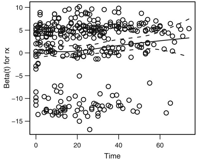
Fig. 21.1 Raw and spline-smoothed scaled Schoenfeld residuals for dose of estrogen, nonlinearly coded from the Cox model fit, with ± 2 standard errors.

21.3 Testing Interactions

Note that the model has several insignificant predictors. These are not deleted, as that would not improve predictive accuracy and it would make accurate confidence intervals hard to obtain. At this point it would be reasonable to test prespecified interactions. Here we test all interactions with dose. Since the multiple terms for many of the predictors (and for rx) make for a great number of d.f. for testing interaction (and a loss of power), we do approximate tests on the data-driven coding of predictors. P-values for these tests are likely to be somewhat anti-conservative.

z.dose − z[,"rx"] # same as saying z[,1] - get first column
z.other − z[,-1] # all but the first column of z
f.ia − cph(S ← z.dose * z.other) # Figure 21.4:
latex (anova (f.ia), file= ' ' , label= ' tab:coxcase-anova2 ' )

The global test of additivity in Table 21.4 has P = 0.27, so we ignore the interactions (and also forget to penalize for having looked for them below!).

21.4 Describing Predictor Effects

Let us plot how each predictor is related to the log hazard of death, including 0.95 confidence bands. Note in Figure 21.2 that due to a peculiarity of the Cox model the standard error of the predicted Xβˆ is zero at the reference values (medians here, for continuous predictors).

	χ2	d.f.	P
z.dose (Factor+Higher Order Factors)	18.74	11	0.0660
All Interactions	12.17	10	0.2738
z.other (Factor+Higher Order Factors)	125.89	20	< 0.0001
All Interactions	12.17	10	0.2738
z.dose ≤ z.other (Factor+Higher Order Factors)	12.17	10	0.2738
TOTAL	129.10	21	< 0.0001

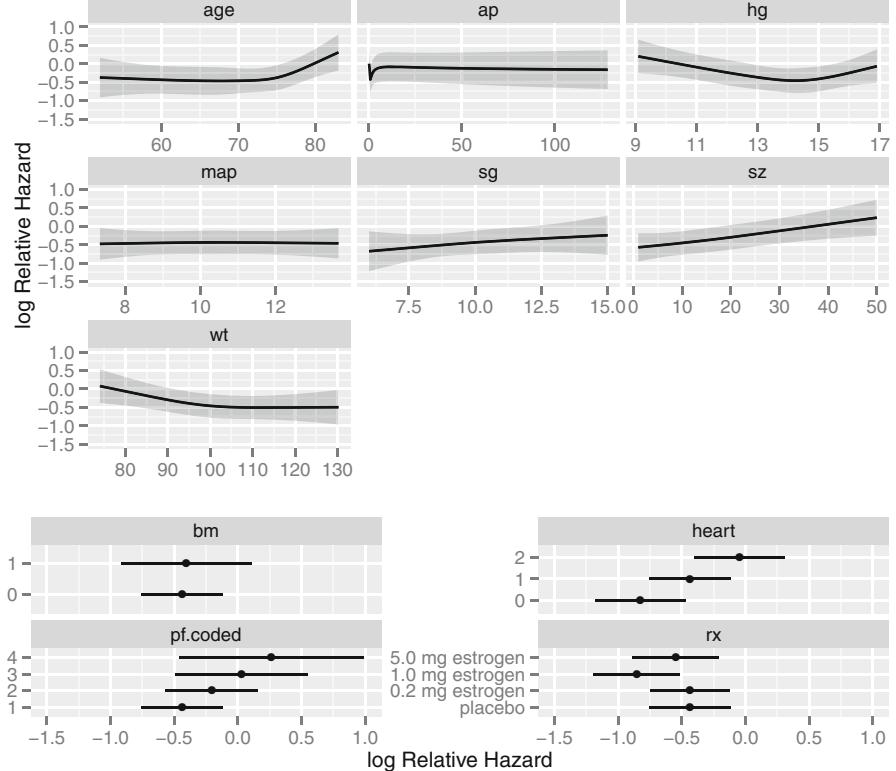
Fig. 21.2 Shape of each predictor on log hazard of death. Y -axis shows Xχˆ, but the predictors not plotted are set to reference values. Note the highly non-monotonic relationship with ap, and the increased slope after age 70 which occurs in outcome models for various diseases.

ggplot ( Predict(f), sepdiscrete= ' vertical ' , nlevels=4,
        vnames = ' names ' ) # Figure 21.2

21.5 Validating the Model

We first validate this model for Somers’ Dxy rank correlation between predicted log hazard and observed survival time, and for slope shrinkage. The bootstrap is used (with 300 resamples) to penalize for possible overfitting, as discussed in Section 5.3.

set.seed (1) # so can reproduce results
v − validate(f, B =300)

Divergence or singularity in 83 samples

latex (v, file= ' ' )

	Index Original Training		Test	Optimism Corrected	n
	Sample	Sample	Sample		Index
Dxy	0.3208	0.3454	0.2954	0.0500	0.2708 217
R2	0.2101	0.2439	0.1754	0.0685	0.1417 217
Slope	1.0000	1.0000	0.7941	0.2059	0.7941 217
D	0.0292	0.0348	0.0238	0.0110	0.0182 217
U	×0.0005	×0.0005	0.0023	×0.0028	0.0023 217
Q	0.0297	0.0353	0.0216	0.0138	0.0159 217
g	0.7174	0.7918	0.6273	0.1645	0.5529 217

Here “training” refers to accuracy when evaluated on the bootstrap sample used to fit the model, and “test” refers to the accuracy when this model is applied without modification to the original sample. The apparent Dxy is 0.32, but a better estimate of how well the model will discriminate prognoses in the future is Dxy = 0.27. The bootstrap estimate of slope shrinkage is 0.79, close to the simple heuristic estimate. The shrinkage coefficient could easily be used to shrink predictions to yield better calibration.

Finally, we validate the model (without using the shrinkage coefficient) for calibration accuracy in predicting the probability of surviving five years. The bootstrap is used to estimate the optimism in how well predicted five-year survival from the final Cox model tracks flexible smooth estimates, without any binning of predicted survival probabilities or assuming proportional hazards.

\[\begin{array}{l|lll} \hline \mathtt{c1} \leftarrow & \mathtt{call} \, \mathtt{b1} \, \mathtt{c2} \, \mathtt{d1} & \mathtt{s2} \, \mathtt{d1} & \mathtt{u} = \mathtt{5} \, \mathtt{t1} \, \mathtt{2} & \mathtt{m} \, \mathtt{x} \, \mathtt{d1} \, \mathtt{m} = \mathtt{t} \\\\ \hline \\ \mathtt{Ung\\_Cox\\_purviaal\\_util\\_tutin\\_st\\_6} & \mathtt{t} \, \mathtt{d1} \, \mathtt{s} & \mathtt{t} \\\\ \hline \\ \mathtt{p1} \, \mathtt{t} \, \mathtt{t} \, \mathtt{d1} & \mathtt{s} \, \mathtt{b} \, \mathtt{t} \, \mathtt{t} \, \mathtt{l} \, \mathtt{s} & \mathtt{F} \, \mathtt{d1} \, \mathtt{s} & \mathtt{t} \\\\ \hline \\ \mathtt{p1} \, \mathtt{t} \, \mathtt{t} \, \mathtt{d1} & \mathtt{s} \, \mathtt{b} \, \mathtt{t} \, \mathtt{t} \, \mathtt{l} \, \mathtt{s} & \mathtt{F} \, \mathtt{d} \, \mathtt{y} \, \mathtt{r} \, \mathtt{e} & \mathtt{21} \, \mathtt{3} \\\\ \hline \end{array}\]

0.0 0.1 0.2 0.3 0.4 0.5 0.6 0.7 0.0 0.1 0.2 0.3 0.4 0.5 0.6 0.7 Predicted 60 Month Survival Fraction Surviving 60 Month

Fig. 21.3 Bootstrap estimate of calibration accuracy for 5-year estimates from the final Cox model, using adaptive linear spline hazard regression361. The line nearer the ideal line corresponds to apparent predictive accuracy. The blue curve corresponds to bootstrap-corrected estimates.

The estimated calibration curves are shown in Figure 21.3, similar to what was done in Figure 19.11. Bootstrap calibration demonstrates some overfitting, consistent with regression to the mean. The absolute error is appreciable for 5-year survival predicted to be very low or high.

21.6 Presenting the Model

To present point and interval estimates of predictor effects we draw a hazard ratio chart (Figure 21.4), and to make a final presentation of the model we draw a nomogram having multiple “predicted value” axes. Since the ap relationship is so non-monotonic, use a 20 : 1 hazard ratio for this variable.

plot(summary (f, ap=c(1,20)), log=TRUE , main= ' ' ) # Figure 21.4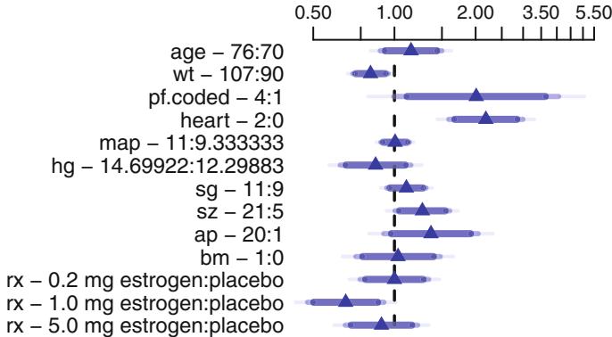

Fig. 21.4 Hazard ratios and multi-level confidence bars for effects of predictors in model, using default ranges except for ap

The ultimate graphical display for this model will be a nomogram relating the predictors to Xβˆ, estimated three– and five-year survival probabilities and median survival time. It is easy to add as many “output” axes as desired to a nomogram.

surv − Survival(f)
surv3 − function (x) surv(3*12,lp=x)
surv5 − function (x) surv(5*12,lp=x)
quan − Quantile(f)
med − function (x) quan(lp=x)/12
ss − c(.05 ,.1,.2,.3,.4,.5,.6,.7,.8,.9,.95)
nom − nomogram (f, ap=c(.1,.5 ,1,2,3,4,5,10,20,30 ,40),
                fun=list(surv3 , surv5 , med),
                funlabel =c( ' 3-year Survival ' , ' 5-year Survival ' ,
                   ' Median Survival Time (years) ' ),
                fun.at=list(ss, ss, c(.5 ,1:6)))
plot(nom , xfrac=.65 , lmgp=.35) # Figure 21.5

21.7 Problems

Perform Cox regression analyses of survival time using the Mayo Clinic PBC dataset described in Section 8.9. Provide model descriptions, parameter estimates, and conclusions.

Assess the nature of the association of several predictors of your choice. For polytomous predictors, perform a log-rank-type score test (or k-sample ANOVA extension if there are more than two levels). For continuous predictors, plot a smooth curve that estimates the relationship between the predictor and the log hazard or log–log survival. Use both parametric and nonparametric (using martingale residuals) approaches. Make a test of H⁰ : predictor is not associated with outcome versus H^a : predictor

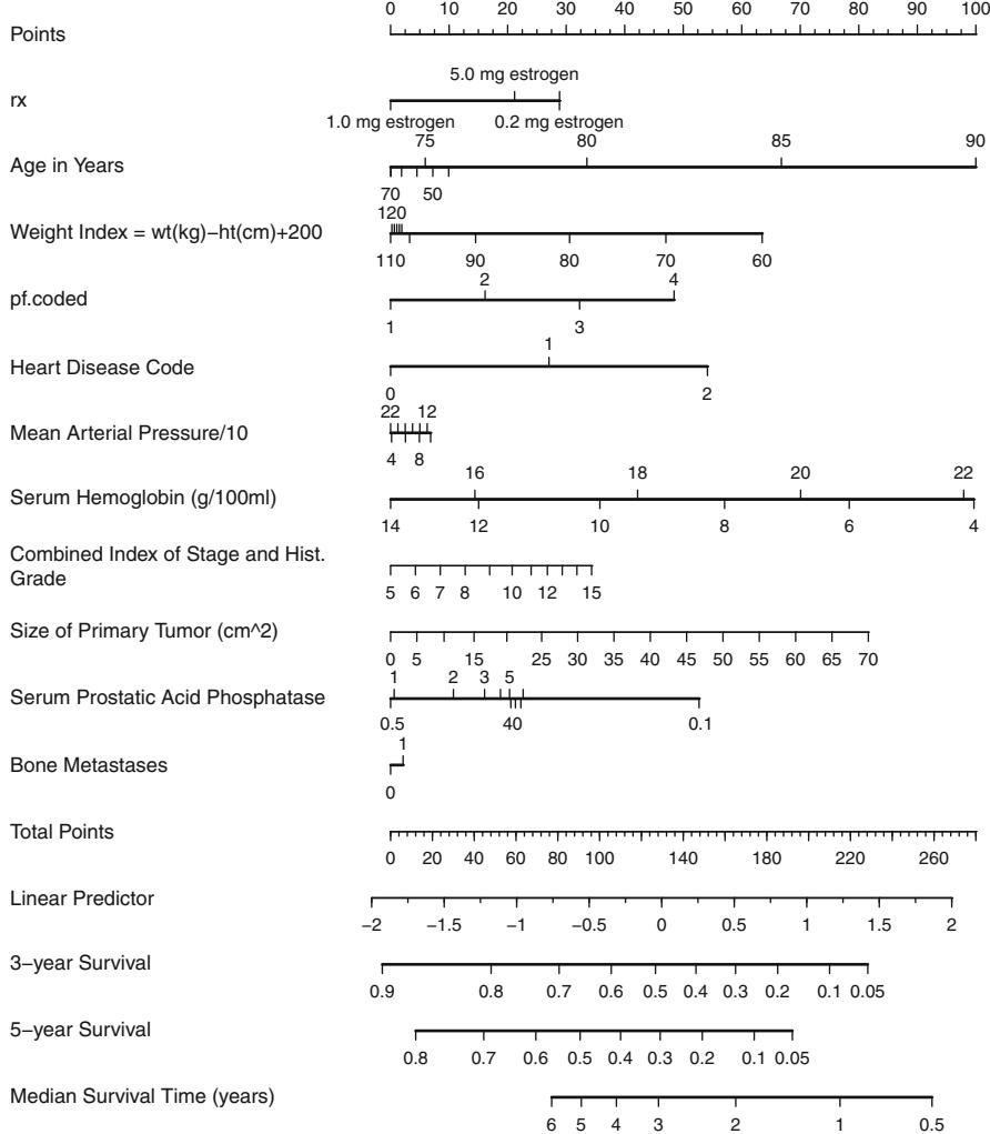
Fig. 21.5 Nomogram for predicting death in prostate cancer trial

is associated (by a smooth function). The test should have more than 1 d.f. If there is no evidence that the predictor is associated with outcome. Make a formal test of linearity of each remaining continuous predictor. Use restricted cubic spline functions with four knots. If you feel that you can’t narrow down the number of candidate predictors without examining the outcomes, and the number is too great to be able to derive a reliable model, use a data reduction technique and combine many of the variables into a summary index.

21.7 Problems 533

1. For factors that remain, assess the PH assumption using at least two methods, after ensuring that continuous predictors are transformed to be as linear as possible. In addition, for polytomous predictors, derive log cumulative hazard estimates adjusted for continuous predictors that do not assume anything about the relationship between the polytomous factor and survival.
1. Derive a final Cox PH model. Stratify on polytomous factors that do not satisfy the PH assumption. Decide whether to categorize and stratify on continuous factors that may strongly violate PH. Remember that in this case you can still model the continuous factor to account for any residual regression after adjusting for strata intervals. Include an interaction between two predictors of your choosing. Interpret the parameters in the final model. Also interpret the final model by providing some predicted survival curves in which an important continuous predictor is on the x-axis, predicted survival is on the y-axis, separate curves are drawn for levels of another factor, and any other factors in the model are adjusted to specified constants or to the grand mean. The estimated survival probabilities should be computed at t = 730 days.
1. Verify, in an unbiased fashion, your “final” model, for either calibration or discrimination. Validate intermediate steps, not just the final parameter estimates.

Appendix A Datasets, R Packages, and Internet Resources

Central Web Site and Datasets

The web site for information related to this book is biostat.mc.vanderbilt. edu/rms, and a related web site for a full-semester course based on the book is http://biostat.mc.vanderbilt.edu/CourseBios330. The main site contains links to several other web sites and a link to the dataset repository that holds most of the datasets mentioned in the text for downloading. These datasets are in fully annotated R save (.sav suffixes) files^a; some of these are also available in other formats. The datasets were selected because of the variety of types of response and predictor variables, sample size, and numbers of missing values. In R they may be read using the load function, load(url()) to read directly from the Web, or by using the Hmisc package’s getHdata function to do the same (as is done in code in the case studies). From the web site there are links to other useful dataset sources. Links to presentations and technical reports related to the text are also found on this site, as is information for instructors for obtaining quizzes and answer sheets, extra problems, and solutions to these and to many of the problems in the text. Details about short courses based on the text are also found there. The main site also has Chapter 7 from the first edition, which is a case study in ordinary least squares modeling.

R Packages

The rms package written by the author maintains detailed information about a model’s design matrix so that many analyses using the model fit are automated. rms is a large package of R functions. Most of the functions in rms analyze model fits, validate them, or make presentation graphics from them,

^a By convention these should have had .rda suffixes.

F.E. Harrell, Jr., Regression Modeling Strategies, Springer Series in Statistics, DOI 10.1007/978-3-319-19425-7

but the packages also contain special model–fitting functions for binary and ordinal logistic regression (optionally using penalized maximum likelihood), unpenalized ordinal regression with a variety of link functions, penalized and unpenalized least squares, and parametric and semiparametric survival models. In addition, rms handles quantile regression and longitudinal analysis using generalized least squares. The rms package pays special attention to computing predicted values in that design matrix attributes (e.g., knots for splines, categories for categorical predictors) are “remembered” so that predictors are properly transformed while predictions are being generated. The functions makes extensive use of a wealth of survival analysis software written by Terry Therneau of the Mayo Foundation. This survival package is a standard part of R.

The author’s Hmisc package contains other miscellaneous functions used in the text. These are functions that do not operate on model fits that used the enhanced design attributes stored by the rms package. Functions in Hmisc include facilities for data reduction, imputation, power and sample size calculation, advanced table making, recoding variables, translating SAS datasets into R data frames while preserving all data attributes (including variable and value labels and special missing values), drawing and annotating plots, and converting certain ^R objects to LATEX371 typeset form. The latter capability, provided by a family of latex functions, completes the conversion to LATEX of many of the objects created by rms. The packages contain several LATEX methods that create LATEX code for typesetting model fits in algebraic notation, for printing ANOVA and regression effect (e.g., odds ratio) tables, and other applications. The LATEX methods were used extensively in the text, especially for writing restricted cubic spline function fits in simplest notation.

The latest version of the rms package is available from CRAN (see below). It is necessary to install the Hmisc package in order to use rms package. The Web site also contains more in-depth overviews of the packages, which run on UNIX, Linux, Mac, and Microsoft Windows systems. The packages may be automatically downloaded and installed using R’s install.packages function or using menus under R graphical user interfaces.

R-help, CRAN, and Discussion Boards

To subscribe to the highly informative and helpful R-help e-mail group, see the Web site. R-help is appropriate for asking general questions about R including those about finding or writing functions to do specific analyses (for questions specific to a package, contact the author of that package). Another resource is the CRAN repository at <www.r-project.org>. Another excellent resource for askings questions about R is <stackoverflow.com/questions/tagged/r>. There is a Google group regmod devoted to the book and courses.

Multiple Imputation

The Impute E-mail list maintained by Juned Siddique of Northwestern University is an invaluable source of information regarding missing data problems. To subscribe to this list, see the Web site. Other excellent sources of online information are Joseph Schafer’s “Multiple Imputation Frequently Asked Questions” site and Stef van Buuren and Karin Oudshoorn’s “Multiple Imputation Online” site, for which links exist on the main Web site.

Bibliography

An extensive annotated bibliography containing all the references in this text as well as other references concerning predictive methods, survival analysis, logistic regression, prognosis, diagnosis, modeling strategies, model validation, practical Bayesian methods, clinical trials, graphical methods, papers for teaching statistical methods, the bootstrap, and many other areas may be found at http://www.citeulike.org/user/harrelfe.

SAS

SAS macros for fitting restricted cubic splines and for other basic operations are freely available from the main Web site. The Web site also has notes on SAS usage for some of the methods presented in the text.

References

Numbers following ≡ are page numbers of citations.

1. O. O. Aalen. Nonparametric inference in connection with multiple decrement models. Scan J Stat, 3:15–27, 1976. ↑413
1. O. O. Aalen. Further results on the non-parametric linear regression model in survival analysis. Stat Med, 12:1569–1588, 1993. ↑518
1. O. O. Aalen, E. Bjertness, and T. Sønju. Analysis of dependent survival data applied to lifetimes of amalgam fillings. Stat Med, 14:1819–1829, 1995. ↑421
1. M. Abrahamowicz, T. MacKenzie, and J. M. Esdaile. Time-dependent hazard ratio: Modeling and hypothesis testing with applications in lupus nephritis. JAMA, 91:1432–1439, 1996. ↑501
1. A. Agresti. A survey of models for repeated ordered categorical response data. Stat Med, 8:1209–1224, 1989. ↑324
1. A. Agresti. Categorical data analysis. Wiley, Hoboken, NJ, second edition, 2002. ↑271
1. H. Ahn and W. Loh. Tree-structured proportional hazards regression modeling. Biometrics, 50:471–485, 1994. ↑41, 178
1. J. Aitchison and S. D. Silvey. The generalization of probit analysis to the case of multiple responses. Biometrika, 44:131–140, 1957. ↑324
1. K. Akazawa, T. Nakamura, and Y. Palesch. Power of logrank test and Cox regression model in clinical trials with heterogeneous samples. Stat Med, 16:583– 597, 1997. ↑4
1. O. O. Al-Radi, F. E. Harrell, C. A. Caldarone, B. W. McCrindle, J. P. Jacobs, M. G. Williams, G. S. Van Arsdell, and W. G. Williams. Case complexity scores in congenital heart surgery: A comparative study of the Aristotal Basic Complexity score and the Risk Adjustment in Congenital Heart Surg (RACHS-1) system. J Thorac Cardiovasc Surg, 133:865–874, 2007. ↑215
1. J. M. Alho. On the computation of likelihood ratio and score test based confidence intervals in generalized linear models. Stat Med, 11:923–930, 1992. ↑ 214
1. P. D. Allison. Missing Data. Sage University Papers Series on Quantitative Applications in the Social Sciences, 07-136. Sage, Thousand Oaks CA, 2001. ↑ 49, 58
13. D. G. Altman. Categorising continuous covariates (letter to the editor). Brit J Cancer, 64:975, 1991. ↑11, 19
1. D. G. Altman. Suboptimal analysis using ‘optimal’ cutpoints. Brit J Cancer, 78:556–557, 1998. ↑19
1. D. G. Altman and P. K. Andersen. A note on the uncertainty of a survival probability estimated from Cox’s regression model. Biometrika, 73:722–724, 1986. ↑11, 517
1. D. G. Altman and P. K. Andersen. Bootstrap investigation of the stability of a Cox regression model. Stat Med, 8:771–783, 1989. ↑68, 70, 341
1. D. G. Altman, B. Lausen, W. Sauerbrei, and M. Schumacher. Dangers of using ‘optimal’ cutpoints in the evaluation of prognostic factors. J Nat Cancer Inst, 86:829–835, 1994. ↑11, 19, 20
1. D. G. Altman and P. Royston. What do we mean by validating a prognostic model? Stat Med, 19:453–473, 2000. ↑6, 122, 519
1. B. Altschuler. Theory for the measurement of competing risks in animal experiments. Math Biosci, 6:1–11, 1970. ↑413
1. C. F. Alzola and F. E. Harrell. An Introduction to S and the Hmisc and Design Libraries, 2006. Electronic book, 310 pages. ↑129
1. G. Ambler, A. R. Brady, and P. Royston. Simplifying a prognostic model: a simulation study based on clinical data. Stat Med, 21(24):3803–3822, Dec. 2002. ↑121
1. F. Ambrogi, E. Biganzoli, and P. Boracchi. Estimates of clinically useful measures in competing risks survival analysis. Stat Med, 27:6407–6425, 2008. ↑ 421
1. P. K. Andersen and R. D. Gill. Cox’s regression model for counting processes: A large sample study. Ann Stat, 10:1100–1120, 1982. ↑418, 513
1. G. L. Anderson and T. R. Fleming. Model misspecification in proportional hazards regression. Biometrika, 82:527–541, 1995. ↑4
1. J. A. Anderson. Regression and ordered categorical variables. J Roy Stat Soc B, 46:1–30, 1984. ↑324
1. J. A. Anderson and P. R. Philips. Regression, discrimination and measurement models for ordered categorical variables. Appl Stat, 30:22–31, 1981. ↑324
1. J. A. Anderson and A. Senthilselvan. A two-step regression model for hazard functions. Appl Stat, 31:44–51, 1982. ↑495, 499, 501
1. D. F. Andrews and A. M. Herzberg. Data. Springer-Verlag, New York, 1985. ↑ 161
1. E. Arjas. A graphical method for assessing goodness of fit in Cox’s proportional hazards model. J Am Stat Assoc, 83:204–212, 1988. ↑420, 495, 502
1. H. R. Arkes, N. V. Dawson, T. Speroff, F. E. Harrell, C. Alzola, R. Phillips, N. Desbiens, R. K. Oye, W. Knaus, A. F. Connors, and T. Investigators. The covariance decomposition of the probability score and its use in evaluating prognostic estimates. Med Decis Mak, 15:120–131, 1995. ↑257
1. B. G. Armstrong and M. Sloan. Ordinal regression models for epidemiologic data. Am J Epi, 129:191–204, 1989. See letter to editor by Peterson. ↑319, 320, 321, 324
1. D. Ashby, C. R. West, and D. Ames. The ordered logistic regression model in psychiatry: Rising prevalence of dementia in old people’s homes. Stat Med, 8:1317–1326, 1989. ↑324
1. A. C. Atkinson. A note on the generalized information criterion for choice of a model. Biometrika, 67:413–418, 1980. ↑69, 204
1. P. C. Austin. A comparison of regression trees, logistic regression, generalized additive models, and multivariate adaptive regression splines for predicting AMI mortality. Stat Med, 26:2937–2957, 2007. ↑41
35. P. C. Austin. Bootstrap model selection had similar performance for selecting authentic and noise variables compared to backward variable elimination: a simulation study. J Clin Epi, 61:1009–1017, 2008. ↑70
1. P. C. Austin and E. W. Steyerberg. Events per variable (EPV) and the relative performance of different strategies for estimating the out-of-sample validity of logistic regression models. Statistical methods in medical research, Nov. 2014. ↑ 112
1. P. C. Austin and E. W. Steyerberg. Graphical assessment of internal and external calibration of logistic regression models by using loess smoothers. Stat Med, 33(3):517–535, Feb. 2014. ↑105
1. P. C. Austin, J. V. Tu, P. A. Daly, and D. A. Alter. Tutorial in Biostatistics:The use of quantile regression in health care research: a case study examining gender differences in the timeliness of thrombolytic therapy. Stat Med, 24:791–816, 2005. ↑392
1. D. Bamber. The area above the ordinal dominance graph and the area below the receiver operating characteristic graph. J Mathe Psych, 12:387–415, 1975. ↑257
1. J. Banks. Nomograms. In S. Kotz and N. L. Johnson, editors, Encyclopedia of Stat Scis, volume 6. Wiley, New York, 1985. ↑104, 267
1. J. Barnard and D. B. Rubin. Small-sample degrees of freedom with multiple imputation. Biometrika, 86:948–955, 1999. ↑58
1. S. A. Barnes, S. R. Lindborg, and J. W. Seaman. Multiple imputation techniques in small sample clinical trials. Stat Med, 25:233–245, 2006. ↑47, 58
1. F. Barzi and M. Woodward. Imputations of missing values in practice: Results from imputations of serum cholesterol in 28 cohort studies. Am J Epi, 160:34–45, 2004. ↑50, 58
1. R. A. Becker, J. M. Chambers, and A. R. Wilks. The New S Language. Wadsworth and Brooks/Cole, Pacific Grove, CA, 1988. ↑127
1. H. Belcher. The concept of residual confounding in regression models and some applications. Stat Med, 11:1747–1758, 1992. ↑11, 19
1. D. A. Belsley. Conditioning Diagnostics: Collinearity and Weak Data in Regression. Wiley, New York, 1991. ↑101
1. D. A. Belsley, E. Kuh, and R. E. Welsch. Regression Diagnostics: Identifying Influential Data and Sources of Collinearity. Wiley, New York, 1980. ↑91
1. R. Bender and A. Benner. Calculating ordinal regression models in SAS and S-Plus. Biometrical J, 42:677–699, 2000. ↑324
1. J. K. Benedetti, P. Liu, H. N. Sather, J. Seinfeld, and M. A. Epton. Effective sample size for tests of censored survival data. Biometrika, 69:343–349, 1982. ↑ 73
1. K. Berhane, M. Hauptmann, and B. Langholz. Using tensor product splines in modeling exposure–time–response relationships: Application to the Colorado Plateau Uranium Miners cohort. Stat Med, 27:5484–5496, 2008. ↑37
1. K. N. Berk and D. E. Booth. Seeing a curve in multiple regression. Technometrics, 37:385–398, 1995. ↑272
1. D. M. Berridge and J. Whitehead. Analysis of failure time data with ordinal categories of response. Stat Med, 10:1703–1710, 1991. ↑319, 320, 324, 417
1. C. Berzuini and D. Clayton. Bayesian analysis of survival on multiple time scales. Stat Med, 13:823–838, 1994. ↑401
1. W. B. Bilker and M. Wang. A semiparametric extension of the Mann-Whitney test for randomly truncated data. Biometrics, 52:10–20, 1996. ↑420
1. D. A. Binder. Fitting Cox’s proportional hazards models from survey data. Biometrika, 79:139–147, 1992. ↑213, 215
1. C. Binquet, M. Abrahamowicz, A. Mahboubi, V. Jooste, J. Faivre, C. Bonithon-Kopp, and C. Quantin. Empirical study of the dependence of the results of multivariable flexible survival analyses on model selection strategy. Stat Med, 27:6470–6488, 2008. ↑420
57. E. H. Blackstone. Analysis of death (survival analysis) and other time-related events. In F. J. Macartney, editor, Current Status of Clinical Cardiology, pages 55–101. MTP Press Limited, Lancaster, UK, 1986. ↑420
1. S. E. Bleeker, H. A. Moll, E. W. Steyerberg, A. R. T. Donders, G. Derkson-Lubsen, D. E. Grobbee, and K. G. M. Moons. External validation is necessary in prediction research: A clinical example. J Clin Epi, 56:826–832, 2003. ↑122
1. M. Blettner and W. Sauerbrei. Influence of model-building strategies on the results of a case-control study. Stat Med, 12:1325–1338, 1993. ↑123
1. D. D. Boos. On generalized score tests. Ann Math Stat, 46:327–333, 1992. ↑213
1. J. G. Booth and S. Sarkar. Monte Carlo approximation of bootstrap variances. Am Statistician, 52:354–357, 1998. ↑122
1. R. Bordley. Statistical decisionmaking without math. Chance, 20(3):39–44, 2007. ↑5
1. R. Brant. Assessing proportionality in the proportional odds model for ordinal logistic regression. Biometrics, 46:1171–1178, 1990. ↑324
1. S. R. Brazer, F. S. Pancotto, T. T. Long III, F. E. Harrell, K. L. Lee, M. P. Tyor, and D. B. Pryor. Using ordinal logistic regression to estimate the likelihood of colorectal neoplasia. J Clin Epi, 44:1263–1270, 1991. ↑324
1. A. R. Brazzale and A. C. Davison. Accurate parametric inference for small samples. Statistical Sci, 23(4):465–484, 2008. ↑214
1. L. Breiman. The little bootstrap and other methods for dimensionality selection in regression: X-fixed prediction error. J Am Stat Assoc, 87:738–754, 1992. ↑ 69, 100, 112, 114, 123, 204
1. L. Breiman. Statistical modeling: The two cultures (with discussion). Statistical Sci, 16:199–231, 2001. ↑11
1. L. Breiman and J. H. Friedman. Estimating optimal transformations for multiple regression and correlation (with discussion). J Am Stat Assoc, 80:580–619, 1985. ↑82, 176, 390
1. L. Breiman, J. H. Friedman, R. A. Olshen, and C. J. Stone. Classification and Regression Trees. Wadsworth and Brooks/Cole, Pacific Grove, CA, 1984. ↑30, 41, 142
1. N. E. Breslow. Covariance analysis of censored survival data. Biometrics, 30:89– 99, 1974. ↑477, 483, 485
1. N. E. Breslow, N. E. Day, K. T. Halvorsen, R. L. Prentice, and C. Sabai. Estimation of multiple relative risk functions in matched case-control studies. Am J Epi, 108:299–307, 1978. ↑483
1. N. E. Breslow, L. Edler, and J. Berger. A two-sample censored-data rank test for acceleration. Biometrics, 40:1049–1062, 1984. ↑501
1. G. W. Brier. Verification of forecasts expressed in terms of probability. Monthly Weather Rev, 78:1–3, 1950. ↑257
1. W. M. Briggs and R. Zaretzki. The skill plot: A graphical technique for evaluating continuous diagnostic tests (with discussion). Biometrics, 64:250–261, 2008. ↑5, 11
1. G. Bron. The loss of the “Titanic”. The Sphere, 49:103, May 1912. The results analysed and shown in a special “Sphere” diagram drawn from the official figures given in the House of Commons. ↑291
1. B. W. Brown, M. Hollander, and R. M. Korwar. Nonparametric tests of independence for censored data, with applications to heart transplant studies. In F. Proschan and R. J. Serfling, editors, Reliability and Biometry, pages 327–354. SIAM, Philadelphia, 1974. ↑505
1. D. Brownstone. Regression strategies. In Proceedings of the 20th Symposium on the Interface between Computer Science and Statistics, pages 74–79, Washington, DC, 1988. American Statistical Association. ↑116
1. J. Bryant and J. J. Dignam. Semiparametric models for cumulative incidence functions. Biometrics, 69:182–190, 2004. ↑420
79. S. F. Buck. A method of estimation of missing values in multivariate data suitable for use with an electronic computer. J Roy Stat Soc B, 22:302–307, 1960. ↑52
1. S. T. Buckland, K. P. Burnham, and N. H. Augustin. Model selection: An integral part of inference. Biometrics, 53:603–618, 1997. ↑10, 11, 214
1. J. Buckley and I. James. Linear regression with censored data. Biometrika, 66:429–36, 1979. ↑447
1. P. Buettner, C. Garbe, and I. Guggenmoos-Holzmann. Problems in defining cutoff points of continuous prognostic factors: Example of tumor thickness in primary cutaneous melanoma. J Clin Epi, 50:1201–1210, 1997. ↑11, 19
1. K. Bull and D. Spiegelhalter. Survival analysis in observational studies. Stat Med, 16:1041–1074, 1997. ↑399, 401, 420
1. K. P. Burnham and D. R. Anderson. Model Selection and Multimodel Inference: A Practical Information-Theoretic Approach. Springer, 2nd edition, Dec. 2003. ↑69
1. S. Buuren. Flexible imputation of missing data. Chapman & Hall/CRC, Boca Raton, FL, 2012. ↑54, 55, 58, 304
1. M. Buyse. R²: A useful measure of model performance when predicting a dichotomous outcome. Stat Med, 19:271–274, 2000. Letter to the Editor regarding Stat Med 18:375–384; 1999. ↑272
1. D. P. Byar and S. B. Green. The choice of treatment for cancer patients based on covariate information: Application to prostate cancer. Bulletin Cancer, Paris, 67:477–488, 1980. ↑161, 275, 521
1. R. M. Califf, F. E. Harrell, K. L. Lee, J. S. Rankin, and Others. The evolution of medical and surgical therapy for coronary artery disease. JAMA, 261:2077–2086, 1989. ↑484, 485, 510
1. R. M. Califf, H. R. Phillips, and Others. Prognostic value of a coronary artery jeopardy score. J Am College Cardiol, 5:1055–1063, 1985. ↑207
1. R. M. Califf, L. H. Woodlief, F. E. Harrell, K. L. Lee, H. D. White, A. Guerci, G. I. Barbash, R. Simes, W. Weaver, M. L. Simoons, E. J. Topol, and T. Investigators. Selection of thrombolytic therapy for individual patients: Development of a clinical model. Am Heart J, 133:630–639, 1997. ↑4
1. A. J. Canty, A. C. Davison, D. V. Hinkley, and V. Venture. Bootstrap diagnostics and remedies. Can J Stat, 34:5–27, 2006. ↑122
1. J. Carpenter and J. Bithell. Bootstrap confidence intervals: when, which, what? A practical guide for medical statisticians. Stat Med, 19:1141–1164, 2000. ↑122, 214
1. W. H. Carter, G. L. Wampler, and D. M. Stablein. Regression Analysis of Survival Data in Cancer Chemotherapy. Marcel Dekker, New York, 1983. ↑477
1. Centers for Disease Control and Prevention CDC. National Center for Health Statistics NCHS. National Health and Nutrition Examination Survey, 2010. ↑ 365
1. M. S. Cepeda, R. Boston, J. T. Farrar, and B. L. Strom. Comparison of logistic regression versus propensity score when the number of events is low and there are multiple confounders. Am J Epi, 158:280–287, 2003. ↑272
1. J. M. Chambers and T. J. Hastie, editors. Statistical Models in S. Wadsworth and Brooks/Cole, Pacific Grove, CA, 1992. ↑x, 29, 41, 128, 142, 245, 269, 493, 498
1. L. E. Chambless and K. E. Boyle. Maximum likelihood methods for complex sample data: Logistic regression and discrete proportional hazards models. Comm Stat A, 14:1377–1392, 1985. ↑215
1. R. Chappell. A note on linear rank tests and Gill and Schumacher’s tests of proportionality. Biometrika, 79:199–201, 1992. ↑495
1. C. Chatfield. Avoiding statistical pitfalls (with discussion). Statistical Sci, 6:240–268, 1991. ↑91
100. C. Chatfield. Model uncertainty, data mining and statistical inference (with discussion). J Roy Stat Soc A, 158:419–466, 1995. ↑vii, 9, 10, 11, 68, 100, 123, 204
1. S. Chatterjee and A. S. Hadi. Regression Analysis by Example. Wiley, New York, fifth edition, 2012. ↑78, 101
1. S. C. Cheng, J. P. Fine, and L. J. Wei. Prediction of cumulative incidence function under the proportional hazards model. Biometrics, 54:219–228, 1998. ↑415
1. S. C. Cheng, L. J. Wei, and Z. Ying. Predicting Survival Probabilities with Semiparametric Transformation Models. JASA, 92(437):227–235, Mar. 1997. ↑ 517
1. F. Chiaromonte, R. D. Cook, and B. Li. Sufficient dimension reduction in regressions with categorical predictors. Appl Stat, 30:475–497, 2002. ↑101
1. B. Choodari-Oskooei, P. Royston, and M. K. B. Parmar. A simulation study of predictive ability measures in a survival model II: explained randomness and predictive accuracy. Stat Med, 31(23):2644–2659, 2012. ↑518
1. B. Choodari-Oskooei, P. Royston, and M. K. B. Parmar. A simulation study of predictive ability measures in a survival model I: Explained variation measures. Stat Med, 31(23):2627–2643, 2012. ↑518
1. A. Ciampi, A. Negassa, and Z. Lou. Tree-structured prediction for censored survival data and the Cox model. J Clin Epi, 48:675–689, 1995. ↑41
1. A. Ciampi, J. Thiffault, J. P. Nakache, and B. Asselain. Stratification by stepwise regression, correspondence analysis and recursive partition. Comp Stat Data Analysis, 1986:185–204, 1986. ↑41, 81
1. L. A. Clark and D. Pregibon. Tree-Based Models. In J. M. Chambers and T. J. Hastie, editors, Statistical Models in S, chapter 9, pages 377–419. Wadsworth and Brooks/Cole, Pacific Grove, CA, 1992. ↑41
1. T. G. Clark and D. G. Altman. Developing a prognostic model in the presence of missing data: an ovarian cancer case study. J Clin Epi, 56:28–37, 2003. ↑57
1. W. S. Cleveland. Robust locally weighted regression and smoothing scatterplots. J Am Stat Assoc, 74:829–836, 1979. ↑29, 141, 238, 315, 356, 493
1. A. Cnaan and L. Ryan. Survival analysis in natural history studies of disease. Stat Med, 8:1255–1268, 1989. ↑401, 420
1. T. J. Cole, C. J. Morley, A. J. Thornton, M. A. Fowler, and P. H. Hewson. A scoring system to quantify illness in babies under 6 months of age. J Roy Stat Soc A, 154:287–304, 1991. ↑324
1. D. Collett. Modelling Survival Data in Medical Research. Chapman and Hall, London, 1994. ↑420, 517
1. D. Collett. Modelling Binary Data. Chapman and Hall, London, second edition, 2002. ↑213, 272, 315
1. A. F. Connors, T. Speroff, N. V. Dawson, C. Thomas, F. E. Harrell, D. Wagner, N. Desbiens, L. Goldman, A. W. Wu, R. M. Califf, W. J. Fulkerson, H. Vidaillet, S. Broste, P. Bellamy, J. Lynn, W. A. Knaus, and T. S. Investigators. The effectiveness of right heart catheterization in the initial care of critically ill patients. JAMA, 276:889–897, 1996. ↑3
1. E. F. Cook and L. Goldman. Asymmetric stratification: An outline for an efficient method for controlling confounding in cohort studies. Am J Epi, 127:626– 639, 1988. ↑31, 231
1. N. R. Cook. Use and misues of the receiver operating characteristic curve in risk prediction. Circulation, 115:928–935, 2007. ↑93, 101, 273
1. R. D. Cook. Fisher Lecture:Dimension reduction in regression. Statistical Sci, 22:1–26, 2007. ↑101
1. R. D. Cook and L. Forzani. Principal fitted components for dimension reduction in regression. Statistical Sci, 23(4):485–501, 2008. ↑101
121. J. Copas. The effectiveness of risk scores: The logit rank plot. Appl Stat, 48:165– 183, 1999. ↑273
1. J. B. Copas. Regression, prediction and shrinkage (with discussion). J Roy Stat Soc B, 45:311–354, 1983. ↑100, 101
1. J. B. Copas. Cross-validation shrinkage of regression predictors. J Roy Stat Soc B, 49:175–183, 1987. ↑115, 123, 273, 508
1. J. B. Copas. Unweighted sum of squares tests for proportions. Appl Stat, 38:71– 80, 1989. ↑236
1. J. B. Copas and T. Long. Estimating the residual variance in orthogonal regression with variable selection. The Statistician, 40:51–59, 1991. ↑68
1. C. Cox. Location-scale cumulative odds models for ordinal data: A generalized non-linear model approach. Stat Med, 14:1191–1203, 1995. ↑324
1. C. Cox. The generalized f distribution: An umbrella for parametric survival analysis. Stat Med, 27:4301–4313, 2008. ↑424
1. C. Cox, H. Chu, M. F. Schneider, and A. Mu˜noz. Parametric survival analysis and taxonomy of hazard functions for the generalized gamma distribution. Stat Med, 26:4352–4374, 2007. ↑424
1. D. R. Cox. The regression analysis of binary sequences (with discussion). J Roy Stat Soc B, 20:215–242, 1958. ↑14, 220
1. D. R. Cox. Two further applications of a model for binary regression. Biometrika, 45(3/4):562–565, 1958. ↑259
1. D. R. Cox. Further results on tests of separate families of hypotheses. J Roy Stat Soc B, 24:406–424, 1962. ↑205
1. D. R. Cox. Regression models and life-tables (with discussion). J Roy Stat Soc B, 34:187–220, 1972. ↑39, 41, 172, 207, 213, 314, 418, 428, 475, 476
1. D. R. Cox and D. Oakes. Analysis of Survival Data. Chapman and Hall, London, 1984. ↑401, 420, 517
1. D. R. Cox and E. J. Snell. A general definition of residuals (with discussion). J Roy Stat Soc B, 30:248–275, 1968. ↑440
1. D. R. Cox and E. J. Snell. The Analysis of Binary Data. Chapman and Hall, London, second edition, 1989. ↑206
1. D. R. Cox and N. Wermuth. A comment on the coefficient of determination for binary responses. Am Statistician, 46:1–4, 1992. ↑206, 256
1. J. G. Cragg and R. Uhler. The demand for automobiles. Canadian Journal of Economics, 3:386–406, 1970. ↑206, 256
1. S. L. Crawford, S. L. Tennstedt, and J. B. McKinlay. A comparison of analytic methods for non-random missingness of outcome data. J Clin Epi, 48:209–219, 1995. ↑58
1. N. J. Crichton and J. P. Hinde. Correspondence analysis as a screening method for indicants for clinical diagnosis. Stat Med, 8:1351–1362, 1989. ↑81
1. N. J. Crichton, J. P. Hinde, and J. Marchini. Models for diagnosing chest pain: Is CART useful? Stat Med, 16:717–727, 1997. ↑41
1. L. A. Cupples, D. R. Gagnon, R. Ramaswamy, and R. B. D’Agostino. Ageadjusted survival curves with application in the Framingham Study. Stat Med, 14:1731–1744, 1995. ↑517
1. E. E. Cureton and R. B. D’Agostino. Factor Analysis, An Applied Approach. Erlbaum, Hillsdale, NJ, 1983. ↑81, 87, 101
1. D. M. Dabrowska, K. A. Doksum, N. J. Feduska, R. Husing, and P. Neville. Methods for comparing cumulative hazard functions in a semi-proportional hazard model. Stat Med, 11:1465–1476, 1992. ↑482, 495, 502
1. R. B. D’Agostino, A. J. Belanger, E. W. Markson, M. Kelly-Hayes, and P. A. Wolf. Development of health risk appraisal functions in the presence of multiple indicators: The Framingham Study nursing home institutionalization model. Stat Med, 14:1757–1770, 1995. ↑81, 101
145. R. B. D’Agostino, M. L. Lee, A. J. Belanger, and L. A. Cupples. Relation of pooled logistic regression to time dependent Cox regression analysis: The Framingham Heart Study. Stat Med, 9:1501–1515, 1990. ↑447
1. D’Agostino, Jr and D. B. Rubin. Estimating and using propensity scores with partially missing data. J Am Stat Assoc, 95:749–759, 2000. ↑58
1. C. E. Davis, J. E. Hyde, S. I. Bangdiwala, and J. J. Nelson. An example of dependencies among variables in a conditional logistic regression. In S. H. Moolgavkar and R. L. Prentice, editors, Modern Statistical Methods in Chronic Disease Epi, pages 140–147. Wiley, New York, 1986. ↑79, 138, 255
1. C. S. Davis. Statistical Methods for the Analysis of Repeated Measurements. Springer, New York, 2002. ↑143, 149
1. R. B. Davis and J. R. Anderson. Exponential survival trees. Stat Med, 8:947– 961, 1989. ↑41
1. A. C. Davison and D. V. Hinkley. Bootstrap Methods and Their Application. Cambridge University Press, Cambridge, 1997. ↑70, 106, 109, 122
1. R. J. M. Dawson. The ‘Unusual Episode’ data revisited. J Stat Edu, 3(3), 1995. Online journal at www.amstat.org/publications/jse/v3n3/datasets. dawson.html. ↑291
1. C. de Boor. A Practical Guide to Splines. Springer-Verlag, New York, revised edition, 2001. ↑23, 40
1. J. de Leeuw and P. Mair. Gifi methods for optimal scaling in r: The package homals. J Stat Software, 31(4):1–21, Aug. 2009. ↑101
1. E. R. DeLong, C. L. Nelson, J. B. Wong, D. B. Pryor, E. D. Peterson, K. L. Lee, D. B. Mark, R. M. Califf, and S. G. Pauker. Using observational data to estimate prognosis: an example using a coronary artery disease registry. Stat Med, 20:2505–2532, 2001. ↑420
1. S. Derksen and H. J. Keselman. Backward, forward and stepwise automated subset selection algorithms: Frequency of obtaining authentic and noise variables. British J Math Stat Psych, 45:265–282, 1992. ↑68
1. T. F. Devlin and B. J. Weeks. Spline functions for logistic regression modeling. In Proceedings of the Eleventh Annual SAS Users Group International Conference, pages 646–651, Cary, NC, 1986. SAS Institute, Inc. ↑21, 24
1. T. DiCiccio and B. Efron. More accurate confidence intervals in exponential families. Biometrika, 79:231–245, 1992. ↑214
1. E. R. Dickson, P. M. Grambsch, T. R. Fleming, L. D. Fisher, and A. Langworthy. Prognosis in primary biliary cirrhosis: Model for decision making. Hepatology, 10:1–7, 1989. ↑178
1. P. J. Diggle, P. Heagerty, K.-Y. Liang, and S. L. Zeger. Analysis of Longitudinal Data. Oxford University Press, Oxford UK, second edition, 2002. ↑143, 147
1. N. Doganaksoy and J. Schmee. Comparisons of approximate confidence intervals for distributions used in life-data analysis. Technometrics, 35:175–184, 1993. ↑ 198, 214
1. Donders, G. J. M. G. van der Heijden, T. Stijnen, and K. G. M. Moons. Review: A gentle introduction to imputation of missing values. J Clin Epi, 59:1087–1091, 2006. ↑49, 58
1. A. Donner. The relative effectiveness of procedures commonly used in multiple regression analysis for dealing with missing values. Am Statistician, 36:378–381, 1982. ↑48, 52
1. D. Draper. Assessment and propagation of model uncertainty (with discussion). J Roy Stat Soc B, 57:45–97, 1995. ↑10, 11
1. M. Drum and P. McCullagh. Comment on regression models for discrete longitudinal responses by G. M. Fitzmaurice, N. M. Laird, and A. G. Rotnitzky. Stat Sci, 8:300–301, 1993. ↑197
1. N. Duan. Smearing estimate: A nonparametric retransformation method. J Am Stat Assoc, 78:605–610, 1983. ↑392
166. J. A. Dubin, H. Muller, and J. Wang. Event history graphs for censored data. ¨ Stat Med, 20:2951–2964, 2001. ↑418, 420
1. R. Dudley, F. E. Harrell, L. Smith, D. B. Mark, R. M. Califf, D. B. Pryor, D. Glower, J. Lipscomb, and M. Hlatky. Comparison of analytic models for estimating the effect of clinical factors on the cost of coronary artery bypass graft surgery. J Clin Epi, 46:261–271, 1993. ↑x
1. S. Durrleman and R. Simon. Flexible regression models with cubic splines. Stat Med, 8:551–561, 1989. ↑40
1. J. P. Eaton and C. A. Haas. Titanic: Triumph and Tragedy. W. W. Norton, New York, second edition, 1995. ↑291
1. B. Efron. The two sample problem with censored data. In Proceedings of the Fifth Berkeley Symposium on Mathematical Statistics and Probability, volume 4, pages 831–853. 1967. ↑505
1. B. Efron. The efficiency of Cox’s likelihood function for censored data. J Am Stat Assoc, 72:557–565, 1977. ↑475, 477
1. B. Efron. Estimating the error rate of a prediction rule: Improvement on crossvalidation. J Am Stat Assoc, 78:316–331, 1983. ↑70, 113, 114, 115, 116, 123, 259
1. B. Efron. How biased is the apparent error rate of a prediction rule? J Am Stat Assoc, 81:461–470, 1986. ↑101, 114
1. B. Efron. Missing data, imputation, and the bootstrap (with discussion). J Am Stat Assoc, 89:463–479, 1994. ↑52, 54
1. B. Efron and G. Gong. A leisurely look at the bootstrap, the jackknife, and cross-validation. Am Statistician, 37:36–48, 1983. ↑114
1. B. Efron and C. Morris. Stein’s paradox in statistics. Sci Am, 236(5):119–127, 1977. ↑77
1. B. Efron and R. Tibshirani. Bootstrap methods for standard errors, confidence intervals, and other measures of statistical accuracy. Statistical Sci, 1:54–77, 1986. ↑70, 106, 114, 197
1. B. Efron and R. Tibshirani. An Introduction to the Bootstrap. Chapman and Hall, New York, 1993. ↑70, 106, 114, 115, 122, 197, 199
1. B. Efron and R. Tibshirani. Improvements on cross-validation: The .632+ bootstrap method. J Am Stat Assoc, 92:548–560, 1997. ↑123, 124
1. G. E. Eide, E. Omenaas, and A. Gulsvik. The semi-proportional hazards model revisited: Practical reparameterizations. Stat Med, 15:1771–1777, 1996. ↑482
1. C. Faes, G. Molenberghs, M. Aerts, G. Verbeke, and M. G. Kenward. The effective sample size and an alternative small-sample degrees-of-freedom method. Am Statistician, 63(4):389–399, 2009. ↑148
1. M. W. Fagerland and D. W. Hosmer. A goodness-of-fit test for the proportional odds regression model. Stat Med, 32(13):2235–2249, 2013. ↑317
1. J. Fan and R. A. Levine. To amnio or not to amnio: That is the decision for Bayes. Chance, 20(3):26–32, 2007. ↑5
1. D. Faraggi, M. LeBlanc, and J. Crowley. Understanding neural networks using regression trees: an application to multiple myeloma survival data. Stat Med, 20:2965–2976, 2001. ↑120
1. D. Faraggi and R. Simon. A simulation study of cross-validation for selecting an optimal cutpoint in univariate survival analysis. Stat Med, 15:2203–2213, 1996. ↑11, 19
1. J. J. Faraway. The cost of data analysis. J Comp Graph Stat, 1:213–229, 1992. ↑10, 11, 97, 100, 115, 116, 322, 393, 396
1. V. Fedorov, F. Mannino, and R. Zhang. Consequences of dichotomization. Pharm Stat, 8:50–61, 2009. ↑5, 19
1. Z. Feng, D. McLerran, and J. Grizzle. A comparison of statistical methods for clustered data analysis with Gaussian error. Stat Med, 15:1793–1806, 1996. ↑ 197, 213
189. L. Ferr´e. Determining the dimension in sliced inverse regression and related methods. J Am Stat Assoc, 93:132–149, 1998. ↑101
1. S. E. Fienberg. The Analysis of Cross-Classified Categorical Data. Springer, New York, second edition, 2007. ↑311, 319
1. P. Filzmoser, H. Fritz, and K. Kalcher. pcaPP: Robust PCA by Projection Pursuit, 2012. R package version 1.9–48. ↑175
1. J. P. Fine and R. J. Gray. A proportional hazards model for the subdistribution of a competing risk. J Am Stat Assoc, 94:496–509, 1999. ↑420
1. D. M. Finkelstein and D. A. Schoenfeld. Combining mortality and longitudinal measures in clinical trials. Stat Med, 18:1341–1354, 1999. ↑420
1. M. Fiocco, H. Putter, and H. C. van Houwelingen. Reduced-rank proportional hazards regression and simulation-based predictino for multi-state models. Stat Med, 27:4340–4358, 2008. ↑420
1. G. M. Fitzmaurice. A caveat concerning independence estimating equations with multivariate binary data. Biometrics, 51:309–317, 1995. ↑214
1. T. R. Fleming and D. P. Harrington. Nonparametric estimation of the survival distribution in censored data. Comm Stat Th Meth, 13(20):2469–2486, 1984. ↑ 413
1. T. R. Fleming and D. P. Harrington. Counting Processes & Survival Analysis. Wiley, New York, 1991. ↑178, 420
1. I. Ford, J. Norrie, and S. Ahmadi. Model inconsistency, illustrated by the Cox proportional hazards model. Stat Med, 14:735–746, 1995. ↑4
1. E. B. Fowlkes. Some diagnostics for binary logistic regression via smoothing. Biometrika, 74:503–515, 1987. ↑272
1. J. Fox. Applied Regression Analysis, Linear Models, and Related Methods. SAGE Publications, Thousand Oaks, CA, 1997. ↑viii
1. J. Fox. An R and S-PLUS Companion to Applied Regression. SAGE Publications, Thousand Oaks, CA, 2002. ↑viii
1. J. Fox. Applied Regression Analysis and Generalized Linear Models. SAGE Publications, Thousand Oaks, CA, second edition, 2008. ↑121
1. Fox, John. Bootstrapping Regression Models: An Appendix to An R and S-PLUS Companion to Applied Regression, 2002. ↑202
1. B. Francis and M. Fuller. Visualization of event histories. J Roy Stat Soc A, 159:301–308, 1996. ↑421
1. D. Freedman, W. Navidi, and S. Peters. On the Impact of Variable Selection in Fitting Regression Equations, pages 1–16. Lecture Notes in Economics and Mathematical Systems. Springer-Verlag, New York, 1988. ↑115
1. D. A. Freedman. On the so-called “Huber sandwich estimator” and “robust standard errors”. Am Statistician, 60:299–302, 2006. ↑213
1. J. H. Friedman. A variable span smoother. Technical Report 5, Laboratory for Computational Statistics, Department of Statistics, Stanford University, 1984. ↑29, 82, 141, 210, 273, 498
1. L. Friedman and M. Wall. Graphical views of suppression and multicollinearity in multiple linear regression. Am Statistician, 59:127–136, 2005. ↑101
1. M. H. Gail. Does cardiac transplantation prolong life? A reassessment. Ann Int Med, 76:815–817, 1972. ↑401
1. M. H. Gail and R. M. Pfeiffer. On criteria for evaluating models of absolute risk. Biostatistics, 6(2):227–239, 2005. ↑5
1. J. C. Gardiner, Z. Luo, and L. A. Roman. Fixed effects, random effects and GEE: What are the differences? Stat Med, 28:221–239, 2009. ↑160
1. J. J. Gaynor, E. J. Feuer, C. C. Tan, D. H. Wu, C. R. Little, D. J. Straus, D. D. Clarkson, and M. F. Brennan. On the use of cause-specific failure and conditional failure probabilities: Examples from clinical oncology data. J Am Stat Assoc, 88:400–409, 1993. ↑414, 415
213. A. Gelman. Scaling regression inputs by dividing by two standard deviations. Stat Med, 27:2865–2873, 2008. ↑121
1. R. B. Geskus. Cause-specific cumulative incidence estimation and the Fine and Gray model under both left truncation and right censoring. Biometrics, 67(1):39–49, 2011. ↑420
1. A. Giannoni, R. Baruah, T. Leong, M. B. Rehman, L. E. Pastormerlo, F. E. Harrell, A. J. Coats, and D. P. Francis. Do optimal prognostic thresholds in continuous physiological variables really exist? Analysis of origin of apparent thresholds, with systematic review for peak oxygen consumption, ejection fraction and BNP. PLoS ONE, 9(1), 2014. ↑19, 20
1. J. H. Giudice, J. R. Fieberg, and M. S. Lenarz. Spending degrees of freedom in a poor economy: A case study of building a sightability model for moose in northeastern minnesota. J Wildlife Manage, 2011. ↑100
1. S. A. Glantz and B. K. Slinker. Primer of Applied Regression and Analysis of Variance. McGraw-Hill, New York, 1990. ↑78
1. M. Glasser. Exponential survival with covariance. J Am Stat Assoc, 62:561–568, 1967. ↑431
1. T. Gneiting and A. E. Raftery. Strictly proper scoring rules, prediction, and estimation. J Am Stat Assoc, 102:359–378, 2007. ↑4, 5, 273
1. A. I. Goldman. EVENTCHARTS: Visualizing survival and other timed-events data. Am Statistician, 46:13–18, 1992. ↑420
1. H. Goldstein. Restricted unbiased iterative generalized least-squares estimation. Biometrika, 76(3):622–623, 1989. ↑146, 147
1. R. Goldstein. The comparison of models in discrimination cases. Jurimetrics J, 34:215–234, 1994. ↑215
1. M. G¨onen and G. Heller. Concordance probability and discriminatory power in proportional hazards regression. Biometrika, 92(4):965–970, Dec. 2005. ↑122, 519
1. G. Gong. Cross-validation, the jackknife, and the bootstrap: Excess error estimation in forward logistic regression. J Am Stat Assoc, 81:108–113, 1986. ↑ 114
1. T. A. Gooley, W. Leisenring, J. Crowley, and B. E. Storer. Estimation of failure probabilities in the presence of competing risks: New representations of old estimators. Stat Med, 18:695–706, 1999. ↑414
1. S. M. Gore, S. J. Pocock, and G. R. Kerr. Regression models and nonproportional hazards in the analysis of breast cancer survival. Appl Stat, 33:176– 195, 1984. ↑450, 495, 500, 501, 503
1. H. H. H. G¨oring, J. D. Terwilliger, and J. Blangero. Large upward bias in estimation of locus-specific effects from genomewide scans. Am J Hum Gen, 69:1357–1369, 2001. ↑100
1. W. Gould. Confidence intervals in logit and probit models. Stata Tech Bull, STB-14:26–28, July 1993. http://www.stata.com/products/stb/journals/ stb14.pdf. ↑186
1. U. S. Govindarajulu, H. Lin, K. L. Lunetta, and R. B. D’Agostino. Frailty models: Applications to biomedical and genetic studies. Stat Med, 30(22):2754– 2764, 2011. ↑420
1. U. S. Govindarajulu, D. Spiegelman, S. W. Thurston, B. Ganguli, and E. A. Eisen. Comparing smoothing techniques in Cox models for exposure-response relationships. Stat Med, 26:3735–3752, 2007. ↑40
1. I. M. Graham and E. Clavel. Communicating risk coronary risk scores. J Roy Stat Soc A, 166:217–223, 2003. ↑122
1. J. W. Graham, A. E. Olchowski, and T. D. Gilreath. How many imputations are really needed? Some practical clarifications of multiple imputation theory. Prev Sci, 8:206–213, 2007. ↑54
233. P. Grambsch and T. Therneau. Proportional hazards tests and diagnostics based on weighted residuals. Biometrika, 81:515–526, 1994. Amendment and corrections in 82: 668 (1995). ↑314, 498, 499, 518
1. P. M. Grambsch and P. C. O’Brien. The effects of transformations and preliminary tests for non-linearity in regression. Stat Med, 10:697–709, 1991. ↑32, 36, 68
1. B. I. Graubard and E. L. Korn. Regression analysis with clustered data. Stat Med, 13:509–522, 1994. ↑214
1. R. J. Gray. Some diagnostic methods for Cox regression models through hazard smoothing. Biometrics, 46:93–102, 1990. ↑518
1. R. J. Gray. Flexible methods for analyzing survival data using splines, with applications to breast cancer prognosis. J Am Stat Assoc, 87:942–951, 1992. ↑ 30, 41, 77, 209, 210, 211, 345, 346, 500
1. R. J. Gray. Spline-based tests in survival analysis. Biometrics, 50:640–652, 1994. ↑30, 41, 500
1. M. J. Greenacre. Correspondence analysis of multivariate categorical data by weighted least-squares. Biometrika, 75:457–467, 1988. ↑81
1. S. Greenland. Alternative models for ordinal logistic regression. Stat Med, 13:1665–1677, 1994. ↑324
1. S. Greenland. When should epidemiologic regressions use random coefficients? Biometrics, 56:915–921, 2000. ↑68, 100, 215
1. S. Greenland and W. D. Finkle. A critical look at methods for handling missing covariates in epidemiologic regression analyses. Am J Epi, 142:1255–1264, 1995. ↑46, 59
1. A. J. Gross and V. A. Clark. Survival Distributions: Reliability Applications in the Biomedical Sciences. Wiley, New York, 1975. ↑408
1. S. T. Gross and T. L. Lai. Nonparametric estimation and regression analysis with left-truncated and right-censored data. J Am Stat Assoc, 91:1166–1180, 1996. ↑420
1. A. Guisan and F. E. Harrell. Ordinal response regression models in ecology. J Veg Sci, 11:617–626, 2000. ↑324
1. J. Guo, G. James, E. Levina, G. Michailidis, and J. Zhu. Principal component analysis with sparse fused loadings. J Comp Graph Stat, 19(4):930–946, 2011. ↑101
1. M. J. Gurka, L. J. Edwards, and K. E. Muller. Avoiding bias in mixed model inference for fixed effects. Stat Med, 30(22):2696–2707, 2011. ↑160
1. P. Gustafson. Bayesian regression modeling with interactions and smooth effects. J Am Stat Assoc, 95:795–806, 2000. ↑41
1. P. Hall and H. Miller. Using generalized correlation to effect variable selection in very high dimensional problems. J Comp Graph Stat, 18(3):533–550, 2009. ↑ 100
1. P. Hall and H. Miller. Using the bootstrap to quantify the authority of an empirical ranking. Ann Stat, 37(6B):3929–3959, 2009. ↑117
1. M. Halperin, W. C. Blackwelder, and J. I. Verter. Estimation of the multivariate logistic risk function: A comparison of the discriminant function and maximum likelihood approaches. J Chron Dis, 24:125–158, 1971. ↑272
1. D. Hand and M. Crowder. Practical Longitudinal Data Analysis. Chapman & Hall, London, 1996. ↑143
1. D. J. Hand. Construction and Assessment of Classification Rules. Wiley, Chichester, 1997. ↑273
1. T. L. Hankins. Blood, dirt, and nomograms. Chance, 13(1):26–37, 2000. ↑104, 122, 267
1. J. A. Hanley and B. J. McNeil. The meaning and use of the area under a receiver operating characteristic (ROC) curve. Radiology, 143:29–36, 1982. ↑257
256. O. Harel and X. Zhou. Multiple imputation: Review of theory, implementation and software. Stat Med, 26:3057–3077, 2007. ↑46, 50, 58
1. F. E. Harrell. The LOGIST Procedure. In SUGI Supplemental Library Users Guide, pages 269–293. SAS Institute, Inc., Cary, NC, Version 5 edition, 1986. ↑ 69
1. F. E. Harrell. The PHGLM Procedure. In SUGI Supplemental Library Users Guide, pages 437–466. SAS Institute, Inc., Cary, NC, Version 5 edition, 1986. ↑ 499
1. F. E. Harrell. Comparison of strategies for validating binary logistic regression models. Unpublished manuscript, 1991. ↑115, 259
1. F. E. Harrell. Semiparametric modeling of health care cost and resource utilization. Available from hesweb1.med.virginia.edu/biostat/presentations, 1999. ↑x
1. F. E. Harrell. rms: R functions for biostatistical/epidemiologic modeling, testing, estimation, validation, graphics, prediction, and typesetting by storing enhanced model design attributes in the fit, 2013. Implements methods in Regression Modeling Strategies, New York:Springer, 2001. ↑127
1. F. E. Harrell, R. M. Califf, D. B. Pryor, K. L. Lee, and R. A. Rosati. Evaluating the yield of medical tests. JAMA, 247:2543–2546, 1982. ↑505
1. F. E. Harrell and R. Goldstein. A survey of microcomputer survival analysis software: The need for an integrated framework. Am Statistician, 51:360–373, 1997. ↑142
1. F. E. Harrell and K. L. Lee. A comparison of the discrimination of discriminant analysis and logistic regression under multivariate normality. In P. K. Sen, editor, Biostatistics: Statistics in Biomedical, Public Health, and Environmental Sciences. The Bernard G. Greenberg Volume, pages 333–343. North-Holland, Amsterdam, 1985. ↑205, 207, 258, 272
1. F. E. Harrell and K. L. Lee. The practical value of logistic regression. In Proceedings of the Tenth Annual SAS Users Group International Conference, pages 1031–1036, 1985. ↑237
1. F. E. Harrell and K. L. Lee. Verifying assumptions of the Cox proportional hazards model. In Proceedings of the Eleventh Annual SAS Users Group International Conference, pages 823–828, Cary, NC, 1986. SAS Institute, Inc. ↑495, 499, 501
1. F. E. Harrell and K. L. Lee. Using logistic model calibration to assess the quality of probability predictions. Unpublished manuscript, 1987. ↑259, 269, 507, 508
1. F. E. Harrell, K. L. Lee, R. M. Califf, D. B. Pryor, and R. A. Rosati. Regression modeling strategies for improved prognostic prediction. Stat Med, 3:143–152, 1984. ↑72, 101, 332, 505
1. F. E. Harrell, K. L. Lee, and D. B. Mark. Multivariable prognostic models: Issues in developing models, evaluating assumptions and adequacy, and measuring and reducing errors. Stat Med, 15:361–387, 1996. ↑xi, 100
1. F. E. Harrell, K. L. Lee, D. B. Matchar, and T. A. Reichert. Regression models for prognostic prediction: Advantages, problems, and suggested solutions. Ca Trt Rep, 69:1071–1077, 1985. ↑41, 72
1. F. E. Harrell, K. L. Lee, and B. G. Pollock. Regression models in clinical studies: Determining relationships between predictors and response. J Nat Cancer Inst, 80:1198–1202, 1988. ↑30, 40
1. F. E. Harrell, P. A. Margolis, S. Gove, K. E. Mason, E. K. Mulholland, D. Lehmann, L. Muhe, S. Gatchalian, and H. F. Eichenwald. Development of a clinical prediction model for an ordinal outcome: The World Health Organization ARI Multicentre Study of clinical signs and etiologic agents of pneumonia, sepsis, and meningitis in young infants. Stat Med, 17:909–944, 1998. ↑xi, 77, 96, 327
273. D. P. Harrington and T. R. Fleming. A class of rank test procedures for censored survival data. Biometrika, 69:553–566, 1982. ↑517
1. T. Hastie. Discussion of “The use of polynomial splines and their tensor products in multivariate function estimation” by C. J. Stone. Appl Stat, 22:177–179, 1994. ↑37
1. T. Hastie and R. Tibshirani. Generalized Additive Models. Chapman and Hall, London, 1990. ↑29, 41, 142, 390
1. T. J. Hastie, J. L. Botha, and C. M. Schnitzler. Regression with an ordered categorical response. Stat Med, 8:785–794, 1989. ↑324
1. T. J. Hastie and R. J. Tibshirani. Generalized Additive Models. Chapman & Hall/CRC, Boca Raton, FL, 1990. ISBN 9780412343902. ↑90, 359
1. W. W. Hauck and A. Donner. Wald’s test as applied to hypotheses in logit analysis. J Am Stat Assoc, 72:851–863, 1977. ↑193, 234
1. X. He and L. Shen. Linear regression after spline transformation. Biometrika, 84:474–481, 1997. ↑82
1. Y. He and A. M. Zaslavsky. Diagnosing imputation models by applying target analyses to posterior replicates of completed data. Stat Med, 31(1):1–18, 2012. ↑59
1. G. Heinze and M. Schemper. A solution to the problem of separation in logistic regression. Stat Med, 21(16):2409–2419, 2002. ↑203
1. R. Henderson. Problems and prediction in survival-data analysis. Stat Med, 14:161–184, 1995. ↑420, 518, 519
1. R. Henderson, M. Jones, and J. Stare. Accuracy of point predictions in survival analysis. Stat Med, 20:3083–3096, 2001. ↑519
1. A. V. Hern´andez, M. J. Eijkemans, and E. W. Steyerberg. Randomized controlled trials with time-to-event outcomes: how much does prespecified covariate adjustment increase power? Annals of epidemiology, 16(1):41–48, Jan. 2006. ↑ 231
1. A. V. Hern´andez, E. W. Steyerberg, and J. D. F. Habbema. Covariate adjustment in randomized controlled trials with dichotomous outcomes increases statistical power and reduces sample size requirements. J Clin Epi, 57:454–460, 2004. ↑231
1. J. E. Herndon and F. E. Harrell. The restricted cubic spline hazard model. Comm Stat Th Meth, 19:639–663, 1990. ↑408, 409, 424
1. J. E. Herndon and F. E. Harrell. The restricted cubic spline as baseline hazard in the proportional hazards model with step function time-dependent covariables. Stat Med, 14:2119–2129, 1995. ↑408, 424, 501, 518
1. I. Hertz-Picciotto and B. Rockhill. Validity and efficiency of approximation methods for tied survival times in Cox regression. Biometrics, 53:1151–1156, 1997. ↑477
1. K. R. Hess. Assessing time-by-covariate interactions in proportional hazards regression models using cubic spline functions. Stat Med, 13:1045–1062, 1994. ↑ 501
1. K. R. Hess. Graphical methods for assessing violations of the proportional hazards assumption in Cox regression. Stat Med, 14:1707–1723, 1995. ↑518
1. T. Hielscher, M. Zucknick, W. Werft, and A. Benner. On the prognostic value of survival models with application to gene expression signatures. Stat Med, 29:818–829, 2010. ↑518, 519
1. J. Hilden and T. A. Gerds. A note on the evaluation of novel biomarkers: do not rely on integrated discrimination improvement and net reclassification index. Statist. Med., 33(19):3405–3414, Aug. 2014. ↑101
1. S. L. Hillis. Residual plots for the censored data linear regression model. Stat Med, 14:2023–2036, 1995. ↑450
1. S. G. Hilsenbeck and G. M. Clark. Practical p-value adjustment for optimally selected cutpoints. Stat Med, 15:103–112, 1996. ↑11, 19
295. W. Hoeffding. A non-parametric test of independence. Ann Math Stat, 19:546– 557, 1948. ↑81, 166
1. H. Hofmann. Simpson on board the Titanic? Interactive methods for dealing with multivariate categorical data. Stat Comp Graphics News ASA, 9(2):16–19, 1999. http://stat-computing.org/newsletter/issues/scgn-09-2.pdf. ↑291
1. J. W. Hogan and N. M. Laird. Mixture models for the joint distribution of repeated measures and event times. Stat Med, 16:239–257, 1997. ↑420
1. J. W. Hogan and N. M. Laird. Model-based approaches to analysing incomplete longitudinal and failure time data. Stat Med, 16:259–272, 1997. ↑420
1. M. Hollander, I. W. McKeague, and J. Yang. Likelihood ratio-based confidence bands for survival functions. J Am Stat Assoc, 92:215–226, 1997. ↑420
1. N. Holl¨ander, W. Sauerbrei, and M. Schumacher. Confidence intervals for the effect of a prognostic factor after selection of an ‘optimal’ cutpoint. Stat Med, 23:1701–1713, 2004. ↑19, 20
1. N. J. Horton and K. P. Kleinman. Much ado about nothing: A comparison of missing data methods and software to fit incomplete data regression models. Am Statistician, 61(1):79–90, 2007. ↑59
1. N. J. Horton and S. R. Lipsitz. Multiple imputation in practice: Comparison of software packages for regression models with missing variables. Am Statistician, 55:244–254, 2001. ↑54
1. D. W. Hosmer, T. Hosmer, S. le Cessie, and S. Lemeshow. A comparison of goodness-of-fit tests for the logistic regression model. Stat Med, 16:965–980, 1997. ↑236
1. D. W. Hosmer and S. Lemeshow. Goodness-of-fit tests for the multiple logistic regression model. Comm Stat Th Meth, 9:1043–1069, 1980. ↑236
1. D. W. Hosmer and S. Lemeshow. Applied Logistic Regression. Wiley, New York, 1989. ↑255, 272
1. D. W. Hosmer and S. Lemeshow. Confidence interval estimates of an index of quality performance based on logistic regression models. Stat Med, 14:2161– 2172, 1995. See letter to editor 16:1301-3,1997. ↑272
1. T. Hothorn, F. Bretz, and P. Westfall. Simultaneous inference in general parametric models. Biometrical J, 50(3):346–363, 2008. ↑xii, 199, 202
1. P. Hougaard. Fundamentals of survival data. Biometrics, 55:13–22, 1999. ↑400, 420, 450
1. B. Hu, M. Palta, and J. Shao. Properties of R² statistics for logistic regression. Stat Med, 25:1383–1395, 2006. ↑272
1. J. Huang and D. Harrington. Penalized partial likelihood regression for rightcensored data with bootstrap selection of the penalty parameter. Biometrics, 58:781–791, 2002. ↑215, 478
1. Y. Huang and M. Wang. Frequency of recurrent events at failure times: Modeling and inference. J Am Stat Assoc, 98:663–670, 2003. ↑420
1. P. J. Huber. The behavior of maximum likelihood estimates under nonstandard conditions. In Proceedings of the Fifth Berkeley Symposium on Mathematical Statistics and Probability, volume 1: Statistics, pages 221–233. University of California Press, Berkeley, CA, 1967. ↑196
1. S. Hunsberger, D. Murray, C. Davis, and R. R. Fabsitz. Imputation strategies for missing data in a school-based multi-center study: the Pathways study. Stat Med, 20:305–316, 2001. ↑59
1. C. M. Hurvich and C. Tsai. Regression and time series model selection in small samples. Biometrika, 76:297–307, 1989. ↑214, 215
1. C. M. Hurvich and C. Tsai. Model selection for extended quasi-likelihood models in small samples. Biometrics, 51:1077–1084, 1995. ↑214
1. C. M. Hurvich and C. L. Tsai. The impact of model selection on inference in linear regression. Am Statistician, 44:214–217, 1990. ↑100
317. L. I. Iezzoni. Dimensions of Risk. In L. I. Iezzoni, editor, Risk Adjustment for Measuring Health Outcomes, chapter 2, pages 29–118. Foundation of the American College of Healthcare Executives, Ann Arbor, MI, 1994. ↑7
1. R. Ihaka and R. Gentleman. R: A language for data analysis and graphics. J Comp Graph Stat, 5:299–314, 1996. ↑127
1. K. Imai, G. King, and O. Lau. Towards a common framework for statistical analysis and development. J Comp Graph Stat, 17(4):892–913, 2008. ↑142
1. J. E. Jackson. A User’s Guide to Principal Components. Wiley, New York, 1991. ↑101
1. K. J. Janssen, A. R. Donders, F. E. Harrell, Y. Vergouwe, Q. Chen, D. E. Grobbee, and K. G. Moons. Missing covariate data in medical research: To impute is better than to ignore. J Clin Epi, 63:721–727, 2010. ↑54
1. H. Jiang, R. Chapell, and J. P. Fine. Estimating the distribution of nonterminal event time in the presence of mortality or informative dropout. Controlled Clin Trials, 24:135–146, 2003. ↑421
1. N. L. Johnson, S. Kotz, and N. Balakrishnan. Distributions in Statistics: Continuous Univariate Distributions, volume 1. Wiley-Interscience, New York, second edition, 1994. ↑408
1. I. T. Jolliffe. Discarding variables in a principal component analysis. I. Artificial data. Appl Stat, 21:160–173, 1972. ↑101
1. I. T. Jolliffe. Principal Component Analysis. Springer-Verlag, New York, second edition, 2010. ↑101, 172
1. M. P. Jones. Indicator and stratification methods for missing explanatory variables in multiple linear regression. J Am Stat Assoc, 91:222–230, 1996. ↑49, 58
1. L. Joseph, P. Belisle, H. Tamim, and J. S. Sampalis. Selection bias found in interpreting analyses with missing data for the prehospital index for trauma. J Clin Epi, 57:147–153, 2004. ↑58
1. M. Julien and J. A. Hanley. Profile-specific survival estimates: Making reports of clinical trials more patient-relevant. CT, 5:107–115, 2008. ↑122
1. A. C. Justice, K. E. Covinsky, and J. A. Berlin. Assessing the generalizability of prognostic information. Ann Int Med, 130:515–524, 1999. ↑122
1. J. D. Kalbfleisch and R. L. Prentice. Marginal likelihood based on Cox’s regression and life model. Biometrika, 60:267–278, 1973. ↑375, 478
1. J. D. Kalbfleisch and R. L. Prentice. The Statistical Analysis of Failure Time Data. Wiley, New York, 1980. ↑411, 412, 414, 420, 436, 441, 483, 496, 517
1. G. Kalton and D. Kasprzyk. The treatment of missing survey data. Surv Meth, 12:1–16, 1986. ↑58
1. E. L. Kaplan and P. Meier. Nonparametric estimation from incomplete observations. J Am Stat Assoc, 53:457–481, 1958. ↑410
1. T. Karrison. Restricted mean life with adjustment for covariates. J Am Stat Assoc, 82:1169–1176, 1987. ↑406, 514
1. T. G. Karrison. Use of Irwin’s restricted mean as an index for comparing survival in different treatment groups—Interpretation and power considerations. Controlled Clin Trials, 18:151–167, 1997. ↑406, 503
1. J. Karvanen and F. E. Harrell. Visualizing covariates in proportional hazards model. Stat Med, 28:1957–1966, 2009. ↑104
1. R. E. Kass and A. E. Raftery. Bayes factors. J Am Stat Assoc, 90:773–795, 1995. ↑71, 214
1. M. W. Kattan, G. Heller, and M. F. Brennan. A competing-risks nomogram for sarcoma-specific death following local recurrence. Stat Med, 22:3515–3525, 2003. ↑519
1. M. W. Kattan and J. Marasco. What is a real nomogram? Sem Onc, 37(1): 23–26, Feb. 2010. ↑104, 122
340. R. Kay. Treatment effects in competing-risks analysis of prostate cancer data. Biometrics, 42:203–211, 1986. ↑276, 414, 495
1. R. Kay and S. Little. Assessing the fit of the logistic model: A case study of children with the haemolytic uraemic syndrome. Appl Stat, 35:16–30, 1986. ↑ 272
1. S. Kele¸s and M. R. Segal. Residual-based tree-structured survival analysis. Stat Med, 21:313–326, 2002. ↑41
1. P. J. Kelly and L. Lim. Survival analysis for recurrent event data: An application to childhood infectious diseases. Stat Med, 19:13–33, 2000. ↑421
1. D. M. Kent and R. Hayward. Limitations of applying summary results of clinical trials to individual patients. JAMA, 298:1209–1212, 2007. ↑4
1. J. T. Kent and J. O’Quigley. Measures of dependence for censored survival data. Biometrika, 75:525–534, 1988. ↑505
1. M. G. Kenward, I. R. White, and J. R. Carpener. Should baseline be a covariate or dependent variable in analyses of change from baseline in clinical trials? (letter to the editor). Stat Med, 29:1455–1456, 2010. ↑160
1. H. J. Keselman, J. Algina, R. K. Kowalchuk, and R. D. Wolfinger. A comparison of two approaches for selecting covariance structures in the analysis of repeated measurements. Comm Stat - Sim Comp, 27:591–604, 1998. ↑69, 160
1. V. Kipnis. Relevancy criterion for discriminating among alternative model specifications. In K. Berk and L. Malone, editors, Proceedings of the 21st Symposium on the Interface between Computer Science and Statistics, pages 376–381, Alexandria, VA, 1989. American Statistical Association. ↑123
1. J. P. Klein, N. Keiding, and E. A. Copelan. Plotting summary predictions in multistate survival models: Probabilities of relapse and death in remission for bone marrow transplantation patients. Stat Med, 12:2314–2332, 1993. ↑415
1. J. P. Klein and M. L. Moeschberger. Survival Analysis: Techniques for Censored and Truncated Data. Springer, New York, 1997. ↑420, 517
1. W. A. Knaus, F. E. Harrell, C. J. Fisher, D. P. Wagner, S. M. Opan, J. C. Sadoff, E. A. Draper, C. A. Walawander, K. Conboy, and T. H. Grasela. The clinical evaluation of new drugs for sepsis: A prospective study design based on survival analysis. JAMA, 270:1233–1241, 1993. ↑4
1. W. A. Knaus, F. E. Harrell, J. Lynn, L. Goldman, R. S. Phillips, A. F. Connors, N. V. Dawson, W. J. Fulkerson, R. M. Califf, N. Desbiens, P. Layde, R. K. Oye, P. E. Bellamy, R. B. Hakim, and D. P. Wagner. The SUPPORT prognostic model: Objective estimates of survival for seriously ill hospitalized adults. Ann Int Med, 122:191–203, 1995. ↑59, 84, 86, 453
1. M. J. Knol, K. J. M. Janssen, R. T. Donders, A. C. G. Egberts, E. R. Heerding, D. E. Grobbee, K. G. M. Moons, and M. I. Geerlings. Unpredictable bias when using the missing indicator method or complete case analysis for missing confounder values: an empirical example. J Clin Epi, 63:728–736, 2010. ↑47, 49
1. G. G. Koch, I. A. Amara, and J. M. Singer. A two-stage procedure for the analysis of ordinal categorical data. In P. K. Sen, editor, BIOSTATISTICS: Statistics in Biomedical, Public Health and Environmental Sciences. Elsevier Science Publishers B. V. (North-Holland), Amsterdam, 1985. ↑324
1. R. Koenker. Quantile Regression. Cambridge University Press, New York, 2005. ISBN-10: 0-521-60827-9; ISBN-13: 978-0-521-60827-5. ↑360
1. R. Koenker. quantreg: Quantile Regression, 2009. R package version 4.38. ↑ 131, 360
1. R. Koenker and G. Bassett. Regression quantiles. Econometrica, 46:33–50, 1978. ↑131, 360, 392
1. M. T. Koller, H. Raatz, E. W. Steyerberg, and M. Wolbers. Competing risks and the clinical community: irrelevance or ignorance? Stat Med, 31(11–12):1089– 1097, 2012. ↑420
359. S. Konishi and G. Kitagawa. Information Criteria and Statistical Modeling. Springer, New York, 2008. ISBN 978-0-387-71886-6. ↑204
1. C. Kooperberg and D. B. Clarkson. Hazard regression with interval-censored data. Biometrics, 53:1485–1494, 1997. ↑420, 450
1. C. Kooperberg, C. J. Stone, and Y. K. Truong. Hazard regression. J Am Stat Assoc, 90:78–94, 1995. ↑178, 419, 420, 422, 424, 450, 473, 506, 508, 518, 530
1. E. L. Korn and F. J. Dorey. Applications of crude incidence curves. Stat Med, 11:813–829, 1992. ↑416
1. E. L. Korn and B. I. Graubard. Analysis of large health surveys: Accounting for the sampling design. J Roy Stat Soc A, 158:263–295, 1995. ↑208
1. E. L. Korn and B. I. Graubard. Examples of differing weighted and unweighted estimates from a sample survey. Am Statistician, 49:291–295, 1995. ↑208
1. E. L. Korn and R. Simon. Measures of explained variation for survival data. Stat Med, 9:487–503, 1990. ↑206, 215, 505, 519
1. E. L. Korn and R. Simon. Explained residual variation, explained risk, and goodness of fit. Am Statistician, 45:201–206, 1991. ↑206, 215, 273
1. D. Kronborg and P. Aaby. Piecewise comparison of survival functions in stratified proportional hazards models. Biometrics, 46:375–380, 1990. ↑502
1. W. F. Kuhfeld. The PRINQUAL procedure. In SAS/STAT 9.2 User’s Guide. SAS Publishing, Cary, NC, second edition, 2009. ↑82, 167
1. G. P. S. Kwong and J. L. Hutton. Choice of parametric models in survival analysis: applications to monotherapy for epilepsy and cerebral palsy. Appl Stat, 52:153–168, 2003. ↑450
1. J. M. Lachin and M. A. Foulkes. Evaluation of sample size and power for analyses of survival with allowance for nonuniform patient entry, losses to follow-up, noncompliance, and stratification. Biometrics, 42:507–519, 1986. ↑513
1. L. Lamport. LATEX: A Document Preparation System. Addison-Wesley, Reading, MA, second edition, 1994. ↑536
1. R. Lancar, A. Kramar, and C. Haie-Meder. Non-parametric methods for analysing recurrent complications of varying severity. Stat Med, 14:2701–2712, 1995. ↑421
1. J. M. Landwehr, D. Pregibon, and A. C. Shoemaker. Graphical methods for assessing logistic regression models (with discussion). J Am Stat Assoc, 79:61– 83, 1984. ↑272, 315
1. T. P. Lane and W. H. DuMouchel. Simultaneous confidence intervals in multiple regression. Am Statistician, 48:315–321, 1994. ↑199
1. K. Larsen and J. Merlo. Appropriate assessment of neighborhood effects on individual health: integrating random and fixed effects in multilevel logistic regression. American journal of epidemiology, 161(1):81–88, Jan. 2005. ↑122
1. M. G. Larson and G. E. Dinse. A mixture model for the regression analysis of competing risks data. Appl Stat, 34:201–211, 1985. ↑276, 414
1. P. W. Laud and J. G. Ibrahim. Predictive model selection. J Roy Stat Soc B, 57:247–262, 1995. ↑214
1. A. Laupacis, N. Sekar, and I. G. Stiell. Clinical prediction rules: A review and suggested modifications of methodological standards. JAMA, 277:488–494, 1997. ↑x, 6
1. B. Lausen and M. Schumacher. Evaluating the effect of optimized cutoff values in the assessment of prognostic factors. Comp Stat Data Analysis, 21(3):307– 326, 1996. ↑11, 19
1. P. W. Lavori, R. Dawson, and T. B. Mueller. Causal estimation of time-varying treatment effects in observational studies: Application to depressive disorder. Stat Med, 13:1089–1100, 1994. ↑231
1. P. W. Lavori, R. Dawson, and D. Shera. A multiple imputation strategy for clinical trials with truncation of patient data. Stat Med, 14:1913–1925, 1995. ↑ 47
382. J. F. Lawless. Statistical Models and Methods for Lifetime Data. Wiley, New York, 1982. ↑420, 450, 485, 517
1. J. F. Lawless. The analysis of recurrent events for multiple subjects. Appl Stat, 44:487–498, 1995. ↑421
1. J. F. Lawless and C. Nadeau. Some simple robust methods for the analysis of recurrent events. Technometrics, 37:158–168, 1995. ↑420, 421
1. J. F. Lawless and K. Singhal. Efficient screening of nonnormal regression models. Biometrics, 34:318–327, 1978. ↑70, 137
1. J. F. Lawless and Y. Yuan. Estimation of prediction error for survival models. Stat Med, 29:262–274, 2010. ↑519
1. S. le Cessie and J. C. van Houwelingen. A goodness-of-fit test for binary regression models, based on smoothing methods. Biometrics, 47:1267–1282, 1991. ↑ 236
1. S. le Cessie and J. C. van Houwelingen. Ridge estimators in logistic regression. Appl Stat, 41:191–201, 1992. ↑77, 209
1. M. LeBlanc and J. Crowley. Survival trees by goodness of fit. J Am Stat Assoc, 88:457–467, 1993. ↑41
1. M. LeBlanc and R. Tibshirani. Adaptive principal surfaces. J Am Stat Assoc, 89:53–64, 1994. ↑101
1. A. Leclerc, D. Luce, F. Lert, J. F. Chastang, and P. Logeay. Correspondence analysis and logistic modelling: Complementary use in the analysis of a health survey among nurses. Stat Med, 7:983–995, 1988. ↑81
1. E. T. Lee. Statistical Methods for Survival Data Analysis. Lifetime Learning Publications, Belmont, CA, second edition, 1980. ↑420
1. E. W. Lee, L. J. Wei, and D. A. Amato. Cox-type regression analysis for large numbers of small groups of correlated failure time observations. In J. P. Klein and P. K. Goel, editors, Survival Analysis: State of the Art, NATO ASI, pages 237–247. Kluwer Academic, Boston, 1992. ↑197
1. J. J. Lee, K. R. Hess, and J. A. Dubin. Extensions and applications of event charts. Am Statistician, 54:63–70, 2000. ↑418, 420
1. K. L. Lee, D. B. Pryor, F. E. Harrell, R. M. Califf, V. S. Behar, W. L. Floyd, J. J. Morris, R. A. Waugh, R. E. Whalen, and R. A. Rosati. Predicting outcome in coronary disease: Statistical models versus expert clinicians. Am J Med, 80:553– 560, 1986. ↑205
1. S. Lee, J. Z. Huang, and J. Hu. Sparse logistic principal components analysis for binary data. Ann Appl Stat, 4(3):1579–1601, 2010. ↑101
1. E. L. Lehmann. Model specification: The views of Fisher and Neyman and later developments. Statistical Sci, 5:160–168, 1990. ↑8, 10
1. S. Lehr and M. Schemper. Parsimonious analysis of time-dependent effects in the Cox model. Stat Med, 26:2686–2698, 2007. ↑501
1. F. Leisch. Sweave: Dynamic Generation of Statistical Reports Using Literate Data Analysis. In W. H¨ardle and B. R¨onz, editors, Compstat 2002 — Proceedings in Computational Statistics, pages 575–580. Physica Verlag, Heidelberg, 2002. ISBN 3-7908-1517-9. ↑138
1. L. F. Le´on and C. Tsai. Functional form diagnostics for Cox’s proportional hazards model. Biometrics, 60:75–84, 2004. ↑518
1. M. A. H. Levine, A. I. El-Nahas, and B. Asa. Relative risk and odds ratio data are still portrayed with inappropriate scales in the medical literature. J Clin Epi, 63:1045–1047, 2010. ↑122
1. C. Li and B. E. Shepherd. A new residual for ordinal outcomes. Biometrika, 99(2):473–480, 2012. ↑315
1. K. Li, J. Wang, and C. Chen. Dimension reduction for censored regression data. Ann Stat, 27:1–23, 1999. ↑101
1. K. C. Li. Sliced inverse regression for dimension reduction. J Am Stat Assoc, 86:316–327, 1991. ↑101
405. K.-Y. Liang and S. L. Zeger. Longitudinal data analysis of continuous and discrete responses for pre-post designs. Sankhy¯a, 62:134–148, 2000. ↑160
1. J. G. Liao and D. McGee. Adjusted coefficients of determination for logistic regression. Am Statistician, 57:161–165, 2003. ↑273
1. D. Y. Lin. Cox regression analysis of multivariate failure time data: The marginal approach. Stat Med, 13:2233–2247, 1994. ↑197, 213, 417, 418
1. D. Y. Lin. Non-parametric inference for cumulative incidence functions in competing risks studies. Stat Med, 16:901–910, 1997. ↑415
1. D. Y. Lin. On fitting Cox’s proportional hazards models to survey data. Biometrika, 87:37–47, 2000. ↑215
1. D. Y. Lin and L. J. Wei. The robust inference for the Cox proportional hazards model. J Am Stat Assoc, 84:1074–1078, 1989. ↑197, 213, 487
1. D. Y. Lin, L. J. Wei, and Z. Ying. Checking the Cox model with cumulative sums of martingale-based residuals. Biometrika, 80:557–572, 1993. ↑518
1. D. Y. Lin and Z. Ying. Semiparametric regression analysis of longitudinal data with informative drop-outs. Biostatistics, 4:385–398, 2003. ↑47
1. J. C. Lindsey and L. M. Ryan. Tutorial in biostatistics: Methods for intervalcensored data. Stat Med, 17:219–238, 1998. ↑420
1. J. K. Lindsey. Models for Repeated Measurements. Clarendon Press, 1997. ↑143
1. J. K. Lindsey and B. Jones. Choosing among generalized linear models applied to medical data. Stat Med, 17:59–68, 1998. ↑11
1. K. Linnet. Assessing diagnostic tests by a strictly proper scoring rule. Stat Med, 8:609–618, 1989. ↑114, 123, 257, 258
1. S. R. Lipsitz, L. P. Zhao, and G. Molenberghs. A semiparametric method of multiple imputation. J Roy Stat Soc B, 60:127–144, 1998. ↑54
1. R. Little and H. An. Robust likelihood-based analysis of multivariate data with missing values. Statistica Sinica, 14:949–968, 2004. ↑57, 59
1. R. J. Little. Missing Data. In Ency of Biostatistics, pages 2622–2635. Wiley, New York, 1998. ↑59
1. R. J. A. Little. Missing-data adjustments in large surveys. J Bus Econ Stat, 6:287–296, 1988. ↑51
1. R. J. A. Little. Regression with missing X’s: A review. J Am Stat Assoc, 87:1227–1237, 1992. ↑50, 51, 54
1. R. J. A. Little and D. B. Rubin. Statistical Analysis with Missing Data. Wiley, New York, second edition, 2002. ↑48, 52, 54, 59
1. G. F. Liu, K. Lu, R. Mogg, M. Mallick, and D. V. Mehrotra. Should baseline be a covariate or dependent variable in analyses of change from baseline in clinical trials? Stat Med, 28:2509–2530, 2009. ↑160
1. K. Liu and A. R. Dyer. A rank statistic for assessing the amount of variation explained by risk factors in epidemiologic studies. Am J Epi, 109:597–606, 1979. ↑206, 256
1. R. Lockhart, J. Taylor, R. J. Tibshirani, and R. Tibshirani. A significance test for the lasso. Technical report, arXiv, 2013. ↑68
1. J. S. Long and L. H. Ervin. Using heteroscedasticity consistent standard errors in the linear regression model. Am Statistician, 54:217–224, 2000. ↑213
1. J. Lubsen, J. Pool, and E. van der Does. A practical device for the application of a diagnostic or prognostic function. Meth Info Med, 17:127–129, 1978. ↑104
1. D. J. Lunn, J. Wakefield, and A. Racine-Poon. Cumulative logit models for ordinal data: a case study involving allergic rhinitis severity scores. Stat Med, 20:2261–2285, 2001. ↑324
1. M. Lunn and D. McNeil. Applying Cox regression to competing risks. Biometrics, 51:524–532, 1995. ↑420
1. X. Luo, L. A. Stfanski, and D. D. Boos. Tuning variable selection procedures by adding noise. Technometrics, 48:165–175, 2006. ↑11, 100
431. G. S. Maddala. Limited-Dependent and Qualitative Variables in Econometrics. Cambridge University Press, Cambridge, UK, 1983. ↑206, 256, 505
1. L. Magee. R² measures based on Wald and likelihood ratio joint significance tests. Am Statistician, 44:250–253, 1990. ↑206, 256, 505
1. L. Magee. Nonlocal behavior in polynomial regressions. Am Statistician, 52:20– 22, 1998. ↑21
1. C. Mallows. The zeroth problem. Am Statistician, 52:1–9, 1998. ↑11
1. M. Mandel. Censoring and truncation—Highlighting the differences. Am Statistician, 61(4):321–324, 2007. ↑420
1. M. Mandel, N. Galae, and E. Simchen. Evaluating survival model performance: a graphical approach. Stat Med, 24:1933–1945, 2005. ↑518
1. N. Mantel. Why stepdown procedures in variable selection. Technometrics, 12:621–625, 1970. ↑70
1. N. Mantel and D. P. Byar. Evaluation of response-time data involving transient states: An illustration using heart-transplant data. J Am Stat Assoc, 69:81–86, 1974. ↑401, 420
1. P. Margolis, E. K. Mulholland, F. E. Harrell, S. Gove, and the WHO Young Infants Study Group. Clinical prediction of serious bacterial infections in young infants in developing countries. Pediatr Infect Dis J, 18S:S23–S31, 1999. ↑327
1. D. B. Mark, M. A. Hlatky, F. E. Harrell, K. L. Lee, R. M. Califf, and D. B. Pryor. Exercise treadmill score for predicting prognosis in coronary artery disease. Ann Int Med, 106:793–800, 1987. ↑512
1. G. Marshall, F. L. Grover, W. G. Henderson, and K. E. Hammermeister. Assessment of predictive models for binary outcomes: An empirical approach using operative death from cardiac surgery. Stat Med, 13:1501–1511, 1994. ↑101
1. G. Marshall, B. Warner, S. MaWhinney, and K. Hammermeister. Prospective prediction in the presence of missing data. Stat Med, 21:561–570, 2002. ↑57
1. R. J. Marshall. The use of classification and regression trees in clinical epidemiology. J Clin Epi, 54:603–609, 2001. ↑41
1. E. Marubini and M. G. Valsecchi. Analyzing Survival Data from Clinical Trials and Observational Studies. Wiley, Chichester, 1995. ↑213, 214, 415, 420, 501, 517
1. J. M. Massaro. Battery Reduction. 2005. ↑87
1. S. E. Maxwell and H. D. Delaney. Bivariate median splits and spurious statistical significance. Psych Bull, 113:181–190, 1993. ↑19
1. M. May, P. Royston, M. Egger, A. C. Justice, and J. A. C. Sterne. Development and validation of a prognostic model for survival time data: application to prognosis of HIV positive patients treated with antiretroviral therapy. Stat Med, 23:2375–2398, 2004. ↑505
1. G. P. McCabe. Principal variables. Technometrics, 26:137–144, 1984. ↑101
1. P. McCullagh. Regression models for ordinal data. J Roy Stat Soc B, 42:109– 142, 1980. ↑313, 324
1. P. McCullagh and J. A. Nelder. Generalized Linear Models. Chapman and Hall/CRC, second edition, Aug. 1989. ↑viii
1. D. R. McNeil, J. Trussell, and J. C. Turner. Spline interpolation of demographic data. Demography, 14:245–252, 1977. ↑40
1. W. Q. Meeker and L. A. Escobar. Teaching about approximate confidence regions based on maximum likelihood estimation. Am Statistician, 49:48–53, 1995. ↑214
1. N. Meinshausen. Hierarchical testing of variable importance. Biometrika, 95(2):265–278, 2008. ↑101
1. S. Menard. Coefficients of determination for multiple logistic regression analysis. Am Statistician, 54:17–24, 2000. ↑215, 272
1. X. Meng. Multiple-imputation inferences with uncongenial sources of input. Stat Sci, 9:538–558, 1994. ↑58
456. G. Michailidis and J. de Leeuw. The Gifi system of descriptive multivariate analysis. Statistical Sci, 13:307–336, 1998. ↑81
1. M. E. Miller, S. L. Hui, and W. M. Tierney. Validation techniques for logistic regression models. Stat Med, 10:1213–1226, 1991. ↑259
1. M. E. Miller, T. M. Morgan, M. A. Espeland, and S. S. Emerson. Group comparisons involving missing data in clinical trials: a comparison of estimates and power (size) for some simple approaches. Stat Med, 20:2383–2397, 2001. ↑58
1. R. G. Miller. What price Kaplan–Meier? Biometrics, 39:1077–1081, 1983. ↑420
1. S. Minkin. Profile-likelihood-based confidence intervals. Appl Stat, 39:125–126, 1990. ↑214
1. M. Mittlb¨ock and M. Schemper. Explained variation for logistic regression. Stat Med, 15:1987–1997, 1996. ↑215, 273
1. K. G. M. Moons, Donders, E. W. Steyerberg, and F. E. Harrell. Penalized maximum likelihood estimation to directly adjust diagnostic and prognostic prediction models for overoptimism: a clinical example. J Clin Epi, 57:1262–1270, 2004. ↑215, 273, 356
1. K. G. M. Moons, R. A. R. T. Donders, T. Stijnen, and F. E. Harrell. Using the outcome for imputation of missing predictor values was preferred. J Clin Epi, 59:1092–1101, 2006. ↑54, 55, 59
1. B. J. T. Morgan, K. J. Palmer, and M. S. Ridout. Negative score test statistic (with discussion). Am Statistician, 61(4):285–295, 2007. ↑213
1. B. K. Moser and L. P. Coombs. Odds ratios for a continuous outcome variable without dichotomizing. Stat Med, 23:1843–1860, 2004. ↑19
1. G. S. Mudholkar, D. K. Srivastava, and G. D. Kollia. A generalization of the Weibull distribution with application to the analysis of survival data. J Am Stat Assoc, 91:1575–1583, 1996. ↑420
1. L. R. Muenz. Comparing survival distributions: A review for nonstatisticians. II. Ca Invest, 1:537–545, 1983. ↑495, 502
1. V. M. R. Muggeo and M. Tagliavia. A flexible approach to the crossing hazards problem. Stat Med, 29:1947–1957, 2010. ↑518
1. H. Murad, A. Fleischman, S. Sadetzki, O. Geyer, and L. S. Freedman. Small samples and ordered logistic regression: Does it help to collapse categories of outcome? Am Statistician, 57:155–160, 2003. ↑324
1. R. H. Myers. Classical and Modern Regression with Applications. PWS-Kent, Boston, 1990. ↑78
1. N. J. D. Nagelkerke. A note on a general definition of the coefficient of determination. Biometrika, 78:691–692, 1991. ↑206, 256, 505
1. W. B. Nelson. Theory and applications of hazard plotting for censored failure data. Technometrics, 14:945–965, 1972. ↑413
1. R. Newson. Parameters behind “nonparametric” statistics: Kendall’s tau, Somers’ D and median differences. Stata Journal, 2(1), 2002. http://www. stata-journal.com/article.html?article=st0007. ↑273
1. R. Newson. Confidence intervals for rank statistics: Somers’ D and extensions. Stata J, 6(3):309–334, 2006. ↑273
1. N. H. Ng’andu. An empirical comparison of statistical tests for assessing the proportional hazards assumption of Cox’s model. Stat Med, 16:611–626, 1997. ↑518
1. T. G. Nick and J. M. Hardin. Regression modeling strategies: An illustrative case study from medical rehabilitation outcomes research. Am J Occ Ther, 53:459–470, 1999. ↑viii, 100
1. M. A. Nicolaie, H. C. van Houwelingen, T. M. de Witte, and H. Putter. Dynamic prediction by landmarking in competing risks. Stat Med, 32(12):2031–2047, 2013. ↑447
1. M. Nishikawa, T. Tango, and M. Ogawa. Non-parametric inference of adverse events under informative censoring. Stat Med, 25:3981–4003, 2006. ↑420
479. P. C. O’Brien. Comparing two samples: Extensions of the t, rank-sum, and log-rank test. J Am Stat Assoc, 83:52–61, 1988. ↑231
1. P. C. O’Brien, D. Zhang, and K. R. Bailey. Semi-parametric and non-parametric methods for clinical trials with incomplete data. Stat Med, 24:341–358, 2005. ↑ 47
1. J. O’Quigley, R. Xu, and J. Stare. Explained randomness in proportional hazards models. Stat Med, 24(3):479–489, 2005. ↑505
1. W. Original. survival: Survival analysis, including penalised likelihood, 2009. R package version 2.37-7. ↑131
1. M. Y. Park and T. Hastie. Penalized logistic regression for detecting gene interactions. Biostat, 9(1):30–50, 2008. ↑215
1. M. K. B. Parmar and D. Machin. Survival Analysis: A Practical Approach. Wiley, Chichester, 1995. ↑420
1. D. Paul, E. Bair, T. Hastie, and R. Tibshirani. “Preconditioning” for feature selection and regression in high-dimensional problems. Ann Stat, 36(4):1595– 1619, 2008. ↑121
1. P. Peduzzi, J. Concato, A. R. Feinstein, and T. R. Holford. Importance of events per independent variable in proportional hazards regression analysis. II. Accuracy and precision of regression estimates. J Clin Epi, 48:1503–1510, 1995. ↑100
1. P. Peduzzi, J. Concato, E. Kemper, T. R. Holford, and A. R. Feinstein. A simulation study of the number of events per variable in logistic regression analysis. J Clin Epi, 49:1373–1379, 1996. ↑73, 100
1. N. Peek, D. G. T. Arts, R. J. Bosman, P. H. J. van der Voort, and N. F. de Keizer. External validation of prognostic models for critically ill patients required substantial sample sizes. J Clin Epi, 60:491–501, 2007. ↑93
1. M. J. Pencina and R. B. D’Agostino. Overall C as a measure of discrimination in survival analysis: model specific population value and confidence interval estimation. Stat Med, 23:2109–2123, 2004. ↑519
1. M. J. Pencina, R. B. D’Agostino, and O. V. Demler. Novel metrics for evaluating improvement in discrimination: net reclassification and integrated discrimination improvement for normal variables and nested models. Stat Med, 31(2):101–113, 2012. ↑101, 142, 273
1. M. J. Pencina, R. B. D’Agostino, and L. Song. Quantifying discrimination of Framingham risk functions with different survival C statistics. Stat Med, 31(15):1543–1553, 2012. ↑519
1. M. J. Pencina, R. B. D’Agostino, and E. W. Steyerberg. Extensions of net reclassification improvement calculations to measure usefulness of new biomarkers. Stat Med, 30:11–21, 2011. ↑101, 142
1. M. J. Pencina, R. B. D’Agostino Sr, R. B. D’Agostino Jr, and R. S. Vasan. Evaluating the added predictive ability of a new marker: From area under the ROC curve to reclassification and beyond. Stat Med, 27:157–172, 2008. ↑93, 101, 142, 273
1. M. S. Pepe. Inference for events with dependent risks in multiple endpoint studies. J Am Stat Assoc, 86:770–778, 1991. ↑415
1. M. S. Pepe and J. Cai. Some graphical displays and marginal regression analyses for recurrent failure times and time dependent covariates. J Am Stat Assoc, 88:811–820, 1993. ↑417
1. M. S. Pepe, G. Longton, and M. Thornquist. A qualifier Q for the survival function to describe the prevalence of a transient condition. Stat Med, 10: 413–421, 1991. ↑415
1. M. S. Pepe and M. Mori. Kaplan–Meier, marginal or conditional probability curves in summarizing competing risks failure time data? Stat Med, 12: 737–751, 1993. ↑415
498. A. Perperoglou, A. Keramopoullos, and H. C. van Houwelingen. Approaches in modelling long-term survival: An application to breast cancer. Stat Med, 26:2666–2685, 2007. ↑501, 518
1. A. Perperoglou, S. le Cessie, and H. C. van Houwelingen. Reduced-rank hazard regression for modelling non-proportional hazards. Stat Med, 25:2831–2845, 2006. ↑518
1. S. A. Peters, M. L. Bots, H. M. den Ruijter, M. K. Palmer, D. E. Grobbee, J. R. Crouse, D. H. O’Leary, G. W. Evans, J. S. Raichlen, K. G. Moons, H. Koffijberg, and METEOR study group. Multiple imputation of missing repeated outcome measurements did not add to linear mixed-effects models. J Clin Epi, 65(6):686– 695, 2012. ↑160
1. B. Peterson and S. L. George. Sample size requirements and length of study for testing interaction in a 1∼k factorial design when time-to-failure is the outcome. Controlled Clin Trials, 14:511–522, 1993. ↑513
1. B. Peterson and F. E. Harrell. Partial proportional odds models for ordinal response variables. Appl Stat, 39:205–217, 1990. ↑315, 321, 324
1. A. N. Pettitt and I. Bin Daud. Investigating time dependence in Cox’s proportional hazards model. Appl Stat, 39:313–329, 1990. ↑498, 518
1. A. N. Phillips, S. G. Thompson, and S. J. Pocock. Prognostic scores for detecting a high risk group: Estimating the sensitivity when applied to new data. Stat Med, 9:1189–1198, 1990. ↑100, 101
1. R. R. Picard and K. N. Berk. Data splitting. Am Statistician, 44:140–147, 1990. ↑122
1. R. R. Picard and R. D. Cook. Cross-validation of regression models. J Am Stat Assoc, 79:575–583, 1984. ↑123
1. L. W. Pickle. Maximum likelihood estimation in the new computing environment. Stat Comp Graphics News ASA, 2(2):6–15, Nov. 1991. ↑213
1. M. C. Pike. A method of analysis of certain class of experiments in carcinogenesis. Biometrics, 22:142–161, 1966. ↑441, 442, 443, 480
1. J. C. Pinheiro and D. M. Bates. Mixed-Effects Models in S and S-PLUS. Springer, New York, 2000. ↑131, 143, 146, 147, 148
1. R. F. Potthoff and S. N. Roy. A generalized multivariate analysis of variance model useful especially for growth curve problems. Biometrika, 51:313–326, 1964. ↑146
1. D. Pregibon. Logistic regression diagnostics. Ann Stat, 9:705–724, 1981. ↑255
1. D. Pregibon. Resistant fits for some commonly used logistic models with medical applications. Biometrics, 38:485–498, 1982. ↑272
1. R. L. Prentice, J. D. Kalbfleisch, A. V. Peterson, N. Flournoy, V. T. Farewell, and N. E. Breslow. The analysis of failure times in the presence of competing risks. Biometrics, 34:541–554, 1978. ↑414
1. S. J. Press and S. Wilson. Choosing between logistic regression and discriminant analysis. J Am Stat Assoc, 73:699–705, 1978. ↑272
1. D. B. Pryor, F. E. Harrell, K. L. Lee, R. M. Califf, and R. A. Rosati. Estimating the likelihood of significant coronary artery disease. Am J Med, 75:771–780, 1983. ↑273
1. D. B. Pryor, F. E. Harrell, J. S. Rankin, K. L. Lee, L. H. Muhlbaier, H. N. Oldham, M. A. Hlatky, D. B. Mark, J. G. Reves, and R. M. Califf. The changing survival benefits of coronary revascularization over time. Circulation (Supplement V), 76:13–21, 1987. ↑511
1. H. Putter, M. Fiocco, and R. B. Geskus. Tutorial in biostatistics: Competing risks and multi-state models. Stat Med, 26:2389–2430, 2007. ↑420
1. H. Putter, M. Sasako, H. H. Hartgrink, C. J. H. van de Velde, and J. C. van Houwelingen. Long-term survival with non-proportional hazards: results from the Dutch Gastric Cancer Trial. Stat Med, 24:2807–2821, 2005. ↑518
519. C. Quantin, T. Moreau, B. Asselain, J. Maccaria, and J. Lellouch. A regression survival model for testing the proportional hazards assumption. Biometrics, 52:874–885, 1996. ↑518
1. R Development Core Team. R: A Language and Environment for Statistical Computing. R Foundation for Statistical Computing, Vienna, Austria, 2013. ↑ 127
1. D. R. Ragland. Dichotomizing continuous outcome variables: Dependence of the magnitude of association and statistical power on the cutpoint. Epi, 3:434–440, 1992. See letters to editor May 1993 P. 274-, Vol 4 No. 3. ↑11, 19
1. B. M. Reilly and A. T. Evans. Translating clinical research into clinical practice: Impact of using prediction rules to make decisions. Ann Int Med, 144:201–209, 2006. ↑6
1. M. Reilly and M. Pepe. The relationship between hot-deck multiple imputation and weighted likelihood. Stat Med, 16:5–19, 1997. ↑59
1. B. D. Ripley and P. J. Solomon. Statistical models for prevalent cohort data. Biometrics, 51:373–374, 1995. ↑420
1. J. S. Roberts and G. M. Capalbo. A SAS macro for estimating missing values in multivariate data. In Proceedings of the Twelfth Annual SAS Users Group International Conference, pages 939–941, Cary, NC, 1987. SAS Institute, Inc. ↑ 52
1. J. M. Robins, S. D. Mark, and W. K. Newey. Estimating exposure effects by modeling the expectation of exposure conditional on confounders. Biometrics, 48:479–495, 1992. ↑231
1. L. D. Robinson and N. P. Jewell. Some surprising results about covariate adjustment in logistic regression models. Int Stat Rev, 59:227–240, 1991. ↑231
1. E. B. Roecker. Prediction error and its estimation for subset-selected models. Technometrics, 33:459–468, 1991. ↑100, 112
1. W. H. Rogers. Regression standard errors in clustered samples. Stata Tech Bull, STB-13:19–23, May 1993. http://www.stata.com/products/stb/journals/ stb13.pdf. ↑197
1. P. R. Rosenbaum and D. Rubin. The central role of the propensity score in observational studies for causal effects. Biometrika, 70:41–55, 1983. ↑3, 231
1. P. R. Rosenbaum and D. B. Rubin. Assessing sensitivity to an unobserved binary covariate in an observational study with binary outcome. J Roy Stat Soc B, 45:212–218, 1983. ↑231
1. P. Royston and D. G. Altman. Regression using fractional polynomials of continuous covariates: Parsimonious parametric modelling. ApplStat, 43:429–453, 1994. Discussion pp. 453–467. ↑40
1. P. Royston, D. G. Altman, and W. Sauerbrei. Dichotomizing continuous predictors in multiple regression: a bad idea. Stat Med, 25:127–141, 2006. ↑19
1. P. Royston and S. G. Thompson. Comparing non-nested regression models. Biometrics, 51:114–127, 1995. ↑215
1. D. Rubin and N. Schenker. Multiple imputation in health-care data bases: An overview and some applications. Stat Med, 10:585–598, 1991. ↑46, 50, 59
1. D. B. Rubin. Multiple Imputation for Nonresponse in Surveys. Wiley, New York, 1987. ↑54, 59
1. S. Sahoo and D. Sengupta. Some diagnostic plots and corrective adjustments for the proportional hazards regression model. J Comp Graph Stat, 20(2):375–394, 2011. ↑518
1. S. Sardy. On the practice of rescaling covariates. Int Stat Rev, 76:285–297, 2008. ↑215
1. W. Sarle. The VARCLUS procedure. In SAS/STAT User’s Guide, volume 2, chapter 43, pages 1641–1659. SAS Institute, Inc., Cary, NC, fourth edition, 1990. ↑79, 81, 101
540. SAS Institute, Inc. SAS/STAT User’s Guide, volume 2. SAS Institute, Inc., Cary NC, fourth edition, 1990. ↑315
1. W. Sauerbrei and M. Schumacher. A bootstrap resampling procedure for model building: Application to the Cox regression model. Stat Med, 11:2093–2109, 1992. ↑70, 113, 177
1. J. L. Schafer and J. W. Graham. Missing data: Our view of the state of the art. Psych Meth, 7:147–177, 2002. ↑58
1. D. E. Schaubel, R. A. Wolfe, and R. M. Merion. Estimating the effect of a time-dependent treatment by levels of an internal time-dependent covariate: Application to the contrast between liver wait-list and posttransplant mortality. J Am Stat Assoc, 104(485):49–59, 2009. ↑518
1. M. Schemper. Analyses of associations with censored data by generalized Mantel and Breslow tests and generalized Kendall correlation. Biometrical J, 26:309– 318, 1984. ↑518
1. M. Schemper. Non-parametric analysis of treatment-covariate interaction in the presence of censoring. Stat Med, 7:1257–1266, 1988. ↑41
1. M. Schemper. The explained variation in proportional hazards regression (correction in 81:631, 1994). Biometrika, 77:216–218, 1990. ↑505, 508
1. M. Schemper. Cox analysis of survival data with non-proportional hazard functions. The Statistician, 41:445–455, 1992. ↑518
1. M. Schemper. Further results on the explained variation in proportional hazards regression. Biometrika, 79:202–204, 1992. ↑505
1. M. Schemper. The relative importance of prognostic factors in studies of survival. Stat Med, 12:2377–2382, 1993. ↑215, 505
1. M. Schemper. Predictive accuracy and explained variation. Stat Med, 22:2299– 2308, 2003. ↑519
1. M. Schemper and G. Heinze. Probability imputation revisited for prognostic factor studies. Stat Med, 16:73–80, 1997. ↑52, 177
1. M. Schemper and R. Henderson. Predictive accuracy and explained variation in Cox regression. Biometrics, 56:249–255, 2000. ↑518
1. M. Schemper and T. L. Smith. Efficient evaluation of treatment effects in the presence of missing covariate values. Stat Med, 9:777–784, 1990. ↑52
1. M. Schemper and J. Stare. Explained variation in survival analysis. Stat Med, 15:1999–2012, 1996. ↑215, 519
1. M. Schmid and S. Potapov. A comparison of estimators to evaluate the discriminatory power of time-to-event models. Stat Med, 31(23):2588–2609, 2012. ↑519
1. C. Schmoor, K. Ulm, and M. Schumacher. Comparison of the Cox model and the regression tree procedure in analysing a randomized clinical trial. Stat Med, 12:2351–2366, 1993. ↑41
1. D. Schoenfeld. Partial residuals for the proportional hazards regression model. Biometrika, 69:239–241, 1982. ↑314, 498, 499, 516
1. D. A. Schoenfeld. Sample size formulae for the proportional hazards regression model. Biometrics, 39:499–503, 1983. ↑513
1. G. Schulgen, B. Lausen, J. Olsen, and M. Schumacher. Outcome-oriented cutpoints in quantitative exposure. Am J Epi, 120:172–184, 1994. ↑19, 20
1. G. Schwarz. Estimating the dimension of a model. Ann Stat, 6:461–464, 1978. ↑214
1. S. C. Scott, M. S. Goldberg, and N. E. Mayo. Statistical assessment of ordinal outcomes in comparative studies. J Clin Epi, 50:45–55, 1997. ↑324
1. M. R. Segal. Regression trees for censored data. Biometrics, 44:35–47, 1988. ↑ 41
1. S. Senn. Change from baseline and analysis of covariance revisited. Stat Med, 25:4334–4344, 2006. ↑159, 160
564. S. Senn and S. Julious. Measurement in clinical trials: A neglected issue for statisticians? (with discussion). Stat Med, 28:3189–3225, 2009. ↑313
1. J. Shao. Linear model selection by cross-validation. J Am Stat Assoc, 88:486– 494, 1993. ↑100, 113, 122
1. J. Shao and R. R. Sitter. Bootstrap for imputed survey data. J Am Stat Assoc, 91:1278–1288, 1996. ↑54
1. X. Shen, H. Huang, and J. Ye. Inference after model selection. J Am Stat Assoc, 99:751–762, 2004. ↑102
1. Y. Shen and P. F. Thall. Parametric likelihoods for multiple non-fatal competing risks and death. Stat Med, 17:999–1015, 1998. ↑421
1. J. Siddique. Multiple imputation using an iterative hot-deck with distance-based donor selection. Stat Med, 27:83–102, 2008. ↑58
1. R. Simon and R. W. Makuch. A non-parametric graphical representation of the relationship between survival and the occurrence of an event: Application to responder versus non-responder bias. Stat Med, 3:35–44, 1984. ↑401, 420
1. J. S. Simonoff. The “Unusual Episode” and a second statistics course. J Stat Edu, 5(1), 1997. Online journal at www.amstat.org/publications/jse/v5n1/ simonoff.html. ↑291
1. S. L. Simpson, L. J. Edwards, K. E. Muller, P. K. Sen, and M. A. Styner. A linear exponent AR(1) family of correlation structures. Stat Med, 29:1825–1838, 2010. ↑148
1. J. C. Sinclair and M. B. Bracken. Clinically useful measures of effect in binary analyses of randomized trials. J Clin Epi, 47:881–889, 1994. ↑272
1. J. D. Singer and J. B. Willett. Modeling the days of our lives: Using survival analysis when designing and analyzing longitudinal studies of duration and the timing of events. Psych Bull, 110:268–290, 1991. ↑420
1. L. A. Sleeper and D. P. Harrington. Regression splines in the Cox model with application to covariate effects in liver disease. J Am Stat Assoc, 85:941–949, 1990. ↑23, 40
1. A. F. M. Smith and D. J. Spiegelhalter. Bayes factors and choice criteria for linear models. J Roy Stat Soc B, 42:213–220, 1980. ↑214
1. L. R. Smith, F. E. Harrell, and L. H. Muhlbaier. Problems and potentials in modeling survival. In M. L. Grady and H. A. Schwartz, editors, Medical Effectiveness Research Data Methods (Summary Report), AHCPR Pub. No. 92-0056, pages 151–159. US Dept. of Health and Human Services, Agency for Health Care Policy and Research, Rockville, MD, 1992. ↑72
1. P. L. Smith. Splines as a useful and convenient statistical tool. Am Statistician, 33:57–62, 1979. ↑40
1. R. H. Somers. A new asymmetric measure of association for ordinal variables. Am Soc Rev, 27:799–811, 1962. ↑257, 505
1. A. Spanos, F. E. Harrell, and D. T. Durack. Differential diagnosis of acute meningitis: An analysis of the predictive value of initial observations. JAMA, 262:2700–2707, 1989. ↑266, 267, 268
1. I. Spence and R. F. Garrison. A remarkable scatterplot. Am Statistician, 47:12– 19, 1993. ↑91
1. D. J. Spiegelhalter. Probabilistic prediction in patient management and clinical trials. Stat Med, 5:421–433, 1986. ↑97, 101, 115, 116, 523
1. D. M. Stablein, W. H. Carter, and J. W. Novak. Analysis of survival data with nonproportional hazard functions. Controlled Clin Trials, 2:149–159, 1981. ↑ 500
1. N. Stallard. Simple tests for the external validation of mortality prediction scores. Stat Med, 28:377–388, 2009. ↑237
1. J. Stare, F. E. Harrell, and H. Heinzl. BJ: An S-Plus program to fit linear regression models to censored data using the Buckley and James method. Comp Meth Prog Biomed, 64:45–52, 2001. ↑447
586. E. W. Steyerberg. Clinical Prediction Models. Springer, New York, 2009. ↑viii
1. E. W. Steyerberg, S. E. Bleeker, H. A. Moll, D. E. Grobbee, and K. G. M. Moons. Internal and external validation of predictive models: A simulation study of bias and precision in small samples. Journal of Clinical Epi, 56(5):441–447, May 2003. ↑123
1. E. W. Steyerberg, P. M. M. Bossuyt, and K. L. Lee. Clinical trials in acute myocardial infarction: Should we adjust for baseline characteristics? Am Heart J, 139:745–751, 2000. Editorial, pp. 761–763. ↑4, 231
1. E. W. Steyerberg, M. J. C. Eijkemans, F. E. Harrell, and J. D. F. Habbema. Prognostic modelling with logistic regression analysis: A comparison of selection and estimation methods in small data sets. Stat Med, 19:1059–1079, 2000. ↑69, 100, 286
1. E. W. Steyerberg, M. J. C. Eijkemans, F. E. Harrell, and J. D. F. Habbema. Prognostic modeling with logistic regression analysis: In search of a sensible strategy in small data sets. Med Decis Mak, 21:45–56, 2001. ↑100, 271
1. E. W. Steyerberg, F. E. Harrell, G. J. J. M. Borsboom, M. J. C. Eijkemans, Y. Vergouwe, and J. D. F. Habbema. Internal validation of predictive models: Efficiency of some procedures for logistic regression analysis. J Clin Epi, 54:774– 781, 2001. ↑115
1. E. W. Steyerberg, A. J. Vickers, N. R. Cook, T. Gerds, M. Gonen, N. Obuchowski, M. J. Pencina, and M. W. Kattan. Assessing the performance of prediction models: a framework for traditional and novel measures. Epi (Cambridge, Mass.), 21(1):128–138, Jan. 2010. ↑101
1. C. J. Stone. Comment: Generalized additive models. Statistical Sci, 1:312–314, 1986. ↑26, 28
1. C. J. Stone, M. H. Hansen, C. Kooperberg, and Y. K. Truong. Polynomial splines and their tensor products in extended linear modeling (with discussion). Ann Stat, 25:1371–1470, 1997. ↑420, 450
1. C. J. Stone and C. Y. Koo. Additive splines in statistics. In Proceedings of the Statistical Computing Section ASA, pages 45–48, Washington, DC, 1985. ↑24, 28, 41
1. D. Strauss and R. Shavelle. An extended Kaplan–Meier estimator and its applications. Stat Med, 17:971–982, 1998. ↑416
1. S. Suissa and L. Blais. Binary regression with continuous outcomes. Stat Med, 14:247–255, 1995. ↑11, 19
1. G. Sun, T. L. Shook, and G. L. Kay. Inappropriate use of bivariable analysis to screen risk factors for use in multivariable analysis. J Clin Epi, 49:907–916, 1996. ↑72
1. B. Tai, D. Machin, I. White, and V. Gebski. Competing risks analysis of patients with osteosarcoma: a comparison of four different approaches. Stat Med, 20:661– 684, 2001. ↑420
1. J. M. G. Taylor, A. L. Siqueira, and R. E. Weiss. The cost of adding parameters to a model. J Roy Stat Soc B, 58:593–607, 1996. ↑101
1. R. D. C. Team. R: A language and environment for statistical computing. R Foundation for Statistical Computing, Vienna, Austria, 2015. ISBN 3-900051- 07-0. ↑127
1. H. T. Thaler. Nonparametric estimation of the hazard ratio. J Am Stat Assoc, 79:290–293, 1984. ↑518
1. P. F. Thall and J. M. Lachin. Assessment of stratum-covariate interactions in Cox’s proportional hazards regression model. Stat Med, 5:73–83, 1986. ↑482
1. T. Therneau and P. Grambsch. Modeling Survival Data: Extending the Cox Model. Springer-Verlag, New York, 2000. ↑420, 447, 478, 517
1. T. M. Therneau, P. M. Grambsch, and T. R. Fleming. Martingale-based residuals for survival models. Biometrika, 77:216–218, 1990. ↑197, 413, 487, 493, 494, 504
606. T. M. Therneau and S. A. Hamilton. rhDNase as an example of recurrent event analysis. Stat Med, 16:2029–2047, 1997. ↑420, 421
1. R. Tibshirani. Estimating transformations for regression via additivity and variance stabilization. J Am Stat Assoc, 83:394–405, 1988. ↑391
1. R. Tibshirani. Regression shrinkage and selection via the lasso. J Roy Stat Soc B, 58:267–288, 1996. ↑71, 215, 356
1. R. Tibshirani. The lasso method for variable selection in the Cox model. Stat Med, 16:385–395, 1997. ↑71, 356
1. R. Tibshirani and K. Knight. Model search and inference by bootstrap “bumping”. Technical report, Department of Statistics, University of Toronto, 1997. http://www-stat.stanford.edu/tibs. Presented at the Joint Statistical Meetings, Chicago, August 1996. ↑xii, 214
1. R. Tibshirani and K. Knight. The covariance inflation criterion for adaptive model selection. J Roy Stat Soc B, 61:529–546, 1999. ↑11, 123
1. N. H. Timm. The estimation of variance-covariance and correlation matrices from incomplete data. Psychometrika, 35:417–437, 1970. ↑52
1. T. Tjur. Coefficients of determination in logistic regression models—A new proposal: The coefficient of discrimination. Am Statistician, 63(4):366–372, 2009. ↑257, 272
1. W. Y. Tsai, N. P. Jewell, and M. C. Wang. A note on the product limit estimator under right censoring and left truncation. Biometrika, 74:883–886, 1987. ↑420
1. A. A. Tsiatis. A large sample study of Cox’s regression model. Ann Stat, 9:93–108, 1981. ↑485
1. B. W. Turnbull. Nonparametric estimation of a survivorship function with doubly censored data. J Am Stat Assoc, 69:169–173, 1974. ↑420
1. J. Twisk, M. de Boer, W. de Vente, and M. Heymans. Multiple imputation of missing values was not necessary before performing a longitudinal mixed-model analysis. J Clin Epi, 66(9):1022–1028, 2013. ↑58
1. H. Uno, T. Cai, M. J. Pencina, R. B. D’Agostino, and L. J. Wei. On the C-statistics for evaluating overall adequacy of risk prediction procedures with censored survival data. Stat Med, 30:1105–1117, 2011. ↑519
1. U. Uzuno=gullari and J.-L. Wang. A comparison of hazard rate estimators for ¨ left truncated and right censored data. Biometrika, 79:297–310, 1992. ↑420
1. W. Vach. Logistic Regression with Missing Values in the Covariates, volume 86 of Lecture Notes in Statistics. Springer-Verlag, New York, 1994. ↑59
1. W. Vach. Some issues in estimating the effect of prognostic factors from incomplete covariate data. Stat Med, 16:57–72, 1997. ↑52, 59
1. W. Vach and M. Blettner. Logistic regression with incompletely observed categorical covariates—Investigating the sensitivity against violation of the missing at random assumption. Stat Med, 14:1315–1329, 1995. ↑59
1. W. Vach and M. Blettner. Missing Data in Epidemiologic Studies. In Ency of Biostatistics, pages 2641–2654. Wiley, New York, 1998. ↑52, 58, 59
1. W. Vach and M. Schumacher. Logistic regression with incompletely observed categorical covariates: A comparison of three approaches. Biometrika, 80:353– 362, 1993. ↑59
1. M. G. Valsecchi, D. Silvestri, and P. Sasieni. Evaluation of long-term survival: Use of diagnostics and robust estimators with Cox’s proportional hazards model. Stat Med, 15:2763–2780, 1996. ↑518
1. S. van Buuren, H. C. Boshuizen, and D. L. Knook. Multiple imputation of missing blood pressure covariates in survival analysis. Stat Med, 18:681–694, 1999. ↑58
1. S. van Buuren, J. P. L. Brand, C. G. M. Groothuis-Oudshoorn, and D. B. Rubin. Fully conditional specification in multivariate imputation. J Stat Computation Sim, 76(12):1049–1064, 2006. ↑55
628. G. J. M. G. van der Heijden, Donders, T. Stijnen, and K. G. M. Moons. Imputation of missing values is superior to complete case analysis and the missingindicator method in multivariable diagnostic research: A clinical example. J Clin Epi, 59:1102–1109, 2006. ↑48, 49
1. T. van der Ploeg, P. C. Austin, and E. W. Steyerberg. Modern modelling techniques are data hungry: a simulation study for predicting dichotomous endpoints. BMC Medical Research Methodology, 14(1):137+, Dec. 2014. ↑41, 100
1. M. J. van Gorp, E. W. Steyerberg, M. Kallewaard, and Y. var der Graaf. Clinical prediction rule for 30-day mortality in Bj¨ork-Shiley convexo-concave valve replacement. J Clin Epi, 56:1006–1012, 2003. ↑122
1. H. C. van Houwelingen and J. Thorogood. Construction, validation and updating of a prognostic model for kidney graft survival. Stat Med, 14:1999–2008, 1995. ↑100, 101, 123, 215
1. J. C. van Houwelingen and S. le Cessie. Logistic regression, a review. Statistica Neerlandica, 42:215–232, 1988. ↑271
1. J. C. van Houwelingen and S. le Cessie. Predictive value of statistical models. Stat Med, 9:1303–1325, 1990. ↑77, 101, 113, 115, 123, 204, 214, 215, 258, 259, 273, 508, 509, 518
1. W. N. Venables and B. D. Ripley. Modern Applied Statistics with S-Plus. Springer-Verlag, New York, third edition, 1999. ↑101
1. W. N. Venables and B. D. Ripley. Modern Applied Statistics with S. Springer-Verlag, New York, fourth edition, 2003. ↑xi, 127, 129, 143, 359
1. D. J. Venzon and S. H. Moolgavkar. A method for computing profile-likelihoodbased confidence intervals. Appl Stat, 37:87–94, 1988. ↑214
1. G. Verbeke and G. Molenberghs. Linear Mixed Models for Longitudinal Data. Springer, New York, 2000. ↑143
1. Y. Vergouwe, E. W. Steyerberg, M. J. C. Eijkemans, and J. D. F. Habbema. Substantial effective sample sizes were required for external validation studies of predictive logistic regression models. J Clin Epi, 58:475–483, 2005. ↑122
1. P. Verweij and H. C. van Houwelingen. Penalized likelihood in Cox regression. Stat Med, 13:2427–2436, 1994. ↑77, 209, 210, 211, 215
1. P. J. M. Verweij and H. C. van Houwelingen. Cross-validation in survival analysis. Stat Med, 12:2305–2314, 1993. ↑100, 123, 207, 215, 509, 518
1. P. J. M. Verweij and H. C. van Houwelingen. Time-dependent effects of fixed covariates in Cox regression. Biometrics, 51:1550–1556, 1995. ↑209, 211, 501
1. A. J. Vickers. Decision analysis for the evaluation of diagnostic tests, prediction models, and molecular markers. Am Statistician, 62(4):314–320, 2008. ↑5
1. S. K. Vines. Simple principal components. Appl Stat, 49:441–451, 2000. ↑101
1. E. Vittinghoff and C. E. McCulloch. Relaxing the rule of ten events per variable in logistic and Cox regression. Am J Epi, 165:710–718, 2006. ↑100
1. P. T. von Hippel. Regression with missing ys: An improved strategy for analyzing multiple imputed data. Soc Meth, 37(1):83–117, 2007. ↑47
1. H. Wainer. Finding what is not there through the unfortunate binning of results: The Mendel effect. Chance, 19(1):49–56, 2006. ↑19, 20
1. S. H. Walker and D. B. Duncan. Estimation of the probability of an event as a function of several independent variables. Biometrika, 54:167–178, 1967. ↑14, 220, 311, 313
1. A. R. Walter, A. R. Feinstein, and C. K. Wells. Coding ordinal independent variables in multiple regression analyses. Am J Epi, 125:319–323, 1987. ↑39
1. A. Wang and E. A. Gehan. Gene selection for microarray data analysis using principal component analysis. Stat Med, 24:2069–2087, 2005. ↑101
1. M. Wang and S. Chang. Nonparametric estimation of a recurrent survival function. J Am Stat Assoc, 94:146–153, 1999. ↑421
1. R. Wang, J. Sedransk, and J. H. Jinn. Secondary data analysis when there are missing observations. J Am Stat Assoc, 87:952–961, 1992. ↑53
652. Y. Wang and J. M. G. Taylor. Inference for smooth curves in longitudinal data with application to an AIDS clinical trial. Stat Med, 14:1205–1218, 1995. ↑215
1. Y. Wang, G. Wahba, C. Gu, R. Klein, and B. Klein. Using smoothing spline ANOVA to examine the relation of risk factors to the incidence and progression of diabetic retinopathy. Stat Med, 16:1357–1376, 1997. ↑41
1. Y. Wax. Collinearity diagnosis for a relative risk regression analysis: An application to assessment of diet-cancer relationship in epidemiological studies. Stat Med, 11:1273–1287, 1992. ↑79, 138, 255
1. L. J. Wei, D. Y. Lin, and L. Weissfeld. Regression analysis of multivariate incomplete failure time data by modeling marginal distributions. J Am Stat Assoc, 84:1065–1073, 1989. ↑417
1. R. E. Weiss. The influence of variable selection: A Bayesian diagnostic perspective. J Am Stat Assoc, 90:619–625, 1995. ↑100
1. S. Wellek. A log-rank test for equivalence of two survivor functions. Biometrics, 49:877–881, 1993. ↑450
1. T. L. Wenger, F. E. Harrell, K. K. Brown, S. Lederman, and H. C. Strauss. Ventricular fibrillation following canine coronary reperfusion: Different outcomes with pentobarbital and ∂-chloralose. Can J Phys Pharm, 62:224–228, 1984. ↑ 266
1. H. White. A heteroskedasticity-consistent covariance matrix estimator and a direct test for heteroskedasticity. Econometrica, 48:817–838, 1980. ↑196
1. I. R. White and J. B. Carlin. Bias and efficiency of multiple imputation compared with complete-case analysis for missing covariate values. Stat Med, 29:2920–2931, 2010. ↑59
1. I. R. White and P. Royston. Imputing missing covariate values for the Cox model. Stat Med, 28:1982–1998, 2009. ↑54
1. I. R. White, P. Royston, and A. M. Wood. Multiple imputation using chained equations: Issues and guidance for practice. Stat Med, 30(4):377–399, 2011. ↑ 53, 54, 58
1. A. Whitehead, R. Z. Omar, J. P. T. Higgins, E. Savaluny, R. M. Turner, and S. G. Thompson. Meta-analysis of ordinal outcomes using individual patient data. Stat Med, 20:2243–2260, 2001. ↑324
1. J. Whitehead. Sample size calculations for ordered categorical data. Stat Med, 12:2257–2271, 1993. See letter to editor SM 15:1065-6 for binary case;see errata in SM 13:871 1994;see kol95com, jul96sam. ↑2, 73, 313, 324
1. J. Whittaker. Model interpretation from the additive elements of the likelihood function. Appl Stat, 33:52–64, 1984. ↑205, 207
1. A. S. Whittemore and J. B. Keller. Survival estimation using splines. Biometrics, 42:495–506, 1986. ↑420
1. H. Wickham. ggplot2: elegant graphics for data analysis. Springer, New York, 2009. ↑xi
1. R. E. Wiegand. Performance of using multiple stepwise algorithms for variable selection. Stat Med, 29:1647–1659, 2010. ↑100
1. A. R. Willan, W. Ross, and T. A. MacKenzie. Comparing in-patient classification systems: A problem of non-nested regression models. Stat Med, 11:1321– 1331, 1992. ↑205, 215
1. A. Winnett and P. Sasieni. A note on scaled Schoenfeld residuals for the proportional hazards model. Biometrika, 88:565–571, 2001. ↑518
1. A. Winnett and P. Sasieni. Iterated residuals and time-varying covariate effects in Cox regression. J Roy Stat Soc B, 65:473–488, 2003. ↑518
1. D. M. Witten and R. Tibshirani. Testing significance of features by lassoed principal components. Ann Appl Stat, 2(3):986–1012, 2008. ↑175
1. A. M. Wood, I. R. White, and S. G. Thompson. Are missing outcome data adequately handled? A review of published randomized controlled trials in major medical journals. Clin Trials, 1:368–376, 2004. ↑58
674. S. N. Wood. Generalized Additive Models: An Introduction with R. Chapman & Hall/CRC, Boca Raton, FL, 2006. ISBN 9781584884743. ↑90
1. C. F. J. Wu. Jackknife, bootstrap and other resampling methods in regression analysis. Ann Stat, 14(4):1261–1350, 1986. ↑113
1. Y. Xiao and M. Abrahamowicz. Bootstrap-based methods for estimating standard errors in Cox’s regression analyses of clustered event times. Stat Med, 29:915–923, 2010. ↑213
1. Y. Xie. knitr: A general-purpose package for dynamic report generation in R, 2013. R package version 1.5. ↑xi, 138
1. J. Ye. On measuring and correcting the effects of data mining and model selection. J Am Stat Assoc, 93:120–131, 1998. ↑10
1. T. W. Yee and C. J. Wild. Vector generalized additive models. J Roy Stat Soc B, 58:481–493, 1996. ↑324
1. F. W. Young, Y. Takane, and J. de Leeuw. The principal components of mixed measurement level multivariate data: An alternating least squares method with optimal scaling features. Psychometrika, 43:279–281, 1978. ↑81
1. R. M. Yucel and A. M. Zaslavsky. Using calibration to improve rounding in imputation. Am Statistician, 62(2):125–129, 2008. ↑56
1. H. Zhang. Classification trees for multiple binary responses. J Am Stat Assoc, 93:180–193, 1998. ↑41
1. H. Zhang, T. Holford, and M. B. Bracken. A tree-based method of analysis for prospective studies. Stat Med, 15:37–49, 1996. ↑41
1. B. Zheng and A. Agresti. Summarizing the predictive power of a generalized linear model. Stat Med, 19:1771–1781, 2000. ↑215, 273
1. X. Zheng and W. Loh. Consistent variable selection in linear models. J Am Stat Assoc, 90:151–156, 1995. ↑214
1. H. Zhou, T. Hastie, and R. Tibshirani. Sparse principal component analysis. J Comp Graph Stat, 15:265–286, 2006. ↑101
1. X. Zhou. Effect of verification bias on positive and negative predictive values. Stat Med, 13:1737–1745, 1994. ↑328
1. X. Zhou, G. J. Eckert, and W. M. Tierney. Multiple imputation in public health research. Stat Med, 20:1541–1549, 2001. ↑59
1. H. Zou, T. Hastie, and R. Tibshirani. On the “degrees of freedom” of the lasso. Ann Stat, 35:2173–2192, 2007. ↑11
1. H. Zou and M. Yuan. Composite quantile regression and the oracle model selection theory. Ann Stat, 36(3):1108–1126, 2008. ↑361
1. D. M. Zucker. The efficiency of a weighted log-rank test under a percent error misspecification model for the log hazard ratio. Biometrics, 48:893–899, 1992. ↑518

Entries in this font are names of software components. Page numbers in bold denote the most comprehensive treatment of the topic.

Symbols

Dxy, 105, 142, 257, 257 –259, 269, 284, 318, 461, 505, 529 censored data, 505, 517 R², 110, 111, 206, 272, 390, 391 adjusted, 74, 77, 105 generalized, 207 significant difference in, 215 c index, 93, 100, 105, 142, 257, 257, 259, 318, 505, 517 censored data, 505 generalized, 318, 505 HbA1c, 365 15:1 rule, 72, 100

A

Aalen survival function estimator, see survival function abs.error.pred, 102 accelerated failure time, see model accuracy, 104, 111, 113, 114, 210, 354, 446 g-index, 105 absolute, 93, 102

apparent, 114, 269, 529 approximation, 119, 275, 287, 348, 469 bias-corrected, 100, 109, 114, 115, 141, 391, 529 calibration, 72–78, 88, 92, 93, 105, 111, 115, 141, 236, 237, 259, 260, 264, 269, 271, 284, 301, 322, 446, 467, 506 discrimination, 72, 92, 93, 105, 111, 111, 257, 259, 269, 284, 287, 318, 331, 346, 467, 505, 506, 508 future, 211 index, 122, 123, 141 ACE, 82, 176, 179, 390, 391, 392 ace, 176, 392 acepack package, 176, 392 actuarial survival, 410 adequacy index, 207 AIC, 28, 69, 78, 88, 172, 204, 204, 210, 211, 214, 215, 240, 241, 269, 275, 277, 332, 374, 375

571

AIC, 134, 135, 277 Akaike information criterion, see AIC analysis of covariance, see ANOCOVA ANOCOVA, 16, 223, 230, 447 ANOVA, 13, 32, 75, 230, 235, 317, 447, 480, 531 anova, 65, 127, 133, 134, 136, 149, 155, 278, 302, 306, 336, 342, 346, 464, 466 anova.gls, 149 areg.boot, 392 –394 aregImpute, 51, 53–56, 59, 304, 305 Arjas plot, 495 asis, 132, 133 assumptions accelerated failure time, 436, 437, 458 additivity, 37, 248 continuation ratio, 320, 321, 338 correlation pattern, 148, 153 distributional, 39, 97, 148, 317, 446, 525 linearity, 21–26 ordinality, 312, 319, 333, 340 proportional hazards, 429, 494–503 proportional odds, 313, 315, 317, 336, 362 AVAS, 390 –392 case study, 393 –398 avas, 392, 394, 395

B

B-spline, see spline function battery reduction, 87 Bayesian modeling, 71, 209, 215 BIC, 211, 214, 269 binary response, see response bj, 131, 135, 447, 449 bootcov, 134–136, 198–202, 319 bootkm, 419

bootstrap, 106–109,114–116 .632, 115, 123 adjusting for imputation, 53 approximate Bayesian, 50 basic, 202, 203 BCa, 202, 203 cluster, 135, 197, 199, 213 conditional, 115, 122, 197 confidence intervals, see confidence intervals, 199 covariance matrix, 135, 198 density, 107, 136 distribution, 201 estimating shrinkage, 77, 115 model uncertainty, 11, 113, 304 overfitting correction, 112, 114, 115, 257, 391 ranks, 117 variable selection, 70, 97, 113, 177, 260, 275, 282, 286 bplot, 134 Breslow survival function estimator, see survival function Brier score, 142, 237, 257 –259, 271, 318

C

CABG, 484 calibrate, 135, 141, 269, 271, 284, 300, 319, 323, 355, 450, 467, 517 calibration, see accuracy caliper matching, 372 cancor, 141 canonical correlation, 141 canonical variate, 82, 83, 129, 141, 167, 169, 393 CART, see recursive partitioning casewise deletion, see missing data categorical predictor, see predictor categorization of continuous variable, 8, 18–21

catg, 132, 133 causal inference, 103 cause removal, 414 censoring, 401 –402, 406, 424 informative, 402, 414, 415, 420 interval, 401, 418, 420 left, 401 right, 402, 418 type I, 401 type II, 402 ciapower, 513 classification, 4, 6 classifier, 4, 6 clustered data, 197, 417 clustering hierarchical, 129, 166, 330 variable, 81, 101, 175, 355 ClustOfVar, 101 coef, 134 coefficient of discrimination, see accuracy collinearity, 78–79 competing risks, 414, 420 concordance probability, see c index conditional logistic model, see logistic model conditional probability, 320, 404, 476, 484 confidence intervals, 10, 30, 35, 64, 66, 96, 136, 185, 198, 273, 282, 391 bootstrap, 107, 109, 119, 122, 135, 149, 199, 201–203, 214, 217 coverage, 35, 198, 199, 389 simultaneous, 136, 199, 202, 214, 420, 517 confounding, 31, 103, 231 confplot, 214 contingency table, 195, 228, 230, 235 contrast, see hypothesis test contrast, 134, 136, 192, 193, 198, 199

convergence, 193, 264 coronary artery disease, 48, 207, 240, 245, 252, 492, 497 correlation structures, 147, 148 correspondence analysis, 81, 129 cost-effectiveness, 4 Cox model, 362, 375, 392, 475 –517 case study, 521 –531 data reduction example, 172 multiple imputation, 54 cox.zph, 499, 516, 517, 526 coxph, 131, 422, 513 cph, 131, 133, 135, 172, 422, 448, 513, 513, 514, 516, 517 cpower, 513 cr.setup, 323, 340, 354 cross-validation, see validation of model cubic spline, see spline function cumcategory, 357 cumulative hazard function, see hazard function cumulative probability model, 359, 361–363, 370, 371 cut2, 129, 133, 334, 419 cutpoint, 21

D

data reduction, 79–88, 275 case study 1, 161–177 case study 2, 277 case study 3, 329 –333 data-splitting, see validation of model data.frame, 309 datadist, 130, 130, 138, 292, 463 datasets, 535 cdystonia, 149 cervical dystonia, 149 diabetes, 317 meningitis, 266, 267 NHANES, 365 prostate, 161, 275, 521 SUPPORT, 59, 453

Titanic, 291 degrees of freedom, 193 effective, 30, 41, 77, 96, 136, 210, 269 generalized, 10 phantom, 35, 111 delayed entry, 401 delta method, 439 describe, 129, 291, 453 deviance, 236, 449, 487, 516 DFBETA, 91 DFBETAS, 91 DFFIT, 91 DFFITS, 91 diabetes, see datasets, 365 difference in predictions, 192, 201 dimensionality, 88 discriminant analysis, 220, 230, 272 discrimination, see accuracy, see accuracy distribution, 317 t, 186 binomial, 73, 181, 194, 235 Cauchy, 362 exponential, 142, 407, 408, 425, 427, 451 extreme value, 362, 363, 427, 437 Gumbel, 362, 363 log-logistic, 9, 423, 427, 440, 442, 503 log-normal, 9, 106, 391, 423, 427, 442, 463, 464 normal, 187 Weibull, 39, 408, 408, 420, 426, 432–437, 444, 448 dose-response, 523 doubly nonlinear, 131 drop-in, 513 dropouts, 143 dummy variable, 1, see indicator variable, 75, 129, 130, 209, 210

E

economists, 71 effective.df, 134, 136, 345, 346 Emax, 353 epidemiology, 38 estimation, 2, 98, 104 estimator Buckley–James, 447, 449 maximum likelihood, 181 mean, 362 penalized, see maximum likelihood, 175 quantile, 362 self-consistent, 525 smearing, 392, 393 explained variation, 273 exponential distribution, see distribution ExProb, 135 external validation, see validation of model

F

failure time, 399 fastbw, 133, 134, 137, 280, 286, 351, 469 feature selection, 94 financial data, 3 fit.mult.impute, 54, 306 Fleming–Harrington survival function estimator, see survival function formula, 134 fractional polynomial, 40 Function, 134, 135, 138, 149, 310, 395 functions, generating R code, 395

G

GAM, see generalized additive model, see generalized additive model gam package, 390 GDF, see degrees of freedom GEE, 147

Gehan–Wilcoxon test, see hypothesis test gendata, 134, 136 generalized additive model, 29, 41, 138, 142, 390 case study, 393 –398 getHdata, 59, 178, 535 ggplot, 134 ggplot2 package, xi, 134, 294 gIndex, 105 glht, 199 Glm, 131, 135, 271 glm, 131, 141, 271 Gls, 131, 135, 149 gls, 131, 149 goodness of fit, 236, 269, 427, 440, 458 Greenwood’s formula, see survival function groupkm, 419

H

hare, 450 hat matrix, 91 Hazard, 135, 448 hazard function, 135, 362, 375, 400, 402, 405, 409, 427, 475, 476 bathtub, 408 cause-specific, 414, 415 cumulative, 402–409 hazard ratio, 429–431, 433, 478, 479, 481 interval-specific, 495–497,502 hazard.ratio.plot, 517 hclust, 129 heft, 419 heterogeneity, unexplained, 4, 231, 400 histSpikeg, 294 Hmisc package, xi, 129, 133, 137, 167, 176, 273, 277, 294, 304, 319, 357, 392, 418, 458, 463, 513, 536 hoeffd, 129

Hoeffding D, 129, 166, 458 Hosmer–Lemeshow test, 236, 237 Hotelling test, see hypothesis test Huber–White estimator, 196 hypothesis test, 1, 18, 32, 99 additivity, 37, 248 association, 2, 18, 32, 43, 66, 129, 235, 338, 486 contrast, 157, 192, 193, 198 equal slopes, 315, 321, 322, 338, 339, 458, 460, 495 exponentiality, 408, 426 Gehan-Wilcoxon, 505 global, 69, 97, 189, 205, 230, 232, 342, 526 Hotelling, 230 independence, 129, 166 Kruskal–Wallis, 2, 66, 129 linearity, 18, 32, 35, 36, 39, 42, 66, 91, 238 log-rank, 41, 363, 422, 475, 486, 513, 518 Mantel–Haenszel, 486 normal scores, 364 partial, 190 Pearson χ², 195, 235 robust, 9, 81, 311 Van der Waerden, 364 Wilcoxon, 1, 73, 129, 230, 257, 311, 313, 325, 363, 364

I

ignorable nonresponse, see missing data imbalances, baseline, 400 improveProb, 142 imputation, 47–57, 83 chained equations, 55, 304 model for, 49, 50, 50–52, 59, 84, 129 multiple, 47, 53, 54, 54–56, 95, 129, 304, 382, 537 censored data, 54

predictive mean matching, 51, 52, 55 single, 52, 56, 57, 138, 171, 275, 276, 334 impute, 129, 135, 138, 171, 276, 277, 334, 461 incidence crude, 416 cumulative, 415 incomplete principal component regression, 170, 275 indicator variable, 16, 17, 38, 39 infinite regression coefficient, 234 influential observations, 90–92, 116, 255, 256, 269, 504 information function, 182, 183 information matrix, 79, 188, 189, 191, 196, 208, 211, 232, 346 informative missing, see missing data interaction, 16, 36, 375 interquartile-range effect, 104, 136 intracluster correlation, 135, 141, 197, 417 isotropic correlation structure, see correlation structures

J

jackknife, 113, 504

K

Kalbfleisch–Prentice estimator, see survival function Kaplan–Meier estimator, see survival function knots, 22 Kullback–Leibler information, 215

L

landmark survival time analysis, 447 lasso, 71, 100, 121, 175, 356 LATEX, 129, 536

latex, 129, 134, 135, 137, 138, 149, 246, 282, 292, 336, 342, 346, 453, 466, 470, 536 lattice package, 134 least squares censored, 447 leave-out-one, see validation of model left truncation, 401, 420 life expectancy, 4, 408, 472 lift curve, 5 likelihood function, 182, 187, 188, 190, 194, 195, 424, 425, 476 partial, 477 likelihood ratio test, 185–186, 189–191, 193–195, 198, 204, 205, 207, 228, 240 linear model, 73, 74, 143, 311, 359, 361, 362, 364, 368, 370, 372 case study, 143 linear spline, see spline function link function, 15 Cauchy, 362 complementary log-log, 362 log-log, 362 probit, 362 lm, 131 lme, 149 local regression, see nonparametric loess, see nonparametric loess, 29, 142, 493 log-rank, see hypothesis test LOGISTIC, 315 logistic model binary, 219–231 case study 1, 275–288 case study 2, 291–310 conditional, 483 continuation ratio, 319–323 case study, 338–340 extended continuation ratio, 321 –322 case study, 340–355

ordinal, 311 proportional odds, 73, 311, 312, 313–319, 333, 362, 364 case study, 333–338 logLik, 134, 135 longitudinal data, 143 lowess, see nonparametric lowess, 141, 294 lrm, 65, 131, 134, 135, 201, 269, 269, 273, 277, 278, 296, 297, 302, 306, 319, 323, 335, 337, 339, 341, 342, 448, 513 lrtest, 134, 135 lsp, 133

M

Mallows’ Cp, 69 Mantel–Haenszel test, see hypothesis test marginal distribution, 26, 417, 478 marginal estimates, see unconditioning martingale residual, 487, 493, 494, 515, 516 matrix, 133 matrx, 133 maximal correlation, 390 maximum generalized variance, 82, 83 maximum likelihood, 147 estimation, 181, 231, 424, 425, 477 penalized, 11, 77, 78, 115, 136, 209–212, 269, 327, 328, 353 case study, 342–355 weighted, 208 maximum total variance, 81 Mean, 135, 319, 448, 472, 513, 514 meningitis, see datasets mgcv package, 390 MGV, see maximum generalized variance MICE, 54, 55, 59

missing data, 143, 302 casewise deletion, 47, 48, 81, 296, 307, 384 describing patterns, see naclus, naplot imputation, see imputation informative, 46, 424 random, 46 MLE, see maximum likelihood model accelerated failure time, 436 –446, 453 case study, 453–473 Andersen–Gill, 513 approximate, 119–123, 275, 287, 349, 352–354, 356 Buckley–James, 447, 449 comparing more than one, 92 Cox, see Cox model cumulative link, see cumulative probability model cumulative probability, see cumulative probability model extended linear, 146 generalized additive, see generalized additive model, 359 generalized linear, 146, 359 growth curve, 146 linear, see linear model, 117, 199, 287, 317, 389 log-logistic, 437 log-normal, 437, 453 logistic, see logistic model longitudinal, 143 ols, 146 ordinal, see ordinal model parametric proportional hazards, 427 quantile regression, see quantile regression semiparametric, see semiparametric model

validation, see validation of model model approximation, see model model uncertainty, 170, 304 model validation, see validation of model modeling strategy, see strategy monotone, 393 monotonicity, 66, 83, 84, 95, 129, 166, 389, 390, 393, 458 MTV, see maximum total variance multcomp package, 199, 202 multi-state model, 420 multiple events, 417

N

na.action, 131 na.delete, 131, 132 na.detail.response, 131 na.fail, 132 na.fun.response, 131 na.omit, 132 naclus, 47, 142, 302, 458, 461 naplot, 47, 302, 461 naprint, 135 naresid, 132, 135 natural spline, see restricted cubic spline nearest neighbor, 51 Nelson estimator, see survival function, 422 Newlabels, 473 Newton–Raphson algorithm, 193, 195, 196, 209, 231, 426 NHANES, 365 nlme package, 131, 148, 149 noise, 34, 68, 69, 72, 209, 488, 523 nomogram, 104, 268, 310, 318, 353, 514, 531 nomogram, 135, 138, 149, 282, 319, 353, 473, 514 non-proportional hazards, 73, 450, 506

noncompliance, 402, 513 nonignorable nonresponse, see missing data nonparametric correlation, 66 censored data, 517 generalized Spearman correlation, 66, 376 independence test, 129, 166 regression, 29, 41, 105, 142, 245, 285 test, 2, 66, 129 nonproportional hazards, 495 npsurv, 418, 419 ns, 132, 133 nuisance parameter, 190, 191

O

object-oriented program, x, 127, 133 observational study, 3, 58, 230, 400 odds ratio, 222, 224, 318 OLS, see linear model ols, 131, 135, 137, 350, 351, 448, 469, 470 optimism, 109, 111, 114, 391 ordered, 133 ordinal model, 311, 359, 361 –363, 370, 371 case study, 327 –356,359–387 probit, 364 ordinal response, see response ordinality, see assumptions orm, 131, 135, 319, 362, 363 outlier, 116, 294 overadjustment, 2 overfitting, 72, 109–110

P

parsimony, 87, 97, 119 partial effect plot, 104, 318 partial residual, see residual partial test, see hypothesis test PC, see principal component, 170, 172, 175, 275

pcaPP package, 175 pec package, 519 penalized maximum likelihood, see maximum likelihood pentrace, 134, 136, 269, 323, 342, 344 person-years, 408, 425 plclust, 129 plot.lrm.partial, 339 plot.xmean.ordinaly, 319, 323, 333 plsmo, 358 Poisson model, 271 pol, 133 poly, 132, 133 polynomial, 21 popower, 319 posamsize, 319 power calculation, see cpower, spower, ciapower, popower pphsm, 448 prcomp, 141 preconditioning, 118, 123 predab.resample, 141, 269, 323 Predict, 130, 134, 136, 149, 198, 199, 202, 278, 299, 307, 319, 448, 466 predict, 127, 132, 136, 140, 309, 319, 469, 517, 526 predictor continuous, 21, 40 nominal, 16, 210 ordinal, 38 principal component, 81, 87, 101, 275 sparse, 101, 175 princomp, 141, 171 PRINQUAL, 82, 83 product-limit estimator, see survival function propensity score, 3, 58, 231 proportional hazards model, see Cox model proportional odds model, see logistic model

prostate, see datasets psm, 131, 135, 448, 448, 460, 464, 513

Q

Q–R decomposition, 23 Q-Q plot, 148 qr, 192 Quantile, 135, 448, 472, 513, 514 quantile regression, 359, 360, 364, 370, 379, 392 composite, 361 quantreg, 131, 360

R

random forests, 100 rank correlation, see nonparametric Rao score test, 186–187, 191, 193–195, 198 rcorr, 166 rcorr.cens, 142, 461, 517 rcorrcens, 461 rcorrp.cens, 142 rcs, 133, 296, 297 rcspline.eval, 129 rcspline.plot, 273 rcspline.restate, 129 receiver operating characteristic curve, 6, 11 area, 92, 93, 111, 257, 346 area, generalized, 318, 505 recursive partitioning, 10, 30, 31, 41, 46, 47, 51, 52, 83, 87, 100, 120, 142, 302, 349 redun, 80, 463 redundancy analysis, 80, 175 regression to the mean, 75, 530 resampling, 105, 112 resid, 134, 336, 337, 460, 516 residual logistic score, 314, 336 martingale, 487, 493, 494, 515, 516 partial, 34, 272, 315, 321, 337

Schoenfeld score, 314, 487, 498, 499, 516, 517, 525, 526 residuals, 132, 134, 269, 336, 337, 460, 516 residuals.coxph, 516 response binary, 219–221 censored or truncated, 401 continuous, 389 –398 ordinal, 311, 327, 359 restricted cubic spline, see spline function ridge regression, 77, 115, 209, 210 risk difference, 224, 430 risk ratio, 224, 430 rms package, xi, 129, 130–141, 149, 192, 193, 198, 199, 211, 214, 319, 362, 363, 418, 422, 535 robcov, 134, 135, 198, 202 robust covariance estimator, see variance–covariance matrix robustgam package, 390 ROC, see receiver operating characteristic curve, 105 rpart, 142, 302, 303 Rq, 131, 135, 360 rq, 131 runif, 460

S

sample size, 73, 74, 148, 233, 363, 486 sample survey, 135, 197, 208, 417 sas.get, 129 sascode, 138 scientific quantity, 20 score function, 182, 183, 186 score test, see Rao score test, 235, 363 score.binary, 86 scored, 132, 133 scoring, hierarchical, 86 scree plot, 172

semiparametric model, 311, 359, 361 –363, 370, 371, 475 sensuc, 134 shrinkage, 75–78, 87, 88, 209–212, 342 –348 similarity measure, 81, 330, 458 smearing estimator, see estimator smoother, 390 Somers’ rank correlation, see Dxy somers2, 346 spca package, 175 sPCAgrid, 175, 179 Spearman rank correlation, see nonparametric spearman2, 129, 460 specs, 134, 135 spline function, 22, 30, 167, 192, 393 B-spline, 23, 41, 132, 500 cubic, 23 linear, 22, 133 normalization, 26 restricted cubic, 24–28 tensor, 37, 247, 374, 375 spower, 513 standardized regression coefficient, 103 state transition, 416, 420 step, 134 step halving, 196 strat, 133 strata, 133 strategy, 63 comparing models, 92 data reduction, 79 describing model, 103, 318 developing imputations, 49 developing model for effect estimation, 98 developing models for hypothesis testing, 99 developing predictive model, 95 global, 94 in a nutshell, ix, 95 influential observations, 90

maximum number of parameters, 72 model approximation, 118, 275, 287 multiple imputation, 53 prespecification of complexity, 64 shrinkage, 77 validation, 109, 110 variable selection, 63, 67 stratification, 225, 237, 238, 254, 418, 419, 481–483, 488 subgroup estimates, 34, 241, 400 summary, 127, 130, 134, 136, 149, 167, 198, 199, 201, 278, 292, 466 summary.formula, 302, 319, 357 summary.gls, 149 super smoother, 29 SUPPORT study, see datasets suppression, 101 supsmu, 141, 273, 390 Surv, 172, 418, 422, 458, 516 survConcordance, 517 survdiff, 517 survest, 135, 448 survfit, 135, 418, 419 Survival, 135, 448, 513, 514 survival function Aalen estimator, 412, 413 Breslow estimator, 485 crude, 416 Fleming–Harrington estimator, 412, 413, 485 Kalbfleisch–Prentice estimator, 484, 485 Kaplan–Meier estimator, 409–413, 414–416, 420 multiple state estimator, 416, 420 Nelson estimator, 412, 413, 418, 485 standard error, 412 survival package, 131, 418, 422, 499, 513, 517, 536

survplot, 135, 419, 448, 458, 460 survreg, 131, 448 survreg.auxinfo, 449 survreg.distributions, 449

T

test of linearity, see hypothesis test test statistic, see hypothesis test time to event, 399 and severity of event, 417 time-dependent covariable, 322, 418, 447, 499–503, 513, 518, 526 Titanic, see datasets training sample, 111–113, 122 transace, 176, 177 transcan, 51, 55, 80, 83, 83–85, 129, 135, 138, 167, 170–172, 175–177, 276, 277, 330, 334, 335, 521, 525 transform both sides regression, 176, 389, 392 transformation, 389, 393, 395 post, 133 pre, 179 tree model, see recursive partitioning truncation, 401

U

unconditioning, 119 uniqueness analysis, 94 univariable screening, 72 univarLR, 134, 135 unsupervised learning, 79

V

val.prob, 109, 135, 271 val.surv, 109, 449, 517 validate, 135, 141, 142, 260, 269, 271, 282, 286, 300, 301, 319, 323, 354, 466, 517

validation of model, 109–116, 259, 299, 318, 322, 353, 446, 466, 506, 529 bootstrap, 114–116 cross, 113, 115, 116, 210 data-splitting, 111, 112, 271 external, 109, 110, 237, 271, 449, 517 leave-out-one, 113, 122, 215, 255 quantities to validate, 110 randomization, 113 varclus, 79, 129, 167, 330, 458, 463 variable selection, 67–72, 171 step-down, 70, 137, 275, 280, 282, 286, 377 variance inflation factors, 79, 135, 138, 255 variance stabilization, 390

variance–covariance matrix, 51, 54, 120, 129, 189, 191, 193, 196–198,208, 211, 215 cluster sandwich, 197, 202 Huber–White estimator, 147 sandwich, 147, 211, 217 variogram, 148, 153 vcov, 134, 135 vif, 135, 138

W

waiting time, 401 Wald statistic, 186, 189, 191, 192, 194, 196, 198, 206, 244, 278 weighted analysis, see maximum likelihood which.influence, 134, 137, 269 working independence model, 197