Event-level prediction of urban crime reveals a signature of enforcement bias in US cities

Event-level prediction of urban crime reveals a signature of enforcement bias in US cities

Victor Rotaru^1,2, Yi Huang¹, Timmy Li^1,2, James Evans^1,2,5 and Ishanu Chattopadhyay^1,4,6 ✓

Policing efforts to thwart crime typically rely on criminal infraction reports, which implicitly manifest a complex relationship between crime, policing and society. As a result, crime prediction and predictive policing have stirred controversy, with the latest artificial intelligence-based algorithms producing limited insight into the social system of crime. Here we show that, while predictive models may enhance state power through criminal surveillance, they also enable surveillance of the state by tracing systemic biases in crime enforcement. We introduce a stochastic inference algorithm that forecasts crime by learning spatio-temporal dependencies from event reports, with a mean area under the receiver operating characteristic curve of ~90% in Chicago for crimes predicted per week within ~1,000 ft. Such predictions enable us to study perturbations of crime patterns that suggest that the response to increased crime is biased by neighbourhood socio-economic status, draining policy resources from socio-economically disadvantaged areas, as demonstrated in eight major US cities.

he emergence of large-scale data and ubiquitous data-driven modelling has sparked widespread government interest in the possibility of predictive policing^1-5, that is, predicting crime before it happens to enable anticipatory enforcement. Such efforts, however, do not document the distribution of crime in isolation but rather its complex relationship with policing and society. In this study, we re-conceptualize the process of crime prediction, build methods to improve upon the state of the art and use this to diagnose both the distribution of reported crime and biases in enforcement. The history of statistics has co-evolved with the history of criminal prediction, but also with the history of enforcement critique. Siméon Poisson published the Poisson distribution and his theory of probability in an analysis of the number of wrongful convictions in a given country⁶. Andrey Markov introduced Markov processes to show that dependencies between outcomes could still obey the central limit theorem to counter Pavel Nekrasov’s argument that, because Russian crime reports obeyed the law of large numbers, “decisions made by criminals to commit crimes must all be independent acts of free will”7.

In this study, we conceptualize the prediction of criminal reports as that of modelling and predicting a system of spatio-temporal point processes unfolding in a social context. We report an approach to predict crime in cities at the level of individual events, with predictive accuracy far greater than has been achieved in the past. Rather than simply increasing the power of states by predicting the when and where of anticipated crime, our tools allow us to audit them for enforcement biases, and garner deep insight into the nature of the dynamical processes through which policing and crime co-evolve in urban spaces.

Classical investigations into the mechanics of crime^8-10 have recently given way to event-level crime predictions that have enticed police forces to deploy them preemptively and stage interventions targeted at lowering crime rates. These efforts have generated multivariate models of time-invariant hotspots^11-13 and estimate both long- and short-term dynamic risks^1-3. One of the

earliest approaches to predictive policing was based on the use of epidemic-type aftershock sequences^4,5, originally developed to model seismic phenomena. While these approaches have suggested the possibility of predictive policing, many achieve only limited out-of-sample performance^4,5. More recently, deep learning architectures have yielded better results¹⁴. Machine learning and artificial intelligence-based systems, however, are often black boxes producing little insight regarding the social system of crime and its rules of organization. Moreover, the issue of how enforcement interacts with, modulates and reinforces crime has rarely been addressed in the context of precise event predictions.

A forecast competition for identifying hotspots prospectively in the City of Portland was organized by the National Institute of Justice (NIJ) in 2017 (https://nij.ojp.gov/funding/real-time-crime-forecasting-challenge), which led to the development of multiple effective approaches^15,16 leveraging point processes to model event dynamics, but not accounting for long-range and time-delayed emergent interactions between spatial locations. Such approaches, although laudable for demonstrating that event-level prediction is possible with actionable accuracy, do not allow for the elucidation of enforcement bias. Informing predictions with the emergent structure of interactions allows us to significantly outperform solutions submitted to the NIJ challenge and simulate realistic enforcement alternatives and consequences.

Results and discussion

Here we show that crime in cities may be predicted reliably one or more weeks in advance, enabling model-based simulations that reveal both the pattern of reported infractions and the pattern of corresponding police enforcement. We learn from publicly recorded historical event logs, and validate on events in the following year beyond those in the training sample. Using incidence data from the City of Chicago, our spatio-temporal network inference algorithm infers patterns of past event occurrences and constructs a communicating network (the Granger network) of local estimators to predict

¹Department of Medicine, University of Chicago, Chicago, IL, USA. ²Department of Computer Science, University of Chicago, Chicago, IL, USA. ³Department of Sociology, University of Chicago, Chicago, IL, USA. ⁴Committee on Quantitative Methods in Social, Behavioral, and Health Sciences, University of Chicago, Chicago, IL, USA. ⁵Santa Fe Institute, Santa Fe, NM, USA. ⁶Committee on Genetics, Genomics, and Systems Biology, University of Chicago, Chicago, IL, USA. ^™e-mail: ishanu@uchicago.edu

Nature Human Behaviour Articles

future infractions. In this study, we consider two broad categories of reported criminal infractions: violent crimes consisting of homicide, assault and battery, and property crimes consisting of burglary, theft and motor vehicle theft. The number of individuals arrested during each recorded event is modelled separately, allowing us to investigate the possibility and pattern of enforcement bias. We note that, while some of these crimes may be more under-reported than others, the relationship between arrests and reports traces police action in response to crime reportage.

We begin by processing event logs to obtain time series of relevant events, stratified by location and discretized in time, yielding sequential event streams for (1) violent crime (v), (2) property crime (u) and (3) number of arrests (w) (Fig. 1a–c). To infer the structure of the Granger network, we learn a finite state probabilistic transducer17,18 for each possible source–target pair s,r and time lag Δ (Fig. 1d), yielding ~2.6billion modelled associations. Links in the network are retained as they predict events at the target better than the target can predict itself19. More details on the problem characteristics and performance are provided in Tables 1 and 2 and Extended Data Table 1, respectively.

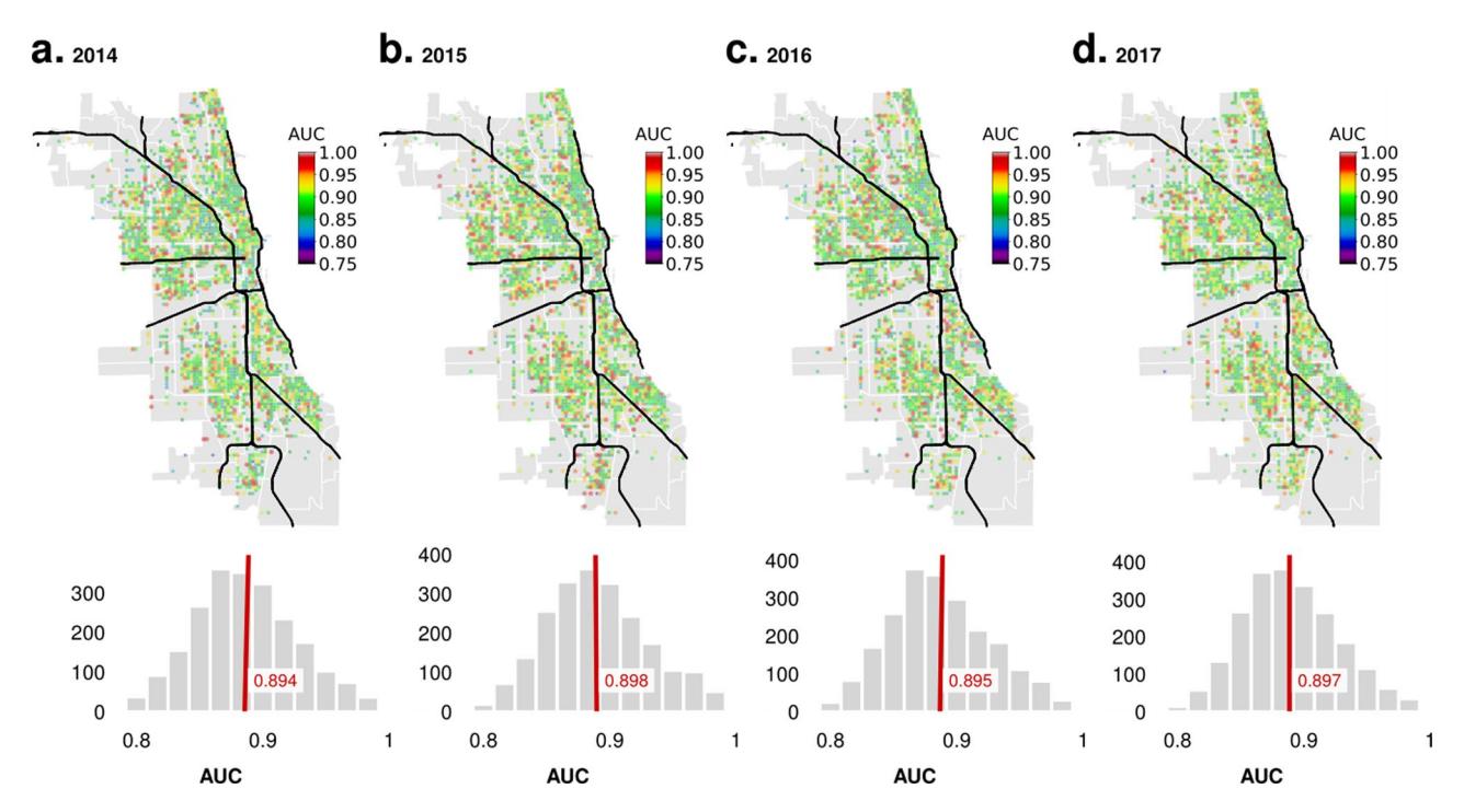
For Chicago, we make predictions separately for violent and property crimes, individually within spatial tiles roughly 1,000 ft across and time windows of 1day, approximately a week in advance, with an area under the receiver operating characteristic curves (AUCs) ranging from 80% to 99% across the city (see below for alternative measures tuned to the concerns of policing policy). We summarize our prediction results in Fig. 2, where panels a and b illustrate the geospatial scatter of AUCs obtained for different spatial tiles and types of crime, while panel c shows the distribution of AUCs. The out-of-sample predictive performance remains stable over time. Our predictions for successive years (each using the three preceding years for training and one year for out-of-sample testing; Extended Data Fig. 1) shows little variation in the average AUC. Inspecting excerpts of the average daily crime rate for successive years also demonstrates a close match between actual and predicted behaviour (Extended Data Fig. 2a,c,e). Meanwhile, Extended Data Fig. 2b,d,f illustrate how the Fourier coefficients match up, showing that we are able to capture crime periodicities at weekly and bi-weekly scales, and beyond.

Unlike previous efforts1–5 , we do not impose predefined spatial constraints. In contrast to the contiguous diffusion encountered in physical systems, criminal reportage may spread across the complex landscape of a modern city unevenly, with regions hyperlinked by transportation networks, socio-demographic similarity and historical collocation, which cannot be captured with spatial diffusion models20. Rather than assuming that distant events across the city will have a weaker influence on prediction compared with those physically closer in space or time, we probe the topological structure emergent from inferred dependencies to estimate the shape, size and organization of neighbourhoods that best predict events at each location. The results (Fig. 2d,e) show that the situation is complex, with the locally predictive neighbourhoods varying widely in geometry and size, which implies that restricting the analysis to small local communities within the city is suboptimal for crime prediction and enforcement analyses. To analyse whether the effect of reported criminal infractions diffuses outward in space and time, we simply calculate the spatio-temporal distances of predictive dependencies, then average across all neighbourhoods in the city, revealing a rapid decay with the time delay in the diffusion rates (Fig. 2f). Interestingly we find that the property and violent crimes differ in their rates of predictive diffusion (Fig. 2f). While signals from property crime decay rapidly, within days, violent reported events appear to shape the dynamics for weeks in the future. These differences in diffusion appear to manifest how people differentially mimic and process exposure to violence21,22.

Forecasting crime by analysing historical patterns has been attempted before23 (see also the unpublished manuscript at https:// arxiv.org/abs/1806.01486). State-of-the-art approaches use machine deep learning tools based on recurrent and convolutional neural networks. In ref. 23, the authors train a neural network model to predict next-day events for 60,348 sample points in Chicago. The model is trained on crime statistics, demographic make-up, meteorological data and Google Street View images to track graffiti, achieving an out-of-sample AUC of 83.3%. Our AUC is demonstrably higher (Table 2 and Extended Data Table 1), and we predict with significantly less data (only past events) and 7 days into the future (instead of the next day). Additionally, the use of demographics and graffiti is problematic because of the possibility of introducing racial and socio-economic bias, with dubious causal value. In ref. 24, the authors combine convolutional and recurrent neural networks with weather, socio-economic, transportation and crime data to predict next-day crime counts in Chicago. As spatial tiles, those authors use standard police beats, which break up Chicago into 274 regions. Police beats reflect the classical notion of neighbourhoods and measure approximately 1 square mile on average25. In comparison, our spatial times are approximately 0.04 square miles, representing a 2,500% higher resolution. This model achieves a classification accuracy of 75.6% for Chicago, in comparison with our accuracy of >90% (Table 2). While this competing model tracks more crime categories, it is limited to next-day predictions with significantly coarser spatial resolution. We also compare the predictive ability of naive autoregressive baseline models (Methods and Extended Data Table 2), which perform poorly but provide a yardstick for meaningful comparison of our claimed performance estimates, which underwrite the application of our approach in revealing emergent biases (Figs. 3 and 4). Apart from AUC and accuracy, we also report other common performance metrics in Table 2, namely the specificity obtained at a fixed sensitivity of 80% and the precision or positive predictive value (PPV).

We also compute the predictive accuracy index (PAI) and the prediction efficiency index (PEI) achieved for each city considered. The PAI16 is defined to be the normalized event rate in identified hotspots (tiles predicted to have events), while the PEI16 is the ratio of the PAI achieved to its maximum achievable value by the same algorithm (thus bounded between 0 and 1; Crime prediction metrics section). The PAI and PEI have emerged as metrics of choice for crime models owing to the need to maximize the volume of crime in predicted hotspots to enable law enforcement. Importantly, PAI/ PEI comparisons are distinct from AUC calculations. Indeed, an algorithm can achieve a high AUC but poor PAI or PEI scores. Our PAI and PEI scores indicate strong performance, with PEI values approaching 1.0 (Fig. 5a).

Finally, a head-to-head comparison of the efficacy of our approach over reported tools is obtained for data used in a recent crime forecast challenge hosted by the NIJ. The Portland Police Department provided crime data from March 2012 up to the end of February 2017, and participants were asked to forecast crime hotspots for four types of incident (burglary, motor vehicle theft, street crime and all calls for service) over the months of March, April and May 2017. In particular, participants were asked to define a grid restricted to Portland boundaries and to predict hotspot grid cells for each type of crime over several forecasting windows. This challenge was a true prospective forecasting test as the validation time period was in the future, non-existent at the time of submission. Forecasts were made for 1week, 2week, 1month, 2month and 3month time windows and scored with the PAI and PEI. These two metrics are not equivalent, as illustrated in the NIJ challenge results, with different teams winning in different categories with respect to the different metrics. While a natural equivalency between PAI and PEI has been suggested16, frameworks that optimize them both have not been reported previously. Our results on ARTICLES NATURE HUMAN BEHAVIOUR

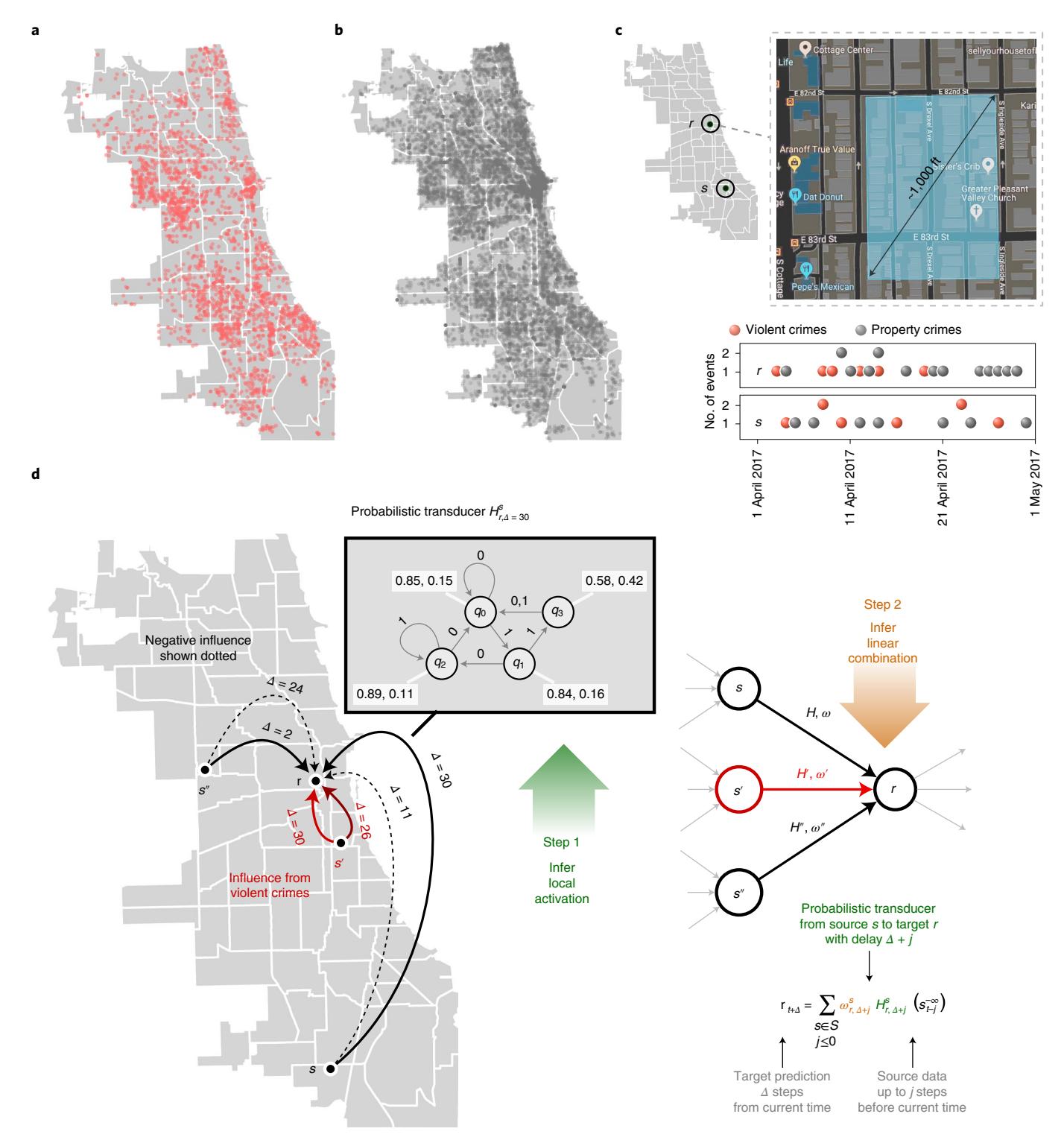
Fig. 1 | Crime data and modelling approach. a,b, Violent crimes (a) and property crimes (b) recorded within the 2 week period between 1 and 15 April 2017. c, Our modelling approach. We break a city into small spatial tiles approximately 1.5 times the size of an average city block and compute models that capture multi-scale dependencies between the sequential event streams recorded at distinct tiles. We treat violent and property crimes separately, and show that these categories have intriguing cross dependencies. d, An illustration of our modelling approach. For example, to predict property crimes at some spatial tile r, we proceed as follows: Step 1: we infer the probabilistic transducers that estimate the event sequence at r by using as input the sequences of recorded infractions (of different categories) at potentially all remote locations (s, s’ and s’’ are shown), where this predictive influence might transpire over different time delays (a few are shown on the edges between s and r). Step 2: we combine these weak estimators linearly to minimize zero-one loss. The inferred transducers can be thought of as inferred local activation rules that are then linearly composed, reversing the approach of linearly combining the input and then passing through fixed activation functions in standard neural net architectures. The connected network of nodes (variables) with probabilistic transducers on the edges forms the Granger network.

Table 1 | Crime event log information for the cities considered Atlanta Austin Detroit Los Angeles Philadelphia San Francisco Chicago Portland No. of variables¹ 510 1,082 1,161 3,287 1,037 975 3,826 9,354 Temporal resolution (days) 2 1 1 1 1 1 1 3 Bounding box of modelled region 33.65° to 33.86° N, 84.54° to 84.31° W 30.14° to 30.48° N, 97.89° to 97.63° W 42.30° to 42.45° N, 83.28° to 82.91° W 33.71° to 34.33° N, 118.65° to 118.16° W 39.88° to 40.12° N, 75.27° to 74.96° W 37.71° to 37.81° N, 122.51° to 122.36° W 41.64° to 42.06° N, 87.88° to 87.52° W 45.23° to 45.81° N, 123.05° to 122.22° W Spatial resolution 983′ ^× 983′ 983′ ^× 983′ 983′ ^× 983′ 983′ ^× 983′ 983′ ^× 983′ 983′ ^× 983′ 951′ ^× 1006′ 591′ ^× 591′ Spatial exclusion threshold² 2.5% 2.5% 2.5% 2.5% 5.0% 2.5% 5.0% 2.0% Training period 1 January 2014–31 December 2018 1 January 2016–31 December 2018 1 January 2012–31 December 2014 1 January 2016–31 December 2018 1 January 2016–31 December 2018 1 January 2014– 31 December 2016 1 January 2014– 31 December 2016 1 March 2012–28 February 2017 Test period 1 January 2019–20 July 2019 1 January 2019–11 April 2019 1 January 2015–11 April 2015 1 January 2019–11 April 2019 1 January 2019–11 April 2019 1 January 2017– 11 April 2017 1 January 2017–11 April 2017 1 March 2017–31 May 2017 Prediction horizon (days) 6 3 3 3 3 3 7 9 Violent crime statistics Event count 2,649, rate 3.98% Event count 20,132, rate 5.45% Event count 20,922, rate 3.72% Event count 72,355, rate 4.83% Event count 33,803, rate 8.11% Event count 23,317, rate 7.16% Event count 179,274, rate 7.7% See Table 1 Property crime statistics Event count 23,522, rate 4.51% Event count 88,929, rate 6.22% Event count 39,840, rate 3.30% Event count 205,435, rate 5.49% Event count 85,683, rate 9.02% Event count 197,835, rate 12.83% Event count 263,661, rate 7.0% See Table 1 Data source opendata. atlantapd.org data. austintexas. gov data. detroitmi.gov data.lacity.org www. opendataphilly. org data.sfgov.org data. cityofchicago.org nij.ojp.gov

City	Property crimes				Violent crimes
	Specifcity1	AUC	Acc.2	PPV3	Specifcity	AUC	Acc.	PPV
Atlanta	0.68	0.90	0.84	0.39	0.71	0.88	0.84	0.38
Austin	0.66	0.87	0.82	0.40	0.66	0.88	0.83	0.38
Detroit	0.72	0.90	0.86	0.37	0.66	0.89	0.84	0.35
Philadelphia	0.64	0.87	0.81	0.48	0.65	0.87	0.81	0.47
Los Angeles	0.66	0.84	0.83	0.39	0.65	0.84	0.83	0.36
San Francisco	0.67	0.86	0.80	0.52	0.65	0.86	0.81	0.42
Chicago	0.68	0.87	0.93	0.43	0.67	0.87	0.94	0.46

Tiles with less than the threshold event rate were excluded.

the data released for this challenge are shown in Fig. 5b, where we outperform the best-performing team in 119 of 120 categories, only under-performing on street crimes at the 3month horizon.

No. of variables indicates the total number of time series considered for violent and property crimes. 2

With the above-discussed predictive performance establishing the validity of our models, we run a series of computational experiments that perturb the rates of violent and property crimes, then log the resulting alterations in future event rates across the city. By inspecting the effect of socio-economic status (SES) on the perturbation response, we investigate whether enforcement and policy biases modulate outcomes. The inferred stress response of the city suggests the presence of a socio-economic enforcement bias (Fig. 3). In wealthier neighbourhoods, the response to elevated crime rates is increased arrests, while arrest rates in disadvantaged neighbourhoods drop but the converse does not occur (Fig. 3e,f). We argue that resource constraints on law enforcement, combined with biased prioritization towards wealthier neighbourhoods, result in reduced enforcement across the remainder of the city. Thus, our results align with suspected enforcement bias within US cities that parallels widely discussed notions of suburban bias in high-SES suburbs26,27. While self-evident at the scale of countries and regions, the existence of unequal resource allocation in cities, where political power and influence concentrate in selective, high-SES neighbourhoods, has been widely suspected28–31. Our analysis corroborates this contention, which shows up robustly for all years analysed, going back over one and a half decades in Chicago. Extended Data Figs. 3–5 show that these patterns are stable over the time period Articles Nature Human Behaviour

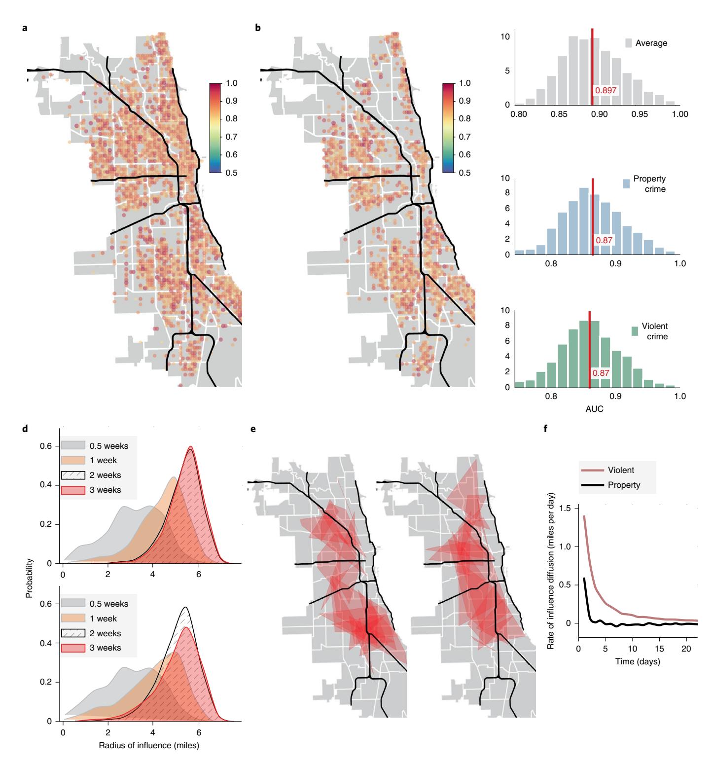
Fig. 2 | Predictive performance of Granger networks. a,b, Out-of-sample AUC for predicting violent (a) and property crimes (b). The prediction is made 1 week in advance, and the event is registered as a successful prediction if we get a hit within ±1 day of the predicted date. c, Distribution of AUC on average, individually for violent and property crimes. Our mean AUC is close to 90%. d–f, Influence diffusion and perturbation space. If we are able to infer a model that predicts event dynamics at a specific spatial tile (the target) using observations from a source tile Δ days in future, we say that the source tile is within the influencing neighbourhood for the target location with a delay of Δ. Spatial radius of influence for 0.5, 1, 2 and 3 weeks (d), for violent (upper panel) and property crimes (lower panel). Note that the influencing neighbourhoods, as defined by our model, are large and approach a radius of 6 miles. Given the geometry of the City of Chicago, this maps to a substantial percentage of the total area of the urban space under consideration, demonstrating that crime manifests demonstrable long-range and almost city-wide influences. Extent of a few inferred neighbourhoods at a time delay of at most 3 days (e). Average rate of influence diffusion measured by number of predictive models inferred that transduce influence as we consider longer and longer time delays (f). Note that the rate of influence diffusion falls rapidly for property crimes, dropping to zero in about 1 week, whereas for violent crimes, the influence continues to diffuse even after 3 weeks.

ARTICLES

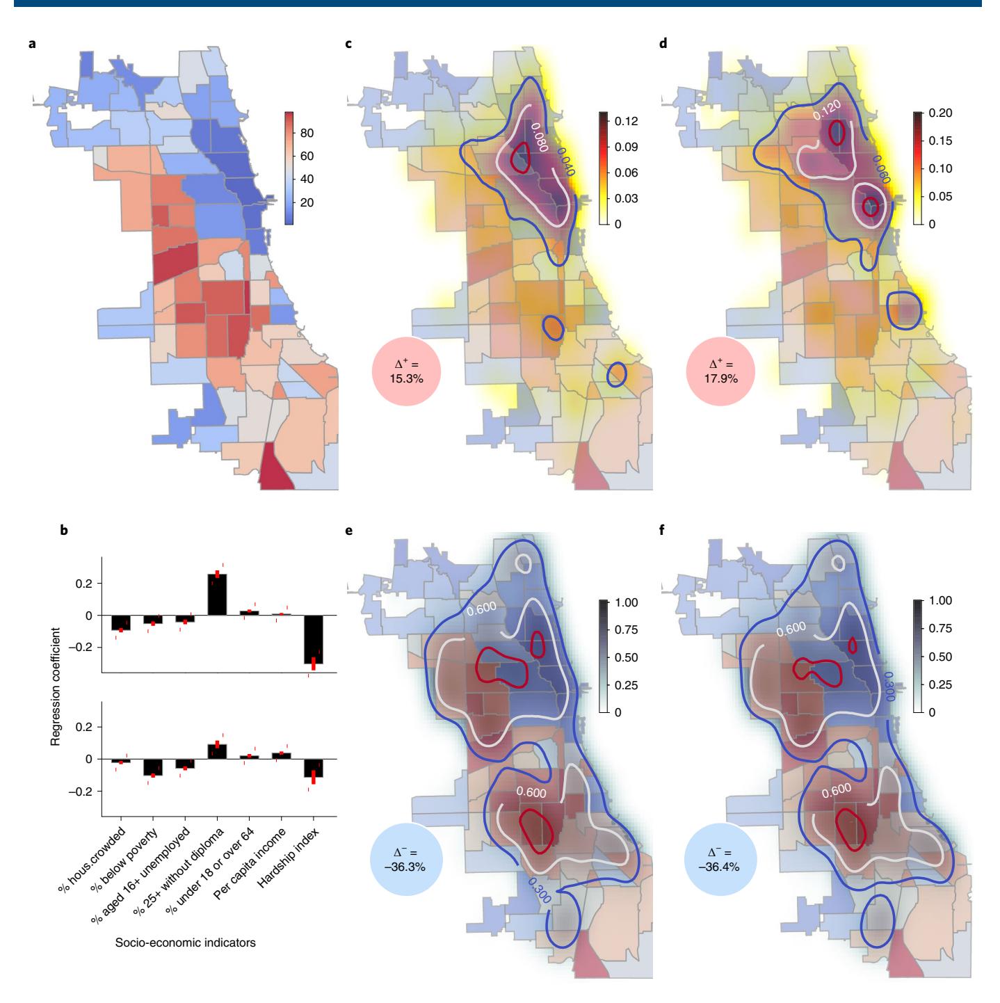
Fig. 3 | Estimating bias. a, Distribution of the economic hardship index⁵³. b, Perturbation in violent (upper) and property (lower) crime rate via multivariable regression, where the hardship index is seen to make a strong negative contribution. Error bars show 95% confidence interval. c-f, Biased response to perturbations in crime rates: \(\Delta^+\) = 15.3% (c), \(\Delta^+\) = 17.9% (d), \(\Delta^-\) = -36.3% (e) and \(\Delta^-\) = -36.4% (f). With a 10% increase in violent or property crime rates, we see an approximately 30% decrease in arrests when averaged over the city. The spatial distribution of locations that experience a positive versus negative change in arrest rate reveals a strong preference favouring high-SES locations. If neighbourhoods are doing better socio-economically, increased crime predicts increased arrests. A strong converse trend is observed in predictions for lower-SES, poor and disadvantaged neighbourhoods, suggesting that, under stress, wealthier neighbourhoods drain resources from their disadvantaged counterparts.

we analyse. Additionally, Extended Data Fig. 3 shows the effect of perturbations across all variables, suggesting that crime reduction from perturbations seems most effective in regions with high crime rates, acknowledging confounding with SES.

The Granger network allows for precise simulation of the impact of complex local and global event patterns and has the potential to emerge as an important tool in policy-making. Thus, empirical validations of model predictions are important. To corroborate claimed disparities in the enforcement response without using our inferred models, we identify similar, naturally occurring patterns in crime and arrest rates across the City of Chicago. Without the use of our models, it is difficult to obtain uniform event stimuli across the city. In one approach, we exploit the seasonality of crime and compare summer months against late winter. Figure 6a (upper panel)

Articles Nature Human Behaviour

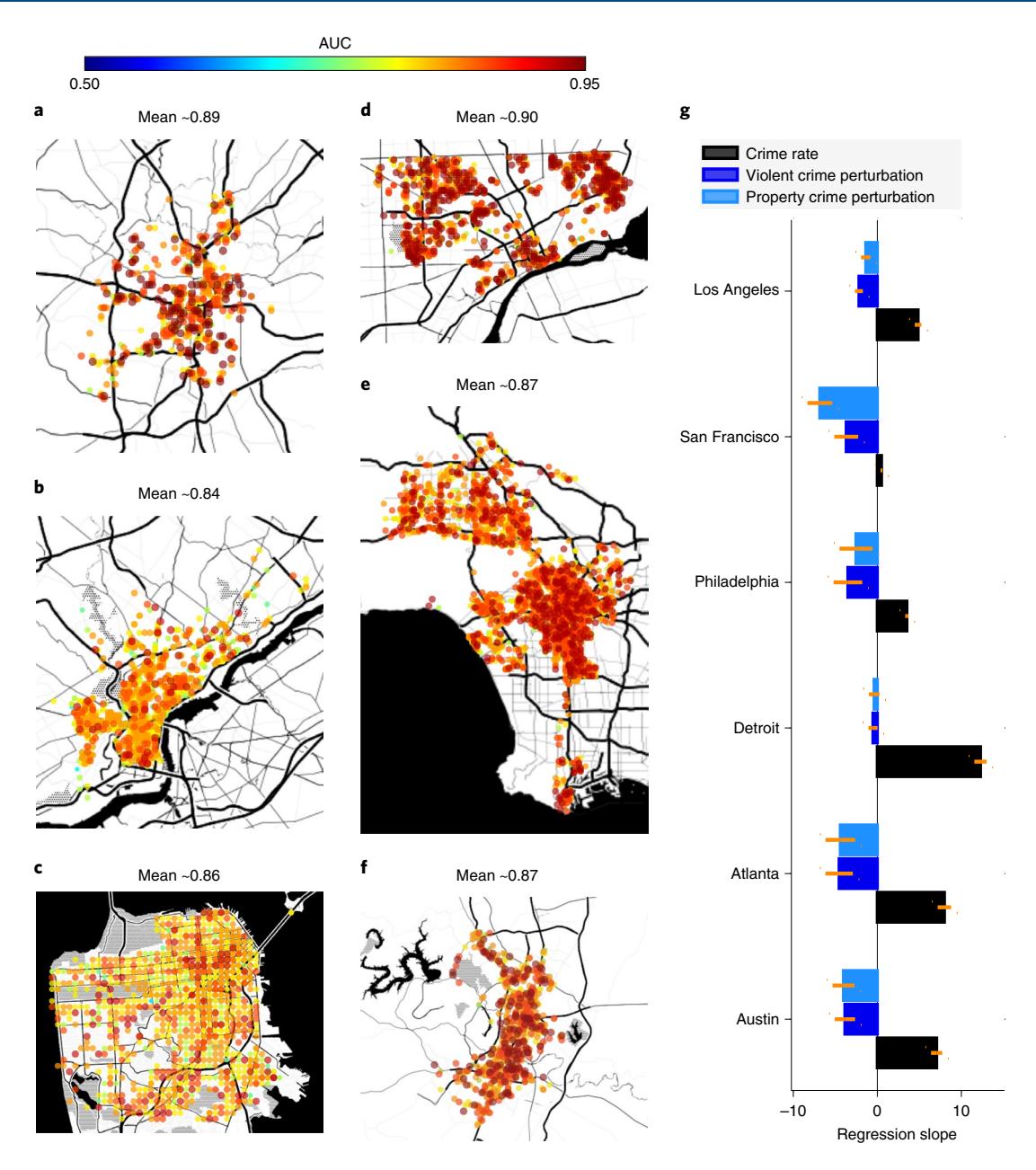
Fig. 4 | Prediction of property and violent crimes across major US cities and the dependency of the perturbation response on the SES of local neighbourhoods. a–f, AUCs obtained in six major US cities: Atlanta (a), Philadelphia (b), San Francisco (c), Detroit (d), Los Angeles (e) and Austin (f), chosen on the basis of the availability of detailed event logs in the public domain. All of these cities show comparably high predictive performance. g, Regression against poverty (standard error bars). Results obtained by regressing crime rate and perturbation response against SES variables (shown here for poverty, as estimated by the 2018 US census). Note that, while the crime rate typically goes up with increasing poverty, the number of events observed 1 week after a positive perturbation of 5–10% increase in crime rate is predicted to fall with increasing poverty. We suggest that this decrease can be explained by disproportionate reallocation of enforcement resources away from disadvantaged neighbourhoods in response to increased event rates, leading to a smaller number of reported crimes.

shows the increase in violent and property crimes from February to June/August, averaged across rich and poor neighbourhoods over 4 years from 2014 to 2017 (along with 95% confidence bounds). Here, we define rich neighbourhoods as communities with hardship index <20 (although the results are not sensitive to the choice of this threshold). We observe that the average percentage increase in the event rate from late winter to summer is broadly comparable across the city, thus approximating a uniform perturbation in crime rate. As shown in Fig. 6a (lower panel), the corresponding deviation of the mean percentage change in the arrest rate from the city-wide average reflects the conclusions above, with wealthier communities

seeing an increase in the arrest rate per unit event with the seasonal rise in crime while others experience a draw-down.

Changes in the enforcement response from winter to summer months do not necessarily establish that an up-tick in arrests in high-SES areas is associated with a down-tick elsewhere in the near future. Thus, we carry out a more granular interrogation of the raw crime data as follows: Aggregating data on the number of daily arrests over Chicago communities (Chicago has 77 community areas32), we compute the correlation between the daily change in the total number of arrests and their 1day delayed versions in neighbouring communities with more economic hardship (higher hardship indices).

ARTICLES

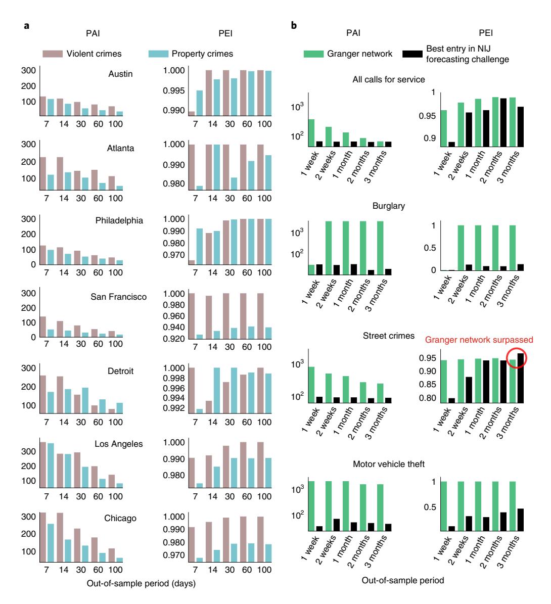
Fig. 5 | The PAI and PEI calculated for seven metropolitan cities. a, The calculated PAI and PEI values. b, A comparison of the PAI and PEI achieved by our approach (Granger network) against the best-performing teams in a crime forecast challenge hosted by the NIJ in 2017 (https://nij.ojp.gov/funding/real-time-crime-forecasting-challenge), where teams attempted to predict hotspots for five different crime categories over different horizons prospectively. Our approach outperforms the teams in all but 1 (highlighted) of 120 categories.

For each community s, we denote as \(\mu(s)\) the value of this correlation minimized over all communities neighbouring s. Figure 6b (upper panel) shows the variation of \(\mu(s)\) with h(s), the hardship index of community s. We see that the arrest rate change in wealthier communities is more strongly anti-correlated with the 1-day-delayed arrest rate change in neighbouring more disadvantaged communities. Figure 6b (lower panel) shows the correlation of \(\mu(s)\) with the average hardship index of communities neighbouring s, computed separately within community groups of similar economic status. We observe that, for wealthier communities, the anti-correlation between the daily change in arrests and its delayed version in lower-SES neighbouring communities is stronger the more economically disadvantaged the neighbours are. The higher the average hardship index of the neighbours, the more negative \(\mu\) is, leading to more negative values in Fig. 6b (lower panel). We also see that this effect vanishes and eventually reverses as the SES of the focal community itself decreases, that is, as their economic status degrades. These direct observations lend credence to the model-based indication of enforcement bias arising from differential resource allocation.

Beyond Chicago, we analyse criminal event logs available in the public domain for seven additional major US cities: Detroit, Philadelphia, Atlanta, Austin, San Francisco, Los Angeles and Portland. In all these cities, we obtain comparably high performance in predicting violent and property crimes, with average AUC values ranging between 86% and 90% (Fig. 4a–f and Supplementary Fig. 1). In addition, our observed pattern of perturbation responses in Chicago, which suggests de-allocation of policing resources from disadvantaged to advantaged neighbourhoods, is replicated in all these cities. While the crime rate increases with degrading SES status of local neighbourhoods, the number of predicted events per week after a positive 5–10% increase in crime rate goes down. Thus, increasing the crime rate leads to a smaller number of reported crimes, a pattern that holds more often in lower-SES neighbourhoods.

Our analysis also sheds light on continuing debate over the choice for neighbourhood boundaries in modelling crime in cities^33–36. Figure 2d–f demonstrates that, despite apparent natural boundaries, predictive signals are often communicated over large

Articles Nature Human Behaviour

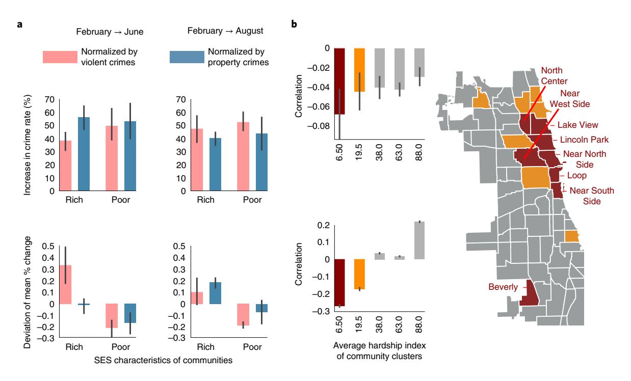
Fig. 6 | Direct observations of the differential response of arrest rate changes with SES variables. a, Upper: increase in violent and property crime rates from February to June or August, averaged over rich (hardship index <20) and poor neighbourhoods (hardship index >20) over 4 years from 2014 to 2017. Error bars show 95% confidence bounds. The average percentage increase in the event rate from late winter to summer is more or less comparable across the city. Lower: the deviation of the mean percentage change in the arrest rate per unit change in crime rate with respect to the city-wide average varies with the average SES of the communities. Wealthier communities see an increase in the arrest rate per unit event, while others experience a draw-down. b, Upper: correlation between the daily change in the number of arrests and their 1 day delayed versions in neighbouring communities with higher hardship indices (μ), versus the hardship index of the communities themselves. Lower: correlation of μ with the average hardship index of neighbouring communities, computed within community groups of similar SES. These results illustrate that, in wealthier communities, the higher the average hardship index of its neighbours, the more negative the μ, whereas this effect vanishes and eventually reverses as communities themselves become poorer. Right: locations of the top two community clusters as per their average hardship indices on a map of Chicago. Note, community colours indicate cluster membership.

distances and decay slowly, especially for violent crimes. More importantly, this study reveals how the ‘correct’ choice of spatial scale should not be a major issue when using sophisticated learning algorithms where optimal scales can be inferred automatically. We find that there exists a skeleton set of spatial tiles that bound predictive dependencies on overall event patterns (Extended Data Fig. 6). These induce a cellular decomposition of the city that identifies functional neighbourhoods, where the cell size adapts automatically to local event dynamics.

Limitations and conclusion

Our ability to probe for the extent of enforcement bias is limited by our dataset on criminal reportage, without the use of direct data on the spatial distribution of police. In large US cities, place and race are often synonymous37,38. Disproportionate police responses in communities of colour can contribute to biases in event logs, which might propagate into inferred models. This possibility has elicited significant push-back against predictive policing39. Our approach is free from manual encoding of features (and thus resistant to the implicit biases of the modellers themselves), but biases arising from disproportionate crime reportage and surveillance almost certainly remain. We doubt that any amount of scrubbing or clever statistical controls can reliably erase such ecological patterning of apparent crime. Any policy informed by our results must keep this caveat in mind.

Differences in the extent to which different communities trust law enforcement are important in analysing crime and enforcement. Diverse communities are often less inclined to call law enforcement for help or to report criminal acts that they might witness, thus obfuscating underlying crime rates. To mitigate these effects, we only consider events, such as homicide, battery, assault, motor vehicle theft and burglary, that are much less likely to be optionally reported by residents, or those which are directly observed by police officers. This is perhaps more true for the types of violent crime considered, and our predictive performance and conclusions replicate for both violent and property crimes. The exception is the City of Portland, where we do consider ‘street crimes’ and ‘all calls for service’ to compare our performance with the NIJ forecast challenge. Our performance holds up in these categories (Fig. 5b), suggesting that these differential reporting issues may not significantly affect our results, but we note that we outperform the competition to a lesser degree for these categories. Finally, for the City of Chicago, we consider arrests as a distinct variable in addition to crimes logged. Importantly, we only consider arrests related to the crimes considered, mitigating the effects of potential over/under-reporting if all such events were to be included.

Despite our caution, one of our key concerns in authoring this study is its potential for misuse, an issue with which predictive policing strategies have struggled40. More important than making good predictions is how such capability will be used. Because policing is as much ‘person based’ as ‘place based’41,42, sending police to an area, regardless of how small that area is, does not dictate the optimal course of action when they arrive, and it is conceivable that good predictions (and intentions) can lead to over-policing or police abuses. For example, our results may be falsely interpreted to mean that there is ‘too much’ policing in low-crime (often predominantly White) communities, and too little policing in higher-crime (often more racially and ethnically diverse) neighbourhoods. A policy based on such a misinterpretation might ramp up enforcement in NATURE HUMAN BEHAVIOUR ARTICLES

Black and Latino neighbourhoods, creating a harmful feedback of sending more police to areas that might already feel over-policed but under-protected⁴³. Instead, our results recommend changes in policy that result in more equitable, need-based resource allocation, with reduced impact based on the SES of individual communities. The tools reported here can then be used to track the extent to which such policies approach this trace of equitable enforcement allocation.

Even with its current limitations, our approach is an addition to the toolbox of computational social science, enabling validation of social theory from observed event incidence, supplementing the use of measurable proxies and potential biases in questionnaire-based data collection strategies. While classical approaches^44–47 broaden our understanding of the societal forces shaping both urban and regional landscapes, these approaches have neither successfully attempted to forecast individual infraction reports nor revealed how these predictive patterns manifest systematic enforcement bias. In this study, we show how the ability of Granger networks to predict such events not only allows precise intervention but also advances the diagnosis and explanation of complex social patterns. We acknowledge the danger that powerful predictive tools place in the hands of over-zealous states in the name of civilian protection, but here we demonstrate their unprecedented ability to audit enforcement biases and hold states accountable in ways inconceivable in the past. We encourage widespread debate regarding how these technologies are used to augment state action in public life and call for transparency that allows for continuous evaluation, reconsideration and critique.

Methods

In this study, we use historical geolocated incidence data of criminal infractions to model and predict future events in Chicago, Philadelphia, San Francisco, Austin, Los Angeles, Detroit and Atlanta. Each of the cities considered has a specific temporal and spatial resolution, which are optimized to maximize predictive performance (Table 1). The predictive performance obtained in these cities is enumerated in Table 2 and Extended Data Table 1. The distribution of AUCs obtained in Chicago for earlier years (2014–2017, predicted individually) is shown in Extended Data Fig. 1.

Data source. The sources of crime incidence data used in this study for the different US cities are enumerated in Table 1. These logs include spatio-temporal event localization along with the nature, category and a brief description of the recorded incident. For the City of Chicago, we also have access to the number of arrests made during or as a result of each event. For Chicago, the log is updated daily, keeping current with a lag of 7 days, and we make predictions for each of the years 2014-2017 (using three years before the target year for model inference and one year for out-of-sample validation) for the prediction results shown in Fig. 1. The evolving nature of the urban scenescape⁴⁸ necessitates that we restrict the modelling window to a few years at a time. The length of this window is decided by trading off the loss of performance from shorter data streams to ignoring the evolution of the underlying generative processes with longer streams. The training and testing periods of the other cities are presented in Table 1. In this study, we consider two broad categories of criminal infractions: violent crimes consisting of homicides, assault, battery, etc. and property crimes consisting of burglary, theft, motor vehicle theft, etc. Drug crimes are excluded from our consideration due to the possibility of ambiguity in the use of violence and the potential for biased documentation of such events. For the City of Chicago, the number of individuals arrested during each recorded event is considered as a separate variable to be modelled and predicted, which allows us to investigate the possibility of enforcement biases in subsequent perturbation analyses.

We also use data on socio-economic variables available at the portal corresponding to Chicago community areas and census tracts, including the percentage of population living in crowded housing, those residing below the poverty line, those unemployed at various age groups, per capita income and the urban hardship index⁴⁹. Such data are also obtained from the City of Chicago data portal. Additionally, we use data on poverty estimates for the other cities, which are obtained from https://www.census.gov.

Spatial and temporal discretization and event quantization. Event logs are processed to obtain time series of relevant events, stratified by occurrence locations. This is accomplished by choosing a spatial discretization and focusing on one individual spatial tile at a time, which allows us to represent the event log as a collection of sequential event streams (Fig. 1c). Additionally, we discretize time and consider the sum total of events recorded within each time window.

The coarseness of these discretizations reflects a trade-off between computational complexity and event localization in space and time. Spatial and temporal discretizations are not chosen independently. A finer spatial discretization dictates a coarser temporal quantization, and vice versa to prevent long stretches with no events and long periods of contiguous event records, both of which wil reduce our ability to obtain reliable predictions. For the City of Chicago, we fix the temporal quantization to 1 day and choose a spatial quantization such that we have high empirical entropy rates for the time series obtained. This results in spatial tiles measuring 0.00276° × 0.0035° in latitude and longitude, respectively, which is approximately 1,000’ across, roughly corresponding to an area of under two by two city blocks. Thus, any two points within our spatial tile are at worst in neighbouring city blocks. We dropped from our analysis the tiles that have too low a crime rate (with <5% of days within the modelling window having any event recorded) to reduce the computational complexity, resulting in N=2,205 spatial tiles in the City of Chicago. The temporal and spatial resolution are adjusted in a similar manner for the other cities (Table 1).

Thus, we end up with three different integer-valued time series at each spatial tile: (1) violent crime (v), (2) property crime (u) and (3) number of arrests (w) in the City of Chicago. For other cities, we have only the first two categories because information on arrests was not available. We ignore the magnitude of the observations and treat them as Boolean variables. Thus, our models simply predict the presence or absence of a particular type of event in a discrete spatial tile within a neighbouring city block and observation window, that is, within the temporal resolution chosen, which is 1 day except for Atlanta, where is it is chosen to be 2 days (Table 1).

Inferring generators of spatio-temporal cross dependence. Let

\(\mathcal{L} = \{\ell_1, \dots, \ell_N\}\) be the set of spatial tiles and \(\mathcal{E} = \{u, v, w\}\) be the set of event categories as described in the last section. At location \(\ell \in \mathcal{L}\) for variable \(e \in \mathcal{E}\) , at time t, we have \((\ell, e)_t \in \{0, 1\}\) , with 1 indicating the presence of at least one event. The set of all such combined variables (space + event type) is denoted as \(\mathcal{E} = \mathcal{L} \times \mathcal{E}\) . Let \(T = \{0, \dots, M-1\}\) denote the training period, consisting of M time steps. Because for any time t, \((\ell, e)_t\) is a random variable, our goal here is to learn its dependence relationships with its own past and with other variables in S to accurately estimate its future distribution for t > T.

To infer the structure of our predictive model, we learn a finite-state probabilistic transducer¹⁸ (referred to as a crossed probabilistic finite state automata (XPFSA), a generalization of probabilistic finite-state automata models for stochastic processes17, see unpublished manuscript at http://arxiv.org/ abs/1406.6651) for each possible source–target pair s, \(r \in S\) . Given a sequence of events at the source, these inferred transducers estimate the distribution of events at target r for some future point in time. The ability to estimate such a non-trivial distribution indicates successful prediction. With too many uncontrollable factors influencing the outcomes, causality cannot be inferred from the data for the problem at hand. Here we characterize directional dependence as the source being able to predict events occurring at the target, better than the target can do by itself. This prediction-centred approach has been called Granger causal influence⁵⁰, but while this has been criticized as a weak indicator of causality, it is directly tuned to the challenge of forecasting future events. Importantly, we do not assume that the underlying processes are independent and identically distributed, or that the model has any particular linear structure. Additionally, predictive dependencies are not restricted to be instantaneous. The source events might impact the target with a time delay, that is, a specific model between the source and target might predict events delayed by an a priori determined number of steps \(\Delta_{\text{max}} \ge \Delta \ge 0\) specific to the model. Here, we model the dependency structure for each integer-valued delay separately. Thus, for source s and target t, we can have \(\Delta_{max} + 1\) transducers, each modelling dependencies for a specific delay in \(\{0, \Delta_{max}\}\) . The maximum number of steps in the time delay \(\Delta_{max}\) is chosen a priori on the basis of the problem at hand.

While these dependencies may differ for different delays, they need not be symmetric between source and target pairs. The complete set, comprising at most \(|\mathcal{S}|^2(\Delta_{\max}+1)\) models, represents a predictive framework for asymmetric multi-scale spatio-temporal phenomena. Note that the number of possible models increases quickly. For example, for the City of Chicago, for \(\Delta_{\max}=60\) with 2,205 spatial tiles and three event categories, the number of inferred models is bounded above by 2.6 billion.

Our approach consists of inferring XPFSAs in two key steps (Fig. 1d and discussion in Supplementary Methods). First, we infer XPFSA models for all source–target pairs and all delays up to \(\Delta_{\max}\) . In the second step, we learn a linear combination of these transducers to maximize the predictive performance. Denoting the observed event sequence in the time interval \((\infty,t]\) at source s as \(s_t^{-\infty}\) , the XPFSA \(\coprod_{r,k}^s\) estimates the distribution of events for the target r at the time step t+k. This is accomplished by learning an equivalence relation on the historical event sequences observed at source s, such that equivalent histories induce an approximately identical future event distribution at target r at k steps in the future. Thus, for example, the XPFSA shown in Fig. 1d has four states, indicating that there are four such equivalence classes of observations that induce the distinct output probabilities shown from each state. Often, this estimate is imprecise due to the possibility of multi-scale and multi-source dependencies, that is, when the target r is predicted by multiple sources with different time delays. In

ARTICLES NATURE HUMAN BEHAVIOUR

the second step, we employ a standard gradient boosting regressor for each target to optimize the linear combination of inferred transducers and learn the scalar weights \(\omega_{s,k}^s\) for the source s, target r and delay k. Detailed pseudocode for the inference algorithms is provided in Supplementary Methods.

To compare with a standard neural net architecture, these probabilistic transducers may be viewed as local non-linear activation functions. With neural networks, we repeatedly compute the affine combination of inputs and apply fixed non-linear activation to the combined input and finally optimize the affine combination weights via backpropagation, but here we first learn the local non-linear activations and then optimize the linear or affine combination of weak estimators. Optimizing the weights is a significantly simpler, local operation and may be done with any standard regressor. In contrast to recurrent neural networks, the role of hidden-layer neurons is partially accounted for by states of the XPFSA, which are a priori undetermined with respect to both their multiplicity and their transition connectivity structure.

Computational and model complexity. We assume the maximum time delay in prediction propagation to be 60 days for all cities, which for the City of Chicago results in at most 2,669,251,725 inferred models, of which 61,650,000 are useful with \(\gamma \ge 0.01\) . The model inference in this case consumed approximately 200k core-hours on 28-core Intel Broadwell processors, when carried out with incidence data over the period from 1 January 2014 to 31 December 2016. The computational costs for other time periods and other cities are comparable and roughly scale with the square of the number of spatial tiles but linearly with the length of the time-quantized data streams considered as input to the inference algorithm.

Crime prediction metrics. For each spatial location, the inferred Granger network maps event histories to a raw risk score as a function of time. The higher this value, the higher the probability of an event of the target type occurring at that location within the specified time window. To make crisp predictions however, we must choose a decision threshold for this raw score. Conceptually identical to the notion of type 1 and type 2 errors in classical statistical analyses, the choice of a threshold trades off false positives (type 1 error) for false negatives (type 2 error). Choosing a small threshold results in predicting a larger fraction of future events correctly, that is, a high true positive rate (TPR), while simultaneously suffering from a higher false positive rate (FPR), and vice versa. The receiver operating characteristic curve (ROC) is the plot of the FPR versus the TPR, as we vary this decision threshold. If our predictor is good, we will consistently achieve high TPR with small FPR, resulting in a large AUC. Importantly, the AUC measures the intrinsic performance, independent of the threshold choice. Thus, the AUC is immune to class imbalance (the fact that crimes are rare events). An AUC of 50% indicates that the predictor does no better than random, whereas an AUC of 100% implies that we can achieve perfect prediction of future events, with zero false positives.

To evaluate the AUC, we treat a positive prediction as correct if there is at least one event recorded in \(\pm 1\) time steps in the target spatial tile.

We also evaluate the PAI and PEI achieved when using our framework. The PAI is defined as follows: Given a set of k predicted hotspot cells, the PAI is determined by computing the ratio of the proportion of crime captured in the hotspots relative to the proportional area of the city flagged as hotspots. Specifically, defining H to be the union of the hotspot cells (which does not need to be connected) and S the spatial region of interest (for example, Portland, Oregon), the PAI is defined as

\[PAI(H) = \frac{N(H)|S|}{|H|N(S)},\] (1)

where N(H) is the number of events in H over the forecasting window and |H| is the size of the hotspot region \(H \subseteq S\) . Letting \(\lambda(H) = N(H)/|H|\) be the estimated intensity of events in region H and \(\overline{\lambda} = N(S)/|S|\) be the total intensity of events in the region of interest, the PAI becomes

\[PAI(H) = \frac{\lambda(H)}{\overline{\lambda}} \propto \lambda(H),\] (2)

which is only a function of \(\lambda(H)\) since \(\overline{\lambda}\) is independent of H. Thus, PAI is interpreted as the average rate of crime in the predicted hotspots relative to the average crime rate in the city. The trends obtained for the PAI and PEI with our approach match those reported in literature (see figure 3 in ref. \(^{16}\) ).

Predictability analysis. In the City of Chicago, we can predict events approximately 1 week in advance at a spatial resolution of \(\pm 1\) city blocks and a temporal resolution of \(\pm 1\) day with a false positive rate of less than 20% and a median true positive rate of 78%. The predictive performance in other cities is enumerated in Table 2. While not directly modelled in the frequency domain, we found that the event forecasts produce very similar signatures in the frequency domain (Extended Data Fig. 2), when compared over the first 150 days of each out-of-sample period (1 year). We also consider prediction periods of 7, 14, 30, 60 and 100 days to evaluate the variation of the PAI and PEI for the cities considered (Fig. 5a).

Spatial neighbourhoods. The degree of directed predictive dependency between one variable (the source stream) on another (the target stream), also called the (Granger-)causal influence, is quantified by the coefficient of dependence ( \(\gamma\) ; Supplementary Methods). Identifying the source–target pairs for which the coefficient of dependency (or Granger causality) is high (Extended Data Fig. 6), we note that there exists a sparse set of spatial tiles that exert nearly all of the directed dependency in the entire set of observed variables. Thus, observing these variables alone would enable us to make good event forecasts. These tiles span the expanse of the city, and a Voronoi decomposition based on the centres of these tiles in shown in Extended Data Fig. 6b. Such a decomposition demonstrates an algorithmic approach to choosing optimal neighbourhoods for urban analysis.

Perturbation analysis. We experimented with positive and negative perturbations to both violent and property crime rates ranging from 1% to 10% of the observed rates. The response to perturbing the crime rates was measured as the relative change from the nominal baseline in the estimated time average for the predicted event frequencies 1 week in the future, corresponding to violent and property crimes and the number of arrests.

The results of our perturbation experiments both shed light on the stability characteristics of crime in Chicago and further allowed us to look for evidence of biased police enforcement responses under stress. Under stress, well-off neighbourhoods tend to drain resources disproportionately from disadvantaged locales (Fig. 3). Economically well-off neighbourhoods in the bottom 25% of the hardship index are much more likely to see a near-proportional increase (~15%) in law enforcement response, measured by the number of predicted arrests on a 10% increase in crime rates (Fig. 3c,d, which shows how regions with increased enforcement response are concentrated in well-off neighbourhoods), while the rest of the city sees a drop in the predicted response of about twice the magnitude (>30%). Increased crimes causes enforcement resources to be drained from disadvantaged neighbourhoods to support their counterparts with better SES. We performed multivariable linear regression analysis to evaluate this question in another way. Here, we regressed the violent and property crime rates, independently, on the variables listed in Fig 3b, including a slope intercept variable in each model. In both models, the hardship index’s strong, negative coefficient for changes in the arrest rate from perturbations that increase the violent and property crime rates contradicts what might be expected in the absence of bias. Lower-SES neighbourhoods have more crime, and so these socio-economic indicators should contribute positively to the arrest rate with increasing crime. These patterns were replicated in our perturbation experiments for all the preceding years we analysed (2014-2017; Extended Data Figs. 4 and 5). The response measured in the property and violent crimes, and associated arrests, from perturbations is detailed in Extended Data Fig. 3.

We also carried out similar perturbation analyses for the other cities, observing the expected increase of observed crime rates, with increasing poverty, but an unexpected decrease in violent and property crimes after a 5–10% simulated up-tick in either crime category (Fig. 4).

Naive baselines: autoregressive integrated moving average (ARIMA) models. To explore the predictive ability of naive baseline models on our datasets, we consider four ARIMA⁵¹ configurations with lag orders of p = 5 and 10, numbers of differencing of d = 1 and 2 and a window of moving average of q = 0. Let \(y_t\) be the series we want to model and \(y_t'\) be \(y_t\) differenced d times, them the ARIMA(p, d, q) models the series \(y_t'\) by

\[y'_{t} = c + \phi_1 y'_{t-1} + \dots + \phi_p y'_{t-p} + \theta_1 \varepsilon_{t-1} + \dots + \theta_q \varepsilon_{t-q} + \varepsilon_t, \tag{3}\]

where \(\phi_1, \dots, \phi_p\) and \(\theta_1, \dots, \theta_q\) are the coefficients to be fitted. In equation (3), the \(y'_{t-k}\) are the historical values of \(y'_t\) whose inclusion models the influence of past values on the current value (autoregression) while the \(\varepsilon_{t-k}\) are white noise terms whose inclusion models the dependence of the current value against current and previous (observed) white noise error terms or random shocks (moving average). Specifically, we use the following models:

\[y_t^{(1)} = c + \phi_1 y_{t-1}' + \dots + \phi_5 y_{t-5}',\] (4)

\[y_t^{(1)} = c + \phi_1 y_{t-1}' + \dots + \phi_5 y_{t-10}',\] (5)

\[y_t^{(2)} = c + \phi_1 y_{t-1}' + \dots + \phi_5 y_{t-5}',\] (6)

\[y_t^{(2)} = c + \phi_1 y_{t-1}' + \dots + \phi_5 y_{t-10}',\] (7)

where \(y_t^{(d)}\) is \(y_t\) different d times ( \(y_t^{(1)} = y_t - y_{t-1}\) and \(y_t^{(2)} = y_t - 2y_{t-1} + y_{t-2}\) ). For simple benchmarks, we apply the ARIMA model to each individual time series, which means that the predictive model is trained without exogenous variables. For the implementation, we use the Python statsmodels package²³, and the result is shown in Extended Data Table 2. The inadequate performance of ARIMA may be

Nature Human Behaviour Articles

because (1) the use of a single datastream limits the ability of ARIMA to capture the interplay between co-evolving processes, and (2) a predetermined lag order fails to capture the possibly varying temporal memory of individual processes.

Reporting summary. Further information on research design is available in the Nature Research Reporting Summary linked to this article.

Data availability

Crime incident data used in this study are in the public domain. The web links for the data sources for seven out of the eight cities considered here are: opendata. atlantapd.org, data.austintexas.gov, data.detroitmi.gov, data.lacity.org, www. opendata.philly.org, data.sfgov.org, and data.cityofchicago.org, and for Portland the data along with the leader-board data for the forecasting challenge were obtained from nij.ojp.gov.

Code availability

Software with source code is available at https://github.com/ zeroknowledgediscovery/Cynet, and the current version of the software may be referenced by https://doi.org/10.5281/zenodo.5730613. Any questions on implementation should be directed to the corresponding author.

Received: 30 January 2021; Accepted: 2 May 2022; Published online: 30 June 2022

References

• 1. Bowers, K. J., Johnson, S. D. & Pease, K. Prospective hot-spotting: the future of crime mapping? Br. J. Criminol. 44, 641–658 (2004).

• 2. Chainey, S., Tompson, L. & Uhlig, S. Te utility of hotspot mapping for predicting spatial patterns of crime. Secur. J. 21, 4–28 (2008).

• 3. Fielding, M. & Jones, V. ‘Disrupting the optimal forager’: predictive risk mapping and domestic burglary reduction in Traford, Greater Manchester. Int. J. Police Sci. Manage. 14, 30–41 (2012).

• 4. Mohler, G. O., Short, M. B., Brantingham, P. J., Schoenberg, F. P. & Tita, G. E. Self-exciting point process modeling of crime. J. Am. Stat. Assoc. 106, 100–108 (2011).

• 5. Mohler, G. O. et al. Randomized controlled feld trials of predictive policing. J. Am. Stat. Assoc. 110, 1399–1411 (2015).

• 6. Poisson, S. D. Probabilité des Jugements en Matiére Criminelle et en Matiére Civile, Précédées des Régles Générales du Calcul des Probabilitiés (Bachelier, 1837).

• 7. Du Sautoy, M. Te Creativity Code: Art and Innovation in the Age of AI (Harvard Univ. Press, 2020).

• 8. Ferdinand, T. N. Demographic shifs and criminality: an inquiry. Br. J. Criminol. 10, 169–175 (1970).

• 9. Cohen, L. & Felson, M. Social change and crime rate trends: a routine activity approach. Am. Sociol. Rev. 44, 588–608 (1979).

• 10. Cohen, L. E. Modeling crime trends: a criminal opportunity perspective. J. Res. Crime Delinquency 18, 138–164 (1981).

• 11. Wang, X. & Brown, D. E. Te spatio-temporal modeling for criminal incidents. Secur. Inform. 1, 2 (2012).

• 12. Liu, H. & Brown, D. E. Criminal incident prediction using a point-pattern-based density model. 19, 603–622 (2003).

• 13. Caplan, J. M., Kennedy, L. W., Barnum, J. D. & Piza, E. L. Crime in context: utilizing risk terrain modeling and conjunctive analysis of case confgurations to explore the dynamics of criminogenic behavior settings. J. Contemp. Crim. Justice 33, 133–151 (2017).

• 14. Kang, H. W. & Kang, H. B. Prediction of crime occurrence from multi-modal data using deep learning. PLoS ONE 12, e0176244 (2017).

• 15. Flaxman, S., Chirico, M., Pereira, P. & Loefer, C. Scalable high-resolution forecasting of sparse spatiotemporal events with kernel methods: a winning solution to the NIJ ‘real-time crime forecasting challenge’. Ann. Appl. Stat. 13, 2564–2585 (2019).

• 16. Mohler, G. & Porter, M. D. Rotational grid, PAI-maximizing crime forecasts. Stat. Anal. Data Min. 11, 227–236 (2018).

• 17. Chattopadhyay, I. & Lipson, H. Abductive learning of quantized stochastic processes with probabilistic fnite automata. Philos. Trans. R. Soc. A 371, 20110543 (2013).

• 18. Mohri, M. Weighted Finite-State Transducer Algorithms. An Overview (Springer, 2004).

• 19. Granger, C. W. J. Testing for causality: a personal viewpoint. J. Econ. Dyn. Control 2, 329 – 352 (1980).

• 20. Papachristos, A. V. & Bastomski, S. Connected in crime: the enduring efect of neighborhood networks on the spatial patterning of violence. Am. J. Sociol. 124, 517–568 (2018).

• 21. Papachristos, A. V., Wildeman, C. & Roberto, E. Tragic, but not random: the social contagion of nonfatal gunshot injuries. Soc. Sci. Med. 125, 139–150 (2015).

• 22. Green, B., Horel, T. & Papachristos, A. V. Modeling contagion through social networks to explain and predict gunshot violence in Chicago, 2006 to 2014. JAMA Intern. Med. 177, 326–333 (2017).

• 23. Kang, H.-W. & Kang, H.-B. Prediction of crime occurrence from multi-modal data using deep learning. PLoS ONE 12, e0176244 (2017).

• 24. Stec, A. & Klabjan, D. Forecasting crime with deep learning. Preprint at https://arxiv.org/abs/1806.01486(2018).

• 25. Hannon, L. Neighborhood residence and assessments of racial profling using census data. Socius 5, 2378023118818746 (2019).

• 26. Meyer, W. B. & Graybill, J. K. Te suburban bias of American society? Urban Geogr. 37, 863–882 (2016).

• 27. Lipton, M. et al. Why Poor People Stay Poor: a Study of Urban Bias in World Development (Australian National Univ. Press, 1977).

• 28. Sternlieb, G. & Jackson, K. T. Crabgrass frontier: the suburbanization of the United States. Political Sci. Q. 101, 493 (1986).

• 29. Duany, A., Plater-Zyberk, E. & Speck, J. Suburban nation: the rise of sprawl and the decline of the American dream. Choice Rev. Online 38, 38–1251–38–1251 (2000).
• 30. Lazare, D. America’s Undeclared War: What’s Killing Our Cities and How to Stop It (Harcourt, 2001).

• 31. Young, I. M. Inclusion and Democracy (Oxford Univ. Press, 2002).

• 32. Kaplan, M. S., Crespo, C. J., Huguet, N. & Marks, G. Ethnic/racial homogeneity and sexually transmitted disease: a study of 77 Chicago community areas. Sex. Transm. Dis. 36, 108–111 (2009).

• 33. Sherman, L. W., Gartin, P. R. & Buerger, M. E. Hot spots of predatory crime: routine activities and the criminology of place. Criminology 27, 27–56 (1989).

• 34. Wooldredge, J. Examining the (ir)relevance of aggregation bias for multilevel studies of neighborhoods and crime with an example comparing census tracts to ofcial neighborhoods in Cincinnati. Criminology 40, 681–710 (2002).
• 35. Mears, D. P. & Bhati, A. S. No community is an island: the efects of resource deprivation on urban violence in spatially and socially proximate communities. Criminology 44, 509–548 (2006).

• 36. Weisburd, D., Grof, E. R., Yang, S.-M. & Telep, C. W. Criminology of Place (Springer, 2014).

• 37. Small, M. L. Four reasons to abandon the idea of ‘the ghetto’. City Community 7, 389–398 (2008).

• 38. Baumgarten, M. Ghetto: the invention of a place, the history of an idea. Jew. Q. 63, 62–63 (2016).

• 39. Heaven, W. D. Predictive policing algorithms are racist. Tey need to be dismantled. MIT ZTechnol. Rev. 17, 2020 (2020).

• 40. Brayne, S. & Christin, A. Technologies of crime prediction: the reception of algorithms in policing and criminal courts. Social Problems 68, 608–624 (2020).

• 41. St. Louis, S. & Greene, J. R. Social context in police legitimacy: giving meaning to police/community contacts. Policing Soc. 30, 656–673 (2020).

• 42. Weisburd, D. Place-based policing. Ideas in American Policing 9, 1–16 (2008).

• 43. Kushnick, L. ‘Over policed and under protected’: Stephen lawrence, institutional and police practices. Sociol. Res. Online 4, 156–166 (1999).

• 44. Cliford, R. S. Juvenile delinquency and urban areas: a study of rates of delinquents in relation to diferential characteristics of local communities in American cities. Am. J. Sociol. 49, 100–101 (1943).

• 45. Sampson, R. J., Raudenbush, S. W. & Earls, F. Neighborhoods and violent crime: a multilevel study of collective efcacy. Science 277, 918–924 (1997).
• 46. Miethe, T. D., Hughes, M. & McDowall, D. Social change and crime rates: an evaluation of alternative theoretical approaches. Soc. Forces 70, 165–185 (1991).

• 47. Braga, A. A. & Clarke, R. V. Explaining high-risk concentrations of crime in the city: social disorganization, crime opportunities, and important next steps. J. Rs. Crime Delinquency 51, 480–498 (2014).

• 48. Silver, D. & Clark, T. Scenescapes: How Qualities of Place Shape Social Life (Univ. of Chicago Press, 2016).

• 49. Nathan, R. P. & Adams, C. F. Four perspectives on urban hardship. Political Sci. Q. 104, 483–508 (1989).

• 50. Granger, C. W. J. Testing for causality. J. Econ. Dyn. Control 2, 329–352 (1980).

• 51. Montero-Manso, P. & Hyndman, R. J. Principles and algorithms for forecasting groups of time series: locality and globality. Int. J. Forecast. 37, 1632–1653 (2021).

• 52. Seabold, S. & Perktold, J. Statsmodels: econometric and statistical modeling with Python. In Proc. 9th Python in Science Conference https://conference. scipy.org/proceedings/scipy2010/pdfs/seabold.pdf (2010).

• 53. Laxy, M., Malecki, K. C., Givens, M. L., Walsh, M. C. & Nieto, F. J. Te association between neighborhood economic hardship, the retail food environment, fast food intake, and obesity: fndings from the Survey of the Health of Wisconsin. BMC Public Health 15, 1–10 (2015).

Articles Nature Human Behaviour

Acknowledgements

Our work greatly benefited from discussion of everyone who participated in our workshop series on crime prediction at the Neubauer Collegium for culture and society (https://neubauercollegium.uchicago.edu/events/uc/crimes\_of\_prediction\_workshop/), and with those with whom we had extended conversations to ground and refine our modelling approach.

Data were provided by the City of Chicago data portal at https://data.cityofchicago. org. The City of Chicago (‘City’) voluntarily provides the data on this website as a service to the public. The City makes no warranty, representation, or guarantee as to the content, accuracy, timeliness, or completeness of any of the data provided at this website (https:// www.chicago.gov/city/en/narr/foia/data\_disclaimer.html), and the authors of this study are solely responsible for the opinions and conclusions expressed in this study. Sources of the crime incidence data for the other cities are tabulated in Table 1. Socio-economic data for metropolitan areas were obtained fromhttps://www.census.gov.

This work is funded in part by the Defense Sciences Office of the Defense Advanced Research Projects Agency projects HR00111890043/P00004 and W911NF2010302, and the Neubauer Collegium for Culture and Society through the Faculty Initiated Research Program 2017. The claims made in this study do not necessarily reflect the position or the policy of the sponsors, and no official endorsement should be inferred.

Author contributions

Y.H. and I.C. worked out key mathematical details of the Granger network framework. V.R., T.L., Y.H. and I.C. implemented the algorithms and generated results. Y.H., V.R.

and T.L. contributed equally in realizing the current implementation of the software. I.C. generated the visualizations in this study. J.E. provided key insights into modelling and interpreting social dynamics. J.E. and I.C. conceived and designed the research, and wrote the paper.

Competing interests

The authors declare no competing interests.

Additional information

Extended data is available for this paper at https://doi.org/10.1038/s41562-022-01372-0.

Supplementary information The online version contains supplementary material available at https://doi.org/10.1038/s41562-022-01372-0.

Correspondence and requests for materials should be addressed to Ishanu Chattopadhyay.

Peer review information Nature Human Behaviour thanks the anonymous reviewers for their contribution to the peer review of this work.

Reprints and permissions information is available at www.nature.com/reprints.

Publisher’s note Springer Nature remains neutral with regard to jurisdictional claims in published maps and institutional affiliations.

© The Author(s), under exclusive licence to Springer Nature Limited 2022

Nature Huma Humann Behhaviour Articles

Extended Data Fig. 1 | Out of Sample Predictive Performance over the Years. We show that the predictive performance is very stable, and variation in mean AUC is limited to the third place of decimal, at least when analyzing the last few years (4 years shown).

Articles Nature Huma Humann Behhaviour

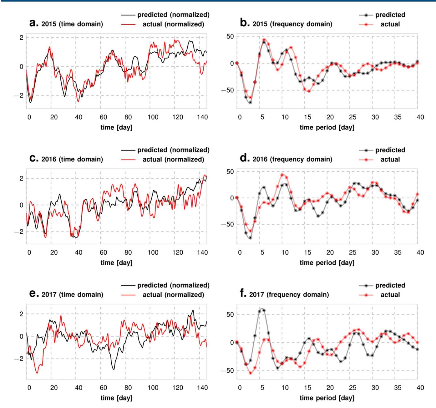
Extended Data Fig. 2 | Comparison of Predicted vs Actual Sample Paths in Time and Frequency Domains. Panels a, c and e show that the predicted and actual sample paths are pretty close for different years, when compared over the first 150 days of each year. Panels b, d and f show that the Fourier coefficients match up pretty well as well. More importantly, while our models do not explicitly incorporate any periodic elements that are being tuned, we still manage to capture the weekly, (approximately) biweekly and longer periodic regularities.

Nature Huma Humann Behhaviour Articles

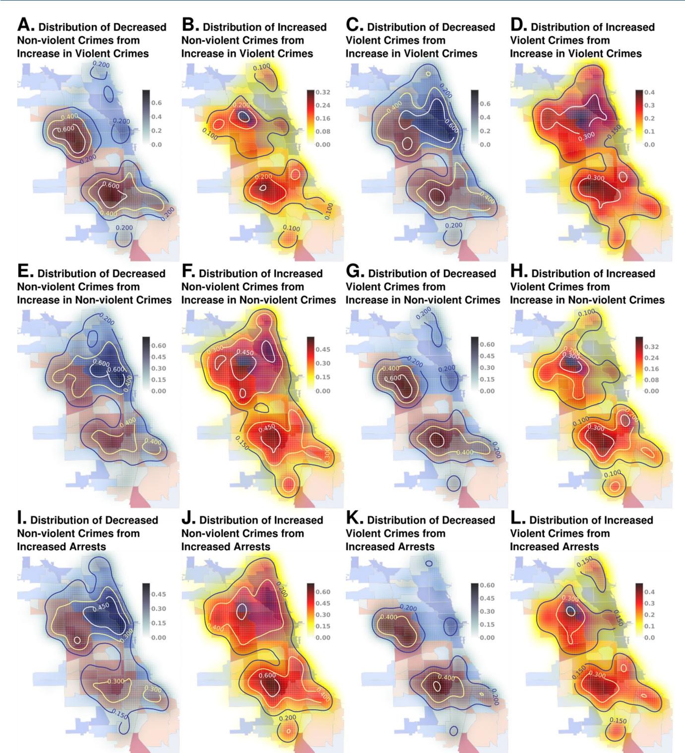
Extended Data Fig. 3 | Perturbation Effects Across Variables. We see that the decrease of violent crimes from increase of property crimes are localized in disadvantaged neighborhoods (panel g). Similarly, the decrease of property crimes from increase of violent crimes is also localized to disadvantaged neighborhoods (panel a), as well as the decreased violent crimes from increased arrests (panel k). We see a weaker localization for the corresponding increases in crime rates under similar perturbations. Looking at other pairs of variables under perturbation (rest of the panels), we generally do not see a very prominent correspondence with the distribution of socio-economic indicators. It seems crimes (and particularly violent crimes) are easier to dampen in locales with high existing crime rates, which is desirable result. But such conclusions are currently confounded by SES variables, and further work is needed to investigate these effects more thoroughly.

Articles Nature Huma Humann Behhaviour

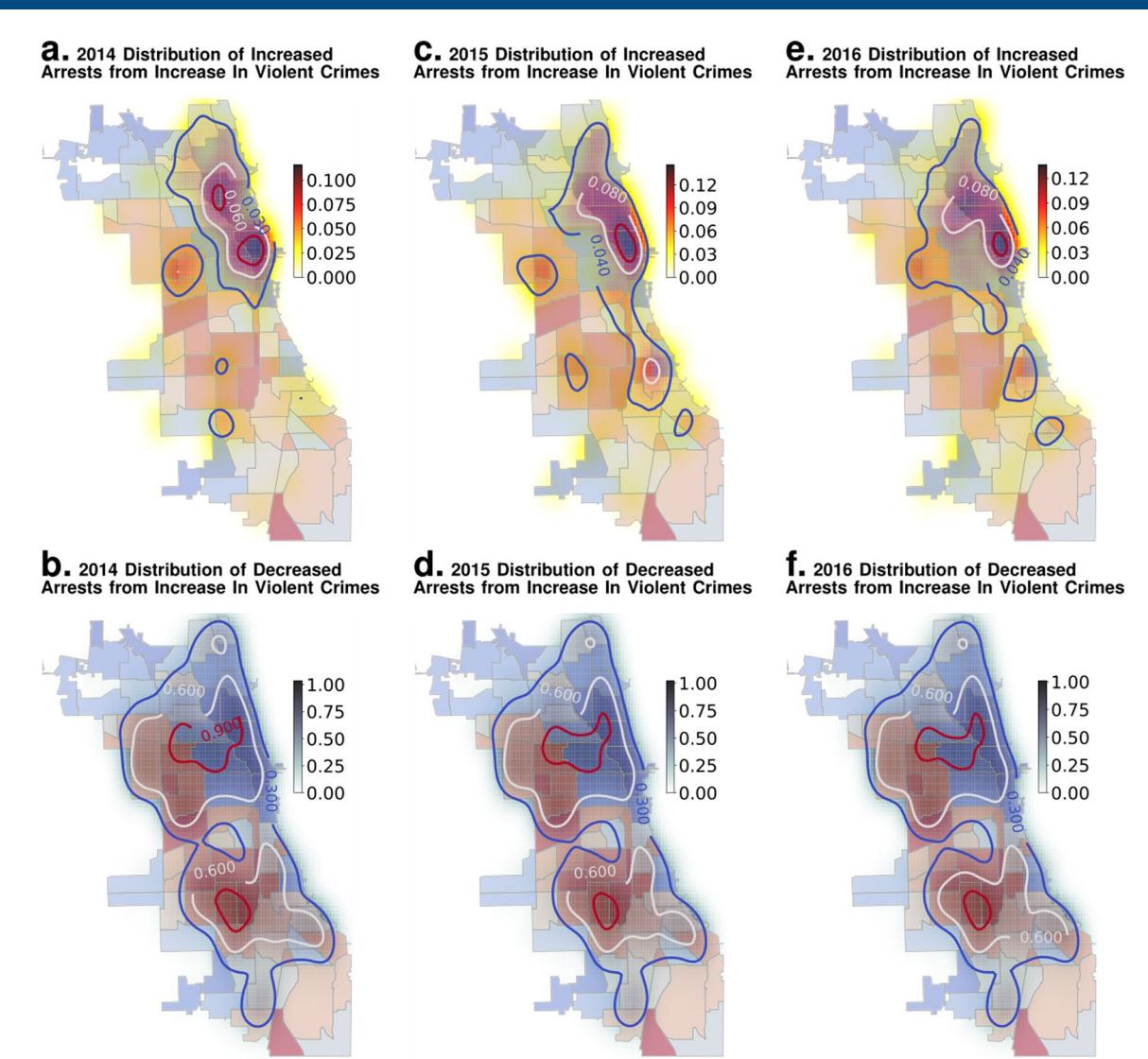
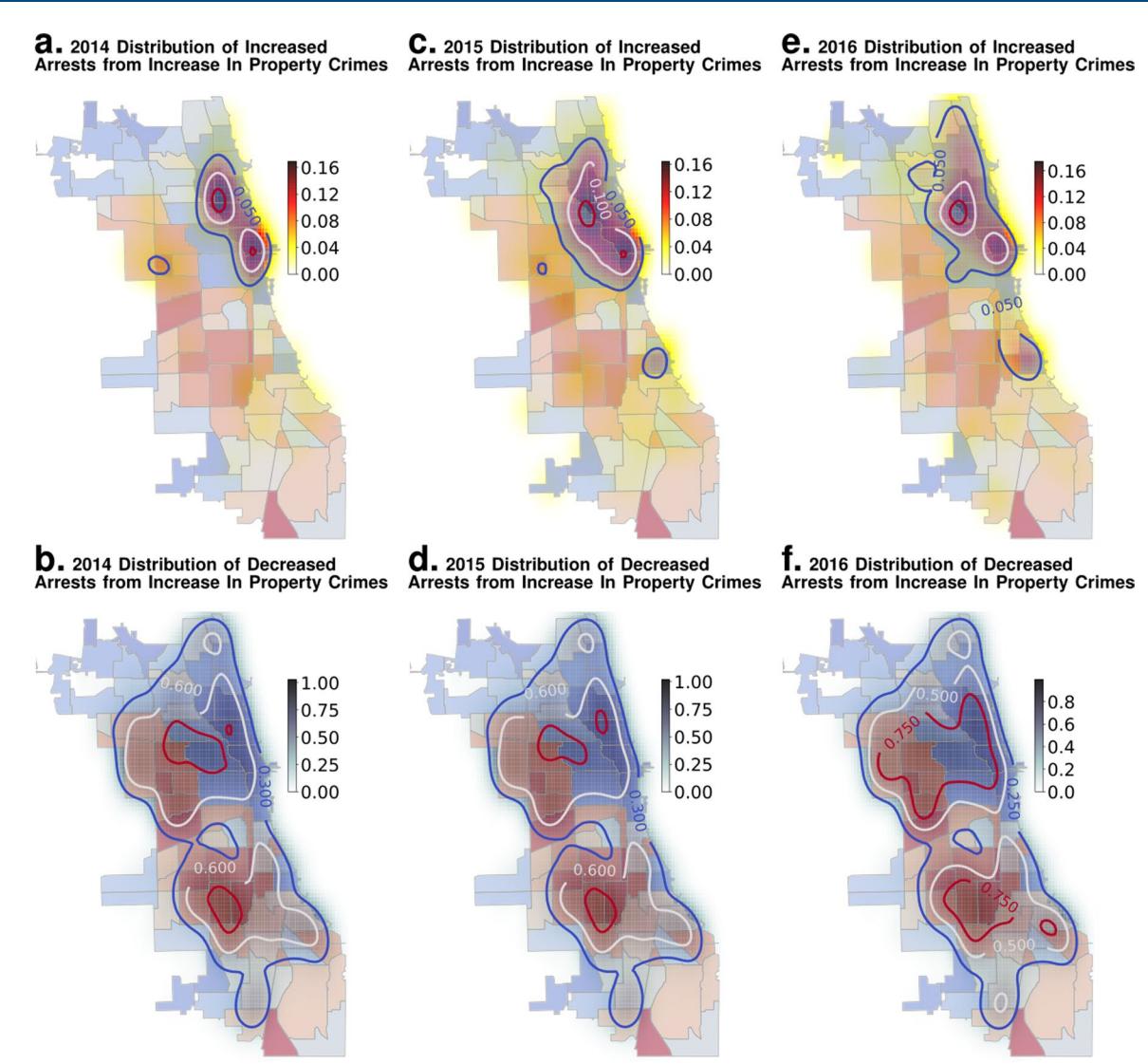
Extended Data Fig. 4 | Stability of Suburban Bias over Years (Violent Crimes). We show that the nature of the perturbation response shown in Fig. 3 holds true for earlier years as well: panels a and b correspond to year 2014, c and d correspond to 2015 and e and f correspond to year 2016, all of which follow the same pattern shown in Fig. 3.

Nature Huma Humann Behhaviour Articles

Extended Data Fig. 5 | Stability of Suburban Bias over Years (Property Crimes). We show that the nature of the perturbation response shown in Fig. 3 holds true for earlier years as well: panels a and b correspond to year 2014, c and d correspond to 2015 and e and f correspond to year 2016, all of which follow the same pattern shown in Fig. 3.

Articles Nature Huma Humann Behhaviour

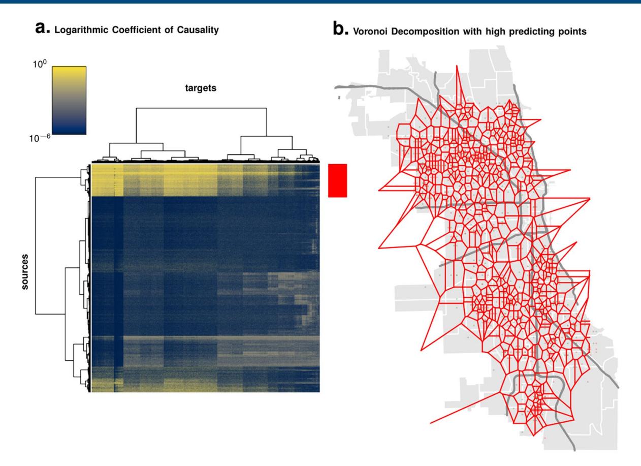
Extended Data Fig. 6 | Automatic Neighborhood Decomposition Using Event Predictability. Using Event Predictability Computing a bi-clustering on the source-vs-target influence matrix (panel A) isolates a set of spatial tiles that are, on average, good predictors for all other tiles. Using this set, we use a Voronoi decomposition of the city (Panel B), which realizes an automatic spatial decomposition of the urban space, driven by event predictability.

Nature Huma Humann Behhaviour Articles

Extended Data Table 1 | Prediction Statistics for Portland. Prediction Statistics for the City of Portland, USA

	specificity †	median AUC	frequency	accuracy††	PPV*
STREET CRIMES	0.82	0.84	7.1%	0.96	0.62
OTHER	0.71	0.81	14.5%	0.92	0.65
MOTOR VEHICLE THEFT	0.82	0.83	3.2%	0.98	0.43
BURGLARY	1.00	0.97	1.2%	1.00	0.85

Articles Nature Huma Humann Behhaviour

Extended Data Table 2 | Naive baseline results: mean AUC achieved with ARIMA models. Naive baseline results: mean AUC achieved with ARIMA models

city	ARIMA (5, 1, 0)	ARIMA (10, 1, 0)	ARIMA (5, 2, 0)	ARIMA (10, 2, 0)
Atlanta	0.65	0.66	0.62	0.66
Austin	0.65	0.68	0.63	0.67
Detroit	0.59	0.62	0.57	0.61
Philadelphia	0.64	0.65	0.63	0.65
Los Angeles	0.64	0.67	0.61	0.66
San Francisco	0.68	0.70	0.66	0.69
Chicago	0.70	0.71	0.67	0.69

Corresponding author(s):	Ishanu Chattopadhyay
Last updated by author(s): Nov 26, 2021

Reporting Summary

Nature Portfolio wishes to improve the reproducibility of the work that we publish. This form provides structure for consistency and transparency in reporting. For further information on Nature Portfolio policies, see our Editorial Policies and the Editorial Policy Checklist.

		Statistics

		For all statistical analyses, confirm that the following items are present in the figure legend, table legend, main text, or Methods section.
n/a	Confirmed
		The exact sample size (n) for each experimental group/condition, given as a discrete number and unit of measurement
	A statement on whether measurements were taken from distinct samples or whether the same sample was measured repeatedly
		The statistical test(s) used AND whether they are one- or two-sided Only common tests should be described solely by name; describe more complex techniques in the Methods section.
	A description of all covariates tested
	A description of any assumptions or corrections, such as tests of normality and adjustment for multiple comparisons
		A full description of the statistical parameters including central tendency (e.g. means) or other basic estimates (e.g. regression coefficient) AND variation (e.g. standard deviation) or associated estimates of uncertainty (e.g. confidence intervals)
	For null hypothesis testing, the test statistic (e.g. F, t, r) with confidence intervals, effect sizes, degrees of freedom and P value noted Give P values as exact values whenever suitable.
		For Bayesian analysis, information on the choice of priors and Markov chain Monte Carlo settings
	For hierarchical and complex designs, identification of the appropriate level for tests and full reporting of outcomes
		Estimates of effect sizes (e.g. Cohen’s d, Pearson’s r), indicating how they were calculated
		Our web collection on statistics for biologists contains articles on many of the points above.
	Software and code
		Policy information about availability of computer code
	Data collection	No software was used
	Data analysis	Analysis was carried out via custom developed software. The software developed was written in C++ and Python 3.x. Software with source code is available at , and the current version of the software may be referenced by

Data

Policy information about availability of data

All manuscripts must include a data availability statement. This statement should provide the following information, where applicable:

For manuscripts utilizing custom algorithms or software that are central to the research but not yet described in published literature, software must be made available to editors and reviewers. We strongly encourage code deposition in a community repository (e.g. GitHub). See the Nature Portfolio guidelines for submitting code & software for further information.

• Accession codes, unique identifiers, or web links for publicly available datasets

the .

• A description of any restrictions on data availability
• For clinical datasets or third party data, please ensure that the statement adheres to our policy

Crime incident data used in this study is in the public domain. The weblinks for the data sources for seven out of the eight cities considered here are as follows: opendata.atlantapd.org, data.austintexas.gov , data.detroitmi.gov, data.lacity.org, www.opendata.philly.org, data.sfgov.org, data.cityofchicago.org, and for Portland the data along with the leader board data for the forecasting challenge was obtained from nij.ojp.gov.

Field-specific reporting
	Please select the one below that is the best fit for your research. If you are not sure, read the appropriate sections before making your selection.
Life sciences	Behavioural & social sciences Ecological, evolutionary & environmental sciences
	For a reference copy of the document with all sections, see nature.com/documents/nr-reporting-summary-flat.pdf
	Behavioural & social sciences study design
	All studies must disclose on these points even when the disclosure is negative.
Study description	Data was quantitative: incidence data for crime in major US cities. The study aimed to model, and predict the dynamics.
Research sample	Eight major US cities
Sampling strategy	All incidence data for urban crime available as spatio-temporal logs. No sampling was done. We used all data that was available from city of law enforcement agencies.
Data collection	Data was obtained from public databases maintained by authorized agencies.
Timing	For Chicago data from 2017 onwards was used. For other cities, we used data on the entire period over which it was made available for by authorized agencies.
Data exclusions	In Chicago we excluded criminal infractions that result from non-violent drug crimes.
Non-participation	Not applicable
Randomization	Not applicable

Reporting for specific materials, systems and methods

We require information from authors about some types of materials, experimental systems and methods used in many studies. Here, indicate whether each material, system or method listed is relevant to your study. If you are not sure if a list item applies to your research, read the appropriate section before selecting a response.

Materials & experimental systems		Methods
n/a	Involved in the study	n/a Involved in the study
	Antibodies	ChIP-seq
	Eukaryotic cell lines	Flow cytometry
	Palaeontology and archaeology	MRI-based neuroimaging
	Animals and other organisms
	Human research participants
	Clinical data
	Dual use research of concern

Reproduced with permission of copyright owner. Further reproduction prohibited without permission.