The Econometricians
Great Minds in Finance
Series Editor
- Professor Colin Read
- Professor of Economics and Finance
- former Dean of the School of Business and Economics
- The State University of New York at Plattsburgh (SUNY) , USA
Aims of the Series
Th is series explores the lives and times, theories and applications of those who have contributed most signifi cantly to the formal study of fi nance. It aims to bring to life the theories that are the foundation of modern fi nance, by examining them within the context of the historical backdrop and the life stories and characters of the ‘great minds’ behind them. Readers may be those interested in the fundamental underpinnings of our stock and bond markets; college students who want to delve into the signifi cance behind the theories; or experts who constantly look for ways to more clearly understand what they do, so they can better relate to their clients and communities.
More information about this series at http://www.springer.com/mycopy/series/15025
The Econometricians
Gauss, Galton, Pearson, Fisher, Hotelling, Cowles, Frisch and Haavelmo
Colin Read
- Professor of Economics and Finance
- former Dean of the School of Business and Economics
- The State University of New York at Plattsburgh (SUNY) , USA
Great Minds in Finance ISBN 978-1-137-34136-5 ISBN 978-1-137-34137-2 (eBook) DOI 10.1057/978-1-137-34137-2
Library of Congress Control Number: 2016948000
© Th e Editor(s) (if applicable) and Th e Author(s) 2016
Th e author(s) has/have asserted their right(s) to be identifi ed as the author(s) of this work in accordance with the Copyright, Designs and Patents Act 1988.
Th is work is subject to copyright. All rights are solely and exclusively licensed by the Publisher, whether the whole or part of the material is concerned, specifi cally the rights of translation, reprinting, reuse of illustrations, recitation, broadcasting, reproduction on microfi lms or in any other physical way, and transmission or information storage and retrieval, electronic adaptation, computer software, or by similar or dissimilar methodology now known or hereafter developed.
Th e use of general descriptive names, registered names, trademarks, service marks, etc. in this publication does not imply, even in the absence of a specifi c statement, that such names are exempt from the relevant protective laws and regulations and therefore free for general use.
Th e publisher, the authors and the editors are safe to assume that the advice and information in this book are believed to be true and accurate at the date of publication. Neither the publisher nor the authors or the editors give a warranty, express or implied, with respect to the material contained herein or for any errors or omissions that may have been made.
Printed on acid-free paper
Th is Palgrave Macmillan imprint is published by Springer Nature Th e registered company is Macmillan Publishers Ltd. London
Preamble
This book is the seventh in a series of discussions about the great minds in the history and theory of fi nance.
The series describes the contributions of those remarkable individuals who expanded our understanding of the underpinnings and theories of modern fi nance. While earlier volumes discussed those who described the importance of growth and interest rates on our economic decisions, described the methods by which we choose assets for our portfolios, discussed whether markets are effi cient, and described the roots and applications of public fi nance, this volume treats the statistical and econometric tools that provide the foundation of all fi nance theory.
The statisticians and econometricians who we describe here collectively created the framework and the techniques with which we have viewed fi nance ever since. Th eir tools were, at times, developed to solve problems that were intuitively unrelated to fi nance, but which were eventually tailored to the unique needs of the discipline. A series of great minds developed their concepts well before theorists and practitioners had access to modern computing, so their theories were necessarily intuitive and geometric, and easy to apply with a pencil and paper and some incredible imagination. While the technological limitations of their day had initially limited and somewhat rigidly defi ned how we now view our fi nancial variables and analyses, the limitations also off er a simplicity and create a vocabulary that is most accessible.
The conceptual framework began with the work of Carl Friedrich Gauss , in his eff orts to describe not only the movement of the planets but also the valuation of a widow’s pension annuity. His commonsense and intuitive approach is now one of the earliest taught statistical concept, and his Gaussian “normal” distribution now underpins much of fi nancial theory. Indeed, his method of least squares , the linear regression model, the concept of maximum likelihood, and the description of data based on its mean and variance have been broadly applied to fi nance problems for the past century, and is the foundation for the courses in statistics we take in our fi nance programs.
Gauss’ contribution was further formalized by the work of Sir Francis Galton in his seemingly unrelated development of the eugenics movement, by Galton’s prodigy, Karl Pearson, the fi rst modern statistician, and by Sir Ronald Fisher , and his further characterizations of Gauss’ distribution. Th en, Harold Hotelling took this burgeoning study of statistics to better understand and discern trends in fi nancial data. Th e totality of their contributions now represents the basis for the introduction to statistical methods studied by every fi nance student ever since.
In particular, the characterization of the properties of various statistics which summarize and represent fi nancial data was an essential step in proving our confi dence in models meant to represent or predict data. Here, Gauss got us started, and so much more. Th e next step was in the construction of mathematical models which can predict our data. Th e enigmatic Francis Galton took the statistical methods formulated by Gauss and produced the intuition for the now familiar and widely employed linear regression model.
Sir Galton fomented a revolution. Th e scientifi c method had advanced humanity’s knowledge manifold in the previous couple of centuries. Galton brought a new level of sophistication to experimental technique and to social sciences. He also produced the foundation for the linear regression model that others would use as a basis for a revolution in analysis and policy making. But, his contribution, while intuitive and important, was incomplete and lacked suffi cient formality. His prodigy, Karl Pearson, added rigor and proposed a multitude of statistical measures still employed today. Th en, the brilliant Sir Ronald Fisher parlayed the poor eyesight he suff ered as a young boy into a geometric interpretation of the statistics Pearson proposed and produced an axiomatic and formal body of results that established modern statistics as a legitimate body of mathematics.
All these individuals were either astrophysicists, geneticists or applied mathematicians, though. None of them understood the particular problems that fi nance theory invoked. Nor did any of these great minds spend time analyzing the data sets necessary to turn the art of fi nance into the science that is today. Th e next necessary leap was to take these tools of mathematical statistics and apply them to problems in fi nance and economics. Th e Great Mind Harold Hotelling was instrumental in expanding the work of Fisher and in bringing it to new and receptive scholars in the USA. However, the time series data so prevalent in fi nance presented peculiar problems. Th e rapid development of the specialized tools of econometrics and fi nancial statistics required a fresh approach.
An heir to a newspaper empire was one of the fi rst to realize that these techniques could be recast on a systematic basis to treat time series data that was particularly relevant to fi nance. While not necessarily a trained scientist himself, Alfred Cowles III was nonetheless an entrepreneur who viewed his role as one who could create an environment for others more scientifi cally skilled to vaunt forward the new disciplines of fi nance and econometrics. He did so by forming an institution that would attract some of the greatest minds in the history of fi nance. Th ese include the Great Minds Milton Friedman , Kenneth Arrow, Jacob Marschak , Harry Markowitz and others.
Two such luminaries who accepted Cowles ’ intuition and largesse were Ragnar Frisch and Trygve Haavelmo , a pair of great minds the Nobel Memorial Prize Committee eventually recognized as the founders of modern econometrics and fi nancial statistics. Th eir extension of statistics to the creation of the more specialized fi eld of econometrics signifi cantly expanded the sophistication and robustness of empirical fi nancial models ever since.
Cowles , Frisch and Haavelmo also established a research agenda that would result in the awarding of Nobel Memorial Prizes to almost a dozen subsequent contributors to the foundations of modern fi nance, most of whom are chronicled elsewhere in this series. Collectively, these Great Minds established the foundation in fi nance that all fi nancial theorists have since followed.
Through their contributions, our theories of finance could be compared to and validated against real-world data. Th ey have allowed subsequent scholars to improve, or perhaps reject their models, have permitted policy makers to off er better public fi nance tools, and have allowed practitioners to discover and tease value from the vast reams of data generated from fi nancial markets. In doing so, these Great Minds helped make the art of investing a modern science.
Preface to the Great M inds in Finance Series
When one mentions the word “finance” to an interested and engaged listener, people respond in a variety of ways. Th e word may elicit a yawn from those who think of fi nance as the mundane process of ensuring the family savings will allow them to maintain their familiar level of consumption in their retirement years. Students of fi nance, at college or in life, think of the term as a mechanism for a battle of wits, with buyers and sellers of securities pitting themselves against each other to see who can profi t best from the same information. A banker might think of the conservative practices one employs with shareholder and depositor money by lending it back out to trustworthy businesses in the region, hopefully to earn a profi t. And tax accountants and lawyers may think of the myriad of ways a corporation can organize to maximize owners’ profi ts and minimize risk. Listeners often prefer to relegate the intricacies of fi nance to an expert, as they would their legal or medical aff airs.
Most people use the terms economics and fi nance synonymously. Th is misconception is understandable. Th e formal discipline of economics defi nes the laws or principles that govern the choices we make in meeting our needs. Th e term economics is derived from the Greek word “oikos,” meaning environment but also referring to one’s house or life. It is combined with “nomics” from the Greek word “nomos,” or “law of,” to label the social science that studies our decisions in furthering our own interests.
Th ese “economic” decisions are primarily thought of as fi nancial because they often involve money. Households attempt to manage their income and wealth to ensure they are able to consume, in the present and the future, in ways that allow them to thrive. Such careful fi nancial decisions that will govern our consumption now and in retirement are so critical for our well-being that it is natural for most people to consider fi nance as economics even though, more correctly, fi nance is a branch of economics that has great relevance in the day-to-day and livelihooddefi ning decisions of us all.
Th is series describes the ancestry, life, times, theories and legacies of the great minds who contributed to the modern formal study of fi nance. Th eir collective contributions address the various interpretations of fi nance not through dry exposition and even drier equations, but through intuition and context, their lives and times, and a few equations and diagrams that each developed to revolutionize fi nancial thought.
Readers may be those interested in the fundamental underpinnings of our stock and bond markets, college students who want to delve into the signifi cance behind the theories, and the experts who constantly look for ways to more clearly understand what they do so they can better relate to their clients and communities. Th e series provides important insights of great minds in fi nance within a context of the events that inspired their moments of brilliance. In doing so, I hope to bring life to the theories that are the foundation of modern fi nance.
Th is series covers the gamut of the study of fi nance, typically through the lives and contributions of great minds upon whose shoulders the discipline stands. From the signifi cance of fi nancial decisions over time and through the cycle of one’s life, to the ways in which investors balance reward and risk, from how the price of a security is determined to whether these prices properly refl ect all available information, we will look at the fundamental questions and answers in fi nance. We delve into theories that govern personal decision-making, those that dictate the decisions of corporations and other similar entities, and the public fi nance of government.
Some of the theories we describe may appear abstract and narrow. A successful theory must be suffi ciently narrow to make strong conclusions. A theory that is overly general will draw the weakest of conclusions that off er little utility. On the contrary, the best theories draw the strongest possible conclusions from the weakest set of assumptions. And, a successful “unifying” theory in fi nance can replace a large number of lesser theories and concepts, just as physicists hold out for a unifying theory that can draw together their isolated understandings from a variety of specialties.
By focusing on the great minds in fi nance, we draw together the concepts that have stood the test of time and have proven themselves to reveal something about the way humans make fi nancial decisions. Th ese principles that have fl owed from individuals who are typically awarded the Nobel Memorial Prize in Economics for their insights, or perhaps shall be awarded someday, allow us to see the fi nancial forest for the trees.
While one might assume that every fi nancial expert would be well versed in these fundamentals, such is not the case. An investor can succeed through sheer intuition without having studied the insights of theorists over a century of fi nancial discovery. Mathematicians and physicists are increasingly employed to develop techniques that recognize patterns in numbers with little regard or understanding of the underlying forces that explain these patterns. And, computer experts can design algorithms that allow great banks of servers to constantly poke and prod the market to induce, and then profi t from, movements in prices of stocks or bonds. By capitalizing on such shifts in prices milliseconds before others take notice, these algorithms can garner pennies, or fractions of pennies, at a time, thousands of times an hour, to yield huge profi ts.
Th ese practitioners do not depend on, or even care about, the fundamental principles that drive markets in the long run. To them, the long run expires within a week or a day. Such “technical analysis” is decidedly transient and short term. In fact, a steady and predictable investment opportunity based on well-known and well-understood information is simply insuffi ciently volatile to yield quick profi ts.
Unfortunately, such technical analysis that depends only on price dynamics in the short term has emerged as the lucrative Holy Grail of modern fi nance. It allows the most skilled practitioners to make money when markets are rising or falling. However, it reveals nothing about how fi nancial decisions should be made in the long run to satisfy an economy’s need for capital, investment, reward and reduced risk. Nor does it make our economy more effi cient. Rather, technical analysts devote a great deal of talent, energy and eff ort as they clamor for others’ pieces of a fi xed economic pie.
Th e giants who have produced the theories and concepts that drive fi nancial fundamentals share one important characteristic. Th ey have developed insights that explain how markets can be used or tailored to create a more effi cient economy. Th ey demonstrate how individuals can trade risk and reward in the same way that a supplier might trade with a consumer of a good. Th rough this process, both sides win. Greater effi ciency is a tide that lifts all boats. Th ese pioneers of fi nance explain how tools can be used to create greater market effi ciency and even suggest the creation of new tools to create effi ciency enhancements that may have proven elusive otherwise.
Global fi nancial markets are experiencing a technological revolution. From a strictly aesthetic perspective, one cannot entirely condemn the tug-of-war struggle for profi ts the technicians seek, even if they do little to enhance, and may even detract from, effi ciency. Th e mathematics and physics of price movements and the sophistication of computer algorithms are fascinating in their own rights. Indeed, my university studies began with a Bachelor of Science degree in physics, followed by a PhD in economics. However, as I began to teach economics and fi nance, I realized that the analytic tools of physics that so pervades theories of modern fi nance has strayed too far from explaining the essence of human fi nancial decision-making.
As I taught the economics of intertemporal choice, the role of money and fi nancial instruments, and the structure of the banking and fi nancial intermediaries, I also recognized that my students had become increasingly fascinated with investment banking and Wall Street. Meanwhile, the developed world experienced the most signifi cant breakdown of fi nancial markets in almost eight decades. I realized that this once-ina-lifetime global fi nancial meltdown arose because we had moved from an economy that produced stuff to one in which a third of all profi ts by 2006 in the USA were made in the fi nancial industry, with little to show but pieces of paper representing wealth that had value only if some were ever ready to buy them.
Many were surprised by the Global Financial Meltdown that soon followed. It became clear that much of our fi nancial understanding lacked perspective. I set out to discover that perspective and research the theories that underpin modern fi nance, with the goal of forming a better understanding how great fi nancial concepts were created. I decided to shift my research from academic research in esoteric fi elds of economics and fi nance and toward better understanding of markets on behalf of the educated public. I began to write a regular business column and a book that documented the unraveling of the Great Recession. Th e book, entitled Global Financial Meltdown: How We Can Avoid the Next Economic Crisis , described the events that gave rise to the most signifi cant economic crisis in our lifetime. I followed that book with “Th e Fear Factor” that explained the important role of fear as a sometimes constructive, and at other times destructive, infl uence in our fi nancial decision-making. I then wrote a book on why many economies at fi rst thrive, and then struggle to survive in Th e Rise and Fall of an Economic Empire . Th roughout, I try to explain the intuition and the understanding that would, at least, help readers make informed decisions in increasingly volatile global economies and fi nancial markets.
In this series of great minds in fi nance, I off er a historical perspective on how the discipline of fi nance developed. I also hope to impart to you how individuals born without great fanfare can be regarded as geniuses, often in their lifetime but sometimes not until years later. Th e lives of each of the individuals treated in this series become extraordinary, not because they made an unfathomable leap in our understanding, but rather because they looked at something in a diff erent way and caused us all to forever look at the problem in this new way. Th at is the test of genius.
Contents
| Part I | Mathematicians and Astronomers | 1 |
|---|---|---|
| 1 | Th e Early Life of Carl Friedrich Gauss | 3 |
| 2 | Th e Times of Carl Friedrich Gauss | 11 |
| 3 | Carl Gauss’ Great Idea | 33 |
| 4 | Th e Later Years and Legacy of Carl Friedrich Gauss | 57 |
| Part II | From Least Squares to Eugenics | 65 |
| 5 | Th e Early Life of Francis Galton | 67 |
| 6 | Th e Times of Francis Galton | 75 |
| 7 | Th e Later Life and Legacy of Sir Francis Galton | 81 |
| 8 | Th e Early Life of Karl Pearson | 83 |
| 9 | Karl Pearson’s Great Idea | 89 |
| 10 | Th e Later Life and Legacy of Karl Pearson | 99 |
| Part III | Th e Formation of Modern Statistics | 109 |
| 11 | Th e Early Life of Ronald Aylmer Fisher | 111 |
| 12 | Th e Times of Ronald Aylmer Fisher | 121 |
| 13 | Ronald Fisher ’s Great Idea | 129 |
| 14 | Later Life and Legacy of Ronald Fisher | 139 |
| 15 | Th e Early Life of Harold Hotelling | 149 |
| 16 | Th e Times of Harold Hotelling | 159 |
| 17 | Harold Hotelling ’s Great Idea | 165 |
| 18 | Th e Later Life and Legacy of Harold Hotelling | 171 |
| Part IV | Th e Birth of a Commission and Econometrics | 175 |
| 19 | Th e Early Life of Alfred Cowles III | 177 |
| 20 | Th e Times of Alfred Cowles III | 187 |
| 21 | Th e Great Idea of Alfred Cowles III | |
| 22 | Legacy and Later Life of Alfred Cowles III | |
| 23 | Th e Early Life of Ragnar Frisch | |
| 24 | Th e Times of Ragnar Frisch | |
| 25 | Ragnar Frisch’s Great Idea | |
| 26 | Legacy and Later Life of Ragnar Frisch | |
| 27 | Th e Early Years of Trygve Haavelmo | |
| 28 | Th e Times of Trygve Haavelmo | |
| 29 | Haavelmo ’s Great Idea | |
| 30 | Legacy and Later Life of Trygve Haavelmo | |
| Part V | What We Have Learned | |
| 31 | Conclusions | |
| Glossary | 251 | |
| Index | 257 |
List of Figures
| Fig. 1.1 | Th e ancestry of Carl Friedrich Gauss | 5 |
|---|---|---|
| Fig. 2.1 | Th e calculation of geometric means | 14 |
| Fig. 2.2 | Th e pentagon in a unit circle | 15 |
| Fig. 2.3 | An isosceles triangle of hypotenuse p and adjacent | |
| and opposite sides q | 18 | |
| Fig. 2.4 | Th e complex plane | 24 |
| Fig. 2.5 | Th e unit circle on the complex plane | 26 |
| Fig. 2.6 | Regular polygons in the unit circle on the complex plane | 28 |
| Fig. 3.1 | Th e Gaussian distribution | 53 |
| Fig. 5.1 | Th e ancestry of Francis Galton | 69 |
| Fig. 8.1 | Th e ancestry of Carl Pearson | 85 |
| Fig. 10.1 | Th e ancestry of Maria Sharpe | 103 |
| Fig. 11.1 | Th e ancestry of Ronald Fisher | 113 |
| Fig. 13.1 | Th e predicted cone of a hypothesis test | 131 |
| Fig. 15.1 | Th e ancestry of the Rawson family | 151 |
| Fig. 15.2 | Th e distant ancestry of Harold Hotelling | 153 |
| Fig. 15.3 | Th e immediate ancestry of Harold Hotelling | 156 |
| Fig. 19.1 | Distant ancestry of Alfred Cowles III | 178 |
| Fig. 19.2 | Immediate ancestry of Alfred Cowles III | 180 |
| Fig. 19.3 | Ancestry of Elizabeth Cheney | 184 |
| Fig. 23.1 | Ancestry of Ragnar Frisch | 202 |
| Fig. 27.1 | Ancestry of the Haavelmo family | 224 |
Part 1: Mathematicians and Astronomers
We begin with the struggle of some great mathematicians who wrestled fi rst with an understanding of problems that concerned their gambling patrons, and then with ways their understanding of probability could be used to better predict the movement of the planets.
Th ese explorations over the seventeenth and eighteenth centuries eventually allowed a very young nineteenth-century theorist to translate the insights of those who came earlier with a discovery that revolutionized almost every aspect of science, including fi nance and statistics. Perhaps what is most surprising, though, is that the genius of Carl Friedrich Gauss came from the most humble of beginnings.
1. The Early Life of Carl Friedrich Gauss
Th ere is perhaps no discipline that is so intrinsically tied to data than the study of fi nance. Every fi nancial theory is formulated not for some esoteric purpose, but rather to better understand future occurrences based on past information. Th is world of fi nancial data is so broad that it makes little sense unless it can be simplifi ed and represented by a few familiar measures. Our models then incorporate these measures to predict movements in fi nancial variables. Th is problem is not unlike the challenge of those who gazed at the planets and stars and tried to predict their motion. One such mathematical explorer enjoyed more success in challenging predictions than any other. His surprisingly humble upbringing almost defi es his incredible insights and contributions to dozens of sciences since, fi nance included.
Th e circle of academics was an extremely small one before the twentieth century. Th ere was no public education, and hence little opportunity for higher education, except for the noble and elite. Nor was science so technical then that it commanded extensive knowledge, or large teams devoted to research. Indeed, intellectual discovery was a luxury supported by family wealth and royal courts which might sponsor one or two such men of ideas.
Th ese prodigies were viewed more as intellectual athletes and mystics. Th ey would be pitted against each other to demonstrate their intellectual cunning and lend pride to their patrons. Th ese were not the circles in which a humble boy of modest means and upbringing could fi nd himself.
Carl Friedrich Gauss was an exception. He also became one of the most exceptional mathematicians of all time, who is spoken in the same breath only with Euclid and Newton .
Gauss came from a family of farmers and laborers. His great-greatgrandfather, Hans Gauss (c.1600–?), was born in Hanover, Germany, and had found his way to Wendeburg, a small farming village in the neighboring district of Peine of Germany’s Lower Saxony region. He had a family of small size in this era: a wife, two sons and four daughters. At fi rst, his family and progeny remained close to home.
His son Henrich Gauss (1 December 1648–25 October 1726) was born in Wendeburg. He married three times. Th e fi rst marriage resulted in a dowry of a farm that had belonged to his fi rst wife, Anna Grove, a widow, in nearby Volkenrode, less than six kilometers to the southeast of Wendeburg (Fig. 1.1 ).
Henrich had a dozen children, four from each marriage, and was left a widower from each of his fi rst two marriages. His last marriage resulted in a son Jurgen.
Jurgen Gauss (or Goos) (3 November 1712–5 July 1774) was born in Volkenrode and grew up tending the farm. However, as one of the last of a dozen children, there would be no room for him on the farm once he became an adult. Instead, he moved to the large German city of Braunschweig, or Brunswiek in Low German, Brunswick in English, at the extreme southern port of the Oker River as it makes its way toward the North Sea. At the time, Brunswick was a major economic and cultural center for Germany. It was also a center for education.
Jurgen Gauss arrived in Brunswick late in the decade of the 1730s, with a new bride, Katharine Magdalene Eggling (5 March 1713–3 April 1774), the daughter of Hans Heinrich Eggling (1667–25 December 1714) and Cathrine Heuer. Soon upon his acceptance as a resident of Brunswick, he took his fi rst job off of the farm, on 23 January 1739. His adopted city fi rst employed him as a day laborer, then as a clay mason and a butcher. Each of the latter occupations entitled Jurgen membership
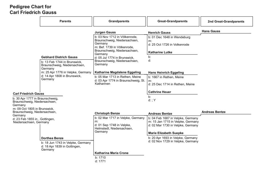
Fig. 1.1 The ancestry of Carl Friedrich Gauss
to guilds, and all would provide him with employment through the four seasons. Th e family enjoyed a level of urban economic comfort not readily aff orded to the youngest child in a farming family.
Jurgen Gauss and Katharine soon secured a small and narrow house for his family, at 10 Ritterbrunnen. Th ey lived in that home for 14 years, and raised four children there, including an eldest son, Gebhard Dietrich Gauss (13 February 1744–14 April 1808). Th e family then moved to a larger home at 30 Wilhelmstrasse, where Jurgen would die of tuberculosis on 5 July 1774, just three months and two days after the death of his wife from a prolonged fever.
By the time his father died, the second child and the eldest son, Gebhard, had worked and learned the family trades. Upon his parents’ death, Gebhard used a dowry from his fi rst wife, Dorothea Emerenzia Warnecke, and a loan from the town’s mayor Wilmerding, to buy out the shares of his family home from his brothers Johanne Franz Heinrich and Peter Heinrich. By the age of 30, Gebhard was able to provide a home and a secure but not affl uent living for his own family.
Gebhard’s fi rst wife did not long enjoy the house, though. She died on 5 September 1775 of tuberculosis as had her father-in-law, but not before giving birth to a boy. Johann Georg Heinrich was born on 14 January 1769.
Seven months after Dorothea Warnecke died, Gebhard married Dorothea Benze, the daughter of a stonemason, Christophe Benze (2 March 1717–1 September 1748). Dorothea’s father died prematurely as well, from pulmonary respiratory illness associated with his profession as a stonemason. He also left a son, Johann Friedrich. Both of Christophe Benze’s children were thoughtful and intelligent, but neither enjoyed the luxury of formal schooling.
Dorothea was illiterate, but she was a kind and nurturing woman by nature. She worked as a maid before she married Gebhard. While Gebhard was also uneducated, he nonetheless managed to be appointed the city’s master of waterworks as he was an experienced stonemason and was reasonably good with sums.
In contrast to his wife’s gentle nature, Gebhard was quite domineering as a father, and was considered rather somewhat uncouth. Yet, he provided reasonably well for his family.
The Arrival of Carl Gauss
Gebhard and his second wife had a son just over a year after their marriage, on 25 April 1776. Carl Friedrich was born in the family home in Brunswick on 30 April 1777, on the Wednesday eight days before the Ascension. He was an only child of the second marriage, but was a half brother to Gebhard’s eldest son Johann.
When a young Carl once quizzed his mother about his birthdate, she could not recall the exact date. Later in life, Carl was able to calculate it based on his mother’s recollection of his birth before the Ascension. At a young age, he used this small family mystery as an opportunity to develop a formula for the day Easter arose for any given year. It did not take long for his family to discover that the young Gauss was a mathematical prodigy.
Carl had great aff ection for his mother, and for her brother, his uncle Johann Friedrich, but had a somewhat awkward relationship with his half brother. Indeed, he did not know his brother Johann Georg very well. More than eight years his senior, Johann struck out on his own as a day laborer before Carl’s tenth birthday. Johann returned home some years later, but an eye injury made him only of limited help to his father. Instead, Johann enlisted in the army for almost a decade, and returned to his family home to take over his father’s trade once his father died on 14 April 1808.
While Carl Friedrich grew up with a harsh and domineering father, he enjoyed the better nature of his kind and devoted mother. In turn, he doted on his mother all his life, until Dorothea’s death at the remarkably advanced age of 97, even through her infi rmities and her affl iction with blindness in her last four years.
Carl harbored fond and vivid memories of his childhood. One of his earliest memories was falling into the river and being saved at a very young age. Th is terrifying memory did not taint his recollections otherwise, though.
He also recalled that he taught himself to read by asking his family members how to pronounce letters on the page. His ability to manipulate numbers became a favorite parlor trick among family friends. When his father would pay his bricklaying workers, a three-year-old Carl once impudently but accurately corrected his father’s calculations. While access to school was out of the question for many children in his neighborhood, his intellectual precociousness compelled his family to consider his education.
In 1784, when young Carl was seven years of age, his father agreed to let him enter nearby St. Katharine’s Volksschule, a people’s school for the more motivated of the children of non-prosperous families. Th e school, which adjoined St. Katharine’s Church, had a teacher named J.G. Buttner who oversaw a dark and dank classroom of 200 children.
Young Gauss endured two years among those 200 classmates, but managed to stand out nonetheless. When the teacher gave his students an assignment he felt would keep them occupied for hours, Gauss almost immediately announced the solution. Th e teacher felt it impossible that Gauss could have so quickly added all the numbers from 1 to 100. Yet, an eight-year-old Gauss reasoned his way to a solution.
Gauss had noticed that the fi rst and last number in the sequence, 1 and 100, added to 101. So did the second and the second to last, 2 and 99, and, indeed, so do all 50 such pairs. Gauss proclaimed that 50 pairs which each add each to 101 must then total 5050. While he may not have been praised for his brilliance, he was at least spared the whip that often accompanied the incorrect answers from lesser classmates.
Headmaster Buttner quickly realized Gauss needed a more sophisticated curriculum. He ordered an advanced textbook for the boy, but professed that there was little he could teach the young prodigy. Fortunately, word got out in Brunswick about the boy wonder. Carl’s father relented on the headmaster’s admonishments that Carl spend the evening studying rather than completing chores, and allowed the neighbor’s boy, Johann Christian Martin Bartels (1769–1836), eight years’ Carl’s senior, and with a strong interest and competency in mathematics, to supplement Carl’s education. By lamplight, Carl learned mathematics together with the much older boy, and kept pace as Bartels absorbed such concepts as the binomial theorem and infi nite series.
Meanwhile, Bartels worked to fi nd a patron for Carl as he pursued his own studies in mathematics. His Collegium teacher, Eberhard August Wilhelm Zimmermann (17 August 1743–4 July 1815), had studied mathematics at the prestigious Göttingen University and was instructing mathematics at the Collegium Carolinum in Brunswick. When Bartels began classes with Zimmerman , he brought the abilities of the 11-yearold Carl Gauss to his professor’s attention. By then, Zimmermann was well respected by the local nobility, and had already been awarded the distinction of Councilor in the region. Seven years later, he was further bestowed a noble title by Duke Karl hette Wilhelm Ferdinand.
Zimmerman accepted the challenge of instructing the young prodigy. Carl Gauss was given the run of the Collegium, despite his young age, and spent almost all his free time at the school.
A few years later, the Duchess Ferdinand came across the young boy reading a book that seemed most advanced for his age. Astonished, she quizzed him on his studies, and was impressed by his knowledge of the classics, of literature and of mathematics.
At the Duchess’ behest, the Duke sent an aide to fetch young Gauss . Th e aide fi rst demanded that Carl’s older brother accompany him to the palace, but Johann Georg insisted it was for his young half brother Carl for whom the Duke beckoned.
Th e Duke took under his wing a young working-class boy, one with rough working-class edges who spoke Low German. Despite these social handicaps, the Duke funded Carl’s regular attendance at the Collegium Carolinum in 1792. Only 15 years old, Carl was already more intellectually advanced than most of the other students. In addition to the annual stipend the Duke paid on behalf of Carl, the Duke also off ered Carl’s teacher Zimmerman expenses to oversee his education, for as long as Gauss attended the local college.
Young Carl studied at the Collegium Carolinum for four years. He was exposed to the Classics, to Greek and Latin and to the mathematics of Sir Isaac Newton (25 December 1642–20 March 1726), Leonard Euler (15 April 1707–18 September 1783) and Joseph-Louis Lagrange (25 January 1736–10 April 1813). By his last year at the college, Gauss had become intellectually captivated by the astronomical explorations of Newton, and had even developed his method of least squares to tease trends from cosmological observations subject to random errors. While also still a teenager at the College, Gauss also became intrigued with prime numbers, a fascination he would continue soon upon his matriculation to the University of Göttingen.
It was at the Collegium that Carl also developed the habit of intellectual innovation primarily for his own curiosity’s sake. He only occasionally felt the need to aggregate his ideas into papers, even though he soon realized the need to record his results. He meticulously began to document his mathematical innovations in a series of dated notebook entries that he kept for his entire life.
On 21 August 1795, when Carl was 18 years old, the Duke ordered an increase in the stipend to be paid to Carl so that Carl could begin attending at the University. Th is sum covered tuition and all living expenses. On 11 October, Gauss left his hometown for the 200-kilometer trip to Göttingen, one of the nation’s most prestigious and accomplished universities. Four days after departing Brunswick, Gauss arrived and was admitted as a mathematics student to Göttingen. Carl chose the university because of its extensive mathematics library. He chose well and remained the pride of Brunswick forever after.
Th e next spring, on 30 March 1796, Gauss published notice of his fi rst major discovery. He recorded that he found a constructible solution to the 17-sided regular polygon problem that had perplexed mathematicians for 2000 years. He later recalled how he awoke from a vacation in Brunswick with the realization of a solution to the problem ( zp −1)/( z −1) = 0, which led to the solution to the constructible 17-gon.
Upon his discovery, Gauss published a notice of his result so that he may lay prior claim within the scientifi c community. Th is he had done rarely in his life because, for him, his exercise of mathematics was to satisfy his own intellectual curiosity and solve his practical problems in astronomy and geodesy. Not always would he fully fl esh out his ideas into a publishable form because, for him, completing the proof was either obvious or unnecessary. And publication was expensive in both time and money. Indeed, it would take Gauss almost a decade to publish the proof of his result on the 17-gon. Th is pattern repeated itself many times over his life. Almost invariably, his briefest assertion of myriad amazing discoveries stood the test of more rigorous treatment, often at the hands of others, and generally requiring hundreds of pages of advanced mathematics, and many decades later.
What is apparent in Gauss ’ brilliance at an early age is that his life was anything but conventional. Th at may be the source of his brilliance. While lesser children of more affl uent parents would enjoy a lifetime of forced stimulation through the minds of tutors and professors, they must always glimpse the world through someone else’s eyes. Gauss knew no such world, nor any such preconceptions. He conceived his intellectual world anew, perhaps because he was often “taught” by those less accomplished and talented than he was. His learning defi ed conventional wisdom. Th is allowed him to look at fundamental problems without any blinders or preconceptions and, for that matter, without anybody telling him his brilliant and unique approaches could not work because, after all, no great mind before him had solved the same problem. His scholarly bravado and courage to take on and solve a two-millennia-old problem, and, in doing so, unite and perhaps even invent three branches of mathematics, can be credited to his upbringing and lack of academic pedigree.
2. The Times of Carl Friedrich Gauss
Gauss loved numbers. When he imagined geometric concepts and from them developed what we would now call abstract algebra, he came to shapes from the perspective that these new approaches would help him better understand the nature of numbers. Ever since his elementary school experience in which he successfully solved a problem for his teacher based on the application of a numerical series, Gauss had numbers, integers and shapes racing in his head. While he was already publishing academic papers of high quality at the age of 18, Gauss had been interested in arithmetic and geometric means for 4 years by then, and, by 17, had explored the representation of average values through power series, and the method of least squares. Gauss developed these concepts from a position of great practicality. He used numbers, and especially their patterns, to better understand practical problems. His choice of study at the University of Göttingen was an ideal match for this intellectual curiosity.
The University of Göttingen, or, in German, Georg-August-Universität Göttingen, GAU for short, is one of Germany’s most prestigious establishments for higher education. It was founded in 1734 by King George II of Great Britain, who was also the Elector of the Kingdom of Hanover. Göttingen began classes in 1737. The quality of the institution has placed its host city at the center of learning in Germany ever since. The brilliant mathematicians Bernhard Riemann (17 September 1826–20 July 1866), David Hilbert (23 January 1862–14 February 1943), Peter Gustav Lejeune Dirichlet (13 February 1805–5 May 1859) and John von Neumann (28 December 1903–8 February 1957), and great physicists such as Max Born (11 December 1882–5 January 1970), Julius Robert Oppenheimer (22 April 1904–18 February 1967), Max Planck (23 April 1858–4 October 1947), Werner Karl Heisenberg (5 December 1901–1 February 1976), Enrico Fermi (29 September 1901–28 November 1954) and Wolfgang Pauli (25 April 1900–15 December 1958) all studied or taught there. So did the international banker and financier John Pierpont “J.P.” Morgan (17 April 1837–31 March 1913). It was also the notorious epicenter of Adolf Hitler’s (20 April 1889–30 April 1945) Great Purge of Jewish academics in 1933. Göttingen was an intellectual capital unparalleled in the celebration of abstract thought since the early 1800s, or perhaps since Carl Friedrich Gauss first studied there.
Those accepted to study at Göttingen were invariably gifted. But, few came from such modest means as had Gauss, nor with such wealthy patrons as Duke Ferdinand. When Gauss was admitted at Göttingen on 15 October 1795,1 at the age of 18, he did not yet know whether he wished to study mathematics or philology. Gauss loved words almost as much as he knew numbers.
Philology was a classical and well-appreciated discipline in the nineteenth century that divined language from the historical written record. Philologists were Renaissance scholars who used their skills in history, linguistics and literary criticism to solve literary and historical puzzles. It was at that time a foundation for what might more broadly be described as the humanities today. The discipline’s goal to solve historical and literary puzzles played to Gauss’ curiosity in the same way as numbers did, and drew upon Gauss’ extensive knowledge of many languages as had his ability to draw upon many methodologies in mathematics.
Fortunately for modern science, mathematics won Gauss’ attention, partly because the patronage he enjoyed allowed him to be less concerned about tuition and eventual salaries, and more receptive to the study of science, with all its economic impracticality. During his first year of study, he mostly read books from the renowned Göttingen library on the humanities, on philology and on travel. But, that first year sparked a passion in mathematics when Gauss managed to devise his first solution to a then intractable mathematical problem. He had become fascinated in the problem of dividing a circle into 17 parts through the creation of a 17-sided polygon constructed only with Euclidean tools.
It is instructive to explore Gauss’ path through the construction of his problem and solution as it tells us much about the brilliance of this 18 year old, on the development of the new field of complex algebra ever since, and on the way Gauss thought, in geometric terms that would become the hallmark of the greatest minds of statistics and econometrics.
The Greeks before the birth of Jesus Christ had been fascinated with the geometries that could be constructed with a simple compass and straightedge. Indeed, these early geometers had no number system yet. These tools of the compass and straightedge were what Euclid (about 300 BC) employed to construct regular polygons. These regular polygons have angles between apexes that are all equal, and sides that are the same length, such as triangles, squares, hexagons and octagons.
The Greeks were fascinated by the properties of such polygons that were contained within a circle. By calculating the area of regular polygons of ever increasing number of sides, they could even approximate the area of a circle and the number pi with great accuracy.
The Greeks quickly discovered that they could easily construct such polygons with an even number of sides by forming isosceles triangles with two equal sides in the space from the center of the circle to its circumference. They could easily construct even-number-sided polygons within the unit circle by further subdividing known polygons with an even number of sides. Such exercises allowed the Greeks to construct extensive proofs of the properties of lines, circles, triangles, squares and octagons.
While they did not actually develop a number system from the length of the sides of these polygons, they were clearly dabbling in number theory. We are reminded of this geometric interpretation when we think of raising a number to the power of two as squaring the number. We can now see these Greek geometers were on the verge of discovering algebra, polynomials, roots of polynomials, negative numbers and imaginary numbers. But, that leap in understanding would take almost two millennia to solve.
For instance, consider the area of a square drawn from the apex F of a semicircle of width AX and height AF = AX, and hence of area AX*AX. The Greeks denoted this as the geometric mean of the lengths AX and AB (Fig. 2.1):
If we denote the length of the longer ray AB as a, the length of the distance between X and B as x, and the length of the shorter rays AF, or AX as b = a−x, then a/x = x/(a−x). The length x is then the geometric mean of a and a−x, and is also the root to the polynomial obtained from equating the ratios a/x and x/(a−x). Cross-multiplying, we can express these ratios as x2 −a(a−x). Then:
x is the root of \[x^2 + ax - a^2 = 0\] .
This value of x, now more commonly expressed as the square root of the product of two numbers a and b, was generated by the Greeks using only the geometric comparisons of sides of polygons. In doing so, the Greeks were solving the roots to common polynomials using geometric analogues, but not yet with a formal algebra.
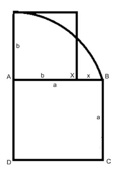
Fig. 2.1 The calculation of geometric means
The ancient Greeks had learned to construct various polygons from the square, and the series of even-sided polygons that were multiples of the four-sided figure and its successors. They could also do the same for the triangle and its even-numbered multiples. Their first challenge, though, was to form a pentagon.
Such a five-sided polygon had mystic charms, as had its relative, the five-sided star. The pentagram was the mystic symbol of the Pythagorean brotherhood. The Greeks showed that the length of the sides of such regular polygons enclosed in a circle of unit radius could be expressed with ratios of integers and their square roots (or geometric means). For instance, a pentagon within a circle can be constructed as five identical equilateral polygons much like five pieces of an evenly cut pie, with the round edges “squared-off.” Such polygons might look as in Fig. 2.2.
We learn in high school trigonometry class that if we divide the 360° of the circle into five identical parts of 72° each, then the width of the first such triangle enclosed in a unit circle is represented by the distance from the origin to the point A, or cos(360°/5) = cos(72°) = ( ) 5 1 - / . 4
The Greeks knew how to construct a unit circle with a compass, and they could find the length of the square root of 5 by observing that its value was simply the geometric mean between 5 and 1. In fact, the Greeks were able to show that they could use only a straightedge and compass, or, equivalently, with the tools of addition, subtraction, ratios and square roots, formed from the congruencies in triangles and formu-
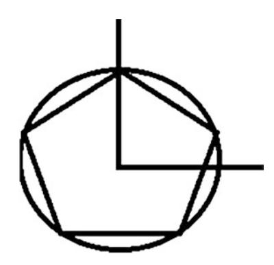
Fig. 2.2 The pentagon in a unit circle
lation of geometric means, to construct polygons with n sides for n = 3, 4, 5, 6, 10 and 15, and, of course, 8, 12 and 16 that follow naturally from the square, the hexagon and the octagon. This realization became a fourth assertion in addition to the Greek’s three famous problems of trisecting an angle, doubling a cube and squaring the circle. The latter problem required the creation of a square with the same area as a given circle.
At the age of 18, Gauss proved that the first two of these assertions of the three famous problems are impossible using only a compass and straightedge. He also showed which n-sided regular polygons was constructible, that is, they could be constructed only with a compass and straightedge, or, equivalently, with sides of a length that are the sum only of ratios of integers or square roots (geometric means). Gauss determined that constructability could occur only if the number of sides is an integer prime number that can be expressed as 2m + 1, where m is an integer.
Had the Greeks known Gauss’ insight, the world would have been spared many person-years trying to construct 7-, 11- and 13-sided polygons over the intervening two millennia. The smallest constructible polygon that remained unconstructed by the Greeks or by those who followed for more than two millennia was the 17-sided heptadecagon—until an 18-year-old Gauss proved its construction, and, in turn, created a new and incredibly important way to look at the correspondence between polygons and the number system.
Gauss’ solution came in a flash of insight. He showed 7-, 11- and 13-sided regular polygons could not be constructed, and demonstrated the constructability of the 17-sided regular polygon. In doing so, he created whole new methods of mathematical analysis without which many of our most profound technological achievements today would have been impossible.
His shear excitement at his discovery also induced him to dedicate his life to the study of mathematics, as opposed to his competing interests in philology and the classics.
Gauss’ original insight was providential. He had realized that the problems the Greeks wrestled with could often be expressed as roots to equations of the form (xp −1)/(x−1) = 0. This family of problems, for various values of p, had intrigued scholars for a century. But, just as Albert Einstein (14 March 1879–18 April 1955) had looked at the problem which perplexed Ludvig Lorenz (18 January 1829–9 June 1891), and Albert Abraham Michelson (19 December 1852–9 May 1931) and Edward Williams Morley (29 January 1838–24 February 1923), among others, and, by casting the nature of the space-time relationship in a different light, completely recast classical physics, Gauss awoke one morning while on holiday in Brunswick with a solution in mind to an equally baffling problem. How he dealt with his first important discovery became the template for his mathematical pragmatism over a lifetime. And his often nonchalant confidence and intellectual dismissiveness that followed also shed light on why some attribute to others the legitimate discoveries he had made.
The Creation of Complex Numbers
The pieces of this first puzzle a teenage Gauss solved were contemplated well before he recast the problem so successfully. While the Greeks had not developed a full-fledged real number system that included irrational numbers, they were adept at geometrical constructs. While the real number system would take some time to be fully fleshed out, even the real number system could not solve Gauss’ problem, though.
The followers of Pythagoras believed that all numbers should be either positive whole numbers. Associated with such natural numbers is the physical analogue of length. The Pythagoreans of the fifth century BC also admitted the rationals that could be represented as the ratio of whole numbers. This created a problem and some arithmetic heresy for the Pythagoreans.
Consider the right isosceles triangle with two sides of equal length q and a hypotenuse of length p. Then, we recall from Pythagoras’ theorem that p2 = 2q2 . Could the ratio p/q of the hypotenuse to one side of the triangle be represented by a ratio of the two smallest whole numbers that share no common factors? (See Fig. 2.3.)
The Pythagoreans relied on geometry in such proofs. At that time, it was arithmetic heresy to conclude the existence of an irrational number that could not be expressed as the ratio of two whole numbers.
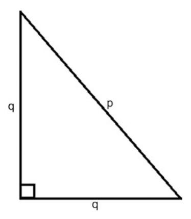
Fig. 2.3 An isosceles triangle of hypotenuse p and adjacent and opposite sides q
Here is the algebraically heretical dilemma. If the length of one side q were an odd number, then twice its square must be even. Hence p2 must be even as well. This implies that p itself must be even since an odd number squared is always odd. Yet, if p is even, it could be represented as 2r, which implies 4r2 = 2q2 , or 2r2 = q2 . Then, q must be even. However, p and q cannot both be even if their ratio p/q has no common factors.
Some intellectually daring Pythagoreans realized this contradiction. An isosceles triangle with unit sides q = 1 must have a hypotenuse of a length p that is the square root of 2. While the Pythagoreans who realized this number must be an irrational violated the brotherhood, they nonetheless admitted the extension of the number system to the irrational roots for some of the integers 3, 5, 6, 7, 8, 10, 11, 12, 13, 14, 15, all the way to the whole number 17.
There remained two other aspects of the number system that the Pythagoreans believed unimaginable. These were the existence of negative and imaginary numbers. Until 1545, no European mathematician had postulated, or had the courage to postulate, their existence. The more complex of these two concepts, the imaginary numbers were actually described first.
Some had come tantalizingly close to discovering imaginary numbers. While Europe was immersed in its Dark Ages, the scholars of Arabia were the princes of science of their day. In Baghdad in the early ninth century, the caliph al-Ma’mun was the patron of a group of learned men known as the House of Wisdom. Al-Khwarizmi (780–850) had developed solutions to quadratic equations but restricted his solutions to those that yielded positive numbers. The negative and imaginary roots for which we are accustomed in high school were discarded as nonsensical.
Three centuries later, the Latin translation by Gerard of Cremona (1114–87) of al-Khwarizmi’s Algebra came to the attention of Leonardo da Pisa (1170–1250). Leonardo was asked to determine the roots of a simple cubic equation x3 + 2x2 +10x = 20. This is a specific version of the general form x3 + ax2 + bx + c = 0, which can be shown to be reducible to a simpler equation:
\[z^3 + pz + q = 0,\]
through a change of variables in which z = x + a/3. If we restrict the parameters and solution to positive numbers, there are three possible versions of the equation to solve. A professor of Arithmetic and Geometry at the University of Bologna, Scipione del Ferro (6 February 1465–5 November 1526) discovered how to solve these three versions, now known as the depressed cubic equation.
In that era, professors held an almost mythical reputation. Their cachet was to be able to discover solutions to problems posed by other professors. These challenges and defenses earned the successful solvers their professorships. Hence, these academic mystics often held close their solution methods. Meanwhile, their patrons considered these scientific mystics exclusive property of their royal courts.
Del Ferro took his secret solutions to his grave in 1526. A notebook that recorded his secrets was inherited by his daughter, Filippa, and her husband Hannival Nave, his former student who assumed del Ferro’s position at the university upon his death.
Scipione del Ferro had confided his secret solution to another one of his students though, named Antonio Maria Fiore. With del Ferro’s insights in hand, Fiore challenged another mathematician, Niccolò Tartaglia (1499–13 December 1557), to a contest to solve a set of cubic equations. Having heard rumors of the existence of a solution to the cubic equation, Tartaglia accepted the challenge and set out to discover a general solution. Indeed, he discovered a more general solution to any cubic equation, while his challenger had in possession only a solution to a particular set of cubic equations. In the contest, which lasted only a couple of hours, Tartaglia was able to solve all 30 of the problems posed to him, while Fiore was unable to solve any of the more general cubic equations Tartaglia had posed.
Gerolamo Cardano (24 September 1501–21 September 1576), one of the three greatest scientific minds of the pre-Renaissance period, had heard of Tartaglia’s triumph and invited Tartaglia to visit Milan under the premise that he had arranged for Tartaglia a patron to fund his work. Instead, upon his arrival in Milan, Tartaglia was asked to reveal to Cardano the solution so Cardano could include it in his forthcoming mathematical treatise. Tartaglia obliged, under the promise that Cardano would not publish his own work until Tartaglia was afforded an opportunity to publish the general solution to cubic equations.
With this tantalizing solution at hand, Cardano went on to further extend and generalize the solution. Once he discovered that it was actually Scipione del Ferro who first discovered a restricted solution, Cardano felt freed from his promise to Tartaglia and included his innovative solution to the general cubic equation in the treatise Ars Magna.
In his treatise, Cardano established a number of principles that would prove useful to Gauss almost three centuries later. First, he demonstrated in Chapter One of his book that equations can have multiple roots. To then, some roots of equations were ignored as impossible because they yielded nonsensical numbers less than zero. For instance, the roots of x2 − 1 are +1 and −1, but contemporaries rejected the notion of a number less than nothing.
Second, Cardano postulated in his Chapter XXXVII the existence of imaginary numbers and complex numbers. He posed the question similar to the following: Find two numbers that sum to two, but for which the product is also two. The correct answer is 1 1 + - and 1 1 - - . He admitted that this expression had no physical significance, but he nonetheless proceeded to explore the implications of such complex numbers.
Cardano’s two mathematical taboos actually both seemed to defy Pythagorean common sense. Numbers were to represent physical quantities one could grasp, literally and physically. One cannot hold something of negative weight nor measure something of negative length. In 1637, René Descartes (March 1596–11 February 1650), the father of modern philosophy, for whom the Cartesian coordinate system was named, published his Discours de la méthode pour bien conduire sa raison, et chercher la vérité dans les sciences. In his Discourse on the Method of Rightly Conducting One’s Reason and of Seeking Truth in the Sciences, he solved the equation x3 − ax + b2 when a and b2 are both positive. He noted that “For any equation one can imagine as many roots as is degree would suggest, but, in many cases no quantity exists which corresponds to what one imagines.”2 Roots that invoke the square root of a negative number were labeled imaginary. Hence, the square root of −1 is designated as “i.”
It took almost another 50 years for someone to propose a physical interpretation of negative numbers. In 1685, John Wallis (23 November 1616–28 October 1703), the English mathematician, the chief mapmaker and cryptographer for the British Parliament, published his book Algebra. In his treatise, he offered an interpretation of negative numbers as corresponding to the left-hand side of a line when the zero mark was somewhere between the left and right extremes.
Indeed, a mapmaker was in a unique position to observe negative numbers, especially the mapmaker to the British Parliament. Navigators measured the 360° of longitude based on the orientation of the Sun at specified times with reference to a time standard maintained at the Royal Observatory in Greenwich, London, England. This location was defined as the zero-degree meridian. Chronometers on ships then referenced the difference between solar time and the time coordinated with Greenwich Mean Time on their chronometers to determine their longitude. A position on a map to the right of Greenwich defined a positive increase in longitude and a new solar time relative to Greenwich Mean Time when the sun reaches a defined point in the sky, while movements to the left result in a decrease, or a negative change, in longitude and solar time relative to Greenwich Mean Time. This description of positions on a line based not on a distance but on a change in distance relative to the origin naturally suggests a physical significance to negative numbers. We now know Wallis’ insight as the real number line which spans both the positive and the negative directions.
In the same year that Wallis published his Algebra, which described the role of negative numbers, an 18-year-old Abraham de Moivre (26 May 1667–27 November 1754) had sought refuge in England from the religious persecution he experienced in France. Thirteen years after his arrival, he had come to know and befriend Isaac Newton (25 December 1642–20 March 1726/7). In his conversations with Newton, he revealed to Newton an interesting result based on Descartes’ imaginary number i. De Moivre noted that:
\[\left(\cos(x) + i * \sin(x)\right)^n = \cos(nx) + i * \sin(nx).\]
The young Gauss would have knowledge of the utility of the real number line and of imaginary numbers. Like Wallis more than a century earlier with his negative numbers, Gauss was the first to offer a geometric intuition to complex numbers that created substance out of the imaginary number line many still regarded as a mathematical oddity, despite their pleasing properties.
The 18-year-old Gauss apparently did not know that the Norwegian mathematician and mapmaker Caspar Wessel (8 June 1745–25 March 1818) had also offered such a geometric interpretation just a few years earlier, in 1799. Like Wallis, Wessel was also a mapmaker who studied directions, and hence vectors. It was a natural extension to consider the real-imaginary coordinate system rather than the conventional real-real coordinate system we all observe on two-dimensional maps and in the ubiquitous x-y graphs. But, his paper, Om directionens analytiske betegning, which he presented to the Royal Danish Academy of Sciences and Letters in 1797, went largely unnoticed and untranslated until 1897.
Buried in the Danish paper was the concept we use today to add vectors. Wessel stated in his On the Analytical Representation of Direction that:
Two straight lines are added if we unite them in such a way that the second line begins where the first one ends and then pass a straight line from the first to the last point of the united lines. This line is the sum of the united lines.
Wessel also applied his notion of vectors and vector addition to the complex plane. However, it was left to Gauss to bring the concept of the complex plane to light in the academic world, and to offer a vivid geometric interpretation with powerful application ever since. He did so as an 18-year-old youth who was trying to solve a problem that perplexed mathematicians for more than two millennia.
Gauss had not set out to legitimize imaginary numbers, nor to define the complex plane. He merely discovered a practical intellectual framework that would allow him to solve a multi-millennial dilemma. Indeed, he would subsequently have discussions with others who recognized the value of the new analytic geometry he discovered in 1796. But while Gauss used his results for his own purposes, he did not publish them until 1831. It was then that he proposed the new term complex number. He described it thus:
If this subject has hitherto been considered from the wrong viewpoint and thus enveloped in mystery and surrounded by darkness, it is largely an unsuitable terminology which should be blamed. Had +1, −1 and -1 , instead of being called positive, negative and imaginary (or worse still, impossible) unity, been given the names say, of direct, inverse and lateral unity, there would hardly have been any scope for such obscurity.3
Gauss’ discovery offered the first bridge between algebra and analytic geometry. By harkening back to the Pythagorean principle that geometric figures be drawn only with a compass and a straightedge, he also reinforced his fascination with the geometric mean, a property that would prove influential in his development of the least squares methodology.
To see his insight, consider the consequence of drawing vectors and geometric figures on a complex plane. In such a representation, with the algebra first proposed by Leonard Euler a half century earlier, and the representation on the complex plane proposed by Caspar Wessel, the horizontal axis is the traditional real number line, and the vertical axis was in units of plus or minus the imaginary number i. In such a complex number plane, a given point is then described by a real part a and an imaginary part b i (Fig. 2.4).
The algebra of imaginary numbers had been fully explored by Euler and others, but the geometric interpretation was novel. The complex algebra had a number of nice properties. For instance, let’s begin with the simplest statement of exponential and trigonometric equivalency.
Recall de Moivre’s identity that was used by the great Leonhard Euler (1707–83) to subsequently determine, in 1748, that \(e^{ix} = \cos(x) + i * \sin(x)\) . The 1965 Nobel Prize-winning physicist Richard Phillips Feynman (11 May 1918–15 February 1988) labeled Euler’s formula “the most remarkable formula in mathematics.” Euler had been exploring the infinite series that represent the exponential and then the two trigonometric functions:
\[e^{x} = \sum_{n=0}^{\infty} \frac{x^{n}}{n!} = 1 + x + \frac{x^{2}}{2!} + \frac{x^{3}}{3!} + \cdots\] for all x
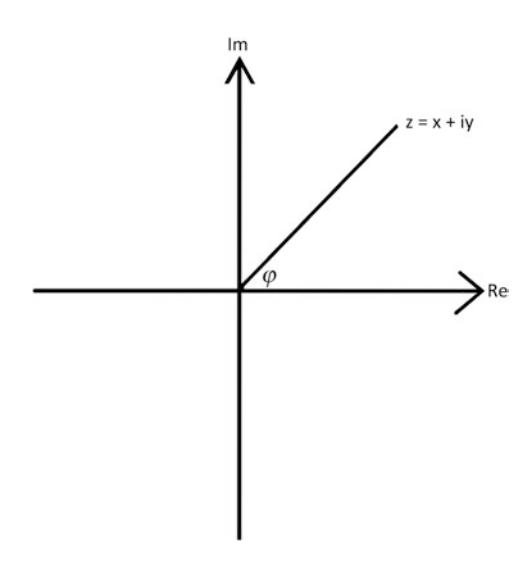
Fig. 2.4 The complex plane
He observed the similarity between the infinite sum above and those of the sine and cosine functions:
\[\sin x = \sum_{n=0}^{\infty} \frac{\left(-1\right)^n}{\left(2n+1\right)!} x^{2n+1} = x - \frac{x^3}{3!} + \frac{x^5}{5!} - \cdots \quad \text{for all } x\]
\[\cos x = \sum_{n=0}^{\infty} \frac{\left(-1\right)^n}{(2n)!} x^{2n} = 1 - \frac{x^2}{2!} + \frac{x^4}{4!} - \dots \quad \text{for all } x\]
He noted that the infinite series terms for \(e^{ix}\) would equal the sum of the terms for \(\cos(x) + i\sin(x)\) . From this observation, he concluded Euler’s identity:
\[e^{ix} = \cos(x) + i\sin(x).\]
This result actually followed quite naturally from an assertion by a brilliant young mathematician named Roger Cotes in the early eighteenth century. Cotes (10 July 1682–5 June 1716) was a scientific prodigy and mathematician who worked closely with Newton in editing Newton’s Principia. The son of Robert Cotes, the rector of Burbage, and Grace Cotes (née Farmer), Roger studied at Trinity College, Cambridge, beginning in 1699 and was taken under Newton’s wing. Upon his graduation, he was given a Trinity Fellowship in 1707, and was appointed the Plumian Professor of Astronomy.
Cotes made two observations that were subsequently refined by Euler and by Gauss. First, in the area of mathematics, he noted in 1714 that:
\[ix = \ln(\cos x + i\sin(x)).\]
It is possible that Cotes failed to observe that \(\sin(x)\) and \(\cos(x)\) are periodic functions that cycle continuously between the values of -1 and 1 as x increases. When, in 1740, Euler instead expressed each side as an exponential, he was left with his familiar Euler’s formula, which he immediately recognized as necessarily periodic. Neither discoverers offered the
now familiar interpretation offered by Wessel and Gauss, even though the interpretation is quite conventional today.
Interestingly, Cotes shared with Gauss a vocation in astronomy and, like Gauss, was interested in how observation errors tend to regress with increased observations, rather than multiply. His interest in predicting the movement of planets, given observational error, was the motivation for what would eventually result in the method of least squares.
With this history at hand, let us now explore Gauss’ insights. As asserted by Gauss, a complex number can be represented as the sum of a real component and an imaginary component representing the sum of two vectors on the complex plane. This vector is the sum of the movement in the real direction and imaginary direction. Thus they sum to a + bi. The parameters a and b then represent distances along the real horizontal axis and the imaginary vertical axis (Fig. 2.5).
In polar coordinates, the distance along the horizontal axis is just as we find for the real plane:
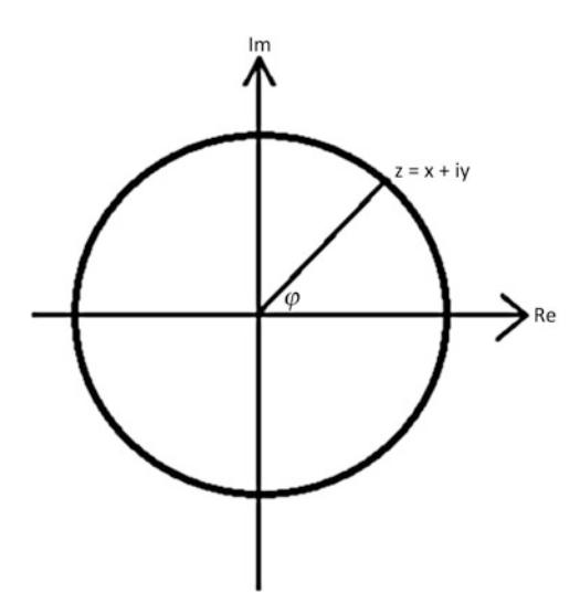
Fig. 2.5 The unit circle on the complex plane
\[x = r\cos(\Theta)\] \[y = r\sin(\Theta),\]
where r is equal to 1 in the case of the unit circle. In general, the real parameters (x, y) of a circle follow the identical equation for a circle as in the real plane:
\[r^2 = x^2 + y^2.\]
Notice, too, that this vector, described by a complex number z = x + iy, can be expressed as \(z = r(\cos(\Theta) + i\cos(\Theta))\) which equals \(re^{i\Theta}\) , from Euler’s Formula. We then see a simple property of the multiplication of complex numbers. Multiplying two complex numbers of polar length \(r_1\) and \(r_2\) and angles \(\Theta\) and \(\Psi\) results in a complex number \((r_1 + r_2)e^{i(\Theta+\Psi)}\) . This is equivalent to the original ray scaled up by a length \(r_2\) and rotated by \(\Psi\) .
Another consequence of Gauss’ complex plane is that any position z multiplied by the imaginary number i results in a rotation of the vector z by one quadrant. For instance, consider a point \(\mathbf{z} = a + b\mathbf{i}\) . The product \(\mathbf{i}^*z\) then yields \(a\mathbf{i} + \mathbf{i}^2b = -b + a\mathbf{i}\) , which is equivalent to the 90° rotation of the ray counterclockwise.
Within this unit circle on the complex plane are contained regular polygons of a very simple form. Note that the expression \(z^3=1\) yields the solution to the apexes of a triangle (below), while \(z^4=1\) yields a square and \(z^6=1\) yields a hexagon. For instance, note that \(z^3=1\) can be factored into \((z-1)^*(z^2+z+1)\) , which yields the three roots \(z_1=1\) , \(z_2=(-1+i(\sqrt{3})/2)\) and \(z_3=z_2=\left(-1-i\left(\sqrt{3}\right)/2\right)\) ). For the square, \(z^4=1\) , or \((z^2-1)(z^2+1)=0\) , which yields roots 1, i, -1, -i and the apexes below within the unit circle.
We now have the tools to understand Gauss’ insight. A regular unit k-polygon is simply a k-sided polygon with k unit radii to each apex \(P_j\) , and k sides, beginning with the ray defining the first apex (1,0). Below are examples of rays forming the apexes of a triangle, a square and a hexagon (Fig. 2.6):
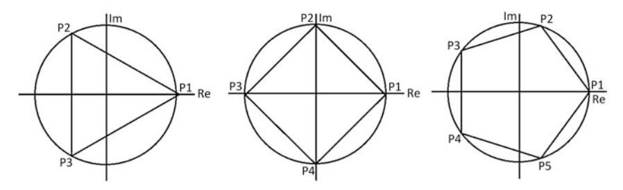
Fig. 2.6 Regular polygons in the unit circle on the complex plane
Notice that, for the triangle, the first apex is given by real and imaginary coordinates (1,0), or z0 = ei*0, the second apex is z1 = ei*2π/3 and the third apex by z2 = ei*4π/3. Each apex is rotated by 120°, or 2π/3 radians. Since complex number multiplication for a unit ray simply represents a rotation, each apex is simply the square, or the cube, or the kth power of the first apex. N rotations for an n-sided polygon is then given by zn = 1 = enΘ = cos(nΘ) + isin(nΘ). Then, this description of an n-sided regular polygon developed by Gauss immediately yields De Moivre’s formula:
\[(\cos(\Theta) + i\sin(\Theta))^n = \cos(n\Theta) + i\sin(n\Theta).\]
In fact, much of the mathematics required for Gauss to visualize regular polygons using a complex plane had already been discovered. His miraculous innovation merely required his brilliant 18-year-old mind to recast these observations geometrically in a powerful way that nobody had seen before. Scholars and students alike have appreciated Gauss’ elegant geometric interpretation ever since.
It may have been Gauss’ ignorance that allowed him to pursue and realize his profound discovery. He was not so indoctrinated into what is, and perhaps what could not be, to not explore his most fruitful path. Instead, he became the first to show the confluence and creation of a few different branches of mathematics—Pythagorean geometry, complex numbers and the roots of equations described by zn = 1. By embracing complex numbers, he also verified that an nth degree polynomial indeed has n roots. If we accept such complex roots, the nth root of unity problem and its relationship to polygons are immediately apparent.
Gauss’ next task was to demonstrate that some of these roots can be described using numbers represented by ratios of whole numbers or their square roots, or the so-called constructible polygons that can be drawn only with a compass and an unmarked straightedge. The Greeks had known they could do so for polygons with 3, 4, 5, 6, 8, 10 and 12 sides. Each of these are what we call a Fermat prime number, or a multiple of a Fermat prime number. The next Fermat prime number in the sequence is 17, where a Fermat prime is given by:
\[F_n = 2^{2^n} + 1\]
To prove that a 17-gon is constructible, Gauss had to show he could calculate \(\cos(2\pi/17)\) using only whole numbers and addition, subtraction, multiplication, division and square roots. He showed, correctly, that:
\[16\cos\frac{2\pi}{17} = -1 + \sqrt{17} + \sqrt{34 - 2\sqrt{17}} + 2\sqrt{17 + 3\sqrt{17} - \sqrt{34 - 2\sqrt{17}} - 2\sqrt{34 + 2\sqrt{17}}}.\]
While it took Gauss a couple of years to write his dissertation into a treatise that proved the assertion he made in 1796, and another three years to rewrite it in the form of the published treatise Disquisitiones Arithmeticae, in Latin, in 1801,5 he nonetheless had signaled to the mathematical world his brilliance in solving a 2000-year-old problem.
In Gauss’ first year at the University of Göttingen, he was never fully secure in his personal finances. When he first entered the Collegium in Brunswick, his funding from the Duke was sufficient, but not permanent. He was overjoyed when the Duke agreed to fund his first year of study at Göttingen, but he remained concerned the funding would continue. Having solved a 2000-year-old problem with an incredibly elegant and profound solution, the 18-year-old Gauss’ mathematical credentials were
becoming established. He gained confidence he would be able to earn the continued financial support of Duke Ferdinand. Gauss then went on to complete his degree in mathematics at Göttingen, with the financial support of his patron, Duke Ferdinand.
Children of wealthy families never felt such financial pressure. They may feel a need to perform intellectually as a matter of pride, but not of necessity. Gauss, though, felt a more pecuniary pressure to perform. He was notorious for his hard work, as an antidote to economic insecurity, which, when combined with his almost uncanny ability to see problems in unique and geometrical ways, resulted in insights such as his constructability solution to the 17-gon. And, with each success came a marginally increased confidence in his future funding.
Fortunately, following Gauss’ first year at Göttingen, the Duke agreed to fund his work to the completion of his thesis. Lesser minds may have translated such financial security into reduced incentives to demonstrate their brilliance. Gauss, though, was academically emboldened. He followed up what he considered to be his greatest work with what others who followed may believe were even more substantial contributions.
For instance, Gauss standardized the use of the imaginary number i as a legitimate number that represents the geometric mean between +1
and −1, that is, i = - 1 1 * . ( ) And, in completing his doctoral dissertation at one of Germany’s greatest universities in 1799, at the age of 22, his Disquisitiones Arithmeticae, dedicated to his patron Duke Frederick, Gauss unified the contributions of the great mathematic minds of his era, including Pierre de Fermat (17 August 1601–12 January 1665), Leonhard Euler (15 April 1707–18 September 1783), Joseph-Louis Lagrange (25 January 1736–10 April 1813) and Adrien-Marie Legendre (18 September 1752–10 January 1833). And, he not only introduced the foundations of a new type of complex analysis and many of its first results. Gauss also established the field of number theory. In doing so, he also made a number of assertions, and sometimes proofs that continue to be validated today. But, just as only a handful of people could absorb the unconventional and complex mathematics and physics of Albert Einstein in 1905, few could absorb Gauss’ work in 1799.
Perhaps the book that 25-year-old Carl Gauss finally published years after his Göttingen thesis might have been more quickly written and easily absorbed had he not written it in Latin. Indeed, his work was one of the last major works among mathematicians to be written in Latin. The language was one still studied by academics of all nations and hence his papers could be read among a wide subset of a very narrow circle of elite mathematicians. Soon thereafter, English would be adopted as the universal language of academicians.
Indeed, his treatise might have been even longer and more expansive, had finances not stood in his way. It was the custom then that the investigator, or his patron, to pay to have their books published. To reduce these costs, Gauss measured his contributions not by the expansiveness of his ideas but by the economy of his brevity. His expositions were terse, to the point that many lesser minds could not fill in the gaps Gauss left. And, he had trimmed a chapter from the book to shorten it and reduce its publication costs. When the Duke of Brunswick eventually discovered Gauss’ fiscal plight, he offered to fund the completion of the book, which was finally published in 1801, two years following the completion of his dissertation.
The most brilliant mathematicians of Gauss’ day quickly understood the contribution, though. Lagrange noted that the book immediately placed Gauss within the highest echelon of mathematicians.
Notes
- H.all, Tord, translated by Albert Froderberg, Carl Friedrich Gauss, MIT Press, Cambridge, Massachusetts, 1970, p. 21.
- Merino, Orlando, “A Short History of Complex Numbers,” January, 2006, http://www.math.uri.edu/~merino/spring06/mth562/ShortHistory ComplexNumbers2006.pdf
- Nahin, Paul J., An Imaginary Tale, Princeton University Press, Princeton, NJ, 1999, at p. 61.
- Feynman, Richard P. (1977). The Feynman Lectures on Physics, vol. I. Addison-Wesley. pp. 22–10.
- Carl Friedrich Gauss, Carl Friedrich, translated by Arthur A. Clarke, Disquisitiones Arithmeticae, Yale University Press, 1965.
3. Carl Gauss’ Great Idea
With what he later considered as his most profound intellectual contribution, the 17-sided regular polygon solution, at hand, Gauss began his most practical explorations in support of a profession that would earn his family a reliable income. In 1800, the Italian astronomer Giuseppe Piazzi (16 July 1746–22 July 1826), a mathematician by training, had been appointed to catalog celestial bodies in a compilation called the Palermo Catalogue of Stars. On the first day of 1801, he claimed he discovered a new planet, Ceres, in between Mars and Jupiter in what we now know as the asteroid belt.
Smaller celestial objects often offered only a fleeting opportunity for observation. Comets, especially, were quite challenging because they were most illuminated when they were near the sun, but were also most obscured by their distance, of approximately the distance from the earth to the sun, and by the brilliance of the sun itself. In addition, their paths are quite elliptical. Indeed, even the planets have slightly elliptical orbits, with the circle simply a special case of the ellipse, in which both axes converge to a central point.
The position of planets or stars relative to the sun has played a significant role in scientific history at other times. In 1915, Albert Einstein asserted in his general theory of relativity that gravity could bend light. No experimental proof could be concocted to substantiate his claim until 1919. Then, a total eclipse of the Sun allowed astronomers to observe that the location of a star in the skyline near the eclipsed sun was displaced by 1.75 seconds of arc over the location the star should have otherwise been positioned. This deviation, which arose as the light of the star was bent by the gravitational force of the sun, was as predicted perfectly by Einstein’s theory. The profound observation made scientific heroes of Einstein, who predicted the deviation, and the astronomer Sir Arthur Stanley Eddington (28 December 1882–22 November 1944), who, on 29 May 1919, made the observation that substantiated Einstein’s general theory of relativity insight.
Piazzi was hoping for an affirmation of similar significance. Following his first sighting of what he thought was a planet on 1 January 1801, Piazzi went on to observe Ceres 24 times over the next 41 days. But, as Ceres neared the Sun, Piazzi lost track of it. The comet’s faintness made the prospects of seeing it again very unlikely unless astronomers knew precisely when and where to look.
Gauss came to the rescue. He took Piazzi’s observational data and predicted when and where Ceres would reappear. On 31 December 1801, almost precisely one year after the first observation, the astronomers Baron Franz Xaver von Zach (4 June 1754–2 September 1832) and Heinrich Wilhelm Matthias Olbers (11 October 1758–2 March 1840) rediscovered what would later be labeled as a large asteroid precisely where Gauss predicted. The grateful Olbers allowed Gauss to name the next asteroid he discovered.
Gauss took to the challenge of the prediction of Ceres’ reappearance with an enthusiasm that would come to define his subsequent career. An observation requires astronomers to note the azimuth, elevation and range of a celestial body. Measurement and atmospheric distortions all conspire to create some randomness in these observations. Gauss was able to compute the six necessary parameters that describe an orbit from just three sets of observations. In doing so, he also was the first to apply a new method of his own creation, the method of least squares.
Gauss’ role in the rediscovery of Ceres has since been reconstructed only by reference to his diaries following his death. In September and October of 1801, very shortly after Piazzi published the data, he applied his customary unconventional approach. He did not follow the path of other astronomers at the time, who would hypothesize a certain orbit, and then “test” their hypothesis against observations. Instead, Gauss took the observations, subject to the random measurement errors, and used them to construct the orbit in what we might now describe as reverse engineering.
Gauss solved the problem in November of 1801. There was not even an observatory in Brunswick at the time. Yet, a 24-year-old theoretical mathematician suddenly became regarded as a brilliant astronomer with the ability to predict the paths of orbiting bodies with only a handful of observations. While Gauss asked that a 17-gon be carved on his tombstone upon his death, his discovery that eluded geometers for millennia was significant only to the most select handful of pure mathematicians. On the other hand, Gauss immediately became the prophet for all those who gaze at the skies. Before the invention of the light bulb, gazing at the stars in the night sky was an almost universal activity for humans who remained awake for more hours each day than for when there was light. His prediction of Ceres’ reappearance was considered almost mystical.
Gauss’ discovery suddenly created many opportunities for him. He was admitted to the Russian Academy of Sciences, and was offered an academic position in St. Petersburg. The Duke wished to keep the homegrown prodigy in Brunswick, though, and offered him an inducement to remain in Brunswick. Ferdinand offered to build Gauss an astronomical observatory and appoint Gauss its director. Another event also cemented Gauss’ decision to remain in Brunswick.
Gauss’ mother had once worked as a maid for a family named Ritter. Two Ritters, Friedrich Behrend and George Karl, were Gauss’ godfathers. He had grown up playing in the Ritter home, and had each year received a present from the Ritters. The domestic bliss of their home was compelling for Gauss, in contrast to the harshness of his upbringing at his father’s hands.
Upon Gauss’ return to Brunswick and his reacquaintance with the Ritters, he met the daughter of Christian Ernst Osthoff (1742–1804) and Johanna Maria Christine Osthoff (née Ahrenholz) (1747–1821). The father of Johanna Elizabeth Rosina Osthoff (8 May 1780–?) was a tanner and associate of the tanners Ritters, Gauss’ godfathers.
Johanna was the star of her parents’ eyes. She was an only child, cheerful and kind, but rather unsophisticated. She offered Gauss someone he described in a letter as a perfect life companion. Gauss courted Johanna for a year before he professed his undying love to her and asked her to marry him. It took her four months and ten days to finally agree to his request. She feared his fame and his worldly life would eclipse her humble desires. Yet, less than a year later, on 9 October 1805, they married at the same St. Katharine’s Church that adjoined the school annex where he first impressed his teachers with his mathematical skills.
The young couple had a child less than a year later, on 21 August 1806. They christened their son Joseph on 24 August, at St. Katharine’s Church.
Things were looking up for Gauss in 1806. Based on his astronomical celebrity, the Duke had bought Gauss a state-of-the-art telescope and Gauss had been instilled as Brunswick’s resident astronomer and observatory director. But, despite these joys, tragedy almost immediately beset Brunswick and his patron. Gauss’ hometown became embroiled in the Napoleonic Wars, and their Duke was enlisted as a combat general allied with Prussia. An attack of his army by Napoleon’s forces caused the Duke to receive a blinding wound on the battlefield. He was permitted to retreat to Brunswick, but was disgraced as Napoleon overtook his town. The Duke was driven into exile, and soon died, on 10 November 1806.
Meanwhile, Gauss had been working as the director of Brunswick’s observatory. When Napoleon’s regime tried to extract a war contribution of 2000 francs from him, numerous scientific luminaries each sent the sum to Gauss, which he promptly returned. With the loss of his beloved patron, his financial pride bruised and his fear of Napoleon’s court well founded, Gauss was miserable in Brunswick. Johanna was unhappy, too, despite the arrival of a daughter, Wilhelmine, on 29 February 1808. Six weeks later, Gauss’ father died in Brunswick. Gauss’ patron removed, and with some jealousy among his fellow residents for his privileged status within Napoleon’s court, Gauss eventually left Brunswick. The Gauss family moved to Göttingen on 21 November 1807.
Yet, despite these sorrowful distractions and melancholy, Gauss remained productive. In 1809, he published his Theoria Motus Corporum Coelestium in Sectionibus Conicis Solem Ambientium, 1 which presented his method for describing the motion of orbiting bodies and his method of least squares. With its publication, Gauss became a member of learned societies around the world. In 1809 and 1810, his renown accelerated, and he received numerous offers for professorships.
Meanwhile, he and Johanna had their third child, Ludwig, on 10 September 1809. He died less than six months later, on 1 March 1810. Preceding him in death was Johanna, on 11 October 1809, as a consequence of two difficult childbirths in a little more than a year.
Gauss was grief-stricken over the loss of his father, his patron, the Duke, his wife and his son in less than four years, and remained bitter of France over its treatment of Germany. Nonetheless, he vowed to remain in Göttingen, to staff its observatory and oversee the construction of a new state-of-the-art observatory. From his vantage point in Göttingen, Gauss observed the Great Comet of 1811 and again successfully calculated its orbit using his method of least squares. One of the brightest comets ever observed, it captivated the attention of citizens worldwide. Some believed it portended to Napoleon’s invasion of Russia, and the War of 1812 between the USA and Great Britain.
While the constructability of the 17-gon harkened Gauss’ arrival among the mathematical elites, his method of least squares cemented his position in the minds of practical scientists and astronomers. The prediction of the movement of celestial bodies, and the study of geodesy, or the understanding of the applied mathematics of the shape and orientation of the earth, was essential for the Age of Exploration within which Gauss lived. Navigation between continents without the aid of land sightings required mechanisms to correct the random measurement errors of navigators.
Men of science, from Galileo to Cotes to Laplace, had offered ways to tease accuracy out of observations subject to random error, by the averaging of observations. Laplace had perhaps the best success when he augmented the work of the physicist and mathematician Roger Joseph Boscovich (18 May 1711–13 February 1787) in the method of least absolute deviation to discern the true observation when observational errors exist.
The term observational errors that we still use today suggests the root of the original problem. These errors were not a mere scientific annoyance. Because observations, and observatories, primarily facilitated oceanic navigation and commerce, understanding and minimizing these errors became a matter of life and death for explorers and mariners. Concerns over observational errors multiplied in proportion to the magnitude and distribution of international exploration, commerce and colonization, and dated back to the sixteenth century and the earliest years of the Age of Exploration. European mariners had word of the discoveries of Italian explorers Christopher Columbus (1451–20 May 1506), and his explorations of Cuba and Central America, and those who immediately followed, from John Cabot (1450–1500), who explored what is now Canada, and Giovanni da Verrazzano (1485–1528), who explored much of eastern North America. These first furays into a new world caused an explosion of subsequent explorations as nations attempted to first lay claim to land and resources, and then induced the exodus of Europeans to the Americas throughout the seventeenth century.
Essential to successful explorations is the accurate determination of location of the featureless sea. Mariners used the difference between the position of the North Star and the indication of their ship’s compass, and the location of the moon against the stars, or the Sun against their ship’s chronometer, to try to discern their location. Each of these measurements and devices was beset with random errors that were compounded by the motion of the ship and the accuracy of a navigator’s readings. A navigator had to decide whether to use the median or the average of multiple observations to try to reduce the effect of errors and more accurately estimate the location of their ship.
This question is not at all trivial. For instance, one might take a set of observations clustered around one answer, but find an observation that deviated significantly from the cluster. Should that observation be rejected as irrelevant? Are all data points equally relevant?
Even the earliest European astronomers understood the challenge. Johannes Kepler (27 December 1571–15 November 1630), the noted astronomer who developed the laws of planetary motion, once puzzled over four measurements for an astronomical observation. In the end, he chose some sort of weighted aggregate of these measures that corresponded neither to their average nor to their median. Clearly, he had developed some methodology to discern the true observation from the measurements riddled with random errors.
Often, when confronted with such dilemmas, his contemporaries used their best judgment, likely also riddled with preconceived biases, to discern a true value. Galileo Galilei (15 February 1564–8 January 1642) was the first to try to assert a scientific approach to the resolution of observational errors in his controversial 1632 book suppressed by the Roman Catholic Church, Dialogue Concerning the Two Chief World Systems. 2
Galileo proposed five principles with regard to the relationship between measurements and the true number they represent, as applied to astronomical observations. He stated:
- The observations represent one true number.
- All observations are prone to errors related to the observer, the instruments and atmospheric conditions.
- These measurements are distributed symmetrically around the true value, or the errors are symmetric about zero.
- Large errors occur less frequently than small errors.
- The most likely true measurement is the one that best fits the observations.
It is the last point that created the greatest discussion. If one simply aggregated the data to calculate its mean, positive errors would cancel out negative errors, and large deviations would overwhelm small ones. Galileo proposed the use of the sum of absolute errors to overcome some of this concern. As such, positive deviations of observations from a hypothesis of the true value would not cancel out negative ones. Then, the researcher could propose a hypothesis that would minimize the sum of the absolute value of errors.
Galileo’s approach is consistent with the concept of Occam’s Razor. Named for William of Ockham (1287–1347), a Franciscan friar and philosopher living in England. It is often stated as “Among competing hypotheses, the one with the fewest assumptions should be selected.” All else remaining the same, the measurement that best fits the data should be accepted.
Yet, despite this logic, and perhaps because Galileo did not offer a full solution to the dilemma, the simplest approach was to simply average the observations. Roger Cotes, Sir Isaac Newton’s contemporary and aide, suggested that measurements that represent points could be likened to the calculation of a center of mass for various weights placed on a ruler. Using this calculation, this center of mass occurs at the average value of the measurements weighted by their mass.
This solution, too, remained controversial. After all, measurements were not the equivalent to the products of distance multiplied by points of mass.
Pierre-Simon Laplace (23 March 1749–5 March 1827) was the first to attempt to postulate a functional form from which errors might follow that was more elaborate than the equal weighting approach that Cotes and other averagers were implicitly using. Laplace was attempting to develop a probability density function for errors that would help him determine which hypothesis would minimize observational errors. He postulated a symmetrical distribution, as Galileo had proposed, and adopted the exponential distribution we now call the Laplace Distribution. Mathematically, such a probability density function is given as follows:
\[p(x) = \frac{1}{2b} e^{\frac{-abs(x-\mu)}{b}}\]
where x is a given observation, \(\mu\) is its true mean, \(abs(x-\mu)\) is the (positive) distance between an observation and the true mean and b is a measure of the spread of the symmetric distribution. Laplace succeeded in producing a measure that had the basis properties Galileo postulated as desirable. However, his function was one of convenience rather than one that flowed directly from intuition.
Gauss was the first to begin applying a more thoughtful approach than that formulated by Laplace. In his journals, which were not published until after his death, he alluded to using his new method as early as 1794, while he was still a student at the Collegium. Later, he applied his methodology to determine the path of the Great Comet in 1811.
Gauss’ interest in the method of least squares flowed from his sense of self. He considered himself an applied mathematician. That description sounds at odds with his first major foray into the academic world based on his solution to the 17-gon. After all, there is little application
to a methodology that could allow one to construct a 17-gon with only an unmarked straightedge and a compass. In fact, even such a construction would be exceedingly complex, as demonstrated by a subsequent author who showed how such a 17-gon could indeed be constructed, a century and more than a hundred pages later. But, from even his seemingly theoretical result flowed an elegant confluence of a number of areas of mathematics: Euclidean geometry, Cartesian number theory and the complex number system. His synthesis is regarded as one of the most elegant and useful in all of mathematics, and has contributed to greater understanding in mathematics, physics and engineering than perhaps any other result.
Gauss was, in essence, a practicing mathematician who immersed himself in research that could lead to innovations that would help solve the practical problems of the time. Essential to science and commerce especially at that time was an understanding of the movement of celestial bodies and an accurate measurement of the shape of the earth, or geodesy. While other academics of wealthier means could live their lives in esoteric research as endowed professors, Gauss had to work to support his research. His research became aligned with his livelihood, as an astronomer and director of his observatories. These questions in astronomy and geodesy were natural foci of his attention, and his method of least squares was his personal “tool of the trade” that afforded him his livelihood.
It was Gauss’ interest in geodesy that first induced him to develop his method of least squares, and introduced him to the world of applied mathematics. Yet, the method he developed he considered so obvious that he had not realized it was also so innovative. Nonetheless, he fully appreciated its utility. He used it not only in his own work in geodesy, but also to motivate his discussions in probability theory in June of 1798, and, of course, in his calculations of the location of Ceres in 1801 and 1802. This was a period early in his professional career, but once he no longer enjoyed the largesse of his benefactor. Gauss was trying to build expertise in areas of practical knowledge for which he thought a livelihood could be forthcoming.
Gauss was also geographically constrained. He had a very strong emotional attachment to Brunswick and Göttingen. This was not because he could not find employment elsewhere. After all, one of his two initial interests in college was philology. He was literate in a number of languages, but, as the product of a simple working-class family, he was very much attached to home.
In the waning years of the 1700s and the early years of the 1800s, Gauss sought out opportunities to build upon his experiences with geodesy and astronomy. He participated in geographical surveys in his region and purchased the tools of his new trade: a sextant, clock and telescope. He taught himself a number of astronomical techniques, and, without even knowing, invented still more. And, he maintained extensive discussions with his associate Olbers on questions of geographic location and astronomical observation. These were practical problems for which he felt his patron, the Duke of Brunswick, would approve. Yet, the practical matter of projecting sections of an irregular but roughly spherical Earth on a two-dimensional map created interesting questions in conformal mapping that had yet been treated sufficiently well. Practical problems that were amenable to clever solutions were challenges Gauss could never fail to accept.
In the summer of 1794 while attending the Collegium, Gauss had read a book by Johann Heinrich Lambert (26 August 1728–25 September 1777). In fact, the young Gauss shared many interests with this Swiss mathematician. Like Gauss, Lambert was interested in Euclidean and non-Euclidean geometry, and the related issue of mapping threedimensional objects, like the Earth, on two-dimensional planes, as is necessary to project an object on a surface of a sphere onto a flat twodimensional map.
Lambert was also an astronomer. In his 1765 volume one of Beyträge zum Gebrauche der Mathematik und deren Anwendung, he wrote about the sum of errors, a notion that intrigued young Gauss. Gauss continued with his fascination of the work of the elder Lambert, and signed all three of his volumes out of the Göttingen library the winter after he arrived. From the bud of an idea, Gauss subsequently recorded in his diary, on 17 June 1798, that he has made discoveries in the calculus of probability. He then referred directly to his method of least squares as a way to glean an underlying functional form from a series of observations subject to random errors. In subsequent correspondences, he stated he had embarked upon the study to offer an explanation or how one might minimize the sum of random errors in the measurement of an unknown function from a large set of observations. He had in mind the creation of a set of tools that would afford him an income as a surveyor and geodesist.
Clearly, his methodology was anticipating how one might describe an elliptical function that would best represent the orbit of an orbiting body based on a handful of its observations. The technique could also be used to position various locations on the surface of the earth, in the threedimensional plane, based on references to observations of the location of celestial bodies. Both applications interested Gauss because they solved practical problems, for which Gauss anticipated he may earn a livelihood, and because each invoked elliptical functions. Indeed, when time came in 1801 to relocate Ceres once it reappeared from behind the Sun, Gauss already had a very good understanding of his method of least squares, even if he may have held the opinion the method was not particularly obscure or difficult to derive.
Gauss became famous for his application of the technique, but infamy soon followed. One of Gauss’ characteristics was that he was most slow to publish results. Indeed, many of his most profound results were never published until biographers or chroniclers discovered them in his notes long after his death.
Gauss’ assertion that he had developed what we now know as the method of least squares was not without controversy, though. In 1805, Adrien-Marie Legendre (18 September 1752–10 January 1833) published the first paper that explicitly described a method Gauss claimed he had been using for years.3
The debate about priority is often a complicated one. While judging by the notes in Gauss’ journal, there is little debate that he referred a number of times to his use of the method of least squares well before Legendre’s paper in 1805, Gauss’ work and correspondence with others at the time are consistent with his claims.
Some of his lack of attention to publication came from his self-view as a working mathematician. His livelihood came before his reputationbuilding. A second aspect was that publication was expensive, especially since he often wrote in Latin, and, during his career, Latin had fallen out of favor. His books would then need to be translated, and he would have to comb through them again to offer corrections.
One of these corrections was telling. In an article he published in 1799 on a method to determine the distance between two points on earth, he noted in a correction to the editor that a translation was in error. He had been describing a method he applied to observations used to estimate the ellipse that runs through two points on the surface of the Earth. Gauss spotted the error and quickly recalculated a solution using his own method of least squares that he employed on a routine basis for such work. His familiarity and facility with the least squared methodology explains how he could so quickly calculate the motion of Ceres when asked two years later.
The greatest controversy in Gauss’ life occurred just a few years later, though. Perhaps one mathematician competed more than any other in the same realm as had Gauss at that time. Legendre was the son of a wealthy family in Paris who was held in very high esteem in the French academic circles for his work on geodesy, elliptical functions and the movement of the planets and comets. In his Nouvelles Méthodes pour la Détermination des Orbites des Comètes in 1805, Legendre was the first to describe in published form the method of least squares.
Upon hearing of the publication, Gauss congratulated Legendre for his contribution, and politely pointed out that he himself had been using the technique since 1794 or 1795 when he needed to “fit” an elliptical curve based on a series of imprecise observations.
The controversy, which nearly rivaled the priority controversy between Newton and Gottfried Wilhelm (von) Leibniz (1 July 1646–14 November 1716) over the discovery of calculus, quickly accelerated. Legendre pointedly asserted that a discovery is not made until it is published. Gauss took that statement as an attack against his personal integrity and credibility, even though he admitted he thought the discovery was not particularly important in its own right.
While Gauss produced significant evidence from colleagues who corroborated that he had discussed his method with them years before Legendre published his treatise, the debate continued until well past Legendre died in 1733. Even today, modern commentators are divided between to whom credit should be given, although most agree that Gauss laid strong claim on the use of the technique first. Indeed, his application of the technique brought Gauss his fame and defined his career following the Ceres discovery.
The issue may nonetheless be settled. Gauss had already been completing a major treatise on the subject when Legendre published his own. While the translation from Latin, and the need for less affluent Gauss to raise the funds for publication, delayed its appearance until 1809, when he managed to publish his Theory of the Motion of Heavenly Bodies Moving about the Sun in Conic Sections, 4 Gauss clearly demonstrated a much more extensive command of the method of least squares than Legendre had described. What we know of the method, including the result that it minimizes the sum of squared errors when errors follow a normal distribution, flows from this publication by Gauss.
Perhaps part of Gauss’ indignation arose because of the immediate recognition Legendre received upon his publication. Meanwhile, Gauss had never published his own method that so accurately predicted the reappearance of Ceres, but obviously could not have made his prediction without the application of such a technique. Certainly, his principle of probability and of the normal distribution provided a much more extensive foundation than the method Legendre derived, and cemented Gauss’ reputation.
In his treatment, Gauss began with the work of Laplace decades earlier. He was the first to demonstrate that the probability density function he derived was an evolution of Laplace’s solution. Rather than the minimization of absolute deviation, Gauss’ treatment minimized the sum of squared errors in estimation. From the premise that the arithmetic mean of observations should provide an unbiased estimate of the true mean parameter, Gauss then demonstrated that, if observation errors are normally distributed, his method of least squares provides the most likely estimate of the true measurements. Our understanding of the nature of errors was expanded in the two years following Gauss’ publication of his method of least squares, to be described later. From these principles Gauss formulated, Laplace completed the analyses we use today by proving the central limit theorem, something that had stymied Laplace since 1783.
In 1810, following a close study of Gauss’ work, Laplace showed that the central limit theorem offered a Bayesian (posterior) justification for Gauss’ least squares methodology. If observations are combined, each of which is an unbiased and independent observation drawn from a large number of observations, then the least squares estimation represents the maximum likelihood estimate and minimizes posterior errors, all with-
out any assumption with regard to the true distribution of errors. This central limit theorem proved that the sum of a number of independent random variables that are identically distributed will tend to a normal distribution
Gauss further extended his model by showing that the least squares approach to a linear regression is optimal if errors have zero mean and are uncorrelated, with equal variances. This result is known as the Gauss-Markov theorem. He also derived the now ubiquitous normal distribution from first principles.
Meanwhile, in the USA, Robert Adrain (30 September 1775–10 August 1843), considered to be the pre-eminent American mathematician of his day, formulated a similar but less broad analysis as had Gauss.
The Normal Distribution
Let us return to the normal distribution that has underpinned finance theory for more than half a century. The story of the normal distribution invokes the same familiar names as Bernoulli, Euler, Laplace, De Moivre, and, as in the case of the method of least squares, the final solver of the puzzle, Carl Friedrich Gauss. It is also a story that was rooted in the needs of astronomers and mariners, although it had less lofty beginnings also in gambling.
While we typically associate the normal distribution with the distribution of non-systematic errors or the random walk in finance, its beginnings were in probability theory, specifically the probability of outcomes in simple gambles in the mid-seventeenth century. Antoine Gombaud, Chevalier de Méré (1607–29 December 1684) was a French writer who adopted for himself a noble title. He was also an amateur mathematician with a fascination with the rolling of dice and other games of chance. He enlisted two eminent mathematicians of the day, Blaise Pascal (19 June 1623–19 August 1662) and Pierre de Fermat (17 August 1601–12 January 1665), to help solve the problems of probability he posed and, in doing so, helped lay the foundation for modern probability theory.
In an effort to stem his gambling losses, Gombaud asked Pascal the odds of having a single six-sided die come up with at least one six in four rolls. The now familiar formula instead asks the probability of not rolling any sixes in four rolls. Then, the probability of rolling at least one six is then one minus the probability of rolling no sixes:
\[Pr(at \text{ least } one \text{ six } in 4 \text{ rolls}) = 1 - (5/6)^4 = 0.5177.\]
Next, he asked the probability of rolling at double sixes at least once in 24 rolls, which is then:
\[Pr(at \text{ least } one \text{ pair of sixes in } 24 \text{ rolls}) = 1 - (35/36)^{24} = 0.4914.\]
This analysis was later generalized by Jacob Bernoulli (6 January, 1655–16 August 1706), who was a member of the famed Bernoulli family of mathematicians and scientists and the developer of what we now call the Bernoulli trial. Also known as a binomial trial, it determines the probability of repetitions of a game of fair odds for which there can be only one of two outcomes in each repetition: either success or failure. For instance, the probability of double sixes in one roll is one out of thirty-six possible outcomes. Then, p is the probability of a success, and q = 1 - p is the probability of a failure, such that p + q = 1. Since there are but two outcomes at each stage, the probability of various possible solutions over repetitions of the game is known as a binomial trial, with the outcomes given as:
\[P(k \text{ successes in } n \text{ rounds}) = {n \choose k} p^k (1-p)^{n-k}\]
where the terms for n and k in brackets, \(\binom{n}{k}\) , is a binomial coefficient. This coefficient, read aloud as “n choose k,” was calculated by Pascal, for which he derived what is now called Pascal’s triangle to aid in its calculation. Jacob Bernoulli was able to approximate the binomial coefficient
well beyond the estimates provided by Pascal and Fermat, but was unable to determine an approximation that was easy to compute. It was left to De Moivre to calculate, in 1733, the probability of coming within d outcomes half the time of n repetitions given even (p = 0.5) odds as:
\[\left(\frac{n^n}{2}\pm\right)d\left(\frac{1}{2}\right)^n = \frac{4}{\sqrt{2\pi n}}e^{-2d^2/n}\]
Notice the immediate resemblance to the now familiar normal curve that every student of statistics learns and which we will soon derive. These early innovators had made progress, but none managed to complete the circle in the creation of a logically consistent and intuitive method of minimized deviations.
Just as mathematics converted finance from an art to a science only relatively recently, the science of games of chance was only a newcomer to the interest of scholars in probability. The first mathematical interest came from early astronomers concerned about the random errors in their observations. As early as the second century BC, the Greek astronomer, geographer and mathematician Hipparchus of Nicaea (c.190–c.120 BC), and one of the founders of trigonometry, proposed that the midrange (or, the median) of multiple observations should be considered the most correct. By the sixteenth century, it is clear from the notes of Danish nobleman and astronomer Tycho Brahe (14 December 1546–24 October 1601) that he used some sort of error-adjusting algorithm to best represent his observations. The astronomers of his day seemed to each incorporate their best guesses, averaging, or choice of a mean to determine the “true” location of a celestial body based on their observations buffeted by random errors.
We had described earlier Galileo’s more systematic approach, which suggests he believed the best method was one that minimized the sum of absolute errors f(x):
\[\min_{x} f(x) = \min_{x} \sum_{i=1}^{n} |x - x_i|\]
It is well known that this minimization yields the median rather than the average value of the set of observations \(x_i\) . We had also noted earlier
that Cotes had argued for a center of mass calculation such that each observation is weighted by its distance from the calculated center. Under such a formulation, if each observation is given a weight \(w_i\) , and these weights sum up to one, then the center of observations x occurs such that:
\[\sum_{i=1}^{n} w_i \left( x - x_i \right) = 0.\]
In such a formulation, we can solve for the central value x:
\[x = \frac{\sum_{i=1}^{n} W_i X_i}{\sum_{i=1}^{n} X_i}.\]
This expression reduces to a simple average when the weights are equal. The issue of the appropriate adjustment for repeated observations that contain a random component was most pressing. There was even testimony to Parliament on the importance of resolving this issue.
Laplace turned his attention to the appropriate error distribution and proposed a symmetric decay function for the probability weighting of observations from the central tendency. He argued that the effect of a small change in one direction or the other, when compared to the central tendency, should equal the proportion of the change to that tendency. From an argument of constant proportional change as one departs from the central tendency, he derived the exponential decay function, which, in his formulation, depended on the absolute distance of an observation from the central tendency. The weighting, or probability assigned to a deviation, then decays exponentially and symmetrically on either side of the central tendency.
Laplace’s more elaborate work on the error function convinced few, though. Daniel Bernoulli (8 February 1700–17 March 1782), the nephew of Jacob Bernoulli, lent his considerable support in 1777 to Cotes’ notion of the center of mass, or simple weighted averaging, under the assumption that all errors are equally likely, despite the pleadings a century earlier of Galileo who argued that small discrepancies are likely more probable than large ones, and hence should hold more weight.
Bernoulli was also offended by the explicit notion of Laplace that errors can occur over an infinite line. To Bernoulli, it was common sense that possible errors should be finite or asymptotically declining in nature.
Yet, averaging, or choosing the median among observations, did not allow astronomers to calculate the reappearance of Ceres in 1801. Gauss, in advocating for a least squares methodology and his eventual normal distribution, noted that, as Galileo claimed, small errors should be more likely than large ones, and the errors should occur symmetrically about the true central tendency. In addition, the most likely occurrences, in a probabilistic sense, ought to coincide with their average. From this, he concluded that departures from the mean ought to follow an error curve that does not look significantly different from the approximation to the Bernoulli trial De Moivre had postulated. Gauss asserted an error function \(\phi(x)\) should be given by:
\[\phi(x) = \frac{h}{\sqrt{\pi}} e^{-h^2 x^2},\]
where h is a precision constant that ensures the sum of these probabilities along the real number line sum to 1. Note that, if the true mean \(\mu\) is given by 0, and the standard deviation \(\sigma\) is given by \(1/\sqrt{2h}\) , the expression reduces to our familiar one for the normal distribution.
To see how Gauss arrived at this conclusion, let us revisit his goal. He wished to discover a probability distribution function that reaches a maximum when the observation x equals the true mean \(\mu\) . The joint probability density for n observations of x is then given by the following product:
\[\phi\bigg(\overline{x}:\mu\bigg)=\prod_{1}^{n}\phi\big(x_{i}-\mu\big)\]
Gauss wanted his distribution to peak when the mean of the set of observations coincides with the true mean \(\mu\) . He had developed a maximum likelihood methodology to determine the mean. Differentiating the product with respect to the true mean and setting the derivative to zero then gives:
\[0 = \phi(\vec{x}:\mu) \sum_{i=1}^{n} \frac{\phi'(x_i:\mu)}{\phi(x_i:\mu)}\]
Let \(z_i = x_i - \mu\) , and \(\Phi(\vec{x}:\mu) = \phi'^{(x_i:\mu)} / \phi(x_i:\mu)\) . Then, if the mean of the observations coincide with the true mean:
\[0 = \sum_{i=1}^{n} z_{i} \text{ and } 0 = \sum_{i=1}^{n} \Phi(z_{i}).\]
Then, \(\Phi\) is proportional to z, or:
\[\frac{\mathrm{d}\phi / \mathrm{d}z}{\phi} = kz \ and \ \mathrm{d}\phi = \phi kz \mathrm{d}z.\]
Integrating both sides of the equation and solving gives:
\[\phi(x-u) = Ce^{\left(\frac{(x-\mu)}{\sigma}\right)^2}\]
where \(k = -1/\sigma^2\) , and where we note that the exponent in the integrand must be negative to ensure the integral remains finite over the entire range of values for x.
Finally, we can determine the arbitrary constant C by noting that the sum of all probabilities must be equal to one:
\[1 = \int_{-\infty}^{\infty} Ce^{-\frac{1}{2}\left(\frac{(x-\mu)}{\sigma}\right)^2} dx.\]
This normalization requires that
\[C = \frac{h}{\sqrt{\pi}}, \quad \phi(x) = \frac{1}{\sigma\sqrt{2\pi}} e^{-\left(\frac{1}{2}\right)((x-\mu)/\sigma)^2}.\]
From this result, we can now determine the probability of finding observations over arbitrary intervals (a, b):
\[\operatorname{Prob}(a < x < b) = \frac{1}{\sigma\sqrt{2\pi}} \int_{a}^{b} e^{-\left(\frac{1}{2}\right)((x-\mu)/\sigma)^{2}} dx.\]
We have already determined that this normal probability distribution function peaks when \(x = \mu\) . Next, we interpret the term \(\sigma\) .
Reverting back to the term z for errors vis-à-vis the mean, the variance of z, \(Var(z) = E(z-E(z))^2\) . Then,
\[Var(z) = \frac{1}{\sigma\sqrt{2\pi}} \int_{-\infty}^{\infty} z^2 e^{-\left(\frac{1}{2}\right)(z/\sigma)^2} dx.\]
Let \(w = z/(\sigma\sqrt{2})\) . Then.
\[Var(z) = \frac{2\sigma^2}{\sqrt{\pi}} \int_{-\infty}^{\infty} we^{-w^2} dx.\]
Next, let u = w and \(v = (-1/2)\exp(-w^2)\) . Then,
\[Var(z) = \frac{2\sigma^2}{\sqrt{\pi}} \left[ \left[ -\frac{w}{2} e^{-w^2} \right] + \frac{1}{2} \int_{-\infty}^{\infty} e^{-w^2} dw \right].\]
The expression in square brackets must be evaluated at the limits \(\pm \infty\) . However, the application of L’Hospital’s rule and imposition of the limits show that this expression reduces to zero. Then,
\[Var(z) = \frac{2\sigma^2}{\sqrt{\pi}} \left( \frac{1}{2} \int_{-\infty}^{\infty} e^{-w^2} dw \right).\]
The solution to this Gaussian integral then yields:
\[Var(z) = \frac{2\sigma^2}{\sqrt{\pi}} \frac{\sqrt{\pi}}{2} = \sigma^2.\]
The variance of the error terms is then given by σ2 . The familiar normal distribution was derived based on Gauss’ premises that the distribution maximum, the average and the median of the probability density function he derived all occur at the true mean μ. He also showed that his distribution has a variance of σ2 and illustrated it has the familiar bell shape we now know. Purists still call it the Gaussian distribution (Fig. 3.1).
The next innovation came at the hands of Laplace. Over the years, Laplace had closely followed Gauss’ maturation as a mathematician, and had remained one of his greatest supporters. Laplace had even intervened to have France’s science academy award Gauss their highest honor, and ensured that Napoleon’s Army treated Gauss well as it rampaged through Europe, Brunswick included. When the nasty row over priority erupted between Gauss and Legendre, Laplace tried to smooth it over. And, when Gauss’ definitive treatment of the method of least squares was finally printed in 1809, Laplace heralded its contribution and set about studying its results. From there flowed one of the most important innovations in statistic: the central limit theorem. Laplace first described it in his 1812 Théorie analytique des probabilités, very shortly after Gauss’ publication of his unifying and extensive work in 1809.
To understand the significance of the central limit theorem, it is helpful to note a characteristic of the mean and variance we just derived. As you recall, the mean is simply the expected value of a random variable,
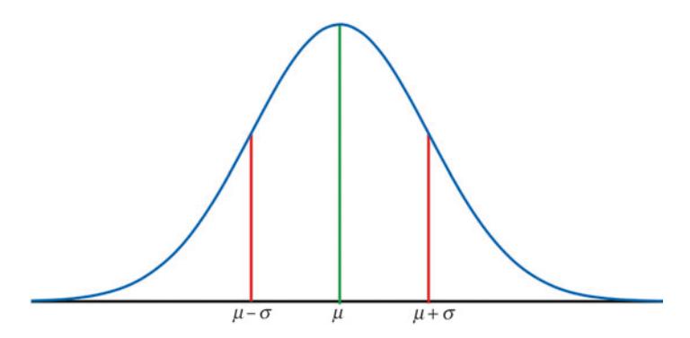
Fig. 3.1 The Gaussian distribution
while the variance is a measure of the squared distance of various points on the probability distribution function to the mean. That is,
\[\mu = E(X)\]
\[\sigma^{2} = Var(X) = E(X^{2}) - \mu^{2}.\]
These are called moments because, like the moments of inertia relative to a center of mass, they are measures of the distance of various points from the central tendency, weighted by their probability, or frequency, or, in the case of physical objects, their mass. In statistics, it is often easier to work with a moment-generating function to determine these various parameters as moments. Then, the mean of a random variable, or the first moment, is simply the first derivative of the moment-generating function, and the variance the second derivative, less the mean-squared, or \(\mu^2\) , and so on. Specifically, the moment-generating function is given by:
\[M(t) = E(e^{tX}) = \sum_{x \in S} e^{tx} f(x).\]
Most, but not all, random variables have such moment-generating functions. The well-behaved random variables have them. Let there be a set of independent and identically distributed (i.i.d.) random variables with, for simplicity, a zero mean and a variance (or second moment) \(\sigma^2\) with moment-generating functions. Then, the sum of the i.i.d. random variables is:
\(S_n = \sum_{i=1}^n X_i.\) Define \(Z_n = S_n / \sqrt{n\sigma_x^2}\) . Then the various means are given by:
\[M_{S_n}(t) = (M_{x_n}(t))^n\] and \(M_{Z_n}(t) = \left(M_{x_n}\left(\frac{t}{\sigma_x\sqrt{n}}\right)\right)^n\) .
We can rewrite an arbitrary moment function \(M_x(s)\) as follows through a Taylor’s theorem expansion:
\[M_{x}(s) = M_{x}(0) + sM'_{x}(0) + \frac{1}{2}s^{2}M''_{x}(0) + \varepsilon_{s},\]
where \(\varepsilon_s/s^2\) converges to zero as s goes to zero. It is simple to see that \(M_x(0) = 1\) , by definition, and, since the first moment is zero, and the second moment \(M_x^{"}(0)\) equals the variance \(\sigma_x^2\) . Then:
\[M_x(s) = 1 + \frac{1}{2}s^2\sigma_x^2 + \varepsilon_s.\]
It is easy to show, through L’Hospital’s rule, that \(\varepsilon_s/s^2\) goes to zero as s goes to zero. Then, \(n\sigma_x^2\varepsilon_s/s^2\) also goes to zero as n goes to infinity. If we let \(s = t/\sqrt{n\sigma_x^2}\) , we see:
\[M_{Z_n}(t) = \left(1 + \frac{1}{2} \left(\frac{t}{\sigma_x \sqrt{n}}\right)^2 \sigma_x^2 + \varepsilon_s\right)^n = \left(1 + \frac{\frac{t^2}{2} + n\varepsilon_s}{n}\right)^n.\]
From the property of the exponential function that:
\[\lim_{n\to\infty} \left(1 + \frac{a_n}{n}\right)^n = e^a.\]
Then we have:
\[\lim_{n\to\infty} M_{Z_n}(t) = \lim_{n\to\infty} \left(1 + \frac{\frac{t^2}{2} + n\varepsilon_s}{n}\right)^n = e^{t^2/2}.\]
This corresponds to the moment-generating function for the standard Gaussian distribution. It shows that as n grows, the distribution of means of i.i.d. random variables follows a normal distribution, even if their underlying distributions are non-normal.
Recall that De Moivre had decades earlier established the result that the distribution of repeated draws described by Bernoulli’s binomial formula converged also to a formula that looks strikingly like Gauss’ normal. While Simon de Laplace was the first to combine this growing chorus that the sum of draws from various distributions approach a normal distribution, it was left to a Russian mathematician Pafnuty Lvovich Chebyshev (4 May 1821–26 November 1894) and his students Andrey (Andrei) Andreyevich Markov (14 June 1856–20 July 1922) and Aleksandr Mikhailovich Lyapunov (6 June 1857–3 November 1918) to provide rigorous proofs of the central limit theorem. As a consequence, the central limit theorem is variously called the Laplace-Markov-Lyapunov theorem.
Notes
- GAUSS, Carl Friedrich (1777–1855). Theoria motus corporum coelestium in sectionibus conicis solem ambientium. Hamburg: Friedrich Perthes and I.H. Besser, 1809.
- Galilei, Galileo (1632), Dialogue Concerning the Two Chief World System, translated by Stillman Drake. Berkeley, CA: University of California Press, 1953.
- Legendre, Adrien-Marie (1805), Nouvelles méthodes pour la détermination des orbites des comètes [New Methods for the Determination of the Orbits of Comets] (in French), Paris: F. Didot.
- Gauss, Carl Friedrich, (1809), Theoria Motus Corporum Coelestium in sectionibus conicis solem ambientium (Theorie der Bewegung der Himmelskörper, die Sonne in Kegelschnitten umkreisen), Theory of the Motion of Heavenly Bodies Moving about the Sun in Conic Sections (English translation by C.H. Davis), reprinted 1963, Dover, New York.
4. The Later Years and Legacy of Carl Friedrich Gauss
At fi rst, Gauss considered his work on the method of least squares to be relatively inconsequential and obvious. He developed his method as a practical solution to problems of observational error in astronomy and geodesy so that he may streamline his calculations and better earn a living for himself and his family. To him, they were a means to a larger end. As a consequence, he did not see any pressing need to quickly publish his technique. Instead, he worked only slowly toward the publication of his collection of algebraic results, his method of least squares included, until 1809.
However, once Legendre published a similar but much less complete analysis a few years before him, and subsequently challenged Gauss for priority, Gauss became quite preoccupied with the priority controversy. Th is controversy with Legendre lasted for decades.
Th e controversy explains two diff erent approaches to the dissemination of results, and of recognition for their respective contributions. Gauss , the pauper’s son, did academic battle with Legendre , the patrician’s son. Gauss’ lack of fi nancial resources certainly prevented him from publishing to the same extent as some of his contemporaries. Gauss also had to maintain employment to provide for his family.
Following the publication of his treatise on algebra, Gauss devoted considerable time designing and building his observatory. Despite the demands of his appointment as the director of the observatory, Gauss continued to publish work that sprung from his solutions to pressing astronomical problems. Beginning in 1816, he published the most thorough treatment to date on hypergeometric functions, his Disquisitiones generales circa seriem infi nitam , an analysis of the method of integration and its approximations, Methodus nova integralium valores per approximationem inveniendi , and additional work on the foundations of statistics and the properties of various estimators, Bestimmung der Genauigkeit der Beobachtungen , one of the fi rst discussions of statistical estimators. As time permitted, he also broadened his research. For instance, his Th eoria attractionis corporum sphaeroidicorum ellipticorum homogeneorum methodus nova tractate developed the exploration called potential theory that is very important in applied and theoretical mathematics and physics alike. Meanwhile, he found new applications to the results he gleaned in his geodesic work for various state and national entities.
His increasing interest in geodesy, and increasing demand for his services, caused Gauss to even further divide his interests, and perhaps delay some of his theoretical contributions to mathematics. He was commissioned with a geodesic survey between his province of Hanover and a portion of Denmark. He would supervise other surveyors by day and then perform the necessary calculations at night. To facilitate his work, he even invented a device, called a heliotrope, which could concentrate light to form highly visible targets for very long range surveying. His device has been used consistently since his invention until the development of the global positioning system (GPS) surveying techniques at the end of the twentieth century. While his method required a clear view of the sun, it revolutionized the utility in performing surveys over very long distances using the triangulation method.
Despite his important work conducting geodesic surveys over long distances, by 1830 Gauss was nonetheless able to publish almost a hundred academic papers from his fi rst introductions to astronomy and geodesy. His work was increasingly recognized for its outstanding scholarship. For instance, his Th eoria Attractionis Corporum Sphaeroidicorum Ellipticorum Homogeneorum Methodo Nova Tractata secured him the Copenhagen University Prize in 1822. Th ere, he began his work on a technique of broad application today, called conformal mapping. Meanwhile, he was preparing additional work on his method of least squares , fi rst in his 1823 Th eoria combinationis observationum erroribus minimis obnoxiae , and a supplement published fi ve years later.
Among pure mathematicians, Gauss is perhaps best known for his development of non-Euclidean geometry. Just like his proof of constructible polygons in 1795, after two millennia of research in vain by others, Gauss was perplexed by the inability to prove Euclid’s fi fth postulate. Over the intervening millennia, no other mathematician had been able to prove the simple statement in Euclid’s Elements :
If a line segment intersects two straight lines forming two interior angles on the same side that sum to less than two right angles, then the two lines, if extended indefi nitely, meet on that side on which the angles sum to less than two right angles.
Th is postulate seemed intuitively obvious to most Euclidean geometers. Also known as the parallel postulate, it was a foundation of axiomatic two-dimensional geometry. A roughly equivalent statement is the triangle postulate that the sum of angles in a triangle must add up to 180°, or pi radians. Yet, Euclid’s fi fth postulate could not be proven based on the four postulates that preceded it.
Gauss established that the parallel postulate could only be proven if other aspects of Euclidean geometry are discarded—hence the application of the term non-Euclidean geometry to the theories that fl owed out of the relaxation of the four postulates.
Th e abandonment of the principles of Euclidean geometry also gave Gauss yet another pause not to publish his work. He was afraid of the controversy that would result should one disprove a logical tenet of Euclidean geometry. After decades of defensiveness over his challenge to Legendre ’s priority claim in the method of least squared, Gauss was reticent to foment additional confl ict. But, as others also came to the conclusion Gauss had held secretly, and in his detailed journals, for decades, Gauss off ered faint praise for the work of others. Yet, he would often marginalize their work somewhat by referencing his own personal discoveries, published or not, in these areas since his fi rst years as a student of mathematics.
Gauss also originated important work in diff erential geometry. In the two-dimensional world of Euclidean geometry, the notion of curvature was relatively basic. However, Gauss’ explorations in the ellipses of astronomy and the hyperbolas of geodesy required him to explore measures of curvature along planes that slice spherical, conical, elliptic or hyperbolic surfaces. Th e slice of one of these planes through a three-dimensional curved surface could be characterized by the degree of curvature that is observed at such intersections. Gauss characterized such intersections based on the maximum and minimum curvature radii that occur along the intersection. Th e product of these two radii is called the Gaussian curvature. Characterization of such curvatures created the important fi eld of diff erential geometry.
Notwithstanding his fundamentally important work in other areas, Gauss regarded his contribution to the creation of fundamental lemmas in diff erential geometry to be some of his most remarkable work. His most widely known contribution was a book he wrote in 1828, entitled Disquisitiones generales circa superfi cies curvas , which fl owed directly from practical problems in his geodesy work.
While Gauss was gaining fame and attention in this period, his personal life was challenging. After the death of his father, he allowed his beloved but sickly mother to move in with the family in 1817. Her care created familial challenges as it off ered one more reason for Gauss to remain in Göttingen, near Brunswick. Meanwhile, his second wife Minna wished Carl would accept a job off ered him at the university in Berlin. Gauss, always reticent to move from his home, kept his family in Göttingen. Th ere his second wife died, in 1831, and his mother died in 1839.
While his family may have preferred otherwise, the academic environment of Göttingen was certainly a rewarding one, even if his varied assignments prevented Gauss from fully immersing himself in but one strand of scholarship. In 1831, the same year his second wife died, Wilhelm Eduard Weber (24 October 1804–23 June 1891), a young physicist, arrived at the university in Göttingen, partly because of Gauss’ endorsements. Gauss had published in the physics literature in application of a principle he developed called the principle of least constraint. His paper Über ein neues allgemeines Grundgesetz der Mechanik, followed by his Principia generalia theoriae fi gurae fl uidorum in statu aequilibrii,
described the geometry of attractive forces, and had helped create an important new fi eld in physics called potential theory. Just as Einstein had united some of the fundamental forces in physics, Gauss’ potential theory and his method of least squares had helped science explain some of the most fundamental observations in the natural world.
Weber and Gauss mutually stimulated their shared interests in magnetism. Gauss was initially interested in magnetism as a geodesist who understood the nature of the magnetic poles of the earth. Together, Weber and Gauss invented the electromagnetic telegraph. Later in life, Weber’s exploration of the interaction between electricity and magnetism both implied a common speed of transmission consistent with the speed of light. From this measure, he and Rudolf Hermann Arndt Kohlrausch (6 November 1809, Göttingen–8 March 1858), a co-author and another Göttingen physicist, denoted this speed by ” c ,” a symbol which is universally used by physicists for the speed of light ever since. Still today the measure of magnetic strength is called the weber . Th e great physicist James Clerk Maxwell (13 June 1831–5 November 1879), the contemporary of Weber and Gauss, based his unifying theory of the equivalence of electricity and magnetism on Weber’s observation of the speed of light. Maxwell’s equations represent the foundation of much of physics since.
Gauss and Weber began working on magnetism together because of Gauss’ geodesy work. In 1832, Friedrich Wilhelm Heinrich Alexander von Humboldt (14 September 1769–6 May 1859), an infl uential Prussian geographer, explorer and philosopher, had sought Gauss’ assistance in measuring the fi eld across the earth arising from the magnetic pole. From this work, Gauss wrote three important papers on terrestrial magnetism. His explorations generated a number of scholarly papers, including Intensitas vis magneticae terrestris ad mensuram absolutam revocata in 1832 , Allgemeine Th eorie des Erdmagnetismus in 1839 and his Allgemeine Lehrsätze in Beziehung auf die im verkehrten Verhältnisse des Quadrats der Entfernung wirkenden Anziehungs - und Abstossungskräfte.
Th e second of these papers proved that a globe can have only two magnetic poles, and used work by Laplace, his colleague, to calculate the position of the magnetic south pole. Th ese papers made substantial contributions to our understanding of not only terrestrial magnetic fi elds but also fi eld theory. For instance, in this body of research, Gauss described, without proof, an important concept in physics, called Dirichlet ‘s principle, which establishes a principle to minimize energy functionals. Th is work was in line with Gauss’ other signifi cant contributions to potential theory.
As Gauss continued his research into terrestrial magnetism, he specifi ed that his new magnetic observatory be built with only non-magnetic materials. Th e greater accuracy and theory he brought to this study caused him to revise substantially what was known about the variation of the earth’s magnetic fi eld, called magnetic declination, as fi rst mapped by Humboldt . Gauss’ improvements greatly improved navigation by compass.
Meanwhile, Weber , Gauss ’ collaborator, with whom he developed a telegraph that could function at a distance of one mile, became immersed in political turmoil in Göttingen. Gauss was conservative, and held strong views consistent with his nationalist pride, but had well learned to keep his views quiet as he had observed the fate that befell his patron, the Duke of Brunswick. Th e younger Weber’s outspoken opposition to a new constitution in the Kingdom of Hannover favored Ernest Augustus. Th e Göttingen Seven , which also included the fairy-tale writers the Brothers Grimm (Wilhelm Carl Grimm [24 February 1786–16 December 1859] and Jacob Ludwig Carl Grimm [4 January 1785–20 September 1863]), opposed the new King of Hannover’s meddling in the Constitution and refused to take oath to it. Th e university relieved these seven of their academic positions. Th eir courage set in motion a popular liberal sentiment in Germany that eventually resulted in their liberal republic.
A dozen years after the demonstrations of Weber and his six colleagues, Weber was reinstated in Göttingen, where he resumed his geomagnetic work with Gauss .
By the time Weber returned, Gauss was assuming a position of a somewhat eccentric and detached observatory director and occasional lecturer. For Gauss, all politics was local, and he found few practical problems of mathematical interest undeserving of exploration.
While Gauss himself never documented his interest in social sciences, his contemporaries related that he was interested in such problems beyond the strictures of science. For instance, he showed an interest in the theory of insurance, what we might called actuarial studies today, on the optimum number of jurors, and the statistical properties of infant mortality.
Th ese latter applications of mathematics to issues of humanity preoccupied Gauss ’ later years. Following his Golden Jubilee lecture in 1849 celebrating his 50th year following his 1799 diploma, Gauss worked to demonstrate how mortality modifi es actuarial tables.
A few years before his Jubilee lecture, the University of Göttingen had approached Gauss to solicit his help in ensuring the solvency of the pension fund that assisted widows of Göttingen professors. At that time, an increase in the number of widows gave pause for concern about the fund’s fi nancial viability. Th e fund received contributions from existing employees, and earned an income from investment of the corpus, net of investment fees. Th e size of the pensions depended on the interaction of these incomes and expenses, on the number of widows drawing from the pension and on the expected number of future claimants. All but the last of these factors was reasonably well understood.
For instance, as he saw his colleagues die, he became concerned about the pensions left to them as funded by the University. He believed the Göttingen University widow’s fund was insuffi ciently endowed. While he had led a relatively simple fi nancial life to that date, he became interested in fi nancial aff airs. Indeed, he also became fascinated in investment, and parlayed his mathematical acumen into a small fortune through his investment in bonds.
Gauss combined the expected increase in the number of professors, and hence their pension premiums, and used recent data and published mortality tables to estimate the adequacy of the fund. After six years of work, from 1845 to 1851, Gauss came to the surprising conclusion that the University could actually increase pension payments to widows. However, he also pointed out that a smaller membership would create smaller future liabilities, even given reasonable assumptions about both fi nancial and demographic growth rates.
In 1855, Gauss attended the ceremonial opening of a new rail link between Göttingen and Hanover. Shortly after that public event, his health began to fail. He died peacefully in his sleep on 23 February 1855, at the age of 77.
Clearly, Gauss knew numbers, even when tabulated in thalers. When he died, his salary was 1000 thalers per year, but his wealth was 170,000 thalers.
It took decades to fully understand Gauss ’ brilliance. Almost 40 years after his death, his meticulous journals were discovered. In those journals were hundreds of ideas of great mathematical signifi cance that he never published, compared to the couple of hundred important ideas which he had published. He was known to avoid publication until his ideas were fully developed and complete. In those journals were notes that established he had discovered some of the most important results of modern mathematics that had since been credited to others, such as Legendre ’s method of least squares , Cauchy’s fundamental theorem of complex analysis , quaternions of Hamilton and work by the eminent mathematicians Abel and Jacobi.
Had Gauss been aff orded more time to document his thoughts, it has been estimated that mathematical sciences, and related fi elds, might have developed half a century later. Imagine if his work, which led to the discoveries of the pre-eminent thinkers of our day, such as Albert Einstein , could have inspired others so much sooner. Had that been the case, there may not have been a prominent Albert Einstein, and scientifi c, social scientifi c and fi nancial history might have been dramatically diff erent. Gauss summed up his unusual approach in a letter to his close friend and non-Euclidean geometry colleague, János Bolyai (15 December 1802–27 January 1860): 1
It is not knowledge, but the act of learning, not possession but the act of getting there, which grants the greatest enjoyment. When I have clarifi ed and exhausted a subject, then I turn away from it, in order to go into darkness again… I imagine the world conqueror must feel thus, who, after one kingdom is scarcely conquered, stretches out his arms for others .
Note
- https://math.dartmouth.edu/archive/m5w00/public_html/quotes. html, accessed 18 January 2016.
Part 2: From Least Squares to Eugenics
Mathematicians from Euclid on played with numbers for practical reasons. Th e Greeks wanted to understand and construct geometric shapes. Newton sought to understand the movement of stars and planets, in the large, and the forces of interaction of objects in the small. Th e Bernoulli and Euler sought to understand forces of nature and the workings of chance. By the seventeenth and eighteenth centuries, mathematicians turned their attention also to pure mathematics, with no obvious application but the satisfaction of human curiosity. Even so, mathematicians epitomized by Gauss used increasingly complex and abstract mathematics in an attempt to better understand the paths of celestial bodies. Th ese tools had yet been applied beyond the physical sciences.
In the physical sciences, there exists a pecking order. Th e pure mathematicians develop intuitions of which only some fi nd practical application among the applied mathematicians. Th ere is a strong overlap between the applied mathematicians and the theoretical physicists. Next on the pecking order are the experimental physicists, theoretical chemists, experimental chemists, and so down the line. As one moves down the pecking order, the mathematical sophistication necessary to solve their various problems declines as mathematical beauty gives way to human practicality.
It is a leap of methodology, then, for the techniques of Gauss to fi nd such rapid application in biology, fi rst, and then the social sciences. It should not be surprising to discover that this dispersion of applied mathematical techniques across the disciplines began with an individual who spanned multiple disciplines himself.
5. The Early Life of Francis Galton
If Gauss lacked pedigree, Francis Sacheverel Galton certainly did not.
Th e Galton name originated in Dorset in the sixteenth century, a county on the southwest shores of England on the English Channel. Over the next fi ve generations, members of the family migrated northwest to the adjoining county of Somerset. Th ere, in 1669, John Galton, the son of Hubert, married Bridget Lacey, the daughter of John Lacey.
Th is couple John and Bridgett Galton had two children, but only the younger son, Samuel John Galton (1671–1743), survived. Samuel John married Sarah Button (8 April 1682–17 April 1753), the daughter of Robert Button and Edith Batt, on 4 September 1703, and they lived their entire lives in Somerset. Th ere, they had three sons and four daughters. Th eir only surviving son was Samuel Galton (1719–79). He migrated to Warwickshire, two counties to the northeast, and raised a family with Mary Farmer, whom he had married in 1746.
Samuel and Lucy Galton were Quakers. Despite their religious vow to nonviolence, Samuel owned a gun manufacturing factory in Birmingham, which was then still part of Warwickshire. Th ey had fi ve children together, but only one son. Th eir heir to the family business was Samuel John Galton (18 June 1753–19 June 1832).
Samuel John Galton married Lucy Barclay (22 March 1757–16 November 1817) on 7 October 1777 in Hartford, England. Lucy’s father was a Scotsman, Robert Barclay (17 November 1732–8 April 1797), while her mother Lucy was born in 1737 in London, England. Already, the Barclay family was well on its way in amassing a banking empire that still exists to this day.
Young Samuel was provided with a fi rst-rate education. He attended the Warrington Academy not long after Joseph Priestley (24 March 1733–8 February 1804), the British philosopher, theologian, dissenting clergyman and educator, had converted the Academy to one of liberal education rather than of one relying on the classics. Priestley advocated for a practical education that included new fi elds of study such as history and philosophy, and instruction in commerce. Young Samuel benefi ted from this new style of education.
In 1773, Samuel Jr. became the manager of the Steelhouse Lane Gun Works. Like many Quakers, Samuel Jr. was intellectually curious and hosted meetings of a local scientifi c circle, the Lunar Society. He was also one of the most successful self-made men within the local scientifi c society (Fig. 5.1 ).
Th e father and son Samuel Sr. and Samuel Jr. were active members of the Society of Friends. By 1790, as England began to arm itself in preparation of war with Europe, and the eventual Napoleonic Wars, the Society of Friends began to question the Galtons’ involvement in gunmaking. Samuel Jr. pointed out to his Friends that the jobs and investment he generated provided for the consumption that fueled the local economy. He also continued to reject the claim that his gun manufacturing promoted violence, even though he was, by then, the largest gun provider for the British government. At the same time, the Galtons had harbored Joseph Priestley during the Priestley Riots of 1791 as a mob was growing by the day in reaction to the civil rights and education programs advocated by Priestley and the Galtons.
Th e Society of Friends refused to abate their assault on the Galton ’s livelihood. Next, they challenged the Galtons over their participation in slave trading. Th is forced the family out of their gun business. Th e Galtons rehabilitated their relationship with the Quakers by retiring to banking in 1804. By the time their son Samuel Tertius Galton (23 March
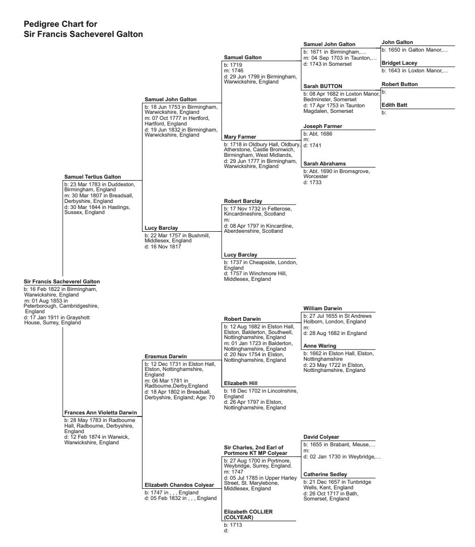
Fig. 5.1 The ancestry of Francis Galton
1783–30 March 1844) took over the family business in 1815, the family had become firmly established as bankers.
Samuel Galton Jr. died in 1832 a wealthy man, with a large fortune estimated at £300,000. By then, his son Samuel Tertius, a well-educated graduate of Cambridge University, had increasingly lived a life of nobility.
He left to others the management of the Galton businesses, and instead devoted himself to the study of economics and his interests in lesser scientifi c pursuits.
On 30 March 1807, Samuel Tertius married Francis Anne Violetta Darwin, the daughter of a fellow Lunar Society member Erasmus Darwin (12 December 1731–18 April 1802), their family physician. Erasmus was a philosopher, slave trade abolitionist and a member of the Darwin-Wedgwood family, of high-quality pottery fame. Th is was a union of two families of high social status.
Samuel and Violetta lived in a large house in an exclusive area of Birmingham, in Th e Larches , the former home of Joseph Priestley. Samuel Galton and Erasmus Darwin had established the Lunar Society. Indeed, within this Lunar Society was a large number of cross-marriages between Darwins, Wedgwoods, Barclays and Galtons. For instance, another of Erasmus’ children was Robert Darwin (1766–1848), the father of Charles Darwin.
Samuel Tertius’ marriage to Violetta required him to break from the Quakers. Th e family of Erasmus Darwin were resolute followers of the Church of England, and the patriarch of the family held great sway. Erasmus, the grandfather of Charles Darwin, was a brilliant physician in his own right who had developed his own theory of evolution based on acquired characteristics, which infl uenced the creation of the eugenics movement a half century later. He was also a Fellow of the Royal Society (FRS). On both the Darwin and Galton sides of the family were intellectuals who immersed themselves in the scientifi c, moral and social studies of the day.
Certainly, Samuel Tertius enjoyed signifi cant intellectual stimulation within his enlarged family. With a wealth that allowed him to devote time to his intellectual pursuits, he shared his father’s interest in tracking all things with elaborate tables and color-coded charts. In the early nineteenth century, the Great Mind David Ricardo (18 April 1772–11 September 1823) was gaining fame as a self-taught economist through his treatises on the value of money and bullion. Samuel, too, weighed into the debate with his 1813 book A Chart Exhibiting the Relationship Between the Amount of Bank of England Notes in Circulation, the Rate of Foreign Exchanges, and the Prices of Gold and Silver Bullion and of Wheat, Accompanied with Explanatory Observations . His contribution to economics was only shortly after Ricardo’s groundbreaking and highly infl uential pamphlet Th e High Price of Bullion, a Proof of the Depreciation of Bank Notes . In Galton ’s exposition, he observed and explained how one line on a chart is correlated with another, an argument that one of his sons would subsequently develop to great eff ect.
The Arrival of Francis Galton
Samuel and Violetta had a string of four girls together, followed by three boys. Th eir youngest, Francis Sacheveral Galton , was born on 16 February 1822. By then, his four sisters were in or nearing their teenage years.
Francis was very much the baby of a most successful and comfortable family. He was especially close to the third eldest of his sisters. She suff ered from a back condition that kept her confi ned to a couch in her room for much of the day. Th ere, she nurtured, played with and educated her young baby brother. By the age of four, Francis could read and write, add and multiply. A year later, he had absorbed Homer’s Illiad .
Francis’ intellectual intensity shaped him into a socially uncomfortable and solitary child, which made his eventual attendance in grammar school somewhat diffi cult. First, he attended a local school, and then, by his tenth birthday, he was sent to a boarding school in Boulogne. After a year of unhappiness, though, he returned home to attend a private school much more to his liking, under the tutelage of Reverend Atwood.
At the private grammar school, Francis thrived. Th en, at the age of 13, he began to attend King Edward’s Grammar School in Birmingham. Th ere, he would endure a brutal, corporal form of classics education for a little more than two years. Th en, at the young age of 15, he began a medical education at Birmingham’s hospital as his father pursued whatever could be done to ensure Francis followed in his grandfather Erasmus’ footsteps.
Th e year 1838 was an important one for Francis. Barely 16 years old, he was at one moment celebrating the beginning of the Victorian era in England, and commencing his medical education at a highly respectable London institution. As a young medical student, he was at fi rst repulsed by the suff ering, but soon garnered a detached scientifi c perspective. Th e next year found himself studying medicine at the renowned Kings College Medical School in London.
Galton thrived in the program but still sought more esoteric scientifi c pursuits. In England at the time, one was not eligible for graduation until the age of 21. His early entry into medical studies meant he had a year to fi ll before he could receive his credentials. He, and his half cousin, consulted about his academic future. Charles Darwin had been biding time visiting London upon the return from his circumnavigation of the world as the documenting botanist on the HMS Beagle . Th ey concocted a plan. Darwin felt, and Galton agreed, that a year studying mathematics at Cambridge might help Galton augment his analytic skills.
Galton enjoyed Trinity College at Cambridge perhaps more than was conducive to his learning. He did not thrive intellectually, but he maintained his academic progress suffi ciently to remain there, and delay the completion of his medical education. While at Cambridge, though, his dear father Samuel Tertius died from a steadily worsening asthma. On 23 October 1844, Francis was left fatherless, but far from penniless.
Earlier that year, in February, Galton had become a member of the Freemasons , a fraternal organization of men who are devoted to collectively doing things together in their world, and individually doing things within their own minds. Dating back to the Middle Ages, the masons are dedicated to continuous social and individual growth.
At the time of his joining of the freemasons, and his certifi cate in 1845, Galton was attempting to complete his studies at Cambridge with honors. However, the stress of his schooling, the loss of his father and other pressures in his life caused him to suff er a nervous breakdown. He briefl y resumed his medical studies, but abandoned them too. In 1847, Cambridge University awarded him his degree with no requirement for further study.
While he had promised his father he would complete his medical studies, Galton had a rather lackluster mathematics degree in hand, and an inheritance that meant he would not need to ever work to support himself. Galton reneged on his compact with his deceased father, and indulged his penchant to travel.
Perhaps imbued with his half cousin’s love for exploration, Galton took to adventures of his own. He sought new experiences, fi rst in Egypt, and then throughout the Middle East, accompanied by a servant and by friends he met there, or whom would join him from England. He eventually bored of his adventures, though, and returned to the life of country gentry in England.
Soon, though, he again yearned to travel, and set out to travel even more extensively. Much of the latter half of the 1840s would be his age of exploration of Africa. Upon his return in the early 1850s, he was celebrated for his adventures. His writings and subsequent speeches to learned societies on his African travels won him respect in London’s intellectual community and the major award from the Royal Geographical Society that David Livingston, of “Dr. Livingston, I presume” notoriety, had just won some time earlier for his own explorations of Africa.
His reputation as a noted adventurer cemented, Galton traveled his circles in London and beyond, often as the toast of the party. On one occasion, in the Christmas holiday season of 1852, he attended a party at his neighbor’s home and met his future wife, Louisa Butler, the daughter of George Butler (5 July 1774–30 April 1853), a well-known mathematician from Cambridge, and sister of other Cambridge students and alumni. Galton fi t well into the family. Francis and Louisa were married on the 1 August 1853.
A marriage-blissful Francis set about to work on a book of his adventures in Africa. His publication became a popular read, and more awards were bestowed upon him. Barely 32 years old, Francis had achieved as much fame as a man of leisure could earn. He augmented his fame with additional highly successful books, and with a lecture series. By 1856, he was appointed a Fellow to the Royal Geographical Society. From his learned base, he gained the friendship of England’s most infl uential thinkers of the day. Among the dozens of intellectuals he came to know was Herbert Simon , the father of Social Darwinism, and the individual who coined the phrase survival of the fi ttest to so compactly, and perhaps erroneously, as a description of the contribution of Galton ‘s cousin, Charles Darwin. Th is troika of Galton, Darwin and Simon collectively began to revolutionize humankinds’ thought on evolutionary destiny from the perspective of both biology and society.
6. The Times of Francis Galton
Lambert Adolphe Jacques Quetelet (22 February 1796–17 February 1874) was a contemporary of Gauss who also directed an observatory, in Brussels, Belgium, 300 miles to the west of Göttingen. Born in Ghent, then part of Napoleon’s French Republic, to a city agent, François-Augustin-Jacques-Henri Quetelet, and Anne Françoise Vandervelde, Adolphe lost his father when he was only seven years old. He channeled that loss into his studies.
Like Gauss, who was 20 years’ Quetelet senior, Quetelet was mathematically precocious. He began to teach mathematics by the age of 19, and graduated with his PhD 4 years later, from the University of Ghent. Also, like Gauss, he was interested in the theory of curves.
A young person of limited means who did not stray far from his geographical heritage, Adolphe, also as had Gauss, sought to build an observatory in a nearby center of his province. He moved to Brussels, assembled his observatory, and became a respected member of his nation’s Royal Academy, and in the nearby Royal Netherlands Academy of Arts and Sciences. Over his career, he mastered the tools necessary to direct an observatory, but he also sought to apply these tools to social issues in what he preferred to call social physics, through his application of the normal distribution and the method of least squares to social issues.
While Gauss used the normal distribution as a way to minimize the effect of errors on astronomical observations, Quetelet recognized that social variables were exceedingly complex and imperfect in their measurement. He sought to use the statistical techniques of scientists to better describe and understand such issues as crime, suicide and marriage rates. In doing so, he positioned himself squarely within an emerging discussion of nature versus nurture. In his era, social philosophers of the day were arguing that the decisions of women and men were a natural exercise of free will, and Quetelet argued that we are influenced in our decisions. As a consequence, our actions might thus be predicted as a function of the forces that impinge on our lives.
Quetelet’s most significant statement on the debate over free will was his 1835 Treatise on Man, Sur l’homme et le développement de ses facultés, ou Essai de physique sociale, published just a dozen years after Gauss fully described the linear regression model and the normal distribution. There, Quetelet formulated the concept of social physics and the measurement of characteristics that describe the “average man.” For instance, our current measure of the body mass index, as a representation of our combination of height and weight, was developed by Quetelet.
Quetelet observed that common social parameters and astronomical errors seemed to be distributed as a normal distribution, just as it describes the errors in astronomical observations. When Isidore Auguste Marie François Xavier Comte (19 January 1798–5 September 1857), a contemporary of his, heard of Quetelet’s social physics, Auguste Comte instead coined the term sociology to explore such influences, characterizations and relationships among members of society to distinguish his more philosophical approach to Quetelet’s more quantitative methodology.
In his various social explorations, Quetelet developed correlations between such physical observables as age, gender, education and alcohol consumption on the rate of crime. This exploration resulted in a chapter “Of the Development of the Propensity to Crime” in his Treatise of Man. In the Treatise, he also asserted that the variations of measureable human characteristics about the average follows Gauss’ normal distribution. He observed that such a normal variation offers the variability in human characteristics that would permit natural or artificial selection to function. Quetelet’s concept even provided an inspiration for Darwin’s explorations in natural selection. It also acted as the motivation for one of the most colorful characters in nineteenth-century social sciences.
This was also an era in which hard sciences began to inspire new social sciences, and this social dimension was increasingly stimulating the public’s interest. Quetelet had begun a new discussion in biology, and the Galton/Darwin pair were ready to further it. Meanwhile, Francis Galton was thriving in the 1850s and 1860s England when the island was at the peak of Victorian geopolitical and intellectual conquest.
Having settled into a house Francis Galton bought only a short distance from London’s Hyde Park, the couple continued to entertain London’s intellectual elite. By then homebound, Galton turned his adventures to mathematics. First, he sought to make more scientific the state of understanding of European meteorology. He solicited from weather experts across Europe thrice-daily weather observations, which he then meticulously plotted for the month of December 1861. From the data, he was the first to observe that wind patterns revolve clockwise around lows, and counterclockwise around high-pressure zones. He labeled these patterns cyclones and anti-cyclones, terms that have stuck since.
Galton’s faith in a more scientific approach to weather predictions of that era caused him to criticize the official weather forecaster of the time, Admiral Fitzroy. Soon, there was a chorus of public criticism of Fitzroy’s forecasts, which caused the Admiral to take his own life. Galton was immediately drafted to head what would become the UK Meteorological Office. From his new position, Galton began to cultivate for himself a reputation as a mathematical and scientific genius.
By the fall of 1860, just a few months after his cousin finally published The Origin of Species, Galton witnessed a gathering at Cambridge which changed the perspective of many in the room, including Galton’s, and the scientific world to follow. Already, Galton had been influenced by Herbert Simon’s influential idea of social evolution. The pessimism of such luminaries in the first half of the century as Thomas “Robert” Malthus was supplanted by a grander and more optimistic design, even if the concept of natural selection was immediately often, and still is, misunderstood.
In Galton’s fantasy, though, was a notion of eugenics, by which humanity would be improved by carefully designed selection. Galton used his position and his writing to advocate for a new form of human breeding, just as animal husbandry had done for centuries, but with the goal of incorporating desirable intellectual skills, in addition to physical characteristics, into future bloodlines, and, more controversially, preventing other less desirable characteristics from perpetuating. Seventy years later, the Nazi movement proposed the culling of what they deem as negative human characteristics to accelerate the process of artificial selection.
Galton’s enthusiasm to further develop how natural variability in human characteristics could be tapped to improve the human race demanded of him greater scientific rigor. He discovered some of the necessary rigor from the work of Quetelet of Belgium. Quetelet had demonstrated from extensive observations of height and girth that human measurements seem to follow a distribution that looked much like the familiar bell-shaped curve Gauss had derived. Galton was emboldened by this new tool of statistical biometrics, and began to apply statistical measures to intelligence.
Just as students today ask professors whether grades are curved, Galton categorized measures of grade scores in the UK and declared that they indeed seem to follow some such curve, even if any formal concept of goodness of fit did not yet exist. He published what was still, to then, anecdotal evidence in a book called Hereditary Genius. 1 His book generated both supporters and detractors. In the former camp, though, was his cousin, Charles Darwin. Charles wrote a most complimentary letter to Francis, and Galton used the praise as inspiration for a more formal scientific treatment of the conclusions he had quickly drawn.
Galton recognized that he would have to shore up his conclusions that various influences determine desired human characteristics. To do so, he employed the same meticulous drawing of tables and graphs as his father had demonstrated to him almost half a century earlier. He began with an experiment in which he gave friends sweet peas of various sizes to grow. He then asked them to return the peas they grow. He plotted the weight of the mother peas to those of the offspring, and verified his intuition that the weight of the parent peas is a relatively reliable determinant of the weight of the offspring seed. Yet, he discovered that parent peas that were larger than average did not produce offspring that were larger yet. Nor would smaller parent seeds produce offspring that were smaller yet. Instead, he established that the weight of offspring seed vary from the mean, on average by only one-third of the deviation from the mean of the weight of the parent seed.
In interpreting this peculiar relationship, Galton said that offspring regress to describe this tendency toward the mean, and coined such an analytic description a regression. The one-third rate was described as the regression coefficient. Some sort of natural process then appeared to Galton to dampen extremes and causes offspring to regress toward the mean.
Galton argued that his technique could actually be used to compare many such interactions. Of course, there is no problem with units when on both axes is a measure of height. The slope of a line that compares one axis to another is a ratio without units, or, if one prefers, a rate of inches to inches. In other circumstances, one might posit that rainfall might influence a crop yield, or, in the finance literature, increased risk might command a greater return, as in the capital asset pricing model (CAPM). In these cases, the correlation between one variable and another might better be described by some sort of correlation coefficient rather than a unitless slope.
It was this statistical extension that Galton set out to establish using his regression model adapted from Gauss’ ordinary least squares methodology. To create the data for his analyses, he established the Anthropometric Laboratory in nearby South Kensington to solicit subjects who would be willing to be measured in a multitude of ways. In his lab, Galton and his researchers established the first extensive database of human measurements and qualities, and even pioneered such lifelong markers as the use of fingerprints.
To some, Galton’s audaciousness and academic entrepreneurship were little more than self-aggrandizement, at best, and derivative at worse. Others heralded him as a genius. There was one certainty, though. Galton always walked along the cliff of controversy. Despite his confidence that he was an exceptional polymath, he was in fact not particularly skilled mathematically.
Galton did not have the mathematical or calculation tools to employ Gauss’ methods. Nor did he have the facility of Gauss’ intuition. Nonetheless, he intuited some mathematical relationships of his own. He argued that the dependence of one generational variable and another should be proportional to the relative variability, or, more correctly, its square root, the standard deviation, of measurements in one generation relative to another. He postulated from his observations that a line correlating two variables becomes flatter as the variability of the measure on the vertical axis becomes smaller relative to the variability of the measure on the horizontal axis. If y is the vertical measure, x the horizontal measure, and Sx and Sy their respective standard deviations, then Galton postulated the relationship between the variables as:
\[y = r(s_x / s_y),\]
where r is the slope of the graph when the two variables are plotted against each other.
While Galton’s analysis was incomplete and non-rigorous, he nonetheless provided a lasting intuition, beyond his coining of the expression regression. He correctly observed that the relative variability of two factors was an important determinant to the scale of their relative graphical depictions, and hence the slope of the regression line. He would leave to one of his laboratory assistants, his prodigy Karl Pearson, to formalize, and hence legitimize his intuition.
Note
- Galton, F., Hereditary Genius, Macmillan, London, 1869.
7. The Later Life and Legacy of Sir Francis Galton
Galton remained preoccupied by his work and by his need to ensure he remained at the center of intellectual thought, however controversial, within the London social scientifi c circles at the time. He spent little time at home, and he and Louisa failed to have children together.
In their later years, and increasingly challenged by health problems, he and Louisa fi nally had an opportunity to travel, often seeking cleansing spas and sanitariums to improve their health. On one such trip in the summer of 1897, Louisa became nauseous and began to suff er from severe diarrhea. She died in her hotel room in France in August of 1897.
Following the death of his wife, Galton embarked on ambitious travel for much of the rest of his life. In 1908, he published his autobiography, and was knighted Sir Francis Galton by King Edward in 1909. He lived to the age of 88, and died on 17 January 1911. Upon his death, he left his estate to endow the Galton Professorship in Eugenics at the University of London.
During his life, Galton was bestowed with many honors. Th ese include the Founders Medal in 1853, which is the highest award given by the Royal Geographical Society, the Silver Medal of the French Geographical Society in 1854, and was elected a member of the Athenaeum Club in 1855. Five years later, in 1860, he was made an FRS.
In 1886, he earned the Gold Medal of the Royal Society, and was named Offi cier de l’Instruction Publique of France in 1891. He secured the DCL at Oxford in 1894, and an DSc (Honorary) from Cambridge in 1895. In 1901, he won the Huxley Medal, off ered by the Anthropological Institute and, in 1902, he was elected Honorary Fellow of Trinity College, Cambridge. In that same year, he rejoiced when he learned the Royal Society awarded him the Darwin Medal, in honor of his cousin. In 1808, he earned the Linnean Society of London’s Darwin-Wallace Medal, and he won the Copley Medal of the Royal Society the year before he died.
While Galton was recognized with many accolades in his lifetime, his greater legacy may have been the creation of his lab and the establishment of the study of eugenics. One of his appointments at the lab complete the mathematics that Galton could not, and helped immortalize Galton ever since. Th e fi rst person to occupy his Galton Chair of Eugenics at the University College of London was his prodigy, Karl Pearson. Pearson documented Galton’s life and contributions in three books written in 1914, 1924 and 1930, and provided rigor to much of Galton’s intuition. Much of Galton’s work we now know from the publications of Pearson.
8. The Early Life of Karl Pearson
One might contrast the life of Gauss with that of Galton . Gauss’ humble beginnings might suggest he had everything to prove. Yet, over his lifetime, and despite his place as perhaps one of the three most accomplished mathematicians of all time, he took far too little time documenting and publishing his contributions. His brilliance was understated in his own lifetime.
On the contrary, Sir Francis Galton was born to the purest of pedigrees and privilege. Th e cousin of Charles Darwin and a member of a family of famous physicians, well-healed bankers and prominent theologians, Galton was a bigger than life personality from an equally impressive family. He had little he’d need to earn, but spent a lifetime trying to establish and enhance his reputation. His brilliance was equally overstated, as perhaps were the accolades he received. Yet, he left a prodigy, Karl Pearson, for whom he endowed an academic chair and hence a livelihood. Pearson spent his career fi lling in the academic blanks Galton had left.
While Galton cultivated a perception that he was a polymath, his prodigy certainly was.
Th e heritage of Karl Pearson was distinctly of Yorkshire roots. His father, William Pearson, Queen’s Council (QC) (1822–?), grew up in the North Riding of Yorkshire, in northwest England. His family were farmers, but William left the region in a dispute over farmland. He departed for the University of Edinburgh in Scotland to the north, where he completed a degree in law with distinction. He arrived in London prepared to establish himself as a barrister. In service to the courts of London, he eventually obtained the highest status of barristers in England, a member of the QC within the Inner Temple of the Royal Courts of Justice.
In London he also met his future wife Fanny Smith. Her father Th omas was a master mariner from Kingston upon Hull in the Eastern Riding of Yorkshire and had come from a long line of seafarers. He had lost his father’s ship on one journey and decided to relocate as a ship’s pilot to the calmer waters of the River Th ames in London.
Fanny was kind and literate, but not educated. Th e family life at home was considered somewhat harsh and disciplined, but it was fi nancially comfortable. Like the family of Francis Galton , the Pearsons, too, were Dissenters and of the Quaker faith.
The Arrival of Carl Pearson
William and Fanny had two sons, the second whom was born on 27 March 1857 and was given the name Carl. Carl’s primary relationship with his parents was through his mother. Th e young boy grew up in a household with a stoic and stern father who arrived home late, prepared his next day’s briefs until midnight and left for work early in the morning. His interactions with both his wife and children were primarily over the holidays, and they were not warm. Carl and his older brother Arthur worried on behalf of their mother (Fig. 8.1 ).
Carl was educated both at home and at a small local school, with additional supplemental lessons off ered by tutors. Th en, at the age of nine, his family moved to Bloomsbury and Carl and Arthur were able to attend the highly regarded University College London School. Th is experimental school off ered the fi nest and most contemporary education theories to a limited number of young students. Carl remained at the school until the age of 16.
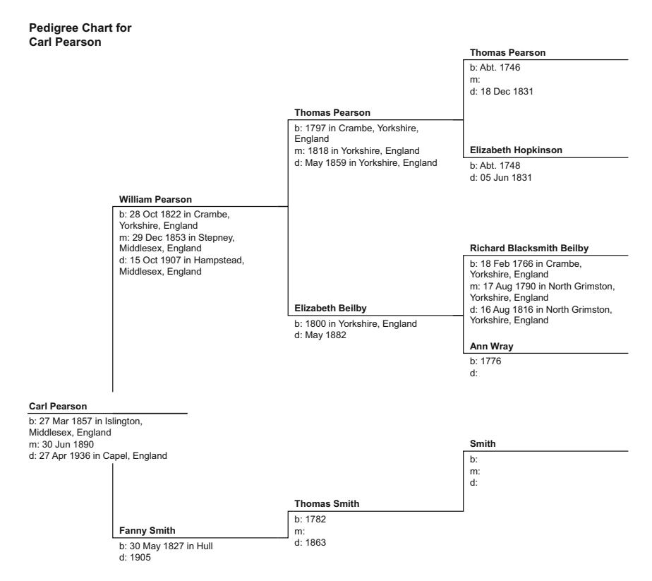
Fig. 8.1 The ancestry of Carl Pearson
By then, his brother had received a scholarship in the study of the classics at Trinity College, Cambridge. Carl’s father wanted at least one of his children to study mathematics, so he secured a Cambridge Wrangler to prepare Carl for the Tripos entrance exam. Wranglers are those who receive the highest honors in their third year studies at Cambridge. Th is honor of Mathematics Wrangler connotes a graduate of intellectual supremacy. Carl was sent to the town of Hitchin, near Cambridge, for fi ve months of intensive mathematical tutoring by a Wrangler in early 1874. Unhappy in Hitchin, he left that summer to be tutored in mathematics at Merton Hall, Cambridge, by a cadre of tutors which included legendary Wrangler John Routh.
Edward John Routh FRS (20 January 1831–7 June 1907) was considered the best among Senior Wranglers in preparing students for the exam. Born in Quebec, Canada, to a well-established family whose father’s ancestors also originated in Yorkshire, Routh studied mathematics at the University of London before he continued on at the Peterhouse in Cambridge. He, too, was prepared by the “senior wrangler maker” William Hopkins FRS (2 February 1793–13 October 1866). Routh himself graduated as a Senior (signifying top) Wrangler, just ahead of the brilliant Scottish mathematical physicist James Clerk Maxwell FRS FRSE (13 June 1831–5 November 1879). Clearly, young Carl could not be in better academic hands.
Routh instructed Carl in a mathematics that was heavily laden with physics. Over the next nine months, Carl studied in preparation of the exam, which permitted him a scholarship at King’s College in Cambridge. He began his University studies on 9 October 1875.
Carl Pearson thrived in this intensive intellectual environment. As a child he was somewhat frail and sickly, and he felt a lack of warmth, caring and inclusiveness. King’s College believed in exercising the mind and the body. Carl’s emotional and physical constitutions were strengthened, and he thrived intellectually. He was also immersed in the Classics and of the Romantic school. He graduated as Th ird Wrangler in 1879, which translates to third in his class.
His academic success also earned him a King’s College Fellowship. Th is lucrative scholarship allows the recipient up to seven years of funding, with no teaching expectations, to pursue his research agenda. Th e scholarship recognized Carl Pearson as among the most distinguished and promising university graduates in the nation.
Carl had yet to travel, though. He was not brought up in a wealthy family as had Francis Galton , and Continental travel was not a luxury his family could aff ord. His fellowship made more options available to him. He had been studying mechanics and engineering, with the hope of becoming an engineering physicist. Germany was the center of the study of physics at the time, so he began to study German and traveled to Heidelberg. While there, he was enticed by the theories of the great philosophers, from Kant and Spinoza to John Locke.
While his exposure to philosophy cemented his desire to be a Freethinker, he also found the lack of spirituality in the philosophy of that era to be depressing. He decided to balance his idealistic philosophical yearnings with the positivistic study of science. However, he was also humbled by the great mathematical physicists of his day, like James Clerk Maxwell , and made a relatively short-lived decision to study international law instead, likely from pressure from his oppressive father. Carl, by then calling himself Karl after his Heidelberg experience, returned to England, completed his law study, was admitted to the bar, but continued to study mathematics on the side, much to his father’s consternation.
9. Karl Pearson’s Great Idea
Almost immediately after he began, Karl gave up the practice of law. Yet, the pressures for him to succeed were almost unrelenting. To free him from the forces of familial conformation, he joined the intellectual circles of London. He lectured locally at the intellectual clubs in Soho, including the Men and Women’s Club. While he considered himself a man of numbers, others increasingly viewed him as a man of words.
From his engineering training, Karl was fascinated by the theory of elasticity. This is a mathematically rigorous application of the principles of physics and engineering that governs the bending of materials such as bridge spans and beams and the forces as objects move through a viscous medium. Karl also pursued an eclectic combination of studies that was not only heavily influenced by the mathematics of the day. He was also fascinated with the philosophy of science that imposed on its practitioners the need to look at familiar problems in unfamiliar ways.
Karl Pearson was especially influenced by a mathematical physicist and philosopher William Kingdon Clifford FRS (4 May 1845–3 March 1879), a brilliant non-Euclidean geometer who argued for the equivalence of mass and energy and the notion of the curvature of space. The intellectual explorations he began in his 1876 On the Space-Theory of Matter was completed by Albert Einstein in Einstein’s general theory of relativity in 1916.
When Clifford died before his last treatise could be completed, Pearson continued Clifford’s work. Pearson eventually published his theory in the American Journal of Mathematics. Meanwhile, he continued to study at Cambridge and Heidelberg, and he soon found a calling he could call uniquely his own: mathematical statistics.
Pearson’s path crossed Francis Galton’s in his intellectual travels within the London and Cambridge academic communities with Galton’s encouragement. Pearson was offered a professorship at the University of London to establish the first department in statistics, but, as a favor to Galton, who was keen to see one of high prominence occupy the chair Galton endowed, he also agreed to continue Galton’s Eugenics Laboratory in Galton’s waning years. Many since have concluded that Pearson was hence a Galton Eugenics evangelist.
Pearson kept his eugenics assignment and his statistics passion quite separate, though, even if both helped pay the bills. Pearson was interested in the mathematics of statistics, and biometrics was an excellent avenue for his theoretical explorations. While he did not so fully subscribe to Galton’s social extensions, he was gracious with regard to the elder Galton, even if he did not consider himself an evangelical follower of the Galton social philosophy. Others did, though.
In fact, their statistical explorations were quite different. Pearson subscribed to the mathematical school established in the era of Gauss, with statistical moments establishing measures of goodness of fit, just as moments were used within the mathematics of elasticity. Meanwhile, Galton was preoccupied with the establishment of correlations. Galton’s analysis was mathematically unsophisticated, while Pearson’s was influenced by engineering and physics. And Galton believed that all data conforms to the normal distribution, while Pearson believed that a variety of distributions govern the various phenomena nature produces.
Pearson likely understood at the onset the importance and implications of the central limit theorem. As we have discussed, it describes the distribution of a asymptotically large number observations from symmetrically distributed probability distributions. Our earlier proof of the central limit theorem demonstrated that the resulting distribution or means would be distributed normally. The intuition can be illustrated by an example. Consider a distribution that is perhaps more unlike a normal distribution than any other. Bernoulli and De Moivre analyzed the binomial distribution such as might occur with the flipping of a coin. Call tails zero and head one. If we continually flip the coin, we would notice an approximately equal-peaked bimodal frequency distribution at 0 and 1.
What about the mean, though? The statistic for the mean will increasingly be centered at ½ as n rises, and will approach a normal distribution. The central limit theorem does not describe the distribution of coin tosses. Rather it determines that the mean of repeated draws from a symmetric distribution will correspond to the distribution’s average, with a predictable variance.
Hence, while the actual distributions were not normal, the mean of repeated draws from these distributions was. Galton may have overreached if he claimed that all real-world biological and sociological data is generated from normal distributions, even if their means may imply so. He and his contemporary Adolphe Quetelet attached greater significance to the normal distribution than was justified by asserting nature is inherently normal.
Pearson’s insight was different. He recognized that the normal distribution was derived from the law of errors, or deviations from the mean, not from an omnipotent natural distribution that generated the observations in the first place. Pearson became the father of modern statistics by recognizing that Gauss’ mean was a measure of central tendency, or a statistic, rather than a process that regresses toward a normally distributed mean in itself.
This observation was significant. Pearson recognized that our scientific perspective inescapably influences our characterization of natural laws. At the age of 34, he wrote one of the most significant commentaries in the philosophy of science, entitled The Grammar of Science. 1 Decades later, Albert Einstein assembled a group of applied mathematicians to understand and discuss the implications of Pearson’s book. These are the importance of the frame of reference of the observer in the relativity of motion, Pearson’s equivalency of matter and energy, the non-existence of the either, time as a fourth dimension and space as a non-Euclidean geometry. These notions were central to Einstein’s argument that a photon can be both a particle and a wave, the Heisenberg’s uncertainty principle, and both Einstein’s special and general theory of relativity.
We remember Pearson as a statistician, though. How he found his path from a philosopher of science to the founder of statistics came from his association with Walter Frank Raphael Weldon DSc FRS (15 March 1860–Oxford, 13 April 1906), an influential Darwinian zoologist who encouraged Pearson to apply his skills to statistics, and who established the new journal Biometrika with Galton and Pearson. In fact, Pearson and Weldon had been working together since 1891, but Weldon did not introduce Pearson to Galton until 1894.
Weldon recognized a number of qualities in Pearson that would well contribute to a new field of representing data through statistics. Pearson was truly a creative polymath able to view problems in original ways, even if he had lost his confidence in making significant contributions to physics, ironically enough given his inspiration of Einstein, perhaps the greatest physicist of all time. Second, Pearson’s Gresham Lectures caught the attention of Weldon. Weldon felt some of the concepts Pearson had developed could be of great use to the study of evolution. Finally, Pearson wanted to make his mark, and was convinced by Weldon that statistics may be the best avenue.
At the time of the lectures, beginning in 1891, Pearson had been teaching geometry to engineers in the Department of Mechanics and Applied Mathematics at the University College London for half a dozen years. In 1890, he received an appointment as the Gresham Chair of Geometry at Gresham College. As part of his appointment, Pearson offered a set of public. In this series, he described his use of new non-Euclidean geometry to problems of mechanics and statics, as would Einstein 14 years later. In this series, he also described problems of statistics, of insurance, and of other applications that could benefit from his form of analysis. Always in search of novel ways to look at apparent problems, Pearson was intellectually intrigued by Weldon’s work in Darwinian zoology. Darwin proposed that natural selection be driven by natural variation, and Galton’s work on natural variation also interested Weldon. Pearson became convinced that this concept of natural variation, and its implications, was a prime candidate for new statistical tools, with random variation the underlying force.
In Weldon, Pearson found the closest of friends, until Weldon’s death in 1906. And, at the University College London, he found an intellectual and academic home. To that point, Pearson had spent five years applying for academic jobs across England, to little avail, and even contemplated returning to law or moving to the USA. Eventually, he accepted an offer to temporarily teach mathematics at King’s College, London, for a year, in 1883, and then the Goldsmid Chair of Mechanism and Applied Mathematics at University College London a year later. The University College would remain his academic home, at many levels, as he established their first Department of Structural Engineering in 1892, the Biometric School a year later and the Drapers’ Biometric Laboratory in 1903, which became the Department of Applied Statistics eight years later.
Pearson’s influential Gresham Lectures at Gresham College within the University of London was a bit of an intellectual diversion, in a number of ways. The Gresham Chairs were founded by Sir Thomas Gresham (c.1519–21 November 1579), the English financier and founder of the Royal Exchange in London. Appointments to these chairs included some of the most prominent intellectuals in England’s intellectual history. The chairs were confined to the study to astronomy, divinity, geometry, law, music, physics and rhetoric. Pearson’s lectures, and those of his guests, including Weldon, were designed to educate the new professional class of London: financiers, artisans and the like. Pearson had to distill complex mathematical notions to make them more accessible and useful to application of questions in commerce, insurance, finance and, hence, statistics. From his lectures came the conclusion that statistics was not merely a tool for sociologists like Galton, but a mathematical discipline of its own right that could enlighten many other branches, from mathematics to physics and astronomy, as well as biology, of course.
In the study of elasticities, Pearson was well familiar with the calculation of moments. His extension of his training to characterize not the properties of materials but the characteristics of data caused him in 1892 to define the standard deviation, as the square root of variance as a measure of the spread of data observations. His goal was a set of measures that could describe the spread and central tendencies of data, even when they don’t necessarily follow the normal distributions Galton prescribed for all natural data.
Pearson was determined to construct measures, of variation, of central tendency that could be used broadly to summarize large data sets, not merely their means. From there, he also developed the histogram to summarize continuous quantitative data.
From the method of moments, Pearson actually produced a number of measures. The first moment, which, as discussed earlier, is equivalent to the definition of a center of gravity, was applied to data to generate the mean, or its central cluster. The second moment, equivalent to the moment of inertia, measured its variance, and the square root the standard deviation. He also described the degree to which a distribution deviates from symmetry as his measure of skewness, and the flatness or prominence of the distribution’s peak its kurtosis. In doing so, Pearson was not providing an axiomatic approach to the specification of the data, but rather was characterizing data based on some standardized definitions. His statistical measures could thus be applied to any distribution.
Pearson also constructed measures by which such varied distributions departed from the normal distribution. He once asked his students if one could always represent data with a normal distribution. Of course, the answer is no. He then constructed the notion of goodness of fit as a measure of deviations from a normal distribution. To do so, he constructed a method of least moments in 1892.
Pearson was not the first to develop measures of goodness of fit. Quetelet and Galton both recognized the imperfections of real data from the normal ideal, especially given the smaller sample sizes from which they worked. Wilhelm Lexis (17 July 1837–24 August 1914), an economist and father of demography, produced his Ratio L to measure such a difference, while Francis Ysidro Edgeworth FBA (8 February 1845–13 February 1926), one of the first mathematical economists, developed a measure of the degree to which the binomial distribution departs from the normal distribution. These measures had an ad hoc nature to them, though. Pearson added some rigor and structure to his measures, usually based on moments. These methods evolved over his Gresham Lectures such that, by the end of the series in May of 1894, the methodology of statistics was established. He even followed these researches up much as Gauss had done, by producing a series a lectures on the methods appropriate for actuaries.
He followed up this work in 1894 almost immediately with a number of new statistical measures that could assist Galton in his work on correlations. Of the almost two dozen measures of correlation Pearson developed, half are still employed today.
Pearson also began working in late 1896 on techniques helpful for economists. He needed a measure of goodness of fit for asymmetric distributions. One such distribution was the gamma distribution, for which he described the chi-square distribution for the goodness of fit for a family of such gamma distributions. This culminated in Pearson’s final academic paper, shortly after his 70th birthday. The chi-square measure is one that can be employed when distributions do not conform to the normal distribution.
Pearson’s contributions primary focused on goodness of fit. Perhaps his most lasting statistical contribution came from his epic 1896 paper to the Philosophical Transactions of the Royal Society of London. Pearson proposed a measure called the correlation coefficient constructed as the mean, or moment, of a set of deviations of the data from the least squares minimizing trend line, in both the horizontal and vertical direction. Pearson proposed the measure for the correlation coefficient as:
\[\sum_{i=1}^{n} \frac{x_i y_i}{n},\]
where x and y are the deviations between the predicted means and the pairs of data. For instance, in the vertical direction, this would be:
\[\sum (y-\hat{y})^2\] .
To understand the calculation of the goodness of fit measure, recall that the parameters of the regression model are calculated as:
\[b = \frac{\sum_{i=1}^{n} (x_i - \bar{x})(Y_i - \bar{Y})}{\sum_{i=1}^{n} (x_i - \bar{x})^2}\]
\[a = \overline{Y} - b\overline{x}\] ,
where Y is assumed to be linearly related to x, or its transformation, and the residual deviations from the regression line follow a normal distribution with consistent variance.
Then, Pearson calculated a product-moment correlation coefficient r given by the sum of the product of deviations divided by the sum of the squared errors:
\[r = \frac{\sum_{i=1}^{n} (x_i - \overline{x}) (Y_i - \overline{Y})}{\sqrt{\sum_{i=1}^{n} (x_i - \overline{x})^2 \sum_{i=1}^{n} (Y_i - \overline{Y})^2}}.\]
The related measure \(r^2\) is the share of total variance of Y that can be explained by the regression representation of Y. Another way to describe this relationship is by considering the total sum of squares in the dependent variable Y compared to the independent variable X.
First, observe that the average value of y is given by summing all observations of the independent variable and dividing by the number of observations n:
\[\overline{y} = \frac{1}{n} \sum_{i=1}^{n} y_i.\]
The total sum of squares then gives an expression that is proportional to the variance of the independent variable:
\[SS_{tot} = \sum_{i} (y_i - \overline{y})^2.\]
Meanwhile the explained portion of the variance is proportional to the second moment generated by the estimated value \(f(x_i)\) relative to the mean, called the explained sum of squares from the regression:
\[SS_{reg} = \sum_{i} (f_i - \overline{y})^2.\]
And, the residual, or unexplained, sum of squares is given by:
\[SS_{res} = \sum_{i} (y_i - f_i)^2.\]
Pearson’s goodness of fit measure, often now called \(R^2\) , is then given by:
\[R^2 \equiv 1 - \frac{SS_{res}}{SS_{tot}}.\]
This framework for goodness of fit can also be employed for the determination of quality of other predictive models. The variation of this goodness of fit measure is then called the coefficient of determination.
By Pearson’s era, much of the history of the statistics to which a finance student will be exposed in their first yearlong course in statistics was at least partially established. Not yet fully explored was the least squares linear regression model and its properties. Later we describe the linear regression model and document the important extensions to finance that were offered by Fisher, Hotelling, Frisch and others.
Note
- Pearson, Karl, The Grammar of Science, Adam and Charles Black Publishers, London, 1892.
10. The Later Life and Legacy of Karl Pearson
Carl Friedrich Gauss was a most unusual polymath. Considered one of the greatest mathematical minds in history, it is possible that there could have been born a dozen like him who went unnoticed throughout life. Gauss grew out of the humblest of beginnings, demonstrated fantastic resilience and rose to great accomplishments, but were it not the help of a benefactor who saw something in young Gauss that no one else could see, we might have never benefi ted from his brilliance. Gauss also rose out of an era in which only the well-to-do could spend a lifetime studying the most esoteric of subjects. Indeed, by some calculations, he never published the majority of his ideas. He was busy maintaining a livelihood for his family at a time when publication was both fi nancially expensive and time consuming.
On the other hand, Sir Francis Galton was born into a family that verged on nobility. Certainly, they were the noble of the medical and banking community, with family members that included Charles Darwin and the Barclay and Wedgwood fortunes. Galton could easily practice a life of leisure if he chose, and, to a large margin, he did. For him, fame was a luxury he could easily aff ord. Indeed, he seemed to crave fame and recognition, and worked to cultivate it. Every door was open to him, even some that should have remained shut, and would have been bolted shut for men of lesser wealth like Gauss , or Pearson.
Galton paved a path for Pearson, and was perhaps even his academic benefactor. Each recognized and rode on the other’s coattails. Certainly, of the two, Pearson was the more academically brilliant. He also was more driven to succeed as he realized that, unlike Galton, he would have to earn each bit of his success.
Pearson could not aff ord the life of an adventurer as could Galton . His brief forays in travel resulted in his awakening to the growing socialist movement on the continent, the writings of such individuals as John Locke and Karl Marx, and the brilliant work of Europe’s leading mathematical physicists, mostly in Heidelberg and Göttingen at that time. He could bring back to London the lofty ideas of these philosophers, but he felt out of the league of their physicists. His admiration for them seemed to cause him to forever change the spelling of his fi rst name from Carl, to the German version Karl, though, like another famous London intellectual at the time, Karl Marx.
In 1885, Karl Pearson found an ideal outlet for his socialist thought, his procreation ideals along the lines of eugenics, and his desire for potentially feisty companionship. He founded Th e Men and Women’s Club , with the goal of attracting an equal number of men and women from the middle and upper middle class who espoused progressive views on socialism, feminism and sexuality.
Th en a 28-year-old bachelor, Pearson fi rmly believed that more empowered and educated women were necessary for national advancement. He gave a paper at the fi rst of the group’s monthly meetings near Soho entitled Th e Woman’s Question , in which he espoused greater access to education, politics and the professions for women, at the time when the woman’s suff rage was increasingly discussed. Just 20 years earlier, the great economist John Stuart Mill (20 May 1806–8 May 1873) had been elected to Parliament partly based on his equally progressive views toward women’s right to vote.
Th ose who believed in women’s suff rage were distinct from the suffragettes who would use violent means to achieve the same desired goals. Th e men attracted to Pearson’s club were drawn from the prevailing liberally oriented men’s clubs for London professionals at the time. Th e vast majority of the women attracted were single and were teachers or writers. Only one of the women had attended university. Indeed, university was quite inaccessible to women of middle-class families in that era.
Th is group of a couple of dozen men and women met in homes around the Kensington area but, over the four-year life of the club, ultimately failed to come to a meeting of the minds between the genders. While the men favored a post-patriarchal society which empowered women and which viewed sex in terms beyond procreation, or in the words of Pearson, a “physical pleasure like climbing a mountain,” the men of the group became increasingly fearful of the feminine energy they were releasing, and as the discussions became stalemated, almost strictly along gender lines. Th e club disbanded in 1889, four years after it began.
At the last meeting of the Men and Women’s Club, in March of 1889, Pearson placed his relationship with Francis Galton ‘s ideas in perspective. He lamented about the dangers of using tools of exact science in the realm of eugenics or economics. His prescience was profound. An overemphasis of the powerful tools of the sciences would detract from the humanity and complexity of real life. To try to attain mathematical perfection within theories of human inexactness suggested to him mathematical zealotry for mathematics’ sake.
He concluded this personal philosophical exploration with a greater sense of the need to use the tools of mathematical statistics to at least inform the better construction of descriptive statistics. Indeed, Pearson harbored hope that the discipline of science could instead act to improve the social dialog and interactions to the point that individuals behaved in a more rational way. If humans could be educated on the scientifi c method, perhaps then their interactions could be more appropriately explored by the tools of modern statistics. In the early part of the decade of the 1890s, Pearson devoted himself to higher education reform so that he may help guide the future of London’s great universities. Th is was a period of upheaval among these institutions, and Pearson felt he could play an important role within such reforms. But, his stakes were higher than simple university reform. He was simultaneously devoted to social reform.
It was this concept and ideal that motivated Pearson’s Grammar of Science series. And while one series does not make a revolution, Pearson clearly devoted substantial emotional and intellectual energy to the extension of the scientifi c method well beyond the traditional walls of the Ivory Tower.
Th e Men and Women’s Club was the spark for his period of personal growth. Th is personal philosophical agenda was not the only lasting benefi t Pearson retained from the Club, however. He was also successful in attracting the attention of his future wife Maria Sharpe (1851–30 June 1928) through the Club.
Unlike Pearson, who came from rural Yorkshire stock, and whose father had escaped his heritage and become educated in law, for which others challenged his true credentials later in life, Maria grew up within intellectualism. Her mother came from a family that included the prominent Unitarian minister Timothy Kenrick.
Kenrick was a Dissenter, a movement opposed to the infl uence of the state on personal faith. While there were a number of dissenting factions through to the nineteenth century, the remaining Dissenters include Baptists, Congregationalists, Presbyterians, Quakers and Unitarians. In particular, the Unitarians were followers of Socinianism, a following that did not accept the Trinitarian doctrine of the Catholic Church. In the eighteenth and nineteenth centuries, the Unitarian and the Quaker movements were highly infl uential and well subscribed in the intellectual circles in England, and among the founding fathers of the USA. Th ey subscribed to the doctrine of free will and rejected original sin. Timothy Kenrick was Maria Sharpe ’s maternal great-grandfather (Fig. 10.1 ).
Maria was not quite convinced of the worthiness of young Mr. Pearson early in their interactions. While he was universally considered philosophically brilliant among the group, he displayed condescension toward women in the group, perhaps especially Maria Sharpe . While he argued for equality, his Victorian upbringing, and perhaps even his patriarchally overwhelming childhood, had convinced him that women were not the intellectual equal of men. But while other women pursued Pearson, Maria Sharpe did not. She sought his advice, and she was rebuff ed. She challenged his thoughts, and he became angry. Perhaps he respected her willingness to stand up to him, because he fi nally proposed shortly after the Men and Women’s Club disbanded. Maria fi nally relented to his marriage requests. Th ey were married on 30 June 1890, the year after the Men and Women’s Club disbanded.
Pedigree Chart for Maria Sharpe
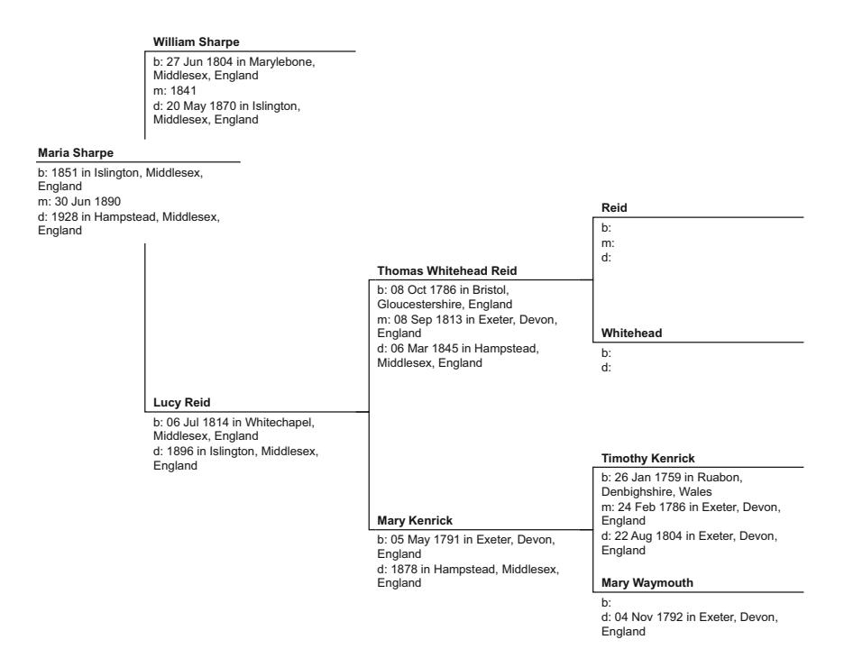
Fig. 10.1 The ancestry of Maria Sharpe
Maria’s concern that she would lose her independence in their relationship was well founded. She soon found herself abandoning her feminist researches and immersing herself in raising ideally eugenic children, hosting the parties one would expect of someone of Karl Pearson’s stature in London, and otherwise retreating to her own thoughts and marital responsibilities.
Together, the Pearsons had three children, Sigrid Loetitia in 1892, Egon in 1895 and Helga Sharpe in 1898. As we shall see, Egon went on to become a renowned statistician in himself, if perhaps not in his own right.
Karl Pearson remained the Galton Professor of Eugenics and the head of the statistics program until his retirement in 1933. He died three years later, on 27 April 1936. His wife had passed away before he did, on 30 June 1928.
Over his life, Pearson published dozens of papers, including a series of 18 papers in the Philosophical Transactions of the Royal Society , with the title “Mathematical Contributions to the Th eory of Evolution,” but with diff erent subtitles relating to evolution, eugenics, sociology, genetics and anthropology. In these papers, he described his moments approach, the chi-squared, correlation ratios, multiple regression , scedasticity, coeffi cient of variation and standard deviation . He also established the general use of lowercase Greek letters to describe population parameters. Pearson claimed to label the Gaussian distribution the “normal curve,” although Gauss had already used the expression normal to denote the quality of his method of least squares that used minimum distances of errors from the predicted function. Such minimum distances, from a geometrical perspective, are denoted by a normal vector, or a line drawn orthogonally at a 90° angle from the data point to the representative curve. Gauss’ geometric perspective also explains the use of squared deviations because the square root of a sum of squared deviations, in each direction, gives the total distance of a point to the function.
Overall, Pearson published over 300 papers on theoretical and applied statistics, social issues such as mental illness, scientifi c issues drawn from astronomy, meteorology, civil engineering, and biology, anthropology and sociology, and philosophical issues. He also worked on a four- volume book on the life of Francis Galton .
Pearson’s papers analyzed the correlation coeffi cient , his method of moments, Pearson’s system of continuous curves that was the precursor to the concept of continuous probability distributions, the chi distance and the P -value, the chi-squared test, a method of curve fi tting by minimizing chi distance (called principle component analysis), the coeffi cient of racial likeness as a way to classify races based on the shape of their skulls, and the establishment of foundations of hypothesis testing that used p -value s and was the precursor to type-I and type-II error analysis.
Pearson also co-founded and edited the journal Biometrika , and edited it until he died, at which time his son Egon took over the editorial responsibility. Th e journal arose because traditional biology journals were unwilling to accept manuscripts of a statistical nature at that time.
Pearson was not without petty fault, though, as we shall see. He jealously protected the reputation of Francis Galton , and he rejected approaches by competing statisticians on sometimes petty, and often provincial, grounds. Ronald Fisher , the subject of our next section, was the most unfortunate recipient of Pearson’s negativity and sometimes confounding fi ckleness and prickliness.
Pearson was true to his ideals, though. Over his lifetime, he variously received a number of awards. In 1896, he was elected FRS, followed two years later with the awarding of the Darwin Medal. In 1911, he was awarded the honorary degree of LLD from St. Andrews University, and, in the same year, was given the DSc from University of London. In 1932, he received the Rudolf Virchow medal by the Berliner Anthropologische Gesellschaft.
But, he also rejected, on purely philosophical grounds, as an avowed socialist, the two most signifi cant awards, including the knighthood accepted by both his predecessor, Francis Galton and, his successor, Ronald Fisher . In 1920, Pearson refused the prestigious Order of the British Empire, and, 1935, a knighthood.
He did not hold the same contempt for learned societies, though, and accepted election to the Royal Society of Medicine, the Royal Society of Edinburgh, the University College London, an Honorary Fellow of King’s College Cambridge and a Member of the Actuaries’ Club.
Perhaps Pearson’s most signifi cant and intellectually revolutionary contribution was not even in statistics. Many consider his Th e Grammar of Science to be his most remarkable contribution. Even Vladimir Ilyich Lenin and Albert Einstein off ered high praise, with Lenin considering his contribution a “conscientious and scrupulous foe of materialism.” Meanwhile, Einstein used it to stimulate his own ideas about relativity and the nature of matter and energy.
On Th ursday, 5 March 1891, Pearson off ered Lecture III in his Gresham series, Th e Concepts of Science. It is there that he may have provoked a scientifi c discussion that revolutionized physics. In his lecture, he developed the concept of relativity. He argued that phenomena may coexist in space, but an individual observer must be able to perceive of them as apart if the events are distinguishable from each other. Space and time thus off er an opportunity to distinguish for an observer events that coexist. One aspect of the distinctness lies in space, and the other in the sequence, or time.
Pearson was arguing that time is simply the dimension that allows us to distinguish the sequence of various pictures of our physical reality as objects shift in position. Sequence also allows us to distinguish between cause and eff ect. Th e time dimension must then only be suffi cient to distinguish the changes in position of the objects around us. Pearson argued that space and time are merely modes of perception, and physics the science that observes and governs these various modes.
Th ese observations, which Pearson included in his Grammar of Science , were most infl uential on a young Albert Einstein . In 1901, Einstein, unable to secure an academic position because of his unconventionality, was struggling to fi nd work in Bern, Switzerland, as a tutor in mathematics and physics. In 1901, Einstein placed an advertisement in the newspaper off ering his tutoring services in his apartment. A young Maurice Solovine (1875–1958), a budding Romanian mathematics and philosophy student, responded to the posting. Quickly, though, Einstein dispelled the notion of tutoring in physics, when he uttered: “It is not necessary to give you lessons in physics, the discussion about the problems which we face in physics today is much more interesting; simply come to me when you wish, I am pleased to be able to talk to you.” 1
Instead, the pair began to indulge discussion of metaphysical issues with Solovine. Solovine suggested that they form a group to discuss the works of great philosophers of science. Soon, mathematician Conrad Habicht (1876–1958) joined what soon became known as the “Akademie Olympia,” or Olympia Academy.
Th ese meetings in Einstein ’s apartment occurred from 1902 to 1904, and also included Paul Habicht (1884–1948), the brother of Conrad Habicht, Einstein’s friend, the mechanical engineer Michele Besso (1873–1955), his classmate Marcel Grossmann (1878–1936), the electrical engineer Lucien Chavan (1868–1942), and Mileva Marić (19 December 1875–4 August 1948), a brilliant Serbian mathematics student and Einstein’s fi rst wife, whom he married on 6 January 1903.
Th e fi rst book Einstein recommended was Pearson’s Grammar of Science , followed by Ernst Mach’s (18 February 1838–19 February 1916) Analyse der Empfi ndungen . Th e group also discussed Henri Poincaré’s Wissenschaft und Hypothese , A System of Logic by John Stuart Mill , David Hume’s Treatise of Human Nature , and books as varied as Baruch Spinoza’s Ethics and Miguel de Cervantes’ Don Quixote . Einstein later recalled that these discussions were instrumental in Einstein’s thinking and his Special Th eory of Relativity , published in 1905. His theory of that year was special because it described the special case of the observation of motion of objects moving at constant velocity based on the relative position of diff erent observers. A decade later, he published his General Th eory of Relativity that allowed these objects to change their velocity—that is, accelerate or decelerate.
Clearly, Pearson’s contribution of the importance of the observer’s perspective, and Machian physics, was instrumental in Einstein ’s thinking. Mach argued that physics should be based on the observer’s perspective, and should substitute the importance of relative motion for the less helpful concept of absolute space and time. He noted that such artifacts of classic absolute space and time physics as inertia and centrifugal force should instead be recast within a larger context. From Mach’s principle and Pearson’s emphasis on diff erent observer frames fl owed Einstein’s most profound theories. Einstein’s extensions of Pearson’s intuition culminated his Special and General Th eories of Relativity that completely revolutionized modern physics.
Note
- https://en.wikipedia.org/wiki/Maurice_Solovine, accessed 3 February 2016.
Part 3: The Formation of Modern Statistics
Th e innovation of the fi rst social scientists, initiated by Quetelet and furthered by Galton and Pearson, was certainly evolutionary, if not necessarily revolutionary. Each suggested concepts and some helpful measures in characterizing data, but none practiced the style of science increasingly demanded in the rapidly expanding scientifi c age. Rather, they were practitioners and engineers of issues often relevant to social science.
While these early intellects became increasingly adept at describing the properties of basic statistical estimators, they had not yet struck upon the need to establish the larger question of statistical validity for an entire model. It would take a fresh and much more rigorous geometric approach to provide the foundation for a new science of statistics. Th is scaff olding was created by Ronald Aylmer Fisher on one side of the Atlantic, and furthered and promoted by Harold Hotelling on the other side.
11. The Early Life of Ronald Aylmer Fisher
Ronald Fisher is remembered as the father of modern statistics. Ironically, Fisher endured much of his life in the unfortunate shadow of Pearson.
Th e Fisher name found its way from humble beginnings. A century and a half before Ronald Fisher was born, his great-great-great- grandfather George Fisher (c.1725–85) migrated from his rural laborer livelihood in Lincolnshire to England’s trade center of London. In the St. James district, he set up shop fi rst as a poultry seller. From their shop in Piccadilly, the Fishers established a lineage of shopkeepers, with the business handed down to each generation. First, John, the only child of George Fisher, took over the business, and then his only child, George, named after his grandfather, resumed the business.
By George’s birth in 1816, the Fisher family had garnered a level of respect within their communities. George was a lay leader at his church, and attained suffi cient wealth and status to aff ord his children an opportunity to attend school. But while his fi rstborn son, George Jr., died before the son could fully inherit the business, George’s second son John (1816–1907) was summoned from medical school to resume the family company.
While John may have partially sacrifi ced the respect a medical career could aff ord, he nonetheless benefi ted from other trappings of an increasingly successful family. His father purchased on his behalf a lifelong Governorship at nearby Christ’s Hospital, and his position within the Piccadilly business community aff orded him the opportunity to meet and then marry Emma Mortimer (1827–), a daughter of Th omas Jackson Mortimer (1781–1833) and Elizabeth Mavor (née Elsworth) (1765–1816).
Th omas Jackson Mortimer maintained and furthered a tradition of gunmaking in his family that had dated back to 1753. In this respect, Ronald Fisher shared a family foundation with Francis Galton . Th e paternal great-grandfather of Galton and the maternal great-grandfather of Fisher both ran gun manufacturing businesses.
Th e Mortimer shop at 34 St. James Street had been producing topquality guns. After his death in 1833, his wife Elizabeth and son Th omas Elsworth Mortimer maintained the business for a couple of years in London, but Th omas soon moved the business to Edinburgh. By 1836, the family fi rm was recognized Gunmaker to His Majesty, King William the IV. Fifteen years later, one of their guns was awarded the Prize Medal at London’s Great Exhibition in 1851. Th e fi rm eventually was transformed into Mortimer and Sons under the leadership of Th omas Jackson Mortimer’s grandson, Th omas Alfred Clark Mortimer (Fig. 11.1 ).
Th e daughter of Th omas Jackson Mortimer, Emma, and her husband from the neighborhood, John Fisher, appreciated education and had a suffi ciently comfortable life to aff ord the same for their children. John and Emma lived above the growing poulterer’s shop in St. James and assisted in the family business until the untimely death of George in 1855, following a slip and fall on an orange peel. 1 John chose to pass the business on to his younger brother and, at the age of 40, turned to the life of a leisure gentleman of London. For the next 50 years, he reigned as the patriarch of the family, fi rst in London, until the age of 74, and then in retirement in Norfolk until his death at the age of 90.
Before his retirement, though, John and Emma raised all but one of their 13 children in the apartment above the poulterer’s shop. Of these children, only fi ve survived childhood. Th e eldest surviving son, George Fisher, was born on 10 August 1843, while the youngest son, John Fisher, Pedigree Chart for Sir Ronald Aylmer Fisher D.Sc and F.R.S.
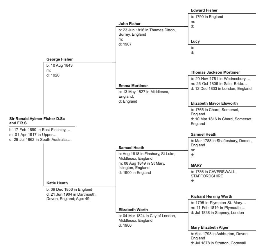
Fig. 11.1 The ancestry of Ronald Fisher
was born 15 years later, on 20 May 1858. John Jr. was aff orded the career that was pre-empted for his father. He completed his medical education at King’s College School and the associated St. George’s Hospital, where he rose to House Surgeon. John Jr. died on 6 November 1918.
Meanwhile, while George maintained the merchant tradition, he did so not by selling poultry. Rather, he established himself as a trader in fi ne arts in partnership within the fi rm Robinson and Fisher. George Fisher’s élan and sophistication aff orded the fi rm a reputation as one of London’s top fi ne arts auction houses.
Already well established and living a comfortable existence by the age of 32, George Fisher married Katie Heath (1845–94??), a woman a dozen years younger than him, and one of three daughters of Samuel Heath (August 1818–1900), an attorney from a long line of attorneys by the same name, and Samuel’s wife, Elizabeth Worth (4 March 1824–1900). Samuel and Elizabeth’s only son, Alfred, broke the tradition of London solicitors by migrating to America’s Wild West, where he became fi rst the sheriff and then the judge in Rawlins, Wyoming. Another of George’s brothers was named a Wrangler at Cambridge University, and, not coincidentally, married one of Katie Heath’s two sisters, Dora.
Clearly, the members of the Fisher family demonstrated education, brilliance and a certain fl air for interesting lives. George, especially, grew wealthy, as was demonstrated by his construction of a mansion on fi ve acres of parkland at the highest point in London, on Heath Hill. Th ere, Heath House, and Inverforth House was the residence for George, Katie and their fi ve children.
Th e courtly residence, in a garden on the hill in the heart of London, could not have been more idyllic for a young boy. Th e residence had ponds and boats, horses and tennis courts. Th eir family maintained a working garden and even kept livestock in case they needed a supply of food should infection plague London. Th eir home was chock-full of history and culture, an interest in world travel and in medicine. George’s home, and his children, represented the best of an extended Fisher family that had found material comforts but also demonstrated the best intellectual and cultural standards within the family. Th eirs was a family only a couple of generations free of a poulterer’s life, but which nonetheless showed that humble beginnings need not constrain intellect and success.
The Arrival of Ronald Fisher
Th e Fishers were patriarchal families, and the hope was to pass this sense and wealth on to sons. Th e fi rst child of George and Katie, Geoff rey, was born in 1876. A year later, Evelyn was born, followed a year after that with a second son, Allan. Th is second son died as a very young child of three, but was followed by Sibyl, Phyllis and Alwyn. Th en, on 17 February 1890, the last child, a boy they named Ronald Aylmer Fisher, was born.
In fact, Ronald’s birth was a bit of a miracle. Katie had a diffi cult pregnancy followed by the heartbreaking birth of a stillborn boy. Moments after this sad announcement, a second, smaller baby arrived. Ronald began life as a surprise gift, and much younger than his three sisters, who were all teenagers or young adults even before Ronald was old enough to begin school. Ronald, more than others, also benefi ted from the increasing comfort aff orded the family.
Just as had Francis Galton , Ronald was doted upon by his older sisters, and was instructed in the classics, learned to read at an early age and found a fascination with mathematics even by the age of three. But, while he was a precocious youngster, his very poor eyesight made it diffi cult for him to read. Instead, his nannies, sisters and mother would read to him, often on the subject of astronomy and geometry, something he could picture and imagine in his head. From this early introduction, he garnered a lifelong interest in astronomy and in the mathematical reasoning that was the basis of geometry, and a yearning for the establishment of the new science of statistics. Even Ronald’s poor eyesight became an asset. It forced him to develop as a visual learner. He became adept at translating mathematical concepts into geometric shapes in his head.
When Ronald’s brother Alwyn, three years his senior, began to attend day school in Hampstead Village, Ronald soon began to tag along. While he was much younger than the other pupils, his intellectual precociousness and his physical neediness seemed universally endearing. He earned special attention from Headmaster Greville, and his report card soon refl ected his brilliance. Despite his youthfulness by two or three years compared to his classmates, he soon scored consistently at the top of his class in science and mathematics.
By the age of 14, Ron was on his way to Harrow, one of the elite preparatory colleges in England. His transition into independence and adulthood arose for yet another reason that year. He lost his beloved mother, Katie, at the early age of 49, following her quickly progressing bout of peritonitis. Gone was his comfortable life on Heath Hill, his doting mother, nurses and sisters, and his ability to excel in small classes. He was thrust into an elite school with older boys, many of whom were brilliant themselves. Yet, despite these hardships and his almost debilitatingly poor eyesight, he earned the school’s highest prize, the Neeld Medal, after only two years at the school. He excelled with the specialized tutoring students at Harrow received, but, because tutoring was by lamplight in the evening, he absorbed subjects using geometric insights he could picture in his head rather than on dimly lit pages that challenged his poor eyesight. It was there that he demonstrated his uncanny ability to picture the solution to complex problems.
Fortunately, Ronald’s accomplishments secured him scholarships. Less than two years following the death of his mother, his father was bankrupt, and the family could no longer aff ord Harrow. At the age of 16, Ronald needed to rely on his innate intelligence by securing a series of scholarships. Th en, in October of 1909, at the age of 19, Ron was off to Cambridge with a full scholarship.
At Cambridge, Ron was popular among his fellow students, but perhaps not for the slightly disheveled nature of his clothes, or his somewhat odd body shape. He was nicknamed Piggy , but seemed unoff ended. His classmates were astounded especially by his mathematical acumen, and his ability to make up for months of lack of attention with hours or days of intense study. He also demonstrated a strong interest in the new fi eld of genetics in his four-year stay at Cambridge.
Th is was a period of infancy in the study of genetics, pioneered only four decades earlier by the work of the Augustinian friar Gregor Mendel (20 July 1822–6 January 1884) and his study of the inheritance of genetic characteristics in peas. Also not fully appreciated yet was the notion of natural selection as pioneered by Francis Galton ’s cousin Charles Darwin. But while Darwin’s theory remained debatable, Ronald Fisher saw the profound link between his work, Mendel’s genetics, and the growing infl uence of eugenics as championed by Galton.
By the time Fisher entered Cambridge, the new statistical journal Biometrika Karl Pearson had founded was seven years old, and Galton ’s legacy had been cemented with the dedication of the Galton Laboratory at the University of London, headed by Karl Pearson. Fisher was well subscribed to Galton’s increasingly populist belief that humanity can be improved through science. Statistics was the methodology that would test and guide the success of the study of eugenics he formulated to improve the genetic stock of humanity.
In 1910, Fisher had joined other eminent Cambridge University luminaries such as the Great Mind John Maynard Keynes and Horace Darwin (13 May 1851–22 September 1928), son of Charles Darwin, in the newly formed Eugenics Society. Fisher had championed this philosophy of eugenics at Cambridge, which off ered a warm reception to the notion of superior human breeding. Young Fisher was a key participant in the creation of a eugenics society at Cambridge. In the fall of 1911, the fi rst meetings of the Cambridge University Eugenics Society were convened in his room. Later that winter, the society attracted Major Leonard Darwin, the youngest son of Charles Darwin, and the president of the Eugenics Education Society of London, to come speak at Cambridge on eugenics reform. Th e following summer, Fisher attended the fi rst meeting, in London, of the International Eugenics Congress. By the second annual meeting of Cambridge’s eugenics society, Fisher was the lead speaker. Th e following year, Fisher addressed the Eugenics Society of London, as a 23-year-old recent graduate of Cambridge.
In his speech in London, Fisher argued that the modern triple set of tools of statistics, genetics and eugenics can help fulfi ll a promise that mankind could enhance its skills commensurate with the forward march of technology. Science and statistics can accelerate the otherwise plodding progress of Mendelian genetics and experimental breeding to ensure the demand for more able men could be met with a growing supply guided by science. He also argued that these statistical tools can guide the enhancement of classes that will most contribute to society.
Of course, this view was taken to great extreme in Adolf Hitler ’s (29 April 1889–30 April 1945) attempt to advance a master race of humans. But, for the fi rst third of the twentieth century, until everything went terribly wrong, the notion that the productivity of humankind could be advanced through science was at times controversial, but was also championed by many of the world’s intellectuals. While various notions of eugenics, such as the selective mating advocated by Plato to produce a guardian class, had been pondered for millennia, it was the British Eugenics Society and the Eugenics Education Society of London that were fi rst spearheading a philosophy of Galton that would soon spread across the Atlantic Ocean and around the developed world. Fisher was a young standard-bearer who was expected to continue the work of Galton following Galton’s death on 17 January 1911.
Fisher had a somewhat evolutionary insight into this eugenics movement, however. He viewed his role as assisting in the synthesis of eugenics, statistics and good science in a way that may elude the experts who advocate within each of these disciplines but compete between them. Fisher also recognized that there is a social aspect to eugenics. He saw the enhancement of qualities designed to advance the individual to be in confl ict with the needs of society. For instance, he warned his colleagues about the need of individuals to indulge in conspicuous consumption to advance their own status, but at the expense of the overall needs of society. He also argued that the goal ought not to allow humankind to advance within our environment. Mankind has the twin responsibility to allow the environment to advance through mankind. Here he was articulating the dual importance of both nurture and nature.
In his youthful exuberance, Fisher may have also been one of its most eugenically evangelistic proponents. He delighted the audience of his talks by speaking of the responsibility of those who view themselves as an exceptional class determined to produce for themselves exceptional off spring. Few of his contemporaries could have imagined the trajectory of the movement and the tragic conclusions to which it could lead.
Meanwhile, Fisher had completed his undergraduate studies at Cambridge, published his fi rst academic paper in mathematics in April of 1912, at the age of 22, and earned the distinction of Wrangler with his results on the Cambridge examinations. He then continued for another year, of graduate studies at Cambridge, to study under the brilliant young astrophysicist F.J.M. Stratton (16 October 1881–2 September 1960) on the theory of errors that Gauss initiated a century earlier.
At the end of his year of graduate studies, Fisher had to navigate the practical problem of employment. He had a fascination since he was a child with agriculture, and traveled to the Canadian prairies to work on a farm near Winnipeg, Manitoba. He returned at the end of the summer fi t and robust, but still without employment. He had hoped that his eff orts in eugenics would parlay itself into work in London, but he had failed to yet win the support of the statistics kingmaker Karl Pearson, who, by then, was running the Galton Laboratory at the University of London.
For half a dozen years, Fisher sought employment in statistics. He was willing to work in the banking industry to pay the bills, but his employers expected him to invest more in his wardrobe than he could aff ord so that he may look a banker instead of the threads of a shabby statistician.
With the onset of the Great War in 1914, Fisher tried to volunteer for active duty, but was rejected because of his extremely poor eyesight. He tried his hand on occasion at teaching at preparatory colleges, but he did not have a natural teacher’s empathy for his students, despite his obvious academic brilliance. Meanwhile, to hedge his vocational bets, he simultaneously tried his hand at hobby farming. Th ere he raised pigs and pursued their horticulture with the keen eye of a statistician. He considered as unsuccessful his eff orts as a school teacher, but with his college chums off at war, and his own academic success thwarted at each turn, he had turned to farming and teaching to pay the bills.
Th e interest in eugenics, and his experiences working on the Canadian farm, made Fisher interested in starting a farm of his own. Th rough his college friends, he had come across a woman named Gudruna Guiness. Th e granddaughter of Henry Grattan Guinness (11 August 1835–21 June 1910), a famous preacher of the Ulster Revival of 1859, and the greatgreat- granddaughter of Arthur Guinness, the founder of the Guinness brewery, Gudruna was a spirited young woman married to one of his college friends. Gudruna entertained Ron’s animal husbandry interests, and off ered her emotional support for his interest. Th ey pursued this parttime interest together, even as Gudruna fanned Ron’s interest in fi nding a companion. She arranged to have him meet her 16-year-old sister, Ruth Eileen Guinness (15 April 1900–15 January 1982), with whom the much older Ron struck a romantic interest. Knowing the age diff erence would be controversial, Ron and Eileen delayed their marriage until she turned 17 years old.
Eileen’s father had died in 1915, and Eileen managed to hide from her family her interest in Ron, and his interest in her, for another two years. Just 11 days after her 17th birthday, Ron and Eileen married, near Ron’s college work in Kent. Th ey left that day to visit with Ron’s family in Streatham, then moved to Bradfi eld to occupy a cottage, raise pigs and produce, and permit Ron to teach at nearby Bradfi eld College.
Together, Eileen and Ron had a boy, named after Ron’s father, and then, in 1920, as Ron’s family, and his sister-in-law moved to adjoining cottages in the village of Markyate, and Ron and Eileen then had a girl,
named after Ron’s mother. Th ey went on to have another boy, and six girls together, one of whom died as a young child.
Meanwhile, Fisher had come to admire and respect the son of Charles Darwin, Major Leonard Darwin (15 January 1850–26 March 1943), and considered the Major a mentor. Eventually, as president of the Eugenics Society, Darwin was able to off er Fisher a modest stipend to perform statistical work for the Society. Th is aff orded Fisher some time to devote to his statistical interests, which parlayed into a paper on the use of the correlation coeffi cient . However, when an academic quarrel erupted between Darwin and Pearson, Fisher came to the defense of his mentor, and somewhat alienated himself from Pearson, who could be prickly with those whom he perceived as detractors. Unfortunately, this feud would accelerate and come to defi ne Fisher’s career.
Note
- Box, Joan Fisher, R.A. Fisher – Th e Life of a Scientist , John Wiley Publisher, New York, 1978, at p. 5.
12. The Times of Ronald Aylmer Fisher
By the time Fisher began to mature as a scholar, theories of evolution and eugenics were already spawning a nascent literature in statistics. Charles Darwin had argued that the natural variations of human qualities are adaptive and evolve over time, while his cousin, Francis Galton, had shown that variations are inherited. Pearson had concluded that such subtleties could not be observed. But, Fisher subsequently produced a paper that showed that such correlations could be observed, and, in doing so, also established the field of biometric genetics. At the same time, he introduced into the statistical vocabulary the term variance, and produced the methodology analysis of variance. Clearly, Fisher’s observations were astute and his contribution profound. But he did so at odds with the then established monarch of modern statistics, Karl Pearson.
One of Fisher’s explorations was to demonstrate how inheritance can affect the correlation of various measures of humans such as height. Fisher’s approach stemmed from his work on the theory of errors in his study of astrophysics under Professor Stratton. He had emphasized this concept of the use of variance, as the square of standard deviations, because variance is always positive, and hence additive. His new analysis of variance was highly effective in determining the factors that affect total variability in a way that we find familiar today. For instance, he showed that Mendelian inheritance explains almost a third of the total variance of the physical qualities he compared. He produced a groundbreaking paper in 1916, The correlation to be expected between relatives on the supposition of Mendelian inheritance, 1 on the analysis of variance. He sent his results to Pearson, and fully expected Pearson to share his academic interest. Of course, as the editor of the premier journal in the subject, Biometrika, Pearson had the ability to greatly accelerate Fisher’s academic status and job prospects. But, he also had the power to stymie them.
Pearson refused to publish Fisher’s results. It would take two years for Fisher to finally have one of the most important papers ever authored in the field to be published, and only through the advocacy of Major Darwin. The paper was presented to the Royal Society of Edinburgh in the summer of 1918, and published in their Transactions in October.
Meanwhile, with the end of the Great War, Fisher became increasingly worried about finding full-time employment. That fall, Fisher received two offers. One was to work at the Galton Laboratory under Pearson, but only if he taught a full teaching load and he permitted Pearson to approve any research destined for publication. Perhaps Pearson recognized he needed to keep friends close and adversaries even closer. Instead, Fisher accepted a position at the Rothamsted Experimental Agricultural Station to perform a yearlong statistical analysis of their data.
The tension between Pearson and Fisher was perhaps inevitable. Statistics developed as a tool to support a discipline that was fundamentally philosophical. The eugenics movement as developed by Galton was more anecdotal than scientific. The rudimentary statistical intuition Galton developed was not based on the first principles of calculus, algebra and geometry that underpin mathematics and the sciences. Then, under Galton’s disciple, Karl Pearson, a number of statistical measures were developed. But they still lacked the mathematical formality and rigorous proofs demanded of the hard sciences. There thus remained a gulf between the hard sciences, to which Fisher aspired, and the Galtonian biometrics. Fisher felt it impossible to establish statistics as a branch of mathematics and science unless it established the necessary rigor. But, for a young turk to suggest so was a figurative slap in the face of the statistical godfather Pearson.
Pearson had recognized that the data observed within the biological sphere failed to follow the familiar normal distribution commonly observed in physics and assumed by early social and biological staisticians such as Quetelet and Galton. Pearson sought to parameterize these data distributions using his frequency curves, not only with the first and second moments of mean and variance, but also with weightings of third and fourth moments, as convenient. In the process, statistics had temporarily been diverted from more fully describing and deriving the properties of the normal distribution. By returning to the underpinnings of the normal distribution, under the Laplacian and Gaussian observations of the central limit theorem, Fisher was shoring up the foundation of modern statistics. But, clearly his approach was a dramatic departure from Pearson’s methodology.
Fisher was most clear on his concern that Pearson’s description of distributions through various weighted moments may offer some simplicity, but was entirely arbitrary. Gauss had derived his distribution based on the optimization of a likelihood function. As had Gauss, Fisher began to champion the maximum likelihood approach.
Fisher’s first volley into the Fisher-Pearson fray occurred when he was only 22 years old. His approach was influenced by a paper published in 1908 under the pseudonym Student. At that time, a chemist named William Sealy Gossett was an employee of the firm Ron’s wife’s great-great-grandfather had started, the Guinness Brewing Company of Dublin, Ireland. The company had instructed Gosset to analyze farm productivity data for plots associated with the brewery. Gosset had brought to the attention of his mentor, F.J.M. Stratton, some results on the distribution of observations. In turn, Professor Stratton brought these results to his young student, Fisher. In 1912, Fisher contacted Gosset and showed Gossett that the results do not precisely fit the normal distribution, but can be expressed as a modification of the normal distribution that takes into account the finite sample size, as opposed to the large, or infinitely sized, samples required by the central limit theorem.
Fisher’s correction of Gosset’s Student t-distribution was relatively minor, but it removed the ad hoc nature of Gosset’s proposal by providing a justification for the recasting. Gosset confided in his friend, Pearson, whom he had come to know when he visited Pearson’s lab for the academic year 1906–07 that Fisher had reworked his results. In a letter to Pearson, he asked Pearson what he thought about Fisher’s correction.
Had Pearson fully comprehended and accepted the note from a 22-year-old graduate student in 1912, he might have offered a correction in his journal to Gosset’s original publication of a paper on the Student t-distribution. Pearson never published such a correction. Instead, Fisher separately published On an Absolute Criterion for Fitting Frequency Curves, in which he derived a maximum likelihood estimate of variance when the sample size is small. In doing so, he constructed a now familiar standard deviation estimate for a sample of size n that includes the now equally common concept of degrees of freedom.
s.d. \[(x) = \sqrt{\frac{(x-m)^2}{n-1}}\] .
Gosset published a subsequent paper on his Student t that included Fisher’s observation of the appropriate correlation between samples drawn from independent variables, called probable error of a correlation coefficient.3 By 1914, the 24-year-old Fisher had incorporated these correct formulations into a paper that demonstrates the theoretical justification of the Student distributions, and sent it for publication to Biometrika. Pearson returned the paper to Fisher with a request that Fisher publish some tables generated from his theoretical approach, and incorporate into his analysis results from Pearson’s ad hoc third and fourth moment approach. Fisher made a somewhat lukewarm effort to barely incorporate Pearson’s demands. His logic was sound. Fisher’s results were based on theory and fundamental principles, while Pearson’s approach typically did not.
To try to fit these square pegs into Pearson’s round holes made no methodological sense. Fisher’s approach was reminiscent of Gauss’ elegant geometric interpretations of a new algebra. Pearson likely realized that Fisher’s approach was sound, because he instructed his lab to begin
to employ Fisher’s methods. However, while he reluctantly conceded to publish Fisher’s work in 1915, clearly he felt Fisher an upstart.
Yet, the nascent statistics discipline led by Pearson failed to publicly recognize the intuition and accuracy of Fisher’s result, just as they had neglected Gosset’s work. Disappointed, but initially undaunted, Fisher continued with his approach, and derived the appropriate properties for most of the statistics we now employ regularly, such as the coefficients of regression, the correlation ratio, the partial correlation coefficient and multiple correlations.
At the same time, Pearson began to discover the limitations of his ad hoc approach. His curves simply could not fit certain circumstances. Fisher offered Pearson an insight that would allow him to make some progress, and Pearson and his colleagues made great advances following Fisher’s suggestion, which culminated in a paper of their own in 1915. In that paper from the Galton lab, the authors nonetheless suggested that Fisher’s approach was flawed by insisting Fisher had employed a dubious Bayesian argument, which Fisher had not.
Eventually, Pearson offered scant solace to Fisher by agreeing to publish Fisher’s superior approach, but only if Fisher would dedicate himself to a few months of tedious calculations to construct the additional tables Pearson requested. Fisher saw little sense, and had little ability to complete these menial calculations absent the resources available to Pearson. In addition, Pearson insinuated that scarce resources during wartime might prevent the publication of Fisher’s paper, and Fisher should instead look elsewhere.
Meanwhile, Fisher had further extended both his intuition and his results to excellent effect. He showed that the skewed curves Pearson was attempting to describe could be transformed rather simply into the normal distribution. His transformation would allow the proper tables to be generated rather easily.
Nonetheless, Pearson continued to deny Fisher access to his Biometrika, and continued to suggest in his papers and in private that Fisher’s approach was in error. Even Major Darwin, Fisher’s esteemed colleague, refused to intervene in opposition to the renowned Karl Pearson over the young and grossly underappreciated Fisher.
The 29-year-old Fisher’s rejection of Pearson’s offer of employment at the Galton Lab in 1919 might have cemented the rivalry each scholar sensed. Pearson of course could do so from a position of power, while the much younger and academically less established Fisher suffered the indignities with a sense of victimhood. By the time Fisher tried once again to have Pearson publish some new results, in 1921, Pearson rejected the paper rather tersely by stating he would prefer Fisher publish his work elsewhere. Academic war was on.
Fisher’s most penetrating round was lobbed in 1922. Perhaps Pearson’s most significant contribution was in his determination of the chi-squared distribution. Pearson had developed a test that is based on a null hypothesis which states that the distribution of occurrences of events in a sample is consistent with a postulated distribution. These mutually exclusive events must sum to a probability of unity. For instance, a simple hypothesis might be that rolls of a six-sided die are fair, or each side numbered from 1 to 6 are equally likely.
Fisher showed that Pearson’s analysis was fundamentally flawed because it did not take properly into account the concept of degrees of freedom. In 1922, the Journal of the Royal Statistical Society agreed to publish Fisher’s more accurate recasting of the chi-squared distribution, along with work by G. Udny Yule (18 February 1871–26 June 1951), a highly respected British statistician, who had prepared a companion paper which showed how Fisher’s superior approach remedied some serious problems in previous analyses.
Pearson, as the editor of Biometrika, thought he held the monopoly on retort when he complained broadly and publicly to his readers that there is a Don Quixote who was tilting at windmills in a high-stakes game that will destroy either modern statistics or Fisher’s own reputation. From his bully pulpit, Pearson defended himself, did not afford Fisher the same luxury and held the editors of the Royal Statistical Society responsible for the academic carnage. Fearful of a war between Goliaths, the Royal Statistical Society refused young David a voice to defend himself against Goliath.
A few years later, and after the retirement of Pearson, Fisher obtained some personal vindication. Pearson’s son, Egon S. Pearson (11 August 1895–21 June 1980), had taken over the lab following his father’ retirement, and had published an article in Biometrika that generated results dramatically contrary to his father’s prediction, and almost precisely what Fisher had predicted. While few statisticians had the level of understanding of either Egon Pearson or Fisher, and still fewer would take Fisher’s side over Pearson, father or son, even if the evidence grossly favored Fisher’s analyses, almost nobody wanted to enter the fray. Fisher’s vindication would be delayed for years.
While Fisher would not realize the success he deserved for many years, he continued to work to recast modern statistics on a foundation as rigorous as would Gauss. In 1922, Fisher published the single most significant statistical work since Gauss’ 1809 magnum opus. His On the Mathematical Foundations of Theoretical Statistics established the vocabulary of statistics employed ever since, and firmly cast its methodology based on the principle of maximum likelihood. In this, and a subsequent addition a couple of years later, Fisher described the goal of statistical measures—to provide statistics that are as efficient as possible in summarizing all available information. Based on that criteria, it was evident that the measures he developed or improved were the standard to be employed in all statistics going forward.
In addition to the cogent statements of various familiar measures and his development of the new analysis of variance, Fisher also described the now familiar F-test. Yet, as productive as he was, Fisher was producing these great works not from a comfortable scholarly position aloft in the ivory tower, but as a working statistician at an agricultural field station. His work at Rothamsted was indeed his most significant.
Rothamsted was by no means the University of London’s Galton Laboratory, but neither was it a rural backwater. It was there that Ronald Fisher supervised a few assistants and budding statisticians in the organization and study of a massive amount of collected crop data, on the surface, but also on the development of modern statistical theory. His major treatise, published in 1922,4 and its extension in 1924 were a tribute to Rothamsted and created the foundation for modern statistics. And it was there that many notable statisticians followed in his founding footsteps.
Notes
- Fisher, R.A., “The Correlation between Relatives on the Supposition of Mendelian Inheritance,” Philosophical Transactions of the Royal Society of Edinburgh, Vol. 52, 1918, pp. 399–433.
- Fisher, R.A., “On an Absolute Criterion for Fitting Frequency Curves,” Statistical Science, Vol. 12, No. 1, February, 1997, pp. 39–41.
- Student, “Probable Error of a Correlation Coefficient,” Biometrika, Vol. 6 No. 2/3, Sept. 1908, pp. 302–310.
- Fisher, R.A., “On the mathematical foundation of theoretical statistics,” Philosophical Transactions of the Royal Society, 1922, pp. 309–368.
13. Ronald Fisher’s Great Idea
While Pearson had spent a lifetime formulating statistics for such individual predictors as a distribution’s mean and variance, and Fisher helped improve Pearson’s statistics, Fisher also offered a new and groundbreaking insight into the overall power of statistical models. While at Rothamsted, Fisher also refined a geometric interpretation of statistical measures that dated back to Gauss, and integrated most of the statistical measures we employ today.
To understand an insight Ronald Fisher originally had when he was just a 19 years old, let us harken back to why Gauss referred to his Gaussian distribution as the normal distribution. To a physicist or geometrically trained mathematician, the term normal is synonymous with orthogonality, or the angle 90°. It is the direction from a given ray, plane or hyperplane along which a vector can minimize the distance between a given point off the plane to a point on the plane. This direction normal to the plane is thus one of great geometric significance. This normal ray was both the key to minimizing the sum of squared errors (SSE), or, likewise, the square root of the sum of the deviation distance between an observation subject to measurement error, and the path which it is expected to follow. This distance then represents the minimum of the root of the SSE.
Fisher understood this geometric interpretation pioneered by Gauss, and well studied by astronomers as the primary method to reconcile error-prone observational data with postulated celestial paths. After all, Fisher entered Cambridge to study astronomy, and continued his graduate studies in astronomy there, under Prof. Stratton, an expert in the error-minimization technique pioneered by Gauss. Fisher’s poor eyesight also required him to think of mathematical problems within a geometric context so that he may visualize the solution. The method Fisher used to then construct meaningful, rather than ad hoc, measures of statistical concepts relied heavily on such geometric visualizations.
To understand his pioneering approach when others, most notably Pearson, were producing measures which lacked any geometric interpretation, consider the simple problem of fitting three data observations \(y_1\) , \(y_2\) and \(y_3\) . These three points can be expressed as the point of a ray, or, more generally, a vector, which begins at the origin (0,0,0) in the Cartesian coordinate system, and ends at the point \(\mathbf{Y} = (y_1, y_2 \text{ and } y_3)\) .
Let us also postulate another vector also starting at the origin and extending to a point \(X = (x_1, x_2, x_3)\) . The question is how far we need to extend that vector, by a multiple \(-\infty < \beta < \infty\) that can come as close to the endpoint of the vector \(\mathbf{Y}\) as possible. By doing so, we minimize the error between the observations \(\mathbf{Y}\) and a proposed function \(\beta \mathbf{X}\) that fits the observed data.
Gauss demonstrated that we minimize this distance by minimizing the SSE in each dimension. Let us define the deviation in each direction as \(E = (\varepsilon_1, \varepsilon_2, \varepsilon_3)\) , where \(\varepsilon_i = y_i - \beta x_i\) . The square root of the sum of these squared errors \(\varepsilon_1^2 + \varepsilon_2^2 + \varepsilon_3^2\) is then equivalent to the distance between the tips of the vectors \(\boldsymbol{Y}\) and \(\boldsymbol{\beta}\boldsymbol{X}\) . Of course, the minimization of this distance provides the same solution as this distance squared, so the SSE has a nice geometric interpretation that it also minimizes the total error represented by the ray between the tips of \(\boldsymbol{Y}\) and \(\boldsymbol{\beta}\boldsymbol{X} = \boldsymbol{Y}\) (Fig. 13.1).
Let us now place this geometry into a statistical context. We can state a null hypothesis that there is no such postulated vector X that can approximate Y. This is equivalent to the statement that \(\beta\) equals zero. If this null hypothesis were true, \((y_1, y_2, \text{ and } y_3) = (\varepsilon_1, \varepsilon_2, \varepsilon_3)\) . If we assume that these errors are i.i.d. with a constant variance, then any vector from the origin
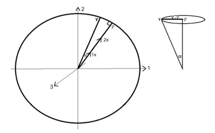
Fig. 13.1 The predicted cone of a hypothesis test
with the same length as Y would then create the same SSE. Such rays would sweep a sphere with a radius equal to the square root of \(y_1^2 + y_2^2 + y_3^2\) .
Then, the accuracy of the alternative hypothesis that the underlying expression is given by \(\beta X\) is given by the chance that the observed ray Y would fall as close to \(\beta X\) relative to any such ray of the same length as Y. This relative probability is given by the area swept out by rays of length Y within the same distance between Y and \(\beta X\) relative to all possible rays of length Y, or the surface area of a conic slice around \(\beta X\) as a share of the entire surface of a sphere of radius \(\beta X\) . This share can then be interpreted as a test of the significance of \(\beta\) .
Geometrically, this measure is proportional to the angle \(\alpha\) between the ray Y and the ray \(\beta X\) . The test of significance then compares the area of the predicted cone compared to the entire area of the sphere. The value of \(\beta\) can then be stated based on this ratio of confidence. Fisher’s t-stat performs that calculation of the relative areas.
We can also use Pythagoras’ theorem to analyze variances using this same methodology. The square of the total length of the observational vector, \(y_1^2 + y_2^2 + y_3^2\) , can be broken into two components, the regression sum of squares plus the SSE. Mathematically, the domain of the observational vector is given by its dimensions that can vary, that is, the number n individual observations. Then, the mean sum of squares per
observation is its sum of squares divided by n, the number of dimensions of the vector. This dimension n Fisher labeled as the degree of freedom.
Fisher pioneered the importance of such degrees of freedom in statistics. The observation vector then has n dimensions for n observations, and hence n degrees of freedom in the number of directions it could vary. On the other hand, the estimation vector for a simple regression is a ray in one direction only, and hence can only vary in its length. It has one degree of freedom. Finally, in the case of three dimensions, the error vector represents the difference between the two, and can vary in two dimensions along the plane defined by the observation and the regression ray. It thus has two degrees of freedom. Their respective mean squares are then their sum of squares divided by their degrees of freedom.
Fisher noted that, if the mean square of the postulated model is much larger than the mean square of the error, then it is likely a better predictor than the null hypothesis that there is no such predictor. The relative size of this ratio is then given by Fisher’s F measure:
\[F = \frac{S_R^2 / n_R}{S_E^2 / n_E} = (n_E / n_R) \cot^2(\infty),\]
where the cotangent of the angle between the observational and the regression vectors gives the ratio of the adjacent regression ray and the opposite error ray. Fisher proposed that a transformation of this F-ratio, given by what he labeled the z-test, as:
\[z = (1/2)\log F,\]
or the log of the square root of F, which is a function of the included angle \(\alpha\) . Fisher also produced one more statistic for the regression. He showed that the square root of the F-test, which again is then related to the included angle \(\alpha\) , is distributed as Student’s t.
Finally, recall the correlation coefficient proposed by Galton and refined by Pearson. Fisher also offered a geometric interpretation of the deviations between observed and predicted values of one dependent variable relative to the observed and predicted values of another independent variable. These deviations y and x, respectively, then yield the correlation coefficient:
\[r = \frac{\sum xy}{\sqrt{\sum x^2 \sum y^2}},\]
which, Fisher observed, is given by \(\cos(\alpha)\) . At each turn, the relevant statistics had been reduced to a firm geometric interpretation, just as Fisher had learned to imagine since he was a child.
While at the Rothamsted Experimental Station, Fisher published his results in his Statistical Methods for Research Workers, which he wrote over two years beginning in 1922. His brilliant interpretation of modern statistics was not particularly well received in Britain, but it was embraced in the USA, which was less allied with the influential Pearsons and the journal Biometrika. More theoretical statisticians had remained wed to the arbitrary multiple moments methodology of the statistical giant, and editor of Biometrika. Meanwhile, young practitioners at first found the theoretical foundations established by Fisher confusing and unnecessary. His foundational approach nonetheless slowly gained appreciation and academic traction. It is now universally appreciated for its rigor, interpretation and significance in the development of measures of obvious geometrical significance.
The Method of Least Squares
Fisher was also instrumental in transforming Gauss’ linear regression method into the technique we rely upon today. In Gauss’ original formulation, consider a problem in which there are three measurements at a given point in time, \(a_i\) , \(b_i\) , \(c_i\) and \(m_i\) , and three coefficients p, q and r to be discovered. We can frame the problem as:
\[m_{i} = p * a_{i} + q * b_{i} + r * c_{i}\]
where \(m_i\) is considered the “independent” variable. Then, if each of these measurements are subject to a measurement error \(v_i\) , we can express the above equation as:
\[v_{i} = p * a_{i,} + q * b_{i}, +r * c_{i} - m_{i}.\]
Then, Gauss’ least squares requires us to choose p, q and r to minimize the squared error term:
\[\min_{p,q,r} \sum_{i=1}^{n} (pa_i + qb_i + dc_i - m_i)^2.\]
Suppressing the index, this produces a set of three first-order equations:
\[aap + abq + acr = am\]
\(bap + bbq + bcr = bm\)
\(cap + cbq + ccr = cm\) .
Gauss used various methods to solve for these systems of linear equations in his solutions to such problems as the reappearance of an asteroid. Many mathematicians also developed favorite methods. However, the use of matrices was not developed until Arthur Cayley (16 August 1821–26 January 1895). Cayley had defined the method of matrices in a German journal article written in French in 1855.¹ We now recognize the system of equations and can solve the system with relative ease. In 1932, two mathematicians employed Cayley’s method to demonstrate how it might be used as a notation to simplify the traditional linear regression solution discussed earlier. Herbert Westren Turnbull (31 August 1885–4 May 1961) and Alexander Craig Aitken (1 April 1895–3 November 1967) produced a version of the now familiar expression for the solution of the parameter matrix:²
\[\hat{\beta} = (X'X)^{-1}X'y.\]
Fisher had derived close relatives to this now familiar form, but without the much more compact matrix notation. Nonetheless, it was Fisher who took this formulation of the linear regression model and derived the various validity tests we use now in his Statistical Methods handbook. These include the F-tests and t-tests, analysis of variance and the R2 value.
A modern approach to Fisher’s results is described next. The method of least squares as applied to the linear regression model has two components. First, we show that the method provides an unbiased set of estimators for a line that best fits a set of observed data. Second, we show that this method produces its unbiased estimate of the linear parameters so long as the errors are symmetric, with a mean of zero, and each observational error is independent of the next. They need not follow a more formal distribution function.
Let us consider a vector of observation points y that linearly depend on a set of independent variables X, which include the constant 1. Let there be a vector of linear coefficients b such that, in the absence of any observational errors,
\[y = Xb\] .
Let us now allow there to be observational errors so that an actual observation yi may be symmetrically distributed around an unbiased value. Then, these errors are given by:
\[y_i - X_i b\] .
and the SSE, in matrix form, is given by:
\[SSE = (y - Xb)'(y - Xb).\]
Gauss determined the expression for the linear coefficients and demonstrated that these coefficient estimates minimize the SSE. To see this, let us differentiate the SSE with respect to the estimated coefficients and set these terms to zero:
\[0 = \frac{\mathrm{d}S}{\mathrm{d}\boldsymbol{b}'}SSE = \frac{\mathrm{d}S}{\mathrm{d}\boldsymbol{b}'}(\boldsymbol{y} - \boldsymbol{X}\boldsymbol{b})'(\boldsymbol{y} - \boldsymbol{X}\boldsymbol{b})\] \[= \frac{\mathrm{d}S}{\mathrm{d}\boldsymbol{b}'}(\boldsymbol{y}'\boldsymbol{y} - \boldsymbol{b}'\boldsymbol{X}'\boldsymbol{y} - \boldsymbol{y}'\boldsymbol{X}\boldsymbol{b} + \boldsymbol{b}'\boldsymbol{X}'\boldsymbol{X}\boldsymbol{b}) = -2\boldsymbol{X}'\boldsymbol{y} + 2\boldsymbol{X}'\boldsymbol{X}\,\hat{\boldsymbol{\beta}},\]
where \(\hat{\beta}\) is the matrix of the estimates of coefficients evaluated at the minimum. Then, we can solve for these linear coefficient estimates \(\hat{\beta}\) as:
\[\hat{\beta} = (X'X)^{-1} X'y.\]
Let us now show that this estimate is unbiased. Let the vector of errors be given by \(\epsilon\) , with each error \(\epsilon_i\) assumed to have a mean of zero and a variance \(\sigma_i^2\) . Since these error terms are independent, the covariances \(\sigma_i \sigma_j = 0\) . Then, we can calculate the expected value of our estimates of the coefficients:
\[E(\hat{\beta}) = E((X'X)^{-1} X'((X\beta + \varepsilon))\]
\[= \beta + E((X'X)^{-1} X'\varepsilon)\]
\[= \beta + (X'X)^{-1} X'E(\varepsilon)\]
\[= \beta.\]
Next, we can discover the variance of the estimates for the coefficients. These are given by:
\[Var(\hat{\beta}) = E((\hat{\beta} - \beta)(\hat{\beta} - \beta)') = E((X'X)^{-1}X'\varepsilon)(X'X)^{-1}X'\varepsilon)'\]
\[= E((X'X)^{-1}X')\varepsilon\varepsilon'X(X'X)^{-1}) = E((X'X)^{-1}X')\sigma^2X(X'X)^{-1})\]
\[=\sigma^{2}E\left(\left(X'X\right)^{-1}X'X\left(X'X\right)^{-1}\right)=\sigma^{2}\left(X'X\right)^{-1}.\]
This derivation required us to specify little with regard to the pattern of errors except that the mean error is zero and individual errors are uncorrelated with each other.
Fisher developed these tools to assist colleagues in their practical analysis of the types of problems regularly faced by research stations such as Rothamsted. It is likely that his sophistication was at first lost on his audience. However, over time, understanding spread, and Fisher is remembered as the father of modern linear regressions and the associated tools of F-tests, t-tests and the R-squared coefficient of determination. It took one of his greatest allies in statistics, though, Harold Hotelling, to popularize and help simplify his analysis and construct the now familiar confidence intervals on the estimate of coefficients.
Notes
- Cayley, Arthur, “Remarques sur la notation des fonctions albebraiques,” Crelle’s Journal fur riene und angewandte Mathematik, Vol., L, 1855, pp. 2820285.
- Turnbull, H.W. and A.C. Aitken, An Introduction to the Theory of Canonical Matrices, Blackie and Sons Ltd., London, 1932.
14. The Later Life and Legacy of Ronald Fisher
Th ere are but a few scholars in any discipline who are simultaneously claimed by multiple disciplines as their own. Th e Great Mind John von Neumann is one such scholar. Th e major award in computer science is a tribute to his leadership and scholarship in the development of computers and their programming. Physicists remember him for his contributions, and the Manhattan Project relied on his expertise in chemical engineering. He was a disciple of David Hilbert and an extraordinary mathematicians, and he was perhaps the most signifi cant father of game theory that added so much to so many disciplines. Finally, he is recognized as one of the cleverest economists who also made signifi cant contributions to fi nance theory. Ronald Fisher shares with von Neumann this unique characteristic of recognition by scholars from many disciplines.
Fisher remained a giant among colleagues at Rothamsted. He was certainly the brightest to have ever joined the illustrious institution, even if many bright scholars followed in his footsteps there. None, however, likely exceeded his degree of eccentricity, nor his ability to scare and intimidate colleagues at one moment, and then smirk and joke with them the next. He had more freedom at the Rothamsted Institute than most in academics, and was only required to lend his incredible skill to problems of his choosing, as an academic bee fl itting from fl ower to fl ower. Th ese may have been the best and most productive years of his academic life.
Fisher inspired a generation of statistical scholars who joined Rothamsted to work with him. Th ese include Joseph Oscar Irwin (17 December 1898–27 July 1982), the British statistician who pioneered the method of biological assays, John Wishart FRSE (28 November 1898–14 July 1956), the Scottish mathematician and agricultural statistician, Frank Yates FRS (12 May 1902–17 June 1994), another pioneer of modern statistics, William Gemmell Cochran (15 July 1909, Rutherglen–29 March 1980), a prominent statistician who founded many statistics departments in the USA, and John Ashworth Nelder (8 October 1924–7 August 2010), the British statistician who made contributions to experimental design, analysis of variance , computational statistics and statistical theory. But while Rothamsted, and its statistical progeny, established modern statistics, it also defi ned the agenda for modern agricultural research stations worldwide.
Much of Fisher’s academic work was centered around his research in agricultural economics at Rothamsted. From that perch, he almost single- handedly developed the concept of a research institute devoted to the creation of solutions to agricultural problems that would benefi t humanity. More than perhaps any single person, he helped fuel the cooperative extension movement that provided research aid and advice from public universities to the agricultural communities, fi rst in the UK, then in the USA and around the world.
Meanwhile, Fisher was increasingly recognized as the emerging fi gure in theoretical statistics, just as his predecessor and often antagonist, Karl Pearson, was nearing retirement. When, in 1929, the opportunity to succeed Pearson at the University of London arose, Fisher could not refuse the opportunity to accept the endowed Galton Chair. However, as with every dimension of his relationship with Pearson, there were complications. Pearson had ensured that his genetic heir, his son Egon , would be aff orded the opportunity to assume some of his duties, while his scholarly heir, Fisher, assumed others. Th e balance the two successors initially forged was a fragile one, fraught with diffi culties.
Th e younger Pearson had retained administration of the world’s only department devoted to statistics, while Fisher was given authority over the Galton Laboratory, and all of Karl Pearson’s former employees. Yet, Fisher remained much more intellectually wed to statistical theory than eugenics, and found tedious the administration he was expected to provide. For the next decade, he was intellectually moving in one direction while the University administration was confi ning and directing him in another. Meanwhile, Egon Pearson had much better skills in, and an emotional advantage with, the university administration. Fisher found little but frustration, and perhaps even cultivated some of his confl icts to reinforce the tension he suff ered. As he had done throughout his life, he made his path more diffi cult than perhaps necessary.
Fisher maintained a particularly frosty relationship with Egon Pearson’s personally appointed colleague, Jerzy Neyman (16 April 1894–5 August 1981). As Karl Pearson’s handpicked successor, Egon had inherited some of his father’s combative personality, and almost all of his loyalties, and enemies. In turn, upon his acceptance to replace his father upon Karl Pearson’s retirement as the professor of statistics at the University of London in 1933, Egon promptly selected Neyman to be his colleague and fellow statistics professor. Th e irony was not lost on Fisher, who is now known as the father of modern statistics, that Fisher would be denied a statistics teaching position at the then hotbed of statistical studies in the world. Instead, Fisher was off ered his perch at the Galton Laboratory, but under the premise that he not be permitted to teach statistics. At a time and place when loyalties were demanded, Neyman had to pick sides, and the side he must pick was obvious.
Th is began a period of renewed feuding between the Pearson allies, which was most of established British statistics, and Ronald Fisher. Certainly, Egon was quite able, perhaps even more so than his father and Karl’s narrow focus on curve parameterization through moments, and Neyman was a true mathematician in the European tradition. In fact, the team of Pearson and Neyman produced some excellent work. But, unlike the criticism of Karl, Egon and Neyman actually took Fisher’s work and fi lled in some of the gaps. In doing so, they provided even a fi rmer foundation for Fisher, even as each of their developments further strengthened and verifi ed Fisher’s intuitions rather than negate them.
Th ese were battles Fisher took to his grave. Neyman delicately removed himself from the almost constant din of professional jealousies when he moved to the University of California at Berkley shortly before World War II. Nonetheless, Fisher remained embittered because of the marginalization he experienced.
Regardless, Fisher left the statistical and fi nance world with a series of innovations beyond his elaboration and geometric justifi cation of Student’s t . We now regularly employ his chi-squared and F -tests, and practicing statisticians use his defi nitions, from the meaning of probability to the concepts of effi ciency and consistency. Fisher also originated the idea of hypothesis testing, and even recommended the adoption of the 95% confi dence level that has become the de facto standard for much hypothesis testing ever since. Even the F -test, which measures the degree to which the variance from two populations are equal, originated with Fisher. Yet, it was the Iowa State University statistician and mathematician George Waddel Snedecor (20 October 1881–15 February 1974) who actually formulated the appropriate distribution to describe the extent to which the ratio of two variances approach unity. He named this ratio of chi-square the F -test in honor of the brilliant Fisher who spent time in Ames, Iowa, during one of his most productive and infl uential visits to the USA. Actually, Fisher preferred other methods to compare and analyze variances, and did not readily adopt the measure named in his honor.
Nonetheless, Snedecor was instrumental in spreading the popularity of Fisherian statistics in the USA. He wrote his own guide for researchers, his 1937 text Statistical Methods , that covered the same materials as had Fisher’s Statistical Methods for Research Workers , but without the cumbersome rhetoric, and with more examples that could guide practical statisticians. Snedecor’s book sold hundreds of thousands of copies and remained one of the most cited statistical treatises for decades following, even though it added little if any to Fisher’s intuitions. In fact, Snedecor quite wittingly became Fisher’s best ambassador in the world of statistics and among US statisticians. His accessible approach was also instrumental in the formation of many departments of statistics of the type Fisher had long advocated.
Beyond his relationship with Egon Pearson and Jerzy Neyman, and while Fisher constantly quarreled with colleagues and administration alike, he was universally appreciated by the students and assistants in his laboratory. Th ey found him intellectually generous, just as had his colleagues at the experimental station. He fed young researchers ideas and assisted them with their analyses. He was paternal, and often jocular, and not particularly overbearing, despite a brilliance obvious to everybody. He would even include them in his active social calendar conducted at his home over weekends.
Fisher also enjoyed the important role as a eugenicist. He was the editor of the Annals of Eugenics , an academic trapping associated with his Galton professorship. From that perch, he was able to keep his pulse on the development of eugenics and statistical biology. But, while Pearson used his position as editor of Biometrika to publish articles of his liking, and submit to rigorous refereeing and delay those he did not, Fisher, perhaps because he was too often subject to the arbitrariness of referees unsympathetic to his novel approach, used the editorship as an opportunity to expedite the publication of research. For that he was appreciated by his colleagues and scholars.
Th e journal also aff orded Fisher and his students an avenue to publish their own work. Quickly, the Annals became a most progressive, respected and highly regarded journal, with Fisher at the helm. In doing so, Fisher helped forge both modern statistics and modern genetics.
Later in his career, Fisher became more intensely interested in issues of biology. He was a genius in experimental design, and played an infl uential role in the resolution of many important agricultural and medical issues of his day, from a statistical biological perspective. He was commissioned by the United States Department of Agriculture to provide knowledge transfer to some large land-grant American public universities so that they may better enhance their statistical expertise and agricultural eff ectiveness. In essence, these emerging statistical departments were constructed in his mold. His reputation was also extending worldwide through the late 1930s and the 1940s, throughout North America, Europe, India and Australia.
Fisher and his Galton Laboratory also increasingly used their expertise to assist in the rapid development of blood testing and serology that is now broadly recognized within the medical community. The Rockefeller Foundation was funding research in Europe to extend the Continent’s intellectual capacity, and agreed to commission Fisher’s lab to begin work on blood groups. Fisher had discovered two new antibodies through their research, and had developed some important tests that assisted in blood typing, and had petitioned to install equipment at the Galton Laboratory to assist in these leading-edge efforts. At the same time, serology became an intense national interest as Great Britain prepared for war. The University of London administration responded by deciding to move his lab to Cambridge so that it may be safer than its London location, and as a part of an effort to reorient their programs to accommodate wartime need.
Fisher opposed the move, and, in his typical fashion, strenuously verbalized his concerns. The laboratory was moved without his approval or cooperation. Despite his concerns, the Galton Laboratory’s blood work continued, primarily at Cambridge, and the status of the laboratory was increased significantly.
During these war years, it was eventually negotiated that Fisher and his theoretical team would work out of Rothamsted. However, Fisher was largely excluded from the war effort. He harbored opinions that the slight may have been because of his association with eugenics, which Hitler was applying in a most distorted manner as a justification for ethnic cleansing. He thought perhaps that some of his associates may have had Communist leanings. Or, his reputation at the University of London as one who was difficult to administer may have induced these well-positioned administrators to steer clear of him during the difficult war years. Regardless, Fisher was left embittered by his treatment during the war, even as his son, George, was training and fighting as an aviator on behalf of England. But while some may have tried to contain Fisher’s personality, they could not contain his vast contributions.
Evolutionary biologists now revere Fisher. He formulated the Fisher’s principle that helped explain how various species divide their biological resources between their sexes.
For most species, the ratio of males to females is one to one. In his 1930 book The Genetical Theory of Natural Selection,1 Fisher produced what is probably the most recognized intellectual concept in evolutionary biology.
He created the concept of parental expenditure and investment to explain that, for most species, this ratio of males to females will converge to unity. Indeed, those that converge to another ratio are often called non - Fisherian ever since his groundbreaking theory.
His reasoning is thus. Let us imagine a species which did not have such a unitary ratio. In particular, let us assume males are less common. Th en such males would have better breeding opportunities than their female counterparts and would produce more off spring per male than per female. Parents predisposed to production of males would then have more male grandchildren, and so on, which would increase the share of males in the population until the ratio approaches unity. Should the ratio overshoot and produce too many males, the system then begins to move in the other direction and produce more females until equilibrium is reestablished with a unitary ratio.
Another way to look at the same problem is from the investment perspective. A young organism of each sex of the species is the product of an endowment of biological capital, and will require additional resource capital to nurture it into independence. Once parental investment ceases, equilibrium is reached when each sex has devoted to it the same amount of such investment because each sex is responsible for half the supply of biological resources for future generations. Natural selection then implies that the devotion of resources to each sex be equal. If it is not, for instance, if females required more resources, then, if the sexes were in equal balance, male production would be a more effi cient avenue to reproduce. From a natural selection perspective, then, more males would be produced as they would have greater reproductive value. Fisher observed that, in bee colonies, for instance, there are many more males, but much more resources are devoted to the survival of each of the rarer females. And, in humans, since boys tend to die in infancy at a greater rate than girls, there is a slight favoring of boys by birth in the population to even out parental investment.
Evolutionary game theorists call this process an unbeatable, or a dominant, strategy. Th is concept of parental investment has also been adopted among ecologists.
Time has allowed various other disciplines to also eventually understand and absorb Fisher’s highly advanced theories that were often well ahead of the current understanding. As he aged, Fisher was increasingly appreciated, but his later years were diffi cult years for Fisher. He felt ostracized and rejected by his employers; he had become increasingly estranged from his wife, Eileen, over their 25 years together; and he then lost his son in active duty in World War II. Fisher was without his laboratory, his only son and his wife. His remaining daughters were in Kenya, Canada and Scotland. He sought solace through employment at the genetics departments of Gonville and Caius College at Cambridge. In April of 1943, Fisher became the Arthur Balfour Professor of Genetics, with a promise from Cambridge that his research would be supported appropriately.
Th e move meant giving up some of the trappings of the Galton Laboratory, including its editorships. Fisher replaced this opportunity through the creation of a new journal, Heredity .
By the end of the war, it was clear that Fisher would not be able to build a serology laboratory and a fi rst-rate research facility as he had come to believe he could. He used the rather limited facilities available to him to stimulate the research he could, but he increasingly realized his greater contribution could be in levering the fl ow of accolades he received in the early 1950s. In 1953, he was elected the president of the Royal Statistical Society, and he used his high-profi le academic pulpit to enhance the important role of statistics within mathematics and the sciences.
He also traveled again to the USA and there continued to infl uence statistical departments. At that time, there were two schools of thought departments designed around important applied research problems, as Fisher had practiced for much of his career since his days at the experimental station. Th e other school of thought was advanced by the mathematician and Great Mind Leonard Jimmie Savage (20 November 1917–1 November 1971), who was regarded as a genius in the philosophy and foundations of statistics. In fact, while Fisher was critical and most vocal of the perspective that statistics develop from the mathematical side rather than from the applied research perspective, luminaries such as Savage nonetheless considered Fisher a good mathematician in his own right.
Fisher remained in this pivotal role to his retirement and beyond. By 1953, Cambridge University was aware of his mandatory retirement age, to occur in 1955. But, Fisher delayed and delayed. By 1957, he was still holding on to an at least ceremonial position, as president of Gonville and Caius College. He lodged on the campus under his own care well beyond the point when he could easily care for himself. He was encouraged to travel, and indeed spent the academic year of 1957–58 at Michigan State University, from which he visited and lectured at some of the best statistics departments in the country, many organized in his image. Th en, in 1959, he was invited to the University of Adelaide to receive an honorary PhD in science.
Fisher so loved the trip to Adelaide that he decided to stay. His children had provided him with no grandchildren, yet, and were spread themselves from England to Kenya and India. To settle in Australia, where he would be most comfortable, was not unreasonable at the time. But, once he settled, it would be diffi cult to subsequently move as his age advanced. He was off ered a ceremonial position at St. Mark’s College, and lived as a lodger with Mrs. Mayo. Th ere he emotionally adopted and mentored her family. He remained intellectually active by editing books and papers he had authored, and fi nally felt relatively immune to the pettiness and quarreling within the discipline and departments in England. He also traveled to see his family, whom were fi nally providing him with grandchildren. Th ese may have been the most fulfi lling and happiest days of his life.
By July of 1962, Fisher began suff ering stomach problems. An X-ray confi rmed that he was suff ering from a constricted colon. Surgery is always diffi cult because of the risk of infection. Complications arose, and Fisher passed away on 29 July 1962 in the company of his doting nurses. After a half century of contributions to the creation of modern statistics, there was an outpouring of fondness and appreciation upon his passing.
In death, Fisher is remembered for his great contributions to the foundation and intuition of statistics. No individual before or since, but perhaps Gauss himself with regard to maximum likelihood estimates, least squares , and the fi rst and second moment ( mean and variance ) approach, has provided a fi rmer foundation to statistics as had Fisher. For his work, he was knighted by Queen Elizabeth II in 1952, elected to the Royal Society in 1929, and won the Linnean Society of London Darwin-Wallace Medal in 1958. In 1963, the annual R.A. Fisher Lectureship Prize was inaugurated in the USA. Th ere is a minor planet, 21451 Fisher, named after him. And, his paper Gene Frequencies in a Cline Determined by Selection and Diff usion was the fi rst to use a computer to calculate a solution in a biology paper. 2
Fisher was well regarded late in life. He earned the Royal Medal from the Royal Society in 1938, its Darwin Medal in 1948 and the Copley Medal in 1955. Th e award was:
in recognition of his numerous and distinguished contributions to developing the theory and application of statistics for making quantitative a vast fi eld of biology.
He was a member of more than 20 academic societies and institutes. In 1934, he was elected to the American Academy of Arts and Sciences, in 1941, to the American Philosophical Society and, in 1948, to International Society of Haematology. Also in 1948, he was elected to the USA’s National Academy of Sciences, and, in 1960, to the Deutsche Akademie der Naturforscher Leopoldina. He also earned honorary degrees to Harvard University in 1936, the University of Calcutta in 1938, the University of London in 1946, the University of Glasgow in 1947, the University of Adelaide in 1959, the University of Leeds in 1961 and the Indian Statistical Institute in 1962. While perhaps few students of fi nance know his name today, his legacy underpins almost all of the statistics we now employ.
Perhaps Fisher’s greatest legacy may go well beyond the foundations of modern statistics he so ably founded. He advocated for new departments of statistics around the world. One great mind took his guidance to heed perhaps more than any other. Next is the story of Harold Hotelling .
Notes
- Fisher, R.A., Th e Genetical Th eory of Natural Selection , Clarendon Press, Oxford, 1930.
- Fisher, R.A., “Gene Frequencies in a Cline Determined by Selection and Diff usion,” Biometrics , Vol. 6, No. 4 (Dec., 1950), pp. 353–361.
15. The Early Life of Harold Hotelling
While the names Gauss , Galton and Fisher may not be well known to fi nance students of statistics, the name Hotelling often elicits at least some acknowledgment. Th is is perhaps because he helped establish statistics, economics and econometrics from a distinctly American perspective. Fisher was experiencing resistance in England over his theories that defi ed the powers that be in Britain’s statistical community. America was more receptive. Its embracement of Fisherian statistics caused the center of mass of the statistics world to migrate across the ocean. Th e primary proponent was an American mathematician and economist whose ancestors made the same migration as founders of America’s fi rst colonies.
Th e mother of Harold Hotelling , Lucy Amelia Rawson, was an off spring of one of the fi rst Secretaries of the Massachusetts Bay Colony. Edward Rawson (16 April 1615–27 August 1693) was born in the village of Gillingham, Dorsetshire, England. His namesake, grandfather Edward Rawson, was a wealthy silk and woolen merchant of Colnbrook, west of London. When the grandfather died in 1603, he left two young sons, Henry and David, to run the family business. David became a tailor in London, and married Margaret Wilson, the daughter of Reverend William Wilson of Windsor. David died when their three children were still very young. Th eir young son Edward was only two years old at the time. His mother also died 11 years later, which left Edward in the care of his extended family.
Th e Rawsons and the Wilsons lived comfortably, and young Edward was hence well educated. When he married Rachel Perne, the Wilson and Perne families were already establishing religious links to the Colonies. Edward’s wife, Rachel, was the daughter of Th omas Perne, and the niece of one of the fi rst settlers in Cambridge, Massachusetts, the Reverend Th omas Hooker. Edward’s maternal grandfather, the Reverend William Wilson of Merton College, Oxford, had rose to Canon of St. George’s Chapel in Windsor. Edward’s uncle, Edmond Wilson, was a wealthy physician in London who had donated 1000 pounds toward establishment of a Massachusetts Bay Colony in 1633. Another uncle, Reverend John Wilson, immigrated to the Colony and ministered over the First Church of Boston.
Th e young couple Edward and Rachel married in 1636, had a daughter who they left with family in England and migrated to the Massachusetts Bay. By 1637 they were settled in Newbury. At the remarkably young age of 23, Edward was selected to be the Public Notary and Register for Newbury, and was continually reelected to that position until 1647. His willingness to accept increasing responsibilities led to his appointment as the Secretary of the Massachusetts Bay Colony, a position which he held for another 36 years (Fig. 15.1 ).
Together, Edward and Rachel Rawson had 12 children, of which only 9 survived past childhood. One of their children, Rebecca Lawson (23 May 1696–?) was the heroine of the popular 1849 book by John G. Whittier entitled Leaves from Margaret Smith’s Journal in the Province of Massachusetts Bay. While three of their sons eventually returned to England, including Edward following his graduation from Harvard College in 1653, two sons, William and the Reverend Grindal (23 January 1659–), remained in the New World.
Born in Boston, William Rawson (21 May 1651–20 September 1726) moved south, fi rst toward Dorchester, and then to Braintree with his wife Ann Glover (1653–29 July 1730). Together they had a son, William Rawson (8 December 1682–October 1769), who married Sarah Crosby (27 July 1684–1734) on 26 October 1710, and settled in Mendon,
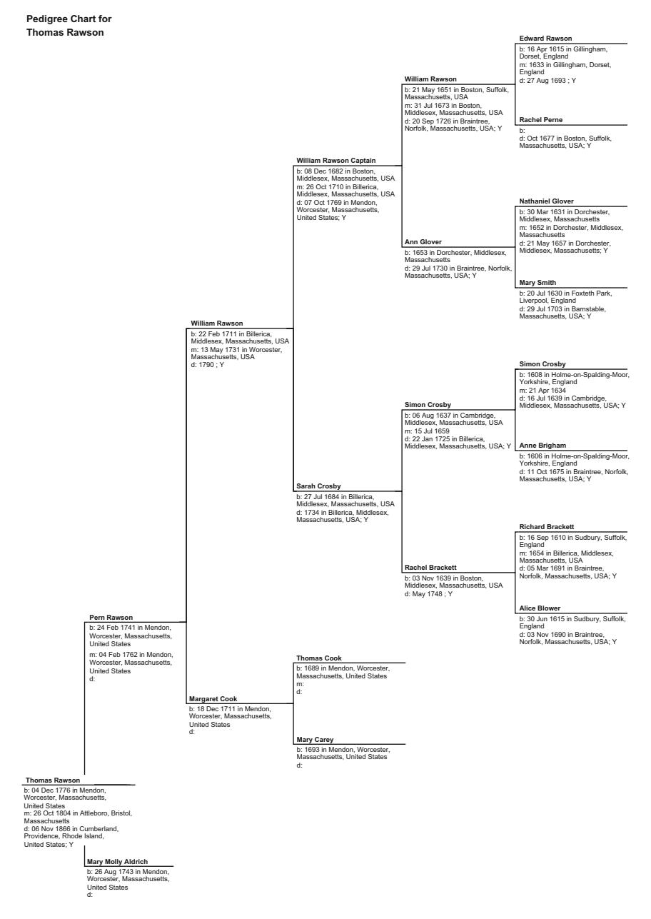
Fig. 15.1 The ancestry of the Rawson family
Worcester County, west of Boston. William, also a graduate of Harvard College, Braintree, captained the local militia, fought in the French and Indian Wars and became the town’s fi rst grammar school teacher. Together, William and his wife Sarah had eight children, two of whom died young, and to whom their fi rstborn William (22 February 1711–90) they passed along the family’s namesake.
Th e fi rstborn, William, also lived in Mendon until his death. Th ere, he married Margaret Cook (18 December 1711–), and raised a son, Pern Rawson (24 February 1741,) named after his uncle. Pern, too, remained in Mendon, where he married Marry Molly Aldrich on 4 February 1762, and had a son, Th omas (4 December 1776–) in the year the USA declared its independence.
Th omas migrated south, toward Rhode Island, as he became an adult. He married Anna Follett (23 December 1782–5 December 1848) in Attleboro, Massachusetts, on 26 October 1804, and they raised a son, Pern “Perry” (22 January 1813–4 February 1907).
Perry began the family’s migration westward to Wisconsin, where their younger son, James Otis Rawson (2 August 1844–25 December 1911), was born. Th e grandfather of Addison “Harold” Hotelling , he married his wife, Lucy Ann Baker (3 November 1850–10 May 1877), in Wisconsin. Shortly after their marriage, James and Lucy had moved to Iowa, where Lucy gave birth to an only daughter Lucy Amelia Rawson (1 May 1875–23 March 1959). Th ey also had three sons together before mother Lucy died prematurely young.
It was this intersection in Iowa that the Hotelling and Rawson families merged. Clair Albert Hotelling (22 June 1869–5 June 1944) was born in Algona, Iowa, to Addison Hiram Hotelling and Ellen Tuttle. He was the only boy in a family with three sisters.
His Hotelling family had perhaps somewhat less illustrious beginnings. He could trace his American heritage back to the arrival of the indigent son of Conrad Martense Houghtaling (1620–2 August 1641) and Maria Pipearts (1625–?). Th is very young couple married on 2 August 1641 in Amsterdam, Netherlands, when Conrad was 21 years old and Maria was 16. Th eir second son, Mathys Coenradt Houghtaling, was born in 1644 but found himself as a young boy in an almshouse, a charitable home for the poor typically sponsored by a church or wealthy benefactor (Fig. 15.2 ).

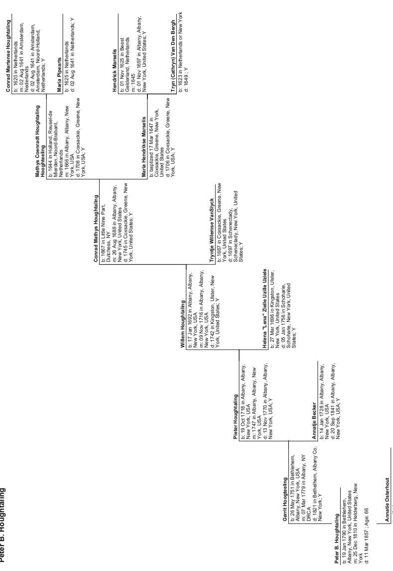
Fig. 15.2 The distant ancestry of Harold Hotelling
d: 1793 ; Y
During this era of the early 1600s, the Dutch West India Company was based on Amsterdam at the heart of one of the world’s wealthiest nations, fueled by rapidly expanding world trade. Th e Dutch political model was unlike some of their competing empires. Th ey did not oppress religion, and they relied on private enterprise as the vehicle for their colonial ambitions.
Th e Dutch East India Company had sponsored the English explorer Henry Hudson (c.1565–1611) to explore an easterly passage to Asia. He was instructed to fi nd a passage along the coast of Russia, which is now called the Northern Passage. When his ship Halve Maen ran into ice, he discarded his orders and instead turned his ship west to seek a route through North America.
By 2 July 1609, Hudson had reached the Grand Banks, south of Newfoundland, and had passed Nova Scotia a couple of weeks later. Over the next month, the ship had navigated past Cape Cod, Massachusetts, and traveled further south to the Chesapeake Bay. From there, Hudson turned back north, past the Delaware River, and, on 11 September, began to sail up the Hudson River adjacent to New York City. Before the end of September, he had reached Albany, the present-day capital of New York State.
Hudson then returned to Europe. He fi rst arrived in Dartmouth, England, where he was arrested as authorities sought his logbook. Instead, he passed the log to the Dutch ambassador so that the Dutch could lay claim to his discoveries in the New World. Th e region from New York City to Albany was subsequently settled by the Dutch as a commercial avenue for the newly formed Dutch West India Company. Th e company’s goal was to establish farmland along the Hudson delta region to feed their soldiers and workers. Nieuw Amsterdam was established after its purchase from the indigent population for 60 guilders.
Th e Company sought settlers, who would be off ered land, and patrons who would earn trading privileges. A mix of the wealthy settlers and cheap labor were sent to settle the region between New York and Albany. Among them was Mathys Coenratsen Houghtaling (1644–1706), who, in 1655, was an 11-year-old orphan living in an almshouse in Amsterdam. He was sent to the New World in that year, eventually briefl y settled fi rst in Coxsackie and then in the farming community of nearby Kinderhook, where he shared a farm with his father-in-law, Hendrik Marseli. By the late 1600s, he was established on his own farm, with his wife Maria Hendrikse (17 March 1647–1706).
Th eir fi rstborn in marriage, Conrad Mathys Houghtaling (1667–1745), married Tryntje Willemse Van Slyck (1667–97) in 1685 in Albany, and they had two sons before Tryntje died at the age of 30. Th eir second son, Willem Houghtaling (17 January 1692–1742), remained for much of his life in Albany, where he married Helena Uzille (27 March 1696–5 January 1756) on 9 November 1716. Th ey had fi ve children together in Albany, including a second son Pieter (19 October 1718–13 November 1770), who also lived in Albany all his life and married a local woman Annatje Becker in 1747.
Th e second child, and fi rst son of Pieter and Annatje, Gerrit Houghtaling (26 May 1751–1821), also lived in Albany for most of his life, and married Annatie Osterhout (1740–93), with whom they shared a son, Peter (19 January 1790–11 March 1857). Peter, too, remained in the Albany County area, married Catherine LaGrange and had nine children with her, including a fi rst son William Helmus Houghtaling (16 February 1813–7 May 1887), their second child.
In the 1860s, the Hotellings, too, made their westward migration. Th e son William Houghtaling moved to Iowa, with Mary Ann Yost (10 March 1816–30 June 1895), whom William had married on 12 March 1835, and with seven children in tow. Th eir third child, and fi rst son, Addison Hiram Hotelling (22 March 1843–17 May 1896) had by then adopted an Americanized version of the family name, and lived much of his life in Iowa. It was there that he met Nellie Tuttle (7 August 1844–7 March 1929), and had fi ve children together, including their second child, and fi rst son, Clair Alberto Hotelling (22 June 1869–5 June 1944).
The Arrival of Harold Hotelling
Clair Hotelling and Lucy Rawson married on 26 June 1894 in Bancroft, Iowa. From there, they began a slow westward migration, fi rst to Fulda, Minnesota, where their fi rst son, Addison “Harold” Hotelling (29 September 1895–26 December 1973), was born, and then on to Seattle, Washington, by the fi rst decade of the twentieth century (Fig. 15.3 ).
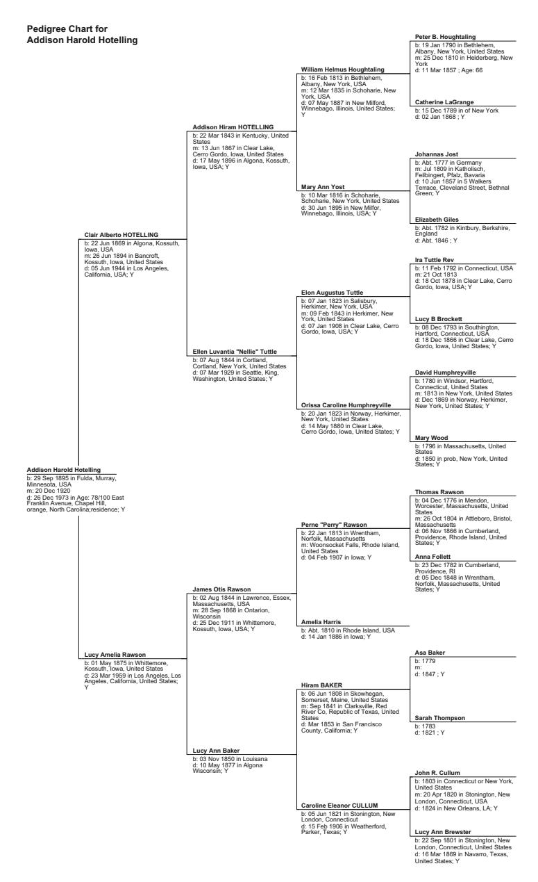
Fig. 15.3 The immediate ancestry of Harold Hotelling
Th e convergence of the Hotelling and the Rawson families came about through an unlikely path, but with farming in common. With a daughter Marjorie (19 September 1904–) just born, the family set out in 1905 for Washington State and arrived by train in Seattle, with by then fi ve children in tow, Clair had been a hay merchant, which was an essential fuel for the transportation segment of the supply chain as hay fed the horses that moved the goods at the turn of the century before the widespread use of automobiles and trucks. Ford began selling cars that were almost immediately popular and aff ordable in 1903, and Clair began to realize that the invention of the automobile may soon doom his comfortable hay-selling business, and decided to seek opportunity in the West.
Th e family were strict observers of the Methodist tradition, and the children were raised within the Church community in Seattle. Unfortunately for his father, though, the family lost their business and savings with the Recession of 1907, and Harold found himself preparing for college and supporting himself through school at the University of Washington by working odd jobs.
One such job at a local newspaper, the Puyallup Herald , caused him to shift his interest from electricity and science to journalism. But with the draft of the Great War, he had to suspend his college education briefl y. Despite his college studies, he was ordered to army camp, where he was promptly kicked by a mule, which resulted in his discharge from the army. When he returned to college, he found the journalism department was in disarray, which made it diffi cult to resume his studies. He was able to substitute courses in economics and thus completed an economic-rich course of study. He then went on to study mathematics in Seattle and at Princeton and Chicago.
Hotelling was most interested in mathematics. One of his most substantial infl uences when he resumed graduate studies in 1920, following his BA graduation in 1919, was his mathematics professor Eric Temple Bell (7 February 1883–21 December 1960). Trained at Stanford, the University of Washington and Columbia University, Bell become recognized in mathematical theory, in particular the Bell series in number theory , but also in his biographies of great mathematicians. Bell was teaching at Washington when Harold was a student, and, throughout his career, inspired dozens of mathematicians and economists not only through his insights but also in his anecdotes and perspectives about the mathematicians who preceded him, through a series of essays collected in his work Men of Mathematics: Th e Lives and Achievements of the Great Mathematicians from Zeno to Poincare . 1 Bell inspired Hotelling’s interest in mathematics in the year 1920.
Someone else also inspired Hotelling that year. On 20 December 1920, Hotelling married Floy Tracy (31 December 1890–2 October 1932). Less than three years later, they had a son together, Eric Bell Hotelling (12 May 1923–2 January 1991), named after his inspiring professor Eric Bell. Th e couple had a daughter together as well, Murial (11 October 1925–). Unfortunately, neither of these children would enjoy their mother’s care and love beyond grammar school. Floy died short of her 32nd birthday.
Hotelling received his master’s degree in mathematics in 1921 and had hoped to attend Columbia with a fellowship to study for a PhD in economics, given his economics studies and his advanced mathematical training. When his application to Columbia was rejected, he instead accepted a fellowship to study additional mathematics at Princeton. Th ere, he studied under Oswald Veblen (24 June 1880–10 August 1960), the nephew of the famed economist Th orstein Veblen (30 July 1857–3 Aug. 1929), and completed a doctorate in mathematics on topology and diff erential geometry in 1924.
With a doctorate at hand, Hotelling found employment as a research associate at the Food Research Institute of Stanford University. It was there that he wrote his fi rst two important papers, one on the mathematical economics theory of depreciation, and another on correlation ratios arising from random data in statistics. His research interests in statistics was piqued, and he became aware of Fisher’s work on the provision of rigorous foundations to statistical concepts, his publication Statistical Methods for Research Workers . He quickly became an American admirer of Ronald Aylmer Fisher, even as Fisher struggled to gain respect in his home country of England. Hotelling had found a kindred spirit in Fisher, who also pictured statistical concepts from a geometric perspective.
Note
- Bell , Eric Temple, Men of Mathematics , Simon and Shuster, New York, 1937.
16. The Times of Harold Hotelling
While at Stanford, Hotelling began teaching in both the areas of mathematics and the burgeoning new theory of statistics. One can see from the names of the courses he taught that he was developing his statistical insights through his pedagogy. His fi rst off ering was in the theory of probability and in statistical inference, and by 1926–27, he was also teaching diff erential geometry and topology. His expertise in this emerging discipline of statistics led to his appointment as an Associate Professor of Mathematics at Stanford by 1927. Clearly, he had made a great impression at a relatively young age of 31 and at one of the best schools in the West.
In that same year, he gave a badly needed and much appreciated nod to Fisher. He had off ered a very favorable review of Fisher’s Statistical Methods for Research Workers , where he included the line, “Th e author’s work is of revolutionary importance and should be far better known in this country.” 1
His admiration of Fisher even inspired him to spend the summer and fall semesters of 1929 with Fisher at his Rothamsted Agricultural Experiment Research Station. From that experience, Hotelling became as enamored with statistics and Fisher as he had become with mathematics and Bell . Th rough Fisher, he had become indoctrinated in the new rigorous study of statistics and conversed with a number of young scholars who would go on to enjoy careers almost as illustrious as Hotelling’s. He was in a hotbed of ideas, and he would, as much as any, contribute more than his share to this new and collective eff ort.
Upon his return to the USA, Hotelling studied and elaborated upon the work on Gosset ’s Student’s t -ratio, as explained and expanded by Fisher, and, from these works, constructed the methodology of confi dence intervals that has remained the heart of statistical testing ever since. His work, Th e Generalization of Student’s Ratio , 2 published in 1931 also marked his movement to Columbia University in New York City, and to a Department of Economics. Barely through that fi rst year, he devoted much energy into developing the discipline of statistics on the American side of the Atlantic Ocean, and began to thoroughly incorporate statistical tools into economics and fi nance.
Hotelling had an advantage in his generalization of Gosset ’s work. Fisher’s youthful elaboration, and gentle correction of the Student analysis of 1908, immediately raised the ire of his nemesis, Karl Pearson, and was the fi rst shot in a war that was subsequently fought on many diff erent battlefronts.
Th e problem was that Fisher was entirely correct, and he knew it. Gosset had worked with Pearson around the time he produced his paper, and, as a practical statistician who experienced the academic largesse of the great Pearson, his allegiances remained. He did not well understand Fisher’s correction of his own work, but he deferred to Pearson in Pearson’s criticism of Fisher. And, while Fisher tried to remain above the fray and correspond privately and publicly with Gosset and Pearson over the Student t statistic, the debate occasionally turned nasty. Pearson could be an academic bully, and had the grandest of bully pulpits, as the editor of Biometrika . But, Fisher, with righteousness on his side, was not willing to be the academic wallfl ower.
Unfortunately, Gosset found himself in the middle of a notorious Pearson-Fisher feud. Gosset respected Fisher’s professor Stratton , and believed that Fisher may have indeed added much to his analysis. On the other hand, he admired and was thankful to Pearson. When Pearson commented on the second edition of Fisher’s book in a 1929 review, he claimed Fisher’s approach was misleading. When Gossett inquired of Fisher whether Pearson’s criticism had merit, Fisher responded somewhat frustratingly at fi rst. He and Gosset then took a step back and had a discourse that motivated Fisher to further shore up his mathematics, as the best defense against Pearson. Fisher discarded his rebuttal of Pearson’s academic jabs and instead worked to clarify his foundational approach.
In two notes in Nature , Gosset and Fisher eventually took the high road. Gosset wrote:
We should, all of us, however, be grateful to Dr. Fisher if he would show us elsewhere on theoretical grounds what sort of modifi cation of his tables we require to make when the samples with which we are working are drawn from (various) populations.
Fisher responded that he appreciated Gosset ’s challenge “that was free from Billingsgate (meaning devoid of abusive language) … (so that) others (can) better understand where we stand.” 3 Th is intellectual challenge helped motivate Fisher to produce the well-founded measures that now constitute modern statistics. Th e dialog also motivated Hotelling to replicate Fisher’s leadership in the infant science of statistics but on the other side of the Atlantic Ocean.
Just as Fisher would hold court at Rothamsted, Hotelling was equally generous with his intellect and with their home in Mountain Lakes, New Jersey. From there, he hosted many gatherings of intellects from the region, and, increasingly, from Europe in an era in which European intellectuals were seeking refuge from the growing nationalistic movement in Germany, ostensibly motivated by eugenics and by Hitler ’s Great Purge in 1933. Hotelling and others at Columbia and at the New School in New York were creating new disciplines and a new informal school of intellectual refugees. Susanna and Harold, and the three sons and two daughters they shared, found themselves sharing their home and their intellectual values with Abraham Wald (31 October 1902–13 December 1950), the founder of a formal structure to integrate into the American academic community many of the intellectual refugees from Europe.
Th en, with the onset of World War II, Hotelling ’s Methodist values were further stimulated. He advocated for a war eff ort to defeat Hitler through the creation of a Statistical Research Group at Columbia that could apply scientifi c principles to such problems as the maximization of the range of aircraft and of problems associated with the weather. He also fi nally convinced Columbia University to establish one of the country’s fi rst departments dedicated to statistics. He wrote his argument in the form of a paper entitled Th e Teaching of Statistics in which he concluded:
“Should statistics be taught in the department of agriculture, anthropology, astronomy, biology, business, economics, education, engineering, medicine, physics, political science, psychology, or sociology, or in all these departments? Should its teaching be entrusted to the department of mathematics, or to a separate department of statistics, and in either of these cases should other departments be prohibited from off ering duplicating courses in statistics, as they are often inclined to do? … [Th e question] to have received too little of the attention of college and university administrative offi cers is …” What sort of persons should be appointed to teach statistics? “… Qualifi cations of a good teacher of statistics include, fi rst and foremost, a thorough knowledge of the subject. Th is statement seems trivial, but it has been ignored in such a way as to bring about the present unfortunate situation. Mathematicians and others, who deplore the tendency of Schools of Education to turn loose on the world teachers who have not specialised in the subjects they are to teach, would do well to consider their own tendency to entrust the teaching of statistics to persons who not only have not specialised in the subject, but have no sound knowledge of it whatever.” 4
To then, most disciplines relegated statistics to a supporting role rather than a unifi ed discipline that could develop on its own. Because much of the earliest work was hidden within astronomy, or was applied to agricultural studies, there was a reluctance for other disciplines as varied as economics, medicine and political science to embrace its tools. It is interesting that his complaints then are still often echoed today.
Ultimately, Hotelling failed to convince Columbia to create a separate statistics department. However, the University of North Carolina was willing to build an entire new program around him. He accepted the challenge and left the academic year after the end of World War II to start a program in Chapel Hill. Th ere, he chaired his own new department and was also off ered the associate directorship of an Institute of Statistics. From his position, he devoted energy once applied to his prolifi c research to the administration of one of the top programs in statistics worldwide. He remained at the University of North Carolina for the rest of his career as the Kenan Professor of Statistics, from 1961 on, until the bestowment of Professor Emeritus upon his retirement in 1966.
Notes
- Hotelling , H., “Review: Statistical Methods for Research Workers by R A Fisher,” J. Amer. Statist. Assoc. 22 (1927), 411–412, at 412.
- Hotelling , Harold. “Th e generalization of student’s ratio.” Annals of Mathematical Statistics (Institute of Mathematical Statistics) 2 (3), 1931, pp. 360–378.
- Fisher, R. A., in Nature, 17 August 1924.
- http://www-groups.dcs.st-and.ac.uk/~history/Biographies/Hotelling . html, accessed 25 February 2016.
17. Harold Hotelling’s Great Idea
Beyond his efforts to establish statistics as a rigorous study and as a tool for modern finance, perhaps Hotelling’s most lasting legacy was in further developing a notion first formulated by Carl Gauss, the method of maximum likelihood.
By the time Hotelling advanced the concept of maximum likelihood estimation (MLE), he was already well known as a mathematical statistician. In 1925, he had written his first academic papers. One was on the derivation of the F-statistic, while another was essential for the development of modern finance. He defined the notion of depreciation as a measure of the decrease in the discounted value of future returns. This would be key for the development of fundamental analysis by John Burr Williams (27 November 1900–15 September 1989), the father of the discounted dividend model in 1938.
Gauss was of course the first to construct the minimized least squares approach based on the premise that his approach then implies an error distribution that is most likely to generate the desired minimized least squares. His approach was further explored by Fisher, in collaboration with Hotelling.
The approach pioneered by Gauss determines the optimal parameter for a given statistic such as a mean or variance. Typically, this estimate for the mean statistic is denoted by a hat, that is, \(\hat{\mu}\) , while the estimate for the standard deviation is given as \(\hat{\sigma}\) . Let us first apply this technique to the normal distribution. The probability \(f(\cdot)\) of generating observed data points \((x_1, \ldots, x_n)\) given the true statistics \(\mu\) and \(\sigma\) is then by:
\[f(x_1,...x_n:\mu,\sigma) = \prod_{i=1}^n \frac{1}{\sigma\sqrt{2\pi}} e^{-(x_i-\mu)^2/2\sigma^2}.\]
Notice that we can perform this maximum likelihood on either the function or on the logarithm of the function since, from the chain rule, maximization of a function corresponds to the maximization of a monotonic transformation of the function such as the logarithm. Gauss took the natural logarithm of the right-hand side to find:
\[\ln(f) = -\frac{1}{2}n\ln(2\pi) - n\ln(\sigma) - \frac{\sum(x_i - \mu)^2}{2\sigma^2}.\]
Then, the estimate of \(\mu\) is determined by differentiating \(\ln(f)\) with respect to \(\mu\) and setting the derivative to 0:
\[\frac{\partial \ln(f)}{\partial \mu} = \frac{\sum (x_i - \mu)}{\sigma^2} = 0\]
Or \[\hat{\mu} = \frac{\sum x_i}{n}\] .
Gauss demonstrated that the maximum likelihood estimate for the mean is the mean itself. In other words, the estimate is unbiased. In addition, by differentiating with respect to the standard deviation, he showed that:
\[\frac{\partial \ln(f)}{\partial \sigma} = -\frac{n}{\sigma} + \frac{\sum (x_i - \mu)^2}{\sigma^3} = 0\]
Or \[\hat{\sigma} = \sqrt{\frac{\sum (x_i - \hat{\mu})^2}{n}}\] .
Again, the estimate of variance is an unbiased estimate of the true statistic.
Fisher had asserted a number of asymptotic properties of the method of maximum likelihood as the sample size grows large, to infinity. As the sample size increases, we find the estimates are:
- Consistent: The sequence of estimates converges toward the true statistic as n rises.
- Asymptotically normal: The distribution of the estimates converges to the Gaussian distribution.
- Efficient: These estimates converge to the theoretical (Cramer-Rao) lower bound as sample size increases. This implies that no other consistent estimator yields lower error than the MLE estimate.
- Sufficient: A statistic is sufficient if the sample cannot give rise to another statistic that yields more information.
Hotelling had become acquainted with Fisher’s work as he completed his PhD on topology under Oswald Veblen and began work at Stanford on the application of statistics. Fisher’s Statistical Methods for Research Workers was the most eloquent and expansive blueprint for such fieldwork at the time, and had been published only a couple of years earlier. Given Hotelling’s PhD in mathematics, and especially in the geometrically intuitive topology, there were few reviewers and adopters of Fisher’s groundbreaking work who could appreciate Fisher’s contributions better than could Hotelling’s.
While Hotelling’s review of Fisher’s work might have appeared overly exuberant and effusive compared to his rather staid British counterparts
at the time, and perhaps because Hotelling had not been drawn into the statistical feuds raging in London and Cambridge at the time that divided people (mostly) into Pearson’s camp, and (occasionally) into Fisher’s camp, or more often neutrality, Hotelling’s review in 1927 of Fisher’s handbook was perhaps one of the most probing and unbiased considerations of Fisher’s contribution. Upon the publication of Fisher’s second edition, Hotelling followed his rave review up with another that exposed Fisher and his foundations to an even broader audience. Then, with his visit to Rothamsted, Hotelling was able to appreciate even more the brilliance of Fisher.
By the time Hotelling visited with Fisher, Fisher had already articulated a theory of maximum likelihood based on his principles of consistency, efficiency and asymptotic normality. Fisher was reviving a methodology that had actually been initiated by Pearson. As you recall, Pearson was fond of describing relationships based on moments. In doing so, he postulated a likelihood ratio, defined as the ratio of the distribution, or frequencies, of observed data over the postulated frequencies from some sort of postulated estimation. By changing the parameters of his estimates slightly, he could recalculate this ratio. He employed a Taylor’s series expansion to explore this ratio as constants are perturbed to discover the constants that yield the best fit.
Pearson’s likelihood ratio approach was actually very close to the maximum likelihood technique more fully described later by Fisher, but Pearson did not take his results far enough to realize the generality of his approach. Early in his career, Fisher corresponded with Pearson to advocate an approach based on the minimization of various aggregate error measurements, but Pearson panned the idea and noted he had gone down such a fruitless path years earlier. Fisher took this as a challenge to place the method of maximum likelihood on a firm theoretical foundation. His work, if successful, in combination with this geometrical foundation he applied to other concepts, would place statistics upon a most firm foundation.
Fisher’s efforts received scant support in England, but he found a kindred spirit in Hotelling. Even before Hotelling’s visit in 1929, the two began to correspond. Their letters continued, as did Hotelling’s writings. In 1930, in Transactions of the American Mathematical Society, Hotelling presented The Consistency and Ultimate Distribution of Optimum Statistics; Hotelling presented to a more receptive world, and with greater success, concepts that Fisher had been struggling to produce.
In the paper, Hotelling lent some support to Fisher’s notion of asymptotic normality, and firmed up the basis for the approach of maximum likelihood. Neither he nor Fisher had completely shored up their theory and advocacy, but they nonetheless showed that the maximum likelihood technique produces efficient estimates in many reasonable cases.
These two individuals seemed to spur and motivate each other. This fruitful Atlantic-spanning relationship, almost none of which is conducted face-toface, but rather through elaborate letters, resulted in proofs of the utility of the maximum likelihood approach under various circumstances, and spawned a literature, much of which was based in the USA. By then, Hotelling had firmly established statistics as a stand-alone discipline within mathematics, had created or inspired numerous departments devoted to statistics, and had encouraged students and colleagues alike to take up these research questions. Various scholars took up the challenge, and most notably Abraham Wald, a colleague and one of the Refugees in Exile that Hotelling had sponsored at Columbia, and an influential member of the Cowles Commission.
By 1943, Wald had managed to prove the asymptotic sufficiency of maximum likelihood estimates that had somewhat eluded Fisher as early as 1922. Meanwhile, on the other side of the Atlantic Ocean, Fisher still suffered for decades the at times malicious marginalization at the hands of Pearson associates. Over time, though, and especially in the USA, the discussion turned not from the general failure of the method of maximum likelihood, but rather on a better understanding of the conditions that might cause the method to fail to perform well. Much of this recasting of Fisher’s theory came from Hotelling and his colleague, Wald, and dates back to Wald’s arrival at the Cowles Foundation in 1938, first in Colorado Springs, then with Hotelling at Columbia and finally back with Cowles once it moved to Chicago.
Today, the method of maximum likelihood remains one of the most enduring and valuable paradigms in modern statistics. It is a fascinating example of the role of personalities in the development of theories, or, in some cases, in the retarding of innovations. And, it also demonstrates how collegial relationships can spur innovation. The ability for ideas to coalesce within an institution is the subject of the next section. By the late 1920s, the finance, economic and statistical world was ready for a new approach that would dramatically accelerate statistical thinking. The Cowles Commission for Research in Economics provided that institution.
18. The Later Life and Legacy of Harold Hotelling
Th ere are a few scholars who are claimed by multiple disciplines. Fisher and von Neumann were two striking examples. Th e same rare ability to span multiple disciplines was demonstrated by Harold Hotelling . He began as a theoretical mathematician who soon found application in economics and in statistics. His location theory and his theory of exhaustible resources are still taught in economics. And, he represented the establishment of statistics as a discipline that now stands on its own, but spawned from the unique combination of theoretical mathematics and practical research methodological studies.
Over his career, Hotelling left an incredible legacy, both in statistics and in the development of economics and fi nance. We know him for his ubiquitous confi dence intervals. Within the discipline of economics, he wrote the incredibly imaginative paper Stability in Competition1 in 1929 that initiated the theory of location analysis. His seminal 1931 work Th e Economics of Exhaustible Resources2 was the fi rst rigorous work in both resource economics and, with the work of the Great Mind Frank Plumpton Ramsey (22 February 1903–19 January 1930), the introduction of decision-making over time, that is the defi ning innovation of fi nance. Like Ramsey, he also analyzed taxation in Edgeworth’s Taxation Paradox and the Nature of Demand and Supply Functions3 in 1932, Demand Functions with Limited Budgets4 in 1935 and Th e General Welfare in Relation to Problems of Taxation and of Railway and Utility Rates in 1938.
His 1938 paper was presented to the Econometric Society as his address in his election as its president. A year earlier, he had been elected a fellow of the American Statistical Association, and rose to its vice presidency by 1941. He also presided over the Institute of Mathematical Statistics, and, in 1972, was conferred with the North Carolina Award for his contributions to many aspects of science.
Hotelling was also infl uential in education. At the Berkeley Symposium in Mathematical Statistics and Probability in 1946, he presented his lecture Th e Place of Statistics in the University in which he noted:
Th e possibilities of teaching quite advanced mathematics to young children have scarcely begun to be explored. Children of kindergarten age are fascinated and thrilled by the wonders of topology, and groups and number theory can be tremendous sensations in the fi fth grade, though all these subjects are ordinarily reserved for graduate students specialising in mathematics. What is lacking is teachers who know mathematics and its applications and who possess enough freedom to teach what they know instead of the long, dull, and relatively useless drill on problems of wall-paperhanging and the like, problems turning on mere conventions which are quickly forgotten – painful, repetitious work which makes children resolve to quit mathematics as soon as possible. 5
It was in teaching his courses in statistics that Harold Hotelling met his second wife, Susanna Porter Edmonson (15 August 1909–14 May 1989), following the untimely death of Floy. Th ey raised three sons and two daughters together.
While he retired from the University of North Carolina at Chapel Hill in 1966, Hotelling remained in North Carolina, where he died after years of poor health, on 26 December 1973.
Notes
- Hotelling , Harold, “Stability in Competition” (PDF), Economic Journal 39 (153), 1929, pp. 41–57.
- Hotelling , Harold, “Th e economics of exhaustible resources.” Journal of Political Economy (Th e University of Chicago Press via JSTOR) 39 (2), April, 1931, pp. 137–175.
- Hotelling , Harold, “Edgeworth ’s taxation paradox and the nature of demand and supply functions.” Journal of Political Economy , 40 (5), October, 1932, pp. 577–616.
- Hotelling , Harold, “Demand functions with limited budgets.” Econometrica , 3 (1), January 1935, pp. 66–78.
- Madow, W.G., “Harold Hotelling as a Teacher,” Th e American Statistician 14 (3), 1960, pp. 15–17.
Part 4: The Birth of a Commission and Econometrics
By the 1930s, statistics had been evolving over a little more than a century and a quarter since Gauss ’ least squares and Laplace’s central limit theorem. First as a tool for astronomical observations and global navigation, it had been adopted by Galton and Pearson as a method by which biological characteristics could be measured and compared. Th is innovation resulted in the creation of the journal Biometrika , with the express goal of improving the measurement and analysis of scientifi c data, but especially in biology. Th is evolution resulted in a revolution in statistical analysis, but which was still confi ned to biological and agricultural questions.
Fischer had determined that modern statistics could not blossom based merely on the clever characterization and aggregation of measurements alone. Nor could it be built on the mere strength of personality of one underfunded and academically marginalized, albeit brilliant, individual. Perhaps more than any single person, Hotelling helped spark the statistics movement on a more receptive side of the Atlantic Ocean. But, despite these contributions in science and statistics, the tools did not treat the problems most common in fi nance. It would take an entire team, some deep pockets, and a few European scholars and war refugees to develop the special tools needed for the peculiar challenges fi nance and economics data present. From these developments emerged the fi rst society to do for economics and fi nance what Pearson, Fisher and Biometrika did for the sciences. It also resulted in a new journal, Econometrica . We next turn to the story of those who made this possible.
19. The Early Life of Alfred Cowles III
Some Great Minds make their mark through shear brilliance. Others make a historically signifi cant contribution not by solving a seemingly intractable problem, but by recognizing, perhaps from a unique vantage point, that a problem exists, or by off ering, from their access to unique resources, a pathway to solve the problem. Alfred Cowles III was a great mind because of his unique ability to motivate others. He also brought to the problem an infectious entrepreneurial spirit, and access to fi nancial resources almost never found among modern academics.
His contributions should come as no surprise.
Th e family name can be traced back to the fi fteenth century. Sir John Cole (1411–1500) haled from Nythway, Devon, England, where he was married to Jane Merlot (1415–1500). Th ey passed their peerage to Sir William Cole (1439–89). Sir William’s son, John Cole (1470–1525), survived his father and his mother, Elizabeth Weston (1455–89), and was survived himself fi rst by Archdeacon Th omas Cole (1494–10 May 1571), his wife, Elizabeth Hargraves (1498–1574), and their son, William Cole (1524–16 February 1600). By the birth of William, and his wife, Anne Colles, the family had moved from Blade, Devon, where they spawned
Pedigree Chart for Giles Hooker Cowles
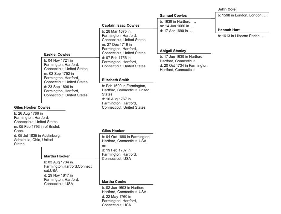
Fig. 19.1 Distant ancestry of Alfred CowlesIII
three generations, to London, England. William and Anne had a son William (1546–1610) who, with his wife, Elizabeth Deards (1550–), would be the last to remain in England (Fig. 19.1 ).
Th eir son, James Cole, was born in Essex, England, in 1563. James married Mary Richards (1564–1601). She died young, but not without two children, Abigail and John Coles (1598–15 September 1675), to support. John sough adventure and opportunity, and arrived in the New World in 1630. Th ere is some evidence that he arrived with his wife, Hannah Hart. Others claim that he married Hannah Bushoup (c.1613–17 March 1683) of Hartford, Connecticut, soon after he arrived in the colonies.
Th ese Coles were farmers. Th e family had followed the Reverend Th omas Hooker (5 July 1586–7 July 1647), the prominent colonial Puritan preacher who dissented from religious leaders in Massachusetts and led a fl ock to found Connecticut. Known as the Father of Connecticut, his family had been prominent Hookers in England dating back to the era of Henry VIII. His descendants include Aaron Burr, the Great Mind John Burr Williams , J.P. Morgan and Alfred Cowles III.
One of his followers, John Cowles Sr., migrated south to Connecticut with Reverend Hooker and bought land in Farmington in 1640. Because there was another John Cole in nearby Hartford at the same time, and whose daughter was accused of witchcraft, John and his wife Hannah (1613–17 May 1683) became known as Cowles, and passed that name on to their eldest son, Samuel (1639–17 April 1690), while their youngest son, John, retained the name Samuel Cowls.
John Cowles represented his region to the Connecticut General Assembly from 1653–54, and then became a founding father of the town of Hadley in Massachusetts, farther west, and then Hatfi eld, across the river, in Connecticut. Meanwhile, their eldest son, Samuel, and his wife Abigail Stanley (17 June 1637–20 October 1734) remained moved to nearby Hartford, and raised a family that included Isaac Cowles (28 March 1675–7 February 1756).
Isaac earned a military title, fi rst as an ensign, then a lieutenant and a captain with the Second Company of Farmington, the local militia. He was married three times, including to Elizabeth Smith (February 1690–16 August 1767), also of Farmington. Together they shared a number of children, including Ezekiel Cowles (4 November 1721–23 September 1806), who, with Martha Hooker (3 August 1734–29 November 1817), the great-great-granddaughter of Reverend Th omas Hooker, raised Gilles Hooker Cowles (26 August 1766–8 July 1835) (Fig. 19.2 ).
Giles was named for his maternal grandfather, Giles Hooker (4 October 1690–19 February 1787). He would fi nd his fortunes in the West. In what will begin a long association between Yale and the Cowles , Giles graduated from Yale University in 1789 and was granted permission to preach by the Western Reserve Association of New Haven, Connecticut. In May of 1791, Gilles Cowles married Sally White (1774–31 July 1830) two years later, and was asked by his church to settle and act as a missionary in the Connecticut Reserve lands of Ohio. From there, he assisted in
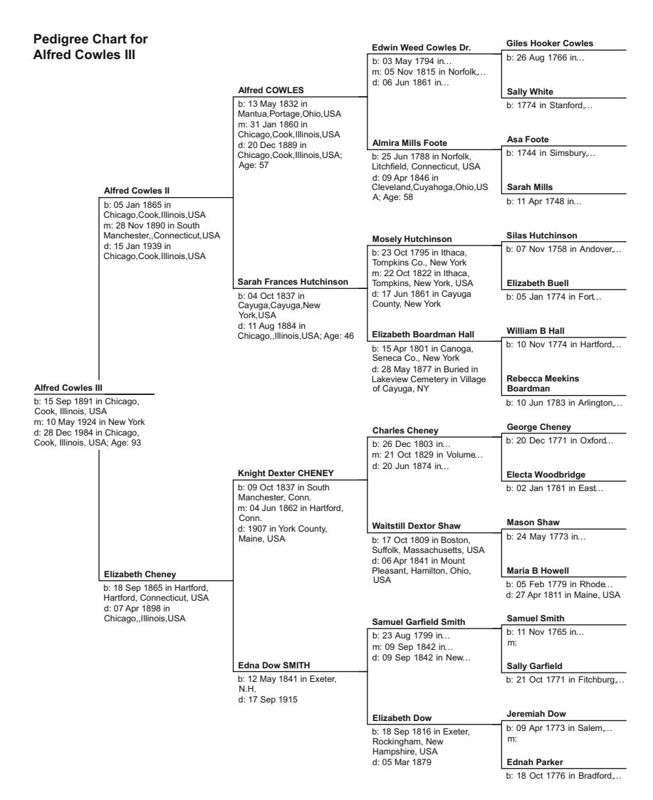
Fig. 19.2 Immediate ancestry of Alfred CowlesIII
the formation of a number of Presbyterian churches in Northeastern Ohio as an itinerant minister fi rst out of Erie. He was eventually instilled as minister in Austinburg in 1811.
Shortly after their marriage, but before their western migration, Giles and Sally had a son, Edwin Weed Cowles (3 May 1794–8 June 1861), the fi rst of their fi ve boys and four girls. Born in Bristol, Connecticut, near Farmington, his ancestors on both sides of the family were all Puritan settlers, including a maternal ancestor Peregrine White, the fi rst white child born in on the Mayfl ower on its way to New England. Educated at the Farmington Academy, Edwin Weed Cowles followed his family West and became a prominent physician in Ohio. He and his wife Almira Mills Foote (28 June 1788–9 April 1848) remained well established in Ohio and raised children of great prominence.
Another son, Henry Cowles , followed his father into the ministry and was one of the fi rst professors at Oberlin College. A daughter, Betsey Cowles (9 February 1810–25 July 1876), the eighth of ten children, became an advocate for education reform and for the advancement of women and abolition of the slave trade.
Edwin Cowles and Alfred Cowles, two other sons of Giles and Sally, married two sisters from Cayuga County, New York, Elizabeth Hutchinson (1827–1910) and Sarah Hutchinson (1837–84).
Th e fi rst son of Edwin and Elizabeth Cowles , Edwin Cowles Jr. (1825–90), had, at a young age, became an apprentice printer and coformed Smead & Cowles Printers. In 1853, he co-founded the Forest City Democrat, and later changed its name to the Cleveland Leader newspaper. He also helped found the Ohio Republican party out of the pressroom at the Leader . When he bought out his partner in the newspaper, Mr. Medill relocated to Chicago and founded the Chicago Tribune with Edwin’s brother Alfred.
Dr. Edwin Weed Cowles and his wife also had another son destined for prominence. Alfred Hutchinson Cowles had studied geology, physics and chemistry at the Ohio State University and Cornell University. He was a student athlete who raced and beat Harvard in the eight-oared crew, and raced at Henley, England. Upon graduation from his studies in geology, he, his father and a brother founded the Pecos Mine in the Cowles Mining District of New Mexico, which would become one of the richest zinc, copper, silver and gold mines in the world.
Th ere, Alfred Hutchinson Cowles and his brother Eugene Hutchinson Cowles (1855–92) developed many new innovations in mining and smelting, including novel methods for aluminum extraction from bauxite, and the construction of the necessary large-scale hydroelectric generation facilities to power these plants. In the process, they became innovators, inventors, patent holders and revolutionizers of modern metallurgy. Th eir patents were imitated by others, most notably the Aluminum Company of America (ALCOA), which used its process in plants most notably in Messena, New York.
Th e new company had been founded by two of Cowles ’ exemployees who had witnessed the development of their process at their Lockport, New York, factory and began to use it to manufacture aluminum in Pittsburgh, Niagara Falls and Massena. Th e Cowles brothers sued for the theft of their intellectual property in federal patent court and won judgments over ALCOA and others worth tens of millions of today’s dollars. Alfred Hutchinson Cowles, the cousin of Alfred Cowles III, contributed to the establishment of a generation of wealthy Cowles sons.
Th e youngest of four boys and a girl of Edwin Weed Cowles and Almira, Alfred Cowles, was born in Austinburg, Ashtabula County, Ohio, on 13 May 1832. Following his comfortable and stimulating upbringing as the son of a highly respected preacher, Alfred started off fi rst as a bookkeeper, then as treasurer and manager of the Chicago Tribune newspaper, and became co-owner of the newspaper, along with John S. Scripps. By then, two sets of Cowles were fi rmly ensconced in publishing. He also married Sarah Frances Hutchinson (4 October 1837–84), and had three boys and a girl.
Th eir middle son, Alfred Jr. (4 January 1865–15 January 1939), followed in his grandfather’s footsteps through his studies at Yale. Th ere, he was a member of the secretive Skull and Bones student society, and continued onto Yale Law School from 1887 to 1888 and then Northwestern University from 1888 to 1889. Upon graduation, he married Elizabeth Cheney (18 September 1865–7 April 1898) of Manchester, Connecticut, on 28 November 1890, with whom he had four boys, the eldest Alfred Cowles III (1891–1984).
Alfred Cowles Jr. was admitted to the Illinois Bar in 1889 and spent much of his career in Chicago practicing law. He took a little more than two years break from his practice to assist in the management of the Chicago Tribune newspaper. He also served as a director of boards for a number of corporations, including the Chicago Tribune and the American Radiator Company, Continental and Commercial National Bank, the Electric Smelting and Aluminum Company, his nephews’ corporation, and other organizations. He was also civically minded. In Chicago, he was a member of the Unitarian fellowship and the University Club. Th eir family resided on the affl uent and exclusive Lake Shore area, at 1130 Lake Shore Drive, on the shore of Lake Michigan.
From the 1700s, and certainly by the mid-1880s onward, the Cowles family had established a tradition of attendance at Yale University. Th ey were also increasingly indoctrinated into one of America’s most secretive societies of the elite, the Order of the Skull and Bones. From presidents such as George Bush to world leaders, this organization contains the elite of the elite. Alfred Cowles II (class of 1886) and III (class of 1913) were members, along with their cousins, William Hutchinson Cowles (class of 1887) and William Sheffi eld Cowles (class of 1921).
Th e family of Alfred Cowles Jr.’s wife, Elizabeth Cheney, was equally illustrious. Th ey were destined from Cheneys who resided in Hartford and nearby Manchester, Connecticut, since founding times (Fig. 19.3 ).
Elizabeth Cheney’s grandfather was one of the Cheney Brothers who founded an industry of silkworm cultivation in Manchester, Connecticut. Th ey began with the cultivation of mulberry trees, and expanded into silk spinning in the 1830s and 1840s. A blight aff ected their tree operation in 1840, but they persevered the drought and a silk market crash to invent new processes and lead the world in silk spinning. Th ey translated their entrepreneurship into an internationally recognized company. Th ey also practiced welfare capitalism in which they dedicated themselves to provide a living wage and safe working environment for their workers in the 1860s, just as industrialists in the Gilded Age were moving in the other direction. Th e corporate patriarchs provided heat and water to the nearby town which housed their workers, built churches and schools and invested in other public facilities. Synthetic fabrics and the Great Depression caused their company to shrink dramatically, which must have been troubling for Alfred Cowles III to observe.
Pedigree Chart for Elizabeth Cheney
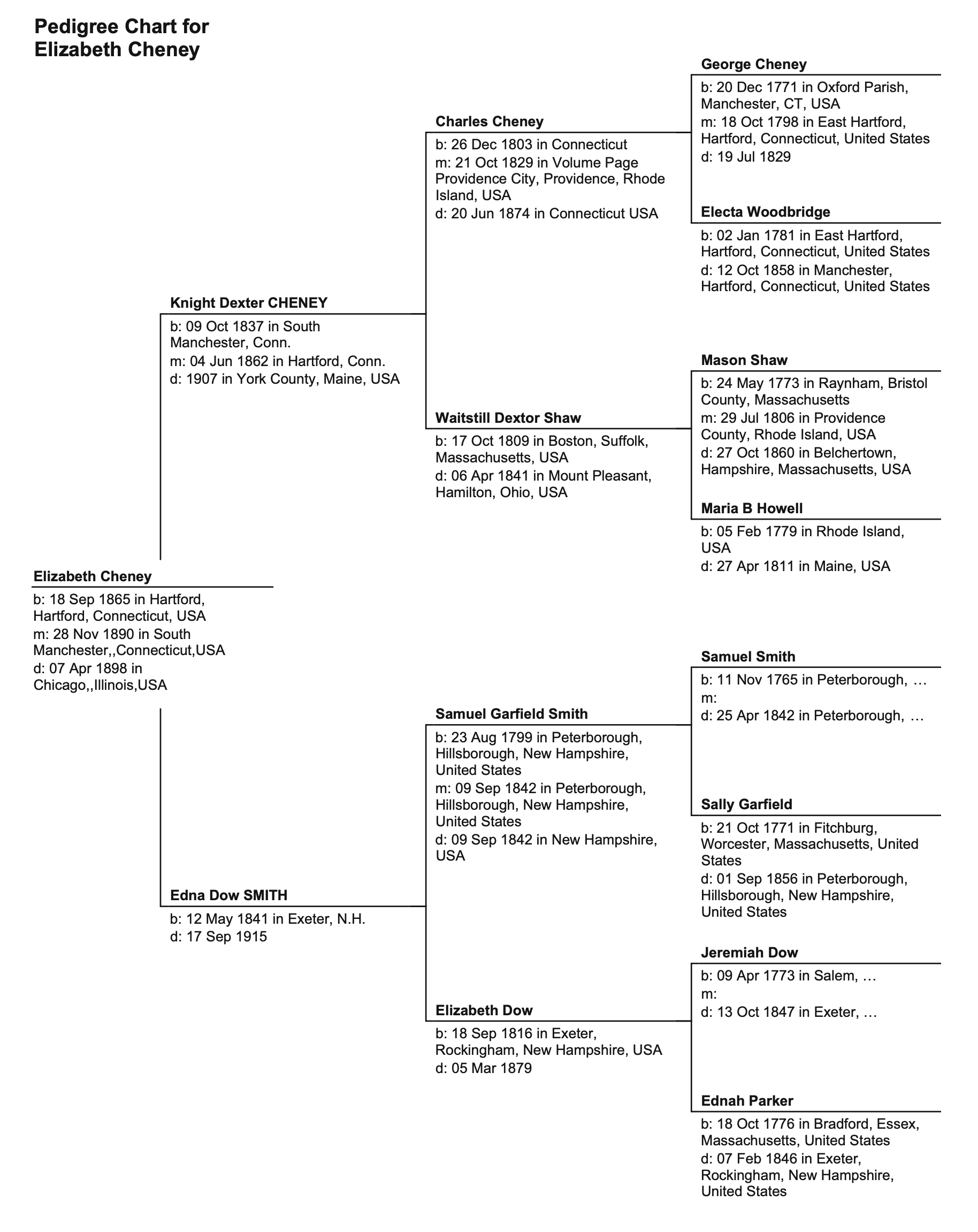
Fig. 19.3 Ancestry of Elizabeth Cheney
The Arrival of Alfred CowlesIII
Alfred C. Cowles III was born on 15 September 1891 with every advantage in American life as the peak of the Gilded Age. His father was a successful lawyer, businessman and part owner of the major newspaper in America’s second city. He was the eldest of four boys, and his family pedigree was often taught at Yale University, one of the nation’s elite schools. In addition to family newspapers in Cleveland and Chicago, his uncle also operated a major newspaper in Spokane, Washington.
Th e family knew young Alfred as Bob. A tall, athletic and handsome young man, he was educated at the exclusive Taft Preparatory School in Watertown, Connecticut, about equidistant from his father’s alma mater of Yale, and his mother’s family business in Manchester. Th e school, founded by the brother of US President William Howard Taft, still maintains today its rich tradition of the education of bright and elite students. Upon graduation from Taft, Cowles migrated 30 miles southeast to New Haven, Connecticut, to attend Yale University. Following graduation from Yale, Alfred had moved to Spokane to learn the newspaper trade from his uncle, William Hutchinson Cowles (1866–1920). Th ere, in 1914, he suff ered typhoid fever.
Alfred recovered from typhoid. With his fragile health at least partially repaired, he moved back to Chicago, the center of rail transportation in the American Midwest, and formed an investment house that purchased and restructured small railroads under the banner Alfred Cowles Railroad. Meanwhile, his investment and acquisitions fi rm also published a regular newsletter on market advice. But, in 1915–16, his health and future were once again cast into jeopardy. Just two years into his career, Cowles became affl icted with tuberculosis. His family commended young Cowles to convalesce in the cool and dry air of Colorado Springs, where he increasingly spent his time, often from a sickbed.
Th e disease, once called consumption, was not an affl iction unknown to the family. Cowles had spent time as a young boy visiting his mother, Elizabeth Cheney Cowles, in Colorado Springs as she tried to recuperate from the terrible lung disease in the dry and cold air of the Rockies. She succumbed to that disease in 1898 and left Alfred II to raise their
four young boys: Alfred (Bob) Cowles III, Knight Cheney Cowles (27 December 1892–1 May 1970), John Cheney Cowles (1894–1972) and Th omas Hooker Cowles (6 June 1895–21 August 1927).
In 1916, just a few years after his graduation, and affl icted with tuberculosis, Bob too was attracted to the therapy that had been demonstrating an improvement in its cure rate since it took the life of his mother. Under the care of Dr. Gerald Webb, the renowned tuberculosis researcher, of Colorado Springs, Bob recovered enough over a year’s stay at a sanitarium to move in with his aunt Sarah Cowles Stewart and her husband Phillip Stewart on Colorado Springs’ “Millionaire Row.”
20. The Times of Alfred Cowles III
Cowles remained in Colorado Springs for two decades. He had survived the stock market turmoil of the late 1920s relatively unscathed fi nancially, and had simultaneously decided to withdraw from both the fi nancial markets and urban congestion before the crash of 1929. He was fi rmly entrenched in the dry mountain air of Colorado Springs.
Cowles spent time between Colorado Springs and Chicago in the intervening years, until he met a young woman 11 years his junior. Cowles had a cousin, Laura Cheney, who was the roommate at Vassar College with an attractive and athletic woman named Elizabeth (Betsy) Strong. Th e Cheney family invited Betsy to take a summer job at their Manchester silkworm enterprise, where she learned how to drive, and met her roommate’s cousin. Albert Cowles III was a self-assured and athletic man with stunning blue eyes and from one of Chicago’s millionaire families. Th ey fell in love, and were married within a year, on 10 May 1924, barely a year after Betsy graduated. Following a honeymoon in Homestead Hot Springs in Virginia, they moved to their newlywed home, at 30 Broadmoor Avenue, within a complex of millionaire cottages and resorts around the private Cheyenne Mountain Country Club and the exclusive Broadmoor Hotel.
Th e young couple were fully immersed in the millionaire country club scene. Th ey partied and entertained, and they made a most handsome couple. Th ey also looked forward to starting a family together, but discovered they could not have children. Instead, they traveled to Boston to adopt, fi rst, Richard Livingston, and then, a few years later, Ann. Th e larger family also moved to a larger home, at 1506 Culebra, in Colorado Springs.
At fi rst, Cowles considered himself a journalist in the family tradition, but he gradually became interested in fi nancial investing, of which his extended family had much to invest. He was the principal in an investment company, and from there, began his life’s work. Meanwhile, his wife became increasingly close to Bob’s aunt, and her husband Philip, the son of a former Vermont governor.
Betsy’s diversion, fi rst through her uncle by marriage, and then through her father, became her emotional salvation. She was a young, capable, well-liked and spontaneous woman, but she found herself married to a man who was incredibly focused, to the point that he appeared to some to be aloof and uninterested. Some speculate his focus arose from days and nights on end in solitude and cold air as he fought for his life against tuberculosis. His intensity was a great quality for one recovering from a debilitating disease, for an investor and aspiring economist, and for a fi nancial theorist. It might not have been the ideal personality for a man married to a vibrant woman much younger than he was.
Betsy’s salvation was her father’s newfound fascination with mountain climbing. He had suff ered physical problems later in life that led his doctor to proclaim that he may lose the ability to walk. He took that diagnosis as a challenge to climb mountains. He brought his daughter into that world, at the highest levels around the world. Betsy became a recognized mountain climber, in Colorado and abroad.
In the 1930s, Betsy fell out of love, and the couple divorced in 1938–39. Th at year, Cowles moved back to Chicago, but continued to support Betsy for the rest of her life, and continued to manage her father’s investments. Ten years later, on 24 October 1949, Cowles remarried, to Louise Lamb Phelps. Betsy later married an air force general, Earle (Pat) Partridge.
Certainly, Cowles ’ diversions centered around his work. He threw his intensity into everything he did, whether or not they generated any income for himself. At the time Cowles was a director of one of the nation’s leading tuberculosis research institutes. Th e Webb-Waring Institute for Medical Research was founded in 1924, by Dr. Gerald R. Webb, a leading tuberculosis researcher, and his colleague Dr. James J. Waring, Chairman of the Department of Medicine of the University of Colorado School of Medicine. As a director of the Institute, Cowles was instrumental in creating both fi nancial viability for the organization and some direction in their medical research that employed statistics.
When he was searching for the best tuberculosis therapy, on behalf of the tuberculosis foundation in Colorado Spring for which he agreed to serve, Cowles schooled himself in the emerging statistics of the 1920s. He successfully constructed an analysis of variance model to predict successful courses for the cure of tuberculosis and proved that certain climates in the USA were more amenable to healing. In fact, Cowles’ fi rst publication was in the Journal of the American Statistical Association , in which he demonstrated that climate was a signifi cant determinant on the death rate from tuberculosis in the USA.
21. The Great Idea of Alfred Cowles III
With his interest in statistics stimulated and the time aff orded with a life of semi-retirement, Cowles became interested in applying statistical principles to a fi nance discipline for which he had developed a professional suspicion that it lacked scientifi c rigor. He had become growingly suspicious of the spurious advice off ered by many fi nancial advisors over the Roaring Twenties, especially in the wake of the Great Crash of 1929, and he had schooled himself on the mathematics of least squares and statistics that could act as the basis for the treatment of fi nance as a science rather than an art. His fi rst project in fi nance was to determine the eff ectiveness and correlation of the advice from 24 market newsletters and stock market performance.
Of course, Cowles could have aff orded to commission economists and statisticians to do his analytic work for him, but he also had the time and interest to take a hands-on approach. To assist him in the statistical theory, he came upon an academic, Harold Th ayer Davis (5 October 1892–14 November 1974), who spent summers in the mountain community of Colorado Springs, Colorado. Davis knew that while the regression calculations could be performed by a team of clerks, he thought a new device called a Hollerith Calculator from a new company called International Business Machines could use punch cards to streamline such calculations. Davis agreed to help Cowles build an analysis unit at Cowles’ Colorado investment offi ce to house the machine and commission the calculations.
Unfortunately, they quickly discovered that the machine was ill-suited for the linear regression calculations Cowles needed. Th is reality forced Cowles to simplify his analysis into a series of simple linear regressions. Accordingly, he developed a methodology to compare estimates and forecasts with random guesses. From this necessary deviation from his research agenda, Cowles quickly developed the hypothesis that neither market analysts nor the state of the art in existing estimation techniques could outperform random stabs in the dark.
Cowles ’ fascination with fi nance theory was piqued. With the encouragement of Davis , he came up with the idea to form a commission that would have as its mission better measurement and estimation in fi nancial markets. Davis, James Glover , a professor of actuarial mathematics and computational methods at the University of Michigan, and Th ornton Fry of Bell Telephone Laboratories would provide the methodological guidance. At the same time, Cowles approached the recently formed Econometric Society to suggest a mutually benefi cial collaboration with its University of Chicago-based scholars.
At fi rst, the various scholars he tried to engage were skeptical, but Cowles ’ pledge of signifi cant funding to advance the state of analysis and expand the use of modern scientifi c tools in fi nance and economics seemed suffi cient to secure their support.
Cowles ’ inspiration for the Commission was to raise the level of analysis of the decision-making sciences, especially fi nance and economics, to take advantage of the new techniques that were being developed by Ronald Fisher , Harold Hotelling and others in the emerging science of statistics. He believed that much of the investment and fi nance discipline was little more than glorifi ed guessing, and was confi dent that the emerging tools of quantitative analysis would lend themselves well to fi nance theory. In turn, problems that arguably brought down the US and other economies in the developed world from 1929 to 1933 could be remedied through the application of science. In doing so, he anticipated a shift of emphasis from the cold world of neo-classical economics that was the rage at the time to a new world of forecasting and better public policy.
By the early 1930s, Cowles had assembled much of the mathematical, statistical and computing resources he would need. He then pressed on his Yale connections to woo the economics discipline. At that time, the most prominent American economist was the Great Mind Irving Fisher (27 February 1867–29 April 1947). A Yale graduate and faculty member, he had known Cowles’ father from college days. In fact, both Cowles’ father and uncle were Yale graduates, as were others who followed him. Fisher was highly prominent, if not partially disgraced by his very public optimism, of the strength of US fi nancial markets even right up to and immediately following the Great Crash.
Fisher himself had built up a fi nancial fortune from his invention of data sorting techniques, one of which was an early version of the once ubiquitous Rolodex. While Fisher irretrievably lost his fortune with the onset of the Great Depression, he was nonetheless a powerful fi gure who, by chance, shared another important characteristic with Cowles . Fisher, too, had suff ered tuberculosis as a young man, and had even spent some time in Colorado Springs. Th ese connections aff orded Cowles a receptive ear from one of the most well-known and respected economists in the country who had, for years, been advocating the formation of a society devoted to scholarly work in econometrics.
Cowles off ered the funding if Fisher could assemble the critical mass of scholars both to create a research commission and to form the Econometric Society that would rival the statistical societies of England. Fisher brought the academics, and Cowles built the facility, fi rst in Colorado Springs.
One motivation of Cowles was his desire to produce a statistical study of whether stock market forecasters are successful in predicting the direction of the market. He believed they did not. Cowles devoted his profound intensity into the analysis of almost fi ve years of data from 7500 investment advisor recommendations from 16 services. From his mammoth study, he demonstrated that only 6 of 16 services provided positive returns, with the average investment service actually yielding fi nancial losses.
His analysis was read at one of the fi rst meetings of his new Econometric Society, and was published in one of the fi rst editions of the new journal Econometrica he funded. His Cowles Commission for Research in Economics, with the motto “Science is Measurement,” quickly became the nation’s most prominent fi nancial and economic research group.
Cowles proved to be one of the Commission’s most insightful researchers early on. His interest began with his stock market research. Like Fisher, who had been for decades collecting data on the infl ation rate, bond prices and bond interest rates, with the goal of developing fi nancial instruments that are immunized from infl ation and money supply manipulation, Cowles realized that data is king. He set about producing stock price databases that would eventually become the Standard & Poor’s 500 index. His indices were much more sophisticated and theoretically sound than the simplistic Dow Jones Industrial Index that was commonly employed at the time.
From his database of stock prices and forecasts, Cowles created a set of 24 time series of forecasts and demonstrated, within the context of a multivariate regression , that most of these forecasts were not statistically correlated to market success. In other words, most forecasts perform no better than random choices. He stated, “Th e most successful records are little, if any, better than what might be expected to result from pure chance.” 1
In eff ect, Cowles was developing an early version of the random walk that was popularized by the Great Mind Paul Samuelson (15 May 1915–13 December 2009) more than 30 years later, in 1964. It was this fi rst volley into the premise that forecasters can’t beat the market that produced what now underpins much of fi nancial theory, and was the subject of an earlier volume in this series on the effi cient market hypothesis.
While Cowles emerged as a competent self-taught scholar, his contribution hardly stopped there. Cowles was an academic benefactor and entrepreneur perhaps without parallel. Never a professor himself, and having never enjoyed the trappings of the Ivory Tower, Cowles nonetheless successfully assembled one of the greatest groups of scholars in academic history.
Aside from some early contributors from the mathematical and computing sciences, Cowles very quickly identifi ed a number of individuals who he felt could help further the creation of a fl edging econometric society.
Th e notion of a random walk is actually related to an important econometric issue. Gauss had developed the method to provide a best fi t of an estimated relationship to data that is subject to random error. If departures from the estimate are random, then the errors of observations in a time series should not show any dependency with adjoining observations, and should vary in size according to a random normal distribution. Th e importance of ensuring there are no serial correlation in errors was a leading-edge statistical concern then, as it remains now. If it can be established, as Cowles and Herbert E. Jones asserted, that there are no such correlations between errors in observations of stock prices, then traditional statistical tools can be employed in the analysis of stock market prices.
Cowles felt that Fisher may share his entrepreneurial ambitions for fi nance theory, even if Fisher forever maintained more optimism than Cowles that stock prices could be predicted. Yet, despite Fisher’s belief that the effi cient market hypothesis could be repealed, he agreed to act as an intermediary to use his infl uence as the president-elect of the American Statistical Association and the President of the newly founded Econometric Society, to work with Cowles to fund a commission and a new journal. Fisher assembled the interested scholars, and Cowles indeed funded the journal, and acted as its treasurer from 1932 to 1954.
Cowles was instrumental in supporting the new Econometric Society, but he was not its founder. Shortly after Christmas, on 29 December 1930, just 14 months after the Great Crash, the Econometric Society was founded. Th is was almost three years after Fisher, Charles Roos (18 May 1901–6 June 1958) and the European economist Ragnar Frisch had assembled to discuss the possibilities at Fisher’s home in New Haven, Connecticut. Indeed, Fisher had been trying to create such a society for a couple of decades by then. But, with the Great Crash, and fi nally, with Cowles’ sponsorship, it appeared the Society, and its journal, would fi nally attain the necessary resources to succeed. Indeed, Cowles’ devotion to research that can better explain the stock market likely also brought to the society interest from businesspeople and government offi cials, beyond the obvious interest of a few dozen economists.
Th e timing was perfect. Th e year 1933 saw breakthroughs in the legitimization of mathematical statistics in Europe and in the political climate for better understanding of both fi nance and public policy in the USA. Cowles and his Commission found itself on the leading edge of both and with the resources and stature to attract the world’s leading scholars.
Another aligning of the stars at the time was the acceleration of nationalism under Adolf Hitler in Germany, and his warped application of Galton ’s eugenics. Some of the brightest applied mathematicians in Germany, Austria and Eastern Europe at the time were of Jewish descent. Many were counseled by colleagues to not risk their fate to an increasingly militant German movement, and some others began to feel less subtle persuasions to leave Europe.
One of the earliest and most formative members of the Cowles Commission was one such European scholar, Jacob Marschak (23 July 1898–27 July 1977). He, Ragnar Frisch and Haavelmo , all joined the Cowles Commission, which, by then, had moved to the University of Chicago to be better able to tap the resources of one of the country’s best economics departments, and, by no small coincidence, the family home of Cowles.
Marschak was a most colorful character. When he joined the Cowles Commission as its research director in 1943, he joined scholars whose families had followed a similar migration from regions in and around the Austro-Hungarian Empire, and found themselves at Cowles, including the families of Milton Friedman (31 July 1912–16 November 2006) and Franco Modigliani (18 June 1918–25 September 2003). Marschak found himself as an immigrant who sought academic refuge at the New School for Social Research in New York City after a four-year stint directing Oxford’s statistics institute in the late 1930s. He had joined the same University in Exile that Harold Hotelling had supported. Many of these almost 200 scholars were brought there by the New School co-founder, Dr. Alvin Johnson (18 December 1874–7 June 1971), between 1933 and 1945.
First at the New School, and then at Cowles , Marschak found himself surrounded by the same eclectic and intellectually diverse scholars who could look at old academic problems in new ways and with new techniques. If they did not have the new techniques yet, they created them.
Marschak and his colleagues at Cowles recognized that the static model which predated the Great Depression was ill-prepared to treat the rapidly evolving economies of the 1930s and beyond. Th e disciplines of economics and fi nance were forced to move beyond the simplistic classical solutions that proclaimed economic booms and busts could not occur, to ones that were more dynamic in nature. Th ese models needed to recognize a richer set of interactions that all come together to determine market equilibrium . Th e tools of the trade were no longer artful rhetoric, but were increasingly founded in mathematics and statistics. Th e Cowles Commission was the epicenter for this groundbreaking new approach.
Associated with the Commission were many of the most brilliant scholars in the nation, indeed the world. Many went on to win Nobel Memorial Prizes in Economics. Some were also associated with the University of Chicago’s department of economics. Th is intersection became problematic, though, as the Commission sometimes eclipsed the stars of the economics department. As a consequence of this growing tension, the Cowles Commission moved in 1955 to another Cowles hinterland, Yale University. Marschak and many others made the move as well.
Th e move allowed the Commission to more deftly depart from the strong neo-classical philosophy of the University of Chicago. It also allowed the Cowles family to continue simultaneously their generous support to both the Cowles Foundation, which it was renamed after the move, and their alma mater of Yale University.
Scholars at the Cowles Commission and the Foundation are now remembered for their development of a number of methodologies in statistics and applications to econometrics. Th ese include the techniques of instrumental variables, indirect least squares and maximum likelihood estimation. Th ey also developed indirect least squares, instrumental variable methods, full information maximum likelihood method and limited information maximum likelihood method.
Each of these techniques is now an important element of the fi nance toolbox.
Th e Commission also produced pioneering work by Great Minds that would go on to secure Nobel Memorial Prizes. Th e scholars who were awarded with the ultimate prize for scholarship in economics and fi nance include Kenneth Arrow (23 August 1921–), Gérard Debreu (4 July 1921–31 December 2004), Tjalling Koopmans (28 August 1910–26 February 1985), Trygve Haavelmo , Lawrence Klein (14 September
1920–20 October 2013), Harry Markowitz (24 August 1927–), Franco Modigliani , Herbert Simon (15 June 1916–9 February 2001) and James Tobin (5 March 1918–11 March 2002).
Th ese exceptional individuals who formulated some of the most profound concepts in fi nance did so not in a vacuum, but within a commission that produced precisely what Cowles was confi dent it would. Cowles primed the pump by producing signifi cant work that preceded later developments in fi nance such as the random walk and the effi cient market hypothesis. Not only did he encourage and facilitate some of the very fi rst applications of modern statistical techniques to fi nance, but he also then funded the scholars who could take the commission much farther toward his vision.
Note
- Cowles , Alfred, III, “Can Stock Market Forecasters Forecast?” Econometrica 1 (3), July 1933, pp. 309–324.
22. Legacy and Later Life of Alfred Cowles III
While Alfred Cowles III was not college-trained in fi nance and economics, he nonetheless attained some of the highest accolades of his fi eld. He was a Fellow of the American Association for Advancement of Science, and a Fellow and Treasurer of the Econometric Society. He also was the principal author of the Cowles Monograph Common Stock Indexes , and contributed to Econometrica and the Journal of American Statistical Association . Some of his publications include Can Stock Market Forecasters Forecast? , a paper read before a joint meeting of the Econometric Society and the American Statistical Association, Cincinnati, Ohio, 31 December 1932. Th is article was subsequently reprinted in Econometrica . 1
Cowles also wrote Analysis of 4½ Years of Forecasting by 41 Advisory Services and Publications , and wrote, with Herbert E. Jones, Some a Posteriori Probabilities in Stock Market Actions . 3 Other Econometrica papers included Stock Market Forecasting , 4 and A Revision of Previous Conclusions Regarding Stock Price Behavior.5
His Cowles Commission Monographs included Common-Stock Indexes, 1871–1937 , 6 Common-Stock Index, 2nd edition , 7 and Supplement to Common-Stock Indexes for 1939 and 1940 . 8
Cowles was also dedicated to other causes. He was a trustee of the Chicago Historical Society, and director at the Chicago Tribune. His philanthropic work included eff orts as a trustee and treasurer for the Illinois Children’s Home & Aid Society, director of both the Home for Destitute Crippled Children and the Chicago Maternity Center, and director and treasurer of the Passavant Memorial Hospital. In Colorado Springs, he was a trustee at Colorado College and a director at the Institute that helped save his life.
Notes
- Cowles , Alfred, III, “Can Stock Market Forecasters Forecast?” Econometrica 1(3), July 1933, pp. 309–324.
- Cowles , Alfred III, “Analysis of 4½ Years of Forecasting by 41 Advisory Services and Publications,” Stock Market Technique , ed. by Richard D. Wychoff , Vol. 2, No. 2, April 1933.
- Cowles , Alfred III and Herbert Jones, “Some a Posteriori Probabilities in Stock Market Actions,” Econometrica , (July 1937), 5(3): 280–294.
- Cowles , Alfred III, “Stock Market Forecasting,” Econometrica , July– October 1944, pp. 206–214.
- Cowles , Alfred III, “A Revision of Previous Conclusions Regarding Stock Price Behavior,” Econometrica (October 1960), 28(4): pp. 909–915.
- Cowles , Alfred III, Common-Stock Indexes, 1871–1937 , 1st edition. Bloomington: Principia Press, Inc. Bloomington, 1938.
- Cowles , Alfred III, Common-Stock Index, 2nd edition , Principia Press, Inc., Bloomington, 1939.
- Cowles , Alfred III, Supplement to Common-Stock Indexes for 1939 and 1940 , University of Chicago Press, Chicago, 1940.
23. The Early Life of Ragnar Frisch
While Cowles and his scholarship were distinctly American, two of the greatest infl uences on the Cowles Commission were distinctly Norwegian. Th is tradition began with Ragnar Frisch .
Th e family name Frisch is German in origin, but the family has lived in Norway for almost four centuries.
In the early summer of 1623, two children were herding cattle along a pathway on Gruveåsen hill near present-day Kongsberg, Norway. At that time, the town, located about 50 miles west and south of Oslo, was part of the Kingdom of Norway and Denmark, under the monarch Christian IV. Th e ox the children were using to help herd their cattle rubbed against the mountainside and revealed a large shiny stone. Th e children, Helga and Jacob, brought the shiny stone to their father, who melted it down and took it into the nearby town of Skien in Telemark County to sell. He fetched such a low price for it that the local police became suspicious it might be stolen. Th e father was given a choice—to be arrested to tell the authorities where he found what turned out to be pure silver from what would become one of the world’s richest mines.
Understanding its economic potential, the King came to Telemark County the next year and declared a new town of Kongsberg. Th e silver mines that grew out of the fi nd are located fi ve miles further west of the town.
Th e King’s Mine and its adjacent complex of tunnels and caverns yielded almost three million pounds of silver between 1623 and its closing in 1957. At its peak, the 80 mines that represented the complex was the largest employer in Norway and supplied more than 10 % of the Kingdom’s gross domestic product over its lifespan. More than 4000 workers mined the silver in its heyday. Th e mine also attracted workers from around Europe who were seeking better jobs. Kongsberg also, quite naturally, became the location of Norway’s offi cial mint (Fig. 23.1 ).
Christopher Frisch was born in 1615 but traveled as a young man to the Kingdom to work the mines. King Christian IV had asked the Electoral Prince of Saxony to send a team from the Mining Academy in Freiberg, Saxony, to assist in the development of the new mines near Kongsberg. Christopher arrived shortly after that request in 1630.
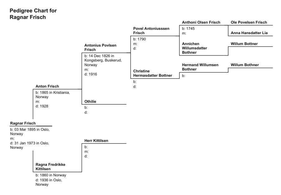
Fig. 23.1 Ancestry of Ragnar Frisch
Th ere he started a family, which included a son Petter Christopherson Frisch (1640–1703). In turn, Paul Pettersen Frisch (1670–1730) married Anne Antonisdatter Nolt, whose father Antonius (1640–77) had also migrated from Germany to work the mines. Paul and Anne had a son Ole Povelsen Frisch (1700–79), who married Anna Hansdatter Lia (1704–71) and had a son together named Anthoni Olsen Frisch (1745–1801).
Anthoni Olsen Frisch and his wife, Annichen Willumsdatter Bothner, were the paternal great-grandparents of Ragnar Anton Kittil Frisch. Th e son of Anthoni and Annichen produced a son, Povel Antoniussen Frisch (1790–?). He and his wife Christine had a son of their own, Antonius Povlsen Frisch (1826–1916), who realized quite quickly that processing the mineral and making jewelry from gold and abundant silver was a safer and economically steadier livelihood. In 1856, Antonius, Ragnar’s grandfather, established a jewelry workshop in Kristiania, Norway.
In turn, the son of Antonius and his wife Othilie were increasingly enjoying a more comfortable lifestyle for their son, Anton Frisch (1865–1928), and his eight siblings. Anton Frisch assumed the family business. He too had expected his only son to someday do so in turn.
The Arrival of Ragnar Frisch
Young Ragnar Anton Kittil Frisch was born to Anton and his wife, Ragna Fredrikke Kittilsen (8 July 1858–1936), on 3 March 1895 in Christiana, Norway, now named Oslo. He drew has family names from both his father’s and mother’s sides. As the son of a skilled craftsman in the heart of Norway, he was raised and schooled well, but his father had always hoped he’d follow in the family footsteps. When Ragnar was in his late teens, his father arranged to have him apprentice in the trade with the David Andersen jewelry workshop.
However, Ragnar’s mother had an alternative plan. She convinced her husband to let Ragnar simultaneously study economics at the University of Oslo as this seemed like the course of study Ragnar could complete the quickest. By 1919, Ragnar had completed his economics degree, with distinction, and, by the following year, he also had his jeweler’s qualifi cation in hand. He began to work at his father’s workshop.
By then, though, Ragnar had become fascinated with the interplay between mathematics and economics. He applied for and was off ered a university fellowship that allowed him to study these two subjects in England and France. Upon his return in post-Great War Norway in 1923, he recognized that his father’s business was suff ering fi nancially and his better option for a livelihood may indeed be the decision sciences. He began studying and publishing in the area of mathematical statistics, and received his PhD in 1926. Almost immediately, Frisch became a leader among the burgeoning fi eld of mathematical statistics and econometrics, despite his relatively young age and his desire to remain in Norway to build the discipline at home.
24. The Times of Ragnar Frisch
By the time Frisch began to lead the development of the new fi eld of econometrics, Ronald Fisher ’s Handbook had been well reviewed by Harold Hotelling , and statistics groups were beginning to sprout across the USA, especially at the major land-grant universities that contained in their mission the need to perform research in support of agriculture. With a fresh PhD in hand by 1926, Frisch was about to join that fray among other founders of econometrics. In 1927 he was off ered a Rockefeller Foundation scholarship to travel to the USA. One of his fi rst collaborations came when he arrived at Yale University in New Haven, Connecticut, to work with the great mind Irving Fisher , just as Cowles was encouraging Fisher to bring to fruition the vision of an Econometric Society.
Th is year in the USA proved most infl uential for both Frisch and statistics and fi nance. As discussed earlier, it was his meeting with Fisher that gave rise to the new Econometric Society that Alfred Cowles III would later underwrite.
Many of the leading fi nance, economics and statistical theorists of the day were trained fi rst as physicists or engineers. Th is included the great mind Irving Fisher , and many of his statistics contemporaries, from Ronald Fisher to Harold Hotelling . Frisch shared that belief the cornerstone of modern fi nance and econometrics must be in the hard sciences rather than political philosophy. His 1926 infl uential article, Sur un problème d’économie pure , 1 established econometrics as a tool and theory at the intersection of mathematics, statistics and economics. He explained:
Intermediate between mathematics, statistics, and economics, we fi nd a new discipline which for lack of a better name, may be called econometrics. Econometrics has as its aim to subject abstract laws of theoretical political economy or “pure” economics to experimental and numerical verifi cation, and thus to turn pure economics, as far as is possible, into a science in the strict sense of the word.
In the article, Frisch spelled out an axiomatic approach to some of the pressing analytic issues of the day. He then published a series of articles on the evolving methodology of econometrics and statistical methods in time series analyses. Not only did those works fi rmly establish economics as a science, and econometrics as an important tool within fi nance and economics, but he also formalized the diff erence between the static analysis performed on events at a given time and the crucially important dynamic analysis that is essential for fi nance theorists to demonstrate how fi nancial variables evolve over time. He was also the fi rst to demonstrate the diff erent roles, and label thusly econometrics, microeconomics and macroeconomics.
Of course, Irving Fisher had made his life interjecting the importance of the time variable, and the role it plays in interest rates, rates of return and infl ation. Clearly, when the two met in the USA in 1928, they were already destined to be kindred spirits.
By early 1928, as Frisch had been visiting Princeton University, he met Charles Frederick Roos of Cornell University, who was also visiting Princeton as a Fellow of the National Research Council. Roos was also chairing a section of the American Association with the Advancement of Science called Section K, which represented economics, sociology and statistics. Roos was a mathematician who was almost instantly fascinated with Frisch’s vision to formalize the mathematical underpinnings of economics and fi nance and to develop the new methodology of econometrics.He and Roos agreed that there was a need to develop an Econometric Society, and decided to travel to Fisher’s home in April of 1928 to solicit his help.
Fisher was at fi rst pessimistic about the possibilities as his eff orts to do the same over the past two decades had garnered little momentum. Fisher asked Frisch and Roos to name a hundred scholars who would be willing to participate. Perhaps he surmised that Frisch, from Europe, and Roos, from mathematics, would be hard-pressed to reach such a critical mass for a new Society.
Frisch and Roos came up with a number of names very quickly, but, after only a few days, hit upon the wall economists label diminishing marginal returns. When they came up with only about 70 names, Fisher quickly added a dozen of his own, and the three men agreed that they had enough to begin their joint eff orts.
In the winter of 1930, the three main associations, the American Economic Association, Section K of the American Association for the Advancement of Science and the American Statistical Association all met in Cleveland. Earlier in 1930, Frisch , Roos and Fisher had sent out invitations to attend a meeting while in Cleveland. Frisch, who had returned to teach at the University of Oslo following the completion of his Rockefeller Foundation scholarship, happened to be in the USA as a visiting professor at Yale, was in attendance in Cleveland, and joined Roos, Fisher and 13 other scholars from the USA and Europe at the Cleveland hotel on 29 December 1930 to inaugurate the new Econometric Society.
Joseph Alois Schumpeter (8 February 1883–8 January 1950), then of the University of Bonn, chaired the meeting, and Fisher was elected its fi rst president. Frisch produced the draft of the Society’s constitution, and a series of meetings, in Lausanne, Switzerland, in September of 1931, and Washington, DC, in December, were agreed upon. By the end of that year, 173 members were elected.
Cowles approached the new society on the behest of his Colorado Springs colleague, Harold T. Davis , the mathematics professor at Indiana University who spent summers in Colorado. Davis knew of the fl edging society and thought their interests aligned perfectly with Cowles’ desire to bring measurement and science to economics and fi nance. Fisher was elated to see that Cowles could help resolve the Econometric Society’s lofty goals but meager dues and budget.
Davis arranged a meeting with Cowles and members of the society, including Harold Hotelling , in New York City in late October 1931 just a few days after Cowles met with Roos and Fisher at Fisher’s home to sketch out a plan for the larger group. From this critical mass of almost a dozen Society members, it was agreed that the president and secretary, Fisher and Roos, would send a proposal out to its members. Most embraced the concept, but some were wary. It was decided that Frisch should come to meet in Colorado Springs to meet with Cowles and represent the European contingent of the Society. Frisch met and stayed with Cowles for a week, and, as he returned to Norway, met briefl y with Roos and Fisher to affi rm his agreement that Cowles and his possible Commission could add much to the Society.
Just a few months later, by February of 1932, an advisory council for the Cowles Commission was assembled, and, by the following summer, its fi rst major research project, the construction of a database of stock prices, including earnings, dividends, recapitalizations and splits, would be constructed. Th e Cowles Commission was chartered in Colorado on 9 September 1932. Its organizational purpose was stated as:
to educate and benefi t its members and mankind, and to advance the scientifi c study and development … of economic theory in its relation to mathematics and statistics.
Cowles was elected a trustee, a laboratory was renovated and the economics faculty of Colorado College were enlisted to create the organization necessary to pursue its fi rst projects. Cowles provided an annual budget of $12,000.
Th e inaugural issue of the journal Econometrics came out in the fi rst month of 1933, with Frisch framing its editorial. Schumpeter off ered the following introduction to the journal:
Th e common sense of the program of our Society centers in the question: Can we not do better than this? Surely it would not be a reasonable policy to sit down and wait till, in the end, things fi nd their level by themselves, and meanwhile to allow econometricians of all countries to fi ght singlehanded their uphill battle. What we want to create is, fi rst, a forum for econometric endeavor of all kinds wide enough to give ample scope to all possible views about our problems, yet not wide enough to be hampered by the weight of an audience which keeps discussion in the ante-rooms of the real points at issue, and forces every speaker or writer to go every time over the same preliminaries.
On this forum, which we think of as international, we want secondly to create a spirit and a habit of cooperation among men of diff erent types of mind by means of discussions of concrete problems of a quantitative and, as far as may be, numerical character. Th e individual problems themselves are, as it were, to teach us how they want to be handled. We want to learn how to help each other, and to understand why, and precisely where, we ourselves, theorists, statisticians, collectors of facts, or our neighbors, do somehow not quite get to where we want to be. No general discussion on principles of scientifi c method can teach us that. We have had enough of it. We know it leads nowhere, and only leaves the parties to the contest where they were before, still more exasperated perhaps by those gentle rudenesses it is customary to administer to each other on such occasions. No general arguments of this kind ever carry conviction to the man who means real work. But, confronted with clear-cut questions, most of us will, we hope, be found to be ready to accept the only competent judgment on, and the only relevant criterion of, scientifi c method, that is the judgment or criterion of the result. Th ere is high remedial virtue in quantitative argument and exact proof. Th at part of our diff erences – no matter whether great or small – which is due to mutual misunderstanding, will vanish automatically as soon as we show each other, in detail and in practice, how our tools work and where they need to be improved. And metaphysical acerbity and sweeping verdicts will vanish with it. Th eoretic and “factual” research will of themselves fi nd their right proportions, and we may not unreasonably expect to agree in the end on the right kind of theory and the right kind of fact and the methods of treating them, not postulating anything about them by program, but evolving them, let us hope, by positive achievement.
We should not indulge in high hopes of producing rapidly results of immediate use to economic policy or business practice. Our aims are fi rst and last scientifi c. We do not stress the numerical aspect just because we think
that it leads right up to the core of the burning questions of the day, but rather because we expect, from constant endeavor to cope with the diffi culties of numerical work, a wholesome discipline, the suggestion of new points of view, and helps in building up the economic theory of the future. But we believe, of course, that indirectly the quantitative approach will be of great practical consequence. Th e only way to a position in which our science might give positive advice on a large scale to politicians and business men, leads through quantitative work. For as long as we are unable to put our arguments into fi gures, the voice of our science, although occasionally it may help to dispel gross errors, will never be heard by practical men. Th ey are, by instinct, econometricians all of them, in their distrust of anything not amenable to exact proof. 2
With the Cowles Commission, an movement was born and a foundation for the scientifi c description of fi nance was established.
Notes
- Frisch , Ragnar, “Sur un problème d’économie pure (On a problem in pure economics).” Norsk Matematisk Forenings Skrifter , Vol. 1, No. 16, 1–40, 1926.
- Schumpeter , Joseph, “Th e Common Sense of Econometrics,” Econometrics , 1, 1, 1932, pp. 5–12.
25. Ragnar Frisch’s Great Idea
The rousing editorial of Joseph Schumpeter was not the only immortal contribution to the first edition of Econometrica. Also in the volume was a paper by Ragnar Frisch and his agricultural economist colleague F.W. Waugh that both postulated and solved a problem that is both somewhat unique and ubiquitous in financial and economic data.
To then, Frisch was well versed in the methods of mathematical statistics in his day, but also appreciated the challenges of extending these same tools to financial analyses. Frisch especially tried to understand the vagaries of the business cycle. It is in this context that he differentiated between the microeconomics of individual markets, for which much of the pre-existing economics literature was devoted, to the macroeconomics of the aggregate economy, which often suffers in opaqueness due to the very aggregation. A few years later, the Great Mind John Maynard Keynes (5 June 1883–21 April 1946) offered an alternative model of the macroeconomy and, for the first time, successfully explained the potential persistence of economic depressions.
In fact, some of Keynes’ concepts on the functioning of the macroeconomy seem to follow from Frisch. By 1929, just as global economies were just showing hints of vulnerability, Frisch was one of the first to understand the limitations of traditional classical economics, and of much of statistics at the time, and the special needs for our better understanding of financial trends. Frisch explained that finance and investment decisions are made over time, but most traditional analysis is made at a point in time. To describe the significance of this difference, he used the analogy of an economist who records the price and quantity of a market in equilibrium over a period in time. On each card, he records the price quantity pair at each point in time over the period. From this analogy, Frisch describes the importance of dynamic analysis. He noted:
When (the economist) believes he has obtained sufficiently large material, he collects the cards. The description of the phenomena is finished and the analysis begins. If during the analysis he disregards the time sequence of the cards, if in other words the analysis is of the kind that he might as well “shuffle the cards” before beginning the analysis, then the analysis is static.
If, on the other hand, he designs the analysis so as to make the time sequence of the cards a factor of special importance, the analysis is dynamic. In the former case, therefore, time is just a kind of auxiliary variable. In the latter case, the time pattern itself is of central importance.1
Clearly, Frisch had an appreciation of the importance of such dynamic analysis over time. Indeed, finance by its very nature is dynamic. A few years later, when the major world economies were in the grips of the first global depression, Frisch further explained why this dynamic nature especially important. In 1933, he wrote “Propagation Problems and Impulse Problems in Dynamic Economics,”2 in which he constructs the first extensive macroeconomic model for the economy. He combined the demand for money necessary to fuel consumption and investment, consumption as a function of the amount of money available and investment which in turn leads to the growth of consumption. This interaction between consumption and investment was in line with, but much more complex than, Irving Fisher’s groundbreaking analyses of consumption and investment, and predated Keynes’ subsequent demonstrations that insufficient consumption and investment can lead to recessions and depressions. From his analysis, he was able to demonstrate, for the first time, that random shocks to the economy could produce wave-like business cycle fluctuations.
From these experiences, Frisch was one of the first among the Cowles Commission scholars to recognize that the tools of mathematical statistics as developed for random observational errors in astronomy and biology must be adapted for the special challenges of econometrics and finance. The statistics to then assumed that errors were drawn from an identical, often normal, distribution, and each was independent of other measurement errors. In other words, there were no discernable trends in the errors.
Second, it is assumed that the explanatory variables were orthogonal to each other. In other words, these variables were uncorrelated with each other. However, in time series data, it is often the case that the size of errors grows as time progresses and the size of the explanatory variables increases, which causes a problem called heteroscedasticity. Also, a time trend shared by the various explanatory variables may cause them to be correlated with each other.
In the latter case, it is a challenge to attach this common trend to any one of the explanatory variables. Frisch asked if this problem would then distort the coefficients and their reliability associated with the estimations.
In a brilliant paper published with the American agricultural economist F.V. Waugh (1898–1974) in the very first edition of Econometrica in 1933, Frisch resolved this dilemma. He demonstrated that the coefficients of estimation in a linear least squares regression remain the same if not detrended of time, or if detrended separately. This proof lent confidence to scholars using the primary tool of the day to analyze the prevailing economic and finance problems of the day.
Consider a linear regression model in which a set of dependent observations Yt over time are postulated to depend on a set of independent variables Xt over time, where the independent variable vector at each point in time also includes the constant unity term. Let there also be a time trend t. Then, the relationship is postulated to be:
\[Y_{\mathbf{t}} = \beta X_{\mathbf{t}} + \alpha T_{\mathbf{t}} + \epsilon_{\mathbf{t}}\]
Frisch and Waugh proposed that the time trend be first removed separately from both the dependent and the independent variables through a series of simple linear regressions:
\[X_{it} = c_{i0} + c_{i1}T + \epsilon_{it}^{x}\]
\[Y_{\mathsf{t}} = c_0 + c_1 t + \epsilon_{\mathsf{t}}^{\mathsf{y}} .\]
Once these subregressions are completed, the residuals \(\boldsymbol{\varepsilon}_{it}^{x}\) and \(\boldsymbol{\varepsilon}_{t}^{y}\) , calculated by subtracting the estimates from the observations of the independent and dependent variables, contain the same information as the original variables, but with the time trend, or, as M. Lovell pointed out in 1963, any other seasonal or dummy variable trends, removed. We can then construct two modified variables based on the means of the original explanatory variables plus the detrended error terms:
\[X_{it}^* = \overline{X}_i + \varepsilon_{it}^x\]
\[Y_{t}^{*} = \overline{Y}_{i} + \varepsilon_{t}^{y}.\]
Finally, we can run the detrended regression:
\[Y_{\mathsf{t}}^* = \beta^* X_{\mathsf{t}}^* + \varepsilon_{\mathsf{t}}^*.\]
Frisch and Waugh showed, and Lovell extended the proof, that the coefficients \(\beta\) and \(\beta^*\) will be identical in either case. This provided the justification necessary to apply the various tools of mathematical statistical regression modeling to the more complicated realm of finance and econometrics, and allowed a vast expansion of the foundations of econometrics.
To see how Frisch and Waugh proved this, and how Lovell extended the method in 1963 to also include the use of dummy variables, let’s consider a simple ordinary least squares regression with only one independent variable. Let,
\[Y_{\rm t} = \beta X_{\rm t} + \alpha T_{\rm t} + \varepsilon_{\rm t}.\]
We will compare the coefficient β from this regression with the corresponding coefficient β* from the following regression without the explicit common trend:
\[Y_{\mathbf{t}} = \boldsymbol{\beta}^* X_{\mathbf{t}} + \boldsymbol{\varepsilon}_{\mathbf{t}}^*.\]
Let us first run a regression of the independent variable Y on the second set of explanatory variables, which could perhaps be a time trend that affects both Y and X. We will also suppress the index t, for simplicity. Then, we can run the following two regressions to remove this common trend from both the X and Y observations:
\[Y = \alpha_{Y}T + \varepsilon^{Y}\]
\[X = \alpha_X T + \varepsilon^X.\]
These two regressions cleanse the observations of the common trends. Then, we can construct a second set of cleansed variables X* and Y* from the means of X and Y and the remaining residuals:
\[Y^* = \overline{Y} + \varepsilon^Y\]
\[X^* = \overline{X} + \varepsilon^X.\]
We now have two expressions for Y and one for X:
\[Y = \beta X + \alpha T + \varepsilon\]
\[Y = \alpha_{Y}T + \varepsilon^{Y}\]
\[X = \alpha_X T + \varepsilon^X.\]
Equating the two expressions for Y gives:
\[\beta X + \alpha T + \varepsilon = \alpha_{Y} T + \varepsilon^{Y}.\]
Substituting into the equation above, the expression for X then gives:
\[\beta(\alpha_X T + \varepsilon^X) + \alpha T + \varepsilon = \alpha_Y T + \varepsilon^Y.\]
Collecting terms yields:
\[\varepsilon^{Y} = \beta \varepsilon^{X} + (\beta \alpha_{X} + \alpha - \alpha_{Y})T + \varepsilon.\]
Before we conclude the proof, we use a pair of properties from least squares regressions. They are:
Property 1 – Least squares regressions produce residuals that are orthogonal too, or uncorrelated with, the explanatory variables.
Property 2 – A regression on a subset of explanatory variables will produce coefficients that are zero if these explanatory variables are uncorrelated with both other explanatory variables and the dependent variable.
This first property implies that both \(\varepsilon^X\) and \(\varepsilon^Y\) are uncorrelated with the trend variable T. Then, the second property implies that all the coefficients in the brackets of the collected terms equal zero, and:
\[\varepsilon^{Y} = \beta \varepsilon^{X} + \varepsilon.\]
If we add to each side of the equation the result that:
\[\overline{Y} = \beta \overline{X}\] .
we find that:
\[\overline{Y} + \varepsilon^{Y} = \beta \left( \overline{X} + \varepsilon^{X} \right) + \varepsilon\]
\[Y^{*} = \beta X^{*} + \varepsilon.\]
Recall the alternate regression without detrending stated that Y X t t = + b e t * * .
Thus, β = β*, and Frisch and Waugh established that the identical coefficients with the same properties will be obtained whether or not common trends in the explanatory and independent variables are removed in advance. This Frisch-Waugh-Lovell theorem greatly expanded the applicability and utility of regression analyses.
With his theorem and an expanded intuition with regard to dynamic analysis and time series results at hand, Frisch was the first to firmly place econometrics, finance and time series analysis on their own unique foundation that would prove indispensable for those associated with the Cowles Commission. He had almost single-handedly created a new intellectual thrust. It is perhaps no coincidence that his prodigy and Norwegian colleague would continue on in this work in the USA as Frisch had long since returned to Norway to build the tradition of sound economic analysis there.
Notes
- Frisch, Ragnar, “Statikk Og Dynamikk I Den Økonomiske Teori,” Nationaløkonomisk Tidsskrift, Bind 3. række, 37, 1929, translated as “Statics and dynamics in economic theory,” Structural Change and Economic Dynamics, 3, 1992, pp. 391–401, at 323.
- Frisch, Ragnar, “Propagation Problems and Impulse Problems in Dynamic Economics.” (1933) In Economic Essays in Honor of Gustav Cassel. Reprinted in R. A. Gordon and L. R. Klein, eds., Readings in Business Cycles. London: Allen & Unwin, 1966.
- Lovell, M., “Seasonal Adjustment of Economic Time Series and Multiple Regression Analysis.” Journal of the American Statistical Association 58 (304), 1963, pp. 993–1010.
26. Legacy and Later Life of Ragnar Frisch
With this lofty beginning, and the combination of Frisch ‘s vision and tenacity and Cowles’ funding, came to be both a new scholarly society and perhaps the greatest research commission ever created in the social sciences.
But, despite the great distance between Colorado Springs and Oslo, Norway, Frisch nonetheless remained engaged in the journal and infl uential in the Commission. His American kindred spirit Roos was the Commission’s fi rst director. Roos moved on in 1937, and was temporarily replaced by Cowles Colorado Springs colleague Harold Davis . Davis and Roos each helped direct Cowles and the Commission for the next couple of years. Th en, in 1938, the Commission convened Frisch, Marschak and the University of Chicago business professor Th eodore O. Yntema to try to entice any of them into directing the Commission. Each felt Colorado Springs’ isolation would be academically problematic.
Th en, with the death of Cowles ’ father in January of 1939, Alfred Cowles III was required to relocate back to his family’s business base in Chicago. On 29 September 1939, one month short of the tenth anniversary of the Great Crash that motivated much of the ensuing discussion, the Cowles Commission was chartered in Chicago. Yntema agreed to serve as its new director.
With the nation at war in 1941, much of the work of the Commission was reoriented toward wartime research. Yntema resigned in 1942 to assist in the war eff ort in Washington, DC, and in 1943 Jacob Marschak became its director. Marschak would supervise the most academically rich period in the existence of the Commission, until the end of his term in July 1948. Over the period, Marschak put the Commission on a highly technical track, and succeeded in attracting a multitude of economists and fi nancial theorists who would go on to win almost a dozen Nobel Prizes.
While Frisch could not be at the Commission in person, he was nonetheless well represented. Certainly, Marschak shared Frisch’s rigor and academic sensibilities. One of the fi rst appointments Marschak made was to a young student of Frisch from the University of Oslo. Trygve Haavelmo would go on to advance the econometric tradition, for the Society and for the discipline.
Th is tradition pioneered by Frisch was one that evolved in the aftermath of the Great Crash, and the suff ering of the Great Depression. Frisch believed econometrics could be used as a tool to improve markets and the economy. Indeed, he felt that econometricians had an essential role in the creation of better markets, government and public policy, not unlike the charge Schumpeter asserted for the Society. Frisch stated that the econometrics discipline should engage in describing the economy, investigating its function in a rational way, predicting its outcome, aiding in better understanding of human decision-making, and engineering social change to create more resilient and prosperous economies.
Frisch did not confi ne himself to the establishment of the foundations of modern economics and fi nance, though. He was also one of the movement’s leading econometricians. With his colleague Frederick W. Waugh , he developed the Frisch-Waugh theorem , which freed econometricians from some of the concerns that estimators are orthogonal, or mutually independent. If the estimators are correlated, these estimates may each have higher estimated variation, but their estimates will nonetheless remain unbiased.
Frisch suff ered fi rst the vagaries of the Great Depression, and then World War II in ways few can imagine. Indeed, he was fortunate to simply survive the war, though. In October of 1943, the Nazis, who had occupied Norway, interred Frisch to a concentration camp, where he would spend a year. He shared this insult with a number of other professors and associates of his Institute.
Upon his release from the Nazi prison in the autumn of 1944, he was still unable to communicate with the USA through regular channels for another year. One of the fi rst correspondences Frisch received was in July of 1945. A letter from his prodigal student, Trygve Haavelmo , described success Haavelmo was having in his residency in the USA during the war years. Haavelmo had just published a major work on the probability approach to econometrics, and noted:
I must have been quite likely with (the article) as the Cowles Commission with Marschak in charge, took up the methods suggested in the article and now has a special group working on further corroboration … I attended a conference about this work in Chicago this winter. Hotelling and others of “the big boys” were also invited, and it was thus quite fun.
Frisch was a devoted and generous mentor, and was pleased to see his young prodigy escape the fate of imprisonment, and, at the same time, help redefi ne modern econometrics. He recognized that neither economics nor politics can solve social problems in isolation. Instead, the political bodies must work with the learned societies to solve problems. Th is was consistent with his Scandinavian colleague Knut Wicksell (20 December 1851–3 May 1926), who established the Stockholm School in this mold. Frisch devoted much of his life after the war to assist the Norwegian government in these lofty technocratic goals.
His devotion to a mix of practical and theoretical problems earned Frisch a number of recognitions. He received the Accademia Nazionale dei Lincei award in 1961, and the fi rst Nobel Memorial Prize ever awarded, in 1969, which he shared with Jan Tinbergen (21 April 1903–9 June 1994). He also left perhaps more unfi nished manuscripts than ones he published. He was a notorious perfectionist, which meant he often failed to polish and publish work that lesser scholars would have nonetheless submitted.
Frisch edited the journal Econometrica for 21 years. Th e annual Frisch Award is off ered every two years in his honor for the best paper in Econometrica . Th ere is also a Frisch Medal, and a Frisch Center named in his honor at the University of Oslo.
He enjoyed a fulfi lling personal life as well. In 1920, he had married Marie Smedal, and they shared a child, Ragna. His wife died in 1952, and he subsequently married an old college friend, Astrid Johannessen. She had graduated from the University of Oslo his same year. Th e daughter of I.M. Johannessen, a shipping magnate from masted ship days, and his wife Julie Caspersen, Astrid grew up in relative comfort. Th ese friends of Ragnar’s parents had produced a daughter for whom Ragnar was lovingly devoted.
Together, Ragnar and Astrid enjoyed Ragnar’s granddaughter, his interests in mountain climbing and beekeeping, and his amateur studies of the eugenics of bees. He admitted his interest in genetics, and its related statistics may have been more of an obsession than an avocation.
27. The Early Years of Trygve Haavelmo
In the 1800s, aside from a few centers of government and company towns, much of Norway remained rural. One such community, Gol, in the county of Buskerud, is a farming and forestry community about an hour’s drive northwest of Oslo. Th ere, a family named Olsen was headed by Halvor (1853–?) and his wife Ingeborg (1857–), formerly Eikro.
Th e couple had four children: Ole Halvorson (1879–1958), son of Halvor, Barbro (1884–1953) and Birgit (1900–85) Halvorsdatter; and Halvor Haavelmo (1886–1967) . Th e surnames of these children either refl ected that they were the son of their father or the daughter of their mother, or, for the second son, a conjunction of the family name and the name of their farm. Hence, their fi nal son, Halvor–Haavelmo did not refl ect the family name, but rather the name of their home and farm.
By the time Halvor Haavelmo and his wife Jenny Gunderson married in 1910, the government had encouraged rural families to depart from past traditions and instead adopt a single paternal surname for all their children. In 1923, Norway’s government legislated this paternal surname custom. Hence, both of the two boys born to Halvor and Jenny, Sverre
Pedigree Chart for Trygve Haavelmo
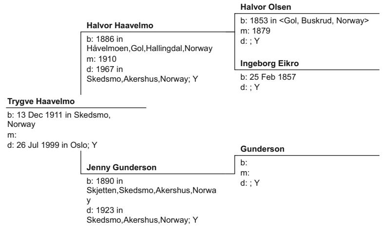
Fig. 27.1 Ancestry of the Haavelmofamily
(1913–84) and Trygve (13 December 1911–28 July 1999) retained the same Haavelmo family name (Fig. 27.1 ).
Th eir father, Halvor, grew up on a farm named Håvålmoen in Gol, but had the opportunity to complete school and attend the Elverum Teacher Training College. He passed the teaching exams in 1907 and took a teaching job in his village of Gol. A year later, he took a job in Skedsmo, about ten miles northeast of Oslo, where he spent the rest of his career.
Halvor was a successful and well-regarded teacher and principal in Skedsmo. He also was appointed mayor of Skedsmo for two terms, and sat for many years on its school board. He maintained an interest in athletics and encouraged sports for his sons as well. Th e younger son, Sverre, was a champion ski jumper at a ski hill Halvor helped establish.
Halvor became the town historian and published a number of volumes on local history. His children were provided every opportunity for a good education.
The Arrival of Trygve Haavelmo
Th e fi rstborn child of Halvor and his wife, Jenny, was born on 13 December 1911 in Skedsmo. While his younger brother had a strong interest in athletics, Trygve was more reserved and studious. His strong academic strengths allowed him to attend Oslo Cathedral School, one of the most elite schools in Norway, with a tradition dating back to its founding in 1153. It was the school of kings (Harald V), the famous painter of Th e Scream , Edvard Munch (1863–1944), the exceptional mathematicians, Caspar Wessel (1745–1818) and Niels Henrik Abel (1802–29), and the Nobel Prize winner Trygve Haavelmo . One of the oldest schools in the world, it retains a strong dedication to the liberal arts.
Trygve went on to study at the University of Oslo in 1930, not long after Ragnar Frisch had received his PhD at Oslo and had returned from his Rockefeller Scholarship in the USA. Like Frisch, when it came time to attend college, the elder son of Halvor Haavelmo was determined to fi nd a course of study at the University of Oslo that would allow him to graduate quickly. And, like Frisch a handful of years earlier, he settled on economics.
At Oslo in the early 1930s, Haavelmo gravitated immediately toward the Frisch , who was 15 years his senior, but only a decade more advanced in his studies because of Frisch’s family’s initial indecision whether Frisch should pursue his studies over the family jewelry business. Frisch and Haavelmo also shared a loyalty to Norway, gentle personalities, a strong quantitative orientation, but also with a fi rm theoretical foundation, and a determination to build their department for economic analysis at the University of Oslo. Perhaps Frisch was more evangelic in his agenda to extend better public policy analysis to a wider audience, while Haavelmo was more circumspect and studious. But, both seemed remarkably similar in their deep understanding of the unique problems in econometric and fi nancial quantitative analysis.
Upon his graduation in 1933, Haavelmo ’s mentor Frisch nominated him to join the Institute of Economics, which Frisch ran. Th ere he was assigned as Frisch’s assistant.
In these years at Oslo, Frisch traveled and visited the USA extensively. By 1936, Haavelmo was ready to pursue advanced study in statistics, and attended University College London, where he studied and worked directly with Egon Pearson, the son of Karl Pearson. During his stay at the University College London, he was undoubtedly drawn somewhat into the battle of the titans, Egon Pearson and Ronald Fisher . While Haavelmo remained loyal to his mentor Pearson, and Pearson’s brilliant colleague, Pearson’s co-developer of the likelihood ratio test, Haavelmo maintained a strong geometric intuition about statistics, which was much more closely aligned with Fisher.
Haavelmo also studied in Oxford, Berlin and Geneva, Switzerland, before he took on his fi rst academic position at the University of Aarhus in Denmark. He remained there for a year before he was aff orded the opportunity to visit and network in the USA in 1939 on a Rockefeller Foundation scholarship. Following completion of his Rockefeller Foundation scholarship, he became associated with the Cowles Commission, and remained in the USA to work on behalf of the Norwegian government’s Nortraship (Norwegian Shipping and Trade Mission) in New York City for the remainder of the war.
28. The Times of Trygve Haavelmo
In 1947, Haavelmo returned to Norway to take up a position alongside Frisch at the University of Oslo. He spent the balance of his career teaching at Oslo, with Frisch as his colleague.
It was his years in the USA before his return, though, that established Haavelmo as one of the fathers of modern econometrics, along with his mentor Frisch . Th ere he published results from his thesis in a 1943 Econometrica article entitled “Th e Probability Approach in Econometrics.”
By the war years, econometrics, especially as it was developed at Cowles , was immersed in the estimation of economic models and hypothesis testing of the signifi cance of these estimates. Haavelmo ’s thesis demonstrated that the state of analysis in econometrics at the time was misleading. To reduce complex interactions of various markets into one reduced-form equation was problematic.
Instead, Haavelmo developed a new paradigm to such econometric analyses in his years in the USA. He did so by applying more advanced tools from mathematical statistics he had gleaned both in his interactions with Jerzy Neyman and Egon Pearson, and in his discussions while at the Cowles Commission. His new theory of economic systems and their estimation was perhaps the single most insightful contribution to modern econometric theory and practice.
Indeed, once various members of the Cowles Commission obtained a copy of Haavelmo ’s PhD dissertation, they invited him to join the Commission and set up a special working group to understand and further his most important contribution.
Much of the interest the Cowles Commission expressed in Haavelmo ’s research can be attributed to the infl uence of Jacob Marschak . Marschak was universally renowned for his ability to spot and mentor young academic talent, and to recognize brilliant concepts. Many of these concepts he developed in his own mind and freely gave them to others to more fully explore, such as the application of the fi rst and second moment mean and variance measure of risk, which eventually formed the basis of the Great Minds Harry Markowitz’s (24 August 1927–) modern portfolio theory, James Tobin’s (5 March 1918–11 March 2002) portfolio separation theorem and William F. Sharpe ’s (16 June 1934–) CAPM . Each of these groundbreaking theories in fi nance were developed in or fl owed out of the work of individuals associated with the Commission under Marschak’s tutelage.
Marschak had come to know Haavelmo from Haavelmo’s New York City days in World War II immediately after he completed his PhD in 1941. While working on behalf of the Norwegian government in support of the war eff ort, Haavelmo attended a weekend econometrics seminar sponsored by Marschak and others. Immensely impressed with Haavelmo’s insights and intellect, Marschak asked Haavelmo to join the Cowles Commission, even if Haavelmo would be unable to physically reside at the Commission in Chicago. In fact, despite his immense infl uence on the Cowles Commission research agenda, Haavelmo was only in residence at Cowles in Chicago for about a year immediately following the end of World War II and his obligation on behalf of the Norwegian government. By March 1947, Haavelmo had returned to his home country to take up a teaching position at his alma mater.
Haavelmo ’s infl uence can be seen in a passage in the annual report for the Cowles Commission written by Marschak in 1943. Th ere he stated:
Th e method of the studies … is conditioned by the following characteristics of economic data and economic theory: (a) the theory is a system of simultaneous equations, not a single equation; (b) some or all of these equations include “random” terms, refl ecting the infl uence of numerous erratic causes in addition to the few “systematic” ones; (c) many data are given in the form of time series, subsequent events being dependent on preceding ones; (d) many published data refer to aggregates rather than to single individuals. Th e statistical tools developed for application in the older empirical sciences are not always adequate to meet all these conditions, and much new mathematical work is needed. To develop and improve suitable methods seems, at the present state of our knowledge, at least as important as the publication of studies on the general theory of economic measurements … It is planned to continue these methodological studies systematically. Th e available results of mathematical analysis are currently applied and tried out in econometric investigations; conversely, new situations arising in the course of practical work present new problems to the mathematician. It is intended to make this hand-in-hand work the basis of the Commission’s activities. 1
Marschak was essentially reading from the Haavelmo script. In doing so, the Cowles Commission was diverging from the original and more simplistic methodology of Alfred Cowles III himself, and into breaking ground and establishing the foundation for all of econometrics ever since. Th is was a period in which econometrics also diverged from its roots in biological statistics. In the latter class of problems, crosssectional data did not present the same sort of problems that fi nancial and market data present. Such data was at a particular point of time, and was typically not aggregated. When fi nancial variables evolve over time, and when economic data is aggregated, two types of problems emerge, as described by both Frisch and Haavelmo. Multicollinearity exists when one factor can infl uence multiple variables at once. In such a case, these multiple variables share similar trends, which makes diffi cult the researcher’s ability to pin the underlying trend down to one particular variable. Th e Frisch- Waugh theorem helped resolve this challenge. Trygve Haavelmo helped resolve the other—the problem of simultaneity and the identifi cation problem .
Note
- Christ, Carl F. (1994). “Th e Cowles Commission Contributions to Econometrics at Chicago: 1939–1955.” Journal of Economic Literature 32 (1), 1994, pp. 30–59, at p. 40.
29. Haavelmo’s Great Idea
Frisch had described implications of the statistical problems unique to econometrics and fi nance in his paper published in the Nordic Statistical Journal in his 1929 “Correlation and Scatter in Statistical Variables” and also in his 1934 book Statistical Confl uence Analysis by Means of Complete Regression Systems.1 Th is work was infl uential on Haavelmo , who followed up Frisch’ work with his Econometrica paper “Th e Statistical Implications of a System of Simultaneous Equations.” 2 Th e Haavelmo paper, at only a dozen pages long, set the agenda for the Cowles Commission over the next decade and econometrics ever since.
In that paper, Haavelmo described a three-equation representation of the determination of national income, and the challenges in the use of the traditional least squares regression model for its estimation. In a consumption- led economy, the consumption equation, as postulated fi rst by Frisch and then more formally by the Great Mind John Maynard Keynes , is the product itself of other underlying equations. It was well known in the discipline that, were the consumption equation not the product of other interactions, both the traditional least squares and its maximum likelihood estimate would be the same, under mild assumptions. Indeed, recall that Gauss had derived the least squares technique from a maximum likelihood perspective.
However, if one postulates that consumption is a linear function of an intercept, likened to Keynes ’ autonomous consumption term, and an induced term that rises proportionally with income, and if, in turn, income depends on the level of consumption spending, the simple linear least squares model is violated because random errors arise both in the simple equation and in the determination of income. Ronald Fisher had treated such a generalization in his maximum likelihood statistics at the beginning of the twentieth century. Haavelmo expanded this methodology of maximum likelihood estimation to both highlight when the least squares model creates biased estimations, and how the method of maximum likelihood can instead be employed.
As a brief example of Haavelmo ’s insights, consider the interaction between the aggregate supply of goods and services in an economy and its aggregate demand. Th e supply comes from the aggregated decisions of millions of market participants who formulate their decisions based in part on the income they would earn from their sales, and the factor payments they must pay to the resources they would employ.
Another equation might describe how the recipients of these factor payments use their income to purchase these same goods and services. In equilibrium , these two equations of aggregate demand and aggregate supply would intersect at an aggregate price and income.
Th e estimation of this system would provide perhaps a corresponding income at the intersection of these two equations. But, one discerned intersection point could actually be the product of many aggregate demand and supply curves. Th e mere identifi cation of the equilibrium intersection point, which is subject to some random error, sheds little light on the precise nature of the two underlying curves. Hence, a wide variety of parameters for candidates for the underlying curves could be consistent with the observed market variables.
Th is observation led to a new line of research that would become the basis for a most fruitful period of research by Cowles Commission fellows, and would lead these fellows to numerous Nobel Prizes. Among them are Nobel Laureates that include Tjalling Koopmans , Kenneth Arrow, Gérard Debreu, James Tobin (5 March 1918–11 March 2002), Franco Modigliani (19 June 1918–25 September 2003), Herbert A. Simon (15 June 1916–9 February 2001), Joseph E. Stiglitz (9 February 1943–), Lawrence Klein (14 September 1920–20 October 2013), Trygve Haavelmo , Leonid Hurwicz (21 August 1917–24 June 2008) and Harry Markowitz (24 August 1927–).
Haavelmo ‘s colleague at Cowles , Tjalling Charles Koopmans (28 August 1910–26 February 1985), one year Haavelmo’s senior, and a graduate of mathematics and economics at Netherlands’ Utrecht University and Leiden University, took up Haavelmo’s challenge. Koopmans had completed a PhD thesis “Linear Regression Analysis of Economic Time Series” in 1936 and had arrived in the USA just before Haavelmo. Koopmans took up Haavelmo’s challenge and, in 1949, published “Identifi cation Problems in Economic Model Construction” in Econometrica . 3
Koopmans , who had by 1949 taken over the helm of the Cowles Commission from Jacob Marschak , wrote:
Where statistical data are used as one of the foundation stones on which the equation system is erected, the modern methods of statistical inference are an indispensable instrument. However, without economic “theory” as another foundation stone, it is impossible to make such statistical inference apply directly to the equations of economic behavior which are most relevant to analysis and to policy discussion. Statistical inference unsupported by economic theory applies to whatever statistical regularities and stable relationships can be discerned in the data. Such purely empirical relationships when discernible are likely to be due to the presence and persistence of the underlying structural relationships, and (if so) could be deduced from a knowledge of the latter. However, the direction of this deduction cannot be reversed – from the empirical to the structural relationships – except possibly with the help of a theory which specifi es the form of the structural relationships, the variables which enter into each, and any further details supported by prior observation or deduction therefrom. Th e more detailed these specifi cations are made in the model, the greater scope is thereby given to statistical inference from the data to the structural equations. We propose to study the limits to which statistical inference, from the data to the structural equations (other than defi nitions), is subject, and the manner in which these limits depend on the support received from economic theory. 4
The vision of Frisch and Haavelmo had by 1949 been fully incorporated into the conventional thinking of econometricians and fi nancial theorists. Haavelmo went further, though. He also articulated an important role for our models to inform public policy. His 1943 paper was not only one of immense statistical signifi cance, but, in a strong Cowles tradition, provided a mathematical laboratory by which policy makers can “experiment” within the economy without holding economic players hostage as laboratory animals. Th is is the avenue of causal inference .
Th is expansion of the role of decision-making theory remains controversial. Often theorists limit their roles to the description of the world around us, not necessarily its activist evolution. Perhaps economists are more susceptible to this doctrinaire trap than fi nancial theorists. After all, fi nancial theory is rarely limited to simple understanding. Some scholars may harbor the profi t motive, as are all fi nancial practitioners. Others develop their theories to correct market imperfections and improve upon their effi ciency.
Often, the Nobel Memorial Prize Committee tries to set an activist scholarly tone, in the interest of Alfred Nobel, who devoted his fortune to not only the description of the world, but also its improvement. Th e Nobel Memorial Prize committee was making a statement in awarding Haavelmo noted:
During the 1930s, noteworthy attempts were made to test economic theories empirically. Th e results of these attempts called attention to two fundamental problems associated with the possibility of testing economic theories. First, economic relations often refer to large aggregates of individuals or fi rms. Th eories regarding such relations can never be expected to conform fully with available data, even in the absence of measurement errors. Th e diffi cult question then is to determine what should be considered suffi ciently good, or better conformity. Second, economists can seldom or never carry out controlled experiments in the same way as natural scientists. Available observations of market outcomes, etc., are results of a multitude of diff erent behavior and relations which have mutually interacting eff ects. Th is gives rise to interdependence problems, i.e., diffi culties in using observed data to identify, estimate, and test the underlying relations in an unambiguous way.
In his dissertation from 1941 and a number of subsequent studies, Trygve Haavelmo was able to show convincingly that both fundamental problems could be solved if economic theories were formulated in probabilistic terms. Methods used in mathematical statistics could then be applied to draw stringent conclusions about underlying relations from the random sample of empirical observations. Haavelrno demonstrated how these methods can be utilized to estimate and test economic theories and use them in forecasting. He also showed that misleading interpretations of individual relations due to interdependence cannot be avoided unless all relations in a theoretical model are estimated simultaneously.
Haavelmo was also recognized for his identifi cation of the interdependence problem. Th e committee noted:
In economic life, every individual decision may be regarded as aff ecting all other decisions through a chain of market relations. Th is economic interdependence creates problems in empirical research because an observed market outcome is the result of a large number of simultaneous or previous decisions and behavioral relations. Th us, an underlying relation can never be observed, as it were, in isolation, but only as conditioned by a number of other simultaneous relations and circumstances in the economy. As Haavelmo showed, interdependence gives rise to diffi culties in specifying, identifying and estimating economic relations.
Th e committee also recognized his marriage of econometrics with thoughtful economic theory when it added:
Once the foundation of probabilistic econometrics had been established, Haavelmo ’s next important research eff ort involved attempts to transform various components of economic theory so that the new econometric methods would be applicable. According to Haavelmo, the prerequisites for achieving this purpose were not only additional assumptions about probability distributions, but also in many instances a more dynamic theoretical formulation. Th ere are two areas in particular – investment theory and economic development theory – where Haavelmo’s approach has resulted in infl uential and far-reaching contributions. In addition to these main lines of research, Haavelmo’s achievements include valuable contributions in numerous areas – from analysis
of macroeconomic fl uctuations and fi scal policy to price theory and the history of economic thought. 5
Haavelmo also made another memorable contribution. In 1944, he wrote a major monograph, “Th e Probability Approach in Econometrics.” 6 In this groundbreaking statement on experimental design, Haavelmo observed:
Th e aim of econometrics, as you may read it on the cover of every issue of Econometrica, is “Th e Advancement of economic theory in its relation to Statistics and Mathematics.” Th at is, econometrics should be an attempt, not only towards more precision in the formulation of economic theories, but perhaps still more an attempt to reach such formulations that the theories lend themselves to testing against actual observations.
So far, however, it seems that most of the energy has been spent on constructing rational models, involving exact relationships that are much too rigid if we would try to identify the theoretical variables involved with some actually observable economic quantities.
Th e relation between such exact economic models and economic reality is, of course, in point of principle similar to the relation between rational mechanics and the bodies and motions observed in the real physical world. But the diff erence in the degree of precision is and is probably always going to be tremendous. In economics it is therefore not suffi cient fi rst to set up a system of exact relationships and then allow for certain small deviations in the applications of facts. We shall have to start out with a probabilistic formulation of our models, from the beginning, otherwise we shall either have to call all our theories wrong or we may call almost any theory right by allowing for suffi ciently large discrepancies (in a subjective manner). 7
Haavelmo elaborated:
What makes a piece of mathematical economics not only mathematics but also economics is, I believe, this: When we set up a system of theoretical relationships and use economic names for the otherwise purely theoretical variables involved, we have in mind some actual experiment, or some design of an experiment, which we could at least imagine arranging, in order to measure those quantities in real economic life that we think might obey the laws imposed on their theoretical namesakes. 8
Th is observation required scholars to fully understand the nature of the variables included in an analysis. Inherent is the notion of autonomy , which he coined to indicate those variables that are not aff ected by others in the analysis, but will in themselves aff ect the analysis. He was also begging the question of causality. Just as Frisch painstakingly described the causality of money supply on consumption and investment through one pathway, and the causality of consumption and investment on output and money demand through another, the econometrician must be most mindful of the way models are constructed, the carefully considered reasons why some variables are considered independent, and others dependent, and how multiple equations in this model are combined and interact. He introduced the important intuition of simultaneity in the equations that govern a model, and warned about the imprudent or careless use of reduced-form equations to summarize other more complex interactions.
Haavelmo went on. He reminded econometricians that “whatever be the ‘explanations’ (of economic relationships) we prefer, it is not to be forgotten that they are all our own artifi cial inventions in a search for an understanding of real life; they are not hidden truths to be ‘discovered.’” 9
Haavelmo also argued, convincingly, if disturbingly, that we implicitly assume the dependent variables we model are a function of a number of independent variables, each which may be prone to its own measurement error, but each which also may be probabilistic in itself—that is, drawn from a range of possible values according to some sort of probability distribution function. Indeed, these independent variables may be, and often are, interrelated, so that joint probability distributions may govern these observations. To merely characterize the relationship between the dependent and the independent variables as accurate, but for a random and identically and independently distributed “measurement” error, is thus simplistic. Th e resulting statistics and confi dence become misleading.
Econometricians were at fi rst taken aback by Haavelmo ’s challenge. Gradually, though, there was growing acceptance about the limitations of such modeling.
Haavelmo was infl uential, if not thoroughly so. Before his monograph, econometricians worried more about their confi dence in the estimation of coeffi cients in a given regression analysis, and less in the signifi cance of the overall model. Following Haavelmo’s line in the sand, individual coeffi cient estimates drawn from probabilistic draws of the corresponding independent variable were deemphasized in favor of the consideration of the overall model, just as Fisher had asserted two decades earlier.
Another implication of his philosophical stance on econometric model building came from the ensuing Monte Carlo technique. In this simulation technique, random draws of independent variables from some predetermined probability distribution function are allowed to “determine” values of corresponding dependent variables. By repeating such draws and predictions, the econometrician can better explore the eff ect of randomness in the draws of independent variables on model outcomes. Without an acknowledgment of the probabilistic nature of economic variables, there would have been little utility in the determination of model robustness through Monte Carlo simulations.
Th is approach was a rich one for the Cowles Commission. With the challenges of Frisch and Haavelmo at hand, many members of the Cowles Commission made signifi cant theoretical and applied econometrics contributions using the Monte Carlo simulation method to test the robustness of econometric modeling results.
Th ese researches in turn resulted in much better understanding of macroeconomic and fi nancial modeling. Indeed, the adopted tool of Monte Carlo simulations, with its explicit acknowledgment of the probabilistic nature of observations on the right-hand side of our fi nancial models, is now a standard methodology in the fi nancial theorist’s toolbox.
Notes
- Frisch , Ragnar, Statistical confl uence analysis by means of complete regression systems , Universitetets Ã, konomiske institutt, 1934.
- Haavelmo , Trygve, “Th e Statistical Implications of a System of Simultaneous Equations,” Econometrica , Vol. 11, Issue 1, 1943, pp. 1–12. Bjerkholt, Olav, “Tracing Haavelmo’s steps from Confl uence Analysis to the Probability Approach,” Memorandum 25/2001 , University of Oslo Department of Economics and the Frisch Center for Economic Research, May 2001, at p. 29.
- Koopmans , Tjalling C, “Identifi cation problems in economic model construction.” Econometrica 17 (2), 1949, pp. 125–144.
- Ibid. at 126.
- “Th e Prize in Economics 1989 Press Release.” Nobelprize.org. Nobel Media AB 2014. Web. 16 March 2016. <http://www.nobelprize.org/nobel_prizes/ economic-sciences/laureates/1989/press.html>
- Haavelmo , Trygve, “Th e Probability Approach in Econometrics.” Supplement to Econometrica, Vol. 12, July, 1944, pp. S1–S115.
- Bjerkholt, Olav, “Tracing Haavelmo ’s Steps from Confl uence Analysis to the Probability Approach,” Memorandum 25/2001 , University of Oslo Department of Economics and the Frisch Center for Economic Research, May 2001, at pp. 27–28.
- Ibid, at p. 5.
- Ibid. at p. 3.
30. Legacy and Later Life of Trygve Haavelmo
Haavelmo explained the reason why our world of fi nancial econometrics may be more complicated than some would like to believe. While he off ered clarity in the reasons why simultaneity of equations and the probabilistic nature of observations must be further considered, members of the Cowles Commission were only partially successful in their completion of Haavelmo’s agenda. It would take decades to fully digest Haavelmo’s observation, and to develop methods such as Monte Carlo simulations, non-parametric testing tools and tests of causality. However, eventually, the discipline made headway.
It should then come as no surprise that the discipline took so long to award Haavelmo with its most important prize, the Sveriges Riksbank Prize in Economics Sciences in Memory of Alfred Nobel in 1989. Indeed, while Haavelmo committed to a lifetime of scholarly work, and had made contributions in his later career to economics and public policy before his retirement in 1979, the Committee noted Haavelmo’s work in probability and in simultaneity :
Th e Sveriges Riksbank Prize in Economic Sciences in Memory of Alfred Nobel 1989 was awarded to Trygve Haavelmo “for his clarifi cation of the probability theory foundations of econometrics and his analyses of simultaneous economic structures.” 1
Haavelmo accepted the award with characteristic modesty. He noted, “I am honored. Anyone would be. But I had nothing to do with making this award. I really have nothing to say,” Haavelmo commented. He further added that the prize “is quite irrelevant to the real issues. I’m exhausted and I have nothing more to say.” 2
Despite his modesty and some of the regrets he shared with Frisch , Haavelmo was recognized well in his life. Over his lifetime, Haavelmo was named a Fellow of the Econometric Society, and the Institute of Mathematical Statistics. He was also a member of the Norwegian Academy of Sciences, the Council of the Econometric Society and the Danish Academy of Sciences. He presided over the Econometric Society in 1957, was named an Honorary Member of the American Economic Association in 1975 and won the Fridtjof Nansen Award for Outstanding Research in 1979. He was a member of the American Academy of Arts and Sciences. He lived out his career at the University of Oslo and retired a Professor Emeritus. He remained unmarried throughout his life.
Increasingly, his research turned to broader economic issues. In 1954, he published a book entitled A Study in the Th eory of Economic Evolution , which performed groundbreaking work on the path by which nations develop economically. Th is book is a cornerstone of economic development theory and was one of the earliest pieces of formal scholarship in this area.
Haavelmo also made a direct contribution to fi nance, with implications on fundamentals analysis. His 1960 A Study in the Th eory of Investment modeled the demand for capital and the sluggishness in its supply. His work has been the basis of much follow-up scholarship that models investment behavior. Haavelmo has also treated environmental economics issues, again well before it became a sub-discipline of its own.
It is often diffi cult for one’s peers who view their colleagues in a more intimate light to gauge the profound, and sometimes forgotten, contributions of someone with whom they may share a department or a nation. Within Norway, Haavelmo is often spoken of much like Frisch —as a teacher and a public servant. While at the Institute of Economics at the University of Oslo, where he began and he subsequently ended his career, he was often the fi rst contact with many students on a variety of their economic interests, just as Frisch was for him. He left a multitude of research students who benefi ted from his academic generosity in the years 1948–1979.
Ten years after he retired from his position of Professor of Economics and Statistics, his contribution was cemented with the awarding of the 1989 Nobel Memorial Prize. By then, though, and up to his death in the Oslo neighborhood of Østerås, Norway, on 28 July 1999, he was remembered as an economic legend by some and as a mentor by many others.
When one asked him once why he returned home to Norway after such a productive decade in the USA in the late 1930s and part of the 1940s, he replied he missed trout fi shing. When his friend pointed out that there is excellent trout fi shing in the USA, Haavelmo noted that they weren’t “Norwegian trout.” 3
Notes
- “Th e Sveriges Riksbank Prize in Economic Sciences in Memory of Alfred Nobel 1989,” Nobelprize.org. Nobel Media AB 2014. Web. 25 March 2016. <http://www.nobelprize.org/nobel_prizes/economic- sciences/ laureates/1989/>
- http://articles.latimes.com/1989-10-12/news/mn-294_1_economics- nobelprize, accessed 16 March 2016.
- Bjerkholt, Olav, “Tracing Haavelmo ’s steps from Confl uence Analysis to the Probability Approach,” Memorandum 25/2001 , University of Oslo Department of Economics and the Frisch Center for Economic Research, May 2001, at p. 30.
Part 5: What We Have Learned
Th is book is the seventh in a series of discussions about the great minds in the history and theory of fi nance. It is somewhat unique in this series in that the other treatments demonstrated a relatively straight line of innovation, with each contribution by a great mind shoring up and expanding the contributions of those who came before.
Th e Great Minds that gave rise to econometrics, though, are much more varied. Th ey included one of humankind’s greatest mathematicians, a charismatic explorer, an early biometrician and an agricultural statistician. From their work in an evolving statistics, an applied mathematician in the USA, a fi nancial entrepreneur and a pair of scholars from Norway turn statistics into the econometric tools now used by fi nancial theorists. We conclude with a brief summary of their collective contributions.
31. Conclusions
Quantitative methods underpin modern fi nancial analysis. Th ese methods combine mathematical techniques developed by Great Minds documented in the series volume Rise of the Quants and the statistical techniques developed by the Great Minds described here.
Th ese econometricians and statisticians fi rst identifi ed problems distinct from those that challenge fi nancial theory. A wave of innovation began with a very practical problem—to predict the movement of planets and other orbiting bodies. Th e fascination with these astronomical movements predated modern computing and simulation methods, so these fi rst analyses had to be performable merely with pen and paper. With necessity as the mother of invention, scholars beginning with Carl Friedrich Gauss and ending with Trygve Haavelmo all derived profound intuitions for how we can organize data generated from the world around us just before the invention of the computer. Th en, with the aid of computerization and numerical methods, the quants took things from there.
Gauss was the fi rst of this handful of scholars to create a compact order from a complex universe. In doing so, he gave us three fundamental tools of modern fi nance: the normal distribution , maximum likelihood estimation and the method of least squares . He even introduced us to the intuition of the central limit theorem, a result that his colleague and friend Pierre-Simon , the Marquis de Laplace generalized in a way that have provided us much intuition ever since. One cannot compete a foundational tract in statistics within our university fi nance curricula without an indoctrination of Gauss’ contributions.
Across the English Channel in the mid-nineteenth century, as Gauss was reaching the eve of his life, an explorer and man of leisure with a remarkable ability to sense the pulse of populism, Sir Francis Galton , was creating in his own mind a theory of eugenics just as his famous cousin Charles Darwin was revolutionizing the theory of evolution. Galton needed some rudimentary statistical techniques to support his hypotheses, and applied some of the insight of Gauss and his method of least squares to demonstrate such tendencies that the height of subsequent generations tends to “regress” toward the mean of their parents’ heights. Galton was no mathematician, though, so it is entirely possible that the statistical movement he fueled with his intuition was not initially informed by Gauss’ brilliance that came before him.
It took Galton ’s successors, fi rst Karl Pearson, and then Ronald Fisher , to create fi rst the measures of basic statistics, some of which Gauss had developed a century later, and then the geometric interpretation for modern hypothesis testing, again by applying the techniques so masterfully developed by Gauss.
Th e story told described a clash of personalities that created a toxic statistical environment on one side of the Atlantic to the point that the statistics discipline could not progress effi ciently until it was eff ectively transplanted to the other side of the Atlantic Ocean. In the USA in the 1920s and 1930s, Harold Hotelling advocated for the statistics and the department that would develop them, and began to use the tool to answer questions of economic and fi nance signifi cance. But, Hotelling had an active mind that drew him in many directions.
It would take a fi nancial entrepreneur and practitioner willing to devote a portion of his family’s fortune to further develop and popularize techniques that could be applied to modern fi nance. Alfred Cowles III, called Bob by his family and friends, created a Cowles Commission for which almost every leading econometrician from Ragnar Frisch to Harry Markowitz and beyond was associated.
Cowles ’ vision for his commission gave rise to the Econometric Society and the journal Econometrics that would do for fi nancial statistics what Biometrika did for biological statistics. He also originated important concepts himself, such as the notion of the random walk and the effi cient market hypothesis .
Our story ends with two individuals. One helped form the Econometric Society and edited its journal for 21 years, and defi ned the problems that make economics and especially fi nance distinct from the statistics of biology. Ragnar Frisch is still considered a father of modern econometrics. It was his Norwegian colleague and prodigy, Trygve Haavelmo , though, who almost single-handedly inspired the agenda which the Cowles Commission would adopt to establish a discipline distinct from mathematical statistics.
Trygve Haavelmo and Ragnar Frisch each won Nobel Memorial Prizes for their contributions. Th e committee recognized these individuals, fi rst in 1969, in the fi rst year of the award, and then two decades later, in 1989, for contributions that may have been diffi cult to understand and absorb at the time, but which were eventually fully incorporated into our toolbox of methods to properly employ data in our fi nancial models.
Th e story does not end with the Cowles Commission of the 1940s, though. From there, Cowles members such as the Great Minds Jacob Marschak , Harry Markowitz and Kenneth Arrow took the results of the Cowles Commission of the 1940s and created the plethora of tools now employed in quantitative fi nance. Th ese subsequent innovations were documented in the book in this series entitled “Th e Rise of the Quants.” We now rely on the mean and variance approach that arose fi rst from the explorations of Carl Friedrich Gauss , a remarkable Great Mind who also spurred the creation of modern statistics and regression modeling.
Th e works of these individuals have defi ned fi nance theory ever since. Th eir contributions allow us to summarize data, construct and then test fi nancial models, and have allowed both practitioners and policy makers to digest huge amounts of data to enhance the effi ciency of our modern markets and economies. Th e modern-day products of their contributions are the test of the genius of the Great Minds described here.
Glossary
Arithmetic Mean A central tendency of a series of numbers based on their sum.
Asymptotic The value a variable converges on in the limit as time goes to infinite.
Binomial Model An options pricing methodology that breaks the dynamic path of the derivatives into a series of steps at various points in time between the valuation date and the expiration date.
Capital Asset Pricing Model A model that relates risk and expected returns based on a mean and variance approach.
Center of Mass A concept in physics in which the sum of the relative positions of mass, weighted by their respective masses, sums to zero.
Classical Model A cohesive set of microeconomic theories about the way markets attain equilibrium.
Collinearity Also called multicollinearity, occurs when two or more independent variables in a multiple regression model are correlated with each other, and thus, one of the variables can be predicted by the other.
Complex Analysis A theory of functions involving complex numbers.
Complex Number A number that can be represented as the sum of a real and an imaginary component.
Constructable Polygon A regular polygon that can be constructed solely through the use of an unmarked compass and straightedge.
Correlation The statistical relationship between two variables. It is typically measured by demonstrating that the movement of one variable is associated with the movement of other.
Correlation Coefficient Most commonly, the Pearson correlation coefficient measures the degree of linear association between two variables.
Covariance A measure of the degree to which returns on two risky assets are correlated in their movement.
Cowles Commission A research institute founded by Alfred Cowles to provide for the theory and decision science that can help explain financial markets.
Derivative In mathematics, the instantaneous rate of change of one variable as a function of the change of another. In finance, a financial instrument that derives its value from another underlying asset or instrument.
Dynamic The analysis of a process as it changes over time.
Econometrics The set of tools used to demonstrate predictable statistical correlations between financial and economic variables.
Efficient Market Hypothesis A theory based on the premise that one cannot systematically beat the market because market prices already properly incorporate all available information.
Equilibrium A state in which all relative forces of influence are in balance and the system remains steady.
Eugenics The science of improvement in humankind through controlled breeding for desirable human characteristics.
Fermat Number A number that can be expressed as 2 1 2n + , where n is a positive integer.
Fermat Prime A prime number, defined as one that can only be divided without a remainder by itself and one, that is also a Fermat number.
First Moment The mean of a variable that can be described by a known probability distribution function.
Frisch-Waugh Theorem A theorem that shows the regression coefficients generated from two variables with a common trend in a least squares regression are identical to the coefficients obtained if the common trend is first removed from the variables.
Gauss-Markov Theorem States that the coefficients generated in an ordinary least squares regression model in which errors have expected values of zero, are uncorrelated, and have equal variances are linear unbiased estimates.
General Theory of Relativity An extension of the Special Theory of Relativity to include bodies that are accelerating.
Geometric Mean A measure of central tendency of a set of numbers based on their product rather than their sum.
Goodness of Fit A model or measure that describes how well a postulated distribution describes a set of observations. The measure is usually a summary statistic that describes the difference between observed and predicted values.
Heteroscedasticity A concept which describes an explanatory variable which exhibits variability that is not constant over the range of the dependent variable that it predicts.
Identification Problem A failure to be able to determine a consistent and an accurate estimate of as statistical relationship because the equation is actually representative of a complex set of other relationships.
Imaginary Number A multiple of the square root of −1.
Independent and Identically Distributed An assumption that each random variable shares the probability distribution as other random variables in the relationship, but each variable is mutually independent.
Intertemporal Models and relationships that include variables which change over time.
Least Squares A method to solve for the relationship between a dependent variable as a weighted sum of independent variables. This technique minimizes the squared difference between the dependent variable and the predicted amount from an estimate of a weighted combination of the independent variables. Before the recent advent of significant computing power, this readily calculable technique was used to estimate relationships between dependent and independent variables.
Keynesian Model A model developed by John Maynard Keynes that demonstrates savings may not necessarily be balanced with new investment and the gross domestic product may differ from that which would result in full employment.
Mean A mathematical technique that can be calculated based on a number of alternative weightings to produce an average for a set of numbers.
Modern Portfolio Theory The set of techniques developed in the 1950s by Harry Markowitz to design optimal portfolios and the most efficient risk-reward tradeoff.
Moment Generating Function A characterization of a random variable X which equals the expected value of the random variable.
Monte Carlo Simulations An algorithm that repeats simulations of a postulated financial relationship with random elements. The Monte Carlo simulation often reveals patterns that cannot be gleaned by analytic methods.
Normal Distribution of Returns A distribution that follows a prescribed and a symmetric pattern that occurs frequently in natural processes.
Number Theory A branch of algebra that considers properties of numbers.
Ordinary Least Squares A methodology that fits a straight line through a number of points to minimize the sum of the squares of the distances from the best fit lines to the points.
P-value Also called the calculated probability, is the probability of finding the observed results when the null hypothesis H0 is true.
Polar Coordinates The description of points on a Cartesian or Complex plane based on their distance and orientation from the origin.
Polygon A multisided geometric shape with at least three sides and angles.
Probability Density Function A function of a continuous random variable that can be integrated over an arbitrary interval to determine the probability that the value of the variable falls within the interval.
Random Walk The expectation that a security return at time t is equal to its last period value plus a stochastic (random) component that is an independent and identically distributed with zero mean and variance σ2
Real Number A number that can represent the distance along the number line.
Rectangular Coordinates The description of points on a Cartesian plane based on the distance from the origin in the direction of each of the dimensions.
Regression A technique used to fit a dependent variable as a weighted sum of independent variables.
Regular Polygon A polygon for which each apex is equiangular and each side is of the same length.
Second Moment A weighted measure of the deviation of a random variable from its mean or first moment.
Simultaneity A condition that occurs when an independent variable and the postulated dependent variable influence each other.
Special Theory of Relativity Einstein’s theory that specified the relationship between space and time. It is based on the concepts that physical laws are identical for all non-accelerating frames of reference, and that the speed of light in a vacuum is a constant for all observers, regardless of their motion relative to the light source.
Standard Deviation A measure of the spread of numbers, as calculated by the square root of their variance.
Static The consideration of mathematical, physical, or economic relationships that do not change over time.
Student’s t Describes properties of the mean of small samples from a normal distribution when the population standard deviation is unknown.
Taylor’s Series The expression of the range of a function arising from deviations of its domain as represented by an infinite series of the function’s derivatives and the deviations of its domain.
Type-I Error The incorrect rejection of a correct null hypothesis. This rejection is often called a false positive.
Type-II Error The failure to reject a false null hypothesis. This acceptance is often called a false negative.
Unit Circle A circle centered at the origin of orthogonal axes and with a radius of unit length.
Variance A specific measure of the sum of distances of a set of data points around their mean value. These distances can be calculated by summing the square of the coordinates for each point.
Volatility A measure of the degree of uncertainty and unexplained movements of a variable over time.
Index
| A | C |
|---|---|
| Adrian, Robert , 46 | capital asset pricing model |
| Aitken, Alexander Craig , 134, | (CAPM) , 79 |
| 137n2 | Cardano, Girolamo , 20, 21 |
| Al-Khwarizmi , 19 | Cayley, Arthur , 134, 137n1 |
| asympotic , 167–9 | center of mass , 40, 49, 54, 149 |
| Chebyshev, Pafnuty , 56 | |
| Classical Model , 251 | |
| B | Cliff ord, William , 89, 90 |
| Bell, Eric , 157, 158 | collinearity , 229 |
| Bernoulli, Jacob , 47, 49, 50, 56, 65, | Columbus, Christopher , 38 |
| 91 | complex analysis , 30, 64 |
| Born, Max , 12 | complex number(s) , 17–31, 41 |
| Boscovich, Roger , 37 | Comte, Isadore , 76 |
| Brahe, Tycho , 48 | constructable polygon , 16, 29 |
1 Note: Page number followed by n denote footnotes
© Th e Author(s) 2016 257 C. Read, Th e Econometricians, Great Minds in Finance, DOI 10.1057/978-1-137-34137-2
| correlation coefficient, 79, 95, 96, | Ferro, Sciopione del, 19, 20 |
|---|---|
| 104, 120, 124, 125, 132, | Feynmann, Richard, 24 |
| 133 | Fiore, Antonio Maria, 19, 20 |
| Cotes, Roger, 25, 26, 37, 39, 40, 49 | Fisher, Irving, 193, 205, 206, 212 |
| Cowles, Alfred III, vii, 177–89, | Fisher, Ronald, vi, 105, 109, |
| 191–200, 200n1–8, 248 | 111–27, 129–37, 139–58, |
| Cremona, Gerald of, 19 | 192, 205, 226, 232, 248 |
| Friedman, Milton, 1vii, 96 | |
| Frisch, Ragnar, vii, 7, 97, 195, 196, | |
| D | 201–10, 210n1, 211–17, |
| Darwin, Charles, 70, 72, 73, 78, 83, | 217n1, 217n2, 219–22, |
| 99, 116, 117, 120, 121, 248 | 225–7, 229, 231, 234, 237, |
| Darwin, Horace, 117 | 238, 238n1, 238n2, 239n7, |
| Darwin, Leonard, 117, 120 | 242, 243, 243n3, 248, 249 |
| Davis, Harold Thayer, 191, 192, | Frisch-Waugh theorem, 220, 229 |
| 207, 208, 219 | Fry, Thornton, 192 |
| derivative, 50, 54, 79, 166 | F-statistic, 165 |
| Descartes, Rene, 21, 22 | |
| Dirichlet, Peter, 12 | |
| dynamic, xi, 197, 206, 212, 217, | G |
| 217n1–2, 235 | Galton, Francis, vi, 67–73, 75–84, |
| 86, 90–5, 99–101, 104, | |
| 105, 109, 112, 115–18, | |
| E | 121–3, 132, 140, 143, 149, |
| Eddington, Arthur, 34 | 175, 196, 248 |
| Edgeworth, Francis, 94, 172 | Gauss, Carl Friedrich,, vi, 3-31, |
| Einstein, Albert, 16, 30, 33, 34, 61, | 33–67, 75, 76, 78–80, 83, |
| 64, 90–2, 105–7 | 90, 91, 94, 99, 100, 104, |
| equilibrium, 145, 197, 212, 232 | 118, 124, 127, 129, 130, |
| eugenics, vi, 65, 66, 70, 78, 81, 82, | 133–5, 147, 149, 165–7, |
| 90, 100, 101, 104, | 175, 195, 232, 247–9 |
| 116–20–122, 141, 143, | Gauss-Markov Theorem, 46 |
| 144, 161, 196, 222, 248 | general theory of relativity, 33, 34, |
| ,,, , , | 90, 92, 107 |
| geometric mean(s), 11, 14–16, 23, 30 | |
| F | Glover, James, 192 |
| Fermat, Pierre de, 30, 46, 48 | goodness of fit, 78, 90, 94, 95, 97 |
| Fermat prime, 29 | Gosset, W.S., 123–5, 160, 161 |
| • | |
| Fermi, Enrico, 12 | Gresham, Thomas, 93 |
| H Haavelmo, Trygve, vii, 196, 197, | L Lagrange, Joseph-Louis, 9, 30, 31 Lambert, Johann, 42 least squares, vi, 9, 11, 23, 26, 34, 37, 40–6, 50, 53, 57, 59, 61, 64–6, 76, 79, 95, 97, 104, 133–7, 147, 165, 175, 191, 197, 213, 214, 216, 231, 232, 237, 248 Legendre, Adrien-Marie, 30, 43–5, 53, 56n3, 57, 59, 64 Leibniz, Gottfried, 44 Lexis, Wilhelm, 94 Lorenz, Ludvig, 17 |
|---|---|
| Humboldt, Friedrich, 61, 62 | Lyapunov, Aleksandr, 56 |
| identification problem, 229, 233, 238n3 imaginary number, 13, 18, 20, 22–4, 27, 30 independent and identically distributed, 46, 54, 237 |
Malthus, Thomas, 77 Markov, Andrey, 56 Marschak, Jacob, vii, 196, 197, 219–21, 228, 229, 233, 249 Maxwell, James, 61, 86, 87 mean(s), vi, ix, 4, 8, 11, 12, 14–16, |
| Johnson, Alvin, 196 | 19, 21, 23, 30, 36, 37, 39–41, 45, 46, 48, 50–4, 56, 57, 72, 75, 79, 91, 94, 95, 97, 100, 123, 127, 129, 131, 132, 135–7, 142, 146, 147, 161, 166, 209, 214, 215, 221, 228, 231, 238n1, 248, 249 |
| Kepler, Johannes, 38 Keynes, John Maynard, 117, 211, 212, 231, 232 Kohlrausch, Rudolf, 61 Koopmans, Tjalling, 197, 232, 233, 238n3 |
Mendel, Gregor, 116 Michelson, Albert, 17 Mill, John Stuart, 100, 107 Modigliani, Franco, 196, 198, 233 Moivre, Abraham de, 22, 24, 28, 46, 48, 50, 56, 91 |
| moment- generating function , 54, 56 | Q |
|---|---|
| Morgan, J.P. , 12, 179 | Quetelet, Lambert Adolphe , 75–8, |
| Morley, Edward , 17 | 91, 94, 109, 123 |
| N Newton, Isaac , 4, 9, 22, 25, 39, 44 normal distribution , vi, 45, 46–56, 76, 90, 91, 93–6, 123, 125, 129, 166, 195, 213, 247 number theory , 13, 30, 41, 157, 172 |
R Ramsey, Frank , 171, 172 real number , 17, 22, 24, 50 Rectangular coordinates , 254 regression(s) , xi, 46, 76, 79, 80, 95–7, 104, 125, 131–5, 137, 191, 192, 194, 213–17, 217n3, 231, 233, |
| O | 237, 238n1, 249 |
| Occam’s Razor , 39 | regular polygon(s) , 10, 13, 15, 16, |
| Ockham, William of , 39 | 27, 28, 33 |
| Olbers, Heinrich , 34, 42 | Ricardo, David , 70, 71 |
| Oppenheimer, Robert , 12 | Riemann, Bernhard , 12 |
| ordinary least squares , 79, 214 | Roos, Charles , 195, 206–8, 219 |
| P | S |
| Pascal, Blaise , 46–8 | Samuelson, Paul , 194 |
| Pauli, Wolfgang , 12 | Savage, Jimmie , 146 |
| Pearson, Egon , 103, 104, 126, 127, | Schumpeter, Joseph , 207, 208, |
| 140, 141, 143, 226, 227 | 211, 220 |
| Pearson, Karl , vi, 80, 82–7, 89–97, | Sharpe, William , 228 |
| 99–107, 116, 118, 120–2, | Simon, Herbert , 73, 77, 198, 233 |
| 125, 140, 141, 160, 226, | simultaneity , 229, 237, 241 |
| 248 | Snedecor, George Waddel , 142 |
| Piazza, Guiseppe , 33, 34 | Special Th eory of Relativity , 107 |
| Pisa, Leonardo da , 19 | standard deviation , 50, 80, 93, 94, |
| Planck, Max , 12 | 104, 121, 124, 166 |
| polar coordinates , 26 | static(s) , 92, 196, 206, 212, |
| polygon(s) , 10, 13–16, 27–9, 33, 59 | 217n1 |
| probability density function , 40, | Stratton, J. M. , 118, 121, 123, 130, |
| 45, 53 | 160 |
| P-value(s) , 104 | Student’s t , 132, 142, 160 |
| T | W |
|---|---|
| Tartaglia, Niccolo , 19, 20 | Wald, Abraham , 161, 169 |
| Turnbull, Herbert Westren , 134, 137n2 | Wallis, John , 21, 22 |
| type-I error , 104 | Waugh, Frederick , 211, 213, 214, |
| type-II error , 104 | 217, 220 |
| Weber, Wilhelm , 60–2 | |
| Weldon, Walter , 92, 93 | |
| U | Wessel, Caspar , 22, 23, 26, 225 |
| unit circle , 13, 15, 26–8 | Williams, John Burr , 165, 179 |
| V | Y |
| variance(s) , vi, 46, 52–5, 91, 93, 94, | |
| Yntema, Th eodore , 219, 220 | |
| 96, 97, 121–4, 127, 129–31, | Yule, G. Udny , 126 |
| 135, 136, 140, 142, 147, | |
| 166, 167, 189, 228, 249 | |
| Z | |
| Veblen, Oswald , 158, 167 | |
| Veblen, Th orstein , 158 Verrezzano, Giovanni , 38 |
Zach, Franz von , 34 Zimmerman, Duke Carl Wilhelm , |