Learn Python Programming
Learn Python Programming
A Comprehensive, Up-to-Date, and Definitive Guide to Learning Python
Fourth Edition
Fabrizio Romano
Heinrich Kruger

Learn Python Programming
Copyright © 2024 Packt Publishing
All rights reserved. No part of this book may be reproduced, stored in a retrieval system, or transmitted in any form or by any means, without the prior written permission of the publisher, except in the case of brief quotations embedded in critical articles or reviews.
Every effort has been made in the preparation of this book to ensure the accuracy of the information presented. However, the information contained in this book is sold without warranty, either express or implied. Neither the author, nor Packt Publishing, and its dealers and distributors will be held liable for any damages caused or alleged to be caused directly or indirectly by this book.
Packt Publishing has endeavored to provide trademark information about all of the companies and products mentioned in this book by the appropriate use of capitals. However, Packt Publishing cannot guarantee the accuracy of this information.
Early Access Publication: Learn Python Programming
Early Access Production Reference: B30992
Published by Packt Publishing Ltd.
Grosvenor House
11 St Paul’s Square
Birmingham
B3 1RB, UK
ISBN: 978-1-83588-294-8
Table of Contents
Learn Python Programming, Fourth Edition: A Comprehensive, Up-to-Date, and Definitive Guide to Learning Python
- 1 A Gentle Introduction to Python
- I. Join our book community on Discord
- A proper introduction
- Enter the Python
- About Python
- Developer productivity
- An extensive library
- Software quality
- Software integration
- Data Science
- Satisfaction and enjoyment
- V. What are the drawbacks?
- Who is using Python today?
- Tech industry
- Financial sector
- Technology and software
- Space and research
- Retail and e-Commerce
- Entertainment and media
- Education and learning platforms
- Government and non-profit
- Setting up the environment
- Installing Python
- Useful installation resources
- Installing Python on Windows
- Installing Python on macOS
- Installing Python on Linux
- The Python Console
- About virtual environments
- Your first virtual environment
- Installing third-party libraries
- The console
- How to run a Python program
- Running Python scripts
- Running the Python interactive shell
- Running Python as a service
- Running Python as a GUI application
- X. How is Python code organized?
- How do we use modules and packages?
- Python’s execution model
- Names and namespaces
- Guidelines for writing good code
- Python culture
- A note on IDEs
- A word about AI
2. 2 Built-In Data Types
- I. Everything is an object
- Immutable sequences
- V. Mutable sequences
- Set types
- Mapping types: dictionaries
- Data types
- Dates and times
- The collections module
- Final considerations
- Small value caching
- How to choose data structures
- About indexing and slicing
- About names
- X. Summary
- 3 Conditionals and Iteration
- I. Conditional programming
- The if statement
- A specialized else: elif
- Nesting if statements
- The ternary operator
- Pattern matching
- Assignment expressions
- Statements and expressions
- Using the walrus operator
- A word of warning
- Putting all this together
- V. A quick peek at the itertools module
- Infinite iterators
- Iterators terminating on the shortest input sequence
- Combinatoric generators
- 4 Functions, the Building Blocks of Code
- I. Why use functions?
- Reducing code duplication
- Splitting a complex task
- Hiding implementation details
- Improving readability
- Improving traceability
- Scopes and name resolution
- The global and nonlocal statements
- Input parameters
- Assignment to parameter names
- Changing a mutable object
- Passing arguments
- Defining parameters
- Return values
- Returning multiple values
- V. A few useful tips
- Recursive functions
- Anonymous functions
- Function attributes
- Built-in functions
- X. Documenting your code
- Importing objects
- Relative imports
- One final example
- 5 Comprehensions and Generators
- I. The map, zip, and filter functions
-
- Nested comprehensions
- Filtering a comprehension
- Dictionary comprehensions
- Set comprehensions
-
- Generator functions
- Going beyond next
- The yield from expression
- Generator expressions
- Some performance considerations
- V. Do not overdo comprehensions and generators
- Name localization
- Generation behavior in built-ins
- One last example
- 6 OOP, Decorators, and Iterators
- I. Decorators
- A decorator factory
- Object-oriented programming (OOP)
- The simplest Python class
- Class and object namespaces
- Attribute shadowing
- The self argument
- Initializing an instance
- OOP is about code reuse
- Accessing a base class
- Multiple inheritance
- Class and static methods
- Private methods and name mangling
- The property decorator
- The cached\_property decorator
- Operator overloading
- Polymorphism a brief overview
- Data classes
- Writing a custom iterator
- 7 Exceptions and Context Managers
- I. Exceptions
- Raising exceptions
- Defining your own exceptions
- Handling exceptions
- Exception Groups
- Not only for errors
- Context managers
- Class-based context managers
- Generator-based context managers
- 8 Files and Data Persistence
- I. Working with files and directories
- Opening files
- Reading and writing to a file
- Checking for file and directory existence
- Manipulating files and directories
- Temporary files and directories
- Directory content
- File and directory compression
- Data interchange formats
- Working with JSON
- I/O, streams, and requests
- Persisting data on disk
- Serializing data with pickle
- Saving data with shelve
- Saving data to a database
- V. Configuration files
- Common formats
- 9 Cryptography and Tokens
- I. The need for cryptography
- Useful guidelines
-
- Random Objects
- Token generation
- Digest comparison
- V. JSON Web Tokens
- Registered claims
- Using asymmetric (public key) algorithms
- Useful references
VII. Summary
10. 10 Testing
- I. Testing your application
- The anatomy of a test
- Testing guidelines
- Unit testing
- Testing a CSV generator
- Test-driven development
Learn Python Programming, Fourth Edition: A Comprehensive, Up-to-Date, and Definitive Guide to Learning Python
Welcome to Packt Early Access. We’re giving you an exclusive preview of this book before it goes on sale. It can take many months to write a book, but our authors have cutting-edge information to share with you today. Early Access gives you an insight into the latest developments by making chapter drafts available. The chapters may be a little rough around the edges right now, but our authors will update them over time.
You can dip in and out of this book or follow along from start to finish; Early Access is designed to be flexible. We hope you enjoy getting to know more about the process of writing a Packt book.
- Chapter 1: A Gentle Introduction to Python
- Chapter 2: Built In Data Types
- Chapter 3: Conditionals and Iterations
- Chapter 4: Functions, the Building Blocks of Code
- Chapter 5: Comprehensions and Generators
- Chapter 6: OOP, Decorators, and Iterators
- Chapter 7: Exceptions and Context Managers
- Chapter 8: Files and Data Persistence
- Chapter 9: Cryptography and Tokens
- Chapter 10: Testing
- Chapter 11: Debugging and Profiling
- Chapter 12: Introduction to Type Hinting
- Chapter 13: Data Science in Brief
- Chapter 14: Introduction to API development
- Chapter 15: CLI Applications
- Chapter 16: Packaging Python Applications
- Chapter 17: Solving Advent of Code with Python (Appendix)
A Gentle Introduction to Python
Join our book community on Discord

https://packt.link/o4zEQ
“Give a man a fish and you feed him for a day. Teach a man to fish and you feed him for a lifetime.”– Chinese proverb
According to Wikipedia, computer programming is:
“Computer programming or coding is the composition of sequences of instructions, called programs, that computers can follow to perform tasks. It involves designing and implementing algorithms, step-by-step specifications of procedures, by writing code in one or more programming languages. Programmers typically use high-level programming languages that are more easily intelligible to humans than machine code, which is directly executed by the central processing unit. Proficient programming usually requires expertise in several different subjects, including knowledge of the application domain, details of programming languages and generic code libraries, specialized algorithms, and formal logic.”
(https://en.wikipedia.org/wiki/Computer\_programming)
In a nutshell, computer programming, or coding, as it is sometimes known, is telling a computer to do something using a language it understands.
Computers are very powerful tools, but unfortunately, they cannot think for themselves. They need to be told everything: how to perform a task; how to evaluate a condition to decide which path to follow; how to handle data that comes from a device, such as a network or a disk; and how to react when something unforeseen happens, in the case of, say, something being broken or missing.
You can code in many different styles and languages. Is it hard? We would say yes and no. It is a bit like writing—it is something that everybody can learn. But what if you want to become a poet? Writing alone is not enough. You have to acquire a whole other set of skills, and this will involve a longer and greater effort.
In the end, it all comes down to how far you want to go down the road. Coding is not just putting together some instructions that work. It is so much more!
Good code is short, fast, elegant, easy to read and understand, simple, easy to modify and extend, easy to scale and refactor, and easy to test. It takes time to be able to write code that has all these qualities at the same time, but the good news is that you are taking the first step towards it at this very moment by reading this book. And we have no doubt you can do it. Anyone can; in fact, we all program all the time, only we are not aware of it.
Let’s say, for example, that you want to make instant coffee. You have to get a mug, the instant coffee jar, a teaspoon, water, and the kettle. Even if you are not aware of it, you are evaluating a lot of data. You are making sure that there is water in the kettle and that the kettle is plugged in, that the mug is clean, and that there is enough coffee in the jar. Then you boil the water and, maybe in the meantime, you put some coffee in the mug. When the water is ready, you pour it into the mug, and stir.
So, how is this programming?
Well, we gathered resources (the kettle, coffee, water, teaspoon, and mug) and we verified some conditions concerning them (the kettle is plugged in, the mug is clean, and there is enough coffee). Then we started two actions (boiling the water and putting coffee in the mug), and when both of them were completed, we finally ended the procedure by pouring water into the mug and stirring.
Can you see the parallel? We have just described the high-level functionality of a coffee program. It was not that hard because this is what the brain does all day long: evaluate conditions, decide to take actions, carry out tasks, repeat some of them, and stop at some point.
All you need now is to learn how to deconstruct all those actions you do automatically in real life so that a computer can actually make some sense of them. You need to learn a language as well so that the computer can be instructed.
So, this is what this book is for. We will show you one way in which you can code successfully, and we will try to do that by means of many simple but focused examples (our favorite kind).
In this chapter, we are going to cover the following:
- Python’s characteristics and ecosystem
- Guidelines on how to get up and running with Python and virtual environments
- How to run Python programs
- How to organize Python code and its execution model
A proper introduction
We love to make references to the real world when we teach coding; we believe they help people to better retain their concepts. However, now is the time to be a bit more rigorous and see what coding is from a more technical perspective.
When we write code, we are instructing a computer about the things it has to do. Where does the action happen? In many places: the computer memory, hard drives, network cables, the CPU, and so on. It is a whole world, which most of the time is the representation of a subset of the real world.
If you write a piece of software that allows people to buy clothes online, you will have to represent real people, real clothes, real brands, sizes, and so on and so forth, within the boundaries of a program.
To do this, you will need to create and handle objects in your program. A person can be an object. A car is an object. A pair of trousers is an object. Luckily, Python understands objects very well.
The two key features any object has, are properties and methods. Let us take the example of a person as an object. Typically, in a computer program, you will represent people as customers or employees. The properties that you store against them are things like a name, a Social Security number, an age, whether they have a driving license, an email, and so on. In a computer program, you store all the data needed in order to use an object for the purpose that needs to be served. If you are coding a website to sell clothes, you probably want to store the heights and weights as well as other measures of your customers so that the appropriate clothes can be suggested to them. So, properties are characteristics of an object. We use them all the time: Could you pass me that pen? —Which one? —The black one. Here, we used the color (black) property of a pen to identify it (most likely it was being kept alongside different colored pens for the distinction to be necessary).
Methods are actions that an object can perform. As a person, I have methods such as speak, walk, sleep, wake up, eat, dream, write, read, and so on. All the things that I can do could be seen as methods of the objects that represent me.
So, now that you know what objects are, that they expose methods that can be run and properties that you can inspect, you are ready to start coding. Coding, in fact, is simply about managing those objects that live in the subset of the world we’re reproducing in our software. You can create, use, reuse, and delete objects as you please.
According to the Data Model chapter on the official Python documentation (https://docs.python.org/3/reference/datamodel.xhtml):
“Objects are Python’s abstraction for data. All data in a Python program is represented by objects or by relations between objects.”
We will take a closer look at Python objects in Chapter 6, OOP, Decorators, and Iterators. For now, all we need to know is that every object in Python has an ID (or identity), a type, and a value.
Once created, the ID of an object never changes. It is a unique identifier for it, and it is used behind the scenes by Python to retrieve the object when we want to use it. The type also never changes. The type states what operations are supported by the object and the possible values that can be assigned to it. We will see Python’s most important data types in Chapter 2, Built-In Data Types. The value of some objects can change, such objects are said to be mutable. If the value cannot be changed, the object is said to be immutable.
How, then, do we use an object? We give it a name, of course! When you give an object a name, then you can use the name to retrieve the object and use it. In a more generic sense, objects, such as numbers, strings (text), and collections, are associated with a name. In other languages, the name is normally called a variable. You can see the variable as being like a box, which you can use to hold data.
Objects represent data. It is stored in databases or sent over network connections. It is what you see when you open any webpage, or work on a document. Computer programs manipulate that data to perform all sorts of actions. They regulate its flow, evaluate conditions, react to events, and much more.
To do all this, we need a language. That is what Python is for. Python is the language we will use together throughout this book to instruct the computer to do something for us.
Enter the Python
Python is the marvelous creation of Guido Van Rossum, a Dutch computer scientist and mathematician who decided to gift the world with a project he was playing around with over Christmas 1989. The language appeared to the public somewhere around 1991, and since then has evolved to be one of the leading programming languages used worldwide today.
We (the authors) started programming when we were both very young. Fabrizio started at the age of 7, on a Commodore VIC-20, which was later replaced by its bigger brother, the Commodore 64. The language it used was BASIC. Heinrich started when he learned Pascal in high school. Between us, we’ve programmed in Pascal, Assembly, C, C++, Java, JavaScript, Visual Basic, PHP, ASP, ASP .NET, C#, and plenty of others we can’t even remember; only when we landed on Python had we finally get the feeling that you go through when you find the right couch in the shop. When all of your body is yelling: Buy this one! This one is perfect!
It took us about a day to become accustomed to it. Its syntax is a bit different from what we were used to, but after getting past that initial feeling of discomfort (like having new shoes), we both just fell in love with it. Deeply. Let us see why.
About Python
Before we get into the gory details, let us get a sense of why someone would want to use Python (we recommend you read the Python page on Wikipedia to get a more detailed introduction).
In our opinion, Python epitomizes the following qualities.
Portability
Python runs everywhere, and porting a program from Linux to Windows or Mac is usually just a matter of fixing paths and settings. Python is designed for portability, and it takes care of specific operating system (OS) quirks
behind interfaces that shield you from the pain of having to write code tailored to a specific platform.
Coherence
Python is extremely logical and coherent. You can see it was designed by a brilliant computer scientist. Most of the time you can just guess how a method is called if you do not know it.
You may not realize how important this is right now, especially if you are not that experienced as a programmer, but this is a major feature. It means less cluttering in your head, as well as less skimming through the documentation, and less need for mappings in your brain when you code.
Developer productivity
According to Mark Lutz (Learning Python, 5th Edition, O’Reilly Media), a Python program is typically one-fifth to one-third the size of equivalent Java or C++ code. This means the job gets done faster. And faster is good. Faster means being able to respond more quickly to the market. Less code not only means less code to write, but also less code to read (and professional coders read much more than they write), maintain, debug, and refactor.
Another important aspect is that Python runs without the need for lengthy and time-consuming compilation and linkage steps, so there is no need to wait to see the results of your work.
An extensive library
Python has an incredibly extensive standard library (it is said to come with batteries included). If that wasn’t enough, the Python international community maintains a body of third-party libraries, tailored to specific needs, which you can access freely at the Python Package Index (PyPI). When you code in Python and realize that a certain feature is required, in most cases, there is at least one library where that feature has already been implemented.
Software quality
Python is heavily focused on readability, coherence, and quality. The language’s uniformity allows for high readability, and this is crucial nowadays, as coding is more of a collective effort than a solo endeavor. Another important aspect of Python is its intrinsic multiparadigm nature. You can use it as a scripting language, but you can also employ object-oriented, imperative, and functional programming styles—it is extremely versatile.
Software integration
Another important aspect is that Python can be extended and integrated with many other languages, which means that even when a company is using a different language as their mainstream tool, Python can come in and act as a gluing agent between complex applications that need to talk to each other in some way. This is more of an advanced topic, but in the real world, this feature is important.
Data Science
Python is among the most popular (if not the most popular) languages used in the fields of Data Science, Machine Learning and Artificial Intelligence today. Knowledge of Python is therefore almost essential for those who want to have a career in these fields.
Satisfaction and enjoyment
Last, but by no means least, there is the fun of it! Working with Python is fun; we can code for eight hours and leave the office happy and satisfied, unaffected by the struggle other coders have to endure because they use languages that do not provide them with the same amount of well-designed data structures and constructs. Python makes coding fun, no doubt about it. And fun promotes motivation and productivity.
These are the major reasons why we would recommend Python to everyone. Of course, there are many other technical and advanced features that we could have mentioned, but they do not really pertain to an introductory section like this one. They will come up naturally, chapter after chapter, as we learn about Python in greater detail.
…
What are the drawbacks?
Probably, the only drawback that one could find in Python, which is not due to personal preferences, is its execution speed. Typically, Python is slower than its compiled siblings. The standard implementation of Python produces, when you run an application, a compiled version of the source code called byte code (with the extension .pyc), which is then run by the Python interpreter. The advantage of this approach is portability, which we pay for with increased runtimes because Python is not compiled down to the machine level, as other languages are.
Despite this, Python speed is rarely a problem today, hence its wide use regardless of this aspect. What happens is that, in real life, hardware cost is no longer a problem, and usually it is easy enough to gain speed by parallelizing tasks. Moreover, many programs spend a great proportion of the time waiting for I/O operations to complete; therefore, the raw execution speed is often a secondary factor to the overall performance.
It is worth noting that Python’s core developers have put great effort into speeding up operations on the most common data structures, in the last few years. This effort, in some cases very successful, has somewhat alleviated this issue.
In situations where speed really is crucial, one can switch to faster Python implementations, such as PyPy, which provides, on average, just over a four-fold speedup by implementing advanced compilation techniques (check https://pypy.org/ for reference). It is also possible to write performance-critical parts of your code in faster languages, such as C or C++, and integrate that with your Python code. Libraries such as pandas and NumPy (which are commonly used for doing data science in Python) use such techniques.
There are a few different implementations of the Python language. In this book, we will use the reference implementation, known as CPython. You can find a list of other implementations at: https://www.python.org/download/alternatives/
If that is not convincing enough, you can always consider that Python has been used to drive the backend of services such as Spotify and Instagram, where performance is a concern. From this, it can be seen that Python has done its job perfectly well.
Who is using Python today?
Python is used in many different contexts, such as system programming, web and API programming, GUI applications, gaming and robotics, rapid prototyping, system integration, data science, database applications, realtime communication, and much more. Several prestigious universities have also adopted Python as their main language in computer science courses.
Here is a list of major companies and organizations that are known to use Python in their technology stack, product development, data analysis, or automation processes:
Tech industry
Google: Uses Python for many tasks including back-end services, data analysis, and artificial intelligence (AI).
Facebook: Utilizes Python for various purposes, including infrastructure management and operational automation.
Instagram: Relies heavily on Python for its backend, making it one of the largest Django (a Python web framework) users.
Spotify: Employs Python mainly for data analysis and backend services.
Netflix: Uses Python for data analysis, operational automation, and security.
Financial sector
JP Morgan Chase: Uses Python for financial models, data analysis, and algorithmic trading.
Goldman Sachs: Employs Python for various financial models and applications.
Bloomberg: Uses Python for financial data analysis and its Bloomberg Terminal interface.
Technology and software
IBM: Utilizes Python for AI, machine learning, and cybersecurity.
Intel: Uses Python for hardware testing and development processes.
Dropbox: The desktop client is largely written in Python.
Space and research
NASA: Uses Python for various purposes, including data analysis and system integration.
CERN: Employs Python for data processing and analysis in physics experiments.
Retail and e-Commerce
Amazon: Uses Python for data analysis, product recommendations, and operational automation.
eBay: Utilizes Python for various backend services and data analysis.
Entertainment and media
Pixar: Uses Python for animation software and scripting in the animation process.
Industrial Light & Magic (ILM): Employs Python for visual effects and image processing.
Education and learning platforms
Coursera: Utilizes Python for web development and backend services.
Khan Academy: Uses Python for educational content delivery and backend services.
Government and non-profit
The United States Federal Government: Has various departments and agencies using Python for data analysis, cybersecurity, and automation.
The Raspberry Pi Foundation: Uses Python as a primary programming language for educational purposes and projects.
Setting up the environment
On our machines (MacBook Pro), this is the latest Python version:
>>> import sys
>>> print(sys.version)
3.12.2 (main, Feb 14 2024, 14:16:36) [Clang 15.0.0 (clang-1500.1.0.2.5)]
So, you can see that the version is 3.12.2, which was out on the 2 nd of October 2023. The preceding text is a little bit of Python code that was typed into a console. We will talk about this in a moment.
All the examples in this book will be run using Python 3.12. If you wish to follow the examples and download the source code for this book, please make sure you are using the same version.
Installing Python
The process of installing Python on your computer depends on the operating system you have. First of all, Python is fully integrated and, most likely, already installed in almost every Linux distribution. If you have a recent version of macOS, it is likely that Python 3 is already there as well, whereas if you are using Windows, you probably need to install it.
Regardless of Python being already installed in your system, you will need to make sure that you have version 3.12 installed.
The place you want to start is the official Python website: https://www.python.org. This website hosts the official Python documentation and many other resources that you will find very useful.
Useful installation resources
The Python website hosts useful information regarding the installation of Python on various operating systems. Please refer to the relevant page for your operating system.
Windows and macOS:
For linux instead, please refer to the following links:
Installing Python on Windows
As an example, this is the procedure to install Python on Windows. Head to https://www.python.org/downloads/ and download the appropriate installer according to the CPU of your computer.
Once you have it, you can double click on it in order to start the installation.
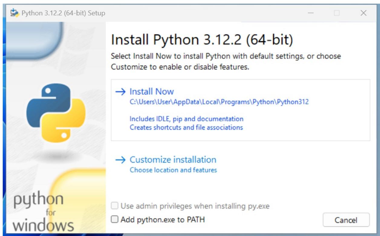
Figure 1.1: Starting the installation process on Windows
We recommend choosing the default install, and NOT ticking the Add python.exe to PATH option to avoid clashes with other versions of Python that might be installed on your machine, potentially by other users.
For a more comprehensive set of guidelines, please refer to the link indicated in the previous paragraph.
Once you click on Install Now, the installation procedure will begin.
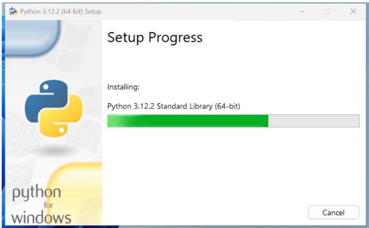
Figure 1.2: Installation in progress
Once the installation is complete, you will land on the final screen.
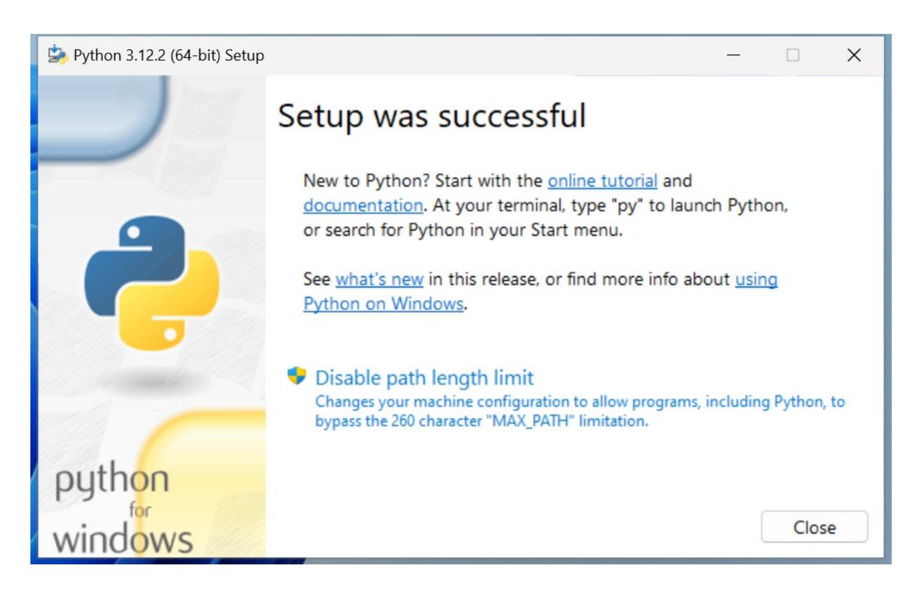
Click on Close to finish the installation.
Now that Python is installed on your system, open a command prompt and run the Python interactive shell by typing py . This command will select the latest version of Python installed on your machine. At the time of writing, 3.12 is the latest available version of Python. In case you have a more recent version installed, you can specify the version with the command py -3.12 .
To open the command prompt in Windows, go to the Start menu, and type cmd in the search box, to start your terminal up. Alternatively, you can also use the Powershell.
Installing Python on macOS
On macOS, the installation procedure is similar to that of Windows. Once you have downloaded the appropriate installer for your machine, complete the installation steps, and then start a terminal by going to Applications > Utilities > Terminal.
Once in the terminal window, you can type python . If that launches the wrong version, you can try and specify either with python3 or python3.12 .
Installing Python on Linux
The process of installing Python on linux is normally a bit more complex than that for Windows or macOS. The best course of action, if you are on a linux machine, is to search the most up-to-date set of steps for your distribution online. These will likely be quite different from one distribution to another, so it is difficult to give an example that would be relevant for everyone. Please do refer to the link in the Useful Installation Resources section, for guidance.
The Python Console
We will use the term console interchangeably to indicate the Linux console, the Windows Command Prompt or the Powershell, and the macOS Terminal. We will also indicate the command-line prompt with the Linux default format, like this:
$ sudo apt-get updateIf you are not familiar with that, please take some time to learn the basics of how a console works. In a nutshell, after the $ sign, you will type your instructions. Pay attention to capitalization and spaces, as they are very important.
Whatever console you open, type python at the prompt ( py on Windows), and make sure the Python interactive shell shows up. Type exit() to quit. Keep in mind that you may have to specify python3 or python3.12 if your OS comes with other Python versions preinstalled.
We often refer to the Python interactive shell simply as the Python console.
This is roughly what you should see when you run Python (it will change in some details according to the version and OS):
$ python
Python 3.12.2 (main, Feb 14 2024, 14:16:36)
[Clang 15.0.0 (clang-1500.1.0.2.5)] on darwin
Type "help", "copyright", "credits" or "license" for more information.
>>>
Now that Python is set up and you can run it, it is time to make sure you have the other tool that will be indispensable to follow the examples in the book: a virtual environment.
About virtual environments
When working with Python, it is very common to use virtual environments. Let us see what they are and why we need them by means of a simple example.
You install Python on your system, and you start working on a website for Client X. You create a project folder and start coding. Along the way, you also install some libraries, for example, the Django framework. Let us say the Django version you installed for Project X is 4.2.
Now, your website is so good that you get another client, Y. She wants you to build another website, so you start Project Y and, along the way, you need to install Django again. The only issue is that now the Django version is 5.0 and you cannot install it on your system because this would replace the version you installed for Project X. You do not want to risk introducing incompatibility issues, so you have two choices: either you stick with the version you have currently on your machine, or you upgrade it and make sure the first project is still fully working correctly with the new version.
Let us be honest, neither of these options is very appealing, right? Definitely not. But there is a solution: virtual environments!
Virtual environments are isolated Python environments, each of which is a folder that contains all the necessary executables to use the packages that a Python project would need (think of packages as libraries for the time being).
So, you create a virtual environment for Project X, install all the dependencies, and then you create a virtual environment for Project Y, and install all its dependencies without the slightest worry because every library you install ends up within the boundaries of the appropriate virtual environment. In our example, Project X will hold Django 4.2, while Project Y will hold Django 5.0.
It is of great importance that you never install libraries directly at the system level. Linux, for example, relies on Python for many different tasks and operations, and if you fiddle with the system installation of Python, you risk compromising the integrity of the entire system. So, take this as a rule: always create a virtual environment when you start a new project.
When it comes to creating a virtual environment on your system, there are a few different methods to carry this out. As of Python 3.5, the suggested way to create a virtual environment is to use the venv module. You can look it up on the official documentation page (https://docs.python.org/3/library/venv.xhtml) for further information.
If you are using a Debian-based distribution of Linux, for example, you will need to install the venv module before you can use it:
$ sudo apt-get install python3.12-venv
Another common way of creating virtual environments is to use the virtualenv third-party Python package. You can find it on its official website: https://virtualenv.pypa.io.
In this book, we will use the recommended technique, which leverages the venv module from the Python standard library.
Your first virtual environment
It is very easy to create a virtual environment, but according to how your system is configured and which Python version you want the virtual environment to run on, you need to run the command properly. Another thing you will need to do, when you want to work with it, is to activate it. Activating virtual environments produces some path juggling behind the scenes so that when you call the Python interpreter from that shell, you are actually calling the active virtual environment one, instead of the system one. We will show you a full example on macOS and Windows (on Linux it will be very similar to that of macOS). We will:
Open a terminal and change into the folder (directory) we use as root for our projects (our folder is code ). We
are going to create a new folder called my-project and change into it.
- Create a virtual environment called lpp4ed .
- After creating the virtual environment, we will activate it. The methods are slightly different between Linux, macOS, and Windows.
- Then, we will make sure that we are running the desired Python version (3.12.X) by running the Python interactive shell.
- Finally, we will deactivate the virtual environment.
Some developers prefer to call all virtual environments with the same name (for example, .venv ). This way they can configure tools and run scripts against any virtual environment by just knowing their location. The dot in .venv is there because in Linux/macOS, prepending a name with a dot makes that file or folder “invisible”.
These steps are all you need to start a project.
We are going to start with an example on macOS (note that you might get a slightly different result, according to your OS, Python version, and so on). In this listing, lines that start with a hash, # , are comments, spaces have been introduced for readability, and an arrow, → , indicates where the line has wrapped around due to lack of space:
fab@m1:~/code$ mkdir my-project # step 1
fab@m1:~/code$ cd my-project
fab@m1:~/code/my-project$ which python3.12 # check system python
/usr/bin/python3.12 # <-- system python3.12
fab@m1:~/code/my-project$ python3.12 -m venv lpp4ed # step 2
fab@m1:~/code/my-project$ source ./lpp4ed/bin/activate # step 3
# check python again: now using the virtual environment's one
(lpp4ed) fab@m1:~/code/my-project$ which python
/Users/fab/code/my-project/lpp4ed/bin/python
(lpp4ed) fab@m1:~/code/my-project$ python # step 4
Python 3.12.2 (main, Feb 14 2024, 14:16:36)
→ [Clang 15.0.0 (clang-1500.1.0.2.5)] on darwin
Type "help", "copyright", "credits" or "license" for more information.
>>> exit()
(lpp4ed) fab@m1:~/code/my-project$ deactivate # step 5
fab@m1:~/code/my-project$
Each step has been marked with a comment, so you should be able to follow along quite easily.
Something to notice here is that to activate the virtual environment, we need to run the lpp4ed/bin/activate script, which needs to be sourced. When a script is sourced, it means that it is executed in the current shell, and its effects last after the execution. This is very important. Also notice how the prompt changes after we activate the virtual environment, showing its name on the left (and how it disappears when we deactivate it).
On a Windows 11 Powershell, the steps are as follows:
PS C:\Users\H\Code> mkdir my-project # step 1
PS C:\Users\H\Code> cd .\my-project\
# check installed python versions
PS C:\Users\H\Code\my-project> py --list-paths
-V:3.12 *
→ C:\Users\H\AppData\Local\Programs\Python\Python312\python.exe
PS C:\Users\H\Code\my-project> py -3.12 -m venv lpp4ed # step 2
PS C:\Users\H\Code\my-project> .\lpp4ed\Scripts\activate # step 3
# check python versions again: now using the virtual environment's
(lpp4ed) PS C:\Users\H\Code\my-project> py --list-paths
 *
→ C:\Users\H\Code\my-project\lpp4ed\Scripts\python.exe
-V:3.12
→ C:\Users\H\AppData\Local\Programs\Python\Python312\python.exe
(lpp4ed) PS C:\Users\H\Code\my-project> python # step 4
Python 3.12.2 (tags/v3.12.2:6abddd9, Feb 6 2024, 21:26:36)
→ [MSC v.1937 64 bit (AMD64)] on win32
Type "help", "copyright", "credits" or "license" for more
→ information.
>>> exit()
(lpp4ed) PS C:\Users\H\Code\my-project> deactivate # step 5
Notice how on Windows, after activating the virtual environment, you can either use the py command or, more directly, python .
At this point, you should be able to create and activate a virtual environment. Please try and create another one on your own. Get acquainted with this procedure—it is something that you will always be doing: we never work system-wide with Python, remember? Virtual environments are extremely important.
The source code for the book contains a dedicated folder for each chapter. When the code shown in the chapter requires third-party libraries to be installed, we will include a requirements.txt file (or an equivalent requirements folder with more than one text file inside) that you can use to install the libraries required to run that code. We suggest that when experimenting with the code for a chapter, you create a dedicated virtual environment for that chapter. This way, you will be able to get some practice in the creation of virtual environments, and the installation of third-party libraries.
Installing third-party libraries
In order to install third-party libraries, we need to use the Python Package Installer, known as pip. Chances are that it is already available to you within your virtual environment, but if not, you can learn all about it on its documentation page: https://pip.pypa.io.
The following example shows how to create a virtual environment and install a couple of third-party libraries taken from a requirements file.
fab@m1:~/code$ mkdir my-project
fab@m1:~/code$ cd my-project
fab@m1:~/code/my-project$ python3.12 -m venv lpp4ed
fab@m1:~/code/my-project$ source ./lpp4ed/bin/activate
(lpp4ed) fab@m1:~/code/my-project$ cat requirements.txt
django==5.0.3
requests==2.31.0
# the following instruction shows how to use pip to install
# requirements from a file
(lpp4ed) fab@m1:~/code/my-project$ pip install -r requirements.txt
Collecting django==5.0.3 (from -r requirements.txt (line 1))
 Using cached Django-5.0.3-py3-none-any.whl.metadata (4.2 kB)
Collecting requests==2.31.0 (from -r requirements.txt (line 2))
 Using cached requests-2.31.0-py3-none-any.whl.metadata (4.6 kB)
 ... more collecting omitted ...
Installing collected packages: ..., requests, django
Successfully installed ... django-5.0.3 requests-2.31.0
(lpp4ed) fab@m1:~/code/my-project$
As you can see at the bottom of the listing, pip has installed both libraries that are in the requirements file, plus a few more. This happened because both django and requests have their own list of third-party libraries that they depend upon, and therefore pip will install them automatically for us.
Now, with the scaffolding out of the way, we are ready to talk a bit more about Python and how it can be used. Before we do that though, allow us to say a few words about the console.
The console
In this era of GUIs and touchscreen devices, it may seem a little ridiculous to have to resort to a tool such as the console, when everything is just about one click away.
But the truth is every time you remove your hand from the keyboard to grab your mouse and move the cursor over to the spot you want to click on, you’re losing time. Getting things done with the console, counter-intuitive though it may at first seem, results in higher productivity and speed. Believe us, we know—you will have to trust us on this.
Speed and productivity are important, and even though we have nothing against the mouse, being fluent with the
console is very good for another reason: when you develop code that ends up on some server, the console might be the only available tool to access the code on that server. If you make friends with it, you will never get lost when it is of utmost importance that you do not (typically, when the website is down, and you have to investigate very quickly what has happened).
If you are still not convinced, please give us the benefit of the doubt and give it a try. It is easier than you think, and you will not regret it. There is nothing more pitiful than a good developer who gets lost within an SSH connection to a server because they are used to their own custom set of tools, and only to that.
Now, let us get back to Python.
How to run a Python program
There are a few different ways in which you can run a Python program.
Running Python scripts
Python can be used as a scripting language; in fact, it always proves itself very useful. Scripts are files (usually of small dimensions) that you normally execute to do something like a task. Many developers end up having their own arsenal of tools that they fire when they need to perform a task. For example, you can have scripts to parse data in a format and render it into another one; or you can use a script to work with files and folders; you can create or modify configuration files—technically, there is not much that cannot be done in a script.
It is rather common to have scripts running at a precise time on a server. For example, if your website database needs cleaning every 24 hours (for example, to regularly clean up expired user sessions), you could set up a Cron job that fires your script at 1:00 A.M. every day.
According to Wikipedia, the software utility Cron is a time-based job scheduler in Unix-like computer operating systems. People who set up and maintain software environments use Cron (or a similar technology) to schedule jobs (commands or shell scripts) to run periodically at fixed times, dates, or intervals.
We have Python scripts to do all the menial tasks that would take us minutes or more to do manually, and at some point, we decided to automate.
Running the Python interactive shell
Another way of running Python is by calling the interactive shell. This is something we already saw when we typed python on the command line of our console.
So, open up a console, activate your virtual environment (which by now should be second nature to you, right?), and type python . You will be presented with a few lines that should look something like this:
(lpp4ed) fab@m1 ~/code/lpp4ed$ python
Python 3.12.2 (main, Feb 14 2024, 14:16:36)
[Clang 15.0.0 (clang-1500.1.0.2.5)] on darwin
Type "help", "copyright", "credits" or "license" for more
information.
>>>
Those >>> are the prompt of the shell. They tell you that Python is waiting for you to type something. If you type a simple instruction, something that fits in one line, that is all you will see. However, if you type something that requires more than one line of code, the shell will change the prompt to … , giving you a visual clue that you are typing a multiline statement (or anything that would require more than one line of code).
Go on, try it out; let us do some basic math:
>>> 3 + 7
10
>>> 10 / 4
2.5
>>> 2 ** 1024
179769313486231590772930519078902473361797697894230657273430081157
732675805500963132708477322407536021120113879871393357658789768814
416622492847430639474124377767893424865485276302219601246094119453
082952085005768838150682342462881473913110540827237163350510684586
298239947245938479716304835356329624224137216The last operation is showing you something incredible. We raise 2 to the power of 1024 , and Python handles this task with no trouble at all. Try to do it in Java, C++, or C#. It will not work, unless you use special libraries to handle such big numbers.
We use the interactive shell every day. It is extremely useful to debug very quickly; for example, to check if a data structure supports an operation. Or to inspect or run a piece of code.
The Django web framework provides an integration for the shell that allows you to work your way through the framework tools, to inspect the data in the database, and much more. You will find that the interactive shell soon becomes one of your dearest friends on this journey you are embarking on.
Another solution, which comes in a much nicer graphic layout, is to use the Integrated Development and Learning Environment (IDLE). It is quite a simple Integrated Development Environment (IDE), which is intended mostly for beginners. It has a slightly larger set of capabilities than the bare interactive shell you get in the console, so you may want to explore it. It comes for free in the Windows and macOS Python installers and you can easily install it on any other system. You can find more information about it on the Python website.
Guido Van Rossum named Python after the British comedy group, Monty Python, so it is rumored that the name IDLE was chosen in honor of Eric Idle, one of Monty Python’s founding members.
Running Python as a service
Apart from being run as a script, and within the boundaries of a shell, Python can be coded and run as an application. We will see examples throughout this book of this mode. We will understand more about it in a moment, when we talk about how Python code is organized and run.
Running Python as a GUI application
Python can also be run as a Graphical User Interface (GUI). There are several frameworks available, some of which are cross-platform, and some others that are platform-specific. A popular example of a GUI application library is Tkinter, which is an object-oriented layer that lives on top of Tk (Tkinter means Tk interface).
Tk is a GUI toolkit that takes desktop application development to a higher level than the conventional approach. It is the standard GUI for Tool Command Language (Tcl), but also for many other dynamic languages, and it can produce rich native applications that run seamlessly under Windows, Linux, macOS, and more.
Tkinter comes bundled with Python; therefore, it gives the programmer easy access to the GUI world.
Other widely used GUI frameworks include:
- PyQT/PySide
- wxPython
- Kivy
Describing them in detail is outside the scope of this book, but you can find all the information you need on the Python website:
https://docs.python.org/3/faq/gui.xhtml
Information can be found in the What GUI toolkits exist for Python? section. If GUIs are what you are looking for, remember to choose the one you want according to some basic principles. Make sure they:
- Offer all the features you may need to develop your project
- Run on all the platforms you may need to support
- Rely on a community that is as wide and active as possible
- Wrap graphic drivers/tools that you can easily install/access
How is Python code organized?
Let us talk a little bit about how Python code is organized. In this section, we will start to enter the proverbial rabbit hole and introduce more technical names and concepts.
Starting with the basics, how is Python code organized? Of course, you write your code into files. When you save a file with the extension .py , that file is said to be a Python module.
If you are on Windows or macOS, which typically hide file extensions from the user, we recommend that you change the configuration so that you can see the complete names of the files. This is not strictly a requirement, only a suggestion that may come in handy when discerning files from each other.
It would be impractical to save all the code that it is required for software to work within one single file. That solution works for scripts, which are usually not longer than a few hundred lines (and often they are shorter than that).
A complete Python application can be made of hundreds of thousands of lines of code, so you will have to scatter it through different modules, which is better, but not good enough. It turns out that even like this, it would still be impractical to work with the code. So, Python gives you another structure, called a package, which allows you to group modules together. A package is nothing more than a folder. In earlier versions of Python one was also required to include a special file, __init__.py . This file does not need to contain any code, and even though its presence is not mandatory anymore, there are practical reasons for which it is always a good idea to include it nonetheless.
As always, an example will make all this much clearer. We have created an illustration structure in our book project, and when we type in the console:
$ tree -v exampleWe get a tree representation of the contents of the ch1/example folder, which contains the code for the examples of this chapter. Here is what the structure of a simple application could look like:
example
├── core.py
├── run.py
└── util
   ├── __init__.py
   ├── db.py
   ├── maths.py
   └── network.py
You can see that within the root of this example, we have two modules, core.py and run.py , and one package, util . Within core.py , there may be the core logic of our application. On the other hand, within the run.py module, we can probably find the logic to start the application. Within the util package, we expect to find various utility tools, and in fact, we can guess that the modules there are named based on the types of tools they hold: db.py would hold tools to work with databases, maths.py would, of course, hold mathematical tools (maybe our application deals with financial data), and network.py would probably hold tools to send/receive data on networks.
As explained before, the __init__.py file is there just to tell Python that util is a package and not just a simple folder.
Had this software been organized within modules only, it would have been harder to infer its structure. We placed a module only example under the ch1/files_only folder; see it for yourself:
$ tree -v files_onlyThis shows us a completely different picture:
files_only
├── core.py
├── db.py
├── maths.py
├── network.py
└── run.py
It is a little harder to guess what each module does, right? Now, consider that this is just a simple example, so you can guess how much harder it would be to understand a real application if we could not organize the code into packages and modules.
How do we use modules and packages?
When a developer is writing an application, it is likely that they will need to apply the same piece of logic in different parts of it. For example, when writing a parser for the data that comes from a form that a user can fill in a web page, the application will have to validate whether a certain field is holding a number or not. Regardless of how the logic for this kind of validation is written, it is likely that it will be needed for more than one field.
For example, in a poll application, where the user is asked many questions, it is likely that several of them will require a numeric answer. These might be:
- What is your age?
- How many pets do you own?
- How many children do you have?
- How many times have you been married?
It would be bad practice to copy/paste (or, said more formally, duplicate) the validation logic in every place where we expect a numeric answer. This would violate the don’t repeat yourself (DRY) principle, which states that you should never repeat the same piece of code more than once in your application. Despite the DRY principle, we feel the need here to stress the importance of this principle: you should never repeat the same piece of code more than once in your application!
There are several reasons why repeating the same piece of logic can be bad, the most important ones being:
- There could be a bug in the logic, and therefore you would have to correct it in every copy.
- You may want to amend the way you carry out the validation, and again, you would have to change it in every copy.
- You may forget to fix or amend a piece of logic because you missed it when searching for all its occurrences. This would leave wrong or inconsistent behavior in your application.
- Your code would be longer than needed for no good reason.
Python is a wonderful language and provides you with all the tools you need to apply the coding best practices. For this example, we need to be able to reuse a piece of code. To do this effectively, we need to have a construct that will hold the code for us so that we can call that construct every time we need to repeat the logic inside it. That construct exists, and it is called a function.
We are not going too deep into the specifics here, so please just remember that a function is a block of organized, reusable code that is used to perform a task. Functions can assume many forms and names, according to what kind of environment they belong to, but for now this is not important. Details will be seen once we are able to appreciate them, later, in the book. Functions are the building blocks of modularity in your application, and they are almost indispensable. Unless you are writing a super-simple script, functions will be used all the time. Functions will be explored in Chapter 4, Functions, the Building Blocks of Code.
Python comes with a very extensive library, as mentioned a few pages ago. Now is a good time to define what a library is: a collection of functions and objects that provide functionalities to enrich the abilities of a language. For example, within Python’s math library, a plethora of functions can be found, one of which is the factorial function, which calculates the factorial of a number.
In mathematics, the factorial of a non-negative integer number, N, denoted as N!, is defined as the product of all positive integers less than or equal to N. For example, the factorial of 5 is calculated as:
The factorial of 0 is 0! = 1, to respect the convention for an empty product.
So, if you wanted to use this function in your code, all you would have to do is to import it and call it with the right input values. Do not worry too much if input values and the concept of calling are not clear right now; please just concentrate on the import part. We use a library by importing what we need from it, which will then be used specifically. In Python, to calculate 5!, we just need the following code:
>>> from math import factorial
>>> factorial(5)
120
Whatever we type in the shell, if it has a printable representation, will be printed in the console for us (in this case, the result of the function call: 120).
Let us go back to our example, the one with core.py , run.py , util , and so on. Here, the package util is our own utility library. This is our custom utility belt that holds all those reusable tools (that is, functions), which we need in our application. Some of them will deal with databases ( db.py ), some with the network ( network.py ), and some will perform mathematical calculations ( maths.py ) that are outside the scope of Python’s standard math library and, therefore, we must code them for ourselves.
We will see in detail how to import functions and use them in their dedicated chapter. Let us now talk about another important concept: Python’s execution model.
Python’s execution model
In this section, we would like to introduce you to some important concepts, such as scope, names, and namespaces. You can read all about Python’s execution model in the official language reference (https://docs.python.org/3/reference/executionmodel.xhtml), of course, but we would argue that it is quite technical and abstract, so let us give you a less formal explanation first.
Names and namespaces
Say you are looking for a book, so you go to the library and ask someone for it. They tell you something like Second Floor, Section X, Row Three. So, you go up the stairs, look for Section X, and so on. It would be very different to enter a library where all the books are piled together in random order in one big room. No floors, no sections, no rows, no order. Fetching a book would be extremely hard.
When we write code, we have the same issue: we have to try and organize it so that it will be easy for someone who has no prior knowledge about it to find what they are looking for. When software is structured correctly, it also promotes code reuse. Furthermore, disorganized software is more likely to contain scattered pieces of duplicated logic.
As a first example, let us take a book. We refer to a book by its title; in Python lingo, that would be a name. Python names are the closest abstraction to what other languages call variables. Names refer to objects and are introduced by name-binding operations. Let us see a quick example (again, notice that anything that follows a # is a comment):
>>> n = 3 # integer number
>>> address = "221b Baker Street, NW1 6XE, London" # Sherlock Holmes' address
>>> employee = {
... 'age': 45,
... 'role': 'CTO',
... 'SSN': 'AB1234567',
... }
>>> # let us print them
>>> n
3
>>> address
'221b Baker Street, NW1 6XE, London'
>>> employee
{'age': 45, 'role': 'CTO', 'SSN': 'AB1234567'}
>>> other_name
Traceback (most recent call last):
File "<stdin>", line 1, in <module>
NameError: name 'other_name' is not defined
>>>Remember that each Python object has an identity, a type, and a value. We defined three objects in the preceding code; let us now examine their types and values:
- An integer number n (type: int , value: 3 )
- A string address (type: str , value: Sherlock Holmes’ address)
- A dictionary employee (type: dict , value: a dictionary object with three key/value pairs)
Fear not, we know we have not covered what a dictionary is. We will see, in Chapter 2, Built-In Data Types, that it is the king of Python data structures.
Have you noticed that the prompt changed from >>> to … when we typed in the definition of employee? That is because the definition spans over multiple lines.
So, what are n , address , and employee ? They are names, and these can be used to retrieve data from within our code. They need to be kept somewhere so that whenever we need to retrieve those objects, we can use their names to fetch them. We need some space to hold them, hence: namespaces!
A namespace is a mapping from names to objects. Examples are the set of built-in names (containing functions that are always accessible in any Python program), the global names in a module, and the local names in a function. Even the set of attributes of an object can be considered a namespace.
The beauty of namespaces is that they allow you to define and organize names with clarity, without overlapping or interference. For example, the namespace associated with the book we were looking for in the library could be used to import the book itself, like this:
from library.second_floor.section_x.row_three import bookWe start from the library namespace, and by means of the dot ( . ) operator, we walk into that namespace. Within this namespace, we look for second_floor , and again we walk into it with the . operator. We then walk into section_x , and finally, within the last namespace, row_three , we find the name we were looking for: book .
Walking through a namespace will be clearer when dealing with real code examples. For now, just keep in mind that namespaces are places where names are associated with objects.
There is another concept, closely related to that of a namespace, which we would like to mention briefly: scope.
Scopes
According to Python’s documentation:
“A scope is a textual region of a Python program, where a namespace is directly accessible.”
Directly accessible means that, when looking for an unqualified reference to a name, Python tries to find it in the namespace.
Scopes are determined statically, but at runtime, they are used dynamically. This means that by inspecting the source code, you can tell what the scope of an object is. There are four different scopes that Python makes accessible (not necessarily all of them are present at the same time, though):
- The local scope, which is the innermost one and contains the local names.
- The enclosing scope; that is, the scope of any enclosing function. It contains non-local names and non-global names.
- The global scope contains the global names.
- The built-in scope contains the built-in names. Python comes with a set of functions that you can use in an offthe-shelf fashion, such as print , all , abs , and so on. They live in the built-in scope.
The rule is the following: when we refer to a name, Python starts looking for it in the current namespace. If the name is not found, Python continues the search in the enclosing scope, and this continues until the built-in scope is searched. If a name has still not been found after searching the built-in scope, then Python raises a NameError exception, which basically means that the name has not been defined (as seen in the preceding example).
The order in which the namespaces are scanned when looking for a name is therefore local, enclosing, global, builtin (LEGB).
This is all theoretical, so let us see an example. To demonstrate local and enclosing namespaces, we will have to define a few functions. Do not worry if you are not familiar with their syntax for the moment—that will come in Chapter 4, Functions, the Building Blocks of Code. Just remember that in the following code, when you see def , it means we are defining a function:
# scopes1.py
# Local versus Global
# we define a function, called local
def local():
    age = 7
    print(age)
# we define age within the global scope
age = 5
# we call, or `execute` the function local
local()
print(age)
In the preceding example, we define the same name age , in both the global and local scopes. When we execute this program with the following command (have you activated your virtual environment?):
$ python scopes1.pyWe see two numbers printed on the console: 7 and 5.
What happens is that the Python interpreter parses the file, top to bottom. First, it finds a couple of comment lines, which are skipped, then it parses the definition of the function local . When called, this function will do two things: it will set up a name to an object representing number 7 and will print it. The Python interpreter keeps going, and it finds another name binding. This time the binding happens in the global scope and the value is 5 . On the next line, there is a call to the function local . At this point, Python executes the function, so at this time, the binding age = 7 happens in the local scope and is printed. Finally, there is a call to the print function, which is executed and will now print 5 .
One particularly important thing to note is that the part of the code that belongs to the definition of the local function is indented by four spaces on the right. Python, in fact, defines scopes by indenting the code. You walk into a scope by indenting, and walk out of it by dedenting. Some coders use two spaces, others three, but the suggested number of spaces to use is four. It is a good measure to maximize readability. We will talk more about all the conventions you should embrace when writing Python code later.
In other languages, such as Java, C#, and C++, scopes are created by writing code within a pair of curly braces: { … } . Therefore, in Python, indenting code corresponds to opening a curly brace, while dedenting code
corresponds to closing a curly brace.
What would happen if we removed that age = 7 line? Remember the LEGB rule. Python would start looking for age in the local scope (function local ), and, not finding it, it would go to the next enclosing scope. The next one, in this case, is the global one. Therefore, we would see the number 5 printed twice on the console. Let us see what the code would look like in this case:
# scopes2.py
# Local versus Global
def local():
    # age does not belong to the scope defined by the local function
    # so Python will keep looking into the next enclosing scope.
    # age is finally found in the global scope
    print(age, 'printing from the local scope')
age = 5
print(age, 'printing from the global scope')
local()
Running scopes2.py will print this:
$ python scopes2.py
5 printing from the global scope
5 printing from the local scope
As expected, Python prints age the first time, then when the function local is called, age is not found in its scope, so Python looks for it following the LEGB chain until age is found in the global scope. Let us see an example with an extra layer, the enclosing scope:
# scopes3.py
# Local, Enclosing and Global
def enclosing_func():
    age = 13
    def local():
        # age does not belong to the scope defined by the local
        # function so Python will keep looking into the next
        # enclosing scope. This time age is found in the enclosing
        # scope
        print(age, 'printing from the local scope')
    # calling the function local
    local()
age = 5
print(age, 'printing from the global scope')
enclosing_func()
Running scopes3.py will print on the console:
$ python scopes3.py
5, 'printing from the global scope'
13, 'printing from the local scope'
As you can see, the print instruction from the function local is referring to age as before. age is still not defined within the function itself, so Python starts walking scopes following the LEGB order. This time age is found in the enclosing scope.
Do not worry if this is still not perfectly clear for now. It will become clearer as we go through the examples in the book. The Classes section of the Python tutorial (https://docs.python.org/3/tutorial/classes.xhtml) has an interesting paragraph about scopes and namespaces. Be sure you read it to gain a deeper understanding of the subject.
Guidelines for writing good code
Writing good code is not as easy as it seems. As we have already said, good code exhibits a long list of qualities that are difficult to combine together. Writing good code is an art. Regardless of where on the path you will be happy to settle, there is something that you can embrace that will make your code instantly better: PEP 8.
A Python Enhancement Proposal (PEP) is a document that describes a newly proposed Python feature. PEPs are also used to document processes around Python language development and to provide guidelines and information. You can find an index of all PEPs at https://www.python.org/dev/peps.
PEP 8 is perhaps the most famous of all PEPs. It lays out a simple but effective set of guidelines to define Python aesthetics so that we write beautiful, idiomatic Python code. If you take just one suggestion out of this chapter, please let it be this: use PEP 8. Embrace it. You will thank us later.
Coding today is no longer a check-in/check-out business. Rather, it is more of a social effort. Several developers collaborate on a piece of code through tools such as Git and Mercurial, and the result is code that is produced by many different hands.
Git and Mercurial are two of the most popular distributed revision control systems in use today. They are essential tools designed to help teams of developers collaborate on the same software.
These days, more than ever, we need to have a consistent way of writing code, so that readability is maximized. When all developers of a company abide by PEP 8, it is not uncommon for any of them landing on a piece of code to think they wrote it themselves (it actually happens to Fabrizio all the time, because he quickly forgets any code he writes).
This has a tremendous advantage: when you read code that you could have written yourself, you read it easily. Without conventions, every coder would structure the code the way they like most, or simply the way they were taught or are used to, and this would mean having to interpret every line according to someone else’s style. It would mean having to lose much more time just trying to understand it. Thanks to PEP 8, we can avoid this. We are such fans of it that, in our team, we will not sign off a code review if the code does not respect PEP8. So, please take the time to study it; this is very important.
Python developers can leverage several different tools to automatically format their code, according to PEP 8 guidelines. Popular such tools are black and ruff. There are also other tools, called linters, which check if the code is formatted correctly, and issue warnings to the developer with instructions on how to fix errors. Famous ones are flake8 and PyLint. We encourage you to use these tools, as they simplify the task of coding wellformatted software.
In the examples in this book, we will try to respect PEP8 as much as we can. Unfortunately, we do not have the luxury of 79 characters (which is the maximum line length suggested by PEP 8), and we will have to cut down on blank lines and other things, but we promise you we will try to lay out the code so that it is as readable as possible.
Python culture
Python has been adopted widely in the software industry. It is used by many different companies for different purposes, while also being an excellent education tool (it is excellent for that purpose due to its simplicity, making it easy to learn; it encourages good habits for writing readable code; it is platform-agnostic; and it supports modern object-oriented programming paradigms).
One of the reasons Python is so popular today is that the community around it is vast, vibrant, and full of brilliant people. Many events are organized all over the world, mostly either around Python or some of its most adopted web frameworks, such as Django.
Python’s source is open, and very often so are the minds of those who embrace it. Check out the community page on the Python website for more information and get involved!
There is another aspect to Python, which revolves around the notion of being Pythonic. It has to do with the fact that Python allows you to use some idioms that are not found elsewhere, at least not in the same form or ease of use (it can feel claustrophobic when one has to code in a language that is not Python, at times).
Anyway, over the years, this concept of being Pythonic has emerged and, the way we understand it, it is something along the lines of doing things the way they are supposed to be done in Python.
To help you understand a little bit more about Python’s culture and being Pythonic, we will show you the Zen of Python—a lovely Easter egg that is very popular. Open a Python console and type import this .
What follows is the result of that instruction:
>>> import this
The Zen of Python, by Tim Peters
Beautiful is better than ugly.
Explicit is better than implicit.
Simple is better than complex.
Complex is better than complicated.
Flat is better than nested.
Sparse is better than dense.
Readability counts.
Special cases aren't special enough to break the rules.
Although practicality beats purity.
Errors should never pass silently.
Unless explicitly silenced.
In the face of ambiguity, refuse the temptation to guess.
There should be one-- and preferably only one --obvious way to do it.
Although that way may not be obvious at first unless you're Dutch.
Now is better than never.
Although never is often better than *right* now.
If the implementation is hard to explain, it's a bad idea.
If the implementation is easy to explain, it may be a good idea.
Namespaces are one honking great idea -- let's do more of those!
There are two levels of reading here. One is to consider it as a set of guidelines that have been put down in a whimsical way. The other one is to keep it in mind, and read it once in a while, trying to understand how it refers to something deeper: some Python characteristics that you will have to understand deeply in order to write Python the way it is supposed to be written. Start with the fun level, and then dig deeper. Always dig deeper.
A note on IDEs
Just a few words about IDEs. To follow the examples in this book, you do not need one; any decent text editor will do fine. If you want to have more advanced features, such as syntax coloring and auto-completion, you will have to get yourself an IDE. You can find a comprehensive list of open-source IDEs (just Google “Python IDEs”) on the Python website.
Fabrizio uses Visual Studio Code, from Microsoft. It is free to use and it provides many features out of the box, which one can even expand by installing extensions.
After working for many years with several editors, including Sublime Text, this was the one that felt most productive to him.
Heinrich, on the other hand, is a hardcore Neovim user. Although it might have a steep learning curve, Neovim is a very powerful text editor that can also be extended with plugins. It also has the benefit of being compatible with its predecessor, Vim, which is installed in almost every system a software developer regularly works on.
Two important pieces of advice:
- Whatever IDE you decide to use, try to learn it well so that you can exploit its strengths, but don’t depend on it too much. Practice working with Vim (or any other text editor) once in a while; learn to be able to do some work on any platform, with any set of tools.
- Whatever text editor/IDE you use, when it comes to writing Python, indentation is four spaces. Do not use tabs, do not mix them with spaces. Use four spaces, not two, not three, not five. Just use four. The whole world works like that, and you do not want to become an outcast because you were fond of the three-spaces layout.
A word about AI
In the last year or so, the world has witnessed the advent of AIs. There are quite a few options on the market now, some of which provide tools for programmers.
The fact that there are instruments able to write pieces of code does not invalidate any of the reasons why one should learn a programming language. AI tools are far from being able to do what a person can do. They are not perfect, and at the time of writing they are mostly useful to help with repetitive, and sometimes menial tasks.
Several IDEs can be integrated with technologies like Github Copilot (and the likes). Visual Studio Code, Zed, Intellij Idea, PyCharm, all provide ways to enhance their capabilities with AI plugins. There are even some new IDEs that were designed specifically around AI features, such as Cursor.
While we do use such tools in our work, we feel it is crucial to stress how important it is for you to try and understand the code examples from this book on your own. Please try to work them out without help from an AI assistant, as that will be an integral part of your learning process.
Summary
In this chapter, we started exploring the world of programming and that of Python. We have barely scratched the surface, only touching upon concepts that will be discussed later on in the book in greater detail.
We talked about Python’s main features, who is using it and for what, and the different ways in which we can write a Python program.
In the last part of the chapter, we flew over the fundamental notions of namespaces, and scopes. We also saw how Python code can be organized using modules and packages.
On a practical level, we learned how to install Python on our system, how to make sure we have the tools we need, such as pip , and we also created and activated our first virtual environment. This will allow us to work in a selfcontained environment without the risk of compromising the Python system installation.
Now you are ready to start this journey with us. All you need is enthusiasm, an activated virtual environment, this book, your fingers, and probably some coffee.
Try to follow the examples; we will keep them simple and short. If you put them under your fingertips, you will retain them much better than if you just read them.
In the next chapter, we will explore Python’s rich set of built-in data types. There is much to cover, and much to learn!
2 Built-In Data Types
Join our book community on Discord

https://packt.link/o4zEQ
“Data! Data! Data!” he cried impatiently. “I can’t make bricks without clay.”– Sherlock Holmes, in The Adventure of the Copper Beeches
Everything you do with a computer is managing data. Data comes in many different shapes and flavors. It is the music you listen to, the movies you stream, the PDFs you open. Even the source of the chapter you’re reading at this very moment is just a file, which is data.
Data can be simple, whether it is an integer number to represent an age, or a complex structure, like an order placed on a website. It can be about a single object or about a collection of them. Data can even be about data—that is, metadata. This is data that describes the design of other data structures, or data that describes application data or its context. In Python, objects are an abstraction for data, and Python has an amazing variety of data structures that you can use to represent data or combine them to create your own custom data.
In this chapter, we are going to cover the following:
- Python objects’ structures
- Mutability and immutability
- Built-in data types: numbers, strings, dates and times, sequences, collections, and mapping types
- The collections module, briefly
- Enumerations
Everything is an object
Before we delve into the specifics, we want you to be very clear about objects in Python, so let us talk a little bit more about them. Everything in Python is an object, and every object has an identity (id), a type and a value. But what really happens when you type an instruction like age = 42 in a Python module?
If you go to https://pythontutor.com/, you can type that instruction into a text box and get its visual representation. Keep this website in mind; it is very useful to consolidate your understanding of what goes on behind the scenes.
So, what happens is that an object is created. It gets an id, the type is set to int (integer number), and the value to 42. A name, age , is placed in the global namespace, pointing to that object. Therefore, whenever we are in the global namespace, after the execution of that line, we can retrieve that object by simply accessing it through its name: age .
If you were to move house, you would put all the knives, forks, and spoons in a box and label it cutlery. This is exactly the same concept. Here is a screenshot of what it may look like (you may have to tweak the settings to get to the same view):
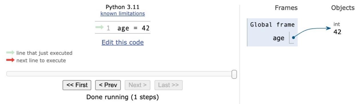
Figure 2.1 – A name pointing to an object.
So, for the rest of this chapter, whenever you read something such as name = some_value , think of a name placed in the namespace that is tied to the scope in which the instruction was written, with a nice arrow pointing to an object that has an id, a type, and a value. There is a little bit more to say about this mechanism, but it is much easier to talk about it using an example, so we will come back to this later.
Mutability
The first fundamental distinction that Python makes on data is about whether the value of an object can change. If the value can change, the object is called mutable, otherwise the object is called immutable.
It is important that you understand the distinction between mutable and immutable because it affects the code you write; take this example:
>>> age = 42
>>> age
42
>>> age = 43 #A
>>> age
43
In the preceding code, on line #A , have we changed the value of age ? Well, no. But now it is 43 (we hear you say…). Yes, it is 43, but 42 was an integer number, of the type int, which is immutable. So, what happened is really that on the first line, age is a name that is set to point to an int object, whose value is 42. When we type age = 43 , what happens is that another int object is created, with the value 43 (also, the id will be different), and the name age is set to point to it. So, in fact, we did not change that 42 to 43—we just pointed the name age to a different location, which is the new int object whose value is 43. Let us see the IDs of the objects:
>>> age = 42
>>> id(age)
4377553168
>>> age = 43
>>> id(age)
4377553200
Notice that we call the built-in id() function to print the IDs. As you can see, they are different, as expected. Bear in mind that age points to one object at a time: 42 first, then 43 —never together.
If you reproduce these examples on your computer, you will notice that the IDs you get will be different. This is of course expected, as they are generated randomly by Python, and will be different every time.
Now, let us see the same example using a mutable object. For this example, let us just use a Person object, that has a property age (ignore the class declaration for now—it is there only for completeness):
>>> class Person:
... def __init__(self, age):
... self.age = age
...
>>> fab = Person(age=48)
>>> fab.age
48
>>> id(fab)
4380878496
>>> id(fab.age)
4377553168
>>> fab.age = 25 # I wish!
>>> id(fab) # will be the same
4380878496
>>> id(fab.age) # will be different
4377552624In this case, we set up an object fab whose type is Person (a custom class). On creation, the object is given the age of 48. We then print it, along with the object ID, and the ID of age as well. Notice that, even after we change age to be 25, the ID of fab stays the same (while the ID of age has changed, of course). Custom objects in Python are mutable (unless you code them not to be). Keep this concept in mind, as it is very important. We willl remind you about it throughout the rest of the chapter.
Numbers
Let us start by exploring Python’s built-in data types for numbers. Python was designed by a man with a master’s degree in mathematics and computer science, so it is only logical that it has extensive support for numbers.
Numbers are immutable objects.
Integers
Python integers have an unlimited range, subject only to the available virtual memory. This means that it doesn’t really matter how big the number you want to store is—as long as it can fit in your computer’s memory, Python will take care of it.
Integer numbers can be positive, negative, or 0 (zero). Their type is int. They support all the basic mathematical operations, as shown in the following example:
>>> a = 14
>>> b = 3
>>> a + b # addition
17
>>> a - b # subtraction
11
>>> a * b # multiplication
42
>>> a / b # true division
4.666666666666667
>>> a // b # integer division
4
>>> a % b # modulo operation (reminder of division)
2
>>> a ** b # power operation
2744
The preceding code should be easy to understand. Just notice one important thing: Python has two division operators, one performs the so-called true division ( / ), which returns the quotient of the operands, and another one, the so-called integer division ( // ), which returns the floored quotient of the operands.
As a historical information, in Python 2 the division operator / behaves differently than in Python 3.
Let us see how division behaves differently when we introduce negative numbers:
>>> 7 / 4 # true division1.75
>>> 7 // 4 # integer division, truncation returns 1
1
>>> -7 / 4 # true division again, result is opposite of previous
-1.75
>>> -7 // 4 # integer div., result not the opposite of previous
-2This is an interesting example. If you were expecting a -1 on the last line, don’t feel bad, it is just the way Python works. Integer division in Python is always rounded toward minus infinity. If, instead of flooring, you want to truncate a number to an integer, you can use the built-in int() function, as shown in the following example:
>>> int(1.75)
1
>>> int(-1.75)
-1
Notice that the truncation is done toward 0 instead.
The int() function can also return integer numbers from string representation in a given base:
>>> int('10110', base=2)
22
It is worth noting that the power operator, ** , also has a built-in function counterpart, pow() , shown in the example below:
>>> pow(10, 3)
1000
>>> 10 ** 3
1000
>>> pow(10, -3)
0.001
>>> 10 ** -3
0.001
There is also an operator to calculate the remainder of a division. It is called the modulo operator, and it is represented by a percentage symbol ( % ):
>>> 10 % 3 # remainder of the division 10 // 3
1
>>> 10 % 4 # remainder of the division 10 // 4
2
The pow() function allows a third argument to perform modular exponentiation. The form with three arguments also accepts a negative exponent in the case where the base is relatively prime to the modulus. The result is the modular multiplicative inverse of the base (or a suitable power of that, when the exponent is negative, but not -1), modulo the third argument. Here’s an example:
>>> pow(123, 4)
228886641
>>> pow(123, 4, 100)
41 # notice: 228886641 % 100 == 41
>>> pow(37, -1, 43) # modular inverse of 37 mod 43
7
>>> (7 * 37) % 43 # proof the above is correct
1
One nice feature introduced in Python 3.6 is the ability to add underscores within number literals (between digits or base specifiers, but not leading or trailing). The purpose is to help make some numbers more readable, such as 1_000_000_000 :
>>> n = 1_024
>>> n
1024
>>> hex_n = 0x_4_0_0 # 0x400 == 1024
>>> hex_n
1024Booleans
Boolean algebra is that subset of algebra in which the values of the variables are the truth values, true and false. In Python, True and False are two keywords that are used to represent truth values. Booleans are a subclass of integers, so True and False behave respectively like 1 and 0 . The equivalent of the int type for Booleans is the bool type, which returns either True or False . Every built-in Python object has a value in the Boolean context, which means they evaluate to either True or False when fed to the bool function.
Boolean values can be combined in Boolean expressions using the logical operators and , or , and not . Let us see a simple example:
>>> int(True) # True behaves like 1
1
>>> int(False) # False behaves like 0
0
>>> bool(1) # 1 evaluates to True in a Boolean context
True
>>> bool(-42) # and so does every non-zero number
True
>>> bool(0) # 0 evaluates to False
False
>>> # quick peek at the operators (and, or, not)
>>> not True
False
>>> not False
True
>>> True and True
True
>>> False or True
True
Booleans are most commonly used in conditional programming, which we will discuss in detail in Chapter 3, Conditionals and Iteration.
You can see that True and False are subclasses of integers when you try to add them. Python upcasts them to integers and performs the addition:
>>> 1 + True
2
>>> False + 42
42
>>> 7 - True
6
Upcasting is a type conversion operation that goes from a subclass to its parent. In this example, True and False , which belong to a class derived from the integer class, are converted back to integers when needed. This topic is about inheritance and will be explained in detail in Chapter 6, OOP, Decorators, and Iterators.
Real numbers
Real numbers, or floating point numbers, are represented in Python according to the IEEE 754 double-precision binary floating point format, which stores them in 64 bits of information divided into three sections: sign, exponent, and mantissa.
Quench your thirst for knowledge about this format on Wikipedia: http://en.wikipedia.org/wiki/Doubleprecision_floating-point_format.
Several programming languages offer two different formats: single and double precision. The former takes up 32 bits of memory, the latter 64. Python supports only the double format. Let us see a simple example:
>>> pi = 3.1415926536 # how many digits of PI can you remember?
>>> radius = 4.5
>>> area = pi * (radius ** 2)
>>> area
63.617251235400005
In the calculation of the area, we wrapped the radius ** 2 within parentheses. Even though that wasn’t necessary because the power operator has higher precedence than the multiplication one, we think the formula reads more easily like that. Moreover, should you get a slightly different result for the area, don’t worry. It might depend on your OS, how Python was compiled, and so on. As long as the first few decimal digits are correct, you know it is a correct result.
The sys.float_info sequence holds information about how floating point numbers will behave on your system. This is an example of what you might see:
>>> import sys
>>> sys.float_info
sys.float_info(
   max=1.7976931348623157e+308, max_exp=1024, max_10_exp=308,
   min=2.2250738585072014e-308, min_exp=-1021, min_10_exp=-307,
   dig=15, mant_dig=53, epsilon=2.220446049250313e-16, radix=2,
   rounds=1
)
Let us make a few considerations here: we have 64 bits to represent floating point numbers. This means we can represent at most 264 (that is 18,446,744,073,709,551,616) distinct numbers. Take a look at the max and epsilon values for floating point numbers, and you will realize that it is impossible to represent them all. There is just not enough space, so they are approximated to the closest representable number. You probably think that only extremely big or extremely small numbers suffer from this issue. If so, the next example will surprise you:
>>> 0.3 - 0.1 * 3 # this should be 0!!!
-5.551115123125783e-17
What does this tell you? It tells you that double precision numbers suffer from approximation issues even when it comes to simple numbers like 0.1 or 0.3. Why is this important? It can be a big problem if you are handling prices, or financial calculations, or any kind of data that requires precision. Don’t worry, Python gives you the Decimal type, which doesn’t suffer from these issues; we’ll see them in a moment.
Complex numbers
Python supports complex numbers out of the box. If you do not know what complex numbers are, they are numbers that can be expressed in the form a + ib, where a and b are real numbers, and i (or j, if you use the engineering notation) is the imaginary unit; that is, the square root of -1. a and b are called, respectively, the real and imaginary parts of the number.
It is perhaps unlikely that you will use them, but nevertheless, let us see a small example:
>>> c = 3.14 + 2.73j
>>> c = complex(3.14, 2.73) # same as above
>>> c.real # real part
3.14
>>> c.imag # imaginary part
2.73
>>> c.conjugate() # conjugate of A + Bj is A - Bj
(3.14-2.73j)
>>> c * 2 # multiplication is allowed
(6.28+5.46j)
>>> c ** 2 # power operation as well
(2.406700000000001+17.1444j)
>>> d = 1 + 1j # addition and subtraction as well
>>> c - d
(2.14+1.73j)
Fractions and Decimals
Let us finish the tour of the number department with a look at fractions and decimals. Fractions hold a rational numerator and denominator in their lowest forms. Let us see a quick example:
>>> from fractions import Fraction
>>> Fraction(10, 6) # mad hatter?
Fraction(5, 3) # notice it has been simplified
>>> Fraction(1, 3) + Fraction(2, 3) # 1/3 + 2/3 == 3/3 == 1/1
Fraction(1, 1)
>>> f = Fraction(10, 6)
>>> f.numerator
5
>>> f.denominator
3
>>> f.as_integer_ratio()
(5, 3)
The as_integer_ratio() method has also been added to integers and Booleans. This is helpful, as it allows you to use it without needing to worry about what type of number is being worked with.
Other than passing the numerator and denominator, fractions can also be initialized by passing strings, decimals, floats, and of course fractions. Let us see an example with floats and strings:
>>> Fraction(0.125)
Fraction(1, 8)
>>> Fraction("3 / 7")
Fraction(3, 7)
>>> Fraction("-.250")
Fraction(-1, 4)
Although Fraction objects can be very useful at times, it is not that common to spot them in commercial software. Instead, it is much more common to see decimal numbers being used in all those contexts where precision is everything; for example, in scientific and financial calculations.
It is important to remember that arbitrary precision decimal numbers come at a price in terms of performance, of course. The amount of data to be stored for each number is greater than it is for Fractions or floats . The way they are handled also requires the Python interpreter to work harder behind the scenes.
Let us see a quick example with decimal numbers:
>>> from decimal import Decimal as D # rename for brevity
>>> D(3.14) # pi, from float, so approximation issues
Decimal('3.140000000000000124344978758017532527446746826171875')
>>> D("3.14") # pi, from a string, so no approximation issues
Decimal('3.14')
>>> D(0.1) * D(3) - D(0.3) # from float, we still have the issue
Decimal('2.775557561565156540423631668E-17')
>>> D("0.1") * D(3) - D("0.3") # from string, all perfect
Decimal('0.0')
>>> D("1.4").as_integer_ratio() # 7/5 = 1.4 (isn't this cool?!)
(7, 5)
Notice that when we construct a Decimal number from a float, it takes on all the approximation issues a float may come with. On the other hand, when we create a Decimal from an integer or a string representation of a number, then the Decimal will have no approximation issues, and therefore no quirky behavior. When it comes to currency or situations in which precision is of utmost importance, use decimals.
This concludes our introduction to built-in numeric types. Let us now look at sequences.
Immutable sequences
Let us explore immutable sequences: strings, tuples, and bytes.
Strings and bytes
Textual data in Python is handled with str objects, more commonly known as strings. They are immutable sequences of Unicode code points.
Unicode code points are the numbers assigned to each character in the Unicode standard, which is a universal character encoding scheme used to represent text in computers. The Unicode standard provides a unique number for every character, regardless of the platform, program, or language, thereby enabling the consistent representation and manipulation of text across different systems. Unicode covers a wide range of characters, including letters from the Latin alphabet, ideographs from Chinese, Japanese, and Korean writing systems, symbols, emojis, and more.
Unlike other languages, Python does not have a char type, so a single character is represented by a string of length 1.
Unicode should be used for the internals of any application. When it comes to storing textual data though, or sending it on the network, you will usually need to encode it, using an appropriate encoding for the medium you are using. The result of an encoding produces a bytes object, whose syntax and behavior is similar to that of strings. String literals are written in Python using single, double, or triple quotes (both single or double). If built with triple quotes, a string can span multiple lines. An example will clarify this:
>>> # 4 ways to make a string
>>> str1 = 'This is a string. We built it with single quotes.'
>>> str2 = "This is also a string, but built with double quotes."
>>> str3 = '''This is built using triple quotes,
... so it can span multiple lines.'''
>>> str4 = """This too
... is a multiline one
... built with triple double-quotes."""
>>> str4 #A
'This too\nis a multiline one\nbuilt with triple double-quotes.'
>>> print(str4) #B
This too
is a multiline one
built with triple double-quotes.
In #A and #B , we print str4 , first implicitly, and then explicitly, using the print() function. A good exercise would be to find out why they are different. Are you up to the challenge? (Hint: look up the str() and repr() functions.)
Strings, like any sequence, have a length. You can get this by calling the len() function:
>>> len(str1)
49
Python 3.9 has introduced two new methods that deal with the prefixes and suffixes of strings. Here’s an example that explains the way they work:
>>> s = "Hello There"
>>> s.removeprefix("Hell")
'o There'
>>> s.removesuffix("here")
'Hello T'
>>> s.removeprefix("Ooops")
'Hello There'
The nice thing about them is shown by the last instruction: when we attempt to remove a prefix or suffix which is not there, the method simply returns a copy of the original string. Behind the scenes, these methods check if the string has a prefix or suffix that matches the argument of the call, and if that is the case, they remove it.
Encoding and decoding strings
Using the encode/decode methods, we can encode Unicode strings and decode bytes objects. UTF-8 is a variablelength character encoding, capable of encoding all possible Unicode code points. It is the most widely used encoding for the web. Also notice that by adding the literal b in front of a string declaration, we are creating a bytes object:
>>> s = "This is üŋíc0de" # unicode string: code points
>>> type(s)
<class 'str'>
>>> encoded_s = s.encode("utf-8") # utf-8 encoded version of s
>>> encoded_s
b'This is \xc3\xbc\xc5\x8b\xc3\xadc0de' # result: bytes object
>>> type(encoded_s) # another way to verify it
<class 'bytes'>
>>> encoded_s.decode("utf-8") # let us revert to the original
'This is üŋíc0de'
>>> bytes_obj = b"A bytes object" # a bytes object
>>> type(bytes_obj)
<class 'bytes'>
Indexing and slicing strings
When manipulating sequences, it is very common to access them at one precise position (indexing), or to get a subsequence out of them (slicing). When dealing with immutable sequences, both operations are read-only.
While indexing comes in one form—zero-based access to any position within the sequence—slicing comes in different forms. When you get a slice of a sequence, you can specify the start and stop positions, along with the step. They are separated with a colon ( : ) like this: my_sequence[start:stop:step] . All the arguments are optional; start is inclusive, and stop is exclusive. It is probably better to see an example, rather than trying to explain them any further with words:
>>> s = "The trouble is you think you have time."
>>> s[0] # indexing at position 0, which is the first char
'T'
>>> s[5] # indexing at position 5, which is the sixth char
'r'
>>> s[:4] # slicing, we specify only the stop position
'The '
>>> s[4:] # slicing, we specify only the start position
'trouble is you think you have time.'
>>> s[2:14] # slicing, both start and stop positions
'e trouble is'
>>> s[2:14:3] # slicing, start, stop and step (every 3 chars)
'erb '
>>> s[:] # quick way of making a copy
'The trouble is you think you have time.'
The last line is quite interesting. If you don’t specify any of the parameters, Python will fill in the defaults for you. In this case, start will be the start of the string, stop will be the end of the string, and step will be the default: 1. This is an easy and quick way of obtaining a copy of the string s (the same value, but a different object). Can you think of a way to get the reversed copy of a string using slicing (do not look it up—find it for yourself)?
String formatting
One useful feature of strings, is that they can be used as templates. This means that they can contain placeholders that can be replaced by arbitrary values using formatting operations. There are several ways of formatting a string. For the full list of possibilities, we encourage you to look up the documentation. Here are some common examples:
>>> greet_old = "Hello %s!"
>>> greet_old % 'Fabrizio'
'Hello Fabrizio!'
>>> greet_positional = "Hello {}!"
>>> greet_positional.format("Fabrizio")
'Hello Fabrizio!'
>>> greet_positional = "Hello {} {}!"
>>> greet_positional.format("Fabrizio", "Romano")
'Hello Fabrizio Romano!'
>>> greet_positional_idx = "This is {0}! {1} loves {0}!"
>>> greet_positional_idx.format("Python", "Heinrich")
'This is Python! Heinrich loves Python!'
>>> greet_positional_idx.format("Coffee", "Fab")
'This is Coffee! Fab loves Coffee!'
>>> keyword = "Hello, my name is {name} {last_name}"
>>> keyword.format(name="Fabrizio", last_name="Romano")
'Hello, my name is Fabrizio Romano'In the previous example, you can see four different ways of formatting strings. The first one, which relies on the % operator, can lead to unexpected errors and should be used with care. A more modern way to format a string is by using the format() string method. You can see, from the different examples, that a pair of curly braces acts as a placeholder within the string. When we call format() , we feed it data that replaces the placeholders. We can specify indexes (and much more) within the curly braces, and even names, which implies we will must call format() using keyword arguments instead of positional ones.
Notice how greet_positional_idx is rendered differently by feeding different data to the call to format .
One feature we want to show you was added to Python in version 3.6, and it is called formatted string literals. This feature is quite cool (and it is faster than using the format() method): strings are prefixed with f , and contain replacement fields surrounded by curly braces.
Replacement fields are expressions evaluated at runtime, and then formatted using the format protocol:
>>> name = "Fab"
>>> age = 48
>>> f"Hello! My name is {name} and I'm {age}"
"Hello! My name is Fab and I'm 48"
>>> from math import pi
>>> f"No arguing with {pi}, it's irrational..."
"No arguing with 3.141592653589793, it's irrational..."
An interesting addition to f-strings, which was introduced in Python 3.8, is the ability to add an equal sign specifier within the f-string clause; this causes the expression to expand to the text of the expression, an equal sign, then the representation of the evaluated expression. This is great for self-documenting and debugging purposes. Here’s an example that shows the difference in behavior:
>>> user = "heinrich"
>>> password = "super-secret"
>>> f"Log in with: {user} and {password}"
'Log in with: heinrich and super-secret'
>>> f"Log in with: {user=} and {password=}"
"Log in with: user='heinrich' and password='super-secret'"
In version 3.12 the f-string syntactic formalization has been upgraded with a few features, which are outlined in PEP 701 (https://peps.python.org/pep-0701/). One of these features is quote reuse:
>>> languages = ["Python", "Javascript"]
>>> f"Two very popular languages: {", ".join(languages)}"
'Two very popular languages: Python, Javascript'
Notice how we have reused double quotes within the curly braces, and this hasn’t broken our code.
Another feature is the ability to write multiline expressions and comments, and also to use backslashes ( ), which wasn’t allowed before.
>>> f"Who knew f-strings could be so powerful? {"\N{shrug}"}"
'Who knew f-strings could be so powerful? ଶ'
Check out the official documentation to learn everything about string formatting and how powerful it can be.
Tuples
The last immutable sequence type we are going to look at here is the tuple. A tuple is a sequence of arbitrary Python objects. In a tuple declaration, items are separated by commas. Tuples are used everywhere in Python. They allow for patterns that are quite hard to reproduce in other languages. Sometimes tuples are used without parentheses; for example, to set up multiple variables on one line, or to allow a function to return multiple objects (in several languages, it is common for functions to only be able to return one object), and in the Python console, tuples can be used implicitly to print multiple elements with one single instruction. We will see examples for all these cases:
>>> t = () # empty tuple
>>> type(t)
<class 'tuple'>
>>> one_element_tuple = (42, ) # you need the comma!
>>> three_elements_tuple = (1, 3, 5) # braces are optional here
>>> a, b, c = 1, 2, 3 # tuple for multiple assignment
>>> a, b, c # implicit tuple to print with one instruction
(1, 2, 3)
>>> 3 in three_elements_tuple # membership test
True
We use the in operator to check whether a value is a member of a tuple. This membership operator can also be used with lists, strings, dictionaries, and with collection and sequence objects, in general.
To create a tuple with one item, we need to put a comma after the item. The reason is that without the comma that item is wrapped in braces on its own, in what can be considered a redundant expression. Notice also that on assignment, braces are optional, so my_tuple = 1, 2, 3 is the same as my_tuple = (1, 2, 3) .
One thing that tuple assignment allows us to do is one-line swaps, with no need for a third temporary variable. Let us first see the traditional way of doing it:
>>> a, b = 1, 2
>>> c = a # we need three lines and a temporary var c
>>> a = b
>>> b = c
>>> a, b # a and b have been swapped
(2, 1)
Now let us see how we would do it in Python:
>>> a, b = 0, 1
>>> a, b = b, a # this is the Pythonic way to do it
>>> a, b
(1, 0)
Look at the line that shows you the Pythonic way of swapping two values. Do you remember what we wrote in Chapter 1, A Gentle Introduction to Python? A Python program is typically one-fifth to one-third the size of equivalent Java or C++ code, and features like one-line swaps contribute to this. Python is elegant, where elegance in this context also means economy.
Because they are immutable, tuples can be used as keys for dictionaries (we will see this shortly). To us, tuples are Python’s built-in data that most closely represent a mathematical vector. This does not mean that this was the reason for which they were created, though. Tuples usually contain a heterogeneous sequence of elements while, on the other hand, lists are, most of the time, homogeneous. Moreover, tuples are normally accessed via unpacking or indexing, while lists are usually iterated over.
Mutable sequences
Mutable sequences differ from their immutable counterparts in that they can be changed after creation. There are two mutable sequence types in Python: lists and byte arrays.
Lists
Python lists are similar to tuples, but they do not have the restrictions of immutability. Lists are commonly used for storing collections of homogeneous objects, but there is nothing preventing you from storing heterogeneous collections as well. Lists can be created in many different ways. Let us see an example:
>>> [] # empty list
[]
>>> list() # same as []
[]
>>> [1, 2, 3] # as with tuples, items are comma separated
[1, 2, 3]
>>> [x + 5 for x in [2, 3, 4]] # Python is magic
[7, 8, 9]
>>> list((1, 3, 5, 7, 9)) # list from a tuple
[1, 3, 5, 7, 9]
>>> list("hello") # list from a string
['h', 'e', 'l', 'l', 'o']
In the previous example, we showed you how to create a list using various techniques. We would like you to take a good look at the line with the comment Python is magic, which we do not expect you to fully understand at this point—especially if you are unfamiliar with Python. That is called a list comprehension: a powerful functional feature of Python, which we will see in detail in Chapter 5, Comprehensions and Generators. We just wanted to spark your curiosity at this point.
Creating lists is good, but the real fun begins when we use them, so let us see the main methods they offer:
>>> a = [1, 2, 1, 3]
>>> a.append(13) # we can append anything at the end
>>> a
[1, 2, 1, 3, 13]
>>> a.count(1) # how many `1` are there in the list?
2
>>> a.extend([5, 7]) # extend the list by another (or sequence)
>>> a
[1, 2, 1, 3, 13, 5, 7]
>>> a.index(13) # position of `13` in the list (0-based indexing)
4
>>> a.insert(0, 17) # insert `17` at position 0
>>> a
[17, 1, 2, 1, 3, 13, 5, 7]
>>> a.pop() # pop (remove and return) last element
7
>>> a.pop(3) # pop element at position 3
1
>>> a
[17, 1, 2, 3, 13, 5]
>>> a.remove(17) # remove `17` from the list
>>> a
[1, 2, 3, 13, 5]
>>> a.reverse() # reverse the order of the elements in the list
>>> a
[5, 13, 3, 2, 1]
>>> a.sort() # sort the list
>>> a
[1, 2, 3, 5, 13]
>>> a.clear() # remove all elements from the list
>>> a
[]
The preceding code gives you a roundup of a list’s main methods. We want to show you how powerful they are using the method extend() as an example. You can extend lists using any sequence type:
>>> a = list("hello") # makes a list from a string
>>> a
['h', 'e', 'l', 'l', 'o']
>>> a.append(100) # append 100, heterogeneous type
>>> a
['h', 'e', 'l', 'l', 'o', 100]
>>> a.extend((1, 2, 3)) # extend using tuple
>>> a
['h', 'e', 'l', 'l', 'o', 100, 1, 2, 3]
>>> a.extend('...') # extend using string
>>> a
['h', 'e', 'l', 'l', 'o', 100, 1, 2, 3, '.', '.', '.']Now, let us see some common operations you can do with lists:
>>> a = [1, 3, 5, 7]
>>> min(a) # minimum value in the list
1
>>> max(a) # maximum value in the list
7
>>> sum(a) # sum of all values in the list
16
>>> from math import prod
>>> prod(a) # product of all values in the list
105
>>> len(a) # number of elements in the list
4
>>> b = [6, 7, 8]
>>> a + b # `+` with list means concatenation
[1, 3, 5, 7, 6, 7, 8]
>>> a * 2 # `*` has also a special meaning
[1, 3, 5, 7, 1, 3, 5, 7]
Notice how easily we can perform the sum and the product of all values in a list. The function prod() , from the math module, is just one of the many additions introduced in Python 3.8. Even if you do not plan to use it that often, it is a good idea to check out the math module and be familiar with its functions, as they can be quite helpful.
The last two lines in the preceding code are also quite interesting, as they introduce us to a concept called operator overloading. In short, this means that operators, such as + , - , * , % , and so on, may represent different operations according to the context they are used in. It does not make any sense to sum two lists, right? Therefore, the + sign is used to concatenate them. Hence, the * sign is used to concatenate the list to itself a number of times specified by the right operand.
Now, let us take a step further and see something a little more interesting. We want to show you how powerful the sorted method can be and how easy it is in Python to achieve results that may require a great deal of effort in other languages:
>>> from operator import itemgetter
>>> a = [(5, 3), (1, 3), (1, 2), (2, -1), (4, 9)]
>>> sorted(a)
[(1, 2), (1, 3), (2, -1), (4, 9), (5, 3)]
>>> sorted(a, key=itemgetter(0))
[(1, 3), (1, 2), (2, -1), (4, 9), (5, 3)]
>>> sorted(a, key=itemgetter(0, 1))
[(1, 2), (1, 3), (2, -1), (4, 9), (5, 3)]
>>> sorted(a, key=itemgetter(1))
[(2, -1), (1, 2), (5, 3), (1, 3), (4, 9)]
>>> sorted(a, key=itemgetter(1), reverse=True)
[(4, 9), (5, 3), (1, 3), (1, 2), (2, -1)]
The preceding code deserves a little explanation. Note that, a is a list of tuples. This means each element in a is a tuple (a 2-tuple in this case). When we call sorted(my_list) , we get a sorted version of my_list . In this case, the sorting on a 2-tuple works by sorting them on the first item in the tuple, and on the second when the first one is the same. You can see this behavior in the result of sorted(a) , which yields [(1, 2), (1, 3), …] . Python also gives us the ability to control which element(s) of the tuple the sorting must be run against. Notice that when we instruct the sorted function, to work on the first element of each tuple (with key=itemgetter(0) ), the result is different: [(1, 3), (1, 2), …] . The sorting is done only on the first element of each tuple (which is the one at position 0). If we want to replicate the default behavior of a simple sorted(a) call, we need to use key=itemgetter(0, 1) , which tells Python to sort first on the elements at position 0 within the tuples, and then on
those at position 1. Compare the results and you will see that they match.
For completeness, we included an example of sorting only on the elements at position 1, and then again, with the same sorting but in reverse order. If you have ever seen sorting in other languages, you should be quite impressed at this moment.
The Python sorting algorithm is very powerful, and it was written by Tim Peters (the author of the Zen of Python). It is aptly named Timsort, and it is a blend between merge and insertion sort and has better time performance than most other algorithms used for mainstream programming languages. Timsort is a stable sorting algorithm, which means that when multiple records score the same in the comparison, their original order is preserved. We have seen this in the result of sorted(a, key=itemgetter(0)), which yielded [(1, 3), (1, 2), …], in which the order of those two tuples was preserved because they had the same value at position 0.
Bytearrays
To conclude our overview of mutable sequence types, let us spend a moment on the bytearray type. Bytearrays are the mutable version of bytes objects. They expose most of the usual methods of mutable sequences as well as most of the methods of the bytes type. Items in a bytearray are integers in the range [0, 256).
To represent intervals, we are going to use the standard notation for open/closed ranges. A square bracket on one end means that the value is included, while a round bracket means that it is excluded. The granularity is usually inferred by the type of the edge elements so, for example, the interval [3, 7] means all integers between 3 and 7, inclusive. On the other hand, (3, 7) means all integers between 3 and 7, exclusive (4, 5, and 6). Items in a bytearray type are integers between 0 and 256; 0 is included, 256 is not.
One reason that intervals are often expressed like this is to ease coding. If we break a range [a, b) into N consecutive ranges, we can easily represent the original one as a concatenation like this:
\[[a,k_1) + [k_1,k_2) + [k_2,k_3) + ... + [k_{N-1},b)\]
The middle points \((k_i)\) being excluded on one end, and included on the other end, allow for easy concatenation and splitting.
Let us see an example with the bytearray type:
>>> bytearray() # empty bytearray object
bytearray(b'')
>>> bytearray(10) # zero-filled instance with given length
bytearray(b'\x00\x00\x00\x00\x00\x00\x00\x00\x00\x0
As you can see, there are a few ways to create a bytearray object. They can be useful in many situations; for example, when receiving data through a socket, they eliminate the need to concatenate data while polling, hence they can prove to be very handy. On line #A, we created a bytearray named as name from the bytes literal b’Lina’ to show you how the bytearray object exposes methods from both sequences and strings, which is extremely handy. If you think about it, they can be considered mutable strings.
Set types
Python also provides two set types, set and frozenset. The set type is mutable, while frozenset is immutable. They are unordered collections of immutable objects. Hashability is a characteristic that allows an object to be used as a set member as well as a key for a dictionary, as we will see very soon.
From the official documentation (https://docs.python.org/3.12/glossary.xhtml#term-hashable):
“An object is hashable if it has a hash value which never changes during its lifetime, and can be compared to other objects. […] Hashability makes an object usable as a dictionary key and a set member, because these data structures use the hash value internally. Most of Python’s immutable built-in objects are hashable; mutable containers (such as lists or dictionaries) are not; immutable containers (such as tuples and frozensets) are only hashable if their elements are hashable. Objects which are instances of user-defined classes are hashable by default. They all compare unequal (except with themselves), and their hash value is derived from their id() .”
Objects that compare equal must have the same hash value. Sets are very commonly used to test for membership; let us introduce the in operator in the following example:
>>> small_primes = set() # empty set
>>> small_primes.add(2) # adding one element at a time
>>> small_primes.add(3)
>>> small_primes.add(5)
>>> small_primes
{2, 3, 5}
>>> small_primes.add(1) # 1 is not a prime!
>>> small_primes
{1, 2, 3, 5}
>>> small_primes.remove(1) # so let us remove it
>>> 3 in small_primes # membership test
True
>>> 4 in small_primes
False
>>> 4 not in small_primes # negated membership test
True
>>> small_primes.add(3) # trying to add 3 again
>>> small_primes
{2, 3, 5} # no change, duplication is not allowed
>>> bigger_primes = set([5, 7, 11, 13]) # faster creation
>>> small_primes | bigger_primes # union operator `|`
{2, 3, 5, 7, 11, 13}
>>> small_primes & bigger_primes # intersection operator `&`
{5}
>>> small_primes - bigger_primes # difference operator `-`
{2, 3}
In the preceding code, you can see two ways to create a set. One creates an empty set and then adds elements one at a time. The other creates the set using a list of numbers as an argument to the constructor, which does all the work for us. Of course, you can create a set from a list or tuple (or any iterable) and then you can add and remove members from the set as you please.
We will look at iterable objects and iteration in the next chapter. For now, just know that iterable objects are objects you can iterate on in a direction.
Another way of creating a set is by simply using the curly braces notation, like this:
>>> small_primes = {2, 3, 5, 5, 3}
>>> small_primes
{2, 3, 5}
Notice we added some duplication to emphasize that the resulting set will not have any. Let us see an example using the immutable counterpart of the set type, frozenset :
>>> small_primes = frozenset([2, 3, 5, 7])
>>> bigger_primes = frozenset([5, 7, 11])
>>> small_primes.add(11) # we cannot add to a frozenset
Traceback (most recent call last):
File "<stdin>", line 1, in <module>
AttributeError: 'frozenset' object has no attribute 'add'
>>> small_primes.remove(2) # neither we can remove
Traceback (most recent call last):
File "<stdin>", line 1, in <module>
AttributeError: 'frozenset' object has no attribute 'remove'
>>> small_primes & bigger_primes # intersect, union, etc. allowed
frozenset({5, 7})As you can see, frozenset objects are quite limited with respect to their mutable counterpart. They still prove very effective for membership test, union, intersection, and difference operations, and for performance reasons.
Mapping types: dictionaries
Of all the built-in Python data types, the dictionary is easily the most interesting. It is the only standard mapping type, and it is the backbone of every Python object.
A dictionary maps keys to values. Keys need to be hashable objects, while values can be of any arbitrary type. Dictionaries are also mutable objects. There are quite a few ways to create a dictionary, so let us give you a simple example of five ways to create a dictionary:
>>> a = dict(A=1, Z=-1)
>>> b = {"A": 1, "Z": -1}
>>> c = dict(zip(["A", "Z"], [1, -1]))
>>> d = dict([("A", 1), ("Z", -1)])
>>> e = dict({"Z": -1, "A": 1})
>>> a == b == c == d == e # are they all the same?
True # They are indeed
All these dictionaries map the key A to the value 1, and Z to the value -1.
Did you notice those double equals? Assignment is done with one equal, while to check whether an object is the same as another one (or five in one go, in this case), we use double equals. There is also another way to compare objects, which involves the is operator, and checks whether the two objects are the same (that is, that they have the same ID, not just the same value), but unless you have a good reason to use it, you should use the double equals instead. In the preceding code, we also used one nice function: zip() . It is named after the real-life zip, which glues together two parts, taking one element from each part at a time. Let us show you an example:
>>> list(zip(["h", "e", "l", "l", "o"], [1, 2, 3, 4, 5]))
[('h', 1), ('e', 2), ('l', 3), ('l', 4), ('o', 5)]
>>> list(zip("hello", range(1, 6))) # equivalent, more pythonic
[('h', 1), ('e', 2), ('l', 3), ('l', 4), ('o', 5)]
In the preceding example, we have created the same list in two different ways, one more explicit, and the other a little bit more Pythonic. Forget for a moment that we had to wrap the list() constructor around the zip() call (the reason is zip() returns an iterator, not a list , so if we want to see the result, we need to exhaust that iterator into something—a list in this case), and concentrate on the result. See how zip() has coupled the first elements of its two arguments together, then the second ones, then the third ones, and so on?
Take a look at the zip of a suitcase, or a purse, or the cover of a pillow, and you will see it works exactly like the one in Python. But let us go back to dictionaries and see how many useful methods they expose for allowing us to manipulate them as we want. Let us start with the basic operations:
>>> d = {}
>>> d["a"] = 1 # let us set a couple of (key, value) pairs
>>> d["b"] = 2
>>> len(d) # how many pairs?
2
>>> d["a"] # what is the value of "a"?
1
>>> d # how does `d` look now?
{'a': 1, 'b': 2}
>>> del d["a"] # let us remove `a`
>>> d
{'b': 2}
>>> d["c"] = 3 # let us add "c": 3
>>> "c" in d # membership is checked against the keys
True
>>> 3 in d # not the values
False
>>> "e" in d
False
>>> d.clear() # let us clean everything from this dictionary
>>> d
{}Notice how accessing keys of a dictionary, regardless of the type of operation we are performing, is done using square brackets. Do you remember strings, lists, and tuples? We were accessing elements at some position through square brackets as well, which is yet another example of Python’s consistency.
Let us now look at three special objects called dictionary views: keys , values , and items . These objects provide a dynamic view of the dictionary entries. They change when the dictionary changes. keys() returns all the keys in the dictionary, values() returns all the values in the dictionary, and items() returns all the (key, value) pairs in the dictionary, as a list of 2-tuples.
Let us exercise all this with some code:
>>> d = dict(zip("hello", range(5)))
>>> d
{'h': 0, 'e': 1, 'l': 3, 'o': 4}
>>> d.keys()
dict_keys(['h', 'e', 'l', 'o'])
>>> d.values()
dict_values([0, 1, 3, 4])
>>> d.items()
dict_items([('h', 0), ('e', 1), ('l', 3), ('o', 4)])
>>> 3 in d.values()
True
>>> ("o", 4) in d.items()
True
There are a few things to note here. First, notice how we are creating a dictionary by iterating over the zipped version of the string ‘hello’ and the list [0, 1, 2, 3, 4] . The string ‘hello’ has two ‘l’ characters inside, and they are paired up with the values 2 and 3 by the zip() function. Notice how in the dictionary, the second occurrence of the ‘l’ key (the one with the value 3), overwrites the first one (the one with the value 2). Another thing to notice is that when asking for any view, the original order in which items were added is preserved.
We will see how these views are fundamental tools when discuss iterating over collections. For now, let us look at some other useful methods exposed by Python’s dictionaries:
>>> d
{'h': 0, 'e': 1, 'l': 3, 'o': 4}
>>> d.popitem() # removes an item
('o', 4)
>>> d
{'h': 0, 'e': 1, 'l': 3}
>>> d.pop("l") # remove item with key `l`
3
>>> d.pop("not-a-key") # remove a key not in dictionary: KeyError
Traceback (most recent call last):
 File "<stdin>", line 1, in <module>
KeyError: 'not-a-key'
>>> d.pop("not-a-key", "default-value") # with a default value?
'default-value' # we get the default value
>>> d.update({"another": "value"}) # we can update dict this way
>>> d.update(a=13) # or this way (like a function call)
>>> d
{'h': 0, 'e': 1, 'another': 'value', 'a': 13}
>>> d.get("a") # same as d['a'] but if key is missing no KeyError
13
>>> d.get("a", 177) # default value used if key is missing
13
>>> d.get("b", 177) # like in this case
177
>>> d.get("b") # key is not there, so None is returnedAll these methods are quite simple to understand, but it is worth talking about that None , for a moment. Every function in Python returns None , unless the return statement is explicitly used to return something else. We will see this in depth when we explore functions in Chapter 4, Functions, the Building Blocks of Code. None is frequently used to represent the absence of a value, and it is quite commonly used as a default value for arguments in function declaration. Inexperienced coders may sometimes write functions that return either False or None . Both False and None evaluate to False in a Boolean context, so it may seem that there is not much difference between them. But actually, we would argue that there is an important difference: False means that we have information, and the information we have is False . None means no information; no information is very different from information that is False . In plain language, if you ask your mechanic Is my car ready?, there is a big difference between the answer No, it is not ( False ) and I have no idea ( None ).
One last method we really like about dictionaries is setdefault() . It behaves like get() , but also sets the key with the given value if it is not there. Let us see an example:
>>> d = {}
>>> d.setdefault("a", 1) # "a" is missing, we get default value
1
>>> d
{'a': 1} # also, the key/value pair ("a", 1) has now been added
>>> d.setdefault("a", 5) # let us try to override the value
1
>>> d
{'a': 1} # no override, as expected
This brings us to the end of this tour of dictionaries. Test your knowledge about them by trying to predict what d looks like after this line:
>>> d = {}
>>> d.setdefault("a", {}).setdefault("b", []).append(1)
Do not worry if it is not immediately obvious to you. We just want to encourage you to experiment with dictionaries.
Python 3.9 added a new union operator, available for dict objects, which was introduced by PEP 584 . When it comes to applying union to dict objects, we need to remember that union for them is not commutative. This becomes evident when the two dict objects we are merging have one or more keys in common. Check out this example:
>>> d = {"a": "A", "b": "B"}
>>> e = {"b": 8, "c": "C"}
>>> d | e
{'a': 'A', 'b': 8, 'c': 'C'}
>>> e | d
{'b': 'B', 'c': 'C', 'a': 'A'}
>>> {**d, **e}
{'a': 'A', 'b': 8, 'c': 'C'}
>>> {**e, **d}
{'b': 'B', 'c': 'C', 'a': 'A'}
>>> d |= e
>>> d
{'a': 'A', 'b': 8, 'c': 'C'}
Here, dict objects d and e have the key ‘b’ in common. In d , the value associated with ‘b’ is ‘B’ ; whereas, in e , it is the number 8. This means that when we merge the two, with e on the righthand side of the union operator, | , the value in e overrides the one in d . The opposite happens, of course, when we swap the positions of those objects in relation to the union operator.
In this example, you can also see how the union can be performed by using the ** operator to produce a dictionary unpacking. It is worth noting that union can also be performed as an augmented assignment operation ( d |= e ), which works in place. Please refer to PEP 584 for more information about this feature.
This completes our tour of built-in data types. Before we conclude this chapter, we want to take a brief look at other data types provided by the standard library.
Data types
Python provides a variety of specialized data types, such as dates and times, container types, and enumerations. There is a whole section in the Python standard library titled Data Types, which deserves to be explored; it is filled with interesting and useful tools for every programmer’s needs. You can find it here: https://docs.python.org/3/library/datatypes.xhtml
In this section, we will give you a brief introduction to dates and times, collections, and enumerations.
Dates and times
The Python standard library provides several data types that can be used to deal with dates and times. This may seem like a simple topic at first, but time zones, daylight saving time, leap years and other quirks can easily trip up an unwary programmer. There are also a huge number of ways to format and localize date and time information. This, in turn makes it challenging to parse dates and times. This probably why it is quite common for professional Python programmers to also rely on various third-party libraries toprovide some much-needed extra power when working with dates and times.
The standard library
We will start with the standard library and finish the session with a little overview of what is out there in terms of the third-party libraries you can use.
From the standard library, the main modules that are used to handle dates and times are datetime , calendar , zoneinfo , and time . Let us start with the imports you will need for this whole section:
>>> from datetime import date, datetime, timedelta, timezone, UTC
>>> import time
>>> import calendar as cal
>>> from zoneinfo import ZoneInfo
The first example deals with dates. Let us see how they look:
>>> today = date.today()
>>> today
datetime.date(2024, 3, 19)
>>> today.ctime()
'Tue Mar 19 00:00:00 2024'
>>> today.isoformat()
'2024-03-19'
>>> today.weekday()
1
>>> cal.day_name[today.weekday()]
'Tuesday'
>>> today.day, today.month, today.year
(19, 3, 2024)
>>> today.timetuple()
time.struct_time(
    tm_year=2024, tm_mon=3, tm_mday=19,
    tm_hour=0, tm_min=0, tm_sec=0,
    tm_wday=1, tm_yday=79, tm_isdst=-1
)
We start by fetching the date for today. We can see that it is an instance of the datetime.date class. Then we get
two different representations for it, following the C and the ISO 8601 format standards, respectively. After that, we ask what day of the week it is, and we get the number 1. Days are numbered 0 to 6 (representing Monday to Sunday), so we grab the value of the sixth element in calendar.day_name (notice in the code that we have aliased calendar with ” cal ” for brevity).
The last two instructions show how to get detailed information out of a date object. We can inspect its day , month , and year attributes, or call the timetuple() method and get a whole wealth of information. Since we are dealing with a date object, notice that all the information about time has been set to 0.
Let us now play with time:
>>> time.ctime()
'Tue Mar 19 21:15:23 2024'
>>> time.daylight
1
>>> time.gmtime()
time.struct_time(
    tm_year=2024, tm_mon=3, tm_mday=19,
    tm_hour=21, tm_min=15, tm_sec=53,
    tm_wday=1, tm_yday=79, tm_isdst=0
)
>>> time.gmtime(0)
time.struct_time(
    tm_year=1970, tm_mon=1, tm_mday=1,
    tm_hour=0, tm_min=0, tm_sec=0,
    tm_wday=3, tm_yday=1, tm_isdst=0
)
>>> time.localtime()
time.struct_time(
    tm_year=2024, tm_mon=3, tm_mday=19,
    tm_hour=21, tm_min=16, tm_sec=6,
    tm_wday=1, tm_yday=79, tm_isdst=0
)
>>> time.time()
1710882970.789991
This example is quite similar to the one before, only here, we are dealing with time. We can see how to get a printed representation of time according to C format standard, and then how to check if daylight saving time is in effect. The function gmtime converts a given number of seconds from the epoch to a struct_time object in UTC. If we don’t feed it any number, it will use the current time.
The epoch is a date and time from which a computer system measures system time. You can see that on the machine used to run this code, the epoch is January 1 st, 1970. This is the point in time used by both Unix and POSIX.
Coordinated Universal Time or UTC is the primary time standard by which the world regulates clocks and time.
We finish the example by getting the struct_time object for the current local time and the number of seconds from the epoch expressed as a float number ( time.time() ).
Let us now see an example using datetime objects, which combine dates and times.
>>> now = datetime.now()
>>> utcnow = datetime.now(UTC)
>>> now
datetime.datetime(2024, 3, 19, 21, 16, 56, 931429)
>>> utcnow
datetime.datetime(
   2024, 3, 19, 21, 17, 53, 241072,
   tzinfo=datetime.timezone.utc
)
>>> now.date()
datetime.date(2024, 3, 19)
>>> now.day, now.month, now.year
(19, 3, 2024)
>>> now.date() == date.today()
True
>>> now.time()
datetime.time(21, 16, 56, 931429)
>>> now.hour, now.minute, now.second, now.microsecond
(21, 16, 56, 931429)
>>> now.ctime()
'Tue Mar 19 21:16:56 2024'
>>> now.isoformat()
'2024-03-19T21:16:56.931429'
>>> now.timetuple()
time.struct_time(
tm_year=2024, tm_mon=3, tm_mday=19,
tm_hour=21, tm_min=16, tm_sec=56,
tm_wday=1, tm_yday=79, tm_isdst=-1
)
>>> now.tzinfo
>>> utcnow.tzinfo
datetime.timezone.utc
>>> now.weekday()
1The preceding example is rather self-explanatory. We start by setting up two instances that represent the current time. One is related to UTC ( utcnow ), and the other one is a local representation ( now ).
You can get date , time , and specific attributes from a datetime object in a similar way to what we have already seen. It is also worth noting that now and utcnow have different values for the tzinfo attribute. now is a naïve object, while utcnow is not.
Date and time objects may be categorized as aware if they include time zone information, or naïve if they don’t.
Let us now see how a duration is represented in this context:
>>> f_bday = datetime(
   1975, 12, 29, 12, 50, tzinfo=ZoneInfo('Europe/Rome')
)
>>> h_bday = datetime(
   1981, 10, 7, 15, 30, 50, tzinfo=timezone(timedelta(hours=2))
)
>>> diff = h_bday - f_bday
>>> type(diff)
<class 'datetime.timedelta'>
>>> diff.days
2109
>>> diff.total_seconds()
182223650.0
>>> today + timedelta(days=49)
datetime.date(2024, 5, 7)
>>> now + timedelta(weeks=7)
datetime.datetime(2024, 5, 7, 21, 16, 56, 931429)
Two objects have been created that represent Fabrizio and Heinrich’s birthdays. This time, in order to show you an alternative, we have created aware objects.
There are several ways to include time zone information when creating a datetime object, and in this example, we are showing you two of them. One uses the ZoneInfo object from the zoneinfo module, introduced in Python 3.9. The second one uses a simple timedelta , an object that represents a duration.
We then create the diff object, which is assigned as the subtraction of them. The result of that operation is an instance of timedelta . You can see how we can interrogate the diff object to tell us how many days Fabrizio and Heinrich’s birthdays are apart, and even the number of seconds that represent that whole duration. Notice that we need to use total_seconds() , which expresses the whole duration in seconds. The seconds attribute represents the number of seconds assigned to that duration. So, a timedelta(days=1) will have seconds equal to 0, and total_seconds() equal to 86,400 (which is the number of seconds in a day).
Combining a datetime with a duration adds or subtracts that duration from the original date and time information. In the last few lines of the example, we can see how adding a duration to a date object produces a date as a result, whereas adding it to a datetime produces a datetime , as it is fair to expect.
One of the more difficult undertakings to carry out using dates and times is parsing. Let us see a short example:
>>> datetime.fromisoformat('1977-11-24T19:30:13+01:00')
datetime.datetime(
   1977, 11, 24, 19, 30, 13,
   tzinfo=datetime.timezone(datetime.timedelta(seconds=3600))
)
>>> datetime.fromtimestamp(time.time())
datetime.datetime(2024, 3, 19, 21, 26, 56, 785166)
We can easily create datetime objects from ISO-formatted strings, as well as from timestamps. However, in general, parsing a date from unknown formats can prove to be a difficult task.
Third-party libraries
To finish off this subsection, we would like to mention a few third-party libraries that you will very likely come across when dealing with dates and times in your code:
- dateutil: Powerful extensions to datetime
- (https://dateutil.readthedocs.io/)
- Arrow: Better dates and times for Python
- (https://arrow.readthedocs.io/)
- Pendulum: Python datetimes made easy
- (https://pendulum.eustace.io/)
- Maya: Datetimes for humansTM
- (https://github.com/kennethreitz/maya)
- Delorean: Time Travel Made Easy
- (https://delorean.readthedocs.io/)
- pytz: World time zone definitions for Python (https://pythonhosted.org/pytz/)
These are some of the most common, and they are worth exploring.
Let us take a look at one final example, this time using the Arrow third-party library:
>>> import arrow
>>> arrow.utcnow()
<Arrow [2024-03-19T21:29:15.076737+00:00]>
>>> arrow.now()
<Arrow [2024-03-19T21:29:26.354786+00:00]>
>>> local = arrow.now("Europe/Rome")
>>> local
<Arrow [2024-03-19T22:29:40.282730+01:00]>
>>> local.to("utc")
<Arrow [2024-03-19T21:29:40.282730+00:00]>
>>> local.to("Europe/Moscow")
<Arrow [2024-03-20T00:29:40.282730+03:00]>
>>> local.to("Asia/Tokyo")
<Arrow [2024-03-20T06:29:40.282730+09:00]>
>>> local.datetime
datetime.datetime(
    2024, 3, 19, 22, 29, 40, 282730,
    tzinfo=tzfile('/usr/share/zoneinfo/Europe/Rome')
)
>>> local.isoformat()
'2024-03-19T22:29:40.282730+01:00'
Arrow provides a wrapper around the data structures of the standard library, plus a whole set of methods and helpers that simplify the task of dealing with dates and times. You can see from this example how easy it is to get the local
date and time in the Italian time zone (Europe/Rome), as well as to convert it to UTC, or to the Russian or Japanese time zones. The last two instructions show how you can get the underlying datetime object from an Arrow one, and the very useful ISO-formatted representation of a date and time.
The collections module
When Python general-purpose built-in containers ( tuple , list , set , and dict ) aren’t enough, we can find specialized container data types in the collections module. They are described in Table 2.1.
Data type Description namedtuple() Factory function for creating tuple subclasses with named fields deque List-like container with fast appends and pops on either end ChainMap Dictionary-like class for creating a single view of multiple mappings Counter Dictionary subclass for counting hashable objects OrderedDict Dictionary subclass with methods that allow for re-ordering entries defaultdict Dictionary subclass that calls a factory function to supply missing values UserDict Wrapper around dictionary objects for easier dictionary subclassing UserList Wrapper around list objects for easier list subclassing UserString Wrapper around string objects for easier string subclassing Table 2.1: Collections module data types
There is not enough space here to cover them all, but you can find plenty of examples in the official documentation; here, we will just give a small example to show you namedtuple , defaultdict , and ChainMap .
namedtuple
A namedtuple is a tuple-like object that has fields accessible by attribute lookup, as well as being indexable and iterable (it is actually a subclass of tuple ). This is a compromise between a fully-fledged object and a tuple, and it can be useful in those cases where you do not need the full power of a custom object, but only want your code to be more readable by avoiding positional indexing. Another use case is when there is a chance that items in the tuple need to change their position after refactoring, forcing the programmer to also refactor all the logic involved, which can be tricky.
For example, say we are handling data about the left and right eyes of a patient. We save one value for the left eye (position 0) and one for the right eye (position 1) in a regular tuple. Here is how that may look:
>>> vision = (9.5, 8.8)
>>> vision
(9.5, 8.8)
>>> vision[0] # left eye (implicit positional reference)
9.5
>>> vision[1] # right eye (implicit positional reference)
8.8
Now let us pretend we handle vision objects all of the time, and, at some point, the designer decides to enhance them by adding information for the combined vision, so that a vision object stores data in this format (left eye, combined, right eye).
Do you see the trouble we’re in now? We may have a lot of code that depends on vision[0] being the left eye information (which it still is) and vision[1] being the right eye information (which is no longer the case). We have to refactor our code wherever we handle these objects, changing vision[1] to vision[2] , and that can be painful. We could have probably approached this a bit better from the beginning, by using a namedtuple . Let us show you what we mean:
>>> from collections import namedtuple
>>> Vision = namedtuple('Vision', ['left', 'right'])
>>> vision = Vision(9.5, 8.8)
>>> vision[0]
9.5
>>> vision.left # same as vision[0], but explicit
9.5
>>> vision.right # same as vision[1], but explicit
8.8If, within our code, we refer to the left and right eyes using vision.left and vision.right , all we need to do to fix the new design issue is change our factory and the way we create instances—the rest of the code won’t need to change:
>>> Vision = namedtuple('Vision', ['left', 'combined', 'right'])
>>> vision = Vision(9.5, 9.2, 8.8)
>>> vision.left # still correct
9.5
>>> vision.right # still correct (though now is vision[2])
8.8
>>> vision.combined # the new vision[1]
9.2
You can see how convenient it is to refer to those values by name rather than by position. After all, as a wise man once wrote, Explicit is better than implicit. This example may be a little extreme; of course, it is not likely that a decent programmer would choose to represent data in a simple tuple in the first place, but you’d be amazed to know how frequently issues similar to this one occur in a professional environment, and how complicated it is to refactor in such cases.
defaultdict
The defaultdict data type is one of our favorites. It allows you to avoid checking whether a key is in a dictionary by simply inserting it for you on your first access attempt, with a default value whose type you pass on creation. In some cases, this tool can be very handy and shorten your code a little. Let us see a quick example. Say we are updating the value of age , by adding one year to it. If age is not there, we assume it was 0 and we update it to 1:
>>> d = {}
>>> d["age"] = d.get("age", 0) + 1 # age not there, we get 0 + 1
>>> d
{'age': 1}
>>> d = {"age": 39}
>>> d["age"] = d.get("age", 0) + 1 # age is there, we get 40
>>> d
{'age': 40}
Now let us see how we could further simplify the first part of the code above, using a defaultdict data type:
>>> from collections import defaultdict
>>> dd = defaultdict(int) # int is the default type (0 the value)
>>> dd["age"] += 1 # short for dd['age'] = dd['age'] + 1
>>> dd
defaultdict(<class 'int'>, {'age': 1}) # 1, as expected
Notice how we just need to instruct the defaultdict factory that we want an int number to be used if the key is missing (we will get 0, which is the default for the int type). Also notice that even though in this example there is no gain on the number of lines, there is definitely a gain in readability, which is very important. You can also use your own functions to customize what value will be assigned to missing keys. To learn more, please refer to the official documentation.
ChainMap
ChainMap is a useful data type which was introduced in Python 3.3. It behaves like a normal dictionary but, according to the Python documentation, is provided for quickly linking a number of mappings so they can be treated as a single unit. This is usually much faster than creating one dictionary and running multiple update calls on it.
ChainMap can be used to simulate nested scopes and is useful in templating. The underlying mappings are stored in a list. That list is public and can be accessed or updated using the maps attribute. Lookups search the underlying mappings successively until a key is found. By contrast, writes, updates, and deletions only operate on the first mapping.
A very common use case is providing defaults, so let us see an example:
>>> from collections import ChainMap
>>> default_connection = {'host': 'localhost', 'port': 4567}
>>> connection = {'port': 5678}
>>> conn = ChainMap(connection, default_connection) # map creation
>>> conn['port'] # port is found in the first dictionary
5678
>>> conn['host'] # host is fetched from the second dictionary
'localhost'
>>> conn.maps # we can see the mapping objects
[{'port': 5678}, {'host': 'localhost', 'port': 4567}]
>>> conn['host'] = 'packtpub.com' # let's add host
>>> conn.maps
[{'port': 5678, 'host': 'packtpub.com'},
{'host': 'localhost', 'port': 4567}]
>>> del conn['port'] # let's remove the port information
>>> conn.maps
[{'host': 'packtpub.com'}, {'host': 'localhost', 'port': 4567}]
>>> conn['port'] # now port is fetched from the second dictionary
4567
>>> dict(conn) # easy to merge and convert to regular dictionary
{'host': 'packtpub.com', 'port': 4567}
This is yet another example of how Python simplifies things for us. You work on a ChainMap object, configure the first mapping as you want, and when you need a complete dictionary with all the defaults as well as the customized items, you can just feed the ChainMap object to a dict constructor. If you have ever coded in other languages, such as Java or C++, you probably will be able to appreciate how precious this is, and how well Python simplifies some tasks.
Enums
Living in the enum module, and definitely worth mentioning, are enumerations. They were introduced in Python 3.4, and we thought it would be a good idea to give you an example on them for the sake of completeness.
The official definition of an enumeration is that it is a set of symbolic names (members) bound to unique, constant values. Within an enumeration, the members can be compared by identity, and the enumeration itself can be iterated over.
Say you need to represent traffic lights; in your code, you might resort to the following:
>>> GREEN = 1
>>> YELLOW = 2
>>> RED = 4
>>> TRAFFIC_LIGHTS = (GREEN, YELLOW, RED)
>>> # or with a dict
>>> traffic_lights = {"GREEN": 1, "YELLOW": 2, "RED": 4}
There’s nothing special about this code. It is something, in fact, that is very common to find. But, consider doing this instead:
>>> from enum import Enum
>>> class TrafficLight(Enum):
... GREEN = 1
... YELLOW = 2
... RED = 4
...
>>> TrafficLight.GREEN
<TrafficLight.GREEN: 1>
>>> TrafficLight.GREEN.name
'GREEN'
>>> TrafficLight.GREEN.value
1
>>> TrafficLight(1)
<TrafficLight.GREEN: 1>
>>> TrafficLight(4)
<TrafficLight.RED: 4>Ignoring for a moment the (relative) complexity of a class definition, you can appreciate how advantageous this approach may be. The data structure is much cleaner, and the API it provides is much more powerful. We encourage you to check out the official documentation to explore all the features you can find in the enum module. We think it is worth exploring, at least once.
Final considerations
That is it. Now you have seen a very good proportion of the data structures that you will use in Python. We encourage you to experiment further with every data type we have seen in this chapter. We also suggest that you skim through the official documentation, just to get an idea of what is available to you when writing Python. That working knowledge can be quite useful when you find it difficult to properly represent data using the most common types.
Before we leap into Chapter 3, Conditionals and Iteration, we would like to share some final considerations about some aspects that, to our minds, are important and not to be neglected.
Small value caching
While discussing objects at the beginning of this chapter, we saw that when we assigned a name to an object, Python creates the object, sets its value, and then points the name to it. We can assign different names to the same value, and we expect different objects to be created, like this:
>>> a = 1000000
>>> b = 1000000
>>> id(a) == id(b)
False
In the preceding example, a and b are assigned to two int objects, which have the same value, but they are not the same object—as you can see, their id is not the same. Let us try with a smaller value:
>>> a = 5
>>> b = 5
>>> id(a) == id(b)
True
Uh-oh! This we didn’t expect! Why are the two objects the same now? We didn’t do a = b = 5 ; we set them up separately. The answer is something called object interning.
Object interning is a memory optimization technique that is used primarily for immytable data types, such as strings and integers in Python. The idea is to reuse existing objects instead of creating new ones every time an object with the same value is required.
This can lead to significant memory savings and performance improvements, because it reduces the load on the garbage collector and speeds up comparisons since they can be done by comparing object identities.
Everything is handled properly, under the hood, so you do not need to worry, but it’s important to know about this feature for those cases where we deal directly with IDs.
How to choose data structures
As we’ve seen, Python provides you with several built-in data types and, sometimes, if you’re not that experienced, choosing the one that serves you best can be tricky, especially when it comes to collections. For example, say you
have many dictionaries to store, each of which represents a customer. Within each customer dictionary, there’s a unique identification code with the key “id” . In what kind of collection would you place them? Well, unless we know more about these customers, it might be hard to produce an answer. We need to ask questions. What kind of access do we need? What sort of operations do we need to perform on each item? How many times? Will the collection change over time? Will we need to modify the customer dictionaries in any way? What is going to be the most frequent operation we have to perform on the collection?
If you can answer those questions, then you will know what to choose. If the collection never shrinks or grows (in other words, it won’t need to add/delete any customer object after creation) or shuffles, then tuples are a possible choice. Otherwise, lists are a good candidate. Every customer dictionary has a unique identifier though, so even a dictionary could work. Let us draft these options for you:
customer1 = {"id": "abc123", "full_name": "Master Yoda"}
customer2 = {"id": "def456", "full_name": "Obi-Wan Kenobi"}
customer3 = {"id": "ghi789", "full_name": "Anakin Skywalker"}
# collect them in a tuple
customers = (customer1, customer2, customer3)
# or collect them in a list
customers = [customer1, customer2, customer3]
# or maybe within a dictionary, they have a unique id after all
customers = {
   "abc123": customer1,
   "def456": customer2,
   "ghi789": customer3,
}
Some customers we have there, right? We probably would not go with the tuple option, unless we wanted to highlight that the collection is not going to change, or to suggest it shouldn’t be modified. We would say that, usually, a list is better, as it allows for more flexibility.
Another factor to keep in mind is that tuples and lists are ordered collections. If you use a set, for example, you would lose the ordering, so you need to know if ordering is important in your application.
What about performance? For example, in a list, operations such as insertion and membership testing can take O(n) time, while they are O(1) for a dictionary. It is not always possible to use dictionaries though, if we don’t have the guarantee that we can uniquely identify each item of the collection by means of one of its properties, and that the property in question is hashable (so it can be a key in dict ).
If you’re wondering what O(n) and O(1) mean, please research “big O notation”. In this context, let us just say that if performing an operation Op on a data structure takes O(f(n)), it would mean that Op takes at most a time t ≤ c * f(n) to complete, where c is some positive constant, n is the size of the input, and f is some function. So, think of O(…) as an upper bound for the running time of an operation (it can also be used to size other measurable quantities, of course).
Another way of understanding whether you have chosen the right data structure is by looking at the code you have to write in order to manipulate it. If writing the logic comes easily and flows naturally, then you probably have chosen correctly, but if you find yourself thinking your code is getting unnecessarily complicated, then you may need to reconsider your choices. It is quite hard to give advice without a practical case though, so when you choose a data structure for your data, try to keep ease of use and performance in mind, and give precedence to what matters most in the context you are in.
About indexing and slicing
At the beginning of this chapter, we saw slicing applied to strings. Slicing, in general, applies to a sequence: tuples, lists, strings, and so on. With lists, slicing can also be used for assignment, although in practice this technique is rarely used, at least, in our experience. Dictionaries and sets cannot be sliced, of course. Let us discuss indexing a bit more in depth.
There is one characteristic regarding Python indexing that we haven’t mentioned before. We will show you by way of an example. How do you address the last element of a collection? Let us see:
>>> a = list(range(10)) # `a` has 10 elements. Last one is 9.
>>> a
[0, 1, 2, 3, 4, 5, 6, 7, 8, 9]
>>> len(a) # its length is 10 elements
10
>>> a[len(a) - 1] # position of last one is len(a) - 1
9
>>> a[-1] # but we don't need len(a)! Python rocks!
9
>>> a[-2] # equivalent to len(a) - 2
8
>>> a[-3] # equivalent to len(a) - 3
7
If list a has 10 elements, then due to the 0-index positioning system of Python, the first one is at position 0 and the last one is at position 9. In the preceding example, the elements are conveniently placed in a position equal to their value: 0 is at position 0, 1 at position 1, and so on.
So, in order to fetch the last element, we need to know the length of the whole list (or tuple, string, and so on) and then subtract 1. Hence: len(a) - 1 . This is so common an operation that Python provides you with a way to retrieve elements using negative indexing. This proves quite useful as it simplifies the code. Figure 2.2 displays a neat diagram about how indexing works on the string “HelloThere” (which is Obi-Wan Kenobi sarcastically greeting General Grievous in Star Wars: Episode III – Revenge of the Sith):
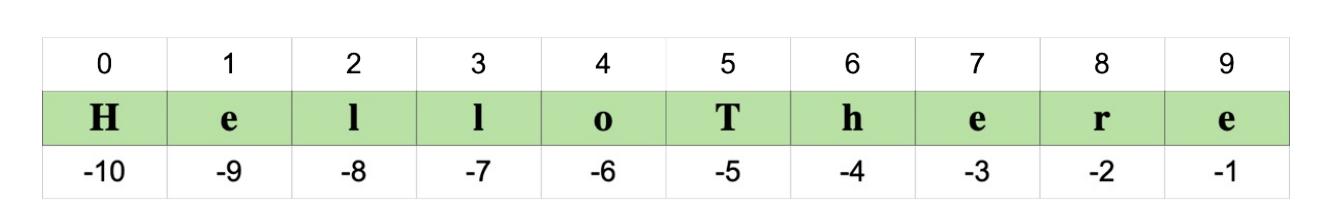
Figure 2.2: Python indexing
Trying to address indexes greater than 9 or smaller than -10 will raise an IndexError , as expected.
About names
You may have noticed that, in order to keep the examples as short as possible, we have named many objects using simple letters, like a , b , c , d , and so on. This is perfectly fine when debugging on the console, or showing that a + b == 7 , but it is bad practice when it comes to professional code (or any type of code, for that matter). We hope you will indulge us where we have done it; the reason is to present the code in a more compact way.
In a real environment though, when you choose names for your data, you should choose them carefully—they should reflect what the data is about. So, if you have a collection of Customer objects, customers is a perfectly good name for it. Would customers_list , customers_tuple , or customers_collection work as well? Think about it for a second. Is it good to tie the name of the collection to the datatype? We do not think so, unless there is a compelling reason. The reasoning behind this is that once customers_tuple starts being used in different parts of your code, and you realize you actually want to use a list instead of a tuple, you have a name tied to the wrong data type, which means you will have to refactor. Names for data should be nouns, and names for functions should be verbs. Names should be as expressive as possible. Python is actually a very good example when it comes to names. Most of the time you can just guess what a function is called if you know what it does.
Chapter 2 from the book Clean Code by Robert C. Martin is entirely dedicated to names. It is a great book that
helped us improve our coding style in many different ways; a must-read, if you want to take your skills to the next level.
Summary
In this chapter, we explored Python’s built-in data types. We have seen how many there are and how much can be achieved just by using them in different combinations.
We have seen number types, sequences, sets, mappings, dates, times, collections, and enumerations). We have also seen that everything is an object and learned the difference between mutable and immutable. We also learned about slicing and indexing.
We have presented the cases with simple examples, but there is much more that you can learn about this subject, so stick your nose into the official documentation and go exploring!
Most of all, we encourage you to try out all the exercises by yourself—get your fingers used to that code, build some muscle memory, and experiment, experiment, experiment. Learn what happens when you divide by zero, when you combine different number types, and when you work with strings. Play with all data types. Exercise them, break them, discover all their methods, enjoy them, and learn them very, very well. If your foundation is not rock solid, how good can your code be? Data is the foundation for everything; data shapes what dances around it.
The more you progress with the book, the more likely it is that you will find some discrepancies or a small typo here and there in our code (or yours). You will get an error message, something will break. That is wonderful! When you code, things break and you have to debug them, all the time, so consider errors as useful exercises to learn something new about the language you’re using, and not as failures or problems. Errors will keep coming up, that is certain, so you may as well start making your peace with them now.
The next chapter is about conditionals and iteration. We will see how to actually put collections to use, and make decisions based on the data that we are presented with. We will start to go a little faster now that your knowledge is building up, so make sure you are comfortable with the contents of this chapter before you move to the next one. Once more, have fun, explore, and break things—it is a very good way to learn.
3 Conditionals and Iteration
Join our book community on Discord

https://packt.link/o4zEQ
“Would you tell me, please, which way I ought to go from here?” “That depends a good deal on where you want to get to.”—Lewis Carroll, from Alice’s Adventures in Wonderland
In the previous chapter, we looked at Python’s built-in data types. Now that you are familiar with data in its many forms and shapes, it is time to start looking at how a program can use it.
According to Wikipedia:
In computer science, control flow (or flow of control) is the order in which individual statements, instructions or function calls of an imperative program are executed or evaluated.
The two main ways of controlling the flow of a program are conditional programming (also known as branching) and looping. These techniques can be combined to produce an endless variety of programs. Rather than attempting to document all the ways of combining looping and branching, we will give you an overview of the flow control constructs available in Python. Then we will work through a couple of example programs. This way, you should get a better feeling for how conditional programming and looping can be used.
In this chapter, we are going to cover the following:
- Conditional programming
- Looping in Python
- Assignment expressions
- A quick peek at the itertools module
Conditional programming
Conditional programming, or branching, is something you do every moment of every day. Essentially, it consists of evaluating conditions and deciding what action to take: if the light is green, then I can cross; if it is raining, then I am taking the umbrella; and if I am late for work, then I will call my manager.
The if statement
The main tool for conditional programming in Python is the if statement. Its function is to evaluate an expression and based on the result, choose which part of the code to execute. As usual, let us look at an example:
conditional.1.py late = True if late:
print("I need to call my manager!")This is the simplest example possible: the if statement evaluates the expression late in a Boolean context (exactly like if we were calling bool(late) ). If the result of the evaluation is True , then we enter the body of the code immediately after the if statement. Notice that the print instruction is indented, which means that it belongs to a scope defined by the if clause. Execution of this code yields:
$ python conditional.1.py
I need to call my manager!
Since late is True , the print() statement was executed. We can expand on the basic if statement, by adding an else clause. This provides an alternative set of instructions to execute when the expression in the if clause evaluates to False .
# conditional.2.py
late = False
if late:
   print("I need to call my manager!") # 1
else:
   print("no need to call my manager...") # 2
This time we set late = False , so when we execute the code, the result is different:
$ python conditional.2.py
no need to call my manager...
Depending on the result of evaluating late , we can either enter block # 1 or block # 2 , but not both. Block # 1 is executed when late evaluates to True , while block # 2 is executed when late evaluates to False . Try assigning False / True values to late and see how the output changes.
A specialized else: elif
Sometimes all you need is to do something if a condition is met (a simple if clause). At other times, you need to provide an alternative, in case the condition is False ( if / else clause). But there are situations where you have more than two paths to choose from. To demonstrate this, we will need an example with a few more options to choose from.
This time, we will create a simple tax calculator. Suppose that taxes are determined as follows: if your income is less than $10,000, you do not need to pay any taxes. If it is between $10,000 and $30,000, you must pay 20% in taxes. If it is between $30,000 and $100,000, you pay 35% in taxes, and if you are fortunate enough to earn over $100,000, you must pay 45% in taxes. Let us translate this into Python code:
# taxes.py
income = 15000
if income < 10000:
   tax_coefficient = 0.0 # 1
elif income < 30000:
   tax_coefficient = 0.2 # 2
elif income < 100000:
   tax_coefficient = 0.35 # 3
else:
   tax_coefficient = 0.45 # 4
print(f"You will pay: ${income * tax_coefficient} in taxes")
When we execute this code, we get the following output:
$ python taxes.py
You will pay: $3000.0 in taxes
Let us go through the example one line at a time. We start by setting up the income value. In the example, your income is $15,000. We enter the if statement. Notice that this time we also introduced the elif clause, which is a contraction of else-if. It differs from a plain else clause in that it also has its own condition. The if expression of income < 10000 evaluates to False , therefore block # 1 is not executed.
The control passes to the next condition: elif income < 30000 . This one evaluates to True , therefore block # 2 is executed, and because of this, Python then resumes execution after the whole if / elif / elif / else construct (which we can just call the if statement from now on). There is only one instruction after the if statement: the print() call, which produces the output telling us that you will pay $3000.0 in taxes this year (15,000 * 20%). Notice that the order is mandatory: if comes first, then (optionally) as many elif clauses as you may need, and then (optionally) a single else clause.
No matter how many lines of code you may have within each block, when one of the conditions evaluates to True , the associated block is executed, and then execution resumes after the whole clause. If none of the conditions evaluates to True (for example, income = 200000 ), then the body of the else clause would be executed (block # 4 ). This example expands our understanding of the behavior of the else clause. Its block of code is executed when none of the preceding if / elif /…/ elif expressions has evaluated to True .
Try to modify the value of income until you can comfortably execute any of the blocks at will. Also test the behavior at the boundaries where the values of the boolean expressions in the if and elif clauses change. It is crucial to test boundaries thoroughly to ensure correctness of your code. Should we allow you to drive at 18 or 17? Are we checking your age with age < 18 or age <= 18 ? You cannot imagine how many times we have had to fix subtle bugs that stemmed from using the wrong operator, so go ahead and experiment with the code. Change some < to <= and set income to be one of the boundary values (10,000, 30,000, 100,000) as well as any value in between. See how the result changes and get a good understanding of it before proceeding.
Nesting if statements
You can also nest if statements. Let us look at another example to show you how. Say your program encounters an error. If the alert system is the console, we print the error. If the alert system is an email, the severity of the error determines which address we should send the alert to. If the alert system is anything other than console or email, we do not know what to do, so we do nothing. Let us put this into code:
# errorsalert.py
alert_system = "console" # other value can be "email"
error_severity = "critical" # other values: "medium" or "low"
error_message = "Something terrible happened!"
if alert_system == "console": # outer
   print(error_message) # 1
elif alert_system == "email":
   if error_severity == "critical": # inner
       send_email("admin@example.com", error_message) # 2
   elif error_severity == "medium":
       send_email("support.1@example.com", error_message) # 3
   else:
       send_email("support.2@example.com", error_message) # 4
Here we have an inner if statement nested within the body of the elif clause of an outer if statement. Notice that the nesting is achieved by indenting the inner if statement.
Let us step through the code and see what happens. We start by assigning values to alert_system , error_severity and error_message . When we enter the outer if statement, if alert_system == “console” evaluates to True , body # 1 is executed, and nothing else happens. On the other hand, if alert_system == “email” evaluates to True , then we enter the inner if statement. In the inner if statement, the error_severity determines whether we send an email to an admin, first-level support, or second-level support (blocks # 2 , # 3 , and # 4 ). The send_email() function is not defined in this example, so trying to run it would give you an error. In the source code of this book, we included a trick to redirect that call to a regular print() function, just so you can experiment on the console without actually sending an email. Try changing the values and see how it all works.
The ternary operator
The next thing we would like to show you is the ternary operator. In Python, this is also known as a conditional
expression. It looks and behaves like a short, in-line version of an if statement. When you just want to choose between two values, depending on some condition, it is sometimes easier and more readable to use the ternary operator instead of a full if statement. For example, instead of:
# ternary.py
order_total = 247 # GBP
# classic if/else form
if order_total > 100:
    discount = 25 # GBP
else:
    discount = 0 # GBP
print(order_total, discount)
We could write:
# ternary.py
# ternary operator
discount = 25 if order_total > 100 else 0
print(order_total, discount)
For simple cases like this, we find it convenient to be able to express that logic in one line instead of four. Remember, as a coder, you spend much more time reading code than writing it, so Python’s conciseness is invaluable.
In some languages (like C or JavaScript) the ternary operator is even more concise. For example, the above could be written as:
discount = order_total > 100 ? 25 : 0;Although Python’s version is slightly more verbose, we think it more than makes up for that by being easier to read and understand.
Are you clear on how the ternary operator works? It is quite simple, something if condition else something-else evaluates to something if condition evaluates to True . Otherwise, if condition is False , the expression evaluates to something-else .
Pattern matching
Structural pattern matching, often just called pattern matching, is a relatively new feature that was introduced in Python 3.10 via PEP 634 (https://peps.python.org/pep-0634). It was partly inspired by the pattern matching capabilities of languages like Haskel, Erlang, Scala, Elixir and Ruby.
Simply put, the match statement compares a value against one or more patterns, and executes the code block associated with the first pattern that matches. Let us see a simple example:
# match.py
day_number = 4
match day_number:
   case 1 | 2 | 3 | 4 | 5:
       print("Weekday")
   case 6:
       print("Saturday")
   case 7:
       print("Sunday")
   case _:
       print(f"{day_number} is not a valid day number")
We start by initializing day_number before entering the match statement. The match statement will attempt to match the value of day_number against a series of patterns, each of which is introduced by the case keyword. In our example we have four patterns. The first 1 | 2 | 3 | 4 | 5 will match any of the values 1 , 2 , 3 , 4 or 5 . This is known as an OR pattern, it consists of a number of sub-patterns separated by | . It matches when any of the subpatterns (in this case the literal values 1 , 2 , 3 , 4 and 5 ) match. The second and third patterns in our example just
consist of the integer literals 6 and 7 , respectively. The final pattern _ is a wildcard pattern, it is a catch-all that matches any value. A match statement can have at most one catch-all pattern, and if one is present, it must be the last pattern.
The body of the first case block whose pattern matches, will be executed. Afterward, execution resumes below the match statement without evaluating any of the remaining patterns. If none of the patterns match, execution resumes below the match statement without executing any of the case bodies. In our example, the first pattern matches, so print(“Weekday”) is executed. Take some time to experiment with this example. Try changing the value of day_number and see what happens when you run it.
The match statement resembles the switch / case statements of languages like C++ and JavaScript. It is, however, much more powerful than that. The variety of different kinds of patterns available and the ability to compose patterns, allows you to do much more than a simple C++ switch statement. For example, Python allows you to match sequences, dictionaries, or even custom classes. You can also capture and assign values to names in patterns. We do not have space here to cover everything you can do with pattern matching, but we encourage you to study the tutorial in PEP 636 (https://peps.python.org/pep-0636) to learn more.
Now that you know everything about controlling the path of the code, let us move on to the next subject: looping.
Looping
If you have any experience with looping in other programming languages, you will find Python’s way of looping a bit different. First of all, what is looping? Looping means being able to repeat the execution of a code block more than once, according to the loop parameters given. There are different looping constructs, which serve different purposes, and Python has distilled all of them down to just two, which you can use to achieve everything you need. These are the for and while statements.
While it is definitely possible to do everything you need using either of them, they do serve different purposes, and therefore they are usually used in different contexts. We will explore this difference thoroughly in this chapter.
The for loop
The for loop is used when looping over a sequence, such as a list, tuple, or collection of objects. Let us start with a simple example and expand on the concept to see what the Python syntax allows us to do:
# simple.for.py
for number in [0, 1, 2, 3, 4]:
   print(number)
This simple snippet of code, when executed, prints all numbers from 0 to 4 . The body of the for loop (the print() line) is executed once for each value in the list [0, 1, 2, 3, 4] . In the first iteration number , is assigned the first value from the sequence, in the second iteration number takes the second value, and so on. After the last item in the sequence, the loop terminates, and execution resumes normally with the code after the loop.
Iterating over a range
We often need to iterate over a range of numbers, and it would be quite tedious to have to do so by hard coding the list somewhere. In such cases, the range() function comes to the rescue. Let us see the equivalent of the previous snippet of code:
# simple.for.py
for number in range(5):
   print(number)
The range() function is used extensively to create sequences in Python programs. You can call it with a single value, which acts as stop (counting will start from 0 ). You can also pass two values ( start and stop ), or even three ( start , stop , and step ). Check out the following example:
>>> list(range(10)) # one value: from 0 to value (excluded)
[0, 1, 2, 3, 4, 5, 6, 7, 8, 9]
>>> list(range(3, 8)) # two values: from start to stop (excluded)
[3, 4, 5, 6, 7]
>>> list(range(-10, 10, 4)) # three values: step is added
[-10, -6, -2, 2, 6]
For the moment, ignore that we need to wrap range(…) within a list. We will explain the reasons for this in Chapter 5, Comprehensions and Generators. You can see that the behavior is analogous to slicing (which we described in the previous chapter): start is included, stop is excluded, and you can add an optional step parameter, which by default is 1 .
Try modifying the parameters of the range() call in our simple.for.py code and see what it prints.
Iterating over a sequence
We now have all the tools to iterate over a sequence, so let us build on that example:
# simple.for.2.py
surnames = ["Rivest", "Shamir", "Adleman"]
for position in range(len(surnames)):
   print(position, surnames[position])
The preceding code adds a little bit of complexity to the game. Execution will show this result:
$ python simple.for.2.py
0 Rivest
1 Shamir
2 Adleman
Let us use the inside-out technique to break it down. We start from the innermost part of what we are trying to understand, and we expand outward. So, len(surnames) is the length of the surnames list: 3 . Therefore, range(len(surnames)) is actually transformed into range(3) . This gives us the range [0, 3) , which is the sequence (0, 1, 2) . This means that the for loop will run three iterations. In the first one, position will take value 0 , while in the second one, it will take value 1 , and value 2 in the third and final iteration. What is (0, 1, 2) , if not the possible indexing positions for the surnames list? At position 0 , we find “Rivest” ; at position 1 , “Shamir” ; and at position 2 , “Adleman” . If you are curious about what these three men created together, change print(position, surnames[position]) to print(surnames[position][0], end=““) , add a final print() outside of the loop, and run the code again.
Now, this style of looping is much closer to languages such as Java or C. In Python, it is quite rare to see code like this. You can just iterate over any sequence or collection, so there is no need to get the list of positions and retrieve elements out of a sequence at each iteration. Let us change the example into a more Pythonic form:
# simple.for.3.py
surnames = ["Rivest", "Shamir", "Adleman"]
for surname in surnames:
   print(surname)
The for loop can iterate over the surnames list, and it gives back each element in order at each iteration. Running this code will print the three surnames, one at a time, which is much easier to read.
What if you wanted to print the position as well, though? Or what if you needed it? Should you go back to the range(len(…)) form? No. You can use the enumerate() built-in function, like this:
# simple.for.4.py
surnames = ["Rivest", "Shamir", "Adleman"]
for position, surname in enumerate(surnames):
   print(position, surname)
This code is quite interesting as well. Notice that enumerate() gives back a two-tuple (position, surname) at each iteration, but still, it is more readable (and more efficient) than the range(len(…)) example. You can call
enumerate() with a start parameter, such as enumerate(iterable, start) , and it will start from start , rather than 0 . Just another little thing that shows you how much thought has been given to designing Python so that it makes your life easier.
You can use a for loop to iterate over lists, tuples, and in general anything that Python calls iterable. This is an important concept, so let us talk about it a bit more.
Iterators and iterables
According to the Python documentation (https://docs.python.org/3.12/glossary.xhtml#term-iterable), an iterable is:
An object capable of returning its members one at a time. Examples of iterables include all sequence types (such as list, str, and tuple) and some non-sequence types like dict, file objects, and objects of any classes you define with an __iter__() method or with a __getitem__() method that implements sequence semantics….Iterables can be used in a for loop and in many other places where a sequence is needed (zip(), map(), …). When an iterable object is passed as an argument to the built-in function iter(), it returns an iterator for the object. This iterator is good for one pass over the set of values. When using iterables, it is usually not necessary to call iter() or deal with iterator objects yourself. The for statement does that automatically for you, creating a temporary unnamed variable to hold the iterator for the duration of the loop.
Simply put, what happens when you write for k in sequence: … body … is that the for loop asks sequence for the next element, it gets something back, it calls that something k , and then executes its body. Then, once again, the for loop asks sequence for the next element, it calls it k again, and executes the body again, and so on and so forth, until the sequence is exhausted. Empty sequences will result in zero executions of the body.
Some data structures, when iterated over, produce their elements in order, such as lists, tuples, dictionaries, and strings, while others, such as sets, do not. Python gives us the ability to iterate over iterables, using a type of object called an iterator.
According to the official documentation, an iterator is:
An object representing a stream of data. Repeated calls to the iterator’s __next__() method (or passing it to the built-in function next()) return successive items in the stream. When no more data are available a StopIteration exception is raised instead. At this point, the iterator object is exhausted and any further calls to its __next__() method just raise StopIteration again. Iterators are required to have an __iter__() method that returns the iterator object itself so every iterator is also iterable and may be used in most places where other iterables are accepted. One notable exception is code which attempts multiple iteration passes. A container object (such as a list) produces a fresh new iterator each time you pass it to the iter() function or use it in a for loop. Attempting this with an iterator will just return the same exhausted iterator object used in the previous iteration pass, making it appear like an empty container.
Do not worry if you do not fully understand all the preceding legalese, as you will in due course. We have put it here to serve as a handy reference for the future.
In practice, the whole iterable/iterator mechanism is hidden behind the code. Unless you need to code your own iterable or iterator for some reason, you will not have to worry about this too much. But it is important to understand how Python handles this key aspect of control flow because it will shape the way in which you write code.
Iterating over multiple sequences
Let us see another example of how to iterate over two sequences of the same length, to work on their respective elements in pairs. Say we have a list of people’s names and a second list of numbers representing their ages. We want to print the pair person/age on one line for each of them. Let us start with an example, which we will refine gradually:
# multiple.sequences.py
people = ["Nick", "Rick", "Roger", "Syd"]
ages = [23, 24, 23, 21]
for position in range(len(people)):
person = people[position]
age = ages[position]
print(person, age)By now, this code should be straightforward. We iterate over the list of positions ( 0 , 1 , 2 , 3 ) because we want to retrieve elements from two different lists. Executing it, we get the following:
$ python multiple.sequences.py
Nick 23
Rick 24
Roger 23
Syd 21
The code works, but it is not very Pythonic. It is cumbersome to have to get the length of people , construct a range , and then iterate over that. For some data structures, it may also be expensive to retrieve items by their position. It would be better if we could iterate over the sequences directly, as we do for a single sequence. Let us try to improve it by using enumerate() :
# multiple.sequences.enumerate.py
people = ["Nick", "Rick", "Roger", "Syd"]
ages = [23, 24, 23, 21]
for position, person in enumerate(people):
   age = ages[position]
   print(person, age)
That is better, but still not perfect. We are iterating properly on people , but we are still fetching age using positional indexing, which we want to lose as well. We can achieve that, by using the zip() function, which we encountered in the previous chapter. Let us use it:
# multiple.sequences.zip.py
people = ["Nick", "Rick", "Roger", "Syd"]
ages = [23, 24, 23, 21]
for person, age in zip(people, ages):
   print(person, age)
That is much more elegant than the original version. When the for loop asks zip(sequenceA, sequenceB) for the next element, it gets back a tuple which is unpacked into person and age . The tuple will have as many elements as the number of sequences we feed to the zip() function. Let us expand a little on the previous example:
# multiple.sequences.unpack.py
people = ["Nick", "Rick", "Roger", "Syd"]
ages = [23, 24, 23, 21]
instruments = ["Drums", "Keyboards", "Bass", "Guitar"]
for person, age, instrument in zip(people, ages, instruments):
   print(person, age, instrument)
In the preceding code, we added the instruments list. Now that we feed three sequences to the zip() function, the for loop gets back a three-tuple at each iteration. The elements of the tuple are unpacked and assigned to person , age , and instrument . Notice that the position of the elements in the tuple respects the position of the sequences in the zip() call. Executing the code will yield the following result:
$ python multiple.sequences.unpack.py
Nick 23 Drums
Rick 24 Keyboards
Roger 23 Bass
Syd 21 Guitar
Note that it is not necessary to unpack the tuples when iterating over multiple sequences like this. You may need to operate on the tuple as a whole within the body of the for loop. It is, of course, perfectly possible to do so:
# multiple.sequences.tuple.py
people = ["Nick", "Rick", "Roger", "Syd"]
ages = [23, 24, 23, 21]
instruments = ["Drums", "Keyboards", "Bass", "Guitar"]
for data in zip(people, ages, instruments):
print(data)This is almost identical to the previous example. The difference is that instead of unpacking the tuple we get from zip(…) , we assign the entire tuple to data .
The while loop
In the preceding pages, we saw the for loop in action. It is useful when you need to loop over a sequence or a collection. The key point to keep in mind when you need to decide which looping construct to use, is that the for loop is best suited in cases where you have to iterate over the elements of some container or other iterable object.
There are other cases though, when you just need to loop until some condition is satisfied, or even loop indefinitely until the application is stopped. In such cases, we do not have something to iterate on, so the for loop would be a poor choice. For situations like this, the while loop is more appropriate.
The while loop is similar to the for loop in that both repeatedly execute a body of instructions. The difference is that the while loop does not loop over a sequence. Instead, it loops as long as a certain condition is satisfied. When the condition is no longer satisfied, the loop ends.
As usual, let us see an example that will clarify everything for us. We want to print the binary representation of a positive number. To do so, we can use a simple algorithm that divides by two until we reach zero and collects the remainders. When we reverse the list of remainders we collected, we get the binary representation of the number we started with. For example, if we want a binary representation of the decimal number 6, the steps would be as follows:
1. 6 / 2 = 3 with remainder 0
2. 3 / 2 = 1 with remainder 1
3. 1 / 2 = 0 with remainder 1
4. The list of remainders is: 0, 1, 1.
5. Reversing this, we get 1, 1, 0, which is also the binary representation of 6: 110.
Let us translate this into Python code. We will calculate the binary representation of the number 39, which is 100111.
# binary.py
n = 39
remainders = []
while n > 0:
   remainder = n % 2 # remainder of division by 2
   remainders.append(remainder) # we keep track of remainders
   n //= 2 # we divide n by 2
remainders.reverse()
print(remainders)
In the preceding code, we highlighted n > 0 , which is the condition to keep looping. Notice how the code matches the algorithm we described: as long as n is greater than 0 , we divide by 2 and add the remainder to a list. At the end (when n has reached 0 ) we reverse the list of remainders to get the binary representation of the original value of n .
We can use the divmod() function to make the code a little shorter (and more Pythonic). The divmod() function takes a number and a divisor and returns a tuple with the result of the integer division and its remainder. For example, divmod(13, 5) would return (2, 3) , and indeed 5 * 2 + 3 = 13.
# binary.2.py
n = 39
remainders = []
while n > 0:
   n, remainder = divmod(n, 2)
   remainders.append(remainder)
remainders.reverse()
print(remainders)Now we reassign n to the result of the division by 2 and remainder to the remainder, in a single line.
The built-in function bin() returns a binary representation of a number. So, apart from examples, or as an exercise, there is no need to implement this yourself in Python.
Note that the condition in a while loop is a condition to continue looping. If it evaluates to True , then the body is executed and then another evaluation follows, and so on, until the condition evaluates to False . When that happens, the loop stops immediately without executing its body. If the condition never evaluates to False , the loop becomes a so-called infinite loop. Infinite loops are used, for example, when polling from network devices: you ask the socket whether there is any data, you do something with it if there is any, then you sleep for a small amount of time, and then you ask the socket again, over and over, without ever stopping.
To better illustrate the differences between for and while loops, let us adapt one of the previous examples ( multiple.sequences.py ) using a while loop:
# multiple.sequences.while.py
people = ["Nick", "Rick", "Roger", "Syd"]
ages = [23, 24, 23, 21]
position = 0
while position < len(people):
   person = people[position]
   age = ages[position]
   print(person, age)
   position += 1
In the preceding code, we have highlighted the initialization, condition, and update of the position variable, which makes it possible to simulate the equivalent for loop code by handling the iteration manually. Everything that can be done with a for loop can also be done with a while loop, even though you can see there is a bit of boilerplate you have to go through to achieve the same result. The opposite is also true, but unless you have a reason to do so, you ought to use the right tool for the job.
To recap, use a for loop when you need to iterate over an iterable, and a while loop when you need to loop according to a condition being satisfied or not. If you keep in mind the difference between the two purposes, you will never choose the wrong looping construct.
Let us now see how to alter the normal flow of a loop.
The break and continue statements
Sometimes you will need to alter the regular flow of a loop. You can either skip a single iteration (as many times as you want), or you can break out of the loop entirely. A common use case for skipping iterations is, for example, when you are iterating over a list of items, but you only need to work on those that satisfy some condition. On the other hand, if you are iterating over a collection to search for an item that meets some requirement, you may want to break out of the loop as soon as you find what you are looking for. There are countless possible scenarios, let us work through a couple of examples together to show you how this works in practice.
Suppose that you want to apply a 20% discount to all products that have an expiration date of today. You can achieve this by using the continue statement, which tells the looping construct ( for or while ) to stop execution of the body immediately and go to the next iteration, if any.
# discount.py
from datetime import date, timedelta
today = date.today()
tomorrow = today + timedelta(days=1) # today + 1 day is tomorrow
products = [
   {"sku": "1", "expiration_date": today, "price": 100.0},
   {"sku": "2", "expiration_date": tomorrow, "price": 50},
   {"sku": "3", "expiration_date": today, "price": 20},
]
for product in products:
print("Processing sku", product["sku"])
if product["expiration_date"] != today:
continue
product["price"] *= 0.8 # equivalent to applying 20% discount
print("Sku", product["sku"], "price is now", product["price"])We start by importing the date and timedelta objects, then we set up our products. Those with sku 1 and 3 have an expiration date of today , which means we want to apply a 20% discount on them. We loop over each product and inspect the expiration date. If it is not (inequality operator: != ) today , we do not want to execute the rest of the body, so we continue. Execution of the loop body stops and goes on to the next iteration. If we run the discount.py module, this is the output:
$ python discount.py
Processing sku 1
Sku 1 price is now 80.0
Processing sku 2
Processing sku 3
Sku 3 price is now 16.0
As you can see, the last two lines of the body have not been executed for sku number 2 .
Let us now see an example of breaking out of a loop. Say we want to tell whether at least one of the elements in a list evaluates to True when fed to the bool() function. Given that we need to know whether there is at least one, when we find it, we do not need to keep scanning the list any further. In Python code, this translates to using the break statement. Let us write this down into code:
# any.py
items = [0, None, 0.0, True, 0, 7] # True and 7 evaluate to True
found = False # this is called a "flag"
for item in items:
   print("scanning item", item)
   if item:
       found = True # we update the flag
       break
if found: # we inspect the flag
   print("At least one item evaluates to True")
else:
   print("All items evaluate to False")
The preceding code makes use of a common programming pattern; you set up a flag variable before starting the inspection of the items. If you find an element that matches your criteria (in this example, that evaluates to True ), you update the flag and stop iterating. After iteration, you inspect the flag and act accordingly. Execution yields:
$ python any.py
scanning item 0
scanning item None
scanning item 0.0
scanning item True
At least one item evaluates to True
See how execution stopped after True was found? The break statement is similar to continue , in that it immediately stops executing the body of the loop, but it also prevents any further iterations from running, effectively breaking out of the loop.
There is no need to write code to detect whether there is at least one element in a sequence that evaluates to True , the built-in function any() does exactly this.
You can use as many continue or break statements as you need, anywhere in a loop body ( for or while ). You can even use both in the same loop.
A special else clause
One of the features we have seen only in the Python language is the ability to have an else clause after a loop. It is very rarely used, but it is useful to have. If the loop ends normally, because of exhaustion of the iterator ( for loop) or because the condition is finally not met ( while loop), then the else suite (if present) is executed. If execution is interrupted by a break statement, the else clause is not executed.
Let us take an example of a for loop that iterates over a group of items, looking for one that would match some condition. If we do not find at least one that satisfies the condition, we want to raise an exception. This means that we want to arrest the regular execution of the program and signal that there was an error, or exception. Exceptions will be the subject of Chapter 7, Exceptions and Context Managers, so do not worry if you do not fully understand them for now. Just bear in mind that they alter the regular flow of the code.
Let us first see how we would do this without the for…else syntax. Say that we want to find, among a collection of people, one that could drive a car:
# for.no.else.py
class DriverException(Exception):
   pass
people = [("James", 17), ("Kirk", 9), ("Lars", 13), ("Robert", 8)]
driver = None
for person, age in people:
   if age >= 18:
       driver = (person, age)
       break
if driver is None:
   raise DriverException("Driver not found.")
Notice the flag pattern again. We set the driver to be None , then if we find one, we update the driver flag. At the end of the loop, we inspect it to see whether one was found. Notice that if a driver is not found, DriverException is raised, signaling to the program that execution cannot continue (we are lacking the driver).
Now, let us see how to do this with an else clause on the for loop:
# for.else.py
class DriverException(Exception):
   pass
people = [("James", 17), ("Kirk", 9), ("Lars", 13), ("Robert", 8)]
for person, age in people:
   if age >= 18:
       driver = (person, age)
       break
else:
   raise DriverException("Driver not found.")
Notice that we no longer need the flag pattern. The exception is raised as part of the loop logic, which makes good sense because the loop is checking for some condition. All we need is to set up a driver object in case we find one because the rest of the code is going to use that information somewhere. Notice the code is shorter and more elegant because the logic is now correctly grouped together where it belongs.
In his Transforming Code into Beautiful, Idiomatic Python video, Raymond Hettinger suggests a much better name for the else statement associated with a for loop: nobreak . If you struggle with remembering how the else works for a for loop, simply remembering this fact should help you.
Assignment expressions
Before we look at some more complicated examples, we would like to briefly introduce you to a feature that was added to the language in Python 3.8, via PEP 572 (https://peps.python.org/pep-0572). Assignment expressions allow us to bind a value to a name in places where normal assignment statements are not allowed. Instead of the normal assignment operator = , assignment expressions use := (known as the walrus operator because it resembles the eyes and tusks of a walrus).
Statements and expressions
To understand the difference between normal assignments and assignment expressions, we need to understand the difference between statements and expressions. According to the Python documentation (https://docs.python.org/3.12/glossary.xhtml#term-statement), a statement is:
…part of a suite (a “block” of code). A statement is either an expression or one of several constructs with a keyword, such as if , while or for .
An expression, on the other hand, is:
A piece of syntax which can be evaluated to some value. In other words, an expression is an accumulation of expression elements like literals, names, attribute access, operators or function calls which all return a value.
The key distinguishing feature of an expression is that it has a value. Notice that an expression can be a statement, but not all statements are expressions. In particular, assignments like name = “heinrich” are not expressions, and so do not have a value. This means that you cannot use an assignment statement in the condition expression of a while loop or if statement (or any other place where a value is required).
This explains why the Python console does not print a value when you assign a value to a name. For example:
>>> name = "heinrich"
>>>
is a statement, which does not have a return value to print.
Using the walrus operator
Without assignment expressions, you would have to use two separate statements if you wanted to bind a value to a name and use that value in an expression. For example, it is quite common to see code like:
# walrus.if.py
remainder = value % modulus
if remainder:
    print(f"Not divisible! The remainder is {remainder}.")
With assignment expressions, we could rewrite this as:
# walrus.if.py
if remainder := value % modulus:
    print(f"Not divisible! The remainder is {remainder}.")
Assignment expressions allow us to write fewer lines of code. Used with care, they can also lead to cleaner, more understandable code. Let us look at a slightly bigger example to see how an assignment expression can simplify a while loop.w
In interactive scripts, we often need to ask the user to choose between a number of options. For example, suppose we are writing an interactive script that allows customers at an ice cream shop to choose what flavor they want. To avoid confusion when preparing orders, we want to ensure that the user chooses one of the available flavors. Without assignment expressions, we might write something like this:
# menu.no.walrus.py
flavors = ["pistachio", "malaga", "vanilla", "chocolate"]
prompt = "Choose your flavor: "
print(flavors)
while True:
   choice = input(prompt)
   if choice in flavors:
       break
   print(f"Sorry, '{choice}' is not a valid option.")
print(f"You chose '{choice}'.")
Take a moment to read this code carefully. Note the condition on the loop: while True means “loop forever,” which is not what we want. We want to stop the loop when the user inputs a valid flavor ( choice in flavors ). To achieve that, we have an if statement and a break inside the loop. The logic to control the loop is not immediately obvious. Despite that, this is actually quite a common pattern when the value needed to control the loop can only be obtained inside the loop.
The input() function is very useful in interactive scripts. It prompts the user for input and returns it as a string.
How can we improve on this? Let us try to use an assignment expression:
# menu.walrus.py
flavors = ["pistachio", "malaga", "vanilla", "chocolate"]
prompt = "Choose your flavor: "
print(flavors)
while (choice := input(prompt)) not in flavors:
   print(f"Sorry, '{choice}' is not a valid option.")
print(f"You chose '{choice}'.")
Now the loop conditional says exactly what we want. That is much easier to understand. The code is also three lines shorter.
We need parentheses around the assignment expression in this example, because the := operator has lower precedence than the not in operator. Try removing them and see what happens.
We have seen examples of using assignment expressions in if and while statements. Besides these use cases, assignment expressions are also useful in lambda expressions (which you will meet in Chapter 4, Functions, the Building Blocks of Code) as well as comprehensions and generators (which you will learn about in Chapter 5, Comprehensions and Generators).
A word of warning
The introduction of the walrus operator in Python was somewhat controversial. Some people feared that it would make it too easy to write ugly, non-Pythonic code. We think that these fears are not entirely justified. As you saw above, the walrus operator can improve code and make it easier to read. Like any powerful feature, it can, however, be abused to write obfuscated code. We would advise you to use it sparingly. Always think carefully about how it impacts the readability of your code.
Putting all this together
Now that we have covered the basics of conditionals and loops, we can move on to the example programs we promised at the beginning of this chapter. We will mix and match here, so you can see how you can use all these concepts together.
A prime generator
Let us start by writing some code to generate a list of prime numbers up to (and including) some limit. Please bear in mind that we are going to write a very inefficient and rudimentary algorithm to find prime numbers. The important thing is to concentrate on those bits in the code that belong to this chapter’s subject.
According to Wikipedia:
A prime number (or a prime) is a natural number greater than 1 that is not a product of two smaller natural numbers. A natural number greater than 1 that is not prime is called a composite number.
Based on this definition, if we consider the first ten natural numbers, we can see that 2, 3, 5, and 7 are primes, while 1, 4, 6, 8, 9, and 10 are not. To determine whether a number, N, is prime, you can divide it by each of the natural numbers in the range [2, N). If the remainder of any division is zero, then the number is not a prime. To generate the sequence of prime numbers, we will consider each natural number, starting from two, up to the limit, and test whether it is a prime. We will write two versions of this, the second of which will exploit the for…else syntax:
# primes.py
primes = [] # this will contain the primes at the end
upto = 100 # the limit, inclusive
for n in range(2, upto + 1):
   is_prime = True # flag, new at each iteration of outer for
   for divisor in range(2, n):
       if n % divisor == 0:
           is_prime = False
           break
   if is_prime: # check on flag
       primes.append(n)
print(primes)
There is quite a lot happening in this code. We start by setting up an empty primes list, which will contain the primes at the end. We set the limit to 100 , and because we want it to be inclusive, we have to iterate over range(2, upto + 1) in our outer for loop (remember that range(2, upto) would stop at upto - 1). The outer loop iterates over the candidate primes—that is, all natural numbers from 2 to upto . Each iteration of this loop tests one number to determine whether it is a prime. In each iteration of the outer loop, we set up a flag (which is set to True at each iteration), and then start dividing the current value of n by all numbers from 2 to n - 1 . If we find a proper divisor for n , it means n is composite, so we set the flag to False and break the loop. Notice that when we break the inner loop, the outer one keeps on going as normal. The reason we break after having found a proper divisor for n is that we do not need any further information to be able to tell that n is not a prime.
When we check the is_prime flag after the inner loop, if it is still True , it means we could not find any number in [2, n) that is a proper divisor for n , therefore n is a prime. We append n to the primes list, and proceed to the next iteration, until n equals 100 .
Running this code outputs:
$ python primes.py
[2, 3, 5, 7, 11, 13, 17, 19, 23, 29, 31, 37, 41, 43, 47, 53, 59, 61,
67, 71, 73, 79, 83, 89, 97]
Before proceeding, we will pose the following question: one of the iterations of the outer loop is different from the rest. Can you tell which iteration this is—and why? Think about it for a moment, go back to the code, try to work it out for yourself, and then keep reading on.
Did you find the answer? Do not feel bad if you did not, the skill to understand what the code does by simply looking at it takes time and experience to learn. It is an important skill to have as a programmer though, so try to exercise it whenever you can. We will tell you the answer now: the first iteration behaves differently from all the others. The reason is that in the first iteration, n is 2 . Therefore, the innermost for loop will not run at all because it is a for loop that iterates over range(2, 2) , which is an empty range. Try it yourself, write a simple for loop with that iterable, put a print in the body, and see what happens when you run it.
We are not going to try to make this code more efficient from an algorithmic point of view. But let us use some of what we learned in this chapter, to at least make it easier to read:
# primes.else.py
primes = []
upto = 100
for n in range(2, upto + 1):
   for divisor in range(2, n):
       if n % divisor == 0:
           break
   else:
       primes.append(n)
print(primes)
Using an else clause on the inner loop allows us to get rid of the is_prime flag. Instead, we append n to the primes list when we know the inner loop has not encountered any break statements. It is only two lines shorter, but the code is simpler, cleaner and reads better. This is important, simplicity and readability count for a lot in programming. Always look for ways to simplify your code and make it easier to read. You will thank yourself when you get back to it months later and have to try to understand what you did before.
Applying discounts
In this example, we want to show you a technique called a lookup table, which we are very fond of. We will start by simply writing some code that assigns a discount to customers based on their coupon value. We will keep the logic down to a minimum here—remember that all we really care about is understanding conditionals and loops:
# coupons.py
customers = [
   dict(id=1, total=200, coupon_code="F20"), # F20: fixed, £20
   dict(id=2, total=150, coupon_code="P30"), # P30: percent, 30%
   dict(id=3, total=100, coupon_code="P50"), # P50: percent, 50%
   dict(id=4, total=110, coupon_code="F15"), # F15: fixed, £15
]
for customer in customers:
   match customer["coupon_code"]:
       case "F20":
           customer["discount"] = 20.0
       case "F15":
           customer["discount"] = 15.0
       case "P30":
           customer["discount"] = customer["total"] * 0.3
       case "P50":
           customer["discount"] = customer["total"] * 0.5
       case _:
           customer["discount"] = 0.0
for customer in customers:
   print(customer["id"], customer["total"], customer["discount"])
We start by setting up some customers. They have an order total, a coupon code, and an ID. We made up four types of coupons: two are for fixed amounts and two are percentage-based. We use a match statement, with a case for each coupon code and a wildcard to handle invalid coupons. We compute the discount and set it as the “discount” key in the customer dictionary.
At the end, we just print out part of the data to see whether our code is working properly:
$ python coupons.py
1 200 20.0
2 150 45.0
3 100 50.0
4 110 15.0
This code is simple to understand, but all those match cases are cluttering the logic. Adding more coupon codes requires adding additional cases and implementing the discount calculation for each case. The discount calculation is very similar in most cases, which makes the code repetitive and violates the DRY principle. In cases like this, you can use a dictionary to your advantage, like this:
# coupons.dict.py
customers = [
   dict(id=1, total=200, coupon_code="F20"), # F20: fixed, £20
   dict(id=2, total=150, coupon_code="P30"), # P30: percent, 30%
   dict(id=3, total=100, coupon_code="P50"), # P50: percent, 50%
   dict(id=4, total=110, coupon_code="F15"), # F15: fixed, £15
]
discounts = {
   "F20": (0.0, 20.0), # each value is (percent, fixed)
   "P30": (0.3, 0.0),
   "P50": (0.5, 0.0),
   "F15": (0.0, 15.0),
}
for customer in customers:
   code = customer["coupon_code"]
   percent, fixed = discounts.get(code, (0.0, 0.0))
   customer["discount"] = percent * customer["total"] + fixed
for customer in customers:
print(customer["id"], customer["total"], customer["discount"])Running the preceding code produces exactly the same output as the snippet before it. The code is two lines shorter, but more importantly, we gained a lot in readability, as the body of the for loop is now just three lines long, and easy to understand. The key idea here is to use a dictionary as a lookup table. In other words, we try to fetch something (the parameters for the discount calculation) from the dictionary based on a code (our coupon_code ). We use dict.get(key, default) to ensure that we can handle codes that are not in the dictionary, by supplying a default value.
Aside from readability, another major advantage of this approach is that we can easily add new coupon codes (or remove old ones) without changing the implementation: we only need to change the data in the lookup table. In a real-world application, we could even store the lookup table in a database and provide an interface for users to add or remove coupon codes at runtime.
Notice that we had to apply some simple linear algebra to calculate the discount. Each discount has a percentage and fixed part in the dictionary, represented by a two-tuple. By applying percent * total + fixed , we get the correct discount. When percent is 0 , the formula just gives the fixed amount, and it gives percent * total when fixed is 0 .
This technique is closely related to dispatch tables, which store functions as values in a table. This allows for even greater flexibility. Some object-oriented programming languages use this technique internally to implement features such as virtual methods.
If you are still unclear as to how this works, we suggest you take your time and experiment with it. Change values and add print() statements to see what is going on while the program is running.
A quick peek at the itertools module
A chapter about iterables, iterators, conditional logic, and looping would not be complete without a few words about the itertools module. According to the Python official documentation (https://docs.python.org/3.12/library/itertools.xhtml), the itertools module:
…implements a number of iterator building blocks inspired by constructs from APL, Haskell, and SML. Each has been recast in a form suitable for Python.The module standardizes a core set of fast, memory efficient tools that are useful by themselves or in combination. Together, they form an “iterator algebra” making it possible to construct specialized tools succinctly and efficiently in pure Python.
We do not have room here to show you everything this module has to offer, so we encourage you to explore it further for yourself. We can promise that you will enjoy it, though. It provides you with three broad categories of iterators. As an introduction, we shall give you a small example of one iterator taken from each category.
Infinite iterators
Infinite iterators allow you to use a for loop as an infinite loop, iterating over a sequence that never ends:
# infinite.py
from itertools import count
for n in count(5, 3):
   if n > 20:
       break
   print(n, end=", ") # instead of newline, comma and space
Running the code outputs:
$ python infinite.py
5, 8, 11, 14, 17, 20,
The count factory class makes an iterator that simply goes on and on counting. In this example, it starts from 5 and keeps adding 3 at every iteration. We need to break it manually if we do not want to get stuck in an infinite
loop.
Iterators terminating on the shortest input sequence
This category is quite interesting. It allows you to create an iterator based on multiple iterators, combining their values according to some logic. The key point here is that the resulting iterator will not break if one of the input iterators is shorter than the rest. It will simply stop as soon as the shortest iterator is exhausted. This may seem rather abstract, so let us give you an example using compress() . This iterator takes a sequence of data and a sequence of selectors and yields only those values from the data sequence that correspond to True values in the selectors sequence. For example, compress(“ABC”, (1, 0, 1)) would give back “A” and “C” because they correspond to 1 . Let us see a simple example:
# compress.py
from itertools import compress
data = range(10)
even_selector = [1, 0] * 10
odd_selector = [0, 1] * 10
even_numbers = list(compress(data, even_selector))
odd_numbers = list(compress(data, odd_selector))
print(odd_selector)
print(list(data))
print(even_numbers)
print(odd_numbers)
Notice that odd_selector and even_selector are 20 elements in length, while data is only 10. compress() will stop as soon as data has yielded its last element. Running this code produces the following:
$ python compress.py
[0, 1, 0, 1, 0, 1, 0, 1, 0, 1, 0, 1, 0, 1, 0, 1, 0, 1, 0, 1]
[0, 1, 2, 3, 4, 5, 6, 7, 8, 9]
[0, 2, 4, 6, 8]
[1, 3, 5, 7, 9]
It is a fast and convenient way of selecting elements out of an iterable. The code is simple, but notice that instead of using a for loop to iterate over each value that is given back by the compress() calls, we used list() , which does the same, but instead of executing a body of instructions, it puts all the values into a list and returns it.
Combinatoric generators
The third category of iterators from itertools is combinatoric generators. Let us look at a simple example on permutations. According to Wolfram MathWorld:
A permutation, also called an “arrangement number” or “order,” is a rearrangement of the elements of an ordered list S into a one-to-one correspondence with S itself.
For example, there are six permutations of ABC : ABC , ACB , BAC , BCA , CAB , and CBA .
If a set has N elements, then the number of permutations of them is N! (N factorial). For example, the string ABC has 3! = 3 * 2 * 1 = 6 permutations. Let us see this in Python:
# permutations.py
from itertools import permutations
print(list(permutations("ABC")))
This short snippet of code produces the following result:
$ python permutations.py
[('A', 'B', 'C'), ('A', 'C', 'B'), ('B', 'A', 'C'), ('B', 'C', 'A'),
('C', 'A', 'B'), ('C', 'B', 'A')]
Be careful when you play with permutations. Their number grows at a rate that is proportional to the factorial of the number of the elements you are permuting, and that number can get really big, really fast.
Summary
In this chapter, we have taken another step toward expanding our Python vocabulary. We have seen how to drive the execution of code by evaluating conditions, along with how to loop and iterate over sequences and collections of objects. This gives us the power to control what happens when our code is run, which means we are getting an idea of how to shape it so that it does what we want, having it react to data that changes dynamically.
We have also seen how to combine everything together in a couple of simple examples, and in the end, we took a brief look at the itertools module, which is full of interesting iterators that can enrich our abilities with Python to a greater degree.
Now it is time to switch gears, take another step forward, and talk about functions. The next chapter is all about them, and they are extremely important. Make sure you are comfortable with what has been covered up to now. We want to provide you with interesting examples, so we will have to go a little faster.
4 Functions, the Building Blocks of Code
Join our book community on Discord

“To create architecture is to put in order. Put what in order? Functions and objects.”– Le Corbusier
In the previous chapters, we have seen that everything is an object in Python, and functions are no exception. But what exactly is a function? A function is a block of reusable code designed to perform a specific task or a related group of tasks. This unit can then be imported and used wherever it is needed. There are many advantages to using functions in your code, as we will see shortly.
In this chapter, we are going to cover the following:
- Functions—what they are and why we should use them
- Scopes and name resolution
- Function signatures—input parameters and return values
- Recursive and anonymous functions
- Importing objects for code reuse
We believe the saying a picture is worth a thousand words is particularly true when explaining functions to someone who is new to this concept, so please take a look at the following diagram in Figure 4.1.
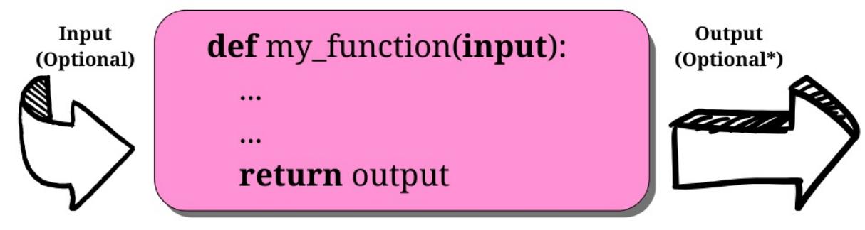
Figure 4.1: An example of a function
As you can see, a function is a block of instructions, packaged as a whole, like a box. Functions can accept input parameters and produce output values. Both of these are optional, as we will see in the examples in this chapter.
A function in Python is defined using the def keyword, after which the name of the function follows, terminated by a pair of parentheses (which may or may not contain input parameters); a colon ( : ) then signals the end of the function definition. Immediately afterward, indented by four spaces, we find the body of the function, which is the set of instructions that the function will execute when called.
Note that the indentation by four spaces is not mandatory, but it is the number of spaces suggested by PEP 8, and, in practice, it is the most widely used spacing measure.
A function may or may not return an output. If a function wants to return an output, it does so by using the return keyword, followed by the desired output. You may have noticed the little * after Optional in the output section of the preceding diagram. This is because a function always returns something in Python, even if you do not explicitly use the return statement. If the function has no return statement in its body, or no value is given to the return statement itself, the function returns None .
This design choice is rooted in several reasons, the most important of which are:
- Simplicity and consistency: Whether the function is explicitly returning a value or not, its behavior is consistent.
- Complexity reduction: Several languages make a distinction between functions (which return a value) and procedures (which do not). Functions in Python can act as both, with no need for separate constructs. This minimizes the number of concepts a programmer must learn.
- Consistency for multiple pathways: Functions with multiple conditional branches will return None when no other return statement is executed. None therefore is a useful default value.
The list provided demonstrates the multitude of factors that can influence an apparently simple design decision. It is the careful and deliberate choices underpinning Python’s design that contribute to its elegance, simplicity, and versatility.
Why use functions?
Functions are among the most important concepts and constructs of any language, so let us give you a few reasons why we need them:
- They reduce code duplication in a program. Encapsulating the instructions for a task in a function that we can import and call whenever we want, allows us to avoid duplicating the implementation.
- They help in splitting a complex task or procedure into smaller blocks, each of which becomes a function.
- They hide the implementation details from their users.
- They improve traceability.
- They improve readability.
Let us now look at a few examples to get a better understanding of each point.
Reducing code duplication
Imagine that you are writing a piece of scientific software, and you need to calculate prime numbers up to a certain limit—as we did in the previous chapter. You have an algorithm to calculate them, so you copy it and paste it to wherever you need to use it. One day, though, a colleague gives you a more performant algorithm to calculate primes. At this point, you need to go over your whole code base and replace the old code with the new one.
This procedure is quite error-prone. You can easily remove parts of the surrounding code by mistake or fail to remove some of the code you meant to replace. You also risk missing some of the places where the prime calculation is done, leaving your software in an inconsistent state where the same action is performed in different ways. What if, instead of replacing code with a better version of it, you need to fix a bug and you miss one of the places? That would be even worse. What if the names of the variables in the old algorithm are different from those used in the new one? That will also complicate things.
To avoid all that, you write a function, get_prime_numbers (upto) , and use it anywhere you need to calculate a list of primes. When your colleague gives you the better implementation, all you need to do is replace the body of that function with the new code,. The rest of the software will automatically adapt, since it is just calling the function.
Your code will be shorter, it will not suffer from inconsistencies between old and new ways of performing a task, nor will undetected bugs be left behind due to copy-and-paste failures or oversights.
Splitting a complex task
Functions are also useful for splitting long or complex tasks into smaller ones. The result is that the code benefits from it in several ways, including readability, testability, and reusability.
To give you a simple example, imagine that you are preparing a report. Your code needs to fetch data from a data source, parse it, filter it, and polish it, and then a whole series of algorithms needs to be run against it, to produce the results that will be written into the report. It is common to see procedures like this that are just one big do_report(data_source) function. There might be hundreds of lines of code that run, before we finally produce the report.
Inexperienced programmers, not well versed in the art of crafting simple, well structured code, may produce functions with hundreds of lines of code. They are hard to follow through, to find the places where things are changing context (such as finishing one task and starting the next one). Let us show you a better approach instead:
# data.science.example.py
def do_report(data_source):
   # fetch and prepare data
   data = fetch_data(data_source)
   parsed_data = parse_data(data)
   filtered_data = filter_data(parsed_data)
   polished_data = polish_data(filtered_data)
   # run algorithms on data
   final_data = analyse(polished_data)
   # create and return report
   report = Report(final_data)
   return report
The previous example is fictitious, of course, but can you see how easy it would be to go through the code? If the end result looks wrong, it would be easy to debug each of the single data outputs in the do_report() function. Moreover, it is even easier to exclude part of the process temporarily from the whole procedure (you just need to comment out the parts that you need to suspend). Code like this is easier to deal with.
Hiding implementation details
Let us stay with the preceding example to talk about this point as well. We can see that, by going through the code of the do_report() function, we can get a surprisingly good understanding without reading one single line of implementation. This is because functions hide the implementation details.
This feature means that, if we do not need to delve into the details, we are not forced to, in the way that we would be if do_report() was just one big, long function. To understand what was going on, we would have to read and understand every single line of its code. When it is broken down into smaller functions, we do not necessarily need to read every line of every one of them to understand what the code does. This reduces the time we spend reading the code and, since in a professional environment reading code takes much more time than writing it, it is important to reduce it to a minimum.
Improving readability
Programmers sometimes do not see the point in writing a function with a body of one or two lines of code, so let us look at an example that shows you why you should probably still do it.
Imagine that you need to multiply two matrices, like in the example below:
Would you prefer to have to read this code:
# matrix.multiplication.nofunc.py
a = [[1, 2], [3, 4]]
b = [[5, 1], [2, 1]]
c = [
[sum(i * j for i, j in zip(r, c)) for c in zip(*b)] for r in a
]
Or would you prefer this:
# matrix.multiplication.func.py
def matrix_mul(a, b):
return [
[sum(i * j for i, j in zip(r, c)) for c in zip(*b)]It is much easier to understand that c is the result of the multiplication of a and b in the second example, and it is much easier to read the code. If we do not need to modify that multiplication logic, we do not even need to go into the implementation details of matrix_mul() . Therefore, readability is improved here while, in the first snippet, we would have to spend time trying to understand what that complicated list comprehension is doing.
Do not worry if you do not understand list comprehensions, as we will study them in Chapter 5, Comprehensions and Generators.
Improving traceability
for r in a
a = [[1, 2], [3, 4]] b = [[5, 1], [2, 1]] c = matrix_mul(a, b)
]
Imagine that we have written some code for an e-commerce website. We display the product prices on several pages. Imagine that the prices in the database are stored with no VAT (sales tax), but we want to display them on the website with VAT at 20%. Here are a few ways of calculating the VAT-inclusive price from the VAT-exclusive price:
# vat.py
price = 100 # GBP, no VAT
final_price1 = price * 1.2
final_price2 = price + price / 5.0
final_price3 = price * (100 + 20) / 100.0
final_price4 = price + price * 0.2
These four different ways of calculating a VAT-inclusive price are all perfectly acceptable; we have encountered all of them in the professional code that we have worked on over the years. Now, imagine that we start selling products in different countries, and some of them have different VAT rates, so we need to refactor the code (throughout the website) in order to make that VAT calculation dynamic.
How do we trace all the places in which we are performing a VAT calculation? Coding today is a collaborative task and we cannot be sure that the VAT has been calculated using only one of those forms. It is going to be difficult.
So, let us write a function that takes the input values vat and price (VAT-exclusive) and returns a VAT-inclusive price:
# vat.function.py
def calculate_price_with_vat(price, vat):
   return price * (100 + vat) / 100
Now we can import that function and use it in any place in the website where we need to calculate a VAT-inclusive price, and when we need to trace those calls we can search for calculate_price_with_vat .
Note that, in the preceding example, price is assumed to be VAT-exclusive, and vat is a percentage value (for example, 19, 20, or 23).
Scopes and name resolution
In Chapter 1, A Gentle Introduction to Python we discussed scopes and namespaces. We are going to expand on that concept now. Finally, we can talk in terms of functions, and this will make everything easier to understand. Let us start with a simple example:
# scoping.level.1.py
def my_function():
   test = 1 # this is defined in the local scope of the function
   print("my_function:", test)
test = 0 # this is defined in the global scope
my_function()
print("global:", test)
We have defined the test name in two different places in the previous example—it is actually in two different scopes. One is the global scope ( test = 0 ), and the other is the local scope of the my_function() function ( test = 1 ). If we execute the code, we will see this:
$ python scoping.level.1.py
my_function: 1
global: 0
It is clear that test = 1 shadows the test = 0 assignment in my_function() . In the global context, test is still 0, as you can see from the output of the program, but we define the test name again in the function body, and we set it to point to the integer 1. Both of the test names therefore exist: one in the global scope, pointing to an int object with a value of 0, the other in the my_function () scope, pointing to an int object with a value of 1. Let us comment out the line with test = 1 . Python searches for the test name in the next enclosing namespace (recall the LEGB rule: local, enclosing, global, built-in, described in Chapter 1, A Gentle Introduction to Python) and, in this case, we will see the value 0 printed twice. Try it in your code.
Now, let us give you a more complex example with nested functions:
# scoping.level.2.py
def outer():
   test = 1 # outer scope
   def inner():
       test = 2 # inner scope
       print("inner:", test)
   inner()
   print("outer:", test)
test = 0 # global scope
outer()
print("global:", test)
In the preceding code, we have two levels of shadowing. One level is in the function outer () , and the other one is in the function inner() .
If we run the code, we get:
$ python scoping.level.2.py
inner: 2
outer: 1
global: 0
Try commenting out the test = 1 line. Can you figure out what the result will be? When reaching the print(‘outer:’, test) line, Python will have to look for test in the next enclosing scope; therefore it will find and print 0, instead of 1. Make sure you comment out test = 2 as well, to see whether you understand what happens and whether the LEGB rule is clear to you, before proceeding.
Another thing to note is that Python gives us the ability to define a function in another function. The inner() function’s name is defined within the namespace of the outer() function, exactly as would happen with any other name.
The global and nonlocal statements
In the preceding example, we can alter what happens to the shadowing of the test name by using one of these two special statements: global and nonlocal . As you can see, when we define test = 2 in the inner() function, we do not overwrite test in the outer() function or in the global scope.
We can get read access to those names if we use them in a nested scope that does not define them, but we cannot modify them because when we write an assignment instruction, we are actually defining a new name in the current scope.
We can use the nonlocal statement to change this behavior. According to the official documentation:
“The nonlocal statement causes the listed identifiers to refer to previously bound variables in the nearest enclosing scope excluding globals.”
Let us introduce it in the inner() function and see what happens:
# scoping.level.2.nonlocal.py
def outer():
   test = 1 # outer scope
   def inner():
       nonlocal test
       test = 2 # nearest enclosing scope (which is 'outer')
       print("inner:", test)
   inner()
   print("outer:", test)
test = 0 # global scope
outer()
print("global:", test)
Notice how in the body of the inner() function we have declared the test name to be nonlocal . Running this code produces the following result:
$ python scoping.level.2.nonlocal.py
inner: 2
outer: 2
global: 0
By declaring test to be nonlocal in the inner() function, we actually bind the test name to the one declared in the outer function. If we removed the nonlocal test line from the inner() function and tried it inside the outer() function, we would get a SyntaxError , because the nonlocal statement works on enclosing scopes, but not in the global one.
Is there a way to get write access to that test = 0 in the global namespace? Yes, we just need to use the global statement:
# scoping.level.2.global.py
def outer():
   test = 1 # outer scope
   def inner():
       global test
       test = 2 # global scope
       print("inner:", test)
   inner()
   print("outer:", test)
test = 0 # global scope
outer()
print("global:", test)
Note that we have now declared the test name to be global , which will bind it to the one we defined in the global namespace ( test = 0 ). Run the code and you should get the following:
$ python scoping.level.2.global.py
inner: 2
outer: 1
global: 2
This shows that the name affected by the test = 2 assignment is now the one in the global scope. This would also work in the outer() function because, in this case, we are referring to the global scope. Try it for yourself and see what changes. Spend some time to get comfortable with scopes and name resolution—it is very important.
As a bonus question, can you tell what would happen if you defined inner() outside outer() in the preceding examples?
Input parameters
At the beginning of this chapter, we saw that a function can take input parameters. Before we delve into all the possible types of parameters, let us make sure you have a clear understanding of what passing an argument to a function means. There are three key points to keep in mind:
- Argument-passing is nothing more than assigning an object to a local variable name
- Assigning an object to an argument name inside a function does not affect the caller
- Changing a mutable object argument in a function does affect the caller
Before we explore the topic of arguments any further, please allow us to clarify the terminology a little. According to the official Python documentation:
“Parameters are defined by the names that appear in a function definition, whereas arguments are the values actually passed to a function when calling it. Parameters define what types of arguments a function can accept.”
We will try to be precise when referring to parameters and arguments, but it is worth noting that they are sometimes used synonymously as well. Let us now look at some examples.
Argument-passing
Take a look at the following code. We declare a name, x , in the global scope, then we declare a function, func(y) , and finally we call it, passing x :
# key.points.argument.passing.py
x = 3
def func(y):
   print(y)
func(x) # prints: 3
When func() is called with x , within its local scope, a name, y , is created, and it is pointed to the same object that x is pointing to. This is better clarified in Figure 4.2 (do not worry about the fact that this example was run with Python 3.11 - this is a feature that has not changed).
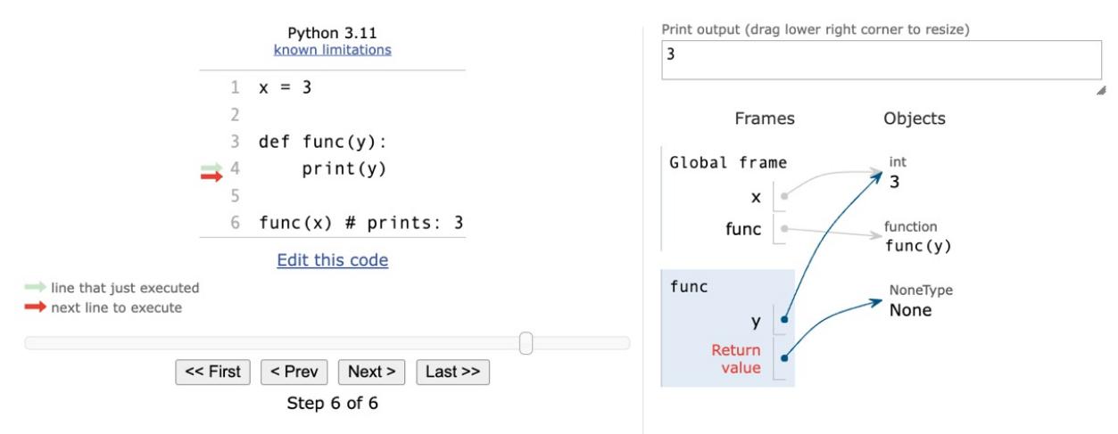
Figure 4.2: Understanding argument-passing with Python Tutor
The right-hand side of Figure 4.2 depicts the state of the program when execution has reached the end, after func() has returned ( None ). Take a look at the Frames column, and note that we have two names, x and func() , in the global namespace (Global frame), pointing respectively to an int (with a value of 3 ) and to a function object. Right beneath it, in the rectangle titled “func”, we can see the function’s local namespace, in which only one name has been defined: y . Because we have called func() with x (line 6 on the left side of the figure), y is pointing to the same object that x is. This is what happens under the hood when an argument is passed to a function. If we had used the name x instead of y in the function definition, things would have been exactly the same (but perhaps a bit confusing at first)—there would be a local x in the function, and a global x outside, as we saw in the Scopes and name resolution section previously in this chapter.
So, in a nutshell, what really happens is that the function creates, in its local scope, the names defined as parameters and, when we call it, we tell Python which objects those names must be pointed toward.
Assignment to parameter names
Assignment to parameter names does not affect the caller. This is something that can be tricky to understand at first, so let us look at an example:
# key.points.assignment.py
x = 3
def func(x):
   x = 7 # defining a local x, not changing the global one
func(x)
print(x) # prints: 3
In the preceding code, when we call the function with func(x) , the instruction x = 7 is executed within the local scope of the func() function; the name x , is pointed to an integer with a value of 7 , leaving the global x unaltered.
Changing a mutable object
Changing a mutable object does affect the caller. This is important because although Python appears to behave differently with mutable objects, the behaviour is, in fact, perfectly consistent. Let us look at an example:
# key.points.mutable.py
x = [1, 2, 3]
def func(x):
   x[1] = 42 # this affects the `x` argument!
func(x)
print(x) # prints: [1, 42, 3]
As you can see, we changed the original object. If you think about it, there is nothing weird in this behavior. When we call func(x) , name x in the function’s namespace is set to point to the same object as the global x . Within the body of the function, we are not changing the global x , in that we are not changing which object it points to. We are merely accessing the element at position 1 in that object and changing its value.
Remember point 2 in the Input parameters section: Assigning an object to a parameter name within a function does not affect the caller. If that is clear to you, the following code should not be surprising:
# key.points.mutable.assignment.py
x = [1, 2, 3]
def func(x):
   x[1] = 42 # this changes the original `x` argument!
   x = "something else" # this points x to a new string object
func(x)
print(x) # still prints: [1, 42, 3]
Look at the two lines we have highlighted. At first, like before, we just access the caller object again, at position 1, and change that value to number 42. Then, we reassign x to point to the ‘something else’ string. This leaves the caller unaltered and, in fact, the output is the same as that of the previous snippet.
Take your time to play around with this concept, and experiment with prints and calls to the id() function until everything is clear in your mind. This is one of the key aspects of Python and it must be very clear, otherwise you risk introducing subtle bugs into your code. Once again, the Python Tutor website (http://www.pythontutor.com/) will help you a lot by giving you a visual representation of these concepts.
Now that we have a good understanding of input parameters and how they behave, let us look at the different ways of passing arguments to functions.
Passing arguments
There are four different ways of passing arguments to a function:
- Positional arguments
- Keyword arguments
- Iterable unpacking
- Dictionary unpacking
Let us look at them one by one.
Positional arguments
When we call a function, each positional argument is assigned to the parameter in the corresponding position in the function definition:
# arguments.positional.py
def func(a, b, c):
   print(a, b, c)
func(1, 2, 3) # prints: 1 2 3
This is the most common way of passing arguments to functions (in some programming languages this is the only way of passing arguments).
Keyword arguments
Keyword arguments in a function call are assigned to parameters using the name=value syntax:
# arguments.keyword.py
def func(a, b, c):
   print(a, b, c)
func(a=1, c=2, b=3) # prints: 1 3 2When we use keyword arguments, the order of the arguments does not need to match the order of the parameters in the function definition. This can make our code easier to read and debug. We do not need to remember (or look up) the order of parameters in a function definition. We can look at a function call and immediately know which argument corresponds to which parameter.
You can also use both positional and keyword arguments at the same time:
# arguments.positional.keyword.py
def func(a, b, c):
   print(a, b, c)
func(42, b=1, c=2)
Keep in mind, however, that positional arguments always have to be listed before any keyword arguments. For example, if you try something like this:
# arguments.positional.keyword.py
func(b=1, c=2, 42) # positional arg after keyword args
You will get the following error:
$ python arguments.positional.keyword.py
  File "arguments.positional.keyword.py", line 7
    func(b=1, c=2, 42) # positional arg after keyword args
                     ^
SyntaxError: positional argument follows keyword argument
Iterable unpacking
Iterable unpacking uses the syntax *iterable_name to pass the elements of an iterable as positional arguments to a function:
# arguments.unpack.iterable.py
def func(a, b, c):
   print(a, b, c)
values = (1, 3, -7)
func(*values) # equivalent to: func(1, 3, -7)
This is a very useful feature, particularly when we need to programmatically generate arguments for a function.
Dictionary unpacking
Dictionary unpacking is to keyword arguments what iterable unpacking is to positional arguments. We use the syntax **dictionary_name to pass keyword arguments, constructed from the keys and values of a dictionary, to a function:
# arguments.unpack.dict.py
def func(a, b, c):
   print(a, b, c)
values = {"b": 1, "c": 2, "a": 42}
func(**values) # equivalent to func(b=1, c=2, a=42)
Combining argument types
We have already seen that positional and keyword arguments can be used together, as long as they are passed in the proper order. We can also combine unpacking (of both kinds) with normal positional and keyword arguments. We can even combine unpacking multiple iterables and dictionaries.
Arguments must be passed in the following order:
- First, positional arguments: both ordinary ( name ) and iterable unpacking ( *name )
- Next come keyword arguments ( name=value ), which can be mixed with iterable unpacking (*name )
- Finally, there is dictionary unpacking ( **name ), which can be mixed with keyword arguments ( name=value )
This will be much easier to understand with an example:
# arguments.combined.py
def func(a, b, c, d, e, f):
   print(a, b, c, d, e, f)
func(1, *(2, 3), f=6, *(4, 5))
func(*(1, 2), e=5, *(3, 4), f=6)
func(1, **{"b": 2, "c": 3}, d=4, **{"e": 5, "f": 6})
func(c=3, *(1, 2), **{"d": 4}, e=5, **{"f": 6})
All the above calls to func() are equivalent and print 1 2 3 4 5 6 . Play around with this example until you are sure you understand it. Pay close attention to the errors you get when you get the order wrong.
The ability to unpack multiple iterables and dictionaries was introduced to Python by PEP 448. This PEP also introduced the ability to use unpacking in contexts other than just function calls. You can read all about it at https://peps.python.org/pep-0448/.
When combining positional and keyword arguments, it is important to remember that each parameter can only appear once in the argument list:
# arguments.multiple.value.py
def func(a, b, c):
   print(a, b, c)
func(2, 3, a=1)
Here, we are passing two values for parameter a : the positional argument 2 and the keyword argument a=1 . This is illegal, so we get an error when we try to run it:
$ python arguments.multiple.value.py
Traceback (most recent call last):
 File "arguments.multiple.value.py", line 5, in <module>
   func(2, 3, a=1)
TypeError: func() got multiple values for argument 'a'
Defining parameters
Function parameters can be classified into five groups.
- Positional or keyword parameters: allow both positional and keyword arguments
- Variable positional parameters: collect an arbitrary number of positional arguments in a tuple
- Variable keyword parameters: collect an arbitrary number of keyword arguments in a dictionary
- Positional-only parameters: can only be passed as positional arguments
- Keyword-only parameters: can only be passed as keyword arguments
All the parameters in the examples we have seen so far in this chapter are regular positional or keyword parameters. We have seen how they can be passed as both positional and keyword arguments. There is not much more to say about them, so let us look at the other categories. Before we do though, let us briefly look at optional parameters.
Optional parameters
Apart from the categories we have looked at here, parameters can also be classified as either required or optional. Optional parameters have a default value specified in the function definition. The syntax is name=value :
# parameters.default.py
def func(a, b=4, c=88):
   print(a, b, c)
func(1) # prints: 1 4 88
func(b=5, a=7, c=9) # prints: 7 5 9
func(42, c=9) # prints: 42 4 9
func(42, 43, 44) # prints: 42, 43, 44Here, a is required, while b has the default value 4 and c has the default value 88 . It is important to note that, with the exception of keyword-only parameters, required parameters must always be to the left of all optional parameters in the function definition. Try removing the default value from c in the above example and see what happens.
Variable positional parameters
Sometimes you may prefer not to specify the exact number of positional parameters to a function; Python provides you with the ability to do this by using variable positional parameters. Let us look at a very common use case, the minimum() function. This is a function that calculates the minimum of its input values:
# parameters.variable.positional.py
def minimum(*n):
   # print(type(n)) # n is a tuple
   if n: # explained after the code
       mn = n[0]
       for value in n[1:]:
           if value < mn:
               mn = value
       print(mn)
minimum(1, 3, -7, 9) # n = (1, 3, -7, 9) - prints: -7
minimum() # n = () - prints: nothing
As you can see, when we define a parameter with an asterisk, * , prepended to its name, we are telling Python that this parameter will collect a variable number of positional arguments when the function is called. Within the function, n is a tuple. Uncomment print(type(n)) to see for yourself, and play around with it for a bit.
Note that a function can have at most one variable positional parameter—it would not make sense to have more. Python would have no way of deciding how to divide up the arguments between them. You also cannot specify a default value for a variable positional parameter. The default value is always an empty tuple.
Have you noticed how we checked whether n was not empty with a simple if n: ? This is because collection objects evaluate to True when non-empty, and otherwise False , in Python. This is the case for tuples, sets, lists, dictionaries, and so on.
One other thing to note is that we may want to throw an error when we call the function with no parameters, instead of silently doing nothing. In this context, we are not concerned about making this function robust, but rather understanding variable positional parameters.
Did you notice that the syntax for defining variable positional parameters looks very much like the syntax for iterable unpacking? This is no coincidence. After all, the two features mirror each other. They are also frequently used together, since variable positional parameters save you from worrying about whether the length of the iterable you are unpacking matches the number of parameters in the function definition.
Variable keyword parameters
Variable keyword parameters are very similar to variable positional parameters. The only difference is the syntax ( ** instead of * ) and the fact that they are collected in a dictionary:
# parameters.variable.keyword.py
def func(**kwargs):
   print(kwargs)
func(a=1, b=42) # prints {'a': 1, 'b': 42}
func() # prints {}
func(a=1, b=46, c=99) # prints {'a': 1, 'b': 46, 'c': 99}
You can see that adding ** in front of the parameter name in the function definition tells Python to use that name to collect a variable number of keyword parameters. As in the case of variable positional parameters, each function can have at most one variable keyword parameter—and you cannot specify a default value.
Just like variable positional parameters resemble iterable unpacking, variable keyword parameters resemble dictionary unpacking. Dictionary unpacking is also often used to pass arguments to functions with variable keyword parameters.
The reason why being able to pass a variable number of keyword arguments is so important may not be evident at the moment, so how about a more realistic example? Let us define a function that connects to a database: we want to connect to a default database by simply calling this function with no parameters. We also want to connect to any other database by passing to the function the appropriate parameters. Before you read on, try to spend a couple of minutes figuring out a solution by yourself:
# parameters.variable.db.py
def connect(**options):
   conn_params = {
       "host": options.get("host", "127.0.0.1"),
       "port": options.get("port", 5432),
       "user": options.get("user", ""),
       "pwd": options.get("pwd", ""),
   }
   print(conn_params)
   # we then connect to the db (commented out)
   # db.connect(**conn_params)
connect()
connect(host="127.0.0.42", port=5433)
connect(port=5431, user="fab", pwd="gandalf")
Note that, in the function, we can prepare a dictionary of connection parameters ( conn_params ) using default values as fallbacks, allowing them to be overwritten if they are provided in the function call. There are better ways to do this with fewer lines of code, but we are not concerned with that right now. Running the preceding code yields the following result:
$ python parameters.variable.db.py
{'host': '127.0.0.1', 'port': 5432, 'user': '', 'pwd': ''}
{'host': '127.0.0.42', 'port': 5433, 'user': '', 'pwd': ''}
{'host': '127.0.0.1', 'port': 5431, 'user': 'fab', 'pwd': 'gandalf'}
Note the correspondence between the function calls and the output, and how default values are overridden according to what was passed to the function.
Positional-only parameters
Starting from Python 3.8, PEP 570 (https://peps.python.org/pep-0570/) introduced positional-only parameters. There is a new function parameter syntax, / , indicating that a set of the function parameters must be specified positionally and cannot be passed as keyword arguments. Let us see a simple example:
# parameters.positional.only.py
def func(a, b, /, c):
   print(a, b, c)
func(1, 2, 3) # prints: 1 2 3
func(1, 2, c=3) # prints 1 2 3
In the preceding example, we define a function func() , which specifies three parameters: a , b , and c . The / in the function signature indicates that a and b must be passed positionally, that is, not by keyword.
The last two lines in the example show that we can call the function passing all three arguments positionally, or we can pass c by keyword. Both cases work fine, as c is defined after the / in the function signature. If we try to call the function by passing a or b by keyword, like so:
func(1, b=2, c=3)This produces the following traceback:
Traceback (most recent call last):
 File "arguments.positional.only.py", line 7, in <module>
   func(1, b=2, c=3)
TypeError: func() got some positional-only arguments
passed as keyword arguments: 'b'
The preceding example shows us that Python is now complaining about how we called func() . We have passed b by keyword, but we are not allowed to do that.
Positional-only parameters can also be optional:
# parameters.positional.only.optional.py
def func(a, b=2, /):
   print(a, b)
func(4, 5) # prints 4 5
func(3) # prints 3 2
Let us see what this feature brings to the language with a few examples borrowed from the official documentation. One advantage is the ability to fully emulate behaviors of existing C-coded functions:
def divmod(a, b, /):
   "Emulate the built in divmod() function"
   return (a // b, a % b)
Another important use case is to preclude keyword arguments when the parameter name is not helpful:
len(obj='hello')In the preceding example, the obj keyword argument impairs readability. Moreover, if we wish to refactor the internals of the len function, and rename obj to the_object (or any other name), the change is guaranteed not to break any client code, because there will not be any call to the len() function involving the now stale obj parameter name.
Finally, using positional-only parameters implies that whatever is on the left of / remains available for use in variable keyword arguments, as shown by the following example:
def func_name(name, /, **kwargs):
   print(name)
   print(kwargs)
func_name("Positional-only name", name="Name in **kwargs")
# Prints:
# Positional-only name
# {'name': 'Name in **kwargs'}
The ability to retain parameter names in function signatures for use in **kwargs can lead to simpler and cleaner code.
Let us now explore the mirror version of positional-only: keyword-only parameters.
Keyword-only parameters
Python 3 introduced keyword-only parameters. We are going to study them only briefly, as their use cases are not that frequent. There are two ways of specifying them, either after the variable positional parameters, or after a bare * . Let us see an example of both:
# parameters.keyword.only.py
def kwo(*a, c):
   print(a, c)
kwo(1, 2, 3, c=7) # prints: (1, 2, 3) 7
kwo(c=4) # prints: () 4
# kwo(1, 2) # breaks, invalid syntax, with the following error
# TypeError: kwo() missing 1 required keyword-only argument: 'c'
def kwo2(a, b=42, *, c):
print(a, b, c)
kwo2(3, b=7, c=99) # prints: 3 7 99
kwo2(3, c=13) # prints: 3 42 13
# kwo2(3, 23) # breaks, invalid syntax, with the following error
# TypeError: kwo2() missing 1 required keyword-only argument: 'c'As anticipated, the function, kwo() , takes a variable number of positional parameters ( a ) and a keyword-only one, c . The results of the calls are straightforward and you can uncomment the third call to see what error Python returns.
The same applies to the function kwo2() , which differs from kwo in that it takes a positional argument, a , a keyword argument, b , and then a keyword-only one, c . You can uncomment the third call to see the error that is produced.
Now that you know how to specify different types of input parameters, let us see how you can combine them in function definitions.
Combining input parameters
You can combine different parameter types in the same function (in fact it is often very useful to do so). As in the case of combining different types of arguments in the same function call, there are some restrictions on ordering:
- Positional-only parameters come first, followed by a / .
- Normal parameters go after any positional-only parameters.
- Variable positional parameters go after normal parameters.
- Keyword-only parameters go after variable positional parameters.
- Variable keyword parameters always go last.
- For positional-only and normal parameters, any required parameters must be defined before any optional parameters. This means that if you have an optional positional-only parameter, all your normal parameters must be optional too. This rule does not affect keyword-only parameters.
These rules can be a bit tricky to understand without an example, so let us look at a couple of them:
# parameters.all.py
def func(a, b, c=7, *args, **kwargs):
   print("a, b, c:", a, b, c)
   print("args:", args)
   print("kwargs:", kwargs)
func(1, 2, 3, 5, 7, 9, A="a", B="b")
Note the order of the parameters in the function definition. The execution of this yields the following:
$ python parameters.all.py
a, b, c: 1 2 3
args: (5, 7, 9)
kwargs: {'A': 'a', 'B': 'b'}
Let us now look at an example with keyword-only parameters:
# parameters.all.pkwonly.py
def allparams(a, /, b, c=42, *args, d=256, e, **kwargs):
   print("a, b, c:", a, b, c)
   print("d, e:", d, e)
   print("args:", args)
   print("kwargs:", kwargs)
allparams(1, 2, 3, 4, 5, 6, e=7, f=9, g=10)
Note that we have both positional-only and keyword-only parameters in the function declaration: a is positionalonly, while d and e are keyword-only. They come after the *args variable positional argument, and it would be the same if they came right after a single * (in which case there would not be any variable positional parameter).
The execution of this yields the following:
$ python parameters.all.pkwonly.py
a, b, c: 1 2 3
d, e: 256 7
args: (4, 5, 6)
kwargs: {'f': 9, 'g': 10}
One other thing to note is the names we gave to the variable positional and keyword parameters. You are free to choose differently but be aware that args and kwargs are the conventional names given to these parameters, at least generically.
More signature examples
To briefly recap on function signatures that use the positional- and keyword-only specifiers, here are some further examples. Omitting the variable positional and keyword parameters, for brevity, we are left with the following syntax:
def func_name(positional_only_parameters, /,
   positional_or_keyword_parameters, *,
   keyword_only_parameters):
First, we have positional-only, then positional or keyword parameters, and finally keyword-only ones.
Some other valid signatures are presented below:
def func_name(p1, p2, /, p_or_kw, *, kw):
def func_name(p1, p2=None, /, p_or_kw=None, *, kw):
def func_name(p1, p2=None, /, *, kw):
def func_name(p1, p2=None, /):
def func_name(p1, p2, /, p_or_kw):
def func_name(p1, p2, /):
All of the above are valid signatures, while the following would be invalid:
def func_name(p1, p2=None, /, p_or_kw, *, kw):
def func_name(p1=None, p2, /, p_or_kw=None, *, kw):
def func_name(p1=None, p2, /):
You can read about the grammar specifications in the official documentation:
https://docs.python.org/3/reference/compound\_stmts.xhtml#function-definitions
A useful exercise for you at this point would be to implement any of the above example signatures, printing out the values of those parameters, like we have done in previous exercises, and play around passing arguments in different ways.
Avoid the trap! Mutable defaults
One thing to be aware of, in Python, is that default values are created at definition time; therefore, subsequent calls to the same function will possibly behave differently according to the mutability of their default values. Let us look at an example:
# parameters.defaults.mutable.py
def func(a=[], b={}):
   print(a)
   print(b)
   print("#" * 12)
   a.append(len(a)) # this will affect a's default value
   b[len(a)] = len(a) # and this will affect b's one
func()
func()func()Both parameters have mutable default values. This means that, if you affect those objects, any modification will stick around in subsequent function calls. See if you can understand the output of those calls:
$ python parameters.defaults.mutable.py
[]
{}
############
[0]
{1: 1}
############
[0, 1]
{1: 1, 2: 2}
############
While this behavior may seem weird at first, it actually makes sense, and it is very handy—when using memoization techniques, for example. Even more interesting is what happens when, between the calls, we introduce one that does not use defaults, such as this:
# parameters.defaults.mutable.intermediate.call.py
func()
func(a=[1, 2, 3], b={"B": 1})
func()
When we run this code, this is the output:
$ python parameters.defaults.mutable.intermediate.call.py
[]
{}
############
[1, 2, 3]
{'B': 1}
############
[0]
{1: 1}
############
This output shows us that the defaults are retained even if we call the function with other values. One question that comes to mind is, how do I get a fresh empty value every time? Well, the convention is the following:
# parameters.defaults.mutable.no.trap.py
def func(a=None):
   if a is None:
       a = []
   # do whatever you want with `a` ...
Note that, by using the preceding technique, if a is not passed when calling the function, we always get a brand new, empty list.
After a thorough exposition of input parameters, it is now time to look at the other side of the coin, returning output values.
Return values
We have already said that to return something from a function we need to use the return statement, followed by what we want to return. There can be as many return statements as needed in the body of a function.
On the other hand, if within the body of a function we do not return anything, or we invoke a bare return statement, the function will return None . This behavior is harmless when it is not needed, but allows for interesting patterns, and confirms Python as a very consistent language.
We say it is harmless because you are never forced to collect the result of a function call. We will show you what we
mean with an example:
# return.none.py
def func():
   pass
func() # the return of this call won't be collected. It's lost.
a = func() # the return of this one instead is collected into `a`
print(a) # prints: None
Note that the whole body of the function is composed only of the pass statement. As the official documentation tells us, pass is a null operation, as, when it is executed, nothing happens. It is useful as a placeholder when a statement is required syntactically but no code needs to be executed. In other languages, we would probably just indicate that with a pair of curly brackets ( {} ), which define an empty scope; but in Python, a scope is defined by indenting code, therefore a statement such as pass is necessary.
Notice also that the first call to func() returns a value ( None ) that we do not collect. As we mentioned before, collecting the return value of a function call is not mandatory.
Let us see a more interesting example. Remember that, in Chapter 1, A Gentle Introduction to Python, we talked about the factorial function. Let us write our own implementation here (for simplicity, we will assume the function is always called correctly with appropriate values, so we do not need to sanity-check the input argument):
# return.single.value.py
def factorial(n):
if n in (0, 1):
return 1
result = n
for k in range(2, n):
result *= k
return result
f5 = factorial(5) # f5 = 120Note that we have two points of return. If n is either 0 or 1, we return 1. Otherwise, we perform the required calculation and return result .
In Python it is common to use the in operator to do a membership check, as we did in the preceding example, instead of the more verbose:
if n == 0 or n == 1:
...Let us now try to write this function a little bit more succinctly:
# return.single.value.2.py
from functools import reduce
from operator import mul
def factorial(n):
return reduce(mul, range(1, n + 1), 1)
f5 = factorial(5) # f5 = 120This simple example shows how Python is both elegant and concise. This implementation is readable even if we have never seen reduce() or mul() . If you cannot read or understand it, set aside a few minutes, and do some research in the Python documentation until its behavior is clear to you. Being able to look up functions in the documentation and understand code written by someone else is a task that every developer needs to be able to perform.
To this end, make sure you look up the help() function, which proves quite helpful when exploring with the console.
Returning multiple values
To return multiple values is easy: you just use tuples. Let us look at a simple example that mimics the divmod()
built-in function:
# return.multiple.py
def moddiv(a, b):
return a // b, a % b
print(moddiv(20, 7)) # prints (2, 6)We could have wrapped the part that is highlighted in the preceding code within brackets, but there is no need for that. The preceding function returns both the result and the remainder of the division, at the same time.
In the source code for this example, we have left a simple example of a test function to make sure the code is doing the correct calculation.
A few useful tips
When writing functions, it is very useful to follow guidelines so that you write them well. We will quickly point some of them out.
Functions should do one thing
Functions that do one thing are easy to describe in one short sentence; functions that do multiple things can be split into smaller functions that do one thing. These smaller functions are usually easier to read and understand.
Functions should be small
The smaller they are, the easier it is to test and write them so that they do one thing.
The fewer input parameters, the better
Functions that take a lot of parameters quickly become hard to manage (among other issues).
Functions should be consistent in their return values
Returning False and returning None are not the same thing, even if, within a Boolean context, they both evaluate to False . False means that we have information ( False ), while None means that there is no information. Try writing functions that return in a consistent way, no matter what happens in their logic.
Functions should have no side effects
In functional programming there is the concept of pure functions. This type of functions adhere to two main principles:
- Deterministic output: this means that given the same set of inputs, the output produced will always be the same. In other words, the function’s behavior is not dependent on any external or global state that might change during execution.
- No side effects: this means that pure functions do not cause any observable side effects in the system. That is, they do not alter any external state, like modifying global variables, or performing I/O operations like reading from or writing to a file or the display.
While you should aim to write pure functions when possible, it is important that those you write should at least have no side effects. They should not affect the value of the arguments they are called with.
This is probably the hardest statement to understand at this point, so we will give you an example using lists. In the following code, note how numbers is not sorted by the sorted() function, which returns a sorted copy of numbers . Conversely, the list.sort() method is acting on the numbers object itself, and that is fine because it is a method (a function that belongs to an object and therefore has the right to modify it):
>>> numbers = [4, 1, 7, 5]
>>> sorted(numbers) # won't sort the original `numbers` list[1, 4, 5, 7]
>>> numbers # let's verify
[4, 1, 7, 5] # good, untouched
>>> numbers.sort() # this will act on the list
>>> numbers
[1, 4, 5, 7]Follow these guidelines and you will automatically shield yourself from certain types of bugs.
Chapter 3 of Clean Code, by Robert C. Martin, is dedicated to functions, and it is one of the best sets of guidelines we have ever read on the subject.
Recursive functions
When a function calls itself to produce a result, it is said to be recursive. Sometimes recursive functions are very useful, in that they make it easier to write the logic. Some algorithms are very easy to write using recursion, while others are not. There is no recursive function that cannot be rewritten in an iterative fashion, so it is usually up to the programmer to choose the best approach for the case at hand.
The body of a recursive function usually has two sections: one where the return value depends on a subsequent call to itself, and one where it does not (called the base case).
As an example, we can consider the (hopefully now familiar) factorial function, N!. The base case is when N is either 0 or 1—the function returns 1 with no need for further calculation. On the other hand, in the general case, N! returns the product:
1 * 2 * ... * (N-1) * NIf you think about it, N! can be rewritten like this: N! = (N-1)! * N. As a practical example, consider this:
5! = 1 * 2 * 3 * 4 * 5 = (1 * 2 * 3 * 4) * 5 = 4! * 5Let us write this down in code:
# recursive.factorial.py
def factorial(n):
if n in (0, 1): # base case
return 1
return factorial(n - 1) * n # recursive caseRecursive functions are often used when writing algorithms, and they can be really fun to write. As an exercise, try to solve a couple of simple problems using both a recursive and an iterative approach. Good candidates for practice might be calculating Fibonacci numbers, or the length of a string—things like that.
When writing recursive functions, always consider how many nested calls you make, since there is a limit. For further information on this, check out sys.getrecursionlimit() and sys.setrecursionlimit() .
Anonymous functions
One last type of function that we want to talk about are anonymous functions. These functions, which are called lambdas in Python, are usually used when a fully-fledged function with its own name would be overkill, and all we want is a quick, simple one-liner.
Imagine that we wanted a list of all the numbers up to a certain value of N that are also multiples of five. We could use the filter() function for this, which will require a function and an iterable as input. The return value is a filter object that, when iterated over, yields the elements from the input iterable for which the function returns True . Without using an anonymous function, we might do something like this:
# filter.regular.py
def is_multiple_of_five(n):return not n % 5
def get_multiples_of_five(n):
return list(filter(is_multiple_of_five, range(n)))Note how we use is_multiple_of_five() to filter through the first n natural numbers. This seems a bit excessive —the task is simple and we do not need to keep the is_multiple_of_five() function around for anything else. Let us rewrite it using a lambda function:
# filter.lambda.py
def get_multiples_of_five(n):
return list(filter(lambda k: not k % 5, range(n)))The logic is the same, but the filtering function is now a lambda. Defining a lambda is very easy and follows this form:
func_name = lambda [parameter_list]: expressionA function object is returned, which is equivalent to this:
def func_name([parameter_list]):
return expressionNote that optional parameters are indicated following the common syntax of wrapping them in square brackets.
Let us look at another couple of examples of equivalent functions, defined in both forms:
# lambda.explained.py
# example 1: adder
def adder(a, b):
return a + b
# is equivalent to:
adder_lambda = lambda a, b: a + b
# example 2: to uppercase
def to_upper(s):
return s.upper()
# is equivalent to:
to_upper_lambda = lambda s: s.upper()The preceding examples are very simple. The first one adds two numbers, and the second one produces the uppercase version of a string. Note that we assigned what is returned by the lambda expressions to a name ( adder_lambda , to_upper_lambda ), but there is no need for that when you use lambdas in the way we did in the filter() example.
Function attributes
Every function is a fully fledged object and, as such, it has several attributes. Some of them are special and can be used in an introspective way to inspect the function object at runtime. The following script is an example that shows a few of them and how to display their value for an example function:
# func.attributes.py
def multiplication(a, b=1):
"""Return a multiplied by b."""
return a * b
if __name__ == "__main__":
special_attributes = [
"__doc__",
"__name__",
"__qualname__",
"__module__",
"__defaults__",
"__code__",
"__globals__",
"__dict__",
"__closure__",
"__annotations__","__kwdefaults__",
]
for attribute in special_attributes:
print(attribute, "->", getattr(multiplication, attribute))We used the built-in getattr() function to get the value of those attributes. getattr(obj, attribute) is equivalent to obj.attribute and comes in handy when we need to dynamically get an attribute at runtime, taking the name of the attribute from a variable (as in this example). Running this script yields:
$ python func.attributes.py
__doc__ -> Return a multiplied by b.
__name__ -> multiplication
__qualname__ -> multiplication
__module__ -> __main__
__defaults__ -> (1,)
__code__ -> <code object multiplication at 0x102ce1550,
file "func.attributes.py", line 2>
__globals__ -> {... omitted ...}
__dict__ -> {}
__closure__ -> None
__annotations__ -> {}
__kwdefaults__ -> NoneWe have omitted the value of the __globals__ attribute, as it was too big. An explanation of the meaning of this attribute can be found in the Callable types section of the Python Data Model documentation page:
https://docs.python.org/3/reference/datamodel.xhtml#the-standard-type-hierarchy
You can use the built-in function dir() to get a list of all the attributes of any object.
One thing to notice in the previous example, is the use of this clause:
if __name__ == "__main__":This line makes sure that whatever follows is only executed when the module is run directly. When you run a Python script, Python sets the __name__ variable to “__main__” in that script. Conversely, when you import a Python script as a module into another script, the __name__ variable is set to the name of the script/module being imported.
Built-in functions
Python comes with a lot of built-in functions. They are available anywhere, and you can get a list of them by inspecting the builtins module with dir(__builtins__) , or by going to the official Python documentation. Unfortunately, we do not have the room to go through all of them here. We have already seen some of them, such as any , bin , bool , divmod , filter , float , getattr , id , int , len , list , min , print , set , tuple , type , and zip , but there are many more, which you should read about at least once. Get familiar with them, experiment, write a small piece of code for each of them, and make sure you have them at your fingertips so that you can use them when needed.
You can find a list of built-in functions in the official documentation, here: https://docs.python.org/3/library/functions.xhtml.
Documenting your code
We are big fans of code that does not need documentation. When we write elegant code, following established principles, the code should come out as self-explanatory, with documentation being almost unnecessary. Nevertheless, adding a docstring to a function, or a comment with important information, can be very useful.
You can find the guidelines for documenting Python in PEP 257 – Docstring conventions: https://peps.python.org/pep-0257/, but we will show you the basics here.
Python is documented with strings, which are aptly called docstrings. Any object can be documented, and we can use either one-line or multi-line docstrings. One-liners are very simple. They should not provide another signature for the function, but instead state its purpose:
# docstrings.py
def square(n):
"""Return the square of a number n."""
return n**2
def get_username(userid):
"""Return the username of a user given their id."""
return db.get(user_id=userid).usernameUsing triple double-quoted strings allows you to expand easily later. Use sentences that end in a period, and do not leave blank lines before or after.
Multiline comments are structured in a similar way. There should be a one-liner that briefly gives you the gist of what the object is about, and then a more verbose description. As an example, we have documented a fictitious connect() function, using the Sphinx notation, in the following example:
def connect(host, port, user, password):
"""Connect to a database.
Connect to a PostgreSQL database directly, using the given
parameters.
:param host: The host IP.
:param port: The desired port.
:param user: The connection username.
:param password: The connection password.
:return: The connection object.
"""
# body of the function here...
return connectionSphinx is one of the most widely used tools for creating Python documentation—in fact, the official Python documentation was written with it. It is definitely worth spending some time checking it out.
The help() built-in function, which is intended for interactive use, creates a documentation page for an object using its docstring.
Importing objects
Now that we know a lot about functions, let us look at how to use them. The whole point of writing functions is to be able to reuse them later and, in Python, this translates to importing them into the namespace where they are needed. There are many ways to import objects into a namespace, but the most common ones are import module_name and from module_name import function_name . Of course, these are quite simplistic examples, but bear with us for the time being.
The import module_name form finds the module_name module and defines a name for it in the local namespace, where the import statement is executed. The from module_name import identifier form is a little bit more complicated than that but basically does the same thing. It finds module_name and searches for an attribute (or a submodule) and stores a reference to identifier in the local namespace. Both forms have the option to change the name of the imported object using the as clause:
from mymodule import myfunc as better_named_funcJust to give you a flavor of what importing looks like, here is an example from a test module of one of Fabrizio’s projects (notice that the blank lines between blocks of imports follow the guidelines from PEP 8 at https://peps.python.org/pep-0008/#imports: standard library first, then third party, and finally local code):
# imports.py
from datetime import datetime, timezone # two imports, same line
from unittest.mock import patch # single import
import pytest # third party libraryfrom core.models import ( # multiline import
Exam,
Exercise,
Solution,
)When we have a structure of files starting in the root of our project, we can use the dot notation to get to the object we want to import into our current namespace, be it a package, a module, a class, a function, or anything else.
The from module import syntax also allows a catch-all clause, from module import * , which is sometimes used to get all the names from a module into the current namespace at once. This practice is frowned upon for several reasons, relating to performance and the risk of silently shadowing other names. You can read all that there is to know about imports in the official Python documentation but, before we leave the subject, let us give you a better example.
Imagine that we have defined a couple of functions, square(n) and cube(n) , in a module, funcdef.py , which is in the util folder. We want to use them in a couple of modules that are at the same level as the util folder, called func_import.py and func_from.py . Showing the tree structure of that project produces something like this:
├── func_from.py
├── func_import.py
├── util
│ ├── __init__.py
│ └── funcdef.pyBefore we show you the code of each module, please remember that in order to tell Python that it is actually a package, we need to put an __init__.py module in it.
There are two things to note about the __init__.py file. First, it is a fully fledged Python module so you can put code into it as you would with any other module. Second, as of Python 3.3, its presence is no longer required to make a folder be interpreted as a Python package.
The code is as follows:
# util/funcdef.py
def square(n):
return n**2
def cube(n):
return n**3
# func_import.py
Import util.funcdef
print(util.funcdef.square(10))
print(util.funcdef.cube(10))
# func_from.py
from util.funcdef import square, cube
print(square(10))
print(cube(10))Both these files, when executed, print 100 and 1000 . You can see how differently we then access the square and cube functions, according to how and what we imported in the current scope.
Relative imports
The type of import we have seen so far is called an absolute import; that is, it defines the whole path of either the module that we want to import or from which we want to import an object. There is another way of importing objects into Python, which is called a relative import. Relative imports are done by adding as many leading dots in front of the module as the number of folders we need to backtrack, to find what we are searching for. Simply put, it is something such as this:
from .mymodule import myfuncRelative imports are quite useful when restructuring projects. Not having the full path in the imports allows the
developer to move things around without having to rename too many of those paths.
For a complete explanation of relative imports, refer to PEP 328: https://peps.python.org/pep-0328/.
In later chapters, we will create projects using different libraries and use several different types of imports, including relative ones, so make sure you take a bit of time to read up about them in the official Python documentation.
One final example
Before we finish off this chapter, let us go through one last example. We could write a function to generate a list of prime numbers up to a limit; we have already seen the code for this in Chapter 3, Conditionals and Iteration, so let us make it a function and, to keep it interesting, let us optimize it a bit.
First of all, we do not need to divide by all the numbers from 2 to N-1 to decide whether a number, N, is prime. We can stop at √N (the square root of N). Moreover, we do not need to test the division for all the numbers from 2 to √N, as we can just use the primes in that range. We leave it up to you to figure out the math for why this works, if you are interested.
Let us see how the code changes:
# primes.py
from math import sqrt, ceil
def get_primes(n):
"""Calculate a list of primes up to n (included)."""
primelist = []
for candidate in range(2, n + 1):
is_prime = True
root = ceil(sqrt(candidate)) # division limit
for prime in primelist: # we try only the primes
if prime > root: # no need to check any further
break
if candidate % prime == 0:
is_prime = False
break
if is_prime:
primelist.append(candidate)
return primelistThe code is the same as that in the previous chapter. We have changed the division algorithm so that we only test divisibility using the previously calculated primes, and we stopped once the testing divisor was greater than the root of the candidate. We used the primelist result list to get the primes for the division and calculated the root value using a fancy formula, the integer value of the ceiling of the root of the candidate. While a simple int(k ** 0.5) + 1 would have also served our purpose, the formula we chose is cleaner and requires a couple of imports, which is what we wanted to show. Check out the functions in the math module—they are very interesting!
Summary
In this chapter, we explored the world of functions. They are very important and, from now on, we will use them in virtually everything we do. We talked about the main reasons for using them, the most important of which are code reuse and implementation hiding.
We saw that a function object is like a box that takes optional inputs and may produce outputs. We can feed input arguments to a function in many different ways, using positional and keyword arguments, and using variable syntax for both types.
You should now know how to write a function, document it, import it into your code, and call it.
In the next chapter we will be picking up the pace a little a bit, so we suggest you spend a bit of time to consolidate and enrich the knowledge you have gathered so far by experimenting with code, and reading the Python official documentation.
5 Comprehensions and Generators
Join our book community on Discord

“It’s not the daily increase but daily decrease. Hack away at the unessential.”– Bruce Lee
The second part of the above quote, “hack away at the unessential,” is to us what makes a computer program elegant. We constantly strive to find better ways of doing things so that we do not waste time or memory.
There are valid reasons for not pushing our code up to the maximum limit: for example, sometimes we have to sacrifice readability or maintainability, to achieve a negligible improvement. It does not make sense to have a web page served in 1 second with unreadable, complicated code, when we could serve it in 1.05 seconds with readable, clean code.
On the other hand, sometimes it is perfectly reasonable to try to shave off a millisecond from a function, especially when the function is meant to be called thousands of times. Every millisecond you save there means seconds saved over thousands of calls, and this could be meaningful for your application.
In light of these considerations, the focus of this chapter will not be to give you the tools to push your code to the absolute limits of performance and optimization no matter what, but rather to enable you to write efficient, elegant code that reads well, runs fast, and does not waste resources in an obvious way.
In this chapter, we are going to cover the following:
- The map() , zip() , and filter() functions
- Comprehensions
- Generators
We will perform several measurements and comparisons and cautiously draw some conclusions. Please do keep in mind that on a different machine with a different setup or operating system, results may vary.
Take a look at this code:
# squares.py
def square1(n):
return n**2 # squaring through the power operator
def square2(n):
return n * n # squaring through multiplicationBoth functions return the square of n , but which is faster? From a simple benchmark that we ran, it looks like the second is slightly faster. If you think about it, it makes sense: calculating the power of a number involves multiplication and therefore, whatever algorithm you may use to perform the power operation, it is not likely to beat a simple multiplication such as the one in square2 .
Do we care about this result? In most cases, no. If you are coding an e-commerce website, chances are you will never need to raise a number to the second power, and if you do, it is likely to be a sporadic operation. You do not need to concern yourself with saving a fraction of a microsecond on a function you call a few times.
So, when does optimization become important? One common case is when you have to deal with huge collections of data. If you are applying the same function on a million customer objects, then you want your function to be tuned up to its best. Gaining one-tenth of a second on a function called one million times saves you 100,000 seconds, which is about 27.7 hours. So, let us focus on collections, and see which tools Python gives you to handle them with efficiency and grace.
Many of the concepts we will see in this chapter are based on iterators and iterables, which we encountered in Chapter 3, Conditionals and Iteration. We will see how to code a custom iterator and iterable objects in Chapter 6, OOP, Decorators, and Iterators.
Some of the objects we are going to explore in this chapter are iterators, which save memory by only operating on a single element of a collection at a time rather than creating a modified copy. As a result, some extra work is needed if we just want to show the result of the operation. We will often resort to wrapping the iterator in a list() constructor. This is because passing an iterator to list() exhausts it and puts all the generated items in a newly created list, which we can easily print to show you its content. Let us see an example of using the technique on a range object:
# list.iterable.txt
>>> range(7)
range(0, 7)
>>> list(range(7)) # put all elements in a list to view them
[0, 1, 2, 3, 4, 5, 6]We have highlighted the result of typing range(7) into a Python console. Notice that it does not show the contents of the range because range never actually loads the entire sequence of numbers into memory. The second highlighted line shows how wrapping the range in a list() allows us to see the numbers it generated.
The map, zip, and filter functions
We will start by reviewing map() , filter() , and zip() , which are the main built-in functions you can employ when handling collections, and then we will learn how to achieve the same results using two important constructs: comprehensions and generators .
map
According to the official Python documentation (https://docs.python.org/3/library/functions.xhtml#map):
map(function, iterable, *iterables)Return an iterator that applies function to every item of iterable, yielding the results. If additional iterables arguments are passed, function must take that many arguments and is applied to the items from all iterables in parallel. With multiple iterables, the iterator stops when the shortest iterable is exhausted.
We will explain the concept of yielding later in the chapter. For now, let us translate this into code—we will use a lambda function that takes a variable number of positional arguments, and returns them as a tuple:
# map.example.txt
>>> map(lambda *a: a, range(3)) # 1 iterable
<map object at 0x7f0db97adae0> # Not useful! Let us use list
>>> list(map(lambda *a: a, range(3))) # 1 iterable
[(0,), (1,), (2,)]
>>> list(map(lambda *a: a, range(3), "abc")) # 2 iterables
[(0, 'a'), (1, 'b'), (2, 'c')]
>>> list(map(lambda *a: a, range(3), "abc", range(4, 7))) # 3
[(0, 'a', 4), (1, 'b', 5), (2, 'c', 6)]
>>> # map stops at the shortest iterator
>>> list(map(lambda *a: a, (), "abc")) # empty tuple is shortest[]
>>> list(map(lambda *a: a, (1, 2), "abc")) # (1, 2) shortest
[(1, 'a'), (2, 'b')]
>>> list(map(lambda *a: a, (1, 2, 3, 4), "abc")) # "abc" shortest
[(1, 'a'), (2, 'b'), (3, 'c')]In the preceding code, you can see why we have to wrap calls in list() . Without it, we get the string representation of a map object, which is not useful in this context.
You can also notice how the elements of each iterable are applied to the function; at first, the first element of each iterable, then the second one of each iterable, and so on. Notice also that map() stops when the shortest of the iterables we called it with is exhausted. This is a very useful behavior; it does not force us to level off all the iterables to a common length, nor does it break if they are not all the same length.
map() is especially useful when you have to apply the same function to one or more collections of objects. As a more interesting example, let us see the decorate-sort-undecorate idiom (also known as Schwartzian transform). It is a technique that was quite popular in older Python versions, when sorting did not support the use of key functions. Nowadays, it is not needed as often, but it still occasionally comes in handy.
Let us see a variation of it in the next example: we want to sort in descending order by the sum of credits accumulated by students, so that the best student will be at position 0. We write a function to produce a decorated object, we sort, and then we undecorate. Each student has credits in three (possibly different) subjects. In this context, to decorate an object means to transform it, either adding extra data to it, or putting it into another object, in a way that allows us to be able to sort the original objects the way we want. This technique has nothing to do with Python decorators, which we will explore later in the book.
After sorting, we revert the decorated objects to get the original ones from them. This is referred to as undecorating.
# decorate.sort.undecorate.py
from pprint import pprint
students = [
dict(id=0, credits=dict(math=9, physics=6, history=7)),
dict(id=1, credits=dict(math=6, physics=7, latin=10)),
dict(id=2, credits=dict(history=8, physics=9, chemistry=10)),
dict(id=3, credits=dict(math=5, physics=5, geography=7)),
]
def decorate(student):
# create a 2-tuple (sum of credits, student) from student dict
return (sum(student["credits"].values()), student)
def undecorate(decorated_student):
# discard sum of credits, return original student dict
return decorated_student[1]
print(students[0])
print(decorate(students[0])
students = sorted(map(decorate, students), reverse=True)
students = list(map(undecorate, students))
pprint(students)Let us start by understanding what each student object is. In fact, let us print the first one:
{'id': 0, 'credits': {'math': 9, 'physics': 6, 'history': 7}}You can see that it is a dictionary with two keys: id and credits . The value of credits is also a dictionary in which there are three subject/grade key/value pairs. As you may recall from Chapter 2, Built-in Data Types, calling dict.values() returns an iterable object, with only the dictionary’s values. Therefore, sum( student[“credits”].values()) for the first student is equivalent to sum((9, 6, 7)) .
Let us print the result of calling decorate with the first student:
(22, {'id': 0, 'credits': {'math': 9, 'physics': 6, 'history': 7}})If we decorate all the students like this, we can sort them on their total number of credits by just sorting the list of tuples. To apply the decoration to each item in students , we call map(decorate, students) . We sort the result, and then we undecorate in a similar fashion.
Printing students after running the whole code yields:
[{'credits': {'chemistry': 10, 'history': 8, 'physics': 9}, 'id': 2},
{'credits': {'latin': 10, 'math': 6, 'physics': 7}, 'id': 1},
{'credits': {'history': 7, 'math': 9, 'physics': 6}, 'id': 0},
{'credits': {'geography': 7, 'math': 5, 'physics': 5}, 'id': 3}]As you can see, the student objects have indeed been sorted by the sums of their credits.
For more on the decorate-sort-undecorate idiom, there is a good introduction in the Sorting HOW TO section of the official Python documentation: https://docs.python.org/3.12/howto/sorting.xhtml#decorate-sortundecorate
One thing to notice about the sorting part is what happens when two or more students share the same total sum. The sorting algorithm would then proceed to sort the tuples by comparing the student objects with each other. This does not make any sense and, in more complex cases, could lead to unpredictable results, or even errors. If you want to avoid this issue, one simple solution is to create a three-tuple instead of a two-tuple, having the sum of credits in the first position, the position of the student object in the original students list in second place, and the student object itself in third place. This way, if the sum of credits is the same, the tuples will be sorted against the position, which will always be different, and therefore enough to resolve the sorting between any pair of tuples.
zip
We have already covered zip() in the previous chapters, so let us just define it properly, after which we want to show you how you could combine it with map() .
According to the Python documentation (https://docs.python.org/3/library/functions.xhtml#zip):
zip(*iterables, strict=False)… returns an iterator of tuples, where the i-th tuple contains the i-th element from each of the argument iterables.Another way to think of zip() is that it turns rows into columns, and columns into rows. This is similar to transposing a matrix.
Let us see an example:
# zip.grades.txt
>>> grades = [18, 23, 30, 27]
>>> avgs = [22, 21, 29, 24]
>>> list(zip(avgs, grades))
[(22, 18), (21, 23), (29, 30), (24, 27)]
>>> list(map(lambda *a: a, avgs, grades)) # equivalent to zip
[(22, 18), (21, 23), (29, 30), (24, 27)]Here, we are zipping together the average and the grade for the last exam for each student. Notice how easy it is to reproduce zip() using map() (the last two instructions of the example). Once again, we have to use list() to visualize the results .
Like map() , zip() will normally stop as soon as it reaches the end of the shortest iterable. This can, however, mask problems with the input data, leading to bugs. For example, suppose we need to combine a list of students’ names and a list of grades into a dictionary mapping each student’s name to their grade. A mistake in data-entry could result in the list of grades being shorter than the list of students. For example:
# zip.strict.txt
>>> students = ["Sophie", "Alex", "Charlie", "Alice"]
>>> grades = ["A", "C", "B"]
>>> dict(zip(students, grades))
{'Sophie': 'A', 'Alex': 'C', 'Charlie': 'B'}Notice that there is no entry for “Alice” in the dictionary. The default behavior of zip() has masked the data error. For this reason, the strict keyword-only parameter was added in Python 3.10. If zip() receives
strict=True as an argument, it raises an exception if the iterables do not all have the same length:
>>> dict(zip(students, grades, strict=True))
Traceback (most recent call last):
File "<stdin>", line 1, in <module>
ValueError: zip() argument 2 is shorter than argument 1The itertools module also provides a zip_longest() function. It behaves like zip() but stops only when the longest iterable is exhausted. Shorter iterables are padded with a value that can be specified as an argument, which defaults to None .
filter
According to the Python documentation (https://docs.python.org/3/library/functions.xhtml#filter):
filter(function, iterable)Construct an iterator from those elements of iterable for which function is true. iterable may be either a sequence, a container which supports iteration, or an iterator. If function is None, the identity function is assumed, that is, all elements of iterable that are false are removed.
Let us see a quick example:
# filter.txt
>>> test = [2, 5, 8, 0, 0, 1, 0]
>>> list(filter(None, test))
[2, 5, 8, 1]
>>> list(filter(lambda x: x, test)) # equivalent to previous one
[2, 5, 8, 1]
>>> list(filter(lambda x: x > 4, test)) # keep only items > 4
[5, 8]Notice how the second call to filter() is equivalent to the first one. If we pass a function that takes one argument and returns the argument itself, only those arguments that are True will make the function return True . This behavior is the same as passing None . It is often a good exercise to mimic some of the built-in Python behaviors. When you succeed, you can say you fully understand how Python behaves in a specific situation.
Armed with map() , zip() , and filter() (and several other functions from the Python standard library) we can manipulate sequences very effectively. But these functions are not the only way to do it. Let us look at one of the most powerful features of Python: comprehensions.
Comprehensions
A comprehension is a concise notation for performing some operation on each element of a collection of objects, and/or selecting a subset of elements that satisfy some condition. They are borrowed from the functional programming language Haskell (https://www.haskell.org/) and, together with iterators and generators, contribute to giving Python a functional flavor.
Python offers several types of comprehensions: list, dictionary, and set. We will concentrate on list comprehensions; once you understand those, the other types will be easy to grasp.
Let us start with a simple example. We want to calculate a list with the squares of the first 10 natural numbers. We could use a for loop and append a square to the list in each iteration:
# squares.for.txt
>>> squares = []
>>> for n in range(10):
... squares.append(n**2)
...
>>> squares
[0, 1, 4, 9, 16, 25, 36, 49, 64, 81]This is not very elegant as we have to initialize the list first. With map() we can achieve the same thing in just one
line of code:
# squares.map.txt
>>> squares = list(map(lambda n: n**2, range(10)))
>>> squares
[0, 1, 4, 9, 16, 25, 36, 49, 64, 81]Now, let us see how to achieve the same result using a list comprehension:
# squares.comprehension.txt
>>> [n**2 for n in range(10)]
[0, 1, 4, 9, 16, 25, 36, 49, 64, 81]This is much easier to read, and we no longer need to use a lambda. We have placed a for loop within square brackets. Let us now filter out the odd squares. We will show you how to do it with map() and filter() first, before then using a list comprehension again:
# even.squares.py
# using map and filter
sq1 = list(
map(lambda n: n**2, filter(lambda n: not n % 2, range(10)))
)
# equivalent, but using list comprehensions
sq2 = [n**2 for n in range(10) if not n % 2]
print(sq1, sq1 == sq2) # prints: [0, 4, 16, 36, 64] TrueWe think that the difference in readability is now evident. The list comprehension reads much better. It is almost English: give us all squares ( n**2 ) for n between 0 and 9 if n is even.
According to the Python documentation (https://docs.python.org/3.12/tutorial/datastructures.xhtml#listcomprehensions):
A list comprehension consists of brackets containing an expression followed by a for clause, then zero or more for or if clauses. The result will be a new list resulting from evaluating the expression in the context of the for and if clauses which follow it.
Nested comprehensions
Let us see an example of nested loops. This is quite common because many algorithms involve iterating on a sequence using two placeholders. The first one runs through the whole sequence, left to right. The second one does, too, but it starts from the first one, instead of 0. The concept is that of testing all pairs without duplication. Let us see the classical for loop equivalent:
# pairs.for.loop.py
items = "ABCD"
pairs = []
for a in range(len(items)):
for b in range(a, len(items)):
pairs.append((items[a], items[b]))
If you print pairs at the end, you get:
$ python pairs.for.loop.py
[('A', 'A'), ('A', 'B'), ('A', 'C'), ('A', 'D'), ('B', 'B'), ('B', 'C'), ('B', 'D'), ('C', 'C'), ('C', 'D'), ('D', 'D')]All the tuples with the same letter are those where b is at the same position as a . Now, let us see how we can translate this to a list comprehension:
# pairs.list.comprehension.py
items = "ABCD"
pairs = [
(items[a], items[b]) for a in range(len(items))
for b in range(a, len(items))
]Notice that because the for loop over b depends on a , it must come after the for loop over a in the comprehension. If you swap them around, you will get a name error.
Another way of achieving the same result is to use the combinations_with_replacement() function from the itertools module (which we briefly introduced in Chapter 3, Conditionals and Iteration). You can read more about it in the official Python documentation.
Filtering a comprehension
We can also apply filtering to a comprehension. Let us first do it with filter() , and find all Pythagorean triples whose short sides are numbers smaller than 10. We obviously do not want to test a combination twice, and therefore we will use a trick similar to the one we saw in the previous example:
# pythagorean.triple.py
from math import sqrt
# this will generate all possible pairs
mx = 10
triples = [
(a, b, sqrt(a**2 + b**2))
for a in range(1, mx)
for b in range(a, mx)
]
# this will filter out all non-Pythagorean triples
triples = list(
filter(lambda triple: triple[2].is_integer(), triples)
)
print(triples) # prints: [(3, 4, 5.0), (6, 8, 10.0)]A Pythagorean triple is a triple (a, b, c) of integer numbers satisfying the equation a2 + b2 = c2.
In the preceding code, we generated a list of three-tuples, triples . Each tuple contains two integer numbers (the legs), and the hypotenuse of the Pythagorean triangle, whose legs are the first two numbers in the tuple. For example, when a is 3 and b is 4, the tuple will be (3, 4, 5.0) , and when a is 5 and b is 7, the tuple will be (5, 7, 8.602325267042627) .
After generating all the triples , we need to filter out all those where the hypotenuse is not an integer number. To achieve this, we filter based on float_number.is_integer() being True . This means that, of the two example tuples we just showed you, the one with hypotenuse 5.0 will be retained, while the one with the 8.602325267042627 hypotenuse will be discarded.
This is good, but we do not like the fact that the triple has two integer numbers and a float—they are all supposed to be integers. We can use map() to fix this:
# pythagorean.triple.int.py
from math import sqrt
mx = 10
triples = [
(a, b, sqrt(a**2 + b**2))
for a in range(1, mx)
for b in range(a, mx)
]
triples = filter(lambda triple: triple[2].is_integer(), triples)
# this will make the third number in the tuples integer
triples = list(
map(lambda triple: triple[:2] + (int(triple[2]),), triples)
)
print(triples) # prints: [(3, 4, 5), (6, 8, 10)]Notice the step we added. We slice each element in triples , taking only the first two elements. Then, we concatenate the slice with a one-tuple, containing the integer version of that float number that we did not like. This code is getting quite complicated. We can achieve the same result with a much simpler list comprehension:
# pythagorean.triple.comprehension.pyfrom math import sqrt
# this step is the same as before
mx = 10
triples = [
(a, b, sqrt(a**2 + b**2))
for a in range(1, mx)
for b in range(a, mx)
]
# here we combine filter and map in one CLEAN list comprehension
triples = [
(a, b, int(c)) for a, b, c in triples if c.is_integer()
]
print(triples) # prints: [(3, 4, 5), (6, 8, 10)]That is cleaner, easier to read, and shorter. There is still room for improvement, though. We are still wasting memory by constructing a list with many triples that we end up discarding. We can fix that by combining the two comprehensions into one:
# pythagorean.triple.walrus.py
from math import sqrt
# this step is the same as before
mx = 10
# We can combine generating and filtering in one comprehension
triples = [
(a, b, int(c))
for a in range(1, mx)
for b in range(a, mx)
if (c := sqrt(a**2 + b**2)).is_integer()
]
print(triples) # prints: [(3, 4, 5), (6, 8, 10)]Now that really is elegant. By generating the triples and filtering them in the same list comprehension, we avoid keeping any triple that does not pass the test in memory. Notice that we used an assignment expression to avoid needing to compute the value of sqrt(a**2 + b**2) twice.
Dictionary comprehensions
Dictionary comprehensions work exactly like list comprehensions, but to construct dictionaries. There is only a slight difference in the syntax. The following example will suffice to explain everything you need to know:
# dictionary.comprehensions.py
from string import ascii_lowercase
lettermap = {c: k for k, c in enumerate(ascii_lowercase, 1)}
If you print lettermap , you will see the following:
$ python dictionary.comprehensions.py
{'a': 1, 'b': 2, 'c': 3, 'd': 4, 'e': 5, 'f': 6, 'g': 7, 'h': 8,
'i': 9, 'j': 10, 'k': 11, 'l': 12, 'm': 13, 'n': 14, 'o': 15,
'p': 16, 'q': 17, 'r': 18, 's': 19, 't': 20, 'u': 21, 'v': 22,
'w': 23, 'x': 24, 'y': 25, 'z': 26}In the preceding code, we are enumerating the sequence of all lowercase ASCII letters (using the enumerate function). We then construct a dictionary with the resulting letter/number pairs as keys and values. Notice how the syntax is similar to the familiar dictionary syntax.
There is also another way to do the same thing:
lettermap = dict((c, k) for k, c in enumerate(ascii_lowercase, 1))In this case, we are feeding a generator expression (we will talk more about these later in this chapter) to the dict constructor.
Dictionaries do not allow duplicate keys, as shown in the following example:
# dictionary.comprehensions.duplicates.py
word = "Hello"
swaps = {c: c.swapcase() for c in word}
print(swaps) # prints: {'H': 'h', 'e': 'E', 'l': 'L', 'o': 'O'}We create a dictionary with the letters of the string “Hello” as keys and the same letters, but with the case swapped, as values. Notice that there is only one “l”: “L” pair. The constructor does not complain; it simply reassigns duplicates to the last value. Let us make this clearer with another example that assigns to each key its position in the string:
# dictionary.comprehensions.positions.py
word = "Hello"
positions = {c: k for k, c in enumerate(word)}
print(positions) # prints: {'H': 0, 'e': 1, 'l': 3, 'o': 4}Notice the value associated with the letter “l”: 3 . The “l”: 2 pair is not there; it has been overridden by “l”: 3 .
Set comprehensions
Set comprehensions are similar to list and dictionary ones. Let us see one quick example:
# set.comprehensions.py
word = "Hello"
letters1 = {c for c in word}
letters2 = set(c for c in word)
print(letters1) # prints: {'H', 'o', 'e', 'l'}
print(letters1 == letters2) # prints: TrueNotice how for set comprehensions, as for dictionaries, duplication is not allowed, and therefore the resulting set has only four letters. Also notice that the expressions assigned to letters1 and letters2 produce equivalent sets.
The syntax used to create letters1 is similar to that of a dictionary comprehension. You can spot the difference only by the fact that dictionaries require keys and values, separated by colons, while sets do not. For letters2 , we fed a generator expression to the set() constructor.
Generators
Generators are based on the concept of iteration, as we said before, and they allow for coding patterns that combine elegance with efficiency.
Generators are of two types:
- Generator functions : These are similar to regular functions, but instead of returning results through return statements, they use yield , which allows them to suspend and resume their state between each call.
- Generator expressions : These are similar to the list comprehensions we have seen in this chapter, but instead of returning a list, they return an object that produces results one by one.
Generator functions
Generator functions behave like regular functions in all respects, except for one difference: instead of collecting results and returning them at once, they are automatically turned into iterators that yield results one at a time.
Suppose we asked you to count from 1 to 1,000,000. You start, and at some point, we ask you to stop. After some time, we ask you to resume. As long as you can remember the last number you reached, you will be able to continue where you left off. For example, if we stopped you after 31,415, you would just go on with 31,416, and so on. The point is that you do not need to remember all the numbers you said before 31,415, nor do you need them to be written down somewhere. Generators behave in much the same way.
Take a good look at the following code:
# first.n.squares.py
def get_squares(n): # classic function approach
return [x**2 for x in range(n)]
print(get_squares(10))
def get_squares_gen(n): # generator approach
for x in range(n):
yield x**2 # we yield, we do not return
print(list(get_squares_gen(10)))The result of the two print statements will be the same: [0, 1, 4, 9, 16, 25, 36, 49, 64, 81] . But there is an important difference between the two functions. get_squares() is a classic function that collects all the squares of numbers in [0, n) in a list, and returns it. On the other hand, get_squares_gen() is a generator and behaves differently. Each time the interpreter reaches the yield line, its execution is suspended. The only reason those print statements return the same result is because we fed get_squares_gen() to the list() constructor, which exhausts the generator completely by asking for the next element until a StopIteration is raised. Let us see this in detail:
# first.n.squares.manual.py
def get_squares_gen(n):
for x in range(n):
yield x**2
squares = get_squares_gen(4) # this creates a generator object
print(squares) # <generator object get_squares_gen at 0x10dd...>
print(next(squares)) # prints: 0
print(next(squares)) # prints: 1
print(next(squares)) # prints: 4
print(next(squares)) # prints: 9
# the following raises StopIteration, the generator is exhausted,
# any further call to next will keep raising StopIteration
print(next(squares))Each time we call next() on the generator object, we either start it (the first next() ) or make it resume from the last suspension point (any other next() ). The first time we call next() on it, we get 0, which is the square of 0, then 1, then 4, then 9, and since the for loop stops after that ( n is 4), the generator naturally ends. A classic function would at that point just return None , but to comply with the iteration protocol, a generator will instead raise a StopIteration exception.
This explains how a for loop works. When you call for k in range(n) , what happens under the hood is that the for loop gets an iterator out of range(n) and starts calling next on it, until StopIteration is raised, which tells the for loop that the iteration has reached its end.
Having this behavior built into every iteration aspect of Python makes generators even more powerful because once we have written them, we will be able to plug them into whatever iteration mechanism we want.
At this point, you are probably asking yourself why you would want to use a generator instead of a regular function. The answer is to save time and (especially) memory.
We will talk more about performance later, but for now, let us concentrate on one aspect: sometimes generators allow you to do something that would not be possible with a simple list. For example, say you want to analyze all permutations of a sequence. If the sequence has a length of N, then the number of its permutations is N!. This means that if the sequence is 10 elements long, the number of permutations is 3,628,800. But a sequence of 20 elements would have 2,432,902,008,176,640,000 permutations. They grow factorially.
Now imagine you have a classic function that is attempting to calculate all permutations, put them in a list, and return it to you. With 10 elements, it would require probably a few seconds, but for 20 elements there is simply no way that it could be done (it would take thousands of years and require billions of gigabytes of memory).
On the other hand, a generator function will be able to start the computation and give you back the first permutation, then the second, and so on. Of course, you will not have the time to process them all—there are too many—but at least you will be able to work with some of them. Sometimes the amount of data you have to iterate over is so huge that you cannot keep it all in memory in a list. In this case, generators are invaluable: they make possible that which otherwise would not be.
So, to save memory (and time), use generator functions whenever possible.
It is also worth noting that you can use the return statement in a generator function. It will cause a StopIteration exception to be raised, effectively ending the iteration. If a return statement were to make the function return something, it would break the iteration protocol. Python’s consistency prevents this and allows us great ease when coding. Let us see a quick example:
# gen.yield.return.py
def geometric_progression(a, q):
k = 0
while True:
result = a * q**k
if result <= 100000:
yield result
else:
return
k += 1
for n in geometric_progression(2, 5):
print(n)The preceding code yields all terms of the geometric progression, a, aq, aq2, aq3, … When the progression produces a term that is greater than 100,000, the generator stops (with a return statement). Running the code produces the following result:
$ python gen.yield.return.py
2
10
50
250
1250
6250
31250The next term would have been 156250 , which is too big.
Going beyond next
Generator objects have methods that allow us to control their behavior: send() , throw() , and close() . The send() method allows us to communicate a value back to the generator object, while throw() and close() , respectively, allow us to raise an exception within the generator and close it. Their use is quite advanced, and we will not be covering them here in detail, but we want to spend a few words on send() , with a simple example:
# gen.send.preparation.py
def counter(start=0):
n = start
while True:
yield n
n += 1
c = counter()
print(next(c)) # prints: 0
print(next(c)) # prints: 1
print(next(c)) # prints: 2The preceding iterator creates a generator object that will run forever. You can keep calling it, and it will never stop. But what if you wanted to stop it at some point? One solution is to use a global variable to control the while loop:
# gen.send.preparation.stop.py
stop = False
def counter(start=0):
n = start
while not stop:
yield n
n += 1
c = counter()
print(next(c)) # prints: 0print(next(c)) # prints: 1
stop = True
print(next(c)) # raises StopIterationWe initially set stop = False , and until we change it to True , the generator will just keep going, like before. After we change stop to True though, the while loop will exit, and the following call to next will raise a StopIteration exception. This trick works, but it is not a satisfactory solution. The function depends on an external variable, which can lead to problems. For example, the generator could inadvertently be stopped if another, unrelated function changes the global variable. Functions should ideally be self-contained and not rely on global state.
The generator send() method, takes a single argument, which is passed into the generator function as the value of the yield expression. We can use this to pass a flag value into the generator to signal that it should stop:
# gen.send.py
def counter(start=0):
n = start
while True:
result = yield n # A
print(type(result), result) # B
if result == "Q":
break
n += 1
c = counter()
print(next(c)) # C
print(c.send("Wow!")) # D
print(next(c)) # E
print(c.send("Q")) # FExecuting this code produces the following output:
$ python gen.send.py
0
<class 'str'> Wow!
1
<class 'NoneType'> None
2
<class 'str'> Q
Traceback (most recent call last):
File "gen.send.py", line 16, in <module>
print(c.send("Q")) # F
^^^^^^^^^^^
StopIterationWe think it is worth going through this code line by line, as if we were executing it, to see whether we can understand what is going on.
We start the generator execution with a call to next() ( #C ). Within the generator, n is set to the same value as start . The while loop is entered, execution stops ( #A ), and n ( 0 ) is yielded back to the caller. 0 is printed on the console.
We then call send() ( #D ), execution resumes, result is set to “Wow!” (still #A ), and its type and value are printed on the console ( #B ). result is not “Q” , so n is incremented by 1 and execution goes back to the top of the loop. The while condition is True , so another iteration of the loop is started. Execution again stops at #A , and n ( 1 ) is yielded back to the caller. 1 is printed on the console.
At this point, we call next() ( #E ), execution is resumed ( #A ), and because we are not sending anything to the generator explicitly, the yield n expression ( #A ) returns None (the behavior is the same as when we call a function that does not return anything). result is therefore set to None , and its type and value are again printed on the console ( #B ). Execution continues, result is not “Q” , so n is incremented by 1, and we start another loop again. Execution stops again ( #A ) and n ( 2 ) is yielded back to the caller. 2 is printed on the console.
Now we call send again ( #F ), this time passing the argument “Q” . The generator resumes, result is set to “Q”
( #A ), and its type and value are printed on the console again ( #B ). When we reach the if statement again, result == “Q” evaluates to True , and the while loop is stopped by the break statement. The generator naturally terminates, which means a StopIteration exception is raised. You can see the traceback of the exception in the last few lines printed on the console.
This is not at all simple to understand at first, so if it is not clear to you, do not be discouraged. You can keep reading and come back to this example later.
Using send() allows for interesting patterns, and it is worth noting that send() can also be used to start the execution of a generator (provided you call it with None ).
The yield from expression
Another interesting construct is the yield from expression. This expression allows you to yield values from a subiterator. Its use allows for quite advanced patterns, so let us see a quick example of it:
# gen.yield.for.py
def print_squares(start, end):
for n in range(start, end):
yield n**2
for n in print_squares(2, 5):
print(n)The code above prints the numbers 4 , 9 , and 16 on the console (on separate lines). By now, we expect you to be able to understand it by yourself, but let us quickly recap what happens. The for loop outside the function gets an iterator from print_squares(2, 5) and calls next() on it until iteration is over. Every time the generator is called, execution is suspended (and later resumed) on yield n**2 , which returns the square of the current n . Let us see how we could use a yield from expression to achieve the same result:
# gen.yield.from.py
def print_squares(start, end):
yield from (n**2 for n in range(start, end))
for n in print_squares(2, 5):
print(n)This code produces the same result, but as you can see, yield from is actually running a sub-iterator, (n**2 …) . The yield from expression returns to the caller each value the sub-iterator is producing. It is shorter and reads better.
Generator expressions
In addition to generator functions, generators can also be created using generator expressions. The syntax to create a generator expression is the same as for a list comprehension, except that we use round brackets instead of square brackets.
A generator expressions will generate the same sequence of values as an equivalent list comprehensions. However, instead of immediately creating a list object containing the entire sequence in memory, the generator will yield the values one at a time. It is important to remember that you can only iterate over a generator once. After that, it will be exhausted.
Let us see an example:
# generator.expressions.txt
>>> cubes = [k**3 for k in range(10)] # regular list
>>> cubes
[0, 1, 8, 27, 64, 125, 216, 343, 512, 729]
>>> type(cubes)
<class 'list'>
>>> cubes_gen = (k**3 for k in range(10)) # create as generator
>>> cubes_gen
<generator object <genexpr> at 0x7f08b2004860>>>> type(cubes_gen)
<class 'generator'>
>>> list(cubes_gen) # this will exhaust the generator
[0, 1, 8, 27, 64, 125, 216, 343, 512, 729]
>>> list(cubes_gen) # nothing more to give
[]As you can see from the output when we try to print it, cubes_gen is a generator object. To see the values it generates, we can use a for loop, a manual set of calls to next , or simply feed it to a list() constructor, which is what we did.
Notice how, once the generator has been exhausted, there is no way to recover the same elements from it again. We need to recreate it if we want to use it from scratch again.
In the next few examples, let us see how to reproduce map() and filter() using generator expressions. First, map() :
# gen.map.py
def adder(*n):
return sum(n)
s1 = sum(map(adder, range(100), range(1, 101)))
s2 = sum(adder(*n) for n in zip(range(100), range(1, 101)))In the previous example, s1 and s2 are both equal to the sum of adder(0, 1) , adder(1, 2) , adder(2, 3) , and so on, which translates to sum(1, 3, 5, …) . We find the generator expression syntax to be much more readable, though.
Now, for filter() :
# gen.filter.py
cubes = [x**3 for x in range(10)]
odd_cubes1 = filter(lambda cube: cube % 2, cubes)
odd_cubes2 = (cube for cube in cubes if cube % 2)In this example, odd_cubes1 and odd_cubes2 are the equivalent: they generate a sequence of odd cubes. Yet again, we prefer the generator syntax. This should be evident when things get a little more complicated:
# gen.map.filter.py
N = 20
cubes1 = map(
lambda n: (n, n**3),
filter(lambda n: n % 3 == 0 or n % 5 == 0, range(N)),
)
cubes2 = ((n, n**3) for n in range(N) if n % 3 == 0 or n % 5 == 0)The preceding code creates two iterators, cubes1 and cubes2 . Both will yield the same sequence of tuples (n, n3) where n is a multiple of 3 or 5. If you print the list of values obtained from either, you get:
[(0, 0), (3, 27), (5, 125), (6, 216), (9, 729), (10, 1000), (12, 1728), (15, 3375), (18, 5832)] .Notice that the generator expression is much easier to read. It may be debatable for trivial examples, but as soon as you start performing more complex operations, the superiority of the generator syntax is evident. It is shorter, simpler, and more elegant.
Now, let us ask you: what is the difference between the following lines of code?
# sum.example.py
s1 = sum([n**2 for n in range(10**6)])
s2 = sum((n**2 for n in range(10**6)))
s3 = sum(n**2 for n in range(10**6))Strictly speaking, they all produce the same sum. The expressions to get s2 and s3 are equivalent because the brackets in s2 are redundant. Both are generator expressions passed to the sum() function.
The expression to get s1 is different, though. Here we are passing the result of a list comprehension to sum() . This wastes both time and memory because we first create a list of a million elements (which has to be stored in memory). We then pass the list to sum, which iterates over it, after which we discard the list. It is much better to use a generator expression, as we do not need to wait for a list to be constructed, and we do not need to store the entire sequence of 1 million values in memory.
So, watch out for extra parentheses when you write your expressions. Details like this are easy to miss, but they can make a significant difference. For example, look at the following code:
# sum.example.2.py
s = sum([n**2 for n in range(10**10)]) # this is killed
# s = sum(n**2 for n in range(10**10)) # this succeeds
print(s) # prints: 333333333283333333335000000000
If we run this, we get:
$ python sum.example.2.py
KilledOn the other hand, if we comment out the first line, and uncomment the second one, this is the result:
$ python sum.example.2.py
333333333283333333335000000000The difference between the two lines is that in the first, the Python interpreter must construct a list with the squares of the first ten billion numbers to pass to the sum function. That list is huge, and we ran out of memory, so the operating system killed the process.
When we remove the square brackets, we no longer have a list. The sum function receives a generator which yields 0, 1, 4, 9, and so on and computes the sum without needing to keep all the values in memory.
Some performance considerations
There are usually multiple ways of achieving the same result. We can use any combination of map() , zip() , and filter() , or choose to go with a comprehension or a generator. We may even decide to go with for loops. Readability is often a factor in choosing between these approaches. List comprehensions or generator expressions are often easier to read than complex combinations of map() and filter() . For more complicated operations, generator functions or for loops are often better.
Besides readability concerns, however, we must also consider performance when deciding which approach to use. There are two factors that that need to be considered when comparing the performance of different implementations: space and time .
Space refers to the amount of memory that your data structures are going to use. The best way to choose is to ask yourself if you really need a list (or tuple), or whether a generator would work instead.
If the answer is yes to the latter, go with the generator, as it will save a lot of space. The same goes for functions: if you do not actually need them to return a list or tuple, then you can transform them into generator functions as well.
Sometimes, you will have to use lists (or tuples); for example, there are algorithms that scan sequences using multiple pointers, others need to iterate over the sequence more than once. A generator (function or expression) can be iterated over only once before it is exhausted, so in these situations it would not be the right choice.
Time is a bit more complicated than space because it depends on more variables, and it is not always possible to state that X is faster than Y with absolute certainty for all cases. However, based on tests run on Python today, we can say that on average, map() exhibits performance similar to comprehensions and generator expressions, while for loops are consistently slower.
To appreciate the reasoning behind these statements fully, we need to understand how Python works, which is a bit
outside the scope of this book as it is quite technical in detail. Let us just say that map() and comprehensions run at C language speed within the interpreter, while a Python for loop is run as Python bytecode within the Python Virtual Machine, which is often much slower.
There are several different implementations of Python. The original one, and still the most common one, is CPython (https://github.com/python/cpython), which is written in C. C is one of the most powerful and popular programming languages still used today.
In the rest of this section, we will perform some simple experiments to verify these performance claims. We will write a small piece of code that collects the results of divmod(a, b) for a set of integer pairs, (a, b) . We will use the time() function from the time module to calculate the elapsed time of the operations that we perform:
# performance.py
from time import time
mx = 5000
t = time() # start time for the for loop
floop = []
for a in range(1, mx):
for b in range(a, mx):
floop.append(divmod(a, b))
print("for loop: {:.4f} s".format(time() - t)) # elapsed time
t = time() # start time for the list comprehension
compr = [divmod(a, b) for a in range(1, mx) for b in range(a, mx)]
print("list comprehension: {:.4f} s".format(time() - t))
t = time() # start time for the generator expression
gener = list(
divmod(a, b) for a in range(1, mx) for b in range(a, mx)
)
print("generator expression: {:.4f} s".format(time() - t))As you can see, we are creating three lists: floop , compr , and gener . Running the code produces the following:
$ python performance.py
for loop: 2.3832 s
list comprehension: 1.6882 s
generator expression: 1.6525 sThe list comprehension runs in ~71% of the time taken by the for loop. The generator expression was slightly faster than that, with ~69%. The difference in time between the list comprehension and generator expression is hardly significant, and if you re-run the example a few times, you will probably also see the list comprehension take less time than the generator expression.
It is worth noting that, within the body of the for loop, we are appending data to a list. This implies that, behind the scenes, the Python interpreter occasionally has to resize the list to allocate space for more items to be appended. We guessed that creating a list of zeros, and simply filling it with the results, might have sped up the for loop, but we were wrong. Try it for yourself; you just need mx * (mx - 1) // 2 elements to be pre-allocated.
The approach we used here for timing execution is rather naïve. In Chapter 11, Debugging and Profiling, we will look at better ways of profiling code and timing execution.
Let us see a similar example that compares a for loop and a map() call:
# performance.map.py
from time import time
mx = 2 * 10**7
t = time()
absloop = []
for n in range(mx):
absloop.append(abs(n))
print("for loop: {:.4f} s".format(time() - t))
t = time()
abslist = [abs(n) for n in range(mx)]
print("list comprehension: {:.4f} s".format(time() - t))
t = time()
absmap = list(map(abs, range(mx)))print("map: {:.4f} s".format(time() - t))This code is conceptually similar to the previous example. The only thing that has changed is that we are applying the abs() function instead of divmod() , and we have only one loop instead of two nested ones. Execution gives the following result:
$ python performance.map.py
for loop: 1.9009 s
list comprehension: 1.0973 s
map: 0.5862 sThis time map was the fastest: it took ~53% of the time required by the list comprehension, and ~31% of the time needed by the for loop.
The results from these experiments give us a rough indication of the relative speed of for loops, list comprehensions, generator expressions and the map() function. Do not rely too heavily on these results though, as the experiments we performed here are rather simplistic, and accurately measuring and comparing execution times is difficult. Measurements can easily be affected by several factors, such as other processes running on the same computer. Performance results are also heavily dependent on the hardware, operating system, and Python version.
It is clear that for loops are slower than comprehensions or map() , so it is worth discussing why we nevertheless often prefer them over the alternatives.
Do not overdo comprehensions and generators
We have seen how powerful comprehensions and generator expressions can be. However, we find that the more you try to do within a single comprehension or a generator expression, the harder it becomes to read, understand, and therefore maintain or change.
If you consider the Zen of Python again, there are a few lines that, we think, are worth keeping in mind when dealing with optimized code:
>>> import this
...
Explicit is better than implicit.
Simple is better than complex.
...
Readability counts.
...
If the implementation is hard to explain, it's a bad idea.
...Comprehensions and generator expressions are more implicit than explicit, can be quite difficult to read and understand, and can be difficult to explain. Sometimes, you have to break them apart using the inside-out technique to understand what is going on.
To give you an example, let us talk a bit more about Pythagorean triples. Just to remind you, a Pythagorean triple is a tuple of positive integers (a, b, c) such that a2 + b2 = c2. We saw how to calculate them in the Filtering a comprehension section, but we did it in a very inefficient way. We were scanning all pairs of numbers below a certain threshold, calculating the hypotenuse, and filtering out those that were not valid Pythagorean triples.
A better way to get a list of Pythagorean triples is to generate them directly. There are many different formulas you can use to do this; here we will use the Euclidean formula. This formula says that any triple (a, b, c), where a = m2 - n2, b = 2mn and c = m2 + n2, with m and n positive integers such that m > n, is a Pythagorean triple. For example, when m = 2 and n = 1, we find the smallest triple: (3, 4, 5).
There is one catch though: consider the triple (6, 8, 10), which is like (3, 4, 5), only all the numbers are multiplied by 2. This triple is Pythagorean, since 62 + 82 = 102, but we can derive it from (3, 4, 5) simply by multiplying each of its elements by 2. The same goes for (9, 12, 15), (12, 16, 20), and in general for all the triples that we can write as (3k, 4k, 5k), with k being a positive integer greater than 1.
A triple that cannot be obtained by multiplying the elements of another one by some factor, k, is called primitive. Another way of stating this is: if the three elements of a triple are coprime, then the triple is primitive. Two numbers are coprime when they do not share any prime factor among their divisors, that is, when their greatest common divisor (GCD) is 1. For example, 3 and 5 are coprime, while 3 and 6 are not because they are both divisible by 3.
The Euclidean formula tells us that if m and n are coprime, and m - n is odd, the triple they generate is primitive. In the following example, we will write a generator expression to calculate all the primitive Pythagorean triples whose hypotenuse, c, is less than or equal to some integer, N. This means we want all triples for which \(m2 + n2 \le N\) . When n is 1, the formula looks like this: \(m2 \le N - 1\) , which means we can approximate the calculation with an upper bound of \(m \le N^{1/2}\) .
To recap: m must be greater than n, they must also be coprime, and their difference m - n must be odd. Moreover, to avoid useless calculations, we will put the upper bound for m at floor(sqrt(N)) + 1.
The floor function for a real number, x, gives the maximum integer, n, such that n < x, for example, floor(3.8) = 3, floor(13.1) = 13. Taking floor(sqrt(N)) + 1 means taking the integer part of the square root of N and adding a minimal margin just to make sure we do not miss any numbers.
Let us put all of this into code, step by step. We start by writing a simple gcd() function that uses Euclid’s algorithm:
# functions.py
def gcd(a, b):
"""Calculate the Greatest Common Divisor of (a, b)."""
while b != 0:
a, b = b, a % b
return aThe explanation of Euclid’s algorithm is available on the web, so we will not spend any time talking about it here as we need to focus on the generator expression. The next step is to use the knowledge we gathered before to generate a list of primitive Pythagorean triples:
# pythagorean.triple.generation.py
from functions import gcd
N = 50
triples = sorted( # 1This is not easy to read, so let us go through it line by line. At #3, we start a generator expression that creates triples. You can see from #4 and #5 that we are looping on m in [1, M], with M being the integer part of sqrt(N), plus 1. On the other hand, n loops within [1, m), to respect the m > n rule. It is worth noting how we calculated sqrt(N), that is, \(N^{**}.5\) , which is just another way to do it that we wanted to show you.
At #6, you can see the filtering conditions to make the triples primitive: (m - n) % 2 evaluates to True when (m - n) is odd, and gcd(m, n) == 1 means m and n are coprime. With these in place, we know the triples will be primitive. This takes care of the innermost generator expression. The outermost one starts at #2 and finishes at #7. We take the triples (a, b, c) in \((\ldots)\) innermost generator…) such that \(c \le N\) .
Finally, at #1, we apply sorting to present the list in order. At #8, after the outermost generator expression is closed, you can see that we specify the sorting key to be the sum a + b + c. This is just our personal preference; there is no mathematical reason behind it.
This code is certainly not easy to understand or explain. Code like this is also difficult to debug, or modify. It should have no place in a professional environment.
Let us see whether we can rewrite this code into something more readable:
# pythagorean.triple.generation.for.py
from functions import gcd
def gen_triples(N):
for m in range(1, int(N**.5) + 1): # 1
for n in range(1, m): # 2
if (m - n) % 2 and gcd(m, n) == 1: # 3
c = m**2 + n**2 # 4
if c <= N: # 5
a = m**2 - n**2 # 6
b = 2 * m * n # 7
yield (a, b, c) # 8
triples = sorted(gen_triples(50), key=sum) # 9This is much easier to read. Let us go through it, line by line. You will see it is also much easier to understand.
We start looping at #1 and #2 , over the same ranges as in the previous example. On line #3 , we filter for primitive triples. On line #4 , we deviate a bit from what we were doing before: we calculate c , and on line #5 , we filter on c being less than or equal to N . We only calculate a and b , and yield the resulting tuple if c satisfies that condition. We could have calculated the values of a and b earlier, but by delaying until we know all conditions for a valid triple are satisfied, we avoid wasting time and CPU cycles. On the last line, we apply sorting with the same key we were using in the generator expression example.
We hope you agree that this example is easier to understand. If we ever need to modify the code, this will be much easier, and less error-prone to work with, than the generator expression.
If you print the results of both examples, you will get this:
[(3, 4, 5), (5, 12, 13), (15, 8, 17), (7, 24, 25), (21, 20, 29), (35, 12, 37), (9, 40, 41)]There is often a trade-off between performance and readability, and it is not always easy to get the balance right. Our advice is to try to use comprehensions and generator expressions whenever you can. But if the code starts to become complicated to modify or difficult to read or explain, you may want to refactor it into something more readable.
Name localization
Now that we are familiar with all types of comprehensions and generator expressions, let us talk about name localization within them. Python 3 localizes loop variables in all four forms of comprehensions: list, dictionary, set, and generator expressions. This behavior is therefore different from that of the for loop. Let us look at some simple examples to show all the cases:
# scopes.py
A = 100
ex1 = [A for A in range(5)]
print(A) # prints: 100
ex2 = list(A for A in range(5))
print(A) # prints: 100
ex3 = {A: 2 * A for A in range(5)}
print(A) # prints: 100
ex4 = {A for A in range(5)}
print(A) # prints: 100
s = 0
for A in range(5):
s += A
print(A) # prints: 4In the preceding code, we declare a global name, A = 100. We then have list, dictionary, and set comprehensions and a generator expression. Even though they all use the name A , none of them alter the global name, A . On the other hand, the for loop at the end does modify the global A . The last print statement prints 4.
Let us see what happens if the global A was not there:
# scopes.noglobal.py
ex1 = [A for A in range(5)]
print(A) # breaks: NameError: name 'A' is not definedThe preceding code would work in the same way with any other type of comprehension or a generator expression. After we run the first line, A is not defined in the global namespace. Once again, the for loop behaves differently:
# scopes.for.py
s = 0
for A in range(5):
s += A
print(A) # prints: 4
print(globals())The preceding code shows that after a for loop, if the loop variable was not defined before it, we can find it in the global namespace. We can verify this, by inspecting the dictionary returned by the globals() built-in function:
$ python scopes.for.py
4
{'__name__': '__main__', '__doc__': None, ..., 's': 10, 'A': 4}Along with various built-in global names (which we have not reproduced here), we see ‘A’: 4 .
Generation behavior in built-ins
Generator-like behavior is quite common among the built-in types and functions. This is a major difference between Python 2 and Python 3. In Python 2, functions such as map() , zip() , and filter() returned lists instead of iterable objects. The idea behind this change is that if you need to make a list of those results, you can always wrap the call in a list() class. On the other hand, if you just need to iterate and want to keep the impact on memory as light as possible, you can use those functions safely. Another notable example is the range() function. In Python 2 it returned a list, and there was another function called xrange() that behaved like the range() function now behaves in Python 3.
The idea of functions and methods that return iterable objects is quite widespread. You can find it in the open() function, which is used to operate on file objects (we will see it in Chapter 8, Files and Data Persistence), but also in enumerate() , in the dictionary keys() , values() , and items() methods, and several other places.
It all makes sense: Python aims to reduce the memory footprint by avoiding wasting space wherever possible, especially in those functions and methods that are used extensively in most situations. At the beginning of this chapter, we said that it makes more sense to optimize the performance of code that has to deal with large collections of objects, rather than shaving off a few milliseconds from a function that we call twice a day. That is precisely what Python itself is doing here.
One last example
Before we finish this chapter, we will show you a simple problem that Fabrizio used to give to candidates for a Python developer role in a company he used to work for.
The problem is the following: write a function that returns the terms of the sequence 0 1 1 2 3 5 8 13 21 …, up to some limit, N.
If you have not recognized it, that is the Fibonacci sequence, which is defined as F(0) = 0, F(1) = 1 and, for any n > 1, F(n) = F(n-1) + F(n-2). This sequence is excellent for testing knowledge about recursion, memoization techniques, and other technical details, but in this case, it was a good opportunity to check whether the candidate knew about generators.
Let us start with a rudimentary version, and then improve on it:
# fibonacci.first.py
def fibonacci(N):
"""Return all fibonacci numbers up to N."""
result = [0]
next_n = 1
while next_n <= N:
result.append(next_n)
next_n = sum(result[-2:])
return result
print(fibonacci(0)) # [0]
print(fibonacci(1)) # [0, 1, 1]
print(fibonacci(50)) # [0, 1, 1, 2, 3, 5, 8, 13, 21, 34]From the top: we set up the result list to a starting value of [0] . Then we start the iteration from the next element ( next_n ), which is 1. While the next element is not greater than N , we keep appending it to the list and calculating the next value in the sequence. We calculate the next element by taking a slice of the last two elements in the result list and passing it to the sum function.
If you struggle to understand the code, it can help to add some print() statements so that you can see how values change during execution.
When the loop condition evaluates to False , we exit the loop and return result . You can see the result of those print statements in the comments next to each of them.
At this point, Fabrizio would ask the candidate the following question: What if I just wanted to iterate over those numbers? A good candidate would then change the code to the following:
# fibonacci.second.py
def fibonacci(N):
"""Return all fibonacci numbers up to N."""
yield 0
if N == 0:
return
a = 0
b = 1
while b <= N:
yield b
a, b = b, a + b
print(list(fibonacci(0))) # [0]
print(list(fibonacci(1))) # [0, 1, 1]
print(list(fibonacci(50))) # [0, 1, 1, 2, 3, 5, 8, 13, 21, 34]This is actually one of the solutions he was given. Now, the fibonacci() function is a generator function. First, we yield 0, and then, if N is 0, we return (this will cause a StopIteration exception to be raised). If that is not the case, we start looping, yielding b at every iteration, before updating a and b . This solution relies on the fact that we only need the last two elements ( a and b )to be able to produce the next one.
This code is much better, has a lighter memory footprint, and all we have to do to get a list of Fibonacci numbers is wrap the call with list() , as usual. We can make it even more elegant, though:
# fibonacci.elegant.py
def fibonacci(N):
"""Return all fibonacci numbers up to N."""
a, b = 0, 1
while a <= N:
yield a
a, b = b, a + bThe whole body of the function is now only four lines, or five if you count the docstring. Notice how, in this case, using tuple assignment ( a, b = 0, 1 and a, b = b, a + b ) helps in making the code shorter and more readable.
Summary
In this chapter, we explored the concepts of iteration and generation a bit more deeply. We looked at the map() ,
zip() , and filter() functions in detail, and learned how to use them as an alternative to a regular for loop approach.
Then we covered the concept of comprehensions to construct lists, dictionaries, and sets. We explored their syntax and how to use them as an alternative to both the classic for loop approach and the map() , zip() , and filter() functions.
Finally, we talked about the concept of generators in two forms: generator functions and expressions. We learned how to save time and space by using generation techniques. We also saw how operations that are infeasible to perform with lists can be performed with generators instead.
We talked about performance and saw that for loops come last in terms of speed, but they provide the best readability and flexibility to change. On the other hand, functions such as map() and filter() , and comprehensions, can be much faster.
The complexity of the code written using these techniques grows exponentially, so to favor readability and ease of maintainability, we still need to use the classic for loop approach at times. Another difference is in the name localization, where the for loop behaves differently from all other types of comprehensions.
The next chapter will be all about objects and classes. It is structurally similar to this one, in that we will not explore many different subjects—just a few of them—but we will try to delve deeper into them.
6 OOP, Decorators, and Iterators
Join our book community on Discord

https://packt.link/o4zEQ
La classe non è acqua. (Class will out.)– Italian saying
Object-oriented programming (OOP) is such a vast topic that entire books have been written about it. In this chapter, we face the challenge of finding the balance between breadth and depth. There are simply too many things to discuss, and plenty of them would take more than this whole chapter if we described them in depth. Therefore, we will try to give you what we think is a good panoramic view of the fundamentals, plus a few things that may come in handy in the next chapters. Python’s official documentation will help in filling the gaps.
In this chapter, we are going to cover the following topics:
- Decorators
- OOP with Python
- Iterators
Decorators
In Chapter 5, Comprehensions and Generators, we measured the execution time of various expressions.
If you recall, we had to capture the start time and subtract it from the current time after execution to calculate the elapsed time. We also printed it on the console after each measurement. That was impractical.
Every time we find ourselves repeating things, an alarm bell should go off. Can we put that code in a function and avoid repetition? Most of the time, the answer is yes, so let us look at an example:
# decorators/time.measure.start.py
from time import sleep, time
def f():
sleep(0.3)
def g():
sleep(0.5)
t = time()
f()
print("f took:", time() - t) # f took: 0.3028988838195801
t = time()
g()
print("g took:", time() - t) # g took: 0.507941722869873In the preceding code, we defined two functions, f() and g() , which do nothing but sleep (for 0.3 and 0.5 seconds, respectively). We used the sleep() function to suspend the execution for the desired amount of time. Notice how the time measure is pretty accurate. Now, how do we avoid repeating that code and those calculations? One first potential approach could be the following:
# decorators/time.measure.dry.py
from time import sleep, time
def f():
sleep(0.3)
def g():
sleep(0.5)
def measure(func):
t = time()
func()
print(func.__name__, "took:", time() - t)
measure(f) # f took: 0.3043971061706543
measure(g) # g took: 0.5050859451293945Much better. The whole timing mechanism has been encapsulated in a function so we do not repeat code. We print the function name dynamically and the code is straightforward. What if we needed to pass any arguments to the function we measure? This code would get just a bit more complex. Let us see an example:
# decorators/time.measure.arguments.py
from time import sleep, time
def f(sleep_time=0.1):
sleep(sleep_time)
def measure(func, *args, **kwargs):
t = time()
func(*args, **kwargs)
print(func.__name__, "took:", time() - t)
measure(f, sleep_time=0.3) # f took: 0.30092811584472656
measure(f, 0.2) # f took: 0.20505475997924805Now, f() is expecting to be fed sleep_time (with a default value of 0.1), so we do not need g() anymore. We also had to change the measure() function so that it now accepts a function, any variable positional arguments, and any variable keyword arguments. In this way, whatever we call measure() with, we redirect those arguments to the call to func() we do inside.
This is good, but we can improve it a bit further. Let us say we somehow want to have that timing behavior built into the f() function, so that we could just call it and have that measure taken. Here is how we could do it:
# decorators/time.measure.deco1.py
from time import sleep, time
def f(sleep_time=0.1):
sleep(sleep_time)
def measure(func):
def wrapper(*args, **kwargs):
t = time()
func(*args, **kwargs)
print(func.__name__, "took:", time() - t)
return wrapper
f = measure(f) # decoration point
f(0.2) # f took: 0.20128178596496582
f(sleep_time=0.3) # f took: 0.30509519577026367
print(f.__name__) # wrapper <- ouch!The preceding code is not so straightforward. Let us see what happens here. The magic is in the decoration point. We reassign f() with whatever is returned by measure() when we call it with f() as an argument. Within measure() , we define another function, wrapper() , and then we return it. So, the net effect is that after the decoration point, when we call f() , we are actually calling wrapper() (you can witness this in the last line of code). Since the wrapper() inside is calling func() , which in this case is a reference to f() , we are closing the loop.
The wrapper() function is, not surprisingly, a wrapper. It takes variable positional and keyword arguments and calls f() with them. It also does the time measurement calculation around the call.
This technique is called decoration, and measure() is, effectively, a decorator. This paradigm became so popular and widely used that, in version 2.4, Python added a special syntax for it. You can read the specifics in PEP 318
(https://peps.python.org/pep-0318/). In Python 3.0 we saw PEP 3129 (https://peps.python.org/pep-3129/) defining class decorators. Finally, in Python 3.9, the decorator syntax was slightly amended, to relax some grammar restrictions; this change was brought about in PEP 614 (https://peps.python.org/pep-0614/).
Let us now explore three cases: one decorator, two decorators, and one decorator that takes arguments. First, the single decorator case:
# decorators/syntax.py
def func(arg1, arg2, ...):
pass
func = decorator(func)
# is equivalent to the following:
@decorator
def func(arg1, arg2, ...):
passInstead of manually reassigning the function to what was returned by the decorator, we prepend the definition of the function with the special syntax, @decorator_name .
We can apply multiple decorators to the same function in the following way:
# decorators/syntax.py
def func(arg1, arg2, ...):
pass
func = deco1(deco2(func))
# is equivalent to the following:
@deco1
@deco2
def func(arg1, arg2, ...):
passWhen applying multiple decorators, it is important to pay attention to the order. In the preceding example, func() is decorated with deco2() first, and the result is decorated with deco1() . A good rule of thumb is the closer the decorator is to the function, the sooner it is applied.
Before we give you another example, let us fix the issue with the function name. Take a look at the highlighted section in the following code:
# decorators/time.measure.deco1.py
def measure(func):
def wrapper(*args, **kwargs):
…
return wrapper
f = measure(f) # decoration point
print(f.__name__) # wrapper <- ouch!We don’t want to lose the original function’s name and docstring when we decorate it. But because f , the decorated function, is reassigned to wrapper , its original attributes are lost, replaced with those of wrapper() . There is an easy fix for that from the functools module. We will fix the issue and rewrite the code to use the @ operator:
# decorators/time.measure.deco2.py
from time import sleep, time
from functools import wraps
def measure(func):
@wraps(func)
def wrapper(*args, **kwargs):
t = time()
func(*args, **kwargs)
print(func.__name__, "took:", time() - t)
return wrapper
@measure
def f(sleep_time=0.1):
"""I'm a cat. I love to sleep!"""
sleep(sleep_time)
f(sleep_time=0.3) # f took: 0.30042004585266113
print(f.__name__) # fprint(f.__doc__ ) # I'm a cat. I love to sleep!All looks good. As you can see, all we need to do is to tell Python that wrapper actually wraps func() (by means of the wraps() function in the highlighted portion of the code above), and you can see that the original name and docstring are maintained.
For the full list of function attributes that are reassigned by func() , please check the official documentation for the functools.update_wrapper() function, here: https://docs.python.org/3/library/functools.xhtml? #functools.update_wrapper.
Let us see another example. We want a decorator that prints an error message when the result of a function is greater than a certain threshold. We will also take this opportunity to show you how to apply two decorators at once:
# decorators/two.decorators.py
from time import time
from functools import wraps
def measure(func):
@wraps(func)
def wrapper(*args, **kwargs):
t = time()
result = func(*args, **kwargs)
print(func.__name__, "took:", time() - t)
return result
return wrapper
def max_result(func):
@wraps(func)
def wrapper(*args, **kwargs):
result = func(*args, **kwargs)
if result > 100:
print(
f"Result is too big ({result}). "
"Max allowed is 100."
)
return result
return wrapper
@measure
@max_result
def cube(n):
return n**3
print(cube(2))
print(cube(5))We had to enhance the measure() decorator, so that its wrapper() now returns the result of the call to func() . The max_result() decorator does that as well, but before returning, it checks that result is not greater than 100 , which is the maximum allowed.
We decorated cube() with both of them. First, max_result() is applied, then measure() . Running this code yields this result:
$ python two.decorators.py
cube took: 9.5367431640625e-07
8
Result is too big (125). Max allowed is 100.
cube took: 3.0994415283203125e-06
125For your convenience, we have separated the results of the two calls with a blank line. In the first call, the result is 8, which passes the threshold check. The running time is measured and printed. Finally, we print the result ( 8 ).
On the second call, the result is 125, so the error message is printed, the result returned, and then it is the turn of measure() , which prints the running time again, and finally, we print the result ( 125 ).
Had we decorated the cube() function with the same two decorators but in a different order, the order of the printed messages would also have been different.
A decorator factory
Some decorators can take arguments. This technique is generally used to produce another decorator (in which case, the object could be called a decorator factory). Let us look at the syntax, and then we will see an example of it:
# decorators/syntax.py
def func(arg1, arg2, ...):
pass
func = decoarg(arg_a, arg_b)(func)
# is equivalent to the following:
@decoarg(arg_a, arg_b)
def func(arg1, arg2, ...):
passAs you can see, this case is a bit different. First, decoarg() is called with the given arguments, and then its return value (the actual decorator) is called with func() .
Let us improve on the example now. We are going back to a single decorator: max_result() . We want to make it so that we can decorate different functions with different thresholds, as we do not want to have to write one decorator for each threshold. Let us therefore amend max_result() so that it allows us to decorate functions by specifying the threshold dynamically:
# decorators/decorators.factory.py
from functools import wraps
def max_result(threshold):
def decorator(func):
@wraps(func)
def wrapper(*args, **kwargs):
result = func(*args, **kwargs)
if result > threshold:
print(
f"Result is too big ({result})."
f"Max allowed is {threshold}."
)
return result
return wrapper
return decorator
@max_result(75)
def cube(n):
return n**3The preceding code shows you how to write a decorator factory. If you recall, decorating a function with a decorator that takes arguments is the same as writing func = decorator(argA, argB)(func) , so when we decorate cube() with max_result(75) , we are doing cube = max_result(75)(cube) .
Let us go through what happens, step by step. When we call max_result(75) , we enter its body. A decorator() function is defined inside, which takes a function as its only argument. Inside that function, we find the usual decoration pattern. We define wrapper() , inside of which we check the result of the original function’s call. The beauty of this approach is that from the innermost level, we can still refer to both func() and threshold , which allows us to set the threshold dynamically.
The wrapper() function returns result , decorator() returns wrapper() , and max_result() returns decorator() . This means that the cube = max_result(75)(cube) instruction actually becomes cube = decorator(cube) . Not just any decorator() though, but one for which threshold has a value of 75 . This is achieved by a mechanism called closure.
Dynamically created functions that are returned by other functions are called closures. Their main feature is that they have full access to the variables and names defined in the local namespace at the time of their creation, even though the enclosing in which they were defined has returned and finished executing.
Running the last example produces the following result:
$ python decorators.factory.pyResult is too big (125). Max allowed is 75.
125The preceding code allows us to use the max_result() decorator with different thresholds, like this:
# decorators/decorators.factory.py
@max_result(75)
def cube(n):
return n**3
@max_result(100)
def square(n):
return n**2
@max_result(1000)
def multiply(a, b):
return a * bNote that every decoration uses a different threshold value.
Decorators are very popular in Python. They are used quite often and they make the code simpler and more elegant.
Object-oriented programming (OOP)
Now that the basics of the decoration pattern have been covered, it is time to explore OOP. We will use the definition from Kindler, E.; Krivy, I. (2011). Object-oriented simulation of systems with sophisticated control (International Journal of General Systems), and adapt it to Python:
Object-oriented programming (OOP) is a programming paradigm based on the concept of “objects”, which are data structures that contain data, in the form of attributes, and code, in the form of functions known as methods. A distinguishing feature of objects is that an object’s method can access and often modify the data attributes of the object with which they are associated (objects have a notion of “self”). In OO programming, computer programs are designed by making them out of objects that interact with one another.
Python has full support for this paradigm. Actually, as we have already said, everything in Python is an object, so this shows that OOP is not just supported by Python, but it is a core feature of the language.
The two main players in OOP are objects and classes. Classes are used to create objects, and we say that objects are instances of classes.
If you struggle to understand the difference between objects and classes, think of it like this. When you hear the word “pen” you know exactly what is the type (or class) of object that the word represents. However, if we say “this pen”, then we’re not referring to a class of objects, but rather to an “instance” of that class: a real object.
When objects are created from a class, they inherit the class attributes and methods. They represent concrete items in the program’s domain.
The simplest Python class
We will start with the simplest class you could ever write in Python:
# oop/simplest.class.py
class Simplest:
pass
print(type(Simplest)) # what type is this object?
simp = Simplest() # we create an instance of Simplest: simp
print(type(simp)) # what type is simp?
# is simp an instance of Simplest?
print(type(simp) is Simplest) # There's a better way to do thisLet us run the preceding code and explain it line by line:
$ python simplest.class.py
<class 'type'><class '__main__.Simplest'>
TrueThe Simplest class we defined has only the pass instruction in its body, which means it doesn’t have any custom attributes or methods. We will print its type ( __main__ is the name of the scope in which top-level code executes), and we are aware that, in the highlighted comment, we wrote object instead of class. As you can see by the result of that print statement, classes are in fact objects themselves. To be precise, they are instances of type . Explaining this concept would lead us to a talk about metaclasses and metaprogramming, advanced concepts that require a solid grasp of the fundamentals to be understood and are beyond the scope of this chapter. As usual, we mentioned it to leave a pointer for you, for when you are ready to explore more deeply.
Let us go back to the example: we created simp , an instance of the Simplest class. You can see that the syntax to create an instance is the same as the syntax for calling a function. Next, we print what type simp belongs to and we verify that simp is, in fact, an instance of Simplest . We will show you a better way of doing this later on in the chapter.
Up to now, it is all very simple. What happens when we write class ClassName(): pass , though? Well, what Python does is to create a class object and assign it a name. This is very similar to what happens when we declare a function using def .
Class and object namespaces
After the class object has been created (which usually happens when the module is first imported), it represents a namespace. We can call that class to create its instances. Each instance inherits the class attributes and methods and is given its own namespace. We already know that in order to walk a namespace, all we need to do is to use the dot ( . ) operator.
Let us look at another example:
# oop/class.namespaces.py
class Person:
species = "Human"
print(Person.species) # Human
Person.alive = True # Added dynamically!
print(Person.alive) # True
man = Person()
print(man.species) # Human (inherited)
print(man.alive) # True (inherited)
Person.alive = False
print(man.alive) # False (inherited)
man.name = "Darth"
man.surname = "Vader"
print(man.name, man.surname) # Darth VaderIn the preceding example, we defined a class attribute called species . Any name defined in the body of a class becomes an attribute that belongs to that class. In the code, we also defined Person.alive , which is another class attribute. You can see that there is no restriction on accessing that attribute from the class. You can see that man , which is an instance of Person , inherits both of them, and reflects them instantly when they change.
The man instance also has two attributes that belong to its own namespace and are therefore called instance attributes: name and surname .
Class attributes are shared among all instances, while instance attributes are not; therefore, you should use class attributes to provide the states and behaviors to be shared by all instances and use instance attributes for data that will be specific to each individual object.
Attribute shadowing
When you search for an attribute on an object, if it is not found, Python extends the search to the attributes on the object’s class (and keeps searching until it is either found or the end of the inheritance chain is reached). This leads to an interesting shadowing behavior. Let us look at an example:
# oop/class.attribute.shadowing.py
class Point:
x = 10
y = 7
p = Point()
print(p.x) # 10 (from class attribute)
print(p.y) # 7 (from class attribute)
p.x = 12 # p gets its own `x` attribute
print(p.x) # 12 (now found on the instance)
print(Point.x) # 10 (class attribute still the same)
del p.x # we delete instance attribute
print(p.x) # 10 (now search has to go again to find class attr)
p.z = 3 # let's make it a 3D point
print(p.z) # 3
print(Point.z)
# AttributeError: type object 'Point' has no attribute 'z'The preceding code is interesting. We defined a class called Point with two class attributes, x and y . When we create an instance of Point , p , you can see that we can access both x and y from the p namespace ( p.x and p.y ). What happens when we do that is that Python doesn’t find any x or y attributes on the instance, and therefore searches the class, and finds them there.
Then we give p its own x attribute by assigning p.x = 12 . This behavior may appear a bit weird at first, but if you think about it, it is exactly the same as what happens in a function that declares x = 12 when there is a global x = 10 outside (see the section about scopes in Chapter 4, Functions, the Building Blocks of Code, for a refresher). We know that x = 12 won’t affect the global one, and for class and instance attributes, it is exactly the same.
After assigning p.x = 12 , when we print it, the search does not need to reach the class attributes because x is found on the instance, so we get 12 printed out. We also print Point.x , which refers to x in the class namespace, to show it is still 10.
Then, we delete x from the namespace of p , which means that, on the next line, when we print it again, Python will have to search for it in the class, because it is no longer found on the instance.
The last three lines show you that assigning attributes to an instance doesn’t mean that they will be found in the class. Instances get whatever is in the class, but the opposite is not true.
What do you think about putting the x and y coordinates as class attributes? Do you think it was a good idea? What if we created another instance of Point ? Would that help to show why instance attributes are needed?
The self argument
From within a class method, we can refer to an instance by means of a special argument, called self by convention. self is always the first attribute of an instance method. Let us examine this behavior together with how we can share not just attributes, but methods with all instances:
# oop/class.self.py
class Square:
side = 8
def area(self): # self is a reference to an instance
return self.side**2
sq = Square()
print(sq.area()) # 64 (side is found on the class)
print(Square.area(sq)) # 64 (equivalent to sq.area())
sq.side = 10
print(sq.area()) # 100 (side is found on the instance)Note how the area() method is used by sq . The two calls, Square.area(sq) and sq.area() , are equivalent, and teach us how the mechanism works. Either you pass the instance to the method call ( Square.area(sq) ), which within the method will take the name self , or you can use a more comfortable syntax, sq.area() , and Python will translate that for you behind the scenes.
Let us look at a better example:
# oop/class.price.py
class Price:
def final_price(self, vat, discount=0):
"""Returns price after applying vat and fixed discount."""
return (self.net_price * (100 + vat) / 100) - discount
p1 = Price()
p1.net_price = 100
print(Price.final_price(p1, 20, 10)) # 110 (100 * 1.2 - 10)
print(p1.final_price(20, 10)) # equivalentThe preceding code shows us that nothing prevents us from using arguments when declaring methods. We can use the exact same syntax as we used with the function, but we need to remember that the first argument will always be the instance that the method will be bound to. We don’t need to necessarily call it self , but it is the convention, and this is one of the few cases where it is very important to abide by it.
Initializing an instance
Have you noticed how, before calling p1.final_price() in the code above, we had to assign net_price to p1 ? There is a better way to do it. In other languages, this would be called a constructor, but in Python, it is not. It is actually an initializer, since it works on an already created instance, and therefore it is called __init__() . It is a magic method, which is run right after the object is created. Python objects also have a __new__() method, which is the actual constructor. In practice, it is not so common to have to override it though; that is a technique that is mostly used when writing metaclasses. Let us now see an example of how to initialize objects in Python:
# oop/class.init.py
class Rectangle:
def __init__(self, side_a, side_b):
self.side_a = side_a
self.side_b = side_b
def area(self):
return self.side_a * self.side_b
r1 = Rectangle(10, 4)
print(r1.side_a, r1.side_b) # 10 4
print(r1.area()) # 40
r2 = Rectangle(7, 3)
print(r2.area()) # 21Things are finally starting to take shape. When an object is created, the __init__() method is automatically run for us. In this case, we wrote it so that when we create a Rectangle object (by calling the class name like a function), we pass arguments to the creation call, like we would on any regular function call. The way we pass parameters follows the signature of the __init__() method, and therefore, in the two creation statements, 10 and 4 will be side_a and side_b for r1 , while 7 and 3 will be side_a and side_b for r2 . You can see that the call to area() from r1 and r2 reflects that they have different instance arguments. Setting up objects in this way is more convenient.
OOP is about code reuse
By now, it should be clear: OOP is all about code reuse. We define a class, we create instances, and those instances can use the methods that are defined in the class. They will behave differently according to how the instances have been set up by the initializer.
Inheritance and composition
This is just half of the story though: OOP is more than just this. We have two main design constructs to use: inheritance and composition.
Inheritance means that two objects are related by means of an Is-A type of relationship. On the other hand, composition means that two objects are related by means of a Has-A relationship. Let us explain with an example where we declare classes for engine types:
# oop/class_inheritance.py
class Engine:
def start(self):
pass
def stop(self):
pass
class ElectricEngine(Engine): # Is-A Engine
pass
class V8Engine(Engine): # Is-A Engine
passThen we want to declare some car types that will use those engines:
class Car:
engine_cls = Engine
def __init__(self):
self.engine = self.engine_cls() # Has-A Engine
def start(self):
print(
f"Starting {self.engine.__class__.__name__} for "
f"{self.__class__.__name__}... Wroom, wroom!"
)
self.engine.start()
def stop(self):
self.engine.stop()
class RaceCar(Car): # Is-A Car
engine_cls = V8Engine
class CityCar(Car): # Is-A Car
engine_cls = ElectricEngine
class F1Car(RaceCar): # Is-A RaceCar and also Is-A Car
pass # engine_cls same as parent
car = Car()
racecar = RaceCar()
citycar = CityCar()
f1car = F1Car()
cars = [car, racecar, citycar, f1car]
for car in cars:
car.start()Running the above prints the following:
$ python class_inheritance.py
Starting Engine for Car... Wroom, wroom!
Starting V8Engine for RaceCar... Wroom, wroom!
Starting ElectricEngine for CityCar... Wroom, wroom!
Starting V8Engine for F1Car... Wroom, wroom!The preceding example shows you both the Is-A and Has-A types of relationships. First of all, let us consider Engine . It is a simple class with two methods, start() and stop() . We then define ElectricEngine and V8Engine , which both inherit from it. You can see this from their definition, which includes Engine within brackets after the name.
This means that both ElectricEngine and V8Engine inherit attributes and methods from the Engine class, which is said to be their base class (or parent class).
The same happens with cars. Car is a base class for both RaceCar and CityCar . RaceCar is also the base class of F1Car . Another way of saying this is that F1Car inherits from RaceCar , which inherits from Car . Therefore, F1Car Is-A RaceCar , and RaceCar Is-A Car . Because of the transitive property, we can say that F1Car Is-A Car as well. CityCar , too, Is-A Car .
When we define class A(B): pass , we say A is the child of B , and B is the parent of A . The parent and base classes are synonyms, and so are child of and derived from. Also, we say that a class inherits from another class, or that it extends it.
This is the inheritance mechanism.
Let us now go back to the code. Each class has a class attribute, engine_cls , which is a reference to the engine class we want to assign to each type of car. Car has a generic Engine , the two race cars have a V8 engine, and the city car has an electric one.
When a car is created in the initializer method, __init__() , we create an instance of whatever engine class is assigned to the car, and set it as the engine instance attribute.
It makes sense to have engine_cls shared among all class instances because it is quite likely that all instances of the same car class will have the same kind of engine. On the other hand, it would not be good to have a single engine (an instance of any Engine class) as a class attribute because that would mean sharing one engine among all car instances, which is incorrect.
The type of relationship between a car and its engine is a Has-A type. A car Has-A engine. This is called composition and reflects the fact that objects can be composed of many other objects. A car Has-A engine, gears, wheels, a frame, doors, seats, and so on.
When using OOP, it is important to describe objects in this way so that we can properly structure our code.
Notice that we had to avoid having dots in the class_inheritance.py script name, as dots in module names make imports difficult. Most modules in the source code of the book are meant to be run as standalone scripts, so we chose to add dots to enhance readability when possible, but in general, you want to avoid dots in your module names.
Before we leave this paragraph, let us verify the correctness of what we stated above with another example:
# oop/class.issubclass.isinstance.py
from class_inheritance import Car, RaceCar, F1Car
car = Car()
racecar = RaceCar()
f1car = F1Car()
cars = [(car, "car"), (racecar, "racecar"), (f1car, "f1car")]
car_classes = [Car, RaceCar, F1Car]
for car, car_name in cars:
for class_ in car_classes:
belongs = isinstance(car, class_)
msg = "is a" if belongs else "is not a"
print(car_name, msg, class_.__name__)
""" Prints:
… (starting enging messages omitted)
car is a Car
car is not a RaceCar
car is not a F1Car
racecar is a Car
racecar is a RaceCar
racecar is not a F1Car
f1car is a Car
f1car is a RaceCar
f1car is a F1Car
"""As you can see, car is just an instance of Car , while racecar is an instance of RaceCar (and by extension of Car ) and f1car is an instance of F1Car (and of both RaceCar and Car , by extension). Similarly, a banana is an instance of Banana. But, also, it is a Fruit. Also, it is Food, right? Same concept. To check whether an object is an instance of a class, use the isinstance() function. It is recommended over sheer type comparison ( type(object) is Class ).
Notice we have left out the prints you get when instantiating the cars. We saw them in the previous example.
Let us also check inheritance. Same setup, but different logic in the for loops:
# oop/class.issubclass.isinstance.pyfor class1 in car_classes:
for class2 in car_classes:
is_subclass = issubclass(class1, class2)
msg = "{0} a subclass of".format(
"is" if is_subclass else "is not"
)
print(class1.__name__, msg, class2.__name__)
""" Prints:
Car is a subclass of Car
Car is not a subclass of RaceCar
Car is not a subclass of F1Car
RaceCar is a subclass of Car
RaceCar is a subclass of RaceCar
RaceCar is not a subclass of F1Car
F1Car is a subclass of Car
F1Car is a subclass of RaceCar
F1Car is a subclass of F1Car
"""Interestingly, we learn that a class is a subclass of itself. Check the output of the preceding example to see that it matches the explanation we provided.
Note that, by convention, class names are written using CapWords, which means ThisWayIsCorrect, as opposed to functions and methods, which are written in snake case, like this_way_is_correct. Also, if you want to use a name in your code that clashes with a Python-reserved keyword or a built-in function or class, the convention is to add a trailing underscore to the name. In the first for loop example, we are looping through the class names using for class_ in … because class is a reserved word. You can refresh your knowledge about conventions by reading PEP 8.
To help you picture the difference between Is-A and Has-A, look at the following diagram:
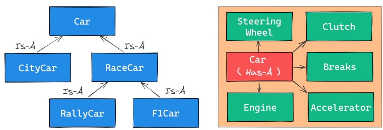
Figure 6.1: Is-A versus Has-A relationships
Accessing a base class
We have already seen class declarations, such as class ClassA: pass and class ClassB(BaseClassName): pass . When we don’t specify a base class explicitly, Python will set the built-in object class as the base class. Ultimately, all classes derive from object . Please remember that, if you do not specify a base class, brackets are optional and in practice are never used.
Therefore, writing class A: pass or class A(): pass or class A(object): pass are all equivalent. The object class is a special class in that it hosts the methods that are common to all Python classes, and it does not allow you to set any attributes on it.
Let us see how we can access a base class from within a class:
# oop/super.duplication.py
class Book:
def __init__(self, title, publisher, pages):
self.title = title
self.publisher = publisher
self.pages = pages
class Ebook(Book):
def __init__(self, title, publisher, pages, format_):
self.title = title
self.publisher = publisher
self.pages = pages
self.format_ = format_Take a look at the preceding code. Three of the input parameters for Book are duplicated in Ebook . This is bad practice because we now have two sets of instructions that are doing the same thing. Moreover, any change in the signature of Book.__init__() will not be reflected in Ebook . Normally we want changes in a base class to be reflected in its children. Let us see one way to fix this issue:
# oop/super.explicit.py
class Book:
def __init__(self, title, publisher, pages):
self.title = title
self.publisher = publisher
self.pages = pages
class Ebook(Book):
def __init__(self, title, publisher, pages, format_):
Book.__init__(self, title, publisher, pages)
self.format_ = format_
ebook = Ebook(
"Learn Python Programming", "Packt Publishing", 500, "PDF"
)
print(ebook.title) # Learn Python Programming
print(ebook.publisher) # Packt Publishing
print(ebook.pages) # 500
print(ebook.format_) # PDFMuch better. We have removed that code duplication. In this example, we tell Python to call the __init__() method of the Book class; we feed self to that call, making sure that we bind it to the present instance.
If we modify the logic within the __init__() method of Book , we do not need to touch Ebook ; the change will transfer automatically.
This approach is good, but it still suffers from a minor issue. Say that we change the name of Book to Liber , which is the Latin word for “book”. We would then have to change the __init__() method of Ebook to reflect that change. This can be avoided by using super :
# oop/super.implicit.py
class Book:
def __init__(self, title, publisher, pages):
self.title = title
self.publisher = publisher
self.pages = pages
class Ebook(Book):
def __init__(self, title, publisher, pages, format_):
super().__init__(title, publisher, pages)
# Another way to do the same thing is:
# super(Ebook, self).__init__(title, publisher, pages)
self.format_ = format_
ebook = Ebook(
"Learn Python Programming", "Packt Publishing", 500, "PDF"
)
print(ebook.title) # Learn Python Programming
print(ebook.publisher) # Packt Publishing
print(ebook.pages) # 500
print(ebook.format_) # PDFsuper() is a function that returns a proxy object that delegates method calls to a parent or sibling class.
Two classes are siblings if they share the same parents.
In this case, super() will delegate that call to Book.__init__() , and the beauty of this approach is that now we are free to change Book to Liber without having to touch the logic in the __init__() method of Ebook at all.
Now that we know how to access a base class from its child, let us explore Python’s multiple inheritance.
Multiple inheritance
In Python we are allowed to define classes that inherit from more than one class. This is called multiple inheritance. When a class has more than one base class, attribute search can follow more than one path. Take a look at the following diagram:
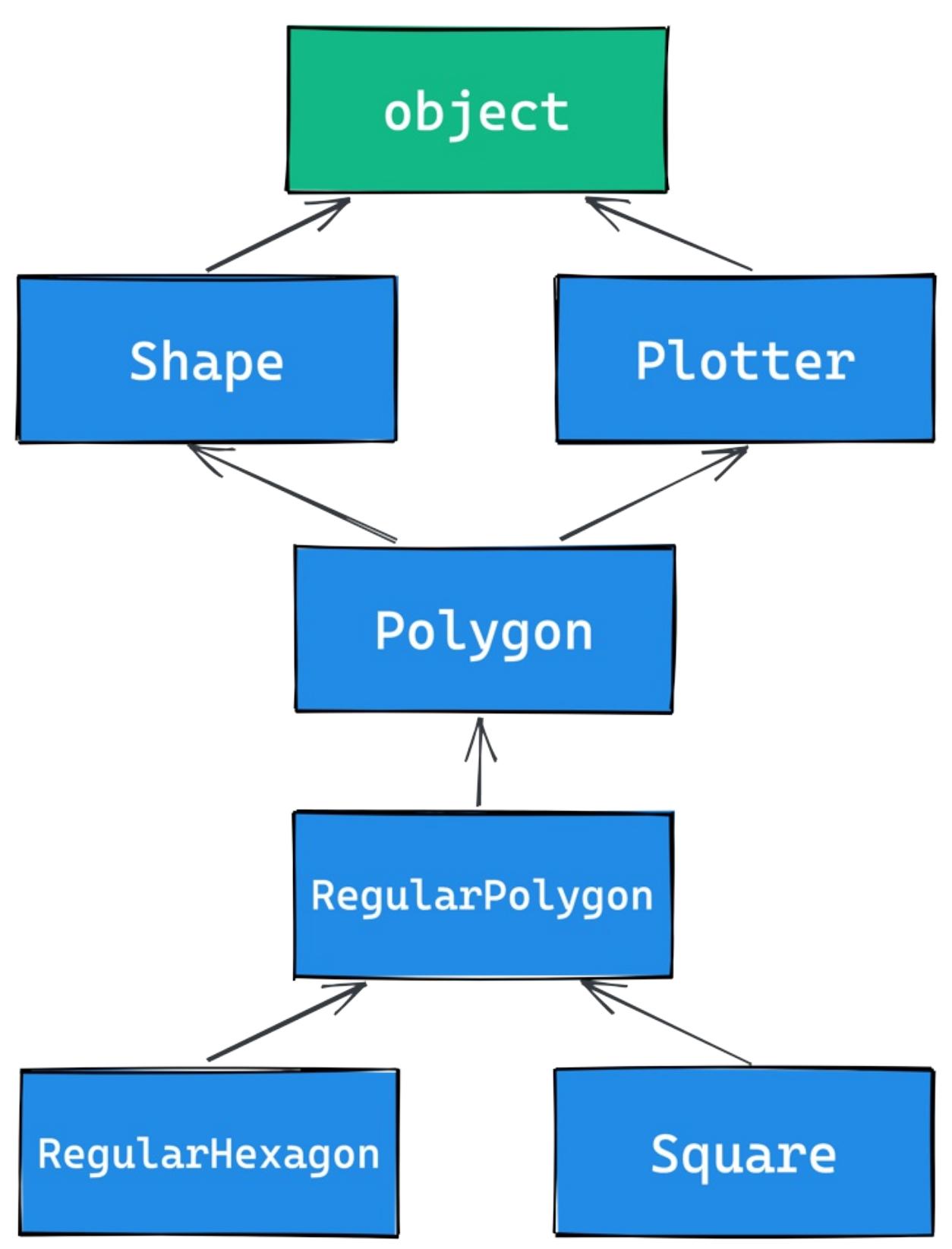
Figure 6.2: A class inheritance diagram
As you can see, Shape and Plotter act as base classes for all the others. Polygon inherits directly from them, RegularPolygon inherits from Polygon , and both RegularHexagon and Square inherit from RegularPolygon . Note also that Shape and Plotter implicitly inherit from object so, from Polygon up to object we have what is known as a diamond. In simpler terms, more than one path to reach a base class. We will see why this matters in a few moments. Let us translate the diagram into code:
# oop/multiple.inheritance.py
class Shape:
geometric_type = "Generic Shape"
def area(self): # This acts as placeholder for the interface
raise NotImplementedError
def get_geometric_type(self):
return self.geometric_type
class Plotter:
def plot(self, ratio, topleft):
# Imagine some nice plotting logic here...
print("Plotting at {}, ratio {}.".format(topleft, ratio))
class Polygon(Shape, Plotter): # base class for polygons
geometric_type = "Polygon"
class RegularPolygon(Polygon): # Is-A Polygon
geometric_type = "Regular Polygon"
def __init__(self, side):
self.side = side
class RegularHexagon(RegularPolygon): # Is-A RegularPolygon
geometric_type = "RegularHexagon"
def area(self):
return 1.5 * (3**0.5 * self.side**2)
class Square(RegularPolygon): # Is-A RegularPolygon
geometric_type = "Square"
def area(self):
return self.side * self.side
hexagon = RegularHexagon(10)
print(hexagon.area()) # 259.8076211353316
print(hexagon.get_geometric_type()) # RegularHexagon
hexagon.plot(0.8, (75, 77)) # Plotting at (75, 77), ratio 0.8.
square = Square(12)
print(square.area()) # 144
print(square.get_geometric_type()) # Square
square.plot(0.93, (74, 75)) # Plotting at (74, 75), ratio 0.93.Take a look at the preceding code: the Shape class has one attribute, geometric_type , and two methods: area() and get_geometric_type() . It is quite common to use base classes (such as Shape , in our example) to define an interface, a set of methods for which children must provide an implementation. There are different and better ways to do this, but we want to keep this example as simple as possible for the time being.
We also have the Plotter class, which adds the plot() method, thereby providing plotting capabilities for any class that inherits from it. Of course, the plot() implementation is just a dummy print() in this example. The first interesting class is Polygon , which inherits from both Shape and Plotter .
There are many types of polygons, one of which is the regular one, which is both equiangular (all angles are equal) and equilateral (all sides are equal), so we create the RegularPolygon class that inherits from Polygon . For a regular polygon, where all sides are equal, we can implement a simple __init__() method, which just takes the length of the side. We create the RegularHexagon and Square classes, which both inherit from RegularPolygon .
This structure is quite long, but hopefully it gives you an idea of how to specialize the classification of your objects.
Now, please take a look at the last eight lines of code. Note that when we call the area() method on hexagon and square , we get the correct area for both. This is because they both provide the correct implementation logic for it. Also, we can call get_geometric_type() on both of them, even though it is not defined on their classes, and Python goes all the way up to Shape to find an implementation for it. Note that, even though the implementation is provided in the Shape class, the self.geometric_type() used for the return value is correctly taken from the caller instance.
The plot() method calls are also interesting and show you how you can enrich your objects with capabilities they
would not otherwise have. This technique is very popular in web frameworks such as Django, which provides special classes called mixins, whose capabilities you can just use out of the box. All you need is to define the desired mixin as one of the base classes for your class.
Multiple inheritance is powerful, but at the same time it can get a bit messy, so we need to make sure we understand what happens when we use it.
Method resolution order
By now, we know that when we ask for someobject.attribute and attribute is not found on that object, Python starts searching in the class that someobject was created from. If it is not there either, Python searches up the inheritance chain until either attribute is found or the object class is reached. This is quite simple to understand if the inheritance chain is only made of single-inheritance steps, which means that classes have only one parent, all the way up to object . However, when multiple inheritance is involved, there are cases when it is not straightforward to predict which class will be searched next if an attribute is not found.
Python provides a way to always know the order in which classes are searched on attribute lookup: the method resolution order (MRO).
The MRO is the order in which base classes are searched for a member during lookup. Since version 2.3, Python uses an algorithm called C3, which guarantees monotonicity.
Let us see the MRO for the Square class from the previous example:
# oop/multiple.inheritance.py
print(square.__class__.__mro__)
# prints:
# (<class '__main__.Square'>, <class '__main__.RegularPolygon'>,
# <class '__main__.Polygon'>, <class '__main__.Shape'>,
# <class '__main__.Plotter'>, <class 'object'>)To get to the MRO of a class, we can go from the instance to its __class__ attribute, and from that to its __mro__ attribute. Alternatively, we could have used Square.__mro__ , or Square.mro() directly, but if you need to do it from an instance, you will have to derive its class dynamically.
Note that the only point of doubt is the branching after Polygon , where the inheritance chain breaks into two ways: one leads to Shape and the other to Plotter . We know by scanning the MRO for the Square class that Shape is searched before Plotter .
Why is this important? Well, consider the following code:
# oop/mro.simple.py
class A:
label = "a"
class B(A):
label = "b"
class C(A):
label = "c"
class D(B, C):
pass
d = D()
print(d.label) # Hypothetically this could be either 'b' or 'c'Both B and C inherit from A , and D inherits from both B and C . This means that the lookup for the label attribute can reach the top ( A ) through either B or C . Depending on which is reached first, we get a different result.
In this preceding example, we get ‘b’ , which is what we were expecting, since B is the leftmost among the base classes of D . But what happens if we remove the label attribute from B ? This would be a confusing situation: will the algorithm go all the way up to A or will it get to C first? Let us find out:
# oop/mro.pyclass A:
label = "a"
class B(A):
pass # was: label = 'b'
class C(A):
label = "c"
class D(B, C):
pass
d = D()
print(d.label) # 'c'
print(d.__class__.mro()) # notice another way to get the MRO
# prints:
# [<class '__main__.D'>, <class '__main__.B'>,
# <class '__main__.C'>, <class '__main__.A'>, <class 'object'>]So, we learn that the MRO is D->B->C->A->object , which means that when we ask for d.label , we get ‘c’ .
In day-to-day programming, it is not common to have to deal with the MRO, but we felt it was important to at least mention it in this paragraph so that, should you get entangled in a complex mixins structure, you will be able to find your way out of it.
Class and static methods
So far, we have written classes with attributes in the form of data and instance methods, but there are two other types of methods that we can find in a class definition: static methods and class methods.
Static methods
When you create a class object, Python assigns a name to it. That name acts as a namespace, and sometimes it makes sense to group functionalities under it. Static methods are perfect for this use case. Unlike instance methods, they do not need to be passed an instance when called. Let us look at an example:
# oop/static.methods.py
class StringUtil:
@staticmethod
def is_palindrome(s, case_insensitive=True):
# we allow only letters and numbers
s = "".join(c for c in s if c.isalnum()) # Study this!
# For case insensitive comparison, we lower-case s
if case_insensitive:
s = s.lower()
for c in range(len(s) // 2):
if s[c] != s[-c - 1]:
return False
return True
@staticmethod
def get_unique_words(sentence):
return set(sentence.split())
print(
StringUtil.is_palindrome("Radar", case_insensitive=False)
) # False: Case Sensitive
print(StringUtil.is_palindrome("A nut for a jar of tuna")) # True
print(StringUtil.is_palindrome("Never Odd, Or Even!")) # True
print(
StringUtil.is_palindrome(
"In Girum Imus Nocte Et Consumimur Igni"
) # Latin palindrome
) # True
print(
StringUtil.get_unique_words(
"I love palindromes. I really really love them!"
)
)
# {'them!', 'palindromes.', 'I', 'really', 'love'}The preceding code is quite interesting. First, we learn that static methods are created by simply applying the
staticmethod decorator to them. You can see that they don’t require any extra arguments so, apart from the decoration, they just look like functions.
We have a class, StringUtil , that acts as a container for functions. Another approach would be to have a separate module with functions inside. It is really a matter of style, most of the time.
The logic inside is_palindrome() should be straightforward for you by now, but, just in case, let us go through it. First, we remove all characters from s that are neither letters nor numbers. We use the join() method of a string object to do this. By calling join() on an empty string, the result is that all elements in the iterable you pass to join() will be concatenated together. We feed join() a generator expression that produces all alphanumeric characters in s in order. This is a normal procedure when analyzing palindromes.
If case_insensitive is True , we lowercase s . Finally, we proceed to check whether s is a palindrome. To do this, we compare the first and last characters, then the second and the second to last, and so on. If, at any point, we find a difference, it means the string isn’t a palindrome, and therefore we can return False . On the other hand, if we exit the for loop normally, it means no differences were found, and we can therefore say the string is a palindrome.
Notice that this code works correctly regardless of the length of the string; that is, if the length is odd or even. The measure len(s) // 2 reaches half of s , and if s is an odd number of characters long, the middle one won’t be checked (for instance, in RaDaR, D is not checked), but we don’t care as it would be compared to itself.
The get_unique_words() method is much simpler: it just returns a set to which we feed a list with the words from a sentence. The set class removes any duplication for us, so we don’t need to do anything else.
The StringUtil class provides us with a container namespace for methods that are meant to work on strings. Another example could have been a MathUtil class with some static methods to work on numbers.
Class methods
Class methods are slightly different from static methods in that, like instance methods, they also receive a special first argument. In their case, it is the class object itself, rather than the instance. A very common use case for class methods is to provide factory capability to a class, which means to have alternative ways to create instances of the class. Let us see an example:
# oop/class.methods.factory.py
class Point:
def __init__(self, x, y):
self.x = x
self.y = y
@classmethod
def from_tuple(cls, coords): # cls is Point
return cls(*coords)
@classmethod
def from_point(cls, point): # cls is Point
return cls(point.x, point.y)
p = Point.from_tuple((3, 7))
print(p.x, p.y) # 3 7
q = Point.from_point(p)
print(q.x, q.y) # 3 7In the preceding code, we show you how to use a class method to create a factory for the Point class. In this case, we want to create a Point instance by passing both coordinates (regular creation p = Point(3, 7) ), but we also want to be able to create an instance by passing a tuple ( Point.from_tuple() ) or another instance ( Point.from_point() ).
Within each class method, the cls argument refers to the Point class. As with the instance method, which takes self as the first argument, the class method takes a cls argument. Both self and cls are named after a convention that you are not forced to follow but are strongly encouraged to respect. This is something that no professional Python coder would change; it is so strong a convention that plenty of tools, such as parsers, linters, and the like, rely on it.
Class and static methods play well together. Static methods are particularly useful for breaking up the logic of a class method to improve its layout.
Let us see an example by refactoring the StringUtil class:
# oop/class.methods.split.py
class StringUtil:
@classmethod
def is_palindrome(cls, s, case_insensitive=True):
s = cls._strip_string(s)
# For case insensitive comparison, we lower-case s
if case_insensitive:
s = s.lower()
return cls._is_palindrome(s)
@staticmethod
def _strip_string(s):
return "".join(c for c in s if c.isalnum())
@staticmethod
def _is_palindrome(s):
for c in range(len(s) // 2):
if s[c] != s[-c - 1]:
return False
return True
@staticmethod
def get_unique_words(sentence):
return set(sentence.split())
print(StringUtil.is_palindrome("radar")) # True
print(StringUtil.is_palindrome("not a palindrome")) # FalseCompare this code with the previous version. First of all, note that even though is_palindrome() is now a class method, we call it in the same way we were calling it when it was a static one. The reason why we changed it to a class method is that after factoring out some of its logic (to _strip_string() and _is_palindrome() ), we need to get a reference to those methods, and if we have no cls in our method, the only option would be to call them by using the name of the class itself, like so: StringUtil._strip_string() and StringUtil._is_palindrome() , which is not good practice, because we would hardcode the class name in the is_palindrome() method, thereby putting ourselves in the position of having to modify it whenever we want to change the class name. Using cls means it will act as the class name, which means our code won’t need any modifications should the class name change.
Notice how the new logic reads much better than the previous version. Moreover, notice that, by naming the factored-out methods with a leading underscore, we are hinting that those methods are not supposed to be called from outside the class, but this will be the subject of the next paragraph.
Private methods and name mangling
If you have any background with languages like Java, C#, or C++, then you know they allow the programmer to assign a privacy status to attributes (both data and methods). Each language has its own slightly different flavor for this, but the gist is that public attributes are accessible from any point in the code, while private ones are accessible only within the scope they are defined in.
In Python there is no such thing. Everything is public; therefore, we rely on conventions and, for privacy, on a mechanism called name mangling.
The convention is as follows: if an attribute’s name has no leading underscores, it is considered public. This means you can access it and modify it freely. When the name has one leading underscore, the attribute is considered private, which means it is intended to be used internally and you should not modify it, or call it from the outside. A very common use case for private attributes is helper methods that are supposed to be used by public ones (possibly in call chains in conjunction with other methods). Another use case is internal data, such as scaling factors, or any other data that we would ideally put in a constant, a variable that once defined cannot change. However, Python has no concept of constants.
We know some programmers who don’t feel at ease with this aspect of Python. In our experience, we have never
encountered situations in which we had bugs because Python lacks private attributes. It is a matter of discipline, best practices, and following conventions.
The amount of freedom Python offers to a developer is the reason why sometimes it is referred to as a language for adults. And of course, there are pros and cons to every design choice. At the end of the day, some people prefer languages that allow more power and might require a bit more responsibility, while others prefer languages that are more constrictive. To each their own, it’s not a matter of right or wrong.
That said, the call for privacy actually makes sense because without it, you risk introducing bugs into your code for real. Let us show you what we mean:
# oop/private.attrs.py
class A:
def __init__(self, factor):
self._factor = factor
def op1(self):
print("Op1 with factor {}...".format(self._factor))
class B(A):
def op2(self, factor):
self._factor = factor
print("Op2 with factor {}...".format(self._factor))
obj = B(100)
obj.op1() # Op1 with factor 100...
obj.op2(42) # Op2 with factor 42...
obj.op1() # Op1 with factor 42... <- This is BADIn the preceding code, we have an attribute called _factor , and let us pretend it is so important that it shouldn’t be modified at runtime after the instance is created because op1() depends on it to function correctly. We’ve named it with a leading underscore, but the issue here is that the call obj.op2(42) modifies it, and this is then reflected in subsequent calls to op1() .
We can fix this undesired behavior by adding a second leading underscore:
# oop/private.attrs.fixed.py
class A:
def __init__(self, factor):
self.__factor = factor
def op1(self):
print("Op1 with factor {}...".format(self.__factor))
class B(A):
def op2(self, factor):
self.__factor = factor
print("Op2 with factor {}...".format(self.__factor))
obj = B(100)
obj.op1() # Op1 with factor 100...
obj.op2(42) # Op2 with factor 42...
obj.op1() # Op1 with factor 100... <- Now it's good!Now it is working as desired. Python is kind of magic and in this case, what is happening is that the name-mangling mechanism has kicked in.
Name mangling means that any attribute name that has at least two leading underscores and at most one trailing underscore, such as __my_attr , is replaced with a name that includes an underscore and the class name before the actual name, such as _ClassName__my_attr .
This means that when you inherit from a class, the mangling mechanism gives your private attribute two different names in the base and child classes so that name collision is avoided. Every class and instance object stores references to their attributes in a special attribute called __dict__ , so let us inspect obj.__dict__ to see name mangling in action:
# oop/private.attrs.py
print(obj.__dict__.keys())
# dict_keys(['_factor'])This is the _factor attribute that we find in the problematic version of this example, but look at the one that is using __factor :
# oop/private.attrs.fixed.py
print(obj.__dict__.keys())
# dict_keys(['_A__factor', '_B__factor'])obj has two attributes now, _A__factor (mangled within the A class), and _B__factor (mangled within the B class). This is the mechanism that ensures that when you do obj.__factor = 42 , __factor in A isn’t changed because you’re actually touching _B__factor , which has no effect on _A__factor .
If you are designing a library with classes that are meant to be used and extended by other developers, you will need to keep this in mind in order to avoid the unintentional overriding of your attributes. Bugs like these can be subtle and hard to spot.
The property decorator
Another thing that would be a crime not to mention is the property decorator. Imagine that you have an age attribute in a Person class and, at some point, you want to make sure that when you change its value, you also check that age is within a proper range, such as [18, 99]. You could write accessor methods, such as get_age() and set_age() (also called getters and setters) and put the logic there. get_age() will most likely just return age , while set_age() will set its value after checking its validity. The problem is that you may already have a some code accessing the age attribute directly, which means you’re now up for some refactoring. Languages like Java overcome this problem by using the accessor pattern basically by default. Many Java Integrated Development Environments (IDEs) autocomplete an attribute declaration by writing getter and setter accessor method stubs for you on the fly.
But we are not learning Java. Python achieves the same result with the property decorator. When you decorate a method with property , you can use the name of the method as if it were a data attribute. Because of this, it is always best to refrain from putting logic that would take a while to complete in such methods because, by accessing them as attributes, we are not expecting to wait.
Let us look at an example:
# oop/property.py
class Person:
def __init__(self, age):
self.age = age # anyone can modify this freely
class PersonWithAccessors:
def __init__(self, age):
self._age = age
def get_age(self):
return self._age
def set_age(self, age):
if 18 <= age <= 99:
self._age = age
else:
raise ValueError("Age must be within [18, 99]")
class PersonPythonic:
def __init__(self, age):
self._age = age
@property
def age(self):
return self._age
@age.setter
def age(self, age):
if 18 <= age <= 99:
self._age = age
else:
raise ValueError("Age must be within [18, 99]")
person = PersonPythonic(39)
print(person.age) # 39 - Notice we access as data attribute
person.age = 42 # Notice we access as data attribute
print(person.age) # 42person.age = 100 # ValueError: Age must be within [18, 99]The Person class may be the first version we write. Then we realize we need to put the range logic in place so, with another language, we would have to rewrite Person as the PersonWithAccessors class and refactor the code that uses Person.age . In Python, we rewrite Person as PersonPythonic (you normally wouldn’t change the name, of course, this is just for the sake of illustration). In PersonPythonic the age is stored in a private _age variable, and we define property getters and setters using the decoration shown, which allows us to keep using the person instances as before. A getter is a method that is called when we access an attribute for reading. On the other hand, a setter is a method that is called when we access an attribute to write it.
Unlike languages that use the getter/setter paradigm, Python allows us to start writing simple code and refactor later, only when we need it; there is no need to pollute the code with accessor methods only because they may be helpful in the future.
The property decorator also allows for read-only data (by not writing the setter counterpart) and for special actions when the attribute is deleted. Please refer to the official documentation to dig deeper.
The cached_property decorator
One convenient use of properties is when we need to run some code to set up the object we want to use. For example, say we needed to connect to a database (or to an API).
In both cases, we might have to set up a client object that knows how to talk to the database (or to the API). It is quite common to use a property, in these cases, so that we can hide away the complexity of having to set the client up, and simply use it. Let us show you a simple example:
# oop/cached.property.py
class Client:
def __init__(self):
print("Setting up the client...")
def query(self, **kwargs):
print(f"Performing a query: {kwargs}")
class Manager:
@property
def client(self):
return Client()
def perform_query(self, **kwargs):
return self.client.query(**kwargs)In the preceding example, we have a dummy Client class, which prints the string “Setting up the client…” every time we create a new instance. It also has a pretend query() method, that prints a string as well. We then have a class, Manager , which has a client property that creates a new instance of Client every time it is called (for example, by a call to perform_query() ).
If we were to run this code, we would notice that every time we call perform_query() on the manager, we see the string “Setting up the client…” being printed. When creating a client is expensive, this code would be wasting resources, so it might be better to cache that client, like this:
# oop/cached.property.py
class ManualCacheManager:
@property
def client(self):
if not hasattr(self, "_client"):
self._client = Client()
return self._client
def perform_query(self, **kwargs):
return self.client.query(**kwargs)The ManualCacheManager class is a bit smarter: the client property first checks if the attribute _client exists on the instance, by calling the built-in hasattr() function. If not, it assigns _client to a new instance of Client . Finally, it simply returns it. Repeatedly accessing the client property on this class will only create one instance of Client , the first time. From the second call on, _client is simply returned with no creation of new instances.
This is such a common need that, in Python 3.8, the functools module added the cached_property decorator. The beauty of using that, instead of our manual solution, is that in case we need to refresh the client, we can simply delete the client property, and the next time we call it, it will recreate a brand new Client for us. Let us see an example:
# oop/cached.property.py
from functools import cached_property
class CachedPropertyManager:
@cached_property
def client(self):
return Client()
def perform_query(self, **kwargs):
return self.client.query(**kwargs)
manager = CachedPropertyManager()
manager.perform_query(object_id=42)
manager.perform_query(name_ilike="%Python%")
del manager.client # This causes a new Client on next call
manager.perform_query(age_gte=18)
Running this code gives the following result:
$ python cached.property.py
Setting up the client... # New Client
Performing a query: {'object_id': 42} # first query
Performing a query: {'name_ilike': '%Python%'} # second query
Setting up the client... # Another ClientPerforming a query: {‘age_gte’: 18} # Third query
As you can see, it is only after we manually delete the manager.client attribute that we get a new one when we invoke manager.perform_query() again.
Python 3.9 also introduces a cache decorator, which can be used in conjunction with the property decorator, to cover scenarios for which cached_property is not suitable. As always, we encourage you to read up on all the details in the official Python documentation and experiment.
Operator overloading
Python’s approach to operator overloading is brilliant. To overload an operator means to give it a meaning according to the context in which it is used. For example, the + operator means addition when we deal with numbers, but concatenation when we deal with sequences.
When using operators, Python calls special methods behind the scenes. For example, the a[k] call on a dictionary roughly translates to type(a).__getitem__(a, k) . We can override these special methods for our purposes.
As an example, let us create a class that stores a string and evaluates to True if ‘42’ is part of that string, and False otherwise. Also, let us give the class a length property that corresponds to the length of the stored string:
# oop/operator.overloading.py
class Weird:
def __init__(self, s):
self._s = s
def __len__(self):
return len(self._s)
def __bool__(self):
return "42" in self._s
weird = Weird("Hello! I am 9 years old!")
print(len(weird)) # 24
print(bool(weird)) # False
weird2 = Weird("Hello! I am 42 years old!")
print(len(weird2)) # 25
print(bool(weird2)) # TrueFor the complete list of magic methods that you can override to provide your custom implementation of operators for your classes, please refer to the Python data model in the official documentation.
Polymorphism – a brief overview
The word polymorphism comes from the Greek polys (many, much) and morphē (form, shape), and its meaning is the provision of a single interface for entities of different types.
In our car example, we call engine.start(), regardless of what kind of engine it is. As long as it exposes the start method, we can call it. That’s polymorphism in action.
In other languages, such as Java, in order to give a function the ability to accept different types and call a method on them, those types need to be coded in such a way that they share an interface. In this way, the compiler knows that the method will be available regardless of the type of the object the function is fed (as long as it extends the specific interface, of course).
In Python, things are different. Polymorphism is implicit, and nothing prevents you from calling a method of an object; therefore, technically, there is no need to implement interfaces or other patterns.
There is a special kind of polymorphism called ad hoc polymorphism, which is what we saw in the last section on operator overloading. This is the ability of an operator to change shape according to the type of data it is applied to.
Polymorphism also allows Python programmers to simply use the interface (methods and properties) exposed from an object rather than having to check which class it was instantiated from. This allows the code to be more compact and feel more natural.
We cannot spend too much time on polymorphism, but we encourage you to check it out by yourself; it will expand your understanding of OOP.
Data classes
Before we leave the OOP realm, there is one last thing we want to mention: data classes. Introduced in Python 3.7 by PEP 557 (https://peps.python.org/pep-0557/), they can be described as mutable named tuples with defaults. You can brush up on named tuples in Chapter 2, Built-In Data Types. Let us dive straight into an example:
# oop/dataclass.py
from dataclasses import dataclass
@dataclass
class Body:
"""Class to represent a physical body."""
name: str
mass: float = 0.0 # Kg
speed: float = 1.0 # m/s
def kinetic_energy(self) -> float:
return (self.mass * self.speed**2) / 2
body = Body("Ball", 19, 3.1415)
print(body.kinetic_energy()) # 93.755711375 Joule
print(body) # Body(name='Ball', mass=19, speed=3.1415)In the previous code, we have created a class to represent a physical body, with one method that allows us to calculate its kinetic energy (using the formula \(E_k = \frac{1}{2}mv^2\) ). Notice that name is supposed to be a string, while mass and speed are both floats, and both are given a default value. It is also interesting that we didn’t have to write any __init__() method; it is done for us by the dataclass decorator, along with methods for comparison and for producing the string representation of the object (implicitly called on the last line by print).
Another thing to notice is how name, mass, and speed are defined. This technique is called type hinting, and will be the subject of Chapter 12, Introduction to Type Hinting.
You can read all the specifications in PEP 557 if you are curious, but for now, just remember that data classes might offer a nicer, slightly more powerful alternative to named tuples, in case you need it.
Writing a custom iterator
Now we have all the tools to appreciate how we can write our own custom iterator. Let us first define what iterable and iterator mean:
- Iterable: An object is said to be iterable if it can return its members one at a time. Lists, tuples, strings, and dictionaries are all iterables. Custom objects that define either of the __iter__() or __getitem__() methods are also iterables.
- Iterator: An object is said to be an iterator if it represents a stream of data. A custom iterator is required to provide an implementation for the __iter__() method that returns the object itself, and an implementation for the __next__() method that returns the next item of the data stream until the stream is exhausted, at which point all successive calls to __next__() simply raise a StopIteration exception. Built-in functions, such as iter() and next() , are mapped to call the __iter__() and __next__() methods on an object, behind the scenes.
Exceptions will be the subject of Chapter 7, Exceptions and Context Managers. They can represent errors during code execution, but are also used to regulate the flow of execution and Python relies on them for mechanisms such the iteration protocol.
Let us write an iterator that returns all the odd characters from a string first, and then the even ones:
# iterators/iterator.py
class OddEven:
def __init__(self, data):
self._data = data
self.indexes = list(range(0, len(data), 2)) + list(
range(1, len(data), 2)
)
def __iter__(self):
return self
def __next__(self):
if self.indexes:
return self._data[self.indexes.pop(0)]
raise StopIteration
oddeven = OddEven("0123456789")
print("".join(c for c in oddeven)) # 0246813579
oddeven = OddEven("ABCD") # or manually...
it = iter(oddeven) # this calls oddeven.__iter__ internally
print(next(it)) # A
print(next(it)) # C
print(next(it)) # B
print(next(it)) # DSo, we provide an implementation for __iter__() that returns the object itself, and one for __next__() . Let us go through it. What needs to happen is the return of _data[0] , _data[2] , _data[4] , … , _data[1] , _data[3] , _data[5] ,… until we have returned every item in the data. To do that, we prepare a list of indexes, such as [0, 2, 4, 6, …, 1, 3, 5, …], and while there is at least one element in it, we pop the first one out and return the element from the data that is at that position, thereby achieving our goal. When indexes is empty, we raise StopIteration , as required by the iterator protocol.
There are other ways to achieve the same result, so go ahead and try to code a different one yourself. Make sure that the end result works for all edge cases, empty sequences, sequences of lengths of 1, 2, and so on.
Summary
In this chapter, we looked at decorators, discovered their purpose, and covered a few examples using one or more at the same time. We also saw decorators that take arguments, which are usually used as decorator factories.
We have scratched the surface of object-oriented programming in Python. We covered all the basics, so you should now be able to understand the code that will come in future chapters. We talked about all kinds of methods and attributes that you can write in a class; we explored inheritance versus composition, method overriding, properties, operator overloading, and polymorphism.
At the end, we very briefly touched on iterators, which should enrich your understanding of generators.
In the next chapter, we are going to learn about exceptions and context managers.
7 Exceptions and Context Managers
Join our book community on Discord

The best-laid schemes o’ mice an’ menGang aft agley– Robert Burns
These famous lines by Robert Burns should be etched into the mind of every programmer. Even if our code is correct, errors will happen. If we do not deal with them properly, they can cause our best-laid schemes to go awry.
Unhandled errors can cause software to crash or misbehave. Depending on the nature of the software in question, this could have serious consequences. Therefore, it is important to learn how to detect and handle errors. We encourage you to cultivate the habit of always thinking about what errors can occur and how your code should respond when they do.
This chapter is all about errors and dealing with the unexpected. We will be learning about exceptions, which are Python’s way of signaling that an error or other exceptional event has occurred. We will also talk about context managers, which provide a mechanism to encapsulate and re-use error handling code.
In this chapter, we are going to cover the following:
- Exceptions
- Context managers
Exceptions
Even though we have not covered the topic yet, we expect that by now you have at least a vague idea of what an exception is. In the previous chapters, we saw that when an iterator is exhausted, calling next() on it raises a StopIteration exception. We got an IndexError when we tried accessing a list at a position that was outside the valid range. We also encountered AttributeError when we tried accessing an attribute that did not exist on an object, and KeyError when we tried to access a nonexistent key in a dictionary. In this chapter, we will discuss exceptions in more depth.
Even though an operation or a piece of code is correct, there are often conditions in which something may go wrong. For example, if we are converting user input from str to int , the user could accidentally type a letter in place of a digit, making it impossible for us to convert that value into a number. When dividing numbers, we may not know in advance whether we might attempt a division by zero. When opening a file, it could be missing or corrupted.
When an error is detected during execution, it is called an exception. Exceptions are not necessarily lethal; in fact, the StopIteration exception is deeply integrated into the Python generator and iterator mechanisms. Normally, however, if you do not take the necessary precautions, an exception will cause your application to break. Sometimes, this is the desired behavior, but in other cases, we want to prevent and control problems such as these. For example, if a user tries to open a corrupted file, we can alert them to the problem and give them an opportunity to fix it. Let us
see an example of a few exceptions:
# exceptions/first.example.txt
>>> gen = (n for n in range(2))
>>> next(gen)
0
>>> next(gen)
1
>>> next(gen)
Traceback (most recent call last):
File "<stdin>", line 1, in <module>
StopIteration
>>> print(undefined_name)
Traceback (most recent call last):
File "<stdin>", line 1, in <module>
NameError: name 'undefined_name' is not defined
>>> mylist = [1, 2, 3]
>>> mylist[5]
Traceback (most recent call last):
File "<stdin>", line 1, in <module>
IndexError: list index out of range
>>> mydict = {"a": "A", "b": "B"}
>>> mydict["c"]
Traceback (most recent call last):
File "<stdin>", line 1, in <module>
KeyError: 'c'
>>> 1 / 0
Traceback (most recent call last):
File "<stdin>", line 1, in <module>
ZeroDivisionError: division by zeroAs you can see, the Python shell is quite forgiving. We can see Traceback so that we have information about the error, but the shell itself still runs normally. This is a special behavior; a regular program or a script would normally exit immediately if nothing were done to handle exceptions. Let us see a quick example:
# exceptions/unhandled.py
1 + "one"
print("This line will never be reached")
If we run this code, we get the following output:
$ python exceptions/unhandled.py
Traceback (most recent call last):
File "exceptions/unhandled.py", line 2, in <module>
1 + "one"
~~^~~~~~~
TypeError: unsupported operand type(s) for +: 'int' and 'str'Because we did nothing to handle the exception, Python immediately exits once an exception occurs (after printing out information about the error).
Raising exceptions
The exceptions we have seen so far were raised by the Python interpreter when it detected an error. However, you can also raise exceptions yourself, when a situation occurs that your own code considers to be an error. To raise an exception, use the raise statement. For example:
# exceptions/raising.txt
>>> raise NotImplementedError("I'm afraid I can't do that")
Traceback (most recent call last):
File "<stdin>", line 1, in <module>
NotImplementedError: I'm afraid I can't do thatThere are no restrictions on which exception types you can raise. This allows you to choose the exception type that best describes the error condition that has occurred. You can also define your own exception types (we will see how to do that in a moment). Notice that the argument we passed to the Exception class is printed out as part of the
error message.
Python has too many built-in exceptions to list here, but they are all documented at https://docs.python.org/3.12/library/exceptions.xhtml#bltin-exceptions.
Defining your own exceptions
As we mentioned above, you can define your own custom exceptions. All you need to do is define a class that inherits from any other exception class. All exceptions derive from BaseException ; however, this class is not intended to be directly subclassed. Your custom exceptions should inherit from Exception instead. In fact, nearly all built-in exceptions also inherit from Exception . Exceptions that do not inherit from Exception are meant for internal use by the Python interpreter.
Tracebacks
The traceback that Python prints when an unhandled exception occurs, may initially look intimidating, but it is quite useful for understanding what happened to cause the exception. Let us look at a traceback and see what it can tell us:
# exceptions/trace.back.py
def squareroot(number):
if number < 0:
raise ValueError("No negative numbers please")
return number**.5
def quadratic(a, b, c):
d = b**2 - 4 * a * c
return (
(-b - squareroot(d)) / (2 * a),
(-b + squareroot(d)) / (2 * a)
)
quadratic(1, 0, 1) # x**2 + 1 == 0Here, we defined a function called quadratic() , which uses the famous quadratic formula to find the solution of a quadratic equation. Instead of using the sqrt() function from the math module, we wrote our own version ( squareroot() ), which raises an exception if the number is negative. When we call quadratic(1, 0, 1) to solve the equation x2+1=0, we will get a ValueError because d is negative. When we run this, we get:
$ python exceptions/trace.back.py
Traceback (most recent call last):
File "exceptions/trace.back.py", line 16, in <module>
quadratic(1, 0, 1) # x**2 + 1 == 0
^^^^^^^^^^^^^^^^^^
File "exceptions/trace.back.py", line 11, in quadratic
(-b - squareroot(d)) / (2 * a),
^^^^^^^^^^^^^
File "exceptions/trace.back.py", line 4, in squareroot
raise ValueError("No negative numbers please")
ValueError: No negative numbers pleaseIt is often useful to read tracebacks from bottom to top. On the very last line, we have the error message, telling us what went wrong: ValueError: No negative numbers please . The preceding lines tell us where the exception was raised (line 4 of exceptions/trace.back.py in the squareroot() function). We can also see the sequence of function calls that got us to the point where the exception was raised: squareroot() was called from line 11 in the function quadratic() , which was called from line 16, at the top level of the module. As you can see, the traceback is like a map that shows us the path through the code to where the exception happened. Following that path and examining the code in each function along the way is often helpful when you want to understand why an exception happened.
There have been several improvements to error messages in Python 3.10, 3.11 and 3.12. For example, the ^^^^ characters underlining the exact part of each statement or expression in the traceback that led to the exception, was added in Python 3.11.
Handling exceptions
To handle an exception in Python, you use the try statement. When you enter the try clause, Python will watch out for one or more different types of exceptions (according to how you instruct it), and if they are raised, it allows you to react.
The try statement is composed of the try clause, which opens the statement, followed by one or more except clauses that define what to do when an exception is caught. The except clauses may optionally be followed by an else clause, which is executed when the try clause is exited without any exception raised. After the except and else clauses, we can have a finally clause (also optional), whose code is executed regardless of whatever happened in the other clauses. The finally clause is typically used to clean up resources. You are also allowed to omit the except and else clauses and only have a try clause followed by a finally clause. This is helpful if we want exceptions to be propagated and handled elsewhere, but we do have some cleanup code that must be executed regardless of whether an exception occurs.
The order of the clauses is important. It must be try , except , else , finally . Also, remember that try must be followed by at least one except clause or a finally clause. Let us see an example:
# exceptions/try.syntax.py
def try_syntax(numerator, denominator):
try:
print(f"In the try block: {numerator}/{denominator}")
result = numerator / denominator
except ZeroDivisionError as zde:
print(zde)
else:
print("The result is:", result)
return result
finally:
print("Exiting")
print(try_syntax(12, 4))
print(try_syntax(11, 0))This example defines a simple try_syntax() function. We perform the division of two numbers. We are prepared to catch a ZeroDivisionError exception, which will occur if we call the function with denominator = 0 . Initially, the code enters the try block. If denominator is not 0 , result is calculated and, after leaving the try block, execution resumes in the else block. We print result and return it. Take a look at the output, and you’ll notice that just before returning result , which is the exit point of the function, Python executes the finally clause.
When denominator is 0 , things change. Our attempt to calculate numerator / denominator raises a ZeroDivisionError . As a result, we enter the except block and print zde .
The else block is not executed because an exception was raised in the try block. Before (implicitly) returning None , we still execute the finally block. Look at the output and see whether it makes sense to you:
$ python exceptions/try.syntax.py
In the try block: 12/4
The result is: 3.0
Exiting
3.0
In the try block: 11/0
division by zero
Exiting
NoneWhen you execute a try block, you may want to catch more than one exception. For example, when calling the divmod() function, you can get a ZeroDivisionError if the second argument is 0 , or TypeError if either argument is not a number. If you want to handle both in the same way, you can structure your code like this:
# exceptions/multiple.py
values = (1, 2)
try:
q, r = divmod(*values)except (ZeroDivisionError, TypeError) as e:
print(type(e), e)This code will catch both ZeroDivisionError and TypeError . Try changing values = (1, 2) to values = (1, 0) or values = (‘one’, 2) , and you will see the output change.
If you need to handle different exception types differently, you can use multiple except clauses, like this:
# exceptions/multiple.py
try:
q, r = divmod(*values)
except ZeroDivisionError:
print("You tried to divide by zero!")
except TypeError as e:
print(e)Keep in mind that an exception is handled in the first block that matches that exception class or any of its base classes. Therefore, when you stack multiple except clauses like we have done here, make sure that you put specific exceptions at the top and generic ones at the bottom. In OOP terms, derived classes should be placed before their base classes. Moreover, remember that only one except handler is executed when an exception is raised.
Python also allows you to use an except clause without specifying any exception type (this is equivalent to writing except BaseException ). You should, however, avoid doing this as it means you will also capture exceptions that are intended for internal use by the interpreter. They include the so-called system-exiting exceptions. These are SystemExit , which is raised when the interpreter exits via a call to the exit() function, and KeyboardInterrupt , which is raised when the user terminates the application by pressing Ctrl + C (or Delete on some systems).
You can also raise exceptions from within an except clause. For example, you might want to replace a built-in exception (or one from a third-party library) with your own custom exception. This is quite a common technique when writing libraries, as it helps shield users from implementation details of the library. Let us see an example:
# exceptions/replace.txt
>>> class NotFoundError(Exception):
... pass
...
>>> vowels = {"a": 1, "e": 5, "i": 9, "o": 15, "u": 21}
>>> try:
... pos = vowels["y"]
... except KeyError as e:
... raise NotFoundError(*e.args)
...
Traceback (most recent call last):
File "<stdin>", line 2, in <module>
KeyError: 'y'
During handling of the above exception, another exception occurred:
Traceback (most recent call last):
File "<stdin>", line 4, in <module>
NotFoundError: yBy default, Python assumes that an exception that happens within an except clause is an unexpected error and helpfully prints out tracebacks for both exceptions. We can tell the interpreter that we are deliberately raising the new exception by using a raise from statement:
# exceptions/replace.py
>>> try:
... pos = vowels["y"]
... except KeyError as e:
... raise NotFoundError(*e.args) from e
...
Traceback (most recent call last):
File "<stdin>", line 2, in <module>
KeyError: 'y'
The above exception was the direct cause of the following exception:
Traceback (most recent call last):File "<stdin>", line 4, in <module>
NotFoundError: yThe error message has changed, but we still get both tracebacks, which is very handy for debugging. If you really wanted to completely suppress the original exception, you could use from None instead of from e (try this yourself).
You can also use raise by itself, without specifying a new exception, to re-raise the original exception. This is sometimes useful if you want to log the fact that an exception has occurred, without suppressing or replacing the exception.
Since Python 3.11, it is also possible to add notes to exceptions. This allows you to add extra information to be displayed as part of the traceback without suppressing or replacing the original exception. To see how this works, we will modify the quadratic formula example from earlier in the chapter, and add a note to the exception:
# exceptions/note.py
def squareroot(number):
if number < 0:
raise ValueError("No negative numbers please")
return number**0.5
def quadratic(a, b, c):
d = b**2 - 4 * a * c
try:
return (
(-b - squareroot(d)) / (2 * a),
(-b + squareroot(d)) / (2 * a),
)
except ValueError as e:
e.add_note(f"Cannot solve {a}x**2 + {b}x + {c} == 0")
raise
quadratic(1, 0, 1)We have highlighted the lines where we add a note and re-raise the exception. The output when we run this looks as follows:
$ python exceptions/note.py
Traceback (most recent call last):
File "exceptions/note.py", line 20, in <module>
quadratic(1, 0, 1)
File "exceptions/note.py", line 12, in quadratic
(-b - squareroot(d)) / (2 * a),
^^^^^^^^^^^^^
File "exceptions/note.py", line 4, in squareroot
raise ValueError("No negative numbers please")
ValueError: No negative numbers please
Cannot solve 1x**2 + 0x + 1 == 0The note has been printed below the original error message. You can add as many notes as you need, by calling add_note() multiple times. The notes must all be strings.
Programming with exceptions can be tricky. You could inadvertently hide bugs by trapping exceptions that would have alerted you to their presence. Play it safe by keeping these simple guidelines in mind:
- Keep the try clause as short as possible. It should contain only the code that may cause the exception(s) that you want to handle.
- Make the except clauses as specific as you can. It may be tempting to just write except Exception , but if you do, you will almost certainly end up catching exceptions you did not actually intend to catch.
- Use tests to ensure that your code handles both expected and unexpected errors correctly. We shall talk more about writing tests in Chapter 10, Testing.
If you follow these suggestions, you will minimize the chance of getting it wrong.
Exception Groups
When working with large collections of data, it can be inconvenient to immediately stop and raise an exception when an error occurs. It is often better to process all the data and report on all errors that occurred at the end. This allows the user to deal with all the errors at once, rather than having to rerun the process multiple times, fixing errors one by one.
One way of achieving this is to build up a list of errors and return it. However, this has the disadvantage that you cannot use a try / except statement to handle the errors. Some libraries have worked around this by creating a container exception class and wrapping the collected errors in an instance of this class. This allows you to handle the container exception in an except clause and inspect it to access the nested exceptions.
Since Python 3.11, there is a new built-in exception class, ExceptionGroup , that was specifically designed as such a container exception. Having this feature built into the language has the advantage that the traceback also shows the tracebacks of each of the nested exceptions.
For example, suppose we need to validate a list of ages to ensure that the values are all positive integers. We could write something like the following:
# exceptions/groups/util.py
def validate_age(age):
if not isinstance(age, int):
raise TypeError(f"Not an integer: {age}")
if age < 0:
raise ValueError(f"Negative age: {age}")
def validate_ages(ages):
errors = []
for age in ages:
try:
validate_age(age)
except Exception as e:
errors.append(e)
if errors:
raise ExceptionGroup("Validation errors", errors)The validate_ages() function calls validate_age() for each element of ages . It catches any exceptions that occur and appends them to the errors list. If the list of errors is not empty after the loops completes, we raise ExceptionGroup , passing in the error message “Validation errors” and the list of errors that occurred.
If we call this from a Python console with a list containing some invalid ages, we get the following traceback:
# exceptions/groups/exc.group.txt
>>> from util import validate_ages
>>> validate_ages([24, -5, "ninety", 30, None])
+ Exception Group Traceback (most recent call last):
| File "<stdin>", line 1, in <module>
| File "exceptions/groups/util.py", line 20, in validate_ages
| raise ExceptionGroup("Validation errors", errors)
| ExceptionGroup: Validation errors (3 sub-exceptions)
+-+---------------- 1 ----------------
| Traceback (most recent call last):
| File "exceptions/groups/util.py", line 15, in validate_ages
| validate_age(age)
| File "exceptions/groups/util.py", line 8, in validate_age
| raise ValueError(f"Negative age: {age}")
| ValueError: Negative age: -5
+---------------- 2 ----------------
| Traceback (most recent call last):
| File "exceptions/groups/util.py", line 15, in validate_ages
| validate_age(age)
| File "exceptions/groups/util.py", line 6, in validate_age
| raise TypeError(f"Not an integer: {age}")
| TypeError: Not an integer: ninety
+---------------- 3 ----------------
| Traceback (most recent call last):
| File "exceptions/groups/util.py", line 15, in validate_ages
| validate_age(age)
| File "exceptions/groups/util.py", line 6, in validate_age| raise TypeError(f"Not an integer: {age}")
| TypeError: Not an integer: None
+------------------------------------Note that we get the traceback for the ExceptionGroup , including the error message we specified when raising it ( “Validation errors” ) and an indication that the group contains three sub-exceptions. Indented below this, we get the traceback for each of the nested sub-exceptions. To aid readability, the sub-exception tracebacks are numbered and separated by dashed lines.
We can handle ExceptionGroup exceptions just like any other type of exception:
# exceptions/groups/handle.group.txt
>>> from util import validate_ages
>>> try:
... validate_ages([24, -5, "ninety", 30, None])
... except ExceptionGroup as e:
... print(e)
... print(e.exceptions)
...
Validation errors (3 sub-exceptions)
(ValueError('Negative age: -5'),
TypeError('Not an integer: ninety'),
TypeError('Not an integer: None'))Note that we can access the nested list of sub-exceptions via the (read-only) exceptions property.
PEP 654 (https://peps.python.org/pep-0654/) which introduced ExceptionGroup to the language, also introduced a new variant of the try / except statement which allows us to handle nested sub-exceptions of particular types within an ExceptionGroup . This new syntax uses the keyword except* instead of except . In our validation example, this allows us to have separate handling for invalid types and invalid values without having to manually iterate and filter the exceptions:
# exceptions/groups/handle.nested.txt
>>> from util import validate_ages
>>> try:
... validate_ages([24, -5, "ninety", 30, None])
... except* TypeError as e:
... print("Invalid types")
... print(type(e), e)
... print(e.exceptions)
... except* ValueError as e:
... print("Invalid values")
... print(type(e), e)
... print(e.exceptions)
...
Invalid types
<class 'ExceptionGroup'> Validation errors (2 sub-exceptions)
(TypeError('Not an integer: ninety'),
TypeError('Not an integer: None'))
Invalid values
<class 'ExceptionGroup'> Validation errors (1 sub-exception)
(ValueError('Negative age: -5'),)The call to validate_ages() raises an exception group containing three exceptions: two instances of TypeError and a ValueError . The interpreter matches each except* clause to the nested exceptions. The first clause matches, so the interpreter creates a new ExceptionGroup containing all the TypeError instances from the original group and assigns this to e within the body of this clause. We print the string “Invalid types” , followed by the type and value of e and then e.exceptions . The remaining exceptions are then matched against the next except* clause. This time all the ValueError instances match so e is assigned to a new ExceptionGroup containing these. We print the string “Invalid values” , again followed by type(e) , e and e.exceptions . At this point, there are no unhandled exceptions left in the group, so execution resumes normally.
It is important to be aware that this behavior is different from a normal try / except statement. In a normal try / except statement, only one except clause is executed: the first that matches the raised exception. In a
try / except* statement, each matching except* clause is executed until there are no unhandled exceptions remaining in the group. If any unhandled exceptions remain after the all the except* clauses have been processed, they will be reraised at the end as a new ExceptionGroup :
# exceptions/groups/handle.nested.txt
>>> try:
... validate_ages([24, -5, "ninety", 30, None])
... except* ValueError as e:
... print("Invalid values")
...
Invalid values
+ Exception Group Traceback (most recent call last):
| File "<stdin>", line 2, in <module>
| File "exceptions/groups/util.py", line 20, in validate_ages
| raise ExceptionGroup("Validation errors", errors)
| ExceptionGroup: Validation errors (2 sub-exceptions)
+-+---------------- 1 ----------------
| Traceback (most recent call last):
| File "exceptions/groups/util.py", line 15, in validate_ages
| validate_age(age)
| File "exceptions/groups/util.py", line 6, in validate_age
| raise TypeError(f"Not an integer: {age}")
| TypeError: Not an integer: ninety
+---------------- 2 ----------------
| Traceback (most recent call last):
| File "exceptions/groups/util.py", line 15, in validate_ages
| validate_age(age)
| File "exceptions/groups/util.py", line 6, in validate_age
| raise TypeError(f"Not an integer: {age}")
| TypeError: Not an integer: None
+------------------------------------Another important point to note is that if an exception is raised within a try / except* statement that is not an ExceptionGroup instance, its type will be matched against the except* clauses. If a match is found, the exception will be wrapped in an ExceptionGroup before being passed to the except* body:
# exceptions/groups/handle.nested.txt
>>> try:
... raise RuntimeError("Ungrouped")
... except* RuntimeError as e:
... print(type(e), e)
... print(e.exceptions)
...
<class 'ExceptionGroup'> (1 sub-exception)
(RuntimeError('Ungrouped'),)This means that it is always safe to assume that the exception being handled within an except* clause is an ExceptionGroup instance.
Not only for errors
Before we move on to talk about context managers, we want to show you a different use of exceptions. In this example, we will demonstrate that exceptions can be used for more than just errors:
# exceptions/for.loop.py
n = 100
found = False
for a in range(n):
if found:
break
for b in range(n):
if found:
break
for c in range(n):
if 42 * a + 17 * b + c == 5096:
found = True
print(a, b, c) # 79 99 95In the code above, we use three nested loops to find a combination of three integers ( a , b , and c ) that satisfy a particular equation. At the start of each of the outer loops, we check the value of a flag ( found ), which is set to True when we find a solution to the equation. This allows us to break out of all three loops as quickly as possible when we have a solution. We find the logic to check the flag rather inelegant, as it obscures the rest of the code, so we came up with an alternative approach:
# exceptions/for.loop.py
class ExitLoopException(Exception):
pass
try:
n = 100
for a in range(n):
for b in range(n):
for c in range(n):
if 42 * a + 17 * b + c == 5096:
raise ExitLoopException(a, b, c)
except ExitLoopException as ele:
print(ele.args) # (79, 99, 95)Hopefully you can appreciate how much more elegant this is. Now the breakout logic is entirely handled with a simple exception whose name even hints at its purpose. As soon as the result is found, we raise ExitLoopException with the values that satisfy our condition, and immediately the control is given to the except clause that handles it. Notice that we can use the args attribute of the exception to get the values that were passed to the constructor.
Context managers
When working with external resources, we usually need to perform some cleanup steps, when we are done. For example, after writing data to a file, we then need to close the file. Failing to clean up properly could result in all manner of bugs. Therefore, we must ensure that our cleanup code will be executed even if an exception happens. We could use try / finally statements, but this is not always convenient and could result in a lot of repetition, as we often have to perform similar cleanup steps whenever we work with a particular type of resource. Context managers solve this problem by creating an execution context in which we can work with a resource and automatically perform any necessary cleanup when we leave that context, even if an exception was raised.
Another use case of context managers is to make temporary changes to the global state of our program. One example of global state that we may want to modify temporarily is the precision for decimal computations. For example, in data science applications, we sometimes need to perform a particular computation to a specific precision, but we want to retain the default precision for the rest of our computations. We could achieve this by doing something like the following:
# context/decimal.prec.py
from decimal import Context, Decimal, getcontext, setcontext
one = Decimal("1")
three = Decimal("3")
orig_ctx = getcontext()
ctx = Context(prec=5)
setcontext(ctx)
print(ctx)
print(one / three)
setcontext(orig_ctx)
print(one / three)Notice that we store the current context, set a new context (with a modified precision), perform our calculation, and finally restore the original context.
You may recall that the Decimal class allows us to perform arbitrary precision computations with decimal numbers. If not, you may want to review the relevant section of Chapter 2, Built-In Data Types now.
Running this produces the following output:
$ python context/decimal.prec.py
Context(prec=5, rounding=ROUND_HALF_EVEN, Emin=-999999,
Emax=999999, capitals=1, clamp=0, flags=[],
traps=[InvalidOperation, DivisionByZero, Overflow])
0.33333
0.3333333333333333333333333333This seems fine, but if an exception happened before we could restore the original context, the results of all subsequent computations would be incorrect. We can fix this by using a try / finally statement:
# context/decimal.prec.try.py
from decimal import Context, Decimal, getcontext, setcontext
one = Decimal("1")
three = Decimal("3")
orig_ctx = getcontext()
ctx = Context(prec=5)
setcontext(ctx)
try:
print(ctx)
print(one / three)
finally:
setcontext(orig_ctx)
print(one / three)That is much safer. Even if an exception does happen in that try block, we will always restore the original context. It is not very convenient to have to save the context and then restore it in try / finally statement every time we need to work with a modified precision, though. Doing so would also violate the DRY principle. We can avoid that by using the localcontext context manager from the decimal module. This handles setting and restoring the context for us:
# context/decimal.prec.ctx.py
from decimal import Context, Decimal, localcontext
one = Decimal("1")
three = Decimal("3")
with localcontext(Context(prec=5)) as ctx:
print(ctx)
print(one / three)
print(one / three)The with statement is used to enter a runtime context defined by the localcontext context manager. When exiting the code block delimited by the with statement, any cleanup operation defined by the context manager (in this case, restoring the decimal context) is executed automatically.
It is also possible to combine multiple context managers in one with statement. This is quite useful for situations where you need to work with multiple resources at the same time:
# context/multiple.py
from decimal import Context, Decimal, localcontext
one = Decimal("1")
three = Decimal("3")
with (
localcontext(Context(prec=5)),
open("output.txt", "w") as out_file
):
out_file.write(f"{one} / {three} = {one / three}\n")Here, we enter a local context and open a file (which acts as a context manager) in one with statement. We perform a calculation and write the result to the file. When we exit the with block, the file is automatically closed, and the default decimal context is restored. Do not worry too much about the details of working with files for now; we will discuss that in detail in Chapter 8, Files and Data Persistence.
Before Python 3.10, surrounding multiple context managers in parentheses, as we did here, would have resulted in a SyntaxError . In older versions of Python, we would have had to fit both context managers into a single line of code or put the line break inside the parentheses of the localcontext() or open() calls.
Apart from decimal contexts and files, many other objects in the Python standard library can be used as context managers. For example:
- Socket objects, which implement a low-level networking interface, can be used as context managers to automatically close network connections.
- The lock classes used for synchronization in concurrent programming use the context manager protocol to automatically release locks.
In the rest of this chapter, we will show you how you can implement your own context managers.
Class-based context managers
Context managers work via two magic methods: __enter__() is called just before entering the body of the with statement and __exit__() is called when exiting the with statement body. This means that you can create your own context manager simply by writing a class that implements these methods:
# context/manager.class.py
class MyContextManager:
def __init__(self):
print("MyContextManager init", id(self))
def __enter__(self):
print("Entering 'with' context")
return self
def __exit__(self, exc_type, exc_val, exc_tb):
print(f"{exc_type=} {exc_val=} {exc_tb=}")
print("Exiting 'with' context")
return TrueHere, we have defined a context manager class called MyContextManager . There are a few interesting things to note about this class. Notice that the __enter__() method returns self . This is quite common, but by no means required: you can return whatever you want from __enter__() , even None . The return value of the __enter__() method will be assigned to the variable named in the as clause of the with statement. Also notice the exc_type , exc_val , and exc_tb parameters of the __exit__() function. If an exception is raised within the body of the with statement, the interpreter will pass the type, value, and traceback of the exception as arguments through these parameters. If no exception is raised, all three arguments will be None .
Also notice that the __exit__() method returns True . This will cause any exception raised within the with statement body to be suppressed (as if we had handled it in a try / except statement). If we had returned False instead, such an exception would continue to be propagated after our __exit__() method has executed. The ability to suppress exceptions means that a context manager can be used as an exception handler. The benefit of this is that we can write our exception handling logic once and reuse it wherever we need it.
Let us see our context manager in action:
# context/manager.class.py
ctx_mgr = MyContextManager()
print("About to enter 'with' context")
with ctx_mgr as mgr:
print("Inside 'with' context")
print(id(mgr))
raise Exception("Exception inside 'with' context")
print("This line will never be reached")
print("After 'with' context")Here, we have instantiated our context manager in a separate statement, before the with statement. We did this to make it easier for you to see what is happening. However, it is much more common for those steps to be combined, like with MyContextManager() as mgr . Running this code produces the following output:
$ python context/manager.class.py
MyContextManager init 140340228792272
About to enter 'with' context
Entering 'with' contextInside 'with' context
140340228792272
exc_type=<class 'Exception'> exc_val=Exception("Exception inside
'with' context") exc_tb=<traceback object at 0x7fa3817c5340>
Exiting 'with' context
After 'with' contextStudy this output carefully to make sure you understand what is happening. We have printed some IDs to help verify that the object assigned to mgr is really the same object that we returned from __enter__() . Try changing the return values from the __enter__() and __exit__() methods and see what effect that has.
Generator-based context managers
If you are implementing a class that represents some resource that needs to be acquired and released, it makes sense to implement that class as a context manager. Sometimes, however, we want to implement context manager behavior, but we do not have a class that it makes sense to attach that behavior to. For example, we may just want to use a context manager to re-use some error handling logic. In such situations, it would be rather tedious to have to write an additional class purely to implement the desired context manager behavior.
The contextmanager decorator from the contextlib module is useful for situations like this. It takes a generator function and converts it into a context manager (if you do not remember how generator functions work, you should review Chapter 5, Comprehensions and Generators). The decorator wraps the generator in a context manager object. The __enter__() method of this object starts the generator and returns whatever the generator yields. If an exception occurs within the with statement body, the __exit__() method passes the exception into the generator (using the generator’s throw method). Otherwise, __exit__() simply calls next on the generator. Note that the generator must only yield once; a RuntimeError will be raised if the generator yields a second time. Let us convert our previous example into a generator-based context manager:
# context/generator.py
from contextlib import contextmanager
@contextmanager
def my_context_manager():
print("Entering 'with' context")
val = object()
print(id(val))
try:
yield val
except Exception as e:
print(f"{type(e)=} {e=} {e.__traceback__=}")
finally:
print("Exiting 'with' context")
print("About to enter 'with' context")
with my_context_manager() as val:
print("Inside 'with' context")
print(id(val))
raise Exception("Exception inside 'with' context")
print("This line will never be reached")
print("After 'with' context")The output from running this is similar to the previous example:
$ python context/generator.py
About to enter 'with' context
Entering 'with' context
139768531985040
Inside 'with' context
139768531985040
type(e)=<class 'Exception'> e=Exception("Exception inside 'with'
context") e.__traceback__=<traceback object at 0x7f1e65a42800>
Exiting 'with' context
After 'with' contextMost context manager generators have a similar structure to my_context_manager() in this example. They have some setup code, followed by a yield inside a try statement. Here, we yielded an arbitrary object so that you can see that the same object is made available via the as clause of the with statement. It is also common to have just a bare yield with no value (in which case None is yielded). This is equivalent to returning None from the __enter__() method of a context manager class. In such cases, the as clause of the with statement will typically be omitted.
Another useful feature of generator-based context managers is that they can also be used as function decorators. This means that if the entire body of a function needs to be inside a with statement context, you could save a level of indentation and just decorate the function instead.
In addition to the contextmanager decorator, the contextlib module also contains many useful context managers. The documentation also provides several helpful examples of using and implementing context managers. Make sure you read it at https://docs.python.org/3/library/contextlib.xhtml.
The examples we gave in this section do not do anything useful. They were created purely to show you how context managers work. Study these examples carefully until you are confident that you understand them completely. Then, start writing your own context managers (both as classes and generators). Try to convert the try / except statement for breaking out of a nested loop that we saw earlier in this chapter into a context manager. The measure decorator that we wrote in Chapter 6, OOP, Decorators, and Iterators, is also a good candidate for converting to a context manager.
Summary
In this chapter, we looked at exceptions and context managers.
We saw that exceptions are Python’s way of signaling that an error has occurred. We showed you how to catch exceptions so that your program does not fail when errors inevitably do happen. We also showed you how you can raise exceptions yourself when your own code detects an error, and that you can even define your own exception types. We saw exception groups and the new syntax that extends the except clause. We ended our exploration of exceptions by seeing that they are not only useful for signaling errors but can also be used as a flow-control mechanism.
We ended the chapter with a brief overview of context managers. We saw how to use the with statement to enter a context defined by a context manager that performs cleanup operations when we exit the context. We also showed you how to create your own context managers, either as part of a class or by using a generator function.
We will see more context managers in action in the next chapter on files and data persistence.
8 Files and Data Persistence
Join our book community on Discord

https://packt.link/o4zEQ
“It is not that I’m so smart, it is just that I stay with problems longer.”– Albert Einstein
In the previous chapters, we explored several different aspects of Python. As the examples have a didactic purpose, we ran them in a simple Python shell or in the form of a Python module. They ran, maybe printed something on the console, and then they terminated, leaving no trace of their brief existence.
Real-world applications are rather different. Naturally, they still run in memory, but they interact with networks, disks, and databases. They also exchange information with other applications and devices, using formats that are suitable for the situation.
In this chapter, we are going to start closing in on the real world by exploring the following:
- Files and directories
- Compression
- Networks and streams
- The JSON data-interchange format
- Data persistence with pickle and shelve , from the standard library
- Data persistence with SQLAlchemy
- Configuration files
As usual, we will try to balance breadth and depth so that by the end of the chapter, you will have a solid grasp of the fundamentals and will know how to fetch further information on the web.
Working with files and directories
When it comes to files and directories, Python offers plenty of useful tools. In the following examples, we will leverage the os , pathlib , and shutil modules. As we will be reading and writing on the disk, we will be using a file, fear.txt , which contains an excerpt from Fear, by Thich Nhat Hanh, as a base for some of our examples.
Opening files
Opening a file in Python is simple and intuitive. In fact, we just need to use the open() function. Let us see a quick example:
# files/open_try.py
fh = open("fear.txt", "rt") # r: read, t: text
for line in fh.readlines():
print(line.strip()) # remove whitespace and print
fh.close()The previous code is straightforward. We call open() , passing the filename, and telling open() that we want to read it in text mode (via the “rt” flag). There is no path information before the filename; therefore, open() will assume the file is in the same folder the script is run from. This means that if we run this script from outside the files folder, then fear.txt will not be found.
Once the file has been opened, we obtain a file object back, fh , which we can use to work on the content of the file. In this case, we use the readlines() method to iterate over all the lines in the file, and print them. We call strip() on each line to get rid of any extra spaces around the content, including the line termination character at the end, since print() will already add one for us. This is a quick and dirty solution that works in this example, but should the content of the file contain meaningful spaces that need to be preserved, you will have to be slightly more careful in how you sanitize the data. At the end of the script, we close the stream.
Closing a file is important, as we do not want to risk failing to release the handle ( fh ) we have on it. When that happens, you can encounter issues such as memory leaks, or the annoying “you cannot delete this file” pop-up that informs you that some software is still using it. Therefore, we need to apply some precautions, and wrap the previous logic in a try/finally block. This means that, whatever error might occur when we try to open and read the file, we can rest assured that close() will be called:
# files/open_try.py
fh = open("fear.txt", "rt")
try:
for line in fh.readlines():
print(line.strip())
finally:
fh.close()The logic is the same, but now it is also safe.
If you are not familiar with the try / finally block, make sure you go back to Chapter 7, Exceptions and Context Managers, and study it.
We can simplify the previous example further, this way:
# files/open_try.py
fh = open("fear.txt") # rt is default
try:
for line in fh: # we can iterate directly on fh
print(line.strip())
finally:
fh.close()The default mode for opening files is “rt” so we do not need to specify it. Moreover, we can simply iterate on fh , without explicitly calling readlines() on it. Python often gives us shorthands to make our code more compact and simpler to read.
All the previous examples produce a print of the file on the console (check out the source code to read the whole content):
An excerpt from Fear - By Thich Nhat Hanh
The Present Is Free from Fear
When we are not fully present, we are not really living. We are not
really there, either for our loved ones or for ourselves. If we are
not there, then where are we? We are running, running, running,
even during our sleep. We run because we are trying to escape from
our fear. […]Using a context manager to open a file
To avoid having to use try / finally blocks throughout our code Python gives us a nicer and equally safe way to do it: by using a context manager. Let us see the code first:
# files/open_with.pywith open("fear.txt") as fh:
for line in fh:
print(line.strip())This example is equivalent to the previous one, but reads better. The open() function returns a file object when invoked by a context manager, and it conveniently calls fh.close() , automatically, when execution exits the context manager scope. This will happen even in the case of errors.
Reading and writing to a file
Now that we know how to open a file, let us see how to read and write to it:
# files/print_file.py
with open("print_example.txt", "w") as fw:
print("Hey I am printing into a file!!!", file=fw)A first approach uses the print() function, with which we are already familiar from previous chapters. After obtaining a file object, this time specifying that we intend to write to it ( “w” ), we can tell the call to print() to direct its output to the file, instead of to the standard output stream as it normally does.
In Python, the standard input, output, and error streams are represented by the file objects sys.stdin , sys.stdout , and sys.stderr . Unless input or output is redirected, reading from sys.stdin usually corresponds to reading from the keyboard and writing to sys.stdout or sys.stderr usually prints to the console screen.
The previous code creates the print_example.txt file if it does not exist, or truncates it if it does, and writes the line Hey I am printing into a file!!! into it.
Truncating a file means erasing its contents without deleting it. After truncation, the file still exists on the filesystem, but it is empty.
This example does the job, but it is not what we typically would do when writing to a file. Let us see a more common approach:
# files/read_write.py
with open("fear.txt") as f:
lines = [line.rstrip() for line in f]
with open("fear_copy.txt", "w") as fw: # w - write
fw.write("\n".join(lines))In this example, we first open fear.txt and collect its content into a list, line by line. Notice that this time we are calling a different method, rstrip() , as an example, to make sure we only strip the whitespace on the right-hand side of every line.
In the second part of the snippet, we create a new file, fear_copy.txt , and we write to it all the strings in lines , joined by a newline, . Python works by default with universal newlines, which means that even though the original file might have a newline that is different to , it will be translated automatically for us before the line is returned. This behavior is, of course, customizable, but normally it is exactly what we want. Speaking of newlines, can you think of one that might be missing in the copy?
Reading and writing in binary mode
Notice that by opening a file passing t in the options (or omitting it, as it is the default), we are opening the file in text mode. This means that the content of the file is treated and interpreted as text.
If you wish to write bytes to a file, you can open it in binary mode. This is a common requirement when you handle files that do not just contain raw text, such as images, audio/video, and, in general, any other proprietary format.
To handle files in binary mode, simply specify the b flag when opening them, as in the following example:
# files/read_write_bin.py
with open("example.bin", "wb") as fw:
fw.write(b"This is binary data...")
with open("example.bin", "rb") as f:
print(f.read()) # prints: b'This is binary data...'In this example, we are still using text as binary data, for simplicity, but it could be anything you want. You can see it is treated as binary by the fact that you get the b prefix in the output string.
Protecting against overwriting an existing file
As we have seen, Python gives us the ability to open files for writing. By using the w flag, we open a file and truncate its content. This means the file is overwritten with an empty file, and the original content is lost. If you wish to only open a file for writing if it does not already exist, you can use the x flag instead, as in the following example:
# files/write_not_exists.py
with open("write_x.txt", "x") as fw: # this succeeds
fw.write("Writing line 1")
with open("write_x.txt", "x") as fw: # this fails
fw.write("Writing line 2")If you run this snippet, you will find a file called write_x.txt in your directory, containing only one line of text. The second part of the snippet, in fact, fails to execute. This is the output we get on our console (the file path has been shortened for editorial purposes):
$ python write_not_exists.py
Traceback (most recent call last):
File "write_not_exists.py", line 6, in <module>
with open("write_x.txt", "x") as fw: # this fails
^^^^^^^^^^^^^^^^^^^^^^^^
FileExistsError: [Errno 17] File exists: 'write_x.txt'Checking for file and directory existence
If you want to make sure a file or directory exists (or does not), the pathlib module is what you need. Let us see a small example:
# files/existence.py
from pathlib import Path
p = Path("fear.txt")
path = p.parent.absolute()
print(p.is_file()) # True
print(path) # /Users/fab/code/lpp4ed/ch08/files
print(path.is_dir()) # True
q = Path("/Users/fab/code/lpp4ed/ch08/files")
print(q.is_dir()) # TrueIn the preceding snippet, we create a Path object that we set up with the name of the text file we want to inspect. We use the parent() method to retrieve the folder in which the file is contained, and we call the absolute() method on it, to extract the absolute path information.
We check if ‘fear.txt’ is a file, and the folder in which it is contained is indeed a folder (or directory, which is equivalent).
The old way to do these operations was to use the os.path module from the standard library. While os.path works on strings, pathlib offers classes representing filesystem paths with semantics appropriate for different operating systems. Hence, we suggest using pathlib whenever possible, and reverting to the old way of doing things only when there is no alternative.
Manipulating files and directories
Let us see a couple of quick examples on how to manipulate files and directories. The first example manipulates the content:
# files/manipulation.py
from collections import Counter
from string import ascii_letters
chars = ascii_letters + " "
def sanitize(s, chars):
return "".join(c for c in s if c in chars)
def reverse(s):
return s[::-1]
with open("fear.txt") as stream:
lines = [line.rstrip() for line in stream]
# let us write the mirrored version of the file
with open("raef.txt", "w") as stream:
stream.write("\n".join(reverse(line) for line in lines))
# now we can calculate some statistics
lines = [sanitize(line, chars) for line in lines]
whole = " ".join(lines)
# we perform comparisons on the lowercased version of `whole`
cnt = Counter(whole.lower().split())
# we can print the N most common words
print(cnt.most_common(3)) # [('we', 17), ('the', 13), ('were', 7)]This example defines two functions: sanitize() and reverse() . They are simple functions whose purpose is to remove anything that is not a letter or space from a string, and produce the reversed copy of a string, respectively.
We open fear.txt and we read its content into a list. Then we create a new file, raef.txt , which will contain the horizontally-mirrored version of the original. We write all the content of lines with a single operation, using join on a newline character. Maybe more interesting is the bit at the end. First, we reassign lines to a sanitized version of itself by means of a list comprehension. Then we put the lines together in the whole string, and finally, we pass the result to a Counter object. Notice that we split the lowercased version of the string into a list of words. This way, each word will be counted correctly, regardless of its case, and, thanks to split() , we don’t need to worry about extra spaces anywhere. When we print the three most common words, we realize that, truly, Thich Nhat Hanh’s focus was on others, as “we” is the most common word in the text:
$ python manipulation.py
[('we', 17), ('the', 13), ('were', 7)]Let us now see an example of manipulation more oriented to disk operations, in which we put the shutil module to use:
# files/ops_create.py
import shutil
from pathlib import Path
base_path = Path("ops_example")
# let us perform an initial cleanup just in case
if base_path.exists() and base_path.is_dir():
shutil.rmtree(base_path)
# now we create the directory
base_path.mkdir()
path_b = base_path / "A" / "B"
path_c = base_path / "A" / "C"
path_d = base_path / "A" / "D"
path_b.mkdir(parents=True)
path_c.mkdir() # no need for parents now, as 'A' has been created
# we add three files in `ops_example/A/B`
for filename in ("ex1.txt", "ex2.txt", "ex3.txt"):
with open(path_b / filename, "w") as stream:
stream.write(f"Some content here in {filename}\n")
shutil.move(path_b, path_d)
# we can also rename files
ex1 = path_d / "ex1.txt"
ex1.rename(ex1.parent / "ex1.renamed.txt")In the preceding code, we start by declaring a base path, which will contain all the files and folders we are going to
create. We then use mkdir() to create two directories: ops_example/A/B and ops_example/A/C . Notice we don’t need to specify parents=True when calling path_c.mkdir() , since all the parents have already been created by the previous call on path_b .
We use the / operator to concatenate directory names; pathlib takes care of using the right path separator for us, behind the scenes.
After creating the directories, we loop to create three files in directory B . Then, we move directory B and its contents to a different name: D . We also could have done this in another way: path_b.rename(path_d) .
Finally, we rename ex1.txt to ex1.renamed.txt . If you open that file, you will see it still contains the original text from the loop logic. Calling tree on the result produces the following:
$ tree ops_example
ops_example
└── A
├── C
└── D
├── ex1.renamed.txt
├── ex2.txt
└── ex3.txtManipulating pathnames
Let us explore the abilities of pathlib a little more by means of an example:
# files/paths.py
from pathlib import Path
p = Path("fear.txt")
print(p.absolute())
print(p.name)
print(p.parent.absolute())
print(p.suffix)
print(p.parts)
print(p.absolute().parts)
readme_path = p.parent / ".." / ".." / "README.rst"
print(readme_path.absolute())
print(readme_path.resolve())Reading the result is probably a good enough explanation for this simple example:
$ python paths.py
/Users/fab/code/lpp4ed/ch08/files/fear.txt
fear.txt
/Users/fab/code/lpp4ed/ch08/files
.txt
('fear.txt',)
(
'/', 'Users', 'fab', 'code', 'lpp4ed',
'ch08', 'files', 'fear.txt'
)
/Users/fab/code/lpp4ed/ch08/files/../../README.rst
/Users/fab/code/lpp4ed/README.rstNote how, in the last two lines, we have two different representations of the same path. The first one ( readme_path.absolute() ) shows two “..” , each of which, in path terms, indicates changing to the parent folder. So, by changing to the parent folder twice in a row, from …/lpp4e/ch08/files/ we go back to …/lpp4e/ . This is confirmed by the last line in the example, which shows the output of readme_path.resolve() .
Temporary files and directories
Sometimes, it is useful to create a temporary directory or file. For example, when writing tests that affect the disk, you can use temporary files and directories to run your logic and assert that it is correct, and to be sure that at the
end of the test run, the test folder has no leftovers. Let us see how to do it in Python:
# files/tmp.py
from tempfile import NamedTemporaryFile, TemporaryDirectory
with TemporaryDirectory(dir=".") as td:
print("Temp directory:", td)
with NamedTemporaryFile(dir=td) as t:
name = t.name
print(name)The preceding example is quite straightforward: we create a temporary directory in the current one ( “.” ), and we create a named temporary file in it. We print the filename, as well as its full path:
$ python tmp.py
Temp directory: /Users/fab/code/lpp4ed/ch08/files/tmpqq4quhbc
/Users/fab/code/lpp4ed/ch08/files/tmpqq4quhbc/tmpypwwhpwqRunning this script will produce a different result every time as these are temporary random names.
Directory content
With Python, you can also inspect the contents of a directory. We will show you two ways of doing this. This is the first one:
# files/listing.py
from pathlib import Path
p = Path(".")
for entry in p.glob("*"):
print("File:" if entry.is_file() else "Folder:", entry)This snippet uses the glob() method of a Path object, applied from the current directory. We iterate over the results, each of which is an instance of a subclass of Path ( PosixPath or WindowsPath , according to which OS we are running). For each entry , we inspect if it is a directory, and print accordingly. Running the code yields the following (we omitted a few results for brevity):
$ python listing.py
File: existence.py
File: manipulation.py
…
File: open_try.py
File: walking.pathlib.pyAn alternative way is to use the Path.walk() method to scan a directory tree. Let us see an example:
# files/walking.pathlib.py
from pathlib import Path
p = Path(".")
for root, dirs, files in p.walk():
print(f"{root=}")
if dirs:
print("Directories:")
for dir_ in dirs:
print(dir_)
print()
if files:
print("Files:")
for filename in files:
print(filename)
print()Running the preceding snippet will produce a list of all the files and directories in the current one, and it will do the same for each sub-directory. In the source code for this book you find another module, walking.py , which does exactly the same but using the os.walk() function instead.
File and directory compression
Before we leave this section, let us give you an example of how to create a compressed file. In the source code of the book we have two examples: one creates a .zip file, while the other one creates a tar.gz file. Python allows you to create compressed files in several different ways and formats. Here, we are going to show you how to create the most common one, ZIP:
# files/compression/zip.py
from zipfile import ZipFile
with ZipFile("example.zip", "w") as zp:
zp.write("content1.txt")
zp.write("content2.txt")
zp.write("subfolder/content3.txt")
zp.write("subfolder/content4.txt")
with ZipFile("example.zip") as zp:
zp.extract("content1.txt", "extract_zip")
zp.extract("subfolder/content3.txt", "extract_zip")In the preceding code, we import ZipFile , and then, within a context manager, we write into it four files (two of which are in a sub-folder, to show how ZIP preserves the full path). Afterward, as an example, we open the compressed file and extract a couple of files from it into the extract_zip directory. If you are interested in learning more about data compression, make sure you check out the Data Compression and Archiving section on the standard library (https://docs.python.org/3.9/library/archiving.xhtml), where you’ll be able to learn all about this topic.
Data interchange formats
Modern software architectures tend to split an application into several components. Whether you embrace the service-oriented architecture paradigm, or you push it even further into the microservices realm, these components will have to exchange data. But even if you are coding a monolithic application whose codebase is contained in one project, chances are that you still have to exchange data with APIs, other programs, or simply handle the data flow between the frontend and backend parts of your website, which likely won’t speak the same language.
Choosing the right format in which to exchange information is crucial. A language-specific format has the advantage that the language itself is likely to provide you with all the tools to make serialization and deserialization a breeze. However, you will lack the ability to talk natively to other components that have been written in different versions of the same language, or in different languages altogether. Regardless of what the future looks like, going with a language-specific format should only be done if it is the only possible choice for the given situation.
According to Wikipedia (https://en.wikipedia.org/wiki/Serialization):
In computing, serialization is the process of translating a data structure or object state into a format that can be stored (for example, in a file or memory data buffer) or transmitted (for example, over a computer network) and reconstructed later (possibly in a different computer environment).
A safer approach is to choose a format that is language-agnostic, and can be spoken by all (or at least most) languages. Fabrizio used to lead a team of programmers from England, Poland, South Africa, Spain, Greece, India, and Italy, to mention a few. They all spoke English, so regardless of their native tongue, they could all understand each other.
In software, some popular formats have become the de facto standard for data interchange. The most famous ones probably are XML, YAML, and JSON. The Python standard library features the xml and json modules, and, on PyPI (https://pypi.org/), you can find a few different packages to work with YAML.
In the Python environment, JSON is perhaps the most commonly used one. It wins over the other two because of being part of the standard library, and for its simplicity. XML tends to be quite verbose, and harder to read.
Moreover, when working with a database like PostgreSQL, the ability to use native JSON fields makes a compelling case for adopting JSON in the application as well.
Working with JSON
JSON is the acronym for JavaScript Object Notation, and it is a subset of the JavaScript language. It has been around for almost two decades now, so it is well known and widely adopted by most languages, even though it is actually language-independent. You can read all about it on its website (https://www.json.org/), but we are going to give you a quick introduction to it now.
JSON is based on two structures:
- A collection of name/value pairs
- An ordered list of values
Unsurprisingly, these two objects map to the dict and list data types in Python, respectively. As data types, JSON offers strings, numbers, objects, and values consisting of true , false , and null . Let us see a quick example to get us started:
# json_examples/json_basic.py
import sys
import json
data = {
"big_number": 2**3141,
"max_float": sys.float_info.max,
"a_list": [2, 3, 5, 7],
}
json_data = json.dumps(data)
data_out = json.loads(json_data)
assert data == data_out # json and back, data matchesWe begin by importing the sys and json modules. Then we create a simple dictionary with some numbers and a list of integers. We wanted to test serializing and deserializing using very big numbers, both int and float , so we put 2 3141 and whatever is the biggest floating point number our system can handle.
We serialize with json.dumps() , which converts data into a JSON formatted string. That data is then fed into json.loads() , which does the opposite: from a JSON formatted string, it reconstructs the data into Python. On the last line, by means of an assertion, we make sure that the original data and the result of the serialization/deserialization through JSON match.
Let us see what JSON data would look like if we printed it:
# json_examples/json_basic.py
info = {
"full_name": "Sherlock Holmes",
"address": {
"street": "221B Baker St",
"zip": "NW1 6XE",
"city": "London",
"country": "UK",
},
}
print(json.dumps(info, indent=2, sort_keys=True))In this example, we create a dictionary with Sherlock Holmes’ data in it. If, like us, you are a fan of Sherlock Holmes, and are in London, you will find his museum at that address (which we recommend visiting; it is small but very nice).
Notice how we call json.dumps() , though. We instruct it to indent with two spaces, and sort keys alphabetically. The result is this:
$ python json_basic.py
{
"address": {
"city": "London",
"country": "UK","street": "221B Baker St",
"zip": "NW1 6XE"
},
"full_name": "Sherlock Holmes"
}The similarity with Python is evident. The one difference is that if you place a comma on the last element in a dictionary, as is customary in Python, JSON will complain.
Let us show you something interesting:
# json_examples/json_tuple.py
import json
data_in = {
"a_tuple": (1, 2, 3, 4, 5),
}
json_data = json.dumps(data_in)
print(json_data) # {"a_tuple": [1, 2, 3, 4, 5]}
data_out = json.loads(json_data)
print(data_out) # {'a_tuple': [1, 2, 3, 4, 5]}In this example, we have used a tuple instead of a list. The interesting bit is that, conceptually, a tuple is also an ordered list of items. It does not have the flexibility of a list, but still, it is considered the same from the perspective of JSON. Therefore, as you can see by the first print() , in JSON a tuple is transformed into a list. Naturally then, the information that the original object was a tuple is lost, and when deserialization happens, what original was a tuple is instead translated to a Python list. It is important that you keep this in mind when dealing with data, as going through a transformation process that involves a format that only comprises a subset of the data structures you can use implies there may be information loss. In this case, we lost the information about the type (tuple versus list).
This is actually a common problem. For example, you cannot serialize all Python objects to JSON, as it is not always clear how JSON should revert that object. Think about datetime , for example. An instance of that class is a Python object that JSON will not be able to serialize. If we transform it into a string such as 2018-03-04T12:00:30Z , which is the ISO 8601 representation of a date with time and time zone information, what should JSON do when deserializing? Should it decide that this is deserializable into a datetime object, so I’d better do it, or should it simply consider it as a string and leave it as it is? What about data types that can be interpreted in more than one way?
The answer is that when dealing with data interchange, we often need to transform our objects into a simpler format prior to serializing them with JSON. The more we manage to simplify our data, the easier it is to represent that data in a format like JSON, which has limitations.
In some cases, though, and mostly for internal use, it is useful to be able to serialize custom objects, so, just for fun, we are going to show you how with two examples: complex numbers and datetime objects.
Custom encoding/decoding with JSON
In the JSON world, we can consider terms like encoding/decoding as synonyms for serializing/deserializing. They basically mean transforming to and back from JSON.
In the following example, we are going to learn how to encode complex numbers – which are not serializable to JSON by default – by writing a custom encoder:
# json_examples/json_cplx.py
import json
class ComplexEncoder(json.JSONEncoder):
def default(self, obj):
print(f"ComplexEncoder.default: {obj=}")
if isinstance(obj, complex):
return {
"_meta": "complex",
"num": [obj.real, obj.imag],
}return super().default(obj)
data = {
"an_int": 42,
"a_float": 3.14159265,
"a_complex": 3 + 4j,
}
json_data = json.dumps(data, cls=ComplexEncoder)
print(json_data)
def object_hook(obj):
print(f"object_hook: {obj=}")
try:
if obj["_meta"] == "complex":
return complex(*obj["num"])
except KeyError:
return obj
data_out = json.loads(json_data, object_hook=object_hook)
print(data_out)We start by defining a ComplexEncoder class as a subclass of JSONEncoder . This class overrides the default() method. This method is called whenever the encoder encounters an object that it cannot encode natively and is expected to return an encodable representation of that object.
The default() method checks whether its argument is a complex object, in which case it returns a dictionary with some custom meta information, and a list that contains both the real and the imaginary part of the number. That is all we need to do to avoid losing information for a complex number. If we receive anything other than an instance of complex , we call the default() method from the parent class.
In the example we then call json.dumps() , but this time we use the cls argument to specify the custom encoder. Finally, the result is printed:
$ python json_cplx.py
ComplexEncoder.default: obj=(3+4j)
{
"an_int": 42, "a_float": 3.14159265,
"a_complex": {"_meta": "complex", "num": [3.0, 4.0]}
}Half the job is done. For the deserialization part, we could have written another class that would inherit from JSONDecoder , but instead we have chosen to use a different technique that is simpler and uses a small function: object_hook() .
Within the body of object_hook() , we find a try block. The important part is the two lines within the body of the try block itself. The function receives an object (note that the function is only called when obj is a dictionary), and if the metadata matches our convention for complex numbers, we pass the real and imaginary parts to the complex() function. The try / except block is there because our function will be called for every dictionary object that is decoded, so we need to handle the case where our _meta key is not present.
The decoding part of the example outputs:
object_hook:
obj={'_meta': 'complex', 'num': [3.0, 4.0]}
object_hook:
obj={'an_int': 42, 'a_float': 3.14159265, 'a_complex': (3+4j)}
{'an_int': 42, 'a_float': 3.14159265, 'a_complex': (3+4j)}You can see that a_complex has been correctly deserialized. As an exercise, we suggest writing your own custom encoders for Fraction and Decimal objects.
Let us now consider a slightly more complex (no pun intended) example: dealing with datetime objects. We are going to split the code into two blocks, first the serializing part, and then the deserializing one:
# json_examples/json_datetime.py
import json
from datetime import datetime, timedelta, timezonenow = datetime.now()
now_tz = datetime.now(tz=timezone(timedelta(hours=1)))
class DatetimeEncoder(json.JSONEncoder):
def default(self, obj):
if isinstance(obj, datetime):
try:
off = obj.utcoffset().seconds
except AttributeError:
off = None
return {
"_meta": "datetime",
"data": obj.timetuple()[:6] + (obj.microsecond,),
"utcoffset": off,
}
return super().default(obj)
data = {
"an_int": 42,
"a_float": 3.14159265,
"a_datetime": now,
"a_datetime_tz": now_tz,
}
json_data = json.dumps(data, cls=DatetimeEncoder)
print(json_data)The reason this example is slightly more complex lies in the fact that datetime objects in Python can either be time zone-aware or not; therefore, we need to handle them carefully. The flow is as before, only we are dealing with a different data type. We start by getting the current date and time information, and we do it both without ( now ) and with ( now_tz ) time zone awareness. We then proceed to define a custom encoder as before, overriding the default() method. The important bits in that method are how we get the time zone offset ( off ) information, in seconds, and how we structure the dictionary that returns the data. This time, the metadata says it is datetime information. We save the first six items from the time tuple (year, month, day, hour, minute, and second), plus the microseconds in the data key, and the offset after that. Good job if you could tell that the value of ‘data’ is a concatenation of tuples.
After the custom encoder, we proceed to create some data, and then we serialize it. The print() statement outputs the following (we have reformatted the output to make it more readable):
$ python json_datetime.py
{
"an_int": 42,
"a_float": 3.14159265,
"a_datetime": {
"_meta": "datetime",
"data": [2024, 3, 29, 23, 24, 22, 232302],
"utcoffset": null,
},
"a_datetime_tz": {
"_meta": "datetime",
"data": [2024, 3, 30, 0, 24, 22, 232316],
"utcoffset": 3600,
},
}Interestingly, we find out that None is translated to null , its JavaScript equivalent. Moreover, we can see that the data seems to have been encoded properly. Let us proceed with the second part of the script:
# json_examples/json_datetime.py
def object_hook(obj):
try:
if obj["_meta"] == "datetime":
if obj["utcoffset"] is None:
tz = None
else:
tz = timezone(timedelta(seconds=obj["utcoffset"]))
return datetime(*obj["data"], tzinfo=tz)
except KeyError:
return objdata_out = json.loads(json_data, object_hook=object_hook)
print(data_out)Once again, we first verify that the metadata is telling us it is a datetime , and then we proceed to fetch the time zone information. Once we have it, we pass the 7-tuple (using * to unpack its values in the call) and the time zone information to the datetime() call, getting back our original object. Let us verify it by printing data_out :
{
"an_int": 42,
"a_float": 3.14159265,
"a_datetime": datetime.datetime(
2024, 3, 29, 23, 24, 22, 232302
),
"a_datetime_tz": datetime.datetime(
2024, 3, 30, 0, 24, 22, 232316,
tzinfo=datetime.timezone(
datetime.timedelta(seconds=3600)
),
),
}As you can see, we got everything back correctly. As an exercise, we suggest you to write the same logic but for a date object, which should be simpler.
Before we move on to the next topic, a word of caution. Perhaps it is counter-intuitive, but working with datetime objects can be quite tricky, so although we are pretty sure this code is doing what it is supposed to do, we want to stress that we only tested it superficially. So, if you intend to use it, please do test it thoroughly. Test for different time zones, test for daylight saving time being on and off, test for dates before the epoch, and so on. You might find that the code in this section needs some modifications to suit your case.
I/O, streams, and requests
I/O stands for input/output, and it broadly refers to the communication between a computer and the outside world. There are several different types of I/O, and it is outside the scope of this chapter to explain all of them, but it is worth going through a couple of examples. The first one will introduce the io.StringIO class, which is an in memory stream for text I/O. The second one instead will escape the locality of our computer, and demonstrate how to perform an HTTP request.
Using an in-memory stream
In-memory objects can be useful in a multitude of situations. Memory is much faster than a hard disk, it is always available, and for small amounts of data can be the perfect choice.
Let us see the first example:
# io_examples/string_io.py
import io
stream = io.StringIO()
stream.write("Learning Python Programming.\n")
print("Become a Python ninja!", file=stream)
contents = stream.getvalue()
print(contents)
stream.close()In the preceding code snippet, we import the io module from the standard library. This module features many tools related to streams and I/O. One of them is StringIO , which is an in-memory buffer in which we have written two sentences, using two different methods, as we did with files in the first examples of this chapter. We can either call StringIO.write() or we can use print() , instructing it to direct the data to our stream.
By calling getvalue() , we can get the content of the stream. We then proceed to print it, and finally we close it. The call to close() causes the text buffer to be immediately discarded.
There is a more elegant way to write the previous code:
# io_examples/string_io.py
with io.StringIO() as stream:
stream.write("Learning Python Programming.\n")
print("Become a Python ninja!", file=stream)
contents = stream.getvalue()
print(contents)Like the built-in open() , io.StringIO() too works well within a context manager block. Notice the similarity with open() : in this case as well, we don’t need to manually close the stream.
When running the script, the output is:
$ python string_io.py
Learning Python Programming.
Become a Python ninja!Let us now proceed with the second example.
Making HTTP requests
In this section, we explore two examples on HTTP requests. We will use the requests library for these examples, which you can install with pip , and it is included in the requirements file for this chapter.
We are going to perform HTTP requests against the httpbin.org (https://httpbin.org/) API, which, interestingly, was developed by Kenneth Reitz, the creator of the requests library itself.
This library is among the most widely adopted:
# io_examples/reqs.py
import requests
urls = {
"get": "https://httpbin.org/get?t=learn+python+programming",
"headers": "https://httpbin.org/headers",
"ip": "https://httpbin.org/ip",
"user-agent": "https://httpbin.org/user-agent",
"UUID": "https://httpbin.org/uuid",
"JSON": "https://httpbin.org/json",
}
def get_content(title, url):
resp = requests.get(url)
print(f"Response for {title}")
print(resp.json())
for title, url in urls.items():
get_content(title, url)
print("-" * 40)The preceding snippet should be straightforward. We declare a dictionary of URLs against which we want to perform HTTP requests. We have encapsulated the code that performs the request into the get_content() function. As you can see, we perform a GET request (by using requests.get() ), and we print the title and the JSON decoded version of the body of the response. Let us spend a few words on this last bit.
When we perform a request to a website, or to an API, we get back a response object encapsulating the data that was returned by the server we performed the request against. The body of some responses from httpbin.org happens to be JSON encoded, so instead of getting the body as it is (by reading resp.text ) and manually decoding it calling json.loads() on it, we simply combine the two by leveraging the json() method of the response object. There are plenty of reasons why the requests package has become so widely adopted, and one of them is its ease of use.
Now, when you perform a request in your application, you will want to have a much more robust approach in dealing with errors and so on, but for this chapter, a simple example will do. We will see more examples of requests in Chapter 14, Introduction to API Development.
Going back to our code, in the end, we run a for loop and get all the URLs. When you run it, you will see the result of each call printed on your console, which should look like this (prettified and trimmed for brevity):
$ python reqs.py
Response for get
{
"args": {"t": "learn python programming"},
"headers": {
"Accept": "*/*",
"Accept-Encoding": "gzip, deflate",
"Host": "httpbin.org",
"User-Agent": "python-requests/2.31.0",
"X-Amzn-Trace-Id": "Root=1-123abc-123abc",
},
"origin": "86.14.44.233",
"url": "https://httpbin.org/get?t=learn+python+programming",
}
… rest of the output omitted …Notice that you might get a slightly different output in terms of version numbers and IPs, which is fine. Now, GET is only one of the HTTP verbs, albeit one of the most commonly used. Let us also look at how to use the POST verb. This is the type of request you make when you need to send data to the server, for example to request the creation of a resource. Every time you submit a form on the web, you are making a POST request. So, let us try to make one programmatically:
# io_examples/reqs_post.py
import requests
url = "https://httpbin.org/post"
data = dict(title="Learn Python Programming")
resp = requests.post(url, data=data)
print("Response for POST")
print(resp.json())The preceding code is very similar to what we saw before, only this time we don’t call get() , but post() , and because we want to send some data, we specify that in the call. The requests library offers much more than this. It is a project that we encourage you to check out and explore, as it is quite likely you will be using it too.
Running the previous script (and applying some prettifying magic to the output) yields the following:
$ python reqs_post.py
Response for POST
{
"args": {},
"data": "",
"files": {},
"form": {"title": "Learn Python Programming"},
"headers": {
"Accept": "*/*",
"Accept-Encoding": "gzip, deflate",
"Content-Length": "30",
"Content-Type": "application/x-www-form-urlencoded",
"Host": "httpbin.org",
"User-Agent": "python-requests/2.31.0",
"X-Amzn-Trace-Id": "Root=1-123abc-123abc",
},
"json": None,
"origin": "86.14.44.233",
"url": "https://httpbin.org/post",
}Notice how the headers are now different, and we find the data we sent in the form of key/value pair of the response body.
We hope these short examples are enough to get you started, especially with requests. The web changes every day, so it is worth learning the basics and then brushing up every now and then.
Persisting data on disk
In this section of this chapter, we will look at how to persist data on disk in three different formats. To persist data means that the data is written to non-volatile storage, like a hard drive, for example, and it is not deleted when the process that wrote it ends its life cycle. We will explore the pickle and shelve modules, as well as a short example that will involve accessing a database using SQLAlchemy, perhaps the most widely adopted ORM library in the Python ecosystem.
Serializing data with pickle
The pickle module, from the Python standard library, offers tools to convert Python objects into byte streams, and vice versa. Even though there is a partial overlap in the API that pickle and json expose, the two are quite different. As we have seen previously in this chapter, JSON is a text format that is human readable, language independent, and supports only a restricted subset of Python data types. The pickle module, on the other hand, is not human readable, translates to bytes, is Python-specific, and, thanks to the wonderful Python introspection capabilities, supports a large number of data types.
Besides the above-mentioned differences between pickle and json , there are also some important security concerns that you need to be aware of if you are considering using pickle . Unpickling erroneous or malicious data from an untrusted source can be dangerous, so if we decide to adopt it in our application, we need to be extra careful.
If you do use pickle , you should consider using a cryptographic signature to ensure that your pickled data has not been tampered with. We will see how to generate cryptographic signatures in Python in Chapter 9, Cryptography and Tokens.
That said, let us see it in action by means of a simple example:
# persistence/pickler.py
import pickle
from dataclasses import dataclass
@dataclass
class Person:
first_name: str
last_name: str
id: int
def greet(self):
print(
f"Hi, I am {self.first_name} {self.last_name}"
f" and my ID is {self.id}"
)
people = [
Person("Obi-Wan", "Kenobi", 123),
Person("Anakin", "Skywalker", 456),
]
# save data in binary format to a file
with open("data.pickle", "wb") as stream:
pickle.dump(people, stream)
# load data from a file
with open("data.pickle", "rb") as stream:
peeps = pickle.load(stream)
for person in peeps:
person.greet()In this example, we create a Person class using the dataclass decorator, which we saw in Chapter 6, OOP, Decorators, and Iterators. The only reason we wrote this example using dataclass is to show you how effortlessly pickle deals with it, with no need for us to do anything we would not do for a simpler data type.
The class has three attributes: first_name , last_name , and id . It also exposes a greet() method, which prints a hello message with the instance data.
We create a list of instances and save it to a file. In order to do so, we use pickle.dump() , to which we feed the
content to be pickled, and the stream to which we want to write. Immediately after that, we read from that same file, using pickle.load() to convert the entire content of the stream back into Python objects. To make sure that the objects have been converted correctly, we call the greet() method on both of them. The result is the following:
$ python pickler.py
Hi, I am Obi-Wan Kenobi and my ID is 123
Hi, I am Anakin Skywalker and my ID is 456The pickle module also allows you to convert to (and from) byte objects, by means of the dumps() and loads() functions (note the s at the end of both names). In day-to-day applications, pickle is usually used when we need to persist Python data that is not supposed to be exchanged with another application. One example we stumbled upon, a few years ago, was the session manager of a flask plugin, which pickles the session object before storing it in a Redis database. In practice, though, you are unlikely to have to deal with this library very often.
Another tool that is possibly used even less, but that proves to be useful when you are short on resources, is shelve .
Saving data with shelve
A “shelf” is a persistent dictionary-like object. The beauty of it is that the values you save into a shelf can be any objects you can pickle , so you’re not restricted like you would be if you were using a database. Albeit interesting and useful, the shelve module is used quite rarely in practice. Just for completeness, let us see a quick example of how it works:
# persistence/shelf.py
import shelve
class Person:
def __init__(self, name, id):
self.name = name
self.id = id
with shelve.open("shelf1.shelve") as db:
db["obi1"] = Person("Obi-Wan", 123)
db["ani"] = Person("Anakin", 456)
db["a_list"] = [2, 3, 5]
db["delete_me"] = "we will have to delete this one..."
print(
list(db.keys())
) # ['ani', 'delete_me', 'a_list', 'obi1']
del db["delete_me"] # gone!
print(list(db.keys())) # ['ani', 'a_list', 'obi1']
print("delete_me" in db) # False
print("ani" in db) # True
a_list = db["a_list"]
a_list.append(7)
db["a_list"] = a_list
print(db["a_list"]) # [2, 3, 5, 7]Apart from the wiring and the boilerplate around it, this example resembles an exercise with dictionaries. We create a Person class and then we open a shelve file within a context manager. As you can see, we use the dictionary syntax to store four objects: two Person instances, a list, and a string. If we print the keys, we get a list containing the four keys we used. Immediately after printing it, we delete the (aptly named) delete_me key/value pair from the shelf. Printing the keys again shows the deletion has succeeded. We then test a couple of keys for membership and, finally, we append number 7 to a_list . Notice how we have to extract the list from the shelf, modify it, and save it again.
There is another way to open a shelf, that speeds up the process a bit:
# persistence/shelf.py
with shelve.open("shelf2.shelve", writeback=True) as db:
db["a_list"] = [11, 13, 17]
db["a_list"].append(19) # in-place append!
print(db["a_list"]) # [11, 13, 17, 19]By opening the shelf with writeback=True , we enable the writeback feature, which allows us to simply append to
a_list as if it was a value within a regular dictionary. The reason this feature is not active by default is that it comes with a price that you pay in terms of memory consumption and slower closing of the shelf.
Now that we have paid homage to the standard library modules related to data persistence, let us look at one of the most widely adopted ORMs in the Python ecosystem: SQLAlchemy.
Saving data to a database
For this example, we are going to work with an in-memory database, which will make things simpler for us. In the source code of the book, we have left a couple of comments to show you how to generate a SQLite file, so we hope you’ll explore that option as well.
You can find a free database browser for SQLite at https://dbeaver.io/. DBeaver is a free multi-platform database tool for developers, database administrators, analysts, and all people who need to work with databases. It supports all popular databases: MySQL, PostgreSQL, SQLite, Oracle, DB2, SQL Server, Sybase, MS Access, Teradata, Firebird, Apache Hive, Phoenix, Presto, etc.
Before we dive into the code, allow us to briefly introduce the concept of a relational database.
A relational database is a database that allows you to save data following the relational model, invented in 1969 by Edgar F. Codd. In this model, data is stored in one or more tables. Each table has rows (also known as records, or tuples), each of which represents an entry in the table. Tables also have columns (also known as attributes), each of which represents an attribute of the records. Each record is identified through a unique key, more commonly known as the primary key, which is comprised of one or more columns in the table. To give you an example: imagine a table called Users , with columns id , username , password , name , and surname .
Such a table would be suitable for containing users of our system; each row would represent a different user. For example, a row with the values 3 , fab , my_wonderful_pwd , Fabrizio , and Romano would represent Fabrizio’s user in the system.
The model is called relational because you can establish relations between tables. For example, if you added a table called PhoneNumbers to this database, you could insert phone numbers into it, and then, through a relation, establish which phone number belongs to which user.
To query a relational database, we need a special language. The main standard is called SQL, which stands for Structured Query Language. It originates from relational algebra, which is a formal system and theoretical framework for manipulating and querying data stored in relational databases. The most common operations you can perform usually involve filtering on the rows or columns, joining tables, aggregating the results according to some criteria, and so on. To give you an example in English, a query on our imaginary database could be: Fetch all users (username, name, surname) whose username starts with “m”, who have at most one phone number. In this example, we are querying for a subset of the rows in the database, and are only interested in three of the columns in the User table for the results. We are filtering on users by taking only those whose username starts with the letter m, and even further, only those who have at most one phone number.
Each database comes with its own flavor of SQL. They all respect the standard to some extent, but none fully do, and they are all different from one another in some respects. This poses an issue in modern software development. If our application contained raw SQL code, it is quite likely that if we decided to use a different database engine, or maybe a different version of the same engine, we would need to amend the SQL code in our application.
This can be quite painful, especially since SQL queries can be quite complex. To alleviate this issue, computer scientists have created code that maps objects of a programming language to tables of a relational database. Unsurprisingly, the name of such a tool is Object-Relational Mapping (ORM).
In modern application development, one would normally start interacting with a database by using an ORM. Should they then find themselves in a situation where they cannot perform a certain query through the ORM, they would then, and only then, resort to using SQL directly. This is a good compromise between having no SQL at all, and using no ORM, which means specializing the code that interacts with the database, with the aforementioned
disadvantages.
In this section, we would like to show an example that leverages SQLAlchemy, one of the most popular third-party Python ORMs. You will have to install it into the virtual environment for this chapter. We are going to define two models ( Person and Email ), each of which maps to a table, and then we are going to populate the database and perform a few queries on it.
Let us start with the model declarations:
# persistence/alchemy_models.py
from sqlalchemy import ForeignKey, String, Integer
from sqlalchemy.orm import (
DeclarativeBase,
mapped_column,
relationship,
)At the beginning, we import some functions and types. We then proceed to write the Person and Email classes, as well as the mandatory base class for them. Let us see these definitions:
# persistence/alchemy_models.py
class Base(DeclarativeBase):
pass
class Person(Base):
__tablename__ = "person"
id = mapped_column(Integer, primary_key=True)
name = mapped_column(String)
age = mapped_column(Integer)
emails = relationship(
"Email",
back_populates="person",
order_by="Email.email",
cascade="all, delete-orphan",
)
def __repr__(self):
return f"{self.name}(id={self.id})"
class Email(Base):
__tablename__ = "email"
id = mapped_column(Integer, primary_key=True)
email = mapped_column(String)
person_id = mapped_column(ForeignKey("person.id"))
person = relationship("Person", back_populates="emails")
def __str__(self):
return self.email
__repr__ = __str__Each model inherits from the Base class, which in this example is a simple class that inherits from SqlAlchemy’s DeclarativeBase . We define Person , which maps to a table called “person”, and exposes the attributes id , name , and age . We also declare a relationship with the Email model, by stating that accessing the emails attribute will fetch all the entries in the Email table that are related to the particular Person instance we are dealing with. The cascade option affects how creation and deletion work, but it is a more advanced concept, so we suggest you ignore it for now and maybe investigate more later.
The last thing we declare is the __repr__() method, which provides us with the official string representation of an object. This is supposed to be a representation that can be used to completely reconstruct the object, but in this example, we simply use it to provide something as output. Python redirects repr(obj) to a call to obj.__repr__() .
We also declare the Email model, which maps to a table called “email” and will contain email addresses, and a reference to the person they belong to. You can see the person_id and person attributes are both about setting a relation between the Email and Person classes. Note also how we declare the __str__() method on Email , and then assign an alias to it, called __repr__() . This means that calling either repr() or str() on Email objects will ultimately result in calling the __str__() method. This is quite a common technique in Python, used to avoid duplicating the same code, so we took the opportunity to show it to you here.
A deeper understanding of this code would require more space than we can afford, so we encourage you to read up on database management systems (DBMS), SQL, relational algebra, and SQLAlchemy.
Now that we have our models, let us use them to persist some data.
Look at the following example (all the snippets presented here, until indicated otherwise, belong to the file alchemy.py in the persistence folder):
# persistence/alchemy.py
from sqlalchemy import create_engine, select, func
from sqlalchemy.orm import Session
from alchemy_models import Person, Email, Base
# swap these lines to work with an actual DB file
# engine = create_engine('sqlite:///example.db')
engine = create_engine("sqlite:///:memory:")
Base.metadata.create_all(engine)First we import the functions and classes we need. We then proceed to create an engine for the application, and finally we instruct SqlAlchemy to create all the tables through the given engine.
The create_engine() function supports a parameter called echo , which can be set to True , False , or the string “debug” , to enable different levels of logging of all statements and the repr() of their parameters. Please refer to the official SQLAlchemy documentation for further information.
In SQLAlchemy, an engine is a core component that serves as the primary interface between Python applications and databases. It manages two crucial aspects of database interactions: connections and SQL statement execution.
After the imports and the creating of the engine and tables, we setup a session via a context manager, using the engine we just created. We start by creating two Person objects.
with Session(engine) as session:
anakin = Person(name="Anakin Skywalker", age=32)
obione = Person(name="Obi-Wan Kenobi", age=40)We then add email addresses to both, using two different techniques. One assigns them to a list, and the other one simply appends them:
obione.emails = [
Email(email="obi1@example.com"),
Email(email="wanwan@example.com"),
]
anakin.emails.append(Email(email="ani@example.com"))
anakin.emails.append(Email(email="evil.dart@example.com"))
anakin.emails.append(Email(email="vader@example.com"))We have not touched the database yet. It is only when we use the session object that something actually happens in it:
session.add(anakin)
session.add(obione)
session.commit()Adding the two Person instances is enough to also add their email addresses (this is thanks to the cascading effect). Calling commit() causes SQLAlchemy to commit the transaction and save the data in the database.
A transaction is an operation that provides something like a sandbox, but in a database context. As long as the transaction hasn’t been committed, we can roll back any modification we have done to the database, and by doing so, revert to the state we were in before starting the transaction itself. SQLAlchemy offers more complex and granular ways to deal with transactions, which you can study in its official documentation, as it is quite an advanced topic.
We now query for all the people whose name starts with Obi by using like() , which hooks to the LIKE operator in SQL:
obione = session.scalar(
select(Person).where(Person.name.like("Obi%"))
)
print(obione, obione.emails)We take the first result of that query (we know we only have Obi-Wan anyway), and print it. We then fetch anakin by using an exact match on his name, just to show you another way of filtering:
anakin = session.scalar(
select(Person).where(Person.name == "Anakin Skywalker")
)
print(anakin, anakin.emails)We then capture Anakin’s ID, and delete the anakin object from the global frame (this does not delete the entry from the database):
anakin_id = anakin.id
del anakinThe reason we do this is because we want to show you how to fetch an object by its ID. To display the full content of the database, we have written a display_info() function. It works by fetching the email addresses first and person objects later, through their relationship with Email . It also provides a count of all objects per model. In the module, this function is defined before entering the context manager that provides the session.
def display_info(session):
# get all emails first
emails = select(Email)
# display results
print("All emails:")
for email in session.scalars(emails):
print(f" - {email.person.name} <{email.email}>")
# display how many objects we have in total
people = session.scalar(
select(func.count()).select_from(Person)
)
emails = session.scalar(
select(func.count()).select_from(Email)
)
print("Summary:")
print(f" {people=}, {emails=}")We call this function, then we fetch and delete anakin . Finally, we display the info again, to verify that he has actually disappeared from the database:
display_info(session)
anakin = session.get(Person, anakin_id)
session.delete(anakin)
session.commit()
display_info(session)The output of all these snippets run together is the following (for your convenience, we have separated the output into four blocks, to reflect the four blocks of code that produce that output):
$ python alchemy.py
Obi-Wan Kenobi(id=2) [obi1@example.com, wanwan@example.com]
Anakin Skywalker(id=1) [
ani@example.com, evil.dart@example.com, vader@example.com
]
All emails:
- Anakin Skywalker <ani@example.com>
- Anakin Skywalker <evil.dart@example.com>
- Anakin Skywalker <vader@example.com>
- Obi-Wan Kenobi <obi1@example.com>
- Obi-Wan Kenobi <wanwan@example.com>
Summary:
people=2, emails=5
All emails:- Obi-Wan Kenobi <obi1@example.com>
- Obi-Wan Kenobi <wanwan@example.com>
Summary:
people=1, emails=2As you can see from the last two blocks, deleting anakin has deleted one Person object and the three email addresses associated with it. Again, this is because cascading took place when we deleted anakin .
This concludes our brief introduction to data persistence. It is a vast and, at times, complex domain that we encourage you to explore, learning as much theory as possible. Lack of knowledge or proper understanding, when it comes to database systems, can impact the number of bugs in the system, as well as its performance.
Configuration files
Configuration files are a crucial component of many Python applications. They allow developers to separate the main application code from settings and parameters. This separation is helpful for maintaining, managing, and distributing software, especially when an application needs to run in different environments – such as development, production, testing – with different configurations.
Configuration files allow:
- Flexibility: Users can change the behaviour of an application without modifying its code. This is particularly useful for applications that are deployed across different environments, or require credentials to a database, API keys, and so on.
- Security: Sensitive information, like authentication credentials, API keys, or secret tokens, should be kept out of the source code and managed separately from the codebase.
Common formats
Configuration files can be written in several formats, each of which has its own syntax and features. A few popular ones are INI , JSON , YAML , TOML , and .env .
In this short section, we are going to briefly explore the INI and TOML formats. In Chapter 14, Introduction to API Development, we will also use a .env file.
The INI Configuration Format
The INI format is a simple text file, divided into sections. Each section contains properties expressed in the form of key/value pairs.
To learn more about this format, please visit https://en.wikipedia.org/wiki/INI\_file.
Let us look at an example INI configuration file:
# config_files/config.ini
[owner]
name = Fabrizio Romano
dob = 1975-12-29T11:50:00Z
[DEFAULT]
title = Config INI example
host = 192.168.1.1
[database]
host = 192.168.1.255
user = redis
password = redis-password
db_range = [0, 32]
[database.primary]
port = 6379
connection_max = 5000
[database.secondary]port = 6380
connection_max = 4000In the preceding text, there are some sections dedicated to a database connection. Common properties can be found in the database section, whereas specific properties are placed in the .primary or .secondary sections, which represent configurations to connect to a primary and secondary database, respectively. There is also an owner section, and a DEFAULT section.
To read this configuration in an application, we can use the configparser module from the standard library (https://docs.python.org/3/library/configparser.xhtml). It is straightforward, in that it will produce an object similar to a dictionary, with the added bonus that the DEFAULT section automatically provides values for all other sections.
Let us see an example session from the Python shell:
# config_files/config-ini.txt
>>> import configparser
>>> config = configparser.ConfigParser()
>>> config.read("config.ini")
['config.ini']
>>> config.sections()
['owner', 'database', 'database.primary', 'database.secondary']
>>> config.items("database")
[
('title', 'Config INI example'), ('host', '192.168.1.255'),
('user', 'redis'), ('password', 'redis-password'),
('db_range', '[0, 32]')
]
>>> config["database"]
<Section: database>
>>> dict(config["database"])
{
'host': '192.168.1.255', 'user': 'redis',
'password': 'redis-password', 'db_range': '[0, 32]',
'title': 'Config INI example'
}
>>> config["DEFAULT"]["host"]
'192.168.1.1'
>>> dict(config["database.secondary"])
{
'port': '6380', 'connection_max': '4000',
'title': 'Config INI example', 'host': '192.168.1.1'
}
>>> config.getint("database.primary", "port")
6379Notice how we import configparser and use it to create a config object. This object exposes various methods; you can get a list of sections, as well as retrieve any value in it.
Internally, configparser stores values as strings, so we need to cast them appropriately, if we want to use them as the Python object they represent. There are some methods on the ConfigParser object, namely getint() , getfloat() , and getboolean() , that will retrieve a value and return it cast to the indicated type, but as you can see the list is rather short.
Notice also how properties from the DEFAULT section are injected in all other sections. Moreover, when a section defines a key that is also present in the DEFAULT section, the value from the original section will not be overwritten by the DEFAULT one. You can see an example of this in the highlighted code, which shows that the title property is present in the database section, and the host one, which is present in both sections, retains the value ‘192.168.1.255’ , correctly.
The TOML Configuration Format
The TOML format is quite popular in Python applications, and it has a richer set of features compared to the INI one. If you wish to learn its syntax, please refer to https://toml.io/.
Here we are going to see a quick example that follows the previous one.
# config_file/config.toml
title = "Config Example"
[owner]
name = "Fabrizio Romano"
dob = 1975-12-29T11:50:00Z
[database]
host = "192.168.1.255"
user = "redis"
password = "redis-password"
db_range = [0, 32]
[database.primary]
port = 6379
connection_max = 5000
[database.secondary]
port = 6380
connection_max = 4000This time we have no DEFAULT section, and properties are specified slightly differently, in that strings are surrounded by quotes, while numbers are not.
We will use the tomllib module from the standard library (https://docs.python.org/3/library/tomllib.xhtml) to read this configuration.
# config_files/config-toml.txt
>>> import tomllib
>>> with open("config.toml", "rb") as f:
... config = tomllib.load(f)
...
>>> config
{
'title': 'Config Example',
'owner': {
'name': 'Fabrizio Romano',
'dob': datetime.datetime(
1975, 12, 29, 11, 50, tzinfo=datetime.timezone.utc
)
},
'database': {
'host': '192.168.1.255',
'user': 'redis',
'password': 'redis-password',
'db_range': [0, 32],
'primary': {'port': 6379, 'connection_max': 5000},
'secondary': {'port': 6380, 'connection_max': 4000}
}
}
>>> config["title"]
'Config Example'
>>> config["owner"]
{
'name': 'Fabrizio Romano',
'dob': datetime.datetime(
1975, 12, 29, 11, 50, tzinfo=datetime.timezone.utc
)
}
>>> config["database"]["primary"]
{'port': 6379, 'connection_max': 5000}
>>> config["database"]["db_range"]
[0, 32]Notice how, this time, the config object is a dictionary. Because of the way we have specified the database.primary and database.secondary sections, tomllib has created a nested structure to represent them.
With TOML, values are correctly cast to Python objects. We have strings, numbers, lists, and even a datetime objects, created from the iso-formatted string representing Fabrizio’s date of birth. On the tomllib documentation page you can find a table with all possible conversions.
Summary
In this chapter, we explored working with files and directories. We learned how to read and write on files, and how to do that elegantly by using context managers. We also explored directories: how to list their content, both recursively and not. We also learned about paths, which are the gateway to accessing both files and directories.
We then briefly saw how to create a ZIP archive and extract its content. The source code of the book also contains an example with a different compression format: tar.gz .
We talked about data interchange formats and have explored JSON in some depth. We had some fun writing custom encoders and decoders for specific Python data types.
Then we explored I/O, both with in-memory streams and HTTP requests.
We saw how to persist data using pickle , shelve , and the SQLAlchemy ORM library.
And finally, we explored two example of configuration files, using the INI and TOML formats.
You should now have a good understanding of how to deal with files and data persistence, and we hope you will take the time to explore these topics in much more depth by yourself.
The next chapter will look at cryptography and tokens.
9 Cryptography and Tokens
Join our book community on Discord

“Three may keep a secret, if two of them are dead.”– Benjamin Franklin, Poor Richard’s Almanack
In this short chapter, we are going to give you a brief overview of the cryptographic services offered by the Python standard library. We are also going to touch upon JSON Web Tokens, an interesting standard for representing claims securely between two parties.
We are going to explore the following:
- Hashlib
- HMAC
- Secrets
- JSON Web Tokens with PyJWT, which seems to be the most popular Python library for dealing with JWTs.
Let us start by taking a moment to talk about cryptography and why it is so important.
The need for cryptography
It is estimated that, as of 2024, there are approximately 5.35 to 5.44 billion people using the internet, worldwide. Every year, more people are using online banking services, shopping online, or just talking to friends and family on social media. All these people expect that their money will be safe, their transactions secure, and their conversations private.
Therefore, if you are an application developer, you must take security very, very seriously. It doesn’t matter how small or insignificant your application is: security should always be a concern for you.
Security in information technology is achieved by employing several different means, but by far the most important one is cryptography. Almost everything you do with your computer or phone should include a layer where cryptography takes place. For example, cryptography is used to secure online payments, to transfer messages over a network in a way that even if someone intercepts them, they will not be able to read them, and to encrypt your files when you back them up in the cloud.
The purpose of this chapter is not to teach you all the intricacies of cryptography — there are entire books dedicated to the subject. Instead, we will show you how you can use the tools that Python offers you to create digests, tokens, and in general, to be on the safe(r) side when you need to implement something cryptography related. As you read this chapter, it is worth bearing in mind that there is much more to cryptography than just encrypting and decrypting data; in fact, you will not find any examples of encryption or decryption in the entire chapter!
Useful guidelines
Always remember the following rule: do not attempt to create your own hash or encryption functions. Simply don’t. Use tools and functions that are there already. It is incredibly tough to invent a good, solid, robust algorithm to do hashing or encryption, so it is best to leave it to professional cryptographers.
It is important to understand cryptography, so try and learn as much as you can about this subject. There is plenty of information on the web, but for your convenience, we will put some useful references at the end of this chapter.
Now, let us dig into the first of the standard library modules we want to show you: hashlib .
Hashlib
This module provides access to a variety of cryptographic hash algorithms. These are mathematical functions that take a message of any size and produce a fixed size result, which is referred to as a hash or digest. Cryptographic hashes have many uses, from verifying data integrity to securely storing and verifying passwords.
Ideally, cryptographic hash algorithms should be:
- Deterministic: The same message should always produce the same hash.
- Irreversible: It should not be feasible to determine the original message from the hash.
- Collision resistant: It should be difficult to find two different messages that produce the same hash.
These properties are crucial for the secure application of hashes. For example, it is considered imperative that passwords are only stored in hashed form.
The irreversibility property ensures that even if a data breach occurs and an attacker gets hold of a password database, it would not be feasible for them to obtain the original passwords. Having the passwords stored only as hashes means that the only way to verify a user’s password when they log in is to compute the hash of the password they provided and compare it against the stored hash. Of course, this will not work if the hash algorithm is not deterministic.
Collision resistance is also important. It ensures data integrity, in that if a hash is used to provide a fingerprint for data, it is crucial that when the data changes, the fingerprint changes too. Collision resistance prevents an attacker from replacing document with a different one that has the same hash. Moreover, many security protocols rely on the uniqueness guaranteed by collision resistant hash functions.
The exact set of algorithms that are available through hashlib vary depending on the underlying libraries used on your platform. Some algorithms, however, are guaranteed to be present on all systems. Let us see how to find out what is available (note that your results might be different from ours):
# hlib.txt
>>> import hashlib
>>> hashlib.algorithms_available
{'sha3_256', 'sha224', 'blake2b', 'sha512_224', 'ripemd160',
'sha1', 'sha512_256', 'sha3_512', 'sha512', 'sha384', 'sha3_384',
'sha3_224', 'shake_256', 'shake_128', 'sm3', 'md5-sha1', 'sha256',
'md5', 'blake2s'}
>>> hashlib.algorithms_guaranteed
{'sha512', 'sha3_256', 'shake_128', 'sha224', 'blake2b',
'shake_256', 'sha384', 'sha1', 'sha3_512', 'sha3_384', 'sha256',
'sha3_224', 'md5', 'blake2s'}By opening a Python shell, we can get the set of available algorithms for our system. If our application talks to thirdparty applications, it is always best to pick an algorithm out of the guaranteed set, though, as that means every platform supports them. Notice that a lot of them start with sha, which stands for secure hash algorithm.
Let us keep going in the same shell: we are going to create a hash for the byte string b”Hash me now!” :
>>> h = hashlib.blake2b()
>>> h.update(b"Hash me")
>>> h.update(b" now!")
>>> h.hexdigest()
'56441b566db9aafcf8cdad3a4729fa4b2bfaab0ada36155ece29f52ff70e1e9d'
'7f54cacfe44bc97c7e904cf79944357d023877929430bc58eb2dae168e73cedf'
>>> h.digest()
b'VD\x1bVm\xb9\xaa\xfc\xf8\xcd\xad:G)\xfaK+\xfa\xab\n\xda6\x15^'
b'\xce)\xf5/\xf7\x0e\x1e\x9d\x7fT\xca\xcf\xe4K\xc9|~\x90L\xf7'
b'\x99D5}\x028w\x92\x940\xbcX\xeb-\xae\x16\x8es\xce\xdf'
>>> h.block_size
128
>>> h.digest_size
64
>>> h.name
'blake2b'Here, we have used the blake2b() cryptographic function, which is quite sophisticated and was added in Python 3.6. After creating the hash object h , we update its message in two steps. Not that we needed to, but sometimes we need to hash data that is not available all at once, so it is good to know we can do it in steps.
Once we have added the entire message, we get the hexadecimal representation of the digest. This will use two characters per byte (as each character represents 4 bits, which is half a byte). We also get the byte representation of the digest, and then we inspect its details: it has a block size (the internal block size of the hash algorithm in bytes) of 128 bytes, a digest size (the size of the resulting hash in bytes) of 64 bytes, and a name.
Let us see what we get if, instead of the blake2b() function, we use sha512() :
>>> hashlib.sha512(b"Hash me too!").hexdigest()
'a0d169ac9487fc6c78c7db64b54aefd01bd245bbd1b90b6fe5648c3c4eb0ea7d'
'93e1be50127164f21bc8ddb3dd45a6b4306dfe9209f2677518259502fed27686'The resulting hash is as long as blake2b’s one. Notice that we can construct the hash object with the message and compute the digest in one line.
Hashing is an interesting topic, and of course, the simple examples we have seen so far are just the start. The blake2b() function allows us a great deal of flexibility thanks to a number of parameters that can be adjusted. This means that it can be adapted for different applications or adjusted to protect against particular types of attacks.
Here, we will just briefly discuss one of these parameters; for the full details, please refer to the official documentation at https://docs.python.org/3/library/hashlib.xhtml. The person parameter is quite interesting. It is used to personalize the hash, forcing it to produce different digests for the same message. This can help to improve security when the same hash function is used for different purposes within the same application:
>>> import hashlib
>>> h1 = hashlib.blake2b(
... b"Important data", digest_size=16, person=b"part-1")
>>> h2 = hashlib.blake2b(
... b"Important data", digest_size=16, person=b"part-2")
>>> h3 = hashlib.blake2b(
... b"Important data", digest_size=16)
>>> h1.hexdigest()
'c06b9af95d5aa6307e7e3fd025a15646'
>>> h2.hexdigest()
'9cb03be8f3114d0f06bddaedce2079c4'
>>> h3.hexdigest()
'7d35308ca3b042b5184728d2b1283d0d'Here we have also used the digest_size parameter to get hashes that are only 16 bytes long.
General-purpose hash functions, like blake2b() or sha512() , are not suitable for securely storing passwords. General-purpose hash functions are quite fast to compute on modern computers, which makes it feasible for an attacker to reverse the hash by brute force (trying millions of possibilities per second until they find a match). Key derivation algorithms like pbkdf2_hmac() are designed to be slow enough to make such brute-force attacks
infeasible. The pbkdf2_hmac() key derivation algorithm achieves this by using many repeated applications of a general-purpose hash function (the number of iterations can be specified as a parameter). As computers get more powerful, it is important to increase the number of iterations we do over time, otherwise the likelihood of a successful brute-force attack on our data increases as time passes.
Good password hash functions should also use salt. Salt is a random piece of data used to initialize the hash function; this randomizes the output of the algorithm and protects against attacks where hashes are compared to tables of known hashes. The pbkdf2_hmac() function supports salting via a required salt parameter.
Here’s how you can use pbkdf2_hmac() to hash a password:
>>> import os
>>> dk = hashlib.pbkdf2_hmac("sha256", b"password123",
... salt=os.urandom(16), iterations=200000)
>>> dk.hex()
'ac34579350cf6d05e01e745eb403fc50ac0e62fbeb553cbb895e834a77c37aed'Notice that we have used os.urandom() to provide a 16-byte random salt, as recommended by the documentation.
We encourage you to explore and experiment with this module, as eventually you will have to use it. Now, let us move on to the hmac module.
HMAC
This module implements the HMAC algorithm, as described by RFC 2104 (https://datatracker.ietf.org/doc/html/rfc2104.xhtml). HMAC (which stands for hash-based message authentication code or keyed-hash message authentication code, depending on who you ask) is a widely used mechanism for authenticating messages and verifying that they have not been tampered with.
The algorithm combines a message with a secret key and generates a hash of the combination. This hash is referred to as a message authentication code (MAC) or signature. The signature is stored or transmitted along with the message. You can verify that the message has not been tampered with by re-computing the signature using the same secret key and comparing it to the previously computed signature. The secret key must be carefully protected, otherwise an attacker with access to the key would be able to modify the message and replace the signature, thereby defeating the authentication mechanism.
Let us see a small example of how to compute a message authentication code:
# hmc.py
import hmac
import hashlib
def calc_digest(key, message):
key = bytes(key, "utf-8")
message = bytes(message, "utf-8")
dig = hmac.new(key, message, hashlib.sha256)
return dig.hexdigest()
mac = calc_digest("secret-key", "Important Message")The hmac.new() function takes a secret key, a message, and the hash algorithm to use. It returns an hmac object, which has a similar interface to the hash objects from hashlib . The key must be a bytes or bytearray object and the message can be any bytes -like object. Therefore, we convert our key and the message into bytes before creating an hmac instance ( dig ), which we use to get a hexadecimal representation of the hash.
We will see a bit more of how HMAC signatures can be used later in this chapter, when we talk about JWTs. Before that, however, we will take a quick look at the secrets module.
Secrets
This small module was added in Python 3.6 and deals with three things: random numbers, tokens, and digest
comparison. It uses the most secure random number generators provided by the underlying operating system, to generate tokens and random numbers suitable for use in cryptographic applications. Let us have a quick look at what it provides.
Random Objects
We can use three functions to produce random objects:
# secrs/secr_rand.py
import secrets
print(secrets.choice("Choose one of these words".split()))
print(secrets.randbelow(10**6))
print(secrets.randbits(32))The first one, choice() , returns an element at random from a non-empty sequence. The second, randbelow() , generates a random integer between 0 and the argument you call it with, and the third, randbits() , generates an integer with the given number of random bits in it. Running that code produces the following output (which will of course be different every time it is run):
$ python secr_rand.py
one
133025
1509555468You should use these functions instead of those from the random module whenever you need randomness in the context of cryptography, as these are specially designed for this task. Let us see what the module provides for tokens.
Token generation
Again, we have three functions for generating tokens, each in a different format. Let us see the example:
# secrs/secr_rand.py
import secrets
print(secrets.token_bytes(16))
print(secrets.token_hex(32))
print(secrets.token_urlsafe(32))The token_bytes() function simply returns a random byte string containing the specified number of bytes (16, in this example). The other two do the same, but token_hex() returns a token in hexadecimal format, and token_urlsafe() returns a token that only contains characters suitable for being included in a URL. Here is the output (which is a continuation from the previous run):
b'\x0f\x8b\x8f\x0f\xe3\xceJ\xbc\x18\xf2\x1e\xe0i\xee1\x99'
98e80cddf6c371811318045672399b0950b8e3207d18b50d99d724d31d17f0a7
63eNkRalj8dgZqmkezjbEYoGddVcutgvwJthSLf5khoLet us see how we can use these tools to write our own random password generator:
# secrs/secr_gen.py
import secrets
from string import digits, ascii_letters
def generate_pwd(length=8):
chars = digits + ascii_letters
return "".join(secrets.choice(chars) for c in range(length))
def generate_secure_pwd(length=16, upper=3, digits=3):
if length < upper + digits + 1:
raise ValueError("Nice try!")
while True:
pwd = generate_pwd(length)
if (
any(c.islower() for c in pwd)
and sum(c.isupper() for c in pwd) >= upper
and sum(c.isdigit() for c in pwd) >= digits):
return pwd
print(generate_secure_pwd())
print(generate_secure_pwd(length=3, upper=1, digits=1))The generate_pwd() function simply generates a random string of a given length by joining together length characters, picked at random from a string that contains all the letters of the alphabet (lowercase and uppercase), and the 10 decimal digits.
Then, we define another function, generate_secure_pwd() , that simply keeps calling generate_pwd() until the random string we get matches some basic requirements. The password must be length characters long, have at least one lowercase character, upper uppercase characters, and digits digits.
If the total number of uppercase characters, lowercase characters, and digits specified by the parameters is greater than the length of the password we are generating, we can never satisfy the conditions. We check for this before starting the loop, and raise a ValueError if the given parameters would result in an infinite loop.
The body of the while loop is straightforward: first we generate the random password, and then we verify the conditions by using any() and sum() . The any function returns True if any of the items in the iterable it is called with evaluate to True . The use of sum() is actually slightly trickier here, in that it exploits polymorphism. As you may recall from Chapter 2, Built-In Data Types, the bool type is a subclass of int , therefore when summing on an iterable of True and False values, they will automatically be interpreted as integers (with the values 1 and 0) by the sum() function. This is an example of polymorphism, which we briefly discussed in Chapter 6, OOP, Decorators, and Iterators.
Running the example produces the following result:
$ python secr_gen.py
mgQ3Hj57KjD1LI7M
b8GOf course you wouldn’t want to use a password of length 3.
One common use of random tokens is in password reset URLs for websites. Here is an example of how we can generate such a URL:
# secrs/secr_reset.py
import secrets
def get_reset_pwd_url(token_length=16):
token = secrets.token_urlsafe(token_length)
return f"https://example.com/reset-pwd/{token}"
print(get_reset_pwd_url())Running the above produced this output:
$ python secr_reset.py
https://example.com/reset-pwd/ML_6_2wxDpXmDJLHrDnrRADigest comparison
This is probably quite surprising, but the secrets module also provides a compare_digest(a, b) function, which is the equivalent of comparing two digests by simply doing a == b . So, why would we need that function? It is because it has been designed to prevent timing attacks. These kinds of attacks can infer information about where the two digests start being different, according to the time it takes for the comparison to fail. So, compare_digest() prevents this attack by removing the correlation between time and failures. We think this is a brilliant example of how sophisticated attacking methods can be. If you raised your eyebrows in astonishment, maybe now it is clearer why we said never to implement cryptography functions by yourself.
This brings us to the end of our tour of the cryptographic services in the Python standard library. Now, let us move on to a different type of token: JWTs.
JSON Web Tokens
JSON Web Token, or JWT, is a JSON-based open standard for creating tokens that assert a number of claims. JWTs are frequently used as authentication tokens. In this context, the claims typically are statements about the identity and permissions of an authenticated user. The tokens are cryptographically signed, which makes it possible to verify that the content of the token has not been modified since it was issued. You can learn all about this technology on the website (https://jwt.io).
This type of token is comprised of three sections, joined together by dots, in the format A.B.C. B is the payload, which is where we put the claims. C is the signature, which is used to verify the validity of the token, and A is a header, which identifies the token as a JWT, and indicates the algorithm used to compute the signature. A, B, and C are all encoded with a URL-safe Base64 encoding (which we will refer to as Base64URL). The Base64URL encoding makes it possible to use JWTs as part of URLs (typically as query parameters); however, JWTs do also appear in other places, including HTTP headers.
Base64 is a popular binary-to-text encoding scheme that represents binary data in an ASCII string format by translating it into a radix-64 representation. The radix-64 representation uses the letters A-Z, a-z, and the digits 0-9, plus the two symbols + and /, giving a total of 64 symbols. Base64 is used, for example, to encode images attached in an email. It happens seamlessly, so the vast majority of users are completely oblivious to this fact. Base64URL is a variant of Base64 encoding where the + and / characters (which have specific meanings in the context of a URL) are replaced with - and _. The = character (which is used for padding in Base64) also has a special meaning within URLs and is omitted in Base64URL.
The way this type of token works is slightly different to what we have seen so far in this chapter. In fact, the information that the token carries is always visible. You just need to decode A and B from Base64URL to get the algorithm and the payload. The security lies in part C, which is an HMAC signature of the header and payload. If you try to modify either the A or B part by editing the header or the payload, encoding it back to Base64URL, and replacing it in the token, the signature will not match, and therefore the token will be invalid.
This means that we can build a payload with claims such as logged in as admin, or something along those lines, and as long as the token is valid, we know we can trust that that user is logged in as an admin.
When dealing with JWTs, you want to make sure you have researched how to handle them safely. Things like not accepting unsigned tokens or restricting the list of algorithms you use to encode and decode, as well as other security measures, are very important and you should take the time to investigate and learn them.
For this part of the code, you will have to have the PyJWT and cryptography Python packages installed. As always, you will find them in the requirements of the source code for this chapter.
Let us start with a simple example:
# jwt/tok.py
import jwt
data = {"payload": "data", "id": 123456789}
algs = ["HS256", "HS512"]
token = jwt.encode(data, "secret-key")
data_out = jwt.decode(token, "secret-key", algorithms=algs)
print(token)
print(data_out)We define the data payload, which contains an ID and some payload data. We create a token using the jwt.encode() function, which takes the payload and a secret key. The secret key is used to generate the HMAC signature of the token header and payload. Next, we decode the token again, specifying the signature algorithms that we are willing to accept. The default algorithm used to calculate the token is HS256 ; in this example, we accept either HS256 or HS512 when decoding (if the token had been generated using a different algorithm, it would be rejected with an exception). Here is the output:
$ python jwt/tok.py
eyJhbGciOiJIUzI1NiIsInR5cCI6IkpXVCJ9.eyJwYXlsb2FkIjoiZGF0YSIsIm...{'payload': 'data', 'id': 123456789}As you can see, the token is a binary string of Base64URL-encoded pieces of data (abridged, to fit on one line). We called jwt.decode() , providing the correct secret key. If we had supplied the wrong key, we would have gotten an error, since the signature can only be verified with the same secret that was used to generate it.
JWTs are often used to transmit information between two parties. For example, authentication protocols that allow websites to rely on third-party identity providers to authenticate users often use JWTs. In such cases, the secret key used to sign tokens needs to be shared between the two parties. Therefore, it is often referred to as a shared secret.
Care must be taken to protect the shared secret, since anyone with access to it can generate valid tokens.
Sometimes, you might want to be able to inspect the content of the token without verifying the signature first. You can do so by simply calling decode() this way:
# jwt/tok.py
jwt.decode(token, options={"verify_signature": False})This is useful, for example, when values in the token payload are needed to recover the secret key, but that technique is quite advanced so we will not be spending time on it in this context. Instead, let us see how we can specify a different algorithm for computing the signature:
# jwt/tok.py
token512 = jwt.encode(data, "secret-key", algorithm="HS512")
data_out = jwt.decode(
token512, "secret-key", algorithms=["HS512"]
)
print(data_out)Here we have used the HS512 algorithm to generate the token and on decoding specified that we would only accept tokens generated using the HS512 algorithm. The output is the original payload dictionary.
Now, while you are free to put whatever you want in the token payload, there are some claims that have been standardized; they are essential for ensuring security, consistency, and interoperability across different systems and applications.
Registered claims
The JWT standard defines the following official registered claims:
- iss : The issuer of the token.
- sub : The subject information about the party this token is carrying information about.
- aud : The audience for the token.
- exp : The expiration time, after which the token is invalid.
- nbf : The not before (time), or the time before which the token is not considered to be valid yet.
- iat : The time at which the token was issued.
- jti : The token ID.
Claims that are not defined in the standard can be categorized as public or private:
- Public: Claims that are publicly allocated for a particular purpose. Public claim names can be reserved by registering them with the IANA JSON Web Token Claims Registry. Alternatively, the claims should be named in a way that ensures that they do not clash with any other public or official claim names (one way of achieving this could be to prepend a registered domain name to the claim name).
- Private: Any other claims that do not fall under the above categories are referred to as private claims. The meaning of such claims is typically defined within the context of a particular application, and they are meaningless outside that context. To avoid ambiguity and confusion, care must be taken to avoid name clashes.
To learn about claims, please refer to the official website. Now, let us see a couple of code examples involving a subset of these claims.
Using asymmetric (public key) algorithms
Sometimes, using a shared secret is not the best option. In such cases, it is possible to use an asymmetric key pair instead of HMAC to generate the JWT signature. In this example, we are going to create a token (and decode it) using an RSA key pair.
Public key cryptography, or asymmetrical cryptography, is any cryptographic system that uses pairs of keys: public keys which may be disseminated widely, and private keys which are known only to the owner. If you are interested
in learning more about this topic, please see the end of this chapter for recommendations. A signature can be generated using the private key, and the public key can be used to verify the signature. Thus, two parties can exchange JWTs and the signatures can be verified without any need for a shared secret.
First, let us create an RSA key pair. We are going to use the ssh-keygen utility from OpenSSH (https://www.ssh.com/academy/ssh/keygen) to do this. In the folder where our scripts for this chapter are, we created a jwt/rsa subfolder. Within it, run the following:
$ ssh-keygen -t rsa –m PEMGive the name key when asked for a filename (it will be saved in the current folder), and simply hit the Enter key when asked for a passphrase.
Having generated our keys, we can now change back to the ch09 folder, and run this code:
# jwt/token_rsa.py
import jwt
data = {"payload": "data"}
def encode(data, priv_filename, algorithm="RS256"):
with open(priv_filename, "rb") as key:
private_key = key.read()
return jwt.encode(data, private_key, algorithm=algorithm)
def decode(data, pub_filename, algorithm="RS256"):
with open(pub_filename, "rb") as key:
public_key = key.read()
return jwt.decode(data, public_key, algorithms=[algorithm])
token = encode(data, "jwt/rsa/key")
data_out = decode(token, "jwt/rsa/key.pub")
print(data_out) # {'payload': 'data'}In this example, we defined a couple of custom functions to encode and decode tokens using private/public keys. As you can see in the encode() function, we are using the RS256 algorithm this time. Notice that when we encode, we provide the private key, which is used to generate the JWT signature. When we decode the JWT, we instead supply the public key, which is used to verify the signature.
The logic is straightforward, and we would encourage you to think about at least one use-case where this technique might be more suitable than using a shared key.
Useful references
Here, you can find a list of useful references if you want to dig deeper into the fascinating world of cryptography:
- Cryptography: https://en.wikipedia.org/wiki/Cryptography
- JSON Web Tokens: https://jwt.io
- RFC standard for JSON Web Tokens: https://datatracker.ietf.org/doc/html/rfc7519
- Hash functions: https://en.wikipedia.org/wiki/Cryptographic\_hash\_function
- HMAC: https://en.wikipedia.org/wiki/HMAC
- Cryptography services (Python STD library): https://docs.python.org/3/library/crypto.xhtml
- IANA JSON Web Token Claims Registry: https://www.iana.org/assignments/jwt/jwt.xhtml
- PyJWT library: https://pyjwt.readthedocs.io/
- Cryptography library: https://cryptography.io/
There is a lot of information on the web, and plenty of books you can study, but we would recommend that you start with the main concepts and then gradually dive into the specifics you want to understand more thoroughly.
Summary
In this short chapter, we explored the world of cryptography in the Python standard library. We learned how to create a hash (or digest) for a message using different cryptographic functions. We also learned how to create tokens and deal with random data in the context of cryptography.
We then took a small tour outside the standard library to learn about JSON Web Tokens, which are commonly used in authentication and claims-related functionalities by modern systems and applications.
The most important thing is to understand that doing things manually can be very risky when it comes to cryptography, so it is always best to leave it to the professionals and simply use the tools we have available.
The next chapter will be about testing our code so that we can be confident that it works the way it is supposed to.
10 Testing
Join our book community on Discord

https://packt.link/o4zEQ
“Just as the wise accepts gold after testing it by heating, cutting, and rubbing it, so are my words to be accepted after examining them, but not out of respect for me.”– Buddha
We love this quote by the Buddha. Within the software world, it translates perfectly into the healthy habit of never trusting code just because someone smart wrote it or because it has been working fine for a long time. If it has not been tested, code is not to be trusted.
Why are tests so important? Well, for one, they give you predictability. Or, at least, they help you achieve high predictability. Unfortunately, there is always some bug that sneaks into the code. But we want our code to be as predictable as possible. What we do not want is to have a surprise, in other words, our code behaving in an unpredictable way. Unpredictability in software that checks the sensors of a plane, or a train, or a nuclear power plant, can lead to disastrous situations.
We need to test our code; we need to check that its behavior is correct, that it works as expected when it deals with edge cases, that it does not hang when the components it is talking to are broken or unreachable, that the performance is well within the acceptable range, and so on.
This chapter is all about that—making sure that your code is prepared to face the scary outside world, that it is fast enough, and that it can deal with unexpected or exceptional conditions.
In this chapter, we are going to explore the following topics:
- General testing guidelines
- Unit testing
- A brief mention of test-driven development
Let us start by understanding what testing is.
Testing your application
There are many kinds of tests, so many, in fact, that companies often have a dedicated department, called quality assurance (QA), made up of individuals whose job is to test the software the company developers produce.
To start making an initial classification, we can divide tests into two broad categories: white-box and black-box tests.
White-box tests are those that exercise the internals of the code; they inspect it down to a fine level of detail. On the other hand, black-box tests are those that consider the software under test as if within a box, the internals of which
are ignored. Even the technology, or the language used inside the box, is not important for black-box tests. What they do is plug some input into one end of the box and verify the output at the other end—that’s it.
There is also an in-between category, called gray-box testing, which involves testing a system in the same way we do with the black-box approach, but having some knowledge about the algorithms and data structures used to write the software and only partial access to its source code.
There are many kinds of tests in these categories, each of which serves a different purpose. To give you an idea, here are a few:
- Frontend tests: They make sure that the client side of your application is exposing the information that it should, all the links, the buttons, the advertising, everything that needs to be shown to the client. They may also verify that it is possible to walk a certain path through the user interface.
- Scenario tests: They make use of stories (or scenarios) that help the tester work through a complex problem or test a part of the system.
- Integration tests: They verify the behavior of the various components of your application when they are working together sending messages through interfaces.
- Smoke tests: Particularly useful when you deploy a new update on your application. They check whether the most essential, vital parts of your application are still working as they should and that they are not on fire. This term comes from when engineers tested circuits by making sure nothing was smoking.
- Acceptance tests, or user acceptance testing (UAT): What a developer does with a product owner (for example, in a SCRUM environment) to determine whether the work that was commissioned was carried out correctly.
- Functional tests: They verify the features or functionalities of your software.
- Destructive tests: They take down parts of your system, simulating a failure, to establish how well the remaining parts of the system perform. These kinds of tests are performed extensively by companies that need to provide a highly reliable service.
- Performance tests: They aim to verify how well the system performs under a specific load of data or traffic so that, for example, engineers can get a better understanding of the bottlenecks in the system that could bring it to its knees in a heavy-load situation, or those that prevent scalability.
- Usability tests, and the closely related user experience (UX) tests: They aim to check whether the user interface is simple and easy to understand and use. They also aim to provide input to the designers so that the UX is improved.
- Security and penetration tests: They aim to verify how well the system is protected against attacks and intrusions.
- Unit tests: They help the developer write the code in a robust and consistent way, providing the first line of feedback and defense against coding mistakes, refactoring mistakes, and so on.
- Regression tests: They provide the developer with useful information about a feature being compromised in the system after an update. Some of the causes for a system being said to have a regression are an old bug resurfacing, an existing feature being compromised, or a new issue being introduced.
Many books and articles have been written about testing, and we have to point you to those resources if you are interested in finding out more about all the different kinds of tests. In this chapter, we will concentrate on unit tests, since they are the backbone of software crafting and form the vast majority of tests that are written by a developer.
Testing is an art, an art that you do not learn from books, unfortunately. You can learn all the definitions (and you should) and try to collect as much knowledge about testing as you can, but you will likely be able to test your software properly only when you have accumulated enough experience.
When you are having trouble refactoring a bit of code, because every little thing you touch makes a test blow up, you learn how to write less rigid and limiting tests, which still verify the correctness of your code but, at the same time, allow you the freedom and joy to play with it, to shape it as you want.
When you are being called too often to fix unexpected bugs in your code, you learn how to write tests more thoroughly, how to come up with a more comprehensive list of edge cases, and strategies to cope with them before they turn into bugs.
When you are spending too much time reading tests and trying to refactor them to change a small feature in the code, you learn to write simpler, shorter, and better-focused tests.
We could go on with this when you… you learn…, but we guess you get the picture. You need to apply yourself and build experience. Our suggestion? Study the theory as much as you can, and then experiment using different approaches. Also, try to learn from experienced coders; it is very effective.
Ideally, the more experienced you become, the more you should feel that source code and unit tests are not two separate things. Tests are not optional. They are intimately connected to the code. Source code and unit tests mutually influence each other.
The anatomy of a test
Before we concentrate on unit tests, let us see what a test is, and what its purpose is.
A test is a piece of code whose purpose is to verify something in our system. It may be that we are calling a function passing two integers, that an object has a property called donald_duck , or that when you place an order on some API, after a minute you can see it dissected into its basic elements, in the database.
A test is typically composed of three sections:
- Preparation: This is where we set up the scene. We prepare all the data, the objects, and the services we need in the places we need them so that they are ready to be used.
- Execution: This is where we execute the bit of logic that is under testing. We perform an action using the data and the interfaces we set up in the preparation phase.
- Verification: This is where we verify the results and make sure they are according to our expectations. We check the returned value of a function, or that some data is in the database, some is not, some has changed, an HTTP request has been made, something has happened, a method has been called, and so on.
While tests usually follow this structure, in a test suite, you will typically find some other constructs that take part in the testing process:
- Setup: This is something quite commonly found in several tests. It is logic that can be customized to run for every test, class, module, or even for a whole session. In this phase, developers usually set up connections to databases, populate them with data that will be needed there for the test to make sense, and so on.
- Teardown: This is the opposite of the setup; the teardown phase takes place after the tests have run. Like the setup, it can be customized to run for every test, class or module, or session. Typically, in this phase, we destroy any artifacts that were created for the test suite and clean up after ourselves. This is important because we do not want to have any lingering objects around and because it helps to make sure that each test starts from a clean slate.
- Fixtures: These are pieces of data used in the tests. By using a specific set of fixtures, outcomes are predictable and therefore tests can perform verifications against them.
In this chapter, we will use the pytest Python library. It is a powerful tool that makes testing easier than it would be if we only used standard library tools. Pytest provides plenty of helpers so that the test logic can focus more on the actual testing than the wiring and boilerplate around it. You will see, when we get to the code, that one of the characteristics of pytest is that fixtures, setup, and teardown often blend into one.
Testing guidelines
Like software, tests can be good or bad, with a whole range of shades in the middle. To write good tests, here are some guidelines:
Keep them as simple as possible. It is okay to violate some good coding rules, such as hardcoding values or duplicating code. Tests need, first and foremost, to be as readable as possible and easy to understand. When tests are hard to read or understand, we can never be confident they are actually making sure our code is performing correctly.
- Tests should verify one thing and one thing only. It is important that we keep them short and contained. It is perfectly fine to write multiple tests to exercise a single object or function. We just need to make sure that each test has one and only one purpose.
- Tests should not make any unnecessary assumptions. This may be tricky to understand at first, but it is important. Verifying that the result of a function call is [1, 2, 3] is not the same as saying the output is a list that contains the numbers 1, 2, and 3. In the former, we are also assuming the ordering; in the latter, we are only assuming which items are in the list. The differences sometimes are quite subtle, but they are still important.
- Tests should exercise the “what,” rather than the “how”. Tests should focus on checking what a function is supposed to do, rather than how it is doing it. For example, focus on the fact that a function is calculating the square root of a number (the what), instead of the fact that it is calling math.sqrt() to do it (the how). Unless we are writing performance tests or we have a particular need to verify how a certain action is performed, we ought to try to avoid this type of testing and focus on the what. Testing the how leads to restrictive tests and makes refactoring hard. Moreover, the type of test we have to write when we concentrate on the how is more likely to degrade the quality of our testing codebase when we amend the software frequently.
- Tests should use the minimal set of fixtures needed to do the job. This is another crucial point. Fixtures tend to grow over time. They also tend to change every now and then. If we use many fixtures and ignore redundancies in the tests, refactoring will take longer. Spotting bugs will be harder. We ought to try to use a set of fixtures that is big enough for the test to perform correctly, but not any bigger.
- Tests should use as few resources as possible. The reason for this is that every developer who checks out our code should be able to run the tests, no matter how powerful their machine is. It could be a skinny virtual machine or a CircleCI setup; tests should run without chewing up too many resources.
- Tests should run as fast as possible. A good test codebase could end up being much longer than the code being tested itself. It varies according to the situation and the developer, but, whatever the length, we will end up having hundreds, if not thousands, of tests to run, which means the faster they run, the faster we can get back to writing code. When using test-driven development (TDD), for example, we run tests very often, so speed is essential.
CircleCI is one of the largest CI/CD (Continuous Integration/Continuous Delivery) platforms available today. It is easy to integrate with services like GitHub, for example. You just need to add some configuration (typically in the form of a file) in the source code, and CircleCI will run tests when new code is prepared to be merged in the current codebase.
Unit testing
Now that we have an idea about what testing is and why we need it, let us introduce the developer’s best friend: the unit test.
Before we proceed with the examples, allow us to share some words of caution: we will try to give you the fundamentals about unit testing, but we do not follow any particular school of thought or methodology to the letter. Over the years, we have tried many different testing approaches, eventually coming up with our own way of doing things, which is constantly evolving. To put it as Bruce Lee would have:
“Absorb what is useful, discard what is useless, and add what is specifically your own.”
Writing a unit test
Unit tests take their name from the fact that they are used to test small units of code. To explain how to write a unit test, let us look at a simple snippet:
# data.py
def get_clean_data(source):
data = load_data(source)
cleaned_data = clean_data(data)
return cleaned_dataThe get_clean_data() function is responsible for getting data from source , cleaning it, and returning it to the
caller. How do we test this function?
One way of doing this is to call it and then make sure that load_data() was called once with source as its only argument. Then we need to verify that clean_data() was called once, with a return value of load_data() . And, finally, we would need to make sure that a return value of clean_data() is what is returned by the get_clean_data() function as well.
To do this, we need to set up the source and run this code, and this may be a problem. One of the golden rules of unit testing is that anything that crosses the boundaries of your application needs to be simulated. We do not want to talk to a real data source, and we do not want to actually run real functions if they are communicating with anything that is not contained in our application. A few examples would be a database, a search service, an external API, or the filesystem.
We need these restrictions to act as a shield, so that we can always run our tests safely without the fear of destroying something in a real data source.
Another reason is that it may be quite difficult for a developer to reproduce the whole architecture on their machine. It may require the setting up of databases, APIs, services, files and folders, and so on, and this can be difficult, timeconsuming, or sometimes not even possible.
Very simply put, an application programming interface (API) is a set of tools for building software applications. An API expresses a software component in terms of its operations, input and output, and underlying types. For example, if you create software that needs to interface with a data provider service, it is likely that you will have to go through their API in order to gain access to the data.
Therefore, in our unit tests, we need to simulate all those things in some way. Unit tests need to be run by any developer without the need for the entire system to be set up on their machine.
A different approach, which we favor when it is possible to do so, is to simulate entities not by using fake objects, but using special-purpose test objects instead. For example, if our code talks to a database, instead of faking all the functions and methods that talk to the database and programming the fake objects so that they return what the real ones would, we would rather spawn a test database, set up the tables and data we need, and then patch the connection settings so that our tests are running real code against the test database. This is advantageous because if the underlying libraries change in a way that introduces an issue in our code, this setup will catch this issue. A test will break. A test with mocks, on the other hand, will blissfully continue to run successfully, because the mocked interface would have no idea about the change in the underlying library. In-memory databases are excellent options for these cases.
One of the applications that allows you to spawn a database for testing is Django. Within the django.test package, you can find several tools that help you write tests so that you won’t have to simulate the dialog with a database. By writing tests this way, you will also be able to check on transactions, encodings, and all other database-related aspects of programming. Another advantage of this approach consists in the ability to check against details that can change from one database to another.
Sometimes, though, it is still not possible. For example, when the software interfaces with an API, and there is no test version of that API, we would need to simulate that API using fakes. In reality, most of the time we end up having to use a hybrid approach, where we use a test version of those technologies that allow this approach, and we use fakes for everything else. Let us now talk about fakes.
Mock objects and patching
First of all, in Python, these fake objects are called mocks. Up to version 3.3, the mock library was a third-party library that basically every project would install via pip but, from version 3.3, it has been included in the standard library under the unittest module, and rightfully so, given its importance and how widespread it is.
The act of replacing a real object or function (or in general, any piece of data structure) with a mock is called patching. The mock library provides the patch tool, which can act as a function or class decorator, and even as a context manager that you can use to mock things out.
Assertions
The verification phase is done through the use of assertions. In most cases, an assertion is a function or method that you can use to verify equality between objects, as well as other conditions. When a condition is not met, the assertion will raise an exception that will cause the test to fail. You can find a list of assertions in the unittest module documentation; however, when using pytest, you will typically use the generic assert statement, which makes things even simpler.
Testing a CSV generator
Let us now adopt a practical approach. We will show you how to test a small piece of code, and we will touch on the rest of the important concepts around unit testing within the context of this example.
We want to write an export() function that does the following: it takes a list of dictionaries, each of which represents a user. It creates a CSV file, puts a header in it, and then proceeds to add all the users who are deemed valid according to some rules. The function will take three parameters: the list of user dictionaries, the name of the CSV file to create, and an indication of whether an existing file with the same name should be overwritten.
To be considered valid, and added to the output file, a user dictionary must satisfy the following requirements: each user must have at least an email, a name, and an age. There can also be a fourth field representing the role, but it is optional. The user’s email address needs to be valid, the name needs to be non-empty, and the age must be an integer between 18 and 65.
This is our task, so now we are going to show you the code, and then we are going to analyze the tests we wrote for it. But, first things first, in the following code snippets, we will be using two third-party libraries: Marshmallow and Pytest. They are both in the requirements of the chapter’ source code, so please make sure you have installed them with pip.
Marshmallow is a library that provides us with the ability to serialize (or dump, in Marshmallow terminology) and deserialize (or load, in Marshmallow terminology) objects and, most importantly, gives us the ability to define a schema that we can use to validate a user dictionary. We will see another library that is used to create schemas, Pydantic, in Chapter 14, Introduction to API Development.
Pytest is one of the best pieces of software we have ever seen. It is used almost everywhere, and has replaced other libraries such as nose, for example. It provides us with useful tools to write tests quite efficiently.
Let us get to the code. We called it api.py just because it exposes a function that we can use to export the CSV. We will show it to you in chunks:
# api.py
from pathlib import Path
import csv
from copy import deepcopy
from marshmallow import Schema, fields, pre_load
from marshmallow.validate import Length, Range
class UserSchema(Schema):
"""Represent a *valid* user."""
email = fields.Email(required=True)
name = fields.Str(required=True, validate=Length(min=1))
age = fields.Int(
required=True, validate=Range(min=18, max=65)
)
role = fields.Str()
@pre_load()
def strip_name(self, data, **kwargs):
data_copy = deepcopy(data)
try:
data_copy["name"] = data_copy["name"].strip()except (AttributeError, KeyError, TypeError):
pass
return data_copy
schema = UserSchema()This first part is where we import all that we need ( Path , csv , deepcopy , and some tools from marshmallow) , and then we define the schema for the users. As you can see, we inherit from marshmallow.Schema , and then we set four fields. Notice we are using two string fields ( Str ), an Email , and an integer ( Int ). These will already provide us with some validation from marshmallow . Notice there is no required=True in the role field.
We need to add a couple of custom bits of code, though. We need to add validation on age to make sure the value is within the range we want. Marshmallow will raise ValidationError if it is not. It will also take care of raising an error should we pass anything but an integer.
We also add validation on name , because the fact that there is a name key in a dictionary does not guarantee that the value of that name is non-empty. We validate that the length of the field’s value is at least one. Notice we do not need to add anything for the email field. This is because marshmallow will validate it for us.
After the fields declarations, we write another method, strip_name() , which is decorated with the pre_load() Marshmallow helper. This method will run before Marshmallow deserializes (loads) the data. As you can see, we make a copy of data first, as in this context it is not a good idea to work directly on a mutable object, and then make sure we strip leading and trailing spaces away from data[‘name’] . That key represents the name field we just declared above. We make sure we do this within a try / except block, so deserialization can run smoothly even in case of errors. The method returns the modified copy of data , and Marshmallow does the rest.
We then instantiate schema , so that we can use it to validate data. So, let us write the export function:
# api.py
def export(filename, users, overwrite=True):
"""Export a CSV file.
Create a CSV file and fill with valid users. If `overwrite`
is False and file already exists, raise IOError.
"""
if not overwrite and Path(filename).is_file():
raise IOError(f"'{filename}' already exists.")
valid_users = get_valid_users(users)
write_csv(filename, valid_users)As you see, its logic is straightforward. If overwrite is False and the file already exists, we raise IOError with a message saying the file already exists. Otherwise, if we can proceed, we simply get the list of valid users and feed it to write_csv() , which is responsible for actually doing the job. Let us see how all these functions are defined:
# api.py
def get_valid_users(users):
"""Yield one valid user at a time from users."""
yield from filter(is_valid, users)
def is_valid(user):
"""Tell if the user is valid."""
return not schema.validate(user)We coded get_valid_users() as a generator, as there is no need to make a potentially big list before writing to a file. We can validate and save them one by one. The is_valid() function simply delegates to marshmallow’s schema.validate() to validate the user. This method returns a dictionary, which is empty if the data is valid according to the schema or else it will contain error information. We do not need to collect the error information for this task, so we simply ignore it, and the is_valid() function simply returns True if the return value from schema.validate() is empty, or False otherwise.
The final piece of code in this module is:
# api.py
def write_csv(filename, users):
"""Write a CSV given a filename and a list of users.
The users are assumed to be valid for the given CSV structure."""
fieldnames = ["email", "name", "age", "role"]
with open(filename, "w", newline="") as csvfile:
writer = csv.DictWriter(csvfile, fieldnames=fieldnames)
writer.writeheader()
writer.writerows(users)Again, the logic is straightforward. We define the header in fieldnames , then we open filename for writing, and we specify newline=“” , which is recommended in the documentation for CSV files. When the file has been created, we get a writer object by using the csv.DictWriter class. This tool maps the user dictionaries to the field names, so we do not need to take care of the ordering.
We write the header first, and then we loop over the users and add them one by one. Notice, this function assumes it is fed a list of valid users, and it may break if that assumption is false (with the default values, it would break if any user dictionary had extra fields).
That’s the code you should try and keep in mind. We suggest you spend a moment going through it again. There is no need to memorize it, and the fact that we have used small helper functions with meaningful names will enable you to follow the testing more easily.
Let us now get to the interesting part: testing the export() function. Once again, we will show you the code in chunks:
# tests/test_api.py
import re
from unittest.mock import patch, mock_open, call
import pytest
from api import is_valid, export, write_csvLet us start from the imports: first we import the re module from the standard library, as it’s needed in one of the tests. Then we bring in some tools from unittest.mock , then pytest , and, finally, we fetch the three functions that we want to actually test: is_valid() , export() , and write_csv() .
Before we can write tests, though, we need to make a few fixtures. As you will see, a fixture in pytest is a function decorated with the pytest.fixture decorator. Fixtures are run before each test to which they are applied. In most cases, we expect a fixture to return something so that we can use it in a test. We have some requirements for a user dictionary, so let us write a couple of users: one with minimal requirements, and one with full requirements. Both need to be valid. Here is the code:
# tests/test_api.py
@pytest.fixture
def min_user():
"""Represent a valid user with minimal data."""
return {
"email": "minimal@example.com",
"name": "Primus Minimus",
"age": 18,
}
@pytest.fixture
def full_user():
"""Represent valid user with full data."""
return {
"email": "full@example.com",
"name": "Maximus Plenus",
"age": 65,
"role": "emperor",
}In this example, the only difference between the users is the presence of the role key, but it should be enough to show you the point.
Notice that instead of simply declaring dictionaries at a module level, we have actually written two functions that return a dictionary, and we have decorated them with the @pytest.fixture decorator. This is because when you
declare a dictionary that is supposed to be used in your tests at the module level, you need to make sure you copy it at the beginning of every test. If you do not, and any of the tests (or the code being tested) modify it, all the following tests might be compromised, as the dictionary would not be in its original form. By using these fixtures, pytest will give us a new dictionary for every test, so we do not need to go through that copy procedure. This helps to respect the principle of independence, which says that each test should be self-contained and independent.
Fixtures are also composable, which means they can be used in one another, which is a useful feature of pytest. To show you this, let us write a fixture for a list of users, in which we put the two we already have, plus one that would fail validation because it has no age. Let us take a look at the following code:
# tests/test_api.py
@pytest.fixture
def users(min_user, full_user):
"""List of users, two valid and one invalid."""
bad_user = {
"email": "invalid@example.com",
"name": "Horribilis",
}
return [min_user, bad_user, full_user]We now have two users that we can use individually, and we also have a list of three users.
The first few tests will test how we validate a user. We will group all the tests for this task within a class. This helps to give related tests a namespace, a place to be. As we will see later, it also allows us to declare class-level fixtures, which are defined just for the tests belonging to the class. One of the benefits of declaring a fixture at a class level is that you can easily override one with the same name that lives outside the scope of the class. Take a look at this code:
# tests/test_api.py
class TestIsValid:
"""Test how code verifies whether a user is valid or not."""
def test_minimal(self, min_user):
assert is_valid(min_user)
def test_full(self, full_user):
assert is_valid(full_user)We start very simply by making sure our fixtures actually pass validation. This helps ensure that our code will correctly validate users that we know to be valid, with minimal as well as full data. Notice that we gave each test function a parameter matching the name of a fixture. This has the effect of activating the fixture for that test. When pytest runs the tests, it will inspect the parameters of each test and pass the return values of the corresponding fixture functions as arguments to the test.
Before we proceed, it would be good to run these two tests, just to make sure everything is wired up correctly. To run the tests, we invoke the pytest command in the shell, from the ch10 folder:
$ pytest tests -vv
===================== test session starts =====================
platform darwin -- Python 3.12.2, pytest-8.1.1, pluggy-1.4.0 --
/Users/fab/.virtualenvs/lpp4ed-ch10/bin/python
cachedir: .pytest_cache
rootdir: /Users/fab/code/lpp4ed
configfile: pyproject.toml
collected 2 items
tests/test_api.py::TestIsValid::test_minimal PASSED [ 50%]
tests/test_api.py::TestIsValid::test_full PASSED [100%]
====================== 2 passed in 0.03s ======================We have instructed the command to search for tests in the tests folder. Moreover, to show you the full detail, we have invoked it with the verbose flag ( -vv ).
After a bit of boilerplate, we find two lines which we highlighted. They represent the full path to each of the tests that ran. First the name of the module where the tests live, then (in this case), the name of the class in which they are defined, and finally their names.
On the right, you can see the progression, indicated as a percentage. In this case we only have two tests for now, so after running the first one we have completed 50% of the test suite, and 100% after the second one. They both passed.
Should any of the tests fail, pytest would print an error and some debug information, so we can inspect what is wrong and fix it. Let us simulate a failure by removing the name key from the min_user fixture, and run the tests again:
$ pytest tests -vv
===================== test session starts =====================
platform darwin -- Python 3.12.2, pytest-8.1.1, pluggy-1.4.0 --
/Users/fab/.virtualenvs/lpp4ed-ch10/bin/python
cachedir: .pytest_cache
rootdir: /Users/fab/code/lpp4ed
configfile: pyproject.toml
collected 2 items
tests/test_api.py::TestIsValid::test_minimal FAILED [ 50%]
tests/test_api.py::TestIsValid::test_full PASSED [100%]
=========================== FAILURES ==========================
___________________ TestIsValid.test_minimal __________________
self = <ch10.tests.test_api.TestIsValid object at 0x103603920>,
min_user = {'age': 18, 'email': 'minimal@example.com'}
def test_minimal(self, min_user):
> assert is_valid(min_user)
E AssertionError: assert False
E + where False = is_valid(
{'age': 18, 'email': 'minimal@example.com'}
)
tests/test_api.py:45: AssertionError
=================== short test summary info ===================
FAILED tests/test_api.py::TestIsValid::test_minimal
- AssertionError: assert False
================= 1 failed, 1 passed in 0.04s =================As you can see in the highlighted sections, pytest reports which tests failed, and a snippet of the code where the failure happened, so we can inspect it and discover what the problem is. On the lefthand side of the snippet, there is a > sign, which indicates the line that threw the error, and underneath, two lines representing the error itself, which in this case is that {‘age’: 18, ‘email’: ‘minimal@example.com’} is not a valid user.
Now that we know how to run tests, please feel free to run them any time you want. A good practice when we run tests is to make sure that they would fail if something was wrong, so feel free to play around with the fixtures and the assertions.
Let us go back to the test suite now. Next task is to test the age. To do that, we are going to use parametrization.
Parametrization is a technique that enables us to run the same test multiple times, but feeding different data to it. It is quite useful as it allows us to write the test only once with no repetition, and the result will be intelligently handled by pytest, which will run all those tests as if they were actually separate, thus providing us with clear error messages when they fail. Another solution would be to write one test with a for loop inside, that runs through all the pieces of data we want to test against. The latter solution is of much lower quality though, as the framework won’t be able to give you specific information as if you were running separate tests. Moreover, should any of the for loop iterations fail, there would be no information about what would have happened after that, as subsequent iterations will not happen. Finally, the body of the test would get more difficult to understand, due to the for loop extra logic. Therefore, parametrization is a far superior choice for this use case.
It also spares us from having to write a bunch of almost identical tests to exhaust all possible scenarios. Let us see how we test the age (we are repeating the class signature for you, but omitting the tests that have already been presented):
# tests/test_api.py
class TestIsValid:
…
@pytest.mark.parametrize("age", range(18))def test_invalid_age_too_young(self, age, min_user):
min_user["age"] = age
assert not is_valid(min_user)We start by writing a test to check that validation fails when the user is too young. According to our rule, a user is too young when they are younger than 18. We check for every age between 0 and 17, by using range() .
If you look at how the parametrization works, you see that we declare the name of an object, age and then we specify which values this object will take. The test will be run once for each of the specified values. In the case of this first test, the values are all those returned by range(18) , which means all integer numbers from 0 to 17 are included. Note that we also add an age parameter to the test. The values specified in the parameterization will be passed as arguments to the test through this parameter.
We also use the min_user() fixture in this test. In this case, we change the age within the min_user() dictionary, and then we verify that the result of is_valid(min_user) is False . We do this by asserting on the fact that not False is True . In pytest, this is how you check for something. You simply assert that something is truthy. If that is the case, the test has succeeded. Should it instead be the opposite, the test will fail.
Note that pytest will re-evaluate the fixture function for each test run that uses it, so we are free to modify the fixture data within the test without affecting any other tests.
Let us proceed and add all the tests needed to make validation fail on the age:
# tests/test_api.py
class TestIsValid:
...
@pytest.mark.parametrize("age", range(66, 100))
def test_invalid_age_too_old(self, age, min_user):
min_user["age"] = age
assert not is_valid(min_user)
@pytest.mark.parametrize("age", ["NaN", 3.1415, None])
def test_invalid_age_wrong_type(self, age, min_user):
min_user["age"] = age
assert not is_valid(min_user)Another two tests. One takes care of the other end of the spectrum, from 66 years of age to 99. And the second one instead makes sure that age is invalid when it is not an integer number, so we pass some values, such as a string, a float, and None , just to make sure. Notice how the structure of these tests are all the same, but, thanks to the parametrization, we feed different input arguments to it.
Now that we have the age-failing logic sorted out, let us add a test that checks when age is within the valid range:
# tests/test_api.py
class TestIsValid:
...
@pytest.mark.parametrize("age", range(18, 66))
def test_valid_age(self, age, min_user):
min_user["age"] = age
assert is_valid(min_user)It is as easy as that. We pass the correct range, from 18 to 65, and remove the not in the assertion. Notice how all tests start with the test_ prefix, so that pytest can discover them.
We can consider the age as being taken care of. Let us move on to write tests on mandatory fields:
# tests/test_api.py
class TestIsValid:
...
@pytest.mark.parametrize("field", ["email", "name", "age"])
def test_mandatory_fields(self, field, min_user):
del min_user[field]
assert not is_valid(min_user)
@pytest.mark.parametrize("field", ["email", "name", "age"])
def test_mandatory_fields_empty(self, field, min_user):min_user[field] = ""
assert not is_valid(min_user)
def test_name_whitespace_only(self, min_user):
min_user["name"] = " \n\t"
assert not is_valid(min_user)These three tests still belong to the same class. The first one tests whether a user is invalid when one of the mandatory fields is missing. Remember that at every test run, the min_user fixture is restored, so we only have one missing field per test run, which is the appropriate way to check for mandatory fields. We simply remove that one key from the dictionary. This time the parametrization object takes the name field , and, by looking at the first test, you see all the mandatory fields in the parametrization decorator: email , name , and age .
In the second one, things are a little different. Instead of removing keys, we simply set them (one at a time) to the empty string. Finally, in the third one, we check for the name to be made of whitespace only.
The previous tests take care of mandatory fields being there and being non-empty, and of the formatting around the name key of a user. Let us now write the last two tests for this class. We want to check that email is valid, and in the second one, the type for email, name, and the role:
# tests/test_api.py
class TestIsValid:
...
@pytest.mark.parametrize(
("email", "outcome"),
[
("missing_at.com", False),
("@missing_start.com", False),
("missing_end@", False),
("missing_dot@example", False),
("good.one@example.com", True),
("δοκιμή@παράδειγμα.δοκιμή", True),
("аджай@экзампл.рус", True),
],
)
def test_email(self, email, outcome, min_user):
min_user["email"] = email
assert is_valid(min_user) == outcomeThis time, the parametrization is slightly more complex. We define two objects ( email and outcome ) and then we pass a list of tuples, instead of a simple list, to the decorator. Each time the test is run, one of those tuples will be unpacked to fill the values of email and outcome , respectively. This allows us to write one test for both valid and invalid email addresses, instead of two separate ones. We define an email address, and we specify the outcome we expect from validation. The first four are invalid email addresses, and the last three are valid. We have used a couple of examples with non-ASCII characters, just to make sure we are not forgetting to include our friends from all over the world in the validation.
Notice how the validation is done, asserting that the result of the call needs to match the outcome we have set.
Let us now write a simple test to make sure validation fails when we feed the wrong type to the fields (again, the age has been taken care of separately before):
# tests/test_api.py
class TestIsValid:
...
@pytest.mark.parametrize(
("field", "value"),
[
("email", None),
("email", 3.1415),
("email", {}),
("name", None),
("name", 3.1415),
("name", {}),
("role", None),
("role", 3.1415),("role", {}),
],
)
def test_invalid_types(self, field, value, min_user):
min_user[field] = value
assert not is_valid(min_user)As we did before, we pass three different values, none of which is actually a string. This test could be expanded to include more values, but, honestly, we shouldn’t need to write tests such as this one. We have included it here just to show you what’s possible, but normally you would focus on making sure the code considers valid types those that have to be considered valid, and that should be enough.
Before we move to the next test class, let us take a moment to talk a bit more about something we briefly touched on when testing the age.
Boundaries and granularity
While checking for the age, we wrote three tests to cover the three ranges: 0-17 (fail), 18-65 (success), and 66-99 (fail). Why did we do this? The answer lies in the fact that we are dealing with two boundaries: 18 and 65. So our testing needs to focus on the three regions those two boundaries define: before 18, within 18 and 65, and after 65. How you do it is not important, as long as you make sure you test the boundaries correctly. This means if someone changes the validation in the schema from 18 <= value <= 65 to 18 <= value < 65 (notice the second <= is now < ), there must be a test that fails on 65.
This concept is known as a boundary, and it is crucial that you recognize them in your code so that you can test against them.
Another important thing is to understand how close to the boundaries to get. In other words, which unit should I use to approach them?
In the case of age, we are dealing with integers, so a unit of 1 will be the perfect choice (which is why we used 16, 17, 18, 19, 20, …). But what if you were testing for a timestamp? Well, in that case, the correct granularity will likely be different. If the code has to act differently according to your timestamp and that timestamp represents seconds, then the granularity of your tests should zoom down to seconds. If the timestamp represents years, then years should be the unit you use. We hope you get the picture. This concept is known as granularity and needs to be combined with that of boundaries, so that by going around the boundaries with the correct granularity, you can make sure your tests are not leaving anything to chance.
Let us now continue with our example and test the export function.
Testing the export function
In the same test module, we defined another class that represents a test suite for the export() function. Here it is:
# tests/test_api.py
class TestExport:
"""Test behavior of `export` function."""
@pytest.fixture
def csv_file(self, tmp_path):
"""Yield a filename in a temporary folder.
Due to how pytest `tmp_path` fixture works, the file does
not exist yet.
"""
csv_path = tmp_path / "out.csv"
yield csv_path
csv_path.unlink(missing_ok=True)
@pytest.fixture
def existing_file(self, tmp_path):
"""Create a temporary file and put some content in it."""
existing = tmp_path / "existing.csv"
existing.write_text("Please leave me alone...")return existingLet us start by analyzing the fixtures. We have defined them at the class level this time, which means they will be available to the tests in the same class. We do not need these fixtures outside of this class, so it does not make sense to declare them at a module level like we did with the user ones.
We need two files. If you recall what we wrote at the beginning of this chapter, when it comes to interaction with databases, disks, networks, and so on, we should mock everything out. However, when possible, we prefer to use a different technique. In this case, we will employ temporary folders, which will be created and deleted within the fixture. We are much happier if we can avoid mocking. To create temporary folders, we employ the tmp_path fixture, from pytest , which is a pathlib.Path object.
The first fixture, csv_file() , provides a reference to a temporary folder. We can consider the logic up to and including the yield as the setup phase. The fixture itself, in terms of data, is represented by the temporary filename. The file itself does not exist yet. When a test runs, the fixture is created, and at the end of the test, the rest of the fixture code (the part after yield , if any) is executed. That part can be considered the teardown phase. In the case of the csv_file() fixture, it consists of calling csv_path.unlink() to delete the csv file (if it exists). You can put much more in each phase of any fixture, and with experience, you will master the art of doing setup and teardown this way. It comes naturally quite quickly.
It is not strictly necessary to delete the csv file after each test. The tmp_path fixture will create a new temporary directory for each test, so there is no risk of files created within this directory interfering with other tests. We chose to delete the file in this fixture only to demonstrate the use of yield in fixtures.
The second fixture, existing_file() , is quite similar to the first one, but we will use it to test that we can prevent overwriting when we call export() with overwrite=False . So, we create a file in the temporary folder, and we put some content into it, just to have the means to verify it hasn’t been touched.
Let us now see the tests (as we did before, we include the class declaration but omit tests which we already presented):
# tests/test_api.py
class TestExport:
...
def test_export(self, users, csv_file):
export(csv_file, users)
text = csv_file.read_text()
assert (
"email,name,age,role\n"
"minimal@example.com,Primus Minimus,18,\n"
"full@example.com,Maximus Plenus,65,emperor\n"
) == textThis test employs the users() and csv_file() fixtures, and immediately calls export() with them. We expect that a file has been created, and populated with the two valid users we have (remember the list contains three users, but one is invalid).
To verify that, we open the temporary file, and collect all its text into a string. We then compare the content of the file with what we expect to be in it. Notice we only put the header, and the two valid users, in the correct order.
Now we need another test to make sure that if there is a comma in one of the values, our CSV is still generated correctly. Being a comma-separated values (CSV) file, we need to make sure that a comma in the data does not break things up:
# tests/test_api.py
class TestExport:
...
def test_export_quoting(self, min_user, csv_file):
min_user["name"] = "A name, with a comma"
export(csv_file, [min_user])
text = csv_file.read_text()
assert ("email,name,age,role\n"
'minimal@example.com,"A name, with a comma",18,\n'
) == textThis time, we do not need the whole users list; we just need one, as we are testing a specific thing and we have the previous test to make sure we are generating the file correctly with all the users. Remember, always try to minimize the work you do within a test.
So, we use min_user() , and put a comma in its name. We then repeat the procedure, which is similar to that of the previous test, and finally we make sure that the name is put in the CSV file surrounded by double quotes. This is enough for any good CSV parser to understand that they should not break on the comma inside the double quotes.
Now, we want one more test, to check that when the file already exists and we do not want to override it, our code won’t do that:
# tests/test_api.py
class TestExport:
...
def test_does_not_overwrite(self, users, existing_file):
with pytest.raises(IOError) as err:
export(existing_file, users, overwrite=False)
err.match(
r"'{}' already exists\.".format(
re.escape(str(existing_file))
)
)
# let us also verify the file is still intact
assert existing_file.read_text() == (
"Please leave me alone..."
)This is an interesting test, because it allows us to show you how you can tell pytest that you expect a function call to raise an exception. We do it in the context manager given to us by pytest.raises() , to which we feed the exception we expect from the call we make inside the body of that context manager. If the exception is not raised, the test will fail.
We like to be thorough in our tests, so we do not want to stop there. We also assert on the message, by using the convenient err.match() helper. Notice that we do not need to use an assert statement when calling err.match() . If the argument does not match, the call will raise an AssertionError , causing the test to fail. We also need to escape the string version of existing_file because on Windows paths have backslashes, which would confuse the regular expression we feed to err.match() .
Finally, we make sure that the file still contains its original content (which is why we created the existing_file() fixture) by reading it and comparing its content to the string we originally wrote to the file.
Final considerations
Before we move on to the next topic, let us wrap up with some considerations.
First, we hope you have noticed that we haven’t tested all the functions we wrote. Specifically, we didn’t test get_valid_users() , validate() , and write_csv() . The reason is that these functions are already implicitly tested by our test suite. We have tested is_valid() and export() , which is more than enough to make sure the schema is validating users correctly, and that the export() function is filtering out invalid users, respecting existing files when needed, and writing a proper CSV. The functions we haven’t tested are the internals; they provide logic that participates in doing something that we have thoroughly tested anyway.
Would adding extra tests for those functions be good or bad? The answer is actually difficult.
The more we test, the less easily we can refactor that code. As it is now, we could easily decide to rename validate() , and we wouldn’t have to change any of the tests we wrote. If you think about it, it makes sense, because as long as validate() provides correct validation to the get_valid_users() function, we do not really need to know about it.
If, instead, we had written tests for the validate() function, then we would have to change them, had we decided to rename it (or to change its signature, for example).
So, what is the right thing to do? Tests or no tests? It will be up to you. You have to find the right balance. Our personal take on this matter is that everything needs to be thoroughly tested, either directly or indirectly. And we try to write the smallest possible test suite that guarantees that. This way, we will have a complete test suite in terms of coverage, but not any bigger than necessary. We need to maintain those tests.
We hope this example made sense to you; we think it has allowed us to touch on the important topics.
If you check out the source code for the book, in the test_api.py module, you will find a couple of extra test classes that will show you how different testing would have been had we decided to go all the way with the mocks. Make sure you read that code and understand it well. It is quite straightforward and will offer you a good comparison with the approach we have shown you here.
Let us now run the full test suite:
$ pytest tests
====================== test session starts ======================
platform darwin -- Python 3.12.2, pytest-8.1.1, pluggy-1.4.0
rootdir: /Users/fab/code/lpp4ed
configfile: pyproject.toml
collected 132 items
tests/test_api.py ..............................................
................................................................
...................... [100%]
====================== 132 passed in 0.14s ======================As mentioned before, make sure you run $ pytest test from within the ch10 folder (add the -vv flag for a verbose output that will show you how parametrization modifies the names of your tests). pytest scans your files and folders, searching for modules that start or end with test_ , like test_*.py , or *_test.py . Within those modules, it grabs test -prefixed functions or test -prefixed methods inside Test -prefixed classes (you can read the full specification in the pytest documentation). As you can see, 132 tests were run in 140 milliseconds, and they all succeeded. We strongly suggest you check out this code and experiment with it. Change something in the code and see whether any test fails. Understand why it fails (or does not). Did the tests pass even though the code is no longer correct? Are the tests too rigid and failing even when you make a change that does not affect the correctness of the output? Thinking about these questions will help you gain a deeper insight into the art of testing.
We also suggest you study the unittest module, and the pytest library too. These are tools you will use all the time, so you need to be familiar with them.
Let us now discuss test-driven development.
Test-driven development
Let us talk briefly about test-driven development (TDD). It is a methodology that was rediscovered by Kent Beck, who wrote Test-Driven Development by Example, Addison Wesley, 2002, which we encourage you to read if you want to learn about the fundamentals of this subject.
TDD is a software development methodology that is based on the continuous repetition of a very short development cycle.
First, the developer writes a test, and makes it run. The test is supposed to check a feature that is not yet part of the code. Maybe it is a new feature to be added, or something to be removed or amended. Running the test will make it fail and, because of this, this phase is called Red.
The developer then writes the minimal amount of code to make the test pass. When the test run succeeds, we have
the so-called Green phase. In this phase, it is okay to write code that cheats, just to make the test pass. This technique is called fake it ’til you make it. In a second iteration of the TDD cycle, tests are enriched with different edge cases, and if there is any cheating code, it will not be able to satisfy all the tests simultaneously, therefore the developer will have to write the actual logic that satisfies the tests. Adding other test cases is sometimes called triangulation.
The last piece of the cycle is where the developer takes care of refactoring code and tests until they are in the desired state. This last phase is called Refactor.
The TDD mantra therefore is Red-Green-Refactor.
At first, it might feel weird to write tests before the code, and we must confess it took us a while to get used to it. If you stick to it, though, and force yourself to learn this slightly counterintuitive method, at some point something almost magical happens, and you will see the quality of your code increase in a way that would not have been possible otherwise.
When we write our code before the tests, we must take care of what the code has to do and how it has to do it, both at the same time. On the other hand, when we write tests before the code, we can concentrate on the what part almost exclusively. Afterwards, when we write the code, we will mostly have to take care of how the code has to implement what is required by the tests. This shift in focus allows our minds to concentrate on the what and how parts separately, yielding a brainpower boost that can feel quite surprising.
There are several other benefits that come from the adoption of this technique:
- Improved Code Quality: Writing tests first ensures that the codebase is thoroughly tested and can lead to fewer bugs and errors in the production code. It encourages developers to write only the code necessary to pass tests, which can result in cleaner, simpler code.
- Better Design Decisions: TDD encourages developers to think about the design and structure of the code from the beginning. This early consideration can lead to better software design and architecture.
- Facilitates Refactoring: With a comprehensive suite of tests in place, developers can confidently refactor and improve the code, knowing that the tests will catch any regressions or issues introduced by changes.
- Documentation: The tests themselves serve as documentation for the codebase. They describe what the code is supposed to do, which can be helpful for new team members or when revisiting old code.
- Reduces Time Spent on Debugging: By catching errors early in the development process, TDD can reduce the amount of time developers spend debugging code.
- Better Understanding of Business Requirements: Having a suite of tests that pass gives developers confidence that their code meets the required specifications and behaves as expected.
On the other hand, there are some shortcomings of this technique:
- Initial Slowdown: Writing tests before writing functional code can slow down the initial development process. This can be particularly challenging in fast-paced development environments or for tight deadlines.
- Learning Curve: TDD requires a different mindset and approach to coding than what many developers are accustomed to. There can be a significant learning curve, and developers may initially find it difficult to write effective tests.
- Overhead for Simple Changes: For very simple changes or fixes, the overhead of writing a test first can seem unnecessary and time-consuming.
- Difficulty with Complex UI or External Systems: Testing can become challenging when dealing with complex user interfaces or interactions with external systems, databases, or APIs. Mocking and stubbing can help, but they also add complexity and maintenance overhead.
We are quite passionate about TDD. However, through years of application, we have encountered scenarios where TDD proves to be less feasible. A prime example is when faced with test suites comprising hundreds or even thousands of tests. In such instances, predetermining the specific tests to alter for a desired change in the source code becomes an almost insurmountable task. It may, at times, be more pragmatic to directly modify the code and observe which tests fail as a result.
Nonetheless, we maintain a firm belief in the value of mastering TDD. While the most significant advantages of TDD may lie in its educational merits rather than its practical application, the knowledge and mindset it instills are invaluable. Mastering TDD to the extent that it can be applied efficiently, leaves an indelible mark on our coding practices, influencing our approach even in projects where TDD is not utilized.
It is essential, therefore, to bear in mind the following principle: always rigorously test your code. This practice is fundamental to ensuring the reliability and integrity of software, regardless of the development methodology employed.
Summary
In this chapter, we explored the world of testing.
We tried to give you a fairly comprehensive overview of testing, especially unit testing, which is the most common type of testing a developer does. We hope we have succeeded in conveying the message that testing is not something that is perfectly defined and that you can learn from a book. You need to experiment with it for a significant amount of time before you get comfortable. Of all the efforts a coder must make in terms of study and experimentation, we would say testing is amongst the most important.
In the next chapter, we are going to explore debugging and profiling, which are techniques that go hand in hand with testing and are crucial to learn well.