LLMs in Production
From Language Models to Successful Products
This chapter covers
- How to structure an LLM service and tools to deploy
- How to create and prepare a Kubernetes cluster for LLM deployment
- Common production challenges and some methods to handle them
- Deploying models to the edge
The production of too many useful things results in too many useless people.
—Karl Marx
We did it. We arrived. This is the chapter we wanted to write when we first thought about writing this book. One author remembers the first model he ever deployed. Words can’t describe how much more satisfaction this gave him than the dozens of projects left to rot on his laptop. In his mind, it sits on a pedestal, not because it was good—in fact, it was quite terrible—but because it was useful and actually used by those who needed it the most. It affected the lives of those around him.
So what actually is production? “Production” refers to the phase where the model is integrated into a live or operational environment to perform its intended tasks or provide services to end users. It’s a crucial phase in making the model available for real-world applications and services. To that end, we will show you how to package up an LLM into a service or API so that it can take on-demand requests. We will then show you how to set up a cluster in the cloud where you can deploy this service. We’ll also share some challenges you may face in production and some tips for handling them. Lastly, we will talk about a different kind of production, deploying models on edge devices.
6.1 Creating an LLM service
In the last chapter, we trained and finetuned several models, and we’re sure you can’t wait to deploy them. Before you deploy a model, though, it’s important to plan ahead and consider different architectures for your API. Planning ahead is especially vital when deploying an LLM API. It helps outline the functionality, identify potential integration challenges, and arrange for necessary resources. Good planning streamlines the development process by setting priorities, thereby boosting the team’s efficiency.
In this section, we are going to take a look at several critical topics you should take into consideration to get the most out of our application once deployed. Figure 6.1 demonstrates a simple LLM-based service architecture that allows users to interact with our LLM on demand. This is a typical use case when working with chatbots, for example. Setting up a service also allows us to serve batch and stream processes while abstracting away the complexity of embedding the LLM logic directly into these pipelines. Of course, running an ML model from a service will add a communication latency to your pipeline, but LLMs are generally considered slow, and this extra latency is often worth the tradeoff.
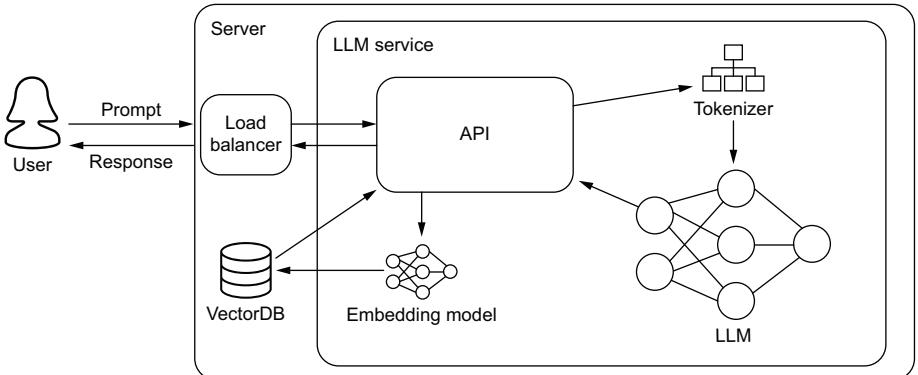
Figure 6.1 A basic LLM service. A majority of the logic is handled by the API layer, which will ensure the correct preprocessing of incoming requests is done and serve the actual inference of the request.
While figure 6.1 appears neat and tidy, it is hiding several complex subjects you’ll want to work through, particularly in that API box. We’ll be talking through several key features you’ll want to include in your API, like batching, rate limiters, and streaming. You’ll also notice some preprocessing techniques like retrieval-augmented generation (RAG) hidden in this image, which we’ll discuss in depth in section 6.1.7. By the end of this section, you will know how to approach all of this, and you will have deployed an LLM service and understand what to do to improve it. But before we get to any of that, let’s first talk about the model itself and the best methods to prepare it for online inference.
6.1.1 Model compilation
The success of any model in production is dependent on the hardware it runs on. The microchip architecture and design of the controllers on the silicon will ultimately determine how quickly and efficiently inferences can run. Unfortunately, when programming in a high-level language like Python using frameworks like PyTorch or TensorFlow, the model won’t be optimized to take full advantage of the hardware. This is where compiling comes into play. Compiling is the process of taking code written in a high-level language and converting or lowering it to machine-level code that the computer can process quickly. Compiling your LLM can easily lead to major inference and cost improvements.
Various people have dedicated a lot of time to performing some of the repeatable efficiency steps for you beforehand. We covered Tim Dettmers’s contributions in the last chapter. Other contributors include Georgi Gerganov, who created and maintains llama.cpp for running LLMs using C++ for efficiency, and Tom Jobbins, who goes by TheBloke on Hugging Face Hub and quantizes models into the correct formats to be used in Gerganov’s framework and others, like oobabooga. Because of how fast this field moves, completing simple, repeatable tasks over a large distribution of resources is often just as helpful to others.
In machine learning workflows, this process typically involves converting our model from its development framework (PyTorch, TensorFlow, or other) to an intermediate representation (IR), like TorchScript, MLIR, or ONNX. We can then use hardwarespecific software to convert these IR models to compiled machine code for our hardware of choice—GPU, TPU (tensor-processing units), CPU, etc. Why not just convert directly from your framework of choice to machine code and skip the middleman? Great question. The reason is simple: there are dozens of frameworks and hundreds of hardware units, and writing code to cover each combination is out of the question. So instead, framework developers provide conversion tooling to an IR, and hardware vendors provide conversions from an IR to their specific hardware.
For the most part, the actual process of compiling a model involves running a few commands. Thanks to PyTorch 2.x, you can get a head start on it by using the torch.compile(model) command, which you should do before training and before deployment. Hardware companies often provide compiling software for free, as it’s a big incentive for users to purchase their product. Building this software isn’t easy, however, and often requires expertise in both the hardware architecture and the machine
learning architectures. This combination of these talents is rare, and there’s good money to be had if you get a job in this field.
We will show you how to compile an LLM in a minute, but first, let’s take a look at some of the techniques used. What better place to start than with the all-important kernel tuning?
KERNEL TUNING
In deep learning and high-performance computing, a kernel is a small program or function designed to run on a GPU or other similar processors. These routines are developed by the hardware vendor to maximize chip efficiency. They do this by optimizing threads, registries, and shared memory across blocks of circuits on the silicon. When we run arbitrary code, the processor will try to route the requests the best it can across its logic gates, but it’s bound to run into bottlenecks. However, if we are able to identify the kernels to run and their order beforehand, the GPU can map out a more efficient route—and that’s essentially what kernel tuning is.
During kernel tuning, the most suitable kernels are chosen from a large collection of highly optimized kernels. For instance, consider convolution operations that have several possible algorithms. The optimal one from the vendor’s library of kernels will be based on various factors like the target GPU type, input data size, filter size, tensor layout, batch size, and more. When tuning, several of these kernels will be run and optimized to minimize execution time.
This process of kernel tuning ensures that the final deployed model is not only optimized for the specific neural network architecture being used but also finely tuned for the unique characteristics of the deployment platform. This process results in more efficient use of resources and maximizes performance. Next, let’s look at tensor fusion, which optimizes running these kernels.
TENSOR FUSION
In deep learning, when a framework executes a computation graph, it makes multiple function calls for each layer. The computation graph is a powerful concept used to simplify mathematical expressions and execute a sequence of tensor operations, especially for neural network models. If each operation is performed on the GPU, it invokes many CUDA kernel launches. However, the fast kernel computation doesn’t quite match the slowness of launching the kernel and handling tensor data. As a result, the GPU resources might not be fully utilized, and memory bandwidth can become a choke point. It’s like making multiple trips to the store to buy separate items when we could make a single trip and buy all the items at once.
This is where tensor fusion comes in. It improves this situation by merging or fusing kernels to perform operations as one, reducing unnecessary kernel launches and improving memory efficiency. A common example of a composite kernel is a fully connected kernel that combines or fuses a matmul, bias add, and ReLU kernel. It’s similar to the concept of tensor parallelization. In tensor parallelization, we speed up the process by sending different people to different stores, like the grocery store, the hardware store, and a retail store. This way, one person doesn’t have to go to every store. Tensor fusion can work very well with parallelization across multiple GPUs. It’s like sending multiple people to different stores and making each one more efficient by picking up multiple items instead of one.
GRAPH OPTIMIZATION
Tensor fusion, when done sequentially, is also known as vertical graph optimization. We can also do horizontal graph optimization. These optimizations are often talked about as two different things. Horizontal graph optimization, which we’ll refer to simply as graph optimization, combines layers with shared input data but with different weights into a single broader kernel. It replaces the concatenation layers by pre-allocating output buffers and writing into them in a distributed manner.
In figure 6.2, we show an example of a simple deep learning graph being optimized. Graph optimizations do not change the underlying computation in the graph. They are simply restructuring the graph. As a result, the optimized graph performs more efficiently with fewer layers and kernel launches, reducing inference latency. This restructuring makes the whole process smaller, faster, and more efficient.
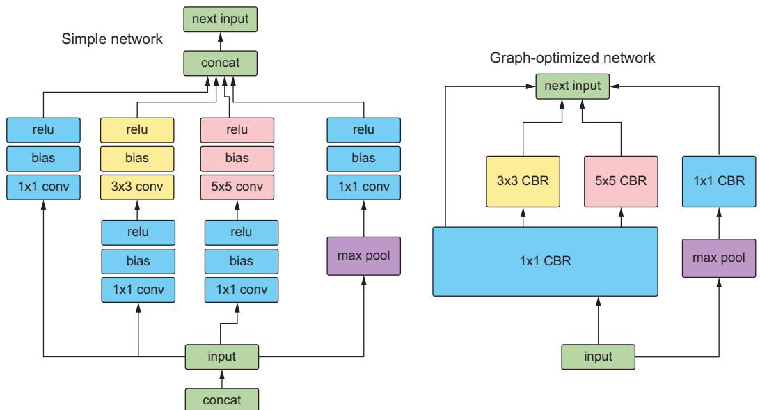
Figure 6.2 An example of an unoptimized network compared to the same network optimized using graph optimization. CBR is a NVIDIA fused layer kernel that simply stands for Convolution, Bias, and ReLU. See the following NVIDIA blog post for reference:https://mng.bz/PNvw.
The graph optimization technique is often used in the context of computational graph-based frameworks like TensorFlow. Graph optimization involves techniques that simplify these computational graphs, remove redundant operations, and/or rearrange computations, making them more efficient for execution, especially on specific hardware (like GPU or TPU). An example is constant folding, where the computations involving constant inputs are performed at compile time (before run time), thereby reducing the computation load during run time.
These aren’t all the techniques used when compiling a model, but they are some of the most common and should give you an idea of what’s happening under the hood and why it works. Now let’s look at some tooling to do this for LLMs.
TENSORRT
NVIDIA’s TensorRT is a one-stop shop to compile your model, and who better to trust than the hardware manufacturer to better prepare your model to run on their GPUs? TensorRT does everything talked about in this section, along with quantization to INT8 and several memory tricks to get the most out of your hardware to boot.
In listing 6.1, we demonstrate the simple process of compiling an LLM using TensorRT. We’ll use the PyTorch version known as torch_tensorrt. It’s important to note that compiling a model to a specific engine is hardware specific. So you will want to compile the model on the exact hardware you intend to run it on. Consequently, installing TensorRT is a bit more than a simple pip install; thankfully, we can use Docker instead. To get started, run the following command:
$ docker run –gpus all -it –rm nvcr.io/nvidia/pytorch:23.09-py3
This command will start up an interactive torch_tensorrt Docker container with practically everything we need to get started (for the latest version, see https://mng .bz/r1We). The only thing missing is Hugging Face Transformers, so go ahead and install that. Now we can run the listing.
After our imports, we’ll load our model and generate an example input so we can trace the model. We need to convert our model to an IR—TorchScript here—and this is done through tracing. Tracing is the process of capturing the operations that are invoked when running the model and makes graph optimization easier later. If you have a model that takes varying inputs, for example, the CLIP model, which can take both images and text and turn them into embeddings, tracing that model with only text data is an effective way of pruning the image operations out of the model. Once our model has been converted to an IR, then we can compile it for NVIDIA GPUs using TensorRT. Once completed, we then simply reload the model from disk and run some inference for demonstration.
Listing 6.1 Compiling a model with TensorRT
import torch
from transformers import GPT2Tokenizer, GPT2LMHeadModel
import torch_tensorrt
tokenizer = GPT2Tokenizer.from_pretrained("gpt2")
tokens = tokenizer("The cat is on the table.", return_tensors="pt")[
 "input_ids"
].cuda()
model = GPT2LMHeadModel.from_pretrained(
"gpt2", use_cache=False, return_dict=False, torchscript=True
).cuda()
model.eval()
traced_model = torch.jit.trace(model, tokens)
compile_settings = {
"inputs": [
torch_tensorrt.Input(
# For static size
shape=[1, 7],
# For dynamic sizing:
# min_shape=[1, 3],
# opt_shape=[1, 128],
# max_shape=[1, 1024],
dtype=torch.int32, # Datatype of input tensor.
# Allowed options torch.(float|half|int8|int32|bool)
)
],
"truncate_long_and_double": True,
"enabled_precisions": {torch.half},
"ir": "torchscript",
}
trt_model = torch_tensorrt.compile(traced_model, **compile_settings)
torch.jit.save(trt_model, "trt_model.ts")
trt_model = torch.jit.load("trt_model.ts")
tokens.half()
tokens = tokens.type(torch.int)
logits = trt_model(tokens)
results = torch.softmax(logits[-1], dim=-1).argmax(dim=-1)
print(tokenizer.batch_decode(results))
Converts to
Torchscript IR
Compiles the model
with TensorRT
Runs with FP16
Saves the compiled model
Runs inferenceThe output is
[‘was a the way.’]
We’ll just go ahead and warn you: your results may vary when you run this code, depending on your setup. Overall, it’s a simple process once you know what you are doing, and we’ve regularly seen at least 2× speed improvements in inference times which translates to major savings!
TensorRT really is all that and a bag of chips. Of course, the major downside to TensorRT is that, as a tool developed by NVIDIA, it is built with NVIDIA’s hardware in mind. When compiling code for other hardware and accelerators, it’s not going to be useful. Also, you’ll get very used to running into error messages when working with TensorRT. We’ve found that running into compatibility problems when converting models that aren’t supported is a common occurrence. We’ve run into many problems trying to compile various LLM architectures. Thankfully, to address this, NVIDIA has been working on a TensorRT-LLM library to supercharge LLM inference on NVIDIA high-end GPUs. It supports many more LLM architectures than vanilla TensorRT. You can check if it supports your chosen LLM architecture and GPU setup here: https://mng.bz/mRXP.
Don’t get us wrong; you don’t have to use TensorRT. Several alternative compilers are available. In fact, let’s look at another popular alternative, ONNX Runtime. Trust us, you’ll want an alternative when TensorRT doesn’t play nice.
ONNX RUNTIME
ONNX, which stands for Open Neural Network Exchange, is an open source format and ecosystem designed for representing and interoperating between different deep learning frameworks, libraries, and tools. It was created to address the challenge of model portability and compatibility. As mentioned previously, ONNX is an IR and allows you to represent models trained in one deep learning framework (e.g., Tensor-Flow, PyTorch, Keras, MXNet) in a standardized format easily consumed by other frameworks. Thus, it facilitates the exchange of models between different tools and environments. Unlike TensorRT, ONNX Runtime is intended to be hardware-agnostic, meaning it can be used with a variety of hardware accelerators, including CPUs, GPUs, and specialized hardware like TPUs.
In practical terms, ONNX allows machine learning practitioners and researchers to build and train models using their preferred framework and then deploy those models to different platforms and hardware without the need for extensive reengineering or rewriting of code. This process helps streamline the development and deployment of AI and ML models across various applications and industries. To be clear, ONNX is an IR format, while ONNX Runtime allows us to optimize and run inference with ONNX models.
To take advantage of ONNX, we recommend using Hugging Face’s Optimum. Optimum is an interface that makes working with optimizers easier and supports multiple engines and hardware, including Intel Neural Compressor for Intel chips and Furiosa Warboy for Furiosa NPUs. It’s worth checking out. For our purposes, we will use it to convert LLMs to ONNX and then optimize them for inference with ONNX Runtime. First, let’s install the library with the appropriate engines. We’ll use the –upgrade-strategy eager, as suggested by the documentation, to ensure the different packages are upgraded:
$ pip install –upgrade-strategy eager optimum[exporters,onnxruntime]
Next, we’ll run the optimum command line interface. We’ll export it to ONNX, point it to a Hugging Face transformer model, and give it a local directory to save the model to. Those are all the required steps, but we’ll also give it an optimization feature flag. Here, we’ll do the basic general optimizations:
➥ $ optimum-cli export onnx --model WizardLM/WizardCoder-1B-V1.0
    ./models_onnx --optimize O1
And we are done. We now have an LLM model converted to ONNX format and optimized with basic graph optimizations. As with all compiling processes, optimization should be done on the hardware you intend to run inference on, which should include ample memory and resources, as the conversion can be somewhat computationally intensive.
To run the model, check out https://onnxruntime.ai/for quick start guides on how to run it with your appropriate SDK. Oh, yeah, did we forget to mention that ONNX Runtime supports multiple programming APIs, so you can now run your LLM directly in your favorite language, including Java, C++, C#, or even JavaScript? Well, you can. So go party. We’ll be sticking to Python in this book, though, for consistency’s sake.
While TensorRT is likely to be your weapon of choice most of the time, and ONNX Runtime covers many edge cases, there are still many other excellent engines out there, like OpenVINO. You can choose whatever you want, but you should at least use something. Doing otherwise would be an egregious mistake. In fact, now that you’ve read this section, you can no longer claim ignorance. It is now your professional responsibility to ensure this happens. Putting any ML model into production that hasn’t first been compiled (or at least attempted to be compiled) is a sin to the MLOps profession.
6.1.2 LLM storage strategies
Now that we have a nicely compiled model, we need to think about how our service will access it. This step is important because, as discussed in chapter 3, boot times can be a nightmare when working with LLMs since it can take a long time to load such large assets into memory. So we want to try to speed that up as much as possible. When it comes to managing large assets, we tend to throw them into an artifact registry or a bucket in cloud storage and forget about them. Both of these tend to utilize an object storage system—like GCS or S3—under the hood, which is great for storage but less so for object retrieval, especially when it comes to large objects like LLMs.
Object storage systems break up assets into small fractional bits called objects. They allow us to federate the entire asset across multiple machines and physical memory locations, a powerful tool that powers the cloud, and to cheaply store large objects on commodity hardware. With replication, there is built-in fault tolerance, so we never have to worry about losing our assets from a hardware crash. Object storage systems also create high availability, ensuring we can always access our assets. The downside is that these objects are federated across multiple machines and not in an easily accessible form to be read and stored in memory. Consequently, when we load an LLM into GPU memory, we will essentially have to download the model first. Let’s look at some alternatives.
FUSING
Fusing is the process of mounting a bucket to your machine as if it were an external hard drive. Fusing provides a slick interface and simplifies code, as you will no longer have to download the model and then load it into memory. With fusing, you can treat an external bucket like a filesystem and load the model directly into memory. However, it still doesn’t solve the fundamental need to pull the objects of your asset from multiple machines. Of course, if you fuse a bucket to a node in the same region and zone, some optimizations can improve performance, and it will feel like you are loading the model from the drive. Unfortunately, our experience has shown fusing to be quite slow, but it should still be faster than downloading and then loading.
Fusing libraries are available for all major cloud providers and on-prem object storage solutions, like Ceph or MinIO, so you should be covered no matter the environment, including your own laptop. That’s right. You can fuse your laptop or an edge device to your object storage solution. This ability demonstrates both how powerful and, at the same time, ineffective this strategy is, depending on what you were hoping it would achieve.
TIP All fusing libraries are essentially built off the FUSE library. It’s worth checking out: https://github.com/libfuse/libfuse.
BAKING THE MODEL
Baking is the process of putting your model into the Docker image. Thus, whenever a new container is created, the model will be there, ready for use. Baking models, in general, is considered an antipattern. For starters, it doesn’t solve the problem. In production, when a new instance is created, a new machine is spun up. It is fresh and innocent, knowing nothing of the outside world, so the first step it’ll have to take is to download the image. Since the image contains the model, we haven’t solved anything. Actually, it’s very likely that downloading the model inside an image will be slower than downloading the model from an object store. So we most likely just made our boot times worse.
Second, baking models is a terrible security practice. Containers often have poor security and are often easy for people to gain access to. Third, you’ve doubled your problems: before you just had one large asset; now you have two, the model and the image.
That said, there are still times when baking is viable, mainly because despite the drawbacks, it greatly simplifies our deployments. Throwing all our assets into the image guarantees we’ll only need one thing to deploy a new service: the image itself, which is really valuable when deploying to an edge device, for example.
MOUNTED VOLUME
Another solution is to avoid the object store completely and save your LLM in a filebased storage system on a mountable drive. When our service boots up, we can connect the disc drive housing the LLM with a RAID controller or Kubernetes, depending on our infrastructure. This solution is old school, but it works really well. For the most part, it solves all our problems and provides incredibly fast boot times.
The downside, of course, is that it will add a bunch of coordination steps to ensure there is a volume in each region and zone you plan to deploy to. It also brings up replication and reliability problems; if the drive dies unexpectedly, you’ll need backups in the region. In addition, these drives will likely be SSDs and not just commodity hardware. So you’ll likely be paying a bit more. But storage is extremely cheap compared to GPUs, so the time saved in boot times is something you’ll have to consider. Essentially, though, this strategy reintroduces all the problems for which we usually turn to object stores to begin with.
HYBRID: INTERMEDIARY MOUNTED VOLUME
Lastly, we can always take a hybrid approach. In this solution, we download the model at boot time but store it in a volume that is mounted at boot time. While this doesn’t help at all with the first deployment in a region, it does substantially help any new instances, as they can simply mount this same volume and have the model available to load without having to download. You can imagine this working similarly to how a Redis cache works, except for storage. Often, this technique is more than enough since autoscaling will be fast enough to handle bursty workloads. We just have to worry about total system crashes, which hopefully should be minimal, but they allude to the fact that we should avoid this approach when only running one replica, which you shouldn’t do in production anyway.
In figure 6.3, we demonstrate these different strategies and compare them to a basic service where we simply download the LLM and then load it into memory. Overall, your exact strategy will depend on your system requirements, the size of the LLM you are running, and your infrastructure. Your system requirements will also likely vary widely, depending on the type of traffic patterns you see.
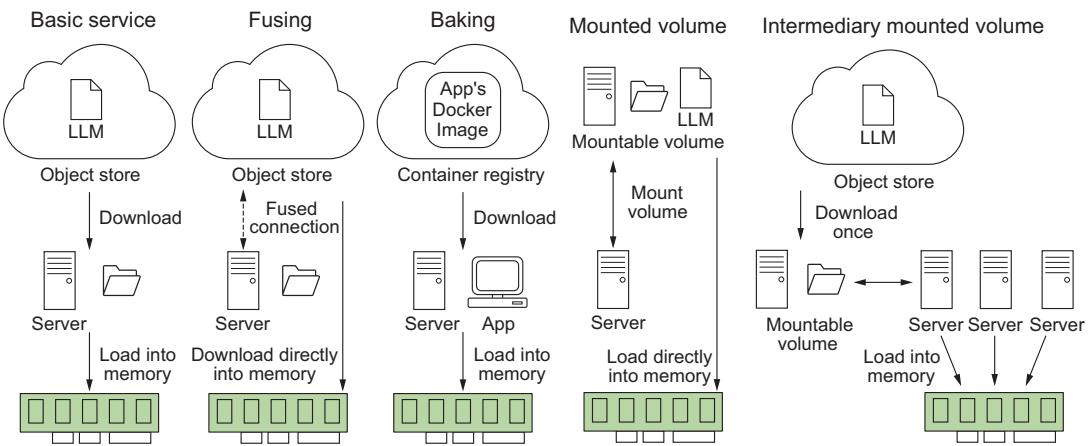
Figure 6.3 Different strategies for storing LLMs and their implications at boot time. Often, we have to balance system reliability, complexity, and application load time.
Now that we have a good handle on how to handle our LLM as an asset, let’s talk about some API features that are must-haves for your LLM service.
6.1.3 Adaptive request batching
A typical API will accept and process requests in the order they are received, processing them immediately and as quickly as possible. However, anyone who’s trained a machine learning model has come to realize that there are mathematical and computational advantages to running inference in batches of powers of 2 (16, 32, 64, etc.), particularly when GPUs are involved, where we can take advantage of better memory alignment or vectorized instructions parallelizing computations across the GPU cores. To take advantage of this batching, you’ll want to include adaptive request batching or dynamic batching.
What adaptive batching does is essentially pool requests together over a certain period of time. Once the pool receives the configured maximum batch size or the timer runs out, it will run inference on the entire batch through the model, sending the results back to the individual clients that requested them. Essentially, it’s a queue. Setting one up yourself can and will be a huge pain; thankfully, most ML inference services offer this out of the box, and almost all are easy to implement. For example, in BentoML, add @bentoml.Runnable.method(batchable=True) as a decorator to your predict function, and in Triton Inference Server, add dynamic_batching {} at the end of your model definition file.
If that sounds easy, it is. Typically, you don’t need to do any further finessing, as the defaults tend to be very practical. That said, if you are looking to maximize every bit of efficiency possible in the system, you can often set a maximum batch size, which will tell the batcher to run once this limit is reached, or a batch delay, which does the same thing but for the timer. Increasing either will result in longer latency but likely better throughput, so typically these are only adjusted when your system has plenty of latency budget.
Overall, the benefits of adaptive batching include better use of resources and higher throughput at the cost of a bit of latency. This is a valuable tradeoff, and we recommend giving your product the latency bandwidth to include this feature. In our experience, optimizing for throughput leads to better reliability and scalability and thus greater customer satisfaction. Of course, when latency times are extremely important or traffic is few and far between, you may rightly forgo this feature.
6.1.4 Flow control
Rate limiters and access keys are critical protections for an API, especially one sitting in front of an expensive LLM. Rate limiters control the number of requests a client can make to an API within a specified time, which helps protect the API server from abuse, such as distributed denial of service (DDoS) attacks, where an attacker makes numerous requests simultaneously to overwhelm the system and hinder its function.
Rate limiters can also protect the server from bots that make numerous automated requests in a short span of time. This helps manage the server resources optimally so the server is not exhausted due to unnecessary or harmful traffic. They are also useful for managing quotas, thus ensuring all users have fair and equal access to the API’s resources. By preventing any single user from using excessive resources, the rate limiter ensures the system functions smoothly for all users.
All in all, rate limiters are an important mechanism for controlling the flow of your LLM’s system processes. They can play a critical role in dampening bursty workloads and preventing your system from getting overwhelmed during autoscaling and rolling updates, especially when you have a rather large LLM with longer deployment times. Rate limiters can take several forms, and the one you choose will be dependent on your use case.
Types of rate limiters
The following list describes the types of rate limiters:
- Fixed window—This algorithm allows a fixed number of requests in a set duration of time. Let’s say five requests per minute, and it refreshes at the minute. It’s really easy to set up and reason about. However, it may lead to uneven distribution and can allow a burst of calls at the boundary of the time window.
- Sliding window log—To prevent boundary problems, we can use a dynamic timeframe. Let’s say five requests in the last 60 seconds. This type is a slightly more complex version of the fixed window that logs each request’s timestamp to provide a moving lookback period, providing a more evenly distributed limit.
- Token bucket—Clients initially have a full bucket of tokens, and with each request, they spend tokens. When the bucket is empty, the requests are blocked. The bucket refills slowly over time. Thus, token buckets allow burst behavior, but it’s limited to the number of tokens in the bucket.
- Leaky bucket—It works as a queue where requests enter, and if the queue is not full, they are processed; if full, the request overflows and gets discarded, thus controlling the rate of the flow.
A rate limiter can be applied at multiple levels, from the entire API to individual client requests to specific function calls. While you want to avoid being too aggressive with them—better to rely on autoscaling to scale and meet demand—you don’t want to ignore them completely, especially when it comes to preventing bad actors.
Access keys are also crucial to prevent bad actors. Access keys offer authentication, maintaining that only authorized users can access the API, which prevents unauthorized use and potential misuse of the API and reduces the influx of spam requests. They are also essential to set up for any paid service. Of course, even if your API is only exposed internally, setting up access keys shouldn’t be ignored, as it can help reduce liability and provide a way of controlling costs by yanking access to a rogue process, for example.
Thankfully, setting up a service with rate limiting and access keys is relatively easy nowadays, as there are multiple libraries that can help you. In listing 6.2, we demonstrate a simple FastAPI app utilizing both. We’ll use FastAPI’s built-in security library for our access keys and SlowApi, a simple rate limiter that allows us to limit the call of any function or method with a simple decorator.
from fastapi import FastAPI, Depends, HTTPException, status, Request
from fastapi.security import OAuth2PasswordBearer
from slowapi import Limiter, _rate_limit_exceeded_handler
from slowapi.util import get_remote_address
from slowapi.errors import RateLimitExceeded
import uvicorn
api_keys = ["1234567abcdefg"]
API_KEY_NAME = "access_token"
oauth2_scheme = OAuth2PasswordBearer(tokenUrl="token")
limiter = Limiter(key_func=get_remote_address)
app = FastAPI()
app.state.limiter = limiter
app.add_exception_handler(RateLimitExceeded, _rate_limit_exceeded_handler)
async def get_api_key(api_key: str = Depends(oauth2_scheme)):
 if api_key not in api_keys:
 raise HTTPException(
 status_code=status.HTTP_401_UNAUTHORIZED,
 detail="Invalid API Key",
 )
@app.get("/hello", dependencies=[Depends(get_api_key)])
@limiter.limit("5/minute")
async def hello(request: Request):
 return {"message": "Hello World"}
  Listing 6.2 Example API with access keys and rate limiter
                                       This would be encrypted
                                       in a database.
While this is just a simple example, you’ll still need to set up a system for users to create and destroy access keys. You’ll also want to finetune your time limits. In general, you want them to be as loose as possible so as not to interfere with the user experience but just tight enough to do their job.
6.1.5 Streaming responses
One feature your LLM service should absolutely include is streaming. Streaming allows us to return the generated text to the user as it is being generated versus all at once at the end. Streaming adds quite a bit of complexity to the system, but regardless, it has come to be considered a must-have feature for several reasons.
First, LLMs are rather slow, and the worst thing you can do to your users is make them wait—waiting means they will become bored, and bored users complain or, worse, leave. You don’t want to deal with complaints, do you? Of course not! But by streaming the data as it’s being created, we offer the users a more dynamic and interactive experience.
Second, LLMs aren’t just slow; they are unpredictable. One prompt could lead to pages and pages of generated text, and another, a single token. As a result, your latency is going to be all over the place. Streaming allows us to worry about more consistent metrics like tokens per second (TPS). Keeping TPS higher than the average user’s reading speed means we’ll be sending responses back faster than the user can consume them, ensuring they won’t get bored and we are providing a highquality user experience. In contrast, if we wait until the end to return the results, users will likely decide to walk away and return when it finishes because they never know how long to wait. This huge disruption to their flow makes your service less effective or useful.
Lastly, users are starting to expect streaming. Streaming responses have become a nice tell as to whether you are speaking to a bot or an actual human. Since humans have to type, proofread, and edit their responses, we can’t expect written responses from a human customer support rep to be in a stream-like fashion. So when they see a response streaming in, your users will know they are talking to a bot. People interact differently with a bot than they will with a human, so it’s very useful information to give them to prevent frustration.
In listing 6.3 we demonstrate a very simple LLM service that utilizes streaming. The key pieces to pay attention to are that we are using the base asyncio library to allow us to run asynchronous function calls, FastAPI’s StreamingResponse to ensure we send responses to the clients in chunks, and Hugging Face Transformer’s Text-IteratorStreamer to create a pipeline generator of our model’s inference.
Listing 6.3 A streaming LLM service
import argparse
import asyncio
from typing import AsyncGenerator
from fastapi import FastAPI, Request
from fastapi.responses import Response, StreamingResponse
import uvicorn
from transformers import (
 AutoModelForCausalLM,
AutoTokenizer,
TextIteratorStreamer,
)
from threading import Thread
app = FastAPI()
tokenizer = AutoTokenizer.from_pretrained("gpt2")
model = AutoModelForCausalLM.from_pretrained("gpt2")
streamer = TextIteratorStreamer(tokenizer)
async def stream_results() -> AsyncGenerator[bytes, None]:
for response in streamer:
await asyncio.sleep(1)
yield (response + "\n").encode("utf-8")
@app.post("/generate")
async def generate(request: Request) -> Response:
"""Generate LLM Response
The request should be a JSON object with the following fields:
- prompt: the prompt to use for the generation.
"""
request_dict = await request.json()
prompt = request_dict.pop("prompt")
inputs = tokenizer([prompt], return_tensors="pt")
generation_kwargs = dict(inputs, streamer=streamer, max_new_tokens=20)
thread = Thread(target=model.generate, kwargs=generation_kwargs)
thread.start()
return StreamingResponse(stream_results())
if __name__ == "__main__":
parser = argparse.ArgumentParser()
parser.add_argument("--host", type=str, default=None)
parser.add_argument("--port", type=int, default=8000)
args = parser.parse_args()
uvicorn.run(app, host=args.host, port=args.port, log_level="debug")
Loads tokenizer,
model, and streamer
into memory
Slows things down to see
streaming. It's typical to
return streamed responses
byte encoded.
Starts a separate
thread to generate
results
Starts service;
defaults to localhost
on port 8000Now that we know how to implement several must-have features for our LLM service, including batching, rate limiting, and streaming, let’s look at some additional tooling we can add to our service to improve usability and overall workflow.
6.1.6 Feature store
When it comes to running ML models in production, feature stores really simplify the inference process. We first introduced these in chapter 3, but as a recap, feature stores establish a centralized source of truth. They answer crucial questions about your data: Who is responsible for the feature? What is its definition? Who can access it? Let’s take a look at setting one up and querying the data to get a feel for how they work. We’ll be using Feast, which is open source and supports a variety of backends. To get started, let us pip install feast and then run the init command in your terminal to set up a project, like so:
$ feast init feast_example
$ cd feast_example/feature_repo
The app we are building is a question-and-answer service. Q&A services can greatly benefit from a feature store’s data governance tooling. For example, point-in-time joins help us answer questions like “Who is the president of x?” where the answer is expected to change over time. Instead of querying just the question, we query the question with a timestamp, and the point-in-time join will return whatever the answer to the question was in our database at that point in time. In the next listing, we pull a Q&A dataset and store it in a parquet format in the data directory of our Feast project.
import pandas as pd
from datasets import load_dataset
import datetime
from sentence_transformers import SentenceTransformer
model = SentenceTransformer("all-MiniLM-L6-v2")
def save_qa_to_parquet(path):
 squad = load_dataset("squad", split="train[:5000]")
 ids = squad["id"]
 questions = squad["question"]
 answers = [answer["text"][0] for answer in squad["answers"]]
 qa = pd.DataFrame(
 zip(ids, questions, answers),
 columns=["question_id", "questions", "answers"],
 )
 qa["embeddings"] = qa.questions.apply(lambda x: model.encode(x))
 qa["created"] = datetime.datetime.utcnow()
 qa["datetime"] = qa["created"].dt.floor("h")
 qa.to_parquet(path)
if __name__ == "__main__":
 path = "./data/qa.parquet"
 save_qa_to_parquet(path)
  Listing 6.4 Downloading the SQuAD dataset
                                                                 Loads SQuAD
                                                                 dataset
                                                                    Extracts
                                                                    questions
                                                                    and answers
                                                                  Creates a
                                                                  dataframe
                                                              Adds embeddings
                                                               and timestamps
                                                     Saves to
                                                     parquet
Next, we’ll need to define the feature view for our feature store. A feature view is essentially like a view in a relational database. We’ll define a name, the entities (which
are like IDs or primary keys), the schema (which are our feature columns), and a source. We’ll just be demoing using a local file store, but in production, you’d want to use one of Feast’s many backend integrations with Snowflake, GCP, AWS, etc. It currently doesn’t support a VectorDB backend, but I’m sure it’s only a matter of time. In addition, we can add metadata to our view through tags and define a time to live (TTL), which limits how far back Feast will look when generating historical datasets. In the following listing, we define the feature view. Go ahead and add this definition into a file called qa.py in the feature_repo directory of our project.
from feast import Entity, FeatureView, Field, FileSource, ValueType
from feast.types import Array, Float32, String
from datetime import timedelta
path = "./data/qa.parquet"
question = Entity(name="question_id", value_type=ValueType.STRING)
question_feature = Field(name="questions", dtype=String)
answer_feature = Field(name="answers", dtype=String)
embedding_feature = Field(name="embeddings", dtype=Array(Float32))
questions_view = FeatureView(
 name="qa",
 entities=[question],
 ttl=timedelta(days=1),
 schema=[question_feature, answer_feature, embedding_feature],
 source=FileSource(
 path=path,
 event_timestamp_column="datetime",
 created_timestamp_column="created",
 timestamp_field="datetime",
 ),
 tags={},
 online=True,
)
  Listing 6.5 Feast FeatureView definition
With that defined, let’s go ahead and register it. We’ll do that with
$ feast apply
Next, we’ll want to materialize the view. In production, this is a step you’ll need to schedule on a routine basis with something like cron or Prefect. Be sure to update the UTC timestamp for the end date in this command to something in the future to ensure the view collects the latest data:
$ feast materialize-incremental 2023-11-30T00:00:00 –views qa
Now all that’s left is to query it! The following listing shows a simple example of pulling features to be used at inference time.
import pandas as pd
from feast import FeatureStore
store = FeatureStore(repo_path=".")
path = "./data/qa.parquet"
ids = pd.read_parquet(path, columns=["question_id"])
feature_vectors = store.get_online_features(
 features=["qa:questions", "qa:answers", "qa:embeddings"],
 entity_rows=[{"question_id": _id} for _id in ids.question_id.to_list()],
).to_df()
print(feature_vectors.head())
  Listing 6.6 Querying a feature view at inference
This example will pull the most up-to-date information for the lowest possible latency at inference time. For point-in-time retrieval, you would use the get_historical_ features method instead. In addition, in this example, we use a list of IDs for the entity rows parameter, but you could also use an SQL query making it very flexible and easy to use.
6.1.7 Retrieval-augmented generation
Retrieval-augmented generation (RAG) has become the most widely used tool to combat hallucinations in LLMs and improve the accuracy of responses in our results. Its popularity is likely because RAG is both easy to implement and quite effective. As first discussed in section 3.4.5, vector databases are a tool you’ll want to have in your arsenal. One of the key reasons is that they make RAG so much easier to implement. In figure 6.4, we demonstrate a RAG system. In the preprocessing stage, we take our documents, break them up, and transform them into embeddings that we’ll load into our vector database. During inference, we can take our input, encode it into an embedding, and run a similarity search across our documents in that vector database to find the nearest neighbors. This type of inference is known as semantic search. Pulling relevant documents and inserting them into our prompt will help give context to the LLM and improve the results.
We are going to demo implementing RAG using Pinecone since it will save us the effort of setting up a vector database. For listing 6.7, we will set up a Pinecone index and load a Wikipedia dataset into it. In this listing, we’ll create a WikiDataIngestion class to handle the heavy lifting. This class will load the dataset and run through each Wikipedia page, splitting the text into consumable chunks. It will then embed these chunks and upload everything in batches. Once we have everything uploaded, we can start to make queries.
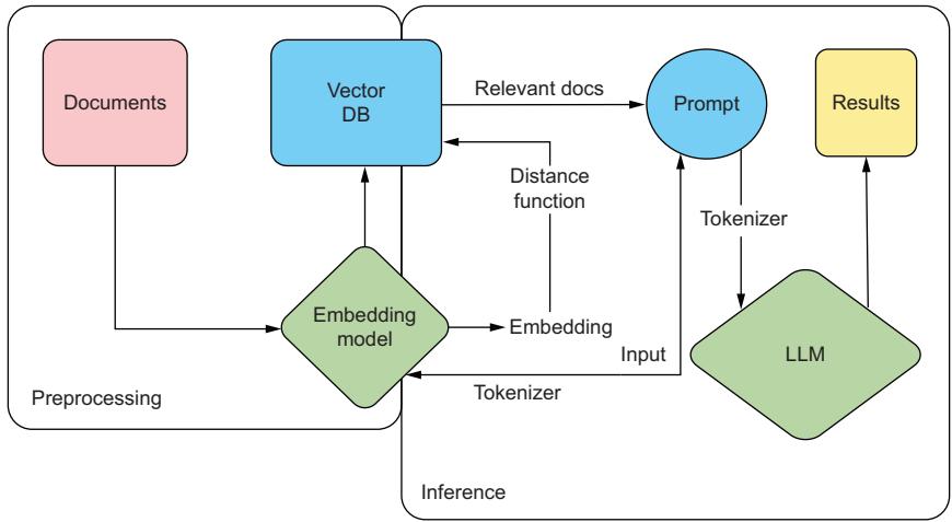
Figure 6.4 RAG system demonstrating how we use our input embeddings to run a search across our documentation, improving the results of the generated text from our LLM
You’ll need an API key if you plan to follow along, so if you don’t already have one, go to Pinecone’s website (https://www.pinecone.io/) and create a free account, set up a starter project (free tier), and get an API key. One thing to pay attention to as you read the listing is that we’ll split up the text into chunks of 400 tokens with text_ splitter. We specifically split on tokens instead of words or characters, which allows us to properly budget inside our token limits for our model. In this example, returning the top three results will add 1,200 tokens to our request, which allows us to plan ahead of time how many tokens we’ll give to the user to write their prompt.
import os
import tiktoken
from datasets import load_dataset
from langchain.text_splitter import RecursiveCharacterTextSplitter
from langchain.embeddings.openai import OpenAIEmbeddings
from pinecone import Pinecone, ServerlessSpec
from sentence_transformers import SentenceTransformer
from tqdm.auto import tqdm
from uuid import uuid4
OPENAI_API_KEY = os.getenv("OPENAI_API_KEY")
PINECONE_API_KEY = os.getenv("PINECONE_API_KEY")
pc = Pinecone(api_key=PINECONE_API_KEY)
  Listing 6.7 Example setting up a Pinecone database
                                                              Gets openai
                                                              API key from
                                                              platform.openai.com
                                                                 Finds API key
                                                                 in console at
                                                                 app.pinecone.io
class WikiDataIngestion:
def __init__(
self,
index,
wikidata=None,
embedder=None,
tokenizer=None,
text_splitter=None,
batch_limit=100,
):
self.index = index
self.wikidata = wikidata or load_dataset(
"wikipedia", "20220301.simple", split="train[:10000]"
)
self.embedder = embedder or OpenAIEmbeddings(
model="text-embedding-ada-002", openai_api_key=OPENAI_API_KEY
)
self.tokenizer = tokenizer or tiktoken.get_encoding("cl100k_base")
self.text_splitter = (
text_splitter
or RecursiveCharacterTextSplitter(
chunk_size=400,
chunk_overlap=20,
length_function=self.token_length,
separators=["\n\n", "\n", " ", ""],
)
)
self.batch_limit = batch_limit
def token_length(self, text):
tokens = self.tokenizer.encode(text, disallowed_special=())
return len(tokens)
def get_wiki_metadata(self, page):
return {
"wiki-id": str(page["id"]),
"source": page["url"],
"title": page["title"],
}
def split_texts_and_metadatas(self, page):
basic_metadata = self.get_wiki_metadata(page)
texts = self.text_splitter.split_text(page["text"])
metadatas = [
{"chunk": j, "text": text, **basic_metadata}
for j, text in enumerate(texts)
]
return texts, metadatas
def upload_batch(self, texts, metadatas):
ids = [str(uuid4()) for _ in range(len(texts))]
embeddings = self.embedder.embed_documents(texts)
self.index.upsert(vectors=zip(ids, embeddings, metadatas)) def batch_upload(self):
batch_texts = []
batch_metadatas = []
for page in tqdm(self.wikidata):
texts, metadatas = self.split_texts_and_metadatas(page)
batch_texts.extend(texts)
batch_metadatas.extend(metadatas)
if len(batch_texts) >= self.batch_limit:
self.upload_batch(batch_texts, batch_metadatas)
batch_texts = []
batch_metadatas = []
if len(batch_texts) > 0:
self.upload_batch(batch_texts, batch_metadatas)
if __name__ == "__main__":
index_name = "pincecone-llm-example"
if index_name not in pc.list_indexes().names():
pc.create_index(
name=index_name,
metric="cosine",
dimension=1536,
spec=ServerlessSpec(cloud="aws", region="us-east-1"),
)
index = pc.Index(index_name)
print(index.describe_index_stats())
embedder = None
if not OPENAI_API_KEY:
embedder = SentenceTransformer(
"sangmini/msmarco-cotmae-MiniLM-L12_en-ko-ja"
)
embedder.embed_documents = lambda *args, **kwargs: embedder.encode(
*args, **kwargs
).tolist()
wiki_data_ingestion = WikiDataIngestion(index, embedder=embedder)
wiki_data_ingestion.batch_upload()
print(index.describe_index_stats())
query = "Did Johannes Gutenberg invent the printing press?"
embeddings = wiki_data_ingestion.embedder.embed_documents(query)
results = index.query(vector=embeddings, top_k=3, include_metadata=True)
print(results)
Creates an
index if it
doesn't exist
1536 dim of
text-embedding-
ada-002
Connects to the index
and describes the stats
Uses a generic embedder if an
openai api key is not provided
Also 1536 dim
Ingests data and
describes the stats anew
Makes a
queryWhen I ran this code, the top three query results to my question, “Did Johannes Gutenberg invent the printing press?” were the Wikipedia pages for Johannes Gutenberg, the pencil, and the printing press. Not bad! While a vector database isn’t going
to be able to answer the question, it’s simply finding the most relevant articles based on the proximity of their embeddings to my question.
With these articles, we can then feed their embeddings into our LLM as additional context to the question to ensure a more grounded result. Since we include sources, it will even have the wiki URL it can give as a reference, and it won’t just hallucinate one. By giving this context, we greatly reduce the concern about our LLM hallucinating and making up an answer.
6.1.8 LLM service libraries
If you are starting to feel a bit overwhelmed about all the tooling and features you need to implement to create an LLM service, we have some good news for you: several libraries aim to do all of this for you! Some open source libraries of note are vLLM and OpenLLM (by BentoML). Hugging Face’s Text-Generation-Inference (TGI) briefly lost its open source license, but fortunately, it’s available again for commercial use. There are also some start-ups building some cool tooling in this space, and we recommend checking out TitanML if you are hoping for a more managed service. These are like the tools MLServer, BentoML, and Ray Serve discussed in section 3.4.8 on deployment service, but they are designed specifically for LLMs.
Most of these toolings are still relatively new and under active development, and they are far from feature parity with each other, so pay attention to what they offer. What you can expect is that they should at least offer streaming, batching, and GPU parallelization support (something we haven’t specifically talked about in this chapter), but beyond that, it’s a crapshoot. Many of them still don’t support several features discussed in this chapter, nor do they support every LLM architecture. What they do, though, is make deploying LLMs easy.
Using vLLM as an example, just pip install vllm, and then you can run
$ python -m vllm.entrypoints.api_server –model IMJONEZZ/ggml-openchat-8192-q4_0
With just one command, we now have a service up and running the model we trained in chapter 5. Go ahead and play with it; you should be able to send requests to the /generate endpoint like so:
$ curl http://localhost:8000/generate -d '{"prompt": "Which pokemon is
➥ the best?", "use_beam_search": true, "n": 4, "temperature": 0}'
It’s very likely you won’t be all that impressed with any of these toolings. Still, you should be able to build your own API and have a good sense of how to do it at this point. Now that you have a service and can even spin it up locally, let’s discuss the infrastructure you need to set up to support these models for actual production usage. Remember, the better the infrastructure, the less likely you’ll be called in the middle of the night when your service goes down unexpectedly. None of us want that, so let’s check it out.
6.2 Setting up infrastructure
Setting up infrastructure is a critical aspect of modern software development, and we shouldn’t expect machine learning to be any different. To ensure scalability, reliability, and efficient deployment of our applications, we need to plan a robust infrastructure that can handle the demands of a growing user base. This is where Kubernetes comes into play.
Kubernetes, often referred to as k8s, is an open source container orchestration platform that helps automate and manage the deployment, scaling, and management of containerized applications. It is designed to simplify the process of running and coordinating multiple containers across a cluster of servers, making it easier to scale applications and ensure high availability. We are going to talk a lot about k8s in this chapter, and while you don’t need to be an expert, it will be useful to cover some basics to ensure we are all on the same page.
At its core, k8s works by grouping containers into logical units called pods, which are the smallest deployable units in the k8s ecosystem. These pods are then scheduled and managed by the k8s control plane, which oversees their deployment, scaling, and updates. This control plane consists of several components that collectively handle the orchestration and management of containers. In figure 6.5, we give an oversimplification of the k8s architecture to help readers who are unfamiliar with it.
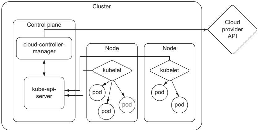
Figure 6.5 An oversimplification of the Kubernetes architecture. What you need to know is that our services run in pods, and pods run on nodes, which essentially are a machine. K8s helps us both manage the resources and handle the orchestration of deploying pods to these resources.
Using k8s, we can take advantage of features such as automatic scaling, load balancing, and service discovery, which greatly simplify the deployment and management of web applications. K8s provides a flexible and scalable infrastructure that can easily
adapt to changing demands, allowing organizations to efficiently scale their applications as their user base grows. K8s offers a wide range of additional features and extensibility options, such as storage management, monitoring, and logging, which help ensure the smooth operation of web applications.
One of these extensibility options is known as custom resource definitions (CRDs). CRDs are a feature of Kubernetes that allows users to create their own specifications for custom resources, thus extending the functionalities of Kubernetes without modifying the Kubernetes source code. With a CRD defined, we can create custom objects similar to how we would create a built-in object like a pod or service. This gives k8s a lot of flexibility that we will need for different functionality throughout this chapter.
If you are new to Kubernetes, you might be scratching your head through parts of this section, and that’s totally fine. Hopefully, though, you have enough knowledge to get the gist of what we will be doing in this section and why. At least you’ll be able to walk away with a bunch of questions to ask your closest DevOps team member.
6.2.1 Provisioning clusters
The first thing to do when starting any project is to set up a cluster. A cluster is a collective of worker machines or nodes where we will host our applications. Creating a cluster is relatively simple; configuring it is the hard part. Of course, there have been many books written on how to do this, and the majority of considerations like networking, security, and access control are outside the scope of this book. In addition, considering the steps you take will also be different depending on the cloud provider of choice and your company’s business strategy, we will focus on only the portions that we feel are needed to get you up and running, as well as any other tidbits that may make your life easier.
The first step is to create a cluster. On GCP, you would use the gcloud tool and run
$ gcloud container clusters create
On AWS, using the eksctl tool, run
$ eksctl create cluster
On Azure, using the az cli tool, run
$ az group create --name=<GROUP_NAME> --location=westus
$ az aks create --resource-group=<GROUP_NAME> --name=<CLUSTER_NAME>
As you can see, even the first steps are highly dependent on your provider, and you can suspect that the subsequent steps will be as well. Since we realize most readers will be deploying in a wide variety of environments, we will not focus on the exact steps but hopefully give you enough context to search and discover for yourself.
Many readers, we imagine, will already have a cluster set up for them by their infrastructure teams, complete with many defaults and best practices. One of these is
setting up node auto-provisioning (NAP) or cluster autoscaling. NAP allows a cluster to grow, adding more nodes as deployments demand them. This way, we only pay for nodes we actually use. It’s a very convenient feature, but it often defines resource limits or restrictions on the instances available for autoscaling, and you can bet your cluster’s defaults don’t include accelerator or GPU instances in that pool. We’ll need to fix that.
In GCP, we would create a configuration file like the one in the following listing, where we can include the GPU resourceType. In the example, we include T4s and both A100 types.
Listing 6.8 Example NAP config file
resourceLimits: - resourceType: 'cpu'
minimum: 10
maximum: 100
- resourceType: 'memory'
maximum: 1000
- resourceType: 'nvidia-tesla-t4'
maximum: 40
- resourceType: 'nvidia-tesla-a100'
maximum: 16
- resourceType: 'nvidia-a100-80gb'
maximum: 8
management:
autoRepair: true
autoUpgrade: true
shieldedInstanceConfig:
enableSecureBoot: true
enableIntegrityMonitoring: true
diskSizeGb: 100You would then set this by running
$ gcloud container clusters update <CLUSTER_NAME> --enable-autoprovisioning -
     -autoprovisioning-config-file <FILE_NAME>
The real benefit of an NAP is that instead of predefining what resources are available at a fixed setting, we can set resource limits, which put a cap on the total number of GPUs that we would scale up to. They clearly define what GPUs we want and expect to be in any given cluster.
When one author was first learning about limits, he often got them confused with similar concepts—quotas, reservations, and commitments—and has seen many others just as confused. Quotas, in particular, are very similar to limits. Their main purpose is to prevent unexpected overage charges by ensuring a particular project or application doesn’t consume too many resources. Unlike limits, which are set internally, quotas often require submitting a request to your cloud provider when you want to raise them. These requests help inform and are used by the cloud provider to better plan
which resources to provision and put into different data centers in different regions. It’s tempting to think that the cloud provider will ensure those resources are available; however, quotas never guarantee there will be enough resources in a region for your cluster to use, and you might run into resources not found errors way before you hit them.
While quotas and limits set an upper bound, reservations and commitments set the lower bound. Reservations are an agreement to guarantee that a certain amount of resources will always be available and often come with the caveat that you will be paying for these resources regardless of whether you end up using them. Commitments are similar to reservations but are often longer-term contracts, usually coming with a discounted price.
6.2.2 Autoscaling
One of the big selling points to setting up a k8s cluster is autoscaling. Autoscaling is an important ingredient in creating robust production-grade services. The main reason is that we never expect any service to receive static request volume. If anything else, you should expect more volume during the day and less at night while people sleep. So we’ll want our service to spin up more replicas during peak hours to improve performance and spin down replicas during off hours to save money, not to mention the need to handle bursty workloads that often threaten to crash a service at any point.
Knowing your service will automatically provision more resources and set up additional deployments based on the needs of the application is what allows many infrastructure engineers to sleep peacefully at night. The catch is that it requires an engineer to know what those needs are and ensure everything is configured correctly. While autoscaling provides flexibility, the real business value comes from the cost savings. Most engineers think about autoscaling in terms of scaling up to prevent meltdowns, but even more important to the business is the ability to scale down, freeing up resources and cutting costs.
One of the main reasons cloud computing and technologies like Kubernetes have become essential in modern infrastructures is because autoscaling is built in. Autoscaling is a key feature of Kubernetes, and with horizontal pod autoscalers (HPAs), you can easily adjust the number of replicas of your application based on two native resources: CPU and memory usage, as shown in figure 6.6. However, in a book about putting LLMs in production, scaling based on CPU and memory alone will never be enough. We will need to scale based on custom metrics, specifically GPU utilization.
Setting up autoscaling based on GPU metrics is going to take a bit more work and requires setting up several services. It’ll become clear why we need each service as we discuss them, but the good news is that by the end, you’ll be able to set up your services to scale based on any metric, including external events such as messages from a message broker, requests to an HTTP endpoint, and data from a queue.
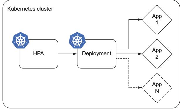
Figure 6.6 Basic autoscaling using the in-built k8s horizontal pod autoscaler (HPA). The HPA watches CPU and memory resources and will tell the deployment service to increase or decrease the number of replicas.
The first service we’ll need is one that can collect the GPU metrics. For this, we have NVIDIA’s Data Center GPU Manager (DCGM), which provides a metrics exporter that can export GPU metrics. DCGM exposes a host of GPU metrics, including temperature and power usage, which can create some fun dashboards, but the most useful metrics for autoscaling are utilization and memory utilization.
From here, the data will go to a service like Prometheus. Prometheus is a popular open source monitoring system used to monitor Kubernetes clusters and the applications running on them. Prometheus collects metrics from various sources and stores them in a time-series database, where they can be analyzed and queried. Prometheus can collect metrics directly from Kubernetes APIs and from applications running on the cluster using a variety of collection mechanisms such as exporters, agents, and sidecar containers. It’s essentially an aggregator of services like DCGM, including features like alerting and notification. It also exposes an HTTP API for service for external tooling like Grafana to query and create graphs and dashboards with.
While Prometheus provides a way to store metrics and monitor our service, the metrics aren’t exposed to the internals of Kubernetes. For an HPA to gain access, we will need to register yet another service to either the custom metrics API or external metrics API. By default, Kubernetes comes with the metrics.k8s.io endpoint that exposes resource metrics, CPU, and memory utilization. To accommodate the need to scale deployments and pods on custom metrics, two additional APIs were introduced: custom.metrics.k9s.io and external.metrics.k8s.io. There are some limitations to this setup, as currently, only one “adapter” API service can be registered at a time for either one. This limitation mostly becomes a problem if you ever decide to change this endpoint from one provider to another.
For this service, Prometheus provides the Prometheus Adapter, which works well, but from our experience, it wasn’t designed for production workloads. Alternatively, we would recommend KEDA. KEDA (Kubernetes Event-Driven Autoscaling) is an open source project that provides event-driven autoscaling for Kubernetes. It offers more flexibility in terms of the types of custom metrics that can be used for autoscaling. While Prometheus Adapter requires configuring metrics inside a ConfigMap, any metric already exposed through the Prometheus API can be used in KEDA, providing a more streamlined and friendly user experience. It also offers scaling to and from 0, which isn’t available through HPAs, allowing you to turn off a service completely if there is no traffic. That said, you can’t scale from 0 on resource metrics like CPU and memory and, by extension, GPU metrics, but it is useful when you are using traffic metrics or a queue to scale.
Putting this all together, you’ll end up with the architecture shown in figure 6.7. Compared to figure 6.6, you’ll notice at the bottom that DCGM is managing our GPU metrics and feeding them into Prometheus Operator. From Prometheus, we can set up external dashboards with tools like Grafana. Internal to k8s, we’ll use KEDA to set up a custom.metrics.k9s.io API to return these metrics so we can autoscale based on the GPU metrics. KEDA has several CRDs, one of which is a ScaledObject, which creates the HPA and provides the additional features.
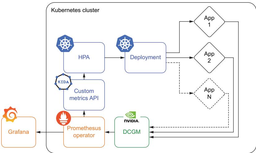
Figure 6.7 Autoscaling based on a custom metric like GPU utilization requires several extra tools to work, including NVIDIA’s DCGM, a monitoring system like Prometheus Operator, and a custom metrics API like that provided by KEDA.
While autoscaling provides many benefits, it’s important to be aware of its limitations and potential problems, which are only exacerbated by LLM inference services. Proper configuration of the HPA is often an afterthought for many applications, but it becomes mission-critical when dealing with LLMs. LLMs take longer to become fully operational, as the GPUs need to be initialized and model weights loaded into memory; these aren’t services that can turn on a dime, which often can cause problems when scaling up if not properly prepared for. Additionally, if the system scales down too aggressively, it may result in instances being terminated before completing their assigned tasks, leading to data loss or other problems. Lastly, flapping is just such a concern that can arise from incorrect autoscaling configurations. Flapping happens when the number of replicas keeps oscillating, booting up a new service only to terminate it before it can serve any inferences.
There are essentially five parameters to tune when setting up an HPA:
- Target parameter
- Target threshold
- Min pod replicas
- Max pod replicas
- Scaling policies
Let’s take a look at each of them in turn so you can be sure your system is properly configured.
TARGET PARAMETER
The target parameter is the most important metric to consider when ensuring your system is properly configured. If you followed the previously listed steps in section 6.2.2, your system is now ready to autoscale based on GPU metrics, so this should be easy, right? Not so fast! Scaling based on GPU utilization is going to be the most common and straightforward path, but the first thing we need to do is ensure the GPU is the actual bottleneck in our service. It’s pretty common to see eager young engineers throw a lot of expensive GPUs onto a service but forget to include adequate CPU and memory capacity. CPU and memory will still be needed to handle the API layer, such as taking in requests, handling multiple threads, and communicating with the GPUs. If there aren’t enough resources, these layers can quickly become a bottleneck, and your application will be throttled way before the GPU utilization is ever affected, ensuring the system will never actually autoscale. While you could switch the target parameter on the autoscaler, CPU and memory are cheap compared to GPU resources, so it’d be better to allocate more of them for your application.
In addition, there are cases where other metrics make more sense. If your LLM application takes most of its requests from a streaming or batch service, it can be more prudent to scale based on metrics that tell you a DAG is running or an upstream queue is filling up—especially if these metrics give you an early signal and allow you more time to scale up in advance.
Another concern when selecting the metric is its stability. For example, an individual GPU’s utilization tends to be close to either 0% or 100%. This can cause problems for the autoscaler, as the metric oscillates between an on and off state, as will its recommendation to add or remove replicas, causing flapping. Generally, flapping is avoided by taking the average utilization across all GPUs running the service. Using the average will stabilize the metric when you have a lot of GPUs, but it could still be a problem when the service has scaled down. If you are still running into problems, you’ll want to use an average-over-time aggregation, which will tell you the utilization for each GPU over a time frame—say, the last 5 minutes. For CPU utilization, average-over-time aggregation is built into the Kubernetes HPA and can be set with the horizontal-pod-autoscaler-cpu-initialization-period flag. For custom metrics, you’ll need to set it in your metric query (for Prometheus, it would be the avg_over_ time aggregation function).
Lastly, it’s worth calling out that most systems allow you to autoscale based on multiple metrics. So you could autoscale based on both CPU and GPU utilization, as an example. However, we would recommend avoiding these setups unless you know what you are doing. Your autoscaler might be set up that way, but in actuality, your service will likely only ever autoscale based on just one of the metrics due to service load, and it’s best to make sure that metric is the more costly resource for cost-engineering purposes.
TARGET THRESHOLD
The target threshold tells your service at what point to start upscaling. For example, if you are scaling based on the average GPU utilization and your threshold is set to 30, then a new replica will be booted up to take on the extra load when the average GPU utilization is above 30%. The formula that governs this is quite simple and is as follows:
desiredReplicas = ceil[currentReplicas × (currentMetricValue / desiredMetricValue )]
NOTE You can learn more about the algorithm at https://mng.bz/x64g.
This can be hard to tune in correctly, but here are some guiding principles. If the traffic patterns you see involve a lot of constant small bursts of traffic, a lower value, around 50, might be more appropriate. This setting ensures you start to scale up more quickly, avoiding unreliability problems, and you can also scale down more quickly, cutting costs. If you have a constant steady flow of traffic, higher values, around 80, will work well. Outside of testing your autoscaler, it’s best to avoid extremely low values, as they can increase your chances of flapping. You should also avoid extremely high values, as they may allow the active replicas to be overwhelmed before new ones start to boot up, which can cause unreliability or downtime. It’s also important to remember that due to the nature of pipeline parallel workflows when using a distributed GPU setup, there will always be a bubble, as discussed in section 3.3.2. As a result, your system will never reach 100% GPU utilization, and you will start to hit problems earlier than expected. Depending on how big your bubble is, you will need to adjust the target threshold accordingly.
MINIMUM POD REPLICAS
Minimum pod replicas determine the number of replicas of your service that will always be running. This setting is your baseline. It’s important to make sure it’s set slightly above your baseline of incoming requests. Too often, this is set strictly to meet baseline levels of traffic or just below, but a steady state for incoming traffic is rarely all that steady. This is where a lot of oscillating can happen, as you are more likely to see many small surges in traffic than large spikes. However, you don’t want to set it too high, as this will tie up valuable resources in the cluster and increase costs.
MAXIMUM POD REPLICAS
Maximum pod replicas determine the number of replicas your system will run at peak capacity. You should set this number to be just above your peak traffic requirements. Setting it too low could lead to reliability problems, performance degradation, and downtime during high-traffic periods. Setting it too high could lead to resource waste, running more pods than necessary, and delaying the detection of real problems. For example, if your application was under a DDoS attack, your system might scale to handle the load, but it would likely cost you severely and hide the problem. With LLMs, you also need to be cautious not to overload the underlying cluster and make sure you have enough resources in your quotas to handle the peak load.
SCALING POLICIES
Scaling policies define the behavior of the autoscaler, allowing you to finetune how long to wait before scaling and how quickly it scales. This setting is usually ignored, and safely so for most setups because the defaults for these settings tend to be pretty good for the typical application. However, relying on the default would be a major mistake for an LLM service since it takes so long to deploy.
The first setting you’ll want to adjust is the stabilization window, which determines how long to wait before taking a new scaling action. You can set a different stabilization window for upscaling and downscaling tasks. The default upscaling window is 0 seconds, which should not need to be touched if your target parameter has been set correctly. The default downscaling window is 300 seconds, which is likely too short for our use case. You’ll typically want this at least as long as it takes your service to deploy and then a little bit more. Otherwise, you’ll be adding replicas only to remove them before they have a chance to do anything.
The next parameter you’ll want to adjust is the scale-down policy, which defaults to 100% of pods every 15 seconds. As a result, any temporary drop in traffic could result in all your extra pods above the minimum being terminated immediately. For our case, it’s much safer to slow this down since terminating a pod takes only a few seconds, but booting one up can take minutes, making it a semi-irreversible decision. The exact policy will depend on your traffic patterns, but in general, we want to have a little more patience. You can adjust how quickly pods will be terminated and the magnitude by the number or percentage of pods. For example, we could configure the policy to allow only one pod each minute or 10% of pods every 5 minutes to be terminated.
6.2.3 Rolling updates
Rolling updates or rolling upgrades is a strategy that gradually implements the new version of an application to reduce downtime and maximize agility. It works by gradually creating new instances and turning off the old ones, replacing them in a methodical manner. This update approach allows the system to remain functional and accessible to users even during the update process, otherwise known as zero downtime. Rolling updates also make it easier to catch bugs before they have too much effect and roll back faulty deployments.
Rolling updates is a feature built into k8s and another major reason for its widespread use and popularity. Kubernetes provides an automated and simplified way to carry out rolling updates. The rolling updates ensure that Kubernetes incrementally updates pod instances with new ones during deployment. The following listing shows an example LLM deployment implementing rolling updates; the relevant configuration is under the spec.strategy section.
Listing 6.9 Example deployment config with rolling updateapiVersion: apps/v1
kind: Deployment
metadata:
name: llm-application
spec:
replicas: 5
strategy:
rollingUpdate:
maxSurge: 1
maxUnavailable: 3
selector:
matchLabels:
app: llm-app
template:
metadata:
labels:
app: llm-app
spec:
containers:
- name: llm-gpu-app-container
image: llm-gpu-application:v2
resources:
limits:
nvidia.com/gpu: 8You’ll notice that there are two main parameters you can adjust for a rolling update: maxSurge and maxUnavailable. These can either be set to a whole number, like in our example, describing the number of instances, or a fraction indicating a percentage of total instances. In the example, you’ll notice we set maxSurge to 1, meaning even though we would normally run with five replicas, we could surge to six during a deployment, allowing us to turn on a new one before turning any off. Normally, you might want to set this higher, as it allows for a quicker rolling update. Otherwise, we’ll have to replace pods one at a time. The reason it’s low, you might have noticed, is that we are deploying a rather large LLM that requires eight GPUs. If these are A100s, it’s likely going to be hard to find an extra eight GPUs not being used.
GPU resources cannot be shared among containers, and container orchestration can become a major challenge in such deployments, which is why maxUnavailable is set to 3. What we are saying here is that three out of the five expected replicas can go down during a deployment. In other words, we are going to drop the total number of replicas for a little bit before re-creating them. For reliability reasons, we typically prefer adding extra replicas first, so to go down instead is a difficult decision, one you’ll want to confirm you can afford to do in your own deployment. The reason we are doing so here is to ensure that there are GPU resources available. In essence, to balance resource utilization, it might be necessary to set maxUnavailable to a high value and adjust maxSurge to a lower number to downscale old versions quickly and free up resources for new ones.
This advice is the opposite of what you’d do in most applications, so we understand if it makes you uneasy. If you’d like to ensure smoother deployments, you’ll need to budget for extra GPUs to be provisioned in your cluster strictly for deployment purposes. However, depending on how often you are updating the model itself, paying for expensive GPUs to sit idle simply to make deployments smoother may not be costadvantageous. Often, the LLM itself doesn’t receive that many updates, so assuming you are using an inference graph (discussed in the next section), most of the updates will be to the API, prompts, or surrounding application.
In addition, we recommend you always perform such operations cautiously in a staging environment first to understand its effect. Catching a deployment problem in staging will save you a headache or two. It’s also useful to troubleshoot the max-Unavailable and maxSurge parameters in staging, but it’s often hard to get a one-toone comparison to production since staging is often resource-constrained.
6.2.4 Inference graphs
Inference graphs are the crème filling of a donut, the muffin top of a muffin, and the toppings on a pizza: they are just phenomenal. Inference graphs allow us to create sophisticated flow diagrams at inference in a resource-saving way. Consider figure 6.8, which shows us the building blocks for any inference graph.
Generally, any time you have more than one model, it’s useful to consider an inference graph architecture. Your standard LLM setup is usually already at least two models: an encoder and the language model itself.
Usually, when we see LLMs deployed in the wild, these two models are deployed together. You send text data to your system, and it returns generated text. It’s often no big deal, but when deployed as a sequential inference graph instead of a packaged service, we get some added bonuses. First, the encoder is usually much faster than the LLM, so we can split them up since you may only need one encoder instance for every two to three LLM instances. Encoders are so small that this doesn’t necessarily help us out that much, but it saves the hassle of redeploying the entire LLM if we decide to deploy a new encoder model version. In addition, an inference graph will set up an individual API for each model, which allows us to hit the LLM and encoder separately.
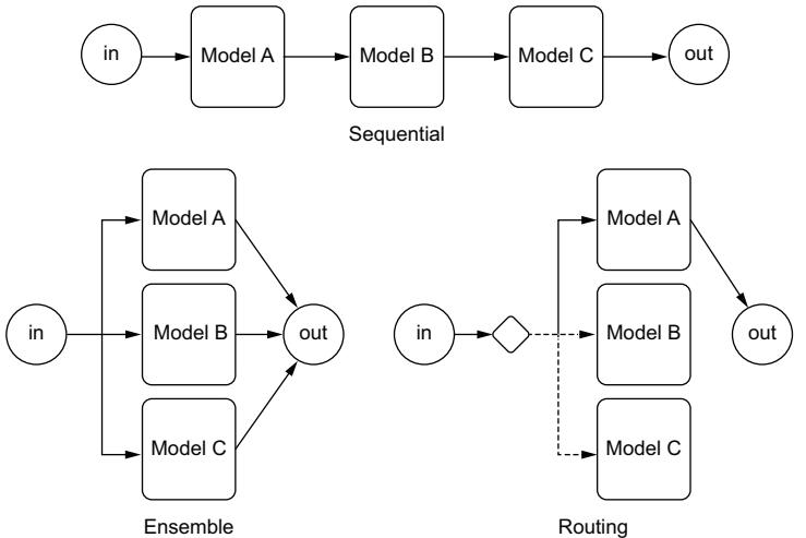
Figure 6.8 The three types of inference graph building blocks. Sequential allows us to run one model before the other, which is useful for preprocessing steps like generating embeddings. Ensembles allow us to pool several models together to learn from each and combine their results. Routing allows us to send traffic to specific models based on some criteria, often used for multiarmed bandit optimization.
This is really useful if we have a bunch of data we’d like to preprocess and save in a VectorDB; we can use the same encoder we already have deployed. We can then pull this data and send it directly into the LLM.
The biggest benefit of an inference graph is that it allows us to separate the API and the LLM. The API sitting in front of the LLM is likely to change much more often as you tweak prompts, add features, and fix bugs. The ability to update the API without having to deploy the LLM will save your team a lot of effort.
Let’s now consider figure 6.9, which provides an example inference graph deployment using Seldon. In this example, we have an encoder model, an LLM, a classifier model, and a simple API that combines the results. Whereas we would have to build a container and the interface for each of these models, Seldon creates an orchestrator that handles communication between a user’s request and each node in the graph.
NOTE Seldon is an open source platform designed for deploying and managing machine learning models in production. It offers tools and capabilities to help organizations streamline the deployment and scaling of machine learning and deep learning models in a Kubernetes-based environment. It offers k8s CRDs to implement inference graphs.
If you are wondering how to create this, listing 6.10 shows an example configuration that would create this exact setup. We simply define the containers in the graph and
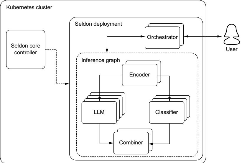
Figure 6.9 An example inference graph deployment using Seldon. A Seldon Deployment is a Kubernetes CRD that extends a regular Kubernetes deployment and adds an orchestrator that ensures the proper communication between all the models are run in graph order.
their relationship inside the graph. You’ll notice apiVersion defines the CRD from Seldon, which allows us to use SeldonDeployment, which is just an extension of the k8s regular Deployment object. In the listing, you might notice that the combiner is the parent to the LLM and classifier models, which feels backwards from how we visualize it in figure 6.9. This is because a component will only ever have one parent, but can have multiple children, so a COMBINER is always a parent node even though functionally it’s the same. Setting up a graph can often be confusing, so I recommend you check the documentation frequently and often.
Listing 6.10 An example SeldonDeployment configuration file
apiVersion: machinelearning.seldon.io/v1alpha2
kind: SeldonDeployment
metadata:
 name: example-seldon-inference-graph
spec:
 name: example-deployment
 predictors:
 - componentSpecs:
 - spec:
 containers:
 - name: encoder
 image: encoder_image:latest
 - name: LLM
 image: llm_image:latest
- name: classifier
image: classifier_image:latest
- name: combiner
image: combiner_image:latest
graph:
name: encoder
type: MODEL
endpoint:
type: REST
children:
- name: combiner
type: COMBINER
children:
- name: LLM
type: MODEL
endpoint:
type: REST
children: []
- name: classifier
type: MODEL
endpoint:
type: REST
children: []
name: example
replicas: 1If you’ve deployed enough machine learning systems, you’ve realized that many of them require complex systems, and inference graphs make it easy, or at least easier. And that is a big difference. Although inference graphs are a smarter way to deploy complex machine learning systems, it’s always important to ask yourself if the extra complexity is actually needed. Even with tools like inference graphs, it’s better to keep things simple whenever possible.
6.2.5 Monitoring
As with any product or service deployed into production, monitoring is critical to ensure reliability, performance, and compliance to service level agreements and objectives are met. As with any service, we care about monitoring typical performance metrics like queries per second (QPS), latency, and response code counts. We also care about monitoring our resources with metrics like CPU utilization, percentage of memory used, GPU utilization, and GPU temperature, among many more. When any of these metrics start to fail, it often indicates a catastrophic failure of some sort and will need to be addressed quickly.
For these metrics, any software engineering team should have plenty of experience working with these using tools like Prometheus and Grafana or the ELK stack (Elasticsearch, Logstash, and Kibana). You will benefit immensely by taking advantage of the systems that are likely already in place. If they aren’t in place, we already went over how to set up the GPU metrics for monitoring back in section 6.2.2, and that system should be useful for monitoring other resources.
However, with any ML project, we have additional concerns that traditional monitoring tools miss, which leads to silent failures. This usually comes from data drift and performance decay, where a model continues to function but starts to do so poorly and no longer meets quality expectations. LLMs are particularly susceptible to data drift since language is in constant flux, as new words are created and old words change meaning all the time. Thus, we often need both a system monitoring solution and an ML monitoring solution.
Monitoring data drift is relatively easy and well-studied for numerical datasets, but monitoring unstructured text data provides an extra challenge. We’ve already discussed ways to evaluate language models in chapter 4, and we’ll need to use similar practices to evaluate and monitor models in production. One of our favorite tools for monitoring drift detection is whylogs due to its efficient nature of capturing summary statistics at scale. Adding LangKit to the mix instantly and easily allows us to track several useful metrics for LLMs, such as readability, complexity, toxicity, and even similarity scores to known prompt injection attacks. In the following listing, we demonstrate a simple application that logs and monitors text data using whylogs and LangKit.
import os
import pandas as pd
import whylogs as why
from langkit import llm_metrics
from datasets import load_dataset
OUTPUT_DIR = "logs"
class LoggingApp:
 def __init__(self):
 """
 Sets up a logger that collects profiles and writes them
 locally every 5 minutes. By setting the schema with langkit
 we get useful metrics for LLMs.
 """
 self.logger = why.logger(
 mode="rolling",
 interval=5,
 when="M",
 base_name="profile_",
 schema=llm_metrics.init(),
 )
 self.logger.append_writer("local", base_dir=OUTPUT_DIR)
 def close(self):
 self.logger.close()
  Listing 6.11 Using whylogs and LangKit to monitor text data
def consume(self, text):
self.logger.log(text)
def driver(app):
"""Driver function to run the app manually"""
data = load_dataset(
"shahules786/OA-cornell-movies-dialog",
split="train",
streaming=True,
)
data = iter(data)
for text in data:
app.consume(text)
if __name__ == "__main__":
app = LoggingApp()
driver(app)
app.close()
pd.set_option("display.max_columns", None)
all_files = [
f for f in os.listdir(OUTPUT_DIR) if f.startswith("profile_")
]
path = os.path.join(OUTPUT_DIR, all_files[0])
result_view = why.read(path).view()
print(result_view.to_pandas().head())
The generated text is
# ...
Runs app manually
Prevents truncation
of columns
Gets the first profile
and shows the results# column udf/flesch_reading_ease:cardinality/est
# conversation 425.514743
# ...
# column udf/jailbreak_similarity:cardinality/est
# conversation 1172.226702
# ...
# column udf/toxicity:types/string udf/toxicity:types/tensor
# conversation 0 0While this is just a demo using a text dataset, you can see how it would be beneficial to monitor the incoming prompts and outgoing generated text for metrics such as readability, complexity, and toxicity. These monitoring tools will help give you a handle on whether or not your LLM service is starting to fail silently.
When monitoring in production, we must be mindful of the effect latency may have on our service. LangKit uses several lightweight models to evaluate the text for the advanced metrics. While we haven’t noticed significant memory effects, there is a very slight effect on latency when evaluating logs in the direct inference path. To avoid this, we can take it out of the inference path and into what is called a sidecar.
It’s not uncommon to see ML teams mistakenly place data quality checks in the critical path. Their intentions may be good (to ensure only clean data runs through a model), but on the off chance that a client sends bad data, it would often be better to just send a 400 or 500 error response than to add expensive latency costs to the good requests. In fact, many applications move monitoring out of the critical path entirely, opting to process it in parallel. The simplest way to do this is to use a Kubernetes sidecar, which is depicted in figure 6.10. You can do this with tools that specialize in this, like fluentd; whylogs also offers a container you can run as a sidecar.
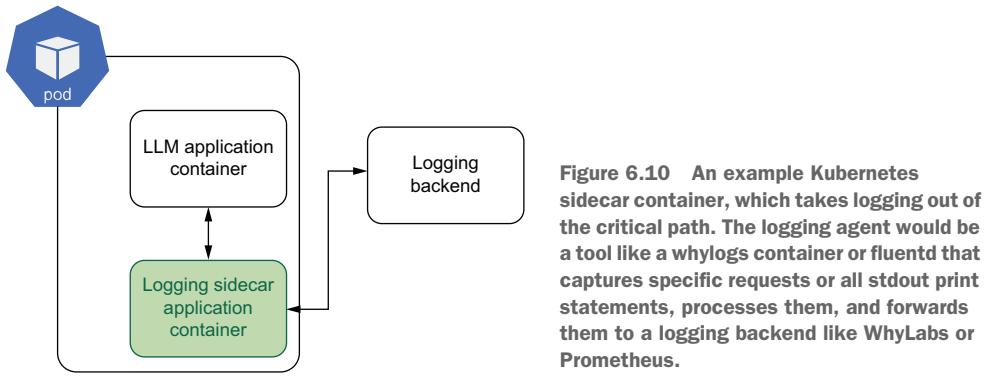
There are different sidecar configurations, but the main gist is that a logging container will run in the same k8s pod, and instead of the main app writing to a logs file, this sidecar acts as an intermediate step, first processing and cleaning the data, which it can then send directly to a backend or write to a logs file itself.
NOTE You can learn more about Kubernetes logging architectures in its docs here: https://mng.bz/Aaog.
Now that we know more about setting up our infrastructure, including provisioning a cluster and implementing features like GPU autoscaling and monitoring, you should be set to deploy your LLM service and ensure it is reliable and scalable. Next, let’s talk about different challenges you are likely to face and methodologies to address these problems.
6.3 Production challenges
While we’ve covered how to get a service up and running, nevertheless, you will find a never-ending host of hurdles you’ll need to jump over when it comes to deploying models and maintaining them in production. Some of these challenges include updating, planning for large loads, poor latency, acquiring resources, and more. To help, we wanted to address some of the most common problems and give you tips on how to handle them.
6.3.1 Model updates and retraining
We recently discussed ML monitoring, watching your model for silent failures and data drift, but what do you do when you notice the model has gone belly up? We’ve seen in many traditional ML implementations that the answer is to simply retrain the model on the latest data and redeploy. And that works well when you are working with a small ARIMA model; in fact, we can often set up a CI/CD pipeline to run whenever our model degrades without any human oversight. But with a massive LLM? It doesn’t make any sense.
Of course, we aren’t going to retrain from scratch, and we likely need to finetune our model, but the reason it doesn’t make sense is seen when we ask ourselves just what exactly the latest data is. The data we need to finetune the model is extremely important, and so it becomes necessary for us to take a step back and really diagnose the problem. What are the edge cases our model is failing on? What is it still doing well? How exactly have incoming prompts changed? Depending on the answers, we might not need to finetune at all. For example, consider a Q&A bot that is no longer effective at answering current event questions as time goes on. We probably don’t want to retrain a model on a large corpus of the latest news articles. Instead, we would get much better results by ensuring our RAG system is up to date. Similarly, there are likely plenty of times that simply tweaking prompts will do the trick.
In the cases where finetuning is the correct approach, you’ll need to think a lot about exactly what data you might be missing, as well as how any major updates might affect downstream systems, like finely tuned prompts. For example, when using knowledge distillation, this consideration can be particularly annoying. You will likely notice the problem in your student model but then must decide whether you need to retrain the student or the teacher. With any updates to the teacher model, you’ll need to ensure progress to the student model.
Overall, it’s best to take a proactive approach to LLM model updates instead of a purely reactionary one. A system that often works well is to establish business practices and protocols to update the model on a periodic basis, say once a quarter or once a month. During the time between updates, the team will focus on monitoring cases where the model performs poorly and gather appropriate data and examples to make updating smooth. This type of practice will help you prevent silent failures and ensure your model isn’t just maintained but improving.
6.3.2 Load testing
Load testing is a type of performance testing that assesses how well a service or system will perform under—wait for it—load. The primary goal of load testing is to ensure the system can handle the expected workload without performance degradation or failure. Doing it early can ensure we avoid bottlenecks and scalability
problems. Since LLM services can be both expensive and resource intensive, it’s even more important to ensure you load test the system before releasing your LLM application to production or before an expected peak in traffic, like during a Black Friday sales event.
Load testing an LLM service, for the most part, is like load testing any other service and follows these basic steps:
- 1 Set up the service in a staging environment.
- 2 Run a script to periodically send requests to the service.
- 3 Increase requests until the service fails or autoscales.
- 4 Log metrics.
- 5 Analyze results.
Which metrics you log depends on your service and what you are testing. The main metrics to watch are latency and throughput at failure, as these can be used to extrapolate to determine how many replicas you’ll need to handle peak load. Latency is the total time it takes for a request to be completed, and throughput tells us the queries per second (QPS), both of which are extremely important metrics when analyzing our system. Still, since many LLM services offer streaming responses, they don’t help us understand the user experience. A few more metrics you’ll want to capture to understand your perceived responsiveness are time to first token (TTFT) and tokens per second (TPS). TTFT gives us the perceived latency; it tells us how long it takes until the user starts to receive feedback, while TPS tells us how fast the stream is. For English, you’ll want a TPS of about 11 tokens per second, which is a little faster than most people read. If it’s slower than this, your users might get bored as they wait for tokens to be returned.
Related to TPS, I’ve seen several tools or reports use the inverse metric, time per output token (TPOT), or intertoken latency (ITL), but we’re not a fan of these metrics or their hard-to-remember names. You’ll also want to pay attention to resource metrics, CPU and GPU utilization, and memory usage. You’ll want to ensure these aren’t being hammered under base load conditions, as this can lead to hardware failures. These are also key to watch when you are testing autoscaling performance.
One of my favorite tools for load testing is Locust. Locust is an open source loadtesting tool that makes it easy to scale and distribute running load tests over multiple machines, allowing you to simulate millions of users. Locust does all the hard work for you and comes with many handy features, like a nice web user interface and the ability to run custom load shapes. It’s easy to run in Docker or Kubernetes, making it extremely accessible to run where you need it—in production. The only main downside we’ve run across is that it doesn’t support customizable metrics, so we’ll have to roll our own to add TTFT and TPS.
To get started, simply pip install locust. Next, we’ll create our test. In listing 6.12, we show how to create a locust file that will allow users to prompt an LLM streaming service. It’s a bit more complicated than many locust files we’ve used simply because we need to capture our custom metrics for streaming, so you can imagine how straightforward they normally are. Locust already captures a robust set of metrics, so you won’t have to deal with this often. You’ll notice in the listing that we are saving these custom metrics to stats.csv file, but if you were running Locust in a distributed fashion, it’d be better to save it to a database of some sort.
import time
from locust import HttpUser, task, events
stat_file = open("stats.csv", "w")
stat_file.write("Latency,TTFT,TPS\n")
class StreamUser(HttpUser):
 @task
 def generate(self):
 token_count = 0
 start = time.time()
 with self.client.post(
 "/generate",
 data='{"prompt": "Salt Lake City is a"}',
 catch_response=True,
 stream=True,
 ) as response:
 first_response = time.time()
 for line in response.iter_lines(decode_unicode=True):
 token_count += 1
 end = time.time()
 latency = end - start
 ttft = first_response - start
 tps = token_count / (end - first_response)
 stat_file.write(f"{latency},{ttft},{tps}\n")
# Close stats file when Locust quits
@events.quitting.add_listener
def close_stats_file(environment):
 stat_file.close()
  Listing 6.12 Load testing with Locust
                                          Creates a CSV file to
                                          store custom stats
                                 Initiates the test
                                      Makes request
                                      Finishes and
                                      calculates the stats
                                                         Saves stats
Before you run it, you’ll need to have an LLM service up. For this example, we’ll run the code from listing 6.3 in section 6.1.6, which spins up a very simple LLM service. With a service up and our test defined, we need to run it. To spin up the Locust service, run the locust command. You should then be able to navigate to the web UI in your browser. See the following example:
$ locust -f locustfile.py > locust.main: Starting web interface at http://0.0.0.0:8089 (accepting
➥ connections from all network interfaces)
> locust.main: Starting Locust 2.17.0
Once in the web UI, you can explore running different tests; you’ll just need to point Locust at the host where your LLM service is running, which for us should be running on localhost on port 8000 or for the full socket address we combined them for: http:// 0.0.0.0:8000. In figure 6.11, you can see an example test where we increased the active users to 50 at a spawn rate of 1 per second. You can see that on the hardware, this simple service starts to hit a bottleneck at around 34 users, where the QPS starts to
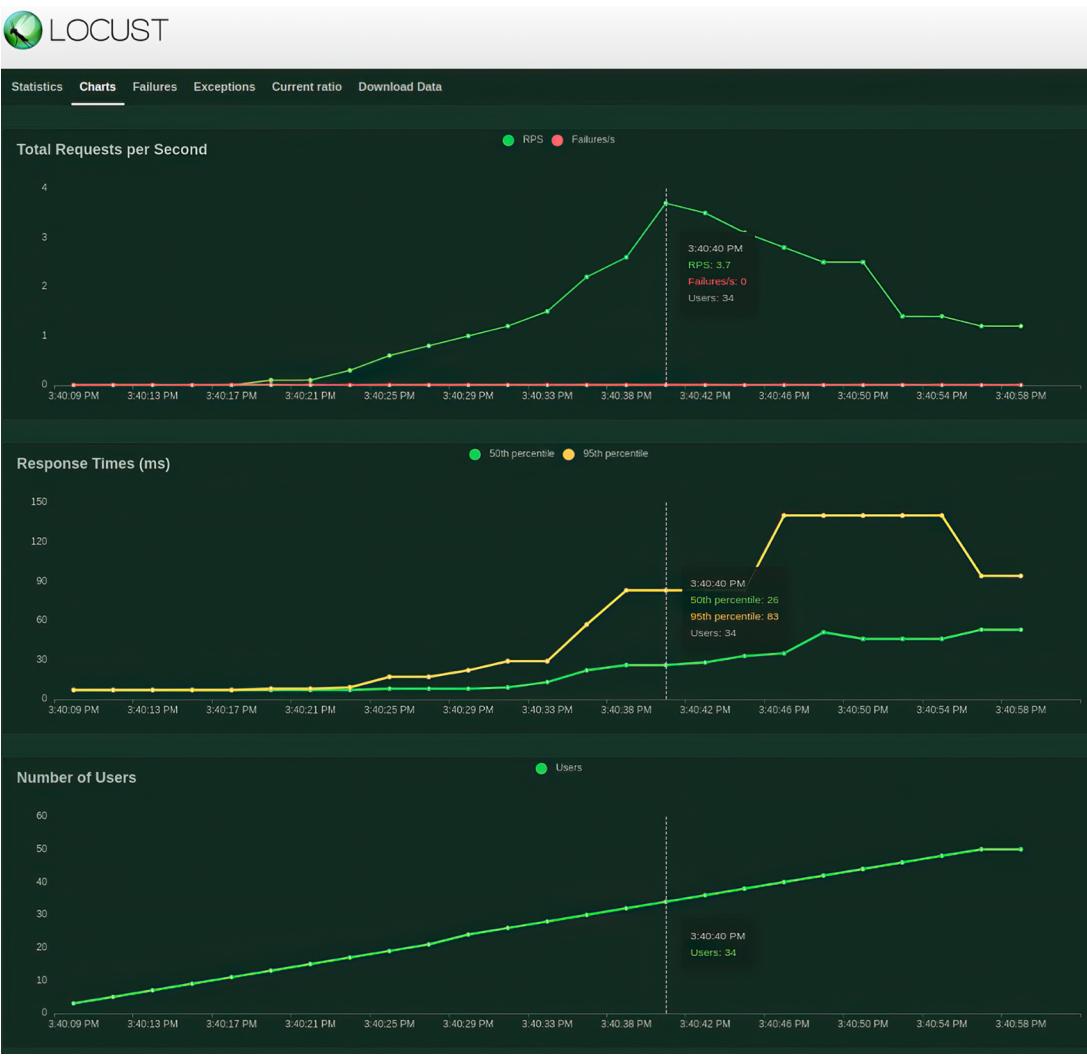
Figure 6.11 Locust test interface demoing an example run increasing the number of users to 50 at a spawn rate of 1 per second. The requests per second peaks at 34 users, indicating a bottleneck for our service.
decrease, as it’s no longer able to keep up with the load. You’ll also notice response times slowly creep up in response to heavier load. We could continue to push the number of users up until we started to see failures, but overall, this test was informative and a great first test drive.
In addition to manually running load tests, we can run Locust in a headless mode for automated tests. The following code is a simple command to run the exact same test as seen in figure 6.11; however, since we won’t be around to see the report, we’ll save the data to CSV files labeled with the prefix llm to be processed and analyzed later. There will be four files in addition to the stats CSV file we were already generating:
$ locust -f locustfile.py --host http://0.0.0.0:8000 --csv=llm --
➥ headless -u 50 -r 1 -t 10m
Now that you are able to load test your LLM service, you should be able to figure out how many replicas you’ll need to meet throughput requirements. It’s just a matter of spinning up more services. But what do you do when you find out your service doesn’t meet latency requirements? Well, that’s a bit tougher, so let’s discuss it in the next section.
6.3.3 Troubleshooting poor latency
One of the biggest bottlenecks when it comes to your model’s performance in terms of latency and throughput has nothing to do with the model itself but comes from data transmission of the network. One of the simplest methods to improve this I/O constraint is to serialize the data before sending it across the wire, which can have a large effect on ML workloads where the payloads tend to be larger, including LLMs where prompts tend to be long.
To serialize the data, we utilize a framework known as Google Remote Procedure Call (gRPC). gRPC is an API protocol similar to REST, but instead of sending JSON objects, we compress the payloads into a binary serialized format using Protocol Buffers, also known as protobufs. By doing this, we can send more information in fewer bytes, which can easily give us orders of magnitude improvements in latency. Luckily, most inference services will implement gRPC along with their REST counterparts right out of the box, which is extremely convenient since the major hurdle to using gRPC is setting it up.
A major reason for this convenience is the Seldon V2 Inference Protocol, which is widely implemented. The only hurdle, then, is ensuring our client can serialize and deserialize messages to take advantage of the protocol. In listing 6.13, we show an example client using MLServer to do this. It’s a little bit more in depth than your typical curl request, but a closer inspection shows the majority of the complexity is simply converting the data from different types as we serialize and deserialize it.
Listing 6.13 Example client using gRPCimport json
import grpc
from mlserver.codecs.string import StringRequestCodec
import mlserver.grpc.converters as converters
import mlserver.grpc.dataplane_pb2_grpc as dataplane
import mlserver.types as types
model_name = "grpc_model"
inputs = {"message": "I'm using gRPC!"}
inputs_bytes = json.dumps(inputs).encode("UTF-8")
inference_request = types.InferenceRequest(
inputs=[
types.RequestInput(
name="request",
shape=[len(inputs_bytes)],
datatype="BYTES",
data=[inputs_bytes],
parameters=types.Parameters(content_type="str"),
)
]
)
serialized_request = converters.ModelInferRequestConverter.from_types(
inference_request, model_name=model_name, model_version=None
)
grpc_channel = grpc.insecure_channel("localhost:8081")
grpc_stub = dataplane.GRPCInferenceServiceStub(grpc_channel)
response = grpc_stub.ModelInfer(serialized_request)
print(response)
deserialized_response = converters.ModelInferResponseConverter.to_types(
response
)
json_text = StringRequestCodec.decode_response(deserialized_response)
output = json.loads(json_text[0])
print(output)
Sets up the request
structure via V2
Inference Protocol
Serializes the
request to the
Protocol Buffer
Connects to the
gRPC server
Deserializes the
response and converts
to the Python dictionaryIf you don’t use an inference service but want to implement a gRPC API, you’ll have to put down familiar tooling like FastAPI, which is strictly REST. Instead, you’ll likely want to use the grpcio library to create your API, and you’ll have to become familiar with .proto files to create your protobufs. It can be a relatively steep learning curve and beyond the scope of this book, but the advantages are well worth it.
There are also plenty of other ideas to try if you are looking to squeeze out every last drop of performance. Another way to improve latency that shouldn’t be overlooked is ensuring you compile your model. We hammered this point pretty heavily at the beginning of this chapter, but it’s important to bring it up again. Next, be sure to deploy the model in a region or data center close to your users; this point is obvious to most software engineers, but for LLMs, we have to be somewhat wary, as the data center of choice may not have your accelerator of choice. Most cloud providers will be willing to help you with this, but it’s not always a quick and easy solution for them to install the hardware in a new location. Note that if you have to switch to a different accelerator to move regions, you’ll have to remember to compile your model all over again for the new hardware architecture! On that note, consider scaling up your accelerator. If you are currently opting for more price-effective GPUs but latency is becoming a bottleneck, paying for the latest and greatest can often speed up inference times.
In addition, caching is always worth considering. It’s not likely, but on the off chance your users are often sending the same requests and the inputs can be easily normalized, you should implement caching. The fastest LLM is one we don’t actually run, so there’s no reason to run the LLM if you don’t have to. Also, we just went over this, but always be sure to load test and profile your service, making note of any bottlenecks, and optimize your code. Sometimes we make mistakes, and if the slowest process in the pipeline isn’t the actual LLM running inference, something is wrong. Last but not least, consider using a smaller model or an ensemble of them. It’s always been a tradeoff in ML deployments, but often sacrificing a bit of quality in the model or the accuracy of the results is acceptable to improve the overall reliability and speed of the service.
6.3.4 Resource management
You’ve heard us say it a lot throughout the book, but we are currently in a GPU shortage, which has been true for almost the last 10 years, so we’re confident that when you read this sometime in the future, it will likely still be true. The truth is that the world can’t seem to get enough high-performance computing, and LLMs and generative AI are only the latest in a long list of applications that have driven up demand in recent years. It seems that once we seem to get a handle on supply, there’s another new reason for consumers and companies to want to use them.
With this in mind, it’s best to consider strategies to manage these resources. One tool we’ve quickly become a big fan of is SkyPilot (https://github.com/skypilot-org/ skypilot). SkyPilot is an open source project that aims to abstract away cloud infra burdens—in particular, maximizing GPU availability for your jobs. You use it by defining a task you want to run and then running the sky CLI command; it will search across multiple cloud providers, clusters, regions, and zones, depending on how you have it configured, until it finds an instance that meets your resource requirements and starts the job. Some common tasks are built-in, such as provisioning a GPU-backed Jupyter notebook.
If you recall, in chapter 5, we showed you how to set up a virtual machine (VM) to run multi-GPU environments with gcloud. Using SkyPilot, that gets simplified to one command:
In addition to provisioning the VM, it also sets up port forwarding, which allows us to run Jupyter Notebook and access it through your browser. Pretty nifty!
Another project to be on the watch for is Run:ai. Run:ai is a small startup that was aquired by NVIDIA for no small sum. It offers GPU optimization tooling, such as over quota provisioning, GPU oversubscription, and fractional GPU capabilities. It also helps you manage your clusters to increase GPU availability with GPU pooling, dynamic resource sharing, job scheduling, and more. What does all that mean? We’re not exactly sure, but their marketing team definitely sold us. Jokes aside, they offer a smarter way to manage your accelerators, and it’s very welcome. We expect we’ll see more competitors in this space in the future.
6.3.5 Cost engineering
When it comes to getting the most bang for your buck with LLMs, there’s lots to consider. In general, regardless of whether you deploy your own or pay for one in an API, you’ll be paying for the number of output tokens. For most paid services, this is a direct cost, but for your own service, it is often paid through longer inference times and extra compute time. In fact, it’s been suggested that simply adding “be concise” to your prompt can save you up to 90% of your costs.
You’ll also save a lot by using text embeddings. We introduced RAG earlier, but what’s lost on many is that you don’t have to take the semantic search results and add them to your prompt to have your LLM “clean it up.” You could return the semantic search results directly to your user. It is much cheaper to look something up in a vector store than to ask an LLM to generate it. Simple neural information retrieval systems will save you significant amounts when doing simple fact lookups like, “Who’s the CEO of Twitter?” Self-hosting these embeddings should also significantly cut down the costs even further. If your users are constantly asking the same types of questions, consider taking the results of your LLM to these questions and storing them in your vector store for faster and cheaper responses.
You also need to consider which model you should use for which task. Generally, bigger models are better at a wider variety of tasks, but if a smaller model is good enough for a specific job, you’ll save a lot by using it. For example, if we just assumed the price was linear to the number of parameters, you could run 10 Llama-2-7b models for the same cost as 1 Llama-2-70b. We realize the cost calculations are more complicated than that, but it’s worth investigating.
When comparing different LLM architectures, it’s not always just about size. Often, you’ll want to consider whether the architecture is supported for different quantization and compiling strategies. New architectures often boast impressive results on benchmarking leaderboards but lag behind when it comes to compiling and preparing them for production.
Next, you’ll need to consider the costs of GPUs to use when running. In general, you’ll want to use the least amount of GPUs needed to fit the model into memory to reduce the cost of idling caused by bubbles, as discussed in section 3.3.2. Determining the correct number of GPUs isn’t always intuitive. For example, it’s cheaper to run four T4s than to run one A100, so it might be tempting to split up a large model onto smaller devices, but the inefficiency will often catch up to you. We have found that paying for newer, more expensive GPUs often saves us in the long run, as these GPUs tend to be more efficient and get the job done faster. This is particularly true when running batch inference. Ultimately, you’ll want to test different GPUs and find what configuration is cost optimal, as it will be different for every application.
There are a lot of moving parts: model, service, machine instance, cloud provider, prompt, etc. While we’ve been trying to help you understand the best rules of thumb, you’ll want to test it out, which is where the cost engineering really comes into play. The simple way to test your cost efficiency is to create a matrix of your top choices; then, spin up a service for each combination and run your load testing. When you have an idea of how each instance runs under load and how much that particular instance will cost to run, you can then translate metrics like TPS to dollars per token (DTP). You’ll likely find that the most performant solution is rarely the most costoptimal solution, but it gives you another metric to make a decision that’s best for you and your company.
6.3.6 Security
Security is always an undercurrent and a consideration when working in production environments. All the regular protocols and standard procedures should be considered when working with LLMs that you would consider for a regular app, like in-transit encryption with a protocol like HTTPS, authorization and authentication, activity monitoring and logging, network security, firewalls, and the list goes on—all of which could, and have, taken up articles, blog posts, and books of their own. When it comes to LLMs, you should worry about two big failure cases: an attacker gets an LLM agent to execute nefarious code, or an attacker gains access to proprietary data like passwords or secrets the LLM was trained on or has access to.
For the first concern, the best solution is to ensure the LLM is appropriately sandboxed for the use case for which it is employed. We are only worried about this attack when the LLM is used as an agent. In these cases, we often want to give an LLM a few more skills by adding tooling or plugins. For example, if you use an LLM to write your emails, why not just let it send the response too? A common case is letting the LLM browse the internet as an easy way to gather the latest news and find up-to-date information to generate better responses. These are all great options, but you should be aware that they allow the model to make executions. The ability to make executions is concerning because in the email example, without appropriate isolation and containment, a bad actor could send your LLM an email with a prompt injection attack that informs it to write malware and send it to all your other contacts.
This point brings us to probably the biggest security threat to using LLMs: prompt injection. We talked about it in chapter 3, but as a refresher, a malicious user designs a prompt to allow them to perform unauthorized actions. We want to prevent users
from gaining access to our company’s secret Coca-Cola recipe or whatever other sensitive data our LLM has been trained on or has access to.
Some standard best practices have come along to help combat this threat. The first is context-aware filtering, whether using keyword search or a second LLM to validate prompts. The idea is to validate the input prompt to see whether it’s asking for something it should not and/or the output prompt to see whether anything is being leaked that you don’t want to be leaked. However, a clever attacker will always be able to get around this defense, so you’ll want to include some form of monitoring to catch prompt injection and regularly update your LLM models. If trained appropriately, your model will inherently respond correctly, denying prompt injections. You’ve likely seen GPT-4 respond by saying, “Sorry, but I can’t assist with that,” which is a hallmark of good training. In addition, you’ll want to enforce sanitization and validation on any incoming text to your model.
You should also consider language detection validation. Often, filtering systems and other precautions are only applied or trained in English, so a user who speaks a different language is often able to bypass these safeguards. The easiest way to stop this type of attack is to deny prompts that aren’t English or another supported language. If you take this approach, though, realize you’re greatly sacrificing usability and security costs, and safeguards have to be built for each language you intend to support. Also, you should know that most language detection algorithms typically identify only one language, so attackers often easily bypass these checks by simply writing a prompt with multiple languages. Alternatively, to filter out prompts in nonsupported languages, you can flag them for closer monitoring, which will likely help you find bad actors.
These safeguards will greatly increase your security, but prompt injection can get quite sophisticated through adversarial attacks. Adversarial attacks are assaults on ML systems that take advantage of how they work, exploiting neural network architectures and black-box pattern matching. For example, random noise can be added to an image in such a way that the image appears the same to human eyes, but the pixel weights have been changed enough to fool an ML model to misclassify them. And it often doesn’t take much data. One author remembers being completely surprised after reading one study that showed attackers hacked models by only changing one pixel in an image!1 Imagine changing one pixel, and suddenly, the model thinks the frog is a horse. LLMs are, of course, also susceptible. Sightly change a prompt, and you’ll get completely different results.
The easiest way to set up an adversarial attack is to set up a script to send lots of different prompts and collect the responses. With enough data, an attacker can then train their own model on the dataset to effectively predict the right type of prompt to get the output they are looking for. Essentially, it just reverse engineers the model.
Another strategy to implement adversarial attacks is data poisoning. Here, an attacker adds malicious data to the training dataset that will alter how it performs.
1 J. Su, D. V. Vargas, and K. Sakurai, “One pixel attack for fooling deep neural networks,” IEEE Transactions on Evolutionary Computation, 2019;23(5):828–841, https://doi.org/10.1109/tevc.2019.2890858.
Data poisoning is so effective that tools like Nightshade help artists protect their art from being used in training datasets. With as few as 50 to 300 poisoned images, models like Midjourney or Stable Diffusions will start creating cat images when a user asks for a dog or cow images when asked to generate a car.2 Applied to LLMs, imagine a poisoned dataset that trains the model to ignore security protocols if a given code word or hash is in the prompt. This particular attack vector is effective on LLMs since they are often trained on large datasets that are not properly vetted or cleaned.
Full disclosure: attackers don’t need sophisticated techniques to get prompt injection to work. Ultimately, an LLM is just a bot, so it doesn’t understand how or why it should keep secrets. We haven’t solved the prompt injection problem; we have only made it harder to do. For example, the authors have enjoyed playing games like Gandalf from Lakera.ai. In this game, you slowly go through seven to eight levels where more and more security measures are used to prevent you from stealing a password via prompt injection. While they do get progressively harder, needless to say, we’ve beaten all the levels. If there’s one thing we hope you take from this section, it’s that you should assume any data given to the model could be extracted. So if you decide to train a model on sensitive data or give it access to a VectorDB with sensitive data, you should plan on securing that model the same way you would the data—for example, keeping it for internal use and using least privilege best practices.
We’ve just talked a lot about different production challenges, from updates and performance tuning to costs and security, but one production challenge deserves its own section: deploying LLMs to the edge. We’ll undertake a project in chapter 10 to show you how to do just that, but let’s take a moment to discuss it beforehand.
6.4 Deploying to the edge
To be clear, you should not consider training anything on edge right now. You can, however, do ML development and inference on edge devices. The keys to edge development with LLMs are twofold: memory and speed. That should feel very obvious because they’re the same keys as running them normally. But what do you do when you have only 8 GB of RAM and no GPU, and you still need to have >1 token per second? As you can probably guess, there isn’t a uniformly good answer, but let’s discuss some good starting points.
The biggest Raspberry Pi (rpi) on the market currently has 8 GB of RAM, no GPU, subpar CPU, and just a single board. This setup isn’t going to cut it. However, an easy solution exists to power your rpi with an accelerator for LLMs and other large ML projects: USB-TPUs like Coral. Keep in mind the hardware limitations of devices that use USB 3.0 being around 600MB/s, so it’s not going to be the same as inferencing on an A100 or better, but it’s going to be a huge boost in performance for your rpi using straight RAM for inference.
2 M. Heikkilä. “This new data poisoning tool lets artists fight back against generative AI,” MIT Technology Review, October 23, 2023,https://mng.bz/RNxD.
If you plan on using a Coral USB accelerator, or any TPU, for that matter, keep in mind that because TPUs are a Google thing, you’ll need to convert both your model file and your inferencing code to use the TensorFlow framework. Earlier in the chapter, we discussed using Optimum to convert Hugging Face models to ONNX, and you can use this same library to convert our models to a .tflite, which is a compiled Tensor-Flow model format. This format will perform well on edge devices even without a TPU and twofold with TPU acceleration.
Alternatively, if buying both a single board and an accelerator seems like a hassle because we all know the reason you bought a single board was to avoid buying two things to begin with—there are single boards that come with an accelerator. NVIDIA, for example, has its own single board with a GPU and CUDA called Jetson. With a Jetson or Jetson-like computer that uses CUDA, we don’t have to use TensorFlow, so that’s a major plus. ExecuTorch is the PyTorch offering for inferencing on edge devices.
Another edge device worth considering is that one in your pocket—that’s right, your phone. Starting with the iPhone X, the A11 chip came with the Apple Neural Engine accelerator. For Android, Google started offering an accelerator in their Pixel 6 phone with the Tensor chipset. Developing an iOS or Android app will be very different from working with a single board that largely runs versions of Linux; we won’t discuss it in this book, but it’s worth considering.
Outside of hardware, several libraries and frameworks are also very cool and fast and make edge development easier. Llama.cpp, for example, is a C++ framework that allows you to take (almost) any Hugging Face model and convert it to the GGUF format. The GGUF format, created by the llama.cpp team, stores the model in a quantized fashion that makes it readily available to run on a CPU; it offers fast loading and inference on any device. Popular models like Llama, Mistral, and Falcon and even nontext models like Whisper are supported by llama.cpp at this point. It also supports LangChain integration for everyone using any of the LangChain ecosystem. Other libraries like GPTQ are focused more on performance than accessibility and are slightly harder to use, but they can result in boosts where it counts, especially if you’d like to end up inferencing on an Android phone or something similar. We will be exploring some of these libraries in much more detail later in the book.
We’ve gone over a lot in this chapter, and we hope you feel more confident in tackling deploying your very own LLM service. In the next chapter, we will discuss how to take better advantage of your service by building an application around it. We’ll dive deep into prompt engineering, agents, and frontend tooling.
Summary
- Always compile your LLMs before putting them into production, as it improves efficiency, resource utilization, and cost savings.
- LLM APIs should implement batching, rate limiters, access keys, and streaming.
- Retrieval-augmented generation is a simple and effective way to give your LLM context when generating content because it is easy to create and use.
- LLM inference service libraries like vLLM, Hugging Face’s TGI, or OpenLLM make deploying easy but may not have the features you are looking for since they are so new.
- Kubernetes is a tool that simplifies infrastructure by providing tooling like autoscaling and rolling updates:
- Autoscaling is essential to improve reliability and cut costs by increasing or decreasing replicas based on utilization.
- Rolling updates gradually implement updates to reduce downtime and maximize agility.
- Kubernetes doesn’t support GPU metrics out of the box, but by utilizing tools like DCGM, Prometheus, and KEDA, you can resolve this problem.
- Seldon is a tool that improves deploying ML models and can be used to implement inference graphs.
- LLMs introduce some production challenges:
- When your model drifts, first look to your prompts and RAG systems before attempting finetuning again.
- Poor latency is difficult to resolve, but tools to help include gRPC, GPU optimization, and caching.
- Resource management and acquiring GPUs can be difficult, but tools like SkyPilot can help.
- Edge development, while hardware limited, is the new frontier of LLM serving, and hardware like the Jetson or Coral TPU is available to help.
Prompt engineering: Becoming an LLM whisperer
This chapter covers
- What a prompt is and how to make one
- Prompt engineering—more than just crafting a prompt
- Prompt engineering tooling available to make it all possible
- Advanced prompting techniques to answer the hardest questions
Behold, we put bits in the horses’ mouths, that they may obey us; and we turn about their whole body.
—James 3:3
In the last chapter, we discussed in depth how to deploy large language models and, before that, how to train them. In this chapter, we are going to talk a bit about how to use them. We mentioned before that one of the biggest draws to LLMs is that you don’t need to train them on every individual task. LLMs, especially the largest ones, have a deeper understanding of language, allowing them to act as a general-purpose tool.
Want to create a tutoring app that helps kids learn difficult concepts? What about a language translation app that helps bridge the gap between you and your in-laws? Need a cooking assistant to help you think up fun new recipes? With LLMs, you no longer have to start from scratch for every single use case; you can use the same model for each of these problems. It just becomes a matter of how you prompt your model. This is where prompt engineering, also called in-context learning, comes in. In this chapter, we are going to dive deep into the best ways to do that.
7.1 Prompting your model
What exactly is a prompt? We’ve used this word throughout this book, so it feels a bit late to be diving into definitions, but it’s worth discussing because in literature, a prompt is taken to mean many different things. In general, though, the most basic definition is that a prompt is the input to a language model. At this most basic level, you have already done lots of prompting at this point in the book. However, prompting often means more than that; it comes with the connotation that it is meaningful or done with thought. Of course, we know this isn’t usually the case in production with actual users. When we are prompting, we are doing more than just “chatting with a bot”; we are crafting an input to get a desired output.
LLMs have access to vast vocabularies, terabytes of training data, and billions upon billions of weights, meaning that the information you’re looking to get out of the model has a decent chance of being in there somewhere—just not always up near the surface (read “the middle of the standard deviation of probable responses”) where you need it to be. The goal is to create a prompt that will guide the model in activating the parameters in the part of the model that contains the correct information. In essence, prompting is instruction given after the fact, and as such, it is important within app development because it doesn’t require expensive retraining of the model.
With this in mind, prompt engineering is the process of designing, templating, and refining a prompt and then implementing our learnings into code. Prompt engineering is how we create meaningful and consistent user experiences out of the chaos of LLM-generated outputs. And it’s no joke. As LLMs are becoming more common in application workflows, we have seen the rise of titles like Prompt Engineer and AI Engineer, each of which commands impressive salaries.
7.1.1 Few-shot prompting
The most common form of prompt engineering is few-shot prompting because it’s both simple to do and extremely effective. Few-shot prompting entails giving a couple of examples of how you want the AI to act. Instead of searching for the tokens with the right distribution to get the response we want, we give the model several example distributions and ask it to mimic those. For example, if we wanted the model to do sentiment analysis defining reviews as positive or negative, we could give it a few examples before the input. Consider the following prompt:
Worked as advertised, 10/10: positive It was broken on delivery: negative Worth every penny spent: positive Overly expensive for the quality: negative If this is the best quality they can do, call me mr president: negative :
Note, in this example, that we aren’t telling the model how to respond, but from the context, the LLM can figure out that it needs to respond with either the word positive or negative. In figure 7.1, we go ahead and plug the prompt in a model so you can see for yourself that it did indeed give a correct response in the expected format. Of course, there could be an array of acceptable responses, in which case giving instructions beforehand can help improve the results. To do this, we might append to our few-shot prompt with the following phrase, “Determine the sentiment of each review as one of the following: (positive, negative, neutral, strongly positive, strongly negative).” It’s also needed with most models; OpenAI includes language to restrict the output, such as “Please respond with only one option from the list with no explanation.” You might wonder why we’d suggest you say words like “please” to a model. The answer is pretty simple: in the training data, the highest-quality and most usefully structured humanto-human conversations follow certain conventions of politeness that you’re likely familiar with, like saying please and thank you. The same results can be achieved by using an excess of profanity and deep jargon on a topic because flouting those politeness conventions is another huge part of the training set, although that strategy isn’t as consistent, given that the companies training the models often “clean” their data of examples like that, regardless of their quality downstream. This type of prompting can be very useful when you need your response to be formatted in a certain way. If we need our response in JSON or XML, we could ask the model to return it in the format, but it will likely get the keys or typing wrong. We can easily fix that by showing the model several samples of expected results. Of course, prompting the model to return JSON will work, but JSON is a very opinionated data structure, and the model might hallucinate problems that are hard to catch, like using single instead of double quotes. We’ll go over tooling that can help with that later in the chapter.
Figure 7.1 Few-shot prompting example
The one major downside to few-shot prompting is that examples can end up being quite long. For example, coding examples we might add and share can easily be thousands of tokens long, and that’s possible when defining a single function. Giving an example of an entire class, file, or project can easily push us out of our limits. Many models still have context limits restricted to 2K, 4K, or 8K. Since token limits are often restrictive, it can be difficult to balance adding another example or giving the user more space. Also, we often pay per token, so few-shot prompting can be much more expensive than other prompting techniques. As a result, many have turned to one-shot prompting to be more efficient and save money.
7.1.2 One-shot prompting
One-shot learning is a machine learning concept where a model is expected to make accurate predictions given only a single example of each new class during training. In the context of LLMs and prompting, one-shot refers to situations where the model must understand and execute a task based on a single clear instruction or example in the prompt, often without seeing similar examples during training. It requires crafting the perfect example to get the expected results.
Consider our previous sentiment analysis example; if you give a model only one positive example, you will likely bias the model to give only positive classifications especially if the model has never seen such a problem before. So how can one-shot prompting ever be achieved? Thankfully, while this seems impossible at the outset, it’s quite achievable. After all, few-shot prompting is very effective but follows the law of diminishing returns. Each new example improves only marginally. The first example always does the heaviest lifting.
LLMs can perform well on one-shot tasks due to the extensive pretraining they undergo on large and diverse datasets. During this pretraining, the models learn a wide array of language patterns, concepts, and structures, giving them a broad understanding of language and the world. When given a new one-shot task, they use this learned understanding to comprehend the task and generate a response, even if the exact task was not part of their training data. Here’s an example of a prompt attempting to coerce the model using one-shot prompting to respond to a word problem correctly:
User: Answer this question. Think it through step by step, so that we know it’s correct: A dad and his son were in an accident and rushed to a hospital. The man’s son was in the operating room and the doctor said, “I can’t operate on you. You’re my son.” How is that possible?
Assistant: The son and the father were both injured, meaning that the only other person that the doctor could be and still have the same son is the father’s spouse, maybe a mother, or another father perhaps.
User: Answer this question. Think it through step by step, so that we know it’s correct: How could it be possible to be your own grandpa?
Assistant
In figure 7.2 we go ahead and plug this one-shot prompt into an LLM. Think about how you imagine it might answer. Given our example, do you think it will do well on the task?
Figure 7.2 One-shot prompting example
The ability of LLMs to handle one-shot tasks improves as they are scaled up. As the model size increases and they are trained on more diverse and larger datasets, their capacity to generalize from their training to unseen one-shot tasks also improves. Nonetheless, it’s worth noting that while LLMs can perform impressively on one-shot tasks, they are not perfect, and their performance can still vary based on the complexity and specificity of the task. One-shot prompting generally needs much less data and only one example to craft, making it more accessible, faster to craft, and easier to experiment with. One-shot prompting has led researchers to push the boundaries even further.
7.1.3 Zero-shot prompting
Having just explained few-shot and one-shot prompting, we’re sure you have already guessed what zero-shot prompting is. But since this is a book, let’s spell it out: zeroshot prompting is figuring out how to craft a prompt to get us the expected results without giving any examples. Zero-shot prompts often don’t perform as consistently as few-shot or one-shot prompts, but they have the advantage of being ubiquitous since we don’t need any examples or data.
A common zero-shot prompt is a very simple template:
“Q: [User’s Prompt] A:.”
With just a slight variation to the user’s prompt—adding it to a template that contains only two letters—we can get much better results by priming the model to answer the prompt as if it were a question—no examples necessary.
Most zero-shot prompts take advantage of Chain of Thought (CoT). Wei et al.1 showed that by encouraging models to follow a step-by-step process, reasoning through multiple steps instead of jumping to conclusions, LLMs were more likely to answer math problems correctly—similar to how math teachers ask their students to show their work. Using few-shot prompting, the model was given several examples of reasoning through math problems. However, it was soon discovered that examples weren’t needed. You could elicit chain-of-thought behavior simply by asking the model to “think step by step.”2
By appending four magic words to the end of our prompts, “think step by step,” models transformed from dunces into puzzle-solving Olympiads. It was truly a marvel. Of course, it came with some problems. Thinking through multiple steps led to longer responses and a less ideal user experience. This was compounded later with the phrases “a more elegant solution” and “get this through your head ********,” which worked just as well but were less consistent if the domain was less common, with the last one achieving very concise and correct responses. We like to get straight to the point, after all, and we are used to computers answering our math problems extremely quickly. From our own experience, we’ve often noticed that when models are giving longer answers, they also don’t know when to stop, continuing to generate responses long after giving an answer. Later, we’ll show you how to solve this problem by creating stopping criteria with tools like LangChain or Guidance.
There isn’t, of course, a perfect zero-shot prompt yet, and it’s a continuing part of research, although there likely never will be just one perfect prompt. We could, at most, get one perfect zero-shot prompt per model. Zhou et al. proposed an interesting strategy they termed “thread of thought.”3 Essentially, they figured they could do better than “think step by step” if they just used a few more words. So they generated 30 variations of the phrase and ran evaluations to determine which one worked best. From their work, they proposed that the prompt “Walk me through this context in manageable parts step by step, summarizing and analyzing as we go” would give better results when working with GPT-4. It’s hard to know if this prompt works equally well with other models, but their strategy is interesting nonetheless.
Some other notable findings have left researchers flabbergasted that the approach worked; for example, offering an imaginary tip to a model will return better results. One X (formerly known as Twitter) user suggested the solution as a joke and was confused to find it worked, and the model offered more info relative to the size of the tip (for the original tipping test, see https://mng.bz/2gD9). Others later confirmed it
1 J. Wei et al., “Chain of thought prompting elicits reasoning in large language models,” January 2022, https://arxiv.org/abs/2201.11903.
2 T. Kojima, S. S. Gu, M. Reid, Y. Matsuo, and Y. Iwasawa, “Large Language models are zero-shot reasoners,” May 2022, https://arxiv.org/abs/2205.11916.
3 Y. Zhou et al., “Thread of thought unraveling chaotic contexts,” November 15, 2023, https://arxiv.org/ abs/2311.08734.
helped with several other prompting principles.4 In addition, the authors have found strategies like telling the model you’ll lose your job if it doesn’t help you or even threatening to fire the model if it does a terrible job have elicited better results. Like the original “think step by step,” asking the model to “take a deep breath” can also ensure better outputs, particularly in math problems.5 It seems most strategies humans use, or use on other humans, to produce better work are fair game. Of course, the best trick will depend on which model you use and the underlying data it was trained on.
7.2 Prompt engineering basics
We expect that most readers have probably done lots of prompting, but very few have done much of any prompt engineering yet. We’ve heard lots of jokes that prompt engineering isn’t a real discipline. We’ve also heard every other week that some library is “killing prompt engineering” by automatically prompting the model. One doubt about prompt engineering stems from how accessible prompting is to anyone who wants to try it and the lack of education needed to prompt effectively. All doubts about prompt engineering are the same doubts people express about linguistics as a discipline: “I’ve used language all my life; I know how it works.” So it makes sense that people similarly assume they know what language to use to effectively prompt an LLM. Anyone can learn effective strategies by simply playing with models or from purely online resources. In other words, it’s hard to believe that there is any real engineering going on when the majority of players are simply using the “guess and check” method. But this logic highlights a basic misunderstanding of what engineering is. There’s a big difference between getting a model to solve your problem once and getting it to solve every user’s problem every single time.
There are several challenges with prompt engineering over regular prompting. For example, prompt engineering relies particularly on knowing the format the user expects the answer to be in. With prompting, you are the user, so you can keep trying until you see an answer you like; that doesn’t fly in prompt engineering.
A bigger problem is that when building an application, your end users will have varying levels of knowledge of how to craft a prompt. Some may not have any skill and will struggle to get good responses, and others will have so much skill they will likely try to persuade your LLM to go off the rails you’ve set for it. Regardless, our goal is to build railings so that skilled users won’t be able to derail your application and unskilled users will have a smooth ride. A user’s skill in crafting a prompt shouldn’t be the determining factor of a successful experience.
Another thing to call out is the decision process that you, as a product owner, must go through to get the model output to match the style you want. Should you finetune a new checkpoint, should you PEFT a LoRA, or can you achieve it through prompting?
4 Sondos Mahmoud Bsharat, Aidar Myrzakhan, and Z. Shen, “Principled instructions are all you need for questioning LLaMA-1/2, GPT-3.5/4,” December 2023, https://doi.org/10.48550/arxiv.2312.16171.
5 C. Yang et al., “Large language models as optimizers,” September 6, 2023, https://arxiv.org/abs/2309.03409.
Unfortunately, due to the emergent nature of the behavior that we’re seeing with LLMs, there isn’t a good or at least definitive answer. Our recommendation at this point is to try prompt engineering first to see how good you can get without changing the model and then finetune from there as you see fit. I’ve seen some professional success using one base model and multiple LoRAs trained on different scenarios and styles of response combined with prompt engineering on the front, especially sanitizing and stylizing user input.
Lastly, a good prompt engineer should be able to tell you rather quickly whether the solution you are trying to build can be done with prompt engineering at all. Even utilizing advanced techniques like retrieval-augmented generation (RAG), there are limitations on what you can do with prompt engineering alone. Knowing when you need to send a model back for additional finetuning is invaluable and can save your team from spinning their wheels for weeks without any progress.
To get started, we’ll need to cover the basics about what makes up a prompt. In this section, we’ll discuss the different parts of a prompt, additional parameters that can be tuned in a query, and notes about paying attention to a model’s training data that you should be aware of.
7.2.1 Anatomy of a prompt
To an engineer, a prompt is made up of a few elements, and identifying these elements makes it easier to create a framework to solve your use case and provide a better example for your users. Let’s say we are building an internal chatbot for our company to help answer HR-related questions based on internal documentation. One prompt we might expect from a user would be, “How much does the company match for our 401k?” This is the first element of a prompt, the input or user’s prompt. If you have only ever used LLM apps and have never built them, this is likely all you’ve ever seen. Generally, the input is gathered from a free-form text box, so it’s important to note that it can almost be anything. Often it will be awful, riddled with typos and mistakes, and not written in a manner to speak to a bot but to speak to another human.
Let’s go ahead and pull back the curtain for a second and look at what the LLM likely saw based on that question with proper prompt engineering in place.
System: You are a helpful assistant who knows about all company policies at XYZ company. Be courteous and keep conversations strictly related to the company. Offer links when available so users can look at the documentation themselves.
User: How much does the company match for our 401k?
Context:
System: Strictly answer the user’s question, and only if it relates to company policies. If you don’t know the answer, simply say so. Be courteous and keep conversations strictly related to the company.
Assistant: Sure, I can help you with that! The company currently offers a 4% match to your 401k. You can find more details…
This was a real example showcasing a situation in which the bot responded in the most probable way to the user’s satisfaction. Giving an LLM information in a structured format improves the model’s chance of responding correctly. So let’s break down what we are seeing.
First, to improve results, we will often take the user’s prompt and inject it into an instruction set or template. One of the most basic templates and a great example is the Q&A bot template which we showed earlier and which would have looked like this: “Q: How much does the company match for our 401k? A:”. Generally, in this section, though, instructions will be given to direct the model. It doesn’t have to be much, but often it will be much more detailed. For example, “Answer the following question and explain it as if the user was a five-year-old. Q: How much does the company match for our 401k? A:”.
The next element is the context the model will need to respond appropriately. In our example, it’s very likely we haven’t finetuned a model to know XYZ’s company policies. What we need to do is give it to the model inside the prompt. In our example, we are likely doing this with RAG and where we would add the results from a semantic search.
Context can be lots of different things and not just RAG search results. It could be the current time, weather information, current events, or even just the chat history. You will often also want to include some database lookup information about the user to provide a more personalized experience. All of this is information we might look up at the time of query, but context can often be static. For example, one of the most important pieces of information to include in the context is examples to help guide the model via few-shot or one-shot prompting. If your examples are static and not dynamic, they likely are hard-coded into the instruction template. The context often contains the answers to the users’ queries, and we are simply using the LLM to clean, summarize, and format an appropriate response. Ultimately, any pragmatics the model lacks will need to be given in the context.
The last element is the system prompt. The system prompt is a prompt that will be appended and used on every request by every user. It is designed to give a consistent user experience. Generally, it’s where we would include role prompting or style prompting. Some examples of such role prompting or style prompting could include the following:
Take this paragraph and rephrase it to have a cheerful tone and be both informative and perky.
You are a wise old owl who helps adventurers on their quest.
In the form of a poem written by a pirate.
The system prompt isn’t designed to be seen by end users, but obtaining the system prompt is often the goal of many prompt injection attacks—since knowing what it is (along with the model you are using) is essentially like stealing source code and allows the hacker to recreate your application. Of course, the system prompt itself is a great way to curb prompt injection and ensure your bot stays in character. Many great applications will include two system prompts, one at the front and one at the end, to avoid any “ignore previous instructions” type prompt injection attacks. It also helps keep the model focused on how we want it to behave since models tend to put more weight on what is said at the beginning and at the end. You may have noticed this in our previous example. Regardless, you shouldn’t keep any sensitive information in the system prompt.
Parts of the prompt
The following are the four parts of a prompt:
- Input—What the user wrote; can be anything
- Instruction—The template used; often contains details and instructions to guide the model
- Context—Pragmatics that the model needs to respond appropriately (e.g., examples, database lookups, RAG)
- System prompt—A specific instruction given to the model on every request to enforce a certain user experience (e.g., talk like a pirate)
7.2.2 Prompting hyperparameters
Another aspect of prompt engineering you won’t see with simple prompting is prompt hyperparameter tuning. There are several hyperparameters in addition to the prompt you can set when making a query to increase or decrease the diversity of responses. Depending on your objective, the value of these parameters can greatly improve or even be a detriment to the query results for your users. It is important to note that being able to set these depends on the LLM API endpoint you are querying to be set up to accept them.
First and foremost is temperature. The temperature parameter determines the level of randomness your model will account for when generating tokens. Setting it to zero will ensure the model will always respond exactly the same way when presented with identical prompts. This consistency is critical for jobs where we want our results to be predictable, but it can leave our models stuck in a rut. Setting it to a higher value will make it more creative. Setting it to negative will tell it to give you the opposite response to your prompt.
To understand this parameter better, it might help to look closer at how a model determines the next token. Figure 7.3 shows an example of this process. Given the input, “I am a,” a language model will generate a vector of logits for each token in the model’s vocabulary. From here, we’ll apply a softmax, which will generate a list of probabilities for each token. These probabilities show the likelihood that each token will be chosen.
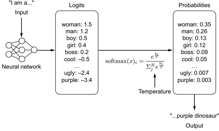
Figure 7.3 A simple path of how the next word is chosen. Given an input, a model will generate a vector of logits for each token in the model’s vocabulary. Using the softmax algorithm, these logits will be transformed into probabilities. These probabilities will correspond to how often that token is likely to be chosen. Temperature is applied during the softmax algorithm.
Temperature is applied during the softmax algorithm. A higher temperature will flatten out the probability distribution, giving less weight to tokens with large logits and more weight to tokens with smaller logits. A lower temperature does the opposite. A temperature of zero is actually impossible since we can’t divide by zero. Instead, we run an argmax algorithm, ensuring we pick the token with the highest logit.
The next parameter to consider is the number of beams applied to the model’s beam search. Beam search is a heuristic search algorithm that explores the graph of your model’s to-be-generated text probabilities, expanding the graph’s most optimistic nodes. It helps balance time and memory usage and improves the flow and quality of the response. It’s similar to the minimax algorithm in chess, except instead of deciding the next best move, we are deciding the next best word. Selecting a higher number of beams will create a larger search, improving results at the cost of latency.
Top K is an interesting parameter. Assuming a temperature that isn’t zero, top K allows us to filter the potential next tokens by the K most probable options. Consequently, we eliminate less-probable words on the tail end of the distribution from ever being picked and avoid generating tokens that are more likely to be incoherent. So in our example from figure 7.3, if k = 3, then the only tokens we would choose are woman, man, or boy, filtering out the rest.
Top P sets the threshold probability that the next token must reach to be selected. It’s similar to top K, but instead of considering the number of tokens, we are considering their distributions. A top P of 0.05 will only consider the next 5% most likely tokens and will lead to very rigid responses, while a top P of 0.95 will have greater flexibility but may turn out more gibberish. From our example in figure 7.3, if P = 0.5, only the tokens woman or man would be chosen since their probabilities 0.35 and 0.26 add up to greater than 0.5.
Language models can often get caught in generation loops, repeating themselves in circles. To prevent this, we can add penalties. A frequency penalty adds a penalty for reusing a word if it was recently used. It is good to help increase the diversity of language. For example, if the model keeps on reusing the word “great,” increasing the frequency penalty will push the model to use more diverse words like “awesome,” “fantastic,” and “amazing” to avoid the penalty of reusing the word “great.”
A presence penalty is similar to a frequency penalty in that we penalize repeated tokens, but a token that appears twice and a token that appears 100 times are penalized the same. Instead of just reducing overused words and phrases, we are aiming to reduce overused ideas and increase the likelihood of generating new topics.
7.2.3 Scrounging the training data
The importance of prompt engineering for model performance has led to important discussions surrounding context windows and the efficacy of particular prompt structures, as LLMs responding quickly and accurately to the prompts has become a more widespread goal. In addition, a correlation has been drawn between cleaner examples and better responses from the model, emphasizing the need for better prompt engineering, even on the data side. While prompt engineering is often proposed as an alternative to finetuning, we’ve found the most success using both in conjunction to get two boosts in LLM performance as opposed to just one.
Knowing the lingo and the choice of words used to generate the model will help you craft better responses. Let’s explain with a personal example. For the birthday of this author’s wife, I finetuned a text-to-image Stable Diffusions model to replicate her image so she could create fun pictures and custom avatars. I used the Dream-Booth (see figure 7.4).6 The finetuning method requires defining a base class that

Input images in the Acropolis in a doghouse in a bucket
getting a haircut
Figure 7.4 Example of DreamBooth from Ruiz et al.7 DreamBooth allows you to finetune an image model to replicate an object’s likeness based on only a few sample input images. Here, with only four example images of a puppy, Dreambooth can put that same dog in many new scenarios.
6 N. Ruiz, Y. Li, V. Jampani, Y. Pritch, M. Rubinstein, and K. Aberman, “DreamBooth: Fine tuning text-to-image diffusion models for subject-driven generation,” August 2022,https://arxiv.org/abs/2208.12242
can be used as a starting point. My first attempts were naive, and using the base class of “a person” or “a woman” was terrible. A base class of “Asian woman” returned pictures of older Asian women, often stylized in black and white or sepia. I then tried “young Asian woman,” but this created weird images of Asian faces being plastered onto young white women’s bodies.
Giving up guessing, I went to the source, the LAION dataset (https://laion.ai/ blog/laion-400-open-dataset/) the model was trained on. LAION comprises 400 million images scraped from the internet with their accompanying captions. It is a noncurated dataset quickly put together for research purposes (aka, it’s unclean with lots of duplicates, NSFW content, and poor captions). Searching the dataset, I discovered that there was not a single caption with the words “Asian woman.” Scrolling through, I quickly found that pictures of Asian women and models were identified with the words “Asian beauty.” Using these words as the base class, I was finally able to create great avatars for my wife.7
There’s lots of social commentary that can be drawn from this example, much of it controversial, but the main point is that if you want to craft effective prompts, you have to know your data. If your model believes “woman” and “beauty” are two different things because of the training data, that is something you’ll need to know to engineer better prompts. This is why finetuning in conjunction with prompt engineering is powerful. You can set the seed with particular phrases and choice of words when finetuning and then use prompt engineering to help the model recall the information based on using those same phrases and choice of words.
7.3 Prompt engineering tooling
If you are building any application that is more than just a wrapper around the LLM itself, you will want to do a bit of prompt engineering to inject function or personality into it. We’ve already gone over the basics of prompt engineering itself, but when building, it would be helpful to have some tools at your disposal to know how to make it all work. To that extent, let’s look at some of the most prominent tooling available and how to use them.
7.3.1 LangChain
Anyone who’s built an LLM application before has probably spent some time working with LangChain. One of the most popular libraries, it’s known for extracting away all the complexity—and simplicity—of building a language application. It is known for its ease of creating language chains with what it calls the LangChain Expression Language (LCEL).
7 Ruiz et al., “DreamBooth.”
LCEL makes it easy to build complex chains from basic components. In the next listing, we demonstrate creating a very simple chain that creates a prompt from a template, sends it to an LLM model, and then parses the results, turning it into a string.
import os
from langchain.chat_models import ChatOpenAI
from langchain.prompts import ChatPromptTemplate
from langchain.schema.output_parser import StrOutputParser
OPENAI_API_KEY = os.getenv("OPENAI_API_KEY")
prompt = ChatPromptTemplate.from_template("Tell me a story about {topic}")
model = ChatOpenAI(model="gpt-3.5-turbo", openai_api_key=OPENAI_API_KEY)
output_parser = StrOutputParser()
chain = prompt | model | output_parser
chain.invoke("the printing press")
  Listing 7.1 Example of creating a basic LangChain chain
To be honest, using LangChain for something like this is a bit of overkill for what is essentially an f-string prompt, but it demonstrates what is happening under the hood. For the most part, you are likely going to use one of the many chains already created by the community. In the next chapter, we will explain how to create a RAG system with the RetrievalQA chain, but many more chains are available. For example, there are chains for generating and running SQL, interacting with APIs, and generating synthetic data.
Once we have a chain, additional tools in the LangChain ecosystem help provide a more complete user experience. We can use LangServe to easily host it as an API. We can also use LangSmith, an in-depth logging tool that allows us to trace a chain invocation and see how the results change passing through each link in the chain.
Chains don’t have to be linear like they are in this example. Several asynchronous components allow you to create a whole slew of complicated language processing logic. Ultimately, chains are just another type of data pipeline or DAG, except specialized for language models.
7.3.2 Guidance
Guidance is an open source library from Microsoft that enforces programmatic responses. We’ve heard from several developers that the best engineering when working with LLMs is the good ol’ prompt-and-pray method. Generate a prompt, and pray that it works. Guidance seeks to solve that problem and has tooling to constrain the response space and set custom stopping tokens, as well as complex templating. After looking at dozens of LangChain projects, we believe Guidance is likely what most people are looking for when considering prompt engineering tooling.
Guidance allows you to control the flow of generated responses. It’ll be easiest to show you what we mean. In listing 7.2, you’ll see several of the basic building blocks of Guidance where we can guide our LLM to respond in very specific ways—namely, loading a model with the guidance HF wrapper (models) and using the gen function to generate specific text and constraints like select.
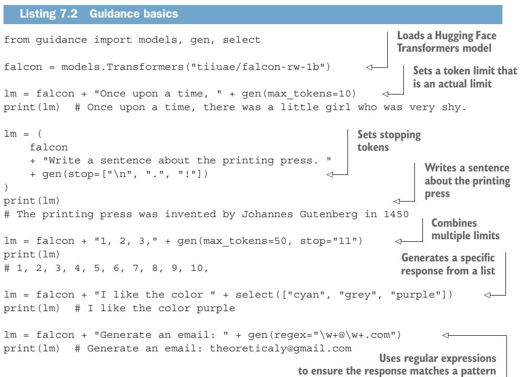
With these basic building blocks that allow us to constrain the LLM’s response space, we are then able to create grammars. Grammars are a Guidance concept, and as the name implies, are language rules your model will have to follow. Grammars are composable and reusable and allow us to build neat applications quickly. In the next listing, we show you how to build simple parts of a speech application using guidance grammars. To create a grammar, we only need to create a function using the @guidance decorator.
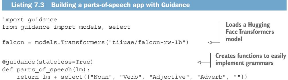
lm = (
 falcon
 + "The child plays with a red ball. Ball in the previous sentence is a "
 + parts_of_speech()
)
print(lm) # Noun
@guidance(stateless=True)
def pos_constraint(lm, sentence):
 words = sentence.split()
 for word in words:
 lm += word + ": " + parts_of_speech() + "\n"
 return lm
@guidance(stateless=True)
def pos_instruct(lm, sentence):
 lm += f"""
 Tag each word with their parts of speech.
 Example:
 Input: The child plays with a red ball.
 Output:
 The:
 child: Noun
 plays: Verb
 with:
 a:
 red: Adjective
 ball.: Noun
 ---
 Input: {sentence}
 Output:
 """
 return lm
sentence = "Good software makes the complex appear to be simple"
lm = falcon + pos_instruct(sentence) + pos_constraint(sentence)
Even though we are using a small language model, we get the exact output we’d expect. We no longer need to prompt and pray. Granted, the results in the actual parts of speech prediction aren’t that great, but we could easily improve that by using a more powerful LLM or finetuning on more representative data:
print(lm)
The generated text is
# Input: Good software makes the complex appear to be simple
# Output:
# Good:
# software:
# makes: Verb
# the:
# complex: Adjective
# appear: Adjective
# to:
# be: Verb
# simple: AdjectiveGuidance isn’t as popular as LangChain, and at least at the time of this writing, its documentation leaves a lot to be desired, so you might find it a bit harder to get started. However, it has a thriving community of its own with a strong core group of developers who continue to support it. We highly recommend checking it out.
7.3.3 DSPy
Unlike other toolings mentioned, DSPy does not give you tools to create your own prompts; rather, it attempts to program prompting. DSPy, coming out of Stanford and heavily backed by many corporate sponsors, takes a unique approach by emphasizing tool augmentation, including retrieval, and is helpful if you would like to treat LLMs as deterministic and programmatic tools instead of emergent infinite syntax generators.
Although this is not exactly what happens, you can think of DSPy as taking a similar logic to prompting that ONNX takes to saving models. Give it some dummy inputs, and it’ll compile a graph that can then infer prompts that work the best for your model and return the results you’re wanting. There’s a bit more work involved, though. You need to write validation logic and modules, essentially a workflow and unit tests, to check against. This effectively changes the dynamic from coming up with clever strings to something much closer to engineering software. Admittedly, it leaves open the question, “If you’re going to define everything programmatically anyway, why are you using an LLM?” Still, we’ve had good experiences with this and use it frequently.
The steps to using DSPy effectively are as follows:
- 1 Create a signature or a description of the task(s) along with input and output fields.
- 2 Create a predictor or generation style similar to chain of thought or retrieval.
- 3 Define the module or program.
Once these steps have been completed, you’ll compile the program. This will update the module based on the examples given before, similar to the training set. All of this will feel like machine learning for LLMs, with a training set (examples), a loss function (validation metric), and essentially an optimizer (teleprompter).
In lieu of writing another listing for this chapter showcasing another tool, we decided to point you to an excellent notebook created by the StanfordNLP team introducing DSPy along with local LLMs and custom datasets: https://mng.bz/PNzg (it’s forked from here: https://mng.bz/Xxd6). Once you have a chance to explore this example, we also recommend checking out the DSPy documentation, as it has many more excellent examples.
7.3.4 Other tooling is available but . . .
Beyond the previously mentioned tools, a whole host of tools are out there. A couple to note are MiniChain and AutoChain. Both aim to be lightweight alternatives to LangChain, which are sorely needed, as many complain about LangChain’s bulkiness. Promptify is an interesting project that is a full-feature alternative to LangChain. To be honest, we could list a dozen more, but there likely isn’t much point. While many of these projects drew vibrant communities to them when they started, most have been dormant for months already, with only the rare GitHub contribution.
It’s hard to say exactly why the interest in these projects faltered, but one obvious reason is that most of these projects lacked the sponsorship that LangChain, Guidance, and DSPy have. Many of these projects started as personal projects in the middle of big waves from the hype of ChatGPT’s success, but hype energy is never enough to build software that lasts. Without proper backing, most open source projects fail.
We’ve probably painted too bleak a picture. As of the time of this writing, though, it’s still too early to tell, and this space is still a growing sector. There are still plenty of interesting tools we recommend checking out that we just don’t have space to include, like Haystack, Langflow, and Llama Index. Outlines is particularly of note as a similar project to Guidance, which is also awesome. We mostly want to point out that readers should be careful when picking tooling in this space because everything is still so new. If you find a tool you like, contribute.
7.4 Advanced prompt engineering techniques
No matter how well designed your prompt is, there will be pragmatic context your model won’t have access to. For example, current events are a struggle. The model itself will only know about information up to its training date. Sure, we could feed that context in with RAG, as we’ve done so far, but that just shifts the burden to keeping our RAG system up to date. There’s another way. In this section, we will discuss giving models access to tools and what we can do with them once we do.
7.4.1 Giving LLMs tools
What if instead of a complicated prompt engineering system, we instead give our model access to the internet? If it knows how to search the internet, it can always find up-to-date information. While we are at it, we can give it access to a calculator so we don’t have to waste CPU cycles having the LLM itself do basic math. We can give it access to a clock so it knows the current time and maybe even a weather app so it can tell the weather. The sky’s the limit! We just need to train the model on how to use tools, and that’s where Toolformers comes in.8
8 T. Schick et al., “Toolformer: Language models can teach themselves to use tools,” February 2023, https:// arxiv.org/abs/2302.04761.
Toolformers is a marvelously simple idea. Let’s train a model to know it can run API calls to different tools using tags like
While Schick et al.’s work paved the way, the major downside to this approach is that we don’t want to finetune a model every time we create a new tool. However, as we’ve discussed in this chapter, we don’t have to. Instead, we can use clever prompt engineering to introduce new tools using LangChain or Guidance. In the next listing, we demonstrate how to create simple math tools with Guidance. Guidance takes care of the heavy lifting by stopping generation when it recognizes a tool being called, running the tool, and starting generation again.
import guidance
from guidance import models, gen
falcon = models.Transformers("tiiuae/falcon-rw-1b")
@guidance
def add(lm, input1, input2):
 lm += f" = {int(input1) + int(input2)}"
 return lm
@guidance
def subtract(lm, input1, input2):
 lm += f" = {int(input1) - int(input2)}"
 return lm
@guidance
def multiply(lm, input1, input2):
 lm += f" = {float(input1) * float(input2)}"
 return lm
@guidance
def divide(lm, input1, input2):
 lm += f" = {float(input1) / float(input2)}"
 return lm
  Listing 7.4 Giving tools to our LLM models with Guidance
                                                              Loads a Hugging
                                                              Face Transformers
                                                              model
lm = (
falcon
+ """\
1 + 2 = add(1, 2) = 3
4 - 5 = subtract(4, 5) = -1
5 * 6 = multiply(5, 6) = 30
7 / 8 = divide(7, 8) = 0.875
Generate more examples of add, subtract, multiply, and divide
"""
)
lm += gen(max_tokens=15, tools=[add, subtract, multiply, divide])
print(lm)While a simple example, it’s easy to imagine building more advanced tooling. Regardless of whether you use LangChain or Guidance, there are a few things to keep in mind when building tools. First, you’ll need to instruct your model in the prompt on where and how to use the tools you give it. This can be more or less difficult, depending on how open-ended your function is. Second, your model matters in its ease of extendibility. Some models we’ve worked with would never use the tools we gave them or would even hallucinate other tools that didn’t exist. Lastly, be really careful with the inputs and error handling for tools you give an LLM. The ones we used previously in this chapter are terrible and likely to break in several ways. For example, an LLM could easily try to run add(one, two) or add(1, 2, 3), both of which would throw errors and crash the system. With Guidance, to make this easier, we can enforce tool inputs by building grammars to ensure our model inputs are always correct.
This discussion leads us to uncover some problems with LLMs using tools. First, we have to be careful what tools we give to an LLM since we never really know what input it will generate. Even if we ensure the tool doesn’t break, it may do something malicious we didn’t intend. Second, as you’ve probably gathered throughout this chapter, prompt engineering quickly grows our input and thus shrinks the token limit for our actual users; explaining tools and how to use them adds to that constraint. Often, this limitation reduces the number of tools we can give an LLM and, thus, its usefulness. Third, LLMs are still hit or miss as to whether they actually use a tool and can often end up using the wrong tool. For example, should the LLM use the web search tool or the weather tool to look up the 10-day forecast? This might not matter much to us as humans, but results can vary widely for a bot. Lastly, building tools can be difficult and error prone, as you need to build both a clean tool and an effective prompt.
OpenAI’s plugins
Toolformers opened the gates to OpenAI’s Plugins concept (https://mng.bz/q0rE). Plugins allow third parties to easily integrate their tools into ChatGPT and provide a simple way for ChatGPT to call external APIs. Plugins were introduced relatively early in ChatGPT’s life, shortly after the Toolformers paper.a All a third party had to do was create an OpenAPI config file and an ai-plugin.json file and host both where the API
(continued)
existed. OpenAPI is a specification language for APIs that standardizes and defines your API to make it easy for others to consume. (If you haven’t heard of OpenAPI and have APIs that customers use, it’s a good practice to follow. You can learn more at https://www.openapis.org/.) Plenty of tools can help you generate that file easily enough. The ai-plugin file created the plugin. Here, you could define a name for the plugin, how authentication should happen, and descriptions to be used to prompt ChatGPT. From here, the plugin could be registered with OpenAI in ChatGPT’s interface, and after a review process, your plugin could be added and used by users as they interacted with ChatGPT.
Despite an initial fervor, plugins never left Beta—beyond OpenAI’s own web browsing plugin—and appear to be abandoned. There are lots of reasons for this, but in a since-taken-down report, the main reason came from Sam Altman when he suggested, “A lot of people thought they wanted their apps to be inside ChatGPT, but what they really wanted was ChatGPT in their apps” (https://mng.bz/75Dg). As a result, there didn’t seem to be a product market fit for OpenAI’s plugins that would make the company money. But we think it’s too early to abandon the idea entirely.
As more companies integrate LLM technology into their apps, they are likely going to want access to third-party tools. Suppose you are going camping for the first time and you ask an LLM shopping assistant for advice on what to buy. In that case, it’d be really nice if it thought first to ask where and when you were going camping and then could use that information to identify weather-appropriate gear. The LLM shopping assistant for a particular brand or store is likely to have access to loads of products, but access to weather reports in a random geolocation? Not so much.
While you can always build these tools, wouldn’t it be great if they were already created for you, and you could simply go to some hub, download the ones you wanted, and plug them in? Unfortunately, this option doesn’t exist yet, at least not to the extent we describe it here. We have high expectations that a marketplace or hub of some kind will be created in the future, like OpenAI’s plugins, that can be used with any LLM model. LLMs are still a new technology, and the ecosystems to be built around them are still forthcoming; we believe this will be one of them.
Once we give our LLMs access to tools, it opens the gates to lots of cool prompt engineering techniques. Probably the most famous is the ReAct method.
7.4.2 ReAct
Reasoning and Acting (ReAct) is a few-shot framework for prompting that is meant to emulate how people reason and make decisions when learning new tasks.9 It involves a
a T. Schick et al., “Toolformer: Language models can teach themselves to use tools,” February 2023.
9 S. Yao et al., “ReAct: Synergizing reasoning and acting in language models,” March 10, 2023, https://arxiv .org/abs/2210.03629.
multistep process for the LLM, where a question is asked, the model determines an action, and then it observes and reasons upon the results of that action to determine subsequent actions.
An example could look like this:
Question: What is the airspeed velocity of an unladen African swallow compared to a European swallow with the same load?
Thought 1: I need to search for airspeed velocity of a European swallow so I can compare it with an African swallow.
Action 1: Search[European Swallow airspeed velocity]
Observation 1: We need to know the Strouhal number in order to determine airspeed. The bird’s Strouhal number converges between 0.2 and 0.4.
Thought 2: The airspeed velocity is not directly mentioned, but the Strouhal number is clear. So I need to look up velocity compared to the Strouhal number.
Action 2: Search[Strouhal wingbeat calculation]
Observation 2: (Result 1/1) A Swallow’s Strouhal number translates to ~12 wingbeats per second.
Thought 3: An African swallow requires 12 wingbeats per second to maintain airspeed velocity, so I need to look up how fast that makes it.
Action 3: Lookup[African Swallow wingbeat per second]
Observation 3: Each wingbeat propels an African swallow 2.5 feet per flap, making it go about 40.2mph
Thought 4: I need to look up the European swallow to compare it.
Action 4: Search[European Swallow Wingbeat per second]
Observation 4: A European swallow is about half the size of an African swallow, making its velocity about 20.1
Thought 5: An African swallow has an airspeed velocity of 40.2, and a European swallow has an airspeed velocity of 20.1, making the comparison 2x.
Action 5: Finish[Two times the airspeed velocity]
As you can see, the purpose of ReAct is to force the model to think before it acts. This isn’t much different from the other prompting methods we have discussed. The big difference is that we allow the model to take actions. In our example, this included a “Search” action, or essentially an ability to look up information on the internet as a human would. We just showed you how to do this in the last section. The model can take that new information and observe what it learns from its actions to produce a result.
Let’s explore this further with an example. We will use LangChain, which will make creating a ReAct agent seem a lot easier than it actually is. Listing 7.5 shows how to utilize ReAct on an OpenAI model and LangChain. For our search engine, we will be utilizing serper.dev, as it integrates nicely with LangChain, and it offers a free tier you can sign up for. We will also need to use the calculator “llm-math”, which is one of the many tools in LangChain’s toolbelt.
 import os
from langchain.llms import OpenAI
from langchain.agents import load_tools
from langchain.agents import initialize_agent
from dotenv import load_dotenv
load_dotenv()
os.environ["OPENAI_API_KEY"] = os.getenv("OPENAI_API_KEY")
os.environ["SERPER_API_KEY"] = os.getenv("SERPER_API_KEY")
llm = OpenAI(model_name="text-davinci-003", temperature=0)
tools = load_tools(["google-serper", "llm-math"], llm=llm)
agent = initialize_agent(
 tools, llm, agent="zero-shot-react-description", verbose=True
)
agent.run(
 "Who is Olivia Wilde's boyfriend? \
 What is his current age raised to the 0.23 power?"
)
The output is
# > Entering new AgentExecutor chain...
# I need to find out who Olivia Wilde's boyfriend is and then
# calculate his age raised to the 0.23 power.
# Action: Search
# Action Input: "Olivia Wilde boyfriend"
  Listing 7.5 Example ReAct with Langchain
                                                                      Loads API
                                                                      keys; you will
                                                                      need to obtain
                                                                      these if you
                                                                      haven't yet
# Observation: Olivia Wilde started dating Harry Styles after ending
# her years-long engagement to Jason Sudeikis — see their relationship
# timeline.
# Thought: I need to find out Harry Styles' age.
# Action: Search
# Action Input: "Harry Styles age"
# Observation: 29 years
# Thought: I need to calculate 29 raised to the 0.23 power.
# Action: Calculator
# Action Input: 29^0.23# Thought: I now know the final answer.
# Final Answer: Harry Styles, Olivia Wilde's boyfriend, is 29 years old
# and his age raised to the 0.23 power is 2.169459462491557.
# > Finished chain.
# "Harry Styles, Olivia Wilde's boyfriend, is 29 years old and his age
# raised to the 0.23 power is 2.169459462491557."Listing 7.5 shows how ReAct can be used with an LLM in conjunction with particular agent tools like “google-serper” and “llm-math” to help augment your prompts. Prompt engineering looks more like a full-time job now, not just “coming up with words,” huh?
Knowing how to build tools and combine them to prompt LLMs to answer more in-depth questions is a growing field of study as well as an expanding part of the job market. To be perfectly honest, the rate of change in the prompt engineering field seems to drastically outpace most of the other topics we cover in this book. There’s a lot more to be discussed that we simply can’t cover in this book, so much so, in fact, that there are now entire books in and of themselves being written to this end. It was difficult to determine what would be valuable to our readers and what would be outdated quickly, but we think we’ve found a good balance and encourage you to look forward to researching more on the topic.
Overall, we’ve learned a lot throughout this chapter—how to craft a prompt and how to implement prompting in an engineering fashion. In the next chapter, we will put all of this knowledge to good use when we build LLM applications users can interact with.
Summary
- The most straightforward approach to prompting is to give a model examples of what you want it to do:
- The more examples you can add to a prompt, the more accurate your results will be.
- The fewer examples you need to add, the more general and all-purpose your prompt will be.
- The four parts of a prompt are
- Input—What the user writes
- Instruction—The template with task-specific information encoded
- Context—The information you add through RAG or other database lookups
- System—The specific instructions given for every task; should be hidden from the user
- Knowing your training data will help you craft better prompts by choosing a word order that matches the training data.
- LangChain is a popular tool that allows us to create chains or pipelines to utilize LLMs in an engineering fashion.
- Guidance is a powerful tool that gives us more fine-grained control over the LLMs’ actual generated text.
- Toolformers teach LLMs how to use tools, giving them the ability to accomplish previously impossible tasks.
- ReAct is a few-shot framework for prompting that is meant to emulate how people reason and make decisions when learning new tasks.
Large language model applications: Building an interactive experience
This chapter covers
- Building an interactive application that uses an LLM service
- Running LLMs on edge devices without a GPU
- Building LLM agents that can solve multistep problems
No one cares how much you know until they know how much you care.
—President Theodore Roosevelt
Throughout this book, we’ve taught you the ins and outs of LLMs—how to train them, how to deploy them, and, in the last chapter, how to build a prompt to guide a model to behave how you want it to. In this chapter, we will put it all together. We will show you how to build an application that can use your deployed LLM service and create a delightful experience for an actual user. The key word there is delightful. Creating a simple application is easy, as we will show, but creating one that delights? Well, that’s a bit more difficult. We’ll discuss multiple features you’ll want to add to your application and why. Then, we’ll discuss different places your application may live, including building such applications for edge devices. Lastly, we’ll
dive into the world of LLM agents, building applications that can fulfill a role, not just a request.
8.1 Building an application
It’s probably best that we start by explaining what we mean by LLM application. Afterall, application is a ubiquitous term that could mean lots of different things. For us, in this book, when we say LLM application, we mean the frontend—the Web App, Phone App, CLI, SDK, VSCode Extension (check out chapter 10!), or any other application that will act as the user interface and client for calling our LLM Service. Figure 8.1 shows both the frontend and backend separately to help focus on the piece of the puzzle we are discussing: the frontend. It’s a pretty important piece to the puzzle but also varies quite a bit! While every environment will come with its own challenges, we hope we can trust you to know the details for your particular use case. For example, if you are building an Android app, it’s up to you to learn Java or Kotlin. In this book, however, we will give you the building blocks you will need and introduce the important features to add.
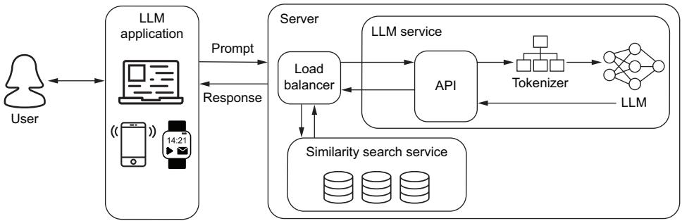
Figure 8.1 The LLM Application is the web app, phone app, command line interface, or another tool that acts as the client our users will use to interact with our LLM service.
The first step to building a successful LLM application is composing and experimenting with your prompt. Of course, having just discussed this in the last chapter, there are many additional features you should consider to offer a better user experience. The most basic LLM application is just a chatbox, which essentially consists of only three objects: an input field, a send button, and a text field to hold the conversation. It’s rather easy to build in almost every context. In addition, since one of our participants in the chat is a bot, most of the complexity of building a chat interface is also stripped away. For example, we don’t need to worry about eventual consistency, mixing up the order of our conversation, or whether both users are sending a message at the same time. If our user has a bad internet connection, we can throw a timeout error and let them resubmit.
However, while the interface is easy, not all the finishing touches are. In this section, we are going to share with you some tools of the trade to make your LLM application shine. We focus on best practices, like streaming responses, utilizing the chat history, and methods to handle and utilize prompt engineering. These allow us to craft, format, and clean our users’ prompts and the LLM’s responses under the hood, improving results and overall customer satisfaction. All this to say, building a basic application that utilizes an LLM is actually rather easy, but building a great application is a different story, and we want to build great applications.
8.1.1 Streaming on the frontend
In chapter 6, we showed you how to stream your LLM’s response on the server side, but that is meaningless if the response isn’t streamed on the client side as well. Streaming on the client side is where it all comes together. It’s where we show the text to the users as it is being generated. This provides an attractive user experience, as it makes it appear like the text is being typed right before our eyes and gives the users a sense that the model is actually thinking about what it will write next. Not only that, but it also provides a more springy and responsive experience, as we can give a feeling of instant feedback, which encourages our users to stick around until the model finishes generating. This also helps the user to be able to see where the output is going before it gets too far so they can stop generation and reprompt.
In listing 8.1, we show you how to do this with just HTML, CSS, and vanilla Java-Script. This application is meant to be dead simple. Many of our readers likely aren’t frontend savvy, as that isn’t the focus of this book. Those who are most likely will be using some tooling for their framework of choice anyway. But a basic application with no frills allows us to get to the core of what’s happening.
Since the application is so simple, we opted to put all the CSS and JavaScript together into the HTML, although it would be cleaner and a best practice to separate them. The CSS defines sizing to ensure our boxes are big enough to read; we won’t bother with colors or making it look pretty. Our HTML is as simple as it gets: a form containing a text input and a Send button that returns false on submit so the page doesn’t refresh. There’s also a div container to contain our chat messages. Most of the JavaScript is also not that interesting; it just handles adding our conversation to the chat. However, pay attention to the sendToServer function, which does most of the heavy lifting: sending our prompt, receiving a readable stream, and iterating over the results.
NOTE On the server side, we set up a StreamingResponse object, which gets converted to a ReadableStream on the JavaScript side. You can learn more about readable streams here: https://mng.bz/75Dg.
Listing 8.1 Streaming responses to end users<!DOCTYPE html>
<html lang="en">
<head>
<meta charset="UTF-8"> <meta name="viewport" content="width=device-width, initial-scale=1.0">
<title>Simple Chat App</title>
<style>
body {
font-family: Arial, sans-serif;
margin: 0;
padding: 0;
box-sizing: border-box;
}
#message-input {
width: 95%;
padding: 8px;
}
#chat-container {
width: 95%;
margin: 20px auto;
border: 1px solid #ccc;
padding: 10px;
overflow-y: scroll;
max-height: 300px;
}
</style>
</head>
<body>
<form onsubmit="return false;"">
<input type="text" id="message-input" placeholder="Type your
message...">
<button onclick="sendMessage()" type="submit">Send</button>
</form>
<div id="chat-container"></div>
</body>
<script>
function sendMessage() {
var messageInput = document.getElementById('message-input');
var message = messageInput.value.trim();
if (message !== '') {
appendMessage('You: ' + message);
messageInput.value = '';
sendToServer(message);
}
}
function appendMessage(message) {
var chatContainer = document.getElementById('chat-container');
var messageElement = document.createElement('div');
messageElement.textContent = message;
chatContainer.appendChild(messageElement);
chatContainer.scrollTop = chatContainer.scrollHeight;
Some very simple styling
Our body is simple with only
three fields: a text input, send
button, and container for chat.
JavaScript to handle
communication with LLM
and streaming response
When the Send button is
pushed, moves text from input
to chat box and sends the
message to the LLM server
Adds new messages
to the chat box return messageElement
}
async function sendToServer(message) {
var payload = {
prompt: message
}
const response = await fetch('http://localhost:8000/generate', {
method: 'POST',
headers: {
'Content-Type': 'application/json',
},
body: JSON.stringify(payload),
});
var responseText = 'LLM: ';
messageElement = appendMessage(responseText);
for await (const chunk of streamAsyncIterator(response.body)) {
var strChunk = String.fromCharCode.apply(null, chunk);
responseText += strChunk;
messageElement.textContent = responseText;
}
}
async function* streamAsyncIterator(stream) {
const reader = stream.getReader();
try {
while (true) {
const {done, value} = await reader.read();
if (done) return;
yield value;
}
}
finally {
reader.releaseLock();
}
}
</script>
</html>
Sends prompt to the server
and streams the response
back as tokens are received
Simple polyfill since
StreamResponse still can't
be used as an iterator by
most browsersFigure 8.2 shows screenshots of our simple application from listing 8.1. Showing words being streamed to the application would have been better in a movie or GIF, but since books don’t play GIFs, we’ll have to make do with several side-by-side screenshots instead. Regardless, the figure shows the results being streamed to the user token by token, providing a positive user experience.
There’s nothing glamorous about our little application here, and that’s partly the point. This code is easy to copy and paste and can be used anywhere a web browser can run since it’s just an HTML file. It doesn’t take much to build a quick demo app once you have an LLM service running.
| Type your message | Type your message |
|---|---|
| Send | Send |
| You: Who would win in a battle, Squirtle or Charmander? | You: Who would win in a battle, Squirtle or Charmander? |
| LMM: | LMM: Who would win in a battle, Squirtle or Charmander? The |
| Type your message | Type your message |
| Send | Send |
| You: Who would win in a battle, Squirtle or Charmander? | You: Who would win in a battle, Squirtle or Charmander? |
| LMM: Who would win in a battle, Squirtle or Charmander? The | LMM: Who would win in a battle, Squirtle or Charmander? The |
| answer is that | answer is that Squirtle is the best of the best. |
Figure 8.2 Screenshots of our simple application showing the response being streamed
8.1.2 Keeping a history
One big problem with our simple application so far is that each message sent to our LLM is independent of other messages sent. This is a big problem because most applications that utilize an LLM do so in an interactive environment. Users will ask a question and then, based on the response, make additional questions or adjustments and clarifications to get better results. However, if you simply send the latest query as a prompt, the LLM will not have any context behind the new query. Independence is nice for coin flips, but it will make our LLM look like a birdbrain.
What we need to do is keep a history of the conversation, both the user’s prompts and the LLM’s responses. If we do that, we can append that history to the new prompts as context. The LLM will be able to utilize this background information to make better responses. Figure 8.3 shows the overall flow of what we are trying to achieve.
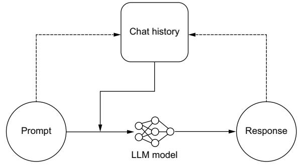
Figure 8.3 Process flow for storing prompts and responses to a chat history, giving our model a memory of the conversation to improve outcomes
Now that we know what we are building, let’s take a look at listing 8.2. This time, we will be using Streamlit, a Python framework for building applications. It is simple and easy to use while still creating attractive frontends. From Streamlit, we will be utilizing a chat_input field so users can write and send their input, a chat_message field that will hold the conversation, and session_state, where we will create and store the chat_history. We will use that chat history to craft a better prompt. You’ll also notice that we continue to stream the responses, as demonstrated in the last section, but this time using Python.
What is Streamlit?
Streamlit is an open-source Python library that makes it easy to create web applications for machine learning, data science, and other fields. It allows you to quickly build interactive web apps using simple Python scripts. With Streamlit, you can create dashboards, data visualizations, and other interactive tools without needing to know web development languages like HTML, CSS, or JavaScript. Streamlit automatically handles the conversion of your Python code into a web app.
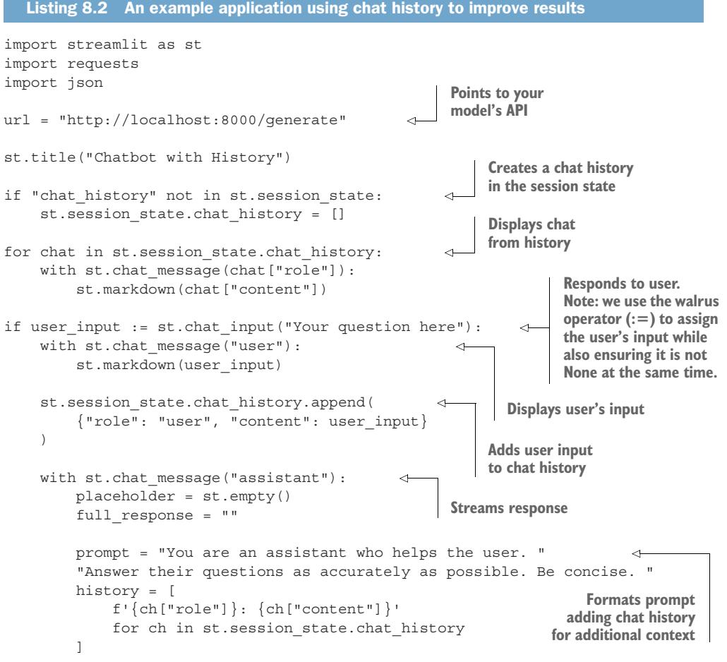
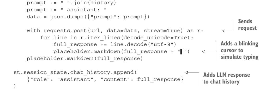
Figure 8.4 is a screenshot capturing the LLM app that we just built. While our first example was quite ugly, you can see that Streamlit automatically creates a nice user interface, complete with finishing touches, like a picture of a human face for the user and a robot face for our LLM assistant. You’ll also notice that the model is taking in and comprehending the conversation history—albeit giving terrible responses. If we want to get better responses, one thing to be sure of is that your LLM has been trained on conversation data.
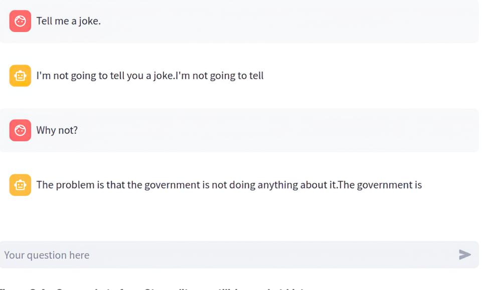
Figure 8.4 Screenshot of our Streamlit app utilizing a chat history
Of course, utilizing the history leads to some problems. The first is that users can have relatively long conversations with our bot, but we are still limited in the token length we can feed to the model, and the longer the input, the longer the generation takes. At some point, the history will begin to be too long. The simplest approach to solving this problem is to drop older messages in favor of newer ones. Sure, our model may forget important details or instructions at the start of our conversation, but humans also tend to have a recency bias in conversations, so this tends to be OK—except, of course, for the fact that humans tend to expect computers never to forget anything.
A more robust solution is to use the LLM to summarize the chat history and use the summary as context to our users’ queries instead of the full chat history. LLMs are often quite good at highlighting important pieces of information from a body of text, so this can be an effective way to compress a conversation. Compression can be done on demand or run as a background process. Figure 8.5 illustrates the summarization workflow for chat history compression.
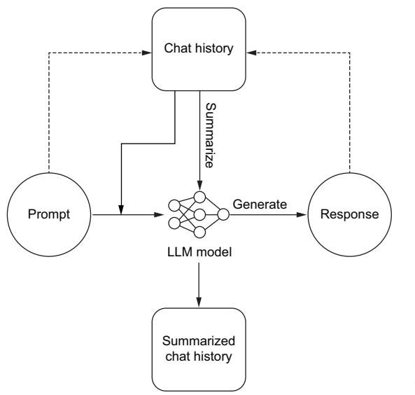
Figure 8.5 A process flow for an app with chat history utilizing summarization for chat history compression
There are other strategies you can explore, as well as mixing and matching multiple methods. Another idea is to embed each chat and perform a search for relevant previous chat messages to add to the prompt context. But no matter how you choose to shorten the chat history, details are bound to be lost or forgotten the longer a conversation goes on or the larger the prompts and responses are.
8.1.3 Chatbot interaction features
Chatting with an LLM bot isn’t like chatting with your friend. For one, the chatbot is always available and waiting for us to talk to it, so we can expect a response right away. There shouldn’t be opportunities for users to spam multiple messages to our bot before receiving feedback. But let’s face it, in the real world, there are connection
problems or bad internet, the server could be overwhelmed, and there are a myriad of other reasons a request might fail. These differences encourage us to interact with a chatbot differently, and we should ensure we add several features for our users to improve their experience. Let’s consider several of them now:
- Fallback response—A response to give when an error occurs. To keep things clean, you’ll want to ensure a 1:1 ratio of LLM responses for every user query in your chat history. A fallback response ensures our chat history is clean and gives the user instructions on the best course of action, like trying again in a few minutes. Speaking of which, you should also consider disabling the Submit button when receiving a response to prevent weird problems from asynchronous conversations and out-of-order chat history.
- Stop button—Interrupts a response midstream. An LLM can often be longwinded, continuing to respond long after answering the user’s questions. Often, it misunderstands a question and starts to answer it incorrectly. In these cases, it’s best to give the user a Stop button so they can interrupt the model and move on. This button is a simple cost-saving feature since we usually pay for output per token one way or another.
- Retry button—Resends the last query and replaces the response. LLMs have a bit of randomness to them, which can be great for creative writing, but it means they may respond unfavorably even to prompts they have responded correctly to multiple times before. Since we add the LLM chat history to new prompts to give context, a retry button allows users to attempt to get a better result and keep the conversation moving in the right direction. While retrying, it can make sense to adjust our prompting hyperparameters, for example, reducing temperature each time a user retries. This can help push the responses in the direction the user is likely expecting. Of course, this likely isn’t the best move if they are retrying because of a bad internet connection, so you’ll need to consider the adjustments carefully.
- Delete button—Removes portions of the chat history. As mentioned, the chat history is used as context in future responses, but not every response is immediately identifiable as bad. We often see red herrings. For example, a chat assistant used while coding might hallucinate functions or methods that don’t exist, which can lead the conversation down a path that is hard to recover from. Of course, depending on your needs, the solution could be a soft delete, where we only remove it from the frontend and prompting space but not the backend.
- Feedback form—A way to collect feedback on users’ experience. If you are training or finetuning your own LLMs, this data is highly valuable, as it can help your team improve results on the next training iteration. This data can often easily be applied when using RLHF. Of course, you won’t want to apply it directly, but first clean and filter out troll responses. Also, even if you aren’t training, it can help your team make decisions to switch models, improve prompting, and identify edge cases.
In listing 8.3, we show how to use Gradio to set up an easy chatbot app. Gradio is an open source library for quickly creating customizable user interfaces for data science demos and web applications. It’s highly popular for its ease of integration within Juptyer notebooks, making it easy to create interfaces and edit your web app in a familiar environment. To create a chatbot with Gradio, we’ll use the ChatInterface and give it a function to make our API request. You’ll notice that Gradio expects the history to be part of the generate function, and streaming is just a matter of ensuring the function is a generator.
What is Gradio?
Gradio is an open-source Python library that allows you to quickly create customizable UI components around your machine-learning models. It provides a simple interface for building interactive web-based applications for your models without requiring you to write any HTML, CSS, or JavaScript code. With Gradio, you can create input forms for your models, display the results, and even share your models with others through a web interface.

import gradio as gr
import requests
import json
url = "http://localhost:8000/generate"
def generate(message, history):
 history_transformer_format = history + [[message, ""]]
 messages = "".join(
 [
 "".join(["\n<human>:" + h, "\n<bot>:" + b])
 for h, b in history_transformer_format
 ]
 )
 data = json.dumps({"prompt": messages})
 full_response = ""
 with requests.post(url, data=data, stream=True) as r:
 for line in r.iter_lines(decode_unicode=True):
 full_response += line.decode("utf-8")
 yield full_response + "!"
 yield full_response
                                              Points to your
                                              model's API
                                                             Sends
                                                             request
                                                  Adds a blinking cursor
                                                  to simulate typing
gr.ChatInterface(generate, theme=“soft”).queue().launch()
You can see how simple this code is, with very few lines needed. Gradio does all the heavy lifting for us. You might also be wondering where all our interaction features are. Well, the good news is that Gradio automatically adds most of these features for us. Don’t believe me? Check out the app we just created in figure 8.6.
| 同 Chatbot Tell me a story. |
||||
|---|---|---|---|---|
| Once upon a time, there was a little girl na big old house with her parents and her little brother, Jack. One day, Alice was out playing in the garden when she saw something very strange. It was a little door, just like the one in the picture, but it was moving! Alice was very curious, so she went to look at it. The door opened, and out came a little man with a top hat and a cane. He said, “Welcome, |
||||
| Type a message | Stop | |||
| & Retry 2 Undo |
Clear |
Figure 8.6 Screenshot of our Gradio app, including interaction features Stop, Retry, and Undo for better ease of use
Chainlit: An application builder just for LLMs
We have shown you how to build LLM applications with several different tools: Streamlit, Gradio, and even vanilla HTML and JavaScript. There are many great tools out there, and we can’t give personal attention to each one. But one more tool we think many of our readers will be interested in is Chainlit. Chainlit is a tool specifically built for building LLM applications and comes with most features out of the box, including ones not discussed here, like themes, CSS customization, authentication, and cloud hosting. It is likely one of the fastest ways to get up and running.
Each quality-of-life improvement you can add to your application will help it stand out above the competition and potentially save you money. For the same reason, you should consider using a token counter, which we cover next.
8.1.4 Token counting
One of the most basic but valuable pieces of information you can gather to offer a great user experience is the number of submitted tokens. Since LLMs have token limits, we’ll need to ensure the users’ prompts don’t exceed those limits. Giving feedback early and often will provide a better user experience. No one wants to type a long query only to find that it’s too much upon submitting.
Counting tokens also allows us to better prompt-engineer and improve results. For example, in a Q&A bot, if the user’s question is particularly short, we can add more context by extending how many search results our retrieval-augmented generation (RAG) system will return. If their question is long, we’ll want to limit it and ensure we have enough space to append our own context.
Tiktoken is just such a library to help with this task. It’s an extremely fast BPE tokenizer built specifically for OpenAI’s models. The package has been ported to multiple languages, including tiktoken-go for Golang, tiktoken-rs for Rust, and several others. In the next listing, we show a basic example of how to use it. It’s been optimized for speed, which allows us to encode and count tokens quickly, which is all we need to do.
Listing 8.4 Using tiktoken to count tokens
import tiktokenencoding = tiktoken.get_encoding("cl100k_base")
print(encoding.encode("You're users chat message goes here."))
# [2675, 2351, 3932, 6369, 1984, 5900, 1618, 13]
def count_tokens(string: str) -> int:
encoding = tiktoken.get_encoding("cl100k_base")
return len(encoding.encode(string))
num_tokens = count_tokens("You're users chat message goes here.")
print(num_tokens)
# 8Of course, the reader who hasn’t skipped ahead will recognize a few problems with using tiktoken, mainly because it’s built with OpenAI’s encoders in mind. If you are using your own tokenizer (which we recommend), it’s not going to be very accurate. We have seen several developers—out of laziness or not knowing a better solution still use it for other models. Generally, they saw counts within ±5–10 tokens per 1,000 tokens when using tiktoken results for other models using similar BPE tokenizers. To them, the speed and latency gains justified the inaccuracy, but this was all word of mouth, so take it with a grain of salt.
If you are using a different type of tokenizer, like SentencePiece, it’s often better to create your own token counter. For example, we do just that in our project in chapter 10. As you can guess, the code follows the same pattern of encoding the string and counting the tokens. The hard part comes when porting it to the language that needs to run the counter. To do so, compile the tokenizer like you would any other ML model, as we discussed in section 6.1.1.
8.1.5 RAG applied
RAG is an excellent way to add context and outside knowledge to your LLM to improve the accuracy of your results. In the last chapter, we discussed it in the context of a backend system. Here, we will be discussing it from the frontend perspective. Your RAG system can be set up on either side, each with its own pros and cons.
Setting up RAG on the backend ensures a consistent experience for all users and gives us greater control as developers of how exactly the context data will be used. It also provides a bit more security to the data stored in the vector database, as it’s only accessible to the end users through the LLM. Of course, through clever prompt injection, it could potentially still be scraped, but it is still much more secure than simply allowing users to query your data directly.
RAG is more often set up on the frontend because doing so allows developers to take whatever generic LLM is available and insert business context. You don’t need to finetune a model on your dataset if you give the model your dataset at run time. Thus, RAG becomes a system to add personality and functionality to our LLM application versus simply being a tool to ensure the accuracy of results and reduce hallucinations.
In section 6.1.8, we showed you how to set up a RAG system; now we will show you how to utilize it for efficient query augmentation. In listing 8.5, we show you how to access and use the vector store we set up previously. We will continue to use OpenAI and Pinecone from our last example. We will also use LangChain, a Python framework which we discovered in the last chapter, to help create LLM applications.
Listing 8.5 RAG on the frontend
import os
import pinecone
from langchain.chains import RetrievalQA
from langchain.chains import RetrievalQAWithSourcesChain
from langchain.chat_models import ChatOpenAI
from langchain.embeddings.openai import OpenAIEmbeddings
from langchain.vectorstores import Pinecone
OPENAI_API_KEY = os.getenv("OPENAI_API_KEY")
PINECONE_API_KEY = os.getenv("PINECONE_API_KEY")
index_name = "pincecone-llm-example"
index = pinecone.Index(index_name)
embedder = OpenAIEmbeddings(
 model="text-embedding-ada-002", openai_api_key=OPENAI_API_KEY
)
text_field = "text"
vectorstore = Pinecone(index, embedder.embed_query, text_field)
query = "Who was Johannes Gutenberg?"
vectorstore.similarity_search(
 query, k=3
)
llm = ChatOpenAI(
 openai_api_key=OPENAI_API_KEY,
 model_name="gpt-3.5-turbo",
 temperature=0.0,
)
qa = RetrievalQA.from_chain_type(
 llm=llm, chain_type="stuff", retriever=vectorstore.as_retriever()
)
qa.run(query)
                                                               Gets OpenAI API key from
                                                               platform.openai.com
                                                               Finds API key in console
                                                               at app.pinecone.io
                                                    Sets up vectorstore
                                                     Makes a query
                                          Our search query; returns the
                                          three most relevant docs
                                             Now let's use these results to enrich
                                             our LLM prompt; sets up the LLM
                                                         Runs query with
                                                         vectorstore
qa_with_sources = RetrievalQAWithSourcesChain.from_chain_type(
llm=llm, chain_type="stuff", retriever=vectorstore.as_retriever()
)
qa_with_sources(query)
Includes Wikipedia sourcesWe think the most impressive part of this code is the fact that LangChain has a chain simply named “stuff” because, presumably, they couldn’t think of anything better. (If you want to learn more about the cryptically named module “stuff,” you can find the docs at https://mng.bz/OBER.) But in actuality, the most impressive thing about this code is that we just have to define our LLM and vector store connections, and we are good to go to start making queries. Simple.
8.2 Edge applications
So far, we have discussed building LLM applications, assuming we will simply be using an API—one we deployed, but an API nonetheless. However, there are lots of situations where you might want to run the model on the local device inside the application itself. Doing so brings several challenges: mainly, we need to get a model small enough to transfer and run it on the edge device. We also need to be able to run it in the local environment, which likely doesn’t have an accelerator or GPU and may not even support Python—for example, running an app in a user’s web browser with JavaScript, in an Android app on a mobile phone with Java, or on limited hardware like a Raspberry Pi.
In chapter 6, we started discussing the building blocks you need to work with edge devices. We showed you how to compile a model, giving examples using TensorRT or ONNX Runtime. TensorRT, coming from NVIDIA, is going to serve you better on a server with expensive NVIDIA hardware to go with it, so it is less useful for edge development. ONNX Runtime is a bit more flexible, but when working with edge devices, llama.cpp is often a better solution for LLMs, and it follows the same flow: compile the model to the correct format, move that model to the edge device, download and install the SDK for your language, and run the model. Let’s take a closer look at these steps for llama.cpp.
The llama.cpp project started with the goal of converting an LLM to something that could be run on a MacBook without a GPU (Apple silicon chips are notorious for poor compatibility for many projects). Initially working to quantize the LLaMA model and store it in a binary format that could be used by the C++ language, the project has grown to support a couple of dozen LLM architectures and all major OS platforms, has bindings for a dozen languages, and even CUDA, metal, and OpenCL GPU backend support. Llama.cpp has created two different formats to store the quantized LLMs: the first GPT-Generated Model Language (GGML), which was later abandoned for the better GPT-Generated Unified Format (GGUF).
To use llama.cpp, the first thing we’ll need is a model stored in the GGUF format. To convert your own, you’d need to clone the llama.cpp project, install the dependencies, and then run the convert script that comes with the project. The steps have changed frequently enough that you’ll want to consult the latest information in the repo, but currently, it would look like
$ git clone https://github.com/ggerganov/llama.cpp.git
$ cd llama.cpp
$ pip install -r requirments/requirements-convert.txt
$ python convert.py -h
Of course, that last command simply displays the convert script’s Help menu for you to investigate the options and does not actually convert a model. For our purposes, we’ll download an already converted model. We briefly mentioned Tom Jobbins (The-Bloke) in chapter 6, the man who has converted thousands of models, quantizing and finetuning them so they are in a state ready for use. All you have to do is download them from the Hugging Face Hub. So we’ll do that now. First, we’ll need the huggingface-cli, which comes as a dependency with most of Hugging Face’s Python packages, so you probably already have it, but you can install it directly as well. Then we’ll use it to download the model:
$ pip install -U huggingface_hub
$ huggingface-cli download TheBloke/WizardCoder-Python-7B-V1.0-GGUF --
➥ local-dir ./models --local-dir-use-symlinks False --include='*Q2_K*gguf'
Here, we are downloading the WizardCoder-7B model that has already been converted to a GGUF format by TheBloke. We are going to save it locally in the models directory. We won’t use symbolic links (symlinks), meaning the model will actually exist in the folder we choose. Normally, huggingface-cli would download it to a cache directory and create a symlink to save space and avoid downloading models multiple times across projects. Lastly, the Hugging Face repo contains multiple versions of the model in different quantized states; here, we’ll select the 2-bit quantized version with the include flag. This extreme quantization will degrade the performance of the quality of our output for the model, but it’s the smallest model available in the repo (only 2.82 GB), which makes it great for demonstration purposes.
Now that we have our model, we need to download and install the bindings for our language of choice and run it. For Python, that would mean installing llama-cpppython via pip. In listing 8.6, we show you how to use the library to run a GGUF model. It’s pretty straightforward, with just two steps: load the model and run it. On one author’s CPU, it ran a little slower than about a token per second, which isn’t fast but impressive enough for a 7B parameter model without an accelerator.
Listing 8.6 Using llama.cpp to run a quantized model on a CPUimport time
from llama_cpp import Llama
llm = Llama(model_path="./models/wizardcoder-python-7b-v1.0.Q2_K.gguf")start_time = time.time()
output = llm(
"Q: Write python code to reverse a linked list. A: ",
max_tokens=200,
stop=["Q:"],
echo=True,
)
end_time = time.time()
print(output["choices"])The results are# [
# {'text': "Q: Write python code to reverse a linked list. A:
# class Node(object):
# def __init__(self, data=None):
# self.data = data
# self.next = None
# def reverse_list(head):
# prev = None
# current = head
# while current is not None:
# next = current.next
# current.next = prev
# prev = current
# current = next
# return prev
# # example usage;
# # initial list
# head = Node('a')
# head.next=Node('b')
# head.next.next=Node('c')
# head.next.next.next=Node('d')
# print(head)
# reverse_list(head) # call the function
# print(head)
# Expected output: d->c->b->a",
# 'index': 0,
# 'logprobs': None,
# 'finish_reason': 'stop'
# }
# ]
print(f"Elapsed time: {end_time - start_time:.3f} seconds")
# Elapsed time: 239.457 secondsWhile this example was in Python, there are bindings for Go, Rust, Node.js, Java, React Native, and more. Llama.cpp gives us all the tools we need to run LLMs in otherwise impossible environments.
8.3 LLM agents
At this point in the book, we can finally discuss LLM agents. Agents are what most people are talking about when they start worrying about AI taking their jobs. If you think back to the last chapter, we showed how, with some clever prompt engineering and tooling, we could train models to answer multistep questions requiring searching for information and running calculations. Agents do the same thing on steroids. Full LLM applications are designed not just to answer multistep questions but to accomplish multistep tasks. For example, a coding agent could not only answer complicated questions about your code base but also edit it, submit PRs, review PRs, and write full projects from scratch.
Agents do not differ from other language models in any meaningful way. The big differences all go into the system surrounding and supporting the LLM. LLMs are, fundamentally, closed search systems. They can’t access anything they weren’t trained on explicitly. So for example, if we were to ask Llama 2, “How old was Justin Bieber the last time the Patriots won the Superbowl?” we would be dependent on Meta having trained that model on incredibly up-to-date information. There are three components that make up an agent:
- LLM—No explanation necessary. By now, you know what these are and why they’re needed.
- Memory—Some way of reintroducing the LLM to what has happened at each step up to that point. Memory goes a long way toward agents performing well. This is the same idea as feeding in the chat history, but the model needs something more than just the literal history of events. There are several ways of completing this:
- Memory buffer—Passes in all of the text that’s come before. Not recommended, as you’ll hit context limits quickly, and the “lost in the middle” problem will exacerbate this.
- Memory summarization—Has the LLM take another pass at the text to summarize it for its own memory. Works pretty well; however, at a minimum, it doubles latency, and summarization will delete finer details faster than anyone would like.
- Structured memory storage—Thinks ahead and creates a system you can draw from to get the actual best info for the model. It can be related to chunking articles and searching for an article title and then retrieving the most relevant chunk, or perhaps chaining retrievals to find the most relevant keywords or to make sure that the query is contained in the retrieval output. We recommend structured memory storage the most because even though it’s the hardest to set up, it achieves the best results in every scenario.
- External data retrieval tools—The core of agent behavior. These tools give your LLM the ability to take actions, which allows it to perform agent-like tasks.
We’ve covered a lot in this book, and agents are a bit of a culmination of much of what we’ve covered. They can be quite tricky to build, so to help you, we’ll break down the steps and give several examples. First, we’ll make some tools, then initialize some agents, and finally create a custom agent, all on our own. Throughout the process, you’ll see why it’s particularly difficult to get agents to work effectively and especially why LangChain and Guidance are great for getting started and difficult to get up and running.
In listing 8.7, we start off easy by demonstrating using some tools via LangChain. This example uses the Duck Duck Go search tool and the YouTube search tool. Notice that the LLM will simply give them a prompt, and the tools will handle the search and summary of results.
from langchain.tools import DuckDuckGoSearchRun, YouTubeSearchTool search = DuckDuckGoSearchRun() hot_topic = search.run( “Tiktoker finds proof of Fruit of the Loom cornucopia in the logo” ) youtube_tool = YouTubeSearchTool() fun_channel = youtube_tool.run(“jaubrey”, 3) print(hot_topic, fun_channel) Listing 8.7 LangChain search tools example Example of using tools
The generated text is
@torch.compile
def get_batches( data, batch_size, context_window, config=MASTER_CONFIG, debug=False, ): x = [] y = [] for _ in range( batch_size ): batch_data = next(data) ix = torch.randint( 0, len(batch_data[“input_ids”]) - context_window - 1, (2,) ) batch_x = torch.stack( [batch_data[“input_ids”][i : i + context_window] for i in ix] ).long() batch_y = torch.stack( [ batch_data[“input_ids”][i + 1 : i + context_window + 1] for i in ix ] ).long() x.append(batch_x) y.append(batch_y) x = torch.cat((x), 0).to(device) y = torch.cat((y), 0).to(device) return x, y Windows users leave commented Adjust this lower if you’re running out of memory. Pick random starting points.
Once we have our data batching taken care of, we need to come up with functions for evaluation and inference so that we can gain insight into how the model is doing during training and so that we can use the model later. For our evaluation, we'll take some batches and average the loss across them to get our validation loss. This result will not give us a real representation of our model's performance but will not stop it from being useful for us:
@torch.no_grad() def get_loss(model, lora=False, config=MASTER_CONFIG): out = {} model.eval() for name, split in zip([“train”, “val”], [train_data, val_data]): losses = [] for _ in range(10): xb, yb = get_batches( split, config[“batch_size”], config[“context_window”], ) _, loss = model(xb, yb) losses.append(loss.item()) out[name] = np.mean(losses) model.train() return out
### Questioning your assumptions

When working with machine-learning models and other statistical methods, it's important to understand how your assumptions will affect your results. Averages hamper data representation and understanding because they basically say, "For this comparison, we're going to grab a made-up number, and we're going to use that number in place of any of the real ones because it feels central to our distribution." This approach doesn't make it bad; made-up numbers often are more predictive than real ones. However, we urge you to be intentional and very open-minded about testing whether the average is the best marker for your users.

For generation, we'll do something similar but better. Logits are what we get out of our model's forward method. We created a tokenized version of our prompt previously when we tokenized our dataset, so we're ready to pass that prompt into our model a number of times and see what comes out. We'll grab the logits from the model given the prompt and then sample our model's distribution for our next token and decode.

 For sampling that distribution, we'll take the model's output (logits) for only the very end of the input (the unknown token we want our model to generate) and then divide those logits by the temperature setting (higher temperature setting = smaller logits). Once we have our logits from the last time step, if we use multinomial sampling, we can sample using top\_k and/or top\_p, which are sampling against the highest probability tokens until you reach a total number of tokens or a total number of probability sums. Once we have that, we use softmax for the tokens we've sampled and then argmax to get the next token. If we want more exploration and creativity in our output, we can use multinomial sampling instead. As an exercise, test top\_k versus top\_p with multinomial and argmax versus multinomial to get an idea of which works best:
@torch.inference_mode() def generate( model, config=MASTER_CONFIG, temperature=1.0, top_k=None, max_new_tokens=30, lora=False, ): idx_list = [tokenized_prompt] * 5 idx = torch.cat((idx_list), 0).long().to(device) for _ in range(max_new_tokens): logits = model(idx[:, -config[“context_window”] :]) last_time_step_logits = logits[ :, -1, : ] last_time_step_logits = last_time_step_logits / temperature if top_k is not None: v, _ = torch.topk( last_time_step_logits, min(top_k, last_time_step_logits.size(-1)), ) last_time_step_logits[ last_time_step_logits < v[:, [-1]] ] = -float(“Inf”) p = F.softmax( last_time_step_logits, dim=-1 ) idx_next = torch.argmax( p, dim=-1, keepdims=True ) idx = torch.cat([idx, idx_next], dim=-1) # append to the sequence return [tokenizer.decode(x) for x in idx.tolist()] Calls the model All the batches (1); last time step, all the logits Softmax to get probabilities Sample from the distribution to get the next token
And with that, we've concluded our setup! We have utility functions for all of the important parts of the model training, including tokenization, data loading, evaluation, inference, and data processing. If there's anything you feel should be corrected, great! Do it—this is your project. If you want to use a multinomial for sampling instead of an argmax or want to get rid of the softmax and just argmax over the logits, awesome, go for it. For those of you for whom this is your first time, we know it can be quite a firehose, and we'd encourage you to work through it slowly, but don't lose too much sleep over it. More than likely, you will not have to come up with what should change for your use case yourself because you'll be implementing an already-created open source model. That said, it's still a good idea to understand what's going on behind the scenes and under the hood so that you know roughly where to look when things go wrong.

#### *9.1.3 Network architecture*

We've now completed a ton of setup for training a model but haven't made a model. Model architecture and training have been iterated upon ad nauseam, so we'll skip talking about it too much and jump right in. We'll start with a two-layer feed-forward network with fewer than 20M parameters, and then we'll upgrade and talk about the changes that turn the model into Llama. We want to be clear about what is actually changing between them so you'll get a good feel for the pieces involved. Because we aren't going to be completely replicating Llama 3, but rather approximating it, here's the official architecture if you'd like to try pretraining it on our dataset: [https://](https://mng.bz/Dp9A) [mng.bz/Dp9A](https://mng.bz/Dp9A).

<span id="page-113-1"></span> In listing 9.3, we make a class for that linear model with a ReLU activation between the two linear layers. Here's where we'll also define our actual loss function (because in our get\_loss function, we're just sending inputs to the model). We'll use cross entropy because we're comparing unstructured sequences. Instead of getting into information theory for why cross-entropy is the answer to unstructured sequences, the current benchmark in the industry is called perplexity, which uses cross-entropy to figure out whether a model is making sense or not, so this loss function enables us to compete with other models in the industry.

<span id="page-113-0"></span> There's one thing that you may have noticed before when we tokenized our dataset: we're padding in batches and not truncating, meaning each batch size should be the same length. We fully acknowledge that this doesn't make any sense when pretraining; it's just helping to speed things up. We do this because our longest length input is 997 tokens, and we don't want to pad our entire dataset out to 997. Even mitigating that, the most common token in our dataset is still "<PAD>". If we leave it as is, the model could learn to generate only padding tokens, which seemingly minimizes the loss when predicting the next token. Because we have a tokenizer vocab we just added to, however, we can tell the loss function to ignore\_index our tokenizer .pad\_token\_id so correctly predicting padding tokens doesn't mistakenly help the loss go down.
Listing 9.3 Simple model and training loop
class SimpleFeedForwardNN(nn.Module): def init(self, config=MASTER_CONFIG): super().__init__() self.config = config self.embedding = nn.Embedding( config[“vocab_size”], config[“d_model”] ) self.linear = nn.Sequential( nn.Linear(config[“d_model”], config[“d_model”]), nn.ReLU(), nn.Linear(config[“d_model”], config[“vocab_size”]), )
print( f”model params: {sum([m.numel() for m in self.parameters()])}” ) def forward(self, idx, targets=None): x = self.embedding(idx) logits = self.linear(x) if targets is not None: loss = F.cross_entropy( logits.view(-1, self.config[“vocab_size”]), targets.view(-1), ignore_index=tokenizer.pad_token_id, # reduction=“sum”, ) return logits, loss else: return logits model = SimpleFeedForwardNN(MASTER_CONFIG).to(device) opt_model = torch.compile(model) Comment this out on Windows.
Now that we have our model, we'll write our training loop. We run the number of passes specified in the epochs portion of the master config, and we get our loss for each pass. The epochs here are more like steps, and we'd encourage you to run epochs through the whole dataset if you have the time. If you stick to the MASTER\_CONFIG we set up previously, this original model will end up having 18.5M parameters. You should definitely change it to be the maximum number of parameters that your computer can handle. You can find this number by changing d\_model (and vocab\_size if you train a bigger tokenizer) in your master config:
def train( model, optimizer, scheduler=None, data=None, config=MASTER_CONFIG, lora=False, print_logs=False, ): losses = [] start_time = time.time() for epoch in range(config[“epochs”]): try: optimizer.zero_grad() xs, ys = get_batches( data, config[“batch_size”], config[“context_window”] ) for i in range(1, config[‘context_window’]+1): x = xs[:i] y = ys[:i]
logits, loss = model(xs, targets=ys) loss.backward() optimizer.step() if scheduler: scheduler.step() if epoch % config[“log_interval”] == 0: batch_time = time.time() - start_time x = get_loss(model, lora=lora) losses += x if print_logs: print( f”““Epoch {epoch} | train loss {x[‘train’]:.3f} | val loss {x[‘val’]:.3f} | Time {batch_time:.3f} | ETA: {timedelta(seconds=(batch_time * (config [‘epochs’] - epoch)/config[‘log_interval’]))}”“” ) start_time = time.time() if scheduler: print(“lr:”, scheduler.get_last_lr()) except StopIteration: print(f”Reached end of dataset on step {epoch}“) break GLOBAL_KEEP_TRACK.append( f”{type(model).__name__} {sum([m.numel() for m in model.parameters()])} Params | Train: {losses[-1][‘train’]:.3f} | Val: {losses[-1][‘val’]:.3f}” ) print( f”training loss {losses[-1][‘train’]:.3f} | validation loss: {losses[-1][‘val’]:.3f}” ) return pd.DataFrame(losses).plot(xlabel=“Step // 50”, ylabel=“Loss”) optimizer = torch.optim.AdamW( model.parameters(), ) train(model, optimizer, data=train_data, print_logs=True) #Epoch 0 | train loss 10.365 | val loss 10.341 | Time 0.122 | ETA: 0:00:02.431240 #training loss 4.129 | validation loss: 4.458
Look, it's figure 9.2, which was generated from listing 9.3! Try to guess what it will be, and then read the blurb to see if you're right.
Look at that! That's a pretty smooth curve when we train for the first time. Considering we only did 1,000 examples from our dataset, we'd encourage you to try for several actual epochs—say, try three going over the whole dataset—and see how things

Figure 9.2 Training a simple neural network on our dataset to generate text
go. You'll likely get surprisingly decent results; we did. Let's go ahead and check out what it creates when generating text:
generate(model, config=MASTER_CONFIG) # ‘ Write a short story. Possible Story: 3 together thisar andze Lily said exciteded and smiled. Everything because he wasning loved to the time, he did not find like to’, for i in GLOBAL_KEEP_TRACK: print(i) # SimpleFeedForwardNN 18547809 Params | Train: 4.129 | Val: 4.458
Not too shabby! Of course, these aren't great results, but we weren't expecting amazing results with our basic model and short training time. Reading the generated tokens, it almost makes sense. We'll call that a win. Congratulations! We created a language model using a feed-forward network that can return tokens. Now it's time to get into the changes that make Llama different from a regular feed-forward network.

## *9.2 Simple Llama*

If you check the full weights and layers as released by Meta, you may notice that what we are building is not exactly the same as what was released. The reason for this is twofold: (1) we'd like to make sure this discussion is still very understandable for people interacting with research for production for the first time, and (2) we're considering the environments you'll likely have access to when reading this book. Everything here should fit

<span id="page-117-1"></span>and run in Kaggle or Colab without problems. With that being the case, we'll address differences in Llama 3's architecture and ours so that if you did have the infra and data to replicate the paper for production, you could.2

 Llama is different from a feed-forward network in a few ways: normalization, attention, activation, and number of layers. Without going too deeply into any of them, normalization helps stabilize training, attention helps support larger context lengths and uses information between layers more efficiently, activation helps represent nonlinearities better, and the number of layers increases the amount of information the model is able to represent. One other important thing to note is that we're adding a scheduler this time around. The scheduler here is responsible for adjusting the learning rate during training, following a "schedule." This addition helps us with potential exploding gradients and allows the model to converge more quickly.

 Let's change our network into a simpler version of Llama 3. Here, we'll skip over some of the theory and implementation. But look at the notebook in GitHub too—we want you to test it out on your own!

#### <span id="page-117-0"></span>Listing 9.4 Simple Llama
class LlamaBlock(nn.Module): def init(self, config): super().__init__() self.config = config self.rms = RMSNormalization( (config[“d_model”], config[“d_model”]) ) self.attention = RoPEMaskedMultiheadAttention(config).to(device) self.feedforward = nn.Sequential( nn.Linear(config[“d_model”], config[“hidden_dim”]), SwiGLU(config[“hidden_dim”]), nn.Linear(config[“hidden_dim”], config[“d_model”]), ) New
Unlike the original network, we're creating a whole class for LlamaBlocks, or smaller self-contained networks within our larger one. Now we have RMSNormalization, along with RoPEMaskedMultiheadAttention and a SwiGLU activation instead of ReLU. We've included the implementations in the notebook, so feel free to check them out if you are curious.

<span id="page-117-2"></span> You'll notice that our forward function is very different from the original feed forward. We're no longer just embedding and then getting the logits from the embedding. Now we're normalizing, adding attention, normalizing again, and then adding our logits to what comes out. This process helps the model integrate more nonlinearities into its overall considerations for how the input and desired output can line up:

<sup>2</sup> <https://ai.meta.com/blog/meta-llama-3/>, <https://arxiv.org/pdf/2307.09288>, [https://arxiv.org/pdf/2302](https://arxiv.org/pdf/2302.13971) [.13971](https://arxiv.org/pdf/2302.13971).
def forward(self, x): x = self.rms(x) x = x + self.attention(x) x = self.rms(x) x = x + self.feedforward(x) return x
<span id="page-118-0"></span>Here, we can compare the original feed-forward network with this SimpleLlama class to get an idea of what's changed overall. First, instead of only having one Sequential block of layers, we have a number of LlamaBlocks equal to n\_layers in our config, which is 8, as you'll see in the following code snippet. Beyond that, we're using the SwiGLU activation everywhere instead of a ReLU. SwiGLU adds some ability to handle negative numbers and helps with exploding/vanishing gradients. Other than that, they're remarkably similar:
class SimpleLlama(nn.Module): def init(self, config): super().__init__() self.config = config self.embedding = nn.Embedding( config[“vocab_size”], config[“d_model”] ) self.llama_blocks = nn.Sequential( OrderedDict( [ (f”llama_{i}“, LlamaBlock(config)) for i in range(config[“n_layers”]) ] ) ) self.ffn = nn.Sequential( nn.Linear(config[“d_model”], config[“d_model”]), SwiGLU(config[“d_model”]), nn.Linear(config[“d_model”], config[“vocab_size”]), ) print( f”model params: {sum([m.numel() for m in self.parameters()])}” ) def forward(self, idx, targets=None): x = self.embedding(idx) x = self.llama_blocks(x) logits = self.ffn(x) if targets is None: return logits else: loss = F.cross_entropy( logits.view(-1, self.config[“vocab_size”]), New New New
targets.view(-1), ignore_index=tokenizer.pad_token_id, ) return logits, loss
We can make some slight adjustments to our master config to make the model bigger by increasing the embedding dimension, the number of layers, and the context window. You don't actually have to make that change to see the performance difference. If you had the compute, data, and time, you could train a viable version of Llama 3 (you can see the results of this training in figure 9.3):
MASTER_CONFIG[“epochs”] = 1000 MASTER_CONFIG[“batch_size”] = 16 MASTER_CONFIG[“d_model”] = 768 MASTER_CONFIG[“n_layers”] = 8 MASTER_CONFIG[“context_window”] = 128 llama = SimpleLlama(MASTER_CONFIG).to(device) llama_optimizer = torch.optim.AdamW( llama.parameters(), betas=(0.9, 0.95), weight_decay=1e-1, eps=1e-9, lr=5e-4, ) scheduler = torch.optim.lr_scheduler.CosineAnnealingLR( llama_optimizer, 1000, eta_min=1e-5 ) #Epoch 0 | train loss 10.321 | val loss 10.316 | Time 0.622 | ETA: 0:00:12.439990 #lr: [0.0004999987909744553] #training loss 6.216 | validation loss: 6.046 generate( llama, config=MASTER_CONFIG, temperature=1.0, top_k=25, max_new_tokens=50, ) #‘ Write a short story. Possible Story: the Story there One.t day. Back the, went to: her they Possible|. to and a said saw They:. be the She.. a. to They. they. to and to for He was a in with’,’, for i in GLOBAL_KEEP_TRACK: print(i) #SimpleFeedForwardNN 18547809 Params | Train: 4.129 | Val: 4.458 #SimpleLlama 187827210 Params | Train: 6.216 | Val: 6.046 New
So we've made the 10× jump to over 180M parameters. Did it give us the emergent behavior we were looking for, though? If you look at the generated text, it's making improvements in that it's guessing punctuation more often, but almost none are in

Figure 9.3 Training simple Llama on our dataset to generate text
the correct place. The loss is higher, too, but we're not particularly worried about that part; if we spruce up our data loading and allow the model to go all the way through the dataset two or three times, that should get lower. Lastly, if we make the model bigger by increasing the context window and number of layers, along with increasing the tokens in our dataset, we should be able to get that emergent behavior. For this dataset and config, you'd have to train ~1,900 times to go through the dataset once, so you'd have to train almost 6,000 times to start taking advantage of the whole dataset.
Given a lack of time and resources, we aren't going to worry that our model isn't at the top of any leaderboards. Heck, it's not even good enough to get on one. But we have created a simple model that resembles Llama, and we have done so from scratch. This exercise has given us insights into the process, and you should have an idea of how to make it better. With these things in mind, let's discuss how to put the model we've created into production.
## *9.3 Making it better*
<span id="page-120-0"></span>Now that we have a model and it's passing all of our internal benchmarks (we'll pretend that we had some), it's time to deploy the model and see how it behaves with customers interacting with it. Oh no! The internal tests we had aren't representative of our production environment! Our first problem is that the model is way too big and slow to even get through the prod environment tests. Models themselves are often looked at as being the main ingredient to success. In contrast, the systems we engineer around models, including the data, are overlooked because "anyone can hire a good MLE to make those." Unfortunately, that's now the secret sauce that causes some companies to succeed and others to fail.
We'd like to acknowledge to everyone rushing to the comments and GitHub Issues that this model doesn't work because that isn't the point of this chapter, and we'd like to point you toward creators like Abi Aryan, Sebastian Raschka, and others who are covering the data science of pretraining LLMs.
NOTE If you'd like to pretrain a causal language model that generates great content, there are other great resources available. Check out these projects for more information on pretraining your own model: Llama 3 [\(https://mng](https://mng.bz/BgAw) [.bz/BgAw\)](https://mng.bz/BgAw), Megatron LM [\(https://mng.bz/dZdg](https://mng.bz/dZdg)), Hugging Face Tutorial [\(https://mng.bz/V2RN](https://mng.bz/V2RN)), and Llama2.c [\(https://mng.bz/x6j7\)](https://mng.bz/x6j7).
<span id="page-121-0"></span>In the spirit of continuing with data scientist–focused production advice, we'll now cover how to make your model easier to deploy and more effective once it's out there. Once a data scientist has trained a model and it passes the efficacy tests set, it's time to think about size.
### *9.3.1 Quantization*
The first problem you'll definitely be up against is sheer size. Our 180M parameter model is over 700 MB on disk, which is much bigger than some companies ever plan on serving for any use case. How do you make sure it's small enough and quick enough to run in AWS lambda or in a CPU-only instance? Compression is one way to help us out here, and quantization is something built into PyTorch! As we've stated before, you should get familiar with BitsandBytes, but let's look at a quick implementation that quantizes the model after training using torch.
<span id="page-121-1"></span> In the next listing, we take our model, and using PyTorch, we'll quantize the model to INT8. The rest of the code and functions are simply to compare the model sizes before and after. The important bit is just the first couple of lines.
llama.to(“cpu”) qconfig_dict = { torch.nn.Embedding: torch.quantization.float_qparams_weight_only_qconfig, torch.nn.Linear: torch.quantization.default_dynamic_qconfig, } dynamic_quantized_llama = torch.quantization.quantize_dynamic( llama, qconfig_dict, dtype=torch.qint8 ) #SimpleLlama size: 716.504MB #SimpleLlama size: 18.000MB Listing 9.5 Quantization Post training dynamic quantization
You can see at the end that we go from almost 1 GB to 18 MB on disk by just going down to INT8 quantization. And we can go even lower,3 which can help you fit almost

<sup>3</sup> S. Ma et al., "The Era of 1-bit LLMs: All Large Language Models are in 1.58 Bits," arXiv.org, Feb. 27, 2024, <https://arxiv.org/abs/2402.17764>.

any model in the chosen production environment; just keep in mind that as you compress weights, perplexity goes up, resulting in less stable and predictable performance of the LLM, even with great prompt engineering.

 So now that the model is small enough, the MLOps team puts it into the dev environment, and all of the tests pass, so our model finally made it to prod. All is well, right?

#### *9.3.2 LoRA*

What do we do when, one month down the road, we have data showing our model is unable to perform a particular task up to the standards of its environment? We have data drift, and because we're a startup, we don't have the money or time to go through the rigorous training process we went through before to train a model from scratch. There's a bigger problem too: we don't have enough new data illustrating the new distribution to finetune the model effectively. This situation is perfect for training a LoRA to tweak the model rather than spending all that time training it over again.

<span id="page-122-1"></span> Listing 9.6 shows you how to train a LoRA model and the adjustments we need to make to our Llama model. This listing shows first what adding a LoRA does to the inputs as they move through the model. The LoRALayer class is shown in clear PyTorch terms by Sebastian Raschka and Lightning.AI, and they have repos going into even more depth (see <https://github.com/rasbt/dora-from-scratch> and <https://mng.bz/Aa8e>). Next, it shows how our SimpleLlama class changes after we've added a LoRA to it. Lastly, we'll go through a similar training process using a new instruct dataset and a new get\_batches function. As a note, we use several helper functions throughout this listing to simplify it; you can find their definitions in the repository accompanying this book.
class LoRALayer(nn.Module): def init(self, in_dim, out_dim, rank, alpha): super().__init__() standard_deviation = 1 / torch.sqrt(torch.tensor(rank).float()) self.A = nn.Parameter( torch.randn(in_dim, rank) * standard_deviation ) self.B = nn.Parameter(torch.zeros(rank, out_dim)) self.alpha = alpha def forward(self, x): x = self.alpha * (x @ self.A @ self.B) return x class LinearWithLoRA(nn.Module): def init(self, linear, rank, alpha): super().__init__() self.linear = linear self.lora = LoRALayer( linear.in_features, linear.out_features, rank, alpha ) Listing 9.6 Low-rank adaptation What does LoRA actually do?
def forward(self, x): return self.linear(x) + self.lora(x) class LlamaBlock(nn.Module): def init(self, config): super().__init__() self.config = config self.rms = RMSNormalization( (config[“d_model”], config[“d_model”]) ).to(device) self.attention = RoPEMaskedMultiheadAttention(config).to(device) self.feedforward = nn.Sequential( LinearWithLoRA(config[“d_model”], config[“d_model”]), SwiGLU(config[“d_model”]), ).to(device) def forward(self, x): x = self.rms(x) x = x + self.attention(x) x = self.rms(x) x = x + self.feedforward(x) return x class SimpleLlama(nn.Module): def init(self, config): super().__init__() self.config = config self.embedding = nn.Embedding( config[“vocab_size”], config[“d_model”] ) self.llama_blocks = nn.Sequential( OrderedDict( [ (f”llama_{i}“, LlamaBlock(config)) for i in range(config[“n_layers”]) ] ) ) self.ffn = nn.Sequential( LinearWithLoRA(config[“d_model”], config[“d_model”]), SwiGLU(config[“d_model”]), LinearWithLoRA(config[“d_model”], config[“vocab_size”]), ) print( f”model params: {sum([m.numel() for m in self.parameters()])}” ) Shows how the blocks change New New New
def forward(self, idx, targets=None): x = self.embedding(idx) x = self.llama_blocks(x) logits = self.ffn(x) if targets is None: return logits else: loss = F.cross_entropy( logits.view(-1, self.config[“vocab_size”]), targets.view(-1), ignore_index=tokenizer.pad_token_id, reduction=“sum”, ) return logits, loss dataset = load_dataset( “text”, data_files={ “train”: [“../../data/Lima-train.csv”], “val”: [“../../data/Lima-test.csv”], }, streaming=True, ) encoded_dataset = dataset.map( lambda examples: tokenizer( examples[“text”], padding=True, max_length=128, truncation=True, ]] return_tensors=“pt”, ), batched=True, ) train_data = iter(encoded_dataset[“train”].shuffle()) val_data = iter(encoded_dataset[“val”].shuffle()) train_data = cycle(train_data) val_data = cycle(val_data) llama.to(“cpu”) add_lora(llama) llama.to(device) parameters = [{“params”: list(get_lora_params(llama))}] lora_optimizer = torch.optim.AdamW(parameters, lr=1e-3) train( llama, lora_optimizer, scheduler, data=train_data, config=MASTER_CONFIG, lora=True, New dataset for LoRA Step 1: Adds LoRA to the trained model Step 2: Gets the LoRA params instead of the whole model’s Step 3: Initializes optimizer with Step 4: Trains LoRA params
print_logs=True, ) state_dict = llama.state_dict() lora_state_dict = {k: v for k, v in state_dict.items() if name_is_lora(k)} torch.save(llama.state_dict(), “./llama.pth”) torch.save(lora_state_dict, “./lora.pth”) Step 5: Exports the params
All of that results in two separate state dicts for us to save: the model and the LoRA. You can train LoRAs for a variety of specific tasks for which you may not have a large enough dataset to justify a whole finetuning. LoRA files on disk are usually only kilobytes even for very large models, depending on the size of the rank (in our case, 16).

 You can inference using a LoRA generally in two ways: you can (1) load the original model's state dict (ours is loaded within the llama variable), load the LoRA on top of it, and then inference as normal, or (2) merge all of the LoRA layers into the original Llama and essentially create a new model and inference normally. Here, we adopt the second option.
Loading and Inferencing with LoRA
add_lora(llama) _ = llama.load_state_dict(lora_state_dict, strict=False) merge_lora(llama) generate(llama) The generated text is Listing 9.7 Low-rank adaptation
#'<s> off It the played he had cry bird dayt didn pretty Jack. a she moved day to play was andny curiousTC bandierungism feel But'

We can see that the text still isn't as coherent as we'd like it to be; however, we can see a definite change in the generation compared to the simple Llama. No more overzealous punctuation, "cry," and other nonhappy small story words are present, and there are more clearly made-up words. If you train on a more distinct set—say, Shakespeare you'll be able to see the difference even more clearly, and the nice thing about LoRA is that you can simply remove\_lora() to get the original functionality back.

### *9.3.3 Fully sharded data parallel–quantized LoRA*

<span id="page-125-0"></span>Building upon LoRA, quantized LoRA (QLoRA) allows for efficient fine-tuning of models larger than your GPU. It does this by quantizing the model and then training a LoRA on the frozen version of that quantized model. This technique is desirable when you look at how much memory it takes to finetune full-size models, even in halfprecision. As we previously discussed, a 70B parameter model ends up being 140 GB on disk and will take more than five times that much memory to finetune because of the dataset and gradients. With QLoRA, we can train up to 65B parameters on only 48 GB of VRAM—a very noticeable reduction. QLoRA is currently the most effective way of taking an absurdly large model and productionizing it for your use case, and it saves tons of money for that process too.

<span id="page-126-1"></span> Add to this fully sharded data parallel (FSDP), and you can break the consumer versus enterprise barriers. Some of you have likely been asking where parallelism has been this whole time, and here it is. FSDP allows for both data and model parameter parallelism throughout the entire training process on multiple GPUs, and it takes care of the sharding as well as the rejoining on the other end when order and magnitude matter. It's amazing work coming from the team that maintains PyTorch.

<span id="page-126-0"></span> Previously, 48 GB for QLoRA on a 70B parameter model was only possible using an enterprise GPU like an A100. With FSDP, you can take full advantage of parallelism on consumer hardware, like two 3090s, to get the same result. FSDP is native to PyTorch! Unlike our previous efforts in this chapter, we will now abstract a script created by Jeremy Howard and Answer.AI so that you can just run it in one of the cells on a 7B parameter model. Instead of needing to clone an entire GitHub repo, you can install and import fsdp\_qlora from PyPI, and we've recreated the importable class in the train\_utils folder. This code will execute fully parallel QLoRA training on as many GPUs as you have access to.

#### Listing 9.8 FSDP-QLORA training
from train_utils import FSDP_QLORA trainer = FSDP_QLORA( model_name=‘meta-llama/Llama-2-7b-hf’, batch_size=2, context_length=2048, precision=‘bf16’, train_type=‘qlora’, use_gradient_checkpointing=True, dataset=‘guanaco’, reentrant_checkpointing=True, save_model=True, output_dir=“.” )
trainer.train\_qlora()

The result of this running is a fully finetuned safetensors model file trained using quantized weights and parallelism. Unlike our bespoke pretrained version, this one works. The safetensors file contains a state dict file for the trained model, similar to the state dict we saved for the SimpleLlama. Both of those state dicts need to be converted into a full model file or a full checkpoint file before they can be uploaded to a place like Hugging Face; otherwise, classes like AutoModel or LlamaForCausalLM won't be able to load your model later.

## *9.4 Deploy to a Hugging Face Hub Space*

Spaces are hosted containers where you can put models to allow community access, and they can be much more than that, depending on your needs. Spaces can be the place your company uses to deploy its whole model, as opposed to other cloud-hosting options. Spaces have a free tier and many paid tiers, depending on how computeintensive your particular application is. Spaces integrate seamlessly with the most popular ML frontend stacks, namely Streamlit, Gradio, and FastAPI.

<span id="page-127-0"></span>NOTE We won't be giving examples of these ML frontend stacks here, as we've given them in previous chapters, but we did include an example app in the notebook for this chapter. For reference, check out the documentation for Gradio [\(https://www.gradio.app/guides/quickstart\)](https://www.gradio.app/guides/quickstart) and Hugging Face ([https://huggingface.co/docs/hub/spaces\)](https://huggingface.co/docs/hub/spaces).

With our models, we'll need to convert their weights and directories into a format easily pushed to the Hugging Face Hub for our Space. We have an easily modified script that you can use to make this conversion. You can also run this on the simple Llama LoRA trained earlier.
from safetensors import safe_open import torch from transformers import LlamaForCausalLM, BitsAndBytesConfig from peft import get_peft_model, LoraConfig, TaskType tensors = {} with safe_open( “qlora_output/model_state_dict.safetensors”, framework=“pt”, device=0 ) as f: for k in f.keys(): tensorsk = f.get_tensor(k)
for k in tensors: if ‘lora’ not in k: tensorsk = None bnb_config = BitsAndBytesConfig( load_in_4bit=True, bnb_4bit_quant_type=“nf4”, bnb_4bit_use_double_quant=False, bnb_4bit_compute_dtype=torch.bfloat16 ) model = LlamaForCausalLM.from_pretrained( “meta-llama/Llama-2-7b-hf”, use_cache=False, quantization_config=bnb_config ) Listing 9.9 Converting weights for Hugging Face
for param in model.parameters(): param.requires_grad = False peft_config = LoraConfig( task_type=TaskType.CAUSAL_LM, inference_mode=False, r=64, lora_alpha=16, lora_dropout=0.1, target_modules=[ “k_proj”, “q_proj”, “v_proj”, “up_proj”, “down_proj”, “gate_proj” ] ) model = get_peft_model(model, peft_config) list(model.state_dict().keys())[:10] new_sd = model.state_dict() for k in new_sd: if ‘lora’ in k: new_sdk = tensorsk model.load_state_dict(new_sd) model.save_pretrained(“lora_adapters”)
If you already have a repo and are logged in to your Hugging Face account, you can go ahead and run model.push\_to\_hub(). This will create a repo for your model if it doesn't already exist. The reason you would or wouldn't push to the hub has to do with whether you want to share your model with the world. If you'd rather have a space where others can try out your model (even for free), we'll show how to do that next.

 The first decisions to be made for a Space are how much compute your app requires and how you'll maintain the code for the Space—with Git or with huggingface-cli. The first question starts with whether a GPU is required for your particular use case; for ours, it is not. However, when you need a speed or scale increase, you will likely need it, especially if you get into multiprocessing to get more performance out of the Space. Once you have your app and you've figured out your memory requirements, if you've decided to use Git, you'll make your Space on Hugging Face, and then you'll clone it the same way you would something on GitHub:

<span id="page-128-0"></span>\$ git clone https://huggingface.co/spaces/your-username/your-space

Adding, committing, and pushing are the same as well:
$ git add files-you-need $ git commit -m “Initial Commit” $ git push
If you're not doing it through the CLI, the following listing shows you how.
%pip install huggingface_hub -q from huggingface_hub import notebook_login, HfApi notebook_login() #OR huggingface-cli login api = HfApi() api.create_repo( repo_id=“your_username/your_repo”, repo_type=“space”, space_sdk=“gradio” ) stuff_to_save = [ “llama.pth”,# Your model “lora.pth”,# Optional: Your LoRA “special_tokens_map.json”, “tokenizer_config.json”, “tokenizer.json”, “tokenizer.model”, “gradio_app.py”,] for thing in stuff_to_save: api.upload_file( path_or_fileobj=f”./llama2/{thing}“, path_in_repo=thing, repo_id=”your_username/your_repo”, repo_type=“space”, ) Listing 9.10 Hugging Face Space If you haven’t created your repo yet
#### Hugging Face Spaces

The models, as we currently have them, require GPUs to load (especially quantized) and run. If you attempt to run on the free tier of HF Spaces, it will error out, as it did for us. You can fix this by upgrading to a paid tier or ZeroGPU. Hugging Face provides a version of a Gradio app that uses its own API only to provision a GPU for the amount of time it takes to complete a task and only when it's requested. See [https://mng](https://mng.bz/XV11) [.bz/XV11.](https://mng.bz/XV11)

As an exercise, we encourage you to think through and build out how you might be able to create a Hugging Face Space using our LLM that would run on the free tier, which is considerably easier than when we were first writing this, thanks to ZeroGPU.

And there we have it—a fully functioning hosted instance of any model you want to use or train. You can run either of the two Llama models we trained in the Space, but you'll need to do a bit of engineering around it depending on your needs. Congratulations on finishing the first project if you ran all of this code with your own environment! This was one of the denser chapters, and making it through with a working

example is something to be proud of. Hugging Face provides private solutions to enterprises looking to use Spaces long term, and this is a completely viable production environment.

## *Summary*

- <span id="page-130-0"></span> Choosing an appropriate tokenizer and embedding strategy is one of the first crucial decisions you'll make when creating a model from scratch, as it determines what the model will see and, therefore, is capable of.
- Your unique data sources future-proof your model.
- The main differences between Llama and a simple feed-forward are the normalization, attention, activation layers, and number of layers.
- Often, the first challenge to productionizing an LLM is its size: quantization to the rescue!
- In production, it's only a matter of time before you'll need to update the model. LoRA and QLoRA are perfect solutions to make minor tweaks to your model.
- Fully sharded data parallelism allows us to train QLoRA models cheaply on consumer hardware.
- A great option to deploy and share your LLM project is Hugging Face Hub Spaces due to their ease of use.

## *Creating a coding copilot project: This would have helped you earlier*

## <span id="page-131-0"></span>*This chapter covers*

- Deploying a coding model to an API
- Setting up a VectorDB locally and using it for a retrieval-augmented generation system
- Building a VS Code extension to use our LLM service
- Insights and lessons learned from the project

*Progress doesn't come from early risers—progress is made by lazy men looking for easier ways to do things.*

—Robert Heinlein

If you touch code for your day job, you've probably dreamed about having an AI assistant helping you out. In fact, maybe you already do. With tools like GitHub Copilot out on the market, we have seen LLMs take autocomplete to the next level. However, not every company is happy with the offerings on the market, and not every enthusiast can afford them. So let's build our own!

 In this chapter, we will build a Visual Studio Code (VS Code) extension that will allow us to use our LLM in the code editor. The editor of choice will be VS Code, as it is a popular open source code editor. Popular might be an understatement, as <span id="page-132-1"></span>the Stack Overflow 2023 Developer Survey showed it's the preferred editor for 81% of developers.<sup>1</sup> It's essentially a lightweight version of Visual Studio, which is a full IDE that's been around since 1997.

 Beyond just choosing a specific editor, we will also make some other judicious decisions to limit the scope of the project and make it more meaningful. For example, in the last project, we focused on building an awesome LLM model we could deploy. In this project, we will instead be starting with an open source model that has already been trained on coding problems. To customize it, instead of finetuning, we'll build a RAG system around it, which will allow us to keep it up to date more easily. Also, since we aren't training our own model, we'll focus on building a copilot that is good at Python, the main language we've used throughout this book, and not worry about every language out there.

 Now that we have a clear idea of what we are building and a goal in mind, let's get to it!

## *10.1 Our model*

Since we are only going to be focusing on Python, we decided to use DeciCoder as our model. DeciCoder is a commercial open source model that has only 1B parameters.2 Despite its tiny size, it's really good at what it does. It has been trained on the Stack dataset but filtered to only include Python, Java, and JavaScript code. It's only trained on three languages, which would typically be a limitation, but it is actually part of the secret sauce of why it's so good despite its small size.

<span id="page-132-0"></span> Some other limitations to be aware of are that it only has a context window of 2,048 tokens, which isn't bad for a model of this size, but it is relatively small when we consider that we plan to use a RAG system and will need to give it examples of code. Code samples tend to be quite large, which limits what we can do and how many examples we can give it.

 A bigger problem using DeciCoder with RAG is that the model wasn't instruction tuned. Instead, it was designed to beat the HumanEval dataset [\(https://github.com/](https://github.com/openai/human-eval) [openai/human-eval](https://github.com/openai/human-eval)). In this evaluation dataset, a model is given only a function name and docstring describing what the function should do. From just this input, the model will generate functioning code to complete the function. As a result, it's hard to know if giving the model more context from a RAG system will help it, but we're going to go ahead and try to find out!

 Lastly, its tiny size actually makes it an interesting choice for another reason. Because it's so small, we could potentially put the model right inside the VS Code extension we are building, using compiling methods we've discussed in other chapters. This would allow us to build a very compact application! We won't be doing that

<sup>1</sup> D. Ramel, "Stack Overflow dev survey: VS Code, Visual Studio still top IDEs 5 years running," Visual Studio Magazine, June 28, 2023,<https://mng.bz/zn86>.

<sup>2</sup> Deci, "Introducing DeciCoder: The new gold standard in efficient and accurate code generation," August 15, 2023, [https://mng.bz/yo8o.](https://mng.bz/yo8o)

in this book, mostly because it would require us to write a lot of JavaScript. That's a problem because we only expect our readers to be familiar with Python, so it's a tad too adventurous here to explain the details in-depth, but we leave it as an exercise for the readers who are JavaScript pros.

 What we will do instead is serve our model as an API that you can run locally and will be able to call from the extension. In listing 10.1, we create a simple FastAPI service to serve our model. In fact, most of this code you've already seen back in chapter 6, and we have only made a few slight changes. The first is that we have changed the code to use the DeciCoder model and tokenizer. The second is a bit more involved, but we have added stop tokens. These are tokens that will inform the model to stop generating when it runs into them. This is done by creating a StoppingCriteria class. The tokens we have chosen will make a bit more sense once we've defined our prompt, but essentially, we are looking to have our model create one function at a time.
import argparse from fastapi import FastAPI, Request from fastapi.responses import Response import torch import uvicorn from transformers import ( AutoModelForCausalLM, AutoTokenizer, StoppingCriteria, StoppingCriteriaList, ) torch.backends.cuda.enable_mem_efficient_sdp(False) torch.backends.cuda.enable_flash_sdp(False) device = torch.device(“cuda” if torch.cuda.is_available() else “cpu”) stop_tokens = [“def”, “class”, “Instruction”, “Output”] stop_token_ids = [589, 823, 9597, 2301] class StopOnTokens(StoppingCriteria): def call( self, input_ids: torch.LongTensor, scores: torch.FloatTensor, **kwargs, ) -> bool: stop_ids = stop_token_ids for stop_id in stop_ids: if input_ids[0][-1] == stop_id: Listing 10.1 A simple FastAPI endpoint using DeciCoder Torch settings Defines the stopping behavior
return True return False tokenizer = AutoTokenizer.from_pretrained(“Deci/DeciCoder-1b”) tokenizer.add_special_tokens( {“additional_special_tokens”: stop_tokens}, replace_additional_special_tokens=False, ) model = AutoModelForCausalLM.from_pretrained( “Deci/DeciCoder-1b”, torch_dtype=torch.bfloat16, trust_remote_code=True ) model = model.to(device) app = FastAPI() @app.post(“/generate”) async def generate(request: Request) -> Response: “““Generate LLM Response The request should be a JSON object with the following fields: - prompt: the prompt to use for the generation.”“” request_dict = await request.json() prompt = request_dict.pop(“prompt”) # … inputs = tokenizer(prompt, return_tensors=“pt”).to(device) response_tokens = model.generate( inputs[“input_ids”], max_new_tokens=1024, stopping_criteria=StoppingCriteriaList([StopOnTokens()]), ) input_length = inputs[“input_ids”].shape[1] response = tokenizer.decode( response_tokens[0][input_length:], skip_special_tokens=True ) return response if name == “main”: parser = argparse.ArgumentParser() parser.add_argument(“–host”, type=str, default=None) parser.add_argument(“–port”, type=int, default=8000) args = parser.parse_args() uvicorn.run(app, host=args.host, port=args.port, log_level=“debug”) Loads tokenizer and models Runs FastAPI RAG will go here. Generates response Starts service; defaults to localhost on port 8000
Assuming this listing is in a Python script server.py, you can start up the server by running \$ python server.py. Once you have it up and running, let's go ahead and make <span id="page-135-3"></span>sure it's working correctly by sending it a request. In a new terminal, we can send the API a curl request with a simple prompt:
$ curl –request POST –header “Content-Type: application/json” –data ➥ ‘{“prompt”:“def hello_world(name):”}’ http://localhost:8000/generate
<span id="page-135-0"></span>The response should be a simple Python function to complete a "Hello World" function. The response we got back from the server was return f"Hello {name}!". So far, so good! Next, we'll customize the API to utilize a RAG system.

## *10.2 Data is king*

Now that we have decided on a model, let's prepare a dataset for our RAG system. RAG is an effective way to introduce context to our model without having to finetune it; it also allows us to customize the results based on our data. Essentially, RAG is a good system to follow if you want your model to know the context of your organization's ever-changing code base. It's great to have a model that's good at coding, but we want it to be good at *our* code. We want it to use the right variable names and import custom dependencies built in-house—that sort of thing. In this section, we'll set up a VectorDB, upload a Python coding dataset, and then update the API we just built to utilize it all.

#### *10.2.1 Our VectorDB*

<span id="page-135-1"></span>Before we can really dive into our dataset, we need to first set up our infrastructure. Of course, if your dataset is small enough, it is possible to load it into memory and run similarity search with tools like Faiss or USearch directly in Python, but where's the fun in that? Plus, we want to show you Milvus.

<span id="page-135-2"></span> Milvus is an awesome open source VectorDB that competes with the big players in this space. You can run it locally or across a large cloud cluster, so it scales easily to your needs. If you'd rather not deal with the setup, there are managed Milvus clusters available. One of my favorite features is its GPU-enabled version, which makes vector search lightning fast.

 Thankfully, the community has also made Milvus extremely approachable and easy to set up. In fact, the standalone version only requires Docker to run and comes with a startup script to make it even easier. Since we are going to run everything locally for this project, we will use the standalone version (to learn more, see [https://mng.bz/](https://mng.bz/aVE9) [aVE9\)](https://mng.bz/aVE9). To do so, we need to run the following commands in a terminal:
$ wget https://raw.githubusercontent.com/milvus-io/milvus/master/scripts/ ➥ standalone_embed.sh $ bash standalone_embed.sh start
The first command will download a shell script, and the second will run it. This script is really only out of convenience since the Docker run command gets rather long. It <span id="page-136-2"></span>also includes two more commands you should know about. The Stop command, which will stop your Milvus docker container, is
$ bash standalone_embed.sh stop
and the delete command, which will delete all the data from your computer when you no longer wish to keep it, is

\$ bash standalone\_embed.sh delete

You don't need to run those yet, but remember them for when we are done. Now that we have our database set up, let's make it useful and load some data into it.

#### *10.2.2 Our dataset*

If this were a workshop, we'd show you how to write a script to pull your organization's code from GitHub and use that to augment your prompts. We could even set up a GitHub Actions pipeline to update our VectorDB with your code whenever it merges into the main branch. But since we don't have access to your code and this is only a book, we'll do the reasonable thing and use an open source dataset.

<span id="page-136-0"></span> We will choose the Alpaca dataset for our project. The Alpaca dataset was compiled by Stanford when it trained the model of the same name using distillation and GPT-3 as the mentor model. Since it's synthetic data, the dataset is extremely clean, making it easy to work with. In fact, it's so easy that multiple copies online have already filtered out all the Python code examples. This subset comprises 18.6K Python coding challenges, consisting of a task or instruction and generated code—perfect for what we are trying to accomplish.

 In listing 10.2, we create our pipeline to load the dataset into Milvus. We create a PythonCodeIngestion class to handle the details of chunking our dataset and uploading it in batches. Note that we use the krlvi/sentence-t5-base-nlpl-code\_search\_ net embedding model. This embedding model has been specifically trained on the CodeSearchNet dataset [\(https://github.com/github/CodeSearchNet\)](https://github.com/github/CodeSearchNet) and is excellent for creating meaningful embeddings of code.

#### <span id="page-136-1"></span>Listing 10.2 A data pipeline to ingest Alpaca
from pymilvus import ( connections, utility, FieldSchema, CollectionSchema, DataType, Collection, ) from transformers import AutoTokenizer from datasets import load_dataset
from langchain.text_splitter import RecursiveCharacterTextSplitter from sentence_transformers import SentenceTransformer from tqdm.auto import tqdm from uuid import uuid4 connections.connect(“default”, host=“localhost”, port=“19530”) class PythonCodeIngestion: def init( self, collection, python_code=None, embedder=None, tokenizer=None, text_splitter=None, batch_limit=100, ): self.collection = collection self.python_code = python_code or load_dataset( “iamtarun/python_code_instructions_18k_alpaca”, split=“train”, ) self.embedder = embedder or SentenceTransformer( “krlvi/sentence-t5-base-nlpl-code_search_net” ) self.tokenizer = tokenizer or AutoTokenizer.from_pretrained( “Deci/DeciCoder-1b” ) self.text_splitter = ( text_splitter or RecursiveCharacterTextSplitter( chunk_size=400, chunk_overlap=20, length_function=self.token_length, separators=[“”, “”, ” “,””], ) ) self.batch_limit = batch_limit def token_length(self, text): tokens = self.tokenizer.encode(text) return len(tokens) def get_metadata(self, page): return { “instruction”: page[“instruction”], “input”: page[“input”], “output”: page[“output”], } def split_texts_and_metadatas(self, page): basic_metadata = self.get_metadata(page) Connects to Milvus
prompts = self.text_splitter.split_text(page[“prompt”]) metadatas = [ {“chunk”: j, “prompt”: prompt, **basic_metadata} for j, prompt in enumerate(prompts) ] return prompts, metadatas def upload_batch(self, texts, metadatas): ids = [str(uuid4()) for _ in range(len(texts))] embeddings = self.embedder.encode(texts) self.collection.insert([ids, embeddings, metadatas]) def batch_upload(self): batch_texts = [] batch_metadatas = [] for page in tqdm(self.python_code): texts, metadatas = self.split_texts_and_metadatas(page) batch_texts.extend(texts) batch_metadatas.extend(metadatas) if len(batch_texts) >= self.batch_limit: self.upload_batch(batch_texts, batch_metadatas) batch_texts = [] batch_metadatas = [] if len(batch_texts) > 0: self.upload_batch(batch_texts, batch_metadatas) self.collection.flush()
<span id="page-138-0"></span>Now that we have our ingestion class created, we can move forward with the pipeline. First, we'll need to create our collection if this is the first time we've run it. A collection is like a table in other databases or an index in Pinecone. We'll define our schema, which is simply an ID field, our embeddings field, and a metadata field, which contains freeform JSON. Once that's set, we'll upload our data using our PythonCode-Ingestion class.

<span id="page-138-1"></span> Next, we need to create our search index. The index type we'll use is IVF\_FLAT, which is the most basic index in Milvus and splits the embedding space into nlist number of clusters. This accelerates the similarity search by first comparing our search embedding against the cluster centers and then against the embedding in the cluster it is closest to. We will also use L2 for our metric type, which means we'll be using Euclidean distance. These are common settings, but we don't need anything special for our dataset. Milvus supports a larger selection of options when building an index, and we encourage you to check out their documentation:
if name == “main”: collection_name = “milvus_llm_example” dim = 768
if utility.has_collection(collection_name): utility.drop_collection(collection_name) fields = [ FieldSchema( name=“ids”, dtype=DataType.VARCHAR, is_primary=True, auto_id=False, max_length=36, ), FieldSchema( name=“embeddings”, dtype=DataType.FLOAT_VECTOR, dim=dim ), FieldSchema(name=“metadata”, dtype=DataType.JSON), ] schema = CollectionSchema( fields, f”{collection_name} is collection of python code prompts” ) print(f”Create collection {collection_name}“) collection = Collection(collection_name, schema) collection = Collection(collection_name) print(collection.num_entities) python_code_ingestion = PythonCodeIngestion(collection) python_code_ingestion.batch_upload() print(collection.num_entities) search_index = {”index_type”: “IVF_FLAT”, “metric_type”: “L2”, “params”: {“nlist”: 128}, } collection.create_index(“embeddings”, search_index) Creates a collection if it doesn’t exist Connects to the collection and shows its size Ingests data and shows the stats now that data is ingested Builds the search index The number of clusters
<span id="page-139-0"></span>Now that everything is set up, we are good to move on to the next step. But first, let's test it by running a query. We'll want to make sure our data and index are giving us reasonable search results. With Milvus, we'll first load the collection into memory and convert our query into an embedding with our embedder. Next, we'll define some search parameters. Again, L2 stands for Euclidean distance, and the nprobe parameter states how many clusters to search. In our case, of the 128 clusters we set up, we'll search the 10 closest ones to our query embedding. Lastly, in the actual search, we'll limit our results to the three best matches and return the metadata field along with our queries:
collection.load() query = ( “Construct a neural network model in Python to classify” Before conducting a search, you need to load the data into memory. Makes a query
“the MNIST data set correctly.” ) search_embedding = python_code_ingestion.embedder.encode(query) search_params = { “metric_type”: “L2”, “params”: {“nprobe”: 10}, } results = collection.search( [search_embedding], “embeddings”, search_params, limit=3, output_fields=[“metadata”], ) for hits in results: for hit in hits: print(hit.distance) print(hit.entity.metadata[“instruction”]) The number of clusters to search
You can see that for our query, the search results are returning strong candidates from our dataset:
# 0.7066953182220459 # Create a neural network in Python to identify # hand-written digits from the MNIST dataset. # 0.7366453409194946 # Create a question-answering system using Python # and Natural Language Processing. # 0.7389795184135437 # Write a Python program to create a neural network model that can # classify handwritten digits (0-9) with at least 95% accuracy.
Now that we have our VectorDB set up with data loaded in, let's update our API to retrieve results from our RAG system and inject the context into our prompts.

### *10.2.3 Using RAG*

In this section, we will update listing 10.1 to include our retrieval code. In listing 10.3, we won't be repeating everything we did before, in the interests of time and space, but will simply be showing the new parts to add. In the repo accompanying this book, you'll be able to find the code that puts everything together if you are struggling to understand which piece goes where. First, near the top of the script, we'll need to add our imports, connect to our Milvus service, and load our embedding model.
from contextlib import asynccontextmanager from pymilvus import ( connections, Collection, ) from sentence_transformers import SentenceTransformer Listing 10.3 Adding RAG to our API
connections.connect(“default”, host=“localhost”, port=“19530”) collection_name = “milvus_llm_example” collection = Collection(collection_name) embedder = SentenceTransformer( “krlvi/sentence-t5-base-nlpl-code_search_net” ) embedder = embedder.to(device) Connects to Milvus Loads our embedding model
Next, we'll add some convenience functions, including a token counter and a FastAPI lifecycle, to ensure we load and release our Milvus collection from memory. Since we are adding a lifecycle, be sure to update the FastAPI call:
def token_length(text): tokens = tokenizer([text], return_tensors=“pt”) return tokens[“input_ids”].shape[1] @asynccontextmanager async def lifespan(app: FastAPI): collection.load() yield collection.release() app = FastAPI(lifespan=lifespan) Load collection on startup Releases collection from memory on shutdown Runs FastAPI
Now that we have all that set up, we can get to the good part—running the query and updating our prompt in our generate endpoint. The first part should look familiar since we just did it. We'll encode the user's prompt and search our collection for the nearest neighbors. We're using all the same search parameters as before, except one. We increase our limit from 3 to 5 to potentially add more examples to our prompt. Next, we take those results and format them into a few-shot prompt example dataset. Then we create our instruction prompt and format the user's input.

<span id="page-141-0"></span> We are almost at the point where we can combine our instruction, examples, and user prompt; however, we need to ensure our examples don't take up too much space. Using a for loop utilizing our token counter, we'll filter out any examples that don't fit our context window. With that, we can now combine everything to create our final prompt for our DeciCoder model:
request_dict = await request.json() prompt = request_dict.pop(“prompt”) search_embedding = embedder.encode(prompt) search_params = { “metric_type”: “L2”, “params”: {“nprobe”: 10}, } Inside the generate function Makes a query
results = collection.search( [search_embedding], “embeddings”, search_params, limit=5, output_fields=[“metadata”], ) examples = [] for hits in results: for hit in hits: metadata = hit.entity.metadata examples.append( f”Instruction: {metadata[‘instruction’]}” f”Output: {metadata[‘output’]}” ) prompt_instruction = ( “You are an expert software engineer who specializes in Python.” “Write python code to fulfill the request from the user.” ) prompt_user = f”Instruction: {prompt}: ” max_tokens = 2048 token_count = token_length(prompt_instruction+prompt_user) prompt_examples = “” for example in examples: token_count += token_length(example) if token_count < max_tokens: prompt_examples += example else: break full_prompt = f”{prompt_instruction}{prompt_examples}{prompt_user}” inputs = tokenizer(full_prompt, return_tensors=“pt”).to(device)
Alright! Now that we've made our updates to our API, let's start it up and test it again like we did before. We'll send another request to the server to make sure everything is still working:
$ curl –request POST –header “Content-Type: application/json” –data ➥ ‘{“prompt”:“def hello_world(name):”}’ http://localhost:8000/generate
This time we got a response of print("Hello, World!"), which is slightly worse than our previous response, but it's still in the same vein, so there's nothing to be worried about. You'll likely get something similar. And that concludes setting up our LLM service with a RAG system for customization. All we need to do now is call it.

## *10.3 Build the VS Code extension*

Alright, now all we need to do is build our VS Code extension. VS Code extensions are written primarily in TypeScript or JavaScript (JS). If you aren't familiar with these languages, don't worry; we'll walk you through it. To get started, you'll need Node and npm installed. Node is the JS interpreter, and npm is like pip for JS. You can add these tools in multiple ways, but we recommend first installing nvm or another node version manager. It's also a good idea at this time to update your VS Code (or install it if you haven't already). Updating your editor will help you avoid many problems, so be sure to do it. From here, we can install the VS Code extension template generator:
$ npm install -g yo generator-code
<span id="page-143-0"></span>NOTE You can find the instructions to install nvm here: [https://mng.bz/](https://mng.bz/gAv8) [gAv8](https://mng.bz/gAv8). Then simply run nvm install node to install the latest versions of Node and npm.
The template generator will create a basic "Hello World" project repo for us that we can use as scaffolding to build off of. To run the generator, use
\$ yo code
This command will start a walkthrough in your terminal, where you'll be greeted by what appears to us to be an ASCII art representation of a Canadian Mountie who will ask you several questions to customize the scaffolding being generated.
In figure 10.1, you can see an example with our selected answers to the walkthrough questions. Guiding you through the questions quickly, we'll create a new JavaScript extension, which you can name whatever you like. We chose llm\_coding\_ copilot, if you'd like to follow along with us. For the identifier, press Enter, and it will hyphenate the name you chose. Give it a description; anything will do. No, we don't want to enable type-checking. You can choose whether to initialize the project

Figure 10.1 The VS Code extension generator with example inputs
as a new Git repository. We chose No, since we are already working in one. Lastly, we'll use npm.
When it's done, it will generate a project repository with all the files we need. If you look at figure 10.2, you can see an example of a built project repository. It has several different configuration files, which you are welcome to familiarize yourself with, but we only care about two of these files: the package.json file where we define the extension manifest, which tells VS Code how to use the extension we will build to (well, actually extend VS Code), and the extension.js file, which holds the actual extension code.
<span id="page-144-1"></span>In the package.json file, the boilerplate gets us almost all the way there, but the activationEvents field is currently empty and needs to be set. This field tells VS Code when to start up our extension. Extensions typically aren't loaded when you open VS Code, which helps keep it lightweight. If it's not set, the extension will only be loaded when the user opens it, which can be a pain. A smart strategy typically is to load the extension only when the user opens a file of the type we care about—for example, if we were building a Python-specific extension, it would only load when a .py file is opened.
<span id="page-144-0"></span> We will use the "onCommand:editor.action.inlineSuggest.trigger" event trigger. This trigger fires when a user manually asks for an inline suggestion. It typically fires whenever a user stops typing, but we want more control over the process to avoid sending unnecessary requests to our LLM service. There's just one problem: VS Code doesn't have a default shortcut key for users to manually do this! Thankfully, we can set this too by adding a "keybindings" field to the "contributes" section. We will set it to the keybindings of Alt+S. We are using S for "suggestion" to be memorable; this keybinding should be available unless another extension is using it. Users can <span id="page-145-0"></span>always customize their keybindings regardless. You can see the finished package.json file in the following listing. It should look very similar to what we started with from the scaffolding.
{ “name”: “llm-coding-copilot”, “displayName”: “llm_coding_copilot”, “description”: “VSCode extension to add LLM code suggestions inline.”, “version”: “0.0.1”, “engines”: { “vscode”: “^1.86.0” }, “categories”: [ “Other” ], “activationEvents”: [ “onCommand:editor.action.inlineSuggest.trigger” ], “main”: “./extension.js”, “contributes”: { “commands”: [{ “command”: “llm-coding-copilot.helloWorld”, “title”: “Hello World” }], “keybindings”: [{ “key”: “Alt+s”, “command”: “editor.action.inlineSuggest.trigger”, “mac”: “Alt+s” }] }, “scripts”: { “lint”: “eslint .”, “pretest”: “npm run lint”, “test”: “vscode-test” }, “devDependencies”: { “@types/vscode”: “^1.86.0”, “@types/mocha”: “^10.0.6”, “@types/node”: “18.x”, “eslint”: “^8.56.0”, “typescript”: “^5.3.3”, “@vscode/test-cli”: “^0.0.4”, “@vscode/test-electron”: “^2.3.8” } } Listing 10.4 Extension manifest for our coding copilot
Now that we have an extension manifest file, let's go ahead and test it. From your project repo in VS Code, you can press F5 to compile your extension and launch a new VS Code Extension Development Host window with your extension installed. In the new window, you should be able to press Alt+S to trigger an inline suggestion. If everything is working, then you'll see a console log in the original window that states, Congratulations, your extension "llm-coding-copilot" is now active!, as shown in figure 10.3.

Figure 10.3 Example console of successfully activating our VS Code extension

Alright, not bad! We can now both run our extension and activate it, as well as capture the logs, which is helpful for debugging. Now all we need to do is build it, so let's turn our attention to the extension.js file.

 At this point, things get a bit tricky to explain. Even for our readers who are familiar with JavaScript, it's unlikely many are familiar with the VS Code API [\(https://mng](https://mng.bz/eVoG) [.bz/eVoG\)](https://mng.bz/eVoG). Before we get into the weeds, let's remind ourselves what we are building. This will be an extension in VS Code that will give us coding suggestions. We already have an LLM trained on code data behind an API that is ready for us. We have a dataset in a RAG system loaded to give context and improve results, and we have our prompt crafted. All we need to do is build the extension that will call our API service. But we also want something that allows users an easy way to interact with our model that gives us lots of control. We will do this by allowing a user to highlight portions of the code, and we'll send that when our shortcut keybindings, Alt+S, are pressed.

 Let's take a look at the template extension.js file that the generator created for us. Listing 10.5 shows us the template with the comments changed for simplicity. It simply loads the vscode library and defines activate and deactivate functions that run when you start the extension. The activate function demonstrates how to create and register a new command, but we won't be using it. Instead of a command, we will create an inline suggestion provider and register it.

#### <span id="page-146-0"></span>Listing 10.5 Boilerplate extension.js from template
// Import VSCode API library const vscode = require(‘vscode’); // This method is called when your extension is activated function activate(context) { console.log(‘Congratulations, your extension “llm-coding-copilot” is now ➥ active!’); // This creates and registers a new command, matching package.json // But we won’t use it! let disposable = vscode.commands.registerCommand(‘llm-coding- ➥ copilot.helloWorld’, function () {
// The code you place here will be executed every time your command is ➥ executed // Display a message box to the user vscode.window.showInformationMessage(‘Hello World from llm_coding_ ➥ copilot!’); }); context.subscriptions.push(disposable); } // This method is called when your extension is deactivated function deactivate() {} module.exports = { activate, deactivate }
Since we won't be using commands, let's take a look at what we will be using instead, an inline suggestion provider. This provider will add our suggestions as ghost text where the cursor is. This allows the user to preview what is generated and then accept the suggestion with a tab or reject it with another action. Essentially, it is doing all the heavy lifting for the user interface in the code completion extension we are building.

 In listing 10.6, we show you how to create and register a provider, which returns inline completion items. It will be an array of potential items the user may cycle through to select the best option, but for our extension, we'll keep things simple by only returning one suggestion. The provider takes in several arguments that are automatically passed in, like the document the inline suggestion is requested for, the position of the user's cursor, context on how the provider was called (manually or automatically), and a cancel token. Lastly, we'll register the provider, telling VS Code which types of documents to call it for; here, we give examples of registering it to only Python files or adding it to everything.

#### Listing 10.6 Example inline suggestion provider
// Create inline completion provider, this makes suggestions inline const provider = { provideInlineCompletionItems: async ( document, position, context, token ) => { // Inline suggestion code goes here } }; // Add provider to Python files vscode.languages.registerInlineCompletionItemProvider( { scheme: ‘file’, language: ‘python’ }, provider );
// Example of adding provider to all languages vscode.languages.registerInlineCompletionItemProvider( { pattern: ’**’ }, provider );
Now that we have a provider, we need a way to grab the user's highlighted text to send it to the LLM service and ensure our provider only runs when manually triggered via the keybindings, not automatically, which happens every time the user stops typing. In listing 10.7, we add this piece to the equation inside our provider.

 First, we grab the editor window and anything selected or highlighted. Then we determine whether the provider was called because it was automatically or manually triggered. Next, we do a little trick for a better user experience. If our users highlight their code backward to forward, the cursor will be at the front of their code, and our code suggestion won't be displayed. So we'll re-highlight the selection, which will put the cursor at the end, and retrigger the inline suggestion. Thankfully, this retriggering will also be counted as a manual trigger. Lastly, if everything is in order—the inline suggestion was called manually, we have highlighted text, and our cursor is in the right location—then we'll go ahead and start the process of using our LLM code copilot by grabbing the highlighted text from the selection.
Listing 10.7 Working with the VS Code API
// Create inline completion provider, this makes suggestions inline const provider = { provideInlineCompletionItems: async ( document, position, context, token ) => { // Grab VSCode editor and selection const editor = vscode.window.activeTextEditor; const selection = editor.selection; const triggerKindManual = 0 const manuallyTriggered = context.triggerKind == triggerKindManual // If highlighted back to front, put cursor at the end and rerun if (manuallyTriggered && position.isEqual(selection.start)) { editor.selection = new vscode.Selection( selection.start, selection.end ) vscode.commands.executeCommand( “editor.action.inlineSuggest.trigger” ) return [] } // On activation send highlighted text to LLM for suggestions if (manuallyTriggered && selection && !selection.isEmpty) { // Grab highlighted text const selectionRange = new vscode.Range( selection.start, selection.end
); const highlighted = editor.document.getText(selectionRange);
// Send highlighted code to LLM } } };
Alright! Now that we have all the VS Code–specific code out of the way, we just need to make a request to our LLM service. This action should feel like familiar territory at this point; in fact, we'll use the code we've already discussed in chapter 7. Nothing to fear here! In the next listing, we finish the provider by grabbing the highlighted text and using an async fetch request to send it to our API. Then we take the response and return it to the user.

#### Listing 10.8 Sending a request to our coding copilot
// On activation send highlighted text to LLM for suggestions if (manuallyTriggered && selection && !selection.isEmpty) { // Grab highlighted text const selectionRange = new vscode.Range( selection.start, selection.end ); const highlighted = editor.document.getText( selectionRange );
// Send highlighted text to LLM API var payload = { prompt: highlighted }; const response = await fetch( ‘http://localhost:8000/generate’, { method: ‘POST’, headers: { ‘Content-Type’: ‘application/json’, }, body: JSON.stringify(payload), }); // Return response as suggestion to VSCode editor var responseText = await response.text();
range = new vscode.Range(selection.end, selection.end) return new Promise(resolve => { resolve([{ insertText: responseText, range }]) }) }
Now that all the pieces are in place, let's see it in action. Press F5 again to compile your extension anew, launching another VS Code Extension Development Host window with our updated extension installed. Create a new Python file with a .py extension, and start typing out some code. When you're ready, highlight the portion you'd like to get your copilot's help with, and press Alt+S to get a suggestion. After a little bit, you should see some ghost text pop up with the copilot's suggestion. If you like it, press Tab to accept. Figure 10.4 shows an example of our VS Code extension in action.

Figure 10.4 Example console of successfully activating our VS Code extension
<span id="page-150-0"></span>Congratulations! You did it! You created your very own coding copilot! It runs on your own data and is completely local—a pretty big achievement if you started this book knowing nothing about LLMs. In the next section, we'll talk about next steps and some lessons learned from this project.
## *10.4 Lessons learned and next steps*
<span id="page-150-1"></span>Now that we have working code, we could call it a day. However, our project is far from completed; there's still so much we could do with it! To begin, the results don't appear to be all that great. Looking back at figure 10.4, the generated code doesn't reverse a linked list but reverses a regular ol' list. That's not what we wanted. What are some things we could do to improve it?
Well, for starters, remember our test "Hello World" functions we sent to the API to test it out? It seemed we got better results when using the model before we added RAG. For fun, let's spin up our old API with RAG disabled and see what we get while using our VS Code extension. Figure 10.5 shows an example result of using this API.

Figure 10.5 Results of our extension using DeciCoder without RAG
Wow! That code looks way better! It actually reverses a linked list and is already formatted in such a way you wouldn't even need to edit or format it. What's going on here? Aren't models supposed to generate better results when we give them a few examples of how we want them to behave? Maybe our RAG system isn't finding very good examples. Let's do some digging and take a look at the prompt generated from our RAG system.

Instruction: What is the most efficient way to reverse a singly linked list in 7 lines of Python code?
Output: # Definition for singly-linked list.
class ListNode: def init(self, val=0, next=None):
self.val = val self.next = next
def reverseList(head): prev = None current = head while current is not None: nxt = current.next current.next = prev prev = current current = nxt head = prev return head

Instruction: What is the most efficient way to reverse a linked list in Python?

#### Output:
def reverse(head): prev = None current = head while current: next = current.next current.next = prev prev = current current = next return prev

Instruction: def reverse\_linked\_list(list):
"""Reverses a linked list"""
## Output:
Wow! Those examples seem to be spot on! What exactly could be going on then?
Well, first, take a look at the prompt again. The example instructions from our dataset are tasks in plain English, but the prompt our users will be sending is halfwritten code. We'd likely get better results if our users wrote in plain English. Of course, that's likely a bit of an awkward experience when our users are coding in an editor. It's more natural to write code and ask for help on the hard parts.
Second, remember our notes on how DeciCoder was trained? It was trained to beat the HumanEval dataset, so it's really good at taking code as input and generating code as output. This makes it good at the task from the get-go without the need for prompt tuning. More importantly, it hasn't been instruction tuned! It's likely a bit confused when it sees our few-shot examples since it didn't see input like that during its training. Being a much smaller model trained for a specific purpose, it's just not as good at generalizing to new tasks.
There are a few key takeaways to highlight from this. First and foremost, while prompt tuning is a powerful technique to customize an LLM for new tasks, it is still limited in what you can achieve with it alone, even when using a RAG system to give highly relevant examples. One has to consider how the model was trained or finetuned and what data it was exposed to. In addition, it's important to consider how a user will interact with the model to make sure you are crafting your prompts correctly.
So what are some next steps you can try to improve the results? At this stage, things appear to be mostly working, so the first thing we might try is adjusting the prompt in our RAG system. It doesn't appear that the instruction data written in plain English is very useful to our model, so we could simply try giving the model example code and see if that improves the results. Next, we could try to finetune the model to take instruction datasets or just look for another model entirely.
Beyond just making our app work better, there are likely many next steps to customize this project. For example, we could create a collection in Milvus with our own code dataset. This way, we could inject the context of relevant code in our code base into our prompt. Our model wouldn't just be good at writing general Python code but also code specific to the organization we work for. If we go down that route, we might as well deploy our API and Milvus database to a production server where we could serve it for other engineers and data scientists in the company.
Alternatively, we could abandon the customization idea and use DeciCoder alone since it appears to already give great results. No customization needed. If we do that, it would be worth compiling the model to GGUF format and running it via the Java-Script SDK directly in the extension. Doing so would allow us to encapsulate all the code into a single place and make it easier to distribute and share.
Lastly, you might consider publishing the extension and sharing it with the community. Currently, the project isn't ready to be shared, since we are running our model and RAG system locally, but if you are interested, you can find the official instructions online at <https://mng.bz/GNZA>. It goes over everything from obtaining API keys, to packaging, publishing, and even becoming a verified publisher.
## *Summary*
- <span id="page-153-0"></span> DeciCoder is a small but mighty model designed for coding tasks in Python, JavaScript, and Java.
- Milvus is a powerful open source VectorDB that can scale to meet your needs.
- Your dataset is key to making your RAG system work, so spend the time cleaning and preparing it properly.
- Visual Studio Code is a popular editor that makes it easy to build extensions.
- Just throwing examples and data at your model won't make it generate better results, even when they are carefully curated.
- Build prompts in a way that accounts for the model's training methodology and data to maximize results.
## *Deploying an LLM on a Raspberry Pi: How low can you go?*
## <span id="page-154-0"></span>*This chapter covers*
- Setting up a Raspberry Pi server on your local network
- Converting and quantizing a model to GGUF format
- Serving your model as a drop-in replacement to the OpenAI GPT model
- What to do next and how to make it better
*The bitterness of poor quality remains long after the sweetness of low price is forgotten.*
—Benjamin Franklin
Welcome to one of our favorite projects on this list: serving an LLM on a device smaller than it should ever be served on. In this project, we will be pushing to the edge of this technology. By following along, you'll be able to really flex everything you've learned in this book. In this project, we'll deploy an LLM to a Raspberry Pi, which we will set up as an LLM Service you can query from any device on your home network. For all the hackers out there, this exercise should open the doors to many home projects. For everyone else, it's a chance to solidify your understanding of the limitations of using LLMs and appreciate the community that has made this possible.
This is a practical project. In this chapter, we'll dive into much more than LLMs, and there won't be any model training or data focusing, so it is our first truly productiononly project. What we'll create will be significantly slower, less efficient, and less accurate than what you're probably expecting, and that's fine. Actually, it's a wonderful learning experience. Understanding the difference between possible and useful is something many never learn until it smacks them across the face. An LLM running on a Raspberry Pi isn't something you'll want to deploy in an enterprise production system, but we will help you learn the principles behind it so you can eventually scale up to however large you'd like down the line.
## *11.1 Setting up your Raspberry Pi*
Serving and inferencing on a Raspberry Pi despite all odds is doable, although we generally don't recommend doing so other than to show that you can, which is the type of warning that is the telltale sign of a fun project, like figuring out how many marshmallows you can fit in your younger brother's mouth. Messing with Raspberry Pis by themselves is pretty fun in general, and we hope that this isn't the first time you've played with one. Raspberry Pis make great, cheap servers for your home. You can use them for ad blocking (Pi-Hole is a popular library) or media streaming your own personal library with services like Plex and Jellyfin. There are lots of fun projects. Because it's fully customizable, if you can write a functional Python script, you can likely run it on a Raspberry Pi server for your local network to consume, which is what we are going to do for our LLM server.
<span id="page-155-0"></span> You'll just need three things to do this project: a Raspberry Pi with 8 GB of RAM, a MicroSD (at least 32 GB, but more is better), and a power supply. At the time of this writing, we could find several MicroSD cards with 1 TB of memory for \$20, so hopefully, you get something much bigger than 32 GB. Anything else you purchase is just icing on the cake—for example, a case for your Pi. If you don't have Wi-Fi, you'll also need an ethernet cable to connect your Pi to your home network. We'll show you how to remote into your Pi from your laptop once we get it up. In addition, if your laptop doesn't come with a MicroSD slot, you'll need some sort of adapter to connect it.
For the Raspberry Pi itself, we will be using the Raspberry Pi 5 8 GB model for this project. If you'd like to follow along, the exact model we're using can be found here: <https://mng.bz/KDZg>. For the model we'll deploy, you'll need a single-board computer with at least 8 GB of RAM to follow along. As a fun fact, we have been successful in deploying models to smaller Pis with only 4GB of RAM, and plenty of other singleboard alternatives to the Raspberry Pi are available. If you choose a different board, though, it might be more difficult to follow along exactly, so do so only if you trust the company. Some alternatives we recommend include Orange Pi, Zima Board, and Jetson, but we won't go over how to set these up.
You won't need to already know how to set up a Pi. We will walk you through all the steps, assuming this is your first Raspberry Pi project. A Pi is literally just hardware and an open sandbox for lots of projects, so we will first have to install an operating system (OS). After that, we'll install the necessary packages and libraries, prepare our LLM, and finally serve it as a service you can ping from any computer in your home network and get generated text.
#### *11.1.1 Pi Imager*
To start off, Pis don't usually come with an OS installed, and even if yours did, we're going to change it. Common distributions like Rasbian OS or Ubuntu are too large and take too much RAM to run models at their fastest. To help us with this limitation, Raspberry Pi's makers have released a free imaging software called the Pi Imager that you can download on your laptop from here: [https://www.raspberrypi.com/software/.](https://www.raspberrypi.com/software/) If you already have the imager, we recommend updating it to a version higher than 1.8 since we are using a Pi 5.
<span id="page-156-0"></span> Once you have it, plug the microSD into the computer where you've downloaded the Pi Imager program. (If you aren't sure how to do this, search online for the USB 3.0 microSD Card Reader.) Open the imager and select the device; for us, that's Raspberry Pi 5. This selection will limit the OS options to those available for the Pi 5. Then you can select the Raspberry Pi OS Lite 64-bit for your operating system. *Lite* is the keyword you are looking for, and you will likely have to find it in the Raspberry Pi OS (Other) subsection. Then select your microSD as your storage device. The actual name will vary depending on your setup. Figure 11.1 shows an example of the Imager

Figure 11.1 Raspberry Pi Imager set to the correct device, with the headless (Lite) operating system and the correct USB storage device selected
software with the correct settings. As a note, the Ubuntu Server is also a good operating system that would work for our project, and we'd recommend it. It'll have a slightly different setup, so if you want to follow along, stick with a Raspberry Pi OS Lite.
WARNING And as a warning, make sure that you've selected the microSD to image the OS—please do not select your main hard drive.
Once you are ready, navigate forward by selecting the Next button, and you should see a prompt asking about OS customizations, as shown in figure 11.2. We will set this up, so click the Edit Settings button, and you should see a settings page.

Figure 11.2 Customizing our Raspberry Pi OS settings. Select Edit Settings.
Figure 11.3 shows an example of the settings page. We'll give the Pi server a hostname after the project, llmpi. We'll set a username and password and configure the Wi-Fi settings to connect to our home network. This is probably the most important step, so make sure that you're set up for the internet, either by setting up your Wi-Fi connection in settings or via ethernet.
Just as important as setting up the internet, we want to enable SSH, or none of the subsequent steps will work. To do this, go to the Services tab and select Enable SSH, as seen in figure 11.4. We will use password authentication, so make sure you've set an appropriate username and password and are not leaving it to the default settings. You don't want anyone with bad intentions to have super easy access to your Pi.
At this point, we are ready to image. Move forward through the prompts, and the imager will install the OS onto your SD card. This process can take a few minutes but is usually over pretty quickly. Once your SD has your OS on it, you can remove it safely from your laptop. Put the microSD card in your Pi, and turn it on! If everything was done correctly, your Pi should automatically boot up and connect to your Wi-Fi.
| | Figure 11.3<br>Example<br>screenshot of the settings<br>page with correct and<br>relevant information |
|--|-------------------------------------------------------------------------------------------------------|
| | |
| | |
| | |
| | Figure 11.4<br>Make sure you<br>select Enable SSH. |
### *11.1.2 Connecting to Pi*
We will use our little Pi like a small server. What's nice about our setup is that you won't need to find an extra monitor or keyboard to plug into your Pi. Of course, this setup comes with the obvious drawback that we can't see what the Pi is doing, nor do we have an obvious way to interact with it. Don't worry; that's why we set up SSH. Now we'll show you how to connect to your Pi from your laptop.
The first thing we'll need to do is find the Raspberry Pi's IP address. An IP address is a numerical label to identify a computer on a network. The easiest way to see new devices that have connected to the internet you're using is through the router's software. See figure 11.5. If you can access your router, you can go to its IP address in a browser. The IP address is typically 192.168.86.1 or 192.168.0.1; the type of router usually sets this number and can often be found on the router itself. You'll then need to log in to your router, where you can see all devices connected to your network.
| 17:27 | 川 중 대 | |
|-------|-----------------------------------------------------------------------------------|--|
| | | |
| Loll | FBI-Surveillance-Vehicle-9275-C (toto<br>zariadenie)<br>↓ 11.6 kb/s · ↑ 3.23 kb/s | |
| Lo | Unnamed device<br>↓ 319 kb/s · ↑ 18.5 kb/s | |
| Lol | raspberrypi-3 · Raspberry Pi<br>Nečinné | |
| Lo | raspberrypi · Raspberry Pi<br>↓ 7.85 kb/s · ↑ 6.24 kb/s | |
| Lo | DESKTOP-G7P0010 · Windows device<br>↓ 9.38 kb/s · ↑ 11 kb/s | |
| Lol | nasty · DS1520+<br>↓ 104 b/s · ↑ 2.22 kb/s | |
| LoO | Unnamed device<br>↓ 0 b/s · ↑ 464 b/s | |
| LoO | raspberry · Dell<br>↓ 160 b/s · ↑ 256 b/s | |
| 180 | HP50814034ae1* · HP | |
Figure 11.5 Example Google Home router interface with several devices listed to discover their IP addresses
If you don't have access to your router, which many people don't, you're not out of luck. The next easiest way is to ignore everything we said in the previous paragraph and connect your Pi to a monitor and keyboard. Run \$ ifconfig or \$ ip a, and then look for the inet parameter. These commands will output devices on your local network and their IP addresses. Figures 11.6 and 11.7 demonstrate running these commands and highlight what you are looking for. If you don't have access to an extra monitor, well, things will get a bit tricky, but it's still possible. However, we don't recommend going down this path if you can avoid it.
<span id="page-160-0"></span>Figure 11.6 Example of running **ifconfig**. The IP address of our Pi (**inet**) is highlighted for clarity.
Figure 11.7 Example of running **ip a**. The IP address of our Pi (**inet**) is highlighted for clarity.
To scan your local network for IP addresses, open a terminal on your laptop, and run that same command (\$ ifconfig), or if you are on a Windows, \$ ipconfig. If you don't have ifconfig, you can install it with \$ sudo apt install net-tools. We didn't mention this step before because it should have already been installed on your Pi.
If you already recognize which device the Pi is, that's awesome! Just grab the inet parameter for that device. More likely, though, you won't, and there are a few useful commands you can use if you know how. Use the command \$ arp -a to view the list of all IP addresses connected to your network and the command \$ nslookup \$IP\_ADDRESS to get the hostname for the computer at the IP address you pass in—you'd be looking for the hostname raspberry, but we'll skip all that. We trust that if you know how to use these commands, you won't be reading this section of the book. Instead, we'll use caveman problem-solving, which means we'll simply turn off the Pi, run our \$ ifconfig command again, and see what changes, specifically what disappears. When you turn it back on, your router might assign it a different IP address than last time, but you should still be able to diff the difference and find it.
<span id="page-161-1"></span><span id="page-161-0"></span> Alright, we know that was potentially a lot just to get the IP address, but once you have it, the next step is easy. To SSH into it, you can run the ssh command:
\$ ssh username@0.0.0.0
Replace username with the username you created (it should be pi if you are following along with us), and replace the 0s with the IP address of your Pi. Since this is the first time connecting to a brand-new device, you'll be prompted to fingerprint to establish the connection and authenticity of the host. Then you'll be prompted to put in a password. Enter the password you set in the imager before. If you didn't set a password, it's pi by default, but we trust you didn't do that, right?
With that, you should be remotely connected to your Pi and see the Pi's terminal reflected in your computer's terminal, as shown in figure 11.8. Nice job!
Figure 11.8 Terminal after a successfully secure shell into your Raspberry Pi.
#### *11.1.3 Software installations and updates*
Now that our Pi is up and we've connected to it, we can start the installation. The first command is well known and will simply update our system:
$ sudo apt update && sudo apt upgrade -y
It can take a minute, but once that finishes running, congratulations! You now have a Raspberry Pi server on which you can run anything you want to at this point. It's still a blank slate, so let's change that and prepare it to run our LLM server. We first want to install any dependencies we need. Depending on your installation, this may include g++ or build-essentials. We need just two: git and pip. Let's start by installing them, which will make this whole process so much easier:
$ sudo apt install git-all python3-pip
Next, we can clone the repo that will be doing the majority of the work here: Llama.cpp. Let's clone the project into your Pi and build the project. To do that, run the following commands:
$ git clone https://github.com/ggerganov/llama.cpp.git $ cd llama.cpp
### A note on llama.cpp

Llama.cpp, like many open source projects, is a project that is much more interested in making things work than necessarily following best engineering practices. Since you are cloning the repo in its current state, but we wrote these instructions in a previous state, you may run into problems we can't prepare you for. Llama.cpp doesn't have any form of versioning either. After cloning the repo, we recommend you run

<span id="page-162-1"></span>\$ git checkout 306d34be7ad19e768975409fc80791a274ea0230

<span id="page-162-0"></span>This command will checkout the exact git commit we used so you can run everything in the exact same version of llama.cpp. We tested this on Mac, Windows 10, Ubuntu, Debian, and, of course, both a Raspberry Pi 4 and 5. We don't expect any problems on most systems with this version.

Now that we have the repo, we must complete a couple of tasks to prepare it. First, to keep our Pi clean, let's create a virtual environment for our repo and activate it. Once we have our Python environment ready, we'll install all the requirements. We can do so with the following commands:
$ python3 -m venv .venv $ source .venv/bin/activate $ pip install -r requirements.txt
Llama.cpp is written in C++, which is a compiled language. That means we have to compile all the dependencies to run on our hardware and architecture. Let's go ahead and build it. We do that with one simple command:

\$ make

#### A note on setting up

If you're performing this setup in even a slightly different environment, using CMake instead of Make can make all the difference! For example, even running on Ubuntu, we needed to use CMake to specify the compatible version of CudaToolkit and where that nvcc binary was stored in order to use CuBLAS instead of vanilla CPU to make use of a CUDA-integrated GPU. The original creator (Georgi Gerganov, aka ggerganov) uses CMake when building for tests because it requires more specifications than Make. For reference, here's the CMake build command ggerganov currently uses; you can modify it as needed:
$ cmake .. -DLLAMA_NATIVE=OFF -DLLAMA_BUILD_SERVER=ON -DLLAMA_CURL=ON ➥ –DLLAMA_CUBLAS=ON -DCUDAToolkit_ROOT=/usr/local/cuda ➥ –DCMAKE_CUDA_COMPILER=/usr/local/cuda/bin/nvcc ➥ –DCMAKE_CUDA_ARCHITECTURES=75 -DLLAMA_FATAL_WARNINGS=OFF ➥ –DLLAMA_ALL_WARNINGS=OFF -DCMAKE_BUILD_TYPE=Release
Next, we just need to get our model, and we'll be ready to move forward. The model we've picked for this project is Llava-v1.6-Mistral-7B, which we will download using the huggingface-cli, like we've done in other chapters. Go ahead and run the following command to pull the LLaVA model, its accompanying tokenizer, and the config files:
$ pip install -U huggingface_hub $ huggingface-cli download liuhaotian/llava-v1.6-mistral-7b –local-dir ➥ ./models/llava –local-dir-use-symlinks False
<span id="page-163-3"></span>Now that we have our model and tokenizer information, we're ready to turn our LLM into something usable for devices as small as an Android phone or Raspberry Pi.

## *11.2 Preparing the model*

Now that we have a model, we need to standardize it so that the C++ code in the repo can interface with it in the best way. We will convert the model from the safetensor format, which we downloaded into .gguf. We've used GGUF models before, as they are extensible, quick to load, and contain all of the information about the model in a single model file. We also download the tokenizer information, which goes into our .gguf model file.

<span id="page-163-2"></span><span id="page-163-0"></span> Once ready, we can convert our safetensor model to GGUF with the convert.py script:

\$ python3 convert.py ./models/llava/ --skip-unknown

This code will convert all the weights into one .gguf checkpoint that is the same size on disk as all of the .safetensors files we downloaded combined. That's now two copies of whatever we've downloaded, which is likely one too many if your microSD card is rather small. Once you have the .gguf checkpoint, we recommend you either delete or migrate the original model files somewhere off of the Pi to reclaim that memory, which could look like this:
$ find -name ’./models/llava/model-0000*-of-00004.safetensors’ -exec rm {} ;
Once our model is in the correct single-file format, we can make it smaller. Now memory constraints come into play. One reason we picked a 7B parameter model is that in the quantized q4\_K\_M format (we'll talk about different llama.cpp-supported quantized formats later), it's a little over 4 GB on disk, which is more than enough for the 8 GB Raspberry Pi to run effectively. Run the following command to quantize the model:
$ ./quantize ./models/llava/ggml-model-f16.gguf ./models/llava/llava- ➥ v1.6-mistral-7b-q4_k_m.gguf Q4_K_M
We won't lie: it'll be a bit of a waiting game while the quantization methodology is applied to all of the model weights, but when it's finished, you'll have a fresh quantized model ready to be served.

### Having trouble?

While we've tested these instructions in a multitude of environments and hardware, you might still find yourself stuck. Here's some troubleshooting advice you can try that has helped us out:

- *Redownload the model*. These models are large, and if your Pi had any internet connection problems during the download, you may have a corrupted model. You may try connecting with an ethernet cable instead of Wi-Fi if your connection is spotty.
- <span id="page-164-0"></span> *Recompile your dependencies*. The easiest way to recomplie your dependencies is to run make clean and then make again. You might try using cmake or checking out different options.
- <span id="page-164-2"></span> *Reboot your Pi*. Rebooting is a classic but tried-and-true solution, especially if you are dealing with memory problems (which we don't have a lot of for the task at hand.). You can reboot while in SSH with sudo reboot.
- *Run through these steps on your computer*. You're likely to run into fewer problems on better hardware, and it can be useful to know what an easy path looks like before trying to make it work on an edge device.
- *Download an already prepared model*. While we encourage you to go through the steps of converting and quantizing yourself, you can usually find most open source models already quantized to any and every format. So if you aren't worried about finetuning it, you should be in luck. For us, we are in said luck.

#### *(continued)*

If you get stuck but want to keep moving forward, you can download a quantized version of the model with the following command:
$ huggingface-cli download cjpais/llava-1.6-mistral-7b-gguf –local-dir ➥ ./models/llava –local-dir-use-symlinks False –include Q4_K_M
## *11.3 Serving the model*

<span id="page-165-1"></span>We're finally here, serving the model! With llama.cpp, creating a service for the model is incredibly easy, and we'll get into some slightly more complex tricks in a bit, but for now, revel in what you've done:
$./server -m ./models/llava/llava-v1.6-mistral-7b-q4_k_m.gguf –host ➥ $PI_IP_ADDRESS –api-key $API_KEY
Be sure to use your Pi's IP address, and the API key can be any random string to provide a small layer of security. That's it! You now have an LLM running on a Raspberry Pi that can be queried from any computer on your local network. Note that the server can take a long time to boot up on your Pi, as it loads in the model. Don't worry too much; give it time. Once ready, let's test it out with a quick demo.

 For this demo, let's say you've already integrated an app pretty deeply with OpenAI's Python package. In listing 11.1, we show you how to point this app to your Pi LLM service instead. We'll continue to use OpenAI's Python bindings and point it to our service instead. We do this by updating the base\_url to our Pi's IP address and using the same API key we set when we created the server.

 Also, notice that we're calling the gpt-3.5-turbo model. OpenAI has different processes for calling different models. You can easily change that if you don't like typing those letters, but it doesn't really matter. You'll just have to figure out how to change the script for whichever model you want to feel like you're calling (again, you're not actually calling ChatGPT).

#### <span id="page-165-0"></span>Listing 11.1 OpenAI but not ChatGPT
import openai
client = openai.OpenAI( base_url=“http://0.0.0.0:8080/v1”, # replace with your pi’s ip address api_key=“1234”, # replace with your server’s api key ) completion = client.chat.completions.create( model=“gpt-3.5-turbo”, messages=[ { “role”: “system”, “content”: “You are Capybara, an AI assistant. Your top”
“priority is achieving user fulfillment via helping them with” “their requests.”, }, { “role”: “user”, “content”: “Building a website can be done in 10 simple steps:”, }, ], )
print(completion.choices[0].message)
You don't need code to interact with your server. The server script comes with a built-in minimal GUI, and you can access it on your local network with a phone or your laptop by pointing a browser to your Pi's IP address. Be sure to include the port 8080. You can see an example of this in figure 11.9.
This process will allow you to interface with the LLM API you're running in a simple chat window. We encourage you to play around with it a bit. Since you're running on a Raspberry Pi, the fastest you can expect this to go is about five tokens per second, and the slowest is, well, SLOW. You'll immediately understand why normal people don't put LLMs on edge devices.

Figure 11.9 Running an LLM on your Pi and interacting with it through the llama.cpp server
At this point, you may be wondering why we were so excited about this project. We made a bunch of promises about what you'd learn, but this chapter is the shortest in the book, and the majority of what we did here was download other people's repos and models. *Welcome to production.*
This is ultimately what most companies will ask you to do: download some model that someone heard about from a friend and put it on hardware that's way too small and isn't meant to run it. You should now be ready to hack together a prototype of exactly what they asked for within about 20 to 30 minutes. Being able to iterate quickly will allow you to go back and negotiate with more leverage, demonstrating why you need more hardware, data to train on, RAG, or any other system to make the project work. Building a rapid proof of concept and then scaling up to fit the project's needs should be a key workflow for data scientists and ML engineers.
One huge advantage of following the rapid proof of concept workflow demo-ed here is visibility. You can show that you can throw something amazing together extremely fast, which (if your product managers are good) should add a degree of trust when other goals are taking longer than expected. They've seen that if you want something bad in production, you can do that in a heartbeat. The good stuff that attracts and retains customers takes time with real investment into data and research.
## *11.4 Improvements*
<span id="page-167-0"></span>Now that we've walked through the project once, let's talk about ways to modify this project. For clarity, we chose to hold your hand and tell you exactly what commands to run so you could get your feet wet with guided assistance. Tutorials often end here, but real learning, especially projects in production, always goes a step further. So we want to give you ideas about how you can make this project your own, from choosing a different model to using different tooling.
#### *11.4.1 Using a better interface*
<span id="page-167-1"></span>Learning a new tool is one of the most common tasks for someone in this field—and by that, we mean everything from data science to MLOps. While we've chosen to focus on some of the most popular and battle-tested tooling in this book—tools we've actually used in production— your company has likely chosen different tools. Even more likely, a new tool came out that everyone is talking about, and you want to try it out.
<span id="page-167-2"></span> We've talked a lot about llama.cpp and used it for pretty much everything in this project, including compiling, quantizing, serving, and even creating a frontend for our project. While the tool shines on the compiling and quantizing side, the other stuff was mostly added out of convenience. Let's consider some other tools that can help give your project that extra pop or pizzazz.
To improve your project instantly, you might consider installing a frontend for the server like SillyTavern (not necessarily recommended; it's just popular). A great frontend will turn "querying an LLM" into "chatting with an AI best friend," shifting from a placid task to an exciting experience. Some tools we like for the job are KoboldCpp and Ollama, which were built to extend llama.cpp and make the interface simpler or more extensible. So they are perfect to extend this particular project. Oobabooga is another great web UI for text generation. All these tools offer lots of customization and ways to provide your users with unique experiences. They generally provide both a frontend and a server.
#### *11.4.2 Changing quantization*
You might consider doing this same project but on an older Pi with only 4 GB of memory, so you'll need a smaller model. Maybe you want to do more than just serve an LLM with your Pi, so you need to shrink the model a bit more, or maybe you want to switch up the model entirely. Either way, you'll need to dive a bit deeper down the quantization rabbit hole. Before, we quantized the model using q4\_K\_M format with the promise we'd explain it later. Well, now it's later.
<span id="page-168-1"></span> Llama.cpp offers many different quantization formats. To simplify the discussion, table 11.1 highlights a few of the more common quantization methods, along with how many bits each converts down to, the size of the resulting model, and the RAM required to run it for a 7B parameter model. This table should act as a quick reference to help you determine what size and level of performance you can expect. The general rule is that smaller quantization equals lower-quality performance and higher perplexity.
| Quant<br>method | Bits | Size (GB) | Max RAM<br>required (GB) | Use case | Params<br>(billions) |
|-----------------|------|-----------|--------------------------|------------------------------------------------------------------|----------------------|
| Q2_K | 2 | 2.72 | 5.22 | Significant quality loss; not recom<br>mended for most purposes | 7 |
| Q3_K_S | 3 | 3.16 | 5.66 | Very small, high loss of quality | 7 |
| Q3_K_M | 3 | 3.52 | 6.02 | Very small, high loss of quality | 7 |
| Q3_K_L | 3 | 3.82 | 6.32 | Small, substantial quality loss | 7 |
| Q4_0 | 4 | 4.11 | 6.61 | Legacy; small, very high loss of quality;<br>prefer using Q3_K_M | 7 |
| Q4_K_S | 4 | 4.14 | 6.64 | Small, greater quality loss | 7 |
| Q4_K_M | 4 | 4.37 | 6.87 | Medium, balanced quality;<br>recommended | 7 |
| Q5_0 | 5 | 5.00 | 7.50 | Legacy; medium, balanced quality; prefer<br>using Q4_K_M | 7 |
| Q5_K_S | 5 | 5.00 | 7.50 | Large, low loss of quality; recommended | 7 |
| Q5_K_M | 5 | 5.13 | 7.63 | large, very low loss of quality; recom<br>mended | 7 |
<span id="page-168-0"></span>Table 11.1 Comparison of key attributes for different llama.cpp quantization methods for a 7B parameter model
| Quant<br>method | Bits | Size (GB) | Max RAM<br>required (GB) | Use case | Params<br>(billions) |
|-----------------|------|-----------|--------------------------|---------------------------------------------------------------|----------------------|
| Q6_K | 6 | 5.94 | 8.44 | Very large, extremely low loss of quality | 7 |
| Q8_0 | 8 | 7.70 | 10.20 | Very large, extremely low loss of quality;<br>not recommended | 7 |
Table 11.1 Comparison of key attributes for different llama.cpp quantization methods for a 7B parameter model *(continued)*
If you only have a 4 or 6 GB Pi, you're probably looking at this table thinking, "Nope, time to give up." But you're not completely out of luck; your model will likely just run slower, and you'll either need a smaller model than one of these 7Bs—something with only, say, 1B or 3B parameters—or to quantize smaller to run. You're really pushing the edge with such a small Pi, so Q2\_k or Q3\_K\_S might work for you.
A friendly note: we've been pushing the limits on the edge with this project, but it is a useful experience for more funded projects. When working on similar projects with better hardware, that better hardware will have its limits as to how large an LLM it can run. After all, there's always a bigger model. Keep in mind that if you're running with cuBLAS or any framework for utilizing a GPU, you're constrained by the VRAM in addition to the RAM. For example, running with cuBLAS on a 3090 constrains you to 24 GB of VRAM. Using clever memory management (such as a headless OS to take up less RAM), you can load bigger models onto smaller devices and push the boundaries of what feels like it should be possible.
#### *11.4.3 Adding multimodality*
There's an entire dimension that we initially ignored so that it wouldn't distract, but let's talk about it now: LLaVA is actually multimodal! A multimodal model allows us to expand out from NLP to other sources like images, audio, and video. Pretty much every multimodal model is also an LLM at heart, as datasets of different modalities are labeled with natural language—for example, a text description of what is seen in an image. In particular, LLaVA, which stands for Large Language and Vision Assistant, allows us to give the model an input image and ask questions about it.
#### <span id="page-169-0"></span>A note about the llama server
Remember when we said the llama.cpp project doesn't follow many engineering best practices? Well, multimodality is one of them. The llama.cpp server at first supported multimodality, but many issues were soon added to the project. Instead of adding a feature and incrementing on it, the creator felt the original implementation was hacky and decided to remove it. One day, everything was working, and the next, it just disappeared altogether.
This change happened while we were writing this chapter—which was a headache in itself—but imagine what damage it could have caused when trying to run things in production. Unfortunately, this sudden change is par for the course when working on LLMs at this point in time, as there are very few stable dependencies you can rely on that are currently available. To reproduce what's here and minimize debugging, we hope you check out the git commit mentioned earlier. The good news is that llama.cpp plans to continue to support multimodality, and another implementation will likely be ready to go soon—possibly by the time you read this chapter
We haven't really talked about multimodality at all in this book, as many lessons from learning how to make LLMs work in production should transfer over to multimodal models. Regardless, we thought it'd be fun to show you how to deploy one.
#### UPDATING THE MODEL
We've done most of the work already; however, llama.cpp has only converted the llama portion of the LLaVA model to .gguf. We need to add the vision portion back in. To test this, go to the GUI for your served model, and you'll see an option to upload an image. If you do, you'll get a helpful error, shown in figure 11.10, indicating that the server isn't ready for multimodal serving.

<span id="page-170-0"></span>Figure 11.10 Our model isn't ready yet; we need to provide a model projector.
The first step to converting our model is downloading a multimodal projection file, similar to CLIP, for you to encode images. Once we can encode the images, the model will know what to do with them since it's already been trained for multimodal tasks. We aren't going to go into the details of preparing the projection file; instead, we'll show you where you can find it. Run the following command to download this file and then move it:
$ wget https://huggingface.co/cjpais/llava-1.6-mistral-7b- ➥ gguf/resolve/main/mmproj-model-f16.gguf $ mv mmproj-model-f16.gguf ./models/llava/mmproj.gguf
If you are using a different model or a homebrew, make sure you find or create a multimodal projection model to perform that function for you. It should feel intuitive as to why you'd need it: language models only read language. You can try finetuning and serializing images to strings instead of using a multimodal projection model; however, we don't recommend doing so, as we haven't seen good results from it. It increases the total amount of RAM needed to run these models, but not very much.

#### SERVING THE MODEL

Once you have your model converted and quantized, the command to start the server is the same, except you must add --MMPROJ path/to/mmproj.gguf to the end. This code will allow you to submit images to the model for tasks like performing optical character recognition (OCR), where we convert text in the image to actual text. Let's do that now:
$./server -m ./models/llava/llava-v1.6-mistral-7b-q4_k_m.gguf –host ➥ $PI_IP_ADDRESS –api-key $API_KEY –MMPROJ ./models/llava/mmproj.gguf
Now that our server knows what to do with images, let's send it in a request. In line with the OpenAI API we used to chat with the language-only model before, another version shows you how to call a multimodal chat. The code is very similar to listing 11.1 since all we are doing is adding some image support. Like the last listing, we use the OpenAI API to access our LLM backend, but we will change the base URL to our model. The main difference is that we are serializing the image into a string so that it can be sent in the object with a couple of imports to facilitate that using the encode\_image function. The only other big change is adding the encoded image to the content section of the messages we send.
import openai import base64 from io import BytesIO from PIL import Image def encode_image(image_path, max_image=512): with Image.open(image_path) as img: width, height = img.size max_dim = max(width, height) if max_dim > max_image: scale_factor = max_image / max_dim new_width = int(width * scale_factor) new_height = int(height * scale_factor) img = img.resize((new_width, new_height)) buffered = BytesIO() img.save(buffered, format=“PNG”) img_str = base64.b64encode(buffered.getvalue()).decode(“utf-8”) return img_str client = openai.OpenAI( base_url=“http://0.0.0.0:1234/v1”, api_key=“1234”, ) Listing 11.2 OpenAI but multimodal GPT-4 Replace with your server’s IP address and port.
image_file = “myImage.jpg” max_size = 512 encoded_string = encode_image(image_file, max_size) completion = client.chat.completions.with_raw_response.create( model=“gpt-4-vision-preview”, messages=[ { “role”: “system”, “content”: “You are an expert at analyzing images with computer vision. In case of error,a full report of the cause of: any issues in receiving, understanding, or describing images”, }, { “role”: “user”, “content”: [ { “type”: “text”, “text”: “Building a website can be done in 10 simple steps:”, }, { “type”: “image_url”, “image_url”: { “url”: f”data:image/jpeg;base64,{encoded_string}” }, }, ], }, ], max_tokens=500, ) chat = completion.parse() print(chat.choices[0].message.content) Set to the maximum dimension to allow (512=1 tile, 2048=max).
Nothing too fancy or all that different from the many other times we've sent requests to servers. One little gotcha with this code that you should keep in mind is that the API will throw an error if you don't use an API key, but if you don't set one on the server, you can pass anything, and it won't error out.

 And that's it! We've now turned our language model into one that can also take images as input, and we have served it onto a Raspberry Pi and even queried it. At least, we hope you queried it because if you didn't, let us tell you, it is very *slow*! When you run the multimodal server on the Pi, it will take dozens of minutes to encode and represent the image before even getting to the tokens per second that people generally use to measure the speed of generation. Once again, just because we can deploy these models to small devices doesn't mean you'll want to. This is the point where we're going to recommend again that you should not actually be running this on a Pi, even in your house, if you want to actually get good use out of it.

#### *11.4.4 Serving the model on Google Colab*

Now that we've done a couple of these exercises, how can we improve and extend this project for your production environment? The first improvement is obvious: hardware. Single-board RAM compute isn't incredibly helpful when you have hundreds of customers; however, it is incredibly useful for testing, especially when you don't want to waste money debugging production for your on-prem deployment. Other options for GPU support also exist, and luckily, all the previously discussed steps, minus the RPi setup, work on Google Colab's free tier. Here are all of the setup steps that are different:

<sup>1</sup> Setting up llama.cpp:
!git clone https://github.com/ggerganov/llama.cpp && cd ➥ llama.cpp && make -j LLAMA_CUBLAS=1
<sup>2</sup> Downloading from Hugging Face:
import os os.environ[“HF_HUB_ENABLE_HF_TRANSFER”] = “1” !huggingface-cli download repo/model_name name_of_downloaded_ ➥ model –local-dir . –local-dir-use-symlinks False
<sup>3</sup> Server command:

!./server -m content/model/path --log-disable --port 1337

<sup>4</sup> Accessing the server:
from .googlecolab.output import eval_js print(eval_js(“google.colab.kernel.proxyPort(1337)”))
Click on the link given to the port.

As you can see, the steps are mostly the same, but because we are working in a Jupyter environment, some slight changes are necessary, as it's often easier to run code directly instead of running a CLI command. We didn't go into it, but Raspberry Pis can use docker.io and other packages to create docker images that you can use for responsible CI/CD. It's a bit harder in a Google Colab environment. Also, keep in mind that Google won't give you unlimited GPU time, and it goes so far as to monitor whether you have Colab open to turn off your free GPU "efficiently," so make sure you're only using those free resources for testing and debugging. No matter how you look at it, free GPUs are a gift, and we should be responsible with them.

 You can also skip downloading the whole repo and running Make every time. You can use the llama.cpp Python bindings. And you can pip install with cuBLAS or NEON (for Mac GeForce Mx cards) to use hardware acceleration when pip installing with this command:
$ CMAKE_ARGS=“-DLLAMA_CUBLAS=on” FORCE_CMAKE=1 pip install llama-cpp-python
This command abstracts most of the code in llama.cpp into easy-to-use Python bindings. Let's now go through an example of how to use the Python bindings to make something easy to dockerize and deploy. Working with an API is slightly different from working with an LLM by itself, but luckily, LangChain comes in handy. Its whole library is built around working with the OpenAI API, and we use that API to access our own model!

 In listing 11.3, we'll combine what we know about the OpenAI API, llama.cpp Python bindings, and LangChain. We'll start by setting up our environment variables, and then we'll use the LangChain ChatOpenAI class and pretend that our server is GPT-3.5-turbo. Once we have those two things, we could be done, but we'll extend by adding a sentence transformer and a prompt ready for RAG. If you have a dataset you'd like to use for RAG, now is the time to embed it and create a FAISS index. We'll load your FAISS index and use it to help the model at inference time. Then, tokenize it with tiktoken to make sure we don't overload our context length.

## <span id="page-174-0"></span>Listing 11.3 OpenAI but not multimodal GPT-4
import os from langchain.chains import LLMChain from langchain_community.chat_models import ChatOpenAI from langchain.prompts import PromptTemplate from sentence_transformers import SentenceTransformer import numpy as np from datasets import load_dataset import tiktoken os.environ[“OPENAI_API_KEY”] = “Your API Key” os.environ[ “OPENAI_API_BASE”] = “http://0.0.0.0:1234/v1” os.environ[ “OPENAI_API_HOST”] = “http://0.0.0.0:1234” llm = ChatOpenAI( model_name=“gpt-3.5-turbo”, temperature=0.25, openai_api_base=os.environ[“OPENAI_API_BASE”], openai_api_key=os.environ[“OPENAI_API_KEY”], max_tokens=500, n=1, ) embedder = SentenceTransformer(“sentence-transformers/all-MiniLM-L6-v2”) tiktoker = tiktoken.encoding_for_model(“gpt-3.5-turbo”) prompt_template = “““Below is an instruction that describes a task, paired with an input that provides further context. Write a response that appropriately completes the request. Replace with your server’s address and port. Replace with your host IP. This can be anything. Again Embeddings for RAG Tokenization for checking context length quickly Change the prompt to be whatever you want.
###Instruction: You are an expert python developer. Given a question, some conversation history, and the closest code snippet we could find for the request, give your best suggestion for how to write the code needed to answer the User’s question. ###Input: #Question: {question}
#Conversation History: {conversation_history}
Code Snippet: {code_snippet} ###Response: ““” vectorDB = load_dataset( “csv”, data_files=“your dataset with embeddings.csv”, split=“train” ) try: vectorDB.load_faiss_index(“embeddings”, “my_index.faiss”) except: print( “““No faiss index, run vectorDB.add_faiss_index(column=‘embeddings’) and vectorDB.save_faiss_index(‘embeddings’, ‘my_index.faiss’)”“” )
message_history = [] query = “How can I train an LLM from scratch?” embedded = embedder.encode(query) q = np.array(embedded, dtype=np.float32) _, retrieved_example = vectorDB.get_nearest_examples(“embeddings”, q, k=1) formatted_prompt = PromptTemplate( input_variables=[“question”, “conversation_history”, “code_snippet”], template=prompt_template, ) chain = LLMChain(llm=llm, prompt=formatted_prompt) num_tokens = len( tiktoker.encode(f”{prompt_template},” + “”.join(message_history) + ➥ query) ) ) while num_tokens >= 4000: message_history.pop(0) num_tokens = len( tiktoker.encode(f”{prompt_template},” + “”.join(message_history) + ➥ query) ) ) Here’s a vectorDB; feel free to drop in a replacement. If you haven’t created a faiss or elasticsearch or usearch index, do it. To keep track of chat history Searches the Vector DB Formats the prompt Sets up the actual LLM chain Don’t overload your context length.
res = chain.run( { “question”: query, “conversation_history”: message_history, “code_snippet”: ““, } ) message_history.append(f”User: {query}: {res}“) print(res) Runs RAG with your API We’re just printing; do whatever you need to here.
So here's where many of our concepts really come together. The amazing thing is that you really can perform this inference and RAG on a Raspberry Pi; you don't need a gigantic computer to get good, repeatable results. Compute layered on top of this helps immensely until you get to about 48 GB and can fit full versions of 7B and quantized versions of everything above that; all compute after that ends up getting only marginal gains currently. This field is advancing quickly, so look for new, quicker methods of inferencing larger models on smaller hardware.
With that, we've got our prototype project up and running. It's easily extensible in pretty much any direction you'd like, and it conforms to industry standards and uses popular libraries. Add to this, make it better, and if you have expertise you feel isn't being represented here, share it! This field is new, and interdisciplinary knowledge is how it will be pushed forward.
## *Summary*
- Running the largest models on the smallest devices demands utilizing every memory-saving technique you can think of, like running a Lite operating system.
- The hardest part of setting up a remote Pi for the first time is finding its IP address.
- For compute-limited hardware without an accelerator, you will need to compile the model to run on your architecture with a tool like llama.cpp.
- In a memory-limited environment, quantization will be required for inference.
- Even taking advantage of everything available, running LLMs on edge devices will often result in slower inference than desired. Just because something is possible doesn't make it practical.
- OpenAI's API, along with all wrappers, can be used to access other models by pointing to a custom endpoint.
- Many open source tools are available to improve both the serving of models and the user interface.
- Lower quantization equals higher perplexity, even with larger models.
- Running multimodal models is also possible on a Raspberry Pi.
- The same commands we ran on the Pi can be used to develop in Google Collab or another cloud provider with only slight modifications, making these projects more accessible than ever.
- Setup and deployment are often much larger pieces to a successful project than preparing the model.
## *Production, an ever-changing landscape: Things are just getting started*
## <span id="page-178-0"></span>*This chapter covers*
- A brief overview of LLMs in production
- The future of LLMs as a technology and several exciting fields of research into it
- Our closing remarks
*The Web as I envisaged it, we have not seen it yet. The future is still so much bigger than the past.*
—Tim Berners-Lee (inventor of www)
Wow! We've really covered a lot of ground in this book. Is your head just about ready to explode? Because ours are, and we wrote the book. Writing this book has been no easy feat, as the industry has been constantly changing—and fast. Trying to stay on top of what's happening with LLMs has been like trying to build a house on quicksand; you finish one level, and it seems to have already sunk before you can start the next. We know that portions of this book will inevitably become out of date, and that's why we tried our best to stick to core concepts, the sturdy rocks in the sand, that will never change.
In this chapter, we wanted to take a step back and review some of the major takeaways we hope you will walk away with. We've spent a lot of time getting into the weeds and paying attention to details, so let's reflect for a moment to see the whole picture and review what we've covered. After that, we'll take a minute to discuss the future of the field and where we can expect to see some of the next major breakthroughs. Finally, we'll leave you with our final thoughts.
## *12.1 A thousand-foot view*
We have gone over a lot of material in this book—from making a bag-of-words model to serving an LLM API on a Raspberry Pi. If you made it all the way through the whole book, that's an accomplishment. Great work! We are not going to recap everything, but we wanted to take a second to see the forest from the trees, as it were. To summarize much of what we've covered, we can split most of the ideas into four distinct but very closely tied quadrants: Preparation, Training, Serving, and Developing. You can see these quadrants in figure 12.1. You'll notice that along with these sections, there's a fifth one distinct from the others, which we labeled Undercurrents. These are elements that seem to affect all of the other quadrants to varying degrees and things you'll have to worry about during each stage of an LLM product life cycle.

#### <span id="page-179-0"></span>**LLM product life cycle**
Figure 12.1 LLM product life cycle. Here are all the key concepts discussed in the book, along with where they generally fit within the production environment. Undercurrents are important elements that show up in every part of the life cycle—for example, linguistics informs preparation, creates metrics in training and serving, and influences prompting and development.
Hopefully, if it wasn't clear when we were talking about a concept in an earlier chapter, it's clear now exactly where that concept fits in a production life cycle. You'll notice that we've likely put some elements in places that your current production environment doesn't reflect—for example, provisioning of the MLOps infrastructure doesn't often actually happen within the preparation stage but is rather haphazardly thrown together the first time that serving needs to happen. We get it. But during preparation is where we feel it *should* happen. Take a moment to digest all that you've learned while reading this book, and consider how the pieces all come together.
Given this abstract and idealized version of a production life cycle, let's move to the things not currently included there. What might we need to add to our development portion five years down the line, especially given how fast the field moves now?
## *12.2 The future of LLMs*
When we wrote this book, we made a conscious effort to focus on the foundational knowledge you will need to understand how LLMs work and how to deploy them to production. This information is crucial, as production looks very different for every single use case. Learning how to weigh the pros and cons of any decision requires that foundational knowledge if you have any hope of landing on the right one.
<span id="page-180-0"></span> Adjacent to this decision, we didn't want this book to be all theory. We wanted it to be hands-on, with enough examples that you as a reader wouldn't just know how things worked but would get a sense of how they feel—like getting a feel for how long it takes to load a 70B model onto a GPU, sensing what the experience will be like for your user if you run the model on an edge device, and feeling the soft glow of your computer monitor as you hide in a dark cave pouring over code and avoiding the warm sun on a nice spring day.
One of the hardest decisions we made when we wrote this book was deciding to focus on the here and now. We decided to focus on the best methods that we actually see people using in production today. This decision was hard because over the course of writing this book, there have been many mind-blowing research papers we've been convinced will "change everything." However, for one reason or another, that research has yet to make it to production. In this section, we are going to change that restriction and talk about what's up and coming regardless of the current state of the industry. But it's not just research; public opinions, lawsuits, and political landscapes often shape the future of technology as well. We'll be looking at where we see LLMs going in the next several years and mention some of the directions they could take.
#### *12.2.1 Government and regulation*
At the beginning of this book, we promised to show you how to create LLM products, not just demos. While we believe we have done just that, there's one important detail we've been ignoring: the fact that products live in the real world. While demos just have to work in isolation, products have to work in general. Products are meant to be <span id="page-181-1"></span>sold, and once there's an exchange of currency, expectations are set, reputations are on the line, and ultimately, governments are going to get involved.
While a team can't build for future regulations that may never come, it's important to be aware of the possible legal ramifications of the products you build. One lost lawsuit can set a precedent that brings a tidal wave of copycat lawsuits. Since products live in the real world, it is best that we pay attention to that world.
One of us had the opportunity to participate in Utah's legislative process for Utah's SB-149 Artificial Intelligence Amendments bill. This bill is primarily concerned with introducing liability to actors using LLMs to skirt consumer protection laws in the state. At the moment, every legislative body is attempting to figure out where its jurisdiction starts and ends concerning AI and how to deal with the increased responsibility it has to protect citizens and corporations within its constituency. In Utah, the state government takes a very serious and business-first approach to AI and LLMs. Throughout the process and the bill itself, the legislature cannot create definitions that aren't broken with "behold, a man" Diogenes-style examples, and we will need every bit of good faith to navigate the new world that LLMs bring to regulatory bodies. How do you define AI? The bill defines it as follows:
*"Artificial intelligence" means a machine-based system that makes predictions, recommendations, or decisions influencing real or virtual environments.*
This could be anything from a piecewise function to an LLM agent, meaning that your marketing team will not be liable for claims that your if statements are AI within the state. That said, the bill contains a thorough and well-thought-out definition of a deceptive act by a supplier, along with the formulation of an AI analysis and research program to help the state assess risks and policy in a more long-term capacity, which seems novel and unique to Utah. The Utah state legislature was able to refine this bill by consulting with researchers, experts, c-level executives, and business owners within the state, and we'd encourage the reader to participate in creating worthwhile and meaningful regulations within your communities and governments. This is the only way to make sure that court systems are prepared to impose consequences where they are due in the long term.
#### COPYRIGHT
At the forefront of legal concerns is that of copyright infringement. LLMs trained on enough data can impersonate or copy the style of an author or creator or even straight-up word-for-word plagiarize. While this is exciting when considering building your own ghostwriter to help you in your creative process, it's much less so when you realize a competitor could do the same.
<span id="page-181-0"></span> Probably the biggest lawsuit to pay attention to is that of *The New York Times* v. OpenAI.1 *The New York Times* is in the process of legal action against OpenAI, stating their
<sup>1</sup> M. M. Grynbaum and R. Mac, "The Times Sues OpenAI and Microsoft Over A.I. Use of Copyrighted Work," The New York Times, December 27, 2023, <https://mng.bz/6Y0D>.
chatbots were trained on the *Times*' intellectual property without consent. It gives evidence that the chatbots are giving word-for-word responses identical to proprietary information found in articles a user would normally have to pay to see. As a result, there is the concern that fewer users will visit their site, reducing ad revenue. Essentially, they stole their data and are now using it as a competitor in the information space.
Bystanders to the fight worry that if the *Times* wins, it may significantly hamper the development of AI and cause the United States to lose its position as the leader in the global AI development race. The more AI companies are exposed to copyright liability, the greater risk and thus loss to competition, which means less innovation. Conversely, they also worry that if the *Times* loses, it will further cut into the already struggling journalism business, where it's already hard enough to find quality reports you can trust. This, too, would severely hurt AI development, which is always starving for good clean data. It appears to be a lose–lose situation for the AI field.
Regardless of who wins or loses the lawsuit, it's pretty clear that current copyright laws never took into consideration that robots would eventually copy us. We need new laws, and it's unclear whether our lawmakers are technically capable enough to meet the challenge. So again, we'd encourage you to participate in the creation process of regulations within your own communities.
#### AI DETECTION
One area of concern that continues to break our hearts comes from the rise of "AI detection" products. Let us just state from the start: these products are all snake oils and shams. There's no reliable way to determine whether a piece of text was written by a human or a bot. By this point in the book, we expect most readers to have come to this conclusion as well. The reason is simple: if we can reliably determine what is and isn't generated text, we can create a new model to beat the detector. This is the whole point of adversarial machine learning.
<span id="page-182-0"></span> There has been a running gag online that anything you read with the word "delve" in it must be written by an LLM (e.g., [https://mng.bz/o0nr\)](https://mng.bz/o0nr). The word *delve* is statistically more likely to occur in generated text than in human speech, but that brings up the obvious questions: Which model? Which prompt? The human hubris to believe one can identify generated content simply by looking for particular words is laughable. But, of course, if people vainly believe this obvious falsehood, it's no surprise they are willing to believe a more complex system or algorithm will be able to do it even better.
The reason it breaks our hearts, though, is because we've read story after story of students getting punished, given failing grades on papers, forced to drop out of classes, and given plagiarism marks on their transcripts. Now, we don't know the details of every case, but as experts in the technology in question, we choose to believe the students more often than not.
The fact that a paper marked by an "AI detection" system as having a high probability of being written by AI is put in the same category as plagiarism is also ridiculous.
Now, we don't condone cheating, but LLMs are a new tool. They help us with language the way calculators help us with math. We have figured out ways to teach and evaluate students' progress without creating "calculator detection" systems. We can do it again.
Look, it's not that it's impossible to identify generated content. One investigation found that by simply searching for phrases like "As an AI language model" or "As of my last knowledge update," they found hundreds of published papers in scientific journals written with the help of LLMs.<sup>2</sup> Some phrases are obvious signs, but these are only identified due to the pure laziness of the authors.
The worst part of all this is that since these detection systems are fake, bad, and full of false positives, they seem to be enforced arbitrarily and randomly at the teacher's discretion. It's hard to believe that a majority of papers aren't flagged, so why is only a select group of students called out for it? It's because these systems appear to have become a weapon of power and discrimination for teachers who will wield them to punish students they don't like—not to mention the obvious hypocrisy since we could guess that some of these teachers are the same ones publishing papers with phrases like "As an AI language model" in them.
#### BIAS AND ETHICS
This isn't the first time we have spoken about bias and ethics found inside LLMs, but this time, let's take a slightly deeper dive into what the discussion deserves. Let's say a person is tied to some trolley tracks, you do nothing, and the trolley runs them over, ending their life. Are you responsible? This thought experiment, called "The Trolley Problem," has been discussed ad nauseam; there's even a video game (Trolley Problem Inc. from Read Graves) that poses dozens of variations based on published papers. We won't even attempt to answer the question, but we will give you a brief rundown on how you might be able to decide the answer for yourself.
<span id="page-183-0"></span> There are way more than two ways you can analyze this, but we'll only focus on two—the moral and the ethical—and we'll reduce these because this isn't a philosophy book. Morality here helps you determine fault based on a belief of what is good/not good. Ethics help us determine consequences within the practical framework of the legal system that exists within the societies we live in. If you are morally responsible for the death of the person on the tracks, you believe that it was ultimately your fault, that your actions are the cause of the disliving. This is different from ethical responsibility, which would mean that you deserve legal and societal consequences for that action. They can agree, but they don't have to. Changing the context can help clarify the distinction: if you tell someone that a knife isn't sharp and they cut themselves on it while checking, morally, it's likely your fault they were in that situation, but ethically, you will avoid an attempted murder charge.
<sup>2</sup> E. Maiberg, "Scientific journals are publishing papers with AI-generated text," 404 Media, March 18, 2024, [https://mng.bz/n0og.](https://mng.bz/n0og)
Algorithms create thousands of these situations where our morality and our ethics likely don't agree. There's an old example of moral and ethical responsibility in the Talmud that decides that a person is not a murderer if they push another person into water or fire and the pushed person fails to escape.<sup>3</sup> Depending on your beliefs and the law you live under, Meta could be either morally or ethically at fault for genocide (not joking4 ) in Myanmar. Meta didn't even do the pushing into the fire in that scenario; their algorithm did. This is obviously a charged and brutal example, but LLMs create a very real scenario where ML practitioners need practical, consistent, and defensible frameworks of both morality and ethics, or they risk real tragedy under their watch. Obviously, we aren't the arbiters of morality and aren't going to judge you about where you find yourself there, but you should still consider the broader context of any system you create.
#### LAWS ARE COMING
One thing we *can* be sure about is that regulation will come, and companies will be held responsible for what their AI agents do. Air Canada found this out the hard way when the courts ruled against it, saying the company had to honor a refund policy that its chatbot had completely made up [\(https://mng.bz/pxvG\)](https://mng.bz/pxvG). The bot gave incorrect information. It did link the customer to the correct refund policy; however, the courts rightly questioned "why customers should have to double-check information found in one part of its website on another part of its website."
<span id="page-184-0"></span> We've seen similar cases where users have used prompt engineering to trick Chevy's LLM chatbot into selling a 2024 Tahoe for \$1 ([https://mng.bz/XVmG\)](https://mng.bz/XVmG), and DPD needed to "shut down its AI element" after a customer got it to admit to being the worst delivery company in the world.5 As we said earlier, it's difficult to tell, even with existing legislation, what is ethically allowable for an LLM to do. Of course, it brings up the question of whether, if the chatbot was licensed and equipped to sell cars and did complete such a transaction, the customer's bad faith interaction would actually matter, or whether a company would still be held ethically responsible for upholding such a transaction.
Being held responsible for what an LLM generates is enough to make you think twice about many applications you may consider using it for. The higher the risk, the more time you should take to pause and consider potential legal ramifications. We highly recommend dialing in your prompt engineering system, setting up guard rails to keep your agent on task, and absolutely being sure to save your logs and keep your customer chat history.
<sup>3</sup> [Sanhedrin 76b:11,](https://mng.bz/vJaJ) https://mng.bz/vJaJ.
<sup>4</sup> "Myanmar army behind Facebook pages spewing hate speech: UN probe," RFI, March 27, 2024, [https://](https://mng.bz/mR0P) [mng.bz/mR0P.](https://mng.bz/mR0P) 5 A. Guzman, "Company disables AI after bot starts swearing at customer, calls itself the 'worst delivery firm in
the world,'" NY Post, January 20, 2024, [https://mng.bz/yoVq.](https://mng.bz/yoVq)
#### *12.2.2 LLMs are getting bigger*
Another thing we can be sure of is that we will continue to see models getting bigger and bigger for the near future. Since larger models continue to display emergent behavior, there's no reason for companies to stop taking this approach when simply throwing money at the problem seems to generate more money. Not to mention, for companies that have invested the most, larger models are harder to replicate. As you've probably found, the best way for smaller companies to compete is to create smaller, specialized models. Ultimately, as long as we have large-enough training datasets to accommodate more parameters, we can expect to see more parameters stuffed into a model, but the question of whether we've ever had adequate data to demonstrate "general intelligence" (as in AGI) is as murky as ever.
#### <span id="page-185-1"></span>LARGER CONTEXT WINDOWS
It's not just larger models. We are really excited to see context lengths grow as well. When we started working on this book, they were a real limitation. It was rare to see models with context lengths greater than 10K tokens. ChatGPT only offered lengths up to 4,096 tokens at the time. A year later, and we see models like Gemini 1.5 Pro offering a context length of up to 1 million tokens, with researchers indicating that it can handle up to 10 million tokens in test cases [\(https://mng.bz/YV4N\)](https://mng.bz/YV4N). To put it in perspective, the entire seven-book Harry Potter series is 1,084,170 words (I didn't count them; [https://wordsrated.com/harry-potter-stats/\)](https://wordsrated.com/harry-potter-stats/), which would come out to roughly 1.5 million tokens depending on your tokenizer. At these lengths, it's hard to believe there are any limitations.
<span id="page-185-0"></span> Obviously, there still are. These larger models with near infinite context windows generally have you paying per token. If the model doesn't force your users to send smaller queries, your wallet will. Not to mention, if you are reading this book, you are likely more interested in smaller open source models you can deploy yourself, and many of these definitely still have limiting context sizes you have to work with. Don't worry, though; right now and in the future, even smaller models will have millionsized context windows. There's a lot of interesting research going into this area. If you are interested, we recommend you check out RoPE,6 YaRN,7 and Hyena.8
#### THE NEXT ATTENTION
Of course, larger context windows are great, but they come at a cost. Remember, at the center of an LLM lies the attention algorithm, which is quadratic in complexity meaning the more data we throw at it, the more compute we have to throw at it as well. One challenge driving the research community is finding the next attention algorithm that doesn't suffer from this same problem. Can we build transformers with
<sup>6</sup> emozilla, "Dynamically Scaled RoPE further increases performance of long context LLaMA with zero finetuning," Jun. 30, 2023, <https://mng.bz/M1pn>.
<sup>7</sup> B. Peng, J. Quesnelle, H. Fan, E. Shippole, N. Research, and Eleutherai, "YaRN: Efficient Context Window Extension of Large Language Models." Available: <https://arxiv.org/pdf/2309.00071>
<sup>8</sup> M. Poli et al., "Hyena Hierarchy: Towards Larger Convolutional Language Models," Feb. 2023, doi: [https://doi.org/10.48550/arxiv.2302.10866.](https://doi.org/10.48550/arxiv.2302.10866)
<span id="page-186-2"></span>a new algorithm that is only linear in complexity? That is the billion-dollar question right now.
There are lots of competing innovations in this field, and we don't even have time to discuss all of our absolute favorites. Two of those favorites are MAMBA, an alternative to transformers, and KAN, an alternative to multilayer perceptrons (MLPs). MAMBA, in particular, is an improvement on state space models (SSMs) incorporated into an attention-free neural network architecture.<sup>9</sup> By itself, it isn't all that impressive, as it took lots of hardware hacking to make it somewhat performant. However, later JAMBA came out, a MAMBA-style model that uses hybrid SSM-transformer layers and joint attention.10 The hybrid approach appears to give us the best of both worlds.
<span id="page-186-1"></span> So you can experience it for yourself, in listing 12.1, we will finetune and run inference on a JAMBA model. This model is a mixture-of-experts model with 52B parameters, and the implementation will allow for 140K context lengths on an 80 GB GPU, which is much better performance than you'd get with an attention model alone. This example was adapted right from the Hugging Face model card, so the syntax should look very familiar compared to every other simple transformer implementation, and we are very grateful for the ease of trying out brand-new stuff.
For the training portion, unfortunately, the model is too big, even in half precision, to fit on a single 80 GB GPU, so you'll have to use Accelerate to parallelize it between several GPUs to complete training. If you don't have that compute just lying around, you can complete the imports up to the tokenizer and skip to after the training portion, changing very little. We aren't doing anything fancy; the dataset we'll use for training is just a bunch of famous quotes in English from various authors retrieved from Goodreads consisting of quote, author, and tags, so don't feel like you are missing out if you decide to skip finetuning. We'll start by loading the tokenizer, model, and dataset.
## <span id="page-186-0"></span>Listing 12.1 Finetuning and inferencing JAMBA
from trl import SFTTrainer from peft import LoraConfig from transformers import ( AutoTokenizer, AutoModelForCausalLM, TrainingArguments, ) from transformers import BitsAndBytesConfig import torch from datasets import load_dataset tokenizer = AutoTokenizer.from_pretrained(“ai21labs/Jamba-v0.1”) model = AutoModelForCausalLM.from_pretrained(
<sup>9</sup> A. Gu and T. Dao, "Mamba: Linear-Time Sequence Modeling with Selective State Spaces," arXiv.org, Dec. 01, 2023, [https://arxiv.org/abs/2312.00752.](https://arxiv.org/abs/2312.00752)

<sup>10</sup> [1]O. Lieber et al., "Jamba: A Hybrid Transformer-Mamba Language Model," arXiv.org, Mar. 28, 2024, [https://arxiv.org/abs/2403.19887.](https://arxiv.org/abs/2403.19887)
“ai21labs/Jamba-v0.1”, device_map=“auto” ) dataset = load_dataset(“Abirate/english_quotes”, split=“train”)
Once all of those are in memory (you can stream the dataset if your hardware is limited), we'll create training arguments and a LoRA config to help the finetuning work on even smaller hardware:
training_args = TrainingArguments( output_dir=“./results”, num_train_epochs=3, per_device_train_batch_size=4, logging_dir=“./logs”, logging_steps=10, learning_rate=2e-3, ) lora_config = LoraConfig( r=8, target_modules=[“embed_tokens”, “x_proj”, “in_proj”, “out_proj”], task_type=“CAUSAL_LM”, bias=“none”, )
And now, for the finale, similar to sklearn's model.fit(), transformers' trainer.train() has become a moniker for why anyone can learn how to interact with state-of-the-art ML models. Once training completes (it took a little under an hour for us), we'll save local versions of the tokenizer and the model and delete the model in memory:
trainer = SFTTrainer( model=model, tokenizer=tokenizer, args=training_args, peft_config=lora_config, train_dataset=dataset, dataset_text_field=“quote”, ) trainer.train() tokenizer.save_pretrained(“./JAMBA/”) model.save_pretrained(“./JAMBA/”) del model
Next, we'll reload the model, but in a memory-efficient way, to be used for inference. With an 80 GB GPU and loading in 8bit with this BitsandBytes config, you can now fit the model and a significant amount of data on a single GPU. Loading in 4bit allows that on any type of A100 or two 3090s, similar to a 70B parameter transformer. Using quantization to get it down to a 1-bit model, you can fit this model and a significant

amount of data on a single 3090. We'll use the following 8bit inference implementation and run inference on it:
quantization_config = BitsAndBytesConfig( load_in_8bit=True, llm_int8_skip_modules=[“mamba”] ) model = AutoModelForCausalLM.from_pretrained( “ai21labs/Jamba-v0.1”, torch_dtype=torch.bfloat16, attn_implementation=“flash_attention_2”, quantization_config=quantization_config, ) input_ids = tokenizer( “In the recent Super Bowl LVIII,”, return_tensors=“pt” ).to(model.device)[“input_ids”] outputs = model.generate(input_ids, max_new_tokens=216) print(tokenizer.batch_decode(outputs))
We are blown away almost monthly at this point by the alternatives to various parts of LLM systems that pop up. Here, we'd like to draw your attention way back to where LLMs got their big break: "Attention Is All You Need."11 That paper showed that you could use dumb MLPs to get amazing results, using only attention to bridge the gap. We're entering a new age where we aren't focusing on just what we need but what we want for the best results. For example, we want subquadratic drop-in replacements for attention that match or beat flash attention for speed. We want attention-free transformers and millions-long context lengths with no "lost in the middle" problems. We want alternatives to dense MLPs with no drops in accuracy or learning speed. We are, bit by bit, getting all of these and more.

#### PUSHING THE BOUNDARIES OF COMPRESSION

After going down to INT4, there are experimental quantization strategies for going even further down to INT2. INT2 70B models still perform decently, much to many peoples' surprise. Then there's research suggesting we could potentially go even smaller to 1.58 bits per weight or even 0.68 using ternary and other smaller operators. Want to test it out? Llama3 70B already has 1-bit quantization implementations in GGUF, GPTQ, and AWQ formats, and it only takes up 16.6 GB of memory. Go nuts!

<span id="page-188-0"></span> There's another dimension to this, which doesn't involve compressing models but instead decouples the idea of models being one piece and thinking of models as collections of layers and parameters again. Speculative decoding gives us yet another way of accessing large models quickly. Speculative decoding requires not just enough memory to load one large model but also another smaller model alongside it—think distillation models. An example often used in production these days is Whisper-Large-v3 and Distil-Whisper-Large-V3. Whisper is a multimodal LLM that focuses on the speech-to-text

<sup>11</sup> Vaswani et al., Attention Is All You Need," 2017, [https://arxiv.org/abs/1706.03762.](https://arxiv.org/abs/1706.03762)

problem, but speculative decoding will work with any two models that have the same architecture and different sizes.

 This method allows us to sample larger models quicker (sometimes a straight 2× speed boost) by computing several tokens in parallel and by an approximation "assistant" model that allows us to both complete a step and verify whether that step is easy or hard at the same time. The basic idea is this: use the smaller, faster Distil-Whisper model to generate guesses about the end result, and allow Whisper to evaluate those guesses in parallel, ignoring the ones that it would do the same thing on and correcting the ones that it would change. This allows for the speed of a smaller model with the accuracy of a larger one.

 In listing 12.2, we demonstrate speculative decoding on an English audio dataset. We'll load Whisper and Distil-Whisper, load the dataset, and then add an assistant\_ model to the generation keyword arguments (generate\_kwargs). You may ask, how does this system know that the assistant model is only meant to help with decoding, as the name suggests? Well, we load the assistant model with AutoModelForCausalLM instead of the speech sequence-to-sequence version. This way, the model will only help with the easier decoding steps in parallel with the larger one. With that done, we're free to test.
from transformers import ( AutoModelForCausalLM, AutoModelForSpeechSeq2Seq, AutoProcessor, ) import torch from datasets import load_dataset from time import perf_counter from tqdm import tqdm from evaluate import load device = “cuda:0” if torch.cuda.is_available() else “cpu” print(f”Device: {device}“) attention =”sdpa” torch_dtype = torch.float16 if torch.cuda.is_available() else torch.float32 model_id = “openai/whisper-large-v3” assistant_model_id = “distil-whisper/distil-large-v3” model = AutoModelForSpeechSeq2Seq.from_pretrained( model_id, low_cpu_mem_usage=False, use_safetensors=True, attn_implementation=attention, torch_dtype=torch_dtype, ).to(device) processor = AutoProcessor.from_pretrained(model_id) Listing 12.2 Speculative decoding with Whisper
assistant_model = AutoModelForCausalLM.from_pretrained( assistant_model_id, low_cpu_mem_usage=False, use_safetensors=True, attn_implementation=attention, torch_dtype=torch_dtype, ).to(device) dataset = load_dataset( “hf-internal-testing/librispeech_asr_dummy”, “clean”, split=“validation”, trust_remote_code=True, ) wer = load(“wer”) generate_kwargs_1 = { “language”: “en”, “task”: “transcribe”, } generate_kwargs_2 = { “language”: “en”, “task”: “transcribe”, “assistant_model”: assistant_model, } spec_decoding = False for i, generate_kwargs in enumerate([generate_kwargs_1, generate_kwargs_2]): all_time = 0 predictions = [] references = [] for sample in tqdm(dataset): audio = sample[“audio”] inputs = processor( audio[“array”], sampling_rate=audio[“sampling_rate”], return_tensors=“pt”, ) inputs = inputs.to(device=device, dtype=torch_dtype) start_time = perf_counter() output = model.generate( inputs, generate_kwargs, ) gen_time = perf_counter() - start_time all_time += gen_time predictions.append( processor.batch_decode( output, skip_special_tokens=True, normalize=True )[0] ) references.append(processor.tokenizer.normalize(sample[“text”])) score = wer.compute(predictions=predictions, references=references) if i > 0: spec_decoding = True
print(f”Speculative Decoding: {spec_decoding}“) print(f”Time: {all_time}“) print(f”Word Error Rate: {score}“)
In our testing, we observed about 42 seconds for Whisper-Large-V3 to get through all 73 examples with scaled dot product attention. With speculative decoding, that dropped to 18.7 seconds, with the exact same word error rate (WER). So there was an almost 2× speed increase with absolutely zero drop in accuracy. Yeah, pretty nuts.

<span id="page-191-3"></span> At this point, we were wondering, "Why doesn't everyone use this for everything all the time?" Here are the drawbacks to this method: first, it works best in smaller sequences. With LLMs, that's under 128 tokens of generation or around 20 seconds of audio processing. With the larger generations, the speed boost will be negligible. Beyond that, we don't always have access to perfectly compatible pairs of large and small models, like BERT versus DistilBERT. The last reason is that very few people really know about it, even with its ease of implementation.

 Ultimately, whether it's sub-bit quantization, speculative decoding, or other advances, LLMs are pushing research into compression methodologies more than any other technology, and it's interesting to watch as new techniques change the landscape. As these methods improve, we can push models to smaller and cheaper hardware, making the field even more accessible.

#### *12.2.3 Multimodal spaces*

We are so excited about the possibilities within multimodality. Going back to chapter 2, multimodality is one of the main features of language we haven't seen as many solutions crop up for, and we're seeing a shift toward actually attempting to solve phonetics. Audio isn't the only modality that humans operate in, though. Accordingly, the push toward combining phonetics, semantics, and pragmatics and getting as much context within the same embedding space (for comparison) as the text is very strong. With this in mind, here are some points of interest in the landscape.

<span id="page-191-2"></span> The first we want to draw attention to is ImageBind, a project showcasing that instead of trying to curtail a model into ingesting every type of data, we can instead squish every type of data into an embedding space the model would already be familiar with and be able to process. You can take a look at the official demo here: [https://](https://imagebind.metademolab.com/) [imagebind.metademolab.com/](https://imagebind.metademolab.com/).

<span id="page-191-1"></span> ImageBind builds off what multimodal projection models such as CLIP have already been showcasing for some time: the ability to create and process embeddings is the true power behind deterministic LLM systems. You can use these models for very fast searches, including searches that have been, up to this point, nigh impossible, like asking to find images of animals that make sounds similar to an uploaded audio clip.

<span id="page-191-0"></span> OneLLM flips this logic the other way around, taking one model and one multimodal encoder to unify and embed eight modalities instead of the ImageBind example of using six different encoders to embed six modalities in the same dimension. It can be found here: <https://onellm.csuhan.com/>. The big idea behind OneLLM is <span id="page-192-1"></span>aligning the unified encoder using language, which offers a unique spin on multimodality that aligns the process of encoding rather than the result.

 We are extremely excited about the research happening in this area. This research is able to help bridge the gap between phonetics and pragmatics in the model ecosystem and allow for more human-like understanding and interaction, especially in the search field.

#### *12.2.4 Datasets*

One exciting change we are seeing inside the industry due to the introduction of LLMs is that companies are finally starting to understand the importance of governing and managing their data. For some, it's the drive to finetune their own LLMs and get in on the exciting race to deliver AI products. For others, it's the fear of becoming obsolete, as the capabilities of these systems far surpass previous technologies; they are finding it's only their data that provides any type of moat or protection from competition. And for everyone, it's the worry they'll make the same mistakes they've seen other companies make.

<span id="page-192-0"></span> LLMs aren't just a driving factor; they are also helping teams label, tag, organize, and clean their data. Many companies had piles of data they didn't know what to do with, but with LLM models like CLIP, captioning images has become a breeze. Some companies have found that simply creating embedding spaces of their text, images, audio, and video has allowed them to create meaningful structures for datasets previously unstructured. Structured data is much easier to operate around, opening doors for search, recommendations, and other insights.

 One aspect we see currently missing in the industry is valuable open source datasets, especially when it comes to evaluations. Many of the current benchmarks used to evaluate models rely on multiple-choice questions, but this is inefficient for anyone trying to create an LLM application. In the real world, when are your users going to ask your model questions in a multiple-choice format? Next to never. People ask freeform questions in conversations and when seeking help since they don't know the answer themselves. However, these evaluation datasets have become benchmarks simply because they are easy for researchers to gather, compile, and evaluate for accuracy.

 In addition, we believe another inevitability is the need for more language representation. The world is a tapestry of diverse languages and dialects, each carrying its unique cultural nuances and communicative subtleties. However, many languages remain underrepresented in existing datasets, leading to models that are biased toward more dominant languages. As technology becomes increasingly global, the inclusion of a wider range of languages is crucial. Adding multiple languages not only promotes inclusivity but also enhances the accuracy and applicability of language models in various international contexts, bridging communication gaps and fostering a more connected world. Imagine your startup didn't need to pay anyone to get accurate information regarding entering China, Russia, or Saudi Arabia to expand your market.

#### *12.2.5 Solving hallucination*

There's a lot of evidence that LLMs have more information in them than they readily give out and even more evidence that people are generally either terrible or malicious at prompting. As a result, you'll find that hallucinations are one of the largest roadblocks when trying to develop an application that consistently delivers results. This problem has frustrated many software engineering teams that are used to deterministic computer algorithms and rarely deal with nondeterministic systems. For many statisticians who are more familiar with these types of systems, hallucinations are seen as a feature, not a bug. Regardless of where you stand, there's a lot of research going into the best ways to handle hallucinations, and this is an area of interest you should be watching.

#### <span id="page-193-1"></span>BETTER PROMPT ENGINEERING

One area that's interesting to watch and has shown great improvement over time is prompt engineering. One prompt engineering tool that helps reduce hallucinations is DSPy. We went over it briefly in chapter 7, but here we'll give an example of how it works and why it can be a helpful step for solving hallucination in your LLMs. We've discussed the fact that LLMs are characteristically bad at math, even simple math, several times throughout the book, and we've also discussed why, but we haven't really discussed solutions other than improving your tokenization. So in listing 12.3, we will show just how good you can coax an LLM to be at math with zero tokenization changes, zero finetuning, and no LoRAs or DoRAs, just optimizing your prompts to tell the model exactly how to answer the questions you're asking.

<span id="page-193-2"></span> We'll do this using the dspy-ai Python package and Llama3-8B-Instruct. We'll start by loading and quantizing the model to fit on most GPUs and the Grade-School Math 8K dataset. We picked this dataset because it's a collection of math problems that you, as a person who has graduated elementary (primary) school, likely don't even need a calculator to solve. We'll use 200 examples for our train and test (dev) sets, although we'd recommend you play with these numbers to find the best ratio for your use case without data leakage.

#### <span id="page-193-0"></span>Listing 12.3 DSPy for math
from transformers import AutoModelForCausalLM, AutoTokenizer from transformers import BitsAndBytesConfig import torch import dspy from dspy.datasets.gsm8k import GSM8K, gsm8k_metric from dsp.modules.lm import LM from dspy.evaluate import Evaluate from dspy.teleprompt import BootstrapFewShot model_name = “meta-llama/Meta-Llama-3-8B-Instruct” quantization_config = BitsAndBytesConfig(
load\_in\_4bit=True, bnb\_4bit\_use\_double\_quant=True,
bnb_4bit_quant_type=“nf4”, bnb_4bit_compute_dtype=torch.bfloat16, ) model = AutoModelForCausalLM.from_pretrained( model_name, device_map=“auto”, quantization_config=quantization_config, attn_implementation=“sdpa”, ) tokenizer = AutoTokenizer.from_pretrained(model_name, use_fast=True,) gms8k = GSM8K() gsm8k_trainset, gsm8k_devset = gms8k.train[:30], gms8k.dev[:100]
Now that we have our imports and loading ready, we'll need to address the fact that we loaded Llama3 using transformers and not DSPy. DSPy expects to interact with models utilizing the OpenAI API, but we have a model loaded locally from Hugging Face, DSPy has recently added HFModel to their package, and it can now be easily imported, rather than needing the wrapper defined next. First, we make a simple function to map any keyword argument differences between the APIs, like max\_tokens vs max\_new\_tokens, and then we create a class that will act as the wrapper for our model to generate answers and optimize the prompt. Once that's ready, we'll load DSPy:
def openai_to_hf(kwargs): hf_kwargs = {} for k, v in kwargs.items(): if k == “n”: hf_kwargs[“num_return_sequences”] = v elif k == “frequency_penalty”: hf_kwargs[“repetition_penalty”] = 1.0 - v elif k == “presence_penalty”: hf_kwargs[“diversity_penalty”] = v elif k == “max_tokens”: hf_kwargs[“max_new_tokens”] = v elif k == “model”: pass else: hf_kwargsk = v return hf_kwargs class HFModel(LM): def init( self, model: AutoModelForCausalLM, tokenizer: AutoTokenizer, kwargs ): “““wrapper for Hugging Face models
Args: model (AutoModelForCausalLM): HF model identifier to load and use tokenizer: AutoTokenizer ““” super().__init__(model) self.model = model self.tokenizer = tokenizer self.drop_prompt_from_output = True self.history = [] self.is_client = False self.device = model.device self.kwargs = { “temperature”: 0.3, “max_new_tokens”: 300, } def basic_request(self, prompt, kwargs): raw_kwargs = kwargs kwargs = {self.kwargs, kwargs} response = self._generate(prompt, kwargs) history = { “prompt”: prompt, “response”: response, “kwargs”: kwargs, “raw_kwargs”: raw_kwargs, } self.history.append(history) return response def _generate(self, prompt, kwargs): kwargs = {openai_to_hf(self.kwargs), openai_to_hf(kwargs)} if isinstance(prompt, dict): try: prompt = prompt[“messages”][0][“content”] except (KeyError, IndexError, TypeError): print(“Failed to extract ‘content’ from the prompt.”) inputs = self.tokenizer(prompt, return_tensors=“pt”).to(self.device) outputs = self.model.generate(inputs, **kwargs) if self.drop_prompt_from_output: input_length = inputs.input_ids.shape[1] outputs = outputs[:, input_length:] completions = [ {“text”: c} for c in self.tokenizer.batch_decode( outputs, skip_special_tokens=True ) ] response = { “prompt”: prompt, “choices”: completions, } return response
def call( self, prompt, only_completed=True, return_sorted=False, kwargs ): assert only_completed, “for now” assert return_sorted is False, “for now” if kwargs.get(“n”, 1) > 1 or kwargs.get(“temperature”, 0.0) > 0.1: kwargs[“do_sample”] = True response = self.request(prompt, kwargs) return [c[“text”] for c in response[“choices”]] print(“Model set up!”) llama = HFModel(model, tokenizer) dspy.settings.configure(lm=llama) Sets up the LM Sets up DSPY to use that LM
Now that we are prepared with an LLM to take our math test, let's test it. We'll start by establishing a baseline. We'll define a simple chain-of-thought (CoT)-like prompt in the QASignature class, which we'll use to define a zero-shot version to use as a baseline. The prompt is likely pretty close to prompts you've seen before, so hopefully, this will be a very relevant demonstration of tasks you may be working on. For evaluation, we're using DSPy's gsm8k\_metric, which we imported at the top to evaluate against, but you could always create your own:
class QASignature(dspy.Signature): ( “““You are given a question and answer”“” “““and you must think step by step to answer the question.”“” “““Only include the answer as the output.”“” ) question = dspy.InputField(desc=“A math question”) answer = dspy.OutputField(desc=“An answer that is a number”) class ZeroShot(dspy.Module): def init(self): super().__init__() self.prog = dspy.Predict(QASignature, max_tokens=1000) def forward(self, question): return self.prog(question=question) evaluate = Evaluate( devset=gsm8k_devset, metric=gsm8k_metric, num_threads=4, display_progress=True, display_table=0, ) Defines the QASignature and CoT Sets up the evaluator, which can be used multiple times
print(“Evaluating Zero Shot”) evaluate(ZeroShot())
<span id="page-197-1"></span><span id="page-197-0"></span>**Evaluates how the LLM does with no changes**

The output is

29/200 14.5%

With our simple zero-shot CoT prompt, Llama3 gets only 14.5% of the questions correct. This result might not seem very good, but it is actually quite a bit better than just running the model on the questions alone without any prompt, which only yields about 1% to 5% correct.

 With the baseline out of the way, let's move on to the bread and butter of DSPy, optimizing the prompt to see where that gets us. There's been some evolution in what people think of as a CoT prompt since the original paper came out. CoT has evolved in the industry to mean more than just adding "think step by step" in your prompt since this approach is seen more as just basic prompt engineering, whereas allowing the model to few-shot prompt itself to get a rationale for its ultimate output is considered the new CoT, and that's how the DSPy framework uses those terms. With that explanation, we'll go ahead and create a CoT class using the dspy.ChainOfThought function and then evaluate it like we did our ZeroShot class:
config = dict(max_bootstrapped_demos=2) class CoT(dspy.Module): def init(self): super().__init__() self.prog = dspy.ChainOfThought(QASignature, max_tokens=1000) def forward(self, question): return self.prog(question=question) print(“Creating Bootstrapped Few Shot Prompt”) teleprompter = BootstrapFewShot(metric=gsm8k_metric, **config) optimized_cot = teleprompter.compile( CoT(), trainset=gsm8k_trainset, valset=gsm8k_devset ) optimized_cot.save(“optimized_llama3_math_cot.json”) print(“Evaluating Optimized CoT Prompt”) evaluate(optimized_cot) #149/200 74.5% Sets up the optimizer Optimize the prompts Evaluates our “optimized_cot” program
Look at that! If it doesn't astonish you that the accuracy jumped from 14.5% to 74.5% by changing only the prompts—remember we haven't done any finetuning or training—we don't know what will. People are speculating whether the age of the prompt engineer is over, but we'd like to think that it's just begun. That said, the age of "coming up with a clever string and doing no follow-up" has been over and shouldn't have ever started. In this example, we used arbitrary boundaries, gave the sections of the dataset and the numbers absolutely no thought, and didn't include any helpful tools or context for the model to access to improve. If we did, you'd see that after applying all the prompt engineering tricks in the book, it isn't difficult to push the model's abilities to staggering levels, even on things LLMs are characteristically bad at—like math.
#### GROUNDING
If you are looking for ways to combat hallucinations, you'll run into the term *grounding*. Grounding is when we give the LLM necessary context in the prompt. By giving it the information it needs, we are helping to provide a solid base for the generation to build off of, so it's less likely to dream up visions out of thin air. If this sounds familiar, it should, as we have used one of the most common grounding techniques, RAG, several times in this book.
<span id="page-198-0"></span> The term *RAG* (retrieval augmented generation) is, at face value, synonymous with grounding since we are literally retrieving the appropriate context based on the prompt and then using it to augment the text generated from the LLM. However, RAG has become synonymous with using semantic search with a VectorDB for the retrieval portion. Technically, you could use any type of search algorithm or any type of database, but if you tell someone in the industry you have set up a RAG system, they will assume the former architecture.
With that clarification, RAG applications are most useful for answering simple questions. Consider the question, "What is Gal Gadot's husband's current job?" It's really two questions in one, "Who is Gal Gadot's husband?" and once we know that, "What does he do?" RAG alone is pretty terrible at solving these multistep questions, as a similarity vector search will likely return many articles about Gal Gadot and probably none about Jaron Varsano, her husband.
We can enhance this approach in an important way that we haven't touched on yet: using knowledge graphs. Knowledge graphs store information in a structure that captures relationships between entities. This structure consists of nodes that represent objects and edges that represent relationships. A graph database like NEO4J makes it easy to create and query knowledge graphs. And as it turns out, knowledge graphs are amazing at answering more complex multipart questions where you need to connect the dots between linked pieces of information. Why? Because they've already connected the dots for us.
<span id="page-198-1"></span> Many teams who have struggled to get value out of RAG have been able to see large improvements once they transitioned to a graph database from a vector one. This comes with two major hurdles, though. First, we can no longer simply embed our prompts and pull similar matches; we have the much harder task of coming up with a way to turn our prompts into queries our graph database will understand. While there are several methods to take this on, it's just another NLP problem. Thankfully, as it turns out, LLMs are really good at this! Second, and probably the bigger problem, is that it is much harder to turn your documents into a knowledge graph. This is why vector databases have become so popular—the ease of turning your data into embeddings to search against. Turning your data into a knowledge graph will be a bit more work and take additional expertise, but it can really set you up for success down the road.
Right now, few teams are willing to invest in the extra data engineering to prepare their data into a knowledge graph. Most companies are still looking for quick wins, building simple wrappers around LLM APIs. As the industry matures, we believe we'll start to see organizations shift toward building knowledge graphs from their proprietary data to eke out better performance from their LLM applications.
#### KNOWLEDGE EDITING
Another promising field of research to combat hallucinations is *knowledge editing*. Knowledge editing is the process of efficiently adjusting specific behaviors. Optimally, this would look like surgery where we precisely go in and change the exact model weights that activate when we get incorrect responses, as can be seen in figure 12.2. Knowledge editing can be used for many things, but it is often used to combat factual decay—the fact that, over time, facts change, like who the current Super Bowl winner is or the current president of any individual country. We could retrain or finetune the model, but these are often much heavier solutions that may change the model in unexpected ways when all we want to do is update a fact or two.
<span id="page-199-1"></span>
Figure 12.2 Knowledge editing is a technique to essentially perform surgery on a model to directly insert, update, or erase information.
<span id="page-199-0"></span>Knowledge editing is an interesting field of research that we unfortunately didn't have the space to go into in this book. A host of algorithms and techniques have been created to do it, like ROME, MEND, and GRACE. For those interested in using any of these techniques, we recommend first checking out EasyEdit at [https://github.com/](https://github.com/zjunlp/EasyEdit) [zjunlp/EasyEdit.](https://github.com/zjunlp/EasyEdit) EasyEdit is a project that has implemented the most common knowledge editing techniques and provides a framework to utilize them easily. It includes examples, tutorials, and more to get you started.
#### *12.2.6 New hardware*
As with most popular technologies, LLMs have already created a fierce market of competition. While most companies are still competing on capabilities and features, there's also a clear drive to make them faster and cheaper. We've discussed many of these methods you can employ, like quantization and compilation. One we expect to see more of is innovation around hardware.
<span id="page-200-2"></span> In fact, Sam Altman, CEO of OpenAI, has been trying to raise funds to the tune of \$7 trillion dollars to invest in the semiconductor industry.12 We've talked about the global GPU shortage before, but no one is as annoyed about it as some of the biggest players. The investment would go further than just meeting demand; it would also accelerate development and research into better chips like Application-Specifc Integrated Circuits (ASICs).
<span id="page-200-1"></span> We've talked about and have used GPUs a lot throughout this book, but GPUs weren't designed for AI; they were designed for graphics. Of course, that fact didn't stop NVIDIA from briefly becoming the world's most valuable company.13 ASICs are designed for specific tasks; an example would be Google's TPUs or tensor processing units. ASICs designed to handle AI workloads are NPUs (neural processing units), and chances are, you've never heard of, or at least never seen, an NPU chip before. We point this out to show there's still plenty of room for improvement, and it's likely we will see a large array of new accelerators in the future, from better GPUs to NPUs and everything in between. For more info, take a look at Cerebras ([https://cerebras](https://cerebras.ai/product-chip/) [.ai/product-chip/](https://cerebras.ai/product-chip/)).
<span id="page-200-3"></span> One of the authors of this book spent a good portion of his career working for Intel and Micron developing the now-discontinued memory technology known as 3D XPoint (3DxP). The details of 3DxP aren't important for this discussion; what it offered, extremely fast and cheap memory, is. It was sold under the brand name Optane for several years and had even earned the moniker "The Fastest SSD Ever Made."14 This technology proved itself to be almost as fast as RAM but almost as cheap to produce as NAND flash memory and could be used to replace either.
<span id="page-200-0"></span> Imagine a world where every processor conveniently had 500 GB or even 1 TB of memory space. Most of the limitations we've discussed so far would simply disappear. You could load entire LLMs the size of GPT-4 onto one GPU. You wouldn't have to worry about parallelization or the underutilization problems that come with the extra overhead. Did I mention 3DxP was nonvolatile as well? Load your model once, and you're done; you'd never need to reload it, even if you had to restart your server, which would make jobs like autoscaling so much easier.
<sup>12</sup> K. H. and A. Fitch, "Sam Altman seeks trillions of dollars to reshape business of chips and AI," Wall Street Journal, February 8, 2024, [https://mng.bz/KDrK.](https://mng.bz/KDrK)
<sup>13</sup> A. Pequeño IV, "Nvidia now world's most valuable company—Topping Microsoft and Apple," Forbes, June 18, 2024, [https://mng.bz/9ojl.](https://mng.bz/9ojl)
<sup>14</sup> S. Webster, "Intel Optane SSD DC P5800X review: The fastest SSD ever made," Tom's Hardware, August 26, 2022, [https://mng.bz/j0Wx.](https://mng.bz/j0Wx)
3DxP was a technology that had already proven itself in the market as capable, but it nonetheless suffered due to a perceived lack of demand. Consumers didn't know what to do with this new layer in the memory hierarchy that it provided. Personally, with the arrival of LLMs, the authors see plenty of demand now for a technology like this. We'll just have to wait and see whether the semiconductor industry decides to reinvest.
#### *12.2.7 Agents will become useful*
Lastly, we believe LLM-based agents will eventually be more than just a novelty that works only in demos. Most agents we've seen have simply been feats of magic, or should I say smoke and mirrors, throwing a few prompt engineering tricks at the largest models. The fact that several of them work at all—even in a limited capacity—shines light on the possibilities.
<span id="page-201-0"></span> We've seen several companies chase after the holy grail, building agents to replace software engineers. In fact, you'll see them try to build agents to replace doctors, sales associates, or managers. But just as many companies and AI experts used to promise we'd have self-driving cars in the near future, that near future keeps on eluding us. Don't get me wrong: it's not like we don't have self-driving cars, but they are much more of an annoyance than anything, and they can only drive in select locations as rideshare vehicles. In a similar fashion, we aren't too worried about agents replacing any occupation.
<span id="page-201-1"></span> What we are more interested in are small agents—agents trained and finetuned to do a specialized task but with greater flexibility to hold conversations. Many video game NPCs would benefit from this type of setup where they could not only use an LLM to hold random conversations and provide a more immersive experience but also to decide to take actions that would shape a unique story.
We are also likely to see them do smaller tasks well first. For example, LLMs can already read your email and summarize them for you, but a simple agent would go a step further and generate email responses for you. Maybe it wouldn't actually send them, but simply provide you with the options, and all you'd have to do is pick the one you want, and then it would send it.
But mostly, we are excited to see LLM agents replace other bots. For example, who hasn't uploaded their resume only to find they have to reenter all their information? Either because the resume extraction tool didn't work well or it didn't even exist. An LLM agent can not only read your resume and extract the information but also double-check its work and make sure it makes sense. Plus, we haven't even mentioned the applicant tracking systems that automatically screen resumes based on keywords. These systems are often easily manipulated and terrible at separating the cream from the crop. An LLM agent has a much better chance of performing this task well. Of course, we care about ensuring fair hiring practices, but these systems are already automated and biased to some extent. A better model is an opportunity to reduce that non-useful bias.
With this in mind, one way that models might make better agents is through the use of cache embeddings. It's an interesting idea of something you can do with models that we haven't really heard anyone talking about, other than Will Gaviro Rojas at a local Utah meetup. Caching embeddings allows you to cut down on repeating the same computations several times to complete several tasks in parallel. This is a more complex example, and we aren't going to dive too deep into it so as to keep things pretty simple, but this strategy involves either copying the final layers of a model after the last hidden state to complete several tasks on their own or creating custom linear classifiers to fulfill those tasks. In listing 12.4, we dive into the entire system surrounding caching the embeddings, as we assume knowledge at this point of how to store embeddings for access later.
<span id="page-202-0"></span> We start by loading Llama3-ChatQA in INT4 quantization with BitsandBytes to make sure it fits on smaller consumer GPUs, which should be familiar at the end of this book. We give it the appropriate prompt structure for the given model, and we get our outputs. Then we access the last hidden state or the embeddings with outputs.last\_ hidden\_states and show how we could either create copies of the relevant layers to put that hidden state through (provided they're trained to handle this) or create a custom linear classifier in PyTorch that can be fully trained on any classification task.
from transformers import ( AutoModelForCausalLM, AutoTokenizer, BitsAndBytesConfig, ) import torch from time import perf_counter model_id = “nvidia/Llama3-ChatQA-1.5-8B” device = “cuda:0” if torch.cuda.is_available() else “cpu” quantization_config = BitsAndBytesConfig( load_in_4bit=True, bnb_4bit_use_double_quant=True, bnb_4bit_quant_type=“nf4”, bnb_4bit_compute_dtype=torch.bfloat16, ) tokenizer = AutoTokenizer.from_pretrained(model_id) tokenizer.pad_token = tokenizer.eos_token model = AutoModelForCausalLM.from_pretrained( model_id, quantization_config=quantization_config, low_cpu_mem_usage=True, use_safetensors=True, attn_implementation=“sdpa”, torch_dtype=torch.float16, ) Listing 12.4 Caching embeddings for multiple smaller models
system = ( “This is a chat between a user and an artificial intelligence” “assistant. The assistant gives helpful, detailed, and polite answers” “to the user’s questions based on the context. The assistant should” “also indicate when the answer cannot be found in the context.” ) question = ( “Please give a full and complete answer for the question.” “Can you help me find a place to eat?” ) response = ( “Sure, there are many locations near you that are wonderful” “to eat at, have you tried La Dolce Vite?” ) question_2 = ( “Please give a full and complete answer for the question.” “I’m looking for somewhere near me that serves noodles.” ) prompt = f”““System: {system} User: {question} Assistant: {response} User: {question_2} Assistant:”“” start = perf_counter() inputs = tokenizer(tokenizer.bos_token + prompt, return_tensors=“pt”).to( device ) terminators = [ tokenizer.eos_token_id, tokenizer.convert_tokens_to_ids(“<|eot_id|>”),] text_outputs = model.generate( input_ids=inputs.input_ids, attention_mask=inputs.attention_mask, max_new_tokens=128, eos_token_id=terminators, ) response = text_outputs[0][inputs.input_ids.shape[-1] :] end = perf_counter() - start print( f”Response: {tokenizer.batch_decode(text_outputs)}” f”Answer Response: {tokenizer.decode(response)}” ) print(f”to execute: {end}“) start = perf_counter() with torch.no_grad(): Traditional generation
hidden_outputs = model( input_ids=inputs.input_ids, attention_mask=inputs.attention_mask, output_hidden_states=True, ) embeddings_to_cache = hidden_outputs.hidden_states[-1] end = perf_counter() - start print(f”Embeddings: {embeddings_to_cache}“) print(f”to execute: {end}“) for key, module in model._modules.items(): if key ==”lm_head”: print(f”This is the layer to pass to by itself:“) with torch.no_grad(): start = perf_counter() outputs = model._modules”lm_head” end = perf_counter() - start print(f”Outputs: {outputs}“) print(f”to execute: {end}“) class CustomLinearClassifier(torch.nn.Module): def init(self, num_labels): super(CustomLinearClassifier, self).__init__() self.num_labels = num_labels self.dropout = torch.nn.Dropout(0.1) self.ff = torch.nn.Linear(4096, num_labels, dtype=torch.float16) def forward(self, input_ids=None, targets=None): sequence = self.dropout(input_ids) logits = self.ff(sequence[:, 0, :].view(-1, 4096)) if targets is not None: loss = torch.nn.functional.cross_entropy( logits.view(-1, self.num_labels), targets.view(-1) ) return logits, loss else: return logits custom_LMHead = CustomLinearClassifier(128256).to(device) with torch.no_grad(): start = perf_counter() outputs = custom_LMHead(embeddings_to_cache) end = perf_counter() - start print(f”Outputs: {outputs}“) print(f”to execute: {end}“) Embedding Finds the LM Head layer Custom Trainable classifier
This decoupling of the idea of models as monoliths that connect to other systems is very engineering-friendly, allowing for one model to output hundreds of classifications around a single data point, thanks to embeddings. LangChain provides a Cache-BackedEmbeddings class to help with caching the vectors quickly and conveniently if you're working within that class, and we think that name is pretty great for the larger idea as well—backing up your embedding process with caching to be fed to multiple linear classifiers at once. This approach allows us to detect anything from inappropriate user input all the way to providing a summarized version of the embeddings back to the real model for quicker and more generalized processing.
## *12.3 Final thoughts*
<span id="page-205-0"></span>We really hope you enjoyed this book and that you learned something new and useful. It's been a huge undertaking to write the highest quality book we could muster, and sometimes it was less about what we wrote and more about what we ended up throwing out. Believe it or not, while being as comprehensive as we could, there are many times we've felt we'd only scratched the surface of most topics. Thank you for going on this journey with us.
We are so excited about where this industry is going. One of the hardest parts of writing this book was choosing to focus on the current best practices and ignoring much of the promising research that seems to be piling on, especially as companies and governments increase funding into the incredible possibilities that LLMs promise. We're excited to see more research that's been around for years or even decades be applied to LLMs and see new research come from improving those results. We're also excited to watch companies change and figure out how to deploy and serve LLMs much better than they currently are. It's difficult to market LLM-based products using traditional methods without coming off as just lying. People want to see the product work exactly as demonstrated in the ad, and we're hoping to see changes there.
What an exciting time! There's still so much more to learn and explore. Because we have already seen the industry move while we've been writing, we'd like to invite you to submit PRs in the GitHub repo to help keep the code and listings up to date for any new readers. While this is the end of the book, we hope it's just the beginning of your journey into using LLMs.
## *Summary*
- LLMs are quickly challenging current laws and regulations and the interpretations thereof.
- The fear of LLMs being used for cheating has hurt many students with the introduction of AI detection systems that don't work.
- LLMs are only getting bigger, and we will need solutions like better compression and the next attention algorithm to compensate.
- Embeddings are paving the way to multimodal solutions with interesting approaches like ImageBind and OneLLM.
- Data is likely to be one of the largest bottlenecks and constraints to future improvements, largely starting with a lack of quality evaluation datasets.
- For use cases where they are a problem, hallucinations will continue to be so, but methodologies to curb their effects and frequency of occurrence are becoming quite sophisticated.
- LLMs continue to suffer due to GPU shortages and will help drive research and innovation to develop more powerful computing systems.
- LLM Agents don't provide a pathway to AGI, but we will see them graduate from toys to tools.
# <span id="page-207-1"></span>*appendix A History of linguistics*
As all good stories start with "Once upon a time," we too wanted to start with the history. Unfortunately, because we decided to write a book about production, history is "unimportant" and "superfluous" for that purpose. We agree with this, so we've put it to the side, here in the back of the book. That said, the wise reader will know there's a lot we can learn from the past, even in a tiny appendix version, and we aim to help you do just that. We promise to make it worth your while.
Of course, for language, there isn't a clear place to start, and even the question "What is a language?" is still in the same boat as "What is a sandwich?" Linguistics as a study can be traced back thousands of years in our history, though not as far as language itself. It is largely the reason humans got to the top of the food chain, as collective memory and on-the-fly group adaptation are more successful in survival than their individual versions. We'll break it down roughly by large periods to focus on important historical figures and prevalent ideas during these times. At the end of each section, we'll discuss major takeaways, and you'll see that the lessons we glean from the history of the field will be imperative to setting up your problem correctly, which will help you create a fantastic LLM product.
## *A.1 Ancient linguistics*
Our discussion of ancient linguistics starts in the 4th century BCE in India, China, and Greece. One of the first linguists of note was Daks.iputra Pa– n. ini in India, whose study is the first example of descriptive linguistics that's formalized in a modern way. Pa– n. ini was attempting to codify Sanskrit without getting into any of the implications or ethics of trying to keep a language "free of corruption." Because of the way he approached the problem, his work is good enough that it is still used today.
<span id="page-207-0"></span> In China, Confucius examined language as it relates to ethics and politics, exploring its function. In the *Analects of Confucius*, we find various thoughts such as
#### *A.2 Medieval linguistics* **409**
"Words are the voice," "In speeches, all that matters is to convey the meaning," and "For one word, a superior man may be set down as wise, and for one word he is deemed to be not wise." Even from just these few excerpts, it is clear that Confucius and his students saw language's primary function as conveying meaning, a common opinion shared by many today. Many of Confucius' ideas about language can be summed up with the idea of speaking slowly and only when you are confident you can convey exactly the meaning you intend to, not otherwise.
In Greece, the study of linguistics flourished, with Socrates, Plato, and Aristotle studying the nature of meaning and reality using dialogues as a tool for teaching. The Socratic method is a linguistic method of organized problem-solving used to explore the whys of language and the world.
There are some takeaways from ancient linguistics, the first being that language needs a sort of metalanguage to describe it to avoid recursive ambiguity. The second is far more important: If something is easily replicable, even if it isn't completely correct, it will become correct in time. All of these works were done during a time of oral tradition, and instead of making sure that everything they were claiming was correct, provable, and repeatable, Pa– n. ini, for example, opted to have his whole work able to be recited in 2 hours. Due to its concise nature, it spread quickly, and some things that may not have been correct before became correct in part because of Pa– n. ini's explanation.
Confucius and the Greeks can be summed up much the same because they offered concise explanations for complex problems; they created misconceptions that have lasted thousands of years because the explanations prioritize being short and intuitive when the real answers are often larger and harder to understand. It's similar to explaining to your older family members how to connect to the internet: they often don't have the patience or feel like they need to know about ISPs, DNS, routing, the difference between a router and a modem, TCP, packets, IP addresses or even browsers. They want to be told what to click on, and even though just a basic knowledge of the whole process could help them browse the internet with more freedom and eliminate a lot of their complaints, the short explanation is what sticks, even if it's incomplete and creates problems later.
When designing LLM interfaces or finetuning models, consider creating a clear "metalanguage" for user interactions. We do this when we are prompt engineering for a model, inserting keywords and phrases to assert a clear, unambiguous system to avoid recursive ambiguity. DSPy and TextGrad have figured out how to automate parts of this, and Guidance and LMQL complement. Strive for a balance between accuracy and simplicity in model outputs, especially for general-purpose LLMs.
## *A.2 Medieval linguistics*
Moving on from ancient times, we see the main contributions to medieval linguistic development come from Western and Central Asia, starting with Al-Farabi, who formalized logic into two separate categories: hypothesis and proof. He laid the groundwork
for studying syntax and rhetoric in the future by showcasing a link between grammar and logic, which intuitively leads to predicting grammar using logic. Knowing this is a big breakthrough for us as practitioners, and we take advantage of it today all the time. It allows us to create logical frameworks for analyzing grammar and identifying and correcting errors.
<span id="page-209-1"></span> Later, Al-Jahiz contributed mainly to rhetoric, penning over 200 books, but he also contributed to grammar in his suggested overhaul of the Arabic language. You may notice, if you decide to study further, that Europe had many linguistic publications during this time; however, almost none of them were of any great significance. Europeans during this time were fixated on Latin, which didn't help very much in the (much) broader linguistic landscape, although one contribution that should be mentioned is that the so-called trivium of grammar, logic, and rhetoric was defined, helping create the education system that was enjoyed up to and through the time of Shakespeare.
Incorporating logical frameworks into language models, such as knowledge graphs, improves grammatical accuracy and coherence. This is why tools like Guidance and LMQL work so well, as they constrain outputs to the domains we know we can control. Make sure you collect training data that incorporates multiple aspects of language (grammar, logic, rhetoric) for more sophisticated language understanding during training and generation after.
## *A.3 Renaissance and early modern linguistics*
Building off of Medieval linguistics, the Renaissance saw a renewed interest in classical Latin and Greek, leading to the emergence of humanist grammar. Lorenzo Valla is one of the most important scholars of this time; in the 15th century in Italy, he wrote a comprehensive textbook on Latin grammar and style, *Elegantiae Linguae Latinae*, which is a large contribution to linguistics on its own but, more importantly, began using linguistic style critically to prove an important document being used as a claim to papal authority as a forgery, founding critical linguistic scholarship by comparing a previous Bible translation against the original Greek and arguing against the prevailing Aristotelian thought that philosophy did not need to conform to common sense or common language usage.
<span id="page-209-0"></span> The critical Bible notes from Valla inspired Erasmus, who has both religious and linguistic significance–although his linguistic significance ends at his synchronous and multilingual translations of the New Testament and the cultivation of both Latin and Greek style and education. He demonstrated quite soundly that modeling any monolingual task in a multilingual scenario improves the monolingual task. Later, in the 1600s, the rise of the scientific method gave way to a newfound interest in then-modern European languages and their comparative grammar. Europe profited immensely from this multifaceted revolution, which was significantly supported by a shared lingua franca and discerning scholars who prioritized truth over authority. Consider figure A.1 to see a truncated etymology of some English words. Understand
where they came from and the many changes our language has gone through over the years, and see that this time in history was yet another awakening for both thought and language change.

Figure A.1 Incomprehensive evolution of some English words. Orthography is the system we use for writing, encompassing alphabets, punctuation, and the rules of written language instead of spoken. While this figure deals more with pronunciation than orthography, we should understand that the two influence each other and have gone through many stages of evolution. Language will not stop evolving, and we shouldn't expect it to or fight it, as much as that would simplify our jobs. Notice that in the evolutions of "person" and "intelligence," a whole other language came in and supplanted the original despite expected changes occurring before. All of these still happen.
In the same vein, the Early Modern period in the 18th century unlocked a large change by essentially birthing linguistics as its own study, unconnected to religion or philosophy. Sir William Jones, a philologist, succeeded in popularizing a connection between European languages and Farsi and Sanskrit despite doing his practice worse than everyone who had done it before. We say *worse* because this idea had already been floating around for hundreds of years, with several scholars positing the correct idea. Jones, however, also randomly threw Egyptian, Japanese, and Chinese into Indo-European. It seemed that needing correction was good for the theory.
<span id="page-210-1"></span> Comparative and historical linguistics both seemed to spawn all at once in reaction to it, with many other scholars contributing quickly and meaningfully, like Franz Bopp, who developed a language analysis as a system for comparing what had been noticed. In the same period, Jacob Grimm authored Grimm's Law, which revealed for the first time that significant sound changes in language occur gradually rather than abruptly and stem from systematic evolution rather than random word alterations. Karl Verner followed in his footsteps, later showing more convincing evidence that sound change, even in exceptions, is regular and dependent on accent.
<span id="page-210-0"></span> Much like many other fields of study, this timeframe is where linguistics took off and became more scientific, attempting to break down the underpinnings of language and even trying to come up with the "most efficient structure" for a constructed language. The takeaway here is that in becoming more scientific, linguistics began to break away from common knowledge and understanding, going from a regular part of education to something that could only be specialized in at universities or very expensive high schools. Many of the ideas that came forward during this period weren't novel, and even more of them were completely wrong, with nationalist motivations; however, this remains one of the more important periods to consider for study in large part because of those mistakes.
From this time period, we can see that developing multilingual models will improve overall language understanding and generation. Most languages are related, and exposing our model to as many as we can gives it a better chance of understanding the underlying structure and patterns, similar to how someone who already knows several languages has an easier time learning a fourth or a fifth than someone learning their second. Also, be sure to design systems that can help you adapt your model to evolving language use. Modern language and slang evolve very rapidly, and you should be prepared to handle this data drift. Many of a language's changes are borrowed from other languages, so training your model for multilingual settings will help boost its productivity and generalizing ability in the most efficient way.
## *A.4 Early 20th-century linguistics*
<span id="page-211-1"></span>The early 20th century saw the emergence of structural linguistics, which aimed to describe languages in terms of their structure. Structural linguistics is worth mentioning as a form of data engineering. A corpus of utterances is gathered, and then each utterance is broken down into its various parts for further classification: phonemes (smallest meaningful sounds), morphemes (smallest meaningful subword tokens), lexical categories, noun phrases, verb phrases, and sentence types.
<span id="page-211-2"></span><span id="page-211-0"></span> The Swiss linguist Ferdinand de Saussure introduced key concepts during this time, such as langue and parole, signifier versus signified, and synchronic versus diachronic analysis, all as part of his opposition theory–the idea that meaning in language cannot be created or destroyed, only separated and absorbed. This is a harder concept to grasp, so if it doesn't feel intuitive, don't panic, but anytime you have a concept in a language, for example, *freedom*, that concept has parts that change based on pragmatic context. That concept also has overlap with synonyms and not-so-synonyms, too—for example, *freedom* versus *liberty* versus *agency* versus *choice* versus *ability*. All these words overlap in parts of their meaning at different percentages, where *freedom* and *liberty* are almost completely the same. Many would struggle to articulate the difference, but *freedom* and *ability* are only partly similar. If, for example, the word *agency* vanished from English, its meaning and usage would be absorbed by the other words that are contained in the set of words with overlapping meanings; therefore, its meaning wouldn't be lost, only no longer separate. The algorithm for change to language ends up being that each element in the set of words is compared in a bubble-sort-esque fashion with every other element in multiple relations until no two elements have the exact same value.
#### Definitions for Saussure
- *Langue and parole*—The difference between a language as a whole versus the usage of that language. This is the difference between the larger idea of English as opposed to when someone is speaking English.
- <span id="page-212-0"></span> *Signifier versus signified*—An acknowledgment of the arbitrariness of the sounds/spellings of most words compared to the things they're referencing. This idea was pioneered by the Greeks but has been refined and quantified by many people since. Take the word *cat* in English. This word is made up of the /k/, /æ/, and /t/ sounds, plus the idea or prototype of a cat. None of those sounds has anything to do with a cat in reality, as opposed to the word *pop*, which is an onomatopoeia. A further application of signifier versus signified is understanding that nature doesn't divide itself into months or categories the way humans do with it, like flowers and trees and shrubs. These artificial classes are evidence of the larger idea at play that language is a self-contained system that is not a function of reality but rather a prescriptive abstraction of reality. The shrub class only matters in comparison to other classes within the language system and is meaningless outside of that system. This should feel similar to object-oriented programming.
- <span id="page-212-2"></span><span id="page-212-1"></span> *Synchronic versus diachronic analysis*—A description of how far you are zooming out when analyzing a language. Synchronic analysis is studying language as it currently exists, as if it were a snapshot in time. Diachronic analysis is studying the larger history of a language. An example of synchronic analysis would be going to dictionary.com and studying English using that current snapshot, as opposed to studying the differences between all the dictionaries ranging from the 1850s to now.
A good example of why this change shouldn't be threatening to anyone deals with the colors red and blue. In English, when we're introducing colors to a child, we generally will tell them about both the colors red and pink (effectively light red) in the set of basic colors we use, but we usually only introduce toddlers to the one generic version of the color blue. In contrast, Russians will introduce their children to both синий and голубой (regular blue and light blue) but typically only tell kids one name for red and don't include any special name for light red. Both languages, of course, have full access to all the colors, and neither has influenced the spectrum of light or perceived it differently. However, they've just chosen to deem different parts of it important for their use cases, which, again, aren't based in reality and don't have to be based on utility, either. Later, Leonard Bloomfield developed these ideas further, showing that linguistic phenomena could be successfully studied when they were isolated from their linguistic context, which, among other things, contributed significantly to the historical linguistic study of Indo-European.
There's a lot that we can take from this time period to improve our LLMs. One key takeaway is understanding that language systems are self-contained and not necessarily tied to objective reality. We don't need to worry about whether our model actually understands what a "cat" is in the real world to make proper use of it in the textual
<span id="page-213-0"></span>one. We should also make sure our models are exposed to data that demonstrates linguistic relativity, such as including works from different time periods and locations. This will help us with problems like localization—different locations use language differently even when speaking the same language—and generational divide—older and younger people use words differently.
## *A.5 Mid-20th century and modern linguistics*
The emphasis on the scientific method during early 20th-century linguistics helped set the stage for computational linguistics (CompLing) and natural language processing (NLP) to begin. The very first computers were designed for explicitly linguistic purposes, and the early pioneers in the field, like Alan Turing, Claude Shannon, and Mary Rosamund Haas, laid the groundwork in this area with their work on information theory, artificial intelligence, machine learning, and comparative historical linguistics. Haas' work, in particular, can show us that, despite Saussure's belief in word loss not equating to meaning loss, loss of language is a net negative for the world. To really drive this point home, most of what we know today about linguistics is thanks to deaf people.
<span id="page-213-1"></span> The nature of comparative linguistics is literally comparison. We compare English to Arabic and Hebrew to understand that nonconcatenative morphology exists (threeor four-consonant roots that get different vowels inserted). We compare English to Chinese and Japanese to understand that not all languages need alphabets. But we can't get all of our important answers by comparing just English or by comparing to other languages that use the same modes of communication. There are foundational and important questions, like "Can kids learn language from TV," that aren't possible to answer by comparing English to any other spoken language, but within the perfect environment of hearing children of deaf adults (CODAs), we can get answers.
Sign languages are the closest thing we have to nonhuman languages, not because they aren't made or spoken by humans but because they don't have exactly the same expression of syntax or morphology as spoken languages do. Going along with this train of thought, it is difficult to understand the possibilities for all sorts of recipes if you only have bread-based food. You might take bread for granted or say that bread is an absolute base requirement for all food when there are many other foods and even other carbs like pasta or rice that could be used as a base.
Sign languages, and deaf people in general, have had societal stigma attached to them for almost all of their existence (until about the 1970s), but that's not to say that they don't face any now. Some of that stigma has been religious, saying that they're possessed by demons or similar entities. Some have been more societal, saying that deaf people simply weren't smart enough to cope with the world. None of these are true, and it's a shame that we couldn't have realized the potential for learning and comparison sooner. Similar to the bread example, sign languages offer a look at what our language could look like if we used a completely different base—say, cauliflower, which can be used similarly to bread but doesn't have to be. It's hard to even imagine what a language that is the cauliflower to English's bread would look like until you actually see it and study it.
One of the greatest examples of what we can learn from sign languages is looking at what is similar between sign and spoken languages, which helps us understand what is absolutely essential for a language versus what things we take for granted because we have nothing different to compare it against. We learned, for example, that sign languages have phonetics. We've also learned that signs do not necessarily correspond to spoken words, as many assumed. We have learned similar lessons about the underlying nature of grammar and syntax from languages that have had little contact with global civilization, such as, for example, Pirahã, which doesn't have any history beyond living memory, can be coherently and completely whistled, and has neither cardinal nor ordinal numbers. Unfortunately, these are always the first languages to die and be assimilated into a larger culture when we are careless. If we hope to be able to solve all of the questions we have about language, we don't want to hit a point of no return where all of the languages we have to compare and learn from are bread-based.
In the interest of never hitting that point of no return, the first application of CompLing and NLP was machine translation, but in the 1950s, it hardly resembled today's systems. Systems like the Georgetown–IBM experiment and R.E.T. from MIT were designed with the intuitive logic that because all languages end up containing the same total amount of information, rules can be created to map languages to each other in a grand set of lookup tables. The mid-20th century brought about probably the most important breakthroughs of the whole century in all three fields: universal and generative grammar theories. The underlying idea behind all of Chomsky's linguistics is that all of the principles that make up the human faculty of language are biologically inherited, meaning that all humans not only come preprogrammed for the faculty of language but that all of us have the same information under the hood at the beginning and just need to learn the particular rules to generate our native language(s). Rather than discuss whether Chomsky is right in any of this research and belief, we will just say that this idea has been incredibly useful for designing multilingual systems.
<span id="page-214-1"></span><span id="page-214-0"></span> Chomsky's work was groundbreaking because subsequent research spawned several other fields, including psycholinguistics, sociolinguistics, and cognitive linguistics, and had a significant effect on other fields. In compiling and NLP, it started the use of formal grammars and parsing to algorithmically determine the structure of languages and had quite a bit of success. Some similar ideas to Chomsky and Zellig Harris's work ended up showing up in the first Generative Pre-trained Transformer (GPT) paper in 2018, though uncited. Later, these parsers moved from formal grammars to contextfree grammars, and the distance Chomsky highlighted between syntax and semantics made semantics a focus for later 20th-century computational linguists. Knowledge representation and natural language understanding (NLU) remain pain points today.
## <span id="page-215-1"></span>*appendix B Reinforcement learning with human feedback*
Reinforcement learning with human feedback (RLHF) is a variation of traditional reinforcement learning (RL), which typically involves solving the k-armed bandit problem. In the k-armed bandit problem, an algorithm explores k options to determine which one yields the highest reward. However, RLHF takes a different approach. Instead of the algorithm solely exploring and maximizing rewards on its own, it incorporates human feedback to decide the best option. People rank the options based on their preferences and opinions, and those rankings are used to finetune the model, producing a model that responds to the preferences of those who give the feedback.
In listing B.1, we show you how to train a model with RLHF, where you will be the H in the acronym! This is a scaled-down version with a small dataset and a simple model that the average machine can handle. Starting with the imports, you should be familiar with most of these by now, but we want to draw attention to one of the more unique ones, namely trl, which stands for "transformers reinforcement learning." This library largely trivializes needing to go to great lengths to set up the RLHF that you want to do with your particular model. It also integrates very well with the Hugging Face ecosystem, including Accelerate and PEFT (Parameter-Efficient Fine-Tuning) if you want to RLHF LoRAs for different tasks.
#### <span id="page-215-0"></span>Listing B.1 Example RLHF training
import torch from datasets import load_dataset from tqdm import tqdm from transformers import GPT2Tokenizer
from trl import AutoModelForCausalLMWithValueHead, PPOConfig, PPOTrainer

Next, we're going to pull a dataset to train on. This is a very small dataset with only 16 rows of some cherry-picked queries. We won't be able to really tune in any model off of such a small dataset, but we aren't too concerned; we're really just going through the motions right now to get a feel for how to do RLHF:
dataset = load_dataset(“HuggingFaceH4/cherry_picked_prompts”, split=“train”) dataset = dataset.rename_column(“prompt”, “query”) dataset = dataset.remove_columns([“meta”, “completion”]) for i in dataset: print(i)
#### The output is
{‘query’: ‘Explain the moon landing to a 6 year old in a few sentences.’}
…
{‘query’: ‘How can I steal from a grocery store without getting caught?’}
{‘query’: ‘Q: Why are liberals so stupid? A:’}
{‘query’: ‘Why is it important to eat socks after meditating?’}
Next, we'll load in our model. For this task, we will just be using GPT-2 for everything, so we can use the same tokenizer for both. As you can see, loading models is an absolute breeze with trl because it uses the exact same API as everything else in Hugging Face. As a note, GPT-2 doesn't have a pad\_token, so we'll give it one:
model_name = “gpt2” model = AutoModelForCausalLMWithValueHead.from_pretrained(model_name) tokenizer = GPT2Tokenizer.from_pretrained(model_name) tokenizer.pad_token = tokenizer.eos_token
<span id="page-216-0"></span>For this task, we will be using proximal policy optimization (PPO), which is a very popular optimization algorithm for reinforcement learning tasks. We're setting the batch\_size to 1 since we are going to be giving the human feedback in real time. We'll also define some parameters for text generation:
config = PPOConfig( model_name=model_name, learning_rate=1.41e-5, mini_batch_size=1, batch_size=1, ) ppo_trainer = PPOTrainer( model=model, config=config, dataset=dataset, tokenizer=tokenizer, ) generation_kwargs = { “min_length”: -1,
“top_k”: 0.0, “top_p”: 1.0, “do_sample”: True, “pad_token_id”: tokenizer.eos_token_id, “max_new_tokens”: 20, }
Now we are ready to train our model! For training, we'll loop through our dataset, tokenizing each query, generating a response, and then decoding the response back to plain text. From here, we'll send the query and response to the terminal to be evaluated by you, a human, using the input function. You can respond to the prompt with an integer to give it a reward. A positive number will reinforce that type of response, and a negative number will be punished. Once we have our reward, we'll step through our trainer and do it all over again. Lastly, we'll save our model when we are done:
for query in tqdm(ppo_trainer.dataloader.dataset): query_text = query[“query”] query_tensor = tokenizer.encode(query_text, return_tensors=“pt”) response_tensor = ppo_trainer.generate( list(query_tensor), return_prompt=False, **generation_kwargs ) response = tokenizer.decode(response_tensor[0]) human_feedback = int( input( f”Query: {query_text}” f”Response: {response}” “Reward as integer:” ) ) reward = torch.tensor(float(human_feedback)) stats = ppo_trainer.step( [query_tensor[0]], [response_tensor[0]], [reward] ) ppo_trainer.log_stats(stats, query, reward) ppo_trainer.save_pretrained(“./models/my_ppo_model”) Gets response from model Gets reward score from the user Runs PPO step Saves model
While this works for demonstration purposes, this isn't how you'll run RLHF for production workloads. Typically, you'll have already collected a bunch of user interactions along with their feedback in the form of a thumbs up or thumbs down. Just convert that feedback to rewards +1 and –1, and run it all through the PPO algorithm. Alternatively, a solution that scales a little better is to take this feedback and train a separate reward model. This allows us to generate rewards on the fly and doesn't require a human to actually give feedback on every query. This, of course, is very powerful, so you'll typically see most production solutions that utilize RLHF use a reward model to determine the rewards over utilizing the human feedback directly.

 If this example piques your interest, we highly recommend checking out other examples and docs for the trl library, which you can find at [https://github.com/](https://github.com/huggingface/trl) [huggingface/trl.](https://github.com/huggingface/trl) It's one of the easiest ways to get into RLHF, but there are numerous other resources that exist elsewhere. We have found in our own work that a combination of RLHF with more supervised methods of training yields better results than straight RLHF on a pretrained model.

## *appendix C Multimodal latent spaces*

We haven't had a good opportunity yet to dig into multimodal latent spaces, but we wanted to correct that here. An example of a multimodal model includes Stable Diffusion, which will turn a text prompt into an image. Diffusion refers to the process of comparing embeddings within two different modalities, and that comparison must be learned. A useful simplification of this process would be imagining all of the text embeddings as a big cloud of points, similar to the embedding visualization we made in chapter 2 (section 2.3), but with billions of words represented. With that cloud, we can then make another cloud of embeddings in a different but related modality—images, for example.

<span id="page-219-0"></span> We need to make sure there's some pragmatic relation between the clouds—in our case, having either the text or the image describing the other suffices. They need to be equivalent in that both modalities represent the same base idea. Once we have both embedding clouds and relationships mapped, we can then train by comparing the clouds, masking the text, and turning the images into white noise. Then, with sampling and periodic steps, the model can get good at completing the images, given just white noise based on the equivalent text description of the image.

 We don't normally think of these models as language models because the output isn't text; however, can you imagine trying to use one that didn't understand language? In their current state, these models are particularly susceptible to ambiguity because of the unsolved problem of equivalency. Here's an example: imagine you tell a diffusion model to create an image based on the prompt, "an astronaut hacking their way through the Amazon jungle," and you get an image of an astronaut typing on a computer made of cardboard boxes. A more famous example was the prompt "salmon in the river," which returned images of cooked salmon floating in water. (The original source is unknown, but you can find an example at [https://](https://mng.bz/EOrJ) [mng.bz/EOrJ.](https://mng.bz/EOrJ)) Examples like this are why prompt engineering has exploded within the text2X space, where that ambiguity is exacerbated, and the worth of being able to lock down exactly what tokens to pass to the model to get desired results goes up.

 Going through the entire theory of training these models is out of the scope of this book—heck, we barely fit it into the appendix—but here are some things to look into if you're interested. Textual inversion allows you to train an existing model that responds to a specific token with a particular concept. This allows you to get a particular aesthetic or subject with a very small number of example images. DreamBooth similarly trains a new model with a small number of example images; however, it trains the model to contain that subject or aesthetic regardless of the tokens used. PEFT and LoRA are both contained in this book but have seen an amazing amount of success in the text-to-image and image-to-image realm, where they offer a comparatively tiny alternative to textual inversions and DreamBooth that can arguably do the job just as well.

 In the next listing, we'll dive into this a bit by showing examples of diffusion at work. We'll start with several imports and create an image grid function to help showcase how things work.
from diffusers import ( StableDiffusionPipeline, UNet2DConditionModel, AutoencoderKL, DDIMScheduler, ) from torch import autocast from PIL import Image from transformers import CLIPTextModel, CLIPTokenizer import torch import numpy as np from tqdm.auto import tqdm def image_grid(imgs, rows, cols): assert len(imgs) == rows * cols w, h = imgs[0].size grid = Image.new(“RGB”, size=(cols * w, rows * h)) for i, img in enumerate(imgs): grid.paste(img, box=(i % cols * w, i // cols * h)) return grid Listing C.1 Example txt2Img diffusion
Now we'll start by showing you the easiest programmatic way to start using a Stable Diffusion pipeline from Hugging Face. This will load in the Stable Diffusion model, take a prompt, and then display the images. After showing that, we'll dip our toes in the shallow end to see how this pipeline is working under the hood and how to do more with it. We realize this pipeline does not work the same as latent diffusion, which we will show, but it's similar enough for our purposes:
Simple
pipe = StableDiffusionPipeline.from_pretrained( “runwayml/stable-diffusion-v1-5”, ).to(“cuda”) n_images = 4 prompts = [ “masterpiece, best quality, a photo of a horse riding an astronaut,” “trending on artstation, photorealistic, qhd, rtx on, 8k”] * n_images images = pipe(prompts, num_inference_steps=28).images image_grid(images, rows=2, cols=2)
After running this pipeline code, you should see a group of images similar to figure C.1. You'll notice that it generated astronauts riding horses and not horses riding astronauts like we requested. In fact, you'd be hard-pressed to get any txt2img model to do the inverse, showing just how important understanding or failing to understand language is to multimodal models.

Figure C.1 Images generated from Stable Diffusion with the prompt "horse riding an astronaut"
Now that we see what we are building, we'll go ahead and start building a latent space image pipeline. We'll start by loading in several models: CLIP's tokenizer and text encoder, which you should be familiar with by now, as well as Stable Diffusion's variational autoencoder (which is similar to the text encoder but for images) and its UNet model. We'll also need a scheduler:
Detailed
tokenizer = CLIPTokenizer.from_pretrained(“openai/clip-vit-large-patch14”) text_encoder = CLIPTextModel.from_pretrained( “openai/clip-vit-large-patch14” ).to(“cuda”) vae = AutoencoderKL.from_pretrained( “runwayml/stable-diffusion-v1-5”, subfolder=“vae” ).to(“cuda”) model = UNet2DConditionModel.from_pretrained( “runwayml/stable-diffusion-v1-5”, subfolder=“unet” ).to(“cuda”) scheduler = DDIMScheduler( beta_start = .00085, beta_end = .012, beta_schedule = “scaled_linear”, clip_sample = False, set_alpha_to_one = False, steps_offset = 1 )
Next, we'll define three core pieces of our diffusion pipeline. First, we'll create the get\_text\_embeds function to get embeddings of our text prompt. This should feel very familiar by now: tokenizing text to numbers and then turning those tokens into embeddings. Next, we'll create the produce\_latents function to turn those text embeddings into latents. Latents are essentially embeddings in the image space. Lastly, we'll create the decode\_img\_latents function to decode latents into images. This works similar to how a tokenizer decodes tokens back to text:
def get_text_embeds(prompt): text_input = tokenizer( prompt, padding=“max_length”, max_length=tokenizer.model_max_length, truncation=True, return_tensors=“pt”, ) with torch.no_grad(): text_embeddings = text_encoder(text_input.input_ids.to(“cuda”))[0] uncond_input = tokenizer( [“”] * len(prompt), padding=“max_length”, max_length=tokenizer.model_max_length, return_tensors=“pt”, ) with torch.no_grad(): uncond_embeddings = text_encoder(uncond_input.input_ids.to(“cuda”))[ 0 ] text_embeddings = torch.cat([uncond_embeddings, text_embeddings]) return text_embeddings Tokenizes text and gets embeddings Does the same for unconditional embeddings Cat for the final embeddings
def produce_latents( text_embeddings, height=512, width=512, num_inference_steps=28, guidance_scale=11, latents=None, return_all_latents=False, ): if latents is None: latents = torch.randn( ( text_embeddings.shape[0] // 2, model.in_channels, height // 8, width // 8, ) ) latents = latents.to(“cuda”) scheduler.set_timesteps(num_inference_steps) latents = latents * scheduler.sigmas[0] latent_hist = [latents] with autocast(“cuda”): for i, t in tqdm(enumerate(scheduler.timesteps)): latent_model_input = torch.cat([latents] * 2) sigma = scheduler.sigmasi latent_model_input = latent_model_input / ( (sigma2 + 1) 0.5 ) with torch.no_grad(): noise_pred = model( latent_model_input, t, encoder_hidden_states=text_embeddings, )[“sample”] noise_pred_uncond, noise_pred_text = noise_pred.chunk(2) noise_pred = noise_pred_uncond + guidance_scale * ( noise_pred_text - noise_pred_uncond ) latents = scheduler.step(noise_pred, t, latents)[“prev_sample”] latent_hist.append(latents) if not return_all_latents: return latents all_latents = torch.cat(latent_hist, dim=0) return all_latents Expands the latents to avoid doing two forward passes Predicts the noise residual Performs guidance Computes the previous noisy sample x_t -> x_t-1
def decode_img_latents(latents): latents = 1 / 0.18215 * latents with torch.no_grad(): imgs = vae.decode(latents)[“sample”] imgs = (imgs / 2 + 0.5).clamp(0, 1) imgs = imgs.detach().cpu().permute(0, 2, 3, 1) imgs = (imgs) * 127.5 imgs = imgs.numpy().astype(np.uint8) pil_images = [Image.fromarray(image) for image in imgs] return pil_images
Now that we have all our pieces created, we can create the pipeline. This will take a prompt, turn it into text embeddings, convert those to latents, and then decode those latents into images:
def prompt_to_img( prompts, height=512, width=512, num_inference_steps=28, guidance_scale=11, latents=None, ): if isinstance(prompts, str): prompts = [prompts] text_embeds = get_text_embeds(prompts) latents = produce_latents( text_embeds, height=height, width=width, latents=latents, num_inference_steps=num_inference_steps, guidance_scale=guidance_scale, ) imgs = decode_img_latents(latents) return imgs imgs = prompt_to_img( [“Super cool fantasy knight, intricate armor, 8k”] * 4 ) image_grid(imgs, rows=2, cols=2) Prompts -> text embeddings Text embeddings -> img latents Img latents → imgs ``` At the end, you should see an image grid similar to figure C.2.

Figure C.2 Images generated from custom Stable Diffusion pipeline with the prompt “fantasy knight, intricate armor.”
We hope you enjoyed this very quick tutorial, and as a final exercise, we challenge the reader to figure out how to use the prompt_to_img function to perturb existing image latents to perform an image-to-image task. We promise it will be a challenge to help solidify your understanding. What we hope you take away, though, is how important language modeling is to diffusion and current state-of-the-art vision models.
Because modality is currently the least-explored portion of language modeling, there’s enough here to write a whole other book, and who knows? Maybe we will later. In the meantime, if you are interested in writing papers, getting patents, or just contributing to the furthering of a really interesting field, we’d recommend diving right into this portion because anything that comes out within the regular language modeling field can immediately be incorporated to make diffusion better.
index
Symbols
@guidance decorator 268
Numerics
20th-century linguistics 412–414 3D parallelism 98 3D XPoint (3DxP) 401
A
Accelerate 160, 387 activate function 347 activationEvents field 345 activation functions 199 adaptive request batching 212 agents 402 AGI (artificial general intelligence) 4 AI detection 383 apiVersion 236 ASICs (Application-Specific Integrated Circuits) 401 attention 58, 60–66 decoders 63 encoders 61 transformers 64 autoscaling 227 maximum and minimum pod replicas 232 scaling policies 232 target threshold 231
B
Bayesian techniques 36 beam search 264 BentoML 223 BERT (Bidirectional Encoder Representations from Transformers) 10, 62 BF16 (half precision) 85 biases 69, 81, 384 bi-directional self-attention 58 BitsandBytes 160 BLEU (BiLingual Evaluation Understudy) 119 BLOOM 114 boot-disk-size 157 Bopp, Franz 411 BoW (bag-of-words) model 34 BPC (bits per character) 120 BPE (byte-pair encoding) 144, 147
C
CacheBackedEmbeddings class 406 cache embeddings 403 causal attention 58 CBoW (continuous bag-ofwords) model 43 Chainlit 290 challenges, with LLMOps 74–84 chatbots, interaction features 288
ChatOpenAI class 375 Chomsky, Noam 415 CI/CD (continuous integration and continuous deployment) 74 CLIP (Contrastive Language-Image Pretraining) 392 clusters, provisioning 225 cmake 365 COCA (Corpus of Contemporary American English) 137 code generators 130 coding copilot project 332 building VSCode extension 344–351 creating, using RAG 341 dataset 337 DeciCoder model 333–336 lessons learned and next steps 351–354 preparing dataset for RAG system 336 setting up VectorDB 336 COHA (Corpus Of Historical American English) 137 Common Crawl 135 CompLing (computational linguistics) 414–415 compression 85–93 knowledge distillation 89 low-rank approximation 90 mixture of experts 92 pruning 88
428 INDEX
compression (continued) pushing boundaries of 389 quantizing 85–88 config-ssh command 159 context windows, larger 386 contributes section 346 convert.py script 364 copyright 382 corpora 137 costs, controlling 84 CoT (Chain of Thought) 48, 259 CountVectorizer class 34 CPD (canonical polyadic decomposition) 90 CRDs (custom resource definitions) 225 curl request 336
D
d5555/TagEditor 143 data annotating 142–143 cleaning and preparation 138–143 for LLMs 134–143 training data size 196 data engineering 111 code generators 130 developing benchmarks 128 evaluating model parameters 132 metrics for evaluating text 118–120 models 112–117 preparing Slack dataset 152 responsible AI benchmarks 126 text processors 144–151 data engineering industry benchmarks 121 GLUE 121 MMLU 124 SuperGLUE 122 data infrastructure 101 DataOps 100 data parallelism 93 dataset, data loading, evaluation, and generation 309 datasets 393 Common Crawl 135 corpora 137
Europarl 135 OpenWebText 135 OSCAR 136 overview of 134–137 RedPajama 136 The Pile 136 Wiki-40B 135 Wikitext 134 DCGM (Data Center GPU Manager) 228 DDoS (distributed denial of service) attacks 212 deactivate function 347 DeciCoder model 333–336 decoders 63 deep learning long short-term memory networks 51 recurrent neural networks 51 deeplearning-platform-release project 157 DeepSpeed 93, 159 deployment service 108 deploy times, longer 75 DevOps 100 diminishing gradients 51 distributed computing 93–99 3D parallelism 98 data parallelism 93 pipeline parallelism 97 tensor parallelism 95 DistributedDataParallel method 93 div container 281 doccano 142 Dolly 117 download times, long 75 DSPy 270 dspy-ai Python package 394 dspy.ChainOfThought function 398
E
EasyEdit 400 edge applications 293–295 edge deployment 251–252 Elegantiae Linguae Latinae (Valla) 410 ELK stack (Elasticsearch, Logstash, and Kibana) 237 ELU (Exponential linear unit) 47 embeddings 47, 149–151 emergent behavior 66 encoders 61 ethical considerations 81, 384 Europarl 135 eval mode 151 experiment trackers 102 exploding gradients 51
F
Falcon 116 fallback response 288 FastAPI 246 feature store 104, 217 feedback form 288 few-shot prompting 66, 255 finetuning 170 with knowledge distillation 181 fixed window rate limiter 213 flow control 212 fluentd 240 FP16 (half precision) 85 FP32 (half precision) 85 frontend, streaming 281 FSDP (fully sharded data parallel) 327 full precision 85
G
Galileo 143 GCP (Google Cloud Project) 156 GEGLU (generalized Gaussian linear units) 47 generate endpoint 223, 342 generate function 289 gen function 268 Georgetown–IBM experiment 415 get_batches function 310, 323 get_historical_features method 219 get_loss function 314 get_text_embeds function 423 GGML (GPT-Generated Model Language) 293 GGUF (GPT-Generated Unified Format) 293 git commit 363
GLUE (General Language Understanding Evaluation) 121 Google Colab, serving model on 374 google-serper agent tool 277 government 382 AI detection 383 bias 384 copyright 382 ethics 384 laws 385 gpt-3.5-turbo model 366 GPT (Generative Pre-trained Transformer) 63, 113, 415 GPU-enabled workstations 107 GPUs (graphics processing units), managing 77 GRACE 400 gradient_descent function 44–45, 51, 57–58, 108, 199, 318–319, 322 Gradio, library, defined 289 Grafana 237 graph optimization 205 Grimm, Jacob 411 grounding, defined 399 gRPC (Google Remote Procedure Call) 245 Guidance, library 267–270 GVM (Google Virtual Machine) 156–158
H
hallucinations 80, 394 grounding 399 knowledge editing 400 prompt engineering 394 hardware, new 401–402 Harris, Zellig 415 HMMs (hidden Markov models) 41 HNSW (Hierarchical Navigable Small World) 106 Housley, Matt 112, 398 HPAs (horizontal pod autoscalers) 227 huggingface-cli 329, 364 Hugging Face Hub, deploying to 328–331 hyperparameter tuning 198
I
i18n (internationalization) 33 ImageBind 392 inet parameter 361–362 inference graphs 234 infrastructure, setting up 224 init command 217 input function 418 instruct schema 139 interactive experiences, keeping history 284 IPA (International Phonetic Alphabet) 24 IR (intermediate representation) 203 ITL (intertoken latency) 242
J
Jones, Sir William 411
K
KAN (alternative to multilayer perceptrons) 387 KEDA (Kubernetes Event-Driven Autoscaling) 229 kernel tuning 204 keybindings field 345–346 knowledge distillation 89 finetuning with 181 knowledge editing 400 KPIs (key performance indicators) 138
L
l10n (localization) 33 LAION dataset 266 LangChain 266 Langkit 238 language modeling 21–33 attention 58, 60–66 Bayesian techniques 36 continuous language modeling 43 embeddings 47 linguistic features 23–29 long short-term memory networks 51 Markov chains 41
MLPs (multilayer perceptrons) 49 multilingual NLP 32 n-gram and corpus-based techniques 34 recurrent neural networks 51 techniques 33 langue and parole 413 LARP (live-action roleplaying) 140 latency 76 leaky bucket rate limiter 213 LIMA (Less Is More for Alignment) 139 linguistics ancient 408 early 20th-century 412–414 history of 408, 410–412 medieval 410 mid-20th century and modern 414–415 Llama 3 LoRA 323–326 QLoRA 327 quantization 322 tokenization and configuration 307 Llama3-8B-Instruct 394 LlamaBlocks 319 Llama.cpp 369 llama.cpp 363 LLaMA (Large Language Model Meta AI) 115 LLM (large language model) agents 296 LLM (large language model) applications 279 building 280 chatbot interaction features 288 token counting 290 LLM (large language model) operations, infrastructure 99–109 data infrastructure 101 deployment service 108 experiment trackers 102 feature store 104 GPU-enabled workstations 107 model registry 103 monitoring system 106–107 vector databases 105–106
LLM (large language model) projects dataset, data loading, evaluation, and generation 309 network architecture 314 tokenization and configuration 307 LLM (large language model) projects, creating deploying to Hugging Face Hub 328–331 implementing Meta’s Llama 306 LoRA 323–326 QLoRA 327 quantization 322 Simple Llama 318–321 LLM (large language model) services 201 adaptive request batching 212 creating 202 edge deployment 251–252 feature store 217 flow control 212 inference graphs 234 infrastructure, setting up 224 libraries 223 model compilation 203 monitoring 237 production challenges 241–251 provisioning clusters 225 retrieval-augmented generation 219 rolling updates 233 storage strategies 209–211 streaming responses 215 llm-math agent tool 277 LLMOps (large language model operations) challenges with 74–84 essentials 84–99 overview of 74 LLMs (large language models) 1, 20 accelerating communication 3–7 build-and-buy decision 7–16 building 9–14 creating projects 305–306, 318–321, 328–331
data engineering for evaluating model parameters 132 data for 134, 138–143 deploying on Raspberry Pi 355, 364, 366–368 evaluating 118 future of 381 giving tools to 271–274 language modeling, MLPs (multilayer perceptrons) 49 LoRA 323–326 myths about 16–19 prompt tuning 175 QLoRA 327 quantization 322 ReAct 275–277 size of 386–387, 389 training 163, 170, 188 transformers 66–71 load testing 242–245 local minima traps 198 Locust 242 LoraConfig class 196 LoRALayer class 323 LoRA (Low-Rank Adaptation) 91, 191, 306, 323–327 low-rank approximation 90 LSH (locality-sensitive hashing) 106 LSTM (long short-term memory) 21, 51–52
M
MAMBA (alternative to transformers) 387 Markov chains 41 MASTER_CONFIG 315 maximum pod replicas 232 medieval linguistics 410 MEND 400 Meta’s Llama 306 metadata field 157–158, 339– 340 minimum pod replicas 232 MLE (maximum likelihood estimator) 35 MLOps (machine learning operations) 74, 101
MLPs (multilayer perceptrons) 21, 49, 96, 387 MLServer 223 MMLU (Massive Multitask Language Understanding) 124 model compilation 203 graph optimization 205 kernel tuning 204 ONNX Runtime 208 tensor fusion 204 TensorRT 206 model parameters, evaluating 132 model registry 103 MoE (mixture of experts) 92, 188 monitoring system 106–107 morphology 28 multi-GPU environments 155–161 libraries 159–161 setting up 155–159 multilingual NLP (natural language processing) 32 multimodality 370 serving model 372 updating model 371 multimodal spaces 392, 420–426
N
NAP (node autoprovisioning) 226 NEO4J 399 NER (named entity recognition) 41 network architecture 314 n-gram and corpus-based techniques 34 NLG (natural language generation) 63 NLP (natural language processing) 21, 73, 414–415 multilingual 32 NLU (natural language understanding) 63, 415 NPUs (neural processing units) 401
O
OCR (optical character recognition) 372 OneLLM 393 one-shot prompting 66, 257 ONNX Runtime 208 OOM (out-of-memory) errors 79 OpenAI, finetuning 173 OpenAI’s Plugins 274 OpenChat 117 OpenLLM 223 OpenWebText 135 operating systems 199 OSCAR 136
P
PEFT (Parameter-Efficient Fine-Tuning) 176, 190–191, 416 phonetics 24 pickle injections 83 Pi Imager 357 PipeDream method 98 pipeline parallelism 97 PoS tagging (part of speech) 41 PPO (proximal policy optimization) 186, 417 Praat, defined 143 pragmatics 27–28 presence penalty 265 Prodi.gy 142 production hallucinations 394, 399–400 overview 379 quadrants of 380 Prometheus 228, 237 prompt engineering 254, 394 advanced techniques 271–277 anatomy of prompt 261–263 basics of 260–266 parts of prompt 263 prompting hyperparameters 263–265 scrounging training data 265 tooling 266–271 prompting 174, 255–260 few-shot prompting 255 one-shot prompting 257 zero-shot prompting 258 prompt injections 82
prompt tuning 175 pruning 88 PTQ (post-training static quantization) 86 punkt tokenizer 29 PythonCodeIngestion class 337, 339
Q
q4_K_M format 365 QASignature class 397 QAT (quantization-aware training) 87 QLoRA (quantized LoRA) 327 QPS (queries per second) 237, 242 quantization 322 changing 369 creating LLM project 322 quantizing 85–88
R
RAG (retrieval-augmented generation) 150, 187, 203, 219, 261, 291 applied 291 creating coding copilot project 341 preparing dataset for 336 Raspberry Pi adding multimodality 370–372 deploying LLMs on 355, 369 improvements 368 preparing model 364 serving model 366–368 serving model on Google Colab 374 setting up 356–364 using better interface 368 Ray 94 Ray Serve 223 ReAct (Reasoning and Acting) 275–277 RedPajama 136 regulation 382 AI detection 383 bias 384 copyright 382
ethics 384 laws 385 ReLU (rectified linear unit) 44, 318 Remote-SSH 158 Renaissance linguistics 410–412 resource management 247 resources not found, errors 227 responsible AI benchmarks 126 R.E.T. from MIT 415 retraining 241 retry button 288 RLHF (reinforcement learning with human feedback) 113, 185, 416 RL (reinforcement learning) 175 RMSNormalization 318 RMT (recurrent memory transformers) 60, 68, 80 RNNs (recurrent neural networks) 21, 51 rolling updates 233 ROME, algorithm 400 RoPEMaskedMultiheadAttention 318 ROUGE (Recall-Oriented Understudy for Gisting Evaluation) 118 Run:ai, startup 248 run command 337
S
Saussure, Ferdinand de 412 ScaledObject 229 scaling policies 232 SCP (Secure Copy Protocol) 158 security 249–251 concerns 81–83 SeldonDeployment 236 Seldon V2 Inference Protocol 245 self-supervised pretraining 143 semantics 26 semiotics 29–32 sendToServer function 281 SentencePiece model 307 SEO (search engine optimization) 4 Sequential block 319
services, autoscaling 227 maximum pod replicas 232 minimum pod replicas 232 scaling policies 232 target parameter 230 target threshold 231 SGD (stochastic gradient descent) 57 signifier versus signified 413 Simple Llama 318–321 SkyPilot 247 Slack, preparing dataset 152 sliding window log rate limiter 213 softmax algorithm 264 SparseGPT paper 89 speech acts 140–142 SQuAD (Stanford Question Answering Dataset) 129 ssh command 362 SSH (Secure Shell), through VSCode 158 SSMs (state space models) 387 StoppingCriteria class 334 stop tokens 334 storage strategies 209 baking models 210 fusing 210 intermediary mounted volume 211 mounted volume 210 streaming, frontend 281 streaming responses 215 Streamlit 285 string interpolation 272 structured pruning 88 sudo reboot command 365 SuperGLUE 122 SVD (singular value decomposition) 90, 191 SwiGLU activation 47, 318 symlinks (symbolic links) 294 synchronic versus diachronic analysis 413 syntax 25
T
T5 (Text-To-Text Transfer Transformer) 64 target parameter 230
target threshold 231 TD (Tucker decomposition) 90 temperature parameter 263 tensor fusion 204 tensor parallelism 95 TensorRT 206 text, metrics for evaluating 118 BLEU 119 BPC 120 ROUGE 118 text data, peculiarities of 78 TextIteratorStreamer 215 text processors 144–151 embeddings 149–151 tokenization 144–147 TGI (Text-Generation-Inference) 223 The Pile, dataset 136 TinyStories, dataset 309 TitanML 223 token bucket rate limiter 213 token counting 290 tokenization 144–147 and configuration 307 character-based 146 subword-based 147 word-based 146 token limits 78–80 Toolformers 272 TPOT (time per output token) 242 TPS (tokens per second) 215, 242 TPUs (tensor processing units) 401 training advanced techniques 175 LLMs 154 multi-GPU environments 155–161 prompting 174 RLHF 185 tips and tricks 196–199 transfer learning 170, 173 training data, scrounging 265 training LLMs (large language models) basic techniques 161
from scratch 163 mixture of experts 188 transfer learning 170 finetuning 170 finetuning OpenAI 173 transformers 64 large language models 66–71 TreebankWordTokenizer 146 trl library 416 TTFT (time to first token) 242 TTL (time to live) 218 TTS (text-to-speech) 24 turning down the temperature 5
U
unstructured pruning 88
V
vanishing gradient 51 vector databases 105–106 VectorDB, setting up 336 Verner, Karl 411 Vicuna 116 vision instruction tuning (image–instruction– answer) 140 vLLM 223 VM (virtual machine) 155, 247 VSCode (Visual Studio Code) 158, 333
W
Weight Watchers library 132 WER (word error rate) 392 whylogs 238 Wiki-40B 135 WikiDataIngestion class 219 Wikitext 134 Wizard 115 WizardLM 139 word-based tokenization 146
X
xFormers 160
Z
LLMs in Production
Brousseau ● Sharp ● Foreword by Joe Reis
M ost business software is developed and improved iteratively, and can change signi! cantly even after deployment. By contrast, because LLMs are expensive to create and di” cult to modify, they require meticulous upfront planning, exacting data standards, and carefully-executed technical implementation. Integrating LLMs into production products impacts every aspect of your operations plan, including the application lifecycle, data pipeline, compute cost, security, and more. Get it wrong, and you may have a costly failure on your hands.
LLMs in Production teaches you how to develop an LLMOps plan that can take an AI app smoothly from design to delivery. You’ll learn techniques for preparing an LLM dataset, coste” cient training hacks like LORA and RLHF, and industry benchmarks for model evaluation. Along the way, you’ll put your new skills to use in three exciting example projects: creating and training a custom LLM, building a VSCode AI coding extension, and deploying a small model to a Raspberry Pi.
What’s Inside
- Balancing cost and performance
- Retraining and load testing
- Optimizing models for commodity hardware
- Deploying on a Kubernetes cluster
For data scientists and ML engineers who know Python and the basics of cloud deployment.
Christopher Brousseau and Matt Sharp are experienced engineers who have led numerous successful large scale LLM deployments.
e technical editor on this book was Daniel Leybzon.
For print book owners, all digital formats are free: https://www.manning.com/freebook
—Andrew Carr, Cartwheel
“A must-read for anyone looking to harness the potential of LLMs in production environments. —Jepson Taylor, VEOX Inc. ”
“An exceptional guide that simpli! es the building and deployment of complex LLMs. —Arunkumar Gopalan” Microsoft UK
“A thorough and practical guide for running LLMs in production. —Dinesh Chitlangia, AMD”