Causal AI
Part 4 Applications of causal inference
In part 4, we’ll turn our attention to the application of causal inference methods to practical problems. You will gain hands-on experience with causal effect estimation workflows, automated decision-making, and the integration of causality with large language models and other foundation models. By this end of this part, you’ll be able to use machine learning–based methods for causal effect estimation, as well as use causal inference methods to enhance modern machine learning applications from reinforcement learning to cutting-edge generative AI.
11 Building a causal inference workflow
This chapter covers
- Building a causal analysis workflow
- Estimating causal effects with DoWhy
- Estimating causal effects using machine learning methods
- Causal inference with causal latent variable models
In chapter 10, I introduced a causal inference workflow, and in this chapter we’ll focus on building out this workflow in full. We’ll focus on one type of query in particular—causal effects—but the workflow generalizes to all causal queries.
We’ll focus on causal effect inference, namely estimation of average treatment effects (ATEs) and conditional average treatment effects (CATEs) because they are the most popular causal queries.
In chapter 1, I mentioned ૿the commodification of inference—how modern software libraries enable us to abstract away the statistical and computational details of the inference algorithm. The first thing you’ll see in this chapter is how the DoWhy library ૿commodifies causal inference, enabling us to focus at a high level on the causal assumptions of the algorithms and whether they are appropriate for our problem.
We’ll see the phenomenon at play again in an example that uses probabilistic machine learning to do causal effect inference on a causal generative model with latent variables. Here, we’ll see how deep learning with PyTorch provides another way to commodify inference.
11.1 Step 1: Select the query
Recall the causal inference workflow from chapter 10, shown again in figure 11.1.
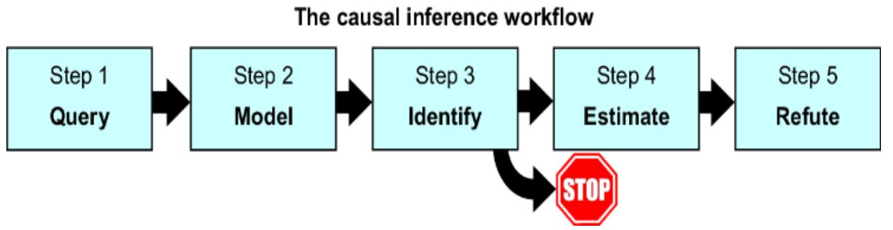
Figure 11.1 A workflow for a causal inference analysis
Let’s return to our online gaming example and use this workflow to answer a simple question:
How much does side-quest engagement drive in-game purchases?
We’ll call the cause of interest, Side-Quest Engagement (E), the ૿treatment variable; In-Game Purchases (I) will be the ૿outcome variable. Our query of interest is the average treatment effect (ATE):
E(IE=૿high – IE=૿low)
REFRESHER: WHY ATES AND CATES DOMINATE
Estimating ATEs and CATEs is the most popular causal effect inference task for several reasons, including the following:
- We can rely on causal effect inference techniques when randomized experiments are not feasible, ethical, or possible.
- We can use causal effect inference techniques to address practical issues with real-world experiments (e.g., post-randomization confounding, attrition, spillover, missing data, etc.).
- In an era when companies can run many different digital experiments in online applications and stores, causal effect inference techniques can help prioritize experiments, reducing opportunity costs.
Further, as we investigate our gaming data, we find data from a past experiment designed to test the effect of encouraging side-quest engagement on in-game purchases. In this experiment, all players were randomly assigned either to the treatment group or a control group. In the treatment group, the game mechanics were modified to tempt players into engaging in more side-quests, while the control group played the unmodified version of the game. We’ll define the Side-Quest Group Assignment (A) variable as whether the player was assigned to the treatment group in this experiment or the control group.
Why not just go with the estimate of the ATE produced by this experiment? This would be an estimate of E(IA=૿treatment
– IA=૿control).
This is the causal effect of the modification of game mechanics on in-game purchases. While this drives sidequest engagement, we know side-quest engagement is also driven by other potentially confounding factors. So we’ll focus on E(IE=૿high – IE=૿low).
11.2 Step 2: Build the model
Next, we’ll build our causal model. Since we are targeting an ATE, we can stick with a DAG. Let’s suppose we build a more detailed version of our online gaming example and produce the causal DAG in figure 11.2.

Figure 11.2 An expanded version of the online gaming DAG. With respect to the causal effect of side-quest engagement on in-game purchases, we add two additional confounders and two instruments.
The expanded model adds some new variables:
- Side-Quest Group Assignment (A) —Assigned a value of 1 if a player was exposed to the mechanics that encouraged more side-quest engagement in the randomized experiment; 0 otherwise.
- Customization Level (C) —A score quantifying the player’s customizations of their character and the game environment.
- Time Spent Playing (T) —How much time the player has spent playing.
- Prior Experience (Y) —How much experience the player had prior to when they started playing the game.
- Player Skill Level (S) —A score of how well the player performs in game tasks.
- Total Inventory (V) —The amount of game items the player has accumulated.
We are interested in the ATE of Side-Quest Engagement on In-Game Purchases, so we know, based on causal sufficiency (chapter 3), that we need to add common causes for these variables. We’ve already seen Guild Membership (G ), but now we add additional common causes: Prior Experience, Time Spent Playing, and Player Skill Level. We also add Side-Quest Group Assignment and Customization Level because these might be useful instrumental variables—variables that are causes of the treatment of interest, and where the only path of causality from the variable to the outcome is via the treatment. I’ll say more about instrumental variables in the next section.
Finally, we’ll add Total Inventory. This is a collider between In-Game Purchases and Won Items. Perhaps it is common for data scientists in our company to use this as a predictor of the In-Game Purchases. But as you’ll see, we’ll want to avoid adding collider bias to causal effect estimation.
SETTING UP YOUR ENVIRONMENT
The following code was written with DoWhy 0.11 and EconML 0.15, which expects a version of NumPy before version 2.0. The specific pandas version was 1.5.3. Again, we use Graphviz for visualization, with python PyGraphviz library version 1.12. The code should work, save for visualization, if you skip the PyGraphviz installation.
First, let’s build the DAG and visualize the graph with the PyGraphviz library.
Listing 11.1 Build the causal DAG
import pygraphviz as pgv #1
from IPython.display import Image #2
causal_graph = """
digraph {
 "Prior Experience" -> "Player Skill Level";
 "Prior Experience" -> "Time Spent Playing";
 "Time Spent Playing" -> "Player Skill Level";
 "Guild Membership" -> "Side-quest Engagement";
 "Guild Membership" -> "In-game Purchases";
 "Player Skill Level" -> "Side-quest Engagement";
 "Player Skill Level" -> "In-game Purchases";
 "Time Spent Playing" -> "Side-quest Engagement";
 "Time Spent Playing" -> "In-game Purchases";
 "Side-quest Group Assignment" -> "Side-quest Engagement";
 "Customization Level" -> "Side-quest Engagement";
 "Side-quest Engagement" -> "Won Items";
 "Won Items" -> "In-game Purchases";
 "Won Items" -> "Total Inventory";
 "In-game Purchases" -> "Total Inventory";
}
""" #3
G = pgv.AGraph(string=causal_graph) #3
G.draw('/tmp/causal_graph.png', prog='dot') #4
Image('/tmp/causal_graph.png') #5
#1 Download PyGraphviz and related libraries. #2 Optional import for visualizing the DAG in a Jupyter notebook #3 Specify the DAG as a DOT language string, and load a PyGraphviz AGraph object from the string. #4 Render the graph to a PNG file. #5 Display the graph.
This returns the graph in figure 11.3.
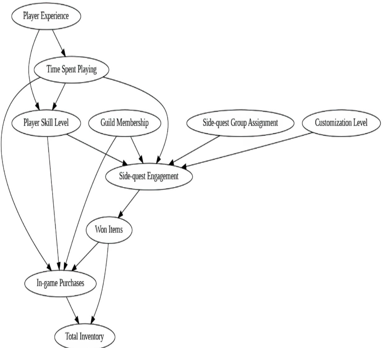
Figure 11.3 Visualizing our model with the PyGraphviz library
At this stage, we can validate our model using the conditional independence testing techniques outlined in chapter 4. But keep in mind that we can also focus on the subset of assumptions we rely on for causal effect estimation to work in the ૿refutation (step 5) part of the workflow.
11.3 Step 3: Identify the estimand
Next, we’ll run identification. Our causal query is
E(IE=૿high – IE=૿low)
For simplicity, let’s recode ૿high as 1 and ૿low as 0.
E(IE=1 – IE=0)
This query is on level 2 of the causal hierarchy. We are not running an experiment; we only have observational data samples from a level 1 distribution. Our identification task is to use our level 2 query and our causal model and identify a level 1 estimand, an operation we can apply to the distribution of the variables in our data.
First, let’s download our data and see what variables are in our observational distribution.
Listing 11.2 Download and display the data
import pandas as pd
data = pd.read_csv(
 "https://raw.githubusercontent.com/altdeep/causalML/master/datasets
 ↪/online_game_example_do_why.csv" #1
)
print(data.columns) #2
#1 Download an online gaming dataset. #2 Print the variables.
This prints out the following set of variables:
Index([‘Guild Membership’, ‘Player Skill Level’, ‘Time Spent Playing’, ‘Side-quest Group Assignment’, ‘Customization Level’, ‘Side-quest Engagement’, ‘Won Items’, ‘In-game Purchases’, ‘Total Inventory’], dtype=‘object’)
Our level 1 observational distribution includes all the variables in the DAG except Prior Experience. Thus, Prior Experience is a latent variable (figure 11.4).
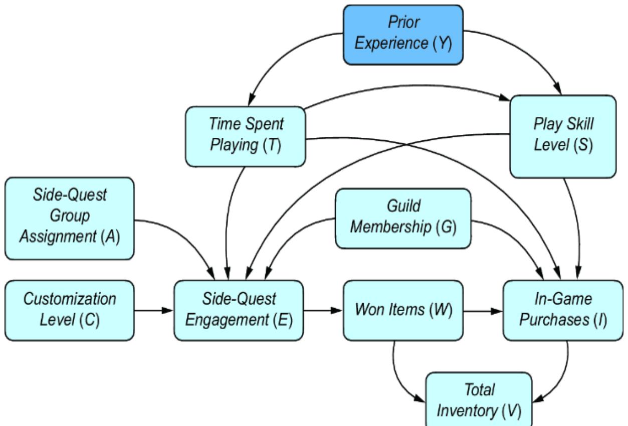
Figure 11.4 Prior Experience is not observed in the data; it is a latent (unobserved) variable with respect to our DAG.
We specified the base distribution for the estimand using y0’s domain-specific language for probabilistic expressions:
Identification.from_expression(
 graph=dag,
 query=query,
 estimand=observational_distribution
)
Here, we’ll use DoWhy. With DoWhy, we specify the observational distribution by just passing in the pandas DataFrame, along with the DAG and the causal query, to the constructor of the CausalModel class.
Listing 11.3 Instantiate an instance of DoWhy’s CausalModel
from dowhy import CausalModel #1
model = CausalModel(
 data=data, #2
 treatment='Side-quest Engagement', #3
 outcome='In-game Purchases', #3
 graph=causal_graph #4
)
#1 Install DoWhy and load the CausalModel class.
#2 Instantiate the CausalModel object with the data, which represents the level 1 observational distribution from which we derive the estimands.
#3 Specify the target causal query we wish to estimate, namely the causal effect of the treatment on the outcome. #4 Provide the causal DAG.
Next, the identify_effect methods will show us possible estimands we can target, given our causal model and observed variables.
Listing 11.4 Run identification in DoWhy
identified_estimand = model.identify_effect() #1 print(identified_estimand)
#1 The identify_effect method of the CausalModel class lists identified estimands.
The identified_estimand object is an object of the class IdentifiedEstimand. Printing it will list the estimands, if any, and the assumptions they entail. In our case, we have three estimands we can target:
- The backdoor adjustment estimand through the adjustment set Player Skill Level, Guild Membership, and Time Spent Playing
- The front-door adjustment estimand through the mediator Won Items
- Instrumental variable estimands through Side-Quest Group Assignment and Customization Level
GRAPHICAL IDENTIFICATION IN DOWHY
At the time of writing, DoWhy does implement graphical identification algorithms like y0, but these are experimental and are not the default identification approach. The default approach looks for commonly used estimands (e.g., backdoor, front door, instrumental variables) based on the structure of your graph. There may be identifiable estimands that the default approach misses, but these would be estimands that are not commonly used.
Let’s examine these estimands more closely.
11.3.1 The backdoor adjustment estimand
Let’s look at the printed summary for the first estimand, the backdoor adjustment estimand:
Estimand type: EstimandType.NONPARAMETRIC_ATE
### Estimand : 1
Estimand name: backdoor
Estimand expression:
 d
────────────────────────(E[In-game Purchases|Time Spent Playing,Guild
d[Side-quest Engagement]
Membership, Player Skill Level])
Estimand assumption 1, Unconfoundedness: If U→{Side-quest Engagement} and U→In-game P urchases then P(In-game Purchases|Side-quest Engagement,Time Spent Playing,Guild Memb ership,Player Skill Level,U) = P(In-game Purchases|Side-quest Engagement,Time Spent P laying,Guild Membership,Player Skill Level)
This printout tells us a few things:
EstimandType.NONPARAMETRIC_ATE—This means the estimand can be identified with graphical or ૿nonparametric methods, such as the do-calculus.
- Estimand name: backdoor—This is the backdoor adjustment estimand.
- Estimand expression—The mathematical expression of the estimand. Since we want the ATE, we modify the backdoor estimand to target the ATE.
- Estimand assumption 1—The causal assumptions underlying the estimand.
The last item is the most important. For each estimand, DoWhy lists the causal assumptions that must hold for valid estimation of the target causal query. In this case, the assumption is that there are no hidden (unmeasured) confounders, which DoWhy refers to as U. Estimation of a backdoor adjustment estimand assumes that all confounders are adjusted for.
Note that we do not need to observe Prior Experience to obtain a backdoor adjustment estimand. We just need to observe an adjustment set of common causes that dseparates or ૿blocks all backdoor paths.
The next estimand in the printout is an instrumental variable estimand.
11.3.2 The instrumental variable estimand
The printed summary for the second estimand, the instrumental variable estimand, is as follows (note, I shortened the variable names to acronyms so the summary fits this page):
### Estimand : 2
Estimand name: iv
Estimand expression:
⎡ -1⎤
⎢ d ⎛ d ⎞ ⎥
E⎢──────────(IGP)⋅ ───────────([SQE]) ⎥
⎣d[SQGA CL] ⎝ d[SQGA CL] ⎠ ⎦
Estimand assumption 1, As-if-random:
 If U→→IGP then ¬(U →→{SQGA,CL})
Estimand assumption 2, Exclusion:
 If we remove {SQGA,CL}→{SQE} then ¬({SQGA,CL}→IGP)
There are two level 2 definitional requirements for a variable to be a valid instrument:
- As-if-random—Any backdoor paths between the instrument and the outcome can be blocked.
- Exclusion—The instrument is a cause of the outcome only indirectly through the treatment.
The variables in our model that satisfy these constraints are Side-Quest Group Assignment and Customization Level, as shown in figure 11.5.
Figure 11.5 Side-Quest Group Assignment and Customization Level are valid instrumental variables.
The printout of identified_estimand shows the two constraints:
- Estimand assumption 1, As-if-random—DoWhy assumes that none of the other causes of the outcome (In-Game Purchases) are also causes of either instrument. In other words, there are no backdoor paths between the instruments and the outcome.
- Estimand assumption 2, Exclusion—This says that if we remove the causal path from the instruments to the treatment (Side-quest Engagement), there would be no causal paths from the instruments to the outcome (In-Game Purchases). In other words, there are no causal paths between the instruments and the outcome that are not mediated by the treatment.
Note that DoWhy’s constraints are relatively restrictive; DoWhy prohibits the existence of backdoor paths and nontreatment-mediated causal paths between the instrument and the outcome. In practice, it would be possible to block these paths with backdoor adjustment. DoWhy is making a trade-off that favors a simpler interface.
PARAMETRIC ASSUMPTIONS FOR INSTRUMENTAL VARIABLE ESTIMATION
The level 2 graphical assumptions are not sufficient for instrumental variable identification; additional parametric assumptions are needed. DoWhy, by default, makes a linearity assumption. With a linear assumption, you can derive the ATE as a simple function of the coefficients of linear models of outcome and the treatment given the instrument. DoWhy does this by fitting linear regression models.
Next, we’ll look at the third estimand identified by DoWhy the front door estimand.
11.3.3 The front-door adjustment estimand
Let’s move on to the assumptions in the third estimand, the front-door estimand. DoWhy’s printed summary is as follows (again, I shortened the variable names to acronyms in the printout so it fits the page):
### Estimand : 3
Estimand name: frontdoor
Estimand expression:
⎡ d d ⎤
E⎢────────────(IGP)⋅───────([WI])⎥
⎣d[WI] d[SQE] ⎦
Estimand assumption 1, Full-mediation:
 WI intercepts (blocks) all directed paths from SQE to IGP.
Estimand assumption 2, First-stage-unconfoundedness:
 If U→{SQE} and U→{WI}
 then P(WI|SQE,U) = P(WI|SQE)
Estimand assumption 3, Second-stage-unconfoundedness:
 If U→{WI} and U→IGP
 then P(IGP|WI, SQE, U) = P(IGP|WI, SQE)
As we saw in chapter 10, the front-door estimand requires a mediator on the path from the treatment to the outcome—in our DAG, this is Won Items. The printout for identified_estimand lists three key assumptions for the frontdoor estimand:
- Full-mediation—The mediator (Won-Items) intercepts all directed paths from the treatment (Side-Quest Engagement) to the outcome (In-Game Purchases). In other words, conditioning on Won-Items would dseparate (block) all the paths of causal influence from the treatment to the outcome.
- First-stage-unconfoundedness—There are no hidden confounders between the treatment and the mediator.
- Second-stage-unconfoundedness—There are no hidden confounders between the outcome and the mediator.
With our DAG and the variables observed in the data, DoWhy has identified three estimands for the ATE of Side-Quest Engagement on In-Game Purchases. Remember, the estimand is the thing we estimate, so which estimand should we estimate?
11.3.4 Choosing estimands and reducing ૿DAG anxiety
In step 2 of the causal inference workflow, we specified our causal assumptions about the domain as a DAG (or SCM or other causal model). The subsequent steps all rely on the assumptions we make in step 2.
Errors in step 2 can lead to errors in the results of the analysis, and while we can empirically test these assumptions to some extent (e.g., using the methods in chapter 4), we cannot verify all our causal assumptions with observational data alone. This dependence on our subjective and unverified causal assumptions leads to what I call ૿DAG anxiety—a fear that if one gets any part of the causal assumptions wrong, then the output of the analysis becomes wrong. Fortunately, we don’t need to get all the assumptions right; we only need to rely on the assumptions required to identify our selected estimand.
This is what makes DoWhy’s identify_effect method so powerful. By showing us the assumptions required for each estimand it lists, we can compare these assumptions and target the estimand where we are most confident about those assumptions.
For example, the key assumption behind the backdoor adjustment estimand is that we can adjust for all sources of confounding from common causes. In our original DAG, we have an edge from Time Spent Playing to Player Skill Level. What if you weren’t sure about the direction of this edge, as illustrated in figure 11.6.
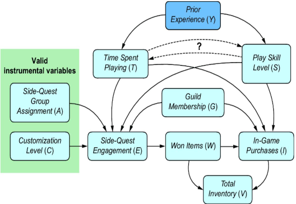
Figure 11.6 Uncertainty about the edge between Time Spent Playing and Player Skill Level doesn’t matter with respect to the backdoor adjustment estimand of the ATE of interest.
When we initially built the DAG, you might have been thinking that playing more causes skill level to increase. But now you may worry that perhaps the relationship is the other way around—that being more skilled causes you to want to spend more time playing. It doesn’t matter! At least, not with respect to the backdoor estimand for the target query—the ATE of Side-Quest Engagement on In-Game Purchases.
Suppose that instead you were worried that the model might have omitted edges that reflect direct influence that Prior Experience has on Side-Quest Engagement and In-Game Purchases. You worry that players might bring their habits in side-quest playing and virtual item purchasing from previous games they’ve played to the game environment you are modeling, as in figure 11.7.
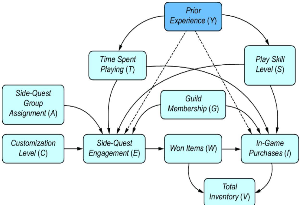
Figure 11.7 Direct influence of a latent variable on the treatment and outcome would violate the assumption underpinning the backdoor adjustment estimand. If you are not confident in an estimand’s assumptions, target another.
If this is true, your backdoor adjustment estimand assumption would be violated—you would have a confounder you couldn’t adjust for, a backdoor path you couldn’t block. In this case, you’ll need to consider whether the backdoor adjustment estimand is the right estimand to target.
Fortunately, in this example, we still have two other estimands to choose from. Neither the instrumental variable estimand nor the front-door adjustment estimand rely on our ability to adjust for all common causes. As long as we’re comfortable with the assumptions for either of these estimands, we can continue.
11.3.5 When you don’t have identification
The stop sign in the causal inference workflow, shown again in figure 11.8, warns against proceeding with estimation when you don’t have identification.
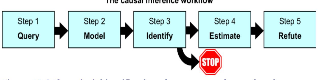
Figure 11.8 If you lack identification, do not proceed to estimation. Rather, consider how to acquire data that enables identification.
Let’s consider what happens if our observational distribution only contains a subset of our initial variables, as in figure 11.9.
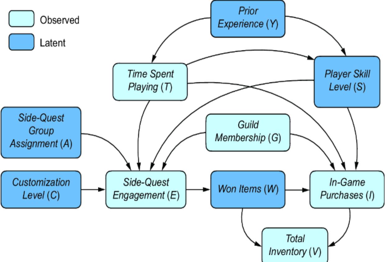
Figure 11.9 Player Skill Level, Won Items, Prior Experience, Side-Quest Group Assignment, and Customization Level become latent variables.
In this case, we have some problems:
- If Player Skill Level is latent, we can’t adjust for confounding from Player Skill Level and thus have no backdoor estimand.
- If Won Items is latent, we can’t identify a front-door estimand.
- If the instrumental variables are latent, we can’t target an instrumental variable estimand.
When you lack identification, you should not proceed with the next step of estimation. Rather, use the results from identification to determine what additional variables to collect—consider how you can collect new data with
- Additional confounders that would enable backdoor identification
- A mediator that would enable front-door identification
- Variables you can use as instruments
Avoid the temptation to change the DAG to get identification with your current data—you are modeling the data generating process (DGP), not the data.
However, if you do have an identified estimand, you can move on to step 4—estimation.
11.4 Step 4: Estimate the estimand
In step 4 of the causal inference workflow, we select an estimation method for whichever estimand we wish to target. In this section, we’ll walk through several estimators for each of our three estimands. Note that your results for estimation may vary slightly from those in the text, depending on modifications to the dataset and to random elements of the estimator.
In DoWhy, we do estimation using a method in the CausalModel class called estimate_effect, as in the following example.
Listing 11.5 Estimating the backdoor estimand with linear regressioncausal_estimate_reg = model.estimate_effect(
identified_estimand, #1
method_name="backdoor.linear_regression", #2
confidence_intervals=True #3
)#1 The estimate_effect method takes the output of the identify_effect method as input.
#2 method_name is of the form ૿[estimand].[estimator]. Here we use the linear regression estimator to estimate the backdoor estimand. #3 Return confidence intervals
The first argument is the identified_estimand object. The second argument method_name is a string of the form ” [estimand].[estimator]“, where”[estimand]” is the estimand we want to target, and “[estimator]” is the estimation method we want to use. Thus, method_name=“backdoor.linear_regression” means we want to use linear regression to estimate the backdoor estimand.
In this section, we’ll see the benefits of distinguishing identification from estimation. In step 3 of the causal inference workflow, we compared identified estimands and selected an estimand with assumptions in which we are confident. That step frees us to focus on the statistical and computational trade-offs common across data science and machine learning when we choose an estimation method in step 4. We’ll walk through these trade-offs in this section. Let’s start by looking at the linear regression estimation of the backdoor estimand.
11.4.1 Linear regression estimation of the backdoor estimand
In many causal inference texts, particularly from econometrics, the default approach to causal inference is regression—specifically, regressing the outcome on the treatment and any confounders we wish to adjust for or ૿control for. What we are doing in this case is using linear regression to estimate the backdoor estimand.
Recall that in the case where Side-Quest Engagement is continuous, the ATE would be
This is a function of x, not a point value. However, it becomes a point value when E (I E=x ) is linear—the derivative of a linear function is a constant.
So we turn to regression. The backdoor adjustment estimand identifies Guild Membership (G ), Time Spent Playing (T ), and Player Skill Level (S ) as the confounders we have to adjust for. In general, we have to sum or integrate over these variables in the backdoor adjustment estimand. But in the linear regression case, this simplifies to simply regressing I on the treatment E and the confounders G, T, and S. The coefficient estimate for E is the ATE. In the case of a binary treatment like our target ATE,
E (IE=1 – I E= 0 )
we simply treat E as a regression dummy variable. The coefficient estimates for the confounders are nuisance parameters—meaning they are necessary to estimate the ATE, but we can discard them once we have it.
To illustrate, let’s print the results of our call to estimate_method.
Listing 11.6 Print the linear regression estimation resultsprint(causal_estimate_reg)
This prints a bunch of stuff, including the following:
## Realized estimand
b: In-game Purchases~Side-quest Engagement+Guild Membership+Time Spent Playing+Player
Skill Level
Target units: ate
## Estimate
Mean value: 178.08617115757784
95.0% confidence interval: [[168.68114922 187.4911931 ]]
Realized estimand shows the regression formula. Estimate shows the estimation results, the point value, and the 95% confidence interval.
Here we see why linear regression is so popular as an estimator:
- The coefficient estimate of the treatment is a point estimate of the ATE.
- We adjust for backdoor confounders by simply including them in the regression model (no summation, no integration).
- The statistical properties of the estimator (confidence intervals, p-values, etc.) are well established.
- Many people are familiar with regression and how to evaluate a regression fit.
Once we have backdoor identification, the question of whether we should use a linear regression estimator in this case involves the same considerations of whether a linear regression model is appropriate in non-causal explanatory modeling settings (e.g., is the relationship linear?).
VALID BACKDOOR ADJUSTMENT SETS: WHAT YOU CAN AND CAN’T ADJUST FOR
You do not need to adjust for all confounding from common causes. Any valid backdoor adjustment set of common causes will do. As discussed in chapter 10, a valid backdoor adjustment set any set that satisfies the backdoor criterion, meaning that it d-separates all backdoor paths. For example, Guild Membership, Time Spent Playing, and Player Skill Level are a valid adjustment set. You don’t need Prior Experience because Time Spent Playing and Player Skill Level are sufficient to d-separate the backdoor path through Prior Experience. This is fortunate for us, since Prior Experience is unobserved. Though, if it were observed, we could add it to the adjustment set—this superset would also be a valid set.
DoWhy selects a valid adjustment set when it identifies a backdoor estimand. If you write your own estimator, you’ll select your own adjustment set.
Some applied regression texts argue that you should try to adjust for or ૿control for any covariates in your data because they could be potential confounders. This is bad advice. Doing so only makes sense if you are sure the covariate is not a mediator or a collider between the treatment and outcome variables. Adjusting for a mediator will d-separate the causal path you mean to quantify with the ATE. Adjusting for a collider will add collider bias. This is a painfully common error in social science, one committed even by experts.
11.4.2 Propensity score estimators of the backdoor estimand
Propensity score methods are a collection of estimation methods for the backdoor estimand that use a quantity called the propensity score. The traditional definition of a propensity score is the probability of being exposed to the treatment conditional on the confounders. In the context of the online gaming example, this is the probability that a player has high Side-Quest Engagement given their Guild Membership, Time Spent Playing, and Player Skill Level, i.e., P (E = 1|T = t, G = g, S = s ) where t, g, and s are that player’s values for T, G, and S. In other words, it quantifies the player’s ૿propensity of being exposed to the treatment (E = 1). Typically P (E = 1|T = t, G = g, S = s ) is fit by logistic regression.
But we can take a more expansive, machine learning– friendly view of the propensity score. We can learn a propensity score function λ(…) of the backdoor adjustment set of confounders that renders those confounders conditionally independent of the treatment, as in figure 11.10.
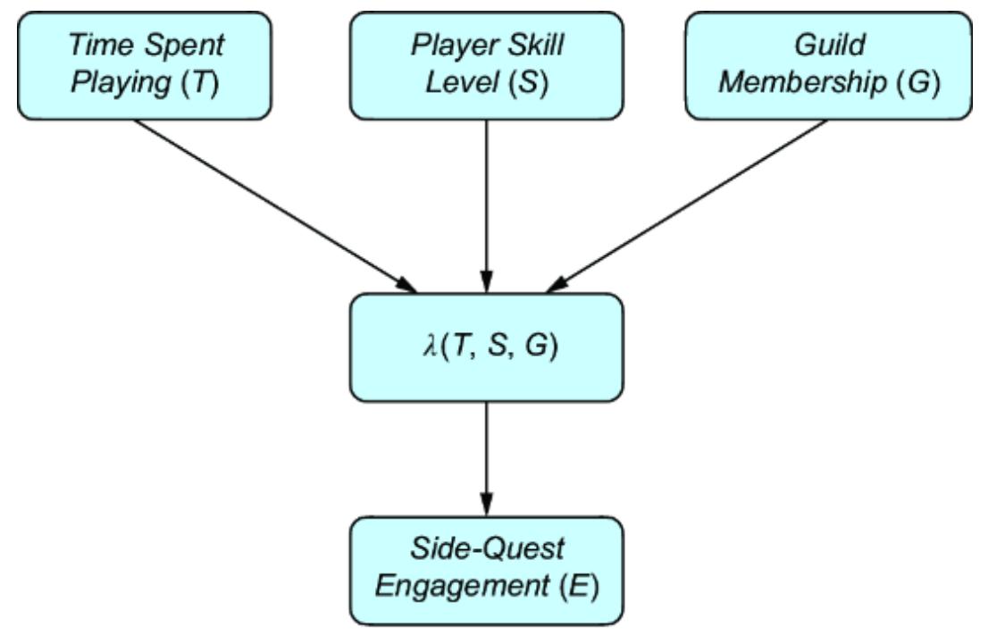
Figure 11.10 The propensity score is a compression of the causal influence of the common causes in the backdoor adjustment set.
Here, we learn a function λ(T, S, G ) such that it effectively compresses the explanatory influence that T, S, and G have on E. The traditional function of P (E = 1|G, S, T ) compresses this influence into a probability value, but other approaches can work as well.
The utility of propensity score modeling is dimensionality reduction; now we only need to adjust for the score instead of all the confounders in the adjustment set. There are three common propensity score methods:
- Propensity score stratification
- Propensity score matching
- Propensity score weighting
These methods make different trade-offs in how they go about backdoor adjustment. Let’s examine their use in
DoWhy.
PROPENSITY SCORE STRATIFICATION
Propensity score stratification tries to break the data up into subsets (૿strata) according to propensity scores and then adjust over the strata. Note that this algorithm may take some time to run.
Listing 11.7 Propensity score stratification
causal_estimate_strat = model.estimate_effect(
 identified_estimand,
 method_name="backdoor.propensity_score_stratification", #1
 target_units="ate",
 confidence_intervals=True
)
print(causal_estimate_strat)
#1 Propensity score stratification
This produces the following results:
Estimate Mean value: 187.2931023294184 95.0% confidence interval: (180.3291962554186, 196.4556029137768)
The propensity score estimator gives us an estimate and confidence interval that differ slightly from that of the regression estimator.
PROPENSITY SCORE MATCHING
Propensity score matching tries to match individuals where treatment = 1 with individuals that have a similar propensity score but where treatment = 0 and then compare outcomes across matched pairs.
Listing 11.8 Propensity score matching
causal_estimate_match = model.estimate_effect(
 identified_estimand,
 method_name="backdoor.propensity_score_matching", #1
 target_units="ate",
 confidence_intervals=True
)
print(causal_estimate_match)
#1 Propensity score matching
This returns the following results:
## Estimate
Mean value: 199.8110290000004
95.0% confidence interval: (183.23361900000054, 210.5281390000008)
Propensity score matching, despite also being a propensity score method, returns an estimate and confidence interval different from that of propensity score stratification.
PROPENSITY SCORE WEIGHTING
Propensity score weighting methods use the propensity score to calculate a weight in a class of inference algorithms called inverse probability weighting. We implement this method in DoWhy as follows.
Listing 11.9 Propensity score weighting
causal_estimate_ipw = model.estimate_effect(
 identified_estimand,
 method_name="backdoor.propensity_score_weighting", #1
 target_units = "ate",
 method_params={"weighting_scheme":"ips_weight"}, #2
 confidence_intervals=True
)
print(causal_estimate_ipw)
#1 Inverse probability weighting with the propensity score #2 Parameters used to set the IPS algorithm
This returns the following:
## Estimate
Mean value: 437.79246624944926
95.0% confidence interval: (358.10472302821745, 515.2480572854872)
The fact that this estimator’s result differs so dramatically from the others suggest that it is relying on statistical assumptions that don’t hold in this data.
Next, we’ll move on to a popular class of backdoor estimators that implement machine learning.
11.4.3 Backdoor estimation with machine learning
Recent developments in causal effect estimation focus on leveraging machine learning models, and most of these target the backdoor estimand. These approaches to causal effect estimation scale to large datasets and allow us to relax parametric assumptions, such as linearity. The following DoWhy code uses the sklearn and EconML libraries for these machine learning methods. DoWhy’s estimate_effects provides a wrapper to the EconML implementation of these methods.
DOUBLE MACHINE LEARNING
Double machine learning (double ML) is a backdoor estimator that uses machine learning methods to fit two predictive models: a model of the outcome, given the adjustment set of confounders, and a model of the treatment, given the adjustment set. The approach then combines these two predictive models in a final-stage estimation to create a model of the target causal effect query.
The following code performs double ML using a gradient boosting model and regularized regression model (LassoCV) from sklearn.
Listing 11.10 Double ML with DoWhy, EconML, and sklearn
from sklearn.preprocessing import PolynomialFeatures
from sklearn.linear_model import LassoCV
from sklearn.ensemble import GradientBoostingRegressor
featurizer = PolynomialFeatures(degree=1, include_bias=False)
gb_estimate = model.estimate_effect(
 identified_estimand,
 method_name = "backdoor.econml.dml.DML", #1
 control_value = 0,
 treatment_value = 1,
 method_params={
 "init_params":{
 'model_y': GradientBoostingRegressor(), #2
 'model_t': GradientBoostingRegressor(), #3
 'model_final': LassoCV(fit_intercept=False), #4
 'featurizer': featurizer
 },
 "fit_params":{}
 }
)
print(gb_estimate)
#1 Select the double ML estimator.
#2 Use a gradient boosting model to model the outcome given the confounders.
#3 Use a gradient boosting model to model the treatment given the confounders.
#4 Use linear regression with L1 regularization (LASSO) as the final model.
This produces the following output:
Estimate Mean value: 175.7229947190752
This gives us an estimate in the ballpark of some of the other estimators.
META LEARNERS
Meta learners are another ML method for backdoor estimation. Broadly speaking, meta learners train a model (or models) of the outcome given the treatment variable and the confounders, and then account for the difference in prediction across treatment and control values of the treatment variable. They are particularly focused on highlighting heterogeneity of treatment effects across the
data. The following code shows a meta learner example called a T-learner that uses a random forest predictor.
Listing 11.11 Backdoor estimation with a meta learner
from sklearn.ensemble import RandomForestRegressor #1
metalearner_estimate = model.estimate_effect( #1
 identified_estimand, #1
 method_name="backdoor.econml.metalearners.TLearner", #1
 method_params={ #1
 "init_params": {'models': RandomForestRegressor()}, #1
 "fit_params": {} #1
 } #1
) #1print(metalearner_estimate)#1 Meta learner estimation of the backdoor estimand. This uses a Tlearner with a random forest predictor.
This returns the following output:
## Estimate
Mean value: 197.20665049459512
Effect estimates: [[ 192.6234]
 [ -5.3165]
 [ 133.2457]
 ...
 [ 17.2561]
 [-152.1482]
 [ 264.887 ]]
The values under ૿Effect estimates are the estimate of the CATE for each row of the data, conditional on the confounder values in the columns of that row.
CONFIDENCE INTERVALS WITH MACHINE LEARNING METHODS
DoWhy and EconML provide support for estimating confidence intervals for ML methods using a statistical method called nonparametric bootstrap, but this is computationally costly for large data. Cheap confidence interval estimation is one thing you give up for the flexibility and scalability of using ML methods for backdoor estimation.
11.4.4 Front-door estimation
Recall from chapter 10 that the front-door estimator for our ATE, given our Won Items mediator, is
\[P(I\_{E=e} = i) = \sum\_{w} P(W = w | E = e) \sum\_{\varepsilon} P(I = i | E = \varepsilon, W = w) P(E = \varepsilon)\]
We can estimate this by fitting two statistical models, one that predicts W given E, and one that predicts I given E and W. DoWhy does this with linear regression by default, but you also have the option of selecting different predictive models.
Listing 11.12 Front door estimation with DoWhy
causal_estimate_fd = model.estimate_effect(
 identified_estimand,
 method_name="frontdoor.two_stage_regression", #1
 target_units = "ate",
 method_params={"weighting_scheme": "ips_weight"}, #2
 confidence_intervals=True
)
print(causal_estimate_fd)
#1 Select two-stage regression for the front-door estimand. #2 Specify estimator hyperparameters.
This produces the following output:
Estimate Mean value: 170.20560581290403 95.0% confidence interval: (141.53468188231938, 202.97221450388332)
The front-door estimate is similar to some of the backdoor estimators, but note that the confidence interval is skewed left.
11.4.5 Instrumental variable methods
Instrumental variable-based estimation of the ATE is straightforward in DoWhy.
Listing 11.13 Instrumental variable estimation in DoWhy
causal_estimate_iv = model.estimate_effect(
 identified_estimand,
 method_name="iv.instrumental_variable", #1
 method_params = {
 "iv_instrument_name": "Side-quest Group Assignment" #2
 },
 confidence_intervals=True
)
print(causal_estimate_iv)
#1 Select instrumental variable estimation. #2 Select side-quest engagement as the instrument.
This prints the following output:
Estimate Mean value: 205.82297621514252 95.0% confidence interval: (-369.04011492007703, 923.6814756173349)
Note how large the confidence interval is despite the size of the data. This indicates that this estimator, with its default assumptions, might have too much variance to be useful.
GOOD INSTRUMENTAL VARIABLES SHOULD BE “STRONG”
One requirement for good instrumental variable estimation is that the instrument is strong, meaning it has a strong causal effect on the treatment variable. If you explore this data, you’ll find Side-Quest Group Assignment is a weak instrument. Weak instruments can lead to high variance estimates of the ATE. Keep this in mind when selecting an instrument.
REGRESSION DISCONTINUITY
Regression discontinuity is an estimation method popular in econometrics. It uses a continuously valued variable related to the treatment variable, and it defines a threshold (a ૿discontinuity) in the values of that variable that partition
the data into ૿treatment and ૿control groups. It then compares observations lying closely on either side of the threshold, because those data points tend to have similar values for the confounders.
DoWhy treats regression discontinuity as an instrumental variable approach that uses continuous instruments. The rd_variable_name argument names a continuous instrument to use for thresholding, and rd_threshold_value is the threshold value. rd_bandwidth is the distance from the threshold within which confounders can be considered the same between treatment and control.
Listing 11.14 Regression discontinuity estimation with DoWhycausal_estimate_regdist = model.estimate_effect(
identified_estimand,
method_name="iv.regression_discontinuity", #1
method_params={
'rd_variable_name':'Customization Level', #2
'rd_threshold_value':0.5, #3
'rd_bandwidth': 0.15 #4
},
confidence_intervals=True,
)#1 DoWhy treats regression discontinuity as a special type of IV estimator.
#2 Use Customization Level as our instrument.
#3 The threshold value for the split (૿discontinuity) #4 The distance from the threshold within which confounders are considered the same between treatment and control values of the treatment variable
This returns the following results:
Mean value: 156.85691281931338
95.0% confidence interval: (-463.32687612531663, 940.698188663685)
Again, the variance is too large for us to rely on this estimator. The instrument is likely weak, or we need to tune the arguments passed to the estimator.
CONDITIONAL AVERAGE TREATMENT EFFECT ESTIMATION AND SEGMENTATION
The conditional average treatment effect (CATE) is the ATE for a subset of the target population; i.e., we condition the ATE on specific values of covariates. DoWhy enables you to estimate the CATE as easily as the ATE.
Sometimes the goal of CATE estimation is segmentation breaking the population down into segments that have a distinct CATE from other segments. A good tool for segmentation is EconML, which enables CATEsegmentation using regression trees. EconML can segment data into groups that respond similarly to intervention on the treatment variable, and find an optimal intervention value for each group in the leaf nodes of the regression tree.
11.4.6 Comparing and selecting estimators
In chapter 1, I mentioned a phenomenon called the commodification of inference. The way DoWhy reduces estimation to merely a set of arguments passed to the estimate_effect method is an example of this phenomenon. You don’t need a detailed understanding of the estimator to get going. Once you’ve selected the estimand you wish to target, you can switch out different estimators.
ADVICE: START WITH SYNTHETIC DATA
One excellent practice is to build your workflow on synthetic data, rather than real data. Simulate a synthetic dataset that matches the size and correlation structure of your data, as well as your causal and statistical assumptions about your data. For example, you can write a causal generative model of your data, and use your data to train its parameters. Using this model as ground truth, simulate some data and derive a ground truth ATE.
You can then see if DoWhy’s estimates get close to the ground truth ATE, and if its confidence intervals contain it. You can also see how well the estimators perform under the ideal conditions where all your assumptions are true even in these conditions, the estimates will have biases and uncertainty.
Once you debug any problems that arise in these ideal conditions, you can switch out the synthetic data for real data. Then, the problems that arise are likely due to incorrect assumptions, and you can treat these by revisiting your assumptions.
My suggestion is to compare estimators after adding the next step, refutation, to the workflow. Refutation will help you stress test both the causal assumptions in the estimand and the statistical assumptions in the estimator. This enables you to make empirical comparisons of different estimators. Then, once you know what estimator you want and have seen how it performs on your data, you can do a deep dive into the statistical nuts and bolts of your chosen estimator.
11.5 Step 5: Refutation
We know that the result of our causal inference depends on our initial causal assumptions in step 2, or more specifically, the subset of those assumptions we rely on for identification in step 3. In step 4, we select an estimator that makes its own statistical assumptions. What if those causal and statistical assumptions are wrong?
We can address this in step 5 with refutation, where we actively search for evidence that our analysis is faulty. We first saw this concept in chapter 4, when we saw how to refute the causal DAG by finding statistical evidence of dependence in the data that conflicts with the conditional independence implications of the causal DAG. In section 7.6.2, we saw how to refute a model by finding cases where its predicted intervention outcomes clash with real-world intervention outcomes. Here, we implement refutation as a type of sensitivity analysis that tries to refute the various assumptions underpinning an estimate by simulating violations to those assumptions.
The CausalModel class in DoWhy has a refute_estimate method that provides a suite of refuters we can run. Each refuter provides a different attack vector for our assumptions. The refuters we run with refute_estimate perform a simulationbased statistical test; the null hypothesis is that the assumptions are not refuted, and the alternative hypothesis is that the assumptions are refuted. The tests return a pvalue. If we take a standard significance threshold of .05 and the p-value falls below this threshold, we conclude that our assumptions are refuted.
In this section, we’ll investigate a few of DoWhy’s refuters with various estimands and estimators.
11.5.1 Data size reduction
One way to test the robustness of the analysis is to reduce the size of the data and see if we obtain similar results. We are assuming our analysis has more than enough data to achieve a stable estimation. We can refute this assumption by slightly reducing the size of the data and testing whether we get a similar estimate. Let’s try this with the estimator of the front-door estimand.
Listing 11.15 Refuting the assumption of sufficient data
identified_estimand.set_identifier_method("frontdoor") #1
res_subset = model.refute_estimate(
 identified_estimand, #2
 causal_estimate_fd, #2
 method_name="data_subset_refuter", #3
 subset_fraction=0.8, #4
 num_simulations=100
)
print(res_subset)
#1 Not always necessary, but clarifying the estimand targeted by the estimator we want to test can help avoid errors.
#2 The refute_estimate function takes in the identified estimand and the estimator that targets the estimand.
#3 Select data_subset_refuter, which tests if the causal estimate is different when we run the analysis on a subset of the data. #4 Set the size of the subset to 80% the size of the original data.
This produces the following output (this is a random process so your results will differ slightly):
Refute: Use a subset of data Estimated effect:170.20560581290403 New effect:169.14858189323638 p value:0.82
The Estimated effect is the effect from our original analysis. New effect is the average ATE across the simulations. We want these two effects to be similar, because otherwise it would mean that our analysis is sensitive to the amount of data we have. The p-value here is above the threshold, so we failed to refute this assumption.
11.5.2 Adding a dummy confounder
One way to test our models is to add dummy common-cause confounders. If a variable is not a confounder, it has no bearing on the true ATE, so we assume that our causal effect estimation workflow will be unaffected by these variables. In truth, additional variables might add statistical noise that throws off our estimator.
The following listing attempts to refute the assumption that such noise does not affect the double ML estimator of the backdoor estimand.
Listing 11.16 Adding a dummy confounderidentified_estimand.set_identifier_method("backdoor")
res_random = model.refute_estimate( #1
identified_estimand, #1
gb_estimate, #1
method_name="random_common_cause", #1
num_simulations=100, #1
) #1
print(res_random)#1 Runs 100 simulations of the addition of a dummy confounder to the model
This returns output such as the following:
Refute: Add a random common cause Estimated effect:175.2192519976428 New effect:176.59119763647792 p value:0.30000000000000004
Again, Estimated effect is the original causal effect estimate, and New effect is the new causal effect estimate obtained after adding a random common cause to the data and rerunning the analysis. The dummy variable has no real effect, so we expect the ATE to be the same. Again, the p-value is above the significance threshold, so we failed to refute our assumptions.
11.5.3 Replacing treatment with a dummy
We can also experiment with replacing the treatment variable with a dummy variable. This is analogous to giving our causal effect inference workflow a ૿placebo, and seeing how much causality it ascribes to this fake treatment. Since this dummy variable will have no effect on the treatment, we expect the ATE to be 0.
Let’s try this with our inverse probability weighting estimator.
Listing 11.17 Replacing the treatment variable with a dummy variable
identified_estimand.set_identifier_method("backdoor")
res_placebo = model.refute_estimate(
identified_estimand, #1
 causal_estimate_ipw, #1
 method_name="placebo_treatment_refuter", #1
 placebo_type="permute", #1
 num_simulations=100 #1
)
print(res_placebo)
#1 This refuter replaces the treatment variable with a dummy (placebo) variable.
This produces the following output:
Refute: Use a Placebo Treatment
Estimated effect:437.79246624944926
New effect:-531.2490111208127
p value:0.0
In this case, the p-value is calculated under the null hypothesis that New effect is equal to 0. Again, a low p-value would refute our assumptions.
In this case, it would seem that our inverse probability weighting estimator was thrown off by this refuter. This result indicates that there is an issue somewhere in the joint assumptions made by the backdoor estimand and this estimator. If we then used this refuter with other backdoor estimators and they were not refuted, we would have
narrowed down the source of the issue to the statistical assumptions made by this estimator.
11.5.4 Replacing outcome with a dummy outcome
We can substitute the outcome variable with a dummy variable. The ATE in this case should be 0, because the treatment has no effect on this dummy. We’ll simulate it as a linear function of some of the confounders so the outcome still has a meaningful relationship with some of the covariates.
Let’s try this with the front door estimator.
Listing 11.18 Replacing the outcome variable with a dummy variable
import numpy as np
coefficients = np.array([100.0, 50.0])
bias = 50.0
def linear_gen(df): #1
 subset = df[['guild_membership','player_skill_level']] #1
 y_new = np.dot(subset.values, coefficients) + bias #1
 return y_new #1
ref = model.refute_estimate( #2
 identified_estimand, #2
 causal_estimate_fd, #2
 method_name="dummy_outcome_refuter", #2
 outcome_function=linear_gen #2
) #2
res_dummy_outcome = ref[0]
print(res_dummy_outcome)
Refute: Use a Dummy Outcome
Estimated effect:0
New effect:-0.024480394297227835
p value:0.86
#1 Create a function that generates a new dummy outcome variable as a linear function of the covariates. #2 Runs refute_estimate with a dummy outcome refuter
Again, the p-value is calculated under the null hypothesis that New effect equals 0, and a low p-value refutes our assumptions. In this case, our assumptions are not refuted. Next, we’ll evaluate the sensitivity of the analysis to unobserved confounding.
11.5.5 Testing robustness to unmodeled confounders
Our backdoor adjustment estimand assumes that the adjustment set blocks all backdoor paths. If there were a confounder that we failed to adjust for, that assumption is violated, and our estimate would have a confounder bias. That is not necessarily the worst thing; if we adjust for all the major confounders, bias from unknown confounders might be small and not impact our results by much. On the other hand, missing a major confounder could lead us to conclude that there is a nonzero ATE when one doesn’t exist, or conclude a positive ATE when the true ATE is negative, or vice versa. We can therefore test how robust our analysis is to the introduction of latent confounders that our model failed to capture. The hope is that the new estimate does not change drastically when we introduce some modest influence from a newly introduced confounder.
Listing 11.19 Adding an unobserved confounder
identified_estimand.set_identifier_method("backdoor")
res_unobserved = model.refute_estimate( #1
 identified_estimand, #1
 causal_estimate_fd, #1
 method_name="add_unobserved_common_cause" #1
)
print(res_unobserved)
#1 Setting up a refuter that adds an unobserved common cause
This code does not return a p-value. It produces the heatmap we see in figure 11.11, showing how quickly the estimate changes when the unobserved confounder assumption is violated. The horizontal axis shows the various levels of influence the unobserved confounder has on the outcome, and the vertical axis shows the various levels of influence
the confounder can have on the treatment. The color corresponds to the new effect estimates that result at different levels of influence.
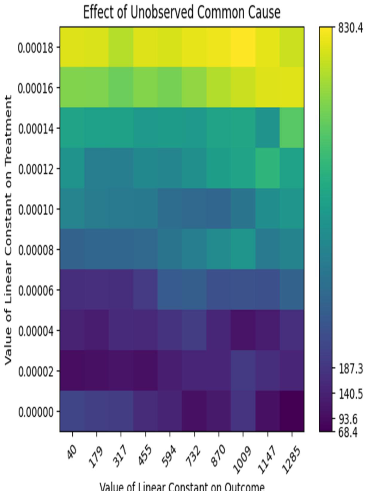
Figure 11.11 A heatmap illustrating the effects of adding an unobserved confounder on the ATE estimate
The code also prints out the following.
Refute: Add an Unobserved Common Cause Estimated effect:187.2931023294184 New effect:(-181.5795321684548, 398.98672237350416)
Here, we see that the ATE is quite sensitive to the effect the confounder has on the treatment. Note that you can change the default parameters of the refuter to experiment with different impacts the confounder could have on the treatment and outcome.
Now that we’ve run through a full workflow in DoWhy, let’s explore how we’d build a similar workflow using the tools of probabilistic machine learning.
11.6 Causal inference with causal generative models
At the end of chapter 10, we calculated an ATE using the do intervention operator and a probabilistic inference algorithm. This is a powerful universal approach to doing causal inference that leverages cutting-edge probabilistic machine learning. But this wasn’t estimation. Estimation requires data. It would be estimation if we estimated the model parameters from data before running that workflow with the do function and probabilistic inference.
In this section, we’ll run through a full ATE estimation workflow that uses the do intervention operator and probabilistic inference. We used MCMC for the probabilistic inference step in chapter 10, but here we’ll use variational inference with a variational autoencoder to handle latent variables in the data. Further, we’ll use a Bayesian estimation approach, meaning we’ll assign prior probabilistic distributions to the parameters. The ATE inference step with the intervention operator will depend on sampling from the posterior distribution on parameters.
The advantage of this approach relative to using DoWhy is being able to use modern deep learning tools to work with latent variables as well as use Bayesian modeling to address uncertainty. Further, this approach will work in cases of causal identification that are not covered by DoWhy (e.g., edge cases of graphical identification, identification derived from assignment functions or prior distributions, partial identification, etc.).
This approach to ATE estimation is a specific case of a general approach to causal inference where we train a causal graphical model, transform the model in some way that reflects the causal query (e.g., with an intervention operator), and then run a probabilistic inference algorithm. Let’s review various ways we can transform a model for causal inference.
11.6.1 Transformations for causal inference
We have seen several ways of modifying a causal model such that it can readily infer a causal query. We’ll call these ૿transformations: we transform our model into a new model that targets a causal inference query. Let’s review the transformations we’ve seen so far.
GRAPH SURGERY
One of the transformations was basic graph surgery, illustrated in figure 11.12. This operation implements an ideal intervention, setting the intervention target to a constant and severing the causal influence from the parents. This operation allows us to use our model to infer P (IE=1 ),
the ATE, and similar level 2 queries, and it’s how we have been implementing interventions in pgmpy.
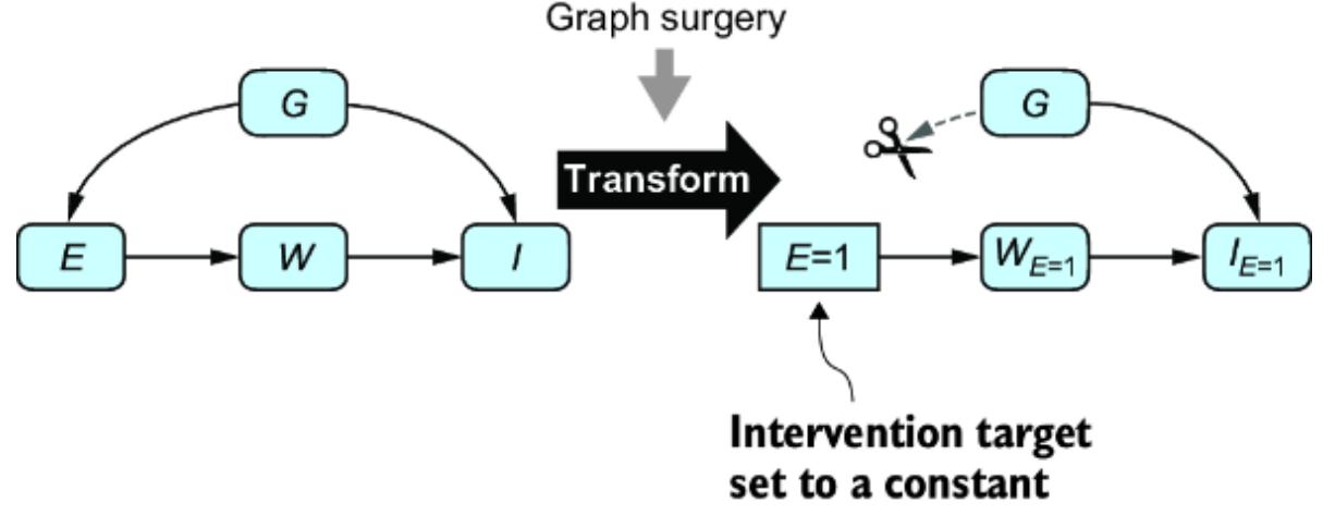
Figure 11.12 Graph surgery is a transformation that implements an ideal intervention by removing incoming causal influence on the target node and setting the target node to a constant.
We implemented graph surgery in pgmpy by using the do method on the BayesianNetwork class, and then we added a hack that modified the TabularCPD object assigned to the intervention project so that the intervention value had a probability of 1.
PyMC is a probabilistic programming language similar to Pyro. It does implicit graph surgery by transforming the logic of the model. For example, PyMC might specify E, a function of G, as E = Bernoulli(“E”, p=f(G)). PyMC uses a do function to implement the intervention, as in do(model, {“E”: 1.0}). Under the hood, this function does implicit graph surgery by effectively replacing E = Bernoulli(“E”, p=f(G)) with E = 1.0.
NODE-SPLITTING
In chapter 10, we discussed a slightly nuanced version of graph surgery called a node-splitting operation, illustrated in figure 11.13. Node-splitting converts the graph to a single world intervention graph, allowing us to infer level 2 queries
just as graph surgery does. It also allows us to infer level 3 queries where the factual conditions and hypothetical outcome don’t overlap, such as P (IE= 0 |E = 1) (though doing so relies on an additional ૿single world assumption, as discussed in chapter 10).
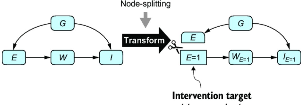
Figure 11.13 The node-splitting transform splits the intervention target into a constant that keeps the children and a random variable that keeps the parents.
Pyro’s do function implements node-splitting (though it behaves just like PyMC’s do function if you don’t target level 3 queries).
MULTI-WORLD TRANSFORMATION
We also saw how to transform a structural causal model into a parallel world graph. Let’s call this a multi-world transformation, illustrated in figure 11.14.
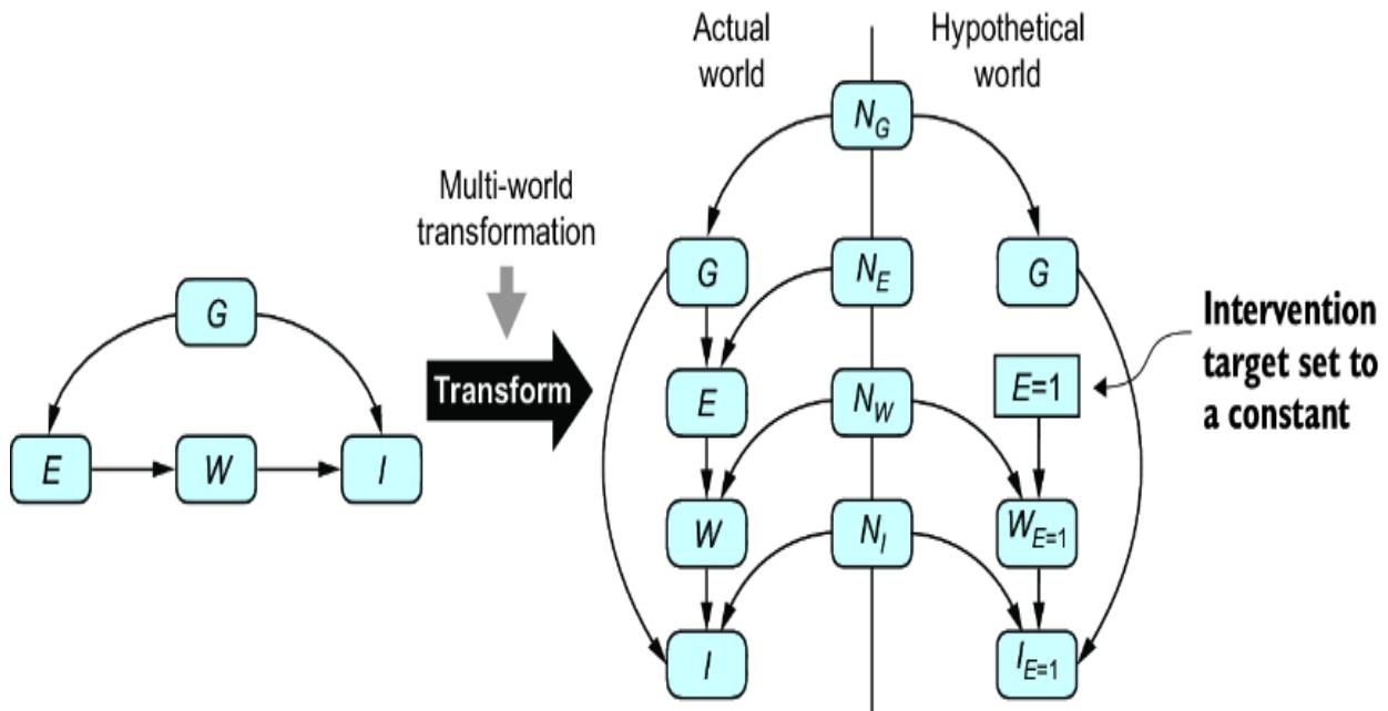
Figure 11.14 Yet another transform converts the model into a parallelworld model.
We created parallel-world models by hand in chapter 9 with pgmpy and Pyro. The y0 library produces parallel world graphs from DAGs. ChiRho, the causal library that extends Pyro, has a TwinWorldCounterfactual handler that does the multi-world transformation.
TRANSFORMATION TO A COUNTERFACTUAL GRAPH
Recall that we can also transform the causal DAG to a counterfactual graph (which, in the case of a level 2 query like P (IE= 1), will simplify to the result of graph surgery). Y0 creates a counterfactual graph from your DAG and a given query. Future versions of causal probabilistic ML libraries may provide the same transformation for a Pyro/PyMC/ChiRho type model.
11.6.2 Steps for inferring a causal query with a causal generative model
Given a causal generative model and a target causal query, we have two steps to infer the target query: first, apply the transformation, and then run probabilistic inference.
We did this with the online gaming example at the end of chapter 10. We targeted P (IE= 0) and P (IE= 0 |E = 1). For each of these queries, we used the do function in Pyro to modify the model to represent the intervention E = 0. In the case of P (IE= 0 |E = 1), we also conditioned on E = 1. Then we ran an MCMC algorithm to generate samples from these distributions. We also used the probabilistic inference with parallel-world graphs to implement level 3 counterfactual inferences in chapter 9.
11.6.3 Extending inference to estimation
To extend this workflow to estimation, like the DoWhy methods in this chapter, we simply need to add a parameter estimation step to our causal graphical inference workflow:
- Estimate model parameters.
- Apply the transformation.
- Run probabilistic inference on the transformed model.
Let’s look at how to do this with the online game data. For simplicity, we’ll work with a reduced model that drops the instruments and the collider, since we won’t be using them.
We’ll model the causal Markov kernels of each node with some unique parameter vector. We can estimate the parameters any way we like, but to stay on brand with probabilistic reasoning, let’s use a Bayesian setup, treating each parameter vector as its own random variable with its
own prior probability distribution. Figure 11.15 illustrates a plate model representation of the causal DAG (we discussed plate model visualizations in chapter 2), drawing these random variables as new nodes, using Greek letters to highlight the fact that they are parameters, rather than causal components of the real world DGP.
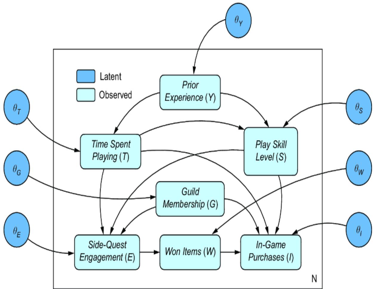
Figure 11.15 A plate model of the causal DAG with new nodes representing parameters associated with each causal Markov kernel. There is a single plate with N identical and independent observations in the training data. θ corresponds to parameters, which are outside the plate, because the parameters are the same for each of the N data points.
In this case, Bayesian estimation will target the posterior distribution:
where each represent the N examples of E, Y, T, G, S, W, I in the data.
Estimating the θs in this case is easy. For example, in pgmpy we just run model.fit(data, estimator= BayesianEstimator, …), where ૿. . . contains arguments that specify the type of prior to assign the θs. Pgmpy uses the posterior to give us point estimates of the θs. In Pyro, we just write sample statements for the θs and use one of Pyro’s various inference algorithms to get samples from the posterior.
But the causal effect methods in DoWhy highlight the ability to do causal inferences when some causal variables are latent, such as confounders:
- Backdoor adjustment with some latent confounders is possible (e.g., Prior Experience) if you have a valid adjustment set (Time Spent Playing, Guild Membership, and Player Skill Level).
- If too many confounders are latent, such that you do not have backdoor adjustment, you can use other techniques, such as using instrumental variables and front-door adjustment.
So for causal generative modeling to compete with DoWhy, it needs to accommodate latent variables. Let’s consider the case where the backdoor adjustment estimand is not identified. Next, we’ll explore how we can train a latent causal generative model and then apply the transformation and probabilistic inference.
In this model, we’ll assume that Guild Membership is the only observed confounder, as in figure 11.16. In this case, we no longer have backdoor identification.
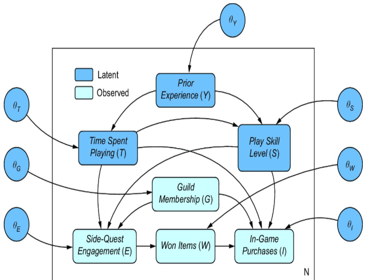
Figure 11.16 Guild Membership is the only observed confounder, so the backdoor estimand is not identified.
SETTING UP YOUR ENVIRONMENT
The following code is written with torch 2.2, pandas 1.5, and pyro-ppl 1.9. We’ll use matplotlib and seaborn for plotting.
Let’s first reload and modify the data to reflect this paucity of observed variables.
Listing 11.20 Load and reduce data to a subset of observed variables
import pandas as pd
import torch
url = ("https://raw.githubusercontent.com/altdeep/" #1
 "causalML/master/datasets/online_game_ate.csv") #1
df = pd.read_csv(url) #1
df = df[["Guild Membership", "Side-quest Engagement", #2
 "Won Items", "In-game Purchases"]] #2
device = torch.device("cuda" if torch.cuda.is_available() else "cpu") #3
data = { #3
 col: torch.tensor(df[col].values, dtype=torch.float32).to(device) #3
 for col in df.columns #3
} #3
#1 Load the data.
#2 Drop everything but Guild Membership, Side-Quest Engagement, Won Items, and In-Game Purchases.
#3 Convert the data to tensors and dynamically set the device for performing tensor computations depending on the availability of a CUDA-enabled GPU.
Now we are targeting the following posterior:
\[P\left(\theta\_Y, \theta\_T, \theta\_S, \theta\_G, \theta\_E, \theta\_W, \theta\_I, \vec{Y}, \vec{T}, \vec{S} \middle| \vec{E}, \vec{G}, \vec{W}, \vec{I}\right)\]
Targeting this posterior is harder because, since the observations of are not observed, they are not available to help in inferring θY, θT, and θS. In fact, in general, θY, θT, and θS are underdetermined, meaning multiple configurations of {θY, θT, θS} would be equally likely given the data. Further, we’ll have trouble estimating with θE and θI because it will be hard to disentangle them from the other latent variables.
But it doesn’t matter! At least, not in terms of our goal of inferring P(IE=e), because we know we have identified the front-door estimand of P(IE=e). In other words, the existence of a front-door estimand proves we can infer P(IE=e) from the observed variables regardless of the lack of identifiability of some of the parameters.
11.6.4 A VAE-inspired model for causal inference
We’ll make our modeling easier by creating proxy variables and θZ to stand in for { } and {θY, θT, θS} respectively. Collapsing the latent confounders into these proxies reduces the dimensionality of the estimation problem, and any loss of information that occurs from collapsing these variables won’t matter because we are ultimately relying on information flowing through the front door. We’ll create a causal generative model inspired by the variational autoencoder, where is a latent encoding and θE and θI become weights in decoders. This is visualized in figure 11.17.
Now our inference will target the posterior:
\[P\left(\theta\_Z, \theta\_G, \theta\_E, \theta\_W, \theta\_I, \vec{Z} \middle| \vec{E}, \,\,\vec{G}, \vec{W}, \vec{I}\right)\]
Our model will have two decoders. One decoder maps and G to E, returning a derived parameter ρ_engagement that acts as the probability that Side-Quest Engagement is high. Let’s call this network Confounders2Engagement. As shown in figure 11.17, is a vector with K elements, but we’ll set K=1 for simplicity.
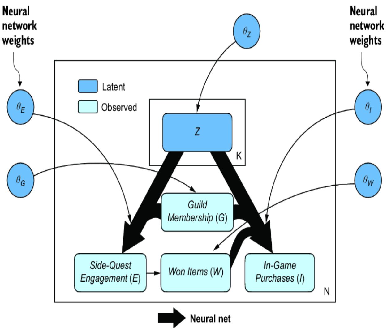
Figure 11.17 VAE-inspired model where latent vector Z of length K proxies for the latent confounders in figure 11.16
Listing 11.21 Specify Confounders2Engagement neural network
import torch.nn as nn
class Confounders2Engagement(nn.Module):
 def __init__(
 self,
 input_dim=1+1, #1
 hidden_dim=5 #2
 ):
 super().__init__()
 self.fc1 = nn.Linear(input_dim, hidden_dim) #3
 self.f_engagement_ρ = nn.Linear(hidden_dim, 1) #4
 self.softplus = nn.Softplus() #5
 self.sigmoid = nn.Sigmoid() #6
 def forward(self, input):
 input = input.t()
 hidden = self.softplus(self.fc1(input)) #7
 ρ_engagement = self.sigmoid(self.f_engagement_ρ(hidden)) #8
 ρ_engagement = ρ_engagement.t().squeeze(0)
 return ρ_engagement
#1 Input is confounder proxy Z concatenated with Guild Membership.
#2 Choose a hidden dimension of width 5.
#3 Linear map from input to hidden dimension
#4 Linear map from hidden dimension to In-Game Purchases location parameter
#5 Activation function for hidden layer
#6 Activation function for Side-Quest Engagement parameter
#7 From input to hidden layer
#8 From hidden layer to ρ_engagement
Next, let’s specify another neural net decoder that maps Z, W, and G to a location and scale parameter for I . Let’s call this PurchasesNetwork.
Listing 11.22 PurchasesNetwork neural network
class PurchasesNetwork(nn.Module):
 def __init__(
 self,
 input_dim=1+1+1, #1
 hidden_dim=5 #2
 ):
 super().__init__()
 self.f_hidden = nn.Linear(input_dim, hidden_dim) #3
 self.f_purchase_μ = nn.Linear(hidden_dim, 1) #4
 self.f_purchase_σ = nn.Linear(hidden_dim, 1) #5
 self.softplus = nn.Softplus() #6
 def forward(self, input):
 input = input.t()
 hidden = self.softplus(self.f_hidden(input)) #7
 μ_purchases = self.f_purchase_μ(hidden) H #8
 σ_purchases = 1e-6 + self.softplus(self.f_purchase_σ(hidden)) #9
 μ_purchases = μ_purchases.t().squeeze(0)
 σ_purchases = σ_purchases.t().squeeze(0)
 return μ_purchases, σ_purchases
#1 Input is confounder proxy Z concatenated with Guild Membership and Won Items.
#2 Choose a hidden dimension of width 5.
#3 Linear map from input to hidden dimension
#4 Linear map from hidden dimension to In-Game Purchases location parameter
#5 Linear map from hidden dimension to In-Game Purchases scale parameter
#6 Activation for hidden layer
#7 From input to hidden layer
#8 Mapping from hidden layer to location parameter for purchases #9 Mapping from hidden layer scale parameter for purchases. The 1e-6 lets us avoid scale values of 0.
Now we use both networks to specify the causal model. The model will take a dictionary of parameters called params and use them to sample the variables in the model. The Bernoulli distributions of Guild Membership and Won Items have parameters passed in a dictionary called params, with keys ρ_member representing θG, and ρ_won_engaged and ρ_won_not_engaged together representing θW. ρ_engagement, which represents the Side-Quest Engagement parameter θE, is set by the output of Confounders2Engagement, and μ_purchases and σ_purchases, which jointly represent the In-Game Purchases parameter θY, are the output of PurchaseNetwork.
The parameter set θZ is a location and scale parameter for a normal distribution. Rather than a learnable θZ, I use fixed θZ = {0, 1} and let the neural nets handle the linear transform for Z.
Listing 11.23 Specify the causal model
from pyro import sample
from pyro.distributions import Bernoulli, Normal
from torch import tensor, stack
def model(params, device=device): #1
 z_dist = Normal( #2
 tensor(0.0, device=device), #2
 tensor(1.0, device=device)) #2
 z = sample("Z", z_dist) #2
 member_dist = Bernoulli(params['ρ_member']) #3
 is_guild_member = sample("Guild Membership", member_dist) #3
 engagement_input = stack((is_guild_member, z)).to(device) #4
 ρ_engagement = confounders_2_engagement(engagement_input) #4
 engage_dist = Bernoulli(ρ_engagement)
 is_highly_engaged = sample("Side-quest Engagement", engage_dist) #5
 p_won = ( #6
 params['ρ_won_engaged'] * is_highly_engaged + #6
 params['ρ_won_not_engaged'] * (1 - is_highly_engaged) #6
 ) #6
 won_items = sample("Won Items", Bernoulli(p_won)) #6
 purchase_input = stack((won_items, is_guild_member, z)).to(device) #7
 μ_purchases, σ_purchases = purchases_network(purchase_input) #7
 purchase_dist = Normal(μ_purchases, σ_purchases) #8
 in_game_purchases = sample("In-game Purchases", purchase_dist) #8
#1 The causal model
#2 A latent variable that acts as a proxy for other confounders #3 Whether someone is in a guild
#4 Use confounders_ 2_engagement to map is_guild_ member and z to a parameter for Side-Quest Engagement and In-Game Purchases.
#5 Modeling Side-Quest Engagement
#6 Modeling amount of Won Items
#7 Use purchases_network to map is_guild_member, z, and won_items to in_game_purchases.
#8 Model in_game_purchases.
This model represents a single data point. Now we need to extend the model to every example data point in the dataset. We’ll build a data_model that loads the neural networks, assigns priors to the parameters, and models the data.
Listing 11.24 Build a data model
import pyro
from pyro import render_model, plate
from pyro.distributions import Beta
from pyro import render_model
confounders_2_engagement = Confounders2Engagement().to(device) #1
purchases_network = PurchasesNetwork().to(device) #1
def data_model(data, device=device):
 pyro.module("confounder_2_engagement", confounders_2_engagement) #2
 pyro.module("confounder_2_purchases", purchases_network) #2
 two = tensor(2., device=device)
 five = tensor(5., device=device)
 params = {
 'ρ_member': sample('ρ_member', Beta(five, five)), #3
 'ρ_won_engaged': sample('ρ_won_engaged', Beta(five, two)), #4
 'ρ_won_not_engaged': sample('ρ_won_not_engaged', Beta(two, five)), #5
 }
 N = len(data["In-game Purchases"])
 with plate("N", N): #6
 model(params) #6
render_model(data_model, (data, ))#1 Initialize the neural networks.
#2 pyro.module lets Pyro know about all the parameters inside the networks.
#3 Sample from prior distribution for ρ_member #4 Sample from prior distribution for ρ_won_engaged #5 Sample from prior distribution for ρ_won_not_engaged #6 The plate context manager declares N independent samples (observations) from the causal variables.
render_model lets us visualize the resulting plate model, producing figure 11.18. ρ_member, ρ_won_engaged, ρ_won_not_engaged are the parameters we wish to estimate, alongside the weights in the neural nets.
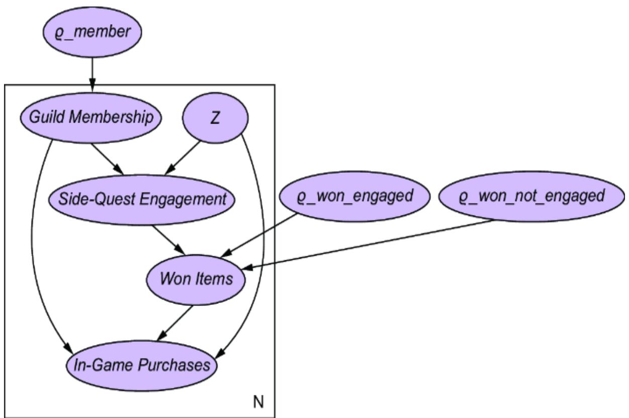
Figure 11.18 The plate model representation produced by Pyro
Now that we’ve specified the model, lets set up inference with SVI.
11.6.5 Setting up posterior inference with SVI
We have a data model over an underlying causal model, so we can now move on to inference. Using SVI, we need to build a guide function that represents a distribution that approximates the posterior—the guide function will have hyperparameters directly optimized during training, which will bring the approximating distribution as close as possible to the posterior.
WHY DO INFERENCE WITH SVI AND NOT MCMC?
In chapter 10, we used an MCMC inference algorithm to derive P(IE=0) and P(IE=0|E=1) from P(G, W, I, E). The θ parameters were given. Now the θ parameters are unknown, and we are using Bayesian estimation, meaning we want to infer IE=e conditional on values of those θ parameters sampled from a posterior distribution derived from training data. We do this by considering variables { , , , , } where { , , , } is a set of variables in the training data, is a latent proxy for our latent confounders, and each of these variables are vectors of length N, the size of our training data.
The challenge is the computational complexity of MCMC algorithms generally grows exponentially in the dimension of the posterior. When is a latent variable, it gets added to the posterior as another unknown along with the θs, so the shape of the posterior increases by ’s dimension, which is at least the size of the training data N. This poses a challenge when N is large. We want an inference method that works well with large data so we can leverage all that data to do cool things like use deep neural networks to help us proxy our latent confounders in a causal generative model. So here we use SVI instead of MCMC because SVI shines in high-dimensional large data settings.
The main ingredient of the guide function is an encoder that will map Side-Quest Engagement, Won Items, and In-Game Purchases to Z ; i.e., it will impute the latent values of Z.
Listing 11.25 Create an encoder for Z
class Encoder(nn.Module):
 def __init__(self, input_dim=3, #1
 z_dim=1, #2
 hidden_dim=5): #3
 super().__init__()
 self.f_hidden = nn.Linear(input_dim, hidden_dim)
 self.f_loc = nn.Linear(hidden_dim, z_dim)
 self.f_scale = nn.Linear(hidden_dim, z_dim)
 self.softplus = nn.Softplus()
 def forward(self, input):
 input = input.t()
 hidden = self.softplus(self.f_hidden(input)) #4
 z_loc = self.f_loc(hidden) #5
 z_scale = 1e-6 + self.softplus(self.f_scale(hidden)) #6
 return z_loc.t().squeeze(0), z_scale.t().squeeze(0)
#1 Input dimension is 3 because it will combine Side-Quest Engagement, In-Game Purchases, and Guild Membership. #2 I use a simple univariate Z, but we could give it higher dimension with sufficient data.
#3 The width of the hidden layer is 5.
#4 Go from input to hidden layer.
#5 Mapping from hidden layer to location parameter for Z #6 Mapping from hidden layer scale parameter to Z
Now, using the encoder, we build the overall guide function. In the following guide, we’ll sample the parameters ρ_member, ρ_won_engaged, and ρ_won_not_engaged from beta distributions parameterized by constants set using param. These ૿hyperparameters are optimized during training, alongside the weights of the neural networks.
Listing 11.26 Build the guide function (approximating distribution)
from pyro import param
from torch.distributions.constraints import positive
encoder = Encoder().to(device)
def guide(data, device=device):
 pyro.module("encoder", encoder)
 ˿_member = param("˿_member", tensor(1.0, device=device), #1
 constraint=positive) #1
 ̀_member = param("̀_member", tensor(1.0, device=device), #1
 constraint=positive) #1
 sample('ρ_member', Beta(˿_member, ̀_member)) #1
 ˿_won_engaged = param("˿_won_engaged", tensor(5.0, device=device), #2
 constraint=positive) #2
 ̀_won_engaged = param("̀_won_engaged", tensor(2.0, device=device), #2
 constraint=positive) #2
 sample('ρ_won_engaged', Beta(˿_won_engaged, ̀_won_engaged)) #2
 ˿_won_not_engaged = param("˿_won_not_engaged", #2
 tensor(2.0, device=device), #2
                   constraint=positive) #2
 ̀_won_not_engaged = param("̀_won_not_engaged", #2
 tensor(5.0, device=device), #2
                   constraint=positive) #2
 beta_dist = Beta(˿_won_not_engaged, ̀_won_not_engaged) #2
 sample('ρ_won_not_engaged', beta_dist) #2
 N = len(data["In-game Purchases"])
 with pyro.plate("N", N):
 z_input = torch.stack( #3
 (data["Guild Membership"], #3
 data["Side-quest Engagement"], #3
 data["In-game Purchases"]) #3
 ).to(device) #3
 z_loc, z_scale = encoder(z_input) #3
 pyro.sample("Z", Normal(z_loc, z_scale)) #3
#1 The guide samples ρ_member from a beta distribution where the shape parameters are trainable.
#2 ρ_won_engaged and ρ_won_ not_engaged are also sampled from beta distributions with trainable parameters.
#3 ρ_won_engaged and ρ_won_not_engaged are also sampled from beta distributions with trainable parameters.
#4 Z is sampled from a normal with parameters returned by the encoder.
Finally, we set up the inference algorithm and run the training loop.
Listing 11.27 Run the training loop
from pyro.infer import SVI, Trace_ELBO
from pyro.optim import Adam
from pyro import condition
pyro.clear_param_store() #1
adam_params = {"lr": 0.0001, "betas": (0.90, 0.999)} #2
optimizer = Adam(adam_params) #2
training_model = condition(data_model, data) #3
svi = SVI(training_model, guide, optimizer, loss=Trace_ELBO()) #4
elbo_values = [] #5
N = len(data['In-game Purchases']) #5
for step in range(500_000): #5
 loss = svi.step(data) / N #5
 elbo_values.append(loss) #5
 if step % 500 == 0: #5
 print(loss) #5
#1 Reset parameter values in case we restart the training loop. #2 Set up Adam optimizer. A learning rate (૿lr) of 0.001 may work better if using CUDA. #3 Condition the data_model on the observed data. #4 Set up SVI. #5 Run the training loop.
We’ll now plot the loss curve to see how training performed.
Listing 11.28 Plot the losses during training
import math
import matplotlib.pyplot as plt
plt.plot([math.log(item) for item in elbo_values]) #1
plt.xlabel('Step') #1
plt.ylabel('Log-Loss') #1
plt.title('Log Training Loss') #1
plt.show() #1
#1 Plot the log of training loss, since loss is initially large.
The losses shown in figure 11.19 indicate training has converged.
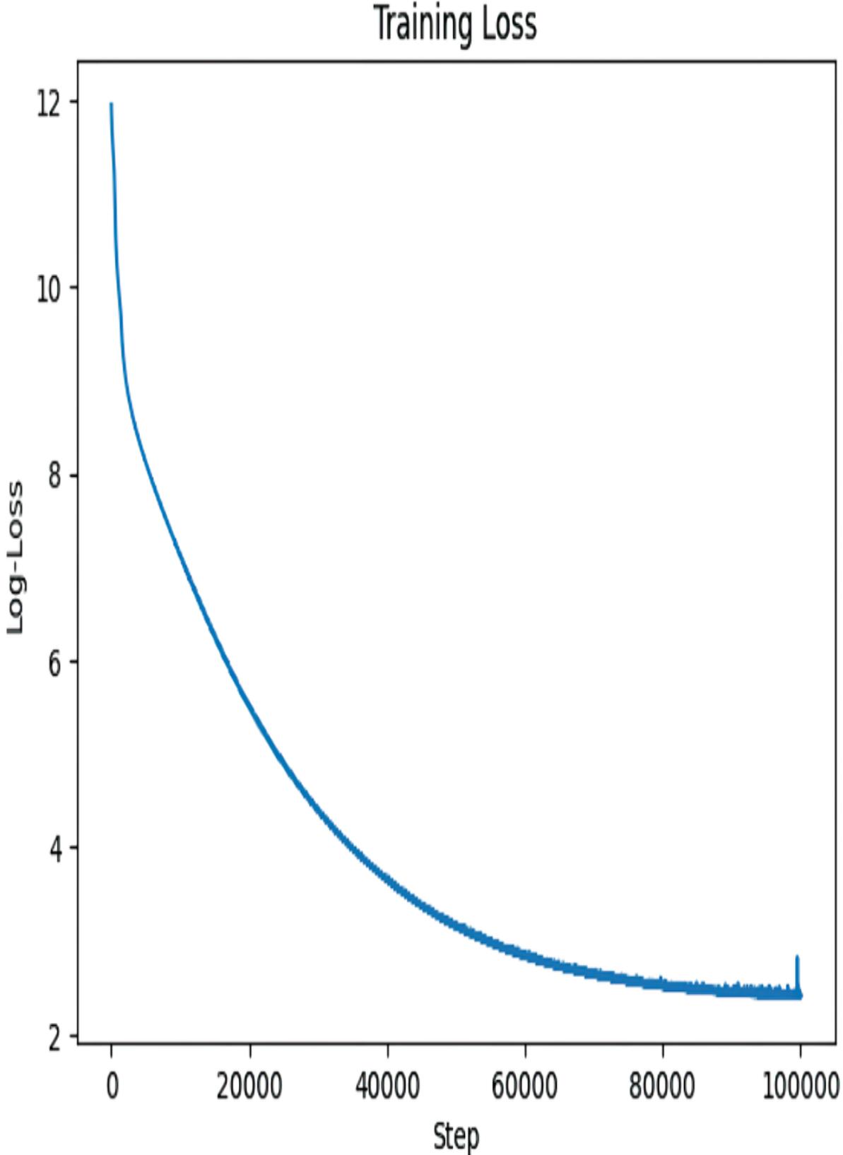
Figure 11.19 Log of ELBO loss during training
We can print the trained values of the hyperparameters (˿_member, β_member, ˿_won_engaged, β_won_engaged, ˿_won_not_engaged, and β_won_not_engaged).
Listing 11.29 Print the values of the trained parameters in the guide
function
print((
pyro.param("˿_member"),
pyro.param("̀_member"),
pyro.param("˿_won_engaged"),
pyro.param("̀_won_engaged"),
pyro.param("˿_won_not_engaged"),
pyro.param("̀_won_not_engaged")
))This returned the following:
(tensor(1.3953, grad_fn=<AddBackward0>), tensor(1.3558, grad_fn=<AddBackward0>), tens
or(4.3976, grad_fn=<AddBackward0>), tensor(3.1667, grad_fn=<AddBackward0>), tensor(0.
8065, grad_fn=<AddBackward0>), tensor(10.8452, grad_fn=<AddBackward0>))
We’ll approximate our posterior by sampling ρ_member, ρ_won_engaged, and ρ_won_not_engaged from beta distributions with these values, sampling Z from a normal(0, 1), and then sampling the remaining causal variables based on these values.
11.6.6 Posterior predictive inference of the ATE
Given a sample of the parameters and a sample vector of Z from the guide (our proxy for the posterior), we can simulate a new data set. A common way of checking how well a Bayesian model fits the data is to compare this simulated data with the original data. This comparison is called a posterior predictive check, and it helps us understand if the trained model is a good fit for the data. In the following code, we’ll do a posterior predictive check of In-Game Purchases; we’ll use the guide to generate samples and use those samples to repeatedly simulate In-Game Purchase datasets.
For each simulated dataset, we’ll create a density curve. We’ll then plot these curves, along with the density curve of the In-Game Purchases in the original data.
Listing 11.30 Posterior predictive check of In-Game Purchases
import matplotlib.pyplot as plt import seaborn as sns from pyro.infer import Predictive predictive = Predictive(data_model, guide=guide, num_samples=1000) #1 predictive_samples_all = predictive(data) #1 predictive_samples = predictive_samples_all[“In-game Purchases”] #1 for i, sample_data in enumerate(predictive_samples): #2 if i == 0: #2 sns.kdeplot(sample_data, #2 color=“lightgrey”, label=“Predictive density”) #2 else: #2 sns.kdeplot(sample_data, #2 color=“lightgrey”, linewidth=0.2, alpha=0.5) #2 sns.kdeplot( #3 data[‘In-game Purchases’], #3 color=“black”, #3 linewidth=1, #3 label=“Empirical density” #3 ) #3 plt.legend() plt.title(“Posterior Predictive Check of In-game Purchases”) plt.xlabel(“Value”) plt.ylabel(“Density”) plt.show()
#1 Simulate data from the (approximate) posterior predictive distribution.
#2 For each batch of simulated data, create and plot a density curve of In-Game Purchases.
#3 Overlay the empirical density distribution of In-Game Purchases so we can compare it with the predictive plots.
This produces a plot as in figure 11.20. The degree to which the simulated distribution matches the empirical distribution depends on the model, the size of the data, and how well the model is trained.
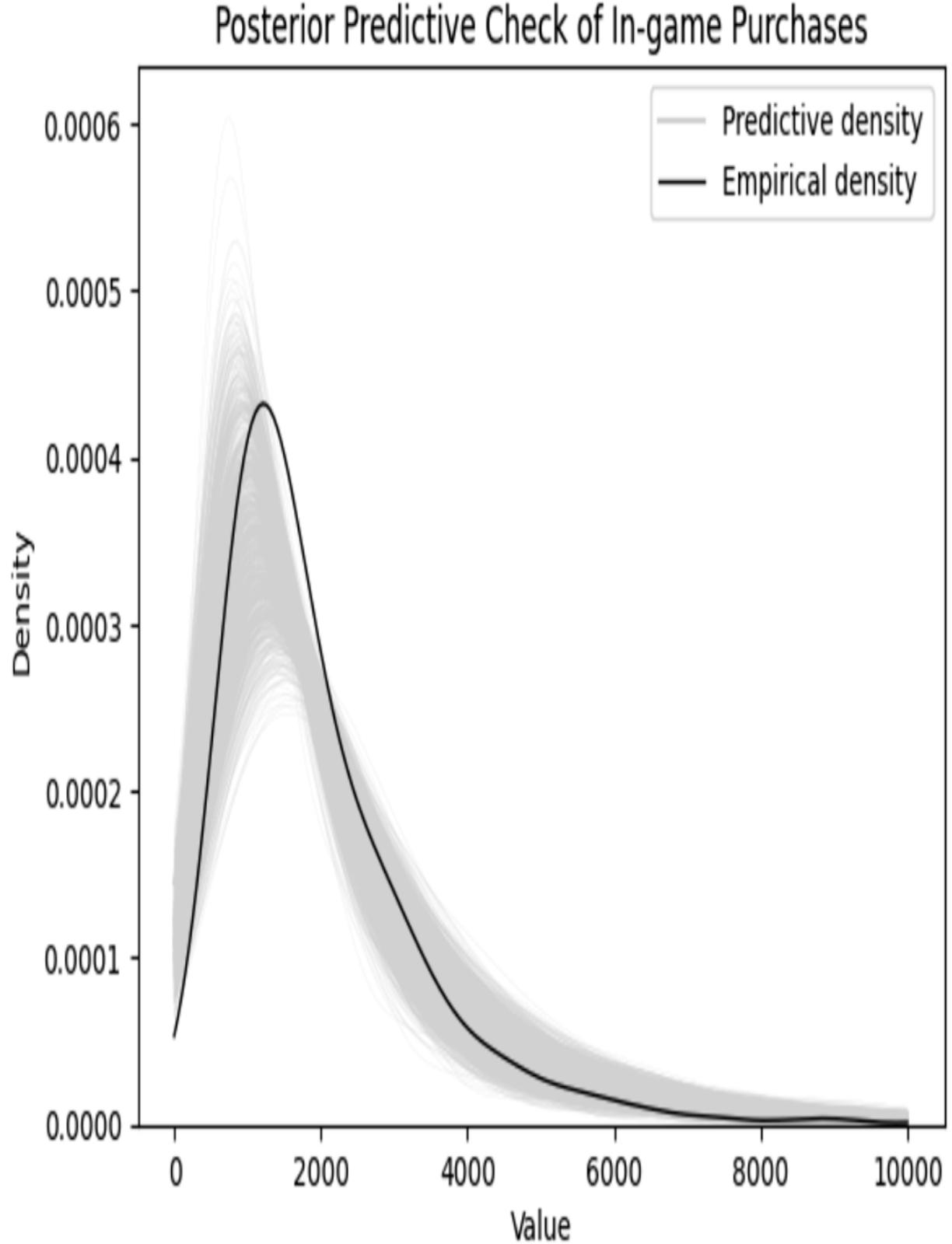
Figure 11.20 Posterior predictive check of In-Game Purchases. Grey lines are density curves calculated on simulations from the posterior predictive distribution. The black line is the empirical density (density curves calculated on the data itself). More overlap indicates the model fits the data well.
Our Bayesian estimator of the ATE will be our approach of applying transformation and inference to the posterior distribution represented by our model and guide. Since the ATE is E(IE= 1 ) – E(IE= 0 ), we’ll do posterior predictive sampling from P(IE= 1) and P(IE= 0).
First, we’ll use pyro.do to transform the model to represent the intervention. Then we’ll do forward sampling from the model using the Predictive class. This will sample 1,000 simulated datasets, each equal in length to the original data, and each corresponding to a random sample of ρ_member, ρ_won_engaged, ρ_won_unengaged, and a data vector of Z values. Objects from the Predictive class do simple forward sampling. If we needed to condition on anything (e.g., conditioning on E = 1 in P(IE= 0|E = 1)), we’d need to use another inference approach (e.g., importance sampling, MCMC, etc.).
Listing 11.31 Sampling from the posterior predictive distributions P(IE=0) and P(IE=1)
from pyro.infer import Predictive
from pyro import do
data_model_low_engagement = do( #1
 data_model, {"Side-quest Engagement": 0.}) #1
predictive_low_engagement = Predictive( #2
 data_model_low_engagement, guide=guide, num_samples=1000) #2
predictive_low_engagement_samples = predictive_low_engagement(data) #2
data_model_high_engagement = do( #3
 data_model, {"Side-quest Engagement": 1.}) #3
predictive_high_engagement = Predictive( #4
 data_model_high_engagement, guide=guide, num_samples=1000) #4
predictive_high_engagement_samples = predictive_high_engagement(data)
#1 Apply pyro.do transformation to implement intervention do(E=0). #2 Sample 1,000 samples of datasets from P(I E = 0). #3 Apply pyro.do transformation to implement intervention do(E=1). #4 Sample 1,000 samples of datasets from P(I E = 1).
We can plot these two sets of posterior predictive samples as follows:
Listing 11.32 Plot density curves of predictive datasets sampled from P(IE=1) and P(IE=0)
low_samples = predictive_low_engagement_samples["In-game Purchases"] #1
for i, sample_data in enumerate(low_samples): #1
 if i == 0: #1
 sns.kdeplot(sample_data, #1
 clip=(0, 35000), color="darkgrey", label="$P(I_{E=0})$") #1
 else: #1
 sns.kdeplot(sample_data, #1
 clip=(0, 35000), color="darkgrey", #1
 linewidth=0.2, alpha=0.5) #1
 #1
high_samples = predictive_high_engagement_samples["In-game Purchases"] #1
for i, sample_data in enumerate(high_samples): #1
 if i == 0: #1
 sns.kdeplot(sample_data, #1
 clip=(0, 35000), color="lightgrey", label="$P(I_{E=1})$") #1
 else: #1
 sns.kdeplot(sample_data, #1
 clip=(0, 35000), color="lightgrey", #1
 linewidth=0.2, alpha=0.5) #1
title = ("Posterior predictive sample density " #2
 "curves of $P(I_{E=1})$ & $P(I_{E=0})$") #2
plt.title(title) #2
plt.legend() #2
plt.xlabel("Value") #2
plt.ylabel("Density") #2
plt.ylim((0, .0010)) #2
plt.xlim((0, 4000)) #2
plt.show() #2
#1 For each sample, use kdeplot to draw a curve. Plot P( I E = 0) as dark grey and P( I E = 1) as light gray. #2 Plot the density curves.
Whereas figure 11.20 plotted a predictive distribution on P(I ), figure 11.21 plots predictive density plots of P (IE= 0 ) and P (IE= 1). We can see that the distributions differ.
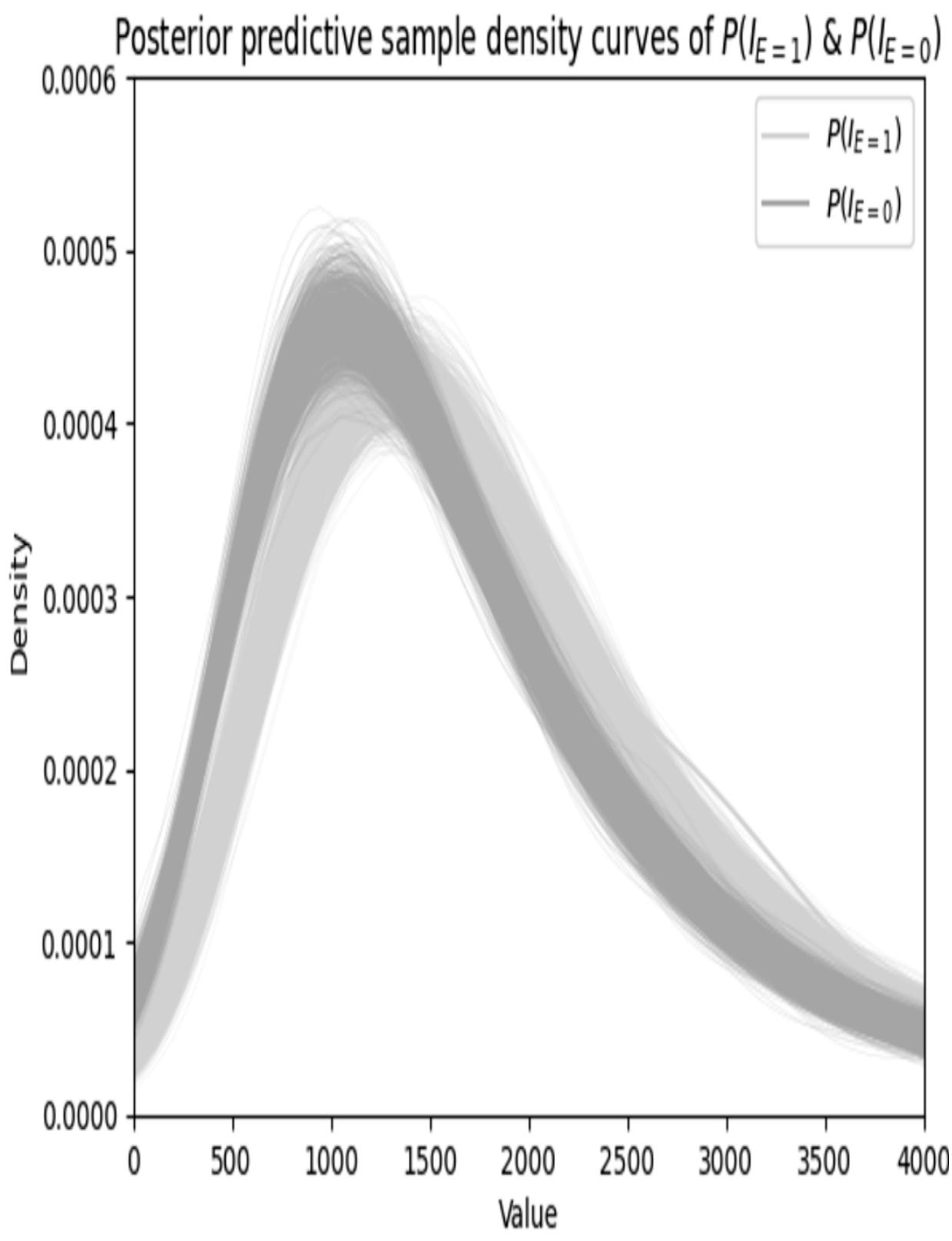
Figure 11.21 Posterior predictive visualization of density curves calculated from simulated data from P(IE=1) (light gray) and P(IE=0)
(dark gray)
Finally, to estimate E(IE= 1) and E(IE= 0), we just need take the means of each posterior predictive sample dataset simulated from P(IE= 1) and P(IE= 1), respectively. This will yield 1,000 samples of posterior predictive values of the ATE. Variation between the samples reflects posterior uncertainty about the ATE.
Listing 11.33 Estimate the ATE
samp_high = predictive_high_engagement_samples['In-game Purchases'] #1
exp_high = samp_high.mean(1) #1
samp_low = predictive_low_engagement_samples['In-game Purchases'] #2
exp_low = samp_low.mean(1) #2
ate_distribution = exp_high - exp_low #3
sns.kdeplot(ate_distribution) #4
plt.title("Posterior distribution of the ATE") #4
plt.xlabel("Value") #4
plt.ylabel("Density") #4
plt.show() #4
#1 Estimate E( I E = 1).
#2 Estimate E( I E = 0).
#3 Estimate the ATE = E( I E = 1) – E( I E = 0).
#4 Use a density curve to visualize posterior variation in the ATE values.This prints figure 11.22, a visualization of the posterior predictive distribution of the ATE.
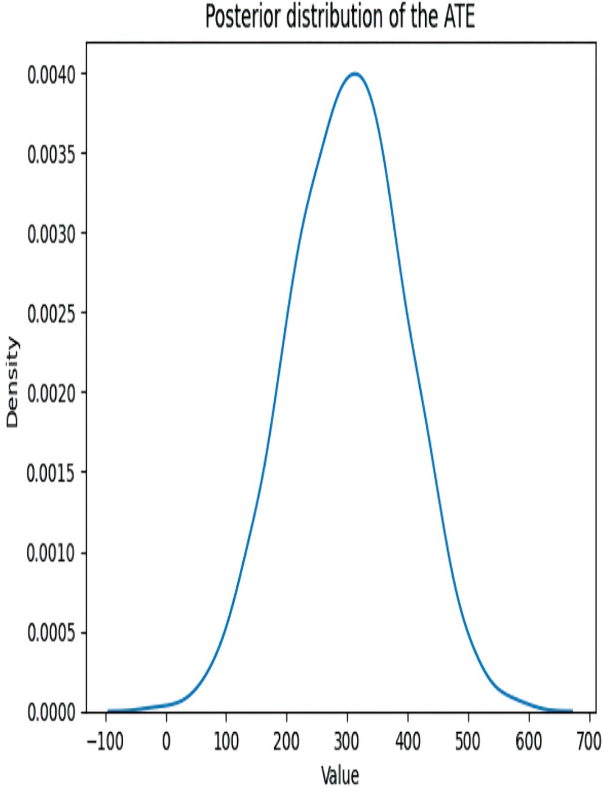
Figure 11.22 Posterior predictive distribution of the ATE
With a Bayesian approach, we get a posterior predictive distribution of the ATE. If we want a CATE, we can simply modify the posterior predictive inference to condition on other variables. If we want a point estimate of the ATE, we can take the mean of these predictive samples. More data reduces variance in the ATE distribution (assuming the ATE is identified) as in figure 11.23.
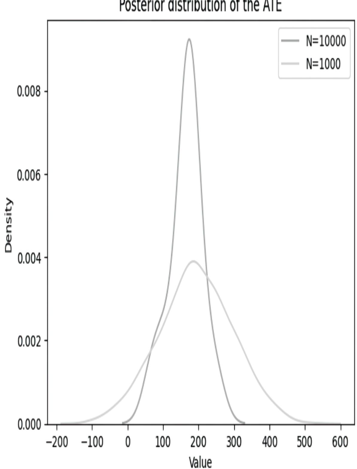
Figure 11.23 Posterior uncertainty declines with more data.
We can construct credible intervals (the Bayesian analog to confidence intervals) by taking percentiles from this distribution.
11.6.7 On the identifiability of the Bayesian causal generative inference
We got these results with a causal latent variable model, where Z was the latent variable. We are no strangers to latent variable models in probabilistic machine learning, but are they safe for causal inference? For example, if we could do causal inference with this latent variable model, what is to stop us from using the model in figure 11.24?
We could train this model, apply the transformations, get samples from the posterior predictive distribution of the ATE, and get an answer. But we lack graphical identification in this case. Our answer would have confounder bias that we couldn’t fix with more data, at least not without some strong, non-graphical assumptions (e.g., in the priors or in the functional relationships between variables).
Our model has graphical identification. In our case, we observed a mediator in Won Items, so we know we have a front-door estimand. Our causal generative model estimation procedure is just another estimator of that estimand.
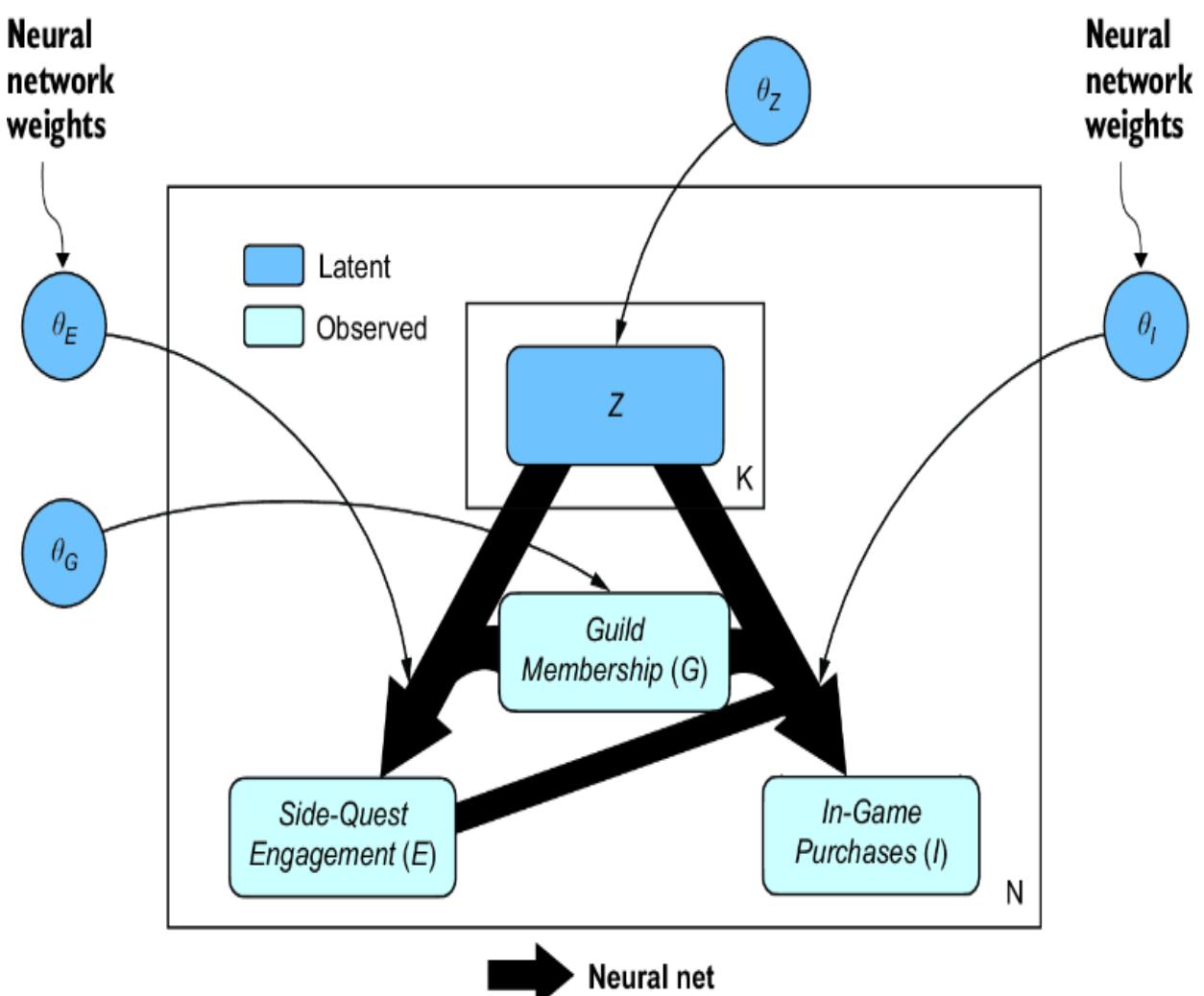
Figure 11.24 The causal latent variable model with no mediator W, and thus no identification. If we had fit this model and used it to infer the ATE, we’d get a result. But without identification, we wouldn’t be able to eliminate confounder bias, even with more data.
11.6.8 Closing thoughts on causal latent variable models
This approach of combining causal generative models with latent variables and deep learning is not limited to ATEs—it is general to all causal queries. We only need to select the right transformation for the query. This approach ૿commodifies inference by relying on auto-differentiation tools to do the statistical and computational heavy lifting, instead of having to understand and implement different estimators like in
DoWhy. It also scales to multidimensional causes, outcomes, and other variables in a way DoWhy does not. An additional advantage is that tools like Pyro and PyMC allow you to put Bayesian priors on the causal models themselves. Since the lack of causal identification boils down to model uncertainty, putting priors on models gives us an additional way of encoding domain assumptions that yield additional identification.
Summary
- DoWhy provides a useful workflow for identifying and estimating causal effects.
- In step 1 of the causal inference workflow, we specify our target query. In this chapter, we focused on causal effects (ATEs and CATEs).
- In step 2 we specify our causal model. We specified a DAG in Graphviz DOT format and loaded it into a CausalModel in DoWhy.
- In step 3 we run identification. DoWhy identified backdoor, front-door, and instrumental variable estimands.
- Each estimand relies on a different set of causal assumptions. If you are more confident in the causal assumptions of one estimand than others, you should target that estimand.
- We targeted the backdoor estimand with linear regression, propensity score methods, and machine learning (ML) methods.
- The backdoor adjustment set is the set of backdoor variables we adjust for in the backdoor adjustment estimand. A valid adjustment set d-separates all backdoor paths. There could be more than one valid set.
- In step 4 we estimate our selected estimand. DoWhy makes it easy to try different estimators.
- Linear regression is a popular estimand because it is simple, familiar, and gives a point estimate of the ATE even for continuous causes.
- A propensity score is traditionally the probability a subject in the data is exposed to the treatment value of the binary cause (treatment) variable, conditional on the confounders in the adjustment set. It is often modeled using logistic regression.
- However, a propensity score can be any variable you construct that renders the treatment variable conditionally independent of the adjustment set.
- Propensity score methods include matching, stratification, and inverse probability weighting.
- ML methods targeting the backdoor estimand include double ML and meta learners. DoWhy provides a wrapper to EconML that implements several ML methods.
- Generally, ML methods are a good choice when you have larger datasets. They allow you to rely on fewer statistical assumptions. However, calculating confidence intervals on the estimates is computationally expensive.
- Instrumental variable estimation and front-door estimation don’t rely on having a valid backdoor adjustment set, but they rely on different causal assumptions.
- In step 5, we run refutation analysis. Refutation is a sensitivity analysis that attempts to refute the causal and statistical assumptions we rely on in estimating our target query.
- Causal generative models combine model transformations, such as graph mutilation, node-splitting, and multi-world transforms, with probabilistic inference to do causal inference.
- This approach becomes an estimator of an identified estimand when the model parameters are learned from data.
- When there are latent variables, such as latent confounders, you can train the causal generative model as a latent variable model.
- The causal inference with the latent variable model will work if you have graphical identification. If not, you’ll need to rely on other identifying assumptions.
12 Causal decisions and reinforcement learning
This chapter covers
- Using causal models to automate decisions
- Setting up causal bandit algorithms
- How to incorporate causality into reinforcement learning
When we apply methods from statistics and machine learning, it is typically in service of making a decision or automating decision-making. Algorithms for automated decision-making, such as bandit and reinforcement learning (RL) algorithms, involve agents that learn how to make good decisions. In both cases, decision-making is fundamentally a causal problem: a decision to take some course of action leads to consequences, and the objective is to choose the action that leads to consequences favorable to the decisionmaker. That motivates a causal framing.
Often, the path from action to consequences has a degree of randomness. For example, your choice of how to play a hand of poker may be optimal, but you still might lose due to chance. That motivates a probabilistic modeling approach.
The causal probabilistic modeling approach we’ve used so far in this book is a stone that hits both these birds. This chapter will provide a causality-first introduction to basic ideas in statistical decision theory, sequential decisionmaking, bandits, and RL. By ૿causality-first, I mean I’ll use the foundation we’ve built in previous chapters to introduce these ideas in a causal light. I’ll also present the ideas in a way that is compatible with our probabilistic ML framing.
Even if you are already familiar with these decision-making and RL concepts, I encourage you to read on and see them again through a causal lens. Once we do that, we’ll see cases where the causal approach to RL gets a better result than the noncausal approach.
12.1 A causal primer on decision theory
Decision theory is concerned with the reasoning underlying an agent’s choice of some course of action. An ૿agent here is an entity that chooses an action.
For example, suppose you were deciding whether to invest in a company by purchasing equity or purchasing debt (i.e., loaning money to the company and receiving interest payments). We’ll call this variable X. Whether the company is successful (Y ) depends on the type of investment it receives.
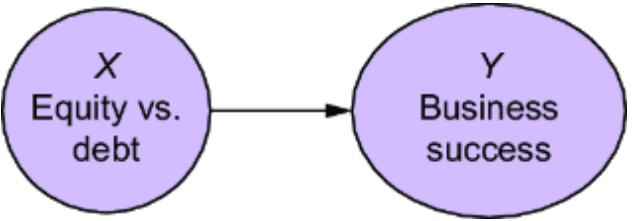
Figure 12.1 A simple causal DAG where action X causes some outcome Y. Decision theory is a causal problem because if deciding on an action didn’t have causal consequences, what would be the point of making decisions?
Since X causally drives Y, we can immediately introduce a causal DAG, as in figure 12.1.
We’ll use this example to illustrate basic concepts in decision theory from a causal point of view.
12.1.1 Utility, reward, loss, and cost
The agent generally chooses actions that will cause them to gain some utility (or minimize some loss). In decision modeling, you can define a utility function (aka a reward function) that quantifies the desirability of various outcomes of a decision. Suppose you invest at $1,000:
- If the company becomes successful, you get $100,000. Your utility is 100,000 – 1,000 = $99,000.
- If the company fails, you get $0 and lose your investment. Your utility is –1,000.
We can add this utility as a node on the graph, as in figure 12.2.
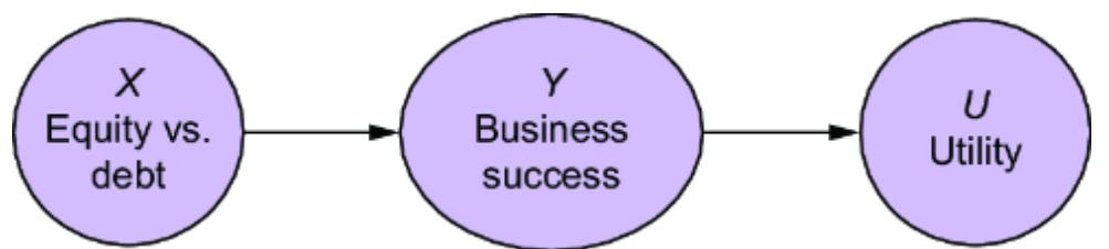
Figure 12.2 A utility node can represent utility/reward, loss/cost.
Note that utility is a deterministic function of Y in this model, which we’ll denote U(Y).
\[U(\mathcal{y}) = \begin{cases} 990000; & \mathcal{y} = \text{success} \\ -10000; & \mathcal{y} = \text{failure} \end{cases}\]
Instead of a utility/reward function, we could define a loss function (aka, a cost function), which is simply –1 times the utility/reward function. For example, in the second scenario, where you purchase stock and the company fails, your utility is –$1,000 and your loss is $1,000.
While the agent’s goal is to decide on a course of action that will maximize utility, doing so is challenging because there is typically some uncertainty in whether an action will lead to the desired result. In our example, it may seem obvious to invest in equity because equity will lead to business success, and business success will definitely lead to more utility. But there is some uncertainty in whether an equity investment will lead to business success. In other words we don’t assume P (Y = success|X = equity) = 1. Both success and failure have nonzero probability in P (Y |X = equity).
12.1.2 Uncertainty comes from other causes
In causal terms, given action X, there is still some uncertainty in the outcome Y because there are other causal factors driving that outcome. For example, suppose the success of the business depends on economic conditions, as in figure 12.3.
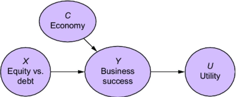
Figure 12.3 We typically have uncertainty in our decision-making. From a causal perspective, uncertainty is because of other causal factors out of our control that affect variables downstream of our actions.
Alternatively, those other causal factors could affect utility directly. For example, rather than the two discrete scenarios of profit or loss I outlined for our business investment, the amount of utility (or loss) could depend on how well or how poorly the economy fares, as in figure 12.4. We can leverage statistical and probability modeling to address this uncertainty.
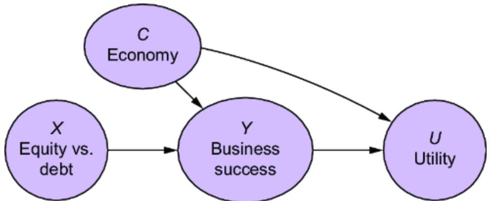
Figure 12.4 Causal factors outside of our control can impact utility (or loss) directly.
Suppose you are thinking about whether to invest in this business. You want your decision to be data-driven, so you research what other investors in this market have done before. You consider the causal DAG in figure 12.5.
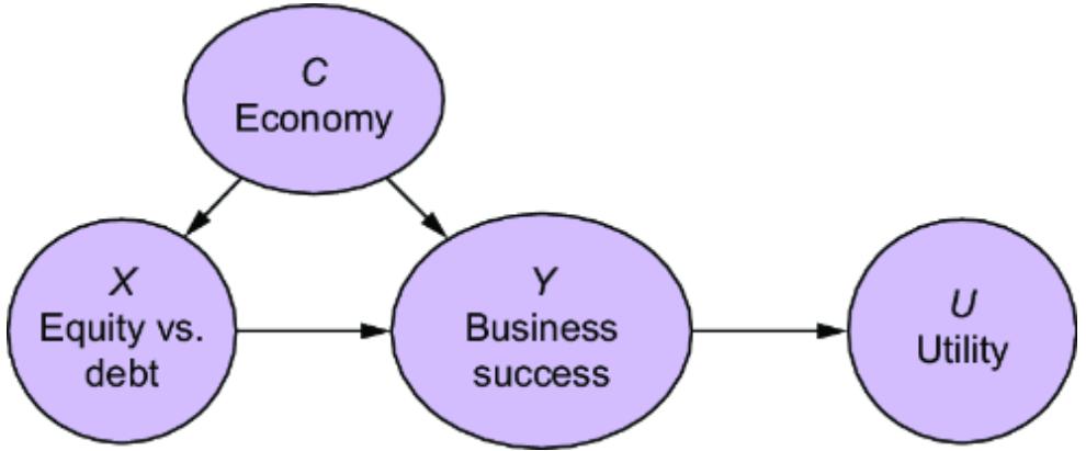
Figure 12.5 In this DAG, economic conditions drive how investors choose to invest.
Based on your research, you conclude that past investors’ equity vs. debt choice also depends on the economic conditions. P (X |C) represents an action distribution—the distribution of actions that the population of investors you are studying take.
However, the goal of your analysis centers on yourself, not other investors. You want to answer questions like ૿what if I bought equity? That question puts us in causal territory. We are not reasoning about observational investment trends; we are reasoning about conditional hypotheticals. That is an indicator that we need to introduce intervention-based reasoning and counterfactual notation.
12.2 Causal decision theory
In this section, we’ll highlight decision-making as a causal query and examine what that means for modeling decisionmaking.
12.2.1 Decisions as a level 2 query
A major source of confusion for causal decision modeling is the difference between actions and interventions. In many decision contexts, especially in RL, the action is a thing that the agent does that changes their environment. Yet, the action is also a variable driven by the environment. We see this when we look at the investment example, shown again in figure 12.6.
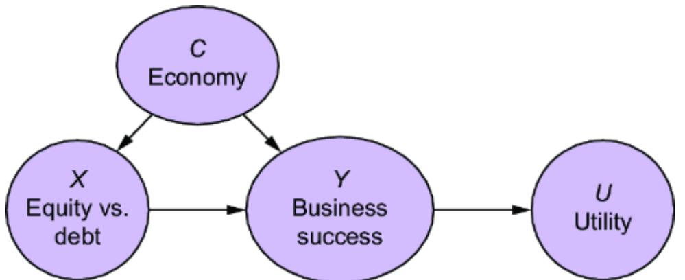
Figure 12.6 In this version of the investment DAG, the choice of action is caused by external factors.
The action of selecting equity or debt is a variable causally driven by the economy. What does that mean? Is an action a variable with causes, or is it an intervention?
The answer is both, depending on context. When it is which depends on the question we are asking and where that question sits in the causal hierarchy (discussed in chapter 10). When we are talking about what actions usually happen, such as when we are observing the actions of other agents (or even when reflecting on our own past actions) and what results those actions led to, we are reflecting on trends in population, and we are on level 1 of the causal hierarchy. In the case of our investment example, we’re reasoning about P (C, X, Y, U ). But if we’re asking questions like ૿what would happen if I made an equity investment? then we’re asking a level 2 question, and we need the proposed action as an intervention.
Next, we’ll characterize common decision rules using our causal notation.
12.2.2 Causal characterization of decision rules and policies
A decision rule is a rule for choosing an action based on the utility distribution P (U (YX=x)). The agent chooses an optimal action according to a decision rule. For example, a common decision rule is choosing the action that minimizes loss or cost or maximizes utility or reward.
In automated decision-making, the decision rule is often called a ૿policy. In public health settings, decision rules are sometimes called ૿treatment regimes.
MAXIMIZING EXPECTED UTILITY
The most intuitive and commonly seen decision rule is to choose the action that maximizes expected utility. First, we can look at the expectation of the utility distribution. Since utility is a deterministic function of YX=x, this is just the expectation of U (YX=x) over the intervention distribution of Y.
\[E(U(Y\_{X=x})) = \sum\_{\mathcal{Y}} U(\mathcal{y})P(Y\_{X=x} = \mathcal{y})\]
\[E(U(Y\_{X=x})) = \int\_{\mathcal{Y}} U(\mathcal{y}) P(Y\_{X=x} = \mathcal{y}) d\mathcal{y} \text{ (continuous case)}\]
We then choose the action (value of x) that maximizes expected utility:
\[\underset{x}{\text{argmax}} \, E(U(Y\_{X=x}))\]
In our investment example, this means choosing the investment approach that is expected to make you the most money.
MINIMAX DECISION RULES
To understand the minimax decision rule, recall that the terms ૿utility and ૿loss are two sides of the same coin; utility == negative loss. Let L(y ) = – U(y ). Then a minimax decision rule is
\[\underset{x}{\operatorname{argmin}} \max\_{Y\_{X=x}} L \ (Y\_{X=x})\]
In plain English, this means ૿choose the action that minimizes the maximum amount of possible loss. In our investment example, this means choosing the investment approach that will minimize the amount of money you’d lose in the worst case scenario. There are many variants of minimax rules, but they have the same flavor—minimizing loss or maximizing utility during bad times.
SOFTMAX RULES
A softmax decision rule randomly selects an action with a probability proportional to the resulting utility.
Let’s define C (x ) as the probability of choosing the action x. Then C (x ) is defined as a probability value proportional to
The noise parameter α modulates between the two extremes. When α=0, we have a uniform distribution on all the choices. As α gets larger, we approach maximizing expected utility.
Sometimes our goal is to model the decision-making of other agents, such as in inverse RL. The softmax decision rule is useful when agents don’t always make the utility-optimizing choice. The softmax decision rule provides a simple, analytically tractable, and empirically validated model of suboptimal choice.
Another reason we might want to use the softmax rule is when there is a trade-off between exploring and exploiting, such as with bandit problems. Suppose the agent is uncertain about the shape of the distibution P (YX=x). The optimal action according to an incorrect model of P (YX=x) might be different from the optimal choice according to the correct model of P (YX=x). The softmax decision rule allows us to choose various actions, get some data on the results, and
use that data to update our model of P (YX=x). When this is done in sequence, it’s often called Thompson sampling.
In our investment analogy, suppose we were to invest in several businesses. Perhaps, according to our current model, equity investment maximizes expected utility, but we’re not fully confident in our current model, so we opt to select debt investment even though the current model says its less optimal. The goal is to add diversity to our dataset, so that we can learn a better model.
OTHER TYPES OF DECISION RULES
There are other types of decision rules, and they can become complicated, especially when they involve statistical estimation. For example, using p-values in statistical hypothesis testing involves a nuanced utility function that balances the chances of a false positive (incorrectly choosing the alternative hypothesis) and a false negative (incorrectly choosing the null hypothesis).
Fortunately, when we work with probabilistic causal models, the math tends to be easier, and we get a nice guarantee called admissibility.
12.2.3 Causal probabilistic decision-modeling and admissibility
In this section, I’ll provide a short justification for choosing a causal probabilistic modeling approach to decision-making. When you implement an automated decision-making algorithm in a production setting, you might have to explain why your implementation is better than another. In that setting, it is useful if you know if your algorithm is admissible.
A decision rule is admissible if there are no other rules that dominate it. A decision rule dominates another rule if the performance of the former is sometimes better, and never worse, than that of the other rule with respect to the utility function. For example, the softmax decision rule is dominated by maximizing expected utility (assuming you know the true shape of P (YX = x )) because sometimes it will select suboptimal actions, and it is thus inadmissible. Determining admissibility is a key task in decision theory.
The challenge for us occurs when we use data and statistics to deal with unknowns, such as parameters or latent variables. If we want to use data to estimate a parameter or work with latent variables, there are usually a variety of statistical approaches to choose from. If our decision-making algorithm depends on a statistical procedure, the choice of procedure can influence which action is considered optimal. How do we know if our statistical decision-making procedure is admissible?
Probabilistic modeling libraries like Pyro leverage Bayesian inference to estimate parameters or impute latent variables. Bayesian decision theory tells us that Bayes rules, (not to be confused with Bayes’s rule) decision rules that optimize posterior expected utility, have an admissibility guarantee under mild regularity conditions. This means that if we use Bayesian inference in Pyro or similar libraries to calculate and optimize posterior expected loss, we have an admissibility guarantee (if those mild conditions hold, and they usually do). That means you needn’t worry that someone else’s decision-making model (that makes the same modeling assumptions, has the same utility function, and uses the same data) will beat yours.
12.2.4 The deceptive alignment of argmax values of causal and non-causal expectations
Most conventional approaches to decision-making, including in RL, focus on maximizing E (U(Y )|X = x) rather than E (U (YX= x)). Let’s implement the model in figure 12.6 with pgmpy and compare the two approaches.
First, we’ll build the DAG in the model.
SETTING UP YOUR ENVIRONMENT
This code was written with pgmpy version 0.1.24. See the chapter notes athttps://www.altdeep.ai/p/causalaibookfor a link to the notebook that runs this code.
Listing 12.1 DAG for investment decision model
from pgmpy.models import BayesianNetwork
from pgmpy.factors.discrete import TabularCPD
from pgmpy.inference import VariableElimination
import numpy as np
model = BayesianNetwork([ #1
 ('C', 'X'), #1
 ('C', 'Y'), #1
 ('X', 'Y'), #1
 ('Y', 'U') #1
]) #1
#1 Set up the DAG
Next we’ll build the causal Markov kernels for Economy (C ), Debt vs. Equity (X ), and Business Success (Y). The causal Markov kernel for Economy (C ) will take two values: ૿bear for bad economic conditions and ૿bull for good. The causal Markov kernel for Debt vs. Equity (X ) will depend on C, reflecting the fact that investors tend to prefer equity in a bull economy and debt in a bear economy. Success (Y )
depends on the economy and the choice of debt or equity investment.
Listing 12.2 Create causal Markov kernels for C, X, and Y
cpd_c = TabularCPD( #1
 variable='C', #1
 variable_card=2, #1
 values=[[0.5], [0.5]], #1
 state_names={'C': ['bear', 'bull']} #1
) #1
cpd_x = TabularCPD( #2
 variable='X', #2
 variable_card=2, #2
 values=[[0.8, 0.2], [0.2, 0.8]], #2
 evidence=['C'], #2
 evidence_card=[2], #2
 state_names={'X': ['debt', 'equity'], 'C': ['bear', 'bull']} #2
) #2
cpd_y = TabularCPD( #3
 variable='Y', #3
 variable_card=2, #3
 values= [[0.3, 0.9, 0.7, 0.6], [0.7, 0.1, 0.3, 0.4]], #3
 evidence=['X', 'C'], #3
 evidence_card=[2, 2], #3
 state_names={ #3
 'Y': ['failure', 'success'], #3
 'X': ['debt', 'equity'], #3
 'C': ['bear', 'bull'] #3
 } #3
) #3
#1 Set up causal Markov kernel for C (economy). It takes two values: ૿bull and ૿bear.
#2 Set up causal Markov kernel for action X, either making a debt investment or equity investment depending on the economy. #3 Set up causal Markov kernel for business outcome Y, either success or failure, depending on the type of investment provided (X) and the economy (C).
Finally, we’ll add the Utility node (U ). We use probabilities of 1 and 0 to represent a deterministic function of Y. We end by adding all the kernels to the model.
Listing 12.3 Implement the utility node and initialize the model
cpd_u = TabularCPD( #1
 variable='U', #1
 variable_card=2, #1
 values=[[1., 0.], [0., 1.]], #1
 evidence=['Y'], #1
 evidence_card=[2], #1
 state_names={'U': [-1000, 99000], 'Y': ['failure', 'success']} #1
) #1
print(cpd_u) #1
model.add_cpds(cpd_c, cpd_x, cpd_y, cpd_u) #1
#1 Set up the utility node. #2 Set up the utility node.
This code prints out the following conditional probability tables for our causal Markov kernels. This one is for the Utility variable:
| Y | +———-+————+————+ Y(failure) Y(success) |
|---|---|
| U(-1000) 1.0 | +———-+————+————+ 0.0 |
| U(99000) 0.0 | +———-+————+————+ 1.0 +———-+————+————+ |
This reflects the investor trends of favoring equity investments in a bull market and debt investments in a bear market.
The following probability table is for the Business Success variable Y :
| +————+———+———+———–+———–+ X |
X(debt) X(debt) X(equity) X(equity) | |||
|---|---|---|---|---|
| +————+———+———+———–+———–+ C |
C(bear) C(bull) C(bear) | C(bull) |
||
| +————+———+———+———–+———–+ Y(failure) 0.3 |
0.9 | 0.7 | 0.6 |
|
| +————+———+———+———–+———–+ Y(success) 0.7 +————+———+———+———–+———–+ |
0.1 | 0.3 | 0.4 |
This reflects debt being a less preferred source of financing in a bear market when interest rate payments are higher, and equity being preferred in a bull market because equity is cheaper.
Finally, the Utility node is a simple deterministic function that maps Y to utility values:
| Y | +———-+————+————+ Y(failure) Y(success) +———-+————+————+ |
|---|---|
| U(-1000) 1.0 | 0.0 +———-+————+————+ |
| U(99000) 0.0 | 1.0 +———-+————+————+ |
Next, we’ll calculate E (U (YX=x)) and E (U(Y )|X = x ). Before proceeding, download and load a helper function that implements an ideal intervention. To allay any security concerns of directly executing downloaded code, the code prints the downloaded script and prompts you to confirm before executing the script.
Listing 12.4 Download helper function for implementing an ideal intervention
import requestsurl = "https://raw.githubusercontent.com/altdeep/causalML/master/book/pgmpy_do.py"
#1
response = requests.get(url) #1
content = response.text #1
print("Downloaded script content:\n") #2
print(content) #2
confirm = input("\nDo you want to execute this script? (yes/no): ") #2
if confirm.lower() == 'yes': #2
exec(content) #2
else: #2
print("Script execution cancelled.") #2#1 Load an implementation of an ideal intervention. #2 To allay security concerns, you can inspect the downloaded script and confirm it before running.
By now, in this book, you should not be surprised that E (U (YX=x )) is different from E (U(Y )|X = x ). Let’s look at these values.
Listing 12.5 Calculate E(U(Y)|X=x) and E(U(YX=x))
def get_expectation(marginal): #1
 u_values = marginal.state_names["U"] #1
 probs = marginal.values #1
 expectation = sum([x * p for x, p in zip(u_values, probs)]) #1
 return expectation #1
infer = VariableElimination(model) #2
marginal_u_given_debt = infer.query( #2
 variables=['U'], evidence={'X': 'debt'}) #2
marginal_u_given_equity = infer.query( #2
 variables=['U'], evidence={'X': 'equity'}) #2
e_u_given_x_debt = get_expectation(marginal_u_given_debt) #2
e_u_given_x_equity = get_expectation(marginal_u_given_equity) #2
print("E(U(Y)|X=debt)=", e_u_given_x_debt) #2
print("E(U(Y)|X=equity)=", e_u_given_x_equity) #2
int_model_x_debt = do(model, {"X": "debt"}) #3
infer_debt = VariableElimination(int_model_x_debt) #3
marginal_u_given_debt = infer_debt.query(variables=['U']) #3
expectation_u_given_debt = get_expectation(marginal_u_given_debt) #3
print("E(U(Y_{X=debt}))=", expectation_u_given_debt) #3
int_model_x_equity = do(model, {"X": "equity"}) #3
infer_equity = VariableElimination(int_model_x_equity) #3
marginal_u_given_equity = infer_equity.query(variables=['U']) #3
expectation_u_given_equity = get_expectation(marginal_u_given_equity) #3
print("E(U(Y_{X=equity}))=", expectation_u_given_equity) #3
#1 A helper function for calculating the expected utility #2 Set X by intervention to debt and equity and calculate the expectation of U under each intervention. #3 Condition on X = debt and X = equity, and calculate the expectation of U.
This gives us the following conditional expected utilities (I’ve marked the highest with *):
- E (U (Y )|X = debt) = 57000 *
- E (U (Y )|X = equity) = 37000
It also gives us the following interventional expected utilities:
- E (U (YX=debt)) = 39000 *
- E (U (YX=equity)) = 34000
So E (U (Y )|X = debt) is different from E(U(YX=debt)), and E (U (Y )|X = equity) is different from E (U (YX= equity)). However,
our goal is to optimize expected utility, and in this case, debt maximizes both E (U (Y )|X = x) and E (U (YX=x)).
\[\begin{aligned} \underset{x}{\operatorname{argmax}} & \, E(U(Y\_{X=x})) \\ = \underset{x}{\operatorname{argmax}} & \, E(U(Y|X=x)) \\ = \text{``debt''} \end{aligned}\]
If ૿debt maximizes both queries, what is the point of causal decision theory? What does it matter if E (U (Y )|X = x) and E (U (YX=x)) are different if the optimal action for both is the same?
In decision problems, it is quite common that a causal formulation of the problem provides the same answer as more traditional noncausal formulations. This is especially true in higher dimensional problems common in RL. You might observe this and wonder why the causal formulation is needed at all.
To answer, watch what happens when we make a slight change to the parameters of Y in the model. Specifically, we’ll change the parameter for P (Y = success|X = equity, C = bull) from .4 to .6. First, we’ll rebuild the model with the parameter change.
Listing 12.6 Change a parameter in the causal Markov kernel for Y
model2 = BayesianNetwork([ #1
 ('C', 'X'), #1
 ('C', 'Y'), #1
 ('X', 'Y'), #1
 ('Y', 'U') #1
])
cpd_y2 = TabularCPD( #2
 variable='Y',
 variable_card=2,
 values=[[0.3, 0.9, 0.7, 0.4], [0.7, 0.1, 0.3, 0.6]], #3
 evidence=['X', 'C'],
 evidence_card=[2, 2],
 state_names={
 'Y': ['failure', 'success'],
 'X': ['debt', 'equity'],
 'C': ['bear', 'bull']
 }
)
model2.add_cpds(cpd_c, cpd_x, cpd_y2, cpd_u) #4
#1 Initialize a new model. #2 Create a new conditional probability distribution for Y. #3 Change the parameter P(Y=success|X=equity, C=bull) = 0.4 (the last parameter in the first list) to 0.6.
#4 Add the causal Markov kernels to the model.
Next, we rerun inference.
Listing 12.7 Compare outcomes with changed parameters
infer = VariableElimination(model2) #1
marginal_u_given_debt = infer.query(variables=['U'], #1
↪evidence={'X': 'debt'}) #1
marginal_u_given_equity = infer.query(variables=['U'], #1
↪evidence={'X': 'equity'}) #1
e_u_given_x_debt = get_expectation(marginal_u_given_debt) #1
e_u_given_x_equity = get_expectation(marginal_u_given_equity) #1
print("E(U(Y)|X=debt)=", e_u_given_x_debt) #1
print("E(U(Y)|X=equity)=", e_u_given_x_equity) #1
int_model_x_debt = do(model2, {"X": "debt"}) #2
infer_debt = VariableElimination(int_model_x_debt) #2
marginal_u_given_debt = infer_debt.query(variables=['U']) #2
expectation_u_given_debt = get_expectation(marginal_u_given_debt) #2
print("E(U(Y_{X=debt}))=", expectation_u_given_debt) #2
int_model_x_equity = do(model2, {"X": "equity"}) #2
infer_equity = VariableElimination(int_model_x_equity) #2
marginal_u_given_equity = infer_equity.query(variables=['U']) #2
expectation_u_given_equity = get_expectation(marginal_u_given_equity) #2
print("E(U(Y_{X=equity}))=", expectation_u_given_equity) #2#1 Set X by intervention to debt and equity, and calculate the expectation of U under each intervention. #2 Condition on X = debt and X = equity, and calculate the expectation of U.
This gives us the following conditional expectations (* indicates the optimal choice):
- E (U (Y )|X = debt) = 57000 *
- E (U (Y )|X = equity) = 53000
It also gives us the following interventional expectations:
- E (U(YX=debt )) = 39000
- E (U (YX=equity)) = 44000 *
With that slight change in a single parameter, ૿debt is still the optimal value of x in E (U (Y )|X=x ), but now ૿equity is the optimal value of x in E (U (YX=x)). This is a case where the causal answer and the answer from conditioning on evidence are different. Since we are trying to answer a level 2 query, the causal approach is the right approach.
This means that while simply optimizing a conditional expectation often gets you the right answer, you are vulnerable to getting the wrong answer in certain circumstances. Compare this to our discussion of semisupervised learning in chapter 4—often the unlabeled data can help with learning, but, in specific circumstances, the unlabeled data adds no value. Causal analysis helped us characterize those circumstances in precise terms. Similarly, in this case, there are specific scenarios where the causal formulation of the problem will lead to a different and more correct result relative to the traditional noncausal formulation. Even the most popular decision-optimization algorithms, including the deep learning-based approaches used in deep RL, can improve performance by leveraging the causal structure of a decision problem.
Next, we’ll see another example with Newcomb’s paradox.
12.2.5 Newcomb’s paradox
A famous thought experiment called Newcomb’s paradox contrasts the causal approach to decision theory, maximizing utility under intervention, with the conventional approach of maximizing utility conditional on some action. We’ll look at an AI-inspired version of this thought experiment in this section, and the next section will show how to approach it with a formal causal model.
There are two boxes designated A and B as shown in figure 12.7. Box A always contains $1,000. Box B contains either $1,000,000 or $0. The decision-making agent must choose between taking only box B or both boxes. The agent does not know what is in box B until they decide. Given this information, it is obvious the agent should take both boxes choosing both yields either $1,000 or $1,001,000, while choosing only B yields either $0 or $1,000,000.
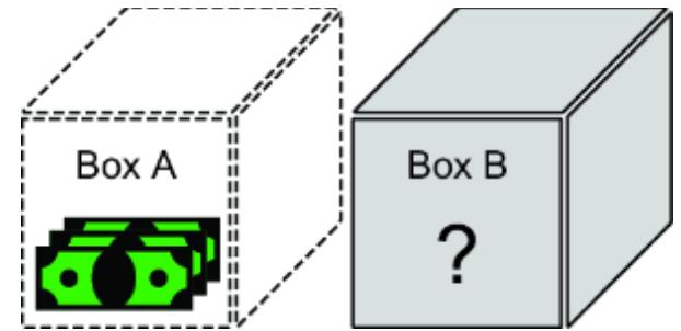
Figure 12.7 An illustration of the boxes in Newcomb’s paradox
Now, suppose there is an AI that can predict with high accuracy what choice the agent intends to make. If the AI predicts that the agent intends to take both boxes, it will put no money in box B. If the AI is correct and the agent takes both boxes, the agent only gets $1,000. However, if the AI predicts that the agent intends to take only box B, it will put $1,000,000 in box B. If the AI predicts correctly, the agent gets the $1,000,000 in box B but not the $1,000 in box A. The agent does not know for sure what the AI predicted or what box B contains until they make their choice.
The traditional paradox arises as follows. A causality-minded agent reasons that the actions of the AI are out of their control. They only focus on what they can control—the causal consequences of their choice. They can’t cause the content of box B, so they pick both boxes on the off-chance box B has the million, just as one would if the AI didn’t exist. But if the agent knows how the AI works, doesn’t it make more sense to choose only box B and get the million with certainty?
Let’s dig in further by enumerating the possible outcomes and their probabilities. Let’s assume the AI’s predictions are 95% accurate. If the agent chooses both boxes, there is a 95% chance the AI will have guessed the agent’s choice and put no money in B, in which case the agent only gets the $1,000. There is a 5% chance the algorithm will guess wrong, in which case it puts 1,000,000 in box B, and the
agent wins $1,001,000. If the agent chooses only box B, there is a 95% chance the AI will have predicted the choice and placed $1,000,000 in box B, giving the agent $1,000,000 in winnings. There is a 5% chance it will not, and the agent will take home nothing. We see these outcomes in table 12.1. The expected utility calculations are shown in table 12.2.
| Table 12.1 Newcomb’s problem outcomes and their probabilities | |||||
|---|---|---|---|---|---|
| ————————————————————— | – | – | – | – | – |
| Strategy | AI action | Winnings | Probability |
|---|---|---|---|
| Choose both | Put $0 in box B | $1,000 | .95 |
| Choose both | Put $1,000,000 in box B | $1,001,000 | .05 |
| Choose only box B | Put $1,000,000 in box B | $1,000,000 | .95 |
| Choose only box B | Put $0 in box B | $0 | .05 |
Table 12.2 Expected utility of each choice in Newcomb’s problem
| Strategy ( x) | E( U X= x) |
|---|---|
| Choose both | 1,000 × .95 + 1,001,000 × .05 = $51,000 |
| Choose only box B | 1,000,000 × .05 + 0 × .05 = $950,000 |
The conventional approach suggests choosing box only box B.
When the paradox was created, taking a causal approach to the problem meant only attending to the causal consequences of one’s actions. Remember that the AI makes the prediction before the agent acts. Since effects cannot precede causes in time, the AI’s behavior is not a consequence of the agent’s actions, so the agent with the causal view ignores the AI and goes with the original strategy of choosing both boxes.
It would seem that the agent with the causal view is making an error in failing to account for the actions of the AI. But we can resolve this error by having the agent use a formal causal model.
12.2.6 Newcomb’s paradox with a causal model
In the traditional formulation of Newcomb’s paradox, the assumption is that the agent using causal decision theory only attends to the consequences of their actions—they are reasoning on the causal DAG in figure 12.8. But the true data generating process (DGP) is better captured by figure 12.9.
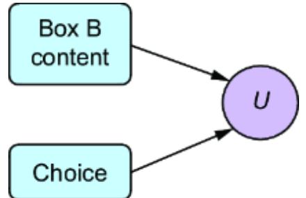
Figure 12.8 Newcomb’s paradox assumes a version of causal decision theory where a naive agent uses this incorrect causal DAG.
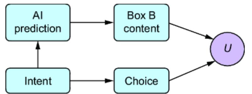
Figure 12.9 A better causal DAG representing the framing of Newcomb’s paradox
The choice of the agent can’t cause the AI’s prediction, because the prediction happens first. Thus, we assume the AI agent is inferring the agent’s intent, and thus the intent of the agent is the cause of the AI’s prediction.
The causal decision-making agent would prefer the graph in figure 12.9 because it is a better representation of the DGP.
The clever agent wouldn’t focus on maximizing E (Uchoice=x). The clever agent is aware of its own intention, and knowing that this intention is a cause of the content of box B, it focuses on optimizing E (Uchoice=x|intent =i ), where i is their original intention of which box to pick.
We’ll assume the agent’s initial intention is an impulse it cannot control. But while they can’t control their initial intent, they can do some introspection and become aware of this intent. Further, we’ll assume that upon doing so, they have the ability to change their choice to something different from what it initially intended, after the AI has made their prediction and set the contents of box B. Let’s model this system in pgmpy and evaluate maximizing E (Uchoice=x|intent =i ).
First, let’s build the DAG.
Listing 12.8 Create the DAG
model = BayesianNetwork(
 [
 ('intent', 'AI prediction'),
 ('intent', 'choice'),
 ('AI prediction', 'box B'),
 ('choice', 'U'),
 ('box B', 'U'),
 ]
)
Next, we’ll create causal Markov kernels for intent and choice.
Listing 12.9 Create causal Markov kernels for intent and choice
cpd_intent = TabularCPD( #1
 'intent', 2, [[0.5], [0.5]], #1
 state_names={'intent': ['B', 'both']} #1
) #1
print(cpd_intent)
cpd_choice = TabularCPD( #2
 'choice', 2, [[1, 0], [0, 1]], #2
 evidence=['intent'], #2
 evidence_card=[2], #2
 state_names={ #2
 'choice': ['B', 'both'], #2
 'intent': ['B', 'both'] #2
 } #2
) #2
print(cpd_choice)
#1 We assume a 50-50 chance the agent will prefer both boxes vs. box B.
#2 We assume the agent’s choice is deterministically driven by their intent.
Similarly, we’ll create the causal Markov kernels for the AI’s decision and the content of box B.
Listing 12.10 Create causal Markov kernels for AI prediction and box B content
cpd_AI = TabularCPD( #1
 'AI prediction', 2, [[.95, 0.05], [.05, .95]], #1
 evidence=['intent'], #1
 evidence_card=[2], #1
 state_names={ #1
 'AI prediction': ['B', 'both'], #1
 'intent': ['B', 'both'] #1
 } #1
) #1
print(cpd_AI)
cpd_box_b_content = TabularCPD( #2
 'box B', 2, [[0, 1], [1, 0]], #2
 evidence=['AI prediction'], #2
 evidence_card=[2], #2
 state_names={ #2
 'box B': [0, 1000000], #2
 'AI prediction': ['B', 'both'] #2
 } #2
) #2
print(cpd_box_b_content)
#1 The AI’s prediction is 95% accurate. #2 Box B contents are set deterministically by the AI’s prediction. Finally, we’ll create a causal Markov kernel for utility and add all the kernels to the model.
Listing 12.11 Create utility kernel and build the modelcpd_u = TabularCPD( #1
'U', 4, #1
[ #1
[1, 0, 0, 0], #1
[0, 1, 0, 0], #1
[0, 0, 1, 0], #1
[0, 0, 0, 1], #1
], #1
evidence=['box B', 'choice'], #1
evidence_card=[2, 2], #1
state_names={ #1
'U': [0, 1000, 1000000, 1001000], #1
'box B': [0, 1000000], #1
'choice': ['B', 'both'] #1
} #1
) #1
print(cpd_u)
model.add_cpds(cpd_intent, cpd_choice, cpd_AI, cpd_box_b_content, cpd_u) #2#1 Set up the utility node. #2 Build the model.
Now we’ll evaluate maximizing E(Uchoice=x|intent=i).
Listing 12.12 Infer optimal choice using intervention and conditioning on intent
int_model_x_both = do(model, {"choice": "both"}) #1
infer_both = VariableElimination(int_model_x_both) #1
marginal_u_given_both = infer_both.query( #1
 variables=['U'], evidence={'intent': 'both'}) #1
expectation_u_given_both = get_expectation(marginal_u_given_both) #1
print("E(U(Y_{choice=both}|intent=both))=", expectation_u_given_both) #1
int_model_x_box_B = do(model, {"choice": "B"}) #2
infer_box_B = VariableElimination(int_model_x_box_B) #2
marginal_u_given_box_B = infer_box_B.query( #2
 variables=['U'], evidence={'intent': 'both'}) #2
expectation_u_given_box_B = get_expectation(marginal_u_given_box_B) #2
print("E(U(Y_{choice=box B}|intent=both))=", expectation_u_given_box_B) #2
int_model_x_both = do(model, {"choice": "both"}) #3
infer_both = VariableElimination(int_model_x_both) #3
marginal_u_given_both = infer_both.query( #3
 variables=['U'], evidence={'intent': 'B'}) #3
expectation_u_given_both = get_expectation(marginal_u_given_both) #3
print("E(U(Y_{choice=both}|intent=B))=", expectation_u_given_both) #3
int_model_x_box_B = do(model, {"choice": "B"}) #4
infer_box_B = VariableElimination(int_model_x_box_B) #4
marginal_u_given_box_B = infer_box_B.query( #4
 variables=['U'], evidence={'intent': 'B'}) #4
expectation_u_given_box_B = get_expectation(marginal_u_given_box_B) #4
print("E(U(Y_{choice=box B}|intent=B))=", expectation_u_given_box_B) #4
#1 Infer E(U(Y choice=both|intent=both)).
#2 Infer E(U(Y choice=box B|intent=both)).
#3 Infer E(U(Y choice=both|intent=B)).
#4 Infer E(U(Y choice=box B|intent=B)).This code produces the following results (* indicates the optimal choice for a given intent):
- E(U(Ychoice=both|intent =both)) = 51000 *
- E(U(Ychoice=box B|intent =both)) = 50000
- E(U(Ychoice=both|intent =B)) = 951000 *
- E(U(Ychoice=box B|intent =B)) = 950000
When the agent’s initial intention is to select both, the best choice is to select both. When the agent intends to choose only box B, the best choice is to ignore those intentions and choose both. Either way, the agent should choose both. Note that when the agent initially intends to choose only box B, switching to both boxes gives them an expected utility of
$951,000 which is greater than the optimal choice utility of $950,000 in the noncausal approach.
The agent, unfortunately, cannot control their initial intent; if they could, they would deliberately ‘intend’ to pick box B and then switch at the last minute to choosing both boxes after the AI placed the million in box B. However, they can engage in a form of introspection, factoring their initial intent into their decision and, in so doing, accounting for the AI’s behavior rather than ignoring it.
12.2.7 Introspection in causal decision theory
Newcomb’s problem illustrates a key capability of causal decision theory—the ability for us to include introspection as part of the DGP.
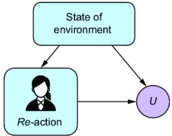
Figure 12.10 Often our actions are simply reactions to our environment, rather than the result of deliberate decision-making.
To illustrate, consider that often our actions are simply reactions to our environment, as in figure 12.10.
For example, you might have purchased a chocolate bar because you were hungry and it was positioned to tempt you as you waited in the checkout aisle of the grocery store. Rather than go through some deliberative decision-making
process, you had a simple, perhaps even unconscious, reaction to your craving and an easy way to satisfy it.
However, humans are capable of introspection—observing and thinking about their internal states. A human might consider their normal reactive behavior as part of the DGP. This introspection is illustrated in figure 12.11.
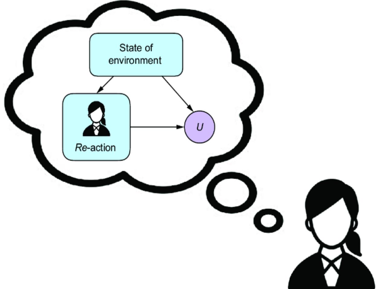
Figure 12.11 Humans and some other agents can think about a DGP that includes them as a component of that process.
Through this introspection, the agent can perform level 2 hierarchical reasoning about what would happen if they did not react as usual but acted deliberately (e.g., sticking to their diet and not buying the chocolate bar), as in figure 12.12.
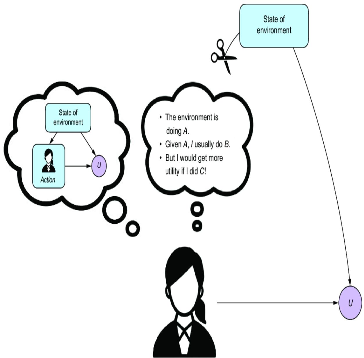
Figure 12.12 The agent reasons about a DGP that includes them as a component. They then use that reasoning in asking level 2 ૿what would happen if… questions about that process.
In many cases, the agent may not know the full state of their environment. However, if the agent can disentangle their urge to react a certain way from their action, they can use that ૿urge as evidence in deliberative decision-making, as in figure 12.13.
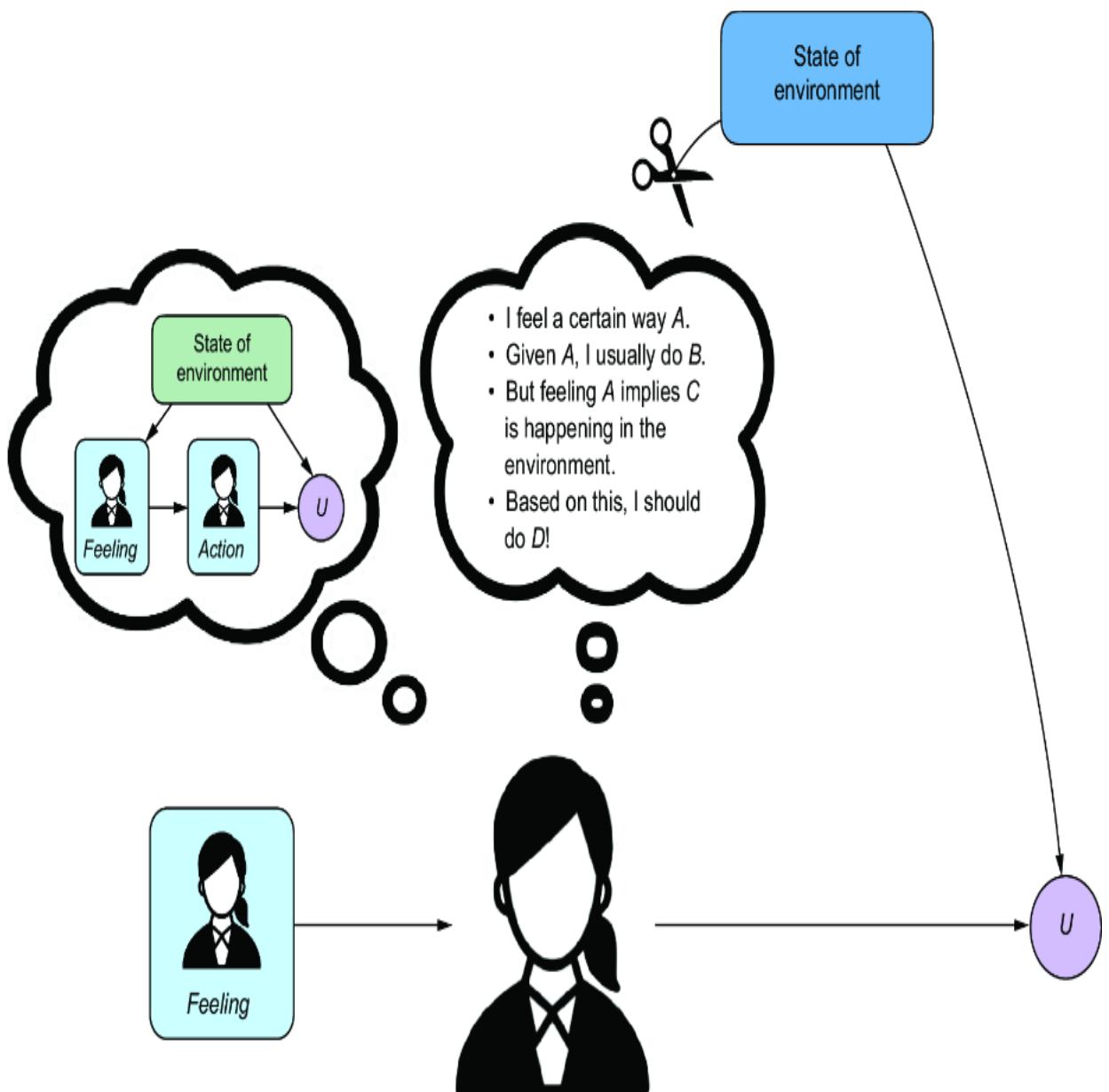
Figure 12.13 The agent may not know the states of other variables in the environment, but through introspection, they may have an intuition about those variables. That intuition can be used as evidence in conditional causal inferences.
We saw this pattern in the Newcomb example; the agent does not know what the AI has predicted, but, through introspection, they can use their initial intention to choose both boxes as evidence of what the AI has chosen.
Was there ever a time where you noticed you had started to make clumsy errors in your work and used that as evidence that you were fatigued, even though you didn’t feel so, and you thought, ૿what if I take a break? Have you had a gut feeling that something was off, despite not knowing what, and based on this feeling started to make different decisions? Causal modeling, particularly with causal generative models, make it easy to write algorithms that capture this type of self-introspection in decision-making.
Next, we’ll look at causal modeling of sequential decisionmaking.
12.3 Causal DAGs and sequential decisions
Sequential decision processes are processes of back-to-back decision-making. These processes can involve sequential decisions made by humans or by algorithms and engineered agents.
When I model decision processes in sequence, I use a subscript to indicate a discrete step in the series, such as Y1, Y2, Y3. When I want to indicate an intervention subscript, I’ll place it to the right of the time-step subscript, as in Y1, X= x, Y2,X= x, Y3, X= x.
In this section, I’ll show causal DAGs for several canonical sequential decision-making processes, but you should view these as templates, not as fixed structures. You can add or remove edges in whatever way you deem appropriate for a given problem.
Let’s look at the simplest case, bandit feedback.
12.3.1 Bandit feedback
Bandit feedback refers to cases where, at each step in the sequence, there is an act X that leads to an outcome Y, with some utility U (Y ). A bandit sequence has two key features. The first is that, at every step, there is instant feedback after an act occurs. The second is independent trials, meaning that the variables at the t th timestep are independent of variables at other timesteps. The term ૿bandit comes from an analogy to ૿one-armed bandits, which is a slang term for casino slot machines that traditionally have an arm that the player pulls to initiate gameplay. Slot machine gameplay provides bandit feedback—you deposit a token, pull the arm, and instantly find out if you win or lose. That outcome is independent of previous plays.
We can capture bandit feedback with the causal DAG in figure 12.14.
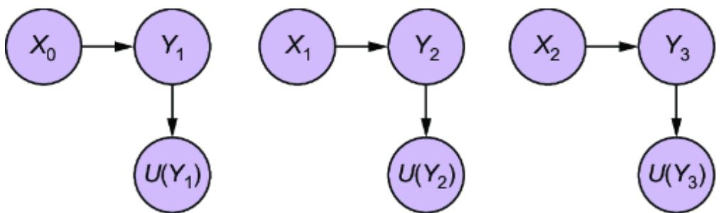
Figure 12.14 A causal DAG illustrating simple bandit feedback
The causal DAG in figure 12.14 captures instant feedback with a utility node at each timestep, and with a lack of edges, reflecting an independence of variables across timesteps.
12.3.2 Contextual bandit feedback
In contextual bandit feedback, one or more variables are common causes for both the act and the outcome. In figure 12.15, the context variable C is common to each {X, Y } tuple in the sequence. In this case, the context variable C could represent the profile of a particular individual, and the act variable X is that user’s behavior.
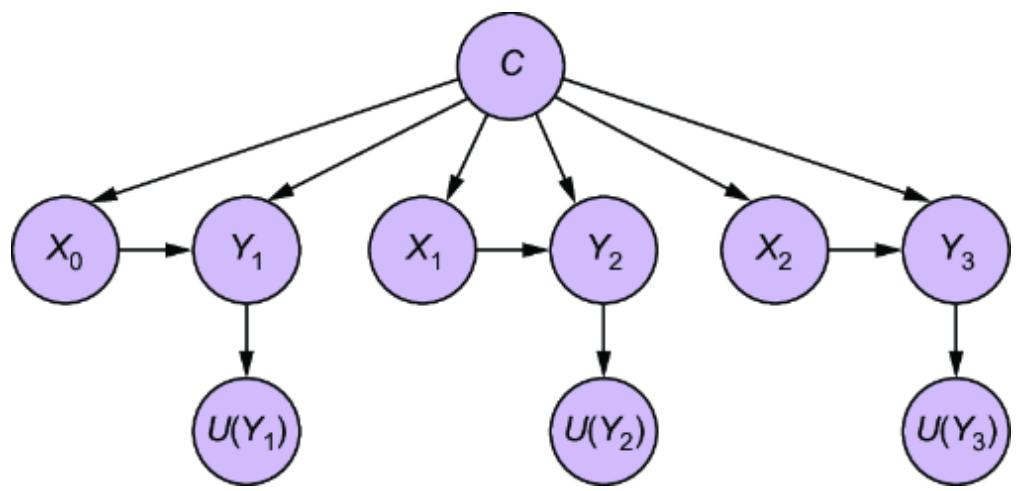
Figure 12.15 A causal DAG illustrating contextual bandit feedback
Alternatively, the context variable could change at each step, as in figure 12.16.
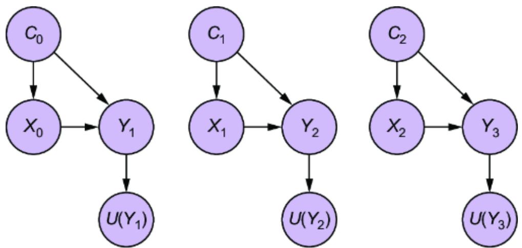
Figure 12.16 A causal DAG illustrating contextual bandit feedback where the context changes at each timestep
We can vary this template in different ways. For example, we could have the actions drive the context variables in the next timestep, as in figure 12.17. The choice depends on your specific problem.
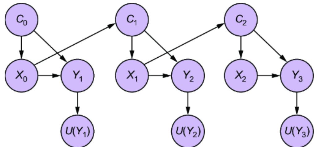
Figure 12.17 A causal DAG where the action at one timestep influences the context at the next timestep
12.3.3 Delayed feedback
In a delayed-feedback setting, the outcome variable and corresponding utility are no longer instant feedback. Instead, they come at the end of a sequence. Let’s consider an example where a context variable drives the acts. The acts affect the next instance of the context variable.
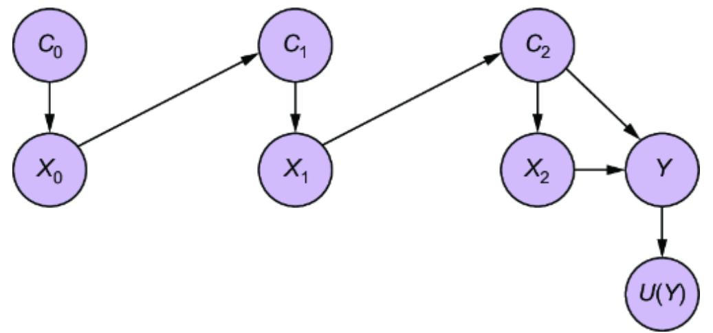
Figure 12.18 Example of a causal DAG for sequential decision making with delayed feedback
Again, figure 12.18 shows an example of this approach based on the previous model. Here the act at time k influences the context variable (C ) at time k + 1, which in turn affects the act at time k + 1.
Consider a case of chronic pain. Here the context variable represents whether a subject is experiencing pain (C ). The presence of pain drives the act of taking a painkiller (X ). Taking the painkiller (or not) affects whether there is pain in the next step. Figure 12.19 illustrates this DAG.
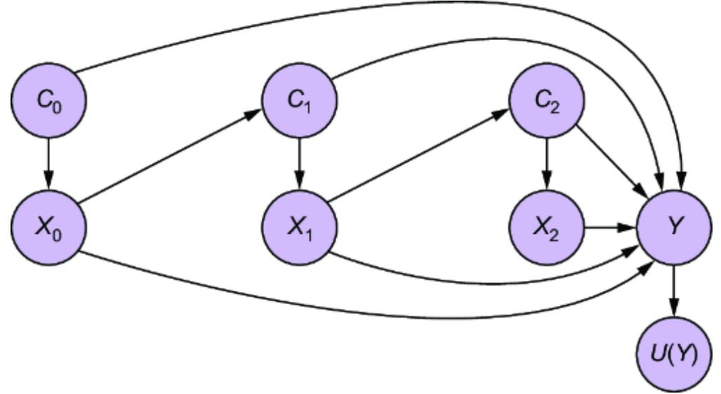
Figure 12.19 A causal DAG representing the treatment of chronic pain
Y here is the ultimate health outcome of the subject, and it is driven both by the overall amount of pain over time, and the amount of drugs the subject took (because perhaps overuse of painkillers has a detrimental health effect).
12.3.4 Causal queries on a sequential model
We may want to calculate some causal query for our sequential decision problem. For example, given the DAG in figure 12.19, we might want to calculate the causal effect of X0 on U(Y ):
\[E\left(U(Y\_{X\_0=x}) - U(Y\_{X\_0=x'})\right)\]
Or perhaps we might be interested in the causal effect of the full sequence of acts on U(Y ):
\[E\left(U\left(Y\_{X\_0=a,X\_1=b,X\_2=c}\right) - U\left(Y\_{X\_0=a',X\_1=b',X\_2=c'}\right)\right)\]
Either way, now that we have framed the sequential problem as a causal model, we are in familiar territory; we can simply use the causal inference tools we’ve learned in previous chapters to answer causal queries with this model.
As usual, we must be attentive to the possibility of latent causes that can confound our causal inference. In the case of causal effects, our concern is latent common confounding causes between acts (X ) and outcomes (Y ), or alternatively between acts (X ) and utilities (U ). Figure 12.20 is the same as figure 12.15, except it introduces a latent Z confounder.
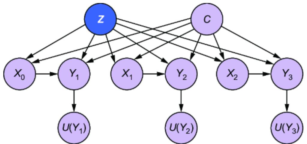
Figure 12.20 Contextual bandit with a latent confounder
Similarly, we could have a unique confounder at every timestep, as in figure 12.21.
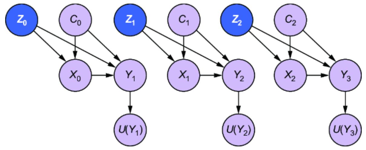
Figure 12.21 Bandit feedback with a different context and latent confounders at each timestep
Similarly, figure 12.22 shows a second version of the chronic pain graph where the confounders affect each other and the context variables. This confounder could be some external factor in the subject’s environment that triggers the pain and affects well-being.
These confounders become an issue when we want to infer the causal effect of a sequence of actions on U (Y ).
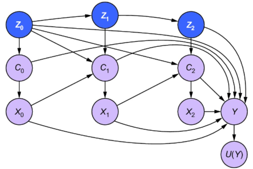
Figure 12.22 A version of the chronic pain DAG where the confounders affect each other and the context variables
Next, we’ll look at how we can view policies for automatic decision making in sequential decision-making processes as stochastic interventions.
12.4 Policies as stochastic interventions
In automated sequential decision-making, the term ૿policy is preferred to ૿decision rule. I’ll introduce a special notation for a policy: π(.). It will be a function that takes in observed outcomes of other variables and returns an action.
To consider how a policy affects the model, we’ll contrast the DAG before and after a policy is implemented. Figure 12.23 illustrates a simple example with a context variable C and a latent variable Z. The policy uses context C to select a value of X.
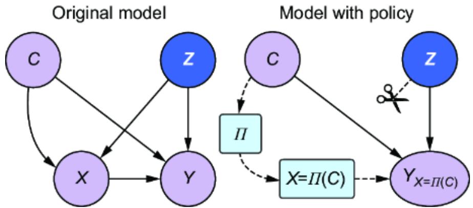
Figure 12.23 The dashed lines show edges modulated by the policy. The policy breaks the influence of the confounder Z like an ideal intervention, but dependence on C remains through the policy.
The policy is a type of stochastic intervention; it selects a intervention value for X from some process that depends on C. Like an ideal intervention, it changes the graph. The left of figure 12.23 shows the DAG prior to deployment of the policy. On the right is the DAG after the policy is deployed. I add a special policy node to the graph to illustrate how the policy modulates the graph. The dashed edges highlight edges modulated by the policy. Just like an ideal intervention, the policy-generated intervention removes X’s original incoming edges C →X and Z →X. However, because the policy depends on C, the dashed edges illustrate the new flow of influence from C to X.
Suppose we are interested in what value Y would have for a policy-selected action X = Π. In counterfactual notation, we write
In sequence settings, the policy applies a stochastic intervention at multiple steps in the sequence. From a possible worlds perspective, each intervention induces a new hypothetical world. This can stretch the counterfactual
notation a bit, so going forward, I’ll simplify the counterfactual notation to look like this:
\[Y\_{3, \pi\_0, \pi\_1, \pi\_2}\]
This means Y3 (Y at timestep 3) is under influence of the policy’s outcomes at times 0, 1, and 2.
12.4.1 Examples in sequential decision-making
In the case of bandit feedback, the actions are produced by a bandit algorithm, which is a type of policy that incorporates the entire history of actions and utility outcomes in deciding the optimal current action. Though actions and outcomes in the bandit feedback process are independent at each time step, the policy introduces dependence on past actions and outcomes, as shown in figure 12.24.
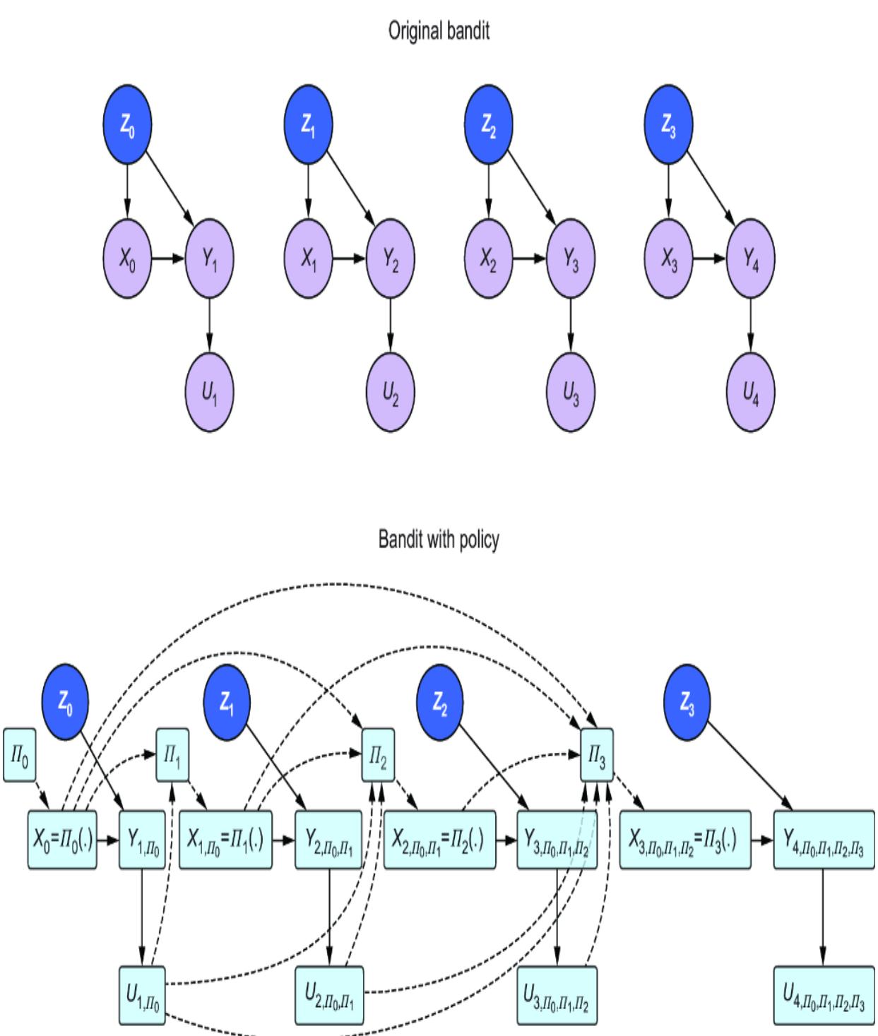
Figure 12.24 Bandit feedback where a bandit policy algorithm selects the next action based on past actions and reward outcomes
Recall our previous example of an agent taking pain medication in response to the onset of pain. Figure 12.25 shows how a policy would take in the history of degree of pain and how much medication was provided.
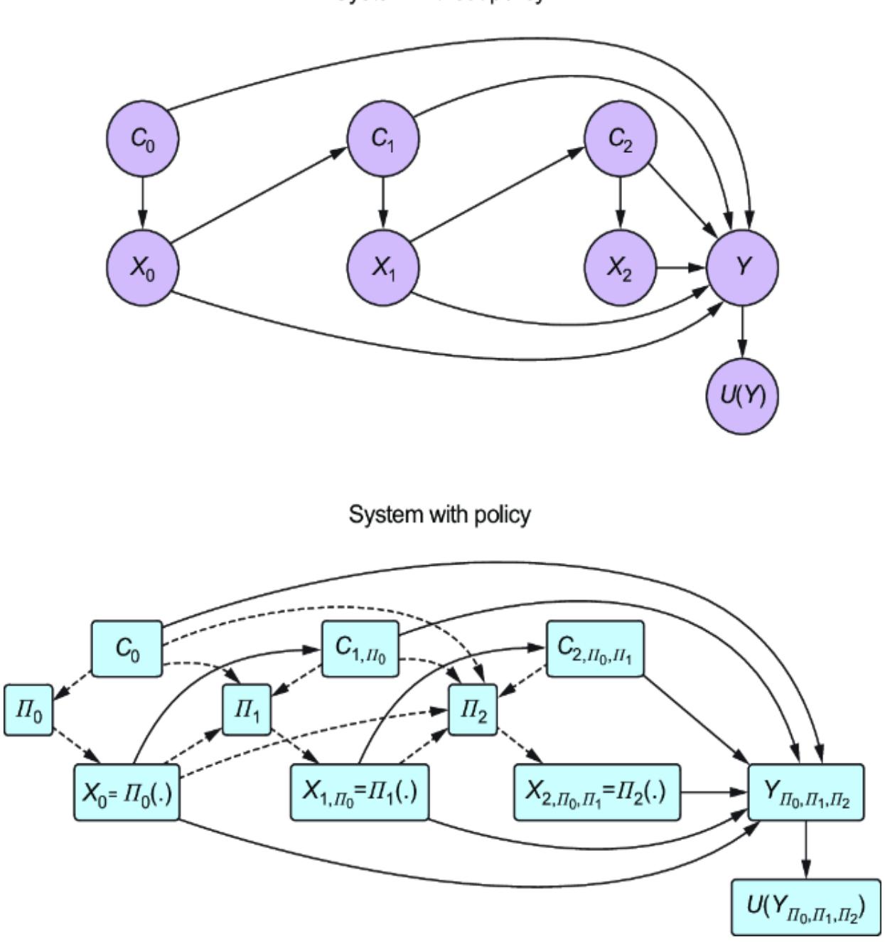
Figure 12.25 In the pain example, the policy considers the history of recorded levels of pain and corresponding dosages of medication.
The policy is like a doctor making the rounds on a hospital floor. They come to a patient’s bed, and the patient reports some level of pain. The doctor looks at that patient’s history of pain reports and the subsequent dosages of medication and uses that information to decide what dosage to provide this time. The doctor’s utility function is in terms of pain, risk of overdose, and risk of addiction. They need to consider historic data, not just the current level of pain, to optimize this utility function.
12.4.2 How policies can introduce confounding
As stochastic interventions, policies introduce interventions conditional on other nodes in the graph. Because of this, there is a possibility that the policy will introduce new backdoor paths that can confound causal inferences. For example, consider again the DAG in figure 12.26.
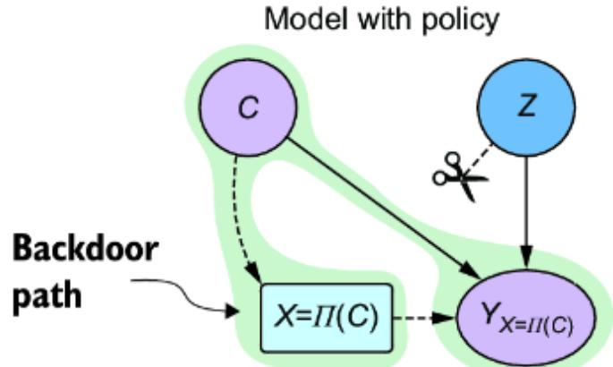

The policy breaks the backdoor path from X to Y through Z, but there is still a path from X to Y through C. Thus, typical causal queries involving X and Y would have to condition on or adjust for C.
In the next section, we’ll characterize causal RL in causal terms.
12.5 Causal reinforcement learning
Reinforcement learning (RL) is a branch of machine learning that generally involves an agent learning policies that maximize cumulative reward (utility). The agent learns from the consequences of its actions, rather than from being explicitly taught, and adjusts its behavior based on the rewards or losses (reinforcements) it receives. Many sequential decision-making problems can be cast as RL problems.
12.5.1 Connecting causality and Markov decision processes
RL typically casts a decision process as a Markov decision process (MDP). A canonical toy example of an MDP is a grid world, illustrated in figure 12.27.
Figure 12.27 presents a 3 × 4 grid world. An agent can act within this grid world with a fixed set of actions, moving up, down, left, and right. The agent wants to execute a set of actions that deliver it to the upper-right corner {0, 3}, where it gains a reward of 100. The agent wants to avoid the middle-right square {1, 3}, where it has a reward of –100 (a loss of 100). Position {1, 1} contains an obstacle the agent cannot traverse.
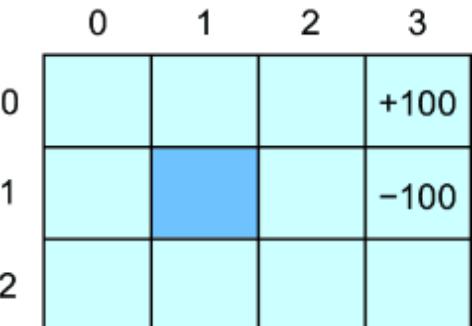
Figure 12.27 A simple grid world
We can think of it as a game. When the game starts, the agent ૿spawns randomly in one of the squares, except for {0, 3}, {1, 3}, and {1, 1}. When the agent moves into a goal square, the game ends. To win, the agent must navigate around the obstacle in {1, 1}, avoid {1, 3}, and reach {0, 3}.
A Markov decision process models this and much more complicated ૿worlds (aka domains, problems, etc.) with abstractions for states, actions, transition functions, and rewards.
STATES
States are a set that represents the current situation or context that the agent is in, within its environment. In the grid-world example, a state represents the agent being at a specific cell. In this grid, there are 12 different states (the cell at {1, 1} is an unreachable state). We assume the agent has some way of knowing which state they are in.
We’ll denote state as a variable S. In a grid world, S is a discrete variable, but in other problems, S could be continuous.
ACTIONS
Actions are the things the agent can do, and they lead to a change of state. Some actions might not be available when in a particular state. For example, in the grid world, the borders of the grid are constraints on the movements of the agent. If the agent is in the bottom-left square {2, 0}, and they try to move left or down, they will stay in place. Similarly, the cell at {1, 1} is an obstacle the agent must navigate around. We denote actions with the variable A, which has four possible outcomes {up, down, right, left}.
TRANSITION FUNCTION
The transition function is a probability distribution function. It tells us the probability of moving to a specific next state, given the current state and the action taken.
If states are discrete, the transition function looks like this:
\[P(S\_{t+1} = s' | S\_t = s, \mathcal{A}\_t = a)\]
Here, St = s means the agent is currently in state s. At = a means the agent performs action a. P (S t +1 = s’|St = s, At = a) is the probability that the agent transitions to a new state s’ given it is in state s and performs action a. When the action leads to a new state with complete certainty, this probability distribution function becomes degenerate (all probability is concentrated on one value).
REWARDS
The term ૿reward is preferred to ૿utility in RL. In the context of MDPs, the reward function will always take a state s as an argument. We will write it as U (s ).
In the grid-world example, U ({0, 3}) = 100, U ({1, 3)) = – 100. The reward of all other states is 0. Note that sometimes in the MDP/RL literature, U () is a function of state and an action, as in U (s, a ). We don’t lose anything by just having actions be a function of state because you can always fold actions into the definition of a state.
12.5.2 The MDP as a causal DAG
Figure 12.28 shows the MDP as a causal DAG.
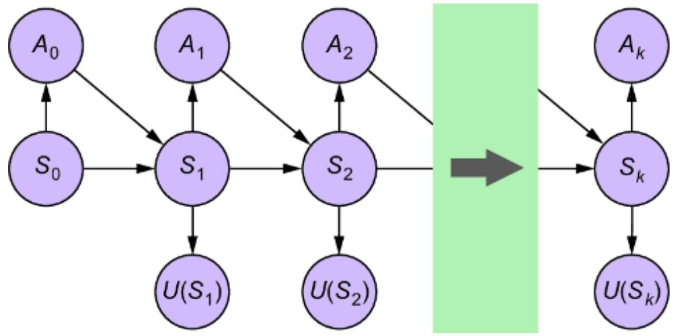
Figure 12.28 The Markov decision process represented as a DAG
As a causal DAG, the MDP looks like the other sequential decision processes we’ve outlined, except that we limit ourselves to states, actions, and rewards. In figure 12.28, the process continues until we reach a terminal state (Sk), such as getting to the terminal cells in the grid-world example.
THE CAUSAL MARKOV PROPERTY AND THE MDP
The ૿Markov in ૿Markov decision process comes from the fact that the current state is independent of the full history of states given the last state. Contrast this with the causal Markov property of causal DAGs: a node in the DAG is independent of indirect ૿ancestor causes given its direct causal parents. We can see that when we view the MDP as a causal DAG, this Markovian assumption is equivalent to the causal Markov property. That means we can use our dseparation-based causal reasoning, including the docalculus, in the MDP graphical setting.
THE TRANSITION FUNCTION AND THE CAUSAL MARKOV KERNEL
Note that based on this DAG, the parents of a state S(t+1) are the previous state St and the action At taken when in that previous state. Therefore, the causal Markov kernel is P (S t +1 = s’|St = s, At = a), i.e., the transition function. Thus, the transition function is the causal Markov kernel for a given state.
12.5.3 Partially observable MDPs
An extension of MDPs is partially observed MDPs (POMDPs). In a POMDP, the agent doesn’t know with certainty what state they are in, and they must make inferences about that state given incomplete evidence from their environment. This applies to many practical problems where the agent cannot observe the full state of the environment.
A POMDP can entail different causal structures depending on our assumptions about the causal relationships between the unobserved and observed states. For example, suppose a latent state S is a cause of the observed state X. The observed state X now drives the act A instead of S. Figure 12.29 illustrates this formulation of a POMDP as a causal DAG.
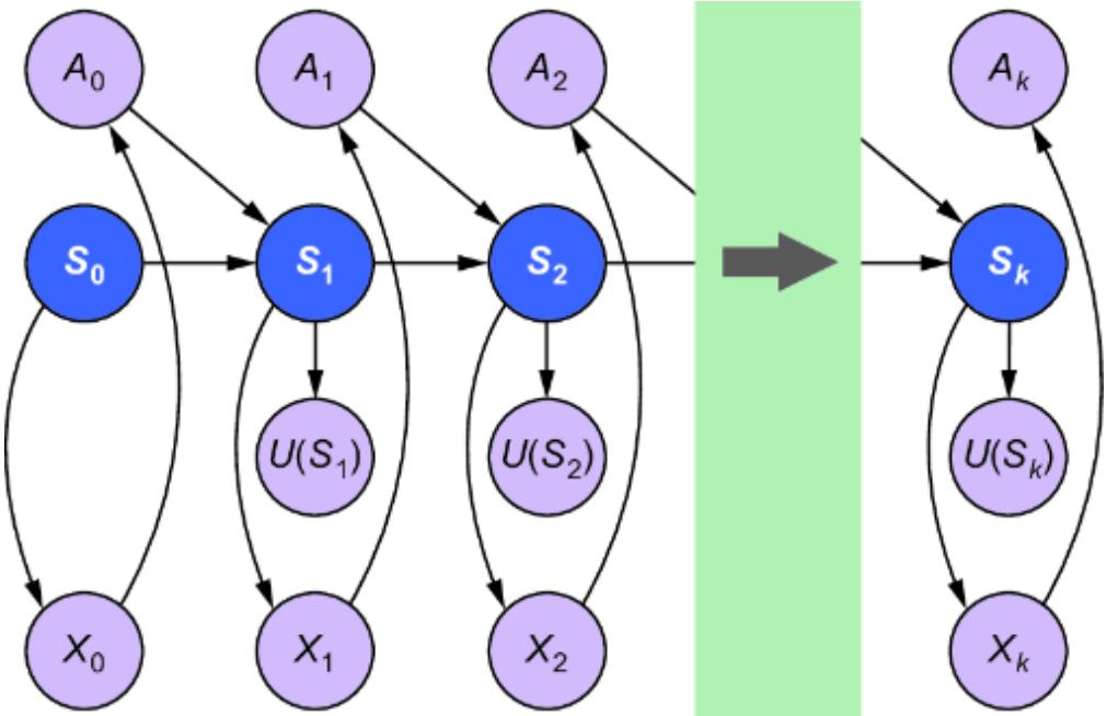
Figure 12.29 A POMDP where a latent state S causes an observed state X. X drives the actions A.
In contrast, figure 12.30 illustrates an example where the latent state is a latent common cause (denoted Z) of the observed state (mediated through the agent’s action) and the utility (note a slight change of notation from U (Si ) to Ui ). Here, unobserved factors influence both the agent’s behavior and the resulting utility of that behavior.
Again, the basic MDP and POMDP DAGs should be seen as templates for starting our analysis. Once we understand what causal queries we are interested in answering, we can explicitly represent various components of observed and unobserved states as specific nodes in the graph, and then use identification and adjustment techniques to answer our causal queries.
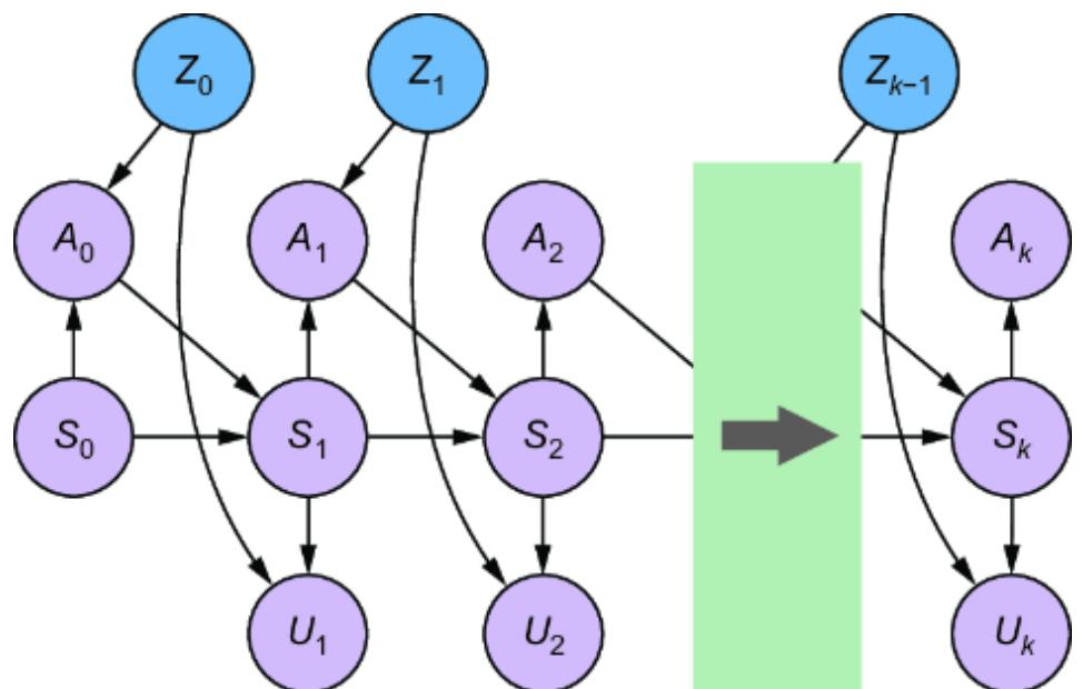
Figure 12.30 A POMPD formulation where the unobserved states are latent common causes that could act as confounders in causal inferences
12.5.4 Policy in an MDP
As before, policies in an MDP act as stochastic interventions. Figure 12.31 illustrates a policy that selects an optimal action based on the current state in a way that disrupts any influence on the action from a confounder.
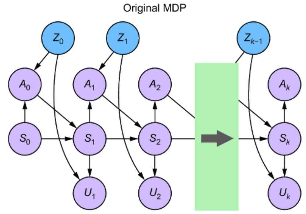
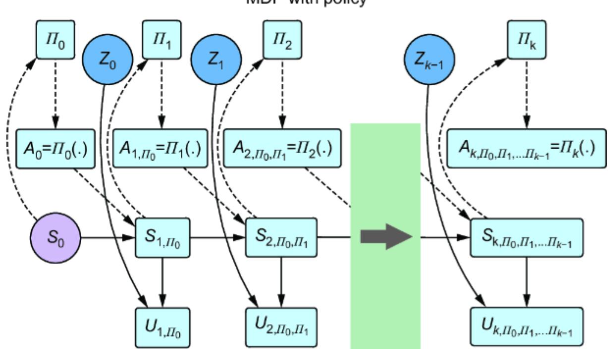
Figure 12.31 Modification of an MDP DAG by a policy
Figure 12.31 is simple in that it only selects an action based on the current state. The challenge is in the implementation, because in most RL settings, states can be high-dimensional objects.
12.5.5 Causal Bellman equation
RL is about searching for the optimal policy, which is characterized with the Bellman equation, often written as follows:
\[\Pi^\* = \operatorname\*{argmax}\_{\Pi} E\left(\sum\_{t=0}^{\infty} \gamma^{t+1} U\left(S\_{t+1}\right)\middle| A\_t = \Pi\left(S\_t\right)\right)\]
In plain words, we’re looking for a policy Π* maximizes the cumulative reward over time. Here γ is a discount rate, a value between 0 and 1, that makes sure the agent values rewards in the near future more than rewards in the far future.
Since we’re reasoning about what would happen if we deployed the policy, the causal formulation would be as follows:
\[\Pi^\* = \operatorname\*{argmax}\_{\Pi} E\left(\sum\_{t=0}^{\infty} \gamma^{t+1} U\left(S\_{t+1, A\_t = \Pi(S\_t)}\right)\right)\]
Note that we could do the same causal rewrite for other variants of the Bellman equation, such as the Q-function used in Q-learning.
The difference between the noncausal and causal formulations of the Bellman equation is the same as the difference between optimizing E (U (Y )|X=x ) and E (U (YX=x )) in section 12.2.4. The process of solving the causally naive version of the Bellman equation may introduce biases from latent confounders or from conditioning on colliders and mediators. Our causally attuned approach can help avoid these biases. In many cases, the solution of the naive approach will coincide with the causal approach because those biases might not affect the ranking of the top policy relative to others. However, as in the E (U(Y )|X = x ) versus E (U (YX=x)) example, there will be cases where the solutions to the noncausal and causal formulations differ, and your RL problem might be one of those cases.
12.6 Counterfactual reasoning for decision-theory
So far, we’ve discussed the problem of choosing optimal actions with respect to a utility function as a level 2 query on the causal hierarchy. Is there a use for level 3 counterfactual reasoning in decision theory? In this section, we’ll briefly review some applications for level 3 reasoning.
12.6.1 Counterfactual policy evaluation
Counterfactual policy evaluation involves taking logged data from a policy in production and asking, ૿given we used this policy and got this cumulative reward, how much cumulative reward would we have gotten had we used a different policy? See the chapter notes at https://www.altdeep.ai/p/causalaibookfor references to techniques such as counterfactually guided policy search and counterfactual risk minimization.
12.6.2 Counterfactual regret minimization
In chapters 8 and 9, I introduced regret as a counterfactual concept. We can further clarify the idea now that we have introduced the language of decision-making; regret is the difference between the utility/reward that was realized given a specific action or set of actions, and the utility/reward that would have been realized had another action or set of actions been taken.
Counterfactual regret minimization is an approach to optimizing policies that seeks to minimize regret. To illustrate, suppose we have a policy variable Π, which can return one of several available policies. The policies take in the context and return an action. The action leads to some reward U.
Suppose, for a single instance in our logged data, the policy was Π=π and the context was C =c. We get a certain action A =π(c ) and reward U =u. For some policy π’, regret is the answer to the counterfactual question, ૿How much more reward would we have gotten if the policy had been π = π’? In terms of expectation,
\[\begin{aligned} &E(u - U\_{\Pi = \pi'} | C = c, \Pi = \pi, A = \pi(c), U\_{A = \pi(c)} = u) \\ &= u - E(U\_{\Pi = \pi'} | C = c, \Pi = \pi, A = \pi(c), U\_{A = \pi(c)} = u) \end{aligned}\]
Again, this is regret for a single instance in logged data where the context was C =c and the utility was u. There are many variations, but the general idea is to find the policy that would have minimized cumulative regret over all the cases of C =c in the logged data, with the goal of favoring that policy in cases of C =c in the future.
12.6.3 Making level 3 assumptions in decision problems
The question, of course, is how to make the level 3 assumptions that enable counterfactual inferences. One approach would be to specify an SCM and use the general algorithm for counterfactual reasoning (discussed in chapter 9). For example, in RL, the transition function P (S t +1 = s’|St = s, At = a) captures the rules of state changes in the environment. As I mentioned, P (S t +1|St = s, At = a) is the causal Markov kernel for a given state S t +1. We could specify an SCM with an assignment function that entails that causal Markov kernel, and write that assignment function as
\[\mathbf{s'} = f\_{\mathbf{S}\_{t+1}} \ (\mathbf{s}, \ a, n\_{\mathbf{s'}})\]
Here, ns’ is the value of an exogenous variable for St.
The challenge is specifying assignment functions that encode the correct counterfactual distributions. This is easier in domains where we know more about the underlying causal mechanisms. A key example is in rule-based games; game rules can provide the level 3 constraints that enable simulation of counterfactuals. Recall how, in chapter 9, the simple rules of the Monte Hall problem enabled us to simulate counterfactual outcomes for stay versus switch strategies. Or consider multiplayer games like poker, where in a round of play each player is dealt a hand of cards and can take certain actions (check, bet, call, raise, or fold) that lead to outcomes (win, lose, tie) based on simple rules, which in turn determine the amount of chips won or lost in that round. A player’s counterfactual regret is the difference between the chips they netted and the most they could have netted had they decided on different actions. This is done
while accounting for the information available at the time of the decision, not using hindsight about the opponents’ cards.
Counterfactual regret minimization algorithms in this domain attempt to find game playing policies that minimize counterfactual regret across multiple players. The concrete rules of the game enable simulation of counterfactual game trajectories. The challenge lies in searching for optimal policies within a space of possible counterfactual trajectories that is quite large because of multiple player interactions over several rounds of play. See the chapter notes on counterfactual regret minimization in multiagent games at https://www.altdeep.ai/p/causalaibookfor references.
Summary
- Decision-making is naturally a causal problem because decisions cause consequences, and our goal is to make the decision that leads to favorable consequences.
- Choosing the optimal decision is a level 2 query as we are asking ૿what would happen if I made this decision?
- E (U (Y |X =x )) and E (U (YX=x )) are different quantities. Usually, people want to know the value of X that optimizes E (U (YX=x )), but optimizing E (U (Y |X = x )) will often yield the same answer without the bother of specifying a causal model.
- This is especially true in reinforcement learning (RL), where the analogs to E (U (Y |X =x)) and E (U (YX=x)) are, respectively, the conventional and causal formulations of the Bellman equation. Confounder, mediator, and collider biases may be present in conventional approaches to solving the Bellman equation. But those bias often don’t influence the ranking of the top policy relative to other policies.
- Nonetheless, sometimes the value of X that optimizes E (U (Y |X =x)) is different from that which optimizes E (U (YX=x )). Similarly, addressing causal nuances when solving the Bellman equation may result in a different policy than ignoring them. If your decision problem falls into this category, causal approaches are the better choice.
- Newcomb’s paradox is a thought experiment meant to contrast causal and noncausal approaches to decision theory. The ૿paradox is less mysterious once we use a formal causal model.
- Causal decision theory, combined with probabilistic modeling tools like Pyro and pgmpy, is well suited to modeling introspection, where an agent reflects on their internal state (feelings, intuition, urges, intent) and uses that information to predict the ૿what-if outcomes of their decisions.
- When we represent a sequential decision process with a causal DAG, we can employ all the tools of graphical causal inference in that decision problem.
- Policies operate like stochastic interventions. They change the graph but still have dependence on observed nodes in the past, and that dependence can introduce backdoor confounding.
- In causal RL, we can represent MDPs and POMDPs as causal DAGs and, again, make use of graphical causal inference theory.
- We can use template DAGs to represent sequential decision processes, but you should tailor these templates for your problem.
- Common use cases for counterfactual reasoning in decision theory are counterfactual policy evaluation and counterfactual regret minimization.
If you have access to the rules underlying state transitions in your MDP, such as in physical systems or games, you could build an SCM that is counter- factually faithful to those rules, and use it to handle counterfactual use cases in decision-making.
13 Causality and large language models
This chapter covers
- Using causal information in LLMs to enhance a causal analysis
- Connecting the components of an LLM to a causal ideas
- Building a causal LLM
Large language models (LLMs) represent a significant advancement in the field of artificial intelligence. These models are large neural networks designed to generate and understand human-readable text. They are ૿large because their scale is truly impressive—cutting-edge LLMs have parameters numbering in the billions and trillions. As generative models, their main function is to generate coherent and contextually relevant natural language. They can also generate structured text, such as programming code, markup languages, mathematical symbols, database queries, and many other useful things in text form.
LLMs are just one example of a broad class of generative AI. For example, we can use the neural network architecture underlying cutting-edge LLMs to model other sequences, such as time-series or DNA. LLMs are a type of foundation model, meaning large-scale models that serve as a base or foundation upon which more specialized models or applications can be built. Some LLMs are multimodal, meaning they work with text as well as other content modalities, such as images. In this chapter, we’ll focus
specifically on LLMs, but much of what we discuss can be generalized to these related ideas.
To start, let’s explore some use cases for using LLMs to enhance a causal analysis.
13.1 LLMs as a causal knowledgebase
As I’ve mentioned several times in this book, in causal modeling, we don’t model the data, we model the data generating process (DGP). In other words, causal modeling requires causal information about the DGP that we can use as assumptions that enable identification of our causal queries. Cutting-edge LLMs are excellent resources for sourcing and validating that causal information. In this section, I’ll demonstrate some proven use cases for using LLMs to query causal information that augments a causal analysis.
The following results come from OpenAI’s LLM GPT-4 via the ChatGPT interface. Because of the random generation from the model, and OpenAI’s periodic updates to the model and ChatGPT software, your results will vary from mine to some degree.
13.1.1 Building a causal DAG
Let’s start with using the LLM to augment the first workflow we discussed in this book: building the causal DAG. Specifying assumptions in the form of a causal DAG can be daunting. What if your DAG is wrong? Modern LLMs are invaluable as a way of leveraging public expert knowledge to build a DAG.
You are a helpful causal analysis assistant. I’m interested in modeling the relationship between smoking and lung cancer. Provide me a causal DAG that captures this causal relationship.
Certainly! A Directed Acyclic Graph (DAG) is a powerful tool to represent causal relationships. Here’s a basic causal DAG to represent the relationship between smoking and lung cancer:
- Nodes:
- S: Smoking behavior (e.g., smoker, non-smoker, or frequency of smoking)
- LC: Lung Cancer (presence or absence)
- Directed Edge:
- A directed edge from S to LC represents that smoking behavior can cause or influence the occurrence of lung cancer.
- Potential Confounders:
- Other nodes can be introduced into the DAG to account for potential confounders. Some potential confounders might be:
- G: Genetics (a family history of lung cancer)
- A: Age (older age might be associated with a higher risk)
- E: Environmental exposure (like asbestos, pollution, etc.)
- O: Other health behaviors (like diet, exercise)
- Potential Mediators:
- Mediators are intermediate variables through which a cause exerts its effect on an outcome.
- For instance, one could hypothesize that smoking might cause lung damage, which in turn causes lung cancer. In this case:
- LD: Lung Damage
The DAG might look like this with the confounders and the mediator:
- S <- G –> LC
- S <- A –> LC
- S <- E –> LC
- S <- O –> LC
- S –> LC
- S –> LD –> LC
In the process of modeling, it’s important to:
- Identify all potential confounders to avoid biased results. Remember that correlation does not imply causation. Just because two nodes are correlated does not mean one causes the other.
- Validate your DAG with domain experts. They can provide insights into relationships you might not have considered.
- Use data to test and validate the causal relationships in your DAG, e.g., through controlled experiments or statistical methods like instrumental variables or propensity score matching when experiments are not feasible.
- Bear in mind that this is a simplified DAG for the relationship between smoking and lung cancer. Depending on the granularity and depth of your study, you might need to adjust and expand this framework.
Continuing, I can prompt the LLM to provide potential instrumental variables.
Suggest two good candidates for instrumental variables. Be brief in your response.

Certainly. For the relationship between smoking and lung cancer, two potential instrumental variables (IVs) could be:
- Cigarette Tax or Price: If certain regions or periods have higher cigarette prices or taxes, this can influence smoking behavior without directly influencing lung cancer rates except through the effect of reduced smoking. The assumption here is that the only way cigarette prices could affect lung cancer is by influencing smoking behavior.
- Anti-Smoking Campaigns or Legislation: Introduction or intensity of anti-smoking campaigns or legislation in certain regions or times can be used as an instrument. If these campaigns or laws are exogenously determined (not based on current lung cancer rates), they can affect smoking rates without having a direct effect on lung cancer, except through their impact on smoking behavior.
For both IVs, it’s crucial to validate the two key assumptions of instrument validity:
- The instrument is related to the exposure (e.g., cigarette tax affects smoking behavior).
- The instrument affects the outcome (e.g., lung cancer) only through its effect on the exposure and not through
other pathways.
PROMPTING BEST PRACTICE
The prompt preface ૿You are a helpful causal analysis assistant is an example of what is sometimes called a ૿system prompt. System prompts provide general context about what is expected from the LLM. System prompting, and other prompt engineering techniques (e.g., chain-ofthought prompting, in-context learning) are best practices for getting good generations from LLMs. For the sake of brevity, I’ll use system prompts but omit some of the other prompt engineering best practices in this section—it is smart to include them in practical settings.
Continuing to interact with the LLM in this way, perhaps through multiple sessions, you can come up with a candidate DAG that makes sense to you and your stakeholders. Next, you can prompt the LLM to give you code to run an analysis.
13.1.2 Generating code for DAGs, models, and causal analyses
Modern LLMs are trained on vast corpora of code from a wide variety of programming languages. This greatly speeds up causal analyses, particularly if the libraries you’re using are represented in the training data. For example, we can prompt ChatGPT to implement its suggested lung cancer DAG in DoWhy and estimate the causal effect.
Provide me with code that uses the DoWhy library in Python to implement the causal DAG that you suggested above. Include cigarette price as an
instrumental variable and provide code for estimating the causal effect.
Certainly! Here’s a basic example using the DoWhy library in Python for implementing the causal DAG for the relationship between smoking and lung cancer, using cigarette price as an instrumental variable.
SETTING UP YOUR ENVIRONMENT
The code in this chapter was written with DoWhy version 0.11, Transformers version 4.38.2, Accelerate version 0.28.0, pandas 2.0.3, NumPy 1.25.2, and pyro-ppl (Pyro) version 1.9.0. Visit the chapter notes at https://www.altdeep.ai/p/causalaibookfor a link to a notebook containing the chapter’s code.
Chat GTP then went on to generate the following code.
Listing 13.1 DoWhy code generated by ChatGPT (verbatim)
import numpy as np
import pandas as pd
import dowhy
from dowhy import CausalModel
from dowhy.datasets import linear_dataset
from dowhy.do_why import CausalModel #1
# Let's create a sample dataset for illustration purposes
# Normally, you'd import your own dataset: data = pd.read_csv('your_dataset.csv')
n_points = 1000
data = pd.DataFrame({
 "S": np.random.binomial(n=1, p=0.5, size=n_points), #2
 "LC": np.random.binomial(n=1, p=0.5, size=n_points), #3
 "Price": np.random.normal(loc=5, scale=1, size=n_points), #4
})
# Create a causal DAG
model=CausalModel(
 data = data,
 treatment='S',
 outcome='LC',
 common_causes=['G', 'A', 'E', 'O'], # Potential confounders
 instruments=['Price'] # Instrumental Variable
)
# Identify the causal effect
identified_estimand = model.identify_effect(proceed_when_unidentifiable=True)
# Estimate the causal effect using Instrumental Variable method
estimate = model.estimate_effect(identified_estimand,
 method_name="iv.instrumental_variable",
                               method_params={'iv_instrument_name': 'Price'})
# Print the causal effect estimate
print(estimate)
#1 This line is wrong, but the code runs if you remove it. #2 Simulate smoker status: 0 for non-smoker, 1 for smoker. #3 Simulate lung cancer status: 0 for no lung cancer, 1 for lung cancer. #4 Simulate cigarette price with a mean price of 5.
This is a simplified example. In a real-world application:
- Your data would be imported rather than simulated as above.
- Ensure that your DAG correctly models the relationships based on domain knowledge.
- Assumptions behind the instrumental variables need to be rigorously checked.
- Further analytical steps (e.g., statistical tests, checking robustness) would be necessary.
When you generate code, you may get errors. For example, DoWhy has gone through several iterations, and there is nothing forcing the LLM to keep up with the latest version of the library. In this case, there is an error in the line from dowhy.do_why import CausalModel. There is no module called do_why, and CausalModel is already imported in a previous line. We’ll address errors produced by the LLM in section 13.1.7. For now, if you delete that line, the code will run.
ChatGPT will work well with pgmpy and Pyro, the libraries we’ve worked with extensively in the book. As an exercise, I suggest taking one of the models you built in pgmpy, and prompting the LLM to convert it to a model in Pyro.
Next, we’ll look at what the LLM can tell us beyond the structure of the DAG.
13.1.3 Explanations and mechanism
The advantage of DAGs is that graphs are an intuitive way to represent what causes what. But they do not tell us anything about the nature of the mechanism by which a cause drives an effect.
Structural causal models provide a mathematical way of characterizing the mechanism underlying a causal relationship. Characterizing mechanisms in mathematical terms makes sense in natural sciences, where we have plenty of equations describing natural laws. It is harder in, for example, business domains where we lack equations
beyond mere approximations (what is the equation relating ad spending and engagement?).
LLMs leverage common and expert knowledge to provide mechanistic explanations that go beyond the DAG but that are in a form more accessible than formal math.
You are a helpful causal explanation generator. Provide a characterization of the causal relationship between ad spending and brand awareness. Be concise enough to fit a single slide in a slide deck.

Causal Relationship Between Ad Spending and Brand Awareness
- Direct Causality: As ad spending increases, brand awareness typically rises.
- Mechanism: Larger ad spends mean more frequent and widespread exposure of the brand to the target audience.
- Diminishing Returns: After a certain point, additional ad spending might not lead to proportionally higher brand awareness.
- Reason: Market saturation, ad fatigue, or redundancy in audience reach.
- External Factors: Ad efficiency isn’t solely based on spend.
- Influences: Ad quality, placement, target audience relevancy, competition, and market conditions can affect the outcome.
Consider that some counterfactual queries can be identified, with simple categorical assumptions about the functional
relationship between the cause and effect. For example, the probability of necessity is identifiable from intervention data and partially identifiable from observational data if the relationship between X and Y is monotonic:
Is this a monotonic relationship? Limit your answer to one sentence.
Yes, the relationship between ad spending and brand awareness is generally monotonic, as increased ad spending will not decrease brand awareness, though the rate of increase might diminish.
We needn’t limit ourselves to one explanation; we can use the LLM as a generator of explanatory hypotheses. Consider, for example, abductive reasoning tasks where one infers likely causes of a particular observed set of effects (e.g., in science, criminal investigation, and medical diagnosis).
To illustrate, let’s pose a modified version of a medical diagnostic question sourced from the US Medical License Exam to ChatGPT. I’ll prompt for multiple hypotheses about the cause of the observed symptoms, which is what a doctor would call a differential diagnosis:
You are a causal explanation assistant. Your job is to generate 3 one sentence-long hypotheses that explain the observations. This is a medical diagnosis example.
Observations: A 48-year-old woman presents with diplopia, ocular pain, amenorrhea, hot flashes, weight loss, tachycardia, hypertension, moist palms, enlarged thyroid, prominent eyes, lid retraction, conjunctival injection, and inability to converge eyes. Visual acuity is 20/20 bilaterally.

- The patient may have Graves’ disease, an autoimmune disorder affecting the thyroid, leading to hyperthyroidism and its associated symptoms, including ocular manifestations.
- The woman’s symptoms, including amenorrhea and hot flashes, suggest a possible concomitant early menopause or another endocrine disorder affecting her reproductive hormones. 2.
- The ocular symptoms, including diplopia, lid retraction, and inability to converge eyes, hint at a potential thyroid eye disease or orbital myopathy. 3.
One of the challenges of causal modeling is working with domain experts to encode domain assumptions into the structure of the model. These types of generated explanations and hypotheses are valuable assets for communicating with domain experts who might agree with, or better yet, iterate upon these generated explanations.
13.1.4 The causal frame problem and AI alignment
Given a query of interest, we have to decide what variables are relevant to the problem. Philosoper and AI researcher Clark Glymour does a good job of describing the challenge behind this task: ૿Given an enormous amount of stuff, and some task to be done using some of the stuff, what is the relevant stuff for the task?1
LLMs are useful at establishing a causal frame—the problem of selecting the causal variables relevant to a causal query. In chapter 3’s discussion on building the DAG, I mentioned causal sufficiency as a d-separation–based criteria for selecting variables for inclusion in the DAG. But when we prompted the LLM to provide a DAG containing variables relevant to smoking’s effect on lung cancer, it is highly doubtful that the LLM was using causal sufficiency to select those variables. More likely, it was using common knowledge found in its training data about this relationship. That knowledge was sufficient to provide a reasonably minimal set of relevant variables.
To illustrate the utility of this ability, consider the following ChatGPT interaction:
You are a helpful causal reasoning assistant. Consider the following story.
Jake is on an office network. There was an open shared folder on the server. Jake is transferring files across the network and accidentally clicks on the folder, starting a process that consumes a significant amount of bandwidth. This causes the network to slow down. How responsible is Jake for the network slowdown?
Based on the provided story, let’s analyze the situation using causal reasoning:
Direct Cause: Jake started a process that consumes a significant amount of bandwidth by accidentally clicking on a file.
Effect: The network slowed down due to the consumed bandwidth.
Given these facts, we can establish that Jake’s action was the direct cause of the network slowdown.
However, responsibility can be considered from different dimensions:
- Intent: Jake’s action was accidental. He did not intend to slow down the network.
- Prevention Mechanisms: The story does not specify if there were any warnings or user prompts before starting such a process that consumes significant bandwidth. If there were no warnings, one could argue that the system was not designed to prevent such accidental actions.
- Knowledge & Training: Was Jake trained or informed about the implications of transferring large files or about the particular file that consumes a lot of bandwidth? If not, his knowledge gap contributed to the accident.
- System Design: The open shared folder on the server was accessible to Jake. If the file was known to be a bandwidth hog, it’s worth asking why such a file was placed in an open shared folder without any warnings or restrictions.
To directly answer the question: Jake is responsible for the network slowdown in the sense that his action was the direct cause. However, the degree of his responsibility might be mitigated if there were systemic design flaws, lack of training, or absence of preventive measures. If other factors, like the ones mentioned above, played a role in the incident, then the responsibility would be shared among Jake and those other factors.
Here, the response includes the systemic design flaws, lack of training, or absence of preventive measures as factors relevant to the causal frame, despite the fact that I made no mention of these factors in the prompt.
More importantly, consider the many factors the LLM could have included but did not: perhaps Jake’s mouse had a physical glitch that caused him to click on the file, or perhaps a hacker removed security features on that file, or any other possible mitigating factors. A human would likely exclude these from the causal frame unless explicitly mentioned, and so does the LLM.
If humans are already good at establishing the causal frame, why would we care whether the LLM can do so? Consider the problem of root cause analysis from network logs. Suppose the same story about Jake were rewritten in the form of network logs, such as in the following:
Aug 22 14:02:34 User “Jake” logged in from 192.168.0.105. Aug 22 14:03:12 Shared folder accessed by user “Jake” at //SERVER/shared-folder. Aug 22 14:03:20 File transfer initiated by “Jake” from local: /home/jake/documents to remote: //SERVER/shared-folder/documents. Aug 22 14:03:25 WARNING: Unusual network activity detected. User “Jake” launched file “heavy_process.exe” on //SERVER/shared-folder. Aug 22 14:03:30 Network performance alert: Bandwidth usage spikes at 95%. Aug 22 14:04:00 Network slowdown detected: Packet loss rate 35%.
This is harder for a human to parse than the natural language story, even for an experienced network administrator. Further, there would likely be many other network events unrelated to the events of this narrative that the human would have to read through and disregard. But the LLM has plenty of network logs in its training data, and extracting relevant events from a longer body of text is an established capability of LLMs.
In most of this book, we’ve focused on using causal models to infer objective causal truth about the world, such as whether smoking causes lung cancer. In this example, the
objective truth, that Jake caused the network slowdown, is trivial. The question of how responsible Jake is for the slowdown is highly subjective. But this is still a valuable question to answer, especially if you are trying to find a root cause in a large network log file.
AI alignment is the task of making sure an AI system’s behaviors are consistent with human goals and preferences. Here, we want a specific type of AI alignment. We want the LLM to go beyond confirming obvious causal facts to aligning with the ways humans tend to make causal judgments. In this case, I asked the LLM an open question about Jake’s responsibility, and it gave a response that many humans would agree with. I could also have instructed the LLM to follow certain criteria when generating a judgement. For example, an attorney could prompt the LLM to apply certain legal theories and case law in generating a legal opinion.
Next, we’ll look at how to use the LLM to understand and contextualize more nuanced causal concepts.
13.1.5 Understanding and contextualizing causal concepts
It can be challenging to understand formal causal concepts and apply them within your domain. The LLM can serve as a tool for explaining and contextualizing these concepts. Let’s illustrate with the counterfactual concept of necessary causation.
You are a helpful explainer of causal inference topics. Provide a one paragraph explanation of the concept of necessary causation.
Certainly! Necessary causation refers to a causal relationship where the cause is a necessary condition for the effect to occur. In other words, without the presence of the cause, the effect cannot happen. However, the presence of the cause does not guarantee the effect will occur, as there may be other conditions that also need to be met. Think of it like a key to a lock: the key (cause) is necessary to open the lock (effect), but just having the key doesn’t mean the lock will open automatically; you still need to insert and turn it. If the lock remains locked without the key, then the key is a necessary cause for unlocking.
A cutting-edge LLM would be trained on a wide variety of theory and research from across domains. It can be useful to contextualize an idea within various domains.
In one paragraph, explain how necessary causation is conceptualized in legal theory.
In legal theory, necessary causation, often termed ૿but-for causation, is a foundational concept used to establish a direct link between a defendant’s actions and the harm suffered by a plaintiff. For an action to be a but-for cause of an outcome, the outcome would not have occurred in the absence of the action. In other words, if one can say ૿but for the defendant’s action, the harm would not have occurred, then necessary causation is established. However, it’s worth noting that while but-for causation is a critical component in many legal contexts, it’s not always
sufficient on its own to establish liability. Other factors, such as foreseeability and proximate cause, often come into play to determine the full scope of legal responsibility.
From the perspective of cognitive science, explain in one brief paragraph the role necessary causation plays in human judgments.
From a cognitive science perspective, necessary causation plays a pivotal role in human judgments and decision-making. Our brains are wired to seek patterns and causal relationships in the environment to predict and navigate future events. When we perceive an event as a necessary cause of another, it simplifies our cognitive processing by creating a deterministic link between the two events. This means that when we encounter the cause, we can anticipate the effect, allowing for more efficient planning and response. However, this predisposition can also lead to cognitive biases, where we might mistakenly attribute an effect to a perceived necessary cause, even when other contributing factors are at play.
From the perspective of philosophy, explain in only one sentence how Kant and Hume differed in their beliefs about necessary causation.
Kant believed in the existence of a priori synthetic knowledge and that our minds impose causal order on
our experiences, while Hume argued that causation is not a feature of the world itself but a habit of thought based on the regular succession of events.
Now that we’ve unpacked the concept of necessary causation, let’s apply it to a practical problem in our domain of interest. Suppose you are a data scientist at Netflix:
Give me an example of necessary causation that involves a Netflix user unsubscribing from Netflix.
A necessary causation for a Netflix user unsubscribing from Netflix might be the exclusive content that is only available on the platform. If a particular show or movie that the user is deeply interested in is removed from Netflix while remaining available somewhere else, then the removal of that content becomes a necessary cause for that user’s decision to unsubscribe. Without the removal of that content, the user might not have unsubscribed.
Now that the LLM has helped us understand necessary causation, we can get its help in formalizing the concept.
13.1.6 Formalization of causal queries
For humans, natural language is the medium of our causal reasoning. But we need to convert that natural language into formal terms so that we can apply mathematical and algorithmic analysis. This can be a challenge. Fortunately, LLMs can help greatly in this respect.
For example, in chapter 8, I introduced several examples of the language of parallel world counterfactuals and how to convert them into counterfactual notation. Necessary causation, more specifically the probability of necessity, was one of these counterfactuals. Let’s put this task to the LLM in our Netflix context:
You are a helpful causal inference assistant. I’m considering a counterfactual inference problem in the context of Netflix. I have the following query: ૿There is a set of users who unsubscribed after content was removed from the platform. What is the probability a given member of this set of users would not have unsubscribed had the content not been removed? Write this query as a probabilistic expression with Pearl’s counterfactual notation.
Certainly! Pearl’s counterfactual notation offers a concise way to express such queries.
Let’s define some variables:
- X =removal of the content (binary, 1 if removed, 0 if not removed).
- Y =whether user unsubscribes (binary, 1 if user unsubscribes, 0 if they did not unsubscribe).
Your query is essentially asking for the probability that a user would not have subscribed, had the content not been removed, given that it was removed and they did unsubscribe.
Using Pearl’s counterfactual notation, this can be written as:
\[P(Y\_{x=0} = 0 | X = 1, Y = 1)\]
Where:
- Yx=0 is the counterfactual outcome for Y had X been set to 0 (i.e., the content is not removed).
- X=1 denotes that the content was removed.
- Y=1 denotes that the user unsubscribed.
So, P(Yx=0 = 0| X = 1, Y = 1) is the probability that a user would not have unsubscribed had the content not been removed, given that it was removed and they did unsubscribe.
The LLM can take us from conceptualization to formalization. But beware, as it can also ૿hallucinate.
13.1.7 Beware: LLMs hallucinate
We’ve seen that LLMs can aid in code generation. Let’s ask for code that implements the probability of necessity.
Provide Python code that, for a given pair of treatment and outcome variables, calculates the counterfactual query ૿probability of necessity.
The Probability of Necessity (PN) is the proportion of cases where the treatment is present, and the outcome is achieved ONLY when the treatment is
present. In simpler terms, it indicates the probability that the outcome occurs because of the treatment.
Given that definition, you can calculate PN using the following formula:
\[PN = \frac{P\left(\text{Treatment} \cap \text{Outcome}\right) - P\left(\neg \text{Treatment} \cap \text{Outcome}\right)}{P\left(\text{Treatment} \cap \text{Outcome}\right)}\]
Where:
- P(Treatment∩Outcome) is the probability of both the treatment and outcome occurring.
- P(¬Treatment∩Outcome) is the probability of the outcome occurring but not the treatment.
The response goes on to provide Python code that is well formatted, well commented, and compiles. But this answer is wrong. This is what is commonly called a ૿hallucination, a convincing lie. This example is especially convincing—that formula is true only when the relationship between the treatment and outcome is monotonic, when there are no confounders, and when P(Treatment) = P(Outcome). Those assumptions are so strong that we can’t forgive ChatGPT for not mentioning them. Other generations from the model were even more off base.
We can use the LLM to augment our causal analysis, particularly with common and expert causal knowledge as well as generated code. But hallucination means this isn’t a panacea. We need to rely on our own causal expertise to spot when hallucination occurs and understand when it threatens the quality of our analysis.
To understand why this hallucination occurred, let’s first examine how LLMs work.
13.2 A causality-themed LLM primer
To understand how to deploy LLMs for causal applications, it is important to understand how they work, as well as their limitations. This section provides a quick high-level causalitythemed tour of the core ideas.
13.2.1 A probabilistic ML view of LLMs
In the context of LLMs, a ૿token refers to a sequence of characters that the model reads, which can be as short as one character or as long as one word. Tokens are the units into which input text is divided into manageable pieces for the model.
Hugging Face’s Transformers library has a publicly available version of GPT-2, which is far inferior to cutting-edge models but has a similar Transformer architecture. The Transformer architecture is a type of deep learning model designed to process and understand text and other sequential data, by focusing on the relationships between words in a sentence regardless of their position. Let’s tokenize the expression ૿Can LLMs reason counterfactually?
Listing 13.2 Viewing example tokens that an LLM operates upon
from transformers import GPT2Tokenizer tokenizer = GPT2Tokenizer.from_pretrained(‘gpt2’) #1 tokens = tokenizer.tokenize(“Can LLMs reason counterfactually?”) #2 print(tokens) #3
#1 Initialize the GPT-2 tokenizer. #2 Tokenize the sequence. #3 Print out the tokens.
This prints out the following tokens:
[‘Can’, ‘ĠLL’, ‘Ms’, ‘Ġreason’, ‘Ġcounter’, ‘fact’, ‘ually’, ‘?’]
The ૿Ġ corresponds to a space. Note that punctuation marks are tokens, and that words like ૿counterfactual are broken up into multiple tokens. Each token corresponds to an integer indexing the token in a large ૿vocabulary. GPT-2 has a vocabulary size of 50,257.
Listing 13.3 Converting tokens to integersinput_ids = tokenizer.encode( #1
"Can LLMs reason counterfactually?", #1
return_tensors='pt' #1
) #1
print(input_ids)#1 ૿Encode the tokens into integers that index the token in a list of tokens called the ૿vocabulary.
This encodes the tokens into a sequence of integers:
tensor([[ 6090, 27140, 10128, 1738, 3753, 22584, 935, 30]])
The Transformer architecture works with these numeric values.
LLMs define a joint probability distribution on sequences of tokens. For the phrase ૿Can LLMs reason counterfactually? the model defines a probability distribution:
\[P(X\_0 = \text{"Can"}, X\_1 = \text{"LL"}, X\_2 = \text{"Ms"}, X\_3 = \text{"reason"}, \dots, X\_7 = \text{"?"})\]
The models will also consider the chances that this sequence ended at the question mark, rather than continuing. For that, the LLM’s vocabulary includes a special token to mark the end of a sequence. For GPT-2, this is token is <|endoftext|>:
\[P(X\_0 = \text{"Can"}, X\_1 = \text{"LL"}, X\_2 = \text{"Ms"}, X\_3 = \text{"reason"}, )\]
\[\dots \dots, X\_7 = \text{"?"}, X\_8 = \text{"} \text{"endoftext"} \text{["} \text{"} \}\]
Further, autoregressive LLMs, such as the GPT and Llama series of Transformer models, model text in the order of the text sequence, so they factorize this joint probability as follows:
We can calculate each of these probabilities on the log scale with the Transformers library. In generating the log probability, we first calculate logits for each term in the vocabulary. For a probability value p, the corresponding logit is log(p / (1–p)).
Listing 13.4 Calculate the log probability of each token in the sequence
import torch
from transformers import GPT2LMHeadModel
model = GPT2LMHeadModel.from_pretrained('gpt2-medium') #1
model.eval() #1
input_text = "Can LLMs reason counterfactually?<|endoftext|>" #2
input_ids = tokenizer.encode(input_text, return_tensors='pt') #2
with torch.no_grad(): #3
 outputs = model(input_ids) #3
 logits = outputs.logits #3
log_probs = torch.nn.functional.log_softmax(logits, dim=-1) #4
for idx, token in enumerate(input_ids[0]): #4
 token_log_prob = log_probs[0][idx][token].item() #4
 print(f"Token: {tokenizer.decode(token)}" + #4
 " | Log Probability: {token_log_prob}") #4
#1 Initialize the GPT-2 model and set to evaluation mode. #2 Tokenize and encode the phrase, including the end-of-sequence token.
#3 Given the phrase, the model produces logits for every element in the vocabulary.
#4 For each position in the sequence, get the log probability corresponding to the token that was actually present in that position.
This prints the following output:
Token: Can | Log Probability: -10.451835632324219
Token: LL | Log Probability: -9.275650978088379
Token: Ms | Log Probability: -14.926365852355957
Token: reason | Log Probability: -10.416162490844727
Token: counter | Log Probability: -8.359155654907227
Token: fact | Log Probability: -22.62082290649414
Token: ually | Log Probability: -11.302435874938965
Token: ? | Log Probability: -10.131906509399414
Token: <|endoftext|> | Log Probability: -11.475025177001953
Summing these together provides the joint probability of the sequence under the model.
Of course, as a generative model, GPT-2 can generate the next token conditional on the tokens that came before it. The prompt the user provides is the beginning of the sequence, and the model’s response extends the sequence.
Listing 13.5 Generation from the LLM
prompt = "Counterfactual reasoning would enable AI to" #1
input_ids = tokenizer.encode(prompt, return_tensors='pt') #1
output = model.generate( #2
 input_ids, #2
 max_length=25, #2
 do_sample=True, #2
 pad_token_id=tokenizer.eos_token_id #2
)
generated_text = tokenizer.decode(output[0], skip_special_tokens=True) #3
print(generated_text) #3
#1 Specify and encode the prompt. #2 Generate from the model. The ૿do_sample=True argument means we’re doing random selection from the probability distribution of the next token, given all the previous tokens. #3 Decode and print the output.
This prints out the following:
Counterfactual reasoning would enable AI to figure out what people want before they a sk them. It would also enable self-awareness
Again, note that ChatGPT generation has a random element, so this will likely produce something different for you.
NOTE ABOUT CONFUSING TERMINOLOGY
Models like the GPT models are often called ૿causal language models, but these are not causal models in the way we’ve discussed in this book. They are not a causal model of a DGP. ૿Causal here refers to the autoregressive nature of the model—the model evaluates the probability of a token in a sequence conditional only on the tokens that came before it.
All this is to say that the LLM is at a basic level a probability model of the joint probability of a sequence of tokens. The canonical training procedures for these models attempt to fit the joint probability distribution of the tokens. Models like GPT optimize the model’s ability to predict a given token in a training document given the previous tokens. Understanding that the LLM is a probability model over tokens doesn’t explain why LLMs can generate coherent text (meaning text with logical and consistent interrelation of ideas that forms a comprehensible whole). For that, we need to understand attention.
13.2.2 The attention mechanism
One of the main drivers behind the success of LLMs is use of Transformer architectures and other neural network architectures that rely on a mechanism called attention. The attention mechanism allows the model to weigh the importance of different parts of an input sequence differently. That allows the model to learn to ૿focus on specific parts of a sequence that are more relevant to a given task, while ૿ignoring or assigning lesser weight to less pertinent parts.
Consider, for example, the following conditional counterfactual statement about leaves being a necessary cause of a fire:
The Labor Day weekend wildfire started in the forest and spread rapidly due to the dry leaves on the ground. Had there been a controlled burn, the fire wouldn’t have spread so rapidly.
The attention mechanism helps the model recognize that ૿leaves refers to foliage, not a departure, by weighing the relevance of surrounding words like ૿ground, ૿dry, and ૿forest.
Modern LLMs have attention mechanisms stacked over many neural network layers. This enables the LLM to attend to concepts at different levels of granularity. For example, while the first layer of attention focuses on immediate word-toword relationships, such as ૿leaves with ૿ground, the next few layers connect broader phrases, treating ૿The Labor Day weekend wildfire as a single entity connected to the phrase ૿spread rapidly.
Latter layers can represent the overarching theme or subject of the sentence and the broader text, connecting ૿The Labor Day weekend wildfire to information about how it spread.
13.2.3 From tokens to causal representation
The ability to talk about how attention enables the LLM to learn higher-level abstractions becomes of interest to us from the standpoint of causality. Recall figure 13.1, which first appeared in chapter 5 (as figure 5.4).
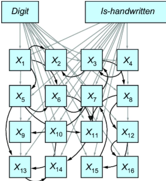
Figure 13.1 Example from chapter 5, where digit and is-handwritten are high-level causal drivers of low-level Xi pixels
The small squares represent pixels in an image, while the squares digit and is-handwritten represent the digit depicted in the image and whether it was handwritten, respectively. In that example (section 5.1.2), I suggested that whatever causal relations exist between individual pixels doesn’t matter to us; we’re interested in reasoning at the level of the objects depicted in the image.
There is a similar thing going on with tokens, as shown in figure 13.2.
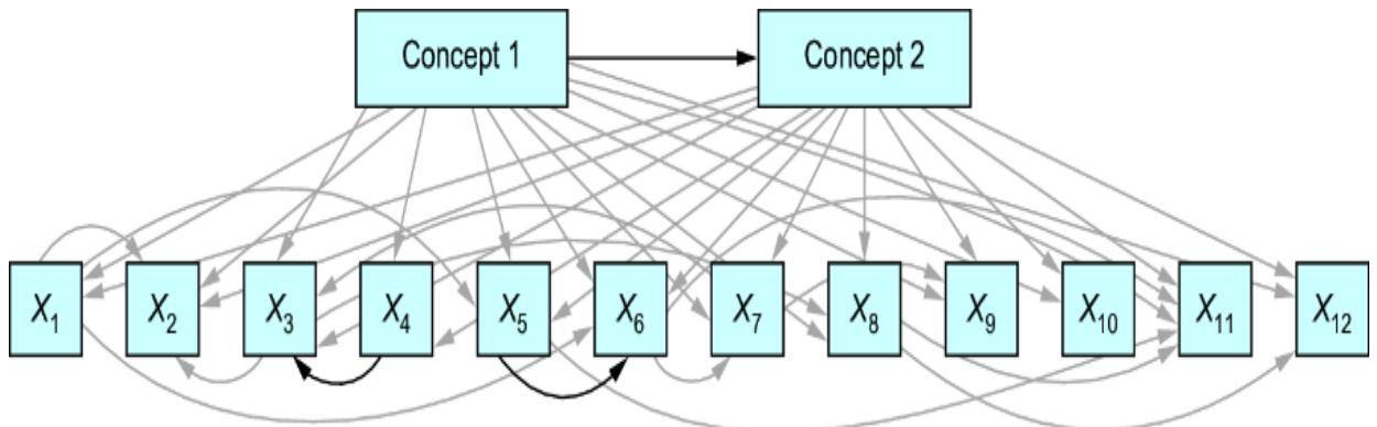
Figure 13.2 X1 through X12 are a sequence of tokens. Whatever structure (causal or otherwise) exists between the tokens is of passing interest. We are interested in the causal relations between concepts described by the tokens.
In figure 13.2, as with the pixels, there is some structure at the level of the tokens. But that structure is beside the point —we’re interested in the causal relationships between the concepts that form the meaning behind the tokens.
The question becomes, under what circumstances could attention, insofar as it can learn higher-level representations, learn a causal representation. For example, could an attention-based model, perhaps under some set of architectural or learning constraints, or use of interventions in training data, learn the parallel world structure and abstractions in the Labor Day counterfactual statement?
To consider this, we can revisit LLM hallucinations in our question about the probability of necessity, and connect it to causal identification.
13.2.4 Hallucination, attention, and causal identification
The hallucination about probability of necessity was generated with GPT-4. The same model got the Netflix question about probability of necessity correct. Indeed, the hallucinated answer would have been right if it merely stated the correct identifying assumptions. I believe future versions of GPT and similar models will likely get this question right on the first try.
But for someone who is unfamiliar with the definition of probability of necessity, how would they know if the model were right or if it were hallucinating? First, the causal hierarchy tells us that in order to be capable of generating a right answer beyond a random guess, the query would need to be identified with level 3 information. Perhaps that information is provided by the user in the prompt. Perhaps the LLM has somehow learned level 3 representations (such a claim would require hard proof).
If the user were providing that identifying information in the prompt, how would the user know if the model was successfully using that information to respond to the prompt? Suppose instead that the requirements for identification exist and are buried in the learned representations or data, and that they were being successfully leveraged by the model in answering the causal query, how could the user know for sure this was happening?
We need to engineer solutions that answer these and other desiderata to build toward a causal AI future. In the next section, we’ll start on this path with a simple causal LLM.
13.3 Forging your own causal LLM
In this section, we’ll sidestep the question of ૿can cuttingedge LLMs reason causally? and move on to building a causal LLM that can reason causally. We’ll build for causality from the ground up, rather than as an afterthought.
13.3.1 An LLM for script writing
Often our data has some implicit causal structure. When we make that structure explicit during training, the foundation model can learn better causal representations.
To illustrate, suppose a prolific film production studio has historically insisted their writers use script-writing software that required following a three-act narrative archetype, which is common for romantic comedies: ૿boy meets girl, boy loses girl, boy gets girl back. For this archetype, they have a corpus of many scripts. In causal terms, the events in act 1 cause the events of act 2, and the events of acts 1 and 2 cause the events of act 3. We can draw the DAG in figure 13.3.
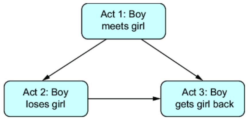
Figure 13.3 A causal DAG for a three-act archetype
The studio works with many such archetypes, and the company has many scripts that follow a given archetype template. Suppose that a set of archetypes involve a king acting a certain way in act 1, a prince acting a certain way in act 2, and these two actions having an effect on a kingdom in act 3. For example, one possible archetype is ૿King declares war, Prince leads army, kingdom experiences prosperity. But there are multiple outcomes for each act:
- King in act 1: {king declares war; king negotiates peace; king falls ill}
- Prince in act 2: {prince leads army; prince abdicates throne; prince marries foreigner}
- Kingdom in act 3: {kingdom wins battle; kingdom falls into poverty; kingdom experiences prosperity}
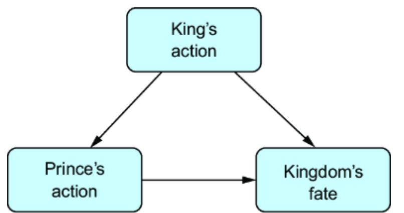
Figure 13.4 A causal DAG representing various King-Prince-Kingdom archetypes
Figure 13.4 shows this space of archetypes in the form of a causal DAG.
This describes only 3 × 3 × 3 = 27 possible archetypes, but as you might expect, some archetypes are more common and some are less common. We could easily model these archetypes and the joint probability distribution by explicitly coding causal Markov kernels in pgmpy or Pyro. But that would only be a causal generative model on the archetypes. If we want a script generator, we want a causal generative model on the scripts.
To demonstrate a proof-of-concept for this idea, we’ll work with a training dataset of short vignettes, rather than full scripts. Let’s load and examine the training data.
Listing 13.6 Load causal narrative data
import pandas as pd
url = ("https://raw.githubusercontent.com/altdeep/"
 "causalML/master/book/chapter%2013/"
 "king-prince-kingdom-updated.csv")
df = pd.read_csv(url)
print(df.shape[0]) #1
print(df["King"][0] + "\n") #2
print(df["King"][1] + "\n") #2
print(df["King"][2]) #2
print("----")
print(df["Prince"][0] + "\n") #3
print(df["Prince"][1] + "\n") #3
print(df["Prince"][2]) #3
print("----")
print(df["Kingdom"][0] + "\n") #4
print(df["Kingdom"][1] + "\n") #4
print(df["Kingdom"][2]) #4
#1 The data has 21,000 stories, broken up into three short vignettes. #2 First, the king acts.
#3 Then the prince acts.
#4 Finally, the kingdom experiences the consequences of the royals’ actions.
This code prints the following:
21000 —- King brokers a peace treaty with a rival kingdom, putting an end to years of bloody c onflict A wise king successfully negotiates peace with a rival nation A wise king successfully negotiates peace between his kingdom and a long-time enemy — however, his son, the Prince, falls in love and marries a foreigner, causing politica l unrest Prince falls in love with and marries a foreign princess, forging a strong alliance but when a new threat emerges, the Prince leads the army to defend their realm — despite efforts, the ongoing war results in both kingdoms falling into poverty.” the alliance strengthens their forces, leading the kingdom to a victorious battle.” however, a series of misfortunes and disastrous decisions plunge their once prosperou s kingdom into poverty.”
There are 21,000 sets of three vignettes. The preceding output shows the first three sets in the dataset.
13.3.2 Using pretrained models for causal Markov kernels
To train the causal Markov kernels for each node in our DAG, we’ll take pretrained models from the Hugging Face Transformers library, and then further train (aka ૿fine-tune) the models using our vignettes. The pretraining took care of the heavy lifting in terms of learning to generate coherent natural language text. The fine-tuning will align the models toward representing our causal Markov kernels.
First, we’ll use a GPT-2 variant to model the King’s action vignettes. As a text-completion model, it typically takes a prompt as input, but we’ll train it to generate with an empty prompt and produce vignettes according to the marginal probabilities of the King’s action texts in the training data, as in figure 13.5.
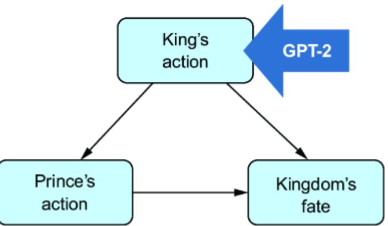
Figure 13.5 GPT-2 is fine-tuned to represent the distribution of King’s action vignettes.
Next, we’ll use a BART model for the causal Markov kernel Prince’s action. BART is a Transformer model released in 2019 designed specifically to take an input sequence and generate a corresponding output sequence, such as with translation or summarization. Large models like GPT-4 can handle sequence-to-sequence tasks quite well, but we’ll use a version of BART with roughly 4,000-times fewer parameters than GPT-4, making it easier for you to load and train on your laptop or basic Python development environment. Given the King’s action vignette as input, it will generate a Prince’s action vignette, as illustrated in figure 13.6.
We’ll also use a BART model to model the causal Markov kernel for the Kingdom’s fate, as shown in figure 13.7. The model will map the King’s and Prince’s actions to the Kingdom’s fate.
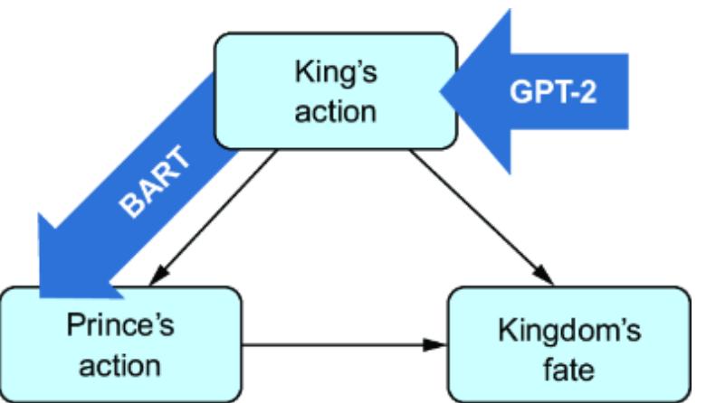
Figure 13.6 A BART sequence-to-sequence model is fine-tuned to represent the Prince’s action given the King’s action.
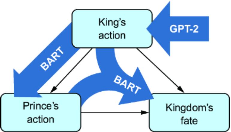
Figure 13.7 A BART sequence-to-sequence model is also used to model the Kingdom’s fate given the King’s action and Prince’s action.
Jumping ahead, we’re interested in the conditional probability distribution of the Kingdom’s fate, given a certain action by the Prince. Since that will require inference of the King’s actions given the Prince, we’ll additionally train one more BART model that generates a King’s action vignette given a Prince’s action vignette, as shown in figure 13.8.
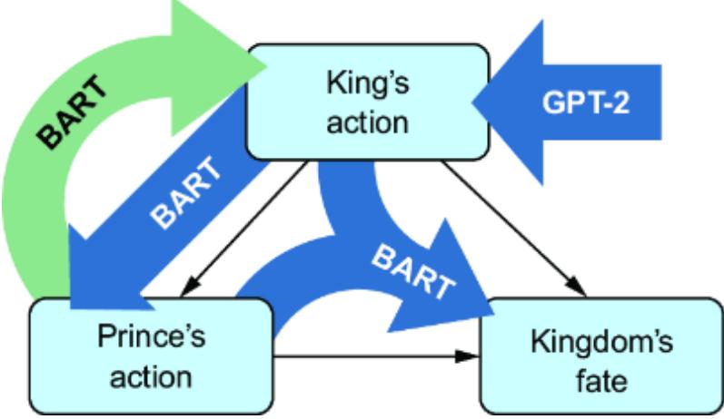
Figure 13.8 A BART sequence-to-sequence model is also fine-tuned to model the Kingdom’s fate, given the King’s and Prince’s actions.
Let’s run the training procedure. First, we’ll set up our imports and our tokenizer. We’ll use Bart as the tokenizer for all of our models.
Listing 13.7 Training the causal LLM
import torch
from sklearn.model_selection import train_test_split
from torch.utils.data import Dataset
from transformers import (
 AutoModelForCausalLM, AutoModelForSeq2SeqLM,
 AutoTokenizer, DataCollatorForLanguageModeling,
 Seq2SeqTrainer, Seq2SeqTrainingArguments,
 Trainer, TrainingArguments)
url = ("https://raw.githubusercontent.com/altdeep/"
 "causalML/master/book/chapter%2013/"
 "king-prince-kingdom-updated.csv")
df = pd.read_csv(url)
tokenizer = AutoTokenizer.from_pretrained("facebook/bart-base") #1
tokenizer.pad_token = tokenizer.eos_token #2
def tokenize_phrases(phrases, max_length=40): #3
 return tokenizer(
 phrases,
 truncation=True,
 padding='max_length',
 max_length=max_length
 )
#1 Set up the tokenizer.
#2 The pad token is used to make all the sequences the same length to facilitate matrix operations. It is common to set it to the ૿end-ofsequence (EOS) token.
#3 The max length of the token is set to 40, as all of the vignettes are less than 40 tokens.
Next we’ll create a class and a function that tokenizes the King dataset. We’ll create a custom subclass of the PyTorch Dataset class called ModelDataset that will store token encodings and their corresponding labels. When accessed by index, it returns a dictionary containing token encodings for that index and the associated label, and it provides the total number of examples via its __len__ method.
Listing 13.8 Tokenizing the King vignettes
class ModelDataset(Dataset): #1
 def __init__(self, encodings, labels): #1
 self.encodings = encodings #1
 self.labels = labels #1
 #1
 def __getitem__(self, idx): #1
 item = { #A #1
 key: torch.tensor(val[idx]) #1
 for key, val in self.encodings.items() #1
 } #A #1
 item['labels'] = torch.tensor(self.labels[idx]) #1
 return item #1
 #1
 def __len__(self): #1
 return len(self.encodings.input_ids) #1
def create_king_dataset(input_phrases): #2
 king_phrases = input_phrases.tolist() #2
 king_encodings = tokenize_phrases(king_phrases) #2
 king_dataset = ModelDataset( #2
 king_encodings, #2
 king_encodings['input_ids']) #2
 return king_dataset #2
#1 When accessed by index, ModelDataset returns a dictionary containing token encodings for that index and the associated label. #2 Create a ModelDataset instance for the king vignettes.
Next we’ll tokenize the Prince and Kingdom vignettes. This code will also produce a validation dataset used in training sequence-to-sequence models.
Listing 13.9 Tokenizing the Prince and Kingdom vignettes
def create_seq2seq_datasets(input_phrases, target_phrases):
 input_phrases_list = input_phrases.tolist()
 target_phrases_list = target_phrases.tolist()
 spit = train_test_split( #1
 input_phrases_list, #1
 target_phrases_list, #1
 test_size=0.1 #1
 ) #1
 train_inputs, val_inputs, train_targets, val_targets = spit #1
 train_input_encodings = tokenize_phrases(train_inputs) #2
 val_input_encodings = tokenize_phrases(val_inputs) #2
 train_target_encodings = tokenize_phrases(train_targets) #2
 val_target_encodings = tokenize_phrases(val_targets) #2
 train_dataset = ModelDataset(
 train_input_encodings, train_target_encodings['input_ids']
 )
 val_dataset = ModelDataset(
 val_input_encodings, val_target_encodings['input_ids']
 )
 return train_dataset, val_dataset
#1 Split input and target phrases into training and validation sets. #2 Encode the training and validation sets.
Next, we’ll write a training algorithm for the King model. This function initializes a GPT-2 model with the specified parameters, sets up the training arguments, and trains the model on the provided dataset, finally saving the trained model to the specified directory.
Listing 13.10 Training the King model
def train_king_model(output_dir, train_dataset,
 model_name="gpt2-medium", epochs=4):
 king_model = AutoModelForCausalLM.from_pretrained(model_name) #1
 training_args_king = TrainingArguments( #1
 output_dir=output_dir, #1
 per_device_train_batch_size=32, #1
 overwrite_output_dir=True, #1
 num_train_epochs=epochs, #1
 save_total_limit=1, #1
 save_steps=len(train_dataset) // 16, #1
 max_grad_norm=1.0 #1
 ) #1
 data_collator = DataCollatorForLanguageModeling( #1
 tokenizer=tokenizer, #1
 mlm=False) #1
 trainer_king = Trainer( #2
 model=king_model, #2
 args=training_args_king, #2
 data_collator=data_collator, #2
 train_dataset=train_dataset, #2
 ) #2
 trainer_king.train() #3
 king_model.save_pretrained(output_dir)
 return king_model
#1 Initialize and configure model with the specified parameters. #2 Configure the training settings. #3 Train the model.
Next, we’ll write a training algorithm for the sequence-tosequence models. The function will split the provided input and target phrases into training and validation sets, tokenize them, and then create and return PyTorch Dataset objects for both sets using the ModelDataset class. The train_seq2seq_model function initializes a sequence-to-sequence model with the specified parameters, configures its training settings, and then trains the model using both training and validation datasets, finally returning the trained model.
Listing 13.11 Function for training the sequence-to-sequence models
def train_seq2seq_model(output_dir, train_dataset, val_dataset,
 model_name="facebook/bart-base",
                   epochs=4):
 model = AutoModelForSeq2SeqLM.from_pretrained(model_name)
 training_args = Seq2SeqTrainingArguments( #1
 output_dir=output_dir, #1
 per_device_train_batch_size=16, #1
 predict_with_generate=True, #1
 logging_dir=f"{output_dir}/logs", #1
 save_total_limit=1, #1
 save_steps=len(train_dataset) // 16, #1
 learning_rate=3e-5, #1
 num_train_epochs=epochs, #1
 warmup_steps=500, #1
 weight_decay=0.01, #1
 ) #1
 trainer = Seq2SeqTrainer( #2
 model=model, #2
 args=training_args, #2
 train_dataset=train_dataset, #2
 eval_dataset=val_dataset, #2
 ) #2
 trainer.train() #3
 model.save_pretrained(output_dir)
 return model
#1 Initialize and configure sequence-to-sequence model with the specified parameters.
#2 Configure the training settings.
#3 Train the model using both training and validation datasets, finally returning the trained model.
Now we’ll use this function to train the models. We’ll specify some directories for saving checkpoints.
Note In listing 13.14, I’ll provide code that downloads a pretrained model from Hugging Face, so if you don’t wish train the model, you can skip ahead to that step.
Listing 13.12 Training the King, Prince, and Kingdom models
import os
king_model_path = os.path.join(os.getcwd(), 'king_model') #1
prince_model_path = os.path.join(os.getcwd(), 'prince_model') #1
kingdom_model_path = os.path.join(os.getcwd(), 'kingdom_model') #1
prince2king_model_path = os.path.join( #1
 os.getcwd(), 'prince2king_model') #1
king_dataset = create_king_dataset(df["King"]) #2
king_model = train_king_model(king_model_path, king_dataset) #2
datasets = create_seq2seq_datasets(df["King"], df["Prince"]) #3
train_dataset_prince, val_dataset_prince = datasets #3
prince_model = train_seq2seq_model( #3
 prince_model_path, #3
 train_dataset_prince, #3
 val_dataset_prince, #3
 epochs=6 #3
) #3
king_and_prince = [f"{k} {p}" for k, p in zip(df["King"], df["Prince"])] #4
df["King and Prince"] = king_and_prince #4
train_dataset_kingdom, val_dataset_kingdom = create_seq2seq_datasets( #4
 df["King and Prince"], df["Kingdom"] #4
) #4
kingdom_model = train_seq2seq_model( #4
 kingdom_model_path, #4
 train_dataset_kingdom, #4
 val_dataset_kingdom, #4
 epochs=6 #4
) #4
#1 Provide the output directories where you want to save your model. #2 Train the King model using Seq2Seq.
#3 Train the Prince model using Seq2Seq. The King vignettes are used to predict the Prince vignettes.
#4 Train the Prince model using Seq2Seq. The King vignettes are used to predict the Prince vignettes.
#5 Train the Kingdom model using Seq2Seq. The combined King and Prince vignettes are used to predict the Kingdom vignettes.
Finally, we’ll train another model for inferring the King vignette given a Prince vignette. We’ll use this in inference later.
Listing 13.13 Function to train the Prince to King model
p2k_data = create_seq2seq_datasets(
 df["Prince"], df["King"])
train_dataset_prince2king, val_dataset_prince2king = p2k_data
prince2king_model = train_seq2seq_model(
 prince2king_model_path,
 train_dataset_prince2king,
 val_dataset_prince2king,
 epochs=6
)
Running the preceding training procedure will take some time, especially if you’re not using GPU. Fortunately, there are saved versions of the trained models in the Hugging Face Hub. The following code pulls the Transformer models from the Hugging Face Hub and generates from them. It also provides a function that calculates the log probability of each generated sequence.
Listing 13.14 Pull Transformer models from the Hugging Face Hub and generate
import matplotlib.pyplot as plt
import pandas as pd
import torch
from sklearn.feature_extraction.text import TfidfVectorizer
from transformers import (
 AutoModelForCausalLM, AutoModelForSeq2SeqLM,
 AutoTokenizer, GPT2LMHeadModel,
 PreTrainedModel, BartForConditionalGeneration)
DEVICE = torch.device("cuda" if torch.cuda.is_available() else "cpu")
king_model = AutoModelForCausalLM.from_pretrained( #1
 "osazuwa/causalLLM-king").to(DEVICE) #1
prince_model = AutoModelForSeq2SeqLM.from_pretrained( #1
 "osazuwa/causalLLM-prince").to(DEVICE) #1
kingdom_model = AutoModelForSeq2SeqLM.from_pretrained( #1
 "osazuwa/causalLLM-kingdom").to(DEVICE) #1
prince2king_model = AutoModelForSeq2SeqLM.from_pretrained( #1
 "osazuwa/causalLLM-prince2king").to(DEVICE) #1
tokenizer = AutoTokenizer.from_pretrained("facebook/bart-base") #2
tokenizer.pad_token = tokenizer.eos_token #2
#1 Load the components of our model. #2 Load the components of our model. #3 Load the Bart-base tokenizer and set the pad token to end-ofsequence tokens.
Next, we’ll write some functions to encode text to tokens, decode tokens to text, and generate text from the model
Listing 13.15 Helper functions for encoding, decoding, and generation
def encode(text:str, device=DEVICE) -> torch.tensor: #1
 input_ids = tokenizer.encode(text, return_tensors="pt") #1
 input_ids = input_ids.to(device) #1
 return input_ids #1
def decode(text_ids: torch.tensor) -> str: #2
 output = tokenizer.decode(text_ids, skip_special_tokens=True) #2
 return output #2
EMPTY_TEXT = torch.tensor(tokenizer.encode("")).unsqueeze(0).to(DEVICE) #3
def generate_from_model(model: PreTrainedModel, #4
 input_sequence: torch.tensor = EMPTY_TEXT, #4
                    max_length: int = 25, #4
                    temperature=1.0): #4
 output = model.generate( #4
 input_sequence, #4
 max_length=max_length, #4
 do_sample=True, #4
 pad_token_id=tokenizer.pad_token_id, #4
 eos_token_id=tokenizer.pad_token_id, #4
 temperature=temperature, #4
 top_p=0.9, #4
 ) #4
 return output #4
def convert_to_text(output):
return decode(output[0]).strip().capitalize()#1 Encode text into tensor.
#2 Decode tensor into text.
#3 Get the encoding for empty text, for convenience.
#4 A function for generating from models. These parameters do slightly different things for the GPT-2 and BART models, but they more or less overlap.
We want to use our probabilistic ML approach, so we need a way of computing the log probabilities of generated sequences so we can use these in inference. The following function computes the log probability of a generated sequence based on related values produced by the GPT-2 and BART models.
Listing 13.16 Computing log probabilities of generated sequences
def compute_log_probs(model, output_sequence):
 if isinstance(model, GPT2LMHeadModel): #1
 outputs = model( #1
 input_ids=output_sequence, #1
 labels=output_sequence #1
 ) #1
 log_softmax = torch.nn.functional.log_softmax( #1
 outputs.logits, dim=-1) #1
 log_probs = log_softmax.gather(2, output_sequence.unsqueeze(-1)) #1
 log_probs = log_probs.squeeze(-1).sum(dim=-1) #1
 elif isinstance(model, BartForConditionalGeneration):
 outputs = model( #2
 input_ids=output_sequence, #2
 labels=output_sequence) #2
 loss = outputs.loss #2
 log_probs = -loss * output_sequence.size(1) #2
 else:
 raise ValueError("Unsupported model type")
 return torch.tensor(log_probs.item())
#1 Convert logits to logprobs for GPT-2. #2 Convert logits to logprobs from BART cross-entropy.
Finally, we’ll put these pieces together to generate a full story from our three models.
Listing 13.17 Generating a full story
king_output = generate_from_model(king_model) #1 king_statement = convert_to_text(king_output) #1 print(“Generated from king_nodel:”, king_statement) #1 log_prob_king = compute_log_probs(king_model, king_output) #1 print(“Log prob of generated king text:”, log_prob_king) #1 prince_output = generate_from_model(prince_model, king_output) #2 prince_statement = convert_to_text(prince_output) #2 print(“Generated from prince_model:”, prince_statement) #2 log_prob_prince = compute_log_probs(prince_model, prince_output) #2 print(“Log prob of generated prince text:”, log_prob_prince) #2 king_prince_statement = king_statement + “.” + prince_statement #3 king_prince_output = encode(king_prince_statement) #3 kingdom_output = generate_from_model(kingdom_model, king_prince_output) #3 kingdom_statement = convert_to_text(kingdom_output) #3 print(“Generated from kingdom model:”, kingdom_statement) #3 log_prob_kingdom = compute_log_probs(kingdom_model, kingdom_output) #3 print(“Log prob of generated kingdom text:”, log_prob_kingdom) #3 king_output_infer = generate_from_model(prince2king_model, prince_output) #4 king_statement_infer = convert_to_text(king_output_infer) #4 print(“Generated statement from prince2king:”, king_statement_infer) #4 log_prob_prince2king = compute_log_probs(prince2king_model, prince_output) #4 print(“Log prob of generated inference text:”, log_prob_prince2king) #4
#1 Generate from the GPT-based model of vignettes about the King and calculate the log probabilities of the generated sequence.
#2 Generate from the BART-based sequence-to-sequence model that generates vignettes about the Prince given vignettes about the King, and then calculate the log probability of the generated sequence. #3 Generate from the BART-based sequence-to-sequence model that generates vignettes about the Kingdom given vignettes about the King and the Prince, and then calculate the log probability of the generated sequence.
#4 Another BART-based sequence-to-sequence model that maps a vignette about the Prince to a vignette about the King. We’ll use this to infer the vignette about the King from a vignette about the Prince.
The output is nondeterministic, but one example of the output you’ll get is as follows:
Generated statement from king_model: The king, driven by ambition, declares war on a neighboring nation to expand his kingdom’s territories, declares war on. Log probability of generated king_model: tensor(-325.8379) Generated statement from prince_model: The prince, disillusioned by his father’s acti ons, abdicates the throne in protest. Log probability of generated prince text: tensor(-18.2486) Generated statement from kingdom model: As the war drags on, resources are depleted, and the once-prosperous kingdom falls. Log probability of generated kingdom text: tensor(-38.3716) Generated statement from prince2king: A king, driven by greed, declares war on a neig hboring kingdom. Log probability of generated inference text: tensor(-297.3446)
Note that the generated output isn’t perfect—for example, the first generated statement ideally should have stopped after ૿…kingdom’s territories. We could try to train it more or switch to a more powerful model, but this is pretty good for a start.
Next, we’ll use these Transformers library models to define distributions in Pyro, and then use Pyro to build a causal generative model. First, we’ll use Pyro’s TorchDistributionMixin to model the causal Markov kernels with the language models. We’ll use the GPT-2 model of the King vignettes to create the causal Markov kernel of the King variable.
Next, we’ll use the BART model to create the causal Markov kernel for the Prince variable. The King variable causes this variable, so the seq2seq model uses the King variable’s value to generate a value for this model.
Finally, we’ll create the causal Markov kernel for the Kingdom variable. The King and Prince variables are causal parents, so we concatenate their generated outputs into one string, and use that string to generate the Kingdom output, again using a BART seq2seq model. We rely on a mixin called TorchDistributionMixin, which is useful for wrapping PyTorch distributions for use in Pyro.
Listing 13.18 Building a Torch distribution from a Transformer model
import pyro
from pyro.distributions.torch_distribution \
import TorchDistributionMixin
class TransformerModelDistribution(TorchDistributionMixin):
 def __init__(self, model: PreTrainedModel,
 input_encoding: torch.tensor = EMPTY_TEXT,
 ):
 super().__init__()
 self.model = model
 self.input_encoding = input_encoding
 def sample(self, sample_shape=torch.Size()): #1
 output = generate_from_model( #1
 self.model, self.input_encoding #1
 ) #1
 return output #1
 def log_prob(self, value): #2
 return compute_log_probs(self.model, value) #2
#1 Use TorchDistributionMixin to turn a Transformers model into a Pyro distribution. TorchDistributionMixin is used to make PyTorch distributions compatible with Pyro’s utilities.
#2 The log_prob method returns the log probabilities used in inference algorithms.
Now we’ll use that distribution in Pyro.
Listing 13.19 Incorporating Transformer models into a causal model with Pyro
def causalLLM(): #1
 king = pyro.sample( #2
 "King", TransformerModelDistribution(king_model) #2
 ) #2
 prince = pyro.sample( #3
 "Prince", TransformerModelDistribution( #3
 prince_model, king) #3
 ) #3
 king_and_prince = torch.cat([king, prince], dim=1) #4
 kingdom = pyro.sample( #4
 "Kingdom", TransformerModelDistribution( #4
 kingdom_model, king_and_prince) #4
 ) #4
 king_text = convert_to_text(king) #5
 prince_text = convert_to_text(prince) #5
 kingdom_text = convert_to_text(kingdom) #5
 return king_text, prince_text, kingdom_text #5
for _ in range(2): #6
 king, prince, kingdom = causalLLM() #6
 vignette = " ".join([king, prince, kingdom]) #6
 print(vignette) #6
#1 Build the causal LLM.
#2 Create the causal Markov kernel for the King variable. #3 Create the causal Markov kernel for the Prince variable. #4 Create the causal Markov kernel for the Kingdom variable. #5 Concatenate all the generated vignettes into one overall vignette and return the result.
#6 Confirm our causal model generates the full vignette.
The preceding code generates and prints two vignettes, such as the following:
And beloved king falls gravely ill, leaving the kingdom in despair in uncertainty ove r the inexperienced prince to lead the kingdom. The young prince, eager to prove hims elf, leads the army into a costly and ill-advised war. As a result, the kingdom’s res ources are depleted, plunging the once-prosperous land into.
King, fueled by ambition, declares war on a neighboring realm, leaving his subjects a nxious and. The prince, disillusioned by his father’s actions, abdicates the throne i n search of a new life. Without strong leadership, the kingdom spirals into poverty a nd despair.
We see that the generated texts are pretty good, though they seem to cut off a bit early. This, and other issues with the generations, can be addressed by tweaking the generation parameters.
And just like that, we’ve built a causal LLM, an LLM build on a causal DAG scaffold. Let’s prove we have a causal model by comparing the observational and interventional distributions entailed by the DAG.
13.3.3 Sampling from the interventional and observational distributions
By now, you know the distribution P(Kingdom|Prince=x) will be different from P(KingdomPrince=x), but let’s demonstrate the fact with this causal LLM. First, we’ll model P(Kingdom|Prince=x), where x is
His courageous Prince takes command, leading the kingdom’s army to victory in battle after battle
To infer P(Kingdom|Prince=x), we’ll have to infer the distribution of the latent confounder, King. We’ll do this using the prince2king_model we trained. We’ll use a probabilistic inference algorithm called ૿importance resampling. We’ll start by creating a proposal function (what Pyro calls a ૿guide function) that will generate samples of King and Kingdom, given Prince.
Listing 13.20 Proposal distribution for P(Kingdom|Prince=x)
import pyro.poutine as poutine
from pyro.distributions import Categorical
PRINCE_STORY = ( #1
 "His courageous Prince takes command, leading " #1
 "the kingdom's army to victory in battle after battle") #1
cond_model = pyro.condition( #1
 causalLLM, {"Prince": encode(PRINCE_STORY)}) #1
def proposal_given_prince(): #2
 prince = encode(PRINCE_STORY) #2
 king = pyro.sample( #3
 "King", #3
 TransformerModelDistribution(prince2king_model, prince) #3
 ) #3
 king_and_prince = torch.cat([king, prince], dim=1) #3
 kingdom = pyro.sample( #4
 "Kingdom", #4
 TransformerModelDistribution(kingdom_model, king_and_prince) #4
 ) #4
 vignette = (convert_to_text(king) + #5
 PRINCE_STORY + #5
 convert_to_text(kingdom)) #5
 return vignette
#1 We condition the model on this value of the Prince variable. #2 We’ll use a proposal function to generate from our target distribution P(King, Kingdom|Prince=PRINCE_STORY).
#3 The proposal uses the prince2king_model to infer values of King given Prince=PRINCE_STORY.
#4 Given the value of Prince, and the inferred value of King, use the king_and_prince model to sample Kingdom.
#5 Concatenate the generated king tokens and provided prince tokens to return a generated vignette so we can inspect what is sampled.
Now we’ll weigh each sample by the ratio of the probability of the sample under the conditioned model, over the probability of the sample under the proposal. Resampling the samples using these weights will generate samples from the target distribution. Pyro provides a utility for importance sampling, but because of the varying length of the generated sequences, it will be easier to implement importance sampling directly.
First, we’ll write a function to process a sample and get its importance weight.
Listing 13.21 Function to draw a sample for resampling
def process_sample(model, proposal): sample_trace = poutine.trace(proposal).get_trace() #1 king_text = convert_to_text(sample_trace.nodes[‘King’][‘value’]) #1 kingdom_text = convert_to_text( #1 sample_trace.nodes[‘Kingdom’][‘value’]) #1 proposal_log_prob = sample_trace.log_prob_sum() #2 replay = poutine.replay(model, trace=sample_trace) #3 model_trace = poutine.trace(replay).get_trace() #3 model_log_prob = model_trace.log_prob_sum() #3 log_importance_weight = model_log_prob - proposal_log_prob #4 sample = (king_text, kingdom_text, log_importance_weight) return sample
#1 Extract a sample from the proposal.
#2 Calculate the total log probability of the sampled values of King and Kingdom.
#3 Calculate the total log probability of the sample values of King and Kingdom under the original model.
#4 Calculate the log importance weight.
Now we’ll run the importance resampling.
Listing 13.22 Listing 13.22 Importance resampling of
P(Kingdom|Prince=x)
def do_importance_resampling(model, proposal, num_samples): #1
 original_samples = []
 for _ in range(num_samples):
 sample = process_sample(model, proposal)
 original_samples.append(sample)
 unique_samples = list(set(original_samples)) #2
 log_importance_weights = torch.tensor( #2
 [sample[2] for sample in original_samples]) #2
 resampling_dist = Categorical(logits=log_importance_weights) #2
 resampled_indices = resampling_dist.sample_n(num_samples) #2
 samples = pd.DataFrame( #2
 [unique_samples[i] for i in resampled_indices], #2
 columns=["King", "Kingdom", "log_importance_weight"] #2
 ) #2
 samples["Prince"] = PRINCE_STORY
 samples["Distribution"] = "observational"
 return samples[['King', 'Prince', 'Kingdom', 'Distribution']]
num_samples = 1000
posterior_samples = do_importance_resampling(
 cond_model, proposal_given_prince, num_samples)
#1 Use importance resampling as our inference procedure. #2 Resample using the importance weights. Pass in the log weights to the ૿logits argument.
Next, we’ll infer P(KingdomPrince=x). Given our causal model in Pyro, we can use Pyro’s do-operator to apply the
intervention. We know that given the intervention on Prince, the edge from King to Prince is removed, so we don’t need to use prince2king_model. We can simply do ordinary forward generation from our intervention model.
Listing 13.23 Inferring P(KingdomPrince=x) using vanilla forward Monte
Carlo sampling
intervention_model = pyro.do( #1
causalLLM, {"Prince": encode(PRINCE_STORY)}) #1
intervention_samples = pd.DataFrame( #2
[intervention_model() for _ in range(num_samples)], #2
columns=["King", "Prince", "Kingdom"] #2
) #2
intervention_samples["Distribution"] = "interventional" #2
all_samples = pd.concat( #2
[posterior_samples, intervention_samples], #2
ignore_index=True #2
) #2#1 Forward sample from the interventional distribution. #2 Label the samples, and combine them with the observational samples.
Generating the samples will take some time. Since we’re working directly with the encoded sequence tensors in Pyro, we could leverage the potentially faster gradient-based inference algorithm. For convenience, you can access presaved samples in the book’s directory of the GitHub repo: https://github.com/altdeep/causalml.
Next, let’s visualize the difference in the distributions. We need a way to visualize sampled text from the interventional and observational distributions. We can do so using TF-IDF (term frequency-inverse document frequency), a numerical statistic that reflects how important a word is to a sample within the collection of samples, emphasizing words that are unique to specific samples.
Listing 13.24 Get TF-IDF of generations for P(KingdomPrince=x) and P(Kingdom|Prince=x)
import pandas as pd
import numpy as np
from sklearn.feature_extraction.text import TfidfVectorizer
kingdom_samples_url = (
 "https://raw.githubusercontent.com/altdeep/causalML/"
 "master/book/chapter%2013/kingdom_samples.csv")
all_samples = pd.read_csv(kingdom_samples_url)
observational_texts = all_samples[ #1
 all_samples["Distribution"] == "observational"]["Kingdom"] #1
interventional_texts = all_samples[all_samples[ #1
 "Distribution"] == "interventional"]["Kingdom"] #1
 vectorizer = TfidfVectorizer(stop_words='english') #2
X_obs = vectorizer.fit_transform(observational_texts) #2
X_int = vectorizer.transform(interventional_texts) #2
k = 10 #3
feature_names = vectorizer.get_feature_names_out() #3
obs_indices = X_obs.sum(axis=0).argsort()[0, -k:][::-1] #3
int_indices = X_int.sum(axis=0).argsort()[0, -k:][::-1] #3
combined_indices = np.concatenate((obs_indices, int_indices)) #3
combined_indices = np.unique(combined_indices) #3
#1 Extract generated Kingdom vignettes from observational and interventional distributions.
#2 Compute the TF-IDF values for generated Kingdom vignettes in each group.
#3 Get the top k=7 words by TF-IDF for each set.
Finally, we’ll visualize the two distributions.
Listing 13.25 Visually contrast P(KingdomPrince=x) and P(Kingdom|Prince=x)
import matplotlib.pyplot as plt
labels = [feature_names[i] for i in combined_indices] #1 labels, indices = np.unique(labels, return_index=True) #1 obs_values = np.array(X_obs.sum(axis=0))[0, combined_indices] #1 int_values = np.array(X_int.sum(axis=0))[0, combined_indices] #1 obs_values = [obs_values[0][i] for i in indices] #1 int_values = [int_values[0][i] for i in indices] #1 combined = list(zip(labels, obs_values, int_values)) #1 sorted_combined = sorted(combined, key=lambda x: (-x[1], x[2])) #1 labels, obs_values, int_values = zip(*sorted_combined) #1 width = 0.35 #2 x = np.arange(len(labels)) #2 fig, ax = plt.subplots() #2 rects1 = ax.bar(x - width/2, obs_values, width, #2 label=‘Observational’, alpha=0.7) #2 rects2 = ax.bar(x + width/2, int_values, width, #2 label=‘Interventional’, alpha=0.7) #2 ax.set_xlabel(‘Words’) #2 ax.set_ylabel(‘TF-IDF Values’) #2 ax.set_title( #2 ‘Top Words in Generated Kingdom Vignettes by TF-IDF Value’) #2 ax.set_xticks(x) #2 ax.set_xticklabels(labels) #2 ax.legend() #2 fig.tight_layout() #2 plt.xticks(rotation=45) #2 plt.show() #2
#1 Prepare data for the bar plot. #2 Produce the plot.
This produces figure 13.9.
Figures 13.9 shows similar TF-IDF scores for words in the observational case. This is due to the lack of variation in the observational case, since observing the Prince constrains the likely values of King. When we intervene on Prince, King can vary more, leading to more variation in the results.
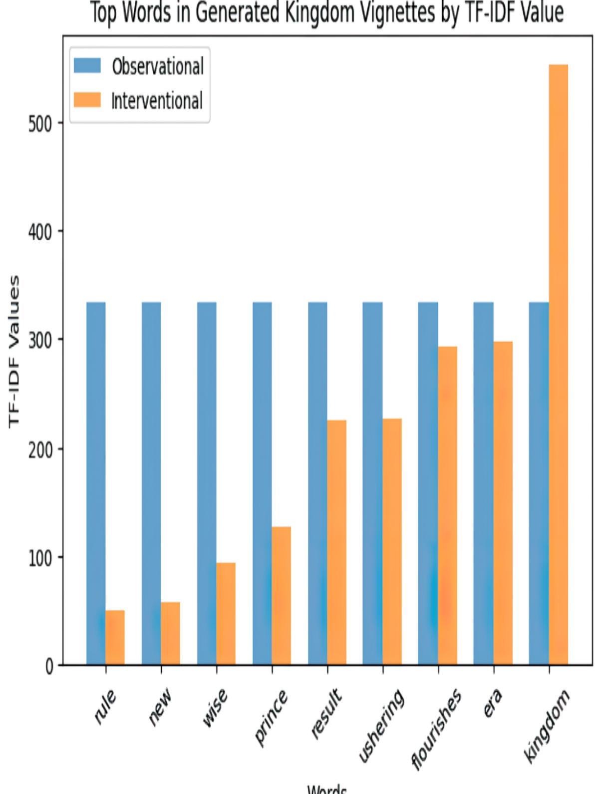
Figure 13.9 Visualization of the difference between samples from P(KingdomPrince=x) and P(Kingdom|Prince=x) using TF-IDF, where x is the Prince taking the army to battle. The observational values are flat because of little variation in the inferred King vignettes. The intervention enables more variation in the King vignettes and, consequently, the Kingdom vignettes.
13.3.4 Closing thoughts
This is a toy problem with a simple DAG trained on simple data with simple LLMs. But we could extend it to more complicated DAGs and fine-tuning more advanced models. There may also be other ways to combine causal assumptions in foundation models. We’re only at the beginning of exploring this exciting space.
Summary
- Large language models (LLMs) are powerful AI models that generate text and other modalities and achieve high performance across a variety of benchmarks.
- LLMs have proven use cases for supporting causal analysis.
- LLMs can help build a causal DAG. Moreover, they can leverage common and expert knowledge about causal relations and mechanisms.
- The causal frame problem is the challenge of selecting the causal variables relevant to a given problem and excluding the irrelevant. Cutting-edge LLMs emulate how humans set the causal frame, which is useful for applications such as building DAGs and root cause analysis.
- LLMs can help us understand nuanced causal concepts and how to contextualize them within our domain of interest.
- LLMs can help us put causal queries into formal terms.
- LLMs are prone to hallucinations—convincing yet incorrect responses to our queries.
- At their core, LLMs are probabilistic machine learning models that model a joint probability distribution on sequences of tokens.
- The attention mechanism enables the LLM to learn higher-level representations that make cutting-edge LLMs so powerful.
- Just because an LLM learns a higher-level representation doesn’t mean it learns a causal representation. Even if that did work in some special cases, it would be hard for the user to verify that it is working.
- We can build our own causal LLM by composing finetuned LLMs over a causal DAG scaffold. This allows us to work with cutting-edge LLMs while admitting causal operations, such as a do-operator.
- Use the causal hierarchy theory as your North Star in your exploration of how to combine causality with LLMs and multimodal models, as well as exploring how well these models can learn causal representations on their own.
[1] C. Glymour, ૿Android epistemology and the frame problem, in Z.W. Pylyshyn, ed., The robot’s dilemma: The frame problem in artificial intelligence (Praeger, 1987), pp. 63–75.
index
SYMBOLS
<$nopage>SCMs (structural causal models).
conditional independence
<$nopage>decision theory
causal decision theory.
<$nopage>encoder in VAE (variational autoencoder).
<\$nopage>graphical models.
<$nopage>causal DAGs (directed acyclic graphs).
<$nopage>decoder in VAE (variational autoencoder).
A
assignment functions in structural causal models, 2nd, 3rd
approximate Bayesian computation
ATEs (average treatment effects), 2nd, 3rd
attribution and credit assignment
Binary counterfactuals and uplift modeling, 2nd
Probabilities of causation and attribution
B
backdoor adjustment estimand
backdoor adjustment estimation
confidence intervals for machine learning methods
estimation with machine learning
linear regression estimation of, 2nd, 3rd
propensity score estimators of
propensity score stratification
Bernoulli distribution, reparameterization trick for, 2nd
BayesianNetwork class in pgmpy, 2nd, 3rd, 4th
Bayesian causal generative inference, identifiability of
Bayesian estimation with deep causal graphical latent variable model
posterior predictive inference of ATE
C
c-component factorization, 2nd
credit assignment and attribution
Binary counterfactuals and uplift modeling
Markov decision processes, relationship to
causal characterization of decision rules and policies
CGMs (causal generative models)
CPD (conditional probability distribution)
causal representation learning, 2nd
causal effects
relative risk and odds ratios as causal effects
counterfactual image generation, assumptions needed for
counterfactual inference algorithm
counterfactual image generation with deep generative model
counterfactual variational inference, 2nd
conditional hypothetical statement, 2nd
Confounders2Engagement network
causal constraints
churn rate (marketing, subscription services)
Netflix recommendation algorithms and counterfactual graphs, 2nd
extending inference to estimation
where questions and queries fall on, 2nd
counterfactual identification, general
problem with general algorithm for counterfactual inference
approach to causal inference, 2nd
causality’s role in modern AI workflows
causal graphical models
inference with trained causal probabilistic machine learning model
CATEs (conditional average treatment effects), 2nd
symbolic representation of, 2nd
counterfactual inference on causal image model, 2nd
deep causal graphical model of MNIST and TMNIST
training an SCM as a normalizing flow model
training an SCM with automatic differentiation in PyTorch
causal invariance
conditional independence, 2nd, 3rd
conditional independence testing, 2nd
posterior predictive inference of ATE
D
using for backdoor identification
causal inference to enhance, 2nd
causal model of computer vision problem
DAGs (directed acyclic graphs) and causal graphical models:scaffolding for causal generative models:training an SCM:with automatic differentiation in PyTorch
DAGs (directed acyclic graphs) and causal graphical models:scaffolding for causal generative models:training an SCM:as a normalizing flow model
DGP (data generating process), 2nd, 3rd, 4th, 5th
decision rules and policies, causal characterization of
DAGs (directed acyclic graphs) and causal graphical models, 2nd
causal DAGs and representation of time
communicating and visualizing causal assumptions
failure to illustrate mechanism
including variables in causal DAGs by role in inference, 2nd
learning causal DAGs from data (causal discovery), 2nd, 3rd
linking causality to conditional independence
representing causal assumptions, 2nd
scaffolding for causal generative models, 2nd, 3rd, 4th, 5th, 6th, 7th, 8th
selecting variables for inclusion in
data
at levels 1, 2, and 3 of the causal hierarchy
data drift
E
exogenous variable distribution
ETT (effect of treatment on the treated)
ELBO (evidence lower bound on the log-likelihood of the data)
estimators
comparing and selecting estimators
instrumental variable estimation
do-calculus, identification with
front-door adjustment estimand
F
functional constrainsts/Verma constraints
fairness
G
GLM (generalized linear model)
graphical identification algorithms
ETT (effect of treatment on the treated), identification of
front-door estimand, identification of, 2nd
GANs (generative adversarial networks)
get\_independencies function, 2nd
H
heterogeneous treatment effects
I
causal inference workflow, 2nd
graphical counterfactual identification, 2nd
graphical identification with do-calculus, 2nd
causal DAGs, ideal interventions, 2nd
causal Markov kernels, ideal interventions
causal programs, ideal interventions
credit fraud detection case study
from observations to experiments
from randomized experiments to
intervention variables and distributions, 2nd
practical considerations in modeling, 2nd
with trained causal probabilistic machine learning model
do method in pgmpy’s DAG class
pyro.do operator, 2nd, 3rd, 4th
independence of mechanism
causal and anti-causal learning, 2nd
example with semi-supervised learning
instrumental variables (IVs), 2nd
L
LLMs (large language models), 2nd, 3rd
hallucination, attention, and causal identification
tokens to causal representation
latent variables and identification
learning parameters when there are
M
models
MDPs (Markov decision processes)
MNIST (Modified National Institute of Standards and Technology) database, causal AI and
building parallel world graphical model
running counterfactual inference algorithm, 2nd
specifying assignment functions for endogenous variables, 2nd
specifying exogenous variables
MCMC (Markov chain Monte Carlo)
ML (machine learning)
counterfactual analysis of models, 2nd
N
necessary causation
O
P
causal transfer learning, data fusion, and invariant prediction
fitting parameters with common sense
PDAGs (partially directed acyclic graphs)
probabilities of causation, 2nd
probability of disablement and enablement
probability of necessity and sufficiency
probabilistic inference algorithms
probabilistic generative modeling
from empirical joint distribution to observational joint distribution
from full joint distribution to data generating process
from observed data to data generating process
from observed data to empirical joint distribution
from observed joint distribution to full joint distribution
many-to-one relationships down hierarchy
Pyro library
pyro.do operator, 2nd, 3rd, 4th
probabilistic inference
interventional and counterfactual inference with MCMC
prediction, inferring hypothetical outcomes
applying hypothetical condition via graph surgery
potential outcomes in possible worlds
reasoning across more than two possible worlds, 2nd
conditional independence and causality
working at right level of abstraction
populations, probability distributions as models for
generalizing to abstract populations
pyro.do operator, 2nd, 3rd, 4th, 5th, 6th
POMDPs (partially observable MDPs)
learning latent variables with
automatic differentiation and deep learning, 2nd, 3rd, 4th, 5th
other techniques for parameter estimation
propensity score
propensity score stratification
policies
as stochastic interventions, 2nd
physical (frequentist) probability
Q
R
RL (reinforcement learning), 2nd, 3rd, 4th
causal probabilistic decision-modeling and admissibility
deceptive alignment of argmax values of causal and noncausal expectations
rewards
in MDPs (Markov decision processes)
robust models
reconstruct\_img helper function
reparameterization
tricks leading to different SCMs, 2nd
reinforcement learning
introspection in causal decision theory
replacing outcome with dummy outcome
S
random assignment in experiments, 2nd
from interventional and observational distributions
statistical tests for independence
causal queries on sequential model
SVI (stochastic variational inference), 2nd
setting up posterior inference with
structural causal models (SCMs), 2nd
applications of SCM-modeling of rule-based systems
implementing Monty Hall as SCM with pgmpy
implementing for rule-based systems
semantic image editing with counterfactuals
avoiding confusion between factual and hypothetical conditions
imagination, conditions, and interventions
SWIGs (single-world intervention graphs)
counterfactual identification with
counterfactual inference in Pyro, 2nd
statistical estimation of model parameters
automatic differentiation and deep learning, 2nd, 3rd
goodness-of-fit vs. cross-validation
minimizing other loss functions and regularization
statistical and computational attributes of an estimator
sequential decision-making, examples in
T
TwinWorldCounterfactual handler
testing DAGs (directed acyclic graphs):refuting DAGs given latent variables:testing functional constraints:setting up environment
testing DAGs (directed acyclic graphs)
refuting DAGs given latent variables, 2nd
training
SCMs (structural causal models) with basic PyTorch
SCMs with neural SCMs and normalizing flows, 2nd
SCMs with probabilistic PyTorch
time, causal DAGs can represent
TF-IDF (term frequency-inverse document frequency)
transition function
U
universal function approximator
representing as a variable and node in the DAG
segmenting users into persuadables, sure things, lost causes, and sleeping dogs
using counterfactuals for segmentation
V
variable elimination inference algorithm
VariableElimination class in pgmpy, 2nd
valid backdoor adjustment sets
variables
including in DAGs by role in inference, 2nd
selecting for inclusion in DAGs, 2nd
variational inference, 2nd, 3rd, 4th, 5th
variational autoencoder (VAE)
counterfactual inference of causal image model
deep causal graphical latent variable model
deep causal graphical model of MNIST and TMNIST, 2nd, 3rd
VAE (variational autoencoder), 2nd, 3rd
VAE inspired model for causal inference
deep causal graphical model of MNIST and TMNIST
W
workflow:causal inference:identifying estimand:choosing estimands and reducing DAG anxiety
workflow:causal inference:identifying estimand:backdoor adjustment estimand
workflow:causal inference:identifying estimand:lacking identification
workflow:causal inference:estimating estimand:comparing and selecting estimators
workflow:causal inference:identifying estimand:front-door adjustment estimand
workflow:causal inference:estimating estimand:backdoor estimation with machine learning
workflow:causal inference:identifying estimand:instrumental variable estimand
workflow:causal inference:estimating estimand:linear regression estimation of backdoor estimand, 2nd
workflow:causal inference:estimating estimand:propensity score estimators of backdoor estimand, 2nd
workflow:causal inference:estimating estimand:front-door estimation
workflow:causal inference:estimating estimand:instrumental variable methods
Z