Causal AI

Chapter 6 ~ 10

Part 3 The causal hierarchy

Part 3 takes a code-first deep dive into the core concepts of causal inference. Readers will explore structural causal models, interventions, multi-world counterfactual reasoning, and causal identification—where we determine what kinds of causal questions you can answer with your model and your data. This part will prepare you to take on the more challenging but rewarding aspects of causal inference, providing practical code-based tools for reasoning about ૿what if scenarios. By the end, you’ll be ready to use causal inference techniques in real-world decision-making scenarios, leveraging both generative modeling frameworks and deep learning tools.

6 Structural causal models

This chapter covers

• Converting a general causal graphical model to a structural causal model
• Mastering the key elements of SCMs
• Implementing SCMs for rule-based systems
• Building an SCM from scratch using additive models
• Combining SCMs with deep learning

In this chapter, I’ll introduce a fundamental causal modeling approach called the structural causal model (SCM). An SCM is a special case of a causal generative model that can encode causal assumptions beyond those we can capture with a DAG. If a DAG tells us what causes what, an SCM tells us both what causes what and how the causes affect the effects. We can use that extra ૿how information to make better causal inferences.

In this chapter, we’ll focus on defining and building an intuition for SCMs using examples in code. In later chapters, we’ll see examples of causal inferences that we can’t make with a DAG alone but we can make with an SCM.

6.1 From a general causal graphical model to an SCM

In the causal generative models we’ve built so far, we defined, for each node, a conditional probability distribution given the node’s direct parents, which we called a causal Markov kernel. We then fit these kernels using data. Specifically, we made a practical choice to use some parametric function class to fit these kernels. For example, we fit the parameters of a probability table using pgmpy’s TabularCPD because it let us work with pgmpy’s convenient d-separation and inference utilities. And we used a neural decoder in a VAE architecture because it solved the problem of modeling a high-dimensional variable like an image. These practical reasons have nothing to do with causality; our causal assumptions stopped at the causal DAG.

Now, with SCMs, we’ll use the parametric function class to capture additional causal assumptions beyond the causal DAG. As I said, the SCM lets us represent additional assumptions of how causes affect their effects; for example, that a change in the cause always leads to a proportional change in the effect. Indeed, a probability table or a neural network can be too flexible to capture assumptions about the ૿how of causality; with enough data they can fit anything and thus don’t imply strong assumptions. More causal assumptions enable more causal inferences, at the cost of additional risk of modeling error.

SCMs are a special case of causal graphical models (CGMs)—one with more constraints than the CGMs we’ve built so far. For clarity, I’ll use CGM to refer to the broader set of causal graphical models that are not SCMs. To make the distinction clear, let’s start by looking at how we might modify a CGM so it satisfies the constraints of an SCM.

6.1.1 Forensics case study

Imagine you are a forensic scientist working for the police. The police discover decomposed human remains consisting of a skull, pelvic bone, several ribs, and a femur. An apparent blunt force trauma injury to the skull leads the police to open a murder investigation. First, they need you to help identify the victim.

When the remains arrive in your lab, you measure and catalog the bones. From the shape of the pelvis, you can quickly tell that the remains most likely belong to an adult male. You note that the femur is 45 centimeters long. As you might suspect, there is a strong predictive relationship between femur length and an individual’s overall height. Moreover, that relationship is causal. Femur length is a cause of height. Simply put, having a long femur makes you taller, and having a short femur makes you shorter.

Indeed, when you consult your forensic text, it says that height is a linear function of femur length. It provides the following probabilistic model of height, given femur length (in males):

ny ~ N(0, 3.3)

y = 25 + 3x + ny

Here, x is femur length in centimeters, and y is height in centimeters. Of course, exact height will vary with other causal factors, and ny represents variations in height from those factors. Ny has a normal distribution with mean 0 and scale parameter 3.3 cm.

This is an example of an SCM. We’ll expand this example as we go, but the key element to focus on here is that our model is assuming the causal mechanism underpinning height (Y  ) is linear. Height (Y  ) is a linear function of its causes, femur length (X ) and Ny, which represents other causal determinants of height.

Linear modeling is an attractive choice because it is simple, stands on centuries of theory, and is supported by countless statistical and linear algebra software libraries. But from a causal perspective, that’s beside the point. Our SCM is not using this linear function because it is convenient. Rather, we are intentionally asserting that the relationship between the cause and the effect is linear—that for a change in femur length, there is a proportional change in height.

Let’s drill down on this example to highlight the differences between a CGM and an SCM.

6.1.2 Converting to an SCM via reparameterization

In this section, we will start by converting the type of CGM we’ve become familiar with into an SCM. Our conversion exercise will highlight those properties and make clear the technical structure of the SCM and how it differs relative to the CGMs we’ve seen so far. Note, however, that this ૿conversion is intended to build intuition; in general, you should build your SCM from scratch rather than try to shoehorn non-SCMs into SCMs, for reasons we’ll see in section 6.2.

Let’s suppose our forensic SCM were a CGM. We might implement it as in figure 6.1.

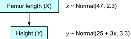
Figure 6.1 A simple two-node CGM. Femur length (X) is a cause of height (Y). X has a normal distribution with a mean of 47 centimeters and a standard deviation of 2.3 centimeters. Y has a distribution with a mean of 25 + 3x centimeters and a standard deviation of 3.3 centimeters.

Recall from chapter 2 that x ~ P (X  ) and y ~ P (Y  |X=x ) means we generate from the probability distribution of X and conditional probability distribution of Y given X. In this case, P (X  ), the distribution of femur length, represented as a normal distribution with a mean of 47 centimeters and a standard deviation of 2.3 centimeters. P (Y  |X=x ) is the distribution on height given the femur length, given as a normal distribution with a mean of 25 + 3x centimeters and a standard deviation of 3.3 centimeters. We would implement this model in Pyro as follows in listing 6.1.

SETTING UP YOUR ENVIRONMENT

The code in this chapter was written using Python version 3.10, Pyro version 1.9.0, pgmpy version 0.1.25, and torch 2.3.0. See https://www.altdeep.ai/p/causalaibookfor links to the notebooks that run the code. We are also using MATLAB for some plotting; this code was tested with version 3.7.

Listing 6.1 Pyro pseudocode of the CGM in figure 6.1

from pyro.distributions import Normal
from pyro import sample
def cgm_model(): #1
 x = sample("x", Normal(47., 2.3)) #1
 y = sample("y", Normal(25. + 3*x, 3.3)) #1
 return x, y #2

#1 x and y are sampled from their causal Markov kernels, in this case normal distributions. #2 Repeatedly calling cgm_model will return samples from P(X, Y).

We are going to convert this model to an SCM using the following algorithm:

• 1. Introduce a new latent causal parent for X called Nx and a new latent causal parent for Y called Ny with distributions P(Nx) and P(Ny).
• 2. Make X and Y deterministic functions of Nx and Ny such that P(X, Y) in this new model is the same as in the old model.

Following these instructions and adding in two new variables, we get figure 6.2.

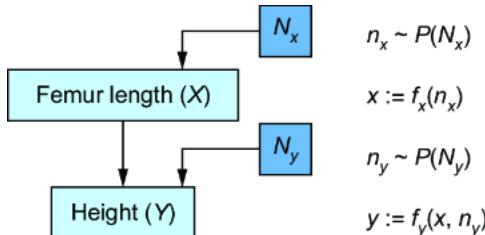
Figure 6.2 To convert the CGM to an SCM, we introduce latent ૿exogenous parents, Nx for X and Ny for Y, and probability distributions P(Nx) and P(Ny) for these latents. We then set X and Y deterministically, given their parents, via functions fx and fy.

We have two new latent variables Nx and Ny with distributions P (Nx) and P (Ny). X and Y each have their own functions fx and fy that that deterministically set X and Y, given their parents in the graph. This difference is key; X and Y are generated in the model described in figure 6.1 but set deterministically in this new model. To emphasize this, I use the assignment operator ૿:= instead of the equal sign ૿= to emphasize that fx and fy assign the values of X and Y.

To meet our goal of converting our CGM to an SCM, we want P (X  ) and P (Y  |X =x ) to be the same across both models. To achieve this, we have to choose P (Nx), P (Ny), fx, and fy such that P (X  ) is still Normal(47, 2.3) and P (Y  |X = x ) is still Normal(25 + 3.3x, 3.3). One option

is to do a simple reparameterization. Linear functions of normally distributed random variables are also normally distributed. We can implement the model in figure 6.3.

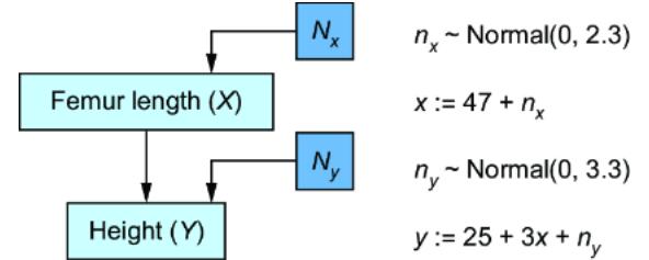
Figure 6.3 A simple reparameterization of the original CGM produces a new SCM model with the same P(X) and P(Y|X) as the original.

In code, we rewrite this as follows.

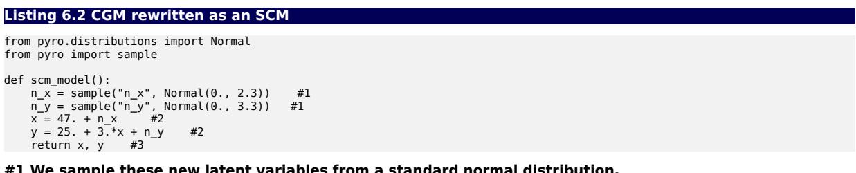
#1 We sample these new latent variables from a standard normal distribution. #2 X and Y are calculated deterministically as linear transformations of n_x and n_y. #3 The returned samples of P(X, Y) match the first model.

With this introduction of new exogenous variables Nx and Ny, some linear functions fx and fy, and a reparameterization, we converted the CGM to an SCM that encodes the same distribution P (X, Y  ). Next, let’s look more closely at the elements we introduced.

6.1.3 Formalizing the new model

To build an SCM, we’re going to assume we’ve already built a causal DAG, as in figure 6.1. In figures 6.2 and 6.3, we see two kinds of variables: exogenous and endogenous. The endogenous variables are the original variables X and Y—we’ll define them as the variables we are modeling explicitly. These are the variables we included in our causal DAG.

The exogenous variables (also called noise variables) are our new nodes Nx and Ny. These variables represent all unmodeled causes of our endogenous variables. In our formulation, we pair each of the endogenous variable with its own exogenous variable parent; X gets new exogenous causal parent Nx, and Y gets exogenous parent Ny. We add these to our DAG for completeness as in figures 6.2 and 6.3.

In our formulation, we’ll assume exogenous variables have no parents and have no edges between one another. In other words, they are root nodes in the graph, and they are independent relative to other exogenous variables. Further, we’ll treat the exogenous variables as latent variables.

Each endogenous variable also gets its own assignment function (also called a structural assignment) fx, and fy. The assignment function deterministically sets the value of the endogenous variables X and Y given values of their parents in the causal DAG.

Assignment functions are how we capture assumptions about the ૿how of causality. For instance, to say that the causal relationship between height (Y  ) and femur length (X  ) is linear, we specify that fx is a linear function.

While the endogenous variables are set deterministically, the SCM generates the values of the exogenous variables from probability distributions. In our femur example, we generate values nx and ny of exogenous variables Nx and Ny from distributions P (Nx) and P (Ny), which are N (0, 2.3) and N (0, 3.3), as seen in figure 6.3.

ELEMENTS OF THE GENERATIVE SCM

• A set of endogenous variables (e.g., X, Y)—These are the variables we want to model explicitly. They are the models we build into our causal DAG.
• A set of exogenous variables (e.g., Nx and Ny)—These variables stand in for unmodeled causes of the endogenous variables. In our formulation, each endogenous variable has one corresponding latent exogenous variable.
• A set of assignment functions (e.g., fx and fy)—Each endogenous variable has an assignment function that sets its value deterministically given its parents (its corresponding exogenous variable and other endogenous variables).
• A set of exogenous variable probability distributions (e.g., P(Nx) and P(Ny))—The SCM becomes a generative model with a set of distributions on the exogenous variables. Given values generated from these distributions, the endogenous variables are set deterministically.

Let’s look at another example of an SCM, this time using discrete variables.

6.1.4 A discrete, imperative example of an SCM

Our femur example dealt with continuous variables like height and length. Let’s now return to our rock-throwing example from chapter 2 and consider a discrete case of an SCM. In this example, either Jenny or Brian or both throw a rock at window if they are inclined to do so. The window breaks depending on whether either or both Jenny and Brian throw and the strength of the windowpane.

How might we convert this model to an SCM? In fact, this model is already an SCM. We captured this with the following code.

Listing 6.3 The rock-throwing example from chapter 2 is an SCM

import pandas as pd
import random
def true_dgp(
 jenny_inclination, #1
 brian_inclination, #1
 window_strength): #1
 jenny_throws_rock = jenny_inclination > 0.5 #2
 brian_throws_rock = brian_inclination > 0.5 #2
 if jenny_throws_rock and brian_throws_rock: #3
 strength_of_impact = 0.8 #3
 elif jenny_throws_rock or brian_throws_rock: #3
 strength_of_impact = 0.6 #3
 else: #3
 strength_of_impact = 0.0 #3
 window_breaks = window_strength < strength_of_impact #4
 return jenny_throws_rock, brian_throws_rock, window_breaks
generated_outcome = true_dgp(
 jenny_inclination=random.uniform(0, 1), #5
 brian_inclination=random.uniform(0, 1), #5
 window_strength=random.uniform(0, 1) #5
)

#1 The input values are instances of exogenous variables.

#2 Jenny and Brian throw the rock if so inclined. jenny_throws_rock and brian_throws_rock are endogenous variables.

#3 strength_of_impact is an endogenous variable. This entire if-then expression is the assignment function for strength of impact.

#4 window_breaks is an endogenous variable. The assignment function is lambda strength_of_impact, window_strength: strength_of_impact > window_strength. #5 Each exogenous variable has a Uniform(0, 1) distribution.

You’ll see that it satisfies the requirements of an SCM. The arguments to the true_dgp function (namely jenny_inclination, brian_inclination, window_strength) are the exogenous variables. The named variables inside the function are the endogenous variables, which are set deterministically by the exogenous variables.

Most SCMs you’ll encounter in papers and textbooks are written down as math. However, this rock-throwing example shows us the power of reasoning causally with an imperative scripting language like Python. Some causal processes are easier to write in code than in math. It is only recently that tools such as Pyro have allowed us to make sophisticated code-based SCMs.

6.1.5 Why use SCMs?

More causal assumptions mean more ability to make causal inferences. The question of whether to use an SCM instead of a regular CGM is equivalent to asking whether the additional causal assumptions encoded in the functional assignments will serve your causal inference goal.

In our femur example, our DAG says femur length causes height. Our SCM goes further and says that for every unit increase in femur length, there is a proportional increase in height. The question is whether that additional information helps us answer a causal question. One example where such a linear assumption helps make a causal inference is the use of instrumental variable estimation of causal effects, which I’ll discuss in chapter 11. This approach relies on linearity assumptions to infer causal effects in cases where the assumptions in the DAG alone are not sufficient to make the inference. Another example is where an SCM can enable us to answer counterfactual queries using an algorithm discussed in chapter 9.

Of course, if your causal inference is relying on an assumption, and that assumption is incorrect, your inference will probably be incorrect. The ૿what assumptions in a DAG are simpler than the additional ૿how assumptions in an SCM. An edge in a DAG is a true or false statement that X causes Y. An assignment function in an SCM model is a statement

about how X causes Y. The latter assumption is more nuanced and quite hard to validate, so it’s easier to get incorrect. Consider the fact that there are longstanding drugs on the market that we know work, but we don’t fully understand their mechanism of action—how they work.

6.1.6 Differences from related approaches

SCMs have a rich history across different fields. You may have seen formulations that are similar to but nonetheless different from what we’ve laid out here. Here, we’ll highlight the differentiating elements of this formulation and why they matter to us.

GENERATIVE SCMS WITH LATENT EXOGENOUS VARIABLES

We want to use our SCMs as generative models. To that end, we treat exogenous variables (variables we don’t want to model explicitly) as latent proxies for unmodeled causes of the endogenous variables. We just need to specify probability distributions of the exogenous variables and we get a generative latent variable model.

FLEXIBLE SELECTION OF ASSIGNMENT FUNCTIONS

You’ll find that the most common applications of SCMs use linear functions as assignment functions, like we did in the femur example. However, in a generative AI setting, we certainly don’t want to constrain ourselves to linear models. We want to work with rich function classes we can write as code, optimize with automatic differentiation, and apply to high-dimensional nonlinear problems, like images. These function classes can do just as well in representing the ૿how of causality.

CONNECTION TO THE DAG

We contextualize the SCM within the DAG-based view of causality. First, we build a causal DAG as in chapters 3 and 4. Each variable in the DAG becomes an endogenous variable (a variable we want to model explicitly) in the SCM. For each endogenous variable, we add a single latent exogenous parent node to the DAG. Next, we define ૿assignment function as a function that assigns a given endogenous variable a value, given the values of its parents in the DAG. All of our DAG-based theory still applies, such as the causal Markov property and independence of mechanism.

Note that not all formulations of the SCM adhere so closely to the DAG. Some practitioners who don’t adopt a graphical view of causality still use SCM-like models (e.g., structural equation modeling in econometrics). And some variations of graphical SCMs allow us to relax acyclicity and work with cycles and feedback loops.

INDEPENDENT EXOGENOUS VARIABLES

Introducing one exogenous variable for every endogenous variable can be a nuisance; sometimes it is easier to treat a node with no parents in the original DAG as exogenous, or have the same exogenous parent for two endogenous nodes. But this approach lets us add exogenous variables in a way that maintains the d-separations entailed by the original DAG. It also allows us to make a distinction between endogenous variables we care to model explicitly, and all the exogenous causes we don’t want to model explicitly. This comes in handy when, for example, you’re building a causal image model like in chapter 5, and you don’t want to explicitly represent all the many causes of the appearance of an image.

6.1.7 Causal determinism and implications to how we model

The defining element of the SCM is that endogenous variables are set deterministically by assignment functions instead of probabilistically by drawing randomly from a distribution conditioned on causal parents. This deterministic assignment reflects the philosophical view of causal determinism, which argues that if you knew all the causal factors of an outcome, you would know the outcome with complete certainty.

The SCM stands on this philosophical foundation. Consider again our femur-height example, shown in figure 6.4.

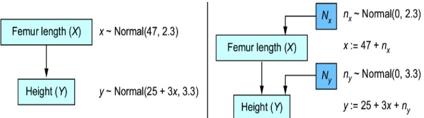
Figure 6.4 The original CGM samples endogenous variables from causal Markov kernels. The new model sets the endogenous variables deterministically.

In the original CGM on the left of figure 6.4, we generate values of X and Y from models of their causal Markov kernels. In the corresponding SCM on the right, the endogenous variables are set deterministically, no longer drawn from distributions. The SCM is saying that given femur length and all the other unmodeled causes of height represented by Ny, height is a certainty.

Note that despite this deterministic view, the SCM is still a probabilistic model of the joint probability distribution of the endogenous variables P(X, Y). But in comparison to the CGM on the left of figure 6.4, the SCM on the right shunts all the randomness of the model to the exogenous variable distributions. X and Y are still random variables in the SCM, because they are functions of Nx and Ny, and a function of a random variable is a random variable. But conditional on the exogenous variables, the endogenous variables are fully determined (degenerate).

The causal determinism leads to eye-opening conclusions for us as causal modelers. First, when we apply a DAG-based view of causality to a given problem, we implicitly assume the ground-truth data generating process (DGP) is an SCM. We already assumed that the ground-truth DGP had an underlying ground-truth DAG. Going a step further and assuming that each variable in that DAG is set deterministically, given all its causes (both those in and outside the DAG), is equivalent to assuming the ground-truth DGP is an SCM. The SCM might be a black box, or we might not be able to easily write it down in math or code, but it is an SCM nonetheless. That means, whether we’re using a traditional CGM or an SCM, we are modeling a ground-truth SCM.

Second, it suggests that if we were to generate from the ground-truth SCM, all the random variation in those samples would be entirely due to exogenous causes. It would not be due to an irreducible source of stochasticity like, for example, Heisenberg’s uncertainty principle or butterfly effects. If such concepts drive the outcomes in your modeling domain, CGMs might not be the best choice.

Now that we know we want to model a ground-truth SCM, let’s explore why we can’t simply learn it from data.

6.2 Equivalence between SCMs

A key thing to understand about SCMs is that we can’t fully learn them from data. To see why, let’s revisit the case where we turned a CGM into an SCM. Let’s see why, in general, this can’t give us the ground-truth SCM.

6.2.1 Reparameterization is not enough

When we converted the generic CGM to the SCM, we used the fact that a linear transformation of a normally distributed random variable produces a normally distributed random variable. This ensured that the joint probability distribution of the endogenous variables was unchanged.

We could use this ૿reparameterization trick (as this technique is called in generative AI) with other distributions. When we apply the reparameterization trick, we are shunting all the uncertainty in those conditional probability distributions to the distributions of the newly introduced exogenous variables. The problem is that different ૿reparameterization tricks can lead to different SCMs with different causal assumptions, leading to different causal inferences.

REPARAMETERIZATION TRICK FOR A BERNOULLI DISTRIBUTION

As an example, let X represent the choice of a weighted coin and Y represent the outcome of a flip of the chosen coin. Y is 1 if we flip heads and 0 if we flip tails. X takes two values, ૿coin A or ૿coin B. Coin A has a .8 chance of flipping heads, and coin B has a .4 chance of flipping heads, as shown in figure 6.5.

Figure 6.5 A simple CGM. X is a choice of one of two coins with different weights on heads and tails. Y is the outcome of the coin flip (heads or tails).

We can simulate an outcome of the flip with a variable Y sampled from a Bernoulli distribution with parameter px, where px is .8 or .4, depending on the value of x.

y ~ Bernoulli(px)

How could we apply the reparameterization trick here to make the outcome Y be the result of a deterministic process?

Imagine that we have a stick that’s one meter long (figure 6.6).

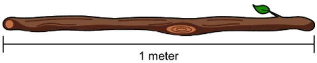
Figure 6.6 To turn the coin flip model into an SCM, first imagine a one meter long stick.

Imagine using a pocket knife to carve a mark that partitions the stick into two regions: one corresponding to ૿tails and one for ૿heads. We cut the mark at a point that makes the length of each region proportional to the probability of the corresponding outcome; the length of the heads region is px meters, and the length of the tails region is 1 – px meters. For coin A, this would be .8 meters (80 centimeters) for the heads region and .2 meters for the tails region (figure 6.7).

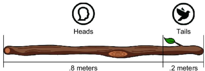
Figure 6.7 Divide the stick into two regions corresponding to each outcome. The length of the region is proportional to the probability of the outcome.

After marking the partition, we will now randomly select a point on the stick’s length where we will break the stick. The probability that the break will occur in a given region is equal to the probability of that region’s associated outcome (figure 6.8). The equality comes from having the length of the region correspond to the probability of the outcome. If the break point is to the left of the partition we cut with our pocket knife, y is assigned 0 (૿heads), and if the break point is to the right, y is assigned 1 (૿tails).

To randomly select a point to break the stick, we can generate from a uniform distribution. Suppose we sample .15 from a uniform(0, 1) and thus break the stick at a point .15 meters along its length, as shown in figure 6.8. The .15 falls into the ૿heads region, so we return heads. If we repeat this stick-breaking procedure many times, we’ll get samples from our target Bernoulli distribution.

In math, we can write this new model as follows:

ny ~ Uniform(0, 1)

y : = I(ny ≤ px)

where px is .8 if X is coin A, or .4 if X is coin B. Here, I(.) is the indicator function that returns 1 if ny < px and 0 otherwise.

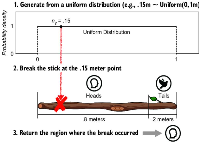
Figure 6.8 Generate from a uniform distribution on 0 to 1 meters, break the stick at that point, and return the outcome associated with the region where the break occurred. Repeated generation of uniform variates will cause breaks in the ૿heads region 80% of the time, because its length is 80% of the full stick length.

This new model is technically an SCM, because instead of Y being generated from a Bernoulli distribution, it is set deterministically by an indicator ૿assignment function. We did a reparameterization that shunted all the randomness to an exogenous variable with a uniform distribution, and that variable is passed to the assignment function.

DIFFERENT “REPARAMETERIZATION TRICKS” LEAD TO DIFFERENT SCMS

The main reason to use SCM modeling is to have the functional assignments represent causal assumptions beyond those captured by the causal DAG. The problem with the reparameterization trick is that different reparameterization tricks applied to the same CGM will create SCMs with different assignment functions, implying different causal assumptions.

To illustrate, suppose that instead of a coin flip, Y was a three-sided die, like we saw in chapter 2 (figure 6.9). X determines which die we’ll throw; die A or die B (figure 6.10). Each die is weighted differently, so they have different probabilities of rolling a 1, 2, or 3.

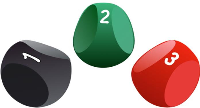
Figure 6.9 Three-sided dice

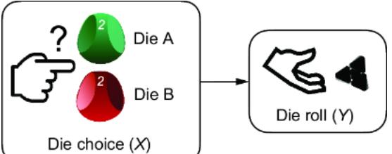
Figure 6.10 Suppose we switch the model from choosing a coin (two outcomes) to choosing a three-sided die (three outcomes).

We can extend the original model from a Bernoulli distribution (which is the same as a categorical distribution with two outcomes) to a categorical distribution with three outcomes:

y ~ Categorical([px1, px2, px3])

where px1, px2, and px3 are the probabilities of rolling a 1, 2, and 3 respectively (note that one of these is redundant, since px1 = 1 – px2 – px3).

We can use the stick-based reparameterization trick here as well; we just need to extend the stick to have one more region. Suppose for die A, the probability of rolling a 1 is px1=.1, rolling a 2 is px2=.3, and rolling a 3 is px3=.6. We’ll mark our stick as in figure 6.11.

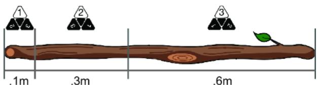
Figure 6.11 Divide the stick into three regions corresponding to outcomes of the three-sided die.

We’ll then use the same selection of a remote region using a generated uniform variate as before (figure 6.12).

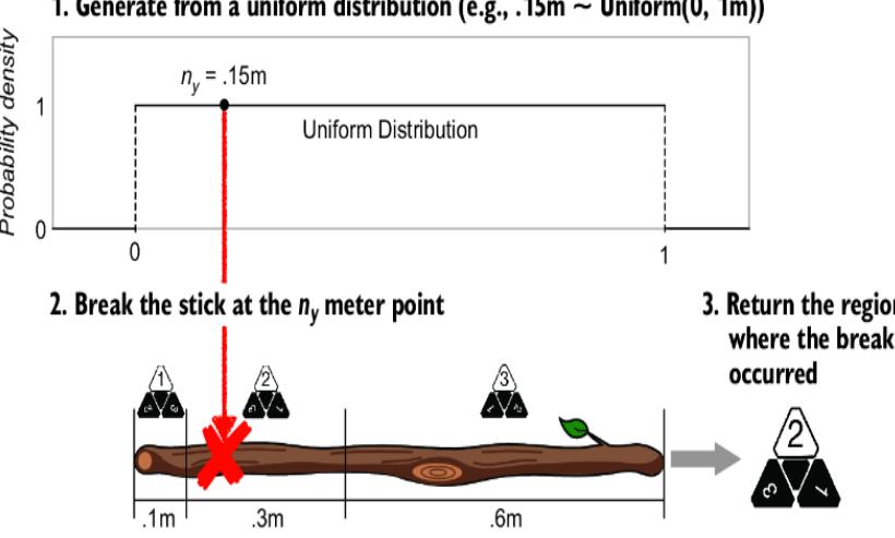
Figure 6.12 The conversion to the stick-breaking SCM when Y has three outcomes

In math we’ll write this as follows:

\[n\_{\mathcal{Y}} \sim Uniform \begin{cases} n\_{\mathcal{Y}} \sim Uniform \begin{cases} 0, & 1 \end{cases} \\ 1, & p\_{x1} \\ 2, & p\_{x1} < n\_{\mathcal{Y}} \le p\_{x1} + p\_{x2} \\ 3, & p\_{x1} + p\_{x2} < n\_{\mathcal{Y}} \le 1 \end{cases}\]

But what if we mark the stick differently, such that we change the ordering of the regions on the stick? In the second stick, the region order is 3, 1, and then 2 (figure 6.13).

Figure 6.13 Two different ways of reparameterizing a causal generative model yield two different SCMs. They encode the same joint probability distribution but different endogenous values given the same exogenous value.

In terms of the probability of each outcome (1, 2, or 3), the two sticks are equivalent—the size of the stick regions assigned to each die-roll outcome are the same on both sticks. But our causal mechanism has changed! These two sticks can return different outcomes for a given value of ny. If we randomly draw .15 and thereby break the sticks at the .15 meter point, the first stick will break in region 2, returning a 2, and the second stick will break in region 3, returning a 3.

In math, the second stick-breaking SCM has this form:

\[n\_{\mathfrak{y}} \sim Uniform\left(0, \ 1\right)\]

\[\mathfrak{y} := \begin{cases} 3, & n\_{\mathfrak{y}} \le p\_{x3} \\ 1, & p\_{x3} < n\_{\mathfrak{y}} \le p\_{x3} + p\_{x1} \\ 2, & p\_{x3} + p\_{x1} < n\_{\mathfrak{y}} \le 1 \end{cases}\]

Metaphorically speaking, imagine that in your modeling domain, the sticks are always marked a certain way, with the regions ordered in a certain way. Then there is no guarantee that a simple reparameterization trick will give you the ground-truth marking. To drive the point home, let’s look back at the reparameterization trick we performed to convert our femur-height model to an SCM (figure 6.14).

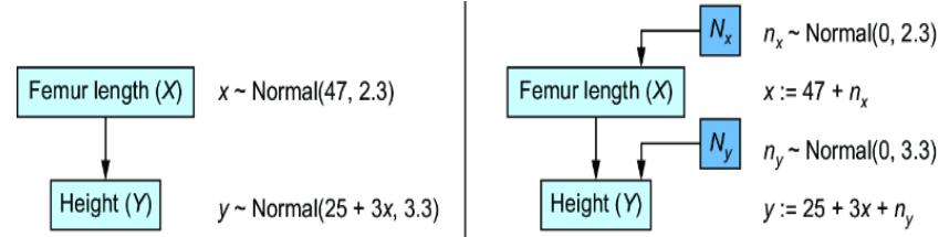
Figure 6.14 Revisiting the femur-height SCM

Suppose we create a new SCM that is the same, except that the assignment function for y now looks like this:

y := 25 + 3x – ny

Now we have a second SCM that subtracts ny instead of adding ny. A normal distribution is symmetric around its mean, so since ny has a normal distribution with mean 0, the probability values of ny and –ny are the same, so the probability distribution of Y is the same in both models. But for the same values of ny and x, the actual assigned values of y will be different. Next, we’ll examine this idea in formal detail.

6.2.2 Uniqueness and equivalence of SCMs

Given a causal DAG and a joint probability distribution on endogenous variables, there can generally be multiple SCMs consistent with that DAG and joint probability distribution. This means that we can’t rely on data alone to learn the ground-truth SCM. We’ll explore this problem of causal identifiability in depth in chapter 10. For now, let’s break this idea down using concepts we’ve seen so far.

MANY SCMS ARE CONSISTENT WITH A DAG AND CORRESPONDING DISTRIBUTIONS

Recall the many-to-one relationships we outlined in figure 2.24, shown again here in figure 6.15.

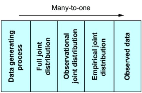
Figure 6.15 We have many-to-one relationships as we move from the DGP to observed data.

If we can represent the underlying DGP as a ground-truth SCM, figure 6.15 becomes as shown in figure 6.16.

SCM	Causal DAG	distribution Full joint	ioint distribution Observational	Empirical joint distribution	Observed data

Figure 6.16 Different SCMs can entail the same DAG structure and distributions. The SCMs can differ in assignment functions (and/or exogenous distributions).

In other words, given a joint distribution on a set of variables, there can be multiple causal DAGs consistent with that distribution—in chapter 4 we called these DAGs a Markov equivalence class. Further, we can have equivalence classes of SCMs—given a causal DAG and a joint distribution, there can be multiple SCMs consistent with that DAG and distribution. We saw this with how the two variants of the stick-breaking die-roll SCM are both consistent with the DAG X (die choice) → Y (die roll) and with the distributions P (X  ) (probability distribution on die selection) and P (Y  |X  ) (probability of die roll).

THE GROUND-TRUTH SCM CAN’T BE LEARNED FROM DATA (WITHOUT CAUSAL ASSUMPTIONS)

When we were working to build a causal DAG in previous chapters, our implied objective was to reproduce the ground-truth causal DAG. Now we seek to reproduce the ground-truth SCM, as in figure 6.16.

In chapter 4, we saw that data cannot distinguish between causal DAGs in an equivalence class of DAGs. Similarly, data alone is not sufficient to recover the ground-truth SCM. Again, consider the stick-breaking SCMs we derived. We derived two marked sticks, with two different orderings of regions. Of course, there are 3 × 2 × 1 = 6 ways of ordering the three outcomes: ({1, 2, 3}, {1, 3, 2}, {2, 1, 3}, {2, 3, 2}, {3, 1, 2}, {3, 2, 1}). That’s six ways of marking the stick and thus six different possible SCMs consistent with the distributions P (X  ) and P(Y  |X  ) (probability of die roll).

Suppose one of these marked sticks was the ground-truth SCM, and it was hidden from us in a black box, as in figure 6.17. Suppose we repeatedly ran the SCM to generate some die rolls. Based on those die rolls, could we figure out how the ground-truth stick was marked? In other words, which of the six orderings was the black box ordering?

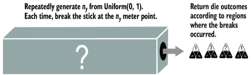
Figure 6.17 Suppose we didn’t know which ૿marked stick was generating the observed die rolls. There would be no way of inferring the correct marked stick from the die rolls alone. More generally, SCMs cannot be learned from statistical information in the data alone.

The answer is no. More generally, because of the many-to-one relationship between SCMs and data, you cannot learn the ground-truth SCM from statistical information in the data alone.

Let that sink in for a second. I’m telling you that even with infinite data, the most cuttingedge deep learning architecture, and a bottomless compute budget, you cannot figure out the true SCM even in this trivial three-outcome stick-breaking example. In terms of statistical likelihood, each SCM is equally likely, given the data. To prefer one SCM to another in the equivalence class, you would need additional assumptions, such as that {1, 2, 3} is the most likely marking because the person marking the stick would probably mark the regions in order. That’s a fine assumption to make, as long as you are aware you are making it.

In the practice of machine learning, we are often unaware that we are making such assumptions. To illustrate, suppose you ran the following experiment. You created a bunch of stick-breaking SCMs and then simulated data from those SCMs. Then you vectorized the SCMs and used them as labels, and the simulated data as features, in a deep supervised learning training procedure focused on predicting the ૿true SCM from simulated data, as illustrated in figure 6.18.

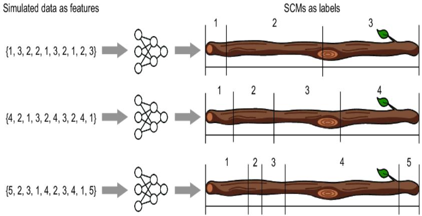
Figure 6.18 You create many SCMs and simulate data from each of them. You could then do supervised learning of a deep net that predicted the ground-truth SCM from the simulated data. Given two SCMs of the same equivalence class, this approach would favor the SCM with attributes that appeared more often in the training data.

Suppose then you fed the trained model data actual samples of three-sided die rolls, with the goal of predicting the ground-truth SCM. That predictive model’s prediction might favor a stick with the {1, 2, 3} ordering over the equivalent {2, 3, 1} ordering. But it would only do so if the {1, 2, 3} ordering was more common in the training data.

ANALOGY TO PROGRAM INDUCTION

The problem of learning an SCM from data is related to the challenge of program induction in computer science. Suppose a program took ૿foo and ૿bar as inputs and returned ૿foobar as the output. What is the program? You might think that the program simply concatenates the inputs. But it could be anything, including one that concatenates the inputs along with the word ૿aardvark, then deletes the ૿aardvark characters, and returns the result. The ૿data (many examples of inputs to and outputs of the program) are not enough distinguish which program of all the possible programs is the correct one. For that you need additional assumptions or constraints, such as an Occam’s razor type of inductive bias that prefers the simplest program (e.g., the program with the minimum description length).

Trying to learn an SCM from data is a special case of this problem. The program’s inputs are the exogenous variable values, and the outputs are the endogenous variable values. Suppose you have the causal DAG, just not the assignment functions. The problem is that an infinite number of assignment functions could produce those outputs, given the inputs. Learning an SCM from data requires additional assumptions to constrain the assignment functions, such as constraining the function class and using Occam’s razor (e.g., model selection criterion).

Next, we’ll dive into implementing an SCM in a discrete rule-based setting.

6.3 Implementing SCMs for rule-based systems

A particularly useful application for SCMs is modeling rule-based systems. By ૿rule-based, I mean that known rules, often set by humans, determine the ૿how of causality. Games are a good example.

To illustrate, consider the Monty Hall problem—a probability-based brain teaser named after the host of a 1960’s game show with a similar setup.

6.3.1 Case study: The Monty Hall problem

A contestant on a game show is asked to choose between three closed doors. Behind one door is a car; behind the others, goats. The player picks the first door. Then the host, who knows what’s behind the doors, opens another door, for example the third door, which has a goat. The host then asks the contestant, ૿Do you want to switch to the second door, or do you want to stay with your original choice? The question is which is the better strategy, switching doors or staying?

The correct answer is to switch doors. This question appeared in a column in Parade magazine in 1990, with the correct answer. Thousands of readers mailed in, including many with graduate-level mathematical training, to refute the answer and say that there is no advantage to switching, that staying or switching have the same probability of winning.

Figure 6.19 illustrates the intuition behind why switching is better. Switching doors is the correct answer because under the standard assumptions, the ૿switch strategy has a probability of two-thirds of winning the car, while the ૿stay strategy has only a one-third probability. It seems counterintuitive because each door has an equal chance of having the car when the game starts. It seems as if, once the host eliminates one door, each remaining door should have a 50-50 chance. This logic is false, because the host doesn’t

eliminate a door at random. He only eliminates a door that isn’t the player’s initial selection and that doesn’t have the car. A third of the times, those are the same door, and two-thirds of the time they are different doors; that one-third to two-thirds asymmetry is why the remaining doors don’t each have a 50-50 chance of having the car.

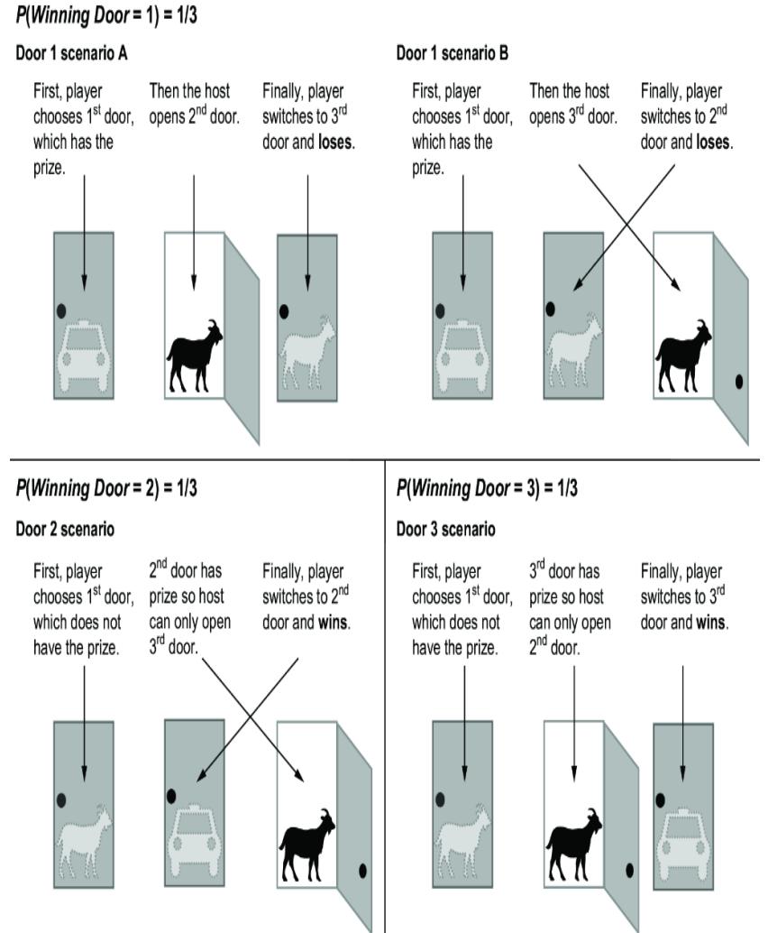
Figure 6.19 The Monty Hall problem. Each door has an equal probability of concealing a prize. The player chooses a door initially, the host reveals a losing door, and the player has the option to switch their initial choice. Contrary to intuition, the player should switch; if they switch, they will win two out of three times. This illustration assumes door 1 is chosen, but the results are the same regardless of the initial choice of door.

6.3.2 A causal DAG for the Monty Hall problem

Causal modeling makes the Monty Hall problem much more intuitive. We can represent this game with the causal DAG in figure 6.20.

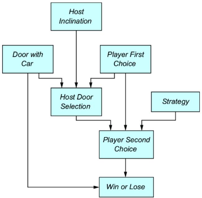
Figure 6.20 A causal DAG for the Monty Hall problem

The possible outcomes for each variable are as follows:

• Door with Car —Indicates the door that has the car behind it. 1st for the first door, 2nd for the second door, or 3rd for the third door.
• Player First Choice —Indicates which door the player chooses first. 1st for the first door, 2nd for the second door, or 3rd for the third door.
• Host Inclination —Suppose the host is facing the doors, such that from left to right they are ordered 1st, 2nd, and 3rd. This Host Inclination variable has two outcomes, Left and Right. When the outcome is Left, the host is inclined to choose the left-most available door; otherwise the host will be inclined to choose the right-most available door.
• Host Door Selection —The outcomes are again 1st, 2nd, and 3rd.
• Strategy —The outcomes are Switch if the strategy is to switch doors from the first choice, or Stay if the strategy is to stay with the first choice.
• Player Second Choice —Indicates which door the player chooses after being asked by the host whether they want to switch or not. The outcomes again are 1st, 2nd, and 3rd.
• Win or Lose —Indicates whether the player wins; the outcomes are Win or Lose. Winning occurs when Player Second Choice == Door with Car.

Next, we’ll see how to implement this as an SCM in pgmpy.

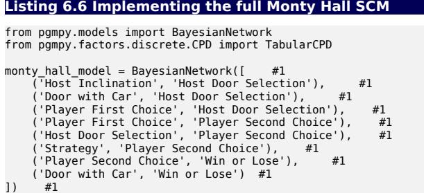
6.3.3 Implementing Monty Hall as an SCM with pgmpy

The rules of the game give us clear logic for the assignment functions. For example, we can represent the assignment function for Host Door Selection with table 6.1.

Table 6.1 A lookup table for Host Door Selection, given Player First Choice, Door with Car, and Host Inclination. It shows which door the host selects, given the player’s first choice, which door has the car, and the Host Inclination, which refers to whether the host will choose the left-most or right-most door in cases when the host has two doors to choose from.

Host Inclination					Left				Right
Door with Car	1st				2nd			3rd			1st			2nd			3rd
Player First Choice	1st	2nd	3rd	1st	2nd	3rd	1st	2nd	3rd	1st	2nd	3rd	1st	2nd	3rd	1st	2nd	3rd
Host Door Selection	2nd	3rd	2nd	3rd	1st	1st	2nd	1st	1st	3rd	3rd	2nd	3rd	3rd	1st	2nd	1st	2nd

When the door with the car and the player’s first choice are different doors, the host can only choose the remaining door. But if the door with the car and the player’s first choice are the same door, the host has two doors to choose from. He will choose the left-most door if Host Inclination is Left. For example, if Door with Car and Player First Choice are both 1st, the host must choose between the 2nd and 3rd doors. He will choose the 2nd door if Host Inclination == Left and the 3rd if Host Inclination == Right.

This logic would be straightforward to write using if-then logic with a library like Pyro. But since the rules are simple, we can use the far more constrained pgmpy library to write this function as a conditional probability table (table 6.2).

Table 6.2 We can convert the Host Door Selection lookup table (table 6.1) to a conditional probability table that we can implement as a TabularCPD object in pgmpy, where the probability of a given outcome is 0 or 1, and thus, deterministic.

Host Inclination						Left				Right
Door with Car		1st			2nd	3rd					1st			2nd			3rd
Player First Choice		1st	2nd	3rd	1st	2nd	3rd	1st	2nd	3rd	1st	2nd	3rd	1st	2nd	3rd	1st	2nd	3r
	1st	0	0	0	0	1	1	0	1	1	0	0	0	0	0	1	0	1	0
Host Door	2nd	1	0	1	0	0	0	1	0	0	0	0	1	0	0	0	1	0	1
Selection	3rd	0	1	0	1	0	0	0	0	0	1	1	0	1	1	0	0	0	0

The entries in the table correspond to the probability of the Host Door Selection outcome given the values of the causes. Each probability outcome is either 0 or 1, given the causal parents, so the outcome is completely deterministic given the parents. Therefore, we can use this as our assignment function, and since it is a conditional probability table, we can implement it using the TabularCPD class in pgmpy.

Listing 6.4 Implementation of Host Door Selection assignment function in pgmpy

from pgmpy.factors.discrete.CPD import TabularCPD
f_host_door_selection = TabularCPD(
 variable='Host Door Selection', #1
 variable_card=3, #2
 values=[ #3
 [0,0,0,0,1,1,0,1,1,0,0,0,0,0,1,0,1,0], #3
 [1,0,1,0,0,0,1,0,0,0,0,1,0,0,0,1,0,1], #3
 [0,1,0,1,0,0,0,0,0,1,1,0,1,1,0,0,0,0] #3
 ], #3
 evidence=[ #4
 'Host Inclination', #4
 'Door with Car', #4
 'Player First Choice' #4
 ], #4
 evidence_card=[2, 3, 3], #5
 state_names={ #6
 'Host Door Selection':['1st', '2nd', '3rd'], #6
 'Host Inclination': ['left', 'right'], #6
 'Door with Car': ['1st', '2nd', '3rd'], #6
 'Player First Choice': ['1st', '2nd', '3rd'] #6
 } #6
) #6

#1 The name of the variable

#2 The cardinality (number of outcomes) #3 The probability table. The values match the value in table 6.2, as long as the ordering of the causal variables in the evidence argument matches the top-down ordering of causal variable names in the table. #4 The conditioning (causal) variables #5 The cardinality (number of outcomes) for each conditioning (causal) variable #6 The state names of each the variables

This code produces f_host_door_selection, a TabularCPD object we can add to a model of the class BayesianNetwork. We can then use this in a CGM as we would a more typical TabularCPD object.

Similarly, we can create a look-up table for Player Second Choice, as shown in table 6.3.

Table 6.3 A lookup table for Player Second Choice, conditional on Player First Choice, Host Door Selection, and Strategy. Player Second Choice cells are empty in the impossible cases where Player First Choice and Host Door Selection are the same.

Strategy		Stay									Switch
Host Door Selection	1st				2nd			3rd			1st			2nd			3rd
Player First Choice	1st	2nd	3rd	1st	2nd	3rd	1st	2nd	3rd	1st	2nd	3rd	1st	2nd	3rd	1st	2nd	3rd
Player Second Choice		2nd	3rd	1st		3rd	1st	2nd			3rd	2nd	3rd		1st	2nd	1st

The host will never choose the same door as the player’s first choice, so Host Door Selection and Player First Choice can never have the same value. The entries of Player Second Choice are not defined in these cases.

Expanding this to a conditional probability table gives us table 6.4. Again, the cells with impossible outcomes are left blank.

Table 6.4 The result of converting the lookup table for Player Second Choice (table 6.3) to a conditional probability table that we can implement as a TabularCPD object

Strategy						Stay				Switch
Host Door Selection		1st			2nd			3rd			1st			2nd			3rd
Player First Choice		1st	2nd	3rd	1st	2nd	3rd	1st	2nd	3rd	1st	2nd	3rd	1st	2nd	3rd	1st	2nd	3rd
Player	1st		0	0	1		0	1	0			0	0	0		1	0	1
Second	2nd		1	0	0		0	0	1			0	1	0		0	1	0
Choice	3rd		0	1	0		1	0	0			1	0	1		0	0	0

Unfortunately, we can’t leave the impossible values blank when we specify a Tabular-CPD, so in the following code, we’ll need to assign arbitrary values to these elements.

Listing 6.5 Implementation of Player Second Choice assignment function in pgmpy

from pgmpy.factors.discrete.CPD import TabularCPD
f_second_choice = TabularCPD(
 variable='Player Second Choice',
 variable_card=3,
 values=[
 [1,0,0,1,0,0,1,0,0,0,0,0,0,0,1,0,1,0], #1
 [0,1,0,0,1,0,0,1,0,1,0,1,0,1,0,1,0,1], #1
 [0,0,1,0,0,1,0,0,1,0,1,0,1,0,0,0,0,0] #1
 ],
 evidence=[
 'Strategy',
 'Host Door Selection',
 'Player First Choice'
 ],
 evidence_card=[2, 3, 3],
 state_names={
 'Player Second Choice': ['1st', '2nd', '3rd'],
 'Strategy': ['stay', 'switch'],
 'Host Door Selection': ['1st', '2nd', '3rd'],
 'Player First Choice': ['1st', '2nd', '3rd']
 }
)

#1 The probability values are 0 or 1, so the assignment function is deterministic. In cases where the parent combinations are impossible, we still have to assign a value.

That gives us a second TabularCPD object. We’ll create one for each node.

First, let’s set up the causal DAG.

#1 Build the causal DAG.

monty_hall_model is now a causal DAG. It will become an SCM after we add the exogenous variable distributions and assignment functions.

The following listing adds the exogenous variable distribution.

Listing 6.7 Create the exogenous variable distributions

p_host_inclination = TabularCPD( #1
 variable='Host Inclination', #1
 variable_card=2, #1
 values=[[.5], [.5]], #1
 state_names={'Host Inclination': ['left', 'right']} #1
) #1
p_door_with_car = TabularCPD( #2
 variable='Door with Car', #2
 variable_card=3, #2
 values=[[1/3], [1/3], [1/3]], #2
 state_names={'Door with Car': ['1st', '2nd', '3rd']} #2
) #2
p_player_first_choice = TabularCPD( #3
 variable='Player First Choice', #3
 variable_card=3, #3
 values=[[1/3], [1/3], [1/3]], #3
 state_names={'Player First Choice': ['1st', '2nd', '3rd']} #3
) #3
p_host_strategy = TabularCPD( #4
 variable='Strategy', #4
 variable_card=2, #4
 values=[[.5], [.5]], #4
 state_names={'Strategy': ['stay', 'switch']} #4
) #4

#1 A CPD for the Host Inclination variable. In cases when the player chooses the door with the car, the host has a choice between the two other doors. This variable is ૿left when the host is inclined to choose the left-most door, and ૿right if the host is inclined to choose the right-most door.

#2 A CPD for the variable representing which door has the prize car. Assume each door has an equal probability of having the car.

#3 A CPD for the variable representing the player’s first door choice. Each door has an equal probability of being chosen.

#4 A CPD for the variable representing the player’s strategy. ૿Stay is the strategy of staying with the first choice, and ૿switch is the strategy of switching doors.

Having created the exogenous distributions, we’ll now create the assignment functions. We’ve already created f_host_door_selection and f_second_choice, so we’ll add f_win_or_lose the assignment function determining whether the player wins or loses.

Listing 6.8 Create the assignment functions

f_win_or_lose = TabularCPD( 
 variable='Win or Lose', 
 variable_card=2, 
 values=[ 
 [1,0,0,0,1,0,0,0,1], 
 [0,1,1,1,0,1,1,1,0], 
 ], 
 evidence=['Player Second Choice', 'Door with Car'], 
 evidence_card=[3, 3], 
 state_names={ 
 'Win or Lose': ['win', 'lose'], 
 'Player Second Choice': ['1st', '2nd', '3rd'], 
 'Door with Car': ['1st', '2nd', '3rd'] 
 } 
)

Finally, we’ll add the exogenous distribution and the assignment functions to monty_hall_model and create the SCM.

Listing 6.9 Create the SCM for the Monty Hall problem

monty_hall_model.add_cpds( 
 p_host_inclination, 
 p_door_with_car, 
 p_player_first_choice, 
 p_host_strategy, 
 f_host_door_selection, 
 f_second_choice, 
 f_win_or_lose 
)

We can run the variable elimination inference algorithm to verify the results of the algorithm. Let’s query the probability of winning, given that the player takes the ૿stay strategy.

Listing 6.10 Inferring the winning strategy

from pgmpy.inference import VariableElimination #1

infer = VariableElimination(monty_hall_model) q1 = infer.query([‘Win or Lose’], evidence={‘Strategy’: ‘stay’}) #2 print(q1) #2 q2 = infer.query([‘Win or Lose’], evidence={‘Strategy’: ‘switch’}) #3 print(q2) #3 q3 = infer.query([‘Strategy’], evidence={‘Win or Lose’: ‘win’}) #4 print(q3) #4

#1 We’ll use the inference algorithm called ૿variable elimination. #2 Print the probabilities of winning and losing when the player uses the ૿stay strategy. #3 Print the probabilities of winning and losing when the player uses the ૿switch strategy. #4 Print the probabilities that the player used a stay strategy versus a switch strategy, given that the player won.

This inference produces the following output:

Win or Lose	+——————-+——————–+ phi(Win or Lose)
Win or Lose(win)	+===================+====================+ 0.3333 +——————-+——————–+
Win or Lose(lose)	0.6667 +——————-+——————–+

The probability of winning and losing under the ૿stay strategy is 1/3 and 2/3, respectively. In contrast, here’s the output for the ૿switch strategy:

Win or Lose	+——————-+——————–+ phi(Win or Lose) +===================+====================+
Win or Lose(win)	0.6667 +——————-+——————–+
Win or Lose(lose)	0.3333 +——————-+——————–+

The probability of winning and losing under the ૿switch strategy is 2/3 and 1/3, respectively. We can also condition on a winning outcome and infer the probability that each strategy leads to that outcome.

+——————+—————–+ Strategy	phi(Strategy)
+==================+=================+ Strategy(stay) +——————+—————–+	0.3333
Strategy(switch) +——————+—————–+	0.6667

These are plain vanilla non-causal probabilistic inferences—we were just validating that our SCM is capable of produce these inferences. In chapter 9, we’ll demonstrate how this SCM enables causal counterfactual inferences that simpler models can’t answer, such as ૿What would have happened had the losing player used a different strategy?

6.3.4 Exogenous variables in the rule-based system

In this Monty Hall SCM, the root nodes (nodes with no incoming edges) in the causal DAG function as the exogenous variables. This is slightly different from our formal definition of an SCM, which states that exogenous variables represent causal factors outside the system. Host Inclination meets that definition, as this was not part of the original description. Door with Car, Player First Choice, and Strategy are another matter. To remedy this, we could introduce exogenous parents to these variables, and set these variables deterministically, given these parents, as we do elsewhere in this chapter. But while modeling this in pgmpy, that’s a bit redundant.

6.3.5 Applications of SCM-modeling of rule-based systems

While the Monty Hall game is simple, do not underestimate the expressive power of incorporating rules into assignment functions. Some of the biggest achievements in AI in previous decades have been at beating expert humans in board games with simple rules. Simulation software, often based on simple rules for how a system transitions from one state to another, can model highly complex behavior. Often, we want to apply causal analysis to rule-based systems engineered by humans (who know and can rewrite those rules), such as an automated manufacturing system.

6.4 Training an SCM on data

Given a DAG, we make a choice of whether to use a CGM or an SCM. Let’s suppose we want to go with the SCM, and we want to ૿fit or ૿train this SCM on data. To do this, we choose some parameterized function class (e.g., linear functions, logistic functions, etc.) for each assignment function. That function class becomes a specific function once we’ve fit its parameters on data. Similarly, for each exogenous variable, we want to specify a canonical probability distribution, possibly with parameters we can fit on data.

In our femur-height example, all the assignment functions were linear functions and the exogenous variables were normal distributions. But with tools like Pyro, you can specify each assignment function and exogenous distribution one by one. Then you can train the parameters just as you would with a CGM. For example, instead of taking this femur-height model from the forensic textbook:

\[n\_Y \sim \mathcal{N}(0, \mathbf{3.3})\]

y = 25 + 3x + ny

you can just fit the parameters α, β, and δ of a linear model on actual forensic data:

ny ~ N (0, δ)

y = α + βx + ny

In this forensics example, we use a linear assignment function because height is proportional to femur length. Let’s consider other ways to capture how causes influence their effects.

6.4.1 What assignment functions should I choose?

The most important choice in an SCM model is your choice of function classes for the assignment functions, because these choices represent your assumptions about the ૿how of causality. You can use function classes common in math, such as linear models. You can also use code (complete with if-then statements, loops, recursion, etc.) like we did with the rock-throwing example.

Remember, you are modeling a ground-truth SCM. You are probably going to specify your assignment functions differently from those in the ground-truth SCM, but that’s fine. You don’t need your SCM to match the ground truth exactly; you just need your model to be right about the ૿how assumptions it is relying on for your causal inferences.

SCMS WITHOUT “HOW” ASSUMPTIONS ARE JUST CGMS

Suppose you built an SCM where every assignment function is a linear function. You are using a linear Gaussian assumption because your library of choice requires it (e.g., LinearGaussianCPD is pretty much your only choice for modeling continuous variables in pgmpy). However, you are not planning on relying on that linear assumption for your causal inference. In this case, while your model checks the boxes of an SCM, it is effectively a CGM with linear models of the causal Markov kernels.

Suppose, for example, that instead of a linear relationship between X and Y, X and Y followed a nonlinear S-curve, and your causal inference was sensitive to this S-curve. Imagine that the ground-truth SCM captured this with an assignment function in the form of the Hill equation (a function that arises in biochemistry and that can capture S-curves). But your SCM instead uses a logistic function fit on data. Your model, though wrong, will be sufficient to make a good causal inference if your logistic assignment function captured everything it needed to about the S-curve for your inference to work.

6.4.2 How should I model the exogenous variable distributions?

In section 6.1.3, we formulated our generative SCM in a particular way, where every node gets its own exogenous variable representing its unmodeled causes. Under that formulation, the role of the exogenous variable distribution is simply to provide sufficient variation for the SCM to model the joint distribution. This means that, assuming you have selected your assignment function classes, you can choose canonical distributions for the exogenous variables based on how well they would fit the data after parameter estimation. Some canonical distributions may fit better than others. You can contrast different choices using standard techniques for model comparison and cross-validation.

These canonical distributions can be parameterized, such as N(0, δ) in

\[n\_Y \sim \mathcal{N}(\mathbf{0}, \mathfrak{G})\]

y = α + βx + ny

A more common approach in generative AI is to use constants in the canonical distribution and only train the parameters of the assignment function:

ny ~ N(0, 1)

y = α + βx + δ ny

Either is fine, as long as your choice captures your ૿how assumptions.

6.4.3 Additive models: A popular choice for SCM modeling

Additive models are SCM templates that use popular trainable function classes for assignment functions. They can be a great place to start in SCM modeling. We’ll look at three common types of additive models: linear Gaussian additive model (LiGAM), linear non-Gaussian additive model (LiNGAM), and the nonlinear additive noise model (ANM). These models each encapsulate a pair of constraints: one on the structure of the assignment functions, and one on the distribution of the additive exogenous variables.

Additivity makes this approach easier because there are typically unique solutions to algorithms that learn the parameters of these additive models from data. In some cases, those parameters have a direct causal interpretation. There are also myriad software libraries for training additive models on data.

Let’s demonstrate the usefulness of additive models with an example. Suppose you were a biochemist studying the synthesis of a certain protein in a biological sample. The sample has some amount of an enzyme that reacts with some precursors in the sample and synthesizes the protein you are interested in. You measure the quantity of the protein you’re interested in. Let X be the amount of enzyme, and let Y be the measured amount of the protein of interest. We’ll model this system with an SCM, which has the DAG in figure 6.21.

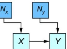
Figure 6.21 The amount of enzyme (X) is a cause the measured quantity of protein (Y).

We have qualitative knowledge of how causes affect effects, but we have to turn that knowledge into explicit choices of function classes for assignment functions and exogenous variable distributions. Additive models are a good place to start.

To illustrate, we’ll focus on the assignment function and exogenous variable distribution for Y, the amount of the target protein in our example. Generating from the exogenous variable, and setting Y via the assignment function, has the following notation:

ny ~ P(Ny)

y := fy(x, ny)

fy(.) denotes the assignment function for y, which takes a value of the endogenous parent X and exogenous parent Ny as inputs.

In an additive assignment function, the exogenous variable is always added to some function of endogenous parents. In our example, this means that the assignment function for Y has the following form:

y := fy(x, ny) = g(x) + ny

Here, g(.) is some trainable function of the endogenous parent(s), and ny is added to the results of that function.

For our protein Y, these models say that the measured amount of protein Y is equal to some function of the enzyme amount g (X  ) plus some exogenous factors, such as noise in the measurement device. This assumption is attractive, because it lets us think of unmodeled exogenous causes as additive ૿noise. In terms of statistical signal processing, it is relatively easy to disentangle some core signal (e.g., g (x )) from additive noise.

In general, let V represent an endogenous variable in the model, VPA represent the endogenous parents of V, and Nv represent an exogenous variable.

\[\nu := f\_{\vee}(\mathsf{V}\_{\mathsf{PA}^\*} \, n\_{\vee}) = g\left(\mathsf{V}\_{\mathsf{PA}}\right) + n\_{\vee}\]

Additive SCMs have several benefits, but here we’ll focus on their benefit as a template for building SCMs. We’ll start with the simplest additive model, the linear Gaussian additive model.

6.4.4 Linear Gaussian additive model

In a linear Gaussian additive model, the assignment functions are linear functions of the parents, and the exogenous variables have a normal distribution.

In our enzyme example, Ny and Y are given as follows:

\[n\_Y \sim \mathsf{N}(\mathbf{0}, \sigma\_Y)\]

y := β0 + βxx + ny

Here, β0 is an intercept term, and βx is a coefficient for X . We are assuming that for every unit increase in the amount of enzyme X, there is a βx increase in the expected amount of the measured protein. Ny accounts for variation around that expected amount due to exogenous causal factors, and we assume it has a normal distribution with a mean of 0 and scale parameter σy. For example, we might assume that Ny is composed mostly of technical noise from the measurement device, such as dust particles that interfere with the sensors. We might know from experience with this device that this noise has a normal distribution.

In general, for variable V with a set of K parents, VPA = {Vpa,1, …, Vpa,K}:

\[\begin{aligned} n\_{\mathcal{Y}} &\sim N(0, \sigma \mathcal{y}) \\ v &:= \beta\_0 + \sum\_j \beta\_x v\_{p a, j} + n\_{\mathcal{Y}} \end{aligned}\]

This model defines parameters: β0 is an intercept term, βj is the coefficient attached to the j th parent, and σv is the scale parameter of Nv’s normal distribution.

Let’s see an example of a LiNGAM model in Pyro.

Listing 6.11 Pyro example of a linear Gaussian model
from pyro import sample
from pyro.distributions import Normal
def linear_gaussian():
 n_x = sample("N_x", Normal(9., 3.))
 n_y = sample("N_y", Normal(9., 3.))
 x = 10. + n_x #1
 y = 2. * x + n_y #2
 return x, y

#1 The distributions of the exogenous variables are normal (Gaussian). #2 The functional assignments are linear.

Linear Gaussian SCMs are especially popular in econometric methods used in the social sciences because the model assumptions have many attractive statistical properties. Further, in linear models, we can interpret a parent causal regressor variable’s coefficient as the causal effect (average treatment effect) of that parent on the effect (response) variable.

6.4.5 Linear non-Gaussian additive models

Linear non-Gaussian additive models (LiNGAM) are useful when the Gaussian assumption on exogenous variables is not appropriate. In our example, the amount of protein Y cannot be negative, but that can easily occur in a linear model if β0, x, or nx have low values. LiNGAM models remedy this by allowing the exogenous variable to have a non-normal distribution.

Listing 6.12 Pyro example of a LiNGAM model

from pyro import sample
from pyro.distributions import Gamma
def LiNGAM():
 n_x = sample("N_x", Gamma(9., 1.)) #1
 n_y = sample("N_y", Gamma(9., 1.)) #1
 x = 10. + n_x #2
 y = 2. * x + n_y #2
 return x, y

#1 Instead of a normal (Gaussian) distribution, the exogenous variables have a gamma distribution with the same mean and variance.

#2 These are the same assignment functions as in the linear Gaussian model.

In the preceding model, we use a gamma distribution. The lowest possible value in a gamma distribution is 0, so y cannot be negative.

6.4.6 Nonlinear additive noise models

As I’ve mentioned, the power of the SCM is the ability to choose functional assignments that reflect how causes affect their direct effects. In our hypothetical example, you are a biochemist. Could you import knowledge from biochemistry to design the assignment function? Here is what that reasoning might look like. (You don’t need to understand the biology or the math, in this example, just the logic).

There is a common mathematical assumption in enzyme modeling called mass action kinetics. In this model, T is the maximum possible amount of the target protein. The biochemical reactions happen in real time, and during that time, the amount of the target protein fluctuates before stabilizing at some equilibrium value Y. Let Y(t) and X(t) be the amount of the target protein and enzyme at a given time point. Mass action kinetics give us the following ordinary differential equation:

\[\frac{dY(t)}{d(t)} = \nu X(t)(T - Y(t)) - \alpha Y(t)\]

Here, v and α are rate parameters that characterize the rates at which different biochemical reactions occur in time. This differential equation has the following equilibrium solution,

\[Y = T \times \frac{\beta X}{1 + \beta X}\]

where Y and X are equilibrium values of Y(t) and X(t), and β = v/α.

As an enzyme biologist, you know that this equation captures something of the actual mechanism underpinning the biochemistry of this system, like physics equations such as Ohm’s law and SIR models in epidemiology. You elect to use this as your assignment function for Y:

\[Y \coloneqq T \times \frac{\beta X}{1 + \beta X} + N\_{\mathcal{Y}}\]

This is a nonlinear additive noise model (ANM). In general, ANMs have the following structure:

\[\mathsf{V} = \mathsf{g} \left( \mathsf{V}\_{\mathsf{p}\mathsf{a}} \right) + \mathsf{N}\_{\mathsf{V}}\]

In our example g (X  ) = T × β X / (1 + β X  ). Ny can be normal (Gaussian) or non-Gaussian.

CONNECTING DYNAMIC MODELING AND SIMULATION TO SCMS

Dynamic models describe how a system’s behavior evolves in time. The use of dynamic modeling, as you saw in the enzyme modeling example, is one approach to addressing this knowledge elicitation problem for SCMs.

In this section, I illustrated how an enzyme biologist could use a domain-specific dynamic model, specifically an ODE, to construct an SCM. An ODE is just one type of dynamic model. Another example is computer simulator models, such as the simulators used in climate modeling, power-grid modeling, and manufacturing. Simulators can also model complex social processes, such as financial markets and epidemics. Simulator software is a growing multibillion dollar market.

In simulators and other dynamic models, specifying the ૿how of causality can be easier than in SCMs. SCMs require assignment functions to explicitly capture the global behavior of the system. Dynamic models only require you to specify the rules for how things change from instant to instant. You can then see global behavior by running the simulation. The trade-off is that dynamic models can be computationally expensive to run, and it is generally difficult to train parameters of dynamic models on data or perform inferences given data as evidence. This has motivated interesting research in combining the knowledge elicitation convenience of dynamic models with the statistical and computational conveniences of SCMs.

Next, we’ll examine using regression tools to train these additive models.

6.4.7 Training additive model SCMs with regression tools

In statistics, regression modeling finds parameter values that minimize the difference between a parameterized function of a set of predictors and a response variable. Regression modeling libraries are ubiquitous, and one advantage of additive SCM models is that they can use those libraries to fit an SCM’s parameters on data. For example, parameters of additive models can be fit with standard linear and nonlinear regression parameter fitting techniques (e.g., generalized least squares). We can also leverage these tools’ regression goodness-of-fit statistics to evaluate how well the model explains the data.

Note that the predictors in a general regression model can be anything you like. Most regression modeling pedagogy encourages you to keep adding predictors that increase goodness-of-fit (e.g., adjusted R-squared) or reduce predictive error. But in an SCM, your predictors are limited to direct endogenous causes.

CAN I USE GENERALIZED LINEAR MODELS AS SCMS?

In statistical modeling, a generalized linear model (GLM) is a flexible generalization of linear regression. In a GLM, the response variable is related to a linear function of the predictors with a link function. Further, variance of the response variable can be a function of the predictors. Examples include logistic regression, Poisson regression, and gamma regression. GLMs are a fundamental statistical toolset for data scientists.

In a CGM (non-SCM), GLMs are good choices as models of causal Markov kernels. But a common question is whether GLMs can be used as assignment functions in an SCM.

Several GLMs align with the structure of additive SCMs, but it’s generally best not to think of GLMs as templates for SCMs. The functional form of assignment functions in an SCM is meant to reflect the nature of the causal relationship between a variable and its causal parents. The functional form of a GLM applies a (in some cases nonlinear) link function to a linear function of the predictors. The link function is designed to map that linear function of the predictors to the mean of a canonical distribution (e.g., normal, Poisson, gamma). It is not designed to reflect causal assumptions.

6.4.8 Beyond the additive model

If the ૿how of an assignment function requires more nuance than you can capture with an additive model, don’t constrain yourself to an additive model. Using biochemistry as an example, it is not hard to come up with scenarios where interactions between endogenous and exogenous causes would motivate a multiplicative model.

For these more complex scenarios, it starts making sense to move toward using probabilistic deep learning tools to implement an SCM.

6.5 Combining SCMs with deep learning

Let’s revisit the enzyme kinetic model, where the amount of an enzyme X is a cause of the amount of a target protein Y, as in figure 6.22.

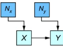
Figure 6.22 The amount of enzyme (X) is a cause of the measured quantity of protein (Y).

I said previously that, based on a dynamic mathematical model popular in the study of enzyme biology, a good candidate for an additive assignment function for Y is

\[Y \coloneqq T \times \frac{\beta X}{1 + \beta X} + N\_{\mathcal{Y}}\]

Further, suppose that we knew from experiments that T was 100 and β was .08.

Ideally, we would want to be able to reproduce these parameter values from data. Better yet, we should like to leverage the automatic differentiation-based frameworks that power modern deep learning.

6.5.1 Implementing and training an SCM with basic PyTorch

First, let’s create a PyTorch version of the enzyme model.

Listing 6.13 Implement the PyTorch enzyme model
from torch import nn
class EnzymeModel(nn.Module): #1
 def __init__(self):
 super().__init__()
 self.β = nn.Parameter(torch.randn(1, 1)) #2
 def forward(self, x):
 x = torch.mul(x, self.β) #3
 x = x.log().sigmoid() #4
 x = torch.mul(x, 100.) #5
 return x
#1 Create the enzyme model.
#2 Initialize the parameter D�.
#3 Calculate the product of enzyme amount X and D�.
#4 Implement the function u / (u + 1) as sigmoid(log(u)), since the sigmoid and log functions are native
PyTorch transforms.
#5 Multiply by T = 100.

Suppose we observed the data from this system, visualized in figure 6.23.

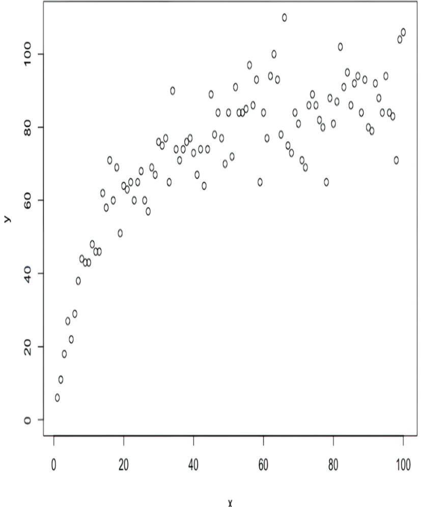
Figure 6.23 Exampled enzyme data. X is the amount of enzyme, and Y is the amount of target protein.

Let’s try to learn β from this data using a basic PyTorch workflow.

Listing 6.14 Fitting enzyme data with PyTorch import pandas as pd from torch import tensor import torch df = pd.read_csv(“https://raw.githubusercontent.com/altdeep /causalML/master/datasets/enzyme-data.csv”) #1 X = torch.tensor(df[‘x’].values).unsqueeze(1).float() #2 Y = torch.tensor(df[‘y’].values).unsqueeze(1).float() #2 def train(X, Y, model, loss_function, optim, num_epochs): #3 loss_history = [] #3 for epoch in range(num_epochs): #3 Y_pred = model(X) #3 loss = loss_function(Y_pred, Y) #3 loss.backward() #3 optim.step() #3 optim.zero_grad() #3 if epoch % 1000 == 0: #4 print(round(loss.data.item(), 6)) #4 torch.manual_seed(1) #5 enzyme_model = EnzymeModel() optim = torch.optim.Adam(enzyme_model.parameters(), lr=0.00001) #6 loss_function = nn.MSELoss() #7 train(X, Y, enzyme_model, loss_function, optim, num_epochs=60000)

#1 Load the enzyme data from GitHub. #2 Convert the data to tensors. #3 Create the training algorithm. #4 Print out losses during training. #5 Set a random seed for reproducibility. #6 Initialize an instance of the Adam optimizer. Use a low value for the learning rate because loss is very sensitive to small changes in D�. #7 Using mean squared loss error is equivalent to assuming Ny is additive and symmetric.

When I run this code with the given random seed, it produces a value of 0.1079 (you can access the value by printing enzyme_model.β.data), which only differs slightly from the ground-truth value of .08. This implementation did not represent the exogenous variable N^y explicitly, but statistics theory tells us that using the mean squared error loss function is equivalent to assuming Ny was additive and had a normal distribution. However, it also assumes that the normal distribution had constant variance, while the funnel shape in the scatterplot indicates the variance of Ny might increase with the value of X.

6.5.2 Training an SCM with probabilistic PyTorch

The problem with this basic parameter optimization approach is that the SCM should encode a distribution P (X, Y  ). So we can turn to a probabilistic modeling approach to fit this model.

Listing 6.15 Bayesian estimation β in a probabilistic enzyme model

import pyro
from pyro.distributions import Beta, Normal, Uniform
from pyro.infer.mcmc import NUTS, MCMC
def g(u): #1
 return u / (1 + u) #1
def model(N): #2
 β = pyro.sample("β", Beta(0.5, 5.0)) #3
 with pyro.plate("data", N): #4
 x = pyro.sample("X", Uniform(0.0, 101.0)) #5
 y = pyro.sample("Y", Normal(100.0 * g(β * x), x**.5)) #6
 return x, y
conditioned_model = pyro.condition( #7
 model, #7
 data={"X": X.squeeze(1), "Y": Y.squeeze(1)} #7
) #7
N = X.shape[0] #8
pyro.set_rng_seed(526) #9
nuts_kernel = NUTS(conditioned_model, adapt_step_size=True) #10
mcmc = MCMC(nuts_kernel, num_samples=1500, warmup_steps=500) #10
mcmc.run(N) #10

#1 The simple transform used in the assignment function for Y (amount of target protein) #2 The probabilistic model #3 A prior on the parameter β that we mean to fit with this model #4 A “plate” for the N=100 identical and independently distributed values of X and Y #5 The marginal probability of the enzyme P(X) is a uniform distribution between 0 and 101. #6 P(Y|X) is the conditional distribution of Y (protein concentration) given X (and β). I model P(Y|X) with a normal distribution with both a mean and variance that depends on Y. #7 Condition the model on the observed evidence. #8 Get the number of examples in the data (100). #9 Set a random seed for reproducibility. #10 To learn β, I use a gradient-based MCMC algorithm called a No-U-Turn Sampler (NUTS). This algorithm is one of many probabilistic approaches for parameter learning, and this choice is independent of the causal elements of your model.

The problem with this approach is that it doesn’t have an explicit representation of the exogenous variables. If we want to use a probabilistic machine learning framework to build an SCM, we need to make exogenous variables explicit. That is challenging with the preceding approach for one very nuanced reason: When I write the following statement in Pyro code, y = pyro.sample(“Y”, Normal(…, …)), Pyro knows to use that normal distribution to calculate the probability value (in more precise terms, the likelihood) of each value of Y in the training data. Those values are used in probabilistic inference algorithms like MCMC. But if I write a statement that represents an assignment function, like y = f(x, ny), Pyro doesn’t automatically know how to calculate probability values for Y, especially since as far as Pyro is concerned, f(.) can be anything.

But there is another problem that is more important than this issue with inference. So far, we’ve been assuming that we conveniently know a domain-based mathematical functional form for Y’s assignment function. It would be nice to use deep learning to fit the assignment functions, but this is problematic.

6.5.3 Neural SCMs and normalizing flows

Suppose we used a neural network to model y = f(x, ny). Indeed for a given SCM, we could use a multilayer neural network to model each variable, given its parents—call this a ૿neural SCM. The problem is that we want the trainable function class we use for our assignment functions to represent our assumptions about the ૿how of causality. Neural networks, as universal function approximators, are, by definition, as assumption-free as curve-fitting functions get. Therefore, to use a neural SCM, we need ways to constrain the neural assignment function to remain faithful to our ૿how assumptions. This could be done with constraints on the training feature, loss function, and elements of the neural network architecture. Normalizing flows are an example of the latter.

Returning to the enzyme modeling example, let’s start by enumerating some basic biological assumptions about the relationships between enzymes and the proteins they help synthesize:

• The process by which the protein leaves the system is independent of the amount of enzyme. So we expect the amount of target protein to monotonically increase, given the amount of enzyme.
• However, systems tend to saturate, such that there are diminishing returns in adding more enzyme.

We need a neural network approach that only allows for monotonic functions with diminishing returns. For this, we’ll use a deep generative modeling approach called normalizing flows.

Normalizing flows model a complex probability density as an invertible transformation of a simple base density. I’m going to use flows to model the distribution of endogenous variables as invertible transformations of exogenous variable distributions. There are many different transformations, but I’m going to use neural splines.1 Splines are a decades-old approach to curve-fitting using piece-wise polynomials; a neural spline is the neural network version of a spline.

Listing 6.16 Initializing splines for assignment functions

from pyro.distributions.transforms import conditional_spline print(conditional_spline(input_dim=1, context_dim=1)) #1

#1 A neural spline transform is a type of invertible PyTorch neural network module.

We get a three-layer neural network with ReLU activation functions:

ConditionalSpline(
 (nn): DenseNN(
 (layers): ModuleList(
 (0): Linear(in_features=1, out_features=10, bias=True)
 (1): Linear(in_features=10, out_features=10, bias=True)
 (2): Linear(in_features=10, out_features=31, bias=True)
 )
 (f): ReLU()
 )
)

Normalizing flows solve our problem of not having a likelihood value for y = f(x, ny). Like other probabilistic machine learning models, they allow us to connect an input random variable (like an exogenous variable) to an output variable (like an endogenous variable) using layers of transformations. The key difference is that normalizing flow models automatically calculate the probability values of instances of the output variable in the data (using the change-of-variable formula from probability theory). That automatic calculation relies on monotonicity; our causal ૿how assumption is that the relationship between enzyme concentration and protein abundance is monotonic, and normalizing flows give us monotonicity.

For example, in the following code, NxDist is the distribution of exogenous variable Nx. We set the distribution as a Uniform(0, 1). f_x is the assignment function for X, implemented as an AffineTransformation that maps this distribution to Uniform(1, 101).

Listing 6.17 Transforming a distribution of Nx to a distribution of X

from pyro.distributions import TransformedDistribution from pyro.distributions.transforms import AffineTransform NxDist = Uniform(torch.zeros(1), torch.ones(1)) #1 f_x = AffineTransform(loc=1., scale=100.0) #2 XDist = TransformedDistribution(NxDist, [f_x]) #3

#1 The exogenous distribution of X is Uniform(0, 1). #2 The assignment function for f_x. The AffineTransform multiplies Nx by 100 and adds 1. #3 XDist is an explicit representation of P(X). Multiplying by 100 and adding 1 gives you a Uniform(1, 101).

So XDist allows us to calculate the probability value of X even when its value is set deterministically by an assignment function. You can calculate the log-probability value of 50 with XDist.log_prob(torch.tensor([50.0])), which under the Uniform(1, 101) distribution will be log(1/100).

Let’s first specify the model.

Listing 6.18 Specify the flow-based SCM
import pyro from pyro.distributions import ( ConditionalTransformedDistribution, Normal, Uniform, TransformedDistribution
) from pyro.distributions.transforms import ( conditional_spline, spline )
import torch from torch.distributions.transforms import AffineTransform
pyro.set_rng_seed(348)
NxDist = Uniform(torch.zeros(1), torch.ones(1)) #1 f_x = AffineTransform(loc=1., scale=100.0) #2 XDist = TransformedDistribution(NxDist, [f_x]) #3
NyDist = Normal(torch.zeros(1), torch.ones(1)) #4 f_y = conditional_spline(input_dim=1, context_dim=1) #5 YDist = ConditionalTransformedDistribution(NyDist, [f_y]) #6

#1 The exogenous distribution of X is Uniform(0, 1).

#2 The assignment function for f_x. The AffineTransform multiplies Nx by 100 and adds 1.

#3 XDist is an explicit representation of P(X). Multiplying by 100 and adding 1 gives you a Uniform(1, 101). #4 The exogenous distribution of Y is Normal(0, 1).

#5 We implement the assignment function for f_y with a neural spline. Optimization will optimize the parameters of this spline.

#6 YDist is an explicit representation of P(Y|X).

Now we run the training.

Listing 6.19 Train the SCM

import matplotlib.pyplot as plt modules = torch.nn.ModuleList([f_y]) #1 optimizer = torch.optim.Adam(modules.parameters(), lr=3e-3) #2 losses = [] maxY = max(Y) #3 Ynorm = Y / maxY #3 for step in range(800): optimizer.zero_grad() #4 log_prob_x = XDist.log_prob(X) #5 log_prob_y = YDist.condition(X).log_prob(Ynorm) #6 loss = -(log_prob_x + log_prob_y).mean() #7 loss.backward() #7 optimizer.step() #7 XDist.clear_cache() YDist.clear_cache() losses.append(loss.item()) plt.plot(losses[1:]) #8 plt.title(“Loss”) #8 plt.xlabel(“step”) #8 plt.ylabel(“loss”) #8

#1 Register the neural spline functional assignment function for Y.

• #2 Initialize the optimizer.
• #3 Normalize Y, since the assignment function is working with neural networks.
• #4 Set all gradients to 0.

#5 Use P(X) to calculate a log likelihood value for each value of X.

#6 Use P(Y|X) to calculate a log likelihood value for each value of Y, given X.

#7 Fit the parameters of the neural network modules using maximum likelihood as an objective. #8 Visualize losses during training.

Figure 6.24 shows the training loss over training.

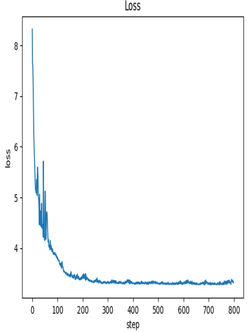
Figure 6.24 Training loss of the flow-based SCM-training procedure

Now we can generate samples from the model and compare them to the training data.

Listing 6.20 Generate from the trained model

x_flow = XDist.sample(torch.Size([100,])) #1 y_flow = YDist.condition(x_flow).sample(torch.Size([100,])) * maxY #1 plt.title(““” Observed values of enzyme concentration Xand protein concentration Y”““) #2 plt.xlabel(‘X’) #2 plt.ylabel(‘Y’) #2 plt.xlim(0, 105) #2 plt.ylim(0, 120) #2 plt.scatter( #2 X.squeeze(1), Y.squeeze(1), color=‘firebrick’, #2 label=‘Actual Data’, #2 alpha=0.5 #2 ) #2 plt.scatter( #2 x_flow.squeeze(1), y_flow.squeeze(), #2 label=‘Generated values from trained model’, #2 alpha=0.5 #2 ) #2 plt.legend() #2 plt.show() #2

#1 Generate synthetic examples from the trained model. #2 Visualize the synthetic examples over the examples in the training data to validate model fit.

Figure 6.25 overlays generated samples with the actual examples in the training data.

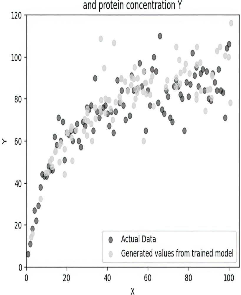
The ability to have multilayered flows as in other neural network frameworks makes this an extremely flexible modeling class. But this is not a mere curve-fitting exercise. With the variational autoencoder example in chapter 5, you saw that you can use neural networks to map causal parents to their child effects in the general class of CGMs. But that is not sufficient for SCMs, even if you set endogenous variables deterministically. Again, SCMs reflect causal assumptions about the ૿how of causality in the form of assignment functions. In this enzyme example, we are asserting that the monotonic relationship between the enzyme and protein abundance is important in the causal inferences we want to make, and so we’re constraining the neural nets (and other transforms) in my assignment functions to those that preserve monotonicity.

Summary

Structural causal models (SCMs) are a type of causal graphical model (CGM) that encode causal assumptions beyond the assumptions encoded in the causal DAG. The causal DAG assumptions capture what causes what. The SCM additionally captures how the causes affect the effects.

• SCMs are composed of exogenous variables, probability distributions on those exogenous variables, endogenous variables, and functional assignments.
• Exogenous variables represent unmodeled causes.
• Endogenous variables are the variables explicitly included in the model, corresponding to the nodes we’ve seen in previous causal DAGs.
• The functional assignments set each endogenous variable deterministically, given its causal parents.
• The SCM’s additional assumptions represent the ૿how of causality in the form of functional assignments.
• SCMs represent a deterministic view of causality, where an outcome is known for certain if all the causes are known.
• You can derive an SCM from a more general (non-SCM) CGM. But given a general CGM, there are potentially multiple SCMs that entail the same DAG and joint probability distribution as that CGM.
• You can’t learn the functional assignments of an SCM from statistical information in the data alone.
• SCMs are an ideal choice for representing well-defined systems with simple, deterministic rules, such as games.
• Additive noise models provide a useful template for building SCMs from scratch.
• Normalizing flows are a useful probabilistic machine learning framework for modeling SCMs when your causal ૿how assumption is monotonicity.

[1] For more information on neural splines, see C. Durkan, A. Bekasov, I. Murray, and G. Papamakarios, ૿Neural spline flows, in Advances in neural information processing systems, 32 (NeurIPS 2019).

7 Interventions and causal effects

This chapter covers

• Case studies of interventions in machine learning engineering contexts
• How interventions relate to A/B tests and randomized experiments
• Implementing interventions on causal models with intervention operators
• Using a causal model to represent many interventional distributions
• Causal effects as natural extensions of an intervention distribution

An intervention is something an agent does to cause other things to happen. Interventions change the data generating process (DGP).

Interventions are the most fundamental concept in how we define causality. For example, the concept of intervention, written in terms of ૿manipulation and ૿varying a factor, is central to this definition from an influential 1979 textbook on experimental design:

The paradigmatic assertion in causal relationships is that manipulation of a cause will result in the manipulation of an effect . . . . Causation implies that by varying one factor I can make another vary. 1

Interventions are how we go from correlation to causality. Correlation is symmetric; the statements ૿Amazon’s laptop sales correlate with Amazon’s laptop bag sales and ૿Amazon’s laptop bag sales correlate with Amazon’s laptop sales are equivalent. But interventions make causality a one-way street: if Amazon recommends the sale of laptops, laptop bag sales will increase, but if Amazon promotes the sale of laptop bags, we wouldn’t expect people to respond by buying new laptops to fill them.

A model must have a way of reasoning about intervention to be admitted to the club of causal models. Any model that lets you reason about how interventions change the DGP is, by definition, a causal model.

You are probably already familiar with interventions in the form of experiments, such as A/B tests or randomized clinical trials. Such experiments focus on inferring causal effects. Put simply, a causal effect is just a comparison of the expected results of different interventions (e.g., a treatment and a control, or ૿A and ૿B in an A/B test).

In this chapter, you’ll learn how to model an intervention and causal effects even if, indeed especially if, we do not or cannot do the intervention in real life. We’ll start this chapter with case studies that motivate modeling interventions. All the datasets and notebooks for executing them are available at https://www.altdeep.ai/p/causalaibook.

7.1 Case studies of interventions

A machine learning model can drive decisions to make ૿interventions. Those interventions can, in turn, create conditions different from those that occurred during model training. This mismatch in training conditions and deployment conditions can lead to problems.

7.1.1 Case study: Predicting the weather vs. business performance

Every day you wake up, look out the window, and guess whether or not it will rain. Based on that guess, you decide whether to take an umbrella on your morning walk to work. Several times you guess and choose incorrectly; you either take an umbrella and it doesn’t rain, making you look like a fop, or you don’t take the umbrella, and it rains, making you look wet. You decide to train a machine learning model that will take detailed atmospheric readings in the morning and produce a prediction of whether or not it will rain. By leveraging machine learning to get more accurate predictions, you expect fewer mistakes in deciding whether to bring the umbrella.

You start by collecting daily atmospheric readings as features, and record whether it rained as labels. After enough days, you have your first block of training data. Next, you train the model on that training data and validate its accuracy on hold-out data. Finally, you deploy the trained model, meaning that you use it daily to decide whether to take or leave your umbrella. As you use the deployed model, you continue to log features and labels daily. Eventually, you have enough additional data for a second training block, and you retrain your model to benefit from both blocks of data, leading to higher accuracy than you had after training on just the first block. You continue to iteratively train the model as you collect more blocks of data. Figure 7.1 illustrates the workflow.

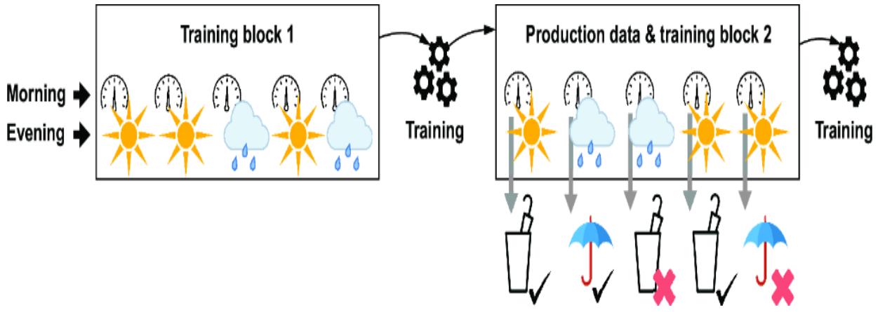
Figure 7.1 Example of a machine learning training workflow where the sensor data is the features, weather is the label, and bringing an umbrella is the decision. After each training block, the new data is used to update the old model, and a new model is deployed. In this case, the decision does not affect future data.

Now let’s consider a parallel example in business. You are a data scientist at a company. Instead of atmospheric readings, you have economic and industry data. Instead of predicting whether the day will be rainy, you are predicting whether the quarter will end with low revenues. Instead of deciding whether to bring an umbrella, you are deciding whether to advertise. Figure 7.2 illustrates the workflow, which mirrors the weather example in figure 7.1 exactly; sunny and rainy days in figure 7.1 map to good and bad quarters in figure 7.2, and the decision to bring or leave the umbrella maps to the decision to advertise or not.

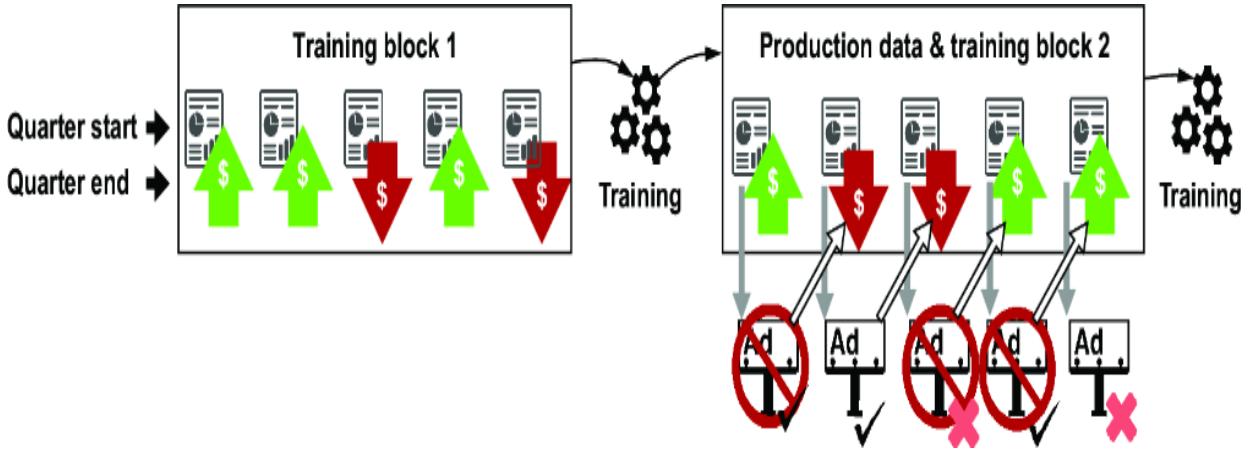
Figure 7.2 This is a mirror example of the workflow in figure 7.1. Business indicators are the features, quarterly performance is the label, and advertising is the decision. In this case, the decision affects future data.

Even though the labels and decisions in the two examples mirror one another, the causal structure of the business example is fundamentally different; the act of bringing an umbrella will not affect the weather in future days, but the act of advertising will affect business in future quarters. As a result, training block 2 represents a different DGP than training block 1 because revenue in training block 2 was affected by advertising. During training, a naive predictive model might go so far as to associate signs of a lousy quarter with high revenue, since, in the past, signs of bad quarters led your company to advertise, which consequently boosted revenue.

We deploy machine learning models to drive or automate decisions. Those decisions do not impact the data in domains like meteorology, geology, and astronomy. But in many, if not most, domains where we want to use machine learning, those model-driven decisions are interventions—actions that change the DGP. That can lead to a mismatch between the model’s training and deployment conditions, leading to problems in the model’s reliability.

Another real-world example of this problem occurs in anomaly detection.

7.1.2 Case study: Credit fraud detection

Anomaly detection seeks to predict when an abnormal event is occurring. One example is detecting a fraudulent transaction on a credit card. Credit card companies do supervised training of predictive models of fraud using transaction data, where attributes of credit card transactions (buying patterns, location, cost of the item, etc.) are the features, and whether the customer later reports the transaction as fraudulent is the label.

As in the weather and business examples, you train a model on an initial training block. After training, you can deploy the algorithm to predict fraud in real time. When a transaction is initiated, the algorithm is run, and a prediction is generated. If the algorithm predicts fraud, the transaction is rejected.

While this system is in deployment, a second training set is being compiled. Some fraud still gets through and is later reported as fraudulent by the customers. Those transactions are labeled fraudulent in this new block of data, but the DGP has changed from the initial training set. The deployed version 1.0 predictive model is rejecting transactions that it predicted were fraudulent, but because they were rejected, you don’t know if they were actual cases of fraud. These rejected transactions are excluded from the next training set because they lack labels.

If the model is retrained on the second block, it may develop a bias toward fraud that slipped past the fraud rejection system and against the cases of fraud that were rejected. This bias can become more severe over several iterations. This process is analogous to a homicide detective who, over

time, does well in solving cases involving uncommon weapons but poorly in cases involving guns.

The filtering of fraudulent transactions in deployment is an intervention. In practice, anomaly detection algorithms address this problem by accounting for interventions in some way.

7.1.3 Case study: Statistical analysis for an online role-playing game

Suppose you are a data scientist at an online role-playing game company. Your leadership wants to know if side-quest engagement (mini-objectives that are tangential to the game’s primary objectives) is a driver of in-game purchases of virtual artifacts. If the answer is yes, the company will intervene in the game dynamics such that players engage in more side-quests.

You do an analysis. You query the database and pull records for a thousand players, the first five of which are shown in table 7.1. This is observational data (in contrast to experimental data) because the data is logged observations of the natural behavior of players as they log in and play. (The full dataset is available in the notebooks for the chapter: https://www.altdeep.ai/p/causalaibook.)

Table 7.1 Example rows from observational data on Side-Quest Engagement and In-Game Purchases

User ID	Side-Quest Engagement	In-Game Purchases
71d44ad5	high	156.77
e6397485	low	34.89
87a5eaf7	high	172.86
c5d78ca4	low	215.74
d3b2a8ed	high	201.07
dc85d847	low	12.93

The standard data science analysis would involve running a statistical test of the hypothesis that there is a difference between the In-Game Purchases of players highly engaged in side-quests and those with low Side-Quest Engagement. The test calculates the mathematical difference between the sample means of In-Game Purchases for both groups. In statistical terms, this difference estimates an effect size. The test will examine whether this estimated effect size is significantly different from zero.

SETTING UP YOUR ENVIRONMENT

The code for this chapter was written with Pyro version 1.9.0, pandas version 2.2.1, and pgmpy version 0.1.25. Using Pyro’s render function to visualize a Pyro model as a DAG will require Graphviz. Visit https://www.altdeep.ai/p/causalaibookfor a link to a notebook that contains the code.

We’ll perform this hypothesis test with the pandas library. First, we’ll pull the data and get the sample means and standard deviations within each group.

Listing 7.1 Load Side-Quest Engagement vs. In-Game Purchases data and summarize

import pandas as pd
data_url = ( #1
 "https://raw.githubusercontent.com/altdeep/causalML/master/" #1
 "datasets/sidequests_and_purchases_obs.csv" #1
) #1
df = pd.read_csv(data_url) #1
summary = df.drop('User ID', axis=1).groupby( #2
 ["Side-quest Engagement"] #2
).agg( #2
 ['count', 'mean', 'std'] #2
) #2
summary

#1 Load the data from the database query into a pandas DataFrame. #2 For each level of Side-Quest Engagement (૿low, ૿high), calculate the sample count (number of players), the sample mean In-Game Purchases amount, and the standard deviation.

This produces the summary in table 7.2.

Table 7.2 Summary statistics from the online game data

Side-Quest Engagement	mean purchases	std	n
low	73.10	75.95	518
high	111.61	55.56	482

This database query pulled 1,000 players, where 482 of them were highly engaged in side-quests and 518 were not. The mean In-Game Purchases amount for highly engaged players is around $112 for high Side-Quest Engagement and $73 for low Side-Quest Engagement. Generalizing beyond this data, we conclude that players who are highly engaged in side-quests spend, on average 112 – 73 = $39 dollars more than those who aren’t. We can run a two-sample Z-test to make sure this difference is significant.

Listing 7.2 Test if effect of engagement on In-Game Purchases is statistically significant

n1, n2 = summary['In-game Purchases']['count'] #1
m1, m2 = summary['In-game Purchases']['mean'] #2
s1, s2 = summary['In-game Purchases']['std'] #3
pooled_std = (s1**2 / n1 + s2**2 / n2) **.5 #4
z_score = (m1 - m2) / pooled_std #5
abs(z_score) > 2. #6

#1 n1 and n2 are the numbers of players in each group (high vs. low engagement).

#2 m1 and m2 are the group sample means.

#3 s1 and s2 are the group standard deviations.

#4 Estimate the standard error of the difference in mean spending by pooling (combining) the group standard deviations.

#5 Convert to a z-score, which has a standard norm under the (null) hypothesis of no difference in spending across engagement levels. #6 Test if the z-score is more than 2 standard deviations from 0, which beats a 5% significance threshold.

Running this code shows that the difference in means is significant. Great, you did some data science that showed you have a statistically significant effect size: In-Game Purchases are significantly higher for players who are highly engaged in side-quests relative to those who are not. Based on your findings, leadership decides to modify the game dynamics to draw players into more side-quests. As a result, In-Game Purchases decline. How could this happen?

7.1.4 From randomized experiments to interventions

By now you’ve probably recognized that the result from listing 7.2 is a textbook example of how correlation doesn’t imply causation. If management wanted to know if intervening on game dynamics would lead to an increase in In-Game Purchases, they should have relied on analysis from a randomized experiment, not simple observational data. We’ll use the randomized experiment to build more intuition for a formal model of intervention and see how that intervention model could simulate a randomized experiment.

7.1.5 From observations to experiments

Suppose that instead of running an observational study, you run an experiment. Rather than pull data from a SQL query, you randomly select a set of 1,000 players and randomly assign them to one of two groups of 500. In one group, the game dynamics are modified such that Side-Quest Engagement is artificially fixed at ૿low, and in the other group it is fixed to ૿high. We’ll then observe their level of In-Game Purchases.

This will create experimental data that is the same size and has roughly the same split between engaged and unengaged players as the observational data in section 7.1.3. Similarly, we’ll run the same downstream analysis. This will let us make an apples-to-apples comparison of using observational versus experimental data.

Table 7.3 shows examples from the experimental data. You can find links to the data in https://www.altdeep.ai/p/causalaibook.

User ID	Side-Quest Engagement	In-Game Purchases
2828924d	low	224.39
7e7c2452	low	19.89
3ddf2915	low	221.26
10c3d883	high	93.21
c5080957	high	61.82
241c8fcf	high	188.76

Table 7.3 Example rows from the experimental data evaluating the effect of Side-Quest Engagement on In-Game Purchases

Again, we summarize the data with the following code.

Listing 7.3 Load experimental data and summarize

import pandas as pd
exp_data_url = ( #1
 "https://raw.githubusercontent.com/altdeep/causalML/master/" #1
 "datasets/sidequests_and_purchases_exp.csv" #1
) #1
df = pd.read_csv(exp_data_url) #1
summary = df.drop('User ID', axis=1).groupby( #2
 ["Side-quest Engagement"] #2
).agg( #2
 ['count', 'mean', 'std'] #2
)
print(summary)

#1 Load the experimental data from the database query into a pandas DataFrame.

#2 For each level of Side-Quest Engagement (૿low, ૿high), calculate the sample count (number of players), the sample mean in-game purchase amount, and the standard deviation.

Table 7.4 shows the same summary statistics for the experimental data as table 7.2 does for the observational data.

Table 7.4 Summary statistics from the online game experimental data

Side-Quest Engagement	mean purchases	std	n
low	92.99	51.67	500
high	131.38	94.84	500

The experiment reflects what happened when the company intervened to increase Side-Quest Engagement. The sign of the effect size is negative relative to our first analysis; we got –38.39, meaning the mean purchases went down $38.39. When we rerun the test of significance in listing 7.4, we see the difference is significant for the experimental data, just as it was for the observational data.

Listing 7.4 Conduct significance test on (experimental) difference in mean purchases

n1, n2 = summary['In-game Purchases']['count'] #1
m1, m2 = summary['In-game Purchases']['mean'] #2
s1, s2 = summary['In-game Purchases']['std'] #3
pooled_std = (s1**2 / n1 + s2**2 / n2) **.5 #4
z_score = (m1 - m2) / pooled_std #5
abs(z_score) > 2. #6

#1 n1 and n2 are the number of players in each group (high vs low engagement).

#2 m1 and m2 are the group sample means.

#3 s1 and s2 are the group standard deviations.

#4 Estimate the standard error of the difference in mean spend by pooling (combining) the group standard deviations.

#5 Convert to a z-score, which has a standard norm under the (null) hypothesis of no difference in spend across engagement levels. #6 Tests if the z-score is more than 2 standard deviations from 0, which beats a 5% significance threshold.

The result shows the difference in group means is again significant. If you had reported the results of this experiment instead of the results of the observational study, you would have correctly concluded that a policy of encouraging higher Side-Quest Engagement would lead to a drop in average In-Game Purchases (and you wouldn’t have recommended doing so).

This experiment had a cost. Many of those 1,000 players who were included in the experiment would have spent more on In-Game Purchases had they not been included in the experiment, and this is especially true for the 500 players assigned to the high side-quests group. That amounts to lost revenue that would have been realized had you not run the experiment. Moreover, the experiment created a suboptimal gaming experience for players who were assigned a level of Side-Quest Engagement that was different from their preferred level. These players are paying the company for a certain experience, and the experiment degraded that experience.

The least ideal outcome is reporting based on our simple two-sample analysis of the observational data; this had no cost, but it gave the wrong answer. A better outcome is running the experiment and getting the correct answer, though this comes at a cost. The ideal outcome is getting the right answer on the observational data for free. To do that, we need a causal model.

7.1.6 From experiments to interventions

Let’s see how we can use a causal model to simulate the results of the experiment from the observational data. First, let’s assume the causal DAG in figure 7.3.

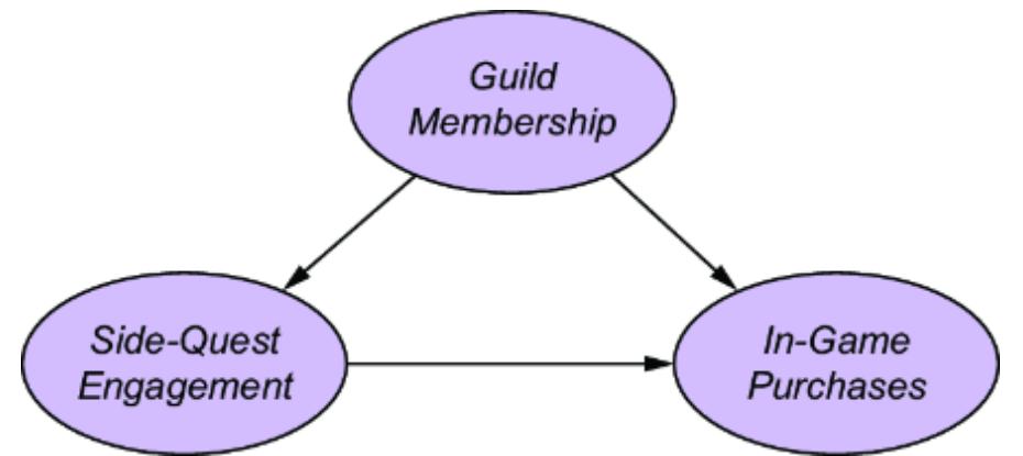
Figure 7.3 A simple DAG showing the causal relationship between Side-Quest Engagement and In-Game Purchases. Guild Membership is a common cause of both.

In our online game, many players are members of guilds. Guilds are groups of players who pool resources and coordinate their gameplay, such as working together on sidequests. Our model assumes that the amount of In-Game Purchases a player makes also depends on whether they are in a guild; members of the same guild pool resources, and many resources are virtual items they must purchase.

Suppose you run a modified version of that initial database query. The query produces the same exact observational

data seen in table 7.1, except this time it includes an additional column indicating Guild Membership. Again, we see six players in table 7.5 (the same six as players shown in table 7.1).

User ID	Side-Quest Engagement	Guild Membership	In-Game Purchases
71d44ad5	high	member	156.77
e6397485	low	nonmember	34.89
87a5eaf7	high	member	172.86
c5d78ca4	low	member	215.74
d3b2a8ed	high	member	201.07
dc85d847	low	nonmember	12.93

Table 7.5 The same observational data as in table 7.1, but with a Guild Membership column

We are going to build a causal graphical model on this observational data using Pyro. To do this, we’ll need to model the causal Markov kernels: the probability distributions of Guild Membership, Side-Quest Engagement given Guild Membership, and In-Game Purchases given Guild Membership and Side-Quest Engagement. In our Pyro model, we’ll need to specify some canonical distributions for these variables and estimate their parameters.

ESTIMATING PARAMETERS AND BUILDING THE MODEL

Pyro can jointly estimate the parameters of each of our causal Markov kernels just as it could the parameters across a complex neural network architecture. But it will make our lives easier to estimate the parameters of each kernel one at a time using everyday data science analysis, leveraging the concept of parameter modularity discussed in chapter 2. Let’s start with Guild Membership.

Listing 7.5 Estimate the probability distribution of Guild Membership

import pandas as pd
full_obs_url = ( #1
 "https://raw.githubusercontent.com/altdeep/causalML/master/" #1
 "datasets/sidequests_and_purchases_full_obs.csv" #1
) #1
df = pd.read_csv(full_obs_url) #1
membership_counts = df['Guild Membership'].value_counts() #2
dist_guild_membership = membership_counts / sum(membership_counts) #2
print(dist_guild_membership) #2

#1 Load the data from the database query into a pandas DataFrame. #2 Calculate the proportions of members vs. nonmembers.

This prints out the following result:

nonmember 0.515 member 0.485 Name: Guild Membership, dtype: float64

These are the proportions of guild members vs. nonmembers in the data. We can use these as estimates of the probability that a player is a member or a nonmember. If we took these proportions as is, they would be maximum likelihood estimates of the probabilities, but for simplicity, we’ll just put it at 50/50 (the probability of being a member is .5).

Next, we’ll do the same for the conditional probability distribution (CPD) of Side-Quest Engagement level given Guild Membership.

Listing 7.6 Estimate the CPD of Side-Quest Engagement given Guild Membership

member_subset = df[(df['Guild Membership'] == 'member')] #1
member_engagement_counts = ( #1
 member_subset['Side-quest Engagement'].value_counts() #1
) #1
dist_engagement_member = ( #1
 member_engagement_counts / sum(member_engagement_counts) #1
) #1
print(dist_engagement_member) #1
nonmember_subset = df[(df['Guild Membership'] == 'nonmember')] #2
nonmember_engagement_counts = ( #2
 nonmember_subset['Side-quest Engagement'].value_counts() #2
) #2
dist_engagement_nonmember = ( #2
 nonmember_engagement_counts / #2
sum(nonmember_engagement_counts) #2
) #2
print(dist_engagement_nonmember) #2

#1 Calculate the probability distribution of Side-Quest Engagement level (૿high vs. ૿low) given that a player is a member of a guild. #2 Calculate the probability distribution of Side-Quest Engagement level (૿high vs. ૿low) given that a player is not a member of a guild.

Listing 7.6 prints the following output proportions of Side-Quest Engagement levels for guild members:

high	0.797938
low	0.202062

The following proportions are for non-guild-members:

high 0.184466 low 0.815534

Again, we’ll round these results. Guild members have an 80% chance of being highly engaged in side-quests, while nonmembers have only a 20% chance of being highly engaged.

Finally, for each combination of Guild Membership and Side-Quest Engagement, we’ll calculate the sample mean and standard deviation of In-Game Purchases. We’ll use these sample statistics as estimates for mean and location parameters in a canonical distribution when we code the

causal Markov kernel for In-Game Purchases in the causal model.

Listing 7.7 Calculate purchase stats across levels of engagement and Guild Membership

purchase_dist_nonmember_low_engagement = df[ #1
 (df['Guild Membership'] == 'nonmember') & #1
 (df['Side-quest Engagement'] == 'low') #1
].drop( #1
 ['User ID', 'Side-quest Engagement', 'Guild Membership'], axis=1 #1 
).agg(['mean', 'std']) #1
print(round(purchase_dist_nonmember_low_engagement, 2)) #1
purchase_dist_nonmember_high_engagement = df[ #2
 (df['Guild Membership'] == 'nonmember') & #2
 (df['Side-quest Engagement'] == 'high') #2
].drop( #2
 ['User ID', 'Side-quest Engagement', 'Guild Membership'], axis=1 #2
).agg(['mean', 'std']) #2
print(round(purchase_dist_nonmember_high_engagement, 2)) #2
purchase_dist_member_low_engagement = df[ #3
 (df['Guild Membership'] == 'member') & #3
 (df['Side-quest Engagement'] == 'low') #3
].drop( #3
 ['User ID', 'Side-quest Engagement', 'Guild Membership'], axis=1 #3
).agg(['mean', 'std']) #3
print(round(purchase_dist_member_low_engagement, 2)) #3
purchase_dist_member_high_engagement = df[ #4
 (df['Guild Membership'] == 'member') & #4
 (df['Side-quest Engagement'] == 'high') #4
].drop( #4
 ['User ID', 'Side-quest Engagement', 'Guild Membership'], axis=1 #4
).agg(['mean', 'std']) #4
print(round(purchase_dist_member_high_engagement, 2)) #4

#1 Estimate the sample mean and standard deviation of In-Game Purchases for non-guild-members with low Side-Quest Engagement. #2 Estimate the sample mean and standard deviation of In-Game Purchases for non-guild-members with high Side-Quest Engagement. #3 Estimate the sample mean and standard deviation of In-Game Purchases for guild members with low Side-Quest Engagement. #4 Estimate the sample mean and standard deviation of In-Game Purchases for guild members with high Side-Quest Engagement.

For non-guild-members with low Side-Quest Engagement, we have these results:

	In-game Purchases
mean	37.95
std	23.80

For non-guild-members with high Side-Quest Engagement, we have

In-game Purchases mean 54.92 std 4.92

For guild members with low Side-Quest Engagement, we have

In-game Purchases mean 223.71 std 5.30

For guild members with high Side-Quest Engagement, we have

	In-game Purchases
mean	125.53
std	53.44

Finally, in listing 7.8, we use these various statistics as parameter estimates in a causal graphical model built in Pyro.

Listing 7.8 Building a causal model of In-Game Purchases in Pyro

import pyro
from torch import tensor
from pyro.distributions import Bernoulli, Normal
def model():
 p_member = tensor(0.5) #1
 is_guild_member = pyro.sample( #1
 "Guild Membership", #1
 Bernoulli(p_member) #1
 ) #1
 p_engaged = (tensor(0.8)*is_guild_member + #2
 tensor(.2)*(1-is_guild_member)) #2
 is_highly_engaged = pyro.sample( #2
 "Side-quest Engagement", #2
 Bernoulli(p_engaged) #2
 ) #2
 get_purchase_param = lambda param1, param2, param3, param4: ( #3
 param1 * (1-is_guild_member) * (1-is_highly_engaged) + #3
 param2 * (1-is_guild_member) * (is_highly_engaged) + #3
 param3 * (is_guild_member) * (1-is_highly_engaged) + #3
 param4 * (is_guild_member) * (is_highly_engaged) #3
 ) #3
 μ = get_purchase_param(37.95, 54.92, 223.71, 125.50) #4
 σ = get_purchase_param(23.80, 4.92, 5.30, 53.49) #4
 in_game_purchases = pyro.sample( #4
 "In-game Purchases", #4
 Normal(μ, σ) #4
 ) #4
 guild_membership = "member" if is_guild_member else "nonmember" #5
 engagement = "high" if is_highly_engaged else "low" #5
 in_game_purchases = float(in_game_purchases) #5
 return guild_membership, engagement, in_game_purchases #5

#1 Probability of being a guild member vs. a nonmember is .5. Using this probability, we generate a Guild Membership value (1 for member, 0 for nonmember) from a Bernoulli distribution.

#2 We generate a value for Side-Quest Engagement from a Bernoulli distribution (1 for high, 0 for low) with a parameter that depends on Guild Membership.

#3 Helper function for calculating parameters for In-Game Purchases #4 We specify the location parameter of a normal distribution on In-Game Purchases using the sample means we found in the observational data.

#5 As with the mean parameters, we specify the scale parameters for a canonical distribution on In-Game Purchases using the standard deviations we found in the data.

To confirm that the Pyro model encodes a causal DAG, we can run pyro.render_ model(model), which produces figure 7.4.

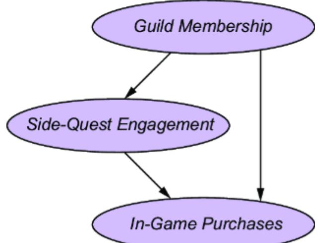
Figure 7.4 Result of calling pyro.render_model with the causal model

LEVERAGING THE PARAMETRIC FLEXIBILITY OF PROBABILISTIC PROGRAMMING

Note the flexibility of our choices for modeling the variables in the Pyro model. For example, in modeling the distribution of In-Game Purchases, we used the normal distribution, but we could have used other distributions. For example, In-Game Purchases cannot be a negative number, so we could have selected a canonical distribution that is only defined for positive numbers, rather than a normal distribution, which is defined for negative and positive numbers. This would be especially useful for nonguild-members with low Side-Quest Engagement, because generation from a normal distribution with a mean of 37.95 and a scale parameter of 23.80 will have about a 5.5% chance of generating a negative value. However, we’re choosing to be a bit lazy and use the normal distribution in this case, since a few negative numbers for In-Game Purchases won’t have much impact on the results of our analysis.

The point is that probabilistic programming tools like Pyro provide us with parametric flexibility, unlike tools like pgmpy. It is good practice to leverage that flexibility to reflect your assumptions about the DGP.

PYRO’S INTERVENTION ABSTRACTION

Pyro has an abstraction for representing an intervention in pyro.do. It takes a model and returns a new model that reflects the intervention. Listing 7.9 shows how we can use pyro.do to change the previous model into one that reflects an intervention that sets Side-Quest Engagement to ૿high and to ૿low.

Listing 7.9 Representing interventions with pyro.do

int_engaged_model = pyro.do( #1
 model, #1
 {"Side-quest Engagement": tensor(1.)} #1
) #1
int_unengaged_model = pyro.do( #2
 model, #2
 {"Side-quest Engagement": tensor(0.)} #2
) #2

#1 An intervention that sets Side-Quest Engagement to 1.0 (i.e., ૿high). This returns a new model. #2 An intervention that sets Side-Quest Engagement to 0.0 (i.e., ૿low). This returns a new model.

Now we have two new models: one with an intervention that sets Side-Quest Engagement to ૿high and one that sets it to ૿low. If our original model is correct, generating 500 examples from each of these new intervened-upon models, and combining them into 1000 examples, effectively simulates the experiment. Remember, we estimated the parameters of this causal model using only the observational data illustrated in table 7.4. If we can train a model on observational data and use it to accurately simulate the results of an experiment, that saves us from actually having to run the experiment.

Listing 7.10 uses int_engaged_model and int_unengaged_model to simulate experimental data. We can confirm that the simulation was effective by comparing the summary statistics of this simulated data to the summary statistics of the actual experimental data.

Listing 7.10 Simulating experimental data with pyro.do interventions

pyro.util.set_rng_seed(123) #1
simulated_experimental_data = [ #2
 int_engaged_model() for _ in range(500) #2
] + [ #2
 int_unengaged_model() for _ in range(500) #2
] #2
simulated_experimental_data = pd.DataFrame( #2
 simulated_experimental_data, #2
 columns=[ #2
 "Guild Membership", #2
 "Side-quest Engagement", #2
 "In-Game Purchases" #2
 ] #2
) #2
sim_exp_df = simulated_experimental_data.drop( #3
 "Guild Membership", axis=1) #3
summary = sim_exp_df.groupby( #4
 ["Side-quest Engagement"] #4
 ).agg( #4
 ['count', 'mean', 'std'] #4
 ) #4
print(summary) #4

#1 Set a random seed for reproducibility.

#2 Simulate 500 rows from each intervention model, and combine them to create simulated experimental data.

#3 The simulated data will include a Guild Membership column. We can drop it to get simulated data that looks like the original experiment. #4 Recreate the statistical summaries of In-Game Purchases for each level of engagement.

This code simulates the experiment, providing the summaries in table 7.6. Again, these are sample statistics from a simulated experiment we created by first estimating some parameters on observational data, second, building a causal generative model with those parameters, and third, using pyro.do to simulate the results of an intervention. Contrast these with the statistics in table 7.7 that we obtained from the actual experimental data.

Table 7.6 Summary statistics from the simulated experiment

Side-Quest Engagement	count	mean	std
high	500	89.897309	52.696709
low	500	130.674021	93.921543

Table 7.7 Summary statistics from the actual experiment

Side-Quest Engagement	count	mean	std
high	500	92.99054	51.673631
low	500	131.38228	94.840705

The two sets of summaries are similar enough that we can say that we’ve successfully replicated the experimental results from the observational data.

7.1.7 Recap

Let’s recap. A causal DAG combined with a Pyro abstraction for an intervention allowed us to do an analysis on an observational dataset that produced the same results as an analysis on an experimental dataset. Had you run this analysis on the initial observational data instead of the simple two-sample statistical test, you would have provided the correct answer to leadership, and they would not have changed the dynamics to increase Side-Quest Engagement.

Note that this wasn’t a free lunch. This analysis required causal assumptions in the form of a causal DAG. Errors in specifying the causal DAG can lead to errors in the output of the analysis. But assuming your causal DAG was correct (or close enough), it would have saved you the actual costs and opportunity costs of running that experiment.

So how exactly does pyro.do work? How does it modify the model to represent an intervention? We’ll answer these questions with the ideas of ideal interventions and intervention operators.

7.2 The ideal intervention and intervention operator

To understand how our simulated experiment worked, we need a concrete definition of intervention. We’ll use a specific definition, called the ideal intervention, and also known as the atomic intervention, structural intervention, surgical intervention, and independent intervention.

The definition of an ideal intervention breaks down into three parts:

• The ideal intervention targets a specific variable or set of variables in the DGP.
• The operation sets those variables to a fixed value.
• By setting the variable to a fixed value, the intervention blocks the influence from the target’s causes, such that the target is now statistically independent of its causes.

We’ll use the notation do(X = x) to represent an ideal intervention that sets X to x. Note that we can have interventions on sets of variables, as in do(X = x, Y = y, Z = z).

7.2.1 Intervention operators

A causal model represents relationships in the DGP. The preceding definition of the ideal intervention describes how it changes the DGP. Now it remains to us to define how our causal models will reflect that change.

An intervention operator is some way of changing our causal model to reflect an intervention. One of the first tasks of creating any novel computational representation of causality is to define an intervention operator for the ideal intervention.

Intervention operators can implement ideal interventions, stochastic interventions (discussed in section 7.5), and other types of interventions. Unless I indicate otherwise, you can assume that ૿intervention operator means ૿intervention operator for ideal interventions.

Fortunately, structural causal models and general causal graphical models have well-defined intervention operators. We’ll explore those, as well as look at intervention operators designed for causal programs like pyro.do.

7.2.2 Ideal interventions in structural causal models

We’ll start with the structural causal model. Let M represent a structural causal model of the online game. We’d write M as follows:

\[M = \{ n\_G \sim P(N\_G); n\_E \sim P(N\_E); n\_I \sim P(N\_I);\]

\[\mathbf{g} := f\_\mathbf{G}(n\_\mathbf{g}); \mathbf{e} := f\_\mathbf{E}(\mathbf{g}, n\_\mathbf{e}); i := f\_\mathbf{I}(\mathbf{g}, \mathbf{e}, n\_i) \}\]

fG, fE, and fI are the assignment functions for G (Guild Membership), E (Side-Quest Engagement ), and I (In-Game Purchases ), respectively.

An ideal intervention do(E=૿high) transforms the model as follows:

\[M^{\text{do}(E:="\text{high}")} = \{ n\_G \sim P(N\_G); n\_E \sim P(N\_E); n\_I \sim P(N\_I); \}\]

\[\text{g} := f\_\mathcal{G}(n\_\mathcal{g}); e := \text{"high"}; i := f\_\mathcal{I}(\mathcal{g}, e, n\_i) \}\]

The intervention operator for the SCM replaces the intervention target E’s assignment function with the intervention value ૿high.

Suppose you have an SCM with a variable (or set of variables) X. You want to apply an intervention do(X = x). The intervention operator replaces the intervention target’s assignment function with the intervention value.

Consider how this meets the three elements of our definition of an ideal intervention:

• The intervention do(X = x) only directly affects the assignment function for X. No other assignment function is affected.
• The intervention explicitly sets X to a specific value.
• Since the value of X is set to a constant, it no longer depends on its direct causal parents.

7.2.3 Graph surgery: The ideal intervention in causal DAGs and causal graphical models

Now we’ll consider how to think graphically about the ideal intervention. First, let’s reexamine the online game’s causal DAG in figure 7.5.

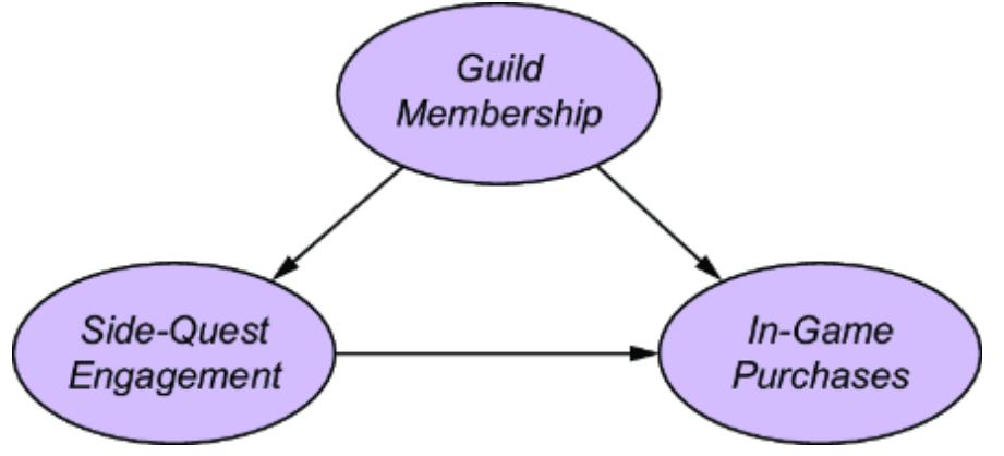
Figure 7.5 The causal DAG for the online game

According to our graph, Guild Membership is the causal parent of Side-Quest Engagement. That parent-child relationship determines a causal Markov kernel—the conditional probability distribution of Side-Quest Engagement, given Guild Membership. Recall our model of this causal Markov kernel, shown in table 7.8.

Table 7.8 Conditional probability table for causal Markov kernel of Side-Quest Engagement

		Guild Membership
		nonmember	member
	low	.8	.2
Side-Quest Engagement	high	.2	.8

Imagine the mechanics of our experiment. Players log on, and the digital experimentation platform selects some players for participation in the experiment. Some of those players are guild members, and some are not.

Consider a player named Jojo, who is not a guild member, who is logging on. Given this information only, he will have a 20% chance of engaging highly in side-quests during this session of gameplay, according to our model.

But the experimentation platform selects him for the experiment. It randomly assigns him to the high Side-Quest Engagement group. Once he is in that group, what is the probability that Jojo will engage highly in side-quests? The answer is 100%. In experimental terms, what is the probability that someone assigned to the treatment group will be exposed to the treatment? 100%. For data scientists familiar with the jargon of A/B testing, what is the probability that someone assigned to group A will be exposed to variant A? 100%.

Indeed, supposing instead of Jojo, the subject was Ngozi, who is a guild member. While originally Ngozi had an 80% chance of being highly engaged in side-quests, upon being assigned to the high Side-Quest Engagement group in the experiment, she changes to having a 100% chance of being highly engaged.

We need to rewrite our conditional probability distribution of Side-Quest Engagement to reflect these new probabilities, as in table 7.9.

Table 7.9 Rewriting the conditional probability table of Side-Quest Engagement to reflect the certainty of engagement level upon being assigned to the high-engagement group in the experiment

		Guild Membership
		nonmember	member
Side-Quest Engagement	low	0.0	0.0
	high	1.0	1.0

Now we see that this modified distribution of Side-Quest Engagement is the same regardless of Guild Membership. That is the definition of probabilistic independence, so we should simplify this conditional probability table to reflect that; we can reduce table 7.9 to table 7.10.

Table 7.10 Rewriting the conditional probability table of Side-Quest Engagement to reflect the fact that engagement level no longer depends on Guild Membership

Side-Quest Engagement	low	0.0
	high	1.0

When we simplify the distribution in this way, we have to recall that this is a model of a causal Markov kernel, which is defined by the graph. Our initial graph says Side-Quest Engagement is caused by Guild Membership. But it seems

that after the experiment randomly allocates players either to the high engagement or low engagement group, that causal dependency is broken; a player’s engagement level is solely determined by the group they are assigned to.

We need an intervention operator that changes our causal graph to reflect this broken causal dependency. This intervention operator is called graph surgery (also known as graph mutlitation), and it’s illustrated in figure 7.6.

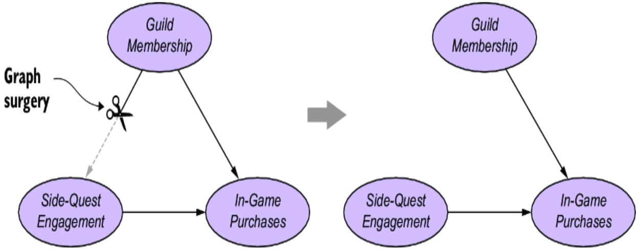
Figure 7.6 Graph surgery removes an incoming edge to the intervention target Side-Quest Engagement.

While Guild Membership is a cause of Side-Quest Engagement in normal settings, the experiment’s intervention on Side-Quest Engagement broke that variable’s causal dependence on Guild Membership. Since that causal dependence is gone, graph surgery changes the graph to one where the edge from Guild Membership to Side-Quest Engagement is snipped.

In general, suppose you have a causal graph with node X. You want to apply an intervention do(X = x). Then you represent that intervention on the causal DAG by ૿surgery removing all incoming edges to X. Graph surgery is available in libraries such as pgmpy. For example, here is how we

would use pgmpy to apply graph surgery to the online gaming DAG.

Listing 7.11 Graph surgery on a DAG in pgmpy
from pgmpy.base import DAG
G = DAG([ #1
 ('Guild Membership', 'Side-quest Engagement'), #1
 ('Side-quest Engagement', 'In-game Purchases'), #1
 ('Guild Membership', 'In-game Purchases') #1
]) #1
G_int = G.do('Side-quest Engagement') #2

#1 Build the causal DAG. #2 The do method in the DAG class applies graph surgery.

We can now plot both the original DAG and the transformed DAG and compare them.

Listing 7.12 Plot the transformed DAG
import pylab as plt
import networkx as nx
pos = { #1
 'Guild Membership': [0.0, 1.0], #1
 'Side-quest Engagement': [-1.0, 0.0], #1
 'In-game Purchases': [1.0, -0.5] #1
} #1
ax = plt.subplot() #2
ax.margins(0.3) #2
nx.draw(G, ax=ax, pos=pos, node_size=3000, #2
 node_color='w', with_labels=True) #2
plt.show() #2
ax = plt.subplot() #3
ax.margins(0.3) #3
nx.draw(G_int, ax=ax, pos=pos, #3
 node_size=3000, node_color='w', with_labels=True) #3
plt.show() #3

#1 Create a dictionary of node positions that we can use to visualize both graphs. #2 Visualize the original graph. #3 Visualize the transformed graph.

These visualizations produce the same DAG as in figure 7.6.

Next, we’ll look at the effect of graph surgery on dseparation and its implications for conditional independence.

7.2.4 Graph surgery and d-separation

Consider how graph surgery affects reasoning with dseparation, as in figure 7.7. Initially, we have two dconnecting paths between Side-Quest Engagement and In-Game Purchases: one path was the direct cause path, and the other was through the common cause of Guild Membership. After graph surgery, only the direct causal path remains.

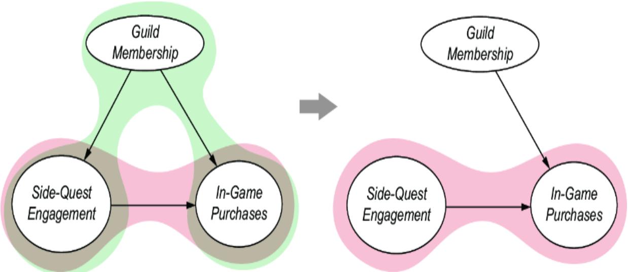
Figure 7.7 In the original DAG on the left, there are two d-connected paths between Side-Quest Engagement and In-Game Purchases. These paths equate to two sources of statistical dependence between the two variables. After graph surgery, only the causal path remains, reflecting causal dependence.

Recall that each d-connected path between two variables is a source of statistical dependence between those variables. When we represent an intervention with graph surgery that removes incoming edges to the intervention target(s), we remove any paths to other nodes that go through that variable’s causes. Only outgoing paths to other nodes remain. As a result, the remaining paths from that variable reflect dependence due to that variable’s causal influence on other variables. The ideal intervention removes the causal influence the target variable receives from its direct parents.

Thus, it removes any dependence on other variables that flows through those parents.

7.2.5 Ideal interventions and causal Markov kernels

Graph surgery on the causal DAG removes the incoming edges to the target node(s). However, for a causal graphical model, we need an intervention operator that changes the graph and goes one step farther to rewrite the causal Markov kernel of the intervention target, as we did when we collapsed table 7.9 into table 7.10.

Initially, our online gaming model has causal Markov kernels {P (G ), P (E |G ), and P (I |E, G )}. In table 7.9 we saw the conditional probability table representation of P (E |G ) and how an intervention reduced it to table 7.10, where 100% of the probability is placed on the outcome ૿high.

Generally, the intervention operator for causal graphical models replaces the causal Markov kernel(s) of the intervention target(s) with a degenerate distribution, meaning a distribution that puts 100% of the probability on one value, namely the intervention value.

When we combine graph surgery with this replacement of the target node’s causal Markov kernel with a degenerate distribution, we have an intervention operator on a causal graphical model that meets the three elements of the definition of ideal intervention:

• You only remove incoming edges for the nodes targeted by the intervention.
• 100% of the probability is assigned to a fixed value.
• Removing the incoming edges to the intervention target means that the variable is no longer causally dependent

on its parents.

In listing 7.11, graph surgery is implemented in the do method in the DAG class. The BayesianNetwork class, our default for building causal graphical models, also has a do method. Like the DAG method, it takes an intervention target. At the time of writing, the method does not take an intervention value and thus does not satisfy the second element of the definition of ideal intervention.

pgmpy uses objects from subclasses of the BaseFactor class (e.g., the TabularCPD class) to represent causal Markov kernels. The do method in the BayesianNetwork class first does graph surgery and then replaces the factor object representing the intervention target’s causal Markov kernel. However, that replacement factor object is not degenerate; it does not assign all the probability value to one outcome. Rather, it returns an object representing the probability distribution of the target variable after marginalizing over its parents in the original unmodified graph. Technically, this is an intervention operator for a stochastic intervention, which I’ll discuss in section 7.5. To build an intervention operator for the ideal intervention, you need to write additional code to modify the factor to assign all probability to the intervention value.

7.2.6 Ideal interventions in a causal program

Recall that in listing 7.10 we simulated an experiment where players were assigned to high-engagement and lowengagement groups using the pyro.do operator. Specifically, we called pyro.do as in following listing.

Listing 7.13 Revisiting pyro.do

int_engaged_model = pyro.do( #1
 model, #1
 {"Side-quest Engagement": tensor(1.)} #1
) #1
int_unengaged_model = pyro.do( #2
 model, #2
 {"Side-quest Engagement": tensor(0.)} #2
) #2

#1 An intervention that sets Side-Quest Engagement to 1.0 (i.e., ૿high). This returns a new model. #2 An intervention that sets Side-Quest Engagement to 0.0 (i.e., ૿low). This returns a new model.

What exactly does pyro.do do? pyro.do is Pyro’s intervention operator. We saw, by using pyro.render_model to generate figure 7.4, that our online gaming model in Pyro has an underlying causal DAG, and therefore is a causal graphical model.

But a deep probabilistic machine learning framework like Pyro allows you to do things that we can’t easily represent with a causal DAG, such as recursion, conditional control flow, or having a random number of variables not realized until runtime. As an intervention operator, pyro.do must work in these cases as well.

The intervention operator in Pyro works by finding calls to pyro.sample, and replacing those calls with an assignment to the intervention value. For example, the online game model had the following line:

is_highly_engaged = pyro.sample("Side-quest Engagement", Bernoulli(p_engaged))

This pyro.sample call generates a value for Side-Quest Engagement. pyro.do(model, {“Side-quest Engagement”: tensor(1.)}) essentially replaces that line with this:

is_highly_engaged = tensor(1.)

(I say ૿essentially because pyro.do does a few other things too, which I’ll discuss in chapter 10).

This replacement is much like the replacement of the assignment function in the SCM, or a causal Markov kernel with a degenerate kernel in a causal graphical model. As an intervention operator, it meets the criteria for an ideal intervention. It targets a specific variable, and it assigns it a specific value. It eliminates its dependence on its causes by removing flow dependence (dependence on results of executing preceding statements in the program).

Using a flexible deep probabilistic machine learning tool like Pyro to build a causal model allows you to construct causal representations beyond DAGs and simple ideal interventions. Doing so puts you in underdeveloped territory in terms of theoretical grounding, but it could lead to interesting new applications.

In the next section, we’ll consider how interventions affect probability distributions.

7.3 Intervention variables and distributions

An ideal intervention fixes the random variable it targets, essentially turning it into a constant. But the intervention indirectly affects all the random variables causally downstream of the target variable. As a result, their probability distributions (joint, conditional, or marginal) change from what they were.

7.3.1 ૿Do and counterfactual notation

Causal modeling uses special notation to help reason about how interventions affect random variables and their

distributions. One common approach is to use the “do” notation. Using our online game as an example, P(I) is the probability distribution of In-Game Purchases across all players, P(I|E=૿high) is the probability distribution of In-Game Purchases given players with ૿high engagement, and P(I|do(E= ૿high)) is the probability distribution of In-Game Purchases given an intervention that sets a player’s engagement level to ૿high. The second column of table 7.11 illustrates extensions of this notation to joint distributions, multiple interventions, and mixing interventions with observations.

Literal	Do-notation	Counterfactual notation
The probability distribution of In Game Purchases across all players	P(I )	P(I )
The probability distribution of In Game Purchases for players with ૿high଀ engagement	P(I E=૿high଀)	P(I E=૿high଀)
The probability distribution of In Game Purchases when a player’s engagement level is set (by intervention) to ૿high଀	P(I do(E= ૿high଀))	P(I E= ૿high଀)
The joint probability distribution of In-Game Purchases and Guild Membership when engagement is set to ૿high଀	P(I, G do(E=૿high଀))	P(I E=૿high଀, GE=૿high଀)
The probability distribution of In Game Purchases when engagement is set to ૿high଀ and membership is set to ૿nonmember଀	P(I do(E =૿high଀, G=૿nonmember଀))	P(I E= ૿high଀, G=૿nonmember଀)
The probability distribution of In Game Purchases for guild members when engagement is set to ૿high଀	P(I do(E =૿high଀), G = ૿member଀)	P(IE =૿high଀ G = ૿member଀)

Table 7.11 Examples of do-notation and counterfactual notation

An alternative is to use counterfactual notation, which uses subscripts to represent a new version of a variable after the system has been exposed to intervention. For example, if I is a variable that represents In-Game Purchases, IE=૿high represents In-Game Purchases under an intervention that sets Side-Quest Engagement to ૿high. If P(I  ) is the probability distribution of In-Game Purchases, then P(IE=૿high) is the probability distribution. Again, table 7.11 contrasts do-notation with counterfactual notation in the third column. Going forward, I’ll mostly use counterfactual notation.

FROM CAUSAL LANGUAGE TO SYMBOLS

In many cases in statistics and machine learning, notation only serves to add formalism and rigor to something just as easily explained in plain language. However, notation is important in causality, because it makes a clear distinction between when we are talking about something causal and when we are not. It is important because making the distinction is harder in plain English. For example, consider the following two questions:

૿What would In-Game Purchases be for a player who was highly engaged in side-quests?

૿What would In-Game Purchases be if a player was highly engaged in side-quests?

Is it obvious to you that the first question corresponds to P(I|E=૿high) and the second to P(IE=૿high)? The first question corresponds to a subset of players who are highly engaged. The traditional conditional probability notation is fine when we want to zoom in on a subset of a distribution or population. The second question asks what if someone were highly engaged. In the next chapter, we’ll see that ૿what if hypothetical questions imply an intervention. But because of the ambiguity of language, someone could ask one question while really meaning the other. The notation gives us an unambiguous way of constructing our causal queries.

Again, in chapter 8, we’ll investigate more examples of mapping language to counterfactual notation.

7.3.2 When causal notation reduces to traditional notation

It is crucial to recognize when a variable and that same variable under intervention are the same. Consider the intervention on engagement, as in figure 7.8.

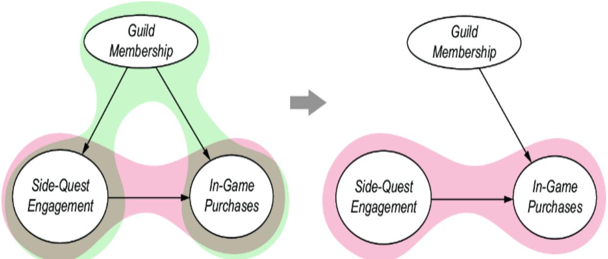
Figure 7.8 In the original DAG (left), there are two d-connected paths between Side-Quest Engagement and In-Game Purchases. These paths equate to two sources of statistical dependence between the two variables. After graph surgery, only the causal path remains, reflecting causal dependence.

Is P (G |E=૿high) (the probability distribution of Guild Membership given high Side-Quest Engagement) the same as P(G)? No. In graphical terms, G and E are d-connected. In probabilistic terms, we can reason that knowing a player’s level of Side-Quest Engagement is predictive of whether they are in a guild.

But is P (GE=૿high) the same as P(G )? Yes. Guild Membership is not affected by the intervention on Side-Quest Engagement because it can only affect variables causally downstream of Side-Quest Engagement. Thus P (GE=૿high) is equivalent to P(G).

In general terms, empirically learning a distribution for a variable YX ^{= x} requires doing the intervention do(X = x) in real life. However, that real-life intervention, at best, has a cost and, at worst, is infeasible or impossible. So if we can equate YX ^{= x} to some distribution involving Y that we can learn from observational data, that’s a win. That’s going from correlation to causation. In trivial cases, we can do this by looking at the graph, as we did with G and GE=૿high. But usually, we’ll need to do some mathematical derivation, either by hand or using algorithms.

This task of deriving equality between variables that are and aren’t subject to intervention is called identification, and it is the heart of causal inference theory. We’ll examine identification at length in chapter 10.

7.3.3 Causal models represent all intervention distributions

As generative models, the causal models we’ve worked with encode a joint probability distribution of components of the DGP. Inference algorithms enable those models to represent (e.g., through Monte Carlo sampling) the conditional distribution of some subset of those components, given the state of the other components.

We’ve now introduced the ideal intervention and how it changes the DGP and, consequently, the joint probability distribution of the variables. Figure 7.9 illustrates how the generative causal model captures the original DGP (and corresponding probability distributions) and any new DGP (and corresponding probability distributions) created by intervening in the original process.

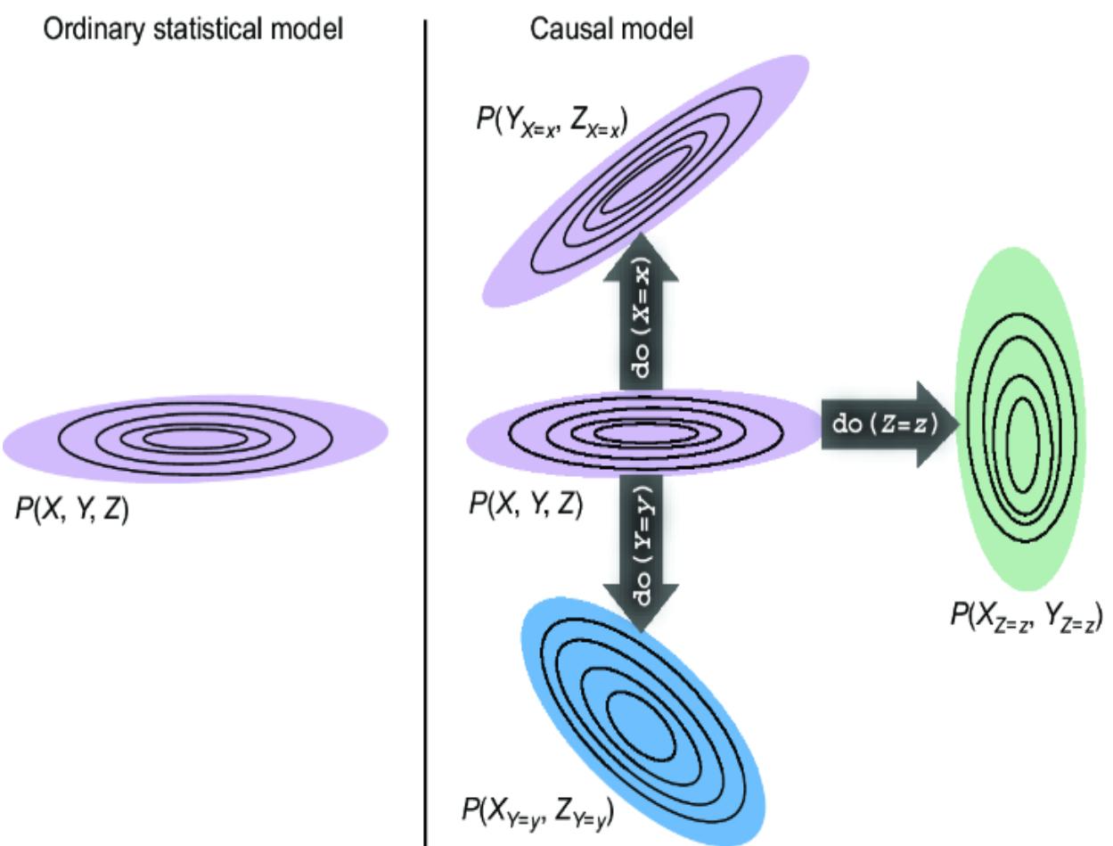
Figure 7.9 Suppose our DGP has variables X, Y, and Z. A traditional generative model (left) uses observations of X, Y, and Z to statistically learn a representation of P(X, Y, Z). A generative causal model (right) encodes a representation P(X, Y, Z) and distributions derived by interventions on X, Y, and Z. In that way, the generative causal model represents a broad family of distributions.

Consider the statistical implications of this idea. Given data, an ordinary generative model learns a representation of the joint probability distribution. But a generative causal model learns not only that distribution but any new distribution that would be derived by applying some set of ideal interventions. That’s how our causal model of the online game was able to reproduce the outcome of an experiment from observational data alone.

7.4 Interventions and causal effects

The most common use case for our formal model of an intervention will be to model causal effects. Now that we’ve defined and formalized interventions, causal effects are easy to think about; they are simply comparisons between the outcomes of interventions.

7.4.1 Average treatment effects with binary causes

The most common causal effect query is the average treatment effect (ATE). Here, we’ll focus on the case where we are interested in the causal effect of X on Y, and X is binary, meaning it has two outcomes: 1 and 0. Binary causes entail experiments where the cause has a ૿treatment value and a ૿control value, such as ૿A/B tests. Using do-notation, the ATE is E (Y  |do(X = 1)) – E (Y  |do(X = 0)) (recall E (…) means ૿the expectation of …). Using counterfactual notation, the ATE is E (YX ⁼ 1) – E (YX ⁼ 0). The advantage of the counterfactual notation is that we can collapse this into one expectation term, E(YX=1 – YX=0).

7.4.2 Average treatment effect with categorical causes

When the cause is categorical, the ATE requires choosing which levels of the cause you want to compare. For example, if X has possible outcomes {a, b, c}, you might select ૿a to be a baseline, and work with two ATEs, E (YX ^{= b} – YX ^{= a}) and E (YX ^{= c} – YX ^{= a}). Alternatively, you may choose to work with all pairwise comparisons of levels of X, or just convert X to a binary variable with outcomes ૿a and ૿not a The choice depends on which ATE is most meaningful to you.

7.4.3 Average treatment effect for continuous causes

If we want to generalize E (YX ⁼ 1 – YX ⁼ 0) to the case where X is continuous, we arrive at derivative calculus. For some baseline do(X = x), imagine changing the intervention value x by some small amount Δ, i.e., do(X = x + Δ). Taking the difference between the two outcomes, we get E (YX ^{= x +} Δ – YX ^{= x}). Then we can ask, what is the rate of change of E(YX) as we make Δ infinitesimally smaller. This brings us to the definition of the derivative:

\[\lim\_{\Delta \to 0} \frac{E(Y\_{X=x+\Delta}) - E(Y\_{X=x})}{\Delta} = d \frac{E(Y\_{X=x})}{dx}\]

Note that this is a function, rather than a point value; when you plug in a value of x, you get the rate of change of YX ^{= x} of the X versus Yx curve.

As a practical example, consider the case of pharmacology, where we want to establish the ATE of a drug dose on a health outcome. The drug dose is continuous, and it usually follows a nonlinear S-curve-like shape; we get more effect as we increase the dose, but eventually the effect gets diminishing returns at higher doses. The derivative gives us the rate of change of the average response for a given dose on the dose-response curve.

7.4.4 Conditional average treatment effect

The conditional average treatment effect (CATE) is an ATE conditioned on other covariates. For example, in our online game example, E(IE=૿high – IE=૿low) is the ATE on In-Game Purchases for Side-Quest Engagement. If we wished to

understand the ATE for guild members, we’d want E(IE=૿high – IE=૿low| G=૿member).

In practical settings, it is often important to work with CATEs instead of ATEs, because CATEs can have big differences with ATEs and other CATEs with different conditions. In other words, CATEs better reflect the heterogeneity of treatment effects across a population. For example, it is possible that the ATE of a drug on a health outcome is positive across the overall population, but the CATE conditioned on a specific subpopulation (e.g., people with a certain allergy) could be negative. Similarly, in advertising, certain ad copy might drive your customers to purchase more on average, but cause some segment of your customers to purchase less. You can optimize the return on investment for your ad campaign by understanding the CATEs for each segment, or to use CATE-based reasoning to do customer segmentation.

Experts often emphasize the importance of measuring heterogenous treatment effects with CATEs, lest one think a point value estimate of an ATE tells the full picture. But in our probabilistic modeling approach, heterogeneity is front and center. If we have a causal graphical model and a model of ideal intervention, then we can model P (YX ^{= x}). If we can model P (YX ^{= x}), then we can model P (YX ⁼ 1 – YX ⁼ 0). We can then use that model to inspect all the variation within P (YX ⁼ 1 – YX ⁼ 0), including who in the target population falls above or below 0 or some other threshold.

7.4.5 Statistical measures of association and causality

In statistics, an effect size is a value that measures the strength or intensity of the relationship between two variables or groups. For example, in our observational

analysis of the online gaming data, we quantified the relationship between Side-Quest Engagement E and In-Game Purchases I as E (I  |E =૿high) – E (I  |E =૿low). Our statistical procedure estimated this true effect size with a difference in sample averages between both groups. We then conducted a hypothesis test. We specified a null hypothesis E (I  |E =૿high) – E (I  |E =૿low) = 0, and then tested if this effect size estimate was statistically different from 0 using a pvalue calculated under some null hypothesis distribution (usually a normal or t-distribution).

A causal effect is just an interventional effect size; in our example, it was E (I  |do(E =૿high)) – E(I  |do(E =૿low)) = E (IE ⁼ ૿high – IE ⁼ ૿low), which is the ATE. The statistical hypothesis testing procedure is the same as before. Indeed, we still need to test if sample-based estimates of ATEs and CATEs are statistically significant. When you conduct a statistical significance test with data from an experiment with a treatment and control, you are testing an estimate of the ATE by definition.

7.4.6 Causality and regression models

Suppose X is continuous, but its relationship with YX is linear. Then the ATE d E (YX=x)/dx is a point value because the derivative of a linear function is a constant. Therefore, if you use a linear model of E (YX), then the coefficient for X in that model corresponds to the ATE for X.

\[\text{If } E(Y\_X) = \beta\_0 + \beta \times X, \text{ then } \text{ATE } = \beta\_0\]

For this reason, linear regression modeling is a popular approach to modeling causal effects (even when people don’t really believe the causal relationship is linear).

This convenience extends to other generalized linear models. Suppose Poisson regression or logistic regression are better models of E (YX) than linear regression. These models capture measures of association between two variables not as a difference in means, but as ratios. For example, we can read relative risk (RR) directly from a Poisson regression model and odds ratios (OR) directly from a logistic regression model. In general, these measures of association have no causal interpretation, but we give them a causal interpretation once we use them with interventional variables. For example, if we are modeling E (YX), and YX is binary, the relative risk and odds ratios are as follows:

\[RR = \frac{P(Y\_{X=1} = 1)}{P(Y\_{X=0} = 1)} = \frac{E(Y\_{X=1})}{E(Y\_{X=0})}\]

\[OR = \frac{\frac{E(Y\_{X=1})}{1 - E(Y\_{X=1})}}{\frac{E(Y\_{X=0})}{1 - E(Y\_{X=0})}}\]

Thus, traditional non-causal ways of quantifying statistical association become measures of causal association once we use them in an interventional context. And when we fit these regression models to data, we can still use all the traditional regression methods for significance testing (Wald tests, Ftests, likelihood ratio tests, etc.).

7.5 Stochastic interventions

Stochastic interventions are an important generalization of ideal interventions. The second rule of the ideal intervention is that the intervention is set to a fixed value. In the stochastic intervention, that value is the outcome of a random process; i.e., it is itself a random variable. Most texts treat stochastic interventions as an advanced topic beyond

the scope of an introduction to causal modeling, but I make special mention of them as they are important in machine learning, where we often seek data-driven automation. Stochastic interventions are important for automatic selection of interventions.

7.5.1 Random assignment in an experiment is a stochastic intervention

For example, the digital experimentation platform in our online gaming experiment automatically assigned players to high- and low-engagement groups. It did so randomly. Random assignment is a stochastic intervention; it targets the Side-Quest Engagement variable and sets its value by digitally flipping a coin.

Note that randomization is more than what we need to arrive at the right answer. Indeed, in our simulation of the experiment, there was no randomization, only ideal interventions. Those ideal interventions were sufficient to dseparate the path Side-Quest Engagement ← Guild Membership → In-Game Purchases, removing the statistical dependence that comes from that path. If randomization is not necessary to quantify the causal relationship, why is it called ૿the gold standard of causal inference? The answer is that randomization works when your causal DAG is wrong.

For example, suppose that when we did the experiment, rather than randomizing players into the high versus low Side-Quest Engagement group, the digital experimentation platform automatically assigned the first 500 players who logged on to the group with high Side-Quest Engagement and the next 500 players to the group with low Side-Quest Engagement. This intervention would be sufficient to dseparate the path Side-Quest Engagement ← Guild Membership → In-Game Purchases. But what if our DAG was wrong, and there are other paths between Side-Quest Engagement and In-Game Purchases through unknown common causes?

Figure 7.10 considers what happens when our DAG is wrong —our model is the DAG on the right. Consider what would happen if, instead, the true DAG were the DAG on the left. For the DAG on the left, the time of day when the player logs on drives both the Side-Quest Engagement and In-Game Purchases.

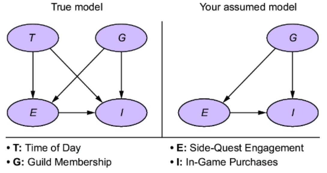
Figure 7.10 Left: the true causal relationships. Right: your (incorrect) causal DAG.

Suppose, for example, people who log on earlier tend not to be logging on with friends. They tend to engage more in side-quests because side-quests are amenable to solo gameplay. People who plan missions with friends tend to log on later, since some friends have real-world appointments during the day. Friends playing together focus more on the game’s primary narrative and avoid side-quests. Also, players tend to spend more money on In-Game Purchases later in the day, corresponding to the broader trend of lateday spending in e-commerce.

When we intervene on a player to assign them to one group or another based on their login, that intervention value now depends on the time of day, as shown in figure 7.11.

The left side of figure 7.11 illustrates the result of an intervention on Side-Quest Engagement that depends on the time of day. As we expected, the intervention performs graph surgery, removing the incoming edges to Side-Quest Engagement E: T→E and G →E. However, the value set by the intervention is now determined by time of day T, via a time_select function. The time_select function assigns ૿high engagement to every player whose login time is before that of the 501st player to log on and ૿low for those who logged in after. After graph surgery, we add back a new causal edge T→E whose mechanism is time_select. Thus, there is still a noncausal statistical association that biases the experiment via the d-connected path I ←T→E.

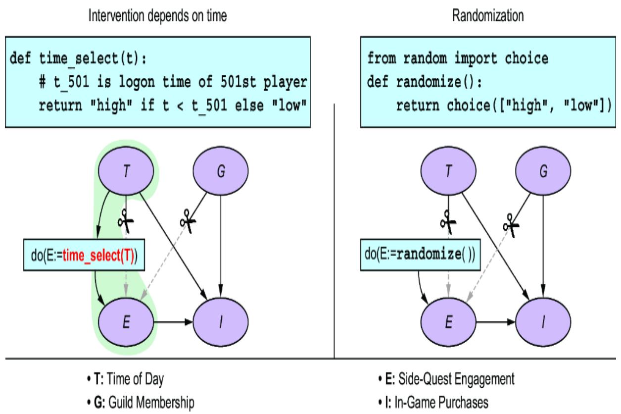
In contrast, randomization on the right side of figure 7.11 did what we hoped, removing all the incoming edges to E. It removed the edge from T→E even though our assumed DAG did not know that T→E existed. Indeed, if there are other unknown common causes between E and I, randomization will remove those incoming edges to E, as in figure 7.12.

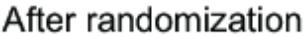
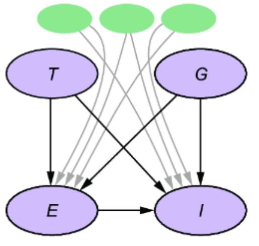
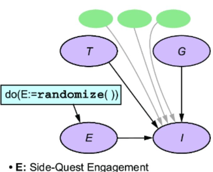
Figure 7.12 Randomization eliminates incoming edges from unknown common causes.

The ability of randomization to eliminate statistical bias from common causes we failed to account for in our assumptions is why it is considered ૿the gold standard of causal inference. But to understand stochastic interventions, note that both assignment mechanisms: one based on login time and the other using randomization, are stochastic interventions. Both set the Side-Quest Engagement level of a player using a random process; one depends on when someone logs in, and the other depends on a coin flip.

7.5.2 Intervention policies

Stochastic interventions are closely related to policies in automated decision-making domains, such as bandit algorithms and reinforcement learning. In these domains, an agent (e.g., a robot, a recommender algorithm) operates in some environment. A policy is an algorithm that takes as input the state of some variables in the environment and returns an action for the agent to execute. If there are

elements of randomness in the selection of that action, it is a stochastic intervention.

In our previous example, randomization is a policy that selects interventions at random. But in automated decisionmaking, most policies choose interventions based on the state of other variables in the system, much like the biased experiment that intervenes based on the time of day variable. Of course, policies in automated decision-making are typically trying to optimize some utility function rather than bias an experiment. We’ll focus on causality in automated decision-making in chapter 12.

7.6 Practical considerations in modeling interventions

I’ll close this chapter with some practical considerations for modeling interventions. We’ll consider how ideal (and stochastic) interventions allow us to model the impossible. Then we’ll make sure we ground that modeling in pragmatism.

7.6.1 Reasoning about interventions that we can’t do in reality

In our online gaming example, we used an intervention operator on a causal model to replicate the results of an experiment. I presented a choice between actually running an experiment and simulating the experiment. Simulation avoids the costs of running the experiment, but running the experiment is more robust to errors in causal assumptions, especially with tools like randomization.

However, there are many times when we can’t run an experiment, because doing so is either infeasible, unethical, or impossible.

• Example of an infeasible experiment —A randomized experiment that tests the effect of interest rates on intergenerational wealth.
• Example of an unethical experiment —A randomized experiment that tests the effect of caffeine on miscarriages.
• Example of an impossible experiment —A randomized experiment that tests the effects of black hole size on spectroscopic redshift.

In these scenarios, simulation with a causal model is our only choice.

7.6.2 Refutation and real-world interventions

Suppose your causal model predicts the outcome of an intervention. You then do that intervention in the real world, such as with a controlled experiment. If your predicted intervention outcome conflicts with your actual intervention outcome, your causal model is wrong.

In chapter 4, we discussed the concept of validating, or rather, refuting, a causal model by checking data for evidence of dependence that violates the conditional independence implications of the model’s DAG. In chapter 11, we’ll extend refutation from the causal DAG all the way to a causal inference of interest (e.g., estimating a causal effect). However, comparing predicted and actual intervention outcomes gives us a stronger refutation standard than the methods in chapters 4 and 11. The catch, of course, is that doing these real-world interventions must be feasible.

Assuming they are, comparing predicted and real-world intervention outcomes provides a nice iterative framework for building a causal model. First, enumerate a set of interventions you can apply in the real world. Select one of those interventions, use your model to predict its outcome, and then do the intervention in the real world. If the outcomes don’t match, update your model so that it does. Repeat until you have exhausted your ability to run realworld interventions.

Doing a real-world intervention usually costs resources and time. To save on costs, use your causal model to predict all the interventions you can run, rank the predicted outcomes according to which are more interesting or surprising, and then prioritize running real-world interventions according to this ranking. Interesting or surprising intervention predictions are likely a sign your model is wrong, so prioritizing them means you’ll make big updates to your model sooner and at less cost. And if your model turns out to be right, you will have spent less to arrive at some important insights into your DGP.

7.6.3 ૿No causation without manipulation

The idea behind ૿no causation without manipulation is that one should define the variables in the causal model such that the mechanics of how one might intervene in it is clear. Clarity here means you could run a real-world experiment that implemented the intervention, or, if the experiment were infeasible, unethical, or impossible, you could at least clearly articulate how the hypothetical experiment would work. ૿No causation without manipulation is essentially trying to tether a causal model’s abstractions to experimental semantics.

For example, proponents of this idea might object to having ૿race as a cause in a causal model, because the concept of race is nebulous from the standpoint of an intervention applied in an experiment—how would you change somebody’s race while holding constant everything about that person not caused by their race? They would prefer defining the variable in terms precise enough to be theoretically intervenable, such as ૿racial bias of loan officer or ૿racial indicators on application form. Of course, we have important questions to ask about fuzzy abstractions like ૿race, so we don’t want to add so much precision that we can’t generalize the results of our analyses in ways that help answer those questions.

One strategy for establishing this tether to experimentation is to include variables in our model that we can manipulate in a hypothetical experiment. For example, if we are interested in the causal relationship wealth → anxiety, we could add a ૿cash subsidy variable and cash subsidy → wealth edge. Cash subsidy represents direct payments to an individual, which is easier to do in an experiment than directly manipulating an individual’s wealth.

7.6.4 Modeling ૿non-ideal interventions

Often the types of interventions we use in practical settings can be challenging to map to ideal interventions. For example, a biologist might be studying the causal relationships between the expression of different genes in a cell, with causal relationships like gene A → gene B → gene C. The biologist might want to know how a stressor in the cellular environment (e.g., a toxin or hypoxia) affects gene expression. The stressor is an intervention; it changes the DGP. However, modeling it as an ideal intervention is challenging because it will likely be unclear which genes those stressors affect directly or what specific amount of

gene expression is set by the stressor. A practical solution for these interventions is to model them explicitly as root nodes in the causal DAG, such as the hypoxia node in figure 7.13.

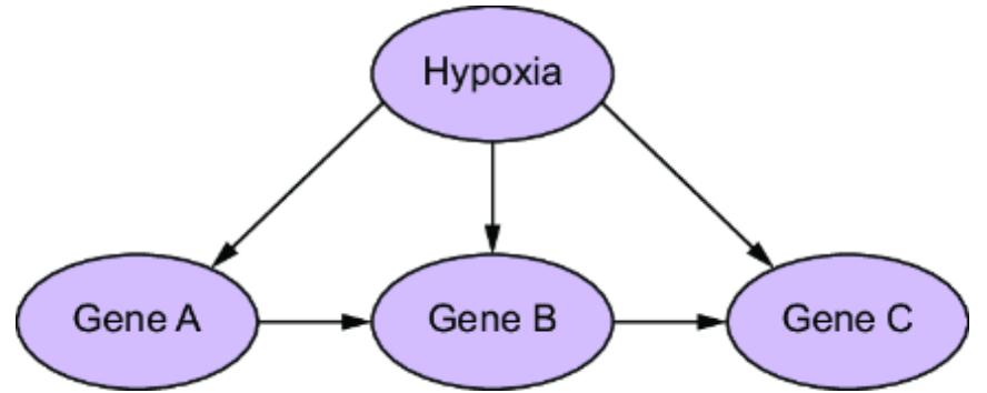
Figure 7.13 ૿Hypoxia is an intervention that has no specific target. Include it as a root node with edges to all variables that are possibly affected.

Explicit representation of interventions as part of the DGP is less expressive than the ideal (or stochastic) intervention, which captures how an arbitrary intervention can change the DGP.

Summary

• An intervention is an action that changes the data generating process (DGP). Interventions are fundamental to defining causality and causal models.
• Many, if not most, machine learning–driven decisions are interventions that can render the model’s deployment environment different from its training environment.
• The ability to model an intervention allows one to simulate the outcome of experiments.
• Simulating experiments with an intervention model can save costs or enable simulated experiments when running an actual experiment is infeasible, unethical, or impossible.
• An ideal intervention targets specific variables, fixes them to a specific value, and renders the target independent of its causal parents.
• Causal effects are simple extensions of intervention distributions. For example, the average treatment effect (ATE) of X on Y is E(YX=1) – E(YX=0), the difference in means between two intervention distributions for Y. Conditional average treatment effects (CATEs) are simply differences in conditional expectations for intervention distributions on Y.
• Stochastic interventions are like ideal interventions, but they fix the intervention targets at a value determined by some random process. That value could depend on the states of other variables in the system. In this way, they are related to policies in automated decisionmaking domains such as bandit algorithms and reinforcement learning.
• An intervention operator describes how a causal model is altered to reflect an ideal (or stochastic) intervention.
• The intervention operator for a structural causal model replaces the target variables assignment function with the intervention value.
• Graph surgery is the intervention operator for causal DAGs.
• The intervention operator for causal graphical models applies graph surgery and replaces the causal Markov kernel for the target with a degenerate distribution that places all probability on the intervention value.
• Causal models can use observational data to statistically learn the observational distribution and any interventional distribution that can be derived through the intervention operator.
• Randomization is a stochastic intervention that eliminates causal influence on the intervention target

from unknown causes.

• ૿No causation without manipulation suggests defining your causal model so that interventions are tethered to hypothetical experiments.
• You can model interventions that don’t meet the ideal intervention standard as root nodes with outgoing edges to variables they may affect.

[1] D.T. Campbell and T.D. Cook, Quasi-experimentation: Design & Analysis Issues for Field Settings (Rand McNally, 1979), p36.

8 Counterfactuals and parallel worlds

This chapter covers

• Motivating examples for counterfactual reasoning
• Turning counterfactual questions into symbolic form
• Building parallel world graphs for counterfactual reasoning
• Implementing the counterfactual inference algorithm
• Building counterfactual deep generative models of images

Marjani, a good friend of mine, once had to choose between two dating prospects at the same time. She had something of a mental score card for an ideal long-term match. She had good chemistry with one guy, but he didn’t rank well on the score card. In contrast, the second guy checked all the boxes, so she chose him. But after some time, despite him meeting all her criteria, she couldn’t muster any feelings for him. It was like a failed ritual summoning; the stars were perfectly aligned, but the summoned spirit never showed up. And so, as any of us would in that situation, she posed the counterfactual question:

I chose a partner based on my criteria and it’s not working out. Would it have worked out if I chose based on chemistry?

Counterfactual queries like this describe hypothetical events that did not occur but could have occurred if something had been different. Counterfactuals are fundamental to how we

define causality; if the answer to Marjani’s question is yes, it implies that choosing based on her score card caused her love life to be unsuccessful.

Counterfactuals are core to the bread-and-butter question of causal effect inference, where we compare observed outcomes to ૿potential outcomes that didn’t happen, like the outcome of Marjani’s love life if she chose a partner based on chemistry. More broadly, answering counterfactual questions is useful in learning policies for better decisionmaking. When some action leads to some outcome, and you ask how a different action might have led to a different outcome, a good answer can help you select better actions in the future. For example, after this experience, Marjani revised her score card to factor in chemistry when considering later romantic prospects.

We’ll look at practical examples in this chapter, but I led with this love and romance example because it is universally relatable. It illustrates how fundamental counterfactual reasoning is to human cognition—our judgments about the world are fueled by our imagination of what could have been.

Note that Marjani’s counterfactual reasoning involves a type of prediction. Like a Marvel superhero film, she is imagining a parallel world where she chose based on chemistry, and she’s predicting the outcome of her love life in that world. But statistical machine learning algorithms are better at making predictions than humans. That insight leads us to the prospect of building AI that automates human-like counterfactual reasoning with statistical machine learning tools.

In this chapter, we’ll pursue that goal by learning to formalize counterfactual questions with probability. In the next chapter, we’ll implement a probabilistic counterfactual inference algorithm that can answer these questions. Let’s start by exploring some practical case studies that motivate algorithmic counterfactual reasoning.

8.1 Motivating counterfactual reasoning

Here, I’ll introduce some case studies demonstrating the business value of answering counterfactual questions. I’ll then argue how they are useful for enhancing decisionmaking.

8.1.1 Online gaming

Recall the online gaming example from chapter 7, where the amount of in-game purchases a player made was driven by their level of engagement in side-quests and whether they were in a guild. Suppose we observed an individual player who was highly engaged in side-quests and had many ingame purchases. A counterfactual question of interest might be, ૿What would their amount of in-game purchases be if their engagement was low?

8.1.2 The streaming wars

The intense competition amongst subscription streaming companies for a finite market of subscribers has been dubbed ૿the streaming wars. Netflix is a dominant player with long experience in the space. It has learned to attract new subscribers by building blockbuster franchises from scratch, such as House of Cards, Stranger Things, and Squid Game.

However, Netflix competes with Amazon, Apple, and Disney —companies with extremely deep pockets. They can

compete with Netflix’s ability to build franchises from scratch by simply buying existing successful franchises (e.g., Star Wars) and making novel content within that franchise (e.g., The Mandalorian).

Suppose that Disney is in talks to buy James Bond, the most valuable spy thriller franchise ever, and Netflix believes that a successful Bond deal may cause it to lose subscribers to Disney. Netflix hopes to prevent this by striking a deal with a famous showrunner to create a new spy-thriller franchise called Dead Drop. This new franchise would combine tried and true spy thriller tropes (e.g., gadgetry, exotic backdrops, car chases, over-the-top action sequences) with the complex characters, diverse representation, and emotionally compelling storylines characteristic of Netflix-produced shows. There is uncertainty about whether Netflix executives can close a deal with the candidate showrunner, as both parties would have to agree on creative control, budget, royalties, etc.

Suppose the Bond deal succeeded, and Disney Plus now runs new series and films set in the ૿Bond-verse. However, the Dead Drop deal fell through. Netflix then acquires data that identifies some subscribers who subsequently left Netflix, subscribed to Disney Plus, and went on to watch the new Bond content.

A Netflix executive would be inclined to ask the following counterfactual: ૿Would those lost subscribers have stayed, had the Dead Drop deal succeeded? Suppose the answer is ૿no, because the Bond content was so strong an attraction that the Dead Drop deal outcome didn’t matter. In this case, the employees who failed to close the deal should not be blamed for losing subscribers.

Or, suppose the Dead Drop deal succeeded, and Netflix subscribers can now watch the new Dead Drop franchise. ૿Would those subscribers who watch Dead Drop have left for the new Bond series on Disney, had the deal failed? Again, if the answer is ૿no, the employees who successfully closed the deal shouldn’t get credit for keeping all those subscribers.

In both cases, answering these questions would help inform future deal-making decisions.

8.1.3 Counterfactuals analysis of machine learning models

In this chapter, we are focusing on using a causal model to reason counterfactually about some data generating process. In machine learning, often the goal is a counterfactual analysis of a machine learning model itself; i.e., given some input features and some output predictions, how would the predictions have differed if the inputs were different? This counterfactual analysis supports explainable AI (XAI), AI fairness, and other tasks.

COUNTERFACTUAL ANALYSIS IN CLASSIFICATION

Consider the task of classification—a trained algorithm takes as input some set of features for a given example and produces a predicted class for that example. For example, given the details of a loan application, an algorithm classifies the application as ૿reject or ૿approve.

Given a rejected application, a counterfactual question naturally arises: ૿Would the application have been approved if some elements of the application were different? Often, the goal of the counterfactual analysis is to find a minimal change to the feature vector that corresponds to a change in the classification. Figure 8.1 illustrates this idea.

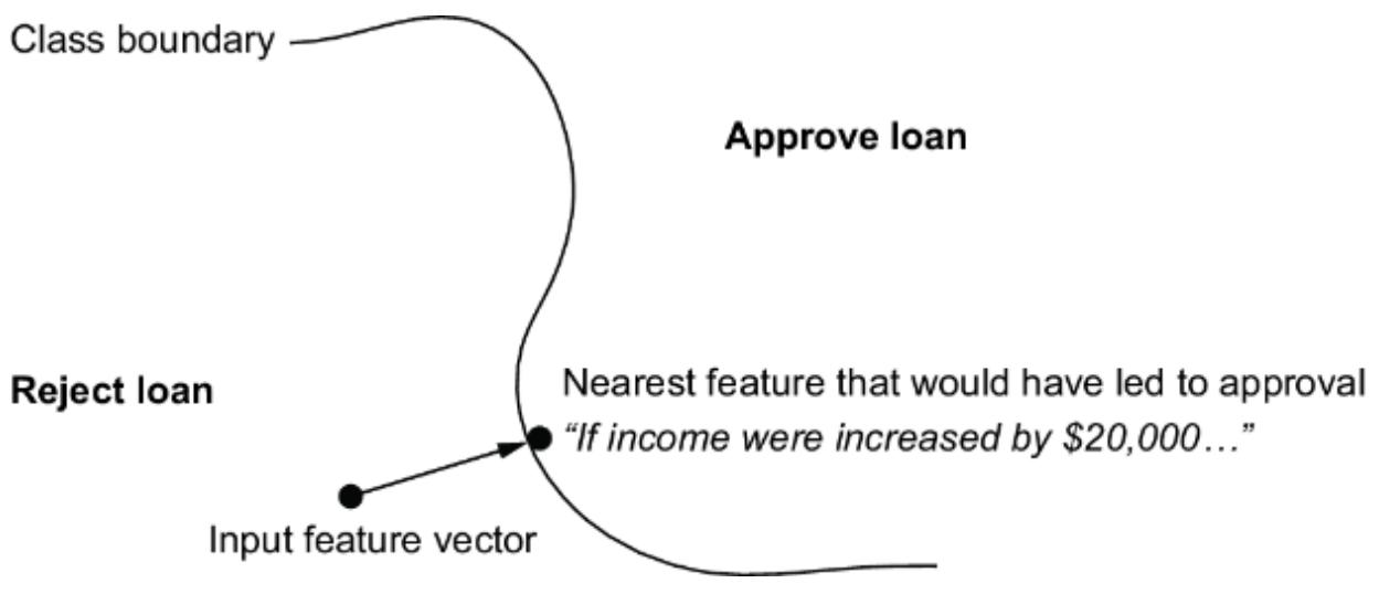
Figure 8.1 What is the minimal change to the input feature that would have led to approval? In this case, the loan would have been approved if income were $20,000 higher.

Finding the minimal change that would have led to approval requires defining a distance metric in the feature space and then finding the feature value on the other side of the class boundary. In this example, the hypothetical condition ૿if the applicant had $20,000 more a year in income . . . corresponds to the smallest change to the feature vector (in terms of distance on the decision surface) that would have led to approval. This type of analysis is useful for XAI; i.e., for understanding how features drive classification on a case-bycase basis.

COUNTERFACTUAL ALGORITHMIC RECOURSE

Increasing salary by $20,000 is unrealistic for most loan applicants. That’s where counterfactual-based algorithmic recourse can be useful. Algorithmic recourse looks for the nearest hypothetical condition that would have led to a different classification. It operates under the constraint that the hypothetical condition was achievable or actionable by the applicant. Figure 8.2 shows how this works.

In this example, the assumption is that increasing income by $5,000 and improving one’s credit score was achievable, according to some criteria (while increasing income by $20,000 was not).

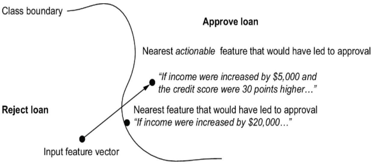
Figure 8.2 In algorithmic recourse, we’re often interested in the nearest actionable feature vector on the other side of the decision boundary.

Algorithmic recourse aims to give individuals subjected to machine learning–based decisions information that they can work with. If one fails an exam and asks why, an explanation of ૿because you are not a genius is less useful than ૿because you didn’t review the practice exam, even though both may be true.

COUNTERFACTUAL FAIRNESS

Counterfactual fairness analysis is a similar analysis that applies in cases where some of the input features correspond to attributes of a person. The idea is that certain attributes of an individual person should not, on ethical grounds, impact the classification. For example, it is unethical to use one’s ethnicity or gender in the decision to offer a loan. Even if such ૿protected attributes are not explicitly coded into the input features, the classification algorithm may have learned

proxies for protected attributes, such as the neighborhood where one lives, one’s social network, shopping habits, etc. It may make sense to have such features in the model, and it may not be obvious when those features behave as proxies for protected attributes.

Figure 8.3 uses the loan algorithm example to illustrate how a counterfactual fairness analysis would ask counterfactual questions. In this case, the counterfactual question is ૿Would this person have been approved if they were of a different ethnicity? The analyst would find features that are proxies for ethnicity and then see if a change to those proxies corresponding to a change in ethnicity would result in a classification of ૿approve. Some techniques attempt to use this analysis during training to produce fairer algorithms.

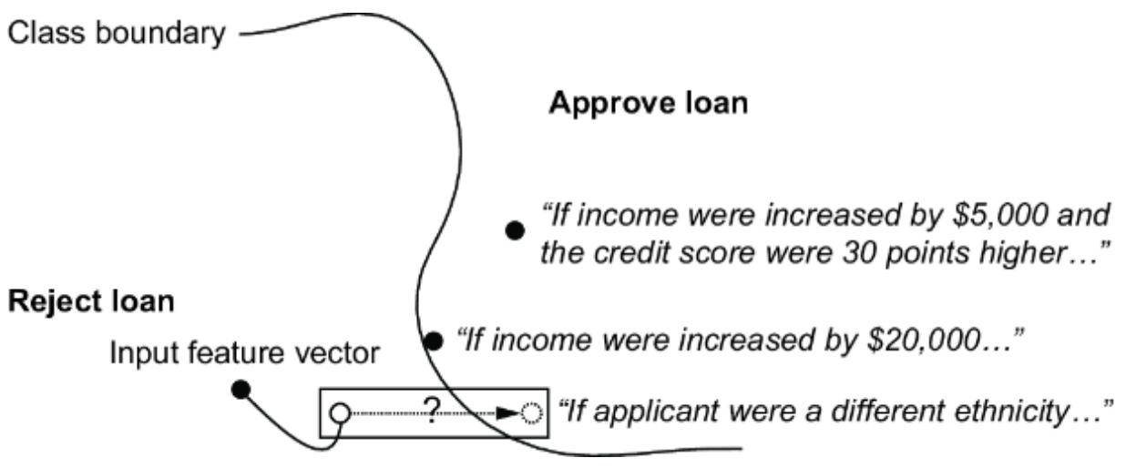
While counterfactual fairness analysis is not enough to solve the broad problem of AI fairness, it is an essential element in the AI fairness toolkit.

8.1.4 Regret and why do we care about what ૿would have happened?

Traditional machine learning is usually forward-looking. Given data, you make a prediction, that prediction drives some decision to be made in the present, and that decision brings about some future cost or benefit. We want good predictions so we can get more future benefits. Imagine, for example, a machine learning algorithm that could accurately forecast the performance of a stock portfolio—that would obviously be quite valuable.

Now, imagine a different algorithm that could accurately tell you how your portfolio would perform today if you had bought different stocks; that would certainly be less valuable than predicting the future. This contrast highlights a common criticism that modeling counterfactuals is backward-looking. For example, the counterfactual questions in our motivating case studies focus on decisions and outcomes that happened in the past. What’s done is done; getting the answers to such questions won’t change the past.

But, first, not all counterfactuals are retrospective. In section 8.3 we’ll model questions like ૿What are the chances the subscriber would churn if you don’t send them a promotion and would not churn if you did send a promotion? (૿Churn means to stop using a product or service within a certain time period.) That question has no past tense, does have business value, and is something we can model.

Second, retrospective counterfactuals help you understand how to make better decisions in the future. Indeed, analyzing how your portfolio would have performed given different allocations—what investors call ૿backtesting—is ideal for comparing various investment strategies. Similarly, the counterfactual insights from a failed Dead Drop deal might

help Netflix executives make a deal with another famous showrunner.

When we consider retrospective reasoning about things that would have or could have been, we arrive at the notion of regret. Regret is about retrospective counterfactual contrasts; given a choice, regret is a comparison between an outcome of the option you chose and an imagined counterfactual outcome of an option you rejected. In colloquial terms, regret is the bad feeling you get when the counterfactual outcome of an option you rejected is better than the option you chose. But cognitive science calls this negative regret; there is also positive regret, which is the good feeling you get when, upon comparing to imagined counterfactual outcomes, you realize you chose the better option (as in, ૿whew, I really dodged a bullet).

Regret can be useful for learning to make better decisions. Suppose you make a choice, you pay a cost (time, effort, resources, etc.), and it leads to an outcome. That gives you a baseline single point of data for learning. Now, suppose that, with the benefit of hindsight, you could imagine with 100% accuracy the outcome that would have occurred had you made a different choice. Now you have two comparable points of data for learning, and you only had to pay a cost for one of them.

Usually your ability to imagine the counterfactual outcome of the rejected option is not 100% accurate. Even with the benefit of hindsight, there is still some uncertainty about the counterfactual outcome. But that’s no problem—we can model that uncertainty with probability. As long as hindsight knowledge provides you with some information about counterfactual outcomes, you can do better than the baseline of learning from a single point of data.

In reinforcement learning and other automated decisionmaking, we often call our decision-making criteria ૿policies. We can incorporate counterfactual analysis and regret in evaluating and updating policies.

8.1.5 Reinforcement learning and automated decision-making

In automated decision-making, a ૿policy is a function that takes in information about a decision problem and automatically selects some course of action. Reinforcement learning algorithms aim to find policies that optimize good outcomes over time.

Automated counterfactual reasoning can credit good outcomes to the appropriate actions. In the investing example, we can imagine an algorithm that periodically backtests different portfolio allocation policies as more recent prices enter the data. Similarly, imagine we were writing a reinforcement learning (RL) algorithm to learn to play a game. We could have the algorithm use saved game instances to simulate how that game instance would have turned out differently if it had used a different policy. The algorithm can quantify the concept of regret by comparing those simulated outcomes to actual outcomes and using the results to learn a better policy. This would reduce the number of games the AI needed to learn a good policy, as well as enable it to learn from simulated conditions that don’t occur normally in the game. We’ll focus more on automated decision-making, bandits, and reinforcement learning in chapter 12.

8.1.6 Steps to answering a counterfactual query

Across each of these applications, we can answer these counterfactual inference questions with the following

workflow:

• 1. Pose the counterfactual question —Clearly articulate the counterfactual question(s) we want to pose in the simplest terms.
• 2. Convert to a mathematical query —Convert the query to mathematical symbols so it is formal enough to apply mathematical or algorithmic analysis.
• 3. Do inference —Run an inference algorithm that will generate an answer to the question.

In the following sections, we’ll focus on steps 1 and 2. In chapter 9, we’ll handle step 3 with an SCM-based algorithm for inferring the query we create in step 2. In chapter 10, we’ll see ways to do step 3 without an SCM but only data and a DAG.

8.2 Symbolic representation of counterfactuals

In chapter 7, we saw the ૿counterfactual notation, which uses subscripts to represent interventions. Now we are going to use this notation for counterfactual expressions. The trick is remembering, as we’ll see, that counterfactual queries are just a special type of interventional queries. We’ll see how interventional queries flow into counterfactual queries by revisiting our online gaming example.

8.2.1 Hypothetical statements and questions

Consider our online gaming case study. When considering how much a player makes, we might say something like this:

The level of in-game purchases for a typical player would be more than $50.

We’ll call this a hypothetical statement. In grammatical terms, I am using a modal verb (e.g., ૿would, ૿could, ૿should in ૿would be more) to intentionally mark hypothetical language rather than using declarative language (e.g., ૿is more or ૿will be more), which we use to make statements about objective facts.

We want to formalize this statement in probability notation. For this statement, we’ll write P (I  >  50)—recall that we used the random variable I to represent In-Game Purchases, E to represent Side-Quest Engagement, and G to represent Guild Membership.

We’ll use hypothetical language in our open questions as well, like this:

What would be the amount of in-game purchases for a typical player?

I am inquiring about the range of values the variable I could take, and I represent that with P(I).

DECLARATIVE VS. HYPOTHETICAL LANGUAGE AND PROBABILITY

Declarative language express certainty, as in ૿amount of in-game purchases is more than $50. In contrast, hypothetical language is used for statements that convey conjecture, imagination, and supposition, as in ૿amount of in-game purchases would be more than $50.

Many of us learn to associate probability notation with declarative language, because of probability theory’s connection to propositional logic: P(I>50) quantifies the probability that the declarative statement ૿amount of ingame purchases is more than $50 is true. But we are going to lean into the hypothetical language.

Hypothetical language has an implicit lack of certainty—we are talking of things that could be, rather than things that are. Lack of certainty is equivalent to uncertainty, and the Bayesian philosophy we adopt in this book nudges us toward using probability to model uncertainty, so using hypothetical language will make it easier for us to formalize the question in probability notation. We’ll find this will help us formalize causal statements and questions.

Note that the tense of the question or statement doesn’t matter when we map it to probabilistic notation. For example, we could have used this phrasing:

What would have been the amount of in-game purchases for a typical player?

Regardless of tense, we use the notation P (I  ) to represent our uncertainty about a variable of interest in our question.

8.2.2 Facts filter hypotheticals to a subpopulation

Suppose my statement was as follows:

The level of in-game purchases for a player with high side-quest engagement would be more than $50. P( I>50| E=૿high)

Here, I am making a statement about a subset of players (those with high side-quest engagement) rather than all players. I’m doing the same when I ask this question:

What would be the level of in-game purchases for players with high side-quest engagement? P( I| E=૿high)

The fact that Side-Quest Engagement is high serves to filter the population of players down to those for whom that fact is true. As discussed in chapter 2, we use conditional probability to zoom in on a subpopulation. In this example, we use P (I  >  50|E=૿high) for the statement, and P (I |E=૿high) for the question.

I’ll use ૿factual conditions to refer to facts, events, and evidence like E = ૿high that narrow down the target population. These factual conditions appear on the right side of ૿| in the conditional probability notation P (.|.). We might normally call them ૿conditions, but I want to avoid confusion with ૿conditional hypothetical, which I’ll introduce next.

8.2.3 Conditional hypotheticals, interventions, and simulation

Now, suppose I made the following statement:

If a player’s side-quest engagement was high, they would spend more than $50 on in-game purchases. P  ( I ^E =૿high>50)

We’ll call this a conditional hypothetical statement. We’ll call the ૿If side-quest engagement was high part the hypothetical condition, and ૿they would spend more than $50 on in-game purchases is the hypothetical outcome.

The hypothetical conditions in conditional hypothetical questions often follow a similar ૿what if style of phrasing:

What would be the amount of in-game purchases for a player if their side-quest engagement was high? P  ( I ^E =૿high)

We will use the intervention notation (i.e., the subscripts in counterfactual notation) to represent these conditions. For the statement, we will use P(IE=૿high>50), and for the question, P (IE=૿high).

IMAGINATION, CONDITIONS, AND INTERVENTIONS

Using the ideal intervention to model hypothetical conditions in conditional hypothetical statements is a philosophical keystone of our causal modeling approach. The idea is that when we pose hypothetical conditionals, we only attend to the causal consequences of the hypothetical conditional.

REFRESHER: IDEAL INTERVENTION

An ideal intervention is a change to the data generating process that does the following:

• 1. Targets a fixed variable (e.g., X)
• 2. Sets that variable to a specific value (e.g., x)
• 3. In so doing, severs the causal influence of that variable’s parents

This definition generalizes to a set of variables.

We sometimes write interventions with do-notation, as in do(X=x). In counterfactual notation, for a variable Y, we write YX=x to indicate that the variable Y is under the influence of an intervention on X. In a DAG, we represent ideal intervention with graph surgery, meaning we cut the incoming edges to the target variable. In an SCM, we represent an ideal intervention by replacing the target variable’s assignment function with the intervention value. Causal libraries often implement these operations for us, often with a function or method called ૿do.

Let me illustrate by counterexample. Suppose we ask this:

What would be the amount of in-game purchases for a player if their side-quest engagement were high?

Suppose we then modeled this with P (I |E = ૿high). Then inference on this query would use not just the causal impact that high engagement has on In-Game Purchases but also the non-causal association through the path E ← G → I; you can infer whether a player is in a guild from their level of Side-Quest Engagement, and Guild Membership also drives In-Game Purchases. But this question is not about Guild

Membership; we’re just interested in how Side-Quest Engagement drives In-Game Purchases.

૿What if hypotheticals use the ideal intervention because they attend only to the causal consequences of the condition. To illustrate, let’s rephrase the previous question to make that implied ideal intervention explicit:

What would be the amount of In-Game Purchases for a player if their side-quest engagement were set to high? P  ( I ^E =૿high)

The verb ૿set connotes the action of intervening. Modeling hypothetical conditions with ideal interventions argues that the original phrasing and this phrasing mean the same thing (going forward, I’ll use the original phrasing).

As humans, we answer ૿what if questions like the preceding P (IE=૿high) question (either the original or rephrased version) by imagining a world where the hypothetical condition is true and then imagining how the hypothetical scenario plays out as a consequence. The variables in our hypothetical condition may have their own causal drivers in the datagenerating process (e.g., Guild Membership is a cause of Side-Quest Engagement), but we ignore those drivers because we are only interested in the consequences of the hypothetical condition. We isolate the variables in a hypothetical condition in our imaginations just as we would in an experiment. The ideal intervention is the right tool for setting a variable independently of its causes.

AVOIDING CONFUSION BETWEEN FACTUAL AND HYPOTHETICAL CONDITIONS

It is particularly easy to confuse ૿factual conditions with ૿hypothetical conditions. To reiterate in general terms, in the question ૿What would Y be if X were x, X = x is a hypothetical condition and we use the notation P (YX=x). In contrast, factual conditions serve to narrow down the population we are asking about. For example, in the question ૿What would Y be for cases where X is x ? X = x is an actual condition used to filter down to cases where X = x. Here, we use notation P (Y  |X = x ).

Keep in mind that we can combine factual and hypothetical conditions, as in the following question:

What would be the amount of in-game purchases for a player in a guild if their side-quest engagement was high? P  ( I ^E =૿high| G= g)

Here, we are asking a conditional hypothetical on a subset of players who are guild members. This query is different from the following:

What would be the amount of in-game purchases for a player if their side-quest engagement was high and they were in a guild? P  ( I ^E =૿high, ^G =૿member)

That said, with the ambiguity of natural language, someone might ask the second question when what they really want is the answer to the first question. It is up to the modeler to dispel confusion, clarify meaning, and write down the correct notation.

8.2.4 Counterfactual statements

In natural language, a counterfactual statement is a conditional hypothetical statement where there is some conflict between factual conditions and hypothetical conditions or outcomes. In other words, it is a conditional hypothetical statement that is ૿counter to the facts.

In everyday language, those conflicting factual conditions could be stated before the statement or implied by context. For our purposes, we’ll require counterfactual statements to state the conflicting factual conditions explicitly:

For a player with low side-quest engagement and an amount of in-game purchases less than $50, if the player’s side-quest engagement were high, they would spend more than $50 on in-game purchases. P  ( I ^E =૿high>50| E=૿low, I  £50)

As a question, we might ask:

What would be the amount of in-game purchases for a player with low side-quest engagement and in-game purchases less than $50 if their side-quest engagement was high? P  ( I ^E =૿high | E=૿low, I  £50)

In both the statement and the question, the factual condition of low engagement conflicts with the hypothetical condition of high engagement. In the statement, the hypothetical outcome where in-game purchases is more than 50 conflicts with the factual condition where it is less than or equal to 50. Similarly, the question considers all possible hypothetical outcomes for in-game purchases, most of which conflict with the factual condition of being less than or equal to 50. We use counterfactual notation to write these queries just as we would other conditional hypotheticals..

OVERVIEW OF TERMINOLOGY IN FORMALIZING COUNTERFACTUALS

Hypothetical language—Used to express hypotheses, conjecture, supposition, and imagined possibilities. In English, it often involves ૿would or ૿could and contrasts with the declarative language. It is arguably easier to formalize causal statements and questions phrased in hypothetical language.

Hypothetical statement—A statement about the world phrased in hypothetical language, such as ૿Y would be y, which we’d write in math as P(Y=y).

Factual conditions—Refer to facts, events, and evidence that narrow down the scope of what’s being talked about (the target population). Used as the conditions in conditional probability. For example, we’d write ૿Where Z is z, Y would be y as P(Y=y|Z=z).

Hypothetical conditions—Conditions that frame a hypothetical scenario, as in ૿what if X were x? or ૿If X were x … We model hypothetical conditions with the ideal intervention and subscript X=x in counterfactual notation.

Conditional hypothetical statement—A hypothetical statement with hypothetical conditions, such as ૿If X were x, Y would be y, which becomes P(YX=x=y). We can add factual conditions like ૿Where Z is z, if X were x, Y would be y becomes P(YX=x=y|Z=z).

Counterfactual statement—A counterfactual statement is a conditional hypothetical statement where the variables in the factual conditions overlap with those in the hypothetical conditions or hypothetical outcomes. For example, in ૿Where X is x, if X were x’, Y would be y (P(YX=x’ =y|X=x)), the factual condition ૿Where X is x

overlaps with the hypothetical condition ૿if X were x’. In ૿Where Y is y, if X were x’, Y would be y’ (P(YX=x’ =y’|Y=y)), the factual condition ૿Where Y is y overlaps with the hypothetical outcome ૿Y would be y.

Consistency rule—You can drop a hypothetical condition in the subscript if a factual condition and a hypothetical condition overlap but don’t conflict. For example, P(YX=x|X=x) = P(Y|X=x).

Note that many texts will use the word ૿counterfactual to describe formal causal queries that don’t necessarily condition on factual conditions, such as YX=x or P(YX=x=y) or P(YX=x=1, YX=x’ =0). I’m using ૿counterfactual statement and other phrases above to describe common hypothetical and counterfactual natural language and to aid in the task of converting to formal counterfactual notation.

Note that we can combine conflicting factual conditions with other non-conflicting factual conditions, such as being a member of the guild in this example:

What would be the amount of in-game purchases for a player in a guild with low side-quest engagement and ingame purchases less than $50 if their side-quest engagement was high? P( I ^E =૿high | E=૿low, I £50, G=૿member)

Figure 8.4 diagrams the elements of a formalized counterfactual query.

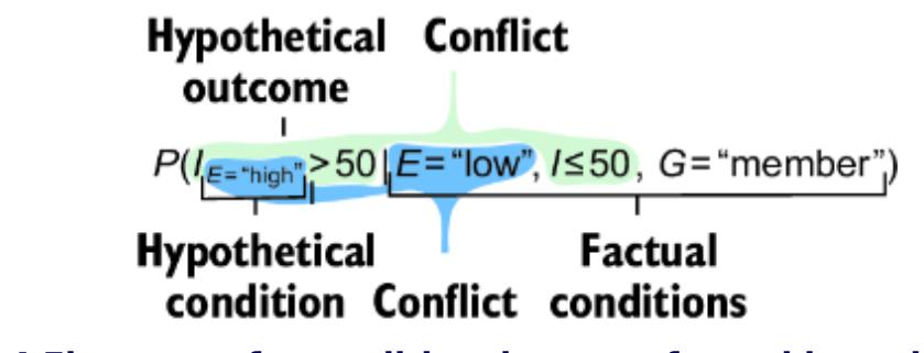
Figure 8.4 Elements of a conditional counterfactual hypothetical formalized in counterfactual notation

FORMALIZING COUNTERFACTUALS WITH LARGE LANGUAGE MODELS

Formalizing a counterfactual question into counterfactual notation is an excellent task for a large language model (LLM). State-of-the-art LLMs perform quite well at benchmarks where a natural language query is converted to a symbolic query, such as an SQL statement, and formalizing a counterfactual question is an example of this task. We’ll look more at LLMs and causality in chapter 13, but for now you can experiment with prompting your favorite LLM to convert questions to counterfactual notation.

8.2.5 The consistency rule

Consider the distribution P (IE=૿high|E = ૿low). Suppose that instead of the subscript E=૿high we had E=૿low, so the distribution is P (IE=૿low |E = ૿low). The consistency rule states that this distribution is equivalent to the simpler P (I |E = ૿low). More generally, P (YX=x|X = x, Z = z ) = P (Y |X = x, Z = z ) for any z.

Intuitively, P (IE=૿low|E=૿low) corresponds to the rather odd question, ૿What would be the amount of in-game purchases for a player with low side-quest engagement if their sidequest engagement was low? In this question, the factual condition and the hypothetical condition overlap but don’t conflict. The consistency rule says that, in this case, we drop the hypothetical condition, saying that this is equivalent to asking ૿What would be the amount of in-game purchases for a player with low side-quest engagement?

Now consider a version of this counterfactual where we observe an actual outcome for in-game purchases. Specifically, consider P (IE=૿high|E =૿low, I=75). This is the corresponding counterfactual question:

What would be the amount of in-game purchases for a player with low side-quest engagement and in-game purchases equal to $75 if their side-quest engagement was high?

Now, instead, suppose we changed it to P (IE=૿low|E = ૿low, I = 75). By the consistency rule, this collapses to P (I  |E =૿low, I = 75):

What would be the amount of in-game purchases for a player with low side-quest engagement and in-game purchases equal to $75?

The answer, of course, is $75. If we ask about the distribution of I conditional on I = 75, then we have a distribution with all the probability value concentrated on 75.

In counterfactual reasoning, we often want to know about hypothetical outcomes for the same variables we observe in the factual conditions. The consistency rule states that if the hypothetical conditions are the same as what actually happened, the hypothetical outcome must be the same as what actually happened.

Recall that we use an intervention to model the hypothetical condition. The rule assures us that if a player had low Side-Quest Engagement and a certain amount of In-Game Purchases, they would have the exact same amount of In-Game Purchases if they were selected for an experiment that randomly selected them for the low Side-Quest Engagement group. That’s important if we expect our causal inferences to predict the outcomes of experiments.

8.2.6 More examples

Table 8.1 presents several additional examples of mapping counterfactual questions to counterfactual notation.

Table 8.1 Examples of counterfactual notation

Question	Type	Distribution in counterfactual notation
What would be the amount of in-game purchases for a typical player?	Hypothetical	P( I)
What would be the amount of in-game purchases for a player with high side-quest engagement?	Hypothetical focused on highly engaged players	P( I E=૿high଀)
What would be the amount of in-game purchases for a player if they had high side-quest engagement?	Conditional hypothetical	P( I =૿high଀) E
What would be the level of engagement and amount of in-game purchases if the player were a guild member?	Conditional hypothetical on two outcomes of interest	P( E =૿member଀, G I =૿member଀) G
What would be the level of in-game purchases for a player if they had high side-quest engagement and they were not a guild member?	Conditional hypothetical with two hypothetical conditions	P( I E =૿high଀, G =૿nonmember଀)
What would be the level of in-game purchases for a player in a guild if they had high side-quest engagement?	Conditional hypothetical focused on guild members	P( I =૿high଀ E G=૿member଀)
For a player with low engagement, what would their level of in-game purchases be if their level of engagement was high?	Counterfactual. Factual condition conflicts with hypothetical condition.	P( I =૿high଀ E E=૿low଀)
For a player who had at most $50 of in-game purchases, what would their level of in-game purchases be if their level of engagement was high?	Counterfactual. Factual condition (in-game purchases of £$50) conflicts with possible hypothetical outcomes (in	P( I =૿high଀ I E £50)

Question	Type	Distribution in counterfactual notation
	game purchases possibly >$50).
For a player who had low engagement and at most $50 of in-game purchases, what would their level of in-game purchases be if their level of engagement was high?	Counterfactual. Factual conditions conflict with a hypothetical condition and possible hypothetical outcomes.	P( I =૿high଀ E E=૿low଀, I £50)
For a player in a guild who had low engagement, what would their level of in game purchases be if their engagement were high and they weren’t a guild member?	Counterfactual. Factual conditions conflict with hypothetical conditions.	P( I E =૿high଀, G =૿nonmember଀ E=૿low଀, G=૿member଀)
What would be the level of engagement if the player were a guild member? Moreover, what would be their level of in-game purchases if they were not a guild member?	Counterfactual. Involves two conflicting hypothetical conditions on two different outcomes.	P( E =૿member଀, G I =૿nonmember଀) G

The last case in table 8.1 is a special case, more common in theory than practice, that does not involve a factual condition but has conflicting hypothetical conditions.

Next, we’ll look at a particular class of counterfactuals that involve binary causes and outcomes.

8.3 Binary counterfactuals

An important subclass of counterfactual query is one we’ll call binary counterfactuals. These are counterfactuals involving binary hypothetical conditions and outcome variables. Binary variables, especially binary causes, arise when we think in terms of observational and experimental studies, where we have ૿exposed and ૿unexposed groups, or ૿treatments and ૿control groups. But binary variables are also useful in reasoning about the occurrence of events; an event either happens or does not.

Binary counterfactual queries deserve special mention because they are often simpler to think about, have simplifying mathematical properties that queries on nonbinary variables lack, and have several practical applications that we’ll cover in this section. Further, you can often word the question you want to answer in binary terms, such that you can convert nonbinary variables to binary variables when formalizing your query. To illustrate, in our online gaming example, suppose a player made $152.34 in online purchases, and we ask ૿Why did this player pay so much? We are not interested in why they paid exactly that specific amount but why they paid such a high amount, where ૿such a high amount is defined as, for example, more than $120. So our binary indicator variable is X = {1 if I ≥ 120 else 0}.

8.3.1 Probabilities of causation

The probabilities of causation are an especially useful class of binary counterfactuals. Their utility lies in helping us answer ૿why questions. They are foundational concepts in practical applications, including attribution in marketing, credit assignment in reinforcement learning, root cause analysis in engineering, and personalized medicine.

Let’s demonstrate the usefulness of the probabilities of causation in the context of a churn attribution problem. In a subscription business model, churn is the rate at which your service loses subscribers, and it has a major impact on the value of a business or business unit. Typically, a company deploys a predictive algorithm that rates subscribers as

having some degree of churn risk. The company wants to discourage subscribers with a high risk of churn from actually doing so. In our example, the company will send a promotion that will entice the subscriber to stay (not churn). The probabilities of causation can help us understand why a user would churn or stay.

Given a binary (true/false) cause X and outcome Y, we’ll define the following probabilities of causation: probability of necessity, of sufficiency, of necessity and sufficiency, of enablement, and of disablement.

PROBABILITY OF NECESSITY

For a binary cause X and binary outcome Y, the probability of necessity (PN) is the query P (YX^{= 0} = 0|X = 1, Y = 1). In plain language, the question underlying PN is ૿For cases where X happened, and Y happened, if X had not happened, would Y not have happened? In other words, did X need to happen for Y to happen?

Let’s consider our churn problem. Let X represent whether we sent a promotion and Y represent whether the user stayed (didn’t churn). In this example, P(YX^{= 0} = 0|X = 1, Y = 1) represents the query ૿For a subscriber who received the promotion and stayed, what are the chances they would have churned if they had not received the promotion? In other words, was the promotional offer necessary to maintain the subscriber?

PROBABILITY OF SUFFICIENCY

The probability of sufficiency (PS) is P (YX⁼ 1= 1|X = 0, Y = 0). A common plain language articulation of PS is ૿For cases where neither X nor Y happened, if X had happened, would Y have happened? In other words, is X happening sufficient to cause Y to happen? For example, ૿for users who did not receive a promotion and didn’t stay (churned), would they have stayed had they received the promotion? In other words, would a promotion have been enough (sufficient) to keep them?

The plain language interpretation of sufficiency can be confusing. The factual conditions of the counterfactual query zoom in on cases where X = 0 and Y = 0 (cases where neither X nor Y happened). However, we’re often interested in looking at cases where X=1 and Y=1 and asking if X was sufficient by itself to cause Y = 1. In other words, given that X happened and Y happened, would Y still have happened even if the various other events that influenced Y had turned out different? But P (YX=1=1|X = 0, Y = 0) entails this interpretation without requiring us to enumerate all the ૿various other events that influenced Y in the query. See the chapter notes athttps://www.altdeep.ai/p/causalaibook for pointers to deeper research discussions on sufficiency.

PROBABILITIES OF CAUSATION AND THE LAW

The probabilities of causation are closely related to legal concepts in the law. It is helpful to know this relationship, since practical applications often intersect with the law, and many stakeholders we work with in practical settings have legal training.

• But-for causation and the probability of necessity—The but-for test is one test for determining causation in tort and criminal law. The way we phrase the probability of necessity is the probabilistic equivalent to the but-for test, rephrasing ૿if X had not happened, would Y not have happened? as ૿but for X happening, would Y have happened?
• Proximal causality and the probability of sufficiency—In law, proximate cause refers to the primacy that a cause X had in the chain of events that directly brings about an outcome (e.g., injury or damage). There is indeed a connection with sufficiency, though not an equivalency. Proximal causality indeed considers whether a causal event was sufficient to cause the outcome, but legal theories of proximal cause often go beyond sufficiency to invoke moral judgments as well.

PROBABILITY OF NECESSITY AND SUFFICIENCY

The probability of necessity and sufficiency (PNS) is P(YX=1= 1, YX=0 = 0). In plain language, P(YX=1= 1, YX=0= 0) reads, ૿Y would be 0 if X were 0 and Y would be 1 if X were 1. For example, ૿What are the chances that a given user would churn if they didn’t receive a promotion and would stay if they did receive a promotion? PNS decomposes as follows:

PROBABILITY OF DISABLEMENT AND ENABLEMENT

The probabilities of disablement (PD) and enablement (PE) are similar to PN and PS, except they do not condition on the cause X.

PD is the query P (YX⁼ 0= 0|Y = 1), meaning ૿For cases where Y happened, if X had not happened would Y not have happened? For the churn problem, PD asks the question ૿What is the overall chance of churn if we don’t send promotions? exclusively in reference to the subpopulation of users who didn’t churn (regardless of whether they received a promotion).

PE is the query P (YX=1=1|Y = 0), or ૿For cases where Y didn’t happen, if X had happened, would Y have happened? In our churn problem, PE asks, ૿What is the overall chance of staying if we send promotions? exclusively in reference to the subpopulation of users who churned (regardless of whether they received a promotion).

The probabilities of causation can work as basic counterfactual primitives in advanced applications of counterfactual analysis. Next, I’ll give an example in the context of attribution.

8.3.2 Probabilities of causation and attribution

The probabilities of causation are the core ingredients for methods that quantify why a given outcome happens. For example, suppose that a company’s network has a faulty server, such that accessing the server can cause the network to crash. Suppose the network crashes, and you’re tasked with analyzing the logs to find the root cause. You find that

your colleague Lazlo has accessed the faulty server. Is Lazlo to blame?

To answer that, you might quantify the chances that Lazlo was a sufficient cause of the crash; i.e., the chance that Lazlo accessing the server was enough to tip the domino that ultimately led to the network to crash. Second, what are the chances that Lazlo was a necessary cause? For example, perhaps Lazlo wasn’t a necessary cause because if he hadn’t accessed the server, someone else would have eventually.

The probabilities of causation need to be combined with other elements to provide a complete view of attribution. One example is the concept of abnormality. The abnormality of a causal event describes whether that event, in some sense, violated expectations. For example, Lazlo might get more blame for crashing the network if it was highly unusual for employees to access that server. We can quantify the abnormality of a causal event with probability; if event X=1 was abnormal, then it was unlikely to have occurred, so we assign a low value to P(X=1). One attribution measure, called actual causal strength (ACS), combines abnormality with probabilities of causation as follows:

\[\text{ACC} = P(X=0) \times PN + P(X=1) \times PS\]

In other words, this approach views attribution as a trade-off between being an abnormal necessary cause and a normal sufficient cause.

There is also a growing body of methods that combine attribution methods from the field of explainable AI (e.g., Shapley and SHAP values) with concepts of abnormality and causal concepts, such as the probabilities of causation. See the book notes athttps://www.altdeep.ai/p/causalaibook for a list of references, including actual causal strength and explainable AI methods.

8.3.3 Binary counterfactuals and uplift modeling

Statistical analysis of campaigns to influence human behavior is common in business, politics, and research. For instance, in our churn example, the goal of offering a promotion is to convince people not to churn. Similarly, businesses advertise to convince people to buy their products, and politicians reach out to voters to get them to vote or donate to a campaign.

One of the challenges of campaigns to influence behavior is identifying who is likely to respond favorably to your attempt to influence so you only spend your limited resources influencing those people. John Wanamaker, a pioneer of the field of marketing, put it best:

Half the money I spend on advertising is wasted; the trouble is I don’t know which half.

Uplift modeling refers to a class of statistical techniques that seek to answer this question with data. However, a data scientist approaching this problem space for the first time will find various statistical approaches, varying in terminology, presumptive data types, modeling assumptions, and modeling approaches, leading to confusion. Binary counterfactuals are quite useful in understanding the problem at a high level and how various solutions succeed or fail at addressing it.

SEGMENTING USERS INTO PERSUADABLES, SURE THINGS, LOST CAUSES, AND SLEEPING DOGS

In our churn example, we can assume there are two kinds of subscribers. For some subscribers, a promotion will influence their decision to churn. Others are non-responders, meaning

people for whom the promotion will have no influence. We can break up the latter non-responders into two groups:

• Lost causes —People who will churn regardless of whether they receive a promotion
• Sure things —People who will stay regardless of whether they receive a promotion

Of the people who do respond to the promotion, we have two groups:

• Persuadables —Subscribers who could be persuaded by a promotion not to leave the service
• Sleeping dogs —Subscribers who would not churn if you didn’t send a promotion, and people who would churn if you did

Sleeping dogs are named for the expression ૿let sleeping dogs lie (last they wake up and bite you). These people will do what you want if you leave them alone, but they’ll behave against your wishes if you don’t. Have you ever received a marketing email from a subscription service and thought, ૿These people send me too much spam! I’m going to cancel. You were a ૿sleeping dog—the company’s email was the kick that woke you up, and you bit them for it. Figure 8.5 shows how our subscribers break down into these four segments.

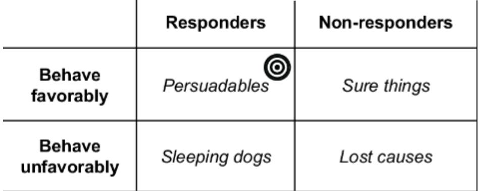
Figure 8.5 In attempts to influence behavior, we break down the target population into these four segments. Given limited resources, we want to target our influence efforts on the persuadables and avoid the others, especially the sleeping dogs.

Promotions have a cost in terms of the additional value you give to the subscriber. You want to avoid spending that cost on subscribers who weren’t going to churn (sure things) and subscribers who were always going to churn (lost causes). And you definitely want to avoid spending that cost only to cause someone to churn (sleeping dogs). So, of these four groups, you want to send your promotions only to the persuadables. The task of statistical analysis is to segment our users into these four groups.

This is where counterfactuals can help us; we can define each segment in probabilistic counterfactual terms:

• Lost causes —People who probably would churn if we send a promotion and still churn if we did not send a promotion; i.e., P(YX=1=0, YX=0=0) is high.
• Sure things —People who probably would stay if we send a promotion and stay if we did not send a promotion; i.e., P(YX=1=1, YX=0=1) is high.
• Persuadables —People who probably would stay if we send a promotion and churn if we did not send a

promotion; i.e., P(YX=1=1, YX=0=0) is high. In other words, PNS is high.

Sleeping dogs —People who probably would churn if we send a promotion and would stay if we did not send a promotion; i.e., P(YX=1=0, YX=0=1) is high.

You can see, in figure 8.6, how the population can be segmented.

	Responders	Non-responders
Behave favorably		P(Yx=1=1, Yx=0=0) P(Yx=1=1, Yx=0=1)
Behave unfavorably		P(Yx=1=0, Yx=0=1) P(Yx=1=0, Yx=0=0)

			Figure 8.6 We can segment the population in counterfactual terms.

USING COUNTERFACTUALS FOR SEGMENTATION

Each subscriber has some set of attributes (demographics, usage habits, content preferences, etc.). Our goal is to convert these attributes to predict whether a subscriber is a persuadable, sleeping dog, lost cause, or sure thing.

Let C represent a set of subscriber attributes. Given a subscriber with attributes C=c, our causal query of interest is P(YX=1, YX=0|C=c). Various statistical segmentation methods seek to define C such that users fall into groups that have high probability for one of the four outcomes of P(YX=1, YX=0|C=c), but before we apply the stats, our first task will be to ensure we can estimate this query using sufficient assumptions and data. We’ll cover how to estimate

counterfactuals with SCMs in chapter 9 and how to use identification with broader estimation techniques in chapter 10.

Now that we’ve learned to pose our causal query and formalize it into math, let’s revisit the steps of making the counterfactual inference, in figure 8.7.

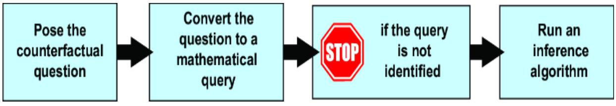
Figure 8.7 The counterfactual inference workflow

In the next section, we’ll study the idea of possible worlds and parallel world graphs. These ideas are important to both identification (determining whether we can answer the question) and the inference algorithm.

8.4 Possible worlds and parallel world graphs

In this section, I’ll introduce the notion of possible worlds and parallel world graphs, an extension of a causal DAG for an SCM that supports counterfactual reasoning across possible worlds.

8.4.1 Potential outcomes in possible worlds

Counterfactual reasoning involves reasoning over possible worlds. A possible world is a way the world is or could be. The actual world is the possible world with the event outcomes we observed. All other possible worlds are hypothetical worlds.

In terms of the data generating process (DGP), the actual world is how the DGP unrolled to produce our data. Other possible worlds are defined by all the ways the DGP could have produced different data.

Potential outcomes are a fundamental concept in causal effect inference. ૿Potential outcomes refers to outcomes of the same variable across differing possible worlds. If you have a headache and take an aspirin, you might say there are two potential outcomes in two possible worlds: one where your headache gets better and one where it doesn’t.

REVIEW OF POSSIBLE WORLD TERMINOLOGY

Possible world—A way the world is or could be

Actual world—A possible world with observed event outcomes

Hypothetical world—A possible world with no observed event outcomes

Potential outcomes—Outcomes of the same variable across differing possible worlds

Parallel worlds—A set of possible worlds being reasoned over, sharing both common and differing attributes

Parallel world graph—A graphical representation of parallel worlds used both for identifying counterfactual queries and in counterfactual inference algorithms

8.4.2 The parallel world graph

A parallel world graph is a simple extension of a causal DAG that captures causality across possible worlds. Continuing with the online gaming example, suppose we are interested in the question, ૿For a player who had low engagement and less than $50 of in-game purchases, what would their level of in-game purchases be if their level of engagement was high? I.e., P(IE=૿high|E=૿low, I<50). For this counterfactual query, we can visualize both the actual and the hypothetical worlds in figure 8.8

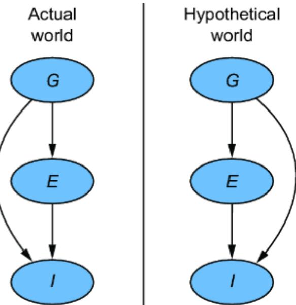
Figure 8.8 To answer the counterfactual query for the online gaming example, we start by duplicating the causal DAG across possible worlds.

We duplicate the causal DAG for the online gaming example across both possible worlds. Having one DAG for each world reflects that the causal structure of the DGP is the same in each world. But we’ll need to connect these DAGs in some way to reason across worlds.

We’ll connect the two worlds using an SCM defined on the causal DAG. We’ll suppose that the original nodes of the DAG are the endogenous variables of the SCM and expand the DAG visualization by adding the exogenous variables. Further, the two causal DAGs will use the same exogenous nodes. We call the resulting graph a parallel world graph (or, for this typical case of two possible worlds, a ૿twin-world graph). Figure 8.9 visualizes the parallel world graph.

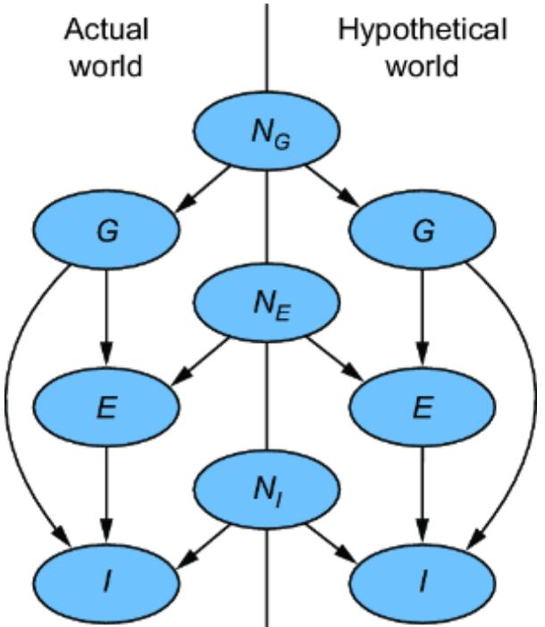
Figure 8.9 In the parallel world graph, we use the exogenous variables in an SCM to unite the duplicate causal DAGs across worlds. The result is a single SCM with duplicate endogenous variables.

REFRESHER: THE STRUCTURAL CAUSAL MODEL (SCM)

An SCM is a causal model with the following components:

• Endogenous variables—Endogenous variables are the variables we specifically want to model.
• Exogenous variables—A set of exogenous variables. Exogenous variables are proxies for all the causes of our endogenous variables we don’t wish to model explicitly. In our formulation, we pair each endogenous variable X with a single exogenous variable NX (there are more general formulations).
• Exogenous distributions—To use the SCM as a generative model, we need a set of marginal probability distributions for each exogenous variable, such as P(NX), which represents the modeler’s uncertainty about the values NX.
• Functional assignments—Each endogenous variable has a functional assignment that sets its value deterministically, given its parents.

For example, written as a generative model, an SCM for our online game model would look as follows.

\[\begin{aligned} n\_G &\sim P(N\_G) \\ n\_E &\sim P(N\_E) \\ n\_I &\sim P(N\_I) \\ \mathbf{g} &= f(n\_G) \\ e &= f(\mathbf{g}, n\_E) \\ i &= f(e, \mathbf{g}, n\_I) \end{aligned}\]

The assignment functions induce the causal DAG; each variable is a node, the exogenous variables are root nodes, and the inputs of a variable’s assignment function correspond to its parents in the DAG. The SCM is a particular case of a causal graphical model where endogenous variables are set by deterministic functions rather than sampled from causal Markov kernels.

The result is a single SCM with one shared set of exogenous variables and duplicate sets of endogenous variables—one set for each possible world. Note that in an SCM, the endogenous variables are set deterministically, given the exogenous variables. So upon observing that E = ૿low and I   < 50 in the actual world, we know that the hypothetical outcomes of E and I must be the same. Indeed, even though Guild Membership (G ) is a latent variable in the actual world, we know that whatever value G takes in the actual world must be the same as in the hypothetical world. In other words, our SCM upholds the consistency rule, as illustrated in figure 8.10. In figure 8.10, the E and I in the actual world are observed variables because we condition on them in the query P (IE=૿high|E = ૿low, I < 50).

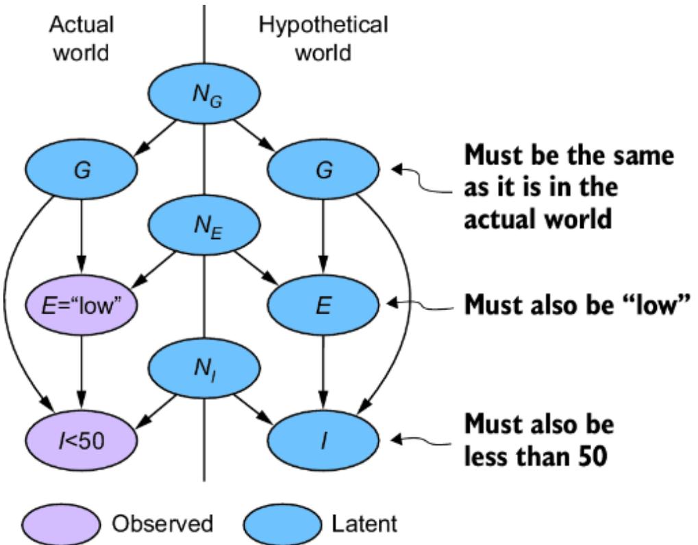
Figure 8.10 In an SCM, the endogenous variables are set deterministically, given the exogenous variables. In this model, the endogenous variables are duplicated across worlds. Therefore, upon observing low engagement and less than $50 of in-game purchases in the actual world, we know that those values must be the same in the hypothetical world unless we change something in the hypothetical world.

8.4.3 Applying the hypothetical condition via graph surgery

The hypothetical world will, typically, differ from the actual world by the hypothetical condition. For example, in P (IE=૿high|E = ૿low, I < 50), ૿if engagement were high (E=૿high) differs from the factual condition ૿engagement was low (E = ૿low). As we’ve discussed, we model the hypothetical condition with the ideal intervention—we intervene on E, setting it to ૿high in the hypothetical world. We model the ideal intervention on the graph with graph

surgery—we’ll remove incoming edges to the E variable in the hypothetical world as in figure 8.11.

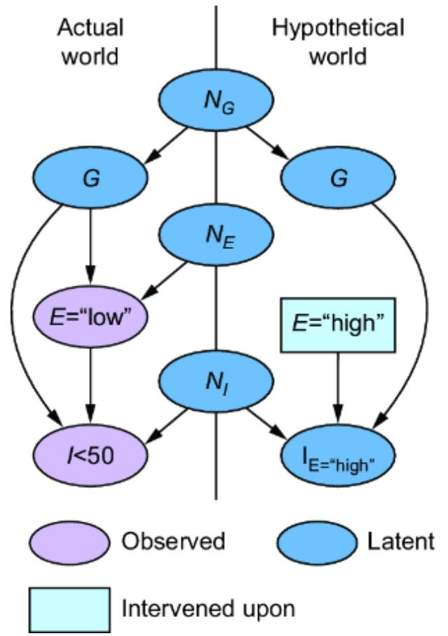
Figure 8.11 The ideal intervention and graph surgery represents the hypothetical condition in the hypothetical world. In this setting, the outcome for I in the hypothetical world can now take a different outcome than it has in the actual world because its parent E has a different outcome than it has in the actual world.

Now the outcome for In-Game Purchases (I  ) in the hypothetical world can take a different outcome than the actual world’s outcome of I = 50 because its causal parent E has different outcomes in each world.

8.4.4 Reasoning across more than two possible worlds

The counterfactual notation and the parallel worlds graph formalism support counterfactual reasoning that extends across more than two possible worlds. To illustrate, let’s refer back to the Netflix example at the beginning of the chapter. Summarizing the story, the key variables in that narrative are as follows:

• Disney is trying to close a deal to buy the Bond franchise. Let B = ૿success if the deal closes. Otherwise, B = ૿fail.
• Netflix is trying to close a deal to start a new spy franchise called Dead Drop. D = ૿success if the Dead Drop deal closes and ૿fail otherwise. If the Bond deal closes, it will affect the terms of this deal. Therefore, B causes D.
• If the Dead Drop deal closes, it will affect engagement in spy-thriller-related content on Netflix. Let E = ૿high if a subscriber’s engagement in Netflix’s spy-thriller content is high and ૿low otherwise.
• The outcome of the Bond deal and the Dead Drop deal will both affect the attrition of spy-thriller fans to Disney. Let A be the rate of attrition to Disney.

With this case study, the following multi-world counterfactual is plausible. Suppose the Bond deal was successful (B = ૿success), but Netflix’s Dead Drop deal failed, and as a result, engagement was low (E = ૿low) and Netflix attrition to Disney is 10 percent. Figure 8.12 illustrates this actual world outcome.

As a Netflix executive, you start wondering about attribution. You assume that engagement would have been high if the

Dead Drop deal had been successful. You ask the following counterfactual question:

Disney’s Bond deal succeeded, the Dead Drop deal failed, and as a result, Netflix’s spy thriller engagement was low, and attrition to Disney was 10%. I assume that had the Dead Drop deal been successful, engagement would have been high. In that case, how much attribution would there have been?

We can implement this assumption with world 2 in the parallel world graph in figure 8.13.

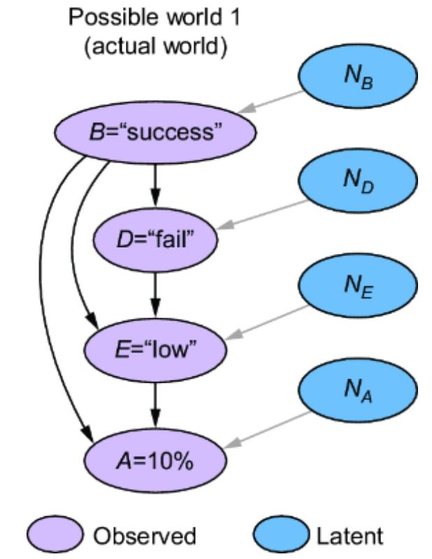
Figure 8.12 A causal DAG representing the Netflix case study. The light gray nodes are observed outcomes in the actual world. The dark nodes are latent variables.

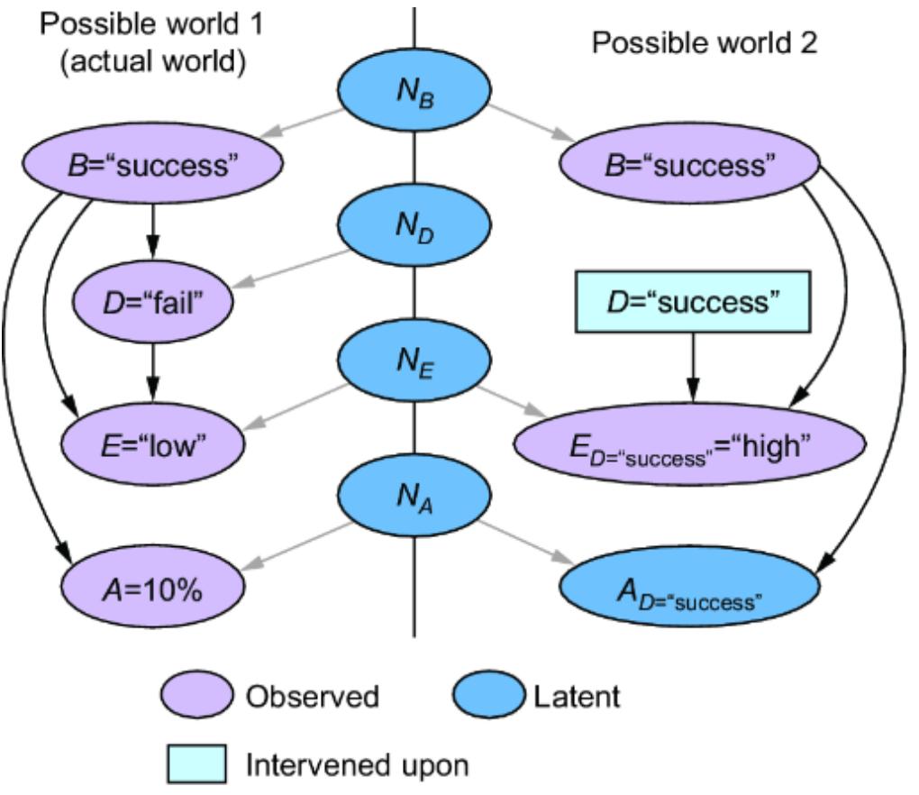
Finally, you wonder what the level of Netflix attrition would be if the Bond deal had failed. But you wonder this based on your second-world assumption that engagement would be high if the Dead Drop deal had been successful. Since the Bond deal failing is a hypothetical condition that conflicts with the Bond deal success condition in the second world, you need a third world, as illustrated in figure 8.14.

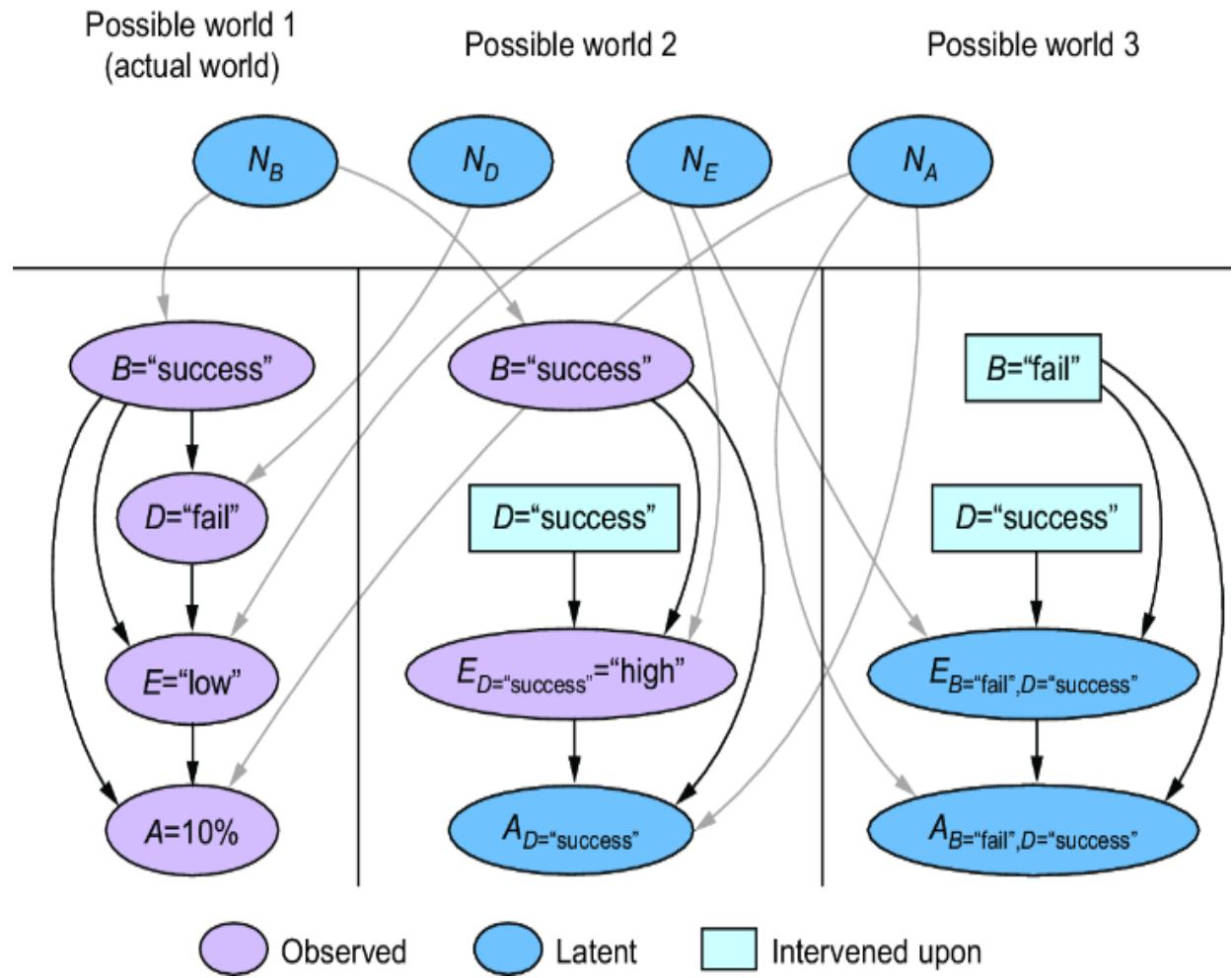
Figure 8.14 Given the actual outcomes in world 1, the hypothetical conditions and outcomes in world 2, you pose conditions in world 3 and reason about attrition in world 3.

In summary, this is the counterfactual question:

Disney’s Bond deal succeeded, the Dead Drop deal failed, and as a result, Netflix’s spy thriller engagement was low, and attrition to Disney was 10%. I assume that had the Dead Drop deal been successful, engagement would have been high. In that case, how much attribution would there have been if the Bond deal had failed?

Note that the preceding reasoning is different from the following:

Disney’s Bond deal succeeded, the Dead Drop deal failed, and as a result, Netflix’s spy thriller engagement was low, and attrition to Disney was 10%. I assume that had the Dead Drop deal been successful and the Bond deal failed, engagement would have been high. In that case, how much attribution would there have been?

Figure 8.15 illustrates the latter question.

Figure 8.15 In the case of assuming EB=૿fail,D=૿success, only two worlds are needed.

The latter question assumes engagement would be high if the Bond deal failed and the Dead Drop deal was successful (EB=૿fail, D=૿success=૿high). In contrast, the former ૿three world question assumes engagement would be high if both deals were successful. Then, in the third world, It allows for

different possible levels of engagement in the hypothetical scenario where the Bond deal failed. For example, perhaps engagement would be high since Netflix would have its spythriller franchise and Disney wouldn’t. Or perhaps, without a Bond reboot there would be less overall interest in spythrillers, resulting in low engagement in Dead Drop.

8.4.5 Rule of thumb: Hypothetical worlds should be simpler

Consider again the endogenous nodes in our online gaming example in figure 8.16. Notice that, in this example, the two worlds have the same sets of endogenous nodes, and the edges in the hypothetical world are a subset of the edges of those in the actual world. In other words, the possible world where we do intervene is simpler than the possible world where we condition on evidence.

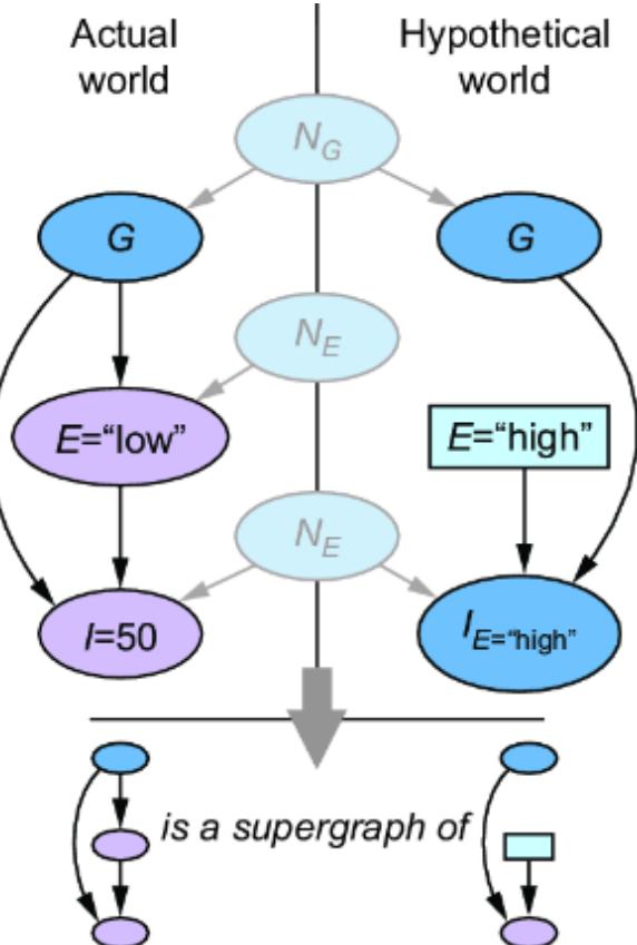
Figure 8.16 The graph representing the possible world with the hypothetical conditional is simpler than the graph representing the actual world.

Similarly, in the three-world graph for the Netflix case study, world 3 is a subgraph of world 2, which is a subgraph of world 1. As an algorithmic rule of thumb, it is useful to have this descending ordering on possible worlds. This rule of thumb reduces the risk of algorithmic instability.

That said, there are use cases for having more complicated hypothetical worlds. For example, a modeler could introduce new nodes as conditions in the hypothetical world. Or they could use stochastic interventions that randomly introduce new edges in the hypothetical world. Indeed, human counterfactual reasoning can be quite imaginative. Exploring such approaches could lead to interesting new algorithms for causal AI.

In the next chapter, we’ll dive into using parallel world graphs in an algorithm for general counterfactual inference.

Summary

• Counterfactual statements describe hypothetical events that potentially conflict with actual events. They are fundamental to defining causality.
• Counterfactual reasoning supports learning policies for better decision-making.
• Counterfactual reasoning involves reasoning over possible worlds. A possible world is a way the world is or could be. The actual world is a possible world with event outcomes we observed. Other possible worlds are hypothetical worlds.
• In machine learning, often the goal is counterfactual analysis of a machine learning model itself. Here, we reason about how a prediction would have been different if elements of the input feature vector were different.
• Counterfactual analysis in classification can help find the minimal change in features that would have led to a different classification.
• Counterfactual analysis supports explainable AI by helping identify changes to features that would have changed the prediction outcome on a case-by-case basis.
• Counterfactual analysis supports algorithmic recourse by identifying actionable changes to features that would change the prediction outcome.
• Counterfactual analysis supports AI fairness by identifying features corresponding to protected attributes where changes to said features would change the prediction outcome.
• ૿Potential outcomes is a commonly used term that refers to outcomes for a given variable from across

possible worlds.

• We can use the ideal intervention and parallel world graphs to model hypothetical conditions in natural language counterfactual statements and questions.
• Counterfactual notation helps represent hypothetical statements and questions in the language of probability. Probability can be used to quantify uncertainty about the truth of hypothetical statements and questions, including counterfactuals.
• Using hypothetical language rather than declarative language helps with formalizing a counterfactual statement or question into counterfactual notation. Using hypothetical language implies imagined possibility, and thus uncertainty, which invites us to think about the probability of a hypothetical statement being true.
• Binary counterfactual queries refer to queries on variables (hypothetical conditions and outcomes) that are binary.
• The probabilities of causation, such as the probability of necessity (PN), probability of sufficiency (PS), and probability of necessity and sufficiency (PNS), are binary counterfactual queries that are useful as primitives in causal attribution methods and other types of advanced causal queries.
• Binary counterfactual queries are also useful for distinguishing between ૿persuadables, ૿sure things, ૿lost causes, and ૿sleeping dogs in uplift modeling problems.
• A parallel world graph is a simple extension of a causal DAG that captures causality across possible worlds. It represents an SCM over possible worlds that share a common set of exogenous variables and duplicate sets of endogenous variables.

9 The general counterfactual inference algorithm

This chapter covers

• Implementing the general counterfactual inference algorithm
• Directly implementing a parallel world DAG as a causal graphical model
• Using a variational inference to implement the algorithm
• Building counterfactual deep generative models of images

The previous chapter taught you how to formalize counterfactuals and use the parallel world graph to reason across possible worlds. In this chapter, I’ll introduce an algorithm for inferring counterfactual queries. Then I’ll present three case studies showing implementations of the algorithm using different probabilistic ML approaches.

I call the algorithm we’ll discuss in this chapter the ૿general algorithm for probabilistic counterfactual inference because you can infer any counterfactual query with this algorithm. The catch is that you need an SCM. Moreover, differences between your SCM and the ground-truth SCM can lead to inaccuracies in your counterfactual inferences. We’ll look more closely at this issue when we discuss identification in chapter 10, where you’ll also learn ways of inferring counterfactuals without knowing the ground-truth SCM. In

this chapter, you’ll see the power of this SCM-based approach, especially in machine learning.

9.1 Algorithm walkthrough

In this section, we’ll do a high-level walkthrough of the general algorithm probabilistic counterfactual inference. The algorithm has three steps commonly called abduction, action, and prediction:

• 1. Abduction —Infer the distribution of the exogenous variables given the factual conditions.
• 2. Action —Implement the hypothetical condition as an ideal intervention (graph surgery) in the hypothetical world.
• 3. Prediction —Use the conditional distribution on the exogenous variables from step 1 to derive the distributions of the hypothetical outcomes.

I’ll illustrate how we can perform these steps using the parallel world graph for our online gaming example, shown again as a parallel world graph in figure 9.1.

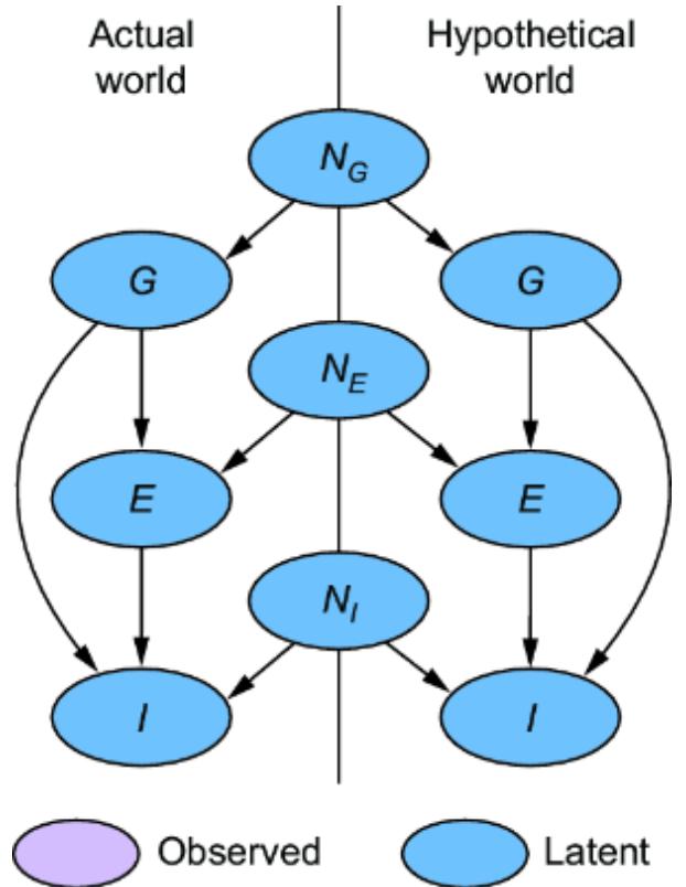
Figure 9.1 A parallel world graph for the online gaming example

Recall that in this example, guild member G is a cause of side-quest engagement E and in-game purchases I. Sidequest engagement is also a cause of in-game purchases.

Note This example changes the condition I < $50 used in chapter 8 to I = $50 in order to make the explanations a bit less verbose. Either condition would work with the algorithm we’re discussing.

Let’s suppose our counterfactual question is ૿For a player with low side-quest engagement and $50 of in-game purchases, what would their level of in-game purchases be if their side-quest engagement were high? The corresponding query is P(IE =૿high|E=૿low, I=50). Let’s examine how to apply the algorithm to this query.

9.1.1 Abduction: Infer the exogenous variables given the observed endogenous variables

The term ૿abduction refers to doing abductive inference, meaning we’re inferring causes from observed outcomes. In our online gaming SCM, we want to infer the latent exogenous variables (NG, NE, and NI ) from the factual conditions (E=૿low and I=50).

In our probabilistic modeling approach, we treat the exogenous variables as latent variables and target them with probabilistic inference. In our example, we infer NE from observing E=૿low. Figures 9.2 and 9.3 illustrate the dconnected paths to inference of NG and NI , respectively.

As you can see in figure 9.2, we have a path from E to NG through the path E←G←NG. Further, observing both E and I opens a collider path to NG: E→I←G←NG. Similarly, in figure 9.3, observing E and I also opens a collider path to NI via E→I←NI .

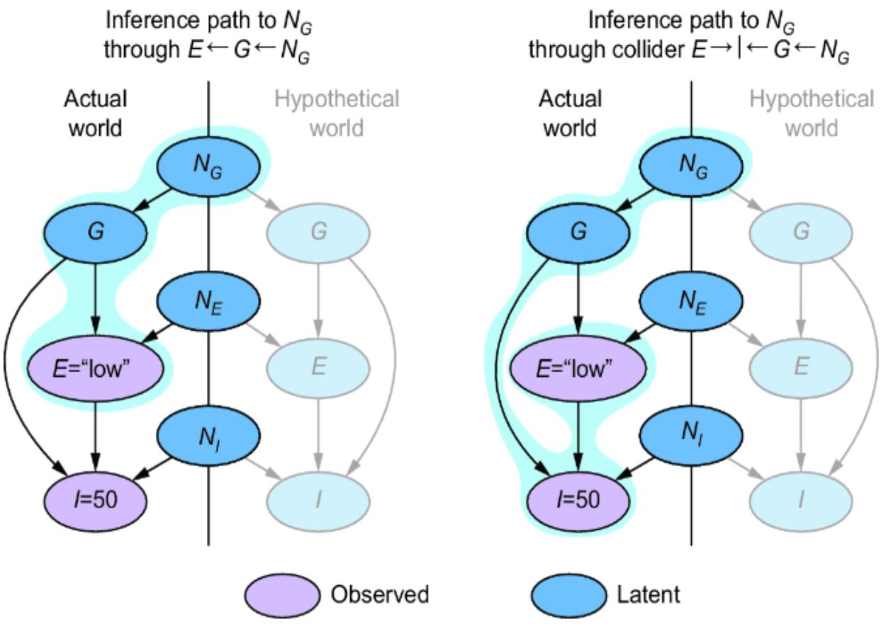
Figure 9.2 To infer the counterfactual outcomes, we infer the exogenous variables conditional on observed outcomes in the actual world. There is a path from E to NG through the path E←G←NG. Also, observing E and I opens a collider path E→I←G←NG.

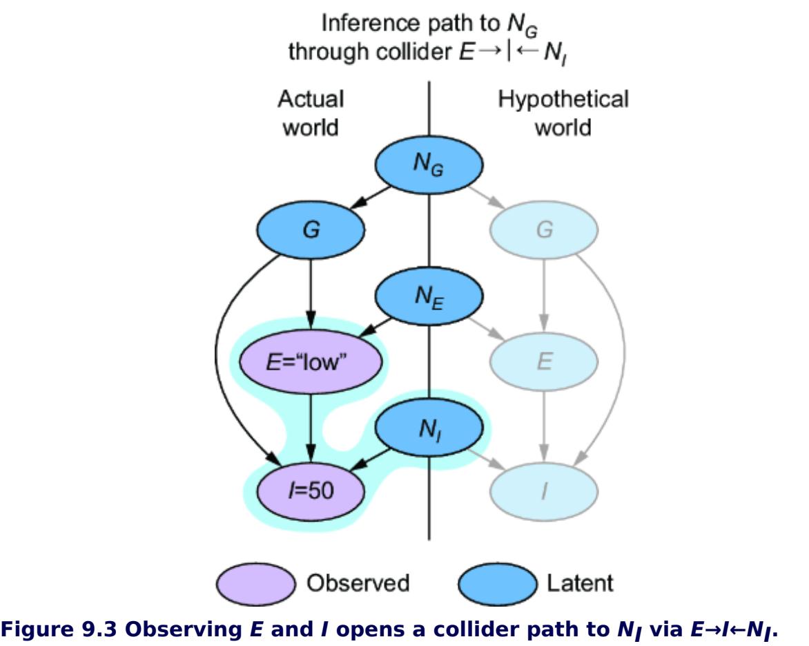
Finally, observing E has a directly connecting path to NE, as shown in figure 9.4.

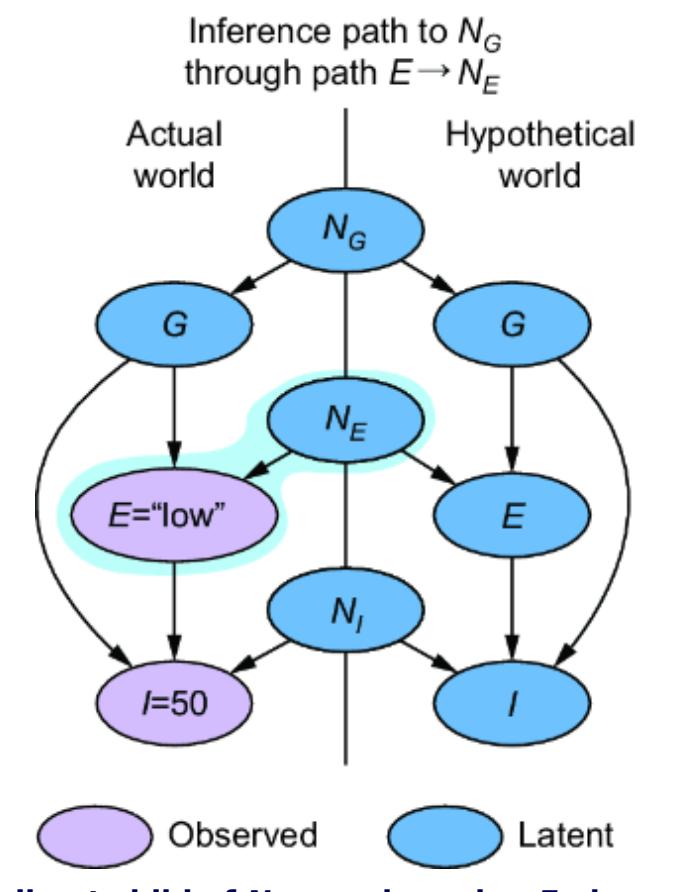
Figure 9.4 E is a direct child of NE, so observing E gives direct information about NE.

Our SCM is a probabilistic model. In the abduction step, we use this model to infer P (NG, NE, NI | E = ૿low, I = 50). That inference will follow these paths of dependence.

9.1.2 Action: Implementing the hypothetical causes

Recall from chapter 8 that we use the ideal intervention to implement hypothetical conditions. Our hypothetical condition is ૿if their side-quest engagement were high, and we implement this with an ideal intervention that sets E to ૿high in the hypothetical world. Since we’re using a graph, we implement the intervention with graph surgery as in figure 9.5.

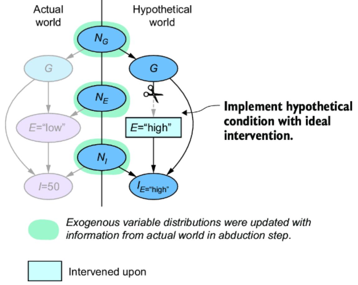
Figure 9.5 Implement the hypothetical condition as an ideal intervention (via graph surgery) in the hypothetical world.

Now the parallel worlds differ. Note that the probability distributions on the exogenous variables have been updated with information from the actual world during the abduction step. In the final step, we’ll propagate this information through this modified hypothetical world.

9.1.3 Prediction: Inferring hypothetical outcomes

We’re working with an SCM, so the values of the variables in the hypothetical world are set deterministically by the exogenous variables. Having updated the exogenous variable distributions conditional on observations in the actual world, we’ll now propagate that actual world

information from the exogenous variables to the endogenous variables in the hypothetical world. If we hadn’t applied the intervention in the hypothetical world, the hypothetical world would mirror everything we observed in the actual world by the law of consistency (see the definition in chapter 8). However, since we applied an intervention in the hypothetical world, the hypothetical variable distributions downstream of that intervention can differ from those in the actual world.

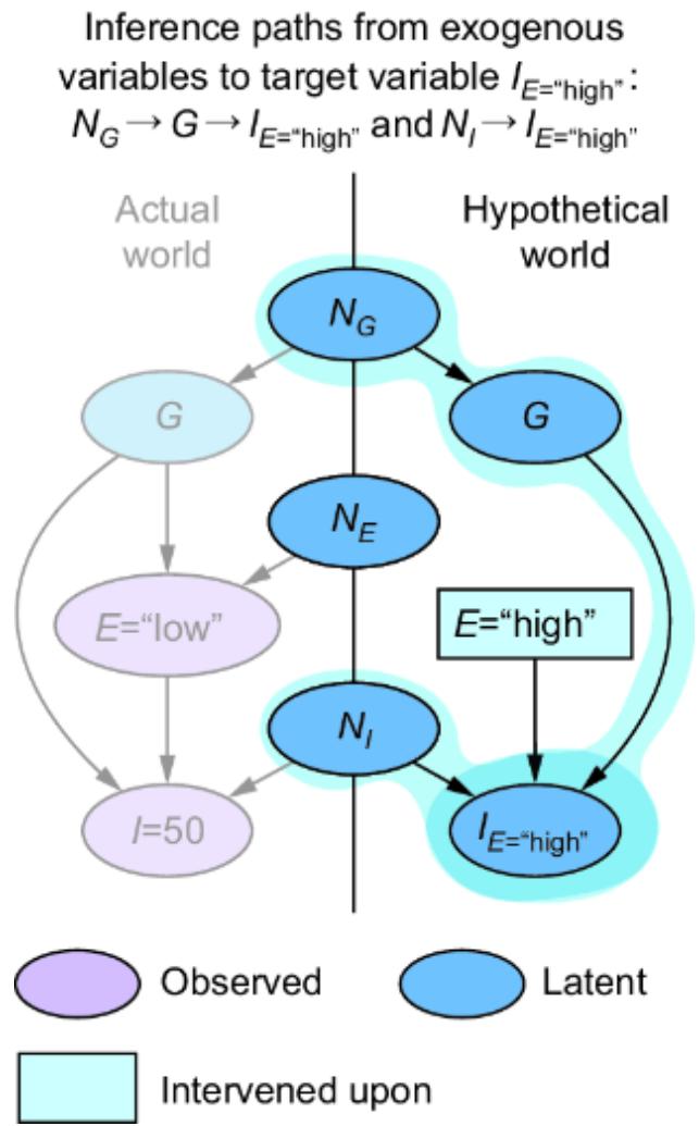
Figure 9.6 Paths for inferring the hypothetical distribution of I from the conditional distribution P(NG, NE, NI| E=૿low, I=50) on the exogenous variables, given the observed actual world outcomes

In our gaming example, our query P (IE=૿high|E = ૿low, I = 50) targets the hypothetical value of IE=૿high. Figure 9.6 illustrates the path of inference from the exogenous variables to the hypothetical value of IE ⁼ ૿high. Note that in this example, the paths of influence only come from NG and NI , since the intervention on E cut NE’s bridge to the hypothetical world.

BE CAREFUL ABOUT D-CONNECTION AND D-SEPARATION ON PARALLEL WORLD GRAPHS

Recall that with a causal DAG, we can use a graphical criterion called d-separation/d-connection to reason about conditional independence in the data generating process using a causal DAG. Indeed, this is what I do when I highlight paths of inference to IE=૿high given E and I via NI and NG. I do this to explain the abduction and prediction steps of the algorithm. However, in general, one cannot rely on d-separation and d-connection to reason about the dependence between endogenous variables across worlds. That’s because the law of consistency requires that the same endogenous variables across worlds must have the same value (unless one of the pairs is impacted by an intervention). Two variables always having the same value is a perfect dependence; the rules of d-separation do not capture that dependence on the parallel world graph.

In the next chapter, I’ll introduce counterfactual graphs, a causal DAG derived from a parallel world graph where the connections between d-separation and independence hold across worlds.

We can see how information flows during inference from factual conditions E=૿low and I=50 in the actual world, through the exogenous variables, to our target variable IE=૿high in the hypothetical world. How we implement the inference depends on our preference for inference algorithms. For example, suppose fG, and fI represent the SCM’s assignment functions for G and I. We could use a simple forward-sampling algorithm:

• 1. Draw a sample of exogenous values nG, nE, and nI from P (NG, NE, NI | E = ૿low, I = 50).
• 2. Derive a sample of the hypothetical value of guild membership g * = fG(nG).
• 3. Derive a sample of the hypothetical value of in-game purchases i * = fI (E = ૿high, g * , nI ).
• 4. Repeat many times to get samples from the distribution P (IE=૿high|E = ૿low, I = 50).
• 5. This would give us samples from our target P (IE=૿high|E = ૿low, I = 50).

9.1.4 Counterfactual Monte Carlo

The output of the general probabilistic counterfactual inference algorithm produces samples from a distribution. Recall from chapter 2 that once you can sample from a distribution, you can apply the Monte Carlo techniques to make inferences based on that distribution. That same is true with counterfactual distributions.

For example, in chapter 8, I introduced the idea of regret, where we compare counterfactual outcomes. For our player who had low engagement and only spent $50, we might ask how much more their in-game purchases would have been had engagement been high. Given the gamer spent $50, we can define a regret variable as RE=e = IE=e – 50. By taking

our samples from P (IE=૿high |E = ૿low, I = 50) and subtracting 50, we get samples from P (RE=૿high |E=૿low, I = 50). We can also take the average of those differences to estimate expected regret E (RE=૿high |E = ૿low, I = 50). Note that E (…) here refers to the expectation operator, not to side-quest engagement.

When we want to use these counterfactual Monte Carlo techniques in automated decision-making algorithms, we are typically posing counterfactual questions about policies. Suppose, for example, a recommendation algorithm recommends certain content to a player based on their profile. We can contrast the amount of in-game purchases they made under one recommendation policy to the amount they would have made under a different policy. We can then adjust the recommendation algorithm in a way that would have minimized cumulative regret across players. We’ll look at automated decision-making more closely in chapter 12.

Next, we’ll explore a few case studies of various ways to implement this algorithm in code.

9.1.5 Introduction to the case studies

There are several ways we can implement this algorithm using modern probabilistic ML tools. In sections 9.2–9.4, we’ll explore three case studies.

MONTY HALL PROBLEM

The first case study will focus on the Monty Hall problem discussed earlier in section 6.3. We’ll use the pgmpy library to implement a full parallel-world graphical SCM. We’ll use pgmpy’s TabularCPD to implement SCM assignment functions, something it wasn’t designed to do. In exchange for this

awkwardness, we’ll be able to leverage pgmpy’s graphbased inference algorithm (VariableElimination) to collapse the abduction and prediction steps into one inference step. Using graph-based inference will save us from implementing an inference algorithm for abduction; we only have to build the model, apply the action step, and run inference.

FEMUR LENGTH AND HEIGHT

Next, we’ll revisit the forensics example from section 6.1, where we have an SCM in which femur length is a cause of height. This example will show us how to do the abduction step with variational inference, a modern and popular probabilistic inference technique that works well with cutting-edge deep learning frameworks.

In this example, we’ll implement the SCM in Pyro, a PyTorchbased library for probabilistic ML. Using Pyro will feel less awkward than pgmpy because Pyro modeling abstractions are more flexible. The trade-off is that we must write explicit inference code for the abduction step.

The example is simple: the data is small, each variable has only one dimension, and the relationships are linear. However, we can use the same variational inference-based abduction technique with the large, high-dimensional, and nonlinear data settings where variational inference shines.

SEMANTIC IMAGE EDITING WITH COUNTERFACTUALS

In the final case study, we’ll examine how we’d apply the counterfactual inference algorithm using a pretrained generative image model in PyTorch. While the Monty Hall and femur length problems are simple problems with simple math, this case study demonstrates the use of the algorithm

on a modern problem with image generation in deep generative AI.

9.2 Case study 1: Monty Hall problem

We’ll start by revisiting the SCM for the Monty Hall problem. Summarizing again, there is a game show where the player starts with a choice of three doors. Behind one door is a car. The player picks a door, say the first door, and the host, who knows what’s behind the doors, opens another door, say the third, which does not have the car. The host gives the player the opportunity to switch doors. In this case, since the player picked the first door and the host revealed that the car is not behind the third door, the player can switch to the second door. The question is whether a strategy of staying with the original choice or switching doors is better.

The answer is, counterintuitively to many, that a switching strategy is better—two times out of three, the switching strategy leads to a win. Figure 9.7 illustrates the possible outcomes of switching.

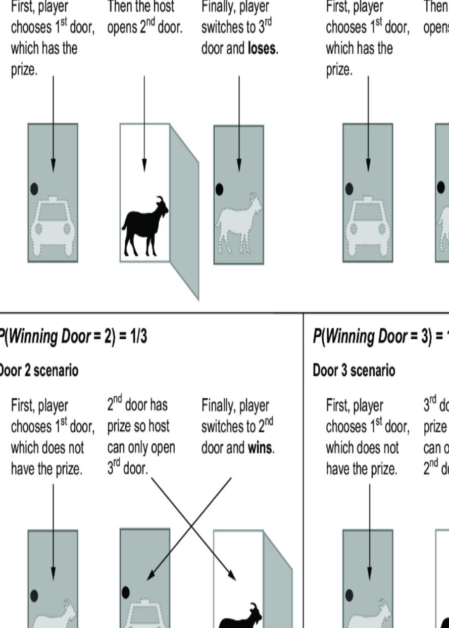
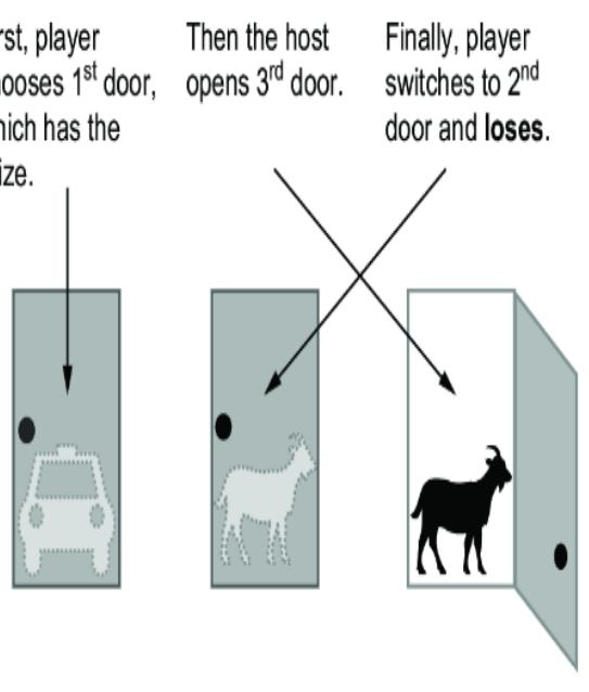
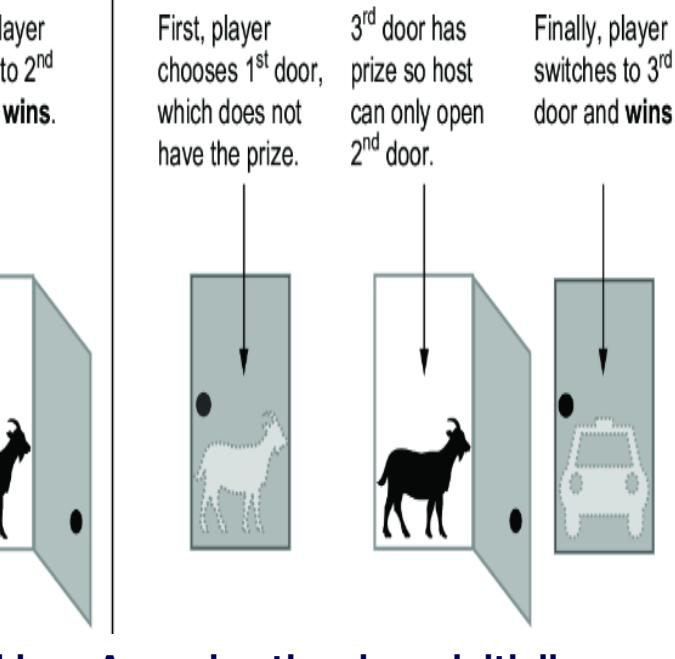
Figure 9.7 The Monty Hall problem. Assuming the player initially chooses the first door, two out of three times the switching strategy will lead to a win. This illustration assumes the first door is chosen, but the results are the same regardless of the initial choice of door.

We’ll explore two counterfactual questions:

• For a player who stayed with their first door and lost, what is the probability that they would have won if they switched doors?
• For a player who lost, what is the probability that they would have won if they switched doors?

We’ll answer these questions with the following steps:

• 1. Build the parallel world model as a generative graphical model in pgmpy.
• 2. Condition on evidence in one world to do inference of outcomes in the other.

Before we start, we’ll download some tools to help us with the analysis. Listing 9.1 downloads some helper functions for working with pgmpy: the do function for implementing ideal interventions and clone for duplicating a TabularCPD object. Also, to generate the visualizations, you’ll need to install the Graphviz visualization library.

SETTING UP YOUR ENVIRONMENT

The code in this chapter was tested with pgmpy version 0.1.25 and Pyro version 1.9.1. I use Matplotlib 3.7 for plotting. Plotting of the DAGs relies on Graphviz.

Graphviz installation depends on your environment. Using Ubuntu 22.04, I installed graphvizl via libgraphviz-dev, and then I installed the Python libraries Graphviz version 0.20.3, PyGraphviz version 1.13, and NetworkX version 3.3.

Depending on your environment, you may need to install pydot version 3.0. Graphviz and pydot are for plotting only, so if you get stuck, you could forgo plotting in the rest of the code.

Listing 9.1 Installing Graphviz and helper functions

import graphviz #1
import networkx as nx #1
from networkx.drawing.nx_agraph import write_dot #1
def plot_graph(G): #1
 dot_format = nx.nx_pydot.to_pydot(G).to_string() #1 
 return graphviz.Source(dot_format) #1
import requests #2
def download_code(url): #2
 response = requests.get(url) #2
 if response.status_code == 200: #2
 code_content = response.text #2
 print("Code fetched successfully.") #2
 return code_content #2
 else: #2
 print("Failed to fetch code.") #2
 return None #2
url_do = ( #3
 "https://raw.githubusercontent.com/altdeep/" #3
 "causalML/master/book/pgmpy_do.py" #3
) #3
code_do = download_code(url_do) #3
url_clone = ( #4
 "https://raw.githubusercontent.com/altdeep/" #4
 "causalML/master/book/chapter%209/hyp_function.py" #4
) #4
code_clone = download_code(url_clone) #4
print(code_do) #5
print(code_clone) #5
#exec(code_do) #5
#exec(code_clone) #5

#1 Install Graphviz libraries for visualization, and create a helper function for plotting graphs. This was tested in Ubuntu 22.04.3 but may depend on your environment. If you have trouble, you can forgo graph plotting and run the rest of the code.

#2 Helper function for downloading some utilities from GitHub #3 Download code for a ૿do function for applying ideal interventions. #4 Download code for a ૿clone helper function for cloning assignment functions across worlds.

#5 It’s good security practice to inspect the downloaded code before executing. Uncomment the ૿exec calls to execute the downloaded code.

Next, we’ll build the full parallel world model as a graphical model. Our first step is to specify the exogenous variable distributions.

9.2.1 Specifying the exogenous variables

We want to implement the model as an SCM, so we’ll create exogenous variables with distributions that entail all the random elements of the game. In other words, given the outcomes of these random elements and the host’s and player’s choices, the outcome of the game will be deterministic.

Specifically, we’ll introduce two rolls of three-sided dice and a coin flip. We’ll call the first die roll Car Door Die Roll; it selects a door for placement of the car. The player rolls the second die, a variable we’ll call 1st Choice Die Roll, to select the player’s first door selection. Both dice rolls assign a 1/3 probability to each outcome. Next, we have a coin flip, which we’ll just call Coin Flip, which I’ll explain shortly.

Listing 9.2 Model building: Specify distributions for exogenous variables

from pgmpy.factors.discrete.CPD import TabularCPD
p_door_with_car = TabularCPD( #1
 variable='Car Door Die Roll', #1
 variable_card=3, #1
 values=[[1/3], [1/3], [1/3]], #1
 state_names={'Car Door Die Roll': ['1st', '2nd', '3rd']} #1
) #1
p_player_first_choice = TabularCPD( #2
 variable='1st Choice Die Roll', #2
 variable_card=3, #2
 values=[[1/3], [1/3], [1/3]], #2
 state_names={'1st Choice Die Roll': ['1st', '2nd', '3rd']} #2
) #2
p_coin_flip = TabularCPD( #3
 variable='Coin Flip', #3
 variable_card=2, #3
 values=[[.5], [.5]], #3
 state_names={'Coin Flip': ['tails', 'heads']} #3
) #3

#1 Prior distribution on exogenous variable for the three-sided die roll that selects which door gets the car

#2 Prior distribution on the exogenous variable for the three-sided die roll that selects the player’s first choice of door

#3 Prior distribution on the exogenous variable for the coin flip. The host flips a coin that determines which door the host chooses to reveal as carless and whether the player chooses a stay or switch strategy.

Next, we’ll build assignment functions for our endogenous variables.

9.2.2 Specifying the assignment functions for the endogenous variables

Our endogenous variables will be Host Door Selection, Strategy (whether taking a switch or stay strategy), 2nd Choice (choosing door 1, 2, 3 based on one’s strategy), and Win or Lose (the outcome of the game).

Our definition of the SCM in chapter 6 assumes a one-to-one pairing between endogenous and exogenous variables—we typically make that assumption of independent exogenous variables because if we knew of a common cause, we’d

usually model it explicitly. Here, we’ll relax that assumption and match each exogenous variable to two endogenous variables:

• 1st Choice Die Roll will drive Host Door Selection and 2nd Choice
• Coin Flip will drive Host Door Selection and Strategy
• Car Door Die Roll will drive Host Door Selection and Win or Lose

We’ll use this simplified approach of matching one exogenous variable to two endogenous variables because it will require less code. This shortcut works well in this case because the exogenous variables precisely encode all the exogenous random elements of the game—these elements completely determine the game’s outcome. We could use the traditional formulation (where each endogenous variable has a unique exogenous variable) and get the same results.

Let’s walk through the steps of the game and then construct the DAG.

STRATEGY

The player will use Coin Flip as the basis of their Strategy decision—if the host flips heads, the player will adopt a switch door strategy. Otherwise, they’ll adopt a strategy of keeping their original choice.

Listing 9.3 Create the assignment function for Strategy

f_strategy = TabularCPD( 
 variable='Strategy', 
 variable_card=2, 
 values=[[1, 0], [0, 1]], 
 evidence=['Coin Flip'], 
 evidence_card=[2], 
 state_names={ 
 'Strategy': ['stay', 'switch'], 
 'Coin Flip': ['tails', 'heads']} 
)

HOST DOOR SELECTION

Host Door Selection depends on which door has the car (Car Door Die Roll) and the player’s initial choice of door (1st Choice Die Roll). The host will use Coin Flip to select a door from two available doors in the event that the winning door and the first choice door are the same. If Coin Flip is heads, they’ll choose the right-most door, otherwise the left-most.

Listing 9.4 Create the assignment function for Host Door Selection

f_host_door_selection = TabularCPD( 
 variable='Host Door Selection', 
 variable_card=3, 
 values=[ 
 [0,0,0,0,1,1,0,1,1,0,0,0,0,0,1,0,1,0], 
 [1,0,1,0,0,0,1,0,0,0,0,1,0,0,0,1,0,1], 
 [0,1,0,1,0,0,0,0,0,1,1,0,1,1,0,0,0,0] 
 ], 
 evidence=['Coin Flip', 
 'Car Door Die Roll', 
 '1st Choice Die Roll'], 
 evidence_card=[2, 3, 3], 
 state_names={ 
 'Host Door Selection':['1st', '2nd', '3rd'], 
 'Coin Flip': ['tails', 'heads'], 
 'Car Door Die Roll': ['1st', '2nd', '3rd'], 
 '1st Choice Die Roll': ['1st', '2nd', '3rd'] 
 } 
)

2ND CHOICE

2nd Choice, the player’s choice of which door to pick in the second round, depends on Strategy, Host Door Selection (the player can’t switch to the door the host opened), and 1st Choice Die Roll (the player must stay with or switch from the door selected in the first round).

Listing 9.5 Create an assignment function for 2nd Choice

f_second_choice = TabularCPD( 
 variable='2nd Choice', 
 variable_card=3, 
 values=[ 
 [1,0,0,1,0,0,1,0,0,0,0,0,0,0,1,0,1,0], 
 [0,1,0,0,1,0,0,1,0,1,0,1,0,1,0,1,0,1], 
 [0,0,1,0,0,1,0,0,1,0,1,0,1,0,0,0,0,0] 
 ], 
 evidence=['Strategy', 'Host Door Selection', 
 '1st Choice Die Roll'], 
 evidence_card=[2, 3, 3], 
 state_names={ 
 '2nd Choice': ['1st', '2nd', '3rd'], 
 'Strategy': ['stay', 'switch'], 
 'Host Door Selection': ['1st', '2nd', '3rd'], 
 '1st Choice Die Roll': ['1st', '2nd', '3rd'] 
 } 
)

WIN OR LOSE

Win or Lose depends on which door the player picked in 2nd Choice and whether that door is the winning door (Car Door Die Roll).

Listing 9.6 Create an assignment function for Win or Lose

f_win_or_lose = TabularCPD( 
 variable='Win or Lose', 
 variable_card=2, 
 values=[ 
 [1,0,0,0,1,0,0,0,1], 
 [0,1,1,1,0,1,1,1,0], 
 ], 
 evidence=['2nd Choice', 'Car Door Die Roll'], 
 evidence_card=[3, 3], 
 state_names={ 
 'Win or Lose': ['win', 'lose'], 
 '2nd Choice': ['1st', '2nd', '3rd'], 
 'Car Door Die Roll': ['1st', '2nd', '3rd'] 
 } 
)

With the exogenous variable distributions and the assignment functions complete, we can build the full parallel world graphical model.

9.2.3 Building the parallel world graphical model

We can now begin building the full parallel world model. First we’ll add the edges that are in the graph.

Listing 9.7 Build the parallel world graphical model
exogenous_vars = ["Car Door Die Roll", #1
 "Coin Flip", #1
               "1st Choice Die Roll"] #1
endogenous_vars = ["Host Door Selection", #1
 "Strategy", #1
                "2nd Choice", "Win or Lose"] #1
actual_world_edges = [ #2
 ('Coin Flip', 'Host Door Selection'), #2
 ('Coin Flip', 'Strategy'), #2
 ('Car Door Die Roll', 'Host Door Selection'), #2
 ('1st Choice Die Roll', 'Host Door Selection'), #2
 ('1st Choice Die Roll', '2nd Choice'), #2
 ('Host Door Selection', '2nd Choice'), #2
 ('Strategy', '2nd Choice'), #2
 ('2nd Choice', 'Win or Lose'), #2
 ('Car Door Die Roll', 'Win or Lose') #2
] #2
possible_world_edges = [ #3
 (a + " Hyp" if a in endogenous_vars else a, #3
 b + " Hyp" if b in endogenous_vars else b) #3
 for a, b in actual_world_edges #3
] #3

#1 Specify lists of the exogenous and endogenous variables in the causal DAG.

#2 Specify the edges of the SCM. #3 Clone the edges for the hypothetical world.

Next, we’ll compile and plot the graph.

Listing 9.8 Compiling and visualizing the parallel world graph

from pgmpy.models import BayesianNetwork
twin_world_graph = BayesianNetwork( #1
 actual_world_edges + #1
 possible_world_edges #1
) #1
twin_world_graph.add_cpds( #2
 p_door_with_car, #3
 p_player_first_choice, #3
 p_coin_flip, #3
 f_strategy, #4
 f_host_door_selection, #4
 f_second_choice, #4
 f_win_or_lose, #4
 clone(f_strategy), #5
 clone(f_host_door_selection), #5
 clone(f_second_choice), #5
 clone(f_win_or_lose), #5
)

plot_graph(twin_world_graph)

#1 Create the parallel world graph. #2 Plot the parallel world graph. #3 Add probability distributions on exogenous variables. #4 Add assignment functions from the SCM. #5 Clone the assignment functions.

The preceding code prints the parallel world graph in figure 9.8.

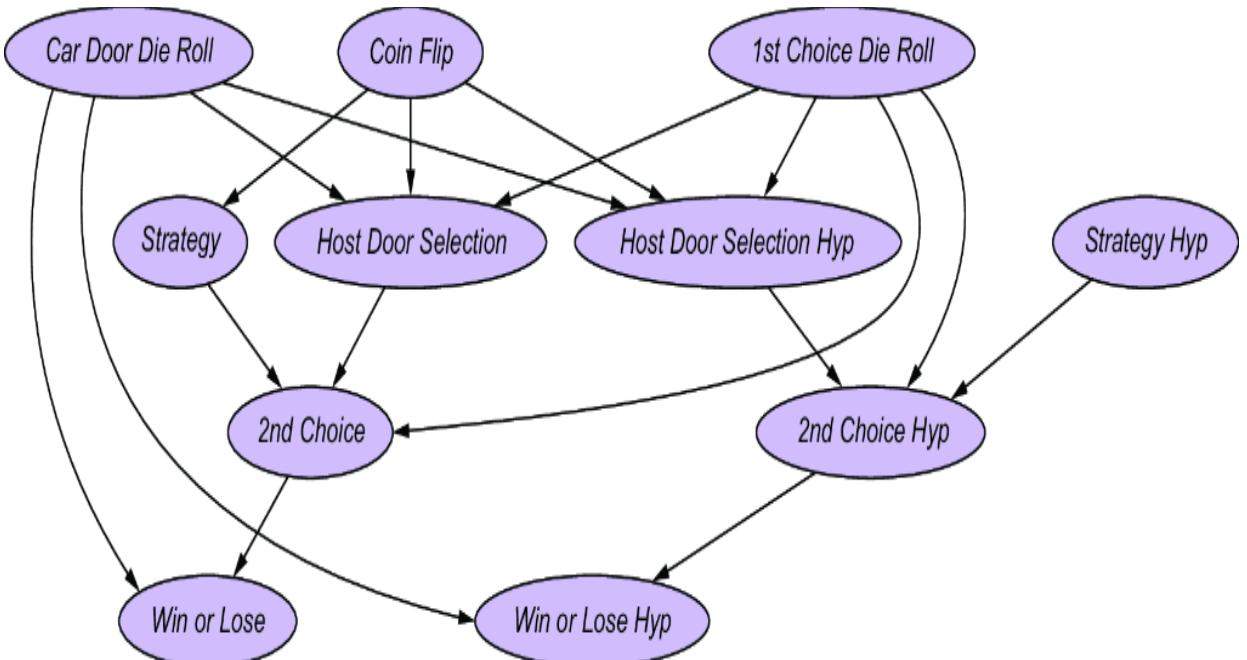
Figure 9.8 The full parallel world graph for our counterfactual question. Hypothetical world variables have the suffix ૿Hyp.

Before we answer our counterfactual questions, we’ll do a quick sanity check to confirm that our model can generate the result that the switching strategy leads to a win twothirds of the time.

Listing 9.9 Confirm correct probability of winning given a switch strategy

from pgmpy.inference import VariableElimination #1
infer = VariableElimination(twin_world_graph) #1
strategy_outcome = infer.query( #2
 ['Win or Lose'], #2
 evidence={"Strategy": "switch"} #2
) #2
print(strategy_outcome)

#1 Instantiate the inference algorithm with variable elimination. #2 Infer the probability distribution of ૿Win or Lose given that the player uses a switch strategy.

This prints the following table.

Win or Lose	+——————-+——————–+ phi(Win or Lose)
Win or Lose(win)	+===================+====================+ 0.6667 +——————-+——————–+
Win or Lose(lose)	0.3333 +——————-+——————–+

As we expect, we win two-thirds of the time when we adopt a strategy of switching doors.

9.2.4 Running the counterfactual inference algorithm

Finally, we’ll use inference to answer our counterfactual questions:

• For a player who stayed with their first door and lost, what is the probability that they would have won if they switched doors?
• For a player who lost, what is the probability that they would have won if they switched doors?

Again, we use variable elimination as our choice of inference algorithm. We’ll use the do function to do the action step and implement the hypothetical condition of switching. Then we’ll use the VariableElimination inference algorithm to do the abduction and prediction steps all in one go.

Listing 9.10 Infer the counterfactual distributions

cf_model = do(twin_world_graph, {'Strategy Hyp': 'switch'}) #1
infer = VariableElimination(cf_model) #2
cf_dist1 = infer.query( #3
 ['Win or Lose Hyp'], #3
 evidence={'Strategy': 'stay', 'Win or Lose': 'lose'} #3
) 
print(cf_dist1)
cf_dist2 = infer.query( #4
 ['Win or Lose Hyp'], #4
 evidence={'Win or Lose': 'lose'} #4
) 
print(cf_dist2)

#1 Action step: Set ૿Strategy Hyp to ૿switch using ૿do, an implementation of an ideal intervention.

#2 Apply variable elimination as our inference algorithm on the parallel world graph.

#3 This inference query answers ૿For a player who used the stay strategy and lost, would they have won if they used the switch strategy? Conditional on ૿Strategy == stay and ૿Win or Lose == lose, we infer the probability distribution of ૿Win or Lose Hyp on the parallel world graph.

#4 This inference query answers ૿For a player who lost, would they have won if they used the switch strategy? Conditional on ૿Win or Lose == lose, we infer the probability distribution of ૿Win or Lose Hyp on the parallel world graph.

For the question ૿For a player who stayed with their first door and lost, what is the probability that they would have won if they switched doors? we have the following probability table:

Win or Lose Hyp	+———————–+————————+ phi(Win or Lose Hyp) +=======================+========================+
Win or Lose Hyp(win)	1.0000 +———————–+————————+
Win or Lose Hyp(lose)	0.0000 +———————–+————————+

The result of the first question is obvious. If the player lost on a stay strategy, their first choice did not have the car. Therefore, one of the other two doors must have had the car. Of those two, the host would have had to open the one without the car. The remaining door would then have had the

car. That is the only door the player could switch to on a switch strategy. So, conditional on losing with a stay strategy, the chances they would have won with a switch strategy are 100%.

For the question ૿For a player who lost, what is the probability that they would have won if they switched doors? we have the following probability table:

Win or Lose Hyp	+———————–+————————+ phi(Win or Lose Hyp)
Win or Lose Hyp(win)	+=======================+========================+ 0.6667 +———————–+————————+
Win or Lose Hyp(lose)	0.3333 +———————–+————————+

The answer to the second question extends from the first. We know from the original results of the model that if a player lost, there is a 2/3 chance they used a stay strategy. As we saw from the first question, in this case, flipping to a switch strategy has a 100% chance of winning. There is a 1/3 chance it was a stay strategy, in which case, by the consistency rule, there is 100% chance of losing.

Using pgmpy’s graphical model inference algorithms enables counterfactual reasoning for discrete variable problems like the Monty Hall problem. In the next case study, we will solve the abduction step with variational inference, which generalizes to a broader class of problems and leverages modern deep learning.

9.3 Case study 2: Counterfactual variational inference

In this next case study, we’ll implement the counterfactual inference algorithm using a generative model in the PyTorchbased probabilistic modeling library Pyro. Here we’ll focus on the example of a forensic SCM where femur length is a cause of human height (discussed earlier in section 6.1).

In the Monty Hall example, all the variables were discrete, and the exogenous causes completely captured the game’s random elements. That allowed us to implement the SCM (albeit awkwardly) using TabularCPD for assignment functions in pgmpy, and then explicitly create a parallel world graphical model. Once that was accomplished, the graphical modeling inference algorithm VariableElimination handled the abduction and prediction steps for us.

In contrast, our second case study presents an approach that generalizes to more types of problems. We’ll use the PyTorch-based deep probabilistic modeling library Pyro. We’ll handle the abduction step using variational inference, a popular inference algorithm in the deep learning era.

In this example, we’ll use this modeling approach to contrast two questions:

• A conditional hypothetical: ૿What would an individual’s height be if their femur length was 46 cm? P(HF=46)
• A parallel-world counterfactual: ૿An individual’s femur is 44 cm, and their height is 165 cm. What would their height be if femur length was 46 cm? P(HF=46|F=44, H=165)

In both cases, we infer a distribution on HF=46 (where H is height and F is femur length), but in the counterfactual case, we condition on having observed F=44 and H=165. Implementing code that contrasts these two distributions on HF=46 will help us understand what makes counterfactual queries unique.

9.3.1 Building the model

To make things more interesting, we’ll modify the model by adding a variable for biological sex, which drives both femur length and height. Figure 9.9 illustrates the new causal DAG. Notice that our questions do not mention anything about sex, so we’ll expect to see sex-related variance in our distributions P(HF=46) and P(HF=46|F=44, H=165).

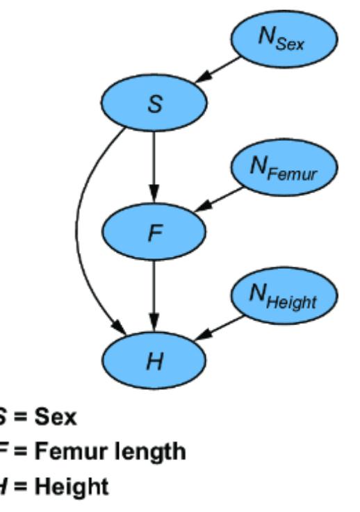
Figure 9.9 The causal DAG for the relationship between femur length and height. Both are driven by biological sex.

The following code below implements the model in Pyro. Note the creation and use of a PseudoDelta distribution function. Endogenous variables are deterministic functions of the exogenous variables, but for variational inference to work, we must assign the endogenous variables a distribution using pyro.sample. We could use the Dirac delta distribution, which would assign all probability value to the output of a variable’s assignment function. But gradientbased optimization won’t work in this case. Instead, we’ll

approximate inference with a ૿pseudo-delta distribution—a normal distribution with a very small scale parameter.

Listing 9.11 Implement the femur SCM in Pyro

from torch import tensor
from pyro.distributions import Bernoulli, Normal
from pyro import sample
from functools import partial #1
PseudoDelta = partial(Normal, scale=.01) #1
def f_sex(N_sex): #2
 return sample("sex", Bernoulli(N_sex)) #2
def f_femur(sex, N_femur): #3
 if sex == tensor(1.0): #3
 μ = 43.7 + 2.3 * N_femur #3
 else: #3
 μ = 40.238 + 1.9 * N_femur #3
 return sample("femur", PseudoDelta(μ)) #3
def f_height(femur, sex, N_height): #4
 if sex == tensor(1.0): #4
 μ = 61.41 + 2.21 * femur + 7.62 * N_height #4
 else: #4
 μ = 54.1 + 2.47 * femur + 7 * N_height #4
 return sample("height", PseudoDelta(μ)) #4
def model(exogenous):
 N_sex = sample("N_sex", exogenous['N_sex']) #5
 N_femur = sample("N_femur", exogenous['N_femur']) #5
 N_height = sample("N_height", exogenous['N_height']) #5
 sex = f_sex(N_sex) #6
 femur = f_femur(sex, N_femur) #6
 height = f_height(femur, sex, N_height) #6
 return sex, femur, height
exogenous = { #7
 'N_sex': Bernoulli(.5), #7
 'N_femur': Normal(0., 1.), #7
 'N_height': Normal(0., 1.), #7
} #7

#1 Enable approximate inference with a ૿pseudo-delta distribution to emulate a deterministic delta distribution.

#2 The assignment function for biological sex

#3 The assignment function for femur length in cm. The assignment uses two linear functions, one for each sex.

#4 The assignment function for height. Again, it uses two linear functions, one for each sex.

#5 Sample from the exogenous variable prior distributions

#6 Obtain the endogenous variables given the exogenous variables.

#7 Specify the prior distributions for the exogenous variables.

Again, there are three steps to our counterfactual inference algorithm:

• 1. Abduction
• 2. Action
• 3. Prediction

Unlike our pgmpy model, we won’t need to clone all the variables for the parallel world. We’ll just use the intervention operator pyro.do to apply the intervention and get an intervention model. For P (HF ⁼ 46), we’ll generate from the intervention model based on samples from P (NSex, NFemur, NHeight ). For the counterfactual distribution, we’ll do the abduction step using a variational inference algorithm to learn P (NSex, NFemur, NHeight|F=44, H=165). Then we’ll generate from the intervention model again, but this time based on samples from P (NSex, NFemur, NHeight |F = 44, H = 165).

DEALING WITH INTRACTABLE LIKELIHOODS

We use variational inference to do the abduction step, inferring the exogenous variables given observed endogenous variables. Variational inference is a likelihoodbased technique. Typically, we get likelihoods by sampling from a distribution and then getting the probability value for that sampled value using the distribution’s probability mass/density function. But we can’t do that for SCMs because endogenous variable values are set by the assignment functions rather than being sampled. The code in this forensic example uses sampling from a ૿pseudo- Dirac delta distribution, meaning a normal distribution with a very small scale parameter. This approach, which provides likelihood values from a normal distribution, falls into a class of methods called approximate Bayesian computation, and it shares some of the trade-offs with other members of that class.

One alternative is to use amortized inference. In this method, you sample many exogenous variable values and use these to calculate many endogenous variable values. Finally, you use these samples to train a model that predicts the exogenous variable value, given the endogenous variable value. You then use this trained model during the abduction step.

Dealing with intractable likelihoods is a broader challenge in probabilistic machine learning, which is beyond the scope of this book. See the chapter notes at https://www.altdeep.ai/p/causalaibookfor links to additional references and resources.

9.3.2 Implementing an intervention with pyro.do

Now let’s pose the conditional hypothetical, ૿What would height be if femur length was 46 cm? Figure 9.10 illustrates the modified DAG representing the ideal intervention that sets femur length to 46.

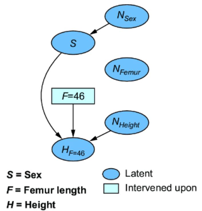
Figure 9.10 We represent the hypothetical condition with an ideal
intervention and graph surgery on the causal DAG.

In Pyro, we’ll apply pyro.do to the original model and get an intervention model. We’ll then repeatedly call the algorithm with the prior on the exogenous variable distribution and return generated endogenous values. We’ll repeat this several times and visualize the intervention distribution on height with a histogram.

Listing 9.12 Sampling from the intervention distribution of ૿if femur length were 46cm

import matplotlib.pyplot as plt
import pyro
int_model = pyro.do(model, data={"femur": tensor(46.0)}) #1
int_samples = [] #2
for _ in range(10000): #2
 _, _, int_height = int_model(exogenous) #2
 int_samples.append(float(int_height)) #2
plt.hist( #3
 int_samples, #3
 bins=20, #3
 alpha=0.5, #3
 label="Intervention Samples", #3
 density=True #3
) #3
plt.ylim(0., .35) #3
plt.legend() #3
plt.xlabel("Height") #3
plt.show() #3

#1 Implement the hypothetical condition ૿…if femur length were 46 cm with pyro.do, which returns a new model that implements the intervention.

#2 Sample from the intervention distribution.

#3 Visualize the intervention distribution with a histogram of samples.

Figure 9.11 shows the resulting histogram of samples from P(HF=46). We’ll contrast this with the histogram from P(HF=46|F=44, H=165).

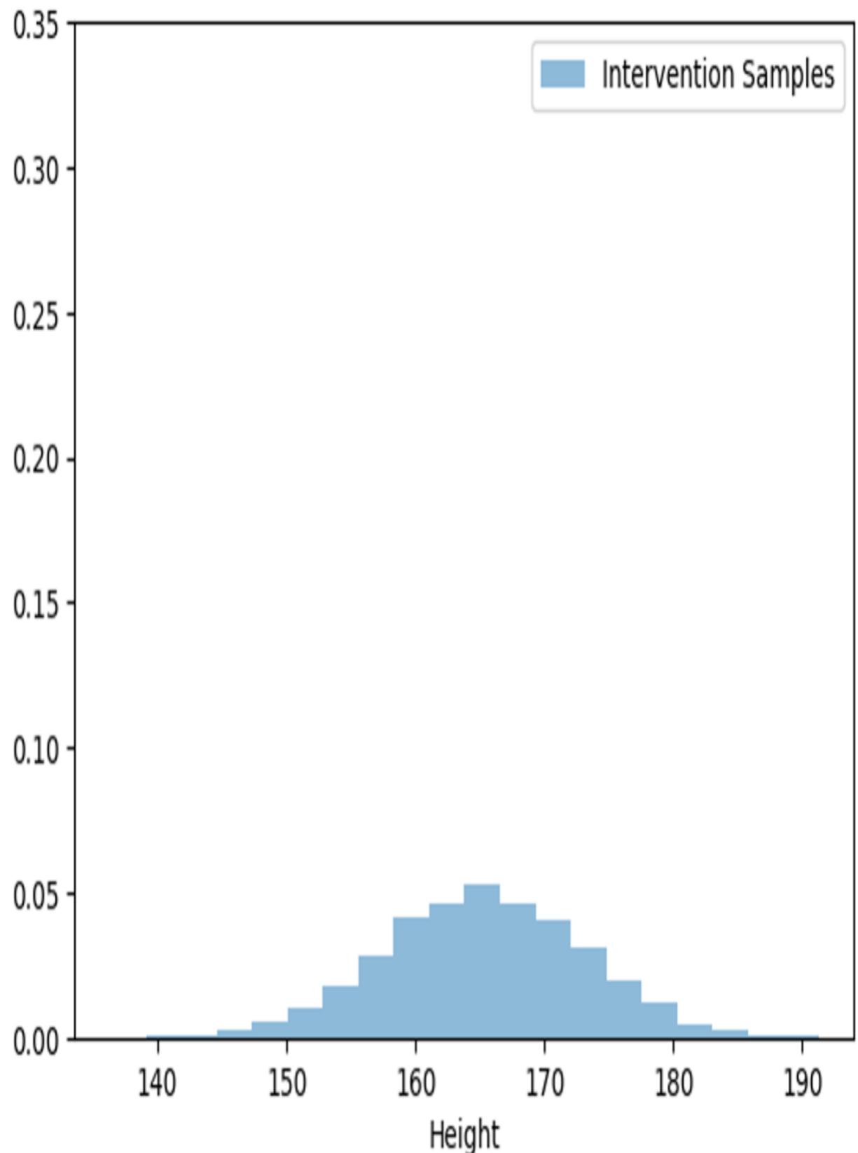
Figure 9.11 This histogram of samples visualizes the interventional distribution—the x-axis corresponds to different ranges of height values, and the y-axis is proportions of the sampled heights that fall within each range.

Now we’ll do the counterfactual inference.

9.3.3 Implementing the abduction step with variational inference

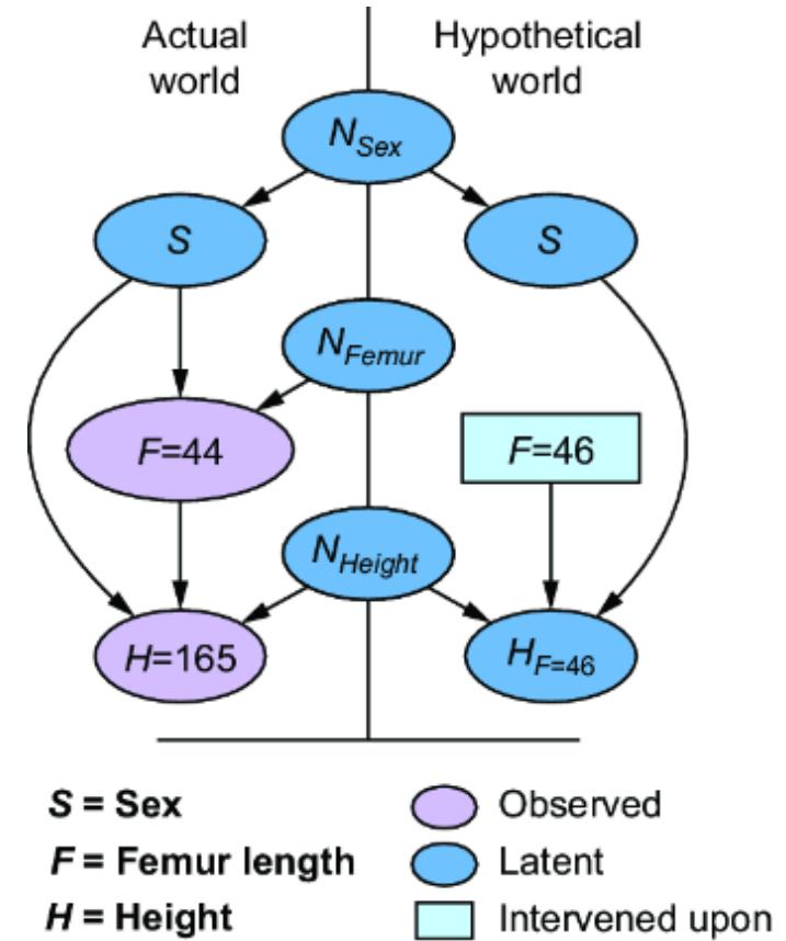
Figure 9.12 The parallel world graph for the femur length counterfactual

Our conditional hypothetical question was, ૿What would an individual’s height be if their femur length was 46 cm? Now we want to answer the counterfactual: ૿An individual’s femur is 44 cm, and their height is 165 cm. What would their height be if their femur length was 46 cm? In other words, we want to extend P (HF ⁼ 46) to P (HF ^{= 46} |F=44, H=165). Figure 9.12 illustrates the corresponding parallel world graph.

Following the counterfactual inference algorithm, we need to do the abduction step and infer P (NSex , NFemur , NHeight |F = 44, H = 165). We’ll use variational inference, where we’ll specify a guide function—a function with trainable parameters representing a distribution Q(NSex , NFemur , NHeight ). The training procedure optimizes the parameters of the guide such that Q(NSex, NFemur, NHeight) closely approximates P (NSex, NFemur, NHeight |F = 44, H = 165).

REFRESHER: PROPOSAL DISTRIBUTIONS AND PYRO’S GUIDE FUNCTION

Pyro’s use of ૿guide functions enables the developer to write their own proposal distributions that ૿propose values for variables in the target distributions. Samplingbased inference algorithms (e.g., importance sampling or MCMC) use the proposal to generate samples and then operate on the samples so they represent the target distribution. Variational inference optimizes the parameters of the proposal distribution such that it becomes close to (or ૿approximates) the target distribution. In contrast to pgmpy’s automatic inference algorithms, guide functions let the developer ૿guide inference as they see fit.

Listing 9.13 Specifying the guide function for variational inference

import torch.distributions.constraints as constraints
from pyro.primitives import param
from pyro.distributions import Delta
def guide(exogenous): #1
 p = param("p", tensor(.5), #2
 constraint=constraints.unit_interval) #2
 n_sex = sample("N_sex", Bernoulli(p)) #2
 sex = sample("sex", Bernoulli(n_sex)) #3
 n_femur_loc = param("n_femur_loc", tensor(0.0)) #4
 n_femur_scale = param( #4
 "n_femur_scale", #4
 tensor(1.0), #4
 constraint=constraints.positive #4
 ) #4
 femur_dist = Normal(n_femur_loc, n_femur_scale) #5
 n_femur = sample("N_femur", femur_dist) #5
 n_height_loc = param("n_height_loc", tensor(0.0)) #5
 n_height_scale = param( #5
 "n_height_scale", #5
 tensor(1.0), #5
 constraint=constraints.positive #5
 ) #5
 height_dist = Normal(n_height_loc, n_height_scale) #5
 n_height = sample("N_height", height_dist) #5
 femur = sample("femur", Delta(n_femur)) #6
 height = sample("height", Delta(n_height)) #6

#1 The exogenous prior distribution is passed to the guide function. The function won’t use this argument, but the signatures of the guide and the model functions must match.

#2 The guide function tries to approximate P(N_sex|femur, height) from a Bernoulli distribution. Optimization targets the parameter of this Bernoulli distribution.

#3 n_sex is either 0 or 1. When passed as a parameter to a Bernoulli, the outcome is deterministic.

#4 The guide function tries to approximate P(N_femur|femur, height) from a normal distribution. Optimization targets the location and scale parameters of this normal distribution.

#5 The guide function tries to approximate P(N_height|femur, height), also from a normal distribution.

#6 Since we condition on femur and height, they are not needed in the guide function. But it is useful to have them in case we want to condition on different outcomes in a new analysis.

DETERMINISTIC ABDUCTION

A special case of the abduction step is when both of the following are true:

• 1. You observe all the endogenous variables.
• 2. The SCM assignment functions are invertible.

In that case, given observations of all the endogenous variables, you can calculate exact point values for the exogenous variables with the inverted assignment functions. Consequently, you apply the assignment functions in the hypothetical world to get point values of the hypothetical outcomes. However, most practical examples fall in the following general case:

• 1. You only condition on some endogenous variables.
• 2. The SCM assignment functions are not invertible.

In our abduction step, we first condition the model on observed values of femur and height.

Listing 9.14 Conditioning on actual values of femur and height

conditioned_model = pyro.condition( 
 model, 
 data={"femur": tensor(44.0), "height": tensor(165.0)} 
)

Next, we infer the exogenous variable, given femur and height, using variational inference.

Listing 9.15 Implementing the abduction step with variational inference

from pyro.infer import SVI, Trace_ELBO
from pyro.optim import Adam
pyro.util.set_rng_seed(123) #1
pyro.clear_param_store() #2
svi = SVI( #3
 model=conditioned_model,
 guide=guide,
 optim=Adam({"lr": 0.003}), #4
 loss=Trace_ELBO() #5
)
losses = [] #6
num_steps = 5000 #7
for t in range(num_steps): #7
 losses.append(svi.step(exogenous)) #7
plt.plot(losses) #8
plt.title("Loss During Training") #8
plt.xlabel("step") #8

plt.ylabel(“loss”) #8

#1 Set a seed for reproducibility. #2 Clear any current parameter values. #3 Initialize the stochastic variational inference algorithm. #4 Optimize the parameters with a learning rate of .003. #5 Use (negative) evidence lower bound (ELBO) as the loss function. #6 Initialize a list to store loss values for plotting. #7 Run the optimization for 5,000 steps. The SVI’s step object has the same signature as the model and the guide, so any model/guide arguments must be passed in here. #8 Plot the loss during training.

Figure 9.13 shows loss during training indicating variational inference converged.

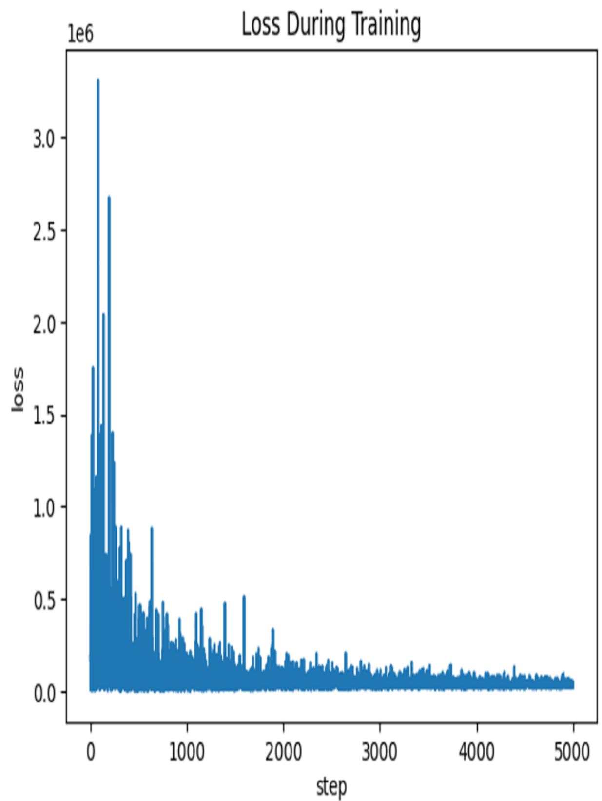
Figure 9.13 Loss during optimization of the parameters of the distribution approximating P(NSex, NFemur, NHeight|F=44, H=165)

After training is completed, we extract the optimized parameters for our updated exogenous variable distribution.

Listing 9.16 Extract parameters of updated exogenous distribution

n_sex_p = param("p").item() #1
n_femur_loc = param("n_femur_loc").item() #1
n_femur_scale = param("n_femur_scale").item() #1
n_height_loc = param("n_height_loc").item() #1
n_height_scale = param("n_height_scale").item() #1
exogenous_posterior = { #2
 'N_sex': Bernoulli(n_sex_p), #2
 'N_femur': Normal(n_femur_loc, n_femur_scale), #2
 'N_height': Normal(n_height_loc, n_height_scale), #2
} #2

#1 Extract the parameter values.

#2 Do the abduction by using the optimized parameters to create new ૿posterior exogenous variable distributions.

One thing to note is that while we typically specify independent prior distributions for exogenous variables in an SCM, exogenous variables are generally conditionally dependent given endogenous variables (because of collider paths!). However, I wrote a guide function that samples the exogenous variables independently, ignoring this conditional dependence. Writing a guide that treats dependent variables as independent is convenient and is common practice, but doing so will add some bias to the results. You can avoid this by doing the extra work of writing a guide function that maintains the dependencies implied by the graph.

COUNTERFACTUAL MODELING WITH CHIRHO

ChiRho is a causal extension of Pyro that seeks to more seamlessly blend the probabilistic modeling approach of Pyro with causal inference. ChiRho has parallel world abstractions and abstractions for implementing counterfactual inference with normalizing flows and the variational inference approach discussed in this example. As an extension to Pyro, the modeling techniques discussed in this case study will also work with ChiRho.

9.3.4 Implementing the action and prediction steps

In the Monty Hall example, we built the parallel world model explicitly. In this example, we can just perform the action step by using pyro.do to get the hypothetical world model, and sample from this model using the updated exogenous variable distribution.

We’ll repeat the procedure of generating samples from the intervention model that set femur length to 46 cm. Recall that we already created the intervention model in listing 9.11 with this line:

int_model = pyro.do(model, data={“femur”: tensor(46.0)})

To sample from the intervention distribution, we called int_model on our original exogenous variable distribution. Now, for the prediction step, we’ll call it again, this time with exogenous_posterior instead of exogenous, because exogenous_posterior encodes all the information from the actual world.

Listing 9.17 Sampling from the counterfactual distribution

cf_samples = [] 
for _ in range(10000): 
 _, _, cf_height = int_model(exogenous_posterior) 
 cf_samples.append(float(cf_height))

Finally, we overlay a histogram of samples from the counterfactual distribution against the interventional distribution histogram in figure 9.14, and we can see the clear differences between these distributions.

Listing 9.18 Comparing the interventional and counterfactual distributions

plt.hist( 
 int_samples, 
 bins=20, 
 alpha=0.5, 
 label="Intervention Samples", 
 density=True 
)
plt.hist( 
 cf_samples, 
 bins=20, 
 alpha=0.5, 
 label="Counterfactual Samples", 
 density=True 
) 
plt.ylim(0., .35) 
plt.legend() 
plt.xlabel("Height") 
plt.show()

The resulting plot, shown in figure 9.14, contrasts histograms of the interventional and counterfactual samples.

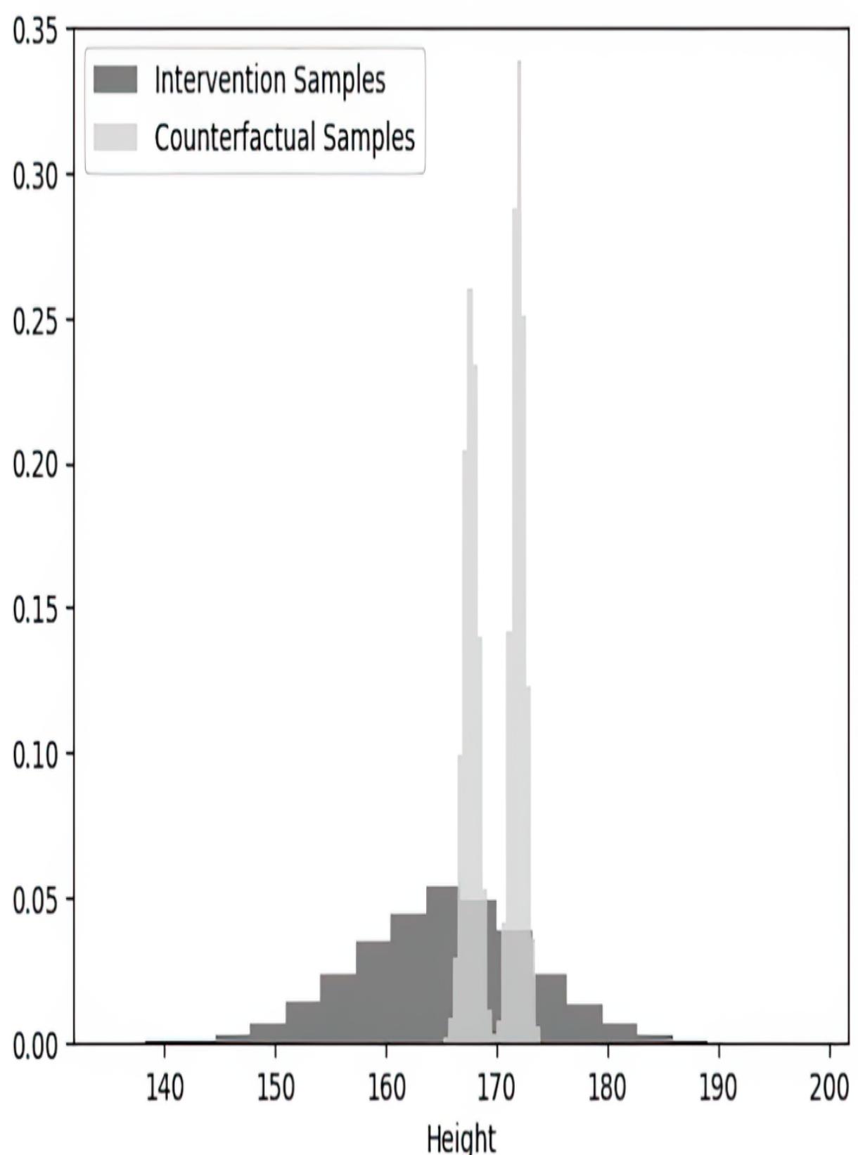
Figure 9.14 Histograms of generated samples from the interventional and counter-factual distributions encoded by the causal model

Figure 9.14 illustrates how the counterfactual distribution generally has much less spread than an interventional distribution representing the same hypothetical conditions. The counterfactual distribution essentially filters the interventional distribution down to cases where the conditions observed in the actual world are true. In this case, we have two height bell curves corresponding to two sexes. Those bell curves have a stronger overlap in the interventional distribution.

In a final example, we’ll evaluate how to run the counterfactual inference algorithm in the context of a generative AI image model.

9.4 Case study 3: Counterfactual image generation with a deep generative model

In generative AI, the user provides an input, and the algorithm generates some output. For example, suppose I wanted to write a script for an alternative history where Harriet Tubman was a pirate captain. I turned to a generative image model for some concept art, posing the text question, ૿What would Harriet Tubman look like as a pirate captain? The model generated the image in figure 9.15.

Figure 9.15 The output of a generative AI image model, given the natural language input prompt ૿What would Harriet Tubman look like as a pirate captain?

The question itself is a counterfactual—Harriet Tubman was not a pirate. We’ll explore natural language counterfactuals with large language models in chapter 13. Here, we’ll reason counterfactually about the image in figure 9.15.

Suppose I like this image, but I want to make an edit—I want to change this image to remove the glasses. One way of doing this is to use a tool like ૿in-fill, where I select the pixels with the glasses and indicate that I want whatever is in the pixels to go away. This would be directly editing the form of the image.

An alternative approach would be semantic editing, where rather than manipulating the pixels in the image, I manipulate some latent representation of the image corresponding to ૿glasses. In effect, I pose the counterfactual question, ૿what would this image look like if the subject were not wearing glasses? Figure 9.16 contrasts the original and ૿counterfactual versions of the image.

Figure 9.16 Given the generated image on the left, the user might prompt the generative AI with the counterfactual question, ૿What would this image look like without the glasses? They would expect something like the image on the right, where conceptual elements of the image not causally downstream of glasses removal should be unaffected.

This is an attractive use case, as manipulating underlying concepts is often preferable to manipulating form, especially when the edits you want to make aren’t all located in the same specific area of pixels. This is especially attractive if our conceptual model is a causal model, so the downstream causal consequences of changing a concept are reflected in the image, while the law of consistency prevents change in

the parts of the image that should be unaffected by the change in concept.

With this use case in mind, this section will use our counterfactual algorithm to implement a form of semantic editing. We’ll start with the actual image. In the abduction step, we’ll infer some latent representation of the image. In the action step, we’ll propose the desired edit, and in the prediction step, we’ll generate the new image.

In this example, we’ll use an SCM built with a variational autoencoder in PyTorch. We’ll also use a simple dataset called dSprites for proof of concept. The dSprites data demonstrates the idea and is simple enough to train a model quickly on an ordinary laptop. See the chapter notes at https://www.altdeep.ai/p/causalaibookfor references with more practical counterfactual image modeling examples.

9.4.1 The dSprites data

The dSprites dataset consists of 2D shapes, each rendered in 8 possible positions, 6 possible scales, and 40 possible rotations. The shapes are composed of 5 independent factors: shape, scale, rotation, x-position, and y-position. Figure 9.17 demonstrates samples from the dataset.

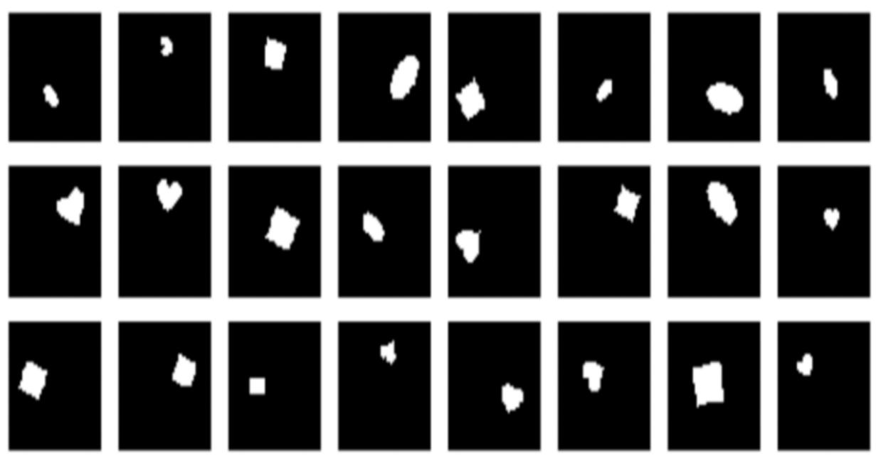
Figure 9.17 The dSprites data features images causally determined by five independent causal factors: shape, scale, rotation, x-position, and y-position.

We’ll treat each of these factors as causes of an image variable, as illustrated in the causal DAG in figure 9.18.

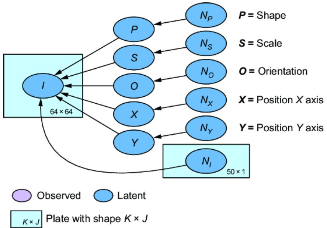
Figure 9.18 The causal DAG for a dSprites image, displayed as a plate model to highlight the shape of NI and I. Ni is the exogenous variable for the image. The model is trained with an encoder-decoder framework that uses a 50 × 1 dimensional image encoding to represent NI.

In the following code, we load a specific image from the dSprites dataset.

Listing 9.19 Load a dSprites image

import torch
from matplotlib import pyplot as plt
import io #1
import urllib.request #1
import numpy as np #1
url = ('https://github.com/altdeep/causalML/blob/master/' #1
 'book/chapter%209/sprites_example.npz?raw=true') #1
with urllib.request.urlopen(url) as response: #1
 data = response.read() #1
file = io.BytesIO(data) #1
npzfile = np.load(file) #1
img_dict = dict(npzfile) #1
img = torch.tensor(img_dict['image'].astype(np.float32) ) #2
plt.imshow(img, cmap='Greys_r', interpolation='nearest') #2
plt.axis('off') #2
plt.title('original') #2
plt.show() #2
causal_factor = torch.from_numpy(img_dict['label']).unsqueeze(0) #3
print(causal_factor) #3

#1 Download dSprites example from GitHub and load it. #2 Plot the dSprites image.

#3 The causal factors of the example are [0 0 1 13 26 14], the first element is always 0, and the second element corresponds to ૿square and is represented by 0. The remaining elements correspond to scale, orientation, and X and Y positions.

This plots the image in figure 9.19.

Figure 9.19 A single example from the dSprites data

Printing causal_factor produces tensor ([[ 0, 0, 1, 13, 26, 14]]). The first element is 0 for all examples in the data. The second element of the causal factor vector corresponds to shape. Square, ellipse, and heart are represented by 0, 1, and 2, respectively. The image contains a square (P  =  0) with scale S = 1, orientation O=13, and position X = 26 and Y = 14.

In this case study, we’ll ask, ૿What would this image look like if the shape were a heart instead of a square? This suggests the parallel-world network in figure 9.20.

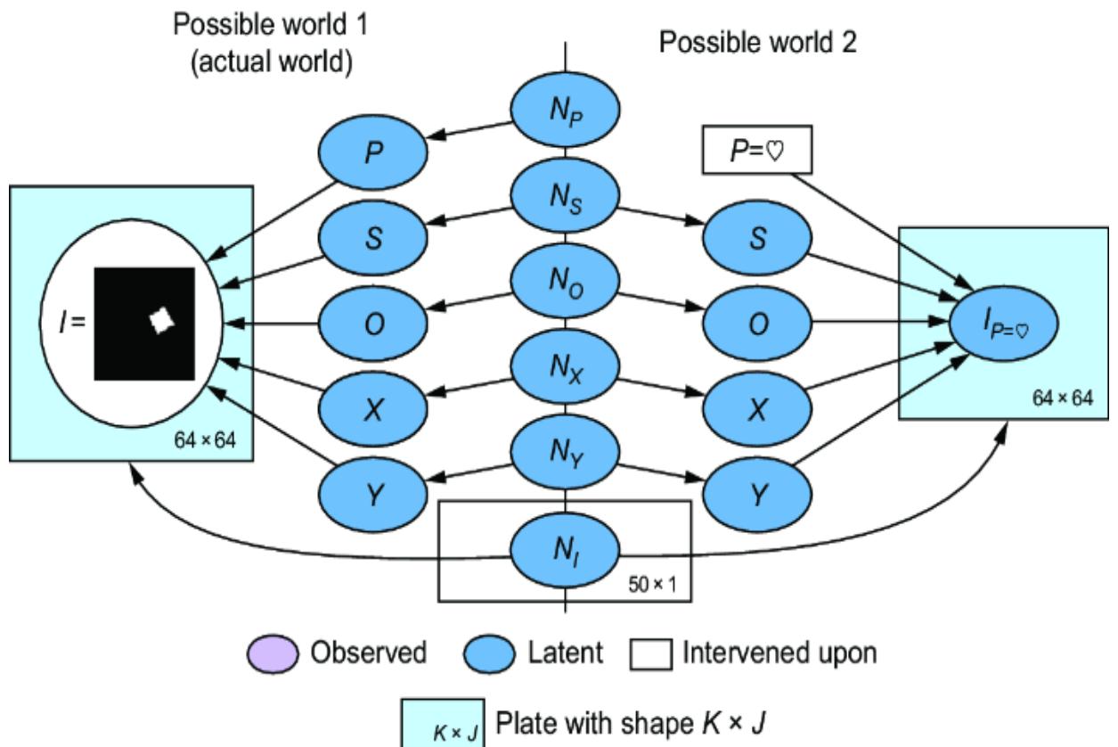
Figure 9.20 The parallel world graph implied by the question ૿Given the image, what would it look like if the shape were a heart?

First, we’ll load a pretrained encoder to map from the image to the exogenous variable for the causal factors. In this simple model, we’ll assume the assignment functions for the exogenous variables of the causal factors are identity functions, i.e., the causal factors and their exogenous variables will have the same values. Let’s start by initializing the encoder.

Listing 9.20 Load the encoder of causal factors

import requests
import torch.nn as nn
CARDINALITY = [1, 3, 6, 40, 32, 32] #1
class EncoderCausalFactors(nn.Module): #2
 def __init__(self, image_dim, factor_dim):
 super(EncoderCausalFactors, self).__init__()
 self.image_dim = image_dim
 self.factor_dim = factor_dim
 hidden_dim = 1000 #3
 self.fc1 = nn.Linear(image_dim, hidden_dim) #4
 self.fc2 = nn.Linear(hidden_dim, hidden_dim) #4
 self.fc3 = nn.Linear(hidden_dim, factor_dim) #4
 self.softplus = nn.Softplus() #4
 self.sigmoid = nn.Sigmoid() #5
 def forward(self, img):
 img = img.reshape(-1, self.image_dim) #6
 hidden1 = self.softplus(self.fc1(img)) #7
 hidden2 = self.softplus(self.fc2(hidden1)) #7
 p_loc = self.sigmoid(self.fc3(hidden2)) #8
 return p_loc #8
encoder_n_causal_factors = EncoderCausalFactors( #9
 image_dim=64*64, #9
 factor_dim=sum(CARDINALITY) #9
) #9

#1 Cardinality in each dimensionality of the causal factors

#2 Encoder for the vector of exogenous parents of the causal factors #3 The hidden layers have a length of 1,000.

#4 Using linear transforms passed through Softplus activation functions #5 The final activation is a sigmoid function.

#6 Flatten the image.

#7 Calculate the hidden layers.

#8 The output layer generates a probability vector that Is used as the parameter of a OneHotCategorical distribution.

#9 Initialize the encoder. The image dimension is 64 × 64 pixels, and the six elements of the causal factor vector are one-hot encoded into a vector of length 1 + 3 + 6 + 40 + 32 + 32 = 114.

Next, we’ll download and load pretrained weights into this encoder from the book’s GitHub repo.

Listing 9.21 Download and load pretrained weights into the encoder of causal factors

url = ('https://github.com/altdeep/causalML/raw/master/' 
 'book/chapter%209/sprites-model-encoder-causal-factors.pt') 
response = requests.get(url) 
response.raise_for_status() 
with open('temp_weights.pt', 'wb') as f: 
 f.write(response.content) 
state_dict = torch.load( 
 'temp_weights.pt', 
 map_location=torch.device('cpu') 
) 
encoder_n_causal_factors.load_state_dict(state_dict)

First, we’ll test that the encoder can recover the causal factors from the image.

Listing 9.22 Generate examples of causal exogenous factors

from pyro import distributions as dist
def decode_one_hot(factor_encoded, cardinality=CARDINALITY): 
 split = [ 
 torch.split(element, cardinality) #1
 for element in factor_encoded #1
 ] #1
 labels = [[int(torch.argmax(vec)) for vec in item] #1
 for item in split] #1
 return torch.tensor(labels) #1
def sample_one_hot(p_encoded, cardinality=CARDINALITY): #2
 split = [torch.split(element, cardinality) #2
 for element in p_encoded] #2
 sample_list = [ #2
 [ #2
 dist.OneHotCategorical(p_vec).sample() #2
 for p_vec in item #2
 ] for item in split #2
 ] #2
 sample = torch.stack([ #2
 torch.cat(samples, -1) #2
 for samples in sample_list #2
 ]) #2
 return sample #2
inferred_cause_p = encoder_n_causal_factors.forward(img) #3
sampled_factors = sample_one_hot( #3
 inferred_cause_p #3
) #3
print(decode_one_hot(sampled_factors)) #3

#1 Helper function that decodes the one-hot encoded output of the encoder

#2 Samples from the output probability vector of encoder_causal_factors #3 Use the encoder to predict causal factors.

Encoding the sampled image prints the causal factors: [ 0, 0, 1, 13, 26, 14]. The encoder accurately recovers the causal factors from the image.

Next, we’ll initialize an encoder that we’ll use for inference of NI , the exogenous variable for the image. This encoder takes an image and an instance of the causal factor vector as an input.

Listing 9.23 An encoder for inference of NI class EncoderNImage(nn.Module): #1 def __init__(self, image_dim, factor_dim, n_image_dim): super(EncoderNImage, self).__init__() self.image_dim = image_dim self.factor_dim = factor_dim self.n_image_dim = n_image_dim hidden_dim = 1000 self.fc1 = nn.Linear( self.image_dim + self.factor_dim, hidden_dim #2 ) #2 self.fc2 = nn.Linear(hidden_dim, hidden_dim) #2 self.fc31 = nn.Linear(hidden_dim, n_image_dim) #2 self.fc32 = nn.Linear(hidden_dim, n_image_dim) #2 self.softplus = nn.Softplus() #2 def forward(self, img, factor): img = img.reshape(-1, self.image_dim) #3 inputs = torch.cat((img, factor), -1) #4 hidden1 = self.softplus(self.fc1(inputs)) #5 hidden2 = self.softplus(self.fc2(hidden1)) #5 n_image_loc = self.fc31(hidden2) #6 n_image_scale = torch.exp(self.fc32(hidden2)) #6 return n_image_loc, n_image_scale #6 encoder_n_image = EncoderNImage( #7 image_dim=64*64, #7 factor_dim=sum(CARDINALITY), #7 n_image_dim=50 #7 ) #7

#1 Encoder used for inference of N I, which serves as both the exogenous variable for the image in causal terms, and the encoding of the image in VAE terms

#2 Using linear transforms passed into a Softplus activation function #3 Flatten the image.

#4 Concatenate the image and the causal factor vector.

#5 Calculate the hidden layers.

#6 Calculate the location and scale parameter of multivariate normal distribution on N I.

#7 Initialize the encoder.

The encoder of the noise variable requires the causal factors to be one-hot encoded, so we’ll create a helper function to do just that.

Listing 9.24 Create a function for one-hot encoding

def encode_one_hot(factor, cardinality=CARDINALITY): 
 new_factor = [] 
 for i, factor_length in enumerate(cardinality): 
 new_factor.append( 
 torch.nn.functional.one_hot( 
 factor[:,i].to(torch.int64), int(factor_length) 
 ) 
 ) 
 new_factor = torch.cat(new_factor, -1) 
 return new_factor.to(torch.float32)

Again, we’ll download and load pretrained weights for the encoder.

Listing 9.25 Load pretrained weights for encoder for inference of NI
weight_url = (“https://github.com/altdeep/causalML/raw/master/” #1
“book/chapter%209/sprites-model-encoder-n-image.pt”) #1 response = requests.get(weight_url) #1
response.raise_for_status() #1
with open(‘temp_weights.pt’, ‘wb’) as f: #1 f.write(response.content) #1
state_dict = torch.load( #1
‘temp_weights.pt’, #1 map_location=torch.device(‘cpu’) #1
) #1
encoder_n_image.load_state_dict(state_dict) #1 n_image_loc, n_image_scale = encoder_n_image.forward( #2
img, #2
encode_one_hot(causal_factor) #2 ) #2
n_image = torch.normal(n_image_loc, n_image_scale) #3

#1 Load the pretrained weights. #2 Pass the image and causal factors into the encoder, and obtain N I location and scale parameters. #3 Generate from the posterior distribution on N I.

Finally, we’ll load a decoder that maps from NI and a causal factor back to an image. In causal terms, the decoder is part of the assignment function for the image.

Listing 9.26 Load and initialize the decoder that maps causes and NI to images

class Decoder(nn.Module): #1
 def __init__(self, image_dim, factor_dim, n_image_dim):
 super(Decoder, self).__init__()
 hidden_dim = 1000
 self.fc1 = nn.Linear(n_image_dim + factor_dim, hidden_dim) #2
 self.fc2 = nn.Linear(hidden_dim, hidden_dim) #2
 self.fc3 = nn.Linear(hidden_dim, hidden_dim) #2
 self.fc4 = nn.Linear(hidden_dim, image_dim) #2
 self.softplus = nn.Softplus() #2
 self.sigmoid = nn.Sigmoid() #2
 def forward(self, n_image, factor):
 inputs = torch.cat((n_image, factor), -1) #3
 hidden1 = self.softplus(self.fc1(inputs)) #4
 hidden2 = self.softplus(self.fc2(hidden1)) #4
 hidden3 = self.softplus(self.fc3(hidden2)) #4
 p_img = self.sigmoid(self.fc4(hidden3)) #5
 return p_img #5
decoder = Decoder( #6
 image_dim=64*64, #6
 factor_dim=sum(CARDINALITY), #6
 n_image_dim=50 #6
) #6

#1 The decoder maps from causal factors and N_image to generate a parameter for a multivariate Bernoulli distribution on images. #2 The model uses linear transforms, a Softplus activate for hidden

layers, and sigmoid activate on the output layer.

#3 The network concatenates n_image and factors in the input layer. #4 The input is passed through three hidden layers with Softplus activation functions.

#5 The output is a probability parameter passed to a multivariate Bernoulli distribution on image pixels. #6 Initialize the encoder.

Again, we’ll download and load pretrained weights into the decoder.

Listing 9.27 Download and load the decoder weights

dcdr_url = ("https://github.com/altdeep/causalML/raw/master/" 
 "book/chapter%209/sprites-model-decoder.pt") 
response = requests.get(dcdr_url) 
response.raise_for_status() 
with open('temp_weights.pt', 'wb') as f: 
 f.write(response.content) 
state_dict = torch.load( 
 'temp_weights.pt', 
 map_location=torch.device('cpu') 
) 
decoder.load_state_dict(state_dict)

Before we generate the counterfactual image, we’ll create a helper function to plot it.

Listing 9.28 Helper function for plotting the counterfactual image

def compare_reconstruction(original, generated): 
 fig = plt.figure() 
 ax0 = fig.add_subplot(121) 
 plt.imshow( 
 original.cpu().reshape(64, 64), 
 cmap='Greys_r', 
 interpolation='nearest' 
 ) 
 plt.axis('off') 
 plt.title('actual') 
 ax1 = fig.add_subplot(122) 
 plt.imshow( 
 generated.reshape(64, 64), 
 cmap='Greys_r', interpolation='nearest') 
 plt.axis('off') 
 plt.title('counterfactual') 
 plt.show()

Now, we’ll specify the SCM. We’ll write a p_n_image function that generates from P(Nimage) and an f_image assignment function for the image.

Listing 9.29 Create an exogenous distribution and assignment function for the image

def p_n_image(n_image_params): #1
 n_image_loc, n_image_scale, n_unif_upper = n_image_params #2
 n_image_norm = dist.Normal( #3
 n_image_loc, n_image_scale #3
 ).to_event(1).sample() #3
 n_image_unif = dist.Uniform(0, n_unif_upper).expand( #4
 torch.Size([1, 64*64]) #4
 ).sample() #4
 n_image = n_image_norm, n_image_unif #5
 return n_image
def f_image(factor, n_image): #6
 n_image_norm, n_image_unif = n_image #7
 p_output = decoder.forward( #8
 n_image_norm, #8
 encode_one_hot(factor) #8
 )
 sim_img = (n_image_unif <= p_output).int() #9
 return sim_img

#1 A function that generates a variate from the N_image exogenous distribution

#2 The parameters of N_image’s distribution include location and scale parameters for a normal distribution and the upper bound of a uniform distribution.

#3 Sample a normal random variate from the normal distribution.

#4 Sample a uniform random variate from a uniform distribution.

#5 Combine these into a single n_image object.

#6 Assignment function for the image

#7 The exogenous noise variable decomposes into one normal and one uniform random variate.

#8 The normal random variate is passed through the decoder to get a probability vector for the pixels.

#9 Each pixel is set deterministically with an indicator function that returns 1 if an element of the uniform variate is less than the corresponding element of the probability vector, or otherwise returns 0.

Finally, we can run through the steps of the counterfactual inference algorithm to answer the question, ૿What would this image look like if it was a heart?

Listing 9.30 Generate a counterfactual image

def abduct(img, factor, smoother=1e-3): #1
 n_image_loc, n_image_scale = encoder_n_image.forward( #2
 img, encode_one_hot(factor) #2
 ) #2
 n_unif_upper = decoder.forward( #3
 n_image_loc, #3
 encode_one_hot(factor) #3
 ) #3
 n_unif_upper = n_unif_upper * (1 - 2 * smoother) + smoother #3
 p_image_params = n_image_loc, n_image_scale, n_unif_upper #4
 return p_image_params
def do_action(factor, element=1, val=2): #5
 intervened_factor = factor.clone() #5
 intervened_factor[0][element] = val #5
 return intervened_factor #5
def predict(intervened_factor, n_image_params): #6
 n_image = p_n_image(n_image_params) #6
 sim_img = f_image(intervened_factor, n_image) #6
 return sim_img #6
def counterfactual(img, factor): #7
 p_image_params = abduct(img, factor) #7
 intervened_factor = do_action(factor) #7
 pred_recon = predict(intervened_factor, p_image_params) #7
 compare_reconstruction(img, pred_recon) #7
counterfactual(img, causal_factor) #8

#1 Abduction step: infer the exogenous variable given the image. #2 Infer the parameters of N_I. First, this includes two parameters of a normal distribution.

#3 Second, we infer the upper bound of a uniform distribution and apply smoothing so it is not exactly 1 or 0.

#4 Combine these together into one inferred parameter set.

#5 Action step: Apply the intervention that sets the shape element to ૿heart (represented by the integer 2).

#6 Prediction step: Generate n_image from P(N_image), and pass this through an assignment function to generate an image.

#7 Apply all three steps: abduct the n_image, apply the intervention, and forward generate the counterfactual image. #8 Plot the result.

Figure 9.21 shows the results.

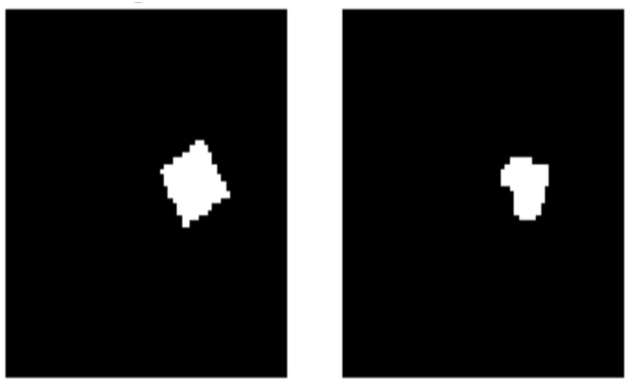
Figure 9.21 The original (left) and counterfactually generated image (right)

This is a proof of concept—there is additional nuance in counterfactual image generation. I’m cheating a bit with this dSprites example. The counterfactual generation works because the causal factors are independent and because the data is quite simple. For counterfactual image generation to work in general, we need to understand and satisfy certain assumptions.

9.4.2 Assumptions needed for counterfactual image generation

In the next chapter, we’ll tackle the problem of identification. Identification is determining what causal questions we can answer, given our modeling assumptions and the data available to us. The counterfactual inference algorithm assumes you have the ground-truth SCM. If you can make

that assumption, you can use the algorithm to answer any counterfactual (or interventional) query.

In most cases, we can’t practicably assume we have the ground-truth SCM. At best, you’ll have an SCM that acts as an approximation of the ground truth. For example, the true process that generated the dSprites images certainly didn’t involve a decoder neural network—we used deep learning with this decoder architecture to approximate that process. As you’ll see in the next chapter, such learned approximations are not guaranteed to produce counterfactuals faithful to the ground-truth data generating process.

But there is something special about the counterfactual generation of images and other media modalities (e.g., text, audio, video). In these cases, mathematical guarantees are less critical when we can simply look (read, listen, etc.) at the generated counterfactual media and evaluate whether it aligns with what we imagine it should be. Does the image in figure 9.21 look like what you imagined replacing the square with a heart would look like? Does the image of pirate captain Harriet Tubman without the spectacles align with your expectations? If so, the tool is quite useful, even without identification guarantees. Here, utility is in terms of aligning with human counterfactual imagination rather than ground-truth accuracy. I have the concept image of Captain Tubman that I wanted, and I can move on to my next creative task.

Summary

The counterfactual inference algorithm requires an SCM and involves three steps: abduction, action, and prediction.

• In the abduction step, we infer the exogenous variables, given observed endogenous variables.
• In the action step, we use an ideal intervention to implement the hypothetical condition in the counterfactual query.
• In the prediction step, we predict the hypothetical outcomes given the hypothetical condition and the distribution of the exogenous variables learned in the abduction step.
• We can implement the counterfactual inference algorithm using different probabilistic machine learning frameworks.
• We can use a causal graphical modeling library like pgmpy to directly implement a generative SCM on a parallel world graph, and use graphical model inference algorithms with graph surgery to infer the counterfactual query.
• We can use modern probabilistic deep learning techniques such as variational inference and normalizing flows to do the abduction step of the counterfactual inference algorithm.
• Deep generative models can often be modified to enable counterfactual generation of media (text, images, audio, video, etc.). While there may be identification questions, you can typically examine the generated counterfactual artifact and validate that it matches your expectations.

10 Identification and the causal hierarchy

This chapter covers

• Motivating examples for identification
• Using y0 for identification and deriving estimands
• How to derive counterfactual graphs in y0
• Deriving SWIGs for graph-based counterfactual identification

The practice of advancing machine learning often relies on a blind confidence that more data and the right architecture can solve any task. For tasks with causal elements, causal identification can make that less of a matter of faith and more of a science. It can tell us when more data won’t help, and what types of inductive biases are needed for the algorithm to work.

Causal identification is the task of determining when we can make a causal inference from purely observational data or a counterfactual inference from observational or experimental data. In statistics and data science, it is the theory that allows us to distill causation from correlation and estimate causal effects in the presence of confounders. But causal identification has applications in AI. For example, suppose a deep learning algorithm achieves high performance on a particular causal reasoning benchmark. The ideas behind causal identification tell us that certain causal inductive biases must be baked into the model architecture, training data, training procedure, hyperparameters (e.g., prompts), and/or benchmark data. By tracking down that causal

information, we can make sure the algorithm can consistently achieve that benchmark performance in new scenarios.

Identification is a theory-heavy part of causal inference. Fortunately, we can rely on libraries to do the theoretical heavy lifting for us and focus on skill-building with these libraries. In this chapter, we’ll focus on a library called y0 (pronounced why-not), which implements algorithms for identification using graphs. By the end of the chapter, we’ll have demystified causal identification and you’ll know how to apply y0’s identification algorithms.

10.1 The causal hierarchy

The causal hierarchy, also known as Pearl’s hierarchy or the ladder of causation, is a three-level hierarchy over the types of causal questions we ask, models we build, data we acquire, and causal inferences we make.

The causal hierarchy consists of three levels:

• 1. Association
• 2. Intervention
• 3. Counterfactual

When we do a statistical or causal analysis, we are reasoning at one of these three levels. When we know at what level we are reasoning, we can determine what kind of assumptions and data we need to rely on to do that reasoning correctly.

10.1.1 Where questions and queries fall on the hierarchy

The questions we ask of our causal model, and the causal queries we formalize from those questions, fall at different levels of the hierarchy. First, level 1 (the association level) is concerned with ૿What is…? questions. Let’s illustrate with the online gaming example, shown again in figure 10.1.

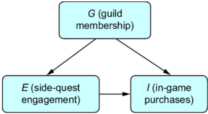
Figure 10.1 The DAG for the online gaming example

An example level 1 question and associated query is

૿What are in-game purchase amounts for players highly engaged in side-quests? P  ( I| E=૿high)

Reasoning at this level aims to describe, model, or detect dependence between variables. At this level, we’re not reasoning about any causal relationships between the variables.

Questions at level 2 (the intervention level) involve noncounterfactual hypothetical conditions, such as

૿What would in-game purchases be for a player if sidequest engagement were high? P  ( I  ^E =૿high)

At level 2, we formalize such questions with the ideal intervention. Note that any query derived from a level 2 query is also a level 2 query, such as ATEs, (e.g., E (IE=૿high – IE=૿low)) and CATEs.

Finally, counterfactual questions and queries fall at level 3 (the counterfactual level):

૿Given this player had low side-quest engagement and low purchases, what would their level of purchases have been if they were more engaged? P( I ^E =૿high| E=૿low, I=૿low)

As with level 2 queries, any query we derive from a level 3 query also falls at level 3. For example, a causal attribution query designed to answer ૿Why did this player have low purchases would be a level 3 query if it were a function of level 3 queries like the probabilities of causation described in section 8.3.

In identification, we work directly with queries. The y0 library in Python gives us a domain specific language for representing queries. The following code implements the query P(IE=e).

Listing 10.1 Creating a query in y0

!pip install git+https://github.com/y0-causal-inference/y0.git@v0.2.0
from y0.dsl import P, Variable #1
E = Variable("E") #2
I = Variable("I") #2
query = P[E](I) #3
query #4

#1 ૿P is for probability distributions, and ૿Variable is for defining. variables.

#2 Define variables G (guild membership), E (side-quest engagement), and I (in-game purchases).

#3 Define the distributional query P(I E).

#4 If running in a notebook environment, this will show a rendered image of P(I E).

SETTING UP YOUR ENVIRONMENT

In this chapter, I rely on version 0.2.0 of the y0 library. As it is a relatively new library, the library’s API is in development and recent versions will deviate slightly from what is shown here. Check out the library’s tutorials for recent developments.

Again, we rely on Graphviz and some custom utilities for plotting DAGs. The Graphviz installation depends on your environment. I am using Ubuntu 22.04 and install Graphviz via libgraphviz-dev. Then I install Python libraries graphviz version 0.20.3, and PyGraphviz version 1.13. The Graphviz code is for plotting only, so if you get stuck, you could forgo plotting for the rest of the code.

The query object is an object of the class Probability. The class’s __repr__ method (which tells Python what to return in the terminal when you call it directly) is implemented such that when we evaluate the object in the last line of the preceding code in a Jupyter notebook, it will display rendered LaTeX (a typesetting/markup language with a focus on math notation), as in figure 10.2.

Figure 10.2 The rendered math image returned when you evaluate the query object in listing 10.1

The causal hierarchy applies to models and data as well.

10.1.2 Where models and assumptions fall on the hierarchy

A ૿model is a set of assumptions about the data generating process (DGP). Those assumptions live at various levels of the hierarchy.

LEVEL 1 ASSUMPTIONS

Models at the associational level have statistical but noncausal assumptions. For example, suppose we’re interested in P(I  |E  = e ), for either value (૿low, ૿high) that e might take. We might fit a linear model to regress in-game purchases I against side-quest engagement E. Or we might train a neural network that maps E to I. These are two statistical models with different parameterizations. In other words, they differ in non-causal, statistical assumptions placed on P(I|E). Once we add causal assumptions, we move to a higher level of the hierarchy.

LEVEL 2 ASSUMPTIONS

Assumptions that we can represent with a causal DAG are level 2 (interventional) assumptions. An example of a level 2 model would be a causal graphical model (aka, a causal Bayesian network)—a probabilistic model trained on a causal DAG. A causal DAG by itself is a level 2 set of assumptions; assumptions about what causes what. Generally, assumptions that let you deduce the consequences of an intervention are level 2 assumptions.

LEVEL 3 ASSUMPTIONS

The canonical example of a level 3 model is a structural causal model. But more generally, assumptions about

mechanism—how variables affect one another—are level 3 (counterfactual) assumptions.

One way to think about this is that any causal assumption you cannot represent in the structure of the DAG is, by process of elimination, a level 3 assumption. For example, suppose your DAG has the edge X →Y. Further, you believe the causal relationship between X and Y is naturally linear. You can’t ૿see linearity on the DAG structure, so linearity is a level 3 assumption.

10.1.3 Where data falls on the hierarchy

Recall the differences between observational data and interventional data. Observational data is passively observed; as a result, it captures statistical associations resulting from dependence between variables in the DGP.

LEVEL 1 DATA

In our online gaming example, the level 1 data was logged examples of side-quest engagement and in-game purchases pulled by a database query. Observational data lives at level 1 of the causal hierarchy.

LEVEL 2 DATA

Interventional data is generated as the result of applying an intervention, such as data collected from a randomized experiment. In the gaming example, this was the data created because of an A/B test that randomly assigned players to different groups where they are coerced into different fixed side-quest engagement levels. Intervention data lives at level 2 of the hierarchy.

LEVEL 3 DATA

Counterfactual data, which lives at level 3 of the hierarchy, is the odd case. Counterfactual data would contain data from across possible worlds. In most domains, we only have data from one world—one potential outcome for each unit of observation in the data.

However, there are special cases where counterfactual data exists. For example, cloud service providers use complex but deterministic policies for allocating resources in the cloud, given various constraints. For one example with a given allocation outcome in the log, we could generate a counterfactual outcome for that example by applying a different allocation policy to that example. Similarly, given data produced by simulation software, we could generate counterfactual data by changing the simulation to reflect a hypothetical condition and then rerunning it with the same initial conditions as the original data.

10.1.4 The causal hierarchy theorem

The causal hierarchy offers us a key insight from something called the causal hierarchy theorem. That insight is this: ૿You cannot answer a level k question without level k assumptions. For example, if you want a causal effect, you need a DAG or some other level 2 (or level 3) assumptions. If you want to answer a counterfactual question, you need level 3 assumptions. And even the most cutting-edge of deep learning models can’t answer level k questions reliably unless they encode a representation of level k assumptions.

More formally, the causal hierarchy theorem establishes that the three layers of the causal hierarchy are, in mathematical jargon, ૿almost always separate. Roughly speaking, ૿separate means that data from a lower level of the

hierarchy is insufficient to infer a query from a higher level of the hierarchy. And ૿almost always means this statement is true except in cases so rare that we can dismiss them as practically unimportant.

Aside from this insight, the causal hierarchy makes understanding identification—perhaps the hardest topic in all causal inference—much easier, as we’ll see in the rest of the chapter.

10.2 Identification and the causal inference workflow

In this section, we’ll look at the workflow for posing and answering causal questions and the role that identification plays in that workflow. We’ll use the online gaming DAG introduced in chapter 7 as an example. Let’s start by building the DAG with y0.

Listing 10.2 Building the online gaming DAG in y0

import requests #1
def download_code(url): #1
 response = requests.get(url) #1
 if response.status_code == 200: #1
 code_content = response.text #1
 print("Code fetched successfully.") #1
 return code_content #1
 else: #1
 print("Failed to fetch code.") #1
 return None #1
url = ( #1
 "https://raw.githubusercontent.com/altdeep/" #1
 "causalML/master/book/chapter%2010/id_utilities.py" #1
) #1
utilities_code = download_code(url) #1
print(utilities_code) #2
# After checking, uncomment the exec call to load utilities
#exec(utilities_code) #2
from y0.graph import NxMixedGraph as Y0Graph #3
from y0.dsl import P, Variable #4
G = Variable("G") #4
E = Variable("E") #4
I = Variable("I") #4
dag = Y0Graph.from_edges( #4
 directed=[ #4
 (G, E), #4
 (G, I), #4
 (E, I) #4
 ] #4
) #4
gv_draw(dag) #5

#1 Install Graphviz for DAG visualization. Download some helper functions for identification and visualization that convert some y0 abstractions into abstractions we’re familiar with.

#2 Inspect the downloaded code before executing as a matter of good security practice. Then uncomment the last line and execute. #3 y0 works with a custom graph class called NxMixedGraph. To avoid confusion, we’ll call it a Y0Graph and use it to implement DAGs. #4 Build the graph.

#5 Draw the graph with a Graphviz helper function.

This produces the graph in figure 10.3.

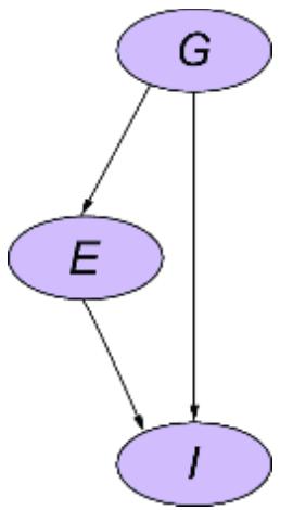
Figure 10.3 Drawing the online gaming graph with y0

Our goal in chapter 7 was to use our model of P(G, E, I ) to simulate from P(IE=૿high) using the intervention operator. In sections 7.1.6 and 7.2.6, we did this simulation and saw empirical evidence that it works for this online game example. Identification means showing that it works in general, based on your model and assumptions. Formally, we want to be sure that level 1 distribution P(G, E, I), or data from that distribution, combined with our DAG,

is enough to simulate from level 2 distribution P(IE=૿high). Identification with y0 confirms that this is indeed possible.

Listing 10.3 Checking identification of P(IE=૿high) from P(G, E, I)

e = E #1
check_identifiable( #2
 dag, #2
 query=P(I @ e), #2
 distribution=P(G, E, I) #2
) #2

#1 Make a lowercase ૿e to represent an intervention value. #2 Check identifiability given the DAG, a distribution, and a target query. Y0 represents ideal interventions with @, so we write P(I E=e as P(I @ e).

This will return True, but what if we didn’t have any observations of guild membership G ? We can use y0 to test if we have identification for P(IE=૿high) from P(E, I ). In other

words, test if it is possible to infer P(IE=૿high) from observations of E and I only.

Listing 10.4 Checking identification of P(IE=૿high) from P(E, I)

check_identifiable(
 dag,
 query=P(I @ e),
 distribution=P(E, I)
)

This will return False, because we don’t have identification for P(IE ^{= e} ) from the DAG and P(E, I) given our graphical assumptions.

LACK OF IDENTIFICATION AND MISGUIDED PROBABILISTIC ML

Y0 shows us that P(IE=e) is not identified from P(E, I) given our online game DAG. Consider the implications of this result from the perspective of probabilistic machine learning (ML). As experts in probabilistic ML, given G is unmeasured, we might be inclined to train a latent variable model on P(E, I) where G is the latent variable. Once we’ve learned that model, we could implement the intervention with graph surgery setting E=e, and then sampling I from the transformed model.

This algorithm would run; it would generate samples. But the lack of identification result from y0 proves that, given only the assumptions in our DAG, we could not consider these to be valid samples from P(IE=e). And training on more data wouldn’t help. The only way this could work is if there were additional causal assumptions constraining inference beyond the assumptions encoded by the DAG.

Given this introduction, let’s define identification.

10.2.1 Defining identification

Suppose I were to randomly choose a pair of numbers, X and Y, and add them together to get Z. Then, I tell you what Z was and ask you to infer the values of X and Y. Could you do it? Not without more information. So, what if I gave you millions of examples of feature Z and label {X, Y  }. Could you train a deep learning model to predict label {X, Y  } from input feature Z  ? Again, no, at least not without strong assumptions on the possible values of {X, Y  }. What if, instead of millions, I gave you billions of examples? No; more data would not help. In statistics, we would say the prediction target {X, Y  } is not identified.

In other words, you want to infer something, and you have an algorithm (e.g., a deep net) that takes in data and produces an answer. That answer will usually be a bit different than the true value because of statistical variation in the input data. If your inference objective is identified, then the more data you input to the algorithm, the more that variance will shrink and your algorithm’s answer will converge to the true answer. If your inference objective is not identified, then more data will not reduce your algorithm’s errors.

Causal identification is just statistical identification across levels of the causal hierarchy. A causal query is identified when your causal assumptions enable you to infer that query using data from a lower level on the hierarchy.

10.2.2 The causal inference workflow

Now that we have defined identification, we can define a full workflow for causal inference. Figure 10.4 shows the full workflow.

Figure 10.4 The causal inference workflow. The identification step is an essential step in the workflow.

Identification is a key step in the workflow. Let’s walk through each of the steps.

STEP 1: POSE YOUR QUERY

First, we pose our causal question as a query. For example, given our question ૿What would in-game purchases be for a player if side-quest engagement was high? our query is P (IE=૿high).

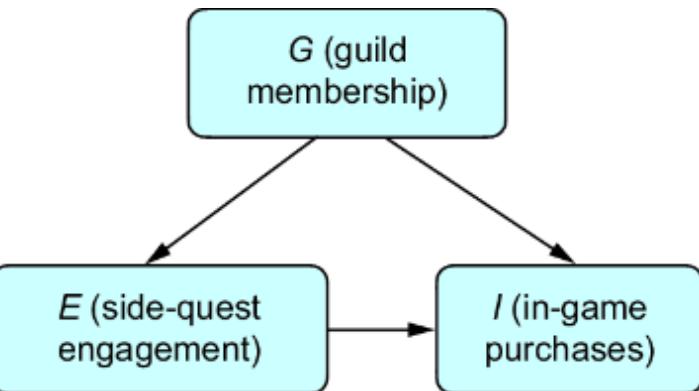
Figure 10.5 Step 2: Build the model to capture your causal assumptions relative to your query. For the query P(IE=૿high), this is our online gaming DAG.

STEP 2: BUILD YOUR MODEL

Next, build a causal model that captures your basic causal assumptions. Our model will be the online game causal DAG, shown again in figure 10.5.

Your model’s assumptions should at least match the level of your query in the causal hierarchy. For example, the query P(IE=૿high) is a level 2 query, so we need at least some level 2 assumptions. The causal DAG is a level 2 causal model, so in our analysis, the DAG provides the necessary level 2 assumptions.

STEP 3: CHECK IDENTIFICATION

Evaluate whether you have identification for your query, given your model assumptions and your available data. If you don’t have identification, you must either observe additional variables in your data or change your assumptions. For example, we could modify our online gaming DAG (changing level 2 assumptions). Or simply stop and conclude you can’t answer the question given your data and knowledge about the problem, and devote your attention elsewhere.

STEP 4: ESTIMATE YOUR QUERY

Once you know you have identification for your query, you can run statistical inference on, or ૿estimate, your query. There are a variety of estimation methods and algorithms, from Bayesian inference to linear regression to propensity scores to double machine learning. We’ll review some estimation methods in the next chapter.

STEP 5: REFUTE YOUR CAUSAL INFERENCE

Refutation is a final step where we conduct sensitivity analysis to evaluate how sensitive our results from step 4 are to violations of our assumptions, including the assumptions

that enabled identification. We’ll see examples of this in chapter 11.

10.2.3 Separating identification and estimation

In many texts, identification and estimation are combined in one step by matching the estimators and practical scenarios where those estimators will work. In this book, we’ll highlight the separation of identification and estimation for several reasons:

• The separation lets us shunt all the causal considerations into the identification step. This helps us be explicit about what causal assumptions we are relying on for estimation to work and builds intuition for when our analysis might fail.
• The estimation step thus simplifies to purely statistical questions, where we consider the usual statistical tradeoffs (bias vs. variance, uncertainty quantification, how well it scales, etc.).
• The separation also allows us to handle estimation with the automatic differentiation capabilities that power cutting-edge deep learning libraries without worrying whether these learning procedures will get the causality wrong.

Next, we’ll dive into the most common identification strategy: backdoor adjustment.

10.3 Identification with backdoor adjustment

Suppose we want to determine the causal effect of engagement on in-game purchases, i.e., E  (IE ⁼ ૿high – IE ⁼ ૿low). We can derive this expectation from the query E (IE=^e = i ), so we focus on P (I ^{E = e} = i  ). We can use the online gaming DAG to prove the following is true:

We’ll see how to derive this equation in the next section. The right side of this equation is a level 1 quantity called an estimand that we can derive from the joint distribution P (I, E, G ).

\[P(I\_{E=\text{"high"}}=i) = \sum\_{\mathbf{g}} P(I=i|E=\text{"high"},G=\mathbf{g})P(G=\mathbf{g})\]

QUERIES, ESTIMANDS, AND ESTIMATORS

In statistics, the estimand is the thing the statistical algorithm (the estimator) estimates. The task of identification is finding (identifying) an estimand for your query. In terms of the causal hierarchy, causal identification is about finding a lower-level estimand for a higher-level query.

In the online gaming backdoor identification example, P(IE=૿high=i) is a level 2 query, and ∑gP(I=i|E=૿high, G=g)P(G=g) is the level 1 estimand called the backdoor adjustment estimand. Backdoor adjustment is an operation we apply to P(E, I, G), where we sum out (or integrate out in the continuous case) the common cause G. In some cases, we’ll see we don’t need to know the estimand explicitly, only that it exists.

We passed our DAG and the intervention-level query P (I ^{E =} ૿high) to y0, and it told us it identified an estimand, an operation applied to P (E, I, G  ) that is equivalent to P (IE ⁼ ૿high). Let’s have y0 display that estimand.

Listing 10.5 Deriving the estimand to get P(IE=૿high) from P(E, I, G)

from y0.graph import NxMixedGraph as Y0Graph from y0.dsl import P, Variable from y0.algorithm.identify import Identification, identify

query = P(I @ e) base_distribution = P(I, E, G)

identification_task = Identification.from_expression( graph=dag, query=query, estimand=base_distribution)

identify(identification_task)

This returns the expression in figure 10.6.

Figure 10.6 Output of y0’s identify function

In our notation, this is ∑ ^g P (I = i |E  =૿high, G  = g) ∑ε,ⁱ P(E  = ε, G  = g, I  = i), which simplifies to ∑ ^g P (I = i |E  = ૿high, G  = g ) P(G  = g ). This is the backdoor adjustment estimand. We’ll see at a high level how y0 derives this estimand. But first, let’s look a bit more closely at this estimand.

10.3.1 The backdoor adjustment formula

In general terms, suppose X is a cause of Y, and we are interested in the intervention-level query P(YX=x). In that case, the backdoor adjustment estimand is ∑gP(X = x, Z  = z) P (Z  = z ). The backdoor adjustment formula equates the causal query P(XX=x) with its estimand:

\[P\left(Y\_{X=x} = y\right) = \sum\_{z} P\left(Y = y | X = x, Z = z\right) P\left(Z = z\right)\]

Here, Z is a set of variables called the adjustment set. The summation is shorthand for summation and integration—you sum over discrete variables in the adjustment set and

integrate over continuous variables. The adjustment set is defined as fa set of variables that satisfies the backdoor criterion—(1) the set collectively d-separates all backdoor paths from X to Y, and (2) it contains no descendants of X.

To understand why we want to d-separate backdoor paths between X and Y, consider again our DAG for our online gaming example in figure 10.7.

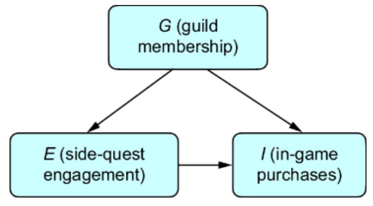
Figure 10.7 The online gaming DAG

What is the difference between P(I |E  =૿high) and P(IE=૿high)? Consider the two paths between E and I in figure 10.8. In the case of P(I |E  =૿high), observing E=૿high gives us information about I by way of its direct causal impact on I, i.e., through path E  →I. But observing E   = ૿high also gives us information about G, and subsequently about I through the backdoor path E ←G →I. A backdoor path between two variables is a d-connected path between a common cause. In the case of P(IE=૿high), we only want the impact on I through the direct path E→I.

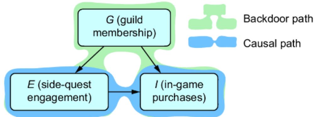
Figure 10.8 E←G→I is a backdoor path where G is a ૿confounder that is a common cause of E and I. We are interested in the statistical signal flowing along the causal path from E to I, but that signal is ૿confounded by the noncausal noise from additional statistical information through G on the backdoor path E←G→I.

We call G a confounder, because the statistical ૿signal flowing along the causal path from E to I is ૿confounded by the noncausal ૿noise from additional statistical information through G on the backdoor path E ←G →I. To address this problem, we seek to d-separate this backdoor path by blocking on G.

We want to identify a backdoor estimand for the query P(IE=૿high). So we substitute I for Y, and E for X in the backdoor adjustment formula. G blocks the backdoor path E G I, so the set G becomes our adjustment set:

P (IE=^e = i) = ∑^g P (I  = i|E  = e, G  = g )P(G  = g )

The backdoor adjustment formula d-separates the backdoor paths by summing out/integrating over, or in other words, ૿adjusting for the backdoor statistical signal, leaving only the signal derived from the direct causal relationship.

NOTE Some texts refer to the G-formula instead of backdoor adjustment formula. The backdoor adjustment formula is just the G-formula where the adjustment set is defined in terms of the backdoor criterion.

While an adjustment set can include non-confounders, in practice, excluding all but a minimal set of backdoorblocking confounders cuts down on complexity and statistical variation. We dive into the statistical considerations of backdoor adjustment in chapter 11.

10.3.2 Demystifying the back door

So where does the backdoor adjustment estimand come from? Let’s consider our online gaming example again. The query is P(I ^{E= e}) where e is ૿high or ૿low. In counterfactual terms, let’s consider two possible worlds, one with our original DAG, and one where we apply the intervention to side-quest engagement (E). Let’s view the parallel world graph in figure 10.9.

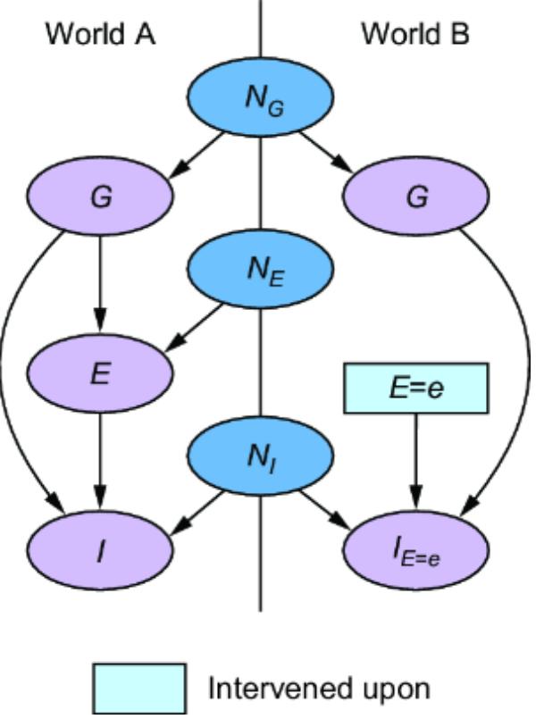
Figure 10.9 We have two parallel worlds: world A where E is not intervened upon, and world B where E is intervened upon.

If you squint hard enough at this graph, you’ll notice that it implies that E is conditionally independent from I ^{E= e} given G. We’ll use some d-separation–based reasoning to see this. Remember that, in general, we can’t use d-separation to reason across worlds on a parallel world graph because the d-separation rules don’t account for nodes that are equivalent across worlds (like G). But we’ll use a trick where we reason about conditional independence between E and I ^{E= e} by looking at a d-connected path from E to G in world A, and then extend that d-connected path from the equivalent G in world B to I ^{E= e}.

First, consider that paths from E in world A to world B have to cross one of two bridges between worlds, NG and NI . But the two paths to NI (E → I ← NI , E ← G → I ← NI ) are both dseparated due to the collider on I.

So we have one d-connected path to world B (E ← G ← NG). Now suppose we look at G in world B; from world B’s G, it is one step to I ^{E= e}. But we know that, by the law of consistency, the value of G in both worlds must be the same; both Gs are the same deterministic function of NG, and neither G is affected by an intervention. So, for convenience, we’ll collapse the two Gs into one node in the parallel world graph (figure 10.10). Looking now at the path E ← G → I ^{E= e}, we can see this path is d-separated by G. Hence, we can conclude E ⊥ I ^{E= e} | G.

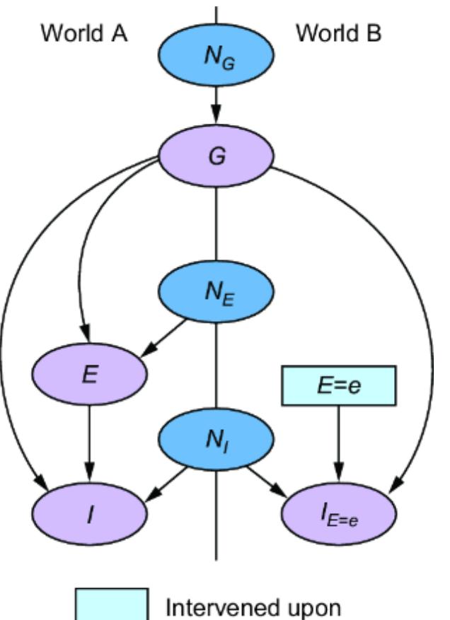
Figure 10.10 Collapsing G across worlds reveals G d-separates E and IE=e.

In causal inference jargon, this simplification is called ignorability. Ignorability means the causal variable E and the counterfactual potential outcomes like I ^{E= e} are conditionally independent given confounders. Ignorability is a common assumption made in causal inference. We can use this ignorability assumption in deriving the backdoor estimand.

Before we start, let’s recall a key definitional fact of conditional independence: if two variables U and V are conditionally independent given Z, then P (U  |Z  = z, V  = v ) = P (U  |Z  = z). Flipping that around, P (U  |Z  = z ) = P (U  |Z  = z, V  = v ). In other words, P (U  |Z   = z) = P (U  |Z   =  z, V    = ૿apples) = P (U  |Z   = z, V  =  ૿oranges); it doesn’t matter what value V takes because, since Z rendered it independent from U, its value has no bearing on U. Introducing V and

giving it whatever value we want is the trick that makes the derivation work. Also, recall the law of total probability says that we can marginalize a variable out of a joint distribution by summing (or integrating) over that variable, as in P (U  = u) = ∑vP (U  = u, V  = v ). The same is true when the joint distribution is subject to intervention, as in P (UW=^w = u) = ∑vP (UW=^w = u, VW=^w = v ).

Now let’s start with the causal query P (I ^E=^e ) and see how to equate it with the backdoor estimand ∑^g P (I  |E  = e, G  = g)P (G  = g ).

• 1. For some value of in-game purchases i, P (IE=^e = i ) = ∑^g P (IE=^e = i, GE=^e = g ) by the law of total probability.
• 2. ∑^g P (IE=e=i, GE=e=g ) = ∑^g P (IE=e=i, G =g ), because we know from our original DAG that G is not affected by the intervention on E.
• 3. Next we use the chain rule to factorize P (IE=^e = i, G  = g ): ∑^g P (IE=^e = i, G  = g ) = ∑^g P (IE=^e = i | G  = g)P (G  = g ).
• 4. Now we come to the trick—P (IE=^e = i  |G  = g ) = P (IE=^e = i  |E  = e, G  = g ) for any value of e, because once we condition on G=g, E=e and IE=^e are independent. So in our derivation, we can replace P (IE=^e = i  |G  = g ) with P (IE=^e = i  |E  = e, G  = g ).
• 5. Once we condition that E  = e, we can use the law of consistency to drop the subscript: ∑^g P (IE=^e = i  |E  = e, G   = g  )P (G  = g  ) = ∑^g P (I  = i  |E  = e, G  = g )P (G  = g  ).

Let’s explain steps 4 and 5. Our ignorability result shows that IE=e and E are conditionally independent given G. So in step 4 we apply the independence trick that lets us introduce E. Further, we set the value of E to be e so it matches the

subscript E=e. This allows us to apply the law of consistency from chapter 8 and drop the subscript E=e.

Voila, we’ve identified a backdoor estimand, an estimand from level 1 of the causal hierarchy, for a level 2 causal query P (IE=e) using level 2 assumptions encoded in a DAG. Causal identification is just coming up with derivations like this. Much, if not most, of traditional causal inference research boils down to doing this kind of math, or writing algorithms that do it for you.

Next, we’ll look at the do-calculus, which provides simple graph-based rules for identification that we can use in identification algorithms.

10.4 Graphical identification with the do-calculus

Graphical identification (sometimes called nonparametric identification) refers to identification techniques that rely on reasoning over the DAG. One of the most well-known approaches to graphical identification is the do-calculus, a set of three rules used for identification with causal graphs. The rules use graph surgery and d-separation to determine cases when you can replace causal terms like IE=e with noncausal terms like I  |E=e. Starting with a query on a higher level of the causal hierarchy, we can apply these rules in sequence to derive a lower-level estimand.

10.4.1 Demystifying the do-calculus

Recall high school geometry, where you saw if-then statements like this:

If the shape is a square, then all the sides are equal.

When you were trying to solve a geometry problem, you used facts like this in the steps of your solution.

Similarly, the do-calculus consists of three rules (if-then statements) of the following form:

If certain variables are d-separated after applying graph surgery to the DAG, then probability query A equals probability query B.

THE RULES OF THE DO-CALCULUS ARE NOT INTUITIVE

The three rules of the do-calculus are not intuitive upon reading them, just as geometric rules like cos2x + sin2x = 1 were not intuitive when you first saw them in high school. But like those geometric rules, we derive the rules of the docalculus from simpler familiar concepts, namely dseparation, ideal interventions, and the rules of probability. And like the rules of geometry, we can use the rules of the do-calculus to prove that a causal query from one level of the hierarchy is equivalent to one from another level.

Practically speaking, we can rely either on software libraries that implement the do-calculus in graphical identification algorithms (like y0) or simply hard-code well-known identification results like the backdoor adjustment estimand. To take away some of the mystery, I’ll introduce the rules and show how they can derive the backdoor estimand. The goal here is not to memorize these rules, but rather to see how they work in a derivation of the backdoor estimand that contrasts with the derivation in the previous section.

In defining these rules, we’ll focus on the target distribution Y under an intervention on X. We want to generalize to all DAGs, so we’ll name two other nodes, Z and W. Z and W will allow us to cover cases where we have another potential

intervention target Z and any node W we’d like to condition upon. Further, while I’ll often refer to individual variables, keep in mind that the rules apply when X, Y, Z, and W are sets of variables.

RULE 1: INSERTION OR REMOVAL OF OBSERVATIONS

If Y and Z are d-separated in your DAG by X and W after the incoming edges to X are removed . . .

Then P  ( Y ^{X = x}=  y | Z    =  z, W    =  w) = P( Y ^{X = x}  =  y | W    =  w).

This is called ૿insertion or removal because we can remove Z =z from P (YX=x=y |Z  = z, W   = w) to get P(YX=^x =y | W  = w) and vice versa.

RULE 2: EXCHANGE OF AN INTERVENTION FOR AN OBSERVATION

If Y and Z are d-separated in your DAG by X and W after incoming edges in X and outgoing edges from Z have been removed . . .

then P  ( Y ^{X = x} , ^{Z = z}= y | W  =  w) = P( Y ^{X = x}  =  y | Z    =    z, W    =    w).

Here we can either exchange the intervention Z=z in P (YX=x, ^Z=^z = y | W   = w) for conditioning on the observation Z  = z to get P(YX=x=y | Z  = z, W  = w), or vice versa.

RULE 3: INSERTION OR REMOVAL OF INTERVENTIONS

For rule 3, we are going to define Z as a set of nodes, and Z(W  ) as the subset of Z that are not ancestors of W.

If Y and Z are d-separated in your DAG by X and W after you remove all incoming edges to X and Z( W) . . .

then P( Y ^{X = x} , ^{Z = z}  =  y | W  =  w) = P( Y ^{X = x}  =  y | W  =  w).

This rule allows you to insert Z=z into P (YX=^x = y | W  = w) to get P (YX=x, Z=^z = y | W  = w) or remove Z=z from P(YX=x, Z=z= y | W=w) to get P (YX=x=y | W  = w).

10.4.2 Using the do-calculus for backdoor identification

Now we’ll use the do-calculus to provide an alternative derivation of the backdoor estimand that differs from our ૿ignorability-based definition. Again, I include this derivation to demystify the application of the do-calculus. Don’t worry if you don’t completely follow each step:

• 1. P (IE=^e = i ) = ∑^g P (IE=^e = i, GE=^e = g ) by the law of total probability.
• 2. ∑^g P (IE=^e =i, GE=^e = g ) = ∑^g P (IE=e, G=^g = i )P  (G ^E=e, I=ⁱ = g ) by way of c-component factorization.
• 3. P (IE=e, G=^g = i) = P (I = i  |E  = e, G  = g ) by rule 2 of the do-calculus.
• 4. P(GE=e, I=ⁱ = g) = P (G  = g) by rule 3 of the do-calculus.
• 5. Therefore, P (IE=^e = i)  = ∑^g P (I  = i  |E  = e, G  = g ) P (G  = g ) by plugging 3 and 4 into 2.

The do-calculus rules are applied in steps 3 and 4.

Note Step 2 uses a factorization rule called ccomponent factorization. A c-component (confounded component) is a set of nodes in a DAG where each pair of observable nodes is connected by a path with edges that always point toward, never away from, the observable nodes (these are the ૿orphaned cousins mentioned in chapter 4). The joint probability of the observed variables can be factorized into c-components, and this fact enabled step 2. Factorizing over c-components is common in identification algorithms. See the references in the chapter notes at

https://www.altdeep.ai/p/causalaibook.

This do-calculus-based derivation is far less intuitive than our ૿ignorability-based derivation. There are two advantages we get in exchange for that of intuition. First, the do-calculus is complete, meaning that if a query has an identifiable estimand using graphical assumptions alone, it can be derived using the do-calculus. Second, we have algorithms that leverage the do-calculus to automate graphical identification.

10.5 Graphical identification algorithms

Graphical identification algorithms, often called ID algorithms, automate the application of graph-based identification systems like the do-calculus. When we used y0 to check for identification of P (IE=^e ) and to derive the backdoor estimand, it was using its implementation of graphical identification algorithms. In this section, we’ll see how we can use these algorithms to identify another useful estimand called the front-door estimand.

10.5.1 Case study: The front-door estimand

In our online gaming example, suppose we were not able to observe guild membership. Then we would not have

backdoor identification of P (IE=e). However, suppose we had a mediator between side-quest engagement (E ) and in-game purchases (I  )—a node on the graph between E and I. Specifically, our mediator represents won items (W  ), as seen in figure 10.11.

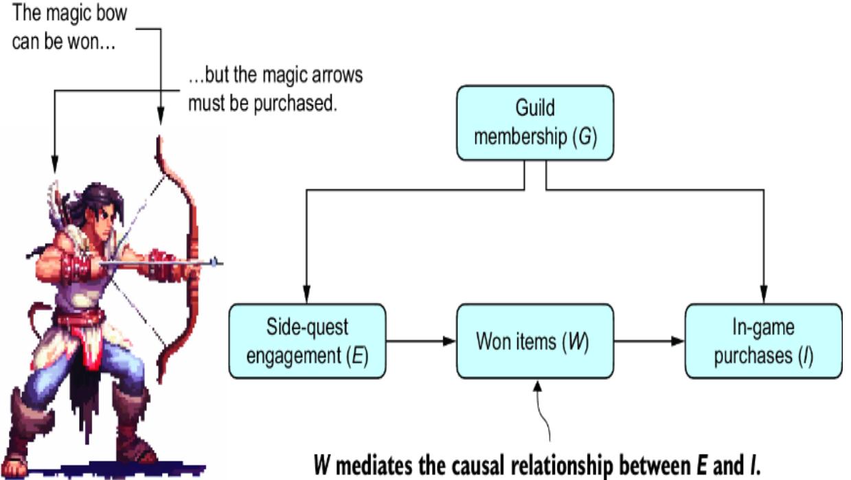
Figure 10.11 Side-quest engagement leads to winning virtual items like this magic bow. Won items drive more in-game purchases, such as magic arrows for the magic bow, so we introduce a mediator ૿won items on the causal path between side-quest engagement and in-game purchases.

The idea of won items is as follows. When a player successfully completes a side-quest, they win a virtual item. The more side-quests they finish, the more items they earn. Those won virtual items and purchased virtual items can complement one another. For example, winning a magic bow motivates purchases of magical arrows. Thus, the amount of won items a player has influences the amount of virtual items they purchase.

Given this graph, we can use y0’s implementation of graphical identification algorithms to derive the front-door estimand.

Listing 10.6 Deriving the front-door estimand in y0

from y0.graph import NxMixedGraph as Y0Graph
from y0.dsl import P, Variable
G = Variable("G") #1
E = Variable("E") #1
I = Variable("I") #1
W = Variable("W") #1
e = E #1
dag = Y0Graph.from_edges( #1
 directed=[ #1
 (G, E), #1
 (G, I), #1
 (E, W), #1
 (W, I) #1
 ] #1
) #1
query=P(I @ e) #2
base_distribution = P(I, E, W) #3
identification_task = Identification.from_expression( #4
 graph=dag, #4
 query=query, #4
 estimand=base_distribution) #4
identify(identification_task) #4

#1 Build a new graph with the mediator variable. #2 Still the same query as in listing 10.5, P(I_{E=e}) #3 But now we observe I, E, and W #4 Finally, we check if the query is identified given the DAG and observational distribution.

This code will return the output in figure 10.12.

Figure 10.12 Y0 renders a math figure as output of identification.

Rearranging the output, and in our notation, this is the result:

\[P = \sum\_{\mathbf{g}, \mathbf{w}} P(W = w | E = e, G = \mathbf{g}) \sum\_{\varepsilon, \iota, \omega} P(I = i | E = \varepsilon, G = \mathbf{g}, W = w) P(E = \varepsilon, W = \omega, I = \iota)\]

Simplifying as before, we get the front-door estimand:

\[P(I\_{E=e} = i) = \sum\_{w} P(W = w | E = e) \sum\_{\varepsilon} P(I = i | E = \varepsilon, W = w) P(E = \varepsilon)\]

Note that there is an outer summation over W and an inner summation over all values of E (with each value of E denoted as ε, distinct from the intervention value e).

10.5.2 Demystifying the front door

Like the backdoor estimand, the do-calculus derivation of the front-door estimand involves repeated substitutions using rules 2 and 3. The rough intuition behind the front-door estimand is that the statistical association between sidequest engagement and in-game purchases comes from both the direct causal path and the path through the backdoor confounder guild membership (G ). The front-door estimand uses the mediator to determine how much of that association is due to the direct causal path; the mediator acts as a gauge of the flow of statistical information through that direct causal path.

A key benefit of the estimand is that it does not require observing a set of confounders that block all possible backdoor paths. Avoiding backdoor adjustment is useful when you have many confounders, are unable to adjust due to latent confounders, or are concerned that there might be some unknown confounders.

Next, we’ll examine how to identify counterfactuals.

10.6 General counterfactual identification

The causal DAG is a level 2 modeling assumption. The causal hierarchy theorem tells us that the graph in general is not sufficient to identify level 3 counterfactual queries. For counterfactual identification from level 1 or level 2 distributions, you need level 3 assumptions. In simple terms, a level 3 assumption is any causal assumption that you can’t represent with a simple causal DAG.

In chapter 9, I introduced the general algorithm for counterfactual inference. The algorithm requires a structural causal model (SCM), which is a level 3 model; it encapsulates level 3 assumptions. With an SCM, the algorithm can infer all counterfactual queries that can be defined on its underlying variables. The cost of this ability is that the SCM must encapsulate all the assumptions needed to answer all those queries. Many of these assumptions cannot be validated with level 1 or level 2 data.

The more assumptions you make, the more vulnerable your inferences are to violations of these assumptions. For this reason, we seek identification techniques that target specific counterfactual queries (rather than every counterfactual query) with the minimal set of level 3 assumptions possible.

10.6.1 The problem with the general algorithm for counterfactual inference

We can see the problem with the general algorithm for counterfactual inference when we apply it to two similar SCMs. Let’s suppose there is a ground-truth SCM that differs from the SCM you are using to run the algorithm. Suppose both SCMs have the exact same underlying DAG and the

same statistical fit on observational and experimental data; in other words, the SCMs provide the same inferences for all level 1 and level 2 queries. Your SCM could still produce different (inaccurate) counterfactual inferences relative to the ground-truth SCM.

To see why, recall the stick-breaking example from chapter 6. I posed two similar but different SCMs. This was the first:

\[n\_{\mathcal{Y}} \sim \text{Uniform}(0, 1)\]

\[\mathcal{Y} := \begin{cases} 1, & n\_{\mathcal{Y}} \le p\_{x1} \\ 2, & p\_{x1} < n\_{\mathcal{Y}} \le p\_{x1} + p\_{x2} \\ 3, & p\_{x1} + p\_{x2} < n\_{\mathcal{Y}} \le 1 \end{cases}\]

And this was the second:

\[n\_{\mathcal{Y}} \sim \text{Uniform}(0, 1)\]

\[\mathcal{Y} := \begin{cases} \mathfrak{B}, & n\_{\mathcal{Y}} \le p\_{x3} \\ 1, & p\_{x3} < n\_{\mathcal{Y}} \le p\_{x3} + p\_{x1} \\ 2, & p\_{x3} + p\_{x1} < n\_{\mathcal{Y}} \le 1 \end{cases}\]

Figure 10.13 visualizes sampling a single value from these models.

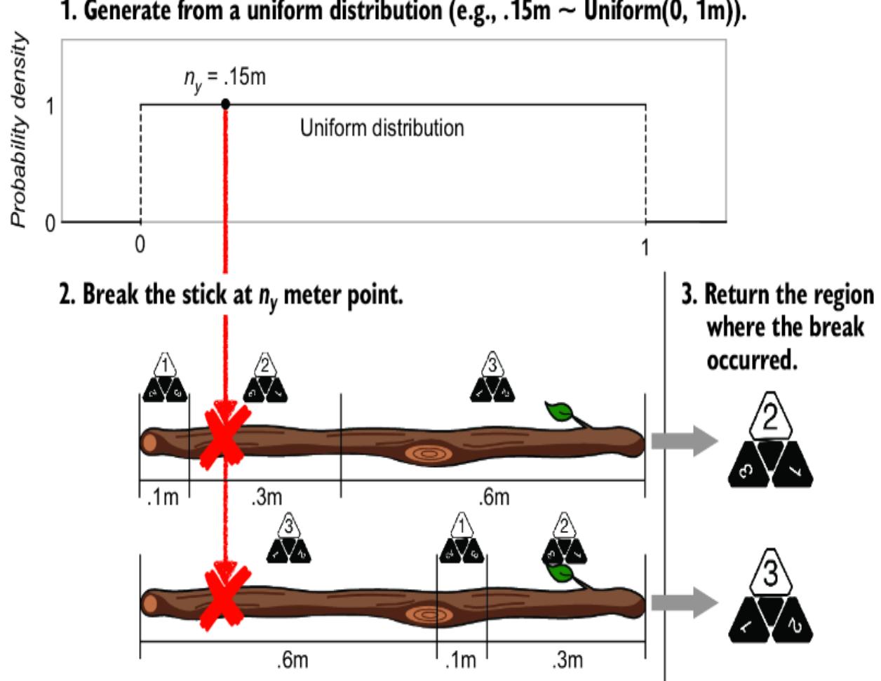
Figure 10.13 Two different SCMs encode the exact same observational and interventional distributions, but given the same exogenous variable value, you can get two different values of the corresponding endogenous variable in each model.

Figure 10.13 shows how, given a value of ny = .15, the sticks break at the .15 meters point, but the first stick will break in region 2, returning a value of 2, while the second stick will break in region 3, returning a 3. They produce different outcomes given the same random input because they differ in a level 3 assumption, i.e., how they process the input.

For this reason, when we go in the opposite direction and apply the abduction step in the general counterfactual inference algorithm, we can get different results across these models. For a given value of the endogenous variable, we

can get different posterior distributions on the exogenous variable.

Figure 10.14 illustrates how the two models, for an observed outcome of 3, would produce different inferences on Ny. For the first SCM, a value of y = 3 means P (Ny |Y  =  3) is a continuous uniform distribution on the range (px1 + px2) to 1, and for the second SCM, it is a continuous uniform distribution on the range 0 to px3. These different distributions of P (Ny |Y  =  3) would lead to different results from the counterfactual inference algorithm. Now suppose SCM 2 is right and SCM 1 is wrong. If we choose SCM 1, our counterfactual inferences will be inaccurate.

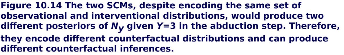
The general case is even harder; there can be many SCMs entailing the same level 1 and 2 assumptions but have different level 3 assumptions. You might learn one of those SCMs by, for example, using a deep neural network-based approach to learn a deep SCM from level 1 and level 2 data. But the deep SCM might not be the right SCM with respect to the counterfactual inferences you want to make.

The general algorithm for counterfactual inference is ideal if you are confident in the ground-truth SCM. But in cases where you aren’t, you can look toward counterfactual identification, where you specify a minimal set of level 3 assumptions that enable you to identify a target counterfactual query.

10.6.2 Example: Monotonicity and the probabilities of causation

Monotonicity is an example of a powerful level 3 assumption. Monotonicity is the simple assumption that the relationship between a cause X and an outcome Y is monotonic: E (Y  |X =x ) either never increases or never decreases as x increases. Note that linearity is a special case of monotonicity.

An intuitive example of monotonicity and non-monotonicity is in the dosage of medicine. In a monotonic dose-response relationship, taking more of the medicine either helps or does nothing. In a non-monotonic dose-response relationship, taking the medicine might help at a normal dose, but taking an overdose might cause the problem to get worse. Monotinicity helps identification by eliminating counterfactual possibilities; if the dose-response relationship is monotonic, when you imagine what would have happened if you took a stronger dose, you can eliminate the possiblity that you would have gotten worse.

Recall the probabilities of causation we saw in chapter 8:

• Probability of necessity (PN): P (YX=0 = 0|X  = 1, Y  = 1)
• Probability of sufficiency (PS): P (YX=1 = 1|X  = 0, Y   = 0)
• Probability of necessity and sufficiency (PNS): P (YX=1 = 1, YX=0 = 0)

Given monotonicity, we can identify the following level 2 estimands for the probabilities of causation.

PN = (P(Y  = 1) – P (YX=0 = 1))/P (X=1, Y=1)

\[\begin{array}{c} \bullet \text{ } \mathsf{PS} = (\mathsf{P} \,(\mathsf{Y}\_{\mathsf{X}=1} = \mathsf{1}) \text{ } \mathsf{-P} \,(\mathsf{Y}=\mathsf{1})) \mathsf{P} \,(\mathsf{X}=\mathsf{0}, \,\mathsf{Y}=\mathsf{0}) \end{array}\]

\[\begin{array}{c} \bullet \text{ PNS} = \mathcal{P} \left( \boldsymbol{\chi}\_{\boldsymbol{\chi}=\boldsymbol{1}} = \mathbf{1} \right) - \mathcal{P} \left( \boldsymbol{\chi}\_{\boldsymbol{\chi}=\boldsymbol{0}} = \mathbf{1} \right) \end{array}\]

We can estimate these level 2 estimands from level 2 data, such as a randomized experiment. And, of course, if we only have observational data, we can use backdoor or front-door adjustment or another identification strategy to infer P (YX=0 =1) and P (YX=1 =1) from that data.

We could derive these estimands by hand again, but instead, let’s think about the monotonicity enabled this identification by eliminating counterfactual possibilities. To see this, consider our uplift modeling question in chapter 8. There, X was whether we sent a promotion, and Y was whether the customer remained a paying subscriber (Y  = 1) or ૿churned (unsubscribed; Y  = 0). We segmented the subscribers as follows:

• Persuadables —Subscribers whose chance of remaining increases when you send a promotion
• Sure things —Subscribers who have a high chance of remaining regardless of whether you send a promotion
• Lost causes —Subscribers who have a low chance of remaining regardless of whether you send a promotion
• Sleeping dogs: Subscribers whose chances of remaining go down when you send a promotion

If you assume monotonicity, you are assuming that sending the promotion either does nothing or increases the chances of remaining. It assumes there are no users who will respond poorly to the promotion. In other words, assuming monotonicity means you assume there are no sleeping dogs.

Now let’s consider how this narrows things down. Suppose you have the following question:

I failed to send a promotion to a customer and they churned. Would they have remained had I sent the promotion? P  ( Y ^X =1  =  1| X    =  0, Y    =  0)

This counterfactual query is the probability of sufficiency. We want to know if sending the promotion would have increased the chances of their remaining. Thinking through the question,

• If the customer was a persuadable, sending the promotion would have increased their chances of remaining.
• If the customer was a lost cause, sending the promotion would have had no effect.
• If the customer was a sleeping dog, sending the promotion would have made them even less likely to remain.

It’s hard to determine if we should have sent the promotion if being a persuadable and being a sleeping dog were both possible for this customer, in one case the promotion would have helped and in the other it would have made churning even more certain. But if we assume monotonicity, we eliminate the possibility that they were a sleeping dog, and can conclude sending the promotion would have helped or, at least, not have hurt their chances of staying.

BAYESIAN MODELING AND COUNTERFACTUAL IDENTIFICATION

Although the graphical identification algorithms will work with some counterfactual queries, we don’t have general algorithms for counterfactual identification. But given our focus on the tools of probabilistic ML, we can look to Bayesian modeling for a path forward.

Identification is fundamentally about uncertainty. For example, in the counterfactual case, a lack of identification means that even with infinite level 1 and level 2 data, you can’t be certain about the true value of the level 3 query. From a Bayesian perspective, we can use probability to handle that uncertainty.

Suppose you have a set of causal assumptions, including non-graphical assumptions, and some level 1 and 2 data. You can take the following Bayesian approach to test whether your assumptions and data are sufficient to identify your counterfactual query:

• 1. Specify a set of SCMs that are diverse yet all consistent with your causal assumptions.
• 2. Place a prior distribution over this set, such that more plausible models get higher prior probability values.
• 3. Obtain a posterior distribution on the SCMs given observational (level 1) and interventional (level 2) data.
• 4. Sample SCMs from the posterior distribution, and for each sample SCM, you apply the general algorithm for counterfactual inference for a specific counterfactual query.

The result would constitute the posterior distribution over this counterfactual inference. If your causal assumptions and your data are enough to identify the counterfactual

query, the posterior on the counterfactual inference will converge to the true value as the size of your data increases. (Successful convergence assumes typical ૿regularity conditions for Bayesian estimation. Results will depend on the quality of the prior.) But even if it doesn’t converge to the true value, your assumptions might still enable convergence to a ballpark region around the true value that is small enough to be useful (this is called partial identification, as described in section 10.9).

The Pyro library, and its causality-focused extension ChiRho, facilitate combining Bayesian and causal ideas in this way.

There are generalizations of monotonicity from binary actions (like sending or not sending a promotion) to multiple actions as in a decision or reinforcement learning problem, see the course notes at

https://www.altdeep.ai/p/causalaibookfor references.

10.7 Graphical counterfactual identification

A conventional causal DAG only encodes level 2 assumptions, but there are graphical techniques for reasoning about counterfactuals. Graphical counterfactual inference only works in special cases, but these cases are quite practical. Further, working with graphs enables us to automate identification with algorithms. To illustrate graphical counterfactual identification, we’ll introduce a new case study.

When you open Netflix, you see the Netflix dashboard, which shows several forms of recommended content. Two of these

are ૿Top Picks For You, which is a personalized selection of shows and movies that Netflix’s algorithms predict you will enjoy based on your past viewing behavior and ratings, and ૿Because You Watched, which recommends content based on things you watched recently. The model of this system includes the following variables:

• T —A variable for the recommendation policy that selects a subscriber’s ૿Top Picks for You content. For simplicity, we’ll consider a policy, ૿+t  , that is currently in production. We’ll use ૿–t  , meaning ૿not t  , to represent alternative policies.
• B —A variable for the recommendation policy that selects a subscriber’s ૿Because You Watched content. Again, we’ll simplify this to a binary variable with policy ૿+b , representing the policy in production, and all alternative policies ૿–b , as in ૿not b .
• V —The amount of engagement that a subscriber has with the content recommended by ૿Because You Watched.
• W —The amount of engagement that a subscriber has with the content recommended by ૿Top Picks for You.
• A —Attrition, meaning whether a subscriber eventually leaves Netflix.
• C —Subscriber context, meaning the type of subscriber (location, demographics, preferences, etc.) we are dealing with.

Recommendation algorithms always take the profile of the subscriber into account, along with the viewership history, so subscriber profile C is a cause of both recommendation policy variables T and B.

In this section, we’ll use y0 to analyze this problem at various levels of the hierarchy. We’ll start by visualizing the graph.

Listing 10.7 Plot the recommendation DAG

T = Variable("T") #1
W = Variable("W") #1
B = Variable("B") #1
V = Variable("V") #1
C = Variable("C") #1
A = Variable("A") #1
t, a, w, v, b = T, A, W, V, B #1
dag = Y0Graph.from_edges(directed=[ #2
 (T, W), #2
 (W, A), #2
 (B, V), #2
 (V, A), #2
 (C, T), #2
 (C, A), #2
 (C, B) #2
]) #2
gv_draw(dag) #3

#1 Define variables for the model. #2 Create the graph. #3 Plot the graph.

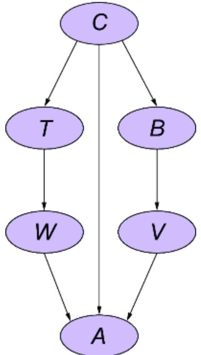
Figure 10.15 Causal DAG for the recommendation algorithm problem

This generates the DAG in figure 10.15.

As a preliminary investigation, you might look at the average treatment effect (ATE, a level 2 query) of the ૿Top Picks for You content on attrition E (AT=+t – AT=–t). Given that attrition A has a binary outcome, we can write this as P (AT=+^t =+a ) – P (AT=–^t = +a ). Focusing on P (AT=–^t = +a ), we know right away that we can identify this via both the (level 2) backdoor and the front door. So let’s move on to an interesting (level 3) counterfactual query called effect of treatment on the treated (ETT).

10.7.1 Effect of treatment on the treated

Recall that you get the ATE directly (without needing to identify and estimate a level 1 estimand) from a randomized experiment. Suppose you ran such an experiment on a cohort of users, and it showed a favorable ATE, such as that +t has a favorable impact on W and A relative to –t. So your team deploys the policy.

Suppose the +t policy works best with users who have watched a lot of movies and thus have more viewing data. For this reason, when the policy is deployed to production, such users are more likely to get assigned the policy. But since they are so highly engaged, they are unlikely to leave, regardless of whether they are assigned the +t or –t policy. We could have a situation where the +t policy looks effective in an experiment where people are assigned policies randomly, regardless of their level of engagement, but in production the assignment is biased to highly engaged people who are indifferent to the policy.

The level 3 query that addresses this is a counterfactual version of the ATE called effect of treatment on the treated (ETT, or sometimes ATT, as in average treatment effect on the treated). We write this as counterfactual query E (AT=+t – AT=–^t |T  =  +t ), as in ૿for people who saw policy +t, how much more attrition do they have relative to what they would have if they had seen –t ? Decomposing for binary A as we did with the ATE, we can write this as P(AT=+t=+a|T  = +t) – P(AT=–^t = +a|T  = +t). P(AT=+^t = +a |T  = +t ) simplifies to P (A  = +a |T  = +t ) by the law of consistency. So we can focus on the second term, P (AT=–t=+a |T=+t ).

In this special case of binary A, we can identify the ETT using graphical identification (for non-binary A, more level 3 assumptions are needed). To do graphical identification for counterfactuals, we can use graphical identification algorithms with counterfactual graphs.

10.7.2 Identification over the counterfactual graph

Y0 can derive an estimand for ETT using a graphical identification algorithm called ૿IDC* (pronounced I-D-Cstar).

GRAPH ID ALGORITHMS, ID, IDC, ID*, IDC*, IN Y0

Some of the core graphical identification algorithms implemented in y0 are ID, ID*, IDC, and IDC*. ID identifies interventional (level 2) queries from a DAG and observational (level 1) data. ID* identifies counterfactual (level 3) queries from observational and experimental (level 1 and level 2) data. IDC and IDC* extend ID and ID* to work on queries that condition on evidence, such as ETT.

The algorithms use the structure of the causal graph to recursively simplify the identification problem by removing irrelevant variables and decomposing the graph into ccomponent subgraphs. They apply the rules of do-calculus to reduce intervention terms, block confounding backdoor paths, and factorize the query into simpler subqueries. If no further simplification is possible due to the graph’s structure, the algorithms return a ‘non-identifiable’ result.

This chapter’s code relies on Y0’s implementations of these algorithms, though Y0 implements other graphical identification algorithms as well.

Listing 10.8 Identifying ETT with a graphical identification algorithm

from y0.algorithm.identify.idc_star import idc_star
idc_star(
 dag,
 outcomes={A @ -t: +a}, #1
 conditions={T: +t} #2
)

#1 Hypothetical outcome A T=–t = +a
#2 Factual condition T = +t

This will produce a rather verbose level 2 estimand. We can then apply level 2 graphical identification algorithms to get a level 1 estimand, which will simplify to the following:

\[P(A\_{T=-t} = +a | T = +t) = \sum\_{c} P(A = +a | C = c, T = -t)P(C = c | T = +t)\]

I’ll show a simple derivation in the next section.

For now, the intuition is that we are applying graphical identification algorithms over something called a counterfactual graph. Up until now, our graph of choice for counterfactual reasoning was the parallel world graph. Indeed, we can have y0 make a parallel world graph for us.

Listing 10.9 Plotting the parallel world graph with y0

from y0.algorithm.identify.cg import make_parallel_worlds_graph
parallel_world_graph = make_parallel_worlds_graph( #1
 dag, #1
 {frozenset([+t])} #1
) #1
gv_draw(parallel_world_graph) #2

#1 The make_parallel_worlds_graph method takes an input DAG and sets of interventions. It constructs a new world for each set. #2 The helper function visualizes the graph in a familiar way.

This graph differs slightly from the ones I’ve drawn because the algorithm applies the subscript for an intervention to every node in the world where the intervention occurred; the subscript indexes all the variables in a world. It’s up to us to reason that C from one world and C+t from another must have the same outcomes, since C+t is not affected by its world’s intervention do(T  = +t ).

Now recall that the problem with the parallel world graph is that d-separation won’t work with it. For example, in figure 10.16, d-separation suggests that C and C+t are conditionally independent given their common exogenous parent NC, but we just articulated that C and C+t must be the same; if C has a value, C+t must have the same value, so they are perfectly dependent.

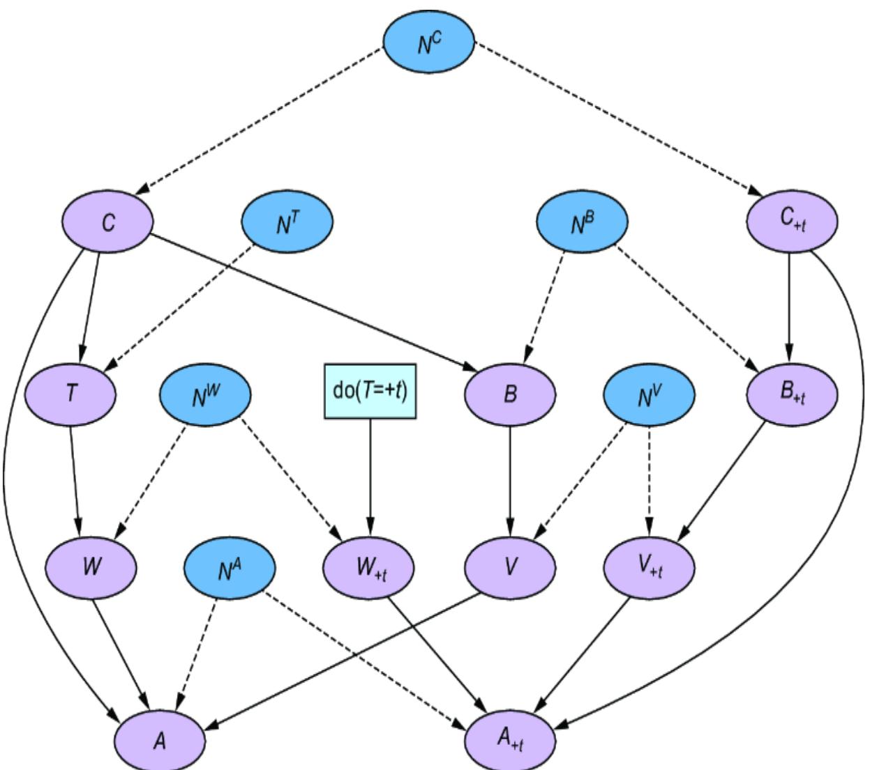
Figure 10.16 A parallel world graph drawn by y0 (and Graphviz). In this version of the parallel world graph, the subscripts indicate a world. For example, +t indicates the world where the intervention do(T=+t) is applied. To prevent confusion, the exogenous variables use superscripts instead of subscripts to indicate their child endogenous variables (e.g., ^NC is the parent of C (and C+t).

We can remedy this with the counterfactual graph. A counterfactual graph is created by using a parallel world graph and the counterfactual query to understand which nodes across worlds in the parallel world graph are equivalent, and then collapsing equivalent nodes into one. The resulting graph contains nodes across parallel worlds that are relevant to the events in the query. Unlike parallel

world graphs, you can use d-separation to reason about counterfactual graphs. We can use y0 to create a counterfactual graph for events AT=–t  =  +a and T  =  +t.

Listing 10.10 Listing 10.10 Counterfactual graph events AT=–t=+a and
T=+t

from y0.algorithm.identify.cg import make_counterfactual_graph

events = {A @ -t: +a, T: +t} #1
cf_graph, _ = make_counterfactual_graph(dag, events)
gv_draw(cf_graph)

#1 Counterfactual graphs work with event outcomes in the query. For P(A T=–t=+a|T=+t), we want events A T=–t =+a and T=+t.

This creates the counterfactual graph in figure 10.17.

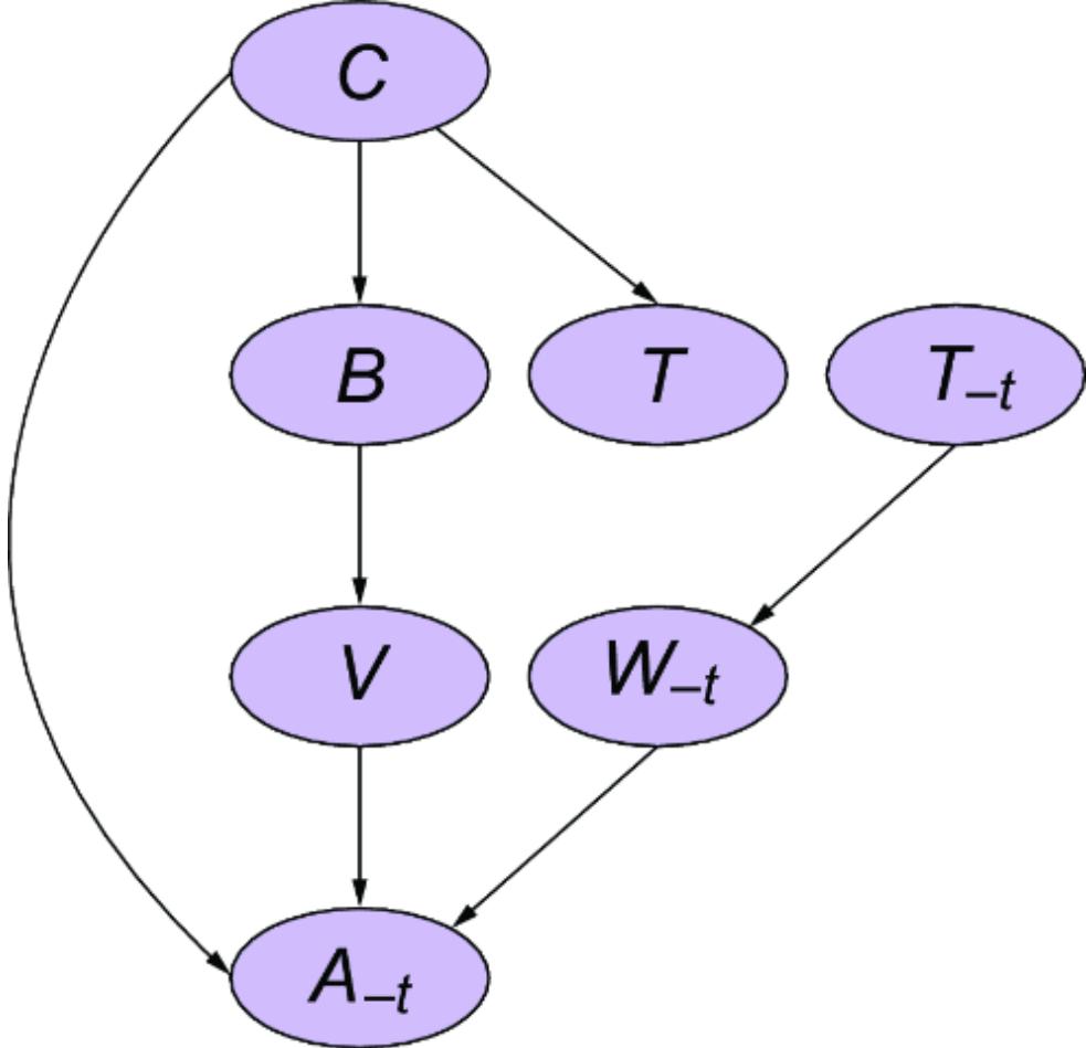
Figure 10.17 Counterfactual graph for events, produced by y0 (and Graphviz). T–t corresponds to the intervention do(T=–t).

At a high level, graphical identification algorithms in y0 do counterfactual identification by working with counterfactual graphs in lieu of conventional DAGs. First, it finds a level 2 estimand for a level 3 query. From there, you can use experimental data to answer the level 2 terms in the estimand, or you can attempt to further derive them to level 1 estimands from the level 2 terms.

GRAPHS ALONE WON’T WORK WHEN YOU CONDITION ON OUTCOME!

Suppose that instead of the ETT term P(AT=–t=+a|T=+t), you were interested in P(AT=–t =+a|T=+t, A=+a), answering the question ૿Given a subscriber exposed to policy +t and later unsubscribed, would they still have unsubscribed had they not been exposed to that policy? Or you could be interested in E(AT=–t – AT=+t|T=+t, A=+a) sometimes called counterfactual regret, which captures the amount the policy +t contributed to an unsubscribed individual’s decision to unsubscribe.

P(AT=–t=+a|T=+t, A=+a) is an example of a query where the hypothetical outcomes and factual conditions are in conflict. In this case, the factual conditions contain an outcome for A, and the hypothetical condition contains an interventional outcome for A. The graphical counterfactual identification techniques mentioned in this section will not work for this type of query. Identification in this case requires additional level 3 assumptions.

This is unfortunate, because this type of counterfactual is precisely the kind of ૿how might things have turned out differently? counterfactual questions that are the most interesting, and the most central to how humans reason and make decisions.

We can also use graphical identification for more advanced queries. For example, suppose you want to isolate how T affects A from how B affects A. You want to focus on users where B was –b. You find the data from a past experiment where ૿Because you watched . . . policy B was randomized. You take that data and zoom in on participants in the experiment who were assigned –b. The outcome of interest in that experiment was V, the amount of engagement with the content recommended in the ૿Because you Watched box. So you have the outcomes of VB=–b for those subscribers of interest. With this new data, you expand your query from P (AT=–^t = +a |T  = +t) to P (AT=–^t =  +a |T  =  +t, B    =  –b, VB=–^b = v ), including VB=–b=v because it is helpful in predicting attrition. Now you have three parallel worlds to reason over: the actual world, the world with do(T   =  +t ), and the world with do(B   =  –b ).

Listing 10.11 Create a parallel world graph for do(T=+t) and do(B=–b)

parallel_world_graph = make_parallel_worlds_graph(
 dag,
 {frozenset([-t]), frozenset([-b])} #1
)
gv_draw(parallel_world_graph)

#1 The second argument enumerates the hypothetical conditions.

This code creates this three-world parallel world graph seen in figure 10.18.

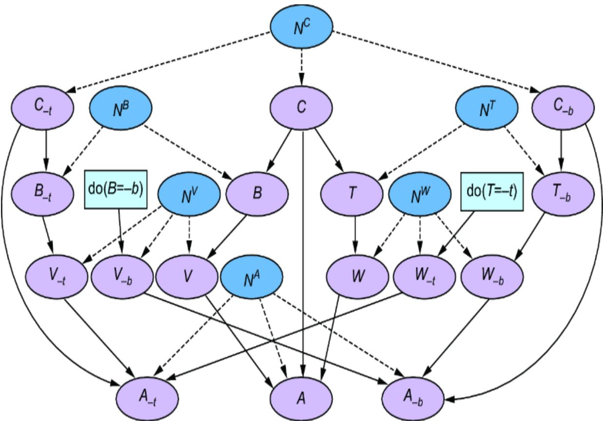
Figure 10.18 A parallel world graph with the actual world T=+t and hypothetical worlds do(T=–t) and do(B=–b). The dashed lines are edges from exogenous variables (dark gray).

Notably, the query P (AT=–t  =  +a |T  = +t, B  =  –b, VB=–^b = v ) collapses the parallel world graph to the same counterfactual graph as P (AT=–^t = +a |T   =  +t ).

Listing 10.12 Counterfactual graph for expanded expression

joint_query = {A @ -t: +a, T: +t, B: -b, V @ -b: +v} cf_graph, _ = make_counterfactual_graph(dag, joint_query) gv_draw(cf_graph)

This gives us the counterfactual graph in figure 10.19, which is the same as the graph in figure 10.17.

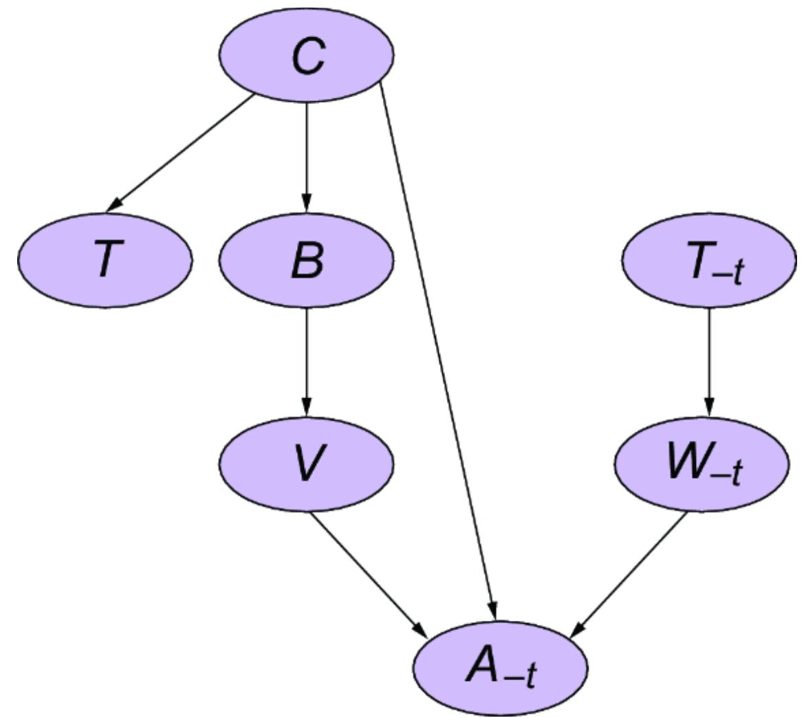
Figure 10.19 The counterfactual graph for P(AT=–t=+a|T=+t, B=–b, VB=–b=v) is the same as for P(AT=–t=+a|T=+t).

Next, we’ll look at another graph-based approach called single-world intervention graphs.

10.7.3 Counterfactual identification with singleworld intervention graphs

Single-world intervention graphs (SWIGs) provide an alternative to counterfactual identification with counterfactual graphs. Like a counterfactual graph, we construct a SWIG using the original causal DAG and the causal query. We’ll use the Netflix recommendation example to construct a SWIG for the interventions do(T  =  –t ) and do (B  =  –b ). Let’s construct a SWIG from a causal DAG.

NODE-SPITTING OPERATION

We have the intervention that targets do(T   =  +t ), and we can implement it with a special kind of graph surgery called a node-splitting operation. We split a new node off the intervention target T, as in figure 10.20. T still represents the same variable as in the original graph, but the new node represents a constant, the intervention value +t. T keeps its parents (in this case C ) but loses its children (in this case W  ) to the new node.

SUBSCRIPT INHERITANCE

Next, every node downstream of the new node inherits the new node’s values as a subscript. For example, in figure 10.21, W and A are downstream of the intervention, so the subscript T⁼ –t is appended to these nodes, so they become WT⁼ -t and AT⁼ -t.

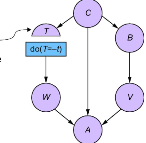
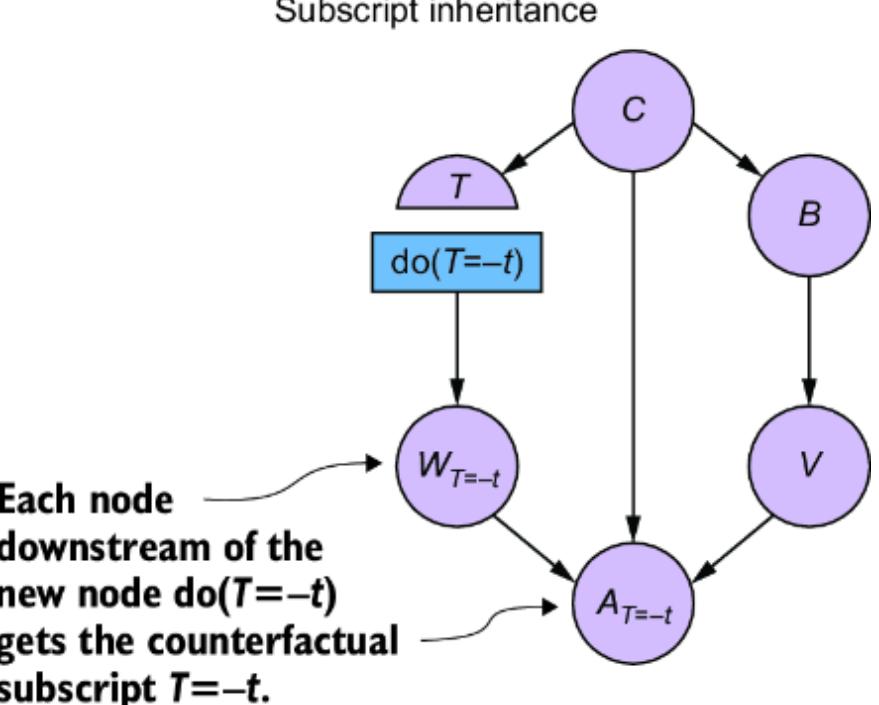
Figure 10.21 Every node downstream of the intervention gets the intervention subscript.

REPEAT FOR EACH INTERVENTION

We repeat this process for each intervention. In figure 10.22, we apply do(B  = –b), and split B and we convert V to VB=–^b and AT=-t to AT=–t,B=–b.

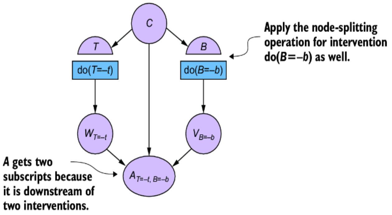
Figure 10.22 A node takes the subscript of all its upstream interventions.

Like the counterfactual graph, the SWIG contains counterfactual variables and admits d-separation. With these properties, we can do identification.

10.7.4 Identification with SWIGs

Suppose we are interested in ETT and want to identify P (AT⁼ –^t =  +a |T  =  +t ). We derive the SWIG in figure 10.23.

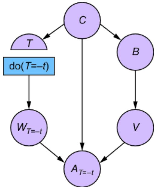
Figure 10.23 We can use the SWIG to derive ETT using the ignorability trick.

With this graph, we can identify P (AT=–^t =  +a |T  = +t ) using the ignorability trick I introduced in section 10.4:

• 1. P(AT=–^t = +a|T  = +t) = ∑^c P (AT=–^t = +a, CT=–t=c |T  =  +t ) by the law of total probability.
• 2. ∑^c P (AT⁼ –^t =  +a, CT=–^t =c  |T  = +t ) = ∑^c P (AT=–^t = +a, C = c |T =+t ), since C is not affected by interventions on T.
• 3. ∑^c P (AT=–^t =  +a, C  = c |T  = +t ) factorizes into ∑^c P (AT=–^t =+a |C  = c, T = +t ) P (C  = c | T  =  +t ) by the chain rule of probability.
• 4. P (AT=–^t =  +a |C = c, T  =  +t ) = P (AT=–^t =  +a |C  = c, T  =  – t ), again by the ignorability trick.
• 5. And as before, P (AT=–^t = +a |C  = c, T  = –t) = P (A =   +a |C  =c , T  =  –t ) by the law of consistency. Thus, P (AT=–^t = +a |T  =  +t ) = ∑^c P(A =  +a |C  = c, T  =  –t ) P(C  = c | T  = +t )

The magic happens in the ignorability trick in step 4, where C’s d-separation of AT=–t and T lets us change T  =  +t to T   =  –t. Notice that the same d-separation exists in the counterfactual graph we derived for P (AT=–^t = +a |T  =  +t ), shown in figure 10.17. The difference is that deriving the SWIG is easy, while deriving the counterfactual graph is nuanced, and one generally uses an algorithm like make_counterfactual_grap in y0.

10.7.5 The single-world assumption

The node-splitting operation relies on a new level 3 assumption. If you are going to node-split a variable X, then you are assuming it is possible to know what value X would naturally take without the intervention and that it would be possible for you intervene before it realized that value. Imagine in our Netflix example that, given a subscriber had profile C=c, the recommendation algorithm was about to assign the subscriber a policy +t for recommending ૿Top picks for you, but before that policy went into effect, you intervened and artificially changed it to –t . It’s possible that the way you forced the policy to be –t had some side effects that changed the recommendation system in some fundamental way, such that in this new system, T would not have been +t, in the first place. With the single-world assumption, you assume you can know T’s natural value would have been +t, and that your intervention wouldn’t change the system in a way that would affect T taking that natural value. You are implicitly making this assumption when you reason with SWIGs.

That assumption allows you to avoid the need to create additional worlds to reason over. You can condition on outcome T = +t and intervene do(T = –t ) in a ૿single world. You can also run experiments, where you apply the intervention do(T = –t ) and test if T (where you know T’s

૿natural values) is conditionally independent of A(T = –t ) given C. This reduces the number of counterfactual queries you can answer, but proponents of SWIGs suggest this is a strength, because it limits you to counterfactuals that can be validated by experiments.

CONTRASTING COUNTERFACTUAL GRAPHS AND SWIGS

Counterfactual graphs and SWIGs are similar in function, but they are distinctly different artifacts.

• Counterfactual graphs —The counterfactual graph works by collapsing equivalent parallel world graph nodes over possible worlds. They only contain nodes relevant to the specific query. They are defined for binary events like {T=+t} and {T=–t}—this works well even with continuous variables, because counterfactual language typically compares one hypothetical condition to one factual condition (e.g., ૿We invested 1 million; what if we had invested {2/more/half/…}?).
• Single-world intervention graphs (SWIGs) —The SWIG works by applying a node-splitting type of graph surgery. Unlike counterfactual graphs, they work with general variables (rather than just binary events) and are not query-specific (all original nodes are present). However, they rely on a single-world assumption—that it is possible to know with certainty what value a variable would have taken had it not been intervened upon.

The primary use case for both graphs is identification. Neither counterfactual graphs nor SWIGs enable identification from level 1 or 2 data of counterfactual queries such as P(AT=–t=+a|T=+t, A=+a) where the same variable appears in the hypothetical outcome and the factual condition. But you can still derive the counterfactual graph for such queries; this is not true for SWIGs. That is useful if you want to reason about

independence across worlds in cases of queries such as P(AT=–t=+a|T=+t, A=+a).

10.8 Identification and probabilistic inference

We’ve seen that a core part of the identification task is deriving an estimand. How does that estimand mesh with a probabilistic machine learning approach?

Consider, for example, our online game model, where ETT = E (IE=૿high – IE=૿low |E   = ૿high) = E (IE=૿high|E  = ૿high) – E (IE=૿low|E  = ૿high). We need to identify P (IE=૿high|E   = ૿high) and P (IE=૿low|E   = ૿high). Recall that P (IE=૿high|E   = ૿high) simplifies to the level 1 query P (I  |E =૿high) by the law of consistency, so the challenge lies with identifying the counterfactual distribution P (IE=૿low|E   =૿high).

Using a probabilistic machine learning approach with Pyro, we know we can infer P (I  |E   = ૿high) by using pyro.condition to condition on E  = ૿high and then running inference. The question is how we’ll infer the counterfactual distribution P (IE=૿low|E  = ૿high).

In the previous section, we saw that we can identify this query with a SWIG (assuming the single-world assumption holds). We used the SWIG to derive the following estimand for P (IE=0=i  |E  = ૿high):

\[\sum\_{\mathbf{g}} P(I=i|G=\mathbf{g}, E=\text{low})P(G=\mathbf{g}|E=\text{high})\]

But what do we do with this estimand with respect to building a model in Pyro? We could construct two Pyro models, one for P(G |E ) and one for P(I  |G, E ), infer P (I   = i  | G   = g, E   = ૿low) and P (G   = g | E   = ૿high) and then do the summation. But this is inelegant relative to our regular approach to probabilistic inference with a causal generative model:

• 1. Implement the full causal generative model.
• 2. Train its parameters on data.
• 3. Apply the intervention operator to simulate an intervention.
• 4. Run an inference algorithm.

In this approach, we build one causal model—we don’t build separate models for the estimand’s components P (G  |E ) and P (I   |G, E  ). Nonetheless, our regular approach to probabilistic inference with a causal generative model does work if we have identification, given the causal assumptions we implement in step 1 and the data we train on in step 2. We don’t even need to know the estimand explicitly; it is enough to know it exists—in other words, that the query is identified (e.g., by using Y0’s check_ identifiable function). With identification, steps 2–4 collectively become just another estimator for that estimand.

To illustrate, let’s consider how we’d sample from P (IE=૿low|E  = ૿high) using a Pyro model of our online gaming example. For simplicity, let’s replace E   = ૿high and E    = ૿low with E   = 1 and E   =  0 respectively. We know P (IE=0|E  = 1) is identified given our causal DAG and the singleword assumption. Fortunately, Pyro’s (and ChiRho’s) do intervention operator implements the SWIG’s node-splitting operation by default (if you used pyro.render_model to visualize an intervention and didn’t get what you expected, this is why). For ordinary interventional queries on a causal DAG, there is no difference between this and the ordinary graph

surgery approach to interventions. But when we want to condition on E   = 1 and intervene to set E   =  0, Pyro will accommodate us. We’ll use this approach to sample from P (IE=0|E   = 1). As a sanity check, we’ll also sample from the plain vanilla intervention distribution P(IE=0) and contrast those samples with samples from P(IE=0|E  = 1).

SETTING UP YOUR ENVIRONMENT

As a change in pace, I’ll illustrate this example using NumPyro instead of Pyro, though the code will work in Pyro with small tweaks. We’ll use NumPyro version 0.15.0. We’ll also use an inference library meant to complement NumPyro and Pyro called Funsor, version 0.4.5. We’ll also use Matplotlib for plotting.

First, let’s build the model.

NUMPYRO VS. PYRO

Pyro extends PyTorch, while NumPyro extends NumPy and automatic differentiation with JAX. The user interfaces are quite similar. If you are less comfortable with PyTorch abstractions and debugging PyTorch errors, or you prefer MCMC-based inference with the Bayesian programming patterns one uses in Stan or PyMC, then you might prefer NumPyro.

Listing 10.13 Generating from P(IE=0) vs. P(IE=0|E=1) in Pyro

import jax.numpy as np
from jax import random
from numpyro import sample
from numpyro.handlers import condition, do
from numpyro.distributions import Bernoulli, Normal
from numpyro.infer import MCMC, NUTS
import matplotlib.pyplot as plt
rng = random.PRNGKey(1)
def model(): #1
 p_member = 0.5 #1
 is_guild_member = sample( #1
 "Guild Membership", #1
 Bernoulli(p_member) #1
 ) #1
 p_engaged = (0.8*is_guild_member + 0.2*(1-is_guild_member)) #1
 is_highly_engaged = sample( #1
 "Side-quest Engagement", #1
 Bernoulli(p_engaged) #1
 ) #1
 p_won_engaged = (.9*is_highly_engaged + .1*(1-is_highly_engaged)) #1
 high_won_items = sample("Won Items", Bernoulli(p_won_engaged)) #1
 mu = ( #1
 37.95*(1-is_guild_member)*(1-high_won_items) + #1
 54.92*(1-is_guild_member)*high_won_items + #1
 223.71*(is_guild_member)*(1-high_won_items) + #1
 125.50*(is_guild_member)*high_won_items #1
 ) #1
 sigma = ( #1
 23.80*(1-is_guild_member)*(1-high_won_items) + #1
 4.92*(1-is_guild_member)*high_won_items + #1
 5.30*(is_guild_member)*(1-high_won_items) + #1
 53.49*(is_guild_member)*high_won_items #1
 ) #1
 norm_dist = Normal(mu, sigma)#1
 in_game_purchases = sample("In-game Purchases", norm_dist) #1

#1 A version of the online gaming model. The weights are estimates from the data (learning procedure not shown here).

Next, we’ll apply the intervention and run inference to sample from P (IE=0).

Listing 10.14 Apply intervention do(E=0) and infer from P(IE=0)

intervention_model = do( #1
 model, #1
 {"Side-quest Engagement": np.array(0.)}) #1
intervention_kernel = NUTS(intervention_model) #2
intervention_model_sampler = MCMC( #2
 intervention_kernel, #2
 num_samples=5000, #2
 num_warmup=200 #2
) #2
intervention_model_sampler.run(rng) #2
intervention_samples = intervention_model_sampler.get_samples() #2
int_purchases_samples = intervention_samples["In-game Purchases"] #2

#1 Apply the do operator to the model. #2 Apply inference to sample from P(I E=0).

We’ll contrast these samples from P (IE=0) with samples we’ll draw from P (IE=0|E  = 1). To infer P (IE=0 |E   = 1), we’ll condition intervention_model on the factual condition E   = 1. Then we’ll run inference again on this conditioned-upon intervened-upon model.

Listing 10.15 Condition intervention model and infer P(IE=0|E=1)

cond_and_int_model = condition( #1
 intervention_model, #1
 {"Side-quest Engagement": np.array(1.)} #1
) #1
int_cond_kernel = NUTS(cond_and_int_model) #2
int_cond_model_sampler = MCMC( #2
 int_cond_kernel, #2
 num_samples=5000, #2
 num_warmup=200 #2
) #2
int_cond_model_sampler.run(rng) #2
int_cond_samples = int_cond_model_sampler.get_samples() #2
int_cond_purchases_samples = int_cond_samples["In-game Purchases"] #2

#1 Now apply the condition operator to sample from P(I E=0|E=1).
#2 Apply inference to sample from P(I E=0|E=1).

Note that Pyro's do and condition subroutines mutually
compose; i.e., for a model with a variable X,
do(condition(model, {"X": 1.}), {"X": 0.}) is equivalent to
condition(do(model, {"X": 0.}), {"X": 1.}).

Finally, we’ll plot samples from P (IE=0) and P (IE=0|E   = 1) and evaluate the difference in these distributions.

Listing 10.16 Plot samples from P(IE=0) and P(IE=0|E=1)

plt.hist( #1
 int_purchases_samples, #1
 bins=30, #1
 alpha=0.5, #1
 label='$P(I_{E=0})$' #1
) #1
plt.hist( #2
 int_cond_purchases_samples, #2
 bins=30, #2
 alpha=0.5, #2
 label='$P(I_{E=0}|E=1)$' #2
) #2
plt.legend(loc='upper left') #2
plt.show() #2

#1 Plot a histogram of samples from P(I E=0). #2 Plot a histogram of samples from P(I E=0|E=1).

This code generates the histograms in figure 10.24.

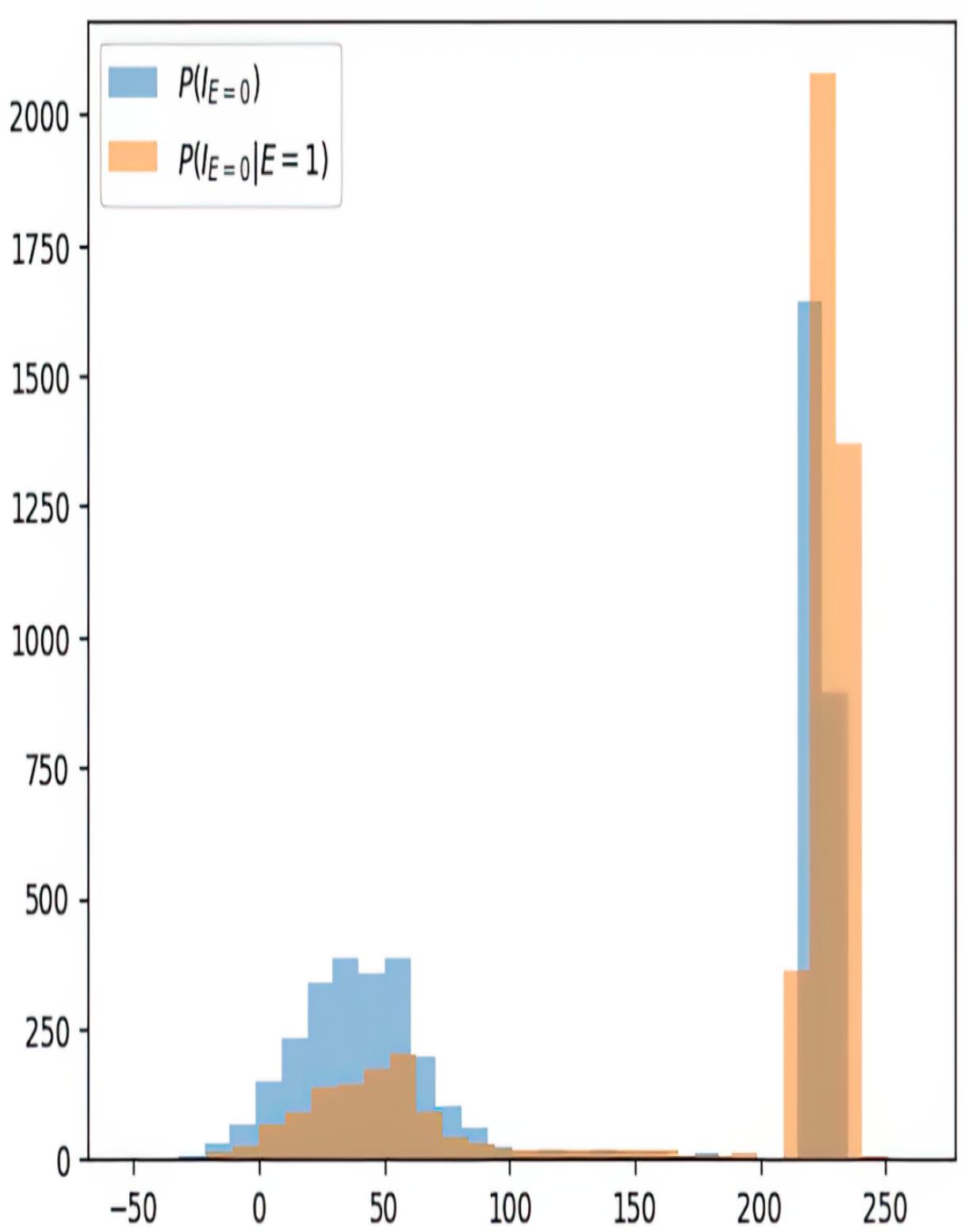
Figure 10.24 Histograms of samples from P(IE=0) and P(IE=0|E=1) generated in Pyro

In this example, the parameters were given. In chapter 11, where we’ll look at estimation, we’ll seamlessly combine this query inference with Bayesian parameter inference from data.

10.9 Partial identification

We’ll close this chapter with a quick note on partial identification. Sometimes a query is not identified, given your assumptions, but it may be partially identifiable. Partial identifiability means you can identify estimands for an upper and lower bound of your query. Partial identification is highly relevant to causal AI because machine learning algorithms often rely on finding and optimizing bounds on objective functions. Let’s walk through a few examples.

MCMC VS. SVI

Here we used Markov chain Monte Carlo (MCMC), but both Pyro and NumPyro have abstractions for stochastic variational inference (SVI). In this example, the parameters (p_member, p_engaged, etc.) of the model are specified. We could also make the parameters unknown variables with Bayesian priors and do the inference on these causal queries P(IE=0) and P(IE=0|E=1); in this case, we’d be doing Bayesian inference of these queries.

But for this we’d need N IID samples from an observational distribution where we had graphical identification (P(G, E, W, I), P(G, E, I), or P(E, W, I)). In the case of P(G, E, W, I), where all the variables in the DAG are observed, the number of unknown variables is just the number of parameters. But in the latter two cases, of P(G, E, I) or P(E, W, I), where there is a latent G or W of size N, the number of unknowns grows with N. In this case, SVI will scale better with large N. We’ll see an example in chapter 11.

Suppose in our online gaming example you ran an experiment where you randomly assigned players to a treatment or control group. Players in the treatment group are exposed to a policy that encourages more side-quest engagement. You reason that since you can’t actually force players to engage in side-quests, it’s better to have this randomized treatment/control variable as a parent of our side-quest engagement variable, as seen in the DAG in figure 10.25.

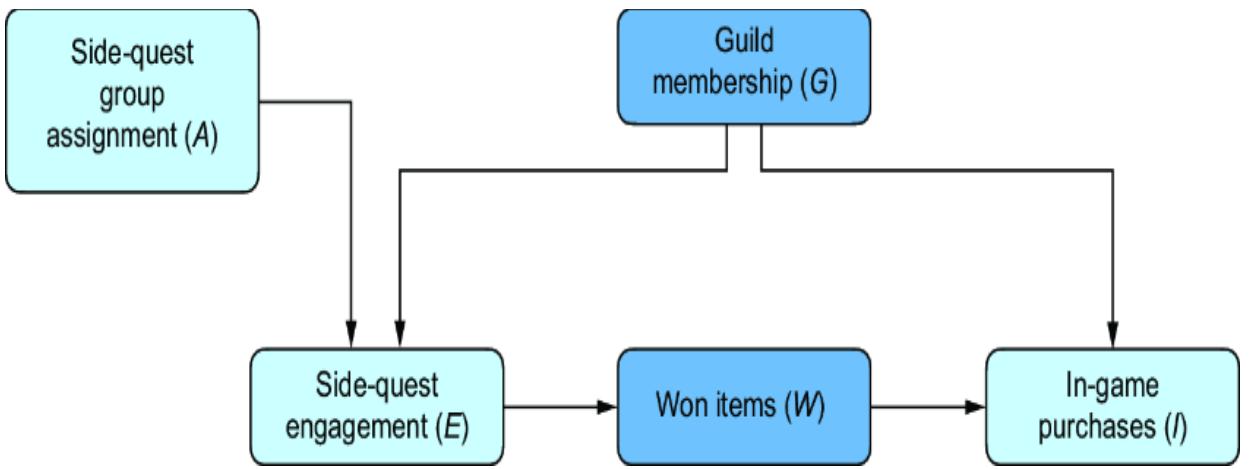
Figure 10.25 We don’t have identification for the ATE of E on I because G and W are unobserved. But we have partial identification given variable A, representing gamers’ assignments in a randomized experiment.

For this new variable A, let A  = 1 refer to the treatment group and A=0 refer to the control group. We have this new variable A, and the average treatment effect of the policy on in-game purchases E(IA=1 – IA=0) is an interesting query. But suppose we’re still ultimately interested in knowing the average treatment effect of side-quest engagement itself on purchases, i.e., E(IE=૿high – IE=૿low).

If guild membership (G ) were observed, we’d have identification through backdoor adjustment. If won items (W  ) were observed, we could use front-door adjustment. But suppose that in this scenario you observe neither. In this case, observing the side-quest group assignment variable would give you partial identification. Suppose that the ingame purchases variable was a binary 1 for ૿high and 0 for ૿low instead of a continuous value. Then the bounds on E(IE=૿high – IE=૿low) are

\[\begin{aligned} LB &= P(I = \text{high} | \mathcal{A} = 1) - P(I = \text{high} | \mathcal{A} = 0) \\ &- P(I = \text{high}, E = \text{low} | \mathcal{A} = 1) - P(I = \text{low}, E = \text{high} | \mathcal{A} = 0) \\ UB &= P(I = \text{high} | \mathcal{A} = 1) - P(I = \text{high} | \mathcal{A} = 0) \\ &- P(I = \text{low}, E = \text{low} | \mathcal{A} = 1) - P(I = \text{high}, E = \text{high} | \mathcal{A} = 0) \end{aligned}\]

These bounds can be the next best thing to having full identification, especially if the bounds are tight. Alternatively, perhaps it is enough to know that the lower bound on the ATE for side-quest engagement is significantly greater than 0.

Similarly, general bounds exist for common counterfactual queries, such as probabilities of causation. For example, suppose you wanted to know if high side-quest engagement was a necessary and sufficient condition of high in-game purchases. You can construct the following bounds on the probability of necessity and sufficiency (PNS):

\[\begin{aligned} \max\left(0, P\left(I\_{E=\text{high}}=\text{high}\right) - P\left(I\_{E=\text{low}}=\text{high}\right)\right) &< PNS\\ &< \min\left(P\left(I\_{E=\text{high}}=\text{high}\right), P\left(I\_{E=\text{low}}=\text{low}\right)\right) \end{aligned}\]

These bounds consist of level 2 quantities like P (IE=e= i ), and you can go on to identify level 1 estimands if possible given your assumptions.

Remember that partial identification bounds are highly specific to your causal assumptions (like the DAG) and the parameterization of the variables; for example, the preceding examples are specific to binary variables. See the chapter notes athttps://www.altdeep.ai/p/causalaibook for links to papers that derived these bounds as well as bounds for other practical sets of assumptions.

Summary

• The importance of causal identification has increased in the AI era as we seek to understand the causal inductive bias in deep learning architectures.
• Libraries like y0 implement strategies for algorithmic identification.
• The causal hierarchy is a three-tiered structure that categorizes the causal questions we pose, the models we develop, and the causal inferences we draw. These levels are association, intervention, and counterfactual.
• Association-level reasoning addresses ૿what is questions and models that answer these questions with basic statistical assumptions.
• Interventional or counterfactual queries fall on their corresponding level of the hierarchy.
• Observational data falls on the associational level, and experimental data falls on the interventional level of the hierarchy. Counterfactual data arises in situations where the modeler can control a deterministic data generating process (DGP).
• Causal identification is the procedure of discerning when causal inferences can be drawn from experimental or observational data. It is done by determining if data at a lower level of the hierarchy can be used to infer a query at a higher level of the hierarchy.
• An example of a causal identification result is the backdoor formula, which equates intervention level query P (YX=x) to association level quantity ∑zP (Y  |X  = x, Z  = z)P (Z   = z), where Z is a set of common causes.
• The causal hierarchy theorem shows how lower-level data is insufficient to infer a distribution at a higher level without higher-level modeling assumptions.
• The do-calculus has three rules that can be used for graph-based identification.
• A counterfactual graph is a DAG that includes variables across counterfactual worlds on one graph. Unlike the parallel world graph, it admits d-separation. We derive the counterfactual graph from the parallel world graph and the target query.
• Graphical identification algorithms automate identification with graphs using rules such as the docalculus.
• Nonparametric identification is identification with nongraphical assumptions, such as assumptions about the functional relationships between variables in the model.
• The ignorability assumption is that the causal variable and the potential outcomes are conditionally independent given confounders.
• Effect of treatment on the treated (ETT) evaluates the effect of a cause on the subset of the population that was exposed to the cause.
• Single world intervention graphs (SWIGs) provide an intuitive alternative to counterfactual identification with do-calculus and counterfactual graphs. They are constructed by applying a node-splitting operation to the original causal DAG. SWIGs use a ૿single-world assumption, which assumes it’s possible to know a variable’s natural value while also intervening on it before it realizes that value without any side-effects that would affect that natural value.
• SWIGs work with variables and a narrow set of counterfactuals under the single-world assumption, while counterfactual graphs can accommodate queries that cannot be graphically identified.
• Pyro implements the SWIG’s node-splitting model of intervention, which enables probabilistic inference of

SWIG-identified quantities.

• Inference of causal queries using a causal graphical model and probabilistic inference algorithms is possible as long as the query is identified, given the model’s assumptions and training data.
• Partial identification means you can at least identify estimands for bounds on a target query. This can be quite useful if you lack full identification, especially since machine learning often works by optimizing bounds on objective functions.