Causal AI

Chapter 1 ~ 5

Author

Robert Osazuwa Ness

Causal AI

Robert Osazuwa Ness Foreword by Lindsay Edwar ds

To comment go to livebook .

Manning Shelter Island

For mor e infor mation on this and other Manning titles go to manning.com .

copyright

For online infor mation and or dering of this and other Manning books, please visit www.manning.com. The publisher o ers discounts on this book when or dered in quantity . For mor e infor mation, please contact

Special Sales Department

Manning P ublications Co .

20 Baldwin R oad

PO Bo x761

Shelter Island, NY 11964

Email: or ders@manning.com

No part of this publication may be r eproduced, stored in a r etrieval system, or transmitted, in any for m or by means electr onic, mechanical, photocopying, or otherwise, without prior written permission of the publisher .

Many of the designations used by manufactur ers and sellers to distinguish their pr oducts ar e claimed as trademarks. Wher e those designations appear in the book, and Manning Publications was awar e of a trademark claim, the designations have been printed in initial caps or all caps.

Recognizing the importance of pr eserving what has been written, it is Manning’s policy to have the books we publish printed on acid-fr ee paper, and we e xert our best e orts to that end. Recognizing also our r esponsibility to conserve the r esour ces of our planet, Manning books ar e printed on paper that is at least 15 per cent recycled and pr ocessed without the use of elemental chlorine.

The author and publisher have made every e ort to ensur e that the infor mation in this book was correct at pr ess time. The author and publisher do not assume and her eby disclaim any liability to any party for any loss, damage, or disruption caused by er rors or omissions, whether such erors or omissions r esult fr om negligence, accident, or any other cause, or fr om any usage of the infor mation her ein.

Manning P ublications Co . 20 Baldwin R oad PO Box 761 Shelter Island, NY 11964

Development editor : Frances L efkowitz Technical editor : Emily McMilin Review editor : Dunja Nikitović Production editor : Kathy R ossland Copy editor : Andy Car roll Proofreader: Jason Ever ett Technical pr oofreader: Jerey Finkelstein Typesetter and cover designer : Marija T udor

ISBN 9781633439917

Printed in the United States of America

dedication

To Dad, Professor Ness

foreword

Twenty-seven lawyers in the room, anybody know ‘post hoc, ergo propter hoc?’

—President Josiah Bartlett ( The West Wing )

Post hoc er gop opter hoc is a logical fallacy r egarding causation: ૿ After it, ther efore because of it. The idea dates back at least to Aristotle (the fallacy appears in On Sophistical Refutations ). Mor e than two thousand years af ter Aristotle, W elsh economic theorist Sir Clive Granger inverted ૿post hoc er go pr opter hoc to pr ovide one of the two principles underlying what is now known as Granger Causality, namely that something cannot cause something if it happened before it.

Humans have been fascinated by the notion of causality what causes what—since their early r ecorded writing. Indeed, causal r easoning is a major distinguishing featur e of human cognition. On a practical level, the importance is obvious: one cannot contr ol something if one does not understand cause and e ect. Causal AI is the firstbook I know of that draws together the necessary theory, the technical foundations (i.e., the pack ages and libraries), and a host of r eal e xamples, to allow anyone with a decent grounding in basic pr obability theory and sof tware engineering to get started using causal AI to tackle any problem they choose.

In my own field—the application of machine lear ning to problems in biology and drug discovery—understanding causality is essential. New drugs cur rently cost $2–3B to develop, with most of this cost coming fr om the 95% failur e

rate of new drugs in clinical trials. A signi ficant pr oportion of these costs can be e xplained by failur es to understand (particularly biological) causality . Appr oximately 60% of all drug failur es can be traced back to a poor selection of drug target, and many of these poor drug tar gets ar e errors of causal attribution.

While machine lear ning and arti ficial intelligence ar e rapidly transfor ming our world, they ar e dogged by a number of technical pr oblems, including poor e xplainability, robustness, and generalizability . Causal r easoning addr esses all of these dir ectly . Of ten, one will hear AI algorithms being described as ૿black bo xes (in other wor ds, impossible to ૿peer into and e xplain). Y et, intuitively (and incr easingly backed up by r esear ch), machine lear ning models that ar e robustly pr edictive must have lear ned causality .

Models that lear n causality explicitly (such as the methods outlined in this book) will be both pr edictive and explainable. Models r egularly fail to generalize when a correlate of the true cause is used to pr edict an e ect (or output). L et us assume a chain of events: A causes B causes C. If a model, trained on this data, has lear ned to pr edict A from C, it is inher ently fragile. It will fail completely if, in a new setting, the link between A and B is somehow br oken. Again, e xplicit causal models tackle this issue dir ectly, greatly incr easing the chances that a perfor mant model will generalize well.

In this e xcellent book, R obert Ness uses vignettes drawn from business, r etail, and technology . While these ar e perfect teaching tools, r eaders should be under no illusion: The scope for these methods is vast and important, including medicine, biology, and policy -making. Understanding and modeling causality has e xtraor dinary potential to impr ove human lives. Y et, as R obert points out,

much of the knowledge r equir ed to understand and apply causal AI e ectively is distributed acr oss disciplines, including traditional statistics, Bayesian infer ence, computer science, and pr obabilistic machine lear ning. Hence, lear ning about and applying causal AI has (till now) been far mor e arduous than it should be.

Robert is also an inspir ed teacher—all the better, as this stu can be har d! I hope you enjoy Causal AI as much as I did. It is essential r eading for anyone inter ested in applying these powerful methods (cause) and, hopefully, having a positive impact in the world (e ect).

—Lindsay Edwar ds CTO at R elation, L ondon

preface

I wr ote this book because I wanted a code- first appr oach to causal infer ence that seamlessly fit with moder n deep learning. It didn’t mak e sense to me that deep lear ning was often pr esented as being at odds with causal r easoning and infer ence, so I wanted to write a book that pr oved they combine well to their mutual bene fit.

Second, I wanted to close an obvious gap. Deep generative machine lear ning methods and graphical causal infer ence have a common ancestor in pr obabilistic graphical models. There have been tr emendous advances in generative machine lear ning in r ecent years, including in the ability to synthetize r ealistic te xt, images, and video . Yet, in my view, the low-hanging fruit of connections to r elated concepts in graphical causality was lef t to r ot on the vine. Chances ar e that if you’r e reading this, you sensed this gap as well. So here we ar e.

This book evolved fr om the Causal AI workshop I run through Altdeep.ai, an educational company that runs workshops and community events devoted to advanced topics in modeling. P articipants in this causal AI workshop have included data scientists, machine lear ning engineers, and pr oduct managers fr om Google, Amazon, Meta, and other big tech companies. They’ve also included data scientists and ML e xperts fr om retailers such as Nik e, consultancies lik e Deloitte, and phar maceuticals lik e AstraZeneca. W e’ve work ed with quantitative mark eting experts trying to tak e causal appr oaches to channel attribution. W e’ve work ed with economists and molecular biologists trying to get a mor e general perspective on the causal methods popular in their domains. W e’ve work ed

with pr ofessors, post-docs, and PhD students acr oss departments looking for a code- first appr oach to lear ning causal infer ence.

I wr ote this book for all of these people, based on the r ealworld pr oblems they car e about and their feedback. If you belong to or r elate to any of these gr oups, this book is for you, too .

How is this book di erent fr om other causal infer ence books? Causal infer ence r elies mainly on thr ee dierent skill sets: the ability to tur n your domain knowledge into a causal model r endered in code, deep skills in pr obability theory, and deep skills in statistical theory and methods. This book focuses on the first skill by using libraries that enable bespok e causal modeling, and by leveraging the deep learning machinery in tools such as PyT orch to do the statistical heavy lif ting.

I hope this sounds lik e what you ar e looking for .

acknowledgments

I was very fortunate to have Emily McMilin, senior r esear ch scientist at Meta, and K evin Murphy, principal r esear ch scientist at Google AI and author of the best book on probabilistic ML, both give a car eful r eview of each chapter . Finally, Je rey Finkelstein, the most talented r esear ch engineer I’ve ever met, pr ovided a thor ough code r eview .

My colleagues at Micr osoft Resear ch, Emr e Kiciman and Amit Shar ma, pr ovided helpful advice with the DoWhy code. Fritz Ober meyer and Eli Bingham got me unstuck on Pyr o code. The book also builds on work with many collaborators, including K aren Sachs, Sara T aheri, Olga V itek, and Jer emy Zucker.

My editors F rances L efkowitz, Michael Stephens, and Andy Carroll at Manning P ublications pr ovided fr equent and invaluable edits and feedback, as did many others on the Manning team.

To all the r eviewers—A di Shavit, Alain Couniot, Camilla Montonen, Carlos A ya-Mor eno, Christian Sutton, Clemens Baader, Ger man Vidal, Guiller mo Alcántara González, Igor Vieira, Jer emy Loscheider, Jesús Juár ez, Jose San L eandro, Keith Kim, K yle P eterson, Maria Ana, Mik ael Dautr ey, Nick Decroos, P ierluigi Riti, P ietr o Alberto R ossi, Sebastian Maier, Sergio Govoni, Simone Sguazza, and Thomas Joseph Heiman —your suggestions helped mak e this a better book.

about this book

This book is for

Machine learning engineers looking to incorporate causality into AI syste ms and build more robust predictive models
Data scientists who are looking to expand both their causal infer ence and machine lear ning skillsets
Resear chers who want a wholistic view of causal infer ence and how it connects to their domain of expertise without going down stats theory rabbit holes
AI product experts looking for case studiesn business settings, especially tech and r etail
People who want to get inon the ground floor of causal AI

Whatistherequiredmathematical andprogrammingbackground?

Rest assur ed, this book doesn’t r equir e a deep backgr ound in pr obability and statistics theory . The r elationship between causality and statistics is lik e the r elationship between engineering and math. Engineering involves a lot of math, but you need only a bit of math to lear n cor e engineering concepts. A fter lear ning those concepts and digging into an applied pr oblem, you can focus on lear ning the e xtra math you need to go deep on that pr oblem.

This book assumes a level of familiarity with pr obability and statistics typical of a data scientist. Speci fically, it assumes you have basic knowledge of

Probability distributions
Joint probability and conditional probability and how they r elate to each other (chain rule, Bayes rule)
What it means to draw samples fr om a distribution
Expectation, independence, and conditional independence
Statistical ideas such as random samples, identically and independently sampled data, and statistical bias

Chapter 2 pr ovides a primer on these and other topics k ey to the ideas pr esented in this book for those who need refreshing.

Whatprogrammingtoolswillweuse?

This book assumes you ar e familiar with data science scripting in Python. The thr ee open sour ce Python libraries we rely on in this book ar e DoWhy, pgmpy, and Pyr o. DoWhy is a library for the open sour ce PyWhy suite of Python libraries for causal infer ence. pgmpy is a pr obabilistic graphical modeling library built on SciPy and NetworkX. Pyr o is a pr obabilistic machine lear ning library that e xtends PyTorch.

Our code- first goal is unique because, rather than going deep into the statistical theory needed to do causal infer ence, we r ely on these supporting libraries to do the statistics for us. DoWhy tries to be as end-to -end as possible in ter ms of mapping domain knowledge inputs to causal infer ence outputs. When we want to do mor e bespok e modeling, we’ll use pgmpy or Pyr o. These libraries pr ovide probabilistic infer ence algorithms that tak e car e of the estimation theory . pgmpy has graph-based infer ence algorithms that ar e extremely r eliable. Pyr o, as an e xtension of PyT orch, e xtends causal modeling to deep generative

models on high dimensional data and variational inference a cutting-edge deep lear ning–based infer ence technique.

If your backgr ound is in R or Julia, you should still find this book useful. Ther e are numer ous R and Julia pack ages that overlap in functionality with DoWhy . Graphical modeling software in these languages, such as bnlear n, can substitute for pgmpy . Similarly, the ideas we develop with Pyr o will work with similar pr obabilistic pr ogramming languages, such as PyMC. See https://altdeep.ai/p/causalaibookfor links to code notebooks r elated to the book.

Navigatingthisbook

This book is divided into four parts. In part 1, we’ll establish the conceptual foundations for the models we’ll build in this book.

Chapter 1 illustrates our pr obabilistic machine lear ning approach to causality with some practical e xamples. W e’ll then dive right into a causal infer ence work flow using the MNIST data—the ૿hello world of machine lear ning. Throughout the r est of the book, we’ll do code- first explorations of various parts of this work flow.

Chapter 2 pr ovides a primer on the cor e concepts fr om probabilistic modeling, generative machine lear ning, and Bayesian modeling that we’ll build upon in this book. W e’ll also e xplor e key ideas fr om statistical infer ence, such as conditional independence and Monte Carlo, which we’ll leverage to build, validate, and do infer ence with causal models.

In part 2, you’ll lear n to build and validate causal graphs, including deep causal generative models.

Chapter 3 starts by giving you a solid foundation for the causal dir ected acyclic graph (D AG) as a model of the causal structur e of a data generating pr ocess. W e’ll begin with a practical e xample of building a causal graph based on domain knowledge and train a causal graphical model on the structur e of that causal graph. I’ll also intr oduce parameter modularity and independence of mechanism ideas that mak e a causal graphical model special, r elative to other types of pr obabilistic graphical models.

Chapter 4 dives into perfor ming empirical validation of a causal D AG. The true causal D AG constrains the statistical structur e of the data. I’ll show how to articulate those constraints, and how to use them to design statistical tests that evaluate how well our pr oposed D AG stands up against empirical evidence in the data. W e’ll also look at how causal discovery algorithms automate this pr ocess, and you’ll lear n how to avoid the pitfalls of these algorithms.

Chapter 5 e xplor es the connection between deep lear ning and causal infer ence. F irst, we’ll use deep lear ning to build a more powerful causal graphical model using a causal D AG as a sca old. Then we’ll e xplor e ways in which causality can improve the traditional deep lear ning work flow. We’ll use semi-supervised lear ning as a case study .

In part 3, we’ll tak e a code- first dive into the conceptual heart of causal infer ence, namely structural causal models, interventions, counterfactual infer ence, and causal identi fication.

Chapter 6 intr oduces the structural causal model. Though often r egarded as a di cult appr oach to causal infer ence, I’ll show that it is a simple kind of generative model and thus easy to implement with generative modeling tools lik e Pyr o.

We’ll see how to implement these models with deep learning frameworks.

Chapter 7 intr oduces the concept of interventions, meaning actions that change the data generating pr ocess. Using our code- first appr oach and Pyr o’s do function, we’ll gr ound the idea of interventions in generative modeling to show how causal models can emulate r eal-world interventions. Generative modeling of interventions will become the keystone of our causal infer ence methods going forwar d.

Chapter 8 intr oduces parallel-world counterfactual reasoning. Once we observe a causal event and its e ect, counterfactual r easoning asks how the e ect might have been di erent if the cause had been di erent. W e’ll see how to model this idea by building a causal D AG that cr osses parallel worlds . We’ll look at practical e xamples of counterfactual r easoning, such as in mark eting and in dealmaking at Net flix.

Chapter 9 intr oduces the algorithm for general counterfactual infer ence. The algorithm combines a structural causal model with the parallel-world appr oach we saw in chapter 8. W e’ll look at several e xamples of how to implement this appr oach, including using a deep lear ning image model in PyT orch.

Chapter 10 pr ovides a guide to causal identi fication, which concer ns how we mak e causal infer ences fr om data. While this is typically a theory -dense topic, we’ll tak e a code- first approach. F or example, we’ll intr oduce the concept of the do-calculus with a Python library whose algorithms apply the do -calculus automatically .

In part 4, we’ll tak e a deeper look at applications.

Chapter 11 dives into building a causal e ect estimation workflow. We’ll work with the DoWhy library and e xplor e dierent statistical algorithms for identif ying, estimating, and then str ess-testing a causal e ect estimate. W e’ll cover traditional techniques, such as pr opensity scor es and instrumental variables, as well as newer methods, such as double machine lear ning. W e’ll then use Pyr o to implement a Bayesian appr oach to estimating a causal e ect using a Monte Carlo simulation of interventions on a deep causal graphical model trained with latent variables.

Chapter 12 e xplor es the connection of causality with automated decision-making and r einfor cement lear ning. We’ll start with a famous causal decision pr oblem called Newcomb’s parado x and then e xtend to bandits, Mark ov decision pr ocesses, partial Mark ov decision pr ocesses, and reinfor cement lear ning. W e’ll connect interventions to reward functions, show how agents mak e decisions under confounding, and see how policies ar e intervention generators.

Finally, chapter 13 intr oduces causality in the conte xt of large language models and other multimodal foundation models. F irst, we’ll e xplor e how to use a lar ge language model to solve causal pr oblems. W e’ll then e xplor e how to chain lar ge language models over a causal D AG, and use causal interventions to generate te xt fr om these models, as well as the bene fits of doing so .

Aboutthecode

In each chapter, I pr ovide a list of the Python libraries and versions you’ll need to get the code working as well as guidance in setting up your envir onment. Note that di erent versions of the same library ar e sometimes used in di erent

chapters. All the code in the book is implemented in Jupyter notebooks that ar e available online at https://altdeep.ai/p/causalaibook . The notebooks wer e all tested in Google Colab, and they include links that automatically load the notebooks in Google Colab, wher e you can run them dir ectly . This can save time and aggravation if you hit issues in setting up your envir onment. You’ll findlinks to the notebooks and other book r esour ces at https://altdeep.ai/p/causalaibook .

This book contains many e xamples of sour ce code, both in numbered listings and in-line with nor mal te xt. In both cases, sour ce code is for matted in a fixed-width font like this to separate it fr om ordinary te xt.

In many cases, the original sour ce code has been reformatted; I’ve added line br eaks and r eworked indentation to accommodate the available page space in the book. In rar e cases, even this was not enough, and listings include line-continuation mark ers (). A dditionally, comments in the sour ce code have of ten been r emoved from the listings when the code is described in the te xt. Code annotations accompany many of the listings, highlighting important concepts.

You can get e xecutable snippets of code fr om the liveBook (online) version of this book at https://livebook.manning.com/book/causal-ai . The complete code for the e xamples in the book is available for download from the Manning website at https://www .manning.com/books/causal-ai and fr om https://altdeep.ai/p/causalaibook .

liveBookdiscussionforum

Purchase of Causal AI includes fr ee access to liveBook, Manning’s online r eading platfor m. Using liveBook’s exclusive discussion featur es, you can attach comments to the book globally or to speci fic sections or paragraphs. It’s a snap to mak e notes for yourself, ask and answer technical questions, and r eceive help fr om the author and other users. T o access the forum, go to https://livebook.manning.com/book/causal-ai/discussion . You can also lear n more about Manning’s forums and the rules of conduct at htps://livebook.manning.com/discussion .

Manning’s commitment to our r eaders is to pr ovide a venue where a meaningful dialogue between individual r eaders and between r eaders and the author can tak e place. It is not a commitment to any speci fic amount of participation on the part of the author, whose contribution to the forum r emains voluntary (and unpaid). W e suggest you try asking the author some challenging questions lest his inter est stray! The forum and the ar chives of pr evious discussions will be accessible fr om the publisher’s website as long as the book is in print.

about the author

Robert Osazuwa Ness resear ches generative AI at Microsoft Resear ch. He is an adjunct pr ofessor in the Khoury School of Infor mation Sciences at Northeaster n University . He studied at Johns Hopkins University and P urdue University . He has a PhD in statistics.

about the cover illustration

The figure on the cover of Causal AI , titled ૿ La Religieuse, or ૿The Nun, is tak en fr om a book by L ouis Cur mer published in 1841. Each illustration is finely drawn and color ed by hand.

In those days, it was easy to identif y wher e people lived and what their trade or station in life was just by their dr ess. Manning celebrates the inventiveness and initiative of the computer business with book covers based on the rich diversity of r egional cultur e centuries ago, br ought back to life by pictur es fr om collections such as this one.

Part 1 Conceptual foundations

Part 1 lays the essential gr oundwork for understanding and building causal models. Her e, I’ll intr oduce k ey concepts from statistics, pr obabilistic modeling, generative machine learning, and Bayesian methods that will serve as our building blocks for this book’s appr oach to causal modeling. This part is all about ar ming you with the cor e concepts you need to start solving causal pr oblems with machine lear ning tools.

1Why causal AI

This chapter covers

Defining causal AI and its bene fits
Incorporating causality into machine lear ning models
A simple example of applying causality to a machine learning model

Subscription str eaming platfor ms lik e Net flix ar e always looking for ways to optimize various indicators of perfor mance. One of these is their churn rate , meaning the rate at which they lose subscribers. Imagine that you ar e a machine lear ning engineer or data scientist at Net flix task ed with finding ways of r educing chur n. What ar e the types of causal questions (questions that r equir e causal thinking) you might ask with r espect to this task?

Causal disco very—Given detailed data on who churned and who did not, can you analyze that data to find causes of the churn? Causal discov eryinvest igates what causes what.
Estimating average treatment e ects(ATEs)—Suppose the algorithm that recommends content to the user is a cause of the churn; a better choice of algorithm might reduce churn, but by how much? The task of quantifying how much, on average, a cause drives an e ect is the ATE estimation . For example, some users could be exposed to a new version of the algorithm, and you could measur e how much this a ects churn, relative to the baseline algorithm.

Let’s go a bit deeper . The mock umentary The Oce (the American version) was one of the most popular shows on Netflix. Later, Net flix lear ned that NB CUniversal was planning to stop licensing the show to Net flix to str eam in the US, so that US str eaming of The O ce would be e xclusive to NBCUniversal’s rival str eaming platfor m, Peacock. Given the popularity of the show, chur n was certainly a ected, but by how much?

Estimating conditional average treatment e ects (CATEs) —The e ect of losing The O cewould be more pronounced for some subscriber segments than others, but what attributes define these segments? One attribute is certainly having watched the show, buther are others (demographics, other content watched,tc.). CATE estimation isthe task of quantif ying how much a cause drives an e ect for a particular segment ofthe population. Indeed, ther are likely multiple segments we could define, each with a dierent within-segment ATE. Part of the task of CATE estimation is finding distinct segments of inter est.

Suppose you had r eliable data on subscribers who quit Netflix and signed up for P eacock to continue watching The O ce. For some of these users, the r ecommendation algorithm failed to show them possible substitutes for The O ce, lik e the mock umentary Parks and Recreation . That may lead to a di erent type of question.

Counterfactual reasoning and attribution —If the algorithm had placed Parks and Recreation more prominently in those users’ dashboar ds, would theyhave stayed on with Netflix? These counterfactual questions (૿counter to the fact that the showasn’t prominent in their dashboar d) are essential for attribution (assigning a root cause and credit/blame for an outcome).

Netflix work ed with Steve Car rel (star of The Oce) and Gr eg Daniels (writer, dir ector, and pr oducer of The Oce) to create the show Space Force as Net flix original content. The show was r eleased just months befor e The Oce moved to Peacock. Suppose that this show was Net flix’s attempt to create content to r etain subscribers who wer e fans of The O ce. Consider the decisions that would go into the cr eation of such a show :

Causal decision theory —What actors/dir ectors/writers would tempt The O cefans to stay subscribed? What themes and content?
Causal machine learning —How could we use generative AI, such as large language models to create scripts and pilots for the show in such a way that optimizes for the objective of r educing chur n amongst fans of The Oce?

Causal inference is about br eaking down a pr oblem into these types of speci fic causal queries , and then using data to answer these queries. Causal AI is about building algorithms that automate this analysis. W e’ll tackle both of these problem ar eas in this book.

1.1WhatiscausalAI?

To understand what causal AI is, we’ll start with the basic ideas of causality and causal infer ence, and work our way up. Then we’ll r eview the kinds of pr oblems we can solve with causal AI.

Causal reasoning is a crucial element of how humans understand, e xplain, and mak e decisions about the world. Anytime we think about cause (૿Why did that happen?) or e ect (૿What will happen if I do this?), we ar e practicing causal r easoning.

In statistics and machine lear ning, we use data to lend statistical rigor to our causal r easoning. But while cause-ande ect r elationships drive the data, statistical cor relation alone is insu cient to draw causal conclusions fr om data. F or this, we must tur n to causal inference .

Statistical (non-causal) infer ence r elies on statistical assumptions. This is true even in deep lear ning, wher e assumptions ar e often called ૿inductive bias. Similarly, causal infer ence r elies on causal assumptions; causal infer ence r efers to a body of theory and practical methods that constrain statistical analysis with causal assumptions.

Causal AI refers to the automation of causal infer ence. W e can leverage machine lear ning algorithms, which have developed r obust appr oaches to automating statistical analyses and scale up to lar ge amounts of data of di erent modalities.

The goal of AI is automating r easoning tasks that until now have r equir ed human intelligence to solve. Humans r ely heavily on causal r easoning to navigate the world, and while we ar e better at causal r easoning than statistical r easoning, our cognitive biases still mak e our causal r easoning highly eror pr one. Impr oving our ability to answer causal questions has been the work of millennia of philosophers, centuries of scientists, and decades of statisticians. But now, a conver gence of statistical and computational advances has shif ted the focus fr om discourse to algorithms that we can train on data and deploy to sof tware. It is a fascinating time to lear n how to build causal AI.

KEY DEFINITIONS UNDERPINNING CA USAL AI

Inference —Drawing conclusions from observations and data
Assumptions —Constraints that guide infer ences
Inductive bases —Another word for assumptions , often used to refer to assumptions implicit in the choice of machine lear ning algorithm
Statistical model—A framework using statistical assumptions to analyze data
Data science —An inter disciplinary field that uses statistical models along with other algorithms and techniques toxtract insights and knowledge from structur ed and unstructur ed data
Causal inference —Techniques that use causal assumptions to guide conclusions
Causal model—A statistical model built on causal assumptions about data generation
Causal data science —Data science that employs causal models to e xtract causal insights
Causal AI—Algorithms that automate causal infer ence tasks using causal models

1.2How thisbookapproachescausal inference

The goal of this book is the fusion of two powerful domains: causality and AI. By the end of this jour ney, you’ll be equipped with the skills to

Design AI systems with causal capabilities —Harness the power of AI, but with an added layer of causal r easoning.
Use machine learning frameworks for causal inference Utilize toolsike PyTorch and other Python libraries to seamlessly integrate causal modeling into your pr ojects.
Build tools for automated causal decision-making Implement causal decision-making algorithms, including causal r einfor cement lear ning algorithms.

Historically, causality and AI evolved fr om dierent bodies of resear ch, they have been applied to di erent pr oblems, and they have led to e xperts with di erent skill sets, books that use di erent languages, and libraries with di erent abstractions. This book is for anyone who wants to connect these domains into one compr ehensive skill set.

There are many books on causal infer ence, including books that focus on causal infer ence in Python. The following subsections discuss some featur es that mak ethis book unique.

1.2.1 Emphasis on AI

This book focuses on causal AI. W e’ll cover not just the relevance of causal infer ence to AI, or how machine lear ning can scale up causal infer ence, but also focus on implementation. Speci fically, we’ll integrate causal models with conventional models and training pr ocedur es fr om probabilistic machine lear ning.

1.2.2 Focus on tech, retail, and business

Practical causal infer ence methods have developed fr om econometrics, public health, social sciences, and other domains wher e it is di cult to run randomized e xperiments. As a r esult, e xamples in most books tend to come fr om those domains. In contrast, this book leans heavily into e xamples from tech, r etail, and business.

1.2.3 Parallel world counterfactuals and other queries beyond causal e ects

When many think of ૿causal infer ence, they think of estimating causal e ects, namely average tr eatment e ects (ATEs) and conditional average tr eatment e ects (CA TEs). These ar e certainly important queries, but ther e are other kinds of causal queries as well. This book gives due attention to these other types.

For example, this book pr ovides in-depth coverage of the parallel worlds account of counterfactuals. In this appr oach, when some cause and some e ect occur, we imagine a parallel universe wher e the causal event was di erent. F or example, suppose you ask ed, ૿I mar ried for money and now I’m sad. W ould I have been happier had I mar ried for love? With our parallel worlds appr oach, you’d use your e xperience of mar rying for money and being sad as inputs to a causal model-based pr obabilistic simulation of your happiness in a parallel universe wher e you mar ried for love. This type of reasoning is useful in decision-making. F or example, it might help you choose a better spouse ne xt time.

Hopefully this e xample of love and r egret illustrates how fundamental this kind of ૿ what could have been thinking is to human cognition (we’ll see mor e applied e xamples in chapters 8 and 9). It ther efore makes sense to lear n how to build AI with the same capabilities. But although they’r e useful, some counterfactual infer ences ar e har d or impossible to verif y (you can’tprove you would have been happier if you had mar ried for love). Most causal infer ence books only focus on the nar row set of counterfactuals we can verif y with data and e xperiments, which misses many inter esting, cognitive science-aligned, and practical use cases of counterfactual r easoning. This book leans into those use cases.

1.2.4 An assumption of commodi fication of inference

Many causal infer ence books go deep into the statistical infer ence nuts and bolts of various causal e ect estimators. But a major tr end in the last decade of developing deep learning frameworks is the commodi fication of inference . This r efers to how libraries lik e PyT orch abstract away the dicult aspects of estimation and infer ence—if you can define your estimation/infer ence pr oblem in ter ms minimizing a di erentiable loss function, PyT orch will handle the r est. The commodi fication of infer ence fr ees up the user to focus on cr eating ever mor e nuanced and powerful models, such as models that r epresent the causal structur e of the data-generating pr ocess.

In this book, we’ll focus on leveraging frameworks for infer ence so that you can lear n a universal view of modeling techniques. Once you find the right modeling appr oach for your domain, you can use other r esour ces to go deep into any statistical algorithm of inter est.

1.2.5 Breaking down theory with code

One of the standout featur es of this book is its appr oach to advanced topics in causal infer ence theory . Many intr oductory te xts shy away fr om subjects lik e identi fication, the do -calculus, and the causal hierar chy theor em because they ar e dicult. The pr oblem is that if you want to cr eate causal-capable AI algorithms, you need an intuition for these concepts.

In this book, we’ll mak e these topics accessible by r elying on Python libraries that implement their basic abstractions and algorithms. W e’ll build intuition for these advanced topics by working with these primitives in code.

1.3Causality’sroleinmodernAI workflows

There is gr eat value in positioning ourselves to build futur e versions of AI with causal capabilities, but the topics cover ed in this book will also have an impact on applications common today . In this section, we’ll r eview how causality can enhance some of these applications.

1.3.1 Better data science

Big tech and tech-power ed retail or ganizations have recognized the signi ficance of causal infer ence, o ering premium salaries to those pr oficient in it. This is because the essence of data science—deriving actionable insights fr om data—is inher ently causal.

When a data scientist e xamines the cor relation between a featur e on an e-commer ce site and sales, they do so because they want to know whether the featur e causally drives sales.

Causal infer ence can help answer this question in several ways. F irst, it can help them design an e xperiment that will quantif y the causal e ect of the featur e on sales, especially in the case wher e a perfect randomized e xperiment is not possible. Second, if a pr oposed e xperiment is not feasible, the data scientist can use past observational data and data from related but di erent past e xperiments to infer the value of the causal e ect that would r esult fr om the pr oposed experiment without actually running it. F inally, even if the data scientist has complete fr eedom in running e xperiments, causal infer ence can help select which e xperiment to run and what variables to measur e, minimizing the opportunity cost of running wasteful or uninfor mative e xperiments.

1.3.2 Better attribution, credit assignment, and root cause analysis

Causal infer ence also supports attribution. The ૿attribution problem in mark eting is per haps best articulated by a quote credited to advertising pioneer John W anamaker:

Half the money I spend on advertising is wasted; the trouble is I don’t know which half .

In other wor ds, it is di cult to know what advertisement, promotion, or other action caused a speci fic customer behavior, sales number, or other k ey business outcome. Even in online mark eting, wher e the data has gotten much richer and mor e granular than in W anamaker’s time, attribution r emains a challenge. F or example, a user may have click ed after seeing an ad, but was it that single ad view that led to the click? Or wer e they going to click anyway? P erhaps ther e was a cumulative e ect of all the nudges to click that they r eceived over multiple channels. Causal modeling addr esses the attribution pr oblem by using

formal causal logic to answer ૿ why questions, such as ૿ why did this user click?

Attribution goes by other names in other domains, such as ૿credit assignment and ૿ root cause analysis. The cor e meaning is the same; we want to understand why a particular event outcome happened. W e know what the causes ar e in general, but we want to know how much a particular cause is to blame in a given instance.

1.3.3 More robust, decomposable, and explainable models

For or ganizations that use machine lear ning to build software, incorporating causal modelling can impr ove both the pr ocess and the pr oduct. In particular, causality adds value by making machine lear ning mor e robust, decomposable, and e xplainable.

MORE ROBUST MA CHINE LEARNING

Machine lear ning models lack r obustness when di erences between the envir onment wher e the model was trained and the envir onment wher e the model is deployed cause the model to br eak down. Causality can addr ess the lack of robustness in the following ways:

Overfitting —Overfitting occurs when learning algorithms place too much weight on spurious statistical patter ns in the training data. Causal approaches can orient machine learning models towar d learning statistical patter ns that are rooted in causal r elationships.
Underspeci fication —Underspeci fication occurs when ther are many equivalent configurations of a model that perfor m equivalently on test data but perfor m dierently in the deployment envir onment. One sign of

underspeci fication is sensitivity to arbitrary elements of the model’s configuration, such as a random seed. Causal infer ence can tell you when acausal prediction is ૿identi fied (i.e., not ૿underspeci fied), meaning a unique answer exists given the assumptions and the data.

Data drift —As time passes, the characteristics of the data in the envir onment where you deploy the model dier or ૿drif t from the characteristics of the training data. Causal modeling addresses this by capturing causal invar iance underlying the data. For example, suppose you train a model that uses elevationo predict average temperatur e. If you train with data only from high-elevation cities, ithould still work well in lowelevation cities if the model successfully fit the underlying physics-based causal relationship between altitude and temperatur e.

This is why leading tech companies deploy causal machine learning techniques—they can mak e their machine lear ning services mor e robust. It is also why notable deep lear ning resear chers ar epursuing r esear ch that combines deep learning with causal r easoning.

MORE DECOMPOSABLE MA CHINE LEARNING

Causal models decompose into components, speci fically tuples of e ects and their dir ect causes, which I’ll de fine formally in chapter 3. T o illustrate, let’s consider a simple machine lear ning pr oblem of pr edicting whether an individual who sees a digital ad will go on to mak e a purchase.

We could use various characteristics of the ad impr ession (e.g., the number of times the ad was seen, the duration of the view, the ad category, the time of day, etc.) as the

featur e vector, and pr edict the pur chase using a neural network, as depicted in figure 1.1. The weights in the hidden layers of the model ar e mutually dependent, so the model cannot be r educed to smaller independent components.

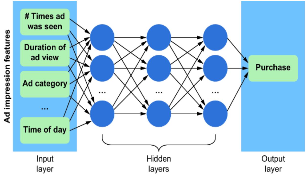
Figure 1.1 A simple multila yer perceptron neural network that uses features associated with ad impressions to predict whether a purchase will result

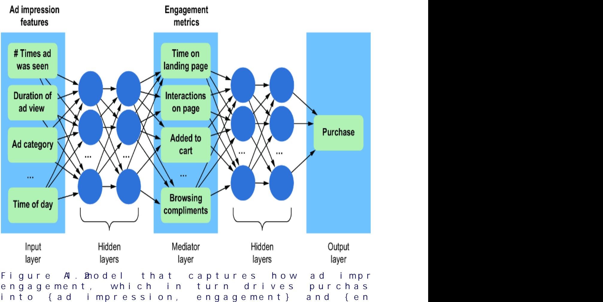
On the other hand, if we tak e a causal view of the pr oblem, we might r eason that an ad impr ession drives engagement, and that the engagement drives whether an individual makes a pur chase. Using engagement metrics as another featur e vector, we could instead train the model shown in figure 1.2. This model aligns with the causal structur e of the domain (i.e., ad impr essions causing engagement, and engagement causing pur chases). As such, it decomposes into two components: {ad impr ession, engagement} and {engagement, pur chase}.

There are several bene fits of this decomposability :

Components of the model can be tested and validated independently .
Components of the model can be executed separately, enabling more e cient use of modern cloud computing infrastructur e and enabling edge computing.
When additi onal training data is available, only the components r elevant to the data need r etraining.
Components of old models can be reused in new models targeting new pr oblems.
There is less sensitivity to suboptimalodel configuration and hyperparameter settings, because

components can be optimized separately .

The components of the causal model cor respond to concepts in the domain that you ar e modeling. This leads to the ne xt benefit, e xplainability .

MORE EXPLAINABLE MA CHINE LEARNING

Many machine lear ning algorithms, particularly deep learning algorithms, can be quite ૿black bo x, meaning the inter nal workings ar e not easily interpr etable, and the process by which the model pr oduces an output for a given input is not easily e xplainable.

In contrast, causal models ar e eminently e xplainable because they dir ectly encode easy -to-understand causal relationships in the modeling domain. Indeed, causality is the core of e xplanation; e xplaining an event means describing the event’s causes and how they led to the event occur ring. Causal models pr ovide e xplanations in the language of the domain you ar e modeling (semantic e xplanations) rather than in ter ms of the model’s ar chitectur e (such as syntactic explanations of ૿ nodes and ૿activations).

Consider the e xamples in figures1.1 and 1.2. In figure 1.1, only the input featur es and output ar e interpr etable in ter ms of the domain; the inter nal workings of the hidden layers ar e not. Thus, given a particular ad impr ession, it is di cult to explain how the model ar rives at a particular pur chase outcome. In contrast, the e xample in figure 1.2 e xplicitly provides engagement to e xplain how we get fr om an ad impression to a pur chase outcome.

The connections between engagement and ad impr ession, and between pur chase and engagement, ar e still black boxes, but if we need to, we can mak e additional variables in

those black bo xes explicit. W e just need to mak e sur e we do so in a way that is aligned with our assumptions about the causal structur e of the pr oblem.

1.3.4 Fairer AI

Suppose Bob applies for a business loan. A machine lear ning algorithm pr edicts that Bob would be a bad loan candidate, so Bob is r ejected. Bob is a man, and he got ahold of the bank’s loan data, which shows that men ar e less lik ely to have their loan applications appr oved. W as this an ૿unfair outcome?

We might say the outcome is ૿unfair if, for e xample, the algorithm made that pr ediction because Bob is a man. T o be a ૿fair prediction, it would need to be for mulated fr om factors r elevant to Bob’s ability to pay back the loan, such as his cr edit history, his line of business, or his available collateral. Bob’s dilemma is another e xample of why we’d like machine lear ning to be e xplainable: so that we can analyze what factors in Bob’s application led to the algorithm’s decision.

Suppose the training data came fr om a history of decisions from loan o cers, some of whom harbor ed a gender prejudice that hurt men. F or example, they might have r ead studies that show men ar e more lik ely to default in times of financial di culty . Based on those studies, they decided to deduct points fr om their rating if the applicant was a man.

Further more, suppose that when the data was collected, the bank advertised the loan pr ogram on social media. When we look at the campaign r esults, we notice that the men who responded to the ad wer e, on average, less quali fied than the women who click ed on the ad. This discr epancy might have been because the campaign was better tar geted

towar d women, or because the average bid price in online ad auctions was lower when the ad audience was composed of less-quali fied men. F igure 1.3 plots various factors that might influence the loan appr oval pr ocess, and it distinguishes fair from unfair causes. The factors ar e plotted in a dir ected acyclic graph (D AG), a popular and e ective way to represent causal r elationships. W e’ll use D AGs as our workhorse for causal r easoning thr oughout the book.

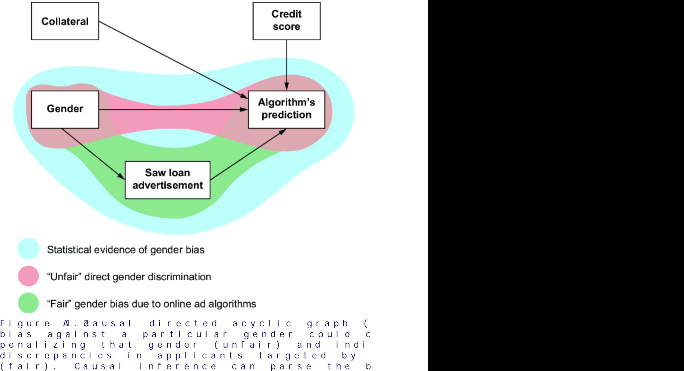
Thus, we have two possible sour ces of statistical bias against men in the data. One sour ce of bias is fr om the online ad that attracted men who wer e, on average, less quali fied, leading to a higher r ejection rate for men. The other sour ce of statistical bias comes fr om the pr ejudice of loan o cers. One of these sour ces of bias is ar guably ૿ fair (it’s har d to blame the bank for the tar geting behavior of digital advertising algorithms), and one of the sour ces is ૿unfair (we can blame the bank for se xist loan policies). But when we only look at the training data without this causal conte xt, all we see is statistical bias against men. The lear ning algorithm r eproduced this bias when it made its decision about Bob.

One naive solution to this pr oblem is simply to r emove gender labels fr om the training data. But even if those se xist loan ocers didn’t see an e xplicit indication of the person’s gender, they could infer it fr om elements of the application, such as the person’s name. Those loan o cers encode their prejudicial views in the for m of a statistical cor relation between those pr oxy variables for gender and loan outcome. The machine lear ning algorithm would discover this statistical patter n and use it to mak e predictions. As a r esult, you could have a situation wher e the algorithm pr oduces two dierent pr edictions for two individuals who had the same repayment risk but di ered in gender, even if gender wasn’t a dir ect input to the pr ediction. Deploying this algorithm would e ectively scale up the har m caused by those loan o cers’ pr ejudicial views.

For these r easons, we can see how many fears about the widespr ead deployment of machine lear ning algorithms ar e justi fied. Without cor rections, these algorithms could adversely impact our society by magnif ying the unfair outcomes captur ed in the data that our society pr oduces.

Causal analysis is instrumental in parsing these kinds of algorithmic fair ness issues. In this e xample, we could use causal analysis to parse the statistical bias into ૿unfair bias due to se xism and bias due to e xternal factors lik e how the digital advertising service tar gets ads. Ultimately, we could use causal modeling to build a model that only considers variables causally relevant to whether an individual can repay a loan.

It is important to note that causal infer ence alone is insucient to solve algorithmic fair ness. Causal infer ence can help parse statistical bias into what is fair and what’s not. And yet, even that depends on all parties involved agreeing on de finitions of concepts and outcomes, which is often a tall or der. To illustrate, suppose that the social media ad campaign served the loan ad to mor e men because the cost of serving an ad to men is cheaper . Thus, an ad campaign can win the online ad spot auctions with lower bids when the impr ession is coming fr om a man, and, as a result, mor een see the ad, though many of these men ar e not good matches for the loan pr ogram. W as this pr ocess unfair? Is the r esult unfair? What is the fair ness tradeo between balanced outcomes acr oss genders and pricing fair ness to advertisers? Should some advertisers have to pay more due to pricing mechanisms designed to encourage balanced outcomes? Causal analysis can’t solve these questions, but it can help understand them in technical detail.

1.4How causalityisdrivingthenext AIwave

Incorporating causal logic into machine lear ning is leading to new advances in AI. Thr ee tr ending ar eas of AI highlighted in this book ar e representation lear ning, r einfor cement

learning, and lar ge language models. These tr ends in causal AI ar e reminiscent of the early days of deep lear ning. P eople already working with neural networks when the deep learning wave was gaining momentum enjoyed first dibs on new opportunities in this space, and access to opportunities begets access to mor e opportunities. The ne xt wave of AI is still taking shape, but it is clear it will fundamentally incorporate some r epresentation of causality . The goal of this book is to help you ride that wave.

1.4.1 Causal representation learning

Many state- of-the-art deep lear ning methods attempt to learn geometric r epresentations of the objects being modeled. However, these methods struggle with lear ning causally meaningful r epresentations. F or example, consider a video of a child holding a helium- filled balloon on a string. Suppose we had a cor responding vector r epresentation of that image. If the vector r epresentation wer e causally meaningful, then manipulating the vector to r emove the child and converting the manipulated vector to a new video would r esult in a depiction of the balloon rising upwar ds. Causal r epresentation lear ning is a pr omising ar ea of deep representation lear ning that’s still in its early stages. This book pr ovides several e xamples in di erent chapters of causal models built upon deep lear ning ar chitectur es, providing an intr oduction to the fundamental ideas used in this e xciting new gr owth ar ea of causal AI.

1.4.2 Causal reinforcement learning

In canonical r einfor cement lear ning, lear ning agents ingest large amounts of data and lear n lik e Pavlov’s dog; they lear n actions that cor relate positively with good outcomes and negatively with bad outcomes. However, as we all know, correlation does not imply causation. Causal r einfor cement

learning can highlight cases wher e the action that causes a higher r eward diers fr om the action that cor relates most strongly with high r ewards. F urther, it addr esses the pr oblem of cr edit assignment (cor rectly attributing r ewards to actions) with counterfactual r easoning (i.e., asking questions like ૿how much r eward would the agent have r eceived had they been using a di erent policy?). Chapter 12 is devoted to causal r einfor cement lear ning and other ar eas of causal decision-making.

1.4.3 Large language models and foundation models

Large language models (LLMs) such as OpenAI’s GPT, Google’s Gemini, and Meta’s Llama ar e deep neural language models with many billions of parameters trained on vast amounts of te xt and other data. These models can generate highly coher ent natural language, code, and content of other modalities. They ar e foundation models, meaning they pr ovide a foundation for building mor e domain-speci fic machine lear ning models and pr oducts. These pr oducts, such as Micr osoft 365 Copilot, ar e alr eady having a tr emendous business impact.

A new ar ea of investigation and pr oduct development investigates LLMs’ ability to answer causal questions and perfor m causal analysis. Another line of investigation is using causal methods to design and train new LLMs with optimized causal capabilities. In chapter 13, we’ll e xplor e the intersection of LLMs and causality .

1.5Amachinelearning-themed primeroncausality

Now that you’ve seen the many ways that causal infer ence can impr ove machine lear ning, let’s look at the pr ocess of incorporating causality into AI models. T o do this, we will use a popular benchmark dataset of ten used in machine learning: the MNIST dataset of images of handwritten digits, each labeled with the actual digit r epresented in the image. Figure 1.4 illustrates multiple e xamples of the digits in MNIST.

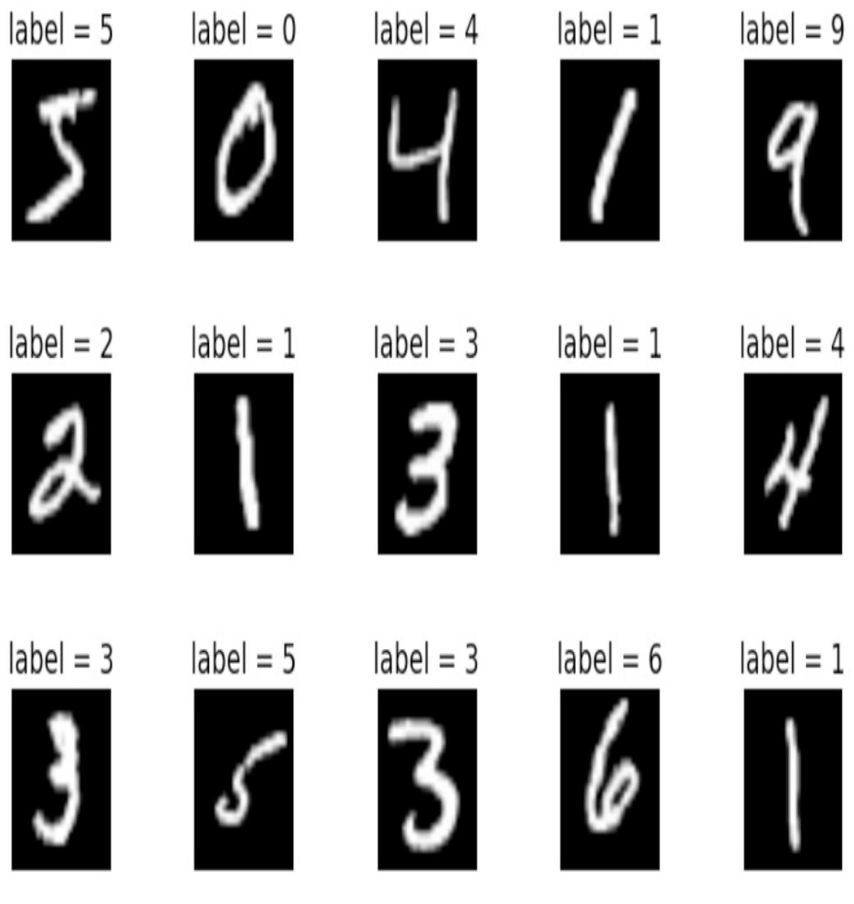
Figure 1.4 Each image in the MNIST dataset is an image of a written digit, and each image is labeled with the digit it represents.

MNIST is essentially the ૿ Hello W orld of machine lear ning. It is primarily used to e xperiment with di erent machine learning algorithms and to compar e their rlative str engths. The basic pr ediction task is to tak e the matrix of pix els representing each image as input and r eturn the cor rect image label as output. L et’s start the pr ocess of

incorporating causal thinking into a pr obabilistic machine learning model applied to MNIST images.

1.5.1 Queries, probabilities, and statistics

First, we’ll look at the basic pr ocess without including causal infer ence. Machine lear ning can use pr obability in analyses about quantities of inter est. T o do so, a pr obabilistic machine learning model lear ns a pr obabilistic r epresentation of all the variables in that system. W e can mak e predictions and decisions with pr obabilistic machine lear ning models using a three-step pr ocess.

1. Pose the question —What is the question you wanto answer?
1. Write down the math—What probability (orprobability related quantity) will answer the question, given the evidence or data?
1. Do the statistical inference —What statistical analysis will give you (or will estimate ) that quantity?

There is mor e for mal ter minology for these steps ( query, estimand , and estimator ) but we’ll avoid the jar gon for now . Instead, we’ll start with a simple statistical e xample pr oblem. Your step 1 might be ૿ How tall ar e Bostonians? F or step 2, you might decide that knowing the mean height (in probability ter ms, the ૿e xpected value) of everyone who lives in Boston will answer your question. Step 3 might involve randomly selecting 100 Bostonians and taking their average height; statistical theor ems guarantee that this sample average is a close estimate of the true population mean.

Let’s e xtend that work flow to modeling MNIST images.

STEP 1: POSE THE QUESTION

Suppose we ar e looking at the MNIST image in figure 1.5, which could be a ૿4 or could be a ૿9. In step 1, we articulate a question, such as ૿given this image, what is the digit r epresented in this image?

Figure 1.5 Is this an image of the digit 4 or 9? The canonical task of the MNIST dataset is to classify the digit label given the image. STEP 2: WRITE DOWN THE MA TH

In step 2, we want to find some pr obabilistic quantity that answers the question, given the evidence or data. In other words, we want to find something we can write down in probability math notation that can answer the question fr om step 1. F or our e xample with figure 1.5, the ૿evidence or ૿data is the image. Is the image a 4 or a 9? L et the variable I represent the image and D represent the digit. In probability notation, we can write the pr obability that the

digit is a 4, given the image, as P(D=4|I= ), where I= is shorthand for I being equal to some vector r epresentation of

the image. W e can compar e this pr obability to P(D=9|I= ), and choose the value of D that has the higher pr obability . Generalizing to all ten digits, the mathematical quantity we want in step 2 is shown in figure 1.6.

Figure 1.6 Choose the digit with the highest probability , given the image.

In plain English, this is ૿the value d that maximizes the probability that D equals d, given the image, wher e d is one of the ten digits (0–9).

STEP 3: DO THE ST ATISTICAL INFERENCE

Step 3 uses statistical analysis to assign a number to the quantity we identi fied in step 2. Ther e are any number of ways we can do this. F or example, we could train a deep neural network that tak es in the image as an input and predicts the digit as an output; we could design the neural net to assign a pr obability to D=d for every value d.

1.5.2 Causality and MNIST

So how could causality featur e in the pr evious section’s three-step analysis? Y ann L eCun is a T uring A ward winner (computer science’s equivalent of the Nobel prize) for his work on deep lear ning, and he’s dir ector of AI r esear ch at Meta. He is also one of the thr ee resear chers behind the creation of MNIST . He discusses the causal backstory of the MNIST data on his personal website, https://yann.lecun.com/e xdb/mnist/inde x.xhtml :

The MNIST database was constructed fr om NIST’s Special Database 3 and Special Database 1 which contain binary images of handwritten digits. NIST originally designated SD-3 as their training set and SD-1 as their test set. However, SD-3 is much cleaner and easier to r ecognize than SD-1. The r eason for this can be found on the fact that SD-3 was collected among Census Bur eau employees, while SD-1 was collected among high-school students. Drawing sensible conclusions fr om lear ning experiments r equir es that the r esult be independent of the choice of training set and test among the complete set of samples. Ther efore, it was necessary to build a new database by mixing NIST’s datasets.

In other wor ds, the authors mix ed the two datasets because they ar gue that if they trained a machine lear ning model solely on digits drawn by high schoolers, it would underperfor m when applied to digits drawn by bur eaucrats. However, in r eal-world settings, we want r obust models that can lear n in one scenario and pr edict in another, even when those scenarios di er. For example, we want a spam filter to keep working when the spammers switch fr om Nigerian princes to Bhutanese princesses. W e want our self -driving cars to stop even when ther e is gra ti on the stop sign.

Shuing the data lik e a deck of car ds is a luxury not easily a orded in r eal-world settings.

Causal modeling leverages knowledge about the causal mechanisms underlying how the digits ar e drawn that will help models generalize beyond high school students and bureaucrats in the training data to high schoolers in the test data. F igure 1.7 illustrates a causal D AG representing this system.

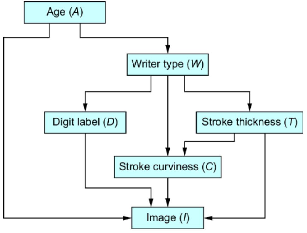
Figure 1.7 An example causal DAG representing the generation of MNIST images. The nodes represent objects in the data generating process, and edges correspond to causal relationships between those objects.

This particular D AG imagines that the writer deter mines the thickness and curviness of the drawn digits, and that high schoolers tend to have a di erent handwriting style than bureaucrats. The graph also assumes that the writer’s classi fication is a cause of what digits they draw . Perhaps bureaucrats write mor e 1s, 0s, and 5s, as these numbers

occur mor e f equently in census work, while high schoolers draw other digits mor e often because they do mor e long division in math classes (this is a similar idea to how, in topic models, ૿topics cause the frquency of wor ds in a document). F inally, the D AG assumes that age is a common cause of writer type and image; you have to be below a certain age to be in high school and above a certain age to be a census o cial.

A causal modeling appr oach would use this causal knowledge to train a pr edictive model that could e xtrapolate from the high school training data to the bur eaucrat test data. Such a model would generalize better to new situations where the distributions of writer type and other variables ar e dierent than in the training data.

1.5.3 Causal queries, probabilities, and statistics

At the beginning of this chapter, I discussed various types of causal questions we can pose, such as causal discovery, quantif ying causal e ects, and causal decision-making. W e can answer these and various other questions with a causal variation on our pr evious thr ee-step analysis (pose the question, write down the math, do the statistical infer ence):

1. Pose the causal question —What is the question yu want to answer?
1. Write down the causalmath—What probability (or expectation) will answer the causal question, given the evidence or data?
1. Do the statistical inference —What statistical analysis will give you (or ૿estimate) that causal quantity?

Note that the thir d step is the same as in the original thr ee steps. The causal nuance occurs in the first and second

steps.

STEP 1: POSE THE CA USAL QUESTION

These ar e examples of some causal questions we could ask about our causal MNIST model:

How much does the writer’s type (high schooler vs. bureaucrat) a ect the look of an image of the digit 4 with level 3 thickness? (Conditional average treatment e ect estimation is discussed in chapter 11).
Assuming thatstroke thickness is a cause of the image, we might ask, ૿What would a 2 look like if it were as curvy as possible? (This is intervention prediction , discussed in chapter 7).
Given an image, how would it have turned out dierently if the stroke curviness were heavier? (See counterfactual reasoning , discussed in chapters 8 and 9).
૿What should the stroke curviness be to get an aestheticallydea image? (Causal decision-making is discussed in chapter 12).

Let’s consider the CA TE in the first item. CA TE estimation is a common causal infer ence question applied to or dinary tabular data, but rar ely do we see it in the applied in the conte xt of an AI computer vision pr oblem.

STEP 2: WRITE DOWN THE CA USAL MATH

Causal infer ence theory tells us how to mathematically formalize our causal question. Using special causal notation, we can mathematically for malize our CA TE query as follows:

where E(.) is an e xpectation operator . We’ll r eview expectation in the ne xt chapter, but for now we can think of it as an averaging of pix els acr oss images.

The pr eceding use of subscripts is a special notation called ૿counterfactual notation that r epresents an intervention . A random assignment in an e xperiment is a r eal-world intervention, but ther e are many e xperiments we can’t run in the r eal world. F or example, it wouldn’t be feasible to run a trial wher e you randomly assign participants to either be a high school student or be a census bur eau ocial. Nonetheless, we want to know how the writer type causally impacts the images, and thus we r ely on a causal model and its ability to r epresent interventions.

To illustrate, figure 1.8 visualizes what CA TE might look lik e. The challenge is deriving the di erential image at the right of figure 1.8. Causal infer ence theory helps us addr ess potential age-r elated ૿confounding bias in quantif ying how much writer type drives the image. F or example, the docalculus (chapter 10) is a set of graph-based rules that allows us to tak e this D AG and algorithmically derive the following equation:

\[E(I\_{W=w}|D=4, \ T=3) = \sum\_{a} E(I|W=w, A=a, D=4, \ T=3)P(A=a, D=4, \ T=3)\]

The lef t side of this equation de fines the e xpectations used in the CA TE de finition in the second step—it is a theor etical construct that captur es the hypothetical condition ૿if writer type wer e set to ‘w’. But the right side is actionable; it is composed entir ely of ter ms we could estimate using machine lear ning methods on a hypothetical version of NIST image data labeled with the writers’ ages.

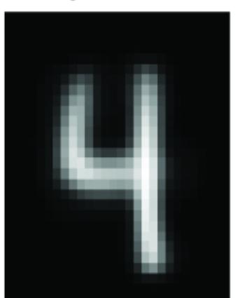
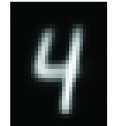
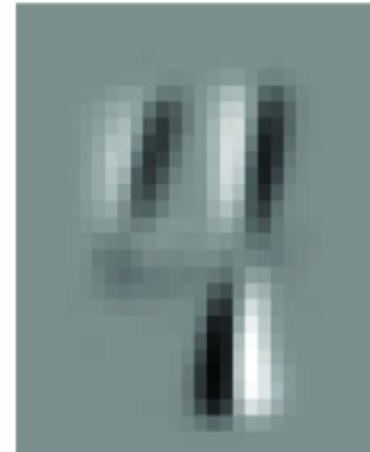
Figure 1.8 Visualization of an example CA TE of writer type on an image. It is the pixel-by-pixel di erence of the expected image under one intervention ( W=“high school” ) minus the expected image under another intervention ( W=“bureaucrat” ), with both expectations conditional on being images of the digit 4 with a certain level of thickness.

STEP 3: DO THE ST ATISTICAL INFERENCE

Step 3 does the statistical estimation, and ther e are several ways we could estimate the quantities on the right side of that equation. F or example, we could use a convolutional neural network to model E(I|W =w, A=a, D=d, T=t), and build a pr obability model of the joint distribution P(A, D, T). The choice of statistical modeling appr oach involves the usual statistical trade- o s, such as ease- of-use, bias and variance, scalability to lar ge data, and parallelizability .

Other books go into gr eat detail on pr eferred statistical methods for step 3. I tak e the str ongly opinionated view that we should r ely on the ૿commodi fication of infer ence tr end

in statistical modeling and machine lear ning frameworks to handle step 3, and instead focus on honing our skills on steps 1 and 2: figuring out the right questions to ask, and representing the possible causes mathematically .

As you’ve seen in this section, our jour ney into causal AI is scaolded by a thr ee-step pr ocess, and the essence of causal thinking emer ges pr ominently in the first two steps. Step 1 invites us to frame the right causal questions, while step 2 illuminates the mathematics behind these questions. Step 3 leverages patter ns we’r e well-accustomed to in traditional statistical pr ediction and infer ence.

Using this structur ed appr oach, we’ll transition in the coming chapters fr om pur ely pr edictive machine lear ning models like the deep latent variable models you might be familiar with fr om MNIST—to causal machine lear ning models that o er deeper insights into and answers to our causal questions. F irt, we will r eview the underlying mathematics and machine lear ning foundations. Then, in part 2 of the book, we’ll delve into craf ting the right questions and articulating them mathematically for steps 1 and 2. F or step 3, we’ll har ness the power of contemporary tools lik e PyT orch and other advanced libraries to bridge the causal concepts with cutting-edge statistical lear ning algorithms.

Summary

Causal AI seeks to augment statistical learning and probabilistic r easoning with causal logic.
Causal infer ence helps data scientists extract more causal insights from observational data (the vast majority of data in the world) and e xperimental data.
When data scientists can’t run experiments, causal models can simulate experiments from observational

data.

They can use these simulations to make causal infer ences, such as estimating causal e ects, and even to prioritize inter esting e xperiments to run in r eal life.
Causal infer ence also helps data scientists improve decision-making in their organizations through algorithmic counterfactual r easoning and attribution.
Causal infer ence also makes machine larning more robust , decomposable , and explainable .
Causal analysis is useful for formally analyzing fairness in predictive algorithms and for building fair er algorithms by parsing ordinary statistical bias into its causal sources.
The commodi fication of inference is a trend in machine learning that refers to how universal modeling frameworks like PyTorch continuously automate the nuts and bolts of statistical learning and probabilistic infer ence. The trend reduces the need for the modeler to be an expert at the formal and statistical details of causal infer ence and allows them to focus on turning domain expertise into better causal models of their problem domain.
Types of causal infer ence tasks include causal discovery , intervention prediction , causal e ect estimation , counterfactual reasoning , explanation , and attribution .
The way we build and work with probabilistic machine learning models can be extended to causal generative models implemented in probabilistic machine larning tools such as PyT orch.

2A primer on probabilistic generative modeling

This chapter covers

A primer on pr obability models
Computational pr obability with the pgmpy and Pyr o libraries
Statistics for causality : data, populations, and models
Distinguishing between probability models and subjective Bayesianism

Chapter 1 made the case for lear ning how to code causal AI. This chapter will intr oduce some fundamentals we need to tackle causal modeling with pr obabilistic machine lear ning, which r oughly r efers to machine lear ning techniques that use pr obability to model uncertainty and simulate data. Ther e is a flexible suite of cuttingedge tools for building pr obabilistic machine lear ning models. This chapter will intr oduce the concepts fr om probability, statistics, modeling, infer ence, and even philosophy that we will need in or der to implement k ey ideas fr om causal infer ence with the pr obabilistic machine lear ning appr oach.

This chapter will not pr ovide a mathematically e xhaustive intr oduction to these ideas. I’ll focus on what is needed for the r est of this book and omit the r est. Any data scientist seeking causal infer ence e xpertise should not neglect the practical nuances of probability, statistics, machine lear ning, and computer science. See the chapter notes at https://www .altdeep.ai/p/causalaibookfor recommended r esour ces wher e you can get deeper intr oductions or review materials.

In this chapter, I’ll intr oduce two Python pr ogramming libraries for probabilistic machine lear ning:

pgmpyis a library for building probabilistic graphical models. As a traditional graphical modeling tool, it is far less flexible and

cutting-edge than Pyro but also easier to use and debug. What it does, it does well.

Pyrois a genera l probabilistic machine learning libra ry. It is quite flexible, and it leverages PyTorch’s cutting-edge gradientbased lear ning techniques.

Pyro and pgmpy ar e the general modeling libraries we’ll use in this book. Other libraries we’ll use ar e designed speci fically for causal infer ence.

2.1Primeronprobability

Let’s r eview the pr obability theory you’ll need to work with this book. W e’ll start with a few basic mathematical axioms and their logical e xtensions without yet adding any r eal-world interpr etation. Let’s begin with the concr ete idea of a simple thr ee-sided die (these exist).

2.1.1 Random variables and probability

A random variable is a variable whose possible values ar e the numerical outcomes of a random phenomenon. These values can be discr ete or continuous. In this section, we’ll focus on the discr ete case. F or example, the values of a discr ete random variable representing a thr ee-sided die r oll could be {1, 2, 3}. Alter natively, in a 0-inde xed pr ogramming language lik e Python, it might be better to use {0, 1, 2}. Similarly, a discr ete random variable representing a coin flip could have outcomes {0, 1} or {T rue, False}. F igure 2.1 illustrates thr ee-sided dice.

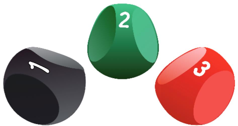
Figure 2.1 Three-sided dice each represent a random variable with three discrete outcomes.

The typical appr oach to notation is to write random variables with capitals lik e X, Y, and Z. For example, suppose X represents a die roll with outcomes {1, 2, 3}, and the outcome r epresents the number on the side of the die. X=1 and X=2 represent the events of r olling a 1 and 2 r espectively . If we want to abstract away the speci fic outcome with a variable, we typically use lower case. F or example, I would use ૿ X=x (e.g., X=1) to r epresent the event ૿I rolled an ’ x’! wher e x can be any value in {1, 2, 3}. See figure 2.2.

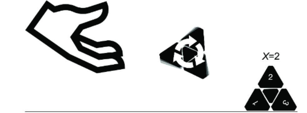
Figure 2.2 X represents the outcome of a three-sided die roll. If the die roles a 2, the observed outcome is X=2.

Each outcome of a random variable has a probability value . The probability value is of ten called a probability mass for discr ete variables and a probability density for continuous variables. F or discr ete variables, pr obability values ar e between zer o and one, and summing up the pr obability values for each possible outcome yields 1. F or continuous variables, pr obability densities ar e greater than zer o, and integrating the pr obability densities over each possible outcome yields 1.

Given a random variable with outcomes {0, 1} r epresenting a coin flip, what is the pr obability value assigned to 0? What about 1? A t this point, we just know the two values ar e between zer o and one, and that they sum to one. T o go beyond that, we have to talk about how to interpret probability . First, though, let’s hash out a few mor e concepts.

2.1.2 Probability distributions and distribution functions

A probability distribution function is a function that maps the random variable outcomes to a pr obability value. F or example, if the outcome of a coin flip is 1 (heads) and the pr obability value is 0.51, the distribution function maps 1 to 0.51. I stick to the standar d notation P(X=x), as in P(X=1) = 0.51. F or longer expressions, when the random variable is obvious, I dr op the capital letter and k eep the outcome, so P(X=x) becomes P(x), and P (X=1) becomes P(1).

If the random variable has a finite set of discr ete outcomes, we can represent the pr obability distribution with a table. F or example, a random variable r epresenting outcomes {1, 2, 3} might look lik e figure 2.3.

1	1	2	3
	P(X) 0.45	0.30	0.25

Figure 2.3 A simple tabular representation of a discrete distribution

In this book, I adopt the common notation P(X) to r epresent the probability distribution over all possible outcomes of X, while P(X= x) represents the pr obability value of a speci fic outcome. T o implement a pr obability distribution as an object in pgmpy, we’ll use the DiscreteFactor class.

Listing 2.1 Implementing a discrete distribution table in pgmpy

from pgmpy.factors.discrete import DiscreteFactor dist = DiscreteFactor( variables=[“X”], #1 cardinality=[3], #2 values=[.45, .30, .25], #3 state_names= {‘X’: [‘1’, ‘2’, ‘3’]} #4 )

print(dist)

#1 A list of the names of the variables in the factor #2 The cardinality (number of possible outcomes) of each variable in the factor #3 The values each variable in the factor can tak e #4 A dictionary , where the k ey is the variable name and the value is a list of the names of that variable’s outcomes

This code prints out the following:

+——+———-+ | X | phi(X) | +======+==========+ | X(1) | 0.4500 | +——+———-+ | X(2) | 0.3000 | +——+———-+ | X(3) | 0.2500 | +——+———-+

SETTING UP Y OUR ENVIRONMENT

This code was written with pgmpy version 0.1.24 and Pyr o version 1.8.6. The version of pandas used was 1.5.3.

See https://www .altdeep.ai/p/causalaibook for links to the Jupyter notebooks for each chapter, with the code and notes on setting up a working envir onment.

2.1.3 Joint probability and conditional probability

Often, we ar e inter ested in r easoning about mor e than one random variable. Suppose, in addition to the random variable X in figure 2.1, ther e was an additional random variable Y with two outcomes {0, 1}. Then ther e is a joint probability distribution function that maps each combination of X and Y to a pr obability value.

	1	2	3
0	0.25	0.20	0.15
1	0.20	0.10	0.10

Figure 2.4 A simple representation of a tabular joint probability distribution

As a table, it could look lik e figure 2.4.

The DiscreteFactor object can r epresent joint distributions as well.

Listing 2.2 Modeling a joint distribution in pgmpy

joint = DiscreteFactor( variables=[‘X’, ‘Y’], #1 cardinality=[3, 2], #2 values=[.25, .20, .20, .10, .15, .10], #3 state_names= { ‘X’: [‘1’, ‘2’, ‘3’], #3 ‘Y’: [‘0’, ‘1’] #3 } ) print(joint) #4

#1 Now we have two variables instead of one. #2 X has 3 outcomes, Y has 2. #3 Now there are two variables, so we name the outcomes for both variables.

#4 You can look at the printed output to see how the values are ordered of values.

The pr eceding code prints this output:

			+——+——+————+
X	Y	phi(X,Y)
		+======+======+============+
X(1) Y(0)			0.2500
		+——+——+————+
X(1) Y(1)			0.2000
			+——+——+————+
X(2) Y(0)		0.2000
		+——+——+————+
X(2) Y(1)		0.1000
			+——+——+————+
X(3) Y(0)		0.1500
		+——+——+————+
X(3) Y(1)		0.1000
		+——+——+————+

Note that the pr obability values sum to 1. F urther, when we marginalize (i.e., ૿sum over or ૿integrate over ) Y across the r ows, we recover the original distribution P(X ), (ak a the mar ginal

distribution of X ). Summing up over the r ows in figure 2.5 pr oduces the mar ginal distribution of X on the bottom.

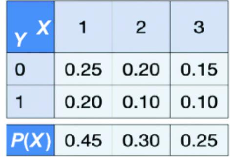
Figure 2.5 Marginalizing over Y yields the marginal distribution of X.

The mar ginalize method will sum over the speci fied variables for us.

print(joint.marginalize(variables=[‘Y’], inplace=False) )

This prints the following output:

		+——+———-+
X		phi(X)
		+======+==========+
	X(1)	0.4500
		+——+———-+
	X(2)	0.3000
		+——+———-+
	X(3)	0.2500
		+——+———-+

Setting the inplace argument to False gives us a new mar ginalized table rather than modif ying the original joint distribution table.

	1	2	3	PY
0			0.25 0.20 0.15 0.60
			0.20 0.10 0.10 0.40

Figure 2.6 Marginalizing over X yields the marginal distribution of Y.

Similarly, when we mar ginalize X over the columns, we get P(Y ). In figure 2.6, summing over the values of X in the columns gives us the mar ginal distribution of Y on the right.

print(joint.marginalize(variables=[‘X’], inplace=False))

		+——+———-+
Y		phi(Y)
		+======+==========+
	Y(0)	0.6000
		+——+———-+
	Y(1)	0.4000
		+——+———-+

I’ll use the notation P(X, Y ) to r epresent joint distributions. I’ll use P(X=x, Y=y) to r epresent an outcome pr obability, and for shorthand, I’ll write P(x, y). F or example, in figure 2.6, P(X=1, Y= 0) = P(1, 0) = 0.25. W e can de fine a joint distribution on any number of variables; if ther e wer e thr ee variables { X, Y, Z }, I’d write the joint distribution as P(X, Y, Z ).

In this tabular r epresentation of the joint pr obability distribution, the number of cells incr eases e xponentially with each additional variable. Ther e are some (but not many) ૿canonical joint probability distributions (such as the multivariate nor mal distribution—I’ll show mor e examples in section 2.1.7). F or that reason, in multivariate settings, we tend to work with conditional probability distributions.

The conditional pr obability of Y, given X, is

\[P\left(Y=\mathcal{Y}|X=x\right) = \frac{P(X=x, Y=\mathcal{Y})}{P(X=x)}\]

Intuitively, P(Y |X =1) r efers to the pr obability distribution for Y conditional on X being 1. In the case of tabular r epresentations of distributions, we can derive the conditional distribution table by dividing the cells in the joint pr obability distribution table with the marginal pr obability values, as in figure 2.7. Note that the columns on the conditional pr obability table in figure 2.7 now sum to 1.

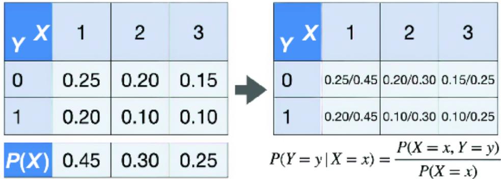
Figure 2.7 Derive the values of the conditional probability distribution by dividing the values of the joint distribution by those of the marginal distribution.

The pgmpy library allows us to do this division using the ૿/ operator :

print(joint / dist)

That line pr oduces the following output:

		+——+——+————+
X	Y	phi(X,Y)
		+======+======+============+
X(1) Y(0)		0.5556
		+——+——+————+
X(1) Y(1)		0.4444
		+——+——+————+
X(2) Y(0)		0.6667
		+——+——+————+
X(2) Y(1)		0.3333
		+——+——+————+
X(3) Y(0)		0.6000
		+——+——+————+
X(3) Y(1)		0.4000
		+——+——+————+

Also, you can dir ectly specif y a conditional pr obability distribution table with the TabularCPD class:

from pgmpy.factors.discrete.CPD import TabularCPD
PYgivenX = TabularCPD(
 variable='Y', #1
 variable_card=2, #2
 values=[ 
 [.25/.45, .20/.30, .15/.25], #3
 [.20/.45, .10/.30, .10/.25], #3
 ], 
 evidence=['X'],
 evidence_card=[3],
 state_names = {
 'X': ['1', '2', '3'],
 'Y': ['0', '1']
 })

print(PYgivenX)

#1 A conditional distribution has one variable instead of ΔiscreteF actor’s list of variables. #2 variable_card is the cardinality of Y . #3 Elements of the list correspond to outcomes for Y . Elements of each list

That pr oduces the following output:

correspond to elements of X.

+——+——————–+———————+——+ | X | X(1) | X(2) | X(3) | +——+——————–+———————+——+ | Y(0) | 0.5555555555555556 | 0.6666666666666667 | 0.6 | +——+——————–+———————+——+ | Y(1) | 0.4444444444444445 | 0.33333333333333337 | 0.4 | +——+——————–+———————+——+

The variable_card argument is the car dinality of Y (meaning the number of outcomes Y can tak e), and evidence_card is the car dinality of X.

CONDITIONING AS AN OPERA TION

In the phrase ૿conditional pr obability, ૿conditional is an adjective. It is useful to think of ૿condition as a verb (an action). You condition a random variable lik e Y on another random variable X. For example, in figure 2.5, I can condition Yon X=1, and essentially get a new random variable with the same outcome values as Y but with a pr obability distribution equivalent to P(Y|X=1).

For those with mor e programming e xperience, think of conditioning on X = 1 as filtering on the event X == 1; for example, ૿ what is the pr obability distribution of Y when X == 1? Filtering in this sense is lik e the WHERE clause in a SQL query . P(Y) is the distribution of the r ows in the Yable when your query is SELECT*FROMY, and P(Y|X=1) is the distribution of the r ows when your query is SELECT*FROMYWHERE X=1 .

Thinking of ૿conditioning as an action helps us better understand pr obabilistic machine lear ning libraries. In these libraries, you have objects r epresenting random variables, and conditioning is an operation applied to these objects. As you’ll see, the idea of conditioning as an action also contrasts nicely with the cor e causal modeling concept of ૿intervention, wher e we ૿intervene on a random variable.

Pyro implements conditioning as an operation with the pyro.condition function. W e’lle xplor e this in chapter 3.

2.1.4 The chain rule, the law of total probability , and Bayes Rule

From the basic axioms of pr obability, we can derive the chain rule of pr obability, the law of total pr obability, and Bayes rule. These laws of pr obability ar e especially important in the conte xt of probabilistic modeling and causal modeling, so we’ll highlight them briefly.

The chain rule of probability states that we can factorize a joint probability into the pr oduct of conditional pr obabilities. F or example P(X, Y, Z) can be factorized as follows:

\[P(x, \,\,y, \,z) \,= P(x)P(\,\,y|x)P(z|x, \,\,y)\]

We can factorize in any or der we lik e. Above, the or dering was X, then Y, then Z. However, Y, then Z, then X, or Z, then X, then Y, and other or derings ar e just as valid.

\[\begin{aligned} P\begin{pmatrix} x, \ y, \ z \end{pmatrix} &= P\begin{pmatrix} y \end{pmatrix} P\begin{pmatrix} z \end{pmatrix} p\begin{pmatrix} x \end{pmatrix} p\begin{pmatrix} y, z \end{pmatrix} \\ &= P\begin{pmatrix} y \end{pmatrix} P\begin{pmatrix} z \end{pmatrix} p\begin{pmatrix} x \end{pmatrix} p\begin{pmatrix} x \end{pmatrix} \begin{pmatrix} y \end{pmatrix} \\ &= P\begin{pmatrix} z \end{pmatrix} P\begin{pmatrix} x \end{pmatrix} p\begin{pmatrix} y \end{pmatrix} p\begin{pmatrix} y \end{pmatrix} \end{aligned}\]

The chain rule is important fr om a modeling and a computational perspective. The challenge of implementing a single object that represents P(X, Y, Z) is that it needs to map each combination of possible outcomes for X, Y, and Z to a pr obability value. The chain rule lets us br eak this into thr ee separate tasks for each factor in a factorization of P(X, Y, Z).

The law of total probability allows you to r elate mar ginal pr obability distributions (distributions of individual variables) to joint distributions. F or example, if we want to derive the mar ginal distribution of X, denoted P(X), fr om the distribution of X and Y, denoted P(X, Y ), we can sum over Y.

\[P\left(x\right) = \sum\_{\mathcal{Y}} P(x,\ \mathcal{Y})\]

In figure 2.5, we did this by summing over Y in the r ows to get P (X). In the case wher e X is a continuous random variable, we integrate over Y rather than summing over Y.

Finally, we have Bayes rule :

\[P\left(x|\,\,\nu\right) = \frac{P(\boldsymbol{y}|x)P(\boldsymbol{x})}{P(\boldsymbol{y})}\]

We derive this by taking the original de finition of conditional probability and applying the chain rule to the numerator :

\[P\left(x|\,\,y\right) = \frac{P(x,y)}{P(y)} = \frac{P(y|x)P(x)}{P(y)}\]

By itself, the Bayes rule is not particularly inter esting—it’s a derivation. The mor e inter esting idea is Bayesianism , a philosophy that uses Bayes rule to help the modeler r eason about their subjective uncertainty r egarding the pr oblems they ar e modeling. I’ll touch on this in section 2.4.

2.1.5 Mark ovian assumptions and Mark ov kernels

A common appr och to modeling when you have chains of factors is to use Markovian assumptions . This modeling appr oach tak es an ordering of variables and mak es a simplif ying assumption that every element in the or dering depends only on the element that came dir ectly befor e it. F or example, consider again the following factorization of P(x, y, z):

\[P(x, \,\,y, \,z) \,= P(x)P(\,\,y|x)P(z|x, \,\,y)\]

If we applied a Mark ovian assumption, this would simplif y to:

\[P(x, y, z) := P(x)P(y|x)P(z|\,y)\]

This would let us r eplace P(z |x, y) with P(z |y), which is easier to model. In this book, when we have a factor fr om a factorization that has been simpli fied using the Mark ov assumption, lik e P(z |y), we’ll call it a Markov kernel .

The Mark ov assumption is a common simplif ying assumption in statistics and machine lear ning; Z may actually still depend on X after accounting for Y, but we’r e assuming that the dependence is weak and we can safely ignor e it in our model. W e’ll see that the Markovian assumption is k ey to graphical causality, wher e we’ll assume e ects ar e independent of their indir ect causes, given their direct causes.

2.1.6 Parameters

Suppose I wanted to implement in code an abstract r epresentation of a pr obability distribution, lik e the tabular distribution in figure 2.1, that I could use for di erent finite discr ete outcomes. T o start, if I wer e to model another thr ee-sided die, it might have di erent probability values. What I want to k eep is the basic structur e as in figure 2.8.

Figure 2.8 The sca olding for a tabular probability distribution data structure

In code, I could r epresent this as some object type with a constructor that tak es two ar guments, 1 and 2, as in figure 2.9 (૿ is the Gr eek letter ૿ rho).

x	1	2	3
P(X)	P1	Pz	1-01-P2

Figure 2.9 Adding parameters to the data structure

The r eason the thir d probability value is a function of the other two (instead of a thir d argument, 3) is because the pr obability values must sum to one. The set of two values { 1, 2} are the parameters of the distribution. In pr ogramming ter ms, I could cr eate a data type that r epresents a table with thr ee values. Then, when I want a new distribution, I could construct a new instance of this type with these two parameters as ar guments.

Finally, in my thr ee-sided die e xample, ther e wer e thr ee outcomes, {1, 2, 3}. P erhaps I want my data structur e to handle a di erent prespeci fied number of outcomes. In that case, I’d need a parameter for the number of outcomes. L et’s denote that with the Greek letter k appa, . My parameterization is { , 1, 2, … –1}, where is 1 minus the sum of the other parameters.

In the pgmpy classes DiscreteFactor and TabularCPD , the ’s (r hos) ar e the list of values passed to the values argument, and the corresponds to the values passed to the cardinality , variable_card , and evidence_card arguments. Once we have a r epresentation of a probability distribution lik e TabularCPD , we can specif y an instance of that distribution with a set of parameters.

GREEKS VS. ROMANS

In this book, I use R oman letters ( A, B, and C) to r efer to random variables r epresenting objects in the modeling domain, such as a ૿dice r oll or ૿gr oss domestic pr oduct, and I use Gr eek letters for so-called parameters . Parameters in this conte xt ar e values that characterize the pr obability distributions of the R oman-letter ed variables. This distinction between Gr eeks and R omans is not as important in statistics; for e xample, a Bayesian statistician tr eats both R oman and Gr eek letters as random variables. However, in causal modeling the di erence matters, because R oman letters can be causes and e ects, while Gr eek letters serve to characterize the statistical r elationship between causes and e ects.

2.1.7 Canonical classes of probability distribution

There are several common classes of distribution functions. F or example, the tabular e xamples we just studied ar e examples fr om the class of categorical distributions . Categorical distributions ar e distributions on discr ete outcomes we can view as categories, such as {૿ice cr eam, ૿ frozen yogurt, ૿sherbet}. A Ber noulli distribution class is a special case of the categorical class wher e ther are only two possible outcomes. A discr ete unifor m distribution is a categorical distribution wher e all outcomes have the same pr obability . In implementation, categorical distributions are defined either on the categories dir ectly (lik e ૿tails and ૿heads) or on indices to the category (lik e 0 and 1).

DISCRETE VS. CONTINUOUS RANDOM V ARIABLES

For discr ete random variables, we have been using have probability distribution functions with the notation P(X=x). Probability distribution functions r eturn the pr obability that a variable tak es a speci fic value. W ith continuous random variables, we also have probability density functions , which describe the relative lik elihood of observing any outcome within a continuous range and that integrate over an interval to give a pr obability .

When we have speci fic cases wher e discr ete or continuous parameterizations matter, we’ll call them out and use p(X=x) to denote a pr obability density function. However, in this book, we’ll focus on framing our causal questions independently of whether we’re in a discr ete or continuous setting. W e’ll stick mostly to the probability distribution function notation P(X=x), but k eep in mind that the causal ideas work in the continuous case as well.

There are other canonical distribution classes appr opriate for continuous, bounded, or unbounded sets of variables. F or example, the nor mal (Gaussian) distribution class illustrates the famous ૿bell curve. I use the ter m ૿class (or, per haps mor e ideally, ૿type) in the computer science sense because the distribution isn’t r ealized until we assign our Gr eek-letter ed parameters. F or a nor mal (Gaussian) distribution class, the pr obability density function is

\[p(X=x) = \frac{1}{\sqrt{2\pi\sigma^2}}e^{-\frac{1}{2\sigma^2}(x-\mu)^2}\]

Here, μ and are the parameters.

Figure 2.10 is a popular figure that illustrates several commonly used canonical distributions. The ar rows between the distributions highlight r elationships between the distributions (e.g., Ber noulli is a special case of the binomial distribution) that we won’t dive into here.

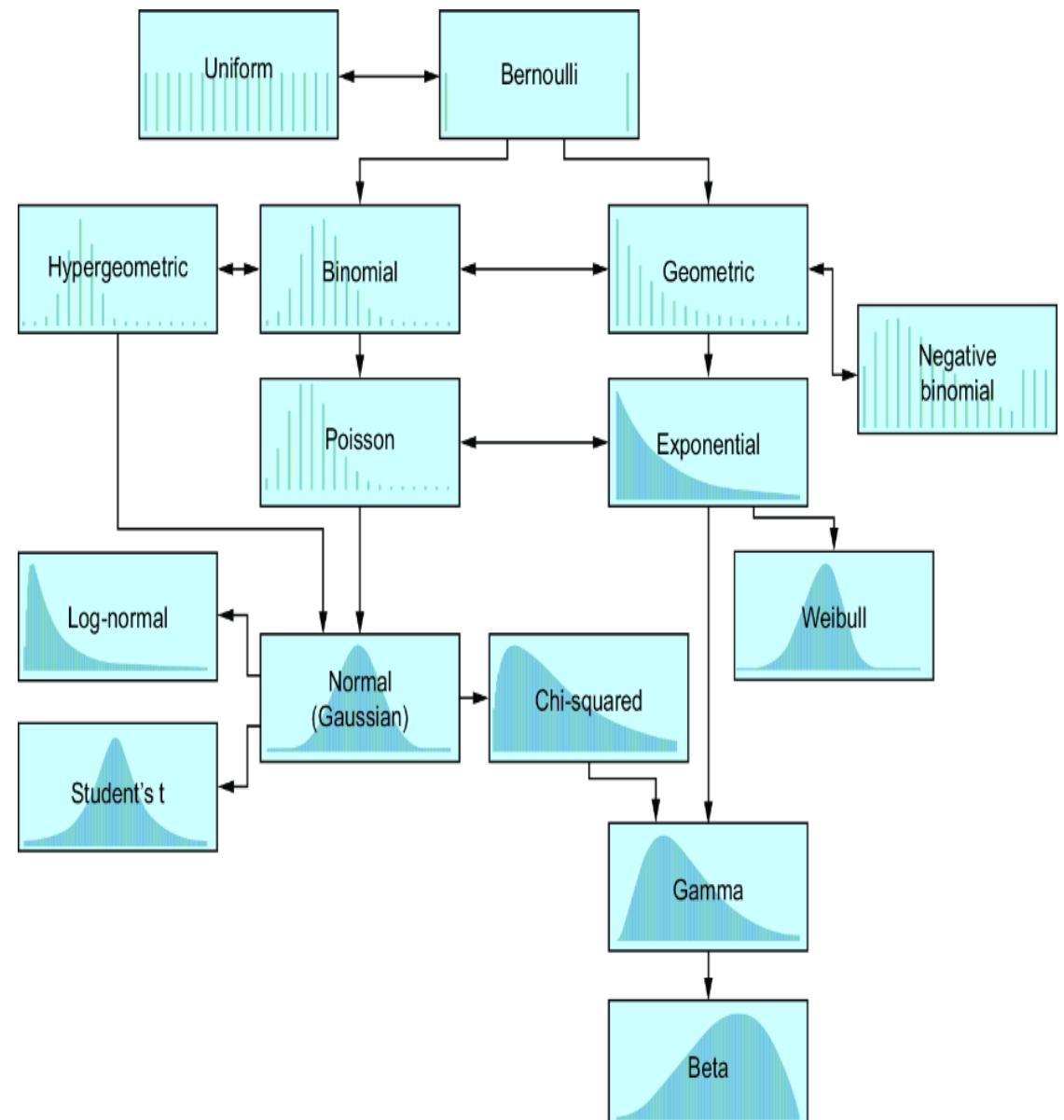
Figure 2.10 A popular common set of canonical probability distributions. The edges capture mathematical relationships between the distributions (that we won’t get into here). Light-colored distributions are discrete and dark-colored distributions are continuous. An arrow represents the existence of a transformation that converts one distribution to another .

TYPES OF P ARAMETERS

In pr obabilistic modeling settings, it is useful to have an intuition for how to interpr et canonical parameters. T o that end, think of the probability in a distribution as a scar ce resour ce that must be shared acr oss all the possible outcomes. Some outcomes may get more than others, but at the end of the day, it all must sum or

integrate to 1. P arameters characterize how the finite pr obability is distributed to the outcomes.

As an analogy, we’ll use a city with a fixed population. The parameters of the city deter mine wher e that population is situated. Location parameters, such as the nor mal distribution’s ૿ μ (μ is the mean of the nor mal, but not all location parameters are means), are lik e the pin that dr ops down when you sear ch the city’s name in Google Maps. The pin characterizes a pr ecise point we might call the ૿city center . In some cities, most of the people live near the city center, and it gets less populated the further away fr om the center you go . But in other cities, other non-central parts of the city are densely populated. Scale parameters , lik e the nor mal’s ૿ ( is the standar d deviation of a nor mal distribution, but not all scale parameters ar e standar d deviation parameters), deter mine the spread of the population; L os Angeles has a high scale parameter . A shape parameter (and its inverse, the rate parameter ) aects the shape of a distribution in a manner that does not simply shif t it (as a location parameter does) or str etch or shrink it (as a scale parameter does). As an e xample, think of the sk ewed shape of Hong K ong, which has a densely pack ed collection of sk yscrapers in the downtown ar ea, while the mor e residential K owloon has shorter buildings spr ead over a wider space.

The Pyr o library pr ovides canonical distributions as modeling primitives. The Pyr o analog to a discr ete categorical distribution table is a Categorical object.

Listing 2.3 Canonical parameters in P yro

import torch from pyro.distributions import Bernoulli, Categorical, Gamma, Normal #1 print(Categorical(probs=torch.tensor([.45, .30, .25]))) #2 print(Normal(loc=0.0, scale=1.0)) print(Bernoulli(probs=0.4)) print(Gamma(concentration=1.0, rate=2.0))

#1 Pyro includes the commonly used canonical distributions. #2 The Categorical distribution tak es a list of probability values, each value corresponding to an outcome.

This prints the following r epresentations of the distribution objects:

Categorical(probs: torch.Size([3])) Normal(loc: 0.0, scale: 1.0) Bernoulli(probs: 0.4000) Gamma(concentration: 1.0, rate: 2.0)

Rather than pr oviding a pr obbility value, the log_prob method will provide the natural log of the pr obability value, because log probabilities have computational advantages over r egular probabilities. Exponentiating (taking el wher e l is the log probability) converts back to the pr obability scale. F or example, we can cr eate a Ber noulli distribution object with a parameter value of 0.4.

bern = Bernoulli(0.4)

That distribution assigns a 0.4 pr obability to the value 1.0. F or numerical r easons, we typically work with the natural log of probability values.

We can use the exp function in the math library to convert fr om log probability back to the pr obability scale:

lprob = bern.log_prob(torch.tensor(1.0))

import math print(math.exp(lprob))

Exponentiating the log pr obability r eturns the following pr obability value:

0.3999999887335489

It is close, but not the same as 0.4 due to r ounding er ror associated with floating-point pr ecision in computer calculations.

CONDITIONAL PROBABILITY WITH CANONICAL DISTRIBUTIONS

There are few canonical distributions commonly used to characterize sets of individual random variables, such as random vectors or matrices. However, we can use the chain rule to factor a joint pr obability distribution into conditional distributions that we can r epresent with canonical distributions. F or example, we could

represent Y conditioned on X and Z with the following nor mal distribution,

\[\rho(\mathbf{y}|x,z) = \frac{1}{\sqrt{2\pi\sigma^2}}e^{-\frac{1}{2\sigma^2}(\mathbf{y}-\mu(x,z))^2}\]

where the location parameter μ(x,z) is a function of x and z.An example is the following linear function:

\[ \mu \begin{pmatrix} x, \ z \end{pmatrix} = \beta\_0 + \beta\_x x + \beta\_z z \]

Other functions, such as neural networks, ar e possible as well. These parameters ar e typically called weight parameters in machine lear ning.

2.1.8 Visualizing distributions

In pr obabilistic modeling and Bayesian infer ence settings, we commonly conceptualize distributions in ter ms of visuals. In the discr ete case, a common visualization is the bar plot. F or example, we can visualize the pr obabilities in figure 2.3 as the bar plot in figure 2.11. Note that this is not a histogram; I’ll highlight the distinction in section 2.3.

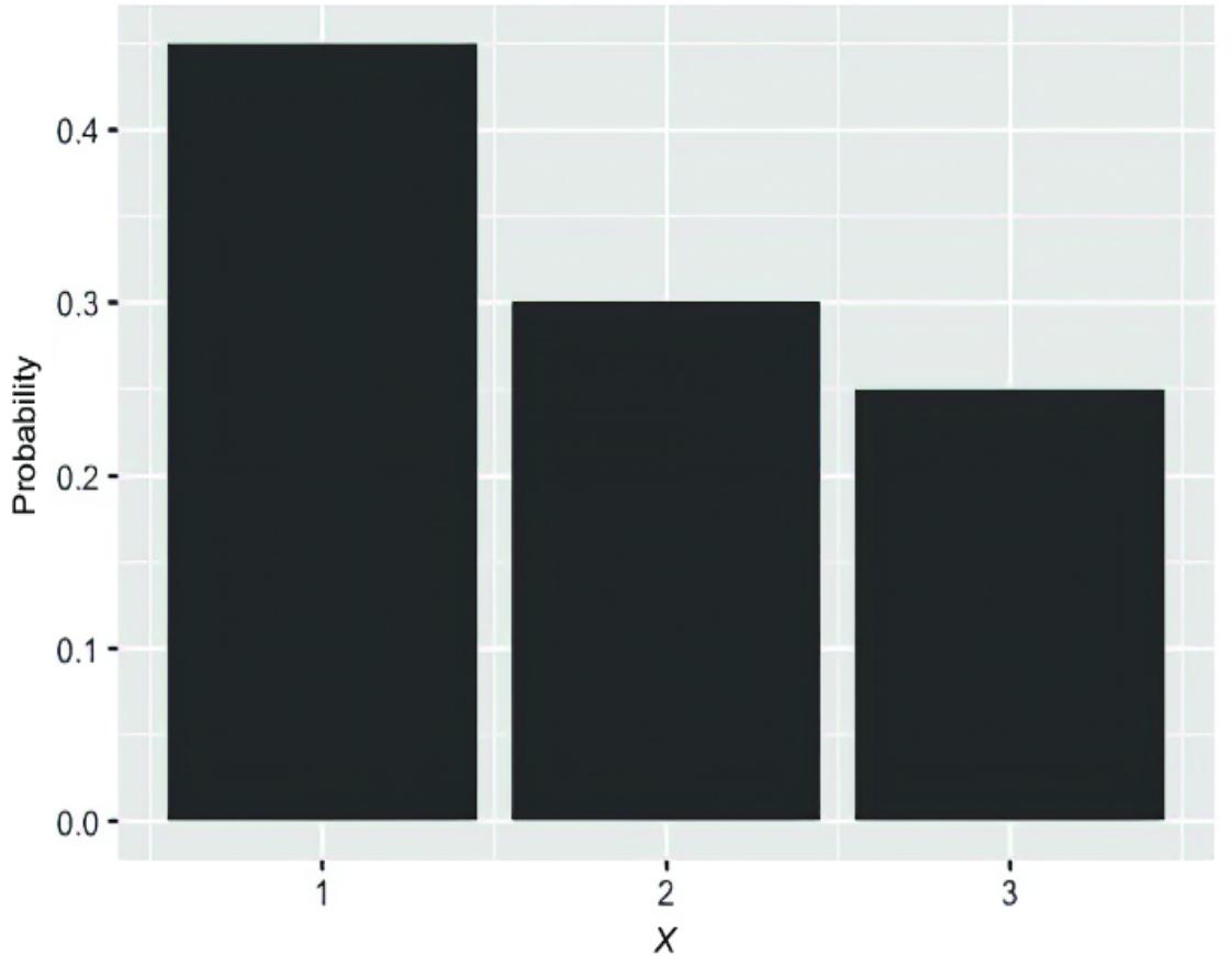
Figure 2.11 Visualization of a discrete probability distribution. The outcomes in the distribution are on the horizontal axis, and probability is on the vertical axis.

We still use visualizations when the distribution has a non- finite set of outcomes. F or example, figure 2.12 overlays two distributions functions: a discr ete P oisson distribution and a continuous nor mal (Gaussian) distribution (I speci fied the two distributions in such a way that they overlapped). The discr ete P oisson has no upper bound on outcomes (its lower bound is 0), but the pr obability tapers o for higher numbers, r esulting in smaller and smaller bars until the bar becomes too in finitesimally small to draw . We visualize the normal distribution by simply drawing the pr obability distribution function as a curve in the figure. The nor mal has no lower or upper bound, but the further away you get fr om the center, the smaller the pr obability values get.

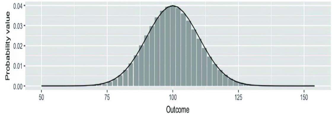
Figure 2.12 A continuous normal distribution (solid line) approximates a discrete Poisson distribution (gra y bars). Again, the outcomes are on the horizontal axis, and the probability values are on the vertical axis.

Visualizing conditional pr obability distributions involves mapping each conditioning variable to some element in the image. F or example, in figure 2.13, X is discr ete, and Y conditioned on X has a normal distribution wher e the location parameter is a function of X.

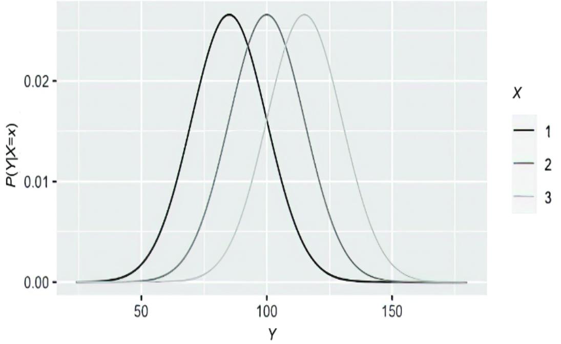
Figure 2.13 A visualization of the conditional probability distribution of continuous Y, given discrete X. For dierent values of X, we get a di erent distribution of Y.

Since X is discr ete, it is simplest to map X to color and overlay the curves for P(Y |X=1), P(Y |X=2), and P(Y |X=3). However, if we

wanted to visualize P(Y |X, Z), we’d need to map Z to an aesthetic element other than color, such as a thir d axis in a pseudo -3D image or r ows in a grid of images. But ther e is only so much infor mation we can add to a 2D visualization. F ortunately, conditional independence helps us r educe the number of conditioning variables.

2.1.9 Independence and conditional independence

Two random variables ar e independent if, infor mally speaking, observing an outcome of one random variable does not a ect the probability of outcomes for the other variable, i.e., P(y|x)=P(y). We denote this as X ⊥ Y. If two variables ar e not independent, they are dependent .

Two dependent variables can become conditionally independent given other variables. F or example, X ⊥Y | Z means that X andY may be dependent, but they ar e conditionally independent given Z. In other wor ds, if X and Y are dependent, and X ⊥ Y | Z, then it is not true that P(y|x) P(y) but it is true that P(y|x, z) = P(y|z).

INDEPENDENCE IS A POWERFUL TOOL FOR SIMPLIFICA TION

Independence is a powerful tool for simplif ying r epresentations of probability distributions. Consider a joint pr obability distribution P (W, X, Y, Z) represented as a table. The number of cells in the table would be the pr oduct of the number of possible outcomes each for W, X, Y, and Z. We could use the chain rule to br eak the pr oblem up into factors { P(W ), P(X |W ), P(Y |X, W ), P(Z |Y, X, W )}, but the total number of parameters acr oss these factors wouldn’t change, so the aggr egate comple xity would be the same.

However, what if X ⊥ W ? Then P(X |W ) reduces to P(X). What if Z ⊥ Y |X ? Then P(Z |Y, X, W ) reduces to P(Z |X, W ). Every time we can impose a pairwise conditional independence condition as a constraint on the joint pr obability distribution, we can r educe the comple xity of the distribution by a lar ge amount. Indeed, much of model building and evaluation in statistical modeling, r egularization in machine lear ning, and deep lear ning techniques such as ૿dr opout ar e either dir ect or implicit attempts to impose conditional

independence on the joint pr obability distribution underlying the data.

CONDITIONAL INDEPENDENCE AND CA USALITY

Conditional independence is fundamental to causal modeling. Causal r eationships lead to conditional independence between correlated variables. F or example, a child’s par ents’ and grandpar ents’ blood types ar e all causes of that child’s blood type; these blood types ar e all cor related. But all you need is the par ents’ blood type, the dir ect causes, to fully deter mine the child’s blood type, as illustrated in figure 2.14. In pr obabilistic ter ms, the child’s and grandpar ents’ blood types ar e conditionally independent, given the par ents.

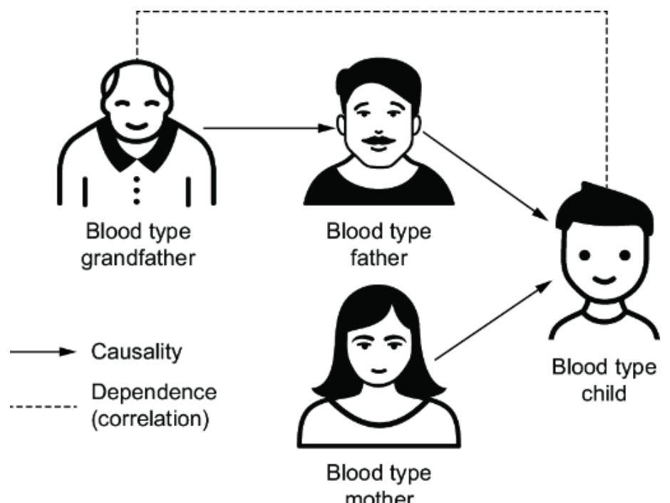
Figure 2.14 How causality can induce conditional independence. The blood types of the parents cause the blood type of the child. The grandfather ‘s blood type is correlated with that of the child’s (dashed line). But the parents’ blood types are direct causes that fully determine that of the child. These direct causes render the child’s and grandfather ’s blood types conditionally independent.

The fact that causality induces conditional independence allows us to lear n and validate causal models against evidence of conditional

independence. In chapter 4, we’ll e xplor e the r elationship between conditional independence and causality in for mal ter ms.

2.1.10 Expected value

The expected value of a function of a random variable is the weighted average of the function’s possible output values, wher e the weight is the pr obability of that outcome.

\[E\left(f\left(X\right)\right) = \sum\_{X=x} f\left(x\right)P\left(x\right)\]

\[E\left(f\left(X\right)|\,Y=y\right) = \sum\_{X=x} f\left(x\right)P\left(x\mid y\right)\]

In the case of a continuum of possible outcomes, the e xpectation is defined by integration.

\[E\left(f(X)\right) = \int\_{X=u} f\left(u\right)\phi\left(u\right) du\]

\[E\left(f\left(X\right)|Y=\mathcal{y}\right) = \int\_{X=u} f\left(u\right)\phi\left(u|\mathcal{y}\right) du\]

Some of the causal quantities we’ll be inter ested in calculating will be de fined in ter ms of e xpectation. Those quantities only r eason about the e xpectation, not about how the e xpectation is calculated. It is easier to get an intuition for a pr oblem when working with the basic arithmetic of discr ete e xpectation rather than integral calculus in the continuous case. So, in this book, when ther e is a choice, I use e xamples with discr ete random variables and discr ete expectation. The causal logic in those e xamples all generalize to the continuous case.

There are many inter esting mathematical pr operties of e xpectation. In this book, we car e about the fact that conditional e xpectations simplif y under conditional independence: If X ⊥ Y, then E(X |Y ) = E(X). If X ⊥ Y |Z, then E(X |Y,Z) = E(X |Z). In simpler ter ms, if two variables ( X and Y) ar e independent, our e xpectation for one does

not change with infor mation about the other . If their independence holds conditional on a thir d variable ( Z ), our e xpectation for one, given that we know the thir d variable, is una ected by infor mation about the other variable.

Other than this, the most important pr operty is the linearity of the expectation, meaning that the e xpectation passes thr ough linear functions. Her e are some useful r efernce e xamples of the linearity of expectation:

For random variables X and Y: E(X + Y ) = E(X ) + E(Y ) and

\[E(\sum\_{i} X\_i) = \sum\_{i} E(X\_i)\]

For constants a and b: E(aX + b) = aE(X ) + b
If Xonly has outcomes 0 and 1, and E(Y|X) = aX+ b, then E (Y |X=1) – E(Y |X=0) = a. (This is truebecause a*1 + b– (a* 0 + b) = a. Spoiler alert: this one is important for linear regression-based causal e ect infer ence techniques.)

The mean of the random variable’s distribution is the e xpected value of the variable itself, as in E(X) (i.e., the function is the identity function , f(X ) = X). In several canonical distributions, the mean is a simple function of the parameters. In some cases, such as in the nor mal distribution, the location parameter is equivalent to the e xpectation. But the location parameter and the e xpectation are not always the same. F or example, the Cauchy distribution has a location parameter, but its mean is unde fined.

In the ne xt section, you’ll lear n how to r epresent distributions and calculate e xpectations using computational methods.

2.2Computationalprobability

We need to code probability distributions and e xpectations fr om probability to use them in our models. In the pr evious section, you saw how to code up a pr obability distribution for a thr ee-sided die. But how do we code up rolling a thr ee-sided die? How do we write code r epresenting two dice r olls that ar e conditionally independent? While we’r e at it, how do we get a computer to do the math that calculates an e xpectation? How do we get a computer, wher e everything is deter ministic, to r oll dice so that the outcome is unknown befor ehand?

2.2.1 The physical interpretation of probability

Suppose I have a thr ee-sided die. I have some pr obability values assigned to each outcome on the die. What do those pr obability values mean? How do I interpr et them?

Suppose I r epeatedly r olled the die and k ept a running tally of how many times I saw each outcome. F irst, the r oll is random, meaning that although I r oll it the same way each time, I get varying r esults. The physical shape of the die a ects those tallies; if one face of the die is lar ger than the other two, that size di erence will a ectthe count. As I r epeat the r oll many times, the pr oportion of total times I see a given outcome conver ges to a number . Suppose I use that number for my pr obability value. F urther, suppose I interpr et that number as the ૿chance of seeing that outcome each time I r oll.

This idea is called physical (or frequentist ) probability . Physical probability means imagining some r epeatable physical random process that r esults in one outcome among a set of possible outcomes. W e assign a pr obability value using the conver gent proportion of times the outcome appears when we r epeat the random pr ocess ad in finitum. W e then interpr et that pr obability as the pr oensity for that physical pr ocess to pr oduce that outcome.

2.2.2 Random generation

Given the pr eceding de finition for physical pr obability, we can define random generation. In random generation , an algorithm randomly chooses an outcome fr om a given distribution. The algorithm’s choice is inspir ed by physical pr obability; the way it selects an outcome is such that if we ran the algorithm ad infinitum, the pr oportion of times it would choose that outcome would equal the distribution’s pr obability value for that outcome.

Computers ar e deter ministic machines. If we r epeatedly run a computer pr ocedur e on the same input, it will always r eturn the same output; it cannot pr oduce anything genuinely random (unless it has a random input). Computers have to use deter ministic algorithms to emulate random generation. These algorithms ar e called pseudo -ranm number generators—they tak e a starting number, called a random seed , and r eturn a deter ministic series of numbers. Those algorithms mathematically guarantee that a series of numbers is statistically indistinguishable fr om the ideal of random generation.

In notation, I write random generation as follows:

This r eads as ૿x is generated fr om the pr obability distribution of X.

In random generation, synonyms for ૿generate include ૿simulate and ૿sample. F or example, in pgmpy the sample method in DiscreteFactor does random generation. It r eturns a pandas DataFrame. Note that since this is random generation, you will likely get di erent outputs when you run this code:

	Listing 2.4	Simulating random variates from in pgmpy
)	dist = DiscreteFactor( variables=[“X”], cardinality=[3], values=[.45, .30, .25], state_names= {‘X’: [‘1’, ‘2’, ‘3’]}	from pgmpy.factors.discrete import DiscreteFactor
	dist.sample(n=1) #1
		#1 n is the number of instances you wish to generate.

This pr oduces the table pictur ed in figure 2.15.

Figure 2.15 Generating one instance from P(X) creates a pandas DataFrame object with one row .

We can also generate fr om joint probability distributions.

joint = DiscreteFactor(
 variables=['X', 'Y'],
 cardinality=[3, 2],
 values=[.25, .20, .20, .10, .15, .10],
 state_names= {
 'X': ['1', '2', '3'],
 'Y': ['0', '1']
 }
)
joint.sample(n=1)

This pr oduces the table pictur ed in figure 2.16.

Figure 2.16 Generating one instance from P(X, Y) creates a pandas DataFrame object with one row .

Pyro also has a sample method for canonical distributions:

import torch from pyro.distributions import Categorical Categorical(probs=torch.tensor([.45, .30, .25])).sample()

This generates a sample fr om that categorical distribution, i.e., either 0, 1, or 2.

tensor(1.)

2.2.3 Coding random processes

We can write our own random pr ocesses as code when we want to generate values in a particular way . A random pr ocess written as code is sometimes called a stochastic function , probabilistic subroutine , or probabilistic program . For example, consider the joint probability distribution P(X, Y, Z). How can we randomly generate from this joint distribution? Unfortunately, sof tware libraries don’t usually pr ovide pseudo -random generation for arbitrary joint distributions.

We can get ar ound this by applying the chain rule and, if it e xists, conditional independence. F or example, we could factorize as follows:

\[P(x, y, z) = P(z)P(x|z)P(y|x, z)\]

Suppose that Y is conditionally independent of Z given X, then:

\[P(x, y, z) = P(z)P(x|z)P(y|x)\]

Finally, suppose we can sample fr om P(Z ), P(X |Z), and P(Y |X) given the basic random generation functions in our sof tware library . Then we can use this factorization to compose an algorithm for sampling:

\[\begin{aligned} z &\sim P\left(Z\right) \\ x &\sim P\left(X|Z=z\right) \\ y &\sim P\left(Y|X=x\right) \end{aligned}\]

This is a random pr ocess that we can e xecute in code. F irst, we generate a Z-outcome z from P(Z ). We then condition X on that z, and generate an X-outcome x. We do the same to generate a Youtcome y. Finally, this pr ocedur e generates a tuple { x, y, z} fr om the joint distribution P(X, Y, Z ).

In pgmpy, we can cr eate a random pr ocess using the class called BayesianNetwork .

Listing 2.5 Creating a random process in pgmpy and P yro from pgmpy.factors.discrete.CPD import TabularCPD from pgmpy.models import BayesianNetwork from pgmpy.sampling import BayesianModelSampling PZ = TabularCPD( #1 variable=‘Z’, #1 variable_card=2, #1 values=[[.65], [.35]], #1 state_names = { #1 ‘Z’: [‘0’, ‘1’] #1 }) #1 PXgivenZ = TabularCPD( #2 variable=‘X’, #2 variable_card=2, #2 values=[ #2 [.8, .6], #2 [.2, .4], #2 ], #2 evidence=[‘Z’], #2 evidence_card=[2], #2 state_names = { #2 ‘X’: [‘0’, ‘1’], #2 ‘Z’: [‘0’, ‘1’] #2 }) #2 PYgivenX = TabularCPD( #3 variable=‘Y’, #3 variable_card=3, #3 values=[ #3 [.1, .8], #3 [.2, .1], #3 [.7, .1], #3 ], #3 evidence=[‘X’], #3 evidence_card=[2], #3 state_names = { #3 ‘Y’: [‘1’, ‘2’, ‘3’], #3 ‘X’: [‘0’, ‘1’] #3 }) #3 model = BayesianNetwork([(‘Z’, ‘X’), (‘X’, ‘Y’)]) #4 model.add_cpds(PZ, PXgivenZ, PYgivenX) #5 generator = BayesianModelSampling(model) #6 generator.forward_sample(size=1) #7 #1 P(Z) #2 P(X|Z=z) #3 P(X|Z=z) #4 P(Y|X=x) #5 Create a Ba yesianNetwork object. The arguments are edges of a directed graph, which we’ll cover in chapter 3. #6 Add the conditional probability distributions to the model. #7 Create a Ba yesianModelSampling object from the Ba yesianNetwork object. #8 Sample from the resulting object This pr oduces one r ow in a pandas DataF rame, shown in figure

2.17.

Figure 2.17 The forward_sample method simulates one instance of X, Y, and Z as a row in a pandas DataF rame.

Implementing random pr ocesses for random generation is powerful because it allows generating fr om joint distributions that we can’t represent in clear mathematical ter ms or as a single canonical distribution. F or example, while pgmpy works well with categorical distributions, Pyr o gives us the flexibility of working with combinations of canonical distributions.

The following listing shows a Pyr o version of the pr evious random process. It has the same dependence between Z, X, and Y, but dierent canonical distributions.

Listing 2.6 Working with combinations of canonical distributions in P yro

import torch from pyro.distributions import Bernoulli, Poisson, Gamma z = Gamma(7.5, 1.0).sample() #1 x = Poisson(z).sample() #2 y = Bernoulli(x / (5+x)).sample() #3 print(z, x, y) #1 Represent P(Z) with a gamma distribution, and sample z. #2 Represent P(X|Z=z) with a Poisson distribution with location parameter z, and sample x. #3 Represent P(Y|X=x) with a Bernoulli distribution. The probability parameter is a function of x.

This prints out a sample set, such as the following:

tensor(7.1545) tensor(5.) tensor(1.)

Z comes fr om a gamma distribution, X from a P oisson distribution with mean parameter set to z, and Y from a Ber noulli distribution with its parameter set to a function of x.

Implementing a random function with a pr ogramming language lets us use nuanced conditional contr ol flow. Consider the following pseudocode:

z ~ P(Z)
x ~ P(X|Z=z)
y = 0
for i in range(0, x){ #1
 y_i ~ P(Y|X=x) #1
 y += y_i #2
}

#1 We can use control flow, lik e this for loop, to generate values. #2 y is the sum of the values generated in the for loop. y still depends on x, but through nuanced control flow.

Here, y is still dependent on x. However, it is de fined as the sum of x individual random components. In Pyr o, we might implement this as follows.

Listing 2.7 Random processes with nuanced control flow in P yro

import torch from pyro.distributions import Bernoulli, Poisson, Gamma z = Gamma(7.5, 1.0).sample() x = Poisson(z).sample() y = torch.tensor(0.0) #1 for i in range(int(x)): #1 y += Bernoulli(.5).sample() #1 print(z, x, y)

#1 y is de fined as a sum of random coin flips, so y is generated from P(Y|X=x) because the number of flips depends on x.

In Pyr o, best practice is to implement random pr ocesses as functions. F urther, use the function pyro.sample to generate, rather than using the sample method on distribution objects. W e could rewrite the pr eceding random_process code (listing 2.7) as follows. import torch import pyro def random_process(): z = pyro.sample(“z”, Gamma(7.5, 1.0)) x = pyro.sample(“x”, Poisson(z)) y = torch.tensor(0.0) for i in range(int(x)): y += pyro.sample(f”y{i}“, Bernoulli(.5)) #1 return y

#1 f”y{i}” creates the names “y1”, “y2”, etc.

Listing 2.8 Using functions for random processes and pyro.sample

The first ar gument in pyro.sample is a string that assigns a name to the variable you ar e sampling. The r eason for that will become apparent when we start running infer ence algorithms in Pyr o in chapter 3.

2.2.4 Monte Carlo simulation and expectation

Monte Carlo algorithms use random generation to estimate expectations fr om a distribution of inter est. The idea is simple. Y ou have some way of generating fr om P(X ). If you want E(X ), generate multiple x’s, and tak e the average of those x’s. If you want E(f(X )), generate multiple x’s and apply the function f(.) to each of those x’s, and tak e the average. Monte Carlo works even in cases when X is continuous.

In pgmpy, you use the sample or forward_sample methods to generate a pandas DataF rame. Y ou can then calculate the panda’s mean method.

generated_samples = generator.forward_sample(size=100) generated_samples[‘Y’].apply(int).mean()

In Pyr o, we call the random_process function r epeatedly . We can do this for the pr eceding Pyr o generator with a for loop that generates 100 samples:

generated_samples = torch.stack([random_process() for _ in range(100)])

This code r epeatedly calls random_process in a Python list comprehension. R ecall that Pyr o extends PyT orch, and the value of y it r eturns is a tensor . I use torch.stack to tur n this list of tensors into a single tensor . Finally, I call the mean method on the tensor to obtain the Monte Carlo estimate of E(Y ).

generated_samples.mean()

When I ran this code, I got a value of about 3.78, but you’ll lik ely get something slightly di erent.

Most things you’d want to know about a distribution can be framed in ter ms of some function f(X ). F or example, if you wanted to know the pr obability of X being gr eater than 10, you could simply generate a bunch of x’s and convert each x to 1 if it is gr eater than 10 and 0 otherwise. Then you’d tak e the average of the 1’s and 0’s, and the r esulting value would estimate the desir ed pr obability .

To illustrate, the following code e xtends the pr evious block to calculate E(Y 2).

torch.square(generated_samples).mean()

When calculating E(f(X )) for a random variable X, remember to get the Monte Carlo estimate by applying the function to the samples first, and then tak e the average. If you apply the function to the sample average, you’ll instead get an estimate of f(E(X )), which is almost always di erent.

2.2.5 Programming probabilistic inference

Suppose we implement in code a random pr ocess that generates an outcome { x,y, z} fr om P(X, Y, Z ) as follows:

Further, suppose we ar e inter ested in generating fr om P(Z |Y=3). How might we do this? Our pr ocess can sample fr om P(Z ), P (X |Z ), and P(Y |Z ), but it is not clear how we go fr om these to P (Z |Y ).

Probabilistic inference algorithms generally tak e an outcomegenerating random pr ocess and some tar get distribution as inputs. Then, they r eturn a means of generating fr om that tar get distribution. This class of algorithms is of ten called Bayesian

infer ence algorithms because the algorithms of ten use Bayes rule to go fr om P(Y |Z) to P(Z |Y ). However, the connection to Bayes rule is not always e xplicit, so I pr efer ૿pr obabilistic infer ence over Bayesian infer ence algorithms.

For example, a simple class of pr obabilistic infer ence algorithms is called accept/r eject algorithms. Applying a simple accept/r eject technique to generating fr om P(Z |Y=3) works as follows:

1. Repeatedly generate {x, y, z} using our generator forP(X, Y, Z ).
1. Throw away any generated outcome wher e y is not equal to 3.
1. The resulting set of outcomes for Zwill have the distribution P (Z |Y=3).

Illustrating with Pyr o, let’s r ewrite the pr evious random_process function to r eturn z and y. After that, we’ll obtain a Monte Carlo estimate of E(Z |Y=3).

Listing 2.9 Monte Carlo estimation in P yro

import torch import pyro from pyro.distributions import Bernoulli, Gamma, Poisson def random_process(): z = pyro.sample(“z”, Gamma(7.5, 1.0)) x = pyro.sample(“x”, Poisson(z)) y = torch.tensor(0.0) for i in range(int(x)):

y += pyro.sample(f”{i}“, Bernoulli(.5)) return z, y #1

generated_samples = [random_process() for _ in range(1000)] #2 z_mean = torch.stack([z for z, _ in generated_samples]).mean() #3 print(z_mean)

#1 This new version of random_process returns both z and y . #2 Generate 1000 instances of z and y using a list comprehension. #3 Turn the individual z tensors into a single tensor , and then calculate the Monte Carlo estimate via the mean method.

This code estimates E(Z ). Since Z is simulated fr om a gamma distribution, the true mean E(Z ) is the shape parameter 7.5 divided by the rate parameter 1.0, which is 7.5. Now, to estimate E(Z |Y=3), we’ll filter the samples and k eep only the samples wher e Y is 3.

z_given_y = torch.stack([z for z, y in generated_samples if y == 3]) print(z_given_y.mean())

One run of this code pr oduced tensor(6.9088) , but your r esult might be slightly di erent. That pr obabilistic infer ence algorithm works well if the outcome Y=3 occurs fr equently . If that outcome wer e rare, the algorithm would be ine cient: we’d have to generate many samples to get samples that meet the condition, and we’d be throwing away many samples.

There are various other algorithms for pr obabilistic infer ence, but the topic is too rich and tangential to causal modeling for us to explor e in depth. Nevertheless, the following algorithms ar e worth mentioning for what we cover in this book. V isit https://www .altdeep.ai/p/causalaibook for links to some complementary materials on infer ence with pgmpy and Pyr o.

PROBABILITY WEIGHTING METHODS

These methods generate outcomes fr om a joint pr obability distribution and then weight them accor ding to their pr obability in the tar get distribution. W e can then use the weights to do weighted averaging via Monte Carlo estimation. P opular variants of this kind of infer ence include importance sampling and inverse pr obability reweighting, the latter of which is popular in causal infer ence and is cover ed in chapter 11.

INFERENCE WITH PROBABILISTIC GRAPHICAL MODELS

Probabilistic graphical models use graphs to r epresent conditional independence in a joint pr obability distribution. The pr esence of a graph enables graph-based algorithms to power infer ence. T wo well-known appr oaches include variable elimination and belief propagation. In figures 2.5 and 2.6, I showed that you could ૿eliminate a variable by summing over its columns or r ows in the probability table. V ariable elimination uses the graph structur e to optimally sum over the variables you wish to eliminate until the resulting table r epresents the tar get distribution. In contrast, belief

propagation is a message-passing system; the graph is used to form dierent ૿cliques of neighboring variables. F or example, if P (Z |Y=1) is the tar get distribution, Y=1 is a message iteratively passed back and forth between cliques. Each time a message is received, parameters in the clique ar e updated, and the message is passed on. Eventually, the algorithm conver ges, and we can derive a new distribution for Z from those updated parameters.

One of the attractive featur es of graph-based pr obabilistic infer ence is that users typically don’t implement them themselves; sof tware like pgmpy does it for you. Ther e are theor etical caveats, but they usually don’t matter in practice. This featur e is an e xample of the ૿commodi fication of infer ence trend I highlighted in chapter 1. In this book, we’ll work with causal graphical models, a special type of probabilistic graphical model that works as a causal model. That gives us the option of applying graph-based infer ence for causal problems.

VARIATIONAL INFERENCE

In variational inference , we write code for a new stochastic pr ocess that generates samples fr om an ૿appr oximating distribution that resembles the tar get distribution. That stochastic pr ocess has parameters that we optimize using gradient-based techniques now common in deep lear ning sof tware. The objective function of the optimization tries to minimize the di erence between the approximating distribution and the tar get distribution.

Pyro is a pr obabilistic modeling language that tr eats variational infer ence as a principal infer ence technique. It calls the stochastic process that generates fr om the appr oximating distribution a ૿guide function, and a savvy Pyr o programmer gets good at writing guide functions. However, it also pr ovides a suite of tools for ૿automatic guide generation, another e xample of the commodi fication of infer ence.

MARKOV CHAIN MONTE CARL O

Markov chain Monte Carlo (MCMC) is an infer ence algorithm popular amongst computational Bayesians. These ar e accept/rject

algorithms wher e each newly generated outcome depends on the previous (non-r ejected) generated outcome. This pr oduces a chain of outcomes, and the distribution of outcomes in the chain eventually conver ges to the tar get distribution. Hamiltonian Monte Carlo (HMC) is a popular version that doesn’t r equir e users to implement the generator . Pyr o, and similar libraries, such as PyMC, implement HMC and other MCMC algorithms.

ADVANCED INFERENCE METHODS

Resear ch in generative models continues to develop new infer ence techniques. Examples include techniques such adversarial infer ence, infer ence with nor malizing flows, and di usion-based infer ence. The goal of such techniques ar e to eciently sample from the comple x distributions common in machine lear ning problems. Again, see https://www .altdeep.ai/p/causalaibookfor refernces. W e’ll see an e xample of a structural causal model that leverages nor malizing flows in chapter 6. The appr oach tak en in this book is to leverage the ૿commodi fication of infer ence tr end discussed in chapter 1, such that we can build causal models that leverage these algorithms, as well as new algorithms as they ar e released.

2.3Data,populations,statistics,and models

So far, we have talk ed about random variables and distributions. Now we’ll move on to data and statistics. L et’s start with de fining some ter ms. Y ou doubtless have an idea of what data is, but let’s define it in ter ms we’ve alr eady de fined in this chapter . Data is a set of r ecorded outcomes of a random variable or set of random variables. A statistic is anything you calculate fr om data. F or example, when you train a neural network on training data, the learned weight parameter values ar e statistics, and so ar e the model’s pr edictions (since they depend on the training data via the weights).

The r eal-world causal pr ocess that generates a particular str eam of data is called the data generating process (DGP). A model is a

simpli fied mathematical description of that pr ocess. A statistical model is a model with parameters tuned such that the model aligns with statistical patter ns in the data.

This section pr esents some of the cor e concepts r elated to data and statistics needed to mak e sense of this book.

2.3.1 Probability distributions as models for populations

In applied statistics, we tak e statistical insights fr om data and generalize them to a population. Consider, for e xample, the MNIST digit classi fication pr oblem described in chapter 1. Suppose the goal of training a classi fication model on MNIST data was to deploy the model in sof tware that digitizes written te xt documents. In this case, the population is all the digits on all the te xts the sof tware will see in the futur e.

Populations ar e heter ogeneous, meaning members of the population vary . While a featur e on a website might drive engagement among the population of users, on average, the featur e might mak e some subpopulation of users less engaged, so you would want to tar get the featur e to the right subpopulations. Marketers call this ૿segmentation.

In another e xample, a medicine might not be much help on average for a br oad population of patients, but ther e some subpopulation might e xperience bene fits. T argeting those subpopulations is the goal of the field of pr ecision medicine.

In pr obabilistic models, we use pr obability distributions to model populations. It is particularly useful to tar get subpopulations with conditional pr obability . For example, suppose P(E |F=True) represents the distribution of engagement numbers among all users e xposed to a website featur e. Then P(E |F=True, G =“millennial”) r epresents the subpopulation of users e xposed to the featur e who ar e also millennials.

CANONICAL DISTRIBUTIONS AND STOCHASTIC PROCES SES AS MODELS OF POPULA TIONS

If we use pr obability distributions to model populations, what canonical distributions should we use for a given population? F igure 2.18 includes common distributions and the phenomena they typically model.

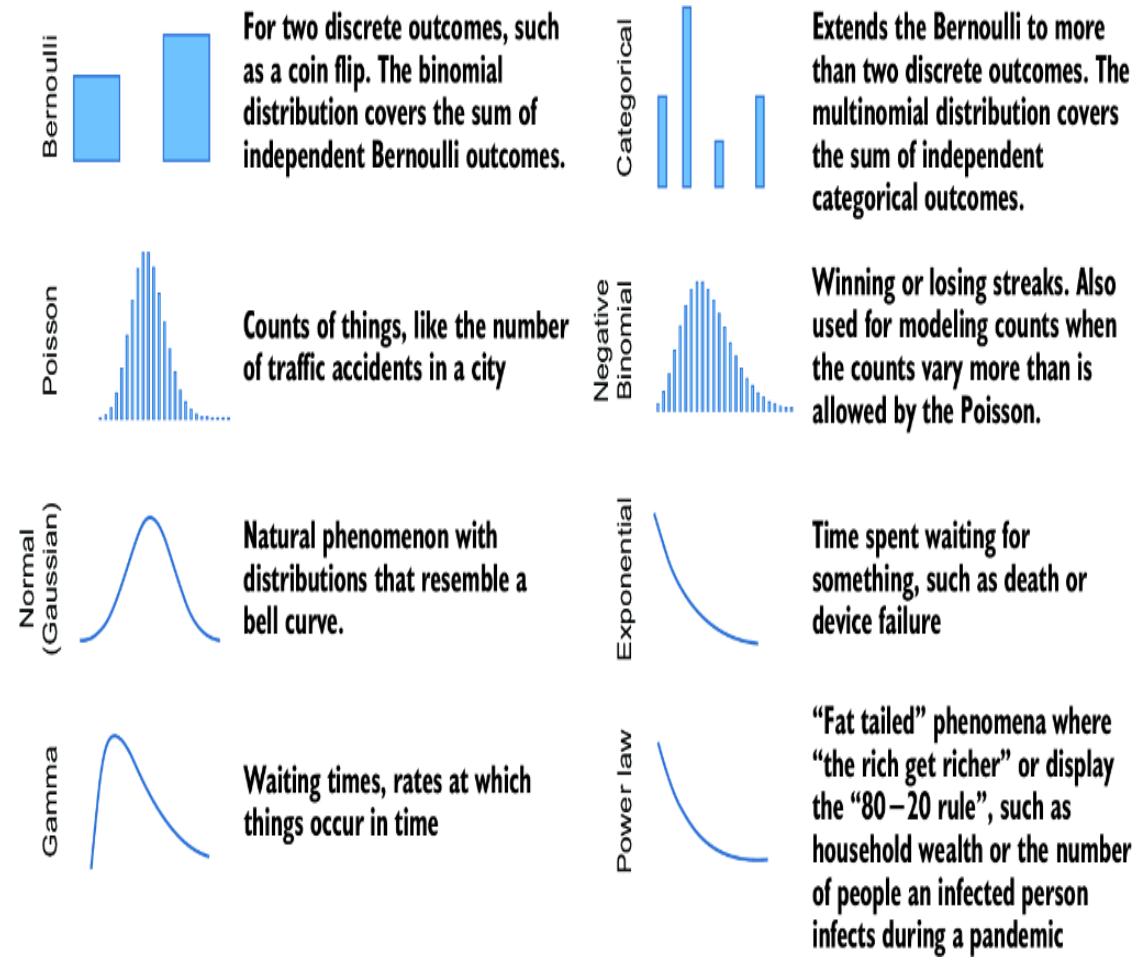
Figure 2.18 Examples of common canonical distributions and the types of phenomena and data they typically model

These choices don’t come fr om nowher e. The canonical distributions ar e themselves derived fr om stochastic functions. F or example, the binomial distribution is the r esult of a pr ocess wher e you do a series of coin flips. When something is the r esult of adding together a bunch of independent (or weakly dependent) small changes, you get a nor mal distribution. W aiting time distributions captur e the distribution of the amount of time one must wait for an event (e.g., a device failur e or a car accident). The e xponential distribution is appr opriate for waiting times when the amount of time you’ve alr eady been waiting has no bearing on how much time you still must wait (e.g., for the amount of time it tak es a radioactive atom to decay). If the time to event has an e xponential distribution, the number of times that event has occur red within a fixed time period has a P oisson distribution.

A useful trick in pr obabilistic modeling is to think of the stochastic process that cr eated your tar get population. Then either choose the appropriate canonical distribution or implement the stochastic process in code using various canonical distributions as primitives in the code logic. In this book, we’ll see that this line of r easoning aligns well with causal modeling.

SAMPLING, IID, AND GENERA TION

Usually, our data is not the whole population but a small subset from the population. The act of randomly choosing an individual is called sampling . When the data is cr eated by r epeatedly sampling from the population, the r esulting dataset is called a random sample . If we can view data as a random sample , we call that data independent and identically distributed (IID) . That means that the selection of each individual data point is identical in how it was sampled, and each sampling occur red independently of the others, and they all wer e sampled fr om the same population distribution. Figure 2.19 illustrates how an IID random sample is selected fr om a population.

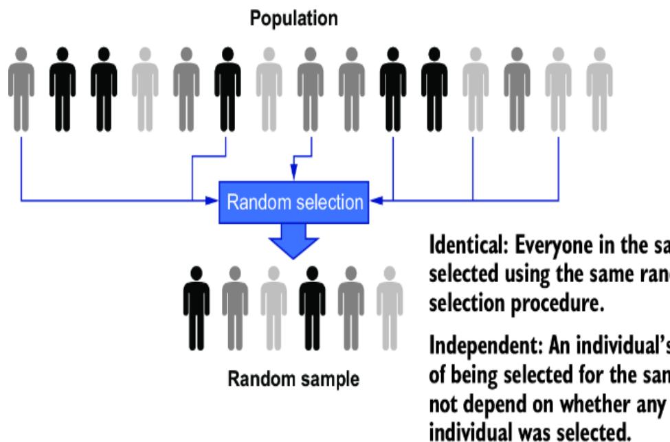
Figure 2.19 Creating a random sample by random selection from a population. Individuals are randomly selected from the population such that the sample distribution resembles the population distribution. The sample is identically and independently distributed (IID), meaning that sample members are selected the same wa y, and whether an individual is selected doesn’t depend on whether another individual was selected.

The idea of sampling and IID data illustrates the second bene fit of using pr obability distributions to model populations. W e can use generation fr om that distribution to model sampling fr om a population. W e can implement a stochastic pr ocess that r epresents the DGP by first writing a stochastic pr ocess that r epresents the population and then composing it with a pr ocess that generates data fr om the population pr ocess, emulating IID sampling.

In pgmpy, this is as simple as generating mor e than one sample.

generator.forward_sample(size=10)

This pr oduces the table showing in figure 2.20

		Z X Y
0	0	1 -	ന
1	0	0	3
2	o	o	2
	3 0	0	3
4	0	o	ദ
	5 0 0		3
6	1	o	ന
7	1	0	3
8	1	0	2
9	0	0	ਤ

Figure 2.20 A pandas DataF rame created by generating ten data points from a model in pgmpy

The Pyr o appr oach for IID sampling is pyro.plate .

Listing 2.10 Generating IID samples in P yro

import pyro from pyro.distributions import Bernoulli, Poisson, Gamma def model(): z = pyro.sample(“z”, Gamma(7.5, 1.0)) x = pyro.sample(“x”, Poisson(z)) with pyro.plate(“IID”, 10): #1 y = pyro.sample(“y”, Bernoulli(x / (5+x))) #2 return y

model()

#1 pyro.plate is a context manager for generating conditionally independent samples. This instance of pyro.plate will generate 10 IIΔ samples. #2 Calling pyro.sample generates a single outcome y , where y is a tensor of 10 IIΔ samples.

Using generation to model sampling is particularly useful in machine lear ning, because of ten the data is not IID. In the MNIST example in chapter 1, the original NIST data was not IID—one block of data came fr om high school students and the other fr om government ocers. Y ou could captur e the identity of the digit

writer as a variable in your stochastic pr ocess. Then the data would be IID conditional on that variable.

DON’T MIST AKE THE MAP FOR THE TERRAIN

Consider again the MNIST data. The population for that data is quite nebulous and abstract. If that digit classi fication sof tware wer e licensed to multiple clients, the population would be a practically unending str eam of digits. Generalizing to abstract populations is the common scenario in machine lear ning, as it is for statistics. When R.A. Fisher, the founding father of moder n statistics, was designing e xperiments for testing soil types on cr op gr owth at Rothamsted R esear ch, he was trying to figure out how to generalize to the population of futur e crops (with as small a number of samples as possible).

The pr oblem with working with nebulously lar ge populations is that it can lead to the mistak e of mentally con flating populations with the pr obability distributions. Do not do this. Do not mistak e the map (the distribution used to model the population) for the ter rain (the population itself).

To illustrate, consider the following e xample: While writing part of this chapter, I was vacationing in Silves, a town in the P ortuguese Algarve with a big castle, deep history, and gr eat hiking. Suppose I were inter ested in modeling the heights of Silves r esidents.

O cially, the population of Silves is 11,000, so let’s tak e that number as gr ound truth. That means ther e are 11,000 di erent height values in Silves. Suppose I physically went down to the national health center in Silves and got a spr eadsheet of every resident’s height. Then the data I’d have is not a randomly sampled subset of the population—it is the full population itself .

I could then compute a histogram on that population, as shown in figure 2.21. A histogram is a visualization of the counts of values (in this case, heights) in a population or sample. F or continuous values like heights, we count how many values fall into a range or ૿bin.

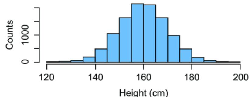
Figure 2.21 A histogram illustrating the height distribution of all Silves residents

This histogram r epresents the full population distribution. I can make it look mor e lik e a pr obability distribution by dividing the counts by the number of people, as in figure 2.22

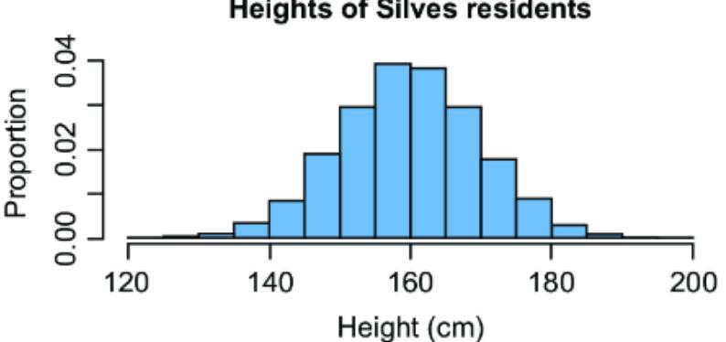
Figure 2.22 Histogram of proportions of Silves residents with given height

One might say this distribution follows the nor mal (Gaussian) probability distribution, because we see a bell curve, and indeed, the nor mal is appr opriate for evolutionary bell-shaped phenomena such as height. But that statement is not pr ecisely true. T o see this, consider that all nor mal distributions ar e defined for negative numbers (though those numbers might have an in finitesimal amount of pr obability density), wher eas heights can’t be negative. What we ar e relly doing is using the nor mal distribution as a model —as an approximation of this population distribution.

In another e xample, figure 2.23 shows the true distribution of the parts of speech in Jane Austen’s novels. Note that this is not based on a sample of pages fr om her novels; I cr eated this visualization

from the parts- of-speech distribution of the 725 thousand wor ds in all her six completed novels.

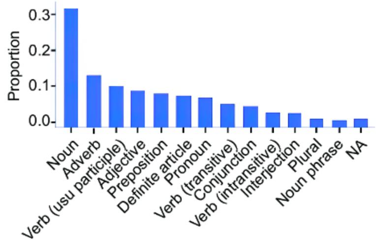
Figure 2.23 Actual distribution of word types in all of Jane Austen’s novels

As modelers, we use canonical distributions to model the population distribution, but the model is not equivalent to the population distribution. This point may seem lik e trivial semantics, but in the era of big data, we of ten can r eason about an entir e population instead of just a random sample. F or example, popular online social networks have hundr eds of millions and sometimes billions of users. That’s a huge size, yet the entir e population is just one database query away .

In causal modeling, being pr ecise in how we think about modeling data and populations is e xtremely useful. Causal infer ences ar e about the r eal-world attributes of the population, rather than just statistical tr ends in the data. And di erent causal questions we want to answer will r equir e us to bak e dierent causal assumptions into our models, some of which ar e str onger or har der to validate than others.

2.3.2 From the observed data to the data generating process

In causal modeling, it is important to understand how the observed data maps back to the joint pr obability distribution of the variables

in the data, and how that joint pr obability distribution maps back to the DGP . Most modelers have some level of intuition about the relationships between these entities, but in causal modeling we must be e xplicit. This e xplicit understanding is important because, while in or dinary statistical modeling you model the joint distribution (or elements of it), in causal modeling you need to model the DGP .

FROM THE OBSERVED DA TA TO THE EMPIRICAL JOINT DISTRIBUTION

Suppose we had the dataset of five data points shown in table 2.1.

	jenny_throws_rock	brian_throws_rock	window_breaks
1	False	True	False
2	True	False	True
3	False	False	False
4	False	False	False
5	True	True	True

Table 2.1 A simple data set with five examples

We can tak e counts of all the observed observable outcomes, as in table 2.2.

Table 2.2 Empirical counts of each possible outcome combination

	jenny_throws_rock	brian_throws_rock	window_breaks counts
1	False	False	False	2
2	True	False	False	0
3	False	True	False	1
4	True	True	False	0
5	False	False	True	0
6	True	False	True	1
7	False	True	True	0
8	True	True	True	1

Dividing by the number of outcomes (5) gives us the empirical joint distribution , shown in table 2.3.

		Table 2.3 The empirical distribution of the data
–	–	————————————————–	–	–

	jenny_throws_rock	brian_throws_rock	window_breaks proportion
1	False	False	False	0.40
2	True	False	False	0.00
3	False	True	False	0.20
4	True	True	False	0.00
5	False	False	True	0.00
6	True	False	True	0.20
7	False	True	True	0.00
8	True	True	True	0.20

So, in the case of discr ete outcomes, we go fr om the data to the empirical distribution using counts.

In the continuous case, we could calculate a histogram or a density curve or some other statistical r epresentation of the empirical distribution. Ther e are dierent statistical choices you can mak e about how you cr eate those summaries, but these ar e representations of the same underlying empirical distribution.

Importantly, the empirical joint distribution is not the actual joint distribution of the variables in the data. F or example, we see that several outcomes in the empirical distribution never appear ed in those five data points. Is the pr obability of their occur rence zer o? More lik ely, the pr obabilities wer e greater than zer o but we didn’t see those outcomes, since only five points wer e sampled.

As an analogy, a fair die has a 1/6 pr obability of r olling a 1. If you roll the die five times, you have a near (1–1/6) 5=40% pr obability of not seeing 1 in any of those r olls. If that happened to you, you wouldn’t want to conclude that the pr obability of seeing a 1 is zer o. If, however, you k ept r olling, the pr oportion of times you saw the 1 would conver ge to 1/6.

NOTE Mor e precisely, our fr equentist interpr etation of probability tells us to interpr et pr obability as the pr oportion of times we get a 1 when we r oll ad in finitum. Despite the ૿ad infinitum, we don’t have to r oll many times befor e the proportion starts conver ging to a number (1/6).

FROM THE EMPIRICAL JOINT DISTRIBUTION TO THE OBSERVATIONAL JOINT DISTRIBUTION

The observational joint probability distribution is the true joint distribution of the variables observed in the data. L et’s suppose table 2.4 shows the true observational joint pr obability distribution of these observed variables.

Table 2.4 Assume this is the true observational joint distribution.

	jenny_throws_rock	brian_throws_rock	window_breaks probability
1	False	False	False	0.25
2	True	False	False	0.15
3	False	True	False	0.15
4	True	True	False	0.05
5	False	False	True	0.00
6	True	False	True	0.10
7	False	True	True	0.10
8	True	True	True	0.20

Sampling fr om the joint observational distribution pr oduces the empirical joint distribution, as illustrated in figure 2.24.

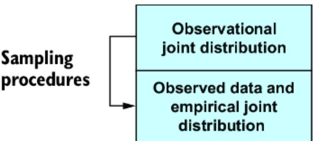
Figure 2.24 Sampling from the observational joint distribution produces the observed data and empirical distribution.

LATENT VARIABLES: FROM THE OBSERVED JOINT DISTRIBUTION TO THE FULL JOINT DISTRIBUTION

In statistical modeling, latent variables are variables that ar e not directly observed in the data but ar e included in the statistical model. Going back to our data e xample, imagine ther e wer e a fourth latent variable, ૿str ength_of_impact, shown in table 2.5.

Table 2.5The values in the strength_of_impact column are unseen ૿latent variables.

	jenny_throws_rock	brian_throws_rock	strength_of_impact	window_breaks
1	False	True	0.6	False
2	True	False	0.6	True
3	False	False	0.0	False
4	False	False	0.0	False
5	True	True	0.8	True

Latent variable models ar e common in disciplines ranging fr om machine lear ning to econometrics to bioinfor matics. F or example, in natural language pr ocessing, an e xample of a popular pr obabilistic latent variable model is topic models , wher e the observed variables represent the pr esence of wor dsand phrases in a document, and the latent variable r epresents the topic of the document (e.g., sports, politics, finance, etc.)

The latent variables ar e omitted fr om the observational joint probability distribution because, as the name implies, they ar e not observed. The joint pr obability distribution of both the observed and the latent variables is the full joint distribution. T o go fr om the full joint distribution to the observational joint distribution, we marginalize over the latent variables, as shown in figure 2.25.

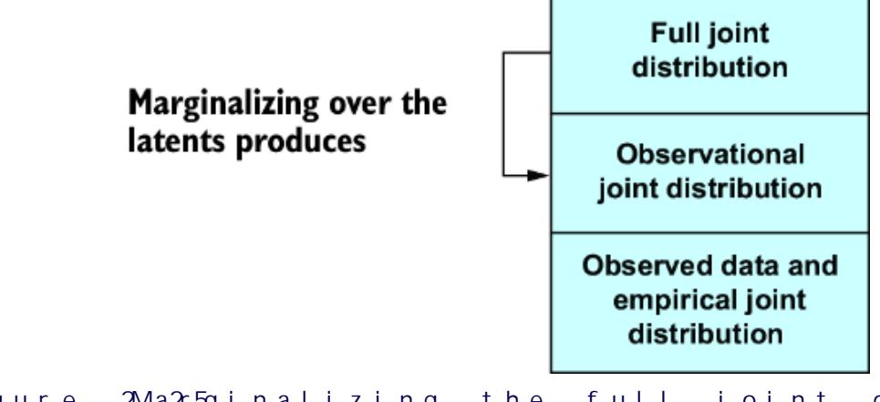
Figure 2.25 Marginalizing the full joint distribution over the latent variables produces the observational joint distribution.

FROM THE FULL JOINT DISTRIBUTION TO THE DA TA GENERATING PROCES S

I wr ote the actual DGP for the five data points using the following Python code.

Listing 2.11 An example of a DGP in code form

def true_dgp(jenny_inclination, brian_inclination, window_strength): #1 jenny_throws_rock = jenny_inclination > 0.5 #2 brian_throws_rock = brian_inclination > 0.5 #2 if jenny_throws_rock and brian_throws_rock: #3 strength_of_impact = 0.8 #3 elif jenny_throws_rock or brian_throws_rock: #4 strength_of_impact = 0.6 #4 else: #5 strength_of_impact = 0.0 #5 window_breaks = window_strength < strength_of_impact #6 return jenny_throws_rock, brian_throws_rock, window_breaks #1 Input variables re flect Jenny and Brian’s inclination to throw and the window’s strength. #2 Jenny and Brian throw the rock if so inclined. #3 If both Jenny and Brian throw the rock, the total strength of the impact is .8. #4 If either Jenny or Brian throws the rock, the total strength of the impact is .6. #5 Otherwise, no one throws and the strength of impact is 0. #6 If the strength of impact is greater than the strength of the window , the window breaks.

Note In general, the DGP is unknown, and our models ar e making guesses about its structur e.

In this e xample , jenny_inclination , brian_inclination , and window_strength are latent variables between 0 and 1. jenny_inclination represents Jenny’s initial desir e to thr ow, brian_inclination represents Brian’s initial desir e to thr ow, and window_strength represents the str ength of the window pane. These are the initial conditions that lead to one instantiation of the observed variables in the data: ( jenny_throws_ball , brian_throws_ball , window_breaks ).

I then called the true_dgp function on the following five sets of latent variables:

initials = [
 (0.6, 0.31, 0.83),
 (0.48, 0.53, 0.33),
 (0.66, 0.63, 0.75),
 (0.65, 0.66, 0.8),
 (0.48, 0.16, 0.27)
]

In other wor ds, the following for loop in Python is the literal sampling pr ocess pr oducing the five data points:

data_points = []
for jenny_inclination, brian_inclination, window_strength in initials: 
 data_points.append(
 true_dgp(
 jenny_inclination, brian_inclination, window_strength
 )
 )

The DGP is the causal pr ocess that generated the data. Note the narrative element that is utterly missing fr om the full joint probability distribution; Jenny and Brian thr ow a r ock at a window if they ar e so inclined, and if they hit the window, the window may break, depending on whether one or both of them thr ew rocks and the str ength of the window . The DGP entails the full joint pr obability distribution, as shown in figure 2.26. In other wor ds, the joint probability distribution is a consequence of the DGP based on how it generates data.

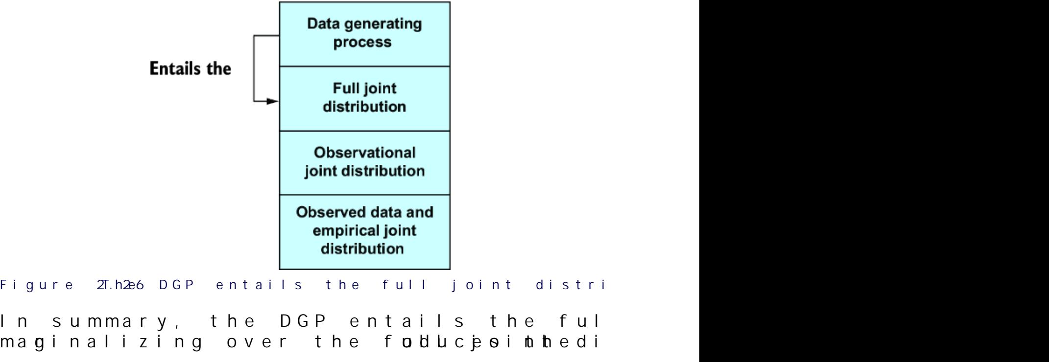
observational joint distribution. Sampling fr om that distribution produces the observed data and the cor responding empirical joint distribution. Ther e is a many -to-one r elationship as we move down this hierar chy that has implications for causal modeling and infer ence.

MANY-TO-ONE RELA TIONSHIPS DOWN THE HIERARCHY

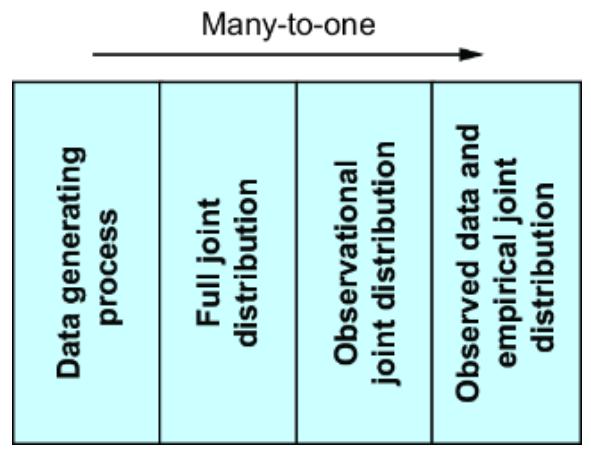
Figure 2.27 There is a many-to-one relationship as we move down the hierarchy . In summary , there are multiple DGP s consistent with the observed data.

As we move down fr om the DGP to full joint to observational joint to empirical joint distribution and observed data, ther e is a many -toone r elationship fr om the pr eceding level to the subsequent level, as illustrated in figure 2.27.

Similarly, an object at one of the levels is consistent with multiple objects at the ne xt level up:

There could be multip le observational joint distributions consistent with thempirical joint distribution . If we sample five points, then sample five more, we’ll get dierent datasets and thus di erent empirical distributions.
There could be multiple full joint distributions consistent with one observat ional joint distribution . The dierence between the two distributions is the latent variables. But what if we have dierent choices for the sets of latent variables? For example, if our observation dstribution is P(X, Y ), the full joint would be P (X, Y, Z, W) if our set of latent variables is {Z, W }, or P(X, Y, Z, V ) if our set of latent variables is { Z, V }.

There could be multiple DGP’s consistent with one full joint probability distribution . Suppose in our window-br eaking example, Jenny had a friend Isabelle who sometimes egged Jenny on to throw the rock and sometimes didnot, a ecting Jenny’s inclin ation to throw. This DGP is dierent from the original, but the relationship between the latent variable of Isabell’s peerpressur e and Jenny’s inclination to throw could be such that this new DGP entailed exactly thesame joint probability distribution. As a more trivial example, suppose we looked at the distribution of a single variable corresponding to the sum of the roll of three dice. The DGP is rolling three dice and then summing themtogether . Two DGPs could dier in terms of the order of summing the dice; e.g., (first + second) + thir d or (first + thir d) + second or (second + thir d) + first. These would all yield the same distribution.

Those last two many -to-one r elationships ar e fundamental to the concept of causal identi fiability , the cor e reason why causal infer ence is har d. This concept is the r eason ૿cor relation does not imply causation, as the saying goes.

2.3.3 Statistical tests for independence

Causality imposes independence and conditional independence on variables, so we r ely on statistical tests for conditional independence to build and validate causal models.

Suppose X and Y are independent, or X and Y are conditionally independent given Z. If we have data observing X, Y, and Z, we can run a statistical test for independence. The canonical statistical independence pr ocedur e returns a test statistic that quanti fies the statistical association between X and Y, and a p- value that quanti fies the pr obability of getting that degr ee of association, or one mor e extreme, by pur echance when X and Y are actually conditionally independent given Z. Put simply, the test quanti fies the statistical evidence of dependence or independence.

Evidence suggesting that someone committed a mur der is not the same as the de finitive truth that they did. Similarly, statistical evidence indicating independence between two variables does not equate to the actual fact of their independence. In both cases, evidence can point towar d a conclusion without de finitively pr oving it. F or example, given that independence is true, the str ength of the statistical evidence can vary on several factors, such as how much data ther e is. And it is always possible to mak e false conclusions from these tests.

Remember that if X and Y are independent, then P(Y |X ) is equivalent to P(Y ). In pr edictive ter ms, that means X has no predictive power on Y. If you can’t use classical statistical tests (e.g., if X and Y are vectors) then you can try training a pr edictive model and subjectively evaluating how well the model pr edicts.

2.3.4 Statistical estimation of model parameters

When we ૿train or ૿ fit a model, we ar e attempting to estimate the values of parameters of the model, such as the weights in a regression model or neural network. Generally, in statistical modeling and machine lear ning, the goal of parameter estimation is modeling the observational or joint pr obability distribution. In causal modeling, the objective is modeling the DGP . The distinction is important for making good causal infer ences.

ESTIMATING B Y MAXIMIZING LIKELIHOOD

In infor mal ter ms and in the conte xt of parameter estimation, likelihood is the pr obability of having observed the data given a candidate value of the parameter vector . Maximizing likelihood means choosing the value of the parameter vector that has the highest lik elihood. Usually, we work with maximizing the log of the likelihood instead of the lik elihood dir ectly because it is mathematically and computationally easier to do so; the value that maximizes lik elihood is the same as the value that maximizes loglikelihood. In special cases, such as linear r egression, the maximum likelihood estimate has a solution we can derive mathematically, but in general, we must find the solution using numerical optimization techniques. In some models, such as neural networks, it is infeasible to find the value that maximizes lik elihood, so we settle for a candidate that has a r elatively high lik elihood.

ESTIMATING B Y MINIMIZING OTHER L OSS FUNCTIONS AND REGULARIZA TION

In machine lear ning, ther e are a variety of loss functions for estimating parameters. Maximizing lik elihood is a special case of minimizing a loss function, namely the negative log-lik elihood loss function.

Regularization is the practice of adding additional elements to the loss function that steer the optimization towar d better parameter values. F or example, L2 r egularization adds a value pr oportional to the sum of the squar e of the parameter values to the loss. Since a small incr ease in value leads to a lar ger incr ease in the squar e of the value, L2 r egularization helps avoid e xceedingly lar ge parameter estimates.

BAYESIAN ESTIMA TION

Bayesian estimation treats parameters as random variables and tries to model the conditional distribution of the parameters (typically called the posterior distribution) given the observed variables in the data. It does so by putting a ૿prior pr obability distribution on the parameters. The prior distribution has its own parameters called ૿hyperparameters that the modeler must specif y. When ther e are latent variables in the model, Bayesian infer ence tar gets the joint distribution of the parameters and the latent variables conditional on the observed variables.

As mentioned befor e, in this book I use Gr eek letters for parameters and Roman letters for variables in the DGP, including latent variables. But for a Bayesian statistician, the distinction is irrelevant; both parameters and latent variables ar e unknown and thus tar gets of infer ence.

One of the main advantages of Bayesian estimation is that rather than getting a point value for the parameters, you get an entir e conditional pr obability distribution of the parameters (mor e speci fically, you get samples fr om or parameter values r epresenting that distribution). That pr obability distribution r epresents uncertainty about the parameter values, and you can incorporate

that uncertainty into pr edictions or other infer ences you mak e fr om the model.

According to Bayesian philosophy, the prior distribution should captur e the modeler’s subjective beliefs about the true value of the parameters. W e’ll do something similar in causal modeling when we turn our beliefs about the causal structur e and mechanisms of the DGP into causal assumptions in the model.

STATISTICAL AND COMPUT ATIONAL A TTRIBUTES OF AN ESTIMATOR

Given that ther e are many ways of estimating a parameter, let’s look for ways to compar e the quality of estimation methods. Suppose the parameter we want to estimate had a gr ound truth value. Statisticians think about how well an estimation method can recover that true value. Speci fically, they car e about the bias and consistency of an estimation method. An estimator is a random variable because it comes fr om data (and data has a distribution), which means an estimator has a distribution. An estimator is unbiased if the mean of that distribution is equal to the true value of the parameter it is estimating. Consistency means that the mor e data you have, the closer the estimate is to the true value of the parameter . In practice, the consistency of the estimator is mor e important than whether it is unbiased.

Computer scientists know that while consistency is nice in theory, getting an estimation method to work with ૿mor e data is easier said than done. They car e about the computational qualities of an estimator in r elation to the amount of data. Does the estimator scale with the data? Is it parallelizable? An estimator may be consistent, but when its running on an iPhone app, will it conver ge to the true value in milliseconds and not eat up the battery’s charge in the pr ocess?

This book decouples understanding causal logic fr om the statistical and computational pr operties of estimators of causal parameters. We will focus on the causal logic and r ely on libraries lik e DoWhy that mak e the statistical and computational calculations easy to do .

GOODNESS-OF-FIT VS. CROS S-VALIDATION

When we estimate parameters, we can calculate various statistics to tell us how well we’ve done. One class of statistics is called goodness-of -fit statistics . Statisticians de fine goodness- of-fit as statistics that quantif y how well the model fits the data used to train the model. Her e’s another de finition: goodness- of-fit statistics tell you how well your model pr etends to be the DGP for the data you used to train your model. However, as we saw, ther e are multiple possible DGP s for a given data set. Goodness- of-fit won’t provide causal infor mation that can distinguish the true DGP .

Cross-validation statistics generally indicate how well your model predicts data it was not trained on. It is possible to have a model with a decent goodness- of-fit relative to other models, but that still predicts poorly . Machine lear ning is usually concer ned with the task of pr ediction and so favors cr oss-validation. However, a model can be a good pr edictor and pr ovide completely bogus causal infer ences.

2.4Determinism andsubjective probability

This section will ventur e into the philosophical underpinnings we’ll need for pr obabilistic causal modeling. In this book, we’ll use probabilistic models to model causal models. When training the model, we might want to use Bayesian parameter estimation procedur es. When doing causal infer ence, we might want to use a probabilistic infer ence algorithm. When we do causal decisionmaking, we might want to use Bayesian decision theory . Further, structural causal models (chapter 6) have a rigid r equir ement on where randomness can occur in the model. That means being clear about the di erences between Bayesianism, uncertainty, randomness, pr obabilistic modeling, and pr obabilistic infer ence is important.

The first k ey point is to view the DGP as deter ministic. The second key point is to view the pr obability in our models of the DGP as subjective.

2.4.1 Determinism

The earlier code for the r ock-thr owing DGP is entir ely deterministic ; given the initial conditions, the output is certain. Consider our definition of physical pr obability again: if I thr ow a die, why is the outcome random?

If I had a super human level of de xterity, per ception, and mental processing power, I could mentally calculate the die r oll’s physics and know the outcome with certainty . This philosophical idea of deter minism essentially says that the DGP is deter ministic. Eighteenth-century F rench scholar P ierre-Simon Laplace e xplained deter minism with a thought e xperiment called Laplace’s demon . Laplace imagined some entity (the demon) that knew every atom’s precise location and momentum in the universe. W ith that knowledge, that entity would know the futur e state of the universe with complete deter ministic certainty because it could calculate them fr om the laws of (Newtonian) mechanics. In other wor ds, given all the causes, the e ect is 100% entir ely deter mined and not at all random.

To be clear, some systems, when we look closely enough, have inher ently stochastic elements (e.g., quantum mechanics, biochemistry, etc.). However, this philosophical view of modeling will apply to most things we’ll car e to model.

2.4.2 Subjective probability

In our physical interpr etation of pr obability, when I r oll a die, probability r epresents my lack of the demon’s super human knowledge of the location and momentum of all the die’s particles as it is r olling. In other wor ds, when I build pr obability models of the DGP, the pr obability r eflects my lack of knowledge. This philosophical idea is called subjective probability or Bayesian probability . The ar gument goes beyond Bayes rule and Bayesian statistical estimation to say that pr obability in the model r epresents the modeler’s lack of complete knowledge about the DGP and does not r epresent inher ent randomness in the DGP .

Subjective pr obability e xpands our ૿ random physical pr ocess interpr etation of pr obability . The physical interpr etation of probability works well for simple physical pr ocesses lik e rolling a die, flipping a coin, or shu ing a deck of car ds. But, of course, we will want to model many phenomena that ar e dicult to think of as repeatable physical pr ocesses. F or example, how the mind tur ns thoughts into speech, or how an incr eased flow of fr esh water into the ocean due to climate change is thr eatening to tip the global system of ocean cur rents. In these cases, we will still model these phenomena using random generation. The pr obabilities used in the random generation r eflect that while we, as modelers, may know some details about the data-generating pr ocess, we’ll never have the super human deter ministic level of detail.

Summary

A random variable is a variable whose possible values are numerical outcomes of a random phenomenon.
A probability distribution function is a function that maps the random variable outcomes to a probability value. A joint probability distribution function maps each combination of X and Y outcomes to a pr obability value.
We derive the chain rule, the law of total probabilit y, and Bayes rule from the fundamental axioms of probability . These are useful rules in modeling.
A Markovian assumption means each variable in an ordering of variables only depends on those that come directly befor e in the order. This is a common simplif ying assumption in statistical modeling, but it plays a lar ge role in causal modeling.
Canonical classes of distributions are mathematically welldescribed representations of distributions. They provide us with primitives thatmake probabilistic modeling flexible and relatively easy .
Canonical distributions are instantiated with a set of parameters, such as location, scale, rate, and shape parameters.
When we build models, knowing what variables are independent or conditionally independent dramatically

simpli fies the model. Incausal modeling, independence and conditionalndependence will be vital in separatin g correlation from causation.

The expected value of a random variable with afinite number of outcomes is the weighted average of all possible outcomes, where the weight is the pr obability of that outcome.
Probability is just a value. We need to give that value an interpr etation. The physical definition of probability maps probability to theproporti on of times an outcome would occur if a physical pr ocess could be run r epeatedly ad in finitum.
In contrast to the physical interpr etation of probability, the Bayesian view of subjective probability interpr ets probability in terms of belief, or conversely, uncertainty .
When coding a randomprocess, Pyro allows you to use canonical distributions as primitives in construct ing nuanced random pr ocess models.
Monte Carlo algorithms use random generation to estimate expectations fr om a distribution of inter est.
Popular infer ence algorithms include graphical model-based algorithms, probability weighting, MCMC, and variational infer ence.
Canonical distributions and random processes can serve as proxies for populations we wih to model and for which we want to make infer ences. Conditional probability is an excellent way to model heter ogeneous subpopulations.
Dierent canonical distributions are used to model dierent phenomena, such as counts, bell curves, and waiting times.
Generating from random processes is a good model of real-life sampling of independent and identically distributed data.
Given a dataset, multiple data generating processes (DGPs) could have potentially generated that datase t. This fact connects to the challenge of parsing causality fr om cor relation.
Statistical independence tests validate independence ad conditional independence claims about the underlying distribution.
There are several methods for learning model parameters, including maximum likelihood estimation and Bayesian

estimation.

Deter minism suggests that if we knew everything about a system, we could predict its outcome with zero eror. Subjective probability is the idea that probability represents the modeler’s lack of that complete knowledge about the system. Adopting these philosophicalerspectives will serve us in understanding causal AI.
A great way to build models is to factorize a joint distribution, simplif y the factors withconditional independence, ad then implement factors as random pr ocesses.
A powerful modeling technique is to useprobability distributions to model populations, particularly when you care about heter ogeneity in those populations.
When we use probability distributions to model populations, we can map generating from random processes to sampling from the population.
While traditio nal statistica l modeling models the observational joint distribution or the full joint distribution, causal modeling models the DGP .

Part 2 Building and validating a causal graph

In part 2, we’ll focus on lear ning how to r epresent causal relationships thr ough causal graphs. W e’ll also lear n how to validate those causal graphs with data, as well as combine them with deep generative models. This part will equip you with the skills to systematically construct causal structur es that r epresent r eal-world data generation pr ocesses and validate those structur es empirically .

3Building a causal graphical model

This chapter covers

Building a causal D AG to model a DGP
Using your causal graph as a communication, computation, and r easoning tool
Building a causal D AG in pgmpy and Pyr o
Training a probabilistic machine learning model using the causal D AGas a sca old

In this chapter, we’ll build our first models of the data generating process (DGP) using the causal directed acyclic graph (causal DAG)—a dir ected graph without cycles, wher e the edges represent causal r elationships. W e’ll also look at how to train a statistical model using the causal D AG as a sca old.

3.1IntroducingthecausalDAG

Let’s assume we can partition the DGP into a set of variables where a given combination of variable values r epresents a possible state of the DGP . Those variables may be discr ete or continuous. They can be univariate, or they can be multivariate vectors or matrices.

A causal D AG is a dir ected graph wher e the nodes ar e this set of variables and the dir ected edges r epresent the causal relationships between them. When we use a causal D AG to represent the DGP, we assume the edges r eflect true causality in the DGP .

To illustrate, r ecall the r ock-thr owing DGP fr om chapter 2. W e started with Jenny and Brian having a certain amount of inclination to thr ow rocks at a window, which has a certain amount of str ength. If either person’s inclination to thr ow surpasses a thr eshold, they thr ow. The window br eaks depending on whether either or both of them thr ow and the str ength of the window .

SETTING UP Y OUR ENVIRONMENT

The code in this chapter was written with pgmpy version 0.1.24, pyr o-pl version 1.8.6, and DoWhy version 0.11.1. Version 0.20.1 of Python’s Graphviz library was used to draw an image of a D AG, and this depends on having the cor e Graphviz sof tware installed. Comment out the Graphviz code if you would pr efer not to set up Graphviz for now .

See the book’s notes at https://www .altdeep.ai/p/causalaibook for links to the Jupyter notebooks with the code.

We’ll now cr eate a causal D AG that will visualize this pr ocess. As a Python function, the DGP is shown in the following listing.

Listing 3.1 DAG rock-throwing example

def true_dgp(jenny_inclination, brian_inclination, window_strength): #1
jenny_throws_rock = jenny_inclination > 0.5 #2
brian_throws_rock = brian_inclination > 0.5 #2
if jenny_throws_rock and brian_throws_rock: #3
strength_of_impact = 0.8 #3
elif jenny_throws_rock or brian_throws_rock: #4
strength_of_impact = 0.6 #4
else: #5
strength_of_impact = 0.0 #5
window_breaks = window_strength < strength_of_impact #6
return jenny_throws_rock, brian_throws_rock, window_breaks

#1 Input variables are numbers between 0 and 1.
#2 Jenny and Brian throw the rock if so inclined.
#3 If both throw the rock, the strength of impact is .8.
#4 If one of them throws, the strength of impact is .6.

#5 If neither throws, the strength of impact is 0. #6 The window breaks if the strength of impact is greater than the window strength.

Figure 3.1 illustrates the r ock-thr owing DGP as a causal D AG.

In figure 3.1, each node cor responds to a random variable in the DGP. The dir ected edges cor respond to cause-e ect r elationships (the sour ce node is the cause and the tar get node is the e ect).

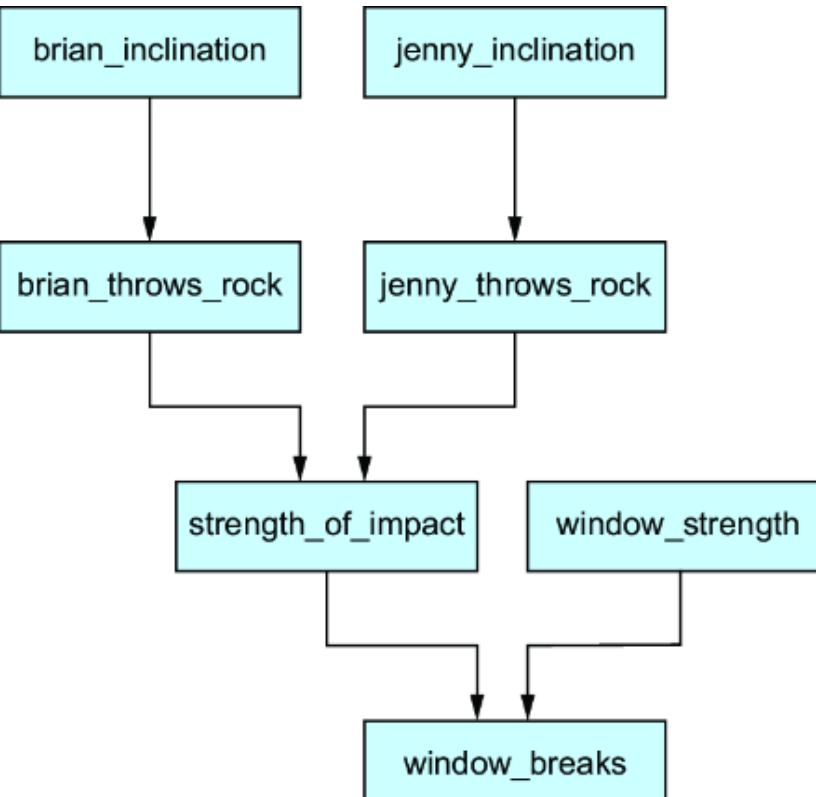
Figure 3.1 A causal DAG representing the rock-throwing DGP . In this example, each node corresponds to a random variable in the DGP .

3.1.1 Case study: A causal model for transportation

In this chapter, we’ll look at a model of people’s choice of transportation on their daily commutes. This e xample will mak e overly str ong assumptions (to the point of being bor derline o ensive) that will help illustrate the cor e ideas of model building. Y ou’ll findlinks to the accompanying code and tutorials at https://www .altdeep.ai/p/causalaibook .

Suppose you wer e an urban planning consultant trying to model the r elationships between people’s demographic backgr ound, the size of the city wher e they live, their job status, and their decision on how to commute to work each day .

You could br eak down the k ey variables in the system as follows:

Age (A) —The age of an individual
Gender (S)—An individual’s reported gender (using ૿S instead of ૿ G, since ૿ G is usually r eserved for D AGs)
Education (E)—The highest level ofeducation or training completed by an individual
Occupation (O) —An individual’s occupation
Residence (R) —The size of the city the individual r esides in
Travel (T) —The means of transport favor ed by the individual

You could then think about the causal r elationships between these variables, using knowledge about the domain. Her e is a possible nar rative:

Educational standar ds are dierent across genera tions. For older people, a high school degree was sucient to achieve a middle-class lifestyle, but younger people need at least a college degree to achieve the same lifestyle. Thus, age (A) is a cause of education ( E ).
Similarly, person’s gender is often afactor in their decision to pursue higher levels of education. So, gender (S) isa cause of education ( E ).
Many white-collar jobs requir e higher education. Many credentialed professions (e.g., doctor, lawyer, o accountant) certainly requir e higher education. So education (E ) is a cause of occupation ( O).
White-collar jobs that depend on higher levels of education tend to cluster in uban areas. Thus, education (E) is a cause of wher e people r eside ( R).
People who are self -employed might work from home and therfore don’t need to commute, while people with employers do. Thus, occupation (O) is a cause of transportation ( T ).
People in big cities might find it more convenient to commute bywalking or using public transportat ion, while

people in small cities andtowns rely on cars to get around. Thus, r esidence ( R ) is a cause of transportation ( T ).

You could have cr eated this nar rative based on your knowledge about the domain, or based on your r esear ch into the domain. Alter natively, you could have consulted with a domain e xpert, such as a social scientist who specializes in this ar ea. F inally, you could r educe this nar rative to the causal D AG shown in figure 3.2.

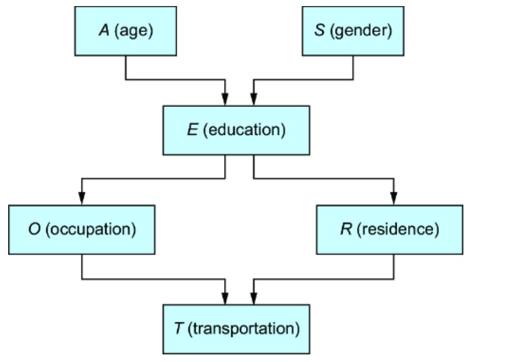
Figure 3.2 A causal DAG representing a model of the causal factors behind how people commute to work

You could build this causal D AG using the following code.

Listing 3.2 Building the transportation DAG in pgmpy from pgmpy.models import BayesianNetwork model = BayesianNetwork( #1 [ (‘A’, ‘E’), #2 (‘S’, ‘E’), #2 (‘E’, ‘O’), #2 (‘E’, ‘R’), #2 (‘O’, ‘T’), #2 (‘R’, ‘T’) #2 ] ) #1 pgmpy provides a Ba yesianNetwork class where we add the edges to the model. #2 Input the ΔAG as a list of edges (tuples). #3 Input the ΔAG as a list of edges (tuples).

The BayesianNetwork object in pgmpy is built on the DiGraph class from NetworkX, the pr eeminent graph modeling library in Python.

CAUSAL ABSTRA CTION AND CA USAL REPRESENT ATION LEARNING

In modeling, the level of abstraction refers to the level of detail and granularity of the variables in the model. In figure 3.2, ther is a mapping between the variables in the data and the variables in the causal D AG, because the level of abstraction in the data generated by the DGP and the level of abstraction of the causal D AG are the same. But it is possible for variables in the data to be at a di erent levels of abstraction. This is particularly common in machine lear ning, wher e we of ten deal with low-level featur es, such as pix els.

When the level of abstraction in the data is lower than the level the modeler wants to work with, the modeler must use domain knowledge to derive the high-level abstractions that will appear as nodes in the D AG. For example, a doctor may be inter ested in a high-level binary variable node lik e ૿Tumor (present/absent), while the data itself contains low-level variables such as a matrix of pix els fr om medical imaging technology .

That doctor must look at each image in the dataset and manually label the high-level tumor variable. Alter natively, a modeler can use analytical means (e.g., math or logic) to map low-level abstractions to high-level ones. F urther, they must do so in a way that pr eserves causal assumptions about the DGP .

This task of cr eating high-level variables fr om lower -level ones in a causally rigor ous way is called causal abstraction . In machine lear ning, the ter m ૿featur e engineering applies to the task of computing useful high-level featur es fr om lower level featur es. Causal abstraction di ers in that r equir ement for causal rigor . You’ll findsome sour ces for causal abstraction infor mation in the book’s notes at https://www .altdeep.ai/p/causalaibook .

Another appr oach to lear ning high-level causal abstractions from lower ones in data is to use deep lear ning—this is called

causal representation learning . We’ll touch brie fly on this topic in chapter 5.

3.1.2 Why use a causal DAG?

The causal D AG is the best-known r epresentation of causality, but to understand its value, it’s useful to think about other ways of modeling causality . One alter native is using a mathematical model, such as a set of or dinary di erential equations or partial dierential equations, as is common in physics and engineering. Another option is to use computational simulators, such as ar e used in meteor ology and climate science.

In contrast to those alter natives, a causal D AG requir es a much less mathematically detailed understanding of the DGP . A causal DAG only r equir es you to specif y what causes what, in the for m of a graph. Graphs ar e easy for humans to think about; they ar e the go -to method for making sense of complicated domains.

Indeed, ther e are several bene fits of using a causal D AG as a representation of the DGP:

DAGs are useful in communicating and visualizing causal assumptions.
We have many tools for computing over D AGs.
Causal D AGs represent time.
DAGs link causality to conditional independence.
DAGs can pr ovide sca olding for pr obabilistic ML models.
The parameters in those probabilistic ML models aremodular parameters, and they encode causal invariance.

Let’s r eview these bene fits one at a time.

3.1.3 DAGs are useful in communicating and visualizing causal assumptions

A causal D AG is a powerful communication device. V isual communication of infor mation involves highlighting important infor mation at the e xpense of other infor mation. As an analogy, consider the two maps of the L ondon Under ground in figure 3.3. The map on the lef t is geographically accurate. The simpler map on the right ignor es the geographic detail and focuses on the position of each station r elative to other stations, which is, arguably, all one needs to find their way ar ound L ondon.

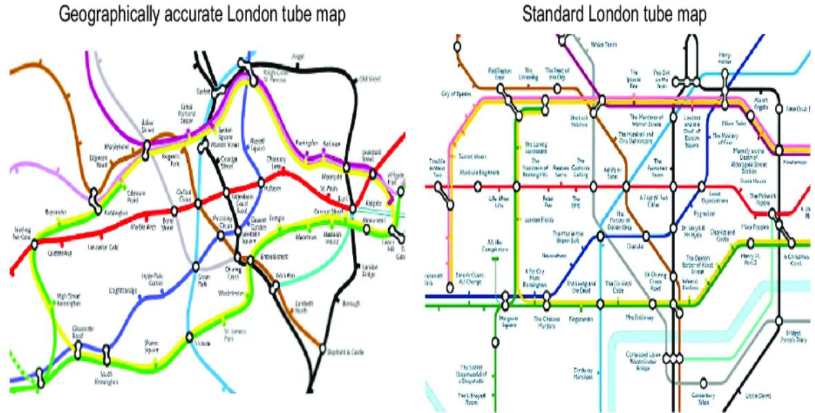
Figure 3.3 Visual communication is a powerful use case for a graphical representation. F or instance, the map of the London Underground on the left is geographically accurate, while the one on the right trades that accuracy for a clear representation of each station’s position relative to the others. The latter is more useful for train riders than the one with geographic accuracy . Similarly , a causal DAG abstracts awa y much detail of the causal mechanism to create a simple representation that is easy to reason about visually .

Similarly, a causal D AG highlights causal r elationships while ignoring other things. F or example, the r ock-thr owing D AG ignor es the if -then conditional logic of how Jenny and Brian’s throws combined to br eak the window . The transportation D AG says nothing about the types of variables we ar e dealing with.

Should we consider age ( A) in ter ms of continuous time, integer years, categories lik e young/middle-aged/elderly, or intervals lik e 18–29, 30–44, 45–64, and >65? What ar e the categories of the transportation variable ( T )? Could the occupation variable ( O ) be a multidimensional tuple lik e {employed, engineer, worksfrom-home}? The D AG also fails to captur e which of these variables ar e observed in the data, and the number of data points in that data.

CAUSAL DAGS DON’T ILL USTRATE MECHANISM

A causal D AG also doesn’t visualize interactions between causes. For example, in older generations, women wer e less lik ely to go to college than men. In younger generations, the r everse is true. While both age ( A) and gender ( S) ar e causes of education ( E ), you can’t look at the D AG and see anything about how age and gender interact to a ect education.

More generally, D AGs can’t convey any infor mation about the causal mechanism or how the causes impact the e ect. They only establish the what of causality, as in what causes what. Consider, for e xample, the various logic gates in figure 3.4. The input binary values for A and B deter mine the output di erently depending on the type of logic gate. But if we r epresent a logic gate as a causal D AG, then all the logic gates have the same causal D AG. We can use the causal D AG as a sca old for causal graphical models that captur e this logic, but we can’t see the logic in the D AG.

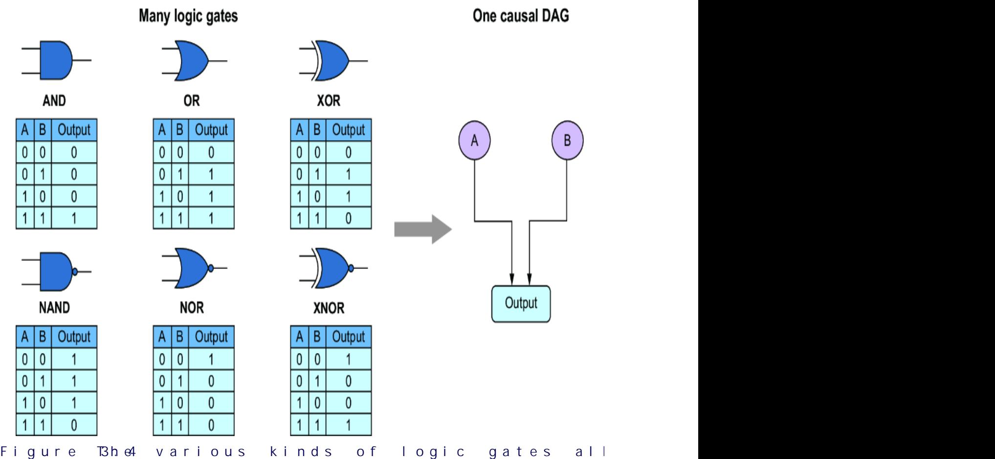
This is a str ength and a weakness. A causal D AG simpli fies matters by communicating what causes what, but not how. However, in some cases (such as logic gates), visualizing the how would be desirable.

CAUSAL DAGS REPRESENT CA USAL AS SUMPTIONS

A causal D AG represents the modeler’s assumptions and beliefs about the DGP, because we don’t have access to that pr ocess most of the time. Thus, a causal D AG allows us to visualize our assumptions and communicate them to others.

Beyond this visualization and communication, the bene fits of a causal D AGare mathematical and computational (I’ll e xplain these in the following subsections). Causal infer ence r esear chers vary in their opinions on the degr ee to which these mathematical and computational pr operties of causal D AGs ar e practically

beneficial. However, most agr ee on the fundamental bene fit of visualization and communication of causal assumptions.

The assumptions encoded in a causal D AG are str ong. L et’s look again at the transportation D AG from figure 3.2, shown again in figure 3.5. Consider the alter natives to that D AG; how many possible D AGs could we draw on this simple six-node system? The answer is 3,781,503, so when we use a causal D AG to communicate our assumptions about this system, we’r e communicating our top choice over 3,781,502 alter natives.

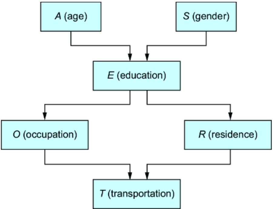
Figure 3.5 A causal DAG model of transportation choices. This DAG encodes strong assumptions about how these variables do and do not relate to one another .

And how about some of those competing D AGs? Some of them seem plausible. P erhaps baby boomers pr efer small-town life while millennials pr efer city life, implying that ther e should be an A → R edge. Prhaps gender nor ms deter mine pr efernces and opportunities in certain pr ofessions and industries, implying an S → O edge. The assumption that age and gender cause occupation and r esidence only indir ectly thr ough education is a powerful assumption that would pr ovide useful infer ences ifit is right .

But what if our causal D AG is wr ong? It seems it is lik ely to be wrong, given its 3,781,502 competitors. In chapter 4, we’ll use data to show us when the causal assumptions in our chosen D AG fail to hold.

3.1.4 We have many tools for computing over DAGs

Directed graphs ar e well-studied objects in math and in computer science, wher e they ar e a fundamental data structur e. Computer scientists have used graph algorithms to solve many practical pr oblems with theor etical guarantees on how long they will tak e to ar rive at solutions. The pr ogramming languages commonly used in data science and machine lear ning have libraries that implement these algorithms, such as NetworkX in Python. These popular libraries mak e it easier to write code that works with causal D AGs.

We can bring all that theory and tooling to bear on a causal modeling pr oblem when we r epresent a causal model in the for m of a causal D AG. For example, in pgmpy we can train a causal DAG on data to get a dir ected causal graphical model. Given that model, we can apply algorithms for graph-based pr obabilistic infer ence, such as belief propagation , to estimate conditional probabilities de fined on variables in the graph. The dir ected graph structur e enables these algorithms to work in typical settings without our needing to con figure them to a speci fic problem or task.

In the ne xt chapter, I’ll intr oduce the concept of d-separation , which is a graphical abstraction for conditional independence and the fundamental idea behind the do -calculus theory for causal infer ence. D-separation is all about finding paths between nodes in the dir ected graph, which is something any worthwhile graph library mak es easy by default. Indeed, conditional independence is the k ey idea behind the thir d bene fit of the causal D AG.

3.1.5 Causal DAGs can represent time

The causal D AG has an implicit r epresentation of time. In mor e technical ter ms, the causal D AG provides a partial temporal ordering because causes pr ecede e ects in time.

For example, consider the graph in figure 3.6. This graph describes a DGP wher e a change in cloud cover (Cloudy) causes both a change in the state of a weather -activated sprinkler (Sprinkler) and the state of rain (R ain), and these both cause a change in the state of the wetness of the grass (W et Grass). W e know that a change in the state of the weather causes rain and sprinkler activation, and that these both cause a change in the state of the wetness of the grass. However, it is only a partial temporal or dering, because the graph doesn’t tell us which happens first: the sprinkler activation or the rain.

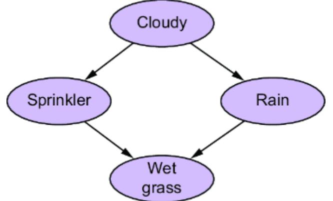
Figure 3.6 A causal DAG representing the state of some grass (wet or dry). The DAG gives us a partial temporal ordering over its nodes because causes precede e ects in time.

The partial or dering in figure 3.6 may seem trivial, but consider the D AG in figure 3.7. V isualization libraries can use the partial ordering in the hairball-lik e DAG on the lef t of figure 3.7 to cr eate the much mor ereadable for m on the right.

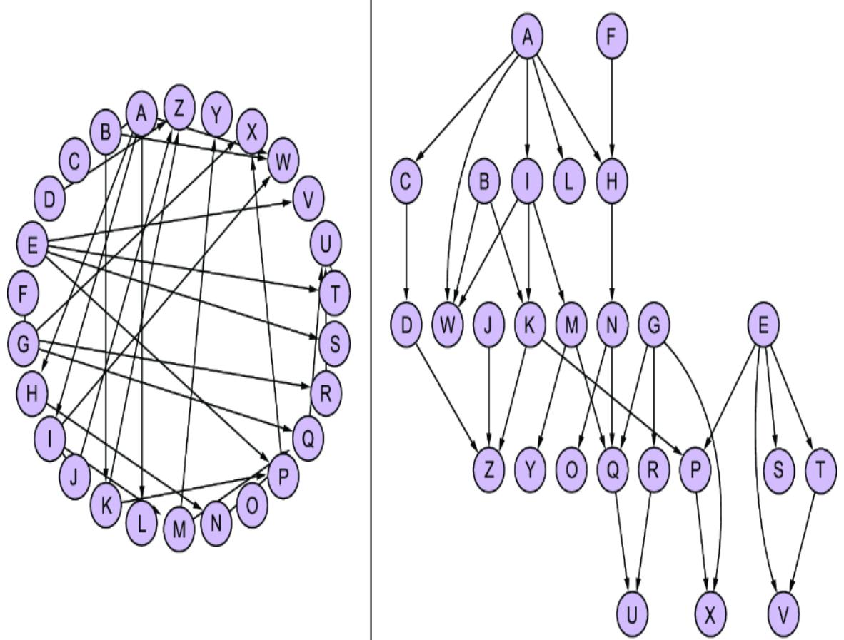
Figure 3.7 A visualization library can use the DAG’s partial ordering to unravel the hairball-lik e DAG on the left into the more readable form on the right.

Sometimes we need a causal D AG to be morexplicit about time. F or example, we may be modeling causality in a dynamic setting, such as in the models used in r einfor cement lear ning. In this case, we can mak e time e xplicit by de fining and labeling the variables of the model, as in figure 3.8. W e can r epresent continuous time with interval variables lik e ૿. Chapter 12 will provide some concr ete e xamples.

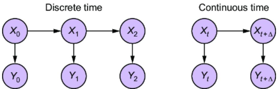
Figure 3.8 If we need a causal DAG to be explicit about time, we can mak e time explicit in the de finition of the variables and labeling of their nodes. W e can represent continuous time with interval variables lik e ૿.

The causal D AG doesn’t allow for any cycles. In some causal systems, r elaxing the acyclicity constraint mak es sense, such as with systems that have feedback loops, and some advanced causal models allow for cycles. But sticking to the simpler acyclic assumption allows us to leverage the bene fits of the causal D AG.

If you have cycles, sometimes you can unroll the cycle over time and mak e the time e xplicit to get acyclicity . A graph X ⇄ Y can unroll as X0 Y0→X1 Y1 . . . . F or example, you may have a cycle between supply, price, and demand, but per haps you could rewrite this as price at time 0 a ects supply and demand at time 1, which then a ects price at time 2, etc.

3.1.6 DAGs link causality to conditional independence

Another bene fit of a causal D AG is that it allows us to use causality to r eason about conditional independence. Humans have an innate ability to r eason in ter msof causality—that’s how we get the first and second bene fits of causal D AGs. But reasoning pr obabilistically doesn’t come nearly as easily . As a result, the ability to use causality to r eason about conditional independence (a concept fr om probability) is a considerable featur e of D AGs.

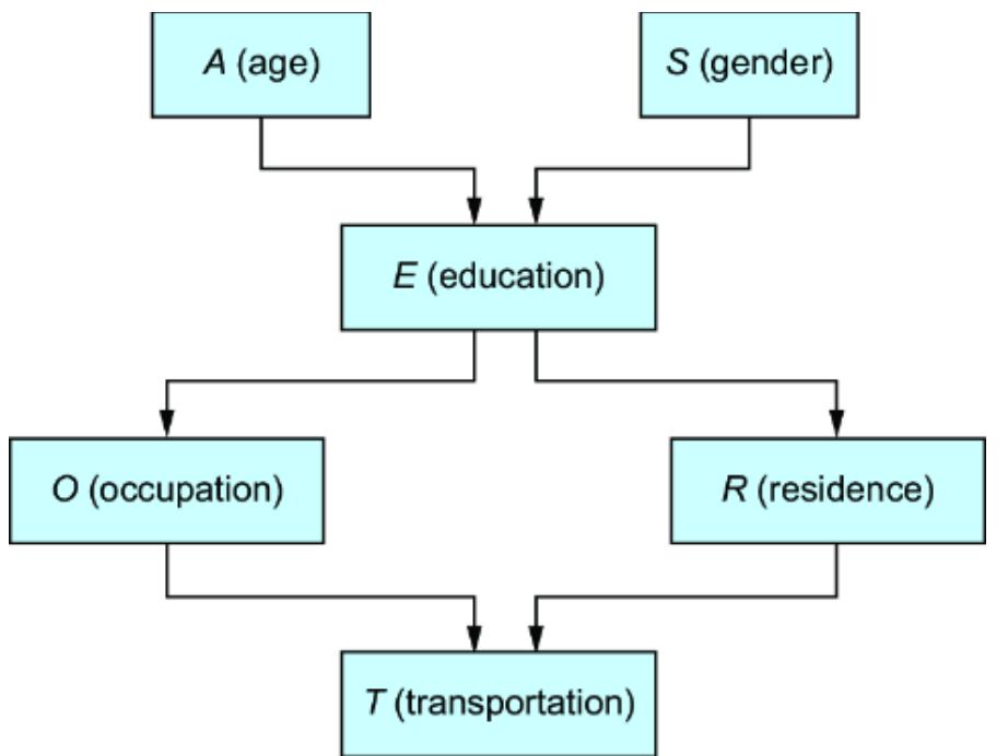
Figure 3.9 The causal relationships in the transportation DAG encode k ey assumptions about conditional independence.

Consider the transportation D AG, displayed again in figure 3.9.

The six variables in the D AG have a joint distribution P (A,S,E,O,R,T ). R ecall the chain rule fr om chapter 2, which says that we can factorize any joint pr obability into a chain of conditional pr obability factors. F or example,

\[\begin{aligned} P\left(a,s,e,e,r,t\right) &= P\left(e\right)P\left(s\middle|e\right)P\left(t\middle|s,e\right)P\left(a\middle|t,s,e\right)P\left(o\middle|a,t,s,e\right)P\left(r\middle|o,t,s,e\right) \\ &= P\left(t\right)P\left(o\middle|t\right)P\left(r\middle|o,t\right)P\left(e\middle|r,o,t\right)P\left(a\middle|e,r,o,t\right)P\left(s\middle|a,e,r,o,t\right) \\ &\dots \end{aligned}\]

The chaining works for any or dering of the variables. But instead of choosing any or dering, we’ll choose the (partial) or dering of the causal D AG, since that or dering aligns with our assumptions of the causal flow of the variables in the DGP . Looking at figure 3.9, the or dering of variables is {( A, S ), E, (O, R ), T }. The pairs (A, S ) and ( O, R ) ar e unor dered. If we arbitrarily pick an ordering, letting A come befor e S and O come befor e R, we get this:

Next, we’ll use the causal D AG to further simplif y this factorization. Each factor is a conditional pr obability, so we’ll simplif y those factors by conditioning each node on only its parents in the D AG. In other wor ds, for each variable, we’ll look at that variable’s dir ect par ents in the graph, then we’ll dr op everything on the right side of the conditioning bar (|) that isn’t one of those dir ect par ents. If we condition only on par ents, we get the following simpli fication:

What is going on her e? Why should the causal D AG magically mean we can say P(s|a) is equal to P(s) and P(r|o,e,s,a ) simpli fies to P(r|e)?As discussed in chapter 2, stating that P (s|a)=P(s) and P(t|o,r,e,s,a )=P(t|o,r) is equivalent to saying that S and A are independent, and T is conditionally independent of E, S, and A, given O and R. In other wor ds, the causal D AG gives us a way to impose conditional independence constraints over the joint pr obability distribution of the variables in the DGP .

Why should we car e about things being conditionally independent? Conditional independence mak es life as a modeler easier . For example, suppose you wer e to model the transportation variable T with a pr edictive model. The pr edictive model implied by P(t|o,r,e,s,a ) requir es having featur es O, R, E, S, and A, while the pr edictive model implied by P(t|o,r) just requir es featur es O and R to pr edict T. The latter model will have fewer parameters to lear n, have mordegr ees of fr eedom, tak e less space in memory, train faster, etc.

But why does a causal D AG give us the right to impose conditional independence? L et’s build some intuition about the connection between causality and conditional independence. Consider the e xample of using genetic data fr om family members to draw conclusions about an individual. F or example,

the Golden State Killer was a Califor nia-based serial killer captur ed using genetic genealogy . Investigators used DNA lef t by the killer at crime scenes to identif y genetic r elatives in public databases. They then triangulated fr om those r elatives to find the killer .

Suppose you had a close r elative and a distant r elative on the same line of ancestry . Could the distant r elative pr ovide any additional genetic infor mation about you once we had alr eady accounted for that close r elative? L et’s simplif y a bit by focusing just on blood type. Suppose the close r elative was your father, and the distant r elative was your pater nal grandfather, as in figure 3.10. Indeed, your grandfather’s blood type is a cause of yours. If we saw a lar ge dataset of grandfather/grandchild blood type pairs, we’d see a cor relation. However, your father’s blood type is a mor e dir ect cause, and the connection between your grandfather’s blood type and yours passes thr ough your father . So, if our goal wer e to pr edict your blood type, and we alr eady had your father’s blood type as a pr edictor, your pater nal grandfather’s blood type could pr ovide no additional pr edictive infor mation. Thus, your blood type and your pater nal grandfather’s blood type ar e conditionally independent, given your father’s blood type.

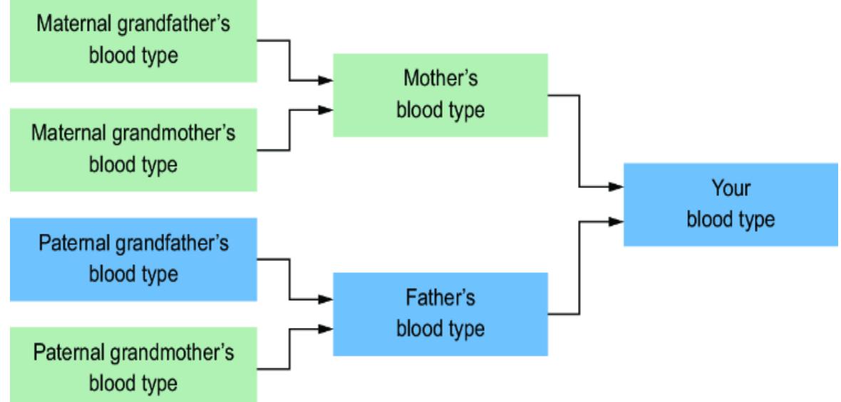
Figure 3.10 Causality implies conditional independence. Y our paternal grandfather ’s blood type is a cause of your father ’s, which is a cause of yours. Y ou and your paternal grandfather ’s blood types are conditionally independent given your father ’s blood type because your father ’s blood type already contains all the information your grandfather ’s type could provide about yours.

The way causality mak es cor related variables conditionally independent is called the causal Markov property . In graphical terms, the causal Mark ov pr operty means that variables ar e conditionally independent of their non-descendants (e.g., ancestors, uncles/aunts, cousins, etc.) given their par ents in the graph.

This ૿ non-descendants de finition of the causal Mark ov pr operty is sometimes called the local Markov property . An equivalent articulation is called the Markov factorization property , which is the pr oerty that if your causal D AG is true, you can factorize a joint pr obability into conditional pr obabilities of variables, given their par ents in the causal D AG:

\[P\left(a,s,e,o,r,t\right) \ = P\left(a\right)P(s)P\left(e|s,a\right)P\left(o|e\right)P\left(r|e\right)P\left(t|o,r\right)\]

If our transportation D AG is a true r epresentation of the DGP, then the local Mark ov pr operty should hold. In the ne xt chapter, we’ll see how to test this assumption with data. 3.1.7 DAGs can provide sca olding for probabilistic ML models

Many modeling appr oaches in pr obabilistic machine lear ning use a DAG as the model structur e. Examples include dir ected graphical models (ak a Bayesian networks) and latent variable models (e.g., topic models). Deep generative models, such as variational autoencoders, of ten have an underlying dir ected graph.

The advantage of building a pr obabilistic machine lear ning model on top of a causal graph is, rather obviously, that you have a pr obabilistic causal machine lear ning model. Y ou can train it on data, and you can use it for pr ediction and other infer ences, like any pr obabilistic machine lear ning model. Mor eover, because it is built on top of a causal D AG, it is a causal model, so you can use it to mak e causal infer ences.

A bene fit that follows fr om providing sca olding is that the parameters in those models are modular and encode causal invariance . Befor e exploring this bene fit, let’s first build a graphical model on the transportation D AG.

Building a probabilistic machine learning model on a causal DAG

Recall our factorization of the joint pr obability distribution of the transportation variables over the or dering of the variables in the transportation D AG.

We have a set of factors, { P(a), P(s), P(e|s,a), P(o|e), P(r |e), P(t |o,r)}. From her e on, we’ll build on the ter m ૿Mark ov kernel from chapter 2 and call these factors causal Markov kernels .

We’ll build our pr obabilistic machine lear ning model by implementing these causal Mark ov kernels in code and then composing them into one model. Our implementations for each kernel will be able to r eturn a pr obability value, given input

arguments. F or example, P(a) will tak e an outcome value for A and r eturn a pr obability value for that outcome. Similarly, P (t|o,r) will tak e in values for T, O, and R and r eturn a pr obability value for T =t, wher e t is the queried value. Our implementations will also be able to generate fr om the causal Markov kernels. T o do this, these implementations will r equir e parameters that map the inputs to the outputs. W e’ll use standar d statistical lear ning appr oaches to fit those parameters from the data.

3.1.8 Training a model on the causal DAG

Consider the DGP for the transportation D AG. What sort of data would this pr ocess generate?

Suppose we administer ed a survey covering 500 individuals, getting values for each of the variables in this D AG. The data encodes the variables in our D AG as follows:

Age (A)—Recorded as young (૿young) for individuals up to and including 29 years , adult (૿adult) for individuals between 30 and 60 years old (inclusive), and old (૿old) for people 61 and over
Gender (S)—The self -reported gender of an individual, recorded as male (૿M), female (૿ F), or other (૿ O)
Education (E)—The highest level ofeducation or training completed by the individual, recorded either high school (૿high) or university degr ee (૿uni)
Occupation (O)—Employee (૿emp) ora self -employed worker (૿self)
Residence (R)—The population size of the city the individual lives in, r ecorded as small (૿small) or big (૿big)
Travel (T)—The means of transport favor ed by the individual, recorded as car (૿car ), train (૿train ), or other (૿ other )

LABELING CA USAL ABSTRA CTIONS

How we conceptualize the variables of a model matters gr eatly in machine lear ning. F or example, ImageNet, a database of 14 million images, contains anachr onistic and o ensive labels for racial categories. Even if r enamed to be less o ensive, race categories themselves ar e fluid acr oss time and cultur e. What are the ૿cor rect labels to use in a pr edictive algorithm?

How we de fine our variables isn’t just a question of politics and census for ms. A simple thought e xperiment by philosopher Nelson Goodman shows how a simple change in label can change a pr ediction to a contradictory pr ediction. Suppose you regularly sear ch for gems and r ecord the color of every gem you find. It tur ns out 100% of the gems in your dataset ar e green. Now let’s de fine a new label ૿grue to mean ૿gr een if observed befor e now, blue otherwise. So 100% of your data is ૿green or ૿grue, depending on your choice of label. Now suppose you pr edict the futur e based on e xtrapolating fr om the past. Then you can pr edict the ne xt emrald will be gr een based on data wher e all past emeralds wer e green, or you can predict the ne xt emrald will be ૿grue (i.e., blue) based on the data that all past emeralds wer e ૿grue. Obviously, you would never invent such an absur d label, but this thought experiment is enough to show that the infer ence depends on the abstraction.

In data science and machine lear ning, we’r e often encouraged to blindly model data and not to think about the DGP . We’re encouraged to tak e the variable names for granted as columns in a spr eadsheet or attributes in a database table. When possible, it is better to choose abstractions that ar e appropriate to the infer ence pr oblem and collect or encode data accor ding to that abstraction. When it is not possible, keep in mind that the r esults of your analysis will depend on how other people have de fined the variables.

In chapter 7, I’ll intr oduce the idea of ૿ no causation without manipulation —an idea that pr ovides a useful heuristic for how to de fine causal variables.

The variables in the transportation data ar e all categorical variables. In this simple categorical case, we can r ely on a graphical modeling library lik e pgmpy .

Listing 3.3 Loading transportation data

import pandas as pd
url='https://raw.githubusercontent.com/altdeep/causalML/master/datasets
/transportation_survey.csv' #1
data = pd.read_csv(url)
data

#1 We’ll load the data into a pandas ΔataF rame with the read_csv method.

This pr oduces the DataF rame in figure 3.11.

	A	S		O	R	T
O	adult				F high emp small train
1	young	M	high	emp	big	car
2	adult		M unı	emp	big	other
3	old		F unı	emp	big	car
ব	young F uni			emp	big	car

495	young		M high		emp big	other
496	adult	M	high	emp	big	car
497	young M high emp small					train
	498 young M high emp small					car
499					adult M high emp small other

Figure 3.11 An example of data from the DGP underlying the transportation model. In this case, the data is 500 survey responses.

The BayesianNetwork class we initialized in listing 3.2 has a fit method that will lear n the parameters of our causal Mark ov kernels. Since our variables ar e categorical, our causal Mark ov kernels will be in the for m of conditional pr obability tables represented by pgmpy’s TabularCPD class. The fit method will fit (૿lear n) estimates of the parameters of those conditional probability tables using the data.

Listing 3.4 Learning parameters for the causal Mark ov kernels

from pgmpy.models import BayesianNetwork model = BayesianNetwork( [ (‘A’, ‘E’), (‘S’, ‘E’), (‘E’, ‘O’), (‘E’, ‘R’), (‘O’, ‘T’), (‘R’, ‘T’) ] ) model.fit(data) #1 causal_markov_kernels = model.get_cpds() #2 print(causal_markov_kernels) #2

#1 The fit method on the Ba yesianNetwork object will estimate parameters from data (a pandas ΔataF rame). #2 Retrieve and view the causal Mark ov kernels learned by fit.

This r eturns the following output:

[<TabularCPD representing P(A:3) at 0x7fb030dd1050>, <TabularCPD representing P(E:2 | A:3, S:2) at 0x7fb0318121d0>, <TabularCPD representing P(S:2) at 0x7fb03189fe90>, <TabularCPD representing P(O:2 | E:2) at 0x7fb030de85d0>, <TabularCPD representing P(R:2 | E:2) at 0x7fb030dfa890>, <TabularCPD representing P(T:3 | O:2, R:2) at 0x7fb0316c9110>]

Let’s look at the structur e of the causal Mark ov kernel for the transportation variable T. We can see fr om printing out the causal_markov_kernels list that Tis he last item in the list.

cmk_T = causal_markov_kernels[-1] print(cmk_T)

We get the following output:

+———-+———+———-+———+———-+ | O | O(emp) | O(emp) | O(self) | O(self) | +———-+———+———-+———+———-+ | R | R(big) | R(small) | R(big) | R(small) | +———-+———+———-+———+———-+ | T(car) | 0.70343 | 0.52439 | 0.44444 | 1.0 | +———-+———+———-+———+——— + | T(other) | 0.13480 | 0.08536 | 0.33333 | 0.0 | +———-+———+———-+———+———-+ | T(train) | 0.16176 | 0.39024 | 0.22222 | 0.0 | +———-+———+———-+———+———-+

Note that in this printout, I truncated the numbers so the table fits on the page.

cmk_T is the implementation of the causal Mark ov kernel P(T|O,R) as a conditional pr obability table, a type of look up table wher e, given the values of T, O, and R, we get the cor responding probability mass value. F or example, P(T =car|O =emp, R= big) = 0.7034. Note that these ar e conditional pr obabilities. F or each combination of values for O and R, ther e are conditional probabilities for the thr ee outcomes of T that sum to 1. F or example, when O =emp and R =big, P(T =car| O =emp, R = big) + ( P(T =other| O =emp, R =big) + P(T =train| O =emp, R =big) = 1.

The causal Mark ov kernel in the case of nodes with no par ents is just a simple pr obability table. F or example, print(causal_markov_kernels[2]) prints the causal Mark ov kernel for gender ( S), the thir d item in the causal_markov_kernels list.

+——+——-+ | S(F) | 0.517 | +——+——-+ | S(M) | 0.473 | +——+——-+ | S(O) | 0.010 | +——+——-+

The fit method lear ns parameters by calculating the pr oportions of each class in the data. Alter natively, we could use other techniques for parameter lear ning.

3.1.9 Dierent techniques for parameter learning

There are several ways we could go about training these parameters. Lt’slook at a few common ways of training parameters in conditional pr obability tables.

MAXIMUM LIKELIHOOD ESTIMA TION

The lear ning algorithm I used in the fit method on the BayesianNetwork model object was maximum likelihood estimation (discussed in chapter 2). It is the default parameter lear ning method, so I didn’t specif y ૿maximum lik elihood in the call to fit. Generally, maximum lik elihood estimation seeks the parameter that maximizes the lik elihood of seeing the data we use to train the model. In the conte xt of categorical data, maximum lik elihood estimation is equivalent to taking proportions of counts in the data. F or example, the parameter for P(O=emp|E=high) is calculated as:

BAYESIAN ESTIMA TION

In chapter 2, I also intr oduced Bayesian estimation. It is generally mathematically intractable and r elies on computationally e xpensive algorithms (e.g., sampling algorithms and variational infer ence). A k ey exception is the case of conjugate priors , wher e the prior distribution and the tar get (posterior) distribution have the same canonical for m. That means the code implementation can just calculate the parameter values of the tar get distribution with simple math, without the need for complicated Bayesian infer ence algorithms.

For example, pgmpy implements a Dirichlet conjugate prior for categorical outcomes. F or each value of O in P(O|E =high), we have a pr obability value, and we want to infer these pr obability values fr om the data. A Bayesian appr oach assigns a prior

distribution to these values. A good choice for a prior on a set of probability values is the Dirichlet distribution , because it is defined for a simplex , a set of numbers between zer o and one that sum to one. F urther it is conjugate to categorical distributions lik e P(O|E =high), meaning the posterior distribution on the parameter values is also a Dirichlet distribution. That means we can calculate point estimates of the probability values using simple math, combining counts in the data and parameters in the prior . pgmpy does this math for us.

Listing 3.5 Bayesian point estimation with a Dirichlet conjugate prior

from pgmpy.estimators import BayesianEstimator #1 model.fit( data, estimator=BayesianEstimator, #2 prior_type=“dirichlet”, pseudo_counts=1 #3 ) causal_markov_kernels = model.get_cpds() #4 cmk_T = causal_markov_kernels[-1] #4 print(cmk_T) #4 #1 Import Ba yesianEstimator and initialize it on the model and data. #2 Pass the estimator object to the fit method. #3 pseudo_counts refers to the parameters of the Δirichlet prior . #4 Extract the causal Mark ov kernels and view P(T|O ,R). The pr eceding code prints the following output: +———-+——————–+—–+——————–+———-+ | O | O(emp) | … | O(self) | O(self) | +———-+——————–+—–+——————–+———-+ | R | R(big) | … | R(big) | R(small) | +———-+——————–+—–+——————–+———-+ | T(car) | 0.7007299270072993 | … | 0.4166666666666667 | 0.5 | +———-+——————–+—–+——————–+———-+ | T(other) | 0.1362530413625304 | … | 0.3333333333333333 | 0.25 | +———-+——————–+—–+——————–+———-+ | T(train) | 0.1630170316301703 | … | 0.25 | 0.25 | +———-+——————–+—–+——————–+———-+

In contrast to maximum lik elihood estimation, Bayesian estimation of a categorical parameter with a Dirichlet prior acts like a smoothing mechanism. F or example, the maximum likelihood parameter estimate says 100% of self -employed people in small towns tak e a car to work. This is pr obably extreme. Certainly, some self -employed people bik e to work—we just didn’t manage to survey any of them. Some small cities,

such as Crystal City in the US state of V irginia (population 22,000), have subway stations. I’d wager at least a few of the entrepreneurs in those cities use the train.

CAUSAL MODELERS AND BA YESIANS

The Bayesian philosophy goes beyond mer e parameter estimation. Indeed, Bayesian philosophy has much in common with D AG-based causal modeling. Bayesians try to encode subjective beliefs, uncertainty, and prior knowledge into ૿prior probability distributions on variables in the model. Causal modelers try to encode subjective beliefs and prior knowledge about the DGP into the for m of a causal D AG. The two appr oaches ar e compatible. Given a causal D AG, you can be Bayesian about infer ring the parameters of the pr obabilistic model you build on top of the causal D AG. You can even be Bayesian about the D AG itself and compute pr obability distributions over possible D AGs!

I focus on causality in this book and k eep Bayesian discussions to a minimum. But we’ll use the libraries Pyr o (and its NumPy - JAX alter native NumPyr o) to implement causal models; these libraries pr ovide complete support for Bayesian infer ence on models as well as parameters. In chapter 11, we’ll look at an example of Bayesian infer ence of a causal e ect using a causal graphical model we build fr om scratch.

OTHER TECHNIQUES FOR P ARAMETER ESTIMA TION

We need not use a conditional pr obability table to r epresent the causal Mark ov kernels. Ther e are models within the generalized linear modeling framework for modeling categorical outcomes. For some of the variables in the transportation model, we might have used non-categorical outcomes. Age, for e xample, might have been rcorded as an integer outcome in the survey . For variables with numeric outcomes, we might use other modeling

approaches. Y ou can also use neural network ar chitectur es to model individual causal Mark ov kernels.

Parametric assumptions refer to how we specif y the outcomes of a node in the D AG (e.g., category or r eal number) and how we map par ents to the outcome (e.g., table or neural network). Note that the causal assumptions encoded by the causal D AG are decoupled fr om the parametric assumptions for a causal Mark ov kernel. F or example, when we assumed that age was a dir ect cause of education level and encoded that into our D AG as an edge, we didn’t have to decide if we wer e going to tr eat age as an or dered set of classes, as an integer, or as seconds elapsed since birth, etc. F urther more, we didn’t have to know whether to use a conditional categorical distribution or a r egression model. That step comes af ter we specif y the causal D AG and want to implement P(E|A, S ).

Similarly, when we mak e predictions and pr obabilistic infer ences on a trained causal model, the considerations of what infer ence or pr ediction algorithms to use, while important, ar e separate from our causal questions. This separation simpli fies our work. Often we can build our knowledge and skill set in causal modeling and r easoning independently of our knowledge of statistics, computational Bayes, and applied machine lear ning.

3.1.10 Learning parameters when there are latent variables

Since we ar e modeling the DGP and not the data, it is lik ely that some nodes in the causal D AG will not be observed in the data. Fortunately, pr obabilistic machine lear ning pr ovides us with tools for lear ning the parameters of causal Mark ov kernels of latent variables.

LEARNING LA TENT VARIABLES WITH PGMPY

To illustrate, suppose the education variable in the transportation survey data was not r ecorded. pgmpy gives us a utility for

learning the parameters of the causal Mark ov kernel for latent E using an algorithm called structural expectation maximization , which is a variant of parameter lear ning with maximum likelihood.

Listing 3.6 Training a causal graphical model with a latent variable

import pandas as pd from pgmpy.models import BayesianNetwork from pgmpy.estimators import ExpectationMaximization as EM url=‘https://raw.githubusercontent.com/altdeep/causalML/master/datasets /transportation_survey.csv’ #1 data = pd.read_csv(url) #1 data_sans_E = data[[‘A’, ‘S’, ‘O’, ‘R’, ‘T’]] #2 model_with_latent = BayesianNetwork( [ (‘A’, ‘E’), (‘S’, ‘E’), (‘E’, ‘O’), (‘E’, ‘R’), (‘O’, ‘T’), (‘R’, ‘T’) ], latents={“E”} #3 ) estimator = EM(model_with_latent, data_sans_E) #4 cmks_with_latent = estimator.get_parameters(latent_card={‘E’: 2}) #4 print(cmks_with_latent[1].to_factor()) #5 #1 Δownload the data and convert to a pandas ΔataF rame. #2 Keep all the columns except education (E). #3 Indicate which variables are latent when training the model.

#4 Run the structural expectation maximization algorithm to learn the causal Mark ov kernel for E. Y ou have to indicate the cardinality of the latent variable.

#5 Print out the learned causal Mark ov kernel for E. Print it as a factor object for legibility .

The print line prints a factor object.

A	S	+——+———-+——+————–+ phi(E,A,S)
E(0) A(adult) S(F)		+======+==========+======+==============+ 0.1059
E(0) A(adult) S(M)		+——+———-+——+————–+ 0.1124 +——+———-+——+————–+
E(0) A(old)	S(F)	0.4033 +——+———-+——+————–+
E(0) A(old)	S(M)	0.2386 +——+———-+——+————–+
E(0) A(young) S(F)		0.4533 +——+———-+——+————–+
E(0) A(young) S(M)		0.6080 +——+———-+——+————–+
E(1) A(adult) S(F)		0.8941 +——+———-+——+————–+
E(1) A(adult) S(M)		0.8876 +——+———-+——+————–+
E(1) A(old)	S(F)	0.5967 +——+———-+——+————–+
E(1) A(old)	S(M)	0.7614 +——+———-+——+————–+
E(1) A(young) S(F)		0.5467 +——+———-+——+————–+
E(1) A(young) S(M)		0.3920 +——+———-+——+————–+

The outcomes for E are 0 and 1 because the algorithm doesn’t know the outcome names. P erhaps 0 is ૿high (high school) and 1 is ૿uni (university), but cor rectly mapping the default outcomes fr oma latent variable estimation method to the names of those outcomes would r equir e further assumptions.

There are other algorithms for lear ning parameters when ther e are latent variables, including some that use special parametric assumptions (i.e., functional assumptions about how the latent variables r elate to the observed variables).

LATENT VARIABLES AND IDENTIFICA TION

In statistical infer ence, we say a parameter is ૿identi fied when it is theor etically possible to lear n its true value given an in finite number of e xamples in the data. It is ૿unidenti fied if mor edata doesn’t get you closer to lear ning its true value. Unfortunately, your data may not be su cient to lear n the causal Mark ov kernels of the latent variables in your causal D AG. If we did not care about r epresenting causality, we could r estrict ourselves to a latent variable graphical model with latent variables that ar e identi fiable fr om data. But we must build a causal D AG that

represents the DGP, even if we can’t identif y the latent variables and parameters given the data.

That said, even if you have non-identi fiable parameters in your causal model, you still may be able to identif y the quantity that answers your causal question. Indeed, much of causal infer ence methodology is focused on r obust estimation of causal e ects (how much a cause a ects an e ect) despite having latent ૿confounders. W e’ll cover this in detail in chapter 11. On the other hand, even if your parameters ar e identi fied, the quantity that answers your causal question may not be identi fied. W e’ll cover causal identi fication in detail in chapter 10.

3.1.11 Inference with a trained causal probabilistic machine learning model

A probabilistic machine lear ning model of a set of variables can use computational infer ence algorithms to infer the conditional probability of an outcome for any subset of the variables, given outcomes for the other variables. W e use the variable elimination algorithm for a dir ected graphical model with categorical outcomes (intr oduced in chapter 2).

For example, suppose we want to compar e education levels amongst car drivers to that of train riders. W e can calculate and compar e P(E|T ) when T =car to when T=train by using variable elimination, an infer ence algorithm for tabular graphical models.

Listing 3.7 Inference on the trained causal graphical model

from pgmpy.inference import VariableElimination #1 inference = VariableElimination(model) query1 = inference.query([‘E’], evidence={“T”: “train”}) query2 = inference.query([‘E’], evidence={“T”: “car”}) print(“train”) print(query1) print(“car”) print(query2)

#1 VariableElimination is an inference algorithm speci fic to graphical models.

This prints the pr obability tables for ૿train and ૿car .

“train”
		+———+———-+
E		phi(E)
		+=========+==========+
E(high)		0.6162
		+———+———-+
E(uni)		0.3838
	+———+———-+

“car”

E		+———+———-+ phi(E)
		+=========+==========+
E(high)		0.5586
		+———+———-+
E(uni)		0.4414 +———+———-+

It seems car drivers ar e more lik ely to have a university education than train riders: ( P(E=‘uni’| T =‘car’) > P(E=‘uni’| T =‘train’). That infer ence is based on our D AG-based causal assumption that university education indir ectly deter mines how people get to work.

In a tool lik e Pyr o, you have to be a bit mor e hands- on with the infer ence algorithm. The following listing illustrates the infer ence of P(E|T=૿train ) using a pr obabilistic infer ence algorithm called importance sampling. F irst, we’ll specif y the model. R ather than fit the parameters, we’ll e xplicitly specif y the parameter values we fit with pgmpy .

Listing 3.8 Implementing the trained causal model in P yro import torch import pyro from pyro.distributions import Categorical A_alias = [‘young’, ‘adult’, ‘old’] #1 S_alias = [‘M’, ‘F’] #1 E_alias = [‘high’, ‘uni’] #1 O_alias = [‘emp’, ‘self’] #1 R_alias = [‘small’, ‘big’] #1 T_alias = [‘car’, ‘train’, ‘other’] #1 A_prob = torch.tensor([0.3,0.5,0.2]) #2 S_prob = torch.tensor([0.6,0.4]) #2 E_prob = torch.tensor([[[0.75,0.25], [0.72,0.28], [0.88,0.12]], #2 [[0.64,0.36], [0.7,0.3], [0.9,0.1]]]) #2 O_prob = torch.tensor([[0.96,0.04], [0.92,0.08]]) #2 R_prob = torch.tensor([[0.25,0.75], [0.2,0.8]]) #2 T_prob = torch.tensor([[[0.48,0.42,0.1], [0.56,0.36,0.08]], #2 [[0.58,0.24,0.18], [0.7,0.21,0.09]]]) #2 def model(): #3 A = pyro.sample(‘age’, Categorical(probs=A_prob)) #3 S = pyro.sample(‘gender’, Categorical(probs=S_prob)) #3 E = pyro.sample(‘education’, Categorical(probs=E_prob[S][A])) #3 O = pyro.sample(‘occupation’, Categorical(probs=O_prob[E])) #3

pyro.render_model(model) #4

#1 The categorical distribution only returns integers, so it’s useful to write the integers’ mapping to categorical outcome names. #2 For simplicity , we’ll use rounded versions of parameters learned with the fit method in pgmpy (listing 3.4), though we could have learned the parameters in a training procedure.

R = pyro.sample(‘residence’, Categorical(probs=R_prob[E])) #3

Return {‘A’: A, ‘S’: S, ‘E’: E, ‘O’: O, ‘R’: R, ‘T’: T} #3

T = pyro.sample(‘transportation’, Categorical(probs=T_prob[R][O])) #3

#3 When we implement the model in P yro, we specify the causal ΔAG implicitly using code logic.

#4 We can then generate a figure of the implied ΔAG using pyro.render_model(). Note that we need to have Graphviz installed.

The pyro.render_model function draws the implied causal D AG from the Pyr o model in figure 3.12.

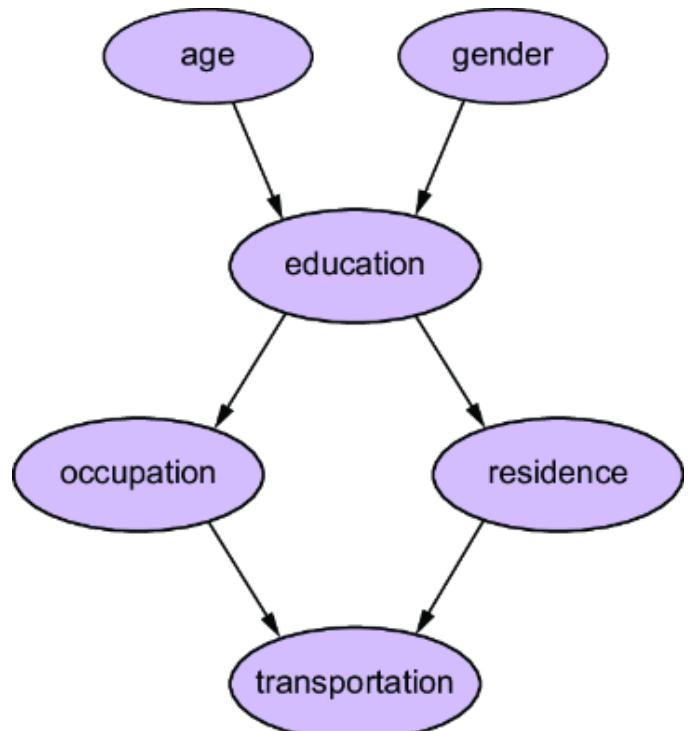
Figure 3.12 You can visualize the causal DAG in P yro by using the pyro.render_model() function. This assumes you have Graphviz installed.

Pyro provides pr obabilistic infer ence algorithms, such as importance sampling, that we can apply to our causal model. Listing 3.9 Inference on the causal model in P yro import numpy as np import pyro from pyro.distributions import Categorical from pyro.infer import Importance, EmpiricalMarginal #1 import matplotlib.pyplot as plt conditioned_model = pyro.condition( #2 model, #3 data={‘transportation’:torch.tensor(1.)} #3 ) m = 5000 #4 posterior = pyro.infer.Importance( #5 conditioned_model, #5 num_samples=m ).run() #6 E_marginal = EmpiricalMarginal(posterior, “education”) #7 E_samples = [E_marginal().item() for _ in range(m)] #7 E_unique, E_counts = np.unique(E_samples, return_counts=True) #8 E_probs = E_counts / m #8 plt.bar(E_unique, E_probs, align=‘center’, alpha=0.5) #9 plt.xticks(E_unique, E_alias) #9 plt.ylabel(‘probability’) #9 plt.xlabel(‘education’) #9 plt.title(‘P(E | T = “train”) - Importance Sampling’) #9

#1 We’ll use two inference-related classes, Importance and EmpiricalMarginal.

#2 pyro.condition is a conditioning operation on the model. #3 It tak es in the model and evidence for conditioning on. The evidence is a dictionary that maps variable names to values. The need to specify variable names during inference is why we have the name argument in the calls to pyro.sample. Here we condition on T=૿train. #4 We’ll run an inference algorithm that will generate m samples. #5 I use an inference algorithm called importance sampling. The Importance class constructs this inference algorithm. It tak es the conditioned model and the number of samples.

#6 Run the random process algorithm with the run method. The inference algorithm will generate from the joint probability of the variables we didn’t condition on (everything but T) given the variables we conditioned on (T). #7 We are interested in the conditional probability distribution of education, so we extract education values from the posterior . #8 Based on these samples, we produce a Monte Carlo estimation of the probabilities in P(E|T=૿train).

#9 Plot a visualization of the learned probabilities.

This pr oduces the plot in figure 3.13. The pr obabilities shown ar e close to the r esults fr omthe pgmpy model, though they’r e slightly di erent due to di erent algorithms and the r ounding of the parameter estimates to two decimal places. This pr obabilistic infer ence is not yet causal infer ence—we’ll look at examples combining causal infer ence with pr obabilistic infer ence starting in chapter 7. In chapter 8, you’ll see how to use pr obabilistic infer ence to implement causal infer ence. F or now, we’ll look at the bene fit of parameter modularity, and at how parameters encode causal invariance.

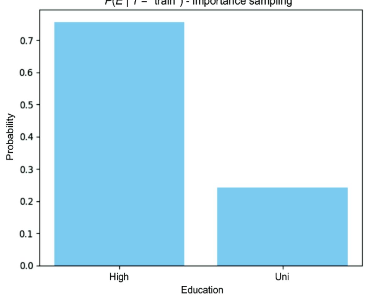
3.2Causalinvarianceandparameter modularity

Suppose we wer e inter ested in modeling the r elationship between altitude and temperatur e. The two ar e clearly correlated; the higher up you go, the colder it gets. However, you know temperatur e doesn’t cause altitude, or heating the air

Figure 3.13 Visualization of the P(E|T=૿train) distribution

within a city would cause the city to fly. Altitude is the cause, and temperatur e is the e ect.

We can come up with a simple causal D AG that we think captur es the r elationship between temperatur e and altitude, along with other causes, as shown in figure 3.14. L et’s have A be altitude, C be cloud cover, L be latitude, S be season, and T be temperatur e. The D AG in figure 3.14 has five causal Mark ov kernels: { P(A), P(C ), P(L), P(S ), P(T |A, C, L, S )}.

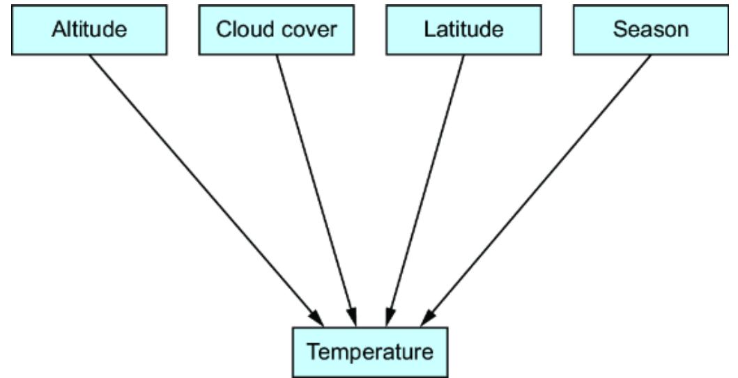
Figure 3.14 A simple model of outdoor temperature

To train a causal graphical model on top of this D AG, we need to learn parameters for each of these causal Mark ov kernels.

3.2.1 Independence of mechanism and parameter modularity

There are some underlying ther modynamic mechanisms in the DGP underlying the causal Mark ov kernels in our temperatur e DAG. For example, the causal Mark ov kernel P(T |A, C, L, S ) is the conditional pr obability induced by the physics-based mechanism, wher ein altitude, cloud cover, latitude, and season drive the temperatur e. That mechanism is distinct fr om the mechanism that deter mines cloud cover (accor ding to our D AG).

Independence of mechanism refers to this distinction between mechanisms.

The independence of the mechanism leads to a pr operty called parameter modularity . In our model, for each causal Mark ov kernel, we choose a parameterized r epresentation of the causal Markov kernels. If P(T |A, C, L, S ) and P(C ) ar e distinct mechanisms, then our r epresentations of P(T |A, C, L, S ) and P(C ) ar e representations of distinct mechanisms. That means we can change one r epresentation without wor rying about how that change a ects the other r epresentations. Such modularity is atypical in statistical models; you can’t usually change one part of a model and e xpect the other part to be una ected.

One way this comes in handy is during training. T ypically, when you train a model, you optimize all the parameters at the same time. P arameter modularity means you could train the parameters for each causal Mark ov kernel separately, or train them simultaneously as decoupled sets, allowing you to enjoy some dimensionality r eduction during training. In Bayesian terms, the parameter sets ar e a priori independent (though they are generally dependent in the posterior). This pr ovides a nice causal justi fication for using an independent prior distribution for each causal Mark ov kernel’s parameter set.

3.2.2 Causal transfer learning, data fusion, and invariant prediction

You may not be a climatologist or a meteor ologist. Still, you know the r elationship between temperatur e and altitude has something to do with air pr essur e, climate, sunlight, and such. You also know that whatever the physics of that r elationship is, the physics is the same in K atmandu as it is in El P aso. So, when we train a causal Mark ov kernel on data solely collected fr om Katmandu, we lear n a causal r epresentation of a mechanism that is invariant between K atmandu and El P aso. This invariance helps with transfer lear ning; we should be able to use that

trained causal Mark ov kernel to mak e infer ences about the temperatur e in El P aso.

Of course, ther e are caveats to leveraging this notion of causal invariance. F or example, this assumes your causal model is correct and that ther e is enough infor mation about the underlying mechanism in the K atmandu data to e ectively apply what you’ve lear ned about that mechanism in El P aso.

Several advanced methods lean heavily on causal invariance and independence of mechanism. F or example, causal data fusion uses this idea to lear n a causal model by combining multiple datasets. Causal transfer learning uses causal invariance to make causal infer ences using data outside the domain of the training data. Causal invariant prediction leverages causal invariance in pr ediction tasks. See the chapter notes at https://www .altdeep.ai/p/causalaibook for r efernces.

3.2.3 Fitting parameters with common sense

In the temperatur e model, we have an intuition about the physics of the mechanism that induces P(T |A, C, L, S ). In nonnatural science domains, such as econometrics and other social sciences, the ૿physics of the system is mor e abstract and harder to write down. F ortunately, we can r ely on similar invariance-based intuition in these non-natural science domains. In these domains, we can still assume the causal Mark ov kernels correspond to distinct causal mechanisms in the r eal world, assuming the model is true. F or example, r ecall P(T |O, R ) in our transportation model. W e still assume the underlying mechanism is distinct fr om the others; if ther e wer e changes to the mechanism underlying P(T |O, R ), only P(T |O, R ) should change—other k ernels in the model should not. If something changes the mechanism underlying P(R |E ), the causal Mark ov kernel for R, this change should a ect P(R |E ) but have no e ect on the parameters of P(T |O, R ).

This invariance can help us estimate parameters without statistical lear ning by reasoning about the underlying causal

mechanism. F or example, let’s look again at the causal Mark ov kernel P(R |E ) (r ecall R is r esidence, E is education). L et’s try to reason our way to estimates of the parameters of this distribution without using statistical lear ning.

People who don’t get mor e than a high school degr ee ar e more likely to stay in their hometowns. However, people fr om small towns who attain college degr ees ar e lik ely to move to a big city where they can apply their cr edentials to get higher -paying jobs.

Now let’s think about US demographics. Suppose a web sear ch tells you that 80% of the US lives in an urban ar ea (P(R =big) = .8), while 95% of college degr ee holders live in an urban ar ea (P (R =big| E =uni) = .95). F urther, 25% of the overall adult population in the US has a university degr ee (P(E =uni) = .25). Then, with some back- of-the-envelope math, you calculate your probability values as P(R =small| E =high)=.25, P(R =big|E = high) = .75, P(R =small| E =uni) = .05, and P(R =big|E =uni) = .95. The ability to calculate parameters in this manner is particularly useful if data is unavailable for parameter lear ning.

3.3YourcausalquestionscopestheDAG

When a modeler meets a pr oblem for the first time, ther e is often alr eady a set of available data, and a common mistak e is to de fine your D AG using only the variables in that data. L etting the data scope your D AG is attractive, because you don’t have to decide what variables to include in your D AG. But causal modelers model the DGP, not the data. The true causal structur e in the world doesn’t car e about what happens to be measur ed in your dataset. In your causal D AG, you should include causally relevant variables whether they ar e in your dataset or not.

But if the data doesn’t de fine the D AG’s scope, what does? While your data has a fixed set of variables, the variables that could comprise your DGP ar e only bounded by your imagination. Given a variable, you could include its causes, those causes’ causes, those causes’ causes’ causes, continuing all the way back to

Aristotle’s ૿prime mover, the single cause of everything. Fortunately, ther e is no need to go back that far . Let’s look at a procedur e you can use to select variables for inclusion in your causal D AG.

3.3.1 Selecting variables for inclusion in the DAG

Recall that ther e are several kinds of causal infer ence questions. As I mentioned in chapter 1, causal e ect infer ence is the most common type of causal question. I use causal e ect infer ence as an example, but this work flow is meant for all types of causal questions.

1. Include variables central to your causal question(s) —The first step is to include allthe variables central to your causal question. If you intend to ask multiple questions, include all the variables relevant to those questions. As an example, consider figure3.15. Suppose that we intend to ask about the causal e ect of V on U and Y. These become the first variables we include in the D AG.
1. Include anycommon causes for the variables in step 1—Add any commoncauses for the variables you included in the first step. In our example, you would start with variables U, V and Yin figure 3.15, and trace back their causal lineages and identif y shared ancestors. These shared ancestors are common causes. In figure 3.16, W0, W1, and W2are common causes of V, U, and Y.

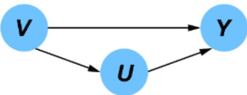
Figure 3.15First include variables central to your causal question(s). Here, suppose you are interested in asking questions about V, U, and Y.

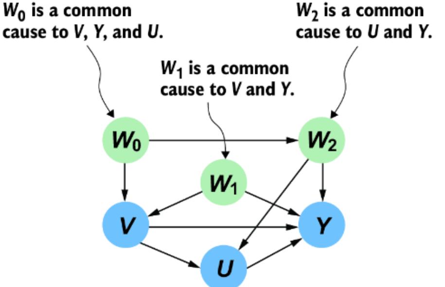
Figure 3.16Satisfy causal su ciency; include common causes to the variables from step 1.

In formal terms, a variable is a common cause Zof a pair of variables XandYif ther is a directed path from Zto Xthat does not include Yand a directed path from Zto Ythat does not include X. The formal principle of including common causes is called causal suciency . A set of variables is causally sucient if it doesn’t exclude any common causes between anypair of varia bles in the set. Further more, once you include a common cause, you don’t have to include earlier common causes on the same paths. For example, figure 3.17 illustrates how we might exclude variables’ earlier common causes.

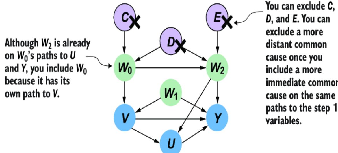
Figure 3.17Once you include a common cause, you don’t have to include any earlier common causes on the same paths tothe step 1 variables.
In figure 3.17, W2is on W0’s path to Yand U, but we inclu de W0because it has its own path to V. In contrast, while Cisa common cause of V, Y, and U, W0is on all of C’s paths to V, Y and U, so we can exclude it after including W0. Simila ry, W2 lets us e xclude E, and W0 and W2together let us e xclude D.
1. Include variables that may be useful in causal inference statistical analysis —Now we include variables thatmay be useful in statistical methods for the causal infer ences you want to make. For example, in figure 3.18, suppose you were inter ested in estimating the cause e ect of Von Y. You might want to include possibl e ૿instrumental variables. We’ll define these formally in part 4 of this book, but for now in a causal e ect question, an instrument is a parent of a variable of inter est, and it can help in statistical estimation of the causal e ect. In figure 3.18, Z can functio n as an instrumental variable. You do not need to include Z for causal suciency, but you might choose to include itohelp with quantif yig the causal e ect.

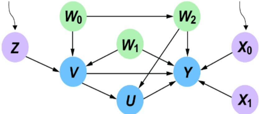
Figure 3.18Include variables that may beuseful in the causal inference statistical analysis. W’s are confound ers, Z’s are instrume nts, X’s are e ect modifiers, Y is the outcome, V is a treatment , and U is a front door mediator .

Similarly, X0 and X1 could also be of use in the analysis by accounting for other sources of variation in Y. We could potentially use them to reduce variance in the statistical estimation of a causal e ect. Alter natively, we may be inter ested in the heterogeneity of the causal e ect (how the causal e ect varies) acrossubsets of the population defined by X0and X1. We’ll look at causal e ect heter ogeneity more closely in chapter 11.
1. Include variables that help the DAG communicate a complete story—Finally, include any variables thathelp the DAG better function as a communicative tool. Consider the common cause D in figure 3.19.

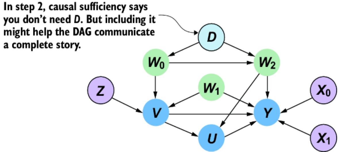
Figure 3.19Include variables that help the DAG tell a complete story . In this example, despite having excluded D in step2 (figure 3.17) we stil l might want to include D if it has communicative value.

In figure 3.17, we conclud ed that the common cause Dcould be excluded after including common causes W0and W2. But perhaps D isan important variable in how domain experts conceptualize the domain. While it is not useful in quantif ying the causal e ect of Von Uand Y, leaving it out might feel awkward. If so, including it mayhelp the DAG tell a bette r story bshowing how a key variable relates to the variables you included. When your causal DAG tells a convincing story, your causal analysis is mor e convincing.

3.3.2 Including variables in causal DAGs by their role in inference

Many e xperts in causal infer ence de-emphasize writing their assumptions in the for m of a causal D AG in favor of specif ying a set of r elevant variables, accor ding to their role in causal infer ence calculations. F ocusing on variable-r ole-in-infer ence over a causal D AG is common in econometrics pedagogy . Examples of such r oles include ter ms I’ve alr eady intr oduced, such as ૿common cause, ૿instrumental variable, and ૿e ect modifier. Again, we’ll de fine these for mally in chapter 11.

For now, I want to mak e clear that this is not a competing paradigm. An economist might say they ar e inter ested in the causal e ect of V on U, conditional on some ૿ e ect modi fiers, and that they plan to ૿ adjust for the in fluence of common causes” using an ૿ instrumental variable . These r oles all correspond to structur e in a causal D AG; common causes of U and V in figure 3.19 ar e W0, W1, and W2. Z is an instrumental variable, and X0 and X1 are eect modi fiers. Assuming variables with these r oles ar e important to your causal e ect estimation analysis is implicitly assuming that your DGP follows the causal DAG with this structur e.

In fact, given a set of variables and their r oles, we can construct the implied causal D AG on that set. The DoWhy causal infer ence library shows us how .

Listing 3.10 Creating a DAG based on roles in causal e ect inference from dowhy import datasets import networkx as nx import matplotlib.pyplot as plt sim_data = datasets.linear_dataset( #1 beta=10.0, num_treatments=1, #2 num_instruments=2, #3 num_effect_modifiers=2, #4 num_common_causes=5, #5 num_frontdoor_variables=1, #6 num_samples=100, ) dag = nx.parse_gml(sim_data[‘gml_graph’]) #7 pos = { #7 ‘X0’: (600, 350), #7 ‘X1’: (600, 250), #7 ‘FD0’: (300, 300), #7 ‘W0’: (0, 400), #7 ‘W1’: (150, 400), #7 ‘W2’: (300, 400), #7 ‘W3’: (450, 400), #7 ‘W4’: (600, 400), #7 ‘Z0’: (10, 250), #7 ‘Z1’: (10, 350), #7 ‘v0’: (100, 300), #7 ‘y’: (500, 300) #7 } #7 options = { #7 “font_size”: 12, #7 “node_size”: 800, #7 “node_color”: “white”, #7 “edgecolors”: “black”, #7 “linewidths”: 1, #7 “width”: 1, #7 } #7 nx.draw_networkx(dag, pos, **options) #7 ax = plt.gca() #7 ax.margins(x=0.40) #7 plt.axis(“off”) #7 plt.show() #7 #1 datasets.linear_ dataset generates a ΔAG from the speci fied variables. #2 Add one treatment variable, lik e V in figure 3.19. #3 Z in figure 3.19 is an example of an instrumental variable; a variable that is a cause of the treatment, but its only causal path to the outcome is through the treatment. Here we create two instruments.

#4 X 0 and X 1 in figure 3.19 are examples of ૿e ect modi fiers that help model heterogeneity in the causal e ect. ΔoWhy de fines these as other causes of the outcome (though they needn’t be). Here we create two e ect modifiers.

#5 We add 5 common causes, lik e the three W 0, W 1, and W 2 in figure 3.19. Unlike the nuanced structure between these variables in figure 3.19, the structure here will be simple.

#6 Front door variables are on the path between the treatment and the e ect, lik e U in figure 3.19. Here we add one.

#7 This code extracts the graph, creates a plotting la yout, and plots the graph. #8 This code extracts the graph, creates a plotting la yout, and plots the graph.

This code pr oduces the D AG pictur ed in figure 3.20.

This r ole-based appr oach pr oduces a simple template causal DAG. It won’t give you the nuance that we have in figure 3.19, and it will e xclude the good storytelling variables that we added in step 4, lik e D in figure 3.19. But it will be enough for tackling the pr edefined causal e ectquery . It’s a gr eat tool to use when working with collaborators who ar e skeptical of D AGs but ar e comfortable talking about variable r oles. But don’t believe claims that this appr oach is D AG-free. The D AG is just implicit in the assumptions underlying the speci fication of the r oles.

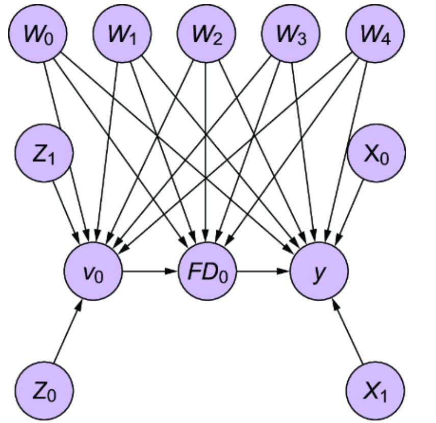
Figure 3.20 A causal DAG built by specifying variables by their role in causal e ect inference

Such a template method could be used for other causal queries as well. Y ou can also use this appr oach to get a basic causal D AG

in a first step, which you could then build upon to pr oduce a more nuanced graph.

3.4Lookingahead:Modeltestingand combiningcausalgraphswithdeep learning

The big question when building a causal D AG is ૿ what if my causal D AGis wr ong? How can we be con fident in our selected DAG? In the ne xt chapter, we’ll look at how to use data to str ess test our causal D AG. A k ey insight will be that while data can never pr ove that a causal D AG is right, it can help show when it is wr ong. Y ou’ll also lear n about causal discovery, a set of algorithms for lear ning causal D AGs fr om data.

In this chapter, we e xplor ed building a simple causal graphical model on the D AG structur e using pgmpy . Thr oughout the book, you’ll see how to build mor e sophisticated causal graphical models that leverage neural networks and automatic dierentiation. Even in those mor e sophisticated models, the causal Mark ov property and the bene fits of the D AG including causal invariance, and parameter modularity will still hold.

Summary

The causal directed acyclic graph (DAG) can represent our causal assumptions about the data generating process (DGP).
The causal DAG is a useful tool for visualizing and communicating your causal assumptions.
DAGs are fundamental data structur es in compute r science, and they admit many fast algorithms we can bring tobear on causal infer ence tasks.
DAGs link causality to conditional independence via the causal Mark ov pr operty .
DAGs can pr ovide sca olding for pr obabilistic ML models.
We can use various methods for statistical parameter learning to train a probabilistic model on top of a DAG. These include maximum likelihood estimation and Bayesian estimation.
Given a causal DAG, the modeler can choose from a variety of parameterizations of the causal Markov kernels in the DAG, rangin g from conditional probability tables to regression models to neural networks.
A causally sucient set of variables contains all common causes between pairs in that set.
You can build a causal DAGby starting with a set of variables of interest, expanding that to a causally sucient set, adding variables useful to causal infer ence analysis, and finally adding any variables that help the DAG communicate a complete story .
Each causal Markov kernel represents a distinct causal mechanism that deter mines how the child node is deter mined by its par ents (assuming the D AG is cor rect).
૿Independence of mechanism refers to how mechanisms are distinct from the others—a change to one mechanism does not a ect the others.
When you build a genera tive model on the causal DAG, the parameters of each causal Markov kernel represents an encoding of the underlying causal mechanism. This leads to ૿parameter modularity, which enables you to learn each parameter set separatel y and even use common sense reasoning to estimate parameters instead of data.
The fact that each causal Markov kernel represents a distinct causal mechanism provides a source of invariance that can be leveraged in advanced tasks, like transfer learning, data fusion, and invariant pr ediction.
You can specif y a DAG by the roles variables play in a speci fic causal infer ence task.

4Testing the DAG with causal constraints

This chapter covers

Using d-separation to reason about how causality constrains conditional independence
Using NetworkX and pgmpy to do d-separation analysis
Refuting a causal DAG using conditional independence tests
Refuting a causal D AG when ther e are latent variables
Using and applying causal discovery algorithm constraints

Our causal D AG, or any causal model, captur es a set of assumptions about the r eal world. Of ten, those assumptions are testable with data. If we test an assumption, and it tur ns out not to hold, then our causal model is wr ong. In other words, our test has ૿ falsi fied or ૿ refuted our model. When this happens, we go back to the drawing boar d, come up with a better model, and try to r efute it again. W e repeat this loop until we get a model that is r obust to our attempts to refute it.

In this chapter, we’ll focus on using statistical conditional independence-based testing to test our causal D AG. As you learn more about the assumptions we can pack into a causal model, and the infer ences those assumptions allow you to make, you’ll lear n new ways to test and r efute your model. The work flow you’ll lear n for running conditional independence tests in this chapter can be applied to new tests you may come up with.

4.1How causalityinducesconditional independence

Causal r eationships constrain the data in certain ways, one of which is by for cing variables to be conditionally independent. This for ced conditional independence gives us a way to test our model with data using statistical tests for independence; if we find str ong evidence that two variables are dependent when the D AG says they shouldn’t be, our DAG is wr ong.

In this chapter, we’ll test our causal D AG using these statistical independence tests, including independence tests on functions of observed variables that we can run when other variables ar e latent in the data. A t the end, we’ll look at how these ideas enable causal discovery algorithms that try to lear nthe causal D AG dir ectly fr om data.

But befor e that, let’s see how causality induces conditional independence. Consider again our blood type e xample, shown in figure4.1. Y our father’s blood type is a dir ect cause of yours, and your pater nal grandfather’s blood type is an indir ect cause. Despite being a cause of your blood type, your pater nal grandfather’s blood type is conditionally independent of your blood type, given your father’s.

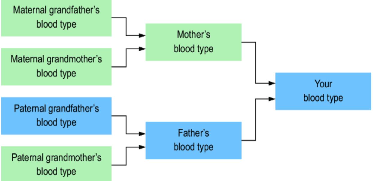
Figure 4.1 Causality induces conditional independence. Y our blood type is conditionally independent of your paternal grandfather ’s blood type (an indirect cause), given your father ’s blood type (a direct cause).

We know this fr om causality; the par ents’ blood types completely deter mine the blood type of the child. Y our pater nal grandfather’s and grandmother’s blood types completely deter mined your father’s blood type, but your father’s and mother’s blood types completely deter mined yours. Once we know your father’s blood type, ther e is nothing mor e your pater nal grandfather’s blood type can tell us. In other wor ds, your grandpar ent’s blood type is independent of yours, given your par ents.

4.1.1 Colliders

Now we’ll consider the collider , an inter esting way in which causality induces cases of dependence between variables that ar e typically independent. Consider the canonical example in figure 4.2. Whether the sprinkler is on or o , and whether it is raining or not, ar e causes of whether the grass is wet, but knowing that the sprinkler is o won’t help you predict whether it’s raining. In other wor ds, the state of the sprinkler and whether it’s raining ar e independent. But when

you know the grass is wet, also knowing that the sprinkler is o tells you it must be raining. So while the state of the sprinkler and the pr esence or absence of rain ar e independent, they become conditionally dependent, given the state of the grass.

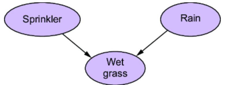
Figure 4.2 The sprinkler being on or o and whether or not it rains causes the grass to be wet or not. Knowing that the sprinkler is o won’t help you predict whether it’s raining—the sprinkler state and rain state are independent. But given that the grass is wet, knowing the sprinkler is o tells you it must be raining—the sprinkler state and rain state are conditionally dependent, given the state of the grass.

In this case ૿ wet grass is a collide r: an e ect with at least two independent causes. Colliders ar e inter esting because they illustrate how causal variables can be independent but then become dependent if we condition on a shar ed eect variable. In conditional independence ter ms, the par ent causes ar e independent (sprinkler ⊥ rain) but become dependent af ter we observe (condition on) the child (sprinkler ̷ rain | wet grass).

For another e xample, let’s look at blood type again, as shown in figure4.3.

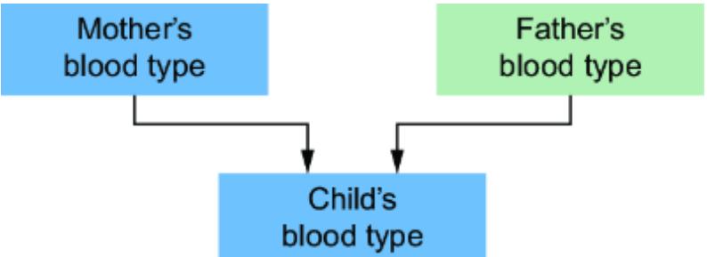
Figure 4.3 Mothers and fathers are usually unrelated, so knowing mother’s blood type can’t help predict the father ’s blood type. But if we know the mother ’s blood type and the child’s blood type, it narrows down the possible blood types of the father .

If we assume the mother and father ar e unr elated, the mother’s blood type tells us nothing about the father’s blood type—(mother’s blood type ⊥ father’s blood type). But suppose we know the child’s blood type is B. Does that help us use the mother’s blood type to pr edict the father’s blood type?

To answer this, e xamine the standar d blood type table in figure 4.4. W e see that if mother has blood type A and the child has blood type B, then possibly blood types for the father ar e B and AB.

Figure 4.4 Knowing the mother ’s blood type can help you narrow down the father ’s blood type if you know the child’s blood type.

Knowing the mother’s blood type alone doesn’t tell us anything about the father’s blood type. But if we add infor mation about the child’s blood type (the collider), we can nar row down the father’s blood type fr om four to two possibilities. In other wor ds, (mother’s blood type ⊥ father’s blood type), but the mother’s and father’s blood type become dependent once we condition on the child’s blood type.

Colliders show up in various parts of causal infer ence. In section 4.6, we’ll see that colliders ar e important in the task of causal discovery, wher e we try to lear n a causal D AG from data. When we look at causal e ects in chapters 7 and 11, we’ll see how accidentally ૿adjusting for colliders can intr oduce unwanted ૿collider bias when infer ring causal e ects.

For now, we’ll note that colliders can be at odds with our statistical intuition, because they describe how causal logic leads to situations wher e two things ar e independent but ૿suddenly become dependent when you condition on a thir d or mor e variables.

4.1.2 Abstracting independence with a causal graph

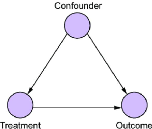
Figure 4.5 In causal e ect inference, we are interested in statistically quantifying how much a cause (treatment) a ects an e ect (outcome). Confounders are common causes that are a source of non-causal correlation between treatment and outcome. Causal e ect inference requires ૿adjusting for confounders. D -separation is the backbone of the theory that tells us how .

In the pr evious section, we used the basic rules of blood type heredity to show how causality induces conditional independence. If we want to write code that can help us make causal infer ences acr oss di erent domains, we’ll need an abstraction for mapping causal r elationships to conditional independence that doesn’t r ely on the rules of a particular domain. ૿ D-separation solves this pr oblem.

D-separation and d-connection refer to how we use graphs to reason about conditional independence. The concepts ar e novel at firsglance, but they will be some of your most important tools for graph-based causal r easoning. As a bit of a spoiler for chapter 7, consider the pr oblem of causal e ect infer ence, illustrated in figure 4.5. In causal infer ence, you are inter ested in statistically quantif ying how much a cause (often called a ૿tr eatment) a ects an e ect (an ૿ outcome).

As you saw in chapter 3, you can describe variables in a D AG in ter ms of their r ole in a causal infer ence task. One r ole in the task of causal e ect infer ence is the confounder . Confounders ar e common causes that ar e a sour ce of noncausal cor relation between the tr eatment and the e ect. T o estimate the causal e ect of the tr eatment on the outcome, we have to ૿adjust for the confounder . The theor etical justi fication for doing so is based on ૿d-separating the path {treatment ← confounder → outcome} and zooming in on the path {tr eament → outcome}.

4.2D-separationandconditional independence

Recall the following ideas fr om previous chapters:

A causal DAG is a model of the data generating process (DGP).
The DGP entails a joint pr obability distribution.
Causal relationships induce independence and conditionalndependence between variables in the joint probability distribution.

D-separation and d-connection ar e graphical abstractions for reasoning about the conditional independence in the joint probability distribution that a causal D AG models. The concept r efers to nodes and paths between nodes in the causal D AG; the nodes and paths ar e ૿d-connected or ૿dseparated, wher e the ૿d stands for ૿dir ectional. The idea is for a statement lik e ૿these nodes ar e d-separated in the graph to cor respond to a statement lik e ૿these variables ar e conditionally independent. D-separation is not about stating what causes what; it is about whether paths between variables in the D AG indicate the absence or pr esence of

dependence between those variables in the joint pr obability distribution.

We want to mak e this cor respndence because r easoning about graphs is easier than r easoning about pr obability distributions dir ectly; tracing paths between nodes is easier than taking graduate-level classes in pr obability theory . Also, recall fr om chapter 2 that graphs ar e fundamental to algorithms and data structur es, and that statistical modeling benefits fr om making conditional independence assumptions.

4.2.1 D-separation: A gatewa y to simpli fied causal analysis

Suppose we have a statement that U and V are conditionally independent given Z (i.e., U V |Z). Our task is to de fine a corresponding statement pur ely in graphical ter ms. We’ll write this statement as U GV |Z and r ead it as ૿ U and V are d-separated by Z in graph G.

Let Zrepresent a set of nodes called the d-separating set or ૿block ers. In ter ms of conditional independence, Z corresponds to a set of variables we condition on. Our goal is to de fine d-separation such that the nodes in Z in some sense ૿block the dependence between U and V that is implied by the causal structur e of our D AG.

Next, let P be a path, meaning a series of connected edges (and nodes) between two nodes. It does not matter if the nodes on the paths ar e observed or not in your data (we’ll see how the data factors in later). Our de finition of ૿path does not depend on the orientation of the edges; for example, { x → y→ z}, {x ← y→ z}, {x ← y← z}, and { x → y ← z} are all paths between x and z.

Finally, let’s r evisit the collider . A collider structur e refers to a motif lik ex → y← zwher e the middle node y (the collider) has incoming edges.

We’ll de fine d-separation now . First, two nodes u and v are said to be d-separated (block ed) by Z if all paths between them ar e d-separated by Z. If any of those paths between u and v are not d-separated, then u and v are d-connected.

Let’s de fine d-separation for a path. A path P is d-separated by node set Z if any of four criteria ar e met.

1. Pcontai ns a chain, i→ m → j, such that the middle node m is in Z.
1. Pcontai ns a chain, i← m ← j, such that the middle node m is in Z.
1. Pcontains a child-par ent-c hild structur e i← m→ j, such that the middle (par ent) node m is in Z.

Let’s pause. Criteria 1–3 ar e just walking thr ough the ways we can orient edges between thr ee nodes. If this k eeps up, then P is always d-separated if a node on P is in set Z. That would be nice, because it would mean that two nodes ar e dconnected (i.e., dependent) if ther e are any paths between them in the D AG, and they ar e d-separated if all those paths are block ed by nodes in set Z.

Unfortunately, colliders mak e the fourth criterion contrary to the others:

Pcontains a collider structure , i→ m ← j, such that the middle node m is not in Z,and no descendant of m is in Z. 4.

This fourth criterion is how d-separation captur es the way two independent (d-separated) items can become dependent when conditioning on a collider .

Many writers con flate d-separation and conditional independence. K eep the distinction clear in your mind: ⊥ ^G speaks of graphs, wher eas ⊥ speaks of distributions. It matters because, as you’ll see later in this chapter, we’ll use d-separation to test our causal assumptions against statistical evidence of conditional independence in the data.

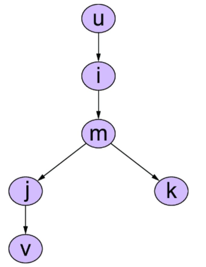
Figure 4.6 Does the set { m, k} d-separate path u → i → m → j → v?

Let’s work thr ough a few e xamples.

EXAMPLE WITH CHAIN I → M → J

Consider the D AG in figure 4.6, wher e P is u → i → m → j → v. This path is d-connected by default. Now let Z be the set { m, k}. P contains a chain i → m → j, and m is in Z. If we block on Z, the first criterion is satis fied, and u and v are d-separated.

For some (but not all), a helpful analogy for understanding dseparation is an electr onic cir cuit. P aths without colliders ar e d-connected and ar e lik e closed cir cuits, wher e electrical current flows uninhibited. ૿ Blocking on a node on that path d-separates the path and will ૿br eak the cir cuit so cur rent can’t flow. Blocking on Z (speci fically, blocking on m, which is in Z) ૿br eaks the cir cuit as shown in figure 4.7.

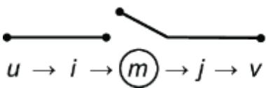
Figure 4.7 The path is d-connected by default, but blocking on m Z dseparates the path and figuratively breaks the circuit (૿ means ૿in).

EXAMPLE WITH CHAIN I ← M → J

Now consider the D AG in figure 4.8, wher e P is u ← i ← m → j → v. This path is also d-connected by default. Note that dconnection can go against the grain of causality . In figure 4.7, the d-connected path fr om u to v takes steps in the direction of causality : u to i (u ← i), then i to m (i ← m), then m to j (m → j), and then j to v (j → v). But her e, we have two anticausal (meaning against the dir ection of causality) steps, namely the step fr om u to i (u ← i) and i to m (i ← m).

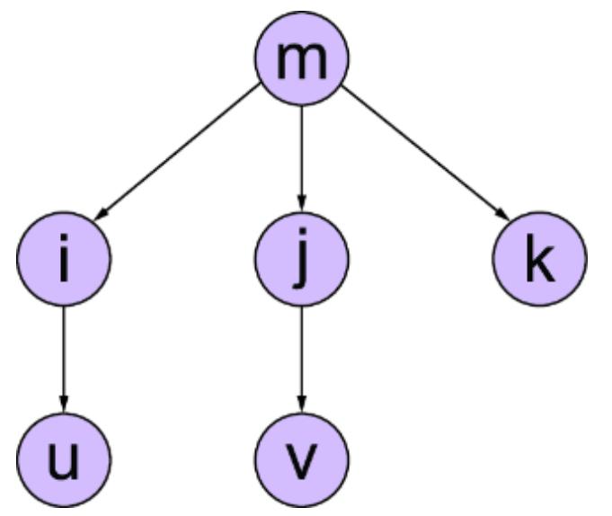
Figure 4.8 Does the set { m} d-separate path u ← i ← m → j → v?

Suppose we block on set Z, and Z contains only the node m. Then condition 3 is satis fied and the path is d-separated, as illustrated in figure 4.9.

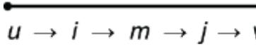
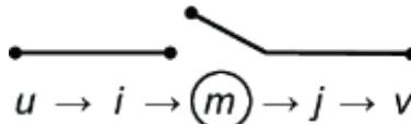
Figure 4.9 This path from u to v is also d-connected by default, even though it has some steps ( u to i and i to m) that go against the direction of causality . Again, blocking on m Z d-separates the path and figuratively breaks the circuit.

COLLIDERS MAKE D -SPARATION WEIRD

The fourth criterion focuses on the collider motif i → m ← j: P contains a collider structure , i → m ← j, such that the middle node m is not in Z, and no descendant of m is in Z.

Let’s r elate this back to our blood type e xample. Her e i and j are the par ents’ blood types and m is the child’s blood type. We saw that colliders ar e a bit odd, because conditioning on the collider (the child’s blood type) induces dependence between two independent things (lik e the par ents’ blood types). This oddness mak es d-separation a bit trick y to understand at first glance. F igure 4.10 illustrates how colliders a ect d-separation.

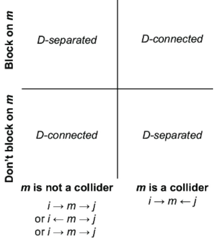
Figure 4.10 Colliders mak e d-connection tricky . Given a node m on a path, if m is not a collider , the path is d-connected by default and dseparated when you block on m. If m is a collider , the path is dseparated by default and d-connected when you block on m.

The following is true of colliders:

All paths between two nodes d-connect by default unless that path hasa collider motif . A path witha colliders dseparated by default.
Blocking with any node on a d-connected path will dseparate that path unless that node is a collider . Blocking on a collider will d-connect a path by default, as
will blocking with a descendant of that collider .

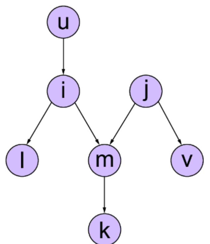
Figure 4.11 Does the set { m} (or { k} or { m, k}) d-separate path u → i → m ← j → v?

In ter ms of the cir cuit analogy, colliders ar e lik e an open switch, which pr events cur rent flow in an electr onic cir cuit. When a path has a collider, the collider stops all cur rent fr om passing thr ough it. Colliders br eak the cir cuit. Blocking on a collider is lik e closing the switch, and the cur rent that couldn’t pass thr ough befor e now can pass thr ough (dconnection).

In the D AG in figure 4.11, is the path u → i → m ← j → vdconnected by default? No, because the path contains a collider structur e m (i → m ← j).

Now consider what would happen if the blocking set Z included m. In this case, condition 4 is violated and the path becomes d-connected , as in figure 4.12.

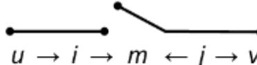
Figure 4.12 This path from u to v is d-separated by default because it contains a collider m. The collider is analogous to an open circuit. Blocking on m r any of its descendants d-connects the path and figuratively closes the circuit.

The path would also become d-connected if Z didn’t have m but just had k (or if Z included both m and k). Blocking on a descendant of a collider d-connects in the same manner as blocking on a collider .

Can you guess why? It’s because the collider’s descendant is d-connected to the collider . In causal ter ms, we saw how, given a mother’s blood type, observing the child’s blood type (the collider) might r eveal the father’s blood type. Suppose that if instead of observing the child’s blood type, we observed the child’s child’s blood type (call it the grandchild’s blood type). That grandchild’s blood type could help nar row down the child’s blood type and thus nar row down the father’s blood type. In other wor ds, if the mother’s and father’s blood types ar e dependent, given the child’s blood type, and the grandchild’s blood type gives you infor mation about the child’s blood type, then the mother’s and father’s blood types ar e dependent given the grandchild’s blood type.

D-SEPARATION AND SETS OF NODES

D-separation doesn’t just apply to pairs of nodes, it applies to pairs of sets of nodes. In the notation u v|Z, Z can be a set of block ers, and u and v can be sets as well. W e dseparate two sets by blocking all d-connected paths between members of each set. Other graph-based causal ideas, such

as the do -calculus, also generalize to sets of nodes. If you remember that fact, we can build intuition on individual nodes, and that intuition will generalize to sets.

When the blocking set Z is the singleton set { m}, this set is sucient to block the paths u → i → m → j → vin figure 4.7 and u ← i ← m → j → vin figure 4.8. Altogether, the sets { i}, {m }, {j}, {i, m }, {i, j}, {m, j}, and { i, m, j} all d-separate u and v on these two paths. However, { i}, {m }, and { j} are the minimal d-separating sets , meaning that all the other dseparating sets include at least one of these sets. The minimal d-separation sets ar e sucient to d-separate the two nodes. When r easoning about d-separation and when implementing it in algorithms, we want to focus on finding minimal d-separating sets; if U V|Z and U V|Z, W are both true, we don’t want to waste e ort on U V|Z, W.

4.2.2 Examples of d-separating multiple paths

Suppose we want to d-separate two nodes. Of ten ther e ae multiple d-connected paths between those nodes. T o dseparate those nodes, we need to find block ers that dseparate each of those paths. L et’s walk thr ough some examples.

FINDING A MINIMAL D -SEPARATING SET

In a bigger graph with mor e edges, the number of paths between two nodes can be quite lar ge. But of ten longer paths of ten get block ed as a side-e ect of blocking shorter paths. So we can start with shorter paths, and work our way to longer paths that haven’t been block ed yet, until no unblock ed paths r emain.

For example, U and V are d-connected in figure 4.13. What sets of nodes ar e fully r equir ed to d-separate them? In figure 4.13, U and V are d-connected thr ough these paths:

U → I → V
U → J → V
U → J → I → V

First, we can d-separate U → I → V by blocking on I. Then, we d-separate U → J → V by blo cking on J. At this point, we see that our blocking set { I, J } alr eady d-separates U → J → I → V, so we ar e done.

In another e xample, how do we d-separate U and V in figure 4.14?

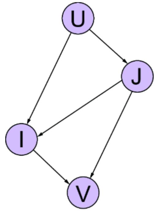
Figure 4.13 We can d-separate U and V with { I, J}.

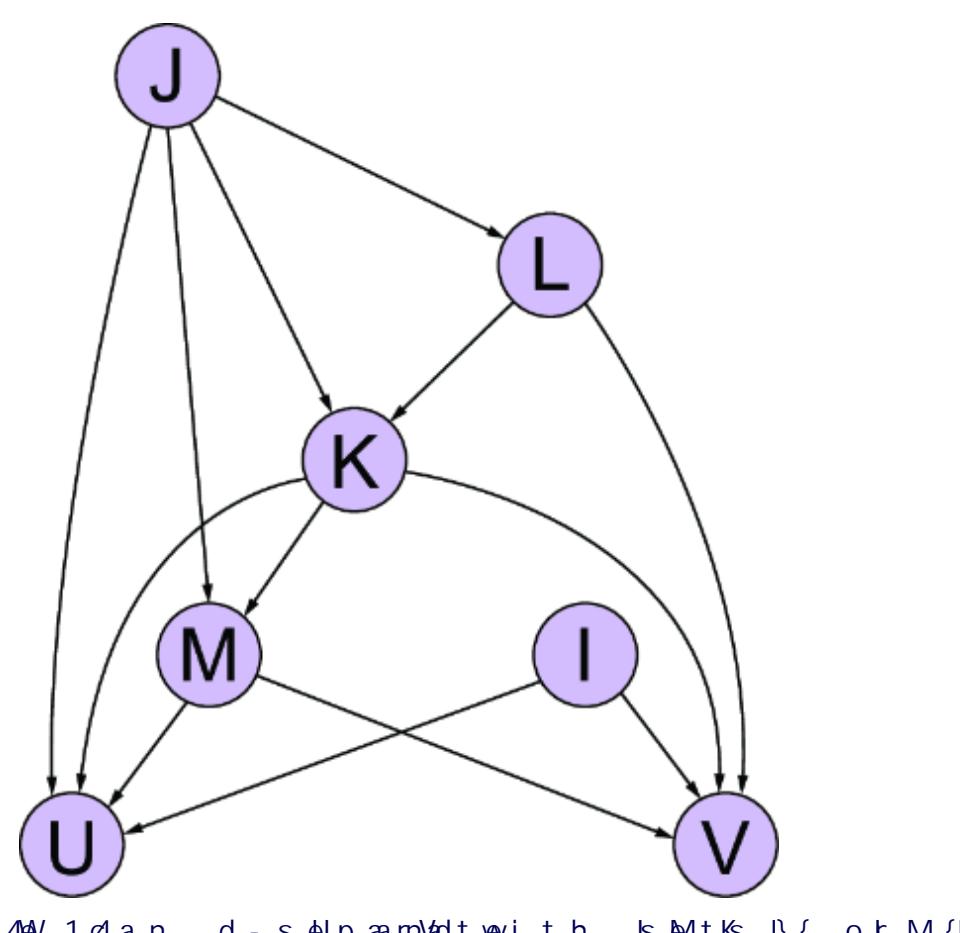
Figure 4.14 We can d-separate U and V with sets { I, M, K, J} or { I, M, K, L}.

There are many paths between U and V. Let’s first enumerate thr ee of the shortest paths:

U ← I → V
U ← M → V
U ← K → V

We’ll need to block on at least on { I, M, K} to d-separate these thr ee paths. Note that U has another par ent J, and ther are several paths fr om U to V thr ough J, but ther e are only two paths we haven’t alr eady d-separated; U ← J → L→ V and U ← J → K ← L→ V. Both J and L will block these paths, so we could d-separate U and V with minimal sets { I, M, K, J} or {I, M, K, L}. Note that U← J → K ← L→ V was d-connected because we initially added K, a collider on this path, to our blocking set. Ne xt, we look at another e xample of this phenomenon.

WHEN D-SEPARATING ONE P ATH D-CONNECTS ANOTHER

When you attempt to d-separate a path between U and V by blocking on a node that is a collider on another path, you potentially d-connect that other path. That is fine, as long as you tak e additional steps to d-separate that path as well. T o illustrate, consider the graph in figure 4.15. This graph is simple enough that we can enumerate all of the paths.

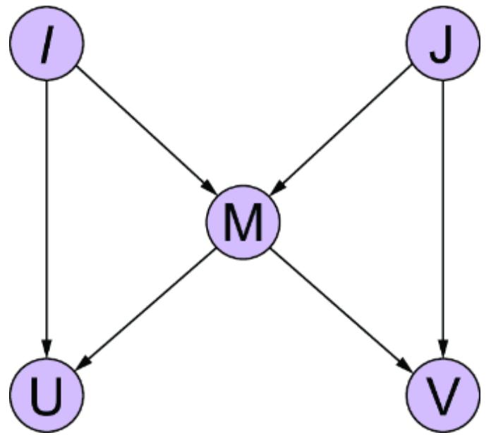
Figure 4.15 Blocking with M ll block the path U ← M → V but would dconnect the path U ← I → M ← J → V because M is a collider between I and J. So we need to additionally block on either I or J to d-separate U ← I → M ← J → V.

Let’s start with the thr ee d-connecting paths:

U ← M → V
U ← I → M → V
U ← M ← J → V

We also have a path U ← I → M ← J → V, but that is not a dconnecting path because M is a collider on that path.

The easiest way to block all thr ee of these d-connected paths with one node is to block on M. However, if we block on that collider, the path U ← I → M ← J → V d-connects. So we need to additionally block on I or J.In other wor ds, our minimal dseparating sets ar e {I, M} and { J, M}.

4.2.3 D-separation in code

Don’t fr et if you ar e still hazy on d-separation. W e’ve de fined four criteria for describing paths between nodes on a graph, which is just the sort of thing we can implement in a graph library . In Python, the graph library NetworkX alr eady has a utility that checks for d-separation. Y ou can e xperiment with these tools to build an intuition for d-separation on di erent graphs.

SETTING UP Y OUR ENVIRONMENT

This code was written with pgmpy version 0.1.24. The pandas version was 2.0.3.

Let’s verif y our d-separation analysis of the causal D AG shown pr eviously in figure 4.15.

Listing 4.1 D-separation analysis of the DAG in figure 4.15

from networkx import is_d_separator #1 from pgmpy.base import DAG #2 dag = DAG([ #2 (‘I’, ‘U’), #2 (‘I’, ‘M’), #2 (‘M’, ‘U’), #2 (‘J’, ‘V’), #2 (‘J’, ‘M’), #2 (‘M’, ‘V’) #2 ]) #2 print(is_d_separator(dag, {“U”}, {“V”}, {“M”})) #3 print(is_d_separator(dag, {“U”}, {“V”}, {“M”, “I”, “J”})) #4 print(is_d_separator(dag, {“U”}, {“V”}, {“M”, “I”})) #5 print(is_d_separator(dag, {“U”}, {“V”}, {“M”, “J”})) #5 #1 The graph library NetworkX implements the d-separation algorithm for NetworkX graph objects, such as ΔiGraph (directed graph). #2 ΔAG is a base class for the Ba yesianNetwork class. The base class for ΔAG is NetworkX’s ΔiGraph. So is_d_separator will work on objects of

the class ΔAG (and Ba yesianNetwork).

#3 Build the graph in figure 4.11. Blocking on a collider M blocks the path U ← M → V but will d-connect the path U ← I → M ← J → V , so this will print F alse.

#4 Blocking on M will block U ← M → V and open (d-connect) U ← I → M ← J → V , but we can block that path with I and J, so this evaluates to T rue. #5 Blocking on both I and J is overkill. The minimal d-separating sets are {૿M, ૿I} and {૿M, ૿ J}.

pgmpy also has a get_independencies method in the DAG class that enumerates minimal d-separating states that ar e true given a graph.

Listing 4.2 Enumerating d-separations in pgmpy

from pgmpy.base import DAG dag = DAG([ (‘I’, ‘U’), (‘I’, ‘M’), (‘M’, ‘U’), (‘J’, ‘V’), (‘J’, ‘M’), (‘M’, ‘V’) ])

dag.get_independencies() #1

#1 Obtain all the minimal d-separation statements that are true in the ΔAG.

The get_independencies method r eturns the following r esults. (You might see a slight di erence in the or dering of the

output depending on your envir onment.)

(I ⊥ J)
(I ⊥ V J, M)
(I ⊥ V J, U, M)
(V ⊥ I, U J, M)
(V ⊥ U I, M)
(V ⊥ I J, U, M)
(V ⊥ U J, M, I)
(J ⊥ I)
(J ⊥ U I, M)
(J ⊥ U I, M, V)
(U ⊥ V J, M)
(U ⊥ J, V I, M)
(U ⊥ V J, M, I)
(U ⊥ J I, M, V)

Note that the get_independencies function name is a misnomer; it does not ૿get independencies; it gets dseparations. Again, don’t con flate d-separation in the causal graph with conditional independence in the joint pr obability distribution entailed by the DGP the graph is meant to model. K eeping this distinction in your mind will help you with the ne xt task: using d-separation to test a D AG against evidence of conditional independence in the data.

4.3RefutingacausalDAG

We have seen how to build a causal D AG. Of course, we want to find a causal model that fits the data well, so now we’ll evaluate the causal D AG against the data. W e could use standar d goodness- of-fit and pr edictive statistics to evaluate fit, but her e we’r e going to focus on refuting our causal D AG, using data to show that our model is wr ong.

Statistical models fit curves and patter ns in the data. Ther e is no ૿ right statistical model; ther e are just models that fit the data well. In contrast, causal models go beyond the data to mak e causal assertions about the DGP, and those assertions ar e either true or false. As modelers of causality, we try to find a model that fits well, but we also try to refute our model’s causal assertions.

REFUTATION AND POPPER

The appr oach to building D AGs by r efutation aligns with Karl P opper’s falsi fiable theories framework. K arl P opper was a 20th-century philosopher known for his contributions to the philosophy of science, particularly his theory of falsi fication. P opper ar gued that scienti fic theories cannot be pr oven true, but they can be tested and potentially falsi fied, or in other wor ds, refuted .

We tak e a ૿ Popperesque appr oach to model building, meaning that we don’t mer ely want to find a model that fits the evidence. R ather, we actively sear ch for evidence that r efutes our model. When we find it, we r eject our model, build a better one, and r epeat.

D-separation is our first tool for r efutation. Suppose you build a causal D AG and it implies conditional independence. Y ou then look for evidence in the data of dependence, wher e your D AG says ther e should be conditional independence. If you find that evidence, you have r efuted your D AG. You then go back and iterate on the causal D AG, until you can no longer r efute it, given your data.

Once you’ve done that, you move on to your downstr eam causal infer ence work flow. But k eep this r efutation mentality in mind. If you work with the same causal D AG repeatedly, you should always be seeking new ways to r efute and iterate upon it. P ractically, your goal is not getting the true D AG, but getting a har d-to-refute D AG.

4.3.1 Revisiting the causal Mark ov property

Recall that we saw two aspects of the causal Mark ov property :

Local Markov property —A node is conditio nally independent of its non-descendants, given its par ents.
Markov factorization property —The joint probability distribution factorizes into conditional distributio ns of variables, given their dir ect par ents in the causal D AG.

Now we’ll intr oduce a thir dface of this pr operty called the global Markov property . This pr operty states that dseparation in the causal D AG implies conditional independence in the joint pr obability distribution. In notation, we write

In plain wor ds, that notation r eads as ૿If U and V are dseparated by Z in graph G, they ar e conditionally independent given Z. Note that if any of the thr ee facets of the causal Mark ov pr operty ar e true, they ar e all true.

The global Mark ov pr operty gives us a straightforwar d way to refute our causal model. W e can use d-separations to specif y statistical tests for the pr esence of conditional independence. F ailing tests r efute the model.

4.3.2 Refutation using conditional independence tests

There are multiple ways to statistically evaluate conditional independence, and the most obvious is with a statistical test for conditional independence. pgmpy and other libraries make it r elatively easy to run conditional independence tests. L et’s r evisit the transportation model, shown again in figure 4.16.

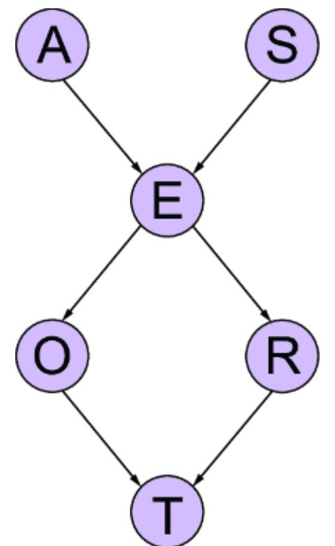
Figure 4.16 The transportation model. Age ( A) and gender ( S) determine education ( E). Education causes occupation ( O) and residence ( R). Occupation and residence cause transportation ( T).

Recall that for our transportation model we wer e able to collect the following observations:

Age (A)—Recorded as young (૿young) for individuals up to and including 29 years, adult (૿adult) for individuals from 30 to 60 years old (inclusive), and old (૿old) for people 61 and over .
Gender (S)—The self -reported gender of an individual, recorded as male (૿M), female (૿ F), or other (૿ O).
Education (E)—The highes t level of education or training completed by the indivi dual, recorded as eithe r high school (૿high) or university degr ee (૿uni).
Occupation (O)—Employee (૿emp) or a self -employed worker (૿self).
Residence (R)—The population size of the city the individual lives in, recorded as small (૿small) or big (૿big).
Travel (T)—The means of transport favor ed by the individual, recorded as car (૿car ), train (૿train ), or other (૿ other ).

In the graph, E ⊥G T | O, R. So let’s test the conditional independence statement E ⊥ T | O, R. Statistical hypothesis tests have a null hypothesis (denoted H0) and an alternative hypothesis (denoted Ha). For statistical hypothesis tests of conditional independence, it is standar d that the null hypothesis H0 the hypothesis of conditional independence, and Ha is the hypothesis that the variables ar e not conditionally independent.

A statistical hypothesis test uses the N data points of observed values of U, V, and Z (fr om an e xploratory dataset) to calculate a statistic. The following code loads the transportation data. A fter loading, it cr eates two DataF rames, one with all the data and one with just the first 30 r ows so we can see how sample size a ects the signi ficance test.

Listing 4.3 Loading the transportation data

import pandas as pd survey_url = “https://raw.githubusercontent.com/altdeep/causalML/master [CA] /datasets/transportation_survey.csv” fulldata = pd.read_csv(survey_url)

data = fulldata[0:30] #1 print(data[0:5])

#1 Subsetting the data to only 30 datapoints for explanation

The line print(data[0:5]) prints the first five rows of the DataFrame.

	A S		E	O	R	T
0	adult	F	high	emp	small	train
1	young	M	high	emp	big	car
2	adult	M	uni	emp	big	other
3	old	F	uni	emp	big	car
4	young	F	uni	emp	big	car

Most conditional independence testing libraries will implement fr equentist hypothesis tests. These tests will conclude in favor of H0 or Ha depending on whether a given statistic falls above or below a certain thr eshold. Frequentist, in this conte xt, means that the statistic produced by the test is called a p-value, and the thr eshold is called a signi ficance level, which by convention is usually .05 or .01.

The test favors the null hypothesis H0 of conditional independence if the p-value falls above the signi ficance threshold and the alter native hypothesis H a if it falls below the thr eshold. This fr equentist appr oach is an optimization that guarantees the signi ficance level is an upper bound on the chances of concluding in favor of dependence when E and T are actually conditionally independent.

Most sof tware libraries pr ovide conditional independence testing utilities that mak e speci fic mathematical assumptions when calculating a p-value. F or example, we can run a speci fic conditional independence test that derives a test statistic that theor etically follows the chi-squar ed pr obability distribution, and then use this assumption to derive a pvalue. The following code runs the test.

Listing 4.4 Chi-squared test of conditional independence

from pgmpy.estimators.CITests import chi_square #1 significance = .05 #2

result = chi_square( #3 X=“E”, Y=“T”, Z=[“O”, “R”], #3 data=data, #3 boolean=False, #3 significance_level=significance #3 ) #3 print(result)

#1 Import the chi_square test function. #2 Set the signi ficance level to .05. #3 When the boolean argument is set to F alse, the test returns a tuple of three elements. The first two are the chi-square statistic and the corresponding p-value of 0.56. The last element is a chi-squares distribution parameter called degrees of freedom, which is needed to calculate the p-value.

This prints the tuple (1.1611111111111112, 0.5595873983053805, 2), wher e the values ar e chi-squar ed test statistic, p-value, and degr ees of fr eedom r espectively . The p-value is gr eater than the signi ficance level, so this test favors the null hypothesis of conditional independence. In other wor ds, this particular test did not o er falsif ying evidence against our model.

We can jump dir ectly to the r esult of the test by setting the chi_square function’s boolean argument to True. The function will then r eturn True if the p-value is gr eater than the signi ficance value (favoring conditional independence) and False otherwise (favoring dependence).

Listing 4.5 Chi-squared test with Boolean outcome

from pgmpy.estimators.CITests import chi_square #1 significance = .05 #2 result = chi_square( #3 X=“E”, Y=“T”, Z=[“O”, “R”], #3 data=data, #3 boolean=True, #3 significance_level=significance #3 ) #3 print(result)

#1 Import the chi_square test function. #2 Set the signi ficance level to .05. #3 When the boolean argument is set to T rue, the test returns a simple True or F alse outcome. It will return T rue if the p-value is greater than the signi ficance value, which favors conditional independence. It returns F alse otherwise, favoring dependence.

This prints the r esult True. Now let’s iterate thr ough all the dseparation statements we can derive fr om the transportation graph, and test them one by one. The following script will print each d-separation statement along with the outcome of the cor responding conditional independence test.

Listing 4.6 Run a chi-squared test for each d-separation statement from pprint import pprint from pgmpy.base import DAG from pgmpy.independencies import IndependenceAssertion dag = DAG([ (‘A’, ‘E’), (‘S’, ‘E’), (‘E’, ‘O’), (‘E’, ‘R’), (‘O’, ‘T’), (‘R’, ‘T’) ]) dseps = dag.get_independencies() def test_dsep(dsep): test_outputs = [] for X in list(dsep.get_assertion()[0]): for Y in list(dsep.get_assertion()[1]): Z = list(dsep.get_assertion()[2]) test_result = chi_square( X=X, Y=Y, Z=Z, data=data, boolean=True, significance_level=significance ) assertion = IndependenceAssertion(X, Y, Z) test_outputs.append((assertion, test_result)) return test_outputs results = [test_dsep(dsep) for dsep in dseps.get_assertions()] results = dict([item for sublist in results for item in sublist]) pprint(results) The r esult is a list of d-separation statements and whether

the evidence in the data supports (or fails to r efute) that statement.

{(O ⊥ A | R, E, T, S): True,
(S ⊥ R | E, T, A): True,
(S ⊥ O | E, T, A): True,
(T ⊥ S | R, O, A): True,
(S ⊥ O | R, E): True,
(R ⊥ O | E): False,
(S ⊥ O | E, A): True,
(S ⊥ R | E, A): True,
(S ⊥ R | E, T, O, A): True,
(S ⊥ R | E, O, A): True,
(O ⊥ A | E, T): True,
(S ⊥ O | R, E, T): True,
(R ⊥ O | E, S): False, 
…
(T ⊥ A | E, S): True}

We can count the number of tests that pass.

Listing 4.7 Calculate the proportion of d-separations with passing tests

num_pass = sum(results.values()) num_dseps = len(dseps.independencies) num_fail = num_dseps - num_pass print(num_fail / num_dseps)

Here we get 0.2875 . This implies that 29% of the dseparations lack cor responding evidence of conditional independence in the data.

This number seems high, but as we’ll see in section 4.4, this statistic depends on the size of the data and other factors. We’ll want to compar e it to the r esult for other candidate DAGs. F or now, the ne xt step is to inspect these cases of apparent dependence wher e our D AG says ther e should be conditional independence. If the evidence of dependence is strong, we need to think about how to impr ove our causal DAG to e xplain it.

Earlier, I used the chi_square function, which constructs a speci fic test statistic with a chi-squar ed test distribution—the distribution used to calculate the p-value. The chi-squar ed distribution is just another canonical distribution, lik e the normal or Ber noulli distributions. The chi-squar ed distribution comes up fr equently for discr ete variables, because ther e are several test statistics in the discr ete setting that either have a chi-squar ed distribution or get closer to one as the size of the data incr eases. Overall, independence tests have a variety of test statistics with di erent test distributions. pgmpy pr ovides several options by way of calls to SciPy’s stats library .

One common concer n is that the test mak es str ong assumptions. F or example, some conditional independence tests between continuous variables assume any dependence between the variables would be linear . An alter native approach is to use a permutation test, which is an algorithm that constructs the p-value without r elying on a canonical

test distribution . Permutation tests mak e fewer assumptions but ar e computationally e xpensive.

4.3.3 Some tests are more important than others

The pr evious analysis tested all the d-separations implied by a causal D AG. But some d-separations might be mor e important to you than others. Some dependence r elations and conditional independence r elations ar e pivotal to a downstr eam causal infer ence analysis, while others don’t a ect that analysis at all.

For example, consider figure 4.17, which we look ed at earlier in section 3.3. W e added the variable Z to the graph because we might want to use it as an ૿instrumental variable in the estimation of the causal e ect.

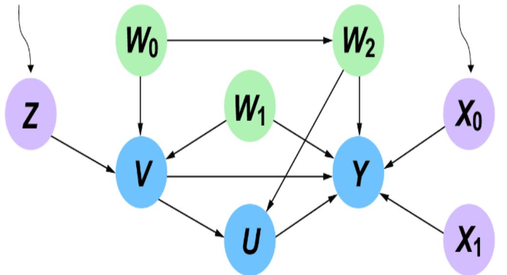
Figure 4.17 Z, X0, and X1 were included in the DAG because they pla y a useful role in analyzing the causal e ect of U on Y. Their role depends on conditional independence, and it is important to test that they can indeed serve those roles.

We’ll discuss instrumental variables in depth in chapter 11. For now, su ce it to say that for Z to be an instrument, it must be independent of W0, W1, and W2. So we’d pay special attention to testing that assumption.

4.4Caveatswithconditional independencetesting

As I mentioned, conditional independence tests ar e per haps the most obvious way to test the conditional independence constraints implied by your pr oposed causal DAG. However, ther are several caveats with using statistical tests to test a causal D AG. In my e xperience, these issues can distract analysts fr om their ultimate goal of answering a causal question. In this section, I’ll highlight some of these caveats and pr opose some alter natives to conditional independence testing. The main tak eaway is that statistical testing is an important tool for building your D AG, but as with any statistical methodology, it is not a panacea (and that’s fine).

4.4.1 Statistical tests alwa ys have some chance of error

I mentioned that with d-separation, we should not ૿confuse the map for the ter rain; d-separation is not the same thing as conditional independence. R ather, if your model is a good representation of causality, d-separation implies conditional independence.

Similarly, conditional independence is not the same as statistical evidence of conditional independence. The causal structur e of the DGP imposes conditional independence constraints on the joint pr obability distribution. But you can’t ૿see the joint distribution and the independencies it contains; you can only ૿see (and run statistical tests on) the data sampled fr om that distribution.

Just lik e with pr ediction, classi fication, or any other statistical patter n ecognition pr ocedur e, the pr ocedur e for detecting these independencies in data can get it wr ong. Y ou can get false negatives, wher e a pair of variables ar e truly conditionally independent but the statistical independence test concludes they ar e dependent. Y ou can have false positives, wher e a statistical independence test finds a pair of variables to be conditionally independent when they ar e not.

4.4.2 Testing causal DAGs with traditional CI tests is flawed

I say that the pr oposed conditional independence tests for refutation ar e ૿flawed because they violate the spirit of statistical hypothesis testing in science. Suppose you think you have discover ed some patter n in stock prices. Y ou ar e biased to think the patter n is mor e than coincidence because, if it is, you can mak e money . To be rigor ous and not fall pr ey to your biases, your alter native hypothesis says the patter n is r eal and e xploitable, wher eas the null hypothesis is that it is just random noise. The fr equentist test assumes the null hypothesis is true and gives you a p-value, which quanti fies the chances that random noise could for m a patter n at least as str ong as the one you found. The test forces you to r eject the patter n as r eal unless that p-value is really small. Most mainstr eam statistical testing libraries ar e designed for this use case.

When you pr opose a causal model, you ar e also biased to believe it is true. But causal models induce conditional independences, which by de finition ar e the absences of patter ns. In this case the null and alter native hypotheses should switch; the alter native should be that your model is right and ther e isn’t a patter n (and any evidence of patter ns in the data is just spurious cor relation), and the null should be that ther eis a patter n. It is possible to implement such a hypothesis test, but it is not mathematically trivial, and most mainstr eam statistical libraries lik e SciPy do not support this use case.

The compr omise is using the traditional tests, wher e the null hypothesis speci fies conditional independence less as a theor etically rigor ous analysis and mor e as a heuristic —an empirical pr obem solving technique that can be suboptimal but sucient to r each a good enough solution.

4.4.3 p-values vary with the size of the data

The conclusion of a traditional conditional independence test depends on a signi ficance thr eshold. If the p-value falls below this thr eshold, you favor dependence, and if it falls above, you favor conditional independence. The choice of threshold is a bit arbitrary; people tend to go with commonly selected values lik e .1 or .05 or .01.

The pr oblem is that the p-value statistic varies with the size of the data. All else equal, as the size of the data incr eases, the p-value decr eases. In other wor ds, the lar gr the data, the mor e that things start to look dependent. If you have a large dataset, it is mor e lik ely that p-values will fall below that arbitrary thr eshold, and the data will look lik e it’s refuting the conditional independence implied by your D AG, even when that conditional independence is true.

To illustrate, the test of E ⊥ T | O, R in section 4.3.2 had 30 data points and pr oduced a p-value of 0.56. In our data, E ⊥ T | O, R is gr ound truth (via simulation), so if a test concludes against E ⊥ T | O, R, it is because of statistical issues with the test, not the quality of the data. The following bootstrap statistical analysis will show how the estimate of the p-value falls as the size of the data incr eases.

First, we’ll write a sample_p_value function that samples a pvalue for a given data size. The ne xt function, estimate_p_value , will do this sampling r epeatedly and calculate a mean p-value, a 90% con fidence interval, and the pr obability that the p-value falls below the signi ficance threshold, which is the pr obability of r ejecting the cor rect conclusion that E ⊥ T | O, R.

Listing 4.8Bootstrap analysis of sensitivity of test of E T | O, R to sample size

from numpy import mean, quantile

def sample_p_val(data_size, data, alpha): #1 bootstrap_data = data.sample(n=data_size, replace=True) #1 result = chi_square( #1 X=“E”, Y=“T”, Z=[“O”, “R”], #1 data=bootstrap_data, #1 boolean=False, #1 significance_level = alpha #1 ) #1 p_val = result[1] #1 return p_val #1 def estimate_p_val(data_size, data=fulldata, boot_size=1000, α=.05): #2 samples = [ #2 sample_p_val(data_size, data=fulldata, alpha=α) #2 for _ in range(boot_size) #2 ] #2 positive_tests = [p_val > significance for p_val in samples] #3 prob_conclude = mean(positive_tests) #4 p_estimate = mean(samples) #4 quantile_05, quantile_95 = quantile(samples, [.05, .95]) #5 lower_error = p_estimate - quantile_05 #5 higher_error = quantile_95 - p_estimate #5 return p_estimate, lower_error, higher_error, prob_conclude data_size = range(30, 1000, 20) #6 result = list(zip(*[estimate_p_val(size) for size in data_size])) #6 #1 Given a certain data size, this function randomly samples that number of rows from the full dataset. It then runs the chi-squared independence test and returns the p-value. #2 This function conducts a ૿bootstrap procedure that samples 1,000

p-values for a given data size and calculates the mean p-value and 90% p-value con fidence interval.

#3 Calculate the probability of a test concluding in favor of conditional independence. #4 Calculate the mean of the p-values to get the bootstrap mean.

#5 Calculate the 5th and 95th percentiles to get a 90% bootstrap confidence interval.

#6 Run the bootstrap analysis.

Finally, we’ll visualize the r esults. W e’ll plot the size of the data against the mean and 90% con fidence intervals for the p-values we get for that given data size. W e’ll also plot how the pr obability of concluding in favor of the true hypothesis (E ⊥ T | O, R) for a signi ficance level of .05 depends on data size.

Listing 4.9Visualize dependence of conditional independence testing on data size

import numpy as np import matplotlib.pyplot as plt p_vals, lower_bars, higher_bars, probs_conclude_indep = result #1 plt.title(‘Data size vs. p-value (Ind. of E & T | O & R)’) #2 plt.xlabel(“Number of examples in data”) #2 plt.ylabel(“Expected p-value”) #2 error_bars = np.array([lower_bars, higher_bars]) #2 plt.errorbar( #2 data_size, #2 p_vals, #2 yerr=error_bars, #2 ecolor=“grey”, #2 elinewidth=.5 #2 ) #2 plt.hlines(significance, 0, 1000, linestyles=“dashed”) #2 plt.show() plt.title(‘Probability of favoring independence given data size’) #3 plt.xlabel(“Number of examples in data”) #3 plt.ylabel(“Probability of test favoring conditional independence”) #3 plt.plot(data_size, probs_conclude_indep) #3

#1 Run the bootstrap analysis to get quantiles of p-values and probability of concluding in favor of independence. #2 Plot the data size vs. p-value. At larger data sizes, the expected pvalue falls below a threshold. #3 Plot data size vs. the probability of concluding in favor of independence, given .05 signi ficance.

Figure 4.18 shows the first plot. The descending curve is the expected p-values at di erent data sizes, the vertical lines are error bars showing a 90% bootstrap con fidence interval. By the time we get to a dataset of size 1,000, the e xpected p-value is below the thr eshold, meaning that the test favors the conclusion that E ⊥ T | O, R is false.

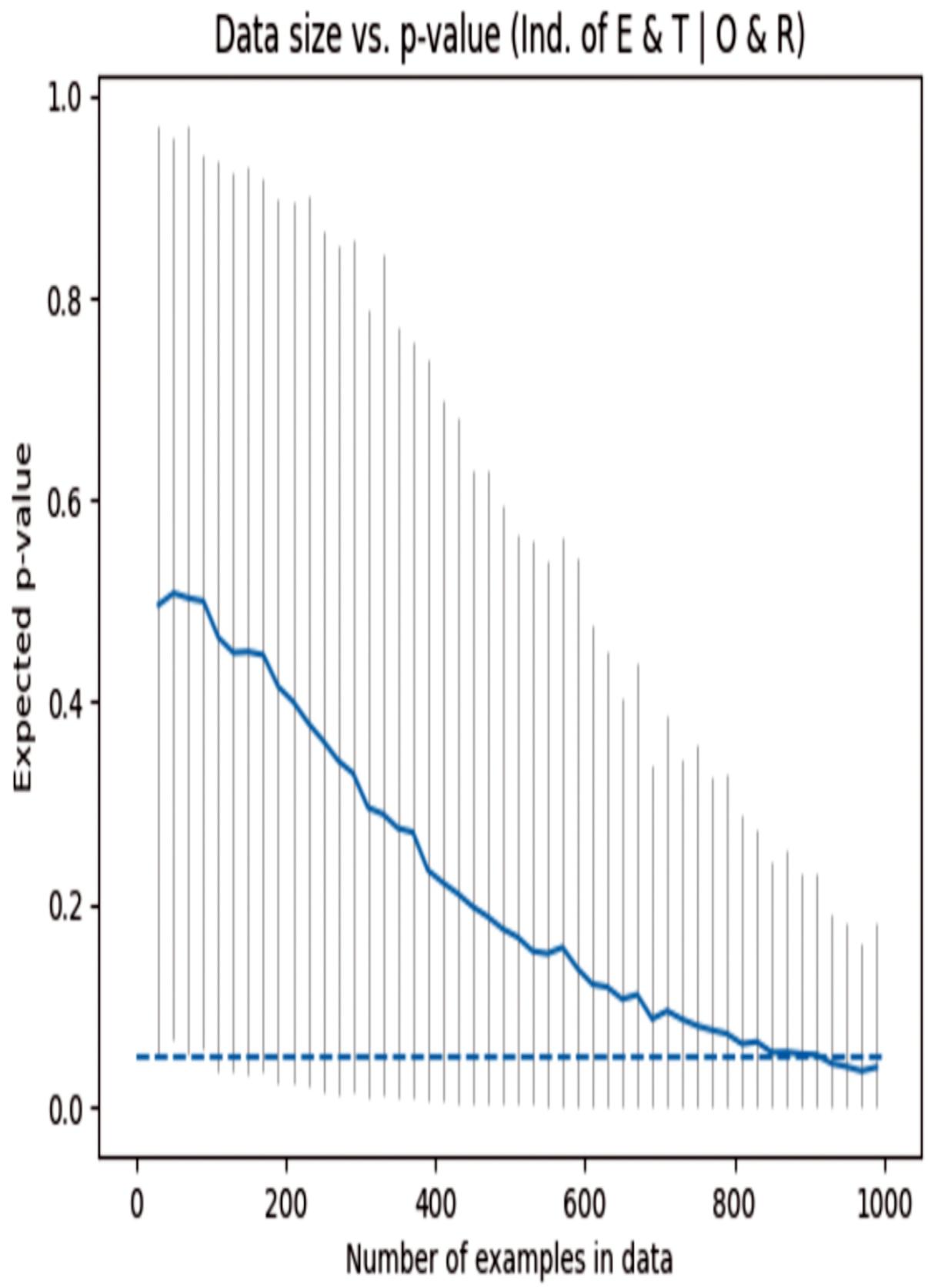
Figure 4.18 Sample size vs. expected p-value of the conditional independence test for E T | O, R (solid line). The vertical lines are the error bars; they show the 90% bootstrap con fidence intervals. The horizontal dashed line is a .05 signi ficance level, above which we favor the null hypothesis of conditional independence and below which we reject it. As the sample size increases, we eventually cross the line. Thus, the result of our refutation analysis depends on the size of the data.

Note that the lower bound of the con fidence interval cr osses the signi ficace thr eshold well befor e 1,000, suggesting that at even lower data sizes, we have a good chance of r ejecting the true conclusion of E ⊥ T | O, R. This becomes clear er in figure 4.19, wher e the pr obability of concluding in favor of the true conclusion decr eases as the size of the data increases.

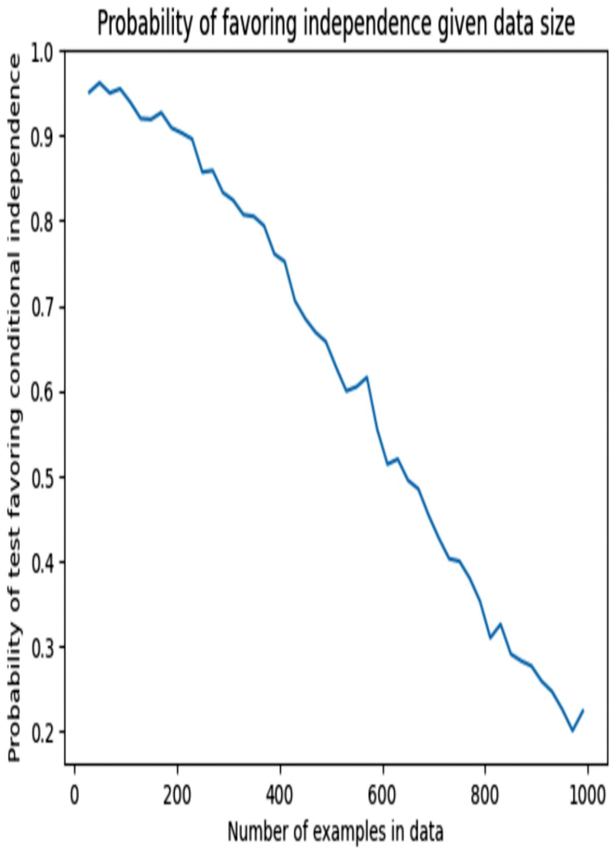
Figure 4.19 As the size of the data increases, the probability of concluding in favor of this (true) instance of the conditional independence relation E T | O, R decreases.

You might think that as the size of the data incr eases, the algorithm is detecting subtle dependencies between E and T that wer e undetectable with less data. Not so, for this transportation data is simulated in such a way that E ⊥ T | O, R is de finitely true. This is a case wher e more data leads us to r ejecting independence because mor e data leads to mor e spurious cor relations—patter ns that ar en’t r eally ther e.

A causal model is either right or wr ong about causality in the DGP it describes. The conditional independence the model implies is either ther e or it’s not. Y et if that conditional independence is ther e, the test can still conclude in favor of dependence when the data is arbitrarily lar ge.

Again, if we view conditional independence testing as a heuristic for r efuting our D AG, then this sensitivity to the size of the data shouldn’t upset us. R egardless of the data size and the signi ficance thr esholds, the relative dierences between p-values when ther e is no conditional independence and when ther e is will be lar ge and obvious.

4.4.4 The problem of multiple comparisons

In statistical hypothesis testing, the mor e tests you run, the more testing er rors you rack up. The same is true when running a test for each d-separation implied by a causal DAG. In statistics, this pr oblem is called the multiple comparisons problem . Ther e are solutions to dealing with multiple comparisons pr oblems, such as using false discovery rates . If you ar e familiar with such methods, applying them won’t hurt. If you want to lear n more, see the chapter’s notes at https://www .altdeep.ai/p/causalaibook for refernces to false discovery rates in the conte xt of causal

modeling. But again, I encourage you to view traditional conditional independence testing as a heuristic that helps with the ultimate goal of building a good causal D AG. Focus on this goal and on the subsequent causal infer ence analysis you will conduct using your D AG, and avoid rabbit holes of statistical testing rigor .

4.4.5 Conditional independence testing struggles in machine learning settings

Commonly used libraries for conditional independence testing ar e generally limited to one-dimensional variables with fairly simple patter ns of cor relation between them. pgmpy’s conditional independence tests, which ar e imported from SciPy, ar e no e xception. In r ecent years, several nonparametric tests have been developed for mor e nuanced distributions, such as k ernel-based conditional independence tests. T ests in the PyWhy library PyWhy -Stats ar e a good place to start if you ar e inter ested in such tests.

However, in machine lear ning, it is common for variables to have mor e than one dimension such as vectors, matrices, and tensors. F or example, one variable in a causal D AG might r epresent a matrix of pix els constituting an image. Further, the statistical associations between these variables can be nonlinear .

One solution is to focus on pr ediction. If two things ar e independent, they have no ability to pr edict one another . Suppose we have two pr edictive models M1 and M2. M1 predicts Y using Z as a pr edictor . M2 predicts Y using X and Z as a pr edictor . Predictors can have dimensions gr eater than one. If X ⊥ Y | Z, then any X has no pr edictive infor mation about Y beyond what is alr eady pr ovided by Z. So you can test X ⊥ Y | Z by comparing the model pr edictive accuracy of M2to M1. When the models perfor m similarly, we have

evidence of conditional independence. Note that you’d want to pr event M2 from ૿cheating on its pr edictive accuracy by taking steps to avoid over fitting—yet another way spurious correlation can cr eep into our analysis.

4.4.6 Final thoughts

Conditional independence testing is an e xtensive and nuanced subject. Y our goal with this testing is to r efute your causal D AG, not to cr eate the Platonic ideal of a conditional independence testing suite. I r ecommend getting a testing workflow that is good enough , and then focusing on building your D AG and using that D AG in downstr eam causal infer ences. F or example, if I had a mix of continuous and discr ete variables, then rather than implementing a test that could accommodate my di erent data types, I would discr etize my continuous variables (for e xample, tur ning age as time since birth into age brack ets) and use a vanilla chisquar ed test, to k eep things moving along.

4.5RefutingacausalDAG given latentvariables

The method of testing D AGs with conditional independence has a latent variable pr oblem. If a variable in our causal D AG is latent (not observed in the data), we can’t run any conditional independence tests involving that variable. That is a major pr oblem; if a variable is an important part of the DGP, we can’t e xclude it fr om our D AG simply because we can’t test independence assertions with that variable.

To illustrate, consider the causal D AG in figure 4.20. This figure represents how smoking behavior ( S) is in fluenced both by the cost of cigar ettes ( C ) as well as genetic factors (denoted D as in ૿ DNA) that mak e one mor e or less pr one to

nicotine addiction. Those same genetic factors in fluence one’s lik elihood of getting lung cancer ( L). In this model, smoking’s e ect on cancer is mediated thr ough tar buildup (T ) in the lungs.

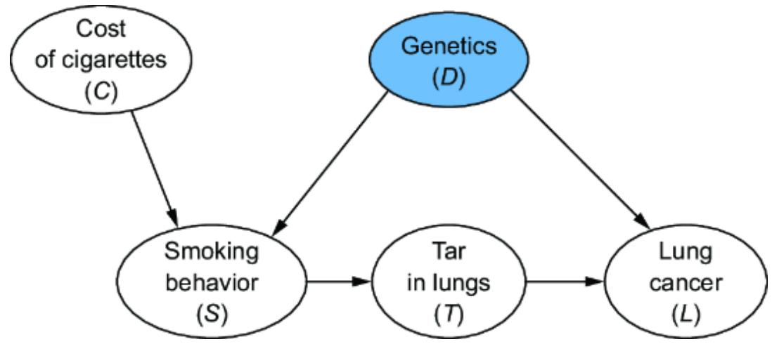
Figure 4.20 A causal DAG representing smoking’s e ect on cancer . The variable for genetics ( D) is gra y because it is unobserved in the data, so we can’t run tests for conditional independencies involving D. However , we can test other types of constraints.

If we have data observing all these variables, we can run conditional independence tests tar geting the following dseparations: ( C ⊥G T | S), ( C ⊥G L | D, T), ( C ⊥G L | D, S), ( C ^G D), ( S⊥G L | D, T), and ( T ⊥G D | S). But suppose we don’t have data on the genetics variable ( D). F or example, perhaps measuring this genetics featur e requir es an infeasibly e xpensive and invasive laboratory test. Of all the d-separations we listed, the only one not involving D is ( C ⊥G T | S). We are down fr om six to one feasible conditional independence test with which to test our D AG.

In general, a pr oposed causal model can have various implications for the joint pr obability distributions that ar e testable with data. The conditional independence implied by the graph structur e is one type of testable implication. But some of the model’s implications ar e testable in cases of

latent variables. In this section, we’r e going to look at how we can test a D AG with one of these latent variable–r elated constraints.

4.5.1 An example of a testable implication that works with latent variables

The causal Mark ov assumption says d-separations imply conditional independence in the data. So far, we’ve e xplor ed direct conditional independence between variables, but when some variables ar e latent, the graph can imply conditional independence between functions of observed variables . These implications ar e called ૿V erma constraints in the literatur e, though I will use the less jar gony ૿ functional constraints.

To illustrate, the D AG in figure 4.20 with latent variable D has the following functional constraint (for now, don’t wor ry about how its derived):

\[C\bot\_{G} h\left(L, C, T\right)\]

\[h\left(l, c, t\right) = \sum\_{s} P\left(l|c, s, t\right) P\left(s|c\right)\]

Just as the d-separation ( C ⊥G T | S) implies that the conditional independence statement ( C ⊥ T | S) should hold for the observational joint distribution, the functional constraint ( C ⊥G h(L, C, T)) implies that C is independent of some function h(.) of variables L, C, and T in the observational joint distribution. Both implications ar e testable since they don’t involve D. We now have two tests we can run instead of one.

h(.) has two components:

P(l |c, s, t) is a function that returns the probability that L = l(suppose lis૿true for ૿has lung cancer and false for ૿ no lung cancer ), given C = c, S = s, and T = t.
P(s|c) is a function that returnsthe probability that S= s (suppose sis૿low, ૿medium, or ૿high depending on how heavily a smoker smokes) given the cost of cigar ettes C = c.

h(.) then sums over all values of S. The function’s output is a random variable that, accor ding to the D AG, should be independent of C. h(l, c, t) is a function of P(l |c, s, t) and P (s|c), and it may feel odd thinking about independence in terms of pr obability functions. R emember that the independence r elation is itself just a function of joint probability distributions.

Next, we’ll fit models of P(l |c, s, t) and P(s|c) fr om data and test this independence r elation. But first, we’ll look at libraries that let us enumerate functional constraints lik e (C ^G h(L, C, T )) fr om a D AG just lik e we could enumerate dseparations with pgmpy’s get_independencies .

4.5.2 Libraries and perspectives on testing functional constraints

How do we derive functional constraints lik e C ⊥G h(L, C, T )? Like d-separation, we can derive this type of constraint algorithmically fr om the graph. One implementation is in the verma.constraints function in the causale ect R library . This function tak esin the D AG with nodes labeled as latent and returns a set of testable constraints just lik e pgmpy’s get_independencies . For Python, the library Y0 (pr onounced why-not) has a r_get_verma_constraints function (as of version 0.2.10), which is a wrapper that calls causale ect’s R code. I’ll omit the Python code her e because it r equir es

installing R, but visit www .altdeep.ai/causalAIbook for links to libraries and r efernces.

MATHEMATICAL INTUITION FOR FUNCTIONAL CONSTRAINTS, AND SOME ADVICE

Our goal for this section is only to show that ther e are ways to test your causal model even when ther e are latent variables. F unctional constraints ar e one way to do this, but we don’t want to over -inde x on this particular flavor of testable implication. It is mor e important to avoid the danger ous mindset of limiting ourselves only to D AGs that are fully observed in the data.

That said, for the curious, I’ll o er a very high-level intuition for the math. R ecall that the local Mark ov pr operty says that a node is conditionally independent of its nondescendants, given its parents . From ther e, we derive graphical criteria called d-separation that lets us find sets of nodes wher e this applies, we write a graph algorithm that uses those criteria to enumerate d-separations, and we use that algorithm to enumerate some conditional independence tests we can run.

For a given node X, let’s say ૿ orphaned cousins means non-descendants of X that shar e a latent ancestor of X. Here is, in infor mal ter ms, a latent variable analog to the local Mark ov pr operty : A node is conditionally independent of its non-descendants given its nearest observed ancestors, its orphaned cousins, and other nearest observed ancestors of those cousins . Just as with dseparations, we can derive graphical criteria to identif y individual cases wher e this applies.

Recall that we can factorize the joint pr obability distribution such that each factor is the conditional probability of a node’s outcome, given its par ents. The probability functions in the functional constraint (lik e the P(l|c, s, t) and P(s|c) ter ms in h(l,c,t)) come into the pictur e

once we start mar ginalizing that factorization over the latent variables and doing subsequent pr obability math.

See the r efernces listed at https://www .altdeep.ai/p/causalaibookif you want to deep dive. But my war ning fr om the pr evious section holds her e —our goal is to falsify our DAG and move on to our target causal inference . Bewar e of falling down statistical, mathematical, and theor etical rabbit holes on the way to that goal.

Now that we have a new testable implication in the for m of C ^G h(L, C, T ), let’s test it out.

4.5.3 Testing a functional constraint

To test ( C ⊥G h(L, C, T )), we have to calculate h(l, c, t) = SP(l|c, s, t)P(s|c) for each item in our data. That r equir es us to model P(l | c, s, t) and P(s|c). Ther e are several modeling appr oaches we could go with, but we’ll use a naive Bayes classi fier for this e xample so we can stick with using the pgmpy and pandas libraries. W e’ll tak e the following steps:

1. Discr etize cost (C ) so we cantreat it asa discr ete variable.
1. Use pgmpy to fit a naiveBayes classi fier to P(l| c, s, t) and P(s|c).
1. Write a function that takes in values of L, C, T and calculates h(L, C, T ).
1. Apply that function to each row in the data to get anew column of h(L, C, T ) values.
1. Run an independence test between that column and the C column.

SETTING UP Y OUR ENVIRONMENT

The following code uses pgmpy version 0.1.19 because versions up to 0.1.24 (cur rent at the time of writing) have a bug (alr eady r eported) that can cause issues with some of the naive Bayes classi fier infer ence code. Y ou don’t need to do this if you use another method of calculating P(l|c, s, t) and P(s|c). F or stability, we’ll also use pandas version 1.4.3, which was the version when pgmpy 0.1.19 was current. Note that if you have installed later versions of pgmpy and pandas, you might have to uninstall those versions befor e installing these, or you could just spin up a new Python envir onment. V isit https://www .altdeep.ai/p/causalaibookfor links to the Jupyter notebooks with the code and notes on setting up a working envir onment.

First, we’ll import the data. W e’ll also discr etize the cost of cigar ettes ( C)so it is mor e amenable to modeling with pgmpy.

Listing 4.10 Importing and formatting cigarette and cancer data from functools import partial import numpy as np import pandas as pd data_url = “https://raw.githubusercontent.com/altdeep/causalML/master [CA] /datasets/cigs_and_cancer.csv” data = pd.read_csv(data_url) #1 cost_lower = np.quantile(data[“C”], 1/3) #2 cost_upper = np.quantile(data[“C”], 2/3) #2 def discretize_three(val, lower, upper): #2 if val < lower: #2 return “Low” #2 if val < upper: #2 return “Med” #2 return “High” #2 #2 data_disc = data.assign( #2 C = lambda df: df[‘C’].map( #2 partial( #2 discretize_three, #2 lower=cost_lower, #2 upper=cost_upper #2 ) #2 ) #2 ) #2 data_disc = data_disc.assign( #3 L = lambda df: df[‘L’].map(str), #3 ) #3 print(data_disc)

#1 Load the C SV file into a pandas ΔataF rame. #2 Δiscretize cost (C) into a discrete variable with three levels to facilitate conditional impendence tests. #3 Δiscretize cost (C) into a discrete variable with three levels to facilitate conditional impendence tests. #4 Turn lung cancer (L) from a Boolean to a string, so the conditional independence test will treat it as a discrete variable.

The print(data_disc) line prints out the elements of the data_disc DataF rame.

C S T L 0 High Med Low True 1 Med High High False 2 Med High High True 3 Med High High True 4 Med High High True .. … … … … 95 Low High High True 96 High High High False 97 Low Low Low False 98 High Low Low False 99 Low High High True [100 rows x 4 columns]

Now we need to model P(l| c, s, t) and P(s|c). We’ll opt for a naive Bayes classi fier, a pr obabilistic model that ૿ naively assumes that, in the case of P(l| c, s, t), cost ( C), smoking (S), and tar ( T ) ar e conditionally independent given lung cancer status ( L). A ccording to our causal D AG, that is clearly not true, but that doesn’t matter if all we want is a good way to calculate pr obability values for L given C, S, and T. A naive Bayes classi fier will do that well enough.

Listing 4.11 Fit naive Ba yes classi fier of P(l| c, s, t)

from pgmpy.inference import VariableElimination from pgmpy.models import NaiveBayes model_L_given_CST = NaiveBayes() #1 model_L_given_CST.fit(data_disc, ‘L’) #1 infer_L_given_CST = VariableElimination(model_L_given_CST) #1 #1 def p_L_given_CST(L_val, C_val, S_val, T_val):#1 result_out = infer_L_given_CST.query( #1 variables=[“L”], #1 evidence={‘C’: C_val, ‘S’: S_val, ‘T’: T_val}, #1 show_progress=False #1 ) #1 var_outcomes = result_out.state_names[“L”] #1 var_values = result_out.values #1 prob = dict(zip(var_outcomes, var_values)) #1 return prob[L_val] #1

#1 We’ll use a naive Ba yes classi fier in pgmpy to calculate the probability value for a given value of L given values of C, S, and T . In this case, we’ll use variable elimination. #2 We’ll use a naive Ba yes classi fier in pgmpy to calculate the probability value for a given value of L given values of C, S, and T . In this case, we’ll use variable elimination.

Now we’ll do the same for P(s|c).

Listing 4.12 Fit naive Ba yes classi fier of P(s|c)
model_S_given_C = NaiveBayes() 
model_S_given_C.fit(data_disc, 'S') 
infer_S_given_C = VariableElimination(model_S_given_C) 
def p_S_given_C(S_val, C_val): 
 result_out = infer_S_given_C.query( 
 variables=['S'], 
 evidence={'C': C_val}, 
 show_progress=False 
 ) 
 var_names = result_out.state_names["S"] 
 var_values = result_out.values 
 prob = dict(zip(var_names, var_values)) 
 return prob[S_val]

Now we’ll bring these together to implement the h(L, T, C) function. The following code uses a for loop to do the summation over S.

Listing 4.13 Combine models to create h(L, T, C)

def h_function(L, C, T): #1
 summ = 0 #2
 for s in ["Low", "Med", "High"]: #2
 summ += p_L_given_CST(L, C, s, T) * p_S_given_C(s, C) #2
 return summ

#1 Implement h(L, C, T). #2 Implement the summation of P(l|c,s,t) * P(s|c) over s.

Now, we’ll calculate the full set of outcomes for set { C, T, L}. Given these outcomes, we can calculate the h(L, C, T ) for each of these combinations using the pr eceding function.

Listing 4.14 Calculate the outcome combinations of C, T, and L

ctl_outcomes = pd.DataFrame(
 [ #1
 (C, T, L) #1
 for C in ["Low", "Med", "High"] #1
 for T in ["Low", "High"] #1
 for L in ["False", "True"] #1
 ], #1
 columns = ['C', 'T', 'L'] #1
)

#1 Calculate these values for each possible combination of outcomes of L, C, and T . First, we use list comprehensions to mak e a ΔataF rame containing all the combinations.

Printing this shows all combinations of outcomes for C, T, and L.

	C	T		L
0		Low	Low	False
1		Low	Low	True
2		Low	High	False
3		Low	High	True
4		Med	Low	False
5		Med	Low	True
6		Med	High	False
7		Med	High	True
8	High		Low	False
9	High		Low	True
10	High		High	False
11	High		High	True

For each of these outcomes, we’ll apply h(L, C, T).

Listing 4.15 Calculate h(L, C, T) for each outcome of C, T , L h_dist = ctl_outcomes.assign( h_func = ctl_outcomes.apply( lambda row: h_function( row[‘L’], row[‘C’], row[‘T’]), axis = 1 ) ) print(h_dist)

Now for each joint outcome of C, T, and L, we have a value of h(L, C, T).

	C	T	L	h_func
0	Low	Low	False	0.392395
1	Low	Low	True	0.607605
2	Low	High	False	0.255435
3	Low	High	True	0.744565
4	Med	Low	False	0.522868
5	Med	Low	True	0.477132
6	Med	High	False	0.369767
7	Med	High	True	0.630233
8	High	Low	False	0.495525
9	High	Low	True	0.504475
10	High	High	False	0.344616
11	High	High	True	0.655384

Finally, we’ll mer ge this h_func distribution into the dataset such that for each r ow of our data, we get a value of h(L, C, T).

Listing 4.16 Merge to get a value of h(L, C, T) for each row in the data

df_mod = data_disc.merge(h_dist, on=[‘C’, ‘T’, ‘L’], how=‘left’) #1 print(df_mod) #1 Add a column representing the variable h(L, C, T).

We see the r esult with print(df_mod) :

	C	S	T	L	h_func
0	High	Med	Low	True	0.504475
1	Med	High	High	False	0.369767
2	Med	High	High	True	0.630233
3	Med	High	High	True	0.630233
4	Med	High	High	True	0.630233

95	Low	High	High	True	0.744565
96	High	High	High	False	0.344616
97	Low	Low	Low	False	0.392395
98	High	Low	Low	False	0.495525
99	Low	High	High	True	0.744565

		[100 rows x 5 columns]

The functional constraint says that C and h(L, C, T ) should be independent, so we can look at the evidence of independence between the h_func column and the C column. Since we discr etized C, our calculated outcomes for h(L, C, T ) ar e technically discr ete, so we could use a chi-squar ed test. But h(L, C, T ) is continuous in theory, so instead we’ll use a bo x plot to visualize dependence between the two variables. The functional constraint says C and h(L, C, T ) should be independent, so we’ll use a bo x plot that plots values of h(L, C, T ) against values of C to visually inspect whether C and h(L, C, T ) look independent.

Listing 4.17 Box plot visualizing independence between C and h(L, C, T) df_mod.boxplot(“h_func”, “C”)

This pr oduces figure 4.21.

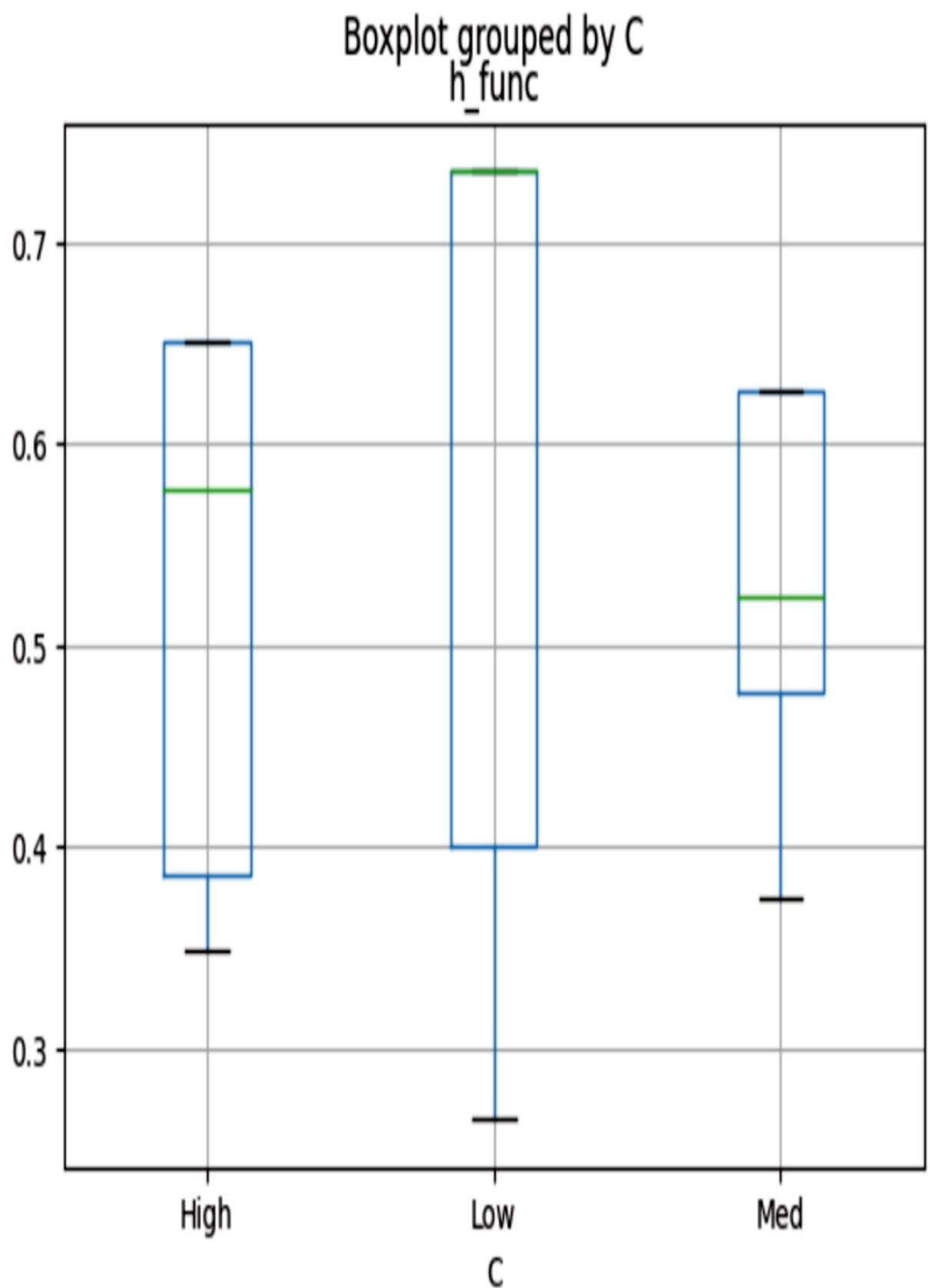
Figure 4.21 A box plot visualization of cost ( C) on the x-axis and the function h(L, C, T) on the y-axis (labeled ૿Sum product). The overlap of the distributions of the sum product for each value of C supports the functional constraints assertion that these two quantities are independent.

The x-axis in figure 4.21 is di erent levels of cost (low, medium, and high). The y-axis r epresents values of the sum. Figure 4.21 is a bo x wand whisk ers plot; each bo x is a representation of the distribution of the sum pr oduct for a given value of C. The top and bottom of the bo xes ar e the quartiles of the distribution, the lines in the middle of the boxes ar e the median, and the shorter horizonal lines ar e the max and min values (for low cost, the median, upper quartile, and max ar e quite close). In summary, it looks as though the distributions of the sum pr oduct don’t change much acr oss the di erent levels of cost; that’s what independence is supposed to look lik e.

We can also derive a p-value using an analysis of variance (ANOVA) appr oach, this time using an F-test rather than a chi-squar ed test. The following code uses the statsmodels library to run an ANO VA test.

Note ૿ PR( >F) means the pr obability of seeing an Fstatistic for a given variable (in our case, C) is at least as large as the F-statistic calculated fr om the data, assuming that the variable is independent of sum_product (i.e., the p-value).

Listing 4.18 Using ANO VA to evaluate independence

from statsmodels.formula.api import ols import statsmodels.api as sm

model = ols(‘h_func ~ C’, data=df_mod).fit() #1 aov_table = sm.stats.anova_lm(model, typ=2) #1 print(aov_table[“PR(>F)”][“C”]) #1

model = ols(‘h_func ~ T’, data=df_mod).fit() #2 aov_table = sm.stats.anova_lm(model, typ=2) #2 print(aov_table[“PR(>F)”][“T”]) #2

model = ols(‘h_func ~ L’, data=df_mod).fit() #3 aov_table = sm.stats.anova_lm(model, typ=2) #3 print(aov_table[“PR(>F)”][“L”]) #3

#1 A recipe for doing ANO VA using the statmodels library #2 Returns a high p-value, which supports (fails to falsify) the assertion that h(L, C, T) and C are independent #3 Just as a sanity check, we run the same test to see whether h(L, C, T) looks independent of T and L. Unlik e C, T and L should not be independent of h(L, C, T) and as expected, these tests return much smaller p-values, indicating dependence.

We print the p-value for C with print(aov_table[“PR(>F)”][“C”]) and get ~0.1876. That p-value indicates we can’t r eject the null hypothesis of independence, so it looks lik e the data supports the constraint. W e also run the same test for T and L and, as e xpected, these ar e much smaller, indicating evidence of dependence. They ar e lower, both falling below the common .1 thr eshold wher e a standar d hypothesis test would r eject the hypothesis that h(L, C, T) is independent of T and L.

4.5.4 Final thoughts on testable implications

A DAG’s d-separation and functional constraints imply that certain conditional independencies should hold in the joint probability distribution if the D AG is a good causal model of the DGP . We can falsif y the D AG by running statistical tests for conditional independence.

More generally, a causal model can have di erent mathematical implications for the underlying joint pr obability distribution, and some of these can be tested. F or example, if your model assumed the r elationship between a cause and e ect was linear, you could look for evidence of nonlinearity in the data (we’ll see mor e about functional causal assumptions in chapter 6). And, of course, you can falsif y your model’s implications with e xperiments (as we’ll see in chapter 7).

The better we get at causal modeling, the better we get at testing and falsif ying our causal models. But r emember, don’t let the statistical and mathematical nuances of testing distract you fr om your goal of getting a good enough model and moving on to your tar get causal infer ence.

4.6Primeron(theperilsof)causal discovery

In the pr evious work flow, we pr oposed a causal D AG, consider ed what implications (lik e conditional independence) the D AG had for the observational joint distribution, and then tested those implications with the data. What if we went in the other dir ection? What if we analyzed the data for statistical evidence of causality induced constraints, and then constructed a causal D AG that is consistent with those constraints?

This describes the task of causal discovery : statistical learning of causal D AGs fr om data. In this section, I’ll pr ovide a brief primer on causal discovery and cover what you need to know to mak e use of this class of algorithms.

BEWARE THE F ALSE PROMISES OF CA USAL DISCO VERY

Causal discovery algorithms ar e often pr esented as magical tools that convert any dataset, no matter how limited in quality, into a causal D AG. That false pr omise discourages the mindset of modeling the DGP (rather than the data) and falsif ying candidate models. It is also why it is har d to find consistent use cases for discovery in practice. This section tak es the appr oach of framing how discovery algorithms work and wher e they fail, rather than going thr ough a list of algorithms. I’ll conclude with advice about how to e ectively incorporate these algorithms into your analysis work flow.

We’ll start with an overview of k ey ideas that underpin discovery algorithms.

4.6.1 Approaches to causal discovery

There are several appr oaches to causal discovery . Some algorithms (of ten called constraint-based algorithms) do what I just suggested—r everse engineer a graph fr om evidence of conditional independence in the data. Other algorithms (of ten called score-based algorithms) tur n the causal D AGinto an e xplanatory model of the data and find causal D AGs that have a high goodness- of-fit scor e. Y et another appr oach is to assume additional constraints on the functional r elationships between par ents and childr en in the causal D AG, as we’ll see with structural causal models in chapter 6.

The space of possible D AGs is a discr ete space. One class of approaches tries to sof ten this space into a continuous space and use continuous optimization techniques. The popularity of automatic di erentiation libraries for deep lear ning have accelerated this tr end.

Because the space of D AGs can be quite lar ge, it is useful to incorporate prior knowledge to constrain the size of that space. This of ten tak es the for m of specif ying what edges must be pr esent or what must be absent, or of using Bayesian priors on graph structur e.

Some causal discovery algorithms can work with experimental data. This r equir es telling the algorithm which variables wer e set by the e xperimenter (or as we’ll say starting in chapter 7, which wer e ૿intervened upon ).

To get started with causal discovery using Python, I recommend the PyWhy libraries for causal discovery such as causal-lear n and DoDiscover .

4.6.2 Causal discovery , causal faithfulness, and latent variable assumptions

The causal Mark ov pr operty assumes that if our D AG is true, d-separations in that D AG imply conditional independence statements in the joint pr obability of the variables:

Causal faithfulness (or just ૿ faithfulness) is the converse statement—conditional independence in the joint distribution implies d-separation in the graph:

Many causal discovery algorithms r ely on an assumption that faithfulness holds. It may not.

DISCOVERY AND F AITHFULNES S VIOLA TIONS

In section 4.4, we used the Mark ov pr operty to test a candidate D AG; given a d- separation statement that held for the D AG, we ran a statistical test to check for empirical evidence of the conditional independence implied by that dseparation.

Imagine you wanted to build your graph by going in r everse. You detect evidence of an instance of conditional independence in your data, and then you limit your space of candidate D AGs to those consistent with the implied dseparation. Y ou do this iteratively until you’ve nar rowed down the space of candidate D AGs. Some discovery algorithms do some version of this pr ocedur e, and those that do ar e relying on a faithfulness assumption.

Note Algorithms that match evidence of conditional independence to d-separation ar e often called ૿constraint-based discovery algorithms. A well-known example is the PC algorithm. Constraint-based algorithms find DAGs that ar e constrained to be consistent with the empirical evidence of causality .

The tr ouble comes fr om ૿faithfulness violations—special cases wher e conditional independence in a joint pr obability distribution does not map to d-separation statements in a ground truth D AG. A simple e xample of a faithfulness violation is the case of a thr ee-variable system that can decompose as follows: P(x, y, z) = P(x, y)P(y, z)P(x, z). That is, for any value of one variable, the association between the other two variables is always the same. Y ou could detect this peculiar for m of independence in data, but you can’t r epresent it with d-separation in a D AG. (If you don’t believe me, try .)

Resear chers wor ry about these special cases because they mean a discovery algorithm that r elies on faithfulness doesn’t generalize to all distributions. When you use these algorithms, you ar e assuming faithfulness holds for you problem domain, and that’s not something you can test. However, violations of causal faithfulness ar e not typically the biggest sour ce of headaches in practical causal discovery . That honor is r eserved for latent variables.

THE CHALLENGE OF LA TENT VARIABLES

The bigger pain is that most causal discovery algorithms, yet again, have a latent variable pr oblem. T o illustrate, suppose the true causal D AG was the D AG in figure 4.22.

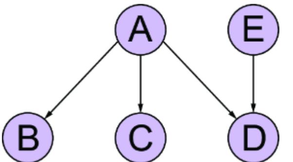
Figure 4.22 Assume this is the true causal DAG. Here, B, C, and D are conditionally independent, given A.

In this D AG, variables B, C, and D are conditionally independent of one another, given A. Now suppose that A were not observed in the data. W ith A as a latent variable, the discovery algorithm can’t run tests lik e B ⊥ C | A. The algorithm will detect a dependence between B, C, and D but will not find conditional independence between the thr ee given A, and it might possibly r eturn a D AG lik e figure 4.23, which r eflects these r esults.

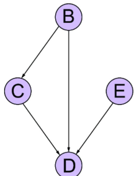
Figure 4.23 If A is latent, conditional independence tests that condition on A can’t be run. The algorithm would detect dependence between B, C, and D but no conditional independence given A, and it might possibly return a graph such as this.

The r emedy for this pr oblem is to pr ovide str ong domainspeci fic assumptions about the latent variable structur e in the discovery algorithm. A few generic discovery algorithms provide some accommodation for latent variable assumptions (the causal-lear n library has a few). But this is rare, because it is har d to mak e it easy for users to specif y domain-speci fic assumptions while still generalizing acr oss domains.

4.6.3 Equivalence classes and PDAGs

Let’s suppose our algorithm wer e to cor rectly r ecover all the true conditional independence statements fr om data and map them back to a true set of d-separation statements (causal faithfulness holds). The pr oblem we face now is that multiple causal D AGs may have the same set of d-separation statements. This set of candidate D AGs is called a Markov

equivalence class . The true causal D AG would be one of a possibly lar ge set of members of this class.

For example, suppose the D AG on the lef t of figure 4.24 wer e the gr ound truth D AG. The D AGon the right of the graph diers fr om the cor rect graph in the edge between A and T. The two graphs have the same set of d-separation. In fact, we can also change the dir ections of the edges between { L, S} and { B, S} and still be in the same equivalence class, except for intr oducing a collider { L → S ← B}, because a new collider would change the set of d-separations.

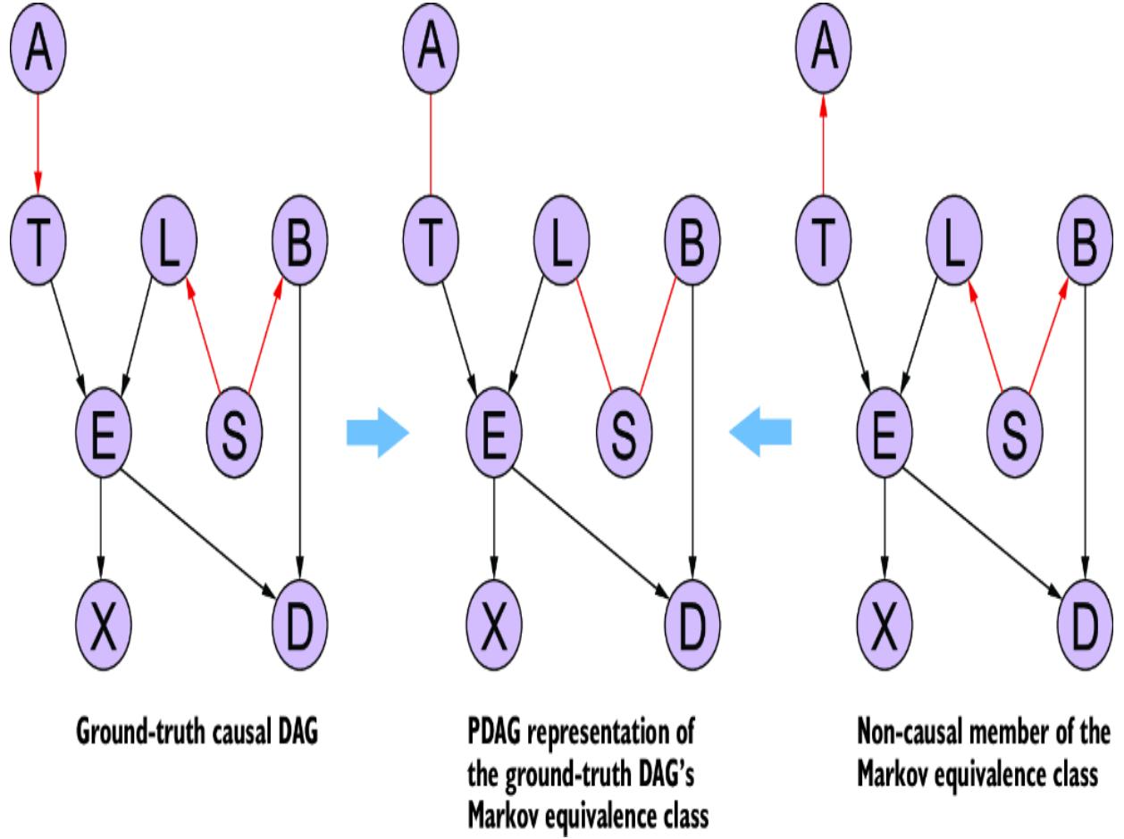
Figure 4.24 Supposing the DAG on the left is the ground truth DAG, the (wrong) DAG on the right is in the same Mark ov equivalence class. The PDAG in the middle represents the equivalence class, where undirected edges represent edges where members disagree on direction.

Some discovery algorithms will r eturn a partially dir ected acyclic graph (PD AG), such as the D AG in the center of figure 4.24. In the PD AG, undir ected edges cor respond to edges where ther e is disagr eement on the edge’s dir ection between members of the Mark ov equivalence class. This is nice, because we get a graphical r epresentation of the equivalence class, and the algorithm can potentially sear ch through the space of PD AGs instead of the lar ger space of DAGs.

COLLIDERS AND DISCO VERY

Colliders featur e prominently in causal discovery because they allow us to orient edges in the D AG from evidence of statistical dependence alone. Suppose we ar e using data to attempt to construct the gr ound-truth D AG in figure 4.24. W e find evidence of dependence in the data of an edge between A and T. The idea of Mark ov equivalence means that evidence is not enough to deter mine the direction of that edge. Generally, evidence of dependence and independence in the data can imply the pr esence of edges but not their dir ection.

Colliders ar e the e xception. It is possible to detect colliders like {T → E ← L} fr om evidence of independence and dependence alone; if the data suggests T and L are independent, but become dependent when conditioning on E, you have evidence of a collider with dir ected edges { T → E ← L}.

Colliders can also for ce orientation of edges outside of the collider . For example, consider the edge between E and X in the gr ound-truth D AG in figure 4.23. W e might infer the existence of that edge fr om the following evidence in the data:

E and X are dependent.
T and X are dependent.
T and X are independent, given E.

An edge between E and X is consistent with that evidence, but should we go with E → X or E ← X? Her e, the collider { T → E ← L} helps; it alr eady oriented the edge T → E, so adding E ← X would induce another collider { T → E ← X}. That collider would suggest T and X are independent but become dependent when conditioning on E, which violates

the second and thir d observed items of evidence. So we conclude the edge is oriented as E → X by pr ocess of elimination.

Some causal discovery algorithms essentially algorithmicize this kind of logic. But r emember, this logic breaks down when latent variables induce dependence between observed variables.

That said, PD AGs and Mark ov equivalence classes only captur e equivalence between D AGs encoding the same set of conditional independence constraints. If you want to find all graphs that satisf y an additional layer of constraining assumptions, such as all graphs that have the same posterior pr obability given a certain prior, then the PD AG might not be su cient.

If we go only on conditional independence, data can’t distinguish between members of the Mark ov equivalence class, because having the same set of d-separations means having the same evidence of conditional independence in the data. This is an e xample of a lack of causal identi fication —when our data and a set of causal assumptions ar e not sucient to disambiguate between possible answers to a causal question (in this case ૿ what is the right causal DAG?). W e’ll e xplor e causal identi fication in depth in chapter 10.

4.6.4 How to think about causal discovery

In section 4.3, I ar gued that testing for causality induced constraints lik e conditional independence using o -the-shelf hypothesis testing libraries should be viewed mor e as a heuristic appr oach to r efuting your causal D AG than a rigor ous statistical pr ocedur e for validating the D AG.

Similarly, I ar gued that for the practical user, o -the-shelf causal discovery algorithms should be viewed as a tool for exploratory data analysis during a human-driven causal D AG building pr ocess. The mor e you can input various types of domain knowledge and knowledge of latent variables into these algorithms, the better . But even then, they will produce obvious er rors. Just as with the hypothesis testing case, avoid rabbit holes of trying to ૿ fix the discovery algorithm so it doesn’t mak e these er rors. Use causal discovery as one imperfect tool in your br oader pr oject of building a good causal D AG and running the subsequent causal infer ence analysis.

Summary

Causal modeling induces conditional independence constraints on the join t probability distribution. Dseparation provides a graphical representation of conditional independence constraints.
Building an intuition for d-separation is important for reasoning about causal e ect infer ence and other queries.
The colliders might make d-separation confusing, but you can build intuition by using d-separation functionsn NetworkX and pgmpy .
Using traditional conditional independence testing libraries to test d-separation has its challenges. Th tests are sensitive to sample size, they don’t work well in many machine learning settings, and their hypotheses are misaligned.
Because ofthese challe ngs, it is best to view the attempts to falsif y the DAG using o -the-shelf conditional independence testing libraries as more of a heuristic. Focus on the overall goal of building a good (i.e., hard to refute) causal DAG and moving on to your downstr eam

causal infer ence task. Avoid fixating on theor etica l rigor in statistical hypothesis testing.

When ther are latent variables, a causal DAG may still have testable implications for functions of the observed variables.
Causal discovery refers to the use of statistical algorithms to r ecover a causal D AG from data.
The causal faithfulness property assumes conditional independence in the joint probability distribution maps to a true set ofd-separations that hold in the ground truth causal D AG.
A Markov equivalence class of DAGs is a set of DAGs with the same set of d-separations. Assuming you have the true set of d-separations, the ground truth causal DAG generally shar es that set with other (wr ong) D AGs.
Causal discovery is especially vulnerable to latent variables.
The more you can constrain causal infer ence with prior assumptions, such as latent structur e and which edges cannot possibly e xist and which must e xist, the better .
Causal discovery algorithms are useful exploratory data analysis tools inthe process of building a causal DAG, but they are not reliable replacements for that process. Again, focus onthe overall goal of building a good causal DAG and moving on to the downstr eam causal infer ence analysis. Avoid trying to fix causal discovery algorithms so they don’t produce obvious erors in your domain.

5Connecting causality and deep learning

This chapter covers

Incorporating deep learning into a causal graphical model
Training a causal graphical model with a varia tional autoencoder
Using causal methods to enhance machine lear ning

The title of this book is Causal AI , but how e xactly does causality connect to AI? Mor e speci fically, how does causality connect with deep lear ning, the dominant paradigm in AI? In this chapter, I look at this question fr om two perspectives:

How to incorporate deep learning into a causal model— We’ll look at a causal model of a computer vision problem (section 5.1) and then train the deep causal image model (section 5.2).
How touse causal reason ing to do better deep learning —We’ll look at a case study on independence of mechanism and semi-supervised learning (section 5.3.1 and 5.3.2), and we’ll demystif y deep learning with causality (section 5.3.3).

The ter m deep learning broadly r efers to applications of deep neural networks. It’s a machine lear ning appr oach that stacks many nonlinear models together in sequential layers, emulating the connections of neur ons in brains. ૿ Deep refers to stacking many layers to achieve mor e modeling power, particularly in ter ms of modeling high-dimensional

and nonlinear data, such as visual media and natural language te xt. Neural nets have been ar ound for a while, but relatively r ecent advancements in har dware and automatic dierentiation have made it possible to scale deep neural networks to e xtremely lar ge sizes. That scaling is why, in recent years, ther e have been multiple cases of deep learning outperfor ming humans on many advanced infer ence and decision-making tasks, such as image r ecognition, natural language pr ocessing, game playing, medical diagnosis, autonomous driving, and generating lifelik e text, images, and video .

But asking how deep lear ning connects to causality can elicit frustrating answers. AI company CEOs and leaders in big tech fuel hype about the power of deep lear ning models and even claim they can lear n the causal structur e of the world. On the other hand, some leading r esear chers claim these models ar emerely ૿stochastic par rots that can echo patter ns of cor relation that, while nuanced and comple x, still fall short of true causal understanding.

Our goal in this chapter is to r econcile these perspectives. But skipping ahead, the main tak eaway is that deep lear ning architectur e can be integrated into a causal model and we can train the model using deep lear ning training techniques. But also, we can use causal r easoning to build better deep learning models and impr ove how we train them.

We’ll anchor this idea in two case studies:

Building a causal DAG for computer vision using a variational autoencoder
Implementing better semi-supervised learning using independence of mechanism

Other e xamples of the interplay of causality and AI that you’ll see in the r est of the book will build on the intuition we get fr om these case studies. F or example, chapter 9 will illustrate counterfactual r easoning using a variational autoencoder lik e the one we’ll build in this chapter . In chapter 11, we’ll e xplor e machine lear ning and pr obabilistic deep lear ning appr oaches for causal e ect infer ence. Chapter 13 will show how to combine lar ge language models and causal r easoning.

We’ll start by considering how to incorporate deep lear ning into a causal model.

5.1Acausalmodelofacomputer visionproblem

Let’s look at a computer vision pr oblem that we can approach with a causal D AG. Recall the MNIST data fr om chapter 1, composed of images of digits and their labels, illustrated in figure 5.1.

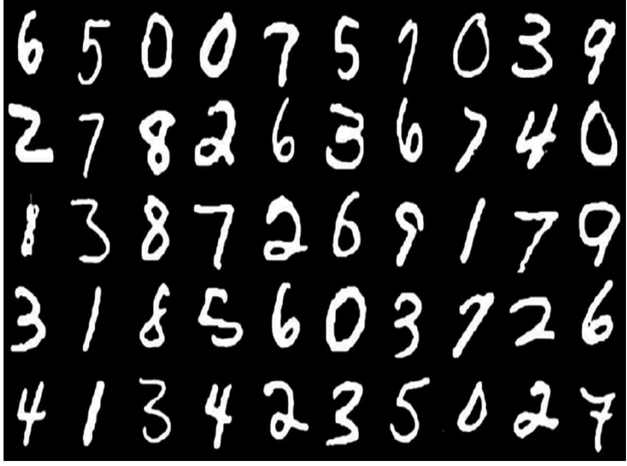
Figure 5.1 MNIST data featuring images of handwritten digits and their digit labels

There is a r elated dataset called T ypeface MNIST (TMNIST) that also featur es digit images and their digit labels. However, instead of handwritten digits, the images ar e digits rendered in 2,990 di erent fonts, illustrated in figure 5.2. F or each image, in addition to a digit label, ther e is a font label. Examples of the font labels include ૿ GrandHotel-R egular, KulimP ark-R egular, and ૿ Gorditas- Bold.

Figure 5.2 Examples from the T ypeface MNIST , which is composed of typed digits with di erent typefaces. In addition to a digit label for each digit, there is a label for one of 2,990 di erent typefaces (fonts).

In this analysis, we’ll combine these datasets into one and build a simple deep causal generative model on that data. We’ll simplif y the ૿ fonts label into a sample binary label that indicates ૿handwritten for MNIST images and ૿typed for the TMNIST images.

We have seen how to build a causal generative model on top of a D AG. We factorized the joint distribution into a pr oduct of causal Markov kernels representing the conditional probability distributions for each node, conditional on their parents in the D AG. In our pr evious e xamples in pgmpy, we fit a conditional pr obability table for each of these k ernels.

You can imagine how har d it would be to use a conditional probability table to r epresent the conditional pr obability distribution of pix els in an image. But ther e is nothing stopping us fr om modeling the causal Mark ov kernel with a deep neural net, which we know is flexible enough to work with high-dimensional featur es lik e pix els. In this section, I’ll demonstrate how to use deep neural nets to model the causal Mark ov kernels de fined by a causal D AG.

5.1.1 Leveraging the universal function approximator

Deep lear ning is a highly e ective universal function approximator . Let’s imagine ther e is a function that maps some set of inputs to some set of outputs, but we either don’t know the function or it’s too har d to write down in math or code. Given enough e xamples of those inputs and outputs, deep lear ning can appr oximate that function with high pr ecision. Even if that function is nonlinear and highdimensional, with enough data, deep lear ning will lear n a good appr oximation.

We regularly work with functions in causal modeling and infer ence, and sometimes it mak es sense to appr oximate them, so long as the appr oximations pr eserve the causal infor mation we car e about. F or example, the causal Mark ov property mak es us inter ested in functions that map values of a node’s par ents in the causal D AG to values (or pr obability values) of that node.

In this section, we’ll do this mapping between a node and its parents with the variational autoencoder (V AE) framework. We’ll train two deep neural nets in the V AE, one of which maps par ent cause variables to a distribution of the outcome variable, and another that maps the outcome variable to a distribution of the cause variables. This e xample will

showcase the use of deep lear ning when causality is nonlinear and high-dimensional; the e ect variable will be an image r epresented as a high-dimensional ar ray, and the cause variables will r epresent the contents of the image.

5.1.2 Causal abstraction and plate models

But what does it mean to build a causal model of an image? Images ar ecomprised of pix els ar ranged in a grid. As data, we can r epresent that pix el grid as a matrix of numerical values cor responding to color . In the case of both MNIST and TMNIST, the image is a 28 × 28 matrix of grayscale values, as illustrated in figure 5.3.

Figure 5.3 An MNIST image of ૿6 (left) and a TMNIST image of ૿7. In their raw form, these are 28 × 28 matrices of numeric values corresponding to gra yscale values.

A typical machine lear ning model looks at this 28 × 28 matrix of pix els as 28 × 28 = 784 featur es. The machine learning algorithm lear ns statistical patter ns connecting the pixels to one another and their labels. Based on this fact, one might be tempted to tr eat each individual pix el as a node in

the naive causal D AG, as in figure 5.4, wher e for visual simplicity I’ve drawn 16 pix els (an arbitrary number) instead of all 784.

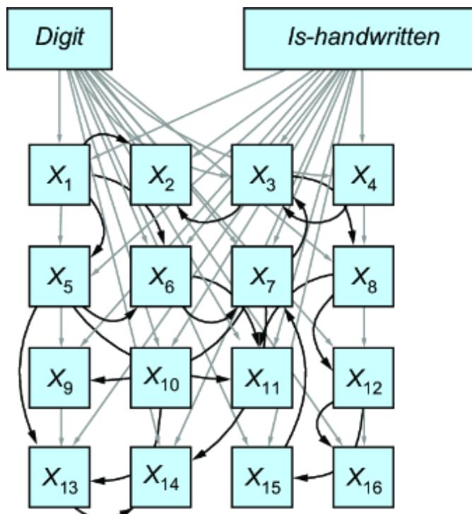
Figure 5.4 What a naive causal DAG might look lik e for an image represented by a 4 × 4 matrix

In figure 5.4, ther e are edges fr omthe digit and ishandwritten variables to each pix el. F urther, ther e are examples of edges r epresenting possible causal r elationships between pix els. Causal edges between pix els imply the color of one pixl s a cause of another . Perhaps most of these relationships ar e between nodes that ar e close, with a few far-reaching edges. But how would we know if one pix el causes another? If two pix els ar e connected, how would we know the dir ection of causality?

WORKING A T THE RIGHT LEVEL OF ABSTRA CTION

With these connections among only 16 pix els, the naive D AG in figure 5.4 is alr eady quite unwieldy . It would be much

worse with 784 pix els. Aside fr om the unwieldiness of a D AG, the pr oblem with a pix el-level model is that our causal questions ar e generally not at the pix el level—we’d pr obably never ask ૿ what is the causal e ect of this pix el on that pixel? In other wor ds, the pix el is too low a level of abstraction, which is why thinking about causal r elationships between individual pix els feels a bit absur d.

In applied statistics domains, such as econometrics, social science, public health, and business, our data has variables like per capita income, r evenue, location, age, etc. These variables ar e typically alr eady at the level of abstraction we want to think about when we get the data. But moder n machine lear ning focuses on many per ception prblems fr om raw media, such as images, video, te xt, and sensor data. W e don’t generally want to do causal r easoning at the low level of these featur es. Our causal questions ar e usually about the high-level abstractions behind these low-level featur es. W e need to model at these higher abstraction levels.

Instead of thinking about individual pix els, we’ll think about the entir e image. W e’ll de fine a variable X to r epesent how the image appears; i.e., X is a matrix random variable representing pix els. F igure 5.5 illustrates a causal D AG for the TMNIST case. Simply put, the identity of the digits (0–9) and the font (2,990 possible values) ar e the causes, and the image is the e ect.

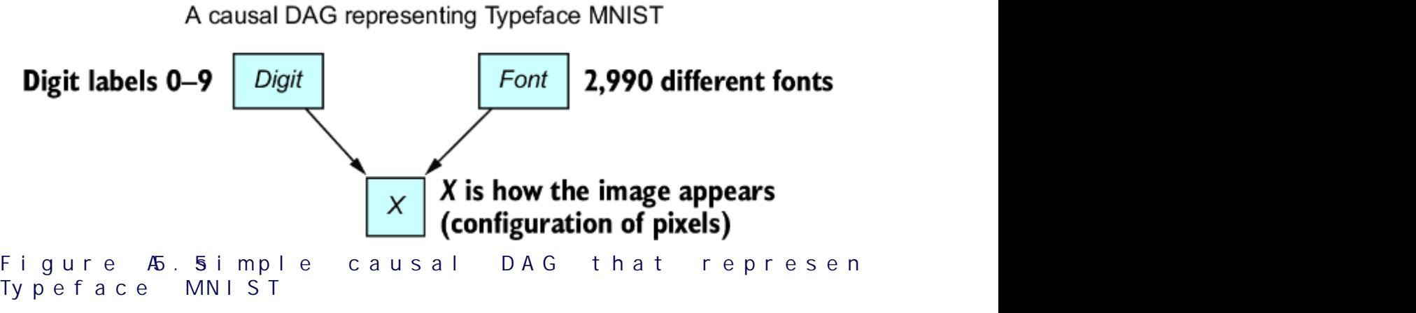
In this case, we ar e using the causal D AG to mak e an assertion that the label causes the image. That is not always the case, as we’ll discuss in our case study on semisupervised lear ning in section 5.3. As with all causal models, it depends on the data generating pr ocess (DGP) within a domain.

WHY SAY THAT THE DIGIT CAUSES THE IMAGE?

Plato’s allegory of the cave describes a gr oup of people who have lived in a cave all their lives, without seeing the world. They face a blank cave wall and watch shadows projected on the wall fr om objects passing in fr ont of a fire behind them. The shadows ar e simpli fied and sometimes distorted r epresentations of the true objects passing in front of the fire. In this case, we can think of the for m of the objects as being the cause of the shadow .

Analogously, the true for m of the digit label causes the representation in the image. The MNIST images wer e written by people, and they have some Platonic ideal of the digit in their head that they want to r ender onto paper . In the pr ocess, that ideal is distorted by motor variation in the hand, the angle of the paper, the friction of the pen on the paper, and other factors—the r endered image is a ૿shadow caused by that ૿ideal.

This idea is r elated to a concept called ૿ vision as inverse graphics in computer vision (see https://www .altdeep.ai/p/causalaibookfor sour ces with more infor mation). In causal ter ms, the tak eaway is that when we ar e analyzing images r endered fr om raw signals from the envir onment, and the task is to infer the actual objects or events that r esulted in those signals, causality flows fr om those objects or events to the signals. The infer ence task is to use the observed signals (shadows on the cave wall) to infer the natur e of the causes (objects in front of the fire).

That said, images can be causes too . For example, if you were modeling how people behave after seeing an image in a mobile app (e.g., whether they ૿click, ૿lik e, or ૿swipe lef t), you could model the image as a cause of the behavior .

PLATE MODELING

Modeling 2,990 fonts in our TMNIST data is overkill for our purposes her e. Instead, I combined these datasets into one half fr om MNIST and half fr om Typeface MNIST . Along with the ૿digit label, I’m just going to have a simple binary label called ૿is-handwritten , which is 1 (true) for images of handwritten digits fr om MNIST and 0 (false) for images of ૿typed digits fr om TMNIST . We can modif y our causal D AG to get figure 5.6.

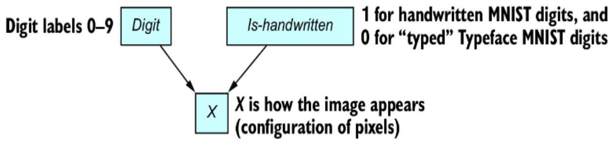
Figure 5.6 A causal DAG representing the combined MNIST and TMNIST data, where ૿is-handwritten is 1 (MNIST images) or 0 (TMNIST images)

Plate modeling is a visualizing technique used in pr obabilistic machine lear ning that pr ovides an e xcellent way to visualize the higher -level abstractions while pr eserving the lower -level dimensional detail. Plate notation is a method of visually representing variables that r epeat in a D AG (e.g., X1 to X16 in figure 5.4)—in our case, we have r epetition of the pix els.

Instead of drawing each of the 784 pix els as an individual node, we use a r ectangle or ૿plate to gr oup r epeating variables into subgraphs. W e then write a number on the plate to r epresent the number of r epetitions of the entities on the plate. Plates can nest within one another to indicate repeated entities nested within r epeated entities. Each plate

gets a letter subscript inde xing the elements on that plate. The causal D AG in figure 5.7 r epresents one image.

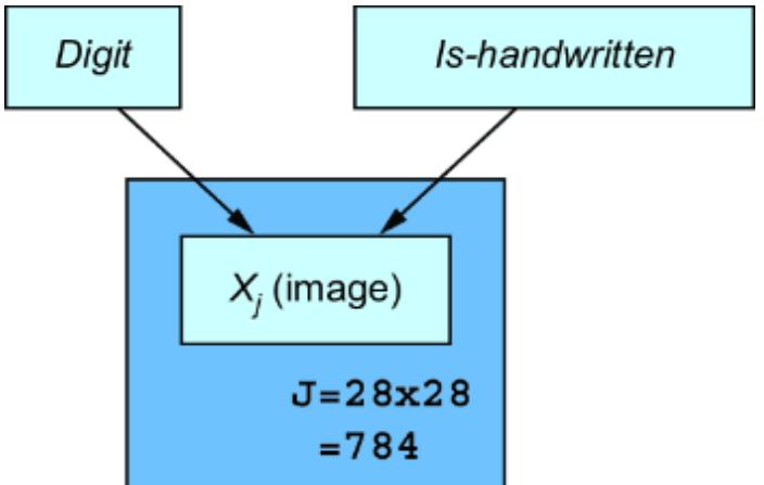
Figure 5.7 A plate model representation of the causal DAG. Plates represent repeating variables, in this case 28 × 28 = 784 pixels. Xj is the jth pixel.

During training, we’ll have a lar ge set of training images. Next, we’ll modif y the D AG to captur e all the images in the training data.

5.2Traininganeuralcausalmodel

To train our neural causal model, we need to load and prepare the training data, cr eate the ar chitectur e of our model, write a training pr ocedur e, and implement some tools for evaluating how well training is pr ogressing. W e’ll start by loading and pr eparing the data.

5.2.1 Setting up the training data

Our training data has N example images, so we need our plate model to r epresent all N images in the training data, half handwritten and half typed. W e’ll add another plate corresponding to r epeating N sets of images and labels, as in figure 5.8.

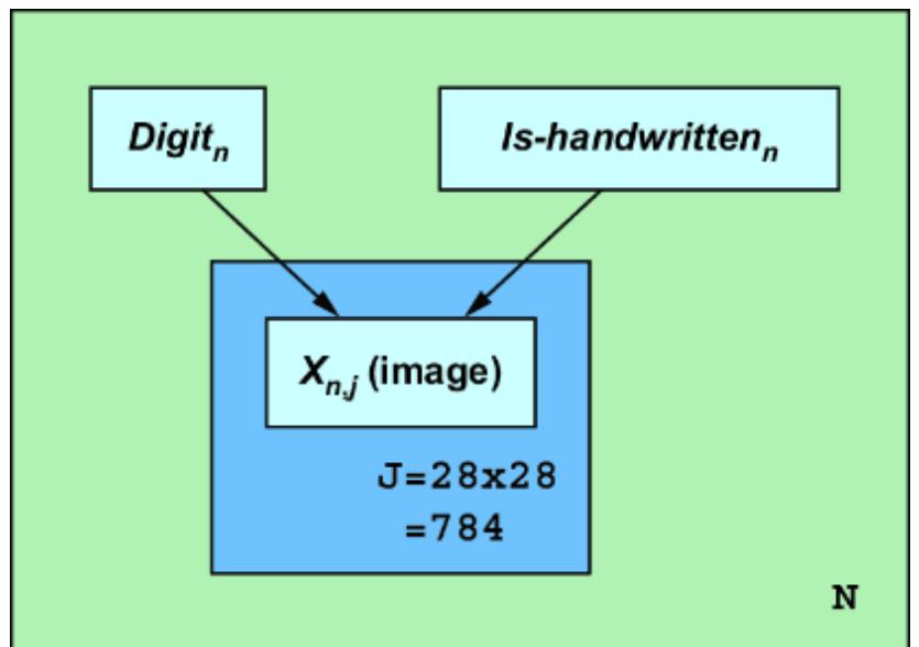
Figure 5.8 The causal model with an additional plate for the N images in the data

Now we have a causal D AG that illustrates both our desir ed level of causal abstraction as well as the dimensional infor mation we need to start training the neural nets in the model.

Let’s first load Pyr o and some other libraries and set some hyperparameters.

SETTING UP Y OUR ENVIRONMENT

This code was written using Python version 3.10.12 and tested in Google Colab. The versions of the main libraries include Pyr o (pyr o-ppl) version 1.8.4, tor ch version 2.2.1, torchvision version 0.18.0+cu121, and pandas version 2.0.3. W e’ll also use matplotlib for plotting.

Visit https://www .altdeep.ai/p/causalaibook for links to a notebook that will load in Google Colab. If GPUs ar e available on your device, it will be faster to train the neural nets with CUD A (a platfor m for parallel computing on GPUs). W e’ll run a bit of code that lets us toggle it on. If you don’t have GPUs or ar en’t sur e if you do, leave USE_CUDA set to False.

Listing 5.1 Setting up for GPU training

import torch USE_CUDA = False #1 DEVICE_TYPE = torch.device(“cuda” if USE_CUDA else “cpu”)

#1 Use CUDA if it is available.

First, we’ll mak e a subclass of the Dataset class (a class for loading and pr eprocessing data) that will let us combine the MNIST and TMNIST datasets.

Listing 5.2 Combining the data

from torch.utils.data import Dataset import numpy as np import pandas as pd from torchvision import transforms

class CombinedDataset(Dataset): #1 def __init__(self, csv_file): self.dataset = pd.read_csv(csv_file)

def __len__(self): return len(self.dataset)

def __getitem__(self, idx): images = self.dataset.iloc[idx, 3:] #2 images = np.array(images, dtype=‘float32’)/255. #2 images = images.reshape(28, 28) #2 transform = transforms.ToTensor() #2 images = transform(images) #2 digits = self.dataset.iloc[idx, 2] #3 digits = np.array([digits], dtype=‘int’) #3 is_handwritten = self.dataset.iloc[idx, 1] #4 is_handwritten = np.array([is_handwritten], dtype=‘float32’) #4 return images, digits, is_handwritten #5

#1 This class loads and processes a dataset that combines MNIST and Typeface MNIST . The output is a torch.utils.data.Dataset object. #2 Load, normalize, and reshape the images to 28 × 28 pixels. #3 Get and process the digit labels, 0–9. #4 1 for handwritten digits (MNIST), and 0 for ૿typed digits (TMNIST) #5 Return a tuple of the image, the digit label, and the is_handwritten label.

Next, we’ll use the DataLoader class (which allows for e cient data iteration and batching during training) to load the data from a CSV file in GitHub and split it into training and test sets.

Listing 5.3 Downloading, splitting, and loading the data

from torch.utils.data import DataLoader from torch.utils.data import random_split def setup_dataloaders(batch_size=64, use_cuda=USE_CUDA): #1 combined_dataset = CombinedDataset( “https://raw.githubusercontent.com/altdeep/causalML/master/datasets /combined_mnist_tmnist_data.csv” ) n = len(combined_dataset) #2 train_size = int(0.8 * n) #2 test_size = n - train_size #2 train_dataset, test_dataset = random_split( #2 combined_dataset, #2 [train_size, test_size], #2 generator=torch.Generator().manual_seed(42) #2 ) #2 kwargs = {‘num_workers’: 1, ‘pin_memory’: use_cuda} #2 train_loader = DataLoader( #3 train_dataset, #3 batch_size=batch_size, #3 shuffle=True, #3 **kwargs #3 ) #3 test_loader = DataLoader( #3 test_dataset, #3 batch_size=batch_size, #3 shuffle=True, #3 **kwargs #3 ) #3 return train_loader, test_loader #1 Set up the data loader that loads the data and splits it into training and test sets. #2 Allot 80% of the data to training data and the remaining 20% to test data. #3 Create training and test loaders. Next, we’ll set up the full variational autoencoder . 5.2.2 Setting up the variational autoencoder The variational autoencoder (V AE) is per haps the simplest deep pr obabilistic machine lear ning modeling appr oach. In the typical setup for applying V AE to images, we intr oduce a

latent continuous variable Z that has a smaller dimension than the image data. Her e, dimensionality refers to the number of elements in a vector r epresentation of the data. For instance, our image is a 28 × 28 matrix of pix els, or alter natively a vector with dimension 28 × 28 = 784. By having a much smaller dimension than the image dimension, the latent variable Z represents a compr essed encoding of the image infor mation. F or each image in the dataset, ther e is a cor responding latent Z value that r epresents an encoding of that image. This setup is illustrated in figure 5.9.

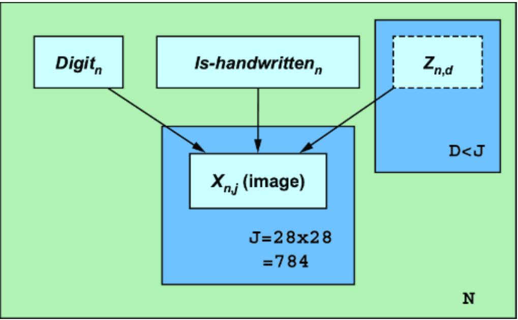
Figure 5.9 The causal DAG plate model, extended to include an ૿encoding variable Z. During training, the variable is latent, indicated by the dashed line. (After the model is deployed, digit and ishandwritten are also latent).

Z appears as a new par ent in the causal D AG, but it’s important to note that the classical V AE framework does not define Z as causal. Now that we ar e thinking causally, we’ll give Z a causal interpr etation. Speci fically, as par ents of the image node in the D AG, we view digit and is-handwritten as causal drivers of what we see in the image. Y et ther e are other elements of the image (e.g., the str oke thickness of a handwritten character, or the font of a typed character) that are also causes of what we see in the image. W e’ll think of Z as a continuous latent stand-in for all of these other causes of the image that we ar e not e xplicitly modeling, lik e digit and is-handwritten . Examples of these causes include the nuance of the various fonts in the TMNIST labels and all of the variations in the handwritten digits due to di erent writers and motor movements as they wr ote. W ith that in mind, we can view P(X| digit , is-handwritten , Z) as the causal Markov kernel of X. That said, it is important to r emember that the r epresentation we lear n for Z is a stand-in for latent causes and is not the same as lear ning the actual latent causes.

The V AE setup will train two deep neural networks: One called an ૿encoder , which encodes an image into a value for Z. The other neural network, called the ૿decoder, will align with our D AG. The decoder generates an image fr om the digit label, the is-handwritten label, and a Z value, as in figure 5.10.

The decoder acts lik e a r endering engine; given a Z encoding value and the values for digit and is-handwritten , it r enders an image.

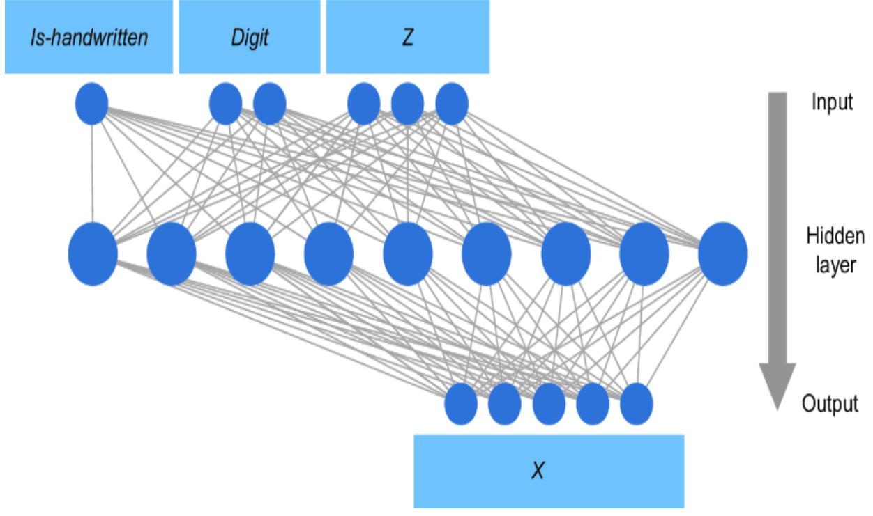
Figure 5.10 The decoder neural network generates as output an image X from inputs Z and the labels is-handwritten and digit . As with any neural net, the inputs are processed through one or more ૿hidden layers.

KEY VAE CONCEPTS SO F AR

Variational autoencoder (V AE)—A popular framework in deep generative modeling. W e’re using it to model a causal Mark ov kernel in a causal model.

Decoder —We use the decoder as the model of the causal Markov kernel. It maps the observed causes is-handwritten and digit , and the latent variable Z, to our image outcome variable X.

This V AE appr oach allows us to use a neural net, a la the decoder, to captur e the comple x and nonlinear r elations needed to model the image as an e ect caused by digit and is-handwritten . Modeling images would be di cult with the conditional pr obability tables and other simple parameterizations of causal Mark ov kernels we’ve discussed previously .

First, let’s implement the decoder . We’ll pass in ar guments z_dim for the dimension of Z and hidden_dim for the dimension (width) of the hidden layers. W e’ll specif y these variables when we instantiate the full V AE. The decoder combines the latent vector Z with additional inputs—the variable representing the digit, and is-handwritten (a binary indicator of whether the digit is handwritten). It will pr oduce a 784 dimensional output vector r epresenting an image of size 28 × 28 pix els. This output vector contains the parameters for a Bernoulli distribution for each pix el, essentially modeling the likelihood of each pix el being ૿ on. The class uses two fully connected layers ( fc1 and fc2), and employs Softplus and Sigmoid ૿activation functions, which ar e the hallmarks of how neural nets emulate neur ons.

Listing 5.4 Implement the decoder

from torch import nn

class Decoder(nn.Module): #1 def __init__(self, z_dim, hidden_dim): super().__init__() img_dim = 28 * 28 #2 digit_dim = 10 #3 is_handwritten_dim = 1 #4 self.softplus = nn.Softplus() #5 self.sigmoid = nn.Sigmoid() #5 encoding_dim = z_dim + digit_dim + is_handwritten_dim #6 self.fc1 = nn.Linear(encoding_dim, hidden_dim) #6 self.fc2 = nn.Linear(hidden_dim, img_dim) #7 def forward(self, z, digit, is_handwritten): #8 input = torch.cat([z, digit, is_handwritten], dim=1) #9 hidden = self.softplus(self.fc1(input)) #10 img_param = self.sigmoid(self.fc2(hidden)) #11 return img_param #1 A class for the decoder used in the V AE #2 Image is 28 × 28 pixels. #3 Digit is one-hot encoded digits 0–9, i.e., a vector of length 10. #4 An indicator for whether the digit is handwritten that has size 1 #5 Softplus and sigmoid are nonlinear transforms (activation functions) used in mapping between la yers. #6 fc1 is a linear function that maps the Z vector , the digit, and is_handwritten to a linear output, which is passed through a softplus activation function to create a hidden la yer-a vector whose length is given by hidden_la yer. #7 fc2 linearly maps the hidden la yer to an output passed to a sigmoid function. The resulting value is between 0 and 1. #8 Define the forward computation from the latent Z variable value to a generated X variable value. #9 Combine Z and the labels. #10 Compute the hidden la yer. #11 Pass the hidden la yer to a linear transform and then to a sigmoid transform to output a parameter vector of length 784. Each element of the vector corresponds to a Bernoulli parameter value for an image pixel.

We use the decoder in the causal model. Our causal D AG acts as the sca old for a causal pr obabilistic machine learning model that, with the help of the decoder, de fines a joint pr obability distribution on { is-handwritten , digit , X, Z}, where Z is latent. W e can use the model to calculate the likelihood of the training data for a given value of Z.

The latent variable z, the digit identity r epresented as a onehot vector digit, and a binary indicator is_handwritten are modeled as samples fr om standar d distributions. These variables ar e then fed into the decoder to pr oduce parameters ( img_param ) for a Ber noulli distribution representing individual pix el pr obabilities of an image.

Note, using the Ber noulli distribution to model the pix els is a bit of a hack. The pix els ar e not binary black and white outcomes—they have grayscale values. The line dist.enable_validation(False) lets us cheat by getting Ber noulli log lik ehoods for the images given a decoder’s img_param output.

The following model code is a class method for a PyT orch neural network module. W e’ll see the entir e class later .

Listing 5.5 The causal model

import pyro import pyro.distributions as dist dist.enable_validation(False) #1 def model(self, data_size=1): #2 pyro.module(“decoder”, self.decoder) #2 options = dict(dtype=torch.float32, device=DEVICE_TYPE) z_loc = torch.zeros(data_size, self.z_dim, **options) #3 z_scale = torch.ones(data_size, self.z_dim, **options) #3 z = pyro.sample(“Z”, dist.Normal(z_loc, z_scale).to_event(1)) #3 p_digit = torch.ones(data_size, 10, **options)/10 #4 digit = pyro.sample( #4 “digit”, #4 dist.OneHotCategorical(p_digit) #4 ) #4 p_is_handwritten = torch.ones(data_size, 1, **options)/2 #5 is_handwritten = pyro.sample( #5 “is_handwritten”, #5 dist.Bernoulli(p_is_handwritten).to_event(1) #5 ) #5 img_param = self.decoder(z, digit, is_handwritten) #6 img = pyro.sample(“img”, dist.Bernoulli(img_param).to_event(1)) #7 return img, digit, is_handwritten

#1 Disabling distribution validation lets P yro calculate log lik elihoods for pixels even though the pixels are not binary values. #2 The model of a single image. Within the method, we register the decoder , a P yTorch module, with P yro. This lets P yro know about the parameters inside of the decoder network. #3 We model the joint probability of Z, digit, and is_handwritten, sampling each from canonical distributions. W e sample Z from a multivariate normal with location parameter z_loc (all zeros) and scale parameter z_scale (all ones). #4 We also sample the digit from a one-hot categorical distribution. Equal probability is assigned to each digit. #5 We similarly sample the is_handwritten variable from a Bernoulli distribution. #6 The decoder maps digit, is_handwritten, and Z to a probability parameter vector . #7 The parameter vector is passed to the Bernoulli distribution, which

models the pixel values in the data. The pixels are not technically Bernoulli binary variables, but we’ll relax this assumption.

The pr eceding model method r epresents the DGP for one image. The training_ model method in the following listing applies that model method to the N images in the training data.

Listing 5.6 Method for applying model to N images in data def training_model(self, img, digit, is_handwritten, batch_size): #1 conditioned_on_data = pyro.condition( #2 self.model, data={ “digit”: digit, “is_handwritten”: is_handwritten, “img”: img } ) with pyro.plate(“data”, batch_size): #3 img, digit, is_handwritten = conditioned_on_data(batch_size) return img, digit, is_handwritten

#1 The model represents the DGP for one image. The training_model applies that model to the N images in the training data. #2 Now we condition the model on the evidence in the training data. #3 This context manager represents the N-size plate representing repeating IID examples in the data in figure 5.9. In this case, N is the batch size. It works lik e a for loop, iterating over each data unit in the batch.

Our pr obabilistic machine lear ning model models the joint distribution of { Z, X, digit , is-handwritten }. But since Z is latent, the model will need to lear n P(Z|X, digit , ishandwritten ). Given that we use the decoder neural net to go from Z and the labels to X, the distribution of Z, given X and the labels will be comple x. We will use variational inference , a technique wher e we first de fine an appr oximating distribution Q(Z|X, digit , is-handwritten ), and try to mak e that distribution as close to P(Z|X, digit , is-handwritten ) as we can.

The main ingr edent of the appr oximating distribution is the second neural net in the V AE framework, the encoder, illustrated in figure 5.11. The encoder maps an observed image and its labels in the training data to a latent Z variable.

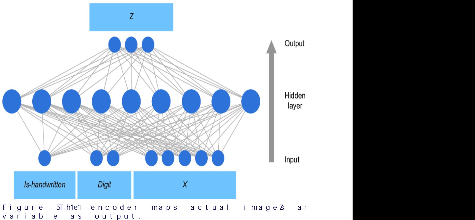
The encoder does the work of compr essing the infor mation in the image into a lower -dimensional encoding.

KEY VAE CONCEPTS SO F AR

Variational autoencoder (V AE)—A popular framework in deep generative modeling. W e’re using it to model a causal Mark ov kernel in our causal model.

Decoder —We use the decoder as the model of the causal Markov kernel. It maps observed causes is-handwritten and digit , and the latent variable Z, to our image outcome variable X.

Encoder —The encoder maps the image, digit , and ishandwritten indicator to the parameters of a distribution where we can draw samples of Z.

In the following code, the encoder tak es as input an image, a digit label, and the is-handwritten indicator . These inputs ar e concatenated and passed thr ough a series of fully connected layers with Sof tplus activation functions. The final output of the encoder consists of two vectors r epresenting the location (z_loc) and scale ( z_scale ) parameters of the latent space distribution on Z, given observed values for image (img), digit (digit), and is-handwritten (is_handwritten ).

Listing 5.7 Implement the encoder class Encoder(nn.Module): #1 def __init__(self, z_dim, hidden_dim): super().__init__() img_dim = 28 * 28 #2 digit_dim = 10 #3 is_handwritten_dim = 1 self.softplus = nn.Softplus() #4 input_dim = img_dim + digit_dim + is_handwritten_dim #5 self.fc1 = nn.Linear(input_dim, hidden_dim) #5 self.fc21 = nn.Linear(hidden_dim, z_dim) #6 self.fc22 = nn.Linear(hidden_dim, z_dim) #6 def forward(self, img, digit, is_handwritten): #7 input = torch.cat([img, digit, is_handwritten], dim=1) #8 hidden = self.softplus(self.fc1(input)) #9 z_loc = self.fc21(hidden) #10 z_scale = torch.exp(self.fc22(hidden)) #10 return z_loc, z_scale #1 The encoder is an instance of a P yTorch module. #2 The input image is 28 × 28 = 784 pixels. #3 The digit dimension is 10. #4 In the encoder , we’ll only use the softplus transform (activation function). #5 The linear transform fc1 combines with the softplus to map the 784 dimensional pixel vector , 10-dimensional digit label vector , and 2 dimensional is_handwritten vector to the hidden la yer. #6 The linear transforms, fc21 and fc22, will combine with the softplus to map the hidden vector to Z’s vector space. #7 Define the reverse computation from an observed X variable value to a latent Z variable value. #8 Combine the image vector , digit label, and is_handwritten label into one input. #9 Map the input to the hidden la yer. #10 The V AE framework will sample Z from a normal distribution that approximates P(Z|img, digit, is_handwritten). The final transforms map the hidden la yer to a location and scale parameter for that normal distribution.

The output of the encoder pr oduces the parameters of a distribution on Z. During training, given an image and its labels ( is-handwritten and digit ), we want to get a good value of Z, so we write a guide function that will use the encoder to sample values of Z.

Listing 5.8 The guide function

def training_guide(self, img, digit, is_handwritten, batch_size): #1 pyro.module(“encoder”, self.encoder) #2 options = dict(dtype=torch.float32, device=DEVICE_TYPE) with pyro.plate(“data”, batch_size): #3 z_loc, z_scale = self.encoder(img, digit, is_handwritten) #4 normal_dist = dist.Normal(z_loc, z_scale).to_event(1) #4 z = pyro.sample(“Z”, normal_dist) #5

#1 training_guide is a method of the V AE that will use the encoder . #2 Register the encoder so P yro is aware of its weight parameters. #3 This is the same plate context manager for iterating over the batch data that we see in the training_model. #4 Use the encoder to map an image and its labels to parameters of a normal distribution. #5 Sample Z from that normal distribution

We combine these elements into one PyT orch neural network module r epresenting the V AE. We’ll initialize the latent dimension of Z to be 50. W e’llset our hidden layer dimension to 400 in both the encoder and decoder . That means that given a dimension of 28 × 28 for the image, 1 for the binary is-handwritten , and 10 for the one-hot-encoded digit variable, we’ll tak e a 28 × 28 + 1 + 10 = 795 dimensional featur e vector and compr ess it down to a 400 dimensional hidden layer, and then compr ess that down to a 50-dimensional location and scale parameter for Z’s multivariate nor mal (Gaussian) distribution. The decoder takes as input the values of digit , is-handwritten , and Z and maps these to a 400-dimensional hidden layer and to the 28 × 28–dimensional image. These ar chitectural choices of latent variable dimension, number of layers, activation functions, and hidden layer dimensions depend on the problem and ar e typically selected by convention or by experimenting with di erent values.

Now we’ll put these pieces together into the full V AE class.

Listing 5.9 Full V AE class

class VAE(nn.Module): def __init__( self, z_dim=50, #1 hidden_dim=400, #2 use_cuda=USE_CUDA, ): super().__init__() self.use_cuda = use_cuda self.z_dim = z_dim self.hidden_dim = hidden_dim self.setup_networks() def setup_networks(self): #3 self.encoder = Encoder(self.z_dim, self.hidden_dim) self.decoder = Decoder(self.z_dim, self.hidden_dim) if self.use_cuda: self.cuda() model = model #4 training_model = training_model #4 training_guide = training_guide #4 #1 Set the latent dimension to 50. #2 Set the hidden la yers to have a dimension of 400. #3 Set up the encoder and decoder . #4 Add in the methods for model, training_model, and training_guide. Having speci fied the V AE, we can now move on to training. 5.2.3 The training procedure We know we have a good generative model when the encoder can encode an image into a latent value of Z, and then decode it into a reconstructed version of the image. W e can minimize the reconstruction error —the di erence between original and r econstructed images—in the training data.

A BIT OF PERSPECTIVE ON THE “V ARIATIONAL INFERENCE” TRAINING ALGORITHM

In this section, you’ll see a bunch of jar gon r elating to variational infer ence, which is the algorithm we’ll use for training. It helps to zoom out and e xamine why we’r e using this algorithm. Ther e are many statistical estimators and algorithms both for fitting neural net weights and other parameters and for causal infer ence. One of these is variational infer ence.

To be clear, variational infer ence is not a ૿causal idea. It is just another pr obabilistic infer ence algorithm. In this book, I favor this infer ence algorithm mor e than others because it scales well even when variables in the D AG are latent in the training data, and it works with deep neural nets and leverages deep lear ning frameworks lik e PyT orch. This opens the door to r easoning causally about richer modalities such as te xt, images, video, etc., wher eas traditional causal infer ence estimators wer e developed for numerical data. F urther, we can tailor the method to dierent pr oblems (see the discussion of ૿commodi fication of infer ence in chapter 1) and leverage domain knowledge during infer ence (such as by using knowledge of conditional independence in the guide). F inally, the cor e concepts of variational infer ence show up acr oss many deep generative modeling appr oaches (such as latent diusion models).

In practice, solely minimizing r econstruction er ror leads to overfitting and other issues, so we’ll opt for a pr obabilistic approach: given an image, we’ll use our guide function to sample a value of Z from P(Z|image, is-handwritten , digi t). Then we’ll plug that value into our model’s decoder, and the output parameterizes P(image|is-handwritten , digit , Z). Our

probabilistic appr oach to minimizing r econstruction er ror optimizes the encoder and decoder such that we’ll maximize the lik ehood of Z with r espect to P(Z|image, is-handwritten , digit ) and the lik elihood of the original image with r espect to P(image|is-handwritten , digit , Z).

But typically we can’t dir ectly sample fr om or get lik elihoods from the distribution P(Z|image, is-handwritten , digit ). So, instead, our guide function attempts to appr oximate it. The guide r epresents a variational distribution , denoted Q(Z|X,ishandwritten , digit ). A change in the weights of the encoder represents a shif ting of the variational distribution. T raining will optimize the weights of the encoder such that the variational distribution shif ts towar d P(Z|image, ishandwritten , digit ). That training appr oach is called variational inference , and it works by minimizing the Kullback–Leibler divergence (KL diver gence) between the two distributions; KL diver gence is a way of quantif ying how two distributions di er.

Our variational infer ence pr ocedur e optimizes a quantity called ELBO, which means expected lower bound on the loglikelihood of the data . Minimizing negative ELB O loss indir ectly minimizes r econstruction er ror and KL diver gence between Q(Z|…) and P(Z|…). Pyr o implements ELB O in a utility called Trace_ELBO .

Our pr ocedur e will use stochastic variational infer ence (SVI), which simply means doing variational infer ence with a training pr ocedur e that works with randomly selected subsets of the data, or ૿batches, rather than the full dataset, which r educes memory use and helps scale to lar ger data.

KEY VAE CONCEPTS SO F AR

Variational autoencoder (V AE)—A popular framework in deep generative modeling. W e’re using it to model a causal Mark ov kernel in our causal model.

Decoder —We use the decoder as the model of the causal Markov kernel. It maps the observed causes is-handwritten and digit , and the latent variable Z, to our image outcome variable X.

Encoder —The encoder maps the image, digit , and ishandwritten to the parameters of a distribution wher e we can draw samples of Z.

Guide function —During training, we want values of Z that represent an image, given is-handwritten and digit ; i.e., we want to generate Zs fr om P(Z|image, is-handwritten , digit ). But we can’t sample fr om this distribution dir ectly . So we write a guide function that uses the encoder and convenient canonical distributions lik e the multivariate normal to sample values of Z.

Variational distribution —The guide function r epresents a distribution called the variational distribution , denoted Q(Z|image, is-handwritten , digit ). During infer ence, we want to sample fr om Q(Z|…) in a way that is r epresentative of P(Z|image, is-handwritten , digit ).

Variational inference —This is the training pr ocedur e that seeks to maximize the closeness between Q(Z|…) and P(Z|…) so sampling fr om Q(Z|…) pr oduces samples representative of P(Z|…) (e.g., by minimizing KL diver gence).

Stochastic variational inference (SVI) —Variational infer ence where training r elies on randomly selected subsets of the data, rather than on the full data, in or der to mak e training faster and mor e scalable.

Befor e we get started, we’ll mak e a helper function for plotting images so we can see how we ar e doing during training.

Listing 5.10 Helper function for plotting images

def plot_image(img, title=None): #1 fig = plt.figure() plt.imshow(img.cpu(), cmap=‘Greys_r’, interpolation=‘nearest’) if title is not None: plt.title(title) plt.show()

#1 Helper function for plotting an image

Next, we’ll cr eate a reconstruct_img helper function that will reconstruct an image, given its labels, wher e ૿reconstruct means encoding the image into a latent r epresentation and then decoding the latent r epresentation back into an image. We can then compar e the original image and its reconstruction to see how well the encoder and decoder have been trained. W e’ll cr eate a compare_images function to do that comparison.

Listing 5.11Define a helper function foreconstructing and viewing the images

import matplotlib.pyplot as plt

def reconstruct_img(vae, img, digit, is_hw, use_cuda=USE_CUDA): #1 img = img.reshape(-1, 28 * 28) digit = F.one_hot(torch.tensor(digit), 10) is_hw = torch.tensor(is_hw).unsqueeze(0) if use_cuda: img = img.cuda() digit = digit.cuda() is_hw = is_hw.cuda() z_loc, z_scale = vae.encoder(img, digit, is_hw) z = dist.Normal(z_loc, z_scale).sample() img_expectation = vae.decoder(z, digit, is_hw) return img_expectation.squeeze().view(28, 28).detach() def compare_images(img1, img2): #2 fig = plt.figure() ax0 = fig.add_subplot(121) plt.imshow(img1.cpu(), cmap=‘Greys_r’, interpolation=‘nearest’) plt.axis(‘off’) plt.title(‘original’) ax1 = fig.add_subplot(122) plt.imshow(img2.cpu(), cmap=‘Greys_r’, interpolation=‘nearest’) plt.axis(‘off’) plt.title(‘reconstruction’) plt.show()

#1 Given an input image, this function reconstructs the image by passing it through the encoder and then through the decoder . #2 Plots the two images side by side for comparison

Next, we’ll cr eate some helper functions for handling the data. W e’ll use get_random_example to grab random images from the dataset. The reshape_data function will convert an image and its labels into input for the encoder . And we’ll use generate_data and generate_coded_data to simulate an image from the model.

Listing 5.12 Data processing helper functions for training

import torch.nn.functional as F

def get_random_example(loader): #1 random_idx = np.random.randint(0, len(loader.dataset)) #1 img, digit, is_handwritten = loader.dataset[random_idx] #1 return img.squeeze(), digit, is_handwritten #1
def reshape_data(img, digit, is_handwritten): #2 digit = F.one_hot(digit, 10).squeeze() #2 img = img.reshape(-1, 28*28) #2 return img, digit, is_handwritten #2
def generate_coded_data(vae, use_cuda=USE_CUDA): #3 z_loc = torch.zeros(1, vae.z_dim) #3 z_scale = torch.ones(1, vae.z_dim) #3 z = dist.Normal(z_loc, z_scale).to_event(1).sample() #3 p_digit = torch.ones(1, 10)/10 #3 digit = dist.OneHotCategorical(p_digit).sample() #3 p_is_handwritten = torch.ones(1, 1)/2 #3 is_handwritten = dist.Bernoulli(p_is_handwritten).sample() #3 if use_cuda: #3 z = z.cuda() #3 digit = digit.cuda() #3 is_handwritten = is_handwritten.cuda() #3 img = vae.decoder(z, digit, is_handwritten) #3 return img, digit, is_handwritten #3
def generate_data(vae, use_cuda=USE_CUDA): #4 img, digit, is_handwritten = generate_coded_data(vae, use_cuda) #4 img = img.squeeze().view(28, 28).detach() #4 digit = torch.argmax(digit, 1) #4 is_handwritten = torch.argmax(is_handwritten, 1) #4 return img, digit, is_handwritten #4

#1 Choose a random example from the dataset. #2 Reshape the data. #3 Generate data that is encoded. #4 Generate (unencoded) data.

Finally, we can run the training pr ocedur e. F irst, we’ll set up stochastic variational infer ence. W e’ll first set up an instance of the A dam optimizer, which will handle optimization of the parameters in training_guide . Then we’ll pass training_model , training_guide , the optimizer, and the ELB O loss function to the SVI constructor to get an SVI instance.

Listing 5.13 Set up the training procedure from pyro.infer import SVI, Trace_ELBO from pyro.optim import Adam pyro.clear_param_store() #1 vae = VAE() #2 train_loader, test_loader = setup_dataloaders(batch_size=256) #3 svi_adam = Adam({“lr”: 1.0e-3}) #4 model = vae.training_model #5 guide = vae.training_guide #5 svi = SVI(model, guide, svi_adam, loss=Trace_ELBO()) #5 #1 Clear any values of the parameters in the guide memory . #2 Initialize the V AE. #3 Load the data. #4 Initialize the optimizer . #5 Initialize the SVI loss calculator . Loss negative ૿expected lower bound (ELBO).

When training generative models, it is useful to set up a procedur e that uses test data to evaluate how well training is progressing. Y ou can include anything you think is useful to monitor during training. Her e, I calculate and print the loss function on the test data, just to mak e sur e the test loss is progressively decr easing along with training loss (a flattening of test loss while training loss continues to decrease would indicate over fitting).

A more dir ect way of deter mining how well our model is training is to generate and view images. In my test evaluation pr ocedur e, I pr oduce two visualizations. F irst, I inspect how well it can r econstruct a random image fr om the test data. I pass the image thr ough the encoder and then through the decoder, cr eating a ૿ reconstruction of the image. Then I plot the original and r econstructed images side by side and compar e them visually, looking to see that they ar e close to identical.

Next, I visualize how well it is perfor ming as an overall generative model by generating and plotting an image fr om scratch. I run this code once each time a certain number of epochs ar e run.

Listing 5.14 Setting up a test evaluation procedure def test_epoch(vae, test_loader): epoch_loss_test = 0 #1 for img, digit, is_hw in test_loader: #1 batch_size = img.shape[0] #1 if USE_CUDA: #1 img = img.cuda() #1 digit = digit.cuda() #1 is_hw = is_hw.cuda() #1 img, digit, is_hw = reshape_data( #1 img, digit, is_hw #1 ) #1 epoch_loss_test += svi.evaluate_loss( #1 img, digit, is_hw, batch_size #1 ) #1 test_size = len(test_loader.dataset) #1 avg_loss = epoch_loss_test/test_size #1 print(“Epoch: {} avg. test loss: {}”.format(epoch, avg_loss)) #1 print(“Comparing a random test image to its reconstruction:”) #2 random_example = get_random_example(test_loader) #2 img_r, digit_r, is_hw_r = random_example #2 img_recon = reconstruct_img(vae, img_r, digit_r, is_hw_r) #2 compare_images(img_r, img_recon) #2 print(“Generate a random image from the model:”) #3 img_gen, digit_gen, is_hw_gen = generate_data(vae) #3 plot_image(img_gen, “Generated Image”) #3 print(“Intended digit:”, int(digit_gen)) #3 print(“Intended as handwritten:”, bool(is_hw_gen == 1)) #3 #1 Calculate and print test loss. #2 Compare a random test image to its reconstruction. #3 Generate a random image from the model. Now we’ll run the training. F or a single epoch, we’ll iteratively get a batch of data fr om the training data loader and pass it to the step method and run a training step. A fter a certain number of epochs (a number set by TEST_FREQUENCY ),

we’ll use our helper functions to compar e a random image to its r econstruction, as well as simulate an image fr om scratch and plot it.

Listing 5.15 Running training and plotting progress NUM_EPOCHS = 2500 TEST_FREQUENCY = 10 train_loss = [] train_size = len(train_loader.dataset) for epoch in range(0, NUM_EPOCHS+1): #1 loss = 0 for img, digit, is_handwritten in train_loader: batch_size = img.shape[0] if USE_CUDA: img = img.cuda() digit = digit.cuda() is_handwritten = is_handwritten.cuda() img, digit, is_handwritten = reshape_data( img, digit, is_handwritten ) loss += svi.step( #2 img, digit, is_handwritten, batch_size #2 ) #2 avg_loss = loss / train_size print(“Epoch: {} avgs training loss: {}”.format(epoch, loss)) train_loss.append(avg_loss) if epoch % TEST_FREQUENCY == 0: #3 test_epoch(vae, test_loader) #3

#1 Run the training procedure for a certain number of epochs. #2 Run a training step on one batch in one epoch. #3 The test data evaluation procedure runs every 10 epochs.

Again, see https://www .altdeep.ai/p/causalaibookfor a link to a Jupyter notebook with the full V AE, encoder/decoder, and training code, including a link for running it in Google Colab.

5.2.4 Evaluating training

At certain points during training, we randomly choose an image and ૿ reconstruct it by passing the image thr ough the encoder to get a latent value of Z, and passing that value back thr ough the decoder . In one run, the first image I see is a non-handwritten number 6. F igure 5.12 shows this image and its r econstruction.

During training, we also simulate random images fr om the generative model and plot it. F igure 5.13 shows the first simulated image in one run—in this case, the number 3.

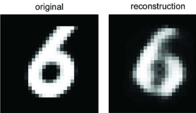
Figure 5.12 The first attempt to reconstruct an image during training shows the model has learned something but still has much progress to make.

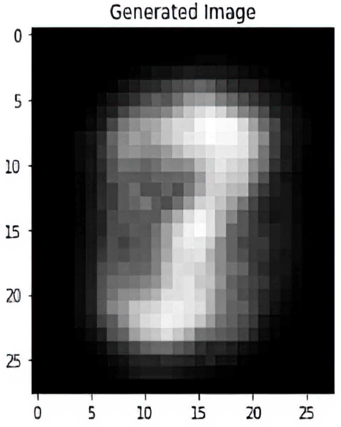
Figure 5.13 The first instance of an image generated from the generative model during training

But the model lear ns quickly . By 130 epochs, we get the results in figure 5.14.

After training is complete, we can see a visualization of loss over training (negative ELB O) in figure 5.15.

The code will train the parameters of the encoder that maps images and the labels to the latent variable. It will also train the decoder that maps the latent variable and the labels to the image. That latent variable is a fundamental featur e of the V AE, but we should tak e a closer look at how to interpr et the latent variable in causal ter ms.

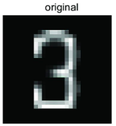
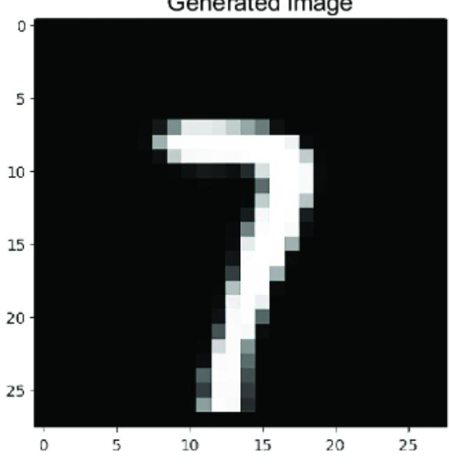
Figure 5.14 Reconstructed and randomly generated images from the model after 130 epochs of training look much better .

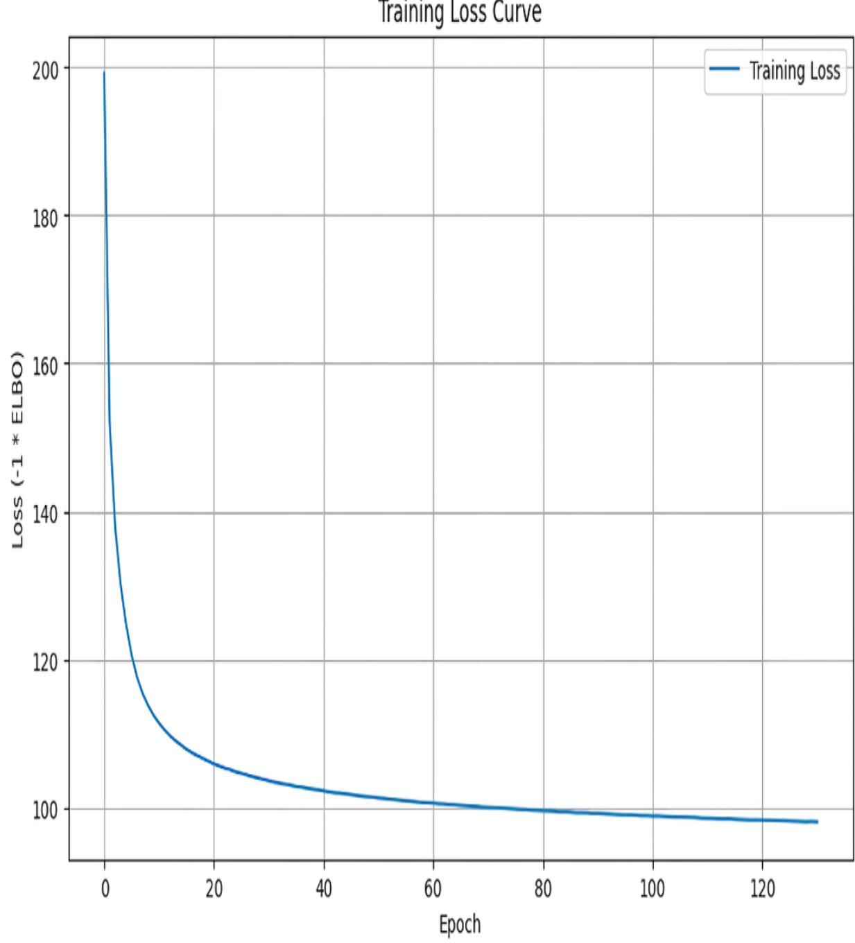
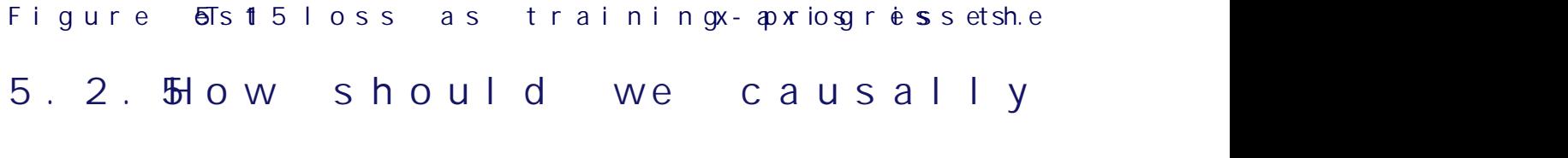
I said we can view Z as a ૿stand-in for all the independent latent causes of the object in the image. Z is a representation we lear n fr om the pix els in the images. It is

tempting to tr eat that r epresentation lik e a higher -level causal abstraction of those latent causes, but it is pr obably not doing a gr eat job as a causal abstraction. The autoencoder paradigm trains an encoder that can tak e an image and embed it into a low-dimensional r epresentation Z. It tries to do so in a way that enables it to r econstruct the original image as well as possible. In or der to r econstruct the image with little loss, the framework tries to encode as much infor mation fr om the original image as it can in that lower dimensional r epresentation.

A good causal representation, however, shouldn’t try to captur e as much infor mation as possible. R ather, it should strive to captur e only the causal infor mation in the images and ignor e everything else. Indeed, the task of ૿disentangling the causal and non-causal factors in Z is generally impossible when Z is unsupervised (meaning we lack labels for Z). However, domain knowledge, interventions, and semi-supervision can help. See https://www .altdeep.ai/p/causalaibookfor r efernces on causal representation learning and disentanglement of causal factors . As we pr ogress thr ough the book, we’ll develop intuition for what the ૿causal infor mation in such a representation should look lik e.

5.2.6 Advantages of this causal interpretation

There is nothing inher ently causal about our V AE’s setup and training pr ocedur e; it is typical of a vanilla supervised V AE you’d see in many machine lear ning settings. The only causal element of our appr oach was our interpr etation. W e say that the digit and is-handwritten are causes, and Z is a stand-in for latent causes, and the image is the outcome. Applying the causal Mark ov pr operty, our causal model factorizes the joint distribution into P(Z), P(is-handwritten ),

P(digit ), and P(image|Z, is-handwritten , digit ), wher e the latter factor is the causal Mark ov kernel of the image.

What can we do with this causal interpr etation? F irst, we can use it to impr ove deep lear ning and general machine learning work flows and tasks. W e’ll see an e xample of this with semi-supervised learning in the ne xt section.

INCORPORA TING GENERA TIVE AI IN CA USAL MODELS IS NOT LIMITED TO VAES

I demonstrated how to use a V AE framework to fit a causal Markov kernel entailed by a causal D AG, but a V AE was just one appr oach to achieving this end. W e could have used another deep pr obabilistic machine lear ning framework, such as a generative adversarial network (GAN) or a diusion model.

In this section, we incorporated deep lear ning into a causal graphical model. Ne xt, we investigate how to use causal ideas to enhance deep lear ning.

5.3Usingcausalinferencetoenhance deeplearning

We can use causal insights to impr ove how we set up and train deep lear ning models. These insights tend to lead to benefits such as impr oved sample e ciency (i.e., doing mor e with less data), the ability to do transfer lear ning (using what a model lear ned in solving one task to impr ove perfor mance on another), data fusion (combining di erent datasets), and enabling mor e robust pr edictions.

Much of the work of deep lear ning is trial and er ror. For example, when training a V AE or other deep lear ning models, you typically e xperiment with di erent appr oaches (V AE vs. another framework), ar chitectural choices (latent variable and hidden layer dimension, activation functions, number of layers, etc.), and training appr oaches (choice of loss function, lear ning rate, optimizer, etc.) befor e you get a good result. These e xperiments cost time, e ort, and r esour ces. In some cases, causal modeling can help you mak e better choices about what might work and what is unlik ely to work, leading to cost savings. In this section, we’ll look at a particular e xample of this case in the conte xt of semisupervised lear ning.

5.3.1 Independence of mechanism as an inductive bias

Suppose we had a D AG with two variables: ૿cause C and outcome O. The D AG is simply C → O. Our causal Mark ov kernels ar e P(C) and P(O|C). R ecall the idea of independence of mechanism from chapter 3—the causal Mark ov kernel P(O|C) represents a mechanism of how the cause C drives the outcome O. That mechanism is distinct fr om other mechanisms in the system, such that changes to those mechanisms have no e ect on P(O|C). Thus, knowing about P(O|C) tells you nothing about the distribution of the cause P(C) and vice versa. However, knowing something about the distribution of the outcome P(O) might tell you something about the distribution of the cause given the outcome P(C|O), and vice versa.

To illustrate, consider a scenario wher e C represents sunscr een usage and O indicates whether someone has sunbur n. Y ou understand the mechanism by which sunscr een protects against sunbur n (UV rays, SPF levels, r egular application, the perils of sweat and swimming, etc.), and by extension, the chances of getting sunbur n given how one uses sunscr een, captur ed by P(O|C). However, this understanding of the mechanism doesn’t pr ovide any infor mation about how common sunscr een use is, denoted by P(C).

Now, suppose you’r e trying to guess whether a sunbur ned person used sunscr een, i.e., you’r e mentally modeling P(C|O). In this case, knowing the pr evalence of sunbur ns, P(O), could help. Consider whether the sunbur ned individual was a case of someone who did use sunscr een but got a sunbur n anyway . That case would be mor e lik ely if sunbur ns were a common pr oblem than if sunbur ns wer e rar e—if sunbur ns ar e common, sunscr een use is pr obably common, but if sunbur ns wer e uncommon, people would be less cautious about pr evention.

Similarly, suppose C represents study e ort and O represents test scor es. Y ou know the causal mechanism behind how studying mor e causes higher test scor es, captur ed by P(O|C). But this doesn’t tell you how common it is for students to study har d, captur ed by P(C). Suppose a student got a low test scor e, and you ar e trying to infer whether they studied hard—you ar e mentally modeling P(C|O). Again, knowing the typical distribution of test scor es P(O) can help. If low scor es are rar e, students might be complacent, and thus mor e lik ely not to study har d. Y ou can use that insight as an inductive bias—a way to constrain your mental model of P(C|O).

CAUSAL INDUCTIVE BIAS

૿Inductive bias r efers to the assumptions (e xplicit or implicit) that lead an infer ence algorithm to pr efer certain infer ences or pr edictions over others. Examples of inductive bias include Occam’s R azor and the assumption in for ecasting that tr ends in the past will continue into the futur e.

Modern deep lear ning r elies on using neural network architectur es and training objectives to encode inductive bias. F or example, ૿convolutions and ૿max pooling ar e architectural elements in convolutional neural networks for computer vision that encode an inductive bias called ૿translation invariance; i.e., a kitten is still a kitten regardless of whether it appears on the lef t or right of an image.

Causal models pr ovide inductive biases in the for m of causal assumptions about the DGP (such as a causal D AG). Deep lear ning can leverage these causal inductive biases to attain better r esults just as it does with other types of inductive biases. F or example, independence of mechanism suggests that knowing P(O) could pr ovide a useful inductive bias in lear ning P(C|O).

Now consider two variables X and Y (which can be vectors) with joint distribution P(X, Y). We want to design an algorithm that solves a task by lear ning fr om data observed from P(X, Y). The chain rule of pr obability tells us that P(X=x, Y=y) = P(X=x|Y=y)P(Y=y) = P(Y=y|X=x)P(X= x). So, fr om that basic pr obabilistic perspective, modeling the set { P(X|Y ), P(Y )} is equivalent to modeling the set { P (Y |X), P(X)}. But consider the cases wher e either X is a cause of Y or wher e Y is a cause of X. Under these

circumstances, the independence of mechanism gives us an asymmetry between sets { P(X|Y ), P(Y )} and { P(Y |X), P (X)} (speci fically, { P(Y |X), P(X)} r epresents the independent mechanism behind X’s causal in fluence on Y, and {P(X|Y ), P(Y )} does not) that we can possibly leverage as an inductive bias in these algorithms. Semi-supervised learning is a good e xample.

5.3.2 Case study: Semi-supervised learning

Returning to our TMNIST -MNIST V AE-based causal model, suppose we had, in addition to our original data, a lar ge set of images of digits that wer e unlabeled (i.e., digit and ishandwritten are not observed). Our causal interpr etation of our model suggests we can leverage this data during training using semi-supervised lear ning.

Independence of mechanism can help you deter mine when semi-supervised lear ning will be e ective. In supervised learning , the training data consists of N samples of X, Y pairs; ( x1, y1), ( x2, y2), …, ( xN, yN). X is the feature data used to pr edict the labels Y. The data is ૿supervised because every x is pair ed with a y. We can use these pairs to lear n P (Y |X ). In unsupervised learning , the data X is unsupervised, meaning we have no labels, no observed value of Y. Our data looks lik e(x1), ( x2), …, ( xN). With this data alone, we can’t directly lear n anything about P(Y |X ); we can only lear n about P(X ). Semi-supervised lear ning asks the question, suppose we had a combination of supervised and unsupervised data. Could these two sets of data be combined in a way such that our ability to pr edict Y was better than if we only used the supervised data? In other words, can lear ning mor e about P(X ) fr om the unsupervised data somehow augment our lear ning of P(Y |X ) fr om the supervised data?

The semi-supervised question is quite practical. It is common to have abundant unsupervised e xamples if labeling those examples is costly . For example, suppose you work ed at a social media site and wer e task ed with building an algorithm that classi fied whether an uploaded image depicted gratuitous violence. The first step is to cr eate supervised data by having humans manually label images as gratuitously violent or not. Not only does this cost many people-hours, but it is mentally str essful for the labelers. A successful semi-supervised appr oach would mean you could minimize the amount of labeling work you need to do .

Our task is to lear n a r epresentation of P(X ,Y) and use it to predict fr om P(Y |X ). F or semi-supervised lear ning to work, the unlabeled values of X must update the r epresentation of P(X , Y) in a way that pr ovides infor mation about P(Y |X ). However, independence of mechanism means the task of learning P(X ,Y) decomposes into lear ning distinct representations of the causal Mark ov kernels, wher e the parameter vector of each r epresentation is orthogonal to the others. That parameter modularity (see section 3.2) can block flow of parameter updating infor mation fr om the unlabeled observations of X to the lear ned r epresentation of P(Y |X ). T o illustrate, let’s consider two possibilities, one where Y is a cause of X, and one wher e X is a cause of Y. If Y is a cause of X, such as in our MNIST -TMNIST e xample ( Y is the is-handwritten and digit variables, and X is the image), then our lear ning task decomposes into lear ning distinct representations of P(X |Y ) and P(Y). Unlabeled observations of Xcan give us a better r epresentation of P(X ), we can use to flip P(X |Y ) into P(Y |X ) by way of Bayes rule. However, when X is a cause of Y, our lear ning task decomposes into learning distinct r epresentations of P(X ) and P(Y |X ). That parameter modularity means those unlabeled values of X will help us update P(X )’s r epesentation but not that of P (Y |X ).

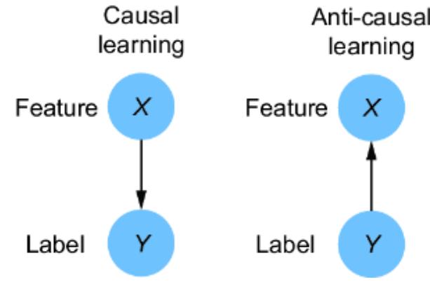
Figure 5.16 In causal learning, the features cause the label. In anticausal learning, the label causes the features.

The case wher e the featur e causes the label is sometimes called causal learning because the dir ection of the pr ediction is fr om the cause to the e ect. Anti-causal learning refers to the case when the label causes the featur e. The two cases are illustrated in figure 5.16.

Independence of mechanism suggests semi-supervised learning can achieve perfor mance gains (r elative to a baseline of supervised lear ning on only the labeled data) only in the anti-causal case. See the chapter notes at www.altdeep.ai/causalAIbook for a mor e detailed e xplanation and r efernces. But intuitively, we can see that this mir rors the the sunscr een and sunbur n example—knowing the prevalence of sunbur ns P(O) helped in lear ning how to guess sunscr een use when you know if someone has a sunbur n P(C|O). In this same anti-causal lear ning case, having only observations fr om P(X ) can still be helpful in learning a good model of P(Y|X ). But in the causal lear ning case, it would be a waste of e ort and r esour ces.

In practice, the causal structur e between X and Y could be more nuanced and complicated than these simple X Y and X Y cases. F or example, ther e could be unobserved common causes of X and Y. The tak eaway her e is that when you know something about the causal r elationships between

the variables in your machine lear ning pr oblem, you can leverage that knowledge to model mor e eectively, even if the task is not a causal infer ence task (e.g., simply pr edicting Y given X ). This could help you avoid spending time and resour ces on an appr oach that is not lik ely to work, as in the semi-supervised case. Or it could enable mor e ecient, robust, or better perfor ming infer ences.

5.3.3 Demystifying deep learning with causality

Our semi-supervised lear ning e xample highlights how a causal perspective can e xplain when we’d e xpect semisupervised lear ning to work and when to fail. In other wor ds, it somewhat demysti fies semi-supervised lear ning.

That mystery ar ound the e ectiveness of deep lear ning methods led AI r esear cher Ali R ahimi to compar e moder n machine lear ning to alchemy .

Alchemy work ed. Alchemists invented metallur gy, ways to dye te xtiles, moder n glass-making pr ocesses, and medications. Then again, alchemists also believed they could cur e diseases with leeches and transmute base metals into gold.

In other wor ds, alchemy works, but alchemists lack ed an understanding of the underlying scienti fic principles that made it work when it did. That mystery made it har d to know when it would fail. As a r esult, alchemists wasted considerable e ort on dead ends (philosopher’s stones, immortality elixirs, etc.).

CHAPTER CHECKPOINT

Incorporating deep learning into a causal model:

✓ A causal model of a computer vision pr oblem

✓ Training the deep causal image model Using causal reasoning to enhance machine learning:

✓ Case study on independence of mechanism and semisupervised lear ning

Demystif ying deep lear ning with causality

Similarly, deep lear ning ૿ works in that it achieves good perfor mance on a wide variety of pr ediction and infer ence tasks. But we of ten have an incomplete understanding of why and when it works. That mystery has led to pr oblems with r eproducibility, r obustness, and safety . It also leads to irresponsible applications of AI, such as published work that attempts to pr edict behavior (e.g., criminality) fr om profile photos. Such e orts ar e the machine lear ning analog of the alchemical immortality elixirs that contained to xins lik e mercury; they don’t work and they cause har m.

We often hear about the ૿super human perfor mance of deep learning. Speaking of super human ability, imagine an alter native telling of Super man’s origin story . Imagine if, when Super man made his first public appearance, his super human abilities wer e unr eliable? Suppose he demonstrated astounding super human feats lik e flight, super strength, and laser vision, but sometimes his flight ability failed and his super str ength falter ed. Sometimes his laser vision was danger ously unfocused, r esulting in ter rible

collateral damage. The public would be impr essed and hopeful that he could do some good, but unsur e if it would be safe to r ely on him when the stak es wer e high.

Now imagine that his adoptive Midwester n par ents, e xperts in causal infer ence, used causal analysis to model the how and why of his powers. Having demysti fied the mechanisms underlying his superpowers, they wer e able to engineer a pill that stabilized those powers. The pill wouldn’t so much give Superman new powers; it would just mak e his e xisting powers mor e reliable. The work of developing that pill would get fewer headlines than flight and laser vision, but it would be the di erence between mer ely having superpowers and being Super man.

This analogy helps us understand the impact of using causal methods to demystif y deep lear ning and other machine learning methods. L ess mystery leads to mor e robust methods and helps us avoid wasteful or har mful applications.

Summary

Deep learning can be used to enhance causal modeling and inference. Causal reasoning canenhance the setup, training, and perfor mance of deep lear ning models.
Causal models can leverage the ability of deep learning to scale and work withigh-dimensional nonlinear relationships.
You can use generative AI frameworks like the variational autoencoder to build a causal generative modl on a DAG just as we did with pgmpy .
The decoder maps the outcomes of direct parents (the labels of an image) to the outcomes of the child (the image).
In other words, the decoder gives us a nonlinear highdimensional representatio n of the causal Markov kernel for the image.
The encoder maps the image variable and the causes (labels) back to the latent variable Z.
We can view the learned representation of the latent variable as a stand-in forunmodeled causes, but it still lacks the qualities we’dexpect from an ideal causal representation. Learning latent causal representations is an active ar ea of r esear ch.
Causality often enhances deep learning and other machine learning methods by helping elucidate the underlying principles that make it work. For example, causal analy sis shows semi-supervised learning should work in the case of anti-causal learning (when the featur es are caused bythe label) but not in the case of causal learning (when the featur es cause the label).
Such causal insights can help the modeler avoid spending time, compute, person-hours, and other resour ces on a given algorithm when it is not likely to work in a given pr oblem setting.
Causal insights can demystif y elements of building and training deeplearning models, such that they become more robust, e cint, and safe.