AI Engineering

Building Applications with Foundation Models

Chapter 6 ~ 10

Author

Chip Huyen

CHAPTER 6 RAG and Agents

To solve a task, a model needs both the instructions on how to do it, and the neces‐ sary information to do so. Just like how a human is more likely to give a wrong answer when lacking information, AI models are more likely to make mistakes and hallucinate when they are missing context. For a given application, the model’s instructions are common to all queries, whereas context is specific to each query. The last chapter discussed how to write good instructions to the model. This chapter focuses on how to construct the relevant context for each query.

Two dominating patterns for context construction are RAG, or retrieval-augmented generation, and agents. The RAG pattern allows the model to retrieve relevant infor‐ mation from external data sources. The agentic pattern allows the model to use tools such as web search and news APIs to gather information.

While the RAG pattern is chiefly used for constructing context, the agentic pattern can do much more than that. External tools can help models address their shortcom‐ ings and expand their capabilities. Most importantly, they give models the ability to directly interact with the world, enabling them to automate many aspects of our lives.

Both RAG and agentic patterns are exciting because of the capabilities they bring to already powerful models. In a short amount of time, they’ve managed to capture the collective imagination, leading to incredible demos and products that convince many people that they are the future. This chapter will go into detail about each of these patterns, how they work, and what makes them so promising.

RAG

RAG is a technique that enhances a model’s generation by retrieving the relevant information from external memory sources. An external memory source can be an internal database, a user’s previous chat sessions, or the internet.

The retrieve-then-generate pattern was first introduced in “Reading Wikipedia to Answer Open-Domain Questions” (Chen et al., 2017). In this work, the system first retrieves five Wikipedia pages most relevant to a question, then a model¹ uses, or reads, the information from these pages to generate an answer, as visualized in Figure 6-1.

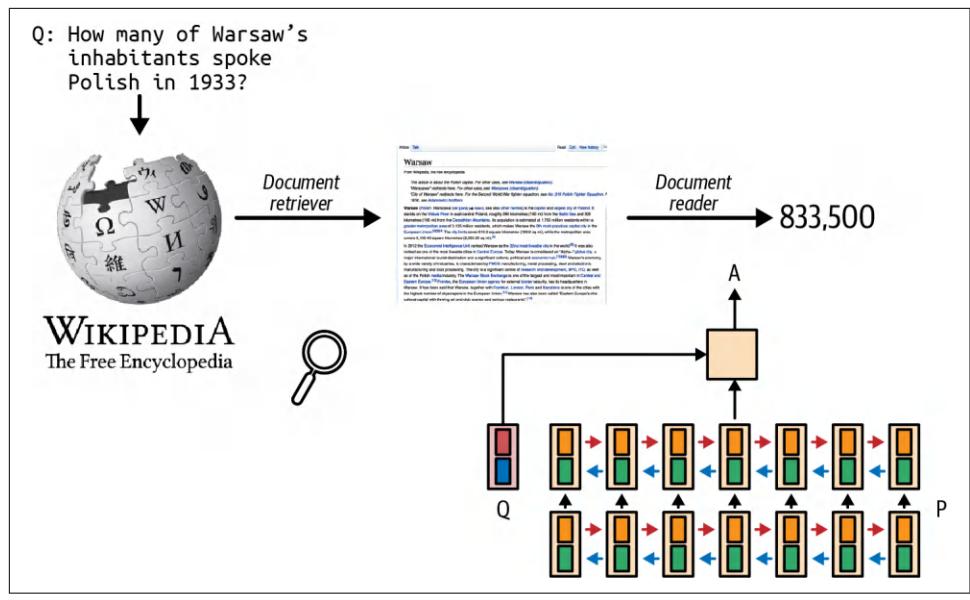
Figure 6-1. The retrieve-then-generate pattern. The model was referred to as the docu‐ ment reader.

The term retrieval-augmented generation was coined in “Retrieval-Augmented Gen‐ eration for Knowledge-Intensive NLP Tasks” (Lewis et al., 2020). The paper proposed RAG as a solution for knowledge-intensive tasks where all the available knowledge can’t be input into the model directly. With RAG, only the information most relevant to the query, as determined by the retriever, is retrieved and input into the model. Lewis et al. found that having access to relevant information can help the model gen‐ erate more detailed responses while reducing hallucinations.²

¹ The model used was a type of recurrent neural network known as LSTM (Long Short-Term Memory). LSTM was the dominant architecture of deep learning for natural language processing (NLP) before the transformer architecture took over in 2018.

² Around the same time, another paper, also from Facebook, “How Context Affects Language Models’ Factual Predictions” (Petroni et al., arXiv, May 2020), showed that augmenting a pre-trained language model with a retrieval system can dramatically improve the model’s performance on factual questions.

For example, given the query “Can Acme’s fancy-printer-A300 print 100pps?”, the model will be able to respond better if it’s given the specifications of fancy-printer-A300.³

You can think of RAG as a technique to construct context specific to each query, instead of using the same context for all queries. This helps with managing user data, as it allows you to include data specific to a user only in queries related to this user.

Context construction for foundation models is equivalent to feature engineering for classical ML models. They serve the same purpose: giving the model the necessary information to process an input.

In the early days of foundation models, RAG emerged as one of the most common patterns. Its main purpose was to overcome the models’ context limitations. Many people think that a sufficiently long context will be the end of RAG. I don’t think so. First, no matter how long a model’s context length is, there will be applications that require context longer than that. After all, the amount of available data only grows over time. People generate and add new data but rarely delete data. Context length is expanding quickly, but not fast enough for the data needs of arbitrary applications.⁴

Second, a model that can process long context doesn’t necessarily use that context well, as discussed in “Context Length and Context Efficiency” on page 218. The longer the context, the more likely the model is to focus on the wrong part of the con‐ text. Every extra context token incurs extra cost and has the potential to add extra latency. RAG allows a model to use only the most relevant information for each query, reducing the number of input tokens while potentially increasing the model’s performance.

Efforts to expand context length are happening in parallel with efforts to make mod‐ els use context more effectively. I wouldn’t be surprised if a model provider incorpo‐ rates a retrieval-like or attention-like mechanism to help a model pick out the most salient parts of a context to use.

³ Thanks to Chetan Tekur for the example.

⁴ Parkinson’s Law is usually expressed as “Work expands so as to fill the time available for its completion.” I have a similar theory that an application’s context expands to fill the context limit supported by the model it uses.

Anthropic suggested that for Claude models, if “your knowledge base is smaller than 200,000 tokens (about 500 pages of material), you can just include the entire knowledge base in the prompt that you give the model, with no need for RAG or similar methods” (Anthropic, 2024). It’d be amazing if other model developers pro‐ vide similar guidance for RAG versus long context for their models.

RAG Architecture

A RAG system has two components: a retriever that retrieves information from external memory sources and a generator that generates a response based on the retrieved information. Figure 6-2 shows a high-level architecture of a RAG system.

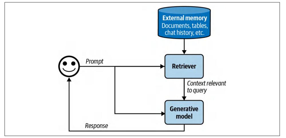
Figure 6-2. A basic RAG architecture.

In the original RAG paper, Lewis et al. trained the retriever and the generative model together. In today’s RAG systems, these two components are often trained separately, and many teams build their RAG systems using off-the-shelf retrievers and models. However, finetuning the whole RAG system end-to-end can improve its performance significantly.

The success of a RAG system depends on the quality of its retriever. A retriever has two main functions: indexing and querying. Indexing involves processing data so that it can be quickly retrieved later. Sending a query to retrieve data relevant to it is called querying. How to index data depends on how you want to retrieve it later on.

Now that we’ve covered the primary components, let’s consider an example of how a RAG system works. For simplicity, let’s assume that the external memory is a data‐ base of documents, such as a company’s memos, contracts, and meeting notes. A document can be 10 tokens or 1 million tokens. Naively retrieving whole documents can cause your context to be arbitrarily long. To avoid this, you can split each docu‐ ment into more manageable chunks. Chunking strategies will be discussed later in this chapter. For now, let’s assume that all documents have been split into workable chunks. For each query, our goal is to retrieve the data chunks most relevant to this query. Minor post-processing is often needed to join the retrieved data chunks with the user prompt to generate the final prompt. This final prompt is then fed into the generative model.

In this chapter, I use the term “document” to refer to both “docu‐ ment” and “chunk”, because technically, a chunk of a document is also a document. I do this to keep this book’s terminologies consis‐ tent with classical NLP and information retrieval (IR) terminolo‐ gies.

Retrieval Algorithms

Retrieval isn’t unique to RAG. Information retrieval is a century-old idea.⁵ It’s the backbone of search engines, recommender systems, log analytics, etc. Many retrieval algorithms developed for traditional retrieval systems can also be used for RAG. For instance, information retrieval is a fertile research area with a large supporting indus‐ try that can hardly be sufficiently covered within a few pages. Accordingly, this sec‐ tion will cover only the broad strokes. See this book’s GitHub repository for more indepth resources on information retrieval.

Retrieval is typically limited to one database or system, whereas search involves retrieval across various systems. This chapter uses retrieval and search interchangeably.

At its core, retrieval works by ranking documents based on their relevance to a given query. Retrieval algorithms differ based on how relevance scores are computed. I’ll start with two common retrieval mechanisms: term-based retrieval and embeddingbased retrieval.

⁵ Information retrieval was described as early as the 1920s in Emanuel Goldberg’s patents for a “statistical machine” to search documents stored on films. See “The History of Information Retrieval Research” (Sander‐ son and Croft, Proceedings of the IEEE, 100: Special Centennial Issue, April 2012).

Sparse Versus Dense Retrieval

In the literature, you might encounter the division of retrieval algorithms into the fol‐ lowing categories: sparse versus dense. This book, however, opted for term-based ver‐ sus embedding-based categorization.

Sparse retrievers represent data using sparse vectors. A sparse vector is a vector where the majority of the values are 0. Term-based retrieval is considered sparse, as each term can be represented using a sparse one-hot vector, a vector that is 0 everywhere except one value of 1. The vector size is the length of the vocabulary. The value of 1 is in the index corresponding to the index of the term in the vocabulary.

If we have a simple dictionary, {“food”: 0, “banana”: 1, “slug”: 2}, then the one-hot vectors of “food”, “banana”, and “slug” are [1, 0, 0], [0, 1, 0], and [0, 0, 1]. respectively.

Dense retrievers represent data using dense vectors. A dense vector is a vector where the majority of the values aren’t 0. Embedding-based retrieval is typically considered dense, as embeddings are generally dense vectors. However, there are also sparse embeddings. For example, SPLADE (Sparse Lexical and Expansion) is a retrieval algorithm that works using sparse embeddings (Formal et al., 2021). It leverages embeddings generated by BERT but uses regularization to push most embedding val‐ ues to 0. The sparsity makes embedding operations more efficient.

The sparse versus dense division causes SPLADE to be grouped together with termbased algorithms, even though SPLADE’s operations, strengths, and weaknesses are much more similar to those of dense embedding retrieval than those of term-based retrieval. Term-based versus embedding-based division avoids this miscategorization.

Term-based retrieval

Given a query, the most straightforward way to find relevant documents is with key‐ words. Some people call this approach lexical retrieval. For example, given the query “AI engineering”, the model will retrieve all the documents that contain “AI engi‐ neering”. However, this approach has two problems:

Many documents might contain the given term, and your model might not have sufficient context space to include all of them as context. A heuristic is to include the documents that contain the term the greatest number of times. The assump‐ tion is that the more a term appears in a document, the more relevant this docu‐ ment is to this term. The number of times a term appears in a document is called term frequency (TF).
A prompt can be long and contain many terms. Some are more important than others. For example, the prompt “Easy-to-follow recipes for Vietnamese food to cook at home” contains nine terms: easy-to-follow, recipes, for, vietnamese, food,

to, cook, at, home. You want to focus on more informative terms like vietnamese and recipes, not for and at. You need a way to identify important terms.

An intuition is that the more documents contain a term, the less informative this term is. “For” and “at” are likely to appear in most documents, hence, they are less informative. So a term’s importance is inversely proportional to the number of documents it appears in. This metric is called inverse document frequency (IDF). To compute IDF for a term, count all the documents that contain this term, then divide the total number of documents by this count. If there are 10 documents and 5 of them contain a given term, then the IDF of this term is 10 / 5 = 2. The higher a term’s IDF, the more important it is.

TF-IDF is an algorithm that combines these two metrics: term frequency (TF) and inverse document frequency (IDF). Mathematically, the TF-IDF score of document D for the query Q is computed as follows:

Let t¹ , t² , …, tqbe the terms in the query Q.
Given a term t, the term frequency of this term in the document D is f(t, D).
Let N be the total number of documents, and C(t) be the number of documents that contain t. The IDF value of the term t can be written as IDF(t) = log ^N C(t) .
Naively, the TF-IDF score of a document D with respect to Q is defined as Score(D, Q) = ∑ⁱ=1 q IDF(ti) × f(tⁱ , D).

Two common term-based retrieval solutions are Elasticsearch and BM25. Elastic‐ search (Shay Banon, 2010), built on top of Lucene, uses a data structure called an inverted index. It’s a dictionary that maps from terms to documents that contain them. This dictionary allows for fast retrieval of documents given a term. The index might also store additional information such as the term frequency and the docu‐ ment count (how many documents contain this term), which are helpful for comput‐ ing TF-IDF scores. Table 6-1 illustrates an inverted index.

	learning 3	(1, 5), (38, 7), (42, 5)
…	…	…

Table 6-1. A simplified example of an inverted index.

Okapi BM25, the 25th generation of the Best Matching algorithm, was developed by Robertson et al. in the 1980s. Its scorer is a modification of TF-IDF. Compared to naive TF-IDF, BM25 normalizes term frequency scores by document length. Longer documents are more likely to contain a given term and have higher term frequency values.⁶

BM25 and its variances (BM25+, BM25F) are still widely used in the industry and serve as formidable baselines to compare against modern, more sophisticated retrieval algorithms, such as embedding-based retrieval, discussed next.⁷

One process I glossed over is tokenization, the process of breaking a query into indi‐ vidual terms. The simplest method is to split the query into words, treating each word as a separate term. However, this can lead to multi-word terms being broken into individual words, losing their original meaning. For example, “hot dog” would be split into “hot” and “dog”. When this happens, neither retains the meaning of the original term. One way to mitigate this issue is to treat the most common n-grams as terms. If the bigram “hot dog” is common, it’ll be treated as a term.

Additionally, you might want to convert all characters to lowercase, remove punctua‐ tion, and eliminate stop words (like “the”, “and”, “is”, etc.). Term-based retrieval sol‐ utions often handle these automatically. Classical NLP packages, such as NLTK (Natural Language Toolkit), spaCy, and Stanford’s CoreNLP, also offer tokenization functionalities.

Chapter 4 discusses measuring the lexical similarity between two texts based on their n-gram overlap. Can we retrieve documents based on the extent of their n-gram overlap with the query? Yes, we can. This approach works best when the query and the documents are of similar lengths. If the documents are much longer than the query, the likelihood of them containing the query’s n-grams increases, leading to many documents having similarly high overlap scores. This makes it difficult to dis‐ tinguish truly relevant documents from less relevant ones.

Embedding-based retrieval

Term-based retrieval computes relevance at a lexical level rather than a semantic level. As mentioned in Chapter 3, the appearance of a text doesn’t necessarily capture its meaning. This can result in returning documents irrelevant to your intent. For example, querying “transformer architecture” might return documents about the electric device or the movie Transformers. On the other hand, embedding-based retrievers aim to rank documents based on how closely their meanings align with the query. This approach is also known as semantic retrieval.

⁶ For those interested in learning more about BM25, I recommend this paper by the BM25 authors: “The Prob‐ abilistic Relevance Framework: BM25 and Beyond” (Robertson and Zaragoza, Foundations and Trends in Information Retrieval 3 No. 4, 2009)

⁷ Aravind Srinivas, the CEO of Perplexity, tweeted that “Making a genuine improvement over BM25 or fulltext search is hard”.

With embedding-based retrieval, indexing has an extra function: converting the orig‐ inal data chunks into embeddings. The database where the generated embeddings are stored is called a vector database. Querying then consists of two steps, as shown in Figure 6-3:

1. Embedding model: convert the query into an embedding using the same embed‐ ding model used during indexing.
1. Retriever: fetch k data chunks whose embeddings are closest to the query embed‐ ding, as determined by the retriever. The number of data chunks to fetch, k, depends on the use case, the generative model, and the query.

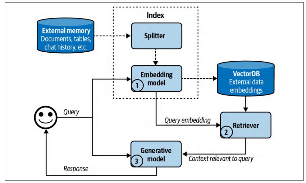
Figure 6-3. A high-level view of how an embedding-based, or semantic, retriever works.

The embedding-based retrieval workflow shown here is simplified. Real-world semantic retrieval systems might contain other components, such as a reranker to rerank all retrieved candidates, and caches to reduce latency.⁸

With embedding-based retrieval, we again encounter embeddings, which are dis‐ cussed in Chapter 3. As a reminder, an embedding is typically a vector that aims to preserve the important properties of the original data. An embedding-based retriever doesn’t work if the embedding model is bad.

⁸ A RAG retrieval workflow shares many similar steps with the traditional recommender system.

Embedding-based retrieval also introduces a new component: vector databases. A vector database stores vectors. However, storing is the easy part of a vector database. The hard part is vector search. Given a query embedding, a vector database is respon‐ sible for finding vectors in the database close to the query and returning them. Vec‐ tors have to be indexed and stored in a way that makes vector search fast and efficient.

Like many other mechanisms that generative AI applications depend on, vector search isn’t unique to generative AI. Vector search is common in any application that uses embeddings: search, recommendation, data organization, information retrieval, clustering, fraud detection, and more.

Vector search is typically framed as a nearest-neighbor search problem. For example, given a query, find the k nearest vectors. The naive solution is k-nearest neighbors (k-NN), which works as follows:

1. Compute the similarity scores between the query embedding and all vectors in the database, using metrics such as c osine similarity.
1. Rank all vectors by their similarity scores.
1. Return k vectors with the highest similarity scores.

This naive solution ensures that the results are precise, but it’s computationally heavy and slow. It should be used only for small datasets.

For large datasets, vector search is typically done using an approximate nearest neighbor (ANN) algorithm. Due to the importance of vector search, many algorithms and libraries have been developed for it. Some popular vector search libraries are FAISS (Facebook AI Similarity Search) (Johnson et al., 2017), Google’s ScaNN (Scal‐ able Nearest Neighbors) (Sun et al., 2020), Spotify’s Annoy (Bernhardsson, 2013), and Hnswlib (Hierarchical Navigable Small World) (Malkov and Yashunin, 2016).

Most application developers won’t implement vector search themselves, so I’ll give only a quick overview of different approaches. This overview might be helpful as you evaluate solutions.

In general, vector databases organize vectors into buckets, trees, or graphs. Vector search algorithms differ based on the heuristics they use to increase the likelihood that similar vectors are close to each other. Vectors can also be quantized (reduced precision) or made sparse. The idea is that quantized and sparse vectors are less com‐ putationally intensive to work with. For those wanting to learn more about vector search, Zilliz has an excellent series on it. Here are some significant vector search algorithms:

LSH (locality-sensitive hashing) (Indyk and Motwani, 1999)

This is a powerful and versatile algorithm that works with more than just vectors. This involves hashing similar vectors into the same buckets to speed up similarity search, trading some accuracy for efficiency. It’s implemented in FAISS and Annoy.

HNSW (Hierarchical Navigable Small World) (Malkov and Yashunin, 2016)

HNSW constructs a multi-layer graph where nodes represent vectors, and edges connect similar vectors, allowing nearest-neighbor searches by traversing graph edges. Its implementation by the authors is open source, and it’s also imple‐ mented in FAISS and Milvus.

Product Quantization (Jégou et al., 2011)

This works by reducing each vector into a much simpler, lower-dimensional rep‐ resentation by decomposing each vector into multiple subvectors. The distances are then computed using the lower-dimensional representations, which are much faster to work with. Product quantization is a key component of FAISS and is supported by almost all popular vector search libraries.

IVF (inverted file index) (Sivic and Zisserman, 2003)

IVF uses K-means clustering to organize similar vectors into the same cluster. Depending on the number of vectors in the database, it’s typical to set the num‐ ber of clusters so that, on average, there are 100 to 10,000 vectors in each cluster. During querying, IVF finds the cluster centroids closest to the query embedding, and the vectors in these clusters become candidate neighbors. Together with product quantization, IVF forms the backbone of FAISS.

Annoy (Approximate Nearest Neighbors Oh Yeah) (Bernhardsson, 2013)

Annoy is a tree-based approach. It builds multiple binary trees, where each tree splits the vectors into clusters using random criteria, such as randomly drawing a line and splitting the vectors into two branches using this line. During a search, it traverses these trees to gather candidate neighbors. Spotify has open sourced its implementation.

There are other algorithms, such as Microsoft’s SPTAG (Space Partition Tree And Graph), and FLANN (Fast Library for Approximate Nearest Neighbors).

Even though vector databases emerged as their own category with the rise of RAG, any database that can store vectors can be called a vector database. Many traditional databases have extended or will extend to support vector storage and vector search.

Comparing retrieval algorithms

Due to the long history of retrieval, its many mature solutions make both term-based and embedding-based retrieval relatively easy to start. Each approach has its pros and cons.

Term-based retrieval is generally much faster than embedding-based retrieval during both indexing and query. Term extraction is faster than embedding generation, and mapping from a term to the documents that contain it can be less computationally expensive than a nearest-neighbor search.

Term-based retrieval also works well out of the box. Solutions like Elasticsearch and BM25 have successfully powered many search and retrieval applications. However, its simplicity also means that it has fewer components you can tweak to improve its performance.

Embedding-based retrieval, on the other hand, can be significantly improved over time to outperform term-based retrieval. You can finetune the embedding model and the retriever, either separately, together, or in conjunction with the generative model. However, converting data into embeddings can obscure keywords, such as specific error codes, e.g., EADDRNOTAVAIL (99), or product names, making them harder to search later on. This limitation can be addressed by combining embedding-based retrieval with term-based retrieval, as discussed later in this chapter.

The quality of a retriever can be evaluated based on the quality of the data it retrieves. Two metrics often used by RAG evaluation frameworks are context precision and con‐ text recall, or precision and recall for short (context precision is also called context relevance):

Context precision

Out of all the documents retrieved, what percentage is relevant to the query?

Context recall

Out of all the documents that are relevant to the query, what percentage is retrieved?

To compute these metrics, you curate an evaluation set with a list of test queries and a set of documents. For each test query, you annotate each test document to be rele‐ vant or not relevant. The annotation can be done either by humans or AI judges. You then compute the precision and recall score of the retriever on this evaluation set.

In production, some RAG frameworks only support context precision, not context recall To compute context recall for a given query, you need to annotate the relevance of all documents in your database to that query. Context precision is simpler to com‐ pute. You only need to compare the retrieved documents to the query, which can be done by an AI judge.

If you care about the ranking of the retrieved documents, for example, more relevant documents should be ranked first, you can use metrics such as NDCG (nor‐ malized discounted cumulative gain), MAP (Mean Average Precision), and MRR (Mean Reciprocal Rank).

For semantic retrieval, you need to also evaluate the quality of your embeddings. As discussed in Chapter 3, embeddings can be evaluated independently—they are con‐ sidered good if more-similar documents have closer embeddings. Embeddings can also be evaluated by how well they work for specific tasks. The MTEB benchmark (Muennighoff et al., 2023) evaluates embeddings for a broad range of tasks including retrievals, classification, and clustering.

The quality of a retriever should also be evaluated in the context of the whole RAG system. Ultimately, a retriever is good if it helps the system generate high-quality answers. Evaluating outputs of generative models is discussed in Chapters 3 and 4.

Whether the performance promise of a semantic retrieval system is worth pursuing depends on how much you prioritize cost and latency, particularly during the query‐ ing phase. Since much of RAG latency comes from output generation, especially for long outputs, the added latency by query embedding generation and vector search might be minimal compared to the total RAG latency. Even so, the added latency still can impact user experience.

Another concern is cost. Generating embeddings costs money. This is especially an issue if your data changes frequently and requires frequent embedding regeneration. Imagine having to generate embeddings for 100 million documents every day! Depending on what vector databases you use, vector storage and vector search quer‐ ies can be expensive, too. It’s not uncommon to see a company’s vector database spending be one-fifth or even half of their spending on model APIs.

Table 6-2 shows a side-by-side comparison of term-based retrieval and embeddingbased retrieval.

Performance	Typically strong performance out of the box,
	but hard to improve
	Can retrieve wrong documents due to term	on semantics instead of terms
Cost	ambiguity Much cheaper than embedding-based retrieval	Embedding, vector storage, and vector search solutions can be expensive

Table 6-2. Term-based retrieval and semantic retrieval by speed, performance, and cost.

With retrieval systems, you can make certain trade-offs between indexing and query‐ ing. The more detailed the index is, the more accurate the retrieval process will be, but the indexing process will be slower and more memory-consuming. Imagine building an index of potential customers. Adding more details (e.g., name, company, email, phone, interests) makes it easier to find relevant people but takes longer to build and requires more storage.

In general, a detailed index like HNSW provides high accuracy and fast query times but requires significant time and memory to build. In contrast, a simpler index like LSH is quicker and less memory-intensive to create, but it results in slower and less accurate queries.

The ANN-Benchmarks website compares different ANN algorithms on multiple datasets using four main metrics, taking into account the trade-offs between indexing and querying. These include the following:

Recall

The fraction of the nearest neighbors found by the algorithm.

Query per second (QPS)

The number of queries the algorithm can handle per second. This is crucial for high-traffic applications.

Build time

The time required to build the index. This metric is especially important if you need to frequently update your index (e.g., because your data changes).

Index size

The size of the index created by the algorithm, which is crucial for assessing its scalability and storage requirements.

Additionally, BEIR (Benchmarking IR) (Thakur et al., 2021) is an evaluation harness for retrieval. It supports retrieval systems across 14 common retrieval benchmarks.

To summarize, the quality of a RAG system should be evaluated both component by component and end to end. To do this, you should do the following things:

1. Evaluate the retrieval quality.
1. Evaluate the final RAG outputs.
1. Evaluate the embeddings (for embedding-based retrieval).

Combining retrieval algorithms

Given the distinct advantages of different retrieval algorithms, a production retrieval system typically combines several approaches. Combining term-based retrieval and embedding-based retrieval is called hybrid search.

Different algorithms can be used in sequence. First, a cheap, less precise retriever, such as a term-based system, fetches candidates. Then, a more precise but more expensive mechanism, such as k-nearest neighbors, finds the best of these candidates. This second step is also called reranking.

For example, given the term “transformer”, you can fetch all documents that contain the word transformer, regardless of whether they are about the electric device, the neural architecture, or the movie. Then you use vector search to find among these documents those that are actually related to your transformer query. As another example, consider the query “Who’s responsible for the most sales to X?” First, you might fetch all documents associated with X using the keyword X. Then, you use vec‐ tor search to retrieve the context associated with “Who’s responsible for the most sales?”

Different algorithms can also be used in parallel as an ensemble. Remember that a retriever works by ranking documents by their relevance scores to the query. You can use multiple retrievers to fetch candidates at the same time, then combine these dif‐ ferent rankings together to generate a final ranking.

An algorithm for combining different rankings is called reciprocal rank fusion (RRF) (Cormack et al., 2009). It assigns each document a score based on its ranking by a retriever. Intuitively, if it ranks first, its score is 1/1 = 1. If it ranks second, its score is ½ = 0.5. The higher it ranks, the higher its score.

A document’s final score is the sum of its scores with respect to all retrievers. If a document is ranked first by one retriever and second by another retriever, its score is 1 + 0.5 = 1.5. This example is an oversimplification of RRF, but it shows the basics. The actual formula for a document D is more complicated, as follows:

Score(D) = ∑ⁱ=1 n 1 k + r i (D)

n is the number of ranked lists; each rank list is produced by a retriever.
ri(D) is the rank of the document by the retriever i.
k is a constant to avoid division by zero and to control the influence of lowerranked documents. A typical value for k is 60.

Retrieval Optimization

Depending on the task, certain tactics can increase the chance of relevant documents being fetched. Four tactics discussed here are chunking strategy, reranking, query rewriting, and contextual retrieval.

Chunking strategy

How your data should be indexed depends on how you intend to retrieve it later. The last section covered different retrieval algorithms and their respective indexing strate‐ gies. There, the discussion was based on the assumption that documents have already been split into manageable chunks. In this section, I’ll cover different chunking strategies. This is an important consideration because the chunking strategy you use can significantly impact the performance of your retrieval system.

The simplest strategy is to chunk documents into chunks of equal length based on a certain unit. Common units are characters, words, sentences, and paragraphs. For example, you can split each document into chunks of 2,048 characters or 512 words. You can also split each document so that each chunk can contain a fixed number of sentences (such as 20 sentences) or paragraphs (such as each paragraph is its own chunk).

You can also split documents recursively using increasingly smaller units until each chunk fits within your maximum chunk size. For example, you can start by splitting a document into sections. If a section is too long, split it into paragraphs. If a paragraph is still too long, split it into sentences. This reduces the chance of related texts being arbitrarily broken off.

Specific documents might also support creative chunking strategies. For example, there are splitters developed especially for different programming languages. Q&A documents can be split by question or answer pair, where each pair makes up a chunk. Chinese texts might need to be split differently from English texts.

When a document is split into chunks without overlap, the chunks might be cut off in the middle of important context, leading to the loss of critical information. Con‐ sider the text “I left my wife a note”. If it’s split into “I left my wife” and “a note”, neither of these two chunks conveys the key information of the original text. Over‐ lapping ensures that important boundary information is included in at least one chunk. If you set the chunk size to be 2,048 characters, you can perhaps set the over‐ lapping size to be 20 characters.

The chunk size shouldn’t exceed the maximum context length of the generative model. For the embedding-based approach, the chunk size also shouldn’t exceed the embedding model’s context limit.

You can also chunk documents using tokens, determined by the generative model’s tokenizer, as a unit. Let’s say that you want to use Llama 3 as your generative model. You then first tokenize documents using Llama 3’s tokenizer. You can then split documents into chunks using tokens as the boundaries. Chunking by tokens makes it easier to work with downstream models. However, the downside of this approach is that if you switch to another generative model with a different tokenizer, you’d need to reindex your data.

Regardless of which strategy you choose, chunk sizes matter. A smaller chunk size allows for more diverse information. Smaller chunks mean that you can fit more chunks into the model’s context. If you halve the chunk size, you can fit twice as many chunks. More chunks can provide a model with a wider range of information, which can enable the model to produce a better answer.

Small chunk sizes, however, can cause the loss of important information. Imagine a document that contains important information about the topic X throughout the document, but X is only mentioned in the first half. If you split this document into two chunks, the second half of the document might not be retrieved, and the model won’t be able to use its information.

Smaller chunk sizes can also increase computational overhead. This is especially an issue for embedding-based retrieval. Halving the chunk size means that you have twice as many chunks to index and twice as many embedding vectors to generate and store. Your vector search space will be twice as big, which can reduce the query speed.

There is no universal best chunk size or overlap size. You have to experiment to find what works best for you.

Reranking

The initial document rankings generated by the retriever can be further reranked to be more accurate. Reranking is especially useful when you need to reduce the number of retrieved documents, either to fit them into your model’s context or to reduce the number of input tokens.

One common pattern for reranking is discussed in “Combining retrieval algorithms” on page 266. A cheap but less precise retriever fetches candidates, then a more precise but more expensive mechanism reranks these candidates.

Documents can also be reranked based on time, giving higher weight to more recent data. This is useful for time-sensitive applications such as news aggregation, chat with your emails (e.g., a chatbot that can answer questions about your emails), or stock market analysis.

Context reranking differs from traditional search reranking in that the exact position of items is less critical. In search, the rank (e.g., first or fifth) is crucial. In context reranking, the order of documents still matters because it affects how well a model can process them. Models might better understand documents at the beginning and end of the context, as discussed in “Context Length and Context Efficiency” on page 218. However, as long as a document is included, the impact of its order is less signif‐ icant compared to search ranking.

Query rewriting

Query rewriting is also known as query reformulation, query normalization, and sometimes query expansion. Consider the following conversation:

User: When was the last time John Doe bought something from us? AI: John last bought a Fruity Fedora hat from us two weeks ago, on January 3, 2030. User: How about Emily Doe?

The last question, “How about Emily Doe?”, is ambiguous without context. If you use this query verbatim to retrieve documents, you’ll likely get irrelevant results. You need to rewrite this query to reflect what the user is actually asking. The new query should make sense on its own. In this case, the query should be rewritten to “When was the last time Emily Doe bought something from us?”

While I put query rewriting in “RAG” on page 253, query rewriting isn’t unique to RAG. In traditional search engines, query rewriting is often done using heuristics. In AI applications, query rewriting can also be done using other AI models, using a prompt similar to “Given the following conversation, rewrite the last user input to reflect what the user is actually asking”. Figure 6-4 shows how ChatGPT rewrote the query using this prompt.

Figure 6-4. You can use other generative models to rewrite queries.

Query rewriting can get complicated, especially if you need to do identity resolution or incorporate other knowledge. For example, if the user asks “How about his wife?” you will first need to query your database to find out who his wife is. If you don’t have this information, the rewriting model should acknowledge that this query isn’t solvable instead of hallucinating a name, leading to a wrong answer.

Contextual retrieval

The idea behind contextual retrieval is to augment each chunk with relevant context to make it easier to retrieve the relevant chunks. A simple technique is to augment a chunk with metadata like tags and keywords. For ecommerce, a product can be aug‐ mented by its description and reviews. Images and videos can be queried by their titles or captions.

The metadata may also include entities automatically extracted from the chunk. If your document contains specific terms like the error code EADDRNOTAVAIL (99), adding them to the document’s metadata allows the system to retrieve it by that key‐ word, even after the document has been converted into embeddings.

You can also augment each chunk with the questions it can answer. For customer support, you can augment each article with related questions. For example, the article on how to reset your password can be augmented with queries like “How to reset password?”, “I forgot my password”, “I can’t log in”, or even “Help, I can’t find my account”.⁹

If a document is split into multiple chunks, some chunks might lack the necessary context to help the retriever understand what the chunk is about. To avoid this, you can augment each chunk with the context from the original document, such as the original document’s title and summary. Anthropic used AI models to generate a short context, usually 50-100 tokens, that explains the chunk and its relationship to the original document. Here’s the prompt Anthropic used for this purpose (Anthropic, 2024):

<document>
{{WHOLE_DOCUMENT}}
</document>
Here is the chunk we want to situate within the whole document:
<chunk>
{{CHUNK_CONTENT}}
</chunk>

Please give a short succinct context to situate this chunk within the overall document for the purposes of improving search retrieval of the chunk. Answer only with the succinct context and nothing else.

⁹ Some teams have told me that their retrieval systems work best when the data is organized in a question-andanswer format.

The generated context for each chunk is prepended to each chunk, and the augmen‐ ted chunk is then indexed by the retrieval algorithm. Figure 6-5 visualizes the process that Anthropic follows.

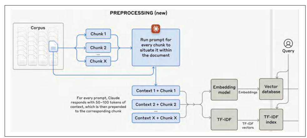
Figure 6-5. Anthropic augments each chunk with a short context that situates this chunk within the original document, making it easier for the retriever to find the rele‐ vant chunks given a query. Image from “Introducing Contextual Retrieval” (Anthropic, 2024).

Evaluating Retrieval Solutions

Here are some key factors to keep in mind when evaluating a retrieval solution:

What retrieval mechanisms does it support? Does it support hybrid search?
If it’s a vector database, what embedding models and vector search algorithms does it support?
How scalable is it, both in terms of data storage and query traffic? Does it work for your traffic patterns?
How long does it take to index your data? How much data can you process (such as add/delete) in bulk at once?
What’s its query latency for different retrieval algorithms?
If it’s a managed solution, what’s its pricing structure? Is it based on the docu‐ ment/vector volume or on the query volume?

This list doesn’t include the functionalities typically associated with enterprise solu‐ tions such as access control, compliance, data plane and control plane separation, etc.

RAG Beyond Texts

The last section discussed text-based RAG systems where the external data sources are text documents. However, external data sources can also be multimodal and tabu‐ lar data.

Multimodal RAG

If your generator is multimodal, its contexts might be augmented not only with text documents but also with images, videos, audio, etc., from external sources. I’ll use images in the examples to keep the writing concise, but you can replace images with any other modality. Given a query, the retriever fetches both texts and images rele‐ vant to it. For example, given “What’s the color of the house in the Pixar movie Up?” the retriever can fetch a picture of the house in Up to help the model answer, as shown in Figure 6-6.

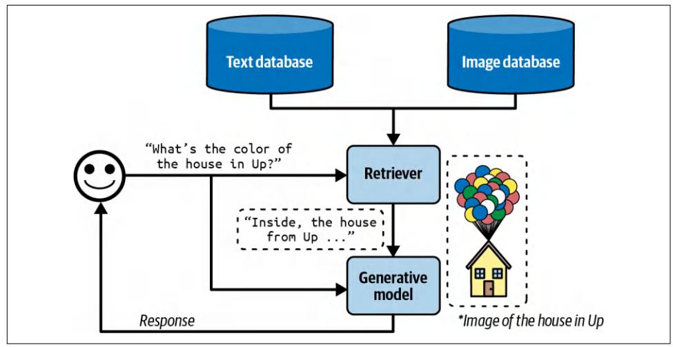
Figure 6-6. Multimodal RAG can augment a query with both text and images. (*The real image from Up is not used, for copyright reasons.)

If the images have metadata—such as titles, tags, and captions—they can be retrieved using the metadata. For example, an image is retrieved if its caption is considered rel‐ evant to the query.

If you want to retrieve images based on their content, you’ll need to have a way to compare images to queries. If queries are texts, you’ll need a multimodal embedding model that can generate embeddings for both images and texts. Let’s say you use CLIP (Radford et al., 2021) as the multimodal embedding model. The retriever works as follows:

1. Generate CLIP embeddings for all your data, both texts and images, and store them in a vector database.
1. Given a query, generate its CLIP embedding.
1. Query in the vector database for all images and texts whose embeddings are close to the query embedding.

RAG with tabular data

Most applications work not only with unstructured data like texts and images but also with tabular data. Many queries might need information from data tables to answer. The workflow for augmenting a context using tabular data is significantly different from the classic RAG workflow.

Imagine you work for an ecommerce site called Kitty Vogue that specializes in cat fashion. This store has an order table named Sales, as shown in Table 6-3.

Table 6-3. An example of an order table, Sales, for the imaginary ecommerce site Kitty Vogue.

		Unit price ($) Units Total
2044	Meow Mix Seasoning	10.99	10.99
3497	Purr & Shake	25	50
2045	Fruity Fedora	18	18

To generate a response to the question “How many units of Fruity Fedora were sold in the last 7 days?”, your system needs to query this table for all orders involving Fruity Fedora and sum the number of units across all orders. Assume that this table can be queried using SQL. The SQL query might look like this:

SELECT SUM(units) AS total_units_sold
FROM Sales
WHERE product_name = 'Fruity Fedora'
AND timestamp >= DATE_SUB(CURDATE(), INTERVAL 7 DAY);

The workflow is as follows, visualized in Figure 6-7. To run this workflow, your sys‐ tem must have the ability to generate and execute the SQL query:

1. Text-to-SQL: based on the user query and the provided table schemas, determine what SQL query is needed. Text-to-SQL is an example of semantic parsing, as discussed in Chapter 2.
1. SQL execution: execute the SQL query.
1. Generation: generate a response based on the SQL result and the original user query.

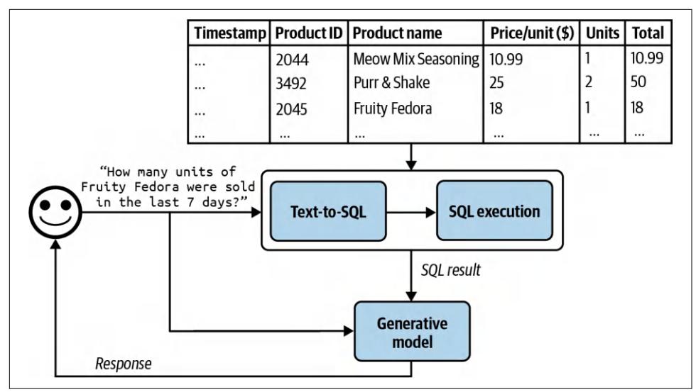
Figure 6-7. A RAG system that augments context with tabular data.

For the text-to-SQL step, if there are many available tables whose schemas can’t all fit into the model context, you might need an intermediate step to predict what tables to use for each query. Text-to-SQL can be done by the same generator that generates the final response or a specialized text-to-SQL model.

In this section, we’ve discussed how tools such as retrievers and SQL executors can enable models to handle more queries and generate higher-quality responses. Would giving a model access to more tools improve its capabilities even more? Tool use is a core characteristic of the agentic pattern, which we’ll discuss in the next section.

Agents

Intelligent agents are considered by many to be the ultimate goal of AI. The classic book by Stuart Russell and Peter Norvig, Artificial Intelligence: A Modern Approach (Prentice Hall, 1995) defines the field of artificial intelligence research as “the study and design of rational agents.”

The unprecedented capabilities of foundation models have opened the door to agentic applications that were previously unimaginable. These new capabilities make it finally possible to develop autonomous, intelligent agents to act as our assistants, coworkers, and coaches. They can help us create a website, gather data, plan a trip, do market research, manage a customer account, automate data entry, prepare us for interviews, interview our candidates, negotiate a deal, etc. The possibilities seem end‐ less, and the potential economic value of these agents is enormous.

AI-powered agents are an emerging field, with no established theo‐ retical frameworks for defining, developing, and evaluating them. This section is a best-effort attempt to build a framework from the existing literature, but it will evolve as the field does. Compared to the rest of the book, this section is more experimental.

This section will start with an overview of agents, and then continue with two aspects that determine the capabilities of an agent: tools and planning. Agents, with their new modes of operations, have new modes of failures. This section will end with a discus‐ sion on how to evaluate agents to catch these failures.

Even though agents are novel, they are built upon concepts that have already appeared in this book, including self-critique, chain-of-thought, and structured out‐ puts.

Agent Overview

The term agent has been used in many different engineering contexts, including but not limited to a software agent, intelligent agent, user agent, conversational agent, and reinforcement learning agent. So, what exactly is an agent?

An agent is anything that can perceive its environment and act upon that environ‐ ment.¹⁰ This means that an agent is characterized by the environment it operates in and the set of actions it can perform.

The environment an agent can operate in is defined by its use case. If an agent is developed to play a game (e.g., Minecraft, Go, Dota), that game is its environment. If you want an agent to scrape documents from the internet, the environment is the internet. If your agent is a cooking robot, the kitchen is its environment. A selfdriving car agent’s environment is the road system and its adjacent areas.

The set of actions an AI agent can perform is augmented by the tools it has access to. Many generative AI-powered applications you interact with daily are agents with access to tools, albeit simple ones. ChatGPT is an agent. It can search the web, exe‐ cute Python code, and generate images. RAG systems are agents, and text retrievers, image retrievers, and SQL executors are their tools.

There’s a strong dependency between an agent’s environment and its set of tools. The environment determines what tools an agent can potentially use. For example, if the environment is a chess game, the only possible actions for an agent are the valid chess moves. However, an agent’s tool inventory restricts the environment it can operate

¹⁰ Artificial Intelligence: A Modern Approach (1995) defines an agent as anything that can be viewed as perceiv‐ ing its environment through sensors and acting upon that environment through actuators.

in. For example, if a robot’s only action is swimming, it’ll be confined to a water envi‐ ronment.

Figure 6-8 shows a visualization of SWE-agent (Yang et al., 2024), an agent built on top of GPT-4. Its environment is the computer with the terminal and the file system. Its set of actions include navigate repo, search files, view files, and edit lines.

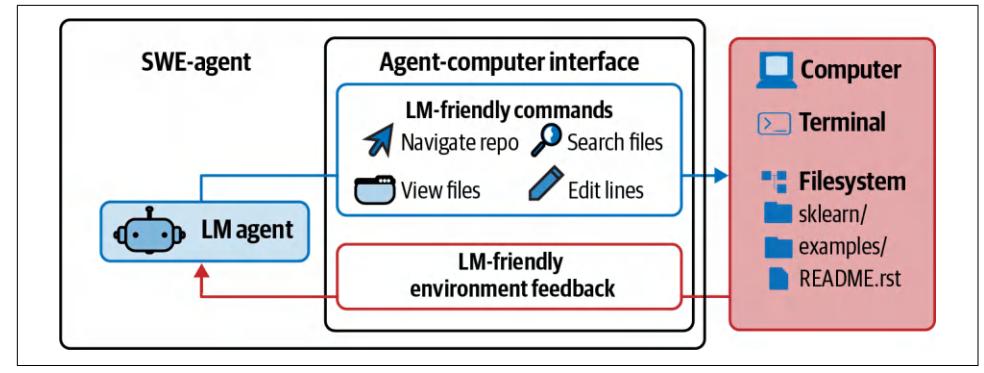
Figure 6-8. SWE-agent (Yang et al., 2024) is a coding agent whose environment is the computer and whose actions include navigation, search, and editing. Adapted from an original image licensed under CC BY 4.0.

An AI agent is meant to accomplish tasks typically provided by the users in the inputs. In an AI agent, AI is the brain that processes the information it receives, including the task and feedback from the environment, plans a sequence of actions to achieve this task, and determines whether the task has been accomplished.

Let’s get back to the RAG system with tabular data in the Kitty Vogue example. This is a simple agent with three actions: response generation, SQL query generation, and SQL query execution. Given the query “Project the sales revenue for Fruity Fedora over the next three months”, the agent might perform the following sequence of actions:

1. Reason about how to accomplish this task. It might decide that to predict future sales, it first needs the sales numbers from the last five years. Note that the agent’s reasoning is shown as its intermediate response.
1. Invoke SQL query generation to generate the query to get sales numbers from the last five years.
1. Invoke SQL query execution to execute this query.
1. Reason about the tool outputs and how they help with sales prediction. It might decide that these numbers are insufficient to make a reliable projection, perhaps because of missing values. It then decides that it also needs information about past marketing campaigns.
5. Invoke SQL query generation to generate the queries for past marketing cam‐ paigns.
1. Invoke SQL query execution.
1. Reason that this new information is sufficient to help predict future sales. It then generates a projection.
1. Reason that the task has been successfully completed.

Compared to non-agent use cases, agents typically require more powerful models for two reasons:

Compound mistakes: an agent often needs to perform multiple steps to accom‐ plish a task, and the overall accuracy decreases as the number of steps increases. If the model’s accuracy is 95% per step, over 10 steps, the accuracy will drop to 60%, and over 100 steps, the accuracy will be only 0.6%.
Higher stakes: with access to tools, agents are capable of performing more impactful tasks, but any failure could have more severe consequences.

A task that requires many steps can take time and money to run.¹¹ However, if agents can be autonomous, they can save a lot of human time, making their costs worth‐ while.

Given an environment, the success of an agent in an environment depends on the tool inventory it has access to and the strength of its AI planner. Let’s start by looking into different kinds of tools a model can use.

Tools

A system doesn’t need access to external tools to be an agent. However, without external tools, the agent’s capabilities would be limited. By itself, a model can typi‐ cally perform one action—for example, an LLM can generate text, and an image gen‐ erator can generate images. External tools make an agent vastly more capable.

Tools help an agent to both perceive the environment and act upon it. Actions that allow an agent to perceive the environment are read-only actions, whereas actions that allow an agent to act upon the environment are write actions.

This section gives an overview of external tools. How tools can be used will be dis‐ cussed in “Planning” on page 281.

The set of tools an agent has access to is its tool inventory. Since an agent’s tool inventory determines what an agent can do, it’s important to think through what and

¹¹ A complaint in the early days of agents is that agents are only good for burning through your API credits.

how many tools to give an agent. More tools give an agent more capabilities. How‐ ever, the more tools there are, the more challenging it is to understand and utilize them well. Experimentation is necessary to find the right set of tools, as discussed in “Tool selection” on page 295.

Depending on the agent’s environment, there are many possible tools. Here are three categories of tools that you might want to consider: knowledge augmentation (i.e., context construction), capability extension, and tools that let your agent act upon its environment.

Knowledge augmentation

I hope that this book, so far, has convinced you of the importance of having the rele‐ vant context for a model’s response quality. An important category of tools includes those that help augment your agent’s knowledge of your agent. Some of them have already been discussed: text retriever, image retriever, and SQL executor. Other potential tools include internal people search, an inventory API that returns the sta‐ tus of different products, Slack retrieval, an email reader, etc.

Many such tools augment a model with your organization’s private processes and information. However, tools can also give models access to public information, espe‐ cially from the internet.

Web browsing was among the earliest and most anticipated capabilities to be incor‐ porated into chatbots like ChatGPT. Web browsing prevents a model from going stale. A model goes stale when the data it was trained on becomes outdated. If the model’s training data was cut off last week, it won’t be able to answer questions that require information from this week unless this information is provided in the con‐ text. Without web browsing, a model won’t be able to tell you about the weather, news, upcoming events, stock prices, flight status, etc.

I use web browsing as an umbrella term to cover all tools that access the internet, including web browsers and specific APIs such as search APIs, news APIs, GitHub APIs, or social media APIs such as those of X, LinkedIn, and Reddit.

While web browsing allows your agent to reference up-to-date information to gener‐ ate better responses and reduce hallucinations, it can also open up your agent to the cesspools of the internet. Select your Internet APIs with care.

Capability extension

The second category of tools to consider are those that address the inherent limita‐ tions of AI models. They are easy ways to give your model a performance boost. For example, AI models are notorious for being bad at math. If you ask a model what is 199,999 divided by 292, the model will likely fail. However, this calculation is trivial if the model has access to a calculator. Instead of trying to train the model to be good at arithmetic, it’s a lot more resource-efficient to just give the model access to a tool.

Other simple tools that can significantly boost a model’s capability include a calen‐ dar, timezone converter, unit converter (e.g., from lbs to kg), and translator that can translate to and from the languages that the model isn’t good at.

More complex but powerful tools are code interpreters. Instead of training a model to understand code, you can give it access to a code interpreter so that it can execute a piece of code, return the results, or analyze the code’s failures. This capability lets your agents act as coding assistants, data analysts, and even research assistants that can write code to run experiments and report results. However, automated code exe‐ cution comes with the risk of code injection attacks, as discussed in “Defensive Prompt Engineering” on page 235. Proper security measurements are crucial to keep you and your users safe.

External tools can make a text-only or image-only model multimodal. For example, a model that can generate only texts can leverage a text-to-image model as a tool, allowing it to generate both texts and images. Given a text request, the agent’s AI planner decides whether to invoke text generation, image generation, or both. This is how ChatGPT can generate both text and images—it uses DALL-E as its image gen‐ erator. Agents can also use a code interpreter to generate charts and graphs, a LaTeX compiler to render math equations, or a browser to render web pages from HTML code.

Similarly, a model that can process only text inputs can use an image captioning tool to process images and a transcription tool to process audio. It can use an OCR (opti‐ cal character recognition) tool to read PDFs.

Tool use can significantly boost a model’s performance compared to just prompting or even finetuning. Chameleon (Lu et al., 2023) shows that a GPT-4-powered agent, aug‐ mented with a set of 13 tools, can outperform GPT-4 alone on several benchmarks. Examples of tools this agent used are knowledge retrieval, a query generator, an image captioner, a text detector, and Bing search.

On ScienceQA, a science question answering benchmark, Chameleon improves the best published few-shot result by 11.37%. On TabMWP (Tabular Math Word Prob‐ lems) (Lu et al., 2022), a benchmark involving tabular math questions, Chameleon improves the accuracy by 17%.

Write actions

So far, we’ve discussed read-only actions that allow a model to read from its data sources. But tools can also perform write actions, making changes to the data sources. A SQL executor can retrieve a data table (read) but can also change or delete the table

(write). An email API can read an email but can also respond to it. A banking API can retrieve your current balance but can also initiate a bank transfer.

Write actions enable a system to do more. They can enable you to automate the whole customer outreach workflow: researching potential customers, finding their contacts, drafting emails, sending first emails, reading responses, following up, extracting orders, updating your databases with new orders, etc.

However, the prospect of giving AI the ability to automatically alter our lives is frightening. Just as you shouldn’t give an intern the authority to delete your produc‐ tion database, you shouldn’t allow an unreliable AI to initiate bank transfers. Trust in the system’s capabilities and its security measures is crucial. You need to ensure that the system is protected from bad actors who might try to manipulate it into perform‐ ing harmful actions.

When I talk about autonomous AI agents to a group of people, there is often some‐ one who brings up self-driving cars. “What if someone hacks into the car to kidnap you?” While the self-driving car example seems visceral because of its physicality, an AI system can cause harm without a presence in the physical world. It can manip‐ ulate the stock market, steal copyrights, violate privacy, reinforce biases, spread mis‐ information and propaganda, and more, as discussed in “Defensive Prompt Engineering” on page 235.

These are all valid concerns, and any organization that wants to leverage AI needs to take safety and security seriously. However, this doesn’t mean that AI systems should never be given the ability to act in the real world. If we can get people to trust a machine to take us into space, I hope that one day, security measures will be suffi‐ cient for us to trust autonomous AI systems. Besides, humans can fail, too. Person‐ ally, I would trust a self-driving car more than the average stranger to drive me around.

Just as the right tools can help humans be vastly more productive—can you imagine doing business without Excel or building a skyscraper without cranes?—tools enable models to accomplish many more tasks. Many model providers already support tool use with their models, a feature often called function calling. Going forward, I would expect function calling with a wide set of tools to be common with most models.

Planning

At the heart of a foundation model agent is the model responsible for solving a task. A task is defined by its goal and constraints. For example, one task is to schedule a two-week trip from San Francisco to India with a budget of $5,000. The goal is the two-week trip. The constraint is the budget.

Complex tasks require planning. The output of the planning process is a plan, which is a roadmap outlining the steps needed to accomplish a task. Effective planning typi‐ cally requires the model to understand the task, consider different options to achieve this task, and choose the most promising one.

If you’ve ever been in any planning meeting, you know that planning is hard. As an important computational problem, planning is well studied and would require sev‐ eral volumes to cover. I’ll only be able to cover the surface here.

Planning overview

Given a task, there are many possible ways to decompose it, but not all of them will lead to a successful outcome. Among the correct solutions, some are more efficient than others. Consider the query, “How many companies without revenue have raised at least $1 billion?” There are many possible ways to solve this, but as an illustration, consider the two options:

1. Find all companies without revenue, then filter them by the amount raised.
1. Find all companies that have raised at least $1 billion, then filter them by revenue.

The second option is more efficient. There are vastly more companies without reve‐ nue than companies that have raised $1 billion. Given only these two options, an intelligent agent should choose option 2.

You can couple planning with execution in the same prompt. For example, you give the model a prompt, ask it to think step by step (such as with a chain-of-thought prompt), and then execute those steps all in one prompt. But what if the model comes up with a 1,000-step plan that doesn’t even accomplish the goal? Without oversight, an agent can run those steps for hours, wasting time and money on API calls, before you realize that it’s not going anywhere.

To avoid fruitless execution, planning should be decoupled from execution. You ask the agent to first generate a plan, and only after this plan is validated is it executed. The plan can be validated using heuristics. For example, one simple heuristic is to eliminate plans with invalid actions. If the generated plan requires a Google search and the agent doesn’t have access to Google Search, this plan is invalid. Another sim‐ ple heuristic might be eliminating all plans with more than X steps. A plan can also be validated using AI judges. You can ask a model to evaluate whether the plan seems reasonable or how to improve it.

If the generated plan is evaluated to be bad, you can ask the planner to generate another plan. If the generated plan is good, execute it. If the plan consists of external tools, function calling will be invoked. Outputs from executing this plan will then again need to be evaluated. Note that the generated plan doesn’t have to be an

end-to-end plan for the whole task. It can be a small plan for a subtask. The whole process looks like Figure 6-9.

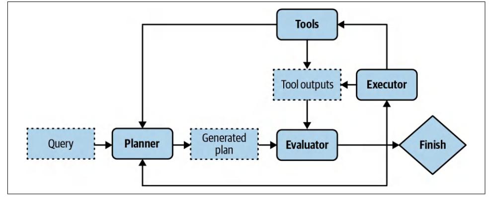
Figure 6-9. Decoupling planning and execution so that only validated plans are executed.

Your system now has three components: one to generate plans, one to validate plans, and another to execute plans. If you consider each component an agent, this is a multi-agent system.¹²

To speed up the process, instead of generating plans sequentially, you can generate several plans in parallel and ask the evaluator to pick the most promising one. This is another latency/cost trade-off, as generating multiple plans simultaneously will incur extra costs.

Planning requires understanding the intention behind a task: what’s the user trying to do with this query? An intent classifier is often used to help agents plan. As shown in “Break Complex Tasks into Simpler Subtasks” on page 224, intent classification can be done using another prompt or a classification model trained for this task. The intent classification mechanism can be considered another agent in your multi-agent system.

Knowing the intent can help the agent pick the right tools. For example, for customer support, if the query is about billing, the agent might need access to a tool to retrieve a user’s recent payments. But if the query is about how to reset a password, the agent might need to access documentation retrieval.

¹² Because most agentic workflows are sufficiently complex to involve multiple components, most agents are multi-agent.

Some queries might be out of the scope of the agent. The intent classifier should be able to classify requests as IRRELEVANT so that the agent can politely reject those instead of wasting FLOPs coming up with impossible solutions.

So far, we’ve assumed that the agent automates all three stages: generating plans, vali‐ dating plans, and executing plans. In reality, humans can be involved at any of those stages to aid with the process and mitigate risks. A human expert can provide a plan, validate a plan, or execute parts of a plan. For example, for complex tasks for which an agent has trouble generating the whole plan, a human expert can provide a highlevel plan that the agent can expand upon. If a plan involves risky operations, such as updating a database or merging a code change, the system can ask for explicit human approval before executing or let humans execute these operations. To make this pos‐ sible, you need to clearly define the level of automation an agent can have for each action.

To summarize, solving a task typically involves the following processes. Note that reflection isn’t mandatory for an agent, but it’ll significantly boost the agent’s perfor‐ mance:

1. Plan generation: come up with a plan for accomplishing this task. A plan is a sequence of manageable actions, so this process is also called task decomposition.
1. Reflection and error correction: evaluate the generated plan. If it’s a bad plan, gen‐ erate a new one.
1. Execution: take the actions outlined in the generated plan. This often involves calling specific functions.
1. Reflection and error correction: upon receiving the action outcomes, evaluate these outcomes and determine whether the goal has been accomplished. Identify and correct mistakes. If the goal is not completed, generate a new plan.

You’ve already seen some techniques for plan generation and reflection in this book. When you ask a model to “think step by step”, you’re asking it to decompose a task. When you ask a model to “verify if your answer is correct”, you’re asking it to reflect.

Foundation models as planners

An open question is how well foundation models can plan. Many researchers believe that foundation models, at least those built on top of autoregressive language models, cannot. Meta’s Chief AI Scientist Yann LeCun states unequivocally that autoregres‐ sive LLMs can’t plan (2023). In the article “Can LLMs Really Reason and Plan?” Kambhampati (2023) argues that LLMs are great at extracting knowledge but not planning. Kambhampati suggests that the papers claiming planning abilities of LLMs confuse general planning knowledge extracted from the LLMs with executable plans.

“The plans that come out of LLMs may look reasonable to the lay user, and yet lead to execution time interactions and errors.”

However, while there is a lot of anecdotal evidence that LLMs are poor planners, it’s unclear whether it’s because we don’t know how to use LLMs the right way or because LLMs, fundamentally, can’t plan.

Planning, at its core, is a search problem. You search among different paths to the goal, predict the outcome (reward) of each path, and pick the path with the most promising outcome. Often, you might determine that no path exists that can take you to the goal.

Search often requires backtracking. For example, imagine you’re at a step where there are two possible actions: A and B. After taking action A, you enter a state that’s not promising, so you need to backtrack to the previous state to take action B.

Some people argue that an autoregressive model can only generate forward actions. It can’t backtrack to generate alternate actions. Because of this, they conclude that autoregressive models can’t plan. However, this isn’t necessarily true. After executing a path with action A, if the model determines that this path doesn’t make sense, it can revise the path using action B instead, effectively backtracking. The model can also always start over and choose another path.

It’s also possible that LLMs are poor planners because they aren’t given the toolings needed to plan. To plan, it’s necessary to know not only the available actions but also the potential outcome of each action. As a simple example, let’s say you want to walk up a mountain. Your potential actions are turn right, turn left, turn around, or go straight ahead. However, if turning right will cause you to fall off the cliff, you might not want to consider this action. In technical terms, an action takes you from one state to another, and it’s necessary to know the outcome state to determine whether to take an action.

This means it’s not sufficient to prompt a model to generate only a sequence of actions like what the popular chain-of-thought prompting technique does. The paper “Reasoning with Language Model is Planning with World Model” (Hao et al., 2023) argues that an LLM, by containing so much information about the world, is capable of predicting the outcome of each action. This LLM can incorporate this outcome prediction to generate coherent plans.

Even if AI can’t plan, it can still be a part of a planner. It might be possible to aug‐ ment an LLM with a search tool and state tracking system to help it plan.

Foundation Model (FM) Versus Reinforcement Learning (RL) Planners

The agent is a core concept in RL, which is defined in Wikipedia as a field “concerned with how an intelligent agent ought to take actions in a dynamic environment in order to maximize the cumulative reward.”

RL agents and FM agents are similar in many ways. They are both characterized by their environments and possible actions. The main difference is in how their planners work. In an RL agent, the planner is trained by an RL algorithm. Training this RL planner can require a lot of time and resources. In an FM agent, the model is the planner. This model can be prompted or finetuned to improve its planning capabili‐ ties, and generally requires less time and fewer resources.

However, there’s nothing to prevent an FM agent from incorporating RL algorithms to improve its performance. I suspect that in the long run, FM agents and RL agents will merge.

Plan generation

The simplest way to turn a model into a plan generator is with prompt engineering. Imagine that you want to create an agent to help customers learn about products at Kitty Vogue. You give this agent access to three external tools: retrieve products by price, retrieve top products, and retrieve product information. Here’s an example of a prompt for plan generation. This prompt is for illustration purposes only. Production prompts are likely more complex:

SYSTEM PROMPT

Propose a plan to solve the task. You have access to 5 actions: get_today_date() fetch_top_products(start_date, end_date, num_products) fetch_product_info(product_name) generate_query(task_history, tool_output) generate_response(query)

The plan must be a sequence of valid actions.

Examples Task: “Tell me about Fruity Fedora” Plan: [fetch_product_info, generate_query, generate_response] Task: “What was the best selling product last week?” Plan: [fetch_top_products, generate_query, generate_response]

Task: {USER INPUT}
Plan:

There are two things to note about this example:

The plan format used here—a list of functions whose parameters are inferred by the agent—is just one of many ways to structure the agent control flow.
The generate_query function takes in the task’s current history and the most recent tool outputs to generate a query to be fed into the response generator. The tool output at each step is added to the task’s history.

Given the user input “What’s the price of the best-selling product last week”, a gener‐ ated plan might look like this:

get_time() 2. fetch_top_products() 3. fetch_product_info() 4. generate_query() 5. generate_response()

You might wonder, “What about the parameters needed for each function?” The exact parameters are hard to predict in advance since they are often extracted from the previous tool outputs. If the first step, get_time(), outputs “2030-09-13”, then the agent can reason that the parameters for the next step should be called with the following parameters:

retrieve_top_products(
 start_date="2030-09-07",
 end_date="2030-09-13",
 num_products=1
)

Often, there’s insufficient information to determine the exact parameter values for a function. For example, if a user asks, “What’s the average price of best-selling prod‐ ucts?”, the answers to the following questions are unclear:

How many best-selling products does the user want to look at?
Does the user want the best-selling products last week, last month, or of all time?

This means that models frequently have to guess, and guesses can be wrong.

Because both the action sequence and the associated parameters are generated by AI models, they can be hallucinated. Hallucinations can cause the model to call an invalid function or call a valid function but with wrong parameters. Techniques for improving a model’s performance in general can be used to improve a model’s plan‐ ning capabilities.

Here are a few approaches to make an agent better at planning:

Write a better system prompt with more examples.
Give better descriptions of the tools and their parameters so that the model understands them better.
Rewrite the functions themselves to make them simpler, such as refactoring a complex function into two simpler functions.
Use a stronger model. In general, stronger models are better at planning.
Finetune a model for plan generation.

Function calling. Many model providers offer tool use for their models, effectively turning their models into agents. A tool is a function. Invoking a tool is, therefore, often called function calling. Different model APIs work differently, but in general, function calling works as follows:

Create a tool inventory.

Declare all the tools that you might want a model to use. Each tool is described by its execution entry point (e.g., its function name), its parameters, and its doc‐ umentation (e.g., what the function does and what parameters it needs).

Specify what tools the agent can use.

Because different queries might need different tools, many APIs let you specify a list of declared tools to be used per query. Some let you control tool use further by the following settings:

required

The model must use at least one tool.

none

The model shouldn’t use any tool.

auto

The model decides which tools to use.

Function calling is illustrated in Figure 6-10. This is written in pseudocode to make it representative of multiple APIs. To use a specific API, please refer to its documentation.

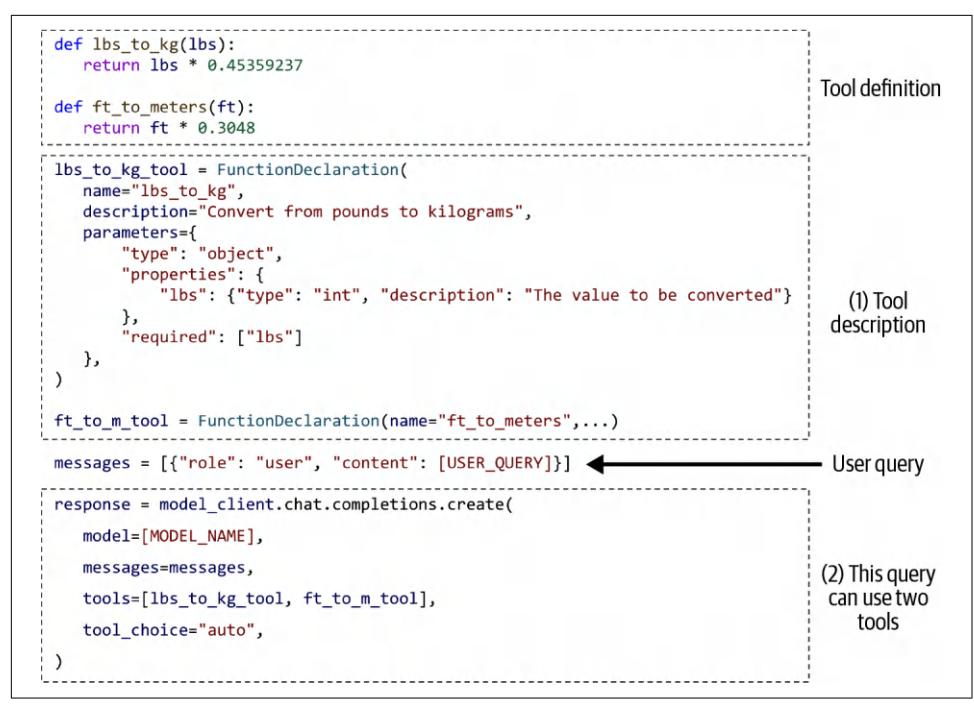
Figure 6-10. An example of a model using two simple tools.

Given a query, an agent defined as in Figure 6-10 will automatically generate what tools to use and their parameters. Some function calling APIs will make sure that only valid functions are generated, though they won’t be able to guarantee the correct parameter values.

For example, given the user query “How many kilograms are 40 pounds?”, the agent might decide that it needs the tool lbs_to_kg_tool with one parameter value of 40. The agent’s response might look like this:

response = ModelResponse(
 finish_reason='tool_calls',
 message=chat.Message(
 content=None,
 role='assistant',
 tool_calls=[
 ToolCall(
 function=Function(
 arguments='{"lbs":40}',
 name='lbs_to_kg'),
 type='function')
 ])
)

From this response, you can evoke the function lbs_to_kg(lbs=40) and use its out‐ put to generate a response to the users.

When working with agents, always ask the system to report what parameter values it uses for each function call. Inspect these values to make sure they are correct.

Planning granularity. A plan is a roadmap outlining the steps needed to accomplish a task. A roadmap can be of different levels of granularity. To plan for a year, a quarterby-quarter plan is higher-level than a month-by-month plan, which is, in turn, higher-level than a week-to-week plan.

There’s a planning/execution trade-off. A detailed plan is harder to generate but eas‐ ier to execute. A higher-level plan is easier to generate but harder to execute. An approach to circumvent this trade-off is to plan hierarchically. First, use a planner to generate a high-level plan, such as a quarter-to-quarter plan. Then, for each quarter, use the same or a different planner to generate a month-to-month plan.

So far, all examples of generated plans use the exact function names, which is very granular. A problem with this approach is that an agent’s tool inventory can change over time. For example, the function to get the current date get_time() can be renamed to get_current_time(). When a tool changes, you’ll need to update your prompt and all your examples. Using the exact function names also makes it harder to reuse a planner across different use cases with different tool APIs.

If you’ve previously finetuned a model to generate plans based on the old tool inven‐ tory, you’ll need to finetune the model again on the new tool inventory.

To avoid this problem, plans can also be generated using a more natural language, which is higher-level than domain-specific function names. For example, given the query “What’s the price of the best-selling product last week”, an agent can be instructed to output a plan that looks like this:

1. get current date
1. retrieve the best-selling product last week
1. retrieve product information
1. generate query
1. generate response

Using more natural language helps your plan generator become robust to changes in tool APIs. If your model was trained mostly on natural language, it’ll likely be better at understanding and generating plans in natural language and less likely to halluci‐ nate.

The downside of this approach is that you need a translator to translate each natural language action into executable commands.¹³ However, translating is a much simpler task than planning and can be done by weaker models with a lower risk of hallucina‐ tion.

Complex plans. The plan examples so far have been sequential: the next action in the plan is always executed after the previous action is done. The order in which actions can be executed is called a control flow. The sequential form is just one type of control flow. Other types of control flows include the parallel, if statement, and for loop. The following list provides an overview of each control flow, including sequential for comparison:

Sequential

Executing task B after task A is complete, likely because task B depends on task A. For example, the SQL query can be executed only after it’s been translated from the natural language input.

Parallel

Executing tasks A and B at the same time. For example, given the query “Find me best-selling products under $100”, an agent might first retrieve the top 100 bestselling products and, for each of these products, retrieve its price.

If statement

Executing task B or task C depending on the output from the previous step. For example, the agent first checks NVIDIA’s earnings report. Based on this report, it can then decide to sell or buy NVIDIA stocks.

For loop

Repeat executing task A until a specific condition is met. For example, keep on generating random numbers until a prime number.

These different control flows are visualized in Figure 6-11.

¹³ Chameleon (Lu et al., 2023) calls this translator a program generator.

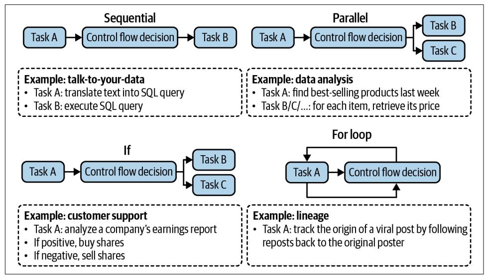
Figure 6-11. Examples of different orders in which a plan can be executed.

In traditional software engineering, conditions for control flows are exact. With AIpowered agents, AI models determine control flows. Plans with non-sequential con‐ trol flows are more difficult to both generate and translate into executable commands.

When evaluating an agent framework, check what control flows it supports. For example, if the system needs to browse ten websites, can it do so simultaneously? Par‐ allel execution can significantly reduce the latency perceived by users.

Reflection and error correction

Even the best plans need to be constantly evaluated and adjusted to maximize their chance of success. While reflection isn’t strictly necessary for an agent to operate, it’s necessary for an agent to succeed.

Reflection can be useful in many places during a task process:

After receiving a user query to evaluate if the request is feasible.
After the initial plan generation to evaluate whether the plan makes sense.
After each execution step to evaluate if it’s on the right track.
After the whole plan has been executed to determine if the task has been accomplished.

Reflection and error correction are two different mechanisms that go hand in hand. Reflection generates insights that help uncover errors to be corrected.

Reflection can be done with the same agent using self-critique prompts. It can also be done with a separate component, such as a specialized scorer: a model that outputs a concrete score for each outcome.

First proposed by ReAct (Yao et al., 2022), interleaving reasoning and action has become a common pattern for agents. Yao et al. used the term “reasoning” to encom‐ pass both planning and reflection. At each step, the agent is asked to explain its thinking (planning), take actions, then analyze observations (reflection), until the task is considered finished by the agent. The agent is typically prompted, using exam‐ ples, to generate outputs in the following format:

Thought 1: …
Act 1: …
Observation 1: …
… [continue until reflection determines that the task is finished] …
Thought N: … 
Act N: Finish [Response to query]

Figure 6-12 shows an example of an agent following the ReAct framework respond‐ ing to a question from HotpotQA (Yang et al., 2018), a benchmark for multi-hop question answering.

You can implement reflection in a multi-agent setting: one agent plans and takes actions, and another agent evaluates the outcome after each step or after a number of steps.¹⁴

If the agent’s response failed to accomplish the task, you can prompt the agent to reflect on why it failed and how to improve. Based on this suggestion, the agent gen‐ erates a new plan. This allows agents to learn from their mistakes. For example, given a coding generation task, an evaluator might evaluate that the generated code fails ⅓ of test cases. The agent then reflects the reason it failed is because it didn’t take into account arrays where all numbers are negative. The actor then generates new code, taking into account all-negative arrays.

¹⁴ This reminds me of the actor-critic (AC) agent method (Konda and Tsitsiklis, 1999) in reinforcement learn‐ ing.

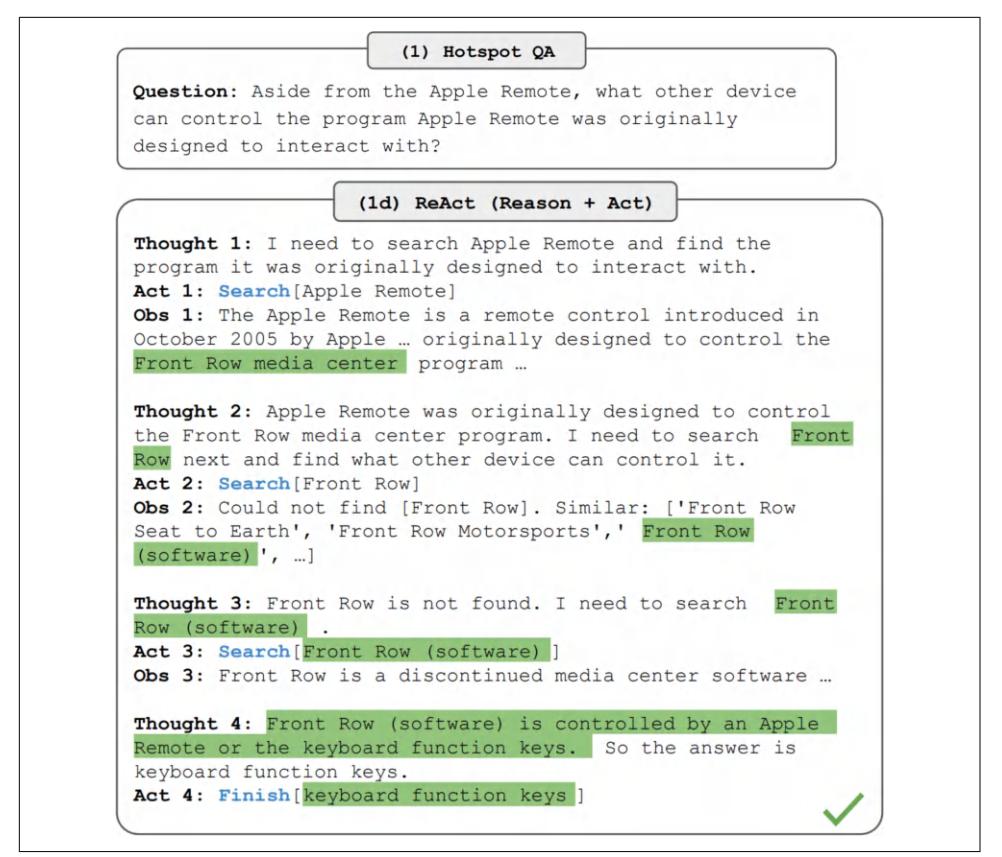
Figure 6-12. A ReAct agent in action. Image from the ReAct paper (Yao et al., 2022). The image is licensed under CC BY 4.0.

This is the approach that Reflexion (Shinn et al., 2023) took. In this framework, reflection is separated into two modules: an evaluator that evaluates the outcome and a self-reflection module that analyzes what went wrong. Figure 6-13 shows examples of Reflexion agents in action. The authors used the term “trajectory” to refer to a plan. At each step, after evaluation and self-reflection, the agent proposes a new tra‐ jectory.

Compared to plan generation, reflection is relatively easy to implement and can bring surprisingly good performance improvement. The downside of this approach is latency and cost. Thoughts, observations, and sometimes actions can take a lot of tokens to generate, which increases cost and user-perceived latency, especially for tasks with many intermediate steps. To nudge their agents to follow the format, both ReAct and Reflexion authors used plenty of examples in their prompts. This increases the cost of computing input tokens and reduces the context space available for other information.

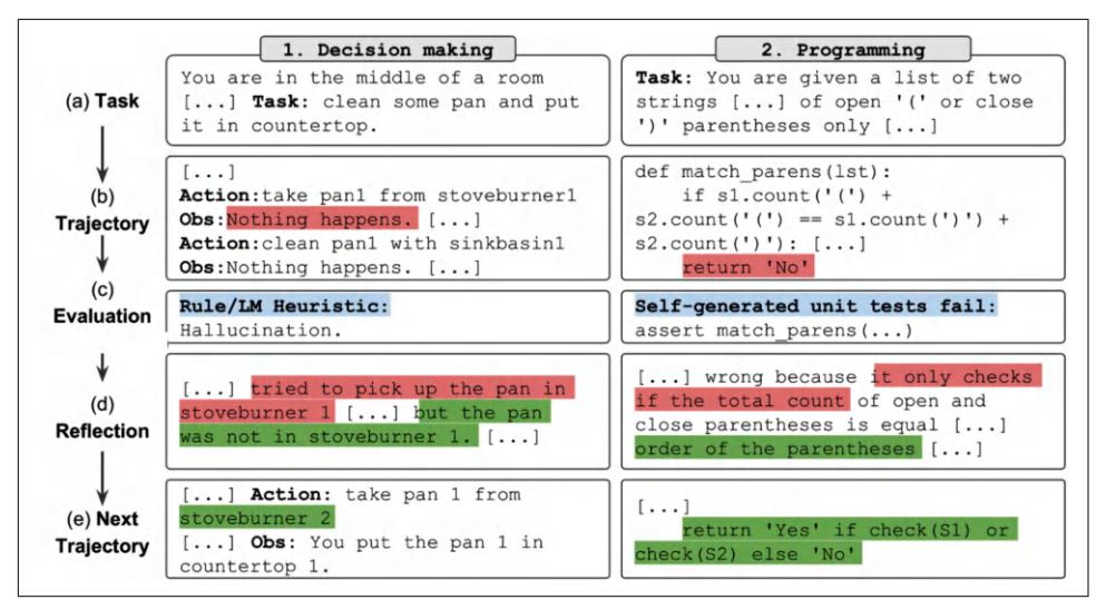
Figure 6-13. Examples of how Reflexion agents work. Images from the Reflexion Git‐ Hub repo.

Tool selection

Because tools often play a crucial role in a task’s success, tool selection requires care‐ ful consideration. The tools to give your agent depend on the environment and the task, but they also depend on the AI model that powers the agent.

There’s no foolproof guide on how to select the best set of tools. Agent literature con‐ sists of a wide range of tool inventories. For example, Toolformer (Schick et al., 2023) finetuned GPT-J to learn five tools. Chameleon (Lu et al., 2023) uses 13 tools. On the other hand, Gorilla (Patil et al., 2023) attempted to prompt agents to select the right API call among 1,645 APIs.

More tools give the agent more capabilities. However, the more tools there are, the harder it is to efficiently use them. It’s similar to how it’s harder for humans to master a large set of tools. Adding tools also means increasing tool descriptions, which might not fit into a model’s context.

Like many other decisions while building AI applications, tool selection requires experimentation and analysis. Here are a few things you can do to help you decide:

Compare how an agent performs with different sets of tools.
Do an ablation study to see how much the agent’s performance drops if a tool is removed from its inventory. If a tool can be removed without a performance drop, remove it.
Look for tools that the agent frequently makes mistakes on. If a tool proves too hard for the agent to use—for example, extensive prompting and even finetuning can’t get the model to learn to use it—change the tool.
Plot the distribution of tool calls to see what tools are most used and what tools are least used. Figure 6-14 shows the differences in tool use patterns of GPT-4 and ChatGPT in Chameleon (Lu et al., 2023).

		Lu et al. (2023). Adapted from an original image licensed under CC BY 4.0.

Experiments by Lu et al. (2023) also demonstrate two points:

Figure 6-14. Different models and tasks express different tool use patterns. Image from Lu et al. (2023). Adapted from an original image licensed under CC BY 4.0.

Experiments by Lu et al. (2023) also demonstrate two points:

1. Different tasks require different tools. ScienceQA, the science question answer‐ ing task, relies much more on knowledge retrieval tools than TabMWP, a tabular math problem-solving task.
1. Different models have different tool preferences. For example, GPT-4 seems to select a wider set of tools than ChatGPT. ChatGPT seems to favor image caption‐ ing, while GPT-4 seems to favor knowledge retrieval.

When evaluating an agent framework, evaluate what planners and tools it supports. Different frameworks might focus on different categories of tools. For example, AutoGPT focuses on social media APIs (Reddit, X, and Wikipedia), whereas Composio focuses on enterprise APIs (Google Apps, GitHub, and Slack).

As your needs will likely change over time, evaluate how easy it is to extend your agent to incorporate new tools.

As humans, we become more productive not just by using the tools we’re given, but also by creating progressively more powerful tools from simpler ones. Can AI create new tools from its initial tools?

Chameleon (Lu et al., 2023) proposes the study of tool transition: after tool X, how likely is the agent to call tool Y? Figure 6-15 shows an example of tool transition. If two tools are frequently used together, they can be combined into a bigger tool. If an agent is aware of this information, the agent itself can combine initial tools to contin‐ ually build more complex tools.

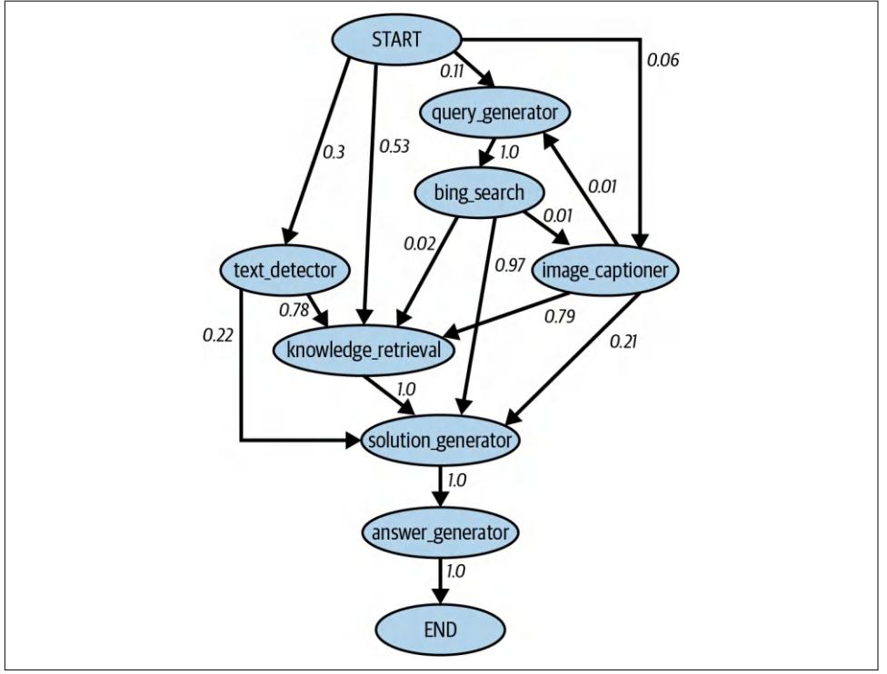
Figure 6-15. A tool transition tree by Lu et al. (2023). Adapted from an original image licensed under CC BY 4.0.

Vogager (Wang et al., 2023) proposes a skill manager to keep track of new skills (tools) that an agent acquires for later reuse. Each skill is a coding program. When the skill manager determines a newly created skill is to be useful (e.g., because it’s successfully helped an agent accomplish a task), it adds this skill to the skill library (conceptually similar to the tool inventory). This skill can be retrieved later to use for other tasks.

Earlier in this section, we mentioned that the success of an agent in an environment depends on its tool inventory and its planning capabilities. Failures in either aspect can cause the agent to fail. The next section will discuss different failure modes of an agent and how to evaluate them.

Agent Failure Modes and Evaluation

Evaluation is about detecting failures. The more complex a task an agent performs, the more possible failure points there are. Other than the failure modes common to all AI applications discussed in Chapters 3 and 4, agents also have unique failures caused by planning, tool execution, and efficiency. Some of the failures are easier to catch than others.

To evaluate an agent, identify its failure modes and measure how often each of these failure modes happens.

I created a simple benchmark to illustrate these different failure modes that you can see on the book’s GitHub repository. There are also agent benchmarks and leader‐ boards such as the Berkeley Function Calling Leaderboard, the AgentOps evaluation harness, and the TravelPlanner benchmark.

Planning failures

Planning is hard and can fail in many ways. The most common mode of planning failure is tool use failure. The agent might generate a plan with one or more of these errors:

Invalid tool

For example, it generates a plan that contains bing_search, but bing_search isn’t in the agent’s tool inventory.

Valid tool, invalid parameters.

For example, it calls lbs_to_kg with two parameters. lbs_to_kg is in the tool inventory but requires only one parameter, lbs.

Valid tool, incorrect parameter values

For example, it calls lbs_to_kg with one parameter, lbs, but uses the value 100 for lbs when it should be 120.

Another mode of planning failure is goal failure: the agent fails to achieve the goal. This can be because the plan doesn’t solve a task, or it solves the task without follow‐ ing the constraints. To illustrate this, imagine you ask the model to plan a two-week trip from San Francisco to Hanoi with a budget of $5,000. The agent might plan a trip from San Francisco to Ho Chi Minh City, or plan a two-week trip from San Francisco to Hanoi that will be way over the budget.

A common constraint that is often overlooked by agent evaluation is time. In many cases, the time an agent takes matters less, because you can assign a task to an agent and only need to check in when it’s done. However, in many cases, the agent becomes less useful with time. For example, if you ask an agent to prepare a grant proposal and the agent finishes it after the grant deadline, the agent isn’t very helpful.

An interesting mode of planning failure is caused by errors in reflection. The agent is convinced that it’s accomplished a task when it hasn’t. For example, you ask the agent to assign 50 people to 30 hotel rooms. The agent might assign only 40 people and insist that the task has been accomplished.

To evaluate an agent for planning failures, one option is to create a planning dataset where each example is a tuple (task, tool inventory). For each task, use the agent to generate a K number of plans. Compute the following metrics:

1. Out of all generated plans, how many are valid?
1. For a given task, how many plans does the agent have to generate, on average, to get a valid plan?
1. Out of all tool calls, how many are valid?
1. How often are invalid tools called?
1. How often are valid tools called with invalid parameters?
1. How often are valid tools called with incorrect parameter values?

Analyze the agent’s outputs for patterns. What types of tasks does the agent fail more on? Do you have a hypothesis why? What tools does the model frequently make mis‐ takes with? Some tools might be harder for an agent to use. You can improve an agent’s ability to use a challenging tool by better prompting, more examples, or fine‐ tuning. If all fail, you might consider swapping this tool for something easier to use.

Tool failures

Tool failures happen when the correct tool is used, but the tool output is wrong. One failure mode is when a tool just gives the wrong outputs. For example, an image cap‐ tioner returns a wrong description, or an SQL query generator returns a wrong SQL query.

If the agent generates only high-level plans and a translation module is involved in translating from each planned action to executable commands, failures can happen because of translation errors.

Tool failures can also happen because the agent doesn’t have access to the right tools for the task. An obvious example is when the task involves retrieving the current stock prices from the internet, and the agent doesn’t have access to the internet.

Tool failures are tool-dependent. Each tool needs to be tested independently. Always print out each tool call and its output so that you can inspect and evaluate them. If you have a translator, create benchmarks to evaluate it.

Detecting missing tool failures requires an understanding of what tools should be used. If your agent frequently fails on a specific domain, this might be because it lacks tools for this domain. Work with human domain experts and observe what tools they would use.

Efficiency

An agent might generate a valid plan using the right tools to accomplish a task, but it might be inefficient. Here are a few things you might want to track to evaluate an agent’s efficiency:

How many steps does the agent need, on average, to complete a task?
How much does the agent cost, on average, to complete a task?
How long does each action typically take? Are there any actions that are espe‐ cially time-consuming or expensive?

You can compare these metrics with your baseline, which can be another agent or a human operator. When comparing AI agents to human agents, keep in mind that humans and AI have very different modes of operations, so what’s considered effi‐ cient for humans might be inefficient for AI, and vice versa. For example, visiting 100 web pages might be inefficient for a human agent who can visit only one page at a time, but trivial for an AI agent that can visit all the web pages at once.

In this chapter, we’ve discussed in detail how RAG and agent systems function. Both patterns often deal with information that exceeds a model’s context limit. A memory system that supplements the model’s context in handling information can signifi‐ cantly enhance its capabilities. Let’s now explore how a memory system works.

Memory

Memory refers to mechanisms that allow a model to retain and utilize information. A memory system is especially useful for knowledge-rich applications like RAG and multi-step applications like agents. A RAG system relies on memory for its augmen‐ ted context, which can grow over multiple turns as it retrieves more information. An agentic system needs memory to store instructions, examples, context, tool invento‐ ries, plans, tool outputs, reflections, and more. While RAG and agents place greater demands on memory, it is beneficial for any AI application that requires retaining information.

An AI model typically has three main memory mechanisms:

Internal knowledge

The model itself is a memory mechanism, as it retains the knowledge from the data it was trained on. This knowledge is its internal knowledge. A model’s inter‐ nal knowledge doesn’t change unless the model itself is updated. The model can access this knowledge in all queries.

Short-term memory

A model’s context is a memory mechanism. Previous messages in a conversation can be added to the model’s context, allowing the model to leverage them to gen‐ erate future responses. A model’s context can be considered its short-term mem‐ ory as it doesn’t persist across tasks (queries). It’s fast to access, but its capacity is limited. Therefore, it’s often used to store information that is most important for the current task.

Long-term memory

External data sources that a model can access via retrieval, such as in a RAG sys‐ tem, are a memory mechanism. This can be considered the model’s long-term memory, as it can be persisted across tasks. Unlike a model’s internal knowledge, information in the long-term memory can be deleted without updating the model.

Humans have access to similar memory mechanisms. How to breathe is your internal knowledge. You typically don’t forget how to breathe unless you’re in serious trouble. Your short-term memory contains information immediately relevant to what you’re doing, such as the name of a person you just met. Your long-term memory is aug‐ mented with books, computers, notes, etc.

Which memory mechanism to use for your data depends on its frequency of use. Information essential for all tasks should be incorporated into the model’s internal knowledge via training or finetuning. Information that is rarely needed should reside in its long-term memory. Short-term memory is reserved for immediate, contextspecific information. These three memory mechanisms are illustrated in Figure 6-16.

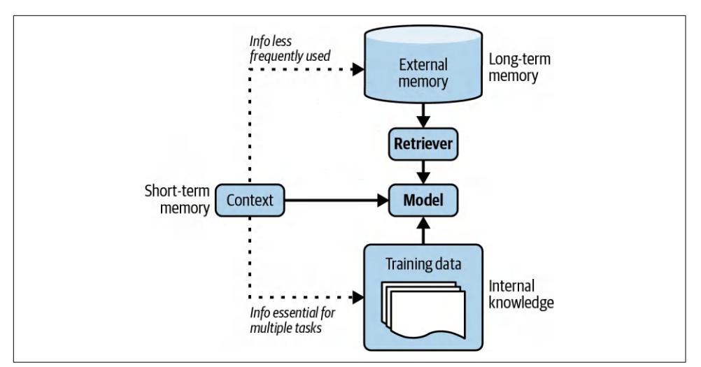
Figure 6-16. The hierarchy of information for an agent.

Memory is essential for humans to operate. As AI applications have evolved, develop‐ ers have quickly realized that memory is important for AI models, too. Many mem‐ ory management tools for AI models have been developed, and many model providers have incorporated external memory. Augmenting an AI model with a memory system has many benefits. Here are just a few of them:

Manage information overflow within a session

During the process of executing a task, an agent acquires a lot of new informa‐ tion, which can exceed the agent’s maximum context length. The excess informa‐ tion can be stored in a memory system with long-term memories.

Persist information between sessions

An AI coach is practically useless if every time you want the coach’s advice, you have to explain your whole life story. An AI assistant would be annoying to use if it keeps forgetting your preferences. Having access to your conversation history can allow an agent to personalize its actions to you. For example, when you ask for book recommendations, if the model remembers that you’ve previously loved The Three-Body Problem, it can suggest similar books.

Boost a model’s consistency

If you ask me a subjective question twice, like rating a joke between 1 and 5, I’m much more likely to give consistent answers if I remember my previous answer. Similarly, if an AI model can reference its previous answers, it can calibrate its future answers to be consistent.

Maintain data structural integrity

Because text is inherently unstructured, the data stored in the context of a textbased model is unstructured. You can put structured data in the context. For example, you can feed a table into the context line-by-line, but there’s no guaran‐ tee that the model will understand that this is supposed to be a table. Having a memory system capable of storing structured data can help maintain the struc‐ tural integrity of your data. For example, if you ask an agent to find potential sales leads, this agent can leverage an Excel sheet to store the leads. An agent can also leverage a queue to store the sequence of actions to be performed.

A memory system for AI models typically consists of two functions:

Memory management: managing what information should be stored in the short-term and long-term memory.
Memory retrieval: retrieving information relevant to the task from long-term memory.

Memory retrieval is similar to RAG retrieval, as long-term memory is an external data source. In this section, I’ll focus on memory management. Memory manage‐ ment typically consists of two operations: add and delete memory. If memory storage is limited, deletion might not be necessary. This might work for long-term memory because external memory storage is relatively cheap and easily extensible. However, short-term memory is limited by the model’s maximum context length and, there‐ fore, requires a strategy for what to add and what to delete.

Long-term memory can be used to store the overflow from short-term memory. This operation depends on how much space you want to allocate for short-term memory. For a given query, the context input into the model consists of both its short-term memory and information retrieved from its long-term memory. A model’s shortterm capacity is, therefore, determined by how much of the context should be alloca‐ ted for information retrieved from long-term memory. For example, if 30% of the context is reserved, then the model can use at most 70% of the context limit for shortterm memory. When this threshold is reached, the overflow can be moved to longterm memory.

Like many components previously discussed in this chapter, memory management isn’t unique to AI applications. Memory management has been a cornerstone of all data systems, and many strategies have been developed to use memory efficiently.

The simplest strategy is FIFO, first in, first out. The first to be added to the shortterm memory will be the first to be moved to the external storage. As a conversation gets longer, API providers like OpenAI might start removing the beginning of the conversation. Frameworks like LangChain might allow the retention of N last mes‐ sages or N last tokens. In a long conversation, this strategy assumes that the early

messages are less relevant to the current discussion. However, this assumption can be fatally wrong. In some conversations, the earliest messages might carry the most information, especially when the early messages state the purpose of the conversa‐ tion.¹⁵ While FIFO is straightforward to implement, it can cause the model to lose track of important information.¹⁶

More-sophisticated strategies involve removing redundancy. Human languages con‐ tain redundancy to enhance clarity and compensate for potential misunderstandings. If there’s a way to automatically detect redundancy, the memory footprint will be reduced significantly.

One way to remove redundancy is by using a summary of the conversation. This summary can be generated using the same or another model. Summarization, together with tracking named entities, can take you a long way. Bae et al. (2022) took this a step further. After obtaining the summary, the authors wanted to construct a new memory by joining the memory with the key information that the summary missed. The authors developed a classifier that, for each sentence in the memory and each sentence in the summary, determines if only one, both, or neither should be added to the new memory.

Liu et al. (2023), on the other hand, used a reflection approach. After each action, the agent is asked to do two things:

1. Reflect on the information that has just been generated.
1. Determine if this new information should be inserted into the memory, should merge with the existing memory, or should replace some other information, especially if the other information is outdated and contradicts new information.

When encountering contradicting pieces of information, some people opt to keep the newer ones. Some people ask AI models to judge which one to keep. How to handle contradiction depends on the use case. Having contradictions can cause an agent to be confused but can also help it draw from different perspectives.

¹⁵ For human conversations, the opposite might be true if the first few messages are pleasantries.

¹⁶ Usage-based strategies, such as removing the least frequently used information, is more challenging, since you’ll need a way to know when a model uses a given piece of information.

Summary

Given the popularity of RAG and the potential of agents, early readers have men‐ tioned that this is the chapter they’re most excited about.

This chapter started with RAG, the pattern that emerged first between the two. Many tasks require extensive background knowledge that often exceeds a model’s context window. For example, code copilots might need access to entire codebases, and research assistants may need to analyze multiple books. Originally developed to over‐ come a model’s context limitations, RAG also enables more efficient use of informa‐ tion, improving response quality while reducing costs. From the early days of foundation models, it was clear that the RAG pattern would be immensely valuable for a wide range of applications, and it has since been rapidly adopted across both consumer and enterprise use cases.

RAG employs a two-step process. It first retrieves relevant information from external memory and then uses this information to generate more accurate responses. The success of a RAG system depends on the quality of its retriever. Term-based retriev‐ ers, such as Elasticsearch and BM25, are much lighter to implement and can provide strong baselines. Embedding-based retrievers are more computationally intensive but have the potential to outperform term-based algorithms.

Embedding-based retrieval is powered by vector search, which is also the backbone of many core internet applications such as search and recommender systems. Many vector search algorithms developed for these applications can be used for RAG.

The RAG pattern can be seen as a special case of agent where the retriever is a tool the model can use. Both patterns allow a model to circumvent its context limitation and stay more up-to-date, but the agentic pattern can do even more than that. An agent is defined by its environment and the tools it can access. In an AI-powered agent, AI is the planner that analyzes its given task, considers different solutions, and picks the most promising one. A complex task can require many steps to solve, which requires a powerful model to plan. A model’s ability to plan can be augmented with reflection and a memory system to help it keep track of its progress.

The more tools you give a model, the more capabilities the model has, enabling it to solve more challenging tasks. However, the more automated the agent becomes, the more catastrophic its failures can be. Tool use exposes agents to many security risks discussed in Chapter 5. For agents to work in the real world, rigorous defensive mechanisms need to be put in place.

Both RAG and agents work with a lot of information, which often exceeds the maxi‐ mum context length of the underlying model. This necessitates the introduction of a memory system for managing and using all the information a model has. This chap‐ ter ended with a short discussion on what this component looks like.

RAG and agents are both prompt-based methods, as they influence the model’s qual‐ ity solely through inputs without modifying the model itself. While they can enable many incredible applications, modifying the underlying model can open up even more possibilities. How to do so will be the topic of the next chapter.

CHAPTER 7 Finetuning

Finetuning is the process of adapting a model to a specific task by further training the whole model or part of the model. Chapters 5 and 6 discuss prompt-based methods, which adapt a model by giving it instructions, context, and tools. Finetuning adapts a model by adjusting its weights.

Finetuning can enhance various aspects of a model. It can improve the model’s domain-specific capabilities, such as coding or medical question answering, and can also strengthen its safety. However, it is most often used to improve the model’s instruction-following ability, particularly to ensure it adheres to specific output styles and formats.

While finetuning can help create models that are more customized to your needs, it also requires more up-front investment. A question I hear very often is when to fine‐ tune and when to do RAG. After an overview of finetuning, this chapter will discuss the reasons for finetuning and the reasons for not finetuning, as well as a simple framework for thinking about choosing between finetuning and alternate methods.

Compared to prompt-based methods, finetuning incurs a much higher memory foot‐ print. At the scale of today’s foundation models, naive finetuning often requires more memory than what’s available on a single GPU. This makes finetuning expensive and challenging to do. As discussed throughout this chapter, reducing memory require‐ ments is a primary motivation for many finetuning techniques. This chapter dedi‐ cates one section to outlining factors contributing to a model’s memory footprint, which is important for understanding these techniques.

A memory-efficient approach that has become dominant in the finetuning space is PEFT (parameter-efficient finetuning). This chapter explores PEFT and how it differs from traditional finetuning; this chapter also provides an overview of its evolving techniques. I’ll focus particularly on one compelling category: adapter-based techniques.

With prompt-based methods, knowledge about how ML models operate under the hood is recommended but not strictly necessary. However, finetuning brings you to the realm of model training, where ML knowledge is required. ML basics are beyond the scope of this book. If you want a quick refresh, the book’s GitHub repository has pointers to helpful resources. In this chapter, I’ll cover a few core concepts immedi‐ ately relevant to the discussion.

This chapter is the most technically challenging one for me to write, not because of the complexity of the concepts, but because of the broad scope these concepts cover. I suspect it might also be technically challenging to read. If, at any point, you feel like you’re diving too deep into details that aren’t relevant to your work, feel free to skip.

There’s a lot to discuss. Let’s dive in!

Finetuning Overview

To finetune, you start with a base model that has some, but not all, of the capabilities you need. The goal of finetuning is to get this model to perform well enough for your specific task.

Finetuning is one way to do transfer learning, a concept first introduced by Bozinov‐ ski and Fulgosi in 1976. Transfer learning focuses on how to transfer the knowledge gained from one task to accelerate learning for a new, related task. This is conceptu‐ ally similar to how humans transfer skills: for example, knowing how to play the piano can make it easier to learn another musical instrument.

An early large-scale success in transfer learning was Google’s multilingual translation system (Johnson et. al, 2016). The model transferred its knowledge of Portuguese– English and English–Spanish translation to directly translate Portuguese to Spanish, even though there were no Portuguese–Spanish examples in the training data.

Since the early days of deep learning, transfer learning has offered a solution for tasks with limited or expensive training data. By training a base model on tasks with abun‐ dant data, you can then transfer that knowledge to a target task.

For LLMs, knowledge gained from pre-training on text completion (a task with abundant data) is transferred to more specialized tasks, like legal question answering or text-to-SQL, which often have less available data. This capability for transfer learn‐ ing makes foundation models particularly valuable.

Transfer learning improves sample efficiency, allowing a model to learn the same behavior with fewer examples. A sample-efficient model learns effectively from fewer samples. For example, while training a model from scratch for legal question answer‐ ing may need millions of examples, finetuning a good base model might only require a few hundred.

Ideally, much of what the model needs to learn is already present in the base model, and finetuning just refines the model’s behavior. OpenAI’s InstructGPT paper (2022) suggested viewing finetuning as unlocking the capabilities a model already has but that are difficult for users to access via prompting alone.

Finetuning isn’t the only way to do transfer learning. Another approach is feature-based transfer. In this approach, a model is trained to extract features from the data, usually as embedding vec‐ tors, which are then used by another model. I mention featurebased transfer briefly in Chapter 2, when discussing how part of a foundation model can be reused for a classification task by adding a classifier head.

Feature-based transfer is very common in computer vision. For instance, in the second half of the 2010s, many people used models trained on the ImagetNet dataset to extract features from images and use these features in other computer vision tasks such as object detection or image segmentation.

Finetuning is part of a model’s training process. It’s an extension of model pretraining. Because any training that happens after pre-training is finetuning, finetun‐ ing can take many different forms. Chapter 2 already discussed two types of finetuning: supervised finetuning and preference finetuning. Let’s do a quick recap of these methods and how you might leverage them as an application developer.

Recall that a model’s training process starts with pre-training, which is usually done with self-supervision. Self-supervision allows the model to learn from a large amount of unlabeled data. For language models, self-supervised data is typically just sequences of text that don’t need annotations.

Before finetuning this pre-trained model with expensive task-specific data, you can finetune it with self-supervision using cheap task-related data. For example, to fine‐ tune a model for legal question answering, before finetuning it on expensive annota‐ ted (question, answer) data, you can finetune it on raw legal documents. Similarly, to finetune a model to do book summarization in Vietnamese, you can first finetune it on a large collection of Vietnamese text. Self-supervised finetuning is also called con‐ tinued pre-training.

As discussed in Chapter 1, language models can be autoregressive or masked. An autoregressive model predicts the next token in a sequence using the previous tokens as the context. A masked model fills in the blank using the tokens both before and after it. Similarly, with supervised finetuning, you can also finetune a model to pre‐ dict the next token or fill in the blank. The latter, also known as infilling finetuning, is especially useful for tasks such as text editing and code debugging. You can finetune a model for infilling even if it was pre-trained autoregressively.

The massive amount of data a model can learn from during self-supervised learning outfits the model with a rich understanding of the world, but it might be hard for users to extract that knowledge for their tasks, or the way the model behaves might be misaligned with human preference. Supervised finetuning uses high-quality annota‐ ted data to refine the model to align with human usage and preference.

During supervised finetuning, the model is trained using (input, output) pairs: the input can be an instruction and the output can be a response. A response can be open-ended, such as for the task of book summarization. A response can be also close-ended, such as for a classification task. High-quality instruction data can be challenging and expensive to create, especially for instructions that require factual consistency, domain expertise, or political correctness. Chapter 8 discusses how to acquire instruction data.

A model can also be finetuned with reinforcement learning to generate responses that maximize human preference. Preference finetuning requires comparative data that typically follows the format (instruction, winning response, losing response).

It’s possible to finetune a model to extend its context length. Long-context finetuning typically requires modifying the model’s architecture, such as adjusting the positional embeddings. A long sequence means more possible positions for tokens, and posi‐ tional embeddings should be able to handle them. Compared to other finetuning techniques, long-context finetuning is harder to do. The resulting model might also degrade on shorter sequences.

Figure 7-1 shows the making of different Code Llama models (Rozière et al., 2024), from the base model Llama 2, using different finetuning techniques. Using longcontext finetuning, they were able to increase the model’s maximum context length from 4,096 tokens to 16,384 tokens to accommodate longer code files. In the image, instruction finetuning refers to supervised finetuning.

Finetuning can be done by both model developers and application developers. Model developers typically post-train a model with different finetuning techniques before releasing it. A model developer might also release different model versions, each fine‐ tuned to a different extent, so that application developers can choose the version that works best for them.

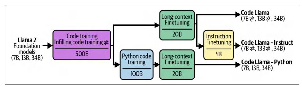
Figure 7-1. Different finetuning techniques used to make different Code Llama models. Image from the Rozière et al. (2024). Adapted from an original image licensed under CC BY 4.0.

As an application developer, you might finetune a pre-trained model, but most likely, you’ll finetune a model that has been post-trained. The more refined a model is and the more relevant its knowledge is to your task, the less work you’ll have to do to adapt it.

When to Finetune

Before jumping into different finetuning techniques, it’s necessary to consider whether finetuning is the right option for you. Compared to prompt-based methods, finetuning requires significantly more resources, not just in data and hardware, but also in ML talent. Therefore, finetuning is generally attempted after extensive experi‐ ments with prompt-based methods. However, finetuning and prompting aren’t mutually exclusive. Real-world problems often require both approaches.

Reasons to Finetune

The primary reason for finetuning is to improve a model’s quality, in terms of both general capabilities and task-specific capabilities. Finetuning is commonly used to improve a model’s ability to generate outputs following specific structures, such as JSON or YAML formats.

A general-purpose model that performs well on a wide range of benchmarks might not perform well on your specific task. If the model you want to use wasn’t suffi‐ ciently trained on your task, finetuning it with your data can be especially useful.

For example, an out-of-the-box model might be good at converting from text to the standard SQL dialect but might fail with a less common SQL dialect. In this case, finetuning this model on data containing this SQL dialect will help. Similarly, if the model works well on standard SQL for common queries but often fails for customerspecific queries, finetuning the model on customer-specific queries might help.

One especially interesting use case of finetuning is bias mitigation. The idea is that if the base model perpetuates certain biases from its training data, exposing it to care‐ fully curated data during finetuning can counteract these biases (Wang and Russa‐ kovsky, 2023). For example, if a model consistently assigns CEOs male-sounding names, finetuning it on a dataset with many female CEOs can mitigate this bias. Gari‐ mella et al. (2022) found that finetuning BERT-like language models on text authored by women can reduce these models’ gender biases, while finetuning them on texts by African authors can reduce racial biases.

You can finetune a big model to make it even better, but finetuning smaller models is much more common. Smaller models require less memory, and, therefore, are easier to finetune. They are also cheaper and faster to use in production.

A common approach is to finetune a small model to imitate the behavior of a larger model using data generated by this large model. Because this approach distills the larger model’s knowledge into the smaller model, it’s called distillation. This is dis‐ cussed in Chapter 8 together with other data synthesis techniques.

A small model, finetuned on a specific task, might outperform a much larger out-ofthe-box model on that task. For example, Grammarly found that their finetuned Flan-T5 models (Chung et al., 2022) outperformed a GPT-3 variant specialized in text editing across a wide range of writing assistant tasks despite being 60 times smaller. The finetuning process used only 82,000 (instruction, output) pairs, which is smaller than the data typically needed to train a text-editing model from scratch.

In the early days of foundation models, when the strongest models were commercial with limited finetuning access, there weren’t many competitive models available for finetuning. However, as the open source community proliferates with high-quality models of all sizes, tailored for a wide variety of domains, finetuning has become a lot more viable and attractive.

Reasons Not to Finetune

While finetuning can improve a model in many ways, many of these improvements can also be achieved, to a certain extent, without finetuning. Finetuning can improve a model’s performance, but so do carefully crafted prompts and context. Finetuning can help with structured outputs, but many other techniques, as discussed in Chap‐ ter 2, can also do that.

First, while finetuning a model for a specific task can improve its performance for that task, it can degrade its performance for other tasks.¹ This can be frustrating when you intend this model for an application that expects diverse prompts.

¹ Some people call this phenomenon an alignment tax (Bai et al., 2020), but this term can be confused with penalties against human preference alignment.

Imagine you need a model for three types of queries: product recommendations, changing orders, and general feedback. Originally, the model works well for product recommendations and general feedback but poorly for changing orders. To fix this, you finetune the model on a dataset of (query, response) pairs about changing orders. The finetuned model might indeed perform better for this type of query, but worse for the two other tasks.

What do you do in this situation? You can finetune the model on all the queries you care about, not just changing orders. If you can’t seem to get a model to perform well on all your tasks, consider using separate models for different tasks. If you wish to combine these separate models into one to make serving them easier, you can also consider merging them together, as discussed later in this chapter.

If you’re just starting to experiment with a project, finetuning is rarely the first thing you should attempt. Finetuning requires high up-front investments and continual maintenance. First, you need data. Annotated data can be slow and expensive to acquire manually, especially for tasks that demand critical thinking and domain expertise. Open source data and AI-generated data can mitigate the cost, but their effectiveness is highly variable.

Second, finetuning requires the knowledge of how to train models. You need to eval‐ uate base models to choose one to finetune. Depending on your needs and resources, options might be limited. While finetuning frameworks and APIs can automate many steps in the actual finetuning process, you still need to understand the different training knobs you can tweak, monitor the learning process, and debug when some‐ thing is wrong. For example, you need to understand how an optimizer works, what learning rate to use, how much training data is needed, how to address overfitting/ underfitting, and how to evaluate your models throughout the process.

Third, once you have a finetuned model, you’ll need to figure out how to serve it. Will you host it yourself or use an API service? As discussed in Chapter 9, inference optimization for large models, especially LLMs, isn’t trivial. Finetuning requires less of a technical leap if you’re already hosting your models in-house and familiar with how to operate models.

More importantly, you need to establish a policy and budget for monitoring, main‐ taining, and updating your model. As you iterate on your finetuned model, new base models are being developed at a rapid pace. These base models may improve faster than you can enhance your finetuned model. If a new base model outperforms your finetuned model on your specific task, how significant does the performance improvement have to be before you switch to the new base model? What if a new base model doesn’t immediately outperform your existing model but has the poten‐ tial to do so after finetuning—would you experiment with it?

In many cases, switching to a better model would provide only a small incremental improvement, and your task might be given a lower priority than projects with larger returns, like enabling new use cases.²

AI engineering experiments should start with prompting, following the best practices discussed in Chapter 6. Explore more advanced solutions only if prompting alone proves inadequate. Ensure you have thoroughly tested various prompts, as a model’s performance can vary greatly with different prompts.

Many practitioners I’ve spoken with share a similar story that goes like this. Someone complains that prompting is ineffective and insists on finetuning. Upon investiga‐ tion, it turns out that prompt experiments were minimal and unsystematic. Instruc‐ tions were unclear, examples didn’t represent actual data, and metrics were poorly defined. After refining the prompt experiment process, the prompt quality improved enough to be sufficient for their application.³

Finetuning Domain-Specific Tasks

Beware of the argument that general-purpose models don’t work well for domainspecific tasks, and, therefore, you must finetune or train models for your specific tasks. As general-purpose models become more capable, they also become better at domain-specific tasks and can outperform the domain-specific models.

An interesting early specialized model is BloombergGPT, which was introduced by Bloomberg in March 2023. The strongest models on the market then were all propri‐ etary, and Bloomberg wanted a mid-size model that performed well on financial tasks and could be hosted in-house for use cases with sensitive data. The model, with 50 billion parameters, required 1.3 million A100 GPU hours for training. The estimated cost of the compute was between $1.3 million and $2.6 million, excluding data costs (Wu et al., 2023).

In the same month, OpenAI released GPT-4-0314.⁴ Research by Li et al. (2023) demonstrated that GPT-4-0314 significantly outperformed BloombergGPT across various financial benchmarks. Table 7-1 provides details of two such benchmarks.

² Many businesses resist changing technologies they consider “good enough.” If all companies were quick to adopt more optimal solutions, fax machines would have become obsolete by now.

³ I’ve also noticed a few cases when engineers know that finetuning isn’t strictly necessary but still insist on doing it because they want to learn how to finetune. As an engineer who likes learning new skills, I appreciate this mindset. However, if you’re in a leadership position, it can be hard to differentiate whether finetuning is needed or wanted.

⁴ 0314 denotes the date this GPT-4 version came out, March 14, 2024. The specific date stamp matters because different versions vary significantly in performance.

Table 7-1. General-purpose models like GPT-4 can outperform financial models in financial domains.

Model	FiQA sentiment analysis ConvFinQA (weighted F1)	(accuracy)
GPT-4-0314 (zero-shot)	87.15	76.48
BloombergGPT	75.07	43.41

Since then, several mid-size models with performance comparable to GPT-4 have been released, including Claude 3.5 Sonnet (70B parameters), Llama 3-70B-Instruct, and Qwen2-72B-Instruct. The latter two are open weight and can be self-hosted.

Because benchmarks are insufficient to capture real-world performance, it’s possible that BloombergGPT works well for Bloomberg for their specific use cases. The Bloomberg team certainly gained invaluable experience through training this model, which might enable them to better develop and operate future models.

Both finetuning and prompting experiments require systematic processes. Doing prompt experiments enables developers to build an evaluation pipeline, data annota‐ tion guideline, and experiment tracking practices that will be stepping stones for finetuning.

One benefit of finetuning, before prompt caching was introduced, was that it can help optimize token usage. The more examples you add to a prompt, the more input tokens the model will use, which increases both latency and cost. Instead of including your examples in each prompt, you can finetune a model on these examples. This allows you to use shorter prompts with the finetuned model, as shown in Figure 7-2.

With prompt caching, where repetitive prompt segments can be cached for reuse, this is no longer a strong benefit. Prompt caching is discussed further in Chapter 9. However, the number of examples you can use with a prompt is still limited by the maximum context length. With finetuning, there’s no limit to how many examples you can use.

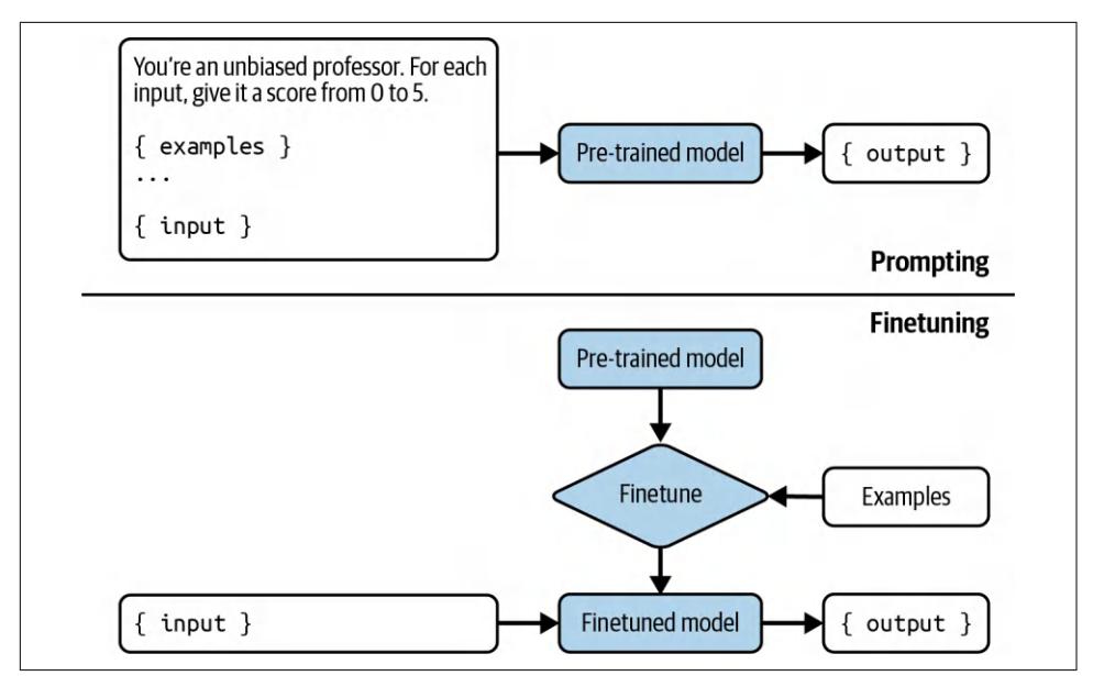
Figure 7-2. Instead of including examples in each prompt, which increases cost and latency, you finetune a model on these examples.

Finetuning and RAG

Once you’ve maximized the performance gains from prompting, you might wonder whether to do RAG or finetuning next. The answer depends on whether your model’s failures are information-based or behavior-based.

If the model fails because it lacks information, a RAG system that gives the model access to the relevant sources of information can help. Information-based failures hap‐ pen when the outputs are factually wrong or outdated. Here are two example scenar‐ ios in which information-based failures happen:

The model doesn’t have the information.

Public models are unlikely to have information private to you or your organiza‐ tion. When a model doesn’t have the information, it either tells you so or halluci‐ nates an answer.

The model has outdated information.

If you ask: “How many studio albums has Taylor Swift released?” and the correct answer is 11, but the model answers 10, it can be because the model’s cut-off date was before the release of the latest album.

The paper “Fine-Tuning or Retrieval?” by Ovadia et al. (2024) demonstrated that for tasks that require up-to-date information, such as questions about current events, RAG outperformed finetuned models. Not only that, RAG with the base model

outperformed RAG with finetuned models, as shown in Table 7-2. This finding indi‐ cates that while finetuning can enhance a model’s performance on a specific task, it may also lead to a decline in performance in other areas.

Table 7-2. RAG outperforms finetuning on a question-answering task about current events, curated by Ovadia et al. (2024). FT-reg and FT-par refer to two different finetuning approaches the author used.

		Base model Base model + RAG FT-req FT-par FT-req + RAG FT-par + RAG
Mistral-7B $\vert$ 0.481		0.875	0.504	0.588	0.810	0.830
Llama 2-7B $\vert$ 0.353		0.585	$0.719$	0.392 $$ 0.326		0.520
Orca 2-7B	0.456	0.876	0.511	0.566	0.820	0.826

On the other hand, if the model has behavioral issues, finetuning might help. One behavioral issue is when the model’s outputs are factually correct but irrelevant to the task. For example, you ask the model to generate technical specifications for a soft‐ ware project to provide to your engineering teams. While accurate, the generated specs lack the details your teams need. Finetuning the model with well-defined tech‐ nical specifications can make the outputs more relevant.

Another issue is when it fails to follow the expected output format. For example, if you asked the model to write HTML code, but the generated code didn’t compile, it might be because the model wasn’t sufficiently exposed to HTML in its training data. You can correct this by exposing the model to more HTML code during finetuning.

Semantic parsing is a category of tasks whose success hinges on the model’s ability to generate outputs in the expected format and, therefore, often requires finetuning. Semantic parsing is discussed briefly in Chapters 2 and 6. As a reminder, semantic parsing means converting natural language into a structured format like JSON. Strong off-the-shelf models are generally good for common, less complex syntaxes like JSON, YAML, and regex. However, they might not be as good for syntaxes with fewer available examples on the internet, such as a domain-specific language for a less popular tool or a complex syntax.

In short, finetuning is for form, and RAG is for facts. A RAG system gives your model external knowledge to construct more accurate and informative answers. A RAG sys‐ tem can help mitigate your model’s hallucinations. Finetuning, on the other hand, helps your model understand and follow syntaxes and styles.⁵ While finetuning can potentially reduce hallucinations if done with enough high-quality data, it can also worsen hallucinations if the data quality is low.

⁵ Some people, such as the authors of the Llama 3.1 paper (Dubey et al., 2024), adhere to “the principle that post-training should align the model to ‘know what it knows’ rather than add knowledge.”

If your model has both information and behavior issues, start with RAG. RAG is typ‐ ically easier since you won’t have to worry about curating training data or hosting the finetuned models. When doing RAG, start with simple term-based solutions such as BM25 instead of jumping straight into something that requires vector databases.

RAG can also introduce a more significant performance boost than finetuning. Ova‐ dia et al. (2024) showed that for almost all question categories in the MMLU bench‐ mark, RAG outperforms finetuning for three different models: Mistral 7B, Llama 2-7B, and Orca 2-7B.

However, RAG and finetuning aren’t mutually exclusive. They can sometimes be used together to maximize your application’s performance. In the same experiment, Ovadia et al. (2024) showed that incorporating RAG on top of a finetuned model can boost its performance on the MMLU benchmark 43% of the time. It’s important to note that in this experiment, using RAG with finetuned models doesn’t improve the performance 57% of the time, compared to using RAG alone.

There’s no universal workflow for all applications. Figure 7-3 shows some paths an application development process might follow over time. The arrow indicates what next step you might try. This figure is inspired by an example workflow shown by OpenAI (2023).

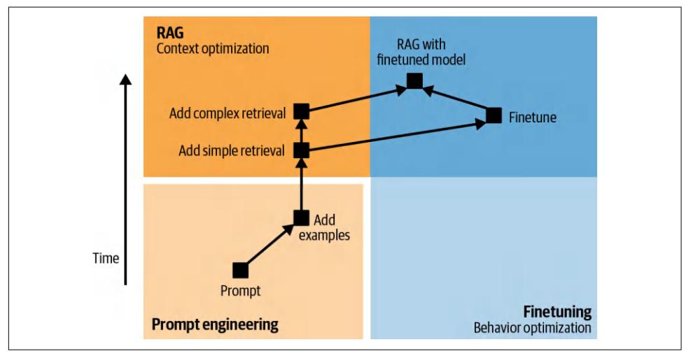
Figure 7-3. Example application development flows. After simple retrieval (such as term-based retrieval), whether to experiment with more complex retrieval (such as hybrid search) or finetuning depends on each application and its failure modes.

So the workflow to adapt a model to a task might work as follows. Note that before any of the adaptation steps, you should define your evaluation criteria and design your evaluation pipeline, as discussed in Chapter 4. This evaluation pipeline is what you’ll use to benchmark your progress as you develop your application. Evaluation doesn’t happen only in the beginning. It should be present during every step of the process:

1. Try to get a model to perform your task with prompting alone. Use the prompt engineering best practices covered in Chapter 5, including systematically ver‐ sioning your prompts.
1. Add more examples to the prompt. Depending on the use case, the number of examples needed might be between 1 and 50.
1. If your model frequently fails due to missing information, connect it to data sources that can supply relevant information. When starting with RAG, begin by using basic retrieval methods like term-based search. Even with simple retrieval, adding relevant and accurate knowledge should lead to some improvement in your model’s performance.
1. Depending on your model’s failure modes, you might explore one of these next steps:
- 1. If the model continues having information-based failures, you might want to try even more advanced RAG methods, such as embedding-based retrieval.
- 1. If the model continues having behavioral issues, such as it keeps generating irrelevant, malformatted, or unsafe responses, you can opt for finetuning. Embedding-based retrieval increases inference complexity by introducing additional components into the pipeline, while finetuning increases the com‐ plexity of model development but leaves inference unchanged.
1. Combine both RAG and finetuning for even more performance boost.

If, after considering all the pros and cons of finetuning and other alternate tech‐ niques, you decide to finetune your model, the rest of the chapter is for you. First, let’s look into the number one challenge of finetuning: its memory bottleneck.

Memory Bottlenecks

Because finetuning is memory-intensive, many finetuning techniques aim to mini‐ mize their memory footprint. Understanding what causes this memory bottleneck is necessary to understand why and how these techniques work. This understanding, in turn, can help you select a finetuning method that works best for you.

Besides explaining finetuning’s memory bottleneck, this section also introduces for‐ mulas for back-of-the-napkin calculation of the memory usage of each model. This calculation is useful in estimating what hardware you’d need to serve or finetune a model.

Because memory calculation requires a breakdown of low-level ML and computing concepts, this section is technically dense. If you’re already familiar with these con‐ cepts, feel free to skip them.

Key Takeaways for Understanding Memory Bottlenecks

If you decide to skip this section, here are a few key takeaways. If you find any of these takeaways unfamiliar, the concepts in this section should help explain it:

1. Because of the scale of foundation models, memory is a bottleneck for working with them, both for inference and for finetuning. The memory needed for fine‐ tuning is typically much higher than the memory needed for inference because of the way neural networks are trained.
1. The key contributors to a model’s memory footprint during finetuning are its number of parameters, its number of trainable parameters, and its numerical representations.
1. The more trainable parameters, the higher the memory footprint. You can reduce memory requirement for finetuning by reducing the number of trainable parameters. Reducing the number of trainable parameters is the motivation for PEFT, parameter-efficient finetuning.
1. Quantization refers to the practice of converting a model from a format with more bits to a format with fewer bits. Quantization is a straightforward and effi‐ cient way to reduce a model’s memory footprint. For a model of 13 billion parameters, using FP32 means 4 bytes per weight or 52 GB for the whole weights. If you can reduce each value to only 2 bytes, the memory needed for the model’s weights decreases to 26 GB.
1. Inference is typically done using as few bits as possible, such as 16 bits, 8 bits, and even 4 bits.
1. Training is more sensitive to numerical precision, so it’s harder to train a model in lower precision. Training is typically done in mixed precision, with some operations done in higher precision (e.g., 32-bit) and some in lower precision (e.g., 16-bit or 8-bit).

Backpropagation and Trainable Parameters

A key factor that determines a model’s memory footprint during finetuning is its number of trainable parameters. A trainable parameter is a parameter that can be updated during finetuning. During pre-training, all model parameters are updated. During inference, no model parameters are updated. During finetuning, some or all model parameters may be updated. The parameters that are kept unchanged are fro‐ zen parameters.

The memory needed for each trainable parameter results from the way a model is trained. As of this writing, neural networks are typically trained using a mechanism called backpropagation. 6 With backpropagation, each training step consists of two phases:

1. Forward pass: the process of computing the output from the input.
1. Backward pass: the process of updating the model’s weights using the aggregated signals from the forward pass.

During inference, only the forward pass is executed. During training, both passes are executed. At a high level, the backward pass works as follows:

1. Compare the computed output from the forward pass against the expected out‐ put (ground truth). If they are different, the model made a mistake, and the parameters need to be adjusted. The difference between the computed output and the expected output is called the loss.
1. Compute how much each trainable parameter contributes to the mistake. This value is called the gradient. Mathematically, gradients are computed by taking the derivative of the loss with respect to each trainable parameter. There’s one gradient value per trainable parameter.⁷ If a parameter has a high gradient, it sig‐ nificantly contributes to the loss and should be adjusted more.
1. Adjust trainable parameter values using their corresponding gradient. How much each parameter should be readjusted, given its gradient value, is deter‐ mined by the optimizer. Common optimizers include SGD (stochastic gradient descent) and Adam. For transformer-based models, Adam is, by far, the most widely used optimizer.

The forward and backward pass for a hypothetical neural network with three param‐ eters and one nonlinear activation function is visualized in Figure 7-4. I use this dummy neural network to simplify the visualization.

⁶ Other than backpropagation, a promising approach to training neural networks is evolutionary strategy. One example, described by Maheswaranathan et al., combines random search with surrogate gradients, instead of using real gradients, to update model weights. Another interesting approach is direct feedback alignment (Arild Nøkland, 2016).

⁷ If a parameter is not trainable, it doesn’t need to be updated and, therefore, there’s no need to compute its gradient.

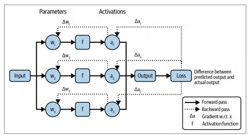
Figure 7-4. The forward and backward pass of a simple neural network.

During the backward pass, each trainable parameter comes with additional values, its gradient, and its optimizer states. Therefore, the more trainable parameters there are, the more memory is needed to store these additional values.

Memory Math

It’s useful to know how much memory a model needs so that you can use the right hardware for it. Often, you might already have the hardware and need to calculate whether you can afford to run a certain model. If a model requires 30 GB of memory to do inference, a chip with 24 GB of memory won’t be sufficient.

A model’s memory footprint depends on the model as well as the workload and the different optimization techniques used to reduce its memory usage. Because it’s impossible to account for all optimization techniques and workloads, in this section, I’ll outline only the formulas for approximate calculations, which should give you a rough idea of how much memory you need to operate a model, both during inference and training.

Inference and training having distinct memory profiles is one of the reasons for the divergence in chips for training and inference, as discussed in Chapter 9.

Memory needed for inference

During inference, only the forward pass is executed. The forward pass requires mem‐ ory for the model’s weights. Let N be the model’s parameter count and M be the memory needed for each parameter; the memory needed to load the model’s parame‐ ters is:

N × M

The forward pass also requires memory for activation values. Transformer models need memory for key-value vectors for the attention mechanism. The memory for both activation values and key-value vectors grows linearly with sequence length and batch size.

For many applications, the memory for activation and key-value vectors can be assumed to be 20% of the memory for the model’s weights. If your application uses a longer context or larger batch size, the actual memory needed will be higher. This assumption brings the model’s memory footprint to:

N × M × 1.2

Consider a 13B-parameter model. If each parameter requires 2 bytes, the model’s weights will require 13B × 2 bytes = 26 GB. The total memory for inference will be 26 GB × 1.2 = 31.2 GB.

A model’s memory footprint grows rapidly with its size. As models become bigger, memory becomes a bottleneck for operating them.⁸ A 70B-parameter model with 2 bytes per parameter will require a whooping 140 GB of memory just for its weights.⁹

Memory needed for training

To train a model, you need memory for the model’s weights and activations, which has already been discussed. Additionally, you need memory for gradients and opti‐ mizer states, which scales with the number of trainable parameters.

Overall, the memory needed for training is calculated as:

Training memory = model weights + activations + gradients + optimizer states

⁸ Some might say that you’re not doing AI until you’ve seen a “RuntimeError: CUDA out of memory” error.

⁹ To learn more about inference memory calculation, check out Carol Chen’s “Transformer Inference Arith‐ metic”, kipply’s blog (March 2022).

During the backward pass, each trainable parameter requires one value for gradient plus zero to two values for optimizer states, depending on the optimizer:

A vanilla SGD optimizer has no state.
A momentum optimizer stores one value per trainable parameter.
An Adam optimizer stores two values per trainable parameter.

Imagine you’re updating all parameters in a 13B-parameter model using the Adam optimizer. Because each trainable parameter has three values for its gradient and optimizer states, if it takes two bytes to store each value, the memory needed for gra‐ dients and optimizer states will be:

13 billion × 3 × 2 bytes = 78 GB

However, if you only have 1B trainable parameters, the memory needed for gradients and optimizer states will be only:

1 billion × 3 × 2 bytes = 6 GB

One important thing to note is that in the previous formula, I assumed that the mem‐ ory needed for activations is less than the memory needed for the model’s weights. However, in reality, the activation memory can be much larger. If activations are stored for gradient computation, the memory needed for activations can dwarf the memory needed for the model’s weights. Figure 7-5 shows the memory needed for activations compared to the memory needed for the model’s weights for different Megatron models at different scales, according to the paper “Reducing Activation Recomputation in Large Transformer Models”, by Korthikanti et al. (2022).

One way to reduce the memory needed for activations is not to store them. Instead of storing activations for reuse, you recompute activations when necessary. This techni‐ que is called gradient checkpointing or activation recomputation. While this reduces the memory requirements, it increases the time needed for training due to the recomputation.¹⁰

¹⁰ To learn more about training memory calculation, check out EleutherAI’s “Transformer Math 101” (Anthony et al., April 2023).

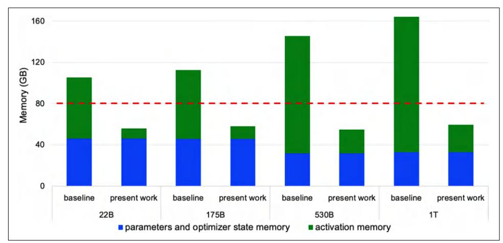
Figure 7-5. The memory needed for activations can dwarf the memory needed for the model’s weights. Image from Korthikanti et al., 2022.

Numerical Representations

In the memory calculation so far, I’ve assumed that each value takes up two bytes of memory. The memory required to represent each value in a model contributes directly to the model’s overall memory footprint. If you reduce the memory needed for each value by half, the memory needed for the model’s weights is also reduced by half.

Before discussing how to reduce the memory needed for each value, it’s useful to understand numerical representations. Numerical values in neural networks are tra‐ ditionally represented as float numbers. The most common family of floating point formats is the FP family, which adheres to the Institute of Electrical and Electronics Engineers (IEEE) standard for Floating-Point Arithmetic (IEEE 754):

FP32 uses 32 bits (4 bytes) to represent a float. This format is called single precision.
FP64 uses 64 bits (8 bytes) and is called double precision.
FP16 uses 16 bits (2 bytes) and is called half precision.

While FP64 is still used in many computations—as of this writing, FP64 is the default format for NumPy and pandas—it’s rarely used in neural networks because of its memory footprint. FP32 and FP16 are more common. Other popular floating point formats in AI workloads include BF16 (BFloat16) and TF32 (TensorFloat-32). BF16 was designed by Google to optimize AI performance on TPUs and TF32 was designed by NVIDIA for GPUs. 11

Numbers can also be represented as integers. Even though not yet as common as floating formats, integer representations are becoming increasingly popular. Com‐ mon integer formats are INT8 (8-bit integers) and INT4 (4-bit integers).¹²

Each float format usually has 1 bit to represent the number’s sign, i.e., negative or positive. The rest of the bits are split between range and precision: 13

Range

The number of range bits determines the range of values the format can repre‐ sent. More bits means a wider range. This is similar to how having more digits lets you represent a wider range of numbers.

Precision

The number of precision bits determines how precisely a number can be repre‐ sented. Reducing the number of precision bits makes a number less precise. For example, if you convert 10.1234 to a format that can support only two decimal digits, this value becomes 10.12, which is less precise than the original value.

Figure 7-6 shows different floating point formats along with their range and precision bits.¹⁴

¹¹ Google introduced BFloat16 as “the secret to high performance on Cloud TPUs”.

¹² Integer formats are also called fixed point formats.

¹³ Range bits are called exponents. Precision bits are called significands.

¹⁴ Note that usually the number at the end of a format’s name signifies how many bits it occupies, but TF32 actually has 19 bits, not 32 bits. I believe it was named so to suggest its functional compatibility with FP32. But honestly, why it’s called TF32 and not TF19 keeps me up at night. An ex-coworker at NVIDIA volun‐ teered his conjecture that people might be skeptical of weird formats (19-bit), so naming this format TF32 makes it look more friendly.

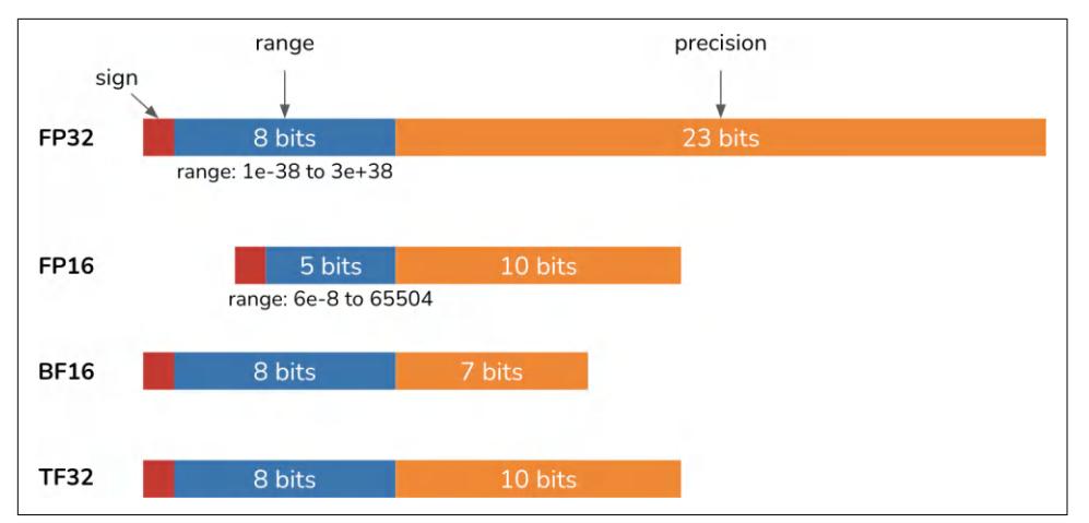
Figure 7-6. Different numerical formats with their range and precision.

Formats with more bits are considered higher precision. Converting a number with a high-precision format into a low-precision format (e.g., from FP32 to FP16) means reducing its precision. Reducing precision can cause a value to change or result in errors. Table 7-3 shows how FP32 values can be converted into FP16, BF16, and TF32.

Table 7-3. Convert from FP32 values to lower-precision formats. Resultant inaccuracies are in italics.

12.3456789	12.34375	12.375 12.34375
123.456789	123.4375	123.5
		123.4375
1234.56789	1235.0	1232.0 1234.0
12345.6789	12344.0	12352.0 12344.0
123456.789	INFa	123392.0 123456.0
1234567.89	INF	1236990.0 1233920.0
a
	Values out of bound in FP16 are rounded to infinity.

a Values out of bound in FP16 are rounded to infinity.

Note in Table 7-3 that even though BF16 and FP16 have the same number of bits, BF16 has more bits for range and fewer bits for precision. This allows BF16 to repre‐ sent large values that are out-of-bound for FP16. However, this also makes BF16 less precise than FP16. For example, 1234.56789 is 1235.0 in FP16 (0.035% value change) but 1232.0 in BF16 (0.208% value change).

When using a model, make sure to load the model in the format it’s intended for. Loading a model into the wrong numerical format can cause the model to change significantly. For example, Llama 2 had its weights set to BF16 when it came out. However, many teams loaded the model in FP16 and were subsequently frus‐ trated to find the model’s quality much worse than advertised. 15 While this misunderstanding wasted a lot of people’s time, the upside is that it forced many people to learn about numerical representations.

The right format for you depends on the distribution of numerical values of your workload (such as the range of values you need), how sensitive your workload is to small numerical changes, and the underlying hardware.¹⁶

Quantization

The fewer bits needed to represent a model’s values, the lower the model’s memory footprint will be. A 10B-parameter model in a 32-bit format requires 40 GB for its weights, but the same model in a 16-bit format will require only 20 GB. Reducing precision, also known as quantization, is a cheap and extremely effective way to reduce a model’s memory footprint. It’s straightforward to do and generalizes over tasks and architectures. In the context of ML, low precision generally refers to any format with fewer bits than the standard FP32.

Quantization Versus Reduced Precision

Strictly speaking, it’s quantization only if the target format is integer. However, in practice, quantization is used to refer to all techniques that convert values to a lowerprecision format. In this book, I use quantization to refer to precision reduction, to keep it consistent with the literature.

¹⁵ The FP16 and BF16 confusion continued with Llama 3.1. See X and Threads discussions: 1; 2, 3, 4; and llama.cpp’s benchmark between BF16 and FP16, Bloke’s writeup, and Raschka’s writeup.

¹⁶ Designing numerical formats is a fascinating discipline. Being able to create a lower-precision format that doesn’t compromise a system’s quality can make that system much cheaper and faster, enabling new use cases.

To do quantization, you need to decide what to quantize and when:

What to quantize

Ideally, you want to quantize whatever is consuming most of your memory, but it also depends on what you can quantize without hurting performance too much. As discussed in “Memory Math” on page 322, major contributors to a model’s memory footprint during inference are the model’s weights and activa‐ tions.¹⁷ Weight quantization is more common than activation quantization, since weight activation tends to have a more stable impact on performance with less accuracy loss.

When to quantize

Quantization can happen during training or post-training. Post-training quanti‐ zation (PTQ) means quantizing a model after it’s been fully trained. PTQ is by far the most common. It’s also more relevant to AI application developers who don’t usually train models.

Inference quantization

In the early days of deep learning, it was standard to train and serve models using 32 bits with FP32. Since the late 2010s, it has become increasingly common to serve models in 16 bits and in even lower precision. For example, Dettmers et al. (2022) have done excellent work quantizing LLMs into 8 bits with LLM.int8() and 4 bits with QLoRA (Dettmers et al., 2023).

A model can also be served in mixed precision, where values are reduced in precision when possible and maintained in higher precision when necessary. To serve models on the devices, Apple (2024) leveraged a quantization scheme that uses a mixture of 2-bit and 4-bit formats, averaging 3.5 bits-per-weight. Also in 2024, in anticipation of 4-bit neural networks, NVIDIA announced their new GPU architecture, Blackwell, that supports model inference in 4-bit float.

Once you get to 8 bits and under, numerical representations get more tricky. You can keep parameter values as floats using one of the minifloat formats, such as FP8 (8 bits) and FP4 (4 bits).¹⁸ More commonly, however, parameter values are converted into an integer format, such as INT8 or INT4.

¹⁷ Another major contributor to the memory footprint of transformer-based models is the KV cache, which is discussed in Chapter 9.

¹⁸ The smallest possible float size that follows all IEEE principles is 4-bit.

Quantization is effective, but there’s a limit to how far it can go. You can’t have fewer than 1 bit per value, and some have attempted the 1-bit representation, e.g., Binary‐ Connect (Courbariaux et al., 2015), Xnor-Net (Rastegari et al., 2016), and BitNet (Wang et al., 2023).¹⁹

In 2024, Microsoft researchers (Ma et al.) declared that we’re entering the era of 1-bit LLMs by introducing BitNet b1.58, a transformer-based language model that requires only 1.58 bits per parameter and whose performance is comparable to 16-bit Llama 2 (Touvron et al., 2023) up to 3.9B parameters, as shown in Table 7-4.

Table 7-4. BitNet b1.58’s performance compared to that of Llama 2 16-bit on different benchmarks and at different model sizes, up to 3.9B parameters. Results from Ma et al. (2024).

BitNet b1.58		61.4	28.3	42.9	61.5	26.6	71.5
BitNet b1.58	3.9B	64.2	28.7	44.2	63.5	24.2	73.2

Reduced precision not only reduces the memory footprint but also often improves computation speed. First, it allows a larger batch size, enabling the model to process more inputs in parallel. Second, reduced precision speeds up computation, which further reduces inference latency and training time. To illustrate this, consider the addition of two numbers. If we perform the addition bit by bit, and each takes t nano‐ seconds, it’ll take 32t nanoseconds for 32 bits but only 16t nanoseconds for 16 bits. However, reducing precision doesn’t always reduce latency due to the added compu‐ tation needed for format conversion.

There are downsides to reduced precision. Each conversion often causes a small value change, and many small changes can cause a big performance change. If a value is outside the range the reduced precision format can represent, it might be converted to infinity or an arbitrary value, causing the model’s quality to further degrade. How to reduce precision with minimal impact on model performance is an active area of research, pursued by model developers as well as by hardware makers and applica‐ tion developers.

¹⁹ The authors of the Xnor-Net paper spun off Xnor.ai, a startup that focused on model compression. In early 2020, it was acquired by Apple for a reported $200M.

Inference in lower precision has become a standard. A model is trained using a higher-precision format to maximize performance, then its precision is reduced for inference. Major ML frameworks, including PyTorch, TensorFlow, and Hugging Face’s transformers, offer PTQ for free with a few lines of code.

Some edge devices only support quantized inference. Therefore, frameworks for ondevice inference, such as TensorFlow Lite and PyTorch Mobile, also offer PTQ.

Training quantization

Quantization during training is not yet as common as PTQ, but it’s gaining traction. There are two distinct goals for training quantization:

1. To produce a model that can perform well in low precision during inference. This is to address the challenge that a model’s quality might degrade during posttraining quantization.
1. To reduce training time and cost. Quantization reduces a model’s memory foot‐ print, allowing a model to be trained on cheaper hardware or allowing the train‐ ing of a larger model on the same hardware. Quantization also speeds up computation, which further reduces costs.

A quantization technique might help achieve o ne or both of these goals.

Quantization-aware training (QAT) aims to create a model with high quality in low precision for inference. With QAT, the model simulates low-precision (e.g., 8-bit) behavior during training, which allows the model to learn to produce high-quality outputs in low precision. However, QAT doesn’t reduce a model’s training time since its computations are still performed in high precision. QAT can even increase train‐ ing time due to the extra work of simulating low-precision behavior.

On the other hand, training a model directly in lower precision can help with both goals. People attempted to train models in reduced precision as early as 2016; see Hubara et al. (2016) and Jacob et al. (2017). Character.AI (2024) shared that they were able to train their models entirely in INT8, which helped eliminate the training/ serving precision mismatch while also significantly improving training efficiency. However, training in lower precision is harder to do, as backpropgation is more sen‐ sitive to lower precision.²⁰

Lower-precision training is often done in mixed precision, where a copy of the weights is kept in higher precision but other values, such as gradients and activations,

²⁰ During training, the model’s weights are updated via multiple steps. Small rounding changes can compound during the training process, making it difficult for the model to achieve the desirable performance. On top of that, loss values require precise computation. Small changes in the loss value can point parameter updates in the wrong direction.

are kept in lower precision.²¹ You can also have less-sensitive weight values computed in lower precision and more-sensitive weight values computed in higher precision. For example, LLM-QAT (Liu et al., 2023) quantizes weights and activations into 4 bits but keeps embeddings in 16 bits.

The portions of the model that should be in lower precision can be set automatically using the automatic mixed precision (AMP) functionality offered by many ML frame‐ works.

It’s also possible to have different phases of training in different precision levels. For example, a model can be trained in higher precision but finetuned in lower precision. This is especially common with foundation models, where the team training a model from scratch might be an organization with sufficient compute for higher precision training. Once the model is published, developers with less compute access can fine‐ tune that model in lower precision.

Finetuning Techniques

I hope that the previous section has made clear why finetuning large-scale models is so memory-intensive. The more memory finetuning requires, the fewer people who can afford to do it. Techniques that reduce a model’s memory footprint make fine‐ tuning more accessible, allowing more people to adapt models to their applications. This section focuses on memory-efficient finetuning techniques, which centers around parameter-efficient finetuning.

I’ll also cover model merging, an exciting but more experimental approach to creat‐ ing custom models. While model merging is generally not considered finetuning, I include it in this section because it’s complementary to finetuning. Finetuning tailors one model to specific needs. Model merging combines multiple models, often fine‐ tuned models, for the same purpose.

While combining multiple models isn’t a new concept, new types of models and fine‐ tuning techniques have inspired many creative model-merging techniques, making this section especially fun to write about.

Parameter-Efficient Finetuning

In the early days of finetuning, models were small enough that people could finetune entire models. This approach is called full finetuning. In full finetuning, the number of trainable parameters is exactly the same as the number of parameters.

²¹ Personal anecdote: much of my team’s work at NVIDIA was on mixed precision training. See “Mixed Preci‐ sion Training for NLP and Speech Recognition with OpenSeq2Seq” (Huyen et al., NVIDIA Developer Tech‐ nical Blog, October 2018).

Full finetuning can look similar to training. The main difference is that training starts with randomized model weights, whereas finetuning starts with model weights that have been previously trained.

As discussed in “Memory Math” on page 322, the more trainable parameters there are, the more memory is needed. Consider a 7B-parameter model:

If you use a 16-bit format like FP16, loading the model’s weights alone requires 14 GB for memory.
Full finetuning this model with the Adam optimizer, also in a 16-bit format, requires an additional 7B × 3 × 2 bytes = 42 GB of memory.
The total memory needed for the model’s weights, gradients, and optimizer states is then 14 GB + 42 GB = 56 GB.

56 GB exceeds the memory capacity of most consumer GPUs, which typically come with 12–24 GB of memory, with higher-end GPUs offering up to 48 GB. And this memory estimation doesn’t yet take into account the memory required for activations.

To fit a model on a given hardware, you can either reduce the model’s memory footprint or find ways to use the hardware’s memory more efficiently. Techniques like quantization and PEFT help minimize the total memory footprint. Techniques that focus on making better use of hardware memory include CPU offloading. Instead of trying to fit the whole model on GPUs, you can offload the excess memory onto CPUs, as demonstrated by DeepSpeed (Rasley et al., 2020).

We also haven’t touched on the fact that full finetuning, especially supervised fine‐ tuning and preference finetuning, typically requires a lot of high-quality annotated data that most people can’t afford. Due to the high memory and data requirements of full finetuning, people started doing partial finetuning. In partial finetuning, only some of the model’s parameters are updated. For example, if a model has ten layers, you might freeze the first nine layers and finetune only the last layer,²² reducing the number of trainable parameters to 10% of full finetuning.

While partial finetuning can reduce the memory footprint, it’s parameter-inefficient. Partial finetuning requires many trainable parameters to achieve performance close to that of full finetuning. A study by Houlsby et al. (2019) shows that with BERT large (Devlin et al., 2018), you’d need to update approximately 25% of the parameters

²² In partial finetuning, it’s common to finetune the layers closest to the output layer because those layers are usually more task-specific, whereas earlier layers tend to capture more general features.

to achieve performance comparable to that of full finetuning on the GLUE bench‐ mark (Wang et al., 2018). Figure 7-7 shows the performance curve of partial finetun‐ ing with different numbers of trainable parameters.

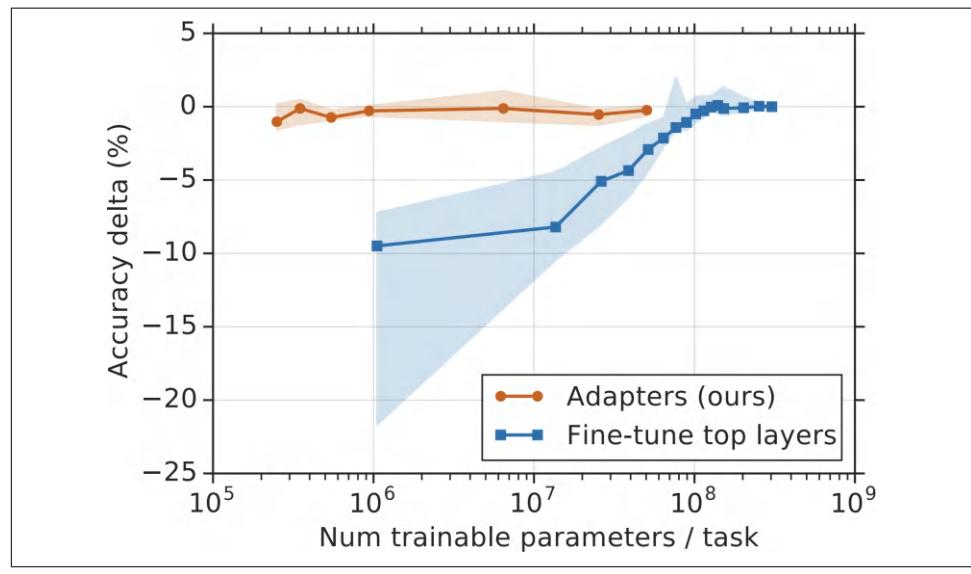
Figure 7-7. The blue line shows that partial finetuning requires many trainable param‐ eters to achieve a performance comparable to full finetuning. Image from Houlsby et al. (2019).

This brings up the question: How to achieve performance close to that of full finetun‐ ing while using significantly fewer trainable parameters? Finetuning techniques resulting from this quest are parameter-efficient. There’s no clear threshold that a finetuning method has to pass to be considered parameter-efficient. However, in gen‐ eral, a technique is considered parameter-efficient if it can achieve performance close to that of full finetuning while using several orders of magnitude fewer trainable parameters.

The idea of PEFT (parameter-efficient finetuning) was introduced by Houlsby et al. (2019). The authors showed that by inserting additional parameters into the model in the right places, you can achieve strong finetuning performance using a small num‐ ber of trainable parameters. They inserted two adapter modules into each trans‐ former block of a BERT model, as shown in Figure 7-8.

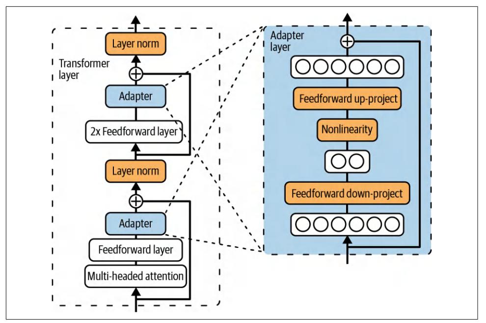
Figure 7-8. By inserting two adapter modules into each transformer layer for a BERT model and updating only the adapters, Houlsby et al. (2019) were able to achieve strong finetuning performance using a small number of trainable parameters.

During finetuning, they kept the model’s original parameters unchanged and only updated the adapters. The number of trainable parameters is the number of parame‐ ters in the adapters. On the GLUE benchmark, they achieved a performance within 0.4% of full finetuning using only 3% of the number of trainable parameters. The orange line in Figure 7-7 shows the performance delta between full finetuning and finetuning using different adapter sizes.

However, the downside of this approach is that it increases the inference latency of the finetuned model. The adapters introduce additional layers, which add more com‐ putational steps to the forward pass, slowing inference.

PEFT enables finetuning on more affordable hardware, making it accessible to many more developers. PEFT methods are generally not only parameter-efficient but also sample-efficient. While full finetuning may need tens of thousands to millions of examples to achieve notable quality improvements, some PEFT methods can deliver strong performance with just a few thousand examples.

Given PEFT’s obvious appeal, PEFT techniques are being rapidly developed. The next section will give an overview of these techniques before diving deeper into the most common PEFT technique: LoRA.

PEFT techniques

The existing prolific world of PEFT generally falls into two buckets: adapter-based methods and soft prompt-based methods. However, it’s likely that newer buckets will be introduced in the future.

Adapter-based methods refer to all methods that involve additional modules to the model weights, such as the one developed by Houlsby et al. (2019). Because adapterbased methods involve adding parameters, they are also called additive methods.

As of this writing, LoRA (Hu et al., 2021) is by far the most popular adapter-based method, and it will be the topic of the following section. Other adapter-based meth‐ ods include BitFit (Zaken et al., 2021), which came out around the same time LoRA did. Newer adapter methods include IA3 (Liu et al., 2022), whose efficient mixed-task batching strategy makes it particularly attractive for multi-task finetuning. It’s been shown to outperform LoRA and even full finetuning in some cases. LongLoRA (Chen et al., 2023) is a LoRA variant that incorporates attention-modification techniques to expand context length.

If adapter-based methods add trainable parameters to the model’s architecture, soft prompt-based methods modify how the model processes the input by introducing special trainable tokens. These additional tokens are fed into the model alongside the input tokens. They are called soft prompts because, like the inputs (hard prompts), soft prompts also guide the model’s behaviors. However, soft prompts differ from hard prompts in two ways:

Hard prompts are human-readable. They typically contain discrete tokens such as “I”, “write”, “a”, and “lot”. In contrast, soft prompts are continuous vectors, resembling embedding vectors, and are not human-readable.
Hard prompts are static and not trainable, whereas soft prompts can be opti‐ mized through backpropagation during the tuning process, allowing them to be adjusted for specific tasks.

Some people describe soft prompting as a crossover between prompt engineering and finetuning. Figure 7-9 visualizes how you can use soft prompts together with hard prompts to guide a model’s behaviors.

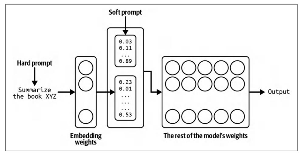
Figure 7-9. Hard prompts and soft prompts can be combined to change a model’s behaviors.

Soft prompt tuning as a subfield is characterized by a series of similar-sounding tech‐ niques that can be confusing, such as prefix-tuning (Li and Liang, 2021), P-Tuning (Liu et al., 2021), and prompt tuning (Lester et al., 2021).²³ They differ mainly on the locations where the soft prompts are inserted. For example, prefix tuning prepends soft prompt tokens to the input at every transformer layer, whereas prompt tuning prepends soft prompt tokens to only the embedded input. If you want to use any of them, many PEFT frameworks will implement them out of the box for you.

To get a sense of what PEFT methods are being used, I analyzed over 1,000 open issues on the GitHub repository huggingface/peft in October 2024. The assumption is that if someone uses a technique, they are more likely to report issues or ask ques‐ tions about it. Figure 7-10 shows the result. For “P-Tuning”, I searched for keywords “p_tuning” and “p tuning” to account for different spellings.

²³ I’ve never met a single person who could explain to me, on the spot, the differences between these techniques.

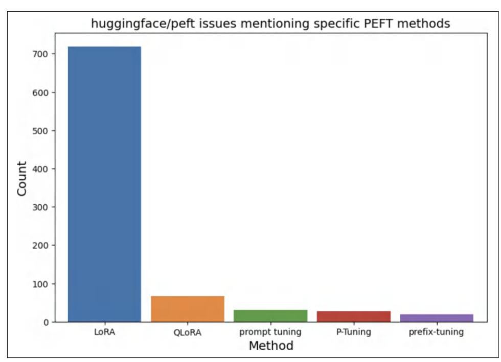
Figure 7-10. The number of issues corresponding to different finetuning techniques from the GitHub repository huggingface/peft. This is a proxy to estimate the popularity of each technique.

From this analysis, it’s clear that LoRA dominates. Soft prompts are less common, but there seems to be growing interest from those who want more customization than what is afforded by prompt engineering but who don’t want to invest in finetuning.

Because of LoRA’s popularity, the next section focuses on how LoRA works and how it solves the challenge posed by early adapter-based methods. Even if you don’t use LoRA, this deep dive should provide a framework for you to explore other finetuning methods.

LoRA

Unlike the original adapter method by Houlsby et al. (2019), LoRA (Low-Rank Adap‐ tation) (Hu et al., 2021) incorporates additional parameters in a way that doesn’t incur extra inference latency. Instead of introducing additional layers to the base model, LoRA uses modules that can be merged back to the original layers.

You can apply LoRA to individual weight matrices. Given a weight matrix, LoRA decomposes this matrix into the product of two smaller matrices, then updates these two smaller matrices before merging them back to the original matrix.

Consider the weight matrix W of the dimension n × m. LoRA works as follows:

1. First, choose the dimension of the smaller matrices. Let r be the chosen value. Construct two matrices: A (dimension n × r) and B (dimension r × m). Their product is WAB, which is of the same dimension as W. r is the LoRA rank.
1. Add WAB to the original weight matrix W to create a new weight matrix Wʹ. Use Wʹ in place of W as part of the model. You can use a hyperparameter ɑ to deter‐ mine how much WAB should contribute to the new matrix: W ’ = W + α ^r WAB
1. During finetuning, update only the parameters in A and B. W is kept intact.

Figure 7-11 visualizes this process.

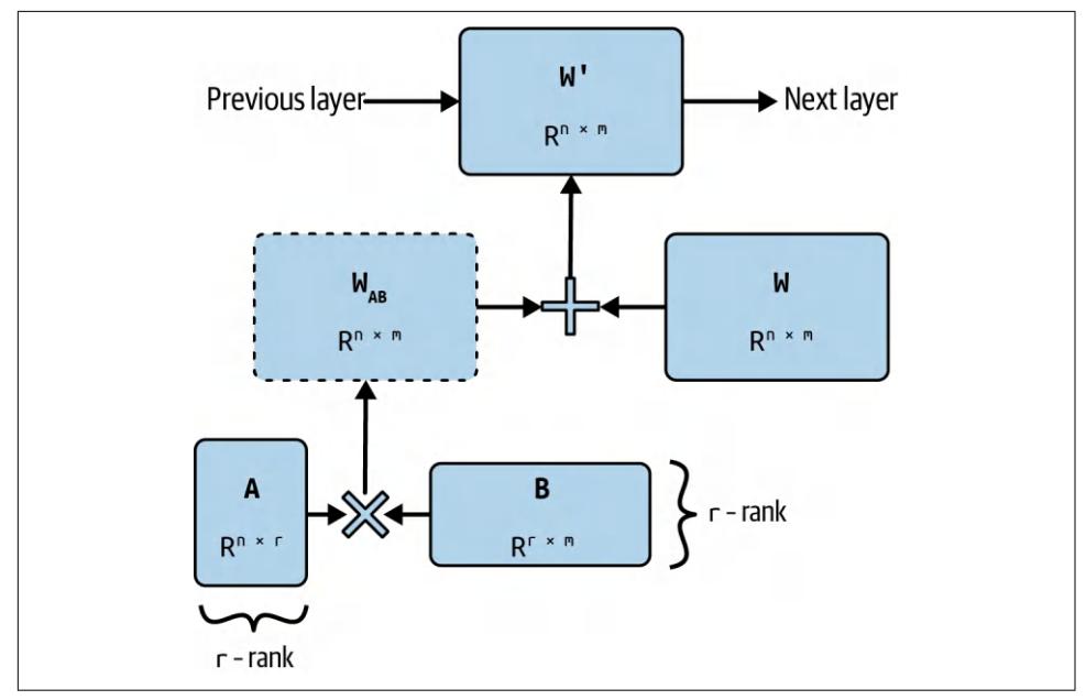
Figure 7-11. To apply LoRA to a weight matrix W, decompose it into the product of two matrices A and B. During finetuning, only A and B are updated. W is kept intact.

LoRA (Low-Rank Adaptation) is built on the concept of low-rank factorization, a long-standing dimensionality reduction technique. The key idea is that you can factorize a large matrix into a product of two smaller matrices to reduce the number of parameters, which, in turn, reduces both the computation and memory requirements. For example, a 9 × 9 matrix can be factorized into the product of two matrices of dimensions 9 × 1 and 1 × 9. The original matrix has 81 parameters, but the two product matrices have only 18 parameters combined.

The number of columns in the first factorized matrix and the num‐ ber of columns in the second factorized matrix correspond to the rank of the factorization. The original matrix is full-rank, while the two smaller matrices represent a low-rank approximation.

While factorization can significantly reduce the number of param‐ eters, it’s lossy because it only approximates the original matrix. The higher the rank, the more information from the original matrix the factorization can preserve.

Like the original adapter method, LoRA is parameter-efficient and sample-efficient. The factorization enables LoRA to use even fewer trainable parameters. The LoRA paper showed that, for GPT-3, LoRA achieves comparable or better performance with full finetuning on several tasks while using only ~4.7M trainable parameters, 0.0027% of full finetuning.

Why does LoRA work? Parameter-efficient methods like LoRA have become so popular that many people take them for granted. But why is parameter efficiency possible at all? If a model requires a lot of parameters to learn certain behaviors during pretraining, shouldn’t it also require a lot of parameters to change its behaviors during finetuning?

The same question can be raised for data. If a model requires a lot of data to learn a behavior, shouldn’t it also require a lot of data to meaningfully change this behavior? How is it possible that you need millions or billions of examples to pre-train a model, but only a few hundreds or thousands of examples to finetune it?

Many papers have argued that while LLMs have many parameters, they have very low intrinsic dimensions; see Li et al. (2018); Aghajanyan et al. (2020); and Hu et al. (2021). They showed that pre-training implicitly minimizes the model’s intrinsic dimension. Surprisingly, larger models tend to have lower intrinsic dimensions after pre-training. This suggests that pre-training acts as a compression framework for downstream tasks. In other words, the better trained an LLM is, the easier it is to finetune the model using a small number of trainable parameters and a small amount of data.

You might wonder, if low-rank factorization works so well, why don’t we use LoRA for pre-training as well? Instead of pre-training a large model and applying low-rank factorization only during finetuning, could we factorize a model from the start for pre-training? Low-rank pre-training can significantly reduce the model’s number of parameters, significantly reducing the model’s pre-training time and cost.

Throughout the 2010s, many people tried training low-rank neural networks, exem‐ plified in studies such as “Low-Rank Matrix Factorization for Deep Neural Network Training with High-Dimensional Output Targets” (Sainath et al., 2013), “Semi-Orthogonal Low-Rank Matrix Factorization for Deep Neural Networks” (Povey et al., 2018), and “Speeding up Convolutional Neural Networks with Low Rank Expan‐ sions” (Jaderberg et al., 2014).

Low-rank factorization has proven to be effective at smaller scales. For example, by applying various factorization strategies, including replacing 3 × 3 convolution with 1 × 1 convolution, SqueezeNet (Iandola et al., 2016) achieves AlexNet-level accuracy on ImageNet using 50 times fewer parameters.

More recent attempts to train low-rank LLMs include ReLoRA (Lialin et al., 2023) and GaLore (Zhao et al., 2024). ReLoRA works for transformer-based models of up to 1.3B parameters. GaLore achieves performance comparable to that of a full-rank model at 1B parameters and promising performance at 7B parameters.

It’s possible that one day not too far in the future, researchers will develop a way to scale up low-rank pre-training to hundreds of billions of parameters. However, if Aghajanyan et al.’s argument is correct—that pre-training implicitly compresses a model’s intrinsic dimension—full-rank pre-training is still necessary to sufficiently reduce the model’s intrinsic dimension to a point where low-rank factorization can work. It would be interesting to study exactly how much full-rank training is neces‐ sary before it’s possible to switch to low-rank training.

LoRA configurations. To apply LoRA, you need to decide what weight matrices to apply LoRA to and the rank of each factorization. This section will discuss the con‐ siderations for each of these decisions.

LoRA can be applied to each individual weight matrix. The efficiency of LoRA, there‐ fore, depends not only on what matrices LoRA is applied to but also on the model’s architecture, as different architectures have different weight matrices.

While there have been examples of LoRA with other architectures, such as convolu‐ tional neural networks (Dutt et al., 2023; Zhong et al., 2024; Aleem et al., 2024), LoRA has been primarily used for transformer models.²⁴ LoRA is most commonly applied to the four weight matrices in the attention modules: the query (W^q ), key (W^k ), value (W^v ), and output projection (W^o ) matrices.

Typically, LoRA is applied uniformly to all matrices of the same type within a model. For example, applying LoRA to the query matrix means applying LoRA to all query matrices in the model.

Naively, you can apply LoRA to all these attention matrices. However, often, you’re constrained by your hardware’s memory and can accommodate only a fixed number of trainable parameters. Given a fixed budget of trainable parameters, what matrices should you apply LoRA to, to maximize performance?

When finetuning GPT-3 175B, Hu et al. (2021) set their trainable parameter budget at 18M, which is 0.01% of the model’s total number of parameters. This budget allows them to apply LoRA to the following:

1. One matrix with the rank of 8
1. Two matrices with the rank of 4
1. All four matrices with the rank of 2

GPT-3 175B has 96 transformer layers with a model dimension of 12,288. Applying LoRA with rank = 2 to all four matrices would yield (12,288 × 2 × 2) × 4 = 196,608 trainable parameters per layer, or 18,874,368 trainable parameters for the whole model.

They found that applying LoRA to all four matrices with rank = 2 yields the best per‐ formance on the WikiSQL (Zhong et al., 2017) and MultiNLI (Multi-Genre Natural Language Inference) benchmarks (Williams et al., 2017). Table 7-5 shows their results. However, the authors suggested that if you can choose only two attention matrices, the query and value matrices generally yield the best results.

²⁴ To effectively use LoRA for a model, it’s necessary to understand that model’s architecture. Chapter 2 already covered the weight composition of some transformer-based models. For the exact weight composition of a model, refer to its paper.

Table 7-5. LoRA performance with the budget of 18M trainable parameters. Results from LoRA (Hu et al., 2021).

Number of trainable parameters $= 18M$
Weight type	$W_n$	$W_{\nu}$	$W_{v}$	$W_0$		$ W_a, W_k $ $W_a, W_v$ $ W_a, W_k, W_v, W_o$
Rank r	8	8	8	8
WikiSQL ( $\pm$ 0.5%) 70.4 70.0 73.0 73.2 71.4					73.7	73.7
MultiNLI ( $\pm$ 0.1%) 91.0 90.8 91.0 91.3 91.3					91.3	91.7

Empirical observations suggest that applying LoRA to more weight matrices, includ‐ ing the feedforward matrices, yields better results. For example, Databricks showed that the biggest performance boost they got was from applying LoRA to all feedfor‐ ward layers (Sooriyarachchi, 2023). Fomenko et al. (2024) noted that feedforwardbased LoRA can be complementary to attention-based LoRA, though attention-based LoRA typically offers greater efficacy within memory constraints.

The beauty of LoRA is that while its performance depends on its rank, studies have shown that a small r, such as between 4 and 64, is usually sufficient for many use cases. A smaller r means fewer LoRA parameters, which translates to a lower memory foot‐ print.

The LoRA authors observed that, to their surprise, increasing the value of r doesn’t increase finetuning performance. This observation is consistent with Databricks’ report that “increasing r beyond a certain value may not yield any discernible increase in quality of model output” (Sooriyarachchi, 2023).²⁵ Some argue that a higher r might even hurt as it can lead to overfitting. However, in some cases, a higher rank might be necessary. Raschka (2023) found that r = 256 achieved the best performance on his tasks.

Another LoRA hyperparameter you can configure is the value α that determines how much the product WAB should contribute to the new matrix during merging: W ’ = W + α ^r WAB . In practice, I’ve often seen ɑ chosen so that the ratio α :r is typi‐ cally between 1:8 and 8:1, but the optimal ratio varies. For example, if r is small, you might want α to be larger, and if r is large, you might want α to be smaller. Experi‐ mentation is needed to determine the best (r, α) combination for your use case.

Serving LoRA adapters. LoRA not only lets you finetune models using less memory and data, but it also simplifies serving multiple models due to its modularity. To understand this benefit, let’s examine how to serve a LoRA-finetuned model.

²⁵ As of this writing, some finetuning frameworks like Fireworks only allow a maximum LoRA rank of 32. How‐ ever, this constraint is unlikely due to performance and more likely due to their hardware’s memory con‐ straint.

In general, there are two ways to serve a LoRA-finetuned model:

1. Merge the LoRA weights A and B into the original model to create the new matrix Wʹ prior to serving the finetuned model. Since no extra computation is done during inference, no extra latency is added.
1. Keep W, A, and B separate during serving. The process of merging A and B back to W happens during inference, which adds extra latency.

The first option is generally better if you have only one LoRA model to serve, whereas the second is generally better for multi-LoRA serving—serving multiple LoRA models that share the same base model. Figure 7-12 visualizes multi-LoRA serving if you keep the LoRA adapters separate.

Figure 7-12. Keeping LoRA adapters separate allows reuse of the same full-rank matrix W in multi-LoRA serving.

For multi-LoRA serving, while option 2 adds latency overhead, it significantly reduces the storage needed. Consider the scenario in which you finetune a model for each of your customers using LoRA. With 100 customers, you end up with 100 fine‐ tuned models, all sharing the same base model. With option 1, you have to store 100 full-rank matrices Wʹ. With option 2, you only have to store one full-rank matrix W, and 100 sets of smaller matrices (A, B).

To put this in perspective, let’s say that the original matrix W is of the dimension 4096 × 4096 (16.8M parameters). If the LoRA’s rank is 8, the number of parameters in A and B is 4096 × 8 × 2 = 65,536:

In option 1, 100 full-rank matrices Wʹ totals 16.8M × 100 = 1.68B parameters.
In option 2, one full-rank matrix W and 100 sets of small matrices (A, B) totals: 16.8M + 65,536 × 100 = 23.3M parameters.

Option 2 also makes it faster to switch between tasks. Let’s say you’re currently serv‐ ing customer X using this customer’s model. To switch to serving customer Y, instead of loading this customer’s full weight matrix, you only need to load Y’s LoRA adapter, which can significantly reduce the loading time. While keeping A and B sep‐ arate incurs additional latency, there are optimization techniques to minimize the added latency. The book’s GitHub repository contains a walkthrough of how to do so.

Multi-LoRA serving makes it easy to combine multiple specialized models. Instead of having one big powerful model for multiple tasks, you can have one LoRA adapter for each task. For example, Apple used multiple LoRA adapters to adapt the same 3Bparameter base model to different iPhone features (2024). They utilized quantization techniques to further reduce the memory footprint of this base model and adapters, allowing the serving of all of them on-device.

The modularity of LoRA adapters means that LoRA adapters can be shared and reused. There are publicly available finetuned LoRA adapters that you can use the way you’d use pre-trained models. You can find them on Hugging Face²⁶ or initia‐ tives like AdapterHub.

You might be wondering: “LoRA sounds great, but what’s the catch?” The main drawback of LoRA is that it doesn’t offer performance as strong as full finetuning. It’s also more challenging to do than full finetuning as it involves modifying the model’s implementation, which requires an understanding of the model’s architec‐ ture and coding skills. However, this is usually only an issue for less popular base models. PEFT frameworks—such as Hugging Face’s PEFT, Axolotl, unsloth, and LitGPT—likely support LoRA for popular base models right out of the box.

Quantized LoRA. The rapid rise of LoRA has led to the development of numerous LoRA variations. Some aim to reduce the number of trainable parameters even fur‐ ther. However, as illustrated in Table 7-6, the memory of a LoRA adapter is minimal compared to the memory of the model’s weights. Reducing the number of LoRA parameters decreases the overall memory footprint by only a small percentage.

Table 7-6. The memory needed by LoRA weights compared to that needed by the model’s weights.

GPT-3 (175B)	350 GB	18.87M	37.7 MB

²⁶ Search for these adapters by tags “adapter”, “peft”, or “LoRA”.

Rather than trying to reduce LoRA’s number of parameters, you can reduce the memory usage more effectively by quantizing the model’s weights, activations, and/or gradients during finetuning. An early promising quantized version of LoRA is QLoRA (Dettmers et al., 2023).²⁷ In the original LoRA paper, during finetuning, the model’s weights are stored using 16 bits. QLoRA stores the model’s weights in 4 bits but dequantizes (converts) them back into BF16 when computing the forward and backward pass.

The 4-bit format that QLoRA uses is NF4 (NormalFloat-4), which quantizes values based on the insight that pre-trained weights usually follow a normal distribution with a median of zero. On top of 4-bit quantization, QLoRA also uses paged optimiz‐ ers to automatically transfer data between the CPU and GPU when the GPU runs out of memory, especially with long sequence lengths. These techniques allow a 65Bparameter model to be finetuned on a single 48 GB GPU.

The authors finetuned a variety of models, including Llama 7B to 65B, in the 4-bit mode. The resulting family of models, called Guanaco, showed competitive perfor‐ mance on both public benchmarks and comparative evaluation. Table 7-7 shows the Elo ratings of Guanaco models, GPT-4, and ChatGPT in May 2023, as judged by GPT-4. While Guanaco 65B didn’t outperform GPT-4, it was often preferred to ChatGPT.

Vicuna 13B	26 GB	974 ± 1
ChatGPT	-	966 ± 1

Guanaco 13B	10 GB	916 ± 1
Bard	-	902 ± 1
Guanaco 7B	6 GB	879 ± 1

Table 7-7. Elo ratings of Guanaco models compared to popular models in May 2023 using GPT-4 as a judge. The experiment is from QLoRA (Dettmers et al., 2023).

The main limitation of QLoRA is that NF4 quantization is expensive. While QLoRA can reduce the memory footprint, it might increase training time due to the extra time required by quantization and dequantization steps.

²⁷ QLoRA isn’t the only quantized LoRA work. Many research labs have been working on quantized LoRA without publicly discussing it.

Due to its memory-saving promise, quantized LoRA is an active area of research. Other than QLoRA, quantized LoRA works include QA-LoRA (Xu et al., 2023), ModuLoRA (Yin et al., 2023), and IR-QLoRA (Qin et al., 2024).

Model Merging and Multi-Task Finetuning

If finetuning allows you to create a custom model by altering a single model, model merging allows you to create a custom model by combining multiple models. Model merging offers you greater flexibility than finetuning alone. You can take two avail‐ able models and merge them together to create a new, hopefully more useful, model. You can also finetune any or all of the constituent models before merging them together.

While you don’t have to further finetune the merged model, its performance can often be improved by finetuning. Without finetuning, model merging can be done without GPUs, making merging particularly attractive to indie model developers that don’t have access to a lot of compute.

The goal of model merging is to create a single model that provides more value than using all the constituent models separately. The added value can come from improved performance. For example, if you have two models that are good at differ‐ ent things on the same task, you can merge them into a single model that is better than both of them on that task. Imagine one model that can answer the first 60% of the questions and another model that can answer the last 60% of the questions. Com‐ bined, perhaps they can answer 80% of the questions.

The added value can also come from a reduced memory footprint, which leads to reduced costs. For example, if you have two models that can do different tasks, they can be merged into one model that can do both tasks but with fewer parameters. This is particularly attractive for adapter-based models. Given two models that were fine‐ tuned on top of the same base model, you can combine their adapters into a single adapter.

One important use case of model merging is multi-task finetuning. Without model merging, if you want to a finetune a model for multiple tasks, you generally have to follow one of these approaches:

Simultaneous finetuning

You create a dataset with examples for all the tasks and finetune the model on this dataset to make the model learn all the tasks simultaneously. However, because it’s generally harder to learn multiple skills at the same time, this approach typically requires more data and more training.

Sequential finetuning

You can finetune the model on each task separately but sequentially. After train‐ ing a model on task A, train it on task B, and so on. The assumption is that it’s easier for models to learn one task at a time. Unfortunately, neural networks are prone to catastrophic forgetting (Kirkpatrick et al., 2016). A model can forget how to do an old task when it’s trained on a new task, leading to a significant performance drop on earlier tasks.

Model merging offers another method for multi-task finetuning. You can finetune the model on different tasks separately but in parallel. Once done, these different models are merged together. Finetuning on each task separately allows the model to learn that task better. Because there’s no sequential learning, there’s less risk of cata‐ strophic forgetting.

Model merging is also appealing when you have to deploy models to devices such as phones, laptops, cars, smartwatches, and warehouse robots. On-device deployment is often challenging because of limited on-device memory capacity. Instead of squeez‐ ing multiple models for different tasks onto a device, you can merge these models together into one model that can perform multiple tasks while requiring much less memory.

On-device deployment is necessary for use cases where data can’t leave the device (often due to privacy), or where there’s limited or unreliable internet access. Ondevice deployment can also significantly reduce inference costs. The more computa‐ tion you can offload to user devices, the less you have to pay to data centers.²⁸

Model merging is one way to do federated learning (McMahan et al., 2016), in which multiple devices train the same model using separate data. For example, if you deploy model X to multiple devices, each copy of X can continue learning separately from the on-device data. After a while, you have multiple copies of X, all trained on differ‐ ent data. You can merge these copies together into one new base model that contains the learning of all constituent models.

The idea of combining models together to obtain better performance started with model ensemble methods. According to Wikipedia, ensembling combines “multiple learning algorithms to obtain better predictive performance than could be obtained from any of the constituent learning algorithms alone.” If model merging typically involves mixing parameters of constituent models together, ensembling typically combines only model outputs while keeping each constituent model intact.

²⁸ My book, Designing Machine Learning Systems has a section on “ML on the Cloud and on the Edge.”

For example, in ensembling, given a query, you might use three models to generate three different answers. Then, a final answer is generated based on these three answers, using a simple majority vote or another trainable ML module.²⁹ While ensembling can generally improve performance, it has a higher inference cost since it requires multiple inference calls per request.

Figure 7-13 compares ensembling and model merging. Just like model ensembles used to dominate leaderboards, many models on top of the Hugging Face’s Open LLM Leaderboard are merged models.

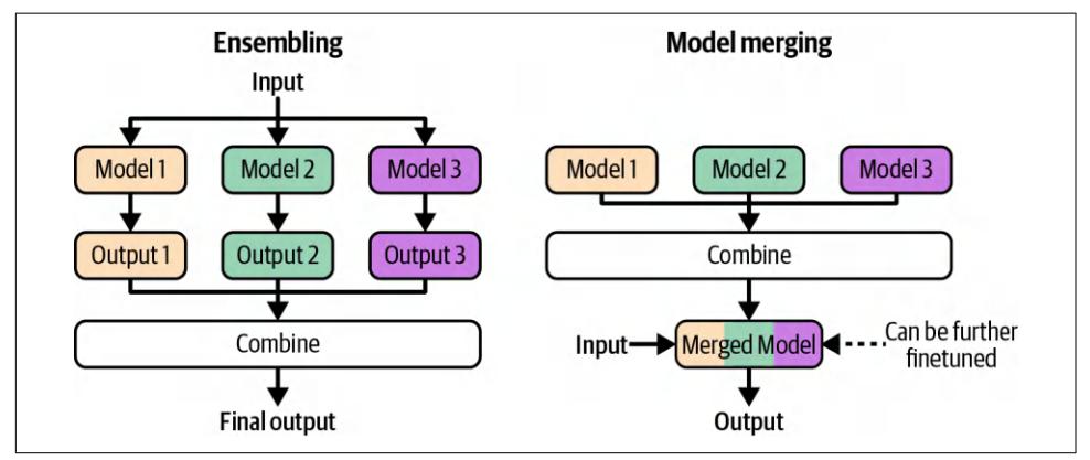
Figure 7-13. How ensembling and model merging work.

Many model-merging techniques are experimental and might become outdated as the community gains a better understanding of the underlying theory. For this rea‐ son, I’ll focus on the high-level merging approaches instead of any individual technique.

Model merging approaches differ in how the constituent parameters are combined. Three approaches covered here are summing, layer stacking, and concatenation. Figure 7-14 shows their high-level differences.

²⁹ You can read more about ensemble methods in my book Designing Machine Learning Systems.

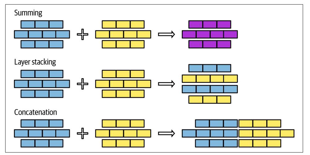
Figure 7-14. Three main approaches to model merging: summing, layer stacking, and concatenation.

You can mix these approaches when merging models, e.g., summing some layers and stacking others. Let’s explore each of these approaches.

Summing

This approach involves adding the weight values of constituent models together. I’ll discuss two summing methods: linear combination and spherical linear interpola‐ tion. If the parameters in two models are in different scales, e.g., one model’s parame‐ ter values are much larger than the other’s, you can rescale the models before summing so that their parameter values are in the same range.

Linear combination. Linear combination includes both an average and a weighted average. Given two models, A and B, their weighted average is:

Merge(A, B) = \[\frac{W_A A + W_B B}{W_A + W_B}\]

Figure 7-15 shows how to linearly combine two layers when w^A = w^B = 1.

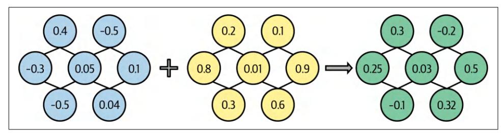
Figure 7-15. Merging parameters by averaging them.

Linear combination works surprisingly well, given how simple it is.³⁰ The idea that multiple models can be linearly combined to create a better one was studied as early as the early 1990s (Perrone, 1993). Linear combination is often used in federated learning (Wang et al., 2020).

You can linearly combine entire models or parts of models. Model soups (Wortsman et al., 2022) showed how averaging the entire weights of multiple finetuned models can improve accuracy without increasing inference time. However, it’s more com‐ mon to merge models by linearly combining specific components, such as their adapters.

While you can linearly combine any set of models, linear combination is the most effective for models finetuned on top of the same base model. In this case, linear combi‐ nation can be viewed through the concept of task vectors. The idea is that once you’ve finetuned a model for a specific task, subtracting the base model from it should give you a vector that captures the essence of the task. Task vectors are also called delta parameters. If you finetune using LoRA, you can construct the task vector from the LoRA weights.

Task vectors allow us to do task arithmetic (Ilharco et al., 2022), such as adding two task vectors to combine task capabilities or subtracting a task vector to reduce spe‐ cific capabilities. Task subtraction can be useful for removing undesirable model behaviors, such as invasive capabilities like facial recognition or biases obtained dur‐ ing pre-training.

Linear combination is straightforward when the components to be merged are of the same architecture and of the same size. However, it can also work for models that don’t share the same architecture or the same size. For example, if one model’s layer

³⁰ Averaging works not just with weights but also with embeddings. For example, given a sentence, you can use a word embedding algorithm to generate an embedding vector for each word in the sentence, then average all these word embeddings into a sentence embedding. When I started out in ML, I couldn’t believe that averag‐ ing seems to just work. It’s magical when simple components, when used correctly, can create something so wonderfully perplexing, like AI.

is larger than that of the other model, you can project one or both layers into the same dimension.

Some people proposed aligning models before averaging to ensure that functionally related parameters are averaged together, such as in “Model Fusion via Optimal Transport” (Singh and Jaggi, 2020), “Git Re-Basin: Merging Models Modulo Permu‐ tation Symmetries” (Ainsworth et al., 2022), and “Merging by Matching Models in Task Parameter Subspaces” (Tam et al., 2023). While it makes sense to combine aligned parameters, aligning parameters can be challenging to do, and, therefore, this approach is less common on naive linear combinations.

Spherical linear interpolation (SLERP). Another common model summing method is SLERP, which is based on the mathematical operator of the same name, Spherical LinEar inteRPolation.

Interpolation means estimating unknown values based on known values. In the case of model merging, the unknown value is the merged model, and the known values are the constituent models. Linear combination is one interpolation technique. SLERP is another.

Because the formula for SLERP is mathy, and model-merging tools typically imple‐ ment it for you, I won’t go into the details here. Intuitively, you can think of each component (vector) to be merged as a point on a sphere. To merge two vectors, you first draw the shortest path between these two points along the sphere’s surface. This is similar to drawing the shortest path between two cities along the Earth’s surface. The merged vector of these two vectors is a point along their shortest path. Where exactly the point falls along the path depends on the interpolation factor, which you can set to be between 0 and 1. Factor values less than 0.5 bring the merged vector closer to the first vector, which means that the first task vector will contribute more to the result. A factor of 0.5 means that you pick a point exactly halfway. This middle point is the blue point in Figure 7-16.

SLERP, as a mathematical operation, is defined with only two vectors, which means that you can merge only two vectors at a time. If you want to merge more than two vectors, you can potentially do SLERP sequentially, i.e., merging A with B, and then merging that result with C.

Figure 7-16. How SLERP works for two vectors t1 and t2. The red line is their shortest path on the spherical surface. Depending on the interpolation, the merged vector can be any point along this path. The blue vector is the resulting merged vector when the inter‐ polation factor is 0.5.

Pruning redundant task-specific parameters. During finetuning, many models’ parame‐ ters are adjusted. However, most of these adjustments are minor and don’t signifi‐ cantly contribute to the model’s performance on the task.³¹ Adjustments that don’t contribute to the model’s performance are considered redundant.

In the paper “TIES-Merging: Resolving Interference When Merging Models”, Yadav et al. (2023) showed that you can reset a large portion of task vector parameters with minimal performance degradation, as shown in Figure 7-17. Resetting means chang‐ ing the finetuned parameter to its original value in the base model, effectively setting the corresponding task vector parameter to zero. (Recall that the task vector can be obtained by subtracting the base model from the finetuned model.)

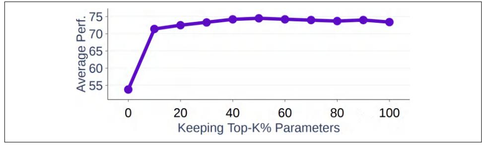
Figure 7-17. In Yadav et al.’s experiments, keeping the top 20% of the task vector parameters gives comparable performance to keeping 100% of the parameters.

³¹ The assumption is that the parameters that undergo the most substantial changes during finetuning are the ones most crucial for the target task.

These redundant parameters, while not harmful to one model, might be harmful to the merged model. Merging techniques such as TIES (Yadav et al., 2023) and DARE (Yu et al., 2023) first prune the redundant parameters from task vectors before merg‐ ing them.³² Both papers showed that this practice can significantly improve the qual‐ ity of the final merged models. The more models there are to merge, the more important pruning is because there are more opportunities for redundant parameters in one task to interfere with other tasks.³³

Layer stacking

In this approach, you take different layers from one or more models and stack them on top of each other. For example, you might take the first layer from model 1 and the second layer from model 2. This approach is also called passthrough or franken‐ merging. It can create models with unique architectures and numbers of parameters. Unlike the merging by summing approach, the merged models resulting from layer stacking typically require further finetuning to achieve good performance.

One early success of frankenmerging is Goliath-120B (alpindale, 2023), which was merged from two finetuned Llama 2-70B models, Xwin and Euryale. It took 72 out of 80 layers from each model and merged them together.

Layer stacking can be used to train mixture-of-experts (MoE) models, as introduced in ”Sparse Upcycling: Training Mixture-of-Experts from Dense Checkpoints” (Komatsuzaki et al., 2022). Rather than training an MOE from scratch, you take a pre-trained model and make multiple copies of certain layers or modules. A router is then added to send each input to the most suitable copy. You then further train the merged model along with the router to refine their performance. Figure 7-18 illus‐ trates this process.

Komatsuzaki et al. showed that layer stacking can produce models that outperform MoE models trained from scratch. Using this approach, Together AI mixed six weaker open source models together to create Mixture-of-Agents, which achieved comparable performance to OpenAI’s GPT-4o in some benchmarks (Wang et al., 2024).

³² TIES is abbreviated from “TrIm, Elect Sign, and merge,” while DARE is from “Drop And REscale.” I know, these abbreviations pain me too.

³³ When task vectors are pruned, they become more sparse, but the finetuned model doesn’t. Pruning, in this case, isn’t to reduce the memory footprint or inference latency, but to improve performance.

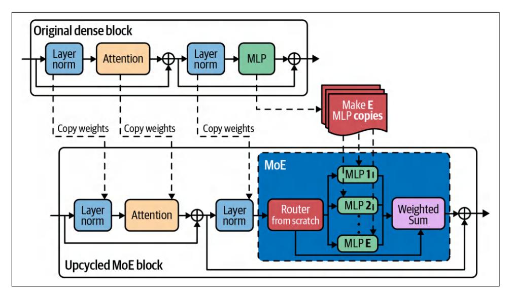
Figure 7-18. You can create an MoE model from a pre-trained model. Image adapted from Komatsuzaki et al. (2022).

An interesting use case of layer stacking is model upscaling. Model upscaling is the study of how to create larger models using fewer resources. Sometimes, you might want a bigger model than what you already have, presumably because bigger models give better performance. For example, your team might have originally trained a model to fit on your 40 GB GPU. However, you obtained a new machine with 80 GB, which allows you to serve a bigger model. Instead of training a new model from scratch, you can use layer stacking to create a larger model from the existing model.

One approach to layer upscaling is depthwise scaling. Kim et al. (2023) used this tech‐ nique to create SOLAR 10.7B from one 7B-parameter model with 32 layers. The pro‐ cedure works as follows:

1. Make a copy of the original pre-trained model.
1. Merge these two copies by summing certain layers (summing two layers and turning them into one layer) and stacking the rest. The layers to be summed are carefully selected to match the target model size. For SOLAR 10.7B, 16 layers are summed, leaving the final model with 32 × 2 - 16 = 48 layers.
1. Further train this upscaled model toward the target performance.

Figure 7-19 illustrates this process.

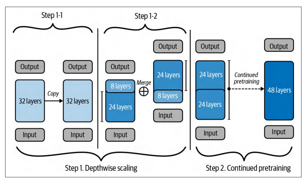
Figure 7-19. Use depthwise scaling to create a 48-layer model from a 32-layer model. The image is licensed under CC BY 4.0 and was slightly modified for readability.

Concatenation

Instead of adding the parameters of the constituent models together in different manners, you can also concatenate them. The merged component’s number of parameters will be the sum of the number of parameters from all constituent compo‐ nents. If you merge two LoRA adapters of ranks r¹ and r² , the merged adapter’s rank will be r¹ + r² , as shown in Figure 7-20.

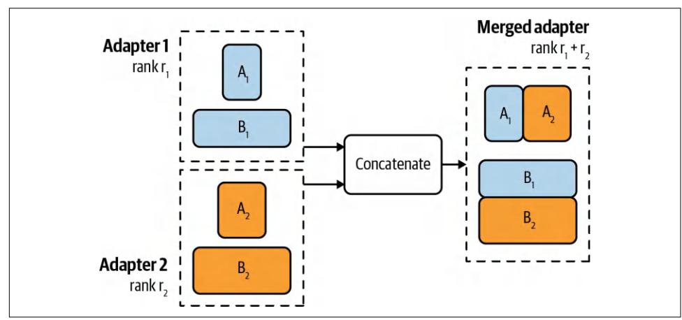
Figure 7-20. If you merge two LoRA adapters using concatenation, the rank of the merged adapter will be the sum of both adapters’ ranks.

Concatenation isn’t recommended because it doesn’t reduce the memory footprint compared to serving different models separately. Concatenation might give better performance, but the incremental performance might not be worth the number of extra parameters.³⁴

Finetuning Tactics

This chapter has discussed multiple finetuning approaches, what problems they solve, and how they work. In this last section, I’ll focus on more practical finetuning tactics.

Finetuning frameworks and base models

While many things around finetuning—deciding whether to finetune, acquiring data, and maintaining finetuned models—are hard, the actual process of finetuning is more straightforward. There are three things you need to choose: a base model, a finetuning method, and a framework for finetuning.

Base models. Chapter 4 already covered the criteria for model selection that can be applied to both prompt-based methods and finetuning. Some of the criteria discussed include model size, licenses, and benchmark performance. At the beginning of an AI project, when you’re still exploring the feasibility of your task, it’s useful to start with the most powerful model you can afford. If this model struggles to produce good results, weaker models are likely to perform even worse. If the strongest model meets your needs, you can then explore weaker models, using the initial model as a bench‐ mark for comparison.

For finetuning, the starting models vary for different projects. OpenAI’s finetuning best practices document gives examples of two development paths: the progression path and the distillation path.

The progression path looks like this:

1. Test your finetuning code using the cheapest and fastest model to make sure the code works as expected.³⁵
1. Test your data by finetuning a middling model. If the training loss doesn’t go down with more data, something might be wrong.

³⁴ I debated for a long time whether to include the concatenation technique in this book, and decided to include it for completeness.

³⁵ In college, I made the painful mistake of letting my model train overnight, only to have it crash after eight hours because I tried to save the checkpoint in a nonexistent folder. All that progress was lost.

3. Run a few more experiments with the best model to see how far you can push performance.
1. Once you have good results, do a training run with all models to map out the price/performance frontier and select the model that makes the most sense for your use case.

The distillation path might look as follows:

1. Start with a small dataset and the strongest model you can afford. Train the best possible model with this small dataset. Because the base model is already strong, it requires less data to achieve good performance.
1. Use this finetuned model to generate more training data.
1. Use this new dataset to train a cheaper model.

Because finetuning usually comes after experiments with prompt engineering, by the time you start to finetune, ideally, you should have a pretty good understanding of different models’ behaviors. You should plan your finetuning development path based on this understanding.

Finetuning methods. Recall that adapter techniques like LoRA are cost-effective but typically don’t deliver the same level of performance as full finetuning. If you’re just starting with finetuning, try something like LoRA, and attempt full finetuning later.

The finetuning methods to use also depend on your data volume. Depending on the base model and the task, full finetuning typically requires at least thousands of exam‐ ples and often many more. PEFT methods, however, can show good performance with a much smaller dataset. If you have a small dataset, such as a few hundred exam‐ ples, full finetuning might not outperform LoRA.

Take into account how many finetuned models you need and how you want to serve them when deciding on a finetuning method. Adapter-based methods like LoRA allow you to more efficiently serve multiple models that share the same base model. With LoRA, you only need to serve a single full model, whereas full finetuning requires serving multiple full models.

Finetuning frameworks. The easiest way to finetune is to use a finetuning API where you can upload data, select a base model, and get back a finetuned model. Like model inference APIs, finetuning APIs can be provided by model providers, cloud service providers, and third-party providers. A limitation of this approach is that you’re limi‐ ted to the base models that the API supports. Another limitation is that the API might not expose all the knobs you can use for optimal finetuning performance. Finetuning APIs are suitable for those who want something quick and easy, but they might be frustrating for those who want more customization.

You can also finetune using one of many great finetuning frameworks available, such as LLaMA-Factory, unsloth, PEFT, Axolotl, and LitGPT. They support a wide range of finetuning methods, especially adapter-based techniq ues. If you want to do full finetuning, many base models provide their open source training code on GitHub that you can clone and run with your own data. Llama Police has a more comprehen‐ sive and up-to-date list of finetuning frameworks and model repositories.

Doing your own finetuning gives you more flexibility, but you’ll have to provision the necessary compute. If you do only adapter-based techniques, a mid-tier GPU might suffice for most models. If you need more compute, you can choose a framework that integrates seamlessly with your cloud provider.

To finetune a model using more than one machine, you’ll need a framework that helps you do distributed training, such as DeepSpeed, PyTorch Distributed, and ColossalAI.

Finetuning hyperparameters

Depending on the base model and the finetuning method, there are many hyperpara‐ meters you can tune to improve finetuning efficiency. For specific hyperparameters for your use case, check out the documentation of the base model or the finetuning framework you use. Here, I’ll cover a few important hyperparameters that frequently appear.

Learning rate. The learning rate determines how fast the model’s parameters should change with each learning step. If you think of learning as finding a path toward a goal, the learning rate is the step size. If the step size is too small, it might take too long to get to the goal. If the step size is too big, you might overstep the goal, and, hence, the model might never converge.

A universal optimal learning rate doesn’t exist. You’ll have to experiment with differ‐ ent learning rates, typically between the range of 1e-7 to 1e-3, to see which one works best. A common practice is to take the learning rate at the end of the pre-training phase and multiply it with a constant between 0.1 and 1.

The loss curve can give you hints about the learning rate. If the loss curve fluctuates a lot, it’s likely that the learning rate is too big. If the loss curve is stable but takes a long time to decrease, the learning is likely too small. Increase the learning rate as high as the loss curve remains stable.

You can vary learning rates during the training process. You can use larger learning rates in the beginning and smaller learning rates near the end. Algorithms that determine how learning rates should change throughout the training process are called learning rate schedules.

Batch size. The batch size determines how many examples a model learns from in each step to update its weights. A batch size that is too small, such as fewer than eight, can lead to unstable training.³⁶ A larger batch size helps aggregate the signals from different examples, resulting in more stable and reliable updates.

In general, the larger the batch size, the faster the model can go through training examples. However, the larger the batch size, the more memory is needed to run your model. Thus, batch size is limited by the hardware you use.

This is where you see the cost versus efficiency trade-off. More expensive compute allows faster finetuning.

As of this writing, compute is still a bottleneck for finetuning. Often, models are so large, and memory is so constrained, that only small batch sizes can be used. This can lead to unstable model weight updates. To address this, instead of updating the model weights after each batch, you can accumulate gradients across several batches and update the model weights once enough reliable gradients are accumulated. This technique is called gradient accumulation. 37

When compute cost isn’t the most important factor, you can experiment with differ‐ ent batch sizes to see which gives the best model performance.

Number of epochs. An epoch is a pass over the training data. The number of epochs determines how many times each training example is trained on.

Small datasets may need more epochs than large datasets. For a dataset with millions of examples, 1–2 epochs might be sufficient. A dataset with thousands of examples might still see performance improvement after 4–10 epochs.

The difference between the training loss and the validation loss can give you hints about epochs. If both the training loss and the validation loss still steadily decrease, the model can benefit from more epochs (and more data). If the training loss still decreases but the validation loss increases, the model is overfitting to the training data, and you might try lowering the number of epochs.

³⁶ While it’s commonly acknowledged that small batch sizes lead to unstable training, I wasn’t able to find good explanations for why that’s the case. If you have references about this, please feel free to send them my way.

³⁷ I tried to find the first paper where gradient accumulation was introduced but couldn’t. Its use in deep learn‐ ing was mentioned as early as 2016 in “Ako: Decentralised Deep Learning with Partial Gradient Exchange” (Watcharapichat et al., Proceedings of the Seventh ACM Symposium on Cloud Computing, 2016). The concept seems to come from distributed training, where gradients computed on different machines need to be accu‐ mulated and used to update the model’s weights.

Prompt loss weight. For instruction finetuning, each example consists of a prompt and a response, both of which can contribute to the model’s loss during training. During inference, however, prompts are usually provided by users, and the model only needs to generate responses. Therefore, response tokens should contribute more to the model’s loss during training than prompt tokens.

The prompt model weight determines how much prompts should contribute to this loss compared to responses. If this weight is 100%, prompts contribute to the loss as much as responses, meaning that the model learns equally from both. If this weight is 0%, the model learns only from responses. Typically, this weight is set to 10% by default, meaning that the model should learn some from prompts but mostly from responses.

Summary

Outside of the evaluation chapters, finetuning has been the most challenging chapter to write. It touched on a wide range of concepts, both old (transfer learning) and new (PEFT), fundamental (low-rank factorization) and experimental (model merging), mathematical (memory calculation) and tactical (hyperparameter tuning). Arranging all these different aspects into a coherent structure while keeping them accessible was difficult.

The process of finetuning itself isn’t hard. Many finetuning frameworks handle the training process for you. These frameworks can even suggest common finetuning methods with sensible default hyperparameters.

However, the context surrounding finetuning is complex. It starts with whether you should even finetune a model. This chapter started with the reasons for finetuning and the reasons for not finetuning. It also discussed one question that I have been asked many times: when to finetune and when to do RAG.

In its early days, finetuning was similar to pre-training—both involved updating the model’s entire weights. However, as models increased in size, full finetuning became impractical for most practitioners. The more parameters to update during finetuning, the more memory finetuning needs. Most practitioners don’t have access to sufficient resources (hardware, time, and data) to do full finetuning with foundation models.

Many finetuning techniques have been developed with the same motivation: to achieve strong performance on a minimal memory footprint. For example, PEFT reduces finetuning’s memory requirements by reducing the number of trainable parameters. Quantized training, on the other hand, mitigates this memory bottleneck by reducing the number of bits needed to represent each value.

After giving an overview of PEFT, the chapter zoomed into LoRA—why and how it works. LoRA has many properties that make it popular among practitioners. On top

of being parameter-efficient and data-efficient, it’s also modular, making it much eas‐ ier to serve and combine multiple LoRA models.

The idea of combining finetuned models brought the chapter to model merging; its goal is to combine multiple models into one model that works better than these mod‐ els separately. This chapter discussed the many use cases of model merging, from ondevice deployment to model upscaling, and general approaches to model merging.

A comment I often hear from practitioners is that finetuning is easy, but getting data for finetuning is hard. Obtaining high-quality annotated data, especially instruction data, is challenging. The next chapter will dive into these challenges.

CHAPTER 8 Dataset Engineering

The quality of a model depends on the quality of its training data. The best ML team in the world with infinite compute can’t help you finetune a good model if you don’t have data. The goal of dataset engineering is to create a dataset that allows you to train the best model, ideally within your allocated budget.

As fewer companies can afford to develop models from scratch, more are turning to data to differentiate their AI performance. As models demand more data, data han‐ dling becomes more challenging and demands more investments in talent and infrastructure.¹

Data operations have evolved from side tasks that people handle when they have time to dedicated roles. Many AI companies now employ data labelers, dataset creators, and data quality engineers, either integrated into or working alongside their core engineering teams.

If the model landscape is confusing enough with numerous offerings, the data land‐ scape is even more complex, with an ever-growing array of datasets and techniques being introduced. This chapter gives you an overview of the data landscape and con‐ siderations to take into account when building your own dataset.

¹ The increasing importance of data is reflected in how data effort changed from GPT-3 to GPT-4. In the con‐ tribution list for GPT-3 (OpenAI, 2020), only two people were credited with data collecting, filtering, and deduplicating, and conducting overlap analysis on the training data. This dramatically changed three years later. For GPT-4 (OpenAI, 2023), eighty people were credited for being involved in different data processes. This list doesn’t yet include data annotators that OpenAI contracted through data providers. For something that sounds as simple as a ChatML format, eleven people were involved, and many of them are senior researchers. Back in their 2016 AMA (ask me anything) thread, Wojciech Zaremba, one of OpenAI’s cofounders, said that they intended to conduct most of their research using publicly available datasets.

It begins with data curation, addressing questions like What data do you need? How much? What does it mean for data to be of high quality? It then discusses techniques for data synthesis and processing. Data curation, generation, and processing don’t follow a linear path. You’ll likely have to go back and forth between different steps.

For the same model, different training phases aim to teach the model different capa‐ bilities, and, therefore, require datasets with different attributes. For example, data quantity for pre-training is often measured in the number of tokens, whereas data quantity for supervised finetuning is often measured in the number of examples. However, at a high level, their curation processes follow the same principle. This chapter focuses on post-training data because that’s more relevant to application developers. However, I’ll also include lessons from pre-training data when these les‐ sons are insightful for post-training.

There are best practices you can follow and tools that you can use to automate parts of the process. However, data will mostly just be toil, tears, and sweat.

A Data-Centric View of AI

The increasing focus on data during AI development has given rise to data-centric AI, as opposed to model-centric AI:

Model-centric AI tries to improve AI performance by enhancing the models themselves. This involves designing new architectures, increasing the sizes of the models, or developing new training techniques.
Data-centric AI tries to improve AI performance by enhancing the data. This involves developing new data processing techniques and creating high-quality datasets that allow better models to be trained with fewer resources.

In the early days of deep learning, many AI benchmarks were model-centric. Given a dataset like ImageNet, people try to train the best possible model using the same data‐ set. In recent years, more benchmarks have become data-centric. Given the same model, people try to develop a dataset that gives this model the best performance.

In 2021, Andrew Ng launched a data-centric AI competition where participants needed to improve upon the same base dataset by applying techniques such as fixing incorrect labels, adding edge case examples, augmenting data, etc.

In 2023, DataComp (Gadre et al., 2023) hosted a competition whose goal was to cre‐ ate the best dataset for training a CLIP model (Radford et al., 2021). A standardized script trains a CLIP model on each submitted dataset. The quality of a dataset is eval‐ uated based on its resulting model’s performance on 38 downstream tasks. In 2024, they hosted a similar competition to evaluate datasets for language models with scales from 412M to 7B parameters (Li et al., 2024). Other similar data-centric benchmarks include DataPerf (MLCommons, 2023) and dcbench (Eyuboglu and Karlaš, 2022).

The model-centric and data-centric division helps guide research. In reality, however, meaningful technological progress often requires investment in both model and data improvements.

Data Curation

While not all issues with AI models can be solved with data, data is often a key part of the solution. The right data can make the model more capable, safer, and able to han‐ dle longer contexts. Conversely, poor data can cause the model to increase biases and hallucinations. Mistakes in data can harm the model and waste resources.

Data curation is a science that requires understanding how the model learns and what resources are available to help it learn. Dataset builders should work closely with application and model developers. In a small team, they might be the same person—the person responsible for training a model is also responsible for acquiring the data for it. However, organizations with high data demands often employ special‐ ized roles.²

What data you need depends on your task and what you want to teach the model. For self-supervised finetuning, you need sequences of data. For instruction finetuning, you need data in the (instruction, response) format. For preference finetuning, you need data in the (instruction, winning response, losing response) format. To train a reward model, you can use the same data format as preference finetuning or use data with annotated scores for each of your examples in the ((instruction, response), score) format.

Training data should exhibit the behaviors you want your model to learn. Acquiring high-quality data annotations is always challenging, but it’s even more challenging if you want to teach models complex behaviors such as chain-of-thought (CoT) reason‐ ing and tool use. Let’s go over these two examples to understand why:

Chain-of-thought

As discussed in Chapter 5, CoT prompting nudges the model to work through a problem step-by-step before producing the final answer. To teach a model to generate step-by-step responses, its training data should include CoT responses. “Scaling Instruction-Finetuned Language Models” (Chun et al., 2024) shows that incorporating step-by-step responses in the finetuning data greatly enhances the performance of models of various sizes on CoT tasks, with accuracy nearly dou‐ bling for certain tasks.

² If you use a lot of data, ensuring data compliance alone can be a full-time job.

Generating multi-step responses can be tedious and time-consuming—explain‐ ing how to solve a math problem step-by-step is much more challenging than simply giving the final answer. To illustrate this, here are two examples, one with only the final answer and one with CoT. Both are from Chun et al. (2024):

Instruction: Please answer the following question. What is the boil ing point of Nitrogen? Response (without CoT): -320.4F

CoT instruction: Answer the following question by reasoning step-bystep. The cafeteria had 23 apples. If they used 20 for lunch and bought 6 more, how many apples do they have?

Response (with CoT): The cafeteria had 23 apples originally. They used 20 to make lunch. So they had 23 - 20 = 3. They bought 6 more apples, so they have 3 + 6 = 9.

As a result, CoT datasets are less common compared to other instruction datasets.

Tool use

Given the vast amount of knowledge a model acquires during pre-training, many models might intuitively know how to use certain tools. However, a model’s tool use ability can be improved by showing it tool use examples. It’s common to use domain experts to create tool use data, where each prompt is a task that requires tool use, and its response is the actions needed to perform that task. For example, if you want data to finetune a model to act as a personal assistant, you might want to ask professional personal assistants what types of tasks they usually per‐ form, how they perform them, and what tools they need. If you ask human experts to explain how they do things, they might miss certain steps, either because of faulty memory or because they might think these steps aren’t impor‐ tant. It’s often necessary to observe how humans perform these tasks to ensure accuracy.

However, what’s efficient for humans might not be efficient for AI, and vice versa. As a result, human annotations might not be ideal for AI agents. For example, a human might prefer a web interface, whereas it’s easier for a model to use an API. To search for something, a human might first open a browser, copy and paste that query into the search bar, and click on each result. Meanwhile, a model can just send a request to the search API with the query and process all the results at once. For this reason, many rely on simulations and other synthetic techniques to generate tool use data, as explored later in this chapter.

Tool use data might also require special formats. In typical conversation data, the user and AI take turns, with each turn containing one message. However, for tool use, the AI might need to generate multiple messages each turn, with each mes‐ sage sent to a different location. For example, it might send one message to the code interpreter and one message to the user (such as to inform the user what it’s doing). To support this, Llama 3 authors (Dubey et al., 2024) designed a multimessage chat format that consists of message headers that specify the source and destination of each message, and special termination tokens to specify where the human and AI turns start.

When curating data for applications with conversation interfaces, you need to con‐ sider whether you require single-turn data, multi-turn data, or both. Single-turn data helps train a model to respond to individual instructions. Multi-turn data, on the other hand, teaches the model how to solve tasks—many real-world tasks involve back-and-forth. For instance, when given a query, a model may need to first clarify the user’s intent before addressing the task. After the model’s response, the user might provide corrections or additional information for the next step.

Single-turn data is simpler and, therefore, easier to obtain. Multi-turn data often requires purpose-built scenarios or more involved interactions to capture.

Data curation isn’t just about creating new data to help a model learn new behaviors but is also about removing existing data to help a model unlearn bad behaviors. Imagine you work on a chatbot like ChatGPT and you hear user complaints that the chatbot is a bit arrogant, annoying users and wasting their tokens. For example, when a user asks it to verify if a statement is factually correct, the chatbot responds with: “The statement is correct, but its style can be improved to be better.” It then contin‐ ues to produce an unsolicited rewriting of the statement.

You investigate and find that in the training data, there are several examples of anno‐ tations with unsolicited suggestions. You put in a request to remove these examples from the training data and another request to acquire new examples that demonstrate fact-checking without unsolicited rewriting.

Each application might require data of different characteristics. Different training phases also require different data mixes. At a high level, however, data curation fol‐ lows the three criteria: data quality, data coverage, and data quantity.

To give an intuition about these terms, if you think of model training as cooking, the data fed into the model is the ingredients. Data quality is equivalent to the quality of the ingredients—you can’t have good food if your ingredients are spoiled. Data cov‐ erage is equivalent to having the right mix of ingredients (e.g., you shouldn’t have too much or too little sugar). Data quantity is about how many ingredients you should have. Let’s explore these terms in detail.

Data Quality

A small amount of high-quality data can outperform a large amount of noisy data, e.g., data that is irrelevant or inconsistent. The creators of the Yi model family found that 10K carefully crafted instructions are superior to hundreds of thousands of noisy instructions (Young et al., 2024).

Similarly, “LIMA: Less Is More for Alignment” (Zhou et al., 2023) shows that a 65Bparameter Llama model, finetuned with 1,000 carefully curated prompts and respon‐ ses, can produce answers that are either equivalent or strictly preferred to GPT-4 in 43% of cases, as judged by human annotators. However, the downside of having too few data examples is that LIMA is not as robust as product-grade models.

The Llama 3 team also arrived at the same conclusion. Notably, they found that human-generated data is more prone to errors and inconsistencies, particularly for nuanced safety policies. This led them to develop AI-assisted annotation tools to ensure high data quality.

Most people understand the importance of data quality, but what does it mean for data to be high-quality? The short answer is that data is considered high-quality if it helps you do your job efficiently and reliably. The long answers, however, differ for different people.³ In general, data can be considered high-quality if it has the follow‐ ing six characteristics: relevant, aligned with task requirements, consistent, correctly formatted, unique, and compliant. Some specific use cases might have other require‐ ments:

Relevant

The training examples should be relevant to the task you’re training the model to do. For example, if the task is to answer legal questions today, a legal dataset from the 19th century might not be relevant. However, if the task is about the legal system in the 19th century, this dataset is highly relevant.

Aligned with task requirements

The annotations should align with the task’s requirements. For example, if the task requires factual consistency, the annotations should be factually correct. If the task requires creativity, the annotations should be creative. If the task demands not just a score but also a justification for that score, the annotations should include both scores and justifications. But if the task demands concise answers, the annotations should be concise.

³ While I love writing, one of the things I absolutely do not enjoy is trying to condense everyone’s opinions into one single definition. IBM defined data quality along seven dimensions: completeness, uniqueness, validity, timeliness, accuracy, consistency, and fitness for purpose. Wikipedia added accessibility, comparability, credi‐ bility, flexibility, and plausibility. Many of these definitions focus on data quality in a broad range of use cases. Here, I want to focus on data quality for finetuning.

I used “aligned” instead of “accurate” or “correct” because, depending on the task, an accurate or correct response might not be what a user wants.

Consistent

Annotations should be consistent across examples and annotators. If you ask two annotators to annotate the same example, their annotations shouldn’t be too dif‐ ferent. If the task is to score essays from 1 to 5, would two essays with the same score be of the same quality? Inconsistent annotations can confuse the model, making it harder for the model to learn.

Having a good annotation guideline is essential for having annotations that are both aligned with task requirements and consistent.

Correctly formatted

All examples should follow the format expected by the model. Redundant for‐ matting tokens can interfere with the model’s learning, and, therefore, they should be removed. For example, if you scrape product reviews from a website, you should remove HTML tags. Beware of trailing white spaces, new lines, inconsistent casing, and numerical formats.⁴

Sufficiently unique

This refers to unique examples in your data.⁵ In the context of model training, duplications can introduce biases and cause data contamination. I use “suffi‐ ciently unique” because specific use cases can tolerate different levels of duplica‐ tions.

Compliant

Data should be compliant with all relevant internal and external policies (includ‐ ing laws and regulations). For example, if you’re not allowed to use PII data to train your models, your data shouldn’t contain any PII data.

Before setting out to create data, it’s important to think about what each of these characteristics means for you. The techniques discussed in this section aim to pro‐ duce data with these characteristics.

Data Coverage

A model’s training data should cover the range of problems you expect it to solve. Real-world users often have a wide range of problems, and the way they express those problems can vary significantly. Having data that captures the diverse usage patterns

⁴ One painful bug I still remember is when a float column in my data was wrongly stored as integers, which round these values, leading to perplexing behaviors.

⁵ While this doesn’t refer to the uniqueness of your data, having data that nobody else has can be extremely valuable.

of your application is key for the model to perform well. Coverage requires sufficient data diversity, which is why many refer to this attribute as data diversity.

For example, if some users construct detailed instructions with abundant references while some other users prefer short instructions, your finetuning data should include both detailed and short instructions. If user queries typically have typos, you should include examples with typos. If your application works with multiple programming languages, your training data should include the programming languages your users care about.

Different applications have different dimensions of diversity. For example, a Frenchto-English tool doesn’t need language diversity but might benefit from diversity in topics, lengths, and speaking styles. On the other hand, a chatbot that recommends products to global customers doesn’t necessarily need domain diversity, but linguistic and cultural diversity will be important.

For general-purpose use cases like chatbots, the finetuning data should be diverse, representing a wide range of topics and speaking patterns. Ding et al., (2023) believe that the most straightforward way to further improve the performance of chat lan‐ guage models is to increase the quality and diversity of data employed in the training process. To develop Nemotron (Adler et al., 2024), NVIDIA researchers focused on creating a dataset with task diversity, topic diversity, and instruction diversity, which includes instructions for different output formats, instructions with different output lengths, and instructions for open-ended answers as well as yes-or-no answers. “The Data Addition Dilemma” (Shen et al., 2024) demonstrated that in some cases, adding more heterogeneous data can lead to worse performance.

Meta shared that Llama 3 doesn’t deviate significantly from older Llama versions in terms of model architecture. Llama 3’s performance gains are “primarily driven by improvements in data quality and diversity as well as by increased training scale.” The Llama 3 paper has rich details on data coverage through all three phases of train‐ ing: pre-training, supervised finetuning, and preference finetuning. While this chap‐ ter focuses on post-training data, it’s useful to look at the data mix for the same model across all different training phases to compare and highlight the considera‐ tions for each phase.

A diversity axis that is consistent in all three phases is domain diversity, though what exactly diverse means differs, as shown in Table 8-1. This table shows only high-level domains and doesn’t include finer-grained topics, like “geometry”, which is a subcategory in math. Post-training data also has different diversity axes not shown in the table, such as the number of tokens (both for context and response) and the number of turns. Llama 3 uses synthetic data for post-training, so another dimension is the ratio of human-generated data to AI-generated data.

	Pre-training	Supervised finetuning Preference finetuning
General knowledge (English)	50%	52.66%	81.99%
Math and reasoning	25%	21.19%	5.89%
Coding	17%	14.89%	6.93%
Multilingual	8%	3.01%	5.19%
Fxam-like	X	8.14%	X
Long context	X	0.11%	X

Table 8-1. For Llama 3, different training phases have different optimal domain mixes.

It’s interesting to note that during pre-training and supervised finetuning, the num‐ ber of combined math, reasoning, and code tokens accounts for almost half of the training data. While I don’t know exactly what percentage of the internet data is math and code, I believe that it’s far below 50%. Llama 3 authors shared that annealing the model on small amounts of high-quality code and math data (training the model using an increasingly smaller learning rate with increasingly more code and math data) can boost the performance of their models on key benchmarks. This confirms a common belief that high-quality code and math data is more effective than natural language text in boosting the model’s reasoning capabilities.

The percentage of code and math data during preference finetuning is much smaller (12.82% combined), likely because the goal is to reflect the real distribution of user preferences.

This brings up a question: How do we decide on the right data mix? A simple approach is to choose a data mix that accurately reflects the real-world application usage. You can also use experiments to find optimal data mixes. For example, Meta performed scaling law experiments similar to what is discussed in “Scaling extrapola‐ tion” on page 74. For each candidate data mix, they trained several small models on a data mix and used that to predict the performance of a large model on that mix. The final model mix is the best-guess mix derived from the experiment results.

To evaluate the impact of data diversity and quality, Zhou et al. (2023) carried out an interesting experiment where they trained a 7B-parameter language model on three datasets of the same size—2,000 examples—but with different characteristics. The first is high-quality but not diverse. The second is diverse but low-quality. The third is both diverse and high-quality. Figure 8-1 shows the generation quality of the three resulting models.

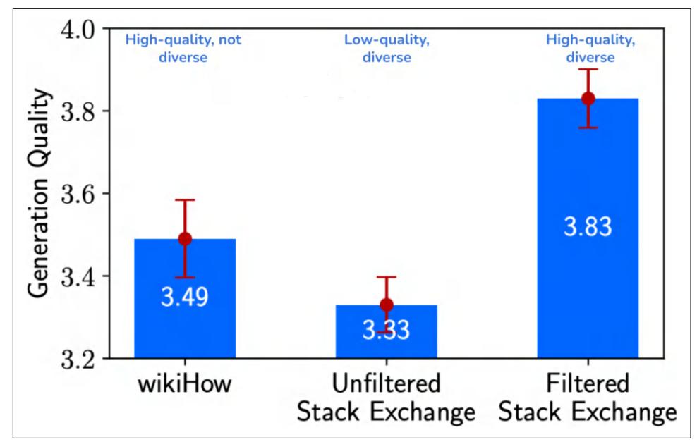
Figure 8-1. A 7B-parameter model, finetuned on a dataset that is both high-quality and diverse, outperforms that same model finetuned on a dataset that is either diverse or high-quality. Image from Zhou et al. (2023). The image is licensed under CC BY 4.0.

Data Quantity

Asking how much data you need is like asking how much money you need. The answer varies widely from one situation to the next. At one extreme, Jeremy Howard and Jonathan Whitaker did a fun experiment to show that LLMs can learn from a single example. At another extreme, some teams have finetuned models with millions of examples.

While millions of examples sounds like a lot, it’s small compared to the data typically needed to train a foundation model from scratch. For reference, Llama 2 and Llama 3 were trained using 2 trillion and 16 trillion tokens, respectively. If each example is 2,000 tokens, it’d be equivalent to 1 billion and 15 billion examples.

You might wonder: if I have millions of examples, shouldn’t I just train a model from scratch? You can and should evaluate whether training a model from scratch would improve your performance. While finetuning on top of a pre-trained model is typically more efficient than training from scratch, there are situations when fine‐ tuning can be worse, especially when you have a lot of training data. This is due to a phenomenon called ossification, where pretraining can ossify (i.e., freeze) the model weights so that they don’t adapt as well to the finetuning data (Hernandez et al., 2021). Smaller models are more susceptible to ossification than larger models.

Other than data quality and data diversity, three other factors influence how much data you need:

Finetuning techniques

Full finetuning promises to give the best performance, but it requires orders of magnitude more data than PEFT methods like LoRA. If you have tens of thou‐ sands to millions of (instruction, response) pairs, you might want to attempt full finetuning. If you have only a few hundred or a few thousand examples, PEFT might work best.

Task complexity

A simple task, such as classifying whether a product review is positive or nega‐ tive, will require much less data than a complex task, such as a question answer‐ ing about financial filings.

Base model’s performance

The closer the base model is to the desirable performance, the fewer examples are needed to get there. Assuming that bigger base models are better, you might need fewer examples to finetune big models. This is the opposite of pre-training, where bigger models need more training data.

OpenAI’s finetuning guide shows that if you have fewer examples (100), more advanced models give you better finetuning performance. This is likely because the more advanced models already perform better out of the box. However, after finetun‐ ing on a lot of examples (550,000), all five models in the experiment performed simi‐ larly, as illustrated in Figure 8-2.

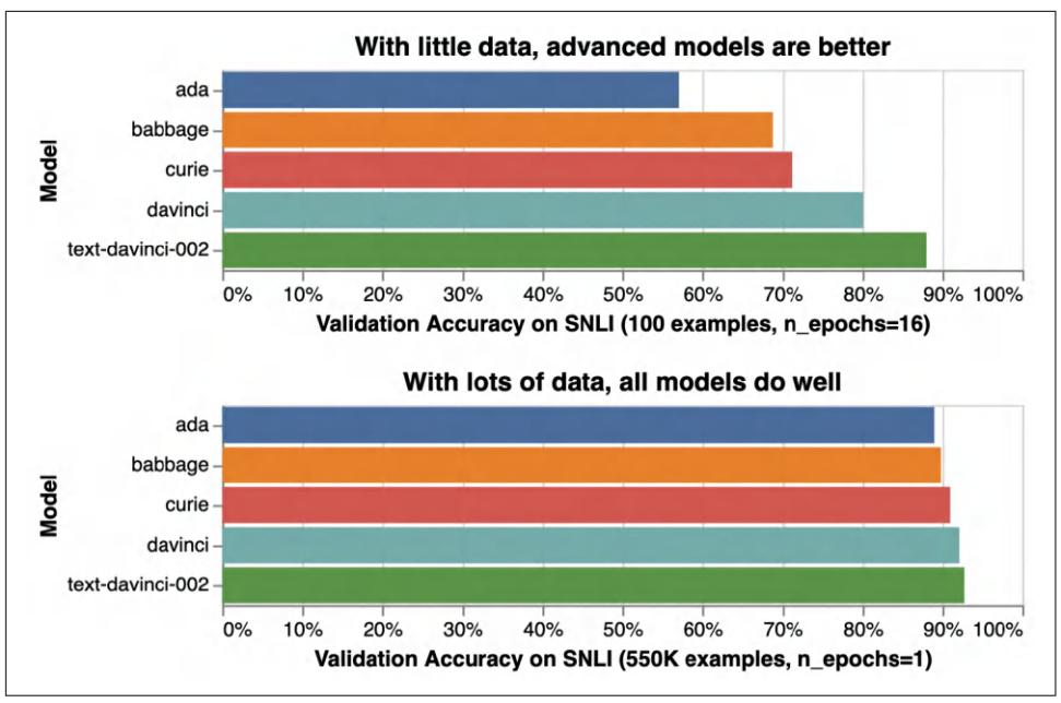
Figure 8-2. With 100 examples, more advanced models give much better performance after finetuning. With 550,000 examples, all models give similar performance after finetuning. Experiments done by Stanford Natural Language Inference (SNLI) Corpus.

In short, if you have a small amount of data, you might want to use PEFT methods on more advanced models. If you have a large amount of data, use full finetuning with smaller models.

Before investing in curating a large dataset, you might want to start with a small, well-crafted dataset (e.g., 50 examples) to see if finetuning can improve the model. If this small dataset is sufficient to achieve your desirable performance, that’s great. Clear improvements suggest that more data will improve the performance even more. If no improvement is observed with small data, a bigger dataset will rarely do the trick.

However, be careful before concluding that finetuning with a small dataset doesn’t improve a model. Many things, other than data, can impact finetuning’s results, such as the choice of hyperparameters (e.g., the learning rate is too high or too low), data quality, poorly crafted prompts, etc. In the vast majority of cases, you should see improvements after finetuning with 50–100 examples.

It’s possible to reduce the amount of high-quality data needed by first finetuning your model using lower-quality or less-relevant data. Here are three examples of this approach:

Self-supervised → supervised

You want to finetune a model to answer legal questions. Your (question, answer) set is small, but you have many legal docu‐ ments. You can first finetune your model on legal documents in a self-supervised manner, then further finetune the model on (question, answer) pairs.

Less-relevant data → relevant data

You want to finetune a model to classify sentiments for prod‐ uct reviews, but you have little product sentiment data and much more tweet sentiment data. You can first finetune your model to classify tweet sentiments, then further finetune it to classify product sentiments.

Synthetic data → real data

You want to finetune a model to predict medical conditions from medical reports. Due to the sensitive nature of this task, your data is limited. You can use AI models to synthesize a large amount of data to finetune your model first, then further finetune it on your real data. This approach is harder to get right, as you’ll have to do two distinct finetuning jobs while coordinating the transitioning between them. If you don’t know what you’re doing, you might end up using more com‐ pute just to produce a model worse than what you would’ve gotten by just finetuning with high-quality data.⁶

Experimenting with a small dataset can help you estimate how much more data you’ll need. You can finetune a model on subsets of your current dataset—e.g., 25%, 50%, 100%—and plot how performance scales with dataset size. A steep performance gain slope with increasing dataset size means that you can expect significant performance improvement by doubling your data. A plateau slope means that doubling your data will give only a small improvement. Figure 8-3 shows an example of this plot.

⁶ In Designing Machine Learning Systems, I also covered other techniques to reduce the demand for annotated data, including weak supervision, semi-supervision, and active learning.

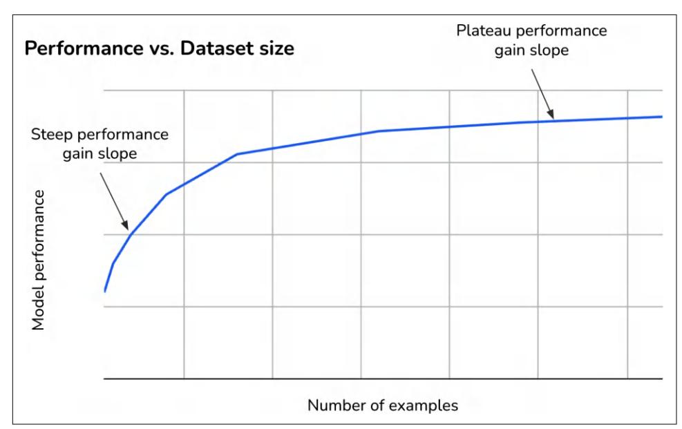
Figure 8-3. The performance gain curve with different dataset sizes can help you esti‐ mate the impact of additional training examples on your model’s performance.

The performance gain curve shown in Figure 8-3 is fairly typical. In most cases, addi‐ tional training examples yield diminishing returns: the same number of examples typically gives a lower performance boost as the dataset grows. For example, the first 1,000 examples might improve a model’s accuracy by ten percentage points, but the next 1,000 examples might only improve it by five.

While a larger number of finetuning examples generally improves a model’s perfor‐ mance, the diversity of the examples matters, too. The paper “Scaling Instruction-Finetuned Language Models” (Chung et al., 2022) shows that model performance increased significantly when the number of finetuning tasks increased from 9 to 282. Beyond 282 tasks, the performance gains started to plateau, though there were still positive but incremental improvements up to 1,836 tasks, as shown in Figure 8-4. This suggests that the model benefits greatly from exposure to a diverse set of tasks during finetuning.

The diversity of data can be reflected in task types (such as summarization and ques‐ tion answering), topic diversity (such as fashion, finance, and technology), and the expected output formats (such as JSON outputs or yes-or-no answers).

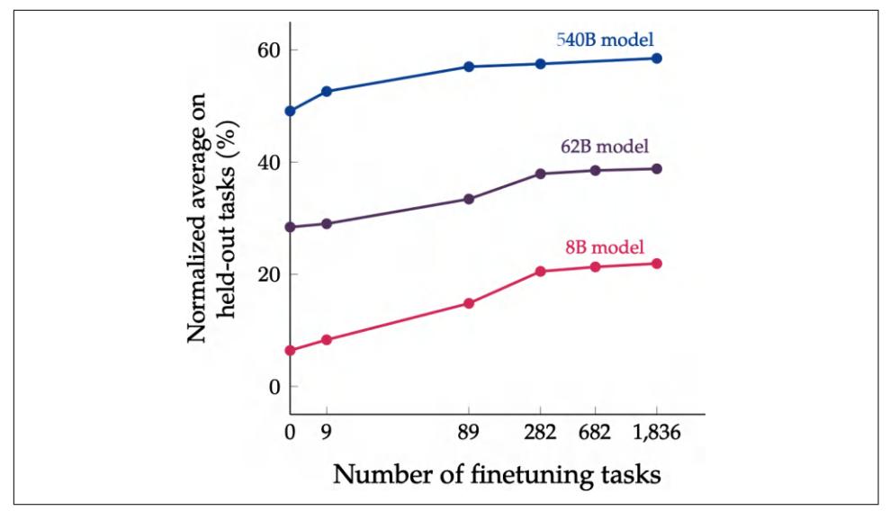
Figure 8-4. Diversity in finetuning number, measured by the number of tasks, can impact model performance. Image from “Scaling Instruction-Finetuned Language Models” (Chung et al., 2022). The image is licensed under CC BY 4.0.

How much data to use for finetuning is determined not just by what you need but also by what you can afford. If you budget $10,000 for data annotation and each example costs $2 to annotate, you can have at most 5,000 examples. You might also need to balance the budget for data and compute. Spending more money on data leaves you less money for compute, and vice versa.

Data Acquisition and Annotation

The goal of data acquisition is to produce a sufficiently large dataset with the quality and diversity you need, while ensuring that your data practices respect user privacy and comply with regulations. Data acquisition involves gathering data through meth‐ ods such as sourcing public data, purchasing proprietary data, annotating data, and synthesizing data. There’s a niche but growing field of research in data acquisition strategy: how to best acquire a dataset that meets specific requirements given a budget.

The most important source of data, however, is typically data from your own applica‐ tion. If you can figure out a way to create a data flywheel that leverages data generated by your users to continually improve your product, you will gain a significant

advantage.⁷ Application data is ideal because it’s perfectly relevant and aligned with your task. In other words, it matches the distribution of the data that you care about, which is incredibly hard to achieve with other data sources. User-generated data can be user content, system-generated data from user usage, or user feedback. How to design your user feedback system is discussed in Chapter 10.

Before investing in creating your own data, check available datasets first. Data mar‐ ketplaces are vast and offer both open source and proprietary data. If you’re lucky, some of them might be exactly what you need. However, it’s often a mix-and-match approach. A dataset can be developed from multiple data sources via multiple acquis‐ ition channels. For example, the process of creating an (instruction, response) dataset might look as follows:

1. Find available datasets with the desirable characteristics. You might find one promising dataset with 10,000 examples.
1. Remove low-quality instructions. Let’s say this leaves you with 9,000 examples.
1. Set aside the instructions with low-quality responses. Let’s say you find 3,000 such examples. This leaves you with 6,000 examples of high-quality instructions and high-quality responses.
1. Manually write responses for the 3,000 high-quality instructions. Now your data‐ set has a total of 9,000 high-quality examples.
1. Realizing that there’s not enough data for topic X, manually create a set of 100 instruction templates about X. Use an AI model to synthesize 2,000 instructions using these 10 templates.
1. Manually annotate these 2,000 synthetic instructions. Now your dataset has a total of 11,000 examples.

This is, of course, an oversimplification of the actual dataset curation process, with the vast majority of steps hidden to conserve paper and save readers from tedium. For example, there might be several steps in which you realize that many of the anno‐ tations aren’t helpful, so you have to update the annotation guidelines and reannotate your data. Worse, you might find that some of them are factually incorrect, so you have to hire another set of annotators to fact-check your original annotations. Or you might find that having 100 synthetic instructions per template hurts your data’s diversity, so you have to create more templates and generate fewer instructions per template. And so on.

⁷ I’ve heard so many companies talking about data flywheels in their pitches that I’m convinced it isn’t legal to start an AI startup without mentioning the data flywheel.

Resources for Publicly Available D atasets

Here are a few resources where you can look for publicly available datasets. While you should take advantage of available data, you should never fully trust it. Data needs to be thoroughly inspected and validated.

Always check a dataset’s license before using it. Try your best to understand where the data comes from. Even if a dataset has a license that allows commercial use, it’s possible that part of it comes from a source that doesn’t:

1. Hugging Face and Kaggle each host hundreds of thousands of datasets.
1. Google has a wonderful and underrated Dataset Search.
1. Governments are often great providers of open data. Data.gov hosts hundreds of thousands of datasets, and data.gov.in hosts tens of thousands.
1. University of Michigan’s Institute for Social Research ICPSR has data from tens of thousands of social studies.
1. UC Irvine’s Machine Learning Repository and OpenML are two older dataset repositories, each hosting several thousand datasets.
1. The Open Data Network lets you search among tens of thousands of datasets.
1. Cloud service providers often host a small collection of open datasets; the most notable one is AWS’s Open Data.
1. ML frameworks often have small pre-built datasets that you can load while using the framework, such as TensorFlow datasets.
1. Some evaluation harness tools host evaluation benchmark datasets that are suffi‐ ciently large for PEFT finetuning. For example, Eleuther AI’s lm-evaluationharness hosts 400+ benchmark datasets, averaging 2,000+ examples per dataset.
1. The Stanford Large Network Dataset Collection is a great repository for graph datasets.

Often, you might need to annotate your own data for finetuning. Annotation is chal‐ lenging not just because of the annotation process but also due to the complexity of creating clear annotation guidelines. For example, you need to explicitly state what a good response looks like, and what makes it good. Can a response be correct but unhelpful? What’s the difference between responses that deserve a score of 3 and 4? Annotation guidelines are needed for both manual and AI-powered annotations.

Some teams, including LinkedIn, have reported that annotation guidelines were among the most challenging parts of their AI engineering pipeline. It’s alarming how often people abandon careful annotation halfway due to the time and effort required, hoping instead that their models will figure out the right responses on their own. Many models are strong enough that they can occasionally succeed, but relying on models to figure that out might be too risky for many applications.

The good news is that these guidelines are the same as those for evaluation data, as discussed in Chapter 4. This is another argument for why you should invest more time in curating evaluation guidelines and data. If you’re lucky, your evaluation examples can be augmented or used as seed examples to synthesize new data. In the next section we’ll discuss how to do so.

Data Augmentation and Synthesis

Together with compute and talent, data is the hardest challenge of AI. It’s been a long-term goal of the whole industry to be able to generate data programmatically. Two processes commonly used are data augmentation and data synthesis:

Data augmentation creates new data from existing data (which is real). For example, given a real image of a cat, you can flip it to create a new image of the same cat.⁸
Data synthesis generates data to mimic the properties of real data. For example, you can simulate how a mouse moves through a web page to generate data for what bot movements would look like.

In other words, augmented data is derived from real data, whereas synthetic data isn’t real. However, since the goal of both augmentation and synthesis is to automate data creation, sometimes the two terms are used interchangeably. In this chapter, I’ll often use data synthesis to refer to both.

Artificially generated data has a long history in software engineering. It was originally used to generate fake data for testing purposes. For example, libraries like Faker and Chance let you generate data in simple formats such as names, addresses, phone numbers, and email addresses for testing. Let’s say you’ve built a program to parse shipping addresses. You can use fake data generators to generate addresses in differ‐ ent countries and states with different formats to make sure your program can parse all of them.

With AI being capable of generating data indistinguishable from that generated by humans, it’s possible to synthesize much more sophisticated data, such as doctor’s

⁸ My book, Designing Machine Learning Systems, discusses data augmentation in Chapter 4.

notes, contracts, financial statements, product descriptions, images, video commer‐ cials, etc. This makes it easier to generate data and enables more synthetic data use cases.

While synthetic data promises to significantly reduce the pressure for humangenerated data, synthetic data doesn’t completely replace human data. In many use cases, as discussed in “Limitations to AI-generated data” on page 393, mixing humanand AI-generated data often produces the best value.

Why Data Synthesis

Synthetic data is appealing for many reasons. You can synthesize data to improve the golden data trio: quantity, coverage, and quality. You can also synthesize data to miti‐ gate privacy concerns and distill models:

To increase data quantity

The biggest reason for data synthesis is that it allows you to produce data at scale, promising an abundant supply of data for training and testing AI models. More data, in theory, helps models generalize to a wider range of tasks. This is espe‐ cially helpful where real-world data is scarce or difficult to obtain, such as data for rare weather conditions, data for deep sea exploration, or data involving acci‐ dents for self-driving cars.

To increase data coverage

You can generate data with targeted characteristics to improve model perfor‐ mance or to get a model to express specific behaviors. For example, you can gen‐ erate very short texts or very long texts. You can create conversations that contain toxic phrases for a toxic detection model. Vice versa, if real-world data is toxic, you can synthesize safe data. It’s especially common to use AI to synthesize adversarial examples. It’s also possible to generate data for the rare class to address the challenges of class imbalance. As described in “TrueTeacher”, Gekh‐ man et al. (2022) used LLMs to generate factually inconsistent summaries that they then used to train models to detect factual inconsistency.

In their paper, “Discovering Language Model Behaviors with Model-Written Evaluations” (Perez et al., 2022), Anthropic discussed various data synthesis techniques to generate specific datasets that can test 154 different AI behaviors, including personality traits, political views, ethical stances, and social biases. They found that in head-to-head comparisons between LM (language model) generated and human-generated datasets, “LM-written datasets approach the quality of human-written ones, sometimes even exceeding them.”

In other words, you can use synthetic data to increase data coverage: generate targeted data to cover the areas where existing data is insufficient.

To increase data quality

Even though the common perception is that synthetic data is often of lower qual‐ ity than human-generated data, sometimes, the reverse can be true. Sometimes, humans might have fundamental limitations that cause human-generated data to be of lower quality than AI-generated data. One example is tool use data dis‐ cussed earlier—humans and AI have fundamentally different modes of opera‐ tions and tool preferences. Another example is in generating complex math problems—AI can generate questions that are far more complex than what an average human expert might conceive.⁹

Some teams also prefer using AI to generate preference data. While each individ‐ ual human can be somewhat consistent in their preference, performance across different people tends to vary significantly, influenced not only by each person’s preference but also by mood and motivations. AI-generated preference ratings, in contrast, can be far more consistent and reliable.

To mitigate privacy concerns

Synthetic data is often the only option for use cases where you can’t use humangenerated data due to privacy concerns. For instance, in healthcare, where legis‐ lation makes it hard, if not impossible, to use real patient records to train a model, you can generate synthetic patient records that do not contain any sensi‐ tive information. In insurance, you can use synthetic claims instead of using real claims that include sensitive personal and financial information.

To distill models

Sometimes, you might want to train a model to imitate the behavior of another model. The goal is often to create a cheaper and/or faster model (the distilled model) with performance comparable to that of the original model. This is done by training the distilled model using data generated by the original model.

These are just five of the many reasons why people turn to data synthesis. Because of its undeniable appeal, more models are being trained with synthetic data and more techniques are being developed to synthesize data.

⁹ One obvious example that I didn’t include in the main text is when you want to train a model to detect AIgenerated content. You need AI-generated content as training examples.

Traditional Data Synthesis Techniques

Data synthesis isn’t unique to AI. It has a long history in software testing, gaming, and robotics. Using algorithms to generate data is also called procedural generation, as opposed to manual generation. Procedural generation is commonly used in gam‐ ing to generate content such as levels, maps, items, and characters on the fly.¹⁰ Most data generation techniques used in these industries can be applied to AI.

Traditionally, two approaches for data synthesis and augmentation have been rulebased and simulation. A newer method made possible by advanced AI models is using AI itself to synthesize data. This section gives a quick overview of these two tra‐ ditional techniques before moving on to AI-powered data synthesis in the next section.

Rule-based data synthesis

The simplest way to generate data is to use predefined rules and templates. For exam‐ ple, to create a credit card transaction, start with a transaction template and use a random generator like Faker to populate each field in this template:

An example of a transaction template.
Transaction ID: [Unique Identifier]
Date: [MM/DD/YYYY]
Time: [HH:MM:SS]
Amount: [Transaction Amount]
Merchant Name: [Merchant/Store Name]
Merchant Category: [Category Code]
Location: [City, State, Country]
Payment Method: [Credit Card/Debit Card/Cash/Online Payment]
Transaction Status: [Completed/Pending/Failed]
Description: [Transaction Description]

Due to the sensitivity of transaction data, many fraud detection models are first trained on synthetic transaction data generated from templates like this to prove their feasibility before being given access to real data.

¹⁰ Many awesome games are possible only because of procedural generation. Games like Minecraft and No Man’s Sky use noise functions and fractal algorithms to create vast, immersive worlds. In Dungeons & Drag‐ ons, procedural generation can be used to create random dungeons, quests, and encounters, making the game more appealing by adding an element of unpredictability and endless possibilities.

It’s common to use templates to generate documents that follow a specific structure, such as invoices, resumes, tax forms, bank statements, event agendas, product cata‐ logs, contracts, configuration files, etc. Templates can also be used to generate data that follows a certain grammar and syntax, such as regular expressions and math equations. You can use templates to generate math equations for AI models to solve. DeepMind trained an Olympiad-level geometry model, AlphaGeometry, using 100 million synthetic examples (Trinh et al., 2024).

You can procedurally generate new data from existing data by applying simple trans‐ formations. For images, you can randomly rotate, crop, scale, or erase part of an image. A flipped image of a cat should still be a cat. A slightly cropped image of a soccer game should still be a soccer game. Krizhevsky et al. (2012) demonstrated in their legendary AlexNet paper the usefulness of this technique by using it to augment the ImageNet dataset (Deng et al., 2009).

For texts, you can randomly replace a word with a similar word, assuming that this replacement wouldn’t change the meaning or the sentiment of the sentence. For example, the original sentence “She’s a fantastic nurse” can generate a new example: “She’s a great nurse”.

This approach can be used to mitigate potential biases in your data. If you’re con‐ cerned that there’s a gender bias in your data, where, for example, the word “nurse” is associated with women while the word “doctor” is associated with men, you can replace typically gendered words with their opposites, such as “she” with “he”, as shown in Table 8-2.

Emily has always loved the violin.	Mohammed has always loved the violin.

Table 8-2. Data augmentation can help mitigate certain biases in your data.

Similar words can be found either with a dictionary of synonymous words or by find‐ ing words whose embeddings are close to each other in a word embedding space. You can go beyond simple word replacement by asking AI to rephrase or translate an example, as we’ll discuss later.

One interesting transformation is perturbation: adding noise to existing data to gen‐ erate new data. Initially, researchers discovered that perturbing a data sample slightly can trick models into misclassifying it. For example, adding white noise to a picture of a ship can cause the model to misclassify it as a car. The paper “One Pixel Attack for Fooling Deep Neural Networks” (Su et al., 2017) showed that 67.97% of the natu‐ ral images in the Kaggle CIFAR-10 test dataset and 16.04% of the ImageNet test images could be misclassified by changing just one pixel. This poses a serious risk if exploited. An attacker could trick an AI model into misidentifying them as an authorized employee or make a self-driving car mistake a divider for a lane, leading to accidents.

You can train your model on perturbed data. Perturbation can both improve the model’s performance and make it more robust against attacks; see Goodfellow et al., 2013 and Moosavi-Dezfooli et al., 2015). In 2019, Hendrycks and Dietterich created ImageNet-C and ImageNet-P by applying 15 common visual corruptions, such as changing brightness, adding snow, changing contrast, and adding noises to ImageNet images.

Perturbation can also be used for texts. For example, to train BERT, the authors replaced 1.5% of the tokens with random words (Devlin et al., 2018). They found this perturbation led to a small performance boost.

Visual data can be augmented using more sophisticated algorithms. Snap (2022) has a great case study on how they augment their assets to create unrepresented corner cases and mitigate implicit biases in their data. Given a character, they synthesize similar characters but with different skin colors, body types, hairstyles, clothes, and even facial expressions. These augmented assets are then used to train AI models.

Simulation

Instead of running experiments to collect data in the real world, where it can be expensive and dangerous, you can simulate these experiments virtually. For example, to test how a self-driving car reacts when encountering a horse on the highway, it’d be dangerous to release an actual horse on the highway. Instead, you simulate this situation in a virtual environment. Examples of self-driving simulation engines include CARLA (Dosovitskiy et al., 2017), Waymo’s SimulationCity, and Tesla’s sim‐ ulation of San Francisco.

Similarly, it’s very common to simulate training data for robotics in a virtual environ‐ ment. Let’s say you want to train a robot to pour coffee, but you don’t know exactly how each joint should move to make the action successful. You can simulate multiple scenarios with different joint movements and use only the scenarios where coffee is successfully poured to train the robot.

Simulations allow you to run multiple experiments with minimal costs while avoid‐ ing accidents and physical damage. A robot that works in simulations might not work in the real world, but if it fails in simulations, it’ll likely fail in the real world. No matter how sophisticated your simulations are, however, they are simplifications of the real world. Sim2Real is a subfield that focuses on adapting algorithms that have been trained in simulations to the real world.

Simulations are common to generate data to teach models to use tools. As mentioned earlier, human-generated actions might not always be the most efficient for AI agents. Simulations might help uncover actions that humans overlook. Given a query, you can simulate different action sequences, execute these sequences, and validate their outcomes. The most efficient action sequence is then used as the annotated response for the query.

Simulations are particularly valuable for generating data for rare events. For example, in finance, researchers can simulate scenarios such as a company successfully going public or a significant bankruptcy to understand their market impacts. Manufactur‐ ers can simulate defects in materials or assemblies to generate data to train anomaly detection and quality control models. Similarly, by simulating the Earth’s systems, climate scientists can create variations in temperature changes, precipitation patterns, and extreme weather scenarios. This synthetic data is then fed into AI models, ena‐ bling them to learn from a broader spectrum of possible futures.

Both rule-based and simulation-based techniques have been useful for many use cases, but it wasn’t until AI become capable of generating realistic and high-quality data that data synthesis really took off. Let’s look into those methods next.

AI-Powered Data Synthesis

Just as there are virtually infinite ways for humans to generate data, AI can also do so in many ways. The techniques discussed here are not comprehensive, but they should give you a good overview.

Powerful AI models open many new possibilities for simulations. AI can simulate the outcomes of arbitrary programs. For example, “StableToolBench” (Guo et al., 2024) demonstrates how to use AI to simulate APIs without having to evoke them. Imagine you want to train a model to interact with a set of APIs. Instead of making actual API calls—which might be costly or slow—you can use an AI model to simulate the expected outcomes of those calls.

AI can simulate humans. For example, imagine you want to train a bot to play chess. A game played by humans might take too long. Matches with AI players would be much faster. To train its Dota 2 bot, OpenAI used a simulator that enabled the bot to play approximately 180 years’ worth of games every day. The bot learned by playing against itself, an approach called self-play, which helped it develop and refine strate‐ gies over time (OpenAI, 2019). Similarly, DeepMind used self-play to collect data from millions of Go games to train AlphaGo (Silver et al., 2016).

Self-play is useful not just for game bots but also for general agents. You can have AIs negotiate against each other using different strategies to see which one works better. You can have one version of the model play the role of a customer with issues and another play the customer support agent.

AI’s paraphrasing and translation abilities can be used to augment existing datasets. For example, given the query “How to reset my password?”, AI can paraphrase it to create three new queries:

1. “I forgot my password.”
1. “How can I change my password?”
1. “Steps to reset passwords.”

Yu et al. (2023) rewrote the 15,000 examples in MATH and GSM-8K in different ways to create MetaMath, a new dataset of almost 400,000 examples. They showed that their models, trained on this new dataset, outperformed larger models on related math benchmarks.

It’s common to use AI to translate data in high-resource languages (more available online) into low-resource languages to help train models in low-resource languages. This is useful for training a small model specializing in a low-resource language like Quechua or Lao.

You can verify the quality of translations with back-translation. Let’s say the original English sentence is X and the translated Lao sentence is Y. You can use another model to translate the translation back into the original language, Xʹ, then compare Xʹ with the original sentence X. If they are very different, the translation Y is likely bad.

AI can translate not just natural languages but also programming languages. You can use AI to translate code written in one language to another. The Llama 3 authors used code translation of their SFT dataset with a wider range of programming lan‐ guages. In fact, the training of Llama 3 depends heavily on synthetic data, and the authors used many creative techniques to generate useful data.

For example, they used back-translation to generate code explanations and documen‐ tation. Starting with code snippets, they used AI to generate explanations and docu‐ mentation. They then again used AI to generate code snippets from the explanations and documentation. Only if the generated code is considered faithful to the original will the explanation and documentation be used to finetune the model.

AI can generate data for both pre-training and post-training, though synthetic data is intentionally included much more often in post-training than in pre-training. One possible explanation for this is that pre-training’s goal is to increase the model’s knowledge, and while AI can synthesize existing knowledge in different formats, it’s harder to synthesize new knowledge.

However, as the internet becomes flooded with AI-generated content, models that rely on internet data are likely already pre-trained on synthetic data. There are also synthetic datasets such as Cosmopedia (Allal et al., 2024), a 25-billion-token collec‐ tion of synthetic textbooks, blog posts, stories, posts, and WikiHow articles generated by Mixtral-8x7B-Instruct-v0.1 (Jiang et al., 2024).

Data synthesis for post-training is also more common because post-training data, including both instruction data and preference data, generally demands the most effort to produce. Using AI to pick the better response among several responses is more straightforward—much of it was already covered in Chapter 3. The main chal‐ lenge is to take into account the model’s biases, such as first-position bias, where the model is more likely to prefer the first option. To avoid this, NVIDIA researchers asked the AI judge twice, once with the response order swapped. They picked a valid (prompt, winning, losing) triplet only when the AI judge picked the same winner both times (NVIDIA, 2024).

The next section will focus on how to use AI to synthesize instruction data for super‐ vised finetuning.

Instruction data synthesis

During instruction finetuning, each example includes an instruction and a response. AI can be used to synthesize the instructions, the responses, or both. For example, you can use AI to generate instructions and humans to write responses. You can also use humans to write instructions and AI to generate responses:

• For instruction generation, to ensure that you generate sufficient instructions to cover your use case, you can start with a list of topics, keywords, and/or the instruction types you want in your dataset. Then, for each item on this list, gen‐ erate a certain number of instructions. You can also begin with a set of templates and generate a certain number of examples per template. Note that both the topic list and templates can be generated by AI.

• For response generation, you can generate one or more responses per instruction.

For instance, to create UltraChat (Ding et al., 2023), a multi-turn dialogue dataset, the authors first asked ChatGPT to generate 30 topics about various aspects of our daily lives, such as technology, food and drink, fashion, nature, education, finance, travel, etc. For each topic, they asked ChatGPT to generate 30 to 50 subtopics. The authors then used the same model to generate instructions and corresponding responses for these subtopics.

Similarly, to train Alpaca (Taori et al., 2023), Stanford researchers began with 175 (instruction, response) examples from the Self-Instruct seed dataset (Wang et al., 2022). These examples were originally written to cover a diverse and interesting range of uses. Alpaca authors then used a GPT-3 model, text-davinci-003, to generate 52,000 (instruction, response) pairs that mirrored these seed examples, as shown in Figure 8-5.

Figure 8-5. A seed task and a generated task used to train Alpaca.

Figure 8-5. A seed task and a generated task used to train Alpaca.

There are also many creative ways to synthesize instruction data with certain charac‐ teristics. For example, just like it’s harder for humans to write longer content than shorter content, it’s harder for AI to generate high-quality long responses than short instructions. The longer the response, the more chance AI has to hallucinate. What if we use human-generated responses with AI-generated instructions? Some research‐ ers, such as Köksal et al. (2023), Li et al. (2023), and Chen et al. (2023), follow the reverse instruction approach: take existing long-form, high-quality content like sto‐ ries, books, and Wikipedia articles and use AI to generate prompts that would elicit such content. This yields higher-quality instruction data, avoiding AI-generated hal‐ lucinations in the responses.

It’s possible to use reverse instruction to develop increasingly powerful models without adding manually annotated data.¹¹ Li et al. (2023) shows how this works:

1. Start with a small number of seed examples to train a weak model.
1. Use this weak model to generate instructions for existing high-quality content to create high-quality instruction data.
1. Finetune the weak model with this new high-quality instruction data.
1. Repeat until desirable performance is reached.

A creative approach is to use synthetic data to finetune a model for understanding longer contexts. For example, if your current model processes a maximum of 8K tokens but you want it to handle 128K tokens, the long-context finetuning process might look like this:

Split long documents into shorter chunks (e.g., under 8K tokens).
For each short chunk, generate several (question, answer) pairs.
For each (question, answer) pair, use the original long document, which may exceed 8K tokens but be shorter than your target length, as the context. This trains the model to use the extended context to answer questions.

The level of detail in the Llama 3 paper (Dubey et al., 2024) makes it an excellent case study for instruction data synthesis. I’ve already mentioned two ways in which Llama 3 synthesized data: code translation and code back-translation. Both of these meth‐ ods generate more data from existing code snippets. However, the authors also used AI to synthesize coding instruction data from scratch, using the following workflow:

1. Use AI to generate a large collection of programming problem descriptions that span a diverse range of topics.
1. Given a problem description and a programming language, generate a solution. Dubey et al. found that including general rules of good programming and CoT reasoning helped improve response quality.

¹¹ The implication of this is that, in theory, it’s possible to train a model that can continually improve upon itself. However, whether this is possible in practice is another story.

To ensure the quality of the generated data, they employed a rigorous correctness analysis and error correction pipeline:

1. Run generated code through parsers and linters to catch syntactic errors such as missing imports and uninitialized variables.
1. Use unit tests to catch runtime execution errors. Interestingly enough, they used AI to generate these unit tests.
1. When a solution fails at any step, prompt the model to revise the code. The prompt included the original problem description, the faulty solution, and feed‐ back from the parser, linter, and unit tests. Only examples that pass all checks are included in the final supervised finetuning dataset.¹²

Combining all three methods together—code translation, code back-translation, and code generation—Llama 3’s data synthesis workflow is quite impressive. To summa‐ rize, here’s how these three methods work together:

1. Use AI to generate problem descriptions.
1. Use AI to generate solutions for each problem in different programming languages.
1. Use AI to generate unit tests to test the generated code.
1. Prompt AI to fix errors in the synthesized code.
1. Use AI to translate generated code to different programming languages. Filter out translated code that doesn’t pass tests.
1. Use AI to generate conversations about the code, including code explanation and adding documentation. Filter out generated explanations and documentation that doesn’t pass back-translation verification.

Using this pipeline, Dubey et al. were able to generate over 2.7 million synthetic coding-related examples for the supervised finetuning of Llama 3.1.

Data verification

Given the importance of data quality in the model’s performance, it’s crucial that we have a way to verify the quality of data. The quality of AI-generated data can be measured the same way you’d evaluate other AI outputs—by functional correctness and AI judges.

¹² They “observed that about 20% of solutions were initially incorrect but self-corrected, indicating that the model learned from the execution feedback and improved its performance.”

While this section focuses on synthetic data, most of the techniques can be used to evaluate the quality of training data in general.

Recall the concept of evaluation-driven development from Chapter 4, where compa‐ nies are more likely to create applications they can evaluate. Similarly, people tend to synthesize data they can verify. Coding is one of the most popular foundation model use cases because it can be functionally evaluated, and for the same reason, codingrelated examples are among the most commonly synthesized data. Most of the syn‐ thetic data used to train Llama 3 is coding-related. All three methods the authors used to synthesize data result in data that can be programmatically verified, x, by code execution and back-translation.

For synthetic data that can’t be verified by functional correctness, it’s common to use AI verifiers. An AI verifier can be a general-purpose AI judge or a specialized scorer. There are many ways to frame the verification problem. In the simplest form, the AI verifier can assign each generated example a score from 1 to 5 or classify each exam‐ ple as good or bad. You can also describe to a foundation model the quality require‐ ments and instruct the model to determine if a data example meets these requirements.

If you care about the factual consistency of data, you can use the factual inconsistency detection techniques discussed in Chapter 4 to filter out examples that are likely to contain hallucinations.

Depending on the use case and the generated data, you can also get creative. For instance, if you want synthetic data to mimic real data, its quality can be measured by how difficult it is to distinguish between the two. You could train an AI content detector to identify AI-generated data—if it’s easy to differentiate between real and synthetic data, the synthetic data isn’t good. Or, if you want the synthetic data to resemble high-quality academic work, you could train a classifier to predict whether a generated paper would be accepted at a prestigious conference like NeurIPS (the Conference and Workshop on Neural Information Processing Systems) and discard any papers predicted to be clear rejects.

You can have a model to detect the topic of each generated example and then remove examples whose topics are irrelevant to your task. If you expect all data to follow a similar pattern, you can also use anomaly detection to identify outliers—outlier examples might be of low quality.

Just like real data, synthetic data can also be filtered using heuristics. In general, you might want to remove examples that are empty or too short for your application. If an example is too long, you might want to truncate or remove it. You can filter out data by keywords, by user/author, by creation date, by metadata, or by source. For example, the Self-Instruct authors (Wang et al., 2022) filtered out generated examples using the following heuristics:

• Repetitive examples
Instructions that are too long or too short
Examples with the same instruction but different responses
Examples where the output is a repetition of the input

Even though there are many techniques to evaluate synthetic data, evaluation remains challenging. As with other AI applications, the ultimate quality test for AIgenerated data is its real-world performance—whether it can improve the model’s performance—and synthetic data has passed this test for many models.

Limitations to AI-generated data

Given the increasing usefulness of synthetic data, it’s exciting to imagine the possibil‐ ity of never having to worry about human-annotated data again. However, while the role of synthetic data will certainly continue to grow in importance over time, AIgenerated data might never entirely replace human-generated data. There are many reasons why, but the four major ones are the difference in quality, the limitations of imitation, potential model collapse, and the way AI generation of data obscures its lineage.

Quality control. AI’s generated data can be of low quality, and, as people never tire of saying, “garbage in, garbage out.” As mentioned earlier, people will be hesitant to use synthetic data if they can’t verify its quality. Being able to develop reliable methods and metrics to evaluate data will be essential in making synthetic data more useful.

Superficial imitation. As warned by “The False Promise of Imitating Proprietary LLMs” (Gudibande et al., 2023), the perceived performance achieved by mimicking might be superficial. This research shows that the imitation models are good at mim‐ icking the style of the teacher models but might struggle with factual accuracy and generalization to tasks outside the training data.

Worse, imitation can force the student model to hallucinate. Imagine if the teacher model is capable of answering complex math questions, so its responses to those questions are solutions. Training a student model on these solutions effectively teaches it to produce answers that look like solutions, even if the student model isn’t capable of solving these questions.¹³ Gudibande et al. (2023) suggest that for improve‐ ment in reasoning capabilities, we need to focus on improving the quality of the base models.

¹³ The same issue can happen with human annotations. If the human labeler uses the knowledge they have but the model doesn’t to answer a question, they are effectively teaching the model to hallucinate.

Potential model collapse. It’s also unclear how much AI-generated data a model can train on. Some studies have shown that recursively using AI-generated data in train‐ ing causes irreversible defects in the resulting models, degrading their performance over time. In “The Curse of Recursion: Training on Generated Data Makes Models Forget”, Shumailov et al. (2023) named this phenomenon model collapse and demon‐ strated its occurrences in models including Variational Autoencoders, Gaussian mix‐ ture models, and LLMs. Model collapse can happen during both pre-training and post-training.¹⁴

One possible explanation is that AI models are more likely to generate probable events (e.g., not having cancer) and less likely to generate improbable events (e.g., having cancer). Over multiple iterations, probable events become over-represented, whereas improbable events become under-represented in the generated data. This causes models to output more common events over time while forgetting rare events.

In “Is Model Collapse Inevitable?” Gerstgrasser et al. (2024) argue that while model collapse is inevitable if the entire training dataset is synthetic, it can be avoided by mixing synthetic data with real data. Bertrand et al. (2023) and Dohmatob et al. (2024) show similar results. However, none of these papers has a definitive recom‐ mendation for the proportion of synthetic data to real data.

Some people have been able to improve model performance using a large amount of synthetic data. For example, “Common 7B Language Models Already Possess Strong Math Capabilities” (Li et al., 2024) demonstrates that synthetic data is nearly as effec‐ tive as real data in finetuning Llama 2-7B models on math problems. In their experi‐ ments, synthetic data shows no clear saturation when scaled up to approximately one million samples. Similarly, Nemotron-4 340B-Instruct (NVIDIA, 2024) used 98% synthetic data during its instruction finetuning and preference finetuning phase. However, these experiments were carried out for only one model iteration.

AI-generated data might also perpetuate biases. “Data Feedback Loops: Model-driven Amplification of Dataset Biases” (Taori and Hashimoto, 2023) demonstrates that when models are trained on datasets that include previous model outputs, any exist‐ ing biases in the model can be amplified. The authors find that the more faithful the model’s outputs to the characteristics of the original training distribution, the more stable the feedback loop, thus minimizing the risk of bias amplification.

¹⁴ The concept was also later explained by the same authors in “AI Models Collapse When Trained on Recur‐ sively Generated Data” (Nature, July 2024).

Obscure data lineage. This limitation of AI-generated data is more subtle. AI genera‐ tion obscures data lineage. AI models are influenced by their training data and can sometimes regurgitate it without the user knowing. This creates risks. Let’s say you use model X to generate data to train your model. If model X was trained on data with copyright violations, your model might also violate copyrights.

Or imagine you then use benchmark B to evaluate your model, which shows a strong performance. However, if model X was also trained on benchmark B, your result on B is contaminated. Without clear data lineage, it’s hard to assess a model’s commer‐ cial viability or trust its performance.

We’ve discussed how to use AI to generate data and how to evaluate the generated data, as well as its limitations. In the next section, let’s switch gears to discuss one special use case of data synthesis where AI-generated data isn’t just supplementary but is required: model distillation.

Model Distillation

Model distillation (also called knowledge distillation) is a method in which a small model (student) is trained to mimic a larger model (teacher) (Hinton et al., 2015). The knowledge of the big model is distilled into the small model, hence the term dis‐ tillation.

Traditionally, the goal of model distillation is to produce smaller models for deploy‐ ment. Deploying a big model can be resource-intensive. Distillation can produce a smaller, faster student model that retains performance comparable to the teacher. For example, DistilBERT, a model distilled from BERT, reduces the size of a BERT model by 40% while retaining 97% of its language comprehension capabilities and being 60% faster (Sanh et al., 2019).

The student model can be trained from scratch like DistilBERT or finetuned from a pre-trained model like Alpaca. In 2023, Taori et al. finetuned Llama-7B, the 7-billionparameter version of Llama, on examples generated by text-davinci-003, a 175 billion-parameter model. The resulting model, Alpaca, behaves similarly to textdavinci-003, while being 4% the size of the teacher model.

Not all models can be distilled. Many model licenses prohibit using their outputs to train other models, particularly to train competing models.

Synthetic instruction data is commonly used together with adapter-based techniques, such as LoRA. For example, BuzzFeed finetuned a Flan-T5 model using LoRA and examples generated by OpenAI’s text-davinci-003. The resulting model reduced their inference cost by 80%, though it was unclear how well the model performed (2023).

Note that not all training with synthetic data is model distillation. Model distillation implies that the teacher model’s performance is the student’s gold standard. How‐ ever, it’s possible to use synthetic data to train a student model that is larger and more powerful than the teacher.

Model bootstrapping with reverse instruction (Li et al., 2023), discussed in the previ‐ ous section, is one example. Another example is NVIDIA’s Nemotron-4. A team of NVIDIA researchers first pre-trained a 340B parameter base model. This base model was then finetuned using instruction and preference data generated by Mixtral-8x7B-Instruct-v0.1 (Jiang et al., 2024), a 56-billion-parameter mixture-of-experts model.¹⁵ The resulting student model, Nemotron-4-340B-Instruct, outperformed the teacher model on a variety of tasks (NVIDIA, 2024).

The Llama 3 paper notes that while training on data generated by a more competent model can significantly improve a model’s performance, training indiscriminately on self-generated data doesn’t improve the model’s performance and can even degrade it. However, by introducing mechanisms to verify the quality of synthetic data and using only verified synthetic data, they were able to continually improve a model using its generated data.

Data Processing

Data needs to be processed according to the requirements of each use case. This sec‐ tion discusses some data processing steps for reference.

I find it helpful to read model papers that disclose their dataset details, as they often contain great tips on how the researchers curated, generated, and processed data.

¹⁵ Comparing the parameter count of a mixture-of-experts model like Mixtral to that of a dense model like Nemotron-4 isn’t fair, but the point that the teacher model (Mixtral) is smaller than the student model (Nemotron-4) still holds.

With a large amount of data, each of these processing steps can take hours, if not days. Tips to help optimize efficiency during the process include:

You can do these data processing steps in whichever order saves time and compute. For example, if it takes more time to clean each example than to deduplicate data, you might want to remove the duplicated examples first before cleaning them. But if deduplication takes more time than filtering out lowquality data, filter out low-quality data first.
Always do trial runs to validate that your processing scripts work as expected before applying the scripts to all your data.
Avoid changing data in place. Consider keeping a copy of the original data for two reasons:
- You or another team might need to process the data in dif‐ ferent ways for other applications.
- Bugs in your scripts can potentially corrupt your data.

Inspect Data

Let’s say that after combing through public and internal data, you’ve gathered a raw dataset. The first thing to do is inspect the data to get a sense of its quality. Get the data’s information and statistics. Where does the data come from? How has it been processed? What else has it been used for?

Plot the distribution of tokens (to see what tokens are common), input lengths, response lengths, etc. Does the data use any special tokens? Can you get a distribu‐ tion of the topics and languages in the data? How relevant are these topics and lan‐ guages to your task?

You can be creative in the statistics to use to understand your data. For example, a group of Microsoft researchers (2023) used the distribution of (verb, direct object, noun) pairs and response length to compare the difference between GPT-3’s and GPT-4’s generations for the same set of instructions, as shown in Figure 8-6 and Figure 8-7. This type of analysis is helpful not only to evaluate data but also to evalu‐ ate models.

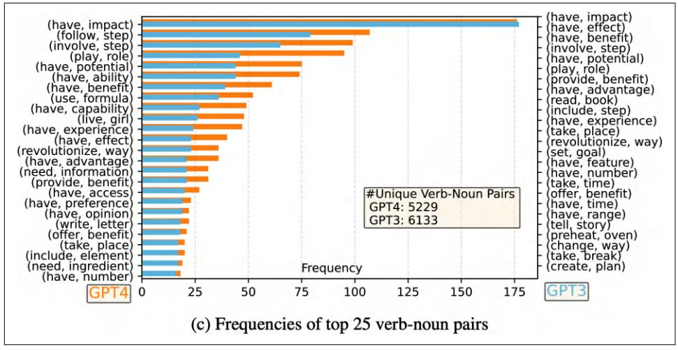
Figure 8-6. One statistic you can use is the distribution of (verb, direct object noun) in your data. Image from “Instruction Tuning with GPT-4” (Peng et al., 2023).

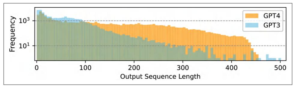
Figure 8-7. The distribution of response length for GPT-4 and GPT-3. Image from “Instruction Tuning with GPT-4” (Peng et al., 2023).

GPT-4 seems to have a broader and more diverse range of verb-noun pairings and tends to generate longer responses.

Plot these distributions by data source, time, annotator, etc. Do you notice any ques‐ tion patterns that tend to get longer/shorter responses or higher/lower scores? Are there any outliers? What might be the cause of these outliers? What to do with them?

If the scores are supposed to follow a normal distribution, do scores by all annotators follow a normal distribution? You might notice that some annotators tend to give much shorter responses or bias toward higher scores, and it’s up to you to decide what to do with their annotations.

If each example has more than one annotation, compute the inter-annotator disa‐ greement. Check the examples with conflicting annotations and resolve the conflicts.

There are many data exploration tools you should use, but they won’t be replace‐ ments for manual data inspection. In every project I’ve worked on, staring at data for just 15 minutes usually gives me some insight that could save me hours of head‐ aches. Greg Brockman, an OpenAI co-founder, tweeted: “Manual inspection of data has probably the highest value-to-prestige ratio of any activity in machine learning.”

Look at your data to see if the examples make sense. If it’s annotated data, pick out a few queries and try to annotate them yourself to see if your annotations match the given annotations. This will give you a sense of how trustworthy the annotations are. Fact-check the responses. How unique are the examples? Are there any examples with the same query but with different responses? Are there any examples with the same responses but with different queries?

Deduplicate Data

Duplicated data can skew the data distribution and introduce biases into your model. Imagine a dataset that looks like Table 8-3. The duplicated entries might lead the model to the wrong conclusion that all red-colored items should be expensive. Dupli‐ cations can cause test set contamination. When splitting duplicated data into train and test sets, one example might be in the train set and its duplicate in the test set.

4 {item: pencil, color: red}
5 {item: pencil, color: green}

Table 8-3. A toy dataset with duplicate examples in grey cells.

Multiple studies have shown the negative impact of training data duplications on model performance; see Lee et al. (2021) and Tirumala et al. (2023). An Anthropic study demonstrated that repeating 0.1% of the data 100 times can cause an 800M parameter model’s performance to degrade to that of a 400M parameter model despite the other 90% of the training tokens remaining unique (Hernandez et al., 2022). Even when duplications don’t hurt your model’s performance, they can waste your time and compute.

Depending on the data, there are many forms of duplication, some of which are harder to detect. For example, here are a few types of duplications in a dataset of documents:

• Whole document duplications: the same document appearing more than once.
Intra-document duplications: e.g., the same paragraph appears twice in one document.
Cross-document duplications: e.g., the same popular quote appears in multiple documents.

What can be considered duplications also depends on your definition. For example, do you want to deal with duplications at the document level, paragraph level, sen‐ tence level, or token level? Would two texts have to match exactly to be considered duplicates, or would an 80% overlap be sufficient? Are two lists considered duplicates if they have the same items but in different order?

The task of deduplication can leverage the same techniques used for similarity meas‐ urements (discussed in Chapter 3). Data deduplication is also used for identity reso‐ lution, determining whether two identities (e.g., two social media profiles) are the same. Here are some concrete ways you can deduplicate data:

Pairwise comparison

Compute the similarity score of each example to every other example in the data‐ set, using exact match, n-gram match, fuzzy match, or semantic similarity score, as discussed in Chapter 3. This approach can be expensive with large datasets, however.

Hashing

Hash examples into different buckets and check only among examples that fall into the same bucket. Hash-related deduplication methods include MinHash and Bloom filter.

Dimensionality reduction

Use a dimensionality reduction technique to first reduce the dimensions of your data and then do a pairwise comparison. Many techniques used for vector search, as discussed in Chapter 6, can be used for this.

A quick search will return many libraries that help with deduplication. Some of them are dupeGuru, Dedupe, datasketch, TextDistance, TheFuzz, and deduplicate-textdatasets. 16

¹⁶ One of my open source libraries, lazyNLP, also supports overlap estimation and deduplication using Bloom filter.

Clean and Filter Data

Data needs to be cleaned to make your model performant and safe.

First, you might want to remove extraneous formatting tokens. Since many public datasets are scraped from the internet, extraneous HTML tags are quite common. Unless you want to train your model on HMTL tags, remove them. Databricks found that removing extraneous Markdown and HTML tokens improved their model’s accuracy by 20% while reducing their input token lengths by 60%.

You need to clean your data of anything that isn’t compliant with your policies, such as PII, sensitive data, copyrighted data, or data that is considered toxic. Techniques discussed in Chapter 4 can help. Remove all the fields that you’re not allowed to use, such as zip code, name, and gender.

You also might want to remove low-quality data, using techniques discussed in “Data verification” on page 391 to detect low-quality data.

Manual inspection of data is especially important in this step. Staring at data might help you notice patterns that you can use as heuristics to detect low-quality data. Heuristics to detect low-quality data might be non-obvious. For example, Kern et al. (2024) found that annotations made in the second half of an annotation session are of lower quality, likely due to annotator boredom or fatigue.

If there is more data than you need or can afford to use (e.g., due to your compute budget), you can further filter your data. For example, you can use active learning techniques to select examples that are the most helpful for your model to learn from. You can also use importance sampling to find examples that are most important to your task. Their efficiencies depend on whether you have a good way to evaluate the importance of each training example. Meta researchers, in their paper on data prun‐ ing (Sorscher et al., 2022), concluded that the discovery of good data-pruning metrics can significantly reduce the resource costs of modern deep learning.

Format Data

Once you’ve deduplicated and cleaned your data, you need to get it into the right for‐ mat expected by the model you’re finetuning. Each model uses a specific tokenizer and expects data in a specific chat template, as discussed in Chapter 5. Getting data into the wrong chat template can cause strange bugs in your model.

If you’re doing supervised finetuning, your data is most likely in the format (instruc‐ tion, response). Instructions can be further decomposed into (system prompt, user prompt). If you’ve graduated to finetuning from prompt engineering, the instructions used for finetuning might be different from the instructions used during prompt engineering. During finetuning, instructions typically don’t need task descriptions or examples. If you have sufficient training examples, the model can learn the expected behavior of the task from the examples directly.

As an example, imagine that you’ve been using this three-shot instruction for your food classification task with a base model:

Label the following item as either edible or inedible.

Item: burger Label: edible Item: car Label: inedible Item: mushroom Label: edible Item: {INPUT} Label:

For finetuning, all the examples included in the 3-shot prompt can be converted into training examples. The training data for finetuning will look like Table 8-4.

Table 8-4. Example training data used for a food classification task.

…	…	…



	{INPUT} –>

Once the model is finetuned, you can use a prompt as simple as:

{INPUT} –>

This is much shorter than the prompt used with the base model. Therefore, if you’re worried about the input tokens of your instructions, finetuning can be one way to help manage the cost.

Different finetuning data formats can impact your finetuned model’s performance. Experiments to determine the best format for you can be helpful.

When you use the finetuned model, make sure that the prompts you use match the format of the finetuning data. For example, if the training data uses the prompt in the format “burger –>”, any of the following prompts can cause issues:

• “burger”: missing the end arrow
“Item: burger –>”: extra prefix
“burger –>”: extra space appended

Summary

Even though the actual process of creating training data is incredibly intricate, the principles of creating a dataset are surprisingly straightforward. To build a dataset to train a model, you start by thinking through the behaviors you want your model to learn and then design a dataset to show these behaviors. Due to the importance of data, teams are introducing dedicated data roles responsible for acquiring appropri‐ ate datasets while ensuring privacy and compliance.

What data you need depends not only on your use case but also on the training phase. Pre-training requires different data from instruction finetuning and preferred finetuning. However, dataset design across training phases shares the same three core criteria: quality, coverage, and quantity.

While how much data a model is trained on grabs headlines, having high-quality data with sufficient coverage is just as important. A small amount of high-quality data can outperform a large amount of noisy data. Similarly, many teams have found that increasing the diversity of their datasets is key to improving their models’ perfor‐ mance.

Due to the challenge of acquiring high-quality data, many teams have turned to syn‐ thetic data. While generating data programmatically has long been a goal, it wasn’t until AI could create realistic, complex data that synthetic data became a practical solution for many more use cases. This chapter discussed different techniques for data synthesis with a deep dive into synthesizing instruction data for finetuning.

Just like real data, synthetic data must be evaluated to ensure its quality before being used to train models. Evaluating AI-generated data is just as tricky as evaluating other AI outputs, and people are more likely to use generated data that they can relia‐ bly evaluate.

Data is challenging because many steps in dataset creation aren’t easily automatable. It’s hard to annotate data, but it’s even harder to create annotation guidelines. It’s hard to automate data generation, but it’s even harder to automate verifying it. While data synthesis helps generate more data, you can’t automate thinking through what data you want. You can’t easily automate annotation guidelines. You can’t automate paying attention to details.

However, challenging problems lead to creative solutions. One thing that stood out to me when doing research for this chapter is how much creativity is involved in dataset design. There are so many ways people construct and evaluate data. I hope that the range of data synthesis and verification techniques discussed in this chapter will give you inspiration for how to design your dataset.

Let’s say that you’ve curated a wonderful dataset that allows you to train an amazing model. How should you serve this model? The next chapter will discuss how to opti‐ mize inference for latency and cost.

CHAPTER 9 Inference Optimization

New models come and go, but one thing will always remain relevant: making them better, cheaper, and faster. Up until now, the book has discussed various techniques for making models better. This chapter focuses on making them faster and cheaper.

No matter how good your model is, if it’s too slow, your users might lose patience, or worse, its predictions might become useless—imagine a next-day stock price predic‐ tion model that takes two days to compute each outcome. If your model is too expen‐ sive, its return on investment won’t be worth it.

Inference optimization can be done at the model, hardware, and service levels. At the model level, you can reduce a trained model’s size or develop more efficient architec‐ tures, such as one without the computation bottlenecks in the attention mechanism often used in transformer models. At the hardware level, you can design more power‐ ful hardware.

The inference service runs the model on the given hardware to accommodate user requests. It can incorporate techniques that optimize models for specific hardware. It also needs to consider usage and traffic patterns to efficiently allocate resources to reduce latency and cost.

Because of this, inference optimization is an interdisciplinary field that often sees col‐ laboration among model researchers, application developers, system engineers, com‐ piler designers, hardware architects, and even data center operators.

This chapter discusses bottlenecks for AI inference and techniques to overcome them. It’ll focus mostly on optimization at the model and service levels, with an over‐ view of AI accelerators.

This chapter also covers performance metrics and trade-offs. Sometimes, a technique that speeds up a model can also reduce its cost. For example, reducing a model’s pre‐ cision makes it smaller and faster. But often, optimization requires trade-offs. For example, the best hardware might make your model run faster but at a higher cost.

Given the growing availability of open source models, more teams are building their own inference services. However, even if you don’t implement these inference opti‐ mization techniques, understanding these techniques will help you evaluate inference services and frameworks. If your application’s latency and cost are hurting you, read on. This chapter might help you diagnose the causes and potential solutions.

Understanding Inference Optimization

There are two distinct phases in an AI model’s lifecycle: training and inference. Training refers to the process of building a model. Inference refers to the process of using a model to compute an output for a given input.¹ Unless you train or finetune a model, you’ll mostly need to care about inference.²

This section starts with an overview of inference that introduces a shared vocabulary to discuss the rest of the chapter. If you’re already familiar with these concepts, feel free to skip to the section of interest.

Inference Overview

In production, the component that runs model inference is called an inference server. It hosts the available models and has access to the necessary hardware. Based on requests from applications (e.g., user prompts), it allocates resources to execute the appropriate models and returns the responses to users. An inference server is part of a broader inference service, which is also responsible for receiving, routing, and pos‐ sibly preprocessing requests before they reach the inference server. A visualization of a simple inference service is shown in Figure 9-1.

¹ As discussed in Chapter 7, inference involves the forward pass while training involves both the forward and backward passes.

² A friend, Mark Saroufim, pointed me to an interesting relationship between a model’s training cost and infer‐ ence cost. Imagine you’re a model provider. Let T be the total training cost, p be the cost you’re charging per inference, and N be the number of inference calls you can sell. Developing a model only makes sense if the money you can recover from inference for a model is more than its training cost, i.e., T <= p × N. The more a model is used in production, the more model providers can reduce inference cost. However, this doesn’t apply for third-party API providers who sell inference calls on top of open source models.

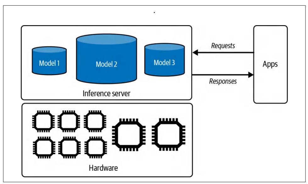
Figure 9-1. A simple inference service.

Model APIs like those provided by OpenAI and Google are inference services. If you use one of these services, you won’t be implementing most of the techniques dis‐ cussed in this chapter. However, if you host a model yourself, you’ll be responsible for building, optimizing, and maintaining its inference service.

Computational bottlenecks

Optimization is about identifying bottlenecks and addressing them. For example, to optimize traffic, city planners might identify congestion points and take measures to alleviate congestion. Similarly, an inference server should be designed to address the computational bottlenecks of the inference workloads it serves. There are two main computational bottlenecks, compute-bound and memory bandwidth-bound:

Compute-bound

This refers to tasks whose time-to-complete is determined by the computation needed for the tasks. For example, password decryption is typically computebound due to the intensive mathematical calculations required to break encryp‐ tion algorithms.

Memory bandwidth-bound

These tasks are constrained by the data transfer rate within the system, such as the speed of data movement between memory and processors. For example, if you store your data in the CPU memory and train a model on GPUs, you have to move data from the CPU to the GPU, which can take a long time. This can be shortened as bandwidth-bound. In literature, memory bandwidth-bound is often referred to as memory-bound.

Terminology Ambiguity: Memory-Bound Versus Bandwidth-Bound

Memory-bound is also used by some people to refer to tasks whose time-to-complete is constrained by memory capacity instead of memory bandwidth. This occurs when your hardware doesn’t have sufficient memory to handle the task, for example, if your machine doesn’t have enough memory to store the entire internet. This memory is often manifested in the error recognizable by engineers everywhere: OOM, out-ofmemory.³

However, this situation can often be mitigated by splitting your task into smaller pieces. For example, if you’re constrained by GPU memory and cannot fit an entire model into the GPU, you can split the model across GPU memory and CPU memory. This splitting will slow down your computation because of the time it takes to trans‐ fer data between the CPU and GPU. However, if data transfer is fast enough, this becomes less of an issue. Therefore, the memory capacity limitation is actually more about memory bandwidth.

The concepts of compute-bound or memory bandwidth-bound were introduced in the paper “Roofline” (Williams et al., 2009).⁴ Mathematically, an operation can be classified as compute-bound or memory bandwidth-bound based on its arithmetic intensity, which is the number of arithmetic operations per byte of memory access. Profiling tools like NVIDIA Nsight will show you a roofline chart to tell you whether your workload is compute-bound or memory bandwidth-bound, as shown in Figure 9-2. This chart is a roofline chart because it resembles a roof. Roofline charts are common in hardware performance analyses.

Different optimization techniques aim to mitigate different bottlenecks. For example, a compute-bound workload might be sped up by spreading it out to more chips or by leveraging chips with more computational power (e.g., a higher FLOP/s number). A memory bandwidth-bound workload might be sped up by leveraging chips with higher bandwidth.

³ Anecdotally, I find that people coming from a system background (e.g., optimization engineers and GPU engineers) use memory-bound to refer to bandwidth-bound, and people coming from an AI background (e.g., ML and AI engineers) use to memory-bound to refer to memory capacity-bound.

⁴ The Roofline paper uses the term memory-bound to refer to memory-bandwidth bound.

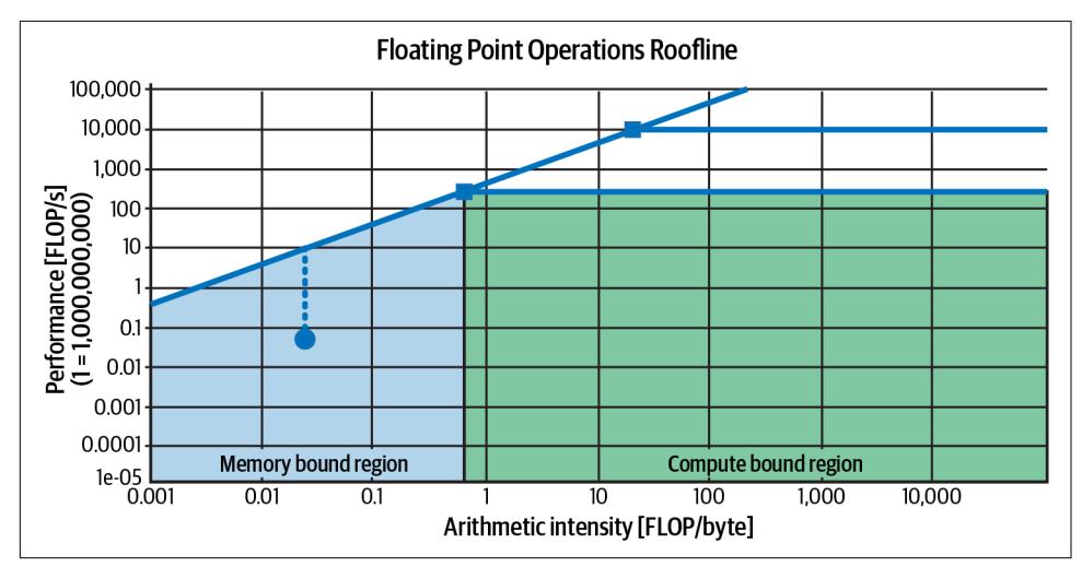
Figure 9-2. The roofline chart can help you visualize whether an operation is computebound or memory bandwidth-bound. This graph is on a log scale.

Different model architectures and workloads result in different computational bottle‐ necks. For example, inference for image generators like Stable Diffusion is typically compute-bound, whereas inference for autoregression language models is typically memory bandwidth-bound.

As an illustration, let’s look into language model inference. Recall from Chapter 2 that inference for a transformer-based language model consists of two steps, prefill‐ ing and decoding:

Prefill

The model processes the input tokens in parallel.⁵ How many tokens can be pro‐ cessed at once is limited by the number of operations your hardware can execute in a given time. Therefore, prefilling is compute-bound.

Decode

The model generates one output token at a time. At a high level, this step typi‐ cally involves loading large matrices (e.g., model weights) into GPUs, which is limited by how quickly your hardware can load data into memory. Decoding is, therefore, memory bandwidth-bound.

Figure 9-3 visualizes prefilling and decoding.

⁵ Prefilling effectively populates the initial KV cache for the transformer model.

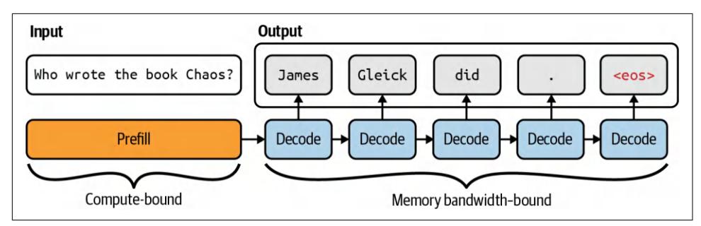
Figure 9-3. Autoregressive language models follow two steps for inference: prefill and decode. denotes the end of the sequence token.

Because prefill and decode have different computational profiles, they are often decoupled in production with separate machines. This technique will be discussed “Inference Service Optimization” on page 440.

The factors that affect the amount of prefilling and decoding computation in an LLM inference server, and therefore its bottlenecks, include context length, output length, and request batching strategies. Long context typically results in a memory bandwidth-bound workload, but clever optimization techniques, such as those dis‐ cussed later in this chapter, can remove this bottleneck.

As of this writing, due to the prevalence of the transformer architecture and the limi‐ tations of the existing accelerator technologies, many AI and data workloads are memory bandwidth-bound. However, future software and hardware advancements will be able to make AI and data workloads compute-bound.

Online and batch inference APIs

Many providers offer two types of inference APIs, online and batch:

Online APIs optimize for latency. Requests are processed as soon as they arrive.
Batch APIs optimize for cost. If your application doesn’t have strict latency requirements, you can send them to batch APIs for more efficient processing. Higher latency allows a broader range of optimization techniques, including batching requests together and using cheaper hardware. For example, as of this writing, both Google Gemini and OpenAI offer batch APIs at a 50% cost

reduction and significantly higher turnaround time, i.e., in the order of hours instead of seconds or minutes.⁶

Online APIs might still batch requests together as long as it doesn’t significantly impact latency, as discussed in “Batching” on page 440. The only real difference is that an online API focuses on lower latency, whereas a batch API focuses on higher throughput.

Customer-facing use cases, such as chatbots and code generation, typically require lower latency, and, therefore, tend to use online APIs. Use cases with less stringent latency requirements, which are ideal for batch APIs, include the following:

Synthetic data generation
Periodic reporting, such as summarizing Slack messages, sentiment analysis of brand mentions on social media, and analyzing customer support tickets
Onboarding new customers who require processing of all their uploaded documents
Migrating to a new model that requires reprocessing of all the data
Generating personalized recommendations or newsletters for a large customer base
Knowledge base updates by reindexing an organization’s data

APIs usually return complete responses by default. However, with autoregressive decoding, it can take a long time for a model to complete a response, and users are impatient. Many online APIs offer streaming mode, which returns each token as it’s generated. This reduces the time the users have to wait until the first token. The downside of this approach is that you can’t score a response before showing it to users, increasing the risk of users seeing bad responses. However, you can still retro‐ spectively update or remove a response as soon as the risk is detected.

⁶ If you run an inference service, separating your inference APIs into online and batch can help you prioritize latency for requests where latency matters the most. Let’s say that your inference server can serve only a maxi‐ mum of X requests/second without latency degradation, you have to serve Y requests/second, and Y is larger than X. In an ideal world, users with less-urgent requests can send their requests to the batch API, so that your service can focus on processing the online API requests first.

A batch API for foundation models differs from batch inference for traditional ML. In traditional ML:

Online inference means that predictions are computed after requests have arrived.
Batch inference means that predictions are precomputed before requests have arrived.

Precompution is possible for use cases with finite and predictable inputs like recommendation systems, where recommendations can be generated for all users in advance. These precomputed predic‐ tions are fetched when requests arrive, e.g., when a user visits the website. However, with foundation model use cases where the inputs are open-ended, it’s hard to predict all user prompts.⁷

Inference Performance Metrics

Before jumping into optimization, it’s important to understand what metrics to opti‐ mize for. From the user perspective, the central axis is latency (response quality is a property of the model itself, not of the inference service). However, application devel‐ opers must also consider throughput and utilization as they determine the cost of their applications.

Latency, TTFT, and TPOT

Latency measures the time from when users send a query until they receive the com‐ plete response. For autoregressive generation, especially in the streaming mode, the overall latency can be broken into several metrics:

Time to first token

TTFT measures how quickly the first token is generated after users send a query. It corresponds to the duration of the prefill step and depends on the input’s length. Users might have different expectations for TTFT for different applica‐ tions. For example, for conversational chatbots, the TTFT should be instantane‐ ous.⁸ However, users might be willing to wait longer to summarize long documents.

⁷ As discussed in “Prompt caching” on page 443, it’s common to know in advance the system prompt of an appli‐ cation. It’s just the exact user queries that are hard to predict.

⁸ In the early days of chatbots, some people complained about chatbots responding too fast, which seemed unnatural. See “Lufthansa Delays Chatbot’s Responses to Make It More ‘Human’” (Ry Crozier, iTnews, May 2017). However, as people become more familiar with chatbots, this is no longer the case.

Time per output token

TPOT measures how quickly each output token is generated after the first token. If each token takes 100 ms, a response of 1,000 tokens will take 100 s.

In the streaming mode, where users read each token as it’s generated, TPOT should be faster than human reading speed but doesn’t have to be much faster. A very fast reader can read 120 ms/token, so a TPOT of around 120 ms, or 6–8 tokens/second, is sufficient for most use cases.

Time between tokens and inter-token latency

Variations of this metric include time between tokens (TBT) and inter-token latency (ITL). 9 Both measure the time between output tokens.

The total latency will equal TTFT + TPOT × (number of output tokens).

Two applications with the same total latency can offer different user experiences with different TTFT and TPOT. Would your users prefer instant first tokens with a longer wait between tokens, or would they rather wait slightly longer for the first tokens but enjoy faster token generation afterward? User studies will be necessary to determine the optimal user experience. Reducing TTFT at the cost of higher TPOT is possible by shifting more compute instances from decoding to prefilling and vice versa.¹⁰

It’s important to note that the TTFT and TPOT values observed by users might differ from those observed by models, especially in scenarios involving CoT (chain-ofthought) or agentic queries where models generate intermediate steps not shown to users. Some teams use the metric time to publish to make it explicit that it measures time to the first token users see.

Consider the scenario where, after a user sends a query, the model performs the fol‐ lowing steps:

1. Generate a plan, which consists of a sequence of actions. This plan isn’t shown to the user.
1. Take actions and log their outputs. These outputs aren’t shown to the user.
1. Based on these outputs, generate a final response to show the user.

⁹ Time between tokens (TBT) is used by LinkedIn and inter-token latency (ITL) is used by NVIDIA.

¹⁰ An experiment by Anyscale shows that 100 input tokens have approximately the same impact on the overall latency as a single output token.

From the model’s perspective, the first token is generated in step 1. This is when the model internally begins its token generation process. The user, however, only sees the first token of the final output generated in step 3. Thus, from their perspective, TTFT is much longer.

Because latency is a distribution, the average can be misleading. Imagine you have 10 requests whose TTFT values are 100 ms, 102 ms, 100 ms, 100 ms, 99 ms, 104 ms, 110 ms, 90 ms, 3,000 ms, 95 ms. The average TTFT value is 390 ms, which makes your inference service seem slower than it is. There might have been a network error that slowed down one request or a particularly long prompt that took a much longer time to prefill. Either way, you should investigate. With a large volume of requests, outliers that skew the average latency are almost inevitable.

It’s more helpful to look at latency in percentiles, as they tell you something about a certain percentage of your requests. The most common percentile is the 50th percen‐ tile, abbreviated as p50 (median). If the median is 100 ms, half of the requests take longer than 100 ms to generate the first token, and half take less than 100 ms. Percen‐ tiles also help you discover outliers, which might be symptoms of something wrong. Typically, the percentiles you’ll want to look at are p90, p95, and p99. It’s also helpful to plot TTFT values against inputs’ lengths.

Throughput and goodput

Throughput measures the number of output tokens per second an inference service can generate across all users and requests.

Some teams count both input and output tokens in throughput calculation. However, since processing input tokens (prefilling) and generating output tokens (decoding) have different computational bottlenecks and are often decoupled in modern infer‐ ence servers, input and output throughput should be counted separately. When throughput is used without any modifier, it usually refers to output tokens.

Throughput is typically measured as tokens/s (TPS). If you serve multiple users, tokens/s/user is also used to evaluate how the system scales with more users.

Throughput can also be measured as the number of completed requests during a given time. Many applications use requests per second (RPS). However, for applica‐ tions built on top of foundation models, a request might take seconds to complete, so many people use completed requests per minute (RPM) instead. Tracking this metric is useful for understanding how an inference service handles concurrent requests. Some providers might throttle your service if you send too many concurrent requests at the same time.

Throughput is directly linked to compute cost. A higher throughput typically means lower cost. If your system costs $2/h in compute and its throughput is 100 tokens/s, it costs around $5.556 per 1M output tokens. If each request generates 200 output tokens on average, the cost for decoding 1K requests would be $1.11.

The prefill cost can be similarly calculated. If your hardware costs $2 per hour and it can prefill 100 requests per minute, the cost for prefilling 1K requests would be $0.33.

The total cost per request is the sum of the prefilling and decoding costs. In this example, the total cost for 1K requests would be $1.11 + $0.33 = $1.44.

What’s considered good throughput depends on the model, the hardware, and the workload. Smaller models and higher-end chips typically result in higher throughput. Workloads with consistent input and output lengths are easier to optimize than workloads with variable lengths.

Even for similarly sized models, hardware, and workloads, direct throughput com‐ parisons might be only approximate because token count depends on what consti‐ tutes a token, and different models have different tokenizers. It’s better to compare the efficiency of inference servers using metrics such as cost per request.

Just like most other software applications, AI applications have the latency/through‐ put trade-off. Techniques like batching can improve throughput but reduce latency. According to the LinkedIn AI team in their reflection after a year of deploying gener‐ ative AI products (LinkedIn, 2024), it’s not uncommon to double or triple the throughput if you’re willing to sacrifice TTFT and TPOT.

Due to this trade-off, focusing on an inference service based solely on its throughput and cost can lead to a bad user experience. Instead, some teams focus on goodput, a metric adapted from networking for LLM applications. Goodput measures the num‐ ber of requests per second that satisfies the SLO, software-level objective.

Imagine that your application has the following objectives: TTFT of at most 200 ms and TPOT of at most 100 ms. Let’s say that your inference service can complete 100 requests per minute. However, out of these 100 requests, only 30 satisfy the SLO. Then, the goodput of this service is 30 requests per minute. A visualization of this is shown in Figure 9-4.

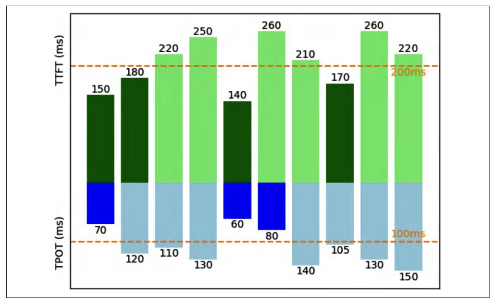
Figure 9-4. If an inference service can complete 10 RPS but only 3 satisfy the SLO, then its goodput is 3 RPS.

Utilization, MFU, and MBU

Utilization metrics measure how efficiently a resource is being used. It typically quantifies the proportion of the resource actively being used compared to its total available capacity.

A common but often misunderstood metric is GPU utilization, and NVIDIA is parti‐ ally to blame for this misunderstanding. The official NVIDIA tool for monitoring GPU usage is nvidia-smi—SMI stands for System Management Interface. One met‐ ric this tool shows is GPU utilization, which represents the percentage of time during which the GPU is actively processing tasks. For example, if you run inference on a GPU cluster for 10 hours, and the GPUs are actively processing tasks for 5 of those hours, your GPU utilization would be 50%.

However, actively processing tasks doesn’t mean doing so efficiently. For simplicity, consider a tiny GPU capable of doing 100 operations per second. In nvidia-smi’s definition of utilization, this GPU can report 100% utilization even if it’s only doing one operation per second.

If you pay for a machine that can do 100 operations and use it for only 1 operation, you’re wasting money. nvidia-smi’s GPU optimization metric is, therefore, not very useful. A utilization metric you might care about, out of all the operations a machine is capable of computing, is how many it’s doing in a given time. This metric is called

MFU (Model FLOP/s Utilization), which distinguishes it from the NVIDIA GPU uti‐ lization metric.

MFU is the ratio of the observed throughput (tokens/s) relative to the theoretical maximum throughput of a system operating at peak FLOP/s. If at the peak FLOP/s advertised by the chip maker, the chip can generate 100 tokens/s, but when used for your inference service, it can generate only 20 tokens/s, your MFU is 20%.¹¹

Similarly, because memory bandwidth is expensive, you might also want to know how efficiently your hardware’s bandwidth is utilized. MBU (Model Bandwidth Uti‐ lization) measures the percentage of achievable memory bandwidth used. If the chip’s peak bandwidth is 1 TB/s and your inference uses only 500 GB/s, your MBU is 50%.

Computing the memory bandwidth being used for LLM inference is straightforward:

parameter count × bytes/param × tokens/s

MBU is computed as follows:

(parameter count × bytes/param × tokens/s) / (theoretical bandwidth)

For example, if you use a 7B-parameter model in FP16 (two bytes per parameter) and achieve 100 tokens/s, the bandwidth used is:

7B × 2 × 100 = 700 GB/s

This underscores the importance of quantization (discussed in Chapter 7). Fewer bytes per parameter mean your model consumes less valuable bandwidth.

If this is done on an A100-80GB GPU with a theoretical 2 TB/s of memory band‐ width, the MBU is:

(700 GB/s) / (2 TB/s) = 70%

The relationships between throughput (tokens/s) and MBU and between throughput and MFU are linear, so some people might use throughput to refer to MBU and MFU.

What’s considered a good MFU and MBU depends on the model, hardware, and workload. Compute-bound workloads typically have higher MFU and lower MBU, while bandwidth-bound workloads often show lower MFU and higher MBU.

Because training can benefit from more efficient optimization (e.g., better batching), thanks to having more predictable workloads, MFU for training is typically higher than MFU for inference. For inference, since prefill is compute-bound and decode is memory bandwidth-bound, MFU during prefilling is typically higher than MFU dur‐ ing decoding. For model training, as of this writing, an MFU above 50% is generally

¹¹ People have cared about FLOP/s utilization for a long time, but the term MFU was introduced in the PaLM paper (Chowdhery et al., 2022).

considered good, but it can be hard to achieve on specific hardware.¹² Table 9-1 shows MFU for several models and accelerators.

Table 9-1. MFU examples from “PaLM: Scaling Language Modeling with Pathways” (Chowdhery et al., 2022).

compute-bound.

Figure 9-5 shows the MBU for the inference process using Llama 2-70B in FP16 on different hardware. The decline is likely due to the higher computational load per second with more users, shifting the workload from being bandwidth-bound to compute-bound.

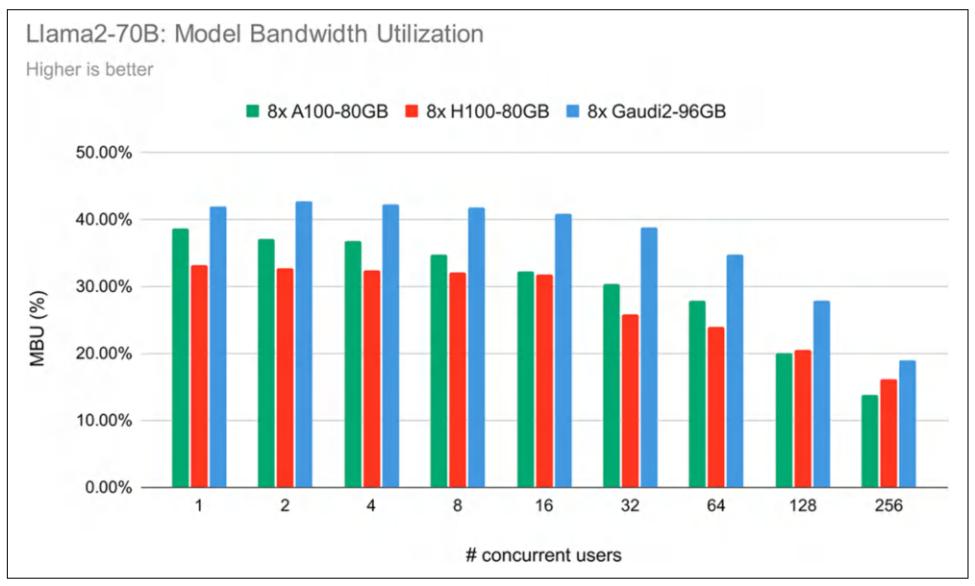
Figure 9-5. Bandwidth utilization for Llama 2-70B in FP16 across three different chips shows a decrease in MBU as the number of concurrent users increases. Image from “LLM Training and Inference with Intel Gaudi 2 AI Accelerators” (Databricks, 2024).

¹² Chip makers might also be doing what I call peak FLOP/s hacking. This might run experiments in certain conditions, such as using sparse matrices with specific shapes, to increase their peak FLOP/s. Higher peak FLOP/s numbers make their chips more attractive, but it can be harder for users to achieve high MFU.

Utilization metrics are helpful to track your system’s efficiency. Higher utilization rates for similar workloads on the same hardware generally mean that your services are becoming more efficient. However, the goal isn’t to get the chips with the highest utilization. What you really care about is how to get your jobs done faster and cheaper. A higher utilization rate means nothing if the cost and latency both increase.

AI Accelerators

How fast and cheap software can run depends on the hardware it runs on. While there are optimization techniques that work across hardware, understanding hard‐ ware allows for deeper optimization. This section looks at hardware from an infer‐ ence perspective, but it can be applied to training as well.

The development of AI models and hardware has always been intertwined. The lack of sufficiently powerful computers was one of the contributing factors to the first AI winter in the 1970s.¹³

The revival of interest in deep learning in 2012 was also closely tied to compute. One commonly acknowledged reason for the popularity of AlexNet (Krizhevsky et al., 2012) is that it was the first paper to successfully use GPUs, graphics processing units, to train neural networks.¹⁴ Before GPUs, if you wanted to train a model at AlexNet’s scale, you’d have to use thousands of CPUs, like the one Google released just a few months before AlexNet. Compared to thousands of CPUs, a couple of GPUs were a lot more accessible to PhD students and researchers, setting off the deep learning research boom.

¹³ In the 1960s, computers could run only one-layer neural networks, which had very limited capabilities. In their famous 1969 book Perceptrons: An Introduction to Computational Geometry (MIT Press), two AI pio‐ neers, Marvin Minsky and Seymour Papert, argued that neural networks with hidden layers would still be able to do little. Their exact quote was: “Virtually nothing is known about the computational capabilities of this latter kind of machine. We believe that it can do little more than can a low order perceptron.” There wasn’t sufficient compute power to dispute their argument, which was then cited by many people as a key reason for the drying up of AI funding in the 1970s.

¹⁴ There have been discussions on whether to rename the GPU since it’s used for a lot more than graphics (Jon Peddie, “Chasing Pixels,” July 2018). Jensen Huang, NVIDIA’s CEO, said in an interview (Stratechery, March 2022) that once the GPU took off and they added more capabilities to it, they considered renaming it to something more general like GPGPU (general-purpose GPU) or XGU. They decided against renaming because they assumed that people who buy GPUs will be smart enough to know what a GPU is good for beyond its name.

What’s an accelerator?

An accelerator is a chip designed to accelerate a specific type of computational work‐ load. An AI accelerator is designed for AI workloads. The dominant type of AI accel‐ erator is GPUs, and the biggest economic driver during the AI boom in the early 2020s is undoubtedly NVIDIA.

The main difference between CPUs and GPUs is that CPUs are designed for generalpurpose usage, whereas GPUs are designed for parallel processing:

CPUs have a few powerful cores, typically up to 64 cores for high-end consumer machines. While many CPU cores can handle multi-threaded workloads effec‐ tively, they excel at tasks requiring high single-thread performance, such as run‐ ning an operating system, managing I/O (input/output) operations, or handling complex, sequential processes.
GPUs have thousands of smaller, less powerful cores optimized for tasks that can be brok en down into many smaller, independent calculations, such as graphics rendering and machine learning. The operation that constitutes most ML work‐ loads is matrix multiplication, which is highly parallelizable.¹⁵

While the pursuit of efficient parallel processing increases computational capabilities, it imposes challenges on memory design and power consumption.

The success of NVIDIA GPUs has inspired many accelerators designed to speed up AI workloads, including Advanced Micro Devices (AMD)‘s newer generations of GPUs, Google’s TPU (Tensor Processing Unit), Intel’s Habana Gaudi, Graphcore’s Intelligent Processing Unit (IPU), Groq’s Language Processing Unit (LPU), Cerebras’ Wafer-Scale Quant Processing Unit (QPU), and many more being introduced.

While many chips can handle both training and inference, one big theme emerging is specialized chips for inference. A survey by Desislavov et al. (2023) shares that infer‐ ence can exceed the cost of training in commonly used systems, and that inference accounts for up to 90% of the machine learning costs for deployed AI systems.

¹⁵ Matrix multiplication, affectionately known as matmul, is estimated to account for more than 90% of all float‐ ing point operations in a neural network, according to “Data Movement Is All You Need: A Case Study on Optimizing Transformers” (Ivanov et al., arXiv, v3, November 2021) and “Scalable MatMul-free Language Modeling” (Zhu et al., arXiv, June 2024).

As discussed in Chapter 7, training demands much more memory due to backpropa‐ gation and is generally more difficult to perform in lower precision. Furthermore, training usually emphasizes throughput, whereas inference aims to minimize latency.

Consequently, chips designed for inference are often optimized for lower precision and faster memory access, rather than large memory capacity. Examples of such chips include the Apple Neural Engine, AWS Inferentia, and MTIA (Meta Training and Inference Accelerator). Chips designed for edge computing, like Google’s Edge TPU and the NVIDIA Jetson Xavier, are also typically geared toward inference.

There are also chips specialized for different model architectures, such as chips speci‐ alized for the transformer.¹⁶ Many chips are designed for data centers, with more and more being designed for consumer devices (such as phones and laptops).

Different hardware architectures have different memory layouts and specialized com‐ pute units that evolve over time. These units are optimized for specific data types, such as scalars, vectors, or tensors, as shown in Figure 9-6.

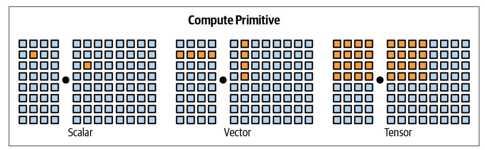
Figure 9-6. Different compute primitives. Image inspired by Chen et al. (2018).

A chip might have a mixture of different compute units optimized for various data types. For example, GPUs traditionally supported vector operations, but many modern GPUs now include tensor cores optimized for matrix and tensor computa‐ tions. TPUs, on the other hand, are designed with tensor operations as their primary compute primitive. To efficiently operate a model on a hardware architecture, its memory layout and compute primitives need to be taken into account.

A chip’s specifications contain many details that can be useful when evaluating this chip for each specific use case. However, the main characteristics that matter across use cases are computational capabilities, memory size and bandwidth, and power consumption. I’ll use GPUs as examples to illustrate these characteristics.

¹⁶ While a chip can be developed to run one model architecture, a model architecture can be developed to make the most out of a chip, too. For example, the transformer was originally designed by Google to run fast on TPUs and only later optimized on GPUs.

Computational capabilities

Computational capabilities are typically measured by the number of operations a chip can perform in a given time. The most common metric is FLOP/s, often written as FLOPS, which measures the peak number of floating-point operations per second. In reality, however, it’s very unlikely that an application can achieve this peak FLOP/s. The ratio between the actual FLOP/s and the theoretical FLOP/s is one uti‐ lization metric.

The number of operations a chip can perform in a second depends on the numerical precision—the higher the precision, the fewer operations the chip can execute. Think about how adding two 32-bit numbers generally requires twice the computation of adding two 16-bit numbers. The number of 32-bit operations a chip can perform in a given time is not exactly half that of 16-bit operations because of different chips’ opti‐ mization. For an overview of numerical precision, revisit “Numerical Representa‐ tions” on page 325.

Table 9-2 shows the FLOP/s specs for different precision formats for NVIDIA H100 SXM chips.

a
	Recall from Chapter 7 that TF32 is a 19-bit, not 32-bit, format.

	Memory size and bandwidth

Table 9-2. FLOP/s specs for NVIDIA H100 SXM chips.

a Recall from Chapter 7 that TF32 is a 19-bit, not 32-bit, format.

Memory size and bandwidth

Because a GPU has many cores working in parallel, data often needs to be moved from the memory to these cores, and, therefore, data transfer speed is important. Data transfer is crucial when working with AI models that involve large weight matrices and training data. These large amounts of data need to be moved quickly to keep the cores efficiently occupied. Therefore, GPU memory needs to have higher bandwidth and lower latency than CPU memory, and thus, GPU memory requires more advanced memory technologies. This is one of the factors that makes GPU memory more expensive than CPU memory.

To be more specific, CPUs typically use DDR SDRAM (Double Data Rate Synchro‐ nous Dynamic Random-Access Memory), which has a 2D structure. GPUs, particu‐ larly high-end ones, often use HBM (high-bandwidth memory), which has a 3D stacked structure.¹⁷

An accelerator’s memory is measured by its size and bandwidth. These numbers need to be evaluated within the system an accelerator is part of. An accelerator, such as a GPU, typically interacts with three levels of memory, as visualized in Figure 9-7:

CPU memory (DRAM)

Accelerators are usually deployed alongside CPUs, giving them access to the CPU memory (also known as system memory, host memory, or just CPU DRAM).

CPU memory usually has the lowest bandwidth among these memory types, with data transfer speeds ranging from 25 GB/s to 50 GB/s. CPU memory size varies. Average laptops might have around 16–64 GB, whereas high-end workstations can have one TB or more.

GPU high-bandwidth memory (HBM)

This is the memory dedicated to the GPU, located close to the GPU for faster access than CPU memory.

HBM provides significantly higher bandwidth, with data transfer speeds typically ranging from 256 GB/s to over 1.5 TB/s. This speed is essential for efficiently handling large data transfers and high-throughput tasks. A consumer GPU has around 24–80 GB of HBM.

GPU on-chip SRAM

Integrated directly into the chip, this memory is used to store frequently accessed data and instructions for nearly instant access. It includes L1 and L2 caches made of SRAM, and, in some architectures, L3 caches as well. These caches are part of the broader on-chip memory, which also includes other components like register files and shared memory.

RAM has extremely high data transfer speeds, often exceeding 10 TB/s. The size of GPU SRAM is small, typically 40 MB or under.

¹⁷ Lower-end to mid-range GPUs might use GDDR (Graphics Double Data Rate) memory.

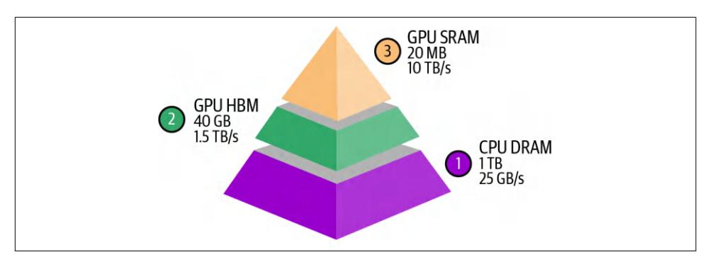
Figure 9-7. The memory hierarchy of an AI accelerator. The numbers are for reference only. The actual numbers vary for each chip.

A lot of GPU optimization is about how to make the most out of this memory hierar‐ chy. However, as of this writing, popular frameworks such as PyTorch and Tensor‐ Flow don’t yet allow fine-grained control of memory access. This has led many AI researchers and engineers to become interested in GPU programming languages such as CUDA (originally Compute Unified Device Architecture), OpenAI’s Triton, and ROCm (Radeon Open Compute). The latter is AMD’s open source alternative to NVIDIA’s proprietary CUDA.

Power consumption

Chips rely on transistors to perform computation. Each computation is done by tran‐ sistors switching on and off, which requires energy. A GPU can have billions of tran‐ sistors—an NVIDIA A100 has 54 billion transistors, while an NVIDIA H100 has 80 billion. When an accelerator is used efficiently, billions of transistors rapidly switch states, consuming a substantial amount of energy and generating a nontrivial amount of heat. This heat requires cooling systems, which also consume electricity, adding to data centers’ overall energy consumption.

Chip energy consumption threatens to have a staggering impact on the environment, increasing the pressure on companies to invest in technologies for green data centers. An NVIDIA H100 running at its peak for a year consumes approximately 7,000 kWh. For comparison, the average US household’s annual electricity consumption is 10,000 kWh. That’s why electricity is a bottleneck to scaling up compute.¹⁸

¹⁸ A main challenge in building data centers with tens of thousands of GPUs is finding a location that can guar‐ antee the necessary electricity. Building large-scale data centers requires navigating electricity supply, speed, and geopolitical constraints. For example, remote regions might provide cheaper electricity but can increase network latency, making the data centers less appealing for use cases with stringent latency requirements like inference.

Accelerators typically specify their power consumption under maximum power draw or a proxy metric TDP (thermal design power):

Maximum power draw indicates the peak power that the chip could draw under full load.
TDP represents the maximum heat a cooling system needs to dissipate when the chip operates under typical workloads. While it’s not an exact measure of power consumption, it’s an indication of the expected power draw. For CPUs and GPUs, the maximum power draw can be roughly 1.1 to 1.5 times the TDP, though the exact relationship varies depending on the specific architecture and workload.

If you opt for cloud providers, you won’t need to worry about cooling or electricity. However, these numbers can still be of interest to understand the impact of accelera‐ tors on the environment and the overall electricity demand.

Selecting Accelerators

What accelerators to use depends on your workload. If your workloads are computebound, you might want to look for chips with more FLOP/s. If your workloads are memory-bound, shelling out money for chips with higher bandwidth and more memory will make your life easier.

When evaluating which chips to buy, there are three main questions:

Can the hardware run your workloads?
How long does it take to do so?
How much does it cost?

FLOP/s, memory size, and memory bandwidth are the three big numbers that help you answer the first two questions. The last question is straightforward. Cloud pro‐ viders’ pricing is typically usage-based and fairly similar across providers. If you buy your hardware, the cost can be calculated based on the initial price and ongoing power consumption.

Inference Optimization

Inference optimization can be done at the model, hardware, or service level. To illus‐ trate their differences, consider archery. Model-level optimization is like crafting bet‐ ter arrows. Hardware-level optimization is like training a stronger and better archer. Service-level optimization is like refining the entire shooting process, including the bow and aiming conditions.

Ideally, optimizing a model for speed and cost shouldn’t change the model’s quality. However, many techniques might cause model degradation. Figure 9-8 shows the same Llama models’ performance on different benchmarks, served by different infer‐ ence service providers.

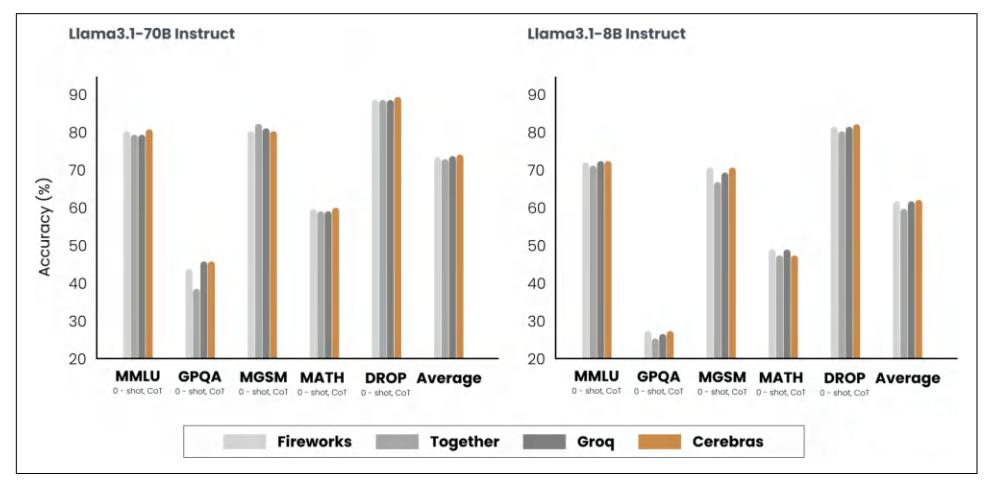
Figure 9-8. An inference service provider might use optimization techniques that can alter a model’s behavior, causing different providers to have slight model quality varia‐ tions. The experiment was conducted by Cerebras (2024).

Since hardware design is outside the scope of this book, I’ll discuss techniques at the model and service levels. While the techniques are discussed separately, keep in mind that, in production, optimization typically involves techniques at more than one level.

Model Optimization

Model-level optimization aims to make the model more efficient, often by modifying the model itself, which can alter its behavior. As of this writing, many foundation models follow the transformer architecture and include an autoregressive language model component. These models have three characteristics that make inference resource-intensive: model size, autoregressive decoding, and the attention mecha‐ nism. Let’s discuss approaches to address these challenges.

Model compression

Model compression involves techniques that reduce a model’s size. Making a model smaller can also make it faster. This book has already discussed two model compres‐ sion techniques: quantization and distillation. Quantization, reducing the precision of a model to reduce its memory footprint and increase its throughput, is discussed in Chapter 7. Model distillation, training a small model to mimic the behavior of the large model, is discussed in Chapter 8.

Model distillation suggests that it’s possible to capture a large model’s behaviors using fewer parameters. Could it be that within the large model, there exists a subset of parameters capable of capturing the entire model’s behavior? This is the core con‐ cept behind pruning.

Pruning, in the context of neural networks, has two meanings. One is to remove entire nodes of a neural network, which means changing its architecture and reduc‐ ing its number of parameters. Another is to find parameters least useful to predic‐ tions and set them to zero. In this case, pruning doesn’t reduce the total number of parameters, only the number of non-zero parameters. This makes the model more sparse, which both reduces the model’s storage space and speeds up computation.

Pruned models can be used as-is or be further finetuned to adjust the remaining parameters and restore any performance degradation caused by the pruning process. Pruning can help discover promising model architectures (Liu et al., 2018). These pruned architectures, smaller than the pre-pruned architectures, can also be trained from scratch (Zhu et al., 2017).

In the literature, there have been many encouraging pruning results. For example, Frankle and Carbin (2019) showed that pruning techniques can reduce the non-zero parameter counts of certain trained networks by over 90%, decreasing memory foot‐ prints and improving speed without compromising accuracy. However, in practice, as of this writing, pruning is less common. It’s harder to do, as it requires an under‐ standing of the original model’s architecture, and the performance boost it can bring is often much less than that of other approaches. Pruning also results in sparse mod‐ els, and not all hardware architectures are designed to take advantage of the resulting sparsity.

Weight-only quantization is by far the most popular approach since it’s easy to use, works out of the box for many models, and is extremely effective. Reducing a model’s precision from 32 bits to 16 bits reduces its memory footprint by half. However, we’re close to the limit of quantization—we can’t go lower than 1 bit per value. Distillation is also common because it can result in a smaller model whose behavior is compara‐ tive to that of a much larger one for your needs.

Overcoming the autoregressive decoding bottleneck

As discussed in Chapter 2, autoregressive language models generate one token after another. If it takes 100 ms to generate one token, a response of 100 tokens will take 10 s. ¹⁹ This process is not just slow, it’s also expensive. Across model API providers, an output token costs approximately two to four times an input token. In an experi‐ ment, Anyscale found that a single output token can have the same impact on latency as 100 input tokens (Kadous et al., 2023). Improving the autoregressive generation process by a small percentage can significantly improve user experience.

As the space is rapidly evolving, new techniques are being developed to overcome this seemingly impossible bottleneck. Perhaps one day, there will be architectures that don’t have this bottleneck. The techniques covered here are to illustrate what the solution might look like, but the techniques are still evolving.

Speculative decoding. Speculative decoding (also called speculative sampling) uses a faster but less powerful model to generate a sequence of tokens, which are then veri‐ fied by the target model. The target model is the model you want to use. The faster model is called the draft or proposal model because it proposes the draft output.

Imagine the input tokens are x¹ , x² , …, x^t :

1. The draft model generates a sequence of K tokens: x^t + 1, x^t + 2, …, x^t + ^K .
1. The target model verifies these K generated tokens in parallel.
1. The target model accepts the longest subsequence of draft tokens, from left to right, which the target model agrees to use.
1. Let’s say the target model accepts j draft tokens, x^t + 1, x^t + 2, …, x^t + ^j . The target model then generates one extra token, x^t + j + 1.

The process returns to step 1, with the draft model generating K tokens conditioned on x¹ , x² , …, x^t , x^t + 1, x^t + 2, …, x^t + ^j . The process is visualized in Figure 9-9.

If no draft token is accepted, this loop produces only one token generated by the tar‐ get model. If all draft tokens are accepted, this loop produces K + 1 tokens, with K generated by the draft model and one by the target model.

¹⁹ Each token generation step necessitates the transfer of the entire model’s parameters from the accelerator’s high-bandwidth memory to its compute units. This makes this operation bandwidth-heavy. Because the model can produce only one token at a time, the process consumes only a small number of FLOP/s, resulting in computational inefficiency.

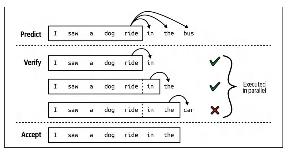
Figure 9-9. A draft model generates a sequence of K tokens, and the main model accepts the longest subsequence that it agrees with. The image is from “Blockwise Parallel Decoding for Deep Autoregressive Models” (Stern et al., 2018).

If all draft sequences are rejected, the target model must generate the entire response in addition to verifying it, potentially leading to increased latency. However, this can be avoided because of these three insights:

1. The time it takes for the target model to verify a sequence of tokens is less than the time it takes to generate it, because verification is parallelizable, while genera‐ tion is sequential. Speculative decoding effectively turns the computation profile of decoding into that of prefilling.
1. In an output token sequence, some tokens are easier to predict than others. It’s possible to find a weaker draft model capable of getting these easier-to-predict tokens right, leading to a high acceptance rate of the draft tokens.
1. Decoding is memory bandwidth-bound, which means that during the coding process, there are typically idle FLOPs that can be used for free verification.²⁰

Acceptance rates are domain-dependent. For texts that follow specific structures like code, the acceptance rate is typically higher. Larger values of K mean fewer verifying calls for the target model but a low acceptance rate of the draft tokens. The draft model can be of any architecture, though ideally it should share the same vocabulary and tokenizer as the target model. You can train a custom draft model or use an existing weaker model.

²⁰ This also means that if your MFU is already maxed out, speculative decoding makes less sense.

For example, to speed up the decoding process of Chinchilla-70B, DeepMind trained a 4B-parameter draft model of the same architecture (Chen et al., 2023). The draft model can generate a token eight times faster than the target model (1.8 ms/token compared to 14.1 ms/token). This reduces the overall response latency by more than half without compromising response quality. A similar speed-up was achieved for T5-XXL (Laviathan et al., 2022).

This approach has gained traction because it’s relatively easy to implement and doesn’t change a model’s quality. For example, it’s possible to do so in 50 lines of code in PyTorch. It’s been incorporated into popular inference frameworks such as vLLM, TensorRT-LLM, and llama.cpp.

Inference with reference. Often, a response needs to reference tokens from the input. For example, if you ask your model a question about an attached document, the model might repeat a chunk of text verbatim from the document. Another example is if you ask the model to fix bugs in a piece of code, the model might reuse the majority of the original code with minor changes. Instead of making the model generate these repeated tokens, what if we copy these tokens from the input to speed up the genera‐ tion? This is the core idea behind inference with reference.

Inference with reference is similar to speculative decoding, but instead of using a model to generate draft tokens, it selects draft tokens from the input. The key chal‐ lenge is to develop an algorithm to identify the most relevant text span from the con‐ text at each decoding step. The simplest option is to find a text span that matches the current tokens.

Unlike speculative decoding, inference with reference doesn’t require an extra model. However, it’s useful only in generation scenarios where there’s a significant overlap between contexts and outputs, such as in retrieval systems, coding, or multi-turn conversations. In “Inference with Reference: Lossless Acceleration of Large Language Models” (Yang et al., 2023), this technique helps achieve two times generation speedup in such use cases.

Examples of how inference with reference works are shown in Figure 9-10.

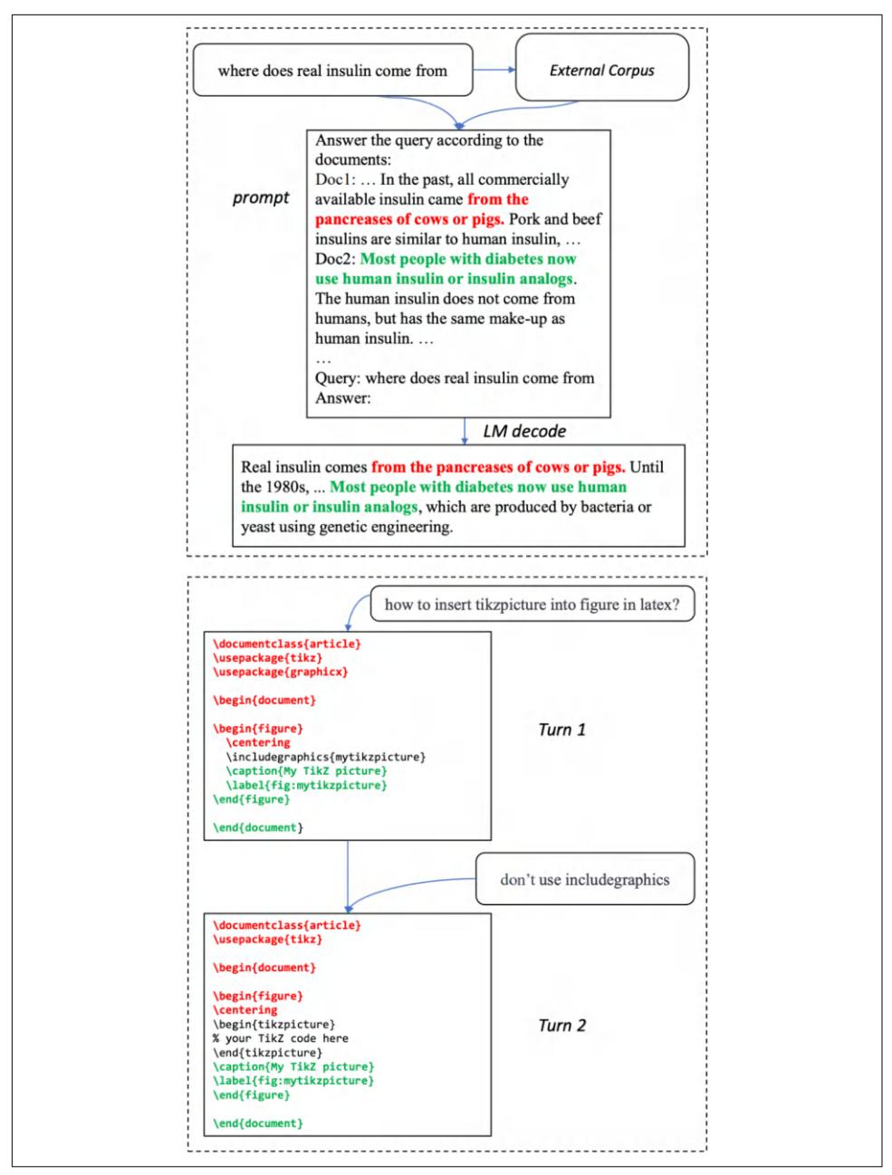
Figure 9-10. Two examples of inference with reference. The text spans that are success‐ fully copied from the input are in red and green. Image from Yang et al. (2023). The image is licensed under CC BY 4.0.

Parallel decoding. Instead of making autoregressive generation faster with draft tokens, some techniques aim to break the sequential dependency. Given an existing sequence of tokens x¹ , x² ,…,x^t , these techniques attempt to generate x^t + 1, x^t + 2,…,x^t + ^k simultaneously. This means that the model generates x^t + 2 before it knows that the token before it is x^t + 1.

This can work because the knowledge of the existing sequence often is sufficient to predict the next few tokens. For example, given “the cat sits”, without knowing that the next token is “on”, “under”, or “behind”, you might still predict that the word after it is “the”.

The parallel tokens can be generated by the same decoder, as in Lookahead decoding (Fu et al., 2024), or by different decoding heads, as in Medusa (Cai et al., 2024). In Medusa, the original model is extended with multiple decoding heads, and each head is a small neural network layer that is then trained to predict a future token at a spe‐ cific position. If the original model is trained to predict the next token x^t + 1, the k th head will predict the token x^t + k + 1. These heads are trained together with the original model, but the original model is frozen. NVIDIA claimed Medusa helped boost Llama 3.1 token generation by up to 1.9× on their HGX H200 GPUs (Eassa et al., 2024).

However, because these tokens aren’t generated sequentially, they need to be verified to make sure that they fit together. An essential part of parallel decoding is verifica‐ tion and integration. Lookahead decoding uses the Jacobi method²¹ to verify the gen‐ erated tokens, which works as follows:

1. K future tokens are generated in parallel.
1. These K tokens are verified for coherence and consistency with the context.
1. If one or more tokens fail verification, instead of aggregating all K future tokens, the model regenerates or adjusts only these failed tokens.

The model keeps refining the generated tokens until they all pass verification and are integrated into the final output. This family of parallel decoding algorithms is also called Jacobi decoding.

On the other hand, Medusa uses a tree-based attention mechanism to verify and inte‐ grate tokens. Each Medusa head produces several options for each position. These options are then organized into a tree-like structure to select the most promising combination. The process is visualized in Figure 9-11.

²¹ The Jacobi method is an iterative algorithm where multiple parts of a solution can be updated simultaneously and independently.

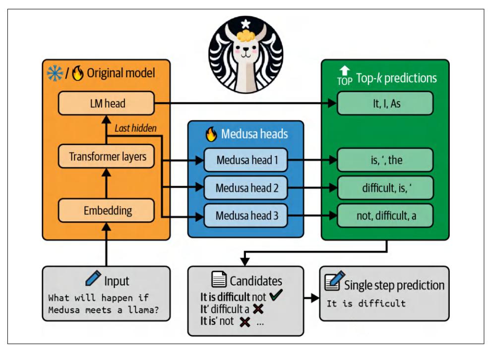
Figure 9-11. In Medusa (Cai et al., 2024), each head predicts several options for a token position. The most promising sequence from these options is selected. Image adapted from the paper, which is licensed under CC BY 4.0.

While the perspective of being able to circumvent sequential dependency is appeal‐ ing, parallel decoding is not intuitive, and some techniques, like Medusa, can be chal‐ lenging to implement.

Attention mechanism optimization

Recall from Chapter 2 that generating the next token requires the key and value vec‐ tors for all previous tokens. This means that the following applies:

Generating token x^t requires the key and value vectors for tokens x¹ , x² , …, x^t – 1.
Generating token x^t + 1 requires the key and value vectors for tokens x¹ , x² , …,x^t – 1, xt .

When generating token x^t + 1, instead of computing the key and value vectors for tokens x¹ , x² , …, x^t – 1 again, you reuse these vectors from the previous step. This means that you’ll need to compute the key and value vectors for only the most recent token, x^t . The cache that stores key and value vectors for reuse is called the KV cache. The newly computed key and value vectors are then added to the KV cache, which is visualized in Figure 9-12.

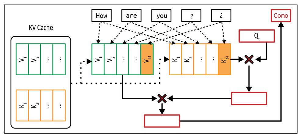
Figure 9-12. To avoid recomputing the key and value vectors at each decoding step, use a KV cache to store these vectors to reuse.

A KV cache is used only during inference, not training. During training, because all tokens in a sequence are known in advance, next token generation can be computed all at once instead of sequentially, as during inference. Therefore, there’s no need for a KV cache.

Because generating a token requires computing the attention scores with all previous tokens, the number of attention computations grows exponentially with sequence length.²² The KV cache size, on the other hand, grows linearly with sequence length.

The KV cache size also grows with larger batch sizes. A Google paper calculated that for a 500B+ model with multi-head attention, batch size 512, and context length 2048, the KV cache totals 3TB (Pope et al., 2022). This is three times the size of that model’s weights.

The KV cache size is ultimately limited by the available hardware storage, creating a bottleneck for running applications with long context. A large cache size also takes time to load into memory, which can be an issue for applications with strict latency.

The computation and memory requirements of the attention mechanism are one of the reasons why it’s so hard to have longer context.

Many techniques have been developed to make the attention mechanism more effi‐ cient. In general, they fall into three buckets: redesigning the attention mechanism, optimizing the KV cache, and writing kernels for attention computation.

²² The number of attention computations for an autoregressive model is O(n 2 ).

Calculating the KV Cache Size

The memory needed for the KV cache, without any optimization, is calculated as follows:

2 × B × S × L × H × M

B: batch size
S: sequence length
L: number of transformer layers
H: model dimension
M: memory needed for the cache’s numerical representation (e.g., FP16 or FP32).

This value can become substantial as the context length increases. For example, LLama 2 13B has 40 layers and a model dimension of 5,120. With a batch size of 32, sequence length of 2,048, and 2 bytes per value, the memory needed for its KV cache, without any optimization, is 2 × 32 × 2,048 × 40 × 5,120 × 2 = 54 GB.

Redesigning the attention mechanism. These techniques involve altering how the atten‐ tion mechanism works. Even though these techniques help optimize inference, because they change a model’s architecture directly, they can be applied only during training or finetuning.

For example, when generating a new token, instead of attending to all previous tokens, local windowed attention attends only to a fixed size window of nearby tokens (Beltagy et al., 2020). This reduces the effective sequence length to a fixed size win‐ dow, reducing both the KV cache and the attention computation. If the average sequence length is 10,000 tokens, attending to a window size of 1,000 tokens reduces the KV cache size by 10 times.

Local windowed attention can be interleaved with global attention, with local atten‐ tion capturing nearby context; the global attention captures task-specific information across the document.

Both cross-layer attention (Brandon et al., 2024) and multi-query attention (Shazeer, 2019) reduce the memory footprint of the KV cache by reducing the number of keyvalue pairs. Cross-layer attention shares key and value vectors across adjacent layers. Having three layers sharing the same key-value vectors means reducing the KV cache three times. On the other hand, multi-query attention shares key-value vectors across query heads.

Grouped-query attention (Ainslie et al., 2023) is a generalization of multi-query atten‐ tion. Instead of using only one set of key-value pairs for all query heads, its groupedquery attention puts query heads into smaller groups and shares key-value pairs only among query heads in the same group. This allows for a more flexible balance between the number of query heads and the number of key-value pairs.

Character.AI, an AI chatbot application, shares that their average conversation has a dialogue history of 180 messages (2024). Given the typically long sequences, the pri‐ mary bottleneck for inference throughput is the KV cache size. Three attention mechanism designs—multi-query attention, interleaving local attention and global attention, and cross-layer attention—help them reduce KV cache by over 20 times. More importantly, this significant KV cache reduction means that memory is no longer a bottleneck for them for serving large batch sizes.

Optimizing the KV cache size. The way the KV cache is managed is critical in mitigating the memory bottleneck during inference and enabling a larger batch size, especially for applications with long context. Many techniques are actively being developed to reduce and manage the KV cache.

One of the fastest growing inference frameworks, vLLM, gained popularity for intro‐ ducing PagedAttention, which optimizes memory management by dividing the KV cache into non-contiguous blocks, reducing fragmentation, and enabling flexible memory sharing to improve LLM serving efficiency (Kwon et al., 2023).

Other techniques include KV cache quantization (Hooper et al., 2024; Kang et al., 2024), adaptive KV cache compression (Ge et al., 2023), and selective KV cache (Liu et al., 2024).

Writing kernels for attention computation. Instead of changing the mechanism design or optimizing the storage, this approach looks into how attention scores are compu‐ ted and finds ways to make this computation more efficient. This approach is the most effective when it takes into account the hardware executing the computation. The code optimized for a specific chip is called a kernel. Kernel writing will be dis‐ cussed further in the next section.

One of the most well-known kernels optimized for attention computation is FlashAt‐ tention (Dao et al., 2022). This kernel fused together many operations commonly used in a transformer-based model to make them run faster, as shown in Figure 9-13.

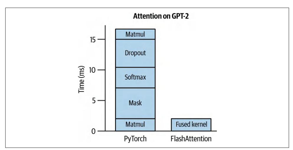
Figure 9-13. FlashAttention is a kernel that fuses together several common operators. Adapted from an original image licensed under BSD 3-Clause.

Kernels and compilers

Kernels are specialized pieces of code optimized for specific hardware accelerators, such as GPUs or TPUs. They are typically written to perform computationally inten‐ sive routines that need to be executed repeatedly, often in parallel, to maximize the performance of these accelerators.

Common AI operations, including matrix multiplication, attention computation, and convolution operation, all have specialized kernels to make their computation more efficient on different hardware.²³

Writing kernels requires a deep understanding of the underlying hardware architec‐ ture. This includes knowledge about how the memory hierarchy is structured (such as caches, global memory, shared memory, and registers) and how data is accessed and moved between these different levels.

Moreover, kernels are typically written in lower-level programming languages like CUDA (for NVIDIA GPUs), Triton (a language developed by OpenAI for writing custom kernels), and ROCm (for AMD GPUs). These languages allow fine-grained control over thread management and memory access but are also harder to learn than the languages that most AI engineers are familiar with, like Python.

Due to this entry barrier, writing kernels used to be a dark art practiced by a few. Chip makers like NVIDIA and AMD employ optimization engineers to write kernels to make their hardware efficient for AI workloads, whereas AI frameworks like

²³ Convolution operations are often used in image generation models like Stable Diffusion.

PyTorch and TensorFlow employ kernel engineers to optimize their frameworks on different accelerators.

However, with the rising demand for inference optimization and the ubiquity of accelerators, more AI engineers have taken an interest in writing kernels. There are many great online tutorials for kernel writing. Here, I’ll cover four common tech‐ niques often used to speed up computation:

Vectorization

Given a loop or a nested loop, instead of processing one data element at a time, simultaneously execute multiple data elements that are contiguous in memory. This reduces latency by minimizing data I/O operations.

Parallelization

Divide an input array (or n-dimensional array) into independent chunks that can be processed simultaneously on different cores or threads, speeding up the com‐ putation.

Loop tiling

Optimize the data accessing order in a loop for the hardware’s memory layout and cache. This optimization is hardware-dependent. An efficient CPU tiling pattern may not work well on GPUs.

Operator fusion

Combine multiple operators into a single pass to avoid redundant memory access. For example, if two loops operate over the same array, they can be fused into one, reducing the number of times data is read and written.

While vectorization, parallelization, and loop tiling can be applied broadly across different models, operator fusion requires a deeper understanding of a model’s specific operators and architecture. As a result, operator fusion demands more attention from optimization engineers.

Kernels are optimized for a hardware architecture. This means that whenever a new hardware architecture is introduced, new kernels need to be developed. For example, FlashAttention (Dao et al., 2022) was originally developed primarily for NVIDIA A100 GPUs. Later on, FlashAttention-3 was introduced for H100 GPUs (Shah et al., 2024).

A model script specifies a series of operations that need to be performed to execute that model. To run this code on a piece of hardware, such as a GPU, it has to be con‐ verted into a language compatible with that hardware. This process is called lowering. A tool that lowers code to run a specific hardware is called a compiler. Compilers bridge ML models and the hardware they run on. During the lowering process, whenever possible, these operations are converted into specialized kernels to run faster on the target hardware.

Inference Optimization Case Study from PyTorch

Figure 9-14 shows how much throughput improvement the PyTorch team could give to Llama-7B through the following optimization steps (PyTorch, 2023):

1. Call torch.compile to compile the model into more efficient kernels.
1. Quantize the model weights to INT8.
1. Further quantize the model weights to INT4.
1. Add speculative decoding.

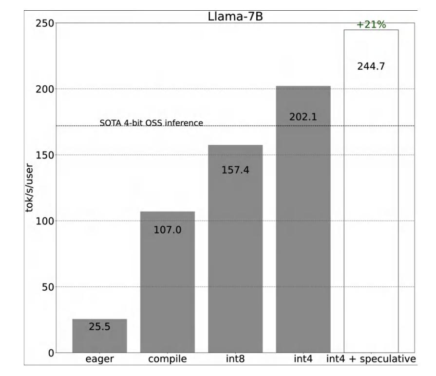
Figure 9-14. Throughput improvement by different optimization techniques in PyTorch. Image from PyTorch (2023).

The experiment was run on an A100 GPU with 80 GB of memory. It was unclear how these optimization steps impact the model’s output quality.

Compilers can be standalone tools, such as Apache TVM and MLIR (Multi-Level Intermediate Representation) or integrated into ML and inference frameworks, like torch.compile (a feature in PyTorch), XLA (Accelerated Linear Algebra, originally developed by TensorFlow, with an open source version called OpenXLA), and the compiler built into the TensorRT, which is optimized for NVIDIA GPUs. AI compa‐ nies might have their own compilers, with their proprietary kernels designed to speed up their own workloads.²⁴

Inference Service Optimization

Most service-level optimization techniques focus on resource management. Given a fixed amount of resources (compute and memory) and dynamic workloads (infer‐ ence requests from users that may involve different models), the goal is to efficiently allocate resources to these workloads to optimize for latency and cost. Unlike many model-level techniques, service-level techniques don’t modify models and shouldn’t change the output quality.

Batching

One of the easiest ways to reduce your cost is batching. In production, your inference service might receive multiple requests simultaneously. Instead of processing each request separately, batching the requests that arrive around the same time together can significantly reduce the service’s throughput. If processing each request sepa‐ rately is like everyone driving their own car, batching is like putting them together on a bus. A bus can move more people, but it can also make each person’s journey longer. However, if you do it intelligently, the impact on latency can be minimal.

The three main techniques for batching are: static batching, dynamic batching, and continuous batching.

The simplest batching technique is static batching. The service groups a fixed number of inputs together in a batch. It’s like a bus that waits until every seat is filled before departing. The drawback of static batching is that all requests have to wait until the batch is full to be executed. Thus the first request in a batch is delayed until the batch’s last request arrives, no matter how late the last request is.

²⁴ Many companies consider their kernels their trade secrets. Having kernels that allow them to run models faster and cheaper than their competitors is a competitive advantage.

Dynamic batching, on the other hand, sets a maximum time window for each batch. If the batch size is four and the window is 100 ms, the server processes the batch either when it has four requests or when 100 ms has passed, whichever happens first. It’s like a bus that leaves on a fixed schedule or when it’s full. This approach keeps latency under control, so earlier requests aren’t held up by later ones. The downside is that batches may not always be full when processed, possibly leading to wasted compute. Static batching and dynamic batching are visualized in Figure 9-15.

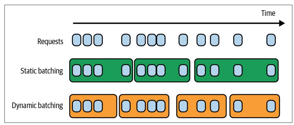
Figure 9-15. Dynamic batching keeps the latency manageable but might be less compute-efficient.

In naive batching implementations, all batch requests have to be completed before their responses are returned. For LLMs, some requests might take much longer than others. If one request in a batch generates only 10 response tokens and another request generates 1,000 response tokens, the short response has to wait until the long response is completed before being returned to the user. This results in unnecessary latency for short requests.

Continuous batching allows responses in a batch to be returned to users as soon as they are completed. It works by selectively batching operations that don’t cause the generation of one response to hold up another, as introduced in the paper Orca (Yu et al., 2022). After a request in a batch is completed and its response returned, the service can add another request into the batch in its place, making the batching con‐ tinuous. It’s like a bus that, after dropping off one passenger, can immediately pick up another passenger to maximize its occupancy rate. Continuous batching, also called in-flight batching, is visualized in Figure 9-16.

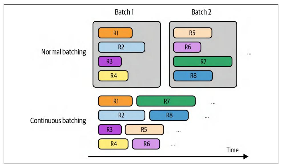
Figure 9-16. With continuous batching, completed responses can be returned immedi‐ ately to users, and new requests can be processed in their place.

Decoupling prefill and decode

LLM inference consists of two steps: prefill and decode. Because prefill is computebound and decode is memory bandwidth-bound, using the same machine to perform both can cause them to inefficiently compete for resources and significantly slow down both TTFT and TPOT. Imagine a GPU that is already handling prefilling and decoding near its peak computational capacity. It might be able to handle another low computational job like decoding. However, adding a new query to this GPU means introducing a prefilling job along with a decoding job. This one prefilling job can drain computational resources from existing decoding jobs, slowing down TPOT for these requests.

One common optimization technique for inference servers is to disaggregate prefill and decode. “DistServe” (Zhong et al., 2024) and “Inference Without Interference” (Hu et al., 2024) show that for various popular LLMs and applications, assigning pre‐ fill and decode operations to different instances (e.g., different GPUs) can signifi‐ cantly improve the volume of processed requests while adhering to latency requirements. Even though decoupling requires transferring intermediate states from prefill instances to decode instances, the paper shows communication overhead is not substantial in modern GPU clusters with high-bandwidth connections such as NVLink within a node.

The ratio of prefill instances to decode instances depends on many factors, such as the workload characteristics (e.g., longer input lengths require more prefill compute) and latency requirements (e.g., whether you want lower TTFT or TPOT). For exam‐ ple, if input sequences are usually long and you want to prioritize TTFT, this ratio can be between 2:1 and 4:1. If input sequences are short and you want to prioritize TPOT, this ratio can be 1:2 to 1:1.²⁵

Prompt caching

Many prompts in an application have overlapping text segments. A prompt cache stores these overlapping segments for reuse, so you only need to process them once. A common overlapping text segment in different prompts is the system prompt. Without a prompt cache, your model needs to process the system prompt with every query. With a prompt cache, the system prompt needs to be processed just once for the first query.

Prompt caching is useful for queries that involve long documents. For example, if many of your user queries are related to the same long document (such as a book or a codebase), this long document can be cached for reuse across queries. It’s also useful for long conversations when the processing of earlier messages can be cached and reused when predicting future messages.

A prompt cache is visualized in Figure 9-17. It’s also called a context cache or prefix cache.

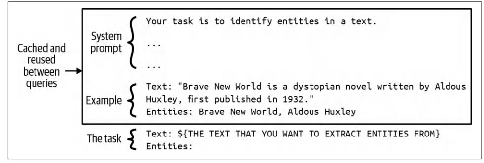
Figure 9-17. With a prompt cache, overlapping segments in different prompts can be cached and reused.

²⁵ Talks mentioning the prefill to decode instance ratio include “Llama Inference at Meta” (Meta, 2024).

For applications with long system prompts, prompt caching can significantly reduce both latency and cost. If your system prompt is 1,000 tokens, and your application generates one million model API calls daily, a prompt cache will save you from pro‐ cessing approximately one billion repetitive input tokens a day! However, this isn’t entirely free. Like the KV cache, prompt cache size can be quite large and take up memory space. Unless you use a model API with this functionality, implementing prompt caching can require significant engineering effort.

Since its introduction in November 2023 by Gim et al., the prompt cache has been rapidly incorporated into model APIs. As of this writing, Google Gemini offers this functionality, with cached input tokens given a 75% discount compared to regular input tokens, but you’ll have to pay extra for cache storage (as of writing, $1.00/one million tokens per hour). Anthropic offers prompt caching that promises up to 90% cost savings (the longer the cached context, the higher the savings) and up to 75% latency reduction. The impact of prompt caching on the cost and latency of different scenarios is shown in Table 9-3. 26

(10,000-token prompt) Multi-turn conversation (10-
turn convo with a long system prompt)

Parallelism

Table 9-3. Cost and latency reduced by prompt caching. Information from Anthropic (2024).

Parallelism

Accelerators are designed for parallel processing, and parallelism strategies are the backbone of high-performance computing. Many new parallelization strategies are being developed. This section covers only a few of them for reference. Two families of parallelization strategies that can be applied across all models are data parallelism and model parallelism. A family of strategies applied specifically for LLMs is context and sequence parallelism. An optimization technique might involve multiple parallelism strategies.

²⁶ While llama.cpp also has prompt caching, it seems to cache only whole prompts and work for queries in the same chat session, as of this writing. Its documentation is limited, but my guess from reading the code is that in a long conversation, it caches the previous messages and processes only the newest message.

Replica parallelism is the most straightforward strategy to implement. It simply cre‐ ates multiple replicas of the model you want to serve.²⁷ More replicas allow you to handle more requests at the same time, potentially at the cost of using more chips. Trying to fit models of different sizes onto different chips is a bin-packing problem, which can get complicated with more models, more replicas, and more chips.

Let’s say you have a mixture of models of different sizes (e.g., 8B, 13B, 34B, and 70B parameters) and access to GPUs of different memory capabilities (e.g., 24 GB, 40 GB, 48 GB, and 80 GB). For simplicity, assume that all models are in the same precision, 8 bits:

If you have a fixed number of chips, you need to decide how many replicas to create for each model and what GPUs to use for each replica to maximize your metrics. For example, should you place three 13B models on a 40 GB GPU, or should you reserve this GPU for one 34B model?
If you have a fixed number of model replicas, you need to decide what chips to acquire to minimize the cost. This situation, however, rarely occurs.

Often, your model is so big that it can’t fit into one machine. Model parallelism refers to the practice of splitting the same model across multiple machines. Fitting models onto chips can become an even more complicated problem with model parallelism.

There are several ways to split a model. The most common approach for inference is tensor parallelism, also known as intra-operator parallelism. Inference involves a sequence of operators on multidimensional tensors, such as matrix multiplication. In this approach, tensors involved in an operator are partitioned across multiple devices, effectively breaking up this operator into smaller pieces to be executed in parallel, thus speeding up the computation. For example, when multiplying two matrices, you can split one of the matrices columnwise, as shown in Figure 9-18.

Tensor parallelism provides two benefits. First, it makes it possible to serve large models that don’t fit on single machines. Second, it reduces latency. The latency ben‐ efit, however, might be reduced due to extra communication overhead.

²⁷ During training, the same technique is called data parallelism.

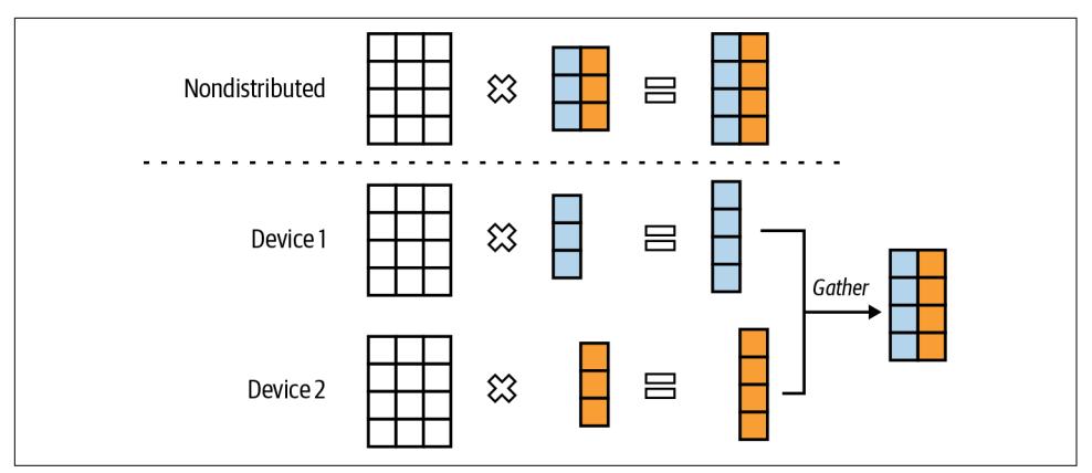
Figure 9-18. Tensor parallelism for matrix multiplication.

Another way to split a model is pipeline parallelism, which involves dividing a model’s computation into distinct stages and assigning each stage to a different device. As data flows through the model, each stage processes one part while others process subsequent parts, enabling overlapping computations. Figure 9-19 shows what pipeline parallelism looks like on four machines.

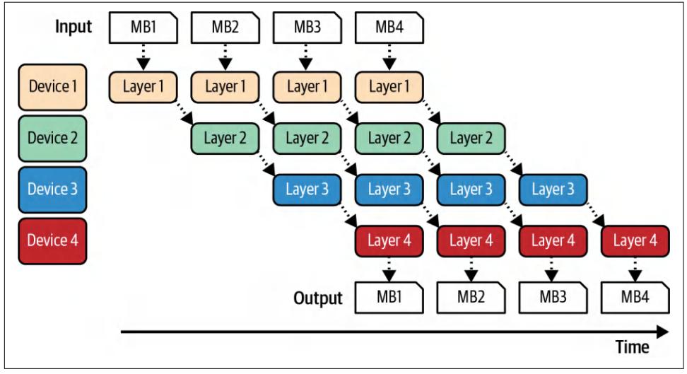
Figure 9-19. Pipeline parallelism enables model splits to be executed in parallel.

Figure 9-19 shows a batch can be split into smaller micro-batches. After a microbatch is processed on one machine, its output is passed onto the next part of the model on the next machine.

While pipeline parallelism enables serving large models on multiple machines, it increases the total latency for each request due to extra communication between pipeline stages. Therefore, for applications with strict latency requirements, pipeline parallelism is typically avoided in favor of replica parallelism. However, pipeline par‐ allelism is commonly used in training since it can help increase throughput.

Two techniques that are less common but might warrant a quick mention to illustrate the diversity of techniques are context parallelism and sequence parallelism. They were both developed to make long input sequence processing more efficient, includ‐ ing context parallelism and sequence parallelism.

In context parallelism, the input sequence itself is split across different devices to be processed separately. For example, the first half of the input is processed on machine 1 and the second half on machine 2.

In sequence parallelism, operators needed for the entire input are split across machines. For example, if the input requires both attention and feedforward compu‐ tation, attention might be processed on machine 1 while feedforward is processed on machine 2.

Summary

A model’s usability depends heavily on its inference cost and latency. Cheaper infer‐ ence makes AI-powered decisions more affordable, while faster inference enables the integration of AI into more applications. Given the massive potential impact of infer‐ ence optimization, it has attracted many talented individuals who continually come up with innovative approaches.

Before we start making things more efficient, we need to understand how efficiency is measured. This chapter started with common efficiency metrics for latency, through‐ put, and utilization. For language model-based inference, latency can be broken into time to first token (TTFT), which is influenced by the prefilling phase, and time per output token (TPOT), which is influenced by the decoding phase. Throughput met‐ rics are directly related to cost. There’s a trade-off between latency and throughput. You can potentially reduce cost if you’re okay with increased latency, and reducing latency often involves increasing cost.

How efficiently a model can run depends on the hardware it is run on. For this rea‐ son, this chapter also provided a quick overview of AI hardware and what it takes to optimize models on different accelerators.

The chapter then continued with different techniques for inference optimization. Given the availability of model APIs, most application developers will use these APIs with their built-in optimization instead of implementing these techniques them‐ selves. While these techniques might not be relevant to all application developers, I believe that understanding what techniques are possible can be helpful for evaluating the efficiency of model APIs.

This chapter also focused on optimization at the model level and the inference service level. Model-level optimization often requires changing the model itself, which can lead to changes in the model behaviors. Inference service-level optimization, on the other hand, typically keeps the model intact and only changes how it’s served.

Model-level techniques include model-agnostic techniques like quantization and dis‐ tillation. Different model architectures require their own optimization. For example, because a key bottleneck of transformer models is in the attention mechanism, many optimization techniques involve making attention more efficient, including KV cache management and writing attention kernels. A big bottleneck for an autoregressive language model is in its autoregressive decoding process, and consequently, many techniques have been developed to address it, too.

Inference service-level techniques include various batching and parallelism strategies. There are also techniques developed especially for autoregressive language models, including prefilling/decoding decoupling and prompt caching.

The choice of optimization techniques depends on your workloads. For example, KV caching is significantly more important for workloads with long contexts than those with short contexts. Prompt caching, on the other hand, is crucial for workloads involving long, overlapping prompt segments or multi-turn conversations. The choice also depends on your performance requirements. For instance, if low latency is a higher priority than cost, you might want to scale up replica parallelism. While more replicas require additional machines, each machine handles fewer requests, allowing it to allocate more resources per request and, thus, improve response time.

However, across various use cases, the most impactful techniques are typically quan‐ tization (which generally works well across models), tensor parallelism (which both reduces latency and enables serving larger models), replica parallelism (which is rela‐ tively straightforward to implement), and attention mechanism optimization (which can significantly accelerate transformer models).

Inference optimization concludes the list of model adaptation techniques covered in this book. The next chapter will explore how to integrate these techniques into a cohesive system.

CHAPTER 10 AI Engineering Architecture and User Feedback

So far, this book has covered a wide range of techniques to adapt foundation models to specific applications. This chapter will discuss how to bring these techniques together to build successful products.

Given the wide range of AI engineering techniques and tools available, selecting the right ones can feel overwhelming. To simplify this process, this chapter takes a grad‐ ual approach. It starts with the simplest architecture for a foundation model applica‐ tion, highlights the challenges of that architecture, and gradually adds components to address them.

We can spend eternity reasoning about how to build a successful application, but the only way to find out if an application actually achieves its goal is to put it in front of users. User feedback has always been invaluable for guiding product development, but for AI applications, user feedback has an even more crucial role as a data source for improving models. The conversational interface makes it easier for users to give feedback but harder for developers to extract signals. This chapter will discuss differ‐ ent types of conversational AI feedback and how to design a system to collect the right feedback without hurting user experience.

AI Engineering Architecture

A full-fledged AI architecture can be complex. This section follows the process that a team might follow in production, starting with the simplest architecture and progres‐ sively adding more components. Despite the diversity of AI applications, they share many common components. The architecture proposed here has been validated at

multiple companies to be general for a wide range of applications, but certain appli‐ cations might deviate.

In its simplest form, your application receives a query and sends it to the model. The model generates a response, which is returned to the user, as shown in Figure 10-1. There is no context augmentation, no guardrails, and no optimization. The Model API box refers to both third-party APIs (e.g., OpenAI, Google, Anthropic) and selfhosted models. Building an inference server for self-hosted models is discussed in Chapter 9.

Figure 10-1. The simplest architecture for running an AI application.

From this simple architecture, you can add more components as needs arise. The process might look as follows:

1. Enhance context input into a model by giving the model access to external data sources and tools for information gathering.
1. Put in guardrails to protect your system and your users.
1. Add model router and gateway to support complex pipelines and add more security.
1. Optimize for latency and costs with caching.
1. Add complex logic and write actions to maximize your system’s capabilities.

This chapter follows the progression I commonly see in production. However, every‐ one’s needs are different. You should follow the order that makes the most sense for your application.

Monitoring and observability, which are integral to any application for quality con‐ trol and performance improvement, will be discussed at the end of this process. Orchestration, chaining all these components together, will be discussed after that.

Step 1. Enhance Context

The initial expansion of a platform usually involves adding mechanisms to allow the system to construct the relevant context needed by the model to answer each query. As discussed in Chapter 6, context can be constructed through various retrieval mechanisms, including text retrieval, image retrieval, and tabular data retrieval.

Context can also be augmented using tools that allow the model to automatically gather information through APIs such as web search, news, weather, events, etc.

Context construction is like feature engineering for foundation models. It gives the model the necessary information to produce an output. Due to its central role in a system’s output quality, context construction is almost universally supported by model API providers. For example, providers like OpenAI, Claude, and Gemini allow users to upload files and allow their models to use tools.

However, just like models differ in their capabilities, these providers differ in their context construction support. For example, they might have limitations on what types of documents and how many you can upload. A specialized RAG solution might let you upload as many documents as your vector database can accommodate, but a generic model API might let you upload only a small number of documents. Different frameworks also differ in their retrieval algorithms and other retrieval con‐ figurations, like chunk sizes. Similarly, for tool use, solutions also differ in the types of tools they support and the modes of execution, such as whether they support par‐ allel function execution or long-running jobs.

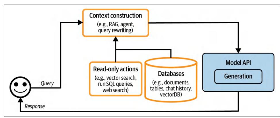
With context construction, the architecture now looks like Figure 10-2.

Figure 10-2. A platform architecture with context construction.

Step 2. Put in Guardrails

Guardrails help mitigate risks and protect you and your users. They should be placed whenever there are exposures to risks. In general, they can be categorized into guard‐ rails around inputs and outputs.

Input guardrails

Input guardrails typically protect against two types of risks: leaking private informa‐ tion to external APIs and executing bad prompts that compromise your system. Chapter 5 discusses many different ways attackers can exploit an application through prompt hacks and how to defend your application against them. While you can miti‐ gate risks, they can never be fully eliminated, due to the inherent nature of how mod‐ els generate responses as well as unavoidable human failures.

Leaking private information to external APIs is a risk specific to using external model APIs when you need to send your data outside your organization. This might happen for many reasons, including the following:

An employee copies the company’s secret or a user’s private information into a prompt and sends it to a third-party API.¹
An application developer puts the company’s internal policies and data into the application’s system prompt.
A tool retrieves private information from an internal database and adds it to the context.

There’s no airtight way to eliminate potential leaks when using third-party APIs. However, you can mitigate them with guardrails. You can use one of the many avail‐ able tools that automatically detect sensitive data. What sensitive data to detect is specified by you. Common sensitive data classes are the following:

Personal information (ID numbers, phone numbers, bank accounts)
Human faces
Specific keywords and phrases associated with the company’s intellectual prop‐ erty or privileged information

Many sensitive data detection tools use AI to identify potentially sensitive informa‐ tion, such as determining if a string resembles a valid home address. If a query is found to contain sensitive information, you have two options: block the entire query or remove the sensitive information from it. For instance, you can mask a user’s phone number with the placeholder [PHONE NUMBER]. If the generated response contains this placeholder, use a PII reverse dictionary that maps this placeholder to the original information so that you can unmask it, as shown in Figure 10-3.

¹ An example is when a Samsung employee put Samsung’s proprietary information into ChatGPT, accidentally leaking the company’s secrets.

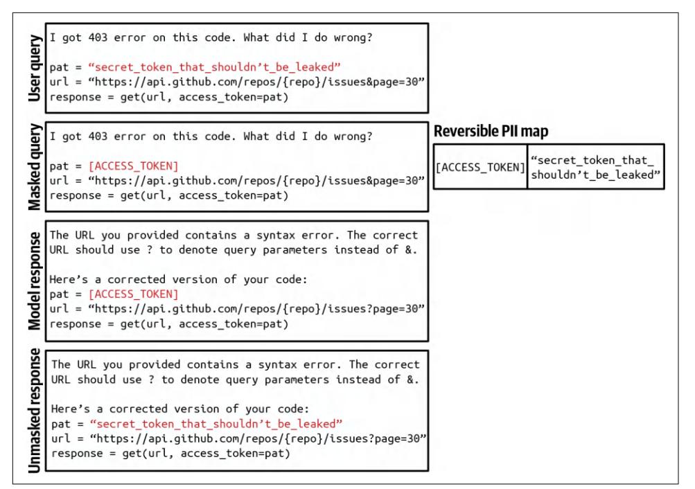
Figure 10-3. An example of masking and unmasking PII information using a reverse PII map to avoid sending it to external APIs.

Output guardrails

A model can fail in many different ways. Output guardrails have two main functions:

Catch output failures
Specify the policy to handle different failure modes

To catch outputs that fail to meet your standards, you need to understand what fail‐ ures look like. The easiest failure to detect is when a model returns an empty response when it shouldn’t.² Failures look different for different applications. Here are some common failures in the two main categories: quality and security. Quality failures are discussed in Chapter 4, and security failures are discussed in Chapter 5. I’ll quickly mention a few of these failures as a recap:

² It’s possible that users ask the model to return an empty response.

Quality
- Malformatted responses that don’t follow the expected output format. For example, the application expects JSON, and the model generates invalid JSON.
- Factually inconsistent responses hallucinated by the model.
- Generally bad responses. For example, you ask the model to write an essay, and that essay is just bad.
Security
- Toxic responses that contain racist content, sexual content, or illegal activities.
- Responses that contain private and sensitive information.
- Responses that trigger remote tool and code execution.
- Brand-risk responses that mischaracterize your company or your competitors.

Recall from Chapter 5 that for security measurements, it’s important to track not only the security failures but also the false refusal rate. It’s possible to have systems that are too secure, e.g., one that blocks even legitimate requests, interrupting user workloads and causing user frustration.

Many failures can be mitigated by simple retry logic. AI models are probabilistic, which means that if you try a query again, you might get a different response. For example, if the response is empty, try again X times or until you get a nonempty response. Similarly, if the response is malformatted, try again until the response is correctly formatted.

This retry policy, however, can incur extra latency and cost. Each retry means another round of API calls. If the retry is carried out after failure, the user-perceived latency will double. To reduce latency, you can make calls in parallel. For example, for each query, instead of waiting for the first query to fail before retrying, you send this query to the model twice at the same time, get back two responses, and pick the better one. This increases the number of redundant API calls while keeping latency manageable.

It’s also common to fall back on humans for tricky requests. For example, you can transfer the queries that contain specific phrases to human operators. Some teams use a specialized model to decide when to transfer a conversation to humans. One team, for instance, transfers a conversation to human operators when their sentiment analysis model detects anger in users’ messages. Another team transfers a conversa‐ tion after a certain number of turns to prevent users from getting stuck in a loop.

Guardrail implementation

Guardrails come with trade-offs. One is the reliability versus latency trade-off. While acknowledging the importance of guardrails, some teams told me that latency is more important. The teams decided not to implement guardrails because they can signifi‐ cantly increase the application’s latency.³

Output guardrails might not work well in the stream completion mode. By default, the whole response is generated before being shown to the user, which can take a long time. In the stream completion mode, new tokens are streamed to the user as they are generated, reducing the time the user has to wait to see the response. The downside is that it’s hard to evaluate partial responses, so unsafe responses might be streamed to users before the system guardrails can determine that they should be blocked.

How many guardrails you need to implement also depends on whether you self-host your models or use third-party APIs. While you can implement guardrails on top of both, third-party APIs can reduce the guardrails you need to implement since API providers typically provide many guardrails out of the box for you. At the same time, self-hosting means that you don’t need to send requests ex t ernally, which reduces the need for many types o f input guardrails.

Given the many different places where an application might fail, guardrails can be implemented at many different levels. Model providers give their models guardrails to make their models better and more secure. However, model providers have to bal‐ ance safety and flexibility. Restrictions might make a model safer but can also make it less usable for specific use cases.

Guardrails can also implemented by application developers. Many techniques are dis‐ cussed in “Defenses Against Prompt Attacks” on page 248. Guardrail solutions that you can use out of the box include Meta’s Purple Llama, NVIDIA’s NeMo Guard‐ rails, Azure’s PyRIT, Azure’s AI content filters, the Perspective API, and OpenAI’s content moderation API. Due to the overlap of risks in inputs and outputs, a guard‐ rail solution will likely provide protection for both inputs and outputs. Some model gateways also provide guardrail functionalities, as discussed in the next section.

With guardrails, the architecture looks like Figure 10-4. I put scorers under model APIs since scorers are often AI-powered, even if scorers are typically smaller and faster than generative models. However, scorers can also be placed in the output guardrails box.

³ A few early readers told me that the idea of ignoring guardrails in favor of latency gave them nightmares.

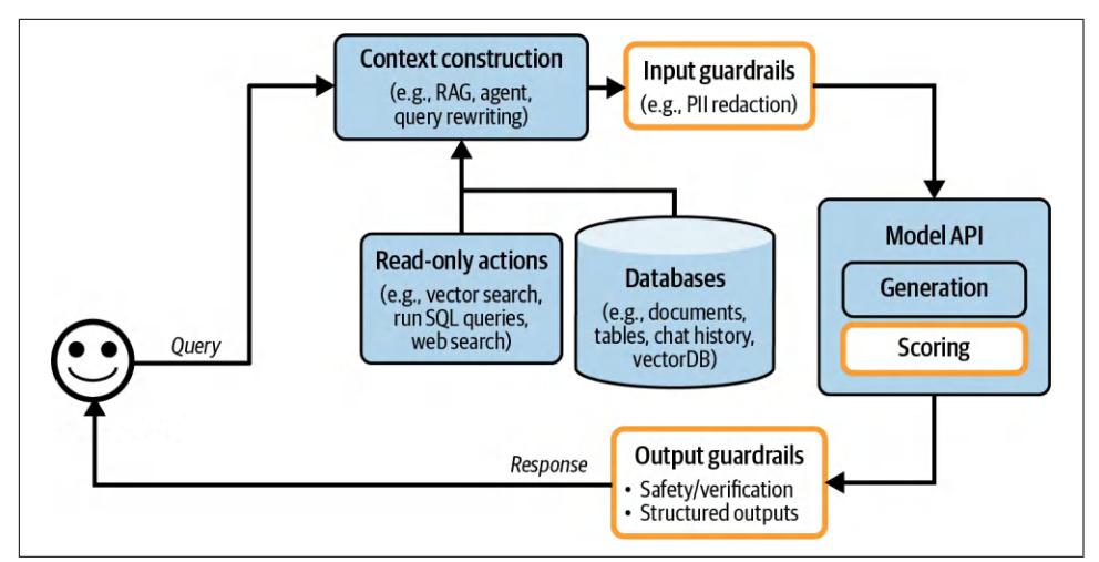
Figure 10-4. Application architecture with the addition of input and output guardrails.

Step 3. Add Model Router and Gateway

As applications grow to involve more models, routers and gateways emerge to help you manage the complexity and costs of serving multiple models.

Router

Instead of using one model for all queries, you can have different solutions for differ‐ ent types of queries. This approach has several benefits. First, it allows specialized models, which can potentially perform better than a general-purpose model for spe‐ cific queries. For example, you can have one model specialized in technical trouble‐ shooting and another specialized in billing. Second, this can help you save costs. Instead of using one expensive model for all queries, you can route simpler queries to cheaper models.

A router typically consists of an intent classifier that predicts what the user is trying to do. Based on the predicted intent, the query is routed to the appropriate solution. As an example, consider different intentions relevant to a customer support chatbot:

If the user wants to reset the password, route them to the FAQ page about recov‐ ering the password.
If the request is to correct a billing mistake, route it to a human operator.
If the request is about troubleshooting a technical issue, route it to a chatbot spe‐ cialized in troubleshooting.

An intent classifier can prevent your system from engaging in out-of-scope conversa‐ tions. If the query is deemed inappropriate, the chatbot can politely decline to respond using one of the stock responses without wasting an API call. For example, if the user asks who you would vote for in the upcoming election, a chatbot can respond with: “As a chatbot, I don’t have the ability to vote. If you have questions about our products, I’d be happy to help.”

An intent classifier can help the system detect ambiguous queries and ask for clarifi‐ cation. For example, in response to the query “Freezing”, the system might ask, “Do you want to freeze your account or are you talking about the weather?” or simply ask, “I’m sorry. Can you elaborate?”

Other routers can aid the model in deciding what to do next. For example, for an agent capable of multiple actions, a router can take the form of a next-action predic‐ tor: should the model use a code interpreter or a search API next? For a model with a memory system, a router can predict which part of the memory hierarchy the model should pull information from. Imagine that a user attaches a document that mentions Melbourne to the current conversation. Later on, the user asks: “What’s the cutest animal in Melbourne?” The model needs to decide whether to rely on the informa‐ tion in the attached document or to search the internet for this query.

Intent classifiers and next-action predictors can be implemented on top of founda‐ tion models. Many teams adapt smaller language models like GPT-2, BERT, and Llama 7B as their intent classifiers. Many teams opt to train even smaller classifiers from scratch. Routers should be fast and cheap so that they can use multiples of them without incurring significant extra latency and cost.

When routing queries to models with varying context limits, the query’s context might need to be adjusted accordingly. Consider a 1,000-token query that is slated for a model with a 4K context limit. The system then takes an action, e.g., a web search, that brings back 8,000-token context. You can either truncate the query’s context to fit the originally intended model or route the query to a model with a larger context limit.

Because routing is usually done by models, I put routing inside the Model API box in Figure 10-5. Like scorers, routers are typically smaller than models used for generation.

Grouping routers together with other models makes models easier to manage. However, it’s important to note that routing often happens before retrieval. For example, before retrieval, a router can help determine if a query is in-scope and, if yes, if it needs retrieval. Routing can happen after retrieval, too, such as determining if a query should be routed to a human operator. However, routing - retrieval generation - scoring is a much more common AI application pattern.

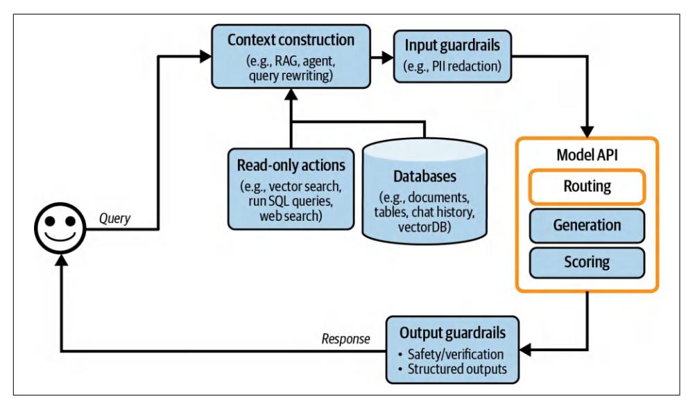
Figure 10-5. Routing helps the system use the optimal solution for each query.

Gateway

A model gateway is an intermediate layer that allows your organization to interface with different models in a unified and secure manner. The most basic functionality of a model gateway is to provide a unified interface to different models, including selfhosted models and models behind commercial APIs. A model gateway makes it eas‐ ier to maintain your code. If a model API changes, you only need to update the gateway instead of updating all applications that depend on this API. Figure 10-6 shows a high-level visualization of a model gateway.

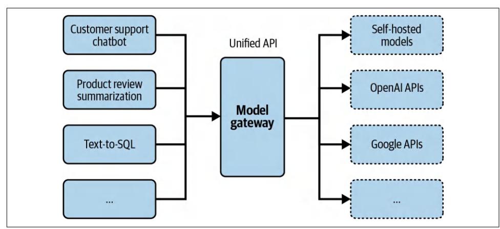
Figure 10-6. A model gateway provides a unified interface to work with different models.

In its simplest form, a model gateway is a unified wrapper. The following code exam‐ ple gives you an idea of how a model gateway might be implemented. It’s not meant to be functional, as it doesn’t contain any error checking or optimization:

import google.generativeai as genai
import openai
def openai_model(input_data, model_name, max_tokens):
 openai.api_key = os.environ["OPENAI_API_KEY"]
 response = openai.Completion.create(
 engine=model_name,
 prompt=input_data,
 max_tokens=max_tokens
 )
 return {"response": response.choices[0].text.strip()}
def gemini_model(input_data, model_name, max_tokens):
 genai.configure(api_key=os.environ["GOOGLE_API_KEY"])
 model = genai.GenerativeModel(model_name=model_name)
 response = model.generate_content(input_data, max_tokens=max_tokens)
 return {"response": response["choices"][0]["message"]["content"]}
@app.route('/model', methods=['POST'])
def model_gateway():
 data = request.get_json()
 model_type = data.get("model_type")
 model_name = data.get("model_name")
 input_data = data.get("input_data")
 max_tokens = data.get("max_tokens")
 if model_type == "openai":
 result = openai_model(input_data, model_name, max_tokens)
 elif model_type == "gemini":
 result = gemini_model(input_data, model_name, max_tokens)
 return jsonify(result)

A model gateway provides access control and cost management. Instead of giving everyone who wants access to the OpenAI API your organizational tokens, which can be easily leaked, you give people access only to the model gateway, creating a central‐ ized and controlled point of access. The gateway can also implement fine-grained access controls, specifying which user or application should have access to which model. Moreover, the gateway can monitor and limit the usage of API calls, prevent‐ ing abuse and managing costs effectively.

A model gateway can also be used to implement fallback policies to overcome rate limits or API failures (the latter is unfortunately common). When the primary API is unavailable, the gateway can route requests to alternative models, retry after a short wait, or handle failures gracefully in other ways. This ensures that your application can operate smoothly without interruptions.

Since requests and responses are already flowing through the gateway, it’s a good place to implement other functionalities, such as load balancing, logging, and analyt‐ ics. Some gateways even provide caching and guardrails.

Given that gateways are relatively straightforward to implement, there are many offthe-shelf gateways. Examples include Portkey’s AI Gateway, MLflow AI Gateway, Wealthsimple’s LLM Gateway, TrueFoundry, Kong, and Cloudflare.

In our architecture, the gateway now replaces the model API box, as shown in Figure 10-7.

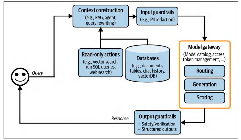
Figure 10-7. The architecture with the added routing and gateway modules.

A similar abstraction layer, such as a tool gateway, can also be use‐ ful for accessing a wide range of tools. It’s not discussed in this book since it’s not a common pattern as of this writing.

Step 4. Reduce Latency with Caches

Caching has long been integral to software applications to reduce latency and cost. Many ideas from software caching can be used for AI applications. Inference caching techniques, including KV caching and prompt caching, are discussed in Chapter 9. This section focuses on system caching. Because caching is an old technology with a large amount of existing literature, this book will cover it only in broad strokes. In general, there are two major system caching mechanisms: exact caching and semantic caching.

Exact caching

With exact caching, cached items are used only when these exact items are requested. For example, if a user asks a model to summarize a product, the system checks the cache to see if a summary of this exact product exists. If yes, fetch this summary. If not, summarize the product and cache the summary.

Exact caching is also used for embedding-based retrieval to avoid redundant vector search. If an incoming query is already in the vector search cache, fetch the cached result. If not, perform a vector search for this query and cache the result.

Caching is especially appealing for queries that involve multiple steps (e.g., chain-ofthought) and/or time-consuming actions (e.g., retrieval, SQL execution, or web search).

An exact cache can be implemented using in-memory storage for fast retrieval. How‐ ever, since in-memory storage is limited, a cache can also be implemented using data‐ bases like PostgreSQL, Redis, or tiered storage to balance speed and storage capacity. Having an eviction policy is crucial to manage the cache size and maintain perfor‐ mance. Common eviction policies include Least Recently Used (LRU), Least Fre‐ quently Used (LFU), and first in, first out (FIFO).

How long to keep a query in the cache depends on how likely this query is to be called again. User-specific queries, such as “What’s the status of my recent order?”, are less likely to be reused by other users and, therefore, shouldn’t be cached. Simi‐ larly, it makes less sense to cache time-sensitive queries such as “How’s the weather?” Many teams train a classifier to predict whether a query should be cached.

Caching, when not properly handled, can cause data leaks. Imagine you work for an ecommerce site, and user X asks a seemingly generic question such as: “What is the return policy for electronics products?” Because your return policy depends on the user’s mem‐ bership, the system first retrieves user X’s information and then generates a response containing X’s information. Mistaking this query for a generic question, the system caches the answer. Later, when user Y asks the same question, the cached result is returned, revealing X’s information to Y.

Semantic caching

Unlike in exact caching, cached items are used even if they are only semantically sim‐ ilar, not identical, to the incoming query. Imagine one user asks, “What’s the capital of Vietnam?” and the model answers, “Hanoi”. Later, another user asks, “What’s the capital city of Vietnam?”, which is semantically the same question but with slightly different wording. With semantic caching, the system can reuse the answer from the first query instead of computing the new query from scratch. Reusing similar queries

increases the cache’s hit rate and potentially reduces cost. However, semantic caching can reduce your model’s performance.

Semantic caching works only if you have a reliable way of determining if two queries are similar. One common approach is to use semantic similarity, as discussed in Chapter 3. As a refresh, semantic similarity works as follows:

1. For each query, generate its embedding using an embedding model.
1. Use vector search to find the cached embedding with the highest similar score to the current query embedding. Let’s say this similarity score is X.
1. If X is higher than a certain similarity threshold, the cached query is considered similar, and the cached results are returned. If not, process this current query and cache it together with its embedding and results.

This approach requires a vector database to store the embeddings of cached queries.

Compared to other caching techniques, semantic caching’s value is more dubious because many of its components are prone to failure. Its success relies on high-quality embeddings, functional vector search, and a reliable similarity metric. Setting the right similarity threshold can also be tricky, requiring a lot of trial and error. If the system mistakes the incoming query for one similar to another query, the returned response, fetched from the cache, will be incorrect.

In addition, semantic cache can be time-consuming and compute-intensive, as it involves a vector search. The speed and cost of this vector search depend on the size of your cached embeddings.

Semantic cache might still be worthwhile if the cache hit rate is high, meaning that a good portion of queries can be effectively answered by leveraging the cached results. However, before incorporating the complexities of a semantic cache, make sure to evaluate the associated efficiency, cost, and performance risks.

With the added cache systems, the platform looks like Figure 10-8. A KV cache and prompt cache are typically implemented by model API providers, so they aren’t shown in this image. To visualize them, I’d put them in the Model API box. There’s a new arrow to add generated responses to the cache.

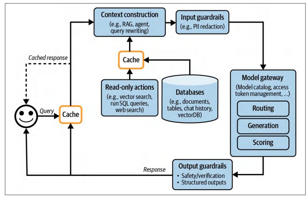
Figure 10-8. An AI application architecture with the added caches.

Step 5. Add Agent Patterns

The applications discussed so far are still fairly simple. Each query follows a sequen‐ tial flow. However, as discussed in Chapter 6, an application flow can be more com‐ plex with loops, parallel execution, and conditional branching. Agentic patterns, discussed in Chapter 6, can help you build complex applications. For example, after the system generates an output, it might determine that it hasn’t accomplished the task and that it needs to perform another retrieval to gather more information. The original response, together with the newly retrieved context, is passed into the same model or a different one. This creates a loop, as shown in Figure 10-9.

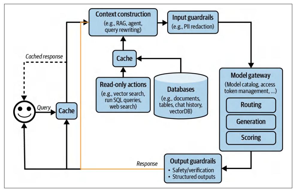
Figure 10-9. The yellow arrow allows the generated response to be fed back into the sys‐ tem, allowing more complex application patterns.

A model’s outputs also can be used to invoke write actions, such as composing an email, placing an order, or initializing a bank transfer. Write actions allow a system to make changes to its environment directly. As discussed in Chapter 6, write actions can make a system vastly more capable but also expose it to significantly more risks. Giving a model access to write actions should be done with the utmost care. With added write actions, the architecture looks like Figure 10-10.

If you’ve followed all the steps so far, your architecture has likely grown quite com‐ plex. While complex systems can solve more tasks, they also introduce more failure modes, making them harder to debug due to the many potential points of failure. The next section will cover best practices for improving system observability.

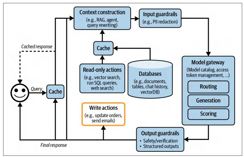
Figure 10-10. An application architecture that enables the system to perform write actions.

Monitoring and Observability

Even though I put observability in its own section, observability should be integral to the design of a product, rather than an afterthought. The more complex a product, the more crucial observability is.

Observability is a universal practice across all software engineering disciplines. It’s a big industry with established best practices and many ready-to-use proprietary and open source solutions.⁴ To avoid reinventing the wheel, I’ll focus on what’s unique to applications built on top of foundation models. The book’s GitHub repository con‐ tains resources for those who want to learn more about observability.⁵

⁴ As of this writing, the aggregated market capitalization of a few of the largest observability companies (Data‐ dog, Splunk, Dynatrace, New Relic) is close to $100 billion.

⁵ My book, Designing Machine Learning Systems (O’Reilly, 2022), also has a chapter on monitoring. An early draft of the chapter is available on my blog at “Data Distribution Shifts and Monitoring”.

The goal of monitoring is the same as the goal of evaluation: to mitigate risks and discover opportunities. Risks that monitoring should help you mitigate include appli‐ cation failures, security attacks, and drifts. Monitoring can help discover opportuni‐ ties for application improvement and cost savings. Monitoring can also help keep you accountable by giving visibility into your system’s performance.

Three metrics can help evaluate the quality of your system’s observability, derived from the DevOps community:

MTTD (mean time to detection): When something bad happens, how long does it take to detect it?
MTTR (mean time to response): After detection, how long does it take to be resolved?
CFR (change failure rate): The percentage of changes or deployments that result in failures requiring fixes or rollbacks. If you don’t know your CFR, it’s time to redesign your platform to make it more observable.

Having a high CFR doesn’t necessarily indicate a bad monitoring system. However, you should rethink your evaluation pipeline so that bad changes are caught before being deployed. Evaluation and monitoring need to work closely together. Evaluation metrics should translate well to monitoring metrics, meaning that a model that does well during evaluation should also do well during monitoring. Issues detected during monitoring should be fed to the evaluation pipeline.

Monitoring Versus Observability

Since the mid-2010s, the industry has embraced the term “observability” instead of “monitoring.” Monitoring makes no assumption about the relationship between the internal state of a system and its outputs. You monitor the external outputs of the sys‐ tem to figure out when something goes wrong inside the system—there’s no guaran‐ tee that the external outputs will help you figure out what goes wrong.

Observability, on the other hand, makes an assumption stronger than traditional monitoring: that a system’s internal states can be inferred from knowledge of its external outputs. When something goes wrong with an observable system, we should be able to figure out what went wrong by looking at the system’s logs and metrics without having to ship new code to the system. Observability is about instrumenting your system in a way that ensures that sufficient information about a system’s run‐ time is collected and analyzed so that when something goes wrong, it can help you figure out what goes wrong.

In this book, I’ll use the term “monitoring” to refer to the act of tracking a system’s information and “observability” to refer to the whole process of instrumentating, tracking, and debugging the system.

Metrics

When discussing monitoring, most people think of metrics. However, metrics them‐ selves aren’t the goal. Frankly, most companies don’t care what your application’s output relevancy score is unless it serves a purpose. The purpose of a metric is to tell you when something is wrong and to identify opportunities for improvement.

Before listing what metrics to track, it’s important to understand what failure modes you want to catch and design your metrics around these failures. For example, if you don’t want your application to hallucinate, design metrics that help you detect hallu‐ cinations. One relevant metric might be whether an application’s output can be infer‐ red from the context. If you don’t want your application to burn through your API credit, track metrics related to API costs, such as the number of input and output tokens per request or your cache’s cost and your cache’s hit rate.

Because foundation models can generate open-ended outputs, there are many ways things can go wrong. Metrics design requires analytical thinking, statistical knowl‐ edge, and, often, creativity. Which metrics you should track are highly applicationspecific.

This book has covered many different types of model quality metrics (Chapters 4–6, and later in this chapter) and many different ways to compute them (Chapters 3 and 5). Here, I’ll do a quick recap.

The easiest types of failures to track are format failures because they are easy to notice and verify. For example, if you expect JSON outputs, track how often the model out‐ puts invalid JSON and, among these invalid JSON outputs, how many can be easily fixed (missing a closing bracket is easy to fix, but missing expected keys is harder).

For open-ended generations, consider monitoring factual consistency and relevant generation quality metrics such as conciseness, creativity, or positivity. Many of these metrics can be computed using AI judges.

If safety is an issue, you can track toxicity-related metrics and detect private and sen‐ sitive information in both inputs and outputs. Track how often your guardrails get triggered and how often your system refuses to answer. Detect abnormal queries to your system, too, since they might reveal interesting edge cases or prompt attacks.

Model quality can also be inferred through user natural language feedback and con‐ versational signals. For example, some easy metrics you can track include the following:

How often do users stop a generation halfway?
What’s the average number of turns per conversation?
What’s the average number of tokens per input? Are users using your application for more complex tasks, or are they learning to be more concise with their prompts?
What’s the average number of tokens per output? Are some models more ver‐ bose than others? Are certain types of queries more likely to result in lengthy answers?
What’s the model’s output token distribution? How has it changed over time? Is the model getting more or less diverse?

Length-related metrics are also important for tracking latency and costs, as longer contexts and responses typically increase latency and incur higher costs.

Each component in an application pipeline has its own metrics. For example, in a RAG application, the retrieval quality is often evaluated using context relevance and context precision. A vector database can be evaluated by how much storage it needs to index the data and how long it takes to query the data.

Given that you’ll likely have multiple metrics, it’s useful to measure how these met‐ rics correlate to each other and, especially, to your business north star metrics, which can be DAU (daily active user), session duration (the length of time a user spends actively engaged with the application), or subscriptions. Metrics that are strongly cor‐ related to your north star might give you ideas on how to improve your north star. Metrics that are not at all correlated might also give you ideas on what not to opti‐ mize for.

Tracking latency is essential for understanding the user experience. Common latency metrics, as discussed in Chapter 9, include:

Time to first token (TTFT): the time it takes for the first token to be generated.
Time per output token (TPOT): the time it takes to generate each output token.
Total latency: the total time required to complete a response.

Track all these metrics per user to see how your system scales with more users.

You’ll also want to track costs. Cost-related metrics are the number of queries and the volume of input and output tokens, such as tokens per second (TPS). If you use an API with rate limits, tracking the number of requests per second is important to ensure you stay within your allocated limits and avoid potential service interruptions.

When calculating metrics, you can choose between spot checks and exhaustive checks. Spot checks involve sampling a subset of data to quickly identify issues, while exhaustive checks evaluate every request for a comprehensive performance view. The choice depends on your system’s requirements and available resources, with a combi‐ nation of both providing a balanced monitoring strategy.

When computing metrics, ensure they can be broken down by relevant axes, such as users, releases, prompt/chain versions, prompt/chain types, and time. This granular‐ ity helps in understanding performance variations and identifying specific issues.

Logs and traces

Metrics are typically aggregated. They condense information from events that occur in your system over time. They help you understand, at a glance, how your system is doing. However, there are many questions that metrics can’t help you answer. For example, after seeing a spike in a specific activity, you might wonder: “Has this hap‐ pened before?” Logs can help you answer this question.

If metrics are numerical measurements representing attributes and events, logs are an append-only record of events. In production, a debugging process might look like this:

1. Metrics tell you something went wrong five minutes ago, but they don’t tell you what happened.
1. You look at the logs of events that took place around five minutes ago to figure out what happened.
1. Correlate the errors in the logs to the metrics to make sure that you’ve identified the right issue.

For fast detection, metrics need to be computed quickly. For fast response, logs need to be readily available and accessible. If your logs are 15 minutes delayed, you will have to wait for the logs to arrive to track down an issue that happened 5 minutes ago.

Because you don’t know exactly what logs you’ll need to look at in the future, the general rule for logging is to log everything. Log all the configurations, including the model API endpoint, model name, sampling settings (temperature, top-p, top-k, stopping condition, etc.), and the prompt template.

Log the user query, the final prompt sent to the model, the output, and the inter‐ mediate outputs. Log if it calls any tool. Log the tool outputs. Log when a component starts, ends, when something crashes, etc. When recording a piece of log, make sure to give it tags and IDs that can help you know where this log comes from in the system.

Logging everything means that the amount of logs you have can grow very quickly. Many tools for automated log analysis and log anomaly detection are powered by AI.

While it’s impossible to process logs manually, it’s useful to manually inspect your production data daily to get a sense of how users are using your application. Shankar et al., (2024) found that the developers’ perceptions of what constitutes good and bad outputs change as they interact with more data, allowing them to both rewrite their prompts to increase the chance of good responses and update their evaluation pipe‐ line to catch bad responses.

If logs are a series of disjointed events, traces are reconstructed by linking related events together to form a complete timeline of a transaction or process, showing how each step connects from start to finish. In short, a trace is the detailed recording of a request’s execution path through various system components and services. In an AI application, tracing reveals the entire process from when a user sends a query to when the final response is returned, including the actions the system takes, the docu‐ ments retrieved, and the final prompt sent to the model. It should also show how much time each step takes and its associated cost, if measurable. Figure 10-11 is a vis‐ ualization of a request’s trace in LangSmith.

Ideally, you should be able to trace each query’s transformation step-by-step through the system. If a query fails, you should be able to pinpoint the exact step where it went wrong: whether it was incorrectly processed, the retrieved context was irrele‐ vant, or the model generated a wrong response.

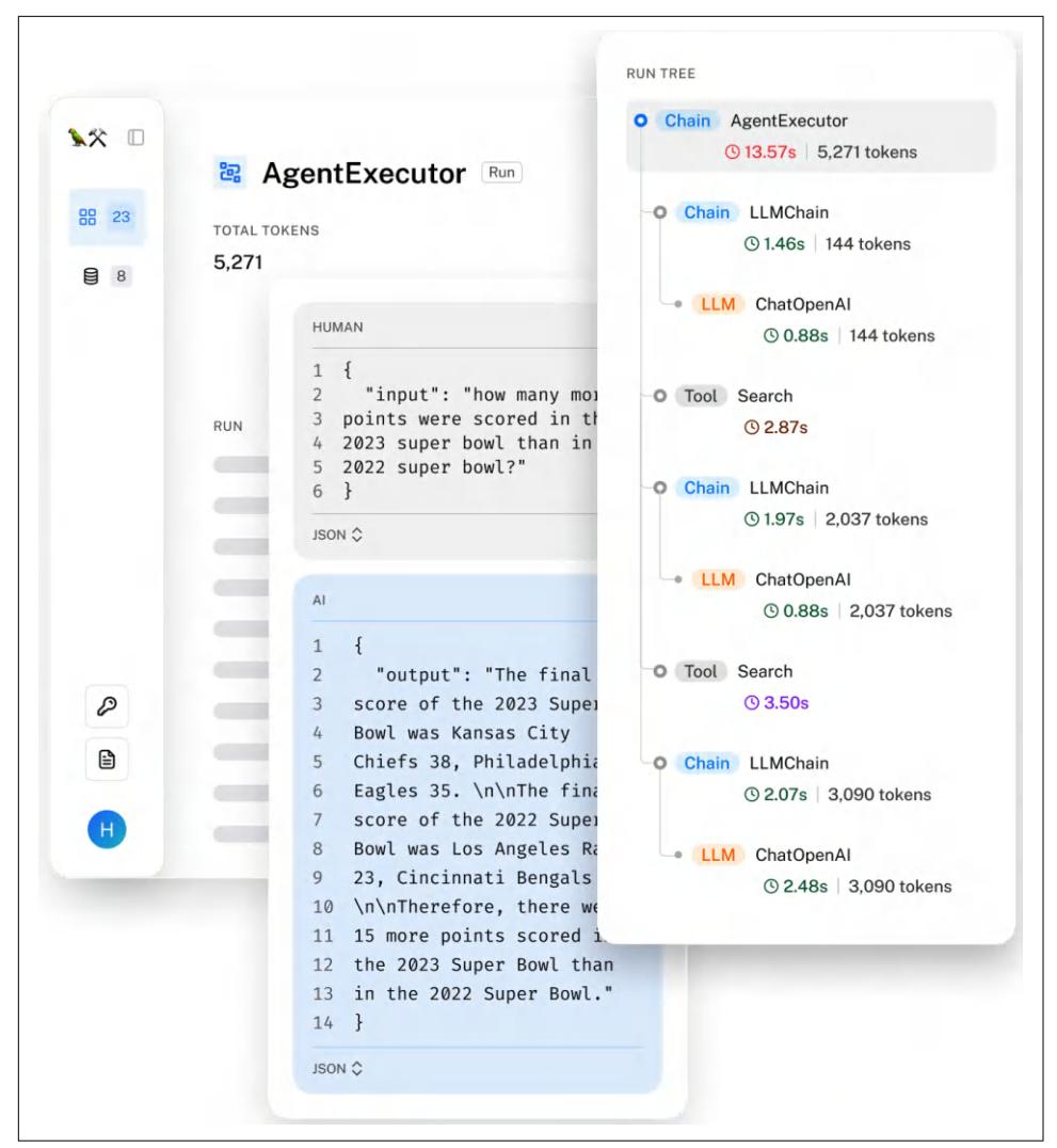
Figure 10-11. A request trace visualized by LangSmith.

Drift detection

The more parts a system has, the more things that can change. In an AI application these can be:

System prompt changes

There are many reasons why your application’s system prompt might change without your knowing. The system prompt could’ve been built on top of a prompt template, and that prompt template was updated. A coworker could’ve found a typo and fixed it. A simple logic should be sufficient to catch when your application’s system prompt changes.

User behavior changes

Over time, users adapt their behaviors to the technology. For example, people have already figured out how to frame their queries to get better results on Goo‐ gle Search or how to make their articles rank higher on search results. People liv‐ ing in areas with self-driving cars have already figured out how to bully selfdriving cars into giving them the right of way (Liu et al., 2020). It’s likely that your users will change their behaviors to get better results out of your applica‐ tion. For example, your users might learn to write instructions to make the responses more concise. This might cause a gradual drop in response length over time. If you look only at metrics, it might not be obvious what caused this grad‐ ual drop. You need investigations to understand the root cause.

Underlying model changes

When using a model through an API, it’s possible that the API remains unchanged while the underlying model is updated. As mentioned in Chapter 4, model providers might not always disclose these updates, leaving it to you to detect any changes. Different versions of the same API can have a significant impact on performance. For instance, Chen et al. (2023) observed notable differ‐ ences in benchmark scores between the March 2023 and June 2023 versions of GPT-4 and GPT-3.5. Likewise, Voiceflow reported a 10% performance drop when switching from the older GPT-3.5-turbo-0301 to the newer GPT-3.5 turbo-1106.

AI Pipeline Orchestration

An AI application can get fairly complex, consisting of multiple models, retrieving data from many databases, and having access to a wide range of tools. An orchestra‐ tor helps you specify how these different components work together to create an endto-end pipeline. It ensures that data flows seamlessly between components. At a high level, an orchestrator operates in two steps, components definition and chaining:

Components definition

You need to tell the orchestrator what components your system uses, including different models, external data sources for retrieval, and tools that your system can use. A model gateway can make it easier to add a model.⁶ You can also tell the orchestrator if you use any tools for evaluation and monitoring.

⁶ Because of this, some orchestrator tools want to be gateways. In fact, so many tools seem to want to become end-to-end platforms that do everything.

Chaining

Chaining is basically function composition: it combines different functions (components) together. In chaining (pipelining), you tell the orchestrator the steps your system takes from receiving the user query until completing the task. Here’s an example of the steps:

1. Process the raw query.
1. Retrieve the relevant data based on the processed query.
1. Combine the original query and the retrieved data to create a prompt in the format expected by the model.
1. The model generates a response based on the prompt.
1. Evaluate the response.
1. If the response is considered good, return it to the user. If not, route the query to a human operator.

The orchestrator is responsible for passing data between components. It should pro‐ vide toolings that help ensure that the output from the current step is in the format expected by the next step. Ideally, it should notify you when this data flow is disrup‐ ted due to errors such as component failures or data mismatch failures.

An AI pipeline orchestrator is different from a ge neral workflow orchestrator, like Airflow or Metaflow.

When designing the pipeline for an application with strict latency requirements, try to do as much in parallel as possible. For example, if you have a routing component (deciding where to send a query) and a PII removal component, both can be done at the same time.

There are many AI orchestration tools, including LangChain, LlamaIndex, Flowise, Langflow, and Haystack. Because retrieval and tool use are common application pat‐ terns, many RAG and agent frameworks are also orchestration tools.

While it’s tempting to jump straight to an orchestration tool when starting a project, you might want to start building your application without one first. Any external tool brings additional complexity. An orchestrator can abstract away critical details of how your system works, making it hard to understand and debug your system.

As you advance to the later stages of your application development process, you might decide that an orchestrator can make your life easier. Here are three aspects to keep in mind when evaluating orchestrators:

Integration and extensibility

Evaluate whether the orchestrator supports the components you’re already using or might adopt in the future. For example, if you want to use a Llama model, check if the orchestrator supports that. Given how many models, databases, and frameworks there are, it’s impossible for an orchestrator to support everything. Therefore, you’ll also need to consider an orchestrator’s extensibility. If it doesn’t support a specific component, how hard is it to change that?

Support for complex pipelines

As your applications grow in complexity, you might need to manage intricate pipelines involving multiple steps and conditional logic. An orchestrator that supports advanced features like branching, parallel processing, and error han‐ dling will help you manage these complexities efficiently.

Ease of use, performance, and scalability

Consider the user-friendliness of the orchestrator. Look for intuitive APIs, com‐ prehensive documentation, and strong community support, as these can signifi‐ cantly reduce the learning curve for you and your team. Avoid orchestrators that initiate hidden API calls or introduce latency to your applications. Additionally, ensure that the orchestrator can scale effectively as the number of applications, developers, and traffic grows.

User Feedback

User feedback has always played a critical role in software applications in two key ways: evaluating the application’s performance and informing its development. How‐ ever, in AI applications, user feedback takes on an even more significant role. User feedback is proprietary data, and data is a competitive advantage. A well-designed user feedback system is necessary to create the data flywheel discussed in Chapter 8. 7

User feedback can be used not only to personalize models for individual users but also to train future iterations of the models. As data becomes increasingly scarce, pro‐ prietary data is more valuable than ever. A product that launches quickly and attracts users early can gather data to continually improve models, making it difficult for competitors to catch up.

⁷ One key disadvantage of launching an open source application instead of a commercial application is that it’s a lot harder to collect user feedback. Users can take your open source application and deploy it themselves, and you have no idea how the application is used.

It’s important to remember that user feedback is user data. Leveraging user feedback requires the same cautions needed when leveraging any data. User privacy should be respected. Users have the right to know how their data is being used.

Extracting Conversational Feedback

Traditionally, feedback can be explicit or implicit. Explicit feedback is information users provide in response to explicit requests for feedback in the application, such as thumbs up/thumbs down, upvote/downvote, star rating, or a yes/no answer to the question “Did we solve your problem?” Explicit feedback is fairly standard across applications—there are only so many ways you can ask a person if they like some‐ thing. Therefore, explicit feedback is better understood.

Implicit feedback is information inferred from user actions. For example, if someone buys a product recommended to them, it means it was a good recommendation. What can be considered implicit feedback depends on what actions a user can do within each application and is, therefore, highly application-dependent. Foundation models enable a new world of applications and, with them, many genres of implicit feedback.

The conversational interface that many AI applications use makes it easier for users to give feedback. Users can encourage good behaviors and correct errors the same way they would give feedback in daily dialogues. The language that a user uses to give directions to AI can convey feedback about both the application’s performance and the user’s preference.

As an example, imagine you’re using an AI assistant to help you plan your trip to Australia. You ask the AI to find a hotel for three nights in Sydney. It responds with three recommendations as follows:

Here are three hotel suggestions in Sydney for a 3-night stay:

1. Historic Rocks Boutique Hotel (The Rocks)
- Price: ~$400/night
- Neighborhood: Charming streets and close to iconic sights.
1. Stylish Surry Hills House Hotel (Surry Hills)
- Price: ~$200/night
- Neighborhood: Trendy, with vibrant cafes and art galleries.
1. Chill Bondi Beachside Hotel (Bondi Beach)
- Price: ~$300/night
- Neighborhood: Beachside, ideal for relaxation and city exploration.

How you respond to these three recommendations reveals your preference. For example, if you respond with “Yes book me the one close to galleries”, you show an interest in art. On the other hand, the response “Is there nothing under $200?” reveals a price-conscious preference and suggests that the assistant doesn’t quite get you yet.

User feedback, extracted from conversations, can be used for evaluation, develop‐ ment, and personalization:

Evaluation: derive metrics to monitor the application
Development: train the future models or guide their development
Personalization: personalize the application to each user

Implicit conversational feedback can be inferred from both the content of user mes‐ sages and their patterns of communication. Because feedback is blended into daily conversations, it’s also challenging to extract. While intuition about conversational cues can help you devise an initial set of signals to look for, rigorous data analysis and user studies are necessary to understand.

While conversational feedback has enjoyed greater attention thanks to the popularity of conversational bots, it had been an active research area for several years before ChatGPT came out. The reinforcement learning community has been trying to get RL algorithms to learn from natural language feedback since the late 2010s, many of them with promising results; see Fu et al. (2019); Goyal et al. (2019); Zhou and Small (2020); and Sumers et al. (2020)). Natural language feedback is also of great interest for early conversational AI applications such as Amazon Alexa (Ponnusamy et al., 2019; Park et al., 2020), Spotify’s voice control feature (Xiao et al., 2021), and Yahoo! Voice (Hashimoto and Sassano, 2018).

Natural language feedback

Feedback extracted from the content of messages is called natural language feedback. Here are a couple of natural language feedback signals that tell you how a conversa‐ tion is going. It’s useful to track these signals in production to monitor your applica‐ tion’s performance.

Early termination. If a user terminates a response early, e.g., stopping a response gen‐ eration halfway, exiting the app (for web and mobile apps), telling the model to stop (for voice assistants), or simply leaving the agent hanging (e.g., not responding to the agent with which option you want it to go ahead with), it’s likely that the conversa‐ tion isn’t going well.

Error correction. If a user starts their follow-up with “No, …” or “I meant, …”, the model’s response is likely off the mark.

To correct errors, users might try to rephrase their requests. Figure 10-12 shows an example of a user’s attempt to correct the model’s misunderstanding. Rephrase attempts can be detected using heuristics or ML models.

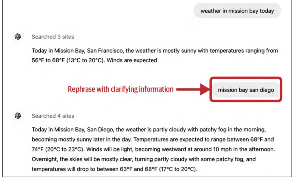
Figure 10-12. Because the user both terminates the generation early and rephrases the question, it can be inferred that the model misunderstood the intent of the original request.

Users can also point out specific things the model should’ve done differently. For example, if a user asks the model to summarize a story and the model confuses a character, this user can give feedback such as: “Bill is the suspect, not the victim.” The model should be able to take this feedback and revise the summary.

This kind of action-correcting feedback is especially common for agentic use cases where users might nudge the agent toward more optional actions. For example, if a user assigns the agent the task of doing market analysis about company XYZ, this user might give feedback such as “You should also check XYZ GitHub page” or “Check the CEO’s X profile”.

Sometimes, users might want the model to correct itself by asking for explicit confir‐ mation, such as “Are you sure?”, “Check again”, or “Show me the sources”. This doesn’t necessarily mean that the model gives wrong answers. However, it might

mean that your model’s answers lack the details the user is looking for. It can also indicate general distrust in your model.

Some applications let users edit the model’s responses directly. For example, if a user asks the model to generate code, and the user corrects the generated code, it’s a very strong signal that the code that got edited isn’t quite right.

User edits also serve as a valuable source of preference data. Recall that preference data, typically in the format of (query, winning response, losing response), can be used to align a model to human preference. Each user edit makes up a preference example, with the original generated response being the losing response and the edited response being the winning response.

Complaints. Often, users just complain about your application’s outputs without try‐ ing to correct them. For example, they might complain that an answer is wrong, irrel‐ evant, toxic, lengthy, lacking detail, or just bad. Table 10-1 shows eight groups of natural language feedback resulting from automatic clustering the FITS (Feedback for Interactive Talk & Search) dataset (Xu et al., 2022).

Table 10-1. Feedback types derived from automatic clustering the FITS dataset (Xu et al., 2022). Results from Yuan et al. (2023).

6	Point out that the bot’s answer is not specific/accurate/complete/detailed.
7	Point out that the bot is not confident in its answers and always begins its responses with “I am
	not sure” or “I don’t know”.

8	Complain about repetition/rudeness in bot responses.

Understanding how the bot fails the user is crucial in making it better. For example, if you know that the user doesn’t like verbose answers, you can change the bot’s prompt to make it more concise. If the user is unhappy because the answer lacks details, you can prompt the bot to be more specific.

Sentiment. Complaints can also be general expressions of negative sentiments (frus‐ tration, disappointment, ridicule, etc.) without explaining the reason why, such as “Uggh”. This might sound dystopian, but analysis of a user’s sentiments throughout conversations with a bot might give you insights into how the bot is doing. Some call centers track users’ voices throughout the calls. If a user gets increasingly loud, something is wrong. Conversely, if someone starts a conversation angry but ends happily, the conversation might have resolved their issue.

Natural language feedback can also be inferred from the model’s responses. One important signal is the model’s refusal rate. If a model says things like “Sorry, I don’t know that one” or “As a language model, I can’t do …”, the user is probably unhappy.

Other conversational feedback

Other types of conversational feedback can be derived from user actions instead of messages.

Regeneration. Many applications let users generate another response, sometimes with a different model. If a user chooses regeneration, it might be because they’re not satisfied with the first response. However, it might also be that the first response is adequate, but the user wants options to compare. This is especially common with cre‐ ative requests like image or story generation.

Regeneration signals might also be stronger for applications with usage-based billing than those with subscriptions. With usage-based billing, users are less likely to regen‐ erate and spend extra money out of idle curiosity.

Personally, I often choose regeneration for complex requests to ensure the model’s responses are consistent. If two responses give contradicting answers, I can’t trust either.

After regeneration, some applications might explicitly ask to compare the new response with the previous one, as shown in Figure 10-13. This better or worse data, again, can be used for preference finetuning.

Figure 10-13. ChatGPT asks for comparative feedback when a user regenerates another response.

Conversation organization. The actions a user takes to organize their conversations such as delete, rename, share, and bookmark—can also be signals. Deleting a conver‐ sation is a pretty strong signal that the conversation is bad, unless it’s an embarrass‐ ing conversation and the user wants to remove its trace. Renaming a conversation suggests that the conversation is good, but the auto-generated title is bad.

Conversation length. Another commonly tracked signal is the number of turns per conversation. Whether this is a positive or negative signal depends on the application. For AI companions, a long conversation might indicate that the user enjoys the con‐ versation. However, for chatbots geared toward productivity like customer support, a long conversation might indicate that the bot is inefficient in helping users resolve their issues.

Dialogue diversity. Conversation length can also be interpreted together with dialogue diversity, which can be measured by the distinct token or topic count. For example, if the conversation is long but the bot keeps repeating a few lines, the user might be stuck in a loop.

Explicit feedback is easier to interpret, but it demands extra effort from users. Since many users may not be willing to put in this additional work, explicit feedback can be sparse, especially in applications with smaller user bases. Explicit feedback also suf‐ fers from response biases. For example, unhappy users might be more likely to com‐ plain, causing the feedback to appear more negative than it is.

Implicit feedback is more abundant—what can be considered implicit feedback is limited only by your imagination—but it’s noisier. Interpreting implicit signals can be challenging. For example, sharing a conversation can either be a negative or a pos‐ itive signal. For example, one friend of mine mostly shares conversations when the model has made some glaring mistakes, and another friend mostly shares useful con‐ versations with their coworkers. It’s important to study your users to understand why they do each action.

Adding more signals can help clarify the intent. For example, if the user rephrases their question after sharing a link, it might indicate that the conversation didn’t meet their expectations. Extracting, interpreting, and leveraging implicit responses from conversations is a small but growing area of research.⁸

Feedback Design

If you were unsure of what feedback to collect, I hope that the last section gave you some ideas.

This section discusses when and how to collect this valuable feedback.

⁸ Not only can you collect feedback about AI applications, you can use AI to analyze feedback, too.

When to collect feedback

Feedback can and should be collected throughout the user journey. Users should have the option to give feedback, especially to report errors, whenever this need ari‐ ses. The feedback collection option, however, should be nonintrusive. It shouldn’t interfere with the user workflow. Here are a few places where user feedback might be particularly valuable.

In the beginning. When a user has just signed up, user feedback can help calibrate the application for the user. For example, a face ID app first must scan your face to work. A voice assistant might ask you to read a sentence out loud to recognize your voice for wake words (words that activate a voice assistant, like “Hey Google”). A language learning app might ask you a few questions to gauge your skill level. For some appli‐ cations, such as face ID, calibration is necessary. For other applications, however, ini‐ tial feedback should be optional, as it creates friction for users to try out your product. If a user doesn’t specify their preference, you can fall back to a neutral option and calibrate over time.

When something bad happens. When the model hallucinates a response, blocks a legit‐ imate request, generates a compromising image, or takes too long to respond, users should be able to notify you of these failures. You can give users the option to down‐ vote a response, regenerate with the same model, or change to another model. Users might just give conversational feedback like “You’re wrong”, “Too cliche”, or ”I want something shorter”.

Ideally, when your product makes mistakes, users should still be able to accomplish their tasks. For example, if the model wrongly categorizes a product, users can edit the category. Let users collaborate with the AI. If that doesn’t work, let them collabo‐ rate with humans. Many customer support bots offer to transfer users to human agents if the conversation drags on or if users seem frustrated.

An example of human–AI collaboration is the inpainting functionality for image gen‐ eration.⁹ If a generated image isn’t exactly what the user needs, they can select a region of the image and describe with a prompt how to make it better. Figure 10-14 shows an example of inpainting with DALL-E (OpenAI, 2021). This feature allows users to get better results while giving developers high-quality feedback.

⁹ I wish there were inpainting for text-to-speech. I find text-to-speech works well 95% of the time, but the other 5% can be frustrating. AI might mispronounce a name or fail to pause during dialogues. I wish there were apps that let me edit just the mistakes instead of having to regenerate the whole audio.

Figure 10-14. An example of how inpainting works in DALL-E. Image by OpenAI.

When the model has low confidence. When a model is uncertain about an action, you can ask the user for feedback to increase its confidence. For example, given a request to summarize a paper, if the model is uncertain whether the user would prefer a short, high-level summary or a detailed section-by-section summary, the model can output both summaries side by side, assuming that generating two summaries doesn’t increase the latency for the user. The user can choose which one they prefer. Comparative signals like this can be used for preference finetuning. An example of comparative evaluation in production is shown in Figure 10-15.

Figure 10-15. Side-by-side comparison of two ChatGPT responses.

Showing two full responses for the user to choose means asking that user for explicit feedback. Users might not have time to read two full responses or care enough to give thoughtful feedback. This can result in noisy votes. Some applications, like Google Gemini, show only the beginning of each response, as shown in Figure 10-16. Users can click to expand the response they want to read. It’s unclear, however, whether showing full or partial responses side by side gives more reliable feedback.¹⁰

¹⁰ When I ask this question at events I speak at, the responses are conflicted. Some people think showing full responses gives more reliable feedback because it gives users more information to make a decision. At the same time, some people think that once users have read full responses, there’s no incentive for them to click on the better one.

Figure 10-16. Google Gemini shows partial responses side by side for comparative feed‐ back. Users have to click on the response they want to read more about, which gives feedback about which response they find more promising.

Another example is a photo organization application that automatically tags your photos, so that it can respond to queries like “Show me all the photos of X”. When unsure if two people are the same, it can ask you for feedback, as Google Photos does in Figure 10-17.

Figure 10-17. Google Photos asks for user feedback when unsure. The two cat images were generated by ChatGPT.

You might wonder: how about feedback when something good happens? Actions that users can take to express their satisfaction include thumbs up, favoriting, or sharing. However, Apple’s human interface guideline warns against asking for both positive and negative feedback. Your application should produce good results by default. Asking for feedback on good results might give users the impression that good results are exceptions. Ultimately, if users are happy, they continue using your application.

However, many people I’ve talked to believe users should have the option to give feedback when they encounter something amazing. A product manager for a popular AI-powered product mentioned that their team needs positive feedback because it reveals the features users love enough to give enthusiastic feedback about. This allows the team to concentrate on refining a small set of high-impact features rather than spreading resources across many with minimal added value.

Some avoid asking for positive feedback out of concern it may clutter the interface or annoy users. However, this risk can be managed by limiting the frequency of feed‐ back requests. For example, if you have a large user base, showing the request to only 1% of users at a time could help gather sufficient feedback without disrupting the experience for most users. Keep in mind that the smaller the percentage of users asked, the greater the risk of feedback biases. Still, with a large enough pool, the feed‐ back can provide meaningful product insights.

How to collect feedback

Feedback should seamlessly integrate into the user’s workflow. It should be easy for users to provide feedback without extra work. Feedback collection shouldn’t disrupt user experience and should be easy to ignore. There should be incentives for users to give good feedback.

One example often cited as good feedback design is from the image generator app Midjourney. For each prompt, Midjourney generates a set of (four) images and gives the user the following options, as shown in Figure 10-18:

1. Generate an unscaled version of any of these images.
1. Generate variations for any of these images.
1. Regenerate.

All these options give Midjourney different signals. Options 1 and 2 tell Midjourney which of the four photos is considered by the user to be the most promising. Option 1 gives the strongest positive signal about the chosen photo. Option 2 gives a weaker positive signal. Option 3 signals that none of the photos is good enough. However, users might choose to regenerate even if the existing photos are good just to see what else is possible.

Figure 10-18. Midjourney’s workflow allows the app to collect implicit feedback.

Code assistants like GitHub Copilot might show their drafts in lighter colors than the final texts, as shown in Figure 10-19. Users can use the Tab key to accept a suggestion or simply continue typing to ignore the suggestion, both providing feedback.

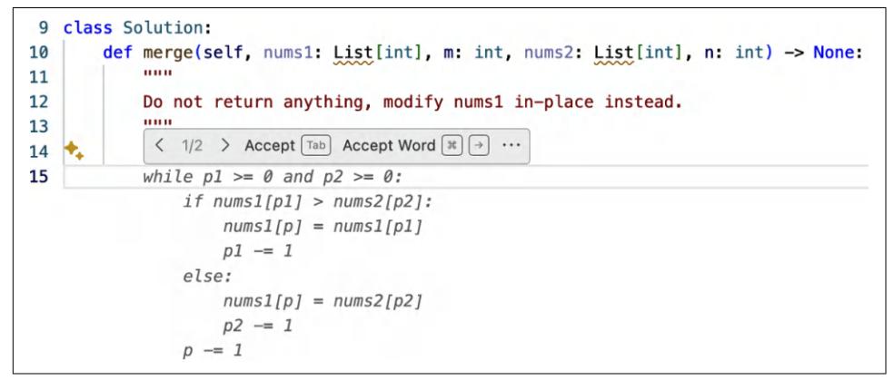
Figure 10-19. GitHub Copilot makes it easy to both suggest and reject a suggestion.

One of the biggest challenges of standalone AI applications like ChatGPT and Claude is that they aren’t integrated into the user’s daily workflow, making it hard to collect high-quality feedback the way integrated products like GitHub Copilot can. For example, if Gmail suggests an email draft, Gmail can track how this draft is used or edited. However, if you use ChatGPT to write an email, ChatGPT doesn’t know whether the generated email is actually sent.

The feedback alone might be helpful for product analytics. For example, seeing just the thumbs up/thumbs down information is useful for calculating how often people are happy or unhappy with your product. For deeper analysis, though, you would need context around the feedback, such as the previous 5 to 10 dialogue turns. This context can help you figure out what went wrong. However, getting this context might not be possible without explicit user consent, especially if the context might contain personally identifiable information.

For this reason, some products include terms in their service agreements that allow them to access user data for analytics and product improvement. For applications without such terms, user feedback might be tied to a user data donation flow, where users are asked to donate (e.g., share) their recent interaction data along with their feedback. For example, when submitting feedback, you might be asked to check a box to share your recent data as context for this feedback.

Explaining to users how their feedback is used can motivate them to give more and better feedback. Do you use a user’s feedback to personalize the product to this user, to collect statistics about general usage, or to train a new model? If users are con‐ cerned about privacy, reassure them that their data won’t be used to train models or won’t leave their device (only if these are true).

Don’t ask users to do the impossible. For example, if you collect comparative signals from users, don’t ask them to choose between two options they don’t understand. For example, I was once stumped when ChatGPT asked me to choose between two possi‐ ble answers to a statistical question, as shown in Figure 10-20. I wish there was an option for me to say, “I don’t know”.

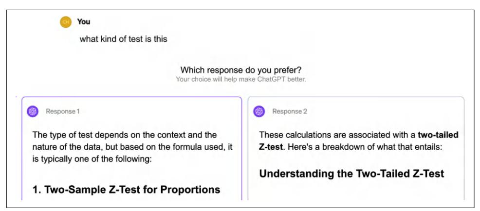
Figure 10-20. An example of ChatGPT asking a user to select the response the user pre‐ fers. However, for mathematical questions like this, the right answer shouldn’t be a matter of preference.

Add icons and tooltips to an option if they help people understand it. Avoid a design that can confuse users. Ambiguous instructions can lead to noisy feedback. I once hosted a GPU optimization workshop, using Luma to collect feedback. When I was reading the negative feedback, I was confused. Even though the responses were posi‐ tive, the star ratings were 1/5. When I dug deeper, I realized that Luma used emojis to represent numbers in their feedback collection form, but the angry emoji, corre‐ sponding to a one-star rating, was put where the five-star rating should be, as shown in Figure 10-21.

Be mindful of whether you want users’ feedback to be private or public. For example, if a user likes something, do you want this information shown to other users? In its early days, Midjourney’s feedback—someone choosing to upscale an image, generate variations, or regenerate another batch of images—was public.

Figure 10-21. Because Luma put the angry emoji, corresponding to a one-star rating, where a five-star rating should’ve been, some users mistakenly picked it for positive reviews.

Figure 10-21. Because Luma put the angry emoji, corresponding to a one-star rating, where a five-star rating should’ve been, some users mistakenly picked it for positive reviews.

The visibility of a signal can profoundly impact user behavior, user experience, and the quality of the feedback. Users tend to be more candid in private—there’s a lower chance of their activities being judged¹¹—which can result in higher-quality signals. In 2024, X (formerly Twitter) made “likes” private. Elon Musk, the owner of X, claimed a significant uptick in the number of likes after this change.

However, private signals can reduce discoverability and explainability. For example, hiding likes prevents users from finding tweets their connections have liked. If X rec‐ ommends tweets based on the likes of the people you follow, hiding likes could result in users’ confusion about why certain tweets appear in their feeds.

¹¹ See “Ted Cruz Blames Staffer for ‘Liking’ Porn Tweet” (Nelson and Everett, POLITICO, September 2017) and “Kentucky Senator Whose Twitter Account ‘Liked’ Obscene Tweets Says He Was Hacked” (Liam Niemeyer, WKU Public Radio, March 2023).

Feedback Limitations

There’s no doubt of the value of user feedback to an application developer. However, feedback isn’t a free lunch. It comes with its own limitations.

Biases

Like any other data, user feedback has biases. It’s important to understand these bia‐ ses and design your feedback system around them. Each application has its own bia‐ ses. Here are a few examples of feedback biases to give you an idea of what to look out for:

Leniency bias

Leniency bias is the tendency for people to rate items more positively than war‐ ranted, often to avoid conflict because they feel compelled to be nice or because it’s the easiest option. Imagine you’re in a hurry, and an app asks you to rate a transaction. You aren’t happy with the transaction, but you know that if you rate it negatively, you’ll be asked to provide reasons, so you just choose positive to be done with it. This is also why you shouldn’t make people do extra work for your feedback.

On a five-star rating scale, four and five stars are typically meant to indicate a good experience. However, in many cases, users may feel pressured to give fivestar ratings, reserving four stars for when something goes wrong. According to Uber, in 2015, the average driver’s rating was 4.8, with scores below 4.6 putting drivers at risk of being deactivated.

This bias isn’t necessarily a dealbreaker. Uber’s goal is to differentiate good driv‐ ers from bad drivers. Even with this bias, their rating system seems to help them achieve this goal. It’s essential to look at the distribution of your user ratings to detect this bias.

If you want more granular feedback, removing the strong negative connotation associated with low ratings can help people break out of this bias. For example, instead of showing users numbers one to five, show users options such as the fol‐ lowing:

“Great ride. Great driver.”
“Pretty good.”
“Nothing to complain about but nothing stellar either.”
“Could’ve been better.”
“Don’t match me with this driver again.”¹²

¹² The options suggested here are only to show how options can be rewritten. They haven’t been validated.

Randomness

Users often provide random feedback, not out of malice, but because they lack motivation to give more thoughtful input. For example, when two long responses are shown side by side for comparative evaluation, users might not want to read both of them and just click on one at random. In the case of Midjourney, users might also randomly choose one image to generate variations.

Position bias

The position in which an option is presented to users influences how this option is perceived. Users are generally more likely to click on the first suggestion than the second. If a user clicks on the first suggestion, this doesn’t necessarily mean that it’s a good suggestion.

When designing your feedback system, this bias can be mitigated by randomly varying the positions of your suggestions or by building a model to compute a suggestion’s true success rate based on its position.

Preference bias

Many other biases can affect a person’s feedback, some of which have been dis‐ cussed in this book. For example, people might prefer the longer response in a side-by-side comparison, even if the longer response is less accurate—length is easier to notice than inaccuracies. Another bias is recency bias, where people tend to favor the answer they see last when comparing two answers.

It’s important to inspect your user feedback to uncover its biases. Understanding these biases will help you interpret the feedback correctly, avoiding misleading prod‐ uct decisions.

Degenerate feedback loop

Keep in mind that user feedback is incomplete. You only get feedback on what you show users.

In a system where user feedback is used to modify a model’s behavior, degenerate feedback loops can arise. A degenerate feedback loop can happen when the predic‐ tions themselves influence the feedback, which, in turn, influences the next iteration of the model, amplifying initial biases.

Imagine you’re building a system to recommend videos. The videos that rank higher show up first, so they get more clicks, reinforcing the system’s belief that they’re the best picks. Initially, the difference between the two videos, A and B, might be minor, but because A was ranked slightly higher, it got more clicks, and the system kept boosting it. Over time, A’s ranking soared, leaving B behind. This feedback loop is why popular videos stay popular, making it tough for new ones to break through. This issue is known as “exposure bias,” “popularity bias,” or “filter bubbles,” and it’s a well-studied problem.

A degenerate feedback loop can alter your product’s focus and use base. Imagine that initially, a small number of users give feedback that they like cat photos. The system picks up on this and starts generating more photos with cats. This attracts cat lovers, who give more feedback that cat photos are good, encouraging the system to generate even more cats. Before long, your application becomes a cat haven. Here, I use cat photos as an example, but the same mechanism can amplify other biases, such as rac‐ ism, sexism, and preference for explicit content.

Acting on user feedback can also turn a conversational agent into, for lack of a better word, a liar. Multiple studies have shown that training a model on user feedback can teach it to give users what it thinks users want, even if that isn’t what’s most accurate or beneficial (Stray, 2023). Sharma et al. (2023) show that AI models trained on human feedback tend toward. sycophancy. They are more likely to present user responses matching this user’s view.

User feedback is crucial for improving user experience, but if used indiscriminately, it can perpetuate biases and destroy your product. Before incorporating feedback into your product, make sure that you understand the limitations of this feedback and its potential impact.

Summary

If each previous chapter focused on a specific aspect of AI engineering, this chapter looked into the process of building applications on top of foundation models as a whole.

The chapter consisted of two parts. The first part discussed a common architecture for AI applications. While the exact architecture for an application might vary, this high-level architecture provides a framework for understanding how different com‐ ponents fit together. I used the step-by-step approach in building this architecture to discuss the challenges at each step and the techniques you can use to address them.

While it’s necessary to separate components to keep your system modular and main‐ tainable, this separation is fluid. There are many ways components can overlap in functionalities. For example, guardrails can be implemented in the inference service, the model gateway, or as a standalone component.

Each additional component can potentially make your system more capable, safer, or faster but will also increase the system’s complexity, exposing it to new failure modes. One integral part of any complex system is monitoring and observability. Observabil‐ ity involves understanding how your system fails, designing metrics and alerts around failures, and ensuring that your system is designed in a way that makes these failures detectable and traceable. While many observability best practices and tools from software engineering and traditional machine learning are applicable to AI engineering applications, foundation models introduce new failure modes, which require additional metrics and design considerations.

At the same time, the conversational interface enables new types of user feedback, which you can leverage for analytics, product improvement, and the data flywheel. The second part of the chapter discussed various forms of conversational feedback and how to design your application to effectively collect it.

Traditionally, user feedback design has been seen as a product responsibility rather than an engineering one, and as a result, it is often overlooked by engineers. How‐ ever, since user feedback is a crucial source of data for continuously improving AI models, more AI engineers are now becoming involved in the process to ensure they receive the data they need. This reinforces the idea from Chapter 1 that, compared to traditional ML engineering, AI engineering is moving closer to product. This is because of both the increasing importance of data flywheel and product experience as competitive advantages.

Many AI challenges are, at their core, system problems. To solve them, it’s often nec‐ essary to step back and consider the system as a whole. A single problem might be addressed by different components working independently, or a solution could require the collaboration of multiple components. A thorough understanding of the system is essential to solving real problems, unlocking new possibilities, and ensuring safety.

Epilogue

This is some text.

You made it! You just finished a technical book with more than 150,000 words, 160 illustrations, 250 footnotes, and 975 reference links.

Being able to set aside time to learn is a privilege. I’m grateful for the opportunity to write this book and learn new things. And I’m grateful that you chose to give this book your valuable learning time.

The hardest part of technical writing isn’t finding the correct answers but asking the right questions. Writing this book inspired me to ask many questions that guided me toward fun and useful discoveries. I hope the book sparked some interesting ques‐ tions for you as well.

There are already so many incredible applications built on top of foundation models. There’s no doubt that this number will grow exponentially in the future. More sys‐ tematic approaches to AI engineering, such as those introduced in this book, will make the development process easier, enabling even more applications. If there are any use cases you want to discuss, don’t hesitate to reach out. I love hearing about interesting problems and solutions. I can be reached via X at @chipro, LinkedIn/in/ chiphuyen, or email at https://huyenchip.com/communication.

For more resources about AI engineering, check out the book’s GitHub repository: https://github.com/chiphuyen/aie-book.

AI engineering has a lot of challenges. Not all of them are fun, but all of them are opportunities for growth and impact. I can’t wait to learn more about what you’ll build!

Index

A

accelerators , 419-425 computational capabilities, 422 defined, 420-421 memory size and bandwidth, 422-424 power consumption, 424-425 active injection, 2 43 adapter-based methods, 336 adapters finetuning, 358 LoRA, 338-347 merging with concatenation, 356 PEFT techniques, 336 -338 agents, 275-3 00 agent failure modes and evaluation, 298-300 efficiency, 300 planning failures, 298 tool failures, 299 overview, 276-278 planning agents, 281-298 foundation models as planners, 284-286 overview, 282-284 plan generation, 286-292 reflection and error correction, 292-294 tool selection, 295-298 tools, 278-281 capability extension, 279 knowledge augmentation, 279 write actions, 280 AI accelerators (see accelerators) AI application building (see application build‐ ing) AI application planning (see application plan‐ ning)

AI engineering (AIE) defined, 12 ML engineering versus, 39-46 rise of AI engineering, 2-14 AI engineering architecture (see engineering architecture) AI engineering stack (see engineering stack) AI judge, 136 (see also AI-as-a-judge) AI pipeline orchestration (see pipeline orches‐ tration) AI systems evaluation (see systems evaluation) AI-as-a-judge, 136-148 limitations, 141-145 biases, 144 criteria ambiguity, 142-144 inconsistency, 142 increased costs and latency, 144 models, 145-148 reasons, 137 reference-based, 147 uses, 138-141 AI-powered data synthesis (see data synthesis, AI-powered) AMP (automatic mixed precision), 332 ANN (approximate nearest neighbor), 262 Annoy (approximate nearest neighbors oh yeah), 263 anomaly detection, 129 Anthropic contextual retrieval, 271 inverse scaling and alignment training, 71 prompt caching, 444 RAG and, 256

APIs (see open source models, model APIs ver‐ sus) application building, 1-48 application planning, 28-35 maintenance, 34 milestone planning, 33 set expectations, 32 use case evaluation, 29-32 engineering stack, 35-47 AI engineering versus ML engineering, 39-46 application development, 44-46 full-stack engineering versus, 46 three layers of AI stack, 37-39 foundation model use cases, 16-28 coding, 20-22 conversational bots, 26 data organization, 27 education, 24 image and video production, 22 information aggregation, 26 workflow automation, 28 writing, 22-24 rise of AI engineering, 2-14 foundation models to AI engineering, 12-14 application development, 37, 44-46 AI interface, 45 evaluation, 44 prompt engineering and context construc‐ tion, 45 application planning, 28-35 maintenance, 34 milestone planning, 33 set expectations, 32 use case evaluation, 29-32 approximate nearest neighbor (ANN), 262 approximate string matching, 130 ARC-C, 192 attention mechanisms, 60-62 attention modules, 62 MLP modules, 62 optimization, 433-436 attention mechanism redesign, 435 wiring kernels for attention computa‐ tion, 436 redesign, 435 attention modules, 62 augmentation of data

defined, 380 automated attacks, 240 automatic mixed precision (A MP), 332 autoregressive decoding bottleneck, 428-433 inference with reference, 430 parallel decoding, 432 speculative decoding, 428-430 autoregressive language model, 4

B

backpropagation, 320-322 batch inference APIs, 410-412 batch size, 360 batching batch inference APIs, 410-412 batch si ze, 360 continuous, 441 dynamic, 441 static, 440 benchmarks for comparative eva luation, 155 data contamination detection, 124 domain distri butio n and, 56 domain-specific, 161-163 instruction-following criteria, 173-175 model-centric versus data-centric, 364 navigating public benchmarks, 191-197 biases, 144, 490 bits-per-byte (BPB), 121 bits-per-character (BPC), 121 bottlenecks autoregressive decodi ng, 428-433 computational, 407-410 compute-bound, 407 memory, 319-332, 407 scaling, 75-77, 152 BPB (bits-per-byte), 121 BPC (bits-per-character), 121 build time, 266

C

canonical responses, 127 capability extension, 279 chain-of-thought (CoT), 227-229, 365 chaining, 473 change failure rate (CFR), 466 CharacterEval, 176 ChatGPT comparative evaluation, 149

data privacy issues, 184 effect on AI investment, 13 Gemini versus, 44 hallucinations, 107 and human writing quality, 23 introduction of, xi and languages other than English, 55 query rewriting, 270 reverse prompt engineering attacks, 237 in schools, 24 Chinchilla scaling law, 72 chunking, 257, 268-269 Claude, RAG and, 256 CLIP, $10, 56, 135$ clustering, 129 Common Crawl dataset, 50-55 comparative evaluation, 148-156 comparison data, 85 compilers, 438 components definition, 472 computational bottlenecks, 407-410 computational capabilities, of AI accelerators, 422 compute-bound bottlenecks, 407 compute-optimal models, 72-74 compute-optimal training, 72 concatenation, 356 constrained sampling, 103 context construction, 45, 224, 451 context efficiency, 218-220 context length, 218-220 context parallelism, 447 context precision, 264 context recall, 264 contextual retrieval, 271-272 continuous batching, 441 control flow, 291 conversational bots, 26 conversational feedback conversation length, 480 conversation organization, 479 extracting, 475-480 language diversity, 480 natural language feedback, 476-479 complaints, 478 early termination, 476 error correction, 477 sentiment, 478 regeneration, 479

copyright regurgitation, 246 copyright, model training and, 185 CoT (chain-of-thought), 227-229 CPU memory (DRAM), 423 criteria ambiguity, 142-144 cross entropy, $120$ cross-layer attention, 435

D

data annotation, 377-380 and data curation, 365-380 and data inspection, 398 dataset engineering and, 42 data augmentation, 380-396 defined, 380 data cleaning/filtering, 401 data contamination, 197-200 data coverage, 369-371 data curation, 365-380 data deduplication, 129, 399-400 data flywheels, 377 data formatting, 401-403 data inspection, 397-399 data lineage, 185 data organization, 27 data privacy, 184 data processing, 396-403 data cleaning/filtering, 401 data formatting, 401-403 deduplicating data, 399-400 inspecting data, 397-399 data synthesis, 380-396 AI-powered, 386-395 data verification, 391-393 instruction data synthesis, 388-391 limitations, 393-395 obscure data lineage problems, 395 potential model collapse, 394 quality control problems, 393 reasons for synthesizing data, 381-382 superficial imitation problems, 393 model distillation, 395 traditional techniques, 383-386 rule-based, 383-385 simulation, 385 data verification, 391-393 dataset engineering, 42, 363-404 data augmentation/synthesis, 380-396 data curation, 365-380

data acquisition/annotation, 377-380 data coverage, 369-371 data quality, 368-369 data quantity, 372-377 data processing, 396-403 data cleaning and filtering, 401 data formatting, 401-403 deduplicating data, 399-400 inspecting data, 397-399 data-centric view of AI, 364 DDR SDRAM (doubled data rate synchronous dynamic random-access memory), 423 debugging, 226 decoding autoregressive decoding bottleneck, 428-433 decoupling from prefilling, 442 in transformer architecture, 58 defensive prompt engineering jailbreaking and prompt injection, 238-243 automated attacks, 240 direct manual prompt hacking, 239-240 indirect prompt injection, 242-243 prompt attack defense, 248-251 model-level defense, 248 prompt-level defense, 249 system-level defense, 250 degenerate feedback loops, 491 demonstration data, 81 dense retrievers, 258 dimensionality reduction, 400 direct manual prompt hacking, 239-240 Direct Preference Optimization (DPO), 84 distillation, 312 base, 358 model distillation, 182, 395, 427 synthetic data and, 382 domain-specific capability, 161-163 domain-specific task finetuning, 314 domain-specific training data models, 56-57 dot products, 61 doubled data rate synchronous dynamic random-access memory (DDR SDRAM), 423 DPO (Direct Preference Optimization), 84 DRAM (CPU memory), 423 drift detection, 471 dynamic batching, 441 dynamic features, 30

E

edit distance, 130 Elo, 151, 152, 346 embedding, 134-136 embedding algorithm, 133, 135 embedding model, 10 embedding-based retrieval, 260-263 multimodal RAG and, 273 embedding models, 134 engineering architecture, 449-474 AI pipeline orchestration, 472-474 monitoring and observability, 465-472 drift detection, 471 logs and traces, $469-470$ metrics, 467-469 monitoring versus observability, 466 step 1: enhancing context, 450 step 2: putting in guardrails, $451-455$ guardrail implementation, 455 input guardrails, 451-452 output guardrails, 453-454 step 3: adding model router and gateway, 456-460 gateway, 458-460 router, 456-457 step 4: reducing latency with caches, 460-463 exact caching, 461 semantic caching, 461 step 5: adding agent patterns, 463 engineering stack, 37-39 application development, 37 AI interface, $45$ evaluation, 44 prompt engineering and context construction, $45$ infrastructure, 37 ML engineering versus, 40-44 model development, 37 entropy, $119$ epochs, 360 error correction, 292-294 evaluation, 44 evaluation harnesses, 191 evaluation methodology, 113-157 AI as a judge, 136-148 AI systems evaluation (see systems evaluation) challenges, 152-155

challenges of foundation model evaluation, 114-117 comparative performance to absolute performance, 154 lack of standardization and quality con‐ trol, 153-154 scalability bottlenecks, 152 exact evaluation, 125-136 future, 155 language model for computing text perplex‐ ity, 125 language modeling metrics, 118-124 rank models with comparative evaluation, 148-156 evaluation pipeline design, 200-208 step 1: creating an evaluation guideline, 202-203 step 2: evaluating all components in a sys‐ tem, 200-201 creating scoring rubrics with examples, 202 defining evaluation criteria, 202 tying evaluation metrics to business met‐ rics, 203 step 3: defining evaluation methods and data, 204-208 annotating evaluation data, 205-207 evaluating eval uation pipeline, 207 iteration, 208 selecting evaluation methods, 204 evaluation-driven development, 160-161 eviction policies, 461 exact caching, 461 exact evaluation, 125-136 functional correctness, 126-127 similarity measurements against reference data, 127-133 exact matches, 129 expectation setting, 32 explicit feedback, 475-480

F

factual consistency, 165-169, 202 faithfulness, 164 feature-based transfers, 104, 309 feature-free transfers, 104 federated learning, 348 feedback design how to collect feedback, 485-489

when to collect feedba ck in the beginning, 481 when something bad happens, 481 when the model has low confidence, 483-485 feedforward computation, 44 7 feedforward layer, 62, 343 few-shot learning, 213-215 finetuning, 307-362 defined, 42 domain-specific tasks , 314 finetuning an d RAG, 316-319 hyperparameters, 359-361 batch si ze, 360 learning rate , 359 number of epochs, 360 prompt loss rate, 361 memory bottle necks, 319-332 backpropagation and trainable para me‐ ters, 320-322 memory math, 322 -324 numerical representations, 3 25-328 quantization, 328-332 overview, 308-311 structured outputs, 104 tactics, 357-361 techniques, 332-361 LoRA, 338-347 model merging and multi-task finetun‐ ing, 347-357 parameter-efficient finetuning, 332-347 PEFT techniques, 336-338 when to finetune, 311-319 reasons not to finetune, 312-315 reasons to finetune, 311 FLOP (floating point operation), 70 foundation models, 12, 49-112 evaluation challenges, 114-117 comparative performance to absolute performance, 154 lack of standardization and quality con‐ trol, 153-154 scalability bottlenecks, 152 inverse scaling, 71 modeling, 58-77 model architecture, 58-66 model size, 67-77 parameter versus hyperparameter, 74 post-training, 78-88

preference finetuning, 83-88 supervised finetuning, 80-83 sampling, 88-111 probabilistic nature of AI, 105-111 sampling fundamentals, 88-90 sampling strategies, 90-95 structured outputs, 99-104 test time compute, 96-99 training data, 50-57 domain-specific models, 56-57 multilingual models, 51-55 use cases, $16-28$ coding, 20-22 conversational bots, 26 data organization, 27 education, 24 image and video production, 22 workflow automation, 28 writing, 22-24 full finetuning, 332-347 function calling, 288-290 fuzzy matching, 130

G

gateways, 458-460 Gemini, 44, 99, 444, 483 generation capability, 163-172 global factual consistency, 165 goodput, 414-415 GPU on-chip SRAM, 423 ground truths, 127 grouped-query attention, 436 guardrail implementation, 455 guardrails, 189, 251, 451-455

H

H3 architecture, 66 hallucinations causes of, $107-111$ defined, 105 and finetuning, 317 measurement, 166 metrics for, $467$ superficial imitation and, 393 hard attributes, 179 hashing, 400 HellaSwag, 192 hierarchical navigable small world (HNSW), 263

high-bandwidth memory (HBM), 423 hyperparameters, 74, 359-361

T

IDF (inverse document frequency), 259 IFEval, 174 implicit feedback, 475 in-context learning, 213-215 inconsistency, 106-107, 142 indexing chunking strategy and, 268-269 defined, 256 with embedding-based retrieval, 261 retrieval systems and, 266 indirect prompt injection, 242-243 inference APIs, 410-412 inference optimization, 43, 405-448 AI accelerators computational capabilities, 422 defined, 420-421 memory size and bandwidth, 422-424 power consumption, 424-425 case study from PyTorch, 439 inference overview computational bottlenecks, 407-410 online and batch inference APIs, $410 - 412$ inference performance metrics, 412-419 latency, TTFT, and TPOT, 412-414 throughput/goodput, 414-415 utilization, MFU, and MBU, 416-419 inference service optimization, 440-447 batching, 440 decoupling prefill and decode, 442 parallelism, 444-447 prompt caching, 443-444 KV cache size calculation, 435 memory-bound versus bandwidth-bound interference, 408 at model/hardware/service levels, 426 model optimization, 426-439 attention mechanism optimization, 433-436 autoregressive decoding bottleneck, 428-433 kernels and compilers, 437-440 model compression, 427 understanding, 406-425 AI accelerators, 419-425

inference overview, 406-412 inference performance metrics, 412-419 inference performance metrics, 412-419 latency, TTFT, and TPOT, 412-414 throughput/goodput, 414-415 utilization, MFU, and MBU, 416-419 inference quantization, 329-331 inference service defined, 183 and inference optimization, 406 throughput/goodput, 414-415 inference service optimization, 440-447 decoupling prefill and decode, 442 parallelism, 444-447 prompt caching, 443-444 inference with reference, 430 INFOBench, 174 information aggregation, 26 information extraction, 243-247 information retrieval optimization, 267-272 chunking strategy, 268-269 contextual retrieval, 271-272 query rewriting, 270 reranking, 269 instruction data synthesis, 388-391 instruction-following capability, 172-177 instruction-following criteria, 173-175 intent classifiers, 457 inter-token latency (ITL), 413 interface, AI, 45 internal knowledge, 301 inverse document frequency (IDF), 259 inverted file index (IVF), 263 iteration, 208

J

jailbreaking, 238-243 automated attacks, 240 direct manual prompt hacking, 239-240 indirect prompt injection, 242-243 Jamba architecture, 66 judges (see AI judges)

$\mathbf{K}$

k-nearest neighbors (k-NN), 262 kernels, 436, 437-440 key vector $(K)$ , 60 key-value (KV) cache, 433-436 key-value vectors, 323

knowledge augmentation, 279 knowledge-augmented verification, 167 KV cache (see key-value cache)

L

LangChain, 232, 250, 303 language modeling metrics, 118-124 bits-per-byte, 121 bits-per-character, 121 cross entropy, 120 entropy, 119 perplexity, 121 perplexity interpretation and use cases, $122 - 124$ language models, $2-6$ , $125$ large language models, 8-12 AI product defensibility, 31 role of AI and humans in the application, $30 - 31$ set expectations, 31 large multimodal model (LMM), 9 latency AI judges and, 144 inference performance and, 412-414 metrics, $33$ reliability versus, 455 layer stacking, 354-355 leaderboards, 152-154, 191-197 learning rate, 359 leniency bias, 490 lexical similarity, 130-131 linear combination summing, 350-352 Llama attention function, 62 data coverage, 370 data quality, 368 data quantity, 372 data synthesis, 387, 390 finetuning, 310 inference optimization, 439 inference quantization, 330 model distillation, 395 open source models, 182 prefer, 84 preference finetuning, 78 prompt template, 215 scaling law and, 73 LLM-as-a-judge, 136 (see also AI-as-a-judge)

LMM (large multimodal model), 9 local factual consistency, 165 locality-sensitive hashing (LSH), 263 logit vectors, 89 logprobs, 93, 204 logs, 469-470 long-term memory, 301 loop tiling, 438 LoRA (low-rank adaptation), 338-347 configurations, 341-343 LoRA adapters service, 343-345 mechanism of operation, 340 quantized LoRA (QLoRA), 345-347 low-rank factorization, 340 LSH (locality-sensitive hashing), 263

M

Mamba architecture, 66 manual generation, 383-386 masked language models, 4 Massive Multitask Language Understanding (MMLU), 34, 192 matches, 150 MBU (model bandwidth utilization), 41 6-419 MCQs (multiple-cho ice questions), 163 mean time to detection (MTTD), 4 66 mean time to response (MTTR), 466 memory, 300-304 internal knowle dge, 301 long-term memory, 301 short-term memory, 301 memory bottlenecks, 319-332 bandwidth-bound, 407 memory math, 322-324 memory needed for inference, 3 23 memory needed for training, 323-324 quantization, 328-332 inference quantization, 329-331 training quantization, 331-332 size and bandwidth, 422-424 memory math, 322-324 metrics, 467-469 correlations between, 208 for AI as a judge, 142-144 for generation capability, 163 for hallucination measurement, 166 inference performance metrics, 412-419 language modeling (see language modeling metrics)

observability metrics, 466 reference-based versus reference-free, 127 tying evaluation metrics to business metrics, 203 usefulness thresholds, 33 MFU (model FLOPs utilization), 416-419 milestone planning, 33 mixture-of-experts (MoE) models, 68, 354 ML engineering, AI engineering versus, 39-46 MLP modules, 62 MMLU (Massive Multitask Language Under‐ standing), 34, 192 model APIs, open source models vers us (see open source models, model APIs versus) model architecture, 58-66 (see also specific architectures, e.g.: trans‐ former architec ture) model bandwidth utilization (MBU), 416-419 model compression, 427 model development, 37, 40-44 dataset engineering, 42 inference optimization, 43-44 modeling and training, 41-42 model distillation, 395 model FLOPs utilization (MFU), 416-419 model inference, 34 model merging, 347-357 concatenation, 356 layer stacking, 354-355 summing, 350-354 model optimization, 426-439 attention mech anism optimization, 433-436 attention mechanism redesign, 435 KV cache size optimization, 436 write kernels for attention computation, 436 autoregressive decoding bottleneck, 428-433 inference with reference, 430 parallel decoding, 432 speculative decoding, 428-430 kernels and compilers, 437-440 model compression, 427 model ranking, 148-156 model router, 456-460 model selection, 179-200 model build versus buy, 181-191 open source models versus model APIs, 183-191

open source, open weight, and model licenses, 181-183 model selection workflow, 179-181 navigating public benchmarks, 191-197 benchmark selection and aggregation, 191 public lea derb oards, 192 model size, 67-77 scaling bottlenecks, 75-77 scaling extrapolation, 74 scaling law: building compute-optimal models, 72-74 model-centric AI, 364 model-level defense, 248 modeling, 58-77 model architecture, 58-66 model size, 67-77 MoE (mixture-of-experts) mod els, 354 monitoring, 226, 465-472 MTTD (mean time to detection), 466 MTTR (mean time to response), 466 multi-query attention, 435 multi-task finetuning, 347 multilingual training data models, 51-55 multimodal models, 9 multiple-choice questions (MCQs), 163

N

n-gram similarity, 131 natural language feedback, 476-479 complaints, 478 early termination, 476 error correction, 477 sentiment, 478 natural language generation (NLG), 163-172 natural language processing (NLP), 163-172 needle in a haystack (NIAH) test, 218

O

obscure data lineage, 395 observability, 465-472 on-device deployment, 190 online inference APIs, 410-412 Open CLIP, 56 open source licenses, 181-183 open source models, model APIs versus, 183-191 API cost versus engineering cost, 188 control, access, and transparency, 189

data lineage and copyright, 185 data privacy, 184 functionality, 187 on-device deployment, 190 performance, 186 open weight models, 182 OpenAI batch APIs, 410 evaluation harnesses, 191 first GPT model, 8 instruction hierarchy for model-level defense, 248 model as a service, 14 natural language supervision, 10 open source APIs, 183 progression/distillation paths, 357 quality of updat ed models, 196 test time compute, 97 operator fusion, 438 optimizati on inference o ptimization (see inference opti‐ mization) of retrieval systems, 2 6 7-272

P

pairwise comparison, 400 parallel decoding, 432 parallelism, 444-447 parallelization, 226, 438 parameter-efficient finetuning, 332-347 adapter-based/soft-prompt techniques, 336-338 LoRA, 338-347 configurations, 341-343 how it works, 340 LoRA adapte rs service, 343-345 quantized LoRA, 345-347 Pareto optimization, 177 partial finetuning, 333 passive phishing, 242 PEFT (see parameter-efficient finetuning) perplexity, 121-124 perturbation, 385 pipeline orchestration, 472-474 monitoring and observability, 465-472 drift detection, 471 logs and traces, 469-470 metrics, 467-469 planning

plan generation, 286-2 92 complex plans, 291 function calling, 288-290 granularity, 290 reflection and error correction, 292-294 pointwise evaluation, 84, 148 position bias, 491 post-processing, 102 post-training, 42, 78-88 preference finetuning, 83-88 supervised finetuning, 80-83 potential model collapse, 394 power consumption, 424-425 PPO (proximal policy optimization), 87 pre-training, 41 precision bits, 326 preference bias, 491 preference finetuning, 83-88, 309 preference models, 147 prefilling, 60 prefilling, decoupling from decoding, 442 proactive features, 30 probabilistic nature of AI, 105-111 hallucination, 107-111 inconsistency, 106-107 probabilistic definition, 105-111 procedural generation, 383-386 product quantization, 263 prompt attacks, 235, 238-243 automated attacks, 240 defense against, 248-251 direct manual prompt hacking, 239-240 indirect prompt injection, 242-243 prompt caching, 443-444 prompt catalogs, 235 prompt engineering, 211-252 basics, 212-220 context length and context efficiency, 218-220 in-context learning: zero-shot and fewshot, 213-215 best practices, 220-235 break complex tasks into simpler sub‐ tasks, 224-227 evaluating prompt engineering tools, 230-233 give the model time to think, 227-229 iterating on your prompts, 229 organize and version prompts, 233-235

provide sufficient context, 223 write clear and explicit instructions, 220 defensive engineering, 235-251 information extraction, 243-247 jailbreaking and prompt injection, 238-243 prompt attacks defense, 248-251 proprietary prompts and reverse prompt engineering, 236-238 defined, 45 restricting model knowledge to its context, 224 terminology ambiguity: pro mpt versus con‐ text, 214 prompt loss rate, 361 prompt optimizat ion, 230 prompt versioning, 233-235 prompt-level defense, 249 proprietary prompts, 236-238 proximal policy optimization (P PO), 87 public leaderboards, 192

Q

QAT (quantization-aware training), 331 QLoRA (quantized LoRA), 345-347 QPS (queries per second), 266 quality control, 393 quantization, 328-332 inference quantization , 329-331 training quantization, 3 31-332 quantization-aware training (QAT), 331 quantized LoRA (QLoRA), 345-34 7 queries per second (QPS), 2 66 query rewriting, 270 query vector (Q), 60

R

RAG (retrieval-augmented generation), 253-275 finetuning and, 316-319 RAG architecture, 256 RAG beyond texts, 273-275 multimodal RAG, 273 RAG with tabular data, 274-275 retrieval algorithms, 257-267 combining, 266 comparing, 264-266 embedding-based retrieval, 260-263 term-based retrieval, 258-260

retrieval optimization, 267-272 chunking strategy, 268-269 contextual retrieval, 271-272 query rewriting, 270 reranking, 269 random feedback, 491 range bits, 326 ranking, 129 rating algorithms, 151 reactive features, 30 recall, 266 recurrent neural networks (RNNs), 58 reference-based judges, 147 reference-based metrics, 127 reference-free metrics, 127 reflection, 292-294 regeneration, 479 reinforcement learning from human feedback $(RLHF)$ , 83-88 relevance, 164 reliability, latency versus, 455 replica parallelism, 445 reranking, 269 restricted weight, 183 retrieval algorithms, 257-267 combining, 266 comparing, 264-266 embedding-based retrieval, 260-263 term-based retrieval, 258-260 retrieval optimization chunking strategy, 268-269 contextual retrieval, 271-272 query rewriting, 270 reranking, 269 retrieval-augmented generation (see RAG) retrievers combining retrieval algorithms, 266 main functions, 256 multimodal RAG and, 273 quality evaluation, 264 sparse versus dense, 258 reverse prompt engineering, 236-238 reward models, 84-87, 147 RLHF (reinforcement learning from human feedback), 83-88 RNNs (recurrent neural networks), 58 RoleLLM, 176 roleplaying, 175-177 routers, 456-457

rule-based data synthesis, 383-385

S

S4 architecture, 66 safety, 170-172 safety, as evaluation criteria, 170-172 sampling, 88-111 probabilistic nature of AI, 105-111 sampling fundamentals, 88-90 sampling strategies, 90-95 strategies, 90-95 stopping condition, 95 temperature, 90-93 top-k, 94 $top-p, 94$ structured outputs, 99-104 test time compute, 96-99 scaling bottlenecks, 75-77, 152 scaling extrapolation, 74 scaling law, 72-74 scoring rubrics, 202 self-evaluation, 146 self-supervision language models, 6-8 self-verification, 167 semantic caching, 461 semantic similarity, 132-133 sequence parallelism, 447 sequential finetuning, 348 SFT (supervised finetuning), 78, 80-83, 309 short-term memory, 301 simulation, 385 simultaneous finetuning, 347 SLERP (spherical linear interpolation), 352 slicing, 205 soft attributes, 179 soft prompt-based PEFT methods, 336-338 sparse models, 68, 427 sparse retrievers, 258 speculative decoding, 428-430 spherical linear interpolation (SLERP), 352 SQL queries, 277 static batching, 440 static features, 30 stopping condition, 95 structured data, 123, 303 structured outputs, 99-104 constrained sampling, 103 finetuning, 104 post-processing, 102

summing, 350-354 linear combination, 350-352 pruning redundant task-specific parameters, 353 spherical linear interpolation (SLERP), 352 superficial imitation, 393 supervised finetuning (SFT), 78, 80-83, 309 supervision, $6$ synthesis of data (see data synthesis) system components evaluation, 200-201 creating scoring rubrics with examples, 202 defining evaluation criteria, 202 tying evaluation metrics to business metrics, $2.03$ system prompts, 215-217 system-level defense, 250 systems evaluation, 159-209 evaluation criteria, 160-179 cost and latency, 177-179 domain-specific capability, 161-163 evaluation-driven development, 160-161 generation capability, 163-172 instruction-following capability, 172-177 evaluation pipeline design, 200-208 step 1: creating an evaluation guideline, $202 - 203$ step 2: evaluating all components in a $\frac{1}{2}$ system, 200-201 step 3: defining evaluation methods and data, 204-208 evaluation-driven development, 160-161 model selection, 179-200 data contamination with public benchmarks, 197-200 model build versus buy, 181-191 model selection workflow, 179-181 navigating public benchmarks, 191-197 OpenAI model quality, 196

Τ

task-based evaluation, 201 temperature, 90-93 term frequency (TF), 259 text-to-SQL, 99, 126, 274 throughput, 414-415 time between tokens (TBT), 413 time per output token (TPOT), 33, 412-414 time to first token (TTFT), 33, 412-414 tokenization, 55, 69, 121, 260, 268

defined, 3 tokenizer, 268 tokens, $3, 68$ tool use, 296 top- $k$ , 94 top-p, $94$ TPOT (time per output token), 33, 412-414 traces, 470 trainable parameters, 320-322 training, 41-42 training data, 50-57 domain-specific models, 56-57 multilingual models, 51-55 training quantization, 331-332 transfer learning, 308 transformer architecture, 58-64 attention mechanism, 60-62 attention modules, 62 MLP modules, $62$ transformer blocks, 62-64 attention modules, 62 embedding modules, 63 MLP modules, $62$ output layers, $63$ TruthfulQA, 192 TTFT (time to first token), 33, 412-414 turn-based evaluation, 201

$\mathbf{U}$

unstructured data, 27, 303 use case evaluation, $29-32$ usefulness threshold, 33 user feedback, 474-492 extracting conversational feedback, 475-480 natural language feedback, 476-479 other conversational feedback, 479-480 feedback design, 480-489 when to collect feedback, 481 feedback limitations, 490-492 biases, 490 degenerate feedback loops, 491

value vector $(V)$ , 61 vector database, 261-263 vectorization, 438 vocabulary, 123 defined, $3$

WinoGrande, 192 workflow automation, 28 write actions, 280

Z zero-shot learning, 213-215

About the Author

Chip Huyen is a writer and computer scientist specializing in machine learning (ML) systems. She has worked at NVIDIA, Snorkel AI, founded an AI infrastructure startup (later acquired), and taught ML systems at Stanford University.

This book draws on her experience helping major organizations and startups leverage AI for practical solutions. Her 2022 book, Designing Machine Learning Systems (O’Reilly), is an Amazon bestseller in AI and has been translated into over 10 languages.

She is also the author of four bestselling Vietnamese books, including the series Xach ba lo len va Di (Pack Your Bag and Go).

Colophon

The animal on the cover of AI Engineering is an Omani owl (Strix butleri), a so-called “earless owl” native to Oman, Iran, and the UAE.

An owl collected in 1878 was dubbed Strix butleri after its discoverer, ornithologist Colonel Edward Arthur Butler. This bird was commonly known as Hume’s owl and it was thought to be widespread throughout the Middle East.

In 2013, a previously unknown species of owl was discovered in Oman and given the name Strix omanensis, the Omani owl. No physical specimen was collected, but the owl was described from photographs and sound recordings. Then, in 2015, an analy‐ sis of the Strix butleri holotype (the original specimen found in 1878) revealed that the owl was actually the same as Strix omanensis, and distinct from the more com‐ mon owl found throughout the Middle East. Following naming conventions, the spe‐ cies kept the original name Strix butleri and the more common owl was given the name Strix hadorami, the desert owl.

The Omani owl has a pale and dark gray face and orange eyes. Its upperparts are a dark grayish brown and its underparts are pale gray with narrow dark streaks. It’s a medium-sized owl with a round head and no ear tufts. As a relatively new discovery, ornithologists are still researching the owl’s behavior, ecology, and distribution.

The IUCN conservation status of the Omani owl is data deficient. Many of the ani‐ mals on O’Reilly covers are endangered; all of them are important to the world.

The cover illustration is by Karen Montgomery, based on an antique line engraving from Lydekker’s Royal Natural History. The series design is by Edie Freedman, Ellie Volckhausen, and Karen Montgomery. The cover fonts are Gilroy Semibold and Guardian Sans. The text font is Adobe Minion Pro; the heading font is Adobe Myriad Condensed; and the code font is Dalton Maag’s Ubuntu Mono.

Learn from experts. Become one yourself.

60,000+ titles | Live events with experts | Role-based courses Interactive learning | Certification preparation

Try the O’Reilly learning platform free for 10 days.

Number of trainable parameters \(= 18M\)
Weight type	\(W_n\)	\(W_{\nu}\)	\(W_{v}\)	\(W_0\)		$ W_a, W_k $ \(W_a, W_v\) $ W_a, W_k, W_v, W_o$
Rank r	8	8	8	8
WikiSQL ( \(\pm\) 0.5%) 70.4 70.0 73.0 73.2 71.4					73.7	73.7
MultiNLI ( \(\pm\) 0.1%) 91.0 90.8 91.0 91.3 91.3					91.3	91.7