Causal Inference: What If

Causal Inference: What If

Miguel A. Hern´an, James M. Robins

January 2, 2025

Copyright 2020, 2024 Miguel Hern´an and James Robins

All rights reserved. No portion of this book can be reproduced for publication without express permission from the copyright holders, except as permitted by U.S. copyright law. For permissions, contact miguel hernan@post.harvard.edu

Cover design by Josh McKible

LaTex design by Roger Logan

Suggested citation: Hern´an MA, Robins JM (2020). Causal Inference: What If. Boca Raton: Chapman & Hall/CRC.

This book is available online at https://miguelhernan.org/whatifbook

A print version (for purchase) is expected to become available soon.

Contents

Introduction: Towards less casual causal inferences vii
I	Causal inference without models	1
1	A definition of causal effect 1.1 Individual causal effects . 1.2 Average causal effects . 1.3 Measures of causal effect 1.4 Random variability 1.5 Causation versus association .	3 3 4 7 8 10
2	Randomized experiments 2.1 Randomization . 2.2 Conditional randomization . 2.3 Standardization 2.4 Inverse probability weighting .	13 13 17 19 20
3	Observational studies 3.1 Identifiability conditions 3.2 Exchangeability 3.3 Positivity . 3.4 Consistency: First, define the counterfactual outcome . 3.5 Consistency: Second, link counterfactuals to the observed data 3.6 The target trial	27 27 29 32 33 37 38
4	Effect modification 4.1 Heterogeneity of treatment effects . 4.2 Stratification to identify effect modification . 4.3 Why care about effect modification 4.4 Stratification as a form of adjustment . 4.5 Matching as another form of adjustment 4.6 Effect modification and adjustment methods .	43 43 45 47 49 51 52
5	Interaction 5.1 Interaction requires a joint intervention . 5.2 Identifying interaction . 5.3 Counterfactual response types and interaction 5.4 Sufficient causes . 5.5 Sufficient cause interaction . 5.6 Counterfactuals or sufficient-component causes?	57 57 58 60 62 65 67

6	Graphical representation of causal effects	71
	6.1 Causal diagrams .	71
	6.2 Causal diagrams and marginal independence .	73
	6.3 Causal diagrams and conditional independence .	76
	6.4 Positivity and consistency in causal diagrams .	77
	6.5 A structural classification of bias .	81
	6.6 The structure of effect modification	83
7	Confounding	85
	7.1 The structure of confounding .	85
	7.2 Confounding and exchangeability	87
	7.3 Confounding and the backdoor criterion	89
	7.4 Confounding and confounders	92
	7.5 Single-world intervention graphs .	95
	7.6 Confounding adjustment	96
8	Selection bias	103
	8.1 The structure of selection bias .	103
	8.2 Examples of selection bias	105
	8.3 Selection bias and confounding .	107
	8.4 Selection bias and censoring	109
	8.5 How to adjust for selection bias	111
	8.6 Selection without bias .	115
9	Measurement bias and “Noncausal” diagrams	119
	9.1 Measurement error	119
	9.2 The structure of measurement error .	120
	9.3 Mismeasured confounders and colliders	122
	9.4 Causal diagrams without mismeasured variables?	124
	9.5 Many proposed causal diagrams include noncausal arrows .	125
	9.6 Does it matter that many proposed diagrams include noncausal
	arrows? .	128
	10 Random variability	131
	10.1 Identification versus estimation .	131
	10.2 Estimation of causal effects .	134
	10.3 The myth of the super-population	136
	10.4 The conditionality “principle” .	138
	10.5 The curse of dimensionality .	142
	II Causal inference with models	145
	11 Why model?	147
	11.1 Data cannot speak for themselves	147
	11.2 Parametric estimators of the conditional mean	149
	11.3 Nonparametric estimators of the conditional mean .	150
	11.4 Smoothing	151
	11.5 The bias-variance trade-off	153

12 IP weighting and marginal structural models	157
12.1 The causal question	157
12.2 Estimating IP weights via modeling	158
12.3 Stabilized IP weights .	161
12.4 Marginal structural models	163
12.5 Effect modification and marginal structural models . 12.6 Censoring and missing data .	165 166
13 Standardization and the parametric g-formula	169
13.1 Standardization as an alternative to IP weighting .	169
13.2 Estimating the mean outcome via modeling .	171
13.3 Standardizing the mean outcome to the confounder distribution	172
13.4 IP weighting or standardization? .	173
13.5 How seriously do we take our estimates? .	175
14 G-estimation of structural nested models	181
14.1 The causal question revisited .	181
14.2 Exchangeability revisited	182
14.3 Structural nested mean models .	183
14.4 Rank preservation	185
14.5 G-estimation	187
14.6 Structural nested models with two or more parameters .	190
15 Outcome regression and propensity scores	193
15.1 Outcome regression	193
15.2 Propensity scores .	195
15.3 Propensity stratification and standardization	196
15.4 Propensity matching .	198
15.5 Propensity models, structural models, predictive models .	199
16 Instrumental variable estimation	203
16.1 The three instrumental conditions	203
16.2 The usual IV estimand	206
16.3 A fourth identifying condition: homogeneity .	208
16.4 An alternative fourth condition: monotonicity	211
16.5 The three instrumental conditions revisited .	214
16.6 Instrumental variable estimation versus other methods .	217
17 Causal survival analysis	221
17.1 Hazards and risks	221
17.2 From hazards to risks	223
17.3 Why censoring matters	226
17.4 IP weighting of marginal structural models	228
17.5 The parametric g-formula .	230
17.6 G-estimation of structural nested models	231
18 Variable selection and high-dimensional data	235
18.1 The different goals of variable selection	235
18.2 Variables that induce or amplify bias .	236
18.3 Causal inference and machine learning .	240
18.4 Doubly robust machine learning estimators	241
18.5 Variable selection is a difficult problem	244

19 Time-varying treatments 19.1 The causal effect of time-varying treatments . 19.2 Treatment strategies . 19.3 Sequentially randomized experiments 19.4 Sequential exchangeability . 19.5 Identifiability under some but not all treatment strategies . 19.6 Time-varying confounding and time-varying confounders . 20 Treatment-confounder feedback 20.1 The elements of treatment-confounder feedback . 20.2 The bias of traditional methods . 20.3 Why traditional methods fail . 20.4 Why traditional methods cannot be fixed 20.5 Adjusting for past treatment 21 G-methods for time-varying treatments 21.1 The g-formula for time-varying treatments 21.2 IP weighting for time-varying treatments 21.3 A doubly robust estimator for time-varying treatments . 21.4 G-estimation for time-varying treatments 21.5 Censoring is a time-varying treatment . 21.6 The big g-formula 22 Target trial emulation 22.1 Intention-to-treat effect and per-protocol effect . 22.2 A target trial with sustained treatment strategies . 22.3 Emulating a target trial with sustained strategies . 22.4 Time zero . 22.5 A unified approach to answer What If questions with data . 23 Causal mediation 23.1 Mediation analysis under attack 23.2 A defense of mediation analysis . 23.3 Empirically verifiable mediation 23.4 An interventionist theory of mediation . References	III Causal inference for time-varying treatments	247
		249
		249
		250
		251
		253
		255
		259
		261
		261
		263
		265
		267
		268
		271
		271
		276
		280
		283
		291
		294
		299
		299
		303
		307
		309 311
		317
		317
		319
		321
		323
		326
Index		345

INTRODUCTION: TOWARDS LESS CASUAL CAUSAL INFERENCES

Causal Inference is an admittedly pretentious title for a book. A complex scientific task, causal inference relies on triangulating evidence from multiple sources and on the application of a variety of methodological approaches. No book can possibly provide a comprehensive description of all methodologies for causal inference across the sciences. The authors of any Causal Inference book will have to choose which aspects of causal inference methodology they want to emphasize.

The title of this introduction reflects our own choices: a book that helps scientists—especially health and social scientists—generate and analyze data to make causal inferences that are explicit about both the causal question and the assumptions underlying the data analysis. Unfortunately, the scientific literature is plagued by studies in which the causal question is not explicitly stated and the investigators’ unverifiable assumptions are not declared. This casual attitude towards causal inference has led to a great deal of confusion. For example, it is not uncommon to find studies in which the effect estimates are hard to interpret because the data analysis methods cannot appropriately answer the causal question (were it explicitly stated) under the investigators’ assumptions (were they declared).

In this book, we stress the need to take the causal question seriously enough to articulate it, and to delineate the separate roles of data and assumptions for causal inference. Once these foundations are in place, causal inferences become necessarily less casual, which helps prevent confusion. The book describes various data analysis approaches to estimate the causal effect of interest under a particular set of assumptions when data are collected on each individual in a population. A key message of the book is that causal inference cannot be reduced to a collection of recipes for data analysis.

This is not a philosophy book. We remain largely agnostic about metaphysical concepts like causality and cause. Instead, we focus on the identification and estimation of causal effects in populations, i.e., numerical quantities that measure changes in the distribution of an outcome under different interventions. For example, we discuss how to estimate the risk of death in patients with serious heart failure if they received a heart transplant versus if they did not. Through actionable causal inference, we want to help decision makers make better decisions.

The book is divided in three parts of increasing difficulty: Part I is about causal inference without models (i.e., nonparametric identification of causal effects), Part II is about causal inference with models (i.e., estimation of causal effects with parametric models), and Part III is about causal inference from complex longitudinal data (i.e., estimation of causal effects of time-varying treatments). Throughout the text, we have interspersed Fine Points and Technical points that elaborate on certain topics mentioned in the main text. Fine Points are designed to be accessible to all readers while Technical Points are designed for readers with intermediate training in statistics. The book provides a cohesive presentation of concepts and methods for causal inference that are currently scattered across journals in several disciplines. We expect that it will be of interest to all professionals that make causal inferences, including epidemiologists, statisticians, psychologists, economists, sociologists, political scientists, computer scientists. . .

This book grew out of our teaching and research activities. Several generations of inquisitive Harvard students helped us sharpen the contents of the book. Decades of methodological work to quantify causal effects in health applications helped us identify what matters in practice and distinguish the essential from the incidental in our research. Therefore, this book needs to be viewed as a (hopefully helpful) synthesis of our teaching and research experience rather than as a systematic review of all prior work. The book includes hundreds of citations—about a third to our own work—but we have, of course, failed to reference every single important contribution to causal inference methodology. Also, because the field is vast and growing, no textbook can stay totally up to date. We preemptively apologize to any colleagues who may not see their work cited here and invite them to contact us. (Many did so during the approximately two decades during which this book was available online before its publication, and the book is better as a result.) Readers interested in the history of a particular methodological development are encouraged to read the academic papers that are referenced throughout the book.

We are grateful to many people who have made this book possible. Stephen Cole, Issa Dahabreh, Sander Greenland, Jay Kaufman, Eleanor Murray, Thomas Richardson, Sonja Swanson, Tyler VanderWeele, and Jan Vandenbroucke provided detailed comments. Goodarz Danaei, Kosuke Kawai, Martin Lajous, and Kathleen Wirth helped create the NHEFS dataset. The sample code in Part II was developed by Roger Logan in SAS, Eleanor Murray and Roger Logan in Stata, Joy Shi and Sean McGrath in R, and James Fiedler in Python. Roger Logan has also been our LaTeX wizard. Randall Chaput helped create the figures in Chapters 1 and 2. Josh McKible designed the book cover. Rob Calver, our patient publisher, encouraged us to write the book and supported our decision to make it freely available online.

In addition, multiple colleagues have helped us improve the book by detecting typos and identifying unclear passages. We especially thank Kafui Adjaye-Gbewonyo, Alvaro Alonso, Katherine Almendinger, Ingelise Andersen, Juan ´ Jos´e Beunza, Karen Biala, Joanne Brady, Alex Breskin, Shan Cai, Yu-Han Chiu, Alexis Dinno, John Ferguson, James Fiedler, Birgitte Frederiksen, Tadayoshi Fushiki, Leticia Grize, Dominik Hangartner, Niels Hagenbuch, Michael Hudgens, John Jackson, Marshall Joffe, Luke Keele, Laura Khan, Dae Hyun Kim, Lauren Kunz, Mart´ın Lajous, Angeliki Lambrou, Wen Wei Loh, Haidong Lu, Mohammad Ali Mansournia, Giovanni Marchetti, Lauren McCarl, Shira Mitchell, Louis Mittel, Hannah Oh, Ibironke Olofin, Robert Paige, Jeremy Pertman, Melinda Power, Bruce Psaty, Brian Sauer, Tomohiro Shinozaki, Ian Shrier, Yan Song, Øystein Sørensen, Etsuji Suzuki, Denis Talbot, Mohammad Tavakkoli, Sarah Taubman, Evan Thacker, Kun-Hsing Yu, Vera Zietemann, Helmut Wasserbacher, Jessica Young, and Dorith Zimmermann.

Part I

Causal inference without models

Chapter 1 A DEFINITION OF CAUSAL EFFECT

As a human being, you are already familiar with causal inference’s fundamental concepts. Through sheer existence, you know what a causal effect is, understand the difference between association and causation, and you have used this knowledge consistently throughout your life. Had you not, you’d be dead. Without basic causal concepts, you would not have survived long enough to read this chapter, let alone learn to read. As a toddler, you would have jumped right into the swimming pool after seeing those who did were later able to reach the jam jar. As a teenager, you would have skied down the most dangerous slopes after seeing those who did won the next ski race. As a parent, you would have refused to give antibiotics to your sick child after observing that those children who took their medicines were not at the park the next day.

Since you already understand the definition of causal effect and the difference between association and causation, do not expect to gain deep conceptual insights from this chapter. Rather, the purpose of this chapter is to introduce mathematical notation that formalizes the causal intuition that you already possess. Make sure that you can match your causal intuition with the mathematical notation introduced here. This notation is necessary to precisely define causal concepts, and will be used throughout the book.

1.1 Individual causal effects

Zeus is a patient waiting for a heart transplant. On January 1, he receives a new heart. Five days later, he dies. Imagine that we can somehow know perhaps by divine revelation—that had Zeus not received a heart transplant on January 1, he would have been alive five days later. Equipped with this information most would agree that the transplant caused Zeus’s death. The heart transplant intervention had a causal effect on Zeus’s five-day survival.

Another patient, Hera, also received a heart transplant on January 1. Five days later she was alive. Imagine we can somehow know that, had Hera not received the heart on January 1, she would still have been alive five days later. Hence the transplant did not have a causal effect on Hera’s five-day survival.

These two vignettes illustrate how humans reason about causal effects: We compare (usually only mentally) the outcome when an action A is taken versus the outcome when the action A is withheld. If the two outcomes differ, we say that the action A has a causal effect, causative or preventive, on the outcome. Otherwise, we say that the action A has no causal effect on the outcome. Karma is another commonly used Epidemiologists, statisticians, economists, and other social scientists refer to the action A as an intervention, an exposure, a policy, or a treatment.

To make our causal intuition amenable to mathematical and statistical analysis we will introduce some notation. Consider a dichotomous treatment variable A (1: treated, 0: untreated) and a dichotomous outcome variable Y Capital letters represent random (1: death, 0: survival). In this book we refer to variables such as A and Y that may have different values for different individuals as random variables. Let Y ^a=1 (read Y under treatment a = 1) be the outcome variable that would have been observed under the treatment value a = 1, and Y ^a=0 (read Y under treatment a = 0) the outcome variable that would have been observed under

term for actions that result in outcomes.

variables. Lower case letters denote particular values of a random variable.

pression “individual i has outcome Y ^a = 1” by writing Y a ⁱ = 1. Technically, when i refers to a specific individual, such as Zeus, Y a i is not a random variable because we are assuming that individual counterfactual outcomes are deterministic (see Technical Point 1.2).

Causal effect for individual i: Y a=1 i ̸= Y a=0 i

if Aⁱ = a, then Y a ⁱ = Y A

the treatment value a = 0. Y ^a=1 and Y ^a=0 are also random variables. Zeus has Y ^a=1 = 1 and Y Sometimes we abbreviate the ex- ^a=0 = 0 because he died when treated but would have survived if untreated, while Hera has Y ^a=1 = 0 and Y ^a=0 = 0 because she survived when treated and would also have survived if untreated.

We can now provide a formal definition of a causal effect for an individual: The treatment A has a causal effect on an individual’s outcome Y if Y ^a=1 ̸= Y ^a=0 for the individual. Thus, the treatment has a causal effect on Zeus’s outcome because Y ^a=1 = 1 ̸= 0 = Y ^a=0, but not on Hera’s outcome because Y ^a=1 = 0 = Y ^a=0. The variables Y ^a=1 and Y ^a=0 are referred to as potential outcomes or as counterfactual outcomes. Some authors prefer the term “potential outcomes” to emphasize that, depending on the treatment that is received, either of these two outcomes can be potentially observed. Other authors prefer the term “counterfactual outcomes” to emphasize that these outcomes represent situations that may not actually occur (that is, counterto-the-fact situations).

For each individual, one of the counterfactual outcomes—the one that corresponds to the treatment value that the individual did receive—is actually factual. For example, because Zeus was actually treated (A = 1), his counterfactual outcome under treatment Y ^a=1 = 1 is equal to his observed (actual) outcome Y = 1. That is, an individual with observed treatment A equal to a, has observed outcome Y equal to his counterfactual outcome Y a . This equality can be succinctly expressed as Y = Y ^A where Y ^A denotes the counterfactual Y a evaluated at the value a corresponding to the individual’s observed treatment A. The equality Y = Y ^A Consistency: is referred to as consistency.

ⁱ = Yⁱ Individual causal effects are defined as a contrast of the values of counterfactual outcomes, but only one of those outcomes is observed for each individual the one corresponding to the treatment value actually experienced by the individual. All other counterfactual outcomes remain unobserved. Because of missing data, individual effects cannot be identified, i.e., they cannot be expressed as a function of the observed data (see Fine Point 2.1 for a possible exception).

1.2 Average causal effects

We needed three pieces of information to define an individual causal effect: an outcome of interest, the actions a = 1 and a = 0 to be compared, and the individual whose counterfactual outcomes Y ^a=0 and Y ^a=1 are to be compared. However, because identifying individual causal effects is generally not possible, we now turn our attention to an aggregated causal effect: the average causal effect in a population of individuals. To define it, we need three pieces of information: an outcome of interest, the actions a = 1 and a = 0 to be compared, and a well-defined population of individuals whose outcomes Y a=0 and Y ^a=1 are to be compared.

Take Zeus’s extended family as our population of interest. Table 1.1 shows the counterfactual outcomes under both treatment (a = 1) and no treatment (a = 0) for all 20 members of our population. Focus on the last column: the outcome Y ^a=1 that would have been observed for each individual if they had received the treatment (a heart transplant). Half of the members of the population (10 out of 20) would have died if they had received a heart transplant. That is, the proportion of individuals that would have developed the outcome had all population individuals received a = 1 is Pr[Y ^a=1 = 1] = 10/20 = 0.5.

Interference. Our definition of a counterfactual outcome implicitly assumes that an individual’s counterfactual outcome under treatment value a does not depend on other individuals’ treatment values. For example, we implicitly assumed that Zeus would die if he received a heart transplant, regardless of whether Hera also received a heart transplant. That is, Hera’s treatment value did not interfere with Zeus’s outcome. On the other hand, suppose that Hera’s getting a new heart upsets Zeus to the extent that he would not survive his own heart transplant, even though he would have survived had Hera not been transplanted. In this scenario, Hera’s treatment interferes with Zeus’s outcome. Interference between individuals is common in studies that deal with contagious agents or educational programs, in which an individual’s outcome is influenced by their social interaction with other population members.

In the presence of interference, the counterfactual Y a i for an individual i is not well defined because an individual’s outcome depends on other individuals’ treatment values. When there is interference, “the causal effect of heart transplant on Zeus’s outcome” is not well defined. Rather, one needs to refer to “the causal effect of heart transplant on Zeus’s outcome when Hera does not get a new heart” or “the causal effect of heart transplant on Zeus’s outcome when Hera does get a new heart.” If other relatives and friends’ treatment also interfere with Zeus’s outcome, then one may need to refer to the causal effect of heart transplant on Zeus’s outcome when “no relative or friend gets a new heart,” “when only Hera gets a new heart,” etc. because the causal effect of treatment on Zeus’s outcome may differ for each particular allocation of hearts. The assumption of no interference was labeled “no interaction between units” by Cox (1958), and is included in the “stable-unit-treatment-value assumption (SUTVA)” described by Rubin (1980). See Halloran and Struchiner (1995), Sobel (2006), Rosenbaum (2007), and Hudgens and Halloran (2009) for a more detailed discussion of the role of interference in the definition of causal effects. Unless otherwise specified, we will assume no interference throughout this book.

Table	1.1

	a=0 Y	a=1 Y
Rheia	0	1
Kronos	1	0
Demeter	0	0
Hades	0	0
Hestia	0	0
Poseidon	1	0
Hera	0	0
Zeus	0	1
Artemis	1	1
Apollo	1	0
Leto	0	1
Ares	1	1
Athena	1	1
Hephaestus	0	1
Aphrodite	0	1
Polyphemus	0	1
Persephone	1	1
Hermes	1	0
Hebe	1	0
Dionysus	1	0

Similarly, from the other column of Table 1.1, we can conclude that half of Table 1.1 the members of the population (10 out of 20) would have died if they had not received a heart transplant. That is, the proportion of individuals that would have developed the outcome had all population individuals received a = 0 is Pr - Y ^a=0 = 1 = 10/20 = 0.5. We have computed the counterfactual risk under treatment to be 0.5 by counting the number of deaths (10) and dividing them by the total number of individuals (20), which is the same as computing the average of the counterfactual outcomes across all individuals in the population. To see the equivalence between risk and average for a dichotomous outcome, use the data in Table 1.1 to compute the average of Y a=1 .

We are now ready to provide a formal definition of the average causal effect in the population: An average causal effect of treatment A on outcome Y is present if Pr - Y ^a=1 = 1 ̸= Pr - Y ^a=0 = 1 in the population of interest. Under this definition, treatment A does not have an average causal effect on outcome Y in our population because both the risk of death under treatment Pr - Y ^a=1 = 1 and the risk of death under no treatment Pr - Y ^a=0 = 1 are 0.5. It does not matter whether all or none of the individuals receive a heart transplant: Half of them would die in either case. When, like here, the average causal effect in the population is null, we say that the null hypothesis of no average causal effect is true. Because the risk equals the average and because the letter E is usually employed to represent the population average or mean (also referred to as ’E’xpectation), we can rewrite the definition of a non-null average causal effect in the population as E[Y ^a=1] ̸= E[Y ^a=0] so that the definition applies to both dichotomous and nondichotomous outcomes.

The presence of an “average causal effect of heart transplant A” is defined by a contrast that involves the two actions “receiving a heart transplant (a = 1)” and “not receiving a heart transplant (a = 0).” When more than two

Multiple versions of treatment. Our definition of a counterfactual outcome under treatment value a also implicitly assumes that there is only one version of treatment value A = a. For example, we said that Zeus would die if he received a heart transplant. This statement implicitly assumes that all heart transplants are performed by the same surgeon using the same procedure and equipment. That is, there is only one version of the treatment “heart transplant.” If there were multiple versions of treatment (e.g., surgeons with different skills), then it is possible that Zeus would survive if his transplant were performed by Asclepios, and would die if his transplant were performed by Hygieia. In the presence of multiple versions of treatment, the counterfactual Y a i for an individual i is not well defined because an individual’s outcome depends on the version of treatment a. When there are multiple versions of treatment, “the causal effect of heart transplant on Zeus’s outcome” is not well defined. Rather, one needs to refer to “the causal effect of heart transplant on Zeus’s outcome when Asclepios performs the surgery” or “the causal effect of heart transplant on Zeus’s outcome when Hygieia performs the surgery.” If other components of treatment (e.g., procedure, place) are also relevant to the outcome, then one may need to refer to “the causal effect of heart transplant on Zeus’s outcome when Asclepios performs the surgery using his rod at the temple of Kos” because the causal effect of treatment on Zeus’s outcome may differ for each particular version of treatment.

Like the assumption of no interference (see Fine Point 1.1), the assumption of no multiple versions of treatment is included in the SUTVA described by Rubin (1980). Robins and Greenland (2000) made the point that if the versions of a particular treatment (e.g., heart transplant) had the same causal effect on the outcome (survival), then the counterfactual Y ^a=1 would be well-defined. VanderWeele (2009a) formalized this point as the assumption of “treatment variation irrelevance,” i.e., the assumption that multiple versions of treatment A = a may exist but they all result in the same outcome Y a i . We return to this issue in Chapter 3 but, unless otherwise specified, we will assume treatment variation irrelevance throughout this book.

E[Y ^a=1] ̸= E[Y

actions are possible (i.e., the treatment is not dichotomous), the particular Average causal effect in population: contrast of interest needs to be specified. For example, “the causal effect of ^a=0] aspirin” is meaningless unless we specify that the contrast of interest is, say, “taking, while alive, 150 mg of aspirin by mouth (or nasogastric tube if need be) daily for 5 years” versus “not taking aspirin.” This causal effect is well defined even if counterfactual outcomes under other interventions are not well defined or do not exist (e.g., “taking, while alive, 500 mg of aspirin by absorption through the skin daily for 5 years”).

Absence of an average causal effect does not imply absence of individual effects. Table 1.1 shows that treatment has an individual causal effect on 12 members (including Zeus) of the population because, for each of these 12 individuals, the value of their counterfactual outcomes Y ^a=1 and Y ^a=0 differ. Of the 12, 6 were harmed by treatment, including Zeus Y ^a=1 − Y ^a=0 = 1 , and 6 were helped Y ^a=1 − Y ^a=0 = −1 . This equality is not an accident: The average causal effect E[Y ^a=1] − E[Y ^a=0] is always equal to the average E[Y ^a=1 − Y ^a=0] of the individual causal effects Y ^a=1 − Y ^a=0, as a difference of averages is equal to the average of the differences. When there is no causal effect for any individual in the population, i.e., Y ^a=1 = Y ^a=0 for all individuals, we say that the sharp causal null hypothesis is true. The sharp causal null hypothesis implies the null hypothesis of no average effect.

As discussed in the next chapters, average causal effects can sometimes be identified from data, even if individual causal effects cannot. Hereafter we refer to ‘average causal effects’ simply as ‘causal effects’ and the null hypothesis of no average effect as the causal null hypothesis. We next describe different measures of the magnitude of a causal effect.

Causal effects in the population. Let E[Y a ] be the mean counterfactual outcome had all individuals in the population received treatment level a. For discrete outcomes, the mean or expected value E[Y a P ] is defined as the weighted sum y y p^{Y a} (y) over all possible values y of the random variable Y a , where p^{Y a} (·) is the probability mass function of Y a , i.e., p^{Y a} (y) = Pr [Y ^a = y]. For dichotomous outcomes, E[Y a ] = Pr [Y ^a = 1]. For continuous outcomes, the expected value E[Y a ] is defined as the integral R yf^{Y a} (y) dy over all possible values y of the random variable Y a , where f^{Y a} (·) is the probability density function of Y a . A common representation of the expected value that applies to both discrete and continuous outcomes is E[Y a ] = R y dF^{Y a} (y), where F^{Y a} (·) is the cumulative distribution function (cdf) of the random variable Y a . We say that there is a non-null average causal effect in the population if E[Y a ] ̸= E[Y a ′ ] for any two values a and a ′ .

The average causal effect, defined by a contrast of means of counterfactual outcomes, is the most commonly used population causal effect. However, a population causal effect may also be defined as a contrast of functionals (including the median, variance, hazard, or cdf) of counterfactual outcomes. In general, a population causal effect can be defined as a contrast of any functional of the marginal distributions of counterfactual outcomes under different actions or treatment values. For example the population causal effect on the variance is defined as V ar(Y ^a=1) − V ar(Y ^a=0), which is zero for the population in Table 1.1 since the distribution of Y ^a=1 and Y ^a=0 are identical—both having 10 deaths out of 20. In fact, the equality of these distributions imply that for any functional (e.g., mean, variance, median, hazard,etc.), the population causal effect on the functional is zero. However, in contrast to the mean, the difference in population variances V ar(Y ^a=1) − V ar(Y ^a=0) does not in general equal the variance of the individual causal effects V ar(Y ^a=1 − Y ^a=0). For example, in Table 1.1, since Y ^a=1 − Y ^a=0 is not constant (−1 for 6 individuals, 1 for 6 individuals and 0 for 8 individuals), V ar(Y ^a=1 − Y ^a=0) > 0 = V ar(Y ^a=1) − V ar(Y ^a=0). We will be able to identify (i.e., compute) V ar(Y ^a=1) − V ar(Y ^a=0) from the data collected in a randomized trial, but not V ar(Y ^a=1 − Y ^a=0) because we can never simultaneously observe both Y ^a=1 and Y ^a=0 for any individual, and thus the covariance of Y a=1 and Y ^a=0 is not identified. The above discussion is true not only for the variance but for any nonlinear functional (e.g., median, hazard).

1.3 Measures of causal effect

population is the average of the individual causal effects Y ^a=1−Y a=0 on the difference scale, i.e., it is a measure of the average individual causal effect. By contrast, the causal risk ratio in the population is not the average of the individual causal effects Y ^a=1/Y ^a=0 on the ratio scale, i.e., it is a measure of causal effect in the population but is not the average of any individual causal effects.

We have seen that the treatment ‘heart transplant’ A does not have a causal effect on the outcome ‘death’ Y in our population of 20 family members of Zeus. The causal null hypothesis holds because the two counterfactual risks Pr - Y ^a=1 = 1 and Pr - Y ^a=0 = 1 are equal to 0.5. There are equivalent ways of representing the causal null. For example, we could say that the risk Pr - Y ^a=1 = 1 minus the risk Pr - Y ^a=0 = 1 is zero (0.5 − 0.5 = 0) or that the risk Pr - Y ^a=1 = 1 divided by the risk Pr - Y ^a=0 = 1 is one (0.5/0.5 = 1). The causal risk difference in the That is, we can represent the causal null by

1. Pr - Y ^a=1 = 1 − Pr - Y ^a=0 = 1 = 0

\[\text{(iii)} \; \frac{\Pr\left[Y^{a=1} = 1\right]}{\Pr\left[Y^{a=0} = 1\right]} = 1\]

\[\text{(iii)} \; \frac{\Pr\left[Y^{a=1}=1\right]/\Pr\left[Y^{a=1}=0\right]}{\Pr\left[Y^{a=0}=1\right]/\Pr\left[Y^{a=0}=0\right]} = 1\]

where the left-hand side of the equalities (i), (ii), and (iii) is the causal risk difference, risk ratio, and odds ratio, respectively.

Suppose now that another treatment A, cigarette smoking, has a causal effect on another outcome Y , lung cancer, in our population. The causal null hypothesis does not hold: Pr - Y ^a=1 = 1 and Pr - Y ^a=0 = 1 are not equal. In

Number needed to treat. Consider a population of 100 million patients in which 20 million would die within five years if treated (a = 1), and 30 million would die within five years if untreated (a = 0). This information can be summarized in several equivalent ways:

• the causal risk difference is Pr - Y ^a=1 = 1 − Pr - Y ^a=0 = 1 = 0.2 − 0.3 = −0.1
• if one treats the 100 million patients, there will be 10 million fewer deaths than if one does not treat those 100 million patients
• one needs to treat 100 million patients to save 10 million lives
• on average, one needs to treat 10 patients to save 1 life

We refer to the average number of individuals that need to receive treatment a = 1 to reduce the number of cases Y = 1 by one as the number needed to treat (NNT). In our example the NNT is equal to 10. For treatments that reduce the average number of cases (i.e., the causal risk difference is negative), the NNT is equal to the reciprocal of the absolute value of the causal risk difference:

\[NNT = \frac{-1}{\Pr\left[Y^{a=1} = 1\right] - \Pr\left[Y^{a=0} = 1\right]}\]

For treatments that increase the average number of cases (i.e., the causal risk difference is positive), one can symmetrically define the number needed to harm. The NNT was introduced by Laupacis, Sackett, and Roberts (1988). Like the causal risk difference, the NNT applies to the population and time interval on which it is based. For a discussion of the relative advantages and disadvantages of the NNT as an effect measure, see Grieve (2003).

this setting, the causal risk difference, risk ratio, and odds ratio are not 0, 1, and 1, respectively. Rather, these causal parameters quantify the strength of the same causal effect on different scales. Because the causal risk difference, risk ratio, and odds ratio (and other summaries) measure the causal effect, we refer to them as effect measures.

Each effect measure may be used for different purposes. For example, imagine a large population in which 3 in a million individuals would develop the outcome if treated, and 1 in a million individuals would develop the outcome if untreated. The causal risk ratio is 3, and the causal risk difference is 0.000002. The causal risk ratio (multiplicative scale) is used to compute how many times treatment, relative to no treatment, increases the disease risk. The causal risk difference (additive scale) is used to compute the absolute number of cases of the disease attributable to the treatment. The use of either the multiplicative or additive scale will depend on the goal of the inference.

1.4 Random variability

At this point you could complain that our procedure to compute effect measures is somewhat implausible. Not only did we ignore the well known fact that the immortal Zeus cannot die, but—more to the point—our population in Table 1.1 had only 20 individuals. The populations of interest are typically much larger.

if, with probability approaching 1, the difference ˆθ−θ approaches zero as the sample size increases towards infinity.

when applied to estimators has a different meaning from that which it has when applied to counterfactual outcomes.

In our tiny population, we collected information from all the individuals. In practice, investigators only collect information on a sample of the population of interest. Even if the counterfactual outcomes of all study individuals were

of individuals in the population who had the outcome under treatment value a, i.e., the probability of death under no treatment Pr - Y ^a=0 = 1 cannot be directly computed. One can only estimate this probability. Consider the individuals in Table 1.1. We have previously viewed them as 1 forming a twenty-person population. Suppose we view them as a random sam- st source of random error: Sampling variability ple from a much larger, near-infinite super-population (e.g., all immortals). We denote the proportion of individuals in the sample who would have died if unexposed as Pr[ ^{c Y a}=0 = 1] = 10/20 = 0.50. The sample proportion Pr[ ^{c Y a}=0 = 1] does not have to be exactly equal to the proportion of individuals who would have died if the entire super-population had been unexposed, Pr - Y ^a=0 = 1 . For example, suppose Pr - Y ^a=0 = 1 = 0.57 in the population but, because of random error due to sampling variability, Pr ^c - Y ^a=0 = 1 = 0.5 in our particular sample. We use the sample proportion Pr [ ^{c Y a} = 1] to estimate the super-population probability Pr [Y ^a = 1] under treatment value a. The “hat” ^a = 1] is an estimator of

known, working with samples prevents one from obtaining the exact proportion

over Pr indicates that the sample proportion Pr [ ^{c Y} the corresponding population quantity Pr [Y ^a = 1]. We say that Pr [ ^{c Y} An estimator ^a = 1] ^ˆθ of ^θ is consistent is a consistent estimator of Pr [Y ^a = 1] because the larger the number of individuals in the sample, the smaller the difference between Pr [ ^{c Y a} = 1] and Pr [Y ^a = 1] is expected to be. This occurs because the error due to sampling variability is random and thus obeys the law of large numbers. Because the super-population probabilities Pr [Y ^a = 1] cannot be computed,

only consistently estimated by the sample proportions Pr [ ^{c Y} Caution: the term ‘consistency’ ^a = 1], one cannot conclude with certainty that there is, or there is not, a causal effect. Rather, a statistical procedure must be used to evaluate the empirical evidence regarding the causal null hypothesis Pr - Y ^a=1 = 1 = Pr - Y ^a=0 = 1 (see Chapter 10 for details).

So far we have only considered sampling variability as a source of random error. But there may be another source of random variability: perhaps the 2 values of an individual’s counterfactual outcomes are not fixed in advance. nd source of random error: Nondeterministic counterfactuals We have defined the counterfactual outcome Y ^a as the individual’s outcome had he received treatment value a. For example, in our first vignette, Zeus would have died if treated and would have survived if untreated. As defined, the values of the counterfactual outcomes are fixed or deterministic for each individual, i.e., Y ^a=1 = 1 and Y ^a=0 = 0 for Zeus. In other words, Zeus has a 100% chance of dying if treated and a 0% chance of dying if untreated. However, we could imagine another scenario in which Zeus has a 90% chance of dying if treated, and a 10% chance of dying if untreated. In this scenario, the counterfactual outcomes are stochastic or nondeterministic because Zeus’s probabilities of dying under treatment (0.9) and under no treatment (0.1) are neither zero nor one. The values of Y ^a=1 and Y ^a=0 shown in Table 1.1 would be possible realizations of “random flips of mortality coins” with these probabilities. Further, one would expect that these probabilities vary across individuals because not all individuals are equally susceptible to develop the outcome. Quantum mechanics, in contrast to classical mechanics, holds that outcomes are inherently nondeterministic. That is, if the quantum mechanical probability of Zeus dying is 90%, the theory holds that no matter how much data we collect about Zeus, the uncertainty about whether Zeus will actually develop the outcome if treated is irreducible.

Nondeterministic counterfactuals. For nondeterministic counterfactual outcomes, the mean outcome under treatment value a, E[Y a ], equals the weighted sum P y y p^{Y a} (y) over all possible values y of the random variable Y a , where the probability mass function p^{Y a} (·) = E [Q^{Y a} (·)], and Q^{Y a} (y) is a random probability of having outcome Y = y under treatment level a. In the example described in the text, Q^{Y a}=1 (1) = 0.9 for Zeus. (For continuous outcomes, the weighted sum is replaced by an integral.)

More generally, a nondeterministic definition of counterfactual outcome does not attach some particular value of the random variable Y a to each individual, but rather an individual-specific statistical distribution Θ^{Y a} (·) of Y a . The nondeterministic definition of causal effect is a generalization of the deterministic definition in which Θ^{Y a} (·) is now a random cdf that may take values between 0 and 1. The average counterfactual outcome in the population E[Y a ] equals E{E [Y a | Θ^{Y a} (·)]}. Therefore, E[Y a ] = E-R y dΘ^{Y a} (y) = R y d E[Θ^{Y a} (y)] = R y dF^{Y a} (y), where F^{Y a} (·) = E- Θ^Y a i (·) .

If the counterfactual outcomes are binary and nondeterministic, the causal risk ratio in the population ^E[Q^{Y a}=1 (1)] ^E[Q^{Y a}=0 (1)] is equal to the weighted average E [W {Q^{Y a}=1 (1) /Q^{Y a}=0 (1)}] of the individual causal effects Q^{Y a}=1 (1) /Q^{Y a}=0 (1) on the ratio scale, with weights W = Q^{Y a}=0 (1) ^E[Q^{Y a}=0 (1)] , provided Q^{Y a}=0 (1) is never equal to 0 (i.e., deterministic) for anyone in the population.

Thus, in causal inference, random error derives from sampling variability, nondeterministic counterfactuals, or both. However, for pedagogic reasons, we will continue to largely ignore random error until Chapter 10. Specifically, we will assume that counterfactual outcomes are deterministic and that we have recorded data on every individual in a very large (perhaps hypothetical) superpopulation. This is equivalent to viewing our population of 20 individuals as a population of 20 billion individuals in which 1 billion individuals are identical to Zeus, 1 billion individuals are identical to Hera, and so on. Hence, until Chapter 10, we will carry out our computations with Olympian certainty.

Then, in Chapter 10, we will describe how our statistical estimates and confidence intervals for causal effects in the super-population are identical irrespective of whether the world is stochastic (quantum) or deterministic (classical) at the level of individuals. In contrast, confidence intervals for the average causal effect in the actual study sample will differ depending on whether counterfactuals are deterministic versus stochastic. Fortunately, super-population effects are in most cases the causal effects of substantive interest.

1.5 Causation versus association

Obviously, the data available from actual studies look different from those shown in Table 1.1. For example, we would not usually expect to learn Zeus’s outcome if treated Y ^a=1 and also Zeus’s outcome if untreated Y ^a=0. In the real world, we only get to observe one of those outcomes because Zeus is either treated or untreated. We referred to the observed outcome as Y . Thus, for each individual, we know the observed treatment level A and the outcome Y as in Table 1.2.

The data in Table 1.2 can be used to compute the proportion of individuals that developed the outcome Y among those individuals in the population that happened to receive treatment value a. For example, in Table 1.2, 7 individuals died (Y = 1) among the 13 individuals that were treated (A = 1). Thus the risk of death in the treated, Pr [Y = 1|A = 1], was 7/13. More generally, the conditional probability Pr [Y = 1|A = a] is defined as the proportion of individuals that developed the outcome Y among those individuals in the population of interest that happened to receive treatment value a.

When the proportion of individuals who develop the outcome in the treated Pr [Y = 1|A = 1] equals the proportion of individuals who develop the outcome in the untreated Pr [Y = 1|A = 0], we say that treatment A and outcome Y are independent, that A is not associated with Y , or that A does not predict Dawid (1979) introduced the sym- Y . Independence is represented by Y ⊥⊥A—or, equivalently, A⊥⊥Y —which is bol ⊥⊥ to denote independence. read as Y and A are independent. Some equivalent definitions of independence are

\[\text{(i)}\ \Pr\left[Y=1|A=1\right]-\Pr\left[Y=1|A=0\right]=0\]

	A	Y
Rheia	0	0
Kronos	0	1
Demeter	0	0
Hades	0	0
Hestia	1	0
Poseidon	1	0
Hera	1	0
Zeus	1	1
Artemis	0	1
Apollo	0	1
Leto	0	0
Ares	1	1
Athena	1	1
Hephaestus	1	1
Aphrodite	1	1
Polyphemus	1	1
Persephone	1	1
Hermes	1	0
Hebe	1	0
Dionysus	1	0

For a continuous outcome Y we define mean independence between treatment and outcome as: E[Y |A = 1] = E[Y |A = 0]. Independence and mean independence are the same concept for dichotomous outcomes.

\[\begin{array}{c} \text{Table 1.2} \\ \hline \text{ } & \text{ } \text{ } \end{array} \qquad \begin{array}{c} \text{(ii) } \frac{\Pr\left[Y=1|A=1\right]}{\Pr\left[Y=1|A=0\right]} = 1 \\ \end{array}\]

\[\text{(iii)} \,\, \frac{\Pr\left[Y = 1 | A = 1\right] / \Pr\left[Y = 0 | A = 1\right]}{\Pr\left[Y = 1 | A = 0\right] / \Pr\left[Y = 0 | A = 0\right]} = 1\]

where the left-hand side of the inequalities (i), (ii), and (iii) is the associational risk difference, risk ratio, and odds ratio, respectively.

We say that treatment A and outcome Y are dependent or associated when Pr [Y = 1|A = 1] ̸= Pr [Y = 1|A = 0]. In our population, treatment and outcome are associated because Pr [Y = 1|A = 1] = 7/13 and Pr [Y = 1|A = 0] = 3/7. The associational risk difference, risk ratio, and odds ratio (and other measures) quantify the strength of the association when it exists. They measure the association on different scales, and we refer to them as association measures. These measures are also affected by random variability. However, until Chapter 10, we will disregard statistical issues by assuming that the population in Table 1.2 is extremely large.

For dichotomous outcomes, the risk equals the average in the population, and we can therefore rewrite the definition of association in the population as E [Y |A = 1] ̸= E [Y |A = 0]. For continuous outcomes Y , we will also define association as E [Y |A = 1] ̸= E [Y |A = 0]. For binary A, Y and A are not associated if and only if they are not statistically correlated.

In our population of 20 individuals, we found (i) no causal effect after comparing the risk of death if all 20 individuals had been treated with the risk of death if all 20 individuals had been untreated, and (ii) an association after comparing the risk of death in the 13 individuals who happened to be treated with the risk of death in the 7 individuals who happened to be untreated. Figure 1.1 depicts the causation-association difference. The population (represented by a diamond) is divided into a white area (the treated) and a smaller grey area (the untreated).

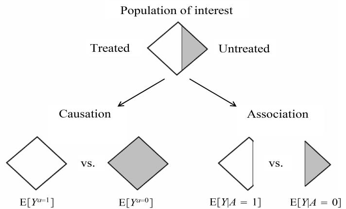
The definition of causation implies a contrast between the whole white diamond (all individuals treated) and the whole grey diamond (all individuals untreated), whereas association implies a contrast between the white (the treated) and the grey (the untreated) areas of the original diamond. That is, inferences about causation are concerned with what if questions in counterfactual worlds, such as “what would be the risk if everybody had been treated?” and “what would be the risk if everybody had been untreated?”, whereas inferences about association are concerned with questions in the actual world, such as “what is the risk in the treated?” and “what is the risk in the untreated?”

We can use the notation we have developed thus far to formalize this distinction between causation and association. The risk Pr [Y = 1|A = a] is a conditional probability: the risk of Y in the subset of the population that meet the condition ‘having actually received treatment value a’ (i.e., A = a). In contrast the risk Pr [Y ^a = 1] is an unconditional—also known as marginal probability, the risk of Y a in the entire population. Therefore, association is defined by a different risk in two disjoint subsets of the population determined by the individuals’ actual treatment value (A = 1 or A = 0), whereas causation is defined by a different risk in the same population under two different The difference between association treatment values (a = 1 or a = 0). Throughout this book we often use the redundant expression ‘causal effect’ to avoid confusions with a common use of ‘effect’ meaning simply association.

These radically different definitions explain the well-known adage “association is not causation.” In our population, there was association because the mortality risk in the treated (7/13) was greater than that in the untreated (3/7). However, there was no causation because the risk if everybody had been treated (10/20) was the same as the risk if everybody had been untreated. This discrepancy between causation and association would not be surprising if those who received heart transplants were, on average, sicker than those who did not receive a transplant. In Chapter 7 we refer to this discrepancy as confounding.

Causal inference requires data like the hypothetical data in Table 1.1, but all we can ever expect to have is real world data like those in Table 1.2. The question is then under which conditions real world data can be used for causal inference. The next chapter provides one answer: conduct a randomized experiment.

Figure 1.1

and causation is critical. Suppose the causal risk ratio of 5-year mortality is 0.5 for aspirin vs. no aspirin, and the corresponding associational risk ratio is 1.5 because individuals at high risk of cardiovascular death are preferentially prescribed aspirin. After a physician learns these results, she decides to withhold aspirin from her patients because those treated with aspirin have a greater risk of dying compared with the untreated. The doctor will be sued for malpractice.

Chapter 2 RANDOMIZED EXPERIMENTS

Does your looking up at the sky make other pedestrians look up too? This question has the main components of any causal question: we want to know whether an action (your looking up) affects an outcome (other people’s looking up) in a specific population (say, residents of Madrid in 2019). Suppose we challenge you to design a scientific study to answer this question. “Not much of a challenge,” you say after some thought, “I can stand on the sidewalk and flip a coin whenever someone approaches. If heads, I’ll look up; if tails, I’ll look straight ahead. I’ll repeat the experiment a few thousand times. If the proportion of pedestrians who looked up within 10 seconds after I did is greater than the proportion of pedestrians who looked up when I didn’t, I will conclude that my looking up has a causal effect on other people’s looking up. By the way, I may hire an assistant to record what people do while I’m looking up.” After conducting this study, you found that 55% of pedestrians looked up when you looked up but only 1% looked up when you looked straight ahead.

Your solution to our challenge was to conduct a randomized experiment. It was an experiment because the investigator (you) carried out the action of interest (looking up), and it was randomized because the decision to act on any study subject (pedestrian) was made by a random device (coin flipping). Not all experiments are randomized. For example, you could have looked up when a man approached and looked straight ahead when a woman did. Then the assignment of the action would have followed a deterministic rule (up for man, straight for woman) rather than a random mechanism. However, your findings would not have been nearly as convincing if you had conducted a nonrandomized experiment. If your action had been determined by the pedestrian’s sex, critics could argue that the “looking up” behavior of men and women differs (women may look up less often than do men after you look up) and thus your study compared essentially “noncomparable” groups of people. This chapter describes why randomization results in convincing causal inferences.

2.1 Randomization

tual theory to the estimation of causal effects via randomized experiments.

In a real world study we will not know both of Zeus’s potential outcomes Y a=1 under treatment and Y ^a=0 under no treatment. Rather, we can only know his observed outcome Y under the treatment value A that he happened to receive. Table 2.1 summarizes the available information for our population of 20 individuals. Only one of the two counterfactual outcomes is known for each individual: the one corresponding to the treatment level that he actually Neyman (1923) applied counterfac- received. The data are missing for the other counterfactual outcomes. As we discussed in the previous chapter, this missing data creates a problem because it appears that we need the value of both counterfactual outcomes to compute effect measures. The data in Table 2.1 are only good to compute association measures.

Randomized experiments, like any other real world study, generate data with missing values of the counterfactual outcomes as shown in Table 2.1. However, randomization ensures that those missing values occurred by chance. As a result, effect measures can be computed —or, more rigorously, consistently estimated—in randomized experiments despite the missing data. Let us be more precise.

Suppose that the population represented by a diamond in Figure 1.1 was

Table
——-

	A	Y	0 Y	1 Y
Rheia	0	0	0	?
Kronos	0	1	1	?
Demeter	0	0	0	?
Hades	0	0	0	?
Hestia	1	0	?	0
Poseidon	1	0	?	0
Hera	1	0	?	0
Zeus	1	1	?	1
Artemis	0	1	1	?
Apollo	0	1	1	?
Leto	0	0	0	?
Ares	1	1	?	1
Athena	1	1	?	1
Hephaestus	1	1	?	1
Aphrodite	1	1	?	1
Polyphemus	1	1	?	1
Persephone	1	1	?	1
Hermes	1	0	?	0
Hebe	1	0	?	0
Dionysus	1	0	?	0

Y ^a⊥⊥A for all a. See also Technical Point 2.1 for other versions of exchangeability.

near-infinite, and that we flipped a coin for each individual in such population. We assigned the individual to the white group if the coin turned tails, and Table 2.1 to the grey group if it turned heads. Note this was not a fair coin because the probability of heads was less than 50%—fewer people ended up in the grey group than in the white group. Next we asked our research assistants to administer the treatment of interest (A = 1), to individuals in the white group and a placebo (A = 0) to those in the grey group. Five days later, at the end of the study, we computed the mortality risks in each group, Pr [Y = 1|A = 1] = 0.3 and Pr [Y = 1|A = 0] = 0.6. The associational risk ratio was 0.3/0.6 = 0.5 and the associational risk difference was 0.3 − 0.6 = −0.3. We will assume that this was an ideal randomized experiment in all other respects: no loss to follow-up, full adherence to the assigned treatment over the duration of the study, a single version of treatment, and double blind assignment (see Chapter 9). Ideal randomized experiments are unrealistic but useful to introduce some key concepts for causal inference. Later in this book we consider more realistic randomized experiments.

Now imagine what would have happened if the research assistants had misinterpreted our instructions and had treated the grey group rather than the white group. Say we learned of the misunderstanding after the study finished. How does this reversal of treatment status affect our conclusions? Not at all. We would still find that the risk in the treated (now the grey group) Pr [Y = 1|A = 1] is 0.3 and the risk in the untreated (now the white group) Pr [Y = 1|A = 0] is 0.6. The association measure would not change. Because individuals were randomly assigned to white and grey groups, the proportion of deaths among the exposed, Pr [Y = 1|A = 1] is expected to be the same whether individuals in the white group received the treatment and individuals in the grey group received placebo, or vice versa. When group membership is randomized, which particular group received the treatment is irrelevant for the value of Pr [Y = 1|A = 1]. The same reasoning applies to Pr [Y = 1|A = 0], of course. Formally, we say that groups are exchangeable.

Exchangeability means that the risk of death in the white group would have been the same as the risk of death in the grey group had individuals in the white group received the treatment given to those in the grey group. That is, the risk under the potential treatment value a among the treated, Pr [Y ^a = 1|A = 1], equals the risk under the potential treatment value a among the untreated, Pr [Y ^a = 1|A = 0], for both a = 0 and a = 1. An obvious consequence of these (conditional) risks being equal in all subsets defined by treatment status in the population is that they must be equal to the (marginal) risk under treatment value a in the whole population: Pr [Y ^a = 1|A = 1] = Pr [Y ^a = 1|A = 0] = Pr [Y ^a = 1]. Because the counterfactual risk under treatment value a is the same in both groups A = 1 and A = 0, we say that the actual treatment A does not predict the counterfactual outcome Y a . Equivalently, exchangeability means that the counterfactual outcome and the actual treatment are independent, or Y Exchangeability: ^a⊥⊥A, for all values a. Randomization is so highly valued because it is expected to produce exchangeability. When the treated and the untreated are exchangeable, we sometimes say that treatment is exogenous, and thus exogeneity is commonly used as a synonym for exchangeability.

The previous paragraph argues that, in the presence of exchangeability, the counterfactual risk under treatment in the white part of the population would equal the counterfactual risk under treatment in the entire population. But the risk under treatment in the white group is not counterfactual at all because the white group was actually treated! Therefore our ideal randomized experiment allows us to compute the counterfactual risk under treatment in the population

Full exchangeability and mean exchangeability. Randomization makes the Y a jointly independent of A which implies, but is not implied by, exchangeability Y ^a⊥⊥A for each a. Formally, let A = {a, a′ , a′′ , …} denote the set of all treatment values present in the population, and Y ^A = n Y a , Y ^a ′ , Y ^a ′′ , …o the set of all counterfactual outcomes. Randomization makes Y ^A⊥⊥A. We refer to this joint independence as full exchangeability . For a dichotomous treatment, A = {0, 1} and full exchangeability is Y ^a=1, Y ^a=0 ⊥⊥A.

For a dichotomous outcome and treatment, exchangeability Y ^a⊥⊥A can also be written as Pr [Y ^a = 1|A = 1] = Pr [Y ^a = 1|A = 0] or, equivalently, as E[Y a |A = 1] = E[Y a |A = 0] for all a. We refer to the last equality as mean exchangeability . For a continuous outcome, exchangeability Y ^a⊥⊥A implies mean exchangeability E[Y a |A = a ′ ] = E[Y a ], but mean exchangeability does not imply exchangeability because distributional parameters other than the mean (e.g., variance) may not be independent of treatment.

Neither full exchangeability Y ^A⊥⊥A nor exchangeability Y ^a⊥⊥A are required to prove that E[Y a ] = E[Y |A = a]. Mean exchangeability is sufficient. As sketched in the main text, the proof has two steps. First, E[Y |A = a] = E[Y a |A = a] by consistency. Second, E[Y a |A = a] = E[Y a ] by mean exchangeability. Because exchangeability and mean exchangeability are identical concepts for the dichotomous outcomes used in this chapter, we use the shorter term “exchangeability” throughout.

Pr - Y ^a=1 = 1 because it is equal to the risk in the treated Pr [Y = 1|A = 1] = 0.3. That is, the risk in the treated (the white part of the diamond) is the same as the risk if everybody had been treated (and thus the diamond had been entirely white). Of course, the same rationale applies to the untreated: the counterfactual risk under no treatment in the population Pr - Y ^a=0 = 1 equals the risk in the untreated Pr [Y = 1|A = 0] = 0.6. The causal risk ratio is 0.5 and the causal risk difference is −0.3. In ideal randomized experiments, association is causation.

Here is another explanation for exchangeability Y ^a⊥⊥A in a randomized experiment. The counterfactual outcome Y a , like one’s genetic make-up, can be thought of as a fixed characteristic of a person existing before the treatment A was randomly assigned. This is because Y a encodes what would have been one’s outcome if assigned to treament a and thus does not depend on the treatment you later receive. Because treatment A was randomized, it is independent of both your genes and Y a . The difference between Y ^a and your genetic make-up is that, even conceptually, you can only learn the value of Y a after treatment is given and then only if one’s treatment A is equal to a.

Caution: Before proceeding, please make sure you understand the difference between ^a⊥⊥A and Y ⊥⊥A. Exchangeability Y ^a⊥⊥A is defined as independence between the counterfactual outcome and the observed treatment. Again, this means that the treated and the untreated would have experienced the same risk of death if they had received the same treatment level (either a = 0 or a = 1). But independence between the counterfactual outcome and the observed treatment Y ^a⊥⊥A does not imply independence between the observed outcome and the observed treatment Y ⊥⊥A. For example, in a randomized experiment in which exchangeability Y Suppose there is a causal effect on ^a⊥⊥A holds and the treatment has a causal effect on the outcome, then Y ⊥⊥A does not hold because the treatment is associated with the observed outcome.

Does exchangeability hold in our heart transplant study of Table 2.1? To answer this question we would need to check whether Y ^a⊥⊥A holds for a = 0 and for a = 1. Take a = 0 first. Suppose the counterfactual data in Table 1.1 are available to us. We can then compute the risk of death under no treatment

Y ^a ⊥⊥ A is different from Y ⊥⊥A. Y

some individuals so that Y ^a=1 ̸= Y ^a=0. Since Y = Y ^A, then Y a with a evaluated at the observed treatment A is the observed Y A, which depends on A, and thus will not be independent of A.

Crossover experiments. Suppose we want to estimate the individual causal effect of lightning bolt use A on Zeus’s blood pressure Y . We define the counterfactual outcomes Y ^a=1 and Y ^a=0 to be 1 if Zeus’s blood pressure is temporarily elevated after calling or not calling a lightning strike, respectively. Suppose we convinced Zeus to use his lightning bolt only when suggested by us. Yesterday morning we asked Zeus to call a lightning strike (a = 1). His blood pressure was elevated after doing so. This morning we asked Zeus to refrain from using his lightning bolt (a = 0). His blood pressure did not increase. We have conducted a crossover experiment in which an individual’s outcome is sequentially observed under two treatment values. One might argue that, because we have observed both of Zeus’s counterfactual outcomes Y ^a=1 = 1 and Y ^a=0 = 0, using a lightning bolt has a causal effect on Zeus’s blood pressure. However, this argument is generally incorrect unless the very strong assumptions i)–iii) given in the next paragraph are true.

In crossover experiments, individuals are observed during two or more periods, say t = 0 and t = 1. An individual i receives a different treatment value Ait in each period t. Let Y a0a¹ i1 be the (deterministic) counterfactual outcome at t = 1 for individual i if treated with a¹ at t = 1 and a⁰ at t = 0. Let Y a⁰ i0 be defined similarly for t = 0. The individual causal effect Y at=1 it − Y at=0 it can be identified if the following three conditions hold: i) no carryover effect of treatment: Y a0,a¹ it=1 = Y a¹ it=1, ii) the individual causal effect does not depend on time: Y at=1 it − Y at=0 it = αⁱ for t = 0, 1, and iii) the counterfactual outcome under no treatment does not depend on time: Y at=0 it = βⁱ for t = 0, 1. Under these conditions, if the individual is treated at time 1 (Ai¹ = 1) but not time 0 (Ai⁰ = 0) then, by consistency, Yi¹ − Yi⁰ is the individual causal effect because Yi¹ − Yi⁰ = Y a1=1 ⁱ¹ − Y a0=0 ⁱ⁰ = Y a1=1 ⁱ¹ − Y a1=0 ⁱ¹ + Y a1=0 ⁱ¹ − Y a0=0 ⁱ⁰ = αⁱ + βⁱ − βⁱ = αⁱ . Similarly if Ai¹ = 0 and Ai⁰ = 1, Yi⁰ − Yi¹ = αⁱ is the individual level causal effect.

Condition (i) implies that the outcome Y at it has an abrupt onset that completely resolves by the next time period. Hence, crossover experiments cannot be used to study the effect of heart transplant, an irreversible action, on death, an irreversible outcome. See also Fine Point 3.2.

Pr - Y ^a=0 = 1|A = 1 = 7/13 in the 13 treated individuals and the risk of death under no treatment Pr - Y ^a=0 = 1|A = 0 = 3/7 in the 7 untreated individuals. Since the risk of death under no treatment is greater in the treated than in the untreated individuals, i.e., 7/13 > 3/7, we conclude that the treated have a worse prognosis than the untreated, i.e., that the treated and the untreated are not exchangeable. Mathematically, we have proven that exchangeability Y ^a⊥⊥A does not hold for a = 0. (You can check that it does not hold for a = 1 Reminder: Our discussion of ran- either.) Thus the answer to the question that opened this paragraph is ‘No’.

But only the observed data in Table 2.1, not the counterfactual data in Table 1.1, are available in the real world. Since Table 2.1 is insufficient to compute counterfactual risks like the risk under no treatment in the treated Pr - Y ^a=0 = 1|A = 1 , we are generally unable to determine whether exchangeability holds in our study. However, suppose for a moment, that we actually had access to Table 1.1 and determined that exchangeability does not hold in our heart transplant study. Can we then conclude that our study is not a randomized experiment? No, for two reasons. First, as you are probably already thinking, a twenty-person study is too small to reach definite conclusions. Random fluctuations arising from sampling variability could explain almost anything. We will discuss random variability in Chapter 10. Until then, let us assume that each individual in our population represents 1 billion individuals that are identical to him or her. Second, it is still possible that a study is a randomized experiment even if exchangeability does not hold in infinite samples. However, unlike the type of randomized experiment described in this section, it would need to be a randomized experiment in which investigators use more than one coin to randomly assign treatment. The next section describes randomized experiments with more than one coin.

domized experiments refers to population or average causal effects because individual causal effects cannot generally be identified. See Fine Point 2.1.

2.2 Conditional randomization

Table	2.2
——-	—–

	L	A	Y
Rheia	0	0	0
Kronos	0	0	1
Demeter	0	0	0
Hades	0	0	0
Hestia	0	1	0
Poseidon	0	1	0
Hera	0	1	0
Zeus	0	1	1
Artemis	1	0	1
Apollo	1	0	1
Leto	1	0	0
Ares	1	1	1
Athena	1	1	1
Hephaestus	1	1	1
Aphrodite	1	1	1
Polyphemus	1	1	1
Persephone	1	1	1
Hermes	1	1	0
Hebe	1	1	0
Dionysus	1	1	0

Table 2.2 shows the data from our heart transplant randomized study. Besides Table 2.2 data on treatment A (1 if the individual received a transplant, 0 otherwise) and outcome Y (1 if the individual died, 0 otherwise), Table 2.2 also contains data on the prognostic factor L (1 if the individual was in critical condition, 0 otherwise), which we measured before treatment was assigned. We now consider two mutually exclusive study designs and discuss whether the data in Table 2.2 could have arisen from either of them.

In design 1 we would have randomly selected 65% of the individuals in the population and transplanted a new heart to each of the selected individuals. That would explain why 13 out of 20 individuals were treated. In design 2 we would have classified all individuals as being in either critical (L = 1) or noncritical (L = 0) condition. Then we would have randomly selected 75% of the individuals in critical condition and 50% of those in noncritical condition, and transplanted a new heart to each of the selected individuals. That would explain why 9 out of 12 individuals in critical condition, and 4 out of 8 individuals in noncritical condition, were treated.

Both designs are randomized experiments. Design 1 is precisely the type of randomized experiment described in Section 2.1. Under this design, we would use a single coin to assign treatment to all individuals (e.g., treated if tails, untreated if heads): a loaded coin with probability 0.65 of turning tails, thus resulting in 65% of the individuals receiving treatment. Under design 2 we would not use a single coin for all individuals. Rather, we would use a coin with a 0.75 chance of turning tails for individuals in critical condition, and another coin with a 0.50 chance of turning tails for individuals in noncritical condition. We refer to design 2 experiments as conditionally randomized experiments because we use several randomization probabilities that depend (are conditional) on the values of the variable L. We refer to design 1 experiments as marginally randomized experiments because we use a single unconditional (marginal) randomization probability that is common to all individuals.

As discussed in the previous section, a marginally randomized experiment is expected to result in exchangeability of the treated and the untreated:

Pr [Y ^a = 1|A = 1] = Pr [Y ^a = 1|A = 0] or Y ^a⊥⊥A for all a.

In contrast, a conditionally randomized experiment will not generally result in exchangeability of the treated and the untreated because, by design, each group may have a different proportion of individuals with bad prognosis.

Thus the data in Table 2.2 could not have arisen from a marginally randomized experiment because 69% treated versus 43% untreated individuals were in critical condition. This imbalance indicates that the risk of death in the treated, had they remained untreated, would have been higher than the risk of death in the untreated. That is, treatment A predicts the counterfactual risk of death under no treatment, and exchangeability Y ^a⊥⊥A does not hold. Since our study was a randomized experiment, you can safely conclude that the study was a randomized experiment with randomization conditional on L.

Our conditionally randomized experiment is simply the combination of two separate marginally randomized experiments: one conducted in the subset of individuals in critical condition (L = 1), the other in the subset of individuals in noncritical condition (L = 0). Consider first the randomized experiment being conducted in the subset of individuals in critical condition. In this subset, the treated and the untreated are exchangeable. Formally, the counterfactual mortality risk under each treatment value a is the same among the treated and the untreated given that they all were in critical condition at the time of treatment assignment. That is,

\[\Pr\left[Y^{a} = 1 | A = 1, L = 1\right] = \Pr\left[Y^{a} = 1 | A = 0, L = 1\right] \text{ or } Y^{a} \perp\!\!\perp A | L = 1 \text{ for all } a, b\]

where Y ^a⊥⊥A|L = 1 means Y ^a and A are independent given L = 1. Similarly, randomization also ensures that the treated and the untreated are exchangeable in the subset of individuals that were in noncritical condition, i.e., Y ^a⊥⊥A|L = 0. When Y ^a⊥⊥A|L = l holds for all values l we simply write Y Conditional exchangeability: ^a⊥⊥A|L. Thus, although conditional randomization does not guarantee un^a⊥⊥A|L for all a conditional (or marginal) exchangeability Y ^a⊥⊥A, it guarantees conditional exchangeability Y ^a⊥⊥A|L within levels of the variable L. In summary, marginal randomization (design 1) produces both marginal exchangeability and conditional exchangeability, whereas conditional randomization (design 2) produces only conditional exchangeability.

We know how to compute effect measures under marginal exchangeability: the causal risk ratio Pr - Y ^a=1 = 1 /Pr - Y ^a=0 = 1 equals the associational risk ratio Pr [Y = 1|A = 1] /Pr [Y = 1|A = 0] in marginally randomized If A = 1, Y experiments because exchangeability ensures that the counterfactual risk un- ^a=0 is missing; der treatment level a, Pr [Y ^a = 1], equals the observed risk among those who received treatment level a, Pr [Y = 1|A = a]. Thus, if the data in Table 2.2 had been collected during a marginally randomized experiment, the causal risk ratio would be readily calculated from the data on A and Y as 7/13 3/7 = 1.26. The question is how to compute the causal risk ratios in a conditionally randomized experiment. Remember that a conditionally randomized experiment is simply the combination of two (or more) separate marginally randomized experiments conducted in different subsets of the population L = 1 and L = 0. Thus we have two options.

First, we compute the average causal effect in each of these subsets or strata of the population. Because association is causation within each subset, the stratum-specific causal risk ratio Pr - Y ^a=1 = 1|L = 1 /Pr - Y ^a=0 = 1|L = 1 among people in critical condition is equal to the stratum-specific associational risk ratio Pr [Y = 1|L = 1, A = 1] /Pr [Y = 1|L = 1, A = 0] among people in critical condition. And analogously for L = 0. We refer to this method to compute stratum-specific causal effects as stratification. Note that the stratumspecific causal risk ratio in the subset L = 1 may differ from the causal risk ratio in L = 0. In that case, we say that the effect of treatment is modified by L, or that there is effect modification by L or that there is treatment effect heterogeneity across levels of L. Stratification and effect modification are discussed in more detail in Chapter 4.

Second, we compute the average causal effect Pr - Y ^a=1 = 1 /Pr - Y ^a=0 = 1 in the entire population, as we have been doing so far. Whether our principal interest lies in the stratum-specific average causal effects versus the average causal effect in the entire population depends on practical and theoretical considerations discussed in detail in Chapter 4 and in Part III. As one example, you may be interested in the average causal effect in the entire population, rather than in the stratum-specific average causal effects, if you do not expect to have information on L for future individuals (e.g., the variable L is expensive to measure) and thus your decision to treat cannot depend on the value of L. Until Chapter 4, we will restrict our attention to the average causal effect in the entire population. The next two sections describe how to use data from conditionally randomized experiments to compute the average causal effect in the entire population. See also Fine Point 2.2 for a discussion of risk periods.

Y

if A = 0, Y ^a=1 is missing. Data are missing completely at random (MCAR) if Pr - A = a|L, Y ^a=1, Y ^a=0 = Pr [A = a], which holds in a marginally randomized experiment. Data are missing at random (MAR) if the probability of A = a conditional on the full data (L, Y ^a=1, Y ^a=0) only depends on the data that would be observed (L, Y ^a ) if A = a. In fact, MAR implies Pr - A = a|L, Y ^a=1, Y ^a=0 = Pr [A = a|L], which holds in a conditionally randomized experiment because, by MAR, Pr - A = 1|L, Y ^a=1, Y ^a=0 cannot depend on Y ^a=0 and 1 − Pr - A = 1|L, Y ^a=1, Y ^a=0 = Pr - A = 0|L, Y ^a=1, Y ^a=0 cannot depend on Y ^a=1. The terms MCAR, MAR, and MNAR (missing not at random) were introduced by Rubin (1976) and Marini, Olsen, and Rubin (1980).

Risk periods. We have defined a risk as the proportion of individuals who develop the outcome of interest during a particular period. For example, the 5-day mortality risk in the treated Pr [Y = 1|A = 1] is the proportion of treated individuals who died during the first five days of follow-up. Throughout the book we often specify the period when the risk is first defined (e.g., 5 days) and, for conciseness, omit it later. That is, we may just say “the mortality risk” rather than “the five-day mortality risk.”

The following example highlights the importance of specifying the risk period. Suppose a randomized experiment was conducted to quantify the causal effect of antibiotic therapy on mortality among elderly humans infected with the plague bacteria. An investigator analyzes the data and concludes that the causal risk ratio is 0.05, i.e., on average antibiotics decrease mortality by 95%. A second investigator also analyzes the data but concludes that the causal risk ratio is 1, i.e., antibiotics have a null average causal effect on mortality. Both investigators are correct. The first investigator computed the ratio of 1-year risks, whereas the second investigator computed the ratio of 100-year risks. The 100-year risk was of course 1 regardless of whether individuals received the treatment. When we say that a treatment has a causal effect on mortality, we mean that death is delayed, not prevented, by the treatment.

2.3 Standardization

Our heart transplant study is a conditionally randomized experiment: the investigators used a random procedure to assign hearts (A = 1) with probability 50% to the 8 individuals in noncritical condition (L = 0), and with probability 75% to the 12 individuals in critical condition (L = 1). First, let us focus on the 8 individuals—remember, they are really the average representatives of 8 billion individuals—in noncritical condition. In this group, the risk of death among the treated is Pr [Y = 1|L = 0, A = 1] = ¹ 4 , and the risk of death among the untreated is Pr [Y = 1|L = 0, A = 0] = ¹ 4 . Because treatment was randomly assigned to individuals in the group L = 0, i.e., Y ^a⊥⊥A|L = 0, the observed risks are equal to the counterfactual risks. That is, in the group L = 0, the risk in the treated equals the risk if everybody had been treated, Pr [Y = 1|L = 0, A = 1] = Pr - Y ^a=1 = 1|L = 0 , and the risk in the untreated equals the risk if everybody had been untreated, Pr [Y = 1|L = 0, A = 0] = Pr - Y ^a=0 = 1|L = 0 . Following a similar reasoning, we can conclude that the observed risks equal the counterfactual risks in the group of 12 individuals in critical condition, i.e., Pr [Y = 1|L = 1, A = 1] = Pr - Y ^a=1 = 1|L = 1 = 2 3 , and Pr [Y = 1|L = 1, A = 0] = Pr - Y ^a=0 = 1|L = 1 = 2 3 .

Suppose now that our goal is to compute the causal risk ratio Pr[Y ^a=1 = 1]/Pr[Y ^a=0 = 1]. The numerator of the causal risk ratio is the risk if all 20 individuals in the population had been treated. From the previous paragraph, we know that the risk if all individuals had been treated is ¹ 4 in the 8 individuals with L = 0 and ² 3 in the 12 individuals with L = 1. Therefore the risk if all 20 individuals in the population had been treated will be a weighted average of 1 4 and ² 3 in which each group receives a weight proportional to its size. Since 40% of the individuals (8) are in group L = 0 and 60% of the individuals (12) are in group L = 1, the weighted average is ^{1 4 × 0}.4 + ^{2 3} × 0.6 = 0.5. Thus the risk if everybody had been treated Pr[Y ^a=1 = 1] is equal to 0.5. By following the same reasoning we can calculate that the risk if nobody had been treated Pr[Y ^a=0 = 1] is also equal to 0.5. The causal risk ratio is then 0.5/0.5 = 1.

More formally, the marginal counterfactual risk Pr[Y ^a = 1] is the weighted average of the stratum-specific risks Pr[Y ^a = 1|L = 0] and Pr[Y ^a = 1|L = 1] with weights equal to the proportion of individuals in the population with

L = 0 and L = 1, respectively. That is, Pr[Y ^a = 1] = Pr[Y ^a = 1|L = 0] Pr [L = 0] + Pr[Y ^a = 1|L = 1] Pr [L = 1]. Or, using a more compact notation, Pr[Y ^a = 1] = P ^l Pr[Y ^a = 1|L = l] Pr [L = l], where P ^l means sum over all values l that occur in the population. Under conditional exchangeability, we can replace the counterfactual risk Pr[Y ^a = 1|L = l] by the observed risk Pr[Y = 1|L = l, A = a] in the expression above. That is, Pr[Y ^a = 1] = P ^l Pr[Y = 1|L = l, A = a] Pr [L = l]. The left-hand side of this equality is an unobserved counterfactual risk whereas the right-hand side includes observed quantities only, which can be computed using data on L, A, and Y . When, as here, a counterfactual quantity can be expressed as a function of the distribution (i.e., the probabilities) of the observed data, we say that the counterfactual quantity is identified (or identifiable); otherwise, we say it is unidentified.

This method is known in epidemiology, demography, and other disciplines as standardization. For example, the numerator P Standardized mean ^l Pr[Y = 1|L = l, A = 1] Pr [L = l] of the causal risk ratio is the standardized risk in the treated using the population as the standard. Under conditional exchangeability, this standardized risk can be interpreted as the (counterfactual) risk that would have been observed had all the individuals in the population been treated.

The standardized risks in the treated and the untreated are equal to the counterfactual risks under treatment and no treatment, respectively. Therefore, the causal risk ratio Pr[^{Y a}=1 = 1] Pr[^{Y a}=0 = 1] can be computed by standardization as P ^l Pr[Y = 1|L = l, A = 1] Pr [L = l] P ^l Pr[Y = 1|L = l, A = 0] Pr [L = l] .

2.4 Inverse probability weighting

fully randomized causally interpreted structured tree graph or FR-CISTG (Robins 1986, 1987) representation of a conditionally randomized experiment. Did we win the prize for the worst acronym ever?

In the previous section we computed the causal risk ratio in a conditionally randomized experiment via standardization. In this section we compute this causal risk ratio via inverse probability weighting. The data in Table 2.2 can be displayed as a tree in which all 20 individuals start at the left and progress over time towards the right, as in Figure 2.1. The leftmost circle of Figure 2.1 is an example of a the tree contains its first branching: 8 individuals were in noncritical condition (L = 0) and 12 in critical condition (L = 1). The numbers in parentheses are the probabilities of being in noncritical, Pr [L = 0] = 8/20 = 0.4, or critical, Pr [L = 1] = 12/20 = 0.6, condition. Let us follow, e.g., the branch L = 0. Of the 8 individuals in this branch, 4 were untreated (A = 0) and 4 were treated (A = 1). The conditional probability of being untreated is Pr [A = 0|L = 0] = 4/8 = 0.5, as shown in parentheses. The conditional probability of being treated Pr [A = 1|L = 0] is 0.5 too. The upper right circle represents that, of the 4 individuals in the branch (L = 0, A = 0), 3 survived (Y = 0) and 1 died (Y = 1). That is, Pr [Y = 0|L = 0, A = 0] = 3/4 and Pr [Y = 1|L = 0, A = 0] = 1/4. The other branches of the tree are interpreted analogously. The circles contain the bifurcations defined by non-treatment variables. We now use this tree to compute the causal risk ratio.

P ^l E[Y |L = l, A = a] × Pr [L = l]

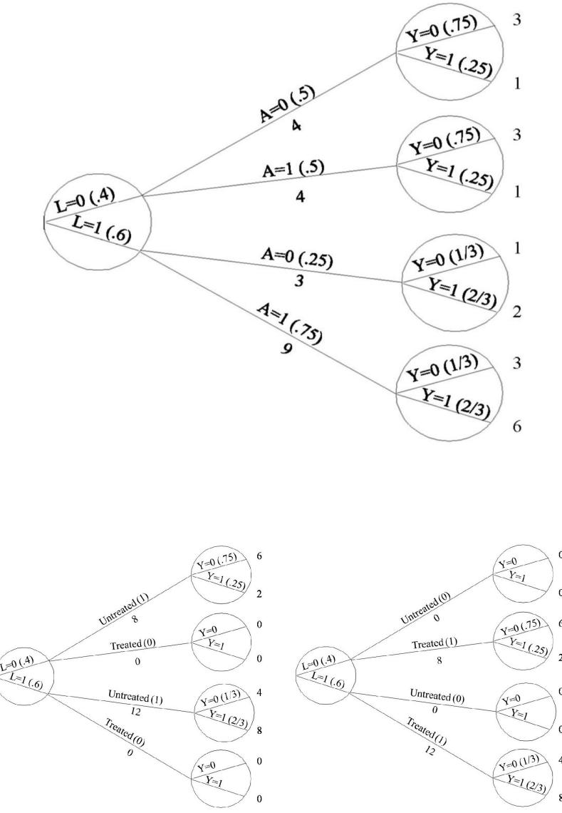
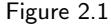
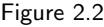
The denominator of the causal risk ratio, Pr[Y ^a=0 = 1], is the counterfactual risk of death had everybody in the population remained untreated. Let us calculate this risk. In Figure 2.1, 4 out of 8 individuals with L = 0 were untreated, and 1 of them died. How many deaths would have occurred had the 8 individuals with L = 0 remained untreated? Two deaths, because if 8 individuals rather than 4 individuals had remained untreated, then 2 deaths rather than 1 death would have been observed. If the number of individuals is multiplied times 2, then the number of deaths is also doubled. In Figure 2.1, 3 out of 12 individuals with L = 1 were untreated, and 2 of them died. How many deaths would have occurred had the 12 individuals with L = 1 remained untreated? Eight deaths, or 2 deaths times 4, because 12 is 3×4. That is, if all 8 + 12 = 20 individuals in the population had been untreated, then 2 + 8 = 10 would have died. The denominator of the causal risk ratio, Pr[Y ^a=0 = 1], is 10/20 = 0.5. The first tree in Figure 2.2 shows the population had everybody remained untreated. Of course, these calculations rely on the condition that treated individuals with L = 0, had they remained untreated, would have had the same probability of death as those who actually remained untreated. This condition is precisely exchangeability given L = 0.

The numerator of the causal risk ratio Pr[Y ^a=1 = 1] is the counterfactual risk of death had everybody in the population been treated. Reasoning as in the previous paragraph, this risk is calculated to be also 10/20 = 0.5, under exchangeability given L = 1. The second tree in Figure 2.2 shows the population had everybody been treated. Combining the results from this and the previous paragraph, the causal risk ratio Pr[Y ^a=1 = 1]/Pr[Y ^a=0 = 1] is equal to 0.5/0.5 = 1. We are done.

Let us examine how this method works. The two trees in Figure 2.2 are a simulation of what would have happened had all individuals in the population been untreated and treated, respectively. These simulations are correct under conditional exchangeability. Both simulations can be pooled to create a hypothetical population in which every individual appears as a treated and as an untreated individual. This hypothetical population, twice as large as the original population, is known as the pseudo-population. Figure 2.3 shows the entire pseudo-population. Under conditional exchangeability Y ^a⊥⊥A|L in the original population, the treated and the untreated are (unconditionally) exchangeable in the pseudo-population because the L is independent of A. That is, the associational risk ratio in the pseudo-population is equal to the causal risk ratio in both the pseudo-population and the original population.

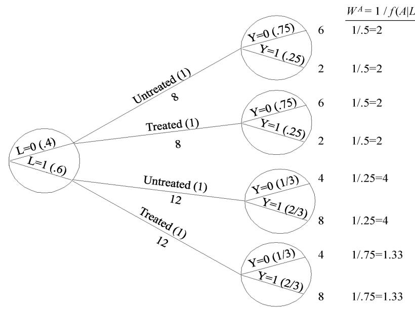
Figure 2.3

posed by Horvitz and Thompson (1952) for surveys in which subjects are sampled with unequal probabilities. See Technical Point 12.1.

This method is known as inverse probability (IP) weighting. To see why, IP weighted estimators were pro- let us look at, say, the 4 untreated individuals with L = 0 in the population of Figure 2.1. These individuals are used to create 8 members of the pseudopopulation of Figure 2.3. That is, each of them receives a weight of 2, which is equal to 1/0.5. Figure 2.1 shows that 0.5 is the conditional probability of staying untreated given L = 0. Similarly, the 9 treated individuals with L = 1

Formal definition of IP weights. An individual’s IP weight depends on the individual’s values of treatment A and covariate L. For example, a treated individual with L = l receives the weight 1/Pr [A = 1|L = l], whereas an untreated individual with L = l ′ receives the weight 1/Pr [A = 0|L = l ′ ]. We can express these weights using a single expression for all individuals—regardless of their individual treatment and covariate values—by using the probability density function (pdf) of A rather than the probability of A. The conditional pdf of A given L evaluated at the values a and l is represented by fA|^L [a|l], or simply as f [a|l]. For discrete variables A and L, f [a|l] is the conditional probability Pr [A = a|L = l]. In a conditionally randomized experiment, f [a|l] is positive for all l such that Pr [L = l] is nonzero.

Since the denominator of the weight for each individual is the conditional density evaluated at the individual’s own values of A and L, it can be expressed as the conditional density evaluated at the random arguments A and L (as opposed to the fixed arguments a and l), that is, as f [A|L]. This notation, which appeared in Figure 2.3, is used to define the IP weights W^A = 1/f [A|L]. It is needed to have a unified notation for the weights because Pr [A = A|L = L] is tautologically equal to 1 and thus not considered proper notation.

As explained in the main text, the mean of the outcome in the pseudo-population Eps [Y |A = a] equals the IP weighted mean of the outcome in the population, E [Y I (A = a) /Pr (A = a|L)], where I (A = a) is 1 when A = a and 0 otherwise. A proof follows:

Eps [Y |A = a] = Eps [Y I (A = a)] /Eps[I (A = a)] (by the laws of probability) = E- WAY I (A = a) /E - I (A = a) W^A (by definition of Eps) = E [Y I (A = a) /Pr (A = a|L)] /E [I (A = a) /Pr (A = a|L)] (because I (A = a) /f (A|L) = I (A = a) /f (a|L)) = E [Y I (A = a) /Pr (A = a|L)] (because E [I (A = a) /Pr (A = a|L)|L] = 1).

in Figure 2.1 are used to create 12 members of the pseudo-population. That is, each of them receives a weight of 1.33 = 1/0.75. Figure 2.1 shows that 0.75 is the conditional probability of being treated given L = 1. Informally, the pseudo-population is created by weighting each individual in the population IP weight: W by the inverse of the conditional probability of receiving the treatment level ^A = 1/f [A|L] that she indeed received. These IP weights are shown in Figure 2.3.

IP weighting yielded the same result as standardization—causal risk ratio equal to 1— in our example above. This is no coincidence: standardization and IP weighting are mathematically equivalent (see Technical Point 2.3). In fact, both standardization and IP weighting can be viewed as procedures to build a new tree in which all individuals receive treatment a. Each method uses a different set of the probabilities to build the counterfactual tree: IP weighting uses the conditional probability of treatment A given the covariate L (as shown in Figure 2.1), standardization uses the probability of the covariate L and the conditional probability of outcome Y given A and L.

Because both standardization and IP weighting simulate what would have been observed if the variable (or variables in the vector) L had not been used to decide the probability of treatment, we often say that these methods adjust for L. In a slight abuse of language we sometimes say that these methods control for L, but this “analytic control” is quite different from the “physical control” in a randomized experiment. Standardization and IP weighting can be generalized to conditionally randomized studies with continuous outcomes (see Technical Point 2.3).

Why not finish this book here? We have a study design (an ideal randomized experiment) that, when combined with the appropriate analytic method (standardization or IP weighting), allows us to compute average causal effects. Unfortunately, randomized experiments are often unethical, impractical, or untimely. For example, it is questionable that an ethical committee would have

approved our heart transplant study. Hearts are in short supply and society favors assigning them to individuals who are more likely to benefit from the transplant, rather than assigning them randomly among potential recipients. Also one could question the feasibility of the study even if ethical issues were ignored: double-blind assignment is impossible, individuals assigned to medical treatment may not resign themselves to forego a transplant, and there may not be compatible hearts for those assigned to transplant. Even if the study were feasible, it would still take several years to complete it, and decisions must be made in the interim. Frequently, conducting an observational study is the least bad option.

Equivalence of IP weighting and standardization. Assume that A is discrete with finite number of values and that f [a|l] is positive for all l such that Pr [L = l] is nonzero. This positivity condition is guaranteed to hold in conditionally randomized experiments. Under positivity, the standardized mean for treatment level a is defined as P l E [Y |A = a, L = l] Pr [L = l] and the IP weighted mean of Y for treatment level a is defined as E I (A = a) Y f [A|L] . The indicator function I (A = a) is the function that takes value 1 for individuals with A = a, and 0 for the others.

We now prove the equality of the IP weighted and standardized means under positivity. By definition of expectation,

\[\operatorname{E}\left[\frac{I\left(A=a\right)Y}{f\left[A\middle|L\right]}\right] = \sum\_{l} \frac{1}{f\left[a\middle|l\right]} \left\{\operatorname{E}\left[Y\middle|A=a, L=l\right]f\left[a\middle|l\right]\Pr\left[L=l\right]\right\} = \sum\_{l} \left\{\operatorname{E}\left[Y\middle|A=a, L=l\right]\Pr\left[L=l\right]\right\} \text{ where in } \operatorname{E}\left[\operatorname{E}\left[Y\middle|A=a\right]\right]\]

the final step we cancelled f [a|l] from the numerator and denominator, and in the first step we did not need to sum over the possible values of A because for any a ′ other than a the quantity I(a ′ ) is zero. The proof treats A and L as discrete but not necessarily dichotomous. For continuous L simply replace the sum over L with an integral.

The proof makes no reference to counterfactuals. However, if we further assume conditional exchangeability, then both the IP weighted and the standardized means are equal to the counterfactual mean E [Y a ]. Here we provide two different proofs of this last statement. First, we prove equality of E [Y a ] and the standardized mean as in the text: E [Y a ] = X E [Y a |L = l] Pr [L = l] = X E [Y a |A = a, L = l] Pr [L = l] = X E [Y |A = a, L = l] Pr [L = l]

l l l where the second equality is by conditional exchangeability and positivity, and the third by consistency. Second, we prove equality of E [Y a ] and the IP weighted mean as follows: E I (A = a) f [A|L] Y is equal to E I (A = a) f [A|L] Y a by consistency. Next, because positivity implies f [a|L] is never 0, we have

E I (A = a) f [A|L] Y a = E E I (A = a) f [a|L] Y a L = E E I (A = a) f [a|L] L E [Y a |L] (by conditional exchangeability)

\[\mathbf{E} = \operatorname{E} \left\{ \operatorname{E} \left[ Y^{a} | L] \right] \text{ (because } \operatorname{E} \left[ \begin{array}{c} I \left( A = a \right) \\ \hline f \left[ a | L \right] \\ \text{.} \end{array} \right] \begin{array}{c} L \\ \hline \end{array} \right\} = \operatorname{E} \left[ Y^{a} \right] \dots\]

When treatment is continuous, which is an unlikely design choice in conditionally randomized experiments, E [I (A = a) Y /f (A|L)] is no longer equal to P ^l E [Y |A = a, L = l] Pr[L = l] and thus is biased for E [Y a ] even under exchangeability. To see this, one can calculate that E [I (A = a) /f (a|l)|L = l] is equal to 0 rather than 1 if we take f(a|l) to be (a version of) the conditional density of A given L = l (with respect to Lebesgue measure). On the other hand, if we continue to take f(a|l) to be Pr [A = a|L = l], the denominator f(a|L = l) is zero on a set with probability 1 so positivity fails. In Section 12.4 we discuss how IP weighting can be generalized to accomodate continuous treatments. In Technical Point 3.1, we discuss that the results above do not hold in the absence of positivity, even for discrete A.

Chapter 3 OBSERVATIONAL STUDIES

Consider again the causal question “does one’s looking up at the sky make other pedestrians look up too?” After considering a randomized experiment as in the previous chapter, you concluded that looking up so many times was too time-consuming and unhealthy for your neck bones. Hence you decided to conduct the following study: Find a nearby pedestrian who is standing in a corner and not looking up. Then find a second pedestrian who is walking towards the first one and not looking up either. Observe and record their behavior during the next 10 seconds. Repeat this process a few thousand times. You could now compare the proportion of second pedestrians who looked up after the first pedestrian did, and compare it with the proportion of second pedestrians who looked up before the first pedestrian did. Such a scientific study in which the investigator observes and records the relevant data is referred to as an observational study.

If you had conducted the observational study described above, critics could argue that two pedestrians may both look up not because the first pedestrian’s looking up causes the other’s looking up, but because they both heard a thunderous noise above or some rain drops started to fall, and thus your study findings are inconclusive as to whether one’s looking up makes others look up. These criticisms do not apply to randomized experiments, which is one of the reasons why randomized experiments are central to the theory of causal inference. However, in practice, the importance of randomized experiments for the estimation of causal effects is more limited. Many scientific studies are not experiments. Much human knowledge is derived from observational studies. Think of evolution, tectonic plates, global warming, or astrophysics. Think of how humans learned that hot coffee may cause burns. This chapter reviews some conditions under which observational studies lead to valid causal inferences.

3.1 Identifiability conditions

ers only randomized experiments in which all participants remain under follow-up and adhere to their assigned treatment throughout the entire study. Chapters 8 and 9 discuss alternative scenarios.

Ideal randomized experiments can be used to identify and quantify average causal effects because the randomized assignment of treatment leads to exchangeability. Take a marginally randomized experiment of heart transplant and mortality as an example: if those who received a transplant had not re-For simplicity, this chapter consid- ceived it, they would have been expected to have the same death risk as those who did not actually receive the heart transplant. As a consequence, an associational risk ratio of 0.7 from the randomized experiment is expected to equal the causal risk ratio.

Observational studies, on the other hand, may be much less convincing (for an example, see the introduction to this chapter). A key reason for our hesitation to endow observational associations with a causal interpretation is the lack of randomized treatment assignment. As an example, take an observational study of heart transplant and mortality in which those who received the heart transplant were more likely to have a severe heart condition. Then, if those who received a transplant had not received it, they would have been expected to have a greater death risk than those who did not actually receive the heart transplant. As a consequence, an associational risk ratio of 1.1 from the observational study would be a compromise between the truly beneficial effect of transplant on mortality (which pushes the associational risk ratio to be under 1) and the underlying greater mortality risk in those who received transplant

(which pushes the associational risk ratio to be over 1). The best explanation for an association between treatment and outcome in an observational study is not necessarily a causal effect of the treatment on the outcome.

While recognizing that randomized experiments have intrinsic advantages for causal inference, sometimes we are stuck with observational studies to answer causal questions. What do we do? A common strategy is to analyze our data as if treatment had been randomly assigned conditional on measured covariates L—though we often know this is at best an approximation. Causal inference from observational data then revolves around the hope that the observational study can be viewed as a conditionally randomized experiment.

Informally, an observational study can be conceptualized as a conditionally Table 3.1 randomized experiment if the following conditions hold:

• 1. the values of treatment under comparison correspond to well-defined interventions that, in turn, correspond to the versions of treatment in the data
• 2. the conditional probability of receiving every value of treatment, though not decided by the investigators, depends only on measured covariates L
• 3. the probability of receiving every value of treatment conditional on L is greater than zero, i.e., positive

In this chapter we describe these three conditions in the context of observational studies. Condition 1 was referred to as consistency in Chapter 1, condition 2 was referred to as exchangeability in the previous chapters, and condition 3 was referred to as positivity in Technical Point 2.3.

We will see that these conditions are often heroic, which explains why causal inferences from observational studies are viewed with suspicion. However, if the analogy between observational study and conditionally randomized experiment happens to be correct, then we can use the methods described in the previous chapter—IP weighting or standardization—to identify causal effects from observational studies. We therefore refer to these conditions as identifiability conditions or assumptions. For example, in the previous chapter, we computed a causal risk ratio equal to 1 using the data in Table 2.2, which arose from a conditionally randomized experiment. If the same data, now shown in Table 3.1, had arisen from an observational study and the three identifiability conditions above held true, we would also compute a causal risk ratio equal to

Importantly, in ideal randomized experiments the identifiability conditions hold by design. That is, for a conditionally randomized experiment, we would only need the data in Table 3.1 to compute the causal risk ratio of 1. In contrast, to identify the causal risk ratio from an observational study, we would need to assume that the identifiability conditions held, which of course may not be true. Causal inference from observational data requires two elements: data and identifiability conditions. See Fine Point 3.1 for a more precise definition of identifiability.

When any of the identifiability conditions does not hold, the analogy between observational study and conditionally randomized experiment breaks down. In that situation, there are other possible approaches to causal inference from observational data, which require a different set of identifiability conditions. One of these approaches is hoping that a predictor of treatment, referred to as an instrumental variable, behaves as if it had been randomly assigned conditional on the measured covariates. We discuss instrumental variable methods in Chapter 16.

	L	A	Y
Rheia	0	0	0
Kronos	0	0	1
Demeter	0	0	0
Hades	0	0	0
Hestia	0	1	0
Poseidon	0	1	0
Hera	0	1	0
Zeus	0	1	1
Artemis	1	0	1
Apollo	1	0	1
Leto	1	0	0
Ares	1	1	1
Athena	1	1	1
Hephaestus	1	1	1
Aphrodite	1	1	1
Polyphemus	1	1	1
Persephone	1	1	1
Hermes	1	1	0
Hebe	1	1	0
Dionysus	1	1	0

Rubin (1974, 1978) extended Ney- 1. man’s theory for randomized experiments to observational studies. Rosenbaum and Rubin (1983) referred to the combination of exchangeability and positivity as weak ignorability, and to the combination of full exchangeability (see Technical Point 2.1) and positivity as strong ignorability.

Identifiability of causal effects. We say that an average causal effect is (nonparametrically) identifiable under a particular set of assumptions if these assumptions imply that the distribution of the observed data is compatible with a single value of the effect measure. Conversely, we say that an average causal effect is nonidentifiable under the assumptions when the distribution of the observed data is compatible with several values of the effect measure. For example, if the study in Table 3.1 had arisen from a conditionally randomized experiment in which the probability of receiving treatment depended on the value of L (and hence conditional exchangeability Y ^a⊥⊥A|L holds by design) then we showed in the previous chapter that the causal effect is identifiable: the causal risk ratio equals 1, without requiring any further assumptions. However, if the data in Table 3.1 had arisen from an observational study, then the causal risk ratio equals 1 only if we supplement the data with the assumption of conditional exchangeability Y ^a⊥⊥A|L. To identify the causal effect in observational studies, we need an assumption external to the data, an identifying assumption. In fact, if we decide not to supplement the data with the identifying assumption, then the data in Table 3.1 are consistent with a causal risk ratio

• lower than 1, if risk factors other than L are more frequent among the treated.
• greater than 1, if risk factors other than L are more frequent among the untreated.
• equal to 1, if all risk factors except L are equally distributed between the treated and the untreated or, equivalently, if Y ^a⊥⊥A|L.

This chapter discusses the three identifiability conditions for nonparametric identification of average causal effects. In Chapter 16, we describe alternative identifiability conditions which suffice for nonparametric identification of average causal effects.

Not surprisingly, observational methods based on the analogy with a conditionally randomized experiment have been traditionally privileged in disciplines in which this analogy is often reasonable (e.g., epidemiology), whereas instrumental variable methods have been traditionally privileged in disciplines in which observational studies cannot often be conceptualized as conditionally randomized experiments given the measured covariates (e.g., economics). Until Chapter 16, we will focus on causal inference approaches that rely on the ability of the observational study to emulate a conditionally randomized experiment. We now describe in more detail each of the three identifiability conditions.

3.2 Exchangeability

outcome is a covariate associated with the outcome Y within levels of treatment. For dichotomous outcomes, independent predictors of the outcome are often referred to as risk factors for the outcome.

We have already said much about exchangeability Y ^a⊥⊥A. In marginally (i.e., An independent predictor of the unconditionally) randomized experiments, the treated and the untreated are exchangeable because the treated, had they remained untreated, would have experienced the same average outcome as the untreated did, and vice versa. This is so because randomization ensures that the independent predictors of the outcome are equally distributed between the treated and the untreated groups.

For example, take the study summarized in Table 3.1. We said in the previous chapter that exchangeability clearly does not hold in this study because 69% treated versus 43% untreated individuals were in critical condition L = 1

at baseline. This imbalance in the distribution of an independent outcome predictor is not expected to occur in a marginally randomized experiment (actually, such imbalance might occur by chance but let us keep working under the illusion that our study is large enough to prevent chance findings).

On the other hand, an imbalance in the distribution of independent outcome predictors L between the treated and the untreated is expected by design in conditionally randomized experiments in which the probability of receiving treatment depends on L. The study in Table 3.1 is such a conditionally randomized experiment: the treated and the untreated are not exchangeable—because the treated had, on average, a worse prognosis at the start of the study—but the treated and the untreated are conditionally exchangeable within levels of the variable L. In the subset L = 1 (critical condition), the treated and the untreated are exchangeable because the treated, had they remained untreated, would have experienced the same average outcome as the untreated did, and vice versa. And similarly for the subset L = 0. An equivalent statement: conditional exchangeability Y ^a⊥⊥A|L holds in conditionally randomized experiments because, within levels of L, all other outcome predictors are equally distributed between the treated and untreated groups.

Back to observational studies. When treatment is not randomly assigned by the investigators, the reasons for receiving treatment are likely to be associated with some outcome predictors. That is, like in a conditionally randomized experiment, the distribution of outcome predictors will generally vary between In Chapter 7, we will refer to these the treated and untreated groups in an observational study. For example, the data in Table 3.1 could have arisen from an observational study in which doctors tend to direct the scarce heart transplants to those who need them most, i.e., individuals in critical condition L = 1. In fact, if the only outcome predictor that is unequally distributed between the treated and the untreated is L, then one can refer to the study in Table 3.1 as either (i) an observational study in which the probability of treatment A = 1 is 0.75 among those with L = 1 and 0.50 among those with L = 0, or (ii) a (nonblinded) conditionally randomized experiment in which investigators randomly assigned treatment A = 1 with probability 0.75 to those with L = 1 and 0.50 to those with L = 0. Both characterizations of the study are logically equivalent. Under either characterization, conditional exchangeability Y ^a⊥⊥A|L holds and standardization or IP weighting can be used to identify the causal effect.

Of course, the crucial question for the observational study is whether L is the only outcome predictor that is unequally distributed between the treated and the untreated. Sadly, the question must remain unanswered, so our investigators need to be willing to work under the assumption that conditional exchangeability Y ^a⊥⊥A|L holds. Also, note that not all variables that are unequally distributed between treatment groups need to be included in L. For example, heart transplants are assigned to individuals with low probability of rejecting the transplant, i.e., a heart with certain human leukocyte antigen (HLA) genes will be assigned to an individual who happen to have compatible genes. Because HLA genes are not predictors of mortality, conditional on L and A, then treatment assignment is essentially random within levels of L and thus HLA needs not be considered in the analysis.

In the absence of randomization, there is no guarantee that conditional exchangeability holds. For example, suppose that, unknown to the investigators, doctors prefer to transplant hearts into nonsmokers. Consider two individuals with L = 1. One of them is a smoker (U = 1) and the other one is a nonsmoker (U = 0), the one with U = 1 has a lower probability of receiving treatment A = 1. When the distribution of smoking, an important outcome predictor,

type of outcome predictors as confounders.

Crossover randomized experiments. In Fine Point 2.1, we described crossover experiments in which an individual is observed during two or more periods—say t = 0 and t = 1—and the individual receives a different treatment value in each period. We showed that individual causal effects can be identified in crossover experiments when the following three strong conditions hold: i) no carryover effect of treatment: Y a0,a¹ it=1 = Y a¹ it=1, ii) the individual causal effect does not depend on time: Y at=1 it − Y at=0 it = αⁱ for t = 0, 1, and iii) the counterfactual outcome under no treatment does not depend on time: Y at=0 it = βⁱ for t = 0, 1. No randomization was required. We now turn our attention to crossover randomized experiments in which the order of treatment values that an individual receives is randomly assigned.

Randomized treatment assignment becomes important when, due to possible temporal effects, we do not assume iii) holds. For simplicity, assume that every individual is randomized to either (Ai¹ = 1, Ai⁰ = 0) or (Ai¹ = 0, Ai⁰ = 1) with probability 0.5. Let Y a1=0 ⁱ¹ − Y a0=0 ⁱ⁰ = rⁱ . Then, under i) and ii) and consistency, if Ai⁰ = 0 and Ai¹ = 1, then Yi¹ − Yi⁰ = αⁱ + rⁱ , and if Ai¹ = 0 and Ai⁰ = 1, then Yi⁰ − Yi¹ = αⁱ − rⁱ . Because rⁱ is unknown we can no longer identify individual causal effects but, since Ai¹ and Ai⁰ are randomized and therefore independent of rⁱ , the mean of (Yi¹ − Yi0) Ai¹ + (Yi⁰ − Yi1) Ai⁰ estimates the average causal effect, i.e., E [αⁱ ]. If we only assume i), then this mean estimates the average of the average treament effects at times 0 and 1, i.e., (E [αi1] + E [αi0]) /2, where αit = Y at=1 it − Y at=0 it .

In conclusion, if assumption 1) of no carryover effect holds, then a crossover experiment can be used to estimate average causal effects. However, for the type of treatments and outcomes we study in this book, the assumption of no carryover effect is implausible.

variables. Because unmeasured variables cannot be used for standardization or IP weighting, the causal effect cannot be identified when the measured variables L are insufficient to achieve conditional exchangeability.

ability, one needs to confirm that Pr [Y ^a = 1|A = a, L = l] = Pr [Y ^a = 1|A ̸= a, L = l]. But this is logically impossible because, for individuals who do not receive treatment a (A ̸= a) the value of Y a is unknown and so the right hand side cannot be empirically evaluated.

We use U to denote unmeasured differs between the treated (with lower proportion of smokers U = 1) and the untreated (with higher proportion of smokers) in the stratum L = 1, conditional exchangeability given L does not hold. Importantly, collecting data on smoking would not prevent the possibility that other imbalanced outcome predictors, unknown to the investigators, remain unmeasured.

Thus exchangeability Y ^a⊥⊥A|L may not hold in observational studies. Specifically, conditional exchangeability Y ^a⊥⊥A|L will not hold if there exist unmeasured independent predictors U of the outcome such that the probability of receiving treatment A depends on U within strata of L. Worse yet, even if conditional exchangeability Y ^a⊥⊥A|L held, the investigators cannot empirically verify that is actually the case. How can they check that the distribution of smoking is equal in the treated and the untreated if they have not collected data on smoking? What about all the other unmeasured outcome predictors U that may also be differentially distributed between the treated and the un-To verify conditional exchange- treated? When analyzing an observational study under conditional exchangeability, we must hope that our expert knowledge guides us correctly to collect enough data so that the assumption is at least approximately true.

Investigators can use their expert knowledge to enhance the plausibility of the conditional exchangeability assumption. They can measure many relevant variables L (e.g., determinants of the treatment that are also independent outcome predictors), rather than only one variable as in Table 3.1, and then assume that conditional exchangeability is approximately true within the strata defined by the combination of all those variables L. Unfortunately, no matter how many variables are included in L, there is no way to test that the assumption is correct, which makes causal inference from observational data a risky task. The validity of causal inferences requires that the investigators’ expert knowledge is correct. This knowledge, encoded as the assumption of exchangeability conditional on the measured covariates, supplements the data in an attempt to identify the causal effect of interest.

3.3 Positivity

times referred to as the experimental treatment assumption.

for all values l with Pr [L = l] ̸= 0 in the population of interest.

Some investigators plan to conduct an experiment to compute the average effect of heart transplant A on 5-year mortality Y . It goes without saying that the investigators will assign some individuals to receive treatment level A = 1 and others to receive treatment level A = 0. Consider the alternative: the investigators assign all individuals to either A = 1 or A = 0. That would be silly. With all the individuals receiving the same treatment level, computing the average causal effect would be impossible. Instead we must assign treatment so that, with near certainty, some individuals will be assigned to each of the treatment groups. In other words, we must ensure that there is a probability greater than zero—a positive probability—of being assigned to each of the treatment levels. This is the positivity condition.

We did not emphasize positivity when describing experiments because positivity is taken for granted in those studies. In marginally randomized ex-The positivity condition is some- periments, the probabilities Pr [A = 1] and Pr [A = 0] are both positive by design. In conditionally randomized experiments, the conditional probabilities Pr [A = 1|L = l] and Pr [A = 0|L = l] are also positive by design for all levels of the variable L that are eligible for the study. For example, if the data in Table 3.1 had arisen from a conditionally randomized experiment, the conditional probabilities of assignment to heart transplant would have been Pr [A = 1|L = 1] = 0.75 for those in critical condition and Pr [A = 1|L = 0] = 0.50 for the others. Positivity holds, conditional on L, because neither of these probabilities is 0 (nor 1, which would imply that the probability of no heart transplant A = 0 would be 0). Thus we say that there is positivity if Pr [A = a|L = l] > 0 for all a involved in the causal contrast. Actually, this definition of positivity is incomplete because, if our study population were restricted to the group L = 1, then there would be no need to require positivity Positivity: Pr [A = a|L = l] > 0 in the group L = 0. Positivity is only needed for the values l that are present in the population of interest.

In addition, positivity is only required for the variables L that are required for exchangeability. For example, in the conditionally randomized experiment of Table 3.1, we do not ask ourselves whether the probability of receiving treatment is greater than 0 in individuals with blue eyes because the variable “having blue eyes” is not necessary to achieve exchangeability between the treated and the untreated. (The variable “having blue eyes” is not an independent predictor of the outcome Y conditional on L and A, and was not even used to assign treatment.) That is, the standardized risk and the IP weighted risk are equal to the counterfactual risk after adjusting for L only; positivity does not apply to variables that, like “having blue eyes”, do not need to be adjusted for.

In observational studies, neither positivity nor exchangeability are guaranteed. For example, positivity would not hold if doctors always transplant a heart to individuals in critical condition L = 1, i.e., if Pr [A = 0|L = 1] = 0, as shown in Figure 3.1. A difference between the conditions of exchangeability and positivity is that positivity can sometimes be empirically verified (see Chapter 12). For example, if Table 3.1 corresponded to data from an observational study, we would conclude that positivity holds for L because there are people at all levels of treatment (i.e., A = 0 and A = 1) in every level of L (i.e., L = 0 and L = 1).Our discussion of standardization and IP weighting in the previous chapter was explicit about the exchangeability condition, but only implicitly assumed the positivity condition (explicitly in Technical Point 2.3). Our previous definitions of standardized risk and IP weighted risk are

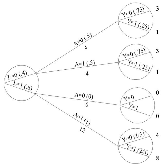
Figure 3.1

3.4 Consistency: First, define the counterfactual outcome

gued that well-defined counterfactuals, or mathematically equivalent concepts, are necessary for meaningful causal inference.

Consistency means that the observed outcome for every treated individual equals her outcome if she had received treatment, and that the observed outcome for every untreated individual equals her outcome if she had remained untreated, i.e., Y ^a = Y for every individual with A = a. This statement seems so obviously true that some readers may be wondering whether there are any situations in which consistency does not hold. After all, if I take aspirin A = 1 and I die (Y = 1), isn’t it the case that my counterfactual outcome Y ^a=1 un-Robins and Greenland (2000) ar- der aspirin equals 1 by definition? The apparent simplicity of the consistency condition is deceptive. Let us unpack consistency by explicitly describing its two main components: (1) a precise definition of the counterfactual outcomes Y ^a via a detailed specification of the superscript a, and (2) the linkage of the counterfactual outcomes to the observed outcomes. This section deals with the first component of consistency.

The methodology for causal inference described in this book is licensed by the existence of well-defined counterfactual outcomes Y a . If Y a is welldefined, then the causal effect Pr - Y ^a=1 = 1 − Pr - Y ^a=0 = 1 is well-defined. A fundamental question is then, how do we know that the counterfactuals are well defined? The answer is straightforward when, as in randomized experiments with perfect adherence to the study protocol, the interventions of

Positivity for standardization and IP weighting. We have defined the standardized mean for treatment level a as P l E [Y |A = a, L = l] Pr [L = l]. However, this expression can only be computed if the conditional quantity E [Y |A = a, L = l] is well defined, which will be the case when the conditional probability Pr [A = a|L = l] is greater than zero for all values l that occur in the population. That is, when positivity holds. (Note the statement Pr [A = a|L = l] > 0 for all l with Pr [L = l] ̸= 0 is effectively equivalent to f [a|L] > 0 with probability 1.) Therefore, the standardized mean is defined as

\[\sum\_{l} \operatorname{E} \left[ Y \middle| A = a, L = l \right] \Pr \left[ L = l \right] \quad \text{if } \Pr \left[ A = a \middle| L = l \right] > 0 \text{ (for all } l \text{ with } \Pr \left[ L = l \right] \neq 0, \text{)}\]

and is undefined otherwise. The standardized mean can be computed only if, for each value of the covariate L in the population, there are some individuals that received the treatment level a.

The IP weighted mean E I (A = a) Y f [A|L] is no longer equal to E I (A = a) Y f [a|L] when positivity does not hold. Specifically, E I (A = a) Y f [a|L] is undefined because the undefined ratio ⁰ 0 occurs in computing the expectation. On the other hand, the IP weighted mean E I (A = a) Y f [A|L] is always well defined since its denominator f [A|L] can never be zero. However, it is now a biased estimate of the counterfactual mean even under exchangeability when positivity fails to hold. In particular, E I (A = a) Y f [A|L] is equal to Pr [L ∈ Q(a)]P l E [Y |A = a, L = l, L ∈ Q(a)] Pr [L = l|L ∈ Q(a)] where Q(a) = {l; Pr (A = a|L = l) > 0} is the set of values l for which A = a may be observed with positive probability. Therefore, under exchangeability, E I (A = a) Y f [A|L] equals E [Y a |L ∈ Q(a)] Pr [L ∈ Q(a)].

From the definition of Q(a), Q(0) cannot equal Q(1) when A is binary and positivity does not hold. In this case the contrast E I (A = 1) Y f [A|L] − E I (A = 0) Y f [A|L] has no causal interpretation, even under exchangeability, because it is a contrast between two different groups. Under positivity, Q(1) = Q(0) and the contrast is the average causal effect if exchangeability holds.

of heart transplant A and 5-year mortality Y . Before enrolling patients in the study, the investigators wrote a protocol in which the two interventions of interest—heart transplant a = 1 and medical therapy a = 0—were described in detail. For example, the investigators specified that individuals assigned to heart transplant were to receive certain pre-operative procedures, anesthesia, surgical technique, post-operative care, and immunosuppressive therapy in an attempt to ensure that each individual receives the same version of the treatment. Had the protocol not specified these details, it is possible that each Fine Point 1.2 introduced the con- doctor had conducted a different version of the treatment “heart transplant”, perhaps using their preferred surgical technique or immunosuppressive therapy. We define Y ^a=1 as the individual’s outcome in this study if the instructions for intervention a = 1 in the protocol of the experiment were followed, and analogously for Y a=0 .

interest are well defined themselves. Consider again a randomized experiment

But how do we know that the counterfactual outcomes are well defined in an observational study? Again, we will have well-defined counterfactuals if we have well-defined interventions. To do so, we need to specify what intervention is represented by a in Y a . For example, for an observational study on the

cept of multiple versions of treatment.

On states and interventions. Variables like socioeconomic status or obesity define states, e.g., being poor, being obese. Causal questions about changes in states are of the form “what if these individuals become poor or obese?”These variables, however, are often not sufficiently well-defined for quantitative causal inference.

As an example, consider “the effect of becoming obese on myocardial infarction”˙ (For simplicity, we use a traditional definition of obesity as body mass index ≥ 30.) The quoted text does not have a meaningful interpretation because, as discussed in the main text, the counterfactual outcome is ill-defined. One might think it would become well defined if we specified the start and end of the intervention (e.g., age 40 years through age 50 years) and the procedure by which body weight would be changed. However, if we specified all these details, we would not be describing the effect of obesity but the effect of whatever interventions we are specifying. Hern´an and Taubman (2008) discuss the tribulations of two world leaders—a despotic king and a clueless president—when considering “the effect of obesity”in their countries.

mathematical conditions for welldefined counterfactual outcomes when the interventions are not well defined. However, those conditions are often extreme and of little practical relevance.

defined depends on the outcome of interest. Consider the effect of obesity on job discrimination—as measured by the proportion of job applicants called for a personal interview after the employer reviews the applicant’s resume and photograph. Here, the treatment is “obesity as perceived by the employer”, rather than “biological obesity”. Therefore, the biological mechanisms that led to obesity may be irrelevant.

effect of heart transplant, we would specify the interventions of interest as for the randomized trial above, and for an observational study on the causal effect of exercise, we would specify duration, frequency, intensity, type (swimming, In Technical Point 6.4, we provide running. . . ) and how the time devoted to exercise would otherwise be spent (rehearsing with your band, watching television. . . ). The difficulty of specifying the treatment a increases for causal questions involving biological (e.g., blood pressure, LDL-cholesterol, body weight) or social (e.g., socioeconomic status) factors or states.

Take the effect of weight gain on fatal myocardial infarction. Suppose that, on Zeus’s 35th birthday, we decided to make him gain 20 kilograms (kg) by age 40 by lowering his daily exercise. He had a fatal myocardial infarction at age 49. Now suppose that, in a parallel universe identical to ours, on Zeus’s 35th birthday we decided to make him gain 20 kg by age 40 by increasing his caloric intake. He did not have a fatal myocardial infarction before age 50. That is, in both universes Zeus gains 20 kg, but only in one of them he had a fatal heart attack.

Because Zeus’s counterfactual outcome under weight gain of 20 kg can be either death or no death, we conclude that specifying a = 1 as “weight gain of 20 kg” is too vague to define the counterfactual outcomes Y a . The problem is that we can only change the value of weight gain by interventions (e.g., diet, exercise) that may have effects on the outcome through causal pathways that Whether causal effects are ill- may not involve exclusively weight gain. See also Fine Point 3.3.

In contrast, if we were interested in the causal effect of a weight loss pill A on mortality, this problem would not arise: “taking the pill” a = 1 is a well-defined intervention because it does not require considering any other interventions (e.g., on diet or exercise). Of course, the value of the counterfactual outcome Y a can still depend on the individual’s values of any previous interventions (e.g., on diet and exercise).

The more precisely we define the meaning of a = 1 and a = 0, the more precise our causal questions are. However, absolute precision in the definition of treatment is neither necessary nor possible. For example, for exercise, we do not need to specify the direction of running (clockwise or counterclockwise) around your neighborhood’s park. Scientists agree that the direction of running is irrelevant because varying it would not lead to different outcomes. That is, we only need sufficiently well-defined interventions a for which no meaningful vagueness remains.

Which begs the question “How do we know that a treatment is sufficiently

Protocols open to interpretation. It is possible that Pr[Y ^a=1 = 1] differs between two randomized experiments with identical populations and protocols. To see this, consider the following scenario.

In both experiments, individuals assigned to a = 1 underwent a surgical operation according to the instructions in the protocol. However, the protocol did not specify how to match patients with surgeons. In the first experiment, individuals assigned to a = 1 were referred to and operated on by experienced surgeons if they were high risk patients, and by less experienced surgeons if they were low risk patients. Because of this, almost no patients died and Pr[Y ^a=1 = 1] was close to 0. In contrast, in the second experiment, individuals assigned to a = 1 were referred to a surgeon without regard to the patient’s risk and the surgeon’s experience. In this study Pr[Y ^a=1 = 1] is far from zero because many high-risk patients were operated on by inexperienced surgeons.

By definition, lack of exchangeability cannot explain the difference in Pr[Y ^a=1 = 1] because both experiments were randomized. Rather, the difference is explained by the different versions of treatment used in each trial. Because the protocol did not specify how to match patients with surgeons, the two trials ended up with different results.

well-defined?” Or, equivalently, how do we know that no meaningful vagueness remains? The answer is “We don’t.” Declaring a treatment sufficiently well-defined is a matter of agreement among experts based on the available substantive knowledge. Today we agree that the direction of running is irrelevant, but future research might prove us wrong if it is demonstrated that, say, leaning the body to the right, but not to the left, while running is harmful. At any point in history, experts who write the protocols of randomized experiments often attempt to eliminate as much vagueness as possible by employing the subject-matter knowledge at their disposal. However, some vagueness is inherent to all causal questions. The vagueness of causal questions can be reduced by a more detailed specification of treatment, but cannot be completely

Even the protocols of randomized experiments may fail to specify some relevant components of the intervention. For example, the protocol of the above heart transplant study did not specify the surgeon’s experience performing heart transplants. Thus, both experienced and inexperienced surgeons participated in the study. Because scant transplant experience is known to affect post-transplant mortality, the risk Pr[Y ^a=1 = 1] had all individuals received treatment according to the protocol will depend on the unknown distribution of experience of the participating surgeons. That is, the average causal effect in a new community with a different distribution of surgical experience will differ from the effect in the trial population, even if the new population follows the exact same protocol as in the trial.

In fact, the value of Pr[Y ^a=1 = 1], and therefore of the average causal effect, may differ between two experiments conducted in the same population and with the same protocol. This discrepancy would arise if the protocol allows for a = 1 to include several versions of treatment with different causal effects on the outcome of interest, and different versions of treatment are used in each experiment. Fine Point 3.4 describes an example of two randomized experiments with the same protocol but different causal effects. A different distribution of versions of treatment affects the transportability of causal effects (see Chapter 4). The same considerations apply to observational studies.

The discussion in this section illustrates an intrinsic feature of causal inference: the articulation of causal questions is contingent on domain expertise and informal judgment. What we view as a meaningful causal question at

In pragmatic trials, the investiga- eliminated. tors may purposely choose not to specify all components of the intervention so that the treatment versions used in the trial reflect what happens in real world settings.

Possible worlds. Philosophers of science have proposed counterfactual theories based on the concept of “possible worlds” (Stalnaker 1968, Lewis 1973). The counterfactual Y a is defined to be the value of Y in the world in which the individual received the treatment that is closest to the actual world. In particular, these philosophers assume that Y ^a = Y if A = a because the closest possible world to the actual world is itself. Hence, under their definition of counterfactuals, consistency always holds.

When A ̸= a, the “closest possible world” and thus the counterfactual Y a are always somewhat ill-defined and vague. Nonetheless, Lewis noted that his definition of counterfactuals is often useful. Robins and Greenland (2000) agreed but also argued that the concept of well-defined interventions should replace the concept of the closest possible world because, in observational studies, counterfactuals are vague and ill-defined to the degree that one fails to make precise the hypothetical interventions and causal contrasts under consideration.

out manipulation” (Holland 1986) captures the idea that meaningful causal inference requires sufficiently well-defined interventions. However, bear in mind that sufficiently well-defined interventions may not be humanly feasible, or practicable, interventions at a particular time in history. For example, the effect of genetic variants on disease was considered sufficiently well defined even before the existence of technology for genetic modification.

present may turn out to be viewed as too vague in the future after learning The phrase “no causation with- that unspecified components of the treatment affect the outcome and therefore the magnitude of the causal effect. Years from now, scientists will probably refine our obesity question in terms of cellular modifications which we barely understand at this time. Again, the term sufficiently well-defined treatment relies on expert consensus, which changes over time. Fine Point 3.5 links this discussion with previous proposals.

Refining the causal question, until it is agreed that no meaningful vagueness remains, is good practice for sound causal inference. For example, declaring our interest in “the effect of obesity” may be viewed as just a starting point for a discussion during which we will sharpen, and possibly modify, the causal question by refining the specification of the treatment until, hopefully, a consensus is reached with our colleagues. The more precisely we specify the treatment, the better defined the causal question is and the fewer opportunities for miscommunication between researchers and decision makers exist.

3.5 Consistency: Second, link counterfactuals to the observed data

issues described in Sections 3.4 and 3.5, see the text and references in Hern´an (2016), and in Robins and Weissman (2016).

As a reminder, the consistency condition says that Y ^a = Y for individuals with A = a. In the previous section, we described the first component of consistency: sufficiently well-defined counterfactual outcomes Y a such that no meaningful vagueness remains. In this section, we describe the second component of consistency in observational studies: ensuring that the equality Y For an expanded discussion of the ^a = Y holds, i.e., linking the counterfactual outcomes to the observed data.

Suppose our goal is quantifying the effect of heart transplant a = 1 vs. medical therapy a = 0 using observational data. We carefully specify the two treatment versions a = 1 and a = 0 of interest. Experts agree that a = 1 and a = 0 are sufficiently well-defined and, therefore, that no meaningful vagueness remains in the specification of the counterfactual outcomes Y ^a=1 and Y a=0 . Specifically, we specified that heart transplant a = 1 includes certain preoperative procedures, anesthesia, surgical technique, post-operative care, and immunosuppressive therapy, as well as surgeons who had conducted at least 10 heart transplants in the last five years. Now suppose that, in our observational data, all surgeons have conducted only between 5 and 9 heart transplants in the last five years. Then, our carefully defined counterfactual outcome Y a=1

cannot be linked to any of the observed outcomes Y because nobody in the study population received the treatment version a = 1.

That is, the validity of the consistency condition is threatened by ill-defined treatments like “weight gain” (previous section), but also by sufficiently welldefined treatments like “heart transplant” that are absent in the data (this section). This latter problem is the result of a lack of (unconditional) positivity for the treatment of interest.

To link the counterfactual outcomes Y ^a=1 and the observed outcomes Y , we have to ensure that only individuals receiving treatment version a = 1 are considered as treated individuals (A = 1) in the analysis, and analogously for the untreated. The implication is that, if we want to quantify the causal effect Pr[Y ^a=1 = 1] − Pr[Y ^a=0 = 1] using observational data, we need data in which some individuals received a = 1 and a = 0. Being able to describe a well-defined intervention a, as we did, is not helpful if the intervention does not occur in the observed data, i.e., if we cannot reasonably assume that the equality Y ^a = Y holds for at least some individuals.

An obvious approach to handling the mismatch between the treatment version of interest and the treatment versions in the observed data is to hypothesize that the effects of those versions of treatment are identical—that is, that there is treatment variation irrelevance (see Fine Point 1.2). In some cases, this hypothesis may be a good approximation. For example, it might be argued that no additional relevant experience is gained after performing 5 transplants and, thus, that we can use observational data in which all surgeons conducted at least 5 transplants to correctly identify the effect of “heart transplant” a = 1 under the protocol requirement that all surgeons had previously Assuming treatment variation irrel- performed at least 10 heart transplants.

In other cases, however, this assumption may not be reasonable. For example, it would be hard to justify that the use of observational data in which all surgeons had conducted only 1 transplant to correctly identify the effect of “heart transplant” a = 1 under the protocol requirement that all surgeons had previously performed at least 10 heart transplants.

Matching the intervention of interest a = 1 with the observed “treatment” value A = 1, and therefore equating the counterfactual outcome Y ^a=1 with the observed outcome Y ^A = Y , requires collecting detailed data. Not only is this information necessary to detect a mismatch between the treatment of interest and the data at hand, but also to have an informed discussion about whether the available versions of treatment can be used in lieu of the treatment version of interest. In our heart transplant study in this section, if information on surgeon experience was not collected, we would not be able to determine whether the counterfactual Y ^a=1 Confusion often arises from the can be linked to the observed Y .

Because data on treatment versions are often unavailable in observational studies, consistency is often compromised. Since achieving consistency is not easy in observational studies, a good practice is to make our reasoning as transparent as possible, so that others can directly challenge our arguments. The next section describes a procedure to achieve that transparency.

3.6 The target trial

exists to match a and A.

The average causal effect is a contrast between mean counterfactual outcomes under different treatment values. Because the counterfactual outcomes need to be well defined, we can imagine a (hypothetical) randomized experiment to

evance may also be reasonable for some biological factors. For example, if interested in the effect of pharmacologically-induced changes in blood pressure, investigators may be willing to assume that the particular medication used to achieve the change is not relevant.

common practice of using the same letter to refer to the hypothetical intervention a and to the observed value A before enough information equivalents—has long been central to the causal inference framework. Dorn (1953), Wold (1954), Cochran (1972), Rubin (1974), Feinstein (1971), and Dawid (2000) used the concept. Robins (1986) generalized it for time-varying treatments.

observational data to compute the proportion of cases attributable to treatment.

fied the key components of the target trial. The acronym PICO (Population, Intervention, Comparator, Outcome) is sometimes used to summarize some of those components (Richardson et al. 1995).

When we are concerned that as- can be achieved. suming conditional exchangeability may not be reasonable given the available data, we can consider alternative identifying assumptions (see Chapter 16) or perform sensitivity analyses.

view, see Pearl (2009), Schwartz et al (2016), and Glymour and Spiegelman (2016).

quantify the causal effect of interest. We refer to that hypothetical experiment The target trial—or its logical as the target experiment or the target trial. When conducting the target trial is not feasible, ethical, or timely, we resort to causal analyses of observational data. Generally, one can view these observational analyses as an attempt to emulate some target trial. If the emulation were successful, there would be no difference between the results from the observational study and from the target trial (had it been conducted).

In this chapter, we have explored three conditions—exchangeability, positivity, consistency—that help equate an observational study with a (conditionally randomized) target experiment. When these conditions hold, we can apply the methods described in the previous chapter—IP weighting or Fine Point 3.6 describes how to use standardization—to compute causal effects from the observational data.

Therefore “what randomized experiment are you trying to emulate?” can be a key question for causal inference from observational data. For each causal effect that we wish to estimate using observational data, we may (i) specify the target trial that we would like to, but cannot, conduct, and (ii) describe how the observational data can be used to emulate that target trial. Specifying the target trial, and therefore the causal effect of interest, requires specifying key components of the trial’s protocol: eligibility criteria, interventions (or, in Hern´an and Robins (2016) speci- general, treatment strategies), assignment, outcomes, start and end of followup, and causal contrasts.

Therefore, a valid emulation of the target trial requires that the observational dataset includes sufficient information to identify eligible individuals, assign them to groups defined by the interventions they receive, and ascertain their outcomes during the follow-up. For example, to estimate the causal effect of heart transplant, we first specify the components of the protocol of the target trial, and then try to emulate each of them using the observational data. Such explicit emulation of a target trial improves causal inference from observational data by making the interventions, and therefore the causal question, well-defined (see Chapter 22 for an extended discussion of the target trial framework). Once the causal question is well-defined via a target trial, investigators can focus on whether and how conditional exchangeability across groups

All of the above assumes that the interventions of interest are sufficiently well-defined to translate them into a hypothetical experiment. But what can we do when, based on current scientific knowledge, the causal question cannot be translated into a target trial? As an example, consider “the causal effect of weight loss” on mortality in individuals who are obese and do not smoke at age 40. Because this causal question is somewhat vague, we replace it by one that specifies the actual intervention that would be implemented to bring about weight loss. For example, we could specify and emulate a target trial about inducing weight loss via, say, exercise or diet.

In contrast to the conceptualization of causal inference from observational data as a target trial emulation, some authors view “the causal effect of A on Y” as a well-defined quantity regardless of what A and Y stand for (as long as For some examples of this point of A temporally precedes Y ). Often the argument goes like this:

Requiring well-defined counterfactual outcomes via a target trial imposes severe restrictions on the causal questions that can be asked. Suppose we study weight loss and heart disease using observational data. We may not be able to characterize precisely the causal effect of weight loss, but is that really so important if indeed some causal effect exists? There is value in learning that many

Attributable fraction. We have described effect measures like the causal risk ratio Pr[Y ^a=1 = 1]/Pr[Y ^a=0 = 1] and the causal risk difference Pr[Y ^a=1 = 1] − Pr[Y ^a=0 = 1], which compare the counterfactual risk under treatment a = 1 with the counterfactual risk under treatment a = 0. However, one could also be interested in measures that compare the observed risk with the counterfactual risk under either treatment a = 1 or a = 0. This latter contrast allows us to compute the proportion of cases that are attributable to treatment in an observational study, i.e., the proportion of cases that would not have occurred had treatment not occurred. For example, suppose that all 20 individuals in our population attended a dinner in which they were served either ambrosia (A = 1) or nectar (A = 0). The following day, 7 of the 10 individuals who received A = 1, and 1 of the 10 individuals who received A = 0, were sick. For simplicity, assume exchangeability of the treated and the untreated so that the causal risk ratio is 0.7/0.1 = 7 and the causal risk difference is 0.7 − 0.1 = 0.6. (In conditionally randomized experiments, one would compute these effect measures via standardization or IP weighting.) It was later discovered that the ambrosia had been contaminated by a flock of doves, which explains the increased risk summarized by both the causal risk ratio and the causal risk difference. We now address the question “What fraction of the cases was attributable to consuming ambrosia?”

In this study we observed 8 cases, i.e., the observed risk was Pr [Y = 1] = 8/20 = 0.4. The risk that would have been observed if everybody had received a = 0 is Pr[Y ^a=0 = 1] = 0.1. The difference between these two risks is 0.4 − 0.1 = 0.3. That is, there is an excess 30% of the individuals who did fall ill but would not have fallen ill if everybody in the population had received a = 0 rather than their treatment A. Because 0.3/0.4 = 0.75, we say that 75% of the cases are attributable to treatment a = 1: compared with the 8 observed cases, only 2 cases would have occurred if everybody had received a = 0. This excess fraction or attributable fraction is defined as

\[\frac{\Pr\left[Y=1\right] - \Pr[Y^{a=0}=1]}{\Pr\left[Y=1\right]}\]

See Fine Point 5.4 for a discussion of the excess fraction in the context of the sufficient-component-cause framework.

The excess fraction is generally different from the etiologic fraction, another version of the attributable fraction which is defined as the proportion of cases mechanically caused by exposure. For example, suppose the untreated (A = 0) would have had 7 cases if they have been treated, but these 7 cases would not have contained the 1 untreated case that actually occurred, i.e., treatment produces 7 cases but prevents 1 case. Also suppose that, if untreated, the treated would have had only 1 case but different from the 7 cases they actually had. Then the excess fraction would not be equal to the etiologic fraction. Here the excess fraction is a lower bound on the etiologic fraction. Because the etiologic fraction does not rely on the concept of excess cases, it can only be computed in randomized experiments under strong assumptions. See Greenland and Robins, 1988 and Robins and Greenland, 1989.

deaths can be prevented if obese people, somehow, lost weight, even if the intervention required for achieving that transformation is unspecified.

This is an appealing argument, but it is problematic for two reasons.

First, unspecified interventions may be unreasonable or impractical. For example, suppose that some investigators are interested in learning about the health effects of weight loss, but they do not propose and explicitly emulate a target trial. Rather, they conduct a simplified analysis that compares the risk of death in obese versus non-obese individuals at age 40. That comparison corresponds implicitly to a target trial in which obese individuals are instantaneously transformed into individuals with a body mass index of 25 at baseline (through a massive liposuction?). Such target trial cannot be emulated because very few people, if anyone, undergo such drastic instantaneous change in the real world, and thus the counterfactual outcomes cannot generally be linked to the observed outcomes. Had this draconian intervention been made are more likely to go unrecognized when they are not explicitly specified.

Danaei et al. (2016) tried to esti- possible. mate the effect of weight loss using observational data. They left unspecified the method used to lose weight, but they carefully specified the timing of the weight loss over many years.

the differences between prediction and causal inference, which is a form of counterfactual prediction, see Hern´an, Hsu, and Healy (2019).

explicit, all scientists, including those who conducted the data analyses, would Extreme or impossible interventions have agreed that consistency does not hold. Explicit target trial emulation prevents investigators from making implicit consistency assumptions that do not cohere with their own beliefs.

In fact, anchoring observational data analyses to a target trial not only helps sharpen the causal question, but also makes the causal inference more relevant for decision makers. This is the case even if the available data are insufficient to emulate a contrast of well-defined interventions. For example, we may not have sufficient data to emulate an intervention that precisely specifies the method used to lose weight (e.g., diet, exercise, a pill), but we may have sufficient data to ensure that other components of the intervention remain realistic. If we had longitudinal data on body weight, we can specify a target trial in which some individuals are assigned to lose 5% of body mass index every year, starting at age 40 and for as long as their body mass index stays over 25. (Part III of this book revolves around interventions that, like this one, are sustained over time.) Though this intervention is not yet well-defined (because it does not specify how the weight loss is achieved), it at least avoids mandating an instantaneous weight loss, which corresponds to an intervention that is impossible to implement. That we may not be able to define well-defined counterfactual outcomes is no excuse to try to make them as less ill-defined as

Second, unspecified interventions make it harder to achieve exchangeability and positivity. Because the set of covariates L that result in conditional exchangeability may vary across interventions, the usual uncertainty regarding conditional exchangeability in observational studies is greatly exacerbated if we forgo characterizing the interventions as well as possible. Also, if the interventions remain unspecified, it is hard to characterize the combinations of values of L that would make it impossible to receive the intervention in the observational data, which increases the risk of an inadvertent violation of positivity.

So what can we do when a target trial cannot be reasonably specified and emulated or, more generally, when the counterfactual outcomes are not sufficiently well defined? In those settings, observational data may still be quite For an extended discussion about useful for non-causal prediction. That obese individuals have a higher mortality risk than nonobese individuals means that obesity is a predictor of—is associated with—mortality. This is an important piece of information to identify individuals at high risk of mortality. By saying that obesity predicts—is associated with—mortality, we remain causally agnostic: obesity might predict mortality in the sense that cigarette smoking predicts lung cancer or in the sense that carrying a lighter predicts lung cancer. Thus the association between obesity and mortality is an interesting hypothesis-generating exercise and a motivation for further research (why does obesity predict mortality anyway?), while acknowledging the magnitude of the association does not necessarily correspond to that of a causal effect.

Observational studies

Chapter 4 EFFECT MODIFICATION

So far we have focused on the average causal effect in an entire population of interest. However, many causal questions are about subsets of the population. Consider again the causal question “does one’s looking up at the sky make other pedestrians look up too?” You might be interested in computing the average causal effect of treatment—your looking up to the sky— in city dwellers and visitors separately, rather than the average effect in the entire population of pedestrians.

The decision whether to compute average effects in the entire population or in a subset depends on the inferential goals. In some cases, you may not care about the variations of the effect across different groups of individuals. For example, suppose you are a policy maker considering the possibility of implementing a nationwide water fluoridation program. Because this public health intervention will reach all households in the population, your primary interest is in the average causal effect in the entire population, rather than in particular subsets. You will be interested in characterizing how the causal effect varies across subsets of the population when the intervention can be targeted to different subsets, or when the findings of the study need to be applied to other populations.

This chapter emphasizes that there is not such a thing as the causal effect of treatment. Rather, the causal effect depends on the characteristics of the particular population under study.

4.1 Heterogeneity of treatment effects

	V	0 Y	1 Y
Rheia	1	0	1
Demeter	1	0	0
Hestia	1	0	0
Hera	1	0	0
Artemis	1	1	1
Leto	1	0	1
Athena	1	1	1
Aphrodite	1	0	1
Persephone	1	1	1
Hebe	1	1	0
Kronos	0	1	0
Hades	0	0	0
Poseidon	0	1	0
Zeus	0	0	1
Apollo	0	1	0
Ares	0	1	1
Hephaestus	0	0	1
Polyphemus	0	0	1
Hermes	0	1	0
Dionysus	0	1	0

Table 4.1 We started this book by computing the average causal effect of heart transplant A on death Y in a population of 20 members of Zeus’s extended family. We used the data in Table 1.1, whose columns show the individual values of the (generally unobserved) counterfactual outcomes Y ^a=0 and Y ^a=1. After examining the data in Table 1.1, we concluded that the average causal effect was null. Half of the members of the population would have died if everybody had received a heart transplant, Pr[Y ^a=1 = 1] = 10/20 = 0.5, and half of the members of the population would have died if nobody had received a heart transplant, Pr[Y ^a=0 = 1] = 10/20 = 0.5. The causal risk ratio Pr[Y ^a=1 = 1]/Pr[Y ^a=0 = 1] was 0.5/0.5 = 1 and the causal risk difference Pr[Y ^a=1 = 1] − Pr[Y ^a=0 = 1] was 0.5 − 0.5 = 0.

We now consider two new causal questions: What is the average causal effect of A on Y in women? And in men? To answer these questions we will use Table 4.1, which contains the same information as Table 1.1 plus an additional column with an indicator V for sex: V = 1 for females (referred to as women in this book) and V = 0 for males (referred to as men). For convenience, we have rearranged the table so that women occupy the first 10 rows, and men the last 10 rows.

Let us first compute the average causal effect in women. To do so, we need to restrict the analysis to the first 10 rows of the table with V = 1. In this subset of the population, the risk of death under treatment is Pr[Y ^a=1 = 1|V = 1] = 6/10 = 0.6 and the risk of death under no treatment is Pr[Y ^a=0 = 1|V = 1] = 4/10 = 0.4. The causal risk ratio is 0.6/0.4 = 1.5 and the causal risk difference is 0.6 − 0.4 = 0.2. That is, on average, heart transplant A increases

the risk of death Y in women.

“woman” in this chapter can be viewed as a slight abuse of notation because these deities are gods and goddesses, not men and women.

E[Y ^a=1 − Y ^a=0|V = 1] ̸= E[Y ^a=1 − Y ^a=0|V = 0]

E[Y ^a=1|V =1] E[^{Y a}=0|^V =1] ̸= E[Y ^a=1|V =0] E[Y ^a=0|V =0]

We do not consider effect modification on the odds ratio scale because the odds ratio is rarely, if ever, the parameter of interest for causal inference.

fect modification by V : ^a=0 = 1|V = 1] = 0.8

Pr[Y Pr[Y ^a=1 = 1|V = 1] = 0.9 Pr[Y ^a=0 = 1|V = 0] = 0.1 Pr[Y ^a=1 = 1|V = 0] = 0.2

Our use of the terms “man” and Let us next compute the average causal effect in men. To do so, we need to restrict the analysis to the last 10 rows of the table with V = 0. In this subset of the population, the risk of death under treatment is Pr[Y ^a=1 = 1|V = 0] = 4/10 = 0.4 and the risk of death under no treatment is Pr[Y ^a=0 = 1|V = 0] = 6/10 = 0.6. The causal risk ratio is 0.4/0.6 = 2/3 and the causal risk difference is 0.4 − 0.6 = −0.2. That is, on average, heart transplant A decreases the risk of death Y in men.

Our example shows that a null average causal effect in the population does not imply a null average causal effect in a particular subset of the population. In Table 4.1, the null hypothesis of no average causal effect is true for the entire population, but not for men or women when taken separately. It just happens that the average causal effects in men and in women are of equal magnitude but in opposite direction. Because the proportion of each sex is 50%, both effects cancel out exactly when considering the entire population. Although exact cancellation of effects is probably rare, heterogeneity of the individual causal effects of treatment is often expected because of variations in individual susceptibilities to treatment. An exception occurs when the sharp null hypothesis of no causal effect is true. Then no heterogeneity of effects exists because the effect is null for every individual and thus the average causal effect in any subset of the population is also null.

See Section 6.6 for a structural clas- We are now ready to provide a definition of effect modifier. We say that V sification of effect modifiers. is a modifier of the effect of A on Y when the average causal effect of A on Y varies across levels of V . Since the average causal effect can be measured using different effect measures (e.g., risk difference, risk ratio), the presence of effect Additive effect modification: modification depends on the effect measure being used. For example, sex V is an effect modifier of the effect of heart transplant A on mortality Y on the additive scale because the causal risk difference varies across levels of V . Sex V is also an effect modifier of the effect of heart transplant A on mortality Y Multiplicative effect modification: on the multiplicative scale because the causal risk ratio varies across levels of V . We only consider variables V that are not affected by treatment A as effect modifiers.

In Table 4.1 the causal risk ratio is greater than 1 in women (V = 1) and less than 1 in men (V = 0). Similarly, the causal risk difference is greater than 0 in women (V = 1) and less than 0 in men (V = 0). That is, there is qualitative effect modification because the average causal effects in the subsets V = 1 and V = 0 are in the opposite direction. In the presence of qualitative effect modification, additive effect modification implies multiplicative effect modification, and vice versa. In the absence of qualitative effect modification, however, one can find effect modification on one scale (e.g., multiplicative) but not on the other (e.g., additive). To illustrate this point, suppose that, in a Multiplicative, but not additive, ef- second study, we computed the quantities shown to the left of this line. In this study, there is no additive effect modification by V because the causal risk difference among individuals with V = 1 equals that among individuals with V = 0, i.e., 0.9 − 0.8 = 0.1 = 0.2 − 0.1. However, in this study there is multiplicative effect modification by V because the causal risk ratio among individuals with V = 1 differs from that among individuals with V = 0, i.e., 0.9/0.8 = 1.1 ̸= 0.2/0.1 = 2. Since one cannot generally state that there is, or there is not, effect modification without referring to the effect measure being used (e.g., risk difference, risk ratio), some authors use the term effect-measure modification, rather than effect modification, to emphasize the dependence of the concept on the choice of effect measure.

4.2 Stratification to identify effect modification

A on Y is computed in each stratum of V . For dichotomous V , the stratified causal risk differences are: Pr[Y ^a=1 = 1|V = 1]− Pr[Y ^a=0 = 1|V = 1] and Pr[Y ^a=1 = 1|V = 0]−

Pr[Y ^a=0 = 1|V = 0]

Stratum V = 0
	L	A	Y
Cybele	0	0	0
Saturn	0	0	1
Ceres	0	0	0
Pluto	0	0	0
Vesta	0	1	0
Neptune	0	1	0
Juno	0	1	1
Jupiter	0	1	1
Diana	1	0	0
Phoebus	1	0	1
Latona	1	0	0
Mars	1	1	1
Minerva	1	1	1
Vulcan	1	1	1
Venus	1	1	1
Seneca	1	1	1
Proserpina	1	1	1
Mercury	1	1	0
Juventas	1	1	0
Bacchus	1	1	0

A stratified analysis is the natural way to identify effect modification by measured variables (see also Fine Point 4.1). To determine whether V modifies the causal effect of A on Y , one computes the effect of A on Y in each level Stratification: the causal effect of (stratum) of the variable V . In the previous section, we used the data in Table 4.1 to compute the causal effect of transplant A on death Y in each of the two strata of sex V . Because the effect differed between the two strata (on both the additive and the multiplicative scale), we concluded that there was (additive and multiplicative) effect modification by V of the causal effect of A on Y .

But the data in Table 4.1 are not the typical data one encounters in real life. Instead of the two columns with each individual’s counterfactual outcomes Y ^a=1 and Y ^a=0, one will find two columns with each individual’s treatment level A and observed outcome Y . How does the unavailability of the counterfactual outcomes affect the use of stratification to detect effect modification? The answer depends on the study design.

Consider first an ideal marginally randomized experiment. In Chapter 2 we demonstrated that, leaving aside random variability, the average causal effect of treatment can be computed using the observed data. For example, the causal risk difference Pr[Y ^a=1 = 1] − Pr[Y ^a=0 = 1] is equal to the observed Table 4.2 associational risk difference Pr[Y = 1|A = 1] − Pr[Y = 1|A = 0]. The same reasoning can be extended to each stratum of the variable V because, if treatment assignment was random and unconditional, exchangeability is expected in every subset of the population. Thus the causal risk difference in women, Pr[Y ^a=1 = 1|V = 1] − Pr[Y ^a=0 = 1|V = 1], is equal to the associational risk difference in women, Pr[Y = 1|A = 1, V = 1] − Pr[Y = 1|A = 0, V = 1]. And similarly for men. Thus, to identify effect modification by V in an ideal experiment with unconditional randomization, one just needs to conduct a stratified analysis, i.e., to compute the association measure in each level of the variable V . Stratification can be used to compute average causal effects in subsets of the population, but not individual effects (see Fine Points 2.1 and 3.2).

Consider now an ideal randomized experiment with conditional randomization. In a population of 40 people, transplant A has been randomly assigned with probability 0.75 to those in severe condition (L = 1), and with probability 0.50 to the others (L = 0). The 40 individuals can be classified into two nationalities according to their passports: 20 are Greek (V = 1) and 20 are Roman (V = 0). The data on L, A, and death Y for the 20 Greeks are shown in Table 2.2 (same as Table 3.1). The data for the 20 Romans are shown in Table 4.2. The population risk under treatment, Pr[Y ^a=1 = 1], is 0.55, and the population risk under no treatment, Pr[Y ^a=0 = 1], is 0.40. (Both risks are readily calculated by using either standardization or IP weighting. We leave the details to the reader.) The average causal effect of transplant A on death Y is therefore 0.55 − 0.40 = 0.15 on the risk difference scale, and 0.55/0.40 = 1.375 on the risk ratio scale. In this population, heart transplant increases the mortality risk.

As discussed in the previous chapter, the calculation of the causal effect would have been the same if the data had arisen from an observational study in which we believe that conditional exchangeability Y ^a⊥⊥A|L holds.

We now discuss how to conduct a stratified analysis to investigate whether nationality V modifies the effect of A on Y . The goal is to compute the causal effect of A on Y in the Greeks, Pr[Y ^a=1 = 1|V = 1]−Pr[Y ^a=0 = 1|V = 1], and in the Romans, Pr[Y ^a=1 = 1|V = 0]−Pr[Y ^a=0 = 1|V = 0]. If these two causal risk differences differ, we will say that there is additive effect modification by

Effect in the treated. This chapter is concerned with average causal effects in subsets of the population. One particular subset is the treated (A = 1). The average causal effect in the treated is not null if Pr[Y ^a=1 = 1|A = 1] ̸= Pr[Y ^a=0 = 1|A = 1] or, by consistency, if

\[\Pr[Y=1|A=1] \neq \Pr[Y^{a=0}=1|A=1].\]

That is, there is a causal effect in the treated if the observed risk among the treated individuals does not equal the counterfactual risk had the treated individuals been untreated. The causal risk difference in the treated is Pr[Y = 1|A = 1] − Pr[Y ^a=0 = 1|A = 1]. The causal risk ratio in the treated, also known as the standardized morbidity ratio (SMR), is Pr[Y = 1|A = 1]/Pr[Y ^a=0 = 1|A = 1]. The causal risk difference and risk ratio in the untreated are analogously defined by replacing A = 1 by A = 0. Figure 4.1 shows the groups that are compared when computing the effect in the treated and the effect in the untreated.

The average effect in the treated will differ from the average effect in the population if the distribution of individual causal effects varies between the treated and the untreated. That is, when computing the effect in the treated, treatment group A = 1 is used as a marker for the factors that are truly responsible for the modification of the effect between the treated and the untreated groups. However, even though one could say that there is effect modification by the pre-treatment variable V even if V is only a surrogate (e.g., nationality) for the causal effect modifiers, one would not say that there is modification of the effect A by treatment A because it sounds confusing. The effect modification is by unidentified variables that have a different distribution between the treatment groups.

See Section 6.6 for a graphical representation of true and surrogate effect modifiers. The bulk of this book is focused on the causal effect in the population because the causal effect in the treated, or in the untreated, cannot be directly generalized to time-varying treatments (see Part III).

V . And similarly for the causal risk ratios if interested in multiplicative effect modification.

The procedure to compute the conditional risks Pr[Y ^a=1 = 1|V = v] and Pr[Y ^a=0 = 1|V = v] in each stratum v has two stages: 1) stratification by V , and 2) standardization by L (or, equivalently, IP weighting with weights Step 2 can be ignored when V is depending on L). We computed the standardized risks in the Greek stratum (V = 1) in Chapter 2: the causal risk difference was 0 and the causal risk ratio was 1. Using the same procedure in the Roman stratum (V = 0), we can compute the risks Pr[Y ^a=1 = 1|V = 0] = 0.6 and Pr[Y ^a=0 = 1|V = 0] = 0.3. (Again, we leave the details to the reader.) Therefore, the causal risk difference is 0.3 and the causal risk ratio is 2 in the stratum V = 0. Because these effect measures differ from those in the stratum V = 1, we say that there is both additive and multiplicative effect modification by nationality V of the effect of transplant A on death Y . This effect modification is not qualitative because the effect is harmful or null in both strata V = 0 and V = 1.

We have shown that, in our study population, nationality V modifies the effect of heart transplant A on the risk of death Y . However, we have made no claims about the causal mechanisms involved in such effect modification. In fact, it is possible that nationality is simply a marker for the causal factor that is truly responsible for the modification of the effect. For example, suppose that the quality of heart surgery is better in Greece than in Rome. One would then find effect modification by nationality. An intervention to improve the quality of heart surgery in Rome could eliminate the modification of the causal See Section 6.6 for a representation effect by passport-defined nationality. Whenever we want to emphasize this distinction, we will refer to nationality as a surrogate effect modifier , and to quality of care as a causal effect modifier .

Therefore, our use of the term effect modification by V does not necessarily

equal to the variables L that are needed for conditional exchangeability (see Section 4.4).

of surrogate and causal effect modifiers using causal graphs.

imply that V plays a causal role in the modification of the effect. To avoid potential confusions, some authors prefer to use the more neutral term “effect heterogeneity across strata of V” rather than “effect modification by V .” The next chapter introduces “interaction,” a concept related to effect modification, that does attribute a causal role to the variables involved.

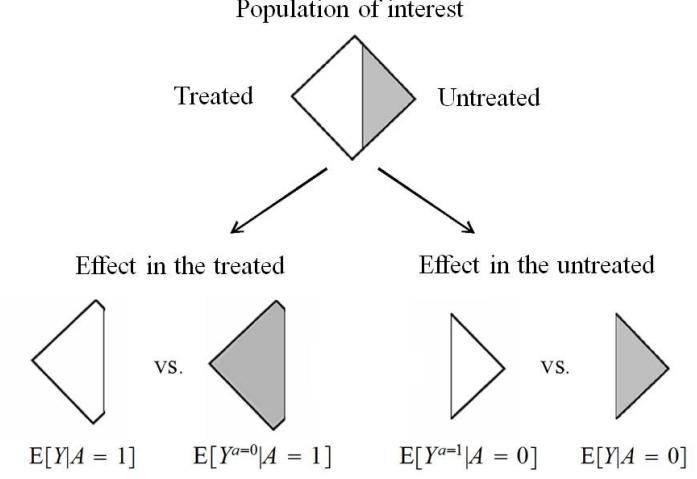
Figure 4.1

4.3 Why care about effect modification

There are several related reasons why investigators are interested in identifying effect modification, and why it is important to collect data on pre-treatment descriptors V even in randomized experiments.

First, if a factor V modifies the effect of treatment A on the outcome Y then the average causal effect will differ between populations with different prevalence of V . For example, the average causal effect in the population of Table 4.1 is harmful in women and beneficial in men, i.e., there is qualitative effect modification. Because there are 50% of individuals of each sex, and the sex-specific harmful and beneficial effects are equal but of opposite sign, the average causal effect in the entire population is null. However, had we conducted our study in a population with a greater proportion of women (e.g., graduating college students), the average causal effect in the entire population would have been harmful. In the presence of non-qualitative effect modification, the magnitude, but not the direction, of the average causal effect may vary across populations. As examples of non-qualitative effect modification, consider the effects of asbestos exposure (which differ between smokers and nonsmokers) and of universal health care (which differ between low-income and high-income families).

That is, the average causal effect in a population depends on the distribution of individual causal effects in the population. There is generally no such a thing as “the average causal effect of treatment A on outcome Y (period)”, but “the average causal effect of treatment A on outcome Y in a population with a particular mix of causal effect modifiers.”

Computing the effect in the treated. We computed the average causal effect in the population under conditional exchangeability Y ^a⊥⊥A|L for both a = 0 and a = 1. Computing the average causal effect in the treated only requires partial exchangeability Y ^a=0⊥⊥A|L. In other words, it is irrelevant whether the risk in the untreated, had they been treated, equals the risk in those who were actually treated. The average causal effect in the untreated is computed under the partial exchangeability condition Y ^a=1⊥⊥A|L.

We now describe how to compute counterfactual means of the form E [Y a |A = a ′ ] under the above assumptions of partial exchangeability. We do so via standardization and via IP weighting:

• Standardization: E[Y a |A = a ′ ] is equal to P l E [Y |A = a, L = l] Pr [L = l|A = a ′ ]. See Miettinen (1972) and

Greenland and Rothman (2008) for a discussion of standardized risk ratios.

• IP weighting: E[Y a |A = a ′ ] is equal to the IP weighted mean E I (A = a) Y f (A|L) Pr [A = a ′ |L] E I (A = a) f (A|L) Pr [A = a ′ |L] with weights

Pr [A = a ′ |L] f (A|L) . For dichotomous A, this equality was derived by Sato and Matsuyama (2003). See Hern´an and Robins (2006a) for further details.

Pearl and Bareinboim (2014), Dahabreh and Hern´an (2019), and others have discussed effect modification in relation to transporting inferences across populations.

ity may not be an issue: Smith and Pell (2003) could not identify any major modifiers of the effect of parachute use on death after “gravitational challenge” (e.g., jumping from an airplane at high altitude). They concluded that conducting randomized trials of parachute use restricted to a particular group of people would not compromise the transportability of the findings to other groups.

The extrapolation of causal effects computed in one population to a second Some refer to lack of transportabil- population is referred to as transportability of causal inferences across populaity as lack of external validity. tions (see Fine Point 4.2). In our example, the causal effect of heart transplant A on risk of death Y differs between men and women, and between Romans Hern´an and VanderWeele (2011), and Greeks. Thus the average causal effect in this population may not be transportable to other populations with a different distribution of effect modifiers such as sex and nationality.

Conditional causal effects in the strata defined by the effect modifiers may be more transportable than the causal effect in the entire population, but there is no guarantee that the conditional effect measures in one population equal the conditional effect measures in another population. This is so because there could be other unmeasured, or unknown, causal effect modifiers whose conditional distributions vary between the two populations (or for other A setting in which transportabil- reasons described in Fine Point 4.2). These unmeasured effect modifiers are not variables needed to achieve exchangeability, but just risk factors for the outcome. Therefore, transportability of effects across populations is a more difficult problem than the identification of causal effects in a single population: one would need to stratify not just on all those things required to achieve exchangeability (which you might have information about, say, by interviewing those who decide how to allocate the treatment) but on unmeasured causes of the outcome for which there is much less information.

Hence, transportability of causal effects is an unverifiable assumption that relies heavily on subject-matter knowledge. For example, most experts would agree that the health effects (on either the additive or multiplicative scale) of increasing a household’s annual income by $100 in Niger cannot be transported to the Netherlands, but most experts would agree that the health effects of use of cholesterol-lowering drugs in Europeans can be transported to Canadians.

Second, evaluating the presence of effect modification is helpful to identify

Day, 1979; Rothman et al., 1980; Saracci, 1980) have referred to additive effect modification as the one of interest for public health purposes.

the groups of individuals that would benefit most from an intervention. In our example of Table 4.1, the average causal effect of treatment A on outcome Y was null. However, treatment A had a beneficial effect in men (V = 0), and a harmful effect in women (V = 1). For example, if physicians knew that there is qualitative effect modification by sex, then, in the absence of additional information, they would treat the next patient only if he happens to be a man. The situation is slightly more complicated when, as in our second example, there is multiplicative, but not additive, effect modification. Here treatment reduces the risk of the outcome by 10% in individuals with V = 0 and also by 10% in individuals with V = 1, i.e., there is no additive effect modification by V because the causal risk difference is 0.1 in all levels of V . Thus, an intervention to treat all patients would be equally effective in reducing risk in both strata of V , despite the fact that there is multiplicative effect modification. In fact, if there is a nonzero causal effect in at least one stratum of V and the counterfactual risk Pr[Y ^a=0 = 1|V = v] varies with v, then effect modification is guaranteed on either the additive or the multiplicative scale.

Several authors (e.g., Blot and Additive, but not multiplicative, effect modification is the appropriate scale to identify the groups that will benefit most from intervention. In the absence of additive effect modification, learning that there is multiplicative effect modification may not be very helpful for decision making.

In our second example, the presence of multiplicative effect modification is expected because the risk under no treatment in the stratum V = 1 equals 0.8. Thus, the maximum possible causal risk ratio in the V = 1 stratum is 1/0.8 = 1.25, which is guaranteed to differ from the causal risk ratio of 2 in the V = 0 stratum. In these situations, multiplicative effect modification arises from the differences in risk under no treatment Pr[Y ^a=0 = 1|V = v] across levels of V . Therefore, as a general rule, it is more informative to report the (absolute) counterfactual risks Pr[Y ^a=1 = 1|V = v] and Pr[Y ^a=0 = 1|V = v] in every level v of V , rather than simply their ratio or difference.

Finally, the identification of effect modification may help understand the biological, social, or other mechanisms leading to the outcome. For example, a greater risk of HIV infection in uncircumcised compared with circumcised men may provide new clues to understand the disease. The identification of effect modification may also be a first step towards characterizing the interactions between two treatments. The terms “effect modification” and “interaction” are sometimes used as synonymous in the scientific literature. This chapter focused on “effect modification.” The next chapter describes “interaction” as a causal concept that is related to, but different from, effect modification.

4.4 Stratification as a form of adjustment

Until this chapter, our only goal was to compute the average causal effect in the entire population. In the absence of marginal randomization, achieving this goal requires adjustment for the variables L that ensure conditional exchangeability of the treated and the untreated. For example, in Chapter 2 we determined that the average causal effect of heart transplant A on mortality Y was null, i.e., the causal risk ratio Pr - Y ^a=1 = 1 /Pr - Y ^a=0 = 1 = 1. We used the data in Table 2.2 to adjust for the factor L via both standardization and IP weighting.

The present chapter adds another potential goal to the analysis: to identify effect modification by variables V . To achieve this goal, we need to stratify by

Transportability. Effects estimated in one population are often intended to make decisions in another population—the target population. Can we “transport” the effect from the study population to the target population? The answer depends on the characteristics of both populations. Specifically, transportability of causal effects across populations may be justified if the following characteristics are similar between the two populations:

• Effect modification: The causal effect of treatment may differ across individuals with different susceptibility to the outcome. For example, if women are more susceptible to the effects of treatment than men, we say that sex is an effect modifier. The distribution of effect modifiers in a population will generally affect the magnitude of the causal effect of treatment in that population. If the distribution of effect modifiers differs between populations, then the magnitude of the causal effect of treatment will differ too.
• Versions of treatment: The causal effect of treatment depends on the distribution of versions of treatment in the population. If this distribution differs between the study population and the target population, then the magnitude of the causal effect of treatment will differ too (Hern´an and VanderWeele, 2011).
• Interference: In the main text we focus on settings with no interference (Fine Point 1.1). Interference exists when treating one individual affects the outcome of others in the population. For example, a socially active individual may convince his friends to join him while exercising, and thus an intervention on that individual’s physical activity may be more effective than an intervention on a socially isolated individual. Therefore, different contact patterns between populations will translate into causal effects of different magnitude.

A growing literature considers transportability methods that use data from the study population to estimate the causal effect in the target population in the presence of effect modification (e.g., Westreich et al. 2017, Rudolph and van der Laan 2017, Dahabreh et al. 2020b).

The transportability of causal inferences across populations may sometimes be improved by restricting our attention to the average causal effects in the strata defined by the effect modifiers, or by using the stratum-specific effects in the study population to reconstruct the average causal effect in the target population. For example, the four stratumspecific effect measures (Roman women, Greek women, Roman men, and Greek men) in our population can be combined in a weighted average to reconstruct the average causal effect in another population with a different mix of sex and nationality. The weight assigned to each stratum-specific measure is the proportion of individuals in that stratum in the second population. However, there is no guarantee that this reconstructed effect will coincide with the true effect in the target population because of possible between-population differences in the distribution of unmeasured effect modifiers, interference patterns, and distribution of versions of treatment.

V in addition to adjusting for L. For example, in this chapter we stratified by nationality V and adjusted for L to determine that the average causal effect of heart transplant A on mortality Y differed between Greeks and Romans. In summary, standardization (or IP weighting) is used to adjust for L and stratification is used to identify effect modification by V .

But stratification is not always used to identify effect modification by V . In practice stratification is often used as an alternative to standardization (and IP weighting) to adjust for L. In fact, the use of stratification as a method to adjust for L is so widespread that many investigators consider the terms “stratification” and “adjustment” as synonymous. For example, suppose you ask an epidemiologist to adjust for the factor L to compute the effect of heart transplant A on mortality Y . Chances are that she will immediately split Table 2.2 into two subtables—one restricted to individuals with L = 0, the other to individuals with L = 1—and would provide the effect measure (say, the risk ratio) in each of them. That is, she would calculate the risk ratios

given L, the risk ratio in the subset L = l measures the average causal effect in the subset L = l because, if Y ^a⊥⊥A|L, then Pr [Y = 1|A = a, L = 0] = Pr [Y ^a = 1|L = 0]

treatments, stratum-specific effect measures may not have a causal interpretation even under exchangeability, positivity, and well-defined interventions (Robins 1986, 1987). See Chapter 20.

addition to exchangeability: the causal effect cannot be computed in subsets L = l in which there are only treated, or untreated, individuals.

Pr [Y = 1|A = 1, L = l] /Pr [Y = 1|A = 0, L = l] = 1 for both l = 0 and l = 1.

These two stratum-specific associational risk ratios can be endowed with a causal interpretation under conditional exchangeability given L: they measure the average causal effect in the subsets of the population defined by L = 0 and L = 1, respectively. They are conditional effect measures. In contrast the risk ratio of 1 that we computed in Chapter 2 was a marginal (uncondi-Under conditional exchangeability tional) effect measure. In this particular example, all three risk ratios—the two conditional ones and the marginal one—happen to be equal because there is no effect modification by L. Stratification necessarily results in multiple stratum-specific effect measures (one per stratum defined by the variables L). Each of them quantifies the average causal effect in a nonoverlapping subset of the population but, in general, none of them quantifies the average causal effect in the entire population. Therefore, we did not consider stratification when describing methods to compute the average causal effect of treatment in the population in Chapter 2. Rather, we focused on standardization and IP weighting.

In addition, unlike standardization and IP weighting, adjustment via stratification requires computing the effect measures in subsets of the population defined by a combination of all variables L that are required for conditional exchangeability. For example, when using stratification to estimate the effect of heart transplant in the population of Tables 2.2 and 4.2, one must compute the effect in Romans with L = 1, in Greeks with L = 1, in Romans with L = 0, and in Greeks with L = 0; but one cannot compute the effect in Romans by simply computing the association in the stratum V = 0 because nationality V , When considering time-varying by itself, is insufficient to guarantee conditional exchangeability.

That is, the use of stratification forces one to evaluate effect modification by all variables L required to achieve conditional exchangeability, regardless of whether one is interested in such effect modification. In contrast, stratification by V followed by IP weighting or standardization to adjust for L allows one to deal with exchangeability and effect modification separately, as described above.

Other problems associated with the use of stratification are noncollapsibility of certain effect measures like the odds ratio (see Fine Point 4.3) and inappropriate adjustment that leads to bias when, in the case for time-varying Stratification requires positivity in treatments, it is necessary to adjust for time-varying variables L that are affected by prior treatment (see Part III).

Sometimes investigators compute the causal effect in only some of the strata defined by the variables L. That is, no stratum-specific effect measure is computed for some strata. This form of stratification is known as restriction. For causal inference, stratification is simply the application of restriction to several comprehensive and mutually exclusive subsets of the population, with exchangeability within each of these subsets. When positivity fails in some strata of the population, restriction is used to limit causal inference to those strata of the original population in which positivity holds (see Chapter 3).

4.5 Matching as another form of adjustment

Matching is another adjustment method. The goal of matching is to construct a subset of the population in which the variables L have the same distribution in both the treated and the untreated. As an example, take our heart transplant example in Table 2.2 in which the variable L is sufficient to achieve conditional to cohort studies only. In casecontrol designs (briefly discussed in Chapter 8), we often match cases and non-cases (i.e., controls) rather than the treated and the untreated. Even if the matching factors suffice for conditional exchangeability, matching in cases and controls does not achieve unconditional exchangeability of the treated and the untreated in the matched population. Adjustment for the matching factors via stratification is required to estimate conditional (stratumspecific) effect measures.

tors increases, so does the probability that no exact matches exist for an individual. There is a vast literature, beyond the scope of this book, on how to find approximate matches in those settings. See Stuart (2010) for an introduction.

exchangeability. For each untreated individual in non critical condition (A = 0, L = 0) randomly select a treated individual in non critical condition (A = 1, L = 0), and for each untreated individual in critical condition (A = 0, L = 1) randomly select a treated individual in critical condition (A = 1, L = 1). We refer to each untreated individual and her corresponding treated individual as a matched pair, and to the variable L as the matching factor. Suppose we formed the following 7 matched pairs: Rheia-Hestia, Kronos-Poseidon, Demeter-Hera, Hades-Zeus for L = 0, and Artemis-Ares, Apollo-Aphrodite, Leto-Hermes for Our discussion on matching applies L = 1. All the untreated, but only a sample of treated, in the population were selected. In this subset of the population comprised of matched pairs, the proportion of individuals in critical condition (L = 1) is the same, by design, in the treated and in the untreated (3/7).

To construct our matched population we replaced the treated in the population by a subset of the treated in which the matching factor L had the same distribution as that in the untreated. Under the assumption of conditional exchangeability given L, the result of this procedure is (unconditional) exchangeability of the treated and the untreated in the matched population. Because the treated and the untreated are exchangeable in the matched population, their average outcomes can be directly compared: the risk in the treated is 3/7, the risk in the untreated is 3/7, and hence the causal risk ratio is 1. Note that matching ensures positivity in the matched population because strata with only treated, or untreated, individuals are excluded from the analysis.

Often one chooses the group with fewer individuals (the untreated in our example) and uses the other group (the treated in our example) to find their matches. The chosen group defines the subpopulation on which the causal effect is being computed. In the previous paragraph we computed the effect in the untreated. In settings with fewer treated than untreated individuals across all strata of L, we generally compute the effect in the treated. Also, matching needs not be one-to-one (matching pairs), but it can be one-to-many (matching sets).

In many applications, L is a vector of several variables. Then, for each untreated individual in a given stratum defined by a combination of values of all the variables in L, we would have randomly selected one (or several) treated individual(s) from the same stratum.

As the number of matching fac- Matching can be used to create a matched population with any chosen distribution of L, not just the distribution in the treated or the untreated. The distribution of interest can be achieved by individual matching, as described above, or by frequency matching. An example of the latter is a study in which one randomly selects treated individuals in such a way that 70% of them have L = 1, and then repeats the same procedure for the untreated.

Because the matched population is a subset of the original study population, the distribution of causal effect modifiers in the matched study population will generally differ from that in the original, unmatched study population, as discussed in the next section.

4.6 Effect modification and adjustment methods

Standardization, IP weighting, stratification/restriction, and matching are different approaches to estimate average causal effects, but they estimate different types of causal effects. These four approaches can be divided into two groups according to the type of effect they estimate: standardization and IP weight-

Pooling of stratum-specific effect measures. Until Chapter 10, we avoid statistical considerations by assuming that we work with the entire population rather than with a sample. Thus we talk about computing causal effects rather than about (consistently) estimating them. In practice, however, we can rarely compute causal effects in the population. We estimate them from samples and wish to obtaining reasonably narrow confidence intervals around our effect estimates.

When dealing with stratum-specific effect measures, a common approach to reduce the variability of the estimates is to combine all stratum-specific effect measures into one pooled stratum-specific effect measure. The idea is that, if there is no effect-measure modification, the pooled effect measure will be a more precise estimate of the common effect measure than each of the stratum-specific effect measures. Pooling methods (e.g., Woolf, Mantel-Haenszel, maximum likelihood) sometimes compute a weighted average of the stratum-specific effect measures with weights chosen to reduce the variability of the pooled estimate. Greenland and Rothman (2008) review some commonly used methods for stratified analysis. Pooled effect measures can also be computed using regression models that include all possible product terms between all covariates L, but no product terms between treatment A and covariates L, i.e., models saturated (see Chapter 11) with respect to L.

The main goal of pooling is to obtain a narrower confidence interval around the common stratum-specific effect measure, but the pooled effect measure is still a conditional effect measure. In our heart transplant example, the pooled stratum-specific risk ratio (Mantel-Haenszel method) was 0.88 for the outcome Z. This result is only meaningful if the stratum-specific risk ratios 2 and 0.5 are indeed estimates of the same stratum-specific causal effect. For example, suppose that the causal risk ratio is 0.9 in both strata but, because of the small sample size, we obtained estimates of 0.5 and 2.0. In that case, pooling would be appropriate and the Mantel-Haenszel risk ratio would be closer to the truth than either of the stratum-specific risk ratios. Otherwise, if the causal stratum-specific risk ratios are truly 0.5 and 2.0, then pooling makes little sense and the Mantel-Haenszel risk ratio could not be easily interpreted. The same issues arise in meta-analyses of studies with heterogeneous treatment effects (Dahabreh et al. 2020a).

In practice, it is not always obvious to determine whether the heterogeneity of the effect measure across strata is due to sampling variability or to effect-measure modification. The finer the stratification, the greater the uncertainty introduced by random variability.

	L	A	Z
Rheia	0	0	0
Kronos	0	0	1
Demeter	0	0	0
Hades	0	0	0
Hestia	0	1	0
Poseidon	0	1	0
Hera	0	1	1
Zeus	0	1	1
Artemis	1	0	1
Apollo	1	0	1
Leto	1	0	0
Ares	1	1	1
Athena	1	1	1
Hephaestus	1	1	1
Aphrodite	1	1	0
Polyphemus	1	1	0
Persephone	1	1	0
Hermes	1	1	0
Hebe	1	1	0
Dionysus	1	1	0

Table 4.3 ing can be used to compute either marginal or conditional effects, stratification/restriction and matching can only be used to compute conditional effects in certain subsets of the population. All four approaches require exchangeability and positivity but the subsets of the population in which these conditions need to hold depend on the causal effect of interest. For example, to compute the conditional effect among individuals with L = l, any of the above methods requires exchangeability and positivity in that subset only; to estimate the marginal effect in the entire population, exchangeability and positivity are required in all levels of L.

In the absence of effect modification, the effect measures (risk ratio or risk difference) computed via these four approaches will be equal. For example, we concluded that the average causal effect of heart transplant A on mortality Y was null both in the entire population of Table 2.2 (standardization and IP weighting), in the subsets of the population in critical condition L = 1 and noncritical condition L = 0 (stratification), and in the untreated (matching). All methods resulted in a causal risk ratio equal to 1. However, the effect measures computed via these four approaches will not generally be equal. To illustrate how the effects may vary, let us compute the effect of heart transplant A on high blood pressure Z (1: yes, 0 otherwise) using the data in Table 4.3. We assume that exchangeability Z ^a⊥⊥A|L and positivity hold. We use the risk ratio scale for no particular reason.

Standardization and IP weighting yield the average causal effect in the

Relation between marginal and conditional causal risk ratios. Suppose we wish to determine under which conditions the marginal risk ratio Pr - Y ^a=1 = 1 /Pr - Y ^a=0 = 1 will be less than 1 given that we know the values of the conditional risk ratios Pr - Y ^a=1 = 1|L = l /Pr - Y ^a=0 = 1|L = l for each stratum l. To do so, note that Pr - Y ^a=1 = 1 /Pr - Y ^a=0 = 1 = P l Pr - Y ^a=1 = 1|L = l /Pr - Y ^a=0 = 1|L = l w (l), with w (l) = Pr - Y ^a=0 = 1|L = l Pr [L = l] /Pr - Y ^a=0 = 1 and P ^l w (l) = 1. Substituting for w (1) and w (0) followed by some algebraic manipulations will provide the condition under which the inequality Pr - Y ^a=1 = 1 /Pr - Y ^a=0 = 1 < 1 holds.

In our data example, Pr - Y ^a=1 = 1|L = l /Pr - Y ^a=0 = 1|L = l is 0.5 for L = 1 and 2.0 for L = 0. Therefore the marginal risk ratio will be less than 1 if and only if Pr - Y ^a=0 = 1|L = 1 /Pr - Y ^a=0 = 1|L = 0 > 2 Pr [L = 0] /Pr [L = 1].

Ta	ble	4.4
—-	—–	—–	–

	V	A	Y
Rheia	1	0	0
Demeter	1	0	0
Hestia	1	0	0
Hera	1	0	0
Artemis	1	0	1
Leto	1	1	0
Athena	1	1	1
Aphrodite	1	1	1
Persephone	1	1	0
Hebe	1	1	1
Kronos	0	0	0
Hades	0	0	0
Poseidon	0	0	1
Zeus	0	0	1
Apollo	0	0	0
Ares	0	1	1
Hephaestus	0	1	1
Polyphemus	0	1	1
Hermes	0	1	0
Dionysus	0	1	1

tion, IP weighting, and stratification can be used in combination with parametric or semiparametric models. For example, standard regression models are a form of stratification in which the association between treatment and outcome is estimated within levels of all the other covariates in the model.

entire population Pr[Z ^a=1 = 1]/Pr[Z ^a=0 = 1] = 0.8 (these and the following Table 4.4 calculations are left to the reader). Stratification yields the conditional causal risk ratios Pr[Z ^a=1 = 1|L = 0]/Pr[Z ^a=0 = 1|L = 0] = 2.0 in the stratum L = 0, and Pr[Z ^a=1 = 1|L = 1]/Pr[Z ^a=0 = 1|L = 1] = 0.5 in the stratum L = 1. Matching, using the matched pairs selected in the previous section, yields the causal risk ratio in the untreated Pr[Z ^a=1 = 1|A = 0]/Pr[Z = 1|A = 0] = 1.0.

We have computed four causal risk ratios and have obtained four different numbers: 0.8, 2.0, 0.5, and 1.0. All of them are correct. Leaving aside random variability (see Technical Point 4.2), the explanation of the differences is qualitative effect modification: Treatment doubles the risk among individuals in noncritical condition (L = 0, causal risk ratio 2.0) and halves the risk among individuals in critical condition (L = 1, causal risk ratio 0.5). The average causal effect in the population (causal risk ratio 0.8) is beneficial because the ratio Pr - Z ^a=0 = 1|L = 1 /Pr - Z ^a=0 = 1|L = 0 of the counterfactual risk under no treatment in the critical group to that in the noncritical group exceeds 2 times the odds Pr [L = 0] /Pr [L = 1] of being in the noncritical group (see Technical Point 4.3). The causal effect in the untreated is null (causal risk ratio 1.0), which reflects the larger proportion of individuals in noncritical condition in the untreated compared with the entire population. This example highlights the primary importance of specifying the population, or the subset of a population, to which the effect measure corresponds.

The previous chapter argued that a well-defined causal effect is a prerequisite for meaningful causal inference. This chapter argues that a well characterized target population is another such prerequisite. Both prerequisites are automatically present in experiments that compare two or more interventions Part II describes how standardiza- in a population that meets certain a priori eligibility criteria. However, these prerequisites cannot be taken for granted in observational studies. Rather, investigators conducting observational studies need to explicitly define the causal effect of interest and the subset of the population in which the effect is being computed. Otherwise, misunderstandings might easily arise when effect measures obtained via different methods are different.

In our example above, one investigator who used IP weighting (and computed the effect in the entire population) and another one who used matching (and computed the effect in the untreated) need not engage in a debate about the superiority of one analytic approach over the other. Their discrepant effect measures result from the different causal question asked by each investigator rather than from their choice of analytic approach. In fact, the second investi

gator could have used IP weighting to compute the effect in the untreated or in the treated (see Technical Point 4.1).

A final note. Stratification can be used to compute average causal effects in subsets of the population, but not individual (subject-specific) effects. As we have discussed earlier, individual causal effects can only be identified under extreme assumptions. See Fine Points 2.1 and 3.2.

Collapsibility and the odds ratio. In the absence of multiplicative effect modification by V , the causal risk ratio in the entire population, Pr[Y ^a=1 = 1]/Pr[Y ^a=0 = 1] is equal to the conditional causal risk ratios Pr[Y ^a=1 = 1|V = v]/Pr[Y ^a=0 = 1|V = v] in every stratum v of V . More generally, the causal risk ratio is a weighted average of the stratum-specific risk ratios. For example, if the causal risk ratios in the strata V = 1 and V = 0 were equal to 2 and 3, respectively, then the causal risk ratio in the population would be greater than 2 and less than 3. That the value of the causal risk ratio (and the causal risk difference) in the population is always constrained by the range of values of the stratum-specific risk ratios is not only obvious but also a desirable characteristic of any effect measure.

Now consider a hypothetical effect measure (other than the risk ratio or the risk difference) such that the population effect measure were not a weighted average of the stratum-specific measures. That is, the population effect measure would not necessarily lie inside of the range of values of the stratum-specific effect measures. Such effect measure would be an odd one. The odds ratio (pun intended) is such an effect measure, as we now discuss.

Suppose the data in Table 4.4 were collected to compute the causal effect of altitude A on depression Y in a population of 20 individuals who were not depressed at baseline. The treatment A is 1 if the individual moved to a high altitude residence (on the top of Mount Olympus), 0 otherwise; the outcome Y is 1 if the individual subsequently developed depression, 0 otherwise; and V is 1 if the individual was a woman, 0 if a man. The decision to move was random, i.e., those more prone to develop depression were as likely to move as the others; effectively Y ^a⊥⊥A. Therefore the risk ratio Pr[Y = 1|A = 1]/Pr[Y = 1|A = 0] = 2.3 is the causal risk ratio in the population, and the odds ratio Pr[Y = 1|A = 1]/Pr[Y = 0|A = 1] Pr[^Y = 1|^A = 0]/Pr[^Y = 0|^A = 0] = 5.⁴ is the causal odds ratio Pr[^{Y a}=1 = 1]/Pr[Y ^a=1 = 0] Pr[^{Y a}=0 = 1]/Pr[^{Y a}=0 = 0] in the population. The risk ratio and the odds ratio measure the same causal effect on different scales.

Let us now compute the sex-specific causal effects on the risk ratio and odds ratio scales. The (conditional) causal risk ratio Pr[Y = 1|V = v, A = 1]/Pr[Y = 1|V = v, A = 0] is 2 for men (V = 0) and 3 for women (V = 1). The (conditional) causal odds ratio Pr[^Y = 1|^{V =} v, A = 1]/Pr[^Y = 0|^{V =} v, A = 1] Pr[^Y = 1|^{V =} v, A = 0]/Pr[^Y = 0|^{V =} v, A = 0] is ⁶ for men (^V = 0) and ⁶ for women (V = 1). The causal risk ratio in the population, 2.3, is in between the sex-specific causal risk ratios 2 and 3. In

contrast, the causal odds ratio in the population, 5.4, is smaller (i.e., closer to the null value) than both sex-specific odds ratios, 6. The causal effect, when measured on the odds ratio scale, is bigger in each half of the population than in the entire population. The population causal odds ratio can be closer to the null value than the non-null stratum-specific causal odds ratio when V is an independent risk factor for Y and, as in our randomized experiment, A is independent of V (Miettinen and Cook, 1981).

We say that an effect measure is collapsible when the population effect measure can be expressed as a weighted average of the stratum-specific measures. In follow-up studies the risk ratio and the risk difference are collapsible effect measures, but the odds ratio—or the rarely used odds difference—is not (Greenland 1987). The noncollapsibility of the odds ratio, which is a special case of Jensen’s inequality (Samuels 1981), may lead to counterintuitive findings like those described above. The odds ratio is collapsible under the sharp null hypothesis—both the conditional and unconditional effect measures are then equal to the null value—and it is approximately collapsible—and approximately equal to the risk ratio—when the outcome is rare (say, < 10%) in every stratum of a follow-up study.

One important consequence of the noncollapsibility of the odds ratio is the logical impossibility of equating “lack of exchangeability” and “change in the conditional odds ratio compared with the unconditional odds ratio.” In our example, the change in odds ratio was about 10% (1 − 6/5.4) even though the treated and the untreated were exchangeable. Greenland, Robins, and Pearl (1999) reviewed the relation between noncollapsibility and lack of exchangeability.

Chapter 5 INTERACTION

Consider again a randomized experiment to answer the causal question “does one’s looking up at the sky make other pedestrians look up too?” We have so far restricted our interest to the causal effect of a single treatment (looking up) in either the entire population or a subset of it. However, many causal questions are actually about the effects of two or more simultaneous treatments. For example, suppose that, besides randomly assigning your looking up, we also randomly assign whether you stand in the street dressed or naked. We can now ask questions like: what is the causal effect of your looking up if you are dressed? And if you are naked? If these two causal effects differ we say that the two treatments under consideration (looking up and being dressed) interact in bringing about the outcome.

When joint interventions on two or more treatments are feasible, the identification of interaction allows one to implement the most effective interventions. Thus understanding the concept of interaction is key for causal inference. This chapter provides a formal definition of interaction between two treatments, both within our already familiar counterfactual framework and within the sufficient-component-cause framework.

5.1 Interaction requires a joint intervention

a corresponding to an intervention on A alone is the joint counterfactual Y a,e if the observed E takes the value e, i.e., Y ^a = Y a,E. In fact, consistency is a special case of this recursive substitution. Specifically, the observed Y = Y ^A = Y A,E, which is our definition of consistency. See also Technical Point 6.2.

Suppose that in our heart transplant example, individuals were assigned to receiving either a multivitamin complex (E = 1) or no vitamins (E = 0) before being assigned to either heart transplant (A = 1) or no heart transplant (A = 0). We can now classify all individuals into 4 treatment groups: vitamins-transplant (E = 1, A = 1), vitamins-no transplant (E = 1, A = 0), no vitamins-transplant (E = 0, A = 1), and no vitamins-no transplant (E = 0, A = 0). For each individual, we can now imagine 4 potential or counterfactual outcomes, one under each of these 4 treatment combinations: Y a=1,e=1 , Y a=1,e=0 , Y ^a=0,e=1, and Y ^a=0,e=0. In general, an individual’s counterfactual outcome Y a,e is the outcome that would have been observed if we had intervened to set the individual’s values of A and E to a and e, respectively. We The counterfactual Y refer to interventions on two or more treatments as joint interventions.

We are now ready to provide a definition of interaction within the counterfactual framework. There is interaction between two treatments A and E if the causal effect of A on Y after a joint intervention that set E to 1 differs from the causal effect of A on Y after a joint intervention that set E to 0. For example, there would be an interaction between transplant A and vitamins E if the causal effect of transplant on survival had everybody taken vitamins were different from the causal effect of transplant on survival had nobody taken vitamins.

When the causal effect is measured on the risk difference scale, we say that there is interaction between A and E on the additive scale in the population if

\[\Pr\left[Y^{a=1,e=1}=1\right] - \Pr\left[Y^{a=0,e=1}=1\right] \neq \Pr\left[Y^{a=1,e=0}=1\right] - \Pr\left[Y^{a=0,e=0}=1\right].\]

For example, suppose the causal risk difference for transplant A when everybody receives vitamins, Pr - Y ^a=1,e=1 = 1 − Pr - Y ^a=0,e=1 = 1 , were 0.1, and that the causal risk difference for transplant A when nobody receives vitamins, Pr - Y ^a=1,e=0 = 1 − Pr - Y ^a=0,e=0 = 1 , were 0.2. We say that there is interaction between A and E on the additive scale because the risk difference Pr - Y ^a=1,e=1 = 1 − Pr - Y ^a=0,e=1 = 1 is less than the risk difference Pr - Y ^a=1,e=0 = 1 − Pr - Y ^a=0,e=0 = 1 . Using simple algebra, it can be easily shown that this inequality implies that the causal risk difference for vitamins E when everybody receives a transplant, Pr - Y ^a=1,e=1 = 1 − Pr - Y ^a=1,e=0 = 1 , is also less than the causal risk difference for vitamins E when nobody receives a transplant A, Pr - Y ^a=0,e=1 = 1 − Pr - Y ^a=0,e=0 = 1 . That is, we can equivalently define interaction between A and E on the additive scale as

\[\Pr\left[Y^{a=1,e=1}=1\right] - \Pr\left[Y^{a=1,e=0}=1\right] \neq \Pr\left[Y^{a=0,e=1}=1\right] - \Pr\left[Y^{a=0,e=0}=1\right] \dots\]

The two inequalities displayed above show that treatments A and E have equal status in the definition of interaction. See also Technical Point 5.1.

Let us now review the difference between interaction and effect modification. As described in the previous chapter, a variable V is a modifier of the effect of A on Y when the average causal effect of A on Y varies across levels of V . Note the concept of effect modification refers to the causal effect of A, not to the causal effect of V . For example, sex was an effect modifier for the effect of heart transplant in Table 4.1, but we never discussed the effect of sex on death. Thus, when we say that V modifies the effect of A we are not considering V and A as variables of equal status, because only A is considered to be a variable on which we could hypothetically intervene. That is, the definition of effect modification involves the counterfactual outcomes Y a , not the counterfactual outcomes Y a,v. In contrast, the definition of interaction between A and E gives equal status to both treatments A and E, as reflected by the two equivalent definitions of interaction shown above. The concept of interaction refers to the joint causal effect of two treatments A and E, and thus involves the counterfactual outcomes Y a,e under a joint intervention.

5.2 Identifying interaction

In previous chapters we have described the conditions that are required to identify the average causal effect of a treatment A on an outcome Y , either in the entire population or in a subset of it. The three key identifying conditions were exchangeability, positivity, and consistency. Because interaction is concerned with the joint effect of two (or more) treatments A and E, identifying interaction requires exchangeability, positivity, and consistency for both treatments.

Suppose that vitamins E were randomly, and unconditionally, assigned by the investigators. Then positivity and consistency hold, and the treated E = 1 and the untreated E = 0 are expected to be exchangeable. That is, the risk that would have been observed if all individuals had been assigned to transplant A = 1 and vitamins E = 1 equals the risk that would have been observed if all individuals who received E = 1 had been assigned to transplant A = 1. Formally, the marginal risk Pr - Y ^a=1,e=1 = 1 is equal to the conditional risk Pr - Y ^a=1 = 1|E = 1 . As a result, we can rewrite the definition of interaction between A and E on the additive scale as

\[\begin{aligned} \Pr\left[Y^{a=1} = 1 | E = 1\right] - \Pr\left[Y^{a=0} = 1 | E = 1\right] \\ \neq \Pr\left[Y^{a=1} = 1 | E = 0\right] - \Pr\left[Y^{a=0} = 1 | E = 0\right] \end{aligned}\]

Interaction on the additive and multiplicative scales. The equality of causal risk differences Pr - Y ^a=1,e=1 = 1 − Pr - Y ^a=0,e=1 = 1 = Pr - Y ^a=1,e=0 = 1 − Pr - Y ^a=0,e=0 = 1 can be rewritten as

\[\Pr\left[Y^{a=1,c=1}=1\right] = \left\{\Pr\left[Y^{a=1,c=0}=1\right] - \Pr\left[Y^{a=0,c=0}=1\right]\right\} + \Pr\left[Y^{a=0,c=1}=1\right].\]

By subtracting Pr - Y ^a=0,e=0 = 1 from both sides of the equation, we get Pr - Y ^a=1,e=1 = 1 − Pr - Y ^a=0,e=0 = 1 =

\[\Pr\left[\Pr\left[Y^{a=1,\epsilon=0}=1\right]-\Pr\left[Y^{a=0,\epsilon=0}=1\right]\right) + \left\{\Pr\left[Y^{a=0,\epsilon=1}=1\right]-\Pr\left[Y^{a=0,\epsilon=0}=1\right]\right\}.\]

This equality is another compact way to show that treatments A and E have equal status in the definition of interaction.

When the above equality holds, we say that there is no interaction between A and E on the additive scale, and we say that the causal risk difference Pr - Y ^a=1,e=1 = 1 − Pr - Y ^a=0,e=0 = 1 is additive because it can be written as the sum of the causal risk differences that measure the effect of A in the absence of E and the effect of E in the absence of A. Conversely, there is interaction between A and E on the additive scale if Pr - Y ^a=1,e=1 = 1 − Pr - Y ^a=0,e=0 = 1 ̸=

\[\Pr\left\{\Pr\left[Y^{a=1,e=0}=1\right]-\Pr\left[Y^{a=0,e=0}=1\right]\right\} + \left\{\Pr\left[Y^{a=0,e=1}=1\right]-\Pr\left[Y^{a=0,e=0}=1\right]\right\}.\]

The interaction is superadditive if the ‘not equal to’ (̸=) symbol can be replaced by a ‘greater than’ (>) symbol. The interaction is subadditive if the ‘not equal to’ (̸=) symbol can be replaced by a ‘less than’ (<) symbol.

Analogously, one can define interaction on the multiplicative scale when the effect measure is the causal risk ratio, rather than the causal risk difference. We say that there is interaction between A and E on the multiplicative scale if

\[\frac{\Pr\left[Y^{a=1,e=1}=1\right]}{\Pr\left[Y^{a=0,e=0}=1\right]} \neq \frac{\Pr\left[Y^{a=1,e=0}=1\right]}{\Pr\left[Y^{a=0,e=0}=1\right]} \times \frac{\Pr\left[Y^{a=0,e=1}=1\right]}{\Pr\left[Y^{a=0,e=0}=1\right]}.\]

The interaction is supermultiplicative if the ‘not equal to’ (̸=) symbol can be replaced by a ‘greater than’ (>) symbol. The interaction is submultiplicative if the ‘not equal to’ (̸=) symbol can be replaced by a ‘less than’ (<) symbol.

which is exactly the definition of modification of the effect of A by E on the additive scale. In other words, when treatment E is randomly assigned, then the concepts of interaction and effect modification coincide. The methods described in Chapter 4 to identify modification of the effect of A by V can now be applied to identify interaction of A and E by simply replacing the effect modifier V by the treatment E.

Now suppose treatment E was not assigned by investigators. To assess the presence of interaction between A and E, one still needs to compute the four marginal risks Pr [Y a,e = 1]. In the absence of marginal randomization, these risks can be computed for both treatments A and E, under the usual identifying assumptions, by standardization or IP weighting conditional on the measured covariates. An equivalent way of conceptualizing this problem follows: rather than viewing A and E as two distinct treatments with two possible levels (1 or 0) each, one can view AE as a combined treatment with four possible levels (11, 01, 10, 00). Under this conceptualization, the identification of interaction between two treatments is not different from the identification of the causal effect of one treatment that we have discussed in previous chapters. The same methods, under the same identifiability conditions, can be used. The only difference is that now there is a longer list of values that the treatment of interest can take, and therefore a greater number of counterfactual outcomes.

Sometimes one may be willing to assume (conditional) exchangeability for

treatment A but not for treatment E, e.g., when estimating the causal effect of A in subgroups defined by E in a randomized experiment. In that case, one cannot generally assess the presence of interaction between A and E, but can still assess the presence of effect modification by E. This is so because one does not need any identifying assumptions involving E to compute the effect of A in each of the strata defined by E. In the previous chapter we used the notation V (rather than E) for variables for which we are not willing to make assumptions about exchangeability, positivity, and consistency. For example, we concluded that the effect of transplant A was modified by nationality V , but we never required any identifying assumptions for the effect of V because we were not interested in using our data to compute the causal effect of V on Y . In Section 4.2 we argued on substantive grounds that V is a surrogate effect modifier; that is, V does not act on the outcome and therefore does not interact with A—no action, no interaction. But V is a modifier of the effect of A on Y because V is correlated with (e.g., it is a proxy for) an unidentified Interaction between A and E with- variable that actually has an effect on Y and interacts with A. Thus there can be modification of the effect of A by another variable without interaction between A and that variable.

In the above paragraphs we have argued that a sufficient condition for identifying interaction between two treatments A and E is that exchangeability, positivity, and consistency are all satisfied for the joint treatment (A, E) with the four possible values (0, 0), (0, 1), (1, 0), and (1, 1). Then standardization or IP weighting can be used to estimate the joint effects of the two treatments and thus to evaluate interaction between them. In Part III, we show that this condition is not necessary when the two treatments occur at different times. For the remainder of Part I (except this chapter) and most of Part II, we will focus on the causal effect of a single treatment A.

In Chapter 1 we described deterministic and nondeterministic counterfactual outcomes. Up to here, we used deterministic counterfactuals for simplicity. However, none of the results we have discussed for population causal effects and interactions require deterministic counterfactual outcomes. In contrast, the following section of this chapter only applies in the case that counterfactuals are deterministic. Further, we also assume that treatments and outcomes are dichotomous.

5.3 Counterfactual response types and interaction

Ta	ble	5.1

Type	a=0 Y	a=1 Y
Doomed	1	1
Helped	1	0
Hurt	0	1
Immune	0	0

Individuals can be classified in terms of their deterministic counterfactual responses. For example, in Table 4.1 (same as Table 1.1), there are four types of people: the “doomed” who will develop the outcome regardless of what treatment they receive (Artemis, Athena, Persephone, Ares), the “immune” who will not develop the outcome regardless of what treatment they receive (Demeter, Hestia, Hera, Hades), the “helped” who will develop the outcome Table 5.1 only if untreated (Hebe, Kronos, Poseidon, Apollo, Hermes, Dyonisus), and the “hurt” who will develop the outcome only if treated (Rheia, Leto, Aphrodite, Zeus, Hephaestus, Polyphemus). Each combination of counterfactual responses is often referred to as a response pattern or a response type. Table 5.1 displays the four possible response types.

When considering two dichotomous treatments A and E, there are 16 possible response types because each individual has four counterfactual outcomes, one under each of the four possible joint interventions on treatments A and

out modification of the effect of A by E is also logically possible, though probably rare, because it requires dual effects of A and exact cancellations (VanderWeele 2009b).

a,e for each Y a, e value
Type	1, 1	0, 1	1, 0	0, 0
1	1	1	1	1
2	1	1	1	0
3	1	1	0	1
4	1	1	0	0
5	1	0	1	1
6	1	0	1	0
7	1	0	0	1
8	1	0	0	0
9	0	1	1	1
10	0	1	1	0
11	0	1	0	1
12	0	1	0	0
13	0	0	1	1
14	0	0	1	0
15	0	0	0	1
16	0	0	0	0

possible response types under two binary treatments and outcome.

that Miettinen’s response types were not invariant to recoding of A and E (i.e., switching the labels “0” and “1”). They partitioned the 16 response types of Table 5.2 into these three equivalence classes that are invariant to recoding.

E: (1, 1), (0, 1), (1, 0), and (0, 0). Table 5.2 shows the 16 response types for two treatments. This section explores the relation between response types and the presence of interaction in the case of two dichotomous treatments A and E and a dichotomous outcome Y .

The first type in Table 5.2 has the counterfactual outcome Y ^a=1,e=1 equal to 1, which means that an individual of this type would die if treated with both transplant and vitamins. The other three counterfactual outcomes are also equal to 1, i.e., Y ^a=1,e=1 = Y ^a=0,e=1 = Y ^a=1,e=0 = Y ^a=0,e=0 = 1, which Table 5.2 means that an individual of this type would also die if treated with (no transplant, vitamins), (transplant, no vitamins), or (no transplant, no vitamins). In other words, neither treatment A nor treatment E has any effect on the outcome of such individual. He would die no matter what joint treatment he is assigned to. Now consider type 16. All the counterfactual outcomes are 0, i.e., Y ^a=1,e=1 = Y ^a=0,e=1 = Y ^a=1,e=0 = Y ^a=0,e=0 = 0. Again, neither treatment A nor treatment E has any effect on the outcome of an individual of this type. She would survive no matter what joint treatment she is assigned to. If all individuals in the population were of types 1 and 16, we would say that neither A nor E has any causal effect on Y ; the sharp causal null hypothesis would be true for the joint treatment (A, E).

Let us now focus our attention on types 4, 6, 11, and 13. Individuals of type 4 would only die if treated with vitamins, whether they do or do not receive a transplant, i.e., Y ^a=1,e=1 = Y ^a=0,e=1 = 1 and Y ^a=1,e=0 = Y ^a=0,e=0 = 0. Individuals of type 13 would only die if not treated with vitamins, whether they do or do not receive a transplant, i.e., Y ^a=1,e=1 = Y ^a=0,e=1 = 0 and Y ^a=1,e=0 = Y ^a=0,e=0 = 1. Individuals of type 6 would only die if treated with transplant, whether they do or do not receive vitamins, i.e., Y ^a=1,e=1 = Y ^a=1,e=0 = 1 and Y ^a=0,e=1 = Y ^a=0,e=0 = 0. Individuals of type 11 would only die if not treated with transplant, whether they do or do not receive vitamins, i.e., Y ^a=1,e=1 = Y ^a=1,e=0 = 0 and Y ^a=0,e=1 = Y Miettinen (1982) described the 16 ^a=0,e=0 = 1.

Of the 16 possible response types in Table 5.2, we have identified 6 types (numbers 1, 4, 6, 11, 13, 16) with a common characteristic: for an individual with one of those response types, the causal effect of treatment A on the outcome Y is the same regardless of the value of treatment E, and the causal effect of treatment E on the outcome Y is the same regardless of the value of treatment A. In a population in which every individual has one of these 6 response types, the causal effect of treatment A in the presence of treatment E, as measured by the causal risk difference Pr - Y ^a=1,e=1 = 1 − Pr - Y ^a=0,e=1 = 1 , would equal the causal effect of treatment A in the absence of treatment E, as measured by the causal risk difference Pr - Y ^a=1,e=0 = 1 − Pr - Y ^a=0,e=0 = 1 . That is, if all individuals in the population have response types 1, 4, 6, 11, 13 and 16 then there will be no interaction between A and E on the additive scale.

Greenland and Poole (1988) noted The presence of additive interaction between A and E implies that, for some individuals in the population, the value of their two counterfactual outcomes under A = a cannot be determined without knowledge of the value of E, and vice versa. That is, there must be individuals in at least one of the following three classes:

• 1. those who would develop the outcome under only one of the four treatment combinations (types 8, 12, 14, and 15 in Table 5.2)
• 2. those who would develop the outcome under two treatment combinations, with the particularity that the effect of each treatment is exactly the opposite under each level of the other treatment (types 7 and 10)

Monotonicity of causal effects. Consider a setting with a dichotomous treatment A and outcome Y . The value of the counterfactual outcome Y ^a=0 is greater than that of Y ^a=1 only among individuals of the “helped” type. For the other 3 types, Y ^a=1 ≥ Y ^a=0 or, equivalently, an individual’s counterfactual outcomes are monotonically increasing (i.e., nondecreasing) in a. Thus, when the treatment cannot prevent any individual’s outcome (i.e., in the absence of “helped” individuals), all individuals’ counterfactual response types are monotonically increasing in a. We then simply say that the causal effect of A on Y is monotonic.

The concept of monotonicity can be generalized to two treatments A and E. The causal effects of A and E on Y are monotonic if every individual’s counterfactual outcomes Y a,e are monotonically increasing in both a and e. That is, if there are no individuals with response types Y ^a=1,e=1 = 0, Y ^a=0,e=1 = 1 , Y ^a=1,e=1 = 0, Y ^a=1,e=0 = 1 , Y ^a=1,e=0 = 0, Y ^a=0,e=0 = 1 , and Y ^a=0,e=1 = 0, Y ^a=0,e=0 = 1 .

3. those who would develop the outcome under three of the four treatment combinations (types 2, 3, 5, and 9)

sult in additivity even when interaction types are present, see Greenland, Lash, and Rothman (2008).

On the other hand, the absence of additive interaction between A and E implies that either no individual in the population belongs to one of the For more on cancellations that re- three classes described above, or that there is a perfect cancellation of equal deviations from additivity of opposite sign. Such cancellation would occur, e.g., if there were an equal proportion of individuals of types 7 and 10, or of types 8 and 12.

The meaning of the term “interaction” is clarified by the classification of individuals according to their counterfactual response types (see also Fine Point 5.1). We now introduce a tool to conceptualize the causal mechanisms involved in the interaction between two treatments.

5.4 Sufficient causes

The meaning of interaction is clarified by the classification of individuals according to their counterfactual response types. We now introduce a tool to represent the causal mechanisms involved in the interaction between two treatments. Consider again our heart transplant example with a single treatment A. As reviewed in the previous section, some individuals die when they are treated, others when they are not treated, others die no matter what, and others do not die no matter what. This variety of response types indicates that treatment A is not the only variable that determines whether or not the outcome Y occurs.

Take those individuals who were actually treated. Only some of them died, which implies that treatment alone is insufficient to always bring about the outcome. As an oversimplified example, suppose that heart transplant A = 1 only results in death in individuals allergic to anesthesia. We refer to the smallest set of background factors that, together with A = 1, are sufficient to inevitably produce the outcome as U1. The simultaneous presence of treatment (A = 1) and allergy to anesthesia (U¹ = 1) is a minimal sufficient cause of the outcome Y .

Now take those individuals who were not treated. Again only some of them died, which implies that lack of treatment alone is insufficient to bring about the outcome. As an oversimplified example, suppose that no heart transplant

More on counterfactual types and interaction. The classification of individuals by counterfactual response types makes it easier to consider specific forms of interaction. For example, we may be interested in learning whether some individuals will develop the outcome when receiving both treatments E = 1 and A = 1, but not when receiving only one of the two. That is, whether individuals with counterfactual responses Y ^a=1,e=1 = 1 and Y ^a=0,e=1 = Y ^a=1,e=0 = 0 (types 7 and 8) exist in the population. VanderWeele and Robins (2007a, 2008) developed a theory of sufficient cause interaction for 2 and 3 treatments, and derived the identifying conditions for synergism that are described here. The following inequality is a sufficient condition for these individuals to exist:

\[\Pr\left[Y^{a=1,e=1}=1\right] - \left(\Pr\left[Y^{a=0,e=1}=1\right] + \Pr\left[Y^{a=1,e=0}=1\right]\right) > 0\]

\[\text{or, equivalently, } \Pr\left[Y^{a=1,e=1}=1\right] - \Pr\left[Y^{a=0,e=1}=1\right] > \Pr\left[Y^{a=1,e=0}=1\right]\]

That is, in an experiment in which treatments A and E are randomly assigned, one can compute the three counterfactual risks in the above inequality, and empirically check that individuals of types 7 and 8 exist.

Because the above inequality is a sufficient but not a necessary condition, it may not hold even if types 7 and 8 exist. In fact this sufficient condition is so strong that it may miss most cases in which these types exist. A weaker sufficient condition for synergism can be used if one knows, or is willing to assume, that receiving treatments A and E cannot prevent any individual from developing the outcome, i.e., if the effects are monotonic (see Technical Point 5.2). In this case, the inequality

\[\Pr\left[Y^{a=1,e=1}=1\right] - \Pr\left[Y^{a=0,e=1}=1\right] > \Pr\left[Y^{a=1,e=0}=1\right] - \Pr\left[Y^{a=0,e=0}=1\right]\]

is a sufficient condition for the existence of types 7 and 8. In other words, when the effects of A and E are monotonic, the presence of superadditive interaction implies the presence of type 8 (monotonicity rules out type 7). This sufficient condition for synergism under monotonic effects was originally reported by Greenland and Rothman in a previous edition of their book. It is now reported in Greenland, Lash, and Rothman (2008).

In genetic research it is sometimes interesting to determine whether there are individuals of type 8, a form of interaction referred to as compositional epistasis. VanderWeele (2010a) reviews empirical tests for compositional epistasis.

A = 0 only results in death if individuals have an ejection fraction less than 20%. We refer to the smallest set of background factors that, together with A = 0, are sufficient to produce the outcome as U2. The simultaneous absence of treatment (A = 0) and presence of low ejection fraction (U² = 1) is another sufficient cause of the outcome Y .

Finally, suppose there are some individuals who have neither U¹ nor U² and that would have developed the outcome whether they had been treated or untreated. The existence of these “doomed” individuals implies that there are some other background factors that are themselves sufficient to bring about the outcome. As an oversimplified example, suppose that all individuals with By definition of background factors, pancreatic cancer at the start of the study will die. We refer to the smallest set of background factors that are sufficient to produce the outcome regardless of treatment status as U0. The presence of pancreatic cancer (U⁰ = 1) is another sufficient cause of the outcome Y .

We described 3 sufficient causes for the outcome: treatment A = 1 in the presence of U1, no treatment A = 0 in the presence of U2, and presence of U⁰ regardless of treatment status. Each sufficient cause has one or more components A = 1 and U¹ = 1 in the first sufficient cause. Figure 5.1 represents each sufficient cause by a circle and its components as sections of the circle. The term sufficient-component causes is often used to refer to the sufficient causes and their components.

the dichotomous variables U cannot be intervened on, and cannot be affected by treatment A.

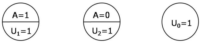
The graphical representation of sufficient-component causes helps visualize a key consequence of effect modification: as discussed in Chapter 4, the magnitude of the causal effect of treatment A depends on the distribution of effect modifiers. Imagine two hypothetical scenarios. In the first one, the population includes only 1% of individuals with U¹ = 1 (i.e., allergy to anesthesia). In the second one, the population includes 10% of individuals with U¹ = 1. The distribution of U² and U⁰ is identical between these two populations. Now, separately in each population, we conduct a randomized experiment of heart transplant A in which half of the population is assigned to treatment A = 1. The average causal effect of heart transplant A on death will be greater in the second population because there are more individuals susceptible to develop the outcome if treated. One of the 3 sufficient causes, A = 1 plus U¹ = 1, is 10 times more common in the second population than in the first one, whereas the other two sufficient causes are equally frequent in both populations.

The graphical representation of sufficient-component causes also helps visualize an alternative concept of interaction, which is described in the next section. First we need to describe the sufficient causes for two treatments A and E. Consider our vitamins and heart transplant example. We have already described 3 sufficient causes of death: presence/absence of A (or E) is irrelevant, presence of transplant A regardless of vitamins E, and absence of transplant A regardless of vitamins E. In the case of two treatments we need to add 2 more ways to die: presence of vitamins E regardless of transplant A, and absence of vitamins regardless of transplant A. We also need to add four more sufficient causes to accommodate those who would die only under certain combination of values of the treatments A and E. Thus, depending on which Greenland and Poole (1988) first background factors are present, there are 9 possible ways to die:

• causes. 1. by treatment A (treatment E is irrelevant)
  • 2. by the absence of treatment A (treatment E is irrelevant)
  • 3. by treatment E (treatment A is irrelevant)
  • 4. by the absence of treatment E (treatment A is irrelevant)
  • 5. by both treatments A and E
  • 6. by treatment A and the absence of E
  • 7. by treatment E and the absence of A
  • 8. by the absence of both A and E
  • 9. by other mechanisms (both treatments A and E are irrelevant)

In other words, there are 9 possible sufficient causes with treatment components A = 1 only, A = 0 only, E = 1 only, E = 0 only, A = 1 and E = 1, A = 1 and E = 0, A = 0 and E = 1, A = 0 and E = 0, and neither A nor E matter. Each of these sufficient causes includes a set of background factors from U1,. . . , U⁸ and U0. Figure 5.2 represents the 9 sufficient-component causes for two treatments A and E.

enumerated these 9 sufficient

Figure 5.1

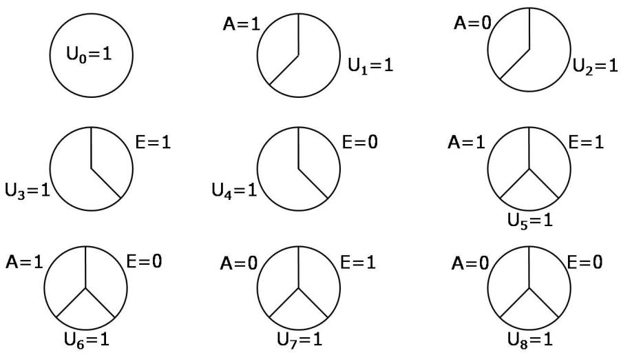
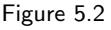
sufficient-component causes is often referred to as “the causal pies.”

Not all 9 sufficient-component causes for a dichotomous outcome and two treatments exist in all settings. For example, if receiving vitamins E = 1 does not kill any individual, regardless of her treatment A, then the 3 sufficient This graphical representation of causes with the component E = 1 will not be present. The existence of those 3 sufficient causes would mean that some individuals (e.g., those with U³ = 1) would be killed by receiving vitamins (E = 1), that is, their death would be prevented by not giving vitamins (E = 0) to them. See also Technical Point 5.3.

5.5 Sufficient cause interaction

The colloquial use of the term “interaction between treatments A and E” evokes the existence of some causal mechanism by which the two treatments work together (i.e., “interact”) to produce certain outcome. Interestingly, the definition of interaction within the counterfactual framework does not require any knowledge about those mechanisms nor even that the treatments work together (see Fine Point 5.3). In our example of vitamins E and heart transplant A, we said that there is an interaction between the treatments A and E if the causal effect of A when everybody receives E is different from the causal effect of A when nobody receives E. That is, interaction is defined by the contrast of counterfactual quantities, and can therefore be identified by conducting an ideal randomized experiment in which the conditions of exchangeability, positivity, and consistency hold for both treatments A and E. There is no need to contemplate the causal mechanisms (physical, chemical, biologic, sociological. . . ) that underlie the presence of interaction.

This section describes a second concept of interaction that perhaps brings us one step closer to the causal mechanisms by which treatments A and E bring about the outcome. This second concept of interaction is not based on counterfactual contrasts but rather on sufficient-component causes, and thus we refer to it as interaction within the sufficient-component-cause framework or, for brevity, sufficient cause interaction.

A sufficient cause interaction between A and E exists in the population if A and E occur together in a sufficient cause. For example, suppose individuals

From counterfactuals to sufficient-component causes, and vice versa. There is a correspondence between the counterfactual response types and the sufficient component causes. In the case of a dichotomous treatment and outcome, suppose an individual has none of the background factors U0, U1, U2. She will have an “immune” response type because she lacks the components necessary to complete all of the sufficient causes, whether she is treated or not. The table below displays the mapping between response types and sufficient-component causes in the case of one treatment A.

Type	a=0 Y	a=1 Y	Component causes
Doomed	1	1	U0 = 1 or {U1 = 1 and U2 = 1}
Helped	1	0	U0 = 0 and U1 = 0 and U2 = 1
Hurt	0	1	U0 = 0 and U1 = 1 and U2 = 0
Immune	0	0	U0 = 0 and U1 = 0 and U2 = 0

A particular combination of component causes corresponds to one and only one counterfactual type. However, a particular response type may correspond to several combinations of component causes. For example, individuals of the “doomed” type may have any combination of component causes including U⁰ = 1, no matter what the values of U¹ and U² are, or any combination including {U¹ = 1 and U² = 1}.

Sufficient-component causes can also be used to provide a mechanistic description of exchangeability Y ^a⊥⊥A. For a dichotomous treatment and outcome, exchangeability means that the proportion of individuals who would have the outcome under treatment, and under no treatment, is the same in the treated A = 1 and the untreated A = 0. That is, Pr[Y ^a=1 = 1|A = 1] = Pr[Y ^a=1 = 1|A = 0] and Pr[Y ^a=0 = 1|A = 1] = Pr[Y ^a=0 = 1|A = 0].

Now the individuals who would develop the outcome if treated are the “doomed” and the “hurt”, i.e., those with U⁰ = 1 or U¹ = 1. The individuals who would get the outcome if untreated are the “doomed” and the “helped”, that is, those with U⁰ = 1 or U² = 1. Therefore there will be exchangeability if the proportions of “doomed” + “hurt” and of “doomed” + “helped” are equal in the treated and the untreated. That is, exchangeability for a dichotomous treatment and outcome can be expressed in terms of sufficient-component causes as Pr[U⁰ = 1 or U¹ = 1|A = 1] = Pr[U⁰ = 1 or U¹ = 1|A = 0] and Pr[U⁰ = 1 or U² = 1|A = 1] = Pr[U⁰ = 1 or U² = 1|A = 0].

For additional details see Greenland and Brumback (2002), Flanders (2006), and VanderWeele and Hern´an (2006). Some of the above results were generalized to the case of two or more dichotomous treatments by VanderWeele and Robins (2008).

with background factors U⁵ = 1 will develop the outcome when jointly receiving vitamins (E = 1) and heart transplant (A = 1), but not when receiving only one of the two treatments. Then a sufficient cause interaction between A and E exists if there exists an individual with U⁵ = 1. It then follows that if there exists an individual with counterfactual responses Y ^a=1,e=1 = 1 and Y ^a=0,e=1 = Y ^a=1,e=0 = 0, a sufficient cause interaction between A and E is present.

Sufficient cause interactions can be synergistic or antagonistic. There is synergism between treatment A and treatment E when A = 1 and E = 1 are present in the same sufficient cause, and antagonism between treatment A and treatment E when A = 1 and E = 0 (or A = 0 and E = 1) are present in the same sufficient cause. Alternatively, one can think of antagonism between treatment A and treatment E as synergism between treatment A and no treatment E (or between no treatment A and treatment E).

Unlike the counterfactual definition of interaction, sufficient cause interaction makes explicit reference to the causal mechanisms involving the treatments A and E. One could then think that identifying the presence of sufficient cause interaction requires detailed knowledge about these causal mechanisms. It turns out that this is not always the case: sometimes we can conclude that

Biologic interaction. In epidemiologic discussions, sufficient-cause interaction is commonly referred to as biologic interaction (Rothman et al, 1980). This choice of terminology might seem to imply that, in biomedical applications, there exist biological mechanisms through which two treatments A and E act on each other in bringing about the outcome. However, this may not be necessarily the case as illustrated by the following example proposed by VanderWeele and Robins (2007a).

Suppose A and E are the two alleles of a gene that produces an essential protein. Individuals with a deleterious mutation in both alleles (A = 1 and E = 1) will lack the essential protein and die within a week after birth, whereas those with a mutation in none of the alleles (i.e., A = 0 and E = 0) or in only one of the alleles (i.e., A = 0 and E = 1, A = 1 and E = 0 ) will have normal levels of the protein and will survive. We would say that there is synergism between the alleles A and E because there exists a sufficient component cause of death that includes A = 1 and E = 1. That is, both alleles work together to produce the outcome. However, it might be argued that they do not physically act on each other and thus that they do not interact in any biological sense.

cepts of synergism and antagonism within the sufficient-componentcause framework.

sufficient cause interaction exists even if we lack any knowledge whatsoever Rothman (1976) described the con- about the sufficient causes and their components. Specifically, if the inequalities in Fine Point 5.1 hold, then there exists synergism between A and E. That is, one can empirically check that synergism is present without ever giving any thought to the causal mechanisms by which A and E work together to bring about the outcome. This result is not that surprising because of the correspondence between counterfactual response types and sufficient causes (see Fine Point 5.2), and because the above inequality is a sufficient but not a necessary condition, i.e., the inequality may not hold even if synergism exists.

5.6 Counterfactuals or sufficient-component causes?

sation was already hinted at by Hume (1748).

framework was developed in philosophy by Mackie (1965). He introduced the concept of INUS condition for Y : an I nsufficient but Necessary part of a condition which is itself Unnecessary but exclusively Sufficient for Y .

The sufficient-component-cause framework and the counterfactual (potential outcomes) framework address different questions. The sufficient-componentcause model considers sets of actions, events, or states of nature which together inevitably bring about the outcome under consideration. The model gives an A counterfactual framework of cau- account of the causes of a particular effect. It addresses the question, “Given a particular effect, what are the various events which might have been its cause?” The potential outcomes or counterfactual model focuses on one particular cause or intervention and gives an account of the various effects of that cause. In contrast to the sufficient-component-cause framework, the potential outcomes framework addresses the question, “What would have occurred if a particular factor were intervened upon and thus set to a different level than it The sufficient-component-cause in fact was?” Unlike the sufficient-component-cause framework, the counterfactual framework does not require a detailed knowledge of the mechanisms by which the factor affects the outcome.

The counterfactual approach addresses the question “what happens?” The sufficient-component-cause approach addresses the question “how does it happen?” For the contents of this book—conditions and methods to estimate the average causal effects of hypothetical interventions—the counterfactual framework is the natural one. The sufficient-component-cause framework is helpful to think about the causal mechanisms at work in bringing about a particular outcome. Sufficient-component causes have a rightful place in the teaching of

More on the attributable fraction. Fine Point 3.6 defined the excess fraction for treatment A as the proportion of cases attributable to treatment A in a particular population, and described an example in which the excess fraction for A was 75%. That is, 75% of the cases would not have occurred if everybody had received treatment a = 0 rather than their observed treatment A. Now consider a second treatment E. Suppose that the excess fraction for E is 50%. Does this mean that a joint intervention on A and E could prevent 125% (75% + 50%) of the cases? Of course not.

Clearly the excess fraction cannot exceed 100% for a single treatment (either A or E). Similarly, it should be clear that the excess fraction for any joint intervention on A and E cannot exceed 100%. That is, if we were allowed to intervene in any way we wish (by modifying A, E, or both) in a population, we could never prevent a fraction of disease greater than 100%. In other words, no more than 100% of the cases can be attributed to the lack of certain intervention, whether single or joint. But then why is the sum of excess fractions for two single treatments greater than 100%? The sufficient-component-cause framework helps answer this question.

As an example, suppose that Zeus had background factors U⁵ = 1 (and none of the other background factors) and was treated with both A = 1 and E = 1. Zeus would not have been a case if either treatment A or treatment E had been withheld. Thus Zeus is counted as a case prevented by an intervention that sets a = 0, i.e., Zeus is part of the 75% of cases attributable to A. But Zeus is also counted as a case prevented by an intervention that sets e = 0, i.e., Zeus is part of the 50% of cases attributable to E. No wonder the sum of the excess fractions for A and E exceeds 100%: some individuals like Zeus are counted twice!

The sufficient-component-cause framework shows that it makes little sense to talk about the fraction of disease attributable to A and E separately when both may be components of the same sufficient cause. For example, the discussion about the fraction of disease attributable to either genes or environment is misleading. Consider the mental retardation caused by phenylketonuria, a condition that appears in genetically susceptible individuals who eat certain foods. The excess fraction for those foods is 100% because all cases can be prevented by removing the foods from their diet. The excess fraction for the genes is also 100% because all cases would be prevented if we could replace the susceptibility genes. Thus the causes of mental retardation can be seen as either 100% genetic or 100% environmental. See Rothman, Greenland, and Lash (2008) for further discussion.

causal inference because they help understand key concepts like the dependence of the magnitude of causal effects on the distribution of background factors (effect modifiers), and the relationship between effect modification, interaction, and synergism.

Though the sufficient-component-cause framework is useful from a pedagogic standpoint, its relevance to actual data analysis is yet to be determined. In its classical form, the sufficient-component-cause framework is deterministic, its conclusions depend on the coding of the outcome, and is by definition limited to dichotomous treatments and outcomes (or to variables that can be recoded as dichotomous variables). This limitation practically rules out the consideration of any continuous factors, and restricts the applicability of the framework to contexts with a small number of dichotomous factors. More recent extensions of the sufficient-component-cause framework to stochastic VanderWeele (2010b) provided settings and to categorical and ordinal treatments might lead to an increased application of this approach to realistic data analysis. Finally, even allowing for these extensions of the sufficient-component-cause framework, we may rarely have the large amount of data needed to study the fine distinctions it makes.

To estimate causal effects more generally, the counterfactual framework will likely continue to be the one most often employed. Some apparently alternative frameworks—causal diagrams, decision theory—are essentially equivalent to the counterfactual framework, as described in the next chapter.

extensions to 3-level treatments. VanderWeele and Robins (2012) explored the relationship between stochastic counterfactuals and stochastic sufficient causes.

Monotonicity of causal effects and sufficient causes. When treatment A and E have monotonic effects, then some sufficient causes are guaranteed not to exist. For example, suppose that cigarette smoking (A = 1) never prevents heart disease, and that physical inactivity (E = 1) never prevents heart disease. Then no sufficient causes including either A = 0 or E = 0 can be present. This is so because, if a sufficient cause including the component A = 0 existed, then some individuals (e.g., those with U² = 1) would develop the outcome if they were unexposed (A = 0) or, equivalently, the outcome could be prevented in those individuals by treating them (A = 1). The same rationale applies to E = 0. The sufficient component causes that cannot exist when the effects of A and E are monotonic are crossed out in Figure 5.3.

Interaction

Chapter 6 GRAPHICAL REPRESENTATION OF CAUSAL EFFECTS

Causal inference generally requires expert knowledge and untestable assumptions about the causal network linking treatment, outcome, and other variables. Earlier chapters focused on the conditions and methods to compute causal effects in oversimplified scenarios (e.g., the causal effect of your looking up on other pedestrians’ behavior, an idealized heart transplant study). The goal was to provide a gentle introduction to the ideas underlying the more sophisticated approaches that are required in realistic settings. Because the scenarios we considered were so simple, there was really no need to make the causal network explicit. As we start to turn our attention towards more complex situations, however, it will become crucial to be explicit about what we know and what we assume about the variables relevant to our particular causal inference problem.

This chapter introduces a graphical tool to represent our qualitative expert knowledge and a priori assumptions about the causal structure of interest. By summarizing knowledge and assumptions in an intuitive way, graphs help clarify conceptual problems and enhance communication among investigators. The use of graphs in causal inference problems makes it easier to follow a sensible advice: draw your assumptions before your conclusions.

6.1 Causal diagrams

ject have been written by Pearl (2009) and Spirtes, Glymour and Scheines (2000).

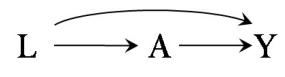
Figure 6.1

This chapter describes graphs, which we will refer to as causal diagrams, to represent key causal concepts. The modern theory of diagrams for causal inference arose within the disciplines of computer science and artificial intelligence. Comprehensive books on this sub- This and the next three chapters are focused on problem conceptualization via causal diagrams.

Take a look at the graph in Figure 6.1. It comprises three nodes representing random variables (L, A, Y ) and three edges (the arrows). We adopt the convention that time flows from left to right, and thus L is temporally prior to A and Y , and A is temporally prior to Y . As in previous chapters, L, A, and Y represent disease severity, heart transplant, and death, respectively.

The presence of an arrow pointing from a particular variable V to another variable W indicates that we know there is a direct causal effect (i.e., an effect not mediated through any other variables on the graph) for at least one individual. Alternatively, the lack of an arrow means that we know that V has no direct causal effect on W for any individual in the population. For example, in Figure 6.1, the arrow from L to A means that disease severity affects the probability of receiving a heart transplant. A standard causal diagram does not distinguish whether an arrow represents a harmful effect or a protective effect. Furthermore, if, as in Figure 6.1, a variable (here, Y ) has two causes, the diagram does not encode how the two causes interact.

Causal diagrams like the one in Figure 6.1 are known as directed acyclic graphs, which is commonly abbreviated as DAGs. “Directed” because the edges imply a direction: because the arrow from L to A is into A, L may cause A, but not the other way around. “Acyclic” because there are no cycles: a variable cannot cause itself, either directly or through another variable.

Directed acyclic graphs have applications other than causal inference. Here

Causal directed acyclic graphs. We define a directed acyclic graph (DAG) G to be a graph whose nodes (vertices) are random variables V = (V1, . . . , VM) with directed edges (arrows) and no directed cycles. We use P A^m to denote the parents of Vm, i.e., the set of nodes from which there is a direct arrow into Vm. The variable V^m is a descendant of V^j (and V^j is an ancestor of Vm) if there is a sequence of nodes connected by edges between V^j and V^m such that, following the direction indicated by the arrows, one can reach V^m by starting at V^j . For example, consider the DAG in Figure 6.1. In this DAG, M = 3 and we can choose V¹ = L, V² = A, and V³ = Y ; the parents P A³ of V³ = Y are (L, A). We will adopt the ordering convention that if m > j, V^m is not an ancestor of V^j . We define the distribution of V to be Markov with respect to a DAG G (equivalently, the distribution factors according to a DAG G) if, for each j, V^j is independent of its non-descendants conditional on its parents. This latter statement is mathematically equivalent to the statement that the density f (V ) of the variables V in DAG G satisfies the Markov factorization

\[f\left(v\right) = \prod\_{j=1}^{M} f\left(v\_j \mid pa\_j\right)\ .\]

A causal DAG is a DAG in which 1) the lack of an arrow from node V^j to V^m (i.e., V^j is not a parent of Vm) can be interpreted as the absence of a direct causal effect of V^j on V^m relative to the other variables on the graph, 2) all common causes, even if unmeasured, of any pair of variables on the graph are themselves on the graph, and 3) any variable is a cause of its descendants. Causal DAGs are of no practical use unless we make an assumption linking the causal structure represented by the DAG to the data obtained in a study. This assumption, referred to as the causal Markov assumption, states that, conditional on its direct causes, a variable V^j is independent of any variable for which it is not a cause. That is, conditional on its parents, V^j is independent of its non-descendants; hence, a causal DAG is Markov with respect to the DAG G.

we focus on causal directed acyclic graphs. A defining property of causal DAGs is that, conditional on its direct causes, any variable on the DAG is independent of any other variable for which it is not a cause. This assumption, referred to as the causal Markov assumption, implies that in a causal DAG the common causes of any pair of variables in the graph must be also in the graph. For a formal definition of causal DAGs, see Technical Point 6.1.

For example, suppose in our study individuals are randomly assigned to heart transplant A with a probability that depends on the severity of their disease L. Then L is a common cause of A and Y , and needs to be included in the graph, as shown in the causal diagram in Figure 6.1. Now suppose in our study all individuals are randomly assigned to heart transplant with the same probability regardless of their disease severity. Then L is not a common cause of A and Y and need not be included in the causal diagram. Figure 6.1 represents a conditionally randomized experiment, whereas Figure 6.2 represents a marginally randomized experiment.

Figure 6.1 may also represent an observational study. Specifically, Figure 6.1 represents an observational study in which we are willing to assume that the assignment of heart transplant A has as parent disease severity L and no other causes of Y . Otherwise, those causes of Y , even if unmeasured, would need to be included in the diagram, as they would be common causes of A and Y . In the next chapter we will describe how the willingness to consider Figure 6.1 as the causal diagram for an observational study is the graphic translation of the assumption of conditional exchangeability given L, Y ^a⊥⊥A|L for all a.

Many people find the graphical approach to causal inference easier to use and more intuitive than the counterfactual approach. However, the two ap-

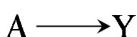
Figure 6.2

Counterfactual models associated with a causal DAG. In this book, a causal DAG G represents an underlying counterfactual model. To provide a formal definition of the counterfactual model represented by a DAG G, we use the following notation. For any random variable W, let W denote the support (i.e., the set of possible values w) of W. For any set of ordered variables W1, . . . , Wm, define w^m = (w1, . . . , wm). Let R denote any subset of variables in V and let r be a value of R. Then V r ^m denotes the counterfactual value of V^m when R is set to r.

A nonparametric structural equation model (NPSEM) represented by a DAG G with vertex set V = (V1, V2, . . . , VM) (ordered such that if i < j then Vⁱ is not a descendant of V^j ) assumes the existence of unobserved random variables (errors) ϵ^m and deterministic unknown functions f^m (pam, ϵm) such that V¹ = f¹ (ϵ1) and the one-step ahead counterfactual V vm−^{1 m} ≡ V pa^{m m} is given by f^m (pam, ϵm). That is, only the parents of V^m have a direct effect on V^m relative to the other variables on G. An NPSEM implies that any variable V^j on the graph can be intervened on, as counterfactuals in which V^j has been set to a specific value v^j are assumed to exist. Both the factual variable V^m and the counterfactuals V r ^m for any R ⊂ V are obtained recursively from V¹ and V vj−¹ j , M ≥ j > 1. For example, V v1 ³ = V v1,V ^v1 2 3 , i.e., the counterfactual value V v1 3 of V³ when V¹ is set to v¹ is the one-step ahead counterfactual V v1,v^{2 3} with v² equal to the counterfactual value V v1 2 of V2. Similarly, V³ = V V1,V ^V1 2 3 and V v1,v^{4 3} = V v1 3 because V⁴ is not a direct cause of V3. The absence of an arrow from V^j to V^k implies that V^j is not a direct cause of V^k for any individual.

Robins (1986) introduced this NPSEM, referred to it as a finest causally interpreted structural tree graph (FCISTG) “as detailed as the data”, and referred to the parents P A^m of V^m as causal risk factors for V^m controlling for the earlier variables in the ordering. Pearl (2009) showed how to represent this model with a DAG. Robins (1986) also proposed often more realistic causally interpreted structural tree graphs in which only a subset of the variables are subject to intervention. For expositional purposes, we will generally assume that every variable can be intervened on, even though the statistical methods considered here do not actually require this assumption.

proaches are intimately linked. Specifically, associated with each graph is an underlying counterfactual model (see Technical Points 6.2 and 6.3). It is this model that provides the mathematical justification for the heuristic, intuitive graphical methods we now describe. However, conventional causal diagrams do not include the underlying counterfactual variables on the graph. Therefore the link between graphs and counterfactuals has traditionally remained hidden. A recently developed type of causal directed acyclic graph—the Single World Richardson and Robins (2013) de- Intervention Graph (SWIG)—seamlessly unifies the counterfactual and graphical approaches to causal inference by explicitly including the counterfactual variables on the graph. We defer the introduction of SWIGs until Chapter 7 as the material covered in this chapter serves as a necessary prerequisite.

Causal diagrams are a simple way to encode our subject-matter knowledge, and our assumptions, about the qualitative causal structure of a problem. But, as described in the next sections, causal diagrams also encode information about potential associations between the variables in the causal network. It is precisely this simultaneous representation of association and causation that makes causal diagrams such an attractive tool. What follows is an informal introduction to graphic rules to infer associations from causal diagrams. Our emphasis is on conceptual insight rather than on formal rigor.

6.2 Causal diagrams and marginal independence

Consider the following two examples. First, suppose you know that aspirin use A has a preventive causal effect on the risk of heart disease Y , i.e., Pr[Y ^a=1 =

veloped the Single World Intervention Graph (SWIG).

Independencies associated with counterfactual models. An FCISTG model does not imply that the causal Markov assumption of Technical Point 6.1 holds; additional statistical independence assumptions are needed. For example, Pearl (2000) usually assumed an NPSEM in which all error terms ϵ^m are mutually independent. We refer to Pearl’s model with independent errors as an NPSEM-IE. In contrast, Robins (1986) only assumed that, given any vM, the one-step ahead counterfactuals V vm−^{1 m} = f^m (pam, ϵm) for m = 1, . . . , M are jointly independent where vm−¹ is a subvector of the vM, and referred to this as the finest fully randomized causally interpreted structured tree graph (FFRCISTG) model as detailed as the data.

More precisely, Robins (1986) made the assumption that for each m, conditional on the factual past V ^m−¹ = vm−1, any future evolution from m + 1 of one-step ahead counterfactuals (consistent with vm−1) is independent of the factual variable Vm. Robins and Richardson (2010) showed that this assumption is equivalent to the assumption of the previous paragraph for a positive distribution. In the absence of positivity, we define the model as in the last paragraph.

Robins (1986) showed his independence assumption implies that the causal Markov assumption holds. An NPSEM-IE is an FFRCISTG but not vice-versa because an NPSEM-IE makes many more independence assumptions than an FFRCISTG (Robins and Richardson 2010).

Unless stated otherwise, a DAG represents an NPSEM but we may need to specify which type. For example, the DAG in Figure 6.2 may correspond to either an NPSEM-IE that implies full exchangeability Y ^a=0, Y ^a=1 ⊥⊥A, or to an FFRCISTG that only implies marginal exchangeability Y ^a⊥⊥A for both a = 0 and a = 1. We will assume that a causal DAG represents an FFRCISTG as detailed as the data whenever we do not mention the underlying model.

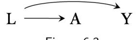
Figure 6.3

S in a DAG is a route that connects R and S by following a sequence of edges such that the route visits no variable more than once. A path is causal if it consists entirely of edges with their arrows pointing in the same direction. Otherwise it is noncausal.

1] ̸= Pr[Y ^a=0 = 1]. The causal diagram in Figure 6.2 is the graphical translation of this knowledge for an experiment in which aspirin A is randomly, and unconditionally, assigned. Second, suppose you know that carrying a lighter A has no causal effect (causative or preventive) on anyone’s risk of lung cancer Y , i.e., Pr[Y ^a=1 = 1] = Pr[Y ^a=0 = 1], and that cigarette smoking L has a causal effect on both carrying a lighter A and lung cancer Y . The causal diagram in Figure 6.3 is the graphical translation of this knowledge. The lack of an arrow between A and Y indicates that carrying a lighter does not have a causal effect on lung cancer; L is depicted as a common cause of A and Y .

To draw Figures 6.2 and 6.3 we only used your knowledge about the causal relations among the variables in the diagram but, interestingly, these causal diagrams also encode information about the expected associations (or, more exactly, the lack of them) among the variables in the diagram. We now argue heuristically that, in general, the variables A and Y will be associated in both Figure 6.2 and 6.3, and describe key related results from causal graphs theory.

Take first the randomized experiment represented in Figure 6.2. Intuitively one would expect that two variables A and Y linked only by a causal arrow would be associated. And that is exactly what causal graphs theory shows: A path between two variables R and when one knows that A has a causal effect on Y , as in Figure 6.2, then one should also generally expect A and Y to be associated. This is of course consistent with the fact that, in an ideal randomized experiment with unconditional exchangeability, causation Pr[Y ^a=1 = 1] ̸= Pr[Y ^a=0 = 1] implies association Pr[Y = 1|A = 1] ̸= Pr[Y = 1|A = 0], and vice versa. A heuristic that captures the causation-association correspondence in causal diagrams is the visualization of the paths between two variables as pipes or wires through which association flows. Association, unlike causation, is a symmetric relationship between two variables; thus, when present, association flows between two variables regardless of the direction of the causal arrows. In Figure 6.2 one could equivalently say that the association flows from A to Y or from Y to A.

Now let us consider the observational study represented in Figure 6.3. We know that carrying a lighter A has no causal effect on lung cancer Y . The question now is whether carrying a lighter A is associated with lung cancer Y . That is, we know that Pr[Y ^a=1 = 1] = Pr[Y ^a=0 = 1] but is it also true that Pr[Y = 1|A = 1] = Pr[Y = 1|A = 0]? To answer this question, imagine that a naive investigator decides to study the effect of carrying a lighter A on the risk of lung cancer Y (we do know that there is no effect but this is unknown to the investigator). He asks a large number of people whether they are carrying lighters and then records whether they are diagnosed with lung cancer during the next 5 years. Hera is one of the study participants. We learn that Hera is carrying a lighter. But if Hera is carrying a lighter (A = 1), then it is more likely that she is a smoker (L = 1), and therefore she has a greater than average risk of developing lung cancer (Y = 1). We then intuitively conclude that A and Y are expected to be associated because the cancer risk in those carrying a lighter (A = 1) is different from the cancer risk in those not carrying a lighter (A = 0), or Pr[Y = 1|A = 1] ̸= Pr[Y = 1|A = 0]. In other words, having information about the treatment A improves our ability to predict the outcome Y , even though A does not have a causal effect on Y . The investigator will make a mistake if he concludes that A has a causal effect on Y just because A and Y are associated. Causal graphs theory again confirms our intuition. In graphic terms, A and Y are associated because there is a flow of association from A to Y (or, equivalently, from Y to A) through the common cause L.

Let us now consider a third example. Suppose you know that certain genetic haplotype A has no causal effect on anyone’s risk of becoming a cigarette smoker Y , i.e., Pr[Y ^a=1 = 1] = Pr[Y ^a=0 = 1], and that both the haplotype A and cigarette smoking Y have a causal effect on the risk of heart disease L. The causal diagram in Figure 6.4 is the graphical translation of this knowledge. The lack of an arrow between A and Y indicates that the haplotype does not have a causal effect on cigarette smoking, and L is depicted as a common effect of A and Y . The common effect L is referred to as a collider on the path A → L ← Y because two arrowheads collide on this node.

Again the question is whether A and Y are associated. To answer this question, imagine that another investigator decides to study the effect of haplotype A on the risk of becoming a cigarette smoker Y (we do know that there is no effect but this is unknown to the investigator). She makes genetic determinations on a large number of children, and then records whether they end up becoming smokers. Apollo is one of the study participants. We learn that Apollo does not have the haplotype (A = 0). Is he more or less likely to become a cigarette smoker (Y = 1) than the average person? Learning about the haplotype A does not improve our ability to predict the outcome Y because the risk in those with (A = 1) and without (A = 0) the haplotype is the same, or Pr[Y = 1|A = 1] = Pr[Y = 1|A = 0]. In other words, we would intuitively conclude that A and Y are not associated, i.e., A and Y are independent or A⊥⊥Y . The knowledge that both A and Y cause heart disease L is irrelevant when considering the association between A and Y . Causal graphs theory again confirms our intuition because it says that colliders, unlike other variables, block the flow of association along the path on which they lie. Thus A and Y are independent because the only path between them, A → L ← Y , is blocked by the collider L.

In summary, two variables are (marginally) associated if one causes the other, or if they share common causes. Otherwise they will be (marginally) independent. The next section explores the conditions under which two variables A and Y may be independent conditionally on a third variable L.

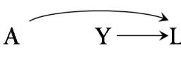
Figure 6.4

6.3 Causal diagrams and conditional independence

We now revisit the settings depicted in Figures 6.2, 6.3, and 6.4 to discuss the concept of conditional independence in causal diagrams.

According to Figure 6.2, we expect aspirin A and heart disease Y to be associated because aspirin has a causal effect on heart disease. Now suppose we obtain an additional piece of information: aspirin A affects the risk of heart disease Y because it reduces platelet aggregation B. This new knowledge is translated into the causal diagram of Figure 6.5 that shows platelet aggregation B (1: high, 0: low) as a mediator of the effect of A on Y .

Once a third variable is introduced in the causal diagram we can ask a new question: is there an association between A and Y within levels of (conditional on) B? Or, equivalently: when we already have information on B, does information about A improve our ability to predict Y ? To answer this question, suppose data were collected on A, B, and Y in a large number of individuals, and that we restrict the analysis to the subset of individuals with low platelet aggregation (B = 0). The square box placed around the node B in Figure 6.5 represents this restriction. (We would also draw a box around B if the analysis Because no conditional indepen- were restricted to the subset of individuals with B = 1.)

Individuals with low platelet aggregation (B = 0) have a lower than average risk of heart disease. Now take one of these individuals. Regardless of whether the individual was treated (A = 1) or untreated (A = 0), we already knew that he has a lower than average risk because of his low platelet aggregation. In fact, because aspirin use affects heart disease risk only through platelet aggregation, learning an individual’s treatment status does not contribute any additional information to predict his risk of heart disease. Thus, in the subset of individuals with B = 0, treatment A and outcome Y are not associated. (The same informal argument can be made for individuals in the group with B = 1.) Even though A and Y are marginally associated, A and Y are conditionally independent (unassociated) given B because the risk of heart disease is the same in the treated and the untreated within levels of B: Pr[Y = 1|A = 1, B = b] = Pr[Y = 1|A = 0, B = b] for all b. That is, A⊥⊥Y |B. Graphically, we say that a box placed around variable B blocks the flow of association through the path A → B → Y .

Let us now return to Figure 6.3. We concluded in the previous section that carrying a lighter A was associated with the risk of lung cancer Y because the path A ← L → Y was open to the flow of association from A to Y . The question we ask now is whether A is associated with Y conditional on L. This Figure 6.6 new question is represented by the box around L in Figure 6.6. Suppose the investigator restricts the study to nonsmokers (L = 0). In that case, learning that an individual carries a lighter (A = 1) does not help predict his risk of lung cancer (Y = 1) because the entire argument for better prediction relied on the fact that people carrying lighters are more likely to be smokers. This argument is irrelevant when the study is restricted to nonsmokers or, more generally, to people who smoke with a particular intensity. Even though A Blocking the flow of association and Y are marginally associated, A and Y are conditionally independent given L because the risk of lung cancer is the same in the treated and the untreated within levels of L: Pr[Y = 1|A = 1, L = l] = Pr[Y = 1|A = 0, L = l] for all l. That is, A⊥⊥Y |L. Graphically, we say that the flow of association between A and Y is interrupted because the path A ← L → Y is blocked by the box around L.

Finally, consider Figure 6.4 again. We concluded in the previous section that having the haplotype A was independent of being a cigarette smoker

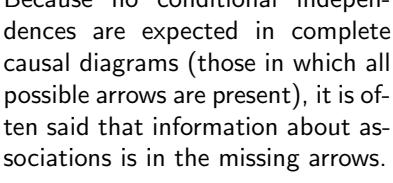
Figure 6.5

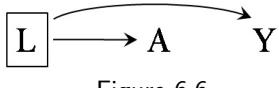
between treatment and outcome through the common cause is the graph-based justification to use stratification as a method to achieve exchangeability.

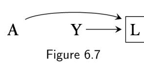
ations due to conditioning on common effects.

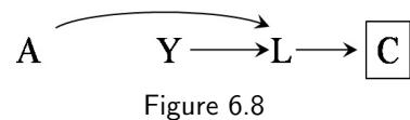
ing the graphical rules is known as “d-separation” (Pearl 1995).

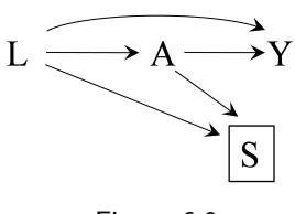
Figure 6.9

Y because the path between A and Y , A → L ← Y , was blocked by the collider L. We now argue heuristically that, in general, A and Y will be conditionally associated within levels of their common effect L. Suppose that the investigators, who are interested in estimating the effect of haplotype A on smoking status Y , restricted the study population to individuals with heart disease (L = 1). The square around L in Figure 6.7 indicates that they are conditioning on a particular value of L. Knowing that an individual with heart disease lacks haplotype A provides some information about her smoking status Figure 6.7 because, in the absence of A, it is more likely that another cause of L such as Y is present. That is, among people with heart disease, the proportion of smokers is increased among those without the haplotype A. Therefore, A and Y are inversely associated conditionally on L = 1. The investigator will make a mistake if he concludes that A has a causal effect on Y just because A and Y are See Chapter 8 for more on associ- associated within levels of L. In the extreme, if A and Y were the only causes of L, then among people with heart disease the absence of one of them would perfectly predict the presence of the other. Causal graphs theory shows that indeed conditioning on a collider like L opens the path A → L ← Y , which was blocked when the collider was not conditioned on. Intuitively, whether two variables (the causes) are associated cannot be influenced by an event in the future (their effect), but two causes of a given effect generally become associated once we stratify on the common effect.

As another example, the causal diagram in Figure 6.8 adds to that in Figure 6.7 a diuretic medication C whose use is a consequence of a diagnosis of heart disease. A and Y are also associated within levels of C because C is a common effect of A and Y . Causal graphs theory shows that conditioning on a variable C affected by a collider L also opens the path A → L ← Y . This path is blocked in the absence of conditioning on either the collider L or its consequence C.

This and the previous section review three structural reasons why two variables may be associated: one causes the other, they share common causes, or they share a common effect and the analysis is restricted to certain level of The mathematical theory underly- that common effect (or of its descendants). Along the way we introduced a number of graphical rules that can be applied to any causal diagram to determine whether two variables are (conditionally) independent. The arguments we used to support these graphical rules were heuristic and relied on our causal intuitions. These arguments, however, have been formalized and mathematically proven. See Fine Point 6.1 for a systematic summary of the graphical rules, and Fine Point 6.2 for an introduction to the concept of faithfulness.

There is another possible source of association between two variables that we have not discussed yet: chance or random variability. Unlike the structural reasons for an association between two variables—causal effect of one on the other, shared common causes, conditioning on common effects—random variability results in chance associations that become smaller when the size of the study population increases.

To focus our discussion on structural associations rather than chance associations, we continue to assume until Chapter 10 that we have recorded data on every individual in a very large (perhaps hypothetical) population of interest.

6.4 Positivity and consistency in causal diagrams

Because causal diagrams encode our qualitative expert knowledge about the causal structure, they can be used as a visual aid to help conceptualize causal

D-separation. We define a path to be either blocked or open according to the following graphical rules.

• 1. If there are no variables being conditioned on, a path is blocked if and only if two arrowheads on the path collide at some variable on the path. In Figure 6.1, the path L → A → Y is open, whereas the path A → Y ← L is blocked because two arrowheads on the path collide at Y . We call Y a collider on the path A → Y ← L.
• 2. Any path that contains a non-collider that has been conditioned on is blocked. In Figure 6.5, the path between A and Y is blocked after conditioning on B. We use a square box around a variable to indicate that we are conditioning on it.
• 3. A collider that has been conditioned on does not block a path. In Figure 6.7, the path between A and Y is open after conditioning on L.
• 4. A collider that has a descendant that has been conditioned on does not block a path. In Figure 6.8, the path between A and Y is open after conditioning on C, a descendant of the collider L.

Rules 1–4 can be summarized as follows. A path is blocked if and only if it contains a non-collider that has been conditioned on, or it contains a collider that has not been conditioned on and has no descendants that have been conditioned on. Two variables are d-separated if all paths between them are blocked (otherwise they are d-connected). Two sets of variables are d-separated if each variable in the first set is d-separated from every variable in the second set. Thus, A and L are not d-separated in Figure 6.1 because there is one open path between them (L → A), despite the other path (A → Y ← L)’s being blocked by the collider Y . In Figure 6.4, however, A and Y are d-separated because the only path between them is blocked by the collider L.

The relationship between statistical independence and the purely graphical concept of d-separation relies on the causal Markov assumption (Technical Point 6.1): In a causal DAG, any variable is independent of its non-descendants conditional on its parents. Pearl (1988) proved the following fundamental theorem: The causal Markov assumption implies that, given any three disjoint sets A, B, C of variables, if A is d-separated from B conditional on C, then A is statistically independent of B given C. The assumption that the converse holds, i.e., that A is d-separated from B conditional on C if A is statistically independent of B given C, is a separate assumption—the faithfulness assumption described in Fine Point 6.2. Under faithfulness, A is conditionally independent of Y given B in Figure 6.5, A is not conditionally independent of Y given L in Figure 6.7, and A is not conditionally independent of Y given C in Figure 6.8. The d-separation rules (‘d-’ stands for directional) to infer associational statements from causal diagrams were formalized by Pearl (1995). An equivalent set of graphical rules, known as “moralization”, was developed by Lauritzen et al. (1990).

methods for causal inference that are derived from graph theory.

problems and guide data analyses. In fact, the formulas that we described in Chapter 2 to quantify treatment effects—standardization and IP weighting can also be derived using causal graphs theory, as part of what is sometimes Pearl (2009) reviews quantitative referred to as the do-calculus. Therefore, our choice of counterfactual theory in Chapters 1-5 did not really privilege one particular approach but only one particular notation.

Regardless of the notation used (counterfactuals or graphs), exchangeability, positivity, and consistency are conditions required for causal inference via standardization or IP weighting. If any of these conditions does not hold, the numbers arising from the data analysis may not be appropriately interpreted as measures of causal effect. In the next section (and in Chapters 7 and 8) we discuss how the exchangeability condition is translated into graph language. Here we focus on positivity and consistency.

Unfortunately, causal graphs cannot encode violations of positivity except in special cases, e.g, when positivity is violated because a treatment A hap-

Faithfulness. In a causal DAG the absence of an arrow from A to Y indicates that the sharp null hypothesis of no causal effect of A on any individual’s Y holds, and an arrow A → Y (as in Figure 6.2) indicates that A has a causal effect on the outcome Y of at least one individual in the population. Thus, we would generally expect that, under Figure 6.2, the average causal effect of A on Y , Pr[Y ^a=1 = 1] − Pr[Y ^a=0 = 1], and the association between A and Y , Pr[Y = 1|A = 1]−Pr[Y = 1|A = 0], are not null. However, that is not necessarily true: a setting represented by Figure 6.2 may be one in which there is neither an average causal effect nor an association. For an example, remember the data in Table 4.1. Heart transplant A increases the risk of death Y in women (half of the population) and decreases the risk of death in men (the other half). Because the beneficial and harmful effects of A perfectly cancel out, the average causal effect is null, Pr[Y ^a=1 = 1] = Pr[Y ^a=0 = 1]. Yet Figure 6.2 is the correct causal diagram because treatment A affects the outcome Y of some individuals—in fact, of all individuals—in the population.

Formally, faithfulness is the assumption that, for three disjoint sets A, B, C on a causal DAG (where C may be the empty set), A independent of B given C implies A is d-separated from B given C. When, as in our example, the causal diagram makes us expect a non-null association that does not actually exist in the data, we say that the joint distribution of the data is not faithful to the causal DAG. In our example the unfaithfulness was the result of effect modification (by sex) with opposite effects of exactly equal magnitude in each half of the population. Such perfect cancellation of effects is rare, and thus we will assume faithfulness throughout this book. Because unfaithful distributions are rare, in practice lack of d-separation (See Fine Point 6.1) can be almost always equated to non-zero association.

There are, however, instances in which faithfulness is violated by design. For example, consider the prospective study in Section 4.5. The average causal effect of A on Y was computed after matching on L. In the matched population, L and A are not associated because the distribution of L is the same in the treated and the untreated. That is, individuals are selected into the matched population because they have a particular combination of values of L and A. The causal diagram in Figure 6.9 represents the setting of a matched study in which selection S (1: yes, 0: no) is determined by both A and L. The box around S indicates that the analysis is restricted to those selected into the matched cohort (S = 1). According to d-separation rules, there are two open paths between A and L when conditioning on S: L → A and L → S ← A. Thus one would expect L and A to be associated conditionally on S. However, matching ensures that L and A are not associated (see Chapter 4). Why the discrepancy? Matching creates an association via the path L → S ← A that is of equal magnitude, but opposite direction, as the association via the path L → A. The net result is a perfect cancellation of the associations. Matching leads to unfaithfulness.

Finally, faithfulness may be violated when there exist deterministic relations between variables on the graph. Specifically, when two variables are linked by paths that include deterministic arrows, then the two variables are independent if all paths between them are blocked, but might also be independent even if some paths are open. In this book we will assume faithfulness unless we say otherwise. Faithfulness is also assumed when the goal of the data analysis is discovering the causal structure (see Fine Point 6.3)

pens to be a deterministic function of a pretreatment variable L. In this case, we bold the L → A arrow to indicate determinism. The first component of consistency—well-defined interventions—means that the arrow from treatment A to outcome Y corresponds to a possibly hypothetical but relatively unambiguous intervention. In the causal diagrams discussed in this book, positivity is implicit unless otherwise specified, and consistency is embedded in the notation because we only consider treatment nodes with relatively well-defined interventions. Note that positivity is concerned with arrows into the treatment nodes, and well-defined interventions are only concerned with arrows leaving the treatment nodes.

Thus, the treatment nodes are implicitly given a different status compared with all other nodes. Some authors make this difference explicit by including decision nodes in causal diagrams. Though this decision-theoretic approach largely leads to the same methods described here, we do not include decision

agrams augmented with decision nodes to represent the interventions of interest (Dawid 2000, 2002).

suggested a concept of causation based on variables that “listen to others,” which continues to assume that for every variable there are well-defined counterfactuals.

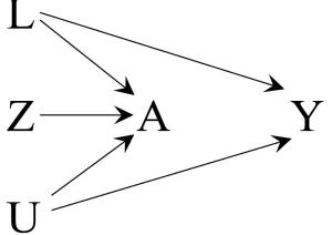
Figure 6.10

nodes in the causal diagrams presented in this chapter. Because we are always explicit about the potential interventions on the variable A, the additional Influence diagrams are causal di- nodes (to represent the potential interventions) would be somewhat redundant. However, we will give a different status to treatment nodes when using SWIGs—causal diagrams with nodes representing counterfactual variables—in subsequent chapters.

The different status of treatment nodes compared with other nodes was also graphically explicit in the causal trees introduced in Chapter 2, in which nontreatment branches corresponding to non-treatment variables L and Y were enclosed in circles, and in the “pies” representing sufficient causes in Chapter 5, which distinguish between potential treatments A and E and background factors U. Also, our discussion on sufficiently well-defined interventions of treatment in Chapter 3 emphasizes the requirements imposed on the treatment variables A that do not apply to other variables.

In contrast, the causal diagrams in this chapter apparently assign the same status to all variables in the diagram—this is indeed the case when causal diagrams are considered as representations of nonparametric structural equations Recently, Pearl (2018, 2019) has models with independent errors (see Technical Point 6.2). The apparently equal status of all variables in causal diagrams may be misleading because some of those variables correspond to ill-defined interventions. It may be okay to draw a causal diagram that includes a node for “obesity” as the outcome Y or even as a covariate L (more about this on Section 9.5). However, for the reasons discussed in Chapter 3, it is generally not okay to draw a causal diagram that includes a node for “obesity” as a treatment A. In causal diagrams, nodes for treatment variables need to correspond to sufficiently well-defined interventions.

For example, suppose that we are interested in the potential causal effect of “weight loss” A on mortality Y , as discussed in Chapter 3. The causal diagram in Figure 6.10 includes nodes for A and Y as well as nodes for factors that affect body weight. For simplicity, the causal diagram includes only 3 of those factors: caloric intake Z which (let us assume) can only affect mortality through weight loss, exercise L which can affect mortality through pathways other than weight loss, and genetic traits U which can affect mortality through other pathways that are also independent of weight loss.

Identifying and interpreting the effect of a treatment A on an outcome Y requires knowledge about how to intervene on A. When there are several potential ways to intervene on A and some of those potential interventions have direct effects on the outcome Y as in Figure 6.10, it becomes unclear what “the effect of A on Y” means. In our example, reducing weight via caloric restriction Z would result in a different risk of mortality than reducing weight via increased exercise L or via genetic manipulation U. Even if one were willing to disregard the ill-defined causal effect, identifying the variables needed to achieve exchangeability would be a formidable challenge, as discussed in Chapter 3.

Being explicit about the interventions of interest is an important step towards having a well-defined causal effect, identifying relevant data, and choosing adjustment variables.

Discovery of causal structure. In this book we use causal diagrams as a way to represent our expert knowledge—or assumptions—about the causal structure of the problem at hand. That is, the causal diagram guides the data analysis. How about going in the opposite direction? Can we learn the causal structure by conducting data analyses without making assumptions about the causal structure? The process of learning components of the causal structure through data analysis is referred to as discovery. See the books by Spirtes et al. (2000) and by Peters et al. (2017) for descriptions of approaches to causal discovery.

We now briefly discuss causal discovery under the assumption that the observed data arose from an unknown causal DAG that includes, in addition to the observed variables, an unknown number of unobserved variables U. Causal discovery is sometimes possible if we assume faithfulness, so that statistical independencies in the observed data distribution imply missing causal arrows on the DAG. Even assuming faithfulness, discovery is often impossible. For example, suppose that we find a strong association between two variables B and C in our data. We cannot learn the causal structure involving B and C because their association is consistent with many causal diagrams: B causes C (B → C), C causes B, (C → B), B and C share an unmeasured cause U (B ←− U → C), B and C have an unobserved common effect U that has been conditioned on, and various combinations. If we knew the time sequence of B and C, we could only rule out causal diagrams with either B → C (if C predates B) or C → B (if B predates C ).

There are, however, some settings in which learning causal structure from data appears possible. For example, consider 3 variables Z, A, Y and we know that their time sequence is Z first, A second, and Y last. In the absence of prior knowledge and empirical data, Figure 6.11 represents a potential causal DAG as we cannot rule out that Z has a direct effect on A and Y , that A has an effect on Y , or that there exists an unmeasured common cause between any pair of variables. We also cannot rule out any subgraph with one or more arrows removed.

Now suppose, hypothetically, that data on variables Z, A, and Y become available for an infinite number of individuals. Our data analysis finds that all 3 variables are marginally associated with each other, and that the only conditional independence that holds is Z⊥⊥Y |A. Then, if we are willing to assume that faithfulness holds, the only possible causal DAG consistent with our analysis is Z → A → Y with perhaps a common cause U¹ of Z and A in addition to (or in place of) the arrow from Z to A. This is because, if either Z was a parent of Y or shared a cause U² with Y , or an unmeasured common cause U³ of A and Y was present, then Z and Y could not have been statistically independent given A (assuming faithfulness). Thus, to explain the marginal dependency of Y and A, there must be a causal arrow from A to Y . (Note that, if an unmeasured common cause of A and Y existed, no conditional independence would be found and then, even assuming faithfulness, we could not determine whether A causes Y .)

In summary, the causal DAG learned implies that Z is not a direct cause (parent) of Y , that no unmeasured common cause of A and Y exists, and that, in fact, the average causal effect of A on Y is identified by E[Y |A = 1]−E[Y |A = 0] because exchangeability holds. Of course, we do not have an infinite sample size. We postpone a discussion about the implications of having a finite sample for causal discovery until Technical Point 10.7.

6.5 A structural classification of bias

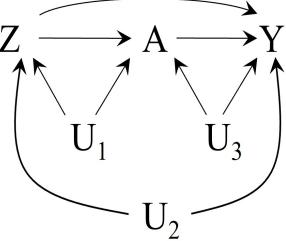
Figure 6.11

The word “bias” is frequently used by investigators making causal inferences. There are several related, but technically different, uses of the term “bias” (see Chapter 10). We say that there is systematic bias when the data are insufficient to identify—compute—the causal effect even with an infinite sample size. (In this chapter, due to the assumption of an infinite sample size, bias refers to systematic bias.) Informally, we often refer to systematic bias as any structural association between treatment and outcome that does not arise from the causal effect of treatment on outcome in the population of interest. Because causal diagrams are helpful to represent different sources of association, we can use causal diagrams to classify systematic bias according to its source, and thus to sharpen discussions about bias.

Take the crucial source of bias that we have discussed in previous chapters:

estimator can be consistent. Review Chapter 1 for a definition of consistent estimator.

variables may cause selection bias under the alternative (i.e., off the null) but not under the null, as described by Greenland (1977) and Hern´an (2017). See also Chapter 18.

sult from (nonstructural) random variability. See Chapter 10.

lack of exchangeability between the treated and the untreated. For the average causal effect in the entire population, we say that there is (unconditional) bias when Pr[Y ^a=1 = 1] − Pr[Y ^a=0 = 1] ̸= Pr[Y = 1|A = 1] − Pr [Y = 1|A = 0], which is the case when (unconditional) exchangeability Y ^a⊥⊥A does not hold. Absence of (unconditional) bias implies that the association measure (e.g., When there is systematic bias, no associational risk ratio or difference) in the population is a consistent estimate of the corresponding effect measure (e.g., causal risk ratio or difference) in the population.

Lack of exchangeability results in bias even when the null hypothesis of no causal effect of treatment on the outcome holds. That is, even if the treatment had no causal effect on the outcome, treatment and outcome would be associated in the data. We then say that lack of exchangeability leads to bias under the null. In the observational study summarized in Table 3.1, there was bias under the null because the causal risk ratio was 1 whereas the associational For example, conditioning on some risk ratio was 1.26. Any causal structure that results in bias under the null will also cause bias under the alternative (i.e., when treatment does have a non-null effect on the outcome). However, the converse is not true.

For the average causal effects within levels of L, we say that there is conditional bias whenever Pr[Y ^a=1 = 1|L = l] − Pr[Y ^a=0 = 1|L = l] differs from Pr[Y = 1|L = l, A = 1] − Pr[Y = 1|L = l, A = 0] for at least one stratum l, which is generally the case when conditional exchangeability Y ^a⊥⊥A|L = l does not hold for all a and l.

So far in this book we have referred to lack of exchangeability multiple times. However, we have yet to explore the causal structures that generate lack of exchangeability. With causal diagrams added to our methodological arsenal, we will be able to describe how lack of exchangeability can result from two different causal structures:

• 1. Common causes: When the treatment and outcome share a common cause, the association measure generally differs from the effect measure. Many epidemiologists use the term confounding to refer to this bias.
• 2. Conditioning on common effects: This structure is the source of bias that many epidemiologists refer to as selection bias under the null.

Chapter 7 will focus on confounding bias due to the presence of common causes, and Chapter 8 on selection bias due to conditioning on common effects. Again, both are examples of bias under the null due to lack of exchangeability.

Chapter 9 will focus on another source of bias: measurement error. So far we have assumed that all variables—treatment A , outcome Y , and covariates L— are perfectly measured. In practice, however, some degree of measurement error is expected. The bias due to measurement error is referred to as measurement bias or information bias. As we will see, some types of measurement Another form of bias may also re- bias also cause bias under the null.

Therefore, in the next three chapters we turn our attention to the three types of systematic bias—confounding, selection, and measurement. These biases may arise both in observational studies and in randomized experiments. The susceptibility to bias of randomized experiments may not be obvious from previous chapters, in which we conceptualized observational studies as some sort of imperfect randomized experiments, while only considering ideal randomized experiments with no participants lost during the follow-up, all participants adhering to their assigned treatment, and unknown treatment assignment for both study participants and investigators. While our quasi-mythological characterization of randomized experiments was helpful for teaching purposes, real

randomized experiments rarely look like that. The remaining chapters of Part I will elaborate on the sometimes fuzzy boundary between experimenting and observing.

Before that, we take a brief detour to describe causal diagrams in the presence of effect modification.

6.6 The structure of effect modification

Identifying potential sources of bias is a key use of causal diagrams: we can use our causal expert knowledge to draw graphs and then search for sources of association between treatment and outcome. Causal diagrams are less helpful to illustrate the concept of effect modification that we discussed in Chapter 4.

Suppose heart transplant A was randomly assigned in an experiment to identify the average causal effect of A on death Y . For simplicity, let us assume that there is no bias, and thus Figure 6.2 adequately represents this study. Computing the effect of A on the risk of Y presents no challenge. Because association is causation, the associational risk difference Pr[Y = 1|A = 1]−Pr [Y = 1|A = 0] can be interpreted as the causal risk difference Pr[Y ^a=1 = 1]−Pr[Y ^a=0 = 1]. The investigators, however, want to go further because they suspect that the causal effect of heart transplant varies by the quality of medical care offered in each hospital participating in the study. Thus, the investigators classify all individuals as receiving high (V = 1) or normal (V = 0) quality of care, compute the stratified risk differences in each level of V as described in Chapter 4, and indeed confirm that there is effect modification by V on the additive scale. The causal diagram in Figure 6.12 includes the effect modifier V with an arrow into the outcome Y but no arrow into treatment A (which is randomly assigned and thus independent of V ). Two important caveats.

First, the causal diagram in Figure 6.12 would still be a valid causal diagram if it did not include V because V is not a common cause of A and Y . It is only because the causal question makes reference to V (i.e., what is the average causal effect of A on Y within levels of V ?), that V needs to be included on the causal diagram. Other variables measured along the path between “quality of care” V and the outcome Y could also qualify as effect modifiers. For example, Figure 6.13 shows the effect modifier “therapy complications” N, which partly mediates the effect of V on Y .

Second, the causal diagram in Figure 6.12 does not necessarily indicate the presence of effect modification by V . The causal diagram implies that both A and V affect death Y , but it does not distinguish among the following three qualitatively distinct ways that V could modify the effect of A on Y :

• 1. The causal effect of treatment A on mortality Y is in the same direction (i.e., harmful or beneficial) in both stratum V = 1 and stratum V = 0.
• 2. The direction of the causal effect of treatment A on mortality Y in stratum V = 1 is the opposite of that in stratum V = 0 (i.e., there is qualitative effect modification).
• 3. Treatment A has a causal effect on Y in one stratum of V but no causal effect in the other stratum A only kills individuals with V = 0.

That is, valid causal graphs such as Figure 6.12 fail to distinguish between the above three different qualitative types of effect modification by V .

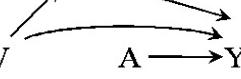
Figure 6.12

Figure 6.13

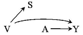
Figure 6.14

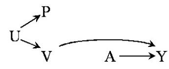
Figure 6.15

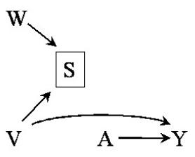
Figure 6.16

fect modification via causal diagrams, see VanderWeele and Robins (2007b)

between W and V in low-cost hospitals S = 0: suppose that lowcost hospitals that use mineral water need to offset the extra cost of mineral water by spending less on components of medical care that decrease mortality. Then use of mineral water would be inversely associated with quality of medical care in low-cost hospitals.

In the above example, the effect modifier V had a causal effect on the outcome. Many effect modifiers, however, do not have a causal effect on the outcome. Rather, they are surrogates for variables that have a causal effect on the outcome. Figure 6.14 includes the variable “cost of the treatment” S (1: high, 0: low), which is affected by “quality of care” V but has itself no effect on mortality Y . An analysis stratified by S (but not by V ) will generally detect effect modification by S even though the variable that truly modifies the effect of A on Y is V . The variable S is a surrogate effect modifier whereas the variable V is a causal effect modifier (see Section 4.2). Because causal and surrogate effect modifiers are often indistinguishable in practice, the concept of effect modification comprises both. As discussed in Section 4.2, some prefer to use the neutral term “heterogeneity of causal effects,” rather than “effect modification,” to avoid confusion. For example, someone might be tempted For a finer classification of ef- to interpret the statement “cost modifies the effect of heart transplant on mortality because the effect is more beneficial when the cost is higher” as an argument to increase the price of medical care without necessarily increasing its quality.

A surrogate effect modifier is simply a variable associated with the causal effect modifier. Figure 6.14 depicts the setting in which such association is due to the effect of the causal effect modifier on the surrogate effect modifier. However, such association may also be due to shared common causes or conditioning on common effects. For example, Figure 6.15 includes the variables “place of residence” (1: Greece, 0: Rome) U and “passport-defined nationality” P (1: Greece, 0: Rome). Place of residence U is a common cause of both quality of care V and nationality P. Thus P will behave as a surrogate effect modifier because P is associated with the causal effect modifier V . Another (admittedly silly) example to illustrate this issue: Figure 6.16 includes the variables “cost of care” S and “use of bottled mineral water (rather than tap water) for drinking at the hospital” W. Use of mineral water W affects cost S but not mortality Y in developed countries. If the study were restricted to Some intuition for the association low-cost hospitals (S = 0), then use of mineral water W would be generally associated with medical care V , and thus W would behave as a surrogate effect modifier. In summary, surrogate effect modifiers can be associated with the causal effect modifier by structures including common causes, conditioning on common effects, or cause and effect.

Causal diagrams are in principle agnostic about the presence of interaction between two treatments A and E. However, causal diagrams can encode information about interaction when augmented with nodes that represent sufficientcomponent causes (see Chapter 5), i.e., nodes with deterministic arrows from the treatments to the sufficient-component causes. Because the presence of interaction affects the magnitude and direction of the association due to conditioning on common effects, these augmented causal diagrams are discussed in Chapter 8.

Chapter 7 CONFOUNDING

Suppose an investigator conducted an observational study to answer the causal question “does one’s looking up to the sky make other pedestrians look up too?” She found an association between a first pedestrian’s looking up and a second one’s looking up. However, she also found that pedestrians tend to look up when they hear a thunderous noise above. Thus it was unclear what was making the second pedestrian look up, the first pedestrian’s looking up or the thunderous noise? She concluded the effect of one’s looking up was confounded by the presence of a thunderous noise.

In randomized experiments treatment is assigned by the flip of a coin, but in observational studies treatment (e.g., a person’s looking up) may be determined by many factors (e.g., a thunderous noise). If those factors affect the risk of developing the outcome (e.g., another person’s looking up), then the effects of those factors become entangled with the effect of treatment. We then say that there is confounding, which is just a form of lack of exchangeability between the treated and the untreated. Confounding is often viewed as the main shortcoming of observational studies. In the presence of confounding, the old adage “association is not causation” holds even if the study population is arbitrarily large. This chapter provides a definition of confounding and reviews the methods to adjust for it.

7.1 The structure of confounding

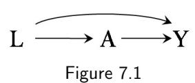
is a noncausal path between treatment and outcome that remains even if all arrows pointing from treatment to other variables (the descendants of treatment) are removed. That is, the path has an arrow pointing into treatment.

The structure of confounding, the bias due to common causes of treatment and outcome, can be represented by using causal diagrams. For example, the diagram in Figure 7.1 (same as Figure 6.1) depicts a treatment A, an outcome Y , and their shared (or common) cause L. This diagram shows two sources of association between treatment and outcome: 1) the path A → Y that represents the causal effect of A on Y , and 2) the path A ← L → Y between A and Y that includes the common cause L. The path A ← L → Y that links A and Y through their common cause L is an example of a backdoor path.

If the common cause L did not exist in Figure 7.1, then the only path In a causal DAG, a backdoor path between treatment and outcome would be A → Y , and thus the entire association between A and Y would be due to the causal effect of A on Y . That is, the associational risk ratio Pr [Y = 1|A = 1] /Pr [Y = 1|A = 0] would equal the causal risk ratio Pr - Y ^a=1 = 1 /Pr - Y ^a=0 = 1 ; association would be causation. But the presence of the common cause L creates an additional source of association between the treatment A and the outcome Y , which we refer to as confounding for the effect of A on Y . Because of confounding, the associational risk ratio does not equal the causal risk ratio; association is not causation.

Examples of confounding abound in observational research. Consider the following examples of confounding for the effect of various kinds of treatments on health outcomes:

• Occupational factors: The effect of working as a firefighter A on the risk of death Y will be confounded if “being physically fit” L is a cause of both being an active firefighter and having a lower mortality risk. This

• Clinical decisions: The effect of drug A (say, aspirin) on the risk of disease Y (say, stroke) will be confounded if the drug is more likely to be prescribed to individuals with certain condition L (say, heart disease) that is both an indication for treatment and a risk factor for the disease. Heart disease L is a risk factor for stroke Y because L has a direct causal effect on Y as in Figure 7.1 or, as in Figure 7.2, because both L and Y are caused by atherosclerosis U, an unmeasured variable. This bias is known as confounding by indication or channeling, the last term often being reserved to describe the bias created by patient-specific risk factors L that encourage doctors to use certain drug A within a class of drugs.
• Lifestyle: The effect of behavior A (say, exercise) on the risk of Y (say, death) will be confounded if the behavior is associated with another behavior L (say, cigarette smoking) that has a causal effect on Y and tends to co-occur with A. The structure of the variables L, A, and Y is depicted in the causal diagram in Figure 7.3, in which the unmeasured variable U represents the sort of personality and social factors that lead to both lack of exercise and smoking. Another frequent problem: subclinical disease U results both in lack of exercise A and an increased risk of clinical disease Y . This form of confounding is often referred to as reverse causation when L is unknown.
• Genetic factors: The effect of a DNA sequence A on the risk of developing certain trait Y will be confounded if there exists a DNA sequence L that has a causal effect on Y and is more frequent among people carrying A. This bias, also represented by the causal diagram in Figure 7.3, is known as linkage disequilibrium or population stratification, the last term often being reserved to describe the bias arising from conducting studies in a mixture of individuals from different ethnic groups. Thus the variable U can stand for ethnicity or other factors that result in linkage of DNA
• Social factors: The effect of income at age 65 A on the level of disability at age 75 Y will be confounded if the level of disability at age 55 L affects both future income and disability level. This bias may be depicted by the causal diagram in Figure 7.1.
• Environmental exposures: The effect of airborne particulate matter A on the risk of coronary heart disease Y will be confounded if other pollutants L whose levels co-vary with those of A cause coronary heart disease. This bias is also represented by the causal diagram in Figure 7.3, in which the unmeasured variable U represent weather conditions that affect the levels of all types of air pollution.

In all these cases, the bias has the same structure: it is due to the presence of a cause (L or U) that is shared by the treatment A and the outcome Y , which results in an open backdoor path between A and Y . We refer to the bias caused by shared causes of treatment and outcome as confounding, and we use other names to refer to biases caused by structural reasons other than the presence of shared causes of treatment and outcome. For simplicity of presentation, we assume throughout this chapter that positivity and consistency hold, that all nodes in the causal diagrams are perfectly measured, that

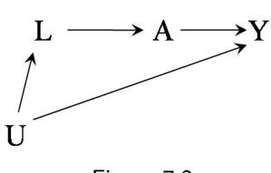
Figure 7.2

Some authors prefer to replace the unmeasured common cause U (and the two arrows leaving it) by a bidirectional edge between the measured variables that U causes.

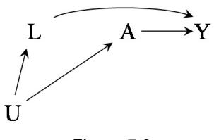
Figure 7.3

sequences. Early statistical descriptions of confounding were provided by Yule (1903) for discrete variables and by Pearson et al. (1899) for continuous variables. Yule described the association due to confounding as “fictitious”, “illusory”, and “apparent”. Pearson et al. (1899) referred to it as a “spurious” correlation. However, there is nothing fictitious, illusory, apparent, or spurious about these associations. Associations due to common causes are quite real associations, though they cannot be causally interpreted as treatment effects. Or, in Yule’s words, they are associations “to which the most obvious physical meaning must not be assigned.”

there are no selection nodes S with a box around them (that is, the data are a random sample from the population of interest), and that random variability is absent. Causal diagrams with selection nodes will be discussed in Chapter 8, and causal diagrams with mismeasured nodes in Chapter 9. Random variability is discussed in Chapter 10.

7.2 Confounding and exchangeability

2009. for a detailed discussion on the relations between confounding and exchangeability.

a=1] a=0 − E[Y E[Y ] =
P l E[Y L = l, A = 1] Pr [L = l] −
P L l E[Y = l, A = 0] Pr [L = l].

backdoor criterion for nonparametric identification of causal effects.

We now link the concept of confounding, which we have defined using causal See Greenland and Robins (1986, diagrams, with the concept of exchangeability, which we have defined using counterfactuals in earlier chapters.

When exchangeability Y ^a⊥⊥A holds, as in a marginally randomized experiment in which all individuals have the same probability of receiving treatment, the average causal effect can be identified without adjustment for any variables. For a binary treatment A, the average causal effect E[Y ^a=1] − E[Y ^a=0] is calculated as the difference of conditional means E[Y |A = 1] − E[Y |A = 0].

When exchangeability Y ^a⊥⊥A does not hold but conditional exchangeability Y ^a⊥⊥A|L does, as in a conditionally randomized experiment in which the probability of receiving treatment varies across values of L, the average causal effect can also be identified. However, as we described in Chapter 2, identification of the causal effect E[Y ^a=1] − E[Y ^a=0] in the population requires Under conditional exchangeability, adjustment for the variables L via standardization or IP weighting. Also, as we described in Chapter 4, conditional exchangeability also allows the identification of the conditional causal effects E[Y ^a=1|L = l] − E[Y ^a=0|L = l] for any value l via stratification.

In practice, if we believe confounding is likely, a key question arises: can we determine whether there exists a set of measured covariates L for which conditional exchangeability holds? Answering this question is difficult because thinking in terms of conditional exchangeability Y ^a⊥⊥A|L is often not intuitive in complex causal systems.

In this chapter, we will see that answering this question is possible if one knows the causal DAG that generated the data. To do so, suppose that we know the true causal DAG (for now, it doesn’t matter how we know it: perhaps we have sufficient subject-matter knowledge, or perhaps an omniscient god gave it to us). How does the causal DAG allow us to determine whether there exists a set of variables L for which conditional exchangeability holds? There are Pearl (1995, 2009) proposed the two main approaches: (i) the backdoor criterion applied to the causal DAG and (ii) the transformation of the causal DAG into a SWIG. Though the use of SWIGs is a more direct approach, it also requires a bit more machinery so we are going to first explain the backdoor criterion; we will describe the SWIG approach in Section 7.5.

A set of covariates L satisfies the backdoor criterion if all backdoor paths between A and Y are blocked by conditioning on L and L contains no variables that are descendants of treatment A. Under faithfulness and a further condition discussed in Technical Point 7.1, conditional exchangeability Y ^a⊥⊥A|L holds if and only if L satisfies the backdoor criterion. (A simple proof of this fact will be given below based on SWIGs.) Hence, we can now answer any query we may have about whether, for a given set of covariates L, conditional exchangeability given L holds. Thus, by trying every subset of measured non-descendants of treatment, we can answer the question of whether conditional exchangeability holds for any subset. (In fact, algorithms exist that can greatly reduce the

Does conditional exchangeability imply the backdoor criterion? That L satisfies the backdoor criterion always implies conditional exchangeability given L, even in the absence of faithfulness. In the main text we also said that, given faithfulness, conditional exchangeability given L implies that L satisfies the backdoor criterion. This last sentence is true under an FFRCISTG model (see Technical Point 6.2). In contrast, under an NPSEM-IE model, conditional exchangeability can hold even if the backdoor criterion does not, as is the case in a causal DAG with nodes A, L, Y and arrows A → L, A → Y . In this book we always assume an FFRCISTG model and faithfulness, unless stated otherwise.

This difference between causal models is due to the fact that the NPSEM-IE, unlike an FFRCISTG model, assumes cross-world independencies between counterfactuals. However a cross-world independence can never be verified, even in principle, by any randomized experiment, which was the very reason that Robins (1986, 1987) did not assume cross-world independencies in his FFRCISTG model. We will return to this issue in Chapter 23.

number of subsets that must be tried in order to answer the question.)

Let us now relate the backdoor criterion (i.e., exchangeability) to confounding. The two settings in which the backdoor criterion is satisfied are

• 1. No common causes of treatment and outcome. In Figure 6.2, there are no common causes of treatment and outcome, and hence no backdoor paths that need to be blocked. Then the set of variables that satisfies the backdoor criterion is the empty set and we say that there is no confounding.
• 2. Common causes of treatment and outcome but a subset L of measured non-descendants of A suffices to block all backdoor paths. In Figure 7.1, the set of variables that satisfies the backdoor criterion is L. Thus, we say that there is confounding, but that there is no residual confounding whose elimination would require adjustment for unmeasured variables (which, of course, is not possible). For brevity, we say that there is no unmeasured confounding.

The first setting describes a marginally randomized experiment in which confounding is not expected because treatment assignment is solely determined by the flip of a coin—or its computerized upgrade: the random number generator—and the flip of the coin cannot cause the outcome. That is, when the treatment is unconditionally randomly assigned, the treated and the untreated are expected to be exchangeable because no common causes exist or, equivalently, because there are no open backdoor paths. Marginal exchangeability, i.e., Y ^a⊥⊥A, is equivalent to no common causes of treatment and outcome.

The second setting describes a conditionally randomized experiment in which the probability of receiving treatment is the same for all individuals with the same value of L but, by design, this probability varies across values of L, that is there is an arrow L → A. This experimental design guarantees confounding if L is also either a cause of the outcome (as in Figure 7.1) or the descendant of an unmeasured cause of the outcome as in Figure 7.2. Hence, there are open backdoor paths. However, conditioning on the covariates L will block all backdoor paths and therefore conditional exchangeability, i.e., Y ^a⊥⊥A|L, will hold. We say that a set L of measured non-descendants of A is a sufficient set for confounding adjustment when conditioning on L blocks all backdoor paths—that is, the treated and the untreated are exchangeable within levels of L.

Take our heart transplant study, a conditionally randomized experiment, as an example. Individuals who received a transplant (A = 1) are different from the others (A = 0) because, had the treated remained untreated, their risk of death Y would have been higher than that of those that were actually untreated—the treated had a higher frequency of severe heart disease L, a common cause of A and Y . The presence of common causes of treatment and outcome implies that the treated and the untreated are not marginally exchangeable but are conditionally exchangeable given L. This second setting is also what one hopes for in observational studies in which many variables L have been measured.

The backdoor criterion does not answer questions regarding the magnitude or direction of confounding. It is logically possible that some unblocked backdoor paths are weak (e.g., if L does not have a large effect on either A or Y ) and thus induce little bias, or that several strong backdoor paths induce bias in opposite directions and thus result in a weak net bias. Because unmeasured confounding is not an “all or nothing” issue, in practice, it is important to consider the expected direction and magnitude of the bias (see Fine Point 7.1).

7.3 Confounding and the backdoor criterion

We now describe several examples of the application of the backdoor criterion to determine whether the causal effect of A on Y is identifiable and, if so, which variables are required to ensure conditional exchangeability. Remember that all causal DAGs in this chapter include perfectly measured nodes that are not conditioned on.

In Figure 7.1 there is confounding because the treatment A and the outcome Y share the cause L, i.e., because there is an open backdoor path between A and Y through L. However, this backdoor path can be blocked by conditioning on L. Thus, if the investigators collected data on L for all individuals, there is no unmeasured confounding given L.

In Figure 7.2 there is confounding because the treatment A and the outcome Y share the unmeasured cause U, i.e., there is a backdoor path between A and Y through U. (Unlike the variables L, A, and Y , the variable U was not measured by the investigators.) This backdoor path could be theoretically blocked, and thus confounding eliminated, by conditioning on U, had data on this variable been collected. However, this backdoor path can also be blocked Figure 7.4 by conditioning on L. Thus, there is no unmeasured confounding given L.

In Figure 7.3 there is also confounding because the treatment A and the outcome Y share the cause U, and the backdoor path can also be blocked by conditioning on L. Therefore there is no unmeasured confounding given L.

Now consider Figure 7.4. In this causal diagram there are no common causes of treatment A and outcome Y , and therefore there is no confounding. The backdoor path between A and Y through L (A ← U² → L ← U¹ → Y ) is blocked because L is a collider on that path. Thus all the association between A and Y is due to the effect of A on Y : association is causation. For example, suppose A represents physical activity, Y cervical cancer, U¹ a precancer lesion, L a diagnostic test (Pap smear) for pre-cancer, and U² a healthconscious personality (more physically active, more visits to the doctor). Then, under the causal diagram in Figure 7.4, the effect of physical activity A on cancer Y is unconfounded and there is no need to adjust for L to compute either Pr[Y ^a=1] or Pr[Y ^a=0] and thus to compute the causal effect in the population.

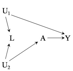
The strength and direction of confounding bias. Suppose you conducted an observational study to identify the effect of heart transplant A on death Y and that you assumed no unmeasured confounding. A thoughtful critic says “the inferences from this observational study may be incorrect because of potential confounding due to cigarette smoking L.” A crucial question is whether the bias results in an attenuated or an exaggerated estimate of the effect of heart transplant. For example, suppose that the risk ratio from your study was 0.6 (heart transplant was estimated to reduce mortality during the follow-up by 40%) and that, as the reviewer suspected, cigarette smoking L is a common cause of A (cigarette smokers are less likely to receive a heart transplant) and Y (cigarette smokers are more likely to die). Because there are fewer cigarette smokers (L = 1) in the heart transplant group (A = 1) than in the other group (A = 0), one would have expected to find a lower mortality risk in the group A = 1 even under the null hypothesis of no effect of treatment A on Y . Adjustment for cigarette smoking will therefore move the effect estimate upwards (say, from 0.6 to 0.7). In other words, lack of adjustment for cigarette smoking resulted in an exaggeration of the beneficial average causal effect of heart transplant.

An approach to predict the direction of confounding bias is the use of signed causal diagrams. Consider the causal diagram in Figure 7.1 with dichotomous L, A, and Y variables. A positive sign over the arrow from L to A is added if L has a positive average causal effect on A (i.e., if the probability of A = 1 is greater among those with L = 1 than among those with L = 0), otherwise a negative sign is added if L has a negative average causal effect on A (i.e., if the probability of A = 1 is greater among those with L = 0 than among those with L = 1). Similarly a positive or negative sign is added over the arrow from L to Y . If both arrows are positive or both arrows are negative, then the confounding bias is said to be positive, which implies that effect estimate will be biased upwards in the absence of adjustment for L. If one arrow is positive and the other one is negative, then the confounding is said to be negative, which implies that the effect estimate will be biased downwards in the absence of adjustment for L. Unfortunately, this simple rule may fail in more complex causal diagrams or when the variables are not dichotomous. See VanderWeele, Hern´an, and Robins (2008) for a more detailed discussion of signed diagrams in the context of average causal effects.

Regardless of the sign of confounding, another key issue is the magnitude of the bias. Biases that are not large enough to affect the conclusions of the study may be safely ignored in practice, whether the bias is upwards or downwards. A large confounding bias requires a strong confounder-treatment association and a strong confounder-outcome association (conditional on the treatment). For discrete confounders, the magnitude of the bias depends also on prevalence of the confounder (Cornfield et al. 1959, Walker 1991). If the confounders are unknown, one can only guess what the magnitude of the bias is. Educated guesses can be organized by conducting sensitivity analyses (i.e., repeating the analyses under several assumptions regarding the magnitude of the bias), which may help quantify the maximum bias that is reasonably expected. See Rosenbaum (2005), Greenland (1996a), Robins, Rotnitzky, and Scharfstein (1999), Greenland and Lash (2008), and VanderWeele and Arah (2011) for detailed descriptions of sensitivity analyses for unmeasured confounding.

7.1 to 7.4: ‘A confounder is any variable that can be used to adjust for confounding.’ Note this definition is not circular because we have previously provided a definition of confounding. Another example of a non-circular definition: “A musician is a person who plays music,” stated after we have defined what music is.

Suppose, as in the last four examples, that data on L, A, and Y suffice to An informal definition for Figures identify the causal effect. In such setting we define L to be a confounder if the data on A and Y do not suffice for identification (i.e., we have structural confounding). We define L to be a non-confounder if data on A, Y alone suffice for identification. These definitions are equivalent to defining L as a confounder if there is conditional exchangeability but not unconditional exchangeability (i.e., structural confounding) and as a non-confounder if there is unconditional exchangeability.

Thus, in Figures 7.1-7.3, L is a confounder because Pr[Y ^a = 1] is identified by the standardized risk P ^l Pr [Y = 1|A = a, L = l] Pr [L = l]. In Figures 7.2 and 7.3, L is not a common cause of A and Y , yet we still say that L is a confounder because it is needed to block the open backdoor path attributable to the unmeasured common cause U of A and Y . In Figure 7.4, L is a nonconfounder and the identifying formula for Pr[Y ^a = 1] is just the conditional

unconditional effects without identification of conditional effects was non-graphically demonstrated by Greenland and Robins (1986). The conditional bias in Figure 7.4 was described by Greenland, Pearl, and Robins (1999) and referred to as Mbias (Greenland 2003) because the structure of the variables involved in it—U2, L, U1—resembles a letter M lying on its side.

or an unmeasured U³ caused both, there would exist a common cause of A and Y , and we would have neither unconditional nor conditional exchangeability given L.

specific: L is a collider on the path A ← U² → L ← U¹ → Y , but not on the path A ← L ← U¹ → Y .

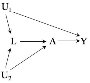
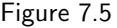
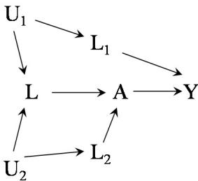
Figure 7.6

mean Pr[Y = 1|A = a].

The possibility of identification of Interestingly, in Figure 7.4, conditional exchangeability given L does not hold and thus the counterfactual risks Pr[Y ^a = 1|L = l] are not equal to the stratum-specific risks Pr[Y = 1|A = a, L = l], and the conditional treatment effects with strata of L are not identified. Further, adjustment for L via standardization P ^l Pr [Y = 1|A = a, L = l] Pr [L = l] gives a biased estimate of Pr[Y a ]. This follows from the fact that adjustment for L would induce bias because conditioning on the collider L opens the backdoor path between A and Y (A ← U² → L ← U¹ → Y ), which was previously blocked by the collider itself. Thus the association between A and Y would be a mixture of the association due to the effect of A on Y and the association due to the open backdoor path. Association would not be causation any more. This is the first example we have seen for which unconditional exchangeability holds but conditional exchangeability does not: the average causal effect is identified, but If U¹ caused U2, or U² caused U1, generally not the conditional causal effects within levels of L. We refer to the resulting bias in the conditional effect as selection bias because it it arises from selecting (conditioning) on the common effect L of two marginally independent variables U¹ and U2, one of which is associated with A and the other with Y (see Chapter 8).

The causal diagram in Figure 7.5 is a variation of the one in Figure 7.4. The difference is that, in Figure 7.5, there is an arrow L → A. The presence of this arrow creates an open backdoor path A ← L ← U¹ → Y because U¹ The definition of collider is path- is a common cause of A and Y , and so confounding exists. Conditioning on L would block that backdoor path but would simultaneously open a backdoor path on which L is a collider (A ← U² → L ← U¹ → Y ).

Therefore, in Figure 7.5, the bias is intractable: attempting to block the confounding path opens a selection bias path. There is neither unconditional exchangeability nor conditional exchangeability given L. A solution to the bias in Figure 7.5 would be to measure either (i) a variable L¹ between U¹ and either A or Y , or (ii) a variable L² between U² and either A or L. In the first case we would have conditional exchangeability given L1. In the second case we would have conditional exchangeability given both L² and L. For example, Figure 7.6 includes the variable L¹ between U¹ and Y and the variable L² between U² and A. See Fine Point 7.2 for a discussion of identification of causal effects depending on what variables are measured in Figure 7.6.

The causal diagrams in this section depict two structural sources of lack of exchangeability that are due to the presence of open backdoor paths between treatment and outcome. The first source is the presence of common causes of treatment and outcome—which creates an open backdoor path. The second source is conditioning on a common effect—which may open a previously blocked backdoor path. For pedagogic purposes, we have reserved the term “confounding” for the first and “selection bias” for the latter. An alternative way to structurally define confounding could be the “bias due to an open backdoor path between A and Y .” This alternative definition is identical to ours except that it labels the bias due to conditioning on L in Figure 7.4 as confounding rather than as selection bias. The alternative definition can be equivalently expressed as follows: confounding is “any systematic bias that would be eliminated by randomized assignment of A”. To see this, note that the bias induced in Figure 7.4 by conditioning on L could not occur in an experiment in which treatment A is randomly assigned because the random assignment ensures the absence of an unmeasured U² that is a common cause of A and L and thus conditioning on L would no longer open a backdoor path.

One interesting distinction between these two definitions is the following.

Identification of conditional and unconditional effects. Under any causal diagram, the causal effects that can be identified depend on the variables that are measured in addition to the treatment and the outcome. Take Figure 7.6 as an example. If we measure only L² (but not L and L1), we have neither unconditional nor conditional exchangeability given L2, and no causal effects can be identified. If we measure L² and L, we have conditional exchangeability given L² and L, but we do not have conditional exchangeability given either L² alone or L alone. However, we can identify:

• The conditional causal effects within joint strata of L² and L. The identifying formula for each of the counterfactual means is E [Y |A = a, L = l, L² = l2].
• The unconditional causal effect. The identifying formula for each of the counterfactual means is P l,l² E [Y |A = a, L = l, L² = l2] Pr [L = l, L² = l2].
• The conditional causal effects within strata of P L. The identifying formula for each of the counterfactual means is l2 E [Y |A = a, L = l, L² = l2] Pr [L² = l2|L = l].
• The conditional causal effects within strata of L2. The identifying formula for each of the counterfactual means is P ^l E [Y |A = a, L = l, L² = l2] Pr [L = l|L² = l2].

If we only measure L1, then we have conditional exchangeability given L¹ so we can identify the conditional causal effects within strata of L¹ and the unconditional causal effect. If we measure L¹ and L, then we can also identify the conditional causal effects within joint strata of L¹ and L, and within strata of L alone. If we measure L, L1, and L2, then we can also identify the conditional effects within joint strata of all three variables.

The existence of a common cause of treatment and the outcome (the structural definition of confounding) is a substantive fact about the study population and the world, independent of the method chosen to analyze the data. On the other hand, the definition of confounding as any bias that would have been eliminated by randomization implies that the existence of confounding depends on the method of analysis. In Figure 7.4, we have no confounding if we do not adjust for L, but we introduce confounding if we do adjust.

Nonetheless, the choice of one definition over the other is just a matter of taste with no practical implications as all our conclusions regarding identifiability are based solely on whether conditional or unconditional exchangeability holds and not on our definition of confounding. The next chapter provides more detail on the distinction between confounding and selection bias.

7.4 Confounding and confounders

In the previous section, we have described how to use causal diagrams to decide whether confounding exists and, if so, to identify whether a given set of measured variables L is a sufficient set for confounding adjustment. The procedure requires a priori knowledge of the causal DAG that includes all causes—both measured and unmeasured—shared by the treatment A and the outcome Y . Once the causal diagram is known, we simply need to apply the backdoor criterion to determine what variables need to be adjusted for.

In contrast, the traditional approach to handle confounding was based mostly on observed associations rather than on prior causal knowledge. The traditional approach first labels variables that meet certain (mostly) associaneed structural knowledge. They only need to know a set of variables that guarantees conditional exchangeability.

tional conditions as confounders and then mandates that these so-called con-Technically, investigators do not founders are adjusted for in the analysis. Confounding is said to exist when the adjusted estimate differs from the unadjusted estimate.

Under the traditional approach, a confounder was defined as a variable that meets the following three conditions: (1) it is associated with the treatment, (2) it is associated with the outcome conditional on the treatment (with “conditional on the treatment” often replaced by “in the untreated”), and (3) it does not lie on a causal pathway between treatment and outcome. However, this traditional approach may lead to inappropriate adjustment. To see why, let us revisit Figures 7.1-7.4.

In Figure 7.1, the variable L is associated with the treatment (because it has a causal effect on A), is associated with the outcome conditional on the treatment (because it has a direct causal effect on Y ), and it does not lie on the causal pathway between treatment and outcome. In Figure 7.2, the variable L is associated with the treatment (because it has a causal effect on A), is associated with the outcome conditional on the treatment (because it shares the cause U with Y ), and it does not lie on the causal pathway between treatment and outcome. In Figure 7.3, L is associated with the treatment (it shares the cause U with A), is associated with the outcome conditional on the treatment (it has a causal effect on Y ), and it does not lie on the causal pathway between treatment and outcome.

Therefore, according to the traditional approach, L is a confounder in the settings represented by Figures 7.1-7.3 and it needs be adjusted for. That was also our conclusion when using the backdoor criterion in the previous section. For Figures 7.1-7.3, there is no discrepancy between the traditional, mostly associational approach and the application of the backdoor criterion to the causal diagram.

Now consider Figure 7.4 again in which there is no confounding and L is a non-confounder by the definition given in Section 7.3. However, L meets the criteria for a traditional confounder: it is associated with the treatment (it shares the cause U² with A), it is associated with the outcome conditional on the treatment (it shares the cause U¹ with Y ), and it does not lie on the causal pathway between treatment and outcome. Hence, according to the traditional approach, L is a confounder that should be adjusted for, even in the absence of confounding! But, as we saw above, adjustment for L results in a biased estimator of the causal effect in the population due to selection bias. Figure 7.7 is another example in which the traditional approach leads to inappropriate adjustment for L by inducing selection bias.

These examples show that associational or statistical criteria are insufficient to characterize confounding. An approach based on a definition of confounder that relies almost exclusively on statistical considerations may lead, as shown by Figures 7.4 and 7.7, to the wrong advice: adjust for a “confounder” even when structural confounding does not exist. To eliminate this problem for Figure 7.4, a follower of the traditional approach might replace the associational condition “(2) it is associated with the outcome conditional on the treatment” by the structural condition “(2) it is a cause of the outcome.” This modified definition of confounder prevents inappropriate adjustment for L in Figure 7.4, but only to create a new problem by not considering L a confounder—that needs to be adjusted for—in Figure 7.2. See Technical Point 7.2.

The traditional approach misleads investigators into adjusting for variables when adjustment is harmful. The problem arises because the traditional approach starts by defining confounders in the absence of sufficient causal knowledge about the sources of confounding, and then mandates adjustment for

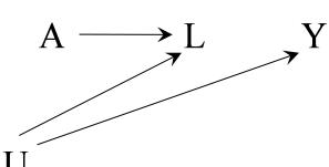
Figure 7.7

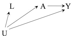
Figure 7.8

Surrogate confounders. Under the causal DAG in Figure 7.8, there is confounding for the effect of A on Y because of the presence of the unmeasured common cause U. The measured variable L is a proxy or surrogate for U. For example, the unmeasured variable socioeconomic status U may confound the effect of physical activity A on the risk of cardiovascular disease Y . Income L is a surrogate for the often ill-defined variable socioeconomic status. Should we adjust for the variable L? On the one hand, it can be said that L is not a confounder because it does not lie on a backdoor path between A and Y . On the other hand, adjusting for the measured L, which is associated with the unmeasured U, may indirectly adjust for some of the confounding caused by U. In the extreme, if L were perfectly correlated with U then it would make no difference whether one conditions on L or on U. Indeed if L is binary and is a nondifferentially misclassified (see Chapter 9) version of U, conditioning on L will result in a partial blockage of the backdoor path A ← U → Y under some weak conditions (Greenland 1980, Ogburn and VanderWeele 2012). Therefore we will typically prefer to adjust, rather than not to adjust, for L.

We refer to variables that can be used to reduce confounding bias even though they are not on a backdoor path (and so could never completely eliminate confounding) as surrogate confounders. A possible strategy to fight confounding is to measure as many surrogate confounders as possible and adjust for all of them. See Chapter 18 for discussion.

those so-called confounders. If the adjusted and unadjusted estimates differ, the traditional approach declares the existence of confounding. However, change in estimates may occur for reasons other than confounding, including selection bias when adjusting for non-confounders (see Chapter 8) and the use of noncollapsible effect measures (see Fine Point 4.3). Attempts to define confounding based on change in estimates have been long abandoned because of these problems.

In contrast, a structural approach starts by explicitly identifying the sources of confounding—the common causes of treatment and outcome that, were they all measured, would be sufficient to adjust for confounding—and then identifies a sufficient set of adjustment variables.

The structural approach makes clear that including a particular variable in a sufficient set depends on the variables already included in the set. For example, in Figures 7.2 and 7.3 the set of variables L is needed to block a backdoor path because the set of variables U is not measured. We could then say that the variables in L are confounders. However, if the variables U had been measured and used to block the backdoor path, then the variables L would not be confounders given U (see also Fine Point 7.3). Given a causal VanderWeele and Shpitser (2013) DAG, confounding is an absolute concept whereas confounder is a relative one.

A structural approach to confounding emphasizes that causal inference from observational data requires a priori causal knowledge. This causal knowledge is summarized in a causal DAG that encodes the researchers’ beliefs or assumptions about the causal network. Of course, there is no guarantee that the researchers’ causal DAG is correct and thus it is possible that, contrary to the researchers’ beliefs, their chosen set of adjustment variables fails to eliminate confounding or introduces selection bias. However, the structural approach to confounding has two important advantages. First, it prevents inconsistencies between beliefs and actions. For example, if you believe Figure 7.4 is the true causal diagram—and therefore that there is no confounding for the effect of A on Y —then you will not adjust for the variable L, regardless of what non-structural definitions of confounder may say. Second, the researchers’ assumptions about confounding become explicit and therefore can be explicitly criticized by other investigators.

also proposed a formal definition of confounder.

Fixing the traditional definition of confounder. Figures 7.4 and 7.7 depict two graphical examples in which the traditional non-graphical definition of confounder and confounding misleads investigators into adjusting for a variable when adjustment for such variable is not only superfluous but also harmful. The traditional definition fails because it relies on two incorrect statistical criteria—conditions (1) and (2)—and one incorrect causal criterion—condition (3). To “fix” the traditional definition one needs to do two things:

• 1. Replace condition (3) by the condition that “there exist variables L and U such that there is conditional exchangeability within their joint levels Y ^a⊥⊥A|L, U. This new condition is stronger than the earlier condition because it effectively implies that L is not on a causal pathway between A and Y and that E[Y a |L = l, U = u] is identified by E[Y |L = l, U = u, A = a].
• 2. Replace conditions (1) and (2) by the following condition: U can be decomposed into two disjoint subsets U¹ and U² (i.e., U = U¹ ∪ U² and U¹ ∩ U² is empty) such that (i) U¹ and A are not associated within strata of L, and (ii) U² and Y are not associated within joint strata of A, L, and U1. The variables in U¹ may be associated with the variables in U2. U¹ can always be chosen to be the largest subset of U that is unassociated with treatment.

If these two new conditions are met we say U is a non-confounder given data on L. These conditions were proposed by Robins (1997a, Theorem 4.3) and further discussed by Greenland, Pearl, and Robins (1999, pp. 45-46, note the condition that U = U¹ ∪ U² was inadvertently left out). These conditions overcome the difficulties found in Figures 7.4 and 7.7 because they allow us to dismiss variables as non-confounders (Robins 1997a). For example, Greenland, Pearl, and Robins applied these conditions to Figure 7.4 to show that there is no confounding.

7.5 Single-world intervention graphs

Exchangeability is translated into graph language as the lack of open paths between the treatment A and outcome Y nodes—other than those originating from A—that would result in an association between A and Y . Chapters 7– 9 describe different ways in which lack of exchangeability can be represented in causal diagrams. For example, in this chapter we discuss confounding, a violation of exchangeability due to the presence of an open backdoor path between treatment and outcome.

The equivalence between unconditional exchangeability Y ^a⊥⊥A and the backdoor criterion seems rather magical: there appears to be no obvious relationship between counterfactual independence and the absence of backdoor paths because counterfactuals are not included as variables on causal diagrams. Since graphs are so useful for evaluating independencies via d-separation, it seems natural to want to construct graphs that include counterfactuals as nodes, so that unconditional and conditional exchangeability can be directly read off the graph.

A new type of graph—Single-world intervention graphs (SWIGs)— unify the counterfactual and graphical approaches by explicitly including the coun-Richardson and Robins (2013) terfactual variables on the graph. A SWIG depicts the variables and causal relations that would be observed in a hypothetical world in which all individuals received treatment level a. That is, a SWIG is a graph that represents a counterfactual world created by a single intervention. In contrast, the variables on a standard causal diagram represent the actual world. A SWIG can then be viewed as a function that transforms a given causal diagram under a given intervention. The following examples describe this transformation.

showed that SWIGs overcome some of the shortcomings of previously proposed twin causal diagrams (Balke and Pearl 1994).

Suppose the causal diagram in Figure 7.2 represents the observed study

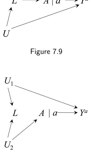
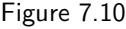
be shown that d-separation also implies statistical independence on the SWIG.

conditional exchangeability Y In the single intervention world, a is a constant and thus cannot affect other variables. When drawing SWIGs, however, we include arrows from a as a convenient way to keep track of the variables directly affected by A in the original DAG.

data. The SWIG in Figure 7.9 is a transformation of Figure 7.2 that represents a world in which all individuals have received an intervention that sets their treatment to the fixed value a.

In the SWIG, the treatment node is split into left and right sides which are to be regarded as separate nodes (variables) once split. The right side encodes the treatment value a under the intervention and inherits all the arrows that were out of A in the original causal DAG. The left side encodes the value of treatment A that would have been observed in the absence of intervention, i.e., the natural value of treatment. It inherits all nodes that were into A on the causal DAG because its causal inputs are the same in the intervened on (counterfactual) world as in the actual world. Note that A does not have an arrow into a because the value a is the same for all individuals, i.e., is a constant in the intervened on world.

We assume that the natural value of treatment A is well defined even though we are generally unable to measure it under intervention a. In some settings, though, A may be measurable: recent experiments suggest that electroencephalogram recordings can detect the choice individuals will make up to 1/2 second before individuals becomes conscious of their decision. If so, A could actually be measured via electroencephalogram, while still leaving 1/2 second to intervene and give treatment a.

In the SWIG, the outcome is Y a , the value of Y in the intervened on world. Because the remaining variables are temporally prior to A, they are not affected by the intervention and therefore take the same value as in the observed world. i.e., they are not labeled as a counterfactual variable. In fact, any variable that is a non-descendant of A need not be labeled as a counterfactual because, under the faithfulness assumption (which we make), treatment has no causal Under an FFRCISTG model, it can effect on its non-descendants for any individual. Under our causal model, conditional exchangeability Y ^a⊥⊥A|L holds because all paths between Y ^a and A are blocked after conditioning on L, i.e., Y ^a and A are d-separated given L.

Consider now the causal diagram in Figure 7.4 and the SWIG in Figure 7.10. Marginal exchangeability Y ^a⊥⊥A holds because, on the SWIG, all paths between Y ^a and A are blocked (without conditioning on L). In contrast, ^a⊥⊥A|L does not hold because, on the SWIG, the path Y ^a ←− U¹ −→ L ←− U² −→ A is open when the collider L is conditioned on. This is why the marginal A-Y association is causal, but the conditional A-Y association given L is not, and thus any method that adjusts for L results in bias. These examples show how SWIGs unify the counterfactual and graphical approaches. In fact it is straightforward to see that, on the SWIG, Y a is dseparated from A given L if and only if L is a non-descendant of A that blocks all backdoor paths from A to Y (see also Fine Point 7.4).

7.6 Confounding adjustment

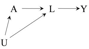
Figure 7.11

In the absence of randomization, causal inference relies on the uncheckable assumption that we have measured a set of variables L that is a sufficient set for confounding adjustment, i.e., a set of non-descendants of treatment A that includes enough variables to block all backdoor paths from A to Y . Under this assumption of conditional exchangeability given L, standardization and IP weighting can be used to compute the average causal effect in the population. But, as discussed in Section 4.6, standardization and IP weighting are not the only available methods to adjust for confounding in observational

Confounders cannot be descendants of treatment, but can be in the future of treatment. Consider the causal DAG in Figure 7.11. L is a descendant of treatment A that blocks all backdoor paths from A to Y . Unlike in Figures 7.4 and 7.7, conditioning on L does not cause selection bias because no collider path is opened. Rather, because the causal effect of A on Y is solely through the intermediate variable L, conditioning on L completely blocks this pathway. This example shows that adjusting for a variable L that blocks all backdoor paths does not eliminate bias when L is a descendant of A.

Since conditional exchangeability Y ^a⊥⊥A|L implies that the adjustment for L eliminates all bias, it must be the case that conditional exchangeability fails to hold and the average treatment effect E[Y ^a=1] − E[Y ^a=0] cannot be identified in this example. This failure can be verified by analyzing the SWIG in Figure 7.12, which depicts a counterfactual world in which A has been set to the value a. In this world, the factual variable L is replaced by the counterfactual variable L a , i.e., the value of L that would have been observed if all individuals had received treatment value a. Since L ^a blocks all paths from Y a to A we conclude that Y ^a⊥⊥A|L ^a holds, but we cannot conclude that conditional exchangeability Y ^a⊥⊥A|L holds as L is not even on the graph. (Under an FFRCISTG, any independence that cannot be read off the SWIG cannot be assumed to hold.) Therefore, we cannot ensure that the average treatment effect E[Y ^a=1] − E[Y ^a=0] is identified from data on (L, A, Y ).

The problem arises because L is a descendant of A, not because L is in the future of A. If, in Figure 7.11, the arrow from A to L did not exist, then L would be a non-descendant of A that blocks all the backdoor paths. Analogously, on the SWIG in Figure 7.12, we can replace L ^a by L as A is no longer a cause of L (note Y a and A are now dseparated by L). Therefore adjusting for L would eliminate all bias, even if L were still in the future of A. What matters is the topology of the causal diagram (which variables cause which variables), not the time sequence of the nodes. Rosenbaum (1984) and Robins (1986, section 11) give non-graphical discussions of the control of confounding by temporally post-treatment variables.

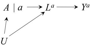
Figure 7.12

tion and matching replaces each individual’s variables L by the individual’s estimated probability of receiving treatment Pr [A = 1|L]: the propensity score (Rosenbaum and Rubin 1983). See Chapter 15.

studies. Methods that adjust for confounders L can be classified into two broad categories:

• G-methods: Standardization, IP weighting, and g-estimation. These methods (the ‘g’ stands for ‘generalized’) exploit conditional exchangeability given L to estimate the causal effect of A on Y in the entire population or in any subset of the population. In our heart transplant study, we used g-methods to adjust for confounding by disease severity L in Sections 2.4 (standardization) and 2.5 (IP weighting). Part II describes model-based extensions of g-methods: the parametric g-formula (standardization), IP weighting of marginal structural models, and gestimation of nested structural models.
• Conventional methods for stratification-based adjustment: Stratification (including restriction) and matching. These methods exploit conditional exchangeability given L to estimate the association between A and Y in subsets defined by L. In our heart transplant study, we used stratification-based methods to adjust for confounding by disease severity A common variation of stratifica- L in Sections 4.4 (stratification) and 4.5 (matching). Part II describes the model-based extension of conventional stratification: outcome regression.

Standardization and IP weighting simulate the A-Y association in the population if backdoor paths involving the measured variables L did not exist. For example, IP weighting achieves this by creating a pseudo-population in which treatment A is independent of the measured confounders L, i.e., by “deleting” the arrow from L to A. In contrast, conventional methods based on stratification do not delete the arrow from L to A but rather compute the conditional effect in a subset of the observed population, which is represented by adding a selection box. In Part III, focused on time-varying treatments, we describe why “deleting” the arrow L → A is advantageous when using standardization or IP weighting, and why g-estimation is the only generally valid stratificationbased method. The bias of conventional stratification-based methods is described in Chapter 20. In settings with time-varying treatments, and therefore time-varying confounders, g-methods are the methods of choice to adjust for confounding because conventional stratification-based methods may result in selection bias.

All the above methods require conditional exchangeability given L. However, confounding can sometimes be handled by methods that do not require conditional exchangeability. Some examples of these methods are differencein-differences (Technical Point 7.3), instrumental variable estimation (Chapter 16), proximal inference (Technical Point 7.3), the front door criterion (Technical Point 7.4), and others. Unfortunately, these methods require alternative assumptions that, like conditional exchangeability, are unverifiable. Therefore, in practice, the validity of the resulting effect estimates is not guaranteed. The choice of adjustment method will depend on which unverifiable assumptions either conditional exchangeability or the alternative conditions—are believed more likely to hold in a particular setting.

Achieving conditional exchangeability may be an unrealistic goal in many observational studies but, as discussed in Section 3.2, expert knowledge about the causal structure can be used to get as close as possible to that goal. Therefore, in observational studies, investigators measure many variables L (which are non-descendants of treatment) in an attempt to ensure that the treated and the untreated are conditionally exchangeable. The hope is that, even though common causes may exist (confounding), the measured variables L are sufficient to block all backdoor paths (no unmeasured confounding). However, there is no guarantee that this attempt will be successful, which makes causal inference from observational data a risky undertaking.

In addition, expert knowledge can be used to avoid adjusting for variables A practical example of the ap- that may introduce bias. At the very least, investigators should generally avoid adjustment for variables affected by either the treatment or the outcome. Of course, thoughtful and knowledgeable investigators could believe that two or more causal structures, possibly leading to different conclusions regarding confounding and confounders, are equally plausible. In that case they would perform multiple analyses and explicitly state the assumptions about causal structure required for the validity of each. Unfortunately, one can never be certain that the set of causal structures under consideration includes the true one; this uncertainty is unavoidable with observational data.

There is a scientific consequence to the always present threat of confounding in observational studies. Suppose you conducted an observational study to quantify the effect of heart transplant A on death Y . You did your best (e.g., consulting subject-matter experts) to identify and measure confounders L, and assumed no unmeasured confounding after adjusting for L. A critic of your study says “the inferences from this observational study may be incorrect because of potential confounding.” The critic is not making a scientific statement, but a logical one. Since the findings from any observational study may be confounded, it is obviously true that those of your study can be confounded. If the critic’s intent was to provide evidence about the shortcomings of your particular study, he failed. His criticism is noninformative because he simply restated a characteristic of observational research that you and the critic already knew before the study was conducted.

plication of expert knowledge of the causal structure to confounding evaluation was described by Hern´an et al (2002).

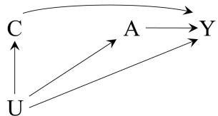
Figure 7.13

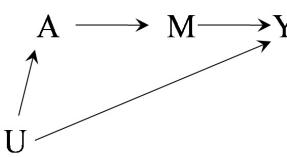
Figure 7.14

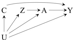
Figure 7.15

To appropriately criticize your study, the critic needs to engage in a scientific conversation. For example, the critic may cite experimental or observational evidence that contradict your findings, or he can say something along the lines of “the inferences from this observational study may be incorrect because of potential confounding due to cigarette smoking, a common cause through which a backdoor path may remain open”. This latter option provides you with a testable challenge to your assumption of no unmeasured confounding. The burden of the proof is again yours. Your next move is to try and adjust for smoking or, if data on smoking could not be obtained, to conduct a sensitivity analysis to investigate the possible bias induced by smoking.

Though the above discussion was restricted to bias due to confounding, the absence of biases due to selection and measurement is also needed for valid causal inference from observational data. But, unlike confounding, these other biases may arise in both randomized experiments and observational studies. After having explored confounding in this chapter, the next chapter presents another potential source of lack of exchangeability between the treated and the untreated: selection of individuals into the analysis.

Difference-in-differences and negative outcome controls. Suppose we want to compute the average causal effect of aspirin A (1: yes; 0: no) on blood pressure Y , but there are unmeasured common causes U of A and Y such as history of heart disease. Then we cannot compute the effect via standardization or IP weighting because there is unmeasured confounding. But there is an alternative method that, under some conditions, may adjust for the unmeasured confounding: the use of negative outcome controls (also known as “placebo tests”).

Suppose further that, for each individual in the population, we have also measured the value of the outcome right before treatment was available. We refer to this pre-treatment outcome C as a negative outcome control (also referred to as negative control outcome). As depicted in Figure 7.13, U is a cause of both Y and C, and treatment A is obviously not a cause of the pre-treatment C. Now, even though the causal effect of A on C is known to be zero, the contrast E [C|A = 1] − E [C|A = 0] is not zero because of confounding by U. In fact, E [C|A = 1] − E [C|A = 0] measures the magnitude of confounding for the effect of A on C on the additive scale. If the magnitude of additive confounding for the effect of A on the negative control outcome C is the same as for the effect of A on the true outcome Y , then we can compute the effect of A on Y in the treated. Specifically, under the assumption of additive equi-confounding E - Y 0 |A = 1 − E - Y 0 |A = 0 = E [C|A = 1] − E [C|A = 0], the effect is

\[\mathbb{E}\left[Y^1 - Y^0 | A = 1\right] = \left(\mathbb{E}\left[Y|A=1\right] - \mathbb{E}\left[Y|A=0\right]\right) - \left(\mathbb{E}\left[C|A=1\right] - \mathbb{E}\left[C|A=0\right]\right)\]

That is, the effect in the treated is equal to the association between treatment A and outcome Y (which is a mixture of the causal effect and confounding) minus the confounding as measured by the association between A and C. Note that the direct arrow from C to Y in Figure 7.13 is not necessary for C to be a negative outcome control.

This method for confounding adjustment is known as difference-in-differences (Card 1990, Meyer 1995, Angrist and Krueger 1999). In practice, the method is often combined with adjustment for measured covariates using parametric or semiparametric approaches (Abadie 2005). However, difference-in-differences is a somewhat restrictive approach to negative outcome controls (Sofer et al. 2016): it requires measurement of the outcome both pre- and post-treatment (or at least that the true outcome Y and the negative control outcome C are measured on the same scale) and it requires additive equi-confounding. Sofer et al. (2016) describe more general methods that allow for Y and C to be on different scales, rely on weaker versions of equi-confounding, and incorporate adjustment for measured covariates. For a general introduction to the use of negative outcome controls to detect confounding, see Lipsitch et al. (2010) and Flanders et al. (2011).

Surprisingly, when one has both a negative outcome control C and a negative treatment control Z, the causal effect can be nonparametrically identified even in the presence of unmeasured confounders U under additional assumptions. In fact, if U, C, and Z are discrete and C and Z have at least as many levels as does U, then the causal effect of A on Y will quite generally be identified (Miao et al. 2018). This identification approach is referred to as proximal causal inference (Cui et al. 2024). Figure 7.15 is one example in which C is a negative outcome control and Z is a negative treatment control.

The front door criterion. The causal diagram in Figure 7.14 depicts a setting in which the treatment A and the binary outcome Y share an unmeasured cause U, and in which there is a variable M that fully mediates the effect of A on Y and that shares no unmeasured causes with either A or Y . Under this causal structure, a data analyst cannot directly use standardization (nor IP weighting) to compute the counterfactual risks Pr - Y ^a=1 = 1 and Pr - Y ^a=0 = 1 because the variable U, which is necessary to block the backdoor path between A and Y , is not available. Therefore, the average causal effect of A on Y cannot be identified using the methods described in previous chapters. However, Pearl (1995) showed that Pr [Y ^a = 1] is identified by the so-called front door formula

\[\sum\_{m} \Pr\left[M = m | A = a\right] \sum\_{a'} \Pr\left[Y = 1 | M = m, A = a'\right] \Pr\left[A = a'\right]\]

Pearl refers to this identification formula as front door adjustment because it relies on the existence of a path from A and Y that, contrary to a backdoor path, goes through a descendant M of A that completely mediates the effect of A on Y . Pearl often uses the term backdoor formula to refer to the identification formula that we refer to as standardization or the point treatment g-formula (Robins 1986). A proof of the front door identification formula follows.

Note that Pr [Y ^a = 1] = P ^m Pr [M^a = m] Pr [Y ^a = 1|M^a = m] and that, under Figure 7.14, Pr [M^a = m] = Pr [M = m|A = a] because there is no confounding for the effect of A on M (i.e., A⊥⊥M^a ), and Pr [Y P ^a = 1|M^a = m] = ^a′ Pr [Y = 1|M = m, A = a ′ ] Pr [A = a ′ ]. To prove the last equality, first note that Pr [Y ^a = 1|M^a = m] = Pr [Y ^m = 1] because (i) Y ^a = Y ^m when M^a = m (A affects Y only through M in Figure 7.14) and (ii) Y ^m⊥⊥M^a by d-separation on a SWIG under the joint intervention in which M is set to m and A to a. Finally, by conditional exchangeability Y ^m⊥⊥M|A on the SWIG where we intervene on M alone, Pr [Y P ^m = 1] = ^a′ Pr [Y = 1|M = m, A = a ′ ] Pr [A = a ′ ].

The above proof requires well-defined counterfactual outcomes Y ^m under interventions on M. In Technical Points 21.11 and 21.12 we present alternative proofs of the front door formula that do not require this condition.

Confounding

Chapter 8 SELECTION BIAS

Suppose an investigator conducted a randomized experiment to answer the causal question “does one’s looking up to the sky make other pedestrians look up too?” She found a strong association between her looking up and other pedestrians’ looking up. Does this association reflect a causal effect? Well, by definition of randomized experiment, confounding bias is not expected in this study. However, there was another potential problem: The analysis included only those pedestrians that, after having been part of the experiment, gave consent for their data to be used. Shy pedestrians (those less likely to look up anyway) and pedestrians in front of whom the investigator looked up (who felt tricked) were less likely to participate. Thus participating individuals in front of whom the investigator looked up (a reason to decline participation) are less likely to be shy (an additional reason to decline participation) and therefore more likely to look up. That is, the process of selection of individuals into the analysis guarantees that one’s looking up is associated with other pedestrians’ looking up, regardless of whether one’s looking up actually makes others look up.

An association created as a result of the process by which individuals are selected into the analysis is referred to as selection bias. Unlike confounding, this type of bias is not due to the presence of common causes of treatment and outcome, and can arise in both randomized experiments and observational studies. Like confounding, selection bias is just a form of lack of exchangeability between the treated and the untreated. This chapter provides a definition of selection bias and reviews the methods to adjust for it.

8.1 The structure of selection bias

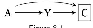
2000. used causal diagrams to describe the structure of bias resulting from selection of individuals.

The term “selection bias” encompasses various biases that arise from the procedure by which individuals are selected into the analysis. Here we focus on bias that would arise even if the treatment had a null effect on the outcome, i.e., selection bias under the null (as described in Section 6.5). The structure of selection bias can be represented by using causal diagrams like the one in Figure 8.1, which depicts dichotomous treatment A, outcome Y , and their common Figure 8.1 effect C. Suppose Figure 8.1 represents a study to estimate the effect of folic acid supplements A given to pregnant women shortly after conception on the fetus’s risk of developing a cardiac malformation Y (1: yes, 0: no) during the first two months of pregnancy. The variable C represents death before birth. A cardiac malformation increases mortality (arrow from Y to C), and folic acid supplementation decreases mortality by reducing the risk of malformations other than cardiac ones (arrow from A to C). The study was restricted Pearl (1995) and Spirtes et al to fetuses who survived until birth. That is, the study was conditioned on no death C = 0 and hence the box around the node C.

The diagram in Figure 8.1 shows two sources of association between treatment and outcome: 1) the open path A → Y that represents the causal effect of A on Y , and 2) the open path A → C ← Y that links A and Y through their (conditioned on) common effect C. An analysis conditioned on C will generally result in an association between A and Y . We refer to this induced association between the treatment A and the outcome Y as selection bias due to conditioning on C. Because of selection bias, the associational risk ratio

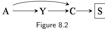
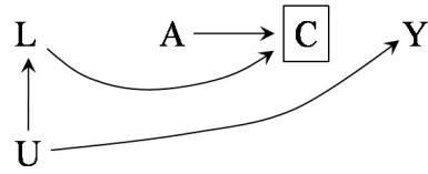
Figure 8.3

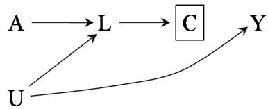
Figure 8.4

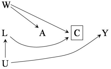
Figure 8.5

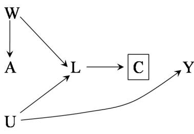
Figure 8.6

Pr[Y = 1|A = 1, C = 0]/Pr[Y = 1|A = 0, C = 0] does not equal the causal risk ratio Pr - Y ^a=1 = 1 /Pr - Y ^a=0 = 1 ; association is not causation. If the analysis were not conditioned on the common effect (collider) C, then the only open path between treatment and outcome would be A → Y , and thus the entire association between A and Y would be due to the causal effect of A on Y . That is, the associational risk ratio Pr[Y = 1|A = 1]/Pr[Y = 1|A = 0] would equal the causal risk ratio Pr - Y ^a=1 = 1 /Pr - Y ^a=0 = 1 ; association would be causation.

The causal diagram in Figure 8.2 shows another example of selection bias. This diagram includes all variables in Figure 8.1 plus a node S representing parental grief (1: yes, 0: no), which is affected by vital status at birth. Suppose the study was restricted to nongrieving parents S = 0 because the others were unwilling to participate. As discussed in Chapter 6, conditioning on a variable S affected by the collider C also opens the path A → C ← Y .

Both Figures 8.1 and 8.2 depict examples of selection bias in which the bias arises because of conditioning on a common effect of treatment and outcome: C in Figure 8.1 and S in Figure 8.2. This bias arises regardless of whether there is an arrow from A to Y , i.e., it is selection bias under the null. Remember that causal structures that result in bias under the null also cause bias when the treatment has a non-null effect. Both confounding due to common causes of treatment and outcome (see previous chapter) and selection bias due to conditioning on common effects of treatment and outcome are examples of bias under the null. However, selection bias under the null can be defined more generally as illustrated by Figures 8.3 to 8.6.

Consider the causal diagram in Figure 8.3, which represents a follow-up study of individuals with HIV infection to estimate the effect of certain antiretroviral treatment A on the 3-year risk of death Y (to reduce clutter, there is no arrow from A to Y ). The unmeasured variable U represents high level of immunosuppression (1: yes, 0: no). Individuals with U = 1 have a greater risk of death. Individuals who drop out from the study or are otherwise lost to follow-up are censored (C = 1). Individuals with U = 1 are more likely to be censored because the severity of their disease prevents them from participating in the study. The effect of U on censoring C is mediated by the presence of symptoms (fever, weight loss, diarrhea, and so on), CD4 count, and viral load in plasma, all included in L, which could or could not be measured. (The role of L, when measured, in data analysis is discussed in Section 8.5; in this section, we take L to be unmeasured.) Individuals receiving treatment are at a greater risk of experiencing side effects, which could lead them to dropout, as represented by the arrow from A to C. The square around C indicates that the analysis is restricted to individuals who remained uncensored (C = 0) because those are the only ones in which Y can be assessed.

According to the rules of d-separation, conditioning on the collider C opens the path A → C ← L ← U → Y and thus association flows from treatment A to outcome Y , i.e., the associational risk ratio is not equal to 1 even though the causal risk ratio is equal to 1. Figure 8.3 can be viewed as a simple transformation of Figure 8.1: the association between Y and C resulting from a direct effect of Y on C in Figure 8.1 is now the result of U, a common cause of Y and C. Some intuition for this bias: If a treated individual with treatment-induced side effects (and thereby at a greater risk of dropping out) did in fact not drop out (C = 0), then it is generally less likely that a second independent cause of dropping out (e.g., U = 1) was present. Therefore, an inverse association between A and U would be expected in those who did not drop out (C = 0). Because U is positively associated with the outcome

More generally, selection bias can W to L in Figure 8.6). be defined as the bias resulting from conditioning on the common effect of two variables, one of which is either the treatment or associated with the treatment, and the other is either the outcome or associated with the outcome (Hern´an, Hern´andez-D´ıaz, and Robins 2004).

Y , restricting the analysis to individuals who did not drop out of this study induces an inverse association between A and Y .

The bias in Figure 8.3 is an example of selection bias that results from conditioning on censoring C, which is a common effect of treatment A and of a cause U of the outcome Y , rather than a common effect of treatment and outcome. We now present three additional causal diagrams that could lead to selection bias by differential loss to follow up. In Figure 8.4 prior treatment A has a direct effect on symptoms L. Restricting the study to the uncensored individuals again implies conditioning on the common effect C of A and U, thereby introducing an association between treatment and outcome. Figures 8.5 and Figures 8.5 and 8.6 show examples 8.6 are variations of Figures 8.3 and 8.4, respectively, in which there is a comof M-bias mon cause W of A and another measured variable. W indicates unmeasured lifestyle/personality/educational variables that determine both treatment (arrow from W to A) and either attitudes toward attending study visits (arrow from W to C in Figure 8.5) or threshold for reporting symptoms (arrow from

We have described some different causal structures, depicted in Figures 8.1-8.6, that may lead to selection bias under the null. In all these cases, the bias is the result of selection on a common effect of two other variables in the diagram, i.e., a collider. We will use the term selection bias to refer to all biases that arise from conditioning on a common effect of two variables, one of which is either the treatment or a cause of treatment, and the other is either the outcome or a cause of the outcome. We now describe some examples of selection bias that share this structure.

8.2 Examples of selection bias

structures leading to lack of exchangeability is not universally made across disciplines. Conditional exchangeability is often referred as “weak ignorability” or “ignorable treatment assignment” in statistics (Rosenbaum and Rubin 1983, Rosenbaum 2002), “selection on observables” in the social sciences (Barnow, Cain, and Goldberger, 1980), and “no ommitted variable bias” or “exogeneity” in econometrics (Imbens, 2004).

Consider the following examples of bias due to the mechanism by which individuals are selected into the analysis:

• Differential loss to follow-up: This is precisely the bias described in the previous section and summarized in Figures 8.3-8.6. It is also referred to The distinction between the two as bias due to informative censoring.
  • Missing data bias,nonresponse bias: The variable C in Figures 8.3-8.6 can represent missing data on the outcome for any reason, not just as a result of loss to follow up. For example, individuals could have missing data because they are reluctant to provide information or because they miss study visits. Regardless of the reasons why data on Y are missing, restricting the analysis to individuals with complete data (C = 0) may result in bias.
  • Healthy worker bias: Figures 8.3–8.6 can also describe a bias that could arise when estimating the effect of an occupational exposure A (e.g., a chemical) on mortality Y in a cohort of factory workers. The underlying unmeasured true health status U is a determinant of both death Y and of being at work C (1: no, 0: yes). The study is restricted to individuals who are at work (C = 0) at the time of outcome ascertainment. (L could be the result of blood tests and a physical examination.) Being exposed to the chemical reduces the probability of being at work in the near future, either directly (e.g., exposure can cause disabling asthma), like in Figures 8.3 and 8.4, or through a common cause W (e.g., certain

Selection bias in case-control studies. Figure 8.1 can be used to represent selection bias in a case-control study. Suppose a certain investigator wants to estimate the effect of postmenopausal estrogen treatment A on coronary heart disease Y . The variable C indicates whether a woman in the study population (the underlying cohort, in epidemiologic terms) is selected for the case-control study (1: no, 0: yes). The arrow from disease status Y to selection C indicates that cases in the population are more likely to be selected than noncases, which is the defining feature of a case-control study. In this particular case-control study, the investigator decided to select controls (Y = 0) preferentially among women with a hip fracture. Because treatment A has a protective causal effect on hip fracture, the selection of controls with hip fracture implies that treatment A now has a causal effect on selection C. This effect of A on C is represented by the arrow A → C. One could add an intermediate node F (representing hip fracture) between A and C, but that is unnecessary for our purposes.

In a case-control study, the association measure (the treatment-outcome odds ratio) is by definition conditional on having been selected into the study (C = 0). If individuals with hip fracture are oversampled as controls, then the probability of control selection depends on a consequence of treatment A (as represented by the path from A to C) and “inappropriate control selection” bias will occur. Again, this bias arises because we are conditioning on a common effect C of treatment and outcome. A heuristic explanation of this bias follows. Among individuals selected for the study (C = 0), controls are more likely than cases to have had a hip fracture. Therefore, because estrogens lower the incidence of hip fractures, a control is less likely to be on estrogens than a case, and hence the A-Y odds ratio conditional on C = 0 would be greater than the causal odds ratio in the population. Other forms of selection bias in case-control studies, including some biases described by Berkson (1946) and incidence-prevalence bias, can also be represented by Figure 8.1 or modifications of it, as discussed by Hern´an, Hern´andez-D´ıaz, and Robins (2004).

2007. used causal diagrams to describe the structure of bias due to the effect of pre-study treatments on selection into the study.

exposed jobs are eliminated for economic reasons and the workers laid off) like in Figures 8.5 and 8.6.

• Self-selection bias, volunteer bias: Figures 8.3-8.6 can also represent a Berkson (1955) described the struc- study in which C is agreement to participate (1: no, 0: yes), A is cigarette ture of bias due to self-selection. smoking, Y is coronary heart disease, U is family history of heart disease, and W is healthy lifestyle. (L is any mediator between U and C such as heart disease awareness.) Under any of these structures, selection bias may be present if the study is restricted to those who volunteered or elected to participate (C = 0).
• Selection affected by treatment received before study entry: Suppose that C in Figures 8.3-8.6 represents selection into the study (1: no, 0: yes) Robins, Hern´an, and Rotnitzky and that treatment A took place before the study started. If treatment affects the probability of being selected into the study, then selection bias is expected. The case of selection bias arising from the effect of treatment on selection into the study can be viewed as a generalization of self-selection bias. This bias may be present in any study that attempts to estimate the causal effect of a treatment that occurred before the study started or in which treatment includes a pre-study component. For example, selection bias may arise when treatment is measured as the lifetime exposure to certain factor (medical treatment, lifestyle behavior…) in a study that recruited 50 year-old participants. In addition to selection bias, it is also possible that there exists unmeasured confounding for the pre-study component of treatment if confounders were only measured during the study.

In addition to the biases described here, as well as in Fine Point 8.1 and Technical Point 8.1, causal diagrams have been used to characterize various induced by attempts to eliminate bias from ascertainment (Robins 2001), to estimate direct effects (Cole and Hern´an 2002), and by conventional adjustment for variables affected by previous treatment (see Part III).

other biases that arise from conditioning on a common effect. These examples show that selection bias may occur in retrospective studies—those in which data on treatment A are collected after the outcome Y occurs—and in prospective studies—those in which data on treatment A are collected before the outcome For example, selection bias may be Y occurs. Further, these examples show that selection bias may occur both in observational studies and in randomized experiments.

Take Figures 8.3 and 8.4, which could depict either an observational study or an experiment in which treatment A is randomly assigned, because there are no common causes of A and any other variable. Individuals in both randomized experiments and observational studies may be lost to follow-up or drop out of the study before their outcome is ascertained. When this happens, the risk Pr[Y = 1|A = a] cannot be computed because the value of the outcome Y is unknown for the censored individuals (C = 1). Therefore only the risk among the uncensored Pr[Y = 1|A = a, C = 0] can be computed. This restriction of the analysis to the uncensored individuals may induce selection bias because uncensored individuals who remained through the end of the study (C = 0) may not be exchangeable with individuals that were lost (C = 1).

Hence a key difference between confounding and selection bias: randomization protects against confounding, but not against selection bias when the selection occurs after the randomization. On the other hand, no bias arises in randomized experiments from selection into the study before treatment is assigned. For example, only volunteers who agree to participate are enrolled in randomized clinical trials, but such trials are not affected by volunteer bias because participants are randomly assigned to treatment only after agreeing to participate (C = 0). Thus none of Figures 8.3-8.6 can represent volunteer bias in a randomized trial. Figures 8.3 and 8.4 are eliminated because treatment cannot cause agreement to participate C. Figures 8.5 and 8.6 are eliminated because, as a result of the random treatment assignment, there cannot exist a common cause of treatment and any other variable.

8.3 Selection bias and confounding

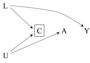
Figure 8.7

tists often refer to unmeasured confounding as selection on unobservables.

In this and the previous chapter, we describe two reasons why the treated and the untreated may not be exchangeable: 1) the presence of common causes of treatment and outcome, and 2) conditioning on common effects of treatment and outcome (or causes of them). We refer to biases due to the presence of common causes as “confounding” and to those due to conditioning on common effects as “selection bias.” This structural definition provides a clear-cut classification of confounding and selection bias, even though it might not coincide perfectly with the traditional terminology of some disciplines. For example, statisticians and econometricians often use the term “selection bias” to refer to both types of biases. Their rationale is that in both cases the bias is due to selection: selection of individuals into the analysis (the structural “selection bias”) or selection of individuals into a treatment (the structural “confound-For the same reason, social scien- ing”). Our goal, however, is not to be normative about terminology, but rather to emphasize that, regardless of the particular terms chosen, there are two distinct causal structures that lead to bias.

The end result of both structures is lack of exchangeability between the treated and the untreated—which implies that these two biases occur even under the null. For example, consider a study restricted to firefighters that aims to estimate the causal effect of being physically active A on the risk

The built-in selection bias of hazard ratios. The causal DAG in Figure 8.8 describes a randomized experiment of the effect of heart transplant A on death at times 1 (Y1) and 2 (Y2). The arrow from A to Y¹ represents that transplant decreases the risk of death at time 1. The lack of an arrow from A to Y² indicates that A has no direct effect on death at time 2. That is, heart transplant does not influence the survival status at time 2 of any individual who would survive past time 1 when untreated (and thus when treated). U is an unmeasured haplotype that decreases the individual’s risk of death at all times. Because of the absence of confounding, the associational risk ratios aRRAY¹ = Pr[Y1=1|A=1] Pr[Y1=1|A=0] and aRRAY² = Pr[Y2=1|A=1] Pr[Y2=1|A=0] are unbiased measures of the effect of A on death at times 1 and 2, respectively. Even though A has no direct effect on Y2, aRRAY² will be less than 1 because it is a measure of the effect of A on total mortality through time 2.

Consider now the time-specific hazard ratio (which, for all practical purposes, is equivalent to the rate ratio). In discrete time, the hazard of death at time 1 is the probability of dying at time 1 and thus the associational hazard ratio is the same as aRRAY¹ . However, the hazard at time 2 is the probability of dying at time 2 among those who survived past time 1. Thus, the associational hazard ratio at time 2 is then aRRAY2|Y1=0 = Pr[Y2=1|A=1,Y1=0] Pr[Y2=1|A=0,Y1=0] . The square around Y¹ in Figure 8.8 indicates this conditioning. Treated survivors of time 1 are less likely than untreated survivors of time 1 to have the protective haplotype U (because treatment can explain their survival) and therefore are more likely to die at time 2. That is, conditional on Y1, treatment A is associated with a higher mortality at time 2. Thus, the hazard ratio at time 1 is less than 1, whereas the hazard ratio at time 2 is greater than 1, i.e., the hazards have crossed. We conclude that the hazard ratio at time 2 is a biased estimate of the direct effect of treatment on mortality at time 2. The bias is selection bias arising from conditioning on a common effect Y¹ of treatment A and of U, which is a cause of Y² that opens the associational path A → Y¹ ← U → Y² between A and Y2. In the survival analysis literature, an unmeasured cause of death that is marginally unassociated with treatment such as U is often referred to as a frailty.

In contrast, the conditional hazard ratio aRRAY2|Y1=0,U is 1 within each stratum of U because the path A → Y¹ ← U → Y² is now blocked by conditioning on the non-collider U. Thus, the conditional hazard ratio correctly indicates the absence of a direct effect of A on Y2. That the unconditional hazard ratio aRRAY2|Y1=0 differs from the stratumspecific hazard ratios aRRAY2|Y1=0,U , even though U is independent of A, shows the noncollapsibility of the hazard ratio (Greenland, 1996b). Unfortunately, the unbiased measure aRRAY2|Y1=0,U of the direct effect of A on Y² cannot be computed because U is unobserved. In the absence of data on U, it is impossible to know whether A has a direct effect on Y2. That is, the data cannot determine whether the true causal DAG generating the data was that in Figure 8.8 or in Figure 8.9. All of the above applies to both observational studies and randomized experiments.

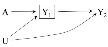
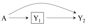
Figure 8.9

of heart disease Y as represented in Figure 8.7. For simplicity, we assume that, unknown to the investigators, A does not cause Y . Parental socioeconomic status L affects the risk of becoming a firefighter C and, through childhood diet, of heart disease Y . Attraction toward activities that involve physical activity (an unmeasured variable U) affects the risk of becoming a firefighter and of being physically active (A). U does not affect Y , and L does not affect A. According to our terminology, there is no confounding because there are no common causes of A and Y . Thus, the associational risk ratio Pr [Y = 1|A = 1] /Pr [Y = 1|A = 0] is expected to equal the causal risk ratio Pr - Y ^a=1 = 1 /Pr - Y ^a=0 = 1 = 1.

However, in a study restricted to firefighters (C = 0), the associational and causal risk ratios would differ because conditioning on a common effect C of causes of treatment and outcome induces selection bias resulting in lack of exchangeability of the treated and untreated firefighters. To the study investigators, the distinction between confounding and selection bias is moot because, regardless of nomenclature, they must adjust for L to make the treated and the untreated firefighters comparable. This example demonstrates that a structural classification of bias does not always have consequences for the analysis has no practical consequences, but disregard for the causal structure may lead to apparent paradoxes. For example, the so-called Simpson’s paradox (1951) was the result of ignoring the difference between common causes and common effects. Interestingly, Blyth (1972) failed to grasp the causal structure of the paradox in Simpson’s example and misrepresented it as an extreme case of confounding. Because most people read Blyth’s paper but not Simpson’s paper, the misunderstanding was perpetuated. See Hern´an, Clayton, and Keiding (2011) for details.

of a study. Indeed, for this reason, many epidemiologists use the term “confounder” for any variable L that needs to be adjusted for, regardless of whether the lack of exchangeability is the result of conditioning on a common effect or the result of a common cause of treatment and outcome.

There are, however, advantages of adopting a structural approach to the classification of sources of non-exchangeability. First, the structure of the problem frequently guides the choice of analytical methods to reduce or avoid the bias. For example, in longitudinal studies with time-varying treatments, identifying the structure allows us to detect situations in which adjustment for confounding via stratification would introduce selection bias (see Part III). In those cases, g-methods are a better alternative. Second, even when understanding the structure of bias does not have implications for data analysis (like in the firefighters’ study), it could still help study design. For example, investigators running a study restricted to firefighters should make sure that they collect information on joint risk factors for the outcome Y and for the selection The choice of terminology usually variable C (i.e., becoming a firefighter), as described in the first example of confounding in Section 7.1. Third, selection bias resulting from conditioning on pre-treatment variables (e.g., being a firefighter) could explain why certain variables behave as “confounders” in some studies but not others. In our example, parental socioeconomic status L would not necessarily need to be adjusted for in studies not restricted to firefighters. Finally, causal diagrams enhance communication among investigators and may decrease the occurrence of misunderstandings.

As an example of the last point, consider the “healthy worker bias”, which in the previous section we described as a bias that arises from conditioning on the variable C—a common effect of (a cause of) treatment and (a cause of) the outcome. Thus the bias can be represented by the causal diagrams in Figures 8.3-8.6. However, the term “healthy worker bias” is also used to describe the bias that occurs when comparing the risk in certain group of workers with that in a group of individuals from the general population.

This second bias can be depicted by the causal diagram in Figure 7.1 in which L represents health status, A represents membership in the group of workers, and Y represents the outcome of interest. There are arrows from L to A and Y because being healthy affects job type and risk of subsequent outcome, respectively. In this case, the bias is caused by the common cause L and we would refer to it as confounding. The use of causal diagrams to represent the structure of the “healthy worker bias” prevents any confusions that may arise from employing the same term for different sources of non-exchangeability.

All the above considerations ignore the magnitude or direction of selection bias and confounding. However, it is possible that some noncausal paths opened by conditioning on a collider are weak and thus induce little bias. Because selection bias is not an “all or nothing” issue, in practice, it is important to consider the expected direction and magnitude of the bias (see Fine Point 8.2).

8.4 Selection bias and censoring

Suppose an investigator conducted a marginally randomized experiment to estimate the average causal effect of wasabi intake on the one-year risk of death (Y = 1). Half of the 60 study participants were randomly assigned to eating meals supplemented with wasabi (A = 1) until the end of follow-up or death, whichever occurred first. The other half were assigned to meals that contained no wasabi (A = 0). After 1 year, 17 individuals died in each group. That is, the associational risk ratio Pr [Y = 1|A = 1] /Pr [Y = 1|A = 0] was 1. Because of randomization, the causal risk ratio Pr - Y ^a=1 = 1 /Pr - Y ^a=0 = 1 is also expected to be 1. (If ignoring random variability bothers you, please imagine the study had 60 million patients rather than 60.)

Unfortunately, the investigator could not observe the 17 deaths that occurred in each group because many patients were lost to follow-up, or censored, before the end of the study (i.e., death or one year after treatment assignment). The proportion of censoring (C = 1) was higher among patients with heart disease (L = 1) at the start of the study and among those assigned to wasabi supplementation (A = 1). In fact, only 9 individuals in the wasabi group and 22 individuals in the other group were not lost to follow-up. The investigator observed 4 deaths in the wasabi group and 11 deaths in the other group. That is, the associational risk ratio Pr [Y = 1|A = 1, C = 0] /Pr [Y = 1|A = 0, C = 0] was (4/9)/(11/22) = 0.89 among the uncensored. The risk ratio of 0.89 in the uncensored differs from the causal risk ratio of 1 in the entire population: There is selection bias due to conditioning on the common effect C.

The causal diagram in Figure 8.3 depicts the relation between the variables L, A, C, and Y in the randomized trial of wasabi. U represents atherosclerosis, an unmeasured variable, that affects both heart disease L and death Y . Figure 8.3 shows that there are no common causes of A and Y , as expected in a marginally randomized experiment, and thus there is no need to adjust for confounding to compute the causal effect of A on Y . On the other hand, Figure 8.3 shows that there is a common cause U of C and Y . The presence of this backdoor path C ← L ← U → Y implies that, were the investigator interested in estimating the causal effect of censoring C on Y (which is null in Figure 8.3), she would have to adjust for confounding due to the common cause U. The backdoor criterion says that such adjustment is possible because the measured variable L can be used to block the backdoor path C ← L ← U → Y .

The causal contrast we have considered so far is “the risk if everybody had been treated”, Pr - Y ^a=1 = 1 , versus “the risk if everybody had remained untreated”, Pr - Y ^a=0 = 1 , and this causal contrast does not involve C at all. Why then are we talking about confounding for the causal effect of C? It turns out that the causal contrast of interest needs to be modified in the presence of censoring or, in general, of selection. Because selection bias would not exist if everybody had been uncensored C = 0, we would like to consider a causal contrast that reflects what would have happened in the absence of censoring.

Let Y ^a=1,c=0 be an individual’s counterfactual outcome if he had received treatment A = 1 and he had remained uncensored C = 0. Similarly, let Y ^a=0,c=0 be an individual’s counterfactual outcome if he had not received treatment A = 0 and he had remained uncensored C = 0. Our causal contrast of interest is now “the risk if everybody had been treated and had remained uncensored”, Pr - Y ^a=1,c=0 = 1 , versus “the risk if everybody had remained untreated and uncensored”, Pr - Y ^a=0,c=0 = 1 For example, we may want to com- .

Often it is reasonable to assume that censoring does not have a causal effect on the outcome (an exception would be a setting in which being lost to follow-up prevents people from getting additional treatment). Because of the lack of effect of censoring C on the outcome Y , one might imagine that the definition of causal effect could ignore censoring, i.e., that we could omit the superscript c = 0. However, omitting the superscript would obscure the fact that considerations about confounding for C become central when computing the causal effect of A on Y in the presence of selection bias. In fact, when

pute the causal risk ratio E - Y ^a=1,c=0 /E - Y ^a=0,c=0 or the causal risk difference E - Y ^a=1,c=0 − E - Y ^a=0,c=0 . from censoring C to the observed outcome Y , we could replace Y by the counterfactual outcome Y c=0 and add arrows Y ^c=0 −→ Y and C −→ Y .

conceptualizing the causal contrast of interest in terms of Y a,c=0, we can think In causal diagrams with no arrow of censoring C as just another treatment. That is, the goal of the analysis is to compute the causal effect of a joint intervention on A and C. To eliminate selection bias for the effect of treatment A, we need to adjust for confounding for the effect of treatment C.

Since censoring C is now viewed as a treatment, it follows that we will need to (i) ensure that the identifiability conditions of exchangeability, positivity, and consistency hold for C as well as for A, and (ii) use analytical methods that are identical to those we would have to use if we wanted to estimate the effect of censoring C. Under these identifiability conditions and using these methods, selection bias can be eliminated via analytic adjustment and, in the absence of measurement error and confounding, the causal effect of treatment A on outcome Y can be identified. The next section explains how to do so.

8.5 How to adjust for selection bias

Though selection bias can sometimes be avoided by an adequate design (see Fine Point 8.1), it is often unavoidable. For example, loss to follow up, selfselection, and, in general, missing data leading to bias can occur no matter how careful the investigator. In those cases, the selection bias needs to be explicitly corrected in the analysis. This correction can sometimes be accomplished by IP weighting (or by standardization), which is based on assigning a weight W^C to each selected individual (C = 0) so that she accounts in the analysis not only for herself, but also for those like her, i.e., with the same values of L and A, who were not selected (C = 1). The IP weight W^C is the inverse of the probability of her selection Pr [C = 0|L, A].

adjust for confounding, W^A = 1/f (A|L), and selection bias. W^C = 1/Pr[C = 0|A, L]. When both confounding and selection bias exist, the product weight W^AW^C can be used to adjust simultaneously for both biases under assumptions described in Chapter 12 and Part III.

To describe the application of IP weighting for selection bias adjustment consider again the wasabi randomized trial described in the previous section. We have described IP weights to The tree graph in Figure 8.10 presents the trial data. Of the 60 individuals in the trial, 40 had (L = 1) and 20 did not have (L = 0) heart disease at the time of randomization. Regardless of their L status, all individuals had a 50/50 chance of being assigned to wasabi supplementation (A = 1). Thus 10 individuals in the L = 0 group and 20 in the L = 1 group received treatment A = 1. This lack of effect of L on A is represented by the lack of an arrow from L to A in the causal diagram of Figure 8.3. The probability of remaining uncensored varies across branches in the tree. For example, 50% of the individuals without heart disease that were assigned to wasabi (L = 0, A = 1), whereas 60% of the individuals with heart disease that were assigned to no wasabi (L = 1, A = 0), remained uncensored. This effect of A and L on C is represented by arrows from A and L into C in the causal diagram of Figure 8.3. Finally, the tree shows how many people would have died (Y = 1) both among the uncensored and the censored individuals. Of course, in real life, investigators would never know how many deaths occurred among the censored individuals. It is precisely the lack of this knowledge which forces investigators to restrict the analysis to the uncensored, opening the door for selection bias. Here we show the deaths in the censored to document that, as depicted in Figure 8.3, treatment A is marginally independent of Y , and censoring C is independent of Y within levels of L. It can also be checked that the risk ratio in the entire population (inaccessible to the investigator) is 1 whereas the risk ratio in the uncensored (accessible to the investigator) is 0.89.

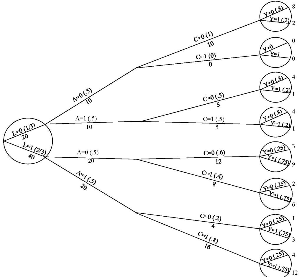
Let us now describe the intuition behind the use of IP weighting to adjust for selection bias. Look at the bottom of the tree in Figure 8.10. There are 20 individuals with heart disease (L = 1) who were assigned to wasabi supplementation (A = 1). Of these, 4 remained uncensored and 16 were lost to follow-up. That is, the conditional probability of remaining uncensored in this group is 1/5, i.e., Pr[C = 0|L = 1, A = 1] = 4/20 = 0.2. In an IP weighted analysis the 16 censored individuals receive a zero weight (i.e., they do not contribute to the analysis), whereas the 4 uncensored individuals receive a weight of 5, which is the inverse of their probability of being uncensored (1/5). IP weighting replaces the 20 original individuals by 5 copies of each of the 4 uncensored individuals. The same procedure can be repeated for the other branches of the tree, as shown in Figure 8.11, to construct a pseudo-population of the same size as the original study population but in which nobody is lost to follow-up. (We let the reader derive the IP weights for each branch of the tree.) The associational risk ratio in the pseudo-population is 1, the same as the risk ratio Pr - Y ^a=1,c=0 = 1 /Pr - Y ^a=0,c=0 = 1 that would have been computed in the original population if nobody had been censored.

Figure 8.10

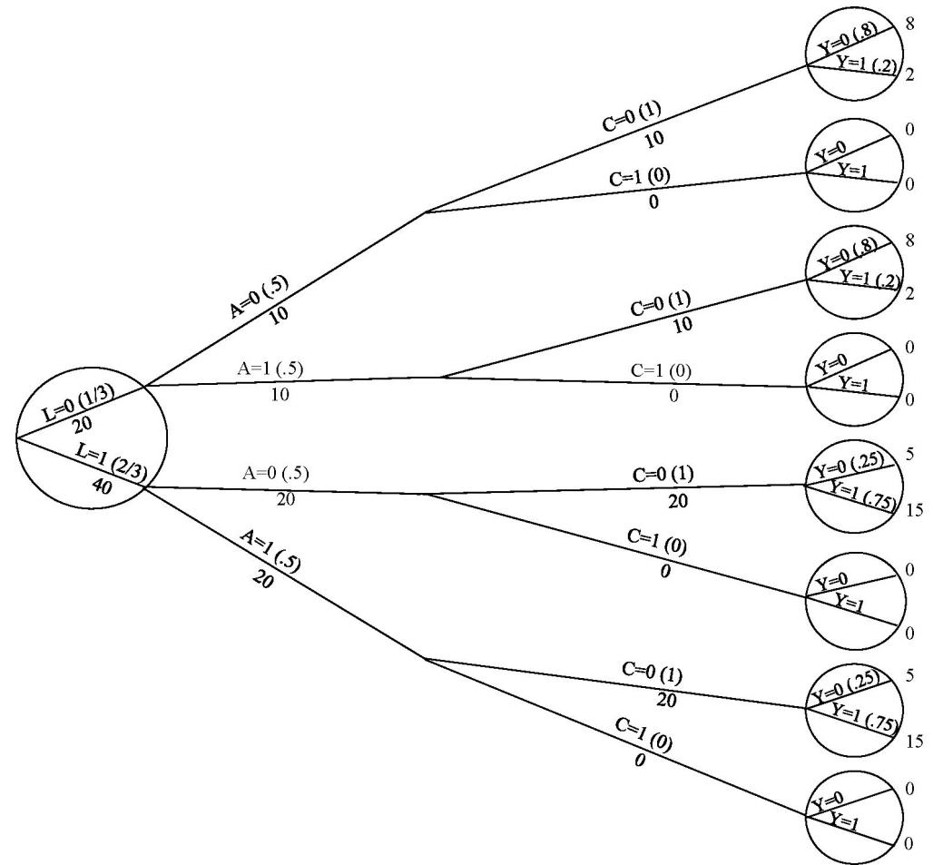
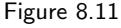
The association measure in the pseudo-population equals the effect measure in the original population if the following three identifiability conditions are met.

First, the average outcome in the uncensored individuals must equal the unobserved average outcome in the censored individuals with the same values of A and L. This provision will be satisfied if the probability of selection Pr[C = 0|L = 1, A = 1] is calculated conditional on treatment A and on all additional factors that independently predict both selection and the outcome, that is, if the variables in A and L are sufficient to block all backdoor paths between C and Y . Unfortunately, one can never be sure that these additional factors were identified and recorded in L, and thus the causal interpretation of the resulting adjustment for selection bias depends on this untestable exchangeability assumption.

Second, IP weighting requires that all conditional probabilities of being uncensored given A and the variables in L must be greater than zero. Note this positivity condition is required for the probability of being uncensored (C = 0) but not for the probability of being censored (C = 1) because we are prevents the outcome of interest from happening. A typical example of competing event is death because, once an individual dies, no other outcomes can occur.

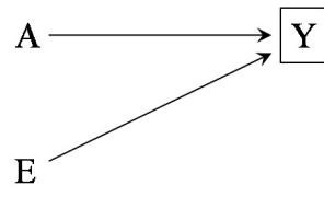
Figure 8.12

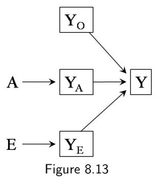
not interested in inferring what would have happened if study individuals had been censored, and thus there is no point in constructing a pseudo-population in which everybody is censored. For example, the tree in Figure 8.10 shows that Pr[C = 1|L = 0, A = 0] = 0, but this zero does not affect our ability to construct a pseudo-population in which nobody is censored.

The third condition is consistency, including sufficiently well-defined interventions. IP weighting is used to create a pseudo-population in which censoring C has been abolished, and in which the effect of the treatment A is the same as in the original population. Thus, the pseudo-population effect measure is equal to the effect measure had nobody been censored. This effect measure may be relatively well defined when censoring is the result of loss to follow up or nonresponse, but not when censoring is defined as the occurrence of a com-A competing event is an event that peting event. For example, in a study aimed at estimating the effect of certain treatment on the risk of Alzheimer’s disease, death from other causes (cancer, heart disease, and so on) is a competing event. Defining death as a form of censoring is problematic: we might not wish to base our effect estimates on a pseudo-population in which all other causes of death have been removed, because it is unclear even conceptually what sort of intervention would produce such a population. Also, no feasible intervention could possibly remove just one cause of death without affecting the others as well.

Finally, one could argue that IP weighting is not necessary to adjust for selection bias in a setting like that described in Figure 8.3. Rather, one might attempt to remove selection bias by stratification (i.e., by estimating the effect measure conditional on the L variables) rather than by IP weighting. Stratification could yield unbiased conditional effect measures within levels of L because conditioning on L is sufficient to block the backdoor path from C to Y . That is, the conditional risk ratio

\[\Pr\left[Y=1|A=1, C=0, L=l\right] / \Pr\left[Y=1|A=0, C=0, L=l\right]\]

can be interpreted as the effect of treatment among the uncensored with L = l. For the same reason, under the null, stratification would work (i.e., it would provide an unbiased conditional effect measure) if the data can be represented by the causal structure in Figure 8.5. Stratification, however, would not work under the structure depicted in Figures 8.4 and 8.6.

Take Figure 8.4. Conditioning on L blocks the backdoor path from C to Y but also opens the path A → L ← U → Y from A to Y because L is a collider on that path. Thus, even if the causal effect of A on Y is null, the conditional (on L) risk ratio would be generally different from 1. And similarly for Figure 8.6. In contrast, IP weighting appropriately adjusts for selection bias under Figures 8.3-8.6 because this approach is not based on estimating effect measures conditional on the covariates L, but rather on estimating unconditional effect measures after reweighting the individuals according to their treatment and their values of L.

This is the first time we discuss a situation in which stratification cannot be used to validly compute the causal effect of treatment, even if the three conditions of exchangeability, positivity, and consistency hold. We will discuss other situations with a similar structure in Part III when considering the effect of time-varying treatments.

8.6 Selection without bias

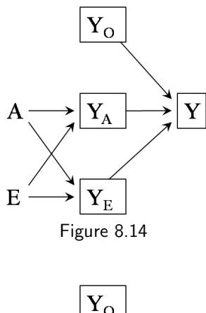
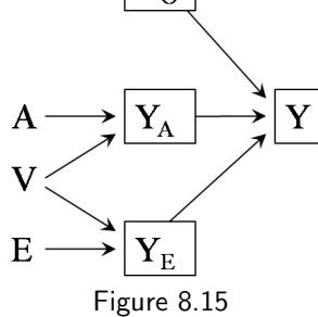
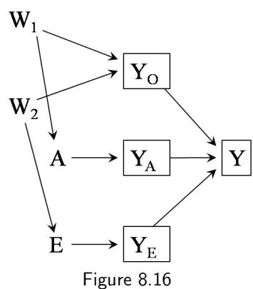
The causal diagram in Figure 8.12 represents a hypothetical study with dichotomous variables surgery A, certain genetic haplotype E, and death Y . According to the rules of d-separation, surgery A and haplotype E are (i) marginally independent, i.e., the probability of receiving surgery is the same for people with and without the genetic haplotype, and (ii) associated conditionally on Y , i.e., the probability of receiving surgery varies by haplotype when the study is restricted to, say, the survivors (Y = 0).

Indeed conditioning on the common effect Y of two independent causes A and E always induces a conditional association between A and E in at least one of the strata of Y (say, Y = 1). However, there is a special situation under which A and E remain conditionally independent within the other stratum (say, Y = 0).

Suppose A and E affect survival through totally independent mechanisms in such a way that E cannot possibly modify the effect of A on Y , and vice versa. For example, suppose that the surgery A affects survival through the removal of a tumor, whereas the haplotype E affects survival through increasing levels of low-density lipoprotein-cholesterol levels resulting in an increased risk of heart attack (whether or not a tumor is present). In this scenario, we can consider 3 cause-specific mortality variables: death from tumor YA, death from heart attack YE, and death from any other causes YO. The observed mortality variable Y is equal to 1 (death) when Y^A or Y^E or Y^O is equal to 1, and Y is equal to 0 (survival) when Y^A and Y^E and Y^O equal 0. The causal diagram in Figure 8.13, an expansion of that in Figure 8.12, represents a causal structure linking all these variables. We assume data on underlying cause of death (YA, YE, YO) are not recorded and thus the only measured variables are those in Figure 8.12 (A, E, Y ).

Because the arrows from YA, Y^E and Y^O to Y are deterministic, conditioning on observed survival (Y = 0) is equivalent to simultaneously conditioning on Y^A = 0, Y^E = 0, and Y^O = 0 as well, i.e., conditioning on Y = 0 implies Y^A = Y^E = Y^O = 0. As a consequence, we find by applying d-separation to Figure 8.13 that A and E are conditionally independent given Y = 0, i.e., when conditioning on collider Y = 0, the path between A and E through Y is blocked by conditioning on the non-colliders YA, Y^E and YO. On the other hand, conditioning on death Y = 1 does not imply conditioning on any specific values of YA, Y^E and Y^O as the event Y = 1 is compatible with 7 possible unmeasured events: (Y^A = 1, Y^E = 0, Y^O = 0), (Y^A = 0, Y^E = 1, Y^O = 0), (Y^A = 0, Y^E = 0, Y^O = 1), (Y^A = 1, Y^E = 1, Y^O = 0), (Y^A = 0, Y^E = 1, Y^O = 1), (Y^A = 1, Y^E = 0, Y^O = 1), and (Y^A = 1, Y^E = 1, Y^O = 1). Thus, A and E are associated given Y = 1, i.e., when conditioning on collider Y = 1, the path between A and E through Y is not blocked.

In contrast with the situation represented in Figure 8.13, the variables A and E will not be independent conditionally on Y = 0 when one of the situations represented in Figures 8.14-8.16 occur. If A and E affect survival through a common mechanism, then there will exist an arrow either from A to Y^E or from E to YA, as shown in Figure 8.14. In that case, A and E will be dependent within both strata of Y . Similarly, if Y^A and Y^E are not independent because of a common cause V as shown in Figure 8.15, A and E will be dependent within both strata of Y . Finally, if the causes Y^A and YO, and Y^E and YO, are not independent because of common causes W¹ and W² as shown in Figure 8.16, then A and E will also be dependent within both strata of Y . When the data can be summarized by Figure 8.13, we say that the data

Multiplicative survival model. When the conditional probability of survival Pr [Y = 0|E = e, A = a] given A and E is equal to a product g(e)h(a) of functions of e and a, we say that a multiplicative survival model holds. A multiplicative survival model

\[\Pr\left[Y=0|E=e,A=a\right] = g(e)h(a)\]

is equivalent to a model that assumes the survival ratio Pr [Y = 0|E = e, A = a] /Pr [Y = 0|E = e, A = 0] does not depend on e and is equal to h(a). The data follow a multiplicative survival model when there is no interaction between A and E for Y = 0 on the multiplicative scale. A proof that Figure 8.13 represents a multiplicative survival model proceeds as follows:

Pr [Y = 0|E = e, A = a] =

Pr [Y^O = 0, Y^A = 0, Y^E = 0|E = e, A = a] = Pr[Y^O = 0] Pr [Y^A = 0|A = a] Pr [Y^E = 0|E = e], where the first equality is by determinism and the second by the DAG factorization.

Now set g(e) = Pr [Y^E = 0|E = e] and h(a) = Pr[Y^O = 0] Pr [Y^A = 0|A = a]. Note if Pr [Y = 0|E = e, A = a] = g(e)h(a), then Pr [Y = 1|E = e, A = a] = 1 − g(e)h(a) does not follow a multiplicative mortality model. Hence, when A and E are conditionally independent given Y = 0, they will be conditionally dependent given Y = 1.

follow a multiplicative survival model (see Technical Point 8.2).

duced by Hern´an, Hern´andez-D´ıaz, and Robins (2004), can be extended to represent the sufficient causes described in Chapter 5 (VanderWeele and Robins, 2007c).

What is interesting about Figure 8.13 is that by adding the unmeasured variables YA, Y^E and YO, which functionally determine the observed variable Augmented causal DAGs, intro- Y , we have created an augmented causal diagram that succeeds in representing both the conditional independence between A and E given Y = 0 and the their conditional dependence given Y = 1.

In summary, conditioning on a collider always induces an association between its causes, but this association could be restricted to certain levels of the common effect. In other words, it is theoretically possible that selection on a common effect does not result in selection bias when the analysis is restricted to a single level of the common effect. Collider stratification is not always a source of selection bias.

The strength and direction of selection bias. We have referred to selection bias as an “all or nothing” issue: either bias exists or it doesn’t. In practice, however, it is important to consider the expected direction and magnitude of the bias.

The direction of the conditional association between 2 marginally independent causes A and E within strata of their common effect Y depends on how the two causes A and E interact to cause Y . For example, suppose that, in the presence of an undiscovered background factor U that is unassociated with A or E, having either A = 1 or E = 1 is sufficient and necessary to cause death (an “or” mechanism), but that neither A nor E causes death in the absence of U. Then among those who died (Y = 1), A and E will be negatively associated, because it is more likely that an individual with A = 0 had E = 1 because the absence of A increases the chance that E was the cause of death. (Indeed, the logarithm of the conditional odds ratio ORAE|^Y =1 will approach minus infinity as the population prevalence of U approaches 1.0.) This “or” mechanism was the only explanation given in the main text for the conditional association of independent causes within strata of a common effect; nonetheless, other possibilities exist.

For example, suppose that in the presence of the undiscovered background factor U, having both A = 1 and E = 1 is sufficient and necessary to cause death (an “and” mechanism) and that neither A nor E causes death in the absence of U. Then, among those who die, those with A = 1 are more likely to have E = 1, i.e., A and E are positively correlated. A standard DAG such as that in Figure 8.12 fails to distinguish between the case of A and E interacting through an “or” mechanism from the case of an “and” mechanism. Causal DAGs with sufficient causation structures (VanderWeele and Robins, 2007c) overcome this shortcoming.

Regardless of the direction of selection bias, another key issue is its magnitude. Biases that are not large enough to affect the conclusions of the study may be safely ignored in practice, whether the bias is upwards or downwards. Generally speaking, a large selection bias requires strong associations between the collider and both treatment and outcome. Greenland (2003) studied the magnitude of selection bias under the null, which he referred to as colliderstratification bias, in several scenarios.

Selection bias

Chapter 9 MEASUREMENT BIAS AND “NONCAUSAL” DIAGRAMS

Suppose an investigator conducted a randomized experiment to answer the causal question “does one’s looking up to the sky make other pedestrians look up too?” She found a weak association between her looking up and other pedestrians’ looking up. Does this weak association reflect a weak causal effect? By definition of randomized experiment, confounding bias is not expected in this study. In addition, no selection bias was expected because all pedestrians’ responses—whether they did or did not look up—were recorded. However, there was another problem: the investigator’s collaborator who was in charge of recording the pedestrians’ responses made many mistakes. Specifically, the collaborator missed half of the instances in which a pedestrian looked up and recorded these responses as “did not look up.” Thus, even if the treatment (the investigator’s looking up) truly had a strong effect on the outcome (other people’s looking up), the misclassification of the outcome will result in a dilution of the association between treatment and the (mismeasured) outcome.

We say that there is measurement bias when the association between treatment and outcome is weakened or strengthened as a result of the process by which the study data are measured. Since measurement errors can occur under any study design—including both randomized experiments and observational studies—measurement bias need always be considered when interpreting effect estimates. This chapter provides a description of biases due to measurement error.

9.1 Measurement error

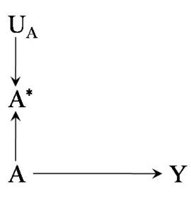
Figure 9.1

In previous chapters we implicitly made the unrealistic assumption that all variables were perfectly measured. Consider an observational study designed to estimate the effect of a cholesterol-lowering drug A on the risk of liver disease Y . We often expect that treatment A will be measured imperfectly. For example, if the information on drug use is obtained by medical record abstraction, the abstractor may make a mistake when transcribing the data, the physician may forget to write down that the patient was prescribed the drug, or the patient may not take the prescribed treatment. Thus, the treatment variable in our analysis data set will not be the true use of the drug, but rather the measured use of the drug. We will refer to the measured treatment as A^∗ (read A-star), which will not necessarily equal the true treatment A for a given individual. The psychological literature sometimes refers to A as the “construct” and to A^∗ as the “measure” or “indicator.” The challenge in observational disciplines is making inferences about the unobserved construct (e.g., cholesterol-lowering drug use) by using data on the observed measure (e.g., information on statin use from medical records).

The causal diagram in Figure 9.1 depicts the variables A, A^∗ , and Y . For simplicity, we chose a setting with neither confounding nor selection bias for the causal effect of A on Y . The true treatment A affects both the outcome Y and the measured treatment A^∗ . The causal diagram also includes the node U^A to represent all factors other than A that determine the value of A^∗ . We refer to the difference between an individual’s mismeasured value A^∗ and true value A as the measurement error of A for that individual. The magnitude and

Independence and nondifferentiality of measurement errors. For each individual, we define the measurement error of A as the difference e^A = A^∗ − A and the measurement error of Y as the difference e^Y = Y ^∗ − Y .

Let f(·) denote a probability density function (pdf). The measurement error e^A of treatment and the measurement error e^Y of outcome are independent if their joint pdf equals the product of each marginal pdf, i.e., f(e^Y , eA) = f(e^Y )f(eA). The measurement error e^A of treatment is nondifferential if its pdf is independent of the outcome Y , i.e., f(eA|Y ) = f(eA). Analogously, the measurement error e^Y of the outcome is nondifferential if its pdf is independent of the treatment A, i.e., f(e^Y |A) = f(e^Y ).

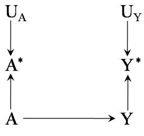
Figure 9.2

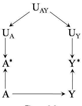
Figure 9.3

Measurement error for discrete vari- direction of the measurement error is determined by the factors in UA. Note ables is known as misclassification. that including the node U^A in the causal diagram is not strictly necessary because U^A is neither a cause shared by other variables on the diagram nor a variable that is conditioned on. We include it, however, to provide an explicit representation of the factors responsible for measurement error and for a direct comparison with the causal diagrams that we will discuss next.

Besides treatment A, the outcome Y can be measured with error too. The causal diagram in Figure 9.2 includes the measured outcome Y ∗ , and the factors U^Y responsible for the measurement error of Y . Figure 9.2 illustrates a common situation in practice. One wants to compute the average causal effect of the treatment A on the outcome Y , but these variables A and Y have not been, or cannot be, measured correctly. Rather, only the mismeasured versions A^∗ and Y ^∗ are available to the investigator who aims at identifying the causal effect of A on Y .

Figure 9.2 also represents a setting in which there is neither confounding nor selection bias for the causal effect of treatment A on outcome Y . According to our reasoning in previous chapters, association is causation in this setting. We can compute any A-Y association measure and endow it with a causal interpretation as the effect of A on Y . For example, the associational risk ratio Pr [Y = 1|A = 1] /Pr [Y = 1|A = 0] is equal to the causal risk ratio Pr - Y ^a=1 = 1 /Pr - Y ^a=0 = 1 . Our implicit assumption in previous chapters, which we now make explicit, was that perfectly measured data on A and Y were available.

We now consider the more realistic setting in which only the mismeasured versions of treatment and outcome, A^∗ and Y ∗ , are available. Then there is no guarantee that the measure of association between A^∗ and Y ^∗ will equal the measure of causal effect of A on Y . The associational risk ratio Pr [Y ^∗ = 1|A^∗ = 1] /Pr [Y ^∗ = 1|A^∗ = 0] will generally differ from the causal risk ratio Pr - Y ^a=1 = 1 /Pr - Y ^a=0 = 1 . We say that there is measurement bias or information bias. In the presence of measurement bias, the identifiability conditions of exchangeability, positivity, and consistency are insufficient to compute the causal effect of treatment A on outcome Y .

9.2 The structure of measurement error

The causal structure of confounding can be summarized as the presence of common causes of treatment and outcome, and the causal structure of selection bias can be summarized as conditioning on common effects of treatment

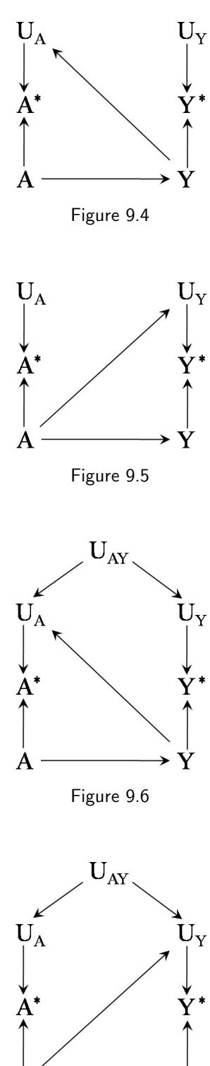
Figure 9.7

and outcome (or of their causes). Measurement bias arises in the presence of measurement error, but there is no single structure to summarize measurement error. This section classifies the structure of measurement error according to two properties—independence and nondifferentiality—that we describe below (see Technical Point 9.1 for formal definitions).

The causal diagram in Figure 9.2 depicts the measurement errors U^A and U^Y for both treatment A and outcome Y , respectively. According to the rules of d-separation, the measurement errors U^A and U^Y are independent because the path between them is blocked by colliders (either A^∗ or Y ∗ ). Independent measurement errors are expected to arise if, e.g., information on both drug use A and liver toxicity Y was obtained from electronic medical records in which data entry errors occurred haphazardly. In other settings, however, the measurement errors for exposure and outcome may be dependent, as depicted in Figure 9.3. For example, dependent measurement errors will occur if the information were obtained retrospectively by phone interview and an individual’s ability to recall her medical history (UAY ) affected the measurement of both treatment A and outcome Y .

Figures 9.2 and 9.3 represent settings in which the factors U^A responsible for the measurement error of the treatment are independent of the true value of the outcome Y , and the factors U^Y responsible for the measurement error for the outcome are independent of the true value of treatment A. We then say that the measurement error for treatment is nondifferential with respect to the outcome, and that the measurement error for the outcome is nondifferential with respect to the treatment. The causal diagram in Figure 9.4 shows an example of independent but differential measurement error in which the true value of the outcome affects the measurement of the treatment (i.e., an arrow from Y to UA). We now describe some examples of differential measurement error of the treatment.

Suppose that the outcome Y was dementia rather than liver toxicity, and that drug use A was ascertained by interviewing study participants. Since the presence of dementia affects the ability to recall A, one would expect an arrow from Y to UA. Similarly, one would expect an arrow from Y to U^A in a study to compute the effect of alcohol use during pregnancy A on birth defects Y if alcohol intake is ascertained by recall after delivery—because recall may be affected by the outcome of the pregnancy. The resulting measurement bias in these two examples is often referred to as recall bias. A bias with the same structure might arise if blood levels of drug A^∗ are used in place of actual drug use A, and blood levels are measured after liver toxicity Y is present—because liver toxicity affects the measured blood levels of the drug. The resulting measurement bias is often referred to as reverse causation bias.

The causal diagram in Figure 9.5 shows an example of independent but differential measurement error in which the true value of the treatment affects the measurement of the outcome (i.e., an arrow from A to U^Y ). A differential measurement error of the outcome will occur if physicians, suspecting that drug use A causes liver toxicity Y , monitored patients receiving drug more closely than other patients. Figures 9.6 and 9.7 depict measurement errors that are both dependent and differential, which may result from a combination of the settings described above.

In summary, we have discussed four types of measurement error: independent nondifferential (Figure 9.2), dependent nondifferential (Figure 9.3), independent differential (Figures 9.4 and 9.5), and dependent differential (Figures 9.6 and 9.7). The particular structure of the measurement error determines the methods that can be used to correct for it. For example, there is a large

The strength and direction of measurement bias. In general, measurement error will result in bias. A notable exception is the setting in which A and Y are unassociated and the measurement error is independent and nondifferential: If the arrow from A to Y did not exist in Figure 9.2, then both the A-Y association and the A^∗ -Y ∗ association would be null. In all other circumstances, measurement bias may result in an A^∗ -Y ∗ association that is either further from or closer to the null than the A-Y association. Worse, even under the independent and nondifferential measurement error structure of Figure 9.2, non-extreme measurement bias may result in A^∗ -Y ∗ and A-Y trends in opposite directions for non-dichotomous ordinal treatments and for continuous treatments. This trend reversal under independent and nondifferential measurement error occurs when the conditional mean of A^∗ given A is a nonmonotonic function of A. See Dosemeci, Wacholder, and Lubin (1990) and Weinberg, Umbach, and Greenland (1994) for details. VanderWeele and Hern´an (2009) described a more general framework using signed causal diagrams.

The magnitude of the measurement bias depends on the magnitude of the measurement error. That is, measurement bias generally increases with the strength of the arrows from U^A to A^∗ and from U^Y to Y ∗ . Causal diagrams do not encode quantitative information, and therefore they cannot be used to describe the magnitude of the bias.

literature on methods for measurement error correction when the measurement error is independent nondifferential. In general, methods for measurement error correction rely on a combination of modeling assumptions and validation samples, i.e., subsets of the data in which key variables are measured with little or no error. The description of methods for measurement error correction is beyond the scope of this book. Rather, our goal is to highlight that the act of measuring variables (like that of selecting individuals) may introduce bias (see Fine Point 9.1 for a discussion of its strength and direction). Realistic causal diagrams need to simultaneously represent biases arising from confounding, selection, and measurement. The best method to fight bias due to mismeasurement is, obviously, to improve the measurement procedures for the variables used in our analysis.

9.3 Mismeasured confounders and colliders

Besides the treatment A and the outcome Y , the confounders L may also be measured with error. Mismeasurement of confounders may result in bias even if both treatment and outcome are perfectly measured.

To see this, consider the causal diagram in Figure 9.8, which includes the variables drug use A, liver disease Y , and history of hepatitis L. Individuals with prior hepatitis L are less likely to be prescribed drug A and more likely to develop liver disease Y . As discussed in Chapter 7, there is confounding for the effect of the treatment A on the outcome Y because there exists an open backdoor path A ← L → Y , but there is no unmeasured confounding given L because the backdoor path A ← L → Y can be blocked by conditioning on L. That is, there is exchangeability of the treated and the untreated conditional on the confounder L, and one can apply IP weighting or standardization to compute the average causal effect of A on Y . The standardized, or IP weighted, risk ratio based on L, Y , and A will equal the causal risk ratio Pr - Y ^a=1 = 1 /Pr - Y ^a=0 = 1 .

Again the implicit assumption in the above reasoning is that the confounder L was perfectly measured. Suppose investigators did not have access to the

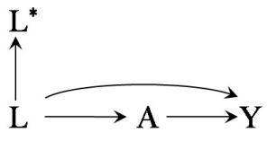
Figure 9.8

structure of this error is not relevant to our discussion. Investigators had data on the mismeasured variable L ∗ rather than on the variable L. Unfortunately, the backdoor path A ← L → Y cannot be generally blocked by conditioning on L ∗ . The standardized (or IP weighted) risk ratio based on L ∗ , Y , and A will generally differ from the causal risk ratio Pr - Y ^a=1 = 1 /Pr - Y ^a=0 = 1 . We then say that there is measurement bias or information bias. The causal diagram in Figure 9.9 shows an example of confounding of the causal effect of A on Y in which L is not the common cause shared by A and Y . Here too mismeasurement of L leads to measurement bias because the backdoor path A ← L ← U → Y cannot be generally blocked by conditioning on L ∗ .

factors U^L responsible for the measurement error of L because the particular

Alternatively, one could view the bias due to mismeasured confounders in Figures 9.8 and 9.9 as a form of unmeasured confounding rather than as a form of measurement bias. In fact the causal diagram in Figure 9.8 is equivalent to that in Figure 7.8. One can think of L as an unmeasured variable and of L ^∗ as a surrogate confounder (see Fine Point 7.2). The particular choice of terminology—unmeasured confounding versus bias due to mismeasurement of the confounders—is irrelevant for practical purposes. In some settings, however, the use of mismeasured variables is sufficient to adjust for confounding. See Fine Point 9.2 for some examples.

Mismeasurement of confounders may also result in apparent effect modification. As an example, suppose that all study participants who reported a prior diagnosis of hepatitis (L ^∗ = 1) and half of those who reported no prior diagnosis of hepatitis (L ^∗ = 0) did actually have a prior diagnosis of hepatitis (L = 1). That is, the true and the measured value of the confounder coincide in the stratum L ^∗ = 1, but not in the stratum L ^∗ = 0. Suppose further that treatment A has no effect on any individual’s liver disease Y , i.e., the sharp null hypothesis holds. When investigators restrict the analysis to the stratum L ^∗ = 1, there will be no confounding by L because all participants included in the analysis have the same value of L (i.e., L = 1). Therefore they will find no association between A and Y in the stratum L ^∗ = 1. However, when the investigators restrict the analysis to the stratum L ^∗ = 0, there will be confounding by L because the stratum L ^∗ = 0 includes a mixture of individuals with both L = 1 and L = 0. Thus the investigators will find a non-null association between A and Y as a consequence of uncontrolled confounding by L. If the investigators are unaware of the fact that there is mismeasurement of the confounder in the stratum L ^∗ = 0 but not in the stratum L ^∗ = 1, they could naively conclude that both the association measure in the stratum L ^∗ = 0 and the association measure in the stratum L ^∗ = 1 can be interpreted as effect measures. Because these two association measures are different, the investigators will say that L ∗ is a modifier of the effect of A on Y even though no effect modification by the true confounder L exists.

Finally, it is also possible that a collider C is measured with error. This situation is represented in the causal diagram in Figure 9.10, which is equivalent to Figure 8.2. When interested in the effect of A on Y under Figure 9.10, conditioning on the mismeasured collider C ^∗ will generally introduce selection

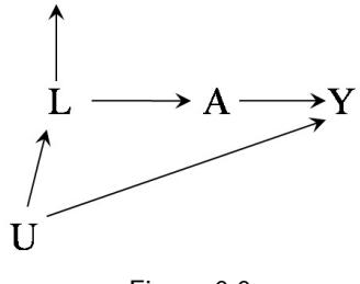
Figure 9.9

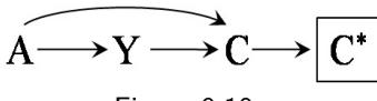
Figure 9.10

When mismeasured confounders are not a problem. In many medical applications, measurement error in the confounders does not introduce any bias. Suppose that high blood pressure L affects both the probability of receiving antihypertensive therapy A and of having a stroke Y . Doctors and patients, however, do not make their treatment decisions based on the true blood pressure L but based on the blood pressure measurement L ∗ that was recorded in the doctor’s office. That is, L ∗ is the only information about blood pressure that is accessible to decision makers.

Figure 9.11 (which is structurally equivalent to Figure 7.2) represents this situation. The possibly mismeasured L ∗ fully mediates the effect of L on A because any component of L that was not captured by L ∗ remained unknown and thus could not influence the decision to administer the treatment. It follows that the backdoor path between A and Y can be blocked by conditioning on either the true L or the measured L ∗ . Therefore, it is irrelevant whether investigators had access to the true L or to the measured L ∗ . Either variable is sufficient to adjust for confounding.

A more extreme example is shown in Figure 9.12. Under this causal diagram, having data on the true L is insufficient to adjust for confounding whereas having data on the measured L ∗ is sufficient to adjust for confounding. The general point is that effects can be identified whenever we have as much information in the data as the decision makers had to make their decisions, regardless of whether that information resulted from perfectly measured variables or from variables measured with error.

bias because C ∗ is a descendant of the collider and therefore a common effect of the treatment A and the outcome Y .

9.4 Causal diagrams without mismeasured variables?

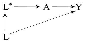
Figure 9.11

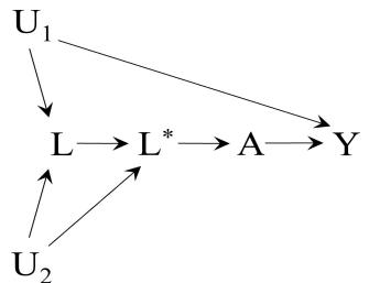
Figure 9.12

When drawing causal diagrams in previous chapters, we have been implicitly making two simplifying, and related, assumptions. In this and the next section we make those assumptions and their implications explicit.

The first assumption is that all variables on the diagram are perfectly measured. This assumption is not realistic because, in practice, measurement error is often unavoidable for treatments, outcomes, confounders, and any other variables of interest. In this chapter, we have described how causal diagrams can be used to represent mismeasured variables under different types of measurement error. We have also explored the consequences of using the mismeasured variables, which are the only ones available to investigators, for the identification of causal effects.

For example, suppose that we are interested in the effect of the treatment A on the outcome Y , but we only have data on the measured treatment A^∗ and the measured outcome Y ∗ . We have seen how measurement error of treatment or outcome may induce a noncausal association between the measured treatment A^∗ and the measured outcome Y ∗ , even if treatment A has a null effect on the outcome Y and even if there is no confounding and no selection bias. Also, in the presence of confounding, we have seen how measurement error of a confounder may prevent the measured confounder L ∗ from blocking a backdoor path that would be successfully blocked if we had access to the true confounder L.

Because all variables can be expected to be measured with some error, it might be argued that a causal diagram should always represent both true and measured values of all its variables. Yet, in many settings, the magnitude of the measurement error may be judged, or known, to be too small to matter. In those settings, a causal DAG that makes no distinction between measured and true values of a variable may be preferable for simplicity. If confounding and selection bias exist under perfect measurement of all variables, then these biases will typically exist under measurement error too (though exceptions exist as shown in Fine Point 9.2). Drawing causal diagrams without measurement error allows us to focus on confounding and selection bias without being distracted by measurement issues.

Considering causal diagrams without measurement error is often a helpful first approximation. Once we have a good understanding of possible biases under perfect measurement, we can add measurement error as an additional layer of complexity. This 2-step approach to the drawing of causal diagrams helps us isolate the study of two sources of bias—confounding and selection without being overburdened by the third one—measurement. We follow this approach in the book: when the emphasis is on confounding and selection bias, we omit the distinction between true and measured values of the variables on the causal diagram.

The second assumption we have made so far, also related to measurement, is a fundamental assumption in any causal diagram. We discuss this assumption in the next section.

9.5 Many proposed causal diagrams include noncausal arrows

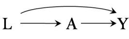
Figure 9.13

Consider the causal diagram in Figure 9.13 (which is equal to Figure 7.1). Let A, Y , and L be three binary variables representing an antiviral treatment given to patients with COVID-19, death, and obesity (defined as body mass index greater than 30), respectively. Patients with obesity are more likely to receive treatment and to be hospitalized in the absence of treatment. Therefore, experts draw a DAG with arrows from L into both A and Y . For simplicity, we will assume that the decision to give treatment is only influenced by L and by the physician’s preference, which is unrelated to any other variables on the diagram. Also for simplicity, we assume no measurement error for any variable. Specifically, the true value of L equals its measured value L ∗ so the latter does not need be included on the diagram.

We have previously discussed how, in causal diagrams, treatment nodes have a different status than other nodes (see Section 6.4). The reason is that meaningful quantitative causal inference about the effect of treatment A on outcome Y requires well-defined, actual or hypothetical, interventions on A. Otherwise the counterfactual outcomes Y a remain undefined and cannot be linked to the observed outcomes Y , i.e., the consistency condition does not hold (see Chapter 3). In our example, the intervention represented by treatment A is well-defined because we have a good understanding of how antiviral treatment can be administered or withheld. Thus, the presence or absence of an arrow from A to Y is well defined too.

We now extend our discussion to nodes that are not considered a treatment, such as obesity L in Figure 9.13. As we discussed extensively in Chapter 3, interventions on obesity L on death are not well defined. Thus, the counterfactual outcomes Y l remain undefined.

So far in this book we have ignored this problem, but many DAGs proposed in the health and social sciences have arrows emanating from variables for which well-defined interventions do not exist, like L in Figure 9.13. Those arrows, like the arrow L → Y in Figure 9.13, do not have a causal interpreta-

Whether interventions are well-defined depends on the outcome of interest. In the main text we said that there may exist well-defined interventions for the effect of L on A even if there are no well-defined interventions for the effect of L on Y . This statement needs a better explanation because, if we truly knew how to intervene on L to study its effect on A, then what would prevent us from using the same intervention to study its effect on Y ?

This apparent contradiction results from an abuse of notation. In our example, we used the symbol L to refer to two concepts: (i) the physical quantity body weight (measured in kilos), and (ii) the recorded value of that quantity (measured in kilos). In a world without measurement error, both (i) and (ii) have the same numerical value and thus conflating both concepts has no practical impact. However, when we described in the main text a well-defined intervention for L on A, we were referring to an intervention on (ii) rather than on (i), and thus a distinction between both concepts is warranted.

Let us use the symbol L to depict the physical quantity “body weight”, and the symbol L ∗ to depict the recording of L. If we add L ∗ to the causal DAG, there would be a deterministic arrow from L to L ∗ (assuming no measurement error) and a regular arrow from L ∗ to A. According to this expanded causal DAG, body weight L only affects treatment A when the doctor learns the value L ∗ . Therefore, if we intervene on the recorded value L ∗ , even if we leave the physical quantity L unchanged, the doctors’ behavior would be the same as if we could somehow intervene on L. It is in this sense that we say in the main text that there are well-defined interventions on L when the outcome is A—the counterfactuals A^l are well defined—but not when the outcome is Y —the counterfactuals Y l are not well defined.

tion. To explore the consequences of using these DAGs with noncausal arrows, we now discuss Figure 9.13 in more detail. Let us consider separately the arrows L → A and L → Y .

When experts drew the arrow from L → A, they were using their subjectmatter knowledge. Experts knew that doctors are more likely to administer treatment to obese patients upon learning that they are obese. One could imagine well-defined interventions for the effect of L on A, such as presenting the treating physician with a patient whose body mass index differs from that of the patient for whom the treatment decision is being made. Therefore, drawing the arrow from L → A is reasonable. For additional discussion on this point, see Fine Point 9.3 after reading the next paragraph.

Were the experts justified in drawing the arrow L → Y ? Suppose the experts know that obese patients are more likely to die, but cannot propose well-defined interventions for the effect of L and Y . Then the arrow L → Y has no causal interpretation. In this chapter and generally throughout the book, we restrict the term causal DAG to DAGs for which all arrows have a well-defined causal interpretation. Therefore, under our restriction and the current state of knowledge, Figure 9.13 is a “noncausal” diagram. We have placed the word “noncausal” in quotes as a reminder that many papers in the causal literature continue to define DAGs that include both causal and noncausal arrows as causal diagrams. See Fine Point 9.4 for more discussion on “noncausal” diagrams.

Now suppose that a second group of experts proposes an alternative interpretation for the known fact that “obese patients are more likely to die”: obesity is a surrogate or proxy for a hidden factor H that has a causal effect on Y . The corresponding causal diagram is Figure 9.14 (structurally identical to Figure 7.2), which includes unmeasured and possibly unknown variables H such as genetic factors, metabolic factors related to body fat stores, microbiota, and probably others not yet discovered by science. According to Figure 9.14, the effect of the factors H on the treatment A is fully mediated through L.

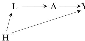
Figure 9.14

“Noncausal”diagrams with well-defined statistical interpretations. Consider a DAG representation for an FFR-CISTG model that assumed (i) the treatment A was the only variable with well-defined interventions with counterfactuals (M^a , Y ^a ) and (ii) the distribution of the variables on the DAG factored according to the DAG, i.e., each variable was conditionally independent of its non-descendants given its parents. In these DAGs, the arrows do not, in general, have a causal interpretation. Rather, the arrows simply encode, via d-separation, the conditional independencies satisfied by the variables on the diagram and on the associated SWIG (see Technical Point 21.12). Under this noncausal interpretation of DAGs, the L → Y arrow need not be removed in Figure 9.13 just because interventions on L are not well-defined.

Richardson and Robins (2013) pointed out serious difficulties with this approach. Specifically, if arrows have no causal interpretation, then there is no reason to expect the distribution of the study variables to be representable by (i.e., factor according to) any (incomplete) DAG. This difficulty is magnified in the presence of unmeasured variables U because then it is not even possible to empirically check some conditional independencies from the observed data. For example, the front door graph of Figure 7.14 implies that Y is independent of A given M and U. Any investigator who chooses Figure 7.14 as the appropriate causal DAG must have had substantive reasons for postulating this conditional independence. Indeed many researchers might find it hard to imagine what those reasons could be other than the belief that A and Y share a common cause U and that the causal effect of A on Y is completely mediated by M—a belief that endows every arrow on the diagram with a causal interpretation. See also Fine Point 9.5.

One can alternatively view the use of noncausal arrows as a response by researchers who are skeptical of the strong causal claim that M-counterfactuals Y ^m exist. This “noncausal” approach interprets Figure 7.14 as representing the hypothesized statistical independence Y ⊥⊥A|M among the observed variables that would hold in a future trial in which A is randomly assigned. Thus, if this independence fails to hold in the future trial, the justification of the strong causal claim that M-counterfactuals exist has been falsified along with the structure in Figure 7.14.

That is, there is no direct arrow from H to A. This assumption is reasonable if, for example, the only information used to make real world treatment decisions is obesity L.

Like Figure 9.13, Figure 9.14 encodes the (reasonable) assumptions that there are well-defined interventions for the effect of obesity L on treatment A—this assumption is represented by the arrow L → A—and that there is no direct effect of L on Y not through A. Therefore, the associated counterfactuals are A^l and Y a , which imply the existence of a well-defined intervention of L on Y with Y ^l = Y A l . That is, Y l is equal to Y a for a equal to the counterfactual Al . In the language of Technical Point 6.2, we say that Y l is obtained from Y a and A^l by recursive substitution. There is no contradiction in Y ^l being welldefined for the causal diagram of Figure 9.14 but not for Figure 9.13 because, assuming Figure 9.14 is a causal diagram, Figure 9.13 is not, as Figure 9.13 fails to include the common cause H of L and Y . See also Fine Point 9.6.

Figure 9.14 also encodes the assumption that well-defined interventions exist for the effect of the unknown factors H on both L and Y . That is, the arrows H → L and H → Y on Figure 9.14 imply that there exist counterfactuals L ^h and Y h , respectively, associated with a well-defined intervention on H. It may seem counterintuitive for us to stipulate simultaneously that (i) the current state of knowledge is insufficient to even characterize many of the factors in H, and (ii) well-defined interventions exist for the effect of H on both L and Y . To explain why we might do so and hence regard Figure 9.14 as a causal diagram under the current state of knowledge, let us define H more precisely.

When, as in Figure 9.13, there exists a variable L on a proposed causal diagram for which Y l is ill-defined, we introduce a high-dimensional parent H

A connection to the front door formula. Figure 9.14 is precisely the front door diagram in Figure 7.14 with L → A substituted for A → M. Hence E - Y l is identified by the front door formula in Technical Point 7.4 with L, l, l′ substituted for A, a, a′ and A, a substituted for M, m.

Suppose a researcher modifies Figure 9.14 by adding a direct L → Y arrow. The justification is that, when dietitians and physical therapists are referred an individual who has a high value of L, they provide additional ancillary care (such as dietary advice, exercises to prevent deep vein thrombosis, etc.), which is not recorded in the medical record available to the researchers. The counterfactual variable Y l in the unmodified diagram in Figure 9.14 differs from the variable Y l in the modified diagram with a direct L → Y arrow. In the unmodified graph, the contrast Y ^l − Y l ′ is the causal effect of l versus l ′ via the causal pathway L → A → Y . In contrast, in the modified graph, Y ^l − Y l ′ is the total effect along the two pathways L → Y and L → A → Y . In fact, in contrast to the unmodified graph, E - Y l is not identified under the modified graph.

One might conjecture that the effect of l versus l ′ along the pathway L → A → Y should be the same in the two graphs and thus remain identified by the front door formula. This conjecture is indeed true, although we must defer a proof until we study the identification of path-specific effects in Chapter 23.

of L that encodes all unmeasured—known and unknown—causal determinants of L (other than any known, but unmeasured, variables U already present on the diagram). H may be a direct cause and thus a parent of other variables such as Y as well. We regard L as the lower-dimensional effect of, or surrogate for, H that has been recorded for data analysis. In our obesity example, the continuous variable body mass index L is an effect of the largely unknown factors H that regulate body weight. In some instances, L may be thought of as a deterministic (many to one) function of H.

Even though we are ignorant of the precise intervention on the components (many unknown) of H that affect Y , we nonetheless assume that there exist factors H that have a causal effect on Y . Because current knowledge does not rule out the existence of well-defined interventions for the effect of H on Y , the arrow H → Y is tentatively justified and therefore we consider Figure 9.14 to be a causal diagram.

In this section, we distinguished between H, unmeasured common causes between two variables when the effect of one of the variables on the other is ill-defined, and U, unmeasured common causes between two variables when the effect of one of the variables on the other is well-defined. In most of the book, we do not make this distinction and simply use U to represent all unmeasured variables.

9.6 Does it matter that many proposed diagrams include noncausal arrows?

We have seen that the original DAG (Figure 9.13) proposed by the experts is not a causal DAG because one of its arrows (the one from L to Y ) cannot be causally interpreted. Yet, despite being causally wrong, this DAG is adequate for causal inference about the effect of treatment A on the outcome Y : regardless of whether we use the noncausal DAG in Figure 9.13 or the causal DAG in Figure 9.14, we conclude that all backdoor paths between A and Y are blocked by conditioning on L.

Thus the DAG in Figure 9.13, which lacks the node U and includes the non-

causal arrow L → Y , correctly guides data analysis because adjusting for L is all that is needed in the identifying formula—standardization or IP weighting in our example—for the average causal effect of A on Y . This conclusion is expected because, in both DAGs, there are no arrows from unmeasured variables into treatment A (see also Fine Point 9.2). This oversimplified scenario illustrates a general issue: in realistic complex settings, expert knowledge is rarely good enough to draw a causal diagram in which all of its components are known.

In fact, many DAGs proposed in the health and social sciences are actually noncausal DAGs because they lack the hidden variables H that make the DAG causal. By including a variable without well-defined interventions for its effect on its descendants (like obesity and its descendant death), we are effectively declaring that our DAG is noncausal. It is, however, possible that the identifying formula for the causal effect of interest is the same when derived from the noncausal DAG and from the causal DAG with hidden nodes. This is exactly what happened in our example: if Figure 9.14 is the correct DAG, using the DAG in Figure 9.13 will result in the same identifying formula.

But noncausal DAGs may be misleading. Consider the DAG in Figure 9.15. Declaring that this DAG is a causal DAG implies that we believe there are welldefined interventions for the effect of L on Y (because there is a direct arrow from L to Y ). Conversely, in the absence of such well-defined interventions, the DAG is noncausal and we can only hope that the identifying formula based on L happens to be correct.

Following our reasoning above, Figure 9.16 depicts our measured variable L is actually a surrogate of an unknown variable H for which well-defined interventions exist. In Figure 9.15 the backdoor path between A and Y is blocked by L, but in Figure 9.16 it is not.

Therefore, if investigators unaware of the status of their measured variable as a surrogate confounder L proposed Figure 9.15 instead of Figure 9.16, they would reach the incorrect conclusion that L is sufficient to block all backdoor paths, as discussed in Section 9.3. When drawing causal DAGs, we need to think carefully whether the variables that happen to be measured are also the variables for which well-defined interventions exist. Otherwise, lack of attention to the noncausal arrows of a DAG may give us false confidence in the validity of our effect estimates. See Fine Point 9.6 for another example.

We have come a long way since we introduced causal diagrams in Chapter 6. Causal DAGs and SWIGs are formidable tools for investigators to organize and communicate their causal assumptions but, as we have seen in this chapter, these diagrams are subject to the same practical constraints that are inherent to causal inference in general. Specifically, a causal arrow X → Y cannot be meaningfully interpreted in the absence of well-defined interventions for the effect of X on Y .

When proposing a causal DAG, we need to think carefully about the interpretation of each of its arrows. A scientifically blind acceptance of DAGs with noncausal arrows may lead to incorrect conclusions for causal inference. This level of scrutiny is unnecessary for causal diagrams representing an electrical circuit in which all interventions are well-defined, but indispensable for the causal diagrams proposed in the health and social sciences.

The above discussion simplifies the concept of well-defined intervention for pedagogic purposes. As discussed in Chapter 3, no intervention is perfectly well-defined but, for some interventions, the scientific consensus is that they

Figure 9.15

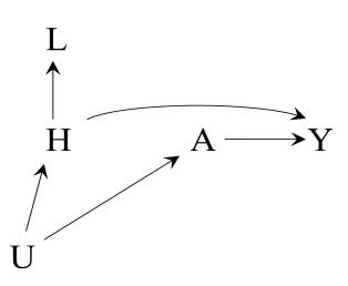
Figure 9.16

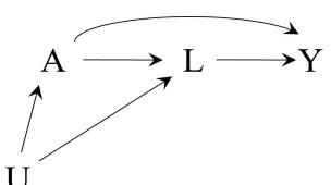
Figure 9.17

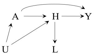
Figure 9.18

From noncausal diagrams to causal diagrams. Suppose some investigators interested in the effect of A on Y proposed the DAG in Figure 9.17. To draw this DAG, they relied on prior knowledge about the temporal order of the variables and the following two facts: (i) the measured variable L is associated with Y , and (ii) there is one set of unmeasured, but known, factors U that affect A and are associated with L. As discussed in Fine Point 7.4, the effect of A on Y is not identifiable if Figure 9.17 is the true causal diagram because L is a descendant of A.

Upon further reflection, the investigators realize that there are no well-defined interventions for the effect of L on Y . Therefore, the arrow L → Y is not a causal arrow and their DAG is not causal. To transform Figure 9.17 into a causal diagram, they add the hidden variable H with a causal arrow into Y and represent L as a surrogate of H. Figure 9.18 depicts their revised DAG. The effect of A on Y is not identifiable if Figure 9.18 is the true causal diagram because the backdoor path A ← U → H → Y cannot be blocked by any measured variable.

Note that the investigators kept the arrow U → A, which implies that they believe that there are well-defined interventions for the effect of U and A. They also redirected the arrows from U and A to L in Figure 9.17 towards H in Figure 9.18. This implies that the investigators believe that there must exist well-defined interventions for the effect of both U and A on H and that the effects of both U and A on L are fully mediated by their effect on H. (Even if L were a deterministic function of H, which is compatible with Figure 9.18, conditioning on L would not block paths through H because H is not a deterministic function of L, as it is of higher dimensionality and complexity than L.)

The inheritance by H in Figure 9.18 of all the arrows into L in Figure 9.17 is not always warranted. For example, U may have direct effect on L as in the causal DAG in Figure 9.19 rather than on H as in Figure 9.18. If, in fact, Figure 9.19 is the true causal DAG then the effect of A on Y would be identifiable because there are no open backdoor paths between A and Y . Note that, in Figure 19.9, the surrogate L cannot be a deterministic function of H as it is also affected by U. An example where, as in Figure 9.19, U has a direct effect on the surrogate L but no direct effect on H is the following: U denotes a physician’s decision to order a particular diagnostic test, L the result of the test, and H the underlying biological determinants of the test result.

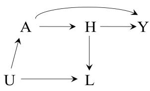
Figure 9.19

are sufficiently well-defined. We have argued that quantitative causal inference fundamentally relies on the (admittedly fuzzy) concept of sufficiently welldefined interventions. Therefore, in the remainder of this book, except for several well sign-posted exceptions, we will assume all DAGs are strictly causal in the sense that every arrow on the DAG represents a sufficiently well-defined intervention. That is, each arrow is associated with an intervention that can be specified in such a way that no meaningful vagueness remains based on current scientific knowledge. In a few years or decades, we may find out that our beliefs, and thus our causal diagrams, were incorrect.

Chapter 10 RANDOM VARIABILITY

Suppose an investigator conducted a randomized experiment to answer the causal question “does one’s looking up to the sky make other pedestrians look up too?” She found an association between her looking up and other pedestrians’ looking up. Does this association reflect a causal effect? By definition of randomized experiment, confounding bias is not expected in this study. In addition, no selection bias was expected because all pedestrians’ responses—whether they did or did not look up—were recorded, and no measurement bias was expected because all variables were perfectly measured. However, there was another problem: the study included only 4 pedestrians, 2 in each treatment group. By chance, 1 of the 2 pedestrians in the “looking up” group, and neither of the 2 pedestrians in the “looking straight” group, was blind. Thus, even if the treatment (the investigator’s looking up) truly had a strong average effect on the outcome (other people’s looking up), half of the individuals in the treatment group happened to be immune to the treatment. The small size of the study population led to a dilution of the estimated effect of treatment on the outcome.

There are two qualitatively different reasons why causal inferences may be wrong: systematic bias and random variability. The previous three chapters described three types of systematic biases: selection bias, measurement bias—both of which may arise in observational studies and in randomized experiments—and unmeasured confounding—which is not expected in randomized experiments. So far we have disregarded the possibility of bias due to random variability by restricting our discussion to huge study populations. In other words, we have operated as if the only obstacles to identify the causal effect were confounding, selection, and measurement. It is about time to get real: the size of study populations in etiologic research rarely precludes the possibility of bias due to random variability. This chapter discusses random variability and how we deal with it.

10.1 Identification versus estimation

The first nine chapters of this book are concerned with the computation of causal effects in study populations of near infinite size. For example, when computing the causal effect of heart transplant on mortality in Chapter 2, we only had a twenty-person study population but we regarded each individual in our study as representing 1 billion identical individuals. By acting as if we could obtain an unlimited number of individuals for our studies, we could ignore random fluctuations and could focus our attention on systematic biases due to confounding, selection, and measurement. Statisticians have a name for problems in which we can assume the size of the study population is effectively infinite: identification problems.

Thus far we have reduced causal inference to an identification problem. Our only goal has been to identify (or, as we often said, to compute) the average causal effect of treatment A on the outcome Y . The concept of identifiability was first described in Section 3.1—and later discussed in Sections 7.2 and 8.4—where we also introduced some conditions generally required to identify causal effects even if the size of the study population could be made arbitrarily large. These so-called identifying conditions were exchangeability, positivity, and consistency.

Our ignoring random variability may have been pedagogically convenient to introduce systematic biases, but also extremely unrealistic. In real research projects, the study population is not effectively infinite and hence we cannot ignore the possibility of random variability. To this end let us return to our twenty-person study of heart transplant and mortality in which 7 of the 13 treated individuals died.

Suppose our study population of 20 can be conceptualized as being a random sample from a super-population so large compared with the study population that we can effectively regard it as infinite. Further, suppose our goal is to make inferences about the super-population. For example, we may want to make inferences about the super-population probability (or proportion) Pr[Y = 1|A = a]. We refer to the parameter of interest in the super-population, the probability Pr[Y = 1|A = a] in this case, as the estimand. An estimator is a rule that takes the data from any sample from the super-population and produces a numerical value for the estimand. This numerical value for a particular sample is the estimate from that sample. The sample proportion of individuals that develop the outcome among those receiving treatment level ^a, Pr[ ^{c Y} = 1 ^{| A = a}], is an estimator of the super-population probability Pr[^Y = 1|^{A = a}]. The estimate from our sample is Pr[ ^{c Y} = 1 ^{| A = a}] = 7/13. More specifically, we say that 7/13 is a point estimate. The value of the estimate will depend on the particular 20 individuals randomly sampled from the super-population.

As informally defined in Chapter 1, an estimator is consistent for a particular estimand if the estimates get (arbitrarily) closer to the parameter as the sample size increases (see Technical Point 10.1 for the formal definition). Thus the sample proportion Pr[ ^{c Y} = 1 ^{| A = a}] consistently estimates the super-population probability Pr[Y = 1|A = a], i.e., the larger the number n of individuals in our study population, the smaller the magnitude of Pr[^Y = 1|^{A = a}] ⁻ Pr[ ^{c Y} = 1 ^{| A = a}] is expected to be. Previous chapters were exclusively concerned with identification; from now on we will be For an introduction to statistics, concerned with statistical estimation.

Even consistent estimators may result in point estimates that are far from the super-population value. Large differences between the point estimate and the super-population value of a proportion are much more likely to happen when the size of the study population is small compared with that of the superpopulation. Therefore it makes sense to have more confidence in estimates that originate from larger study populations. In the absence of systematic biases, statistical theory allows one to quantify this confidence in the form of a confidence interval around the point estimate. The larger the size of the study population, the narrower the confidence interval. A common way to construct a 95% confidence interval for a point estimate is to use a 95% Wald confidence interval centered at a point estimate. It is computed as follows.

First, estimate the standard error of the point estimate under the assumption that our study population is a random sample from a much larger superpopulation. Second, calculate the upper limit of the 95% Wald confidence interval by adding 1.96 times the estimated standard error to the point estimate, and the lower limit of the 95% confidence interval by subtracting 1.96 times the estimated standard error from the point estimate. For example, consider our estimator Pr[ ^{c Y} = 1 ^{| A = a}] = ˆ^p of the super-population parameter Pr[^Y = 1|^{A = a}] = ^p. Its standard error is ^q p(1−p) n (the standard error of a binomial) and thus its estimated standard error is ^q pˆ(1−pˆ) ⁿ = q (7/13)(6/13) ¹³ = 0.138. Recall that the Wald 95% confidence interval for a parameter θ based on an estimator ^θb is ^θb±1.96×se^b θb where se^b θb is an estimate of the (exact

see the book by Wasserman (2004). For a more detailed introduction, see Casella and Berger (2002).

tered at pˆ is only guaranteed to be valid in large samples. For simplicity, here we assume that our sample size is sufficiently large for the validity of our Wald interval.

confidence interval, a Bayesian 95% credible interval can be interpreted as “there is a 95% probability that the estimand is in the interval”. However, for a Bayesian, probability is defined not as a frequency over hypothetical repetitions but as degree-of-belief. In this book we adopt the frequency definition of probability. See Fine Point 11.2 for more on Bayesian intervals.

confidence intervals other than the Wald interval (Casella and Berger, 2002). One of these might be preferred over the Wald interval, which can be badly anti-conservative in small samples (Brown et al, 2001). or large sample) standard error of ^θb and 1.96 is the upper 97.5% quantile of a standard normal distribution with mean 0 and variance 1. Therefore the 95% Wald confidence interval for our estimate is 0.27 to 0.81. The length and centering of the 95% Wald confidence interval will vary from sample to sample.

A Wald confidence interval cen- A 95% confidence interval is calibrated if the estimand is contained in the interval in 95% of random samples, conservative if the estimand is contained in more than 95% of samples, and anticonservative otherwise. We will say that a confidence interval is valid if, for any value of the true parameter, the interval is either calibrated or conservative, i.e. it covers the true parameter at least 95% of the time. We would like to choose the valid interval whose width is narrowest.

The validity of confidence intervals is defined in terms of the frequency of coverage in repeated samples from the super-population, but we only see one of those samples when we conduct a study. Why should we care about what would have happened in other samples that we did not see? One important answer is that the definition of confidence interval also implies the following. Suppose we and all of our colleagues keep conducting research studies for the rest of our lifetimes. In each new study, we construct a valid 95% confidence interval for the parameter of interest. Then, at the end of our lives, we can look back at all the studies that were conducted, and conclude that the parameters of interest were trapped in—or covered by—the confidence interval in at least 95% of the studies. Unfortunately, we will have no way of identifying the (up to) 5% of the studies in which the confidence interval failed to include the super-population quantity.

Importantly, the 95% confidence interval from a single study does not imply that there is a 95% probability that the estimand is in the interval. In our example, we cannot conclude that the probability that the estimand lies between the values 0.27 and 0.81 is 95%. The estimand is fixed, which implies that either it is or it is not included in the particular interval (0.27, 0.81). In this sense, the probability that the estimand is included in that interval is either 0 or 1. A confidence interval only has a frequentist interpretation. Its In contrast with a frequentist 95% level (e.g., 95%) refers to the frequency with which the interval will trap the unknown super-population quantity of interest over a collection of studies (or in hypothetical repetitions of a particular study).

Confidence intervals are often classified as either small-sample or largesample confidence intervals. A small-sample valid (conservative or calibrated) confidence interval is one that is valid at all sample sizes for which it is defined. Small-sample calibrated confidence intervals are sometimes called exact confidence intervals. A large-sample (equivalently, asymptotic) valid confidence interval is one that is valid only in large samples. A large-sample calibrated 95% confidence interval is one whose coverage becomes arbitrarily close to 95% as the sample size increases. The Wald confidence interval for Pr[Y = 1|A = a] = p mentioned above is a large-sample calibrated confidence interval, but not a small-sample valid interval. (There do exist small-sample There are many valid large-sample valid confidence intervals for p, but they are not often used in practice.) When the sample size is small, a valid large-sample confidence interval, such as the Wald 95% confidence interval of our example above, may not be valid. In this book, when we use the term 95% confidence interval, we mean a large-sample valid confidence interval, like a Wald interval, unless stated otherwise. See also Fine Point 10.1.

However, not all consistent estimators can be used to center a valid Wald confidence interval, even in large samples. Most users of statistics will consider an estimator unbiased if it can center a valid Wald interval and biased if it

Fine Point 10.1

Honest confidence intervals. The smallest sample size at which a large-sample, valid 95% confidence interval covers the true parameter at least 95% of the time may depend on the unknown value of the true parameter. We say a large-sample valid 95% confidence interval is uniform or honest if there exists a sample size n at which the interval is guaranteed to cover the true parameter value at least 95% of the time, whatever be the value of the true parameter. We demand honest intervals because, in the absence of uniformity, at any finite sample size there may be data generating distributions under which the coverage of the true parameter is much less than 95%. Unfortunately, for a large-sample, honest confidence interval, the smallest such n is generally unknown and is difficult to determine even by simulation. See Robins and Ritov (1997) for technical details.

In the remainder of the text, when we refer to valid confidence intervals, we will mean large-sample honest confidence intervals. By definition, any small-sample valid confidence interval is uniform or honest for all n for which the interval is defined.

cannot (see Technical Point 10.1 for details). For now, we will equate the term bias with the inability to center valid Wald confidence intervals. Also, bear in mind that confidence intervals only quantify uncertainty due to random error, and thus the confidence we put on confidence intervals may be excessive in the presence of systematic biases (see Fine Point 10.2 for details).

10.2 Estimation of causal effects

Suppose our heart transplant study was a marginally randomized experiment, and that the 20 individuals were a random sample of all individuals in a nearly infinite super-population of interest. Suppose further that all individuals in the super-population were randomly assigned to either A = 1 or A = 0, and that all of them adhered to their assigned treatment. Exchangeability of the treated and the untreated would hold in the super-population, i.e., Pr[Y ^a = 1] = Pr[Y = 1|A = a], and therefore the causal risk difference Pr[Y ^a=1 = 1] − Pr[Y ^a=0 = 1] equals the associational risk difference Pr[Y = 1|A = 1]−Pr[Y = 1|A = 0] in the super-population.

Because our study population is a random sample of the super-population, the sample proportion of individuals that develop the outcome among those with observed treatment value ^{A = a}, Pr[ ^{c Y} = 1 ^{| A = a}], is an unbiased estimator of the super-population probability Pr[Y = 1|A = a]. Because of exchangeability in the super-population, the sample proportion Pr[ ^{c Y} = 1 ^{| A =} a] is also an unbiased estimator of Pr[Y ^a = 1]. Thus, traditional statistical “testing”of the causal null hypothesis Pr[Y ^a=1 = 1] = Pr[Y ^a=0 = 1] boils down to comparing the sample proportions Pr [ ^{c Y} = 1 ^{| A} = 1] = 7/13 and Pr [ ^{c Y} = 1 ^{| A} = 0] = 3/7. Standard statistical methods can also be used to compute 95% confidence intervals for the causal risk difference and causal risk ratio in the super-population, which are estimated by (7/13) − (3/7) and (7/13)/(3/7), respectively. Slightly more involved, but standard, statistical procedures are used in observational studies to obtain confidence intervals for standardized, IP weighted, or stratified association measures.

There is an alternative way to think about sampling variability in randomized experiments. Suppose only individuals in the study population, not all individuals in the super-population, are randomly assigned to either A = 1

Bias and consistency in statistical inference. We have discussed systematic bias (due to unknown sources of confounding, selection, or measurement error) and consistent estimators in earlier chapters. Here we discuss these and other concepts of bias, and describe how they are related.

To provide a formal definition of consistent estimator for an estimand θ, suppose we observe n independent, identically distributed (i.i.d.) copies of a vector-valued random variable whose distribution P lies in a set M of distributions (our model). Then the estimator ^θbⁿ is consistent for ^{θ = θ} (P) in model ^M if ^θbⁿ converges to ^θ in probability for every P ∈ M i.e.

\[\Pr\_P\left[\left|\widehat{\theta}\_n - \theta\left(P\right)\right| > \varepsilon\right] \to 0 \text{ as } n \to \infty \text{ for every } \varepsilon > 0, P \in \mathcal{M}.\]

The estimator ^θbⁿ is exactly unbiased in model ^M if, for every ^P ∈ M,E^P h θbn i = θ (P). The exact bias under P is the difference E^P h θbn i ^{− θ} (P). We denote the estimator by ^θbⁿ rather than by simply ^θb to emphasize that the estimate depends on the sample size n. On the other hand, the parameter θ (P) is a fixed, though unknown, quantity depending on P ∈ M. When P is the distribution generating the data in our study, we often suppress the P in the notation and write E h θbn i = θ. For many parameters θ, such as the risk ratio Pr[Y = 1|A = 1]/Pr[Y = 1|A = 0], exactly unbiased estimators do not exist.

A systematically biased estimator is neither consistent nor exactly unbiased. Robins and Morgenstern (1987) argue that most applied researchers (e.g., epidemiologists) will declare an estimator unbiased only if it can center a valid Wald confidence interval. They show that under this definition, an estimator is only unbiased if it is uniformly asymptotic normal and unbiased (UANU), as only UANU estimators can center valid standard Wald intervals for θ (P) under the model ^M. An estimator ^θbⁿ is UANU in model ^M if there exists sequences ^σn (P) such that the z-statistic ^θb^{n − θ} (P) /σⁿ (P) converges uniformly to a standard normal random variable in the following sense: for t ∈ R,

\[\sup\_{P \in \mathcal{M}} |\Pr\_P \left[ n^{1/2} \left( \widehat{\theta}\_n - \theta \left( P \right) \right) / \sigma\_n \left( P \right) < t \right] - \Phi \left( t \right)| \to 0 \text{ as } n \to \infty\]

where Φ (t) is the standard normal cumulative distribution function (Robins and Ritov,1997).

All inconsistent estimators and some consistent estimators (see Chapter 18 for examples) are biased under this definition. In this book, when we say an estimator is unbiased (without further qualification) we mean that it is UANU.

or A = 0. Because of the presence of random sampling variability, we do not expect that exchangeability will exactly hold in our sample. For example, suppose that only the 20 individuals in our study were randomly assigned to either heart transplant (A = 1) or medical treatment (A = 0). Suppose further that each individual can be classified as good or bad prognosis at the time of randomization. We say that the groups A = 0 and A = 1 are exchangeable if they include exactly the same proportion of individuals with bad prognosis. By chance, it is possible that 2 out of the 13 individuals assigned to A = 1 and 3 of the 7 individuals assigned to A = 0 had bad prognosis. However, if we increased the size of our sample then there is a high probability that the relative imbalance between the groups A = 1 and A = 0 would decrease.

Under this conceptualization, there are two possible targets for inference. First, investigators may be agnostic about the existence of a super-population and restrict their inference to the sample that was actually randomized. This is See Robins (1988) and Green- referred to as randomization-based inference, and requires taking into account some technicalities that are beyond the scope of this book. Second, investigators may still be interested in making inferences about the super-population from which the study sample was randomly drawn. From an inference stand-

land (1991) for a discussion of randomization-based inference.

Fine Point 10.2

Uncertainty from systematic biases. The width of the usual Wald-type confidence intervals is a function of the standard error of the estimator and thus reflects only uncertainty due to random error. However, the possible presence of systematic bias due to confounding, selection, or measurement is another important source of uncertainty. The larger the study population, the smaller the random error is both absolutely and as a proportion of total uncertainty, and hence the more the usual Wald confidence interval will understate the true uncertainty.

The stated 95% confidence in a 95% confidence interval becomes overconfidence as population size increases because the interval excludes uncertainty due to systematic biases, which are not diminished by increasing the sample size. As a consequence, some authors advocate referring to such intervals by a less confident name, calling them compatibility intervals instead. The renaming recognizes that such intervals can only show us which effect sizes are highly compatible with the data under our adjustment assumptions and methods (Amrhein et al. 2019; Greenland 2019). The compatibility concept is weaker than the confidence concept, for it does not demand complete confidence that our adjustment removes all systematic biases.

Regardless of the name of the intervals, the uncertainty due to systematic bias is usually a central part of the discussion section of scientific articles. However, most discussions revolve around informal judgments about the potential direction and magnitude of the systematic bias. Some authors argue that quantitative methods need to be used to produce intervals around the effect estimate that integrate random and systematic sources of uncertainty. These methods are referred to as quantitative bias analysis. See the book by Lash, Fox, and Fink (2009). Bayesian alternatives are discussed by Greenland and Lash (2008), and Greenland (2009a, 2009b).

point, this latter case turns out to be mathematically equivalent to the conceptualization of sampling variability described at the start of this section in which the entire super-population was randomly assigned to treatment. That is, randomization followed by random sampling is equivalent to random sampling followed by randomization.

In many cases we are not interested in the first target. To see why, consider a study that compares the effect of two first-line treatments on the mortality of cancer patients. After the study ends, we may determine that it is better to initiate one of the two treatments, but this information is now irrelevant to the actual study participants. The purpose of the study was not to guide the choice of treatment for patients in the study but rather for a group of individuals similar to—but larger than—the studied sample. Heretofore we have assumed that there is a larger group—the super-population—from which the study participants were randomly sampled. We now turn our attention to the concept of the super-population.

10.3 The myth of the super-population

As discussed in Chapter 1, there are two sources of randomness: sampling variability and nondeterministic counterfactuals. Below we discuss both.

Consider our estimate Pr[ ^{c Y} = 1 ^{| A} = 1] = ˆ^p = 7/13 of the superpopulation risk Pr[Y = 1|A = a] = p. Nearly all investigators would report a binomial confidence interval ˆp±1.96^q pˆ(1−pˆ) ⁿ = 7/13±1.96^q (7/13)(6/13) ¹³ for the probability p. If asked why these intervals, they would say it is to incorporate the uncertainty due to random variability. But these intervals are valid only if ˆp has a binomial sampling distribution. So we must ask when would that happen. In fact there are two scenarios under which ˆp has a binomial sampling

distribution.

cal Point 10.1 means that our data were a random sample of size n from a super-population.

Robins (1988) discussed these two we have considered so far. scenarios in more detail.

• Scenario 1. The study population is sampled at random from an essentially infinite super-population, sometimes referred to as the source The term i.i.d. used in Techni- or target population, and our estimand is the proportion p = Pr[Y = 1|A = 1] of treated individuals who developed the outcome in the superpopulation. It is then mathematically true that, in repeated random samples of size 13 from the treated individuals in the super-population, the number of individuals who develop the outcome among the 13 is a binomial random variable with success probability Pr[Y = 1|A = 1]. As a result, the 95% Wald confidence interval calculated in the previous section is asymptotically calibrated for Pr[Y = 1|A = 1]. This is the model
  • Scenario 2. The study population is not sampled from a hypothetical super-population. Rather (i) each individual i among the 13 treated individuals has an individual nondeterministic (stochastic) counterfactual probability p a=1 i (ii) the observed outcome Yⁱ = Y a=1 i for subject i occurs with probability p a=1 i and (iii) p a=1 i takes the same value, say p, for each of the 13 treated individuals. Then the number of individuals who develop the outcome among the 13 treated is a binomial random variable with success probability p. As a result, the 95% confidence interval calculated in the previous section is asymptotically calibrated for p.

Scenario 1 assumes a hypothetical super-population. Scenario 2 does not. However, Scenario 2 is untenable because the probability p a=1 i of developing the outcome when treated will almost certainly vary among the 13 treated individuals due to between-individual differences in risk. For example we would expect the probability of death p a=1 i to have some dependence on an individual’s genetic make-up. If the p a=1 i are nonconstant then the estimand of interest in the actual study population would generally be the average, say p, of the 13 p a=1 i . But in that case the number of treated who develop the outcome is not a binomial random variable with success probability p, and the 95% confidence interval for p calculated in the previous section is not asymptotically calibrated but conservative.

Therefore, any investigator who reports a binomial confidence interval for Pr[Y = 1|A = a], and who acknowledges that there exists between-individual variation in risk, must be implicitly assuming Scenario 1: the study individuals were sampled from a near-infinite super-population and that all inferences are concerned with quantities from that super-population. Under Scenario 1, the number with the outcome among the 13 treated is a binomial variable regardless of whether the underlying counterfactual is deterministic or stochastic.

An advantage of working under the hypothetical super-population scenario is that nothing hinges on whether the world is deterministic or nondeterministic. On the other hand, the super-population is generally a fiction; in most studies individuals are not randomly sampled from any near-infinite population. Why then has the myth of the super-population endured? One reason is that it leads to simple statistical methods.

A second reason has to do with generalization. As we mentioned in the previous section, investigators generally wish to generalize their findings about treatment effects from the study population (e.g., the 20 individuals in our heart transplant study) to some large target population (e.g., all immortals in the Greek pantheon). The simplest way of doing so is to assume the study population is a random sample from a large population of individuals who are potential recipients of treatment. Since this is a fiction, a 95% confidence interval computed under Scenario 1 should be interpreted as covering the super-population parameter had, often contrary to fact, the study individuals been sampled randomly from a near infinite super-population. In other words, confidence intervals obtained under Scenario 1 should be viewed as what-if statements.

It follows from the above that an investigator might not want to entertain Scenario 1 if the size of the pool of potential recipients is not much larger than the size of the study population, or if the target population of potential recipients is believed to differ from the study population to an extent that cannot be accounted for by sampling variability. Here we will accept that individuals were randomly sampled from a super-population, and explore the consequences of random variability for causal inference in that context. We first explore this question in a simple randomized experiment.

10.4 The conditionality “principle”

Table 10.1 summarizes the data from a randomized trial to estimate the average causal effect of treatment A (1: yes, 0: no) on the 1-year risk of death Y (1: yes, 0: no). The experiment included 240 individuals, 120 in each treatment group. The associational risk difference is Pr[Y = 1|A = 1] − Pr[Y = 1|A = 0] = ^{24 120} − 42 ¹²⁰ = −0.15. Suppose the experiment had been conducted in a super-population of near-infinite size, the treated and the untreated would be exchangeable, i.e., Y ^a⊥⊥A, and the associational risk difference would equal the causal risk difference Pr - Y ^a=1 = 1 − Pr - Y ^a=0 = 1 The estimated variance of the un- . Suppose the study investigators computed a 95% confidence interval (−0.26, −0.04) around the point estimate −0.15 and published an article in which they concluded that treatment was beneficial because it reduced the risk of death by 15 percentage points.

However, the study population had only 240 individuals and is therefore likely that, due to chance, the treated and the untreated are not perfectly exchangeable. Random assignment of treatment does not guarantee exact ex-Table 10.1 changeability for the sample consisting of the 240 individuals in the trial; it only guarantees that any departures from exchangeability are due to random variability rather than to a systematic bias. In fact, one can view the uncertainty resulting from our ignorance of the chance correlation between unmeasured baseline risk factors and the treatment A in the study sample as contributing to the length 0.22 of the confidence interval.

A few months later the investigators learn that information on a third Table 10.2 variable, cigarette smoking L (1: yes, 0: no), had also been collected and decide to take a look at it. The study data, stratified by L, is shown in Table 10.2. Unexpectedly, the investigators find that the proportion of individuals receiving treatment among smokers (80/120) is twice that among nonsmokers (40/120), which suggests that the treated and the untreated are not exchangeable and thus that adjustment for smoking is necessary. When the investigators adjust via stratification, the associational risk difference in smokers, Pr[Y = 1|A = 1, L = 1] − Pr[Y = 1|A = 0, L = 1], is equal to 0. The associational risk difference in nonsmokers, Pr[Y = 1|A = 1, L = 0] − Pr[Y = 1|A = 0, L = 0], is also equal to 0. The adjusted analysis suggests treatment has no effect in both smokers and nonsmokers, even though the marginal risk difference −0.15 suggested a net beneficial effect in the study population.

adjusted estimator is 24 120 96 120 ¹²⁰ + 42 120 78 120 ¹²⁰ = 31 ⁹⁶⁰⁰ . The Wald 95% confidence interval is then −0.15 ± 31 ⁹⁶⁰⁰ 1/² × 1.96 = (−0.26, −0.04).

	Y = 1	Y = 0
A = 1	24	96
A = 0	42	78

L = 1	Y = 1	Y = 0
A = 1	4	76
A = 0	2	38
L = 0	Y = 1	Y = 0
A = 1	20	20

A formal statement of the conditionality principle. The likelihood for the observed data has three factors: the density of Y given A and L, the density of A given L, and the marginal density of L. Consider a simple example with one dichotomous L, exchangeability Y ^a⊥⊥A|L, the stratum-specific risk difference sRD = Pr (Y = 1|L = l, A = 1) − Pr (Y = 1|L = l, A = 0) known to be constant across strata of L, and in which the parameter of interest is the stratumspecific causal risk difference. Then the likelihood of the data is

\[\prod\_{i=1}^{n} f\left(Y\_i | L\_i, A\_i; sRD, p\_0\right) \times f\left(A\_i | L\_i; \alpha\right) \times f\left(L\_i; \rho\right)\]

where p⁰ = (p01, p02) with p0^l = Pr (Y = 1|L = l, A = 0), α, and ρ are nuisance parameters associated with the conditional density of Y given A and L, the conditional density of A given L, and the marginal density of L, respectively. See, for example, Casella and Berger (2002).

The data on A and L are said to be S-ancillary for the parameter of interest when, as in this case, the distribution of the data conditional on these variables depends on the parameter of interest, but the joint density of A and L does not share parameters with f (Yⁱ |Lⁱ , Aⁱ ; sRD, p0). The conditionality principle states that one should always perform inference on the parameter of interest conditional on any S-ancillary statistics. Thus one should condition on the Sancillary statistic {Aⁱ , Lⁱ ;i = 1, .., n}. Analogously, if the risk ratio (rather than the risk difference) were known to be constant across strata of L, {Aⁱ , Lⁱ ;i = 1, .., n} remains S-ancillary for the risk ratio.

An exact ancillary statistic is defined to be an S-ancillary statistic whose marginal distribution is known. In our example, this would require that α and ρ be known.

justed estimator is described in Technical Point 10.5. The Wald 95% confidence interval is then (−0.076, 0.076).

The estimated variance of the ad- These new findings are disturbing to the investigators. Either someone did not assign the treatment at random (malfeasance) or randomization did not result in approximate exchangeability (very very bad luck). A debate ensues among the investigators. Should they retract their article and correct the results? They all agree that the answer to this question would be affirmative if the problem were due to malfeasance. If that were the case, there would be confounding by smoking and the effect estimate should be adjusted for smoking. But they all agree that malfeasance is impossible given the study’s quality assurance procedures. It is therefore clear that the association between smoking and treatment is entirely due to bad luck. Should they still retract their article and correct the results?

One investigator says that they should not retract the article. His argument goes as follows: “Okay, randomization went wrong for smoking, but why should we privilege the adjusted over the unadjusted estimator? It is likely that imbalances on other unmeasured factors U cancelled out the effect of the chance imbalance on L, so that the unadjusted estimator is still the closer to the true value in the super-population.” A second investigator says that they should retract the article and report the adjusted null result. Her argument goes as follows: “We should adjust for L because the strong association between L and A introduces confounding in our effect estimate. Within levels of L, we have mini randomized trials and the confidence intervals around the corresponding point estimates will reflect the uncertainty due to the possible U-A associations conditional on L.”

To determine which investigator is correct, here are the facts of the matter. Suppose, for simplicity, the true causal risk difference is constant across strata of L, and suppose we could run the randomized experiment trillions of times. We then select only (i.e., condition on) those runs in which smoking L and

Approximate ancillarity. Suppose that the stratum-specific risk difference (sRDl) is known to vary over strata of L. Under our usual identifiability assumptions, the causal risk difference in the population is identified by the standardized risk difference

\[RD\_{std} = \sum\_{l} \left[ \Pr\left(Y = 1 | L = l, A = 1; \upsilon\right) - \Pr\left(Y = 1 | L = l, A = 0; \upsilon\right) \right] f\left(l; \rho\right)\]

which depends on the parameters υ = {sRD^l , p0,l; l = 0, 1} and ρ (see Technical Point 10.2). In unconditionally randomized experiments, RDstd equals the associational RD, Pr (Y = 1|A = 1) − Pr (Y = 1|A = 0), because A⊥⊥L in the super-population. Due to the dependence of RDstd on ρ, {Aⁱ , Lⁱ ;i = 1, .., n} is no longer exactly ancillary and in fact no exact ancillary exists.

Consider the statistic ^{Se =} ORdAL ⁻ ORAL where ORAL ⁼ ORAL (α) = Pr(A=1|L=1;α) Pr(A=0|L=0;α) Pr(A=1|L=0;α) Pr(A=0|L=1;α) is the A-L odds ratio in the super-population, and ORdAL is ORAL but with the the population proportions Pr (^{A = a}|^{L = l}; ^α) replaced by the empirical sample proportions Pr ( ^{c A = a}|^{L = l}). ^Se is asymptotically normal with mean ⁰ conditional on the ^Li and thus its distribution depends on ^α. Let ^{Sb =} S/^e se^b (Se), where se^b (Se) is an estimate of the standard error of ^Se. The distribution of ^Sb converges to a standard normal distribution in large samples, so that ^Sb quantifies the ^A-^L association in the data on a standardized scale. For example, if ^Sb = 2, then ^Sb is two standard deviations above its (asymptotic) expected value of 0.

When the true value of ORAL is known, ^Sb is referred to as an approximate (or large sample) ancillary statistic. To see why, consider a randomized experiment with ORAL = 1. Then ^Sb, like an exact ancillary statistic, i) can be computed from the data (i.e., ^{Sb =} ORdAL ^{− 1} /se^b (Se)), ii) ^Sb has an approximately known distribution, iii) the likelihood factors into a term ^f (A|L; ^α) that governs the distribution of ^Se and a term ^f (^{Y |}L, A; ^υ) ^f (L; ^ρ) that does not depend on ^α, and iv) conditional on ^Sb, the adjusted estimate of RDstd is unbiased, while the unadjusted estimate of RDstd is biased (Technical Point 10.4 defines and compares adjusted and unadjusted estimators). Any other statistic that quantifies the A-L association Pr( ^{c A}=1|L=1) Pr( ^{c A}=1|L=0) ^{− 1}, can be used in place of ^Se.

Now consider a continuity principle wherein inferences about an estimand should not change discontinuously in response to an arbitrarily small known change in the data generating distribution (Buehler 1982). If one accepts both the conditionality and continuity principles, then one should condition on an approximate ancillary statistic. For example, when ORAL = 1 is known, the continuity principle would be violated if, following the conditionality principle, we treated the unadjusted estimate of RDstd as biased when sRD^l was known to be a constant, but treated it as unbiased when the sRD^l were almost constant. We will say that a researcher who always conditions on both exact and approximate ancillaries follows the extended conditionality principle.

treatment A are as strongly positively associated as in the observed data. We would find that, within each level of L, the fraction of these runs in which any given pre-treatment risk factor U for Y was positively associated with A essentially equals the number of runs in which it was negatively associated. (This is true even if U and L are highly correlated in both the super-population and in the study data.)

As a consequence, the adjusted estimate of the treatment effect is unbiased but the unadjusted estimate is greatly biased when averaged over these runs. The unconditional efficiency of the Unconditionally—over all the runs of the experiment—both the unadjusted and adjusted estimates are unbiased but the variance of the adjusted estimate is smaller than that of the unadjusted estimate. That is, the adjusted estimator is both conditionally unbiased and unconditionally more efficient. Hence either from the conditional or unconditional point of view, the Wald interval centered on the adjusted estimator is the better analysis and the article needs to be retracted. The second investigator is correct.

adjusted estimator results from the adjusted estimator being the maximum likelihood estimator (MLE) of the risk difference when data on L are available.

Comparison between adjusted and unadjusted estimators. The adjusted estimator of RDstd in Technical Point 10.3 is the parametric maximum likelihood estimator RDdMLE, which replaces the population proportions in the RDstd by their sample proportions. The unadjusted estimator of RDstd is RDdUN ⁼ Pr ( ^{c Y} = 1|^A = 1) ⁻ Pr ( ^{c Y} = 1|^A = 0). Unconditionally, both RDdMLE and RDdUN are asymptotically normal and unbiased for RDstd with asymptotic variances aV ar RDdMLE and aV ar RDdUN .

In the text we stated that RDdUN is both unconditionally inefficient and conditionally biased. We now explain that both properties are logically equivalent. Robins and Morgenstern (1987) prove that RDdMLE has the same asymptotic distribution conditional on the approximate ancillary ^Sb as it does unconditionally, which implies aV ar RDdMLE = aV ar RDdMLE|S^b . They also show that aV ar RDdMLE equals aV ar RDdUN − h aCov S, ^b RDdUN i² . Hence RDdUN is unconditionally inefficient if and only if aCov S, ^b RDdUN ̸= 0, i.e., ^Sb and RDdUN are correlated unconditionally. Further, the conditional asymptotic bias aE h RDdUN ^|S^b i ⁻ RDstd is shown to equal aCov S, ^b RDdUN ^Sb. Hence, RDdUN is conditionally biased if and only if it is unconditionally inefficient. It can be shown that aCov

S, ^b RDdUN = 0 if and only if L⊥⊥Y |A. Therefore, when data on a measured risk factor for ^Y are available, RDdMLE is preferred over RDdUN . The estimator RDdUN ⁻ aCov S, ^b RDdUN ^Sb corrects the bias of RDdUN , and thus has the same asymptotic distribution as RDdMLE given the approximate ancillary ^Sb.

The idea that one should condition on the observed L-A association is an example of what is referred to in the statistical literature as the conditionality principle. In statistics, the observed L-A association is said to be an ancillary statistic for the causal risk difference. The conditionality principle states that inference on a parameter should be performed conditional on ancillary statistics (see Technical Points 10.2 and 10.3 for details).

In the above discussion about the findings of the randomized experiment, some of the investigators intuitively followed the conditionality principle because they considered an estimator to be biased when it cannot center a valid Wald confidence interval conditional on any ancillary statistics. For such researchers, our previous definition of bias was not sufficiently restrictive. They would say that an estimator is unbiased if and only if it can center a valid Wald interval conditional on ancillary statistics. Technical Point 10.5 argues that most researchers implicitly follow the conditionality principle.

When confronted with the frequentist argument that “Adjustment for L is unnecessary because unconditionally—over all the runs of the experiment the unadjusted estimate is unbiased,” investigators that intuitively apply the conditionality principle would aptly respond “Why should the various L-A associations in other hypothetical studies affect what I do in my study? In my study L acts as a confounder and adjustment is needed to eliminate bias.” This is a convincing argument for both randomized experiments and observational studies as long as, like in the randomized experiment of our example, the number of measured confounders is not large. However, when the number of measured confounders is large, strictly following the conditionality principle is no longer a wise strategy.

Most researchers intuitively follow the extended conditionality principle. Consider again the randomized trial data in Table 10.2. Assuming without loss of generality that the sRD is constant over the strata of a dichotomous L, the estimated variance of the MLE of sRD is ^Vb⁰Vb¹/ ^Vb^{0 + V}b¹ where ^Vb^l is the estimated variance of RDd^l .

Two possible choices for ^Vb¹ are ^Vb obs ¹ = 4 80 76 80 ⁸⁰ + 2 40 38 40 ⁴⁰ = 1.^{78 × 10}−^{3 =} and ^Vbexp ¹ = 4 80 76 80 ⁶⁰ + 2 40 38 40 ⁶⁰ = 1.58 × 10−³ that differ only in that ^Vb obs ¹ divides by the observed number of individuals in stratum L = 1 with A = 1 and A = 0 (80 and ⁴⁰, respectively) while ^Vbexp 1 divides by the expected number of subjects (60) given that ^A⊥⊥L. Mathematically, ^Vb obs 1 is the variance estimator based on the observed information and ^Vbexp 1 is the estimator based on the expected information.

In our experience, nearly all researchers would choose ^Vb obs ¹ over ^Vbexp 1 as the appropriate variance estimator. Results of Efron and Hinkley (1978) and Robins and Morgenstern (1987) imply that such researchers are implicitly conditioning on an approximate ancillary ^Sb and thus, whether aware of this fact or not, are following the extended conditionality principle. Specifically, these authors proved that the variance of RDd^l , and thus of the MLE, conditioned on an approximate ancillary ^Sb differs from the unconditional variance by order ⁿ −3/2 . (As noted in Technical Point 10.4, the conditional and unconditional asymptotic variance of an MLE are equal, as equality of asymptotic variances implies equality only up to order n −1 .) Further, they showed that the variance estimator based on the observed information differs from the conditional variance by less than order n −3/2 , while an estimator based on the expected information differs from the unconditional variance by less than n −3/2 . Thus, a preference for ^Vb obs ¹ over ^Vbexp 1 implies a preference for conditional over unconditional inference.

10.5 The curse of dimensionality

The derivations in previous sections above are based on an asymptotic theory that assumed the number of strata of L was small compared with the sample size. In this section, we study the cases in which the number of strata of a vector L can be very large, even much larger than the sample size.

Suppose the investigators had measured 100 pre-treatment binary variables rather than only one, then the pre-treatment variable L formed by combining the 100 variables L = (L1, …, L100) has 2¹⁰⁰ strata. When, as in this case, there are many possible combinations of values of the pre-treatment variables, we say that the data is of high dimensionality. For simplicity, suppose that there is no additive effect modification by L, i.e., the super-population risk difference Pr[Y = 1|A = 1, L = l] − Pr[Y = 1|A = 0, L = l] is constant across the 2¹⁰⁰ strata. In particular, suppose that the constant stratum-specific risk difference is 0.

The investigators debate again whether to retract the article and report their estimate of the stratified risk difference. They have by now agreed that they should follow the conditionality principle because the unadjusted risk difference −0.15 is conditionally biased. However, they notice that, when there are 2¹⁰⁰ strata, a 95% confidence interval for the risk difference based on the adjusted estimator is much wider than that based on the unadjusted estimator. This is exactly the opposite of what was found when L had only two strata. In fact, the 95% confidence interval based on the adjusted estimator may be so wide as to be completely uninformative.

To see why, note that, because 2¹⁰⁰ is much larger than the number of individuals (240), there will at most be only a few strata of L that will contain both a treated and an untreated individual. Suppose only one of 2¹⁰⁰ strata contains a single treated individual and a single untreated individual, and no other stratum contains both a treated and untreated individual. Then the

Can the curse of dimensionality be reversed? In high-dimensional settings with many strata of L, informative conditional inference for the common risk difference given the exact ancillary statistic {Aⁱ , Lⁱ ;i = 1, ..n} is not possible regardless of the estimator used. This is not true for unconditional inference in marginally randomized experiments. For example, the unconditional statistical behavior of the unadjusted estimator RDdUN is unaffected by the dimension of L. In particular, it remains unbiased with the width of the associated Wald 95% confidence interval proportional to 1/n1/² . Because RDdUN relies on prior information not used by the MLE, it is an unbiased estimator of the common risk difference only if it is known that A⊥⊥L in the super-population.

However, even unconditionally, the confidence intervals associated with the MLE, i.e., the adjusted estimator, remain uninformative. This raises the question of whether data on L can be used to construct an estimator that is also unconditionally unbiased but that is more efficient that the unadjusted estimator. In Chapter 18 we show that this is sometimes possible.

95% confidence interval for the common risk difference based on the adjusted estimator is (−1, 1) , and therefore completely uninformative, because in the single stratum with both a treated and an untreated individual, the empirical risk difference could be −1, 0, or 1 depending on the value of Y for each individual. In contrast, the 95% confidence interval for the common risk difference based on the unadjusted estimator remains (−0.26, −0.04) as above because its width is unaffected by the fact that more covariates were measured. These results reflect the fact that the adjusted estimator is only guaranteed to be more efficient than the unadjusted estimator when the ratio of number of individuals to the number of unknown parameters is large (a frequently used rule of thumb is a minimum ratio of 10, though the minimum ratio depends on the characteristics of the data).

What should the investigators do? By trying to do the right thing following the conditionality principle—in the simple setting with one dichotomous variable, they put themselves in a corner for the high-dimensional setting. This is the curse of dimensionality: conditional on all 100 covariates the marginal estimator is still biased, but now the conditional estimator is Robins and Ritov (1997) provide a uninformative. This shows that, just because conditionality is compelling in simple examples, it should not be raised to a principle since it cannot be carried through for high-dimensional models. Though we have discussed this issue in the context of a randomized experiment, our discussion applies equally to observational studies. See Technical Point 10.6.

Finding a solution to the curse of dimensionality is a difficult problem and an active area of research. In Chapter 18 we review this research and offer some practical guidance. Chapters 11 through 17 provide necessary background information on the use of models for causal inference.

technical description of the curse of dimensionality.

Implications of random variability for causal discovery. In Fine Point 6.3 we explained that, under faithfulness, we could sometimes learn the causal structure if we had an infinite amount of data. After the concepts introduced in this chapter, we are now ready to consider the implications for causal discovery of only having a finite sample.

Suppose we have data on 3 variables Z, A, Y and we know that their time sequence is Z first, A second, and Y last. Our data analysis finds that the empirical odds ratio of Y and Z equal to 1 at every level of A. All other odds ratios, marginal and conditional, are far from 1. In Fine Point 6.3 we showed that, if Z⊥⊥Y |A in the super-population (which would require an infinite sample size) then, under faithfulness, the only possible causal diagram is Z → A → Y with perhaps a common cause U of Z and A in addition to (or in place of) the arrow from Z to A. It follows that the risk difference E[Y |A = 1] − E[Y |A = 0] is the average causal effect of A on Y . But, in practice, evidence of conditional or unconditional independence must be based on a finite sample size.

Robins et al. (2003) showed that, even if one is willing to assume faithfulness, inferences based on faithfulness are non-uniform, i.e., no matter how big the sample size n, even if the empirical odds ratio of Y and Z were equal to 1 at every level of A, there exist faithful distributions with the following properties: a) due to sampling variability, the true odds ratio of Y and Z at each level of A, although not equal to 1, is so close to 1 that empirical conditional odds ratios of 1 are unsurprising, and yet b) the average causal effect of A on Y is zero. As a consequence, no honest 95% frequentist confidence interval for the average causal effect of A on Y can ever exclude the value 0 even when the empirical risk difference estimate of E[Y |A = 1] − E[Y |A = 0] is quite large (say, 0.2) and is many (say 30) times greater than its standard error.

Even so, advocates of causal discovery may cogently argue that, given the empirical data above, a Bayesian (with priors not depending on sample size) who believes in faithfulness will generally have a (highest posterior density) 95% credible interval for the average causal effect of A on Y that is nearly centered on the empirical risk difference, with width not much greater than the standard error of the empirical risk difference. Thus, this credible interval easily excludes zero whenever graphs with Z and Y d-separated by A are given a non-negligible prior probability.

The striking difference between the honest frequentist confidence intervals and these credible intervals is a consequence of the fact that Bayesian inference for causal effects can be very sensitive to choice of prior in the causal discovery setting. For example, many epidemiologists, including the authors, would argue that, in an observational study, the prior probability given to any causal diagram that lacks a common cause of A and Y (such as the graph Z → A → Y ) should be essentially zero. To believe otherwise, A and Y must have had no common cause from the big bang till now. A Bayesian who shares our prior belief may have (depending on other aspects of the prior) a 95% credible interval much wider and with a center much closer to 0 than the credible interval described above.

In summary, in finite samples and even under faithfulness, data alone cannot distinguish the causal diagram Z → A → Y under which Z⊥⊥Y |A in the super-population from another causal diagram under which Z is almost independent of Y given A in the super-population. Therefore the validity of causal discovery from observational data relies heavily on a priori subject-matter knowledge about the plausibility of various causal diagrams.

Part II

Causal inference with models

Chapter 11 WHY MODEL?

Do not worry. No more chapter introductions around the effect of your looking up on other people’s looking up. We squeezed that example well beyond what seemed possible. In Part II of this book, most examples involve real data. The data sets can be downloaded from the book’s web site.

Part I was mostly conceptual. Calculations were kept to a minimum, and could be carried out by hand. In contrast, the material described in Part II requires the use of computers to fit regression models, such as linear and logistic models. Because this book cannot provide a detailed introduction to regression techniques, we assume that readers have a basic understanding and working knowledge of these commonly used models. Our web site provides links to computer code in R, SAS, Stata, and Python to replicate the analyses described in the text. The code margin notes specify the portion of the code that is relevant to the analysis described in the text.

This chapter describes the differences between the nonparametric estimators used in Part I and the parametric (model-based) estimators used in Part II. It also reviews the concept of smoothing and, briefly, the bias-variance trade-off involved in any modeling decision. The chapter motivates the need for models in data analysis, regardless of whether the analytic goal is causal inference or, say, prediction. We will take a break from causal considerations until the next chapter. Please bear in mind that the statistical literature on modeling is vast; this chapter can only highlight some of the key issues.

11.1 Data cannot speak for themselves

Consider a study population of 16 individuals infected with the human immunodeficiency virus (HIV). Unlike in Part I of this book, we will not view these individuals as representatives of 1 billion individuals identical to them. Rather, these are just 16 individuals randomly sampled from a large, possibly hypothetical super-population: the target population.

At the start of the study each individual receives a certain level of a treatment A (antiretroviral therapy), which is maintained during the study. At the end of the study, a continuous outcome Y (CD4 cell count, in cells/mm³ ) is measured in all individuals. We wish to consistently estimate the mean of Y among individuals with treatment level A = a in the population from which the 16 individuals were randomly sampled. That is, the estimand is the unknown population parameter E[Y |A = a].

As defined in Chapter 10, an estimator E[ ^{b Y |A = a}] of E[^{Y |A = a}] is some function of the data that is used to estimate the unknown population parame-See Chapter 10 for a rigorous defi- ter. Informally, a consistent estimator E[ ^{b Y |A = a}] meets the requirement that nition of a consistent estimator. “the larger the sample size, the closer the estimate to the population value E[^{Y |A = a}].” Two examples of possible estimators E[ ^{b Y |A = a}] are (i) the sample average of Y among those receiving A = a, and (ii) the value of the first observation in the dataset that happens to have the value A = a. The sample average of Y among those receiving A = a is a consistent estimator of the population mean; the value of the first observation with A = a is not. In practice we require all estimators to be consistent, and therefore we use the sample average to estimate the population mean.

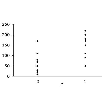
Figure 11.1

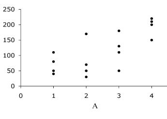
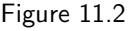
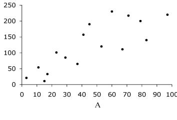
Figure 11.3

Suppose treatment A is a dichotomous variable with two possible values: no treatment (A = 0) and treatment (A = 1). Half of the individuals were treated (A = 1). Figure 11.1 is a scatter plot that displays each of the 16 individuals as a dot. The height of the dot indicates the value of the individual’s outcome Y . The 8 treated individuals are placed along the column A = 1, and the 8 untreated along the column A = 0. As defined in Chapter 10, an estimate of the mean of Y among individuals with level A = a in the population is the numerical result of applying the estimator—in our case, the sample average—to a particular data set.

Our estimate of the population mean in the treated is the sample average 146.25 for those with A = 1, and our estimate of the population mean in the untreated is the sample average 67.50 in those with A = 0. Under exchangeability of the treated and the untreated, the difference 146.25 − 67.50 would be interpreted as an estimate of the average causal effect of treatment A on the outcome Y in the target population. However, this chapter is not about making causal inferences. Our current goal is simply to motivate the need for models when trying to estimate population quantities like the mean E[Y |A = a], irrespective of whether the estimates do or do not have a causal interpretation.

Now suppose treatment A is a polytomous variable that can take 4 possible values: no treatment (A = 1), low-dose treatment (A = 2), medium-dose treatment (A = 3), and high-dose treatment (A = 4). A quarter of the individuals received each treatment level. Figure 11.2 displays the outcome value for the 16 individuals in the study population. To estimate the population means in the 4 groups defined by treatment level, we compute the corresponding sample code: Program 11.1 averages. The estimates are 70.0, 80.0, 117.5, and 195.0 for A = 1, A = 2, A = 3, and A = 4, respectively.

Figures 11.1 and 11.2 depict examples of discrete (categorical) variables with 2 and 4 categories, respectively. Because the number of study individuals is fixed at 16, the number of individuals per category decreases as the number of categories increases. The sample average in each category is still an exactly unbiased estimator of the corresponding population mean, but the probability that the sample average is close to the corresponding population mean decreases as the number of individuals in each category decreases. The length of the 95% confidence intervals (see Chapter 10) for the category-specific means will be greater for the data in Figure 11.2 than for the data in Figure 11.1.

Finally, suppose that A represents the dose of treatment in mg/day, and that it takes integer values from 0 to 100 mg. Figure 11.3 displays the outcome value for each of the 16 individuals. Because the number of possible values of treatment is much greater than the number of individuals in the study, there are many values of A that no individual received. For example, there are no individuals with treatment dose A = 90 in the study population.

This creates a problem: how can we estimate the mean of the outcome Y among individuals with treatment level A = 90 in the target population? The estimator we used for the data in Figures 11.1 and 11.2—the treatment-specific sample average—is undefined for treatment levels for which there are zero individuals in Figure 11.3. If treatment A were a truly continuous variable, then the sample average would be undefined for nearly all treatment levels. (A continuous variable A can be viewed as a categorical variable with an uncountably infinite number of categories.)

The above description shows that we cannot always let the data “speak for themselves” to obtain a meaningful estimate. Rather, we often need to supplement the data with a model, as we describe in the next section.

11.2 Parametric estimators of the conditional mean

We want to estimate the mean of Y among individuals with treatment level A = 90, i.e., E[Y |A = 90], from the data in Figure 11.3. Suppose we expect the mean of Y among individuals with treatment level A = 90 to lie between the mean among individuals with A = 80 and the mean among individuals with A = 100. In fact, suppose we knew that the treatment-specific population mean of Y is a linear function of the value of treatment A throughout the range of A. More precisely, we know that the mean of Y , E[Y |A], increases (or decreases) from some value θ⁰ for A = 0 by θ¹ units per unit of A. Or, more compactly,

\[\operatorname{E}[Y|A] = \theta\_0 + \theta\_1 A\]

More generally, the restriction on This equation is a restriction on the shape of conditional mean function E[Y |A]. This particular restriction is referred to as a linear mean model, and the quantities θ⁰ and θ¹ are referred to as the parameters of the model. Models that describe the conditional mean function in terms of a finite number of parameters are referred to as parametric conditional mean models. In our example, the parameters θ⁰ and θ¹ define a straight line that crosses (intercepts) the vertical axis at θ⁰ and that has a slope θ1. That is, the model specifies that all conditional mean functions are straight lines, though their intercepts and slopes may vary.

We are now ready to combine the data in Figure 11.3 with our parametric mean model to estimate E[Y |A = a] for all values a from 0 to 100. The first step is to obtain estimates ˆθ⁰ and ˆθ¹ of the parameters θ⁰ and θ1. The second step is to use these estimates to estimate the mean of Y for any value A = a. For example, to estimate the mean of Y among individuals with treatment level ^A = 90, we use the expression E[ ^{b Y |A} = 90] = ^ˆθ⁰ + 90ˆθ1. The estimate E[ ^{b Y |}A] for each individual is referred to as the predicted value.

An exactly unbiased estimator of θ⁰ and θ¹ can be obtained by the method of ordinary least squares. A nontechnical motivation of the method follows. Consider all possible candidate straight lines for Figure 11.3, each of them with a different combination of values of intercept θ⁰ and slope θ1. For each candidate line, one can calculate the vertical distance from each dot to the line (the residual), square each of those 16 residuals, and then sum the 16 squared residuals. The line for which the sum is the smallest is the “least squares” line, and the parameter values ˆθ⁰ and ˆθ¹ of this “least squares” line are the “least squares” estimates. The values ˆθ⁰ and ˆθ¹ can be easily computed using linear algebra, as described in any statistics textbook.

In our example, the parameter estimates are ˆθ⁰ = 24.55 and ˆ code: Program 11.2 θ¹ = 2.14, which define the straight line shown in Figure 11.4. The predicted mean of ^Y among individuals with treatment level ^A = 90 is therefore E[ ^{b Y |A} = 90] = 24.55 + 90 × 2.14 = 216.9. Because ordinary least squares estimation uses all data points to find the best line, the mean of Y in the group A = a, i.e., E[Y |A = a], is estimated by borrowing information from individuals who have values of treatment A not equal to a.

So what is a model? A model is defined by an a priori restriction on the joint distribution of the data. Our linear conditional mean model says that the conditional mean function E[Y |A] is a straight line, which restricts its shape. For example, the model restricts the mean of Y for A = 90 to be between the mean of Y for A = 80 and the mean of Y for A = 100. This restriction is encoded by the parameters θ⁰ and θ1. A parametric conditional mean model

the shape of the relation is known as the functional form and, by some authors, as the dose-response curve. We do not use the latter term because it suggests that the dose of treatment causally effects the response, which could be false in the presence of confounding.

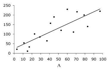
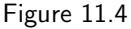
Under the assumption that the variance of the residuals does not depend on A (homoscedasticity), the Wald 95% confidence intervals are (−21.2, 70.3) for θ0, (1.28, 2.99) for θ1, and (172.1, 261.6) for E[Y |A = 90].

is, through its a priori restrictions, adding information to compensate for the lack of sufficient information in the data.

Parametric estimators—those based on a parametric conditional mean model allow us to estimate quantities that cannot be estimated otherwise, e.g., the mean of Y among individuals in the target population with treatment level A = 90 when no such individuals exist in the study population. But this is not a free lunch. When using a parametric model, the inferences are correct only if the restrictions encoded in the model are correct, i.e. if the model is correctly specified. Thus model-based causal inference—to which a large fraction of the remainder of this book is devoted—relies on the condition of (approximately) no model misspecification. Because parametric models are rarely, if ever, perfectly specified, a certain degree of model misspecification is almost always expected. This can be at least partially rectified by using nonparametric estimators, which we describe in the next section.

11.3 Nonparametric estimators of the conditional mean

Let us return to the data in Figure 11.1. Treatment A is dichotomous and we want to consistently estimate the mean of Y in the treated E[Y |A = 1] and in the untreated E[Y |A = 0]. Suppose we have become so enamored with models that we decide to use one to estimate these two quantities. Again we proposed a linear model

\[\operatorname{E}[Y|A] = \theta\_0 + \theta\_1 A\]

where E[Y |A = 0] = θ⁰ + 0 × θ¹ = θ⁰ and E[Y |A = 1] = θ⁰ + 1 × θ¹ = θ⁰ + θ1. We use the least squares method to obtain estimates of the parameters θ⁰ and θ1. These estimates are ˆθ⁰ = 67.5 and ˆ code: Program 11.2 θ¹ = 78.75. We therefore estimate E[ ^{b Y |A} = 0] = 67.5 and E[ ^{b Y |A} = 1] = 146.25. Note that our model-based estimates of the mean of Y are identical to the sample averages we calculated In this book we define “model” in Section 11.1. This is not a coincidence but an expected finding.

Let us take a second look at the model E[Y |A] = θ⁰ + θ1A with a dichotomous treatment A. If we rewrite the model as E[Y |A = 1] = E[Y |A = 0] + θ1, we see that the model simply states that the mean in the treated E[Y |A = 1] is equal to the mean in the untreated E[Y |A = 0] plus a quantity θ1, where θ¹ may be negative, positive or zero. But this statement is of course always true! The model imposes no restrictions whatsoever on the values of E[Y |A = 1] and E[Y |A = 0]. Therefore E[Y |A = a] = θ⁰ + θ1A with a dichotomous treatment A is not a model because it lets the data speak for themselves, just like the sample average does. “Models” which do not impose restrictions on the distribution of the data are saturated models. Because they formally look like models even if they do not fit our definition of model, saturated models are ordinarily referred to as models too.

Generally, the model is saturated whenever the number of parameters in a conditional mean model is equal to the number of unknown conditional means in the population. For example, the linear model E[Y |A] = θ⁰ + θ1A has two parameters and, when A is dichotomous, there exist two unknown conditional means: the means E[Y |A = 1] and E[Y |A = 0]. Since the values of the two A saturated model has the same parameters are not restricted by the model, neither are the values of the means. As a contrast, consider the data in Figure 11.3 where A can take values from 0 to 100. The linear model E[Y |A] = θ⁰ +θ1A has two parameters but estimates 101 quantities, i.e., E[Y |A = 0],E[Y |A = 1], …, E[Y |A = 100]. The only hope

as an a priori mathematical restriction on the possible states of nature (Robins, Greenland 1986). Part I was entitled “Causal inference without models” because it only described saturated models.

number of unknowns on both sides of the equal sign.

Fine Point 11.1

Fisher consistency. Our definition of a nonparametric estimator in the main text coincides with what is known in statistics as a Fisher consistent estimator (Fisher 1922). That is, an estimator of a population quantity that, when calculated using the entire population rather than a sample, yields the true value of the population parameter. By definition, a Fisher consistent estimator lacks any model restrictions but, as discussed in the text, a Fisher consistent estimate may not exist for many population quantities. Technically, Fisher consistent estimators, when they exist, are the nonparametric maximum likelihood estimators of population quantities under a saturated model.

In the statistical literature, the term nonparametric estimator is sometimes used to refer to estimators that are not Fisher consistent but that impose very weak restrictions, such as kernel regression models. See Technical Point 11.1 for details.

assumptions that we have to make to compute the parameter even if we had an infinite amount of data. Modeling assumptions are the additional assumptions that we have to make to estimate the parameter because we do not have an infinite amount of data. Formally, identifiability assumptions make the parameter a unique function of the joint distribution of the observed data.

for unbiasedly estimating 101 quantities with these two parameters is to be fortunate to have all 101 means E[Y |A = a] lie along a straight line. When a model has only a few parameters but it is used to estimate many population quantities, we say that the model is parsimonious.

Here we define nonparametric estimators of the conditional mean function as those that produce estimates from the data without any a priori restrictions Identifiability assumptions are the on the conditional mean function (see Fine Point 11.1 for a more rigorous definition). An example of a nonparametric estimator of the population mean E[Y |A = a] for a dichotomous treatment is its empirical version, the sample average or, equivalently, the saturated model described in this section. When A is discrete with 100 levels and no individual in the sample has A = 90, no nonparametric estimator of E[Y |A = 90] exists. All methods for causal inference that we described in Part I of this book—standardization, IP weighting, stratification, matching—were based on nonparametric estimators of population quantities under a saturated model because they did not impose any a priori restrictions on the value of the effect estimates. In contrast, most methods for causal inference described in Part II of this book rely on estimators that are parametric estimators of some part of the distribution of the data. Parametric estimation is one approach used to borrow information when, as is often the case, data are unable to speak for themselves.

11.4 Smoothing

is used with two different meanings. A model is linear when it is expressed as a linear combination of parameters and functions of the variables, even if the latter are nonlinear functions (e.g., higher powers or logarithms) of the covariates.

Consider again the data in Figure 11.3 and the linear model E[Y |A] = θ0+θ1A. The parameter θ¹ is the difference in mean outcome per unit of treatment dose A. Because θ¹ is a single number, the model specifies that the difference in mean outcome Y per unit of treatment A must be constant throughout the entire range of A, i.e., the model requires the conditional mean outcome to Caution: Often the term “linear” follow a straight line as a function of treatment dose A. Figure 11.4 shows the best-fitting straight line.

But one can imagine situations in which the difference in mean outcome is larger for a one-unit change at low doses of treatment, and smaller for a oneunit change at high doses. This would be the case if, once the treatment dose reaches certain level, higher doses have an increasingly small effect. Under this scenario, the model E[Y |A] = θ⁰ + θ1A is incorrect. However, linear models can be made more flexible.

For example, suppose we fit the model E[Y |A] = θ⁰ + θ1A + θ2A² , where A² = A × A is A-squared, to the data in Figure 11.3. This is still referred to as a linear model because the conditional mean is expressed as a linear combination, i.e., as the sum of the products of each covariate (A and A² ) with its associated coefficient (the parameters θ¹ and θ2) plus an intercept (θ0). However, whenever θ² is not zero, (θ0, θ1, θ2) now define a curve—a parabola—rather than a straight line. We refer to θ¹ as the parameter for the linear term A, and to θ² as the parameter for the quadratic term A² .

The curve under the 3-parameter linear model E[Y |A] = θ⁰ + θ1A + θ2A² can be found via ordinary least squares estimation applied to the data in Figure 11.3. The estimated curve is shown in Figure 11.5. The parameter estimates are ˆθ⁰ = −7.41, ˆθ¹ = 4.11, and ˆ code: Program 11.3 θ² = −0.02. The predicted mean of Y among individuals with treatment level A = 90 is obtained from the expression E[ ^{b Y |A} = 90] = ^ˆθ⁰ + 90ˆθ¹ + 90 ^× 90ˆθ² = 197.1.

We could keep adding parameters for a cubic term (θ3A³ ), a quartic term (θ4A⁴ )… until we reach a 15th-degree term (θ15A15). At that point the number of parameters in our model equals the number of data points (individuals). The shape of the curve would change as the number of parameters increases. In general, the more parameters in the model, the more inflection points will appear.

That is, the curve generally becomes more “wiggly,” or less smooth, as the number of parameters increase. A linear model with 2 parameters—a straight line—is the smoothest model. A linear model with as many parameters as data points is the least smooth model because it has as many possible inflection points as data points. In fact, such model interpolates the data, i.e., each data point in the sample lies on the estimated conditional mean function.

Often modeling can be viewed as a procedure to transform noisy data into more or less smooth curves. This smoothing occurs because the model borrows information from many data points to predict the outcome value at a particular combination of values of the covariates. The smoothing results from E[Y |A = a] being estimated by borrowing information from individuals with A not equal to a. All parametric estimators incorporate some degree of smoothing.

The degree of smoothing depends on how much information is borrowed across individuals. The 2-parameter model E[Y |A] = θ⁰ + θ1A estimates E[Y |A = 90] by borrowing information from all individuals in the study population to find the least squares straight line. A model with as many parameters as individuals does not borrow any information to estimate E[Y |A] at the values of A that occur in the data, though it borrows information (by interpolation) for values of A that do not occur in the data.

Intermediate degrees of smoothing can be achieved by using an intermediate number of parameters or, more generally, by restricting the number of individ-We used a model for continuous uals that contribute to the estimation. For example, to estimate E[Y |A = 90] we could decide to fit a 2-parameter model E[Y |A] = θ⁰ + θ1A restricted to individuals with treatment doses between 80 and 100. That is, we would only borrow information from individuals in a 10-unit window of A = 90. The wider the window around A = 90, the more smoothing would be achieved.

In our simplistic examples above, all models included a single covariate (with either a single parameter for A or two parameters for A and A² ) so that the curves can be represented on a two-dimensional book page. In realistic applications, models often include many different covariates so that the curves are really hyperdimensional surfaces. Regardless of the dimensionality of the problem, the concept of smoothing remains invariant: the fewer parameters in the model, the smoother the prediction (response) surface will be.

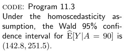
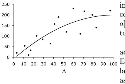
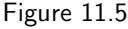
outcomes as an example. The same reasoning applies to models for dichotomous outcomes such as logistic models (see Technical Point 11.1)

Model dimensionality and the relation between frequentist and Bayesian intervals. In frequentist statistical inference, probability is defined as frequency. In Bayesian inference, probability is defined as degree-of-belief—a concept very different from probability as frequency (de Finetti 1972). Chapter 10 described the confidence intervals used in frequentist statistical inference. Bayesian statistical inference uses credible intervals, which have a more natural interpretation: A Bayesian 95% credible interval means that, given the observed data, “there is a 95% probability that the estimand is in the interval”. However, in part because of the requirement to specify the investigators’ degree of belief, Bayesian inference is less commonly used than frequentist inference.

Interestingly, in simple, low-dimensional parametric models with large sample sizes, 95% Bayesian credible intervals are also 95% frequentist confidence intervals, whereas in high-dimensional or nonparametric models, a Bayesian 95% credible interval may not be a 95% confidence interval as it may trap the estimand much less than 95% of the time. The underlying reason for these results is that Bayesian inference requires the specification of a prior distribution for all unknown parameters. In low-dimensional parametric models the information in the data swamps that contained in reasonable priors. As a result, inference is relatively insensitive to the particular prior distribution selected. However, this is no longer the case in high-dimensional models. Therefore if the true parameter values that generated the data are unlikely under the chosen prior distribution, the center of Bayes credible interval will be pulled away from the true parameters and towards the parameter values given the greatest probability under the prior.

11.5 The bias-variance trade-off

In previous sections we have used the 16 individuals in Figure 11.3 to estimate the mean outcome Y among people receiving a treatment dose of A = 90 in the target population, E[Y |A = 90]. Since nobody in the study population received A = 90, we could not let the data speak for themselves. So we combined the data with a linear model. The estimate E[ ^{b Y |A} = 90] varied with the model. Under the 2-parameter model E[Y |A] = θ⁰ + θ1A, the estimate was 216.9 (95% confidence interval: 172.1, 261.6). Under the 3-parameter model E[Y |A] = θ⁰ + θ1A + θ2A² , the estimate was 197.1 (95% confidence interval: 142.8, 251.5). We used two different parametric models that yielded two different estimates. Which one is better? Is 216.9 or 197.1 closer to the mean in the target population?

If the relation is truly curvilinear, then the estimate from the 2-parameter model will be biased because this model assumes a straight line. On the other hand, if the relation is truly a straight line, then the estimates from both models will be valid. This is so because the 3-parameter model E[Y |A] = θ⁰ + θ1A + θ2A² is correctly specified whether the relation follows a straight line (in which case θ² = 0) or a parabolic curve (in which case θ² ̸= 0). One safe strategy would be to use the 3-parameter model E[Y |A] = θ⁰ + θ1A + θ2A² rather than the 2-parameter model E[Y |A] = θ⁰ + θ1A. Because the 3-parameter model is correctly specified under both a straight line and a parabolic curve, it is less likely to be biased. In general, the larger the number of parameters in the model, the fewer restrictions the model imposes; the less smooth the model, the more protection afforded against bias from model misspecification.

Although less smooth models may yield a less biased estimate, they also result in a larger variance, i.e., wider 95% confidence intervals around the estimate. For example, the estimated 95% confidence interval around E[ ^{b Y |A =} 90] was much wider when we used the 3-parameter model than when we used the 2-parameter model. However, when the estimate E[ ^{b Y |A} = 90] based on the 2-parameter model is biased, the standard (nominal) 95% confidence interval

Fine Point 11.2 discusses the impli- of the time. cations of model dimensionality for frequentist and Bayesian intervals.

is not calibrated, i.e., it does not cover the true parameter E[Y |A = 90] 95%

This bias-variance trade-off is at the heart of many data analyses. Investigators using models need to decide whether some protection against bias—by, say, adding more parameters to the model—is worth the cost in terms of variance. Though some formal procedures exist to aid these decisions, in practice many investigators decide which model to use based on criteria like tradition, interpretability of the parameters, and software availability. In this book we will usually assume that our parametric models are correctly specified. This is an unrealistic assumption, but it allows us to focus on the problems that are specific to causal analyses. Model misspecification is, after all, a problem that can arise in any sort of data analysis, regardless of whether the estimates are endowed with a causal interpretation. In practice, careful investigators will always question the validity of their models and will conduct alternative analysis under different model specifications that are compatible with existing expert knowledge. Their goal is to assess the sensitivity of their estimates to model specification.

We are now ready to describe the use of models for causal inference.

A taxonomy of commonly used models. The main text describes linear conditional mean models of the form E[Y |X] = θX ≡ Pp i=0 θiXⁱ where X is a vector of covariates X0, X1, …X^p with X⁰ = 1 for all n individuals. These models are a subset of larger class of conditional mean models (McCullagh and Nelder, 1989; McCulloch, Searle, and Neuhaus, 2008) which have two components: a linear functional form or predictor ^Pp i=0 θiXⁱ and a link function g {·}

such that g {E[Y |X]} = Pp i=1 θiXⁱ .

The linear conditional mean models described in the main text uses the identity link function. Conditional mean models for outcomes with strictly positive values (e.g., counts, the numerator of incidence rates) often use the log link function to ensure that all predicted values will be greater than zero, i.e., log {E[Y |X]} = Pp i=0 ^θiXⁱ so E[^{Y |}X] = exp P^p i=0 θiXⁱ . Conditional mean models for dichotomous outcomes (i.e., those that only take values 0 and 1) often use a logit link i.e., log n E[Y |X] 1−E[Y |X] o = Pp i=0 θiXⁱ , so that E[^{Y |}X] = expit P^p i=0 θiXⁱ . This link ensures that all predicted values will be greater than 0 and less than 1. Conditional mean models that use the logit function, referred to as logistic regression models, are widely used in this book. For these links (referred to as canonical links) we can estimate θ by maximum likelihood under a normal working model for the identity link, a Poisson working model for the log link, and a logistic regression model for the logit link. These estimates are consistent for θ as long as the conditional mean model for E[Y |X] is correct. Generalized estimating equation (GEE) models, often used to deal with repeated measures, are a further example of a conditional mean model (Liang and Zeger, 1986).

Conditional mean models only specify a parametric form for E[Y |X] but do not otherwise restrict the distribution of Y |X or the marginal distribution of X. Therefore, when X or Y are continuous, a parametric conditional mean model is a semiparametric model for the joint distribution of the data (X, Y ) because parts of the distribution are modeled parametrically whereas others are left unrestricted. The model is semiparametric because the set of all unrestricted components of the joint distribution cannot be represented by a finite number of parameters.

Conditional mean models themselves can be generalized by relaxing the assumption that E[Y |X] takes a parametric form. For example, a kernel regression model does not impose a specific functional form on E[Y |X] but rather estimates E[^{Y |X = x}] for any ^x by ^Pn i=1 w^h (x − Xi) Yi/ Pn i=1 w^h (x − Xi) where w^h (z) is a positive function, known as a kernel function, that attains its maximum value at z = 0 and decreases to 0 as |z| gets large at a rate that depends on the parameter h subscripting w. As another example, generalized additive models (GAMs) replace the linear combination Pp i=0 ^θiXⁱ of a conditional mean model by a sum of smooth functions ^Pp i=0 fi(Xi). The model can be estimated using a backfitting algorithm with fi(·) estimated at iteration k by, e.g., kernel regression (Hastie and Tibshirani 1990).

In the text we discuss smoothing with parametric models which specify an a priori functional form for E[Y |X = x], such as a parabola. In estimating E [Y |X = x], the model may borrow information from values of X that are far from x. In contrast, kernel regression models do not specify an a priori functional form and borrow information only from values of X near to x when estimating E [Y |X = x]. A kernel regression model is an example of a “non-parametric” regression model. This use of the term “nonparametric” differs from our previous usage. Our nonparametric estimators of E [Y |X = x] only used those individuals for whom X equalled x exactly; no information was borrowed even from close neighbors. Here “nonparametric” estimators of E [Y |X = x] use individuals with values of X near to x. How near is controlled by a smoothing parameter referred to as the bandwidth h.

Why model?

Chapter 12 IP WEIGHTING AND MARGINAL STRUCTURAL MODELS

Part II is organized around the causal question “what is the average causal effect of smoking cessation on body weight gain?” In this chapter we describe how to use IP weighting to estimate this effect from observational data. Though IP weighting was introduced in Chapter 2, we only described it as a nonparametric method. We now describe the use of models together with IP weighting which, under additional assumptions, will allow us to tackle high-dimensional problems with many covariates and nondichotomous treatments.

To estimate the effect of smoking cessation on weight gain we will use real data from the NHEFS, an acronym that stands for (ready for a long name?) National Health and Nutrition Examination Survey Data I Epidemiologic Follow-up Study. The NHEFS was jointly initiated by the National Center for Health Statistics and the National Institute on Aging in collaboration with other agencies of the United States Public Health Service. A detailed description of the NHEFS, together with publicly available data sets and documentation, can be found at wwwn.cdc.gov/nchs/nhanes/nhefs/. For this and future chapters, we will use a subset of the NHEFS data that is available from this book’s web site. We encourage readers to improve upon and refine our analyses.

12.1 The causal question

viduals with known sex, age, race, weight, height, education, alcohol use and intensity of smoking at the baseline (1971-75) and followup (1982) visits, and who answered the medical history questionnaire at baseline. See Fine Point 12.1.

Mean baseline	A
characteristics	1	0
Age, years	46.2	42.8
Men, %	54.6	46.6
White, %	91.1	85.4
University, %	15.4	9.9
Weight, kg	72.4	70.3
Cigarettes/day	18.6	21.2
Years smoking	26.0	24.1
Little exercise, %	40.7	37.9
Inactive life, %	11.2	8.9

Our goal is to estimate the average causal effect of smoking cessation (the treatment) A on weight gain (the outcome) Y . To do so, we will use data We restricted the analysis to indi- from 1566 cigarette smokers aged 25-74 years who, as part of the NHEFS, had a baseline visit and a follow-up visit about 10 years later. Individuals were classified as treated A = 1 if they reported having quit smoking before the follow-up visit, and as untreated A = 0 otherwise. Each individual’s weight gain Y was measured (in kg) as the body weight at the follow-up visit minus the body weight at the baseline visit. Most people gained weight, but quitters gained more weight on average. The average weight gain was E[ ^{b Y |A} = 1] = 4.⁵ kg in the quitters, and E[ ^{b Y |A} = 0] = 2.0 kg in the non-quitters. The difference E[Y |A = 1] − E[Y |A = 0] was therefore estimated to be 2.5, with a 95% confidence interval from 1.7 to 3.4.

We define E[Y ^a=1] as the mean weight gain that would have been observed Table 12.1 if all individuals in the population had quit smoking before the follow-up visit, and E[Y ^a=0] as the mean weight gain that would have been observed if all individuals in the population had not quit smoking. We define the average causal effect on the additive scale as E[Y ^a=1] − E[Y ^a=0], i.e., the difference in mean weight that would have been observed if everybody had been treated compared with untreated. This is the causal effect that we will be primarily concerned with in this and the next chapters.

The associational difference E[Y |A = 1] − E[Y |A = 0], which we estimated in the first paragraph of this section, is generally different from the causal difference E[Y ^a=1] − E[Y ^a=0]. The former will not generally have a causal interpretation if quitters and non-quitters differ with respect to characteristics that affect weight gain. For example, quitters were on average 4 years older than non-quitters (quitters were 44% more likely to be above age 50 than non-

Setting a bad example. Our smoking cessation example is convenient: it does not require deep subject-matter knowledge and the data are publicly available. One price we have to pay for this convenience is potential selection bias.

We classified individuals as treated A = 1 if they reported (i) being smokers at baseline in 1971-75, and (ii) having quit smoking in the 1982 survey. Condition (ii) implies that the individuals included in our study did not die and were not otherwise lost to follow-up between baseline and 1982 (otherwise they would not have been able to respond to the survey). That is, we selected individuals into our study conditional on an event—responding the 1982 survey—that occurred after the start of the treatment—smoking cessation. If treatment affects the probability of selection into the study, we might have selection bias as described in Chapter 8. (Because different individuals quit smoking at different times, A is actually a time-varying treatment, which we will ignore throughout Part II. Time-varying treatments are discussed in Part III.)

A randomized experiment of smoking cessation would not have this problem. Each individual would be assigned to either smoking cessation or no smoking cessation at baseline, so that their treatment group would be known even if the individual did not make it to the 1982 visit. In Section 12.6 we describe how to deal with potential selection bias due to censoring or missing data for the outcome—something that may occur in both observational studies and randomized experiments—but the situation described in this Fine Point is different: the missing data concerns the treatment itself. This selection bias can be handled through sensitivity analysis, as was done by Hern´an et al. (2008, Appendix 3).

The choice of this example allows us to describe, in our own analysis, a ubiquitous problem in published analyses of observational data that emulate a target trial: a misalignment of treatment assignment and eligibility at the start of follow-up (Hern´an et al. 2016). Though we decided to ignore this issue in order to keep our analysis simple, didactic convenience would not be a good excuse to avoid dealing with this bias in real life.

descriptive statistics shown in this section

quitters), and older people gained less weight than younger people, regardless Fine Point 7.3 defined surrogate of whether they did or did not quit smoking. We say that age is a (surroconfounders. gate) confounder of the effect of A on Y and our analysis needs to adjust for age. The unadjusted estimate 2.5 might underestimate the true causal effect E[Y ^a=1] − E[Y ^a=0].

code: Program 12.1 computes the As shown in Table 12.1, quitters and non-quitters also differed in their distribution of other variables such as sex, race, education, baseline weight, and intensity of smoking. If these variables are confounders, then they also need to be adjusted for in the analysis. In Chapter 18 we discuss strategies for confounder selection. Here we assume that the following 9 variables, all measured at baseline, are sufficient to adjust for confounding: sex (0: male, 1: female), age (in years), race (0: white, 1: other), education (5 categories), intensity and duration of smoking (number of cigarettes per day and years of smoking), physical activity in daily life (3 categories), recreational exercise (3 categories), and weight (in kg). That is, L represents a vector of 9 measured covariates. In the next section we use IP weighting to adjust for these covariates.

12.2 Estimating IP weights via modeling

IP weighting creates a pseudo-population in which the arrow from the covariates L to the treatment A is removed. More precisely, the pseudo-population has the following two properties: A and L are statistically independent and P the mean Eps[Y |A = a] in the pseudo-population equals the standardized mean ^l E[Y |A = a, L = l] Pr [L = l] in the actual population. These properties are true even if conditional exchangeability Y ^a⊥⊥A|L does not hold in the acment Pr [A = 1|L] is known as the propensity score. More about propensity scores in Chapter 15.

The estimated IP weights W^A ranged from 1.05 to 16.7, and their mean was 2.00.

model because it has 2 parameters, θ⁰ and θ1, to estimate two quantities, E[Y |A = 1] and E[Y |A = 0]. In this model, θ¹ = E[Y |A = 1] − E[Y |A = 0].

tual population (see Technical Point 2.3). Now, if conditional exchangeability Y ^a⊥⊥A|L holds in the actual population, then these properties imply that (i) the mean of Y a is the same in both populations, (ii) unconditional exchangeability (i.e., no confounding) holds in the pseudo-population, (iii) the counterfactual mean E[Y a ] in the actual population is equal to Eps[Y |A = a] in the pseudo-population, and (iv) association is causation in the pseudo-population. Please reread Chapter 2 if you need a refresher on IP weighting.

Informally, the pseudo-population is created by weighting each individual by the inverse (reciprocal) of the conditional probability of receiving the treatment level that she indeed received. The individual-specific IP weights for treatment A are defined as W^A = 1/f (A|L). For our dichotomous treatment A, the denominator f (A|L) of the IP weight is the probability of quit-The conditional probability of treat- ting conditional on the measured confounders, Pr [A = 1|L], for the quitters, and the probability of not quitting conditional on the measured confounders, Pr [A = 0|L], for the non-quitters. We only need to estimate Pr [A = 1|L] because Pr [A = 0|L] = 1 − Pr [A = 1|L].

In Section 2.4 we estimated the quantity Pr [A = 1|L] nonparametrically: we simply counted how many people were treated (A = 1) in each stratum of L, and then divided this count by the number of individuals in the stratum. All the information required for this calculation was taken from a causally interpreted structured tree graph with 4 branches (2 for L times 2 for A). But nonparametric estimation of Pr [A = 1|L] is out of the question when, as in our example, we have high-dimensional data with many confounders, some of The curse of dimensionality was in- them with many levels. Even if we were willing to recode all 9 confounders troduced in Chapter 10. except age to a maximum of 6 categories each, our tree would still have over 2 million branches. And many more millions if we use the actual range of values of duration and intensity of smoking, and weight. We cannot obtain meaningful nonparametric stratum-specific estimates when there are 1566 individuals distributed across millions of strata. We need to resort to modeling.

To obtain parametric estimates of Pr [A = 1|L] in each of the millions of strata defined by L, we fit a logistic regression model for the probability of quitting smoking with all 9 confounders included as covariates. We used linear and quadratic terms for the (quasi-)continuous covariates age, weight, intensity and duration of smoking, and we included no product terms between the covariates. That is, our model restricts the possible values of Pr [A = 1|L] such that, on the logit scale, the conditional relation between the continuous covariates and the risk of quitting can be represented by a parabolic curve, and each covariate’s contribution to the (logit of the) risk is independent of that of the code: Program 12.2 other covariates. Under these parametric restrictions, we were able to obtain an estimate Pr [ ^{c A} = 1|L] for each combination of ^L values, and therefore for each of the 1566 individuals in the study population.

The next step is computing the difference ^Ebps[^{Y |A} = 1] ^{− E}bps[^{Y |A} = 0] in the pseudo-population created by the estimated IP weights. If there is no confounding for the effect of A in the pseudo-population and the model for Pr [A = 1|L] is correct, association is causation and an unbiased estimator E[Y |A] = θ⁰ + θ1A is a saturated of the associational difference Eps[Y |A = 1] − Eps[Y |A = 0] in the pseudopopulation is also an unbiased estimator of the causal difference E[Y ^a=1] − E[Y ^a=0] in the actual population.

Our approach to estimate Eps[Y |A = 1] − Eps[Y |A = 0] in the pseudopopulation was to fit the (saturated) linear mean model E[Y |A] = θ⁰ + θ1A by weighted least squares, with individuals weighted by their estimated IP weights ^Wc: 1/Pr [ ^{c A} = 1|L] for the quitters, and 1/ ^{1 −} Pr [ ^{c A} = 1|L] for the

Horvitz-Thompson estimators. In Technical Point 3.1, we defined the “apparent” IP weighted mean for treatment level a, E I (A = a) Y f (A|L) , which is equal to the counterfactual mean E[Y a ] under positivity and exchangeability. This IP weighted mean is consistently estimated by the original Horvitz-Thompson (1952) estimator ^Eb I (A = a) Y f (A|L) with ^Eb the sample average operator and ^f (A|L) assumed to be known. In this chapter, however, we estimated E[^Y a ] via the IP weighted least squares estimate ˆθ⁰ + ˆθ1a, which for binary A is a modified Horvitz-Thompson estimator often referred to as Hajek estimator Eb I (A = a) Y f (A|L) Eb I (A = a) (Hajek 1971).

The Hajek estimator is an (asymptotically) unbiased estimator of E

f (A|L)

I (A = a) Y f (A|L) I (A = a) f (A|L) which, under positivity, is equal

to E I (A = a) Y f (A|L) because E I (A = a) f (A|L) = 1. In practice, the Hajek estimator is preferred because, unlike the Horvitz-Thompson estimator, it is guaranteed to lie between 0 and 1 for dichotomous Y , even when f (A|L) is unknown and replaced by the predicted value ˆf (A|L) obtained from the fit of a misspecified model.

E

On the other hand, if positivity does not hold, then the ratio E I (A = a) Y f (A|L) E I (A = a) f (A|L) equals P l E [Y |A = a, L = l, L ∈ Q(a)] Pr [L = l|L ∈ Q(a)] and, if exchangeability holds, it equals E [Y a |L ∈ Q(a)], where Q(a) = {l; Pr (A = a|L = l) > 0} is the set of values l for which A = a may be observed with positive probability. Therefore, as discussed in Technical Point 3.1, the difference between Hajek estimators with a = 1 versus

a = 0 does not have a causal interpretation in the absence of positivity. Under non-positivity, the ratio of the limit of the Horvitz-Thompson estimator to that of the Hajek estimator is no longer 1 but rather Pr [Q(a)], as the denominator of the Hajek estimator converges to Pr [Q(a)] rather to 1.

mates ˆθ⁰ and ˆθ¹ with weight W of θ⁰ and θ¹ are the minimizers of P ^{i W}cⁱ [Yⁱ − (θ⁰ + θ1Ai)]² . If ^Wcⁱ = 1 for all individuals i, we obtain the ordinary least squares estimates described in the previous chapter.

non-quitters. The parameter estimate ˆθ¹ was 3.4. That is, we estimated that quitting smoking increases weight by ˆθ¹ = 3.4 kg on average. See Technical The weighted least squares esti- Point 12.1 for a formal definition of the estimator.

To obtain a 95% confidence interval around the point estimate ˆθ¹ = 3.4 we need a method that takes the IP weighting into account. One possibility is to use statistical theory to derive the corresponding variance estimator. This approach requires that the data analyst programs the estimator, which is not generally available in standard statistical software. A second possibility is to approximate the variance by nonparametric bootstrapping. This approach requires appropriate computing resources, or lots of patience, for large databases. A third possibility is to use the robust variance estimator (e.g., as used for GEE models with an independent working correlation) that is a standard option in most statistical software packages. The 95% confidence intervals based on the robust variance estimator are valid but, unlike the above analytic and bootstrap estimators, conservative—they cover the super-population parameter more than 95% of the time. The conservative 95% confidence interval around ˆθ¹ was (2.4, 4.5). In this chapter, all confidence intervals for IP weighted

estimates are conservative. If the model for Pr [A = 1|L] is misspecified, the estimates of θ⁰ and θ¹ will be biased and, like we discussed in the previous chapter, the confidence intervals may cover the true values less than 95% of the time.

12.3 Stabilized IP weights

The goal of IP weighting is to create a pseudo-population in which there is no association between the covariates L and treatment A. In Chapter 2 we showed how the original study population in Figure 2.1 was transformed into the pseudo-population in Figure 2.3 by using the IP weights W^A = 1/f (A|L). The size of the pseudo-population is twice that of the original study population, which reflects the fact that the average of the weights W^A is 2. Informally, the weights simulate a pseudo-population that is formed by two copies of the original study population, one of which is treated and the other untreated.

However, there are other ways to create a pseudo-population in which A and L are independent. For example, a pseudo-population in which all individuals have a probability of receiving A = 1 equal to 0.5 and a probability of receiving A = 0 also equal to 0.5, regardless of their values of L. Such pseudo-population is constructed by using IP weights 0.5/f (A|L). This pseudo-population would be of the same size as the study population and it would be algebraically equal to the pseudo-population of the previous paragraph if all weights are divided by 2. Hence, the expected mean of the weights 0.5/f (A|L) is 1 and the effect estimate obtained in the pseudo-population created by weights 0.5/f (A|L) is equal to that obtained in the pseudo-population created by weights 1/f (A|L). (You can check this empirically by using the data in Figure 2.1, or see the proof in Technical Point 12.2.) The same goes for any other IP weights p/f (A|L) with 0 < p ≤ 1. The weights W^A = 1/f (A|L) are just one particular example of IP weights with p = 1.

Let us take our reasoning a step further. The key requirement for confounding adjustment is that, in the pseudo-population, the probability of treatment A does not depend on the confounders L. We can achieve this requirement by assigning treatment with the same probability p to everyone in the pseudopopulation. But we can also achieve it by creating a pseudo-population in which different people have different probabilities of treatment, as long as the probability of treatment does not depend on the value of L. For example, a common choice is to assign to the treated the probability of receiving treatment Pr [A = 1] in the original population, and to the untreated the probability of The average causal effect in the not receiving treatment Pr [A = 0] in the original population. Thus the IP weights are Pr [A = 1] /f (A|L) for the treated and Pr [A = 0] /f (A|L) for the untreated or, more compactly, f (A) /f (A|L).

Figure 12.1 shows the pseudo-population that is created by the IP weights f (A) /f (A|L) when applied to the data in Figure 2.1, where Pr [A = 1] = 13/20 = 0.65 and Pr [A = 0] = 7/20 = 0.35. Under the identifiability conditions of Chapter 3, the pseudo-population resembles a hypothetical randomized experiment in which 65% of the individuals in the study population have been randomly assigned to A = 1, and 35% to A = 0. Note that, to preserve the 65/35 ratio, the number of individuals in each branch cannot be integers. Fortunately, non-whole people are no big deal in mathematics.

In our smoking cessation example, the IP weights f (A) /f (A|L) range from 0.33 to 4.30, whereas the IP weights 1/f (A|L) range from 1.05 to 16.7. The

treated subpopulation can be estimated by using IP weights in which the numerator is Pr[A = 1|L]. See Technical Point 4.1.

stabilizing factor f (A) in the numerator is responsible for the narrower range of the f (A) /f (A|L) weights. The IP weights W^A = 1/f (A|L) are referred to as nonstabilized weights, and the IP weights SW^A = f (A) /f (A|L) are referred to as stabilized weights. The mean of the stabilized weights is expected to be 1 because the size of the pseudo-population equals that of the study population.

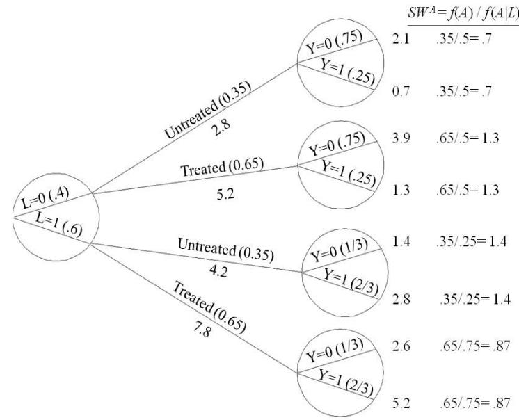
Figure 12.1

that the estimated weights SW^A have mean 1 (Hern´an and Robins 2006a). Deviations from 1 indicate model misspecification or possible violations, or near violations, of positivity. See Fine Point 12.2 for more on checking positivity.

The estimated IP weights SW^A ranged from 0.33 to 4.30, and their mean was 1.00.

Let us now re-estimate the effect of quitting smoking on body weight by using the stabilized IP weights SWA. First, we need an estimate of the con-In data analyses one should check ditional probability Pr [A = 1|L] to construct the denominator of the weights. We use the same logistic model we used in Section 12.2 to obtain a parametric estimate Pr [ ^{c A} = 1|L] for each of the 1566 individuals in the study population. Second, we need to estimate Pr [A = 1] for the numerator of the weights. We can obtain a nonparametric estimate by the ratio 403/1566 or, equivalently, by fitting a saturated logistic model for Pr [A = 1] with an intercept and no covariates. Finally, we estimate the causal difference E[Y ^a=1] − E[Y ^a=0] by fitting the mean model E[Y |A] = θ⁰ + θ1A with individuals weighted by their estimated stabilized IP weights: Pr [ ^{c A} = 1] /Pr [ ^{c A} = 1|L] for the quitters, and ^{1 −} Pr [ ^{c A} = 1] / ^{1 −} Pr [ ^{c A} = 1|L] for the non-quitters. Under our assumptions, we estimated that quitting smoking increases weight by ˆθ¹ = 3.4 kg (95% code: Program 12.3 confidence interval: 2.4, 4.5) on average. This is the same estimate we obtained earlier using the nonstabilized IP weights W^A rather than the stabilized IP weights SW^A.

If nonstabilized and stabilized IP weights result in the same estimate, why use stabilized IP weights then? Because stabilized weights typically result in narrower 95% confidence intervals than nonstabilized weights. However, the statistical superiority of the stabilized weights can only occur when the (IP weighted) model is not saturated. In our above example, the two-parameter model E[Y |A] = θ⁰ + θ1A was saturated because treatment A could only take 2 possible values. In many settings (e.g., time-varying or continuous treatments), the weighted model cannot possibly be saturated and therefore stabi-

Checking positivity. In our study, there are 4 white women aged 66 years and none of them quit smoking. That is, the probability of A = 1 conditional on (a subset of) L is 0. Positivity, a condition for IP weighting, is empirically violated. There are two possible ways in which positivity can be violated:

• Structural violations: The type of violations described in Chapter 3. Individuals with certain values of L cannot possibly be treated (or untreated). An example: when estimating the effect of exposure to certain chemicals on mortality, being off work is an important confounder because people off work are more likely to be sick and to die, and a determinant of chemical exposure—people can only be exposed to the chemical while at work. That is, the structure of the problem guarantees that the probability of treatment conditional on being off work is exactly 0 (a structural zero). We’ll always find zero cells when conditioning on that confounder.
• Random violations: The type of violations described in the first paragraph of this Fine Point. Our sample is finite so, if we stratify on several confounders, we will start finding zero cells at some places even if the probability of treatment is not really zero in the target population. This is a random, not structural, violation of positivity because the zeroes appear randomly at different places in different samples of the target population. An example: our study happened to include 0 treated individuals in the strata “white women age 66” and “white women age 67”, but it included a positive number of treated individuals in the strata “white women age 65” and “white women age 69.”

Each type of positivity violation has different consequences. In the presence of structural violations, causal inferences cannot be made about the entire population using IP weighting or standardization. The inference needs to be restricted to strata in which structural positivity holds. See Technical Point 12.1 for details. In the presence of random violations, we used our parametric model to estimate the probability of treatment in the strata with random zeroes using data from individuals in the other strata. In other words, we use parametric models to smooth over the zeroes. For example, the logistic model used in Section 12.2 estimated the probability of quitting in white women aged 66 by interpolating from all other individuals in the study. Every time we use parametric estimation of IP weights in the presence of zero cells—like we did in estimating ˆθ¹ = 3.4—, we are effectively assuming random nonpositivity.

lized weights are used. The next section describes the use of stabilized weights for a continuous treatment.

12.4 Marginal structural models

This is a (saturated) marginal level a structural mean model for a dichotomous treatment A.

Consider the following linear model for the mean outcome under treatment

\[\mathbb{E}[Y^a] = \beta\_0 + \beta\_1 a\]

This model is different from all models we have described so far: the outcome variable of this model is counterfactual—and hence generally unobserved. Therefore the model cannot be fit to the data of any real-world study. Models for the marginal mean of a counterfactual outcome are referred to as marginal structural mean models.

The parameters for treatment in structural mean models correspond to average causal effects. In the above model, the parameter β¹ is equal to E[Y ^a=1] − E[Y ^a=0] because E[Y a ] = β⁰ under a = 0 and E[Y a ] = β⁰ + β¹ under a = 1. In previous sections, we have estimated the average causal effect of smoking cessation A on weight change Y defined as E[Y ^a=1] − E[Y ^a=0]. structural models is null preservation (see Chapter 9): when the null hypothesis of no average causal effect is true, a marginal structural model is never misspecified. For example, under this null hypothesis, marginal structural model E[Y a ] = β0+β1a+β2a 2 is correctly specified with β¹ = β² = 0 and β⁰ = E[Y a ] for any a. If conditional exchangeability holds, then E[Y ] = β0.

A (nonsaturated) marginal struc- structural model tural mean model for a continuous treatment A.

The estimated SW^A ranged from 0.19 to 5.10 with mean 1.00. We assumed constant variance (homoscedasticity), which seemed reasonable after inspecting a residuals plot. Other choices of distribution (e.g., truncated normal with heteroscedasticity) resulted in similar estimates.

In other words, we have estimated the parameter β¹ of a marginal structural model.

Specifically, we used IP weighting to construct a pseudo-population, and then fit the model E[Y |A] = θ⁰ + θ1A to the pseudo-population data by using IP weighted least squares. Under our assumptions, association is causation in the pseudo-population. That is, the parameter θ¹ from the IP weighted associational model E[Y |A] = θ⁰ + θ1A can be endowed with the same causal interpretation as the parameter β¹ from the structural model E[Y a ] = β⁰ + β1a. It follows that a consistent estimate ˆθ¹ of the associational parameter in the pseudo-population is also a consistent estimator of the causal effect β¹ = E[Y ^a=1] − E[Y ^a=0] in the population.

The marginal structural model E[Y a ] = β⁰ + β1a is saturated because smoking cessation A is a dichotomous treatment. That is, the model has 2 unknowns on both sides of the equation: E[Y ^a=1] and E[Y ^a=0] on the left-hand side, and β⁰ and β¹ on the right-hand side. Thus sample averages computed A desirable property of marginal in the pseudo-population were enough to estimate the causal effect of interest.

But treatments are often polytomous or continuous. For example, consider the new treatment A “change in smoking intensity” defined as number of cigarettes smoked per day in 1982 minus number of cigarettes smoked per day at baseline. Treatment A can now take many values such as −25 if an individual decreased his number of daily cigarettes by 25, or 40 if an individual increased his number of daily cigarettes by 40. Let us say that we are interested in estimating the difference in average weight change under different changes in treatment intensity in the 1162 individuals who smoked 25 or fewer cigarettes per day at baseline. That is, we want to estimate E[Y a ]−E[Y a ′ ] for any values a and a ′ .

Because treatment A can take dozens of values, a saturated model with as many parameters becomes impractical. We will have to consider a nonsaturated structural model to specify the dose-response curve for the effect of treatment A on the mean outcome Y . If we believe that a parabola appropriately describes the dose-response curve, then we would propose the marginal

\[\operatorname{E}[Y^a] = \beta\_0 + \beta\_1 a + \beta\_2 a^2\]

where a ² = a × a is a-squared and E[Y ^a=0] = β⁰ is the average weight gain under a = 0, i.e., under no change in smoking intensity between baseline and 1982.

Suppose we want to estimate the average causal effect of increasing smoking intensity by 20 cigarettes per day compared with no change, i.e., E[Y ^a=20] − E[Y ^a=0]. According to our structural model, E[Y ^a=20] = β⁰ + 20β¹ + 400β2, and thus E[Y ^a=20] − E[Y ^a=0] = 20β¹ + 400β2. Now we need to estimate the parameters β¹ and β2. To do so, we need to estimate IP weights SW^A to create a pseudo-population in which there is no confounding by L, and then fit the associational model E[Y |A] = θ⁰ +θ1A+θ2A² code: Program 12.4 to the pseudo-population data.

To estimate the stabilized weights SW^A = f (A) /f (A|L) we need to estimate f (A|L). For a dichotomous treatment A, f (A|L) is a probability so we used a logistic model to estimate Pr [A = 1|L]. For a continuous treatment A, f (A|L) is a probability density function (pdf). Unfortunately, pdfs are generally hard to estimate, particularly when L is high-dimensional with continuous components, which is why using IP weighting for continuous treatments will often be dangerous. In our example, we assumed that the density f (A|L) was normal (Gaussian) with mean µ^L = E[A|L] and constant variance σ 2 . We then

more stable estimation of IP weights is an active area of research. See the work by Imai and Ratkovic (2015), Wang and Zubizarreta (2020), Kallus and Santacatterina (2018), and Avagyan and Vansteelandt (2021).

tural logistic model for a dichotomous treatment. For a continuous treatment, we would specify a nonsaturated logistic model.

used a linear regression model to estimate the mean E[A|L] and variance of residuals σ 2 for all combinations of values of L. We also assumed that the density f (A) in the numerator was normal. One should be careful when using IP weighting for continuous treatments because the effect estimates may be The development of methods for exquisitely sensitive to the choice of the model or algorithm used to estimate the conditional density f (A|L).

Our IP weighted estimates of the parameters of the marginal structural model were βˆ ⁰ = 2.005, βˆ ¹ = −0.109, and βˆ ² = 0.003. According to these estimates, the mean weight gain (95% confidence interval) would have been 2.0 kg (1.4, 2.6) if all individuals had kept their smoking intensity constant, and 0.9 kg (−1.7, 3.5) if all individuals had increased smoking by 20 cigarettes/day between baseline and 1982. The estimate of E[Y ^a=20] − E[Y ^a=0] is therefore 2.0 − 0.9 = 1.10 kg.

One can also consider a marginal structural model for a dichotomous outcome. For example, if interested in the causal effect of quitting smoking A (1: yes, 0: no) on the risk of death D (1: yes, 0: no) by 1992, one could consider This is a saturated marginal struc- a marginal structural logistic model like

\[\text{logit}\,\text{Pr}[D^a = 1] = \alpha\_0 + \alpha\_1 a\_1\]

where exp (α1) is the causal odds ratio of death for quitting versus not quitting smoking. The parameters of this model are consistently estimated, under our assumptions, by fitting the logistic model logit Pr[D = 1|A] = θ⁰ + θ1A to code: Program 12.5 the pseudo-population created by IP weighting. We estimated the causal odds ratio to be exp ˆθ1 = 1.0 (95% confidence interval: 0.8, 1.4).

12.5 Effect modification and marginal structural models

Marginal structural models do not include covariates when the target parameter is the average causal effect in the population. However, one may include covariates—which may be non-confounders—in a marginal structural model to assess effect modification. Suppose it is hypothesized that the effect of smoking cessation varies by sex V (0: male, 1: female). To examine this hypothesis, we add the covariate V to our marginal structural mean model:

\[\operatorname{E}\left[Y^{a}|V\right] = \beta\_0 + \beta\_1 a + \beta\_2 V a + \beta\_3 V\]

Additive effect modification is present if β² ̸= 0. Technically, this is not a marginal model any more—because it is conditional on V —but the term The parameter β³ does not gener- “marginal structural model” is still applied.

We can estimate the model parameters by fitting the linear regression model E [Y |A, V ] = θ0+θ1A+θ2V A+θ3V via weighted least squares with IP weights W^A or SW^A. In most settings, the vector of covariates L should include V . Even when V and A are independent given the other components of L and V is not needed to ensure exchangeability, including V in L will generally increase the efficiency with which the parameters of the marginal structural model are estimated.

Because we are considering a model for the effect of treatment within levels of V , we now have the choice to use either f [A] or f [A|V ] in the numerator of the stabilized weights. IP weighting based on the stabilized weights SW^A (^V ) = ^f [A|^V ] f [A|L] generally results in narrower confidence intervals around

ally have a causal interpretation as the effect of V . Remember that we are assuming exchangeability, positivity, and consistency for treatment A, not for sex V.

action between 2 treatments A and B (as opposed to effect modification of treatment A by variable V ; see Chapter 5), we would include parameters for both A and B in the marginal structural model, and would estimate IP weights with the joint probability of both treatments in the denominator. We would assume exchangeability, positivity, and consistency for A and B.

the effect estimates. Some intuition for the generally increased statistical efficiency of SW^A (V ) is that the variance of the weights SW^A (V ) is less than that of the weights SWA. We estimate SW^A (V ) using the same approach as for SWA, except that we add the covariate V to the logistic model for the numerator of the weights.

The particular subset V of L that an investigator chooses to include in the marginal structural model should only reflect the investigator’s substantive interest. For example, a variable V should be included in the marginal structural model if the investigator both believes that V may be an effect modifier and has greater substantive interest in the causal effect of treatment within levels of the covariate V than in the entire population. In our example, we found no strong evidence of effect modification by sex as the 95% confidence interval around the parameter estimate ˆ code: Program 12.6 θ² was (−2.2, 1.9). If the investigator chooses to include all variables L in the marginal structural model, the stabilized weights SW^A (L) equal 1 and IP weighting is unnecessary because, under conditional exchangeability, the marginal structural model is then the (unweighted) out-If we were interested in the inter- come regression model that serves to fully adjust for all confounding by L (see Chapter 15). For this reason, in a slightly humorous vein, we refer to a marginal structural model that conditions on all variables L needed for exchangeability as a faux marginal structural model.

In Part I we discussed that effect modification and confounding are two logically distinct concepts. Nonetheless, many students have difficulty understanding the distinction because the same statistical methods—stratification (Chapter 4) or regression (Chapter 15)—are often used both for confounder adjustment and detection of effect modification. Thus, there may be some advantage to teaching these concepts using marginal structural models, because then methods for confounder adjustment (IP weighting) are distinct from methods for detection of effect modification (adding treatment-covariate product terms to a marginal structural model).

12.6 Censoring and missing data

When estimating the causal effect of smoking cessation A on weight gain Y , we restricted the analysis to the 1566 individuals with a body weight measurement at the end of follow-up in 1982. There were, however, 63 additional individuals who met our eligibility criteria but were excluded from the analysis because their weight in 1982 was not known. Selecting only individuals with nonmissing outcome values—that is, censoring from the analysis those with missing values—may introduce selection bias, as discussed in Chapter 8.

Let censoring C be an indicator for measurement of body weight in 1982: 1 if body weight is unmeasured (i.e., the individual is censored), and 0 if body weight is measured (i.e., the individual is uncensored). Our analysis was necessarily restricted to uncensored individuals, i.e., those with C = 0, because those were the only ones with known values of the outcome Y . That is, in sections 12.2 and 12.4 we did not fit the (weighted) outcome regression model E[Y |A] = θ⁰ + θ1A, but rather the model E[Y |A, C = 0] = θ⁰ + θ1A restricted to individuals with C = 0.

Unfortunately, even under the null, selecting only uncensored individuals for the analysis is expected to induce bias when C is either a collider on a pathway between treatment A and the outcome Y , or the descendant of one such collider. See the causal diagrams in Figures 8.3 to 8.6. Our data are

and treatment are WA,C = 1/f (A, C = 0|L), where the joint density of A and C is factored as f (A, C = 0|L) = f (A|L) × Pr [C = 0|L, A].

Some variables in L may have by treatment. zero coefficients in the model for f (A|L) but not in the model for Pr [C = 0|L, A], or vice versa. Nonetheless, in large samples, it is always more efficient to keep all variables L that independently predict the outcome in both models.

have mean 1 when the model for Pr [C = 0|A] is correctly specified. See Technical Point 12.2 for more on stabilized IP weights.

consistent with the structure depicted by those causal diagrams: treatment A is associated with censoring C—5.8% of quitters versus 3.2% nonquitters were censored—and at least some predictors of Y are associated with C—the average baseline weight was 76.6 kg in the censored versus 70.8 in the uncensored.

Because censoring due to loss to follow-up can introduce selection bias, we are generally interested in the causal effect if nobody in the study population had been censored. In our example, the goal becomes estimating the mean weight gain if everybody had quit smoking and nobody’s outcome had been censored, E[Y ^a=1,c=0], and the mean weight gain if nobody had quit smoking and nobody’s outcome had been censored E[Y ^a=0,c=0]. Then the causal effect of interest is E[Y ^a=1,c=0] − E[Y ^a=0,c=0], a joint effect of A and C as we discussed in Chapter 8. The use of the superscript c = 0 makes it explicit the causal contrast that many have in mind when they refer to the causal effect of treatment A, even if they choose not to use the superscript c = 0.

This causal effect can be estimated by using IP weights WA,C = W^A ×W^C The IP weights for censoring in which W^C = 1/Pr [C = 0|L, A] for the uncensored individuals and W^C = 0 for the censored individuals. The IP weights WA,C adjust for both confounding and selection bias under the identifiability conditions of exchangeability for the joint treatment (A, C) conditional on L—that is, Y a,c=0⊥⊥ (A, C)|L—, joint positivity for (A = a, C = 0), and consistency. If some of the variables in L are affected by treatment A as in Figure 8.4, the conditional independence Y a,c=0⊥⊥ (A, C)|L will not generally hold. In Part III we show that there are alternative exchangeability conditions that license us to use IP weighting to estimate the joint effect of A and C when some components of L are affected

Remember that the weights W^C = 1/Pr [C = 0|L, A] create a pseudopopulation with the same size as that of the original study population before censoring, and in which there is no arrow from either L or A into C. In our example, the estimates of IP weights for censoring W^C will create a pseudo-population with (approximately) 1566 + 63 = 1629 in which, under our assumptions, there is no selection bias because there is no selection. That is, we fit the weighted model E[Y |A, C = 0] = θ⁰ + θ1A with weights WA,C to estimate the parameters of the marginal structural model E[Y a,c=0] = β0+β1a in the entire population.

Alternatively, one can use stabilized IP weights SWA,C = SW^A × SW^C . The estimated IP weights SW The censoring weights SW^C = Pr [C = 0|A] /Pr [C = 0|L, A] create a pseudo- ^C population of the same size as the original study population after censoring, and in which there is no arrow from L into C. In our example, the estimates of IP weights for censoring SW^C will create a pseudo-population of (approximately) 1566 uncensored individuals. That is, the stabilized weights do not eliminate censoring in the pseudo-population, they make censoring occur at random with respect to the measured covariates L. Therefore, under our assumption of conditional exchangeability of censored and uncensored individuals given L (and A), the proportion of censored individuals in the pseudopopulation is identical to that in the study population: there is selection but no selection bias.

To obtain parametric estimates of Pr [C = 0|L, A] in our example, we fit a logistic regression model for the probability of being uncensored to the 1629 individuals in the study population. The model included the same covariates we used earlier to estimate the weights for treatment. Under these parametric restrictions, we obtained an estimate Pr [ ^{c C} = 0|L, A] and an estimate of SW^C for each of the 1566 uncensored individuals. Using the stabilized weights SWA,C = SW^A × SW^C we estimated that quitting smoking increases weight

More on stabilized weights. The stabilized weights SW^A = f [A] f [A|L] are part of the larger class of stabilized weights g [A] f [A|L] , where g [A] is any function of A that is not a function of L. When unsaturated structural models are used, weights ^g [A] f [A|L] are preferable over weights ¹ f [A|L] because there exist functions g [A] (often f [A] is one) that can be used to construct more efficient estimators of the causal effect in a nonsaturated marginal structural model. Although the IP weighted mean E g (A) I (A = a) Y f (A|L) with weights ^g [A] f [A|L] is no longer equal to the counterfactual mean E [Y a ] under exchangeability and positivity, the Hajek version of the IP weighted mean E g (A) I (A = a) Y f (A|L) /E g (A) I (A = a) f (A|L) does equal E [Y a ], since E g (A) I (A = a) Y f (A|L) = ^g (a) E I (A = a) Y f (A|L) = g (a) E [Y a ] and E g (A) I (A = a) f (A|L) = g (a). The Hajek mean is the solution u to the equation E g [A] f [A|L] (Y − u) = 0. Similarly, in the simplest marginal structural model E[Y a ] = ^{β0 + β}1a, the weighted least squares estimators ^βb0, ^βb¹ with weights ^g [A] f [A|L] solve the estimating equations Eb g [A] f [A|L] [^{Y −} (β^{0 + β}1A)] 1 A = 0. The estimates ^βb⁰ of ^E - Y 0 and ^βb0+βb¹ of ^E - Y 1 are precisely the Hajek versions of the weighted mean with the expectations replaced by sample averages. Finally, arguing as in Technical Point 2.2, it can be shown that, in the pseudo-population created using the weights ^g [A] f [A|L] , the mean of Y given A = a still equals E [Y a ].

The estimated IP weights SWA,C ranged from 0.35 to 4.09, and their mean was 1.00.

by ˆ code: Program 12.7 θ¹ = 3.5 kg (95% confidence interval: 2.5, 4.5) on average. This is almost the same estimate we obtained earlier using IP weights SWA, which suggests that either there is no selection bias by censoring or that our measured covariates are unable to eliminate it.

We now describe an alternative to IP weighting to adjust for confounding and selection bias: standardization.

Chapter 13 STANDARDIZATION AND THE PARAMETRIC G-FORMULA

In this chapter we describe how to use standardization to estimate the average causal effect of smoking cessation on body weight gain. We use the same observational data set as in the previous chapter. Though standardization was introduced in Chapter 2, we only described it as a nonparametric method. We now describe the use of models together with standardization, which will allow us to tackle high-dimensional problems with many covariates and nondichotomous treatments. As in the previous chapter, we provide computer code to conduct the analyses.

In practice, investigators will often have a choice between IP weighting and standardization as the analytic approach to obtain effect estimates from observational data. Both methods are based on the same identifiability conditions, but on different modeling assumptions.

13.1 Standardization as an alternative to IP weighting

In the previous chapter we estimated the average causal effect of smoking cessation A (1: yes, 0: no) on weight gain Y (measured in kg) using IP weighting. In this chapter we will estimate the same effect using standardization. Our analyses will also be based on NHEFS data from 1629 cigarette smokers aged 25-74 years who had a baseline visit and a follow-up visit about 10 years later. Of these, 1566 individuals had their weight measured at the follow-up visit and are therefore uncensored (C = 0).

We define E[Y a,c=0] as the mean weight gain that would have been observed if all individuals had received treatment level a and if no individuals had been censored. The average causal effect of smoking cessation can be expressed as the difference E[Y ^a=1,c=0] − E[Y ^a=0,c=0], i.e., the difference in mean weight that would have been observed if everybody had been treated and uncensored compared with untreated and uncensored.

As shown in Table 12.1, quitters (A = 1) and non-quitters (A = 0) differ with respect to the distribution of predictors of weight gain. The observed associational difference E[Y |A = 1, C = 0] − E[Y |A = 0, C = 0] = 2.5 is expected to differ from the causal difference E[Y ^a=1,c=0] − E[Y ^a=0,c=0]. Again we assume that the vector of variables L is sufficient to adjust for confounding and selection bias, and that L includes the baseline variables sex (0: male, 1: female), age (in years), race (0: white, 1: other), education (5 categories), intensity and duration of smoking (number of cigarettes per day and years of smoking), physical activity in daily life (3 categories), recreational exercise (3 categories), and weight (in kg).

As in the previous chapter, we will One way to adjust for the variables L is IP weighting, which creates a pseudo-population in which the distribution of the variables in L is the same in the treated and in the untreated. Then, under the assumptions of exchangeability and positivity given L, we estimate E[Y a,c=0] by simply computing E[ ^{b Y |A =} a, C = 0] as the average outcome in the pseudo-population. If ^A were a continuous treatment (contrary to our example), we would also need a structural model to estimate E[Y |A, C = 0] in the pseudo-population for all

assume that the components of L required to adjust for C are unaffected by A. Otherwise, we would need to use the more general approach described in Part III.

Structural positivity. Lack of structural positivity precludes the identification of the average causal effect in the entire population when using IP weighting. Positivity is also necessary for standardization because, when Pr [A = a|L = l] = 0 and Pr [L = l] ̸= 0, then the conditional mean outcome E[Y |A = a, L = l] is undefined.

But the practical impact of deviations from positivity may vary greatly between IP weighted and standardized estimates that rely on parametric models. When using standardization, one can ignore the lack of positivity if one is willing to rely on parametric extrapolation. That is, one can fit a model for E[Y |A, L] that will smooth over the strata with structural zeroes. This smoothing will introduce bias into the estimation, and therefore the nominal 95% confidence intervals around the estimates will cover the true effect less than 95% of the time. Also, note the different purpose of modeling in this setting with structural positivity: we model not because we lack enough data, but because we want to estimate a quantity that cannot be identified even with an infinite amount of data (because of structural non-positivity). This is an important distinction.

In general, in the presence of violations or near-violations of positivity, the standard error of the treatment effect will be smaller for standardization than for IP weighting. This does not necessarily mean that standardization is preferred over IP weighting; the difference in the biases may swamp the differences in standard errors.

under conditional exchangeability, positivity, and consistency, the standardized mean in the treated equals the mean if everyone had been treated. The extension to censoring is trivial: just replace A = a by (A = a, C = 0) in the proof and definitions.

treated can be estimated by standardization as described in Technical Point 4.1. One just needs to replace Pr[L = l] by Pr[L = l|A = 1] in the expression to the right.

possible values of A. IP weighting requires estimating the joint distribution of treatment and censoring. For the dichotomous treatment smoking cessation, we estimated Pr [A = a, C = 0|L] and computed IP probability weights with this joint probability in the denominator.

As discussed in Chapter 2, an alternative to IP weighting is standardization. Under exchangeability and positivity conditional on the variables in L, Technical Point 2.3 proves that, the standardized mean outcome in the uncensored treated is a consistent estimator of the mean outcome if everyone had been treated and had remained uncensored E[Y ^a=1,c=0]. Analogously, the standardized mean outcome in the uncensored untreated is a consistent estimator of the mean outcome if everyone had been untreated and had remained uncensored E[Y ^a=0,c=0]. See Fine Point 13.1 for a discussion of the relative impact of deviations from positivity in IP weighting and in standardization.

To compute the standardized mean outcome in the uncensored treated, we first need to compute the mean outcomes in the uncensored treated in each stratum l of the confounders L, i.e., the conditional means E[Y |A = 1, C = 0, L = l] in each of the strata l. In our smoking cessation example, we would need to compute the mean weight gain Y among those who quit smoking and remained uncensored in each of the (possibly millions of) strata defined by the combination of values of the 9 variables in L.

The standardized mean in the uncensored treated is then the weighted average of these conditional means using as weights the prevalence of each value l in the study population, i.e., Pr [L = l]. That is, the conditional mean from the stratum with the greatest number of individuals has the greatest weight in the computation of the standardized mean. The standardized mean in the uncensored untreated is computed analogously except that the A = 1 in the conditioning event is replaced by A = 0.

The average causal effect in the More compactly, the standardized mean in the uncensored who received treatment level a is

\[\sum\_{l} \operatorname{E}[Y|A=a, C=0, L=l] \times \Pr\left[L=l\right]\]

When, as in our example, some of the variables in L are continuous, one needs to replace Pr [L = l] by the probability density function (pdf) f^L [l], and the above sum becomes an integral.

The next two sections describe how to estimate the conditional means of the outcome Y and the distribution of the confounders L, the two types of quantities required to estimate the standardized mean.

13.2 Estimating the mean outcome via modeling

Ideally, we would estimate the set of conditional means E[Y |A = 1, C = 0, L = l] nonparametrically. We would compute the average outcome among the uncensored treated in each of the strata defined by different combination of values of the variables L. This is precisely what we did in Section 2.3, where all the information required for this calculation was taken from Table 2.2.

But nonparametric estimation of E[Y |A = 1, C = 0, L = l] is out of the question when, as in our current example, we have high-dimensional data with many confounders, some of them with multiple levels. We cannot obtain meaningful nonparametric stratum-specific estimates of the mean outcome in the treated when there are only 403 treated individuals distributed across millions of strata. We need to resort to modeling. The same rationale applies to the conditional mean outcome in the uncensored untreated E[Y |A = 0, C = 0, L = l].

To obtain parametric estimates of E[Y |A = a, C = 0, L = l] in each of the millions of strata defined by L, we fit a linear regression model for the mean weight gain with treatment A and all 9 confounders in L included as covariates. We used linear and quadratic terms for the (quasi-)continuous covariates age, weight, intensity and duration of smoking. That is, our model restricts the possible values of E[Y |A = a, C = 0, L = l] such that the conditional relation between the continuous covariates and the mean outcome can be represented by a parabolic curve. We included a product term between smoking cessation A and intensity of smoking. That is, our model imposes the restriction that each covariate’s contribution to the mean does not depend on that of the other covariates, except that the contribution of smoking cessation A varies linearly code: Program 13.1 with intensity of prior smoking.

Under these parametric restrictions, we obtained an estimate E[ ^{b Y |A =} a, C = 0, L = l] for each combination of values of A and L, and therefore for each of the 403 uncensored treated (A = 1, C = 0) and each of the 1163 uncensored untreated (A = 0, C = 0) individuals in the study population. For example, we estimated that individuals with the combination of values {non-quitter, male, white, age 26, college dropout, 15 cigarettes/day, 12 years of smoking habit, moderate exercise, very active, weight 112 kg} had a mean In general, the standardized mean weight gain of 0.34 kg (the individual with unique identifier 24770 happened to have these combination of values, you may take a look at his predicted value). Overall, the mean of the estimated weight gain was 2.6 kg, same as the mean of the observed weight gain, which ranged from −41.3 to 48.5 kg across different combinations of covariates.

Remember that our goal is to estimate the standardized mean P ^l E[Y |A = a, C = 0, L = l]×Pr [L = l] in the treated (A = 1) and in the untreated (A = 0). More formally, the standardized mean should be written as an integral because some of the variables in L are essentially continuous, and thus their distribution cannot be represented by a probability function. Regardless of these notational issues, we have already estimated the means E[Y |A = a, C = 0, L = l] for all values of treatment A and confounders L.

of Y is written as

R E [Y |A = a, C = 0, L = l] dF^L (l) where F^L (·) is the joint cumulative distribution function (cdf) of the random variables in L. When, as in this chapter, L is a vector of baseline covariates unaffected by treatment, we can average over the observed values of L to nonparametrically estimate this integral.

The next step is standardizing these means to the distribution of the confounders L for all values l.

13.3 Standardizing the mean outcome to the confounder distribution

	L	A	Y
Rheia	0	0
Kronos	0	0
Demeter	0	0
Hades	0	0
Hestia	0	0
Poseidon	0	0
Hera	0	0
Zeus	0	0
Artemis	1	0
Apollo	1	0
Leto	1	0
Ares	1	0
Athena	1	0
Hephaestus	1	0
Aphrodite	1	0
Polyphemus	1	0
Persephone	1	0
Hermes	1	0
Hebe	1	0
Dionysus	1	0

Third block: All treated
	L	A	Y
Rheia	0	1
Kronos	0	1
Demeter	0	1
Hades	0	1
Hestia	0	1
Poseidon	0	1
Hera	0	1
Zeus	0	1
Artemis	1	1
Apollo	1	1
Leto	1	1
Ares	1	1
Athena	1	1
Hephaestus	1	1
Aphrodite	1	1
Polyphemus	1	1
Persephone	1	1
Hermes	1	1
Hebe	1	1
Dionysus	1	1

The standardized mean is a weighted average of the conditional means E[Y |A = Second block: All untreated a, C = 0, L = l]. When all variables in L are discrete, each mean receives a weight equal to the proportion of individuals with values L = l, i.e., Pr [L = l]. In principle, these proportions Pr [L = l] could be calculated nonparametrically from the data: we would divide the number of individuals in the strata defined by L = l by the total number of individuals in the population. This is precisely what we did in Section 2.3, where all the information required for this calculation was taken from Table 2.2. However, this method becomes tedious for high-dimensional data with many confounders, some of them with multiple levels, as in our smoking cessation example.

Fortunately, we do not need to estimate Pr [L = l]. We only need to estimate E [Y |A = a, C = 0, L = l] for the l value of each individual i in the study, and then compute the average ¹ n Pn i=1 E [ ^{b Y |A =} a, C = 0, Lⁱ ] where n is the number of individuals in the study. This is so because the weighted mean P l E [Y |A = a, C = 0, L = l] Pr [L = l] can also be written as the double expectation E [E [Y |A = a, C = 0, L]].

We now describe a simple computational method to estimate the standardized means P ^l E[Y |A = a, C = 0, L = l]×Pr [L = l] in the treated (A = 1) and in the untreated (A = 0) with many confounders, without ever explicitly estimating Pr [L = l]. We first apply the method to the data in Table 2.2, in which there was no censoring, the confounder L is only one variable with two levels, and Y is a dichotomous outcome, i.e., the mean E[Y |A = a, C = 0, L = l] is the risk Pr[Y = 1|A = a, L = l] of developing the outcome. Then we apply it to the real data with censoring and many confounders. The method has 4 steps: expansion of dataset, outcome modeling, prediction, and standardization by averaging.

Table 2.2 has 20 rows, one per individual in the study. We now create a new dataset in which the data of Table 2.2 is copied three times. That is, the analytic dataset has 60 rows in three blocks of 20 individuals each. We leave the first block of 20 rows as is, i.e., the first block is identical to the data in Table 2.2. We modify the data of the second and third blocks as shown in the margin. In the second block, we set the value of A to 0 (untreated) for all 20 individuals; in the third block we set the value of A to 1 (treated) for all individuals. In the second and third blocks, we delete the data on the outcome for all individuals, i.e., the variable Y is assigned a missing value. As described below, we will use the second block to estimate the standardized mean in the untreated and the third block for the standardized mean in the treated.

Next we use the 3-block dataset to fit a regression model for the mean outcome given treatment A and the confounder L. We add a product term A × L to make the model saturated. Note that only the rows in the first block of the dataset (the actual data) will contribute to the estimation of the parameters of the model because the outcome is missing for all rows in the second and third blocks.

The next step is to use the parameter estimates from the first block to

predict the outcome values for all rows in the second and third blocks. (That
is, we combine the values of the columns L and A with the regression estimates
to impute the missing value for the outcome Y .) The predicted outcome values
for the second block are the mean estimates for each combination of values of L
and A = 0, and the predicted values for the third block are the mean estimates
for each combinations of values of L and A = 1.

Finally, we compute the average of all predicted values in the second block. Because 60% of rows have value L = 1 and 40% have value L = 0, this average gives more weight to rows with L = 1. That is, the average of all predicted values in the second block is precisely the standardized mean outcome in the untreated. We are done. To estimate the standardized mean outcome in the treated, we compute the average of all predicted values in the third block.

code: Program 13.2 The above procedure yields exactly the same estimates of the standardized means (0.5 for both of them) as the direct calculation in Section 2.3. Both approaches are completely nonparametric. In this chapter we did not directly estimate the distribution of L, but rather average over the observed values of L, i.e., its empirical distribution.

The use of the empirical distribution for standardizing is the way to go in more realistic examples, like our smoking cessation study, with high-dimensional L. The procedure for our study is analogous to the one described above for the data in Table 2.2. We add the second and third blocks to the dataset, fit the regression model for E[Y |A = a, C = 0, L = l] as described in the previous code: Program 13.3 section, and generate the predicted values. The average predicted value in the second block—the standardized mean in the untreated—was 1.66, and the average predicted value in the third block—the standardized mean in the treated was 5.18. Therefore, our estimate of the causal effect E[Y ^a=1,c=0]−E[Y ^a=0,c=0] code: Program 13.4 was 5.18−1.66 = 3.5 kg. To obtain a 95% confidence interval for this estimate we used a statistical technique known as bootstrapping (see Technical Point 13.1). In summary, we estimated that quitting smoking increases body weight by 3.5 kg (95% confidence interval: 2.6, 4.5).

13.4 IP weighting or standardization?

We have now described two ways in which modeling can be used to estimate the average causal effect of a treatment: IP weighting (previous chapter) and standardization (this chapter). In our smoking cessation example, both yielded almost exactly the same effect estimate. Indeed Technical Point 2.3 proved that the standardized mean equals the IP weighted mean.

Why are we then bothering to estimate the standardized mean in this chapter if we had already estimated the IP weighted mean in the previous chapter? It turns out that the IP weighted and the standardized mean are only exactly equal when no models are used to estimate them. Otherwise they are expected to differ. To see this, consider the quantities that need to be modeled to implement either IP weighting or standardization. IP weighting models Pr [A = a, C = 0|L], which we estimated in the previous chapter by fitting parametric logistic regression models for Pr [A = a|L] and Pr [C = 0|A = a, L]. Standardization models the conditional means E[Y |A = a, C = 0, L = l], which we estimated in this chapter using a parametric linear regression model.

In practice some degree of misspecification is inescapable in all models, and model misspecification will introduce some bias. But the misspecification of the treatment model (IP weighting) and the outcome model (standardization)

Bootstrapping. In Chapter 10, we discussed the foundations of random variability for causal effects. Effect estimates need to be presented with measures of variability such as the standard error (or functions of the standard error like the 95% confidence interval). Because of the computational difficulty to obtain exact estimates, in practice standard error estimates are often based on large-sample approximations, which rely on asymptotic considerations. However, sometimes even large-sample approximations are too complicated to be calculated.

The bootstrap is an alternative method for estimating standard errors and computing 95% confidence intervals. We sketch below the simplest version, the nonparametric bootstrap, which we used to compute the 95% confidence interval around the effect estimate of smoking cessation.

Take the study population of 1629 individuals. Sample with replacement 1629 individuals from the study population, so that some of the original individuals may appear more than once while others may not be included at all. This new sample of size 1629 is referred to as a “bootstrap sample.” Compute the effect of interest in the bootstrap sample (e.g., by using standardization as described in the main text). Now create a second bootstrap sample by again sampling with replacement 1629 individuals. Compute the effect of interest in the second bootstrap sample using the same method as for the first bootstrap sample. By chance, the first and second bootstrap sample will generally include a different number of copies of each individual, and therefore will result in different effect estimates. Repeat the procedure in a large number (say, 1000) of bootstrap samples. It turns out that the standard deviation of the 1000 effect estimates in the bootstrap samples consistently estimates the standard error of the effect estimate in the study population. The 95% confidence interval is then computed by using the usual normal approximation: ±1.96 times the estimate of the standard error. See, e.g., Wasserman (2004) for an introduction to the statistical theory underlying the bootstrap.

We used this bootstrap method with 1000 bootstrap samples to obtain the 95% confidence interval described in the main text for the standardized mean difference. The bootstrap is a general method for large samples: Generally, when the limiting distribution of an estimator is normal, 95% Wald confidence intervals centered on the estimator with standard errors estimated by the nonparametric bootstrap will be calibrated in large samples. Thus, a 95% Wald confidence interval for the IP weighted estimates from marginal structural models will be calibrated if standard errors are estimated by the bootstrap, but it will often be conservative and wider if estimated by the (square root of) the robust variance estimator described earlier.

Though the nonparametric bootstrap is a simple method, it can be computationally intensive for very large datasets. It is therefore common to see published estimates that are based on only 200-500 bootstrap samples. While this reduction in samples would have resulted in an almost identical confidence interval in our example, that may not be always the case. A better way to overcome these computational challenges, while preserving the advantages of bootstrapping, is the clever approach known as “bag of little bootstraps”(Kleiner et al. 2014).

will not generally result in the same magnitude and direction of bias in the effect estimate. Therefore the IP weighted estimate will generally differ from the standardized estimate because unavoidable model misspecification will affect the point estimates differently. Large differences between the IP weighted and standardized estimate will alert us to the presence of serious model misspecification in at least one of the estimates. Small differences do not guarantee absence of serious model misspecification, but will be reassuring—though logically possible, it is unlikely that badly misspecified models resulting in bias of similar magnitude and direction for both methods.

In our smoking cessation example, both the IP weighted and the standardized estimates are similar. After rounding to one decimal place, the estimated weight gain due to smoking cessation was 3.5 kg regardless of whether we fit a model for treatment A (IP weighting) or for the outcome Y (standardization). In neither case did we fit a model for the confounders L, as we did not need the distribution of the confounders to obtain the IP weighted estimate and we were able to use the empirical distribution of L (a nonparametric method) to

compute the standardized estimate.

Both IP weighting and standardization are estimators of the g-formula, a general method for causal inference first described in 1986. (Part III provides a definition of the g-formula in settings with time-varying treatments.) We say that standardization is a plug-in g-formula estimator because it simply replaces the conditional mean outcome in the g-formula by its estimates. When, like in this chapter, those estimates come from parametric models, we refer to the method as the parametric g-formula. Because here we were only interested in the average causal effect, we estimated parametrically the conditional mean outcome.

More generally, the parametric g-formula for the probability density function or pdf) requires estimates of the conditional distribution of the outcome Robins (1986) described the gen- within levels of A and L to compute its standardized value. In the absence of time-varying confounders (see Part III), the parametric g-formula does not require parametric modeling of the distribution of the confounders.

Often there is no need to choose between IP weighting and the parametric g-formula. When both methods can be used to estimate a causal effect, just use both methods. Also, whenever possible, use doubly robust methods that combine models for treatment and for outcome in the same estimator. Under exchangeability and positivity given L, a doubly robust estimator consistently estimates the average causal effect if either the model for the treatment or the model for the outcome is correct, without knowing which of the two models is the correct one. A particular doubly robust estimator, the doubly robust plugin estimator is discussed in Fine Point 13.2. A second doubly robust estimator, the augmented IP weighted estimator, is discussed in Technical Point 13.2. The mathematical relationship between the two is discussed in Technical Point 13.3.

Finally, note that we used the parametric g-formula to estimate the average causal effect in the entire population of interest. Had we been interested in the average causal effect in a particular subset of the population, we could have restricted our calculations to that subset. For example, if we had been interested in potential effect modification by sex, we would have estimated the standardized means in men and women separately. Both IP weighting and the parametric g-formula can be used to estimate average causal effects in either the entire population or a subset of it.

13.5 How seriously do we take our estimates?

We spent Part I of this book reviewing the definition of average causal effect, the assumptions required to estimate it, and many potential biases. The discussion was purely conceptual, the data examples hypersimplistic. A key message was that a causal analysis of observational data is sharper when explicitly emulating a (hypothetical) randomized experiment—the target trial.

The analyses in this and the previous chapter are our first attempts at estimating causal effects from real data. Using both IP weighting and the parametric g-formula we estimated that the mean weight gain would have been 5.2 kg if everybody had quit smoking compared with 1.7 kg if nobody had quit smoking. Both methods estimated that quitting smoking increases weight by 3.5 kg (95% confidence interval: 2.5, 4.5) on average in this particular population. In the next chapters we will see that similar estimates are obtained when using g-estimation, outcome regression, and propensity scores.

The compatibility of estimates across methods is reassuring because each

eralization of standardization to time-varying treatments and confounders, and named it the gcomputation algorithm formula. Because this name is very long, some authors have abbreviated it to g-formula and other authors to g-computation. Even though gformula and g-computation are synonyms, this book uses only the former term because the latter term is frequently confused with gestimation, a different method described in Chapter 14.

A doubly robust plug-in estimator. The previous chapter describes IP weighting, a method that requires a correct model for treatment A conditional on the confounders L. This chapter describes standardization, a method that requires a correct model for the outcome Y conditional on treatment A and the confounders L. How about a method that requires a correct model for either treatment A or outcome Y ? That is precisely what doubly robust estimation does. Under the usual identifiability assumptions, a doubly robust estimator consistently estimates the causal effect if at least one of the two models is correct (and one need not know which of the two models is correct). That is, doubly robust estimators give us two chances to get it right.

There are many types of doubly robust estimators. Here we describe a doubly robust estimator (Bang and Robins, 2005) for the average causal effect of a dichotomous treatment A on an outcome Y . For simplicity, we consider a setting without censoring.

To obtain a doubly robust estimate of the average causal effect, first estimate the IP weight W^A = 1/f (A|L) as described in the previous chapter. Then fit an outcome regression model like the one described in this chapter—a generalized linear model with a canonical link—for E[Y |A, L, R] that adds the covariate R, where R = W^A if A = 1 and R = −W^A if A = 0. Finally, use the predicted values with A set to 1 for every individual from the outcome model to obtain an estimate of the standardized mean outcomes under A = 1, and repeat but with A = 0 set to 0 to obtain an estimate of the standardized mean outcome under A = 0. Then the difference of the two estimators is a doubly robust plug-in estimator of the average causal effect.

method’s estimate is based on different modeling assumptions. However, observational effect estimates are always open to serious criticism. Even if we do not wish to transport our effect estimate to other populations (Chapter 4) and even if there is no interference between individuals, the validity of our estimates for the target population requires many conditions. We classify these conditions in three groups.

First, the identifiability conditions of exchangeability, positivity, and consistency (Chapter 3) need to hold for the observational study to resemble the target trial. The quitters and the non-quitters need to be exchangeable conditional on the 9 measured covariates L (see Fine Point 14.2). Unmeasured confounding (Chapter 7) or selection bias (Chapter 8, Fine Point 12.2) would Methods based on outcome regres- prevent conditional exchangeability. Positivity requires that the distribution of the covariates L in the quitters fully overlaps with that in the non-quitters. Fine Point 13.1 discussed the different impact of deviations from positivity for nonparametric IP weighting and standardization. Regarding consistency, note that there are multiple versions of both quitting smoking (e.g., quitting progressively, quitting abruptly) and not quitting smoking (e.g., increasing intensity of smoking by 2 cigarettes per day, reducing intensity but not to zero). Our effect estimate corresponds to a somewhat vague hypothetical intervention in the target population that randomly assigns these versions of treatment This dependence of the numerical with the same frequency as they actually have in the study population. Other hypothetical interventions might result in a different effect estimate.

Second, all variables used in the analysis need to be correctly measured. Measurement error in the treatment A, the outcome Y , or the confounders L will generally result in bias (Chapter 9). In practice, some degree of mismeasurement of most variables is unavoidable.

Third, all models used in the analysis need to be correctly specified (Chapter 11). Suppose that the correct functional form for the continuous covariate age in the treatment model is not the parabolic curve we used but rather a curve represented by a complex polynomial. Then, even if all the confounders

sion (including doubly robust methods) can be used in the absence of positivity, under the assumption that the outcome model is correctly specified to extrapolate beyond the data. See Fine Point 13.1.

estimate on the exact interventions is important when the estimates are used to guide decision making in public policy or clinical medicine (Hern´an 2016).

requires the following conditions

• exchangeability
• positivity
• consistency
• no measurement error
• no model misspecification

founders, alternative sets of identifiability conditions are proximal causal inference (Technical Point 7.3) and the front door criterion (Technical Point 7.4).

had been correctly measured and included in L, IP weighting would not fully adjust for confounding. Model misspecification has a similar effect as measurement error in the confounders.

Ensuring that each of these conditions hold, at least approximately, is the investigator’s most important task. If these conditions could be guaranteed to hold, then the data analysis would be trivial. The problem is, of course, that one cannot ever expect that any of these conditions will hold perfectly. Unmeasured confounders, nonoverlapping confounder distributions, ill-defined interventions, mismeasured variables, and misspecified models will typically The validity of our causal inferences lurk behind our estimates. Some of these problems may be addressed empirically, but others will remain a matter of subject-matter judgement, and therefore open to criticism that cannot be refuted by our data. For example, we can propose different model specifications but we cannot adjust for variables that were not measured.

The effect estimates reported above are only unbiased for the average causal effect of smoking cessation if all of these (heroic) conditions hold. The more our study deviates from those conditions, the more biased our effect estimate may be. These conditions are not empirically testable because we lack of data on the distribution of the counterfactual outcomes. Therefore, in practice, we make the assumption that the above conditions are approximately met. Our assumption needs to be supported by expert knowledge, as we discussed in Section 7.6 for lack of exchangeability due to confounding.

Expert knowledge, however, is incomplete. As a result, existing expert knowledge is typically compatible with a range of conditions from essentially perfect exchangeability because all known confounders are unmeasured to moderate lack of exchangeability because perhaps we do not know about some confounders. Therefore, in practice, we need to conduct analyses under different assumptions to explore the sensitivity of our effect estimates to our original assumptions. In this book, we refer to sensitivity analysis for confounding (see citations in Fine Point 7.1) via negative outcome controls (Technical Point 7.5) and g-estimation (Fine Point 14.2), for selection bias (Fine Point 12.1), and for model misspecification (Section 11.5). The sensitivity of the effect estimates to our reliance on unverifiable conditions can also be explored via quantitative bias analysis (Fine Point 10.2) or, sometimes, by using alternative In the presence of unmeasured con- unverifiable conditions such as those required for instrumental variable estimation (see Chapter 16). Ideally, sensitivity analyses would be incorporated in all causal inference research projects.

A healthy skepticism of causal inferences drawn from observational data is necessary. To be productive, this skepticism needs to be grounded on expert knowledge about the validity of our assumptions. A key step towards less casual causal inferences is the realization that the discussion should primarily revolve around each of the above assumptions. We only take our effect estimates as seriously as we take the conditions that are needed to endow them with a causal interpretation.

Augmented IP weighted estimator. Suppose we have a dichotomous treatment A, an outcome Y , and a vector of measured variables L that satisfy positivity and exchangeability (consistency is assumed). For simplicity, we consider estimation of the counterfactual mean outcome under treatment E[Y ^a=1] rather than the causal effect. Then E[Y ^a=1] can be written as either E[b(L)], where b(L) = E[Y |A = 1, L], or E[ AY π(L) ], where π(L) = Pr [A = 1|L]. In this chapter, we described a plug-in g-formula estimator ¹ n Pn i=1 ˆb(Li) that replaces the conditional mean outcome by its estimate from a (say, linear) parametric regression model for b(L) and averages it over all n individuals in the study. In the previous chapter, we described a Horvitz-Thompson IP weighted estimator ¹ n Pn i=1 AiYⁱ πˆ(Li) that replaces the probability of treatment by its estimate from a (say, logistic) parametric regression model for π(L) and averages it over the n individuals. The bias of the plug-in g-formula estimator will be large if the estimate ˆb(L) is far from b(L), and the bias of the IP weighted estimator will be large if πˆ(L) is far from π(L).

A doubly robust estimator of E[Y ^a=1] appropriately combines the estimate ˆb(L) from the outcome model and the estimate πˆ(L) from the treatment model. There are many forms of doubly robust estimators, like the one described in Fine Point 13.2 for the average causal effect. All doubly robust estimators involve a correction of the outcome regression model by a function that involves the treatment model, which can also be viewed as a correction of the Horvitz-Thompson estimator by a function that involves the outcome regression model. For example, consider the following doubly robust estimator of E[Y ^a=1]:

\[ \hat{\mathcal{E}}[Y^{a=1}]\_{DR} = \frac{1}{n} \sum\_{i=1}^{n} \left[ \hat{b}(L\_i) + \frac{A\_i}{\hat{\pi}(L\_i)} \left( Y\_i - \hat{b}(L\_i) \right) \right], \]

which can also be written as ¹ n Pn i=1 h AiY^{i π}ˆ(Li) − A^{i π}ˆ(Li) − 1 ˆb(Li) i . Motivated by the latter formula E[ ^{b Y a}=1]DR is referred to as the augmented IP weighted estimator.

Under exchangeability and positivity, the bias of this doubly robust estimator of E[Y ^a=1] is small if either the estimate ^ˆb(L) is close to ^b(L) or the estimate ^πˆ(L) is close to ^π(L). Specifically, the difference E[ ^{b Y a}=1]DR−E[Y ^a=1] will converge in probability to

\[\mathrm{E}\left[\pi(L)\left(\frac{1}{\pi(L)} - \frac{1}{\pi^\*(L)}\right)(b(L) - b^\*(L))\right],\]

where π ∗ (l) and b ∗ (l) are the probability limits of πˆ(l) and ˆb(l). It follows that our doubly robust estimator is (asymptotically) unbiased when either the parametric outcome model is correct [so b ∗ (l) = b(l)] or the parametric treatment model is correct [so π ∗ (l) = π(l)]. Furthermore, we do not need to know which one of the two models is correct. Of course, one does not expect any parametric model to be correctly specified if the vector L is very high-dimensional and thus even the bias of our doubly robust estimator may be large.

However, all doubly robust estimators have the property that the bias depends on the product of the error ^{1 π}(l) − 1 πˆ(l) in the estimation of ¹ π(l) with the error b(l)−ˆb(l) in the estimation of b(l). As we discuss in Chapter 18, this property which is known as second-order bias—allows us to construct doubly-robust estimators of E[Y ^a=1] that may have small bias by estimating π(l) and b(l) with machine learning estimators rather than with standard parametric models. This is because, in high-dimensional settings in which large amounts of data are available, machine learning estimators based on complex algorithms, produce more accurate estimators of π(l) and b(l) than standard parametric models.

The relationship between the augmented IP weighted estimator and the doubly robust plug-in estimator. Consider again the counterfactual mean outcome E[Y a ] ≡ ψ^a and assume the identifiability conditions hold. Then, ψ^a = E[b(a, L)], where b(a, L) = E[Y |A = a, L]; also, ψ^a = E [I (A = a) Y /f (a|L)]. As discussed in Technical Point 13.2, the augmented IP weighted (AIPW) estimator ^ψba,AIPW of the counterfactual mean outcome E[^Y a ] ≡ ψ^a is

\[\,\_2P\_n\left[\frac{\mathbf{I}(A=a)\,Y}{\widehat{f}\,(A|L)} - \left(\frac{\mathbf{I}(A=a)}{\widehat{f}\,(A|L)} - 1\right)\widehat{b}\,(a,L)\right] \\ = P\_n\left[\widehat{b}\,(a,L) + \mathbf{I}\,(A=a)\left\{Y - \widehat{b}\,(A,L)\right\} / \widehat{f}\,(A|L)\right]\]

where Pn[H] ≡ 1 n Pn i=1 ^Hi for any ^H, and ^fb(a|L) and ^bb (a, L) are estimators of ^f (a|L) and ^b (a, L), respectively (Robins et al. 1994, Robins and Ritov 1997). The estimator is doubly robust because (i) if ^fb(a|L) is consistent then the left-hand side of the above equality converges in probability to ^ψa = E [I (^{A = a}) Y /f (a|L)] and (ii) if ^bb (a, L) is consistent, the right-hand side of the equality converges to ψ^a = E[b(a, L)]. It follows that the AIPW estimator ^ψb1,AIPW ^{− ψ}b0,AIPW of the average causal effect E[^Y 1 ] − E - Y 0 = ψ¹ − ψ⁰ is doubly robust as it is consistent if either (i) ^fb(^a = 1|L) = 1 ^{− f}b(^a = 0|L) is consistent or (ii) both ^bb (1, L) and ^bb (0, L) are consistent.

Now that we have a doubly robust AIPW estimator, how do we obtain the doubly robust plug-in estimator of Fine Point 13.2? From the right-hand side of the above equality, we have ^ψb1,AIPW ^{− ψ}b0,AIPW ^{= Pn} h ^bb (1, L) i − Pⁿ h ^bb (0, L) i − Pⁿ {^{Y −}bb(A,L)} ^fb(A|L) {I (A = 1) − I (A = 0)} . If we want a doubly robust plug-in estimator Pⁿ h ^bb (1, L) i − Pⁿ h ^bb (0, L) i , we require that, in every sample,

\[P\_n \left[ \frac{Y - \widehat{b}\left(A, L\right)}{\widehat{f}\left(A|L\right)} \left\{ \mathbf{I}\left(A = 1\right) - \mathbf{I}\left(A = 0\right) \right\} \right] = 0\]

This above equation will hold if ^bb (A, L) = ^b A, L; β, ^{b θb} is the iteratively reweighted least squares (IRLS) estimate of the model E[Y |A, L] = b (A, L; β, θ) = ϕ h m (A, L; β) + θ n {I(A=1)−I(A=0)} ^fb(A|L) oi, where ϕ is the inverse of a canonical link function such as the log, logit, or linear link. This follows because the equation above is the score equation corresponding to the parameter θ (Robins 1999, Bang and Robins 2005, Scharfstein et al. 1999). The resulting plug-in estimator is precisely the estimator of Fine Point 13.2. The estimator is a targeted minimum loss-based estimator (TMLE), also known as a targeted maximum likelihood estimator, and {I(A=1)−I(A=0)} ^fb(A|L) = A ^πb(|L) ⁻ (1−A) (1−πb(|L)) is the “clever covariate” in the nomenclature later introduced by van der Laan and Rubin (2006).

There exists more than one choice of model that will insure the above displayed equation holds. For example, one could use the model for E[Y |A, L] that replaces the θ term in above model by the sum θ¹ A ^πb(|L) ^{+ θ2} (1−A) (1−πb(|L)) and estimate both θ¹ and θ² (Scharfstein et al 1999, Bang and Robins 2005). This latter estimator is also a TMLE but now with 2 clever covariates ^{A π}b(|L) and (1−A) (1−πb(|L)) . An advantage of the 2-clever covariate model over the 1-clever covariate model is that Pⁿ h ^bb (1, L) i and Pⁿ h ^bb (0, L) i are now also doubly robust plugin estimators of E[Y ^a=1] and E[Y ^a=0] while Pⁿ h ^bb (1, L) i − Pⁿ h ^bb (0, L) i remains a doubly robust estimator of the average treatment effect.

180 Standardization and the parametric g-formula

Chapter 14 G-ESTIMATION OF STRUCTURAL NESTED MODELS

In the previous two chapters, we described IP weighting and standardization to estimate the average causal effect of smoking cessation on body weight gain. In this chapter we describe a third method to estimate the average causal effect: g-estimation. We use the same observational NHEFS data and provide simple computer code to conduct the analyses.

IP weighting, standardization, and g-estimation are often collectively referred to as g-methods because they are designed for application to generalized treatment contrasts involving treatments that vary over time. The application of g-methods to treatments that do not vary over time in Part II of this book may then be overkill since there are alternative, simpler approaches. However, by presenting g-methods in a relatively simple setting, we can focus on their main features while avoiding the more complex issues described in Part III.

IP weighting and standardization were introduced in Part I (Chapter 2) and then described with models in Part II (Chapters 12 and 13, respectively). In contrast, we have waited until Part II to describe g-estimation. There is a reason for that: describing g-estimation is facilitated by the specification of a structural model, even if the model is saturated. Models whose parameters are estimated via g-estimation are known as structural nested models. The three g-methods are based on different modeling assumptions.

14.1 The causal question revisited

stricted the analysis to NHEFS individuals with known sex, age, race, weight, height, education, alcohol use and intensity of smoking at the baseline (1971-75) and followup (1982) visits, and who answered the medical history questionnaire at baseline.

In the last two chapters we have applied IP weighting and standardization to estimate the average causal effect of smoking cessation (the treatment) A on As in previous chapters, we re- weight gain (the outcome) Y . To do so, we used data from 1566 cigarette smokers aged 25-74 years who were classified as treated A = 1 if they quit smoking, and as untreated A = 0 otherwise. We assumed that exchangeability of the treated and the untreated was achieved conditional on the L variables: sex, age, race, education, intensity and duration of smoking, physical activity in daily life, recreational exercise, and weight. We defined the average causal effect on the difference scale as E[Y ^a=1,c=0] − E[Y ^a=0,c=0], i.e., the difference in mean weight that would have been observed if everybody had been treated and uncensored compared with untreated and uncensored.

The quantity E[Y ^a=1,c=0] − E[Y ^a=0,c=0] measures the average causal effect in the entire population. But sometimes one can be interested in the average causal effect in a subset of the population. For example, one may want to estimate the average causal effect in individuals aged 45—E[Y ^a=1,c=0|age = 45] − E[Y ^a=0,c=0|age = 45]—, in women, in those with low educational level, etc. To estimate the effect in a subset of the population one can use marginal structural models with product terms (see Chapter 12) or apply standardization to that subset only (Chapter 13).

Suppose that the investigator is interested in estimating the causal effect of smoking cessation A on weight gain Y in each of the strata defined by combinations of values of the variables L. In our example, there are many such strata. One of them is the stratum {non-quitter, female, white, age 26, college dropout, 15 cigarettes/day, 12 years of smoking habit, moderate exercise, very active,

weight 112 kg}. As described in Chapter 4, investigators with extremely large datasets could partition the study population into mutually exclusive subsets or non-overlapping strata, each of them defined by a particular combination of values l of the variables in L, and then estimate the average causal effect in each of the strata. In Section 12.5 we explain that an alternative approach is to add all variables L, together with product terms between each component of L and treatment A, to the marginal structural model. Then the stabilized weights SW^A (L) equal 1 and no IP weighting is necessary because the (unweighted) outcome regression model, if correctly specified, fully adjusts for all confounding by L (see Chapter 15).

In this chapter we will use g-estimation to estimate the average causal effect of smoking cessation A on weight gain Y in each strata defined by the covariates L. This conditional effect is represented by E[Y ^a=1,c=0|L]−E[Y ^a=0,c=0|L]. Before describing g-estimation, we will present structural nested models and rank preservation, and, in the next section, articulate the condition of exchangeability given L in a new way.

14.2 Exchangeability revisited

of this section repetitious and unnecessary given our previous discussions of conditional exchangeability. If that is the case, we could not be happier.

not distinguish between vector and scalar parameters when we believe it does not create any confusion.

As a reminder (see Chapter 2), in our example, conditional exchangeability im-You may find the first paragraph plies that, in any subset of the study population in which all individuals have the same values of L, those who did not quit smoking (A = 0) would have had the same mean weight gain as those who did quit smoking (A = 1) if they had not quit, and vice versa. In other words, conditional exchangeability means that the outcome distribution in the treated and the untreated would be the same if both groups had received the same treatment level. When the distribution of the outcomes Y ^a under treatment level a is the same for the treated and the untreated, each of the counterfactual outcomes Y a is independent of the actual treatment level A, within levels of the covariates, or Y ^a⊥⊥A|L for both a = 1 and a = 0.

Take the counterfactual outcome under no treatment Y ^a=0. When conditional exchangeability holds, knowing the value of Y ^a=0 does not help differentiate between quitters and nonquitters with a particular value of L. That is, the conditional (on L) probability of being a quitter is the same for all values of the counterfactual outcome Y ^a=0. Mathematically, we write

\[\Pr[A=1|Y^{a=0},L] = \Pr[A=1|L]\]

which is an equivalent definition of conditional exchangeability for a dichotomous treatment A.

Expressing conditional exchangeability in terms of the conditional probability of treatment will be helpful when we describe g-estimation later in this chapter. Specifically, suppose we propose the following parametric logistic For simplicity, in this book we do model for the probability of treatment

\[\log \text{Pr}[A=1|Y^{a=0}, L] = \alpha\_0 + \alpha\_1 Y^{a=0} + \alpha\_2 L^2\]

where α² is a vector of parameters, one for each component of L. If L has p components L1, …L^p then α2L = P^{p j}=1 α2jL^j . This model is the same one we used to estimate the denominator of the IP weights in Chapter 12, except that this model also includes the counterfactual outcome Y ^a=0 as a covariate.

Of course, we can never fit this model to a real data set because we do not know the value of the variable Y ^a=0 for all individuals. But suppose for a second that we had data on Y ^a=0 for all individuals, and that we fit the above logistic model. If there is conditional exchangeability and the model is correctly specified, what estimate would you expect for the parameter α1? Pause and think about it before going on (the response can be found near the end of this paragraph) because we will be estimating the parameter α¹ when implementing g-estimation. If you have already guessed what its value should be, you have already understood half of g-estimation. Yes, the expected value of the estimate of α¹ is zero because Y ^a=0 does not predict A conditional on L. We now introduce the other half of g-estimation: the structural model.

14.3 Structural nested mean models

We are interested in estimating the average causal effect of treatment A within levels of L, i.e., E[Y ^a=1|L] − E[Y ^a=0|L]. (For simplicity, suppose there is no censoring until later in this section.) We can also represent this effect by E[Y ^a=1 − Y ^a=0|L] because the difference of the means is equal to the mean of the differences. If there were no effect-measure modification by L, these differences would be constant across strata, i.e., E[Y ^a=1 −Y ^a=0|L] = β¹ where β¹ would be the average causal effect in each stratum and also in the entire population. Our structural model for the conditional causal effect would be E[Y ^a − Y ^a=0|L] = β1a. Unlike a model for the conditional means E[Y a |L], a model for the mean differences E[Y ^a−Y ^a=0|L] includes neither an intercept β⁰ nor a term β2L because both terms cancel out when computing the difference.

More generally, there may be effect modification by L. For example, the causal effect of smoking cessation may be greater among heavy smokers than among light smokers. To allow for the causal effect to depend on L we can add a product term to the structural model, i.e., E[Y ^a−Y ^a=0|L] = β1a+β2aL, where β² is a vector of parameters. Under conditional exchangeability Y ^a⊥⊥A|L, the conditional effect will be the same in the treated and in the untreated because the treated and the untreated are, on average, the same type of people within levels of L. Thus, under exchangeability, the structural model can also be written as

\[\operatorname{E}[Y^a - Y^{a=0} | A = a, L] = \beta\_1 a + \beta\_2 a L^2\]

Robins (1994) first described the which is referred to as a structural nested mean model. The parameters β¹ and β² (again, a vector), which are estimated by g-estimation, quantify the average causal effect of smoking cessation A on Y within levels of A and L.

In Chapter 13 we considered parametric models for the mean outcome Y that, like structural nested models, were also conditional on treatment A and covariates L. Those outcome models were the basis for standardization when estimating the parametric g-formula. In contrast with those parametric models, structural nested models are semiparametric because they are agnostic about both the intercept and the main effect of L—that is, there is no parameter β⁰ and no parameter β³ for a term β3L. As a result of leaving these parameters unspecified, structural nested models make fewer assumptions and can be more robust to model misspecification than the parametric g-formula. See Fine Point 14.1 for a description of the relation between structural nested models and the marginal structural models of Chapter 12.

In the presence of censoring, our causal effect of interest is not E[Y ^a=1 −

class of structural nested models. These models are “nested” when the treatment is time-varying. See Part III for an explanation.

Fine Point 14.1

Relation between marginal structural models and structural nested models. Consider a marginal structural mean model for the average outcome under treatment level a within levels of a continuous covariate V , a component of L,

\[\mathcal{E}[Y^a|V] = \beta\_0 + \beta\_1 a + \beta\_2 aV + \beta\_3 V\]

The sum β¹ + β2v is the average causal effect E[Y ^a=1 − Y ^a=0|V = v] among individuals with V = v, and the sum

β⁰ +β3v is the mean counterfactual outcome under no treatment E[Y ^a=0|V = v] in those individuals. Suppose the only inferential goal is the average causal effect β1+β2v, i.e., we are not interested in estimating β0+β3v = E[Y ^a=0|V = v]. Then we would write the model as E[Y a |V ] = E[Y ^a=0|V ] + β1a + β2aV or, equivalently, as

\[\operatorname{E}[Y^a - Y^{a=0} | V] = \beta\_1 a + \beta\_2 aV\]

which is referred to as a semiparametric marginal structural mean model because, unlike the marginal structural models in Chapter 12, it leaves the mean counterfactual outcomes under no treatment E[Y ^a=0|V ] completely unspecified. If only interested in the conditional effects of A given V , semiparametric marginal structural models are more robust than parametric ones when V is continuous or high-dimensional because misspecification of the parametric model β⁰ + β3V for E[Y ^a=0|V ] may result in biased estimates of the treatment effect even when the model β1a + β2aV is correct. This bias arises because the estimates of (β0, β3) can be correlated with the estimates of (β1, β2).

A semiparametric marginal structural model conditional on a strict subset V of the confounders L needed for exchangeability is identical to a structural nested model for the effect of a blip of treatment conditional on covariates V , such as β1a + β2aV . Therefore, to estimate β¹ and β² in the absence of censoring, we first create a pseudo-population with IP weights SWA(V ) = f (A|V ) /f (A|L). In this pseudo-population there is only confounding by V and therefore the semiparametric marginal structural model is a structural nested model whose parameters are estimated by g-estimation with V substituted by L and each individual’s contribution weighted by SWA(V ).

Consider the special case of a semiparametric marginal structural mean model within levels of all variables in L, rather than only a subset V so that SWA(V ) are equal to 1 for all individuals. That is, let us consider the model E[Y ^a−Y ^a=0|L] = β1a+β2aL, which we refer to as a faux semiparametric marginal structural model. Under conditional exchangeability, this model is the structural nested mean model we use in this chapter.

essary to adjust for selection bias when using g-estimation with a time-fixed (as opposed to a timevarying) treatment that does not affect any variable in L, and an outcome measured at a single time point. That is, if as we have been assuming Y ^a⊥⊥ (A, C)|L, we can apply g-estimation to the uncensored subjects without having to use IP weights.

Y ^a=0|A, L] but E[Y ^a=1,c=0 − Y ^a=0,c=0|A, L], i.e., the average causal effect if everybody had remained uncensored. Estimating this difference requires adjustment for both confounding and selection bias (due to censoring C = 1) for the effect of treatment A. As described in the previous two chapters, IP weighting and standardization can be used to adjust for these two biases. Gestimation, on the other hand, can only be used to adjust for confounding, not Technically, IP weighting is not nec- selection bias. Thus, when using g-estimation, one first needs to adjust for selection bias due to censoring by IP weighting. In practice, we can first estimate nonstabilized IP weights for censoring to create a pseudo-population in which nobody is censored, and then apply g-estimation to the pseudo-population. In our smoking cessation example, we can use the nonstabilized IP weights W^C = 1/Pr [C = 0|L, A] that we estimated in Chapter 12. Again we assume that the vector of variables L is sufficient to adjust for both confounding and selection bias.

All the g-estimation analyses described in this chapter incorporate IP weights to adjust for the potential selection bias due to censoring. Under the assumption that the censored and the uncensored are exchangeable conditional on the measured covariates L, the structural nested mean model E[Y ^a − Y ^a=0|A =

Multiplicative structural nested mean models. In the text we only consider additive structural nested mean models. When the outcome variable Y can only take positive values, a multiplicative structural nested mean model is often preferred. An example of a multiplicative structural nested mean model is

\[\log\left(\frac{\mathrm{E}[Y^a|A=a,L]}{\mathrm{E}[Y^{a=0}|A=a,L]}\right) = \beta\_1 a + \beta\_2 aL\]

which can be fit by g-estimation, as described in Section 14.5, with H(ψ † ) defined to be Y exp h −ψ † 1 a − ψ † 2 aLi .

Originally, the above multiplicative model could only be used for a binary (0, 1) outcome variable Y when the probability of Y = 1 was small in all strata of L, which prevented the model from predicting probabilities greater than 1. Richardson, Robins and Wang (2017) overcome this rare outcome restriction by replacing the baseline risk Pr[Y = 1|A = 0, L] as the nuisance parameter with the conditional log-odds product. Also, these authors generalized multiplicative structural nested mean models for rare binary outcomes to time-varying treatments and used g-estimation to construct doubly robust estimators of the causal parameters (Wang et al. 2022). Before these developments, in the setting of a non-rare binary outcome Y it had been suggested to fit a structural nested logistic model such as

\[\text{logit}\Pr[Y^a = 1 | A = a, L] - \text{logit}\Pr[Y^{a=0} = 1 | A = a, L] = \beta\_1 a + \beta\_2 a L\]

However, structural nested logistic models have two major drawbacks. First, the model is not collapsible, i.e., the marginal causal odds ratio is not a weighted average of the conditional causal odds ratios (Fine Point 4.3). Second, the model does not generalize easily to time-varying treatments. For details, see Robins (1999) and Tchetgen Tchetgen and Rotnitzky (2011).

a, L] = β1a + β2aL, when applied to the pseudo-population created by the IP weights W^C , is really a structural model in the absence of censoring:

\[E[Y^{a,c=0} - Y^{a=0,c=0} | A = a, L] = \beta\_1 a + \beta\_2 a L^2\]

For simplicity, we will omit the superscript c = 0 hereafter in this chapter.

In this chapter we will use g-estimation of a structural nested mean model to estimate the effect of the dichotomous treatment “smoking cessation”, but structural nested models can also be used for continuous treatment variables like “change in smoking intensity” (see Chapter 12). For continuous variables, the model needs to specify the dose-response function for the effect of treatment A on the mean outcome Y . For example, E[Y ^a−Y ^a=0|A = a, L] = β1a+β2a ²+ β3aL+β4a ²L, or E[Y ^a −Y ^a=0|A = a, L] could be a smooth function splines, of A and L. For a discussion of structural nested mean models for dichotomous outcomes, see Technical Point 14.1.

We now turn our attention to the concept of rank preservation, which will help us describe g-estimation of structural nested models.

14.4 Rank preservation

In our smoking cessation example, all individuals can be ranked according to code: Program 14.1 the value of their observed outcome Y . Subject 23522 is ranked first with weight gain of 48.5 kg, individual 6928 is ranked second with weight gain 47.5 kg… and individual 23321 is ranked last with weight gain of −41.3 kg. Similarly we could think of ranking all individuals according to the value of their

counterfactual outcome under treatment Y ^a=1 if the value of Y ^a=1 were known for all individuals rather than only for those who were actually treated. Suppose for a second that we could actually rank everybody according to Y ^a=1 and also according to Y ^a=0. We would then have two lists of individuals ordered from larger to smaller value of the corresponding counterfactual outcome. If both lists are in identical order we say that there is rank preservation.

When the effect of treatment A on the outcome Y is exactly the same, on the additive scale, for all individuals in the study population, we say that additive rank preservation holds. For example, if smoking cessation increases everybody’s body weight by exactly 3 kg, then the ranking of individuals according to Y ^a=0 would be equal to the ranking according to Y ^a=1, except that in the latter list all individuals will be 3 kg heavier. A particular case of additive rank preservation occurs when the sharp null hypothesis is true (see Chapter 1), i.e., if treatment has no effect on the outcomes of any individual in the study population. For the purposes of structural nested mean models we will care about additive rank preservation within levels of L. This conditional additive rank preservation holds if the effect of treatment A on the outcome Y is exactly the same for all individuals with the same values of L.

An example of an (additive conditional) rank-preserving structural model is

\[Y\_i^a - Y\_i^{a=0} = \psi\_1 a + \psi\_2 a L\_i \quad \text{for all individuals } i\]

where ψ¹ + ψ2l is the constant causal effect for all individuals with covariate values L = l. That is, for every individual i with L = l, the value of Y a=1 i is equal to Y a=0 ⁱ + ψ¹ + ψ2l. An individual’s counterfactual outcome under no treatment Y a=0 i is shifted by ψ¹ +ψ2l to obtain the value of her counterfactual outcome under treatment. Figure 14.1 shows an example of additive rank preservation within the stratum L = l. The bell-shaped curves represent the distribution of the counterfactual outcomes Y ^a=0 (left curve) and Y ^a=1 (right curve). The two dots in the upper part of the figure represent the values of the two counterfactual outcomes for individual i, and the two dots in the lower part represent the values of the two counterfactual outcomes for individual j.

The arrows represent the shifts from Y ^a=0 to Y ^a=1, which are equal to ψ¹ + ψ2l for all individuals in this stratum. Figure 14.2 shows an example of rank preservation within another stratum L = l ′ . The distribution of the counterfactual outcomes is different from that in stratum L = l. For example, the mean of Y ^a=0 in Figure 14.1 is to the left of the mean of Y ^a=0 in Figure 14.2, which means that, on average, individuals in stratum L = l have a smaller weight gain under no smoking cessation than individuals in stratum L = l ′ . The shift from Y ^a=0 to Y ^a=1 is ψ¹ + ψ2l ′ for all individuals with L = l ′ , as shown for individuals p and q.

For most treatments and outcomes, the individual causal effect is not expected to be constant—not even approximately constant—across individuals with the same covariate values, and thus (additive conditional) rank preservation is scientifically implausible. In our example we do not expect that smoking cessation affects equally the body weight of all individuals with the same values of L. Some people are—genetically or otherwise—more susceptible to the effects of smoking cessation than others, even within levels of the covariates L. The individual causal effect of smoking cessation will vary across people: after quitting smoking some individuals will gain a lot of weight, some will gain little, and others may even lose some weight. Reality may look more like the situation depicted in Figure 14.3, in which the shift from Y ^a=0 to Y a=1 varies across individuals with the same covariate values, and even ranks are

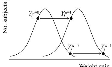
Figure 14.1

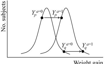
Figure 14.2

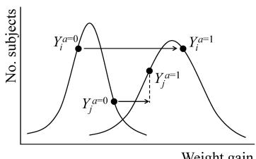
Figure 14.3

is well defined in the absence of rank preservation. For example, for the setting depicted in Figure 14.3, one could propose a model to estimate the average causal effect within strata of L, even when the treatment effects of individuals with the same value of L are not all identical.

14.5 G-estimation

not preserved since the outcome for individual i is less than that for individual j when a = 0 but not when a = 1.

Because of the implausibility of rank preservation, one should not generally use methods for causal inference that rely on it. In fact none of the methods we consider in this book require rank preservation. For example, the marginal structural mean models from Chapter 12 are models for average causal effects, not for individual causal effects, and thus they do not assume rank preservation. The estimated average causal effect of smoking cessation on weight gain was 3.5 kg (95% confidence interval: 2.5, 4.5). This average effect is agnostic as to whether rank preservation of individual causal effects holds. Similarly, the structural nested mean model in the previous section made no assumptions about rank preservation.

A structural nested mean model The additive rank-preserving model in this section makes a much stronger assumption than non-rank-preserving models: the assumption of constant treatment effect for all individuals with the same value of L. There is no reason why we would want to use such an unrealistic rank-preserving model in practice. And yet we use it in the next section to introduce g-estimation because g-estimation is easier to understand for rank-preserving models, and because the g-estimation procedure is actually the same for rank-preserving and nonrank-preserving models. Note that the (conditional additive) rank-preserving structural model is a structural mean model—the mean of the individual shifts from Y ^a=0 to Y ^a=1 is equal to each of the individual shifts within levels of L.

This section links the material in the previous three sections. Suppose the goal is estimating the parameters of the structural nested mean model E[Y ^a − Y ^a=0|A = a, L] = β1a. For simplicity, we first consider a model with a single parameter β1. Because the model lacks product terms β2aL, we are effectively assuming that the average causal effect of smoking cessation is constant across strata of L, i.e., no additive effect modification by L.

We also assume that the additive rank-preserving model Y a ⁱ − Y a=0 ⁱ = ψ1a is correctly specified for all individuals i. Then the individual causal effect ψ¹ is equal to the average causal effect β¹ in which we are interested. We write the rank-preserving model as Y ^a −Y ^a=0 = ψ1a, without a subscript i to index individuals because the model is the same for all individuals. For reasons that will soon be obvious, we write the model in the equivalent form

\[Y^{a=0} = Y^a - \psi\_1 a\]

The first step in g-estimation is linking the model to the observed data. To do so, remember that an individual’s observed outcome Y is, by consistency, the counterfactual outcome Y ^a=1 if the person received treatment A = 1 or the counterfactual outcome Y ^a=0 if the person received no treatment A = 0. Therefore, if we replace the fixed value a in the structural model by each individual’s value A—which will be 1 for some and 0 for others—then we can replace the counterfactual outcome Y ^a by the individual’s observed outcome Y ^A = Y .

The rank-preserving structural model then implies an equation in which each individual’s counterfactual outcome Y ^a=0 is a function of his observed data on treatment and outcome and the unknown parameter ψ1:

\[Y^{a=0} = Y - \psi\_1 A\]

If this model were correct and we knew the value of ψ¹ then we could calculate the counterfactual outcome under no treatment Y ^a=0 for each individual in the study population. But we don’t know ψ1. Estimating it is precisely the goal of our analysis.

Let us play a game. Suppose a friend of yours knows the value of ψ¹ but he only tells you that ψ¹ is one of the following: ψ † = −20, ψ † = 0, or ψ † = 10. He challenges you: “Can you identify the true value ψ¹ among the 3 possible values ψ † ?” You accept the challenge. For each individual, you compute

\[H(\psi^\dagger) = Y - \psi^\dagger A\]

for each of the three possible values ψ † . The newly created variables H(−20), H(0), and H(10) are candidate counterfactuals. Only one of them is the counterfactual outcome Y ^a=0. More specifically, H(ψ † ) = Y ^a=0 if ψ † = ψ1. In this game, choosing the correct value of ψ¹ is equivalent to choosing which one of the three candidate counterfactuals H(ψ † ) is the true counterfactual Y ^a=0 = H(ψ1). Can you think of a way to choose the right H(ψ † )?

Remember from Section 14.2 that the assumption of conditional exchangeability can be expressed as a logistic model for treatment given the counterfactual outcome and the covariates L. When conditional exchangeability holds, Rosenbaum (1987) proposed a ver- the parameter α¹ for the counterfactual outcome should be zero. So we have a simple method to choose the true counterfactual out of the three variables H(ψ † ). We fit three separate logistic models

\[\text{logit}\,\text{Pr}[A=1|H(\psi^\dagger),L] = \alpha\_0 + \alpha\_1 H(\psi^\dagger) + \alpha\_2 L,\]

one per each of the three candidates H(ψ † ). The candidate H(ψ † ) with α¹ = 0 is the counterfactual Y ^a=0, and the corresponding ψ † Important: G-estimation does not is the true value ψ1. For example, suppose that H(ψ † = 10) is unassociated with treatment A given the covariates L. Then our estimate ψˆ ¹ of ψ¹ is 10. We are done. That was g-estimation.

In practice, however, we need to g-estimate the parameter ψ¹ in the absence of a friend who knows the right answer and likes to play games. Therefore we will need to search over all possible values ψ † until we find the one that results in an H(ψ † ) with α¹ = 0. Because not all possible values can be tested—there is an infinite number of values ψ † in any given interval—we can conduct a fine search over the possible range of ψ † values from −20 to 20 by increments of 0.01. The finer the search, the closer to the true estimate ψˆ ¹ we will get, but code: Program 14.2 also the greater the computational demands.

In our smoking cessation example, we first computed each individual’s value of the 31 candidates H(2.0), H(2.1), H(2.2), …H(4.9), and H(5.0) for values ψ † between 2.0 and 5.0 by increments of 0.1. We then fit 31 separate logistic models for the probability of smoking cessation. These models were exactly like the one used to estimate the denominator of the IP weights in Chapter 12, except that we added to each model one of the 31 candidates H(ψ † ). The parameter estimate ˆα¹ for H(ψ † ) was closest to zero for values H(3.4) and H(3.5). A finer search found that the minimum value of ˆα¹ (which was essentially zero) was for H(3.446). Thus, our g-estimate ψˆ ¹ of the average causal effect ψ¹ = β¹ of smoking cessation on weight gain is 3.4 kg.

To compute a 95% confidence interval around our g-estimate of 3.4, we used the P-value for a Wald test of α¹ = 0 in the logistic models fit above.

sion of this procedure for non-timevarying treatments.

test whether conditional exchangeability holds; it assumes that conditional exchangeability holds.

Fine Point 14.2

Sensitivity analysis for unmeasured confounding. G-estimation relies on the fact that α¹ = 0 if conditional exchangeability given L holds. Now consider a setting in which conditional exchangeability does not hold. For example, suppose that the probability of quitting smoking A is lower for individuals whose spouse is a smoker, and that the spouse’s smoking status is associated with important determinants of weight gain Y not included in L. That is, there is unmeasured confounding by spouse’s smoking status. Because now the variables in L are insufficient to achieve exchangeability of the treated and the untreated, the treatment A and the counterfactual Y ^a=0 are associated conditional on L. That is, α¹ ̸= 0 and we cannot apply g-estimation as described in the main text.

But g-estimation does not require that α¹ = 0. Suppose that, because of unmeasured confounding by the spouse’s smoking status, α¹ is expected to be 0.1 rather than 0. Then we can apply g-estimation as described in the text except that we will test whether α¹ = 0.1 rather than whether α¹ = 0. G-estimation does not require that conditional exchangeability given L holds, but that the magnitude of nonexchangeability—the value of α1—is known. This property of g-estimation can be used to conduct sensitivity analyses for unmeasured confounding.

If we believe that L may not sufficiently adjust for confounding, then we can repeat our g-estimation analysis under different scenarios of unmeasured confounding, represented by a range of values of α1, and plot the effect estimates under each of them. Such plot shows how sensitive our effect estimate is to unmeasured confounding of different direction and magnitude. One practical problem for this approach is how to quantify the unmeasured confounding on the α¹ scale (is 0.1 a lot of unmeasured confounding?) Robins, Rotnitzky, and Scharfstein (1999) provide technical details on sensitivity analysis for unmeasured confounding using g-estimation.

may be used. For example, a Score test simplifies the calculations (it doesn’t require fitting multiple models) and, in large samples, is essentially equivalent to a Wald test.

of the logistic models is necessarily restricted to uncensored individuals (C = 0), and the contribution of each individual is weighted by the estimate of the individual’s IP weight SW^C . See Technical Point 14.2.

As expected, the P-value was 1—it was actually 0.998—for ψ Any valid test other than the Wald † = 3.446, which is the value ψ † that results in a candidate H(ψ † ) with a parameter estimate αˆ¹ = 0. Of the 31 logistic models that we fit for ψ † values between 2.0 and 5.0, the P-value was greater than 0.05 in all models with H(ψ † ) based on ψ † values between approximately 2.5 and 4.5. That is, using the conventional statistical jargon, the test “did not reject the null hypothesis” at the 5% level for the subset of ψ † values between 2.5 and 4.5. By inverting the test results, we concluded that the limits of the 95% confidence interval around 3.4 are 2.5 and 4.5. Another option to compute the 95% confidence interval is bootstrapping of the g-estimation procedure.

More generally, the 95% confidence interval for a g-estimate is determined by finding the set of values of ψ † that result in a P-value> 0.05 when testing for α¹ = 0. The 95% confidence interval is obtained by inversion of the statistical test for α¹ = 0, with the limits of the 95% confidence interval being the limits of the set of values ψ † with P-value> 0.05. In our example, the statistical test In the presence of censoring, the fit was based on a robust variance estimator because of the use of IP weighting to adjust for censoring. Therefore our 95% confidence interval is conservative in large samples, i.e., it will trap the true value at least 95% of the time. In large samples, bootstrapping would result in a non-conservative, and thus possibly narrower, 95% confidence interval for the g-estimate.

Back to non-rank-preserving models. The g-estimation algorithm (i.e., the computer code implementing the procedure) for ψ¹ produces a consistent estimate of the parameter β¹ of the mean model, assuming the mean model is correctly specified (that is, if the average treatment effect is equal in all levels of L). This is true regardless of whether the individual treatment effect is constant, i.e., regardless of whether the conditional additive rank preservation holds. In other words, the validity of the g-estimation algorithm does not actually require that H(β1) = Y ^a=0 for all individuals, where β¹ is the parameter value in the mean model. Rather, the algorithm only requires that H(β1) and

Y ^a=0 have the same conditional mean given L.

Interestingly, the above g-estimation procedure can be readily modified to incorporate a sensitivity analysis for unmeasured confounding, as described in Fine Point 14.2.

14.6 Structural nested models with two or more parameters

We have so far considered a structural nested mean model with a single parameter β1. The lack of product terms β2aL implies that we believe that the average causal effect of smoking cessation does not vary across strata of L. The structural nested model will be misspecified—and thus our causal inferences will be wrong—if there is indeed effect modification by some components V of L but we failed to add a product term β2aV . This is in contrast with the saturated marginal structural model E[Y a ] = β⁰ + β1a, which is not misspecified if we fail to add terms β2aV and β3V even if there is effect modification by V . Marginal structural models that do not condition on V estimate the average As discussed in Chapter 12, a de- causal effect in the population, whereas those that condition on V estimate the average causal effect within levels of V . Structural nested models estimate, by definition, the average causal effect within levels of the covariates L, not the average causal effect in the population. Omitting product terms in structural nested models when there is effect modification will generally lead to bias due to model misspecification.

Fortunately, the g-estimation procedure described in the previous section can be generalized to models with product terms. For example, suppose we believe that the average causal effect of smoking cessation depends on the baseline level of smoking intensity V . We may then consider the structural nested mean model E[Y ^a − Y ^a=0|A = a, L] = β1a + β2aV . Because the structural model has two parameters, β¹ and β2, we also need to include two parameters in the IP weighted logistic model for Pr[A = 1|H(β † ), L] with β † = β † 1 , β† 2 and H(β † ) = Y − β † ¹A − β † ²AV . For example, we could fit the logistic model

\[\text{logit}\Pr[A=1|H(\beta^\dagger),L] = \alpha\_0 + \alpha\_1 H(\beta^\dagger) + \alpha\_2 H(\beta^\dagger)V + \alpha\_3 L\]

and find the combination of values of β † 1 and β † 2 that result in a H(β † ) that is independent of treatment A conditional on the covariates L. That is, we need to search the combination of values β † 1 and β † 2 that make both α¹ and α² equal to zero. Because the model has two parameters, the search must be conducted over a two-dimensional space. Thus a systematic, brute force search will be more involved than that described in the previous section.

However, even though we motivated g-estimation by using a parameter search, a search over the possible values of the parameters is not generally necessary for g-estimation. In fact, for linear mean models like the one discussed here, the estimate can be directly calculated using a formula, i.e., the estimator has closed form . For nonlinear structural nested mean models, no closed form estimator exists but we can use standard optimization techniques based on derivatives, such as Newton-Raphson, because g-estimation can be seen as solving an estimating equation for the model parameters (see Technical Point 14.2 for details). For certain structural nested models for survival analysis, a search is required because the estimating equation is not differentiable with respect to the model parameters (see Chapter 17).

sirable property of marginal structural models is null preservation: when the null hypothesis of no average causal effect is true, the model is never misspecified. Structural nested models preserve the null too. In contrast, although the parametric g-formula preserves the null for time-fixed treatments, it loses this property in the time-varying setting (see Part III).

In our smoking cessation example, the g-estimates were βˆ ¹ = 2.86 and βˆ code: Program 14.3 ² = 0.03. The corresponding 95% confidence intervals can most easily be calculated by bootstrapping. In the more general case, we would consider a model that allows the average causal effect of smoking cessation to vary across all strata of the variables in L. For a dichotomous treatment, the unsaturated linear model E[Y ^a − Y ^a=0] = β1a + a P^{p j}=1 β2jL^j has p + 1 parameters β1, β21,…β2p, where β2^j is the parameter corresponding to the product term aL^j and L^j represents one of the p components of L. The average causal effect in the entire study population can then be calculated as β¹ + 1 n P i P^{p j}=1 β2jLij , where n is the number of individuals in the study.

After having described g-methods, we now review two methods that are arguably the most commonly used approaches to adjust for confounding: outcome regression and propensity scores.

G-estimation of structural nested mean models. Consider the structural nested mean model

\[\operatorname{E}\left[Y - Y^{a=0} | A, L\right] = A \gamma\left(L; \beta\right).\]

where γ L; β † is a known function, β † is usually a vector-valued parameter, and γ L; β † = 0 = 0. An asymptotically unbiased and normally distributed estimate of β can be obtained by g-estimation under the assumptions described in the text, including a correctly specified parametric model for E [A|L] . Specifically, our estimate of β is the value of β † that minimizes the association between H(β † ) = Y − Aγ L; β † and A conditional on L. When we base our g-estimate on the score test (see, e.g., Casella and Berger 2002), this procedure is equivalent to finding the parameter value β † that solves the estimating equation

\[\sum\_{i=1}^{n} \mathcal{I}\left[C\_i = 0\right] W\_i^C H\_i(\beta^\dagger) \left(A\_i - \mathcal{E}\left[A|L\_i\right]\right) q(L\_i) = 0\]

where q(Li) is a (user-specified) vector function of the same dimension as β, I [Cⁱ = 0] is an indicator for censoring for individual i, and the IP weight W^C i and the expectation E [A|Lⁱ ] = Pr [A = 1|Lⁱ ] are replaced by their estimates. E [A|Lⁱ ] can be estimated from a logistic model for treatment conditional on the covariates L in which individual i’s contribution is weighted by W^C i if Cⁱ = 0 and it is zero otherwise. [Because A and L are observed on all individuals, we could also estimate E [A|Lⁱ ] by an unweighted logistic regression of A on L using all individuals.] The choice of the vector function q(Li) affects the statistical efficiency of the estimator, but not its consistency. That is, although all choices of the function will result in valid confidence intervals, the length of the confidence interval will depend on the function. Robins (1994) provided a formal description of structural nested mean models, and derived the function that minimizes confidence interval length.

The solution to the equation has a closed form when γ L; β † is linear in β † , i.e., γ L; β † = β †,T d(L) for a known vector function d(L) of the same dimension as β. In that case, if we choose q(L) = d(L), βˆ equals

\[\left(\sum\_{i=1}^{n} \mathbf{I}\left[C\_i = 0\right] W\_i^C A\_i \left(A\_i - \mathbb{E}\left[A|L\_i\right]\right) d(L\_i) d(L\_i)^T\right)^{-1} \sum\_{i=1}^{n} \mathbf{I}\left[C\_i = 0\right] W\_i^C Y\_i \left(A\_i - \mathbb{E}\left[A|L\_i\right]\right) d(L\_i)^T\]

A natural question is whether we can increase statistical efficiency by replacing Hi(β † ) by a nonlinear function, such as - Hi(β † ) 3 , in the above estimating equation and still preserve consistency of the estimate. Nonlinear functions of Hi(β † ) cannot be used in our estimating equation for models that, like the structural nested mean models described in this chapter, impose only mean independence conditional on L, i.e., E [H(β1)|A, L] = E [H(β1)|L], for identification. Nonlinear functions of Hi(β † ) can be used for models that impose distributional independence, i.e., H(β1)⊥⊥A|L, like structural nested distribution models (not described in this chapter) that map percentiles of the distribution of Y ^a given (A = a, L) into percentiles of the distribution of Y ⁰ given (A = a, L).

The estimator of β is consistent only if the models used to estimate E [A|L] and Pr [C = 1|A, L] are both correct. We can construct a more robust estimator by replacing H(β † ) by H(β † )−E - H(β † )|L in the estimating equation, and then estimating the latter conditional expectation by fitting an unweighted linear model for E - H(β † )|L = E- Y ^a=0|L among the uncensored individuals. If this model is correct then the estimate of β solving the modified estimating equation remains consistent even if both the above models for E [A|L] and Pr [C = 1|A, L] are incorrect. Thus we obtain a consistent estimator of β if either (i) the model for E - H(β † )|L or (ii) both models for E [A|L] and Pr [C = 1|A, L] are correct, without knowing which of (i) or (ii) is correct. We refer to such an estimator as being doubly robust.Technical Point 21.6 describes the closed-form of this doubly robust estimator for the linear structural nested mean model with time-varying treatments (see Robins 2000).

Chapter 15 OUTCOME REGRESSION AND PROPENSITY SCORES

Outcome regression and various versions of propensity score analyses are the most commonly used parametric methods for causal inference. You may rightly wonder why it took us so long to include a chapter that discusses these methods. So far we have described IP weighting, standardization, and g-estimation—the g-methods. Presenting the most commonly used methods after the least commonly used ones seems an odd choice on our part. Why didn’t we start with the simpler and widely used methods based on outcome regression and propensity scores? Because these methods do not work in general.

More precisely, the simpler outcome regression and propensity score methods—as described in a zillion publications that this chapter cannot possibly summarize—work fine in simpler settings, but these methods are not designed to handle the complexities associated with causal inference with time-varying treatments. In Part III we will again discuss g-methods but will say less about conventional outcome regression and propensity score methods. This chapter is devoted to causal methods that are commonly used but have limited applicability for complex longitudinal data.

15.1 Outcome regression

age causal effect as E[Y ^a=1,c=0] − E[Y ^a=0,c=0]. We assumed that exchangeability of the treated and the untreated was achieved conditional on the L variables sex, age, race, education, intensity and duration of smoking, physical activity in daily life, recreational exercise, and weight.

model as a faux marginal structural model because it has the form of a marginal structural model but IP weighting is not required to estimate its parameters. The stabilized IP weights SW^A(L) are all equal to 1 because the model is conditional on the entire vector L rather than on a subset V of L.

In the last three chapters we have described IP weighting, standardization, and g-estimation to estimate the average causal effect of smoking cessation Reminder: We defined the aver- (the treatment) A on weight gain (the outcome) Y . We also described how to estimate the average causal effect within subsets of the population, either by restricting the analysis to the subset of interest or by adding product terms in marginal structural models (Chapter 12) and structural nested models (Chapter 14). Take structural nested models. These models include parameters for the product terms between treatment A and the variables L, but no parameters for the variables L themselves. This is an attractive property of structural nested models because we are interested in the causal effect of A on Y within levels of L but not in the (noncausal) relation between L and Y . A method g-estimation of structural nested models—that is agnostic about the functional form of the L-Y relation is protected from bias due to misspecifying this relation.

On the other hand, if we were willing to specify the L-Y association within In Chapter 12, we referred to this levels of A, we would consider the structural model

\[\operatorname{E}[Y^{a,c=0}|L] = \beta\_0 + \beta\_1 a + \beta\_2 a L + \beta\_3 L^2\]

where β² and β³ are vector parameters. The average causal effects of smoking cessation A on weight gain Y in each stratum of L are a function of β¹ and β2, the mean counterfactual outcomes under no treatment in each stratum of L are a function of β⁰ and β3. The parameter β³ is usually referred as the main effect of L, but the use of the word effect is misleading because β³ may not have an interpretation as the causal effect of L (there may be confounding for L). The parameter β³ simply quantifies how the mean of the counterfactual Y ^a=0,c=0 varies as a function of L, as we can see in our structural model. See

Nuisance parameters. Suppose our goal is to estimate the causal parameters β1and β2. If we do so by fitting the outcome regression model E[Y a,c=0|L] = β0+β1a+β2aL+β3L, our estimates of β1and β² will in general be consistent only if β⁰ + β3L correctly models the dependence of the mean E[Y ^a=0,c=0|L] on L. We refer to the parameters β⁰ and β³ as nuisance parameters because they are not our parameters of primary interest.

On the other hand, if we estimate β1and β² by g-estimation of the structural nested model E[Y a,c=0 −Y ^a=0,c=0|L] = β1a+β2aL, then our estimates of β1and β² will in general be consistent only if the conditional probability of treatment given L Pr[A = 1|L] is correct. That is, the parameters of the treatment model such as logit Pr[A = 1|L] = α⁰ + α1L are now the nuisance parameters.

For example, bias would arise in the outcome regression model if a covariate L is modeled with a linear term β3L when it should actually be linear and quadratic β3L+β4L 2 . Structural nested models are not subject to misspecification of an outcome regression model because the L-Y relation is not specified in the structural model. However, bias would arise when using g-estimation of structural nested models if the L-A relation is misspecified in the treatment model. Symmetrically, outcome regression models are not subject to misspecification of a treatment model. For fixed treatments that do not vary over time, deciding what method to use boils down to deciding which nuisance parameters—those in the outcome model or in the treatment model—we believe can be more accurately estimated. When possible, a better alternative is to use doubly robust methods (see Fine Point 13.2).

Fine Point 15.1 for a discussion of parameters that, like β⁰ and β3, do not have a causal interpretation.

The counterfactual mean outcomes if everybody in stratum l of L had been treated and remained uncensored, E[Y ^a=1,c=0|L = l], are equal to the corresponding mean outcomes in the uncensored treated, E[Y |A = 1, C = 0, L = l], under exchangeability, positivity, and well-defined interventions. And analogously for the untreated. Therefore the parameters of the above structural model can be estimated via ordinary least squares by fitting the outcome regression model

\[\operatorname{E}[Y|A,C=0,L] = \alpha\_0 + \alpha\_1 A + \alpha\_2 AL + \alpha\_3 L\_1\]

as described in Section 13.2. Like stratification in Chapter 3, outcome regression adjusts for confounding by estimating the causal effect of treatment in each stratum of L. If the variables L are sufficient to adjust for confounding (and selection bias) and the outcome model is correctly specified, no further adjustment is needed. That is, the parameters α of the regression model equal β⁰ and β³ specify the dependence the parameters β of the structural model.

In Section 13.2, outcome regression was an intermediate step towards the estimation of a standardized outcome mean. Here, outcome regression is the end of the procedure. Rather than standardizing the estimates of the conditional means to estimate a marginal mean, we just compare the conditional mean estimates. In Section 13.2, we fit a regression model with only one product term in β² (between A and smoking intensity). That is, a model in which we a priori set most product terms equal to zero. Using the same model as in Section 13.2, here we obtained the parameter estimates βˆ ¹ = 2.6 and βˆ ² = 0.05. As an example, the effect estimate E[ ^{b Y |A} = 1, C = 0, L]−E[ ^{b Y |A} = 0, C = 0, L] code: Program 15.1 was 2.8 (95% confidence interval: 1.5, 4.1) for those smoking 5 cigarettes/day, and 4.4 (95% confidence interval: 2.8, 6.1) for 40 cigarettes/day. A common approach to outcome regression is to assume that there is no effect modification by any variable in L. Then the model is fit without any product terms and βˆ ¹ is an estimate of both the conditional and marginal average causal effects

of Y ^a=0,c=0 on L, which is required when the model is used to estimate (i) the mean counterfactual outcomes and (ii) the conditional (within levels of L) effect on the multiplicative rather than additive scale.

of treatment. In our example, a model without any product terms yielded the estimate 3.5 (95% confidence interval: 2.6, 4.3) kg.

In this chapter we did not need to explain how to fit an outcome regression model because we had already done it in Chapter 13 when estimating the components of the parametric g-formula. It is equally straightforward to use outcome regression for discrete outcomes. For a dichotomous outcome Y one could fit a logistic model for Pr [Y = 1|A = a, C = 0, L].

15.2 Propensity scores

Here we only consider propensity scores for dichotomous treatments. Propensity score methods, other than IP weighting and g-estimation and other related doubly-robust estimators, are difficult to generalize to non-dichotomous treatments.

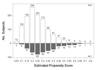
Figure 15.1

to sampling variability, the true propensity score only approximately “balances” the covariates L. The estimated propensity score based on a correct model gives better balance in general.

When using IP weighting (Chapter 12) and g-estimation (Chapter 14), we estimated the probability of treatment given the covariates L, Pr [A = 1|L], for each individual. Let us refer to this conditional probability as π(L). The value of π(L) is close to 0 for individuals who have a low probability of receiving treatment and is close to 1 for those who have a high probability of receiving treatment. That is, π(L) measures the propensity of individuals to receive treatment given the information available in the covariates L. No wonder that π(L) is referred to as the propensity score.

In an ideal randomized trial in which half of the individuals are assigned code: Program 15.2 to treatment A = 1, the propensity score π(L) = 0.5 for all individuals. Also note that π(L) = 0.5 for any choice of L. In contrast, in observational studies some individuals may be more likely to receive treatment than others. Because treatment assignment is beyond the control of the investigators, the true propensity score π(L) is unknown, and therefore needs to be estimated from the data.

In our example, we can estimate the propensity score π(L) by fitting a logistic model for the probability of quitting smoking A conditional on the covariates L. This is the same model that we used for IP weighting and gestimation. Under this model, individual 22941 was estimated to have the lowest estimated propensity score (0.053), and individual 24949 the highest (0.793). Figure 15.1 shows the distribution of the estimated propensity score in quitters A = 1 (bottom) and nonquitters A = 0 (top). As expected, those who quit smoking had, on average, a greater estimated probability of quitting (0.312) than those who did not quit (0.245). If the distribution of π(L) were the same for the treated A = 1 and the untreated A = 0, then there would be no confounding due to L, i.e., there would be no open path from L to A on a causal diagram.

Individuals with the same propensity score π(L) will generally have different values of some covariates L. For example, two individuals with π(L) = 0.2 may differ with respect to smoking intensity and exercise, and yet they may be equally likely to quit smoking given all the variables in L. That is, both individuals have the same conditional probability of ending up in the treated group A = 1. If we consider all individuals with a given value of π(L) in the In the study population, due super-population, this group will include individuals with different values of L (e.g., different values of smoking intensity and exercise), but the distribution of L will be the same in the treated and the untreated, that is, A⊥⊥L|π(L). We say the propensity score balances the covariates between the treated and the untreated.

Of course, the propensity score only balances the measured covariates L, which does not prevent residual confounding by unmeasured factors. Randomization balances both the measured and the unmeasured covariates, and thus

Balancing scores and prognostic scores. As discussed in the text, the propensity score π(L) balances the covariates between the treated and the untreated. In fact, the propensity score π(L) is the simplest example of a balancing score. More generally, a balancing score b(L) is any function of the covariates L such that A⊥⊥L|b(L). That is, for each value of the balancing score, the distribution of the covariates L is the same in the treated and the untreated. Rosenbaum and Rubin (1983) proved that exchangeability and positivity based on the variables L implies exchangeability and positivity based on a balancing score b(L). If it is sufficient to adjust for L, then it is sufficient to adjust for a balancing score b(L), including the propensity score π(L). The causal diagram in Figure 15.2 depicts the propensity score for the setting represented in Figure 7.1: the π(L) can be viewed as an intermediate node between L and A with a deterministic arrow from L to π(L). By noting that π(L) blocks all backdoor paths from A to L we have given a proof of the sufficiency of adjusting for π(L).

An alternative to a balancing score b(L) is a prognostic score s(L), i.e., a function of the covariates L such that Y ^a=0⊥⊥L|s(L). Adjustment methods can be developed for both balancing scores and prognostic scores, but methods for prognostic scores require stronger assumptions and cannot be readily extended to time-varying treatments. See Hansen (2008) and Abadie et al. (2013) for a discussion of prognostic scores.

it is the preferred method to eliminate confounding. See Technical Point 15.1 for a formal definition of a balancing score.

founding and selection bias, then π(L) is sufficient too. This result was derived by Rosenbaum and Rubin in a seminal paper published in 1983.

In a randomized experiment, the es- in Chapter 2, holds. timated π(L) adjusts for both systematic and random imbalances in covariates, and thus does better than adjustment for the true π(L) which ignores random imbalances.

Like all methods for causal inference that we have discussed, the use of If L is sufficient to adjust for con- propensity score methods requires the identifying conditions of exchangeability, positivity, and consistency. The use of propensity score methods is justifed by the following key result: Exchangeability of the treated and the untreated within levels of the covariates L implies exchangeability within levels of the propensity score π(L). That is, conditional exchangeability Y ^a⊥⊥A|L implies Y ^a⊥⊥A|π(L). Further, positivity within levels of the propensity score π(L) which means that no individual has a propensity score equal to either 1 or 0—holds if and only if positivity within levels of the covariates L, as defined

Under exchangeability and positivity within levels of the propensity score π(L), the propensity score can be used to estimate causal effects using stratification (including outcome regression), standardization, and matching. The next two sections describe how to implement each of these methods. As a first step, we must start by estimating the propensity score π(L) from the observational data and then proceeding to use the estimated propensity score in lieu of the covariates L for stratification, standardization, or matching.

15.3 Propensity stratification and standardization

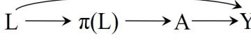
Figure 15.2

The average causal effect among individuals with a particular value s of the propensity score π(L), i.e., E[Y ^a=1,c=0|π(L) = s] − E[Y ^a=0,c=0|π(L) = s] is equal to E[Y |A = 1, C = 0, π(L) = s] − E[Y |A = 0, C = 0, π(L) = s] under the identifying conditions. This conditional effect might be estimated by restricting the analysis to individuals with the value s of the true propensity score. However, the propensity score π(L) is generally a continuous variable that can take any value between 0 and 1. It is therefore unlikely that two individuals will have exactly the same value s. For example, only individual 22005 had an estimated π(L) of 0.6563, which means that we cannot estimate the causal effect among individuals with π(L) = 0.6563 by comparing the treated and the untreated with that particular value.

One approach to deal with the continuous propensity score is to create strata that contain individuals with similar, but not identical, values of π(L). The deciles of the estimated π(L) is a popular choice: individuals in the population are classified in 10 strata of approximately equal size, then the causal code: Program 15.3 effect is estimated in each of the strata. In our example, each decile contained approximately 162 individuals. The effect of smoking cessation on weight gain ranged across deciles from 0.0 to 6.6 kg, but the 95% confidence intervals around these point estimates were wide.

We could have also obtained these effect estimates by fitting an outcome regression model for E[Y |A, C = 0, π(L)] that included as covariates treatment A, 9 indicators for the deciles of the estimated π(L) (one of the deciles is the reference level and is already incorporated in the intercept of the model), and 9 product terms between A and the indicators. Most applications of outcome regression with deciles of the estimated π(L) do not include the product terms, i.e., they assume no effect modification by π(L). In our example, a model without product terms yields an effect estimate of 3.5 kg (95% confidence interval: 2.6, 4.4). See Fine Point 15.2 for more on effect modification by the propensity score.

Stratification on deciles or other functions of the propensity score raises a potential problem: in general the distribution of the continuous π(L) will differ between the treated and the untreated within some strata (e.g., deciles). If, e.g., the average π(L) were greater in the treated than in the untreated in some strata, then the treated and the untreated might not be exchangeable in those strata. This problem did not arise in previous chapters, when we used functions of the propensity score to estimate the parameters of structural models Caution: the denominator of the via IP weighting and g-estimation, because those methods used the numerical value of the estimated probability rather than a categorical transformation like deciles. Similarly, the problem does not arise when using outcome regression for E[Y |A, C = 0, π(L)] with the estimated propensity score π(L) as a continuous covariate rather than as a set of indicators. When we used this latter approach in our example the effect estimate was 3.6 (95% confidence interval: 2.7, 4.5) kg.

The validity of our inference depends on the correct specification of the relationship between π(L) and the mean outcome Y (which we assumed to be linear). However, because the propensity score is a one-dimensional summary Though the propensity score is one- of the multi-dimensional L, it is easy to guard against misspecification of this relationship by fitting flexible models cubic splines rather than a single linear term for the propensity score. Note that IP weighting and g-estimation were agnostic about the relationship between propensity score and outcome.

When our parametric assumptions for E[Y |A, C = 0, π(L)] are correct, plus exchangeability and positivity hold, the model estimates the average causal effects within all levels s of the propensity score E[Y ^a=1,c=0|π(L) = s] − E[Y ^a=0,c=0|π(L) = s]. If we were interested in the average causal effect in the entire study population E[Y ^a=1,c=0] − E[Y ^a=0,c=0], we would standardize the conditional means E[Y |A, C = 0, π(L)] by using the distribution of the code: Program 15.4 propensity score. The procedure is the same one described in Chapter 13 for continuous variables, except that we replace the variables L by the estimated π(L). Note that the procedure can naturally incorporate a product term between treatment A and the estimated π(L) in the outcome model. In our example, the standardized effect estimate was 3.6 (95% confidence interval: 2.7, 4.6) kg.

IP weights for a dichotomous treatment A is not the propensity score π(L), but a function of π(L). The denominator is π(L) for the treated (A = 1) and 1 − π(L) for the untreated (A = 0).

dimensional, we still need to estimate it from a model that regresses treatment on a high-dimensional L. The same applies to IP weighting and g-estimation.

15.4 Propensity matching

matched population has the π(L) distribution of the treated, of the untreated, or any other arbitrary distribution.

that nobody knew how to compute the variance of the effect estimate. That is no longer the case thanks to the work of Abadie and Imbens (2006).

fined within levels of the propensity score, i.e., Pr [A = a|π(L) = s] > 0 for all s such that Pr [π(L) = s] is nonzero.

The process of matching on the propensity score π(L) is analogous to matching on a single continuous variable L, a procedure described in Chapter 4. After propensity matching, the There are many forms of propensity matching. All of them attempt to form a matched population in which the treated and the untreated are exchangeable because they have the same distribution of π(L). For example, one can match the untreated to the treated: each treated individual is paired with one (or more) untreated individuals with the same propensity score value. The subset of the original population comprised by the treated-untreated pairs (or sets) is the matched population. Under exchangeability and positivity given π(L), association measures in the matched population are consistent estimates of effect A drawback of matching used to be measures: the associational risk ratio in the matched population consistently estimates the causal risk ratio in the matched population.

Again, it is unlikely that two individuals will have exactly the same values of the propensity score π(L). In our example, propensity score matching will be carried out by identifying, for each treated individual, one (or more) untreated individuals with a close value of π(L). A common approach is to match treated individuals with a value s of the estimated π(L) with untreated individuals who have a value s ± 0.05, or some other small difference. For example, treated individual 1089 (estimated π(L) of 0.6563) might be matched with untreated individual 1088 (estimated π(L) of 0.6579). There are numerous ways of defining closeness, and a detailed description of these definitions is beyond the scope of this book.

Defining closeness in propensity matching entails a bias-variance tradeoff. If the closeness criteria are too loose, individuals with relatively different values of π(L) will be matched to each other, the distribution of π(L) will differ between the treated and the untreated in the matched population, and exchangeability will not hold. On the other hand, if the closeness criteria are too tight and many individuals are excluded by the matching procedure, there will be approximate exchangeability but the effect estimate may have wider 95% confidence intervals.

The definition of closeness is also related to that of positivity. In our smok-Remember: positivity is now de- ing cessation example, the distributions of the estimated π(L) in the treated and the untreated overlapped throughout most of the range (see Figure 15.1). Only 2 treated individuals (0.01% of the study population) had values greater than those of any untreated individual. When using outcome regression on the estimated π(L) in the previous section, we effectively assumed that the lack of untreated individuals with high π(L) estimates was due to chance—random nonpositivity—and thus included all individuals in the analysis. In contrast, most propensity matched analyses would not consider those two treated individuals close enough to any of the untreated individuals, and would exclude them. Matching does not distinguish between random and structural nonpositivity.

The above discussion illustrates how the matched population may be very different from the target (super)population. In theory, propensity matching can be used to estimate the causal effect in a well characterized target population. For example, when matching each treated individual with one or more untreated individuals and excluding the unmatched untreated, one is estimating the effect in the treated (see Fine Point 15.2). In practice, however, propensity matching may yield an effect estimate in a hard-to-describe subset of the study population. For example, under a given definition of closeness, some treated individuals cannot be matched with any untreated individuals

and thus they are excluded from the analysis. As a result, the effect estimate corresponds to a subset of the population that is defined by the values of the estimated propensity score that have successful matches.

That propensity matching forces investigators to restrict the analysis to treatment groups with overlapping distributions of the estimated propensity score is often presented as a strength of the method. One surely would not want to have biased estimates because of violations of positivity, right? However, leaving aside issues related to random variability (see above), there is a price to be paid for restrictions based on the propensity score. Suppose that, after inspecting Figure 15.1, we conclude that we can only estimate the effect of smoking cessation for individuals with an estimated propensity score less than 0.67. Who are these people? It is unclear because individuals do not come with a propensity score tattooed on their forehead. Because the matched population is not well characterized, it is hard to assess the transportability of the effect estimate to other populations.

Even if every subject came with When positivity concerns arise, restriction based on real-world variables (e.g., age, number of cigarettes) leads to a more natural characterization of the causal effect. In our smoking cessation example, the two treated individuals with estimated π(L) > 0.67 were the only ones in the study who were over age 50 and had smoked for less than 10 years. We could exclude them and explain that our effect estimate only applies to smokers under age 50 and to smokers 50 and over who had smoked for at least 10 years. This way of defining the target population is more natural than defining it as those with estimated π(L) < 0.67.

Using propensity scores to detect the overlapping range of the treated and the untreated may be useful, but simply restricting the study population to that range is a lazy way to ensure positivity. The automatic positivity ensured by propensity matching needs to be weighed against the difficulty of assessing transportability when restriction is solely based on the value of the estimated propensity scores.

15.5 Propensity models, structural models, predictive models

In Part II of this book we have described two different types of models for causal inference: propensity models and structural models. Let us now compare them.

Propensity models are models for the probability of treatment A given the variables L that are used to achieve conditional exchangeability. We have used propensity models for matching and stratification in this chapter, for IP weighting in Chapter 12, and for g-estimation in Chapter 14. The parameters of propensity models are nuisance parameters (see Fine Point 15.1) without a causal interpretation because a variable L and treatment A may be associated for many reasons—not only because the variable L causes A. For example, the association between L and A can be interpreted as the effect of L on A under Figure 7.1, but not under Figures 7.2 and 7.3. Yet propensity models are useful for causal inference, often as the basis of the estimation of the parameters of structural models, as we have described in this and previous chapters.

Structural models describe the relation between the treatment A and some component of the distribution (e.g., the mean) of the counterfactual outcome Y a , either marginally or within levels of the variables L. For continuous treatments, a structural model is often referred to as a dose-response model. The parameters for treatment in structural models are not nuisance parameters:

her propensity score tattooed on her forehead, the population could still be ill-characterized because the same propensity score value may mean different things in different settings.

Effect modification and the propensity score. A reason why matched and unmatched estimates may differ is effect modification. As an example, consider the common setting in which the number of untreated individuals is much larger than the number of treated individuals. Propensity matching often results in almost all treated individuals being matched and many untreated individuals being unmatched and therefore excluded from the analysis. When this occurs, the distribution of causal effect modifiers in the matched population will resemble that in the treated. Therefore, the effect in the matched population will be closer to the effect in the treated than to the effect that would have been estimated by methods that use data from the entire population. See Technical Point 4.1 for alternative ways to estimate the effect of treatment in the treated via IP weighting and standardization.

Effect modification across propensity strata may be interpreted as evidence that decision makers know what they are doing, e.g. that doctors tend to treat patients who are more likely to benefit from treatment (Kurth et al 2006). However, the presence of effect modification by π(L) may complicate the interpretation of the estimates. Consider a situation with qualitative effect modification: “Doctor, according to our study, this drug is beneficial for patients who have a propensity score between 0.11 and 0.93 when they arrive at your office, but it may kill those with propensity scores below 0.11,” or “Ms. Minister, let’s apply this educational intervention to children with propensity scores below 0.57 only.” The above statements are of little policy relevance because, as discussed in the main text, they are not expressed in terms of the measured variables L.

Finally, besides effect modification, there are other reasons why matched estimates may differ from the overall effect estimate: violations of positivity in the non-matched, an unmeasured confounder that is more/less prevalent (or that is better/worse measured) in the matched population than in the unmatched population, etc. As discussed for individual variables L in Chapter 4, apparent effect modification might be explained by differences in residual confounding across propensity strata.

of the relation between structural nested models and faux semiparametric marginal structural models, and other subtleties.

predict sexual orientation, political views, and personality traits (Kosinski et al, 2013). This is purely predictive, not necessarily causal.

they have a direct causal interpretation as outcome differences under different treatment values a. We have described two classes of structural models: marginal structural models and structural nested models. Marginal structural models include parameters for treatment, for the variables V that may be effect modifiers, and for product terms between treatment and variables V . The choice of V reflects only the investigator’s substantive interest in effect modification (see Section 12.5). If no covariates V are included, then the model is truly marginal. If all variables L are included as possible effect modifiers, See Fine Point 14.1 for a discussion then the marginal structural model becomes a faux marginal structural model. Structural nested models include parameters for treatment and for product terms between treatment A and all variables in L that are effect modifiers.

We have presented outcome regression as a method to estimate the parameters of faux marginal structural models for causal inference. However, outcome regression is also widely used for purely predictive, as opposed to causal, purposes. For example, online retailers use sophisticated outcome regression models to predict which customers are more likely to purchase their products. The goal is not to determine whether your age, sex, income, geographic origin, A study found that Facebook Likes and previous purchases have a causal effect on your current purchase. Rather, the goal is to identify those customers who are more likely to make a purchase so that specific marketing programs can be targeted to them. It is all about association, not causation. Similarly, doctors use algorithms based on outcome regression to identify patients at high risk of developing a serious disease or dying. The parameters of these predictive models do not necessarily have any causal interpretation and all covariates in the model have the same status, i.e., there are no treatment variable A and variables L.

The dual use of outcome regression in both causal inference method and

in prediction has led to many misunderstandings. One of the most important misunderstandings has to do with variable selection procedures. When the interest lies exclusively on outcome prediction, investigators may want to select any variables that, when included as covariates in the model, improve its predictive ability. Many well-known variable selection procedures—e.g., forward selection, backward elimination, stepwise selection—and more recent developments in machine learning are used to enhance prediction. These are powerful tools for investigators who are interested in prediction, especially when dealing with very high-dimensional data.

Unfortunately, statistics courses and textbooks have not always made a sharp difference between causal inference and prediction. As a result, these variable selection procedures for predictive models have often been applied to causal inference models. A possible result of this mismatch is the inclusion of superfluous—or even harmful—covariates in propensity models and structural models. Specifically, the application of predictive algorithms to causal inference models may result in inflated variances and greater bias.

The problem arises because of the widespread, but mistaken, belief that It is not uncommon for propen- propensity models should predict treatment A as well as possible. Propensity models do not need to predict treatment very well. They just need to include the variables L that guarantee exchangeability. Covariates that are strongly associated with treatment, but are not necessary to guarantee exchangeability, do not help reduce bias. If these covariates were included in L, adjustment can result in estimates with very large variances, or even amplify existing bias.

Consider the following example. Suppose all individuals in a certain study attend either hospital Aceso or hospital Panacea. Doctors in hospital Aceso give treatment A = 1 to 99% of the individuals, and those in hospital Panacea give A = 0 to 99% of the individuals. Suppose the variable Hospital has no effect on the outcome (except through its effect on treatment A) and is therefore not necessary to achieve conditional exchangeability. Say we decide to add Hospital as a covariate in our propensity model anyway. The propensity score π(L) in the target population is about 0.99 for individuals in hospital Aceso and 0.01 for those in hospital Panacea, but by chance we may end up with a study population in which everybody in hospital Aceso has A = 1 or If we perfectly predicted treatment, everybody in hospital Panacea has A = 0 for some strata defined by L. That is, our effect estimate may have a near-infinite variance without any reduction in confounding. That treatment is now very well predicted is irrelevant for causal inference purposes.

Besides variance inflation, a predictive attitude towards variable selection for causal inference models—both propensity models and outcome regression models—may also result in self-inflicted bias. For example, the inclusion of colliders as covariates may result in systematic bias even if colliders may be effective covariates for purely predictive purposes, and the inclusion of instruments (see next chapter) may amplify bias due to unmeasured variables. We will return to these issues in Chapter 18.

In general, causal inference methods based on models—propensity models and structural models—require no misspecification of the functional form for the covariates. To reduce the possibility of model misspecification, we use flexible specifications cubic splines rather than linear terms. In addition, these causal inference methods require the conditions of exchangeability, positivity, and well-defined interventions for unbiased causal inferences. In the next chapter we describe a very different type of causal inference method that does not require exchangeability of treatment.

sity analyses to report measures of predictive power like Mallows’s Cp. The relevance of these measures for causal inference is questionable.

then all treated individuals would have π(L) = 1 and all untreated individuals would have π(L) = 0. There would be no overlap and the analysis would be impossible.

202 Outcome regression and propensity scores

Chapter 16 INSTRUMENTAL VARIABLE ESTIMATION

The causal inference methods described so far in this book rely on a key untestable assumption: all variables needed to adjust for confounding and selection bias have been identified and correctly measured. If this assumption is incorrect—and it will always be to a certain extent—there will be residual bias in our causal estimates.

It turns out that there exist other methods that can validly estimate causal effects under an alternative set of assumptions that do not require measuring all adjustment factors. Instrumental variable estimation is one of those methods. Economists and other social scientists reading this book can breathe now. We are finally going to describe a very common method in their fields, a method that is unlike any other we have discussed so far.

16.1 The three instrumental conditions

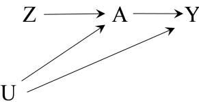
Figure 16.1

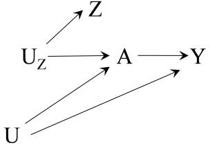
Figure 16.2

anteed if, for example, participants were inadvertently unblinded by side effects of treatment.

The causal diagram in Figure 16.1 depicts a randomized trial: Z is the randomization assignment indicator (1: treatment, 0: placebo), A is an indicator for receiving treatment (1: yes, 0: no) because not all participants adhere to their assignment, Y the outcome, and U all factors (some unmeasured) that affect both the outcome and the adherence. Because participants and their doctors do not know whether the pill they are given is treatment or placebo, they are said to be “blinded” and the study is referred to as a double-blind placebo-controlled randomized trial.

Suppose we want to consistently estimate the average causal effect of A on Y . Whether we use IP weighting, standardization, g-estimation, stratification, or matching, we need to correctly measure, and adjust for, variables that block the backdoor path A ← U → Y , i.e., we need to ensure conditional exchangeability of the treated and the untreated. Unfortunately, all these methods will result in biased effect estimates if some of the necessary variables are unmeasured, imperfectly measured, or misspecified in the model.

Instrumental variable (IV) methods are different: they may be used to attempt to identify the average causal effect of A on Y in this randomized trial, even if we did not measure the variables normally required to adjust for the confounding caused by U. To perform their magic, IV methods need an instrumental variable Z, or an instrument. A variable Z is an instrument because it meets three instrumental conditions:

1. Z is associated with A

2. Z does not affect Y except through its potential effect on A

3. Z and Y do not share causes

See Technical Point 16.1 for a more rigorous definition of these conditions, which we will use in the other technical points.

Condition (ii) would not be guar- In the double-blind randomized trial described above, the randomization indicator Z is an instrument. Condition (i) is met because trial participants are more likely to receive treatment if they were assigned to treatment, condition (ii) is expected by the double-blind design, and condition (iii) is expected by the random assignment of Z.

The instrumental conditions, formally. Instrumental condition (i), sometimes referred to as the relevance condition, is non-null association between Z and A, or Z⊥⊥A does not hold. Condition (i) is expected to hold in randomized experiments because treatment assignment is expected to influence the treatment received.

Instrumental condition (ii), commonly known as the exclusion restriction, is the condition of “no direct effect of Z on Y .” At the individual level, condition (ii) is Y z,a ⁱ = Y z ′ ,a ⁱ = Y a i for all z, z′ , all a, all individuals i. However, for some results presented in this chapter, only the population level condition (ii) is needed, i.e., E [Y z,a] = Eh Y z ′ ,ai . Both versions of condition (ii) are expected to hold in double-blind randomized experiments because assignment is not expected to influence the outcome (e.g., through behavioral changes) if assignment is unknown to all individuals. Condition (ii) is trivially true for surrogate instruments.

Instrumental condition (iii) can be written as marginal exchangeability Y a,z⊥⊥Z for all a, z, which holds in the SWIGs corresponding to Figures 16.1, 16.2, and 16.3. Together with condition (ii) at the individual level, it implies Y ^a⊥⊥Z. A stronger condition (iii) is joint exchangeability, or {Y z,a; a ∈ [0, 1], z ∈ [0, 1]} ⊥⊥Z for dichotomous treatment and instrument. See Technical Point 2.1 for a discussion on different types of exchangeability and Technical Point 16.2 for a description of results that require each version of exchangeability. Both versions of condition (iii) are expected to hold in randomized experiments because Z is randomly assigned.

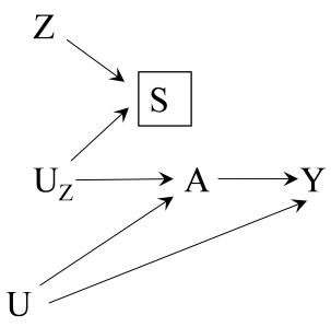
Figure 16.3

date instrument Z “price in state of birth” is associated with smoking cessation A through the unmeasured variable U^Z “price in place of residence”.

Figure 16.1 depicts a special case in which the instrument Z has a causal effect on the treatment A. We then refer to Z as a causal instrument. Sometimes the causal instrument is unmeasured and we use a measured proxy or surrogate instrument Z that is associated with the unmeasured causal instrument UZ. A surrogate instrument does not have a causal effect on treatment A, but meets the instrumental conditions with the Z-A association (i) now resulting from the cause U^Z shared by Z and A, and with condition (iii) modified as “Z and Y do not share causes except for UZ”. Both causal and surrogate instruments can be used for IV estimation, with some caveats described in Section 16.4. As a curiosity, Figure 16.3 depicts an example of an unusual surrogate instrument Z in a selected population: the Z-A association arises from conditioning on a common effect S of the unmeasured causal instrument U^Z and the surrogate instrument Z.

In previous chapters we have estimated the effect of smoking cessation on weight change using various causal inference methods applied to observational data. To estimate this effect using IV methods, we need an instrument Z. Since there is no randomization indicator in an observational study, consider the following candidate for an instrument: the price of cigarettes. It can be argued that this variable meets the three instrumental conditions if (i) cigarette price affects the decision to quit smoking, (ii) cigarette price affects weight change only through its effect on smoking cessation, and (iii) no common causes of cigarette price and weight change exist. Fine Point 16.1 reviews some proposed instruments in observational studies.

To fix ideas, let us propose an instrument Z that takes value 1 when the Condition (i) is met if the candi- average price of a pack of cigarettes in the U.S. state where the individual was born was greater than $1.50, and takes value 0 otherwise. Unfortunately, we cannot determine whether our variable Z is actually an instrument. Of the three instrumental conditions, only condition (i) is empirically verifiable. To verify this condition we need to confirm that the proposed instrument Z and the treatment A are associated, i.e., that Pr [A = 1|Z = 1] − Pr [A = 1|Z = 0] > 0. The probability of quitting smoking is 25.8% among those with Z = 1 and 19.5% among those with Z = 0; the risk difference Pr [A = 1|Z = 1] −

Fine Point 16.1

Candidate instruments in observational studies. Many variables have been proposed as instruments in observational studies and it is not possible to review all of them here. Three commonly used categories of candidate instruments are

• Genetic factors: The proposed instrument is a genetic variant Z that is associated with treatment A and that, supposedly, is only related with the outcome Y through A. For example, when estimating the effects of alcohol intake on the risk of coronary heart disease, Z can be a polymorphism associated with alcohol metabolism (say, ALDH2 in Asian populations). Causal inference from observational data via IV estimation using genetic variants is part of the framework known as Mendelian randomization (Katan 1986, Davey Smith and Ebrahim 2004, Didelez and Sheehan 2007, VanderWeele et al. 2014).
• Preference: The proposed instrument Z is a measure of the physician’s (or a care provider’s) preference for one treatment over the other. The idea is that a physician’s preference influences the prescribed treatment A without having a direct effect on the outcome Y . For example, when estimating the effect of prescribing COX-2 selective versus non-selective nonsteroidal anti-inflammatory drugs on gastrointestinal bleeding, U^Z can be the physician’s prescribing preference for drug class (COX-2 selective or non-selective). Because U^Z is unmeasured, investigators replace it in the analysis by a (measured) surrogate instrument Z, such as “last prescription issued by the physician before current prescription” (Korn and Baumrind 1998, Earle et al. 2001, Brookhart and Schneeweiss 2007).
• Access: The proposed instrument Z is a measure of access to the treatment. The idea is that access impacts the use of treatment A but does not directly affect the outcome Y . For example, physical distance or travel time to a facility has been proposed as an instrument for treatments available at such facilities (McClellan et al. 1994, Card 1995, Baiocchi et al. 2010). Another example: calendar period has been proposed as an instrument for a treatment whose accessibility varies over time (Hoover et al. 1994, Detels et al. 1998). In the main text we use “price of the treatment”, another measure of access, as a candidate instrument.

Pr [A = 1|Z = 0] is therefore 6%. When, as in this case, Z and A are weakly associated, Z is often referred as a weak instrument (more on weak instruments in Section 16.5).

On the other hand, conditions (ii) and (iii) cannot be empirically verified. To verify condition (ii), we would need to prove that Z can only cause the outcome Y through the treatment A. We cannot prove it by conditioning on A, which is a collider on the pathway Z ←− U^Z → A ←− U → Y in Figure 16.2, because that would induce an association between Z and Y even if condition (ii) held true. And we cannot, of course, prove that condition (iii) holds because we can never rule out confounding for the effect of any variable. Conditions (ii) and (iii) can some- We can only assume that conditions (ii) and (iii) hold. IV estimation, like all methods we have studied so far, is based on untestable assumptions.

In observational studies we cannot prove that our proposed instrument Z is truly an instrument. We refer to Z as a proposed or candidate instrument because we can never guarantee that the structures represented in Figures 16.1 and 16.2 are the ones that actually occur. The best we can do is to use subject-matter knowledge to build a case for why the proposed instrument Z may be reasonably assumed to meet conditions (ii) and (iii); this is similar to how we use subject-matter knowledge to justify the identifying assumptions of the methods described in previous chapters.

But let us provisionally assume that Z is an instrument. Now what? Can we now see the magic of IV estimation in action? Can we consistently estimate the average causal effect of A on Y without having to identify and measure

times be empirically falsified by using data on instrument, treatment, and outcome. However, falsification tests only reject the conditions for a small subset of violations. For most violations, the test has no statistical power, even for an arbitrarily large sample size (Balke and Pearl 1997, Bonet 2001, Glymour et al. 2012).

Bounds: Partial identification of causal effects. For a dichotomous outcome Y , the average causal effect Pr - Y ^a=1 = 1 − Pr - Y ^a=0 = 1 can take values between −1 (if all individuals develop the outcome unless they were treated) and 1 (if no individuals develop the outcome unless treated). The bounds of the average causal effect are (−1, 1). The distance between these bounds can be cut in half by using the data: because for each individual we know the value of either her counterfactual outcome Y ^a=1 (if the individual was actually treated) or Y ^a=0 (if the individual was actually untreated), we can compute the causal effect after assigning the most extreme values possible to each individual’s unknown counterfactual outcome. This will result in bounds of the average causal effect that are narrower but still include the null value 0. For a continuous outcome Y , deriving bounds requires the specification of the minimum and maximum values for the outcome; the width of the bounds will vary depending on the chosen values.

The bounds for Pr - Y ^a=1 = 1 −Pr - Y ^a=0 = 1 can be further narrowed if there is a variable Z that meets instrumental condition (ii) at the population level (see Technical Point 16.1) and marginal exchangeability (iii) (Robins 1989; Manski 1990). The width of these so-called natural bounds, Pr[A = 1|Z = 0] + Pr[A = 0|Z = 1], is narrower than that of the bounds identified from the data alone. Sometimes narrower bounds—the so-called sharp bounds—can be achieved when marginal exchangeability is replaced by joint exchangeability (Balke and Pearl 1997; Richardson and Robins 2014).

The conditions necessary to achieve the sharp bounds can also be derived from the SWIGs under joint interventions on z and a corresponding to any of the causal diagrams depicted in Figures 16.1, 16.2, and 16.3. Richardson and Robins (2010, 2014) showed that the conditions Y a,z⊥⊥ (Z, A)|U and Z⊥⊥U, together with a population level condition (ii) within levels of U, i.e., E [Y z,a|U] = Eh Y z ′ ,a|U i , are sufficient to obtain the sharp bounds. These conditions, which hold for all three SWIGs, imply Z⊥⊥U, Y ⊥⊥Z|U, A, and that E [Y z,a] is given by the g-formula R E [Y |A = a, U = u] dF(u) ignoring Z, which reflects that Z has no direct effect on Y within levels of U. Dawid (2003) proved that these latter conditions lead to the sharp bounds. Under further assumptions, Richardson and Robins derived yet narrower bounds. See also Richardson, Evans, and Robins (2011).

Unfortunately, all these partial identification methods (i.e., methods for bounding the effect) are often relatively uninformative because the bounds are wide. Swanson et al (2018) review partial identification methods for binary instruments, treatments, and outcomes. Swanson et al. (2015a) describe a real-world application of several partial identification methods and discuss their relative advantages and disadvantages.

There is a way to decrease the width of the bounds: making parametric assumptions about the form of the effect of A on Y . Under sufficiently strong assumptions described in Section 16.2, the upper and lower bounds converge into a single number and the average causal effect is point identified.

the confounders? Sadly, the answer is no without further assumptions. An instrument by itself does not allow us to identify the average causal effect of smoking cessation A on weight change Y , but only identifies certain upper and lower bounds. Typically, the bounds are very wide and often include the null value (see Technical Point 16.2).

In our example, these bounds are not very helpful. They would only confirm what we already knew: smoking cessation can result in weight gain, weight loss, or no weight change. Unfortunately, that is all an instrument can offer unless one is willing to make additional unverifiable assumptions. Sections 16.3 and 16.4 review additional conditions under which the IV estimand is the average causal effect. Before that, we review the methods to do so.

16.2 The usual IV estimand

When a dichotomous variable Z is an instrument, i.e., meets the three instrumental conditions (i)-(iii), and an additional condition (iv) described in the struments, which are the commonest ones. For a continuous instrument Z, the usual IV estimand is Cov(Y,Z) Cov(A,Z) , where Cov means covariance.

estimand is the ratio of two effects of Z: the effect of Z on Y and the effect of Z on A. Each of these effects can be consistently estimated without adjustment because Z is randomly assigned.

For simplicity, we exclude individuals with missing outcome or instrument. In practice, we could use IP weighting to adjust for possible selection bias before using IV estimation.

next section holds, then the average causal effect of treatment on the additive scale E- Y ^a=1 − E - Y ^a=0 We will focus on dichotomous in- is identified and equals

\[\frac{\operatorname{E}\left[Y|Z=1\right] - \operatorname{E}\left[Y|Z=0\right]}{\operatorname{E}\left[A|Z=1\right] - \operatorname{E}\left[A|Z=0\right]},\]

which is the usual IV estimand for a dichotomous instrument. (Note E [A|Z = 1] = Pr [A = 1|Z = 1] for a dichotomous treatment). Technical Point 16.3 provides a proof of this result in terms of an additive structural mean model, but you might want to wait until the next section before reading it.

To intuitively understand the usual IV estimand, consider again the ran-In randomized experiments, the IV domized trial from the previous section. The numerator of the IV estimand is the average causal effect of assignment Z on Y —the intention-to-treat effect and the denominator is the average causal effect of assignment Z on A—a measure of adherence to, or compliance with, the assigned treatment. When there is perfect adherence, the denominator is equal to 1, and the effect of A on Y equals the effect of Z on Y . As adherence worsens, the denominator starts to get closer to 0, and the effect of A on Y becomes greater than the effect of Z on Y . The lower the adherence, the greater the difference between the effect of A on Y —the IV estimand—and the effect of Z on Y .

The IV estimand bypasses the need to adjust for the confounders by inflating the effect of assignment (the numerator). The magnitude of the inflation increases as adherence decreases, i.e., as the Z-A risk difference (the denominator) gets closer to zero. The same rationale applies to the instruments used in observational studies, where the denominator of the IV estimator may equal either the causal effect of the causal instrument Z on A (Figure 16.1), or the noncausal association between the surrogate instrument Z and the treatment A (Figures 16.2 and 16.3).

Also known as the Wald estimator The standard IV estimator is calculated as the ratio of the estimates of the (Wald 1940). numerator and the denominator of the usual IV estimand. In our smoking cessation example with a dichotomous instrument Z (1: state with high cigarette price, 0: otherwise), the numerator estimate E [ ^{b Y |Z} = 1] ⁻ E [ ^{b Y |Z} = 0] equals ².^{686 − 2}.536 = 0.1503 and the denominator E [ ^{b A}|^Z = 1] ⁻ E [ ^{b A}|^Z = 0] equals Code: Program 16.1 0.2578 − 0.1951 = 0.0627. Therefore, the usual IV estimate is the ratio 0.1503/0.0627 = 2.4 kg. Under the three instrumental conditions (i)-(iii) plus condition (iv) from next section, this is an estimate of the average causal effect of smoking cessation on weight gain in the population.

We estimated the numerator and denominator of the IV estimand by simply calculating the four sample averages E [ ^{b A}|^Z = 1], E [ ^{b A}|^Z = 0], E [ ^{b Y |Z} = 1], and E [ ^{b Y |Z} = 0]. Equivalently, we could have fit two (saturated) linear models to estimate the differences in the denominator and the numerator. The model for the denominator would be E [A|Z] = α⁰ + α1Z, and the model for the numerator E [Y |Z] = β⁰ + β1Z.

An alternative method to calculate the standard IV estimator is the twostage-least-squares estimator . The procedure is as follows. First, fit the firststage treatment model E [A|Z] = α⁰ + α1Z, and generate the predicted values E [ ^{b A}|Z] for each individual. Second, fit the second-stage outcome model E [^{Y |}Z] = ^{β0 + β}1E [ ^{b A}|Z]. The parameter estimate ^βb¹ will always be nu-Code: Program 16.2 merically equivalent to the standard IV estimate. Thus, in our example, the two-stage-least-squares estimate was again 2.4 kg.

The 2.4 point estimate has a very large 95% confidence interval: −36.5 to 41.3. This is expected for our proposed instrument because the Z-A association is weak and there is much uncertainty in the first-stage model. A commonly

used rule of thumb is to declare an instrument as weak if the F-statistic from the first-stage model is less than 10 (it was a meager 0.8 in our example). We will revisit the problems raised by weak instruments in Section 16.5.

Some of the assumptions implicit in regarding the two-stage-least-squares estimator as identifying the causal effect of treatment can be made more explicit by using additive or multiplicative structural mean models, like the ones described in Technical Points 16.3 and 16.4, for IV estimation. The parameters Code: Program 16.3 of structural mean models can be estimated via g-estimation. In addition, in the presence of measured common causes L of the instrument and the outcome that therefore must be adjusted for in the analysis, the trade-offs involved in the choice between two-stage-least-squares linear models and structural mean models can be similar to those involved in the choice between outcome regression and structural nested models for non-IV estimation (see Chapters 14 and 15).

Anyway, the above estimators are only valid when the usual IV estimand can be interpreted as the average causal effect of treatment A on the outcome Y . For that to be true, a fourth identifying condition needs to hold in addition to the three instrumental conditions.

16.3 A fourth identifying condition: homogeneity

The three instrumental conditions (i)-(iii) are insufficient to ensure that the IV estimand is the average causal effect of treatment A on Y . A fourth condition, effect homogeneity (iv), is needed. Here we describe four possible homogeneity conditions (iv) in order of (historical) appearance.

The most extreme, and oldest, version of homogeneity condition (iv) is constant effect of treatment A on outcome Y across individuals. In our example, this condition would hold if smoking cessation made every individual in the population gain (or lose) the same amount of weight, say, exactly 2.4 kg. A constant effect is equivalent to additive rank preservation which, as we discussed in Section 14.4, is scientifically implausible for most treatments and Yet additive rank preservation was outcomes—and impossible for dichotomous outcomes, except under the sharp null or universal harm (or benefit). In our example, we expect that, after quitting smoking, some individuals will gain a lot of weight, some will gain little, and others may even lose some weight. Therefore, we are not generally willing to accept the homogeneity assumption of constant effect as a reasonable condition (iv).

A second, less extreme homogeneity condition (iv) for dichotomous Z and A is equality of the average causal effect of A on Y across levels of Z in both the treated and in the untreated, i.e., E - Y ^a=1 − Y ^a=0|Z = 1, A = a = E - Y ^a=1 − Y ^a=0|Z = 0, A = a Even when condition (iii) Y for a = 0, 1. This additive homogeneity condi- ^a⊥⊥Z tion (iv) was the one used in the mathematical proof of Technical Point 16.3. An alternative homogeneity condition on the multiplicative scale is discussed in Technical Point 16.4. (This multiplicative homogeneity condition leads to an IV estimand that is different from the usual IV estimand.)

The above homogeneity condition is expressed in terms that are not naturally intuitive. How can subject-matter experts provide arguments in support of a constant average causal effect within levels of the proposed instrument Z and the treatment A in any particular study? More natural—even if still untestable—homogeneity conditions (iv) would be stated in terms of effect modification by possibly known (even if unmeasured) confounders U. One

implicitly assumed in many early IV analyses using the two-stage-leastsquares estimator.

holds—as in the SWIGs for Figures 16.1, 16.2, 16.3—Y ^a⊥⊥Z|A does not generally hold. Therefore the treatment effect may depend on Z, i.e., the less extreme homogeneity condition may not hold.

Additive structural mean models and IV estimation. Consider the following saturated, additive structural mean model for a dichotomous treatment A and an instrument Z as depicted in Figures 16.1, 16.2, or 16.3:

\[\operatorname{E}\left[Y^{a=1} - Y^{a=0} \vert A=1, Z\right] = \beta\_0 + \beta\_1 Z\]

This model can also be written as E - Y − Y ^a=0|A, Z = A (β⁰ + β1Z). The parameter β⁰ is the average causal effect of treatment among the treated individuals with Z = 0, and β⁰ + β¹ is the average causal effect of treatment among the treated individuals with Z = 1. Thus β¹ quantifies additive effect modification by Z.

If we a priori assume that there is no additive effect modification by Z, then β¹ = 0 and β⁰ is exactly the usual IV estimand (Robins 1994). That is, the usual IV estimand is the parameter of an additive structural mean model for the effect of treatment on the treated under no effect modification by Z.

The proof is simple. When Z is an instrument, condition (ii) holds, which implies E - Y ^a=0|Z = 1 = E- Y ^a=0|Z = 0 . Under the above structural model, this conditional mean independence can be rewritten as E [Y − A (β⁰ + β1)|Z = 1] = E [Y − Aβ0|Z = 0]. Solving the above equation with β¹ = 0 we have

\[\beta\_0 = \frac{\operatorname{E}\left[Y|Z=1\right] - \operatorname{E}\left[Y|Z=0\right]}{\operatorname{E}\left[A|Z=1\right] - \operatorname{E}\left[A|Z=0\right]}\]

You may wonder why we a priori set β¹ = 0. The reason is that we have an equation with two unknowns (β⁰ and β1) and that equation exhausts the constraints on the data distribution implied by the three instrumental conditions. Since we need an additional constraint, which by definition will be untestable, we arbitrarily choose β¹ = 0 (rather than, say, β¹ = 2). This is what we mean when we say that an instrument is insufficient to identify the average causal effect.

Therefore, to conclude that the average causal effect of treatment in the treated β⁰ = E - Y ^a=1 − Y ^a=0|A = 1, Z = z = E- Y ^a=1 − Y ^a=0|A = 1 equals the average causal effect in the study population E - Y ^a=1 − E - Y ^a=0 —and thus that the usual IV estimand is E - Y ^a=1 − E - Y ^a=0 —we must assume that the effects of treatment in the treated and in the untreated are identical, which is an additional untestable assumption.

Hence, under the additional assumption β¹ = 0, β⁰ = E- Y ^a=1 − Y ^a=0|A = 1, Z = z = E- Y ^a=1 − Y ^a=0|A = 1 for any z is the average causal effect of treatment in the treated.

To conclude that β⁰ is the average causal effect in the study population E - Y ^a=1 − E - Y ^a=0 —and thus that E - Y ^a=1 − E - Y ^a=0 is the usual IV estimand—we must assume that the effects of treatment are identical in the treated and in the untreated, i.e., the parameter for Z is also 0 in the structural model for A = 0. This is an additional untestable assumption.

that, if U is an additive effect modifier, then it would not be reasonable for us to believe that the previous additive homogeneity condition (iv) holds.

2018. proposed the homogeneity condition “t(U) is a constant” and proved that it was a special case of the general condition. See a proof in Technical Point 16.5

such condition is that U is not an additive effect modifier, i.e., that the average causal effect of A on Y is the same at every level of the unmeasured confounder U or E- Y ^a=1|U −E - Y ^a=0|U = E- Y ^a=1 −E - Y ^a=0 Hern´an and Robins (2006b) showed . This third homogeneity condition (iv) is often implausible because some unmeasured confounders may also be effect modifiers. For example, the magnitude of weight gain after smoking cessation may vary with prior intensity of smoking, which may itself be an unmeasured confounder for the effect of smoking cessation on weight gain.

Another type of homogeneity condition (iv) is that the Z-A association on the additive scale is constant across levels of the unmeasured confounders U, Wang and Tchetgen Tchetgen i.e., E [A|Z = 1, U] − E [A|Z = 0, U] = E [A|Z = 1] − E [A|Z = 0]. Both this condition and the earlier condition E - Y ^a=1|U − E - Y ^a=0|U = E- Y ^a=1 − E - Y ^a=0 are special cases of the following (much more) general condition: the modification by U of the effect of the treatment A on the outcome Y , e (U) ≡ E - Y ^a=1 − Y ^a=0|U , is uncorrelated with the modification by U of the Z-A association on the additive scale, t(U) ≡ E [A|Z = 1, U] − E [A|Z = 0, U],

Multiplicative structural mean models and IV estimation. Consider the following saturated, multiplicative (loglinear) structural mean model for a dichotomous treatment A

\[\frac{\operatorname{E}\left[Y^{a=1}|A=1,Z\right]}{\operatorname{E}\left[Y^{a=0}|A=1,Z\right]} = \exp\left(\beta\_0 + \beta\_1 Z\right),\]

which can also be written as E [Y |A, Z] = E- Y ^a=0|A, Z exp [A (β⁰ + β1Z)]. For a dichotomous Y , exp (β0) is the causal risk ratio in the treated individuals with Z = 0 and exp (β⁰ + β1) is the causal risk ratio in the treated with Z = 1. Thus β¹ quantifies multiplicative effect modification by Z. If we a priori assume that β¹ = 0—and additionally assume no multiplicative effect modification by Z in the untreated—then the causal effect on the multiplicative (risk ratio) scale is E - Y ^a=1 /E - Y ^a=0 = exp (β0), and the causal effect on the additive (risk difference) scale is

\[\mathbb{E}\left[Y^{a=1}\right] - \mathbb{E}\left[Y^{a=0}\right] = \mathbb{E}\left[Y|A=0\right]\left(1 - \mathbb{E}\left[A\right]\right)\left[\exp\left(\beta\_0\right) - 1\right] + \mathbb{E}\left[Y|A=1\right]\mathbb{E}\left[A\right]\left[1 - \exp\left(-\beta\_0\right)\right]\]

The proof, which relies on the instrumental conditions, can be found in Robins (1989) and Hern´an and Robins (2006b).

That is, if we assume a multiplicative structural mean model with no multiplicative effect modification by Z in the treated and in the untreated, then the average causal effect E - Y ^a=1 − E - Y ^a=0 remains identified, but no longer equals the usual IV estimator. As a consequence, our estimate of E - Y ^a=1 − E - Y ^a=0 will depend on whether we assume no additive or multiplicative effect modification by Z. Unfortunately, it is not possible to determine which, if either, assumption is true even if we had an infinite sample size (Robins 1994) because, when considering saturated additive or multiplicative structural mean models, we have more unknown parameters to estimate than equations to estimate them with. That is precisely why we need to make modeling assumptions such as homogeneity.

i.e., Cov [e (U), t(U)] = 0. The previous two conditions are special cases of Cov [e (U), t(U)] = 0 because they can be expressed as “e(U) is a constant”and “t(U) is a constant”, respectively, and the covariance of any variable with a constant is always 0.

Because of the perceived implausibility of the homogeneity conditions in many settings, the possibility that IV methods can validly estimate the average causal effect of treatment seems questionable. There are two approaches that bypass the homogeneity conditions.

One approach is the introduction of baseline covariates in the models for IV estimation. To do so, it is safer to use structural mean models, which impose fewer parametric assumptions than two-stage-linear-squares estimators. The inclusion of covariates in a structural mean model allows the treatment effect Also, models can be used to in- in the treated to vary with Z by imposing constraints on how the treatment effect varies within levels of the covariates. See Section 16.5. and Technical Point 16.6 for more details on structural mean models with covariates.

Another approach is to use an alternative condition (iv) that does not require effect homogeneity. When combined with the three instrumental conditions (i)-(iii), this alternative condition allows us to endow the usual IV estimand with a causal interpretation, even though it does not suffice to identify the average causal effect in the population. We review this alternative condition (iv) in the next section.

corporate multiple proposed instruments simultaneously, to handle continuous treatments, and to estimate causal risk ratios when the outcome is dichotomous (see Palmer et al. 2011 for a review).

Proof of the general homogeneity condition. We wish to show that E[Y ^a=1 − Y ^a=0] = E[^{Y |}Z=1]−E[^{Y |}Z=0] E[A|Z=1]−E[A|Z=0] under the causal diagram in Figure 16.1 and the general homogeneity condition of zero covariance Cov (e (U), t(U)) = 0, where e (U) and t(U) are defined in the main text.

To do so, note that E [e (U)] = E[Y ^a=1 − Y ^a=0]. Further, E [t(U)] = E [A|Z = 1] − E [A|Z = 0] because U⊥⊥Z. Hence the zero covariance condition implies E[e (U)t(U)]/ {E [A|Z = 1] − E [A|Z = 0]} = E[Y ^a=1−Y ^a=0]. It remains to show that E [Y |Z = 1] − E [Y |Z = 0] = E[e (U)t(U)]. To do so, write Y = A Y ^a=1 − Y ^a=0 + Y a=0 . Because Y ^a⊥⊥ (A, Z)|U and U⊥⊥Z in Figure 16.1, we have E [Y |Z] equal to = P u P ^a={0,1} E [Y |A = a, Z, U = u] Pr (A = a|Z, U = u) f (u|Z) = P u E[Y ^a=1 − Y ^a=0|U = u] Pr (A = 1|Z, U = u) + E- Y ^a=0|U = u f (u). Thus, E [Y |Z = 1] − E [Y |Z = 0] = E-E[Y ^a=1 − Y ^a=0|U] {Pr (A = 1|Z = 1, U) − Pr (A = 1|Z = 0, U)} as required.

16.4 An alternative fourth condition: monotonicity

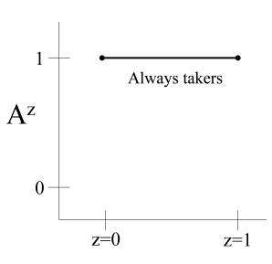
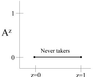
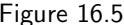
Consider again the double-blind randomized trial with randomization indicator Z, treatment A, and outcome Y . For each individual in the trial, the counterfactual variable Az=1 is the value of treatment—1 or 0—that an individual would have taken if he had been assigned to receive treatment (z = 1). The counterfactual variable Az=0 is analogously defined as the treatment value if the individual had been assigned to receive no treatment (z = 0).

If we knew the values of the two counterfactual treatment variables Az=1 and Az=0 for each individual, we could classify all individuals in the study population into four disjoint subpopulations:

• 1. Always-takers: Individuals who will always take treatment, regardless of the treatment group they were assigned to. That is, individuals with both Az=1 = 1 and Az=0 = 1.
• 2. Never-takers: Individuals who will never take treatment, regardless of the treatment group they were assigned to. That is, individuals with both Az=1 = 0 and Az=0 = 0.
• 3. Compliers or cooperative: Individuals who will take treatment when assigned to treatment, and no treatment when assigned to no treatment. That is, individuals with A^z=1 = 1 and A^z=0 = 0.
• 4. Defiers or contrarians: Individuals who will take no treatment when assigned to treatment, and treatment when assigned to no treatment. That is, individuals with A^z=1 = 0 and A^z=0 = 1.

Figure 16.5 Note that these subpopulations—often referred as compliance types or principal strata—are not generally identified. If we observe that an individual was assigned to Z = 1 and took treatment A = 1, we do not know whether she is a complier or an always-taker. If we observe that an individual was assigned to Z = 1 and took treatment A = 0, we do not know whether he is a defier or a never-taker.

When no defiers exist, we say that there is monotonicity because the instrument Z either does not change treatment A—as shown in Figure 16.4 for always-takers and Figure 16.5 for never-takers—or increases the value of treatment A—as shown in Figure 16.6 for compliers. For defiers, the instrument

More general structural mean models. Consider an additive structural mean model that allows for continuous and/or multivariate treatments A, instruments Z, and pre-instrument covariates V . Such model assumes

\[\operatorname{E}\left[Y - Y^{a=0} | Z, A, V\right] = \gamma\left(Z, A, V; \beta\right).\]

where γ (Z, A, V ; β) is a known function, β is an unknown (possibly vector-valued) parameter, and γ (Z, A = 0, V ; β) = 0. That is, an additive structural mean model is a model for the average causal effect of treatment level A compared with treatment level 0 among the subset of individuals at level Z of the instrument and level V of the confounders whose observed treatment is precisely A. The parameters of this model can be identified via g-estimation under the conditional counterfactual mean independence assumption E - Y ^a=0|Z = 1, V = E- Y ^a=0|Z = 0, V .

Analogously, a general multiplicative structural mean model assumes

\[\operatorname{E}\left[Y|Z,A,V\right] = \operatorname{E}\left[Y^{a=0}|Z,A,V\right]\exp\left[\gamma\left(Z,A,V;\beta\right)\right]\]

where γ (Z, A, V ; β) is a known function, β is an unknown parameter vector, and γ (Z, A = 0, V ; β) = 0. The parameters of this model can also be identified via g-estimation under analogous conditions. Identification conditions and efficient estimators for structural mean models were discussed by Robins (1994) and reviewed by Vansteelandt and Goetghebeur (2003). More generally, g-estimation of nested additive and multiplicative structural mean models can extend IV methods for time-fixed treatments and confounders to settings with time-varying treatments and confounders.

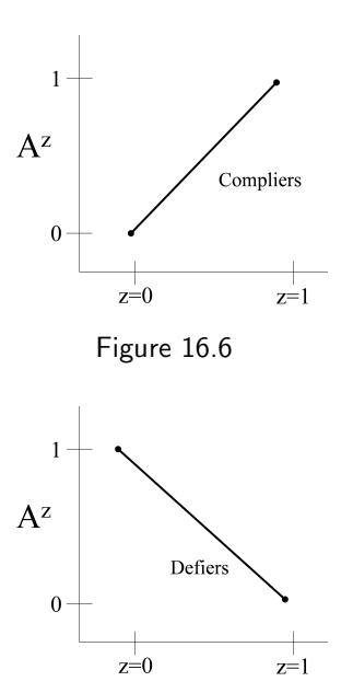
Z would decrease the value of treatment A—as shown in Figure 16.7. More generally, monotonicity holds when Az=1 ≥ Az=0 for all individuals.

Now let us replace any of the homogeneity conditions from the last section by the monotonicity condition, which will become our new condition (iv). Then the usual IV estimand does not equal the average causal effect of treatment E - Y ^a=1 −E - Y ^a=0 any more. Rather, under monotonicity (iv), the usual IV estimand equals the average causal effect of treatment in the compliers, that is

\[\operatorname{E}\left[Y^{a=1} - Y^{a=0} \middle| A^{z=1} = 1, A^{z=0} = 0\right].\]

Technical Point 16.6 shows a proof for this equality under the assumption that Z was effectively randomly assigned. As a sketch of the proof, the equality between the usual IV estimand and the effect in the compliers holds because the effect of assignment Z on Y —the numerator of the IV estimand—is a weighted average of the effect of Z in each of the four principal strata. However, the effect of Z on Y is exactly zero in always-takers and never-takers because the effect of Z is entirely mediated through A and the value of A in those subpopulations is fixed, regardless of the value of Z they are assigned to. Also, no defiers exist under monotonicity (iv). Therefore the numerator of the IV estimand is the effect of Z on Y in the compliers—which is the same as the effect of A on Y in the compliers—times the proportion of compliers in the population, which is precisely the denominator of the usual IV estimand.

In observational studies, the usual IV estimand can also be used to estimate the effect in the compliers in the absence of defiers. Technically, there are no compliers or defiers in observational studies because the proposed instrument Z is not treatment assignment, but the term compliers refers to individuals with (A^z=1 = 1, A^z=0 = 0) and the term defiers to those with (A^z=1 = 0, A^z=0 = 1). In our smoking cessation example, the compliers are the individuals who would quit smoking in a state with high cigarette price and who would not quit smoking in a state with low price. Conversely, the defiers are the individuals fect” (CACE) is a local average treatment effect (LATE) in a subpopulation, not the global average causal effect in the entire population. Greenland (2000) refers to compliers as cooperative, and to defiers as non-cooperative, to prevent confusion with the concept of (observed) compliance in randomized trials.

goes beyond the old story of looking for an object where the light is strong enough to see; rather, we have control over the light, but choose to let it fall where it may and then proclaim that whatever it illuminates is what we were looking for all along.”

der strong assumptions, investigators can characterize the compliers in terms of their distribution of the observed variables (Angrist and Pischke 2009, Baiocchi et al 2014).

posed by Swanson and Hern´an (2014). Also Swanson et al (2015b) showed empirically the existence of defiers in an observational setting.

who would not quit smoking in a state with high cigarette price and who The “compliers average causal ef- would quit smoking in a state with low price. If no defiers exist and the causal instrument is dichotomous (see below and Technical Point 16.6), then 2.4 kg is the IV effect estimate in the compliers.

The replacement of homogeneity by monotonicity was welcomed in the mid-1990s as the salvation of IV methods. While homogeneity is often an implausible condition (iv), monotonicity appeared credible in many settings. IV methods under monotonicity (iv) cannot identify the average causal effect in the population, only in the subpopulation of compliers, but that seemed a price worth paying in order to keep powerful IV methods in our toolbox. However, the estimation of the average causal effect of treatment in the compliers under monotonicity (iv) has been criticized on several grounds.

First, the relevance of the effect in the compliers is questionable. The Deaton (2010) on the CACE: “This subpopulation of compliers is not identified and, even though the proportion of compliers in the population can be calculated (it is the denominator of the usual IV estimand, see Technical Point 16.7), it varies from instrument to instrument and from study to study. Therefore, causal inferences about the effect in the compliers are difficult to use by decision makers. Should they prioritize the administration of treatment A = 1 to the entire population because treatment has been estimated to be beneficial among the compliers, which happen to be 6% of the population in our example but could be a smaller or larger group in the real world? What if treatment is not as beneficial in always-takers and never-takers, the majority of the population? Unfortunately, the decision maker cannot know who is included in the 6%. Rather than arguing that the effect of the compliers is of primary interest, it may be better to accept that A mitigating factor is that, un- interest in this estimand is not the result of its practical relevance, but rather of the (often erroneous) perception that it is easy to identify.

Second, monotonicity is not always a reasonable assumption in observational studies. The absence of defiers seems a safe assumption in randomized trials: we do not expect that some individuals will provide consent for participation in a trial with the perverse intention to do exactly the opposite of what they are asked to do. Further, monotonicity is ensured by design in trials in which those assigned to no treatment are prevented from receiving treatment, i.e., there are no always-takers or defiers. In that scenario, the effect in the compliers is actually the effect in the treated.

However, monotonicity is harder to justify for some instruments proposed in observational studies. Consider the proposed instrument “physician preference” to estimate the treatment effect in patients attending a clinic where two physicians with different preferences work. The first physician usually prefers to prescribe the treatment, but she makes exceptions for her patients The example to the right was pro- with diabetes (because of some known contraindications). The second usually prefers to not prescribe the treatment, but he makes exceptions for his more physically active patients (because of some perceived benefits). Any patient who was both physically active and diabetic would have been treated contrary to both of these physicians’ preferences, and therefore would be labeled as a defier. That is, monotonicity is unlikely to hold when the decision to treat is the result of weighing multiple criteria or dimensions of encouragement that include both risks and benefits. In these settings, the proportion of defiers may not be negligible.

The situation is even more complicated for the surrogate instruments Z represented by Figures 16.2 and 16.3. If the causal instrument U^Z is continuous (e.g., the true, unmeasured physician’s preference), then the standard IV estimand using a dichotomous surrogate instrument Z (e.g., some mea

continuous causal instrument UZ: Au^z is a non-decreasing function of u^z on the support of U^Z (Angrist and Imbens 1995, Heckman and Vytlacil 1999).

difficulties to define monotonicity, and introduce the concept of global and local monotonicity in observational studies.

and Rubin (1997), and Greenland (2000) describe examples of full compliance in the control group.

Martens et al. (2006) showed that instruments are guaranteed to be weak in the presence of strong confounding, because a strong A-U association leaves little residual variation for a strong A-UZ, or A-Z,

association.

sured surrogate of preference) is not the effect in a particular subpopulation of compliers. Rather, the standard IV estimand identifies a particular weighted average of the effect in all individuals in the population, which makes it difficult to interpret. Therefore the interpretation of the IV estimand as the effect in the compliers is questionable when the proposed dichotomous instrument is Definition of monotonicity for a not causal, even if monotonicity held for the continuous causal instrument U^Z (see Technical Point 16.7 for details).

Last, but definitely not least important, the partitioning of the population into four subpopulations or principal strata may not be justifiable. In many realistic settings, the subpopulation of compliers is an ill-defined subset of the population. For example, using the proposed instrument “physician preference” in settings with multiple physicians, all physicians with the same preference level who could have seen a patient would have to treat the patient Swanson et al (2015b) discuss the in the exact same way. This is not only an unrealistic assumption, but also essentially impossible to define in many observational studies in which it is unknown which physicians could have seen a patient. A stable partitioning into compliers, defiers, always takers and never takers also requires deterministic counterfactuals (not generally required to estimate average causal effects), no interference (e.g., I may be an always-taker, but decide not to take treatment when my friend doesn’t), absence of multiple versions of treatment and other Sommer and Zeger (1991), Imbens forms of heterogeneity (a complier in one setting, or for a particular instrument, may not be a complier in another setting).

In summary, if the effect in the compliers is considered to be of interest, relying on monotonicity (iv) seems a promising approach in double-blind randomized trials with two arms and all-or-nothing compliance, especially when one of the arms will exhibit full adherence by design. However, caution is needed when using this approach in more complex settings and observational studies, even if the proposed instrument were really an instrument.

16.5 The three instrumental conditions revisited

The previous sections have discussed the relative advantages and disadvantages of choosing monotonicity or homogeneity as the condition (iv). Our discussion implicitly assumed that the proposed instrument Z was in fact an instrument. However, in observational studies, the proposed instrument Z will fail to be a valid instrument if it violates either of the instrumental conditions (ii) or (iii), and will be a weak instrument if it only barely meets condition (i).

In all these cases, the use of IV estimation may result in substantial bias even if condition (iv) held perfectly. We now discuss each of the three instrumental conditions.

Condition (i), a Z-A association, is empirically verifiable. Before declaring Z as their proposed instrument, investigators will check that Z is associated In the context of linear models, with treatment A. However, when the Z-A association is weak as in our smoking cessation example, the instrument is said to be weak (see Fine Point 16.2). Three serious problems arise when the proposed instrument is weak.

First, weak instruments yield effect estimates with wide 95% confidence intervals, as in our smoking cessation example in Section 16.2. Second, weak instruments amplify bias due to violations of conditions (ii) and (iii). A proposed instrument Z which is weakly associated with treatment A yields a small denominator of the IV estimator. Therefore, violations of conditions (ii) and (iii) that affect the numerator of the IV estimator (e.g., unmeasured con-

Fine Point 16.2

Defining weak instruments There are two related, but different, definitions of weak instrument in the literature:

• 1. An instrument is (substantively) weak if the true value of the Z-A association—the denominator of the IV estimand—is “small.”
• 2. An instrument is (statistically) weak if the F-statistic associated to the observed Z-A association is “small,” typically meaning less than 10.

In our smoking cessation example, the proposed instrument met both definitions: the risk difference was only 6% and the F-statistic was a meager 0.8.

The first definition, based on the true value of the Z-A association, reminds us that, even if we had an infinite sample, the IV estimator greatly amplifies any biases in the numerator when using a proposed weak instrument (the second problem of weak instruments in the main text). The second definition, based on the statistical properties of the Z-A association, reminds us that, even if we had a perfect instrument Z, the IV estimator can be biased in finite samples (the third problem of weak instruments in the main text).

documented this bias. Their paper was followed by many others that investigated the shortcomings of weak instruments.

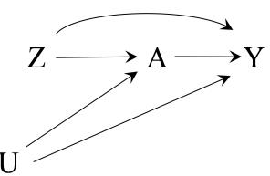
founding for the instrument, a direct effect of the instrument) will be greatly exaggerated. In our example, any bias affecting the numerator of the IV es-Bound, Jaeger and Baker (1995) timator would be multiplied by approximately 15.9 (1/0.0627). Third, even with a valid instrument and a large sample size, weak instruments introduce bias in the standard IV estimator.

To understand the nature of this third problem, consider a randomly generated dichotomous variable Z. In an infinite population, the denominator of the IV estimand will be exactly zero—there is a zero association between treatment A and a completely random variable—and the IV estimate will be undefined. However, in a study with a finite sample, chance will lead to an association between the randomly generated Z and the unmeasured confounders U—and therefore between Z and treatment A—that is weak but not exactly zero. If we propose this random Z as an instrument, the denominator of the IV estimator will be very small rather than zero. As a result the numerator Code: Program 16.4 will be incorrectly inflated, which will yield potentially very large bias. In fact, our proposed instrument “Price higher than $1.50” behaves like a randomly generated variable. Had we decided to define Z as price higher than $1.60, $1.70, $1.80, or $1.90, the IV estimate would have been 41.3, −40.9, −21.1, or −12.8 kg, respectively. In each case, the 95% confidence interval around the estimate was huge. Given how much bias and variability weak instruments may create, a strong proposed instrument that slightly violates conditions (ii) and (iii) may be preferable to a less invalid, but weaker, proposed instrument.

Condition (ii), the absence of a direct effect of the instrument on the outcome, cannot be verified from the data. A deviation from condition (ii) can be represented by a direct arrow from the instrument Z to the outcome Y , as shown in Figure 16.8. This direct effect of the instrument that is not mediated Figure 16.8 through treatment A will contribute to the numerator of the IV estimator, and it will be incorrectly inflated by the denominator as if it were part of the effect of treatment A.

Condition (ii) may be violated when a continuous or multi-valued treatment A is replaced in the analysis by a coarser (e.g., dichotomized) version A^∗ . Figure 16.9 shows that, even if condition (ii) holds for the original treatment A, it does not have to hold for its dichotomized version A^∗ , because the path

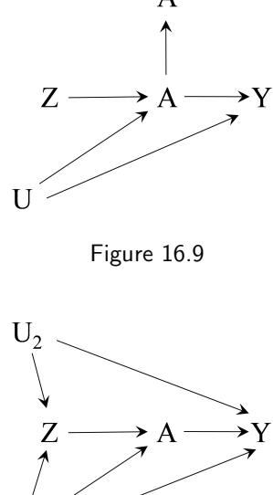
Figure 16.10

Code: Program 16.5

Z → A → Y represents a direct effect of the instrument Z that is not mediated through the treatment A^∗ whose effect is being estimated in the IV analysis. In practice, many treatments are replaced by coarser versions for simplicity of interpretation. Coarsening of treatment is problematic for IV estimation, but not necessarily for the methods discussed in previous chapters.

Condition (iii), no confounding for the effect of the instrument on the outcome, is also unverifiable. Figure 16.10 shows confounding due to common causes of the proposed instrument Z and outcome Y , which may (U1) or may not (U2) be causes of treatment A. In observational studies, the possibility of confounding for the proposed instrument always exists (same as for any other variable not under the investigator’s control). Confounding contributes to the numerator of the IV estimator and is incorrectly inflated by the denominator as if it were part of the effect of treatment A on the outcome Y .

Sometimes condition (iii), and the other conditions too, can appear more plausible within levels of the measured covariates. Rather than making the unverifiable assumption that there is absolutely no confounding for the effect of Z on Y , we might feel more comfortable making the unverifiable assumption that there is no unmeasured confounding for the effect of Z on Y within levels of the measured pre-instrument covariates V . We could then apply IV estimation repeatedly in each stratum of V , and pool the IV effect estimates under the assumption that the effect in the population (under homogeneity) or in the compliers (under monotonicity) is constant within levels of V . Alternatively we could include the variables V as covariates in the two-stage modeling. In our example, this reduced the size of the effect estimate and increased its 95% confidence interval.

Another frequent strategy to support condition (iii) is to check for balanced distributions of the measured confounders across levels of the proposed instrument Z. The idea is that, if the measured confounders are balanced, it may be more likely that the unmeasured ones are balanced too. However, this practice may offer a false sense of security: even small imbalances can lead to counterintuitively large biases because of the bias amplification discussed above.

A violation of condition (iii) may occur even in the absence of confounding for the effect of Z on Y . The formal version of condition (iii) requires exchangeability between individuals with different levels of the proposed instrument. Such exchangeability may be violated because of either confounding (see above) or selection bias. A surprisingly common way in which selection bias may be introduced in IV analyses is the exclusion of individuals with certain values of treatment A. For example, if individuals in the population may receive treatment levels A = 0, A = 1, or A = 2, an IV analysis restricted to Swanson et al. (2015c) describe individuals with A = 1 or A = 2 may yield a non-null effect estimate even if this selection bias in detail. the true causal effect is null. This exclusion does not introduce bias in non-IV analyses whose goal is to estimate the effect of treatment A = 1 versus A = 2.

All the above problems related to conditions (i)-(iii) are exacerbated in IV analyses that use simultaneously multiple proposed instruments in an attempt to alleviate the weakness of a single proposed instrument. Unfortunately, the larger the number of proposed instruments, the more likely that some of them will violate one of the instrumental conditions.

16.6 Instrumental variable estimation versus other methods

IV estimation differs from all previously discussed methods in at least three aspects.

First, IV estimation replaces the assumption of conditional exchangeability by other assumptions. IP weighting and standardization require that the treated and the untreated are exchangeable conditional on the measured variables. In contrast, IV estimation can provide valid effect estimates, even if con-IV estimation is not the only ditional exchangeability does not hold, when conditions (i)-(iv) hold. Therefore, the choice of method will depend on whether, in a particular research setting, it is easier to identify and measure the confounders of the effect of A on Y or to find an instrument Z and expect that there is monotonicity or no relevant effect heterogeneity.

Second, relatively minor violations of conditions (i)-(iv) for IV estimation may result in large biases. The foundation of IV estimation is that the denominator blows up the numerator. Therefore, when the conditions do not hold perfectly or the instrument is weak, there is potential for serious bias in either direction. As a result, an IV estimate may sometimes be more biased than an unadjusted estimate. In contrast, IP weighting and standardization tend to result in slightly biased estimates when their identifiability conditions are only slightly violated, and adjustment is less likely to introduce a large bias. The sensitivity of IV estimates to departures from its identifiability conditions Baiocchi et al. (2014) review some highlights the importance of sensitivity analyses.

Third, the ideal setting for the applicability of standard IV estimation is more restrictive than that for other methods. As discussed in this chapter, standard IV estimation is better reserved for settings with lots of unmeasured confounding, a truly dichotomous and time-fixed treatment A, and a strong (and causal) proposed instrument Z, and in which either effect homogeneity or—if one is genuinely interested in the effect in the compliers—monotonicity is expected to hold. A consequence of these restrictions is that IV estimation is generally used to answer causal questions about point interventions. For this reason, IV estimation will not be a prominent method in Part III of this book, which is devoted to time-varying treatments and the contrast of complex treatment strategies that are sustained over time.

Transparency requires proper re- Causal inference relies on transparency of assumptions and on triangulation of results from methods that depend on different sets of assumptions. IV estimation is therefore an attractive approach because it depends on a different set of assumptions than other methods. However, because of the wide 95% confidence intervals typical of IV estimates, the value added by using this approach will often be small. Also, users of IV estimation need to be critically aware of the limitations of the method. While this statement obviously applies to any causal inference method, the potentially counterintuitive direction and magnitude of bias in IV estimation requires especial attention.

method that ignores conditional exchangeability for identification of causal effects. Other approaches like regression discontinuity analysis (see Fine Point 16.3) and difference-in-differences (see Technical Point 7.3) do too.

approaches to quantify how sensitive IV estimates are to violations of key assumptions.

porting of IV analyses. See some suggested guidelines by Brookhart et al (2010), Swanson and Hern´an (2013), and Baiocchi et al. (2014).

Monotonicity and the effect in the compliers. Consider a dichotomous causal instrument Z, like the randomization indicator described in the text, and treatment A. Imbens and Angrist (1994) proved that the usual IV estimand equals the average causal effect in the compliers E - Y ^a=1 − Y ^a=0|Az=1 − Az=0 = 1 under monotonicity (iv), i.e., when no defiers exist. Baker and Lindeman (1994) had a related proof for a binary outcome. See also Angrist, Imbens, and Rubin (1996), and the associated discussion, and Baker, Kramer, and Lindeman (2016). A proof follows.

The effect of treatment assignment (the intention-to-treat effect) can be written as the weighted average of the intention-to-treat effects in the four principal strata:

\[\begin{aligned} \operatorname{E}\left[Y^{z=1} - Y^{z=0}\right] &= \operatorname{E}\left[Y^{z=1} - Y^{z=0} | A^{z=1} = 1, A^{z=0} = 1\right] \operatorname{Pr}\left[A^{z=1} = 1, A^{z=0} = 1\right] \qquad \text{(always-takes)}\\ &+ \operatorname{E}\left[Y^{z=1} - Y^{z=0} | A^{z=1} = 0, A^{z=0} = 0\right] \operatorname{Pr}\left[A^{z=1} = 0, A^{z=0} = 0\right] \qquad \text{(never-takes)}\\ &+ \operatorname{E}\left[Y^{z=1} - Y^{z=0} | A^{z=1} = 1, A^{z=0} = 0\right] \operatorname{Pr}\left[A^{z=1} = 1, A^{z=0} = 0\right] \qquad \text{(completeness)}\\ &+ \operatorname{E}\left[Y^{z=1} - Y^{z=0} | A^{z=1} = 0, A^{z=0} = 1\right] \operatorname{Pr}\left[A^{z=1} = 0, A^{z=0} = 1\right] \qquad \text{(definitions)} \end{aligned}\]

However, the intention-to-treat effect in both the always-takers and the never-takers is zero, because Z does not affect A in these two strata and, by individual-level condition (ii) of Technical Point 16.1, Z has no independent effect on Y . If we assume that no defiers exist, then the above sum is simplified to

\[\operatorname{E}\left[Y^{z=1} - Y^{z=0}\right] = \operatorname{E}\left[Y^{z=1} - Y^{z=0} | A^{z=1} = 1, A^{z=0} = 0\right] \operatorname{Pr}\left[A^{z=1} = 1, A^{z=0} = 0\right] \qquad \text{(compressive)}.\]

But, in the compliers, the effect of Z on Y equals the effect of A on Y (because Z = A), that is E - Y ^z=1 − Y ^z=0|Az=1 = 1, Az=0 = 0 = E- Y ^a=1 − Y ^a=0|Az=1 = 1, Az=0 = 0 . Therefore, the effect in the compliers is

\[\mathbb{E}\left[Y^{a=1} - Y^{a=0} \middle| A^{z=1} = 1, A^{z=0} = 0\right] = \frac{\mathbb{E}\left[Y^{z=1} - Y^{z=0}\right]}{\Pr\left[A^{z=1} = 1, A^{z=0} = 0\right]}\]

which is the usual IV estimand if we assume that Z is randomly assigned, as random assignment implies Z⊥⊥ {Y a,z, A^z ; z = 0, 1; a = 0, 1}. Under this joint independence and consistency, the intention-to-treat effect E - Y ^z=1 − Y ^z=0 in the numerator equals E [Y |Z = 1] − E [Y |Z = 0], and the proportion of compliers Pr - Az=1 = 1, Az=0 = 0 in the denominator equals Pr [A = 1|Z = 1] − Pr [A = 1|Z = 0]. To see why the latter equality holds, note that the proportion of always-takers Pr - A^z=0 = 1 = Pr [A = 1|Z = 0] and the proportion of never-takers Pr - A^z=1 = 0 = Pr [A = 0|Z = 1]. Since, under monotonicity (iv), there are no defiers, the proportion of compliers Pr - A^z=1 − A^z=0 = 1 is the remainder 1 − Pr [A = 1|Z = 0] − Pr [A = 0|Z = 1] = 1 − Pr [A = 1|Z = 0] − (1 − Pr [A = 1|Z = 1]) = Pr [A = 1|Z = 1] − Pr [A = 1|Z = 0], which completes the proof.

The above proof only considers the setting depicted in Figure 16.1 in which the instrument Z is causal. When, as depicted in Figures 16.2 and 16.3, data on a surrogate instrument Z—but not on the causal instrument UZ—are available, Hern´an and Robins (2006b) proved that the average causal effect in the compliers (defined according to UZ) is also identified by the usual IV estimator. Their proof depends critically on two assumptions: that Z is independent of A and Y given the causal instrument UZ, and that U^Z is binary. However, this independence assumption has often little substantive plausibility unless U^Z is continuous. A corollary is that the interpretation of the IV estimand as the effect in the compliers is questionable in many applications of IV methods to observational data in which Z is at best a surrogate for UZ.

Fine Point 16.3

Regression discontinuity design. Suppose we are interested in the effect of a new antiviral treatment A on oxygen levels Y , a continuous outcome measured 1 week later. The treatment is indicated for anyone who arrives at the hospital with a diagnosis of COVID-19. However, because the treatment is in short supply, the health authorities prohibit administering the treatment to people under age 65 to guarantee that everybody aged 65 years and older receives it. That is, the probability of receiving treatment Pr [A = 1|L < 65] = 0 and Pr [A = 1|L ≥ 65] = 1 where L is age. There is no positivity: the treated and the untreated do not have overlapping values of the confounder L.

In the absence of positivity, we need to make alternative assumptions to identify the causal effect. A reasonable assumption is that the conditional means of the counterfactual outcomes given L, E - Y ^a=1|L and E - Y ^a=0|L , are continuous in L. In other words, if we could plot these means along the age axis (we can’t because the means are counterfactual are thus unobserved), we would not observe any jumps in the lines. Under this continuity assumption, together with the exchangeability assumption that individuals close to both sides of the threshold are comparable, a discontinuity in the conditional mean of the observed mean given L, E [Y |L], around L = 65 could be interpreted as a consequence of the probability of treatment changing abruptly at age 65. Whether the mean of Y jumps at the threshold can be empirically checked by plotting the observed data. (Strictly speaking, we only need continuity around the threshold L = 65 for our purposes.)

Therefore, under the continuity assumption, we could estimate an average causal effect of A as the difference between the mean outcome Y in individuals immediately above the threshold (say, those aged 65 years and 1 month) and the mean outcome in individuals immediately below the threshold (say, those aged 64 years and 11 months). If a bandwidth of 1 month around the threshold is too small (because too few individuals in the data are in that range), we would need to increase the bandwidth around the threshold. For example, we could use a bandwidth of 1 year by comparing individuals aged 64 versus individuals aged 65. The choice of the bandwidth is critical: wide intervals of age may introduce bias by comparing individuals who are not exchangeable. Once the bandwidth is fixed, we fit linear regression models on both sides of the threshold L = 65 to estimate the mean outcome on each side of the threshold. To help determine the bandwidth around the threshold, one can use data-adaptive procedures such as cross-validation (see Fine Point 18.2). Also, the regression model can include covariates if that is considered necessary to achieve conditional exchangeability.

The method described above is known as a regression discontinuity design, which was first proposed by Thistlewaite and Campbell (1960). It can be used when a single covariate L is used to assign treatment, under the continuity assumption that the relation between L and Y is smooth (i.e., no jumps). A regression discontinuity design estimates the average causal effect of treatment A on outcome Y in the subset of the population with values of L close to the threshold. This conditional effect may differ from the average causal effect in the population if L is an effect modifier. Note that a regression discontinuity design will result in biased estimates of the conditional effect if treatments other than A also change around the threshold (e.g., if health authorities also restrict the use of scarce intensive care units to people aged 65 and older) or if high-risk individuals aware of the threshold manipulate their own data (e.g., if at risk individuals aged 63 and 64 find a way to provide fake documentation that shows an older age).

More specifically, we have described here a sharp regression discontinuity design in which the probability of treatments jumps from 0 to 1 at the threshold. A fuzzy regression discontinuity design is an extension of the method that allows the jump in the probability of treatment from a value greater than 0 to a value less than 1. This extension, which relies on the monotonicity assumption, estimates the average causal effect in a subset of a subset of the population: the compliers with values of L close to the threshold. For estimation details see Hahn, Todd and van der Klaauw (2001) and Imbens and Lemieux (2008).

Chapter 17 CAUSAL SURVIVAL ANALYSIS

In previous chapters we have been concerned with causal questions about the treatment effects on outcomes occurring at a particular time point. For example, we have estimated the effect of smoking cessation on weight gain measured in the year 1982. Many causal questions, however, are concerned with treatment effects on the time until the occurrence of an event of interest. For example, we may want to estimate the causal effect of smoking cessation on the time until death, whenever death occurs. This is an example of a survival analysis.

The use of the word “survival” does not imply that the event of interest must be death. The term “survival analysis”, or the equivalent term “failure time analysis”, is applied to any analyses about time to an event, where the event may be death, marriage, incarceration, cancer, flu infection, etc. Survival analyses require some special considerations and techniques because the failure time of many individuals may occur after the study has ended and is therefore unknown. This chapter outlines basic techniques for survival analysis in the simplified setting of time-fixed treatments.

17.1 Hazards and risks

Suppose we want to estimate the average causal effect of smoking cessation A (1: yes, 0: no) on the time to death T with time measured from the start of follow-up. This is an example of a survival analysis: the outcome is time to an event of interest that can occur at any time after the start of followup. In most follow-up studies, the event of interest is not observed to happen for all, or even the majority of, individuals in the study. This is so because most follow-up studies have a date after which there is no information on any individuals: the administrative end of follow-up.

After the administrative end of follow-up, no additional data can be used. Individuals who do not develop the event of interest before the administrative end of follow-up have their survival time administratively censored, i.e., we know that they survived beyond the administrative end of follow-up, but we do not know for how much longer. For example, let us say that we conduct the above survival analysis among the 1629 cigarette smokers from the NHEFS who were aged 25-74 years at baseline and who were alive through 1982. For all individuals, the start of follow-up is January 1, 1983 and the administrative end of follow-up is December 31, 1992. We define the administrative censoring time to be the difference between the date of administrative end of follow-up and date at which follow-up begins. In our example, this time is the same—120 In a study with staggered entry months—for all individuals because the start of follow-up and the administra tive end of follow-up are the same for everybody. Of the 1629 individuals, only 318 individuals died before the end of 1992, so the survival time of the remaining 1311 individuals is administratively censored.

Administrative censoring is a problem intrinsic to survival analyses—studies of smoking cessation and death will rarely, if ever, follow a cohort of individuals until extinction—but administrative censoring is not the only type of censoring that may occur in survival analyses. Like any other causal analyses, survival

(i.e., with a variable start of followup date) different individuals will have different administrative censoring times, even when the administrative end of follow-up date is common to all.

Fine Point 17.1

Competing events As described in Section 8.5, a competing event is an event (typically, death) that prevents the event of interest (e.g., stroke) from happening: individual who die from other causes (say, cancer) cannot ever develop stroke. In survival analyses, the key decision is whether to consider competing events a form of non-administrative censoring.

• If the competing event is considered a censoring event, then the analysis is effectively an attempt to simulate a population in which death from other causes is somehow either abolished or rendered independent of the risk factors for stroke. The resulting effect estimate is hard to interpret and may not correspond to a meaningful estimand (see Chapter 8). In addition, the censoring may introduce selection bias under the null, which would require adjustment (by, say, IP weighting) using data on the measured risk factors for the event of interest.
• If the competing event is not considered a censoring event, then the analysis effectively sets the time to event to be infinite. That is, dead individuals are considered to have probability zero of developing stroke between their death and the administrative end of follow-up. The estimate of the effect of treatment on stroke is hard to interpret because a non-null estimate may arise from a direct effect of treatment on death, which would prevent the occurrence of stroke.

An alternative to the handling of competing events is to create a composite event that includes both the competing event and the event of interest (e.g., death and stroke) and conduct a survival analysis for the composite event. This approach effectively eliminates the competing events, but fundamentally changes the causal question. Again, the resulting effect estimate is hard to interpret because a non-null estimate may arise from either an effect of treatment on stroke or on death. Another alternative is to restrict the inference to the principal stratum of individuals who would not die regardless of the treatment level they received. This approach targets a sort of local average effect, as defined in Chapter 16, which makes both interpretation and valid estimation especially challenging.

None of the above strategies provides a satisfactory solution to the problem of competing events. Indeed the presence of competing events raises logical questions about the meaning of the causal estimand that cannot be bypassed by statistical techniques. For a detailed description of approaches to handle competing events and their challenges, see the discussion by Young et al. (2019). More recently, Stensrud et al. (2020, 2021) proposed an approach based on separable effects, a concept discussed in Technical Point 23.3.

analysis may also need to handle non-administrative types of censoring, such as loss to follow-up (e.g., dropout from the study) and competing events (see Fine Point 17.1). In previous chapters we have discussed how to adjust for the selection bias introduced by non-administrative censoring via standardization or IP weighting. The same approaches can be applied to survival analyses. Therefore, in this chapter, we will focus on administrative censoring. We defer a more detailed consideration of non-administrative censoring to Part III of the book because non-administrative censoring is generally a time-varying process, For simplicity, we assume that any- whereas the time of administrative censoring is fixed at baseline.

In our example, the month of death T can take values subsequent from 1 (January 1983) to 120 (December 1992). T is known for 102 treated (A = 1) and 216 untreated (A = 0) individuals who died during the follow-up, and is administratively censored (that is, all we know is that it is greater than 120 months) for the remaining 1311 individuals. Therefore we cannot compute the mean survival E[ ^{b T}] as we did in previous chapters with the outcome of interest. Rather, in survival analysis we need to use other measures that can accommodate administrative censoring. Some common measures are the survival probability, the risk, and the hazard. Let us define these quantities, which are functions of the survival time T.

The survival probability Pr [T > k], or simply the survival at month k, is

one without confirmed death survived the follow-up period. In reality, some individuals may have died but confirmation (by, say, a death certificate or a proxy interview) was not feasible. Also for simplicity, we will ignore the problem described in Fine Point 12.1.

derived from survival curves are years of life lost and the restricted mean survival time.

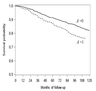
Figure 17.1

Code: Program 17.1

A conventional statistical test to compare survival curves (the logrank test) yielded a P-value= 0.005.

the proportion of individuals who survived through time k. If we calculate the survivals at each month until the administrative end of follow-up kend = 120 and plot them along a horizontal time axis, we obtain the survival curve. The survival curve starts at Pr [T > 0] = 1 for k = 0 and then decreases monotonically—that is, it does not increase—with subsequent values of k = 1, 2, …kend. Alternatively, we can define risk, or cumulative incidence, at time k as one minus the survival 1 − Pr [T > k] = Pr [T ≤ k]. The cumulative incidence curve starts at Pr [T ≤ 0] = 0 and increases monotonically during the follow-up.

Other effect measures that can be In survival analyses, a natural approach to quantify the treatment effect is to compare the survival or risk under each treatment level at some or all times k. Of course, in our smoking cessation example, a contrast of these curves may not have a causal interpretation because the treated and the untreated are probably not exchangeable. However, suppose for a second (actually, until Section 17.4) that quitters (A = 1) and non-quitters (A = 0) are marginally exchangeable. Then we can construct the survival curves shown in Figure 17.1 and compare Pr [T > k|A = 1] versus Pr [T > k|A = 0] for all times k. For example, the survival at 120 months was 76.2% among quitters and 82.0% among non-quitters. Alternatively, we could contrast the risks rather than the survivals. For example, the 120-month risk was 23.8% among quitters and 18.0% among non-quitters.

At any time k, we can also calculate the proportion of individuals who develop the event among those who had not developed it before k. This is the hazard Pr [T = k|T > k − 1]. Technically, this is the discrete time hazard, i.e., the hazard in a study in which time is measured in discrete intervals as opposed to measured continuously. Because in real-world studies, time is indeed measured in discrete intervals (years, months, weeks, days…) rather than in a truly continuous fashion, here we will refer to the discrete time hazard as, simply, the hazard.

The risk and the hazard are different measures. The denominator of the risk—the number of individuals at baseline—is constant across times k and its numerator—all events between baseline and k—is cumulative. That is, the risk will stay flat or increase as k increases. On the other hand, the denominator of the hazard—the number of individuals alive at k—varies over time t and its numerator includes only recent events—those during interval k. That is, the hazard may increase or decrease over time. In our example, the hazard at 120 months was 0% among quitters (because the last death happened at 113 months in this group) and 1/986 = 0.10% among non-quitters, and the hazard curves between 0 and 120 months had roughly the shape of a letter M.

A frequent approach to quantify the treatment effect in survival analyses is to estimate the ratio of the hazards in the treated and the untreated, known as the hazard ratio. However, the hazard ratio is problematic for the reasons described in Fine Point 17.2. Therefore, the survival analyses in this book privilege survival/risk over hazard. However, that does not mean that we should completely ignore hazards. The estimation of hazards is often a useful intermediate step for the estimation of survivals and risks.

17.2 From hazards to risks

In survival analyses, there are two main ways to arrange the analytic dataset. In the first data arrangement each row of the database corresponds to one person. This data format—often referred to as the “wide”format when there are time-varying treatments and confounders—is the one we have used so far in this book. In the analyses of the previous section, the dataset had 1629 rows, one per individual.

In the second data arrangement each row of the database corresponds to a person-time. That is, the first row contains the information for person 1 at k = 0, the second row the information for person one at k = 1, the third row the information for person 1 at k = 2, and so on until the follow-up of person one ends. The next row contains the information of person 2 at k = 0, etc. This person-time (or “long”) data format is the one we will use in most survival analyses in this chapter and in all analyses with time-varying treatments in Part III. In our smoking cessation example, the person-time dataset has 176, 764 rows, one per person-month.

To encode survival information through k in the person-time data format, it is helpful to define a time-varying indicator of event Dk. For each person at each month k, the indicator D^k takes value 1 if T ≤ k and value 0 if T > k. The causal diagram in Figure 17.2 shows the treatment A and the Figure 17.2 event indicators D¹ and D² at times 1 and 2, respectively. The variable U represents the (generally unmeasured) factors that increase susceptibility to the event of interest. Note that sometimes these susceptibility factors are time-varying too. In that case, they can be depicted in the causal diagram as U0, U1…, and so on. Part III deals with the case in which the treatment itself is time-varying.

In the person-time data format, the row for a particular individual at time k includes the indicator Dk+1. In our example, the first row of the person-By definition, everybody had to sur- time dataset, for individual one at k = 0, includes the indicator D1, which is 1 if the individual died during month 1 and 0 otherwise; the second row, for individual one at k = 1, includes the indicator D2, which is 1 if the individual died during month 2 and 0 otherwise; and so on. The last row in the dataset for each individual is either her first row with Dk+1 = 1 or the row corresponding to month 119.

Using the time-varying outcome variable Dk, we can define survival at k as Pr [D^k = 0], which is equal to Pr [T > k], and risk at k as Pr [D^k = 1], which is equal to Pr [T ≤ k]. The hazard at k is defined as Pr [D^k = 1|Dk−¹ = 0]. For k = 1 the hazard is equal to the risk because everybody is, by definition, alive at k = 0.

The survival probability at k is the product of the conditional probabilities of having survived each interval between 0 and k. For example, the survival at k = 2, Pr [D² = 0], is equal to survival probability at k = 1, Pr [D¹ = 0], times the survival probability at k = 2 conditional on having survived through k = 1, Pr [D² = 0|D¹ = 0]. More generally, the survival at k is

\[\Pr\left[D\_k = 0\right] = \prod\_{m=1}^k \Pr\left[D\_m = 0 | D\_{m-1} = 0\right]\]

That is, the survival at k equals the product of one minus the hazard at all previous times. If we know the hazards through k we can easily compute the survival at k (or the risk at k, which is just one minus the survival).

The hazard at k, Pr [D^k = 1|Dk−¹ = 0], can be estimated nonparametrically by dividing the number of cases during the interval k by the number of individuals alive at the end of interval k − 1. If we substitute this estimate into the above formula the resulting nonparametric estimate of the survival Pr [D^k = 0] at k is referred to as the Kaplan-Meier, or product-limit, estima-

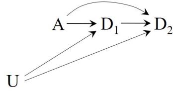
vive month 0 in order to be included in the dataset, i.e., D⁰ = 0 for all individuals.

The hazards of hazard ratios When using the hazard ratio as a measure of causal effect, two important properties of the hazard ratio need to be taken into account.

First, because the hazards vary over time, the hazard ratio generally does too. That is, the ratio at time k may differ from that at time k + 1. However, many published survival analyses report a single hazard ratio, which is usually the consequence of fitting a Cox proportional hazards model that assumes a constant hazard ratio by ignoring interactions with time. The reported hazard ratio is a weighted average of the k-specific hazard ratios, which makes it hard to interpret. If the risk is rare and censoring only occurs at a common administrative censoring time kend, then the weight of the hazard ratio at time k is proportional to the total number of events among untreated individuals that occur at k. (Technically, the weights are equal to the conditional density at k of T given A = 0 and T < kend.) Because it is a weighted average, the reported hazard ratio may be 1 even if the survival curves are not identical. In contrast to “the” hazard ratio, ratios and differences of survival probabilities and risks are defined with respect to a fixed time period, e.g., the 5-year survival difference, the 120-month risk ratio.

Second, even if we presented the time-specific hazard ratios, their causal interpretation is not straightforward. Suppose treatment kills all high-risk individuals by time k and has no effects on others. Then the hazard ratio at time k + 1 compares the treated and the untreated individuals who survived through k. In the treated group, the survivors are all low-risk individuals (because the high-risk ones have already been killed by treatment); in the untreated group, the survivors are a mixture of high-risk and low-risk individuals (because treatment did not weed out the former). As a result the hazard ratio at k + 1 will be less than 1 even though treatment is not beneficial for any individual.

This apparent paradox is an example of selection bias due to conditioning on a post-treatment variable (i.e., being alive at k) which is affected by treatment. For example, the hazard ratio at time 2 is the probability Pr [D² = 1|D¹ = 0, A] of the event at time 2 among those who survived time 1. As depicted in the causal diagram of Figure 17.3, the conditioning on the collider D¹ will generally open the path A → D¹ ← U → D² and therefore induce an association between treatment A and event D² among those with D¹ = 0. This built-in selection bias of hazard ratios does not happen if the survival curves are the same in the treated and the untreated, i.e., if there are no arrows from A into the indicators for the event. Hern´an (2010) described an example of this problem.

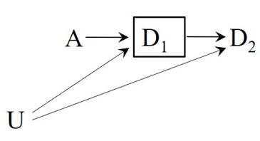
Figure 17.3

multiple rows of the person-time data structure, the standard error of the parameter estimates outputted by a routine logistic regression program will be correct if the hazards model is correct.

tor. Figure 17.1 was constructed using the Kaplan-Meier estimator, which is an excellent estimator of the survival curve, provided the total number of failures over the follow up period is reasonably large. Typically, the number of cases during each interval is low (or even zero) and thus the nonparametric estimates of the hazard Pr [D^k = 1|Dk−¹ = 0] at k will be very unstable. If our interest is in estimation of the hazard at a particular k, smoothing via a parametric model may be required (see Chapter 11 and Fine Point 17.3).

An easy way to parametrically estimate the hazards is to fit a logistic regression model for Pr [Dk+1 = 1|D^k = 0] that, at each k, is restricted to individuals who survived through k. The fit of this model is straightforward when using the person-time data format. In our example, we can estimate the hazards in the treated and the untreated by fitting the logistic model

\[\text{logit } \Pr\left[D\_{k+1} = 1 | D\_k = 0, A\right] = \theta\_{0,k} + \theta\_1 A + \theta\_2 A \times k + \theta\_3 A \times k^2\]

Although each person occurs in where θ0,k is a time-varying intercept that can be estimated by some flexible function of time such as θ0,k = θ⁰ + θ4k + θ5k 2 . The flexible time-varying intercept allows for a time-varying hazard and the product terms between treatment A and time (θ2A×k +θ3A×k 2 ) allow the hazard ratio to vary over time. See Technical Point 17.1 for details on how a logistic model approximates a hazards model. Functions other than the logit (e.g., the probit) can also be used to model dichotomous outcomes and therefore to estimate hazards.

We then compute estimates of the survival Pr [Dk+1 = 0|A = a] by multiplying the estimates of one minus the estimates of Pr [Dk+1 = 1|D^k = 0, A = a]

Fine Point 17.3

Models for survival analysis. Methods for survival analysis need to accommodate the expected censoring of failure times due to administrative end of follow-up.

Nonparametric approaches to survival analysis, like constructing Kaplan-Meier curves, make no assumptions about the distribution of the unobserved failure times due to administrative censoring. On the other hand, parametric models for survival analysis assume a particular statistical distribution (e.g., exponential, Weibull) for the failure times or hazards. The logistic model described in the main text to estimate hazards is an example of a parametric model.

Other models for survival analysis, like the Cox proportional hazards model and the accelerated failure time (AFT) model, do not assume a particular distribution for the failure times or hazards. In particular, these models are agnostic about the shape of the hazard when all covariates in the model have value zero—often referred to as the baseline hazard. These models, however, impose a priori restrictions on the relation between the baseline hazard and the hazard under other combinations of covariate values. As a result, these methods are referred to as semiparametric methods.

See the book by Hosmer, Lemeshow, and May (2008) for a review of applied survival analysis. More formal descriptions can be found in the books by Fleming and Harrington (2005) and Kalbfleisch and Prentice (2002).

Code: Program 17.2 provided by the logistic model, separately for the treated and the untreated. Figure 17.4 shows the survival curves obtained after parametric estimation of the hazards. These curves are a smooth version of those in Figure 17.1.

The validity of this procedure requires no misspecification of the hazards model. In our example, this assumption seems plausible because we obtained essentially the same survival estimates as in the previous section when we estimated the survival in a fully nonparametric way. A 95% confidence interval around the survival estimates can be easily constructed via bootstrapping of the individuals in the population.

17.3 Why censoring matters

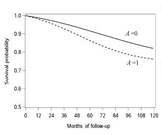
Figure 17.4

The only source of censoring in our study is a common administrative censoring time kend = 120 that is identical for all individuals. In this simple setting the procedure described in the previous section to estimate the survival is overkill. One can simply estimate the survival probabilities Pr [Dk+1 = 0|A = a] by the fraction of individuals who received treatment a and survived to k + 1, or by fitting separate logistic models for Pr [Dk+1 = 0|A] at each time, for k = 0, 1, …, kend.

Now suppose that individuals start the follow-up at different dates—there is staggered entry into the study—but the administrative end of follow-up date is common to all. Because the administrative censoring time is the difference between the administrative end of follow-up and the time of start of followup, different individuals will have different administrative censoring times. In this setting it is helpful to define a time-varying indicator C^k for censoring by time k. For each person at each month k, the indicator C^k takes value 0 if the administrative end of follow-up is greater than k and 1 otherwise. In the person-time data format, the row for a particular individual at time k includes the indicator Ck+1. We did not include this variable in our dataset because Ck+1 = 0 for all individuals at all times k before 120 months. In the general case with random (i.e., individual-specific) administrative censoring, the indicator Ck+1 will transition from 0 to 1 at different times k for different

Approximating the hazard ratio via a logistic model. The (discrete-time) hazard ratio Pr[Dk+1=1|Dk=0,A=1] Pr[Dk+1=1|Dk=0,A=0] is exp (α1) at all times k+1 in the hazards model Pr [Dk+1 = 1|D^k = 0, A] = Pr [Dk+1 = 1|D^k = 0, A = 0]×exp (α1A). If we take logs on both sides of the equation, we obtain log Pr [Dk+1 = 1|D^k = 0, A] = α0,k + α1A where α0,k = log Pr [Dk+1 = 1|D^k = 0, A = 0].

Suppose the hazard at k + 1 is small, i.e., Pr [Dk+1 = 1|D^k = 0, A] ≈ 0. Then one minus the hazard at k + 1 is close to one, and the hazard is approximately equal to the odds: Pr [Dk+1 = 1|D^k = 0, A] ≈ Pr[Dk+1=1|Dk=0,A] Pr[Dk+1=0|Dk=0,A] . We then have

\[\log \frac{\Pr\left[D\_{k+1} = 1 | D\_k = 0, A\right]}{\Pr\left[D\_{k+1} = 0 | D\_k = 0, A\right]} = \text{logit} \Pr\left[D\_{k+1} = 1 | D\_k = 0, A\right] \approx \alpha\_{0, k} + \alpha\_1 A\]

That is, if the hazard is close to zero at k + 1, we can approximate the log hazard ratio α¹ by θ¹ in a logistic model logit Pr [Dk+1 = 1|D^k = 0, A] = θ0,k + θ1A like the one we used in the main text (Thompson 1977). As a rule of thumb, the approximation is often considered to be accurate enough when Pr [Dk+1 = 1|D^k = 0, A] < 0.1 for all k.

This rare event condition can almost always be guaranteed to hold: we just need to define a time unit k that is short enough for Pr [Dk+1 = 1|D^k = 0, A] < 0.1. For example, if D^k stands for lung cancer, k may be measured in years; if D^k stands for infection with the common cold virus, k may be measured in days. The shorter the time unit, the more rows in the person-time dataset used to fit the logistic model.

people.

Our goal is to estimate the survival curve that would have been observed if nobody had been censored before kend, where kend is the maximum administrative censoring time in the study. That is, our goal is to estimate the survival Pr [D^k = 0|A = a] that would have been observed if the value of the timevarying indicators D^k were known even after censoring. Technically, we can also refer to this quantity as Pr h Dc=0 ^k = 0|A = a i where c = (c1, c2…ckend ). As discussed in Chapter 12, the use of the superscript c = 0 makes explicit the quantity that we have in mind. We sometimes choose to omit the superscript c = 0 when no confusion can arise. For simplicity, suppose that the time of start of follow-up was as if randomly assigned to each individual, which would be the case if there were no secular trends in any variable. Then the administrative censoring time, and therefore the indicator C, is independent of both treatment and death time.

We cannot validly estimate this survival Pr [D^k = 0|A = a] at time k by simply computing the fraction of individuals who received treatment level a and survived and were not censored through k. This fraction is a valid estimator of the joint probability Pr [Ck+1 = 0, Dk+1 = 0|A = a], which is not what we want. To see why, consider a study with kend = 2 and in which the following happens:

• Pr [C¹ = 0] = 1, i.e., nobody is censored by k = 1
• Pr [D¹ = 0|C⁰ = 0] = 0.9, i.e., 90% of individuals survive through k = 1
• Pr [C² = 0|D¹ = 0, C¹ = 0] = 0.5, i.e., a random half of survivors is censored by k = 2
• Pr [D² = 0|C² = 0, D¹ = 0, C¹ = 0] = 0.9, i.e., 90% of the remaining individuals survive through k = 2

The fraction of uncensored survivors at k = 2 is 1 × 0.9× 0.5× 0.9 = 0.405. However, if nobody had been censored, i.e., if Pr [C² = 0|D¹ = 0, C¹ = 0] =

1, the survival would have been 1 × 0.9 × 1 × 0.9 = 0.81. This example motivates how correct estimation of the survivals Pr [D^k = 0|A = a] requires the procedures described in the previous section. Specifically, under (as if) randomly assigned censoring, the survival Pr [D^k = 0|A = a] at k is

\[\prod\_{m=1}^{k} \Pr\left[D\_m = 0 \middle| D\_{m-1} = 0, C\_m = 0, A = a\right] \text{ for } k < k\_{end}\]

The estimation procedure is the same as described above except that we either use a nonparametric estimate of, or fit a logistic model for, the cause-specific hazard Pr [Dk+1 = 1|D^k = 0, Ck+1 = 0, A = a].

Often we are not ready to assume that censoring is as if randomly assigned. When there is staggered entry, an individual’s time of administrative censoring depends on the calendar time at study entry (later entries have shorter values of kend) and calendar time may itself be associated with the outcome. Therefore, the above procedure will need to be adjusted for baseline calendar time. In addition, there may be other baseline prognostic factors that are unequally distributed between the treated (A = 1) and the untreated (A = 0), which also requires adjustment. The next sections extend the above procedure to incorporate adjustment for baseline confounders via g-methods. In Part III we extend the procedure to settings with time-varying treatments and confounders.

17.4 IP weighting of marginal structural models

When the treated and the untreated are not exchangeable, a direct contrast of their survival curves cannot be endowed with a causal interpretation. In our smoking cessation example, we estimated that the 120-month survival was lower in quitters than in non-quitters (76.2% versus 82.0%), but that does not necessarily imply that smoking cessation increases mortality. Older people are more likely to quit smoking and also more likely to die. This confounding by age makes smoking cessation look bad because the proportion of older people is greater among quitters than among non-quitters.

Let us define D a,c=0 k as a counterfactual time-varying indicator for death at k under treatment level a and no censoring. For simplicity of notation, we will write D a,c=0 k as D^{a k} when, as in this chapter, it is clear that the goal is estimating the survival in the absence of censoring. For additional simplicity, in the remainder of this chapter we omit C^k = 0 from the conditioning event of the hazard at k, Pr [Dk+1 = 0|D^k = 0, L = l, A]. That is, we write all expressions as if all individuals had a common administrative censoring time, like in our smoking cessation example.

Suppose we want to compare the counterfactual survivals Pr - D^a=1 ^k+1 = 0 and Pr - D^a=0 ^k+1 = 0 that would have been observed if everybody had received treatment (a = 1) and no treatment (a = 0), respectively. That is, the causal contrast of interest is

Pr - D^a=1 ^k+1 = 0 vs. Pr - D^a=0 ^k+1 = 0 for k = 0, 2, …kend − 1

Because of confounding, this contrast may not be validly estimated by the contrast of the survivals Pr [Dk+1 = 0|A = 1] and Pr [Dk+1 = 0|A = 0] that we described in the previous sections. Rather, a valid estimation of the quantities Pr - D^{a k}+1 = 0 for a = 1 and a = 0 typically requires adjustment for

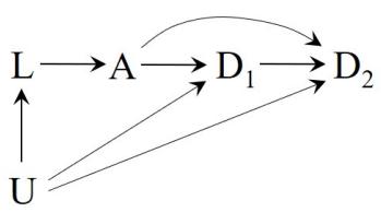
Figure 17.5

confounders, which can be achieved through several methods. This section focuses on IP weighting. Let us assume that the treated (A = 1) and the untreated (A = 0) are exchangeable within levels of the L variables, as represented in the causal diagram of Figure 17.5. Like in Chapters 12 to 15, L includes the variables sex, age, race, education, intensity and duration of smoking, physical activity in daily life, recreational exercise, and weight. We also assume positivity and consistency. The estimation of IP weighted survival curves has two steps.

First, we estimate the stabilized IP weight SW^A for each individual in the study population. The procedure is exactly the same as the one described in Chapter 12. We fit a logistic model for the conditional probability Pr [A = 1|L] of treatment (i.e., smoking cessation) given the variables in ^L. The denominator of the estimated SW^A Code: Program 17.3 is Pr [ ^{c A} = 1|L] for treated individuals and ^{1 −} Pr [ ^{c A} = 1|L] for untreated individuals, where Pr [ ^{c A} = 1|L] is the predicted value from the logistic model. The numerator of the estimated weight SW^A is Pr [ ^{c A} = 1] for the treated and ^{1 −} Pr [ ^{c A} = 1] for the untreated, where Pr [ ^{c A} = 1] can be estimated nonparametrically or as the predicted value from a logistic model for the marginal probability Pr [A = 1] of treatment. See Chapter 11 for details on predicted values.

The application of the estimated weights SW^A creates a pseudo-population in which the variables in L are independent from the treatment A, which eliminates confounding by those variables. In our example, the weights had mean 1 (as expected) and ranged from 0.33 to 4.21.

Second, using the person-time data format, we fit a hazards model like the one described above except that individuals are weighted by their estimated SWA. Technically, this IP weighted logistic model estimates the parameters of the marginal structural logistic model

\[\text{logit } \Pr\left[D\_{k+1}^a = 0 | D\_k^a = 0\right] = \beta\_{0,k} + \beta\_1 a + \beta\_2 a \times k + \beta\_3 a \times k^2\]

That is, the IP weighted model estimates the time-varying hazards that would have been observed if all individuals in the study population had been treated (a = 1) and the time-varying hazards if they had been untreated (a = 0).

The estimates of Pr - D^{a k}+1 = 0|D^{a k} = 0 from the IP weighted hazards models can then be multiplied over time (see previous section) to obtain an estimate of the survival Pr - D^{a k}+1 = 0 that would have been observed under treatment a = 1 and under no treatment a = 0. The resulting curves are shown in Figure 17.6.

In our example, the 120-month survival estimates were 80.7% under smoking cessation and 80.5% under no smoking cessation; difference 0.2% (95% confidence interval from −4.1% to 3.7% based on 500 bootstrap samples). Though the survival curve under treatment was lower than the curve under no treatment for most of the follow-up, the maximum difference never exceeded −1.4% with a 95% confidence interval from −3.4% to 0.7%. That is, after adjustment for the covariates L via IP weighting, we found little evidence of an effect of smoking cessation on mortality at any time during the follow-up. The validity of this procedure requires no misspecification of both the treatment model and the marginal hazards model.

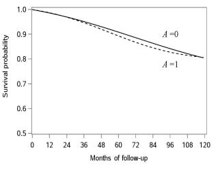
Figure 17.6

17.5 The parametric g-formula

In the previous section we estimated the survival curve under treatment and under no treatment in the entire study population via IP weighting. To do so, we adjusted for L and assumed exchangeability, positivity, and consistency. Another method to estimate the marginal survival curves under those assumptions is standardization based on parametric models, i.e., the parametric g-formula.

The survival Pr - D^{a k}+1 = 0 at k+ 1 under treatment level a is the weighted average of the survival conditional probabilities at k + 1 within levels of the covariates L and treatment level A = a, with the proportion of individuals in each level l of L as the weights. That is, under exchangeability, positivity, and consistency, Pr - D^{a k}+1 = 0 equals the standardized survival

\[\sum\_{l} \Pr\left[D\_{k+1} = 0 | L = l, A = a\right] \Pr\left[L = l\right] \dots\]

For a formal proof, see Section 2.3.

Therefore, the estimation of the parametric g-formula has two steps. First, we need to estimate the conditional survivals Pr [Dk+1 = 0|L = l, A = a] using our administratively censored data. Second, we need to compute their weighted average over all values l of the covariates L. We describe each of these two steps in our smoking cessation example.

For the first step we fit a parametric hazards model like the one described in Section 17.2, except that the variables in L are included as covariates. If the model is correctly specified, it validly estimates the time-varying hazards Pr [Dk+1 = 1|D^k = 0, L, A] within levels of treatment A and covariates L. The product of one minus the conditional hazards

\[\prod\_{m=0}^{k} \Pr\left[D\_{m+1} = 0 | D\_m = 0, L = l, A = a\right]\]

is equal to the conditional survival Pr [Dk+1 = 0|L = l, A = a]. Because of conditional exchangeability given L, the conditional survival for a particular set of covariate values L = l and A = a can be causally interpreted as the survival that would have been observed if everybody with that set of covariates had received treatment value a. That is,

\[\Pr\left[D\_{k+1} = 0 | L = l, A = a\right] = \Pr\left[D\_{k+1}^a = 0 | L = l\right].\]

Therefore the conditional hazards can be used to estimate the survival curve under treatment (a = 1) and no treatment (a = 0) within each combination In Chapter 12 we referred to models of values l of L. For example, we can use this model to estimate the survival curves under treatment and no treatment for white men aged 61, with college education, low levels of exercise, etc. However, our goal is estimating the marginal, not the conditional, survival curves under treatment and under no treatment.

For the second step we compute the weighted average of the conditional Code: Program 17.4 survival across all values l of the covariates L, i.e., we standardize the survival to the confounder distribution. To do so, we use the method described in Section 13.3 to standardize means: standardization by averaging after expansion of dataset, outcome modeling, and prediction. This method can be used even when some of the variables in L are continuous so that the sum over values l is formally an integral. The resulting curves are shown in Figure 17.7.

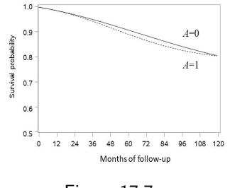
Figure 17.7

conditional on all the covariates L as faux marginal structural models.

The procedure is analogous to the one described in Chapter 13.

In our example, the survival curve under treatment was lower than the curve under no treatment during the entire follow-up, but the maximum difference never exceeded −2.0% (95% confidence interval from −5.6% to 1.8%). The 120 month survival estimates were 80.4% under smoking cessation and 80.6% under no smoking cessation; difference 0.2% (95% confidence interval from −4.6% to 4.1%). That is, after adjustment for the covariates L via standardization, we found little evidence of an effect of smoking cessation on mortality at any time during the follow-up. Note that the survival curves estimated via IP weighting (previous section) and the parametric g-formula (this section) are similar but not identical because they rely on different parametric assumptions: the IP weighted estimates require no misspecification of a model for treatment and a model for the unconditional hazards; the parametric g-formula estimates require no misspecification of a model for the conditional hazards.

17.6 G-estimation of structural nested models

mate a hazard ratio because structural nested logistic models do not generalize easily to time-varying treatments (Technical Point 14.1).

and Robins (1997b) described survival analysis with instrumental variables that exhibit similar problems to those described here for structural nested models.

evident when treatment is timevarying. See Chapter 21.

The previous sections describe causal contrasts that compare survivals, or risks, under different levels of treatment A. The survival was computed from hazards estimated by logistic regression models. This approach is feasible when the analytic method is IP weighting of marginal structural models or the parametric g-formula, but not when the method is g-estimation of structural nested models. As explained in Chapter 14, structural nested models are models for conditional causal contrasts (e.g., the difference or ratio of covariate-specific means under different treatment levels), not for the components of those con-In fact, we may not even approxi- trasts (e.g., each of the means under different treatment levels). Therefore we cannot estimate survivals or hazards using a structural nested model.

We can, however, consider a structural nested log-linear model to model the ratio of cumulative incidences (i.e., risks) under different treatment levels. Structural nested cumulative failure time models do precisely that (see Technical Point 17.2), but they are best used when failure is a rare event because log-linear models do not naturally impose an upper limit of 1 on the risk. For non-rare failures, we can instead consider a structural nested log-linear model to model the ratio of cumulative survival probabilities (i.e., 1− risk) under dif-Tchetgen Tchetgen et al (2015) ferent treatment levels. Structural nested cumulative survival time models do precisely that (see Technical Point 17.2), but they are best used when survival is rare because log-linear models do not naturally impose an upper limit of 1 on the survival. A more general option is to use a structural nested model that models the ratio of survival times under different treatment options. That is, an accelerated failure time (AFT) model.

Let T a ⁱ be the counterfactual time of survival for individual i under treatment level a. The effect of treatment A on individual i’s survival time can be measured by the ratio T a=1 i /T ^a=0 i of her counterfactual survival times under treatment and under no treatment. If the survival time ratio is greater than 1, then treatment is beneficial because it increases the survival time; if the ratio is less than 1, then treatment is harmful; if the ratio is 1, then treatment has no effect. Suppose, temporarily, that the effect of treatment is the same for every individual in the population.

The “nested” component is only We could then consider the structural nested accelerated failure time (AFT) model T a i /T ^a=0 ⁱ = exp (−ψ1a), where ψ¹ measures the expansion (or contraction) of each individual’s survival time attributable to treatment. If ψ¹ < 0 then treatment increases survival time, if ψ¹ > 0 then treatment decreases

Structural nested cumulative failure time (CFT) models and cumulative survival time (CST) models. For a time-fixed treatment, a (non-nested) structural CFT model is a model for the ratio of the counterfactual risk under treatment value a divided by the counterfactual risk under treatment value 0 conditional on treatment A and covariates L. The general form of the model is

\[\frac{\Pr\left[D\_k^a = 1 | L, A\right]}{\Pr\left[D\_k^{a=0} = 1 | L, A\right]} = \exp[\gamma\_k(L, A; \psi)]\]

where γk(L, A; ψ) is a function of treatment and covariate history indexed by the (possibly vector-valued) parameter ψ. For consistency, exp[γk(L, A; ψ)] must be 1 when A = 0 because then the two treatment values being compared are identical, and when there is no effect of treatment at time m on outcome at time k. An example of such a function is γk(L, A; ψ) = ψA so ψ = 0 corresponds to no effect, ψ < 0 to beneficial effect, and ψ > 0 to harmful effect.

Analogously, for a time-fixed treatment, a (non-nested) structural CST model is a model for the ratio of the counterfactual survival under treatment value a divided by the counterfactual survival under treatment level 0 conditional on treatment A and covariates L. The general form of the model is

\[\frac{\Pr\left[D\_k^a = 0 | L, A\right]}{\Pr\left[D\_k^{a=0} = 0 | L, A\right]} = \exp[\gamma\_k(L, A; \psi)]\]

Although CFT and CST models differ only in whether we specify a multiplicative model for Pr [D^{a k} = 1|L, A] versus for Pr [D^{a k} = 0|L, A], the meaning of γk(L, A; ψ) differs because a multiplicative model for risk is not a multiplicative model for survival, whenever the treatment effect is non-null. When we let the time index k be continuous rather than discrete, a structural CST model is equivalent to a structural additive hazards model (Tchetgen Tchetgen et al., 2015) as any model for Pr [D^{a k} = 0|L, A] /Pr - Da=0 ^k = 0|L, A induces a model for the difference in the time-specific hazards of T a and T ^a=0, and vice-versa.

The use of structural CFT models requires that, for all values of the covariates L, the conditional cumulative probability of failure under all treatment values satisfies a particular type of rare failure assumption. In this “rare failure” context, the structural CFT model has an advantage over AFT models: it admits unbiased estimating equations that are differentiable in the model parameters and thus are easily solved. Page (2005) and Picciotto et al. (2012) provided further details on structural CFT and CST models. For a time-varying treatment, this class of models can be viewed as a special case of the multivariate structural nested mean model (Robins 1994). See Technical Point 14.1.

serves the usual interpretation of positive parameters indicating harm and negative parameters indicating benefit.

The negative sign in front of ψ pre- survival time, if ψ¹ = 0 then treatment does not affect survival time. More generally, the effect of treatment may depend on covariates L so a more general structural AFT would be T a i /T ^a=0 ⁱ = exp (−ψ1a − ψ2aLi), with ψ¹ and ψ² (a vector) constant across individuals. Rearranging the terms, the model can be written as

\[T\_i^{a=0} = T\_i^a \exp\left(\psi\_1 a + \psi\_2 a L\_i\right) \text{ for all individuals } i\]

Following the same reasoning as in Chapter 14, consistency of counterfactuals implies the model T a=0 ⁱ = Tⁱ exp (ψ1Aⁱ + ψ2AiLi), in which the counterfactual time T a i is replaced by the actual survival time T A ⁱ = Tⁱ . The parameters ψ¹ and ψ² can be estimated by a modified g-estimation procedure (to account for administrative censoring) that we describe later in this section.

The above structural AFT is unrealistic because it is both deterministic and rank-preserving. It is deterministic because it assumes that, for each individual, the counterfactual survival time under no treatment T ^a=0 can be computed without error as a function of the observed survival time T, treatment A, and covariates L. It is rank-preserving because, under this model, if deterministic non-rank-preserving structural nested AFT models.

proaches, known as directed search methods, for approximate searching are available in statistical software. The Nelder-Mead Simplex method is an example of a directed search method.

	Type
	1	2	3
a=0 T	36	72	108
a=1 T	24	48	72

Table 17.1

Because of the implausibility of rank preservation, one should not generally use methods for causal inference that rely on it, as we discussed in Chapter 14. And yet again we will use a rank-preserving model here to describe g-estimation for structural AFT models because g-estimation is easier to understand for rank-preserving models, and because the g-estimation procedure is actually Robins (1997b) described non- the same for rank-preserving and non-rank-preserving models.

Consider the simpler rank-preserving model T a=0 ⁱ = Tⁱ exp (ψAi) without a product term between treatment and covariates. G-estimation of the parameter ψ of this structural AFT model would be straightforward if administrative censoring did not exist, i.e., if we could observe the time of death T for all individuals. In fact, in that case the g-estimation procedure would be the same as we described in Section 14.5. The first step would be to compute candidate counterfactuals Hi(ψ † ) = Tⁱ exp ψ †Aⁱ under many possible values ψ † of the causal parameter ψ. The second step would be to find the value ψ † Less computationally intensive apthat results in a Hi(ψ † ) that is independent of treatment A in a logistic model for the probability of A = 1 with Hi(ψ † ) and the confounders L as covariates. Such value ψ † would be the g-estimate of ψ.

However, this procedure cannot be implemented in the presence of administrative censoring at time K because Hi(ψ † ) cannot be computed for individuals with unknown Tⁱ . One might then be tempted to restrict the g-estimation procedure to individuals with an observed survival time only, i.e., those with Tⁱ ≤ K. Unfortunately, that approach results in selection bias. To see why, consider the following oversimplified scenario.

We conduct a 60-month randomized experiment to estimate the effect of a dichotomous treatment A on survival time T. Only 3 types of individuals participate in our study. Type 1 individuals are those who, in the absence of treatment, would die at 36 months (T ^a=0 = 36). Type 2 individuals are those who in the absence of treatment, would die at 72 months (T ^a=0 = 72). Type 3 individuals are those who in the absence of treatment, would die at 108 months (T ^a=0 = 108). That is, type 3 individuals have the best prognosis and type 1 individuals have the worst one. Because of randomization, we expect that the proportions of type 1, type 2, and type 3 individuals are the same in each of the two treatment groups A = 1 and A = 0. That is, the treated and the untreated are expected to be exchangeable.

Suppose that treatment A = 1 decreases the survival time compared with A = 0. Table 17.1 shows the survival time under treatment and under no treatment for each type of individual. Because the administrative end of follow-up is K = 60 months, the death of type 1 individuals will be observed whether they are randomly assigned to A = 1 or A = 0 (both survival times are less than 60), and the death of type 3 individuals will be administratively censored whether they are randomly assigned to A = 1 or A = 0 (both survival times are greater than 60). The death of type 2 individuals, however, will only be observed if they are assigned to A = 1. Hence an analysis that welcomes all individuals with non-administratively censored death times will have an imbalance of individual types between the treated and the untreated. Exchangeability will be broken because the A = 1 group will include type 1 and type 2 individuals, whereas the A = 0 group will include type 1 individuals only. Individuals in the A = 0 group will have, on average, a worse prognosis than those in the A = 1 group, which will make treatment look better than it really is. This selection bias (Chapter 8) arises when treatment has a non-null effect on survival time.

Artificial censoring Let K(ψ) be the minimum survival time under no treatment that could possibly correspond to an individual who actually died at time K (the administrative end of follow-up). For a dichotomous treatment A, K(ψ) = inf {K exp (ψA)}, which implies that K(ψ) = K exp (ψ × 0) = K if treatment contracts the survival time (i.e., ψ > 0), K(ψ) = K exp (ψ × 1) = K exp (ψ) if treatment expands the survival time (i.e., ψ < 0), and K(ψ) = K exp (0) = K if treatment does not affect survival time (i.e., ψ = 0).

All individuals who are administratively censored (i.e., T > K) have ∆(ψ) = 0 because there is at least one treatment level (the one they actually received) under which their survival time is greater than K, i.e., H(ψ) ≥ K(ψ). Some of the individuals who are not administratively censored (i.e., T ≤ K) also have ∆(ψ) = 0 and are excluded from the analysis—they are artificially censored—to avoid selection bias.

The artificial censoring indicator ∆(ψ) is a function of H(ψ) and K. Under conditional exchangeability given L, all such functions, when evaluated at the true value of ψ, are conditionally independent of treatment A given the covariates L. That is, g-estimation of the AFT model parameters can be performed based on ∆(ψ) rather than H(ψ). Technically, ∆(ψ) is substituted for H(ψ) in the estimating equation of Technical Point 14.2. For practical estimation details, see the Appendix of Hern´an et al (2005).

viduals from the analysis is often referred to as artificial censoring. See Technical Point 17.3.

The point estimate of ψ is the value that corresponds to the minimum of the estimating function described in Technical Point 17.3.; the limits of the 95% confidence interval are the values that correspond to the value 3.84 (χ ² with one degree of freedom) of the estimating function.

To avoid this selection bias, one needs to select individuals whose survival time would have been observed by the end of follow-up whether they had been treated or untreated, i.e., those with T a=0 ⁱ ≤ K and T a=1 ⁱ ≤ K. In our example, we will have to exclude all type 2 individuals from the analysis in order to preserve exchangeability. That is, we will not only exclude administratively This exclusion of uncensored indi- censored individuals with Tⁱ > K, but also some uncensored individuals with known survival time Tⁱ ≤ K because their survival time would have been greater than K if they had received a treatment level different from the one they actually received.

We then define an indicator ∆(ψ), which takes value 0 when an individual is excluded and 1 when she is not. The g-estimation procedure is then modified by replacing the variable H(ψ † ) by the indicator ∆(ψ † ). See Technical Point 17.3 for details. In our example, the g-estimate ψˆ from the rank-preserving structural AFT model T ^a=0 Code: Program 17.5 ⁱ = Tⁱ exp (ψAi) was −0.047 (95% confidence interval: −0.223 to 0.333). The number exp −ψˆ = 1.05 can be interpreted as the median survival time that would have been observed if all individuals in the study had received a = 1 divided by the median survival time that would have been observed if all individuals in the study had received a = 0. This survival time ratio suggests little effect of smoking cessation A on the time to death.

As we said in Chapter 14, structural nested models, including AFT models, have rarely been used in practice. A practical obstacle for the implementation of the method is the lack of user-friendly software. An even more serious obstacle in the survival analysis setting is that the parameters of structural AFT models need to be estimated through search algorithms that are not guaranteed to find a unique solution. This problem is exacerbated for models with two or more parameters ψ. As a result, the few published applications of this method tend to use simplistic AFT models that do not allow for the treatment effect to vary across covariate values.

This state of affairs is unfortunate because subject-matter knowledge (e.g., biological mechanisms) is easier to translate into parameters of structural AFT models than into those of structural hazards models. This is especially true when using non-deterministic and non-rank preserving structural AFT models.

Chapter 18 VARIABLE SELECTION AND HIGH-DIMENSIONAL DATA

In the previous chapters, we have described several adjustment methods to estimate the causal effect of a treatment A on an outcome Y , including stratification and outcome regression, standardization and the parametric g-formula, IP weighting, and g-estimation. Each of these methods carry out the adjustment in different ways but all these methods rely on the same condition: the set of adjustment variables L must include sufficient information to achieve conditional exchangeability between the treated A = 1 and the untreated A = 0—or, equivalently, to block all backdoor paths between A and Y without opening other biasing paths.

In practice, a common question is how to select the variables L for adjustment. This chapter offers some guidelines for variable selection when the goal of the data analysis is causal inference. Because the variable selection criteria for causal inference are not the same as for prediction, widespread procedures for variable selection in predictive analyses may not be directly transferable to causal analyses. This chapter summarizes the problems of incorrect variable selection in causal analyses and outlines some practical guidance.

18.1 The different goals of variable selection

all confounders for the effect of A on Y , the association between each confounder and the outcome cannot be causally interpreted because we do not adjust for the confounders of the confounders.

concept that does not apply when the estimand is an association rather than a causal effect.

As we have discussed throughout this book, valid causal inferences usually require adjustment for confounding and other biases. When an association measure between a treatment A and an outcome Y may be partly or fully explained by confounders L, adjustment for these confounders needs to be incorporated into the data analysis. Otherwise, the association measure cannot Even if the outcome model includes be interpreted as a causal effect measure.

But if the goal of the data analysis is purely predictive, no adjustment for confounding is necessary. If we just want to quantify the association between smoking cessation A and weight gain Y , we simply estimate that association from the data by comparing the average weight gain between those who did and did not quit smoking. More generally, if we want to develop a predictive model for weight gain, we will want to include covariates (like smoking cessation, baseline weight, and annual income) that predict weight gain. We do not ask the question of whether those covariates are confounders because there is no treatment variable whose effect can be confounded. In predictive models, we do not try to endow any parameter estimates with a causal interpretation Reminder: Confounding is a causal and therefore we do not try to adjust for confounding because the concept of confounding does not even apply.

The distinction between predictive/associational models and causal models was discussed in Section 15.5. Suppose clinical investigators use outcome regression to identify patients at high risk of developing heart failure. The goal is classification, which is a form of prediction. The parameters of these predictive models do not necessarily have any causal interpretation and all covariates in the model have the same status, i.e., there are no treatment variable A and adjustment variables L. For example, a prior hospitalization may be identified as a useful predictor of future heart failure, but nobody would suggest we stop admitting people to the hospital in order to prevent heart failures. Identifying

patients with bad prognosis (prediction) is different from identifying the best course of action to prevent or treat a disease (causal inference).

For pure prediction, investigators want to use variables that improve predictive ability. Most prediction algorithms include so-called tuning parameters whose values must chosen in order to optimize predictive accuracy. For instance, the lasso and ridge regression both include a regularization parameter than shrinks regression coefficients towards zero. However the appropriate degree of shrinkage (i.e., the magnitude of the regularization parameter) needs to be adaptively chosen from the data. For neural nets the tuning parameters include the depth and width of the network. Often the choice of tuning parameter is made using cross-validation (see Fine Point 18.2). Cross-validation is also used to choose between competing algorithms as no single algorithm gives better predictions than the others in all data sets.

Because some selection algorithms such as deep neural nets are “black-box” procedures, it is not always easy to explain how the variables are selected or why the algorithms works. One point of view is that it does not necessarily matter; that is, for purely predictive purposes in a particular population and setting, whatever algorithm that works to improve prediction is fair game, regardless of interpretability.

Another point of view is that interpretable algorithms are needed because physicians will not feel comfortable in their treatment decisions, especially for patients with an unusual mixture of symptoms, if they cannot articulate to themselves and the patient the medical reasons behind these decisions. Furthermore, black-box algorithms may perform poorly when deployed to new settings because they are likely to rely on local, often noncausal, features of the training setting that are not present in the new settings. Finally, black-box algorithms can bake in often predictive, but nonetheless (socially) discriminatory, practices because the training set data were collected when those practices were in place.

A causal analysis requires different considerations. Unlike in a predictive analysis, in a causal analysis a thoughtful selection of confounders is needed if one is to believe the treatment effect estimates have a causal interpretation. Automatic variable selection procedures may work for prediction, but not generally for causal inference. Variable selection algorithms may select variables for adjustment that introduce bias in the effect estimate. There are several reasons why this bias may arise. Some of these reasons have been described earlier in the book; others have not been described yet. The next section summarizes all of them.

18.2 Variables that induce or amplify bias

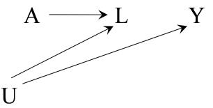
Figure 18.1

Imagine that we have unlimited computational power and a dataset with a quasi-infinite number of individuals (the rows of the dataset) and many variables measured for each individual (the columns of the data set), including treatment A, outcome Y , and a moderate number of discrete variables X, some of which may be confounders of the effect of A on Y . In this setting, we can afford to adjust for as many variables in the dataset as we wish, without computational, numerical, or statistical constraints. Thus, were our goal simply to predict Y from A and X (under a standard least squares loss; see Technical Point 18.1), we could optimally predict Y by simply using the average of Y in every joint stratum of A and X.

Fine Point 18.1

Variable selection procedures for regression models Suppose we want to fit a regression model with predictive purposes, but the database includes so many potential predictors—perhaps even more than individuals—that including all of them in the model is either impossible or results in very unstable predictions. Several approaches exist to deal with this problem in regression models. A detailed description of these procedures can be found in many books. See, e.g., the books by Hastie, Tibshirani, and Friedman (2009), and by Harrell (2015). Below we briefly outline some of the existing approaches.

One approach is to select a subset of the available variables. A conceptually simple way to find the best subset would be to first decide the number of variables in the model, then fit all possible combinations of models with that number of variables, and finally choose the best one according to some pre-specified criterion (e.g., Akaike’s Information criterion). However, this approach becomes computationally infeasible for a massive number of variables and, for a finite dataset, is not guaranteed to select the model with smallest prediction error. More computationally efficient methods to select variables are forward selection (start with no variables and, in each step of the algorithm, add the variable that leads to the greatest improvement), backward elimination (start with all variables and, in each step, delete the variable that leads to the smallest improvement), and stepwise selection (a combination of forward selection and backward elimination). The variable selection algorithm ends when no further improvement is possible, with improvement again defined according to some pre-specified criterion. These algorithms are easy to implement but, on the other hand, they do not explore all possible subsets of variables.

An alternative to subset selection is shrinkage. The idea is to modify the estimation method by adding a “penalty” that forces the model parameter estimates (other than the intercept) to be closer to zero than they would have been in the absence of the penalty. That is, most parameter estimates are shrunk towards zero. As a result of this shrinkage, the variance decreases and the prediction becomes more stable. The two best known shrinkage methods are ridge regression and the lasso or “least absolute shrinkage and selection operator”, which was proposed by Santosa and Symes (1986) and rediscovered by Tibshirani (1996). Unlike ridge regression, the lasso allows some parameter values to be exactly zero. Therefore, the lasso is both a shrinkage method and a subset selection method.

justing for covariates using stratification, remember that the adjusted association measure may differ from the unadjusted association measure, even when no confounding exists. See Fine Point 4.3.

However, suppose we want to unbiasedly estimate the average causal effect of a binary treatment A on the outcome Y , i.e., E - Y ^a=1 − E - Y ^a=0 . Then the goal of covariate adjustment is to eliminate as much confounding as possible by using the information contained in the measured variables X. We Collapsibility reminder: When ad- could easily adjust for all measured variables X via stratification/outcome regression, standardization/g-formula, IP weighting, or g-estimation. Are there any reasons to adjust for only a subset of X rather than simply adjust for all available variables X? The answer is yes. Even in this ideal setting, we want to ensure that some variables are not selected for adjustment because adjustment for those variables would induce bias. The next examples illustrate this point when some of the variables L in X are causally affected by A.

Suppose the causal structure of the problem is represented by the causal diagram of Figure 18.1 (same as Figure 7.7) in which the variable L is a collider. Here the average causal effect E[Y ^a=1] − E[Y ^a=0] = 0 is unbiasedly estimated by E [Y |A = 1] − E [Y |A = 0] since there is no confounding by L. Suppose now we try to estimate the average causal effect by adjusting for L via the g-formula P ^l E [Y |A = 1, L = l] Pr (L = l) − P ^l E [Y |A = 0, L = l] Pr (L = l). This contrast differs from E [Y |A = 1] − E [Y |A = 0]—and thus is biased because L is both conditionally associated with Y given A and marginally associated with A, so Pr (L = l) ̸= Pr (L = l|A). Because the A-Y association adjusted for L is expected to be non-null even though the causal effect of treatment A on the outcome Y is null, we say that there is selection bias under the null. The same bias is expected to arise when we adjust for a variable L

Fine Point 18.2

Overfitting and cross-validation. Overfitting is a common problem of all variable selection methods for regression models: The variables are selected to predict the data points as well as possible, without taking in consideration that some of the variation observed in the data is purely random. As a result, the model predicts very well for the individuals used to estimate the model parameters, but the model predicts poorly for future individuals who were not used to estimate the model parameters. The same problem arises in predictive algorithms such as random forests, neural networks, and other machine learning algorithms.

A straightforward solution to the overfitting problem is to split the sample in two parts: a training sample used to run the predictive algorithm (that is, to estimate the model parameters when using regression) and a validation sample used to evaluate the accuracy of the algorithm’s predictions. For a sample size n, we use v individuals for the validation set and n − v individuals for the training set. When using the lasso, the degree of shrinkage in the training sample may be guided by the model’s performance in the validation sample.

The obvious downside of splitting the sample into training and validation subsamples is that the predictive algorithm only uses—e.g., the model parameters are estimated in—a subset of individuals, which increases the variance. A solution is to repeat the splitting process multiple times, which increases the effective number of individuals used by the predictive algorithm. Then one can evaluate the algorithm’s predictive accuracy as the average over all the validation samples. This procedure is known as cross-validation or out-of-sample testing. Different forms of cross-validation exist.

A procedure referred to as “leave-v-out cross-validation” analyzes all possible partitions of the sample into training sample and validation sample of size v. However, examining all such partitions may become computationally infeasible for moderately large values of n and v. Two possible fixes for this problem are (i) to choose v = 1 or (ii) to evaluate only a sample of the partitions. For example, in “k-fold cross validation”, the sample is split into k subsamples of equal size. Then each one of the subsamples is used as the validation sample with the other k − 1 subsamples as its training sample. A common choice is k = 10. See the book by Hastie, Tibshirani, and Friedman (2009) for a description of cross-validation and related techniques Deep learning algorithms based on neural networks with many layers often seem nearly immune to overfitting when massive amounts of training data are available, e.g., speech recognition, images (Goodfellow, Bengio, Courville 2016). A deep neural network is a parametric model with often thousands, millions, or even billions unknown parameters and therefore often fits the training data exactly. Astonishingly, the fitted model still can successfully predict the outcomes of future individuals (sampled from the same population) with small error. Trying to explain this phenomenon is one of the most active current research areas in machine learning.

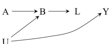
Figure 18.2

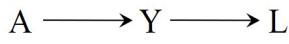
that, as in the causal diagram of Figure 18.2, is a descendant of the collider B. You may want to review Chapter 8 for more examples of causal structures with colliders and their descendants.

Selection bias may also appear when adjusting for a noncollider affected by treatment, like the variable L in the causal diagram in Figure 18.3. Here the average causal effect E[Y ^a=1] − E[Y ^a=0] ̸= 0 is also unbiasedly estimated by E [Y |A = 1] − E [Y |A = 0] since there is no confounding by L. However, if we try to estimate the average causal effect by adjusting for L (as if it were a pre-treatment variable), the g-formula contrast will differ from E [Y |A = 1] − E [Y |A = 0] for the same reasons as in the previous paragraph.

Now suppose that the arrow from A to Y had been absent, i.e., that the null hypothesis of no effect of A on Y were true and so E[Y ^a=1]−E[Y ^a=0] = 0. Then A and Y would be independent (both marginally and conditionally on L) and the g-formula contrast would be zero and thus unbiased. The key reason for this result is that, under the null, A no longer has a causal effect on L. Figure 18.3 That is, unlike in Figures 18.1 and 18.2, adjusting for L in Figure 18.3 results in selection bias only when A has a non-null causal effect on Y . We then say that there is selection bias under the alternative or off the null (see Section 6.5).

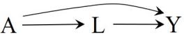
blocks the path A → L → Y but not the path A → Y . Thus the A-Y association adjusted for L is a biased estimator of the total effect of A on Y but an unbiased estimator of the direct effect of A on Y that is not mediated through L.

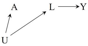
expert knowledge to adjustment was described by Hern´an et al (2002).

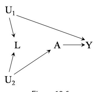
When the adjustment variable is affected by the treatment A and affects the outcome Y , we say that the variable is a mediator . Consider the causal diagram in Figure 18.4, which includes the mediator L on a causal path from Figure 18.4 the treatment A to the outcome Y . The A-Y association adjusted for the mediator L, or its descendants, will differ from the effect of treatment A on the outcome Y because the adjustment blocks the component of the effect that In Figure 18.4, adjusting for L goes through L. Sometimes this problem is referred to as overadjustment for mediators when the average causal effect of A on Y is the contrast of interest.

The bias-inducing variables discussed above share a common feature: they are affected by treatment and therefore they are post-treatment variables. One might then think that we should always avoid adjustment for variables that occur after treatment A. The rule of not adjusting for post-treatment variables would be easy to follow because the temporal sequence of the adjustment variables and the treatment is usually known. Unfortunately, following this simple rule may result in the exclusion of useful adjustment variables, as we discussed in Fine Point 7.4. Consider the causal diagram in Figure 18.5. The variable L is a post-treatment variable, but it can be used to block the backdoor path between treatment A and outcome Y . Therefore, the A-Y association adjusted for L is an unbiased estimator of the effect of A on Y , whereas the unadjusted A-Y association is a biased estimator. The take home message is that causal graphs do not care about temporal order. Thus, when A does not affect L, the correct analysis must be the same whether L is temporally before or temporally after A.

The problem is that, even when we know the temporal order of the vari-Figure 18.5 ables, we cannot determine from the data whether or not A affects L. In fact, given the temporal ordering A L Y , any joint distribution of (A, L, Y ) without any independencies is compatible with several causal graphs. So the decision whether to adjust for L must be based on information outside of the data. That is, whether to adjust for L cannot be determined via any automated procedures that rely exclusively on statistical associations. For example, as discussed in Chapter 7, there is no way to distinguish a collider from a con-An example of the application of founder by using data only. Rather, the exclusion of bias-inducing variables from the adjustment set needs to be guided by subject-matter knowledge about the causal structure of the problem.

We next turn to the question of adjustment for variables L that are temporally prior to treatment A, i.e., our temporal ordering is now L A Y . Suppose, for simplicity, that the sample size is very large, greatly exceeding the number of covariates X available for adjustment. As a consequence, the variance of any estimator will be negligible and the only issue is bias. In this setting it is commonly believed that an estimator that adjusts for all available pretreatment covariates will minimize the bias. However, this belief is wrong for two separate reasons.

Consider the causal diagram of Figure 18.6 (same as Figure 7.4), which includes a pre-treatment variable L. Because L is a collider on a path from A to Y , adjusting for it will introduce selection bias, which we referred to as M-bias in Chapter 7. Again, the observed data cannot distinguish between Figure 18.6 confounders and colliders, so one must rely on whatever external information one may have to decide whether or not to adjust for a pre-treatment variable L. In fact, it is also possible that L is both a confounder and a collider—if there were an arrow from L to A in Figure 18.6—which implies that the average causal effect cannot be identified, regardless of whether we do or do not adjust for L.

There is one additional reason to avoid indiscriminate adjustment for pre-

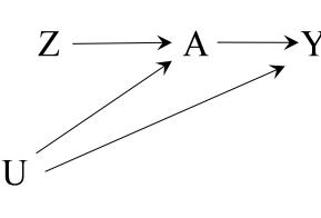
if all the equations in the structural equation model corresponding to the causal diagram are linear (Wooldridge 2010, Pearl 2011), but may also occur in more realistic settings (Ding et al. 2017).

treatment variables: bias amplification, a phenomenon we have not yet described in this book. Consider the causal diagram of Figure 18.7 (same as Figure 16.1), which represents a setting in which the causal effect of treatment A on the outcome Y is confounded by the unmeasured variable U. Because U is not available in the data, we cannot adjust for U and the confounding is intractable. Adjustment for the variable Z—using the g-formula as above with L replaced by Z—does not eliminate confounding because Z is not on Figure 18.7 any backdoor path from the treatment A to the outcome Y . In fact, Z is an instrument—which can be used for instrumental variable estimation in some situations described in Chapter 16—and therefore useless for direct confounding adjustment by the g-formula.

Interestingly, even though Z cannot be used to adjust away the confounding bias due to U, adjustment for the instrument Z can amplify the confounding bias due to U. That is, the A-Y association adjusted for Z may be further from Bias amplification is guaranteed the effect of A on Y than the A-Y association not adjusted for Z. This bias amplification due to adjusting for an instrument Z, often referred to as Z-bias, is a reason to avoid adjustment for variables that, like Z, are instruments. Bias amplification, however, is not guaranteed: adjustment for Z could also reduce the bias due to confounding by the unmeasured variable U. Generally, it is not possible to know whether adjustment for an instrument will amplify or reduce bias.

In summary, even if we had no computational constraints and a quasiinfinite sample size, it is not advisable to adjust for all available variables X. Ideally, the adjustment set would not include any variables that may introduce or amplify bias. Because these bias-inducing variables cannot be empirically identified by purely statistical algorithms, expert knowledge is needed to guide variable selection.

18.3 Causal inference and machine learning

For the remainder of this chapter, we will assume that we have somehow succeeded at ensuring that X includes no variables that may induce or amplify bias (i.e., no variables that would destroy conditional exchangeability if adjusted for) while still including all confounders L of the average causal effect of A on Y (i.e., all variables needed to achieve conditional exchangeability).Furthermore, we assume positivity holds. Our next problem is to estimate this effect E - Y ^a=1 − E - Y ^a=0 in practice when X is very high-dimensional or includes multiple continuous variables.

If we have good estimates of E - Y ^a=1 and E- Y ^a=0 , their difference will be a good estimate of E - Y ^a=1 − E - Y ^a=0 . Thus, for simplicity, we will focus on the estimation of E - Y ^a=1 .

Depending on the adjustment method that we choose, the variables X will be used in different ways. When using the plug-in g-formula (standardization) to estimate E - Y ^a=1 , we will estimate the mean outcome Y conditional on the variables X among individuals with A = 1, which we refer to as b(X); when using IP weighting, we will estimate the probability of treatment A conditional on the variables X, which we refer to as π(X). We can produce estimates ˆb(x) and ˆπ(x) via the sort of traditional parametric models (e.g., generalized linear models with linear, logistic, or log links) with the number of parameters much smaller than the sample size that we have described in Part II of this book. When X is high-dimensional, such models are certain to be misspecified. As

a consequence, both ˆb(x) and ˆπ(x) will fail to be consistent for the true b(x) and π(x).

To reduce the possibility of model misspecification, we might want to fit richly parameterized generalized linear models with linear predictor θ T P s (x) = j θ^j s^j (x), where s (X) is a very high-dimensional vector of transformations of the covariate vector X. The vector s (X) generally contains both flexible high-dimensional transformations (e.g., cubic splines) of individual variables in X and cross-variable products of these transformations. For concreteness, suppose we choose a logit link so ˆb(x) = expit θbT b s (x) and ˆπ(x) = expit θbT π s (x) where θ^b and θ^π are the parameters of the models for b(x) and π(x). Even if the estimated functions ˆb(x) and ˆπ(x) based on these models are consistent, in finite samples the errors ˆb(x) − b (x) and ˆπ(x) − π(x) will be much greater than would be the case for a correctly specified low-dimensional parametric model. In fact the dimension of s (X) may frequently exceed the number of individuals n contributing data to the study. In that case, a fit of Remember that some of the vari- the model will fail to converge and no estimate of θ will be returned.

Possible ways forward are to fit the parametric model with linear predictor θ T s (X) by adding a lasso or ridge penalty (see Fine Point 18.1), to use a variable selection algorithm such as stepwise selection, or to estimate the conditional expectations b(X) and π(X) using other predictive machine learning algorithms such as tree-based algorithms (e.g., random forests) or neural networks (e.g., deep learning). As discussed in Fine Point 18.2, deep learning algorithms fit a model often containing thousands or millions of parameters. Machine learning algorithms can Other machine learning algorithms also effectively fit thousands of parameters. In most cases with large sample sizes and many covariates X, machine learning algorithms outperform traditional parametric models for the accurate prediction of conditional expectations.

However, predictive machine learning algorithms do not by themselves suffice to adequately adjust for confounding in high-dimensional settings. In the next section we explain that these algorithms must be used in conjunction with doubly robust estimators with two modifications: sample splitting and crossfitting. This is necessary if we hope to construct valid 95% Wald confidence intervals, i.e., intervals that trap the causal parameter of interest at least 95% of the time.

18.4 Doubly robust machine learning estimators

be greater when there is some degree of confounding in the superpopulation since, in that case, Wald confidence intervals will not be centered on an unbiased estimator of the causal effect (see Chapter 10).

ables in X may not even be confounders so we would not need to adjust for them if we knew which

use cross-validation (see Fine Point 18.2) to optimize predictive accu-

variables they were.

racy.

Valid Wald intervals for ψ = E- Y ^a=1 require that the bias of the estimator be much less than the standard error of the estimator. The standard error of most estimators ^Eb - Y ^a=1 of E- Y ^a=1 scale as 1/ √ n times a constant, where ⁿ is the sample size. Hence, we require that the bias of ^Eb - Y ^a=1 to be much less than 1/ √ The degree of undercoverage will n. In addition to small bias, in order to have valid Wald intervals centered on ^Eb - Y ^a=1 , we generally need ^Eb - Y ^a=1 to also be asymptotically normal, which is generally easier to achieve than small bias.

A small bias is easier to achieve with doubly robust estimators than with non-doubly robust estimators, because the bias ^Eb - Y ^a=1 − E - Y ^a=1 of a doubly robust estimator depends on the product of the errors ^{1 π}(x) − 1 πˆ(x) and b(x) − ˆb(x), which can be small. Indeed the bias is less than 1/ √ n if both errors are much smaller than 1/ ^{√4 n}, which can often be achieved by machine

mators is referred to as a secondorder bias. See Technical Point 13.2 for details.

as the nuisance sample because we use it to estimate the nuisance regressions for b(X) and π(X). Fine Point 15.1 reviews the concept of nuisance parameters.

are not new procedures. However, the idea of combining these procedures with machine learning has not been emphasized until recently.

learning estimators if the functions π(x) and b(x) are either quite smooth, i.e., have many derivatives, or very sparse, i.e., depend on only few components This property of doubly robust esti- of the vector X, even though how many and which components are unknown. In contrast, the IP weighted and plug-in g-formula estimators of E - Y ^a=1 can have bias as large as the errors ^{1 π}(x) − 1 πˆ(x) and b(x) − ˆb(x), respectively. If so, neither the IP weighted estimator nor the plug-in g-formula estimator of E - Y ^a=1 can generally center a valid Wald confidence interval because, with high-dimensional X, it is known that the error of any possible estimator ˆπ(x) or ˆb(x) of π(x) or b(x) must exceed 1/ √ n.

But, if we hope to construct valid 95% Wald confidence intervals, the doubly robust machine learning estimators of the previous paragraph need to incorporate sample splitting and cross-fitting. We now describe these two procedures and their rationale. Technical Point 18.1 summarizes the steps of the estimation process.

We begin by describing sample splitting. First, we randomly divide the study population of n individuals into two halves: an estimation sample of size We may refer to the training sample n/2 and a training sample of equal size. Second, we apply the predictive machine learning algorithms to the training sample in order to obtain estimators of ˆb(x) and ˆπ(x) for the conditional expectations b (x) = E[Y |X = x, A = 1] and π (x) = E[A|X = x], respectively. Third, we compute the doubly robust estimator of the average causal effect in the estimation sample using the estimators of ˆb(x) and ˆπ(x) from the training sample. We have now obtained a doubly robust machine learning estimate of the average causal effect in a random half of the study population.

To understand the need for sample splitting, let us compare the split-sample version with the full-sample version of the augmented IP weighted (AIPW) doubly robust estimator of Technical Point 13.2. The estimation sample used in the split-sample AIPW estimator of E - Y ^a=1 is statistically independent of the split-sample estimators of ^bb (x) and ^πb (x), which use only the training sample data. As a consequence, under weak conditions described in Technical Point 18.2, the estimator is asymptotically normal with standard error that scales like 1/ √ n with the product bias described ealier. It follows that, if the product bias is less than 1/ √ n, Wald intervals centered on the split-sample estimator will be valid.

In contrast, the full-sample AIPW estimator of E - Y ^a=1 is

\[\frac{1}{n}\sum\_{i=1}^{n}\left[\widehat{b}\left(X\_{i}\right)+\frac{A\_{i}}{\widehat{\pi}\left(X\_{i}\right)}\left\{Y\_{i}-\widehat{b}\left(X\_{i}\right)\right\}\right],\]

where ^bb (x) and ^πb (x) are now estimated by a machine learning algorithm applied to all ⁿ individuals’ data. Thus ^bb (x) and ^πb (x) are correlated with the full-sample AIPW estimator. This correlation, if sufficiently large, can affect the bias, variance, and asymptotic normality of the full-sample estimator in unpredictable ways. Unfortunately, the magnitude of the correlation is unknown and cannot be well estimated. Hence, the split-sample estimator is Sample splitting and cross-fitting much preferred to the full-sample estimator in high-dimensional settings.

The only difficulty with using the doubly robust split-sample estimator is that its variance and standard error correspond to a sample size of n/2. As a result, our confidence interval will be wider than the one we would have obtained if we had been able to use the entire sample of n individuals. A way to overcome this problem is cross-fitting.

We now describe how cross-fitting recovers the statistical efficiency lost by sample splitting. First, we repeat the above procedure but swapping the roles

Augmented IP weighted split-sample and cross-fit estimator. The augmented IP weighted (AIPW) estimator of ψ = E- Y ^a=1 is a doubly robust estimator described in Technical Point 13.2. The following algorithm computes the AIPW split-sample estimator ^ψb and the cross-fit estimator ^ψbcross-fit:

• 1. Randomly split the n study subjects into 2 parts: an estimation sample of size q and a training sample of size ntr = n − q with q/n ≈ 1/2.
• 2. Estimate ^bb (x) and ^πb (x) of ^b (x) = E[^{Y |A} = 1, X ^{= x}] and ^π (x) = pr[^A = 1^{| X = x}] from the training sample data using machine learning algorithms.
• 3. Compute the split-sample AIPW estimator

\[\widehat{\psi} = \frac{1}{q} \sum\_{i=1}^{q} \left[ \widehat{b}\left(X\_i\right) + \frac{A\_i}{\widehat{\pi}\left(X\_i\right)} \left\{ Y\_i - \widehat{b}\left(X\_i\right) \right\} \right],\]

from the q subjects in the estimation sample.

4. Compute the cross-fit estimator

\[ \widehat{\psi}\_{\text{cross-fit}} = \left(\widehat{\psi} + \overline{\widehat{\psi}}\right) / 2. \]

where ^ψb is ^ψb but with the training and estimation sample swapped.

An alternative cross-fit estimator with improved finite sample behavior is computed as follows: (i) divide the sample of size ⁿ into M > ² equal-sized random samples, (ii) compute ^ψb(m) , m = 1, 2, . . . , M, using sample m as estimation sample and the remaining ^{M − 1} samples as the training sample, and (iii) compute ^ψbcross-fit ⁼ 1 M P^{M m}=1 ^ψb(m) .

of the estimation and training halves of the study population. That is, we use the half formerly reserved for estimation as the new training sample, and the half formerly used for training as the new estimation sample. We then compute the doubly robust estimator of the average causal effect in the new estimation sample using the estimators of ˆb(x) and ˆπ(x) from the new training sample. We have now obtained a doubly robust machine learning estimate of the average causal effect in the other random half of the population.

The next step is to compute the average of the two doubly robust estimates from each half of the population. This average will be our doubly robust estimate of the effect in the entire study population. A 95% confidence interval around this estimate can be constructed by bootstrapping, either by adding and subtracting 1.96 times the bootstrap standard error or by using the 2.5 and 97.5 percentiles of the bootstrap estimates as the bounds of the interval.

We are done. Through sample splitting and cross-fitting, we can combine doubly robust estimation and machine learning to obtain causal effect estimates Lin et al. (2020) constructed esti- which have known statistical properties and which use all the available data. An active area of research is the development of procedures to detect whether the bias of doubly robust split-sample estimators is the order of or larger than the standard error and, if so, to obtain estimates with smaller bias in the estimation sample without having to redo the machine learning component in the training sample.

mators based on higher order influence functions that had smaller bias than doubly robust cross-fit estimators without significantly increasing their variance.

Statistical properties of split-sample and cross-fit estimators. Conditional on the training sample data ^Tr, ^bb (x) and ^πb (x) are fixed functions. Hence ^ψb is the sum of independent and identically distributed random variables and thus, by the central limit theorem, it is asymptotically normal conditional on ^Tr with standard error se ψb proportional to n −1/2 . The exact conditional bias of ^ψb is

\[\operatorname{E}\left[\widehat{\psi} - \psi \middle| T\_r \right] = \operatorname{E}\left[\pi\left(X\_i\right) \left(\frac{1}{\widehat{\pi}\left(X\_i\right)} - \frac{1}{\pi\left(X\_i\right)}\right) \left\{b\left(X\right) - \widehat{b}\left(X\right)\right\} \left| Tr \right|\right]\]

To characterize the unconditional statistical properties of ^ψb and ^ψbcross-fit, we must take into account that ^E h ^{ψb − ψ}|T^r i is random through its dependence on the training sample data via ^ˆb and ^πb. If (i) ^bb (x) and ^πb (x) are consistent for the true b (x) and π (x) (in mean square), and (ii) E h ^{ψb − ψ}|T^r i /se ψb converges to ⁰ in probability, then ^ψb and ^ψbcross-fit are asymptotically normal and unbiased.

Thus, when (i) and (ii) hold, 95% Wald confidence intervals ^{ψb ± 1}.^{96 ×} se^b ψb and ^ψbcross-fit ^{± 1}.^{96 ×} se^{b ψ}bcross-fit are valid and, in fact, are calibrated. Here se^{b ψ}bcross-fit and se^b ψb can be computed with the bootstrap. Further, n 1/2 seb ^ψbcross-fit is semiparametric efficient with standard error n var n b (X) + ^A π(X) [^{Y − b} (X)]oo1/² , which is smaller than the standard error of ^ψb by a factor of 1/^√ 2. Note if the rate of convergence of ^{1 π}b(x) ⁻ 1 π(x) is n ^−α and that of ^b (x) ^{− bb} (x) is ⁿ −ϵ , the bias E h ^{ψb − ψ}|T^r i is o n −1/2 if ^{α +} ϵ > ¹/2. Thus if ^bb (x) has a rate of convergence slower than n −1/4 , the bias can still be o n −1/2 if ^πb (x) has a sufficiently fast rate of convergence. The same holds with the roles of ^bb (x) and ^πb (x) swapped.

18.5 Variable selection is a difficult problem

The methods outlined in the previous section invalidate the widespread belief that any data-adaptive procedure to select adjustment variables will inevitably result in incorrect confidence intervals. As we have seen, the combination of causal inference methods with machine learning algorithms for confounder selection can, under certain conditions, result in correct statistical inference. However, doubly robust machine learning does not solve all our problems for at least three reasons (in addition to that described in the previous section).

First, in many applications, the available subject-matter knowledge may be insufficient to identify all important confounders or to rule out variables that induce or amplify bias. Thus there is no guarantee that doubly robust machine learning estimators will have a small bias.

Second, the implementation of doubly robust estimators has been difficult and computationally expensive when combined with machine learning—in highdimensional settings with time-varying treatments. This is especially true for causal survival analysis. As a result, most published examples of causal inference from complex longitudinal data use single robust estimators, which are the ones we have largely emphasized in Part III of this book. However, the methods outlined in this chapter are quickly becoming routine in some fields.

Third, doubly robust machine learning can yield a variance of the causal effect that equals the variance that would have been obtained if the true conditional expectations b(X) and π(X) were known. However, there is no guarantee that such variance will be small enough for meaningful causal inference.

Suppose that we obtain a doubly robust machine learning estimate of the causal effect, as described in the previous section, only to find out that its (correct) variance is too big to be useful. This will happen, even when we have estimated the propensity score and outcome regression with small product bias, if some of the covariates in X are strongly associated with the treatment A. Then the probability of treatment π(X) may be near 0 or near 1 for individuals with a particular value of X. As a result, the effect estimate will have a very large variance and thus a very wide (but often correct) 95% confidence interval. Since we do not like very wide 95% confidence intervals, even if they are correct, we may be tempted to throw out the variables in X that This result raises a puzzling philo- are causing the “problem” and then repeat the data analysis. If we did that, we would be fundamentally changing the game. Using the data to discard covariates in X that are associated with treatment, but not so much with the outcome, makes it no longer possible to guarantee that the 95% confidence interval around the effect estimate is valid. The tension between including all potential confounders to eliminate bias and excluding some variables to reduce the variance is hard to resolve.

Given all of the above, developing a clear set of general guidelines for variable selection may not be possible. In fact, so much methodological research is ongoing around these issues that this chapter cannot possibly be prescriptive. As discussed in Section 13.5, the best scientific advice for causal inference may be to carry out multiple sensitivity analyses: implement several analytic methods and inspect the resulting effect estimates. If the various effect estimates are compatible, we will be more confident in the results. If the various effect estimates are not compatible, our job as researchers is to try to understand why.

sophical question: If the confidence interval is invalid when we use the data to rule out, say, 5 variables that make the variance too large, then why should the confidence interval be valid if we had happened to receive a dataset that did not include those 5 variables? Given that we always work with datasets in which some potential confounders are not recorded, how should we interpret confidence intervals in any observational analysis?

246 Variable selection and high-dimensional data

Part III

Causal inference for time-varying treatments

Chapter 19 TIME-VARYING TREATMENTS

So far this book has dealt with fixed treatments which do not vary over time. However, many causal questions involve treatments that vary over time. For example, we may be interested in estimating the causal effects of medical treatments, lifestyle habits, employment status, marital status, occupational exposures, etc. Because these treatments may take different values for a single individual over time, we refer to them as time-varying treatments.

Restricting our attention to time-fixed treatments during Parts I and II of this book helped us introduce basic concepts and methods. It is now time to consider more realistic causal questions that involve the contrast of hypothetical interventions that are played out over time. Part III extends the material in Parts I and II to time-varying treatments. This chapter describes some key terminology and concepts for causal inference with time-varying treatments. Though we have done our best to simplify those concepts (if you don’t believe us, check out the causal inference literature), this is still one of the most technical chapters in the book. Unfortunately, further simplification would result in too much loss of rigor. But if you made it this far, you are qualified to understand this chapter.

19.1 The causal effect of time-varying treatments

assume that no individuals were lost to follow-up or died during this period, and we will also assume that all variables were perfectly measured.

lished papers, we use zero-based indexing for time. That is, the first time of possible treatment is k = 0 rather than k = 1.

Consider a time-fixed treatment variable A (1: treated, 0: untreated) at time zero of follow-up and an outcome variable Y measured 60 months later. We have previously defined the average causal effect of A on the outcome Y as the contrast between the mean counterfactual outcome Y ^a=1 under treatment and the mean counterfactual outcome Y ^a=0 under no treatment, that is, E - Y ^a=1 − E - Y ^a=0 . Because treatment status is determined at a single time (time zero) for everybody, the average causal effect does not need to make reference to the time at which treatment occurs. In contrast, causal contrasts that involve time-varying treatments need to incorporate time explicitly.

To see this, consider a time-varying dichotomous treatment A^k that may For simplicity, we will provisionally change at every month k of follow-up, where k = 0, 1, 2…K with K = 59. For example, in a 5-year follow-up study of individuals infected with the human immunodeficiency virus (HIV), A^k takes value 1 if the individual receives antiretroviral therapy in month k, and 0 otherwise. No individuals received treatment before the start of the study at time 0, i.e., A⁻¹ = 0 for all individuals.

We use an overbar to denote treatment history, i.e., A¯ ^k = (A0, A1, …Ak) is the history of treatment from time 0 to time k. When we refer to the entire treatment history through K, we often represent A¯^K as For compatibility with many pub- A¯ without a subscript. In our HIV study, an individual who receives treatment continuously throughout the follow-up has treatment history A¯ = (A⁰ = 1, A¹ = 1, …A⁵⁹ = 1) = (1, 1, …1), or A¯ = ¯1. Analogously, an individual who never receives treatment during the follow-up has treatment history A¯ = (0, 0, …0) = ¯0. Most individuals are treated during part of the follow-up only, and therefore have intermediate treatment histories with some 1s and some 0s—which we cannot ple considers an outcome measured at a fixed time. However, the concepts discussed in this chapter also apply to time-varying outcomes and failure time outcomes (see Technical Point 21.8).

to denote possible realizations of a random variable: a^k is a realization of treatment Ak.

represent as compactly as ¯1 and ¯0.

Suppose Y measures health status—with higher values of Y indicating To keep things simple, our exam- better health—at the end of follow-up at time K + 1 = 60. We would like to estimate the average causal effect of the time-varying treatment A¯ on the outcome Y . But we can no longer define the average causal effect of a time-varying treatment as a contrast at a single time k, because the contrast E - Y ^ak=1 −E - Y ^ak=0 quantifies the effect of treatment A^k at a single time k, not the effect of the time-varying treatment A^k at all times k between 0 and 59.

Indeed we will have to define the average causal effect as a contrast between Remember that we use lower-case the counterfactual mean outcomes under two treatment strategies that involve treatment at all times between the start (k = 0) and the end (k = K) of the follow-up. As a consequence, the average causal effect of a time-varying treatment is not uniquely defined. In the next section, we describe many possible definitions of average causal effect for a time-varying treatment.

19.2 Treatment strategies

compare treatment strategies was first articulated by Robins (1986, 1987, 1997a).

A treatment strategy—also referred to as a plan, policy, protocol, or regime— A general counterfactual theory to is a rule to assign treatment at each time k of follow-up. For example, two treatment strategies are “always treat” and “never treat” during the followup. The strategy “always treat” is represented by ¯a = (1, 1, …1) = ¯1, and the strategy “never treat” is represented by ¯a = (0, 0, …0) = ¯0. We can now define an average causal effect of A¯ on the outcome Y as the contrast between the mean counterfactual outcome Y ^a¯=¯1 under the strategy “always treat” and the mean counterfactual outcome Y ^a¯=¯0 under the strategy “never treat”, i.e., E - Y a¯=¯1 − E - Y a¯=¯0 .

But there are many other possible causal effects for the time-varying treatment A¯, each of them defined by a contrast of outcomes under two particular treatment strategies. For example, we might be interested in the average causal effect defined by the contrast E [Y a¯ ]−E h Y a¯ ′ i that compares the strategy “treat at every other month” ¯a = (1, 0, 1, 0…) with the strategy “treat at all months except the first one” ¯a ′ = (0, 1, 1, 1…). The number of possible contrasts is very large: we can define at least 2^K treatment strategies because there are 2^K possible combinations of values (a0, a1, …aK) for a dichotomous ak. In fact, as we next explain, these 2^K such strategies do not exhaust all possible treatment strategies.

To define even more treatment strategies in our HIV example, consider the time-varying covariate L^k which denotes CD4 cell count (in cells/µL) measured at month k in all individuals. The variable L^k takes value 1 when the CD4 cell count is low, which indicates a bad prognosis, and 0 otherwise. At time zero, all individuals have a high CD4 cell count, L⁰ = 0. We could then consider the strategy “do not treat while L^k = 0, start treatment when L^k = 1 and treat continuously after that time”. This treatment strategy is different from the ones considered in the previous paragraph because we cannot represent it by a rule ¯a = (a0, a1, …aK) under which all individuals get the same treatment a⁰ at time k = 0, a¹ at time k = 1, etc. Now, at each time, some individuals will be treated and others will be untreated, depending on the value of their evolving Lk. This is an example of a dynamic treatment strategy, a rule in which the treatment a^k at time k depends on the evolution of an individual’s

Deterministic and random treatment strategies. A deterministic dynamic treatment strategy is a rule g = - g⁰ (¯a−1, l0), … g^K a¯K−1, ¯lK , where g^k a¯k−1, ¯lk specifies the treatment assigned at k to an individual with past history a¯k−1, ¯lk . An example in our HIV study: g^k a¯k−1, ¯lk is 1 if an individual’s CD4 cell count (a function of ¯lk) was low at or before k; otherwise g^k a¯k−1, ¯lk is 0. A deterministic static treatment strategy is a rule g = [g⁰ (¯a−1), … g^K (¯aK−1)], where g^k (¯ak−1) does not depend on ¯lk. We will often abbreviate g^k a¯k−1, ¯lk as g a¯k−1, ¯lk .

Most static and dynamic strategies we are interested in comparing are deterministic treatment strategies, which assign a particular value of treatment (0 or 1) to each individual at each time. More generally, we could consider random treatment strategies that do not assign a particular value of treatment, but rather a probability of receiving a treatment value. Random treatment strategies can be static (e.g., “independently at each month, treat individuals with probability 0.3 and do not treat with probability 0.7”) or dynamic (e.g., “independently at each month, treat individuals whose CD4 cell count is low with probability 0.3, but do not treat individuals with high CD4 cell count”).

We refer to the strategy g for which the mean counterfactual outcome E [Y g ] is maximized (when higher values of outcome are better) as the optimal treatment strategy. For a drug treatment, the optimal strategy will almost always be dynamic because treatment needs to be discontinued when toxicity develops. Also, no random strategy can ever be preferred to the optimal deterministic strategy. However, random strategies (i.e., randomized trials) remain scientifically necessary because, before the trial, it is unknown which deterministic strategy is optimal. See Young et al. (2014) for a taxonomy of treatment strategies. In the text, except if noted otherwise, the letter g will refer only to deterministic treatment strategies.

time-varying covariate(s) L¯ ^k. Strategies ¯a for which treatment does not depend on covariates are non-dynamic or static treatment strategies. See Fine Point 19.1 for a formal definition.

Causal inference with time-varying treatments involves the contrast of counterfactual outcomes under two or more treatment strategies. The average causal effect of a time-varying treatment is only well-defined if the treatment strategies of interest are specified. In our HIV example, we can define an average causal effect based on the difference E [Y a¯ ] − E h Y a¯ ′ i that contrasts strategy ¯a (say, “always treat”) versus strategy ¯a ′ (say, “never treat”), or on the difference E [Y a¯ ] − E [Y g ] that contrasts strategy ¯a (“always treat”) versus strategy g (say, “treat only after CD4 cell count is low”). Note we will often use g to represent any—static or dynamic—strategy. When we use it to represent a static strategy, we sometimes write Y g=¯a rather than just Y ^g or Y a¯ .

That is, there is not a single definition of causal effect for time-varying treatments. Even when only two treatment options—treat or do not treat exist at each time k, we can still define as many causal effects as pairs of treatment strategies exist. In the next section, we describe a study design under which all these causal effects can be validly estimated: the sequentially randomized experiment.

19.3 Sequentially randomized experiments

The causal diagrams in Figures 19.1, 19.2, and 19.3 summarize three situations that can occur in studies with time-varying treatments. In all three diagrams, A^k represents the time-varying treatment, L^k the set of measured variables, Y the outcome, and U^k the set of unmeasured variables at k that are common

On the definition of dynamic strategies. Each dynamic strategy g = - g0 a¯−1, ¯l0 , … g^K a¯K−1, ¯lK that depends on past treatment and covariate history is associated with a dynamic strategy g ′ = - g ′ 0 ¯l0 , … g′ K ¯lK that depends only on past covariate history. By consistency (see Technical Point 19.2), an individual will have the same treatment, covariate, and outcome history when following strategy g from time zero as when following strategy g ′ from time zero. In particular, Y ^g = Y g ′ and L¯^g (K) = L¯^g ′ (K). Specifically, g ′ is defined in terms of g recursively by g ′ 0 (l0) = g⁰ (¯a−¹ = 0, l0) (by convention, a¯−¹ can only take the value zero) and g ′ k ¯lk = g^k - g ′ k ¯lk−¹ , ¯lk . For any strategy g for which treatment at each k already does not depend on past treatment history, g and g ′ are the identical set of functions. The above definition of g ′ in terms of g guarantees that an individual has followed strategy g through time t in the observed data, i.e., A^k = g^k A¯ ^k−1,L¯ k for k ≤ t, if and only if the individual has followed strategy g ′ through t, i.e., A^k = g ′ k L¯ k for k ≤ t.

always include all common causes of any two variables on the graph.

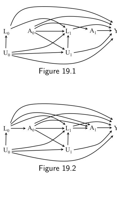
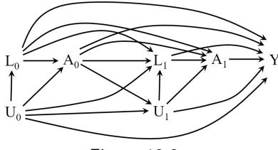
Figure 19.3

By definition, a causal graph must causes of at least two other variables on the causal graph. Because the covariates U^k are not measured, their values are unknown and therefore unavailable for the analysis. In our HIV study, the time-varying CD4 cell count L^k is a consequence of the true, but unmeasured, chronic damage to the immune system Uk. The greater an individual’s immune damage Uk, the lower her CD4 cell count L^k and her health status Y . For simplicity, the causal diagrams show only the first two times of follow-up k = 0 and k = 1, and we assume that all participants adhered to the assigned treatment.

The causal diagram in Figure 19.1 lacks arrows from either the measured covariates L¯ ^k or the unmeasured covariates U¯ ^k into treatment Ak. The causal diagram in Figure 19.2 has arrows from the measured covariates L¯ ^k, but not from the unmeasured covariates U¯ ^k, into treatment Ak. The causal diagram in Figure 19.3 has arrows from both the measured covariates L¯ ^k and the unmeasured covariates U¯ ^k into treatment Ak.

Figure 19.1 could represent a randomized experiment in which treatment A^k at each time k is randomly assigned with a probability that depends only on prior treatment history (for simplicity, we will assume perfect adherence throughout). Our HIV study would be represented by Figure 19.1 if, e.g., an individual’s treatment value at each month k were randomly assigned with probability 0.5 for individuals who did not receive treatment during the previous month (Ak−¹ = 0), and with probability 1 for individuals who did receive treatment during the previous month k (Ak−¹ = 1). When interested in the contrast of static treatment strategies, Figure 19.1 is the proper generalization of no confounding by measured or unmeasured variables for time-varying treatments. Under this causal diagram, the counterfactual outcome mean E [Y a¯ ] if everybody had followed the static treatment strategy ¯a is simply the mean outcome E- Y |A = ¯a among those who followed the strategy ¯a. (Interestingly, the same is not true for dynamic strategies. The counterfactual mean E [Y g ] under a dynamic strategy g that depends on the variables L is only the mean outcome among those who followed the strategy g if the probability of receiving treatment A^k = 1 is exactly 0.5 at all times k at which treatment A^k depends on Lk. Otherwise, identifying E [Y g ] requires the application of g-methods to data on L, A, and Y under either Figure 19.1 or Figure 19.2.)

Figure 19.2 could represent a randomized experiment in which treatment A^k at each time k is randomly assigned by the investigators with a probability that depends on prior treatment and measured covariate history. Our study would be represented by Figure 19.2 if, e.g., an individual’s treatment value

at each month k were randomly assigned with probability 0.4 for untreated individuals with high CD4 cell count (Ak−¹ = 0, L^k = 1), 0.8 for untreated individuals with low CD4 cell count (Ak−¹ = 0, L^k = 0), and 0.5 for previously treated individuals, regardless of their CD4 cell count (Ak−¹ = 1). In Figure 19.2, there is confounding by measured, but not unmeasured, variables for the time-varying treatment.

An experiment in which treatment is randomly assigned at each time k to each individual is referred to as a sequentially randomized experiment. Therefore Figures 19.1 and 19.2 could represent sequentially randomized experiments. On the other hand, Figure 19.3 cannot represent a randomized experiment: the value of treatment A^k at each time k depends partly on unmeasured variables U which are causes of L^k and Y , but unmeasured variables obviously cannot be used by investigators to assign treatment. That is, a sequentially randomized experiment can be represented by a causal diagram with many time points k = 0, 1…K and with no direct arrows from the unmeasured prognostic factors U into treatment A^k at any time k.

In observational studies, decisions about treatment often depend on outcome predictors such as prognostic factors. Therefore, observational studies will be typically represented by either Figure 19.2 or Figure 19.3 rather than Figure 19.1. For example, suppose our HIV follow-up study were an observational study (not an experiment) in which the lower the CD4 cell count Lk, the more likely a patient is to be treated. Then our study would be represented by Figure 19.2 if, at each month k, treatment decisions in the real world were made based on the values of prior treatment and CD4 cell count history (A¯ ^k−1, L¯ ^k), but not on the values of any unmeasured variables U¯ ^k. Thus, an observational study represented by Figure 19.2 would differ from a sequentially randomized experiment only in that the assignment probabilities are unknown (but could be estimated from the data). Unfortunately, it is impossible to show empirically whether an observational study is represented by the causal diagram in either Figure 19.2 or Figure 19.3. Observational studies represented by Figure 19.3 have unmeasured confounding, as we describe later.

Sequentially randomized experiments are not frequently used in practice. However, the concept of sequentially randomized experiment is helpful to understand some key conditions for valid estimation of causal effects of timevarying treatments. The next section presents these conditions formally.

19.4 Sequential exchangeability

As described in Parts I and II, valid causal inferences about time-fixed treatments typically require conditional exchangeability Y ^a⊥⊥A|L. When exchangeability Y ^a⊥⊥A|L holds, we can obtain unbiased estimates of the causal effect of treatment A on the outcome Y if we appropriately adjust for the variables in L via standardization, IP weighting, g-estimation, or other methods. We expect conditional exchangeability to hold in conditionally randomized experiments a trial in which individuals are assigned treatment with a probability that depends on the values of the covariates L. Conditional exchangeability holds in observational studies if the probability of receiving treatment depends on the measured covariates L and, conditional on L, does not further depend on any unmeasured, common causes of treatment and outcome.

Similarly, causal inference with time-varying treatments requires adjusting for the time-varying covariates L¯ ^k to achieve conditional exchangeability at [A⁰ = g(L0), A¹ = g(A0, L0, L1)] equal to (i.e., compatible with) the treatment they would have received under strategy g through the end of follow-up, the counterfactual outcome Y g is equal (by consistency) to the observed outcome Y and therefore also to the counterfactual outcome under the static strategy (a0, a1) with a⁰ = A0, a¹ = A1.

tional exchangeability for Y holds, i.e., for all static strategies a¯, Y ^a¯⊥⊥Ak|A¯ ^k−¹ = ¯ak−1. Unconditional exchangeability implies that association is causation, i.e., E [Y a¯ ] = E- Y |A¯ = ¯a .

tion of causal effects, the identifying formula will be the g-formula (see Chapter 21). In rare cases not relevant to our discussion, effects can be identified by formulas that are related to, but not equal to, the g-formula (e.g., Technical Point 7.3).

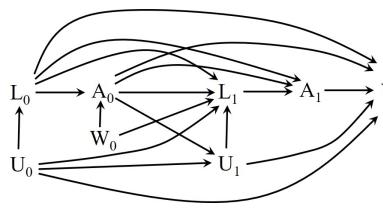
Figure 19.4

each time point, i.e., sequential conditional exchangeability. For example, in a study with two time points, sequential conditional exchangeability is the combination of conditional exchangeability at both the first time and the second time of the study. That is, Y ^g⊥⊥A0|L⁰ and Y For those with treatment history ^g⊥⊥A1|A⁰ = g(L0), L0, L1. (For brevity, in this book we drop the word “conditional” and simply say sequential exchangeability.) We will refer to this set of conditional independences as sequential exchangeability for Y ^g under any—static or dynamic—strategy g that involves interventions on both components of the time-varying treatment (A0, A1).

A sequentially randomized experiment—an experiment in which treatment A^k at each time k is randomly assigned with a probability that depends only on the values of their prior covariate history L¯ ^k and treatment history A¯ ^k−1—implies sequential exchangeability for Y g . That is, for any strategy g, the treated and the untreated at each time k are exchangeable for Y g conditional on prior covariate history L¯ ^k and any observed treatment history A¯ ^k−¹ = g(A¯ ^k−2,L¯ ^k−1) compatible with strategy g. Formally, sequential exchangeability for Y g is defined as

\[Y^g \perp A\_k | \bar{A}\_{k-1} = g(\bar{A}\_{k-2}, \bar{L}\_{k-1}), \bar{L}\_k \text{ for all strategies } g \text{ and } k = 0, 1...K\]

In Figure 19.1, sequential uncondi- This form of sequential exchangeability (there are others, as we will see) always holds in any causal graph which, like Figure 19.2, has no arrows from the unmeasured variables U into the treatment variables A. Therefore sequential exchangeability for Y ^g holds in sequentially randomized experiments and observational studies in which the probability of receiving treatment at each time depends on their treatment and measured covariate history A¯ ^k−1,L¯ k and, conditional on this history, does not depend on any unmeasured causes of the outcome.

That is, in observational studies represented by Figure 19.2 the mean of the counterfactual outcome E [Y ^g Whenever we talk about identifica- ] under all strategies g is identified, whereas in observational studies represented by Figure 19.3 no mean counterfactual outcome E [Y g ] is identified. In observational studies represented by other causal diagrams, the mean counterfactual outcome E [Y g ] under some but not all strategies g is identified.

For example, consider an observational study represented by the causal diagram in Figure 19.4, which includes an unmeasured variable W0. In our HIV example, W⁰ could be an indicator for a scheduled clinic visit at time 0 that was not recorded in our database. In that case W⁰ would be a cause shared by treatment A⁰ and the measured (with some error) CD4 cell count L1, with U¹ representing the underlying but unknown true value of CD4 cell count. Even though W⁰ is unmeasured, the mean counterfactual outcome is still identified under any static strategy g = ¯a; however, the mean counterfactual outcome E [Y g ] is not identified under any dynamic strategy g with treatment assignment depending on L1. To illustrate why identification is possible under some but not all strategies, we will use SWIGs in the next section.

In addition to some form of sequential exchangeability, causal inference involving time-varying treatments also requires a sequential version of the conditions of positivity and consistency. In a sequentially randomized experiment, both sequential positivity and consistency are expected to hold (see Technical Point 19.2). Below we will assume that sequential positivity and consistency hold. Under the three identifiability conditions, we can identify the mean counterfactual outcome E [Y g ] under a strategy of interest g as long as we use methods that appropriately adjust for treatment and covariate history A¯ ^k−1,L¯ k , such as the g-formula (standardization), IP weighting, and g-estimation.

Positivity and consistency for time-varying treatments. The positivity condition needs to be generalized from the fixed version “if f^L (l) ̸= 0, fA|^L (a|l) > 0 for all a and l” to the sequential version

If fA¯k−1,L¯^k a¯k−1, ¯lk ̸= 0, then fAk|A¯k−1,L¯^k ak|a¯k−1, l^k > 0 for all a¯k, l^k

In a sequentially randomized experiment, positivity will hold if the randomization probabilities at each time k are never either 0 nor 1, no matter the past treatment and covariate history. If we are interested in a particular strategy g, the above positivity condition needs to only hold for treatment histories compatible with g, i.e., for each k, a^k = g a¯k−1, l^k .

The consistency condition also needs to be generalized from the fixed version “If A = a for a given individual, then Y ^a = Y for that individual” to the sequential version

\[Y^{\bar{a}} = Y^{\bar{a}"} \text{ if } \mathbb{Z}^\* = \mathbb{Z}; \ Y^{\bar{a}} = Y \text{ if } \overline{A} = \bar{a}; \ \bar{L}\_k^{\bar{a}} = \bar{L}\_k^{\bar{a}"} \text{ if } \mathbb{Z}\_{k-1}^\* = \mathbb{Z}\_{k-1}; \ \bar{L}\_k^{\bar{a}} = \bar{L}\_k \text{ if } \overline{A}\_{k-1} = \mathbb{Z}\_{k-1}\]

where L¯a¯ k is the counterfactual L-history through time k under strategy a. Technically, the identification of effects of time-varying treatments on Y requires weaker consistency conditions: “If A = a for a given individual, then Y ^a¯ = Y for that individual” is sufficient for static strategies, and “For any strategy g, if A^k = g^k Ak−1,L^k at each time k for a given individual, then Y ^g = Y” is sufficient for dynamic strategies. However, the stronger sequential consistency is a natural condition that we will always accept.

Note that, if we expect that the interventions “treat in month k” corresponding to A^k = 1 and “do not treat in month k” corresponding to A^k = 0 are sufficiently well defined at all times k, then all static and dynamic strategies involving A^k will be similarly well defined.

19.5 Identifiability under some but not all treatment strategies

a generalized backdoor criterion for static strategies. Robins (1997a) extended the procedure to dynamic strategies.

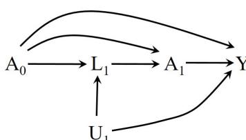
Figure 19.5

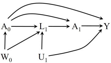
Figure 19.6

Pearl and Robins (1995) proposed In Chapter 7, we presented a graphical rule—the backdoor criterion—to assess whether exchangeability holds for a time-fixed treatment under a particular causal diagram. The backdoor criterion can be generalized for time-varying treatments. For example, for static strategies, a sufficient condition for identification of the causal effect of treatment strategies is that, at each time k, all backdoor paths into A^k that do not go through any future treatment are blocked.

However, the generalized backdoor criterion does not directly show theconnection between blocking backdoor paths and sequential exchangeability, because the procedure is based on causal directed acyclic graphs that do not include counterfactual outcomes. An alternative graphical check for identifiability of causal effects is based on SWIGs, also discussed in Chapter 7. SWIGs are especially helpful for time-varying treatments.

Consider the causal diagrams in Figures 19.5 and 19.6, which are simplified versions of those in Figures 19.2 and 19.4. We have omitted the nodes U⁰ and L⁰ and the arrow from A⁰ to U1. In addition, the arrow from L¹ to Y is absent so L¹ is no longer a direct cause of Y . Figures 19.5 and 19.6 (like Figures 19.2 and 19.4) differ in whether A^k and subsequent covariates L^t for t > k share a cause Wk.

As discussed in Part I of this book, a SWIG represents a counterfactual world under a particular intervention. The SWIG in Figure 19.7 represents the world in Figure 19.5 if all individuals had received the static strategy (a0, a1), where a⁰ and a¹ can take values 0 or 1. For example, Figure 19.7 can be used to represent the world under the strategy “always treat” (a⁰ = 1, a¹ = 1) or under the strategy “never treat” (a⁰ = 0, a¹ = 0). To construct this SWIG, we

The many forms of sequential exchangeability. Consider a sequentially randomized experiment of a time-varying treatment A^k with multiple time points k = 0, 1, …K. The SWIG that represents this experiment is just a longer version of Figure 19.7. The following conditional independence can be directly read from the SWIG:

\[\left(Y^{\overline{a}}, \underline{L}\_{k+1}^{\overline{a}}\right) \sqcup A\_k^{\overline{a}\_{k-1}} \left|\bar{A}\_{k-1}^{\overline{a}\_{k-2}}, \bar{L}\_k^{\overline{a}\_{k-1}}\right|\]

where L a ^k+1 is the counterfactual covariate history from time k + 1 through the end of follow-up. The above conditional independence implies Y a , L^a k+1 ⊥⊥A ak−¹ k |A¯ ak−^{2 k}−^{1 = a}k−1,L¯ ak−¹ k for the particular instance A¯ ak−^{2 k}−¹ = ak−1, with ak−¹ being a component of strategy a. Because of consistency, the last conditional independence statement equals

\[(Y^{\overline{a}}, \underline{L}\_{k+1}^{\overline{a}}) \perp A\_k | \bar{A}\_{k-1} = \overline{a}\_{k-1}, \bar{L}\_k\]

When this statement holds for all a, we say that there is sequential exchangeability . Interestingly, even though this sequential exchangeability condition only refers to static strategies g = a, it is equivalent to the seemingly stronger

\[\left(Y^g, \underline{L}\_{k+1}^g\right) \sqcup A\_k |\bar{A}\_{k-1} = g\left(\bar{A}\_{k-1}, \bar{L}\_k\right), \bar{L}\_k \text{ for all } g,\]

and, if positivity holds, is therefore sufficient to identify the outcome and covariate distribution under any static and dynamic strategies g (Robins 1986). This identification results from the joint conditional independence between Y a , L^a k+1 and Ak. Note that, for dynamic strategies, sequential exchangeability does not follow from the separate independences Y ^a⊥⊥Ak|A¯ ^k−¹ = ak−1,L¯ ^k and L a ^k+1⊥⊥Ak|A¯ ^k−¹ = ak−1,L¯ k.

Stronger conditional independences are expected to hold in a sequentially randomized experiment, but they (i) cannot be read from SWIGs and (ii) are not necessary for identification of the causal effects of treatment strategies in the population. For example, a sequentially randomized trial implies the stronger joint independence Y a , L^{a k}+1; all a ⊥⊥Ak|A¯ ^k−1,L¯ k.

An even stronger condition that is expected to hold in sequentially randomized experiments is

\[\left(Y^{\bar{A}}, \bar{L}^{\bar{A}}\right) \sqcup A\_k |\bar{A}\_{k-1}, \bar{L}\_k\right.\]

where, for a dichotomous treatment Ak, A¯ denotes the set of all 2 ^K static strategies a¯, Y A¯ denotes the set of all counterfactual outcomes Y a¯ , and L¯A¯ denotes the set of all counterfactual covariate histories. Using a terminology analogous to that of Technical Point 2.1, we refer to this joint independence condition as full sequential exchangeability .

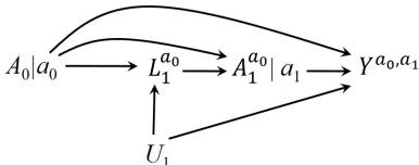
Figure 19.7

first split the treatment nodes A⁰ and A1. The right side of the split treatments represents the value of treatment under the intervention. The left side represents the value of treatment that would have been observed when intervening on all previous treatments. Therefore, the left side of A⁰ is precisely A⁰ because there are no previous treatments to intervene on, and the left side of A¹ is the counterfactual treatment A a⁰ 1 that would be observed after setting A⁰ to the value a0. All arrows into a given treatment in the original causal diagram now point into the left side, and all arrows out of a given treatment now originate from the right side. The outcome variable is the counterfactual outcome Y ^a0,a¹ and the covariates L are replaced by their corresponding counterfactual variables. Note that we write the counterfactual variable corresponding to L¹ under strategy (a0, a1) as L a⁰ 1 , rather than L a0,a¹ 1 , because a future intervention on A¹ cannot affect the value of earlier L1.

Unlike the directed acyclic graph in Figure 19.5, the SWIG in Figure 19.7 does include the counterfactual outcome, which means that we can visually check for exchangeability using d-separation.

1

a⁰

In Figure 19.7, by d-separation, both Y ^a0,a1⊥⊥A⁰ and Y ^a0,a1⊥⊥A 1 |A0, La⁰ hold for any static strategy (a0, a1). This second conditional independence holds even though there seems to be an open path A a^{0 1} ← a⁰ → L a^{0 1} ← U¹ → Y a0,a¹ . However, this path is actually blocked for the following reason. In the counterfactual world, a⁰ is a constant and in probability statements constants are always implicitly conditioned on even though, by convention, they are not shown in the conditioning event. See Fine Point 19.2 for details.

The second conditional independence Y ^a0,a1⊥⊥A a⁰ 1 |A0, La⁰ 1 implies, by definition, Y ^a0,a1⊥⊥A a⁰ 1 |A⁰ = a0, La⁰ 1 in the subset of individuals who received treatment A⁰ = a0. Therefore, by consistency, we conclude that Y Y ^a0,a1⊥⊥A⁰ and Y ^a0,a1⊥⊥A1|A⁰ = a0, L¹ hold under the causal diagram in Figure 19.5, which corresponds to the SWIG in Figure 19.7 where we can actually check for exchangeability. If there were multiple time points, we would say that

\[Y^{\bar{a}} \sqcup A\_k | \bar{A}\_{k-1} = \bar{a}\_{k-1}, \bar{L}\_k \text{ for } k = 0, 1...K\]

We refer to the above condition as static sequential exchangeability for Y a¯ , which is weaker than sequential exchangeability for Y g , because it only requires conditional independence between counterfactual outcomes Y a¯ indexed by static strategies g = ¯a and treatment Ak. Static sequential exchangeability is sufficient to identify the mean counterfactual outcome under any static strategy g = ¯a. See also Technical Point 19.3.

Static sequential exchangeability also holds under the causal diagram in Figure 19.6, as can be checked by applying d-separation to its corresponding SWIG in Figure 19.8. Thus, in an observational study represented by Figure 19.6, we can identify the mean counterfactual outcome under any static strategy (a0, a1). Let us return to Figure 19.5. Let us now assume that the arrow from L¹ to A¹ were missing. In that case, the arrow from L a⁰ 1 to A a⁰ 1 would also be missing from the SWIG in Figure 19.7. It would then follow by d-separation that sequential unconditional exchangeability holds, and therefore that the mean counterfactual outcome under any static strategy could be identified without data on L1. Now let us assume that, in Figure 19.5, there was an arrow from U¹ to A1. Then the SWIG in Figure 19.7 would include an arrow from U¹ to A a⁰ 1 , and so no form of sequential exchangeability would hold. The counterfactual mean would not be identified under any strategy.

We now discuss SWIGs under dynamic treatment strategies. Figure 19.9 represents the world of Figure 19.5 under a dynamic strategy g = [g0, g1(L1)] in which treatment A⁰ is assigned a fixed value g⁰ (either 0 or 1), and treatment A¹ at time k = 1 is assigned a value g1(L g 1 ) that depends on the value of L g 1 that was observed after having assigned treatment value g⁰ at time k = 0. For example, g may be the strategy “do no treat at time 0, treat at time 1 only if CD4 cell count is low, i.e., if L g ¹ = 1”. Under this strategy g⁰ = 0 for everybody, and g1(L g 1 ) = 1 when L g ¹ = 1 and g1(L g 1 ) = 0 when L g ¹ = 0. Therefore the SWIG includes an arrow from L g 1 to g1(L g 1 ). This arrow was not part of the original causal graph; it exists only in the counterfactual world associated with this dynamic strategy. We therefore draw this arrow differently from the others, even though we need to treat it as any other arrow when evaluating d-separation. The outcome in the SWIG is the counterfactual outcome Y g under the dynamic strategy g which uses L¹ to assign treatment A1.

By applying d-separation to the SWIG in Figure 19.9, we find that both Y ^g⊥⊥A⁰ and Y ^g⊥⊥A g 1 |A⁰ = g0, L^{g 1} hold for any strategy g. That is, sequential exchangeability for Y ^g holds, which means that we can identify the mean counterfactual outcome under all strategies g (see also Fine Point 19.2). This result, however, does not hold for the causal diagram in Figure 19.6.

^a0,a1⊥⊥A a⁰ 1 |A⁰ = a0, La⁰ 1 equals Y ^a0,a1⊥⊥A1|A⁰ = a0, L¹ because, by consistency, L a^{0 1} = L¹ and A a^{0 1} = A¹ when A⁰ = a0.

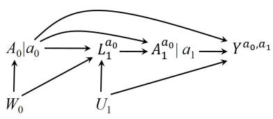
Figure 19.8

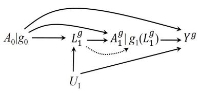
Figure 19.9

Figure 19.10

Arrows from intervention nodes in SWIGs When drawing SWIGs, we include arrows from the node a into future variables even though, in a single intervention world, a is a constant and thus cannot affect other variables. One reason we do this is that is a convenient device to keep track of the variables directly affected by A in the original DAG. A second reason is described in Technical Point 21.10.

To illustrate why this is important, consider two causal diagrams: 1) the causal DAG in Figure 7.14 and 2) a causal DAG equal to Figure 7.14 except that it also includes a direct arrow from A to Y . The SWIGs corresponding to these two DAGs would be identical if we did not include arrows leaving from a. As a result, we could not use the SWIG to infer that the causal effect of A on Y is identified in DAG 1 (using the front door formula) but not in DAG 2. Therefore, when using d-separation on a SWIG, we need to remember that all paths that include any intervention node a are blocked even if we do not explicitly condition on a in the notation.

The same logic applies for any intervention node under deterministic strategies. Suppose that we include a baseline confounder L⁰ in Figure 19.9 and we consider a deterministic dynamic strategy with g⁰ replaced by g0(L0). Then, when checking Y ^g⊥⊥A g 1 |A0, L0, L^g 1 , we do not need to explicitly condition also on g0(L0) because g0(L0) becomes a constant conditional on L0. However, we need to remember that, when conditioning on L0, paths through g0(L0) are blocked. When we instantiate A⁰ at g (L0) and use consistency, the statistical independence Y ^g⊥⊥A g 1 |A0, L0, L^g 1 becomes the exchangeability condition Y ^g⊥⊥A1|A⁰ = g (L0), L0, L¹ described above.

On the other hand, under a random strategy g that assigns a random treatment value A +,g 0 to each individual from a distribution that possibly depends on L0, we would explicitly include A +,g 0 on the SWIG (replacing g0(L0)) and also in the conditioning event when we check for d-separation, because A +,g 0 is no longer perfectly determined by L0. Richardson and Robins (2013) showed that a necessary condition for identifiability by the g-formula for such a random strategy is that Y ^g⊥⊥A g 1 |A0, A+,g 0 , L0, L^g 1 holds. They also considered strategies that depend on the natural value of treatment (Robins et al. 2004), i.e., strategies that assign treatment A +,g t at time t based on A g t , for which they provided exchangeability conditions that license identification by the extended g-formula. Strategies that depend on the natural value of treatment have recently been referred to as “modified treatment policies”(Diaz et al. 2021).

Y ^g⊥⊥A g 1 |A0, L^{g 1} which, by consistency, implies Y ^g⊥⊥A1|A⁰ = g0, L¹

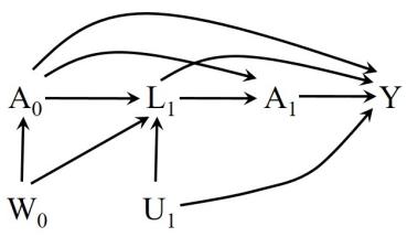
Figure 19.11

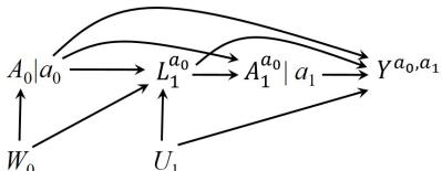
Figure 19.12

What we read from the SWIG is The SWIG in Figure 19.10 represents the world of Figure 19.6 under a dynamic treatment strategy g = [g0, g1(L1)]. By applying d-separation to the SWIG in Figure 19.10, we find that Y ^g⊥⊥A⁰ does not hold because of the open path A⁰ ← W⁰ → L g ¹ → g1(L g 1 ) → Y g . That is, sequential exchangeability for Y ^g does not hold, which means that we cannot identify the mean counterfactual outcome for any strategy g.

In summary, in observational studies (or sequentially randomized trials) represented by Figure 19.5, sequential exchangeability for Y ^g holds, and therefore the data can be used to validly estimate causal effects involving static and dynamic strategies. On the other hand, in observational studies represented by Figure 19.6, only the weaker condition for static strategies holds, and therefore the data can be used to validly estimate causal effects involving static strategies, but not dynamic strategies. Another way to think about this is that in the counterfactual world represented by the SWIG in Figure 19.10, the distribution of Y ^g depends on the distribution of g1(L g 1 ) and thus of L g 1 . However, the distribution of L g 1 is not identifiable due to the path A⁰ ← W⁰ → L g 1 .

One last example. Consider Figure 19.11 which is equal to Figure 19.6 except for the presence of an arrow from L¹ to Y , and its corresponding SWIG under a static strategy in Figure 19.12. We can use d-separation to show that neither sequential exchangeability for Y ^g nor static sequential exchangeability for Y ^a¯ hold. Therefore, in observational study represented by Figure 19.11, we cannot use the data to validly estimate causal effects involving any strategies.

No form of sequential exchangeability is guaranteed to hold in observational studies. Achieving approximate exchangeability requires expert knowledge, which will guide investigators in the design of their studies to measure as many of the relevant variables L¯ ^k as possible. For example, in an HIV study, experts would agree that time-varying variables like CD4 cell count, viral load, and symptoms need to be appropriately measured and adjusted for.

But the question “Are the measured covariates sufficient to ensure sequential exchangeability?” can never be answered with certainty. Yet we can use our expert knowledge to organize our beliefs about exchangeability and represent them in a causal diagram. Figures 19.1 to 19.4 are examples of causal diagrams that summarize different scenarios. Note that we drew these causal diagrams in the absence of selection (e.g., censoring by loss to follow-up) so that we can concentrate on confounding here.

Consider Figure 19.5. Like in Part I of this book, suppose that we are interested in the effect of the time-fixed treatment A¹ on the outcome Y . We say that there is confounding for the effect of A¹ on Y because A¹ and Y share the cause U, i.e., because there is an open backdoor path between A¹ and Y through U. To estimate this effect without bias, we need to adjust for confounders of the effect of the treatment A¹ on the outcome Y , as explained in Chapter 7. In other words, we need to be able to block all open backdoor paths between A¹ and Y . This backdoor path A¹ ←− L¹ ←− U −→ Y cannot be blocked by conditioning on the common cause U because U is unmeasured and therefore unavailable to the investigators. However, this backdoor path can be blocked by conditioning on L1, which is measured. Thus, if the investigators collected data on L¹ for all individuals, there would be no unmeasured confounding for the effect of A1. We then say that L¹ is a confounder for the effect of A1, even though the actual common cause of A¹ and Y was the unmeasured U (re-read Section 7.3 if you need to refresh your memory about confounding and causal diagrams).

after conditioning on collider L1: A¹ ←− A⁰ −→ L¹ ←− U −→ Y This second backdoor path can be safely blocked by conditioning on prior treatment A0, assuming it is available to investigators.

sometimes referred to as timedependent confounders.

A second backdoor path gets open As discussed in Chapter 7, the confounders do not have to be direct causes of the outcome. In Figure 19.5, the arrow from the confounder L¹ to the outcome Y does not exist. Then the source of the confounding (i.e., the causal confounder) is the unmeasured common cause U. Nonetheless, because data on L¹ suffice to block the backdoor paths from A¹ to Y and thus to control confounding, we refer to L¹ as a confounder for the effect of A¹ on Y .

Now imagine the very long causal diagram that contains all time points k = 0, 1, 2…, and in which L^k affects subsequent treatments Ak, Ak+1… and shares unmeasured causes U^k with the outcome Y . Suppose that we want to estimate the causal effects on the outcome Y of treatment strategies defined by interventions on A0, A1, A2. Then, at each time k, the covariate history L¯ k will be needed, together with the treatment history A¯ k−1, to block the backdoor paths between treatment A^k and the outcome Y . Thus, no unmeasured confounding for the effect of A¯ requires that the investigators collected data on L¯ ^k for all individuals. We then say that the time-varying covariates in L¯ k are time-varying confounders for the effect of the time-varying treatment A¯ Time-varying confounders are on Y at several (or, in our example, all) times k in the study. See Fine Point 19.3 for a more precise definition of time-varying confounding.

Unfortunately, we cannot empirically confirm that all confounders, whether time-fixed or time-varying, are measured. That is, we cannot empirically differentiate between Figure 19.2 with no unmeasured confounding and Figure 19.3 with unmeasured confounding. Interestingly, even if all confounders were

A definition of time-varying confounding. In the absence of selection bias, we say there is confounding for causal effects involving E [Y a¯ ] if E [Y a¯ ] ̸= E [Y |A = ¯a], that is, if the mean outcome had, contrary to fact, all individuals in the study followed strategy a¯ differs from the mean outcome among the subset of individuals who followed strategy a¯ in the actual study.

We say the confounding is solely time-fixed (i.e., wholly attributable to baseline covariates) if E [Y a¯ |L0] = E [Y |A = ¯a, L0], as would be the case if the only arrows pointing into A¹ in Figure 19.2 were from A⁰ and L0. In contrast, if the identifiability conditions hold, but E [Y a¯ |L0] ̸= E [Y |A = ¯a, L0], we say that time-varying confounding is present. If the identifiability conditions do not hold, as in Figure 19.3, we say that there is unmeasured confounding.

A sufficient condition for no time-varying confounding is unconditional sequential exchangeability for Y a¯ , i.e., Y ^a¯⊥⊥Ak|A¯ ^k−¹ = ¯ak−1. This condition holds in sequentially randomized experiments, like the one represented in Figure 19.1, in which treatment A^k at each time k is randomly assigned with a probability that depends only on the values of prior treatment history A¯ ^k−1. In fact, the causal diagram in Figure 19.1 can be greatly simplified. To do so, first note that L¹ is not a common cause of any two nodes in the graph so it can be omitted from the graph. Once L¹ is gone, then both L⁰ and U¹ can be omitted too because they cease to be common causes of two nodes in the graph. In the graph without L0, L1, and U1, the node U⁰ can be omitted too. That is, the causal diagram in Figure 19.1 can be simplified to include only the nodes A0, A¹ and Y .

correctly measured and modeled, most adjustment methods may still result in biased estimates when comparing treatment strategies. The next chapter explains why g-methods are the appropriate approach to adjust for time-varying confounders.

Chapter 20 TREATMENT-CONFOUNDER FEEDBACK

The previous chapter identified sequential exchangeability as a key condition to identify the causal effects of timevarying treatments. Suppose that we have a study in which the strongest form of sequential exchangeability holds: the measured time-varying confounders are sufficient to validly estimate the causal effect of any treatment strategy. Then the question is what confounding adjustment method to use. The answer to this question highlights a key problem in causal inference about time-varying treatments: treatment-confounder feedback.

When treatment-confounder feedback exists, using traditional adjustment methods may introduce bias in the effect estimates. That is, even if we had all the information required to validly estimate the average causal effect of any treatment strategy, we would be generally unable to do so. This chapter describes the structure of treatment-confounder feedback and the reasons why traditional adjustment methods fail.

20.1 The elements of treatment-confounder feedback

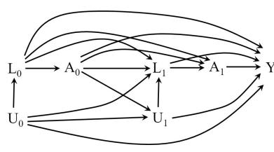
Figure 20.1

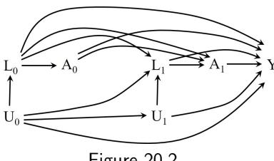
Figure 20.2

Consider again the sequentially randomized trial of individuals with HIV that we discussed in the previous chapter. For every person in the study, we have data on treatment A^k (1: treated, 0: untreated) and covariates L^k at each month of follow-up k = 0, 1, 2…K, and on an outcome Y that measures health status at month K + 1. The causal diagram in Figure 20.1, which is equal to the one in Figure 19.2, represents the first two months of the study. The time-varying covariates L^k are time-varying confounders. (As in the previous chapter, we are using this example without censoring so that we can focus on confounding.)

Something else is going on in Figure 20.1. Not only is there an arrow from CD4 cell count L^k to treatment Ak, but also there is an arrow from treatment Ak−¹ to future CD4 cell count Lk—because receiving treatment Ak−¹ increases future CD4 cell count Lk. That is, the confounder affects the treatment and the treatment affects the confounder. There is treatment-confounder feedback (see also Fine Point 20.1).

Note that time-varying confounding can occur without treatment-confounder feedback. The causal diagram in Figure 20.2. is the same as the one in Figure 20.1, except that the arrows from treatment Ak−¹ to future L^k and U^k have been deleted. In a setting represented by this diagram, the timevarying covariates L^k are time-varying confounders, but they are not affected by prior treatment. Therefore, there is time-varying confounding, but there is no treatment-confounder feedback.

Treatment-confounder feedback creates an interesting problem for causal inference. To state the problem in its simplest form, let us simplify the causal diagram in Figure 20.1 a bit more. Figure 20.3 is the smallest subset of Figure 20.1 that illustrates treatment-confounder feedback in a sequentially randomized trial with two time points. When drawing the causal diagram in Figure 20.3, we made four simplifications:

• Because our interest is in the implications of confounding by L1, we

Representing feedback cycles with acyclic graphs. Interestingly, an acyclic graph—like the one in Figure 20.1—can be used to represent a treatment-confounder feedback loop or cycle. The trick to achieve this visual representation is to elaborate the treatment-confounder feedback loop in time. That is, Ak−¹ → L^k → A^k → Lk+1 and so on.

The representation of feedback cycles with acyclic graphs also requires that time be considered as a discrete variable. That is, we say that treatment and covariates can change during each interval [k, k + 1) for k = 0, 1, …K, but we do not specify when exactly during the interval the change takes place. This discretization of time is not a limitation in practice: the length of the intervals can be chosen to be as short as the granularity of the data requires. For example, in a study where individuals see their doctors once per month or less frequently (as in our HIV example), time may be safely discretized into month intervals. In other cases, year intervals or day intervals may be more appropriate. Also, as we said in Chapter 17, time is typically measured in discrete intervals (years, months, days) any way, so the discretization of time is often not even a choice.

did not bother to include a node L⁰ for baseline CD4 cell count. Just suppose that treatment A⁰ is marginally randomized and treatment A¹ is conditionally randomized given L1.

• The unmeasured variable U⁰ is not included.
• There is no arrow from A⁰ to A1, which implies that treatment is assigned using information on L¹ only.
• There are no arrows from A0, L¹ and A¹ to Y , which would be the case if treatment has no causal effect on the outcome Y of any individual, i.e., the sharp null hypothesis holds.

None of these simplifications affect the arguments below. A more complicated causal diagram would not add any conceptual insights to the discussion in this chapter; it would just be harder to read.

Now suppose that treatment has no effect on any individual’s Y , which implies the causal diagram in Figure 20.3 is the correct one, but the investigators do not know it. Also suppose that we have data on treatment A⁰ in month 0 and A¹ in month 1, on the confounder CD4 cell count L¹ at the start of month 1, and on the outcome Y at the end of follow-up. We wish to use these data to estimate the average causal effect of the static treatment strategy “always treat”, (a⁰ = 1, a¹ = 1), compared with the static treatment strategy “never treat”, (a⁰ = 0, a¹ = 0) on the outcome Y , i.e., E - Y ^a0=1,a1=1 − E - Y ^a0=0,a1=0 . According to Figure 20.3, the true, but unknown to the investigator, average causal effect is 0 because there are no forward-directed paths from either treatment variable to the outcome. That is, one cannot start at either A⁰ or A¹ and, following the direction of the arrows, arrive at Y .

Figure 20.3 can depict a sequentially randomized trial because there are no direct arrows from the unmeasured U into the treatment variables. Therefore, as we discussed in the previous chapter, we should be able to use the observed data on A0, L1, A1, and Y to conclude that E - Y ^a0=1,a1=1 − E - Y ^a0=0,a1=0 is equal to 0. However, as we explain in the next section, we will not generally be able to correctly estimate the causal effect when we adjust for L¹ using traditional methods, like stratification, outcome regression, and matching. That is, in this example, an attempt to adjust for the confounder L¹ using these methods will generally result in an effect estimate that is different from 0, and thus invalid.

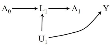
Figure 20.3

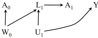
Figure 20.4

quentially randomized trial or an observational study with no unmeasured confounding; Figure 20.4 represents an observational study.

In other words, when there are time-varying confounders and treatmentconfounder feedback, traditional methods cannot be used to correctly adjust Figure 20.3 represents either a se- for those confounders. Even if we had sufficient longitudinal data to ensure sequential exchangeability, traditional methods would not generally provide a valid estimate of the causal effect of any treatment strategies. In contrast, g-methods appropriately adjust for the time-varying confounders even in the presence of treatment-confounder feedback.

This limitation of traditional methods applies to settings in which the timevarying confounders are affected by prior treatment as in Figure 20.3, but also to settings in which the time-varying confounders share causes W with prior treatment as in Figure 20.4, which is a subset of Figure 19.4. We refer to both Figures 20.3 and 20.4 (and Figures 19.2 and 19.4) as examples of treatmentconfounder feedback. The next section explains why traditional methods cannot adequately handle treatment-confounder feedback.

20.2 The bias of traditional methods

herence to the assigned treatment strategy and no losses to follow-up.

Table 20.1

N	A0	L1	A1	Mean Y
2400	0	0	0	84
1600	0	0	1	84
2400	0	1	0	52
9600	0	1	1	52
4800	1	0	0	76
3200	1	0	1	76
1600	1	1	0	44
6400	1	1	1	44

which treatment A^k were affected by Lk, then L^k would be a timevarying confounder

cause there is no arrow from L¹ to Y . Otherwise, A⁰ would have an effect on Y through L¹

To illustrate the bias of traditional methods, let us consider a (hypothetical) This is an ideal trial with full ad- sequentially randomized trial with 32, 000 individuals with HIV and two time points k = 0 and k = 1. Treatment A⁰ = 1 is randomly assigned at baseline with probability 0.5. Treatment A¹ is randomly assigned in month 1 with a probability that depends only on the value of CD4 cell count L¹ at the start of month 1—0.4 if L¹ = 0 (high), 0.8 if L¹ = 1 (low). The outcome Y , which is measured at the end of follow-up, is a function of CD4 cell count, concentration of virus in the serum, and other clinical measures, with higher values of Y signifying better health.

Table 20.1 shows the data from this trial. To save space, the table displays one row per combination of values of A0, L1, and A1, rather than one row per individual. For each of the eight combinations, the table provides the number of subjects N and the mean value of the outcome E [Y |A0, L1, A1]. Thus, row 1 shows that the mean of the 2400 individuals with (A⁰ = 0, L¹ = 0, A¹ = 0) was E [Y |A⁰ = 0, L¹ = 0, A¹ = 0] = 84. In this sequentially randomized trial, the identifiability conditions—sequential exchangeability, positivity, consistency hold. By design, there are no confounders for the effect of A⁰ on Y , and L¹ is the only confounder for the effect of A¹ on Y so (conditional on L1) sequential If there were additional times k at exchangeability holds. By inspection of Table 20.1, we can conclude that the positivity condition is satisfied, because otherwise one or more of the eight rows would have zero individuals.

The causal diagram in Figure 20.3 depicts this sequentially randomized experiment when the sharp null hypothesis holds. To check whether the data in Figure 20.3 represents the null be- Table 20.1 are consistent with the causal diagram in Figure 20.3, we can separately estimate the average causal effects of each of the time-fixed treatments A⁰ and A¹ within levels of past covariates and treatment, which should all be null. In the calculations below, we will ignore random variability.

A quick inspection of the table shows that the average causal effect of treatment A¹ is indeed zero in all four strata defined by A⁰ and L1. Consider the effect of A¹ in the 4000 individuals with A⁰ = 0 and L¹ = 0, whose data are shown in rows 1 and 2 of Table 20.1. The mean outcome among those who did not receive treatment at time 1, E [Y |A⁰ = 0, L¹ = 0, A¹ = 0], is 84, and the mean outcome among those who did receive treatment at time 1,

G-null test. Suppose the sharp null hypothesis is true. Then any counterfactual outcome Y g is the observed outcome Y . In this setting, sequential exchangeability for all Y g can be written as Y ⊥⊥A0|L⁰ and Y ⊥⊥A1|A0, L0, L¹ in a study with two time points. (We have used the fact that, for any values of a⁰ and l0, there exist strategies g such that a⁰ = g(l0).) Therefore, under sequential exchangeability, a test of these conditional independencies is a test of the sharp null. This is the g-null test (Robins 1986). Note the first independence implies no causal effect of A⁰ in any strata defined by L0, and the second independence implies no causal effect of A¹ in any strata defined by L¹ and A0.

More generally, the g-null theorem of Robins (1986) says that, under sequential randomization for all g, the above two independencies hold if and only if the distribution of Y g and therefore the mean E [Y g ] is the same for all g, and also equal to the distribution and mean of the observed Y .

\[\text{E}\left[Y|A\_0=0, L\_1=0, A\_1=1\right], \text{ is also 84. Therefore the difference } \frac{1}{2}\]

\[\mathbb{E}\left[Y|A\_0=0, L\_1=0, A\_1=1\right] - \mathbb{E}\left[Y|A\_0=0, L\_1=0, A\_1=0\right]\]

is zero. Because the identifiability conditions hold, this associational difference validly estimates the average causal effect

\[\mathbb{E}\left[Y^{a\_1=1}|A\_0=0, L\_1=0\right] - \mathbb{E}\left[Y^{a\_1=0}|A\_0=0, L\_1=0\right]\]

in the stratum (A⁰ = 0, L¹ = 0). Similarly, it is easy to check that the average causal effect of treatment A¹ on Y is zero in the remaining three strata (A⁰ = 0, L¹ = 1), (A⁰ = 1, L¹ = 0), (A⁰ = 1, L¹ = 1), by comparing the mean outcome between rows 3 and 4, rows 5 and 6, and rows 7 and 8, respectively.

We can now show that the average causal effect of A⁰ is also zero. To do so, we need to compute the associational difference E [Y |A⁰ = 1] − E [Y |A⁰ = 0] which, because of randomization, is a valid estimator of the causal contrast E - Y ^a0=1 − E - Y ^a0=0 . The mean outcome E [Y |A⁰ = 0] among the 16, 000 The weighted average is individuals treated at time 0 is the weighted average of the mean outcomes in rows 1, 2, 3 and 4, which is 60. And E [Y |A⁰ = 1], computed analogously, is also 60. Therefore, the average causal effect of A⁰ is zero.

We have confirmed that the causal effects of A⁰ and A¹ (conditional on the past) are zero when we treat A⁰ and A¹ separately as time-fixed treatments. What if we now treat the joint treatment (A0, A1) as a time-varying treatment and compare two treatment strategies? For example, let us say that we want to compare the strategies “always treat” versus “never treat”, that is (a⁰ = 1, a¹ = 1) versus (a⁰ = 0, a¹ = 0). Because the identifiability conditions hold, the data in Table 20.1 should suffice to validly estimate this effect.

Because the effect for each of the individuals components of the strategy, a⁰ and a1, is zero, it follows from the g-null theorem (see Technical Point 20.1) that the average causal effect E - Y ^a0=1,a1=1 − E - Y ^a0=0,a1=0 is zero. But is this what we conclude from the data if we use conventional analytic methods? To answer this question, let us conduct two data analyses. In the first one, we do not adjust for the confounder L1, which should give us an incorrect effect estimate. In the second one, we do adjust for the confounder L¹ via stratification.

1. We compare the mean outcome in the 9600 individuals who were treated at both times (rows 6 and 8 of Table 20.1) with that in the 4800 individuals who were untreated at both times (rows 1 and 3). The respective averages are E [Y |A⁰ = 1, A¹ = 1] = 54.7, and E [Y |A⁰ = 0, A¹ = 0] =

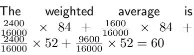
3200 ^{9600 ×} 76 + ^{6400 9600} × 44 = 54.7 E [Y |A⁰ = 0, A¹ = 0] 2400 ^{4800 ×} 84 + ^{2400 4800} × 52 = 68.0

Note that, because the effect is stratum L¹ = 1 is also −8. −8 in both strata of L1, it is not possible that a weighted average of the stratum-specific effects will yield the correct value 0.

E [Y |A⁰ = 1, A¹ = 1] 68. The associational difference is 54.7−68 = −13.3 which, if interpreted causally, would mean that not being treated at either time is better than being treated at both times. This analysis gives the wrong answer—a non-null difference—because E [Y |A⁰ = a0, A¹ = a1] is not a valid estimator of E [Y a0,a¹ ]. Adjustment for the confounder L¹ is needed.

2. We adjust for L¹ via stratification. That is, we compare the mean outcome in individuals who were treated with that in individuals who were untreated at both times, within levels of L1. For example, take the stratum L¹ = 0. The mean outcome in the treated at both times, E [Y |A⁰ = 1, L¹ = 0, A¹ = 1], is 76 (row 6). The mean outcome in the untreated at both times, E [Y |A⁰ = 0, L¹ = 0, A¹ = 0], is 84 (row 1). The associational difference is 76 − 84 = −8 which, if interpreted causally, would mean that, in the stratum L¹ = 0, not being treated at either time is better than being treated at both times. Similarly, the difference E [Y |A⁰ = 1, L¹ = 1, A¹ = 1] − E [Y |A⁰ = 0, L¹ = 1, A¹ = 0] in the

What? We said that the effect estimate should be 0, not −8. How is it possible that the analysis adjusted for the confounder also gives a wrong answer? This estimate reflects the bias of traditional methods to adjust for confounding when there is treatment-confounder feedback. The next section explains why the bias arises.

20.3 Why traditional methods fail

Table 20.1 shows data from a sequentially randomized trial with treatmentconfounder feedback, as represented by the causal diagram in Figure 20.3. Even though no data on the unmeasured variable U¹ (immunosuppression level) is available, all three identifiability conditions hold: U¹ is not needed if we have data on the confounder L1. Therefore, as discussed in Chapter 19, we should be able to correctly estimate causal effects involving any static or dynamic treatment strategies. And yet our analyses in the previous section did not yield the correct answer, whether or not we adjusted for L1.

The problem was that we did not use the correct method to adjust for confounding. Stratification is a commonly used method to adjust for confounding, but it cannot handle treatment-confounder feedback. Stratification means estimating the association between treatment and outcome in subsets—strata—of the study population defined by the confounders—L¹ in our example. Because the variable L¹ can take only two values—1 if the CD4 cell count is low, and 0 otherwise—there are two such strata in our example. To estimate the causal effect in those with L¹ = l, we selected (i.e., conditioned or stratified on) the subset of the population with value L¹ = l.

But stratification can have unintended effects when the association measure is computed within levels of a variable L¹ that is caused by prior treatment A0. Indeed Figure 20.5 shows that conditioning on L1—a collider—opens the path A⁰ −→ L¹ ←− U¹ −→ Y . That is, stratification induces a noncausal association between the treatment A⁰ at time 0 and the unmeasured variable U1, and therefore between A⁰ and the outcome Y , within levels of L1. Among those with low CD4 count (L¹ = 1), being on treatment (A⁰ = 1) becomes a marker for severe immunosuppression (high value of U1); among those with a high level

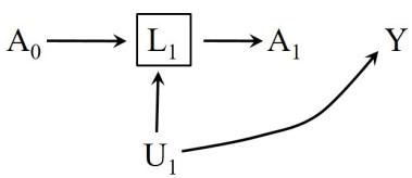
Figure 20.5

Confounders on the causal pathway. Conditioning on confounders L¹ which are affected by previous treatment can create selection bias even if the confounder is not on a causal pathway between treatment and outcome. In fact, no such causal pathway exists in Figures 20.5 and 20.6.

On the other hand, in Figure 20.7 the confounder L¹ for subsequent treatment A¹ lies on a causal pathway from earlier treatment A⁰ to outcome Y , i.e., the path A⁰ −→ L¹ −→ Y . If U¹ were not a common cause of L¹ and Y in Figure 20.7 (i.e., if there were no selection bias), the A-Y associations within strata of L¹ would be an unbiased estimate of the direct effects of A⁰ on Y not through L1, but still would not be an unbiased estimate of the overall effect of A¯ on Y , because the effect of A⁰ mediated through L¹ is not included.

It is sometimes said that variables on a causal pathway between treatment and outcome cannot be considered as confounders, because adjusting for those variables will result in a biased effect estimate. However, this characterization of confounders is inaccurate for time-varying treatments. Figure 20.7 shows that a confounder for subsequent treatment A¹ can be on a causal pathway between past treatment A⁰ and the outcome. As for whether adjustment for confounders on a causal pathway induces bias for the effect of a treatment strategy, that depends on the choice of adjustment method. Stratification will indeed induce bias; g-methods will not.

of CD4 (L¹ = 0), being off treatment (A⁰ = 0) becomes a marker for milder immunosuppression (low value of U1). Thus, the side effect of stratification is to induce an association between treatment A⁰ and outcome Y .

In other words, stratification eliminates confounding for A¹ at the cost of introducing selection bias for A0. The associational differences

\[\operatorname{E}\left[Y|A\_0=1, L\_1=l, A\_1=1\right] - \operatorname{E}\left[Y|A\_0=0, L\_1=l, A\_1=0\right]\]

may be different from 0 even if, as in our example, treatment has no effect on the outcome of any individuals at any time. This bias arises from choosing a subset of the study population by selecting on a variable L¹ affected by (a component A⁰ of) the time-varying treatment. The net bias depends on the relative magnitude of the confounding that is eliminated and the selection bias that is created.

Technically speaking, the bias of traditional methods will occur not only when the confounders are affected by prior treatment (in randomized experiments or observational studies), but also when the confounders share an unmeasured cause W⁰ with prior treatment (in observational studies). In the observational study depicted in Figure 20.6, conditioning on the collider L¹ opens the path A⁰ ←− W⁰ −→ L¹ ←− U¹ −→ Y . For this reason, we referred to both settings in Figures 20.3 and 20.4—which cannot be distinguished using the observed data—as examples of treatment-confounder feedback.

The causal diagrams that we have considered to describe the bias of traditional methods are all very simple. They only represent settings in which treatment does not have a causal effect on the outcome. However, conditioning on a confounder in the presence of treatment-confounder feedback also induces bias when treatment has a non-null effect, as in Figure 20.7. The presence of arrows from A0, A1, or L¹ to Y does not change the fact that conditioning on L¹ creates an association between A⁰ and Y that does not have a causal interpretation (see also Fine Point 20.2). Also, our causal diagrams had only two time points and a limited number of nodes, but the bias of traditional methods will also arise from high-dimensional data with multiple time points and variables. In fact, the presence of time-varying confounders affected by previous treatment at multiple times increases the possibility of a large bias.

Figure 20.6

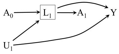
Figure 20.7

In general, valid estimation of the effect of treatment strategies is only possible when the joint effect of the treatment components A^k can be estimated simultaneously and without bias. As we have just seen, this may be impossible to achieve using stratification, even when data on all time-varying confounders are available.

20.4 Why traditional methods cannot be fixed

We showed that stratification cannot be used as a confounding adjustment method when there is treatment-confounder feedback. But what about other traditional methods? For example, we could have used parametric outcome regression, rather than nonparametric stratification, to adjust for confounding. Would outcome regression succeed where plain stratification failed?

This question is particularly important for settings with high-dimensional data, because in high-dimensional settings we will be unable to conduct a simple stratified analysis like we did in the previous section. Consider data generated under Figure 20.5. Treatment A^k occurs at two months k = 0, 1, which means that there are only 2² = 4 static treatment strategies ¯a. But when the treatment A^k occurs at multiple points k = 0, 1…K, we will not be The number of data combinations able to present a table with all the combinations of treatment values. If, as is not infrequent in practice, K is of the order of 100, then there are 2¹⁰⁰ static treatment strategies ¯a, a staggering number that far exceeds the sample size of any study. The total number of treatment strategies is much greater when we consider dynamic strategies as well.

As we have been arguing since Chapter 11, we will need modeling to estimate average causal effects involving E [Y a¯ ] when there are many possible treatment strategies ¯a. To do so, we will need to hypothesize a dose-response function for the effect of treatment history ¯a on the mean outcome Y . One possibility would be to assume that the effect of treatment strategies ¯a increases linearly as a function of the cumulative treatment under each strategy. Under this assumption, all strategies that assign treatment for exactly three months have the same effect, regardless of the period when those three months of treatment occur the first 3 months of follow-up, the last 3 months of followup, etc. The price paid for modeling is yet another threat to the validity of our estimates due to possible model misspecification of the dose-response function.

And yet paying this price does not buy any protection against the failure of traditional methods. In the presence of treatment-confounder feedback, regression modeling cannot possibly remove the bias of conventional stratificationbased methods because regression is a conventional stratification-based method itself. For example, suppose that we have data generated under Figure 20.5. Let us define cumulative treatment cum A¯ = A⁰ + A1, which can take 3 values: 0 (if the individuals remains untreated at both times), 1 (if the subject is treated at time 1 only or at time 2 only), and 2 (if the subject is treated at both times). The treatment strategies of interest can then be expressed as “always treat” cum (¯a) = 2, and “never treat” cum (¯a) = 0, and the average causal effect as E - Y cum(¯a)=2 − E - Y cum(¯a)=0 . Again, any valid method should estimate that the value of this difference is 0.

Under the assumption that the mean outcome E - Y |A, L ¯ 1 depends linearly on the covariate cum A¯ , we could fit the outcome regression model

\[\operatorname{E}\left[Y|\bar{A},L\_1\right] = \theta\_0 + \theta\_1 cum\left(\bar{A}\right) + \theta\_2 L\_1\]

is even greater because there are multiple confounders L^k measured at each time point k.

The associational difference E - Y |cum A¯ = 2, L¹ −E - Y |cum A¯ = 0, L¹ is equal to θ1×2. (The model correctly assumes that the difference is the same in the strata L¹ = 1 and L¹ = 0.) Therefore some might want to interpret θ¹ × 2 as the average causal effect of “always treat” versus “never treat” within levels of the covariate L1. But such causal interpretation is unwarranted because, as Figure 20.5 shows, conditioning on L¹ induces an association between A0, a component of treatment cum A¯ , and the outcome Y . This implies that θ1 and therefore the associational difference of means—is non-zero even if the true causal effect is zero and the regression model for E - Y |A, L ¯ 1 is correct. A similar argument can be applied to matching. G-methods are needed to appropriately adjust for time-varying confounders in the presence of treatmentconfounder feedback.

20.5 Adjusting for past treatment

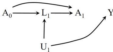
Figure 20.8

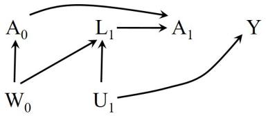
Figure 20.9

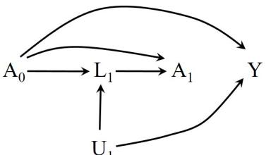
Figure 20.10

One more thing before we discuss g-methods. For simplicity, we have so far described treatment-confounder feedback under simplified causal diagrams in which past treatment does not directly affect subsequent treatment. That is, the causal diagrams in Figures 20.3 and 20.4 did not include an arrow from A⁰ to A1. We now consider the more general case in which past treatment may directly affect subsequent treatment.

As an example, suppose doctors in our HIV study use information on past treatment history A¯ ^k−¹ when making a decision about whether to prescribe treatment A^k at time k. To represent this situation, we add an arrow from A⁰ to A¹ to the causal diagrams in Figures 20.3 and 20.4, as depicted in Figures 20.8 and 20.9.

The causal diagrams in Figures 20.8 and 20.9 show that, in the presence of treatment-confounder feedback, conditioning on L¹ is insufficient to block all backdoor paths between treatment A¹ and outcome Y . Indeed conditioning on L¹ opens the path A¹ ← A⁰ → L¹ ← U¹ → Y in Figure 20.8, and the path A¹ ← A⁰ ← W⁰ → L¹ ← U¹ → Y in Figure 20.9. Of course, regardless of whether treatment-confounder feedback exists, conditioning on past treatment history is always required when past treatment has a non-null effect on the outcome, as in the causal diagram of Figure 20.10. Under this diagram, treatment A⁰ is a confounder of the effect of treatment A1.

Therefore, sequential exchangeability at time k generally requires conditioning on treatment history A¯ ^k−¹ before k; conditioning only on the covariates L is not enough. That is why, in this and in the previous chapter, all the conditional independence statements representing sequential exchangeability were conditional on treatment history.

Past treatment plays an important role in the estimation of effects of timefixed treatments too. Suppose we are interested in estimating the effect of the time-fixed treatment A1—as opposed to the effect of a treatment strategy involving both A⁰ and A1—on Y . (Sometimes the effect of A¹ is referred to as the short-term effect of the time-varying treatment A¯.) Then lack of adjustment for past treatment A⁰ will generally result in selection bias if there is treatment-confounder feedback, and in confounding if past treatment A⁰ directly affects the outcome Y . In other words, the difference E [Y |A¹ = 1, L1]−E [Y |A¹ = 0, L1] would not be zero even if treatment A¹ had no effect on any individual’s outcome Y , as in Figures 20.8-20.10. In practice, when making causal inferences about time-fixed treatments, bias may arise in

treatment, the analysis would not need to be restricted to new users.

domly mismeasured treatment may lead to bias away from the null.

analyses that compare current users (A¹ = 1) versus nonusers (A¹ = 0) of treatment. To avoid the bias, one can adjust for prior treatment history or restrict the analysis to individuals with a particular treatment history. This If one could correctly adjust for past is the idea behind “new-user designs” for time-fixed treatments: restrict the analysis to individuals who had not used treatment in the past.

The requirement to adjust for past treatment has additional bias implications when past treatment is mismeasured. As discussed in Section 9.3, a mismeasured confounder may result in effect estimates that are biased, either upwards or downwards. In our HIV example, suppose investigators did not have access to the study participants’ medical records. Rather, to ascertain prior treatment, investigators had to ask participants via a questionnaire. Since not all participants provided an accurate recollection of their treatment history, treatment A⁰ was measured with error. Investigators had data on the mismeasured variable A^∗ 0 rather than on the variable A0. To depict this setting in Figures 20.8-20.10, we add an arrow from the true treatment A⁰ to the mismeasured treatment A^∗ 0 , which shows that conditioning on A^∗ 0 cannot block the biasing paths between A¹ and Y that go through A0. Investigators will then conclude that there is an association between A¹ to Y , even after adjusting for A^{∗ 0} and L1, despite the lack of an effect of A¹ on Y .

Therefore, when treatment is time-varying, we find that, contrary to a widespread belief, mismeasurement of treatment—even if the measurement er-Robins (1987) showed that ran- ror is independent and non-differential—may cause bias under the null. This bias arises because past treatment is a confounder for the effect of subsequent treatment, even if past treatment has no causal effect on the outcome. Furthermore, under the alternative, this imperfect bias adjustment may result in an exaggerated estimate of the effect.

Chapter 21 G-METHODS FOR TIME-VARYING TREATMENTS

In the previous chapter we described a dataset with a time-varying treatment and treatment-confounder feedback. We showed that, when applied to this dataset, traditional methods for confounding adjustment could not correctly adjust for confounding. Even though the time-varying treatment had a zero causal effect on the outcome, traditional adjustment methods yielded effect estimates that were different from the null.

This chapter describes the solution to the bias of traditional methods in the presence of treatment-confounder feedback: the use of g-methods—the g-formula, IP weighting, g-estimation, and their doubly-robust generalizations. Using the same dataset as in the previous chapter, here we show that the three g-methods yield the correct (null) effect estimate. For time-fixed treatments, we described the g-formula in Chapter 13, IP weighting of marginal structural models in Chapter 12, and g-estimation of structural nested models in Chapter 15. Here we introduce each of the three g-methods for the comparison of static treatment strategies under the identifiability conditions described in Chapter 19: sequential exchangeability, positivity, and consistency.

21.1 The g-formula for time-varying treatments

Table 21.1
————	–	–	–	–

N	A0	L1	A1	Mean Y
2400	0	0	0	84
1600	0	0	1	84
2400	0	1	0	52
9600	0	1	1	52
4800	1	0	0	76
3200	1	0	1	76
1600	1	1	0	44
6400	1	1	1	44

Consider again the data from the sequentially randomized experiment in Table 20.1 which, for convenience, we reproduce again here as Table 21.1. Suppose we are only interested in the effect of the time-fixed treatment A1. That is, suppose we want to contrast the mean counterfactual outcomes E - Y ^a1=1 and E - Y ^a1=0 . In Parts I and II we have showed that, under the identifiability conditions, each of the means E [Y a¹ ] is a weighted average of the mean outcome E [Y |A¹ = a1, L¹ = l1] conditional on the (time-fixed) treatment and confounders. Specifically, E [Y a¹ ] equals the weighted average

\[\sum\_{l\_1} \to \left[ Y \middle| A\_1 = a\_1, L\_1 = l\_1 \right] f\left(l\_1\right), \text{ where } f\left(l\_1\right) = \Pr\left[L\_1 = l\_1\right].\]

because, as shown in the previous chapter, only L¹ is needed to make the treated (A¹ = 1) and the untreated (A¹ = 0) conditionally exchangeable. This weighted average is the g-formula for E [Y a¹ ]: the mean outcome standardized to the distribution of the confounders (here, L¹ only) in the study population.

But, in the sequentially randomized experiment of Table 21.1, the treatment A = (A0, A1) is time-varying and, as we saw in the previous chapter, there is treatment-confounder feedback. That means that traditional adjustment methods cannot be relied on to unbiasedly estimate the causal effect of time-varying treatment A. For example, traditional methods may not provide valid estimates of the mean outcome under “always treat” E - Y ^a0=1,a1=1 and the mean outcome under “never treat” E - Y ^a0=0,a1=0 even in a sequentially randomized experiment in which sequential exchangeability holds. In contrast, the g-formula can be used to calculate the counterfactual means E [Y a0,a¹ ] in a sequentially randomized experiment. To do so, the above expression of the g-formula for time-fixed treatments needs to be generalized.

The g-formula for E [Y a0,a¹ ] under the identifiability conditions (described in Chapter 19) will still be a weighted average, but now it will be a weighted average of the mean outcome E [Y |A⁰ = a0, A¹ = a1, L¹ = l1] conditional on the time-varying treatment and confounders required to achieve sequential exchangeability. The weights are the distribution of the confounder L¹ given the past which, in this case, is the past value of treatment corresponding to the The g-formula for time-varying intervention. Specifically, the g-formula

\[\sum\_{l\_1} \to \left[ Y \middle| A\_0 = a\_0, A\_1 = a\_1, L\_1 = l\_1 \right] f\left( l\_1 \middle| a\_0 \right)\]

equals E [Y a0,a¹ ] under (static) sequential exchangeability for Y a0,a¹ . That is, for a time-varying treatment, the g-formula estimator of the counterfactual mean outcome under the identifiability conditions is the mean outcome standardized to the distribution of the confounders in the study population, with every factor in the expression conditional on past treatment and covariate history. This conditioning on prior history is not necessary in the time-fixed case in which both treatment and confounders are measured at a single time point.

The g-formula is only computable (i.e., well-defined) if, for any value l¹ such that f (l1|a0) ̸= 0, there are individuals with (A⁰ = a0, A¹ = a1, L¹ = l1) in the population. This is equivalent to the definition of positivity given in Technical Point 19.2 and a generalization for time-varying treatments of the discussion of positivity in Technical Point 3.1.

Let us apply the g-formula to estimate the causal effect E - Y ^a0=1,a1=1 − E - Y ^a0=0,a1=0 from the sequentially randomized experiment of Table 21.1. The g-formula estimate for the mean E - Y ^a0=0,a1=0 is 84×0.25+52×0.75 = 60. The g-formula estimate for the mean E - Y ^a0=1,a1=1 is 76×0.50+44×0.50 = 60. Therefore the estimate of the causal effect E - Y ^a0=1,a1=1 − E - Y ^a0=0,a1=0 is 0, as expected. The g-formula succeeds where traditional methods failed.

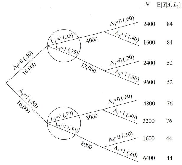
Another way to think of the g-formula is as a simulation. Under sequential exchangeability for Y and L¯ jointly, the g-formula simulates the counterfactual outcome Y ^a¯ and covariate history L¯a¯ that would have been observed if everybody in the study population had followed treatment strategy ¯a. In other

treatments was first described by Robins (1986, 1987). X

In a study with 2 time points, the g-formula for “never treat” is E [Y |A⁰ = 0, A¹ = 0, L¹ = 0] × Pr [L¹ = 0|A⁰ = 0] + E [Y |A⁰ = 0, A¹ = 0, L¹ = 1] × Pr [L¹ = 1|A⁰ = 0]

Figure 21.1

terfactuals

Y a¯ ,L¯a¯

resentation of the data in Table 21.1. Under the aforementioned identifiability condition, the g-formula can be viewed as a procedure to build a new tree in which all individuals follow strategy ¯a. For example, the causally interpreted structured tree graph in Figure 21.2 shows the counterfactual population that would have been observed if all individuals have followed the strategy “always treat” (a⁰ = 1, a¹ = 1).

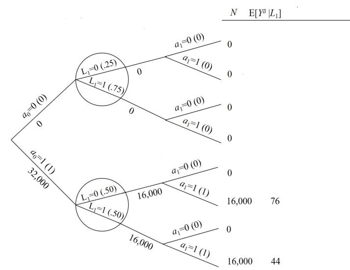
Figure 21.2

• ity, Pr [L¹ = l1|A⁰ = a0] = Pr - L a=0 ¹ = l¹ and E [Y |A⁰ = a0, A¹ = a1, L¹ = l1] = E [Y a0,a¹ |L a^{0 1} = l1].
• Thus the g-formula is P l1 E [Y a0,a¹ |L a^{0 1} = l1] Pr [L a^{0 1} = l1], which equals E [Y a0,a¹ ] as required.

To simulate this counterfactual population we (i) assign probability 1 to Under sequential exchangeabil- receiving treatment a⁰ = 1 and a¹ = 1 at times k = 0 and k = 1, respectively, and (ii) assign the same probability Pr [L¹ = l1|A⁰ = a0] and the same mean E [Y |A⁰ = a0, A¹ = a1, L¹ = l1] as in the original study population.

Two important points. First, the value of the g-formula depends on what, if anything, has been included in L. As an example, suppose we do not collect data on L¹ because we believe, incorrectly, that our study is represented by a causal diagram like the one in Figure 20.8 after removing the arrow from L¹ to A1. Thus we believe L¹ is not a confounder and hence not necessary for identification. Then the g-formula in the absence of data on L¹ becomes E [Y |A⁰ = a0, A¹ = a1] because there is no covariate history to adjust for. However, because our study is actually represented by the causal graph in Figure 20.8. (under which treatment assignment A¹ is affected by L1), the g-formula that fails to include L¹ no longer has a causal interpretation.

Second, even when the g-formula has a causal interpretation, each of its components may lack a causal interpretation. As an example, consider the causal diagram in Figure 20.9 under which only static sequential exchangeability holds. The g-formula that includes L¹ correctly identifies the mean of Y a . Remarkably, regardless of whether we add arrows from A⁰ and A¹ to Y , the gformula continues to have a causal interpretation as E [Y a¯ ], even though neither of its components—E [Y |A⁰ = a0, A¹ = a1, L¹ = l1] and Pr [L¹ = l1|A⁰ = a0] has any causal interpretation at all. That is, Pr [L¹ = l1|A⁰ = a0] ̸= Pr [L a^{0 1} = l1] and E [Y |A⁰ = a0, A¹ = a1, L¹ = l1] ̸= E [Y a0,a¹ |L a^{0 1} = l1]. The last two inequalities will be equalities in a sequential randomized trial like the one represented in Figures 20.1 and 20.2.

Treatment and covariate history When describing g-methods, we often refer to the treatment and covariate history that is required to achieve sequential exchangeability. For the g-formula, we say that its components are conditional on prior treatment and covariate history. For example, the factor corresponding to the probability of a discrete confounder L² at time k = 2

\[f\left(l\_2|\overline{A}\_1=\bar{a}\_1, \overline{L}\_1=\bar{l}\_1\right) = \Pr\left[L\_2=l\_2|A\_0=a\_0, A\_1=a\_1, L\_0=l\_0, L\_1=l\_1\right]\]

is conditional on treatment and confounders at prior times 0 and 1; the factor at time k = 3 is conditional on treatment and confounders at times 0, 1, and 2, and so on.

However, the term “history” need not be defined temporally because, as explained in Fine Point 7.4, confounders can theoretically be in the temporal future of a treatment. Conversely, as explained along with Figure 7.4, adjusting for some variables in the temporal past of treatment may introduce selection bias (referred to as M-bias). Therefore, in this book, the causally relevant “history” at time k should be understood as the set of treatments and confounders that are needed to achieve conditional exchangeability for treatment Ak. In most cases this use of history will correspond to the chronological history.

Now let us generalize the g-formula to high-dimensional settings with multiple times k. The g-formula is

\[\sum\_{\bar{l}} \to \left[ Y \vert \bar{A} = \bar{a}, \bar{L} = \bar{l} \right] \prod\_{k=0}^{K} f\left( l\_k \vert \bar{a}\_{k-1}, \bar{l}\_{k-1} \right),\]

where the sum is over all possible ¯l-histories (¯ Technical Point 21.1 shows a lk−¹ is the history through time k − 1). The sum P ¯l can also be written as P l^K …P l1 P l0 . Under sequential exchangeability for Y ^a¯ given L¯ ^k, A¯ k at each time k, this expression equals the counterfactual mean E [Y a¯ ] under treatment strategy ¯a. Fine Point 21.1 presents a more nuanced definition of the term “history”.

In practice, however, the components of the g-formula cannot be directly computed if the data are high-dimensional, as is expected in observational studies with multiple confounders or time points. The quantities E - Y |A¯ = ¯a,L¯ = ¯l and f lk|a¯k−1, ¯lk−¹ will need to be estimated. For example, we can fit a linear regression model to estimate the conditional means E - Y |A¯ = ¯a,L¯ = ¯l of the outcome variable at the end of follow-up, and logistic regression models to estimate the distribution of the discrete confounders L^k at each time k ̸= 0 (the distribution of L⁰ can be estimated without models as described in Section 13.3). The estimates from these models, ^Eb - Y |A¯ = ¯a,L¯ = ¯l and fb lk|a¯k−1, ¯lk−¹ , will then be plugged in into the g-formula. Since Chapter 13, we have referred to this estimator as the plug-in g-formula and, when the estimates used in the plug-in g-formula are based on parametric models, we have referred to the plug-in g-formula as the parametric g-formula.

For simplicity, this chapter largely focuses on the g-formula under deterministic strategies. However, under sequential exchangeability, the g-formula can be used to compute the counterfactual mean of the outcome under a random treatment strategy f int. An example of a random (static) strategy is “independently at each time k, treat individuals with probability 0.3 and do not treat with probability 0.7”, where f int 1|a¯k−1, ¯lk = 0.3. That is, f int ak|a¯k−1, ¯lk is the conditional probability of treatment a^k at time k under the treatment

more general expression for the gformula, which can be used to compute densities, not just means.

The g-formula density The g-formula density for Y,L evaluated at y, ¯l for a deterministic static strategy a¯ is

\[f\left(y|\bar{a}\_K,\bar{l}\_K\right)\prod\_{k=0}^K f\left(l\_k|\bar{a}\_{k-1},\bar{l}\_{k-1}\right).\]

The static g-formula density for Y is simply the marginal density of Y under the g-formula density for Y,L :

\[\int \dots \int f\left(y|\bar{a}\_K, \bar{l}\_K\right) \prod\_{k=0}^K dF\left(l\_k|\bar{a}\_{k-1}, \bar{l}\_{k-1}\right),\]

where the integral notation R is used to accommodate settings in which some components of L^k are continuous.

The g formula density for Y,L and for Y for a dynamic deterministic strategy g = (g0, …, gK), with g^k ak−1, l^k taking values in the support of Ak, simply replaces a^k by a g k in the above formulae. Here, a g k is recursively defined for k = 0, …, K, by a g ^k ≡ g^k a g k−1 , l^k ≡ - g0 a g −1 , l⁰ , …, g^k a g k−1 , l^k with a g −1 defined to be 0. A static strategy is the special case of a dynamic strategy when each g^k ak−1, l^k is a constant function.

In more generality, given observed data O = A, ¯ X, Y and unobserved data U, where X is the set of all measured variables other than treatment A¯ and outcome Y , the inputs of the g-formula are (i) a deterministic treatment strategy g, (ii) a causal DAG representing the observed data (and their unmeasured common causes), (iii) a subset L of X for which we wish to adjust, and (iv) a choice of a total ordering of L, A¯, and Y consistent with the topology of the DAG, i.e., an ordering such that each variable comes after its ancestors. The vector L^k consists of all variables in L after Ak−¹ and before A^k in the ordering. The chosen ordering will usually, but not always, be temporal as discussed in Fine Point 21.1. When sequential exchangeability for Y g and positivity holds for the chosen ordering, the g-formula density for Y equals the density f^{Y g} (y) that would have been observed in the study population if all individuals had followed strategy g. Otherwise, the g-formula can still be computed, but it lacks a causal interpretation. When positivity and exchangeability for Y g ,L g hold (e.g., no arrow from any variable either in U or in X but not in L directly into any treatment variable), the g-formula density for Y,L equals the density f^{Y g},L g y, l .

strategy (or intervention) f int. Then, the general g-formula expression is

\[\sum\_{\bar{a},\bar{l}} \mathrm{E}\left[Y|\bar{A}=\bar{a},\bar{L}=\bar{l}\right] \prod\_{k=0}^{K} f\left(l\_k|\bar{a}\_{k-1},\bar{l}\_{k-1}\right) \prod\_{k=0}^{K} f^{int}\left(a\_k|\bar{a}\_{k-1},\bar{l}\_k\right) \dots\]

Note this is the formula for the observed mean of Y if we replace f int ak|a¯k−1, ¯lk by the observed conditional probability of treatment f ak|a¯k−1, ¯lk .

This expression of the g-formula is general enough to accommodate both code: The gfoRmula R pack- deterministic and random strategies. Under a deterministic treatment strategy, f int ak|a¯k−1, ¯lk is always 1 for the values of a^k mandated by the strategy and 0 for the others. For example, under the strategy “never treat” or ¯a = (0, 0, …0), the probability f int 0|a¯k−1, ¯lk = 1 at all k. Since f int ak|a¯k−1, ¯lk equals 1 for the mandated values of treatment and 0 for all other values of treatment, it is not necessary to include the f int factors, or the sum over ¯a, in the above formula. Our publicly available software implements this general expression of the g-formula and therefore can accommodate any treatment strategy.

age (Lin et al. 2019) is available through CRAN. The GFORMULA SAS macro is available through GitHub. See the book’s web site.

21.2 IP weighting for time-varying treatments

Suppose we are only interested in the effect of the time-fixed treatment A¹ in Table 21.1. We then want to contrast the counterfactual mean outcomes E - Y ^a1=1 and E- Y ^a1=0 . As we have seen in Chapter 12, under the identifiability conditions, each of the counterfactual means E [Y a¹ ] is the mean Eps [Y |A¹ = a1] in the pseudo-population created by the subject-specific nonstabilized weights WA¹ = 1/f (A1|L1) or the stabilized weights SWA¹ = f (A1) /f (A1|L1). The denominator of the IP weights is, informally, an individual’s probability of receiving the treatment value that he or she received, conditional on the individual’s confounder values. One can estimate Eps [Y |A¹ = a1] from the observed study data by the average of Y among subjects with A¹ = a¹ in the pseudo-population.

When treatment and confounders are time-varying, these IP weights for time-fixed treatments need to be generalized. For a time-varying treatment A = (A0, A1) and time-varying covariates L¯ = (L0, L1) at two time points, the nonstabilized IP weights are

\[W^{\vec{A}} = \frac{1}{f\left(A\_0|L\_0\right)} \times \frac{1}{f\left(A\_1|A\_0, L\_0, L\_1\right)} = \prod\_{k=0}^{1} \frac{1}{f\left(A\_k|\vec{A}\_{k-1}, \vec{L}\_k\right)}\]

and the stabilized IP weights are

\[\left|SW\right|^{A} = \frac{f\left(A\_{0}\right)}{f\left(A\_{0}|L\_{0}\right)} \times \frac{f\left(A\_{1}|A\_{0}\right)}{f\left(A\_{1}|A\_{0},L\_{0},L\_{1}\right)} = \prod\_{k=0}^{1} \frac{f\left(A\_{k}|\bar{A}\_{k-1}\right)}{f\left(A\_{k}|\bar{A}\_{k-1},\bar{L}\_{k}\right)}\]

where A⁻¹ is 0 by definition. The denominator of the IP weights for a timevarying treatment is, informally, an individual’s probability of receiving the treatment history that he or she received, conditional on the individual’s treatment and covariate history.

Suppose we want to contrast the counterfactual means E - Y ^a0=1,a1=1 and E - Y ^a0=0,a1=0 . Under the identifiability assumptions for static strategies, each counterfactual mean E [Y a0,a¹ ] is the mean Eps [Y |A⁰ = a0, A¹ = a1] in the pseudo-population created by the nonstabilized weights WA¯ or the stabilized weights SWA¯ Similar to the result for time-fixed . That is, the IP weighted estimator of each counterfactual mean is the average of Y among individuals with A = (A0, A1) in the pseudopopulation.

Let us apply IP weighting to the data from Table 21.1. The causally interpreted structured tree graph in Figure 21.3 is the tree graph in Figure 21.1 with additional columns for the nonstabilized IP weights W^A¯ and the number of individuals in the corresponding pseudo-population N^W for each treatment and covariate history. The pseudo-population has a size of 128, 000, i.e., the 32, 000 individuals in the original population multiplied by 4, the number of static strategies. Because there is no L⁰ in this study, the denominator of the IP weights simplifies to f (A0) f (A1|A0, L1).

The IP weighted estimator for the counterfactual mean E - Y ^a0=0,a1=0 is the mean Eps [Y |A⁰ = 0, A¹ = 0] in the pseudo-population, which we estimate as the average outcome among the 32, 000 individuals with (A⁰ = 0, A¹ = 0) in the pseudo-population. From the tree in Figure 21.3, the estimate is 84× 8000 ³²⁰⁰⁰+ 52 × 24000 ³²⁰⁰⁰ = 60. Similarly, the IP weighted estimate of E - Y ^a0=1,a1=1 is also 60. Therefore the estimate of the causal effect E - Y ^a0=1,a1=1 −E - Y ^a0=0,a1=0 is 0, as expected. IP weighting, like the g-formula, succeeds where traditional methods failed.

treatment in Technical Point 12.2, Eps [Y |A⁰ = a0, A¹ = a1] equals E h W^A¯ Y I (A⁰ = a0, A¹ = a1) i = ^E[SWA¯ ^Y I(A0=a0,A1=a1)] ^E[SWA¯ I(A0=a0,A1=a1)] , for both the nonstabilized and stabilized pseudo-populations, regardless of whether sequential exchangeability holds.

when using stabilized weights SWA¯ in Figure 21.3 (check for yourself). However, Prps - A^k = 1|A¯ ^k−1,L¯ k is 1/2 in the nonstabilized pseudo-population and Prps - A^k = 1|A¯ k−1 in the stabilized pseudo-population.

Figure 21.3

siders only static strategies. For a description of IP weighting with dynamic strategies, see Technical Point 21.2.

Note that our nonparametric estimates of E [Y a0,a¹ ] based on the g-formula The same estimate of 0 is obtained are precisely equal to those based on IP weighting. This equality has nothing to do with causal inference. That is, even if the identifiability conditions did not hold—so neither the g-formula nor IP weighting estimates have a causal interpretation—both approaches would yield the same number.

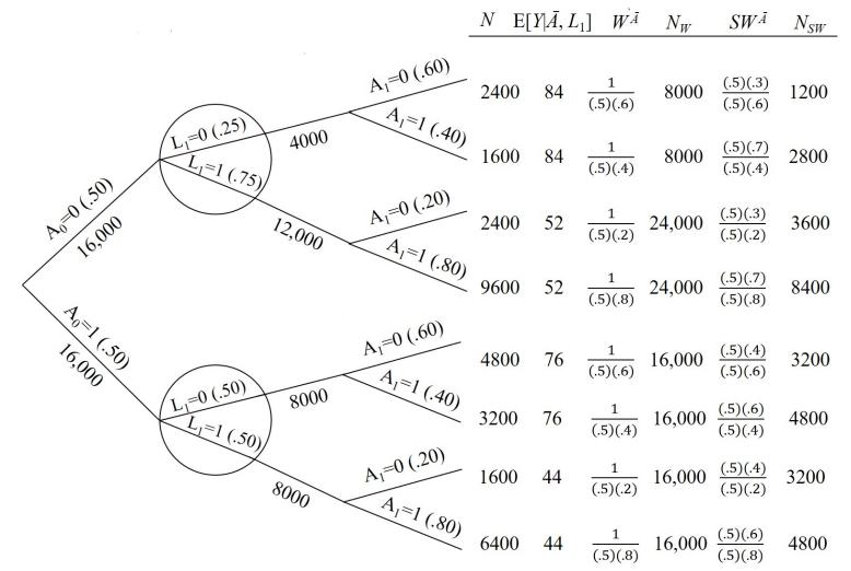
Let us generalize IP weighting to high-dimensional settings with multiple times k = 0, 1…K. The general form of the nonstabilized IP weights is

\[W^{\vec{A}} = \prod\_{k=0}^{K} \frac{1}{f\left(A\_k | \vec{A}\_{k-1}, \vec{L}\_k\right)}\]

and the general form of the stabilized IP weights is

\[SW^{\bar{A}} = \prod\_{k=0}^{K} \frac{f\left(A\_k|\bar{A}\_{k-1}\right)}{f\left(A\_k|\bar{A}\_{k-1}, \bar{L}\_k\right)}\]

When the identifiability conditions hold, these IP weights create a pseudopopulation in which (i) the mean of Y a¯ is identical to that in the actual population, but (ii) like on Figure 19.1, the randomization probabilities at each time k are the constant 1/2 (nonstabilized weights) or depend at most on past treatment history (stabilized weights). Hence the average causal effect E [Y a¯ ] − E h Y a¯ ′ i is Eps - Y |A = ¯a − Eps - Y |A = ¯a ′ Our description in the text con- because sequential unconditional exchangeability holds in both pseudo-populations.

In a true sequentially randomized trial, the quantities f Ak|A¯ ^k−1,L¯ k are known by design. Therefore we can use them to compute nonstabilized IP weights and the estimates of E [Y a¯ ] and E [Y a¯ ] − E h Y a¯ ′ i are guaranteed to be unbiased. In contrast, in observational studies, the quantities f Ak|A¯ ^k−1,L¯ k will need to be estimated from the data. When the data are high-dimensional, we can, for example, fit a logistic regression model to estimate the conditional probability of a dichotomous treatment Pr - A^k = 1|A¯ ^k−1,L¯ k at each time ^k. The estimates ^fb Ak|A¯ ^k−1,L¯ k from these models will then replace f Ak|A¯ ^k−1,L¯ k in W^A¯ . If the estimates ^fb Ak|A¯ ^k−1,L¯ k are based on a misspecified logistic model for the Pr - A^k = 1|A¯ ^k−1,L¯ k , the resulting estimates of

IP weighting for dynamic treatment strategies. Consider the deterministic dynamic strategy g = (g0, …, gK) with g^k ≡ g^k ak−1, l^k . The g-formula for an outcome Y under g equals E h Y I(A¯^K = A g K)WA¯ i , where a g ^K was defined in Technical Point 21.1. Further, E h Y I(A¯^K = A g K)WA¯ i = Eps[Y |A¯^K = A g ^K] where ^Eps[^{Y |}A¯^{K = A} g ^K] is the mean of Y among the members of the pseudo-population who follow strategy g. Unlike for static strategies, E h Y I(A¯^K = A g K)SWA¯ i /E h I(A¯^K = A g K)SWA¯ i does not equal the g-formula because the numerator of SWA¯ depends on A. Hence stabilized weights cannot be used with dynamic strategies. For a random dynamic strategy f int , the g-formula is equal to E Y Q K k=0 f int Ak|A¯ ^k−1,L¯ k WA¯ = E Y Q K k=0 f int(Ak|A¯k−1,L¯k) ^f(Ak|A¯k−1,L¯k) .

is to fit a single model for Pr - A^k = 1|A¯ ^k−1,L¯ k rather than a separate model at each time k. The model includes functions of time k—a time-varying intercept as covariates, and possibly product terms with other covariates.

model misspecification even when the estimates from both parametric approaches are similar, as they may both be biased in the same direction.

unsaturated. Remember, saturated models have an equal number of unknowns on both sides of the equation.

E [Y a¯ ] and E [Y a¯ ]−E h Y a¯ ′ i will be biased. For stabilized weights SWA¯ In practice, a common approach we must also obtain an estimate of ^fb Ak|A¯ k−1 for the numerator. Even if this estimate is based on a misspecified model, the estimates of E [Y a¯ ] and E [Y a¯ ] − E h Y a¯ ′ i remain unbiased, although ^fb(ak|ak−1) in the stabilized pseudo-population will no longer be consistent for the observed data density f (ak|ak−1).

Suppose that we obtain two estimates of E [Y a¯ ], one using the parametric g-formula and another one using IP weights estimated via parametric models, and that the two estimates differ by more than can be reasonably explained by sampling variability (the sampling variability of the difference of the estimates There is no logical guarantee of no can be quantified by bootstrapping). We can then conclude that the parametric models used for the g-formula or the parametric models used for IP weighting (or both) are misspecified. This conclusion is always true, regardless of whether the identifiability assumptions hold. An implication is that one should always estimate E [Y a¯ ] using both methods and, if the estimates differ substantially (according to some prespecified criterion), reexamine all the models and modify them where necessary. In the next section, we describe how doubly-robust estimators can help deal with model misspecification.

Also, as we discussed in the previous section, it is not infrequent that the number of unknown quantities E [Y a¯ ] far exceeds the sample size. Thus we need to specify a model that combines information from many strategies to help estimate a given E [Y a¯ ]. For example, we can hypothesize that the effect of treatment history ¯a on the mean outcome increases linearly as a function of the cumulative treatment cum (¯a) = P K k=0 a^k under strategy ¯a. This hypothesis This marginal structural model is is encoded in the marginal structural mean model

\[\operatorname{E}\left[Y^{\bar{a}}\right] = \beta\_0 + \beta\_1 cum\left(\bar{a}\right)\]

for all a, which is a more general version of the marginal structural mean model for time-fixed treatments discussed in Chapter 12. There are 2^K different unknown quantities on the left hand side of model, one for each of the 2^K different strategies ¯a, but only 2 unknown parameters β⁰ and β¹ on the right hand side. The parameter β¹ measures the average causal effect of the timevarying treatment A¯. The average causal effect E [Y a¯ ] − E h Y a¯=0 i is equal to β¹ × cum (¯a).

As discussed in Chapter 12, to estimate the parameters of the marginal

structural model, we can fit the linear regression model

\[\operatorname{E}\left[Y|\overline{A}\right] = \theta\_0 + \theta\_1 cum\left(\overline{A}\right)\]

proven that, under a correctly specified model for E - Y |A , both ordinary and weighted least squares estimates are consistent for the associational parameter θ1. This proof assumes that the weights only depend on A. When, as in our case, the weights depend on covariates L that are correlated with Y given A, the weighted regression is no longer consistent for θ1.

statistical power against the particular directions of misspecification mentioned above, especially when using the weights SWA¯ and the bootstrap to estimate the variance.

In statistics courses, it is often by ordinary least squares in either the stabilized or nonstabilized pseudopopulation. This is mathematically equivalent to fitting the same linear model by weighted least squares in the original study population, with weights SWA¯ or WA¯ , respectively (in an actual data analysis, these weights are replaced by their estimates). Under the identifiability conditions, the weighted least squares estimate of θ¹ is consistent for the causal parameter β¹ rather than for the associational parameter θ1.

As also discussed in Chapter 12, the variance of ^βb¹—and thus of the contrast E [Y a¯ ] − E h Y a¯=0 i —can be estimated by the nonparametric bootstrap or by computing its analytic variance (which requires additional statistical analysis and programming). We can also construct a conservative 95% confidence interval by using the robust variance estimator of ^βb1, which is directly outputted by most statistical software packages. For a non-saturated marginal structural model the width of the intervals will typically be narrower when the model is fit with the weights SWA¯ than with the weights WA¯ , so the SWA¯ weights are preferred.

Of course, the estimates of E [Y a¯ ] will be incorrect if the marginal structural mean model is misspecified, that is, if the mean counterfactual outcome depends on the treatment strategy through a function of the time-varying treatment other than cumulative treatment cum (¯a) (say, cumulative treatment only in the final 5 months P K k=K−5 ak) or depends nonlinearly (say, quadratically) on cumulative treatment. However, if we fit the model

\[\operatorname{E}\left[Y|\overline{A}\right] = \theta\_0 + \theta\_1 cum\left(\overline{A}\right) + \theta\_2 cum\_{-5}\left(\overline{A}\right) + \theta\_3 cum\left(\overline{A}\right)^2\]

with weights SWA¯ or WA¯ , a Wald test on two degrees of freedom of the joint This test will generally have good hypothesis θ² = θ³ = 0 is a test of the null hypothesis that our marginal structural model is correctly specified. That is, IP weighting of marginal structural models is not subject to the g-null paradox described in Technical Point 21.3. In practice, one might choose to use a marginal structural model that includes different summaries of treatment history A as covariates, and that uses flexible functions like, say, cubic splines.

Finally, as we discussed in Section 12.5, we can use a marginal structural model to explore effect modification by a subset V of the covariates in L0. For example, for a dichotomous baseline variable V , we would elaborate our marginal structural mean model as

\[\operatorname{E}\left[Y^{\bar{a}}|V\right] = \beta\_0 + \beta\_1 cum\left(\bar{a}\right) + \beta\_2 V + \beta\_3 cum\left(\bar{a}\right)V\]

The parameters of this model can be estimated by fitting the ordinary linear regression model E - Y |A, V = θ0+θ1cum A +θ2V +θ3V cum A by weighted least squares with IP weights W^A¯ or, better, SW^A¯ (V ) = Y K k=0 f Ak|A¯ ^k−1, V f Ak|A¯ ^k−1,L¯ k .

In the presence of treatment-confounder feedback, V can only include baseline variables. If V had components of L^k for k > 0 then the parameters θ1and θ³ could be different from 0 even if treatment had no effect on the mean outcome at any time.

We now describe a doubly robust estimator of the counterfactual mean E [Y g ] for any strategy g.

The g-null paradox. When using the parametric g-formula, model misspecification will result in biased estimates of E [Y a¯ ], even if the identifiability conditions hold. Suppose there is treatment-confounder feedback and the sharp null hypothesis of no effect of treatment on Y is true, i.e.,

Y ^a¯ − Y a¯ ′ = 0 with probability 1 for all a¯ ′ and a¯.

Then the value of the g-formula for E [Y a¯ ] is the same for any strategy a¯, even though E - Y |A¯ = ¯a,L¯ = ¯l and f lk|a¯k−1, ¯lk−¹ will both depend on a¯ as discussed in Chapter 20. Now suppose we use standard non-saturated parametric models E - Y |A¯ = ¯a,L¯ = ¯l; θ and f lk|a¯k−1, ¯lk−1; φ based on distinct (i.e., variation-independent) parameters θ and φ to estimate the components of the g-formula. Then Robins and Wasserman (1997) showed that, when L^k has any discrete components, these models cannot all be correctly specified because the estimated value of the g-formula for E [Y a¯ ] will generally depend on a¯. As a consequence, inference based on the estimated g-formula might theoretically result in the sharp null hypothesis being falsely rejected, even in a sequentially randomized experiment. This phenomenon is referred to as the null paradox of the estimated g-formula for time-varying treatments. For additional discussion, see Cox and Wermuth (1999) and McGrath et al. (2022). Fortunately, the g-null paradox has not prevented null parametric g-formula effect estimates in practice, presumably because the bias induced by the paradox is small compared with typical random variability.

In contrast, as described in Chapters 12 and 14, neither IP weighting of marginal structural mean models nor gestimation of structural nested mean models suffer from the null paradox. These models are correctly specified under the sharp null no matter what functional form we choose for treatment. For example, the marginal structural mean model E [Y a¯ ] = β⁰ + β1cum (¯a) is correctly specified under the null because, in that case, β¹ = 0 and E [Y a¯ ] would not depend on the function of a¯. Also, as defined in Section 21.4, any structural nested mean model γ^k ak−1, lk, β is correctly specified under the sharp null with β = 0 being the true parameter value and γ^k ak−1, lk, β = 0, regardless of the function of past treatment and covariate history.

21.3 A doubly robust estimator for time-varying treatments

two chances to get it right when, as in most observational studies, there are many confounders and non-saturated models are required.

Part II briefly mentioned doubly robust methods that combine IP weighting and the g-formula. As we know, IP weighting requires a correct model for treatment A conditional on the confounders L, and the g-formula requires a correct model for the outcome Y conditional on treatment A and the confounders L. Doubly robust methods require a correct model for either treatment A or outcome Y . If at least one of the two models is correct (and one need not know which of the two models is correct), a doubly robust estimator consistently Doubly robust estimators give us estimates the causal effect. Fine Point 13.2 described a doubly robust plugin estimator for the average causal effect of a time-fixed treatment A on an outcome Y . In this section, we first review a slightly different doubly robust plug-in estimator for time-fixed treatments and then extend it to time-varying treatments.

Suppose we want to construct a doubly robust estimator of the average causal effect E - Y ^a=1 − E - Y ^a=0 of a time-fixed binary treatment A on a binary outcome Y under exchangeability, positivity, and consistency in a setting with many confounders L. We will construct doubly robust estimators of E [Y a ] as previously discussed in Technical Points 13.2 and 13.3. The difference between doubly robust estimators for E - Y ^a=1 and for E- Y ^a=0 is a doubly robust estimator of the average causal effect. Our doubly robust procedure for E [Y a ] will use estimates of an outcome model for E[Y |A = a, L = l] and a model for Pr[A = 1|L] and then combine them appropriately. Our procedure has three steps.

The first step is to compute the predicted values ^fb(a|L) ^≡ Pr [ ^{c A = a}|L] from the treatment model. The second step is to compute the predicted values E [ ^{b Y |A =} a, L] = ^b a, L; ^θb from the maximum likelihood fit restricted to individuals with A = a of the linear logistic model b (a, L; θ) that includes Wˆ ^a = ¹/fb(a|L) as a covariate, such as ^b (a, L; ^θ) = expit θa,⁰ + θa,1L + θa,2Wˆ ^a . The third step is to estimate E - Y ^a=1 and E- Y ^a=0 as the standardized means Eb h b ¹, L; ^θb i and ^Eb h b ⁰, L; ^θb i , where E denotes the sample average over ^b all individuals, both treated and untreated. The difference ^Eb h b ¹, L; ^θb i − Eb h b ⁰, L; ^θb i is a doubly robust estimator of the causal effect E - Y ^a=1 − E - Y ^a=0 . That is, under the identifiability conditions, this estimator consistently estimates the average causal effect if either the model for the treatment is correct or the models for the outcome are correct. It is important to realize that treated and untreated individuals with the same value of L also have the same value of b ¹, L; ^θb = expit ^θb1,^{0 + θ}b1,1^{L + θ}b1,2/fb(^a = 1|L) . They also have the same value of b ⁰, L; ^θb = expit ^θb0,^{0 + θ}b0,1^{L + θ}b0,2/fb(^a = 0|L) .

Let us now extend this doubly robust estimator to settings with timevarying treatments in which we are interested in comparing the counterfactual means E [Y a¯ ] and Eh Y a¯ ′ i under two treatment strategies ¯a and ¯a ′ This doubly robust estimator is due . The doubly robust procedure to estimate E [Y a¯ ] for a time-varying treatment follows the same 3 steps as the procedure to estimate E [Y a ] for a time-fixed treatment. However, as we will see, the second step is a bit more involved because it requires the fitting of sequential regression models. To simplify notation, we show how to obtain a doubly robust estimator of E [Y a¯ ] under the treatment strategy “always treated”, i.e., ¯a = 1 where 1 = 1^K is the vector of K + 1 1’s.

The first step requires fitting a regression model π^k L¯ ^k; α for π^k L¯ k = Pr - A^k = 1|A¯ ^k−¹ = 1k−1,L¯ k pooled over all persons and times k. An individual contributes to the fit of the model at time k only if the individual has been treated (continuously) through k − 1, i.e., A¯ ^k−¹ = 1k−1. We then use predicted values π^k L¯ k; αb from this model to estimate for those individuals treated through m (A¯^m = 1m), the time-varying IP weights WA^m = Q^m k=0 1 f Ak|A¯ ^k−1,L¯ k which equals ^{W1m =} Q^m k=0 1 ^πk(L¯k) . That is, for an always-treated individual with A¯^K = 1K, we assign a different weight W^1m for each time point m rather than just the single weight W^1K at the end of follow-up as we did in the previous section. For example, if we fit the parametric model π^k L¯ ^k; α = expit (α0,k + α2Lk) for Pr - A^k = 1|A¯ ^k−¹ = 1,L¯ k , then, in our example of Table 21.1 with two time points (K = 1), the predicted values Pr ^c - A¹ = 1|A⁰ = 1,L¯ 1 and Pr [ ^{c A0} = 1|L0] are ^πb¹ = expit ( ˆα0,¹ + ˆα2L1) and ^πb⁰ = expit (ˆα0,⁰ + ˆα2L0) (because ^{A−1 ≡} 0). Here, we used the abbreviation ^πb^k for ^πk L¯ k; αb . We then compute the time-varying IP weight estimates Wˆ ^1m = Q^m k=0 1 πbk for individuals treated through m. We have reached the end of Step 1.

The second step requires fitting a separate outcome model b^m L¯m; β^m at each time m, starting from the last time K and ending at m = 0. The time m regression model is only fit to individuals treated through m and includes Wˆ ^1m = Wˆ ^Am as a covariate. The time K model has dependent variable Y . The time m model for m < K has as dependent variable the predicted outcomes from the fit of the time ^m + 1 model, i.e., ^Bb^m+1 ^{= b}bm+1 L¯m+1; βm+1 . When

to Bang and Robins (2005) and is closely related to an earlier estimator (Robins, 2000). The estimator is a targeted minimum loss-based estimator (TMLE), also known as a targeted maximum likelihood estimator, in the nomenclature later introduced by van der Laan and Rubin (2006) and van der Laan and Gruber (2012).

A K+2 robust augmented IP weighted estimator. We consider the case K = 1 as the argument generalizes to arbitrary ^K. The ICE plug-in estimator of the g-formula ^ψ is ^ψbgfor ^{= P}n[bb0(L0)], where ^Pn denotes a sample average, ^bb0(L0) = E[ ^{b b}b1(L0, L1)|A⁰ = 1, L0], and ^bb1(L0, L1) = E[ ^{b Y |}L0, A⁰ = 1, L1, A¹ = 1]. The IP weighted estimator ^ψbIPW of ^ψ is ^Pn[A0A1Y /(πb⁰πb¹))] where ^πb⁰ and ^πb¹ are estimates of ^π0 = Pr(A⁰ = 1|L0) and ^π1 = Pr(A¹ = 1 ^|L0, L1, A^{0 =} 1). Robins et al. (1994) derived an augmented IP weighted estimator ^ψbT R ^{= P}n[UbT R] of ^ψ where

\[ \hat{U}\_{TR} = A\_0 A\_1 Y / (\hat{\pi}\_0 \hat{\pi}\_1) - \frac{A\_0}{\hat{\pi}\_0} (\frac{A\_1}{\hat{\pi}\_1} - 1) \hat{b}\_1 (L\_0, L\_1) - \{\frac{A\_0}{\hat{\pi}\_0} - 1\} \hat{b}\_0 (L\_0) \]

We now show that ^ψbT R is triply (i.e., ^K + 2) robust. First, ^ψbT R is consistent (singly robust) for ^ψ if ^πb⁰ and ^πb¹ are consistent since the sample averages of the last 2 terms of ^UbT R are then consistent for ⁰ and the sample average of the first term is precisely ^ψbIPW . Second, ^ψbT R is doubly robust because ^ψbT R is consistent when E[ ^{b Y |}L0, A⁰ = 1, L1, A¹ = 1] and E[ ^{b b}1(L0, L1)^{| A0} = 1, L0] are consistent for E(^{Y |}L0, A⁰ = 1, L1, A¹ = 1) and E[b1(L0, L1)^{| A0} = 1, L0]. Here E[ ^{b b}1(L0, L1)^{| A0} = 1, L0] applies the same regression algorithm to the true ^b1(L0, L1) as was applied to ^bb1(L0, L1) to obtain ^bb0(L0). To see this, we arrange terms to obtain ^UbT R ^{= b}b0(L0)+ ^A0A^{1 π}b0πb¹ (^{Y −}bb1(L0, L1))+ ^A0 πb0 (bb1(L0, L1)−bb0(L0)). The sample averages of the last 2 terms are consistent for ⁰ and the sample average of the first term is ^ψbgfor. Third, ^ψbT R is triply robust because it is consistent if both ^bb1(L0, L1) and ^πb⁰ are consistent (Molina et al. 2017). This follows because ^UbT R can be rewritten as ^{A0 b}b1(L0, L1)/πb^{0 +} A0A^{1 π}b0πb¹ (^{Y − b}b1(L0, L1)) ⁻ A⁰ πb0 − 1 ^bb0(L0). Hence, the sample average of the last 2 terms converges to zero and the sample average of the first converges to E[b0(L⁰ )]. However it is not consistent when only ^πb¹ and E[ ^{b b}1(L0, L1)^{| A0 = a}0, L0] are consistent.

By modifying our estimator ^ψbT R we can construct a quadruply robust (i.e., ^{2 K}+1) estimator ^ψbQR that is consistent when only ^πb¹ and E[ ^{b b}1(L0, L1)^{| A0 = a}0, L0] are consistent (Tchetgen Tchetgen 2009). Let

\[ \widetilde{b}\_0(L\_0) = \widehat{\mathcal{E}}\left[\frac{A\_1 Y}{\widehat{\pi}\_1} - \left(\frac{A\_1}{\widehat{\pi}\_1} - 1\right) \: \widehat{b}\_1(L\_0, L\_1) \, | \, A\_0 = 1, L\_0\right], \]

Then ^ψbQR ^{= P}n[UbQR], where ^UbQR is ^UbT R except with ^bb0(L0) replaced by ^eb0(L0). The advantage of ^eb0(L0) over ^bb0(L0) is that ^eb0(L0) is itself doubly robust in the sense that it is consistent for ^b0(L0) = E[b1(L0, L1)^{| A0} = 1, L0] if E[ ^{b b}1(L0, L1)^{| A0} = 1, L0] is consistent for ^b0(L0) and either ^πb¹ or ^bb1(L0, L1) = E[ ^{b Y |}L0, A⁰ = 1, L1, A¹ = 1] are consistent, which implies that ^ψbQR is quadruply robust.

a logistic model b^m L¯m; β^m = expit h γmX^m + ςmWˆ ^1m i ; X^m is a vector function of covariates L¯^m and β^m = (γm, ςm). Even though ^Bb^K is not a whole number, it is guaranteed to be in [0,1] and thus can be used as the outcome variable in a logistic model. For a continuous Y , we could fit a linear regression model γmX^m + ςmWˆ ¹m.

we reach the predicted value ^Bb^{0 = b0} L¯ ⁰; ^βb For a binary Y , we could fit we have completed step 2.

In step 3 we compute our estimate of ^Eb h Y a¯=1 i as the sample average over all individuals of ^Bb⁰. If (i) the outcome models ^bm L¯m; β^m are correctly specified for all m, or (ii) the treatment models π^k L¯ ^k; α are correctly specified for all ^m, then ^Eb h Y a¯=1 i will be (asymptotically) unbiased for E h Y a¯=1 i . In that case, ^Eb h Y a¯=1 i is said to be doubly robust. However, ^Eb h Y a¯=1 i is actually multiply robust since it is also (asymptotically) unbiased for E h Y a¯=1 i if, for any m ∈ {0, 1, .., K − 1}, the treatment model is correct for times 0 to m and the outcome model is correct for times m + 1 to K. We refer to this property of the estimator as K + 2 robustness. In Technical Points 21.4 and 21.5, we explain why these robustness properties are true and we show there exist estimators with even better robustness properties than ^Eb h Y a¯=1 i . In fact, we

A plug-in K+2 robust estimator. A potential drawback of the estimator ^ψbT R of Technical Point 21.12 was that, for binary ^Y , ^ψbT R could lie outside the support [0, 1] of ^ψ in a given sample. In contrast, ^ψbgfor ^{= Pn} h ^bb0(L0) i is a plug-in estimator of ψ and always lies within [0, 1] if one estimates E[Y |L0, A⁰ = a0, L1, A¹ = a1] and b0(L0) = E[b1(L0, L1)| A⁰ = a0, L0] using (parametric or nonparametric) logistic regression models. One obtains a plug-in estimator ^ψbT R,plug ^{= Pn} h ^bb0(L0) i that is also triply robust if, for

\[ \hat{U}\_{TR} = \hat{b}\_0(L\_0) + \frac{A\_0 A\_1}{\hat{\pi}\_0 \hat{\pi}\_1} (Y - \hat{b}\_1(L\_0, L\_1)) + \frac{A\_0}{\hat{\pi}\_0} (\hat{b}\_1(L\_0, L\_1) - \hat{b}\_0(L\_0)) \]

it can be guaranteed that Pⁿ h A0A^{1 π}b0πb¹ (^{Y − b}b1(L0, L1))ⁱ and Pⁿ h A⁰ πb0 (bb1(L0, L1) ^{− b}b0(L0))ⁱ are both zero in every sample. For example, one achieves Pⁿ h A0A^{1 π}b0πb¹ (^{Y − b}b1(L0, L1))ⁱ = 0 by including a univariate term θ¹ n A0A^{1 π}b0πb¹ o in a linear logistic model for b1(L0, L1) = E [Y |L0, A⁰ = 1, L1, A¹ = 1] with dependent variable Y fit by maximum likelihood to individuals with A⁰ = A¹ = 1. One next achieves Pⁿ h A⁰ πb0 (bb1(L0, L1) ^{− b}b0(L0))ⁱ = 0 by including a term θ⁰ A⁰ πb0 in a logistic model for ^b0(L0) ^≡ E[b1(L0, L1)^{| A0 = a}0, L0] with dependent variable ^bb1(L0, L1) fit by maximizing a logistic likelihood to individuals with ^A0 = 1. The estimator E[ ^{b Y} a=1 ] given in the main text is an instance of ^ψbT R,plug.

this estimator was actually K + 2 robust. Rotnitzky et al. (2017) studied the asymptotic bias of this and other multiply robust estimator when using nonparametric and machine learning estimators of the treatment and outcome regression functions.

exhibit an estimator of E h Y a¯=1 i that is 2K+1 Molina et al. (2017) noted that robust.

To estimate the counterfactual mean E h Y a¯=0 i under the treatment strategy “never treated”, repeat the above steps using ¯a = 0 where a = 0^K is the vector of K + 1 0’s. The difference of means estimated under each strategy is a multiply robust estimator of the average causal effect E h Y a¯=1 i − E h Y a¯=0 i .

The multiply robust estimator described here can only be used to estimate the counterfactual mean E [Y a¯ ] under a static treatment strategy ¯a. Technical Point 21.6 describes a multiply robust estimator for the counterfactual mean E [Y g ] under a treatment strategy g that can be either static or dynamic and either deterministic or random. This estimator is sometimes referred to as a targeted minimum loss-based estimator (TMLE).

The implementation of multiply robust estimators has been historically hampered by computational constraints and lack of user-friendly software, especially for hazards-based survival analysis. We anticipate that, in the near future, software will become available and these multiply robust estimators (fit using machine learning and sample splitting) will become more common when studying the effect of complex treatment strategies on failure time outcomes. See Fine Point 21.2 for a description of the different representations of the g-formula and their connections to the above estimator.

21.4 G-estimation for time-varying treatments

If we were only interested in the effect of the time-fixed treatment A¹ in Table 21.1, we might have recourse to structural nested mean models for the conditional causal effect of a time-fixed treatment within levels of the covariates, as described in Chapter 14. Those models had a single equation because there was

A multiply robust estimator. Let f g am|am−1, l^m denote the treatment density at time m under strategy g. For a static a ∗ , f g am|am−1, l^m = I (a^m = a ∗ ^m); for a deterministic dynamic g, f g am|am−1, l^m = I a^m = g^m am−1, l^m ; and for a random dynamic f int , f g am|am−1, l^m = f int am|am−1, l^m . Let C g ^k = I Q^{k m}=0 f g Am|Am−1,L^m = 0 equal 0 if an individual’s observed treatment history A^k is compatible with g and 1 otherwise. The following algorithm computes a multiply robust plug-in estimator ^ψbdr,plug of ^ψ = E [^Y g ] based on one proposed by Rotnitzky et al. (2017), which is closely related to estimators by Robins (2000), Bang and Robins (2005), van der Laan and Gruber (2012), and Petersen et al. (2014).

• 1. Fit models f^m am|am−1, lm; α^m for f am|am−1, l^m for m = 0, 1…K.. Obtain the MLE αˆ^m of the vector parameter αm. For each time m, compute the weight Wˆ g,^m = Q^m k=0 f g (Ak|A¯k−1,L¯k) ^fk(Ak|A¯k−1,L¯k; ˆαk)
• 2. Set TˆK+1 = Y.
• 3. Recursively, for m = K, K − 1, …, 0.

0

1. Fit a generalized linear model b^m A¯m,L¯m; γm, ς^m = ϕ h γmd^m A¯m,L¯^m + ςmWˆ g,^m i , with ϕ an inverse canonical link, for the conditional expectation E h Tˆm+1|A¯m,L¯m, C^{g m} = 0ⁱ by iteratively reweighted least squares (IRLS) among individuals with C g ^m = 0; then (γbm,ςbm) satisfies Eb I (C g ^m = 0) dm(A¯m,L¯m) Wˆ g,m Tˆm+1 − b^{m A}¯m,L¯m; ^γbm,ςb^m = 0 (b) set Tˆ^m = P a^m b^{m a}m, ^A¯m−1,L¯m; ^γbm,ςb^m f g am|A¯m−1,L¯^m 4. ^ψbdr,plug ^{= Eb} h Tˆ i

As pointed out by Molina et al. (2017), ^ψbdr,plug is ^K + 2 robust because, in addition to being doubly robust, it is also (asymptotically) unbiased for ψ when, for any p ∈ {1, …, K}, the models b^m A¯m,L¯m; γm, ς^m are correctly specified for m ∈ {K, …, p} and the models f^m am|am−1, lm; α^m are correctly specified for m ∈ {p − 1, …, 0}.

When Wˆ g,^m is not used as a covariate, the above algorithm computes the iterative conditional expectation (ICE) estimator of the g-formula for E[Y g ] (Fine Point 21.2), which is a non-doubly robust estimator of the g-formula.

a single time point k = 0. The extension to time-varying treatments requires that the model specifies as many equations as time points in the data. For the time-varying treatment A = (A0, A1) at two time points in Table 21.1, we specify a (saturated) additive structural nested mean model with two equations

\[\begin{aligned} \text{For time } k=0 &\text{: } \operatorname{E}\left[Y^{a\_0, a\_1=0} - Y^{a\_0=0, a\_1=0} | A\_0 = a\_0 \right] = \beta\_0 a\_0\\ \text{For time } k=1 &\text{: } \operatorname{E}\left[Y^{a\_0, a\_1} - Y^{a\_0, a\_1=0} | L\_1^{a\_0} = l\_1, A\_0 = a\_0, A\_1^{a\_0} = a\_1 \right] = \beta\_1 a\_1\\ &= a\_1 \left(\beta\_{11} + \beta\_{12} l\_1 + \beta\_{13} a\_0 + \beta\_{14} a\_0 l\_1 \right) \end{aligned}\]

By consistency, the conditional expectation for time k = 1 can be written as E- Y ^a0,a¹ − Y ^a0,a1=0|L¹ = l1, A⁰ = a0, A¹ = a¹ . Since we assume sequential exchangeability for Y , we can and will replace (i) the conditional expectation for k = 0 by E- Y ^a0,a1=0 − Y ^a0=0,a1=0 since A⁰ = a⁰ can be removed from the conditioning event, and (ii) the conditional expectation for k = 1 by E - Y ^a0,a¹ − Y ^a0,a1=0|L a^{0 1} = l1, A⁰ = a⁰ since A a^{0 1} = a¹ can be removed from the conditioning event.

Representations of the g-formula. The g-formula can be mathematically represented in several ways. These different representations of the g-formula are nonparametrically equivalent but lead to different estimators in practice. Throughout this book we have emphasized a representation of the g-formula that is the generalized version of standardization (in the epidemiologic jargon). That is, the g-formula for a mean outcome is P ^l E [Y |A = a, L = l] f (l) for a time-fixed treatment and, as described in this chapter, P ¯l E - Y |A¯ = ¯a,L¯ = ¯l Q K k=0 f lk|a¯k−1, ¯lk−¹ for a time-varying treatment. Because a plug-in estimator based on this representation of the g-formula requires estimates of the joint density of the confounders Q K k=0 f lk|a¯k−1, ¯lk−¹ over time, we refer to it as a joint density modeling estimator of the g-formula. An alternative representation of the g-formula is as iterated conditional expectations. For a time-fixed treatment, we implicitly used this g-formula representation E [E [Y |A = a, L = l]] in Section 13.3. For a time-varying treatment, the

representation is an iterated conditional expectation (ICE) that can be recursively defined (Robins 1986). A plug-in estimator based on the ICE representation of the g-formula requires the fitting of sequential predictive algorithms (e.g., regression models). The ICE estimator is described in Section 21.3 and Technical Point 21.4, where we combine it with the estimation of IP weights to construct doubly (actually K + 2) robust estimators.

Another representation of the g-formula is IP weighting. In fact, as shown in Technical Point 2.3 for time-fixed treatments, the standardized mean and the IP weighted mean are equal under positivity. The same is true for timevarying treatments (Robins and Rotnitzky, 1992; Robins, 1993; Young et al., 2014). As described in this chapter, an estimator based on the IP weighting representation of the g-formula requires the estimation of the conditional density of treatment over time given past treatment and covariate history. We refer to these estimators as IP weighted estimators rather than as g-formula estimators.

• β¹¹ in individuals with A⁰ = 0, La0=0 ¹ = 0
• β¹¹ +β¹² in those with A⁰ = 0, L^a0=0 ¹ = 1
• β¹¹ +β¹³ in those with A⁰ = 1, L^a0=1 ¹ = 0
• β11+β12+β13+β¹⁴ in those with A⁰ = 1, L^a0=1 ¹ = 1

By consistency, L a^{0 1} = L¹ when A⁰ = a0.

Hence the equation at time k = 1 models the effect of treatment at time k = 1 within each of the 4 treatment and covariate histories defined by (A0, L1). This component of the model is saturated because the 4 parameters β¹ in the second equation parameterize the effect of a¹ on Y within the 4 possible levels of past treatment and covariate history. The first equation models the effect Effect of a¹ is: of treatment at time k = 0 when treatment at time k = 1 is set to zero. This component of the model is also saturated because it has one parameter β⁰ to estimate the effect within the only possible history (there is no prior treatment or covariates, so everybody has the same history). The two equations of the structural nested model are the reason why the model is referred to as nested. The first equation models the effect of receiving treatment at time 0 and never again after time 0, the second equation models the effect of receiving treatment at time 1 and never again after time 1, and so on if we had more time points.

Let us use g-estimation to estimate the parameters of our structural nested model with K = 1. We follow the same approach as in Chapter 14. We start by considering the additive rank-preserving structural nested model for each individual i

\[\begin{aligned} Y\_i^{a\_0,0} &= Y\_i^{0,0} + \psi\_0 a\_0 \\ Y\_i^{a\_0,a\_1} &= Y\_i^{a\_0,0} + \psi\_{11} a\_1 + \psi\_{12} a\_1 L\_{1,i}^{a\_0} + \psi\_{13} a\_1 a\_0 + \psi\_{14} a\_1 a\_0 L\_{1,i}^{a\_0}, \end{aligned}\]

where the second equation is restricted to individuals with A⁰ = a0. That is, the second equation is actually two equations, one for individuals with A⁰ = 1 and one for individuals with A⁰ = 0. This allows us to replace, by consistency, L a^{0 1},i by L1,i, which will be needed for identification of the model parameters from the observed data when, as in Figure 19.6, we do not have sequential exchangeability for L1. We represent Y a0=0,a1=0 i by Y 0,0 i to simplify (1994). Note that to fit an unsaturated structural nested mean model by g-estimation, positivity is not required.

the notation.

The first equation is a rank-preserving model because the effect ψ⁰ is exactly the same for every individual. Thus if Y 0,0 i for subject i exceeds Y 0,0 j for subject j, the same ranking of i and j will hold for Y ¹,0—the model preserves ranks across strategies. Also, under equation 2, if Y 1,0 i for subject i exceeds Y 1,0 j for subject j, we can only be certain that Y 1,1 i for individual i also exceeds Y 1,1 j for individual j if both have the same values a⁰ of A0,i and l¹ of L1,i = L a^{0 1},i. Because the preservation of the ranking is conditional on local factors (i.e., the value L a0=1 1 ), we refer to the second equation as a conditionally, or locally, rank-preserving model.

As discussed in Chapter 14, rank preservation is biologically implausible because of individual heterogeneity in unmeasured genetic and environmental risks. That is why our primary interest is in the structural nested mean model, which is totally agnostic as to whether or not there is additional effect The proof can be found in Robins heterogeneity across individuals due to unmeasured factors. However, given sequential exchangeability for Y , a class of g-estimators (described below) of ψ for the rank-preserving model are consistent for the parameters β of the mean model, even if the rank-preserving model is misspecified.

The first step in g-estimation is linking the model to the observed data, as we did in Chapter 14 for a time-fixed treatment. To do so, note that, by consistency, the counterfactual outcome Y a0,a¹ is equal to the observed outcome Y for individuals who happen to be treated with treatment values a⁰ and a1. Formally, Y ^a0,a¹ = Y ^A0,A¹ = Y for individuals with (A⁰ = a0, A¹ = a1). Similarly Y ^a0,⁰ = Y A0,0 for individuals with (A⁰ = a0, A¹ = 0), and L a^{0 1} = L¹ for individuals with A⁰ = a0. Now we can rewrite the structural nested model in terms of the observed data as

\[\begin{aligned} Y^{A\_0,0} &= Y - \left(\psi\_{11}A\_1 + \psi\_{12}A\_1L\_1 + \psi\_{13}A\_1A\_0 + \psi\_{14}A\_1A\_0L\_1\right), \\ Y^{0,0} &= Y^{A\_0,0} - \psi\_0A\_0 \end{aligned}\]

(we are omitting the individual index i to simplify the notation).

The second step in g-estimation is to use the observed data to compute the candidate counterfactuals H¹ ψ † and H⁰ ψ † . To do so, we use the structural nested model with the true value ψ of the parameter replaced by some value ψ † :

\[\begin{aligned} H\_1 \left( \psi^\dagger \right) &= Y - \left( \psi\_{11}^\dagger A\_1 + \psi\_{12}^\dagger A\_1 L\_1 + \psi\_{13}^\dagger A\_1 A\_0 + \psi\_{14}^\dagger A\_1 A\_0 L\_1 \right), \\ H\_0 \left( \psi^\dagger \right) &= H\_1 \left( \psi^\dagger \right) - \psi\_0^\dagger A\_0 \end{aligned}\]

As in Chapter 14, the goal is to find the value ψ † of the parameters that is equal to the true value ψ. When ψ † = ψ and Ak−¹ = ak−1, the candidate counterfactual H^k ψ † equals the true counterfactual Y ^ak−1,0^k under treatment ak−¹ through time k − 1 and treatment 0 afterwards. We can now use sequential exchangeability to conduct g-estimation at each time point. Fine Point 21.3 describes how to g-estimate the parameters ψ of our saturated structural nested model. It turns out that all parameters of the structural nested model are 0, which implies that all counterfactual means E [Y g ] under any static or dynamic strategy g are equal to 60. This result agrees with those obtained by the g-formula and by IP weighting. G-estimation, like the g-formula and IP weighting, succeeds where traditional methods failed.

In practice, however, we will encounter observational studies with multiple times k and multiple covariates L^k at each time. In general, a structural

G-estimation with a saturated structural nested model. Sequential exchangeability at k = 1 implies that, within any of the four joint strata of (A0, L1), the mean of Y A0,0 among individuals with A¹ = 1 is equal to the mean among individuals with A¹ = 0. Therefore, the means of H¹ ψ † must also be equal when ψ † = ψ.

Consider first the stratum (A0, L1) = (0, 0). From data rows 1 and 2 in Table 21.2, we find that the mean of H¹ (ψ) is 84 when A¹ = 0 and 84 − ψ¹¹ when A¹ = 1. Hence ψ¹¹ = 0. Next we equate the means of H¹ (ψ) in data rows 3 and 4 corresponding to stratum (A0, L1) = (0, 1) to obtain 52 = 52 − ψ¹¹ − ψ12. Since ψ¹¹ = 0, we conclude ψ¹² = 0. Continuing we equate the means of H¹ (ψ) in data rows 5 and 6 to obtain 76 = 76 − ψ¹¹ − ψ13. Since ψ¹¹ = ψ¹² = 0, we conclude ψ¹³ = 0. Finally, equating the means of H¹ (ψ) in data rows 7 and 8, we obtain 44 = 44 − ψ¹¹ − ψ¹² − ψ¹³ − ψ¹⁴ so ψ¹⁴ = 0 as well.

To estimate ψ0, we first substitute the values ψ11, ψ12, ψ13, and ψ¹⁴ into the expression for the mean of H⁰ (ψ) in Table 21.2. In this example, all parameters were equal to 0, so the mean of H⁰ (ψ) was equal to the mean of the observed outcome Y . We then use the first equation of the structural equation model to compute the mean of H⁰ (ψ) for each data row in the table by subtracting ψ0A⁰ from the mean of H¹ (ψ), as shown in Table 21.3. Sequential exchangeability Y ⁰,0⊥⊥A⁰ at time k = 0 implies that the means of H⁰ (ψ) among the 16, 000 subjects with A⁰ = 1 and the 16, 000 subjects with A⁰ = 0 are identical. The mean of H⁰ (ψ) is 84 × 0.25 + 52 × 0.75 = 60 among individuals with A⁰ = 0, (76 − ψ0) × 0.5 + (44 − ψ0) × 0.5 = 60 − ψ⁰ among individuals with A⁰ = 1. Hence ψ⁰ = 0. We have completed g-estimation.

	Table 21.2

A0	L1	A1	Mean H1 (ψ)
0	0	0	84
0	0	1	84 − ψ1,1
0	1	0	52
0	1	1	52 − ψ11 − ψ12
1	0	0	76
1	0	1	76 − ψ11 − ψ13
1	1	0	44
1	1	1	44 − ψ11 − ψ12
			−ψ13 − ψ14

Table 21.3
A0	L1	A1	Mean H0 (ψ)
0	0	0	84
0	0	1	84
0	1	0	52
0	1	1	52
1	0	0	76 − ψ0
1	0	1	− 76 ψ0
1	1	0	44 − ψ0
1	1	1	− 44 ψ0

γk ak−1, lk, 0 = 0 so β = 0 under the null hypothesis of no effect of treatment.

nested mean model has as many equations as time points k = 0, 1…K. The most general form of structural nested mean models that we discuss in the main text is the following (even more general structural nested mean models are discussed in Technical Point 21.13). For each time k = 0, 1…K,

\[\begin{aligned} \mathrm{E}\left[Y^{\overline{a}\_{k-1},a\_k}\underline{\emptyset}\_{k+1} - Y^{\overline{a}\_{k-1},\underline{\emptyset}\_k}|\overline{L}\_k^{\overline{a}\_{k-1}} = \overline{l}\_k, \overline{A}\_{k-1} = \overline{a}\_{k-1}, A\_k = a\_k\right] \\ &= a\_k \gamma\_k\left(\overline{a}\_{k-1}, \overline{l}\_k, \beta\right) \end{aligned}\]

where ak−1, ak, 0k+1 is a static strategy that assigns treatment ak−¹ between times 0 and k−1, treatment a^k at time k, and treatment 0 from time k = 1 until the end of follow-up K. The strategies ak−1, ak, 0k+1 and (ak−1, 0^k ) differ only in that the former has treatment a^k at k while the latter has treatment 0 at time k. Here each γ^k ak−1, lk, ψ† is a known function of a parameter vector ψ † such that γ^k ak−1, lk, ψ† = 0 = 0 and β is the true value of ψ † . Again, under sequential exchangeability for Y , we can drop A^k = a^k from the above conditioning event. In our example with K = 1, γ⁰ a⁻1, l0, β is just β⁰ (l⁰ and a⁻¹ can both be taken to be identically 0) and γ¹ a0, l1, β is β¹¹ + β12l¹ + β13a⁰ + β14a0l1.

Thus, a structural nested mean model is a model for the effect on the mean of Y of a last blip of treatment of magnitude a^k at k, as a function γk ak−1, lk, β of past treatment and covariate history ak−1, l^k . See Technical Point 21.7 for the relationship between structural nested models and marginal structural models.

We are now ready to discuss estimation of the parameters of a general structural nested mean model with blip funcion γ^k ak−1, lk, β This blip function satisfies . To motivate our estimation procedure, we will use the fact that a correctly specified locally rank preserving model with true parameter ψ is also a correctly specified structural nested mean model with true parameter β = ψ (though the converse is

Marginal structural models and structural nested models. A structural nested mean model is a semiparametric marginal structural mean model if and only if, for all ak−1, lk, β ,

\[\gamma\_k \left( \overline{a}\_{k-1}, \overline{l}\_k, \beta \right) = \gamma\_k \left( \overline{a}\_{k-1}, \beta \right)\]

does not depend on lk. Specifically, it is a semiparametric marginal structural mean model with the functional form

\[\operatorname{E}\left[Y^{\overline{a}}\right] = \alpha\_0 + \sum\_{k=0}^{K} a\_k \gamma\_k \left(\overline{a}\_{k-1}, \beta\right),\]

where ^a0 = E^h Y 0^K i is an unknown constant. However, such a structural nested mean model is not simply a marginal structural mean model, because it also imposes the additional strong assumption that effect modification by past covariate history is absent. In contrast, a marginal structural model is agnostic as to whether there is effect modification by time-varying covariates.

If we specify a structural nested mean model γ^k (ak−1, β), then we can estimate β either by g-estimation or IP weighting. However the most efficient g-estimator will be more efficient than the most efficient IP weighted estimator when the structural nested mean model (and thus the marginal structural mean model) is correctly specified, because g-estimation uses the additional assumption of no effect modification by past covariates to increase efficiency.

In contrast, suppose the marginal structural mean model is correct but the structural nested mean model is incorrect because γ^k ak−1, lk, β ̸= γ^k (ak−1, β). Then the g-estimates of β and E - Y a will be biased, while the IP weighted estimates remain unbiased. Thus we have a classic variance-bias trade off. Given the marginal structural model, g-estimation can increase efficiency if γ^k ak−1, lk, β = γ^k (ak−1, β), but introduces bias otherwise.

not true). Given a structural nested mean model, we can define

\[H\_k\left(\psi^\dagger\right) = Y - \sum\_{j=k}^K A\_j \gamma\_j\left(\overline{A}\_{j-1}, \overline{L}\_j, \psi^\dagger\right),\]

A correctly specified locally rank preserving model with true parameter vector ψ is equivalent to the statement that H^k (ψ) is exactly equal to the counterfactual Y ^Ak−1,0^k in which the effects of the treatments from time j through K have been removed. In particular, H⁰ (ψ) is the value of Y ⁰ under no treatment.

However, if the assumption of local rank preservation is incorrect (as will essentially always be the case if there is a treatment effect) but the structural nested mean model is correct, we still have that E - H^k (β)|Ak,L^k equals E h Y ^Ak−1,0^k |Ak,L^k i and that E [H⁰ (β)] equals E ^h Y 0 i . Thus, E h Y 0 i can be consistently estimated as the sample average of H⁰ βb if we obtain a consistent estimator of ^βb. This is what g-estimation provides.

With multiple time points or covariates, we will need to fit an unsaturated structural nested mean model. For example, we might hypothesize that the function γ^k ak−1, lk, β is the same for all k. The simplest model would be γk ak−1, lk, β = β1, which assumes that the effect of a last blip of treatment is the same for all past histories and all times k. Other options are β¹ + β2k, which assumes that the effect varies linearly with the time k of treatment, and β¹ + β2k + β3ak−¹ + β4l^k + β5lkak−1, which allows the effect of treatment at k to be modified by the most recent treatment and covariate values.

and time) the value of H^k ψ † for each ψ † on a grid from ψlow to ψup, say ψlow, ψlow + 0.1, ψlow + 0.2, …, ψup. Then, for each value of ψ † , we will fit a pooled (over time) logistic regression

model

\[\text{logit}\,\text{Pr}\left[A\_k = 1 | H\_k\left(\psi^\dagger\right), \overline{L}\_k, \overline{A}\_{k-1}\right] = \alpha\_0 + \alpha\_1 H\_k\left(\psi^\dagger\right) + \alpha\_2 W\_k\]

for the probability of treatment at time k for k = 0, …, K. Here W^k = w^k Lk, Ak−¹ is a vector of covariates calculated from an individual’s covariate and treatment data Lk, Ak−¹ , α² is a row vector of unknown parameters, and each person contributes K + 1 observations. The g-estimate of β is the grid value of ψ † The limits of the 95% confidence for which the estimate of α¹ is closest to 0. We can eliminate the need to search over the grid by defining the estimate ^βb to be the value of ψ † such that the p-value of the score test of ^α1 = 0 is equal to 1. That is ^βb is the value of ψ † that solves

\[\sum\_{i=1,k=0}^{i=N,k=K} \left\{ A\_i - \text{expit} \left( \widehat{\alpha}\_0 + \widehat{\alpha}\_2 W\_{i,k} \right) \right\} H\_{i,k} \left( \psi^\dagger \right) = 0\]

where ^αb⁰ and ^αb² are obtained by fitting the above logistic model with the term ^α1 set to 0. Standard equation solvers can be used. The estimator ^βb will be consistent if (i) the structural nested mean model is correct, (ii) sequential exchageability for Y holds, (iii) the model logit Pr - A^k = 1|Lk, Ak−¹ = α⁰ + α0W^k is correct, and (iv) H^k ψ † enters the above logistic model linearly (i.e., as H^k ψ † ) rather than as H^k ψ † ² or any other non-linear function (see Technical Point 14.2).

The procedure described above is the generalization to time-varying treatments of the g-estimation procedure described in Chapter 14. For simplicity, we considered a structural nested model with a single parameter β1, which implies that the effect does not vary over time k or by treatment and covariate history. Suppose now that the parameter β is a vector. To be concrete suppose we consider the model with γ^k ak−1, lk, β = β⁰ + β1k + β2ak−¹ + β3l^k + β4lkak−¹ so β is 5-dimensional and l^m is 1-dimensional. Now to estimate 5 parameters one requires 5 additional covariates in the treatment model. For example, we could fit the model logit Pr - A^k = 1|H^k ψ † ,Lk, Ak−¹ =

\[\left(\alpha\_0 + H\_k\left(\psi^\dagger\right)\right)\left(\alpha\_1 + \alpha\_2k + \alpha\_3 A\_{k-1} + \alpha\_4 L\_k + \alpha\_5 L\_k A\_{k-1}\right) + \alpha\_6 W\_k\]

A 95% joint confidence interval for The particular choice of covariates does not affect the consistency of the point estimate of β, but it determines the width of its confidence interval.

The earlier g-estimation procedure then requires a search over a 5-dimensional grid, one dimension for each component β^j of β. So if we had 20 grid points for each component we would have 20⁵ different values of β on our 5 dimensional grid. However, when the dimension of β is greater than 2, finding the g-estimate ^βb by a grid search may be computationally difficult. In that case we can eliminate the need to search over the grid by defining the g-estimate ^βb to be the

interval for ψ are the limits of the set of values ψ † that result in a Pvalue > 0.05 when testing for α¹ = 0.

β^j are the set of values for which the 5 degree-of-freedom score test does not reject at the 5% level. A less computationally demanding approach is the univariate 95% Wald confidence intervalβb^{j ± 1}.⁹⁶ times its standard error.

A closed form estimator for linear structural nested mean models. When, as in all the examples we have discussed, γk Ak−1,Lk, β = β ^T R^k is linear in β with R^k = r^k L¯ ^k, A¯ k−1 being a vector of known functions, then, given the model logit Pr - A^k = 1|Lk, Ak−¹ = α ^{T W}k, there is an explicit closed form expression for ^βb given by

\[\widehat{\beta} = \left\{ \sum\_{i=1, k=0}^{i=N, k=K} A\_{i,k} X\_{i,k} \left( \widehat{\alpha} \right) Q\_{i,k} S\_{i,k}^T \right\}^{-1} \left\{ \sum\_{i=1, k=0}^{i=N, k=K} Y\_i X\_{i,k} \left( \widehat{\alpha} \right) Q\_{i,k} \right\}\]

with ^Xi,k (αb) = - Ai,k − expit αb ^T Wi,k, Si,k = Pⁱ=N,j=^{K i}=1,j=^k Ri,j , and the choice of dimension-β functions Qi,k = qk L¯ i,k, A¯ i,k−1 affects efficiency but not consistency. See Robins (1994) for the optimal choice of Qk.

In fact, when γ^k ak−1, lk, β is linear in β, we can obtain a closed-form 2 ^K+1 multiply robust estimator ^βe of ^β by specifying a working model ς ^T D^k = ς ^T d^k L¯ ^k, A¯ k−1 for E - H^k (β)|L¯ ^k, A¯ k−1 = Eh Y ^Ak−1,0^k |L¯ ^k, A¯ k−1 i and defining

\[\left( \begin{array}{c} \widetilde{\beta} \\ \widetilde{\varsigma} \end{array} \right) = \left\{ \sum\_{i=1, k=0}^{i=N, k=K} \left( \begin{array}{c} A\_{i,k} X\_{i,k} \left( \widehat{\alpha} \right) Q\_{i,k} \\ D\_{i,k} \end{array} \right) \left( S\_{i,k}^T, D\_{i,k}^T \right) \right\}^{-1} \left\{ \sum\_{i=1, k=0}^{i=N, k=K} Y\_i \left( \begin{array}{c} X\_{i,k} \left( \widehat{\alpha} \right) Q\_{i,k} \\ D\_{i,k} \end{array} \right) \right\}\]

Specifically, ^βe will be a consistently asymptotically normal estimator of ^ψ if, for each ^k, either the model ^{ς T} D^k for E h Y ^Ak−1,0^k |L¯ ^k, A¯ k−1 i is correct or the model for logit Pr - A^k = 1|Lk, Ak−¹ is correct.

value of ψ † such that the p-value of the score test of α1−⁵ = (α1, …, α5) ^T = 0 is equal to 1. That is ^βb is the value of ^ψ † that solves the 5 dimensional estimating equation

\[\sum\_{i=1,k=0}^{i=N,k=K} \left\{ A\_i - \text{expit}\left(\hat{\alpha}\_0 + \hat{\alpha}\_6^T W\_{i,k}\right) \right\} H\_{i,k}\left(\psi^\dagger\right) \left(1, k, A\_{i,k-1}, L\_{i,k}, L\_{i,k} A\_{i,k-1}\right)^T = 0\]

where ^αb⁰ and ^αb⁶ are obtained by fitting the above logistic model with ^α1−⁵ set to zero. Standard equation solvers can be used. Indeed, the solution ^βb to this last equation exists in closed form when, as in all examples discussed in this section, the structural nested mean model is linear in β. See Technical Point 21.8, which also describes a multiply robust form of the estimator.

Given a consistent g-estimator ^βb of the parameters of the structural nested mean model, the last step is the estimation of the counterfactual mean E [Y g ] under the strategies g of interest. As discussed earlier, E h Y 0 i can be consistently estimated by the sample average ^Eb h H⁰ βb i . If there is no effect modification by past covariate history, i.e., γ^k ak−1, lk, β = γ^k (ak−1, β) then E - Y a under a static strategy a is estimated as

\[ \triangle \left[ Y^{\overline{\pi}} \right] = \widehat{\mathbf{E}} \left[ Y^{\overline{\mathbb{D}}\_K} \right] + \sum\_{k=0}^K a\_k \gamma\_k \left( \overline{a}\_{k-1}, \widetilde{\boldsymbol{\beta}} \right), \]

On the other hand, if the structural nested mean model depends on L^k or we want to estimate E [Y g ] under a dynamic strategy g, then we need to simulate the L^k using the algorithm described in Technical Point 21.9.

Estimation of E [Y g ] after g-estimation of a structural nested mean model. Suppose the identifiability assumptions hold, one has obtained a doubly robust g-estimate ^βe of a structural nested mean model ^γk ak−1, lk, β and one wishes to estimate E [Y g ] under a dynamic strategy g. To do so, one can use the following steps of a Monte Carlo algorithm:

• 1. Estimate the mean response E h Y 0^K i had treatment always been withheld by the sample average of H⁰ βe over the ^N study subjects. Call the estimate ^Eb h Y 0^K i .
• 2. Fit a parametric model for f lk|a¯k−1, ¯lk−¹ to the data, pooled over persons and times, and let ^fb lk|a¯k−1, ¯lk−¹ denote the estimate of f lk|a¯k−1, ¯lk−¹ under the model.
• 3. Do for v = 1, …, V ,
  • 1. Draw ^lv,⁰ from ^fb(l0).
  • 2. Recursively for ^k = 1, …, K draw ^lv,k from ^fb lk|a¯v,k−1, ¯lv,k−¹ with a¯v,k−¹ = gk−¹ lv,k−¹ , the treatment history corresponding to the strategy g.

\[\begin{aligned} \text{(c) Let } \hat{\Delta}\_{g,v} &= \sum\_{j=0}^{j=K} a\_{v,j} \gamma\_j \left( \overline{a}\_{v,j-1}, \overline{l}\_{v,j}, \hat{\beta} \right) \text{ be the } v^{th} \text{ Monte Carlo estimate of } Y^g - Y^{\overline{0}\_K}, \text{ where } a\_{v,j} = g\_{v,j}(\overline{l}\_{v,j-1}). \end{aligned}\]

4. Let E [ ^{b Y} g ] = ^Eb h Y 0^K i + vX=V v=1 ^∆b g,v/V be the estimate of E [ ^{b Y} g ] .

If the model for f lk|a¯k−1, ¯lk−¹ , the structural nested mean model γ^k ak−1, lk, β , and either the treatment model Pr - A^k = 1|Lk, Ak−¹ or the outcome model E h Y ^Ak−1,0^k |L¯ ^k, A¯ k−1 i are correctly specified, then E [ ^{b Y} g ] is consistent for E [Y g ]. Confidence intervals can be obtained using the nonparametric bootstrap.

Note that γ^{k a}k−1, ^lk, ^βe will converge to ⁰ if the estimate ^βe is consistent for ^β = 0. Thus ^∆b g,v will converge to zero and E [ ^{b Y} g ] to ^Eb h Y 0^K i even if the model for f lk|a¯k−1, ¯lk−¹ is incorrect. That is, the structural nested mean model preserves the null if the identifiability conditions hold and we either know (as in a sequentially randomized experiment) Pr - A^k = 1|Lk, Ak−¹ or have a correct model for either Pr - A^k = 1|Lk, Ak−¹ or E h Y ^Ak−1,0^k |L¯ ^k, A¯ k−1 i for each k.

21.5 Censoring is a time-varying treatment

You may want to re-read Section Throughout this chapter we have used an example in which there is no cen-12.6 for a refresher on censoring. soring: the outcomes of all individuals in Table 21.1 are known. In practice, however, we will often encounter situations in which some individuals are lost to follow-up and therefore their outcome values are unknown or (right-)censored. We have discussed censoring and methods to handle it in Part II of the book. In Chapter 8, we showed that censoring may introduce selection bias, even under the null. In Chapter 12, we discussed how we are generally interested in the causal effect if nobody in the study population had been censored.

However, in Part II we only considered a greatly simplified version of censoring under which we did not specify when individuals were censored during the follow-up. That is, we considered censoring C as a time-fixed variable. A more realistic view of censoring is as a time-varying variable C1, C2, …CK+1,

(C = 0) induces selection bias under the null when C is either a collider on a pathway between treatment A and the outcome Y , or the descendant of one such collider.

makes it explicit the causal contrast that many have in mind when they refer to the causal effect of treatment A¯, even if they choose not to use the superscript c¯ = ¯0.

The estimated IP weights SW^C¯ have mean 1 when the model for Pr C^k = 0|A¯ ^k−1, Ck−¹ = 0,L¯ k is correctly specified.

Conditioning on being uncensored where C^m is an indicator that takes value 0 if the individual remains uncen sored at time m and takes value 1 otherwise. Censoring is a monotonic type of missing data, i.e., if an individual’s C^m = 0 then all previous censoring indicators are also zero (C¹ = 0, C² = 0….Cm−¹ = 0). Also, by definition, C⁰ = 0 for all individuals in a study; otherwise they would have not been included in the study.

If an individual is censored at time m, i.e., when C^m = 1, then treatments, confounders, and outcomes measured after time m are unobserved. Therefore, the analysis becomes necessarily restricted to uncensored person-times, i.e., those with C^m = 0. For example, the g-formula for the counterfactual mean outcome E [Y a¯ ] from section 21.1 needs to be rewritten as

\[\sum\_{\bar{l}} \to \left[ Y \middle| \bar{C} = \bar{0}, \bar{A} = \bar{a}, \bar{L} = \bar{l} \right] \prod\_{k=0}^{K} f\left( l\_k | c\_k = 0, \bar{a}\_{k-1}, \bar{l}\_{k-1} \right),\]

with all the terms being conditional on remaining uncensored.

Suppose the identifiability conditions hold with treatment A^m replaced by (Am, Cm+1) at all times m. Then it is easy to show that the above expression corresponds to the g-formula for the counterfactual mean outcome E - Y a, ¯ c¯=¯0 The use of the superscript c¯ = ¯0 under the joint treatment (¯a, c¯ = ¯0), i.e., the mean outcome that would have been observed if all individuals have received treatment strategy ¯a and no individual had been lost to follow-up.

The counterfactual mean E - Y a, ¯ c¯=¯0 can also be estimated via IP weighting of a structural mean model when the identifiability conditions hold for the joint treatment A, ¯ C¯ . To estimate this mean, we might fit, e.g., the outcome regression model

\[\operatorname{E}\left[Y|\overline{A},\bar{C}=\bar{0}\right] = \theta\_0 + \theta\_1 cum\left(\overline{A}\right)\]

to the pseudo-population created by the nonstabilized IP weights WA¯ × WC¯ where

\[W^{\bar{C}} = \prod\_{k=1}^{K+1} \frac{1}{\Pr\left(C\_k = 0 | C\_{k-1} = 0, \bar{A}\_{k-1}, \bar{L}\_{k-1}\right)}\]

We estimate the denominator of the weights by fitting a logistic regression model for Pr C^k = 0|Ck−¹ = 0, A¯ ^k−1,L¯ k−1 . Technical Point 21.10 shows the extension to survival analysis with a failure time outcome.

In the pseudo-population created by the nonstabilized IP weights, the censored individuals are replaced by copies of uncensored individuals with the same values of treatment and covariate history. Therefore the pseudopopulation has the same size as the original study population before censoring, that is, before any losses to follow-up occur. The nonstabilized IP weights abolish censoring in the pseudo-population.

Or we can use the pseudo-population created by the stabilized IP weights SW^A¯ × SW^C¯ Remember: , where

\[SW^{\bar{C}} = \prod\_{k=1}^{K+1} \frac{\Pr\left(C\_k = 0 | C\_{k-1} = 0, \bar{A}\_{k-1}\right)}{\Pr\left(C\_k = 0 | C\_{k-1} = 0, \bar{A}\_{k-1}, \bar{L}\_{k-1}\right)}\]

We estimate the denominator and numerator of the IP weights via two separate models for Pr C^k = 0|Ck−¹ = 0, A¯ ^k−1,L¯ k−1 and Pr C^k = 0|Ck−¹ = 0, A¯ k−1 , respectively.

The pseudo-population created by the stabilized IP weights is of the same size as the original study population after censoring, i.e., the proportion of

Survival analysis with time-varying treatments. Chapter 17 describes g-methods to estimate the effect of point interventions on failure time outcomes. This chapter describes g-methods to estimate the effect of sustained strategies on non-failure time outcomes. In practice, we often use g-methods to estimate the effect of sustained strategies on failure time outcomes by combining the methods described in Chapter 17 with those in this chapter. Below we sketch two approaches, based on the g-formula and on IP weighting, to estimate the counterfactual risk Pr h D a, ¯ c¯=¯0 ^k+1 = 1ⁱ under treatment strategy a¯ if sequential exchangeability, positivity, and consistency hold. The causal diagram in Figure 21.4 depicts such setting with two time points and the failure time outcome represented by time-varying indicators as in Chapter 17. From each indicator D^k there should be arrows into all future variables on the graph, but we omitted these arrows to reduce clutter. For simplicity, we also omitted the time-varying indicators for censoring.

The risk Pr h D a, ¯ c¯=¯0 ^k+1 = 1ⁱ is identified by 1 minus the g-formula for Pr h D a, ¯ c¯=¯0 ^k+1 = 0ⁱ :

\[\begin{aligned} \sum\_{\bar{l}\_k} \Pr\left[D\_{k+1} = 0 | \bar{A}\_k = \bar{a}\_k, \bar{L}\_k = \bar{l}\_k, D\_k = C\_{k+1} = 0\right] \times \\ \prod\_{m=0}^k f\left(l\_m | \bar{a}\_{m-1}, \bar{l}\_{m-1}, D\_m = C\_m = 0\right) \Pr\left[D\_m = 0 | \bar{A}\_{m-1} = \bar{a}\_{m-1}, \bar{L}\_{m-1} = \bar{l}\_{m-1}, D\_{m-1} = C\_m = 0\right] \dots \end{aligned}\]

A plug-in g-formula estimate can then be obtained by fitting models for the discrete-time hazards Pr - Dk+1 = 1|A¯ ^k = ¯ak,L¯ ^k = ¯lk, D^k = Ck+1 = 0 and for the conditional density f lk|a¯k−1, ¯lk−1, D^k = C^k = 0 of the confounders L over time. As described in Chapter 17, a pooled logistic model can be used to approximate the hazards. See Young et al. (2011) for details and an application. Wen et al. (2021) describe ICE g-formula estimators.

An alternative is to fit a pooled logistic model for the hazards Pr - Dk+1 = 1|A¯ ^k = ¯ak,L¯ ^k = ¯lk, D^k = Ck+1 = 0 in which each individual at time k receives the time-varying nonstabilized IP weight WA¯ ^{k × W}C¯ k , where

\[W\_k^{\bar{A}} = \prod\_{m=0}^k \frac{1}{f\left(A\_m | \bar{A}\_{m-1}, D\_m = C\_m = 0, \bar{L}\_m\right)}, \quad W\_k^{\bar{C}} = \prod\_{m=1}^k \frac{1}{\Pr\left(C\_m = 0 | \bar{A}\_{m-1}, D\_{m-1} = C\_{m-1} = 0, \bar{L}\_{m-1}\right)},\]

or its corresponding stabilized IP weight at each time k. The parameters of that model estimate the parameters of a marginal structural pooled logistic model for Pr h D a, ¯ c¯=¯0 ^k+1 = 1|D a, ¯ c¯=¯0 ^k = 0ⁱ (Robins 1998a). For details and an application, see Hern´an et al. (2001). Wen et al. (2022) review multiply robust estimators for survival analysis with time-varying treatments.

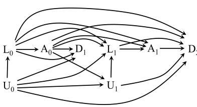
Figure 21.4

censored individuals in the pseudo-population is identical to that in the study population at each time k. The stabilized weights do not eliminate censoring in the pseudo-population, they make censoring occur at random at each time k with respect to the measured covariate history L¯ ^k. That is, there is selection but no selection bias. Regardless of the type of IP weights used, in the pseudo-population there are no arrows from L^k and A^k into future C^m for m > k. Importantly, under the exchangeability conditions for the joint treatment A, ¯ C¯ , IP weighting can unbiasedly estimate the joint effect of A, ¯ C¯ even when some components of L¯ are affected by prior treatment.

Finally, when using g-estimation of structural nested models, we first need to adjust for selection bias due to censoring by IP weighting. In practice, this means that we first estimate nonstabilized IP weights W^C¯ for censoring to create a pseudo-population in which nobody is censored, and then apply g-estimation to the pseudo-population.

21.6 The big g-formula

This chapter and the previous two chapters privilege methods that rely on sequential exchangeability given the measured covariates L and identification by the g-formula. The reason is that, in practice, few causal analyses of complex longitudinal data have relied on other identifying conditions and formulas. For example, there are few realistic applications based on the identifying conditions under which the front door formula is the identifying formula. However, regardless of substantive plausibility and practical applications, different identifying conditions and their formulas are mathematically linked to sequential exchangeability and the g-formula based on all variables—both measured and unmeasured—as we now explain.

When sequential exchangeability holds given the measured covariates L, we have discussed how the g-formula based on the measured time-varying covariates L identifies causal effects of a time-varying treatment A on an outcome Y . Now suppose we have a causal DAG with both observed variables A,L, Y and unobserved variables U, and that the measured variables L are insufficient to achieve sequential exchangeability.

For any causal DAG, the combination of measured and unmeasured variables X = (L,U) ensures (joint) sequential exchangeability as any parent of a treatment variable is contained in either A or X. Therefore, if every variable on a causal diagram were measured and positivity held, the g-formula based on X would identify the counterfactual mean E [Y g ] under any treatment strategy g. We refer to the g-formula with L replaced by X as the big g-formula because it is not based solely on the observed data.

Given a causal DAG, treatment A and outcome Y , a treatment strategy g, and factuals A,L, Y, U We refer to , we can explicitly write down the big g-formula for the distribution (density) of Y g . The big g-formula depends only on the distribution of the factuals A,L, Y, U .

The big g-formula is the right formula to identify the counterfactual density under any treatment strategy, but the big g-formula cannot be used in practice because it includes unmeasured variables. An interesting math question is then: can the big g-formula be reduced to a functional of the joint distribution of the observed data A,L, Y ? If it can, then we will have a new formula that is not expressed as a g-formula but that (i) reproduces the results of the big g-formula (and therefore is a correct formula) and (ii) is written in terms of the distribution of the observed variables only (and therefore is a formula that can be used in data analyses).

For example, under the identifying conditions referred to as the front door criterion, the big g-formula for E[Y a ] reduces to a formula that only includes observed variables—the front door formula (see the proof in Technical Point 21.11). Therefore, the front door formula is a valid formula for the mean of E [Y a ] under the front door assumptions embedded in the causal diagram of Figure 7.14.

More generally, we would like to be able to answer the following two ques-These questions were completely tions. First, can we always determine whether the big g-formula can be rewritten as a formula that depends only on the distribution of the observed variables A,L, Y , while making no assumptions other than the joint distribution of A,L, Y, U obeys the d-separation relations implied by the causal DAG? Second, when the answer to the previous question is yes, can we explicitly display such an identifying formula? Both of these questions have been answered in the affirmative.

Importantly, these are purely mathematical questions about properties of

A,L, Y,U as factuals to distinguish them from counterfactuals. Factuals are variables that exist in the actual world. In contrast to the observed variables, some factuals, such as U, are not available for data analysis, often because they were not measured.

settled by the work of Tian and Pearl (2002), Shpitser and Pearl (2006), and Huang and Valtorta (2006).

A big g-formula proof of the front door formula. In Technical Point 7.4, we provided a proof of the front door formula for the counterfactual probability Pr [Y ^a = y] under the causal diagram of Figure 7.14. Here we provide another proof using the big g-formula. This second proof relies on the conditional independencies implied by Figure 7.14, but it does not require that the counterfactuals Y ^m exist.

The big g-formula for Pr [Y ^a = y] under Figure 7.14 is

\[\sum\_{m} \sum\_{u} \Pr[Y = y | M = m, A = a, U = u] \Pr[M = m | A = a, U = u] \Pr[U = u].\]

Since data on U are not available, Pr [Y ^a = y] is identified if and only if the big g-formula depends exclusively on the distribution of the observed data (Y, M, A). We now show that is indeed the case because, under the above assumptions, the g-formula reduces to the front door formula.

P Using d-separation, we can rewrite the big g-formula as ^m Pr[M = m|A = a] P ^u Pr[Y = y|M = m, U = u] { P ^a′ Pr[U = u|A = a ′ ] Pr[A = a ′ ]} by U⊥⊥M|A and A⊥⊥Y |M, U = P ^m Pr[M = m|A = a] P ^a′ { P ^u Pr[Y = y|M = m, A = a ′ , U = u] Pr[U = u|M = m, A = a ′ ]}Pr[A = a ′ ] by U⊥⊥M|A and A⊥⊥Y |M, U ′ ′

= P ^m Pr[M = m|A = a] P ^a′ Pr[Y = y|M = m, A = a ] Pr[A = a ], which is the front door formula.

We now provide yet another proof of the front door formula that also does not require that the counterfactuals Y m exist. After establishing that Pr [Y ^a = y] is a function of the distribution of (Y, M, A, U) given by the big g-formula, we can apply a coupling argument. Suppose all agree on substantive grounds that a well-defined Y ^m does not exist. Yet any factual data distribution that is Markov with respect to Figure 7.14 is compatible with an underlying FFRCISTG model “as detailed as the data”(Robins and Richardson, 2010) which, by definition, formally includes a variable Y m. The proof in Technical Point 7.4 demonstrated that, under this model, the big g-formula equals the front door formula. It follows that there cannot exist a factual distribution Markov with respect to Figure 7.14 where this equality fails; for if it failed, that factual distribution would not be compatible with an FFRCISTG model “as detailed as the data”.

Technical Point 21.12 presents an alternative proof of the front door formula based on a SWIG property.

distributions over A,L, Y, U known to obey certain independence relations characterized by d-separation on the DAG. That is, these questions make no reference to either counterfactuals or to causality. The only connection to causality is the claim that the DAG is a causal DAG. If so, the big g-formula will have a causal interpretation. If not, the affirmative answers, though still true, will have no causal meaning. Of course, in observational analyses, we can never know with certainty that a graph that we conjecture to be a causal diagram is indeed a causal diagram.

A front door formula proof using d-separation of treatment nodes on SWIGs. Here we provide another proof of the front door formula using an important property of SWIGs that we have yet to discuss.

Given a causal diagram G, let G^a be the associated SWIG for strategy a, and B^a and C a two disjoint subsets of the observed non-treatment nodes Y a ,L a . We assume only treatment counterfactuals are well-defined. The SWIG G^a satisfies the following property (Shpitser et al., 2022): If the fixed node a^m is d-separated from B^a conditional on C a , then Pr B^a = b|C ^a = c does not depend on am. This property does not conflict with the previously discussed fact that any path that contains a treatment a^m as a non-endpoint is blocked. To make clear what the new property means, consider the SWIG G^a implied by the front door diagram in Figure 7.14. On SWIG G^a , define B^a = Y a and C ^a = M^a ′ , A . Then a is d-separated from B^a given C a as the only path from a to Y ^a goes through the non-collider M^a ′ in C a . Thus, according to our property E [Y a |M^a , A] = Eh Y a ′ |M^a ′ , Ai for any a and a ′ . Note the property is not cross-world; rather, it specifies a relationship between different single-world counterfactual distributions.

We now use this SWIG property to prove the front door formula when well-defined counterfactuals Y ^m do not exist. We continue to assume that (Y a , M^a , A) factor according to the SWIG G^a and Y a ′ , M^a ′ , A factor according to the SWIG G^a ′ . We follow the proof in Technical Point 7.4 until we come to the point where we must prove

\[\operatorname{E}\left[Y^{a}|M^{a}\right] = \sum\_{a'} \operatorname{E}\left[Y|M, A=a'\right] \operatorname{Pr}\left(A=a'\right).\]

We now have E [Y a |M^a ] = P ^a′ E [Y a |M^a , A = a ′ ] Pr (A = a ′ |M^a ) = P ^a′ E [Y a |M^a , A = a ′ ] Pr (A = a ′ ) by M(a) dseparated from A. Our new SWIG property implies that E [Y a |M^a , A = a ′ ] = Eh Y a ′ |M^a ′ , A = a ′ i = E [Y |M, A = a ′ ] where the last equality is by consistency. Thus, E [Y a |M^a ] = P ^a′ E [Y |M, A = a ′ ] Pr (A = a ′ ) as required. Interestingly, it follows that, although E [Y a |M^a ] = Eh Y a ′ |M^a ′ i for all a, a′ , nonetheless E [Y a |M^a ] ̸= E [Y |M] because E [Y |M] = P ^a′ E [Y |M, A = a ′ ] Pr (A = a ′ |M) and, unlike the counterfactual M^a , the observed factual M = M^A is not independent of A.

Formal definition of a general structural nested mean model. Robins (2004) noted there is nothing special about ¯0 as the strategy that is followed after a final blip of treatment in a structural nested mean model (SNMM). We can instead define the blip functions relative to an arbitrary strategy g as follows. Given g = (g0, g1, …, gK), an additive SNMM is a model for the causal effect on Y (conditional on treatment and covariate history through time t) of a blip a^t of treatment at t and then following g from time t + 1 onward versus following g from time t onward. That is, an additive SNMM models the counterfactual contrast

\[\gamma\_t^g \left( \overline{a}\_t \overline{l}\_t \right) = \mathcal{E}[Y^{\overline{a}\_{t-1}, a\_t, \underline{g}\_{t+1}} - Y^{\overline{a}\_{t-1}, g\_t, \underline{g}\_{t+1}} \, | \, \overline{A}\_{t-1} = \overline{a}\_{t-1}, A\_t = a\_t, \overline{L}\_t = \overline{l}\_t]\]

for t = 0, …, K with a = (a0, a1, …, aK), g ^t+1 = (gt+1, …, gK). We write γ g t at,l^t as γ g t at−1,at, l^t and Y at−1,g t as Y at−1,g^t ,g ^t+1 when we want to emphasize the unique role of a^t and gt. Note that γ g t at−1,at, l^t ≡ 0 when a^t = gt at−1, lt . If, as in the main text, we assume sequential exchangeability, then A^t = a^t can be dropped from the conditioning event in the definition of γ g t at,l^t .

An SNMM assumes γ g t at,l^t = γ g t at,lt; β where γ g t at,lt; β † is a known function taking the value 0 if the finite-dimensional parameter vector β † equals 0 or a^t = g^t at−1, lt . If we define

\[H\_k\left(\gamma^g\right) = Y - \sum\_{t=k}^K \gamma\_t^g\left(\overline{A}\_t, \overline{L}\_t\right),\]

it follows from consistency alone (Robins 2004) that E[H^k (γ g )|Lk, Ak] = E[Y Ak−1,g ^k |Lk, Ak] for k = 0, …, K and E[H⁰ (γ g )] = E[Y g ]. Therefore, if we can identify the γ g t at,l^t , we can identify E[Y Ak−1,g ^k |Lk, Ak] and E[Y g ]. Under positivity and sequential exchangeability, the last set-off equation implies E[H^k (γ g )|Lk, Ak] = E[H^k (γ g )|Lk, Ak−1] which implies the γ g t at,l^t are nonparametrically identified. Robins (2004) also defined an optimal regime structural nested model (opt-SNMM) and showed how, under positivity and sequential exchangeability, one can use the opt-SNMM to estimate the optimal treatment strategy gopt = arg maxg[E (Yg)].

But sequential exchangeability is not the only possible identifying assumption. For example, Zahn et al. (2022) showed that the γ g t at,l^t are identified under a time-varying parallel trends assumption that generalizes the identifying assumption typically made for difference-in-differences estimation with time-varying treatments and covariates.

In Technical Point 21.9, we took g in the SNMM to be the strategy “never treat”, i.e., g = 0, and we described an algorithm to identify E[Y g ] for every strategy g under the assumption of sequential exchangeability. When sequential exchangeability does not hold, we can use other assumptions (e.g., time-varying parallel trends) that suffice to identify E[Y g ] for the g used to define the SNMM, but not to identify E[Y g ′ ] for any other strategy g ′ . To do so, we need additional assumptions. For example Shahn et al. (2022) showed that if, in addition to assuming time-varying parallel trends, one assumes that, conditional on past treatment and measured covariate history, there is no additive effect modification by unmeasured confounders U, then E[Y g ′ ] is identified for all g ′ . This implies that the optimal strategy gopt = argmax^g ′ E[Y g ′ ] is identified. Shahn et al. (2022) show how one can use structural nested mean models to estimate gopt.

Chapter 22 TARGET TRIAL EMULATION

As discussed in Part I, causal inference from observational data can be viewed as an attempt to emulate a hypothetical randomized trial, which we refer to as the target trial. However, Parts I and II only referred to simplistic target trials that compared time-fixed treatments. Since we now have all the tools that are needed to tackle causal inferences with time-varying treatments, we are now ready to discuss realistic target trials that compare sustained treatment strategies. This chapter generalizes the concept of the target trial to sustained treatment strategies and outlines a unified framework for causal inference, regardless of whether the data arose from a randomized experiment or an observational study.

This chapter also describes a taxonomy of causal effects that may be of interest when emulating a target trial, including observational analogs of intention-to-treat and per-protocol effects. Valid estimation of those causal effects generally requires data on time-varying prognostic factors and treatments, as well as appropriate adjustment for those time-varying factors using g-methods. It is precisely the development of g-methods that makes the concepts discussed here something more than a formal exercise: if data are available on all important fixed and time-varying confounders, the effects of interest can now be validly estimated.

22.1 Intention-to-treat effect and per-protocol effect

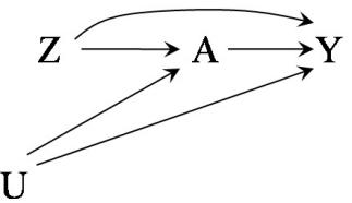
Figure 22.1

Consider a randomized trial in which individuals at risk of being infected by a dangerous virus are randomly assigned to a joint treatment of immediate vaccination plus an experimental antiviral therapy in case of being infected (Z = 1) or to standard of care (Z = 0), which includes no vaccination and no antiviral therapy. Figure 22.1 represents this trial with assigned treatment Z, received treatment A, and outcome (death) Y . For a given individual, the value of Z and A may differ because of lack of adherence to the assigned treatment some individuals assigned to vaccine (Z = 1) may not receive it (A = 0) because they refuse to be vaccinated, some individuals assigned to no vaccine (Z = 0) may still obtain a vaccine (A = 1) outside of the study. The variable U represents the unmeasured risk factors that influence an individual’s decision to get vaccinated.

As shown in Figure 22.1, the assigned treatment Z can have a causal effect on the outcome Y through two different pathways. First, treatment assignment Z may affect the outcome Y simply because it affects the received treatment A. Individuals assigned to vaccine are more likely to receive a vaccine, as represented by the arrow from Z to A. If receiving a vaccine has a causal effect on mortality, as represented by the arrow from A to Y , then assignment to vaccine has a causal effect on the outcome Y through the pathway Z → A → Y .

Second, treatment assignment Z may affect the outcome Y through pathways that are not mediated by received treatment A. For example, awareness of the assigned treatment might lead to changes in the participants’ behavior individuals aware of having been assigned to vaccination plus a promising antiviral therapy may become less careful about being infected. These behavioral changes are represented by the direct arrow from Z to Y .

The exclusion restriction (again). The existence of the arrow Z → Y in Figure 22.1 represents a direct effect of assignment on the outcome not through treatment. When this arrow exists, we say that the exclusion restriction does not hold. See Technical Point 16.1 for a formal discussion of the exclusion restriction.

Often investigators try to partly “de-contaminate” the effect of Z by eliminating the arrow Z → Y as shown in Figure 22.2 (same as Figure 16.1), which depicts the exclusion restriction of no direct arrow from Z to Y . To do so, they withhold knowledge of the assigned treatment Z from participants and their doctors. For example, investigators would administer the vaccine to those randomly assigned to Z = 1, and a placebo (an identical injection except that it does not contain vaccine) to those assigned to Z = 0. Because participants and their doctors do not know whether the injection they are given is the active treatment or a placebo, they are said to be “blinded” and the study is referred to as a double-blind placebo-controlled randomized trial. In Chapter 16, we used the concept of double-blind placebo-controlled randomized trial to motivate the concept of instrumental variable.

A double-blind treatment assignment is often unfeasible. Many studies cannot be effectively blinded because there is no practical way of administering a convincing placebo (e.g., for open heart surgery), because side effects of a treatment will make apparent who is taking it, etc. Also, blinding (and placebo control) is not advised when investigators are interested in quantifying the treatment effect in the real world, in which no blinding (or placebo) exists.

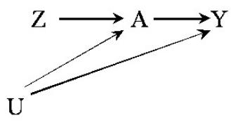
Figure 22.2

by the contrast Pr[Y ^z=1,a=1 = 1] vs. Pr[Y ^z=0,a=0 = 1] or, under the exclusion restriction, by the contrast Pr[Y ^a=1 = 1] vs. Pr[Y ^a=0 = 1]. In the text we use the latter for notational simplicity.

Hence, the causal effect of the assigned treatment Z depends not only on the strength of the arrow A −→ Y (the effect of the received treatment), but also on the strength of the arrows Z −→ A (the degree of adherence to the assigned treatment in the study) and Z −→ Y (the concurrent behavioral changes). The effect of Z is not “the effect of treating with A” but rather “the effect of assigning participants to being treated with A” or “the effect of having the intention of treating with A,” which is why the effect of randomized assignment Z is often referred to as the intention-to-treat effect.

No confounding is expected for the effect of assigned treatment because Z is randomly assigned. Exchangeability Y ^z⊥⊥Z is expected to hold for the assigned treatment Z because there are no backdoor paths from Z to Y in Figure 22.1. Association between Z and Y implies a causal effect of Z on Y , whether or not all individuals adhered to the assigned treatment. The associational risk ratio Pr[Y = 1|Z = 1]/Pr[Y = 1|Z = 0] equals the causal intention-to-treat risk ratio Pr[Y ^z=1 = 1]/Pr[Y ^z=0 = 1]. The analysis that estimates the unadjusted association between Z and Y to estimate the intention-to-treat effect is referred to as an intention-to-treat analysis. See Fine Point 22.2 for common variations of the intention-to-treat analysis that are generally biased.

Now consider the causal effect of treatment that would have been observed if all individuals had adhered to their assigned treatment as specified in the pro-The per-protocol effect is defined tocol of the experiment, which we refer to as the per-protocol effect. Throughout most of this book, we have assumed perfect adherence to the assigned treatment so that the values of assigned treatment Z and received treatment A coincide for all participants. that is, we assumed that U does not exist and thus the treated (A = 1) and the untreated (A = 0) are exchangeable, Y ^a⊥⊥A.

Consider now a setting in which U represents high risk of infection (1: yes, 0: no) and in which individuals at high risk of infection (U = 1) in the Z = 0 group tend to seek vaccination (A = 1) outside of the study. If that occurs, then the group A = 1 would include a higher proportion of high-risk individuals than the group A = 0: the groups A = 1 and A = 0 would not be exchangeable, and thus the associational risk ratio Pr[Y = 1|A = 1]/Pr[Y = 1|A = 0] would not equal the (causal) per-protocol risk ratio Pr[Y ^a=1 = 1]/Pr[Y ^a=0 = 1]. As

Pseudo-intention-to-treat analysis and modified intention-to-treat analysis. An intention-to-treat analysis is unbiased for the intention-to-treat effect because it includes all randomized individuals. Therefore, variations of the intention-to-treat analysis that only include a subset of the randomized individuals may be biased.

When some individuals do not complete the follow-up, their outcomes are unknown and thus the analysis needs to be restricted to individuals with complete follow-up. Thus, we can only conduct a pseudo-intention-to-treat analysis Pr[Y = 1|Z = 1, C = 0]/Pr[Y = 1|Z = 0, C = 0] where C = 0 indicates that an individual remained uncensored until the measurement of Y . As described in Chapter 8, censoring may induce selection bias and thus the pseudo-intentionto-treat estimate may be a biased estimate, in either direction, of the intention-to-treat effect. In the presence of loss to follow-up or other forms of censoring, the intention-to-treat analysis of randomized experiments requires appropriate adjustment for selection bias. See Section 21.5 and Little et al. (2012) for additional discussion.

For sustained treatment strategies, a common approach is to restrict the intention-to-treat analysis to individuals who at least initiated their assigned strategy (e.g., took at least one pill). This approach, known as a modified intention-totreat analysis, includes only a subset of randomized individuals and may therefore be biased for the intention-to-treat effect. A modified intention-to-treat analysis generally requires adjustment for the risk factors that affect adherence.

indicated by the backdoor path A ← U → Y , there is confounding for the effect of A on Y and estimating the per-protocol effect requires adjustment. That is, estimation of the per-protocol effect requires viewing the randomized experiment as an observational study. Fine Point 22.3 describes conventional approaches to quantify the per-protocol effect that missed this point.

The lack of confounding largely explains why the intention-to-treat effect is privileged in many randomized experiments: “the effect of having the intention of treating with A” may not be the effect that we want—“the effect of treating with A” or the per-protocol effect—but it is easier to compute. As often occurs when a less interesting quantity is easier to compute than a more interesting quantity, we tend to come up with arguments to justify the use of the less interesting quantity. The intention-to-treat effect is no exception. We now discuss why several well-known justifications for the intention-to-treat effect need to be taken with a grain of salt.

A common justification for the intention-to-treat effect is that it preserves the null. That is, if treatment A has a null effect on Y , then assigned treatment Z will also have a null effect on Y . Null preservation is a key property because In statistical terms, the intention- it ensures no effect will be declared when no effect exists. More formally, under the sharp causal null hypothesis and the exclusion restriction, it can be shown that Pr[Y = 1|Z = 1]/Pr[Y = 1|Z = 0] = Pr[Y ^a=1 = 1]/Pr[Y ^a=0 = 1] = 1. However, this equality is not true when the exclusion restriction does not hold, as represented in Figure 22.1. In those cases—experiments that are not doubleblind placebo-controlled—the effect of A may be null while the effect of Z is non-null. To see that, mentally erase the arrow A −→ Y in Figure 22.1: there is still an arrow from Z to Y .

A related justification for the intention-to-treat effect is that its value is “closer to the null than the value of the per-protocol effect”. The intuition is that, if imperfect adherence results in an attenuation—not an exaggeration—of the effect, the intention-to-treat risk ratio Pr[Y = 1|Z = 1]/Pr[Y = 1|Z = 0] will have a value between 1 and that of the per-protocol risk ratio Pr[Y ^a=1 = 1]/Pr[Y ^a=0 = 1]. The intention-to-treat effect could thus be interpreted as a lower bound for the per-protocol effect, i.e., the intention-to-treat effect is a conservative estimate of the per-protocol effect. Unfortunately, the intention-

to-treat analysis provides a valid though perhaps underpowered—αlevel test of the null hypothesis of no average treatment effect in double-blind placebo-controlled randomized experiments.

Na¨ıve per-protocol analyses. In randomized trials, two common approaches to attempt to estimate the per-protocol effect of treatment A are “as treated” and so-called “per protocol” analyses.

A conventional as-treated analysis compares the distribution of the outcome Y in those who received treatment (A = 1) versus those who did not receive treatment (A = 0), regardless of their treatment assignment Z. Clearly, a conventional as-treated comparison will be confounded if the reasons that moved participants to take treatment were associated with prognostic factors U that were not measured, as in Figures 22.1 and 22.2. On the other hand, consider a setting in which all backdoor paths between A and Y can be blocked by conditioning on measured factors L, as in Figure 22.3. Then an as-treated analysis needs to adjust for the factors L.

A conventional per-protocol analysis—sometimes referred to as an on-treatment analysis—only includes individuals who adhered to the study protocol: the so-called per-protocol population of participants with A = Z. The analysis then compares, in the per-protocol population only, the distribution of the outcome Y in those who were assigned to treatment (Z = 1) versus those who were not assigned to treatment (Z = 0). That is, a conventional per-protocol analysis is just an intention-to-treat analysis restricted to the per-protocol population. This restriction will generally result in a biased estimate of the per-protocol effect. To see why, consider the causal diagram in Figure 22.4, which includes an indicator of selection S into the per-protocol population: S = 1 if A = Z and S = 0 otherwise. Unless the per-protocol analysis appropriately measures and adjusts for the factors L, selection bias will arise because conditioning on S = 1 opens the noncausal path Z → A ← L ← U → Y .

That is, as-treated and per-protocol analyses are observational analyses of a randomized experiment and, like any observational analysis, require appropriate adjustment for confounding and selection bias to obtain valid estimates of the per-protocol effect. For examples and additional discussion, see Hern´an and Hern´andez-D´ıaz (2012).

intention-to-treat analyses applies to non-inferiority trials, in which the goal is to show that one treatment is not inferior to the other.

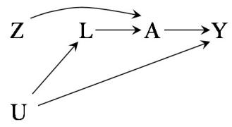
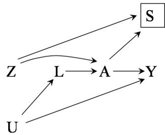
Figure 22.4

to-treat effect is not always conservative, because an attenuated effect is not guaranteed. See Fine Point 22.4

The argument against conservative Even in settings in which the intention-to-treat is conservative, that may not be a good thing. Suppose that the goal is evaluating a treatment’s safety: one could na¨ıvely conclude that a treatment A is safe because the intentionto-treat effect of Z on the adverse outcome is close to null, even if treatment A causes the adverse outcome in a significant fraction of patients. The explanation may be that many individuals assigned to Z = 1 did not take, or stopped taking, treatment before developing the adverse outcome. Then the intentionto-treat effect would be a dangerous way to define the effect of treatment.

In summary, exclusive reliance on intention-to-treat effect estimates is hard to justify for randomized trials with substantial non-adherence and for those evaluating harms rather than benefits. The per-protocol effect is often a more natural estimand for researchers and decision makers (e.g., clinicians, patients). Estimating the per-protocol effect requires adjustment for confounding under Figure 22.3 the assumption of exchangeability conditional on the measured covariates, or under alternative assumptions such as those required for instrumental variable estimation (see Chapter 16).

The above discussion revolved largely around time-fixed treatments. When, as often happens, the randomized trial studies sustained strategies under which treatment can vary over time, the probability of non-adherence increases greatly. Then the intention-to-treat becomes increasingly noninformative compared with the per-protocol effect, defined as the effect that would have been observed if everyone had adhered to their assigned treatment strategy throughout the follow-up. Estimating the per-protocol effect for sustained strategies, both in a true randomized trial and in an observational analysis that emulates it, generally requires g-methods.

More misunderstandings about the intention-to-treat effect. A commonly heard argument is that the intentionto-treat effect measures treatment’s effectiveness in the real world because it incorporates the fact that people will not perfectly adhere to the assigned treatment. In contrast, the per-protocol effect would measure treatment’s efficacy under perfect adherence to treatment. Using this terminology, it is often argued that “efficacy” does not reflect a treatment’s effect in real conditions, and thus one is justified to report the intention-to-treat effect as the primary finding from a randomized experiment because “effectiveness” is the most realistic measure of a treatment’s effect.

This reasoning is problematic for several reasons. First, the intention-to-treat effect measures the effect of assigned treatment under the adherence conditions observed in a particular experiment. The actual adherence in real life may be different (e.g., participants in a study may adhere better if they are closely monitored), and may actually be affected by the findings from that particular experiment (e.g., people will be more likely to adhere to a treatment after they learn it works). Second, if effectiveness is the goal, we should refrain from conducting double-blind placebo-controlled randomized clinical trials because, in real life, both patients and doctors are aware of the received treatment and no placebos are used. A true effectiveness measure should incorporate the effects stemming from assignment awareness (e.g., behavioral changes) that are eliminated in double-blind randomized experiments. Third, individuals who are planning to adhere to the treatment prescribed by their doctors will be more interested in the per-protocol effect than in the intention-to-treat effect.

Another common argument is that the intention-to-treat effect is guaranteed to be conservative. This is not true in all settings. If the per-protocol effect of treatment is not monotonic (i.e, not in the same direction for all individuals; see Technical Point 5.2) and the degree of non-adherence is high, then the per-protocol effect may be closer to the null than the intention-to-treat effect. Even for monotonic effects, the intention-to-treat effect is not necessarily conservative in head-to-head trials in which individuals are assigned to one of two active treatments. Suppose individuals with a painful disease were randomly assigned to either an expensive drug (Z = 1) or ibuprofen (Z = 0). The goal was to determine which drug results in a lower risk of severe pain Y after 1 year of follow-up. Unknown to the investigators, both drugs are equally effective to reduce pain, i.e., the per-protocol risk ratio is 1. However, adherence to ibuprofen happened to be lower than adherence to the expensive drug because of a mild side effect that could be easily palliated. As a result, the intention-to-treat risk ratio was greater than 1, and the investigators wrongly concluded that ibuprofen was less effective than the expensive drug to reduce severe pain. For more details, see the discussion by Robins (1998b) and Hern´an and Hern´andez-D´ıaz (2012).

22.2 A target trial with sustained treatment strategies

We are now ready to discuss target trials that compare sustained treatment strategies. Because the ultimate goal is to emulate these trials using real world observational data, we will only consider pragmatic trials with features that resemble the real world. In particular, participants and their treating physicians need to be aware of the treatment they receive (i.e., the treatment assignment is not blinded), nobody receives a placebo (i.e., both strategies g and g ′ involve either active treatments or no treatment), and participants are monitored as frequently and intensely as regular patients outside of the study. A trial with pragmatic features is preferable when the goal is quantifying the effects of treatment strategies under realistic conditions.

To fix ideas, consider a randomized trial to estimate the effect of antiretroviral therapy on the 5-year risk of death among individuals with HIV infection. Eligible participants—18 years and older, no AIDS, no previous use of antiretroviral therapy—are randomly assigned to either treatment strategy g or treatment strategy g ′ at the start of follow-up k = 0 (baseline). Their follow-up starts at the time of assignment and ends at death (the outcome of interest), loss to follow-up, or 60 months after baseline, whichever occurs earlier.

Let A^k take value 1 if the individual receives therapy at time k and 0 otherwise, for k = 0, 1, 2…K with K = 59. Our trial will assign eligible individuals to either the strategy g¹ “receive treatment A^k = 1 continuously during the follow-up unless a contraindication or toxicity arises” or the strategy g⁰ “receive treatment A^k = 0 continuously during the follow-up”. Let the assignment indicator Z takes value 1 if the individual is assigned to g¹ and 0 In previous chapters we considered if assigned to g0. Let D^k be an indicator for death (1: yes, 0: no) and C^k an indicator for censoring (1: yes, 0: no) by month k = 1, 2…K + 1.

Let us now define the intention-to-treat and per-protocol effects in a randomized trial with sustained treatment strategies. Additional contrasts of sustained strategies—referred to as direct effects—are described in Technical Point 22.1.

The intention-to-treat effect is contrast of the static strategies

• (z = 1, c¯^K = ¯0): be assigned to strategy g¹ at baseline and remain under study until the end of follow-up
• (z = 0, c¯^K = ¯0): be assigned to strategy g⁰ at baseline and remain under study until the end of follow-up

The intention-to-treat effect at time k can then be expressed as the contrast of the counterfactual risks of death Pr h D z=1,c¯k=¯0 ^k = 1ⁱ − Pr h D z=0,c¯k=¯0 ^k = 1ⁱ under assignment to strategy g¹ versus g⁰ if nobody had been lost to follow-up through time k (¯c^k = ¯0).

In some randomized trials, assignment to and initiation of the treatment strategies occur simultaneously. That is, all individuals assigned to strategy g¹ start to receive treatment at time 0, regardless of whether they continue taking it after baseline, and no individuals assigned to strategy g⁰ receive treatment at time 0, regardless of whether they start taking it after baseline. In those cases, the intention-to-treat effect is not only the effect of assignment but also the effect of initiation of treatment Pr h D a0=1,c¯k=¯0 ^k = 1ⁱ −Pr h D a0=0,c¯k=¯0 ^k = 1ⁱ .

Like in any randomized trial, some participants will deviate from the protocol by not adhering to their assigned strategy. During the follow-up, some individuals assigned to g¹ will stop treatment for no clinical reason, some individuals assigned to g⁰ will start treatment, some individuals will use non-approved concomitant treatments, etc. The intention-to-treat effect is agnostic about these protocol deviations, which are the result of decisions made after baseline. This agnosticism implies that the magnitude of the intention-to-treat effect may heavily depend on the particular patterns of protocol deviations that occur during the conduct of each trial. Two studies with the same protocol but conducted in different settings may have different intention-to-treat effect estimates and neither of them is biased. Due to the limitations of the intention-to-treat effect, we want to complement it with the per-protocol effect.

The per-protocol effect is defined by a contrast of the outcome distribution under the interventions:

• receive treatment strategy g¹ continuously between baseline k = 0 and end of follow-up
• receive treatment strategy g⁰ continuously between baseline k = 0 and end of follow-up

The per-protocol effect at time k can then be expressed as the contrast of the counterfactual risks of death Pr h D g1,c¯k=¯0 ^k = 1ⁱ − Pr h D g0,c¯k=¯0 ^k = 1ⁱ under full

the causal effect of treatment on an outcome Y measured at the end of follow-up. In this trial, the outcome is a failure time, i.e., time to death (see Technical Point 21.10).

Controlled direct effects. Consider the average causal effect of a treatment A on an outcome Y when a mediator M is set to a particular value. We refer to this quantity as the direct effect of A on Y not through M. If the mediator M could take two values (0 or 1), then we can define the direct effect of A on Y when M is set to 1 and the direct effect of A on Y when M is set to 0. On the additive scale, these two direct effects are defined by the counterfactual differences E - Y ^a=1,m=1 −E - Y ^a=0,m=1 and E - Y ^a=1,m=0 −E - Y ^a=0,m=0 , respectively. These direct effects, which are often referred to as average controlled direct effects, could, in principle, be identified by conducting an experiment with sequential randomization for both treatment A and mediator M, or by emulating such target experiment using observational data. Technical Point 22.2 describes other types of direct effects for which no target experiment exists.

Suppose we conduct a randomized experiment in which participants are randomly assigned at baseline to either treatment A = 1 or A = 0 and one month after baseline to either treatment M = 1 or M = 0. Thus all individuals will be placed in one of four groups: (A = 1, M = 1), (A = 1, M = 0), (A = 0, M = 1), or (A = 0, M = 0). The outcome of interest Y is measured at 3 months in all individuals (for simplicity, suppose no individuals were lost to follow-up or died). This study design allows us to consistently estimate the controlled direct effects because the randomization of both A and M ensures that the counterfactual quantities E [Y a,m] = Pr [Y a,m = 1] are consistently estimated by the observed risks Pr [Y = 1|A = a, M = m].

The controlled direct effects can also be validly estimated in observational studies as long as the identifiability conditions of consistency, positivity, and exchangeability hold for both A and M. A precise characterization of these identifiability conditions was actually provided in Chapter 19 because a controlled direct effect is just a particular case of a contrast of treatment strategies sustained over time. To see so, simply replace A and M by A⁰ and A¹ in the above expressions. More generally, both the treatment A and the mediator M can be time-varying themselves.

adherence to strategy g¹ versus g⁰ if nobody had been lost to follow-up through time k (¯c^k = ¯0).

Sensible trial protocols will not mandate that treatment be continued no matter what happens to the individual. For example, our strategy g¹ of continuous treatment mandates treatment discontinuation when a contraindication or toxicity arises. That is, the per-protocol effect generally involves the comparison of dynamic strategies (“do this, if X happens then do this other thing”) rather than static strategies (“do this, no matter what happens”).

Sometimes the study protocol is not explicit about the dynamic nature of the treatment strategies. For example, the protocol may simplify the description of strategy g¹ as “receive treatment A^k = 1 continuously during the follow-Ideally, to avoid confusions about up” without explicitly stating that the therapy must be discontinued “when a contraindication or toxicity arises”. This simplified description of strategy g¹ may lead to misunderstandings. Specifically, an individual assigned to g¹ who discontinues therapy because of toxicity should not be labeled as someone who is not adhering to strategy g1. In fact, that person is perfectly adhering to strategy g¹ as (it should have been) stated in the protocol. When doing otherwise is not an option in the real world, discontinuation of the originally assigned treatment or initiation of other medically indicated treatments cannot possibly be considered a deviation from protocol. Because the per-protocol effect is defined by a contrast of realistic strategies, it is particularly relevant for causal inference research which seeks to provide evidence for decisions in the real world.

In fact, the per-protocol effect is often the implicit target of inference. For example, often investigators question the fidelity of the interventions implemented in the study to the interventions described in the protocol, and say that there is “bias”. This language indicates that the investigators are really

what should or should not be deemed as nonadherence throughout the follow-up, the protocol would fully specify the treatment strategies of interest. Then the per-protocol effect would be welldefined (Hern´an and Robins, 2017).

Pure direct effects and principal stratum direct effects. Besides the controlled direct effects described in Technical Point 22.1, there exist other definitions of the average direct effect of a treatment A on an outcome Y when a potential mediator M is set to a particular value.

The pure direct effect (also known as natural direct effect) of A on Y not through M is the average causal effect of A on Y if the value of M had been set to the value that M would have taken if A had been set to 0, i.e., if M had been set to the value Ma=0 (which is 1 for some individuals and 0 for others). The pure direct effect, defined by the contrast E h Y ^a=1,Ma=0 i − E h Y ^a=0,Ma=0 i , is a cross-world quantity because E h Y ^a=1,Ma=0 i includes a counterfactual outcome simultaneously indexed by both a = 1 and a = 0. Therefore, the pure direct effect cannot be identified from a randomized experiment on A, M, or both, and cannot be identified from observational data under an FFRCISTG model (see Technical Point 6.2). Nonetheless, estimation of pure direct effects is often the goal of causal mediation analyses because total treatment effects can be decomposed into pure direct and total indirect effects. Pure direct effects were introduced by Robins and Greenland (1992); Pearl (2001) renamed them as natural direct effects and showed that, for certain causal graphs, the pure direct effect can be identified from the observed data under his NPSEM-IE model because, unlike the FFRCISTG model, the NPSEM-IE model assumes untestable cross-world independencies that cannot be refuted from randomized experiments on A, M, or both. For a review, see the book by VanderWeele (2015).

The principal stratum direct effect of A on Y if the value of M had been set to m is the average causal effect of A on Y in the subset of the population whose value of M would have been equal to m regardless of the value of A, i.e., in the subset of the population with Ma=0 = Ma=1 = m. Then the principal stratum direct effect is defined by the contrast E - Y ^a=1,m|Ma=0 = Ma=1 = m − E - Y ^a=0,m|Ma=0 = Ma=1 = m . Interestingly, this is equal to E - Y ^a=1|Ma=0 = Ma=1 = m −E - Y ^a=0 = 1|Ma=0 = Ma=1 = m . Therefore, principal stratum direct effects do not involve joint counterfactuals Y a,m, just the counterfactuals Y a in a subset of the population so, in that sense, they are the total (rather than direct) effect of treatment in that subset of the population. It follows that, unlike controlled or pure direct effects, principal stratum direct effects do not require that interventions on M are well-defined. Principal stratum direct effects have little policy relevance when A affects M in almost all individuals, because then they apply to the very small subset of the population with Ma=0 = Ma=1. In practice, M is often coarsened (typically into a binary indicator) to increase the size of the principal stratum, but coarsening itself may make the principal stratum direct effect less scientifically relevant (Robins et al. 2007). Principal stratum direct effects were introduced by Robins (1986) and popularized by Rubin (2004). Frangakis and Rubin (2002) following Robins (1986), used the concept of principal stratum as a tool to handle competing events. In Chapter 23, we consider an interventionist theory of mediation (Robins and Richardson 2010) which offers yet another type of direct effect.

interested in comparing the interventions implemented during the follow-up as specified in the protocol (i.e., the per-protocol effect) and not in the effect of assignment to the interventions at baseline (i.e., the intention-to-treat effect) because nonadherence after baseline cannot possibly bias the effect of assignment at baseline.

Finally, let us consider the effect of receiving interventions other than the ones specified in the study protocol. Suppose that, while our trial is being conducted, a consensus started to emerge that strategy g⁰ “receive treatment A^k = 0 continuously during the follow-up” is inferior to strategy g1. Therefore some physicians began to recommend initiation of therapy when the clinical course worsened when the CD4 cell count (Lk) first dropped below 200 cells/µL. As a result, many individuals in the trial who were assigned to strategy g⁰ actually followed the modified strategy g ′ ⁰ “receive treatment A^k = 0 continuously during the follow-up but, after L^k < 200, switch to treatment A^k = 1”. The contrast of outcome distributions under the interventions

• receive treatment strategy g¹ continuously between baseline k = 0 and end of follow-up

• receive treatment strategy g ′ 0 continuously between baseline k = 0 and end of follow-up

corresponds to neither the intention-to-treat effect nor the original per-protocol effect. Rather, it is a question about the per-protocol effect in a hypothetical target trial in which individuals are randomized to either strategy g¹ or g ′ 0 .

This example illustrates how causal effects of interest that do not correspond to the original per-protocol effect can be conceptualized as per-protocol effects in target trials that can be emulated using the randomized trial data. Interestingly, if the strategies of interest differ from those in the actual trial, it is actually disadvantageous to have all participants in the actual trial adhere to the strategies specified in the protocol. Complete adherence implies that the trial data cannot be used to emulate a target trial with a different protocol (because no individuals followed the protocol of the new target trial in the actual data). For example, a randomized trial with full adherence in which individuals with HIV are assigned to different CD4 cell count thresholds at which to initiate antiretroviral therapy is of little use to emulate a trial in which individuals are assigned to either continuous treatment or no treatment, and vice versa. It is precisely the noncompliance that allows us to use the data from a given randomized trial to emulate other randomized trials that answer different, perhaps more relevant, causal questions.

more details about the estimation of per-protocol effects in randomized trials.

In randomized trials with sustained treatment strategies, estimating perprotocol effects raises the same issues as any comparison of sustained strategies See Hern´an and Robins (2017) for in an observational study. As we discuss later, valid estimation of the perprotocol effect generally demands that trial investigators collect post-randomization data on adherence to the strategy and on time-varying prognostic factors associated with adherence.

22.3 Emulating a target trial with sustained strategies

If conducting a pragmatic randomized trial is not possible, we may attempt to emulate it through the analysis of existing observational data. We then refer to the trial as the target trial for our observational analysis.

Specifying the protocol of the target trial is a useful device to clarify the causal question of interest that we wish our observational analysis to answer. At the very least, we need to specify the following key components of the protocol: eligibility criteria, start and end of follow-up, treatment strategies, outcomes of interest, causal contrast, and data analysis plan. Note that a precise specification of the protocol of the target trial may require some exploration of the available data. For example, only after having determined that the data included information on HIV diagnosis, can we reasonably propose to emulate a target trial of individuals with HIV.

Analogs of the causal effects described in the previous sections for randomized trials can be proposed for observational analyses that emulate a target trial.

Emulating an intention-to-treat effect is rarely possible in observational analyses of existing data because the actual assignment to a treatment strategy is unknown. In our example, the closest observational analog of the intentionto-treat effect is a comparison of initiation of the different treatment strategies. A comparison of initiators parallels the intention-to-treat analysis in target trials in which assignment and initiation of the treatment strategies always occur (rather than dispensing) of antiretroviral therapy, a comparison of groups according to whether they did or did not receive a prescription of therapy at baseline would be somewhat more analogous to the intention-to-treat analysis in the target trial.

pares initiators is equivalent to the modified intention-to-treat analysis described in Fine Point 22.2

together at baseline, regardless of whether individuals continue on the strate-If we had data on prescription gies after baseline. We can define this observational analog of the intention-to treat effect by a contrast of the outcome distribution under the hypothetical interventions

• initiate treatment A⁰ = 1 at baseline and remain under study until the end of follow-up
• initiate treatment A⁰ = 0 at baseline and remain under study until the end of follow-up

This observational analog of the intention-to-treat effect at time k can then be expressed as the contrast of the counterfactual risks Pr h D a0=1,c¯k=¯0 ^k = 1ⁱ −

Pr h D a0=0,c¯k=¯0 ^k = 1ⁱ . Unlike a true intention-to-treat effect that defines the groups according to assigned strategy, this contrast defines them according to initiation of each strategy. If we were using this contrast in a randomized trial, we would be including in the same group all individuals who did not take any dose of treatment at baseline, regardless of whether they were assigned An observational analysis that com- to strategy g¹ or g0. If initiation of treatment occurs shortly after assignment to treatment, our observational analog roughly preserves a key feature of the intention-to-treat effect: the contrast is defined by interventions occurring shortly after baseline.

An observational analog of the per-protocol effect, on the other hand, is defined identically as that for the target trial. In randomized trials we differentiated between the original per-protocol effect and the per-protocol effects in alternative target trials. In observational studies this difference is unnecessary because, in the absence of a pre-specified protocol, each per-protocol effect corresponds to a particular target trial. In general, we can only use observational data to emulate target trials whose intended interventions are actually followed by at least some individuals in the study. In some settings, however, investigators may be willing to use modeling, e.g., dose-response structural models, to extrapolate beyond the interventions that are actually present in the data.

Defining the causal effects in observational studies in reference to those in the target trial forces us to be explicit about the strategies that are compared. This explicit specification of the treatment strategies prevents bias because it makes it obvious that certain data analyses involve comparisons that cannot be translated into a contrast between hypothetical interventions. These data analyses should therefore be avoided when the goal of the analysis is to help decision makers choose one of several courses of action, as we discussed in Sections 3.5 and 3.6.

Another advantage of an explicit definition of the treatment strategies in observational analyses is clarity. As discussed in Fine Point 22.4, some investigators insist in classifying causal effects into either “efficacy” (loosely defined: the effect of treatment that would be observed under perfect conditions) or “effectiveness” (loosely defined: the effect of treatment that would be observed under realistic conditions). Sometimes the intention-to-treat effect in a randomized trial is interpreted as the effectiveness of treatment and the perprotocol effect in the same trial as the efficacy of treatment. Other times the intention-to-treat effect in a randomized trial is interpreted as efficacy (even under imperfect conditions such as non-adherence) whereas the per-protocol effect in the observational study that emulates it is interpreted as effectiveness (even under perfect adherence). That is, especially in settings with sustained

strategies over long periods, the labels “effectiveness” and “efficacy” are ambiguous: it is often difficult to argue that either an intention-to-treat effect in a setting with nonadherence or a per-protocol effect in a real world setting measures the causal effect of treatment under perfect conditions.

Rather than insisting on an artificial efficacy-effectiveness dichotomy, it may be more helpful to accept that all causal effects are placed somewhere along the effectiveness continuum. An explicit definition of the treatment strategies that define the causal effect of interest is then more informative because decision makers need information about the effect of well-defined interventions.

22.4 Time zero

A crucial component of target trial emulation is the determination of the start of follow-up, also referred to as baseline or time zero, in the observational analysis. Eligibility criteria need to be met at that point but not later; study outcomes begin to be counted after that point but not earlier.

In randomized experiments, the time zero for each individual is the time when they are assigned to a treatment strategy while meeting the eligibility criteria. For example, in our randomized trial of antiretroviral therapy, time zero is the time when the treatment strategies are assigned (the time of randomization), which usually occurs shortly before, or at the same time as, treatment is initiated. We do not start the follow-up, say, 2 years before or after treatment assignment. Starting before randomization would not be reasonable because the treatment strategies had yet to be assigned and the eligibility criteria have not yet been defined, much less met; starting follow-up after randomization is potentially biased as deaths during the first two years of the trial would be excluded from the analysis and any short-term effects of treatment would be missed. Even more problematic, if treatment does indeed have a short-term effect, then more susceptible individuals would have died by year 2 in the group assigned to active treatment but not in the other group. This differential proportion of susceptible individuals after two years destroys the baseline comparability achieved by randomization and opens the door to selection bias.

The same rules regarding time zero apply to observational analyses and randomized trials, and for the same reasons. Generally, the follow-up in the observational analysis should start at the time the follow-up would have started in the target trial. Otherwise the effect estimates may be hard to interpret and biased because of selection affected by treatment. Nonetheless, in observational Example: The highly publicized dis- studies for causal inference, errors in the emulation of time zero of the target trial are very frequent. These errors occur because of two common problems: 1) sometimes there is not a unique choice of time zero, and 2) sometimes the treatment strategies cannot be uniquely assigned at time zero. We now describe solutions for each of these two problems.

First, the problem of non-unique time zero. Consider two scenarios, according to how many times the eligibility criteria can be met throughout an individual’s lifetime:

1. Eligibility criteria can be met at a single time. This is the simplest setting. Follow-up starts at the only time the eligibility criteria are met. For example, consider a study in persons with HIV to compare immediate initiation of antiretroviral therapy when the CD4 cell count first drops

crepancy between the estimates of the effect of postmenopausal hormone therapy on heart disease in observational studies and a randomized trial was partly due to mishandling of time zero in the former (Hern´an et al. 2008).

below 500 cells/µL versus delayed initiation when the CD4 cell count first drops below 350 cells/µL. The follow-up of eligible individuals starts the first time their CD4 cell count drops below 500.

2. Eligibility criteria can be met at multiple times. This is the situation that often leads to confusion. For example, consider a study to compare initiation versus no initiation of hormone therapy among postmenopausal women with no history of chronic disease and no use of hormone therapy during the previous two years. If a woman meets these eligibility criteria continuously between age 51 and 65, when should her follow-up start? At age 51, 52, 53. . . ? In the target trial a woman would be eligible to be recruited at multiple times during her lifetime, i.e., she has multiple eligible times.

In settings with multiple eligibility times, there are several alternatives to choose the time zero of each individual among her eligible times. One could choose as time zero: a) the first eligible time, b) a randomly chosen eligible time, c) every eligible time, etc. Strategy c) requires emulating multiple sequential target trials, each of them with a different start of follow-up. The number of sequential trials depends on the frequency with which data on treatment and covariates are collected:

• If fixed schedule for data collection at pre-specified times (e.g., every two years, like in many epidemiologic cohorts), then emulate a new trial starting at each pre-specified time.
• If subject-specific schedule for data collection (e.g., electronic medical An unbiased choice of time unit can records), then choose a fixed time unit (e.g., a day, week or month), and emulate a new trial starting at each time unit.

From a statistical standpoint, the sequential emulation strategy c) can be more efficient than the previous ones because it uses more of the available data. However, because individuals may be included in multiple target trials, appropriate adjustment of the variance of the effect estimate is required. This can be achieved by bootstrapping the entire analysis.

Second, let us talk about how to tackle the impossibility of assigning a unique treatment strategy to each individual. Consider a target trial in which individuals whose CD4 cell count just dropped below 500 cells/µL are assigned to one of the following strategies: (1) start therapy immediately, (2) start therapy when CD4 cell count drops below 350 cells/µL, (3) start therapy when CD4 cell drops below 200 cells/µL. When emulating this target trial using observational data, we will find individuals who started therapy at time zero (i.e, when their CD4 cell count first dropped below 500 cells/µL) and therefore we will assign them to strategy (1). Other individuals, however, did not start therapy at time zero, which means that their data are compatible with following both strategy (2) and strategy (3) at baseline. Which strategy should we assign them to?

One possibility is to choose a single strategy at random and assign them to that strategy, but that would be statistically inefficient. Another possibility is to create two exact copies—clones—of each of these individuals in the data and assign each of the two clones to a different strategy. Clones are then censored at the time their data stop being consistent with the arm they were assigned to. For example, if the individual does not start therapy when CD4 drops to 350, then the clone assigned to “start therapy when CD4 cell count drops to

vary from study to study. For example, consider a study in which both the time-varying treatment and confounders change more then once a week for many individuals. Then choosing a week or a month as the time unit will introduce bias. This bias could be eliminated by using by the choice of a day as the unit of time. If daily data on treatment and confounders are not available, the bias could not be fully corrected.

Grace periods. Consider a trial to compare immediate initiation of antiretroviral therapy at time zero versus delayed initiation. In the real world, antiretroviral therapy cannot be started exactly on the same day that it is assigned. Depending on the health care system, it may take weeks or months until the requisite clinical and administrative procedures are completed and patients are adequately informed. Therefore, investigators need to define a grace period (say, 3 months) after time zero during which initiation is still considered to be immediate. Otherwise the study would be estimating the effect of strategies that do not occur frequently in reality or that could not be successfully implemented in practice.

A consequence of using a grace period is that an individual’s observed data is consistent with more than one strategy for the duration of the grace period. For example, in the above study, the introduction of a 3-month grace period implies that the interventions are redefined as “initiate therapy within 3 months of time zero cells/µL” versus “never initiate therapy”. Therefore individuals who start therapy in month 3 after baseline have data consistent with both strategies during months 1 and 2. Had some of them died during those 2 months, to which strategy should we have assigned those deaths? As described in the text, we could randomly assign these individuals to one of the two strategies or, better, we could create two clones of each individual and assign each of the two clones to a different strategy. Clones are censored when their data are no longer compatible with their assigned strategy. For example, if the individual starts therapy in month 3, then the clone assigned to “start after 3 months” would be censored at that time. The potential bias introduced by censoring can be handled via IP weighting.

When using grace periods with cloning and censoring, the intention-to-treat effect cannot be estimated because almost everyone will contribute a clone to each of the treatment strategies. Because each individual is assigned to all strategies at baseline, a contrast based on baseline assignment (i.e., an “intention-to-treat analysis”) will compare groups with essentially identical outcomes. Therefore, analyses with grace period at baseline are geared towards estimating some form of per-protocol effect and thus will generally need to incorporate adequate adjustment.

Finally, note that a well-defined initiation strategy with a grace period should specify the timing of initiation during the grace period. For details, see the Appendix in Cain et al. (2010).

censoring + weighting procedure, see Robins et al. (2008) and Cain et al. (2010). For related work, see van der Laan and Petersen (2007).

350” would be censored at that time. The potential bias introduced by this likely informative censoring would need to be corrected by adjusting for time-For a description of the cloning + varying factors via IP weighting. Importantly, if the individual had died before either clone was censored, then both clones would have died and therefore the death would have been assigned to both strategies. This double allocation of events prevents the bias that could arise if events occurring during the waiting period were systematically assigned to one of the two strategies only.

Again, because individuals may be included multiple times in the analysis via their clones, appropriate adjustment of the variance of the effect estimate is required via bootstrapping. The cloning + censoring + weighting procedure can be combined with sequential target trial emulation when the eligibility criteria can be met at multiple times. Fine Point 22.5 describes the handling of strategies that can be initiated during a grace period after time zero rather than exactly at time zero.

22.5 A unified approach to answer What If questions with data

This book describes and integrates two causal inference frameworks: counterfactuals and causal diagrams. Explicit target trial emulation recapitulates both frameworks and grounds them to actionable causal inference. By organizing causal inference around a deeply familiar scientific concept—the experimentthe target trial framework helps investigators use their subject-matter knowledge to articulate well-defined causal inference questions. Once the causal question is stated with little ambiguity, study design and data analysis flow naturally.

The target trial framework is applicable to a wide range of causal questions across many disciplines, regardless of the terminology and methodology privileged in each field. For example, economists often refer to confounding and conditional exchangeability as omitted variable bias and selection on observables, respectively, and traditional social scientists are unlikely to use g-methods because their causal questions are not typically organized around time-varying treatments. But these disciplinary differences are superficial compared with the fundamental task that all health and social scientists interested in causal inference face: they all need to articulate their causal questions as a contrast of well-defined counterfactuals. The target trial framework facilitates that task by helping define the well-defined interventions that lead to well-defined counterfactuals.

The target trial framework also provides a common language to unify the causal analysis of randomized and observational studies. Aside from baseline randomization, there are no other necessary differences between analyses of observational data that emulate a target trial and of true randomized trials (see Fine Point 22.6). That is, a randomized trial can be viewed as a follow-up study with baseline randomization and observational longitudinal data as a follow-up study without baseline randomization.

The similarities between follow-up studies with and without baseline randomization are increasingly apparent in the health and social sciences as a growing number of randomized experiments attempt to estimate the effects of sustained treatment strategies over long periods in real world settings. These studies are a far cry from the short experiments in tightly controlled settings that put randomized trials at the top of the hierarchy of study designs in the mid-20th century. For causal questions involving treatment strategies sustained over long periods, randomized experiments with the potential for substantial deviations from protocol (e.g., imperfect adherence to the assigned strategy, loss to follow-up) are subject to confounding and selection biases that we have learned to associate exclusively with observational studies.

In particular, when estimating a per-protocol effect, both randomized trials and observational studies may need adjustment for time-varying prognostic fac-Time-varying confounding in obser- tors that predict drop-out (selection bias) and treatment (confounding). That is, the methodology for causal inference described in this book applies equally to the per-protocol analyses of randomized trials and observational studies. And, for the same reasons that success is not guaranteed when estimating causal effects from observational data, the per-protocol effect estimates from randomized trials may be biased too.

In view of these similarities, one might expect that randomized experiments and observational studies would be analyzed similarly, except adjustment for baseline confounders in observational analyses to estimate the analog of the intention-to-treat effect. In practice, however, the typical analyses of randomized experiments and observational studies differ radically, which is both perplexing and, as we argue below, problematic.

A natural question is whether the “intention-to-treat analysis” and the so-called “per-protocol analysis” commonly used in randomized trials validly estimate the intention-to-treat effect and per-protocol effect, respectively.

A typical intention-to-treat analysis compares the distribution of outcomes between randomized groups without any form of adjustment for confounding

vational studies is a bias with the same structure as nonrandom noncompliance in randomized trials.

How do the data of randomized experiments and observational studies differ? Only three things distinguish the data from randomized experiments and observational studies. In randomized experiments, (i) no baseline confounding is expected because of randomization, (ii) the randomization probabilities are known, and (iii) the assignment to a treatment strategy is known for each individual at baseline.

An observational analysis can emulate (i) if one measures and appropriately adjusts for a sufficient set of covariates, and (ii) if the model for treatment assignment given the past is correctly specified. Interestingly, (iii) is not necessary for estimating the per-protocol effect in either randomized experiments or observational studies because efficient estimators (that are functions of the sufficient statistic) do not use this information. That is, the analyst does not need to know the strategies being compared, much less who was assigned to which strategy: in a randomized trial, you can delete the randomization assignment from the dataset and still estimate a per-protocol effect if a sufficient set of confounders was measured. In a trial of dynamic strategies with perfect adherence, a sufficient set is all time-fixed and time-varying covariates used by the strategies in assigning treatment (Robins 1986).

or selection bias. Lack of adjustment for baseline confounding is justified by randomization: the randomized groups are expected to be exchangeable because they are expected to have the same risk of the outcome if both groups had been assigned to the same treatment strategy. No adjustment for postrandomization confounding (e.g., due to nonadherence) is required because, again, there cannot be post-randomization confounding for the effect of baseline assignment.

However, baseline randomization cannot ensure exchangeability between those who are and are not lost to follow-up after randomization. Because the strategies that define the intention-to-treat effect require that the individuals remain in the study until their outcome variable can be ascertained, an intention-to-treat effect estimate calculated among those who are not lost to follow-up may be affected by post-randomization selection bias if prognostic factors influence, or are associated with, differential loss to follow-up. Therefore, valid estimation of the intention-to-treat effect may require an “intentionto-treat analysis” adjusted for post-randomization (time-varying) prognostic Fine Point 22.2 refers to an factors to eliminate selection bias from loss to follow-up. For example, in a randomized trial of antiretroviral therapy among HIV patients, g-methods will be needed if the probability of dropping out of the study is influenced by the onset of symptoms or other risk factors for the outcome.

In addition to the primary intention-to-treat analysis, many randomized trials also report the results from a so-called per-protocol analysis restricted to individuals who adhered to the instructions specified in the study protocol, as described in Fine Point 22.3 for point interventions. For sustained treatment strategies, individuals are censored at the first time they deviate from the protocol. That is, the remaining per-protocol population at each time is the set of individuals that are still adhering to the protocol. No adjustment of any Fine Point 22.3 refers to a per- kind is performed. This unadjusted analysis is questionable for three reasons.

First, like in an intention-to-treat analysis, there may be selection bias due to differential loss to follow-up. If so, adjustment for post-baseline (timevarying) risk factors via g-methods will be needed.

Second, the analysis partly disregards the randomized groups and therefore the subset of individuals who remain on protocol under one strategy may not be exchangeable with the subset on protocol under another strategy. That is, this “per-protocol analysis” is akin to an observational analysis and thus requires

intention-to-treat analysis that does not even attempt to adjust for selection bias as a pseudointention-to-treat analysis.

protocol analysis that does not even attempt to adjust for confounding as a na¨ıve per-protocol analysis.

methods are always needed when the treatment has a causal effect on the outcome. The reason is that treatment A^k affects all variables after time k through its effect on the time-varying indicator Dk+1, as discussed in Technical Point 21.10.

stances, decisions based on quality randomized trials may be inferior to decisions based on severely confounded observational data, as described in Fine Points 22.7 and 22.8.

g-methods to adjust for bias due to time-varying risk factors that affect the decision to stay on protocol. Instrumental variable estimation (Chapter 16) can sometimes be used to validly estimate per-protocol effects without explicit For failure time outcomes, g- adjustment for any variables, but the validity of these methods depends on having a valid instrument and on strong modeling assumptions. Some forms of instrumental variable estimation are a particular case of g-estimation (see Technical Point 16.6).

Third, this conventional per-protocol analysis ignores that the sustained treatment strategies under comparison are dynamic strategies. A common mistake is censoring individuals who discontinue treatment as if treatment discontinuation were, by definition, a deviation from protocol—which is why this analysis is also known as on-treatment analysis. We have discussed above that individuals who stop treatment because of toxicity or a contraindication are not deviating from protocol and therefore should not be censored.

All the above considerations apply to the analysis of both randomized trials and observational data to emulate a target trial. When the goal is estimating a per-protocol effect or its observational analog, the analysis of randomized trials and observational studies should be identical. If we feel compelled to adjust for time-varying confounding and selection bias in the analysis of observational studies, we should feel equally compelled to adjust for post-randomization confounding and selection bias in the analysis of randomized trials. Adjustment for time-varying factors using g-methods will generally be necessary for perprotocol analyses of both randomized trials and observational studies. The target trial framework and g-methods make it possible to implement a unified approach to causal inference for sustained treatment strategies. Historically, randomized experiments have been considered far superior to observational studies for the purpose of making causal inferences and aiding decision-making. Under some extremely rare circum- Unfortunately, randomized experiments are not always available because they may be expensive, infeasible, unethical, or just untimely to support an urgent decision. Therefore, as much as we value the benefits of randomization, it is a fact that many decisions will need to be made in the absence of evidence from randomized trials. When we cannot conduct the randomized experiment that would answer our causal question, we resort to attempting to emulate it using observational data. It is therefore important to use a sound approach to design and analyze observational studies. Making the target trial explicit is one step in that direction. When the goal is to assist decision making, the analysis of existing observational data need to explicitly emulate a trial and be evaluated with respect to how well they emulate their target trial.

A counterintuitive comparison of a randomized trial and an observational study. An untested over-the-counter treatment A was used by many individuals with lung cancer in a country. This worried the country’s drug regulator who, in response, funded a double-blind placebo-controlled randomized trial of A in a random sample of 20% of individuals diagnosed with lung cancer over the next year. All trial participants adhered to their assigned treatment. The 60-month mortality risk was 55% in the treatment arm and 45% in the placebo arm as shown in the table below:

	A = 0	A = 1
Y = 1	450	550
Y = 0	550	450
	1000	1000

As a result, the regulator banned the treatment. Later, an observational study was conducted on the 80% of lung cancer patients not selected into the trial. This study found a mortality risk of 0% in both the treated and the untreated over the same period as the trial. How can the observational and the randomized trial data be reconciled?

Let us first remember that individuals can be classified into counterfactual types: 1) “doomed”(Y ^a=0 = Y ^a=1 = 1), 2) “hurt”(Y ^a=0 = 0, Y ^a=1 = 1), 3) “helped”(Y ^a=0 = 1, Y ^a=1 = 0), and 4) “immune”(Y ^a=0 = Y ^a=1 = 0). By random sampling and randomization, the following three groups have the same distribution of counterfactual types: the 1000 individuals treated in the trial, the 1000 individuals untreated in the trial, and the 8000 individuals in the observational study. The key observayion is that the 0% mortality in the observational study implies (i) there are no “doomed”individuals, (ii) all individuals with Y ^a=1 = 1 must have been of type “hurt” and received A = 0, and (iii) all individuals with Y ^a=0 = 1 must have been of type “helped” and received A = 1.

We next use these observations to reconstruct the trial data by counterfactual type. As argued above, the 550 individuals with A = 1 who died (Y ^a=1 = 1) were of type “hurt”. By randomization there must also be 550 “hurt”individuals with A = 0 who, of course, survived. Arguing similarly, we can fill in the table for type “helped”.

“Hurt”	A = 0	A = 1	“Helped”	A = 0	A = 1
Y = 1	0	550	Y = 1	450	0
Y = 0	550	0	Y = 0	0	450
	550	550		450	450

Combining the two tables, we recover the overall trial data, which implies that there are no “immune”individuals.

We conclude that the regulator should relicense treatment A and recommend that the current practice be continued, as the observational study demonstrated that somehow every individual with lung cancer had private knowledge, unavailable to the trialists, as to whether treatment was personally harmful or beneficial. We next describe an extreme scenario that could explain the source of this private knowledge.

Suppose that there was a 55/45 ethnic split in the population and that, for genetic reasons, the treatment was uniformly harmful to individuals with lung cancer in the first group (i.e., all are of type “hurt”), but was uniformly beneficial to all individuals with cancer in the second group (i.e., all are of type “helped”). Also suppose that, at some time before the trial, individuals with cancer in the first ethnic group refrained from taking the treatment after having seen several of the group’s members quickly die after taking it. Conversely, suppose all individuals with cancer in the second ethnic group chose to take the treatment after having seen several of the group’s members survive after taking it. In other words, suppose that there is both (i) maximal qualitative effect modification by ethnic group and (ii) maximal confounding by ethnic group in the observational data.

The extreme setting described above is of course unrealistic, but it is useful to explain an important point: The randomized trial compared the strategies “treat everybody”and “treat nobody”, but the optimal strategy is “treat only individuals in ethnic group 2”. When data on the effect modifier (i.e., ethnic group) are not obtained, it is not possible to assign individuals to the optimal strategy in a randomized trial. In contrast, in the observational study, all individuals followed the optimal strategy and thus had the optimal outcome of no deaths. Thus, the confounded observational study, and not the unconfounded randomized trial, revealed the correct policy.

Generalizing Fine Point 22.7 to realistic settings The above discussion can be generalized to more realistic settings in order to show that a design in which randomized trial and observational data are combined may be more informative than a design with randomized trial data alone, provided individuals in both the randomized and observational data are random samples of all individuals eligible for the trial.

Suppose we conduct a randomized trial for a binary treatment A and an outcome Y in a population in which a treatment is already in use (lower values of Y are preferable). Further suppose that, as may occasionally happen, the mean outcome E[Y ] in the observational study is less than the mean outcome in both arms of the randomized trial, which implies E[Y ] is less than both E[Y ^a=0] and E - Y ^a=1 . Then, we might choose to leave the current community practice with respect to the treatment unchanged.

We next demonstrate that E[Y ] = E[Y g ] for a strategy g that differs from the strategies “treat everybody” a = 1 and “treat nobody” a = 0 compared in the trial. Specifically, let U be a sufficient set of unmeasured, possibly unknown, pre-treatment covariates sufficient to ensure Y ^a ⨿ A|U and let Pr[A = 1|U] be the associated propensity score in the observational data. Then the above equality holds for the random strategy g in which treatment A = 1 is randomly assigned with probability Pr[A = 1|U] , as this choice gives the random strategy g that generated the observational data on A, Y and the unknown U. Even though the strategy g cannot be implemented because data on U is unavailable, the above discussion could motivate the investigators to measure pre-treatment covariates V , which can be used to analyze the randomized trial data to find and then implement a deterministic dynamic strategy g ∗ (x) such that E[Y g ∗ ], as estimated from the unconfounded randomized trial data, is less than the observational E[Y ].

Chapter 23 CAUSAL MEDIATION

In Part III, we have presented approaches to estimate the causal effect of a time-varying treatment on an outcome. Our goal was to quantify changes in the outcome distribution under different treatment strategies that are sustained over time. Our goal was not to determine how treatment exerted its effect on the outcome. We now turn our attention to causal mediation: the study of the causal pathways through which the treatment affects the outcome.

The study of causal mediation can be seen as a special case of causal inference with time-varying treatments. Rather than having a single treatment that takes different values over time, in mediation analysis we have two different variables—the treatment of interest and the mediator—at different times. This chapter describes a theoretical framework for causal mediation that, like the rest of the book, is based on hypothetical interventions that can be mapped into a target trial. Unlike other approaches to mediation that are based on pure direct effects and total indirect effects, an interventionist framework for mediation opens the door to empirical verification of the causal estimates, a desirable condition for any scientific endeavor.

23.1 Mediation analysis under attack

Consider a randomized trial in which a random sample of cigarette smokers are assigned to either smoking cessation (A = 0) or to continuation of smoking (A = 1). Suppose that there was perfect adherence: all individuals assigned to A = 0 quit smoking and all individuals assigned to (A = 1) continued to smoke. The investigators found a beneficial effect of smoking cessation on the risk of myocardial infarction Y at 1 year, i.e., E [Y |A = 1] > E [Y |A = 0]

After the beneficial effect of smoking cessation A on the risk of heart disease Y has been established, the investigators wonder whether the benefit is a consequence of the effect of A on reducing hypertension M. Besides data on treatment A at baseline and outcome Y at one year, they also have data on the presence of hypertension M measured at 6 months. (For simplicity, suppose that no individual experienced the outcome Y in the first 6 months.) The causal diagram in Figure 23.1 depicts these variables under the assumption that interventions on M are sufficiently well defined.

Investigators are interested in decomposing the total effect of A on Y into the indirect causal pathways mediated by M and the direct pathways not mediated by M. We then say that investigators are interested in a causal mediation analysis.

In the previous chapter we introduced several approaches to formalize the concept of direct effects (Technical Points 22.1 and 22.2) but not the concept Robins and Greenland (1992) intro- of indirect effect. To formalize the decomposition of a total treatment into direct and indirect effects, we can define the pure direct effect and the total indirect effect of A on Y .

The pure direct effect of A on Y not through M is the average causal effect of A on Y if, for each individual, the value of M had been set to the value that M would have taken if A had been set to 0, i.e., if M had been set to the value M^a=0 (which is 1 for some individuals and 0 for others). The pure direct

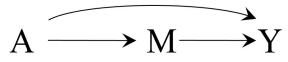
Figure 23.1

duced the pure direct effect and the total indirect effect.

Proof of the mediation formula. In the setting depicted by the causal diagram in Figure 23.1 with treatment A, mediator M, and outcome Y , the counterfactual mean E h Y ^a=1,Ma=0 i is equal to

= P ^m E - Y ^a=1,m|Ma=0 = m Pr[Ma=0 = m] by the laws of probability = P ^m E - Y ^a=1,m Pr[Ma=0 = m] by the cross-world conditional independence Y ^a=1,m⊥⊥Ma=0 = P ^m E [Y |A = 1, M = m] Pr[M = m|A = 0] by exchangeability and consistency.

The cross-world conditional independence used above is assumed when the causal diagram represents an NPSEM-IE, but not when it represents an FFRCISTG model.

effect is then the contrast

\[\mathbb{E}\left[Y^{a=1,M^{a=0}}\right] - \mathbb{E}\left[Y^{a=0,M^{a=0}}\right]\]

In our example, the pure direct effect is the effect of smoking cessation A if we could assign to each person the value of hypertension M (1 or 0) that the person would have had if she had quit smoking. This value of hypertension M is known for individuals who actually quit smoking, but it remains unknown for individuals who continued to smoke. We therefore say that E h Y a=1,Ma=0 i , and therefore the pure direct effect, is a cross-world quantity because it involves a counterfactual outcome indexed by two treatment values, a = 1 and a = 0, Pearl (2001) referred to the pure di- that cannot occur simultaneously for the same individual in the same world.

The total indirect effect, also a cross-world quantity, is defined as

\[\operatorname{E}\left[Y^{a=1,M^{a=1}}\right] - \operatorname{E}\left[Y^{a=1,M^{a=0}}\right]\]

The sum of the pure direct effect and the total indirect effect E h Y a=1,Ma=1 i − E h Y a=0,Ma=0 i is, by consistency, the total effect E - Y ^a=1 − E - Y ^a=0 .

In Figure 23.1, there do not exist unmeasured common causes of the mediator M and the outcome Y . If common causes were present, no direct effects could be identified, including controlled direct effects and the mediation effects, i.e., the pure direct and the total indirect effects. To identify the mediation effects, we need to identify the cross world quantity E h Y ^a=1,Ma=0 i under the causal diagram in Figure 23.1. The so-called mediation formula does that:

\[\sum\_{m} \operatorname{E} \left[ Y \mid A = 1, M = m \right] \Pr[M = m \mid A = 0]\]

The proof is shown in Technical Point 23.1.

The mediation formula seems surprising because it identifies a cross-world counterfactual quantity whose value cannot be empirically confirmed by any In some very unusual situations, experimental intervention on A and M, not even in principle. To achieve this, however, one needs to assume that the causal diagram in Figure 23.1 represents an NPSEM-IE rather than an FFRCISTG, the latter of which is the counterfactual model that we have been using throughout the book (see Technical Point 6.2).

The proof of the mediation formula requires the unverifiable assumption that some counterfactual variables defined in separate worlds are independent. Specifically, the proof requires that the value of the outcome Y ^a=1,m in a world

rect effect and the total indirect effect as the natural direct effect and the natural indirect effect, respectively.

we could identify the value of this cross-world counterfactual quantity by a crossover trial (see Fine Points 2.1 and 3.2).

pure direct effect and the total indirect effect are not point identified, but sharp bounds can be obtained (Robins and Richardson 2010).

in which we have jointly intervened by setting the value of treatment to 1 and the value of the mediator to m is independent from the value of the mediator Ma=0 in a world in which we have intervened to set the value of treatment to 0. Therefore, the variables Y ^a=1,m and Ma=0 cannot be simultaneously observed for the same individual in a single world, and thus their independence is not empirically verifiable in any experiment in which A and M are randomly assigned singly or jointly (see Technical Point 7.1).

These cross-world independencies are assumed under an NPSEM-IE but Under an FFRCISTG model, the not under an FFRCISTG model. This is one reason for our privileging an FFRCISTG model over an NPSEM-IE: because cross-world independencies cannot be verified by any randomized experiment, we want to use causal inference methods whose results are, in principle, verifiable.

Based on this discussion, some policy makers are unimpressed that the investigators can identify the pure direct effect. As a cross-world parameter, they find the pure direct effect to be without policy or public health importance because it does not correspond to any intervention. To convince these skeptics, advocates of the NPSEM-IE will need to work harder.

23.2 A defense of mediation analysis

The investigators of the smoking cessation trial, as advocates of the NPSEM-IE, prepare the following rationale to convince the skeptics about the practical utility of the pure direct effect.

“Suppose that, starting a year from now, nicotine-free cigarettes will be available and that your policy goal is learning the benefits of nicotine-free cigarettes as soon as possible. To do so, we use the already collected data from the above smoking cessation trial to estimate the two-year risk of heart disease Y under an intervention requiring all smokers to change to nicotine-free cigarettes Pearl (2001) provided a similar ar- (when they become available). Suppose that strong experimental evidence exists that (i) the entire causal effect of nicotine on the outcome Y (heart disease) is through its effect on the mediator M (hypertension), and that (ii) the non-nicotine components in cigarettes have no direct causal effect on the mediator M (hypertension). Under assumptions (i) and (ii), the hypertensive status M of a smoker of nicotine-free cigarettes will equal her hypertensive status under non-exposure to cigarettes and hence E h Y ^a=1,Ma=0 i will be the risk of heart disease in smokers were all smokers to change to nicotine-free cigarettes a year from now. That is exactly your public health effect of interest and this is what the mediation formula would compute when applied to the data of our study”.

This is interesting. To argue for the substantive importance of the parameter Eh Y ^a=1,Ma=0 i , the NPSEM-IE advocates tell a story about the effect of an intervention on the nicotine content of cigarettes—an intervention that makes no reference to the mediator M at all. Also, they make the “no direct effect” assumptions (i) and (ii) about the absence of direct effects of variables that were not even included on the causal diagram in Figure 23.1.

The investigators’ story states that the variable A can be decomposed into two separable components N and O. The separable component N directly

gument to justify the use of pure direct effects.

When the mediation formula is the g-formula. According to the causal diagram in Figure 23.3, exchangeability holds for the separable components N and O and therefore the mean E - Y ⁿ=0,o=1 may be identified by the g-formula. However, in the smoking cessation trial described in the main text, no individual has data (N = 0, O = 1). Therefore, positivity does not hold and it appears that the g-formula cannot identify E - Y ⁿ=0,o=1 . But, given exchangeability and consistency, positivity is a sufficient but not necessary condition for identification by the g-formula; identification only requires that the g-formula is a function of the observed data distribution. We now show that the deterministic bold arrows in Figure 23.2 and the no direct effect assumptions (i) and (ii) together imply that the g-formula is indeed a function of the observed data distribution of (A, M, Y )—that function being the mediation formula.

Under an FFRCISTG represented by Figure 23.2, if data on N and O were available, the mean E - Y ⁿ=0,o=1 would be identified by the g-formula

\[\sum\_{m} \operatorname{E} \left[ Y \mid O=1, M=m \right] \Pr(M=m \mid N=0)\]

since, in the g-formula N = 0 needs not be included in the first conditioning event and O = 1 needs not be included in the second conditioning event because N is not a parent of Y and O is not a parent of M in Figure 23.2. Furthermore, even though positivity does not hold, the g-formula is a function of the observed data distribution only because O = 1 if and only if A = 1 and N = 0 if and only if A = 0. Thus, we can rewrite the g-formula for E - Y ⁿ=0,o=1 as

\[\sum\_{m} \operatorname{E} \left[ Y \mid A=1, M=m \right] \Pr(M=m \mid A=0)\]

which is exactly the mediation formula. This derivation, based on the g-formula, is somewhat heuristic because of the presence of null sets arising from determinism between N, O and L. Robins et al. (2022) provide an alternative, rigorous proof using the SWIG Markov property described in Technical Point 21.12.

Not only does the g-formula equal the mediation formula under the expanded causal diagram in Figure 23.2, but the g-formula also equals the front door formula under the expanded causal diagram in Figure 23.7, as shown in Technical Point 23.3.

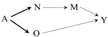
Figure 23.2

fect” assumptions. Assumption (i) says that there is no direct effect of N on Y when controlling for (setting) the value of M.

affects M but not Y . The separable component O directly affects Y but not M. Also, according to the story, each separable component can in principle be intervened on separately. For example, Y ⁿ=0,o=1 represents the counterfactual outcome under an intervention that removes (only) the nicotine component of cigarettes.

The most direct representation of this causal story is provided by an FFR-CISTG model represented by the causal DAG in Figure 23.2 where N is a binary variable representing nicotine exposure, and O is a binary variable representing exposure to the other non-nicotine components of a cigarette. The bold arrows from A to N and O indicate deterministic relationships. This is because, in the actual data from the trial, either one continues to smoke normal cigarettes so A = N = O = 1, or quits smoking cigarettes so A = N = O = 0. These are “no controlled direct ef- The absence of an arrow from N to Y encodes assumption (i) that N does not have a direct effect on Y . The absence of an arrow from O to M encodes assumption (ii) that O does not have an effect on M. Figure 23.3 shows the associated SWIG. If O is not a cause of M for every individual we can additionally write the random variable Mn,o as Mⁿ.

Under this characterization of the problem, the g-formula that identifies E - Y ⁿ=0,o=1 is exactly the mediation formula (see proof in Technical Point 23.2). Let us review the lessons we learned.

For a researcher that initially accepted an NPSEM-IE associated with the

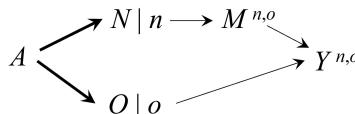
Figure 23.3

DAG in Figure 22.1, the mean E h Y ^a=1,Ma=0 i was already identified by the mediation formula so the story of separable effects of N and O did not contribute to identification. Rather, it served only to show that the parameter E h Y ^a=1,Ma=0 i —and thus the pure direct effect and the total indirect effect encodes a parameter E - Y ⁿ=0,o=1 of public health interest. For a researcher that takes the FFRCISTG point of view, the story not only provides an interventional interpretation of the mean E h Y ^a=1,Ma=0 i as the mean E - Y ⁿ=0,o=1 , but in addition makes both means identifiable via the g-formula or, equivalently, the mediation formula. In fact, when we interpret absence of an arrow as an absence of a direct causal effect for all individuals, Y ^a=1,Ma=0 and Y ⁿ=0,o=1 are equal for every individual.

This characterization of the problem also allows us to define and identify the separable direct effect of the component N on the outcome Y , E- Y ⁿ=1,o=1 − E - Y ⁿ=0,o=1 , which is a controlled direct effect for the separable component N. This effect is also equal to the total indirect effect E - Y ^a=1 − E h Y a=1,Ma=0 i . Analogously, E - Y ⁿ=1,o=1 − E - Y ⁿ=1,o=0 is the pure direct effect Eh Y a=1,Ma=0 i − E - Y ^a=0 .

23.3 Empirically verifiable mediation

The interventional interpretation of E h Y a=1,Ma=0 i is only valid if the story about the separable effects of N and O is correct and Figure 23.3 represents an FFRCISTG. An advantage of the interventional interpretation is that the validity of this story can be, in principle, empirically refuted via a randomized trial, as we now describe.

When nicotine-free cigarettes become available in a year, we conduct a new randomized trial in which a random sample of cigarette smokers are randomly assigned to one of three groups: smoking cessation (A = N = O = 0), continuation of smoking of standard cigarettes (A = N = O = 1), or continuation of smoking of nicotine-free cigarettes (N = 0, O = 1). That is, the new trial has the same two arms as the original trial plus an additional arm of nicotine-free cigarettes. In the absence of temporal trends, the mean outcomes for the first two arms should be the same in both trials. We assume that the sample size of both trials is large enough to ignore sampling variability.

By randomization, the mean outcome E [Y |N = 0, O = 1] in the new trial is expected to equal E - Y ⁿ=0,o=1 . Therefore, if our story is correct, we expect that E [Y |N = 0, O = 1] will equal the mediation formula from the earlier trial. Otherwise, the N and O story has been empirically refuted, which implies that one or more of the following assumptions is incorrect: (i) no direct effect of nicotine on the outcome, (ii) no direct effect of other, non-nicotine components on the mediator, (iii) no unmeasured common cause U of M and Y on the causal diagram in Figure 23.2.

If E [Y |N = 0, O = 1] differs from the mediation formula, we can use the data from this new trial to investigate which of the assumptions (i)-(iii) are false. To do so, we start by checking whether O and M are associated among those with N = 0, i.e.,

\[\operatorname{E}\left[M|N=0,O=1\right] - \operatorname{E}\left[M|N=0,O=0\right] \neq 0\]

Empirical falsification of the assumptions for separable effects. Suppose we had conducted the three-arm trial with interventions on N and O, and found that N and Y are associated within joint levels of M and O. Then, as stated in the main text, we conclude that either assumption (i) or assumption (iii), or both, are false.

To determine which of the two assumptions are false, we would need another randomized trial with, say, 8 arms in which we intervene on M as well as on N and O. If N has no direct effect on Y except through M, N will be independent of Y given M and O in the eight-arm trial. If M and Y do not share an unmeasured common cause, the conditional distribution of Y given M within levels of N and O should be the same in the three-arm trial and in the eight-arm trial.

One might wonder how Figure 23.2 can have an unmeasured common cause of M and Y left off the graph if we are correct in assuming that Figure 23.1 represents an FFRCISTG model with no common causes of M and Y . The explanation is that common causes may only be present (i.e., active) under interventions that assign different values of N and O to each person. The FFRCISTG model associated with Figure 23.1, unlike that associated with Figure 23.2, only considers interventions A = N = O = 1 and A = N = O = 0 that assign the same value to each person. Interestingly, if a common cause U of Y and M is the only reason E [Y |N = 0, O = 1] in the new trial differs from the mediation formula, it is still the case that Y ⁿ=0,o=1 = Y ^a=1,Ma=0 for every individual. However, E - Y ⁿ=0,o=1 = Eh Y a=1,Ma=0 i is not identified by the mediation formula. Robins et al. (2022) describe a hypothetical but realistic study of treatment for river blindness under which Figure 23.1 is an FFRCISTG but Figure 23.2 is not because a common cause U of Y and M is missing from the latter graph.

If that is the case, then assumption (ii) is refuted and the arrow O → M should be added to Figure 23.2 (and the corresponding arrow to Figure 22.3).

We next check whether N and Y are associated within joint levels of M and O, i.e., whether

\[\operatorname{E}\left[Y|N=1, O=1, M=m\right] - \operatorname{E}\left[Y|N=0, O=1, M=m\right] \neq 0\]

for some values of m. If that is the case, then assumption (i) is refuted (which implies that an arrow N → Y should be added to the causal diagrams) or an unmeasured common cause U of M and Y exists (and should be added to the causal diagrams). See Fine Point 23.1.

Now suppose that in two years, when the results of the new trial become available, the mean outcome estimates are equal in the arms that correspond to the same intervention in both trials, but the estimate of the mean outcome in the third arm of the new trial, E [Y |N = 0, O = 1], differs from the mediation formula in the first trial. How would different people react?

Both a person who had assumed that Figure 23.1 was an NPSEM-IE and a person who only assumed that it was an FFRCISTG would agree that the story of separable effects of O and N was incorrect, and that E - Y ⁿ=0,o=1 is correctly estimated by the mean outcome in the third arm of the new trial and not by the mediation formula in the earlier trial.

Those who had assumed an NPSEM-IE can continue to believe that the mean Eh Y ^a=1,Ma=0 i is still equal to the mediation formula, but they cannot justify the policy interest of the pure direct effect as the effect of taking nicotinefree cigarettes. Those who assumed an FFRCISTG may have little interest in the original mediation formula. Instead they will be interested in what they have learned about the effects of nicotine-free cigarettes on the outcome from the three-arm randomized trial. They will also be interested in learning that one or more of the following assumptions were false: (i) no direct effect of nicotine on the outcome, (ii) no direct effect of other, non-nicotine components on the mediator, (iii) no unmeasured common cause U of M and Y .

Y ^a=1,Ma=0 i were always point identified by the mediation formula, the sharp bounds in Robins and Richardson (2010) would be violated.

Continue to assume that Figure 23.1 represents an FFRCISTG model and that E- Y ⁿ=0,o=1 in the future nicotine-free cigarette trial differs from the mediation formula. An interesting question is whether treatment A can always be decomposed into other (possibly unknown) intervenable components N′ and O′ If E such that Figure 23.2 is an FFRCISTG and the no direct effect assumptions h (i) and (ii) hold, in which case E h Y n ′=0,o′=1i would equal E h Y ^a=1,Ma=0 i and both would equal the mediation formula? The answer is no, since otherwise E h Y ^a=1,Ma=0 i would always be point identified by the mediation formula, which is not the case.

23.4 An interventionist theory of mediation

ation was presented by Robins and Richardson (2010) and extended by Robins, Richardson, and Shpitser (2022). The theory has been extended to survival analysis (Didelez 2019, Aalen et al. 2020), competing risks (Stensrud et al. 2020, 2021), and settings with interference (Shpitser et al. 2021).

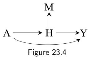
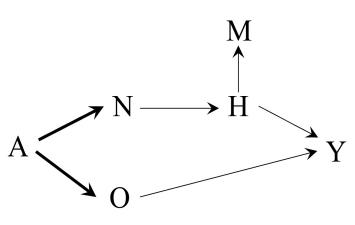
Figure 23.5

Stensrud et.al. (2021) emphasized the need for the above equalities of mean outcomes across arms of the six-arm trial.

In this chapter we have introduced an interventionist theory of causal medi-This theory of interventionist medi- ation that differs from the standard approach based on pure direct and total indirect effects. Because the interventionist theory was developed in response to perceived deficiencies in the standard theory, we first described the standard theory and its problematic aspects resting on the use of cross-world (nested) counterfactuals. However, the interventionist theory can be viewed as autonomous, providing a self-contained framework for discussing mediation without reference to cross-world nested counterfactuals.

To do so, we used a (simplified) randomized trial with a time-fixed treatment as an intervention. The key idea was reframing the mediation question as a question about the effects of interventions on substantively meaningful, separable components (N and O) of treatment A on Y . If N and O are separable effects of A, then, in a future randomized trial with six arms:

• 1. treat with a = 1
• 2. treat with a = 0
• 3. treat with n = 1, o = 1
• 4. treat with n = 0, o = 0
• 5. treat with n = 0, o = 1
• 6. treat with n = 1, o = 0)

then the following two statements are true. First, the mean of the outcome Y in the first arm equals that in the third and the mean outcome in the second arm equals that in the fourth. Second, E - Y ⁿ=0,o=1 is identified as the mean outcome in the fifth arm and E - Y ⁿ=1,o=0 as the mean outcome in the sixth arm of the future trial, regardless of whether E - Y ⁿ=0,o=1 is not identified from the observed data.

We can use currently available data on A, M, and Y to identify the separable effects of N and O under the assumptions of (i) no unmeasured common cause of the mediator M and the outcome Y and (ii) no direct effects of the component O on the mediator M and of component N on outcome Y . In particular, E - Y ⁿ=0,o=1 equals the mediation formula.

Separable effects with a surrogate mediator. In the following we adopt the theory of causal diagrams introduced in Section 9.5. Since the arrow from M to Y is only causally interpretable when there exist well-defined interventions for the effect of M on Y , the DAG in Figure 23.1 is not causal when those interventions do no exist. That is, M is not a mediator but rather a surrogate for an unknown variable H that is the true mediator for which well-defined interventions exist. The causal DAG in Figure 23.4 represents this scenario.

Consider the causal diagram in Figure 23.5, which is an extension of Figure 23.4 with separable components N and O. In contrast to Figure 23.2, N and Y are not d-separated given M and O in Figure 23.5. Suppose, surprisingly, we observe that N and Y are independent given M and O in our three-arm trial data. How should we interpret this observation? There are 4 possibilities: a) we were mistaken: Figure 23.1 rather than 23.4 is the true causal diagram and M is the true causal mediator, b) M is a one-to-one deterministic function of the true causal mediator H, c) there is a non-deterministic faithfulness violation in Figure 23.4, and d) N and O are not conditionally independent but the three-arm trial was too small to detect their dependence. Advocates of causal discovery would tend to adopt interpretation a) if the sample size in the three-arm trial was large (see Technical Point 10.7).

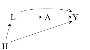
Figure 23.6

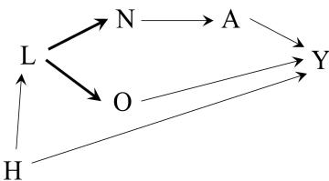
Figure 23.7

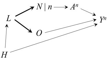
Figure 23.8

We now discuss one further reason to prefer an interventionist approach over earlier approaches to causal mediation. Specifically, it is often the case that

interventions on the putative mediator M are not well-defined and counterfactuals like Y a,m are then not meaningful. Then neither the pure direct effect nor the controlled direct effects (described in Technical Point 22.1) based on M exist. In contrast, the interventionist theory is concerned with effects that exist, even if interventions on M are not well-defined, as long as substantively meaningful separable components N and O exist and can be intervened on as discussed above.

To summarize, an interventionist approach to mediation include the following components.

• the hypothesis that treatment A can be decomposed into multiple, substantially meaningful, separable components, each of which contributes to the overall effect of treatment and which can, in principle be independently intervened on
• the assumptions needed to identify the effects of the separable components are, in principle, empirically verifiable in future randomized trials in which these components are actually intervened on
• well-defined interventions on a purported mediator need not exist
• enhanced communication with subject-matter experts owing to the substantive specificity of the separable components
• when the identifying assumptions hold, the identifying g-formula is identical to the mediation formula; however, the identified causal effects refer to interventions on the separable components.

For simplicity, we considered an example with only two separable components, but the interventionist framework can accommodate multiple separable components of treatment, including those that vary over time.

In this chapter we have reviewed theoretical concepts of mediation, but we have not emphasized the practical aspects of data analyses to estimate pure

Path-specific effects and the front door formula. Under Figure 23.6, which is the modified version of Figure 9.14, the total effect of L on Y is not identified. This is because the contribution of the pathway L → Y to the total effect cannot be separated from the confounding effect of H. In contrast, under the unmodified causal diagram in Figure 9.14 lacking the L → Y edge, we showed in Fine Point 9.5 that the total effect of L on Y was identified by the front door formula, as L → A → Y was the sole causal pathway.

We now consider whether the effect of L along the pathway L → A → Y is also identified, and by the same front door formula when the L → Y edge is present. In the spirit of this chapter, we shall use the substantive story in Fine Point 9.5 to provide an interventionist formulation of this question. Figure 23.7 is an expanded graph where N records the value of BMI L reported to the physician responsible for prescribing drug A, and O records the value of L used to determine referral to physical therapy and diet counseling. The bold arrows indicate a deterministic relationship, since, in the observed data, we always have L = N = O. Figure 23.8 is a SWIG representing an (unethical) intervention in which a value n of BMI different from the truth L = N was reported to the physician, but the true value L = O was used for the referrals. In contrast with earlier in the this chapter, only N has been intervened on. Further, as was our goal, the effect on Y of the intervention on n is restricted to the path through A. Since L ≡ O even in the intervened world, we have no need of O. We therefore remove O from Figures 23.7 and 23.8 and again have Y as a child of L. Then noting trivially that Y ⁿ ⨿ N|L on Figure 23.8, E [Y ⁿ] should be given by the g-formula based on Figure 23.7 which equals

\[\sum\_{l,a} \operatorname{E}\left[Y|A=a, L=l\right] \Pr[L=l] \Pr[A=a|N=n] = \sum\_{a} \left\{ \sum\_{l} \operatorname{E}\left[Y|A=a, L=l\right] \Pr[L=l] \right\} \Pr[A=a|L=n]\]

where the last equality is by the determinism L ≡ N in the data. The right hand side is indeed the front door formula.

However, this derivation is somewhat heuristic due to the presence of null sets arising from determinism. A rigorous proof is readily obtained by combining determinism with the approach used in Technical Point 21.12 to prove the front door formula. Note also that, substantively speaking, one generally would not consider N and O as separable components of L. But that is irrelevant. What matters is that our substantive causal story implies an expanded graph 23.7 containing the new intervention variable N that is deterministically related to L in the actual world (Stensrud et al., 2023). Wen et al. (2023) have independently and concurrently obtained results essentially equivalent to those of this technical point. Fulcher et al. (2020) had earlier shown that the above front door formula identifies the cross world counterfactual quantity E[Y L,Al=ⁿ ] under the NPSEM-IE model associated with Figure 23.6. Both Wen et al. and this Technical Point can be seen as interventionist reformulations of Fulcher et al’s result.

direct effects and separable direct effects. In the previous chapter, we adopted a similar approach when introducing controlled direct effects and principal stratum direct effects. We hope that our presentation has clarified the scientific advantages of an interventionist approach to the identification of direct effects.

In the absence of randomized trials with actual interventions on either the mediator (for controlled direct effects) or components of treatment (for separable direct effects), all these methodologies rely on observational data and therefore on the exchangeability assumptions that we have discussed throughout the book. Hence, valid mediation analyses require adjustment for the confounders for the effect of treatment and for the effect of the mediator in For separable effects, additional is- addition to other assumptions that we discussed in this chapter. Our causal diagram in Figure 23.1 was intended as a teaching device to explore theoretical issues related to mediation in a simplified setting, not as a realistic representation of most studies of causal mediation. In practice, causal mediation analyses are observational analyses that rely on more heroic assumptions than non-mediation analyses.

sues arise if there is a measured cause of M and Y that is a child of N and O (Robins and Richardson 2010; Robins et al. 2022).

References

• Aalen OO, Stensrud MJ, Didelez V, Daniel R, Røysland K, Strohmaier S (2020). Time-dependent mediators in survival analysis: Modeling direct and indirect effects with the additive hazards model. Biometrical Journal 62(3):532–549
• Abadie A (2005). Semiparametric difference-in-differences estimators. The Review of Economic Studies 72(1): 1-19.
• Abadie A, Chingos MM, West MR (2018). Endogenous stratification in randomized experiments. The Review of Economics and Statistics 100 (4): 567–580.
• Abadie A, Imbens GW (2006). Large sample properties of matched estimates for average treatment effects. Econometrica 74:235-267.
• Amrhein V, Greenland S, McShane B (2019). Scientists rise up against statistical significance. Nature 567:305-307.
• Angrist JD, Imbens GW (1995). Two-stage least squares estimation of average causal effects in models with variable treatment intensity. Journal of the American Statistical Association 90:431-442.
• Angrist JD, Imbens GW, Rubin DB (1996). Identification of causal effects using instrumental variables. Journal of the American Statistical Association 91:444-455.
• Angrist JD, Krueger AB (1999). Empirical strategies in labor economics. In: Ashenfelter O, Card D, eds. Handbook of Labor Economics 3A, 1277- 1366. Elsevier.
• Angrist JD, Pischke J-S (2009). Mostly Harmless Econometrics: An Empiricist’s Companion. Princeton University Press.
• Avagyan V, Vansteelandt S (2021). Stable inverse probability weighting estimation for longitudinal studies. Scandinavian Journal of Statistics 48(3), 1046– 1067.
• Baiocchi M, Small D, Lorch S, Rosenbaum P (2010). Building a sttronger instrument in an observational study of perinatal care for premature infants. Journal of the American Statistical Association 105(492): 1285- 1296.
• Baiocchi M, Cheng J, Small D (2014). Instrumental variable methods for causal inference. Statistics in Medicine 33: 2297-2340.
• Baker SG, Lindeman KS (1994). The paired availability design, a proposal for evaluating epidural analgesia during labor. Statistics in Medicine 13:2269-2278.
• Baker SG, Kramer BS, Lindeman KL (2016). Latent class instrumental variables. A clinical and biostatistical perspective. Statistics in Medicine 35:147-160 (errata in Statistics in Medicine 2019; 38: 901).
• Balke A, Pearl J (1994). Probabilistic evaluation of counterfactual queries. In Proceedings of the Twelfth National Conference on Artificial Intelligence, Volume I, pp. 230-237.
• Balke A, Pearl J (1997). Bounds on treatment effects from studies with imperfect compliance. Journal of the American Statistical Association 92(439):1171-1176.
• Bang H, Robins JM (2005). Doubly robust estimation in missing data and causal inference models. Biometrics 61: 962-972 (errata in Biometrics 2008;64:650).
• Barnow SN, Cain GG, Goldberger AS (1980). Issues in the analysis of selectivity bias. In: Evaluation Studies (Vol. 5). Stromsdorfer EW, Farkas G, eds. Beverly Hills, CA: Sage Publication.
• Berkson J (1946). Limitations of the application of fourfold table analysis to hospital data. Biometrics 2: 47-53.
• Berkson J (1955). The statistical study of association between smoking and lung cancer. Proceedings of the Staff Meetings of the Mayo Clinic 30: 319-348.
• Blot WJ, Day NE (1979). Synergism and interaction: are they equivalent? [letter] American Journal of Epidemiology 110:99-100.
• Blyth CR (1972). On Simpson’s paradox and the sure-thing principle. Journal of the American Statistical Association 67:364-66.
• Bonet B (2001). Instrumentality tests revisited. In: Proceedings of the Seventeenth Conference on Uncertainty in Artificial Intelligence. San Francisco, CA: Morgan Kaufmann, pp. 48-55.
• Bound J, Jaeger D, Baker R (1995). Problems with instrumental variables estimation when the correlation between the instruments and the endogenous explanatory variables is weak. Journal of the American Statistical Association 90:443-450.
• Brown LD, Cai T, DasGupta A (2001). Interval estimation for a binomial proportion (with discussion). Statistical Science 16:101-133.
• Brookhart MA, Schneeweiss S (2007). Preference-based instrumental variable methods for the estimation of treatment effects: assessing validity and interpreting results. International Journal of Biostatistics 3:14.
• Brookhart MA, Rassen J, Schneeweiss S (2010). Instrumental variable methods in comparative safety and effectiveness research. Pharmacoepidemiology and Drug Safety 19:537-554.
• Buehler RJ (1982). Some ancillary statistics and their properties. Rejoinder. Journal of the American Statistical Association 77:593-594.
• Cain LE, Robins JM, Lanoy E, Logan R, Costagliola D, Hern´an MA. When to start treatment? A systematic approach to the comparison of dynamic regimes using observational data. International Journal of Biostatistics 2010; 6(2) Article 18.
• Card D (1990). The Impact of the Mariel Boatlift on the Miami Labor Market. Industrial and Labor Relations Review 43(2):245-257.
• Card D (1995). Using geographic variation in college proximity to estimate the return to schooling. In: Christofides LN, Grant EK, Swidinsky R, eds. Aspects of labor market behavior: Essays in honour of John Vanderkamp. Toronto, Canada: University of Toronto Press.
• Casella G, Berger RL (2002). Statistical Inference, 2nd ed. Pacific Grove, CA: Duxbury Press.
• Cochran WG (1972). Observational studies. In: Bancroft TA, ed. Statistical Papers in Honor of George W Snedecor. Iowa State University Press, pp. 77-90
• Cole SR, Hern´an MA (2002). Fallibility in estimating direct effects. International Journal of Epidemiology 31(1):163-165.
• Cornfield J, Haenszel W, Hammond EC, Lilienfeld AM, Shimkin MB, Wynder EL (1959). Smoking and lung cancer: Recent evidence and a discussion of some questions. Journal of the National Cancer Institute 22:173- 203. Reprinted in International Journal of Epidemiology 2009; 38(5): 1175-1191.
• Cox DR (1958). Planning of Experiments. New York, NY: John Wiley and Sons.
• Cox DR, Wermuth N (1999). Likelihood factorizations for mixed discrete and continuous variables. Scandinavian Journal of Statistics 26(2): 209–220.
• Cui Y, Pu H, Shi X, Miao W, Tchetgen Tchetgen EJ (2024). Semiparametric proximal causal inference. Journal of the American Statistical Association 119(546): 1348-1359.
• Dahabreh IJ, Hern´an (2019). Extending inferences from a randomized trial to a target population. European Journal of Epidemiology 34(8): 719- 722.
• Dahabreh IJ, Petito LC, Robertson SE, Hern´an MA, Steingrimsson JA (2020a). Toward causally interpretable meta-analysis: transporting inferences from multiple randomized trials to a new target population. Epidemiology 31(3):334-344.
• Dahabreh IJ, Robertson SE, Steingrimsson JA, Stuart EA, Hern´an MA (2020b). Extending inferences from a randomized trial to a new target population. Statistics in Medicine 39(14):1999-2014.
• Danaei G, Robins JM, Hu FB, Manson J, Hern´an MA (2016). Effect of weight loss on coronary heart disease and mortality in middle-aged or older women: sensitivity analysis for unmeasured confounding by undiagnosed disease. Epidemiology 27(2): 302-310.
• Davey Smith G, Ebrahim S (2004). Mendelian randomization: prospects, potentials, and limitations. International Journal of Epidemiology 33: 30-42.
• Dawid AP (1979). Conditional independence in statistical theory (with discussion). Journal of the Royal Statistical Society B 41:1-31.
• Dawid AP (2000). Causal inference without counterfactuals (with discussion). Journal of American Statistical Association 95: 407-424.
• Dawid AP (2002). Influence diagrams for causal modelling and inference. International Statistical Review 70: 161-189.
• Dawid, A. P. (2003). Causal inference using influence diagrams: The problem of partial compliance (with discussion). In: Green PJ, Hjort NL, Richardson S, eds. Highly Structured Stochastic Systems. New York, NY: Oxford University Press, 45-65.
• de Finetti (1972). Probability, Induction, and Statistics. John Wiley & Sons.
• Deaton A (2010). Instruments, randomization, and learning about development. Journal of Economic Literature 48 424-455.
• Detels R, Mu˜noz A, McFarlane G, Kingsley LA, Margolick JB, Giorgi J, Schrager L, Phair J, for the Multicenter AIDS Cohorts Study (1998). JAMA 280(17): 1497-1503.
• Diaz I, Williams N, Hoffman KL, Schenck EJ (2021). Nonparametric causal effects based on longitudinal modified treatment policies. Journal of the American Statistical Association 118(542):846-857.
• Didelez V (2019). Defining causal mediation with a longitudinal mediator and a survival outcome. Lifetime Data Analysis 25(4):593–610.
• Didelez V, Sheehan N (2007). Mendelian randomization as an instrumental variable approach to causal inference. Statistical Methods in Medical Research 16: 309-330.
• Ding P, VanderWeele TJ, Robins JM (2017). Instrumental variables as bias amplifiers with general outcome and confounding. Biometrika 104(2): 291-302.
• Dorn HF (1953). Philosophy of inferences for retrospective studies. American Journal of Public Health 43: 677-83.
• Dosemeci M, Wacholder S, Lubin JH (1990). Does nondifferential misclassification of exposure always bias a true effect toward the null value? American Journal of Epidemiology 132:746-748.
• Earle CC, Tsai JS, Gelber RD, Weinstein MC, Neumann PJ, Weeks JC (2001). Cancer in the elderly: instrumental variable and propensity analysis. Journal of Clinical Oncology 19(4): 1064-1070.
• Efron B, Hinkley DV (1978). Assessing the accuracy of the maximum likelihood estimator: observed versus expected Fisher information. Biometrika 65: 657-687.
• Feinstein AR (1971). Clinical biostatistics. XI. Sources of ‘chronology bias’ in cohort statistics. Clinical Pharmacology and Therapeutics 12(5): 864- 79.
• Fisher RA (1922). On the mathematical foundations of theoretical statistics. Philosophical Transactions of the Royal Society of London. Series A; 222 (594–604): 309-368.
• Flanders WD (2006). On the relation of sufficient component cause models with potential (counterfactual) models. European Journal of Epidemiology 21: 847-853.
• Flanders WD, Klein M, Darrow LA, Strickland MJ, Sarnat SE, Sarnat JA, Waller LA, Winquist A, Tolbert PE (2011). A Method for Detection of Residual Confounding in Time-series and Other Observational Studies. Epidemiology 22(1): 59-67.
• Fleming TR, Harrington DP (2005). Counting Processes and Survival Analysis, 2nd ed. New York: Wiley.
• Frangakis CE, Rubin DB (2002). Principal stratification in causal inference. Biometrics 58(1); 21-29.
• Fulcher IR, Shpitser I, Marealle S, Tchetgen Tchetgen EJ (2020). Robust inference on population indirect causal effects: the generalized front door criterion. Journal of the Royal Statistical Society Series B: Statistical Methodology 82(1); 199-214.
• Glymour MM, Spiegelman D (2016). Evaluating public health interventions: 5. Causal inference in public health research-Do sex, race, and biological factors cause health outcomes? American Journal of Public Health 107(1): 81-85.
• Glymour MM, Tchetgen Tchetgen EJ, Robins JM (2012). Credible Mendelian randomization studies: approaches for evaluating the instrumental variable assumptions. American Journal of Epidemiology 175: 332-339.
• Goodfellow I, Bengio Y, Courville A (2016). Deep Learning. Cambridge, MA: MIT Press.
• Greenland S (1977). Response and follow-up bias in cohort studies. American Journal of Epidemiology 106(3):184-187.
• Greenland S (1980). The effect of misclassification in the presence of covariates. American Journal of Epidemiology 112(4):564-569.
• Greenland S (1987). Interpretation and choice of effect measures in epidemiologic analyses. American Journal of Epidemiology 125(5):761-768.
• Greenland S (1991). On the logical justification of conditional tests for twoby-two contingency tables. The American Statistician 45(3):248-251.
• Greenland S (1996a). Basic methods for sensitivity analysis of bias. International Journal of Epidemiology 25(6):1107-1116.
• Greenland S (1996b). Absence of confounding does not correspond to collapsibility of the rate ratio or rate difference. Epidemiology 7(5):498-501.
• Greenland S (2000). An introduction to instrumental variables for epidemiologists. International Journal of Epidemiology 29(4):722-729.
• Greenland S (2003). Quantifying biases in causal models: classical confounding versus collider-stratification bias. Epidemiology 14:300-306.
• Greenland S (2009a). Bayesian perspectives for epidemiologic research. III. Bias analysis via missing-data methods. International Journal of Epidemiology 38:1662-1673.
• Greenland S (2009b). Relaxation penalties and priors for plausible modeling of nonidentified bias sources. Statistical Science 24:195-210.
• Greenland S (2019). Some misleading criticisms of P-values and their resolution with S-values. The American Statistician 73(supplement 1): 106- 114.
• Greenland S, Brumback B (2002). An overview of relations among causal modelling methods. International Journal of Epidemiology 31:1030-1037.
• Greenland S, Lash TL (2008). Bias analysis. In: Rothman KJ, Greenland S, Lash TL, eds. Modern Epidemiology, 3rd edition. Philadelphia, PA: Lippincott Williams & Wilkins, pp. 345-380.
• Greenland S, Lash TL, Rothman KJ (2008). Concepts of interaction. In: Rothman KJ, Greenland S, Lash TL, eds. Modern Epidemiology, 3rd edition. Philadelphia, PA: Lippincott Williams & Wilkins, pp. 71-83.
• Greenland S, Poole C (1988). Invariants and noninvariants in the concept of interdependent effects. Scandinavian Journal of Work, Environment & Health 14(2):125–129.
• Greenland S, Robins JM (1986). Identifiability, exchangeability, and epidemiological confounding. International Journal of Epidemiology 15:413- 19.
• Greenland S, Robins JM (1988). Conceptual problems in the definition and interpretation of attributable fractions. American Journal of Epidemiology 128:1185-1197.
• Greenland S, Robins JM (2009). Identifiability, exchangeability, and confounding revisited. Epidemiologic Perspectives & Innovations 6:4.
• Greenland S, Pearl J, Robins JM (1999). Causal diagrams for epidemiologic research. Epidemiology 10:37-48.
• Greenland S, Robins JM, Pearl J (1999). Confounding and collapsibility in causal inference. Statistical Science 14:29-46.
• Greenland S, Rothman KJ (2008). Introduction to stratified analysis. In: Rothman KJ, Greenland S, Lash TL, eds. Modern Epidemiology, 3rd edition. Philadelphia, PA: Lippincott Williams & Wilkins, pp. 258-282.
• Grieve AP (2003). The number needed to treat: a useful clinical measure or a case of the Emperor’s new clothes? Pharmaceutical Statistics 2:87-102.
• Hajek J (1971). Comment on “An essay on the logical foundations of survey sampling by D. Basu”. In: Godambe VP, Sprott DA, eds. Foundations of Statistical Inference. New York City, NY: Holt, Rinehart, and Winston; 1971 (p. 236).
• Halloran ME, Struchiner CJ (1995). Causal inference in infectious diseases. Epidemiology 6: 142-151.
• Hahn J, Todd P, van der Klaauw W (2001). Identification and estimation of treatment effects with a regression discontinuity design. Econometrica 69: 201-209
• Hansen BB (2008). The prognostic analogue of the propensity score. Biometrika 95(2): 481-488.
• Harrell FE (2015). Regression Modeling Strategies: With Applications to Linear Models, Logistic and Ordinal Regression, and Survival Analysis. New York: Springer.
• Hastie TJ, Tibshirani RJ (1990). Generalized Additive Models. London: Chapman & Hall.
• Hastie TJ, Tibshirani RJ, Friedman J (2009). The Elements of Statistical Learning: Data Mining, Inference,and Prediction, 2nd ed. New York: Springer.
• Heckman JJ, Vytlacil EJ (1999). Local instrumental variables and latent variable models for identifying and bounding treatment effects. Proceedings of the National Academy of Sciences USA 96:4730-4734.
• Hern´an MA (2010). The hazards of hazard ratios. Epidemiology 21(1):13-15.
• Hern´an MA (2016). Does water kill? A call for less casual causal inferences. Annals of Epidemiology 26: 674-680.
• Hern´an MA (2017). Selection bias without colliders. American Journal of Epidemiology 21(1):13-15.
• Hern´an MA, Brumback B, Robins JM (2001). Marginal structural models to estimate the joint causal effect of nonrandomized treatments. Journal of the American Statistical Association 96(454):440–448.
• Hern´an MA, Clayton D, Keiding N (2011). The Simpson’s paradox unraveled. International Journal of Epidemiology 40:780-785.
• Hern´an MA, Cole SR, Margolick JB, Cohen MH, Robins JM (2005). Structural accelerated failure time models for survival analysis in studies with time-varying treatments. Pharmacoepidemiology and Drug Safety 14(7):477- 491.
• Hern´an MA, Hern´andez-D´ıaz S, Werler MM, Mitchell AA (2002). Causal knowledge as a prerequisite for confounding evaluation: an application to birth defects epidemiology. American Journal of Epidemiology 155:176- 184.
• Hern´an MA, Hern´andez-D´ıaz S, Robins JM (2004). A structural approach to selection bias. Epidemiology 15:615-625.
• Hern´an MA, Hern´andez-D´ıaz S (2012). Beyond the intention to treat in comparative effectiveness research. Clinical Trials; 9(1):48-55.
• Hern´an MA, Hsu J, Healy B (2019). A second chance to get causal inference right: a classification of data science tasks. Chance 32(1):42-49.
• Hern´an MA, Robins JM (2006a). Estimating causal effects from epidemiological data. Journal of Epidemiology and Community Health 60: 578-586.
• Hern´an MA, Robins JM (2006b). Instruments for causal inference: An epidemiologist’s dream? Epidemiology 17(4): 360-372.
• Hern´an MA, Alonso A, Logan R, Grodstein F, Michels KB, Willett WC, Manson JE, Robins JM (2008). Observational studies analyzed like randomized experiments: an application to postmenopausal hormone therapy and coronary heart disease (with discussion). Epidemiology 19(6):766-779.
• Hern´an MA, Robins JM (2016). Using big data to emulate a target trial when a randomized trial is not available. American Journal of Epidemiology 183(8):758-764.
• Hern´an MA, Robins JM (2017). Per-protocol analyses of pragmatic trials. New England Journal of Medicine 377(14): 1391-1398.
• Hern´an MA, Sauer BC, Hern´andez-D´ıaz S, Platt R, Shrier I (2016). Specifying a target trial prevents immortal time bias and other self-inflicted injuries in observational analyses. Journal of Clinical Epidemiology 79: 70-75.
• Hern´an MA, Taubman SL (2008). Does obesity shorten life? The importance of well-defined interventions to answer causal questions. International Journal of Obesity 32: S8-S14.
• Hern´an MA, VanderWeele TJ (2011). Compound treatments and transportability of causal inference. Epidemiology 22:368-377.
• Holland PW (1986). Statistics and causal inference (with discussion). Journal of the American Statistical Association 81:945-961.
• Hoover DR, Mu˜noz A, He Y, Taylor JMG, Kingsley L, Chmiel JS, Saah A (1994). The effectiveness of interventions on incubation of AIDS as measured by secular increases within the population. Statistics in Medicine 13:2127-2139.
• Horvitz DG, Thompson DJ (1952). A generalization of sampling without replacement from a finite universe. Journal of the American Statistical Association 47:663-685.
• Huang Y, Valtorta M (2006). Pearl’s calculus of intervention is complete. In: Proceedings of the 22nd Conference in Uncertainty in Artificial Intelligence. Cambridge, MA: AUAI Press, pp. 217-224.
• Hosmer DW, Lemeshow S, May S (2008). Applied Survival Analysis: Regression Modelling of Time to Event Data. Hoboken, NJ: Wiley.
• Hudgens MG, Halloran ME (2009). Towards causal inference with interference. Journal of the American Statistical Association 103:832-842.
• Hume D (1748). An Enquiry Concerning Human Understanding. Reprinted and edited 1993, Indianapolis/Cambridge: Hacket.
• Imai K, Ratkovic M (2015). Robust estimation of inverse probability weights for marginal structural models. Journal of the American Statistical Association 110, 1013–1023.
• Imbens GW (2004). Nonparametric estimation of average treatment effects under exogeneity: a review. The Review of Economics and Statistics 86 (1): 4–29.
• Imbens GW, Angrist JD (1994). Identification and estimation of local average treatment effects. Econometrica 62:467-475.
• Imbens GW, Rubin DB (1997). Estimating outcome distributions for compliers in instrumental variables models. Review of Economic Studies 64:555-574.
• Imbens G, Lemieux T (2008). Regression discontinuity designs: A guide to practice. Journal of Econometrics 142 (2): 615–635.
• Kalbfleisch and Prentice (2002). The Statistical Analysis of Failure Time Data. Hoboken, NJ: Wiley.
• Kallus N, Santacatterina M (2018). Optimal balancing of time-dependent confounders for marginal structural models. arXiv preprint arXiv:1806.01083.
• Katan MB (1986). Apolipoprotein E isoforms, serum cholesterol, and cancer. Lancet, 1:507-508.
• Kleiner A, Talwalkar A, Sarkar P, Jordan MI (2014). A scalable bootstrap for massive data. Journal of the Royal Statistical Society B, 76 (Part 4):795-816.
• Kosinski S, Stillwell D, Graepel T (2013). Private traits and attributes are predictable from digital records of human behavior. Proceedings of the National Academy of Sciences 110(15): 5802-5805.
• Kurth T, Walker AM, Glynn RJ, Chan KA, Gaziano JM, Berger K, Robins JM (2006). Results of multivariable logistic regression, propensity matching, propensity adjustment, and propensity-based weighting under conditions of nonuniform effect. American Journal of Epidemiology 163(3): 262-270.
• Korn EL, Baumrind S (1998). Clinician preferences and the estimation of causal treatment differences. Statistical Science 13:209-235
• Laupacis A, Sackett DL, Roberts RS (1988). An assessment of clinically useful measures of the consequences of treatment. New England Journal of Medicine 318:1728-1733.
• Lauritzen SL, Dawid AP, Larsen BN, Leimer H-G (1990). Independence properties of directed Markov fields. Networks 20:491-505.
• Lash TL, Fox MP, Fink AK (2009). Applying Quantitative Bias Analysis to Epidemiologic Data. New York: Springer.
• Lewis D (1973). Counterfactuals. Oxford: Blackwell.
• Liang K-Y, Zeger SL (1986). Longitudinal data analysis using generalized linear models. Biometrika 73(1):13-22.
• Lin V, McGrath S, Zhang Z, Logan RW, Petito LC, Young JG, Hern´an MA (2019). gfoRmula: Parametric G-Formula. R package version 0.2.1. https://CRAN.R-project.org/package=gfoRmula.
• Lin L, Mukherjee R, Robins JM (2020). On nearly assumption-free tests of nominal confidence interval coverage for causal parameters estimated by machine learning. Statistical Science 35(3): 518-539.
• Lipsitch M, Tchetgen Tchetgen E, Cohen T. Negative controls: a tool for detecting confounding and bias in observational studies. Epidemiology 21(3):383-8 (erratum in Epidemiology 2010;21(4):589).
• Little RJ, D’Agostino R, Cohen ML, et al (2012). The prevention and treatment of missing data in clinical trials. New England Journal of Medicine 367(14): 1355-60.
• Mackie JL (1965). Causes and conditions. American Philosohpical Quartely 2:245-264.
• McClellan M, McNeil BJ, Newhouse JP (2004). Does more intensive treatment of acute myocardial infarction in the elderly reduce mortality? Analysis using instrumental variables. JAMA 272(11):859-866.
• Manski CF (1990). Nonparametric bounds on treatment effects. American Economic Review 80(2):319-323.
• Marini MM, Olsen AR, Rubin DB (1980). Maximum-likelihood estimation in panel studies with missing data. Sociological Methodology 11:314-357.
• Martens E, Pestman W, de Boer A, Belitser S, Klungel OH (2006). Instrumental variables: applications and limitations. Epidemiology 17(4):260- 267.
• McCullagh P, Nelder JA (1989). Generalized Linear Models, 2nd ed. London: Chapman & Hall.
• McCulloch CE, Searle SE, Neuhaus JM (2008). Generalized, Linear, and Mixed Models, 2nd ed. New York, NY: Wiley.
• McGrath S, Young JG, Hern´an MA (2022). Revisiting the g-null paradox. Epidemiology 33(1):114-120.
• Meyer BD (1995). Natural and quasi-experiments in economics. Journal of Business & Economic Statistics 13(2):151-161.
• Miao W, Geng Z, Tchetgen Tchetgen EJ (2018). Identifying causal effects With proxy variables of an unmeasured confounder. Biometrika 105(4):987-993.
• Miettinen OS (1972). Standardization of risk ratios. American Journal of Epidemiology 96:383-388.
• Miettinen OS (1982). Causal and preventive interdependence: elementary principles. Scandinavian Journal of Work, Environment & Health 8:159- 168.
• Miettinen OS, Cook EF (1981). Confounding: Essence and detection. American Journal of Epidemiology 1981; 114:593-603.
• Molina J, Rotnitzky A, Sued M, Robins JM (2017) Multiple robustness in factorized likelihood models. Biometrika 104(3):561-581.
• Neyman J (1923). On the Application of Probability Theory to Agricultural Experiments: Essay on Principles, Section 9. Translated in Statistical Science 1990; 5:465-480.
• Ogburn EL, VanderWeele TJ (2012). On the nondifferential misclassification of a binary confounder. Epidemiology; 23(3):433-439.
• Page J (2005). Doubly Robust Estimation: Structural Nested Cumulative Failure Time Models, Sc.D. dissertation, Departments of Epidemiology and Biostatistics, Harvard School of Public Health, Boston, MA.
• Palmer TM, Sterne JAC, Harbord RM, Lawlor DA, Sheehan NA, Meng S, Granelli R, Davey Smith G, Didelez V (2011). Instrumental variable estimation of causal risk ratios and causal odds ratios in Mendelian randomization analyses. American Journal of Epidemiology 173(12): 1392-1403.
• Pearl J (1988). Probabilistic Reasoning in Intelligent Systems. San Mateo, CA: Morgan Kaufmann.
• Pearl J (1995). Causal diagrams for empirical research. Biometrika; 82:669- 710.
• Pearl J (2001). Direct and Indirect Effects. In: Breese J, Koller D, eds. Proceedings of the Seventeenth Conference on Uncertainty and Artificial Intelligence. San Francisco, CA: Morgan Kaufmann, pp. 411-420.
• Pearl J (2009). Causality: Models, Reasoning, and Inference, 2nd ed. New York: Cambridge University Press.
• Pearl J (2011). Understanding bias amplification. American Journal of Epidemiology 174(11):1223-1227.
• Pearl J (2018). Does obesity shorten life? Or is it the soda? On nonmanipulable causes. Journal of Causal Inference 6(2); pp. 20182001.
• Pearl J (2019). On the interpretation of do(x). Journal of Causal Inference 7(1); pp. 20192002.
• Pearl J, Bareinboim (2014). External validity: From do-calculus to transportability Across Populations. Statistical Science 29(4): 579-595.
• Pearl J, Robins JM (1995). Probabilistic evaluation of sequential plans from causal models with hidden variables. In: Proceedings of the 11th Conference on Uncertainty in Artificial Intelligence. Montreal, Canada, pp. 444-453.
• Pearson K, Lee A, Bramley-Moore L (1899). VI. Mathematical contributions to the Theory of Evolution.—VI. Genetic (Reproductive) selection: Inheritance of fertility in man, and of fecundity in thoroughbred horses. Philosophical Transactions of the Royal Society of London, Series A 192: 258-331.
• Peters J, Janzing D, Sch¨olkopf B (2017). Elements of Causal Inference: Foundations and Learning Algorithms. Cambridge, MA: MIT Press.
• Petersen M, Schwab J, Gruber S, Blaser N, Schomaker M, van der Laan M (2014). Targeted maximum likelihood estimation for dynamic and static longitudinal marginal structural working models. Journal of Causal Inference 2(2):147-185.
• Picciotto S, Hern´an MA, Page J, Young JG, Robins JM (2012). Structural nested cumulative failure time models for estimating the effects of interventions. Journal of the American Statistical Association 107(499):886- 900.
• Richardson TS, Robins JM (2010). Analysis of the binary instrumental variable model. In: Dechter R, Geffner H, Halpern JY, eds. Heuristics, Probability and Causality: A Tribute to Judea Pearl. College Publications, UK.
• Richardson TS, Robins JM (2014). ACE bounds; SEMs with equilibrium conditions. Statistical Science 29(3):363-366.
• Richardson TS, Evans RJ, Robins JM (2010). Transparent parametrizations of models for potential outcomes. In: Bernardo JM, Bayarri MJ, Berger JO, Dawid AP, eds. Bayesian Statistics 9. Oxford University Press.
• Richardson TS, Robins JM (2013). Single world intervention graphs (SWIGs): A unification of counterfactual and graphical approaches to causality. Working Paper 128, Center for Statistics and the Social Sciences, Seattle, WA.
• Richardson TS, Robins JM, Wang L (2017). On modeling and estimation for the relative risk and risk difference. Journal of the American Statistical Association 112(519): 1121-1130.
• Richardson WS, Wilson MC, Nishikawa J, Hayward RSA (1995). The wellbuilt clinical question: a key to evidence-based decisions. ACP Journal Club 123(3):A12-13.
• Robins JM (1986). A new approach to causal Inference in mortality studies with sustained exposure periods -Application to control of the healthy worker survivor effect. Mathematical Modelling 7:1393-1512 (errata in Computers and Mathematics with Applications 1987;14:917-921).
• Robins JM (1987). Addendum to “A new approach to causal inference in mortality studies with sustained exposure periods -Application to control of the healthy worker survivor effect”. Computers and Mathematics with Applications 14 (9-12):923-945 (errata in Computers and Mathematics with Applications 1987;18:477).
• Robins JM (1988). Confidence intervals for causal parameters. Statistics in Medicine 7:773-785.
• Robins JM (1989). The analysis of randomized and non-randomized AIDS treatment trials using a new approach to causal inference in longitudinal studies. In: Sechrest L, Freeman H, Mulley A, eds. Health Services Research Methodology: A Focus on AIDS. U.S. Public Health Service, National Center for Health Services Research, 113-159.
• Robins JM (1993). Analytic methods for estimating HIV treatment and cofactor effects. In: Methodological Issues of AIDS Mental Health Research. Ostrow DG, Kessler R, eds. New York: Plenum Publishing, pp. 213-290.
• Robins JM. (1994). Correcting for non-compliance in randomized trials using structural nested mean models. Communications in Statistics 23:2379- 2412.
• Robins JM (1997a). Causal Inference from Complex Longitudinal Data. Latent Variable Modeling and Applications to Causality. Berkane M, ed. New York, NY: Springer Verlag, pp. 69-117.
• Robins JM (1997b). Structural nested failure time models. In: Survival Analysis, Andersen PK, Keiding N, Section Editors. Encyclopedia of Biostatistics, Armitage P, Colton T (eds). Chichester, UK: John Wiley & Sons, 4372-4389.
• Robins JM (1998a). Marginal structural models. 1997 Proceedings of the Section on Bayesian Statistical Science. Alexandria, Virginia: American Statistical Association, 1-10.
• Robins JM (1998b). Correction for non-compliance in equivalence trials. Statistics in Medicine 17: 269–302.
• Robins JM (1999). Marginal structural models versus structural nested models as tools for causal inference. In: Halloran E, Berry D. Statistical Models in Epidemiology: The Environment and Clinical Trials. New York, Springer-Verlag: 95-134.
• Robins JM (2000). Robust estimation in sequentially ignorable missing data and causal inference models. 1999 Proceedings of the Section on Bayesian Statistical Science. Alexandria, Virginia: American Statistical Association, pp. 6-10.
• Robins JM (2001). Data, design, and background knowledge in etiologic inference. Epidemiology 11(3):313-320.
• Robins JM, Greenland S (1986). The role of model selection in causal inference from nonexperimental data. American Journal of Epidemiology 123(3): 392-402.
• Robins JM, Greenland S (1989). Estimability and estimation of excess and etiologic fraction. Statistics in Medicine 8:845-859.
• Robins JM, Greenland S (1992). Identifiability and exchangeability for direct and indirect effects. Epidemiology 3(2):143-155.
• Robins JM, Greenland S (2000). Comment on “Causal inference without counterfactuals.” Journal of the American Statistical Association 95:477- 82.
• Robins JM, Hern´an MA, Rotnitzky A (2007). Effect modification by timevarying covariates. American Journal of Epidemiology 166:994-1002.
• Robins JM, Hern´an MA, Siebert U (2004). Effects of multiple interventions. In: Comparative Quantification of Health Risks: Global and Regional Burden of Disease Attributable to Selected Major Risk Factors Vol II. Ezzati M, Lopez AD, Rodgers A, Murray CJL, eds. Geneva: World Health Organization, 2004.
• Robins JM, Morgenstern H (1987). The foundations of confounding in epidemiology. Computers & Mathematics with Applications 14(9-12): 869- 916.
• Robins JM, Orellana L, Rotnitzky A (2008). Estimation and extrapolation of optimal treatment and testing strategies. Statistics in Medicine 27(23):4678-721.
• Robins JM, Richardson TS (2010). Alternative graphical causal models and the identification of direct effects. In: Causality and Psychopathology: Finding the Determinants of Disorders and Their Cures. P. Shrout, ed. New York, NY: Oxford University Press.
• Robins JM, Richardson TS, Shpitser I (2022). An interventionist approach to mediation analysis. In: Probabilistic and Causal Inference: The Works of Judea Pearl. Geffner H, Dechter R, Halpern JY, eds. New York, NY: Association for Computing Machinery.
• Robins JM, Ritov Y (1997). Toward a curse of dimensionality appropriate (CODA) asymptotic theory for semiparametric models. Statistics in Medicine 17:285-319.
• Robins JM, Rotnitzky A (1992). Recovery of information and adjustment for dependent censoring using surrogate markers. In: AIDS Epidemiology – Methodological Issues. Jewell N, Dietz K, Farewell V, eds. Boston, MA: Birkh¨auser, pp. 297-331.
• Robins JM, Rotnitzky A, Scharfstein D (1999). Sensitivity analysis for selection bias and unmeasured confounding in missing data and causal inference models. In: Halloran ME, Berry D, eds. Statistical Models in Epidemiology: The Environment and Clinical Trials. New York, NY: Springer-Verlag, pp. 1-92.
• Robins JM, Rotnitzky A, Vansteelandt S (2007). Discussion on “Principal stratification designs to estimate input data missing due to death.” Biometrics 63(3):650-654.
• Robins JM, Rotnitzky A, Zhao LP (1994) Estimation of regression coefficients when some regressors are not always observed. Journal of the American Statistical Association 89: 846-866
• Robins JM, Scheines R, Spirtes P, Wasserman L (2003). Uniform consistency in causal inference. Biometrika 90(3):491-515.
• Robins JM, Wasserman L (1997). Estimation of effects of sequential treatments by reparameterizing directed acyclic graphs. In: Geiger D, Shenoy P, eds. Proceedings of the Thirteenth Conference on Uncertainty in Artificial Intelligence. San Francisco, CA: Morgan Kaufmann, pp. 409-420.
• Robins JM, Weissman M (2016). Counterfactual causation and streetlamps. What is to be done? International Journal of Epidemiology 45(6):1830- 1835.
• Rosenbaum PR (1984). The consequences of adjustment for a concomitant variable that has been affected by the treatment. Journal of the Royal Statistical Society Series A 147:656-666.
• Rosenbaum PR (1987). Model-based direct adjustment. Journal of the American Statistical Association 82:387-394.
• Rosenbaum PR (2007). Interference between units in randomized experiments. Journal of the American Statistical Association 102:191-200.
• Rosenbaum PR (2002). Observational Studies, 2nd edition. New York, NY: Springer-Verlag.
• Rosenbaum PR (2005). Sensitivity analysis in observational studies. In: Encyclopedia of Statistics in Behavioral Sciences, Everitt BS, Howell DC T (eds). Chichester, UK: John Wiley & Sons, 4:1809-1814.
• Rosenbaum PR, Rubin DB (1983). The central role of the propensity score in observational studies for causal effects. Biometrika 70:41-55.
• Rothman KJ (1976). Causes. American Journal of Epidemiology 104:587- 592.
• Rothman KJ, Greenland S, Walker AM (1980). Concepts of interaction. American Journal of Epidemiology 112:467-470.
• Rothman KJ, Greenland S, Poole C, Lash TL (2008). Causation and Causal Inference. In: Rothman KJ, Greenland S, Lash TL, eds. Modern Epidemiology, 3rd ed. Philadelphia, PA: Lippincott Williams and Wilkins.
• Rubin DB (1974). Estimating causal effects of treatments in randomized and nonrandomized studies. Journal of Educational Psychology 56:688-701.
• Rubin DB (1976). Inference and missing data (with discussion). Biometrika 63:581-592.
• Rubin DB (1978). Bayesian inference for causal effects: The role of randomization. Annals of Statistics 6:34-58.
• Rubin DB (1980). Discussion of “Randomized analysis of experimental data: the Fisher randomization test” by Basu D. Journal of the American Statistical Association 75:591-593.
• Rubin DB (2004). Direct and indirect effects via potential outcomes. Scandinavian Journal of Statistics 31(2):161-170.
• Rudolph KE, van der Laan MJ (2017). Robust estimation of encouragementdesign intervention effects transported across sites. Journal of the Royal Statistical Society Series B 79(5):1509-1525.
• Samuels ML (1981). Matching and design efficiency in epidemiological studies. Biometrika 68:577-588.
• Santosa F, Symes WW (1986). Linear inversion of band-limited reflection seismograms. SIAM Journal on Scientific and Statistical Computing 7 (4): 1307-1330.
• Saracci R (1980). Interaction and synergism. American Journal of Epidemiology 112:465-466.
• Sato T, Matsuyama Y (2003). Marginal structural models as a tool for standardization. Epidemiology 14:680-686.
• Scharfstein DO, Rotnitzky A, Robins JM (1999). Adjusting for nonignorable drop-out using semiparametric nonresponse models. Journal of the American Statistical Association 94(448): 1096-1120.
• Schwartz S, Gatto NM, Campbell UB (2016). Causal identification: a charge of epidemiology in danger of marginalization. Annals of Epidemiology 26(10):669-673.
• Shahn Z, Dukes O, Richardson D, Tchetgen Tchetgen EJ, Robins JM (2022). Structural nested mean models under parallel trends assumptions. arXiv preprint arXiv:2204.10291.
• Shpitser I, Pearl J (2006). Identification of joint interventional distributions in recursive semi-Markovian causal models. In: Proceedings of the 21st National Conference on Artificial Intelligence. Menlo Park, CA: AAAI Press, pp. 1219-1226.
• Shpitser I, Richardson TS, Robins JM (2022). Multivariate counterfactual systems and causal graphical models. In: Probabilistic and Causal Inference: The Works of Judea Pearl. Geffner H, Dechter R, Halpern JY, eds. New York, NY: Association for Computing Machinery.
• Shpitser I, Tchetgen Tchetgen EJ, Andrews R (2021). Modeling interference via symmetric treatment decomposition. arXiv preprint arXiv:1709.01050
• Simpson EH (1951). The interpretation of interaction in contingency tables. Journal of the Royal Statistical Society, Series B 13:238-241.
• Smith GCS, Pell JP (2003). Parachute use to prevent death and major trauma related to gravitational challenge: systematic review of randomised controlled trials. British Medical Journal 327:1459-1461.
• Sobel ME (2006). What do randomized studies of housing mobility demonstrate? Journal of the American Statistical Association 101: 1398-1407.
• Sofer T, Richardson DB, Colicino E, Schwartz J, Tchetgen Tchetgen EJ (2016). On negative outcome control of unobserved confounding as a generalization of difference-in-differences. Statistical Science 31(3): 348- 361.
• Sommer A, Zeger SL (1991). On estimating efficacy from clinical trials. Statistics in Epidemiology 10:45-52.
• Spirtes P, Glymour C, Scheines R (2000). Causation, Prediction and Search, 2nd ed. Cambridge, MA: MIT Press.
• Stalnaker RC (1968). A theory of conditionals. In Rescher N, ed. Studies in Logical Theory. Oxford: Blackwell. Reprinted in Jackson F, ed. Conditionals. Oxford: Oxford University Press, 1991.
• Stensrud MJ, Young JG, Didelez V, Robins JM, Hern´an MA (2020). Separable effects for causal inference in the presence of competing risks. Journal of the American Statistical Association 117(537):175-183.
• Stensrud MJ, Hern´an MA, Tchetgen Tchetgen EJ, Robins JM, Didelez V, Young JG (2021). A generalized theory of separable effects in competing event settings. Lifetime Data Analysis 27(4):588-631.
• Stensrud MJ, Robins JM, Sarvet A, Tchetgen Tchetgen EJ, Young JG (2023). Conditional separable effects. Journal of the American Statistical Association (in press).
• Stuart EA (2010). Matching methods for causal inference. Statistical Science 25, 1-21.
• Swanson SA, Hern´an MA (2013). How to report instrumental variables analyses (suggestions welcome). Epidemiology 24(3): 370-374.
• Swanson SA, Hern´an MA (2014). Think globally, act globally: An epidemiologist’s perspective on instrumental variable estimation. Statistical Science 29(3): 371-374.
• Swanson SA, Hern´an MA, Miller M, Robins JM, Richardson T (2018). Partial identification of the average treatment effect using instrumental variables: Review of methods for binary instruments, treatments, and outcomes. Journal of the American Statistical Association 113(522):933-947.
• Swanson SA, Holme Ø, Løberg M, Kalager M, Bretthauer M, Hoff G, Aas E, Hern´an MA (2015a). Bounding the per-protocol effect in randomized trials: an application to colorectal cancer screening. Trials 16:541.
• Swanson SA, Miller M, Robins JM, Hern´an MA (2015b). Definition and evaluation of the monotonicity condition for preference-based instruments. Epidemiology 26:414-420.
• Swanson SA, Miller M, Robins JM, Hern´an MA (2015c). Selecting on treatment: a pervasive form of bias in instrumental variable analysis. American Journal of Epidemiology 181(3):191-197.
• Tchetgen Tchetgen EJ (2009). A commentary on G. Molenberghs’s review of missing data methods. Drug Information Journal 43(4):433–435.
• Tchetgen Tchetgen EJ, Rotnitzky A (2011). Double-robust estimation of an exposure-outcome odds ratio adjusting for confounding in cohort and case-control studies. Statistics in Medicine 30(4):335-47.
• Tchetgen Tchetgen EJ, Stefan W, Vansteelandt S, Martinussen T, Glymour M (2015). Instrumental variable estimation in a survival context. Epidemiology 26(3): 402-410.
• Thistlewaite D, Campbell D (1960). Regression-discontinuity analysis: An alternative to the ex-post facto experiment. Journal of Educational Psychology 51:309-317.
• Thompson WA (1977). On the treatment of grouped observations in life studies. Biometrics 33:463-470.
• Tian J, Pearl J (2002). A general identification condition for causal effects. In: Proceedings of the 18th National Conference on Artificial Intelligence. Menlo Park, CA: AAAI Press/MIT Press, pp. 567–573.
• Tibshirani R (1996). Regression shrinkage and selection via the lasso. Journal of the Royal Statistical Society Series B 58 (1): 267-288.
• van der Laan MJ, Petersen ML (2007). Causal effect models for realistic individualized treatment and intention to treat rules. International Journal Biostatistics 3(1): Article 3.
• van der Laan MJ, Rubin D (2006). ) Targeted maximum likelihood learning. International Journal of Biostatistics 2(1): Article 11.
• van der Laan MJ, Gruber S (2012). Targeted minimum loss based estimation of causal effects of multiple time point interventions. International Journal of Biostatistics 8(1): Article 9.
• VanderWeele TJ (2009a). Concerning the consistency assumption in causal inference. Epidemiology 20:880-883.
• VanderWeele TJ (2009b). On the distinction between interaction and effect modification. Epidemiology 20:863-871.
• VanderWeele TJ (2010a). Empirical tests for compositional epistasis. Nature Reviews Genetics 11:166.
• VanderWeele TJ (2010b). Sufficient cause interactions for categorical and ordinal exposures with three levels. Biometrika 97:647-659.
• VanderWeele TJ (2015). Explanation in Causal Inference. Methods for Mediation and Interaction. New York, NY: Oxford University Press.
• VanderWeele TJ, Hern´an MA (2006). From counterfactuals to sufficient component causes and vice versa. European Journal of Epidemiology 21:855-858.
• VanderWeele TJ, Hern´an MA (2009). Results on differential and dependent measurement error of the exposure and the outcome using signed directed acyclic graphs. American Journal of Epidemiology 175(12):1303-1310.
• VanderWeele TJ, Hern´an MA. Causal inference under multiple versions of treatment. Journal of Causal Inference 2013; 1(1):1-20.
• VanderWeele TJ, Hern´an MA, Robins JM (2008). Causal directed acyclic graphs and the direction of unmeasured confounding bias. Epidemiology 19:720-728.
• VanderWeele TJ, Arah OA (2011). Bias formulas for sensitivity analysis of unmeasured confounding for general outcomes, treatments, and confounders. Epidemiology 22:42-52.
• VanderWeele TJ, Robins JM (2007a). The identification of synergism in the sufficient-component-cause framework. Epidemiology 18:329-339.
• VanderWeele TJ, Robins JM (2007b). Four types of effect modification. A classification based on directed acyclic graphs. Epidemiology 18; 561-568.
• VanderWeele TJ, Robins JM (2007c). Directed acyclic graphs, sufficient causes, and the properties of conditioning on a common effect. American Journal of Epidemiology 166; 1096-1104.
• VanderWeele TJ, Robins JM (2008). Empirical and counterfactual conditions for sufficient cause interactions. Biometrika 95:49-61.
• VanderWeele TJ, Robins JM (2012). Stochastic counterfactuals and stochastic sufficient causes. Statistica Sinica 22:379-392.
• VanderWeele TJ, Shpitser I (2013). On the definition of a confounder. Annals of Statistics 41(1): 196-220.
• VanderWeele TJ, Tchetgen Tchetgen EJ, Cornelis M, Kraft P (2014). Methodological challenges in Mendelian randomization. Epidemiology 25(3):427- 435.
• Vansteelandt S, Goetghebeur E (2003). Causal inference with generalized structural mean models. Journal of the Royal Statistical Society - Series B 65;817-835.
• Wald A (1940). The fitting of straight lines if both variables are subject to error. Annals of Mathematical Statistics 11:284-300.
• Walker AM (1991). Observation and Inference: An Introduction to the Methods of Epidemiology. Newton Lower Falls, MA: Epidemiology Resources, Inc.
• Wang L, Meng X, Richardson TS, Robins JM (2022). Coherent modeling of longitudinal causal effects on binary outcomes. Biometrics (in press).
• Wang L, Tchetgen Tchetgen E (2018). Bounded, efficient and multiply robust estimation of average treatment effects using instrumental variables. Journal of the Royal Statistical Society Series B 80 (Part 3):531-550.
• Wang Y, Zubizarreta JR (2020). Minimal dispersion approximately balancing weights: Asymptotic properties and practical considerations. Biometrika 107, 93–105.
• Wasserman L (2004). All of Statistics: A Concise Course in Statistical Inference. New York, NY: Springer.
• Weinberg CR, Umbach DM, Greenland S (1994). When will nondifferential misclassification of an exposure preserve the direction of a trend? American Journal of Epidemiology 140:565-571.
• Wen L, Young JG, Robins JM, Hern´an MA (2021). Parametric g-formula implementations for causal survival analyses. Biometrics 77(2):740-753.
• Wen L, Hern´an MA, Robins JM (2022). Multiply robust estimators of causal effects for survival outcomes. Scandinavian Journal of Statistics 49:1304- 1328.
• Wen L, Sarvet AL, Stensrud MJ (2023). Causal effects of intervening variables in settings with unmeasured confounding. arXiv preprint arXiv:2305.00349.
• Westreich D, Edwards JK, Lesko CR, Stuart E, Cole SR (2017). Transportability of trial results using inverse odds of sampling weights. American Journal of Epidemiology 186(8):1010-1014.
• Wold H (1954). Causality and econometrics Econometrica 22(2):162-177.
• Wooldridge JM (2010). Econometric Analysis of Cross section and Panel Data. Cambridge, MA: MIT Press, 2nd edition.
• Young JG, Cain LE, Robins JM, O’Reilly E, Hern´an MA (2011). Comparative effectiveness of dynamic treatment regimes: an application of the parametric g-formula. Statistics in Biosciences 3:119-143.
• Young JG, Hern´an MA, Robins JM (2014). Identification, estimation and approximation of risk under interventions that depend on the natural value of treatment using observational data. Epidemiologic Methods 3(1):1-19.
• Young JG, Stensrud MJ, Tchetgen Tchetgen EJ, Hern´an MA (2019). A causal framework for classical statistical estimands in failure time settings with competing events. Statistics in Medicine 39(8):1199-1236.
• Yule GU (1903). Notes on the theory of association of attributes in statistics. Biometrika 2:121-134.

Index

accelerated failure time model, 226 administrative end of follow-up, 221 ancillarity, 140 antagonism, 66 as-treated analysis, 302 association, 10 measures, 11 attributable fraction, 40, 68 backdoor criterion, 87 generalized, 255 backdoor path, 85 balancing score, 196 Bayesian interval, 133 bias, 81, 134, 135 amplificatiion, 240 collider, 117 confounding, see confounding healthy worker, 86, 105 information, see measurement bias M-bias, see M-bias measurement, see measurement bias missing data, see missing data nonresponse, 105 of traditional methods, 263 selection, see selection bias self-selection, 106 systematic, see systematic bias under the alternative, 82 under the null, 82 volunteer, 106 blip function, 287 bootstrapping, 174 bounds for causal effect, 206 natural, 206 sharp, 206 causal DAG, 72, 125

feedback cycles, 262 for time-varying treatments, 251 causal diagrams, 71 augmented, 116 DAG, see causal DAG signed, 90 twin, 95 causal discovery, 81, 144 causal effect, see effect censoring, 109, 166, 226 administrative, 221 artificial, 234 as a time-varying treatment, 291 informative, 105 loss to follow-up, 105, 222 channeling, see confounding cloning, 310 collapsibility, 51, 56 collider, 75, 91, 237 mismeasured, 123 compatibility interval, 136, see confidence interval competing event, 114, 222 compliance types, see principal strata compositional epistasis, 63 conditionality principle, 138, 139 confidence interval, 132 anticonservative, 133 asymptotic, 133 calibrated, 133 conservative, 133 exact, 133 frequentist, 133 honest, 134 large-sample, 133 of doubly robust machine learning estimators, 243 small-sample, 133

doubly robust machine learning

valid, 133 Wald, 132 confounder, 90 mismeasured, 122 on causal pathway, 266 surrogate, 94, 129 time-varying, 259 traditional definition, 93, 95 confounding, 12, 82, 85 by indication, 86 strength and direction, 90 structure, 85 time-varying, 260 unmeasured, 88 confounding adjustment, 96 sufficient set, 88, 96 consistency, 4, 33 for censoring, 114 in causal diagrams, 80 sequential, 254, 255 continuity principle, 140 conventional methods, 97 counterfactual outcomes, 4 deterministic, 9 nondeterministic, 10 counterfactual response type, 60 Cox proportional hazards model, 226 cross-fitting, 242 cross-validation, 236, 238 crossover experiment, 16, see randomized experiment cumulative incidence, see risk curse of dimensionality, 142, 159 d-separation, 78 difference-in-differences, 100, 297 direct effect natural, see pure direct effect controlled, 305 principal stratum, 306 pure, 306 separable, 321 directed acyclic graph, 71, see causal DAG

dose-response curve, 149, 164 doubly robust estimator, 175 augmented inverse probability weighted, 178, 179 based on g-estimation, 192 for time-varying treatments, 280, 284 plug-in, 176

estimator, 242 effect average causal effect, 5 conditional, 51 direct, see direct effect in the compliers, 213, 218 in the treated, 46, 48, 161, 170 in the untreated, 52 individual causal effect, 4, 31 measures, 7 on additive scale, 8 on multiplicative scale, 8 population causal effect, 7 effect modification, 18, 44, 50 additive, 44, 165 in causal diagrams, 83 in marginal structural models, 165 in structural nested models, 288 multiplicative, 44 qualitative, 44 with propensity scores, 200 effect modifier, 44 causal, 46, 84 surrogate, 46, 84 effect-measure modification, 44 estimand, 132 estimate, 9, 132 estimator, 9, 132 closed form, 190, 290 consistent, 9, 132, 135 doubly robust, see doubly robust estimator exactly unbiased, 135 Fisher consistent, 151 nonparametric, 150 parametric, 149 systematically biased, 135 etiologic fraction, 40 excess fraction, 40, 68 exchangeability, 14, 29 and confounding, 87 conditional, 18, 30 expressed parametrically, 182 for censoring, 113 full, 15 in causal diagrams, 72 marginal, 18 mean, 15 partial, 48

sequential, see sequential exchangeability exclusion restriction, 204, 215, 300 exogeneity, 14, 105 experimental treatment assumption, see positivity exposure, see treatment faithfulness, 79 finest causally interpreted structural tree graph, 73 FFRCISTG, 74, 88 frailty, 108 front door criterion, 101 front door formula, 101, 295, 296 functional form, 149 g-computation, see g-formula g-computation algorithm formula, see g-formula g-estimation, 187, 192 for survival analysis, 231 for time-varying treatments, 283 g-formula, 101 as a simulation, 272 big, 294 for a density, 275 for survival analysis, 230 for time-varying treatments, 271 front door formula, 295 general expression, 275 ICE, 285 mediation formula, 320 parametric, 175, 274 plug-in, 175, 274 representations, 285 g-methods, 97, 271 g-null paradox, 280 g-null test, 264 grace period, 311 Hajek estimator, 160 hazard, 223 discrete time, 223 hazard ratio, 223 built-in selection bias, 225 via a logistic model, 227 via a proportional hazards model, 225 heterogeneity of treatment effects, see effect modification

hidden variable, 126 homogeneity in IV estimation, 208 homoscedasticity, 149 Horvitz-Thompson estimator, 160 identifiability, 27, 29 conditions, 28 nonparametric, 29 identification, 131 partial, 206 ignorability, 28, 105 independence, 11 conditional, 76 cross-world, 88, 319 mean independence, 11 instrument, 203 bias amplification, 240 candidate, 205 causal, 204 surrogate, 204 weak, 205, 215 instrumental conditions, 203, 204, 214 falsification tests for, 205 instrumental variable, see instrument instrumental variable estimation, 206, 314 additive structural mean models, 209 multiplicative structural mean models, 210 usual estimand, 207 Wald estimator, 207 intention-to-treat analysis, 300 modified, 301 pseudo-, 301 intention-to-treat effect, 300, 304 observational analog, 308 interaction, 57 additive, 57 biologic, see sufficient cause interaction in causal diagrams, 84 multiplicative, 59 subadditive, 59 submultiplicative, 59 sufficient cause, 65 superadditive, 59 supermultiplicative, 59 interference, 5, 50 intervention, see treatment

joint, 57

sufficiently well-defined, 35, 80, 114, 125, 312 inverse probability weighting augmented, 179 inverse probability weighting, 22 augmented, 178 for censoring, 167, 292 for survival analysis, 228 for time-varying treatments, 276 nonstabilized, 158, 276, 277 stabilized, 161, 167, 168, 276, 277 vs. standardization, 173 with models, 158 iterated conditional expectation, see g-formula ICE Kaplan-Meier curve, 224, 226 karma, see treatment kernel function, 155 lasso regression, 236 least squares ordinary, 149, 279 two-stage, 207 weighted, 159, 279 link function, 155 linkage disequilibrium, 86 local average treatment effect, see effect in the compliers M-bias, 91, 105, 239, 274 machine learning algorithms, 241 Mantel-Haenszel method, 53 marginal structural model, 163 faux, 166, 193 for the mean, 163 for time-varying treatments, 278 logistic, 165 semiparametric, 184 vs. structural nested model, 184, 288 matching, 51, 79 with propensity scores, 198 measurement bias, 82 strength and direction, 122 measurement error, 119 independent, 120, 121 nondifferential, 120, 121 mediation formula, 318 and the g-formula, 320 mediator, 76, 239, 305

Mendelian randomization, 205 misclassification, 120 missing data, 18, 105, 166 model, 149 for the mean outcome, 171 generalized additive, 155 linear, 149 marginal structural, see marginal structural model misspecification, 150 multiplicative survival, 116 parametric, 149 parsimonious, 151 predictive, 200 rank-preserving, 186 saturated, 150 semiparametric, 155, 183, 226 structural, 199 structural nested, see structural nested model monotonicity, 62, 303 in IV estimation, 211, 218 multiply robust estimator, 283, 284

negative outcome controls, 100 nonparametric structural equation model, 73 NPSEM-IE, 74, 88 nuisance parameter, 194 null hypothesis of no average causal effect, 5, 44 sharp causal null, 6, 44, 186 null preservation, 164, 190, 301 number needed to treat, 8

observational study, 27, 72 ommitted variable bias, 105 on-treatment analysis, 302 outcome regression, 193 overadjustment for mediators, 239 overfitting, 238

per protocol analysis, 302 per-protocol effect, 300, 304 observational analog, 308 placebo, 300 placebo controls, see negative outcome controls plan, see treatment strategy point estimate, see estimate

policy, see treatment, see treatment strategy pooling, 53 population stratification, 86 posible worlds, 37 positivity, 25, 32 for censoring, 113 for g-formula, 272 for propensity score, 196, 198 in causal diagrams, 78 sequential, 254, 255 structural, 170 violations, 163 potential outcomes, see counterfactual outcomes pragmatic trial, 303 predicted value, 149 predictive algorithm, 236 black-box, 236 interpretable, 236 principal strata, 211 prognostic score, 196 propensity score, 97, 159, 195 proximal causal inference, 100 pseudo-population, 22, 158, 161 pure direct effect, 317 random error, 10 random variability, 8 randomization, 13 conditional, 17 randomization-based inference, 135 randomized experiment, 13 conditionally randomized, 17, 30, 72 crossover, 31 double-blind, 203, 300 ideal, 14 marginally randomized, 17, 29, 72 placebo-controlled, 203, 300 sequentially, 253 rank preservation, 185, 286 additive, 186 local, 286 regime, see treatment strategy regression discontinuity design, 219 relevance condition in IV estimation, 204, 214 residual, 149 restriction, 51

reverse causation, 86 ridge regression, 236 risk, 223 robust variance, 160, 279 sample splitting, 242 sampling variability, 9, 134 selection bias, 103 in case-control studies, 106 in hazard ratios, 108 strength and direction, 117 structure, 103 under the alternative, 82, 238 under the null, 82, 103, 237 selection on observables, 105 selection on unobservables, 107 selection without bias, 115 sensitivity analysis, 177, 245 for model misspecification, 154 for selection bias, 158 for unmeasured confounding, 90 in instrumental variable estimation, 217 using g-estimation, 189 sequential emulation, 310 sequential exchangeability, 254, 256 full, 256 static, 257 unconditional, 254 shrinkage methods, 237 Simpson’s paradox, 109 single-world intervention graphs, see SWIG smoothing, 151, 225 stable-unit-treatment-value assumption, see SUTVA standard error, 132 standardization, 20 vs. inverse probability weighting, 173 of the mean outcome, 172 with models, 169 with propensity scores, 197 stratification, 18 as a form of adjustment, 49 bias for time-varying treatments, 265 to identify effect modification, 45 with propensity scores, 197

structural nested model, 183 accelerated failure time model, 231 cumulative failure time model, 231, 232 cumulative survival time model, 231, 232 logistic, 185 mean model, 183, 284 multiplicative, 185 saturated, 287 vs. marginal structural model, 184, 288 with two or more parameters, 190 sufficient cause, 62 sufficient-component cause, 63 super-population, 9, 132, 137 survival analysis, 221 models, 226 with time-varying treatments, 293 SUTVA, 5, 6 SWIG, 95 arrows from intervention nodes, 258 for time-varying treatments, 255 synergism, 66 systematic bias, 81, 135, 136

target trial, 39 emulation, 307 protocol components, 307 with sustained strategies, 303 targeted maximum likelihood estimation, see TMLE targeted minimum loss-based estimation, see TMLE time zero, 309 TMLE, 179, 281, 283 total indirect effect, 318 transportability, 48, 50 treatment, 3 history, 249, 274 mismeasured, 269 multiple versions, 6, 34, 50 natural value of, 96 strategy, see treatment strategy time-varying, 249 treatment strategy, 250 deterministic, 251 dynamic, 250, 252, 278 optimal, 251 random, 251 static, 251 treatment variation irrelevance, 6 treatment-confounder feedback, 261 variable selection, 235

in regression models, 237

target experiment, see target trial