Probabilistic Machine Learning: Advanced Topics

Chapter 34 ~ 36

Part VI

Action

34 Decision making under uncertainty

34.1 Statistical decision theory

Bayesian inference provides the optimal way to update our beliefs about hidden quantities H given observed data X = x by computing the posterior p(H|x). However, at the end of the day, we need to turn our beliefs into actions that we can perform in the world. How can we decide which action is best? This is where decision theory comes in. In this section, we give a brief introduction. For more details, see e.g., [DeG70; Ber85b; KWW22].

34.1.1 Basics

In statistical decision theory, we have an agent or decision maker, who wants to choose an action from a set of possible actions, a → A, given some observations or data x. We assume the data comes from some environment that is external to the agent; we characterize the state of this environment by a hidden or unknown variable h → H, known as the state of nature. Finally, we assume we know a loss function ω(h, a), that specifies the loss we incur if we take action a when the state of nature is h. The goal is to define a policy, also called a decision procedure, which specifies which action (decision) to take in response to each possible observation or dataset, a = ε(x), so as to minimize the expected loss, also called the risk. That is, the optimal policy is given by

\[\delta^\*(\cdot) = \operatorname\*{argmin}\_{\delta} R(\delta) \tag{34.1}\]

where the risk is given by

\[R(\delta) = \mathbb{E}\left[\ell(h, \delta(\mathbf{X}))\right] \tag{34.2}\]

The key question is how to define the above expectation. We can use a frequentist or Bayesian approach, as we discuss below.1

^1. If the state of nature corresponds to the parameters of a model, we denote them by ω = h. In this case, the action is often denoted by ωˆ = a, and the decision procedure ω is called an estimator. In statistics, it is common to assume that the dataset x comes from a known model with parameters ω, and then to use ε(ω, ωˆ) to assess the quality of the estimator. However, in machine learning, we usually focus on the accuracy of prediction of future observations, rather than predicting some inherently unknowable quantity like “nature’s parameters”. Let us assume the predictor gets access (in the future) to some (optional) context (input) variables c, and has to predict unknown (output) observations y. We make this prediction using a function yˆ = f(c). We then define the loss as ε(f, f ^ˆ|c) = ! ^ε(y, ^f ˆ(c))f(y|c)dy, where ε(y, yˆ) is defined in terms of observable data (e.g., 0-1 loss), and f(y|c) is nature’s unknown prediction function.

34.1.2 Frequentist decision theory

In frequentist decision theory, we treat the state of nature h as a fixed but unknown quantity, and treat the data X as random. Hence we take expectations wrt the data, which gives us the frequentist risk:

\[r(\delta|h) = \mathbb{E}\_{p(\mathbf{z}|h)}\left[\ell(h,\delta(\mathbf{z}))\right] = \int p(\mathbf{z}|h)\ell(h,\delta(\mathbf{z}))d\mathbf{z} \tag{34.3}\]

The idea is that a good estimator will have low risk across many di!erent datasets.

Unfortunately, the state of nature is not known, so the above quantity cannot be computed. There are several possible solutions to this. One idea is to put a prior distribution on h, denoted ϑ(h), and then to compute the Bayes risk, also called the integrated risk:

\[R\_{\pi}(\delta) \triangleq \mathbb{E}\_{p(h)}\left[r(\delta|h)\right] = \int \pi(h)p(x|h)\ell(h,\delta(x))\,dh\,dx\tag{34.4}\]

A decision rule that minimizes the Bayes risk is known as a Bayes estimator. (Confusingly, such an estimator does not need to be constructed using Bayesian principles; see Section 34.1.4 for a discussion.)

Of course the use of a prior might seem undesirable in the context of frequentist statistics. We can therefore use the maximum risk instead. This is defined as follows:

\[R\_{\max}(\delta) = \max\_{h} r(\delta|h) \tag{34.5}\]

Minimizing the maximum risk gives rise to a minimax estimator:

\[\delta^\* = \min\_{\delta} \max\_h r(\delta|h) \tag{34.6}\]

Minimax estimators have a certain appeal. However, computing them can be hard. And furthermore, they are very pessimistic. In fact, one can show that all minimax estimators are equivalent to Bayes estimators under a least favorable prior, since max^ε Rε(ε) = max^h R(h, ε) = Rmax(ε). In most statistical situations (excluding game theoretic ones), assuming nature is an adversary is not a reasonable assumption. See [BS94, p449] for further discussion of this point.

34.1.3 Bayesian decision theory

In Bayesian decision theory, we treat the data as an observed constant, x, and the state of nature as an unknown random variable. The posterior expected loss, or posterior risk, for picking action a is defined as follows:

\[\rho\_{\pi}(a|\mathbf{z}) \triangleq \mathbb{E}\_{p\_{\pi}(h|\mathbf{z})} \left[ \ell(h, a) \right] = \int \ell(h, a) p\_{\pi}(h|\mathbf{z}) dh \tag{34.7}\]

We can evaluate such a loss empirically if we have access to a holdout set of “future” data, that is not used by the estimator. We see that the decision procedure ω(X) maps the training set X to a prediction function f ˆ. This can of course be represented parameterically as ωˆ, but we evaluate performance in data space (which can be measured) rather than parameter space (which cannot).

where pε(h|x) ↑ ϑ(h)p(x|h). Similarly we can define the posterior expected loss or posterior risk for an estimator using

\[\rho\_{\pi}(\delta|\mathbf{x}) = \rho\_{\pi}(\delta(\mathbf{x})|\mathbf{x}) = \mathbb{E}\_{p\_{\pi}(h|\mathbf{x})} \left[ \ell(h, \delta(\mathbf{x})) \right] \tag{34.8}\]

The optimal policy minimizes the posterior risk, and is given by

\[\delta^\*(\mathbf{x}) = \operatorname\*{argmin}\_{\delta} \rho\_\pi(\delta|\mathbf{x}) = \operatorname\*{argmin}\_{a \in \mathcal{A}} \rho\_\pi(a|\mathbf{x}) \tag{34.9}\]

That is, we just need to compute the optimal action for each observation x.

An alternative, but equivalent, way of stating this result is as follows. Let us define a utility function U(h, a) to be the desirability of each possible action in each possible state. If we set U(h, a) = ↓ω(h, a), then the optimal policy is as follows:

\[\delta^\*(\mathbf{z}) = \operatorname\*{argmax}\_{a \in \mathcal{A}} \mathbb{E}\_h \left[ U(h, a) \right] \tag{34.10}\]

This is called the maximum expected utility principle.

34.1.4 Frequentist optimality of the Bayesian approach

We see that the Bayesian approach, given by Equation (34.9), which picks the best action for each individual observation x, will also optimize the Bayes risk in Equation (34.4), which picks the best policy for all possible observations. This follows from Fubini’s theorem which lets us exchange the order of integration in a double integral (this is equivalent to the law of iterated expectation):

\[R\_B(\delta) = \mathbb{E}\_{p(\mathbf{z})} \left[ \rho(\delta | \mathbf{z}) \right] = \mathbb{E}\_{p(h | \mathbf{z})p(\mathbf{z})} \left[ \ell(h, \delta(\mathbf{z})) \right] \tag{34.11}\]

\[=\mathbb{E}\_{p(h)}\left[r(\delta|h)\right] = \mathbb{E}\_{p(h)p(\mathfrak{a}|h)}\left[\ell(h,\delta(\mathfrak{x}))\right] \tag{34.12}\]

See Figure 34.1 for an illustration. The above result tells us that the Bayesian approach has optimal frequentist properties.

More generally, one can show that any admissable policy2 is a Bayes policy with respect to some, possibly improper, prior distribution, a result known as Wald’s theorem [Wal47]. (See [DR21] for a more general version of this result.) Thus we arguably lose nothing by “restricting” ourselves to the Bayesian approach (although we need to check that our modeling assumptions are adequate, a topic we discuss in Section 3.9). See [BS94, p448] for further discussion of this point.

Another advantage of the Bayesian approach is that is constructive, that is, it specifies how to create the optimal policy (estimator) given a particular dataset. By contrast, the frequentist approach allows you to use any estimator you like; it just derives the properties of this estimator across multiple datasets, but does not tell you how to create the estimator.

34.1.5 Examples of one-shot decision making problems

In the sections below, we give some common examples of one-shot decision making problems (i.e., making a single decision, not a sequence of decisions) that arise in ML applications.

^2. An estimator is said to be admissible if it is not strictly dominated by any other estimator. We say that ω¹ dominates ^ω2 if ^R(ω, ^ω1) ^{→ R}(ω, ^ω2) for all ^ω. The domination is said to be strict if the inequality is strict for some ω→.

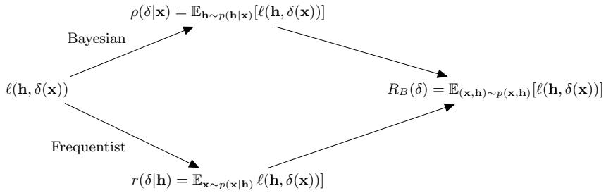
Figure 34.1: Illustration of how the Bayesian and frequentist approaches to decision making incur the same Bayes risk.

34.1.5.1 Classification

Suppose the states of nature correspond to class labels, so H = Y = {1,…,C}. Furthermore, suppose the actions also correspond to class labels, so A = Y. In this setting, a very commonly used loss function is the zero-one loss ω01(y→, yˆ), defined as follows:

\[\begin{array}{c|ccc} & \hat{y} = 0 & \hat{y} = 1 \\ \hline y^\* = 0 & 0 & 1 \\ y^\* = 1 & 1 & 0 \\ \end{array} \tag{34.13}\]

We can write this more concisely as follows:

\[\mathbb{I}\ell\_{01}(y^\*,\hat{y}) = \mathbb{I}(y^\* \neq \hat{y}) \tag{34.14}\]

In this case, the posterior expected loss is

\[\rho(\hat{y}|\mathbf{x}) = p(\hat{y} \neq y^\*|\mathbf{x}) = 1 - p(y^\* = \hat{y}|\mathbf{x}) \tag{34.15}\]

Hence the action that minimizes the expected loss is to choose the most probable label:

\[\delta(\mathbf{x}) = \operatorname\*{argmax}\_{y \in \mathcal{Y}} p(y|\mathbf{z}) \tag{34.16}\]

This corresponds to the mode of the posterior distribution, also known as the maximum a posteriori or MAP estimate.

We can generalize the loss function to associate di!erent costs for false positives and false negatives. We can also allow for a “reject action”, in which the decision maker abstains from classifying when it is not su”ciently confident. This is called selective prediction; see Section 19.3.3 for details.

34.1.5.2 Regression

Now suppose the hidden state of nature is a scalar h → R, and the corresponding action is also a scalar, y → R. The most common loss for continuous states and actions is the ω² loss, also called squared error or quadratic loss, which is defined as follows:

\[\ell\_2(h, y) = (h - y)^2 \tag{34.17}\]

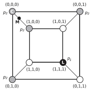
Figure 34.2: A distribution on a discrete space in which the mode (black point L, with probability p1) is untypical of most of the probability mass (gray circles, with probability p² < p1). The small black circle labeled M (near the top left) is the posterior mean, which is not well defined in a discrete state space. C (the top left vertex) is the centroid estimator, made up of the maximizer of the posterior marginals. See text for details. From Figure 1 of [CL07]. Used with kind permission of Luis Carvalho.

In this case, the risk is given by

\[\rho(y|\mathbf{z}) = \mathbb{E}\left[ (h-y)^2 | \mathbf{z} \right] = \mathbb{E}\left[ h^2 | \mathbf{z} \right] - 2y \mathbb{E}\left[ h|\mathbf{z} \right] + y^2 \tag{34.18}\]

The optimal action must satisfy the condition that the derivative of the risk (at that point) is zero (as explained in Chapter 6). Hence the optimal action is to pick the posterior mean:

\[\frac{\partial}{\partial y}\rho(y|x) = -2\mathbb{E}\left[h|x\right] + 2y = 0 \implies \delta(x) = \mathbb{E}\left[h|x\right] = \int h \, p(h|x) dh \tag{34.19}\]

This is often called the minimum mean squared error estimate or MMSE estimate.

34.1.5.3 Parameter estimation

Suppose the states of nature correspond to unknown parameters, so ^H = ! = ^RD. Furthermore, suppose the actions also correspond to parameters, so A = !. Finally, we assume the observed data (that is input to the policy/estimator) is a dataset, such as D = {(xn, yn) : n =1: N}. If we use quadratic loss, then the optimal action is to pick the posterior mean. If we use 0-1 loss, then the optimal action is to pick the posterior mode, i.e., the MAP estimate:

\[\delta(\mathcal{D}) = \hat{\boldsymbol{\theta}} = \operatorname\*{argmax}\_{\boldsymbol{\theta} \in \Theta} p(\boldsymbol{\theta}|\mathcal{D}) \tag{34.20}\]

34.1.5.4 Estimating discrete parameters

The MAP estimate is the optimal estimate when the loss function is 0-1 loss, ω(ω, ωˆ) = I $ ^{ω ↔︎= ωˆ} % , as we show in Section 34.1.5.1. However, this does not give any “partial credit” for estimating some of

the components of ω correctly. An alternative is to use the Hamming loss:

\[\ell(\boldsymbol{\theta}, \boldsymbol{\hat{\theta}}) = \sum\_{d=1}^{D} \mathbb{I}\left(\theta\_d \neq \hat{\theta}\_d\right) \tag{34.21}\]

In this case, one can show that the optimal estimator is the vector of max marginals

\[\hat{\boldsymbol{\theta}} = \left[ \underset{\boldsymbol{\theta}\_d}{\text{argmax}} \int\_{\boldsymbol{\theta}\_{-d}} p(\boldsymbol{\theta} | \mathcal{D}) d\boldsymbol{\theta}\_{-d} \right]\_{d=1}^{D} \tag{34.22}\]

This is also called the maximizer of posterior marginals or MPM estimate. Note that computing the max marginals involves marginalization and maximization, and thus depends on the whole distribution; this tends to be more robust than the MAP estimate [MMP87].

For example, consider a problem in which we must estimate a vector of binary variables. Figure 34.2 shows a distribution on {0, ¹}³, where points are arranged such that they are connected to their nearest neighbors, as measured by Hamming distance. The black state (circle) labeled L (configuration (1,1,1)) has probability p1, and corresponds to the MAP estimate. The 4 gray states have probability p² < p1; and the 3 white states have probability 0. Although the black state is the most probable, it is untypical of the posterior: all its nearest neighbors have probability zero, meaning it is very isolated. By contrast, the gray states, although slightly less probable, are all connected to other gray states, and together they constitute much more of the total probability mass.

In the example in Figure 34.2, we have p(ς^j = 0) = 3p² and p(ς^j = 1) = p² + p¹ for j =1:3. If 2p² > p1, the vector of max marginals is (0, 0, 0). This MPM estimate can be shown to be a centroid estimator, in the sense that it minimizes the squared distance to the posterior mean (the center of mass), yet it (usually) represents a valid configuration, unlike the actual mean (fractional estimates do not make sense for discrete problems). See [CL07] for further discussion of this point.

34.1.5.5 Structured prediction

In some problems, such as natural language processing or computer vision, the desired action is to return an output object y → Y, such as a set of labels or body poses, that not only is probable given the input x, but is also internally consistent. For example, suppose x is a sequence of phonemes and y is a sequence of words. Although x might sound more like y = “How to wreck a nice beach” on a word-by-word basis, if we take the sequence of words into account then we may find (under a language model prior) that y = “How to recognize speech” is more likely overall. (See Figure 34.3.) We can capture this kind of dependency amongst outputs, given inputs, using a structured prediction model, such as a conditional random field (see Section 4.4).

In addition to modeling dependencies in p(y|x), we may prefer certain action choices yˆ, which we capture in the loss function ω(y, yˆ). For example, referring to Figure 34.3, we may be reluctant to assume the user said yˆt=“nudist” at step t unless we are very confident of this prediction, since the cost of mis-categorizing this word may be higher than for other words.

Given a loss function, we can pick the optimal action using minimum Bayes risk decoding:

\[\hat{y} = \min\_{\hat{y} \in \mathcal{Y}} \sum\_{y \in \mathcal{Y}} p(y|x) \ell(y, \hat{y}) \tag{34.23}\]

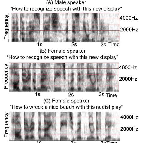
Figure 34.3: Spectograms for three di!erent spoken sentences. The x-axis shows progression of time and the y-axis shows di!erent frequency bands. The energy of the signal in di!erent bands is shown as intensity in grayscale values with progression of time. (A) and (B) show spectrograms of the same sentence “How to recognize speech with this new display” spoken by two di!erent speakers, male and female. Although the frequency characterization is similar, the formant frequencies are much more clearly defined in the speech of the female speaker. (C) shows the spectrogram of the utterance “How to wreck a nice beach with this nudist play” spoken by the same female speaker as in (B). (A) and (B) are not identical even though they are composed of the same words. (B) and (C) are similar to each other even though they are not the same sentences. From Figure 1.2 of [Gan07]. Used with kind permission of Madhavi Ganapathiraju.

We can approximate the expectation empirically by sampling ^M solutions ^ym ↘ ^p(y|x) from the posterior predictive distribution. (Ideally these are diverse from each other.) We use the same set of M samples to approximate the minimization to get

\[\hat{\mathfrak{y}} \approx \min\_{\mathbf{y}^j, i \in \{1, \dots, M\}} \sum\_{j \in \{1, \dots, M\}} p(\mathbf{y}^j | \mathbf{x}) \ell(\mathbf{y}^j, \mathbf{y}^i) \tag{34.24}\]

This is called empirical MBR [Pre+17a], who applied it to computer vision problems. A similar approach was adopted in [Fre+22], who applied it to neural machine translation.

34.1.5.6 Fairness

Models trained with ML are increasingly being used to high-stakes applications, such as deciding whether someone should be released from prison or not, etc. In such applications, it is important that we focus not only on accuracy, but also on fairness. A variety of definitions for what is meant by fairness have been proposed (see e.g., [VR18]), many of which entail conflicting goals [Kle18]. Below we mention a few common definitions, which can all be interpreted decision theoretically.

We consider a binary classification problem with true label Y , predicted label Yˆ and sensitive attribute S (such as gender or race). The concept of equal opportunity requires equal true positive rates across subgroups, i.e., ^p(Y^ˆ = 1|^Y = 1, S = 0) = ^p(Y^ˆ = 1|^Y = 1, S = 1). The concept of equal

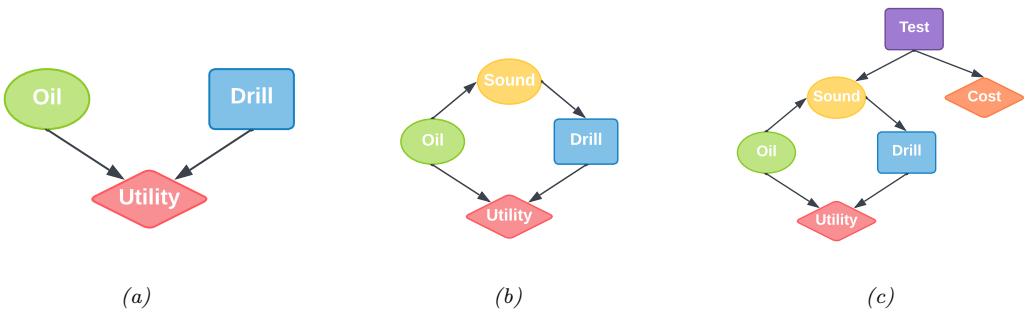
Figure 34.4: Influence diagrams for the oil wildcatter problem. Ovals are random variables (chance nodes), squares are decision (action) nodes, diamonds are utility (value) nodes. (a) Basic model. (b) An extension in which we have an information arc from the Sound chance node to the Drill decision node. (c) An extension in which we get to decide whether to perform a test or not, as well as whether to drill or not.

odds requires equal true positive rates across subgroups, and also equal false positive rates across subgroups, i.e., ^p(Y^ˆ = 1|^Y = 0, S = 0) = ^p(Y^ˆ = 1|^Y = 0, S = 1). The concept of statistical parity requires positive predictions to be una!ected by the value of the protected attribute, regardless of the true label, i.e., ^p(Y^ˆ = 1|^S = 0) = ^p(Y^{ˆ |S} = 1).

For more details on this topic, see e.g., [KR19].

34.2 Decision (influence) diagrams

When dealing with structured multi-stage decision problems, it is useful to use a graphical notation called an influence diagram [HM81; KM08], also called a decision diagram. This extends directed probabilistic graphical models (Chapter 4) by adding decision nodes (also called action nodes), represented by rectangles, and utility nodes (also called value nodes), represented by diamonds. The original random variables are called chance nodes, and are represented by ovals, as usual.

34.2.1 Example: oil wildcatter

As an example (from [Rai68]), consider creating a model for the decision problem faced by an oil “wildcatter”, which is a person who drills wildcat wells, which are exploration wells drilled in areas not known to be oil fields.

Suppose you have to decide whether to drill an oil well or not at a given location. You have two possible actions: d = 1 means drill, d = 0 means don’t drill. You assume there are 3 states of nature: o = 0 means the well is dry, o = 1 means it is wet (has some oil), and o = 2 means it is soaking (has a lot of oil). We can represent this as a decision diagram as shown in Figure 34.4(a).

Suppose your prior beliefs are p(o) = [0.5, 0.3, 0.2], and your utility function U(d, o) is specified by the following table:

	o = 0	o = 1	o = 2
d = 0	0	0	0
d = 1	↓70	50	200

We see that if you don’t drill, you incur no costs, but also make no money. If you drill a dry well, you lose $70; if you drill a wet well, you gain $50; and if you drill a soaking well, you gain $200.

What action should you take if you have no information beyond your prior knowledge? Your prior expected utility for taking action d is

\[\text{EU}(d) = \sum\_{o=0}^{2} p(o)U(d, o) \tag{34.25}\]

We find EU(d = 0) = 0 and EU(d = 1) = 20 and hence the maximum expected utility is

\[\text{MEU} = \max\{\text{EU}(d=0), \text{EU}(d=1)\} = \max\{0, 20\} = 20 \tag{34.26}\]

Thus the optimal action is to drill, d^→ = 1.

34.2.2 Information arcs

Now let us consider a slight extension to the model, in which you have access to a measurement (called a “sounding”), which is a noisy indicator about the state of the oil well. Hence we add an O ⇐ S arc to the model. In addition, we assume that the outcome of the sounding test will be available before we decide whether to drill or not; hence we add an information arc from S to D. This is illustrated in Figure 34.4(b). Note that the utility depends on the action and the true state of the world, but not the measurement.

We assume the sounding variable can be in one of 3 states: s = 0 is a di!use reflection pattern, suggesting no oil; s = 1 is an open reflection pattern, suggesting some oil; and s = 2 is a closed reflection pattern, indicating lots of oil. Since S is caused by O, we add an O ⇐ S arc to our model. Let us model the reliability of our sensor using the following conditional distribution for p(S|O):

	s = 0	s = 1	s = 2
o = 0	0.6	0.3	0.1
o = 1	0.3	0.4	0.3
o = 2	0.1	0.4	0.5

Suppose the sounding observation is s. The posterior expected utility of performing action d is

\[\text{EU}(d|s) = \sum\_{o=0}^{2} p(o|s)U(o,d)\tag{34.27}\]

We need to compute this for each possible observation, s → {0, 1, 2}, and each possible action, d → {0, 1}. If s = 0, we find the posterior over the oil state is p(o|s = 0) = [0.732, 0.219, 0.049], and hence EU(d = 0|s = 0) = 0 and EU(d = 1|s = 0) = ↓30.5. If s = 1, we similarly find EU(d = 0|s = 1) = 0 and EU(d = 1|s = 1) = 32.9. If s = 2, we find EU(d = 0|s = 2) = 0 and EU(d = 1|s = 2) = 87.5. Hence the optimal policy d→(s) is as follows: if s = 0, choose d = 0 and get $0; if s = 1, choose d = 1 and get $32.9; and if s = 2, choose d = 1 and get $87.5.

The maximum expected utility of the wildcatter, before seeing the experimental sounding, can be computed using

\[\text{MEU} = \sum\_{s} p(s) \text{EU}(d^\*(s)|s) \tag{34.28}\]

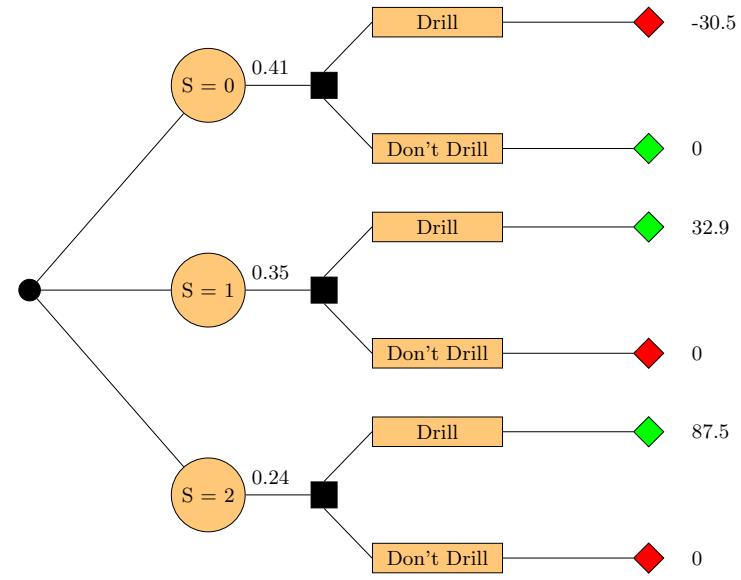
Figure 34.5: Decision tree for the oil wildcatter problem. Black circles are chance variables, black squares are decision nodes, diamonds are the resulting utilities. Green leaf nodes have higher utility than red leaf nodes.

where prior marginal on the outcome of the test is p(s) = ) ^o p(o)p(s|o) = [0.41, 0.35, 0.24]. Hence the MEU is

MEU = 0.41 ⇒ 0+0.35 ⇒ 32.9+0.24 ⇒ 87.5 = 32.2 (34.29)

These numbers can be summarized in the decision tree shown in Figure 34.5.

34.2.3 Value of information

Now suppose you can choose whether to do the test or not. This can be modelled as shown in Figure 34.4(c), where we add a new test node T. If T = 1, we do the test, and S can enter states {0, 1, 2}, determined by O, exactly as above. If T = 0, we don’t do the test, and S enters a special unknown state. There is also some cost associated with performing the test.

Is it worth doing the test? This depends on how much our MEU changes if we know the outcome of the test (namely the state of S). If you don’t do the test, we have MEU = 20 from Equation (34.26). If you do the test, you have MEU = 32.2 from Equation (34.29). So the improvement in utility if you do the test (and act optimally on its outcome) is $12.2. This is called the value of perfect information (VPI). So we should do the test as long as it costs less than $12.2.

In terms of graphical models, the VPI of a variable S can be determined by computing the MEU for the base influence diagram, G, in Figure 34.4(b), and then computing the MEU for the same influence diagram where we add information arcs from S to the action node, and then computing the di!erence. In other words,

\[\text{VPI} = \text{MEU}(\mathcal{G} + S \to D) - \text{MEU}(\mathcal{G}) \tag{34.30}\]

where D is the decision node and S is the variable we are measuring. This will tell us whether it is worth adding obtaining measurement S.

34.2.4 Computing the optimal policy

In general, given an influence diagram, we can compute the optimal policy automatically by modifiying the variable elimination algorithm (Section 9.5), as explained in [LN01; KM08]. The basic idea is to work backwards from the final action, computing the optimal decision at each step, assuming all following actions are chosen optimally. When the influence diagram has a simple chain structure, as in a Markov decision process (Section 34.5), the result is equivalent to Bellman’s equation (Section 34.5.5).

34.3 A/B testing

Suppose you are trying to decide which version of a product is likely to sell more, or which version of a drug is likely to work better. Let us call the versions you are choosing between A and B; sometimes version A is called the control, and version B is called the treatment. (Sometimes the di!erent actions are called “arms”.)

A very common approach to such problems is to use an A/B test, in which you try both actions out for a while, by randomly assigning a di!erent action to di!erent subsets of the population, and then you measure the resulting accumulated reward from each action, and you pick the winner. (This is sometimes called a “test and roll” approach, since you test which method is best, and then roll it out for the rest of the population.)

A key problem in A/B testing is to come up with a decision rule, or policy, for deciding which action is best, after obtaining potentially noisy results during the test phase. Another problem is to choose how many people to assign to the treatment, n1, and how many to the control, n0. The fundamental tradeo! is that using larger values of n¹ and n⁰ will help you collect more data and hence be more confident in picking the best action, but this incurs an opportunity cost, because the testing phase involves performing actions that may not result in the highest reward. (This is an example of the exploration-exploitation tradeo!, which we discuss more in Section 34.4.3.) In this section, we give a simple Bayesian decision theoretic analysis of this problem, following the presentation of [FB19].3 More details on A/B testing can be found in [KTX20].

34.3.1 A Bayesian approach

We assume the ⁱ’th reward for action ^j is given by ^Yij ↘ ^N (µ^j , ^{φ2 j} ) for i =1: n^j and j =0:1, where j = 0 corresponds to the control (action A), j = 1 corresponds to the treatment (action B), and n^j is the number of samples you collect from group j. The parameters µ^j are the expected reward for action j; our goal is to estimate these parameters. (For simplicity, we assume the φ^{2 j} are known.)

We will adopt a Bayesian approach, which is well suited to sequential decision problems. For simplicity, we will use Gaussian priors for the unknowns, ^µj ↘ ^N (m^j , ↼ ^{2 j} ), where m^j is the prior mean reward for action j, and ↼^j is our confidence in this prior. We assume the prior parameters are known. (In practice we can use an empirical Bayes approach, as we discuss in Section 34.3.2.)

^3. For a similar set of results in the time-discounted setting, see https://chris-said.io/2020/01/10/ optimizing-sample-sizes-in-ab-testing-part-I.

34.3.1.1 Optimal policy

Initially we assume the sample size of the experiment (i.e., the values n¹ for the treatment and n⁰ for the control) are known. Our goal is to compute the optimal policy or decision rule ϑ(y1, y0), which specifies which action to deploy, where y^j = (y1^j ,…,yn^j ,j ) is the data from action j.

The optimal policy is simple: choose the action with the greater expected posterior expected reward:

\[\pi^\*(\boldsymbol{y}\_1, \boldsymbol{y}\_0) = \begin{cases} 1 & \text{if } \mathbb{E}\left[\boldsymbol{\mu}\_1 | \boldsymbol{y}\_1\right] \ge \mathbb{E}\left[\boldsymbol{\mu}\_0 | \boldsymbol{y}\_0\right] \\ 0 & \text{if } \mathbb{E}\left[\boldsymbol{\mu}\_1 | \boldsymbol{y}\_1\right] < \mathbb{E}\left[\boldsymbol{\mu}\_0 | \boldsymbol{y}\_0\right] \end{cases} \tag{34.31}\]

All that remains is to compute the posterior. over the unknown parameters, µ^j . Applying Bayes’ rule for Gaussians (Equation (2.121)), we find that the corresponding posterior is given by

\[p(\mu\_j | \mathbf{y}\_j, n\_j) = \mathcal{N}(\mu\_j | \hat{m}\_j, \hat{\tau}\_j^2) \tag{34.32}\]

\[1/\ \hat{\tau}\_j^2 = n\_j/\sigma\_j^2 + 1/\tau\_j^2\tag{34.33}\]

\[ \hat{m}\_j \mid \hat{\tau}\_j^2 = n\_j \overline{y}\_j / \sigma\_j^2 + m\_j / \tau\_j^2 \tag{34.34} \]

We see that the posterior precision (inverse variance) is a weighted sum of the prior precision plus n^j units of measurement precision. We also see that the posterior precision weighted mean is a sum of the prior precision weighted mean and the measurement precision weighted mean.

Given the posterior, we can plug m ↭ ^j into Equation (34.31). In the fully symmetric case, where n¹ = n0, m¹ = m⁰ = m, ↼¹ = ↼⁰ = ↼ , and φ¹ = φ⁰ = φ, we find that the optimal policy is to simply “pick the winner”, which is the arm with higher empirical performance:

\[\pi^\*(y\_1, y\_0) = \mathbb{I}\left(\frac{m}{\tau^2} + \frac{\overline{y}\_1}{\sigma^2} > \frac{m}{\tau^2} + \frac{\overline{y}\_0}{\sigma^2}\right) = \mathbb{I}\left(\overline{y}\_1 > \overline{y}\_0\right) \tag{34.35}\]

However, when the problem is asymmetric, we need to take into account the di!erent sample sizes and/or di!erent prior beliefs.

34.3.1.2 Optimal sample size

We now discuss how to compute the optimal sample size for each arm of the experiment, i.e, the values n⁰ and n1. We assume the total population size is N, and we cannot reuse people from the testing phase,

The prior expected reward in the testing phase is given by

\[\mathbb{E}\left[R\_{\text{test}}\right] = n\_0 m\_0 + n\_1 m\_1 \tag{34.36}\]

The expected reward in the roll phase depends on the decision rule ϑ(y1, y0) that we use:

\[\mathbb{E}\_{\pi} \left[ R\_{\text{coll}} \right] = \int\_{\mu\_1} \int\_{\mu\_0} \int\_{\mathbf{y}\_1} \int\_{\mathbf{y}\_0} \left( N - n\_1 - n\_0 \right) \left( \pi(\mathbf{y}\_1, \mathbf{y}\_0) \mu\_1 + (1 - \pi(\mathbf{y}\_1, \mathbf{y}\_0)) \mu\_0 \right) \tag{34.37}\]

\[0 \times p(\mathfrak{y}\_0|\mu\_0)p(\mathfrak{y}\_1|\mu\_1)p(\mu\_0)p(\mu\_1)d\mathfrak{y}\_0d\mathfrak{y}\_1d\mu\_0d\mu\_1 \tag{34.38}\]

For ϑ = ϑ^→ one can show that this equals

\[\mathbb{E}\left[R\_{\text{roll}}\right] \stackrel{\Delta}{=} \mathbb{E}\_{\pi \ast} \left[R\_{\text{roll}}\right] = \left(N - n\_1 - n\_0\right) \left(m\_1 + e\Phi(\frac{e}{v}) + v\phi(\frac{e}{v})\right) \tag{34.39}\]

where ↽ is the Gaussian pdf, ” is the Gaussian cdf, e = m⁰ ↓ m¹ and

\[v = \sqrt{\frac{\tau\_1^4}{\tau\_1^2 + \sigma\_1^2/n\_1} + \frac{\tau\_0^4}{\tau\_0^2 + \sigma\_0^2/n\_0}}\tag{34.40}\]

In the fully symmetric case, Equation (34.39) simplifies to

\[\mathbb{E}\left[R\_{\text{coll}}\right] = \underbrace{(N-2n)m}\_{R\_a} + \underbrace{(N-2n)\frac{\sqrt{2}\tau^2}{\sqrt{\pi}\sqrt{2\tau^2 + \frac{2}{n}\sigma^2}}}\_{R\_b} \tag{34.41}\]

This has an intuitive interpretation. The first term, Ra, is the prior reward we expect to get before we learn anything about the arms. The second term, Rb, is the reward we expect to see by virtue of picking the optimal action to deploy.

Let us we write R^b = (N ↓ 2n)Ri, where Rⁱ is the incremental gain. We see that the incremental gain increases with n, because we are more likely to pick the correct action with a larger sample size; however, this gain can only be accrued for a smaller number of people, as shown by the N ↓ 2n prefactor. (This is a consequence of the explore-exploit tradeo!.)

The total expected reward is given by adding Equation (34.36) and Equation (34.41):

\[\mathbb{E}\left[R\right] = \mathbb{E}\left[R\_{\text{test}}\right] + \mathbb{E}\left[R\_{\text{roll}}\right] = Nm + (N - 2n)\left(\frac{\sqrt{2}\tau^2}{\sqrt{\pi}\sqrt{2\tau^2 + \frac{2}{n}\sigma^2}}\right) \tag{34.42}\]

(The equation for the nonsymmetric case is given in [FB19].)

We can maximize the expected reward in Equation (34.42) to find the optimal sample size for the testing phase, which (from symmetry) satisfies n^{→ 1} = n^{→ 2} = n→, and from ^d dn^↑ E [R]=0 satisfies

\[m^\* = \sqrt{\frac{N}{4}u^2 + \left(\frac{3}{4}u^2\right)^2} - \frac{3}{4}u^2 \le \sqrt{N}\frac{\sigma}{2\tau} \tag{34.43}\]

where u² = ^{ϖ2 ϱ2} . Thus we see that the optimal sample size n^→ increases as the observation noise φ increases, since we need to collect more data to be confident of the right decision. However, the optimal sample size decreases with ↼ , since a prior belief that the e!ect size ε = µ¹ ↓ µ⁰ will be large implies we expect to need less data to reach a confident conclusion.

34.3.1.3 Regret

Given a policy, it is natural to wonder how good it is. We define the regret of a policy to be the di!erence between the expected reward given perfect information (PI) about the true best action

and the expected reward due to our policy. Minimizing regret is equivalent to making the expected reward of our policy equal to the best possible reward (which may be high or low, depending on the problem).

An oracle with perfect information about which µ^j is bigger would pick the highest scoring action, and hence get an expected reward of ^NE [max(µ1, µ2)]. Since we assume ^µj ↘ ^N (m, ↼ ²), we have

\[\mathbb{E}\left[R|PI\right] = N\left(m + \frac{\tau}{\sqrt{\pi}}\right) \tag{34.44}\]

Therefore the regret from the optimal policy is given by

\[\mathbb{E}\left[R|PI\right] - \left(\mathbb{E}\left[R\_{\text{test}}|\pi^\*\right] + \mathbb{E}\left[R\_{\text{coll}}|\pi^\*\right]\right) = N\frac{\tau}{\sqrt{\pi}}\left(1 - \frac{\tau}{\sqrt{\tau^2 + \frac{\sigma^2}{n^\*}}}\right) + \frac{2n^\*\tau^2}{\sqrt{\pi}\sqrt{\tau^2 + \frac{\sigma^2}{n^\*}}}\tag{34.45}\]

One can show that the regret is O( ⇓ N), which is optimal for this problem when using a time horizon (population size) of N [AG13].

34.3.1.4 Expected error rate

Sometimes the goal is posed as best arm identification, which means identifying whether µ¹ > µ⁰ or not. That is, if we define ε = µ¹ ↓ µ0, we want to know if ε > 0 or ε < 0. This is naturally phrased as a hypothesis test. However, this is arguably the wrong objective, since it is usually not worth spending money on collecting a large sample size to be confident that ε > 0 (say) if the magnitude of ε is small. Instead, it makes more sense to optimize total expected reward, using the method in Section 34.3.1.1.

Nevertheless, we may want to know the probability that we have picked the wrong arm if we use the policy from Section 34.3.1.1. In the symmetric case, this is given by the following:

\[\Pr(\pi(y\_1, y\_0) = 1 | \mu\_1 < \mu\_0) = \Pr(Y\_1 - Y\_0 > 0 | \mu\_1 < \mu\_0) = 1 - \Phi\left(\frac{\mu\_1 - \mu\_0}{\sigma \sqrt{\frac{1}{n\_1} + \frac{1}{n\_0}}}\right) \tag{34.46}\]

The above expression assumed that µ^j are known. Since they are not known, we can compute the expected error rate using E [Pr(ϑ(y1, y0)=1|µ¹ < µ0)]. By symmetry, the quantity E [Pr(ϑ(y1, y0)=0|µ¹ > µ0)] is the same. One can show that both quantities are given by

\[\text{Prob. error} = \frac{1}{4} - \frac{1}{2\pi} \arctan\left(\frac{\sqrt{2}\tau}{\sigma} \sqrt{\frac{n\_1 n\_0}{n\_1 + n\_0}}\right) \tag{34.47}\]

As expected, the error rate decreases with the sample size n¹ and n0, increases with observation noise φ, and decreases with variance of the e!ect size ↼ . Thus a policy that minimizes the classification error will also maximize expected reward, but it may pick an overly large sample size, since it does not take into account the magnitude of ε.

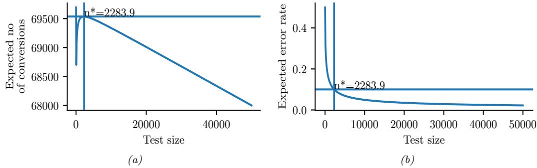
Figure 34.6: Total expected profit (a) and error rate (b) as a function of the sample size used for website testing. Generated by ab\_test\_demo.ipynb.

34.3.2 Example

In this section, we give a simple example of the above framework. Suppose our goal is to do website testing, where have two di!erent versions of a webpage that we want to compare in terms of their click through rate. The observed data is now binary, yij ↘ Ber(µ^j ), so it is natural to use a beta prior, µ^j ↘ Beta(⇀, ⇁) (see Section 3.4.1). However, in this case the optimal sample size and decision rule is harder to compute (see [FB19; Sta+17] for details). As a simple approximation, we can assume ^yij ↘ ^N (µ^j , ^φ2), where ^µj ↘ ^N (m, ↼ ²), ^{m = ς ς}+^φ , ↼ ^{2 =} ςφ (ς+φ)2(ς+φ+1) , and ^{φ2 = m}(1 ^{↓ m}).

To set the Gaussian prior, [FB19] used empirical data from about 2000 prior A/B tests. For each test, they observed the number of times the page was served with each of the two variations, as well as the total number of times a user clicked on each version. Given this data, they used a hierarchical Bayesian model to infer µ^j ↘ N (m = 0.68, ↼ = 0.03). This prior implies that the expected e!ect size is quite small, E [|µ¹ ↓ µ0|] = 0.023. (This is consistent with the results in [Aze+20], who found that most changes made to the Microsoft Bing EXP platform had negligible e!ect, although there were occasionally some “big hits”.)

With this prior, and assuming a population of N = 100, 000, Equation (34.43) says that the optimal number of trials to run is n^{→ 1} = n^{→ 0} = 2284. The expected reward (number of clicks or conversions) in the testing phase is E [Rtest] = 3106, and in the deployment phase E [Rroll] = 66, 430, for a total reward of 69, 536. The expected error rate is 10%.

In Figure 34.6a, we plot the expected reward vs the size of the test phase n. We see that the reward increases sharply with n to the global maximum at n^→ = 2284, and then drops o! more slowly. This indicates that it is better to have a slightly larger test than one that is too small by the same amount. (However, when using a heavy tailed model, [Aze+20] finds that it is better to do lots of smaller tests.)

In Figure 34.6b, we plot the probability of picking the wrong action vs n. We see that tests that are larger than optimal only reduce this error rate marginally. Consequently, if you want to make the misclassification rate low, you may need a large sample size, particularly if µ¹ ↓ µ⁰ is small, since then it will be hard to detect the true best action. However, it is also less important to identify the best action in this case, since both actions have very similar expected reward. This explains why classical methods for A/B testing based on frequentist statistics, which use hypothesis testing

methods to determine if A is better than B, may often recommend sample sizes that are much larger than necessary. (See [FB19] and references therein for further discussion.)

34.4 Contextual bandits

This section is co-authored with Lihong Li.

In Section 34.3, we discussed A/B testing, in which the decision maker tries two di!erent actions, a⁰ and a1, a fixed number of times, n¹ and n0, measures the resulting sequence of rewards, y¹ and y0, and then picks the best action to use for the rest of time (or the rest of the population) so as to maximize expected reward.

We can obviously generalize this beyond two actions. More importantly, we can generalize this beyond a one-stage decision problem. In particular, suppose we allow the decision maker to try an action at, observe the reward rt, and then decide what to do at time step t + 1, rather than waiting until n¹ + n⁰ experiments are finished. This immediate feedback allows for adaptive policies that can result in much higher expected reward (lower regret). We have converted a one-stage decision problem into a sequential decision problem. There are many kinds of sequential decision problems, but in this section, we consider the simplest kind, known as a bandit problem (see e.g., [LS19; Sli19]).

34.4.1 Types of bandit

In a multi-armed bandit problem (MAB) there is an agent (decision maker) that can choose an action from some policy a^t ↘ ϑ^t at each step, after which it receives a reward sampled from the environment, r^t ↘ pR(at), with expected value R(s, a) = E [R|a]. 4

We can think of this in terms of an agent at a casino who is faced with multiple slot machines, each of which pays out rewards at a di!erent rate. A slot machine is sometimes called a onearmed bandit, so a set of K such machines is called a multi-armed bandit; each di!erent action corresponds to pulling the arm of a di!erent slot machine, a^t → {1,…,K}. The goal is to quickly figure out which machine pays out the most money, and then to keep playing that one until you become as rich as possible.

We can extend this model by defining a contextual bandit, in which the input to the policy at each step is a randomly chosen state or context s^t → S. The states evolve over time according to some arbitrary process, s^t ↘ p(st|s1:t↓¹), independent of the actions of the agent. The policy now has the form a^t ↘ ϑt(at|st), and the reward function now has the form r^t ↘ pR(rt|st, at), with expected value R(s, a) = E [R|s, a]. At each step, the agent can use the observed data, D1:^t where D^t = (st, at, rt), to update its policy, to maximize expected reward.

In the finite horizon formulation of (contextual) bandits, the goal is to maximize the expected cumulative reward:

\[J \triangleq \sum\_{t=1}^{T} \mathbb{E}\_{p\_R(r\_t|s\_t, a\_t)\pi\_t(a\_t|s\_t)p(s\_t|s\_{1:t-1})}[r\_t] = \sum\_{t=1}^{T} \mathbb{E}\left[r\_t\right] \tag{34.48}\]

^4. This is known as a stochastic bandit. It is also possible to allow the reward, and possibly the state, to be chosen in an adversarial manner, where nature tries to minimize the reward of the agent. This is known as an adversarial bandit.

(Note that the reward is accrued at each step, even while the agent updates its policy; this is sometimes called “earning while learning”.) In the infinite horizon formulation, where T = ↖, the cumulative reward may be infinite. To prevent J from being unbounded, we introduce a discount factor 0 < γ < 1, so that

\[J \triangleq \sum\_{t=1}^{\infty} \gamma^{t-1} \mathbb{E}\left[r\_t\right] \tag{34.49}\]

The quantity 1 ↓ γ can be interpreted as the probability that the agent is terminated at any moment in time (in which case it will cease to accumulate reward).

Another way to write this is as follows:

\[J = \sum\_{t=1}^{\infty} \gamma^{t-1} \mathbb{E}\left[r\_t\right] = \sum\_{t=1}^{\infty} \gamma^{t-1} \mathbb{E}\left[\sum\_{a=1}^{K} R\_a(s\_t, a\_t)\right] \tag{34.50}\]

where we define

\[R\_a(s\_t, a\_t) = \begin{cases} R(s\_t, a) & \text{if } a\_t = a \\ 0 & \text{otherwise} \end{cases} \tag{34.51}\]

Thus we conceptually evaluate the reward for all arms, but only the one that was actually chosen (namely at) gives a non-zero value to the agent, namely rt.

There are many extensions of the basic bandit problem. A natural one is to allow the agent to perform multiple plays, choosing M ⇔ K distinct arms at once. Let a^t be the corresponding action vector which specifies the identity of the chosen arms. Then we define the reward to be

\[r\_t = \sum\_{a=1}^{K} R\_a(s\_t, \mathbf{a}\_t) \tag{34.52}\]

where

\[R\_a(s\_t, \mathbf{a}\_t) = \begin{cases} R(s\_t, a) & \text{if } a \in \mathbf{a}\_t \\ 0 & \text{otherwise} \end{cases} \tag{34.53}\]

This is useful for modeling resource allocation problems.

Another variant is known as a restless bandit [Whi88]. This is the same as the multiple play formulation, except we additionally assume that each arm has its own state vector s^{a t} associated with it, which evolves according to some stochastic process, regardless of whether arm a was chosen or not. We then define

\[r\_t = \sum\_{a=1}^{K} R\_a(s\_t^a, \mathbf{a}\_t) \tag{34.54}\]

where s^{a t} ↘ ^p(s^{a t |}s^a 1:t↓¹) is some arbitrary distribution, often assumed to be Markovian. (The fact that the states associated with each arm evolve even if the arm is not picked is what gives rise to the term “restless”.) This can be used to model serial dependence between the rewards given by each arm.

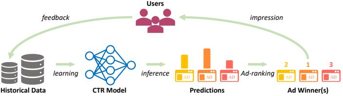
Figure 34.7: Illustration of the feedback problem in online advertising and recommendation systems. The click through rate (CTR) model is used to decide what ads to show, which a!ects what data is collected, which a!ects how the model learns. From Figure 1–2 of [Du+21]. Used with kind permission of Chao Du.

34.4.2 Applications

Contextual bandits have many applications. For example, consider an online advertising system. In this case, the state s^t represents features of the web page that the user is currently looking at, and the action a^t represents the identity of the ad which the system chooses to show. Since the relevance of the ad depends on the page, the reward function has the form R(st, at), and hence the problem is contextual. The goal is to maximize the expected reward, which is equivalent to the expected number of times people click on ads; this is known as the click through rate or CTR. (See e.g., [Gra+10; Li+10; McM+13; Aga+14; Du+21; YZ22] for more information about this application.)

Another application of contextual bandits arises in clinical trials [VBW15]. In this case, the state s^t are features of the current patient we are treating, and the action a^t is the treatment the doctor chooses to give them (e.g., a new drug or a placebo). Our goal is to maximize expected reward, i.e., the expected number of people who get cured. (An alternative goal is to determine which treatment is best as quickly as possible, rather than maximizing expected reward; this variant is known as best-arm identification [ABM10].)

34.4.3 Exploration-exploitation tradeo!

The fundamental di”culty in solving bandit problems is known as the exploration-exploitation tradeo!. This refers to the fact that the agent needs to try multiple state/action combinations (this is known as exploration) in order to collect enough data so it can reliably learn the reward function R(s, a); it can then exploit its knowledge by picking the predicted best action for each state. If the agent starts exploiting an incorrect model too early, it will collect suboptimal data, and will get stuck in a negative feedback loop, as illustrated in Figure 34.7. This is di!erent from supervised learning, where the data is drawn iid from a fixed distribution (see e.g., [Jeu+19] for details).

We discuss some solutions to the exploration-exploitation problem below.

34.4.4 The optimal solution

In this section, we discuss the optimal solution to the exploration-exploitation tradeo!. Let us denote the posterior over the parameters of the reward function by b^t = p(ω|ht), where h^t = {s1:t↓¹, a1:t↓¹, r1:t↓¹} is the history of observations; this is known as the belief state or information state. It is a finite su”cient statistic for the history ht. The belief state can be

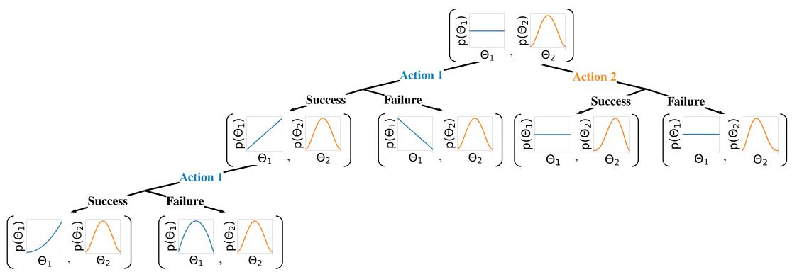
Figure 34.8: Illustration of sequential belief updating for a two-armed beta-Bernoulli bandit. The prior for the reward for action 1 is the (blue) uniform distribution Beta(1, 1); the prior for the reward for action 2 is the (orange) unimodal distribution Beta(2, 2). We update the parameters of the belief state based on the chosen action, and based on whether the observed reward is success (1) or failure (0).

updated deterministically using Bayes’ rule:

\[\mathbf{b}\_{t} = \text{BayesRule}(\mathbf{b}\_{t-1}, a\_t, r\_t) \tag{34.55}\]

For example, consider a context-free Bernoulli bandit, where pR(r|a) = Ber(r|µa), and µ^a = pR(r = 1|a) = R(a) is the expected reward for taking action a. Suppose we use a factored beta prior

\[p\_0(\theta) = \prod\_a \text{Beta}(\mu\_a | \alpha\_0^a, \beta\_0^a) \tag{34.56}\]

where ω = (µ1,…,µK). We can compute the posterior in closed form, as we discuss in Section 3.4.1. In particular, we find

\[p(\boldsymbol{\theta}|\mathcal{D}\_t) = \prod\_a \text{Beta}(\mu\_a | \underbrace{\alpha\_0^a + N\_t^0(a)}\_{\alpha\_t^a}, \underbrace{\beta\_0^a + N\_t^1(a)}\_{\beta\_t^a}) \tag{34.57}\]

where

\[N\_t^r(a) = \sum\_{s=1}^{t-1} \mathbb{I}(a\_s = a, r\_s = r) \tag{34.58}\]

This is illustrated in Figure 34.8 for a two-armed Bernoulli bandit.

We can use a similar method for a Gaussian bandit, where ^pR(r|a) = ^N (r|µa, ^{φ2 a}), using results from Section 3.4.3. In the case of contextual bandits, the problem becomes more complicated. If we assume a linear regression bandit, pR(r|s, a; ω) = N (r|ε(s, a) ^Tω, φ²), we can use Bayesian linear regression to compute p(ω|Dt) in closed form, as we discuss in Section 15.2. If we assume a logistic regression bandit, pR(r|s, a; ω) = Ber(r|φ(ε(s, a) ^Tω)), we can use Bayesian logistic regression to compute p(ω|Dt), as we discuss in Section 15.3.5. If we have a neural bandit of the form pR(r|s, a; ω) = GLM(r|f(s, a; ω)) for some nonlinear function f, then posterior inference becomes more challenging, as we discuss in Chapter 17. However, standard techniques, such as the extended Kalman filter (Section 17.5.2) can be applied. (For a way to scale this approach to large DNNs, see the “subspace neural bandit” approach of [DMKM22].)

Regardless of the algorithmic details, we can represent the belief state update as follows:

\[p(\mathbf{b}\_t | \mathbf{b}\_{t-1}, a\_t, r\_t) = \mathbb{I}\left(\mathbf{b}\_t = \text{BayesRule}(\mathbf{b}\_{t-1}, a\_t, r\_t)\right) \tag{34.59}\]

The observed reward at each step is then predicted to be

\[p(r\_t|\mathbf{b}\_t) = \int p\_R(r\_t|s\_t, a\_t; \theta) p(\theta|\mathbf{b}\_t) d\theta \tag{34.60}\]

We see that this is a special form of a (controlled) Markov decision process (Section 34.5) known as a belief-state MDP.

In the special case of context-free bandits with a finite number of arms, the optimal policy of this belief state MDP can be computed using dynamic programming (see Section 34.6); the result can be represented as a table of action probabilities, ϑt(a1,…,aK), for each step; this is known as the Gittins index [Git89]. However, computing the optimal policy for general contextual bandits is intractable [PT87], so we have to resort to approximations, as we discuss below.

34.4.5 Upper confidence bounds (UCBs)

The optimal solution to explore-exploit is intractable. However, an intuitively sensible approach is based on the principle known as “optimism in the face of uncertainty”. The principle selects actions greedily, but based on optimistic estimates of their rewards. The most important class of strategies with this principle are collectively called upper confidence bound or UCB methods.

To use a UCB strategy, the agent maintains an optimistic reward function estimate R˜t, so that ^R˜t(st, a) ⇑ ^R(st, a) for all ^a with high probability, and then chooses the greedy action accordingly:

\[a\_t = \operatorname\*{argmax}\_a \tilde{R}\_t(s\_t, a) \tag{34.61}\]

UCB can be viewed a form of exploration bonus, where the optimistic estimate encourages exploration. Typically, the amount of optimism, ^R˜^{t ↓ R}, decreases over time so that the agent gradually reduces exploration. With properly constructed optimistic reward estimates, the UCB strategy has been shown to achieve near-optimal regret in many variants of bandits [LS19]. (We discuss regret in Section 34.4.7.)

The optimistic function R˜ can be obtained in di!erent ways, sometimes in closed forms, as we discuss below.

34.4.5.1 Frequentist approach

One approach is to use a concentration inequality [BLM16] to derive a high-probability upper bound of the estimation error: ^|Rˆt(s, a) ^{↓ R}t(s, a)^{| ⇔ ε}t(s, a), where ^Rˆ^t is a usual estimate of ^R (often the MLE), and ε^t is a properly selected function. An optimistic reward is then obtained by setting R˜t(s, a) = Rˆt(s, a) + εt(s, a).

As an example, consider again the context-free Bernoulli bandit, R(a) ↘ Ber(µ(a)). The MLE Rˆt(a)=ˆµt(a) is given by the empirical average of observed rewards whenever action a was taken:

\[ \hat{\mu}\_t(a) = \frac{N\_t^1(a)}{N\_t(a)} = \frac{N\_t^1(a)}{N\_t^0(a) + N\_t^1(a)}\tag{34.62} \]

where N^{r t} (a) is the number of times (up to step t ↓ 1) that action a has been tried and the observed reward was r, and Nt(a) is the total number of times action a has been tried:

\[N\_t(a) = \sum\_{s=1}^{t-1} \mathbb{I}\left(a\_t = a\right) \tag{34.63}\]

Then the Cherno!-Hoe!ding inequality [BLM16] leads to εt(a) = c/Nt(a) for some proper constant c, so

\[ \bar{R}\_t(a) = \hat{\mu}\_t(a) + \frac{c}{\sqrt{N\_t(a)}} \tag{34.64} \]

34.4.5.2 Bayesian approach

We may also derive R˜ from Bayesian inference. If we use a beta prior, we can compute the posterior in closed form, as shown in Equation (34.57). The posterior mean is ^µˆt(a) = ^E [µ(a)|ht] ^{= ςa} t ς^{a t} +φ^a t . From Equation (3.17), the posterior standard deviation is approximately

\[ \hat{\sigma}\_t(a) = \sqrt{\mathcal{V}[\mu(a)|h\_t]} \approx \sqrt{\frac{\hat{\mu}\_t(a)(1-\hat{\mu}\_t(a))}{N\_t(a)}}\tag{34.65} \]

We can use similar techniques for a Gaussian bandit, where ^pR(R|a, ^ω) = ^N (R|µa, ^{φ2 a}), µ^a is the expected reward, and φ^{2 a} the variance. If we use a conjugate prior, we can compute p(µa, φa|Dt) in closed form (see Section 3.4.3). Using an uninformative version of the conjugate prior, we find E [µa|ht] = µˆt(a), which is just the empirical mean of rewards for action a. The uncertainty in this estimate is the standard error of the mean, given by Equation (3.133), i.e., ^V [µa|ht] ⁼ φˆt(a)/ Nt(a), where φˆt(a) is the empirical standard deviation of the rewards for action a.

This approach can also be extended to contextual bandits, modulo the di”culty of computing the belief state.

Once we have computed the mean and posterior standard deviation, we define the optimistic reward estimate as

\[ \hat{R}\_t(a) = \hat{\mu}\_t(a) + c\hat{\sigma}\_t(a) \tag{34.66} \]

for some constant c that controls how greedy the policy is. We see that this is similar to the frequentist method based on concentration inequalities, but is more general.

34.4.5.3 Example

Figure 34.9 illustrates the UCB principle for a Gaussian bandit. We assume there are 3 actions, and we represent p(R(a)|Dt) using a Gaussian. We show the posterior means Q(a) = µ(a) with a vertical dotted line, and the scaled posterior standard deviations cφ(a) as a horizontal solid line.

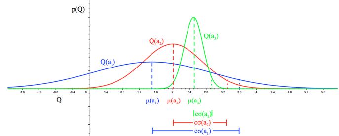
Figure 34.9: Illustration of the reward distribution Q(a) for 3 di!erent actions, and the corresponding lower and upper confidence bounds. From [Sil18]. Used with kind permission of David Silver.

34.4.6 Thompson sampling

A common alternative to UCB is to use Thompson sampling [Tho33], also called probability matching [Sco10]. In this approach, we define the policy at step t to be ϑt(a|st, ht) = pa, where p^a is the probability that a is the optimal action. This can be computed using

\[p\_a = \Pr(a = a\_\* | s\_t, h\_t) = \int \mathbb{I}\left(a = \operatorname\*{argmax}\_{a'} R(s\_t, a'; \theta)\right) p(\theta | h\_t) d\theta \tag{34.67}\]

If the posterior is uncertain, the agent will sample many di!erent actions, automatically resulting in exploration. As the uncertainty decreases, it will start to exploit its knowledge.

To see how we can implement this method, note that we can compute the expression in Equation (34.67) by using a single Monte Carlo sample ^ω˜^t ↘ ^p(ω|ht). We then plug in this parameter into our reward model, and greedily pick the best action:

\[a\_t = \operatorname\*{argmax}\_{a'} R(s\_t, a'; \tilde{\theta}\_t) \tag{34.68}\]

This sample-then-exploit approach will choose actions with exactly the desired probability, since

\[p\_a = \int \mathbb{I}\left(a = \operatorname\*{argmax}\_{a'} R(s\_t, a'; \tilde{\theta}\_t)\right) p(\tilde{\theta}\_t | h\_t) = \Pr\_{\theta\_t \sim p(\theta | h\_t)}\left(a = \operatorname\*{argmax}\_{a'} R(s\_t, a'; \tilde{\theta}\_t)\right) \tag{34.69}\]

Despite its simplicity, this approach can be shown to achieve optimal (logarithmic) regret (see e.g., [Rus+18] for a survey). In addition, it is very easy to implement, and hence is widely used in practice [Gra+10; Sco10; CL11].

In Figure 34.10, we give a simple example of Thompson sampling applied to a linear regression bandit. The context has the form s^t = (1, t, t²). The true reward function has the form R(st, a) = w^{T a}st. The weights per arm are chosen as follows: w⁰ = (↓5, 2, 0.5), w¹ = (0, 0, 0), w² = (5, ↓1.5, ↓1). Thus we see that arm 0 is initially worse (large negative bias) but gets better over time (positive slope), arm 1 is useless, and arm 2 is initially better (large positive bias) but gets worse over time. The observation noise is the same for all arms, φ² = 1. See Figure 34.10(a) for a plot of the reward function.

We use a conjugate Gaussian-gamma prior and perform exact Bayesian updating. Thompson sampling quickly discovers that arm 1 is useless. Initially it pulls arm 2 more, but it adapts to the non-stationary nature of the problem and switches over to arm 0, as shown in Figure 34.10(b).

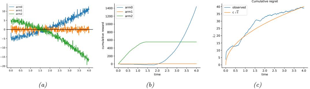
Figure 34.10: Illustration of Thompson sampling applied to a linear-Gaussian contextual bandit. The context has the form s^t = (1, t, t²). (a) True reward for each arm vs time. (b) Cumulative reward per arm vs time. (c) Cumulative regret vs time. Generated by thompson\_sampling\_linear\_gaussian.ipynb.

34.4.7 Regret

We have discussed several methods for solving the exploration-exploitation tradeo!. It is useful to quantify the degree of suboptimality of these methods. A common approach is to compute the regret, which is defined as the di!erence between the expected reward under the agent’s policy and the oracle policy ϑ→, which knows the true reward function. (Note that the oracle policy will in general be better than the Bayes optimal policy, which we disucssed in Section 34.4.4.)

Specifically, let ϑ^t be the agent’s policy at time t. Then the per-step regret at t is defined as

\[l\_t \triangleq \mathbb{E}\_{p(s\_t)} \left[ R(s\_t, \pi\_\*(s\_t)) \right] - \mathbb{E}\_{\pi\_t(a\_t|s\_t)p(s\_t)} \left[ R(s\_t, a\_t) \right] \tag{34.70}\]

If we only care about the final performance of the best discovered arm, as in most optimization problems, it is enough to look at the simple regret at the last step, namely l^T . Optimizing simple regret results in a problem known as pure exploration [BMS11], since there is no need to exploit the information during the learning process. However, it is more common to focus on the cumulative regret, also called the total regret or just the regret, which is defined as

\[L\_T \triangleq \mathbb{E}\left[\sum\_{t=1}^T l\_t\right] \tag{34.71}\]

Here the expectation is with respect to randomness in determining ϑt, which depends on earlier states, actions and rewards, as well as other potential sources of randomness.

Under the typical assumption that rewards are bounded, L^T is at most linear in T. If the agent’s policy converges to the optimal policy as T increases, then the regret is sublinear: L^T = o(T). In general, the slower L^T grows, the more e”cient the agent is in trading o! exploration and exploitation.

To understand its growth rate, it is helpful to consider again a simple context-free bandit, where R^→ = argmax^a R(a) is the optimal reward. The total regret in the first T steps can be written as

\[L\_T = \mathbb{E}\left[\sum\_{t=1}^T R\_\* - R(a\_t)\right] = \sum\_{a \in \mathcal{A}} \mathbb{E}\left[N\_{T+1}(a)\right] (R\_\* - R(a)) = \sum\_{a \in \mathcal{A}} \mathbb{E}\left[N\_{T+1}(a)\right] \Delta\_a \tag{34.72}\]

where N^T +1(a) is the total number of times the agent picks action a up to step T, and #^a = R→↓R(a) is the reward gap. If the agent under-explores and converges to choosing a suboptimal action (say, aˆ), then a linear regret is su!ered with a per-step regret of #aˆ. On the other hand, if the agent over-explores, then Nt(a) will be too large for suboptimal actions, and the agent also su!ers a linear regret.

Fortunately, it is possible to achieve sublinear regrets, using some of the methods discussed above, such as UCB and Thompson sampling. For example, one can show that Thompson sampling has O( ⇓KT log ^T) regret [RR14]. This is shown empirically in Figure 34.10(c).

In fact, both UCB and Thompson sampling are optimal, in the sense that their regrets are essentially not improvable; that is, they match regret lower bounds. To establish such a lower bound, note that the agent needs to collect enough data to distinguish di!erent reward distributions, before identifying the optimal action. Typically, the deviation of the reward estimate from the true reward decays at the rate of 1/ ⇓ N, where N is the sample size (see e.g., Equation (3.133)). Therefore, if two reward distributions are similar, distinguishing them becomes harder and requires more samples. (For example, consider the case of a bandit with Gaussian rewards with slightly di!erent means and large variance, as shown in Figure 34.9.)

The following fundamental result is proved by [LR85] for the asymptotic regret (under certain mild assumptions not given here):

\[\liminf\_{T \to \infty} L\_T \ge \log T \sum\_{a:\Delta\_a > 0} \frac{\Delta\_a}{D\_{\text{KL}}(p\_R(a) \parallel p\_R(a\_\*))}\tag{34.73}\]

Thus, we see that the best we can achieve is logarithmic growth in the total regret. Similar lower bounds have also been obtained for various bandits variants.

34.5 Markov decision problems

In this section, we generalize the discussion of contextual bandits by allowing the state of nature to change depending on the actions chosen by the agent. The resulting model is called a Markov decision process or MDP, as we explain in detail below. This model forms the foundation of reinforcement learning, which we discuss in Chapter 35.

34.5.1 Basics

A Markov decision process [Put94] can be used to model the interaction of an agent and an environment. It is often described by a tuple ∝S, A, p, pR, p0′, where S is a set of environment states, A a set of actions the agent can take, p a transition model, p^R a reward model, and p⁰ the initial state distribution. The interaction starts at time t = 0, where the initial state s⁰ ↘ p0. Then, at time t ⇑ 0, the agent observes the environment state s^t → S, and follows a policy ϑ to take an action a^t → A. In response, the environment emits a real-valued reward signal r^t → R and enters a new state st+1 → S. The policy is in general stochastic, with ϑ(a|s) being the probability of choosing action a in state s. We use ϑ(s) to denote the conditional probability over A if the policy is stochastic, or the action it chooses if it is deterministic. The process at every step is called a transition; at time t, it consists of the tuple (st, at, rt, st+1), where a^t ↘ ϑ(st), st+1 ↘ p(st, at), and r^t ↘ pR(st, at, st+1). Hence, under policy ϑ, the probability of generating a trajectory ϑ of length T

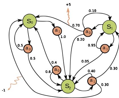
Figure 34.11: Illustration of an MDP as a finite state machine (FSM). The MDP has three discrete states (green cirlces), two discrete actions (orange circles), and two non-zero rewards (orange arrows). The numbers on the black edges represent state transition probabilities, e.g., p(s^↑ = s0|a = a0, s^↑ = s1)=0.7; most state transitions are impossible (probability 0), so the graph is sparse. The numbers on the yellow wiggly edges represent expected rewards, e.g., R(s = s1, a = a0, s^↑ = s0) = +5; state transitions with zero reward are not annotated. From https: // en. wikipedia. org/ wiki/ Markov\_ decision\_ process . Used with kind permission of Wikipedia author waldoalvarez.

can be written explicitly as

\[p(\boldsymbol{\pi}) = p\_0(s\_0) \prod\_{t=0}^{T-1} \pi(a\_t|s\_t) p(s\_{t+1}|s\_t, a\_t) p\_R(r\_t|s\_t, a\_t, s\_{t+1}) \tag{34.74}\]

It is useful to define the reward function from the reward model pR, as the average immediate reward of taking action a in state s, with the next state marginalized:

\[R(s, a) \triangleq \mathbb{E}\_{p(s'|s, a)} \left[ \mathbb{E}\_{p\_R(r|s, a, s')} \left[ r \right] \right] \tag{34.75}\]

Eliminating the dependence on next states does not lead to loss of generality in the following discussions, as our subject of interest is the total (additive) expected reward along the trajectory. For this reason, we often use the tuple ∝S, A, p, R, p0′ to describe an MDP.

In general, the state and action sets of an MDP can be discrete or continuous. When both sets are finite, we can represent these functions as lookup tables; this is known as a tabular representation. In this case, we can represent the MDP as a finite state machine, which is a graph where nodes correspond to states, and edges correspond to actions and the resulting rewards and next states. Figure 34.11 gives a simple example of an MDP with 3 states and 2 actions.

The field of control theory, which is very closely related to RL, uses slightly di!erent terminology. In particular, the environment is called the plant, and the agent is called the controller. States are denoted by ^{xt → X ∞ RD}, actions are denoted by ^{ut → U ∞ RK}, and rewards are denoted by costs c^t → R. Apart from this notational di!erence, the fields of RL and control theory are very similar (see e.g., [Son98; Rec19; Ber19]), although control theory tends to focus on provably optimal methods (by making strong modeling assumptions, such as linearity), whereas RL tends to tackle harder problems with heuristic methods, for which optimality guarantees are often hard to obtain.

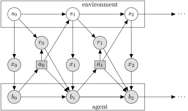
Figure 34.12: Illustration of a partially observable Markov decision process (POMDP) with hidden environment state s^t which generates the observation xt, controlled by an agent with internal belief state b^t which generates the action at. The reward r^t depends on s^t and at. Nodes in this graph represent random variables (circles) and decision variables (squares).

34.5.2 Partially observed MDPs

An important generalization of the MDP framework relaxes the assumption that the agent sees the hidden world state s^t directly; instead we assume it only sees a potentially noisy observation generated from the hidden state, o^t ↘ p(·|st, at). The resulting model is called a partially observable Markov decision process or POMDP (pronounced “pom-dee-pee”). Now the agent’s policy is a mapping from all the available data to actions, a^t ↘ ϑ(ht), where h^t = (a1, o1,…,a^t↓¹, ot) is the past history of observations and actions, plus the current observation. See Figure 34.12 for an illustration. MDPs are a special case where o^t = st.

In general, POMDPs are much harder to solve than MDPs (see e.g., [KLC98]). The optimal solution is to compute the belief state b^t = p(st|ht), and then to define the corresponding belief state MDP, in which the transition dynamics is a deterministic update given by Bayes rule, and the observation model averages out the hidden state st. However, solving this belief state MDP is computationally intractable. A common approximation is to use the last several observed inputs, say o^t↓k:t, in lieu of the full history, and then to treat this as a fully observed MDP. Various other approximations are discussed in [Mur00b].

34.5.3 Episodes and returns

The Markov decision process describes how a trajectory ϑ = (s0, a0, r0, s1, a1, r1,…) is stochastically generated. If the agent can potentially interact with the environment forever, we call it a continuing task. Alternatively, the agent is in an episodic task, if its interaction terminates once the system enters a terminal state or absorbing state; s is absorbing if the next state from s is always s with 0 reward. After entering a terminal state, we may start a new epsiode from a new initial state s⁰ ↘ p0. The episode length is in general random. For example, the amount of time a robot takes to reach its goal may be quite variable, depending on the decisions it makes, and the randomness in the environment. Note that we can convert an episodic MDP to a continuing MDP by redefining the

transition model in absorbing states to be the initial-state distribution p0. Finally, if the trajectory length T in an episodic task is fixed and known, it is called a finite horizon problem.

Let ϑ be a trajectory of length T, where T may be ↖ if the task is continuing. We define the return for the state at time t to be the sum of expected rewards obtained going forwards, where each reward is multiplied by a discount factor γ → [0, 1]:

\[G\_t \triangleq r\_t + \gamma r\_{t+1} + \gamma^2 r\_{t+2} + \dots + \gamma^{T-t-1} r\_{T-1} \tag{34.76}\]

\[\hat{r} = \sum\_{k=0}^{T-t-1} \gamma^k r\_{t+k} = \sum\_{j=t}^{T-1} \gamma^{j-t} r\_j \tag{34.77}\]

G^t is sometimes called the reward-to-go. For episodic tasks that terminate at time T, we define G^t = 0 for t ⇑ T. Clearly, the return satisfies the following recursive relationship:

\[G\_t = r\_t + \gamma (r\_{t+1} + \gamma r\_{t+2} + \dotsb) = r\_t + \gamma G\_{t+1} \tag{34.78}\]

The discount factor γ plays two roles. First, it ensures the return is finite even if T = ↖ (i.e., infinite horizon), provided we use γ < 1 and the rewards r^t are bounded. Second, it puts more weight on short-term rewards, which generally has the e!ect of encouraging the agent to achieve its goals more quickly (see Section 34.5.5.1 for an example). However, if γ is too small, the agent will become too greedy. In the extreme case where γ = 0, the agent is completely myopic, and only tries to maximize its immediate reward. In general, the discount factor reflects the assumption that there is a probability of 1 ↓ γ that the interaction will end at the next step. For finite horizon problems, where T is known, we can set γ = 1, since we know the life time of the agent a priori.5

34.5.4 Value functions

Let ϑ be a given policy. We define the state-value function, or value function for short, as follows (with E^ε [·] indicating that actions are selected by ϑ):

\[V\_{\pi}(s) \stackrel{\Delta}{=} \mathbb{E}\_{\pi} \left[ G\_0 | s\_0 = s \right] = \mathbb{E}\_{\pi} \left[ \sum\_{t=0}^{\infty} \gamma^t r\_t | s\_0 = s \right] \tag{34.79}\]

This is the expected return obtained if we start in state s and follow ϑ to choose actions in a continuing task (i.e., T = ↖).

Similarly, we define the action-value function, also known as the Q-function, as follows:

\[Q\_{\pi}(s, a) \triangleq \mathbb{E}\_{\pi} \left[ G\_0 | s\_0 = s, a\_0 = a \right] = \mathbb{E}\_{\pi} \left[ \sum\_{t=0}^{\infty} \gamma^t r\_t | s\_0 = s, a\_0 = a \right] \tag{34.80}\]

This quantity represents the expected return obtained if we start by taking action a in state s, and then follow ϑ to choose actions thereafter.

Finally, we define the advantage function as follows:

\[A\_{\pi}(s, a) \triangleq Q\_{\pi}(s, a) - V\_{\pi}(s) \tag{34.81}\]

5. We may also use ϑ = 1 for continuing tasks, targeting the (undiscounted) average reward criterion [Put94].

This tells us the benefit of picking action a in state s then switching to policy ϑ, relative to the baseline return of always following ϑ. Note that Aε(s, a) can be both positive and negative, and Eε(a|s) [Aε(s, a)] = 0 due to a useful equality: Vε(s) = Eε(a|s) [Qε(s, a)].

34.5.5 Optimal value functions and policies

Suppose ϑ^→ is a policy such that V^ε↑ ⇑ V^ε for all s → S and all policy ϑ, then it is an optimal policy. There can be multiple optimal policies for the same MDP, but by definition their value functions must be the same, and are denoted by V^→ and Q→, respectively. We call V^→ the optimal state-value function, and Q^→ the optimal action-value function. Furthermore, any finite MDP must have at least one deterministic optimal policy [Put94].

A fundamental result about the optimal value function is Bellman’s optimality equations:

\[V\_\*(s) = \max\_a R(s, a) + \gamma \mathbb{E}\_{p(s'|s, a)} \left[ V\_\*(s') \right] \tag{34.82}\]

\[Q\_\*(s, a) = R(s, a) + \gamma \mathbb{E}\_{p(s'|s, a)} \left[ \max\_{a'} Q\_\*(s', a') \right] \tag{34.83}\]

Conversely, the optimal value functions are the only solutions that satisfy the equations. In other words, although the value function is defined as the expectation of a sum of infinitely many rewards, it can be characterized by a recursive equation that involves only one-step transition and reward models of the MDP. Such a recursion play a central role in many RL algorithms we will see later in this chapter. Given a value function (V or Q), the discrepancy between the right- and left-hand sides of Equations (34.82) and (34.83) are called Bellman error or Bellman residual.

Furthermore, given the optimal value function, we can derive an optimal policy using

\[\pi\_\*(s) = \operatorname\*{argmax}\_a Q\_\*(s, a) \tag{34.84}\]

\[=\operatorname\*{argmax}\_{a}\left[R(s,a) + \gamma \mathbb{E}\_{p(s'|s,a)}\left[V\_{\*}(s')\right]\right] \tag{34.85}\]

Following such an optimal policy ensures the agent achieves maximum expected return starting from any state. The problem of solving for V→, Q^→ or ϑ^→ is called policy optimization. In contrast, solving for V^ε or Q^ε for a given policy ϑ is called policy evaluation, which constitutes an important subclass of RL problems as will be discussed in later sections. For policy evaluation, we have similar Bellman equations, which simply replace maxa{·} in Equations (34.82) and (34.83) with Eε(a|s) [·].

In Equations (34.84) and (34.85), as in the Bellman optimality equations, we must take a maximum over all actions in A, and the maximizing action is called the greedy action with respect to the value functions, Q^→ or V→. Finding greedy actions is computationally easy if A is a small finite set. For high dimensional continuous spaces, we can treat a as a sequence of actions, and optimize one dimension at a time [Met+17], or use gradient-free optimizers such as cross-entropy method (Section 6.7.5), as used in the QT-Opt method [Kal+18a]. Recently, CAQL (continuous action Q-learning, [Ryu+20]) proposed to use mixed integer programming to solve the argmax problem, leveraging the ReLU structure of the Q-network. We can also amortize the cost of this optimization by training a policy a^→ = ϑ→(s) after learning the optimal Q-function.

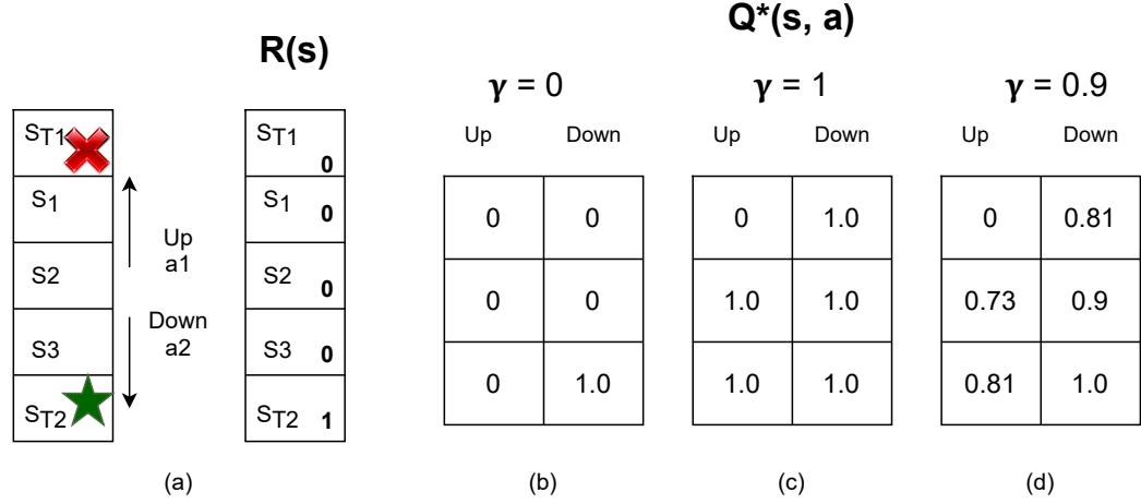
Figure 34.13: Left: illustration of a simple MDP corresponding to a 1d grid world of 3 non-absorbing states and 2 actions. Right: optimal Q-functions for di!erent values of ω. Adapted from Figures 3.1, 3.2, 3.4 of [GK19].

34.5.5.1 Example

In this section, we show a simple example, to make concepts like value functions more concrete. Consider the 1d grid world shown in Figure 34.13(a). There are 5 possible states, among them ST¹ and ST² are absorbing states, since the interaction ends once the agent enters them. There are 2 actions, ∈ and ∋. The reward function is zero everywhere except at the goal state, ST2, which gives a reward of 1 upon entering. Thus the optimal action in every state is to move down.

Figure 34.13(b) shows the Q^→ function for γ = 0. Note that we only show the function for non-absorbing states, as the optimal Q-values are 0 in absorbing states by definition. We see that Q→(s3, ∋)=1.0, since the agent will get a reward of 1.0 on the next step if it moves down from s3; however, Q→(s, a)=0 for all other state-action pairs, since they do not provide nonzero immediate reward. This optimal Q-function reflects the fact that using γ = 0 is completely myopic, and ignores the future.

Figure 34.13(c) shows Q^→ when γ = 1. In this case, we care about all future rewards equally. Thus Q→(s, a)=1 for all state-action pairs, since the agent can always reach the goal eventually. This is infinitely far-sighted. However, it does not give the agent any short-term guidance on how to behave. For example, in s2, it is not clear if it is should go up or down, since both actions will eventually reach the goal with identical Q→-values.

Figure 34.13(d) shows Q^→ when γ = 0.9. This reflects a preference for near-term rewards, while also taking future reward into account. This encourages the agent to seek the shortest path to the goal, which is usually what we desire. A proper choice of γ is up to the agent designer, just like the design of the reward function, and has to reflect the desired behavior of the agent.

34.6 Planning in an MDP

In this section, we discuss how to compute an optimal policy when the MDP model is known. This problem is called planning, in contrast to the learning problem where the models are unknown, which is tackled using reinforcement learning (see Chapter 35). The planning algorithms we discuss are based on dynamic programming (DP) and linear programming (LP).

For simplicity, in this section, we assume discrete state and action sets with γ < 1. However, exact calculation of optimal policies often depends polynomially on the sizes of S and A, and is intractable, for example, when the state space is a Cartesian product of several finite sets. This challenge is known as the curse of dimensionality. Therefore, approximations are typically needed, such as using parametric or nonparametric representations of the value function or policy, both for computational tractability and for extending the methods to handle MDPs with general state and action sets. In this case, we have approximate dynamic programming (ADP) and approximate linear programming (ALP) algorithms (see e.g., [Ber19]).

34.6.1 Value iteration

A popular and e!ective DP method for solving an MDP is value iteration (VI). Starting from an initial value function estimate V0, the algorithm iteratively updates the estimate by

\[V\_{k+1}(s) = \max\_{a} \left[ R(s, a) + \gamma \sum\_{s'} p(s'|s, a) V\_k(s') \right] \tag{34.86}\]

Note that the update rule, sometimes called a Bellman backup, is exactly the right-hand side of the Bellman optimality equation Equation (34.82), with the unknown V^→ replaced by the current estimate Vk. A fundamental property of Equation (34.86) is that the update is a contraction: it can be verified that

\[\max\_{s} \left| V\_{k+1}(s) - V\_{\*}(s) \right| \le \gamma \max\_{s} \left| V\_{k}(s) - V\_{\*}(s) \right| \tag{34.87}\]

In other words, every iteration will reduce the maximum value function error by a constant factor. It follows immediately that V^k will converge to V→, after which an optimal policy can be extracted using Equation (34.85). In practice, we can often terminate VI when V^k is close enough to V→, since the resulting greedy policy wrt V^k will be near optimal. Value iteration can be adapted to learn the optimal action-value function Q→.

In value iteration, we compute V→(s) and ϑ→(s) for all possible states s, averaging over all possible next states s↗ at each iteration, as illustrated in Figure 34.14(right). However, for some problems, we may only be interested in the value (and policy) for certain special starting states. This is the case, for example, in shortest path problems on graphs, where we are trying to find the shortest route from the current state to a goal state. This can be modeled as an episodic MDP by defining a transition matrix p(s↗ |s, a) where taking edge a from node s leads to the neighboring node s↗ with probability 1. The reward function is defined as R(s, a) = ↓1 for all states s except the goal states, which are modeled as absorbing states.

In problems such as this, we can use a method known as real-time dynamic programming or RTDP [BBS95], to e”ciently compute an optimal partial policy, which only specifies what to do for the reachable states. RTDP maintains a value function estimate V . At each step, it performs

a Bellman backup for the current state s by V (s) △ max^a Ep(s↓|s,a) [R(s, a) + γV (s↗ )]. It picks an action a (often with some exploration), reaches a next state s↗ , and repeats the process. This can be seen as a form of the more general asynchronous value iteration, that focuses its computational e!ort on parts of the state space that are more likely to be reachable from the current state, rather than synchronously updating all states at each iteration.

34.6.2 Policy iteration

Another e!ective DP method for computing ϑ^→ is policy iteration. It is an iterative algorithm that searches in the space of deterministic policies until converging to an optimal policy. Each iteration consists of two steps, policy evaluation and policy improvement.

The policy evaluation step, as mentioned earlier, computes the value function for the current policy. Let ϑ represent the current policy, v(s) = Vε(s) represent the value function encoded as a vector indexed by states, r(s) = ) ^a ϑ(a|s)R(s, a) represent the reward vector, and T(s↗ ) |s) = ^a ϑ(a|s)p(s↗ |s, a) represent the state transition matrix. Bellman’s equation for policy evaluation can be written in the matrix-vector form as

\[ v = r + \gamma \mathbf{T}v\tag{34.88}\]

This is a linear system of equations in |S| unknowns. We can solve it using matrix inversion: ^v = (^{I ↓ γ}T)↓¹r. Alternatively, we can use value iteration by computing ^vt+1 ^{= r + γ}Tv^t until near convergence, or some form of asynchronous variant that is computationally more e”cient.

Once we have evaluated V^ε for the current policy ϑ, we can use it to derive a better policy ϑ↗ , thus the name policy improvement. To do this, we simply compute a deterministic policy ϑ↗ that acts greedily with respect to V^ε in every state; that is, ϑ↗ (s) = argmaxa{R(s, a) + γE [Vε(s↗ )]}. We can guarantee that V^ε↓ ⇑ Vε. To see this, define r↗ , T↗ and v↗ as before, but for the new policy ϑ↗ . The definition of ϑ↗ implies r↗ + γT↗ v ⇑ r + γTv = v, where the equality is due to Bellman’s equation. Repeating the same equality, we have

\[v \le r' + \gamma \mathbf{T}' v \le r' + \gamma \mathbf{T}'(r' + \gamma \mathbf{T}' v) \le r' + \gamma \mathbf{T}'(r' + \gamma \mathbf{T}'(r' + \gamma \mathbf{T}' v)) \le \cdots \tag{34.89}\]

\[\mathbf{r} = (\mathbf{I} + \gamma \mathbf{T}' + \gamma^2 \mathbf{T}'^2 + \cdots) \\ \mathbf{r} = (\mathbf{I} - \gamma \mathbf{T}')^{-1} \\ \mathbf{r} = \mathbf{v}' \tag{34.90}\]

Starting from an initial policy ϑ0, policy iteration alternates between policy evaluation (E) and improvement (I) steps, as illustrated below:

\[ \pi\_0 \xrightarrow{E} V\_{\pi\_0} \xrightarrow{I} \pi\_1 \xrightarrow{E} V\_{\pi\_1} \cdots \xrightarrow{I} \pi\_\* \xrightarrow{E} V\_\* \tag{34.91} \]

The algorithm stops at iteration k, if the policy ϑ^k is greedy with respect to its own value function V^εk . In this case, the policy is optimal. Since there are at most |A||S| deterministic policies, and every iteration strictly improves the policy, the algorithm must converge after finite iterations.

In PI, we alternate between policy evaluation (which involves multiple iterations, until convergence of Vε), and policy improvement. In VI, we alternate between one iteration of policy evaluation followed by one iteration of policy improvement (the “max” operator in the update rule). In generalized policy improvement or GPI, we are free to intermix any number of these steps in any order. The process will converge once the policy is greedy wrt its own value function.

The above result follows from the policy improvement theorem, which we now describe, following [SB18, p78]. Let ϑ and ϑ↗ be any pair of deterministic policies such that Qε(s, ϑ↗ (s)) ⇑ Vε(s). Then

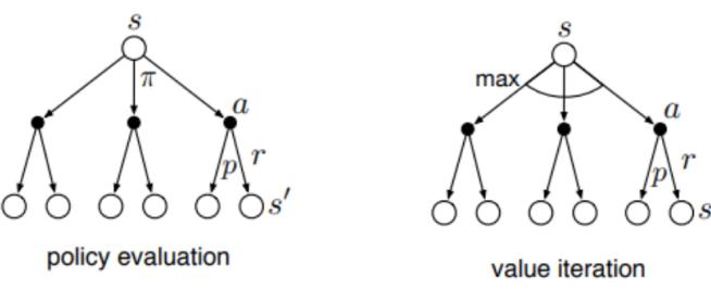
Figure 34.14: Policy iteration vs value iteration represented as backup diagrams. Empty circles represent states, solid (filled) circles represent states and actions. Adapted from Figure 8.6 of [SB18].

the new policy ϑ↗ must be as good or better than ϑ, i.e., V^ε↓ (s) ⇔ Vε(s). If there is at least one state in which this is a strict inequality, than ϑ↗ is an improvement on ϑ. We can construct such a ϑ↗ by setting ϑ↗ (s) = a^→ ↔︎= ϑ(s) where a^→ is the greedy action, ϑ↗ (s) = argmax^a ) ^s↓,r p(s↗ , r|s, a)[r + γVε(s↗ )]. This can often be approximated using some kind of lookahead search process.

Note that policy evaluation computes V^ε whereas value iteration computes V→. This di!erence is illustrated in Figure 34.14, using a backup diagram. Here the root node represents any state s, nodes at the next level represent state-action combinations (solid circles), and nodes at the leaves representing the set of possible resulting next state s↗ for each possible action. In the former case, we average over all actions according to the policy, whereas in the latter, we take the maximum over all actions.

34.6.3 Linear programming

While dynamic programming is e!ective and popular, linear programming (LP) provides an alternative that finds important uses, such as in o!-policy RL (Section 35.5). The primal form of LP is given by

\[\min\_{V} \sum\_{s} p\_{0}(s)V(s) \quad \text{s.t.} \quad V(s) \ge R(s, a) + \gamma \sum\_{s'} p(s'|s, a)V(s), \quad \forall (s, a) \in \mathcal{S} \times \mathcal{A} \tag{34.92}\]

where p0(s) > 0 for all s → S, and can be interpreted as the initial state distribution. It can be verified that any V satisfying the constraint in Equation (34.92) is optimistic [Put94], that is, V ⇑ V→. When the objective is minimized, the solution V will be “pushed” to the smallest possible value, which is V→. Once V^→ is found, any action a that makes the constraint tight in state s is optimal in that state.

The dual LP form is sometimes more intuitive:

\[\max\_{d\geq 0} \sum\_{s,a} d(s,a)R(s,a) \quad \text{s.t.} \quad \sum\_{a} d(s,a) = (1-\gamma)p\_0(s) + \gamma \sum\_{\bar{s},\bar{a}} p(s|\bar{s},\bar{a})d(\bar{s},\bar{a}) \quad \forall s \in \mathcal{S} \tag{34.93}\]

Any nonnegative d satisfying the constraint above is the normalized occupancy distribution of

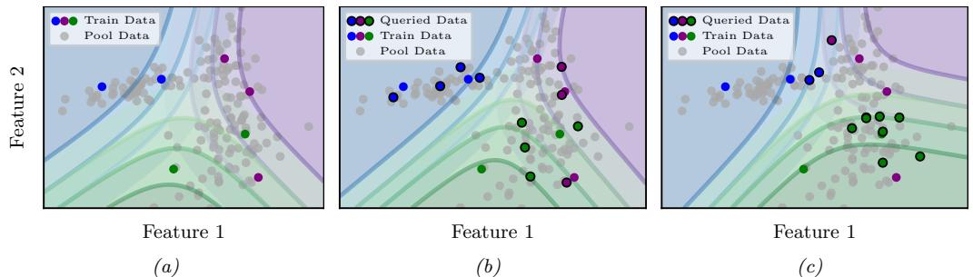
Figure 34.15: Decision boundaries for a logistic regression model applied to a 2-dimensional, 3-class dataset. (a) Results after fitting the model on the initial training data; the test accuracy is 0.818. (b) results after further training on 11 randomly sampled points; accuracy is 0.848. (c) Results after further training on 11 points chosen with margin sampling (see Section 34.7.3); accuracy is 0.969. Generated by active\_learning\_visualization\_class.ipynb.

some corresponding policy ϑd(a|s) ↭ d(s, a)/ ) ^a↓ d(s, a↗ ): 6

\[d(s, a) = (1 - \gamma) \sum\_{t=0}^{\infty} \gamma^t p(s\_t = s, a\_t = a | s\_0 \sim p\_0, a\_t \sim \pi\_d(s\_t)) \tag{34.94}\]

The constant (1 ↓ γ) normalizes d to be a valid distribution, so that it sums to unity. With this interpretation of d, the objective in Equation (34.93) is just the average per-step reward under the normalized occupancy distribution. Once an optimal solution d^→ is found, an optimal policy can be immediately obtained by ϑ→(a|s) = d→(s, a)/ ) ^a↓ d→(s, a↗ ).

A challenge in solving the primal or dual LPs for MDPs is the large number of constraints and variables. Approximations are needed, where the variables are parameterized (either linearly or nonlinearly), and the constraints are sampled or approximated (see e.g., [dV04; LBS17; CLW18]).

34.7 Active learning

This section is coauthored with Zeel B Patel.

In this section, we discuss active learning (AL), in which the agent gets to choose which data it wants to use so as to learn the underlying predictive function as quickly as possible, i.e., using the smallest amount of labeled data. This can be much more e”cient than using randomly collected data, as illustrated in Figure 34.15. This is useful when labels are expensive to collect, e.g., for medical image classification [GIG17; Wal+20].

There are many approaches to AL, as reviewed in [Set12; Ren+21; ZSH22]. In this section, we just consider a few methods.

^6. If ” ^a↓ d(s, a^↑ )=0 for some state s, then ϖd(s) may be defined arbitrarily, since s is not visited under the policy.

Problem	Goal	Action space
Active learning Bayesian optimization Contextual bandits	argminf [ω(f →(x), f(x))] Ep(x) argmaxx f →(x) ↑X argmaxε [R→(x, a)] Ep(x)ε(a x)	choose x at which to get y = f →(x) choose x at which to evaluate f →(x) a R→(x, a) choose at which to evaluate

Table 34.1: Comparison among active learning, Bayesian optimization, and contextual bandits in terms of goal and action space.

34.7.1 Active learning scenarios

One of the earliest AL methods is known as membership query synthesis [Ang88]. In this scenario the agent can generate an arbitrary query x ↘ p(x) and then ask the oracle for its label, y = f(x). (An “oracle” is the term given to a system that knows the true answer to every possible question.) This scenario is mostly of theoretical interest, since it is hard to learn good generative models, and it is rarely possible to have access to an oracle on demand (although human-power crowd computing platforms can be considered as oracles with high latency).

Another scenario is stream-based selective sampling [ACL89], where the agent receives a stream of inputs, x1, x2,…, and at each step must decide whether to request the label or not. Again, this scenario is mostly of theoretical interest.

The last and widely used setting for machine learning is pool-based-sampling [LG94], where the pool of unlabeled samples X is available from the beginning. At each step we apply an acquisition function to each candidate in the batch, to decide which one to collect the label for. We then collect the label, update the model with the new data, and repeat the process until we exhaust the pool, run out of time, or reach some desired performance. In the subsequent sections, we will focus only on pool-based sampling.

34.7.2 Relationship to other forms of sequential decision making

(Pool-based) active learning is closely related to Bayesian optimization (BO, Section 6.6) and contexual bandit problems (Section 34.4). The connections are discussed at length [Tou14], but in brief, the methods di!er because they solve slightly di!erent objective functions, as summarized in Table 34.1. In particular, in active learning, our goal is to identify a function f : X ⇐ Y that will incur minimum expected loss when applied to random inputs x; in BO, our goal is to identify an input point x where the function output f(x) is maximal; and in bandits, our goal is to identify a policy ϑ : X ⇐ A that will give maximum expected reward when applied to random inputs (contexts) x. (We see that the goal in AL and bandits is similar, but in bandits the agent only gets to choose the action, not the state, so only has partial control over where the (reward) function is evaluated.)

In all three problems, we want to find the optimum with as few actions as possible, so we have to solve the exploration-exploitation problem (Section 34.4.3). One approach is to represent our uncertainty about the function using a method such as a Gaussian process (Chapter 18), which lets us compute p(f|D1:t). We then define some acquisition function ⇀(x) that evaluates how useful it would be to query the function at input location x, given the belief state p(f|D1:t) and we pick as our next query xt+1 = argmax^x ⇀(x). (In the bandit setting, the agent does not get to choose the state x, but does get to choose action a.) For example, in BO, it is common to use probability of

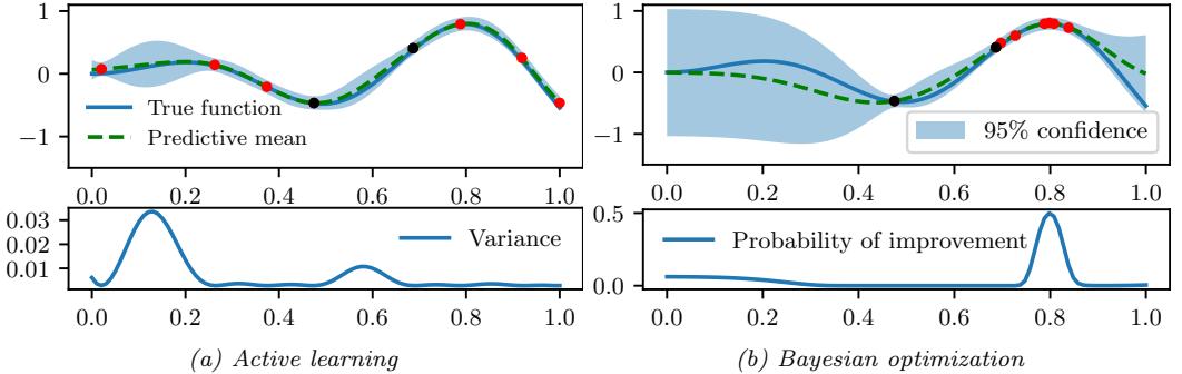
Figure 34.16: Active learning vs Bayesian optimization. Active learning tries to approximate the true function well. Bayesian optimization tries to find maximum value of the true function. Initial and queried points are denoted as black and red dots respectively. Generated by bayes\_opt\_vs\_active\_learning.ipynb.

improvement (Section 6.6.3.1), and for AL of a regression task, we can use the posterior predictive variance. The objective for AL will cause the agent to query “all over the place”, whereas for BO, the agent will “zoom in” on the most promising regions, as shown in Figure 34.16. We discuss other acquisition functions for AL in Section 34.7.3.

34.7.3 Acquisition strategies

In this section, we discuss some common AL heuristics for choosing which points to query.

34.7.3.1 Uncertainty sampling

An intuitive heuristic for choosing which example to label next is to pick the one for which the model is currently most uncertain. This is called uncertainty sampling. We already illustrated this in the case of regression in Figure 34.16, where we represented uncertainty in terms of the posterior variance.

For classification problems, we can measure uncertainty in various ways. Let ^pn = [p(^{y = c}|xn)]^C c=1 be the vector of class probabilities for each unlabeled input xn. Let Uⁿ = ⇀(pn) be the uncertainty for example n, where ⇀ is an acquisition function. Some common choices for ⇀ are: entropy sampling [SW87a], which uses ⇀(p) = ^↓)^{C c}=1 p^c log pc; margin sampling, which uses ⇀(p) = p² ↓ p1, where p¹ is the probability of the most probable class, and p² is the probability of the second most probable class; and least confident sampling, which uses ⇀(p)=1 ↓ p^c↑ , where c^→ = argmax^c pc. The di!erence between these strategies is shown in Figure 34.17. In practice it is often found that margin sampling works the best [Chu+19].

34.7.3.2 Query by committee

In this section, we discuss how to apply uncertainty sampling to models, such as support vector machines (SVMs), that only return a point prediction rather than a probability distribution. The basic approach is to create an ensemble of diverse models, and to use disagreement between the

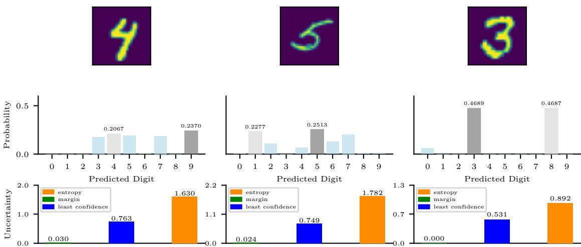
Figure 34.17: Outputs of a logistic regression model fit on some training points, and then applied to 3 candidate query inputs. We show the predicted probabilites for each class label. The highlighted dark gray is the max probability, the light gray bar is the 2nd highest probability. The least confident scores for the 3 inputs are: 1 → 0.23 = 0.76, 1 → 0.25 = 0.75, and 1 → 0.47 = 0.53, so we pick the first query. The entropy scores are: 1.63, 1.78 and 0.89, so we pick the second query. The margin scores are: 0.237 → 0.2067 = 0.0303, 0.2513 → 0.2277 = 0.0236, and 0.4689 → 0.4687 = 0.0002, so we pick the third query. Generated by active\_learning\_comparison\_mnist.ipynb.

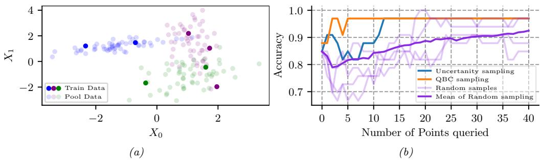
Figure 34.18: (a) Random forest (RF) classifier applied to a 2-dimensional, 3-class dataset. (b) Accuracy vs number of query points for margin sampling vs random sampling. We represent uncertainty using either a single RF (based on the predicted distribution over labels induced by the trees in the forest), or a committee containing an RF and a logistic regression model. Generated by active\_learning\_compare\_class.ipynb.

model predictions as a form of uncertainty. (This can be useful even for probabilistic models, such as DNNs, since model uncertainty can often be larger than parametric uncertainty, as we discuss in the section on deep ensembles, Section 17.3.9.)

In more detail, suppose we have K ensemble members, and let c^{k n} be the predicted class from member k on input xn. Let vnc = )^{K k}=1 I ck ⁿ = c be the number of votes cast for class c, and qnc = vnc/C be the induced distribution. (A similar method can be used for regression models, where we use the standard deviation of the prediction across the members.) We can then use margin sampling or entropy sampling with distribution qn. This approach is called query by committee (QBC) [SOS92], and can often out-perform vanilla uncertainty sampling with a single model, as we show in Figure 34.18.

34.7.3.3 Information theoretic methods

A natural acquisition strategy is to pick points whose labels will maximimally reduce our uncertainty about the model parameters w. This is known as the information gain criterion, and was first proposed in [Lin56]. It is defined as follows:

\[\alpha(\mathbf{z}) \triangleq \mathbb{H}\left(p(w|\mathcal{D})\right) - \mathbb{E}\_{p(y|\mathbf{z}, \mathcal{D})} \left[\mathbb{H}\left(p(w|\mathcal{D}, \mathbf{z}, y)\right)\right] \tag{34.95}\]

(Note that the first term is a constant wrt x, but we include it for later convenience.) This is equivalent to the expected change in the posterior over the parameters which is given by

\[\alpha'(\mathbf{z}) \stackrel{\Delta}{=} \mathbb{E}\_{p(y|\mathbf{z}, \mathcal{D})} \left[ D\_{\text{KL}} \left( p(\mathbf{w}|\mathcal{D}, \mathbf{z}, y) \parallel p(\mathbf{w}|\mathcal{D}) \right) \right] \tag{34.96}\]

Using symmetry of the mutual information, we can rewrite Equation (34.95) as follows:

\[\alpha(\mathbf{z}) = \mathbb{H}\left(\mathbf{w}|\mathcal{D}\right) - \mathbb{E}\_{p\left(y\mid\mathbf{z},\mathcal{D}\right)}\left[\mathbb{H}\left(\mathbf{w}|\mathcal{D},\mathbf{z},y\right)\right] \tag{34.97}\]

\[\mathbb{T} = \mathbb{I}(\boldsymbol{w}, \boldsymbol{y} | \mathcal{D}, \boldsymbol{x}) \tag{34.98}\]

\[\mathcal{B} = \mathbb{H}\left(y|x,\mathcal{D}\right) - \mathbb{E}\_{p(w|\mathcal{D})}\left[\mathbb{H}\left(y|x,w,\mathcal{D}\right)\right] \tag{34.99}\]

The advantage of this approach is that we now only have to reason about the uncertainty of the predictive distribution over outputs y, not over the parameters w. This approach is called Bayesian active learning by disagreement or BALD [Hou+11; Hou+12].

Equation (34.99) has an interesting interpretation. The first term prefers examples x for which there is uncertainty in the predicted label. Just using this as a selection criterion is equivalent to uncertainty sampling, which we discussed above. However, this can have problems with examples which are inherently ambiguous or mislabeled. By adding the second term, we penalize such behavior, since we add a large negative weight to points whose predictive distribution is entropic even when we know the parameters. Thus we ignore aleatoric (intrinsic) uncertainty and focus on epistemic uncertainty.

34.7.4 Batch active learning

In many applications, we need to select a batch of unlabeled examples at once, since training a model on single examples is too slow. This is called batch active learning. The key challenge is that we need to ensure the di!erent queries that we request are diverse, so we maximize the information gain. Various methods for this problem have been devised; here we focus on the BatchBALD method of [KAG19], which extends the BALD method of Section 34.7.3.3.

34.7.4.1 BatchBALD

The naive way to extend the BALD score to a batch of B candidate query points is to define

\[\alpha\_{\text{BaldD}}(\{x\_1, \ldots, x\_B\}, p(w|\mathcal{D})) = \alpha\_{\text{BaldD}}(x\_{1:B}, p(w|\mathcal{D})) = \sum\_{i=1}^{B} \mathbb{I}(y\_i; w|x\_i, \mathcal{D}) \tag{34.100}\]

However this may pick points that are quite similar in terms of their information content. In BatchBALD, we use joint conditional mutual information between the set of labels and the parameters:

\[\alpha\_{\text{BBALL}}(\mathbf{z}\_{1:B}, p(\mathbf{w}|\mathcal{D})) = \mathbb{I}(y\_{1:B}; \mathbf{w}|\mathbf{z}\_{1:B}, \mathcal{D}) = \mathbb{H}(y\_{1:B}|\mathbf{z}\_{1:B}, \mathcal{D}) - \mathbb{E}\_{p(\mathbf{w}|\mathcal{D})} \left[ \mathbb{H}(y\_{1:B}|\mathbf{z}\_{1:B}, \mathbf{w}, \mathcal{D}) \right] \tag{34.101}\]

To understand how this di!ers from BALD, we will use information diagrams for representing MI in terms of Venn diagrams, as explained in Section 5.3.2. In particular, [Yeu91a] showed that we can define a signed measure, µ→, for discrete random variables x and y such that I(x; y) = µ→(x ̸ y), H(x, y) = µ→(x ∪ y), Ep(y) [H(x|y)] = µ→(x  y), etc. Using this, we can interpret standard BALD as the sum of the individual intersections, ) ⁱ µ→(yⁱ ̸ w), which double counts overlaps between the yi, as shown in Figure 34.19(a). By contrast, BatchBALD takes overlap into account by computing

\[\mathbb{I}(y\_{1:B}; \boldsymbol{w} | \boldsymbol{x}\_{1:B}, \mathcal{D}) = \mu^\*(\cup\_i y\_i \cap \boldsymbol{w}) = \mu^\*(\cup\_i y\_i) - \mu^\*(\cup\_i y\_i \mid \boldsymbol{w}) \tag{34.102}\]

This is illustrated in Figure 34.19(b). From this, we can see that ⇀BBALD ⇔ ⇀BALD. Indeed, one can show7

\[\mathbb{I}(y\_{1:B}, w | x\_{1:B}, \mathcal{D}) = \sum\_{i=1}^{B} \mathbb{I}(y\_i, w | x\_{1:B}, \mathcal{D}) - \mathbb{T}\mathbb{C}(y\_{1:B} | x\_{1:B}, \mathcal{D}) \tag{34.103}\]

where TC is the total correlation (see Section 5.3.5.1).

34.7.4.2 Optimizing BatchBALD

To avoid the combinatorial explosion that arises from jointly scoring subsets of points, we can use a a greedy approximation for computing BatchBALD one point at a time. In particular, suppose at step n ↓ 1 we already have a partial batch Aⁿ↓¹. The next point is chosen using

\[\mathbf{x}\_n = \underset{\mathbf{w} \in \mathcal{D}\_{\text{pool}} \backslash \mathcal{A}\_{n-1}}{\text{argmax}} \quad \alpha\_{\text{BBALD}}(\mathcal{A}\_{n-1} \cup \{\mathbf{x}\}, p(\mathbf{w}|\mathcal{D})) \tag{34.104}\]

We then add xⁿ to Aⁿ↓¹ to get An. Fortunately the BatchBALD acquisition function is submodular, as shown in [KAG19]. Hence this greedy algorithm is within 1 ↓ 1/e ≃ 0.63 of optimal (see Section 6.9.4.1).

^7. See http://blog.blackhc.net/2022/07/kbald/

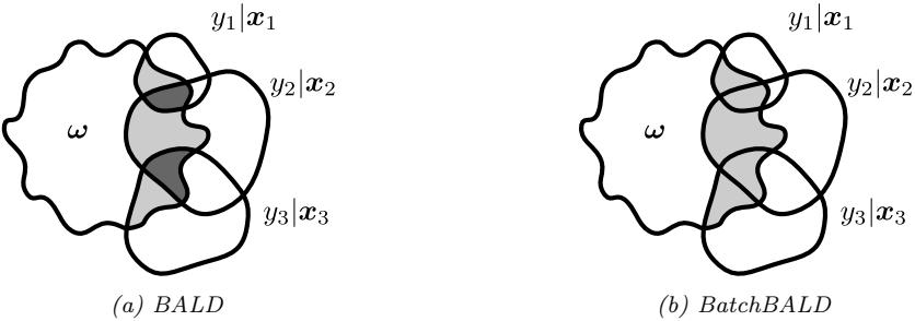
Figure 34.19: Intuition behind BALD and BatchBALD. Dpool is an unlabelled dataset (from which x1:^b are taken) , Dtrain is the current training set, w is set of model parameters, p(y|x,w, Dtrain) are output predictions for datapoint x. BALD overestimates the joint mutual information whereas BatchBALD takes the overlap between variables into account. Areas contributing to the respective score are shown in grey, and areas that are double-counted in dark grey. From Figure 3 of [KAG19]. Used with kind permission of Andreas Kirsch.

34.7.4.3 Computing BatchBALD

Computing the joint (conditional) mutual information is intractable, so in this section, we discuss how to approximate it. For brevity we drop the conditioning on x and D. With this new notation, the objective becomes

\[\alpha\_{\text{BBALL}}(\mathbf{z}\_{1:B}, p(\mathbf{w}|\mathcal{D})) = \mathbb{H}(y\_1, \dots, y\_B) - \mathbb{E}\_{p(\mathbf{w})} \left[ \mathbb{H}(y\_1, \dots, y\_B|\mathbf{w}) \right] \tag{34.105}\]

Note that the ^yi are conditionally independent given ^w, so ^H(y1,…,yB|w) = )^{B i}=1 H(yi|w). Hence we can approximate the second term with Monte Carlo:

\[\mathbb{E}\_{p(\mathbf{w})}\left[\mathbb{H}(y\_1,\ldots,y\_B|\mathbf{w})\right] \approx \frac{1}{S} \sum\_{i=1}^n \sum\_{s} \mathbb{H}(y\_i|\hat{w}\_s) \tag{34.106}\]

where wˆ ^s ↘ p(w|D).

The first term, H(y1,…,yB), is a joint entropy, so is harder to compute. [KAG19] propose the following approximation, summing over all possible label sequences in the batch, and leveraging the fact that p(y) = Ep(w) [p(y|w)]:

\[\mathbb{E}\left(\mathbf{y}\_{1:B}\right) = \mathbb{E}\_{p(\mathbf{w})p(\mathbf{y}\_{1:B}|vw)}\left[-\log p(\mathbf{y}\_{1:B}|\mathbf{w})\right] \tag{34.107}\]

\[\approx \sum\_{\hat{y}\_{1:B}} \left( \frac{1}{S} \sum\_{s=1}^{S} p(\hat{y}\_{1:B} | \hat{w}\_s) \right) \log \left( \frac{1}{S} \sum\_{s=1}^{S} p(\hat{y}\_{1:B} | \hat{w}\_s) \right) \tag{34.108}\]

The sum over all possible labels sequences can be made more e”cient by noting that p(y1:n|w) = p(yn|w)p(y1:n↓¹|w), so when we implement the greedy algorithm, we can incrementally update the probabilities, reusing previous computations. See [KAG19] for the details.

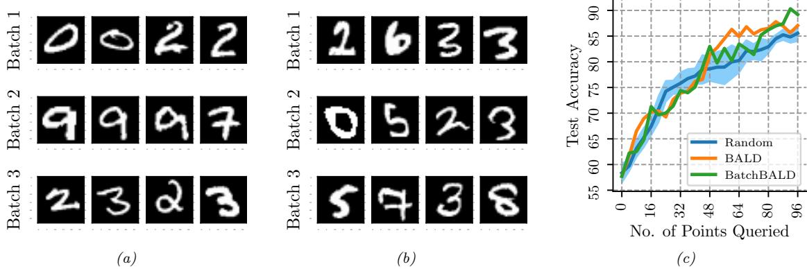
Figure 34.20: Three batches (each of size 4) queried from the MNIST pool by (a) BALD and (b) BatchBALD. (c) Plot of accuracy vs number of points queried. BALD may select replicas of single informative datapoint while BatchBALD selects diverse points, thus increasing data e”ciency. Generated by batch\_bald\_mnist.ipynb.

34.7.4.4 Experimental comparison of BALD vs BatchBALD on MNIST

In this section, we show some experimental results applying BALD and BatchBALD to train a CNN on the standard MNIST dataset. We use a batch size of 4, and approximate the posterior over parameters p(w|D) using MC dropout (Section 17.3.1). In Figure 34.20(a), we see that BALD selects examples that are very similar to each other, whereas in Figure 34.20(b), we see that BatchBALD selects a greater diversity of points. In Figure 34.20(c), we see that BatchBALD results in more e”cient learning than BALD, which in turn is more e”cient than randomly sampling data.

35 Reinforcement learning

This chapter is co-authored with Lihong Li.

35.1 Introduction

Reinforcement learning or RL is a paradigm of learning where an agent sequentially interacts with an initially unknown environment. The interaction typically results in a trajectory, or multiple trajectories. Let ϑ = (s0, a0, r0, s1, a1, r1, s2,…,s^T ) be a trajectory of length T, consisting of a sequence of states st, actions at, and rewards rt. 1 The goal of the agent is to optimize her actionselection policy, so that the discounted cumulative reward, G⁰ ↭ )^{T ↓1 t}=0 γ^t rt, is maximized for some given discount factor γ → [0, 1].

In general, G⁰ is a random variable. We will focus on maximizing its expectation, inspired by the maximum expected utility principle (Section 34.1.3), but note other possibilities such as conditional value at risk2 that can be more appropriate in risk-sensitive applications.

We will focus on the Markov decision process, where the generative model for the trajectory ϑ can be factored into single-step models. When these model parameters are known, solving for an optimal policy is called planning (see Section 34.6); otherwise, RL algorithms may be used to obtain an optimal policy from trajectories, a process called learning.

In model-free RL, we try to learn the policy without explicitly representing and learning the models, but directly from the trajectories. In model-based RL, we first learn a model from the trajectories, and then use a planning algorithm on the learned model to solve for the policy. See Figure 35.1 for an overview. This chapter will introduce some of the key concepts and techniques, and will mostly follow the notation from [SB18]. in textbooks such as [Sze10; SB18; Aga+22; Pla22; ID19], and reviews such as [Aru+17; FL+18; Li18; Mur24]. For details on how RL relates to control theory, see e.g., [Son98; Rec19; Ber19; Mey22].

35.1.1 Overview of methods

In this section, we give a brief overview of how to compute optimal policies when the MDP model is not known. Instead, the agent interacts with the environment and learns from the observed

^1. Note that the time starts at 0 here, while it starts at 1 when we discuss bandits (Section 34.4). Our choices of notation are to be consistent with conventions in respective literature.

^2. The conditional value at risk, or CVaR, is the expected reward conditioned on being in the worst 5% (say) of samples. See [Cho+15] for an example application in RL.

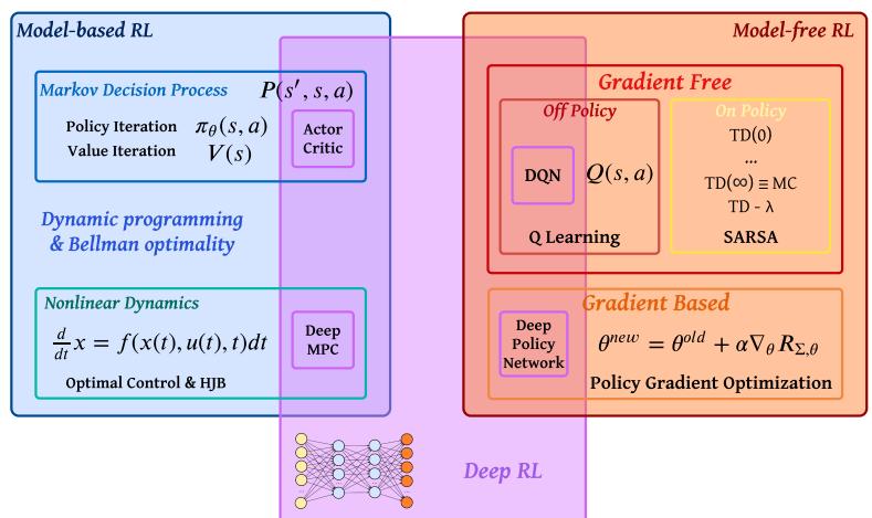
REINFORCEMENT LEARNING

Figure 35.1: Overview of RL methods. Abbreviations: DQN = Deep Q network (Section 35.2.6); MPC = Model Predictive Control (Section 35.4); HJB = Hamilton-Jacobi-Bellman equation; TD = temporal di!erence learning (Section 35.2.2). Adapted from a slide by Steve Brunton.

Method	Functions learned	On/O!	Section
SARSA	Q(s, a)	On	Section 35.2.4
Q-learning	Q(s, a)	O!	Section 35.2.5
REINFORCE	ϑ(a s)	On	Section 35.3.2
A2C	ϑ(a s), V (s)	On	Section 35.3.3.1
TRPO/PPO	ϑ(a s), A(s, a)	On	Section 35.3.4
DDPG	a = ϑ(s), Q(s, a)	O!	Section 35.3.5
Soft actor-critic	ϑ(a s), Q(s, a)	O!	Section 35.6.1
Model-based RL	p(s↗ s, a)	O!	Section 35.4

Table 35.1: Summary of some popular methods for RL. On/o! refers to on-policy vs o!-policy methods.

trajectories. This is the core focus of RL. We will go into more details into later sections, but first provide this roadmap.

We may categorize RL methods by the quantity the agent represents and learns: value function, policy, and model; or by how actions are selected: on-policy (actions must be selected by the agent’s current policy), and o!-policy. Table 35.1 lists a few representative examples. More details are given in the subsequent sections. We will also discuss at greater depth two important topics of o!-policy learning and inference-based control in Sections 35.5 and 35.6.

35.1.2 Value-based methods

In a value-based method, we often try to learn the optimal Q-function from experience, and then derive a policy from it using Equation (34.84). Typically, a function approximator (e.g., a neural network), Qw, is used to represent the Q-function, which is trained iteratively. Given a transition (s, a, r, s↗ ), we define the temporal di!erence (also called the TD error) as

\[r + \gamma \max\_{a'} Q\_{\mathbf{w}}(s', a') - Q\_{\mathbf{w}}(s, a)\]

Clearly, the expected TD error is the Bellman error evaluated at (s, a). Therefore, if Q^w = Q→, the TD error is 0 on average by Bellman’s optimality equation. Otherwise, the error provides a signal for the agent to change w to make Qw(s, a) closer to R(s, a) + γ max^a↓ Qw(s↗ , a↗ ). The update on Q^w is based on a target that is computed using Qw. This kind of update is known as bootstrapping in RL, and should not be confused with the statistical bootstrap (Section 3.3.2). Value based methods such as Q-learning and SARSA are discussed in Section 35.2.

35.1.3 Policy search methods

In policy search, we try to directly maximize J(ϑω) wrt the policy parameter ω. If J(ϑω) is di!erentiable wrt ω, we can use stochastic gradient ascent to optimize ω, which is known as policy gradient, as described in Section 35.3.1. The basic idea is to perform Monte Carlo rollouts, in which we sample trajectories by interacting with the environment, and then use the score function estimator (Section 6.3.4) to estimate ∀ωJ(ϑω). Here, J(ϑω) is defined as an expectation whose distribution depends on ω, so it is invalid to swap ∀ and E in computing the gradient, and the score function estimator can be used instead. An example of policy gradient is REINFORCE.

Policy gradient methods have the advantage that they provably converge to a local optimum for many common policy classes, whereas Q-learning may diverge when approximation is used (Section 35.5.3). In addition, policy gradient methods can easily be applied to continuous action spaces, since they do not need to compute argmax^a Q(s, a). Unfortunately, the score function estimator for ∀ωJ(ϑω) can have a very high variance, so the resulting method can converge slowly.

One way to reduce the variance is to learn an approximate value function, Vw(s). and to use it as a baseline in the score function estimator. We can learn Vw(s) using one of the value function methods similar to Q-learning. Alternatively, we can learn an advantage function, Aw(s, a), and use it to estimate the gradient. These policy gradient variants are called actor critic methods, where the actor refers to the policy ϑ^ω and the critic refers to V^w or Aw. See Section 35.3.3 for details.

35.1.4 Model-based RL

Value-based methods, such as Q-learning, and policy search methods, such as policy gradient, can be very sample ine”cient, which means they may need to interact with the environment many times before finding a good policy. If an agent has prior knowledge of the MDP model, it can be more sample e”cient to first learn the model, and then compute an optimal (or near-optimal) policy of the model without having to interact with the environment any more.

This approach is called model-based RL. The first step is to learn the MDP model including the p(s↗ |s, a) and R(s, a) functions, e.g., using DNNs. Given a collection of (s, a, r, s↗ ) tuples, such a model can be learned using standard supervised learning methods. The second step can be done

by running an RL algorithm on synthetic experiences generated from the model, or by running a planning algorithm on the model directly (Section 34.6). In practice, we often interleave the model learning and planning phases, so we can use the partially learned policy to decide what data to collect. We discuss model-based RL in more detail in Section 35.4.

35.1.5 Exploration-exploitation tradeo!

A fundamental problem in RL with unknown transition and reward models is to decide between choosing actions that the agent knows will yield high reward, or choosing actions whose reward is uncertain, but which may yield information that helps the agent get to parts of state-action space with even higher reward. This is called the exploration-exploitation tradeo!, which has been discussed in the simpler contextual bandit setting in Section 34.4. The literature on e”cient exploration is huge. In this section, we briefly describe several representative techniques.

35.1.5.1 ϖ-greedy

A common heuristic is to use an –greedy policy ϑ↼, parameterized by - → [0, 1]. In this case, we pick the greedy action wrt the current model, ^{at =} argmax^{a R}ˆt(st, a) with probability ¹↓-, and a random action with probability -. This rule ensures the agent’s continual exploration of all state-action combinations. Unfortunately, this heuristic can be shown to be suboptimal, since it explores every action with at least a constant probability -/|A|.

35.1.5.2 Boltzmann exploration

A source of ine”ciency in the –greedy rule is that exploration occurs uniformly over all actions. The Boltzmann policy can be more e”cient, by assigning higher probabilities to explore more promising actions:

\[\pi\_{\tau}(a|s) = \frac{\exp(\hat{R}\_{t}(s\_{t}, a)/\tau)}{\sum\_{a'} \exp(\hat{R}\_{t}(s\_{t}, a')/\tau)}\tag{35.1}\]

where ↼ > 0 is a temperature parameter that controls how entropic the distribution is. As ↼ gets close to 0, ϑ^ϱ becomes close to a greedy policy. On the other hand, higher values of ↼ will make ϑ(a|s) more uniform, and encourage more exploration. Its action selection probabilities can be much “smoother” with respect to changes in the reward estimates than –greedy, as illustrated in Table 35.2.

35.1.5.3 Upper confidence bounds and Thompson sampling

The upper confidence bound (UCB) (Section 34.4.5) and Thompson sampling (Section 34.4.6) approaches may also be extended to MDPs. In contrast to the contextual bandit case, where the only uncertainty is in the reward function, here we must also take into account uncertainty in the transition probabilities.

As in the bandit case, the UCB approach requires to estimate an upper confidence bound for all actions’ Q-values in the current state, and then take the action with the highest UCB score. One way to obtain UCBs of the Q-values is to use count-based exploration, where we learn the optimal

Rˆ(s, a1)	Rˆ(s, a2)	ϑ↼(a s1)	ϑ↼(a s2)	ϑϱ (a s1)	ϑϱ (a s2)
1.00	9.00	0.05	0.95	0.00	1.00
4.00	6.00	0.05	0.95	0.12	0.88
4.90	5.10	0.05	0.95	0.45	0.55
5.05	4.95	0.95	0.05	0.53	0.48
7.00	3.00	0.95	0.05	0.98	0.02
8.00	2.00	0.95	0.05	1.00	0.00

Table 35.2: Comparison of ε-greedy policy (with ε = 0.1) and Boltzmann policy (with ϑ = 1) for a simple MDP with 6 states and 2 actions. Adapted from Table 4.1 of [GK19].

Q-function with an exploration bonus added to the reward in a transition (s, a, r, s↗ ):

\[ \hat{r} = r + \alpha / \sqrt{N\_{s,a}} \tag{35.2} \]

where Ns,a is the number of times action a has been taken in state s, and ⇀ ⇑ 0 is a weighting term that controls the degree of exploration. This is the approach taken by the MBIE-EB method [SL08] for finite-state MDPs, and in the generalization to continuous-state MDPs through the use of hashing [Bel+16]. Other approaches also explicitly maintain uncertainty in state transition probabilities, and use that information to obtain UCBs. Examples are MBIE [SL08], UCRL2 [JOA10], and UCBVI [AOM17], among many others.

Thompson sampling can be similarly adapted, by maintaining the posterior distribution of the reward and transition model parameters. In finite-state MDPs, for example, the transition model is a categorical distribution conditioned on the state. We may use the conjugate prior of Dirichlet distributions (Section 3.4) for the transition model, so that the posterior distribution can be conveniently computed and sampled from. More details on this approach are found in [Rus+18].

Both UCB and Thompson sampling methods have been shown to yield e”cient exploration with provably strong regret bounds (Section 34.4.7) [JOA10], or related PAC bounds [SLL09; DLB17], often under necessary assumptions such as finiteness of the MDPs. In practice, these methods may be combined with function approximation like neural networks and implemented approximately.

35.1.5.4 Optimal solution using Bayes-adaptive MDPs

The Bayes optimal solution to the exploration-exploitation tradeo! can be computed by formulating the problem as a special kind of POMDP known as a Bayes-adaptive MDP or BAMDP [Duf02]. This extends the Gittins index approach in Section 34.4.4 to the MDP setting.

In particular, a BAMDP has a belief state space, B, representing uncertainty about the reward model pR(r|s, a, s↗ ) and transition model p(s↗ |s, a). The transition model on this augmented MDP can be written as follows:

\[T^{+}(s\_{t+1}, b\_{t+1}|s\_t, b\_t, a\_t, r\_t) = T^{+}(s\_{t+1}|s\_t, a\_t, b\_t)T^{+}(b\_{t+1}|s\_t, a\_t, r\_t, s\_{t+1})\tag{35.3}\]

\[=\mathbb{E}\_{b\_t}\left[T(s\_{t+1}|s\_t, a\_t)\right] \times \mathbb{I}\left(b\_{t+1} = p(R, T|h\_{t+1})\right) \tag{35.4}\]

where E^bt [T(st+1|st, at)] is the posterior predictive distribution over next states, and p(R, T|ht+1) is the new belief state given ht+1 = (s1:t+1, a1:t+1, r1:t+1), which can be computed using Bayes’ rule.

Similarly, the reward function for the augmented MDP is given by

\[R^{+}(r|s\_t, b\_t, a\_t, s\_{t+1}, b\_{t+1}) = \mathbb{E}\_{b\_{t+1}}\left[R(s\_t, a\_t, s\_{t+1})\right] \tag{35.5}\]

For small problems, we can solve the resulting augmented MDP optimally. However, in general this is computationally intractable. [Gha+15] surveys many methods to solve it more e”ciently. For example, [KN09] develop an algorithm that behaves similarly to Bayes optimal policies, except in a provably small number of steps; [GSD13] propose an approximate method based on Monte Carlo rollouts. More recently, [Zin+20] propose an approximate method based on meta-learning (Section 19.6.4), in which they train a (model-free) policy for multiple related tasks. Each task is represented by a task embedding vector m, which is inferred from h^t using a VAE (Section 21.2). The posterior p(m|ht) is used as a proxy for the belief state bt, and the policy is trained to perform well given s^t and bt. At test time, the policy is applied to the incrementally computed belief state; this allows the method to infer what kind of task this is, and then to use a pre-trained policy to quickly solve it.

35.2 Value-based RL

In this section, we assume the agent has access to samples from p and p^R by interacting with the environment. We will show how to use these samples to learn optimal Q-functions from which we can derive optimal policies.

35.2.1 Monte Carlo RL

Recall that Qε(s, a) = E [Gt|s^t = s, a^t = a] for any t. A simple way to estimate this is to take action a, and then sample the rest of the trajectory according to ϑ, and then compute the average sum of discounted rewards. The trajectory ends when we reach a terminal state, if the task is episodic, or when the discount factor γ^t becomes negligibly small, whichever occurs first. This is the Monte Carlo estimation of the value function.

We can use this technique together with policy iteration (Section 34.6.2) to learn an optimal policy. Specifically, at iteration k, we compute a new, improved policy using ϑk+1(s) = argmax^a Qk(s, a), where Q^k is approximated using MC estimation. This update can be applied to all the states visited on the sampled trajectory. This overall technique is called Monte Carlo control.

To ensure this method converges to the optimal policy, we need to collect data for every (state, action) pair, at least in the tabular case, since there is no generalization across di!erent values of Q(s, a). One way to achieve this is to use an –greedy policy. Since this is an on-policy algorithm, the resulting method will converge to the optimal –soft policy, as opposed to the optimal policy. It is possible to use importance sampling to estimate the value function for the optimal policy, even if actions are chosen according to the –greedy policy. However, it is simpler to just gradually reduce -.

35.2.2 Temporal di!erence (TD) learning

The Monte Carlo (MC) method in Section 35.2.1 results in an estimator for Qε(s, a) with very high variance, since it has to unroll many trajectories, whose returns are a sum of many random rewards generated by stochastic state transitions. In addition, it is limited to episodic tasks (or finite horizon

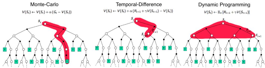
Figure 35.2: Backup diagrams of V (st) for Monte Carlo, temporal di!erence, and dynamic programming updates of the state-value function. Used with kind permission of Andy Barto.

truncation of continuing tasks), since it must unroll to the end of the episode before each update step, to ensure it reliably estimates the long term return.

In this section, we discuss a more e”cient technique called temporal di!erence or TD learning [Sut88]. The basic idea is to incrementally reduce the Bellman error for sampled states or state-actions, based on transitions instead of a long trajectory. More precisely, suppose we are to learn the value function V^ε for a fixed policy ϑ. Given a state transition (s, a, r, s↗ ) where a ↘ ϑ(s), we change the estimate V (s) so that it moves towards the bootstrapping target (Section 35.1.2)

\[V(s\_t) \leftarrow V(s\_t) + \eta \left[r\_t + \gamma V(s\_{t+1}) - V(s\_t)\right] \tag{35.6}\]

where ▷ is the learning rate. The term multiplied by ▷ above is known as the TD error. A more general form of TD update for parametric value function representations is

\[\mathbf{w} \leftarrow \mathbf{w} + \eta \left[ r\_t + \gamma V\_\mathbf{w}(s\_{t+1}) - V\_\mathbf{w}(s\_t) \right] \nabla\_\mathbf{w} V\_\mathbf{w}(s\_t) \tag{35.7}\]

of which Equation (35.6) is a special case. The TD update rule for learning Q^ε is similar.

It can be shown that TD learning in the tabular case, Equation (35.6), converges to the correct value function, under proper conditions [Ber19]. However, it may diverge when approximation is used (Equation (35.7)), an issue we will discuss further in Section 35.5.3.

The potential divergence of TD is also consistent with the fact that Equation (35.7) is not SGD (Section 6.3.1) on any objective function, despite a very similar form. Instead, it is an example of bootstrapping, in which the estimate, Vw(st), is updated to approach a target, r^t + γVw(st+1), which is defined by the value function estimate itself. This idea is shared by DP methods like value iteration, although they rely on the complete MDP model to compute an exact Bellman backup. In contrast, TD learning can be viewed as using sampled transitions to approximate such backups. An example of non-bootstrapping approach is the Monte Carlo estimation in the previous section. It samples a complete trajectory, rather than individual transitions, to perform an update, and is often much less e”cient. Figure 35.2 illustrates the di!erence between MC, TD, and DP.

35.2.3 TD learning with eligibility traces

A key di!erence between TD and MC is the way they estimate returns. Given a trajectory ϑ = (s0, a0, r0, s1,…,s^T ), TD estimates the return from state s^t by one-step lookahead, Gt:t+1 = r^t +

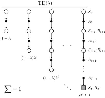
Figure 35.3: The backup diagram for TD(ϖ). Standard TD learning corresponds to ϖ = 0, and standard MC learning corresponds to ϖ = 1. From Figure 12.1 of [SB18]. Used with kind permission of Richard Sutton.

γV (st+1), where the return from time t + 1 is replaced by its value function estimate. In contrast, MC waits until the end of the episode or until T is large enough, then uses the estimate Gt:^T = ^{rt + γ}rt+1 ⁺ ··· ^{+ γT ↓}t↓¹r^{T ↓1}. It is possible to interpolate between these by performing an ⁿ-step rollout, and then using the value function to approximate the return for the rest of the trajectory, similar to heuristic search (Section 35.4.1.1). That is, we can use the n-step estimate

\[G\_{t:t+n} = r\_t + \gamma r\_{t+1} + \dots + \gamma^{n-1} r\_{t+n-1} + \gamma^n V(s\_{t+n}) \tag{35.8}\]

The corresponding n-step version of the TD update becomes

\[V(s\_t) \leftarrow V(s\_t) + \eta \left[G\_{tt+n} - V(s\_t)\right] \tag{35.9}\]

Rather than picking a specific lookahead value, n, we can take a weighted average of all possible values, with a single parameter ◁ → [0, 1], by using

\[G\_t^\lambda \stackrel{\Delta}{=} (1-\lambda)\sum\_{n=1}^\infty \lambda^{n-1} G\_{t:t+n} \tag{35.10}\]

This is called the ^◁-return. The coe”cient of ^{1 ↓ ◁} = (1 + ^{◁ + ◁2 +} ···)↓¹ in the front ensures this is a convex combination of n-step returns. See Figure 35.3 for an illustration.

An important benefit of using the geometric weighting in Equation (35.10) is that the corresponding TD learning update can be e”ciently implemented, through the use of eligibility traces, even though G↽ ^t is a sum of infinitely many terms. The method is called TD(◁), and can be combined with many algorithms to be studied in the rest of the chapter. See [SB18] for a detailed discussion.

35.2.4 SARSA: on-policy TD control

TD learning is for policy evaluation, as it estimates the value function for a fixed policy. In order to find an optimal policy, we may use the algorithm as a building block inside generalized policy

iteration (Section 34.6.2). In this case, it is more convenient to work with the action-value function, Q, and a policy ϑ that is greedy with respect to Q. The agent follows ϑ in every step to choose actions, and upon a transition (s, a, r, s↗ ) the TD update rule is

\[Q(s,a) \leftarrow Q(s,a) + \eta \left[r + \gamma Q(s',a') - Q(s,a)\right] \tag{35.11}\]

where a↗ ↘ ϑ(s↗ ) is the action the agent will take in state s↗ . After Q is updated (for policy evaluation), ϑ also changes accordingly as it is greedy with respect to Q (for policy improvement). This algorithm, first proposed by [RN94], was further studied and renamed to SARSA by [Sut96]; the name comes from its update rule that involves an augmented transition (s, a, r, s↗ , a↗ ).

In order for SARSA to converge to Q→, every state-action pair must be visited infinitely often, at least in the tabular case, since the algorithm only updates Q(s, a) for (s, a) that it visits. One way to ensure this condition is to use a “greedy in the limit with infinite exploration” (GLIE) policy. An example is the –greedy policy, with - vanishing to 0 gradually. It can be shown that SARSA with a GLIE policy will converge to Q^→ and ϑ^→ [Sin+00].

35.2.5 Q-learning: o!-policy TD control

SARSA is an on-policy algorithm, which means it learns the Q-function for the policy it is currently using, which is typically not the optimal policy (except in the limit for a GLIE policy). However, with a simple modification, we can convert this to an o!-policy algorithm that learns Q→, even if a suboptimal policy is used to choose actions.

The idea is to replace the sampled next action a↗ ↘ ϑ(s↗ ) in Equation (35.11) with a greedy action in s↗ : a↗ = argmax^b Q(s↗ , b). This results in the following update when a transition (s, a, r, s↗ ) happens

\[Q(s,a) \leftarrow Q(s,a) + \eta \left[r + \gamma \max\_{b} Q(s',b) - Q(s,a)\right] \tag{35.12}\]

This is the update rule of Q-learning for the tabular case [WD92]. The extension to work with function approximation can be done in a way similar to Equation (35.7). Since it is o!-policy, the method can use (s, a, r, s↗ ) triples coming from any data source, such as older versions of the policy, or log data from an existing (non-RL) system. If every state-action pair is visited infinitely often, the algorithm provably converges to Q^→ in the tabular case, with properly decayed learning rates [Ber19]. Algorithm 35.1 gives a vanilla implementation of Q-learning with –greedy exploration.

35.2.5.1 Example

Figure 35.4 gives an example of Q-learning applied to the simple 1d grid world from Figure 34.13, using γ = 0.9. We show the Q-function at the start and end of each episode, after performing actions chosen by an –greedy policy. We initialize Q(s, a)=0 for all entries, and use a step size of ▷ = 1, so the update becomes Q→(s, a) = r + γQ→(s↗ , a→), where a^→ =∋ for all states.

35.2.5.2 Double Q-learning

Standard Q-learning su!ers from a problem known as the optimizer’s curse [SW06], or the maximization bias. The problem refers to the simple statistical inequality, E [max^a Xa] ⇑ max^a E [Xa],

1	1	54

Algorithm 35.1:	Q-learning	with –greedy	exploration
——————–	————	——————	————-

	1 Initialize value function parameters w
	2 repeat
3	Sample starting state s of new episode
4	repeat
5	* argmaxb Qw(s, b), 1 ↓ - with probability Sample action a = random action, with probability -
6	Observe state s↗ , reward r
7	Compute the TD error: ε = r + γ maxa↓ Qw(s↗ , a↗ ) ↓ Qw(s, a)
8	w △ w + ▷ε∀wQw(s, a)
9	s △ s↗
10	until state s is terminal
11 until converged

for a set of random variables {Xa}. Thus, if we pick actions greedily according to their random scores {Xa}, we might pick a wrong action just because random noise makes it appealing.

Figure 35.5 gives a simple example of how this can happen in an MDP. The start state is A. The right action gives a reward 0 and terminates the episode. The left action also gives a reward of 0, but then enters state B, from which there are many possible actions, with rewards drawn from N (↓0.1, 1.0). Thus the expected return for any trajectory starting with the left action is ↓0.1, making it suboptimal. Nevertheless, the RL algorithm may pick the left action due to the maximization bias making B appear to have a positive value.

One solution to avoid the maximization bias is to use two separate Q-functions, Q¹ and Q2, one for selecting the greedy action, and the other for estimating the corresponding Q-value. In particular, upon seeing a transition (s, a, r, s↗ ), we perform the following update

\[Q\_1(s, a) \leftarrow Q\_1(s, a) + \eta \left[ r + \gamma Q\_2 \left( s', \operatorname\*{argmax}\_{a'} Q\_1(s', a') \right) - Q\_1(s, a) \right] \tag{35.13}\]

and may repeat the same update but with the roles of Q¹ and Q² swapped. This technique is called double Q-learning [Has10]. Figure 35.5 shows the benefits of the algorithm over standard Q-learning in a toy problem.

35.2.6 Deep Q-network (DQN)

When function approximation is used, Q-learning may be hard to use in practice due to instability problems. Here, we will describe two important heuristics, popularized by the deep Q-network or DQN work [Mni+15], which was able to train agents to outperform humans at playing Atari games, using CNN-structured Q-networks.

The first technique, originally proposed in [Lin92], is to leverage an experience replay bu!er, which stores the most recent (s, a, r, s↗ ) transition tuples. In contrast to standard Q-learning which updates the Q-function when a new transition occurs, the DQN agent also performs additional updates using transitions sampled from the bu!er. This modification has two advantages. First, it

		Q-function episode start			Episode Time Step Action	r + γ Q*(s’ , α) (s,α,r , s’)			Q-function episode end
			UP DOWN							UP DOWN
	S1	0	0	1	1	(S1 , D,0,S2)	0 + 0.9 X 0 = 0	S1	0	0
				1	2	(S2 ,U,0,S1)	0 + 0.9 X 0 = 0
Q1	S2	0	0	1	3	(S1 , D,0,S2)	0 + 0.9 X 0 = 0	S2	0	0
	S3	0	0	1 1	4 5	(S2 , U,0,S1) (S3 , D,1,ST2)	0 + 0.9 X 0 = 0 1	S3	0	1
	S1	0	0					S1	0	0
				2	1	(S1 , D,0,S2)	0 + 0.9 x 0 = 0
Q2	S2	0	0	2	2	(S2 , D,0,S3)	0 + 0.9 x 1 = 0.9	S2	0	0.9
	S3	0	1	2	3	(S3 , D,0,ST2)	1	S3	0	1
	S1			3	1	(S1 , D,0,S2)	0 + 0.9 x 0.9 = 0.81	S1
		0	0	3	2	(S2 , D,0,S3)	0 + 0.9 x 1 = 0.9		0	0.81
Q3	S2	0	0.9	3	3	(S3 , D,0,S2)	0 + 0.9 x 0.9 = 0.81	S2	0	0.9
				3	4	(S2 , D,0,S3)	0 + 0.9 x 1 = 0.9
	S3	0	1	3	5	(S3 , D,0,ST2)	1	S3	0.81	1
				4	1	(S1 , D,0,S2)	0 + 0.9 x 0.9 = 0.81
	S1	0	0.81	4	2	(S2 , U,0,S1)	0 + 0.9 x 0.81 = 0.73	S1	0	0.81
Q4	S2			4	3	(S1 , D,0,S2)	0 + 0.9 x 0.9 = 0.81	S2
		0	0.9	4	4	(S2 , U,0,S3)	0 + 0.9 x 0.81 = 0.73		0.73	0.9
	S3	0.81	1	4	5	(S1 , D,0,S3)	0 + 0.9 x 0.9 = 0.81	S3	0.81	1
				4	6	(S2 , D,0,S3)	0 + 0.9 x 1 = 0.9
				4	7	(S2 , D,0,S3)	1
	S1	0	0.81					S1	0	0.81
	S2			5	1	(S1 , U, 0,ST1)	0	S2
Q5		0.73	0.9						0.73	0.9
	S3	0.81	1					S3	0.81	1

Figure 35.4: Illustration of Q learning for the 1d grid world in Figure 34.13 using ε-greedy exploration. At the end of episode 1, we make a transition from S³ to S^{T 2} and get a reward of r = 1, so we estimate Q(S3, ↑)=1. In episode 2, we make a transition from S² to S3, so S² gets incremented by ωQ(S3, ↑)=0.9. Adapted from Figure 3.3 of [GK19].

improves data e”ciency as every transition can be used multiple times. Second, it improves stability in training, by reducing the correlation of the data samples that the network is trained on.

The second idea to improve stability is to regress the Q-network to a “frozen” target network computed at an earlier iteration, rather than trying to chase a constantly moving target. Specifically, we maintain an extra, frozen copy of the Q-network, Q^w→ , of the same structure as Qw. This new Q-network is to compute bootstrapping targets for training Qw, in which the loss function is

\[\mathcal{L}^{\text{DQN}}(\mathbf{w}) = \mathbb{E}\_{(s, a, r, s') \sim U(\mathcal{D})} \left[ \left( r + \gamma \max\_{a'} Q\_{\mathbf{w}} \left( s', a' \right) - Q\_{\mathbf{w}}(s, a) \right)^2 \right] \tag{35.14}\]

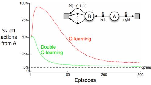
Figure 35.5: Comparison of Q-learning and double Q-learning on a simple episodic MDP using ε-greedy action selection with ε = 0.1. The initial state is A, and squares denote absorbing states. The data are averaged over 10,000 runs. From Figure 6.5 of [SB18]. Used with kind permission of Richard Sutton.

where U(D) is a uniform distribution over the replay bu!er D. We then periodically set w^↓ △ w, usually after a few episodes. This approach is an instance of fitted value iteration [SB18].

Various improvements to DQN have been proposed. One is double DQN [HGS16], which uses the double learning technique (Section 35.2.5.2) to remove the maximization bias. The second is to replace the uniform distribution in Equation (35.14) with one that favors more important transition tuples, resulting in the use of prioritized experience replay [Sch+16a]. For example, we can sample transitions from D with probability p(s, a, r, s↗ ) ^↑ (|ε^| + ⁰)⇀, where ^ε is the corresponding TD error (under the current Q-function), 0 > 0 a hyperparameter to ensure every experience is chosen with nonzero probability, and ▷ ⇑ 0 controls the “inverse temperature” of the distribution (so ▷ = 0 corresponds to uniform sampling). The third is to learn a value function V^w and an advantage function Aw, with shared parameter w, instead of learning Qw. The resulting dueling DQN [Wan+16] is shown to be more sample e”cient, especially when there are many actions with similar Q-values.

The rainbow method [Hes+18] combines all three improvements, as well as others, including multi-step returns (Section 35.2.3), distributional RL [BDM17] (which predicts the distribution of returns, not just the expected return), and noisy nets [For+18b] (which adds random noise to the network weights to encourage exploration). It produces state-of-the-art results on the Atari benchmark.

35.3 Policy-based RL

In the previous section, we considered methods that estimate the action-value function, Q(s, a), from which we derive a policy, which may be greedy or softmax. However, these methods have three main disadvantages: (1) they can be di”cult to apply to continuous action spaces; (2) they may diverge if function approximation is used; and (3) the training of Q, often based on TD-style updates, is not directly related to the expected return garnered by the learned policy.

In this section, we discuss policy search methods, which directly optimize the parameters of the policy so as to maximize its expected return. However, we will see that these methods often benefit from estimating a value or advantage function to reduce the variance in the policy search process.

35.3.1 The policy gradient theorem

We start by defining the objective function for policy learning, and then derive its gradient. We consider the episodic case. A similar result can be derived for the continuing case with the average reward criterion [SB18, Sec 13.6].

We define the objective to be the expected return of a policy, which we aim to maximize:

\[\mathbb{E}\left[J(\pi)\triangleq\mathbb{E}\_{p\_0,\pi}\left[G\_0\right]=\mathbb{E}\_{p\_0(s\_0)}\left[V\_{\pi}(s\_0)\right]=\mathbb{E}\_{p\_0(s\_0)\pi(a\_0|s\_0)}\left[Q\_{\pi}(s\_0,a\_0)\right]\tag{35.15}\]

We consider policies ϑ^ω parameterized by ω, and compute the gradient of Equation (35.15) wrt ω:

\[\nabla\_{\boldsymbol{\theta}}J(\pi\_{\boldsymbol{\theta}}) = \mathbb{E}\_{p\_0(s\_0)} \left[ \nabla\_{\boldsymbol{\theta}} \left( \sum\_{a\_0} \pi\_{\boldsymbol{\theta}}(a\_0|s\_0) Q\_{\pi \boldsymbol{\theta}}(s\_0, a\_0) \right) \right] \tag{35.16}\]

\[=\mathbb{E}\_{p\_0(s\_0)}\left[\sum\_{a\_0}\nabla\pi\_{\theta}(a\_0|s\_0)Q\_{\pi\_{\theta}}(s\_0,a\_0)\right]+\mathbb{E}\_{p\_0(s\_0)\pi\_{\theta}(a\_0|s\_0)}\left[\nabla\_{\theta}Q\_{\pi\_{\theta}}(s\_0,a\_0)\right] \tag{35.17}\]

Now we calculate the term ∀ωQ^εω (s0, a0):

\[\nabla\_{\theta} Q\_{\pi\theta}(s\_0, a\_0) = \nabla\_{\theta} \left[ R(s\_0, a\_0) + \gamma \mathbb{E}\_{p(s\_1|s\_0, a\_0)} \left[ V\_{\pi\theta}(s\_1) \right] \right] = \gamma \nabla\_{\theta} \mathbb{E}\_{p(s\_1|s\_0, a\_0)} \left[ V\_{\pi\theta}(s\_1) \right] \tag{35.18}\]

The right-hand side above is in a form similar to ∀ωJ(ϑω). Repeating the same steps as before gives

\[\nabla\_{\boldsymbol{\theta}} J(\pi\_{\boldsymbol{\theta}}) = \sum\_{t=0}^{\infty} \gamma^{t} \mathbb{E}\_{p\_{t}(s)} \left[ \sum\_{a} \nabla\_{\boldsymbol{\theta}} \pi\_{\boldsymbol{\theta}}(a|s) Q\_{\pi\_{\boldsymbol{\theta}}}(s, a) \right]\_{\boldsymbol{\eta}} \tag{35.19}\]

\[\mathcal{E} = \frac{1}{1-\gamma} \mathbb{E}\_{p\_{\pi\_{\theta}}^{\infty}(s)} \left[ \sum\_{a} \nabla\_{\theta} \pi\_{\theta}(a|s) Q\_{\pi\_{\theta}}(s, a) \right] \tag{35.20}\]

\[=\frac{1}{1-\gamma}\mathbb{E}\_{p^{\infty}\_{\pi\_{\theta}}(s)\pi\_{\theta}(a|s)}\left[\nabla\_{\theta}\log\pi\_{\theta}(a|s)\ Q\_{\pi\_{\theta}}(s,a)\right] \tag{35.21}\]

where pt(s) is the probability of visiting s in time t if we start with s⁰ ↘ p⁰ and follow ϑω, and p^{↔︎ εω} (s) = (1 ↓ γ) )^{↔︎ t}=0 γ^t pt(s) is the normalized discounted state visitation distribution. Equation (35.21) is known as the policy gradient theorem [Sut+99].

In practice, estimating the policy gradient using Equation (35.21) can have a high variance. A baseline b(s) can be used for variance reduction (Section 6.3.4.1):

\[\nabla\_{\theta} J(\pi\_{\theta}) = \frac{1}{1 - \gamma} \mathbb{E}\_{p\_{\pi\_{\theta}}^{\infty}(s)\pi\_{\theta}(a|s)} \left[ \nabla\_{\theta} \log \pi\_{\theta}(a|s) (Q\_{\pi \sigma}(s, a) - b(s)) \right] \tag{35.22}\]

A common choice for the baseline is b(s) = V^εω (s). We will discuss how to estimate it below.

35.3.2 REINFORCE

One way to apply the policy gradient theorem to optimize a policy is to use stochastic gradient ascent. Suppose ϑ = (s0, a0, r0, s1,…,s^T ) is a trajectory with s⁰ ↘ p⁰ and ϑω. Then,

\[\nabla\_{\theta} J(\pi\_{\theta}) = \frac{1}{1 - \gamma} \mathbb{E}\_{p\_{\pi\_{\theta}}^{\infty}(s)\pi\_{\theta}(a|s)} \left[ \nabla\_{\theta} \log \pi\_{\theta}(a|s) Q\_{\pi\_{\theta}}(s, a) \right] \tag{35.23}\]

\[\approx \sum\_{t=0}^{T-1} \gamma^t G\_t \nabla\_\theta \log \pi\_\theta(a\_t|s\_t) \tag{35.24}\]

where the return G^t is defined in Equation (34.76), and the factor γ^t is due to the definition of p^↔︎ ε^ω where the state at time t is discounted.

We can use a baseline in the gradient estimate to get the following update rule:

\[\theta \gets \theta + \eta \sum\_{t=0}^{T-1} \gamma^t (G\_t - b(s\_t)) \nabla\_\theta \log \pi\_\theta(a\_t|s\_t) \tag{35.25}\]

This is called the REINFORCE algorithm [Wil92].3 The update equation can be interepreted as follows: we compute the sum of discounted future rewards induced by a trajectory, compared to a baseline, and if this is positive, we increase ω so as to make this trajectory more likely, otherwise we decrease ω. Thus, we reinforce good behaviors, and reduce the chances of generating bad ones.

We can use a constant (state-independent) baseline, or we can use a state-dependent baseline, b(st) to further lower the variance. A natural choice is to use an estimated value function, Vw(s), which can be learned, e.g., with MC. Algorithm 35.2 gives the pseudocode where stochastic gradient updates are used with separate learning rates.

Algorithm 35.2: REINFORCE with value function baseline

Initialize policy parameters ω, baseline parameters w ² repeat Sample an episode ϑ = (s0, a0, r0, s1,…,s^T ) using ϑ^ω Compute G^t for all t → {0, 1,…,T ↓ 1} using Equation (34.76) for t = 0, 1,…,T ↓ 1 do ε = G^t ↓ Vw(st) // scalar error w △ w + ▷wε∀wVw(st) ^ω △ ^{ω + ▷}ωγ^t ε∀^ω log ϑω(at|st) until converged

35.3.3 Actor-critic methods

An actor-critic method [BSA83] uses the policy gradient method, but where the expected return is estimated using temporal di!erence learning of a value function instead of MC rollouts. The term

^3. The term “REINFORCE” is an acronym for “REward Increment = nonnegative Factor x O!set Reinforcement x Characteristic Eligibility”. The phrase “characteristic eligibility” refers to the ↑ log ϖω(at|st) term; the phrase “o!set reinforcement” refers to the G^t ↓ b(st) term; and the phrase “nonnegative factor” refers to the learning rate ϱ of SGD.

“actor” refers to the policy, and the term “critic” refers to the value function. The use of bootstrapping in TD updates allows more e”cient learning of the value function compared to MC. In addition, it allows us to develop a fully online, incremental algorithm, that does not need to wait until the end of the trajectory before updating the parameters (as in Algorithm 35.2).

Concretely, consider the use of the one-step TD(0) method to estimate the return in the episodic csae, i.e., we replace G^t with Gt:t+1 = rt+γVw(st+1). If we use Vw(st) as a baseline, the REINFORCE update in Equation (35.25) becomes

\[\theta \leftarrow \theta + \eta \sum\_{t=0}^{T-1} \gamma^t \left( G\_{t:t+1} - V\_{\mathbf{w}}(s\_t) \right) \nabla\_{\theta} \log \pi\_{\theta}(a\_t|s\_t) \tag{35.26}\]

\[\theta = \theta + \eta \sum\_{t=0}^{T-1} \gamma^t \left( r\_t + \gamma V\_{\mathbf{w}}(s\_{t+1}) - V\_{\mathbf{w}}(s\_t) \right) \nabla\_{\theta} \log \pi\_{\theta}(a\_t|s\_t) \tag{35.27}\]

35.3.3.1 A2C and A3C

Note that rt+1 + γVw(st+1) ↓ Vw(st) is a single sample approximation to the advantage function A(st, at) = Q(st, at) ↓ V (st). This method is therefore called advantage actor critic or A2C (Algorithm 35.3). If we run the actors in parallel and asynchronously update their shared parameters, the method is called asynchrononous advantage actor critic or A3C [Mni+16].

Algorithm 35.3: Advantage actor critic (A2C) algorithm

Initialize actor parameters ω, critic parameters w ² repeat Sample starting state s⁰ of a new episode for t = 0, 1, 2,… do Sample action a^t ↘ ϑω(·|st) Observe next state st+1 and reward r^t ε = r^t + γVw(st+1) ↓ Vw(st) w △ w + ▷wε∀wVw(st) ^ω △ ^{ω + ▷}ωγ^t ε∀^ω log ϑω(at|st) until converged

35.3.3.2 Eligibility traces

In A2C, we use a single step rollout, and then use the value function in order to approximate the expected return for the trajectory. More generally, we can use the n-step estimate

\[G\_{t:t+n} = r\_t + \gamma r\_{t+1} + \gamma^2 r\_{t+2} + \dots + \gamma^{n-1} r\_{t+n-1} + \gamma^n V\_\mathbf{w}(s\_{t+n}) \tag{35.28}\]

and obtain an n-step advantage estimate as follows:

\[A^{(n)}\_{\\\pi\_{\theta}}(s\_t, a\_t) = G\_{t:t+n} - V\_{\mathbf{w}}(s\_t) \tag{35.29}\]

The n steps of actual rewards are an unbiased sample, but have high variance. By contrast, Vw(st+n+1) has lower variance, but is biased. By changing n, we can control the bias-variance tradeo!. Instead of using a single value of n, we can take an weighted average, with weight proportional to ◁ⁿ for A(n) ^εω (st, at), as in TD(◁). The average can be shown to be equivalent to

\[A^{(\lambda)}\_{\pi\_{\theta}}(s\_t, a\_t) \triangleq \sum\_{\ell=0}^{\infty} (\gamma \lambda)^{\ell} \delta\_{t+l} \tag{35.30}\]

where ε^t = r^t + γVw(st+1) ↓ Vw(st) is the TD error at time t. Here, ◁ → [0, 1] is a parameter that controls the bias-variance tradeo!: larger values decrease the bias but increase the variance, as in TD(◁). We can implement Equation (35.30) e”ciently using eligibility traces, as shown in Algorithm 35.4, as an example of generalized advantage estimation (GAE) [Sch+16b]. See [SB18, Ch.12] for further details.

Algorithm 35.4: Actor critic with eligibility traces

Initialize actor parameters ω, critic parameters w ² repeat Initialize eligibility trace vectors: z^ω △ 0, z^w △ 0 Sample starting state s⁰ of a new episode for t = 0, 1, 2,… do Sample action a^t ↘ ϑω(·|st) Observe state st+1 and reward r^t Compute the TD error: ε = r^t + γVw(st+1) ↓ Vw(st) z^w △ γ◁wz^w + ∀wVw(s) ^zω △ γ◁ωz^{ω + γt} ∀^ω log ϑω(at|st) w △ w + ▷wεz^w ω △ ω + ▷ωεz^ω until converged

35.3.4 Bound optimization methods

In policy gradient methods, the objective J(ω) does not necessarily increase monotonically, but rather can collapse especially if the learning rate is not small enough. We now describe methods that guarantee monotonic improvement, similar to bound optimization algorithms (Section 6.5).

We start with a useful fact that relate the policy values of two arbitrary policies [KL02]:

\[J(\pi') - J(\pi) = \frac{1}{1 - \gamma} \mathbb{E}\_{p^{\infty}\_{\pi'}(s)} \left[ \mathbb{E}\_{\pi'(a|s)} \left[ A\_{\pi}(s, a) \right] \right] \tag{35.31}\]

where ϑ can be interpreted as the current policy during policy optimization, and ϑ↗ a candidate new policy (such as the greedy policy wrt Qε). As in the policy improvement theorem (Section 34.6.2), if E^ε↓(a|s) [Aε(s, a)] ⇑ 0 for all s, then J(ϑ↗ ) ⇑ J(ϑ). However, we cannot ensure this condition to hold when function approximation is used, as such a uniformly improving policy ϑ↗ may not be

representable by our parametric family, {ϑω}ω↑!. Therefore, nonnegativity of Equation (35.31) is not easy to ensure, when we do not have a direct way to sample states from p^↔︎ ε↓ .

One way to ensure monotonic improvement of J is to improve the policy conservatively. Define ϑ^ϑ = ςϑ↗ + (1 ↓ ς)ϑ for ς → [0, 1]. It follows from the policy gradient theorem (Equation (35.21), with ω = [ς]) that J(ϑϑ) ↓ J(ϑ) = ςL(ϑ↗ ) + O(ς2), where

\[L(\pi') \triangleq \frac{1}{1-\gamma} \mathbb{E}\_{p\_{\pi}^{\infty}(s)} \left[ \mathbb{E}\_{\pi'(a|s)} \left[ A\_{\pi}(s,a) \right] \right] = \frac{1}{1-\gamma} \mathbb{E}\_{p\_{\pi}^{\infty}(s)\pi(a|s)} \left[ \frac{\pi'(a|s)}{\pi(a|s)} A\_{\pi}(s,a) \right] \tag{35.32}\]

In the above, we have switched the state distribution from p^{↔︎ ε↓} in Equation (35.31) to p^{↔︎ ε} , while at the same time introducing a higher order residual term of O(ς²). The linear term, ςL(ϑ↗ ), can be estimated and optimized based on episodes sampled by ϑ. The higher order term can be bounded in various ways, resulting in di!erent lower bounds of J(ϑϑ) ↓ J(ϑ). We can then optimize ς to make sure this lower bound is positive, which would imply J(ϑϑ) ↓ J(ϑ) > 0. In conservative policy iteration [KL02], the following (slightly simplified) lower bound is used

\[J^{\rm CPI}(\pi\_{\theta}) \stackrel{\Delta}{=} J(\pi) + \theta L(\pi') - \frac{2\varepsilon\gamma}{(1-\gamma)^2} \theta^2 \tag{35.33}\]

where 0 = max^s |E^ε↓(a|s) [Aε(s, a)] |.

This idea can be generalized to policies beyond those in the form of ϑϑ, where the condition of a small enough ς is replaced by a small enough divergence between ϑ↗ and ϑ. In safe policy iteration [Pir+13], the divergence is the maximum total variation, while in trust region policy optimization (TRPO) [Sch+15b], the divergence is the maximum KL-divergence. In the latter case, ϑ↗ may be found by optimizing the following lower bound

\[J^{\rm TRPO}(\pi') \stackrel{\Delta}{=} J(\pi) + L(\pi') - \frac{\varepsilon \gamma}{(1 - \gamma)^2} \max\_{s} D\_{\rm KL} \left( \pi(s) \parallel \pi'(s) \right) \tag{35.34}\]

where 0 = maxs,a |Aε(s, a)|.

In practice, the above update rule can be overly conservative, and approximations are used. [Sch+15b] propose a version that implements two ideas: one is to replace the point-wise maximum KL-divergence by some average KL-divergence (usually averaged over p^{↔︎ εω} ); the second is to maximize the first two terms in Equation (35.34), with ϑ↗ lying in a KL-ball centered at ϑ. That is, we solve

\[\underset{\pi'}{\text{argmax}}\,L(\pi') \quad \text{s.t.} \quad \mathbb{E}\_{p\_{\pi}^{\infty}(s)}\left[D\_{\text{KL}}\left(\pi(s) \parallel \pi'(s)\right)\right] \leq \delta \tag{35.35}\]

for some threshold ε > 0.

In Section 6.4.2.1, we show that the trust region method, using a KL penalty at each step, is equivalent to natural gradient descent (see e.g., [Kak02; PS08b]). This is important, because a step of size ▷ in parameter space does not always correspond to a step of size ▷ in the policy space:

\[d\rho(\theta\_1, \theta\_2) = d\rho(\theta\_2, \theta\_3) \not\Rightarrow d\_\pi(\pi\_{\theta\_1}, \pi\_{\theta\_2}) = d\_\pi(\pi\_{\theta\_2}, \pi\_{\theta\_3}) \tag{35.36}\]

where dω(ω1, ω2) = ↙ω¹ ↓ ω2↙ is the Euclidean distance, and dε(ϑ1, ϑ2) = DKL (ϑ¹ ↙ ϑ2) the KL distance. In other words, the e!ect on the policy of any given change to the parameters depends on where we are in parameter space. This is taken into account by the natural gradient method, resulting in faster and more robust optimization. The natural policy gradient can be approximated using the KFAC method (Section 6.4.4), as done in [Wu+17].

Other than TRPO, another approach inspired by Equation (35.34) is to use the KL-divergence as a penalty term, replacing the factor 20γ/(1 ^{↓ γ})² by a tuning parameter. However, it often works better, and is simpler, by using the following clipped objective, which results in the proximal policy optimization or PPO method [Sch+17]:

\[J^{\rm PPO}(\pi') \stackrel{\Delta}{=} \frac{1}{1-\gamma} \mathbb{E}\_{p\_{\pi}^{\infty}(s)\pi(a|s)} \left[ \kappa\_{\epsilon} \left( \frac{\pi'(a|s)}{\pi(a|s)} \right) A\_{\pi}(s,a) \right] \tag{35.37}\]

where 1↼(x) ↭ clip(x, 1 ↓ -, 1 + -) ensures |1(x) ↓ 1| ⇔ -. This method can be modified to ensure monotonic improvement as discussed in [WHT19], making it a true bound optimization method.

35.3.5 Deterministic policy gradient methods

In this section, we consider the case of a deterministic policy, that predicts a unique action for each state, so a^t = µω(st), rather than a^t ↘ ϑω(st). We assume the states and actions are continuous, and define the objective as

\[J(\mu\_{\varPhi}) \stackrel{\Delta}{=} \frac{1}{1-\gamma} \mathbb{E}\_{p^{\infty}\_{\mu\_{\varPhi}}(s)} \left[ R(s, \mu\_{\varPhi}(s)) \right] \tag{35.38}\]

The deterministic policy gradient theorem [Sil+14] provides a way to compute the gradient:

\[\nabla\_{\theta} J(\mu\_{\theta}) = \frac{1}{1 - \gamma} \mathbb{E}\_{p\_{\mu\_{\theta}}^{\infty}(s)} \left[ \nabla\_{\theta} Q\_{\mu\_{\theta}}(s, \mu\_{\theta}(s)) \right] \tag{35.39}\]

\[=\frac{1}{1-\gamma}\mathbb{E}\_{p^{\infty}\_{\mu\theta}(s)}\left[\nabla\_{\theta}\mu\_{\theta}(s)\nabla\_{a}Q\_{\mu\theta}(s,a)|\_{a=\mu\_{\theta}(s)}\right] \tag{35.40}\]

where ∀ωµω(s) is the M ⇒ N Jacobian matrix, and M and N are the dimensions of A and ω, respectively. For stochastic policies of the form ϑω(a|s) = µω(s) + noise, the standard policy gradient theorem reduces to the above form as the noise level goes to zero.

Note that the gradient estimate in Equation (35.40) integrates over the states but not over the actions, which helps reduce the variance in gradient estimation from sampled trajectories. However, since the deterministic policy does not do any exploration, we need to use an o!-policy method, that collects data from a stochastic behavior policy ⇁, whose stationary state distribution is p^↔︎ φ . (See Section 35.5 for details on o!-policy RL.) The original objective, J(µω), is approximated by the following:

\[\mathbb{E}\left[J\_b(\mu\_\theta)\stackrel{\Delta}{=}\mathbb{E}\_{p\_\beta^\infty(s)}\left[V\_{\mu\theta}(s)\right]=\mathbb{E}\_{p\_\beta^\infty(s)}\left[Q\_{\mu\theta}(s,\mu\_\theta(s))\right]\right] \tag{35.41}\]

with the o!-policy deterministic policy gradient from [DWS12] is approximated by

\[\nabla\_{\boldsymbol{\theta}} J\_{b}(\mu\_{\boldsymbol{\theta}}) \approx \mathbb{E}\_{p\_{\boldsymbol{\beta}}^{\infty}(s)} \left[ \nabla\_{\boldsymbol{\theta}} \left[ Q\_{\mu \boldsymbol{\theta}}(s, \mu\_{\boldsymbol{\theta}}(s)) \right] \right] = \mathbb{E}\_{p\_{\boldsymbol{\beta}}^{\infty}(s)} \left[ \nabla\_{\boldsymbol{\theta}} \mu\_{\boldsymbol{\theta}}(s) \nabla\_{a} Q\_{\mu \boldsymbol{\theta}}(s, a) \big|\_{a = \mu\_{\boldsymbol{\theta}}(s)} ds \right] \tag{35.42}\]

where we have a dropped a term that depends on ∀ωQ^µω (s, a) and is hard to estimate [Sil+14].

To apply Equation (35.42), we may learn Q^w ≃ Qµ^ω with TD, giving rise to the following updates:

\[\delta = r\_t + \gamma Q\_{\mathbf{w}}(s\_{t+1}, \mu\_{\theta}(s\_{t+1})) - Q\_{\mathbf{w}}(s\_t, a\_t) \tag{35.43}\]

\[w\_{l+1} \gets w\_l + \eta\_{\mathbf{w}} \delta \nabla\_{\mathbf{w}} Q\_{\mathbf{w}}(s\_t, a\_t) \tag{35.44}\]

\[ \theta\_{t+1} \gets \theta\_t + \eta\_\theta \nabla\_\theta \mu\_\theta(s\_t) \nabla\_a Q\_\mathbf{w}(s\_t, a)|\_{a = \mu\_\theta(s\_t)} \tag{35.45} \]

This avoids importance sampling needed by other o!-policy methods (see Section 35.5.1.2). In particular, we avoid IS in the actor update because of the deterministic policy gradient, and we avoid IS in the critic update because of the use of Q-learning.

If ^Qw is linear in ^w, and uses features of the form ^ε(s, a) = ^aT∀ωµω(s), where ^a is the vector representation of a, then we say the function approximator for the critic is compatible with the actor; in this case, one can show that the above approximation does not bias the overall gradient.

The basic o!-policy DPG method has been extended in various ways. The DDPG algorithm of [Lil+16], which stands for “deep deterministic policy gradient”, uses the DQN method (Section 35.2.6) to update Q that is represented by deep neural networks. In more detail, the actor tries to maximize the output of the critic by minimizing LP G(s) = ↓Q(sg(s), ϑ(s)), where sg is the stop-gradient operator, which ensures the state argument is considered frozen. The critic tries to minimize the 1-step TD loss, LTD(s, a, r, s↗ )=[Q(s, a) ↓ (r + γsg(Q(s↗ , ϑ(s↗ )))]², where Q is the target critic network4, ϑ is the target actor network, and the samples (s, a, r, a↗ ) are drawn from a replay bu!er.

An extension of DDPG, known as TD3, stands for “twin delayed DDPG” [FHM18], extends the method by using double DQN (Section 35.2.5.2) and other heuristics to further improve performance. The REDQ method of [Che+20d] extended double DQN to the setting where we use an ensemble of more than 2 Q networks, providing even more robustness in the case where the number of policy updates per observed data point is large. (A high UTD ratio is critical for sample e”ciency.) The D4PG algorithm [BM+18], which stands for “distributed distributional DDPG”, extends DDPG to handle distributed training, and to handle distributional RL (i.e., working with distributions of rewards instead of expected rewards [BDM17]).

The recent Amago algorithm [GFZ24] shows how to extend DDPG to the case where the actor and critic are both defined in terms of a shared transformer sequence model. To do this, they define a unified objective L = E[◁0LTD + ◁1LP G], where the TD and policy gradient losses are dynamically normalized using the Pop-Art method of [Has+16] to allow for a fixed set of hyper-parameter values for ◁i, even as the range of the losses change over time. (Pop-Art stands for “Preserving Outputs Precisely, while Adaptively Rescaling Targets”.)

35.3.6 Gradient-free methods

The policy gradient estimator computes a “zeroth order” gradient, which essentially evaluates the function with randomly sampled trajectories. Sometimes it can be more e”cient to use a derivativefree optimizer (Section 6.7), that does not even attempt to estimate the gradient. For example, [MGR18] obtain good results by training linear policies with random search, and [Sal+17b] show how to use evolutionary strategies to optimize the policy of a robotic controller.

^4. The use of target networks is needed to ensure stability, so the Q function is not trying to predict itself directly, but instead is trying to predict an exponential moving average (EMA) version of itself. In particular we use Q(s, a) = Q(s, a|ς^↑ ), where ς^↑ = φς + (1 ↓ φ)ς, where ς are the parameters of the main Q network, and φ ↔︎ 1 ensures that Q slowly catches up with Q.

35.4 Model-based RL

Model-free approaches to RL typically need a lot of interactions with the environment to achieve good performance. For example, state of the art methods for the Atari benchmark, such as rainbow (Section 35.2.6), use millions of frames, equivalent to many days of playing at the standard frame rate. By contrast, humans can achieve the same performance in minutes [Tsi+17]. Similarly, OpenAI’s robot hand controller [And+20] learns to manipulate a cube using 100 years of simulated data.

One promising approach to greater sample e”ciency is model-based RL (MBRL). In this approach, we first learn the transition model and reward function, p(s↗ |s, a) and R(s, a), then use them to compute a near-optimal policy. This approach can significantly reduce the amount of real-world data that the agent needs to collect, since it can “try things out” in its imagination (i.e., the models), rather than having to try them out empirically.

There are several ways we can use a model, and many di!erent kinds of model we can create. Some of the algorithms mentioned earlier, such as MBIE and UCLR2 for provably e”cient exploration (Section 35.1.5.3), are examples of model-based methods. MBRL also provides a natural connection between RL and planning (Section 34.6) [Sut90]. We discuss some examples in the sections below, and refer to [MBJ20; PKP21; MH20] for more detailed reviews.

35.4.1 Model predictive control (MPC)

So far in this chapter, we have focused on trying to learn an optimal policy ϑ→(s), which can then be used at run time to quickly pick the best action for any given state s. However, we can also avoid performing all this work in advance, and wait until we know what state we are in, call it st, and then use a model to predict future states and rewards that might follow for each possible sequence of future actions we might pursue. We then take the action that looks most promising, and repeat the process at the next step. More precisely, we compute

\[\mathbf{a}\_{t:t+H-1}^{\*} = \underset{\mathbf{a}\_{t:t+H-1}}{\operatorname{argmax}} \mathbb{E}\left[\sum\_{h=0}^{H-1} R(s\_{t+h}, a\_{t+h}) + \hat{V}(s\_{t+H})\right] \tag{35.46}\]

where the expectation is over state sequences that might result from executing at:t+H↓¹ from state st. Here, H is called the planning horizon, and Vˆ (st+H) is an estimate of the reward-to-go at the end of this H-step look-ahead process. This is known as receeding horizon control or model predictive control (MPC) [MM90; CA13]. We discuss some special cases of this below.

35.4.1.1 Heuristic search

If the state and action spaces are finite, we can solve Equation (35.46) exactly, although the time complexity will typically be exponential in H. However, in many situations, we can prune o! unpromising trajectories, thus making the approach feasible in large scale problems.

In particular, consider a discrete, deterministic MDP where reward maximization corresponds to finding a shortest path to a goal state. We can expand the successors of the current state according to all possible actions, trying to find the goal state. Since the search tree grows exponentially with depth, we can use a heuristic function to prioritize which nodes to expand; this is called best-first search, as illustrated in Figure 35.6.

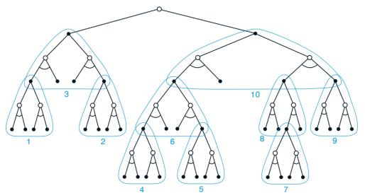
Figure 35.6: Illustration of heuristic search. In this figure, the subtrees are ordered according to a depth-first search procedure. From Figure 8.9 of [SB18]. Used with kind permission of Richard Sutton.

If the heuristic function is an optimistic lower bound on the true distance to the goal, it is called admissible; If we aim to maximize total rewards, admissibility means the heuristic function is an upper bound of the true value function. Admissibility ensures we will never incorrectly prune o! parts of the search space. In this case, the resulting algorithm is known as A^→ search, and is optimal. For more details on classical AI heuristic search methods, see [Pea84; RN19].

35.4.1.2 Monte Carlo tree search (MCTS)

Monte Carlo tree search or MCTS is similar to heuristic search, but learns a value function for each encountered state, rather than relying on a manually designed heuristic (see e.g., [Mun14] for details). MCTS is inspired by UCB for bandits (Section 34.4.5), but applies to general sequential decision making problems including MDPs [KS06].

The MCTS method forms the basis of the famous AlphaGo and AlphaZero programs [Sil+16; Sil+18], which can play expert-level Go, chess, and shogi (Japanese chess), using a known model of the environment. The MuZero method of [Sch+20] and the Stochastic MuZero method of [Ant+22] extend this to the case where the world model is also learned. The action-value functions for the intermediate nodes in the search tree are represented by deep neural networks, and updated using temporal di!erence methods that we discuss in Section 35.2. MCTS can also be applied to many other kinds of seqential decision problems, such as experiment design for sequentially creating molecules [SPW18].

35.4.1.3 Trajectory optimization for continuous actions

For continuous actions, we cannot enumerate all possible branches in the search tree. Instead, Equation (35.46) can be viewed as a nonlinear program, where at:t+H↓¹ are the real-valued variables to be optimized. If the system dynamics are linear and the reward function corresponds to negative quadratic cost, the optimal action sequence can be solved mathematically, as in the linear-quadratic-Gaussian (LQG) controller (see e.g., [AM89; HR17]). However, this problem is hard in general and often solved by numerical methods such as shooting and collocation [Die+07; Rao10; Kal+11]. Many of them work in an iterative fashion, starting with an initial action sequence followed by a step to improve it. This process repeats until convergence of the cost.

An example is di!erential dynamic programming (DDP) [JM70; TL05]. In each iteration, DDP starts with a reference trajectory, and linearizes the system dynamics around states on the trajectory to form a locally quadratic approximation of the reward function. This system can be solved using LQG, whose optimal solution results in a new trajectory. The algorithm then moves to the next iteration, with the new trajectory as the reference trajectory.

Other alternatives are possible, including black-box (gradient-free) optimization methods like the cross-entropy method. (see Section 6.7.5).

35.4.2 Combining model-based and model-free

In Section 35.4.1, we discussed MPC, which uses the model to decide which action to take at each step. However, this can be slow, and can su!er from problems when the model is inaccurate. An alternative is to use the learned model to help reduce the sample complexity of policy learning.

There are many ways to do this. One approach is to generate rollouts from the model, and then train a policy or Q-function on the “hallucinated” data. This is the basis of the famous dyna method [Sut90]. In [Jan+19], they propose a similar method, but generate short rollouts from previously visited real states; this ensures the model only has to extrapolate locally.

In [Web+17], they train a model to predict future states and rewards, but then use the hidden states of this model as additional context for a policy-based learning method. This can help overcome partial observability. They call their method imagination-augmented agents. A related method appears in [Jad+17], who propose to train a model to jointly predict future rewards and other auxiliary signals, such as future states. This can help in situations when rewards are sparse or absent.

35.4.3 MBRL using Gaussian processes

This section gives some examples of dynamics models that have been learned for low-dimensional continuous control problems. Such problems frequently arise in robotics. Since the dynamics are often nonlinear, it is useful to use a flexible and sample-e”cient model family, such as Gaussian processes (Section 18.1). We will use notation like s and a for states and actions to emphasize they are vectors.

35.4.3.1 PILCO

We first describe the PILCO method [DR11; DFR15], which stands for “probabilistic inference for learning control”. It is extremely data e”cient for continuous control problems, enabling learning from scratch on real physical robots in a matter of minutes.

PILCO assumes the world model has the form st+1 = f(st, at) + ϖt, where ϖ^t ↘ N (0, !), and f is an unknown, continuous function.5 The basic idea is to learn a Gaussian process (Section 18.1)) approximation of f based on some initial random trajectories, and then to use this model to generate “fantasy” rollout trajectories of length T, that can be used to evaluate the expected cost of the current policy, J(ϑω) = )^{T t}=1 E^at↘ε^ω [c(st)], where s⁰ ↘ p0. This function and its gradients wrt ω can be computed deterministically, if a Gaussian assumption about the state distribution at each step is made, because the Gaussian belief state can be propagated deterministically through the

^5. An alternative, which often works better, is to use f to model the residual, so that st+1 = s^t + f(st, at) + εt.

Figure 35.7: (a) A cart-pole system being controlled by a policy learned by PILCO using just 17.5 seconds of real-world interaction. The goal state is marked by the red cross. The initial state is where the cart is stationary on the right edge of the workspace, and the pendulum is horizontal. For a video of the system learning, see https: // bit. ly/ 35fpLmR . (b) A low-quality robot arm being controlled by a block-stacking policy learned by PILCO using just 230 seconds of real-world interaction. From Figures 11, 12 from [DFR15]. Used with kind permission of Marc Deisenroth.

GP model. Therefore, we can use deterministic batch optimization methods, such as Levenberg-Marquardt, to optimize the policy parameters ω, instead of applying SGD to sampled trajectories. (See https://github.com/mathDR/jax-pilco for some JAX code.)

Due to its data e”ciency, it is possible to apply PILCO to real robots. Figure 35.7a shows the results of applying it to solve a cart-pole swing-up task, where the goal is to make the inverted pendulum swing up by applying a horizontal force to move the cart back and forth. The state of the system ^{s → R4} consists of the position ^x of the cart (with ^x = 0 being the center of the track), the velocity ^x˙, the angle ^ς of the pendulum (measured from hanging downward), and the angular velocity ˙ ς. The control signal a → R is the force applied to the cart. The target state is s^→ = (0, 2, ϑ, 2), corresponding to the cart being in the middle and the pendulum being vertical, with velocities unspecified. The authors used an RBF controller with 50 basis functions, amounting to a total of 305 policy parameters. The controller was successfully trained using just 7 real world trials.6

Figure 35.7b shows the results of applying PILCO to solve a block stacking task using a lowquality robot arm with 6 degrees of freedom. A separate controller was trained for each block. The state space ^{s → R3} is the 3d location of the center of the block in the arm’s gripper (derived from an RGBD sensor), and the control ^{a → R4} corresponds to the pulse widths of four servo motors. A linear policy was successfully trained using as few as 10 real world trials.

35.4.3.2 GP-MPC

[KD18a] have proposed an extension to PILCO that they call GP-MPC, since it combines a GP dynamics model with model predictive control (Section 35.4.1). In particular, they use an open-loop control policy to propose a sequence of actions, at:t+H↓1, as opposed to sampling them from a policy. They compute a Gaussian approximation to the future state trajectory, p(st+1:t+H|at:t+H↓¹, st), by moment matching, and use this to deterministically compute the expected reward and its gradient wrt at:t+H↓¹ (as opposed to the policy parameters ω). Using this, they can solve Equation (35.46)

^{6. 2} random initial trials, each 5 seconds, and then 5 policy-generated trials, each 2.5 seconds, totalling 17.5 seeconds.

to find a^{→ t}:t+H↓1; finally, they execute the first step of this plan, a^{→ t} , and repeat the whole process.

The advantage of GP-MPC over policy-based PILCO is that it can handle constraints more easily, and it can be more data e”cient, since it continually updates the GP model after every step (instead of at the end of an trajectory).

35.4.4 MBRL using DNNs

Gaussian processes do not scale well to large sample sizes and high dimensional data. Deep neural networks (DNNs) work much better in this regime. However, they do not naturally model uncertainty, which can cause MPC methods to fail. We discuss various methods for representing uncertainty with DNNs in Section 17.1. Here, we mention a few approaches that have been used for MBRL.

The deep PILCO method uses DNNs together with Monte Carlo dropout (Section 17.3.1) to represent uncertainty [GMAR16]. [Chu+18] proposed probabilistic ensembles with trajectory sampling or PETS, which represents uncertainty using an ensemble of DNNs (Section 17.3.9). Many other approaches are possible, depending on the details of the problem being tackled.

Since these are all stochastic methods (as opposed to the GP methods above), they can su!er from a high variance in the predicted returns, which can make it di”cult for the MPC controller to pick the best action. We can reduce variance with the common random number trick [KSN99], where all rollouts share the same random seed, so di!erences in J(ϑω) can be attributed to changes in ω but not other factors. This technique was used in PEGASUS [NJ00] 7 and in [HMD18].

35.4.5 MBRL using latent-variable models

In this section, we describe some methods that learn latent variable models, rather than trying to predict dynamics directly in the observed space, which is hard to do when the states are images.

35.4.5.1 World models

The “world models” paper [HS18] showed how to learn a generative model of two simple video games (CarRacing and a VizDoom-like environment), such that the model can be used to train a policy entirely in simulation. The basic idea is shown in Figure 35.8. First, we collect some random experience, and use this to fit a VAE model (Section 21.2) to reduce the dimensionality of the images, ^{xt → R64}⇒64⇒³, to a latent ^{zt → R64}. Next, we train an RNN to predict ^p(zt+1|zt, ^at, ^ht), where ^ht is the deterministic RNN state, and a^t is the continuous action vector (3-dimensional in both cases). The emission model for the RNN is a mixture density network, in order to model multi-modal futures. Finally, we train the controller using z^t and h^t as inputs; here z^t is a compact representation of the current frame, and h^t is a compact representation of the predicted distribution over zt+1.

The authors of [HS18] trained the controller using a derivative free optimizer called CMA-ES (covariance matrix adaptation evolutionary strategy, see Section 6.7.6.2). It can work better than policy gradient methods, as discussed in Section 35.3.6. However, it does not scale to high dimensions. To tackle this, the authors use a linear controller, which has only 867 parameters.8 By contrast,

^7. PEGASUS stands for “Policy Evaluation-of-Goodness And Search Using Scenarios”, where the term “scenario” refers to one of the shared random samples.

^8. The input is a 32-dimensional zt plus a 256-dimensional ht, and there are 3 outputs. So the number of parameters is (32 + 256) ↗ 3 + 3 = 867, to account for the weights and biases.

Figure 35.8: (a) Illustration of an agent interacting with the VizDoom environment. (The yellow blobs represent fireballs being thrown towards the agent by various enemies.) The agent has a world model, composed of a vision system V and a memory RNN M, and has a controller C. (b) Detailed representation of the memory model. Here h^t is the deterministic hidden state of the RNN at time t, which is used to predict the next latent of the VAE, zt+1, using a mixture density network (MDN). Here ϑ is a temperature parameter used to increase the variance of the predictions, to prevent the controller from exploiting model inaccuracies. From Figures 4, 6 of [HS18]. Used with kind permission of David Ha.

VAE has 4.3M parameters and MDN-RNN 422k. Fortunately, these two models can be trained in an unsupervised way from random rollouts, so sample e”ciency is less critical than when training the policy.

So far, we have described how to use the representation learned by the generative model as informative features for the controller, but the controller is still learned by interacting with the real world. Surprisingly, we can also train the controller entirely in “dream mode”, in which the generated images from the VAE decoder at time t are fed as input to the VAE encoder at time t + 1, and the MDN-RNN is trained to predict the next reward rt+1 as well as zt+1. Unfortunately, this method does not always work, since the model (which is trained in an unsupervised way) may fail to capture task-relevant features (due to underfitting) and may memorize task-irrelevant features (due to overfitting). The controller can learn to exploit weaknesses in the model (similar to an adversarial attack) and achieve high simulated reward, but such a controller may not work well when transferred to the real world.

One approach to combat this is to artificially increase the variance of the MDN model (by using a temperature parameter ↼ ), in order to make the generated samples more stochastic. This forces the controller to be robust to large variations; the controller will then treat the real world as just another kind of noise. This is similar to the technique of domain randomization, which is sometimes used for sim-to-real applications; see e.g., [MAZA18].

35.4.5.2 PlaNet and Dreamer

In [HS18], they first learn the world model on random rollouts, and then train a controller. On harder problems, it is necessary to iterate these two steps, so the model can be trained on data collected by the controller, in an iterative fashion.

In this section, we describe one method of this kind, known as PlaNet [Haf+19]. PlaNet

Figure 35.9: Illustration of some image-based control problems used in the PlaNet paper. Inputs are 64↓64↓3. (a) The cartpole swingup task has a fixed camera so the cart can move out of sight, making this a partially observable problem. (b) The reacher task has a sparse reward. (c) The cheetah running task includes both contacts and a larger number of joints. (d) The finger spinning task includes contacts between the finger and the object. (e) The cup task has a sparse reward that is only given once the ball is caught. (f) The walker task requires balance and predicting di”cult interactions with the ground when the robot is lying down. From Figure 1 of [Haf+19]. Used with kind permission of Danijar Hafner.

uses a POMDP model, where z^t are the latent states, s^t are the observations, a^t are the actions, and r^t are the rewards. It fits a recurrent state space model (Section 29.13.2) of the form p(zt|z^t↓¹, a^t↓¹)p(st|zt)p(rt|zt) using variational inference, where the posterior is approximated by q(zt|s1:t, a1:t↓1). After fitting the model to some random trajectories, the system uses the inference model to compute the current belief state, and then uses the cross entropy method to find an action sequence for the next H steps to maximize expected reward, by optimizing in latent space. The system then executes a^{→ t} , updates the model, and repeats the whole process. To encourage the dynamics model to capture long term trajectories, they use the “latent overshooting” training method described in Section 29.13.3. The PlaNet method outperforms model-free methods, such as A3C (Section 35.3.3.1) and D4PG (Section 35.3.5), on various image-based continuous control tasks, illustrated in Figure 35.9.

Although PlaNet is sample e”cient, it is not computationally e”cient. For example, they use CEM with 1000 samples and 10 iterations to optimize trajectories with a horizon of length 12, which requires 120, 000 evaluations of the transition dynamics to choose a single action. [AY20] improve this by replacing CEM with di!erentiable CEM, and then optimize in a latent space of action sequences. This is much faster, but the results are not quite as good. However, since the whole policy is now di!erentiable, it can be fine-tuned using PPO (Section 35.3.4), which closes the performance gap at negligible cost.

A recent extension of the PlaNet paper, known as Dreamer, was proposed in [Haf+20]. In this paper, the online MPC planner is replaced by a policy network, ϑ(at|zt), which is learned using gradient-based actor-critic in latent space. The inference and generative models are trained by maximizing the ELBO, as in PlaNet. The policy is trained by SGD to maximize expected total reward as predicted by the value function, and the value function is trained by SGD to minimize MSE between predicted future reward and the TD-◁ estimate (Section 35.2.2). They show that Dreamer gives better results than PlaNet, presumably because they learn a policy to optimize the long term reward (as estimated by the value function), rather than relying on MPC based on short-term rollouts.

35.4.6 Robustness to model errors

The main challenge with MBRL is that errors in the model can result in poor performance of the resulting policy, due to the distribution shift problem (Section 19.2). That is, the model is trained to predict states and rewards that it has seen using some behavior policy (e.g., the current policy), and then is used to compute an optimal policy under the learned model. When the latter policy is followed, the agent will experience a di!erent distribution of states, under which the learned model may not be a good approximation of the real environment.

We require the model to generalize in a robust way to new states and actions. (This is related to the o!-policy learning problem that we discuss in Section 35.5.) Failing that, the model should at least be able to quantify its uncertainty (Section 19.3). These topics are the focus of much recent research (see e.g., [Luo+19; Kur+19; Jan+19; Isl+19; Man+19; WB20; Eys+21]).

35.5 O!-policy learning

We have seen examples of o!-policy methods such as Q-learning. They do not require that training data be generated by the policy it tries to evaluate or improve. Therefore, they tend to have greater data e”ciency than their on-policy counterparts, by taking advantage of data generated by other policies. They are also easier to be applied in practice, especially in domains where costs and risks of following a new policy must be considered. This section covers this important topic.

A key challenge in o!-policy learning is that the data distribution is typically di!erent from the desired one, and this mismatch must be dealt with. For example, the probability of visiting a state s at time t in a trajectory depends not only on the MDP’s transition model, but also on the policy that is being followed. If we are to estimate J(ϑ), as defined in Equation (35.15), but the trajectories are generated by a di!erent policy ϑ↗ , simply averaging rewards in the data gives us J(ϑ↗ ), not J(ϑ). We have to somehow correct for the gap, or “bias”. Another challenge is that o!-policy data can also make an algorithm unstable and divergent, which we will discuss in Section 35.5.3.

Removing distribution mismatches is not unique in o!-policy learning, and is also needed in supervised learning to handle covariate shift (Section 19.2.3.1), and in causal e!ect estimation (Chapter 36), among others. O!-policy learning is also closely related to o#ine reinforcement learning. However, o!-policy RL emphasizes the distributional mismatch between data and the agent’s policy, while o#ine RL emphasizes that the data is static and no further online interaction with the environment is allowed [LP03; EGW05; Lev+20]. Clearly, in the o#ine scenario with fixed data, o!-policy learning is typically a critical technical component.

Finally, while this section focuses on MDPs, most methods can be simplified and adapted to the special case of contextual bandits (Section 34.4). In fact, o!-policy methods have been successfully used in numerous industrial bandit applications (see e.g., [Li+10; Bot+13; SJ15; HLR16]).

35.5.1 Basic techniques

We start with four basic techniques, and will consider more sophisticated ones in subsequent sections. The o!-policy data is assumed to be a collection of trajectories: ^D = {^ϑ (i) }¹⇑i⇑ⁿ, where each trajectory is a sequence as before: ϑ (i) = (s (i) ⁰ , a(i) ⁰ , r(i) ⁰ , s(i) ¹ …). Here, the reward and next states are sampled according to the reward and transition models; the actions are chosen by a behavior policy, denoted ϑb, which is di!erent from the target policy, ϑe, that the agent is evaluating or

improving. When ϑ^b is unknown, we are in a behavior-agnostic o!-policy setting.

35.5.1.1 Direct method

A natural approach to o!-policy learning starts with estimating the unknown reward and transition models of the MDP from o!-policy data. This can be done using regression and density estimation methods on the reward and transition models, respectively, to obtain Rˆ and Pˆ; see Section 35.4 for further discussions. These estimated models then give us an inexpensive way to (approximately) simulate the original MDP, and we can apply on-policy methods on the simulated data. This method directly models the outcome of taking an action in a state, thus the name direct method, and is sometimes known as regression estimator and plug-in estimator.

While the direct method is natural and sometimes e!ective, it has a few limitations. First, a small estimation error in the simulator has a compounding e!ect in long-horizon problems (or equivalently, when the discount factor γ is close to 1). Therefore, an agent that is optimized against an MDP simulator may overfit the estimation errors. Unfortunately, learning the MDP model, especially the transition model, is generally di”cult, making the method limited in domains where Rˆ and Pˆ can be learned to high fidelity. See Section 35.4.6 for a related discussion.

35.5.1.2 Importance sampling

The second approach relies on importance sampling (IS) (Section 11.5) to correct for distributional mismatches in the o!-policy data. To demonstrate the idea, consider the problem of estimating the target policy value J(ϑe) with a fixed horizon T. Correspondingly, the trajectories in D are also of length T. Then, the IS o!-policy estimator, first adopted by [PSS00], is given by

\[\hat{J}\_{\rm IS}(\pi\_e) \triangleq \frac{1}{n} \sum\_{i=1}^n \frac{p(\boldsymbol{\pi}^{(i)}|\pi\_e)}{p(\boldsymbol{\pi}^{(i)}|\pi\_b)} \sum\_{t=0}^{T-1} \boldsymbol{\gamma}^t \boldsymbol{r}\_t^{(i)} \tag{35.47}\]

It can be verified that E^εb Jˆ IS(ϑe) = J(ϑe), that is, Jˆ IS(ϑe) is unbiased, provided that p(ϑ |ϑb) > 0 whenever ^p(^{ϑ |}ϑe) ^&gt; ⁰. The importance ratio, ^p(ε(i)|εe) ^p(ε(i)|εb) , is used to compensate for the fact that the data is sampled from ϑ^b and not ϑe. Furthermore, this ratio does not depend on the MDP models, because for any trajectory ϑ = (s0, a0, r0, s1,…,s^T ), we have from Equation (34.74) that

\[\frac{p(\boldsymbol{\sigma}|\boldsymbol{\pi}\_{e})}{p(\boldsymbol{\sigma}|\boldsymbol{\pi}\_{b})} = \frac{p(s\_{0})\prod\_{t=0}^{T-1} \pi\_{e}(a\_{t}|s\_{t})p(s\_{t+1}|s\_{t},a\_{t})p\_{R}(r\_{t}|s\_{t},a\_{t},s\_{t+1})}{p(s\_{0})\prod\_{t=0}^{T-1} \pi\_{b}(a\_{t}|s\_{t})p(s\_{t+1}|s\_{t},a\_{t})p\_{R}(r\_{t}|s\_{t},a\_{t},s\_{t+1})} = \prod\_{t=0}^{T-1} \frac{\pi\_{c}(a\_{t}|s\_{t})}{\pi\_{b}(a\_{t}|s\_{t})}\tag{35.48}\]

This simplification makes it easy to apply IS, as long as the target and behavior policies are known. If the behavior policy is unknown, we can estimate it from D (using, e.g., logistic regression or DNNs), and replace ϑ^b by its estimate ϑˆ^b in Equation (35.48). For convenience, define the per-step importance ratio at time t by ϖt(ϑ ) ↭ ϑe(at|st)/ϑb(at|st), and similarly, ϖˆt(ϑ ) ↭ ϑe(at|st)/ϑˆb(at|st).

Although IS can in principle eliminate distributional mismatches, in practice its usability is often limited by its potentially high variance. Indeed, the importance ratio in Equation (35.47) can be arbitrarily large if p(ϑ (i) ^|ϑe) ^{∃ p}(^ϑ (i) |ϑb). There are many improvements to the basic IS estimator. One improvement is based on the observation that the reward r^t is independent of the trajectory

beyond time t. This leads to a per-decision importance sampling variant that often yields lower variance (see Section 11.6.2 for a statistical motivation, and [LBB20] for a further discussion):

\[\hat{J}\_{\rm PDIS}(\pi\_e) \stackrel{\Delta}{=} \frac{1}{n} \sum\_{i=1}^n \sum\_{t=0}^{T-1} \prod\_{t' \le t} \rho\_{t'}(\boldsymbol{\pi}^{(i)}) \gamma^t r\_t^{(i)} \tag{35.49}\]

There are many other variants such as self-normalized IS and truncated IS, both of which aim to reduce variance possibly at the cost of a small bias; precise expressions of these alternatives are found, e.g., in [Liu+18b]. In the next subsection, we will discuss another systematic way to improve IS.

IS may also be applied to improve a policy against the policy value given in Equation (35.15). However, directly applying the calculation of Equation (35.48) runs into a fundamental issue with IS, which we will discuss in Section 35.5.2. For now, we may consider the following approximation of policy value, averaging over the state distribution of the behavior policy:

\[J\_b(\pi\_\theta) \triangleq \mathbb{E}\_{p\_\beta^\infty(s)} \left[ V\_\pi(s) \right] = \mathbb{E}\_{p\_\beta^\infty(s)} \left[ \sum\_a \pi\_\theta(a|s) Q\_\pi(s, a) \right] \tag{35.50}\]

Di!erentiating this and ignoring the term ∀ωQε(s, a), as suggested by [DWS12], gives a way to (approximately) estimate the o!-policy policy-gradient using a one-step IS correction ratio:

\[\begin{split} \nabla\_{\theta} J\_{b}(\pi\_{\theta}) &\approx \mathbb{E}\_{p\_{\beta}^{\infty}(s)} \left[ \sum\_{a} \nabla\_{\theta} \pi\_{\theta}(a|s) Q\_{\pi}(s,a) \right] \\ &= \mathbb{E}\_{p\_{\beta}^{\infty}(s) \beta(a|s)} \left[ \frac{\pi\_{\theta}(a|s)}{\beta(a|s)} \nabla\_{\theta} \log \pi\_{\theta}(a|s) Q\_{\pi}(s,a) \right] \end{split}\]

Finally, we note that in the tabular MDP case, there exists a policy ϑ^→ that is optimal in all states (Section 34.5.5). This policy maximizes J and J^b simultaneously, so Equation (35.50) can be a good proxy for Equation (35.15) as long as all states are “covered” by the behavior policy ϑb. The situation is similar when the set of value functions or policies under consideration is su”ciently expressive: an example is a Q-learning like algorithm called Retrace [Mun+16; ASN20]. Unfortunately, in general when we work with parametric families of value functions or policies, such a uniform optimality is lost, and the distribution of states has a direct impact on the solution found by the algorithm. We will revisit this problem in Section 35.5.2.

35.5.1.3 Doubly robust

It is possible to combine the direct and importance sampling methods discussed previously. To develop intuition, consider the problem of estimating J(ϑe) in a contextual bandit (Section 34.4), that is, when T = 1 in D. The doubly robust (DR) estimator is given by

\[\hat{J}\_{\rm DR}(\pi\_e) \triangleq \frac{1}{n} \sum\_{i=1}^n \left( \frac{\pi\_e(a\_0^{(i)} | s\_0^{(i)})}{\hat{\pi}\_b(a\_0^{(i)} | s\_0^{(i)})} \left( r\_0^{(i)} - \hat{Q}(s\_0^{(i)}, a\_0^{(i)}) \right) + \hat{V}(s\_0^{(i)}) \right) \tag{35.51}\]

where Qˆ is an estimate of Q^εe , which can be obtained using methods discussed in Section 35.2, and ^Vˆ (s) = ^Eεe(a|s) Qˆ(s, a) . If ϑˆ^b = ϑb, the term Qˆ is canceled by Vˆ on average, and we get the

IS estimate that is unbiased; if Qˆ = Qε^e , the term Qˆ is canceled by the reward on average, and we get the estimator as in the direct method that is also unbiased. In other words, the estimator Equation (35.51) is unbiased, as long as one of the estimates, ϑˆ^b and Qˆ, is right. This observation justifies the name doubly robust, which has its origin in causal inference (see e.g., [BR05]).

The above DR estimator may be extended to MDPs recursively, starting from the last step. Given a length-T trajectory ϑ , define Jˆ DR[T] ↭ 0, and for t<T,

\[ \hat{J}\_{\rm DR}[t] \stackrel{\Delta}{=} \hat{V}(s\_t) + \hat{\rho}\_t(\tau) \left( r\_t + \gamma \hat{J}\_{\rm DR}[t+1] - \hat{Q}(s\_t, a\_t) \right) \tag{35.52} \]

where ^Qˆ(st, at) is the estimated cumulative reward for the remaining ^{T ↓ t} steps. The DR estimator of J(ϑe), denoted Jˆ DR(ϑe), is the average of Jˆ DR[0] over all n trajectories in D [JL16]. It can be verified (as an exercise) that the recursive definition is equivalent to

\[\hat{J}\_{\rm DR}[0] = \hat{V}(s\_0) + \sum\_{t=0}^{T-1} \left( \prod\_{t'=0}^{t} \hat{\rho}\_{t'}(\tau) \right) \gamma^t \left( r\_t + \gamma \hat{V}(s\_{t+1}) - \hat{Q}(s\_t, a\_t) \right) \tag{35.53}\]

This form can be easily generalized to the infinite-horizon setting by letting T ⇐ ↖ [TB16]. Other than double robustness, the estimator is also shown to result in minimum variance under certain conditions [JL16]. Finally, the DR estimator can be incorporated into policy gradient for policy optimization, to reduce gradient estimation variance [HJ20].

35.5.1.4 Behavior regularized method

The three methods discussed previously do not impose any constraint on the target policy ϑe. Typically, the more di!erent ϑ^e is from ϑb, the less accurate our o!-policy estimation can be. Therefore, when we optimize a policy in o#ine RL, a natural strategy is to favor target policies that are “close” to the behavior policy. Similar ideas are discussed in the context of conservative policy gradient (Section 35.3.4).

One approach is to impose a hard constraint on the proximity between the two policies. For example, we may modify the loss function of DQN (Equation (35.14)) as follows

\[\mathcal{L}\_1^{\text{DQN}}(\boldsymbol{w}) \stackrel{\Delta}{=} \mathbb{E}\_{\left(s, a, r, s'\right) \sim \mathcal{D}} \left[ \left( r + \gamma \max\_{\pi: D(\boldsymbol{\pi}, \pi\_b) \le \varepsilon} \mathbb{E}\_{\pi(a'|s')} \left[ Q\_{\mathbf{w}^-} (s', a') \right] - Q\_{\mathbf{w}} (s, a) \right)^2 \right] \tag{35.54}\]

In the above, we replace the max^a↓ operation by an expectation over a policy that stays close enough to the behavior policy, measured by some distance function D. For various instantiations and further details, see e.g, [FMP19; Kum+19a].

We may also impose a soft constraint on the proximity, by penalizing target policies that are too di!erent. The DQN loss function can be adapted accordingly:

\[\mathcal{L}\_2^{\rm DQN}(\mathbf{w}) \triangleq \mathbb{E}\_{(s, a, r, s') \sim \mathcal{D}} \left[ \left( r + \gamma \max\_{\pi} \mathbb{E}\_{\pi(a'|s')} \left[ Q\_{\mathbf{w}^-}(s', a') \right] - \alpha \gamma D(\pi(s'), \pi\_b(s')) - Q\_{\mathbf{w}}(s, a) \right)^2 \right] \tag{35.55}\]

This idea has been used in contextual bandits [SJ15] and empirically studied in MDPs by [WTN19].

There are many choices for the function D, such as the KL-divergence, for both hard and soft constraints. More detailed discussions and examples can be found in [Lev+20].

Finally, behavior regularization and previous methods like IS can be combined, where the former ensures lower variance and greater generalization of the latter (e.g., [SJ15]). Furthermore, most proposed behavior regularized methods consider one-step di!erence in D, comparing ϑ(s) and ϑb(s) conditioned on s. In many cases, it is desired to consider the di!erence between the long-term distributions, p^{↔︎ φ} and p↔︎, which we will discuss next.

35.5.2 The curse of horizon

The IS and DR approaches presented in the previous section all rely on an importance ratio to correct distributional mismatches. The ratio depends on the entire trajectory, and its variance grows exponentially in the trajectory length T. Correspondingly, the o!-policy estimate of either the policy value or policy gradient can su!er an exponentially large variance (and thus very low accuracy), a challenge called the curse of horizon [Liu+18b]. Policies found by approximate algorithms like Q-learning and o!-policy actor-critic often have hard-to-control error due to distribution mismatches.

This section discusses an approach to tackling this challenge, by considering corrections in the state-action distribution, rather than in the trajectory distribution. This change is critical: [Liu+18b] describes an example, where the state-action distributions under the behavior and target policies are identical, but the importance ratio of a trajectory grows exponentially large. It is now more convenient to assume the o!-policy data consists of a set of transitions: D = {(si, ai, ri, s↗ ⁱ)}¹⇑i⇑^m, where (si, ai) ↘ p^D (some fixed but unknown sampling distribution, such as p^{↔︎ φ} ), and rⁱ and s↗ ⁱ are sampled from the MDP’s reward and transition models. Given a policy ϑ, we aim to estimate the correction ratio 3→(s, a) = p^{↔︎ ε} (s, a)/pD(s, a), as it allows us to rewrite the policy value (Equation (35.15)) as

\[J(\pi) = \frac{1}{1 - \gamma} \mathbb{E}\_{p\_{\pi}^{\infty}(s, a)} \left[ R(s, a) \right] = \frac{1}{1 - \gamma} \mathbb{E}\_{p\_{\beta}^{\infty}(s, a)} \left[ \zeta\_{\*}(s, a) R(s, a) \right] \tag{35.56}\]

For simplicity, we assume the initial state distribution p⁰ is known, or can be easily sampled from. This assumption is often easy to satisfy in practice.

The starting point is the following linear program formulation for any given ϑ:

\[\max\_{d\geq 0} -\mathcal{D}\_{\mathbb{f}}\left(d\|p\_{\mathcal{D}}\right)\qquad \text{s.t.} \quad d(s,a) = (1-\gamma)\mu\_{0}(s)\pi(a|s) + \gamma\sum\_{\bar{s},\bar{a}}p(s|\bar{s},\bar{a})d(\bar{s},\bar{a})\pi(a|s) \quad \forall (s,a) \tag{35.57}\]

where D^f is the f-divergence (Section 2.7.1). The constraint is a variant of Equation (34.93), giving similar flow conditions in the space of S ⇒ A under policy ϑ. Under mild conditions, p^{↔︎ ε} is the only solution that satisfies the flow constraints, so the objective does not a!ect the solution, but will facilitate the derivation below. We can now obtain the Lagrangian, with multipliers {4(s, a)}, and use the change-of-variables 3(s, a) = d(s, a)/pD(s, a) to obtain the following optimization problem:

\[\max\_{\zeta \ge 0} \min\_{\nu} \mathcal{L}(\zeta, \nu) = \mathbb{E}\_{\mathsf{p}\mathsf{D}\,(s, a)} \left[ -f(\zeta(s, a)] + (1 - \gamma) \mathbb{E}\_{\mathsf{p}\mathsf{O}\,(s)\pi\,(a|s)} \left[ \nu(s, a) \right] \tag{35.58}\]

\[+ \mathbb{E}\_{\mathsf{\pi}\left(a'|s'\right)\mathbb{A}\left(s'|s, a\right)\mathsf{p}\_{\mathsf{D}}\left(s, a\right)} \left[ \zeta(s, a) \left( \gamma \nu(s', a') - \nu(s, a) \right) \right]\]

It can be shown that the saddle point to Equation (35.58) must coincide with the desired correction ratio 3→. In practice, we may parameterize 3 and 4, and apply two-timescales stochastic gradient

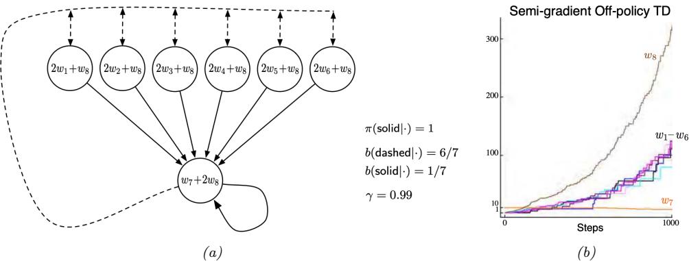
Figure 35.10: (a) A simple MDP. (b) Parameters of the policy diverge over time. From Figures 11.1 and 11.2 of [SB18]. Used with kind permission of Richard Sutton.

descent/ascent on the o!-policy data D to solve for an approximate saddle-point. This is the DualDICE method [Nac+19a], which is extended to GenDICE [Zha+20d].

Compared to the IS or DR approaches, Equation (35.58) does not compute the importance ratio of a trajectory, thus generally has a lower variance. Furthermore, it is behavior-agnostic, without having to estimate the behavior policy, or even to assume data consists of a collection of trajectories. Finally, this approach can be extended to be doubly robust (e.g., [UHJ20]), and to optimize a policy [Nac+19b] against the true policy value J(ϑ) (as opposed to approximations like Equation (35.50)). For more examples along this line of approach, see [ND20] and the references therein.

35.5.3 The deadly triad

Other than introducing bias, o!-policy data may also make a value-based RL method unstable and even divergent. Consider the simple MDP depicted in Figure 35.10a, due to [Bai95]. It has 7 states and 2 actions. Taking the dashed action takes the environment to the 6 upper states uniformly at random, while the solid action takes it to the bottom state. The reward is 0 in all transitions, and γ = 0.99. The value function V^w uses a linear parameterization indicated by the expressions shown inside the states, with ^{w → R8}. The target policies ^ϑ always chooses the solid action in every state. Clearly, the true value function, Vε(s)=0, can be exactly represented by setting w = 0.

Suppose we use a behavior policy b to generate a trajectory, which chooses the dashed and solid actions with probabilities 6/7 and 1/7, respectively, in every state. If we apply TD(0) on this trajectory, the parameters diverge to ↖ (Figure 35.10b), even though the problem appears simple! In contrast, with on-policy data (that is, when b is the same as ϑ), TD(0) with linear approximation can be guaranteed to converge to a good value function approximate [TR97].

The divergence behavior is demonstrated in many value-based bootstrapping methods, including TD, Q-learning, and related approximate dynamic programming algorithms, where the value function is represented either linearly (like the example above) or nonlinearly [Gor95; Ber19]. The root cause of these divergence phenomena is that bootstrapping methods typically are not minimizing a fixed objective function. Rather, they create a learning target using their own estimates, thus potentially creating a self-reinforcing loop to push the estimates to infinity. More formally, the problem is that the contraction property in the tabular case (Equation (34.87)) may no longer hold when V is approximated by Vw.

In general, an RL algorithm can become unstable when it has these three components: o!-policy learning, bootstrapping (for faster learning, compared to MC), and function approximation (for generalization in large scale MDPs). This combination is known as the deadly triad [SB18]. It highlights another important challenge introduced by o!-policy learning, and is a subject of ongoing research (e.g., [van+18; Kum+19a]).

A general way to ensure convergence in o!-policy learning is to construct an objective function function, the minimization of which leads to a good value function approximation; see [SB18, Ch. 11] for more background. A natural candidate is the discrepancy between the left and right hand sides of the Bellman optimality Equation (34.82), whose unique solution is V→. However, the “max” operator is not friendly to optimization. Instead, we may introduce an entropy term to smooth the greedy policy, resulting in a di!erential square loss in path consistency learning (PCL) [Nac+17]:

\[\min\_{V, \pi} \mathcal{L}^{\text{PCL}}(V, \pi) \triangleq \mathbb{E}\left[\frac{1}{2} \left(r + \gamma V(s') - \lambda \log \pi(a|s) - V(s)\right)^2\right] \tag{35.59}\]

where the expectation is over (s, a, r, s↗ ) tuples drawn from some o!-policy distribution (e.g., uniform over D). Minimizing this loss, however, does not result in the optimal value function and policy in general, due to an issue known as “double sampling” [SB18, Sec. 11.5].

This problem can be mitigated by introducing a dual function in the optimization [Dai+18]

\[\min\_{V, \pi} \max\_{\nu} \mathcal{L}^{\text{SEEDD}}(V, \pi; \nu) \triangleq \mathbb{E}\left[\nu(s, a) \big(r + \gamma V(s') - \lambda \log \pi(a|s) - V(s)\big)^2 - \nu(s, a)^2/2\right] \tag{35.60}\]

where 4 belongs to some function class (e.g., a DNN [Dai+18] or RKHS [FLL19]). It can be shown that optimizing Equation (35.60) forces 4 to model the Bellman error. So this approach is called smoothed Bellman error embedding, or SBEED. In both PCL and SBEED, the objective can be optimized by gradient-based methods on parameterized value functions and policies.

35.5.4 Some common o!-policy methods

Some common online but o!-policy RL methods include: Q-learning, which we discuss in Section 35.2.5; SAC (soft actor-critic), which we discuss in Section 35.6.1; DDPG (deep deterministic policy gradient) and related methods (such as TD3), which we discuss in Section 35.3.5; and MPO (MAP policy optimziation) [Abd+18a], which is a bound optimization method based on EM (c.f., the on-policy PPO method in Section 35.3.4).

35.6 Control as inference

In this section, we will discuss another approach to policy optimization, by reducing it to probabilistic inference. This is called control as inference, see e.g., [Att03; TS06; Tou09; BT12; KGO12; HR17; Lev18]. This approach allows one to incorporate domain knowledge in modeling, and apply powerful tools from approximate inference (see e.g., Chapter 7), in a consistent and flexible framework.

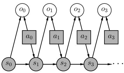
Figure 35.11: A graphical model for optimal control. States and actions are observed, while optimality variables are not. Adapted from Figure 1b of [Lev18].

35.6.1 Maximum entropy reinforcement learning

We now describe a graphical model that exemplifies such a reduction, which results in RL algorithms that are closely related to some discussed previously. The model allows a trade-o! between reward and entropy maximization, and recovers the standard RL setting when the entropy part vanishes in the trade-o!. Our discussion mostly follows the approach of [Lev18].

Figure 35.11 gives a probabilistic model, which not only captures state transitions as before, but also introduces a new variable, ot. This variable is binary, indicating whether the action at time t is optimal or not, and has the following probability distribution:

\[p(o\_t = 1 | s\_t, a\_t) = \exp(\lambda^{-1} R(s\_t, a\_t))\tag{35.61}\]

for some temperature parameter ◁ > 0 whose role will be clear soon. In the above, we have assumed without much loss of generality that R(s, a) < 0, so that Equation (35.61) gives a valid probability. Furthermore, we can assume a non-informative, uniform action prior, p(at|st), to simplify the exposition, for we can always push p(at|st) into Equation (35.61). Under these assumptions, the likelihood of observing a length-T trajectory ϑ , when optimality achieved in every step, is:

\[\begin{split} p(\boldsymbol{\tau}|\mathbf{o}\_{0:T-1} = \mathbf{1}) &\propto p(\boldsymbol{\tau}, \mathbf{o}\_{0:T-1} = \mathbf{1}) \propto p(s\_0) \prod\_{t=0}^{T-1} p(o\_t = 1|s\_t, a\_t) p(s\_{t+1}|s\_t, a\_t) \\ &= p(s\_0) \prod\_{t=0}^{T-1} p(s\_{t+1}|s\_t, a\_t) \exp\left(\frac{1}{\lambda} \sum\_{t=0}^{T-1} R(s\_t, a\_t)\right) \end{split} \tag{35.62}\]

The intuition of Equation (35.62) is clearest when the state transitions are deterministic. In this case, p(st+1|st, at) is either 1 or 0, depending on whether the transition is dynamically feasible or not. Hence, ^p(^{ϑ |}o0:^{T ↓1 = 1}) is either proportional to exp(◁↓¹ )^{T ↓1 t}=0 R(st, at)) if ϑ is feasible, or 0 otherwise. Maximizing reward is equivalent to inferring a trajectory with maximum p(ϑ |o0:^{T ↓1} = 1).

The optimal policy in this probabilistic model is given by

\[p(a\_t | s\_t, \mathbf{o}\_{t:T-1} = \mathbf{1}) = \frac{p(s\_t, a\_t | \mathbf{o}\_{t:T-1} = \mathbf{1})}{p(s\_t | \mathbf{o}\_{t:T-1} = \mathbf{1})} = \frac{p(\mathbf{o}\_{t:T-1} = \mathbf{1} | s\_t, a\_t) p(a\_t | s\_t) p(s\_t)}{p(\mathbf{o}\_{t:T-1} = \mathbf{1} | s\_t) p(s\_t)}\]

\[\propto \frac{p(\mathbf{o}\_{t:T-1} = \mathbf{1} | s\_t, a\_t)}{p(\mathbf{o}\_{t:T-1} = \mathbf{1} | s\_t)}\tag{35.63}\]

The two probabilities in Equation (35.63) can be computed as follows, starting with p(o^{T ↓1} = ¹|s^{T ↓1}, a^{T ↓1}) = exp(◁↓¹R(s^{T ↓1}, a^{T ↓1})),

\[p(\mathbf{o}\_{t:T-1} = \mathbf{1} | s\_t, a\_t) = \int\_{\mathcal{S}} p(\mathbf{o}\_{t+1:T-1} = \mathbf{1} | s\_{t+1}) p(s\_{t+1} | s\_t, a\_t) \exp(\lambda^{-1} R(s\_t, a\_t)) ds\_{t+1} \tag{35.64}\]

\[p(\mathbf{o}\_{t:T-1} = \mathbf{1}|s\_t) = \int\_{\mathcal{A}} p(\mathbf{o}\_{t:T-1} = \mathbf{1}|s\_t, a\_t) p(a\_t|s\_t) da\_t \tag{35.65}\]

The calculation above is expensive. In practice, we can approximate the optimal policy using a parametric form, ϑϑ(at|st). The resulted probability of trajectory ϑ now becomes

\[p\_{\theta}(\tau) = p(s\_1) \prod\_{t=0}^{T-1} p(s\_{t+1}|s\_t, a\_t) \pi\_{\theta}(a\_t|s\_t) \tag{35.66}\]

If we optimize ς so that DKL (pϑ(ϑ ) ↙ p(ϑ |o0:^{T ↓1} = 1)) is minimized, which can be simplified to

\[D\_{\rm KL}\left(p\_{\theta}(\tau) \parallel p(\tau | \mathbf{o}\_{0:T-1} = \mathbf{1})\right) = -\mathbb{E}\_{p\_{\theta}}\left[\sum\_{t=0}^{T-1} \lambda^{-1} R(s\_t, a\_t) + \mathbb{H}(\pi\_{\theta}(s\_t))\right] + \text{const} \tag{35.67}\]

where the constant term only depends on the uniform action prior p(at|st), but not ω. In other words, the objective is to maximize total reward, with an entropy regularization favoring more uniform policies. Thus this approach is called maximum entropy RL, or MERL. If ϑ^ω can represent all stochastic policies, a softmax version of the Bellman equation can be obtained for Equation (35.67):

\[Q\_\*(s\_t, a\_t) = \lambda^{-1} R(s\_t, a\_t) + \mathbb{E}\_{p(s\_{t+1}|s\_t, a\_t)} \left[ \log \int\_{\mathcal{A}} \exp(Q\_\*(s\_{t+1}, a\_{t+1})) da \right] \tag{35.68}\]

with the convention that Q→(s^T , a)=0 for all a, and the optimal policy has a softmax form: ϑ→(at|st) ↑ exp(Q→(st, at)). Note that the Q^→ above is di!erent from the usual optimal Q-function (Equation (34.83)), due to the introduction of the entropy term. However, as ◁ ⇐ 0, their di!erence vanishes, and the softmax policy becomes greedy, recovering the standard RL setting.

The soft actor-critic (SAC) algorithm [Haa+18a; Haa+18b] is an o!-policy actor-critic method whose objective function is equivalent to Equation (35.67) (by taking T to ↖):

\[J^{\rm SAC}(\boldsymbol{\theta}) \stackrel{\scriptstyle \Delta}{=} \mathbb{E}\_{p\_{\pi\_{\boldsymbol{\theta}}}^{\infty}(s)\pi\_{\boldsymbol{\theta}}(a|s)} \left[ R(s,a) + \lambda \, \mathbb{H}(\pi\_{\boldsymbol{\theta}}(s)) \right] \tag{35.69}\]

Note that the entropy term has also the added benefit of encouraging exploration.

To compute the optimal policy, similar to other actor-critic algorithms, we will work with the “soft” state- and action-function approximations, parameterized by w and u, respectively:

\[Q\_{\mathbf{w}}(s,a) = R(s,a) + \gamma \mathbb{E}\_{p(s'|s,a)} \left[ V\_{\mathbf{u}}(s',a') - \lambda \log \pi\_{\theta}(a'|s') \right] \tag{35.70}\]

\[V\_{\mathbf{u}}(s, a) = \lambda \log \sum\_{a} \exp(\lambda^{-1} Q\_{\mathbf{w}}(s, a)) \tag{35.71}\]

This induces an improved policy (with entropy regularization): ^ϑw(a|s) = exp(◁↓¹Qw(s, a))/Zw(s), where Zw(s) = ) ^a exp(◁↓¹Qw(s, a)) is the normalization constant. We then perform a soft policy improvement step to update ω by minimizing E [DKL (ϑω(s) ↙ ϑw(s))] where the expectation may be approximated by sampling s from a replay bu!er D.

In [Haa+18b; Haa+18a], they show that the SAC method outperforms the o!-policy DDPG algorithm (Section 35.3.5) and the on-policy PPO algorithm (Section 35.3.4) by a wide margin on various continuous control tasks. For more details, see [Haa+18b].

There is a variant of soft actor-critic, which only requires to model the action-value function. It is based on the observation that both the policy and soft value function can be induced by the soft action-value function as follows:

\[V\_{\mathbf{w}}(s) = \lambda \log \sum\_{a} \exp \left( \lambda^{-1} Q\_{\mathbf{w}}(s, a) \right) \tag{35.72}\]

\[\pi\_{\mathbf{w}}(a|s) = \exp\left(\lambda^{-1}(Q\_{\mathbf{w}}(s,a) - V\_{\mathbf{w}}(s))\right) \tag{35.73}\]

We then only need to learn w, using approaches similar to DQN (Section 35.2.6). The resulting algorithm, soft Q-learning [SAC17], is convenient if the number of actions is small (when A is discrete), or if the integral in obtaining V^w from Q^w is easy to compute (when A is continuous).

It is interesting to see that algorithms derived in the maximum entropy RL framework bears a resemblance to PCL and SBEED in Section 35.5.3, both of which were to minimize an objective function resulting from the entropy-smoothed Bellman equation.

35.6.2 Other approaches

VIREL is an alternative model to maximum entropy RL [Fel+19]. Similar to soft actor-critic, it uses an approximate action-value function, Qw, a stochastic policy, ϑω, and a binary optimality random variable o^t at time t. A di!erent probability model for o^t is used

\[p(o\_t = 1 | s\_t, a\_t) = \exp\left(\frac{Q\_{\mathbf{w}}(s\_t, a\_t) - \max\_a Q\_{\mathbf{w}}(s\_t, a)}{\lambda\_{\mathbf{w}}}\right) \tag{35.74}\]

The temperature parameter ◁^w is also part of the parameterization, and can be updated from data.

An EM method can be used to maximize the objective

\[\mathcal{L}(\boldsymbol{w}, \boldsymbol{\theta}) = \mathbb{E}\_{p(\boldsymbol{s})} \left[ \mathbb{E}\_{\pi\_{\boldsymbol{\theta}}(\boldsymbol{a}|\boldsymbol{s})} \left[ \frac{Q\_{\mathbf{w}}(\boldsymbol{s}, \boldsymbol{a})}{\lambda\_{\mathbf{w}}} \right] + \mathbb{H}(\pi\_{\boldsymbol{\theta}}(\boldsymbol{s})) \right] \tag{35.75}\]

for some distribution p that can be conveniently sampled from (e.g., in a replay bu!er). The algorithm may be interpreted as an instance of actor-critic. In the E-step, the critic parameter w is fixed, and the actor parameter ω is updated using gradient ascent with stepsize ▷^ω (for policy improvement):

\[ \theta \gets \theta + \eta\_{\theta} \nabla\_{\theta} \mathcal{L}(w, \theta) \tag{35.76} \]

In the M-step, the actor parameter is fixed, and the critic parameter is updated (for policy evaluation):

\[\mathbf{w} \leftarrow \mathbf{w} + \eta\_{\mathbf{w}} \nabla\_{\mathbf{w}} \mathcal{L}(\mathbf{w}, \boldsymbol{\theta}) \tag{35.77}\]

Finally, there are other possibilities of reducing optimal control to probabilistic inference, in addition to MERL and VIREL. For example, we may aim to maximize the expectation of the trajectory return G, by optimizing the policy parameter ω:

\[J(\pi\_{\theta}) = \int G(\tau)p(\tau|\theta)d\tau\tag{35.78}\]

It can be interpreted as a pseudo-likelihood function, when the G(ϑ ) is treated as probability density, and solved (approximately) by a range of algorithms (see e.g., [PS07; Neu11; Abd+18b]). Interestingly, some of these methods have a similar objective as MERL (Equation (35.67)), although the distribution involving ω appears in the second argument of DKL. As discussed in Section 2.7.1, this forwards KL-divergence is mode-covering, which in the context of RL is argued to be less preferred than the mode-seeking, reverse KL-divergence used by MERL. For more details and references, see [Lev18].

Control as inference is also closely related to active inference; this is based on the free energy principle which is popular in neuroscience (see e.g., [Fri09; Buc+17; SKM18; Ger19; Maz+22]). The FEP is equivalent to using variational inference (see Section 10.1) to perform state estimation (perception) and parameter estimation (learning). In particular, consider a latent variable model with hidden states s, observations y, and parameters ω. Following Section 10.1.1.1, we define the variational free energy to be Fp, q = DKL (q(s, ω|y) ↙ p(s, ω|y)) ↓ log p(y). State estimation corresponds to solving minq(s|y,ω) F(y), and parameter estimation corresponds to solving minq(ω|y) F(y), just as in variational Bayes EM (Section 10.3.5).

If p(s, y|ω) is a nonlinear hierarchical Gaussian model, and q(s|y, ω) is a Gaussian mean field approximation — where q(s|y, ω) = N (s|sˆ, H) is a Laplace approximation, with the mode sˆ, being computed using gradient descent, and H being the Hessian at the mode — then we recover the method known as predictive coding (see e.g., [RB99; Fri03; Spr17; HM20; MSB21; Mar21; OK22; Sal+23]). This can be considered a non-amortized version of a VAE (Section 21.2), where inference (E step) is done with iterated gradient descent, and parameter estimation (M step) is also done with gradient descent. (A more e”cient incremental EM version of predictive coding, which updates {sˆⁿ : n =1: N} and ω in parallel, was recently presented in [Sal+24].) For more details on predictive coding, see Supplementary Section 8.1.4.)

To extend the above method to decision making problems we define the expected free energy as F(a) = Eq(y|a) [F(y)], where q(y|a) is the posterior predictive distribution over observations given actions sequence a. We then define the policy to be ϑ(a) = softmax(F(a)). To guide the agent towards preferred outcomes, we define the prior over states as ^p(s) ^{↑ eR}(s) , where R is the reward function. Alternatively, we can define the prior over observations as ^p(y) ^{↑ eR}(y) . Either way, the generative model is defined in terms of what the agent wants to achieve, rather than being an “objective” model of reality. The advantage of this approach is that it automatically induces goal-directed information-seeking behavior, rather than than the maxent approach which models uncertainty in a goal-independent way. Despite this di!erence, the technique of active inference is very similar to control as inference, as explained in [Mil+20; WIP20; LÖW21].

35.6.3 Imitation learning

In previous sections, an RL agent is to learn an optimal sequential decision making policy so that the total reward is maximized. Imitation learning (IL), also known as apprenticeship learning and learning from demonstration (LfD), is a di!erent setting, in which the agent does not observe rewards, but has access to a collection Dexp of trajectories generated by an expert policy ϑexp; that is, ϑ = (s0, a0, s1, a1,…,s^T ) and a^t ↘ ϑexp(st) for ϑ → Dexp. The goal is to learn a good policy by imitating the expert, in the absence of reward signals. IL finds many applications in scenarios where we have demonstrations of experts (often humans) but designing a good reward function is not easy, such as car driving and conversational systems. See [Osa+18] for a survey up to 2018.

35.6.3.1 Imitation learning by behavior cloning

A natural method is behavior cloning, which reduces IL to supervised learning; see [Pom89] for an early application to autonomous driving. It interprets a policy as a classifier that maps states (inputs) to actions (labels), and finds a policy by minimizing the imitation error, such as

\[\min\_{\pi} \mathbb{E}\_{p\_{\pi\_{\text{exp}}}^{\infty}(s)} \left[ D\_{\text{KL}} \left( \pi\_{\text{exp}}(s) \parallel \pi(s) \right) \right] \tag{35.79}\]

where the expectation wrt p^{↔︎ ε}exp may be approximated by averaging over states in Dexp. A challenge with this method is that the loss does not consider the sequential nature of IL: future state distribution is not fixed but instead depends on earlier actions. Therefore, if we learn a policy ϑˆ that has a low imitation error under distribution p^{↔︎ ε}exp , as defined in Equation (35.79), it may still incur a large error under distribution p^{↔︎ εˆ} (when the policy ϑˆ is actually run). Further expert demonstrations or algorithmic augmentations are often needed to handle the distribution mismatch (see e.g., [DLM09; RGB11]).

35.6.3.2 Imitation learning by inverse reinforcement learning

An e!ective approach to IL is inverse reinforcement learning (IRL) or inverse optimal control (IOC). Here, we first infer a reward function that “explains” the observed expert trajectories, and then compute a (near-)optimal policy against this learned reward using any standard RL algorithms studied in earlier sections. The key step of reward learning (from expert trajectories) is the opposite of standard RL, thus called inverse RL [NR00a].

It is clear that there are infinitely many reward functions for which the expert policy is optimal, for example by several optimality-preserving transformations [NHR99]. To address this challenge, we can follow the maximum entropy principle (Section 2.4.7), and use an energy-based probability model to capture how expert trajectories are generated [Zie+08]:

\[p(\mathbf{r}) \propto \exp\left(\sum\_{t=0}^{T-1} R\_{\theta}(s\_t, a\_t)\right) \tag{35.80}\]

where R^ω is an unknown reward function with parameter ω. Abusing notation slightly, we denote by Rω(ϑ ) = )^{T ↓1 t}=0 Rω(st, at)) the cumulative reward along the trajectory ϑ . This model assigns exponentially small probabilities to trajectories with lower cumulative rewards. The partition function, Z^ω ↭ ^ε exp(Rω(ϑ )), is in general intractable to compute, and must be approximated. Here, we can

take a sample-based approach. Let Dexp and D be the sets of trajectories generated by an expert, and by some known distribution q, respectively. We may infer ω by maximizing the likelihood, p(Dexp|ω), or equivalently, minimizing the negative log-likelihood loss

\[\mathcal{L}(\boldsymbol{\theta}) = -\frac{1}{|\mathcal{D}\_{\text{exp}}|} \sum\_{\boldsymbol{\tau} \in \mathcal{D}\_{\text{exp}}} R\_{\boldsymbol{\theta}}(\boldsymbol{\tau}) + \log \frac{1}{|\mathcal{D}|} \sum\_{\boldsymbol{\tau} \in \mathcal{D}} \frac{\exp(R\_{\boldsymbol{\theta}}(\boldsymbol{\tau}))}{q(\boldsymbol{\tau})} \tag{35.81}\]

The term inside the log of the loss is an importance sampling estimate of Z that is unbiased as long as q(ϑ ) > 0 for all ϑ . However, in order to reduce the variance, we can choose q adaptively as ω is being updated. The optimal sampling distribution (Section 11.5), q→(ϑ ) ↑ exp(Rω(ϑ )), is hard to obtain. Instead, we may find a policy ϑˆ which induces a distribution that is close to q→, for instance, using methods of maximum entropy RL discussed in Section 35.6.1. Interestingly, the process above produces the inferred reward R^ω as well as an approximate optimal policy ϑˆ. This approach is used by guided cost learning [FLA16], and found e!ective in robotics applications.

35.6.3.3 Imitation learning by divergence minimization

We now discuss a di!erent, but related, approach to IL. Recall that the reward function depends only on the state and action in an MDP. It implies that if we can find a policy ϑ, so that p^{↔︎ ε} (s, a) and p^{↔︎ ε}exp (s, a) are close, then ϑ receives similar long-term reward as ϑexp, and is a good imitation of ϑexp in this regard. A number of IL algorithms find ϑ by minimizing the divergence between p^{↔︎ ε} and p^{↔︎ ε}exp . We will largely follow the exposition of [GZG19]; see [Ke+19b] for a similar derivation.

Let f be a convex function, and D^f the f-divergence (Section 2.7.1). From the above intuition, we want to minimize D^f $ p^↔︎ εexp D D Dp^↔︎ ε % . Then, using a variational approximation of D^f [NWJ10a], we can solve the following optimization problem for ϑ:

\[\min\_{\pi} \max\_{\mathbf{w}} \mathbb{E}\_{p\_{\pi\_{\text{exp}}}^{\infty}(s,a)} \left[ T\_{\mathbf{w}}(s,a) \right] - \mathbb{E}\_{p\_{\pi}^{\infty}(s,a)} \left[ f^\*(T\_{\mathbf{w}}(s,a)) \right] \tag{35.82}\]

where T^w : S ⇒ A ⇐ R is a function parameterizd by w. The first expectation can be estimated using Dexp, as in behavior cloning, and the second can be estimated using trajectories generated by policy ϑ. Furthermore, to implement this algorithm, we often use a parametric policy representation ϑω, and then perform stochastic gradient updates to find a saddle-point to Equation (35.82).

With di!erent choices of the convex function f, we can obtain many existing IL algorithms, such as generative adversarial imitation learning (GAIL) [HE16b] and adversarial inverse RL (AIRL) [FLL18], as well as new algorithms like f-divergence max-ent IRL (f-MAX) and forward adversarial inverse RL (FAIRL) [GZG19; Ke+19b].

Finally, the algorithms above typically require running the learned policy ϑ to approximate the second expectation in Equation (35.82). In risk- or cost-sensitive scenarios, collecting more data is not always possible, Instead, we are in the o!-policy IL setting, working with trajectories collected by some policy other than ϑ. Hence, we need to correct the mismatch between p^{↔︎ ε} and the o!-policy trajectory distribution, for which techniques from Section 35.5 can be used. An example is ValueDICE [KNT20], which uses a similar distribution correction method of DualDICE (Section 35.5.2).

36 Causality

This chapter is written by Victor Veitch and Alex D’Amour.

36.1 Introduction

The bulk of machine learning considers relationships between observed variables with the goal of summarizing these relationships in a manner that allows predictions on similar data. However, for many problems, our main interest is to predict how system would change if it were observed under di!erent conditions. For instance, in healthcare, we are interested in whether a patient will recover if given a certain treatment (as opposed to whether treatment and recovery are associated in the observed data). Causal inference addresses how to formalize such problems, determine whether they can be solved, and, if so, how to solve them. This chapter covers the fundamentals of this subject. Code examples for the discussed methods are available at https://github.com/vveitch/ causality-tutorials. For more information on the connections between ML and causal inference, see e.g., [Kad+22; Xia+21a].

To make the gap between observed data modeling and causal inference concrete, consider the relationships depicted in Figure 36.1a and Figure 36.1b. Figure 36.1a shows the relationship between deaths by drowning and ice cream production in the United States in 1931 (the pattern holds across most years). Figure 36.1b shows the relationship between smoking and lung cancer across various countries. In each case, there is a strong positive association. Faced with this association, we might ask: could we reduce drowning deaths by banning ice cream? Could we reduce lung cancer by banning cigarettes? We intuitively understand that these interventional questions have di!erent answers, despite the fact that the observed associations are similar. Determining the causal e!ect of some intervention in the world requires some such causal hypothesis about the world.

For concreteness, consider three possible explanations for the association between ice cream and drowning. Perhaps eating ice cream does cause people to drown — due to stomach cramps or similar. Or, perhaps, drownings increase demand for ice cream — the survivors eat huge quantities of ice cream to handle their grief. Or, the association may be due (at least in part) to a common cause: warm weather makes people more likely to eat ice cream and more likely to go swimming (and, hence, to drown). Under all three scenarios, we can observe exactly the same data, but the implications for an ice cream ban are very di!erent. Hence, answering questions about what will happen under an intervention requires us to incorporate some causal knowledge of the world — e.g., which of these scenarios is plausible?

Our goal in this chapter to introduce the essentials of estimating causal e!ects. The high-level

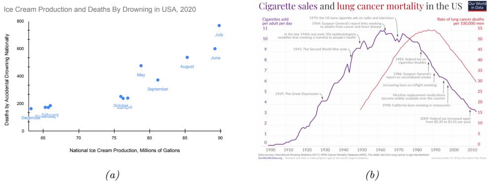
Figure 36.1: Correlation is not causation. (a) Ice cream production is strongly associated with deaths by drowning. Ice cream production data from the US Department of Agriculture National Agricultural Statistics Service. Drowning data from the National Center for Health Statistics at the United States Centers for Disease Control. (b) Smoking is strongly associated with lung cancer. From ourworldindata. org/ smoking-big-problem-in-brief . Used with kind permission of Max Roser.

approach has three steps.

• Causal estimands: The first step is to formally define the quantities we want to estimate. These are summaries of how the world would change under intervention, rather than summaries of the world as it has already been observed. E.g., we want to formalize “The expected number of drownings in the United States if we ban ice cream”.
• Identification: The next step is to identify the causal estimands with quantities that can, in principle, be estimated from observational data. This step involves codifying our causal knowledge of the world and translating this into a statement such as, “The causal e!ect is equal to the expected number of drownings after adjusting for month”. This step tells us what causal questions we could answer with perfect knowledge of the observed data distribution.
• Estimation: Finally, we must estimate the observable quantity using a finite data sample. The form of causal estimands favors certain e”cient estimation procedures that allow us to exploit non-parametric (e.g., machine learning) predictive models.

In this chapter, we’ll mainly focus on the estimation of the causal e!ect of an intervention averaged over all members of a population, known as the average treatment e!ect or ATE. This is the most common problem in applied causal inference work. It is in some sense the simplest problem, and will allow us to concretely explain the use and importance of the fundamental causal concepts. These causal concepts include structural causal models, causal graphical models, the do-calculus, and e”cient estimation using influence function techniques. This problem is also useful for understanding the role that standard predictive modeling and machine learning play in estimating causal quantities.

36.2 Causal formalism

In causal inference, the goal is to use data to learn about how the outcome in the world would change under intervention. In order to make such inferences, we must also make use of our causal knowledge of the world. This requires a formalism that lets us make the notion of intervention precise and lets us encode our causal knowledge as assumptions.

36.2.1 Structural causal models

Consider a setting in which we observe four variables from a population of people: Ai, an indicator of whether or not person i smoked at a particular age, Yi, an indicator of whether or not person i developed lung cancer at a later age, Hi, a “health consciousness” index that measures a person’s health-consciousness (perhaps constructed from a set of survey responses about attitudes towards health), and Gi, an indicator for whether the person has a genetic predisposition towards cancer. Suppose we observe a dataset of these variables drawn independently and identically from a population, (Ai, Yi, Hi) iid ↘ ^Pobs, where “obs” stands for “observed”.

In standard practice, we model data like these using probabilistic models. Notably, there are many di!erent ways to specify a probabilistic model for the same observed distribution. For example, we could write a probabilistic model for Pobs as

\[A \sim P^{\text{obs}}(A) \tag{36.1}\]

\[H|A \sim P^{\text{obs}}(H|A) \tag{36.2}\]

\[Y|A,H \sim P^{\text{obs}}(Y|H,A) \tag{36.3}\]

\[G|A,H,Y\rangle \sim P^{\text{obs}}(G|A,H,Y) \tag{36.4}\]

This is a valid factorization, and sampling variables in this order would yield valid samples from the joint distribution Pobs. However, this factorization does not map well to a mechanistic understanding of how these variables are causally related in the world. In particular, it is perhaps more plausible that health-consciousness H causally precedes smoking status A, since a person’s health-consciousness would influence their decision to smoke.

These intuitions about causal ordering are intimately tied to the notion of intervention. Here, we will focus on a notion of intervention that can be represented in terms of “structural” models that describe mechanistic relationships between variables. The fundamental objects that we will reason about are structural causal models, or SCM’s. SCM’s resemble probabilistic models, but they encode additional assumptions (see also Section 4.7). Specifically, SCM’s serve two purposes: they describe a probabilistic model and they provide semantics for transforming the data-generating process through intervention.

Formally, SCM’s describe a mechanistic data generating process with an ordered sequence of equations that resemble assignment operations in a program. Each variable in a system is determined by combining other modeled variables (the causes) with exogenous “noise” according to some (unknown) deterministic function. For instance, a plausible SCM for Pobs might be

\[G \leftarrow f\_{\mathcal{G}}(\xi\_0) \tag{36.5}\]

\[H \leftarrow f\_H(\xi\_1) \tag{36.6}\]

\[A \leftarrow f\_A(H, \xi\_2) \tag{36.7}\]

\[Y \gets f\_Y(G, H, A, \xi\_3) \tag{36.8}\]

where the (unknown) functions f are fixed, and the variables 5 are unmeasured causes, modeled as independent random “noise” variables. Conceptually, the functions fG, fH, fA, f^Y describe deterministic physical relationships in the real world, while the variables 5 are hidden causes that are su”cient to distinguish each unit i in the population. Because we assume that each observed unit i is drawn at random from the population, we model 5 as random noise.

SCM’s imply probabilistic models, but not the other way around. For example, our example SCM implies probabilistic model for the observed data based on the factorization Pobs(G, H, A, Y ) = ^Pobs(G)Pobs(H)Pobs(^{A | H})Pobs(^{Y |} A, H). Thus, we could sample from the SCM in the same way we would from a probabilistic model: draw a set of noise variables 5 and evaluate each assignment operation in the SCM in order.

Beyond the probabilistic model, an SCM encodes additional assumptions about the e!ects of interventions. This can be formalized using the do-calculus (as in the verb “to do”), which we describe in Section 36.8; But in brief, interventions are represented by replacing assignment statements. For example, if we were interested in the distribution of Y in the hypothetical scenario that smoking were eliminated, we could set the second line of the SCM to be A △ 0. We would denote this by P(Y |do(A = 0), H). Because the f functions in the SCM are assumed to be invariant mechanistic relationships, the SCM encodes the assumption that this edited SCM generates data that we would see if we really applied this intervention in the world. Thus, the ordering of statements in an SCM are load-bearing: they imply substantive assumptions about how the world changes in response to interventions. This is in contrast to more standard probabilistic models where variables can be rearranged by applications of Bayes’ Rule without changing the substantive implications of the model. (See also Section 4.7.3.)

We note that structural causal model may not incorporate all possible notions of causality. For example, laws based on conserved quantities or equilibria — e.g., the ideal gas law — do not trivially map to SCMs, though these are fundamental in disciplines such as physics and economics. Nonetheless, we will confine our discussion to SCMs.

36.2.2 Causal DAGs

SCM’s encode many details about the assumed generative process of a system, but often it is useful to reason about causal problems at a higher level of abstraction. In particular, it is often useful to separate the causal structure of a problem from the particular functional form of those causal relationships. Causal graphs provide this level of abstraction. A causal graph specifies which variables causally a!ect other variables, but leaves the parametric form of the structural equations f unspecified. Given an SCM, the corresponding causal graph can be drawn as follows: for each line of the SCM, draw arrows from the variables on the right hand side to variables on the left hand side. The causal DAG for our smoking-cancer example is shown in Figure 36.2. In this way, causal DAGs are related to SCMs in the same way that probabilistic graphical models (PGMs) are related

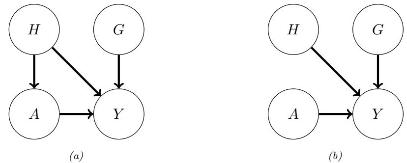
Figure 36.2: (a) Causal graph illustrating relationships between smoking A, cancer Y , health conciousness H, and genetic cancer pre-disposition G. (b) “Mutilated” causal graph illustrating relationships under an intervention on smoking A.

to probabilistic models.

In fact, in the same way that SCMs imply a probabilistic model, causal DAGs imply a PGM. Functionally, causal graphs behave as probabilistic graphical models (Chapter 4). They imply conditional independence relationships between the variables in the observed data in same way. They obey the Markov property: If X △ Y ⇐ Z then X ¬¬ Z|Y ; recall d-separation (Section 4.2.4.1). Additionally, if X ⇐ Y △ Z then, usually, X ↔︎¬¬ Z|Y (even if X and Z are marginally independent). In this case, Y is called a collider for X and Z.

Conceptually, the di!erence between causal DAGs and PGMs is that probabilistic graphical models encode our assumptions about statistical relationships, whereas causal graphs encode our (stronger) assumptions about causal relationships. Such causal relationships can be used to derive how statistical relationships would change under intervention.

Causal graphs also allow us to reason about the causal and non-causal origins of statistical dependencies in observed data without specifying a full SCM. In a causal graph, two variables — say, A and D — can be statistically associated in di!erent ways. First, there can be a directed path from (ancestor) A to (descendant) D. In this case, A is a causal ancestor of D and interventions on A will propagate through to change D; P(D|do(A = a)) ↔︎= P(D|do(A = a↗ )). For example, smoking is a causal ancestor of cancer in our example. Alternatively, A and D could share a common cause — there is some variable C such that there is a directed path from C to A and from C to D. If A and D are associated only through such a path then interventions on A will not change the distribution of D. However, it is still the case that P(D|A = a) ↔︎= P(D|A = a↗ ) — observing di!erent values of A changes our guess for the value of D. The reason is that A carries information about C, which carries information about D. For example, suppose we lived in a world where there was no e!ect of smoking on developing cancer (e.g., everybody vapes), there would nevertheless be an association between smoking and cancer because of the path A △ H ⇐ Y . The existence of such “backdoor paths” is one core reason that statistical and causal association are not the same. Of course, more complicated variants of these associations are possible — e.g., C is itself only associated with A through a backdoor path — but this already captures the key distinction between causal and non-causal paths.

Recall that our aim in introducing SCMs and causal graphs is to enable us to formalize our causal

knowledge of the world and to make precise what interventional quantities we’d like to estimate. Writing down a causal graph gives a simple formal way to encode our knowledge of the causal structure of a problem. Usefully, this causal structure is su”cient to directly reason about the implications of interventions without fully specifying the underlying SCM. The key observation is that if a variable A is intervened on then, after intervention, none of the other variables are causes of A. That is, when we replace a line of an SCM with a statement directly assigning a variable a particular value, we cut o! all dependencies that variable had on its causal parents. Accordingly, in the causal graph, the intervened on variable has no parents. This leads us to the graph surgery notion of intervention: an intervention that sets A to a is the operation that deletes all incoming edges to A in the graph, and then conditions on A = a in the resulting probability distribution (which is defined by the conditional independence structure of the post-surgery graph). We’ll use Pearl’s do notation to denote this operation. P(X|do(A = a)) is the distribution of X given A = a under the mutilated graph that results from deleting all edges going into A. Similarly, E[X|do(A = a)] ↭ EP(X|do(A=a))[X]. Thus, we can formalize statements such as “the average e!ect of receiving drug A” as

\[\text{ATE} = E[Y|\text{do}(A=1)] - \mathbb{E}[Y|\text{do}(A=0)],\tag{36.9}\]

where ATE stands for average treatment e!ect.

For concreteness, consider our running example. We contrast the distribution that results by conditioning on A with the distribution that results from intervening on A:

\[\mathbf{P}(Y, H, G | A = a) = \mathbf{P}(Y | H, G, A = a)\mathbf{P}(G)\mathbf{P}(H | A = a) \tag{36.10}\]

\[\mathbf{P}(Y, H, G | \text{do}(A = a)) = \mathbf{P}(Y | H, G, A = a)\mathbf{P}(G)\mathbf{P}(H) \tag{36.11}\]

The key di!erence between these two distributions is that the standard conditional distribution describes a population where health consciousness H has the distribution that we observe among individuals with smoking status A = a, while the interventional distribution described a population where health consciousness H follows the marginal distribution among all individuals. For example, we would expect P(H | A = smoker) to put more mass on lower values of H than the marginal health consciousness distribution P(H), which would also include non-smokers. The intervention distribution thus incorporates a hypothesis of how smoking would a!ect the subpopulation of individuals who tend to be too health conscious to smoke in the observed data.

36.2.3 Identification

A central challenge in causal inference is that many di!erent SCM’s can produce identical distributions of observed data. This means that, on the basis of observed data alone, we cannot uniquely identify the SCM that generated it. This is true no matter how large of a data sample is available to us.

For example, consider the setting where there is a treatment A that may or may not have an e!ect on outcome Y , and where both the treatment and outcome are known to be a!ected by some unobserved common binary cause U. Now, we might be interested in the causal estimand E[Y |do(A = 1)]. In general, we can’t learn this quantity from the observed data. The problem is that, we can’t tell apart the case where the treatment has a strong e!ect from the case where the treatment has no e!ect, but U = 1 both causes people to tend to be treated and increases the probability of a positive outcome. The same observation shows we can’t learn the (more complicated) interventional distribution P(Y |do(A = 1)) (if we could learn this, then we’d get the average e!ect automatically).

Thus, an important part of causal inference is to augment the observed data with knowledge about the underlying causal structure of the process under consideration. Often, these assumptions can narrow the space of SCM’s su”ciently so that there is only one value of the causal estimand that is compatible with the observed data. We say that the causal estimand is identified or identifiable under a given set of assumptions if those assumptions are su”cient to provide a unique answer. There are many di!erent sets of su”cient conditions that yield identifiable causal e!ects; we call each set of su”cient conditions an identification strategy.

Given a set of assumptions about the underlying SCM, the most common way to show that a causal estimand is identified is by construction. Specifically, if the causal estimand can be written entirely in terms of observable probability distributions, then it is identifed. We call such a function of observed distributions a statistical estimand. Once such a statistical estimand has been recovered, we can then construct and analyze an estimator for that quantity using standard statistical tools. As an example of a statistical estimand, in the SCM above, it can be shown the ATE as defined in Equation (36.9), is equal to the following statistical estimand

\[\text{ATE } \stackrel{\text{(\*)}}{=} \tau^{\text{ATE }} \stackrel{\text{\\_ATE }}{=} \mathbb{E}[\mathbb{E}[Y|H, A=1] - \mathbb{E}[Y|H, A=0]],\tag{36.12}\]

where the equality (∅) only holds because of some specific properties of the SCM. Note that the RHS above only involves conditional expectations between observed variables (there are no do operators), so ↼ ATE is only a function of observable probability distributions.

There are many kinds of assumptions we might make about the SCM governing the process under consideration. For example, the following are assertions we might make about the system in our running example:

• 1. The probability of developing cancer is additive on the logit scale in A, G, and H (i.e., logistic regression is a well-specified model).
• 2. For each individual, smoking can never decrease the probability of developing cancer.
• 3. Whether someone smokes is influenced by their health consciousness H, but not by their genetic predisposition to cancer G.

These assumptions range from strong parametric assumptions fully specifying the form of the SCM equations, to non-parametric assumptions that only specify what the inputs to each equation are, leaving the form fully unspecified. Typically, assumptions that fully specify the parametric form are very strong, and would require far more detailed knowledge of the system under consideration than we actually have. The goal in identification arguments is to find a set of assumptions that are weak enough that they might be plausibly true for the system under consideration, but which are also strong enough to allow for identification of the causal e!ect.

If we are not willing to make any assumptions about the functional form of the SCM, then our assumptions are just about which variables a!ect (and do not a!ect) the other variables. In this sense, such which-a!ects-which assumptions are minimal. These assumptions are exactly the assumptions captured by writing down a (possibly incomplete) causal DAG, showing which variables are parents of each other variable. The graph may be incomplete because we may not know whether each possible edge is present in the physical system. For example, we might be unsure whether the gene G actually has a causal e!ect on health consciousness H. It is natural to ask to what extent we can identify

causal e!ects only on the basis of partially specified causal DAGs. It turns out much progress can be made based on such non-parametric assumptions; we discuss this in detail in Section 36.8.

We will also discuss certain assumptions that cannot be encoded in a causal graph, but that are still weaker than assuming that full functional forms are known. For example, we might assume that the outcome is a!ected additively by the treatment and any confounders, with no interaction terms between them. These weaker assumptions can enable causal identification even when assuming the causal graph alone does not.

It is worth emphasizing that every causal identification strategy relies on assumptions that have some content that cannot be validated in the observed data. This follows directly from the ill-posedness of causal problems: if the assumptions used to identify causal quantities could be validated, that would imply that the causal estimand was identifiable from the observed data alone. However, since we know that there are many values of the causal estimand that are compatible with observed data, it follows that the assumptions in our identification strategy must have unobservable implications.

36.2.4 Counterfactuals and the causal hierarchy

Structural causal models let us formalize and study a hierarchy of di!erent kinds of query about the system under consideration. The most familiar is observational queries: questions that are purely about statistical associations (e.g., “Are smoking and lung cancer associated in the population this sample was drawn from?”). Next is interventional queries: questions about causal relationships at the population level (e.g., “How much does smoking increase the probability of cancer in a given population?”). The rest of this chapter is focused on the defintion, identification, and estimation of interventional queries. Finally, there are counterfactual queries: questions about causal relationships at the level of specific individuals, had something been di!erent (e.g., “Would Alice have developed cancer had she not smoked?”). This causal hierarchy was popularized by [Pea09a, Ch. 1].

Interventional queries concern the prospective e!ect of an intervention on an outcome; for example, if we intervene and prevent a randomly sampled individual from smoking, what is the probability they develop lung cancer? Ultimately, the probability statement here is about our uncertainity about the “noise” variables 5 in the SCM. These are the unmeasured factors specific to the randomly selected individual. The distribution is determined by the population from which that individual is sampled. Thus, interventional queries are statements about populations. Interventional queries can be written in terms of conditional distributions using do-notation, e.g., P(Y |do(A = 0)). In our example, this represents the distribution of lung cancer outcomes for an individual selected at random and prevented from smoking.

Counterfactual queries concern how an observed outcome might have been di!erent had an intervention been applied in the past. Counterfactual queries are often framed in terms of attributing a given outcome to a particular cause. For example, would Alice have developed cancer had she not smoked? Did most smokers with lung cancer develop cancer because they smoked? Counterfactual queries are so called because they require a comparison of counterfactual outcomes within individuals. In the formalism of SCM’s, counterfactual outcomes for an individual i are generated by running the same values of 5ⁱ through di!erently intervened SCMs. Counterfactual outcomes are often written in terms of potential outcomes notation. In our running smoking example, this would look like:

\[Y\_i(a) \triangleq f\_Y(G\_i, H\_i, a, \xi\_{3,i}).\tag{36.13}\]

That is, Yi(a) is the outcome we would have seen had A been set to a while all of Gi, Hi, 53,i were kept fixed.

It is important to understand what distinguishes interventional and fundamentally counterfactual queries. Just because a query can be written in terms of potential outcomes does not make it a counterfactual query. For example, the average treatment e!ect, which is the canonical interventional query, is easy to write in potential outcomes notation:

\[\text{ATE} = \mathbb{E}[Y\_i(1) - Y\_i(0)]. \tag{36.14}\]

Instead, the key dividing line between counterfactual and interventional queries is whether the query requires knowing the joint distribution of potential outcomes within individuals, or whether marginal distributions of potential outcomes across individuals will su”ce. An important signature of a counterfactual query is conditioning on the value of one potential outcome. For example, “the lung cancer rate among smokers who developed cancer, had they not smoked” is a counterfactual query, and can be written as:

\[\mathbb{E}[Y\_i(0) \mid Y\_i(1) = 1, A\_i = 1] \tag{36.15}\]

Answering this query requires knowing how individual-level cancer outcomes are related (through 53,i) across the worlds where the each individual i did and did not smoke. Notably, this query cannot be rewritten using do-notation, because it requires a distinction between Y (0) and Y (1) while the ATE can: E[Y | do(A = 1)] ↓ E[Y | do(A = 0)].

Counterfactual queries require categorically more assumptions for identification than interventional ones. For identifying interventional queries, knowing the DAG structure of an SCM is often su”cient, while for counterfactual queries, some assumptions about the functional forms in the SCM are necessary. This is because only one potential outcome is ever observed for each individual, so the dependence between potential outcomes within individuals is not observable. For example, the data in our running example provide no information on how individual-level smoking and non-smoking cancer risk are related. Thus, answering a question like “Did smokers who developed cancer have lower non-smoking cancer risk than smokers who did not develop cancer?”, requires additional assumptions about how characteristics encoded in 5ⁱ are translated to cancer outcomes. To answer this question without such assumptions, we would need to observe smokers who developed cancer in the alternate world where they did not smoke. Because they compare how individuals would have turned out under di!erent generating processes, counterfactual queries are often referred to as cross-world quantities. (See [SP07] for a description of when it is possible to identify such counterfactual quantities from data.) On the other hand, interventional queries only require understanding the marginal distributions of potential outcomes Yi(0) and Yi(1) across individuals; thus, no cross-world information is necessary at the individual level.

We conclude this section by noting that counterfactual outcomes and potential outcomes notation are often conceptually useful, even if they are not used to explicitly answer counterfactual queries. Many causal queries are more intuitive to formalize in terms of potential outcomes. E.g., “Would I have smoked if I was more health conscious?” may be more intuitive than “Would a randomly sampled individual from the same population have smoked had they been subject to an intervention that made them more health concious?”. In fact, some schools of causal inference use potential outcomes, rather than DAGs, as their primary conceptual building block [See IR15]. Causal graphs and potential outcomes both provide ways to formulate interventional queries and causal assumptions. Ultimately, these are mathematically equivalent. Nevertheless, practically, they have di!erent strengths. The main advantage of potential outcomes is that counterfactual statements often map more directly to our mechanistic understanding of the world. This can make it easier to articulate causal desiderata and causal assumptions we may wish to use. On the other hand, the potential outcomes notation does not automatically distinguish between interventional and counterfactual queries. Additionally, causal graphs often give an intuitive and easy way of articulating assumptions about structural causal models involving many variables—potential outcomes get quickly unwieldly. In short: both formalizations have distinct advantages, and those advantages are simply about how easy it is to translate our causal understanding of the world into crisp mathematical assumptions.

36.3 Randomized control trials

We now turn to the business of estimating causal e!ects from data. We begin with randomized control trials, which are experiments designed to make the causal concerns as simple as possible.

The simplest situation for causal estimation is when there are no common causes of A and Y . The world is rarely so obliging as to make this the case. However, sometimes we can design an experiment to enforce the no-common-causes structure. In randomized control trials we assign each participant to either the treatment or control group at random. Because random assignment does not depend on any property of the units in the study, there are no causes of treatment assignment, and hence also no common causes of Y and A.

In this case, it’s straightforward to see that P(Y |do(A = a)) = P(Y |a). This is essentially by definition of the graph surgery: since A has no parents, the mutilated graph is the same as the original graph. Indeed, the graph surgery definition is chosen to make this true: any sensible formalization of causality should have this identification result.

It is common to use RCTs to study the average treatment e!ect,

\[\text{ATE} = E[Y|\text{do}(A=1)] - \mathbb{E}[Y|\text{do}(A=0)]. \tag{36.16}\]

This is the expected di!erence between being assigned treatment and assigned no treatment for a randomly chosen member of the population. It’s easy to see that in an RCT this causal quantity is identified as a parameter ↼ RCT of the observational distribution:

\[ \tau^{\rm RCT} = \mathbb{E}[Y|A=1] - \mathbb{E}[Y|A=0]. \]

Then, a natural estimator is:

\[\hat{\tau}^{\text{RCT}} \triangleq \frac{1}{n\_A} \sum\_{i:A\_i=1} Y\_i - \frac{1}{n - n\_A} \sum\_{i:A\_i=0} Y\_i,\tag{36.17}\]

where n^A is the number of units who received treatment. That is, we estimate the average treatment e!ect as the di!erence between the average outcome of the treated group and the average outcome of the untreated (control) group.1

Randomized control trials are the gold standard for estimating causal e!ects. This is because we know by design that there are no confounders that can produce alternative causal explanations of the

^1. There is a literature on e”cient estimation of causal e!ects in RCT’s going back to Fisher [Fis25] that employ more sophisticated estimators. See also Lin [Lin13a] and Bloniarz et al. [Blo+16] for more modern treatments.

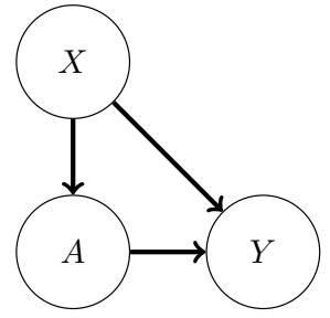
Figure 36.3: A causal DAG illustrating a situation where treatment A and outcome Y are both influenced by observed confounders X.

data. In particular, the assumption of the triangle DAG—there are no unobserved confounders—is enforced by design. However, there are limitations. Most obviously, randomized control trials are sometimes infeasible to conduct. This could be due to expense, regulatory restrictions, or more fundamental di”culties (e.g., in developmental economics, the response of interest is sometimes collected decades after treatment). Additionally, it may be di”cult to ensure that the participants in an RCT are representative of the population where the treatment will be deployed. For instance, participants in drug trials may skew younger and poorer than the population of patients who will ultimately take the drug.

36.4 Confounder adjustment

We now turn to the problem of estimating causal e!ects using observational (i.e., not experimental) data. The most common application of causal inference is estimating the average treatment e!ect (ATE) of an intervention. The ATE is also commonly called the average causal e!ect, or ACE. Here, we focus on the important special case where the treatment A is binary, and we observe the outcome Y as well as a set of common causes X that influence both A and Y .

36.4.1 Causal estimand, statistical estimand, and identification

Consider a problem where we observe treatment A, outcome Y , and covariates X, which are drawn iid from some unknown distribution P. We wish to learn the average treatment e!ect: the expected di!erence between being assigned treatment and assigned no treatment for a randomly chosen member of the population. Following the discussion in the introduction, there are three steps to learning this quantity: mathematically formalize the causal estimand, give conditions for the causal estimand to be identified as a statistical estimand, and, finally, estimate this statistical estimand from data. We now turn to the first two steps.

The average treatment e!ect is defined to be the di!erence between the average outcome if we intervened and set A to be 0, versus the average outcome if we intervented and set A to be 1. Using the do notation, we can write this formally as

\[\text{ATE} = \mathbb{E}[Y|\text{do}(A=1)] - \mathbb{E}[Y|\text{do}(A=0)]. \tag{36.18}\]

The next step is to articulate su”cient conditions for the ATE to be identified as a statistical estimand (a parameter of distribution P). The key issue is the possible presence of confounders. Confounders are “common cause” variables that a!ect both the treatment and outcome. When there are confounding variables in observed data, the sub-population of people who are observed to have received one level of the treatment A will di!er from the rest of the population in ways that are relevant to their observed Y . For example, there is a strong positive association between horseback riding in childhood (treatment) and healthiness as an adult (outcome) [RB16]. However, both of these quantities are influenced by wealth X. The population of people who rode horses as children (A = 1) is wealthier than the population of people who did not. Accordingly, the horseback-riding population will have better health outcomes even if there is no actual causal benefit of horseback riding for adult health.

We’ll express the assumptions required for causal identification in the form of a causal DAG. Namely, we consider the simple triangle DAG in Figure 36.3, where the treatment and outcome are influenced by observed confounders X. It turns out that the assumption encoded by this DAG su”ces for identification. To understand why this is so, recall that the target causal e!ect is defined according to the distribution we would see if the edge from X to A was removed (that’s the meaning of do). The key insight is that because the intervention only modifies the relationship between X and A, the structural equation that generates outcomes Y given X and A, illustrated in Figure 36.3 as the A ⇐ Y △ X, is the same even after the X ⇐ A edge is removed. For example, we might believe that the physiological processes by which smoking status A and confounders X produce lung cancer Y remain the same, regardless of how the decision to smoke or not smoke was made. Second, because the intervention does not change the composition of the population, we would also expect the distribution of background characteristics X to be the same between the observational and intervened processes.

With these insights about invariances between observed and interventional data, we can derive a statistical estimand for the ATE as follows.

Theorem 2 (Adjustment with no unobserved confounders). We observe A, Y, X ↘ P. Suppose that

• 1. (Confounders observed) The data obeys the causal structure in Figure 36.3. In particular, X contains all common causes of A and Y and no variable in X is caused by A or Y .
• 2. (Overlap) 0 < P(A = 1|X = x) < 1 for all values of x. That is, there are no individuals for whom treatment is always or never assigned.

Then, the average treatment e!ect is identified as ATE = ↼ , where

\[\tau = \mathbb{E}[\mathbb{E}[Y|A=1, X]] - \mathbb{E}[\mathbb{E}[Y|A=0, X]].\tag{36.19}\]

Proof. First, we expand the ATE using the tower property of expectation, conditioning on X. Then, we apply the invariances discussed above:

\[ATE = \mathbb{E}[Y|\text{do}(A=1)] - \mathbb{E}[Y|\text{do}(A=0)] \tag{36.20}\]

\[=\mathbb{E}[\mathbb{E}[Y|\text{do}(A=1),X]]-\mathbb{E}[\mathbb{E}[Y|\text{do}(A=0),X]]\tag{36.21}\]

\[\mathbb{E} = \mathbb{E}[\mathbb{E}[Y|A=1, X]] - \mathbb{E}[\mathbb{E}[Y|A=0, X]] \tag{36.22}\]

The final equality is the key to passing from a causal to observational quantity. This follows because, from the causal graph, the conditional distribution of Y given A, X is the same in both the original

graph and in the mutilated graph created by removing the edge from X to A. This mutilated graph defines P(Y |do(A = 1), X), so the equality holds.

The condition that 0 < P(A = 1|X = x) < 1 is required for the first equality (the tower property) to be well defined.

Note that Equation (36.19) is a function of only conditional expectations and distributions that appear in the observed data distribution (in particular, it contains no “do” operators). Thus, if we can fully characterize the observed data distribution P, we can map that distribution to a unique ATE.

It is useful to note how ↼ di!ers from the naive estimand E[Y |A = 1] ↓ E[Y |A = 0] that just reports the treatment-outcome association without adjusting for confounding. The comparison is especially clear when we write out the outer expectation in ↼ explicitly as an integral over X:

\[\tau = \int \mathbb{E}[Y \mid A=1, X] P(X) dX - \int \mathbb{E}[Y \mid A=0, X] P(X) dX \tag{36.23}\]

We can write the naive estimand in a similar form by applying the tower property of expectation:

\[\mathbb{E}[Y \mid A=1] - \mathbb{E}[Y \mid A=0] = \int \mathbb{E}[Y \mid A=1, X]P(X \mid A=1)dX - \int \mathbb{E}[Y \mid A=0, X]P(X \mid A=0)dX \tag{36.24}\]

The key di!erence is the probability distribuiton over X that is being integrated over. The observational di!erence in means integrates over the distinct conditional distributions of confounders X, depending on the value of A. On the other hand, in the ATE estimand ↼ , we integrate over the same distribution P(X) for both levels of the treatment.

Overlap In addition to the assumption on the causal structure, identification requires that there is su”cient random variation in how treatments are assigned.

Definition 1. A distribution P on A, X satisfies overlap if 0 < P(A = 1|x) < 1 for all x. It satisfies strict overlap if - < P(A = 1|x) < 1 ↓ - for all x and some - > 0.

Overlap is the requirement that any unit could have either recieved the treatment or not.

To see the necessity of overlap, consider estimating the e!ectiveness of a drug in a study where patient sex is a confounder, but the drug was only ever prescribed to male patients. Then, conditional on a patient being female, we would know that patient was assigned to control. Without further assumptions, it’s impossible to know the e!ect of the drug on a population with female patients, because there would be no data to inform the expected outcome for treated female patients, that is, E[Y | A = 1, X = female]. In this case, the statistical estimand equation 36.19 would not be identifiable. In the same vein, strict overlap ensures that the conditional distributions at each stratum of X can be estimated in finite samples.

Overlap can be particularly limiting in settings where we are adjusting for a large number of covariates (in an e!ort to satisfy no unobserved confounding). Then, certain combinations of traits may be very highly predictive of treatment assignment, even if individual traits are not. E.g., male patients over age 70 with BMI greater than 25 are very rarely assigned the drug. If such groups represent a significant fraction of the target population, or have significantly di!erent treatment e!ects, then this issue can be problematic. In this case, the strict overlap assumption puts very strong restrictions on observational studies: for an observational study to satisfy overlap, most dimensions of the confounders X would need to closely mimic the balance we would expect in an RCT [D’A+21].

36.4.2 ATE estimation with observed confounders

We now return to estimating the ATE using observed — i.e., not experimental — data. We’ve shown that in the case where we observe all common causes of the treatment and outcome, the ATE is causally identified with a statistical estimand ↼ . We now consider several strategies for estimating this quantity using a finite data sample. Broadly, these techniques are known as backdoor adjustment.2

Recall that the defining characteristic of a confounding variable is that it a!ects both treatment and outcome. Thus, an adjustment strategy may aim to account for the influence of confounders on the observed outcome, the influence of confounders on treatment, or both. We discuss each of these strategies in turn.

36.4.2.1 Outcome model adjustment

We begin with an approach to covariate adjustment that relies on modeling the conditional expectation of the outcome Y given treatment A and confounders X. This strategy is often referred to as gcomputation or outcome adjustment.3 To begin, we define

Definition 2. The conditional expected outcome is the function Q given by

\[Q(a,x) = \mathbb{E}[Y|A=a, X=x]. \tag{36.25}\]

Substituting this definition into the definition of our estimand ↼ , Equation (36.19), we have ↼ ^{= E}[Q(1, x) ^{↓ Q}(0, x)]. This suggests a procedure for estimating ↼ : fit a model ^Qˆ for ^Q and then report

\[ \hat{\tau}^Q \stackrel{\triangle}{=} \frac{1}{n} \sum\_{i} \hat{Q}(1, x\_i) - \hat{Q}(0, x\_i). \tag{36.26} \]

To fit ^Qˆ, recall that ^E[^{Y |}a, x] = argmin^{Q E}[(^{Y ↓ Q}(A, X)²]. That is, the minimizer (among all functions) of the squared loss risk is the conditional expected outcome.4 So, to approximate Q, we simply use mean squared error to fit a predictor that predicts Y from A and X.

The estimation procedure takes several steps. We first fit a model Qˆ to predict Y . Then, for each unit i, we predict that unit’s outcome had they received treatment Qˆ(1, xi) and we predict their outcome had they not received treatment Qˆ(0, xi). 5 If the unit actually did receive treatment (aⁱ = 1) then Qˆ(0, xi) is our guess about what would have happened in the counterfactual case that they did not. The estimated expected gain from treatment for this individual is ^Qˆ(1, xi) ^{↓ Q}ˆ(0, xi)—the

^2. As we discuss in Section 36.8, this backdoor adjustment references the estimand returned by the do-calculus to eliminate confounding from a backdoor path. This also generalizes the approaches discussed here to some cases where we do not observe all common causes.

^3. The “g” stands for generalized, for now-inscrutable historical reasons [Rob86].

^4. To be precise, this definition applies when X and Y are square-integrable, and the minimzation taken over measurable functions.

^5. This interpretation is justified by the same conditions as Theorem 2.

di!erence in expected outcome between being treated and not treated. Finally, we estimate the outer expectation with respect to P(X) — the true population distribution of the confounders — using the empirical distribution P( ˆ X)=1/n) ⁱ εxⁱ . In e!ect, this means we substitute the expectation (over an unknown distribution) by an average over the observed data.

Linear regression It’s worth saying something more about the special case where Q is modeled as a linear function of both the treatment and all the covariates. That is, the case where we assume the identification conditions of Theorem 2 and we additionally assume that the true, causal law (the SCM) governing Y yields: Q(A, X) = E[Y |A, X] = E[f^Y (A, X, 5)|A, X] = ⇁⁰ + ⇁AA + ⇁XX. Plugging in, we see that Q(1, X) ↓ Q(0, X) = ⇁^A (and so also ↼ = ⇁A). Then, the estimator for the average treatment e!ect reduces to the estimator for the regression coe”cient ⇁A. This “fit linear regression and report the regression coe”cient” remains a common way of estimating the association between two variables in practice. The expected-outcome-adjustment procedure here may be viewed as a generalization of this procedure that removes the linear parametric assumption.

36.4.2.2 Propensity Score Adjustment

Outcome model adjustment relies on modeling the relationship between the confounders and the outcome. A popular alternative is to model the relationship between the confounders and the treatment. This strategy adjusts for confounding by directly addressing sampling bias in the treated and control groups. This bias arises from the relationship between the confounders and the treatment. Intuitively, the e!ect of confounding may be viewed as due to the di!erence between P(X|A = 1) and P(X|A = 0) — e.g., the population of people who rode horses as children is wealthier than the population of people who did not. When we observe all confounding variables X, this degree of overor under-representation can be adjusted away by reweighting samples such that the confounders X have the same distribution in the treated and control groups. When the confounders are balanced between the two groups, then any di!erences between them must be attributable to the treatment.

A key quantity for balancing treatment and control groups is the propensity score, which summarises the relationship between confounders and treatment.

Definition 3. The propensity score is the function g given by g(x) = P(A = 1|X = x).

To make use of the propensity score in adjustment, we first rewrite the estimand ↼ in a suggestive form, leveraging the fact that A → {0, 1}:

\[\tau = \mathbb{E}[\frac{YA}{g(X)} - \frac{Y(1-A)}{1-g(X)}].\tag{36.27}\]

This identity can be verified by noting that E[Y A|X] = E[Y |A = 1, X]P(A = 1|X)+0, rearranging for E[Y |A = 1, X], doing the same for E[Y |A = 0, X], and substituting in to Equation (36.19). Note that the identity is just a mathematical fact about the statistical estimand — it does not rely on any causal assumptions, and holds whether or not ↼ can be interpreted as a causal e!ect.

This expression suggests the inverse probability of treatment weighted estimator, or IPTW estimator:

\[\hat{\tau}^{\text{IPTV}} \stackrel{\Delta}{=} \frac{1}{n} \sum\_{i} \frac{Y\_i A\_i}{\hat{g}(X\_i)} - \frac{Y\_i (1 - A\_i)}{1 - \hat{g}(X\_i)}.\tag{36.28}\]

Here, gˆ is an estimate of the propensity score function. Recall from Section 14.2.1 that if a model is wellspecified and the loss function is a proper scoring rule then risk minimizer g^→ = argmin^g E[L(A, g(X))] will be g→(X) = P(A = 1|X). That is, we can estimate the propensity score by fitting a model that predicts A from X. Cross-entropy and squared loss are both proper scoring rules, so we may use standard supervised learning methods.

In summary, the procedure is to estimate the propensity score function (with machine learning), and then to plug the estimated propensity scores gˆ(xi) into Equation (36.28). The IPTW estimator computes a di!erence of weighted averages between the treated and untreated group. The e!ect is to upweight the outcomes of units who were unlikely to be treated but who nevertheless actually, by chance, recieved treatment (and similarly for untreated). Intuitively, such units are typical for the untreated population. So, their outcomes under treatment are informative about what would have happened had a typical untreated unit received treatment.

A word of warning is in order. Although the IPTW is asymtotically valid and popular in practice, it can be very unstable in finite samples. If estimated propensity scores are extreme for some values of x (that is, very close to 0 or 1), then the corresponding IPTW weights can be very large, resulting in a high-variance estimator. In some cases, this instability can be mitigated by instead using the Hajek version of the estimator.

\[\hat{\tau}^{\text{h-IPW}} \stackrel{\Delta}{=} \sum\_{i} Y\_i A\_i \frac{\mathbf{1}\_{\{\hat{g}(X\_i)\}}}{\sum\_{i} A\_i \langle \hat{g}(X\_i) \rangle} - \sum\_{i} Y\_i (1 - A\_i) \frac{\mathbf{1}\_{\{1 - \hat{g}(X\_i)\}}}{\sum\_{i} (1 - A\_i) \langle (1 - \hat{g}(X\_i)) \rangle}. \tag{36.29}\]

However, extreme weights can persist even after self-normalization, either because there are truly strata of X where treatment assignment is highly imbalanced, or because the propensity score estimation method has overfit. In such cases, it is common to apply heuristics such as weight clipping.

See Khan and Ugander [KU21] for a longer discussion of inverse-propensity type estimators, including some practical improvements.

36.4.2.3 Double machine learning

We have seen how to estimate the average treatment e!ect using either the relationship between confounders and outcome, or the relationship between confounders and treatment. In each case, we follow a two step estimation procedure. First, we fit models for the expected outcome or the propensity score. Second, we plug these fitted models into a downstream estimator of the e!ect.

Unsurprisingly, the quality of the estimate of ↼ depends on the quality of the estimates Qˆ or gˆ. This is problematic because Q and g may be complex functions that require large numbers of samples to estimate. Even though we’re only interested in the 1-dimensional parameter ↼ , the naive estimators described thus far can have very slow rates of convergence. This leads to unreliable inference or very large confidence intervals.

Remarkably, there are strategies for combining Q and g in estimators that, in principle, do better than using either Q or g alone. The augmented inverse probability of treatment weighted estimator (AIPTW) is one such estimator. It is defined as

\[\hat{\tau}^{\text{APPTW}} \triangleq \frac{1}{n} \sum\_{i} \hat{Q}(1, X\_i) - \hat{Q}(0, X\_i) + A\_i \frac{Y\_i - \hat{Q}(1, X\_i)}{\hat{g}(X\_i)} - (1 - A\_i) \frac{Y\_i - \hat{Q}(0, X\_i)}{1 - \hat{g}(X\_i)}.\tag{36.30}\]

That is, ↼ˆAIPTW is the outcome adjustment estimator plus a stabilization term that depends on the propensity score. This estimator is a particular case of a broader class of estimators that are

refered to as semi-parametrically e”cient or double machine-learning estimators [Che+17e; Che+17d]. We’ll use the later terminology here.

We now turn to understanding the sense in which double machine learning estimators are robust to misestimation of the nuisance functions Q and g. To this end, we define the influence curve of ↼ to be the function ↽ defined by6

\[\phi(X\_i, A\_i, Y\_i; Q, g, \tau) \stackrel{\Delta}{=} Q(1, X\_i) - Q(0, X\_i) + A\_i \frac{Y\_i - Q(1, X\_i)}{g(x\_i)} - (1 - A\_i) \frac{Y\_i - Q(0, X\_i)}{1 - g(X\_i)} - \tau. \tag{36.31}\]

By design, ↼ˆAIPTW ^↓ ↼ ^{= 1} n ) ⁱ ↽(Xi; Q, ^ˆ g, ^ˆ ↼ ), where ^Xi = (Xi, Ai, Yi). We begin by considering what would happen if we simply knew Q and g, and didn’t have to estimate them. In this case, the estimator would be ↼ˆideal = ¹ n ) ⁱ ↽(Xi; Q, g, ↼ ) + ↼ and, by the central limit theorem, we would have:

\[\sqrt{n}(\hat{\tau}^{\text{ideal}} - \tau) \xrightarrow{d} \text{Normal}(0, \mathbb{E}[\phi(\mathbf{X}\_i; Q, g, \tau)^2]). \tag{36.32}\]

This result characterizes the estimation uncertainity in the best possible case. If we knew Q and g, we could rely on this result for, e.g., finding confidence intervals for our estimate.

The question is: what happens when Q and g need to be estimated? For general estimators and nuisance function models, we don’t expect the ⇓n-rate of Equation (36.32) to hold. For instance, ⇓n(↼ˆ^{Q ↓} ↼ ) only converges if ⇓nE[(Q^{ˆ ↓ Q})2] 1 ² ⇐ 0. That is, for the naive estimator we only get the ⇓n rate for estimating ↼ if we can also estimate Q at the ⇓n rate — a much harder task! This is the issue that the double machine learning estimator helps with.

To understand how, we decompose the error in estimating ↼ as follows:

\[\sqrt{n}(\hat{\tau}^{\text{AIPTV}} - \tau) \tag{36.33}\]

\[\mathbf{x} = \frac{1}{\sqrt{n}} \sum\_{i} \phi(\mathbf{X}\_i; Q, g, \tau) \tag{36.34}\]

\[+\frac{1}{\sqrt{n}}\sum\_{i} \phi(\mathbf{X}\_{i};\hat{Q},\hat{g},\tau) - \phi(\mathbf{X}\_{i};Q,g,\tau) - \mathbb{E}[\phi(\mathbf{X};\hat{Q},\hat{g},\tau) - \phi(\mathbf{X};Q,g,\tau)]\tag{36.35}\]

\[+\sqrt{n}\mathbb{E}[\phi(\mathbf{X};\boldsymbol{\hat{Q}},\boldsymbol{\hat{g}},\boldsymbol{\tau})-\phi(\mathbf{X};\boldsymbol{Q},\boldsymbol{g},\boldsymbol{\tau})]\tag{36.36}\]

We recognize the first term, Equation (36.34), as ⇓n(↼ˆideal ^↓ ↼ ), the estimation error in the optimal case where we know Q and g. Ideally, we’d like the error of ↼ˆAIPTW to be asymptotically equal to this ideal case—which will happen if the other two terms go to 0.

The second term, Equation (36.35), is a penalty we pay for using the same data to estimate Q, g and to compute ↼ . For many model classes, it can be shown that such “empirical process” terms go to 0. This can also be guaranteed in general by using di!erent data for fitting the nuisance functions and for computing the estimator (see the next section).

The third term, Equation (36.36), captures the penalty we pay for misestimating the nuisance functions. This is where the particular form of the AIPTW is key. With a little algebra, we can show

^6. Influence curves are the foundation of what follows, and the key to generalizing the analysis beyond the ATE. Unfortunately, going into the general mathematics would require a major digression, so we omit it. However, see references at the end of the chapter for some pointers to the relevant literature.

that

\[\mathbb{E}[\phi(\mathbf{X};\hat{Q},\hat{g})-\phi(\mathbf{X};Q,g)]=\mathbb{E}[\frac{1}{g(X)}(\hat{g}(X)-g(X))(\hat{Q}(1,X)-Q(1,X))\tag{36.37}\]

\[+\frac{1}{1-g(X)}(\hat{g}(X)-g(X))(\hat{Q}(0,X)-Q(0,X))\,. \tag{36.38}\]

The important point is that estimation errors of Q and g are multiplied together. Using the Cauchy-Schwarz inequality, we find that ⇓nE[↽(X; Q, ^{ˆ g}ˆ) ^↓ ↽(X; Q, g)] ⇐ ⁰ as long as ⇓ⁿ max^{a E}[(Qˆ(a, X) ^↓ Q(a, X))²] 1 ^{2 E}[(gˆ(X) ^{↓ g}(X))²] 1 ² ⇐ 0. That is, the misestimation penalty will vanish so long as the product of the misestimation errors is o( ⇓n). For example, this means that ↼ can be estimated at the (optimal) ⇓n rate even when the estimation error of each of Q and g only decreases as o(n↓1/4).

The upshot here is that the double machine learning estimator has the special property that the weak condition ⇓nE(Qˆ(T,X) ^{↓ Q}(T,X))²E(ˆg(X) ^{↓ g}(X))² ⇐ ⁰ su”ces to imply that

\[\sqrt{n}(\hat{\tau}^{\text{AIPTW}} - \tau) \xrightarrow{d} \text{Normal}(0, \mathbb{E}[\phi(\mathbf{X}\_i; Q, g, \tau)^2])\tag{36.39}\]

(though strictly speaking this requires some additional technical conditions we haven’t discussed). This is not true for the earlier estimators we discussed, which require a much faster rate of convergence for the nuisance function estimation.

The AIPTW estimator has two further nice properties that are worth mentioning. First, it is non-parametrically e”cient. This means that this estimator has the smallest possible variance of any estimator that does not make parametric assumptions; namely, E[↽(Xi; Q, g, ↼ )²]. This means, for example, that this estimator yields the smallest confidence intervals of any approach that does not rely on parametric assumptions. Second, it is doubly robust: the estimator is consistent (converges to the true ↼ as ⁿ ⇐ ↖) as long as at least one of either ^Qˆ or ^gˆ is consistent.

36.4.2.4 Cross fitting

The term Equation (36.35) in the error decomposition above is the penalty we pay for reusing the same data to both fit Q, g and to compute the estimator. For many choices of model for Q, g, this term goes to 0 quickly as n gets large and we achieve the (best case) ⇓n error rate. However, this property doesn’t always hold.

As an alternative, we can always randomly split the available data and use one part for model fitting, and the other to compute the estimator. E!ectively, this means the nuisance function estimation and estimator computation are done using independent samples. It can then be shown that the reuse penalty will vanish. However, this comes at the price of reducing the amount of data available for each of nuisance function estimation and estimator computation.

This strategy can be improved upon by a cross fitting approach. We divide the data into K folds. For each fold ^j we use the other ^{K ↓ 1} folds to fit the nuisance function models ^Qˆ↓^j , ^gˆ↓^j . Then, for each datapoint i in fold j, we take Qˆ(ai, xi) = Qˆ↓^j (ai, xi) and gˆ(xi) = gˆ↓^j (xi). That is, the estimated conditional outcomes and propensity score for each datapoint are predictions from a model that was not trained on that datapoint. Then, we estimate ↼ by plugging {Qˆ(ai, xi), ^gˆ(xi)}ⁱ into Equation (36.30). It can be shown that this cross fitting procedure has the same asymptotic guarantee — the central limit theorem at the ⇓n rate — as described above.

36.4.3 Uncertainty quantification

In addition to the point estimate ↼ˆ of the average treatment e!ect, we’d also like to report a measure of the uncertainity in our estimate. For example, in the form of a confidence interval. The asymptotic normality of ⇓n↼ˆ (Equation (36.39)) provides a means for this quantification. Namely, we could base confidence intervals and similar on the limiting variance E[↽(Xi; Q, g, ↼ )2]. Of course, we don’t actually know any of Q, g, or ↼ . However, it turns out that it su”ces to estimate the asymptotic variance with ¹ n ) ⁱ ↽(Xi; Q, ^ˆ g, ^ˆ ↼ˆ)² [Che+17e]. That is, we can estimate the uncertainity by simply plugging in our fitted nuisance models and our point estimate of ↼ into

\[\hat{V}[\hat{\tau}] = 1/n \sum\_{i} \phi(\mathbf{X}\_i; \hat{Q}, \hat{g}, \hat{\tau})^2. \tag{36.40}\]

This estimated variance can then be used to compute confidence intervals in the usual manner. E.g., we’d report a 95% confidence interval for ↼ as ↼^{ˆ ± 1}.96 Vˆ[ˆ↼ ]/n.

Alternatively, we could quantify the uncertainity by bootstrapping. Note, however, that this would require refitting the nuisance functions with each bootstrap model. Depending on the model and data, this can be prohibitively computationally expensive.

36.4.4 Matching

One particularly popular approach to adjustment-based causal estimation is matching. Intuitively, the idea is to match each treated unit to an untreated unit that has the same (or at least similar) values of the confounding variables and then compare the observed outcomes of the treated unit and its matched control. If we match on the full set of common causes, then the di!erence in outcomes is, intuitively, a noisy estimate of the e!ect the treatment had on that treated unit. We’ll now build this up a bit more carefully. In the process we’ll see that matching can be understood as, essentially, a particular kind of outcome model adjustment.

For simplicity, consider the case where X is a discrete random variable. Define A^x to be the set of treated units with covariate value x, and C^x to be the set of untreated units with covariate value x. In this case, the matching estimator is:

\[\hat{\tau}^{\text{matching}} = \sum\_{x} \hat{\mathbf{P}}(x) \{ \frac{1}{|\mathcal{A}\_{x}|} \sum\_{i \in \mathcal{A}\_{x}} Y\_{i} - \frac{1}{|\mathcal{C}\_{x}|} \sum\_{j \in \mathcal{C}\_{x}} Y\_{j} \}, \tag{36.41}\]

where P( ˆ x) is an estimator of P(X = x) — e.g., the fraction of units with X = x. Now, we can rewrite Yⁱ = Q(Ai, Xi) + 5ⁱ where 5ⁱ is a unit-specific noise term defined by the equation. In particular, we have that E[5i|Ai, Xi]=0. Substituting this in, we have:

\[\hat{\tau}^{\text{matching}} = \sum\_{x} \hat{\mathbb{P}}(x) \big( Q(1, x) - Q(0, x) \big) + \sum\_{x} \hat{\mathbb{P}}(x) \big( \frac{1}{|\mathcal{A}\_{x}|} \sum\_{i \in \mathcal{A}\_{x}} \xi\_{i} - \frac{1}{|\mathcal{C}\_{x}|} \sum\_{j \in \mathcal{C}\_{x}} \xi\_{j} \big). \tag{36.42}\]

We can recognize the first term as an estimator of usual target parameter ↼ (it will be equal to ↼ if P( ˆ x) = P(x)). The second term is a di!erence of averages of random variables with expectation 0, and so each term will converge to 0 as long as |Ax| and |Cx| each go to infinity as we see more and more data. Thus, we see that the matching estimator is a particular way of estimating the parameter

↼ . The procedure can be extended to continuous covariates by introducing some notion of values of X being close, and then matching close treatment and control variables.

There are two points we should emphasize here. First, notice that the argument here has nothing to do with causal identification. Matching is a particular technique for estimating the observational parameter ↼ . Whether or not ↼ can be interpreted as an average treatment e!ect is determined by the conditions of Theorem 2 — the particular estimation strategy doesn’t say anything about this. Second, notice that in essence matching amounts to a particular choice of model for Qˆ. Namely, Qˆ(1, x) = ¹ |Ax| ) ⁱ↑A^{x Yi} and similarly for ^Qˆ(0, x). That is, we estimate the conditional expected outcome as a sample mean over units with the same covariate value. Whether this is a good idea depends on the quality of our model for Q. In situations where better models are possible (e.g., a machine-learning model fits the data well), we might expect to get a more accurate estimate by using the conditional expected outcome predictor directly.

There is another important case we mention in passing. In general, when using adjustment based identification, it su”ces to adjust for any function ↽(X) of X such that A ¬¬ X|↽(X). To see that adjusting for only ↽(X) su”ces, first notice that g(X) = P(A = 1|X) = P(A = 1|↽(X)) only depends on ↽(X), and then recall that we can write the target parameter as ↼ = E[ Y A ^g(X) ^{↓ Y} (1↓A) ¹↓g(X) ], whence ↼ only depends on X through g(X). That is: replacing X by a reduced version ↽(X) such that g(X) = P(A = 1|↽(X)) can’t make any di!erence to ↼ . Indeed, the most popular choice of ↽(X) is the propensity score itself, ↽(X) = g(X). This leads to propensity score matching, a two step procedure where we first fit a model for the propensity score, and then run matching based on the estimated propensity score values for each unit. Again, this is just a particular estimation procedure for the observational parameter ↼ , and says nothing about whether it’s valid to interpret ↼ as a causal e!ect.

36.4.5 Practical considerations and procedures

when performing causal analysis, many issues can arise in practice, some of which we discuss below.

36.4.5.1 What to adjust for

Choosing which variables to adjust for is a key detail in estimating causal e!ects using covariate adjustment. The criterion is clear when one has a full causal graph relating A, Y , and all covariates X to each other. Namely, adjust for all variables that are actually causal parents of A and Y . In fact, with access to the full graph, this criterion can be generalized somewhat — see Section 36.8.

In practice, we often don’t actually know the full causal graph relating all of our variables. As a result, it is common to apply simple heuristics to determine which variables to adjust for. Unfortunately, these heuristics have serious limitations. However, exploring these is instructive.

A key condition in Theorem 2 is that the covariates X that we adjust for must include all the common causes. In the absence of a full causal graph, it is tempting to condition on as many observed variables as possible to try to ensure this condition holds. However, this can be problematic. For instance, suppose that M is a mediator of the e!ect of A on Y — i.e., M lies on one of the directed paths between A and Y . Then, conditioning on M will block this path, removing some of the causal e!ect. Note that this does not always result in an attenuated, or smaller-magnitude, e!ect estimate. The e!ect through a given mediator may run in the opposite direction of other causal pathways from the treatment; thus conditioning on a mediator can inflate or even flip the sign of a treatment

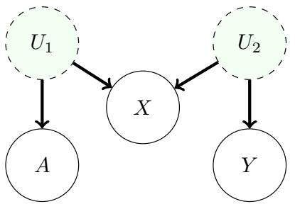
Figure 36.4: The M-bias causal graph. Here, A and Y are not confounded. However, conditioning on the covariate X opens a backdoor path, passing through U¹ and U² (because X is a colider). Thus, adjusting for X creates bias. This is true even though X need not be a pre-treatment variable.

e!ect. Alternatively, if C is a collider between A and Y — a variable that is caused by both — then conditioning on C will induce an extra statistical dependency between A and Y .

Both pitfalls of the “condition on everything” heuristic discussed above both involve conditioning on variables that are downstream of the treatment A. A natural response is to this is to limit conditioning to all pre-treatment variables, or those that are causally upstream of the treatment. Importantly, if there is a valid adjustment set in the observed covariates X, then there will also be a valid adjustment set among the pre-treatment covariates. This is because any open backdoor path between A and Y must include a parent of A, and the set of pre-treatment covariates includes these parents. However, it is still possible that conditioning on the full set of pre-treatment variables can induce new backdoor paths between A and Y through colliders. In particular, if there is a covariate D that is separately confounded with the treatment A and the outcome Y then D is a collider, and conditioning on D opens a new backdoor path. This phenomenon is known as m-bias because of the shape of the graph [Pea09c], see Figure 36.4.

A practical refinement of the pre-treatment variable heuristic is given in VanderWeele and Shpitser [VS11]. Their heuristic suggests conditioning on all pre-treatment variables that are causes of the treatment, outcome, or both. The essential qualifier in this heuristic is that the variable is causally upstream of treatment and/or outcome. This eliminates the possibility of conditioning on covariates that are only confounded with treatment and outcome, avoiding m-bias. Notably, this heuristic requires more causal knowledge than the above heuristics, but does not require detailed knowledge of how di!erent covariates are causally related to each other.

The VanderWeele and Shpitser [VS11] criterion is a useful rule of thumb, but other practical considerations often arise. For example, if one has more knowledge about the causal structure among covariates, it is possible to optimize adjustment sets to minimize the variance of the resulting estimator [RS20]. One important example of reducing variance by pruning adjustment sets is the exclusion of variables that are known to only be a parent of the treatment, and not of the outcome (so called instruments, as discussed in Section 36.5).

Finally, adjustment set selection criteria operate under the assumption that there actually exists a valid adjustment set among observed covariates. When there is no set of observed covariates in X that block all backdoor paths, then any adjusted estimate will be biased. Importantly, in this case, the bias does not necessarily decrease as one conditions on more variables. For example, conditioning

on an instrumental variable often results in an estimate that has higher bias, in addition to the higher variance discussed above. This phenomenon is known as bias amplification or z-bias; see Section 36.7.2. A general rule of thumb is that variables that explain away much more variation in the treatment than in the outcome can potentially amplify bias, and should be treated with caution.

36.4.5.2 Overlap

Recall that in addition to no-unobserved-confounders, identification of the average treatment e!ect requires overlap: the condition that 0 < P(A = 1|x) < 1 for the population distribution P. With infinite data, any amount of overlap will su”ce for estimating the causal e!ect. In realistic settings, even near failures can be problematic. Equation (36.39) gives an expression for the (asymptotic) variance of our estimate: E[↽(Xi; Q, ˆ g, ˆ ↼ˆ)²]/n. Notice that ↽(Xi; Q, ˆ g, ˆ ↼ˆ)² involves terms that are proportional to 1/g(X) and 1/(1 ↓ g(X). Accordingly, the variance of our estimator will balloon if there are units where g(x) ≃ 0 or g(x) ≃ 1 (unless such units are rare enough that they don’t contribute much to the expectation).

In practice, a simple way to deal with potential overlap violation is to fit a model gˆ for the treatment assignment probability — which we need to do anyways — and check that the values gˆ(x) are not too extreme. In the case that some values are too extreme, the simplest resolution is to cheat. We can simply exclude all the data with extreme values of gˆ(x). This is equivalent to considering the average treatment e!ect over only the subpopulation where overlap is satisfied. This changes the interpretation of the estimand. The restricted subpopulation ATE may or may not provide a satisfactory answer to the real-world problem at hand, and this needs to be justified based on knowledge of the real-world problem.

36.4.5.3 Choice of estimand and average treatment e!ect on the treated

Usually, our goal in estimating a causal e!ect is qualitative. We want to know what the sign of the e!ect is, and whether it’s large or small. The utility of the ATE is that it provides a concrete query we can use to get a handle on the qualitative question. However, it is not sacrosanct; sometimes we’re better o! choosing an alternative causal estimand that still answers the qualitative question but which is easier to estimate statistically. The average treatment e!ect on the treated or ATT,

\[\text{ATT} \stackrel{\Delta}{=} \mathbb{E}\_{X|A=1}[\mathbb{E}[Y|X, \text{do}(A=1)] - E[Y|X, \text{do}(A=0)]],\tag{36.43}\]

is one such an estimand that is frequently useful.

The ATT is useful when many members of the population are very unlikely to receive treatment, but the treated units had a reasonably high probability of receiving the control. This can happen if, e.g., we sample control units from the general population, but the treatment units all self-selected into treatment from a smaller subpopulation. In this case, it’s not possible to (non-parametrically) determine the treatment e!ect for the control units where no similar unit took treatment. The ATT solves this obstacle by simply omitting such units from the average.

If we have the causal structure Figure 36.3, and the overlap condition P(A = 1|X = x) < 1 for all X = x then the ATT is causally identified as

\[ \tau^{\text{ATT}} = \mathbb{E}\_{X|A=1}[\mathbb{E}[Y|A=1,X] - E[Y|A=0,X]].\tag{36.44} \]

Note that the required overlap condition here is weaker than for identifying the ATE. (The proof is the same as Theorem 2.)

The estimation strategies for the ATE translate readily to estimation strategies for the ATT. Namely, estimate the nuisance functions the same way and then simply replace averages over all datapoints by averages over the treated datapoints only. In principle, it’s possible to do a little better than this by making use of the untreated datapoints as well. A corresponding double machine learning estimator is

\[\hat{\tau}^{\text{ATT}-\text{AIPW}} \stackrel{\Delta}{=} \frac{1}{n} \sum\_{i} \frac{A\_i}{\mathbf{P}(A=1)} (Y\_i - \hat{Q}(0, X\_i)) - \frac{(1 - A\_i)\hat{g}(X\_i)}{\mathbf{P}(A=1)(1 - \hat{g}(X\_i))} (Y\_i - \hat{Q}(0, X\_i). \tag{36.45})\]

. The variance of this estimator can be estimated by

\[\begin{split} \phi^{\text{ATT}}(\mathbf{X}\_{i}; Q, g, \tau) & \triangleq \frac{1}{n} \sum\_{i} \left[ \frac{A\_{i}}{\mathbf{P}(A=1)} (Y\_{i} - \hat{Q}(0, X\_{i})) \\ & - \frac{(1 - A\_{i})\hat{g}(X\_{i})}{\mathbf{P}(A=1)(1 - \hat{g}(X\_{i}))} (Y\_{i} - \hat{Q}(0, X\_{i}) - \frac{A\_{i}\tau}{\mathbf{P}(A=1)}) \right] \end{split} \tag{36.46}\]

\[\hat{\mathbb{V}}[\hat{\tau}^{\text{ATT}-\text{AIPTW}}] \stackrel{\Delta}{=} \frac{1}{n} \sum\_{i} \phi^{\text{ATT}}(\mathbf{X}\_{i}; \hat{Q}, \hat{g}, \hat{\tau}^{\text{ATT}-\text{AIPTW}})^{2}. \tag{36.47}\]

Notice that the estimator for the ATT doesn’t require estimating Q(1, X). This can be a considerable advantage when the treated units are rare. See Chernozhukov et al. [Che+17e] for details.

36.4.6 Summary and practical advice

We have seen a number of estimators that follow the general procedure:

• 1. Fit statistical or machine-learning models Qˆ(a, x) as a predictor for Y , and/or gˆ(x) as a predictor for A
• 2. Compute the predictions Qˆ(0, xi), Qˆ(1, xi), gˆ(xi) for each datapoint, and
• 3. Combine these predictions into an estimate of the average treatment e!ect.

Importantly, no single estimation approach is a silver bullet. For example, the double machinelearning estimator has appealing theoretical properties, such as asymptotic e”ciency guarantees and a recipe for estimating uncertainity without needing to bootstrap the model fitting. However, in terms of the quality of point estimates, the double ML estimators can sometimes underperform their more naive counterparts [KS07]. In fact, there are cases where each of outcome regression, propensity weighting, or doubly robust methods will outperform the others.

One di”culty in choosing an estimator in practice is that there are fewer guardrails in causal inference than there are in standard predictive modeling. In predictive modeling, we construct a train-test split and validate our prediction models using the true labels or outcomes in the held-out dataset. However, for causal problems, the causal estimands are functionals of a di!erent datagenerating process from the one that we actually observed. As a result, it is impossible to empirically validate many aspects of causal estimation using standard techniques.

The e!ectiveness of a given approach is often determined by how much we trust the specification of our propensity score or outcome regression models gˆ(x) and Qˆ(a, x), and how well the treatment and control groups overlap in the dataset. Using flexible models for the nuisance functions g and Q can alleviate some of the concerns about model misspecification, but our freedom to use such models is often constrained by dataset size. When we have the luxury of large data, we can use flexible models; on the other hand, when the dataset is relatively small, we may need to use a smaller parametric family or stringent regularization to obtain stable estimates of Q and g. Similarly, if overlap is poor in some regions of the covariate space, then flexible models for Q may be highly variable, and inverse propensity score weights may be large. In these cases, IPTW or AIPTW estimates may fluctuate wildly as a function of large weights. Meanwhile, outcome regression estimates will be sensitive to the specification of the Q model and its regularization, and can incur bias that is di”cult to measure if the specification or regularization does not match the true outcome process.

There are a number of practical steps that we can take to sanity-check causal estimates. The simplest check is to compute many di!erent ATE estimators (e.g., outcome regression, IPTW, doubly robust) using several comparably complex estimators of Q and g. We can then check whether they agree, at least qualitatively. If they do agree then this can provide some peace of mind (although it is not a guarantee of accuracy). If they disagree, caution is warranted, particularly in choosing the specification of the Q and g models.

It is also important to check for failures of overlap. Often, issues such as disagreement between alternative estimators can be traced back to poor overlap. A common way to do this, particularly with high-dimensional data, is to examine the estimated (ideally cross-fitted) propensity scores gˆ(xi). This is a useful diagnostic, even if the intention is to use an outcome regression approach that only incorporates and estimated outcome regression function Qˆ(a, xi). If overlap issues are relevant, it may be better to instead estimate either the average treatment e!ect on the treated, or the “trimmed” estimand given by discarding units with extreme propensities.

Uncertainty quantification is also an essential part of most causal analyses. This frequently takes the form of an estimate of the estimator’s variance, or a confidence interval. This may be important for downstream decision-making, and can also be a useful diagnostic. We can calculate variance either by bootstrapping the entire procedure (including refitting the models in each bootstrap replicate), or computing analytical variance estimates from the AIPTW estimator. Generally, large variance estimates may indicate issues with the analysis. For example, poor overlap will often (although not always) manifest as extremely large variances under either of these methods. Small variance estimates should be treated with caution, unless other checks, such as overlap checks, or stability across di!erent Q and g models, also pass.

The previous advice only addresses the statistical problem of estimating ↼ from a data sample. It does not speak to whether or not ↼ can reasonably be interpreted as an average treatment e!ect. Considerable care should be devoted to whether or not the assumption that there are no unobserved confounders is reasonable. There are several methods for assessing the sensitivity of the ATE estimate to violations of this assumption. See Section 36.7. Bias due to unobserved confounding can be substantial in practice—often overwhelming bias due to estimation error—so it is wise to conduct such an analysis.

36.5 Instrumental variable strategies

Adjustment-based methods rely on observing all confounders a!ecting the treatment and outcome. In some situations, it is possible to identify interesting causal e!ects even when there are unobserved

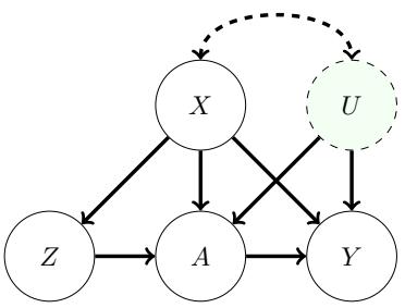
Figure 36.5: Causal graph illustrating the instrumental variable setup. The treatment A and outcome Y are both influenced by unobserved confounder U. Nevertheless, identification is sometimes possible due to the presence of the instrument Z. We also allow for observed covariates X that we may need to adjust for. The dashed arrow between U and X indicates a statistical dependency where we remain agnostic to the particular causal relationship.

confounders. We now consider strateges based on instrumental variables. The instrumental variable graph is shown in Figure 36.5. The key ingredient is the instrumental variable Z, a variable that has a causal e!ect on Y only through its causal e!ect on A. Informally, the identification strategy is to determine the causal e!ect of Z on Y , the causal e!ect of Z on A, and then combine these into an estimate of the causal e!ect of A on Y .

For this identification to strategy to work the instrument must satisfy three conditions. There are observed variables (confounders) X such that:

• 1. Instrument relevance Z ↔︎¬¬ A|X: the instrument must actually a!ect the treatment assignment.
• 2. Instrument unconfoundedness Any backdoor path between Z and Y is blocked by X, even conditional on A.
• 3. Exclusion restriction All directed paths from Z to Y pass through A. That is, the instrument a!ects the outcome only through its e!ect on A.

(It may help conceptually to first think through the case where X is the empty set — i.e., where the only confounder is the unobserved U). These assumptions are necessary for using instrumental variables for causal identification, but they are not quite su”cient. In practice, they must be supplemented by an additional assumption that depends more closely on the details of the problem at hand. Historically, this additional assumption was usually that both the instrument-treatment and treatment-outcome relationships are linear. We’ll examine some less restrictive alternatives below.

Before moving on to how to use instrumental variables for identification, let’s consider how we might encounter instruments in practice. The key is that it’s often possible to find, and measure, variables that a!ect treatment and that are assigned (as if) at random. For example, suppose we are interested in measuring the e!ect of taking a drug A on some health outcome Y . The challenge is that whether a study participant actually takes the drug can be confounded with Y —e.g., sicker people may be more likely to take their medication, but have worse outcomes. However, the assignment of treatments to patients can be randomized and this random assignment can be viewed as an instrument. This random assignment with non-compliance scenario is common in practice. The random assignment — the instrument — satisfies relevance (so long as assigning the drug a!ects the probability of the patient taking the drug). It also satisfies unconfoundedness (because the instrument is randomized). And, it plausibly satisfies exclusion restriction: telling (or not telling) a patient to take a drug has no e!ect on their health outcome except through influencing whether or not they actually take the drug. As a second example, the judge fixed e!ects research design uses the identity of the judge assigned to each criminal case to infer the e!ect of incarceration on some life outcome of interest (e.g., total lifetime earnings). Relevance will be satisfied so long as di!erent judges have di!erent propensities to hand out severe sentences. The assignment of trial judges to cases is randomized, so unconfoundedness will also be satisfied. And, exclusion restriction is also plausible: the particular identity of the judge assigned to your case has no bearing on your years-later life outcomes, except through the particular sentence that you’re subjected to.

It’s important to note that these assumptions require some care, particularly exclusion restriction. Relevance can be checked directly from the data, by fitting a model to predict the treatment from the instrument (or vice versa). Unconfoundedness is often satisfied by design: the instrument is randomly assigned. Even when literal random assignment doesn’t hold, we often restrict to instruments where unconfoundedness is “obviously” satisfied — e.g., using number of rainy days in a month as an instrument for sun exposure. Exclusion restriction is trickier. For example, it might fail in the drug assignment case if patients who are not told to take a drug respond by seeking out alternative treatment. Or, it might fail in the judge fixed e!ects case if judges hand out additional, unrecorded, punishments in addition to incarceration. Assessing the plausibility of exclusion restriction requires careful consideration based on domain expertise.

We now return to the question of how to make use of an instrument once we have it in hand. As previously mentioned, getting causal identification using instrumental variables requires supplementing the IV assumptions with some additional assumption about the causal process.

36.5.1 Additive unobserved confounding

We first consider additive unobserved confounding. That is, we assume that the structural caual model for the outcome has the form:7

\[Y \gets f(A, X) + f\_U(U). \tag{36.48}\]

In words, we assume that there are no interaction e!ects between the treatment and the unobserved confounder — everyone responds to treatment in the same way. With this additional assumption, we see that E[Y |X, do(A = a)] ↓ E[Y |X, do(A = a↗ )] = f(a, X) ↓ f(a↗ , X). In this setting, our goal is to learn this contrast.

Theorem 3 (Additive confounding identification). If the instrumental variables assumptions hold and also additive unobserved confounding holds, then there is a function ˜f(a, x) where

\[\mathbb{E}[Y|x,\text{do}(A=a)] - \mathbb{E}[Y|x,\text{do}(A=a')] = \hat{f}(a,x) - \hat{f}(a',x),\tag{36.49}\]

for all x, a, a↗ and such that ˜f satisfies

\[\mathbb{E}[Y|z,x] = \int \tilde{f}(a,x)p(a|z,x)da. \tag{36.50}\]

^7. We roll the unit-specific variables ↼ into U to avoid notational overload.

Here, p(a|z, x) is the conditional probability density of treatment. In particular, if there is a unique function g that satisfies

\[\mathbb{E}[Y|z,x] = \int g(a,x)p(a|z,x)da,\tag{36.51}\]

then g = ˜f and this relation identifies the target causal e!ect.

Before giving the proof, lets understand the point of this identification result. The key insight is that both the left hand side of Equation (36.51) and p(a|z, x) (appearing in the integrand) are identified by the data, since they involve only observational relationships between observed variables. So, ˜f is identified implicitly as one of the functions that makes Equation (36.51) true. If there is a unique such function, then this fully identifies the causal e!ect.

Proof. With the additive unobserved confounding assumption, the instrument unconfoundedness implies that U ¬¬ Z|X. Then, we have that:

\[\mathbb{E}[Y|Z,X] = \mathbb{E}[f(A,X)|Z,X] + \mathbb{E}[f\_U(U)|Z,X] \tag{36.52}\]

= E[f(A, X)|Z, X] + E[f^U (U)|X] (36.53)

\[\mathbf{x} = \mathbb{E}[\bar{f}(A, X) | Z, X],\tag{36.54}\]

where ˜^{f = f}(A, X) +E[f^U (U)|X]. Now, identifying just ˜^f would su”ce for us, because we could then identify contrasts between treatements: f(a, x) ↓ f(a↗ , x) = ˜f(a, x) ^↓ ˜f(a↗ , x). (The term E[f^U (U)|x] cancels out). Accordingly, we rewrite Equation (36.54) as:

\[\mathbb{E}[Y|z,x] = \int \bar{f}(a,x)p(a|z,x)da. \tag{36.55}\]

It’s worth dwelling briefly on how the IV assumptions come into play here. The exclusion restriction is implied by the additive unobserved confounding assumption, which we use explicilty. We also use the unconfoundedness assumption to conclude U ¬¬ Z|X. However, we do not use relevance. The role of relevance here is in ensuring that few functions solve the relation Equation (36.51). Informally, the solution g is constrained by the requirement that it hold for all values of Z. However, di!erent values of Z only add non-trivial constraints if p(a|z, x) di!er depending on the value of z — this is exactly the relevance condition.

Estimation The basic estimation strategy is to fit models for E[Y |z, x] and p(a|z, x) from the data, and then solve the implicit equation Equation (36.51) to find g consistent with the fitted models. The procedures for doing this can vary considerably depending on the particulars of the data (e.g., if Z is discrete or continuous) and the choice of modeling strategy. We omit a detailed discussion, but see e.g., [NP03; Dar+11; Har+17; SSG19; BKS19; Mua+20; Dik+20] for various concrete approaches.

It’s also worth mentioning an additional nuance to the general procedure. Even if relevance holds, there will often be more than one function that satisfies Equation (36.51). So, we have only identified ˜^f as a member of this set of functions. In practice, this ambiguity is defeated by making some additional structural assumption about ˜f. For example, we model ˜f with a neural network, and then choose the network satisfying Equation (36.51) that has minimum l2-norm on the parameters (i.e., we pick the l2-regularized solution).

36.5.2 Instrument monotonicity and local average treatment e!ect

We now consider an alternative assumption to additive unobserved confounding that is applicable when both the instrument and treatment are binary. It will be convenient to conceptualize the instrument as assignment-to-treatment. Then, the population divides into four subpopulations:

1. Compliers, who take the treatment if assigned to it, and who don’t take the treatment otherwise.

• 2. Always takers, who take the treatment no matter their assignment.
• 3. Never takers, who refuse the treatment no matter their assignment.
• 4. Defiers, who refuse the treatment if assigned to it, and who take the treatment if not assigned.

Our goal in this setting will be to identify the average treatment e!ect among the compliers. The local average treatment e!ect (or complier average treatment e!ect) is defined to be8

\[\text{LATE} = \mathbb{E}[Y|\text{do}(A=1), \text{complier}] - \mathbb{E}[Y|\text{do}(A=0), \text{complier}].\tag{36.56}\]

The LATE requires an additional assumption for identification. Namely, instrument monotonicity: being assigned (not assigned) the treatment only increases (decreases) the probability that each unit will take the treatment. Equivalently, P(defier) = 0.

We can then write down the identification result.

Theorem 4. Given the instrumental variable assumptions and instrument monotonicty, the local average treatment is identified as a parameter ↼ LATE of the observational distributional; that is, LATE = ↼ LATE. Namely,

\[\tau^{\text{LATE}} = \frac{\mathbb{E}[\mathbb{E}[Y|X, Z=1] - \mathbb{E}[Y|X, Z=0]]}{\mathbb{E}[\mathbf{P}(A=1|X, Z=1) - \mathbf{P}(A=1|X, Z=0)]}.\tag{36.57}\]

Proof. We now show that, given the IV assumptions and monotonicity, LATE = ↼ LATE. First, notice that

\[\tau^{\text{LATE}} = \frac{\mathbb{E}[Y|\text{do}(Z=1)] - \mathbb{E}[Y|\text{do}(Z=0)]}{\text{P}(A=1|\text{do}(Z=1)) - \text{P}(A=1|\text{do}(Z=0))}.\tag{36.58}\]

This follows from backdoor adjustment, Theorem 2, applied to the numerator and denominator separately. Our strategy will be to decompose E[Y |do(Z = z)] into the contributions from the compliers, the units that ignore the instrument (the always/never takers), and the defiers. To that end, note that P(complier|do(Z = z)) = P(complier) and similarly for always/never takers and defiers — interventions on the instrument don’t change the composition of the population. Then,

\[\mathbb{E}[Y|\text{do}(Z=1)] - \mathbb{E}[Y|\text{do}(Z=1)] \tag{36.59}\]

\[\mathbf{x} = \left( \mathbb{E} [Y \vert \text{complier}, \text{do}(Z=1)] - \mathbb{E} [Y \vert \text{complier}, \text{do}(Z=0)] \right) \mathbf{P} (\text{complier}) \tag{36.60}\]

\[+\left(\mathbb{E}[Y|\text{always}/\text{never}, \text{do}(Z=1)] - \mathbb{E}[Y|\text{always}/\text{never}, \text{do}(Z=0)]\right) \text{P(always/\text{never})}\tag{36.61}\]

\[+\left(\mathbb{E}[Y|\text{defier},\mathrm{do}(Z=1)]-\mathbb{E}[Y|\text{defier},\mathrm{do}(Z=0)]\right)\mathrm{P}(\text{defier}).\tag{36.62}\]

^8. We follow the econometrics literature in using “LATE” because “CATE” is already commonly used for conditional average treatment e!ect.

The key is the e!ect on the complier subpopulation, Equation (36.60). First, by definition of the complier population, we have that:

\[\mathbb{E}[Y|\text{complier}, \text{do}(Z=z)] = \mathbb{E}[Y|\text{complier}, \text{do}(A=z)].\tag{36.63}\]

That is, the causal e!ect of the treatment is the same as the causal e!ect of the instrument in this subpopulation — this is the core reason why access to an instrument allows identification of the local average treatment e!ect. This means that

\[\text{LATE} = \mathbb{E}[Y|\text{complier}, \text{do}(Z=1)] - \mathbb{E}[Y|\text{complier}, \text{do}(Z=0)]. \tag{36.64}\]

Further, we have that P(complier) = P(A = 1|do(Z = 1)) ↓ P(A = 1|do(Z = 0)). The reason is simply that, by definition of the subpopulations,

\[\mathbf{P}(A=1|\text{do}(Z=1)) = \mathbf{P}(\text{complier}) + \mathbf{P}(\text{always taken})\tag{36.65}\]

\[\mathbf{P}(A=1|\text{do}(Z=0)) = \mathbf{P}(\text{always taker}).\tag{36.66}\]

Now, plugging the expression for P(complier) and Equation (36.64) into Equation (36.60) we have that:

\[\mathbb{E}\left(\mathbb{E}[Y|\text{complier}, \text{do}(Z=1)] - \mathbb{E}[Y|\text{complier}, \text{do}(Z=0)]\right) \mathbb{P}(\text{complier})\tag{36.67}\]

\[\mathbf{P} = \text{LATE} \times \left( \mathbf{P}(A=1|\text{do}(Z=1)) - \mathbf{P}(A=1|\text{do}(Z=0)) \right) \tag{36.68}\]

This gives us an expression for the local average treatment e!ect in terms of the e!ect of the instrument on the compliers and the probability that a unit takes the treatment when assigned/not-assigned.

The next step is to show that the remaining instrument e!ect decomposition terms, Equations (36.61) and (36.62), are both 0. Equation (36.61) is the causal e!ect of the instrument on the always/never takers. It’s equal to 0 because, by definition of this subpopulation, the instrument has no causal e!ect in the subpopulation — they ignore the instrument! Mathematically, this is just E[Y |always/never, do(Z = 1)] = E[Y |always/never, do(Z = 0)]. Finally, Equation (36.62) is 0 by the instrument monotonicity assumption: we assumed that P(defier) = 0.

In totality, we now have that Equations (36.60) to (36.62) reduces to:

\[\mathbb{E}[Y|\text{do}(Z=1)] - \mathbb{E}[Y|\text{do}(Z=1)] \tag{36.69}\]

\[\mathbf{P} = \text{LATE} \times \left( \mathbf{P}(A=1|\text{do}(Z=1)) - \mathbf{P}(A=1|\text{do}(Z=0)) \right) + 0 + 0 \tag{36.70}\]

Rearranging for LATE and plugging in to Equation (36.58) gives the claimed identification result.

36.5.2.1 Estimation

For estimating the local average treatment e!ect under the monotone instrument assumption, there is a double-machine learning approach that works with generic supervised learning approaches. Here, we want an estimator ↼ˆLATE for the parameter

\[\tau^{\text{LATE}} = \frac{\mathbb{E}[\mathbb{E}[Y|X, Z=1] - \mathbb{E}[Y|X, Z=0]]}{\mathbb{E}[\mathbf{P}(A=1|X, Z=1) - \mathbf{P}(A=1|X, Z=0)]}.\tag{36.71}\]

To define the estimator, it’s convenient to introduce some additional notation. First, we define the nuisance functions:

\[\mu(z, x) = \mathbb{E}[Y|z, x] \tag{36.72}\]

\[m(z,x) = \mathcal{P}(A=1|x,z) \tag{36.73}\]

\[p(x) = \mathbf{P}(Z = 1|x). \tag{36.74}\]

We also define the score ↽ by:

\[\phi\_{Z\to Y}(\mathbf{X};\mu,p) \triangleq \mu(1,X) - \mu(0,X) + \frac{Z(Y-\mu(1,X))}{p(X)} - \frac{(1-Z)(Y-\mu(0,X))}{1-p(X)}\tag{36.75}\]

\[\phi\_{Z\to A}(\mathbf{X};m,p) \stackrel{\Delta}{=} m(1,X) - m(0,X) + \frac{Z(A-m(1,X))}{p(X)} - \frac{(1-Z)(A-m(0,X))}{1-p(X)}\tag{36.76}\]

\[ \phi(\mathbf{X}; \mu, m, p, \tau) \stackrel{\Delta}{=} \phi\_{Z \to Y}(\mathbf{X}; \mu, p) - \phi\_{Z \to A}(\mathbf{X}; m, p) \times \tau \tag{36.77} \]

Then, the estimator is defined by a two stage procedure:

• 1. Fit models µ, ˆ m, ˆ pˆ for each of µ, m, p (using supervised machine learning).
• 2. Define ↼ˆLATE as the solution to ¹ n ) ⁱ ↽(Xi; ˆµ, m, ˆ p, ˆ ↼ˆLATE)=0. That is,

\[\hat{\tau}^{\text{LATE}} = \frac{\frac{1}{n} \sum\_{i} \phi\_{Z \to Y}(\mathbf{X}\_i; \hat{\mu}, \hat{p})}{\frac{1}{n} \sum\_{i} \phi\_{Z \to A}(\mathbf{X}\_i; \hat{m}, \hat{p})} \tag{36.78}\]

It may help intuitions to notice that the double machine learning estimator of the LATE is e!ectively the double machine learning estimator of of the average treatment e!ect of Z on Y divided by the double machine learning estimator of the average treatment e!ect of Z on A.

Similarly to Section 36.4, the nuisance functions can be estimated by:

• 1. Fit a model µˆ that predicts Y from Z, X by minimizing mean square error.
• 2. Fit a model mˆ that predicts A from Z, X by minimizing mean cross-entropy.
• 3. Fit a model pˆ that predicts Z from X by minimizing mean cross-entropy.

As in Section 36.4, reusing the same data for model fitting and computing the estimator can potentially cause problems. This can be avoided with use a cross-fitting procedure as described in Section 36.4.2.4. In this case, we split the data into K folds and, for each fold k, use all the but the k’th fold to compute estimates µˆ↓^k, mˆ ^↓k, pˆ↓^k of the nuisance parameters. Then we compute the nuisance estimates for each datapoint i in fold k by predicting the required quantity using the nuisance model fit on the other folds. That is, if unit i is in fold k, we compute µˆ(zi, xi) ↭ µˆ↓k(zi, xi) and so forth.

The key result is that if we use the cross-fit version of the estimator and the estimators for the nuisance functions converge to their true values in the sense that

\[\begin{aligned} \text{1. } \mathbb{E}(\hat{\mu}(Z,X) - \mu(Z,X))^2 &\to 0, \mathbb{E}(\hat{m}(Z,X) - m(Z,X))^2 \to 0, \text{ and } \mathbb{E}(\hat{p}(X) - p(X))^2 \to 0\\ \text{2. } \sqrt{\mathbb{E}[(\hat{p}(X) - p(X))^2]} &\times \left(\sqrt{\mathbb{E}[(\hat{\mu}(Z,X) - \mu(Z,X))^2]} + \sqrt{\mathbb{E}[(\hat{m}(Z,X) - m(Z,X))^2]}\right) = o(\sqrt{n}) \end{aligned}\]

then (with some omitted technical conditions) we have asymptotic normality at the ⇓n-rate:

\[\sqrt{n}(\hat{\tau}^{\text{LATE-cf}} - \tau^{\text{LATE}}) \xrightarrow{d} \text{Normal}(0, \frac{\mathbb{E}[\phi(\mathbf{X}; \mu, m, p, \tau^{\text{LATE}})^2]}{\mathbb{E}[m(1, X) - m(0, X)]^2}).\tag{36.79}\]

As with double machine learning for the confounder adjustment strategy, the key point here is that we can achieve the (optimal) ⇓n rate for estimating the LATE under a relatively weak condition on how well we estimate the nuisance functions — what matters is the product of the error in p and the errors in µ, m. So, for example, a very good model for how the instrument is assigned (p) can make up for errors in the estimation of the treatment-assignment (m) and outcome (µ) models.

The double machine learning estimator also gives a recipe for quantifying uncertainity. To that end, define

\[ \hat{\tau}\_{Z \to A} \triangleq \frac{1}{n} \sum\_{i} \phi z\_{Z \to A}(\mathbf{X}\_i; \hat{m}, \hat{p}) \tag{36.80} \]

\[\hat{\mathbb{V}}[\hat{\tau}^{\text{LATE}}] \stackrel{\scriptstyle \triangleq}{=} \frac{1}{\hat{\tau}\_{Z \to A}^{2}} \frac{1}{n} \sum\_{i} \phi(\mathbf{X}\_{i}; \hat{\mu}, \hat{m}, \hat{p}, \hat{\tau}^{\text{LATE}})^{2}. \tag{36.81}\]

Then, subject to suitable technical conditions, Vˆ[↼ˆLATE↓cf] can be used as an estimate of the variance of the estimator. More precisely,

\[ \sqrt{n}(\hat{\tau}^{\text{LATE}} - \tau^{\text{LATE}}) \xrightarrow{d} \text{Normal}(0, \hat{\mathbb{V}}[\hat{\tau}^{\text{LATE}}]).\tag{36.82} \]

Then, confidence intervals or p-values can be computed using this variance in the usual way. The main extra condition required for the variance estimator to be valid is that the nuisance parameters must all converge at rate O(n↓1/⁴) (so an excellent estimator for one can’t fully compensate for terrible estimators of the others). In fact, even this condition is unnecessary in certain special cases — e.g., when p is known exactly, which occurs when the instrument is randomly assigned. See Chernozhukov et al. [Che+17e] for technical details.

36.5.3 Two stage least squares

Commonly, the IV assumptions are supplemented with the following linear model assumptions:

\[A\_i \gets \alpha\_0 + \alpha Z\_i + \delta\_A X\_i + \gamma\_A X\_i + \xi\_i^A \tag{36.83}\]

\[Y\_i \gets \beta\_0 + \beta A\_i + \delta Y X\_i + \gamma\_Y X\_i + \xi\_i^Y \tag{36.84}\]

That is, we assume that the real-world process for treatment assignment and the outcome are both linear. In this case, plugging Equation (36.83) into Equation (36.84) yields

\[Y\_i \gets \tilde{\beta}\_0 + \beta \alpha Z\_i + \tilde{\delta} X\_i + \tilde{\gamma} X\_i + \tilde{\xi}\_i. \tag{36.85}\]

The point is that ⇁, the average treatment e!ect of A on Y , is equal to the coe”cient ⇁⇀ of the instrument in the outcome-instrument model divided by the coe”cient ⇀ of the instrument in the treatment-instrument model. So, to estimate the treatment e!ect, we simply fit both linear models and divide the estimated coe”cients. This procedure is called two stage least squares.

The simplicity of this procedure is seductive. However, the required linearity assumptions are hard to satisfy in practice and frequently lead to severe issues. A particularly pernicious version of this is that linear-model misspecfication together with weak relevance can yield standard errors for the estimate that are far too small. In practice, this can lead us to find large, significant estimates from two stage least squares when the truth is actually a weak or null e!ect. See [Rei16; You19; ASS19; Lal+21] for critical evaluations of two stage least squares in practice.

36.6 Di!erence in di!erences

Unsurprisingly, time plays an important role in causality. Causes precede e!ects, and we should be able to incorporate this knowledge into causal identification. We now turn to a particular strategy for causal identification that relies on observing each unit at multiple time points. Data of this kind is sometimes called panel data. We’ll consider the simplest case. There are two time periods. In the first period, none of the units are treated, and we observe an outcome Y0ⁱ for each unit. Then, a subset of the units are treated, denoted by Aⁱ = 1. In the second time period, we again observe the outcomes Y1ⁱ for each unit, where now the outcomes of the treated units are a!ected by the treatment. Our goal is to determine the average e!ect receiving the treatment had on the treated units. That is, we want to know the average di!erence between the outcomes we actually observed for the treated units, and the outcomes we would have observed on those same units if they had not been treated. The general strategy we look at is called di!erence in di!erences. 9

As a concrete motivating example, consider trying to determine the e!ect raising minimum wage on employment. The concern here is that, in an e”cient labor market, increasing the price of workers will reduce the demand for them, thereby driving down employment. As such, it seems increasing minimum wage may hurt the people the policy is nominally intended to help. The question is: how strong is this e!ect in practice? Card and Krueger [CK94a] studied this e!ect using di!erence in di!erences. The Philadelphia metropolitan area includes regions in both Pennsylvania and New Jersey (di!erent US states). On April 1st 1992, New Jersey raised its minimum wage from $4.25 to $5.05. In Pennsylvania, the wage remained constant at $4.25. The strategy is to collect employment data from fast food restaurants (which pay many employees minimum wage) in each state before and after the change in minimum wage. In this case, for restaurant i, we have Y0i, the number of full time employees in February 1992, and Y1i, the number of full time employees in November 1992. The treatment is simply Aⁱ = 1 if the restaurant was located in New Jersey, and Aⁱ = 0 if located in Pennsylvania. Our goal is to estimate the average e!ect of the minimum wage hike on employment in the restaurants a!ected by it (i.e., the ones in New Jersey).

The assumption in classical di!erence-in-di!erences is the following structural equation:

\[Y\_{ti} \leftarrow W\_i + S\_t + \tau A\_i \mathbb{I}\left(t = 1\right) + \xi\_{ti},\tag{36.86}\]

with E[5ti|Wi, St, Ai]=0. Here, Wⁱ is a unit specific e!ect that is constant across time (e.g., the location of the restuarant or competence of the management) and S^t is a time-specific e!ect that applies to all units (e.g., the state of the US economy at each time). Both of these quantities are treated as unobserved, and not explicitly accounted for. The parameter ↼ captures the target causal e!ect. The (strong) assumption here is that unit, time, and treatment e!ects are all additive. This

^9. See github.com/vveitch/causality-tutorials/blob/main/di!erence_in_di!erences.ipynb.

assumption is called parallel trends, because it is equivalent to assuming that, in the absence of treatment, the trend over time would be the same in both groups. It’s easy to see that under this assumption, we have:

\[ \tau = \mathbb{E}[Y\_{1i} - Y\_{0i}|A=1] - \mathbb{E}[Y\_{1i} - Y\_{0i}|A=0]. \tag{36.87} \]

That is, the estimand first computes the di!erence across time for both the treated and untreated group, and then computes the di!erence between these di!erences across the groups. The obvious estimator is then

\[\hat{\tau} = \frac{1}{n\_A} \sum\_{i:A\_i=1} Y\_{1i} - Y\_{0i} - \frac{1}{n - n\_A} \sum\_{i:A\_i=0} Y\_{1i} - Y\_{0i},\tag{36.88}\]

where n^A is the number of treated units.

The root identification problem addressed by di!erence-in-di!erences is that E[Wi|Aⁱ = 1] ↔︎= E[Wi|Aⁱ = 0]. That is, restaurants in New Jersey may be systematically di!erent from restuarants in Pennsylvania in unobserved ways that a!ect employment.10 This is why we can’t simply compare average outcomes for the treated and untreated. The identification assumption is that this unitspecific e!ect is the only source of statistical association with treatment; in particular we assume the time-specific e!ect has no such issue: E[S1ⁱ ↓ S0i|Aⁱ = 1] = E[S1ⁱ ↓ S0i|Aⁱ = 0]. Unfortunately, this assumption can be too strong. For instance, administrative data shows employment in Pennsylvania falling relative to employment in New Jersey between 1993 and 1996 [AP08, §5.2]. Although this doesn’t directly contradict the parallel trends assumption used for identification, which needs to hold only in 1992, it does make it seem less credible.

To weaken the assumption, we’ll look at a version that requires parallel trends to hold only after adjusting for covariates. To motivate this, we note that there were several di!erent types of fast food restaurant included in the employment data. These vary, e.g., in the type of food they serve, and in cost per meal. Now, it seems reasonable the trend in employment may depend on the type of restuarant. For example, more expensive chains (such as KFC) might be more a!ected by recessions than cheaper chains (such as McDonald’s). If expensive chains are more common in New Jersey than in Pennsylvania, this e!ect can create a violation of parallel trends — if there’s recession a!ecting both states, we’d expect employment to go down more in New Jersey than in Pennsylvania. However, we may find it credible that McDonald’s restaurants in New Jersey have the same trend as McDonald’s in Pennsylvania, and similarly for KFC.

The next step is to give a definition of the target causal e!ect that doesn’t depend on a parametric model, and a non-parametric statement of the identification assumption to go with it. In words, the causal estimand will be the average treatment e!ect on the units that received the treatment. To make sense of this mathematically, we’ll introduce a new piece of notation:

\[\mathbb{P}^{A=1}(Y|\text{do}(A=a)) \triangleq \int \mathbb{P}(Y|A=a,\text{parents of }Y)d\mathbb{P}(\text{parents of }Y|A=1) \tag{36.89}\]

\[\mathbb{E}^{A=1}[Y|\text{do}(A=a)] \stackrel{\Delta}{=} \mathbb{E}\_{\mathbb{P}^{A=1}}[Y|\text{do}(A=a)]\tag{36.90}\]

In words: recall that the ordinary do operator works by replacing P(parents|A = a) by the marginal distribution P(parents), thereby breaking the backdoor associations. Now, we’re replacing the

^10. This is similar to the issue that arises from unobserved confounding, except Wⁱ need not be a cause of the treatment assignment.

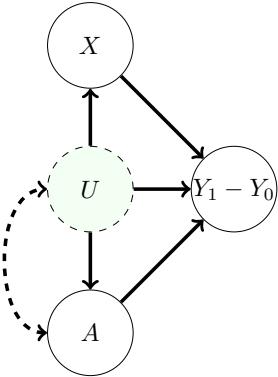
Figure 36.6: Causal graph assumed for the di!erence-in-di!erences setting. Here, the outcome of interest is the di!erence between the pre- and post-treatment period, Y¹ → Y0. This di!erence is influenced by the treatment, unobserved factors U, and observed covariates X. The dashed arrow between U and A indicates a statistical dependency between the variables, but where we remain agnostic to the precise causal mechanism. For example, in the minimum wage example, U might be the average income in restaurant’s neighbourhood, which is dependent on the state, and hence also the treatment.

distribution P(parents|A = a) by P(parents|A = 1), irrespective of the actual treatment value. This still breaks all backdoor associations, but is a better match for our target of estimating the treatment e!ect only among the treated units.

To formalize a causal estimand using the do-calculus, we need to assume some partial causal structure. We’ll use the graph in Figure 36.6. With this in hand, our causal estimand is the average treatment e!ect on the units that received the treatment, namely:

\[\text{ATT}^{\text{DiD}} = \mathbb{E}^{A=1} [Y\_1 - Y\_0 | \text{do}(A=1)] - \mathbb{E}^{A=1} [Y\_1 - Y\_0 | \text{do}(A=0)] \, \text{} \tag{36.91}\]

In the minimum wage example, this is the average e!ect of the minimum wage hike on employment in the restaurants a!ected by it (i.e., the ones in New Jersey).

Finally, we formalize the identification assumption that, conditional on X, the trends in the treated and untreated groups are the same. The conditional parallel trends assumption is:

\[\mathbb{E}^{A=1}[Y\_1 - Y\_0 | X, \text{do}(A=0)] = \mathbb{E}[Y\_1 - Y\_0 | X, A=0]. \tag{36.92}\]

In words, this says that for treated units with covariates X, the trend we would have seen had we not assigned treatment is the same as the trend we actually saw for the untreated units with covariates X. That is, if New Jersey had not raised its minimum wage, then McDonald’s in New Jersey would have the same expected change in employment as McDonald’s in Pennsylvania.

With this in hand, we can give the main identification result:

Theorem 5 (Di!erence in di!erences identification). We observe A, Y0, Y1, X ↘ P. Suppose that

• 1. (Causal structure) The data follows the causal graph in Figure 36.6.
• 2. (Conditional parallel trends) ^EA=1[Y^{1 ↓ Y}0|X, do(^A = 0)] = ^E[Y^{1 ↓ Y}0|X, A = 0].

3. (Overlap) P(A = 1) > 0 and P(A = 1|X = x) < 1 for all values of x in the sample space. That is, there are no covariate values that only exist in the treated group.

Then, the average treatment e!ect on the treated is identified as ATTDiD = ↼ DiD, where

\[\tau^{\rm DiD} = \mathbb{E}[\mathbb{E}[Y\_1 - Y\_0 | A=1, X] - \mathbb{E}[Y\_1 - Y\_0 | A=0, X] | A=1]. \tag{36.93}\]

Proof. First, by unrolling definitions, we have that

\[\mathbb{E}^{A=1}[Y\_1 - Y\_0 | \text{do}(A=1), X] = \mathbb{E}[Y\_1 - Y\_0 | A=1, X]. \tag{36.94}\]

The interpretation is the near-tautology that the average e!ect among the treated under treatment is equal to the actually observed average e!ect among the treated. Next,

\[\mathbb{E}^{A=1}[Y\_1 - Y\_0 | \text{do}(A=0), X] = \mathbb{E}[Y\_1 - Y\_0 | A=0, X]. \tag{36.95}\]

is just the conditional parallel trends assumption. The result follows immediately.

(The overlap assumption is required to make sure all the conditional expectations are well defined).

36.6.1 Estimation

With the identification result in hand, the next task is to estimate the observational estimand Equation (36.93). To that end, we define ^Y˜ ↭ ^{Y1 ↓ Y}0. Then, we’ve assumed that Y, X, A ˜ iid ↘ P for some unknown distribution ^P, and our target estimand is ^E[E[Y˜ ^|A = 1, X] ^{↓ E}[Y˜ ^|A = 0, X]|^A = 1]. We can immediately recognize this as the observational estimand that occurs in estimating the average treatment e!ect through adjustment, described in Section 36.4.5.3. That is, even though the causal situation and the identification argument are di!erent between the adjustment setting and the di!erence in di!erences setting, the statistical estimation task we end up with is the same. Accordingly, we can use all of the estimation tools we developed for adjustment. That is, all of the techniques there — expected outcome modeling, propensity score methods, double machine learning, and so forth — were purely about the statistical task, which is the same between the two scenarios.

So, we’re left with the same general recipe for estimation we saw in Section 36.4.6. Namely,

• 1. Fit statistical or machine-learning models ^Qˆ(a, x) as a predictor for ^Y˜ ^{= Y1 ↓ Y}0, and/or ^gˆ(x) as a predictor for A.
• 2. Compute the predictions Qˆ(0, xi), Qˆ(1, xi), gˆ(xi) for each datapoint.
• 3. Combine these predictions into an estimate of the average treatment e!ect on the treated.

The estimator in the third step can be the expected outcome model estimator, the propensity weighted estimator, the double machine learning estimator, or any other strategy that’s valid in the adjustment setting.

36.7 Credibility checks

Once we’ve chosen an identification strategy, fit our models, and produced an estimate, we’re faced with a basic question: should we believe it? Whether the reported estimate succeeds in capturing

the true causal e!ect depends on whether the assumptions required for causal identification hold, the quality of the machine learning models, and the variability in the estimate due to only having access to a finite data sample. The latter two problems are already familiar from machine learning and statistical practice. We should, e.g., assess our models by checking performance on held out data, examining feature importance, and so forth. Similarly, we should report measures of the uncertainity due to finite sample (e.g., in the form of confidence intervals). Because these procedures are already familiar practice, we will not dwell on them further. However, model evaluation and uncertainity quantification are key parts of any credible causal analysis.

Assessing the validity of identification assumptions is trickier. First, there are assumptions that can in fact be checked from data. For example, overlap should be checked in analysis using backdoor adjustment or di!erence in di!erences, and relevance should be checked in the instrumental variable setting. Again, checking these conditions is absolutely necessary for a credible causal analysis. But, again, this involves only familiar data analysis, so we will not discuss it further. Next, there are the causal assumptions that cannot be verified from data; e.g., no unobserved confounding in backdoor adjustment, the exclusion restriction in IV, and conditional parallel trends in DiD. Ultimately, the validity of these assumptions must be assessed using substantive causal knowledge of the particular problem under consideration. However, it is possible to conduct some supplementary analyses that make the required judgement easier. We now discusstwo such techniques.

36.7.1 Placebo checks

In many situations we may be able to find a variable that can be interepreted as a “treatment” that is known to have no e!ect on the outcome, but which we expect to be confounded with the outcome in a very similar fashion to the true treatment of interest. For example, if we’re trying to estimate the e”cacy of a COVID vaccine in preventing symptomatic COVID, we might take our placebo treatment to be vaccination against HPV. We do not expect that there’s any causal e!ect here. However, it seems plausible that latent factors that cause an individual to seek (or avoid) HPV vaccination and COVID vaccination are similar; e.g., health concientiousness, fear of needles, and so forth. Then, if our identification strategy is valid for the COVID vaccine, we’d also expect it to be to be valid for HPV vaccination. Accordingly, the estimation procedure we use for estimating the COVID e!ect should, when applied to HPV, yield ↼ˆ ≃ 0. Or, more precisely, the confidence interval should contain 0. If this does not happen, then we may suspect that there are still some confounding factors lurking that are not adequately handled by the identification procedure.

A similar procedure works when there is a variable that can be interpreted as an outcome which is known to not be a!ected by the treatment, but that shares confounders with the outcome we’re actually interested in. For example, in the COVID vaccination case, we might take the null outcome to be symptomatic COVID within 7 days of vaccination [Dag+21]. Our knowledge of both the biological mechanism of vaccination and the amount of time it takes to develop symptoms after COVID infection (at least 2 days) lead us to conclude that it’s unlikely that the treatment has a causal e!ect on the outcome. However, the properties of the treated people that a!ect how likely they are to develop symptomatic COVID are largely the same in the 7 day and, e.g., 6 month window. That includes factors such as risk aversion, baseline health, and so forth. Again, we can apply our identification strategy to estimate the causal e!ect of the treatment on the null outcome. If the confidence interval does not include 0, then we should doubt the credibility of the analysis.

36.7.2 Sensitivity analysis to unobserved confounding

We now specialize to the case of estimating the average causal e!ect of a binary treatment by adjusting for confounding variables, as described in Section 36.4. In this case, causal identification is based on the assumption of ‘no unobserved confounding’; i.e., the assumption that the observed covariates include all common causes of the treatment assignment and outcome. This assumption is fundamentally untestable from observed data, but its violation can induce bias in the estimation of the treatment e!ect — the unobserved confounding may completely or in part explain the observed association. Our aim in this part is to develop a sensitivity analysis tool to aid in reasoning about potential bias induced by unobserved confounding.

Intuitively, if we estimate a large positive e!ect then we might expect the real e!ect is also positive, even in the presence of mild unobserved confounding. For example, consider the association between smoking and lung cancer. One could argue that this association arises from a hormone that predisposes carriers to both an increased desire to smoke and to a greater risk of lung cancer. However, the association between smoking and lung cancer is large — is it plausible that some unknown hormonal association could have a strong enough influence to explain the association? Cornfield et al. [Cor+59] showed that, for a particular observational dataset, such an umeasured hormone would need to increase the probability of smoking by at least a factor of nine. This is an unreasonable e!ect size for a hormone, so they conclude it’s unlikely the causal e!ect can be explained away.

We would like a general procedure to allow domain experts to make judgments about whether plausible confounding is “mild” relative to the “large” e!ect. In particular, the domain expert must translate judgments about the strength of the unobserved confounding into judgments about the bias induced in the estimate of the e!ect. Accordingly, we must formalize what is meant by strength of unobserved confounding, and to show how to translate judgments about confounding strength into judgments about bias.

A prototypical example, due to Imbens [Imb03] (building on [RR83]), illustrates the broad approach. As above, the observed data consists of a treatment A, an outcome Y , and covariates X that may causally a!ect the treatment and outcome. Imbens [Imb03] then posits an additional unobserved binary confounder U for each patient, and supposes that the observed data and unobserved confounder were generated according to the following assumption, known as Imbens’ Sensitivity Model:

\[U\_i \stackrel{\text{iid}}{\sim} \text{Bern(1/2)}\tag{36.96}\]

\[A\_i|X\_i, U\_i \stackrel{ind}{\sim} \text{Bern}(\text{sig}(\gamma X\_i + \alpha U\_i))\tag{36.97}\]

\[Y\_i|X\_i, A\_i, U\_i \stackrel{\text{ind}}{\sim} \mathcal{N}(\tau A\_i + \beta X\_i + \delta U\_i, \sigma^2). \tag{36.98}\]

where sig is the sigmoid function.

If we had observed Ui, we could estimate (↼ˆ, γˆ, ⇁ˆ, ⇀ˆ, ˆε, φˆ²) from the data and report ↼ˆ as the estimate of the average treatment e!ect. Since Uⁱ is not observed, it is not possible to identify the parameters from the data. Instead, we make (subjective) judgments about plausible values of ⇀ how strongly Uⁱ a!ects the treatment assignment — and ε — how strongly Uⁱ a!ects the outcome. Contingent on plausible ⇀ = ⇀^→ and ε = ε→, the other parameters can be estimated. This yields an estimate of the treatment e!ect ↼ˆ(⇀→, ε→) under the presumed values of the sensitivity parameters.

The approach just outlined has a major drawback: it relies on a parametric model for the full data generating process. The assumed model is equivalent to assuming that, had U been observed, it

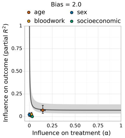
Figure 36.7: Austen plot showing how strong an unobserved confounder would need to be to induce a bias of 2 in an observational study of the e!ect of combination blood pressure medications on diastolic blood pressure [Dor+16]. We chose this bias to equal the nominal average treatment e!ect estimated from the data. We model the outcome with Bayesian Additive Regression Trees and the treatment assignment with logistic regression. The curve shows all values treatment and outcome influence that would induce a bias of 2. The colored dots show the influence strength of (groups of) observed covariates, given all other covariates. For example, an unobserved confounder with as much influence as the patient’s age might induce a bias of about 2.

would have been appropriate to use logistic regression to model treatment assignment, and linear regression to model the outcome. This assumption also implies a simple, parametric model for the relationships governing the observed data. This restriction is out of step with modern practice, where we use flexible machine-learning methods to model these relationships. For example, the assumption forbids the use of neural networks or random forests, though such methods are often state-of-the-art for causal e!ect estimation.

Austen plots We now turn to developing an alternative an adaptation of Imbens’ approach that fully decouples sensitivity analysis and modeling of the observed data. Namely, the Austen plots of [VZ20]. An example Austen plot is shown in Figure 36.7. The high-level idea is to posit a generative model that uses a simple, interpretable parametric form for the influence of the unobserved confounder, but that puts no constraints on the model for the observed data. We then use the parametric part of the model to formalize “confounding strength” and to compute the induced bias as a function of the confounding.

Austen plots further adapt two strategies pioneered by Imbens [Imb03]. First, we find a parameterization of the model so that the sensitivity parameters, measuring strength of confounding, are on a standardized, unitless scale. This allows us to compare the strength of hypothetical unobserved confounding to the strength of observed covariates, measured from data. Second, we plot the curve of all values of the sensitivity parameter that would yield given level of bias. This moves the analyst

judgment from “what are plausible values of the sensitivity parameters?” to “are sensitivity parameters this extreme plausible?”

Figure 36.7, an Austen plot for an observational study of the e!ect of combination medications on diastolic blood pressure, illustrates the idea. A bias of 2 would su”ce to undermine the qualitative conclusion that the blood-pressure treatment is e!ective. Examining the plot, an unobserved confounder as strong as age could induce this amount of confounding, but no other (group of) observed confounders has so much influence. Accordingly, if a domain expert thinks an unobserved confounder as strong as age is unlikely then they may conclude that the treatment is likely e!ective. Or, if such a confounder is plausible, they may conclude that the study fails to establish e”cacy.

Setup The data are generated independently and identically (Yi, Ai, Xi, Ui) iid ↘ P, where Uⁱ is not observed and P is some unknown probability distribution. The approach in Section 36.4 assumes that the observed covariates X contain all common causes of Y and A. If this ‘no unobserved confounding’ assumption holds, then the ATE is equal to parameter, ↼ , of the observed data distribution, where

\[\tau = \mathbb{E}[\mathbb{E}[Y|X, A=1] - \mathbb{E}[Y|X, A=0]].\tag{36.99}\]

This observational parameter is then estimated from a finite data sample. Recall from Section 36.4 that this involves estimating the conditional expected outcome Q(A, X) = E[Y |A, X] and the propensity score g(X) = P(A = 1|X), then plugging these into an estimator ↼ˆ.

We are now concerned with the case of possible unobserved confounding. That is, where U causally a!ects Y and A. If there is unobserved confounding then the parameter ↼ is not equal to the ATE, so ↼ˆ is a biased estimate. Inference about the ATE then divides into two tasks. First, the statistical task: estimating ↼ as accurately as possible from the observed data. And, second, the causal (domain-specific) problem of assessing bias = ATE ↓ ↼ . We emphasize that our focus here is bias due to causal misidentification, not the statistical bias of the estimator. Our aim is to reason about the bias induced by unobserved confounding — the second task — in a way that imposes no constraints on the modeling choices for Qˆ, gˆ, and ↼ˆ used in the statistical analysis.

Sensitivity model Our sensitivity analysis should impose no constraints on how the observed data is modeled. However, sensitivity analysis demands some assumption on the relationship between the observed data and the unobserved confounder. It is convenient to formalize such assumptions by specifying a probabilistic model for how the data is generated. The strength of confounding is then formalized in terms of the parameters of the model (the sensitivity parameters). Then, the bias induced by the confounding can be derived from the assumed model. Our task is to posit a generative model that both yields a useful and easily interpretable sensitivity analysis, and that avoids imposing any assumptions about the observed data.

To begin, consider the functional form of the sensitivity model used by Imbens [Imb03].

\[\text{logit}(\mathbf{P}(A=1|x,u)) = h(x) + \alpha u \tag{36.100}\]

\[\mathbb{E}[Y|a, x, u] = l(a, x) + \delta u,\tag{36.101}\]

for some functions h and l. That is, the propensity score is logit-linear in the unobserved confounder, and the conditional expected outcome is linear.

By rearranging Equation (36.100) to solve for u and plugging in to Equation (36.101), we see that it’s equivalent to assume ^E[^{Y |}t, x, u] = ˜l(t, x) + ˜εlogitP(^A = 1|x, u). That is, the unobserved

confounder u only influences the outcome through the propensity score. Accordingly, by positing a distribution on P(A = 1|x, u) directly, we can circumvent the need to explicitly articulate U (and h).

Definition 36.7.1. Let g˜(x, u) = P(A = 1|x, u) denote the propensity score given observed covariates x and the unobserved confounder u.

The insight is that we can posit a sensitivity model by defining a distribution on g˜ directly. We choose:

\[|\tilde{g}(X,U)|X \sim \text{Beta}(g(X)(1/\alpha - 1), (1 - g(X))(1/\alpha - 1)).\]

That is, the full propensity score g˜(X, U) for each unit is assumed to be sampled from a Beta distribution centered at the observed propensity score g(X). The sensitivity parameter ⇀ plays the same role as in Imbens’ model: it controls the influence of the unobserved confounder U on treatment assignment. When ⇀ is close to 0 then g˜(X, U)|X is tightly concentrated around g(X), and the unobserved confounder has little influence. That is, U minimally a!ects our belief about who is likely to receive treatment. Conversely, when ⇀ is close to 1 then g˜ concentrates near 0 and 1; i.e., knowing U would let us accurately predict treatment assignment. Indeed, it can be shown that ⇀ is the change in our belief about how likely a unit was to have gotten the treatment, given that they were actually observed to be treated (or not):

\[\alpha = \mathbb{E}[\tilde{g}(X, U) | A = 1] - \mathbb{E}[\tilde{g}(X, U) | A = 0]. \tag{36.102}\]

With the g˜ model in hand, we define the Austen sensitivity model as follows:

\[|\tilde{g}(X,U)|X \sim \text{Beta}(g(X)(1/\alpha - 1), (1 - g(X))(1/\alpha - 1))\tag{36.103}\]

\[A|X, U \sim \text{Bern}(\tilde{g}(X, U))\tag{36.104}\]

\[\mathbb{E}[Y|A,X,U] = Q(A,X) + \delta \left( \text{logit} \bar{g}(X,U) - \mathbb{E}[\text{logit} \bar{g}(X,U)|A,X] \right). \tag{36.105}\]

This model has been constructed to satisfy the requirement that the propensity score and conditional expected outcome are the g and Q actually present in the observed data:

\[\begin{aligned} \mathbb{P}(A=1|X) &= \mathbb{E}[\mathbb{E}[T|X,U]|X] = \mathbb{E}[\tilde{g}(X,U)|X] = g(X),\\ \mathbb{E}[Y|A,X] &= \mathbb{E}[\mathbb{E}[Y|A,X,U]|A,X] = Q(A,X). \end{aligned}\]

The sensitivity parameters are ⇀, controlling the dependence between the unobserved confounder and the treatment assignment, and ε, controlling the relationship with the outcome.

Bias We now turn to calculating the bias induced by unobserved confounding. By assumption, X and U together su”ce to render the average treatment e!ect identifiable as:

ATE = E[E[Y |A = 1, X, U] ↓ E[Y |A = 0, X, U]].

Plugging in our sensitivity model yields,

\[\mathbf{ATE} = \mathbb{E}[Q(1, X) - Q(0, X)] + \delta(\mathbb{E}[\operatorname{logit}\tilde{g}(X, U) | X, A = 1] - \mathbb{E}[\operatorname{logit}\tilde{g}(X, U) | X, A = 0]).\]

The first term is the observed-data estimate ↼ , so

bias = ε(E[logit˜g(X, U)|X, A = 1] ↓ E[logit˜g(X, U)|X, A = 0]).

Then, by invoking beta-Bernoulli conjugacy and standard beta identities,11 we arrive at,

11. We also use the recurrence relation ↽(x + 1) ↓ ↽(x)=1/x, where ↽ is the digamma function.

Theorem 6. Under the Austen sensitivity model, Equation (36.105), an unobserved confounder with influence ⇀ and ε induces bias in the estimated treatment e!ect equal to

\[\mathbf{bias} = \frac{\delta}{1/\alpha - 1} \mathbb{E} \left[ \frac{1}{g(X)} + \frac{1}{1 - g(X)} \right].\]

That is, the amount of bias is determined by the sensitivity parameters and by the realized propensity score. Notice that more extreme propensity scores lead to more extreme bias in response to unobserved confounding. This means, in particular, that conditioning on a covariate that a!ects the treatment but that does not directly a!ect the outcome (an instrument) will increase any bias due to unobserved confounding. This general phenomena is known as z-bias.

Sensitivity parameters The Austen model provides a formalization of confounding strength in terms of the parameters ⇀ and ε and tells us how much bias is induced by a given strength of confounding. This lets us translate judgments about confounding strength to judgments about bias. However, it is not immediately obvious how to translate qualitative judgements such as “I think any unobserved confounder would be much less important than age” to judgements about the possible values of the sensitivity parameters.

First, because the scale of ε is not fixed, it may be di”cult to compare the influence of potential unobserved confounders to the influence of reference variables. To resolve this, we reexpress the outcome-confounder strength in terms of the (non-parametric) partial coe”cient of determination:

\[R\_{Y, \text{par}}^2(\alpha, \delta) = 1 - \frac{\mathbb{E}(Y - \mathbb{E}[Y | A, X, U])^2}{\mathbb{E}(Y - Q(A, X))^2}.\]

The key to computing the reparameterization is the following result

Theorem 7. Under the Austen sensitivity model, Equation (36.105), the outcome influence is

\[R\_{Y, \text{par}}^2(\alpha, \delta) = \delta^2 \sum\_{a=0}^1 \frac{\mathbb{E}[\psi\_1 \{ g(X)^a (1 - g(X))^{1 - a} (1/\alpha - 1) + 1 [A = a] \} ]}{\mathbb{E}[(Y - Q(A, X))^2]},\]

where 6¹ is the trigamma function.

See Veitch and Zaveri [VZ20] for the proof.

By design, ⇀ — the strength of confounding influence on on treatment assignment — is already on a fixed, unitless scale. However, because the measure is tied to the model it may be di”cult to interpret, and it is not obvious how to compute reference confounding strength values from the observed data. The next result clarifies these issues.

Theorem 8. Under the Austen sensitivity model, Equation (36.105),

\[\alpha = 1 - \frac{\mathbb{E}[\tilde{g}(X, U)(1 - \tilde{g}(X, U))]}{\mathbb{E}[g(X)(1 - g(X))]}.\]

See Veitch and Zaveri [VZ20] for the proof. That is, the sensitivity parameter ⇀ measures how much more extreme the propensity scores become when we condition on U. That is, ⇀ is a measure

of the extra predictive power U adds for A, above and beyond the predictive power in X. It may also be insightful to notice that

\[\alpha = R\_{A, \text{par}}^2 = 1 - \frac{\mathbb{E}[(A - \hat{g}(X, U))^2]}{\mathbb{E}[(A - g(X))^2]}. \tag{36.106}\]

That is, ⇀ is just the (non-parametric) partial coe”cient of determination of U on A—the same measure used for the outcome influence. (To see this, just expand the expectations conditional on A = 1 and A = 0).

Estimating bias In combination, Theorems 6 and 7 yield an expression for the bias in terms of ⇀ and R² Y,par. In practice, we can estimate the bias induced by confounding by fitting models for ^Qˆ and gˆ and replacing the expectations by means over the data.

36.7.2.1 Calibration using observed data

The analyst must make judgments about the influence a hypothetical unobserved confounder might have on treatment assignment and outcome. To calibrate such judgments, we’d like to have a reference point for how much the observed covariates influence the treatment assignment and outcome. In the sensitivity model, the degree of influence is measured by partial R^{2 Y} and ⇀. We want to measure the degree of influence of an observed covariate Z given the other observed covariates *X.

For the outcome, this can be measured as:

\[R\_{Y\cdot Z\vert T,X\backslash Z}^2 \triangleq 1 - \frac{\mathbb{E}(Y - Q(A,X))^2}{\mathbb{E}(Y - \mathbb{E}[Y|A,X\backslash Z])^2}.\]

In practice, we can estimate the quantity by fitting a new regression model Qˆ^Z that predicts Y from A and *X. Then we compute

\[R\_{Y \cdot Z \mid T, X \nmid Z}^2 = 1 - \frac{\frac{1}{n} \sum\_{i} (y\_i - \hat{Q}(t\_i, x\_i))^2}{\frac{1}{n} \sum\_{i} (y\_i - \hat{Q}\_Z(t\_i, x\_i \backslash z\_i))^2}.\]

Using Theorem 8, we can measure influence of observed covariate Z on treatment assignment given Xin an analogous fashion to the outcome. We define g^X<sup>Z(X) = P(A = 1|X), then fit a model for g^X<sup>Z* by predicting A from *X, and estimate

\[ \hat{\alpha}\_{Z|X\backslash Z} = 1 - \frac{\frac{1}{n} \sum\_{i} \hat{g}(x\_i)(1 - \hat{g}(x\_i))}{\frac{1}{n} \sum\_{i} \hat{g}\_{X\backslash Z}(x\_i \backslash z\_i)(1 - \hat{g}\_{X\backslash Z}(x\_i \backslash z\_i))}. \]

Grouping covariates The estimated values ⇀ˆ^X<sup>Z and ^Rˆ² Y,X<sup>Z measure the influence of ^Z conditioned on all the other confounders. In some cases, this can be misleading. For example, if some piece of information is important but there are multiple covariates providing redundant measurements, then the estimated influence of each covariate will be small. To avoid this, group together related or strongly dependent covariates and compute the influence of the entire group in aggregate. For example, grouping income, location, and race as ‘socioeconomic variables’.

36.7.2.2 Practical use

We now have su”cient results to produce Austen plots such as Figure 36.7. At a high level, the procedure is:

• 1. Produce an estimate ↼ˆ using any modeling tools. As a component of this, estimate the propensity score gˆ and conditional outcome model Qˆ.
• 2. Pick a level of bias that would su”ce to change the qualitative interpretation of the estimate (e.g., the lower bound of a 95% confidence interval).
• 3. Plot the values of ⇀ and R² Y,par that would su”ce to induce that much bias. This is the black curve on the plot. To calculate these values, use Theorems 6 and 7 together with the estimated gˆ and Qˆ.
• 4. Finally, compute reference influence level for (groups of) observed covariates. In particular, this requires fitting reduced models for the conditional expected outcome and propensity that do not use the reference covariate as a feature.

In practice, an analyst only needs to do the model fitting parts themselves. The bias calculations, reference value calculations, and plotting can be done automatically with standard libraries.12.

Austen plots are predicated on Equation (36.105). This assumption replaces the purely parametric Equation (36.98) with a version that eliminates any parametric requirements on the observed data. However, we emphasize that Equation (36.105) does, implicitly, impose some parametric assumption on the structural causal relationship between U and A, Y . Ultimately, any conclusion drawn from the sensitivity analysis depends on this assumption, which is not justified on any substantive grounds. Accordingly, such sensitivity analyses can only be used to informally guide domain experts. They do not circumvent the need to thoroughly adjust for confounding. This reliance on a structural assumption is a generic property of sensitivity analysis.13 Indeed, there are now many sensitivity analysis models that allow the use of any machine learning model in the data analysis [e.g., RRS00; FDF19; She+11; HS13; BK19; Ros10; Yad+18; ZSB19; Sch+21a]. However, none of these are yet in routine use in practice. We have presented Austen plots here not because they make an especially virtuous modeling assumption, but because they are (relatively) easy to understand and interpret.

Austen plots are most useful in situations where the conclusion from the plot would be ‘obvious’ to a domain expert. For instance, in Figure 36.7, we can be confident that an unobserved confounder similar to socioeconomic status would not induce enough bias to change the qualitative conclusion. By contrast, Austen plots should not be used to draw conclusions such as, “I think a latent confounder could only be 90% as strong as ‘age’, so there is evidence of a small non-zero e!ect”. Such nuanced conclusions might depend on issues such as the particular sensitivity model we use, or finite-sample variation of our bias and influence estimates, or on incautious interpretation of the calibration dots. These issues are subtle, and it would be di”cult to resolve them to a su”cient degree that a sensitivity analysis would make an analysis credible.

^12. See github.com/vveitch/causality-tutorials/blob/main/Sensitivity\_Analysis.ipynb.

^13. In extreme cases, there can be so little unexplained variation in A or Y that only a very weak confounder could be compatible with the data. In this case, essentially assumption free sensitivity analysis is possible [Man90].

Calibration using observed data The interpretation of the observed-data calibration requires some care. The sensitivity analysis requires the analyst to make judgements about the strength of influence of the unobserved confounder U, conditional on the observed covariates X. However, we report the strength of influence of observed covariate(s) Z, *conditional on the other observed covariates X. The di!erence in conditioning sets can have subtle e!ects.

Cinelli and Hazlett [CH20] give an example where Z and U are identical variables in the true model, but where influence of U given A, X is larger than the influence of Z given A, X. (The influence of Z* given X, U would be the same as the influence of U given X). Accordingly, an analyst is not justified in a judgment such as, “I know that U and Z are very similar. I see Z has substantial influence, but the dot is below the line. Thus, U will not undo the study conclusions”. In essence, if the domain expert suspects a strong interaction between U and Z then naively eyeballing the dot-vs-line position may be misleading. A particular subtle case is when U and Z are independent variables that both strongly influence A and Y . The joint influence on A creates an interaction e!ect between them when A is conditioned on (the treatment is a collider). This a!ects the interpretation of R^{2 Y} ·U|X,A. Indeed, we should generally be skeptical of sensitivity analysis interpretation when it is expected that a strong confounder has been omitted. In such cases, our conclusions may depend substantively on the particular form of our sensitivity model, or other unjustifiable assumptions.

Although the interaction problem is conceptually important, its practical significance is unclear. We often expect the opposite e!ect: if U and Z are dependent (e.g., race and wealth) then omitting U should increase the apparent importance of Z — leading to a conservative judgement (a dot artifically towards the top right part of the plot).

36.8 The do-calculus

We have seen several strategies for identifying causal e!ects as parameters of observational distributions. Confounder adjustment (Section 36.4) relied only on the assumed causal graph (and overlap), which specified that we observe all common causes of A and Y . On the other hand, instrumental variable methods and di!erence-in-di!erences each relied on both an assumed causal graph and partial functional form assumptions about the underlying structural causal model. Because functional form assumptions can be quite di”cult to justify on substantive grounds, it’s natural to ask when causal identification is possible from the causal graph alone. That is, when can we be agnostic to the particular functional form of the structural causal models?

There is a general “calculus of intervention”, known as the do-calculus, that gives a general recipe for determining when the causal assumptions expressed in a causal graph can be used to identify causal e!ects [Pea09c]. The do-calculus is a set of three rewrite rules that allows us to replace statements where we condition on variables being set by intervention, e.g. P(Y |do(A = a)), with statements involving only observational quantities, e.g. EX[P(Y |A = a, X)]. When causal identification is possible, we can repeatedly apply the three rules to boil down our target causal parameter into an expression involving only the observational distribution.

36.8.1 The three rules

To express the rules, let X, Y , Z, and W be arbitrary disjoint sets of variables in a causal DAG G.

Rule 1 The first rule allows us to insert or delete observations z:

\[p(y|\text{do}(x), z, w) = p(y|\text{do}(x), w) \text{ if } (Y \perp Z|X, W)\_{G\_{\overline{X}}} \tag{36.107}\]

where G^X denotes cutting edges going into X, and (Y ¬ Z|X,W)G^X denotes conditional independence in the mutilated graph. The rule follows from d-separation in the mutilated graph. This rule just says that conditioniong on irrelevant variables leaves the distribution invariant (as we would expect).

Rule 2 The second rule allows us to replace do(z) with conditioning on (seeing) z. The simplest case where can do this is: if Z is a root of the causal graph (i.e., it has no causal parents) then p(y|do(z)) = p(y|z). The reason is that the do operator is equivalent to conditioning in the mutilated causal graph where all the edges into Z are removed, but, because Z is a root, the mutilated graph is just the original causal graph. The general form of this rule is:

\[p(y|\text{do}(x), \text{do}(z), w) = p(y|\text{do}(x), z, w) \text{ if } (Y \perp Z | X, W)\_{\text{G}\_{\overline{X}\underline{Z}}} \tag{36.108}\]

where GXZ cuts edges going into X and out of Z. Intutively, we can replace do(z) by z as long as there are no backdoor (non-directed) paths between z and y. If there are in fact no such paths, then cutting all the edges going out of Z will mean there are no paths connecting Z and Y , so that Y ¬¬ Z. The rule just generalizes this line of reasoning to allow for extra observed and intervened variables.

Rule 3 The third rule allows us to insert or delete actions do(z):

\[p(y|\text{do}(x), \text{do}(z), w) = p(y|\text{do}(x), w) \text{ if } (Y \perp Z | X, W)\_{G\_{\overline{XZ}^\pi}} \tag{36.109}\]

where GXZ^↑ cuts edges going into X and Z→, and where Z^→ is the set of Z-nodes that are not ancestors of any W-node in GX. Intuitively, this condition corresponds to intervening on X, and checking whether the distribution of Y is invariant to any intervention that we could apply on Z.

36.8.2 Revisiting backdoor adjustment

We begin with a more general form of the adjustment formula we used in Section 36.4.

First, suppose we observe all of A’s parents, call them X. For notational simplicity, we’ll assume for the moment that X is discrete. Then,

\[p(Y=y|\text{do}(A=a)) = \sum\_{x} p(Y=y|x, \text{do}(A=a)) p(x|\text{do}(A=a)) \tag{36.110}\]

\[y = \sum\_{x} p(Y=y|x, A=a)p(x). \tag{36.111}\]

The first line is just a standard probability relation (marginalizing over x). We are using causal assumptions in two ways in the second line. First, p(x|do(A = a)) = p(x): the treatment has no causal e!ect on X, so interventions on A don’t change the distribution of X. This is rule 3, Equation (36.109). Second, p(Y = y|x, do(A = a)) = p(Y = y|x, A = a). This equality holds because conditioning on the parents blocks all non-directed paths from A to Y , reducing the causal e!ect to be the same as the observational e!ect. The equality is an application of rule 2, Equation (36.108).

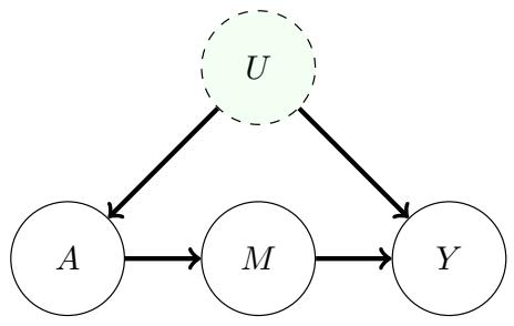
Figure 36.8: Causal graph illustrating the frontdoor criterion setup. The e!ect of the treatment A on outcome Y is entirely mediated by mediator M. This allows us infer the causal e!ect even if the treatment and outcome are confounded by U.

Now, what if we don’t observe all the parents of A? The key issue is backdoor paths: paths between A and Y that contain an arrow into A. These paths are the general form of the problem that occurs when A and Y share a common cause. Suppose that we can find a set of variables S such that (1) no node in S is a descendant of A; and (2) S blocks every backdoor path between A and Y . Such a set is said to satisfy the backdoor criterion. In this case, we can use S instead of X in the adjustment formula, Equation (36.111). That is,

\[p(Y=y|\text{do}(A=a)) = \mathbb{E}\_S[p(Y=y|S,A=a)].\tag{36.112}\]

The proof follows the invocation of rules 3 and 2, in the same way as for the case where S is just the parents of A. Notice that requiring S to not contain any descendants of A means that we don’t risk conditioning on any variables that mediate the e!ect, nor any variables that might be colliders either would undermine the estimate.

The backdoor adjustment formula generalizes the adjust-for-parents approach and adjust-for-allcommon-causes approach of Section 36.4. That’s because both the parents of A and the common causes satisfy the backdoor criterion.

In practice, the full distribution p(Y = y|do(A = a)) is rarely used as the causal target. Instead, we try to estimate a low-dimensional parameter of this distribution, such as the average treatment e!ect. The adjustment formula immediately translates in the obvious way. If we define

\[\tau = \mathbb{E}\_S[\mathbb{E}[Y|A=1, S] - \mathbb{E}[Y|A=0, S]],\]

then we have that ATE = ↼ whenever S satisfies the backdoor criteria. The parameter ↼ can then be estimated from finite data using the methods described in Section 36.4, using S in place of the common causes X.

36.8.3 Frontdoor adjustment

Backdoor adjustment is applicable if there’s at least one observed variable on every backdoor path between A and Y . As we have seen, identification is sometimes still possible even when this condition doesn’t hold. Frontdoor adjustment is another strategy of this kind. Figure 36.8 shows the causal

structure that allows this kind of adjustment strategy. Suppose we’re interested in the e!ect of smoking A on developing cancer Y , but we’re concerned about some latent genetic confounder U.

Suppose that all of the directed paths from A to Y pass through some set of variables M. Such variables are called mediators. For example, the e!ect of smoking on lung cancer might be entirely mediated by the amount of tar in the lungs and measured tissue damage. It turns out that if all such mediators are observed, and the mediators do not have an unobserved common cause with A or Y , then causal identification is possible. To understand why this is true, first notice that we can identify the causal e!ect of A on M and the causal e!ect of M on A, both by backdoor adjustment. Further, the mechanism of action of A on Y is: A changes M which in turn changes Y . Then, we can combine these as:

\[p(Y|\text{do}(A=a)) = \sum\_{m} p(Y|\text{do}(M=m))p(M=m|\text{do}(A=a))\tag{36.113}\]

\[=\sum\_{m}\sum\_{a'}p(Y|a',m)p(a')p(m|a)\tag{36.114}\]

The second line is just backdoor adjustment applied to identify each of the do expressions (note that A blocks the M-Y backdoor path through U).

Equation (36.114) is called the front-door formula [Pea09b, §3.3.2]. To state the result in more general terms, let us introduce a definition. We say a set of variables M satisfies the front-door criterion relative to an ordered pair of variables (A, Y ) if (1) M intercepts all directed paths from A to Y ; (2) there is no unblocked backdoor path from A to M; and (3) all backdoor paths from M to Y are blocked by A. If M satisfies this criterion, and if p(A, M) > 0 for all values of A and M, then the causal e!ect of A on Y is identifiable and is given by Equation (36.114).

Let us interpret this theorem in terms of our smoking example. Condition 1 means that smoking A should have no e!ect on cancer Y except via tar and tissue damage M. Conditions 2 and 3 mean that the genotype U cannot have any e!ect on M except via smoking A. Finally, the requirement that p(A, M) > 0 for all values implies that high levels of tar in the lungs must arise not only due to smoking, but also other factors (e.g., pollutants). In other words, we require p(A = 0, M = 1) > 0 so we can assess the impact of the mediator in the untreated setting.

We can now use the do-calculus to derive the frontdoor criterion; following [PM18b, p236]. Assuming

the causal graph G shown in Figure 36.8:

\[\begin{aligned} p(y|\text{do}(a)) &= \sum\_{m} p(y|\text{do}(a), m) p(m|\text{do}(a)) & \text{(probability axioms)} \\ &= \sum\_{m} p(y|\text{do}(a), \text{do}(m)) p(m|\text{do}(a)) & \text{(rule 2 using } G\_{\overline{\mathfrak{S}}^{\*}}) \\ &= \sum\_{m} p(y|\text{do}(a), \text{do}(m)) p(m|a) & \text{(rule 2 using } G\_{\overline{\mathfrak{S}}^{\*}}) \\ &= \sum\_{m} p(y|\text{do}(m)) p(m|a) & \text{(rule 3 using } G\_{\overline{\mathfrak{S}}^{\*}}) \\ &= \sum\_{a'} \sum\_{m} p(y|\text{do}(m), a') p(a'|\text{do}(m)) p(m|a) & \text{(probability axioms)} \\ &= \sum\_{a'} \sum\_{m} p(y|m, a') p(a'|\text{do}(m)) p(m|a) & \text{(rule 2 using } G\_{\overline{\mathfrak{S}}^{\*}}) \\ &= \sum\_{a'} \sum\_{m} p(y|m, a') p(a') p(m|a) & \text{(rule 3 using } G\_{\overline{\mathfrak{S}}^{\*}}) \end{aligned}\]

Estimation To estimate the causal distribution from data using the frontdoor criterion we need to estimate each of p(y|m, a), p(a), and p(m|a). In practice, we can fit models pˆ(y|m, a) by predicting Y from M and A, and pˆ(m|a) by predicting M from A. We can estimate p(a) by the empirical distribution of A. Then,

\[\sum\_{a'} \sum\_{m} \hat{p}(a')\hat{p}(y|m,a')\hat{p}(m|a),\tag{36.115}\]

We usually have more modest targets than the full distribution p(y|do(a)). For instance, we may be content with just estimating the average treatment e!ect. It’s straightforward to derive a formula for this using the frontdoor adjustment. Similarly to backdoor adjustment, more advanced estimators of the ATE through frontdoor e!ect are possible in principle. For example, we might combine fitted models for E[Y |m, a] and P(M|a). See Fulcher et al. [Ful+20] for an approach to robust estimation via front door adjustment, as well as a generalization of the front door approach to more general settings.

36.9 Further reading

There is an enormous and growing literature on the intersection of causality and machine learning.

First, there are many textbooks on theoretical and practical elements of causal inference. These include Pearl [Pea09c], focused on causal graphs, Angrist and Pischke [AP08], focused on econometrics, Hernán and Robins [HR20b], with roots in epidemiology, Imbens and Rubin [IR15], with origin in statistics, and Morgan and Winship [MW15], for a social sciences perspective. The introduction to causality in Shalizi [Sha22, §7] is also recommended, particularly the treatment of matching.

Double machine-learning has featured prominently in this chapter. This is a particular instantiation of non-parametric estimation. This topic has substantial theoretical and practical importance in modern causal inference. The double machine learning work includes estimators for many commonly encountered scenarios [Che+17e; Che+17d]. Good references for a lucid explanation of how and why non-parametric estimation works include [Ken16; Ken17; FK21]. Usually, the key guarantees of non-parametric estimator are asymptotic. Generally, there are many estimators that share optimal asymptotic guarantees (e.g., the AIPTW estimator given in Equation (36.30)). Although these are asymptotically equivalent, in finite samples their behavior can be very di!erent. There are estimators that preserve asymptotic guarantees but aim to improve performance in practical finite sample regimes [e.g., vR11].

There is also considerable interest in the estimation of heterogeneous treatment e!ects. The question here is: what e!ect would this treatment have when applied to a unit with such-and-such specific characteristics? E.g., what is the e!ect of this drug on women over the age of 50? The causal identification arguments used here are more-or-less the same as for the estimation of average case e!ects. However, the estimation problems can be substantially more involved. Some reading includes [Kün+19; NW20; Ken20; Yad+21].

There are several commonly applicable causal identification and estimation strategies beyond the ones we’ve covered in this chapter. Regression discontinuity designs rely on the presence of some sharp, arbitrary non-linearity in treatment assignment. For example, eligibility for some aid programs is determined by whether an individual has income below or above a fixed amount. The e!ect of the treatment can be studied by comparing units just below and just above this threshhold. Synthetic controls are a class of methods that try to study the e!ect of a treatment on a given unit by constructing a synthetic version of that unit that acts as a control. For example, to study the e!ect of legislation banning smoking indoors in California, we can construct a synthetic California as a weighted average of other states, with weights chosen to balance demographic characteristics. Then, we can compare the observed outcome of California with the outcome of the synthetic control, constructed as the weighted average of the outcomes of the donor states. See Angrist and Pischke [AP08] for a textbook treatment of both strategies. Closely related are methods that use time series modeling to create synthetic outcomes. For example, to study the e!ect of an advertising campaign beginning at time T on product sales Yt, we might build a time series model for Y^t using data in the t<T period, and then use this model to predict the values of (Yˆt)t>T we would have seen had the campaign not been run. We can estimate the causal e!ect by comparing the factual, realized Y^t to the predicted, counterfactual, Yˆt. See Brodersen et al. [Bro+15] for an instantiation of this idea.

In this chapter, our focus has been on using machine learning tools to estimate causal e!ects. There is also a growing interest in using the ideas of causality to improve machine learning tools. This is mainly aimed at building predictors that are robust when deployed in new domains [SS18b; SCS19; Arj+20; Mei18b; PBM16a; RC+18; Zha+13a; Sch+12b; Vei+21] or that do not rely on particular ‘spurious’ correlations in the training data [RPH21; Wu+21; Gar+19; Mit+20; WZ19; KCC20; KHL20; TAH20; Vei+21]