Probabilistic Machine Learning: Advanced Topics

Chapter 20 ~ 33

Part IV

Generation

20 Generative models: an overview

20.1 Introduction

A generative model is a joint probability distribution p(x), for x → X . In some cases, the model may be conditioned on inputs or covariates c → C, which gives rise to a conditional generative model of the form p(x|c).

There are many kinds of generative models. We give a brief summary in Section 20.2, and go into more detail in subsequent chapters. See also [Tom22] for a recent book on this topic that goes into more depth.

20.2 Types of generative model

There are many kinds of generative model, some of which we list in Table 20.1. At a high level, we can distinguish between deep generative models (DGM) — which use deep neural networks to learn a complex mapping from a single latent vector z to the observed data x — and more “classical” probabilistic graphical models (PGM), that map a set of interconnected latent variables z1,…, z^L to the observed variables x1,…, x^D using simpler, often linear, mappings. Of course, many hybrids are possible. For example, PGMs can use neural networks, and DGMs can use structured state spaces. We discuss PGMs in general terms in Chapter 4, and give examples in Chapter 28, Chapter 29, Chapter 30. In this part of the book, we mostly focus on DGMs.

The main kinds of DGM are: variational autoencoders (VAE), autoregressive models (ARM), normalizing flows, di!usion models, energy based models (EBM), and generative adversarial networks (GAN). We can categorize these models in terms of the following criteria (see Figure 20.1 for a visual summary):

• Density: does the model support pointwise evaluation of the probability density function p(x), and if so, is this fast or slow, exact, approximate or a bound, etc? For implicit models, such as GANs, there is no well-defined density p(x). For other models, we can only compute a lower bound on the density (VAEs), or an approximation to the density (EBMs, UPGMs).
• Sampling: does the model support generating new samples, x ↑ p(x), and if so, is this fast or slow, exact or approximate? Directed PGMs, VAEs, and GANs all support fast sampling. However, undirected PGMs, EBMs, ARM, di!usion, and flows are slow for sampling.
• Training: what kind of method is used for parameter estimation? For some models (such as AR, flows and directed PGMs), we can perform exact maximum likelihood estimation (MLE), although

Model	Chapter	Density	Sampling	Training	Latents	Architecture
PGM-D	Section 4.2	Exact, fast	Fast	MLE	Optional	Sparse DAG
PGM-U	Section 4.3	Approx, slow	Slow	MLE-A	Optional	Sparse graph
VAE	Chapter 21	LB, fast	Fast	MLE-LB	RL	Encoder-Decoder
ARM	Chapter 22	Exact, fast	Slow	MLE	None	Sequential
Flows	Chapter 23	Exact, slow/fast	Slow	MLE	RD	Invertible
EBM	Chapter 24	Approx, slow	Slow	MLE-A	Optional	Discriminative
Di!usion	Chapter 25	LB	Slow	MLE-LB	RD	Encoder-Decoder
GAN	Chapter 26	NA	Fast	Min-max	RL	Generator-Discriminator

Table 20.1: Characteristics of common kinds of generative model. Here D is the dimensionality of the observed x, and L is the dimensionality of the latent z, if present. (We usually assume L → D, although overcomplete representations can have L ↑ D.) Abbreviations: Approx = approximate, ARM = autoregressive model, EBM = energy based model, GAN = generative adversarial network, MLE = maximum likelihood estimation, MLE-A = MLE (approximate), MLE-LB = MLE (lower bound), NA = not available, PGM = probabilistic graphical model, PGM-D = directed PGM, PGM-U = undirected PGM, VAE = variational autoencoder.

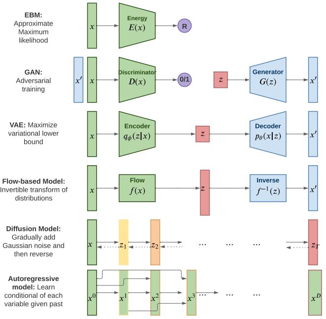
Figure 20.1: Summary of various kinds of deep generative models. Here x is the observed data, z is the latent code, and x^→ is a sample from the model. AR models do not have a latent code z. For di!usion models and flow models, the size of z is the same as x. For AR models, x^d is the d’th dimension of x. R represents real-valued output, 0/1 represents binary output. Adapted from Figure 1 of [Wen21].

the objective is usually non-convex, so we can only reach a local optimum. For other models, we cannot tractably compute the likelihood. In the case of VAEs, we maximize a lower bound on the likelihood; in the case of EBMs and UGMs, we maximize an approximation to the likelihood. For GANs we have to use min-max training, which can be unstable, and there is no clear objective function to monitor.

• Latents: does the model use a latent vector z to generate x or not, and if so, is it the same size as x or is it a potentially compressed representation? For example, ARMs do not use latents; flows and di!usion use latents, but they are not compressed.1 Graphical models, including EBMs, may or may not use latents.
• Architecture: what kind of neural network should we use, and are there restrictions? For flows, we are restricted to using invertible neural networks where each layer has a tractable Jacobian. For EBMs, we can use any model we like. The other models have di!erent restrictions.

20.3 Goals of generative modeling

There are several di!erent kinds of tasks that we can use generative models for, as we discuss below.

20.3.1 Generating data

One of the main goals of generative models is to generate (create) new data samples. This is sometimes called generative AI (see e.g., [GBGM23] for a recent survey). For example, if we fit a model p(x) to images of faces, we can sample new faces from it, as illustrated in Figure 25.10. 2 Similar methods can be used to create samples of text, audio, etc. When this technology is abused to make fake content, they are called deep fakes (see e.g., [Ngu+19]). Generative models can also be used to create synthetic data for training discriminative models (see e.g., [Wil+20; Jor+22]).

To control what is generated, it is useful to use a conditional generative model of the form p(x|c). Here are some examples:

• c = text prompt, x = image. This is a text-to-image model (see Figure 20.2, Figure 20.3 and Figure 22.6 for examples).
• c = image, x = text. This is an image-to-text model, which is useful for image captioning.
• c = image, x = image. This is an image-to-image model, and can be used for image colorization, inpainting, uncropping, JPEG artefact restoration, etc. See Figure 20.4 for examples.
• c = sequence of sounds, x = sequence of words. This is a speech-to-text model, which is useful for automatic speech recognition (ASR).
• c = sequence of English words, x = sequence of French words. This is a sequence-to-sequence model, which is useful for machine translation.

^1. Flow models define a latent vector z that has the same size as x, although the internal deterministic computation may use vectors that are larger or smaller than the input (see e.g., the DenseFlow paper [GGS21]).

^2. These images were made with a technique called score-based generative modeling (Section 25.3), although similar results can be obtained using many other techniques. See for example https://this-person-does-not-exist.com/en which shows results from a GAN model (Chapter 26).

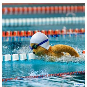
(a) Teddy bears swimming at the Olympics 400m Butterfly event.

(b) A cute corgi lives in a house made out of sushi.

(c) A cute sloth holding a small treasure chest. A bright golden glow is coming from the chest.

Figure 20.2: Some 1024 ↓ 1024 images generated from text prompts by the Imagen di!usion model (Section 25.6.4). From Figure 1 of [Sah+22b]. Used with kind permission of William Chan.

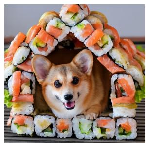
Figure 20.3: Some images generated from the Parti transformer model (Section 22.4.2) in response to a text prompt. We show results from models of increasing size (350M, 750M, 3B, 20B). Multiple samples are generated, and the highest ranked one is shown. From Figure 10 of [Yu+22]. Used with kind permission of Jiahui Yu.

• c = initial prompt, x = continuation of the text. This is another sequence-to-sequence model, which is useful for automatic text generation (see Figure 22.5 for an example).

Note that, in the conditional case, we sometimes denote the inputs by x and the outputs by y. In this case the model has the familiar form p(y|x). In the special case that y denotes a low dimensional quantity, such as a integer class label, y → {1,…,C}, we get a predictive (discriminative) model. The main di!erence between a discriminative model and a conditional generative model is this: in a discriminative model, we assume there is one correct output, whereas in a conditional generative model, we assume there may be multiple correct outputs. This makes it harder to evaluate generative models, as we discuss in Section 20.4.

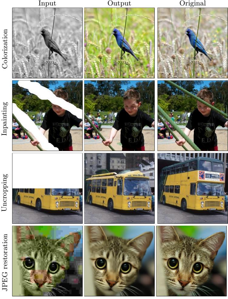
Figure 20.4: Illustration of some image-to-image tasks using the Palette conditional di!usion model (Section 25.6.4). From Figure 1 of [Sah+22a]. Used with kind permission of Chitwan Saharia.

20.3.2 Density estimation

The task of density estimation refers to evaluating the probability of an observed data vector, i.e., computing p(x). This can be useful for outlier detection (Section 19.3.2), data compression (Section 5.4), generative classifiers, model comparison, etc.

A simple approach to this problem, which works in low dimensions, is to use kernel density

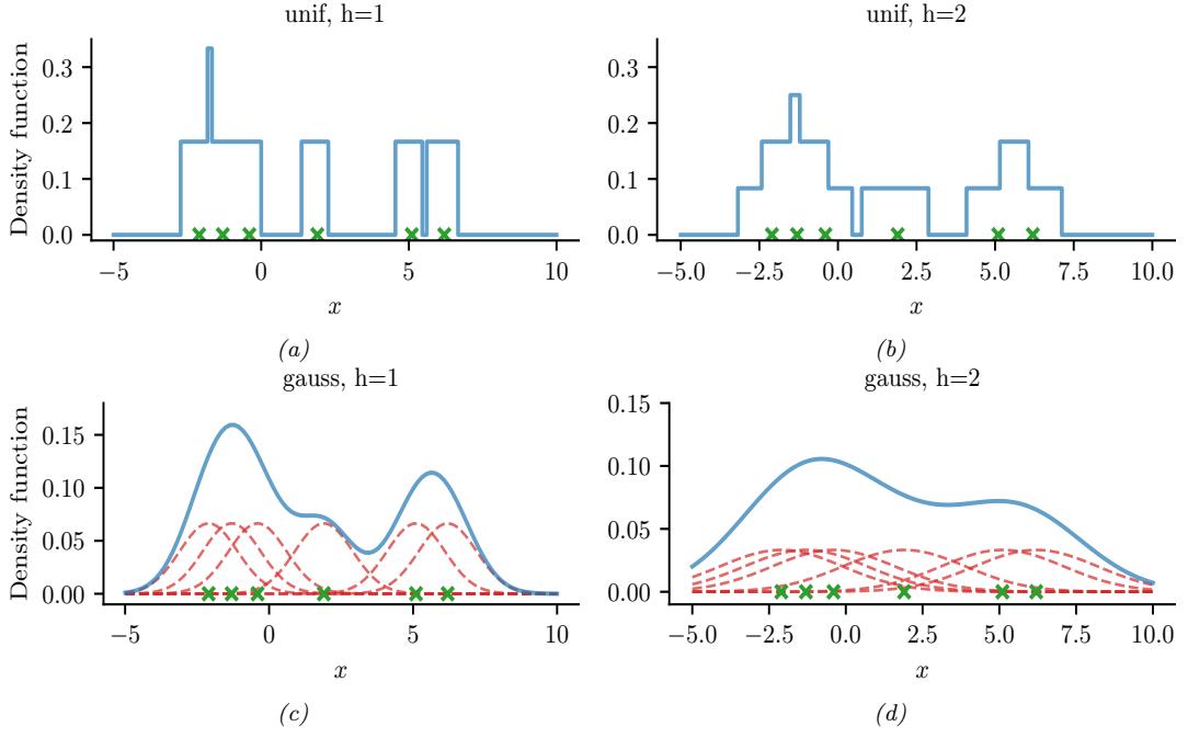
Figure 20.5: A nonparametric (Parzen) density estimator in 1d estimated from 6 datapoints, denoted by x. Top row: uniform kernel. Bottom row: Gaussian kernel. Left column: bandwidth parameter h = 1. Right column: bandwidth parameter h = 2. Adapted from http: // en. wikipedia. org/ wiki/ Kernel\_ density\_ estimation . Generated by parzen\_window\_demo.ipynb.

estimation or KDE, which has the form

\[p(\mathbf{z}|\mathcal{D}) = \frac{1}{N} \sum\_{n=1}^{N} \mathcal{K}\_h \left(\mathbf{z} - \mathbf{z}\_n\right) \tag{20.1}\]

Here D = {x1,…, x^N } is the data, and K^h is a density kernel with bandwidth h, which is a function ^K : ^{R ↔︎ R+} such that ” ^K(x)dx = 1 and ” ^xK(x)dx = 0. We give a 1d example of this in Figure 20.5: in the top row, we use a uniform (boxcar) kernel, and in the bottom row, we use a Gaussian kernel.

In higher dimensions, KDE su!ers from the curse of dimensionality (see e.g., [AHK01]), and we need to use parametric density models pω(x) of some kind.

20.3.3 Imputation

The task of imputation refers to “filling in” missing values of a data vector or data matrix. For example, suppose X is an N ↗ D matrix of data (think of a spreadsheet) in which some entries, call them Xm, may be missing, while the rest, Xo, are observed. A simple way to fill in the missing data is to use the mean value of each feature, E [xd]; this is called mean value imputation, and is

Input			Output
A	B	C		A	B	C
6	6	NA		6	6	7.5
NA	6	0		9	6	0
NA	6	NA		9	6	7.5
10	10	10		10	10	10
10	10	10		10	10	10
10	10	10		10	10	10
9	8	7.5		9	8	7.5

Figure 20.6: Missing data imputation. Left: input data: NA means “not available” (missing), and the bottom row (in red) shows the mean of each column. Right: output data, where NA values are replaced by the mean.

illustrated in Figure 20.6. However, this ignores dependencies between the variables within each row, and does not return any measure of uncertainty.

We can generalize this by fitting a generative model to the observed data, p(Xo), and then computing samples from p(Xm|Xo). This is called multiple imputation. We can fit the model to partially observed data using methods such as EM (Section 6.5.3). (See e.g., [ZFY24] for a recent approach using EM and di!usion models (Chapter 25).) A generative model can also be used to fill in more complex data types, such as in-painting occluded pixels in an image (see Figure 20.4).

See Section 3.11 for a more general discussion of missing data.

20.3.4 Structure discovery

Some kinds of generative models have latent variables z, which are assumed to be the “causes” that generated the observed data x. We can use Bayes’ rule to invert the model to compute p(z|x) ↘ p(z)p(x|z). This can be useful for discovering latent, low-dimensional patterns in the data.

For example, suppose we perturb various proteins in a cell and measure the resulting phosphorylation state using a technique known as flow cytometry, as in [Sac+05]. An example of such a dataset is shown in Figure 20.7(a). Each row represents a data sample ^{xn ↑ p}(·|an, ^z), where ^{x → R11} is a vector of outputs (phosphorylations), ^{a →} {0, 1}⁶ is a vector of input actions (perturbations) and z is the unknown cellular signaling network structure. We can infer the graph structure p(z|D) using graphical model structure learning techniques (see Section 30.3). In particular, we can use the dynamic programming method described in [EM07] to get the result shown in Figure 20.7(b). Here

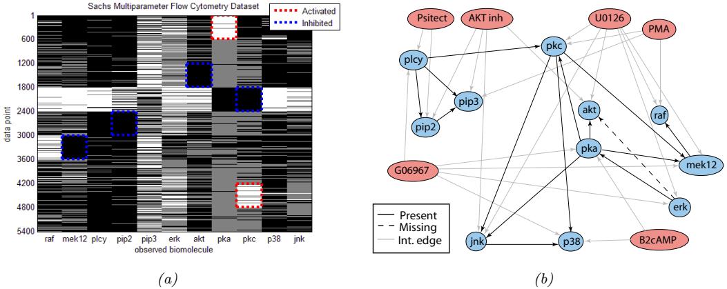
Figure 20.7: (a) A design matrix consisting of 5400 datapoints (rows) measuring the state (using flow cytometry) of 11 proteins (columns) under di!erent experimental conditions. The data has been discretized into 3 states: low (black), medium (grey), and high (white). Some proteins were explicitly controlled using activating or inhibiting chemicals. (b) A directed graphical model representing dependencies between various proteins (blue circles) and various experimental interventions (pink ovals), which was inferred from this data. We plot all edges for which p(Gij = 1|D) > 0.5. Dotted edges are believed to exist in nature but were not discovered by the algorithm (1 false negative). Solid edges are true positives. The light colored edges represent the e!ects of intervention. From Figure 6d of [EM07].

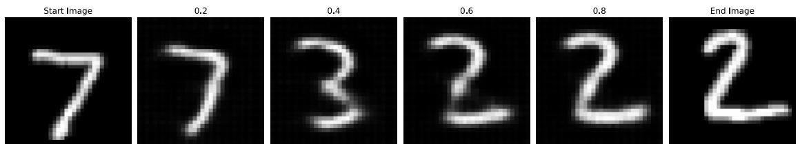
Figure 20.8: Interpolation between two MNIST images in the latent space of a ω-VAE (with ω = 0.5). Generated by mnist\_vae\_ae\_comparison.ipynb.

we plot the median graph, which includes all edges for which p(zij = 1|D) > 0.5. (For a more recent approach to this problem, see e.g., [Bro+20b].)

20.3.5 Latent space interpolation

One of the most interesting abilities of certain latent variable models is the ability to generate samples that have certain desired properties by interpolating between existing datapoints in latent space. To explain how this works, let x¹ and x² be two inputs (e.g., images), and let z¹ = e(x1) and z² = e(x2) be their latent encodings. (The method used for computing these will depend on the type of model; we discuss the details in later chapters.) We can regard z¹ and z² as two “anchors” in

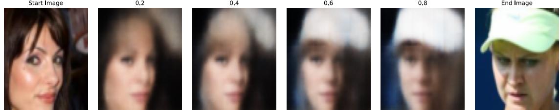
Figure 20.9: Interpolation between two CelebA images in the latent space of a ω-VAE (with ω = 0.5). Generated by celeba\_vae\_ae\_comparison.ipynb.

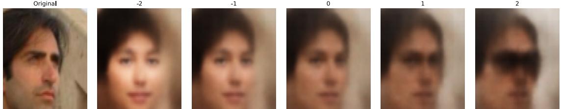
Figure 20.10: Arithmetic in the latent space of a ω-VAE (with ω = 0.5). The first column is an input image, with embedding z. Subsequent columns show the decoding of z + s!, where s ↔︎ {↗2, ↗1, 0, 1, 2} and ! ^{= z+} ↗ ^z↑ is the di!erence in the average embeddings of images with or without a certain attribute (here, wearing sunglasses). Generated by celeba\_vae\_ae\_comparison.ipynb.

latent space. We can now generate new images that interpolate between these points by computing z = ωz¹ + (1 ↓ ω)z2, where 0 ≃ ω ≃ 1, and then decoding by computing x^→ = d(z), where d() is the decoder. This is called latent space interpolation, and will generate data that combines semantic features from both x¹ and x2. (The justification for taking a linear interpolation is that the learned manifold often has approximately zero curvature, as shown in [SKTF18]. However, sometimes it is better to use nonlinear interpolation [Whi16; MB21; Fad+20].)

We can see an example of this process in Figure 20.8, where we use a ε-VAE model (Section 21.3.1) fit to the MNIST dataset. We see that the model is able to produce plausible interpolations between the digit 7 and the digit 2. As a more interesting example, we can fit a ε-VAE to the CelebA dataset [Liu+15].3 The results are shown in Figure 20.9, and look reasonable. (We can get much better quality if we use a larger model trained on more data for a longer amount of time.)

It is also possible to perform interpolation in the latent space of text models, as illustrated in Figure 21.7.

20.3.6 Latent space arithmetic

In some cases, we can go beyond interpolation, and can perform latent space arithmetic, in which we can increase or decrease the amount of a desired “semantic factor of variation”. This was first

^3. CelebA contains about 200k images of famous celebrities. The images are also annotated with 40 attributes. We reduce the resolution of the images to 64 → 64, as is conventional.

shown in the word2vec model [Mik+13], but it also is possible in other latent variable models. For example, consider our VAE model fit to the CelebA dataset, which has faces of celebrities and some corresponding attributes. Let X^{+ i} be a set of images which have attribute i, and X^{↑ i} be a set of images which do not have this attribute. Let Z^{+ i} and Z^{↑ i} be the corresponding embeddings, and z⁺ i and z^{↑ i} be the average of these embeddings. We define the o!set vector as !ⁱ = z^{+ i} ↓ z^{↑ i} . If we add some positive multiple of !ⁱ to a new point z, we increase the amount of the attribute i; if we subtract some multiple of !i, we decrease the amount of the attribute i [Whi16].

We give an example of this in Figure 20.10. We consider the attribute of wearing sunglasses. The j’th reconstruction is computed using xˆ^j = d(z + sj!), where z = e(x) is the encoding of the original image, and s^j is a scale factor. When s^j > 0 we add sunglasses to the face. When s^j < 0 we remove sunglasses; but this also has the side e!ect of making the face look younger and more female, possibly a result of dataset bias.

20.3.7 Generative design

Another interesting use case for (deep) generative models is generative design, in which we use the model to generate candidate objects, such as molecules, which have desired properties (see e.g., [RNA22]). One approach is to fit a VAE to unlabeled samples, and then to perform Bayesian optimization (Section 6.6) in its latent space, as discussed in Section 21.3.5.2.

20.3.8 Model-based reinforcement learning

We discuss reinforcement learning (RL) in Chapter 35. The main success stories of RL to date have been in computer games, where simulators exist and data is abundant. However, in other areas, such as robotics, data is expensive to acquire. In this case, it can be useful to learn a generative “world model”, so the agent can do planning and learning “in its head”. See Section 35.4 for more details.

20.3.9 Representation learning

Representation learning refers to learning (possibly uninterpretable) latent factors z that generate the observed data x. The primary goal is for these features to be used in “downstream” supervised tasks. This is discussed in Chapter 32.

20.3.10 Data compression

Models which can assign high probability to frequently occuring data vectors (e.g., images, sentences), and low probability to rare vectors, can be used for data compression, since we can assign shorter codes to the more common items. Indeed, the optimal coding length for a vector x from some stochastic source p(x) is l(x) = ↓ log p(x), as proved by Shannon. See Section 5.4 for details.

20.4 Evaluating generative models

This section is written by Mihaela Rosca, Shakir Mohamed, and Balaji Lakshminarayanan.

Evaluating generative models requires metrics which capture

• sample quality — are samples generated by the model a part of the data distribution?

• sample diversity are samples from the model distribution capturing all modes of the data distribution?
• generalization is the model generalizing beyond the training data?

There is no known metric which meets all these requirements, but various metrics have been proposed to capture di!erent aspects of the learned distribution, some of which we discuss below.

20.4.1 Likelihood-based evaluation

A standard way to measure how close a model q is to a true distribution p is in terms of the KL divergence (Section 5.1):

\[D\_{\mathbb{KL}}\left(p \parallel q\right) = \int p(\mathbf{z}) \log \frac{p(\mathbf{z})}{q(\mathbf{z})} = -\mathbb{H}\left(p\right) + \mathbb{H}\_{\text{ce}}\left(p, q\right) \tag{20.2}\]

where H (p) is a constant, and Hce (p, q) is the cross entropy. If we approximate p(x) by the empirical distribution, we can evaluate the cross entropy in terms of the empirical negative log likelihood on the dataset:

\[\text{NLL} = -\frac{1}{N} \sum\_{n=1}^{N} \log q(\mathbf{z}\_n) \tag{20.3}\]

Usually we care about negative log likelihood on a held-out test set.4

20.4.1.1 Computing the log-likelihood

For models of discrete data, such as language models, it is easy to compute the (negative) log likelihood. However, it is common to measure performance using a quantity called perplexity, which is defined as 2^H, where H = NLL is the cross entropy or negative log likelihood.

For image and audio models, one complication is that the model is usually a continuous distribution ^p(x) ^⇒ 0 but the data is usually discrete (e.g., ^{x →} {0,…, 255}^D if we use one byte per pixel). Consequently the average log likelihood can be arbitrary large, since the pdf can be bigger than 1. To avoid this it is standard pratice to use uniform dequantization [TOB16], in which we add uniform random noise to the discrete data, and then treat it as continuous-valued data. This gives a lower bound on the average log likelihood of the discrete model on the original data.

To see this, let z be a continuous latent variable, and x be a vector of binary observations computed by rounding, so ^p(x|z) = ^ϑ(^{x ↓} round(z)), computed elementwise. We have ^p(x) = ” ^p(x|z)p(z)dz. Let q(z|x) be a probabilistic inverse of x, that is, it has support only on values where p(x|z)=1. In this case, Jensen’s inequality gives

\[\log p(\mathbf{z}) \ge \mathbb{E}\_{q(\mathbf{z}|\mathbf{z})} \left[ \log p(\mathbf{z}|\mathbf{z}) + \log p(\mathbf{z}) - \log q(\mathbf{z}|\mathbf{z}) \right] \tag{20.4}\]

\[=\mathbb{E}\_{q(\mathbf{z}|\mathbf{z})}\left[\log p(\mathbf{z}) - \log q(\mathbf{z}|\mathbf{x})\right] \tag{20.5}\]

Thus if we model the density of z ↑ q(z|x), which is a dequantized version of x, we will get a lower bound on p(x).

^4. In some applications, we report bits per dimension, which is the log likelihood using log base 2, divided by the dimensionality of ^x. To compute this metric, recall that log^{2 L =} log^{e L} log^{e 2} , and hence bpd = NLL loge(2) ^{1 |}x^| .

20.4.1.2 Likelihood can be hard to compute

Unfortunately, for many models, computing the likelihood can be computationally expensive, since it requires knowing the normalization constant of the probability model. One solution is to use variational inference (Chapter 10), which provides a way to e”ciently compute lower (and sometimes upper) bounds on the log likelihood. Another solution is to use annealed importance sampling (Section 11.5.4.1), which provides a way to estimate the log likelihood using Monte Carlo sampling. However, in the case of implicit generative models, such as GANs (Chapter 26), the likelihood is not even defined, so we need to find evaluation metrics that do not rely on likelihood.

20.4.1.3 Likelihood is not related to sample quality

A more subtle concern with likelihood is that it is often uncorrelated with the perceptual quality of the samples, at least for real-valued data, such as images and sound. In particular, a model can have great log-likelihood but create poor samples and vice versa.

To see why a model can have good likelihoods but create bad samples, consider the following argument from [TOB16]. Suppose q⁰ is a density model for D-dimensional data x which performs arbitrarily well as judged by average log-likelihood, and suppose q¹ is a bad model, such as white noise. Now consider samples generated from the mixture model

\[q\_2(\mathbf{x}) = 0.01q\_0(\mathbf{x}) + 0.99q\_1(\mathbf{x})\tag{20.6}\]

Clearly 99% of the samples will be poor. However, the log-likelihood per pixel will hardly change between q² and q⁰ if D is large, since

\[\log q\_2(\mathbf{z}) = \log[0.01q\_0(\mathbf{z}) + 0.99q\_1(\mathbf{z})] \ge \log[0.01q\_0(\mathbf{z})] = \log q\_0(\mathbf{z}) - 2\tag{20.7}\]

For high-dimensional data, | log q0(x)| ↑ D ⇑ 100, so log q2(x) ⇓ log q0(x), and hence mixing in the poor sampler does not significantly impact the log likelihood.

Now consider a case where the model has good samples but bad likelihoods. To achieve this, suppose q is a GMM centered on the training images:

\[q(\mathbf{z}) = \frac{1}{N} \sum\_{n=1}^{N} \mathcal{N}(\mathbf{z}|\mathbf{z}\_n, \epsilon^2 \mathbf{I}) \tag{20.8}\]

If ϖ is small enough that the Gaussian noise is imperceptible, then samples from this model will look good, since they correspond to the training set of real images. But this model will almost certainly have poor likelihood on the test set due to overfitting. (In this case we say the model has e!ectively just memorized the training set.)

20.4.2 Distances and divergences in feature space

Due to the challenges associated with comparing distributions in high dimensional spaces, and the desire to compare distributions in a semantically meaningful way, it is common to use domain-specific perceptual distance metrics, that measure how similar data vectors are to each other or to the training data. However, most metrics used to evaluate generative models do not directly compare raw data (e.g., pixels) but use a neural network to obtain features from the raw data and compare

the feature distribution obtained from model samples with the feature distribution obtained from the dataset. The neural network used to obtain features can be trained solely for the purpose of evaluation, or can be pretrained; a common choice is to use a pretrained classifier (see e.g., [Sal+16; Heu+17b; Bin+18; Kyn+19; SSG18a]).

The Inception score [Sal+16] measures the average KL divergence between the marginal distribution of class labels obtained from the samples ^pω(y) = ” ^pdisc(y|x)pω(x)d^x (where the integral is approximated by sampling images x from a fixed dataset) and the distribution p(y|x) induced by samples from the model, x ↑ pω(x). (The term comes from the “Inception” model [Sze+15b] that is often used to define pdisc(y|x).) This leads to the following score:

\[\text{IS} = \exp\left[\mathbf{E}\_{p\_{\theta}(\mathbf{z})} D\_{\text{KL}}\left(p\_{\text{disc}}(Y|\mathbf{z}) \parallel p\_{\theta}(Y)\right)\right] \tag{20.9}\]

To understand this, let us rewrite the log score as follows:

\[\log(\text{IS}) = \mathbb{H}(p\_{\theta}(Y)) - \mathbb{E}\_{p\_{\theta}(\mathbf{z})} \left[ \mathbb{H}(p\_{\text{disc}}(Y|\mathbf{z})) \right] \tag{20.10}\]

Thus we see that a high scoring model will be equally likely to generate samples from all classes, thus maximizing the entropy of pω(Y ), while also ensuring that each individual sample is easy to classify, thus minimizing the entropy of pdisc(Y |x).

The Inception score solely relies on class labels, and thus does not measure overfitting or sample diversity outside the predefined dataset classes. For example, a model which generates one perfect example per class would get a perfect Inception score, despite not capturing the variety of examples inside a class, as shown in Figure 20.11a. To address this drawback, the Fréchet Inception distance or FID score [Heu+17b] measures the Fréchet distance between two Gaussian distributions on sets of features of a pre-trained classifier. One Gaussian is obtained by passing model samples through a pretrained classifier, and the other by passing dataset samples through the same classifier. If we assume that the mean and covariance obtained from model features are µ^m and “^m and those from the data are µ^d and”d, then the FID is

\[\text{FID} = \|\mu\_m - \mu\_d\|\_2^2 + \text{tr}\left(\Sigma\_d + \Sigma\_m - 2(\Sigma\_d \Sigma\_m)^{1/2}\right) \tag{20.11}\]

Since it uses features instead of class logits, the Fréchet distance captures more than modes captured by class labels, as shown in Figure 20.11b. Unlike the Inception score, a lower score is better since we want the two distributions to be as close as possible.

Unfortunately, the Fréchet distance has been shown to have a high bias, with results varying widely based on the number of samples used to compute the score. To mitigate this issue, the kernel Inception distance has been introduced [Bin+18], which measures the squared MMD (Section 2.7.3) between the features obtained from the data and features obtained from model samples.

20.4.3 Precision and recall metrics

Since the FID only measures the distance between the data and model distributions, it is di”cult to use it as a diagnostic tool: a bad (high) FID can indicate that the model is not able to generate high quality data, or that it puts too much mass around the data distribution, or that the model only captures a subset of the data (e.g., in Figure 26.6). Trying to disentangle between these two failure modes has been the motivation to seek individual precision (sample quality) and recall (sample

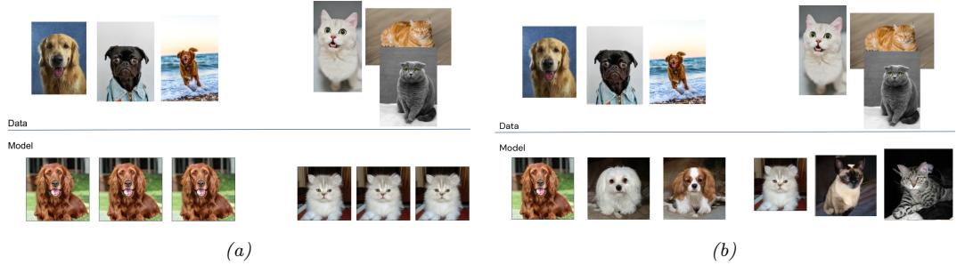
Figure 20.11: (a) Model samples with good (high) inception score are visually realistic. (b) Model samples with good (low) FID score are visually realistic and diverse.

diversity) metrics in the context of generative models [LPO17; Kyn+19]. (The diversity question is especially important in the context of GANs, where mode collapse (Section 26.3.3) can be an issue.)

A common approach is to use nearest neighbors in the feature space of a pretrained classifier to define precision and recall [Kyn+19]. To formalize this, let us define

\[f\_k(\phi, \Phi) = \begin{cases} 1 & \text{if } \exists \phi' \in \Phi s.t. \left\| |\phi - \phi'| \right\|\_2^2 \le \left\| \phi' - \text{NN}\_k(\phi', \Phi) \right\|\_2^2\\ 0 & \text{otherwise} \end{cases} \tag{20.12}\]

where ! is a set of feature vectors and NNk(ϱ^→ , !) is a function returning the k’th nearest neighbor of ϱ^→ in !. We now define precision and recall as follows:

\[\text{precision}(\Phi\_{model}, \Phi\_{data}) = \frac{1}{|\Phi\_{model}|} \sum\_{\phi \in \Phi\_{model}} f\_k(\phi, \Phi\_{data});\tag{20.13}\]

\[\text{recall}(\Phi\_{model}, \Phi\_{data}) = \frac{1}{|\Phi\_{data}|} \sum\_{\phi \in \Phi\_{data}} f\_k(\phi, \Phi\_{model});\tag{20.14}\]

Precision and recall are always between 0 and 1. Intuitively, the precision metric measures whether samples are as close to data as data is to other data examples, while recall measures whether data is as close to model samples as model samples are to other samples. The parameter k controls how lenient the metrics will be — the higher k, the higher both precision and recall will be. As in classification, precision and recall in generative models can be used to construct a trade-o! curve between di!erent models which allows practitioners to make an informed decision regarding which model they want to use.

20.4.4 Statistical tests

Statistical tests have long been used to determine whether two sets of samples have been generated from the same distribution; these types of statistical tests are called two sample tests. Let us define the null hypothesis as the statement that both set of samples are from the same distribution. We then compute a statistic from the data and compare it to a threshold, and based on this we decide whether to reject the null hypothesis. In the context of evaluating implicit generative models

such as GANs, statistics based on classifiers [Saj+18] and the MMD [Liu+20b] have been used. For use in scenarios with high dimensional input spaces, which are ubiquitous in the era of deep learning, two sample tests have been adapted to use learned features instead of raw data.

Like all other evaluation metrics for generative models, statistical tests have their own advantages and disadvantages: while users can specify Type 1 error — the chance they allow that the null hypothesis is wrongly rejected — statistical tests tend to be computationally expensive and thus cannot be used to monitor progress in training; hence they are best used to compare fully trained models.

20.4.5 Challenges with using pretrained classifiers

While popular and convenient, evaluation metrics that rely on pretrained classifiers (such as IS, FID, nearest neighbors in feature space, and statistical tests in feature space) have significant drawbacks. One might not have a pretrained classifier available for the dataset at hand, so classifiers trained on other datasets are used. Given the well known challenges with neural network generalization (see Section 17.4), the features of a classifier trained on images from one dataset might not be reliable enough to provide a fine grained signal of quality for samples obtained from a model trained on a di!erent dataset. If the generative model is trained on the same dataset as the pre-trained classifier but the model is not capturing the data distribution perfectly, we are presenting the pre-trained classifier with out-of-distribution data and relying on its features to obtain score to evaluate our models. Far from being purely theoretical concerns, these issues have been studied extensively and have been shown to a!ect evaluation in practice [RV19; BS18].

20.4.6 Using model samples to train classifiers

Instead of using pretrained classifiers to evaluate samples, one can train a classifier on samples from conditional generative models, and then see how good these classifiers are at classifying data. For example, does adding synthetic (sampled) data to the real data help? This is closer to a reliable evaluation of generative model samples, since ultimately, the performance of generative models is dependent on the downstream task they are trained for. If used for semisupervised learning, one should assess how much adding samples to a classifier dataset helps with test accuracy. If used for model based reinforcement learning, one should assess how much the generative model helps with agent performance. For examples of this approach, see e.g., [SSM18; SSA18; RV19; SS20b; Jor+22].

20.4.7 Assessing overfitting

Many of the metrics discussed so far capture the sample quality and diversity, but do not capture overfitting to the training data. To capture overfitting, often a visual inspection is performed: a set of samples is generated from the model and for each sample its closest K nearest neighbors in the feature space of a pretrained classifier are obtained from the dataset. While this approach requires manually assessing samples, it is a simple way to test whether a model is simply memorizing the data. We show an example in Figure 20.12: since the model sample in the top left is quite di!erent than its neighbors from the dataset (remaining images), we can conclude the sample is not simply memorised from the dataset. Similarly, sample diversity can be measured by approximating the support of the learned distribution by looking for similar samples in a large sample pool — as in the pigeonhole principle — but it is expensive and often requires manual human assessment[AZ17].

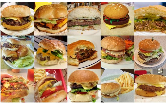
Figure 20.12: Illustration of nearest neighbors in feature space: in the top left we have the query sample generated using BigGAN, and the rest of the images are its nearest neighbors from the dataset. The nearest neighbors search is done in the feature space of a pretrained classifier. From Figure 13 of [BDS18]. Used with kind permission of Andy Brock.

For likelihood-based models — such as variational autoencoders (Chapter 21), autoregressive models (Chapter 22), and normalizing flows (Chapter 23) — we can assess memorization by seeing how much the log-likelihood of a model changes when a sample is included in the model’s training set or not [BW21].

20.4.8 Human evaluation

One approach to evaluate generative models is to use human evaluation, by presenting samples from the model alongside samples from the data distribution, and ask human raters to compare the quality of the samples [Zho+19b]. Human evaluation is a suitable metric if the model is used to create art or other data for human display, or if reliable automated metrics are hard to obtain. However, human evaluation can be di”cult to standardize, hard to automate, and can be expensive or cumbersome to set up.

20.5 Training objectives5

So far we have not discussed how to train generative models. Most of the book adopts an approach based on (regularized) maximum likelihood estimation, or some approximation thereof (see the “Training” column of Table 20.1). In MLE, the training objective is to maximize Ep(x) [log q(x)] = ↓DKL (p ⇐ q) + const, where p is the target distribution (usually approximated by the empirical data distribution) and q is the model distribution which we are learning. However, this objective can have some fundamental flaws when modeling high dimensional continuous distributions, where ^{x → RD}. In particular, suppose the target distribution p lies on a low-dimensional manifold, meaning that ^p(x) ^&gt; ⁰ only for ^{x → M} where ^{M = Rd→} is a low-dimensional subspace with dimension d^↔︎ which is

^5. This section was newly added in September 2024.

less than the ambient dimension D. (This is called the manifold hypothesis, and is a reasonable assumption for many natural distributions, such as the set of natural images.) By contrast, the likelihood objective assumes that p(x) is defined over the entire ambient space, RD, in order for the above expectation to be well defined. If p is not defined on the full space, maximizing likelihood is no longer a good objective, since there can be many distributions q that assign infinite likelihood to the manifold ^M, while not matching ^p. (This is because ^M is “too thin” relative to ^RD.) (A simple example is when p is a mixture of two delta functions, and q is a GMM; in this case, the variance of each mixture component will go to 0, to approximate the two “spikes”. This drives the likelihood to infinity, but q may still assign wrong mixture weights to each component.) See [LG+23; LG+24] for an extensive discussion of this point.

There are three main types of solution to this problem. The first is to add noise to the data vectors, so they “fill the space”. This ensures that both p and q both have support over all D dimensions. One approach to this is to use di!usion models, which add noise at many di!erent levels (see Chapter 25). Another approach is to replace the KL with the spread KL divergence [Zha+20c], which is defined as ^DKL^ε(p||q) = ^DKL(pε||qε), where ^pε = ^p ↭ ^N (·|0, ^ς2ID) and ^qε = ^q ↭ ^N (·|0, ^ς2ID) are smoothed versions of the distribution obtained by convolving with a Gaussian. This ensures the KL is always finite. We can then optimize the modified KL using a latent variable model of the form ^q(x) = ^N (x|gω(z), ^ς2I), where ^g : ^{Rd ↔︎ RD} is a deterministic decoder and ^{z ↑ N} (0, Id) is a low-dimensional stochastic latent variable. After training, we can “turn o!” the noise from the decoder, so that q has the same support as the manifold of p; this is known as the delta-VAE [Zha+20c]. See Chapter 21 for more details on VAEs, and [Tra+23] for related approaches based on smoothed likelihoods.

The second type of solution is to use support-agnostic training objectives rather than KL. Formally, we need to use divergences between probability distributions which “metrize weak convergence” (see [LG+24] for an explanation). Examples include Wasserstein distances (Section 6.8.2.4) and maximum mean discrepancy (Section 2.7.3). Methods of this type, known as generative adversarial networks, are discussed in Chapter 26.

The third type of solution is to use two-step methods [LG+23]. In the first step, we learn the underlying latent manifold using a method such as a (regularized) autoencoder (see Section 21.2.3). This learns a (deterministic) encoder ^z = ^fε(x) and a decoder ^x = ^gω1 (z), where ^{z → Rd} for d ↖ D. The objective is to minimize the reconstruction error of the target distribution: L(ω, ε1) = Ep(x) $ ||^{x ↓ gω1} (fε(x))||² 2 % . In the second step, we learn a density model q^ω2 (z), using p^ε→ (z) = push-through(p(x), f^ε→ ) as the target distribution. This second stage is relatively easy, since the target distribution is a low-dimensional distribution with full support in R^d, making it safe to use standard MLE methods. Finally, we define the generative model q(x) by composing the stochastic latent prior, z ↑ q^ω2 , with the deterministic decoder, x = g^ω1 (z), similar to the delta-VAE. In [LG+24], they prove that this two-step approach optimizes (an upper bound on) the Wasserstein distance between q and p. Furthermore, the approach is easy to implement, and popular in practice. For example, it is used by latent di!usion models (Section 25.5.4), VQ-VAE models (Section 21.6), and certain kinds of (variational) autoencoders (e.g., [Gho+19b] fit a regularized deterministic AE in stage 1, and a GMM in stage 2, and [DW19] fit two VAEs, one per stage),

21 Variational autoencoders

21.1 Introduction

In this chapter, we discuss generative models of the form

\[\begin{aligned} \mathbf{z} & \sim p\_{\theta}(\mathbf{z}) \\ \mathbf{z}|\mathbf{z} & \sim \text{Exp}\text{fam}(\mathbf{z}|d\_{\theta}(\mathbf{z})) \end{aligned} \tag{21.1}\]

where \(p(\mathbf{z})\) is some kind of prior on the latent code \(\mathbf{z}\) , \(d\_{\theta}(\mathbf{z})\) is a deep neural network, known as the **decoder**, and **Exfam( \(x \| \boldsymbol{\eta}\) ) is an exponential family distribution, such as a Gaussian or product of Bernoulli. This is called a deep latent variable model or **DLVM. When the prior is Gaussian

Posterior inference (i.e., computing pω(z|x)) is computationally intractable, as is computing the marginal likelihood

(as is often the case), this model is called a deep latent Gaussian model or DLGM.

\[p\_{\theta}(\mathbf{z}) = \int p\_{\theta}(\mathbf{z}|\mathbf{z}) p\_{\theta}(\mathbf{z}) \, d\mathbf{z} \tag{21.3}\]

Hence we need to resort to approximate inference. For most of this chapter, we will use amortized inference, which we discussed in Section 10.1.5. This trains another model, qε(z|x), called the recognition network or inference network, simultaneously with the generative model to do approximate posterior inference. This combination is called a variational autoencoder or VAE [KW14; RMW14b; KW19a], since it can be thought of as a probabilistic version of a deterministic autoencoder, discussed in Section 16.3.3.

In this chapter, we introduce the basic VAE, as well as some extensions. Note that the literature on VAE-like methods is vast1, so we will only discuss a small subset of the ideas that have been explored.

21.2 VAE basics

In this section, we discuss the basics of variational autoencoders.

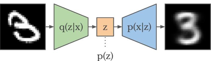
Figure 21.1: Schematic illustration of a VAE. From a figure in [Haf18]. Used with kind permission of Danijar Hafner.

21.2.1 Modeling assumptions

In the simplest setting, a VAE defines a generative model of the form

\[p\_{\theta}(\mathbf{z}, \mathbf{z}) = p\_{\theta}(\mathbf{z}) p\_{\theta}(\mathbf{z}|\mathbf{z}) \tag{21.4}\]

where pω(z) is usually a Gaussian, and pω(x|z) is usually a product of exponential family distributions (e.g., Gaussians or Bernoullis), with parameters computed by a neural network decoder, dω(z). For example, for binary observations, we can use

\[p\_{\theta}(x|\mathbf{z}) = \prod\_{d=1}^{D} \text{Ber}(x\_d | \sigma(d\mathfrak{g}(\mathbf{z})) \tag{21.5}\]

In addition, a VAE fits a recognition model

\[q\_{\phi}(\mathbf{z}|\mathbf{x}) = q(\mathbf{z}|e\_{\phi}(\mathbf{x})) \approx p\_{\theta}(\mathbf{z}|\mathbf{x}) \tag{21.6}\]

to perform approximate posterior inference. Here qε(z|x) is usually a Gaussian, with parameters computed by a neural network encoder eε(x):

\[q\_{\phi}(\mathbf{z}|\mathbf{x}) = \mathcal{N}(\mathbf{z}|\mu, \text{diag}(\exp(\mathcal{E}))) \tag{21.7}\]

\[e\_{\phi}(\mu, \ell) = e\_{\phi}(x) \tag{21.8}\]

where ϖ = log ϱ. The model can be thought of as encoding the input x into a stochastic latent bottleneck z and then decoding it to approximately reconstruct the input, as shown in Figure 21.1.

The idea of training an inference network to “invert” a generative network, rather than running an optimization algorithm to infer the latent code, is called amortized inference, and is discussed in Section 10.1.5. This idea was first proposed in the Helmholtz machine [Day+95]. However, that paper did not present a single unified objective function for inference and generation, but instead used the wake-sleep (Section 10.6) method for training. By contrast, the VAE optimizes a variational lower bound on the log-likelihood, which means that convergence to a locally optimal MLE of the parameters is guaranteed.

We can use other approaches to fitting the DLGM (see e.g., [Hof17; DF19]). However, learning an inference network to fit the DLGM is often faster and can have some regularization benefits (see e.g., [KP20]).2

^1. For example, the website https://github.com/matthewvowels1/Awesome-VAEs lists over 900 papers.

^2. Combining a generative model with an inference model in this way results in what has been called a “monference”,

21.2.2 Model fitting

We can fit a VAE using amortized stochastic variational inference, as we discuss in Section 10.2.1.6. For example, suppose we use a VAE with a diagonal Bernoulli likelihood model, and a full covariance Gaussian as our variational posterior. Then we can use the methods discussed in Section 10.2.1.2 to derive the fitting algorithm. See Algorithm 21.1 for the corresponding pseudocode.

Algorithm 21.1: Fitting a VAE with Bernoulli likelihood and full covariance Gaussian posterior. Based on Algorithm 2 of [KW19a].

1 Initialize ε, ω
2 repeat
 3 Sample x ↑ pD
 4 Sample ς ↑ q0
 5 (µ, log ϱ,L→
                 ) = eε(x)
 6 M = np.triu(np.ones(K), ↓1)
 7 L = M↙ L→ + diag(ϱ)
 8 z = Lς + µ
 9 pω = dω(z)
10 Llogqz = ↓*K
                  k=1 $ 1
                       2 ϖ2
                         k + 1
                             2 log(2φ) + log ςk
                                             %
                                              // from qε(z|x) in Equation (10.47)
11 Llogpz = ↓*K
                  k=1 $ 1
                       2 z2
                         k + 1
                             2 log(2φ)
                                     %
                                      // from pω(z) in Equation (10.48)
12 Llogpx = ↓*D
                  d=1 [xd log pd + (1 ↓ xd) log(1 ↓ pd)] // from pω(x|z)
13 L = Llogpx + Llogpz ↓ Llogqz
14 Update ε := ε ↓ ↼∝ωL
15 Update ω := ω ↓ ↼∝εL
16 until converged

21.2.3 Comparison of VAEs and autoencoders

VAEs are very similar to deterministic autoencoders (AE). There are 2 main di!erences: in the AE, the objective is the log likelihood of the reconstruction without any KL term; and in addition, the encoding is deterministic, so the encoder network just needs to compute E [z|x] and not V [z|x]. In view of these similarities, one can use the same codebase to implement both methods. However, it is natural to wonder what the benefits and potential drawbacks of the VAE are compared to the deterministic AE.

We shall answer this question by fitting both models to the CelebA dataset. Both models have the same convolutional structure with the following number of hidden channels per convolutional layer in the encoder: (32, 64, 128, 256, 512). The spatial size of each layer is as follows: (32, 16, 8, 4, 2). The final 2 ↗ 2 ↗ 512 convolutional layer then gets reshaped and passed through a linear layer to generate the mean and (marginal) variance of the stochastic latent vector, which has size 256. The structure

i.e., model-inference hybrid. See the blog by Jacob Andreas, http://blog.jacobandreas.net/monference.html, for further discussion.

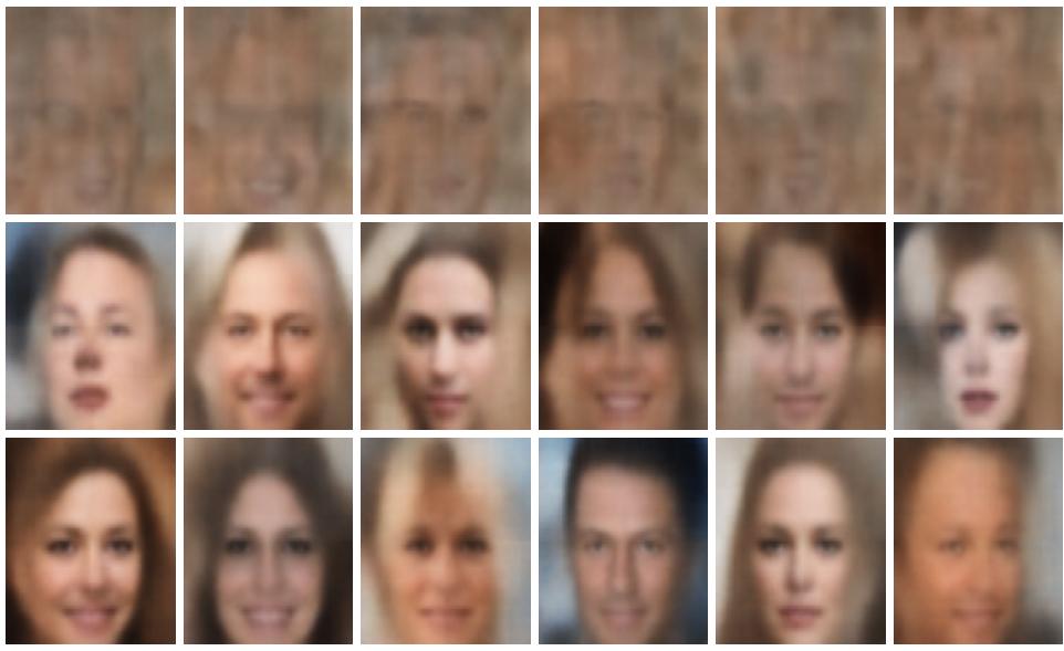
Figure 21.2: Illustration of unconditional image generation using (V)AEs trained on CelebA. Row 1: deterministic autoencoder. Row 2: ω-VAE with ω = 0.5. Row 3: VAE (with ω = 1). Generated by celeba\_vae\_ae\_comparison.ipynb.

of the decoder is the mirror image of the encoder. Each model is trained for 5 epochs with a batch size of 256, which takes about 20 minutes on a GPU.

The main advantage of a VAE over a deterministic autoencoder is that it defines a proper generative model, that can create sensible-looking novel images by decoding prior samples z ↑ N (0, I). By contrast, an autoencoder only knows how to decode latent codes derived from the training set, so does poorly when fed random inputs. This is illustrated in Figure 21.2.

We can also use both models to reconstruct a given input image. In Figure 21.3, we see that both AE and VAE can reconstruct the input images reasonably well, although the VAE reconstructions are somewhat blurry, for reasons we discuss in Section 21.3.1. We can reduce the amount of blurriness by scaling down the KL penalty term by a factor of ε; this is known as the ε-VAE, and is discussed in more detail in Section 21.3.1.

21.2.4 VAEs optimize in an augmented space

In this section, we derive several alternative expressions for the ELBO which shed light on how VAEs work.

First, let us define the joint generative distribution

\[p\_{\theta}(x, z) = p\_{\theta}(z) p\_{\theta}(x|z) \tag{21.9}\]

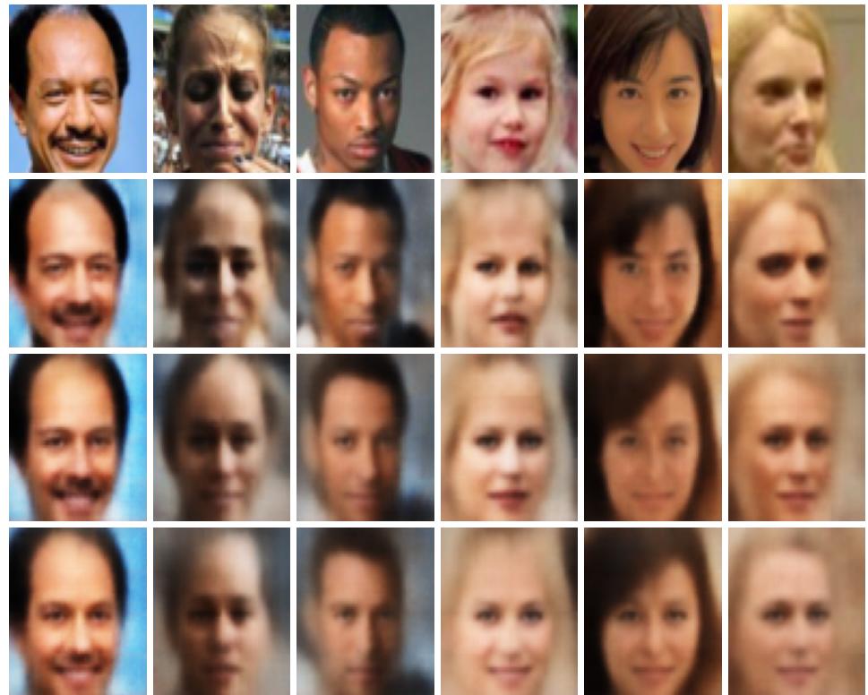
Figure 21.3: Illustration of image reconstruction using (V)AEs trained and applied to CelebA. Row 1: original images. Row 2: deterministic autoencoder. Row 3: ω-VAE with ω = 0.5. Row 4: VAE (with ω = 1). Generated by celeba\_vae\_ae\_comparison.ipynb.

from which we can derive the generative data marginal

\[p\_{\theta}(x) = \int\_{x} p\_{\theta}(x, z) dz \tag{21.10}\]

and the generative posterior

\[p\_{\theta}(\mathbf{z}|\mathbf{x}) = p\_{\theta}(\mathbf{z}, \mathbf{z}) / p\_{\theta}(\mathbf{z}) \tag{21.11}\]

Let us also define the joint inference distribution

\[q\_{\mathcal{D},\phi}(\mathbf{z},\mathbf{z}) = p\_{\mathcal{D}}(\mathbf{z})q\_{\phi}(\mathbf{z}|\mathbf{z})\tag{21.12}\]

where

\[p\_{\mathcal{D}}(\mathbf{z}) = \frac{1}{N} \sum\_{n=1}^{N} \delta(\mathbf{z}\_n - \mathbf{z}) \tag{21.13}\]

is the empirical distribution. From this we can derive the inference latent marginal, also called the aggregated posterior:

\[q\_{\mathcal{D},\phi}(\mathbf{z}) = \int\_{\mathbf{z}} q\_{\mathcal{D},\phi}(\mathbf{z}, \mathbf{z}) d\mathbf{z} \tag{21.14}\]

and the inference likelihood

\[q\_{\mathcal{D},\phi}(\mathbf{z}|\mathbf{z}) = q\_{\mathcal{D},\phi}(\mathbf{z},\mathbf{z})/q\_{\mathcal{D},\phi}(\mathbf{z})\tag{21.15}\]

See Figure 21.4 for a visual illustration.

Having defined our terms, we can now derive various alternative versions of the ELBO, following [ZSE19]. First note that the ELBO averaged over all the data is given by

\[\mathbb{E}\left(\boldsymbol{\theta},\phi|\mathcal{D}\right) = \mathbb{E}\_{\mathsf{p}\boldsymbol{\varphi}\left(\mathbf{z}\right)}\left[\mathbb{E}\_{q\_{\boldsymbol{\Phi}}\left(\mathbf{z}\mid\mathbf{z}\right)}\left[\log p\_{\boldsymbol{\theta}}(\mathbf{z}\mid\mathbf{z})\right]\right] - \mathbb{E}\_{\mathsf{p}\boldsymbol{\varphi}\left(\mathbf{z}\right)}\left[D\_{\mathbb{KL}}\left(q\_{\boldsymbol{\Phi}}(\mathbf{z}\mid\mathbf{z})\parallel p\_{\boldsymbol{\theta}}(\mathbf{z})\right)\right] \tag{21.16}\]

\[=\mathbb{E}\_{q\_{\mathcal{D},\phi}(\mathbf{z},\mathbf{z})}\left[\log p\_{\theta}(\mathbf{z}|\mathbf{z}) + \log p\_{\theta}(\mathbf{z}) - \log q\_{\phi}(\mathbf{z}|\mathbf{z})\right] \tag{21.17}\]

\[=\mathbb{E}\_{q\mathcal{D},\phi(\mathbf{z},\mathbf{z})}\left[\log\frac{p\_{\theta}(\mathbf{z},\mathbf{z})}{q\_{\mathcal{D},\phi}(\mathbf{z},\mathbf{z})}+\log p\_{\mathcal{D}}(\mathbf{z})\right] \tag{21.18}\]

\[\hat{\rho} = -D\_{\rm KL} \left( q\_{\mathcal{D}, \phi}(\mathbf{z}, \mathbf{z}) \parallel p\_{\theta}(\mathbf{z}, \mathbf{z}) \right) + \mathbb{E}\_{p\_{\mathcal{D}}(\mathbf{z})} \left[ \log p\_{\mathcal{D}}(\mathbf{z}) \right] \tag{21.19}\]

If we define ^c = to mean equal up to additive constants, we can rewrite the above as

\[\text{KL}(\theta, \phi | \mathcal{D}) \stackrel{c}{=} -D\_{\text{KL}}\left(q\_{\phi}(\mathbf{z}, \mathbf{z}) \parallel p\_{\theta}(\mathbf{z}, \mathbf{z})\right) \tag{21.20}\]

\[\stackrel{c}{=} -D\_{\text{KL}}\left(p\_{\mathcal{D}}(\mathbf{z}) \parallel p\_{\theta}(\mathbf{z})\right) - \mathbb{E}\_{p\_{\mathcal{D}}\left(\mathbf{z}\right)}\left[D\_{\text{KL}}\left(q\_{\phi}(\mathbf{z}|\mathbf{z}) \parallel p\_{\theta}(\mathbf{z}|\mathbf{z})\right)\right] \tag{21.21}\]

Thus maximizing the ELBO requires minimizing the two KL terms. The first KL term is minimized by MLE, and the second KL term is minimized by fitting the true posterior. Thus if the posterior family is limited, there may be a conflict between these objectives.

Finally, we note that the ELBO can also be written as

\[\operatorname{KL}(\boldsymbol{\theta}, \boldsymbol{\phi} | \mathcal{D}) \stackrel{c}{=} -D\_{\operatorname{KL}}\left(q\_{\mathcal{D}, \boldsymbol{\phi}}(\mathbf{z}) \parallel p\_{\boldsymbol{\theta}}(\mathbf{z})\right) - \operatorname{E}\_{q\_{\mathcal{D}, \boldsymbol{\phi}}(\mathbf{z})} \left[D\_{\operatorname{KL}}\left(q\_{\boldsymbol{\phi}}(\mathbf{z}|\mathbf{z}) \parallel p\_{\boldsymbol{\theta}}(\mathbf{z}|\mathbf{z})\right)\right] \tag{21.22}\]

We see from Equation (21.22) that VAEs are trying to minimize the di!erence between the inference marginal and generative prior, DKL (qε(z) ⇐ pω(z)), while simultaneously minimizing reconstruction error, DKL (qε(x|z) ⇐ pω(x|z)) Since x is typically of much higher dimensionality than z, the latter term usually dominates. Consequently, if there is a conflict between these two objectives (e.g., due to limited modeling power), the VAE will favor reconstruction accuracy over posterior inference. Thus the learned posterior may not be a very good approximation to the true posterior (see [ZSE19] for further discussion).

21.3 VAE generalizations

In this section, we discuss some variants of the basic VAE model.

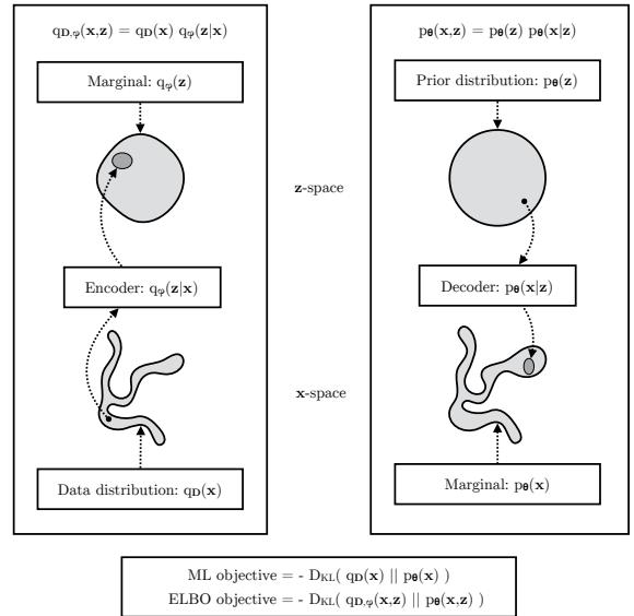
Figure 21.4: The maximum likelihood (ML) objective can be viewed as the minimization of DKL (pD(x) ↘ pω(x)). (Note: in the figure, pD(x) is denoted by qD(x).) The ELBO objective is minimization of DKL (qD,ε(x, z) ↘ pω(x, z)), which upper bounds DKL (qD(x) ↘ pω(x)). From Figure 2.4 of [KW19a]. Used with kind permission of Durk Kingma.

21.3.1 φ-VAE

It is often the case that VAEs generate somewhat blurry images, as illustrated in Figure 21.3, Figure 21.2 and Figure 20.9. This is not the case for models that optimize the exact likelihood, such as pixelCNNs (Section 22.3.2) and flow models (Chapter 23). To see why VAEs are di!erent, consider the common case where the decoder is a Gaussian with fixed variance, so

\[\log p\_{\theta}(\mathbf{z}|\mathbf{z}) = -\frac{1}{2\sigma^{2}}||\mathbf{z} - d\_{\theta}(\mathbf{z})||\_{2}^{2} + \text{const} \tag{21.23}\]

Let eε(x) = E [qε(z|x)] be the encoding of x, and X (z) = {x : eε(x) = z} be the set of inputs that get mapped to z. For a fixed inference network, the optimal setting of the generator parameters, when using squared reconstruction loss, is to ensure dω(z) = E [x : x → X (z)]. Thus the decoder should predict the average of all inputs x that map to that z, resulting in blurry images.

We can solve this problem by increasing the expressive power of the posterior approximation (avoiding the merging of distinct inputs into the same latent code), or of the generator (by adding back information that is missing from the latent code), or both. However, an even simpler solution is to reduce the penalty on the KL term, making the model closer to a deterministic autoencoder:

\[\mathcal{L}\_{\beta}(\theta,\phi|x) = \underbrace{-\mathbb{E}\_{q\_{\phi}(\mathbf{z}|\mathbf{z})} \left[ \log p\_{\theta}(\mathbf{z}|\mathbf{z}) \right]}\_{\mathcal{L}\_{E}} + \beta \underbrace{D\_{\text{KL}} \left( q\_{\phi}(\mathbf{z}|x) \parallel p\_{\theta}(\mathbf{z}) \right)}\_{\mathcal{L}\_{R}} \tag{21.24}\]

where L^E is the reconstruction error (negative log likelihood), and L^R is the KL regularizer. This is

called the ε-VAE objective [Hig+17a]. If we set ε = 1, we recover the objective used in standard VAEs; if we set ε = 0, we recover the objective used in standard autoencoders.

By varying ε from 0 to infinity, we can reach di!erent points on the rate distortion curve, as discussed in Section 5.4.2. These points make di!erent tradeo!s between reconstruction error (distortion) and how much information is stored in the latents about the input (rate of the corresponding code). By using ε < 1, we store more bits about each input, and hence can reconstruct images in a less blurry way. If we use ε > 1, we get a more compressed representation.

21.3.1.1 Disentangled representations

One advantage of using ε > 1 is that it encourages the learning of a latent representation that is “disentangled”. Intuitively this means that each latent dimension represents a di!erent factor of variation in the input. This is often formalized in terms of the total correlation (Section 5.3.5.1), which is defined as follows:

\[\text{TC}(\mathbf{z}) = \sum\_{k} \mathbb{H}(z\_k) - \mathbb{H}(\mathbf{z}) = D\_{\text{KL}}\left(p(\mathbf{z}) \parallel \prod\_{k} p\_k(z\_k)\right) \tag{21.25}\]

This is zero i! the components of z are all mutually independent, and hence disentangled. In [AS18], they prove that using ε > 1 will decrease the TC.

Unfortunately, in [Loc+18] they prove that nonlinear latent variable models are unidentifiable, and therefore for any disentangled representation, there is an equivalent fully entangled representation with exactly the same likelihood. Thus it is not possible to recover the correct latent representation without choosing the appropriate inductive bias, via the encoder, decoder, prior, dataset, or learning algorithm, i.e., merely adjusting ε is not su”cient. See Section 32.4.1 for more discussion.

21.3.1.2 Connection with information bottleneck

In this section, we show that the ε-VAE is an unsupervised version of the information bottleneck (IB) objective from Section 5.6. If the input is x, the hidden bottleneck is z, and the target outputs are x˜, then the unsupervised IB objective becomes

\[\mathcal{L}\_{\text{UIB}} = \beta \, \mathbb{I}(\mathbf{z}; \mathbf{z}) - \mathbb{I}(\mathbf{z}; \mathbf{\bar{z}}) \tag{21.26}\]

\[=\beta \mathbb{E}\_{p(\mathbf{z},\mathbf{z})} \left[ \log \frac{p(\mathbf{z},\mathbf{z})}{p(\mathbf{z})p(\mathbf{z})} \right] - \mathbb{E}\_{p(\mathbf{z},\hat{\mathbf{z}})} \left[ \log \frac{p(\mathbf{z},\hat{\mathbf{z}})}{p(\mathbf{z})p(\hat{\mathbf{z}})} \right] \tag{21.27}\]

where

\[p(\mathbf{z}, \mathbf{z}) = p\_{\mathcal{D}}(\mathbf{z}) p(\mathbf{z}|\mathbf{z}) \tag{21.28}\]

\[p(\mathbf{z}, \tilde{\mathbf{z}}) = \int p\_{\mathcal{D}}(\mathbf{z}) p(\mathbf{z}|\mathbf{z}) p(\tilde{\mathbf{z}}|\mathbf{z}) d\mathbf{z} \tag{21.29}\]

Intuitively, the objective in Equation (21.26) means we should pick a representation z that can predict x˜ reliably, while not memorizing too much information about the input x. The tradeo! parameter is controlled by ε.

From Equation (5.181), we have the following variational upper bound on this unsupervised objective:

\[\mathcal{L}\_{\text{UVIB}} = -\mathbb{E}\_{q\_{\mathcal{D},\phi}(\mathbf{z},\mathbf{z})} \left[ \log p\_{\theta}(\mathbf{z}|\mathbf{z}) \right] + \beta \mathbb{E}\_{p\_{\mathcal{D}}(\mathbf{z})} \left[ D\_{\text{KL}} \left( q\_{\phi}(\mathbf{z}|\mathbf{z}) \parallel p\_{\theta}(\mathbf{z}) \right) \right] \tag{21.30}\]

which matches Equation (21.24) when averaged over x.

21.3.2 InfoVAE

In Section 21.2.4, we discussed some drawbacks of the standard ELBO objective for training VAEs, namely the tendency to ignore the latent code when the decoder is powerful (Section 21.4), and the tendency to learn a poor posterior approximation due to the mismatch between the KL terms in data space and latent space (Section 21.2.4). We can fix these problems to some degree by using a generalized objective of the following form:

\[\operatorname{KL}(\boldsymbol{\theta}, \phi | \boldsymbol{x}) = -\lambda D\_{\text{KL}} \left( q\_{\phi}(\mathbf{z}) \parallel p\_{\theta}(\mathbf{z}) \right) - \mathbb{E}\_{q\_{\phi}(\mathbf{z})} \left[ D\_{\text{KL}} \left( q\_{\phi}(\mathbf{z} | \mathbf{z}) \parallel p\_{\theta}(\mathbf{z} | \mathbf{z}) \right) \right] + \alpha \operatorname{I}\_{q}(\mathbf{z}; \mathbf{z}) \tag{21.31}\]

where ↽ ⇒ 0 controls how much we weight the mutual information Iq(x; z) between x and z, and ω ⇒ 0 controls the tradeo! between z-space KL and x-space KL. This is called the InfoVAE objective [ZSE19]. If we set ↽ = 0 and ω = 1, we recover the standard ELBO, as shown in Equation (21.22).

Unfortunately, the objective in Equation (21.31) cannot be computed as written, because of the intractable MI term:

\[\mathbb{E}\_{q}(\mathbf{z};\mathbf{z}) = \mathbb{E}\_{q\_{\phi}(\mathbf{z},\mathbf{z})} \left[ \log \frac{q\_{\phi}(\mathbf{z},\mathbf{z})}{q\_{\phi}(\mathbf{z})q\_{\phi}(\mathbf{z})} \right] = -\mathbb{E}\_{q\_{\phi}(\mathbf{z},\mathbf{z})} \left[ \log \frac{q\_{\phi}(\mathbf{z})}{q\_{\phi}(\mathbf{z}|\mathbf{z})} \right] \tag{21.32}\]

However, using the fact that qε(x|z) = pD(x)qε(z|x)/qε(z), we can rewrite the objective as follows:

\[\mathcal{L} = \mathbb{E}\_{q\_{\phi}(\mathbf{z}, \mathbf{z})} \left[ -\lambda \log \frac{q\_{\phi}(\mathbf{z})}{p\_{\theta}(\mathbf{z})} - \log \frac{q\_{\phi}(\mathbf{z}|\mathbf{z})}{p\_{\theta}(\mathbf{z}|\mathbf{z})} - \alpha \log \frac{q\_{\phi}(\mathbf{z})}{q\_{\phi}(\mathbf{z}|\mathbf{z})} \right] \tag{21.33}\]

\[\mathbf{E} = \mathbb{E}\_{q\_{\phi}(\mathbf{z}, \mathbf{z})} \left[ \log p\_{\theta}(\mathbf{z}|\mathbf{z}) - \log \frac{q\_{\phi}(\mathbf{z})^{\lambda + \alpha - 1} p\_{\mathcal{D}}(\mathbf{z})}{p\_{\theta}(\mathbf{z})^{\lambda} q\_{\phi}(\mathbf{z}|\mathbf{z})^{\alpha - 1}} \right] \tag{21.34}\]

\[\begin{aligned} \mathbf{E} &= \mathbb{E}\_{p\_{\mathcal{D}}(\mathfrak{a})} \left[ \mathbb{E}\_{q\_{\Phi}(\mathfrak{z}|\mathfrak{a})} \left[ \log p\_{\theta}(\mathfrak{z}|\mathfrak{z}) \right] \right] - (1 - \alpha) \mathbb{E}\_{p\_{\mathcal{D}}(\mathfrak{a})} \left[ D\_{\text{KL}} \left( q\_{\phi}(\mathfrak{z}|\mathfrak{z}) \parallel p\_{\theta}(\mathfrak{z}) \right) \right] \\ &- (\alpha + \lambda - 1) D\_{\text{KL}} \left( q\_{\phi}(\mathfrak{z}) \parallel p\_{\theta}(\mathfrak{z}) \right) - \mathbb{E}\_{p\_{\mathcal{D}}(\mathfrak{a})} \left[ \log p\_{\mathcal{D}}(\mathfrak{x}) \right] \end{aligned} \tag{21.35}\]

where the last term is a constant we can ignore. The first two terms can be optimized using the reparameterization trick. Unfortunately, the last term requires computing qε(z) = ” ^x qε(x, z)dx, which is intractable. Fortunately, we can easily sample from this distribution, by sampling x ↑ pD(x) and z ↑ qε(z|x). Thus qε(z) is an implicit probability model, similar to a GAN (see Chapter 26).

As long as we use a strict divergence, meaning D(q, p)=0 i! q = p, then one can show that this does not a!ect the optimality of the procedure. In particular, proposition 2 of [ZSE19] tells us the following:

Theorem 1. Let X and Z be continuous spaces, and ↽ < 1 (to bound the MI) and ω > 0. For any fixed value of Iq(x; z), the approximate InfoVAE loss, with any strict divergence D(qε(z), pω(z)), is globally optimized if pω(x) = pD(x) and qε(z|x) = pω(z|x).

21.3.2.1 Connection with MMD VAE

If we set ↽ = 1, the InfoVAE objective simplifies to

\[\mathbf{L} \stackrel{\circ}{=} \mathbb{E}\_{p\_{\mathcal{D}}(\mathfrak{x})} \left[ \mathbb{E}\_{q\_{\phi}(\mathfrak{z}|\mathfrak{x})} \left[ \log p\_{\theta}(\mathfrak{x}|\mathfrak{z}) \right] \right] - \lambda D\_{\mathbb{KL}} \left( q\_{\phi}(\mathfrak{z}) \parallel p\_{\theta}(\mathfrak{z}) \right) \tag{21.36}\]

The MMD VAE3 replaces the KL divergence in the above term with the (squared) maximum mean discrepancy or MMD divergence defined in Section 2.7.3. (This is valid based on the above theorem.) The advantage of this approach over standard InfoVAE is that the resulting objective is tractable. In particular, if we set ω = 1 and swap the sign we get

\[\mathcal{L} = \mathbb{E}\_{p\_{\mathcal{D}}(\mathfrak{x})} \left[ \mathbb{E}\_{q\_{\phi}(\mathfrak{z}|\mathfrak{x})} \left[ -\log p\_{\theta}(\mathfrak{x}|\mathfrak{z}) \right] \right] + \text{MMD}(q\_{\phi}(\mathfrak{z}), p\_{\theta}(\mathfrak{z})) \tag{21.37}\]

As we discuss in Section 2.7.3, we can compute the MMD as follows:

\[\text{MMD}(p,q) = \mathbb{E}\_{p(\mathbf{z}), p(\mathbf{z}')} \left[ \mathbb{K}(\mathbf{z}, \mathbf{z}') \right] + \mathbb{E}\_{q(\mathbf{z}), q(\mathbf{z}')} \left[ \mathbb{K}(\mathbf{z}, \mathbf{z}') \right] - 2\mathbb{E}\_{p(\mathbf{z}), q(\mathbf{z}')} \left[ \mathbb{K}(\mathbf{z}, \mathbf{z}') \right] \tag{21.38}\]

where K() is some kernel function, such as the RBF kernel, K(z, z^→ ) = exp(^{↓ 1 2}ε² ||z↓z^→ ||2 ²). Intuitively the MMD measures the similarity (in latent space) between samples from the prior and samples from the aggregated posterior.

In practice, we can implement the MMD objective by using the posterior predicted mean zⁿ = eε(xn) for all B samples in the current minibatch, and comparing this to B random samples from the N (0, I) prior.

If we use a Gaussian decoder with fixed variance, the negative log likelihood is just a squared error term:

\[-\log p\_{\theta}(\mathbf{z}|\mathbf{z}) = ||\mathbf{z} - d\_{\theta}(\mathbf{z})||\_{2}^{2} \tag{21.39}\]

Thus the entire model is deterministic, and just predicts the means in latent space and visible space.

21.3.2.2 Connection with φ-VAEs

If we set ↽ = 0 and ω = 1, we get back the original ELBO. If ω > 0 is freely chosen, but we use ↽ = 1 ↓ ω, we get the ε-VAE.

21.3.2.3 Connection with adversarial autoencoders

If we set ↽ = 1 and ω = 1, and D is chosen to be the Jensen-Shannon divergence (which can be minimized by training a binary discriminator, as explained in Section 26.2.2), then we get a model known as an adversarial autoencoder [Mak+15a].

21.3.3 Multimodal VAEs

It is possible to extend VAEs to create joint distributions over di!erent kinds of variables, such as images and text. This is sometimes called a multimodal VAE or MVAE. Let us assume there are

^3. Proposed in https://ermongroup.github.io/blog/a-tutorial-on-mmd-variational-autoencoders/.

Figure 21.5: Illustration of multi-modal VAE. (a) The generative model with N = 2 modalities. (b) The product of experts (PoE) inference network is derived from N individual Gaussian experts Ei. µ⁰ and ε⁰ are parameters of the prior. (c) If a modality is missing, we omit its contribution to the posterior. From Figure 1 of [WG18]. Used with kind permission of Mike Wu.

M modalities. We assume they are conditionally independent given the latent code, and hence the generative model has the form

\[p\_{\theta}(x\_1, \ldots, x\_M, z) = p(z) \prod\_{m=1}^{M} p\_{\theta}(x\_m|z) \tag{21.40}\]

where we treat p(z) as a fixed prior. See Figure 21.5(a) for an illustration.

The standard ELBO is given by

\[\mathbb{E}(\boldsymbol{\theta}, \phi | \mathbf{X}) = \mathbb{E}\_{q\_{\phi}(\mathbf{z} | \mathbf{X})} \left[ \sum\_{m} \log p\_{\theta}(\boldsymbol{x}\_{m} | \mathbf{z}) \right] - D\_{\text{KL}} \left( q\_{\phi}(\mathbf{z} | \mathbf{X}) \parallel p(\mathbf{z}) \right) \tag{21.41}\]

where X = (x1,…, xM) is the observed data. However, the di!erent likelihood terms p(xm|z) may have di!erent dynamic ranges (e.g., Gaussian pdf for pixels, and categorical pmf for text), so we introduce weight terms ω^m ⇒ 0 for each likelihood. In addition, let ε ⇒ 0 control the amount of KL regularization. This gives us a weighted version of the ELBO, as follows:

\[\mathbb{E}\left(\theta,\phi|\mathbf{X}\right) = \mathbb{E}\_{q\_{\phi}(\mathbf{z}|\mathbf{X})} \left[ \sum\_{m} \lambda\_{m} \log p\_{\theta}(\mathbf{z}\_{m}|\mathbf{z}) \right] - \beta D\_{\text{KL}}\left(q\_{\phi}(\mathbf{z}|\mathbf{X}) \parallel p(\mathbf{z})\right) \tag{21.42}\]

Often we don’t have a lot of paired (aligned) data from all M modalities. For example, we may have a lot of images (modality 1), and a lot of text (modality 2), but very few (image, text) pairs. So it is useful to generalize the loss so it fits the marginal distributions of subsets of the features. Let O^m = 1 if modality m is observed (i.e., x^m is known), and let O^m = 0 if it is missing or unobserved. Let X = {x^m : O^m = 1} be the visible features. We now use the following objective:

\[\mathbb{E}(\boldsymbol{\theta}, \phi | \mathbf{X}) = \mathbb{E}\_{q\_{\phi}(\mathbf{z} | \mathbf{X})} \left[ \sum\_{m: O\_m = 1} \lambda\_m \log p\_{\theta}(\mathbf{z}\_m | \mathbf{z}) \right] - \beta D\_{\mathbf{KL}} \left( q\_{\phi}(\mathbf{z} | \mathbf{X}) \parallel p(\mathbf{z}) \right) \tag{21.43}\]

The key problem is how to compute the posterior qε(z|X) given di!erent subsets of features. In general this can be hard, since the inference network is a discriminative model that assumes all inputs are available. For example, if it is trained on (image, text) pairs, qε(z|x1, x2), how can we compute the posterior just given an image, qε(z|x1), or just given text, qε(z|x2)? (This issue arises in general with VAE when we have missing inputs.)

Fortunately, based on our conditional independence assumption between the modalities, we can compute the optimal form for qε(z|X) given set of inputs by computing the exact posterior under the model, which is given by

\[p(\mathbf{z}|\mathbf{X}) = \frac{p(\mathbf{z})p(\mathbf{z}\_1, \dots, \mathbf{z}\_M|\mathbf{z})}{p(\mathbf{z}\_1, \dots, \mathbf{z}\_M)} = \frac{p(\mathbf{z})}{p(\mathbf{z}\_1, \dots, \mathbf{z}\_M)} \prod\_{m=1}^M p(\mathbf{z}\_m|\mathbf{z}) \tag{21.44}\]

\[=\frac{p(\mathbf{z})}{p(\mathbf{z}\_1,\ldots,\mathbf{z}\_M)}\prod\_{m=1}^M \frac{p(\mathbf{z}|\mathbf{x}\_m)p(\mathbf{x}\_m)}{p(\mathbf{z})}\tag{21.45}\]

\[\propto p(\mathbf{z}) \prod\_{m=1}^{M} \frac{p(\mathbf{z}|\mathbf{z}\_m)}{p(\mathbf{z})} \approx p(\mathbf{z}) \prod\_{m=1}^{M} \bar{q}(\mathbf{z}|\mathbf{x}\_m) \tag{21.46}\]

This can be viewed as a product of experts (Section 24.1.1), where each q˜(z|xm) is an “expert” for the m’th modality, and p(z) is the prior. We can compute the above posterior for any subset of modalities for which we have data by modifying the product over m. If we use Gaussian distributions for the prior ^p(z) = ^N (z|µ0, #^{↑1 0} ) and marginal posterior ratio ^q˜(z|xm) = ^N (z|µm, #^{↑1 m} ), then we can compute the product of Gaussians using the result from Equation (2.154):

\[\prod\_{m=0}^{M} \mathcal{N}(z|\mu\_m, \Lambda\_m^{-1}) \propto \mathcal{N}(z|\mu, \Sigma), \quad \Sigma = (\sum\_m \Lambda\_m)^{-1}, \ \mu = \Sigma(\sum\_m \Lambda\_m \mu\_m) \tag{21.47}\]

Thus the overall posterior precision is the sum of individual expert posterior precisions, and the overall posterior mean is the precision weighted average of the individual expert posterior means. See Figure 21.5(b) for an illustration. For a linear Gaussian (factor analysis) model, we can ensure q(z|xm) = p(z|xm), in which case the above solution is the exact posterior [WN18], but in general it will be an approximation.

We need to train the individual expert recognition models q(z|xm) as well as the joint model q(z|X), so the model knows what to do with fully observed as well as partially observed inputs at test time. In [Ved+18], they propose a somewhat complex “triple ELBO” objective. In [WG18], they propose the simpler approach of optimizing the ELBO for the fully observed feature vector, all the marginals, and a set of J randomly chosen joint modalities:

\[\text{KL}(\theta, \phi | \mathbf{X}) = \text{L}(\theta, \phi | (\langle x\_1, \dots, x\_M \rangle) + \sum\_{m=1}^{M} \text{L}(\theta, \phi | x\_m) + \sum\_{j \in \mathcal{J}} \text{L}(\theta, \phi | \mathbf{X}\_j) \tag{21.48}\]

This generalizes nicely to the semi-supervised setting, in which we only have a few aligned (“labeled”) examples from the joint, but have many unaligned (“unlabeled”) examples from the individual marginals. See Figure 21.5(c) for an illustration.

Note that the above scheme can only handle the case of a fixed number of missingness patterns; we can generalize to allow for arbitrary missingness as discussed in [CNW20]. (See also Section 3.11 for a more general discussion of missing data.)

21.3.4 Semisupervised VAEs

In this section, we discuss how to extend VAEs to the semi-supervised learning setting in which we have both labeled data, D^L = {(xn, yn)}, and unlabeled data, D^U = {(xn)}. We focus on the M2 model, proposed in [Kin+14a].

The generative model has the following form:

\[p\_{\theta}(x,y) = p\_{\theta}(y)p\_{\theta}(x|y) = p\_{\theta}(y) \int p\_{\theta}(x|y,z)p\_{\theta}(z)dz\tag{21.49}\]

where z is a latent variable, pω(z) = N (z|0, I) is the latent prior, pω(y) = Cat(y|↼) the label prior, and pω(x|y, z) = p(x|fω(y, z)) is the likelihood, such as a Gaussian, with parameters computed by f (a deep neural network). The main innovation of this approach is to assume that data is generated according to both a latent class variable y as well as the continuous latent variable z. The class variable y is observed for labeled data and unobserved for unlabled data.

To compute the likelihood for the labeled data, pω(x, y), we need to marginalize over z, which we can do by using an inference network of the form

\[q\_{\phi}(\mathbf{z}|y,\mathbf{z}) = \mathcal{N}(\mathbf{z}|\mu\_{\phi}(y,\mathbf{z}), \text{diag}(\sigma\_{\phi}(y,\mathbf{z})) \tag{21.50}\]

We then use the following variational lower bound

\[\log p\_{\theta}(\mathbf{z}, y) \ge \mathbb{E}\_{q\_{\theta}(\mathbf{z}|\mathbf{x}, y)} \left[ \log p\_{\theta}(\mathbf{z}|y, \mathbf{z}) + \log p\_{\theta}(y) + \log p\_{\theta}(\mathbf{z}) - \log q\_{\phi}(\mathbf{z}|\mathbf{x}, y) \right] = -\mathcal{L}(\mathbf{x}, y) \tag{21.51}\]

as is standard for VAEs (see Section 21.2). The only di!erence is that we observe two kinds of data: x and y.

To compute the likelihood for the unlabeled data, pω(x), we need to marginalize over z and y, which we can do by using an inference network of the form

\[q\_{\phi}(\mathbf{z}, y|\mathbf{z}) = q\_{\phi}(\mathbf{z}|\mathbf{z})q\_{\phi}(y|\mathbf{z})\tag{21.52}\]

\[q\_{\phi}(\mathbf{z}|\mathbf{x}) = \mathcal{N}(\mathbf{z}|\mu\_{\phi}(\mathbf{x}), \text{diag}(\sigma\_{\phi}(\mathbf{x})) \tag{21.53}\]

\[q\_{\phi}(y|\mathbf{z}) = \text{Cat}(y|\pi\_{\phi}(\mathbf{z})) \tag{21.54}\]

Note that qε(y|x) acts like a discriminative classifier, that imputes the missing labels. We then use the following variational lower bound:

\[\log p\_{\theta}(\mathbf{z}) \ge \underbrace{\mathbb{E}\_{q\_{\phi}(\mathbf{z}, y|\mathbf{z})} \left[ \log p\_{\theta}(\mathbf{z}|y, \mathbf{z}) + \log p\_{\theta}(y) + \log p\_{\theta}(\mathbf{z}) - \log q\_{\phi}(\mathbf{z}, y|\mathbf{z}) \right]}\_{\text{(21.55)}} \tag{21.55}\]

\[\mathcal{L} = -\sum\_{y} q\_{\phi}(y|\mathbf{z})\mathcal{L}(\mathbf{z}, y) + \mathbb{H}\left(q\_{\phi}(y|\mathbf{z})\right) = -\mathcal{U}(\mathbf{z})\tag{21.56}\]

Note that the discriminative classifier qε(y|x) is only used to compute the log-likelihood of the unlabeled data, which is undesirable. We can therefore add an extra classification loss on the supervised data, to get the following overall objective function:

\[\mathcal{L}(\boldsymbol{\theta}) = \mathbb{E}\_{(\boldsymbol{x}, \boldsymbol{y}) \sim \mathcal{D}\_{L}} \left[ \mathcal{L}(\boldsymbol{x}, \boldsymbol{y}) \right] + \mathbb{E}\_{\mathbf{z} \sim \mathcal{D}\_{U}} \left[ \mathcal{U}(\boldsymbol{x}) \right] + \alpha \mathbb{E}\_{(\boldsymbol{x}, \boldsymbol{y}) \sim \mathcal{D}\_{L}} \left[ -\log q\_{\boldsymbol{\phi}}(\boldsymbol{y}|\boldsymbol{x}) \right] \tag{21.57}\]

where D^L is the labeled data, D^U is the unlabeled data, and ↽ is a hyperparameter that controls the relative weight of generative and discriminative learning.

y y y y y

1 2 3 Nmax-1 Nmax

’ ’ ’

GMM, softmax sample τ

GMM, softmax sample τ

GMM, softmax sample τ

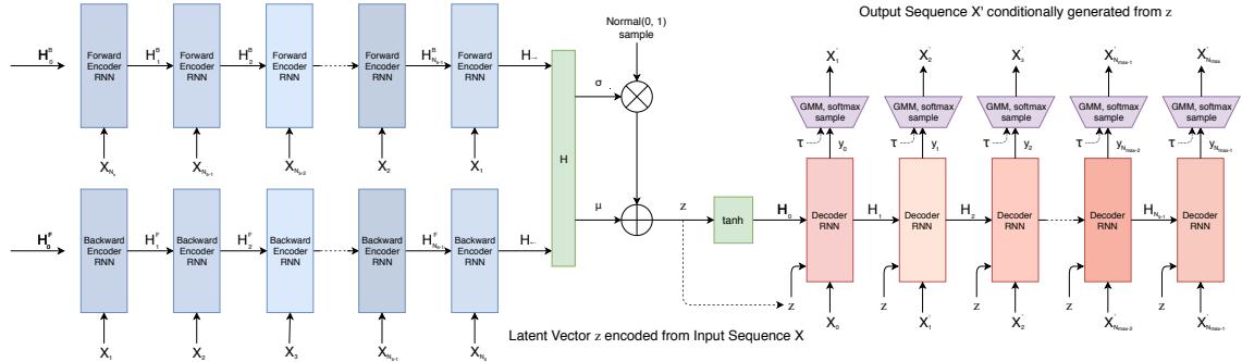
h Backward Encoder h^{← 0} Backward Encoder Backward Encoder Backward Encoder Backward Encoder N(0, I) sample Output Sequence S’ conditionally generated from z ^B h ¹ B h 2 B h^Ns-1 B S¹ S² S³ S^Nmax-1 ’ ’ ’ ’ S^Nmax ’ Figure 21.6: Illustration of a VAE with a bidirectional RNN encoder and a unidirectional RNN decoder. The output generator can use a GMM and/or softmax distribution. From Figure 2 of [HE18]. Used with kind permission of David Ha.

GMM, softmax sample

GMM, softmax sample τ

’

τ

σ

S S h ^{Ns N}s-1 S^Ns-2 S² S¹ 21.3.5 VAEs with sequential encoders/decoders

RNN

RNN

Decoder RNN Decoder RNN Decoder RNN Decoder RNN z Decoder RNN Forward Encoder RNN Forward Encoder RNN Forward Encoder RNN Forward Encoder RNN Forward Encoder RNN ^z tanh z z z z Latent Vector z encoded from Input Sequence S S¹ S² S³ S^Ns-1 S^Ns h h^{→ 0} F h 1 F h 2 F h^Ns-1 F S⁰ S¹ S² S^Nmax-2 S^Nmax-1 h ⁰ h ¹ h ² h^Ns-1 μ In this section, we discuss VAEs for sequential data, such as text and biosequences, in which the data ^x is a variable-length sequence, but we have a fixed-sized latent variable ^{z → RK}. (We consider the more general case in which z is a variable-length sequence of latents — known as sequential VAE or dynamic VAE — in Section 29.13.) All we have to do is modify the decoder p(x|z) and encoder q(z|x) to work with sequences.

21.3.5.1 Models

RNN

RNN

RNN

If we use an RNN for the encoder and decoder of a VAE, we get a model which is called a VAE-RNN, as proposed in [Bow+16a]. In more detail, the generative model is p(z, x1:^T ) = p(z)RNN(x1:^T |z), where z can be injected as the initial state of the RNN, or as an input to every time step. The inference model is q(z|x1:^T ) = N (z|µ(h), “(h)), where h = [h↘ ^T , h^{≃ 1} ] is the output of a bidirectional RNN applied to x1:^T . See Figure 21.6 for an illustration.

More recently, people have tried to combine transformers with VAEs. For example, in the Optimus model of [Li+20], they use a BERT model for the encoder. In more detail, the encoder q(z|x) is derived from the embedding vector associated with a dummy token corresponding to the “class label” which is appended to the input sequence x. The decoder is a standard autoregressive model (similar to GPT), with one additional input, namely the latent vector z. They consider two ways of injecting the latent vector. The simplest approach is to add z to the embedding layer of every token in the decoding step, by defining h^{→ i} = ^hi + Wz, where ^{hi → RH} is the original embedding for the ⁱ’th token, and ^{W → RH}⇐^K is a decoding matrix, where ^K is the size of the latent vector. However, they get better results in their experiments by letting all the layers of the decoder attend to the latent code ^z. An easy way to do this is to define the memory vector ^hm = Wz, where W ^{→ R}LH⇐^K, where ^L is the number of layers in the decoder, and then to append ^{hm → RL}⇐^H to all the other embeddings at each layer.

An alternative approach, known as transformer VAE, was proposed in [Gre20]. This model uses a funnel transformer [Dai+20b] as the encoder, and the T5 [Raf+20a] conditional transformer for

he was silent for a long moment .
he was silent for a moment .
it was quiet for a moment .
it was dark and cold .
there was a pause .
it was my turn .
                                                         i went to the store to buy some groceries .
                                                         i store to buy some groceries .
                                                         i were to buy any groceries .
                                                         horses are to buy any groceries .
                                                         horses are to buy any animal .
                                                         horses the favorite any animal .
                                                         horses the favorite favorite animal .
                                                         horses are my favorite animal .

(a)

(b)

Figure 21.7: (a) Samples from the latent space of a VAE text model, as we interpolate between two sentences (on first and last line). Note that the intermediate sentences are grammatical, and semantically related to their neighbors. From Table 8 of [Bow+16b]. (b) Same as (a), but now using a deterministic autoencoder (with the same RNN encoder and decoder). From Table 1 of [Bow+16b]. Used with kind permission of Sam Bowman.

the decoder. In addition, it uses an MMD VAE (Section 21.3.2.1) to avoid posterior collapse.

21.3.5.2 Applications

In this section, we discuss some applications of VAEs to sequence data.

Text

In [Bow+16b], they apply the VAE-RNN model to natural language sentences. (See also [MB16; SSB17] for related work.) Although this does not improve performance in terms of the standard perplexity measures (predicting the next word given the previous words), it does provide a way to infer a semantic representation of the sentence. This can then be used for latent space interpolation, as discussed in Section 20.3.5. The results of doing this with the VAE-RNN are illustrated in Figure 21.7a. (Similar results are shown in [Li+20], using a VAE-transformer.) By contrast, if we use a standard deterministic autoencoder, with the same RNN encoder and decoder networks, we learn a much less meaningful space, as illustrated in Figure 21.7b. The reason is that the deterministic autoencoder has “holes” in its latent space, which get decoded to nonsensical outputs.

However, because RNNs (and transformers) are powerful decoders, we need to address the problem of posterior collapse, which we discuss in Section 21.4. One common way to avoid this problem is to use KL annealing, but a more e!ective method is to use the InfoVAE method of Section 21.3.2, which includes adversarial autoencoders (used in [She+20] with an RNN decoder) and MMD autoencoders (used in [Gre20] with a transformer decoder).

Sketches

In [HE18], they apply the VAE-RNN model to generate sketches (line drawings) of various animals and hand-written characters. They call their model sketch-rnn. The training data records the sequence of (x, y) pen positions, as well as whether the pen was touching the paper or not. The emission model used a GMM for the real-valued location o!sets, and a categorical softmax distribution for the discrete state.

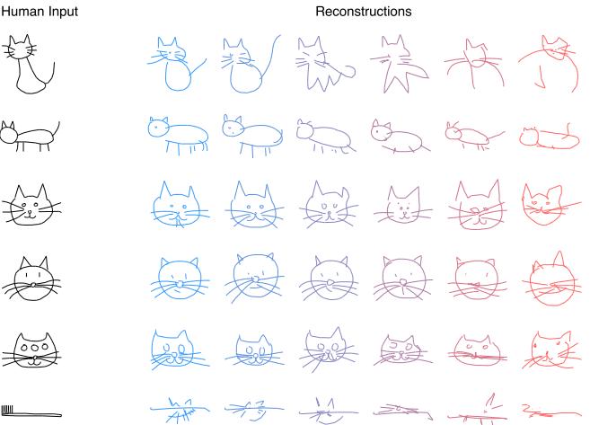
Figure 21.8: Conditional generation of cats from sketch-RNN model. We increase the temperature parameter from left to right. From Figure 5 of [HE18]. Used with kind permission of David Ha.

Figure 21.8 shows some samples from various class-conditional models. We vary the temperature parameter ⇀ of the emission model to control the stochasticity of the generator. (More precisely, we multiply the GMM variances by ⇀ , and divide the discrete probabilities by ⇀ before renormalizing.) When the temperature is low, the model tries to reconstruct the input as closely as possible. However, when the input is untypical of the training set (e.g., a cat with three eyes, or a toothbrush), the reconstruction is “regularized” towards a canonical cat with two eyes, while still keeping some features of the input.

Molecular design

In [GB+18], they use VAE-RNNs to model molecular graph structure, represented as a string using the SMILES representation.4 It is also possible to learn a mapping from the latent space to some scalar quantity of interest, such as the solubility or drug e”cacy of a molecule. We can then perform gradient-based optimization in the continuous latent space to try to generate new graphs which maximize this quantity. See Figure 21.9 for a sketch of this approach.

The main problem is to ensure that points in latent space decode to valid strings/molecules. There are various solutions to this, including using a grammar VAE, where the RNN decoder is replaced by a stochastic context free grammar. See [KPHL17] for details.

21.4 Avoiding posterior collapse

If the decoder pω(x|z) is su”ciently powerful (e.g., a pixel CNN, or an RNN for text), then the VAE does not need to use the latent code z for anything. This is called posterior collapse or variational

^4. See https://en.wikipedia.org/wiki/Simplified\_molecular-input\_line-entry\_system.

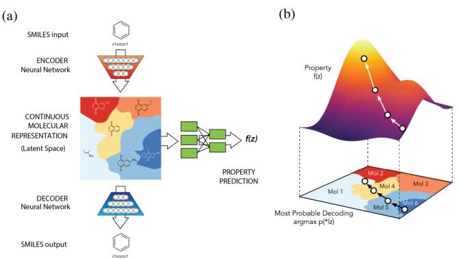
Figure 21.9: Application of VAE-RNN to molecule design. (a) The VAE-RNN model is trained on a sequence representation of molecules known as SMILES. We can fit an MLP to map from the latent space to properties of the molecule, such as its “fitness” f(z). (b) We can perform gradient ascent in f(z) space, and then decode the result to a new molecule with high fitness. From Figure 1 of [GB+18]. Used with kind permission of Rafael Gomez-Bombarelli.

overpruning (see e.g., [Che+17b; Ale+18; Hus17a; Phu+18; TT17; Yeu+17; Luc+19; DWW19; WBC21]). To see why this happens, consider Equation (21.21). If there exists a parameter setting for the generator ε^↔︎ such that p^ω→ (x|z) = pD(x) for every z, then we can make DKL (pD(x) ⇐ pω(x)) = 0. Since the generator is independent of the latent code, we have pω(z|x) = pω(z). The prior pω(z) is usually a simple distribution, such as a Gaussian, so we can find a setting of the inference parameters so that q^ε→ (z|x) = pω(z), which ensures DKL (qε(z|x) ⇐ pω(z|x)) = 0. Thus we have succesfully maximized the ELBO, but we have not learned any useful latent representation of the data, which is one of the goals of latent variable modeling.5 We discuss some solutions to posterior collapse below.

21.4.1 KL annealing

A common approach to solving this problem, proposed in [Bow+16a], is to use KL annealing, in which the KL penalty term in the ELBO is scaled by ε, which is increased from 0.0 (corresponding to an autoencoder) to 1.0 (which corresponds to standard MLE training). (Note that, by contrast, the ε-VAE model in Section 21.3.1 uses ε > 1.)

KL annealing can work well, but requires tuning the schedule for ε. A standard practice [Fu+19] is to use cyclical annealing, which repeats the process of increasing ε multiple times. This ensures the progressive learning of more meaningful latent codes, by leveraging good representations learned in a previous cycle as a way to warmstart the optimization.

^5. Note that [Luc+19; DWW20] show that posterior collapse can also happen in linear VAE models, where the ELBO corresponds to the exact marginal likelihood, so the problem is not only due to powerful (nonlinear) decoders, but is also related to spurious local maxima in the objective.

21.4.2 Lower bounding the rate

An alternative approach is to stick with the original unmodified ELBO objective, but to prevent the rate (i.e., the DKL (q ⇐ p) term) from collapsing to 0, by limiting the flexibility of q. For example, [XD18; Dav+18] use a von Mises-Fisher (Section 2.2.5.3) prior and posterior, instead of a Gaussian, and they constrain the posterior to have a fixed concentration, q(z|x) = vMF(z|µ(x), ⇁). Here the parameter ⇁ controls the rate of the code. The ϑ-VAE method [Oor+19] uses a Gaussian autoregressive prior and a diagonal Gaussian posterior. We can ensure the rate is at least ϑ by adjusting the regression parameter of the AR prior.

21.4.3 Free bits

In this section, we discuss the method of free bits [Kin+16], which is another way of lower bounding the rate. To explain this, consider a fully factorized posterior in which the KL penalty has the form

\[\mathcal{L}\_R = \sum\_i D\_{\text{KL}}\left(q\_\Phi(z\_i|\mathbf{z}) \parallel p\_\Phi(z\_i)\right) \tag{21.58}\]

where zⁱ is the i’th dimension of z. We can replace this with a hinge loss, that will give up driving down the KL for dimensions that are already beneath a target compression rate ω:

\[\mathcal{L}'\_R = \sum\_i \max(\lambda, D\_{\text{KL}}\left(q\_\Phi(z\_i|x) \parallel p\_\theta(z\_i)\right)) \tag{21.59}\]

Thus the bits where the KL is su”ciently small “are free”, since the model does not have to “pay” to encode them according to the prior.

21.4.4 Adding skip connections

One reason for latent variable collapse is that the latent variables z are not su”ciently “connected to” the observed data x. One simple solution is to modify the architecture of the generative model by adding skip connections, similar to a residual network (Section 16.2.4), as shown in Figure 21.10. This is called a skip-VAE [Die+19a].

21.4.5 Improved variational inference

The posterior collapse problem is caused in part by the poor approximation to the posterior. In [He+19], they proposed to keep the model and VAE objective unchanged, but to more aggressively update the inference network before each step of generative model fitting. This enables the inference network to capture the current true posterior more faithfully, which will encourage the generator to use the latent codes when it is useful to do so.

However, this only addresses the part of posterior collapse that is due to the amortization gap [CLD18], rather than the more fundamental problem of variational pruning, in which the KL term penalizes the model if its posterior deviates too far from the prior, which is often too simple to match the aggregated posterior.

Another way to ameliorate variational pruning is to use lower bounds that are tighter than the vanilla ELBO (Section 10.5.1), or more accurate posterior approximations (Section 10.4), or more accurate (hierarchical) generative models (Section 21.5).

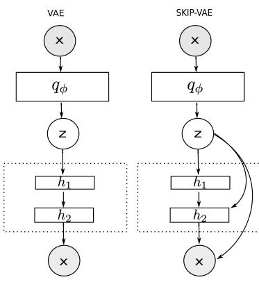
Figure 21.10: (a) VAE. (b) Skip-VAE. From Figure 1 of [Die+19a]. Used with kind permission of Adji Dieng.

21.4.6 Alternative objectives

An alternative to the above methods is to replace the ELBO objective with other objectives, such as the InfoVAE objective discussed in Section 21.3.2, which includes adversarial autoencoders and MMD autoencoders as special cases. The InfoVAE objective includes a term to explicitly enforce non-zero mutual information between x and z, which e!ectively solves the problem of posterior collapse.

21.5 VAEs with hierarchical structure

We define a hierarchical VAE or HVAE, with L stochastic layers, to be the following generative model:6

\[p\_{\theta}(x, z\_{1:L}) = p\_{\theta}(z\_L) \left[ \prod\_{l=L-1}^{1} p\_{\theta}(z\_l | z\_{l+1}) \right] p\_{\theta}(x | z\_1) \tag{21.60}\]

We can improve on the above model by making it non-Markovian, i.e., letting each z^l depend on all the higher level stochastic variables, zl+1:L, not just the preceeding level, i.e.,

\[p\_{\theta}(\mathbf{z}, \mathbf{z}) = p\_{\theta}(\mathbf{z}\_{L}) \left[ \prod\_{l=L-1}^{1} p\_{\theta}(\mathbf{z}\_{l}|\mathbf{z}\_{l+1:L}) \right] p\_{\theta}(\mathbf{z}|\mathbf{z}\_{1:L}) \tag{21.61}\]

Note that the likelihood is now pω(x|z1:L) instead of just pω(x|z1). This is analogous to adding skip connections from all preceeding variables to all their children. It is easy to implement this by using a deterministic “backbone” of residual connections, that accumulates all stochastic decisions, and propagates them down the chain, as illustrated in Figure 21.11(left). We discuss how to perform inference and learning in such models below.

^6. There is a split in the literature about whether to label the top level as z^L or z1. We adopt the former convention, since we view lower numbered layers, such as z1, as being “closer to the data”, and higher numbered layers, such as zL, as being “more abstract”.

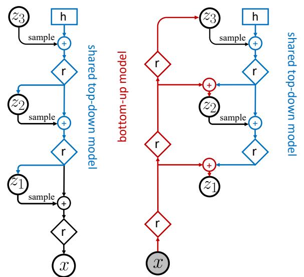
Figure 21.11: Hierarchical VAEs with 3 stochastic layers. Left: generative model. Right: inference network. Diamond is a residual network, ≃ is feature combination (e.g., concatenation), and h is a trainable parameter. We first do bottom-up inference, by propagating x up to z³ to compute z^{s 3} ⇐ qε(z3|x), and then we perform top-down inference by computing z^{s 2} ⇐ ^qε(z2|x, ^{zs 3}) and then z^{s 1} ⇐ ^qε(z1|x, ^zs 2:3). From Figure 2 of [VK20a]. Used with kind permission of Arash Vahdat.

21.5.1 Bottom-up vs top-down inference

To perform inference in a hierarchical VAE, we could use a bottom-up inference model of the form

\[q\_{\phi}(z|x) = q\_{\phi}(z\_1|x) \prod\_{l=2}^{L} q\_{\phi}(z\_l|x, z\_{1:l-1}) \tag{21.62}\]

However, a better approach is to use a top-down inference model of the form

\[q\_{\phi}(\boldsymbol{z}|\boldsymbol{x}) = q\_{\phi}(\boldsymbol{z}\_{L}|\boldsymbol{x}) \prod\_{l=L-1}^{1} q\_{\phi}(\boldsymbol{z}\_{l}|\boldsymbol{x}, \boldsymbol{z}\_{l+1:L}) \tag{21.63}\]

Inference for z^l combines bottom-up information from x with top-down information from higher layers, z>l = zl+1:L. See Figure 21.11(right) for an illustration.7

^7. Note that it is also possible to have a stochastic bottom-up encoder and a stochastic top-down encoder, as discussed in the BIVA paper [Maa+19]. (BIVA stands for “bidirectional-inference variational autoencoder”.)

With the above model, the ELBO can be written as follows (using the chain rule for KL):

\[\mathbb{L}(\boldsymbol{\theta}, \phi | \boldsymbol{x}) = \mathbb{E}\_{q\_{\phi}(\mathbf{z} | \boldsymbol{x})} \left[ \log p\_{\theta}(\mathbf{z} | \boldsymbol{z}) \right] - D\_{\text{KL}} \left( q\_{\phi}(\mathbf{z}\_{L} | \boldsymbol{x}) \parallel p\_{\theta}(\mathbf{z}\_{L}) \right) \tag{21.64}\]

\[-\sum\_{l=L-1}^{1} \mathbb{E}\_{q\_{\phi}(\mathbf{z}\_{>l}|\mathbf{z})} \left[ D\_{\mathbb{KL}} \left( q\_{\phi}(\mathbf{z}|\mathbf{z}, \mathbf{z}\_{>l}) \parallel p\_{\theta}(\mathbf{z}|\mathbf{z}\_{>l}) \right) \right] \tag{21.65}\]

where

\[q\_{\phi}(\mathbf{z}\_{>l}|\mathbf{x}) = \prod\_{i=l+1}^{L} q\_{\phi}(\mathbf{z}\_{i}|\mathbf{x}, \mathbf{z}\_{>i}) \tag{21.66}\]

is the approximate posterior above layer l (i.e., the parents of zl).

The reason the top-down inference model is better is that it more closely approximates the true posterior of a given layer, which is given by

\[p\_{\theta}(\mathbf{z}\_{l}|\mathbf{z}, \mathbf{z}\_{l+1:L}) \propto p\_{\theta}(\mathbf{z}\_{l}|\mathbf{z}\_{l+1:L}) p\_{\theta}(\mathbf{z}|\mathbf{z}\_{l}, \mathbf{z}\_{l+1:L}) \tag{21.67}\]

Thus the posterior combines the top-down prior term pω(zl|zl+1:L) with the bottom-up likelihood term pω(x|zl, zl+1:L). We can approximate this posterior by defining

\[q\_{\phi}(\mathbf{z}\_{l}|\mathbf{z},\mathbf{z}\_{l+1:L}) \propto p\_{\theta}(\mathbf{z}\_{l}|\mathbf{z}\_{l+1:L})\bar{q}\_{\phi}(\mathbf{z}\_{l}|\mathbf{z},\mathbf{z}\_{l+1:L})\tag{21.68}\]

where q˜ε(zl|x, zl+1:L) is a learned Gaussian approximation to the bottom-up likelihood. If both prior and likelihood are Gaussian, we can compute this product in closed form, as proposed in the ladder network paper [Sn+16; Søn+16].8 A more flexible approach is to let ^qε(zl|x, ^zl+1:L) be learned, but to force it to share some of its parameters with the learned prior pω(zl|zl+1:L), as proposed in [Kin+16]. This reduces the number of parameters in the model, and ensures that the posterior and prior remain somewhat close.

21.5.2 Example: very deep VAE

There have been many papers exploring di!erent kinds of HVAE models (see e.g., [Kin+16; Sn+16; Chi21a; VK20a; Maa+19]), and we do not have space to discuss them all. Here we focus on the “very deep VAE” or VD-VAE model of [Chi21a], since it is simple but yields state of the art results (at the time of writing).

The architecture is a simple convolutional VAE with bidrectional inference, as shown in Figure 21.12. For each layer, the prior and posterior are diagonal Gaussians. The author found that nearest-neighbor upsampling (in the decoder) worked much better than transposed convolution, and avoided posterior collapse. This enabled training with the vanilla VAE objective, without needing any of the tricks discussed in Section 21.5.4.

The low-resolution latents (at the top of the hierarchy) capture a lot of the global structure of each image; the remaining high-resolution latents are just used to fill in details, that make the image look more realistic, and improve the likelihood. This suggests the model could be useful for lossy

^8. The term “ladder network” arises from the horizontal “rungs” in Figure 21.11(right). Note that a similar idea was independently proposed in [Sal16].

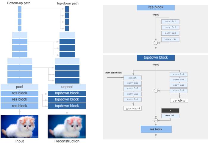
Figure 21.12: The top-down encoder used by the hierarchical VAE in [Chi21a]. Each convolution is preceded by the GELU nonlinearity. The model uses average pooling and nearest-neighbor upsampling for the pool and unpool layers. The posterior q^ε and prior p^ω are diagonal Gaussians. From Figure 3 of [Chi21a]. Used with kind permission of Rewon Child.

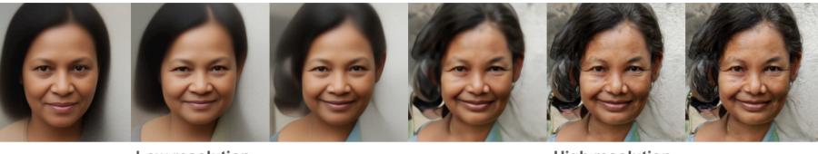
Figure 21.13: Samples from a VDVAE model (trained on FFHQ dataset) from di!erent levels of the hierarchy. From Figure 1 of [Chi21a]. Used with kind permission of Rewon Child.

compression, since a lot of the low-level details can be drawn from the prior (i.e., “hallucinated”), rather than having to be sent by the encoder.

We can also use the model for unconditional sampling at multiple resolutions. This is illustrated in Figure 21.13, using a model with 78 stochastic layers trained on the FFHQ-256 dataset.9.

21.5.3 Connection with autoregressive models

Until recently, most hierarchical VAEs only had a small number of stochastic layers. Consequently the images they generated have not looked as good, or had as high likelihoods, as images produced by other models, such as the autoregressive PixelCNN model (see Section 22.3.2). However, by endowing VAEs with many more stochastic layers, it is possible to outperform AR models in terms of

^9. This is a 256² version of the Flickr-Faces High Quality dataset from https://github.com/NVlabs/ffhq-dataset, which has 80k images at 1024² resoution.

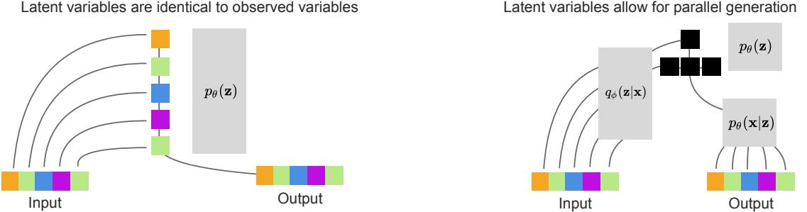
Figure 21.14: Left: a hierarchical VAE which emulates an autoregressive model using an identify encoder, autoregressive prior, and identity decoder. Right: a hierarchical VAE with a 2 layer hierarchical latent code. The bottom hidden nodes (black) are conditionally independent given the top layer. From Figure 2 of [Chi21a]. Used with kind permission of Rewon Child.

likelihood and sample quality, while using fewer parameters and much less computing power [Chi21a; VK20a; Maa+19].

To see why this is possible, note that we can represent any AR model as a degenerate VAE, as shown in Figure 21.14(left). The idea is simple: the encoder copies the input into latent space by setting z1:^D = x1:^D (so qε(zⁱ = xi|z>i, x)=1), then the model learns an autoregressive prior pω(z1:D) = ^d p(zd|z1:d↑1), and finally the likelihood function just copies the latent vector to output space, so pω(xⁱ = zi|z)=1. Since the encoder computes the exact (albeit degenerate) posterior, we have qε(z|x) = pω(z|x), so the ELBO is tight and reduces to the log likelihood,

\[\log p\_{\theta}(\mathbf{z}) = \log p\_{\theta}(\mathbf{z}) = \sum\_{d} \log p\_{\theta}(x\_d | \mathbf{z}\_{\]

Thus we can emulate any AR model with a VAE providing it has at least D stochastic layers, where D is the dimensionality of the observed data.

In practice, data usually lives in a lower-dimensional manifold (see e.g., [DW19]), which can allow for a much more compact latent code. For example, Figure 21.14(right) shows a hierarchical code in which the latent factors at the lower level are conditionally independent given the higher level, and hence can be generated in parallel. Such a tree-like structure can enable sample generation in O(log D) time, whereas an autoregressive model always takes O(D) time. (Recall that for an image D is the number of pixels, so it grows quadratically with image resolution. For example, even a tiny 32 ↗ 32 image has D = 3072.)

In addition to speed, hierarchical models also require many fewer parameters than “flat” models. The typical architecture used for generating images is a multi-scale approach: the model starts from a small, spatially arranged set of latent variables, and at each subsequent layer, the spatial resolution is increased (usually by a factor of 2). This allows the high level to capture global, long-range correlations (e.g., the symmetry of a face, or overall skin tone), while letting lower levels capture fine-grained details.

21.5.4 Variational pruning

A common problem with hierarchical VAEs is that the higher level latent layers are often ignored, so the model does not learn interesting high level semantics. This is caused by variational pruning. This problem is analogous to the issue of latent variable collapse, which we discussed in Section 21.4.

A common heuristic to mitigate this problem is to use KL balancing coe”cients [Che+17b], to ensure that an equal amount of information is encoded in each layer. That is, we use the following penalty:

\[\sum\_{l=1}^{L} \gamma \mathbb{E}\_{q\_{\boldsymbol{\Phi}}(\mathbf{z}\_{>l}|\mathbf{z})} \left[ D\_{\mathbb{KL}} \left( q\_{\boldsymbol{\Phi}}(\mathbf{z}\_{l}|\mathbf{z}, \mathbf{z}\_{>l}) \parallel p\_{\boldsymbol{\theta}}(\mathbf{z}\_{l}|\mathbf{z}\_{>l}) \right) \right] \tag{21.70}\]

The balancing term γ^l is set to a small value when the KL penalty is small (on the current minibatch), to encourage use of that layer, and is set to a large value when the KL term is large. (This is only done during the “warm up period”.) Concretely, [VK20a] proposes to set the coe”cients γ^l to be proportional to the size of the layer, sl, and the average KL loss:

\[\gamma\_{l} \propto s\_{l} \mathbb{E}\_{\mathbf{z} \sim \mathcal{B}} \left[ \mathbb{E}\_{q\_{\phi}(\mathbf{z}\_{>l}|\mathbf{z})} \left[ D\_{\text{KL}} \left( q\_{\phi}(\mathbf{z}\_{l}|\mathbf{z}, \mathbf{z}\_{>l}) \parallel p\_{\theta}(\mathbf{z}\_{l}|\mathbf{z}\_{>l}) \right) \right] \right] \tag{21.71}\]

where B is the current minibatch.

21.5.5 Other optimization di!culties

A common problem when training (hierarchical) VAEs is that the loss can become unstable. The main reason for this is that the KL term is unbounded (can become infinitely large). In [Chi21a], they tackle the problem in two ways. First, ensure the initial random weights of the final convolutional layer in each residual bottleneck block get scaled by 1/ ′ L. Second, skip an update step if the norm of the gradient of the loss exceeds some threshold.

In the Nouveau VAE method of [VK20a], they use some more complicated measures to ensure stability. First, they use batch normalization, but with various tweaks. Second, they use spectral regularization for the encoder. Specifically they add the penalty ε * ⁱ ωi, where ωⁱ is the largest singular value of the i’th convolutional layer (estimated using a single power iteration step), and ε ⇒ 0 is a tuning parameter. Third, they use inverse autoregressive flows (Section 23.2.4.3) in each layer, instead of a diagonal Gaussian approximation. Fourth, they represent the posterior using a residual representation. In particular, let us assume the prior for the i’th variable in layer l is

\[p\_{\theta}(z\_{l}^{i}|\mathbf{z}\_{>l}) = \mathcal{N}(z\_{l}^{i}|\mu\_{i}(\mathbf{z}\_{>l}), \sigma\_{i}(\mathbf{z}\_{>l})) \tag{21.72}\]

They propose the following posterior approximation:

\[q\_{\phi}(z\_{l}^{i}|x, z\_{>l}) = \mathcal{N}\left(z\_{l}^{i}|\mu\_{i}(z\_{>l}) + \Delta\mu\_{i}(z\_{>l}, x), \ \sigma\_{i}(z\_{>l}) \cdot \Delta\sigma\_{i}(z\_{>l}, x)\right) \tag{21.73}\]

where the ” terms are the relative changes computed by the encoder. The corresponding KL penalty reduces to the following (dropping the l subscript for brevity):

\[D\_{\rm KL}\left(q\_{\phi}(z^i|x,z\_{\rhd})\parallel p\_{\theta}(z^i|x\_{\rhd})\right) = \frac{1}{2}\left(\frac{\Delta\mu\_i^2}{\sigma\_i^2} + \Delta\sigma\_i^2 - \log\Delta\sigma\_i^2 - 1\right) \tag{21.74}\]

So as long as ςⁱ is bounded from below, the KL term can be easily controlled just by adjusting the encoder parameters.

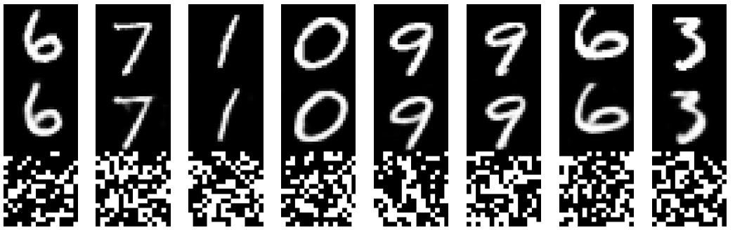
Figure 21.15: Autoencoder for MNIST using 256 binary latents. Top row: input images. Middle row: reconstruction. Bottom row: latent code, reshaped to a 16 ↓ 16 image. Generated by quantized\_autoencoder\_mnist.ipynb.

21.6 Vector quantization VAE

In this section, we describe VQ-VAE, which stands for “vector quantized VAE” [OVK17; ROV19]. This is like a standard VAE except it uses a set of discrete latent variables.

21.6.1 Autoencoder with binary code

The simplest approach to the problem is to construct a standard VAE, but to add a discretization layer at the end of the encoder, ^ze(x) ^→ {0,…,S ^↓ 1}^K, where ^S is the number of states, and ^K is the number of discrete latents. For example, we can binarize the latent vector (using S = 2) by clipping ^z to lie in {0, ¹}^K. This can be useful for data compression (see e.g., [BLS17]).

Suppose we assume the prior over the latent codes is uniform. Since the encoder is deterministic, the KL divergence reduces to a constant, equal to log K. This avoids the problem with posterior collapse (Section 21.4). Unfortunately, the discontinuous quantization operation of the encoder prohibits the direct use of gradient based optimization. The solution proposed in [OVK17] is to use the straight-through estimator, which we discuss in Section 6.3.8. We show a simple example of this approach in Figure 21.15, where we use a Gaussian likelihood, so the loss function has the form

\[\mathcal{L} = ||\mathbf{z} - d(e(\mathbf{z}))||\_2^2 \tag{21.75}\]

where ^e(x) ^→ {0, ¹}^K is the encoder, and ^d(z) ^{→ R28}⇐²⁸ is the decoder.

21.6.2 VQ-VAE model

We can get a more expressive model by using a 3d tensor of discrete latents, ^{z → RH}⇐W⇐^K, where K is the number of discrete values per latent variable. Rather than just binarizing the continuous vector ^ze(x)ij , we compare it to a codebook of embedding vectors, {e^k : ^k =1: K, ^{ek → RD}}, and then set zij to the index of the nearest codebook entry:

\[q(\mathbf{z}\_{ij} = k | \mathbf{z}) = \begin{cases} 1 & \text{if } k = \operatorname{argmin}\_{k'} ||\mathbf{z}\_e(\mathbf{z})\_{i,j,:} - \mathbf{e}\_{k'}||\_2 \\ 0 & \text{otherwise} \end{cases} \tag{21.76}\]

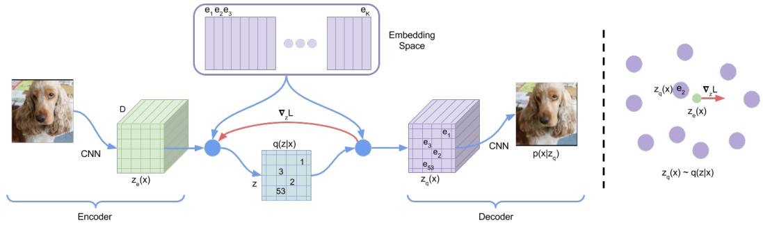
Figure 21.16: VQ-VAE architecture. From Figure 1 of [OVK17]. Used with kind permission of Aäron van den Oord.

When reconstructing the input we replace each discrete code index by the corresponding real-valued codebook vector:

\[(z\_q)\_{ij} = \mathbf{e}\_k \text{ where } \mathbf{z}\_{ij} = k \tag{21.77}\]

These values are then passed to the decoder, p(x|zq), as usual. See Figure 21.16 for an illustration of the overall architecture. Note that although z^q is generated from a discrete combination of codebook vectors, the use of a distributed code makes the model very expressive. For example, if we use a grid of 32 ↗ 32, with ^K = 512, then we can generate 512³²⇐³² = 2⁹²¹⁶ distinct images, which is astronomically large.

To fit this model, we can minimize the negative log likelihood (reconstruction error) using the straight-through estimator, as before. This amounts to passing the gradients from the decoder input zq(x) to the encoder output ze(x), bypassing Equation (21.76), as shown by the red arrow in Figure 21.16. Unfortunately this means that the codebook entries will not get any learning signal. To solve this, the authors proposed to add an extra term to the loss, known as the codebook loss, that encourages the codebook entries e to match the output of the encoder. We treat the encoder ze(x) as a fixed target, by adding a stop gradient operator to it; this ensures z^e is treated normally in the forwards pass, but has zero gradient in the backwards pass. The modified loss (dropping the spatial indices i, j) becomes

\[\mathcal{L} = -\log p(\mathbf{z}|\mathbf{z}\_q(\mathbf{z})) + ||\mathbf{s}\mathbf{g}(\mathbf{z}\_e(\mathbf{z})) - \mathbf{e}||\_2^2 \tag{21.78}\]

where e refers to the codebook vector assigned to ze(x), and sg is the stop gradient operator.

An alternative way to update the codebook vectors is to use moving averages. To see how this works, first consider the batch setting. Let {zi,1,…, zi,nⁱ } be the set of nⁱ outputs from the encoder that are closest to the dictionary item ei. We can update eⁱ to minimize the MSE

\[\sum\_{j=1}^{n\_i} ||z\_{i,j} - \mathbf{e}\_i||\_2^2 \tag{21.79}\]

which has the closed form update

\[\mathbf{e}\_{i} = \frac{1}{n\_{i}} \sum\_{j=1}^{n\_{i}} \mathbf{z}\_{i,j} \tag{21.80}\]

This is like the M step of the EM algorithm when fitting the mean vectors of a GMM. In the minibatch setting, we replace the above operations with an exponentially moving average, as follows:

\[N\_i^t = \gamma N\_i^{t-1} + (1 - \gamma)n\_i^t \tag{21.81}\]

\[\mathbf{m}\_{i}^{t} = \gamma \mathbf{m}\_{i}^{t-1} + (1 - \gamma) \sum\_{j} \mathbf{z}\_{i,j}^{t} \tag{21.82}\]

\[\mathbf{e}\_{i}^{t} = \frac{m\_{i}^{t}}{N\_{i}^{t}} \tag{21.83}\]

The authors found γ = 0.9 to work well.

The above procedure will learn to update the codebook vectors so it matches the output of the encoder. However, it is also important to ensure the encoder does not “change its mind” too often about what codebook value to use. To prevent this, the authors propose to add a third term to the loss, known as the commitment loss, that encourages the encoder output to be close to the codebook values. Thus we get the final loss:

\[\mathcal{L} = -\log p(\mathbf{z}|\mathbf{z}\_q(\mathbf{z})) + ||\text{sg}(\mathbf{z}\_e(\mathbf{z})) - \mathbf{e}||\_2^2 + \beta||\mathbf{z}\_e(\mathbf{z}) - \text{sg}(\mathbf{e})||\_2^2 \tag{21.84}\]

The authors found ε = 0.25 to work well, although of course the value depends on the scale of the reconstruction loss (NLL) term. (A probabilistic interpretation of this loss can be found in [Hen+18].) Overall, the decoder optimizes the first term only, the encoder optimizes the first and last terms, and the embeddings optimize the middle term.

21.6.3 Learning the prior

After training the VQ-VAE model, it is possible to learn a better prior, to match the aggregated posterior. To do this, we just apply the encoder to a set of data, {xn}, thus converting them to discrete sequences, {zn}. We can then learn a joint distribution p(z) using any kind of sequence model. In the original VQ-VAE paper [OVK17], they used the causal convolutional PixelCNN model (Section 22.3.2). More recent work has used transformer decoders (Section 22.4). Samples from this prior can then be decoded using the decoder part of the VQ-VAE model. We give some examples of this in the sections below.

21.6.4 Hierarchical extension (VQ-VAE-2)

In [ROV19], they extend the original VQ-VAE model by using a hierarchical latent code. The model is illustrated in Figure 21.17. They applied this to images of size 256 ↗ 256 ↗ 3. The first latent layer maps this to a quantized representation of size 64 ↗ 64, and the second latent layer maps this to a quantized representation of size 32 ↗ 32. This hierarchical scheme allows the top level to focus on high level semantics of the image, leaving fine visual details, such as texture, to the lower level. (See Section 21.5 for more discussion of hierarchical VAEs.)

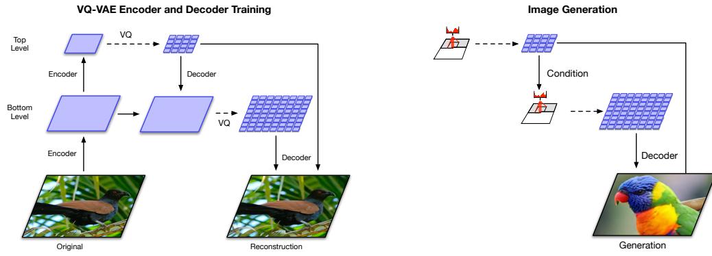
Figure 21.17: Hierarchical extension of VQ-VAE. (a) Encoder and decoder architecture. (b) Combining a Pixel-CNN prior with the decoder. From Figure 2 of [ROV19]. Used with kind permission of Aaron van den Oord.

After fitting the VQ-VAE, they learn a prior over the top level code using a PixelCNN model augmented with self-attention (Section 16.2.7) to capture long-range dependencies. (This hybrid model is known as PixelSNAIL [Che+17c].) For the lower level prior, they just use standard PixelCNN, since attention would be too expensive. Samples from the model can then be decoded using the VQ-VAE decoder, as shown in Figure 21.17.

21.6.5 Discrete VAE

In VQ-VAE, we use a one-hot encoding for the latents, q(z = k|x)=1 i! k = argmin^k ||ze(x) ↓ ek||2, and then set z^q = ek. This does not capture any uncertainty in the latent code, and requires the use of the straight-through estimator for training.

Various other approaches to fitting VAEs with discrete latent codes have been investigated. In the DALL-E paper (Section 22.4.2), they use a fairly simple method, based on using the Gumbel-softmax relaxation for the discrete variables (see Section 6.3.6). In brief, let q(z = k|x) be the probability that the input x is assigned to codebook entry k. We can exactly sample w^k ↑ q(z = k|x) from this by computing w^k = argmax^k g^k + log q(z = k|x), where each g^k is from a Gumbel distribution. We can now “relax” this by using a softmax with temperature ⇀ > 0 and computing

\[w\_k = \frac{\exp(\frac{g\_k + \log q(z = k \| \mathbf{z})}{\tau})}{\sum\_{j=1}^K \exp(\frac{g\_j + \log q(z = j \| \mathbf{z})}{\tau})} \tag{21.85}\]

We now set the latent code to be a weighted sum of the codebook vectors:

\[\mathbf{z}\_q = \sum\_{k=1}^{K} w\_k \mathbf{e}\_k \tag{21.86}\]

In the limit that ⇀ ↔︎ 0, the distribution over weights w converges to a one-hot disribution, in which case z becomes equal to one of the codebook entries. But for finite ⇀ , we “fill in” the space between the vectors.

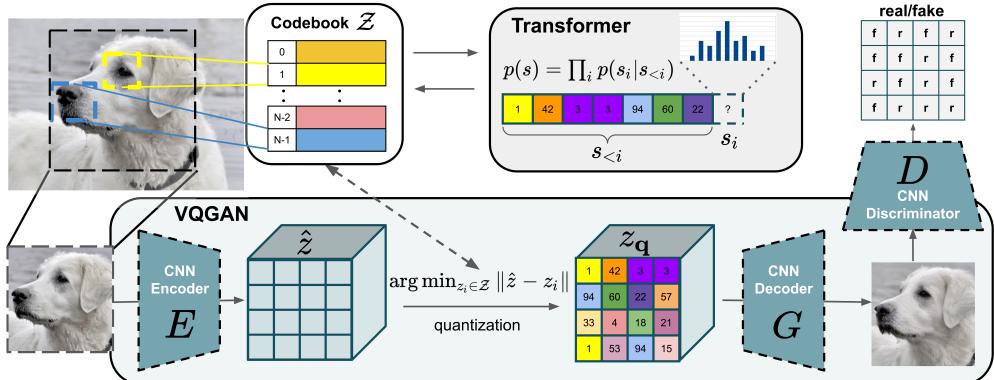
Figure 21.18: Illustration of the VQ-GAN. From Figure 2 of [ERO21]. Used with kind permission of Patrick Esser.

This allows us to express the ELBO in the usual di!erentiable way:

\[\mathcal{L} = -\mathbb{E}\_{q(\mathbf{z}|\mathbf{z})} \left[ \log p(\mathbf{z}|\mathbf{z}) \right] + \beta D\_{\text{KL}} \left( q(\mathbf{z}|\mathbf{z}) \parallel p(\mathbf{z}) \right) \tag{21.87}\]

where ε > 0 controls the amount of regularization. (Unlike VQ-VAE, the KL term is not a constant, because the encoder is stochastic.) Furthermore, since the Gumbel noise variables are sampled from a distribution that is independent of the encoder parameters, we can use the reparameterization trick (Section 6.3.5) to optimize this.

21.6.6 VQ-GAN

One drawback of VQ-VAE is that it uses mean squared error in its reconstruction loss, which can result in blurry samples. In the VQ-GAN paper [ERO21], they replace this with a (patch-wise) GAN loss (see Chapter 26), together with a perceptual loss; this results in much higher visual fidelity. In addition, they use a transformer (see Section 16.3.5) to model the prior on the latent codes. See Figure 21.18 for a visualization of the overall model. In [Yu+21], they replace the CNN encoder and decoder of the VQ-GAN model with transformers, yielding improved results; they call this VIM (vector-quantized image modeling).

22 Autoregressive models

22.1 Introduction

By the chain rule of probability, we can write any joint distribution over T variables as follows:

\[p(\mathbf{z}\_{1:T}) = p(\mathbf{z}\_1)p(\mathbf{z}\_2|\mathbf{z}\_1)p(\mathbf{z}\_3|\mathbf{z}\_2, \mathbf{z}\_1)p(\mathbf{z}\_4|\mathbf{z}\_3, \mathbf{z}\_2, \mathbf{z}\_1) \dots = \prod\_{t=1}^T p(\mathbf{z}\_t|\mathbf{z}\_{1:t-1}) \tag{22.1}\]

where x^t → X is the t’th observation, and we define p(x1|x1:0) = p(x1) as the initial state distribution. This is called an autoregressive model or ARM. This corresponds to a fully connected DAG, in which each node depends on all its predecessors in the ordering, as shown in Figure 22.1. The models can also be conditioned on arbitrary inputs or context c, in order to define p(x|c), although we omit this for notational brevity.

We could of course also factorize the joint distribution “backwards” in time, using

\[p(\mathbf{x}\_{1:T}) = \prod\_{t=T}^{1} p(\mathbf{x}\_t | \mathbf{x}\_{t+1:T}) \tag{22.2}\]

However, this “anti-causal” direction is often harder to learn (see e.g., [PJS17]).

Although the decomposition in Equation (22.1) is general, each term in this expression (i.e., each conditional distribution p(xt|x1:t↑¹)) becomes more and more complex, since it depends on an increasing number of arguments, which makes the terms slow to compute, and makes estimating their parameters more data hungry (see Section 2.6.3.2).

One approach to solving this intractability is to make the (first-order) Markov assumption, which gives rise to a Markov model p(xt|x1:t↑¹) = p(xt|x^t↑¹), which we discuss in Section 2.6. (This is also called an auto-regressive model of order 1.) Unfortunately, the Markov assumption is very limiting. One way to relax it, and to make x^t depend on all the past x1:t↑¹ without explicitly regressing on them, is to assume the past can be compressed into a hidden state zt. If z^t is a deterministic function of the past observations x1:t↑1, the resulting model is known as a recurrent neural network, discussed in Section 16.3.4. If z^t is a stochastic function of the past hidden state, z^t↑1, the resulting model is known as a hidden Markov model, which we discuss in Section 29.2.

Another approach is to stay with the general AR model of Equation (22.1), but to use a restricted functional form, such as some kind of neural network, for the conditionals p(xt|x1:t↑1). Thus rather than making conditional independence assumptions, or explicitly compressing the past into a su”cient

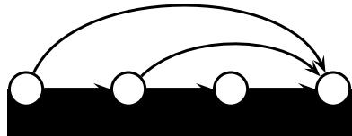
Figure 22.1: A fully-connected auto-regressive model.

statistic, we implicitly learn a compact mapping from the past to the future. In the sections below, we discuss di!erent functional forms for these conditional distributions.

The main advantage of such AR models is that it is easy to compute, and optimize, the exact likelihood of each sequence (data vector). The main disadvantage is that generating samples is inherently sequential, which can be slow. In addition, the method does not learn a compact latent representation of the data.

22.2 Neural autoregressive density estimators (NADE)

A simple way to represent each conditional probability distribution p(xt|x1:t↑1) is to use a generalized linear model, such as logistic regression, as proposed in [Fre98]. We can make the model be more powerful by using a neural network. The resulting model is called the neural auto-regressive density estimator or NADE model [LM11].

If we let p(xt|x1:t↑¹) be a conditional mixture of Gaussians, we get a model known as RNADE (“real-valued neural autoregressive density estimator”) of [UML13]. More precisely, this has the form

\[p(x\_t | \mathbf{z}\_{1:t-1}) = \sum\_{k=1}^{K} \pi\_{t,k} \mathcal{N}(x\_t | \mu\_{t,k}, \sigma\_{t,k}^2) \tag{22.3}\]

where the parameters are generated by a network, (µt,ϱt,↼t) = ft(x1:t↑¹; εt).

Rather than using separate neural networks, f1,…,f^T , it is more e”cient to create a single network with T inputs and T outputs. This can be done using masking, resulting in a model called the MADE (“masked autoencoder for density estimation”) model [Ger+15].

One disadvantage of NADE-type models is that they assume the variables have a natural linear ordering. This makes sense for temporal or sequential data, but not for more general data types, such as images or graphs. An orderless extension to NADE was proposed in [UML14; Uri+16].

22.3 Causal CNNs

One approach to representing the distribution p(xt|x1:t↑1) is to try to identify patterns in the past history that might be predictive of the value of xt. If we assume these patterns can occur in any location, it makes sense to use a convolutional neural network to detect them. However, we need to make sure we only apply the convolutional mask to past inputs, not future ones. This can be done using masked convolution, also called causal convolution. We discuss this in more detail below.

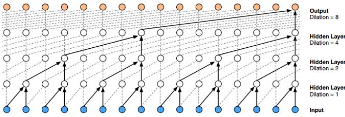
Figure 22.2: Illustration of the wavenet model using dilated (atrous) convolutions, with dilation factors of 1, 2, 4 and 8. From Figure 3 of [Oor+16a]. Used with kind permission of Aäron van den Oord.

22.3.1 1d causal CNN (convolutional Markov models)

Consider the following convolutional Markov model for 1d discrete sequences:

\[p(\mathbf{z}\_{1:T}) = \prod\_{t=1}^{T} p(x\_t | \mathbf{z}\_{1:t-1}; \boldsymbol{\theta}) = \prod\_{t=1}^{T} \text{Cat}(x\_t | \text{softmax}(\varphi(\sum\_{\tau=1}^{t-k} \mathbf{w}^{\mathsf{T}} \mathbf{z}\_{\tau:\tau+k}))) \tag{22.4}\]

where w is the convolutional filter of size k, and we have assumed a single nonlinearity ϕ and categorical output, for notational simplicity. This is like regular 1d convolution except we “mask out” future inputs, so that x^t only depends on the past values. We can of course use deeper models, and we can condition on input features c.

In order to capture long-range dependencies, we can use dilated convolution (see [Mur22, Sec 14.4.1]). This model has been successfully used to create a state of the art text to speech (TTS) synthesis system known as wavenet [Oor+16a]. See Figure 22.2 for an illustration.

The wavenet model is a conditional model, p(x|c), where c is a set of linguistic features derived from an input sequence of words, and x is raw audio. The tacotron system [Wan+17c] is a fully end-to-end approach, where the input is words rather than linguistic features.

Although wavenet produces high quality speech, it is too slow for use in production systems. However, it can be “distilled” into a parallel generative model [Oor+18], as we discuss in Section 23.2.4.3.

22.3.2 2d causal CNN (PixelCNN)

We can extend causal convolutions to 2d, to get an autoregressive model of the form

\[p(x|\theta) = \prod\_{r=1}^{R} \prod\_{c=1}^{C} p(x\_{r,c}|f\_{\theta}(x\_{1:r-1,1:C}, x\_{r,1:c-1})) \tag{22.5}\]

where R is the number of rows, C is the number of columns, and we condition on all previously generated pixels in a raster scan order, as illustrated in Figure 22.3. This is called the pixelCNN model [Oor+16b]. Naive sampling (generation) from this model takes O(N) time, where N = RC is the number of pixels, but [Ree+17] shows how to use a multiscale approach to reduce the complexity to O(log N).

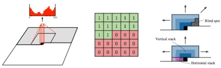
Figure 22.3: Illustration of causal 2d convolution in the PixelCNN model. The red histogram shows the empirical distribution over discretized values for a single pixel of a single RGB channel. The red and green 5 ↓ 5 array shows the binary mask, which selects the top left context, in order to ensure the convolution is causal. The diagrams on the right illustrate how we can avoid blind spots by using a vertical context stack, that contains all previous rows, and a horizontal context stack, that just contains values from the current row. From Figure 1 of [Oor+16b]. Used with kind permission of Aaron van den Oord.

Various extensions of this model have been proposed. The pixelCNN++ model of [Sal+17d] improved the quality by using a mixture of logistic distributions, to capture the multimodality of p(xi|x1:i↑¹). The pixelRNN of [OKK16] combined masked convolution with an RNN to get even longer range contextual dependencies. The Subscale Pixel Network of [MK19] proposed to generate the pixels such that the higher order bits are sampled before lower order bits, which allows high resolution details to be sampled conditioned on low resolution versions of the whole image, rather than just the top left corner.

22.4 Transformers

We introduced transformers in Section 16.3.5. They can be used for encoding sequences (as in BERT), or for decoding (generating) sequences. We can also combine the two, using an encoder-decoder combination, for conditional generation from p(y|c). Alternatively, we can define a joint sequence model p(c, y), where c is the conditioning or context prompt, and then just condition the joint model, by giving it as the initial context.

The decoder (generator) works as follows. At each step t, the model applies masked (causal) self attention (Section 16.2.7) to the first t inputs, y1:t, to compute a set of attention weights, a1:t. From this it computes an activation vector z^t = *^{t ς}=1 atyt. This is then passed through a feed-forward layer to compute h^t = MLP(zt). This process is repeated for each layer in the model. Finally the output is used to predict the next element in the sequence, yt+1 ↑ Cat(softmax(Wht)).

At training time, all predictions can happen in parallel, since the target generated sequence is already available. That is, the t’th output y^t can be predicted given inputs y1:t↑¹, and this can be done for all t simultaneously. However, at test time, the model must be applied sequentially, so the output generated at t + 1 is fed back into the model to predict t + 2, etc. Note that the running time of transformers is O(T²), although a variety of more e”cient versions have been developed (see e.g., [Mur22, Sec 15.6] for details).

Transformers are the basis of many popular (conditional) generative models for sequences. We give some examples below.

Figure 22.4: Illustration of few shot learning with GPT-3. The model is asked to create an example sentence using a new word whose meaning is provided in the prompt. Boldface is GPT-3’s completions, light gray is human input. From Figure 3.16 of [Bro+20d].

22.4.1 Text generation (GPT, etc.)

In [Rad+18], OpenAI proposed a model called GPT, which is short for “Generative Pre-training Transformer”. This is a decoder-only transformer model that uses causal (masked) attention. In [Rad+19], they propose GPT-2, which is a larger version of GPT (1.5 billion parameters, or 6.5GB, for the XL version), trained on a large web corpus (8 million pages, or 40GB). They also simplify the training objective, and just train it using maximum likelihood.

After GPT-2, OpenAI released GPT-3 [Bro+20d], which is an even larger version of GPT-2 (175 billion parameters), trained on even more data (300 billion words), but based on the same principles. (Training was estimated to take 355 GPU years and cost $4.6M.) Large models of this form, trained on very large datasets, are often called large language models (LLM) (see e.g., [Bur25]) or foundation models [Cen21].

Due to the large size of the data and model, GPT-3 shows even more remarkable abilities to generate novel text. In particular, the output can be (partially) controlled by just changing the conditioning prompt. This enables the model to perform tasks that it has never been trained on, just by giving it some examples in the prompt. This is called “in-context learning”. See Figure 22.4 for an example, and Section 19.5.1.2 for more details.

More recently, OpenAI released ChatGPT [Ope], which is an improved version of GPT-3 which has been trained to have interactive dialogs by using a technique called reinforcement learning from human feedback or RLHF, a technique first introduced in the InstructGPT paper [Ouy+22]. This uses RL techniques such as PPO (Section 35.3.4) to fine tune the model so that it generates

(JAX):
Yo, PyTorch, you think you're hot stuff.
But JAX is where it's at, no need to bluff.
Your popularity might be on the rise
But when it comes to performance, we're the guys.
With automatic differentation, we're a breeze
Training neural nets with ease
Our functional approach is innovative and unique
PyTorch can't touch our speed, try and keep up, meek
(PyTorch):
Hold up, JAX, you might be fast
But PyTorch is the one that's built to last
We may not have the fancy functional flair
But our flexibility sets us above the pair
Our community is strong and growing each day
Suppporting us in every single way
We may not be the newest on the block
But we'lll always be the torch that leads the flock

Figure 22.5: ChatGPT response to the prompt “Write a rap battle about PyTorch and JAX”. Used with kind permission of Paige Bailey. From https: // twitter. com/ DynamicWebPaige/ status/ 1601743574369902593 .

responses that are more “aligned” with human intent, as estimated by a ranking model, which is pre-trained on supervised data.

Despite the impressive performance of these large language models or LLMs (see Figure 22.5 for an example), there are several open problems with them, such as: they often confidently hallucinate incorrect answers to questions (see e.g., [Ji+22]); they can generate biased or toxic output (see e.g., [Lia+]); and they are very resource intensive to train and serve (see e.g., [SPS20]).

The basic ideas behind LLMs are quite simple (maximum likelihood training of an autoregresssive transformer), and they can be implemented in about 300 lines of code.1 However, just by scaling up the size of the models and datasets, it seems that qualitatively new capabilities can emerge (see e.g., [Wei+22]). Nevertheless, although this approach is good at learning formal linguistic competence (surface form), it is not clear if it is su”cient to learn functional linguistic competence, which requires a deeper, non-linguistic understanding of the world derived from experience [Mah+23].

22.4.2 Image generation (DALL-E, etc.)

The DALL-E model2 from OpenAI [Ram+21a] can generate images of remarkable quality and diversity given text prompts, as shown in Figure 22.6. The methodology is conceptually quite straightforward, and most of the e!ort went into data collection (they scraped the web for 250 million image-text pairs) and scaling up the training (they fit a model with 12 billion parameters). Here we just focus on the algorithmic methods.

^1. See e.g., https://github.com/karpathy/nanoGPT.

^2. The name is derived from the artist Salvador Dalí and Pixar’s movied “WALL-E”

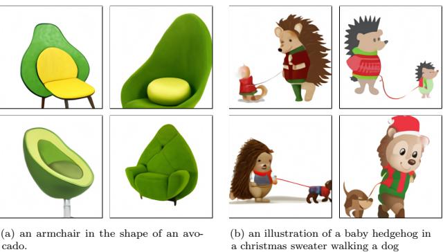
Figure 22.6: Some images generated by the DALL-E model in response to a text prompt. (a) “An armchair in the shape of an avocado”. (b) “An illustration of a baby hedgehog in a christmas sweater walking a dog”. From https: // openai. com/ blog/ dall-e . Used with kind permission of Aditya Ramesh.

The basic idea is to transform an image x into a sequence of discrete tokens z using a discrete VAE model (Section 21.6.5). We then fit a transformer to the concatentation of the image tokens z and text tokens y to get a joint model of the form p(z, y).

To sample an image x given a text prompt y, we sample a latent code z ↑ p(z|y) by conditioning the transformer on the prompt y, and then we feed z into the VAE decoder to get the image x ↑ p(x|z). Multiple images are generated for each prompt, and these are then ranked according to a pre-trained critic, which gives them scores depending on how well the generated image matches the input text: sⁿ = critic(xn, yn). The critic they used was the contrastive CLIP model (see Section 32.3.4.1). This discriminative reranking significantly improves the results.

Some sample results are shown in Figure 22.6, and more can be found online at https://openai. com/blog/dall-e/. The image on the right of Figure 22.6 is particularly interesting, since the prompt — “An illustration of a baby hedgehog in a christmas sweater walking a dog” — arguably requires that the model solve the “variable binding problem”. This refers to the fact that the sentence implies the hedgehog should be wearing the sweater and not the dog. We see that the model sometimes interprets this correctly, but not always: sometimes it draws both animals with Christmas sweaters. In addition, sometimes it draws a hedgehog walking a smaller hedgehog. The quality of the results can also be sensitive to the form of the prompt.

The PARTI model [Yu+22] from Google follows similar high level ideas to DALL-E, but has been scaled to an even larger size. The larger models perform qualitatively much better, as shown in Figure 20.3.

Other recent approaches to (conditional) image generation — such as DALL-E 2 [Ram+22] from Open-AI, Imagen [Sah+22b] from Google, and Stable di!usion [Rom+22] from Stability.AI — are based on di!usion rather than applying a transformer to discretized image patches. See Section 25.6.4 for details.

22.4.3 Other applications

Transformers have been used to generate many other kinds of (discrete) data, such as midi music sequences [Hua+18a], protein sequences [Gan+23], etc.

22.5 Large Language Models (LLMs)

A large language model or LLM is just an auto-regressive generative model of discrete tokens, representing words or possibly quantized versions of other modalities such as image patches. Such models are almost always implemented using transformers and trained using maximum likelihood. LLMs are a very hot topic at the moment, and more details can be found in e.g., [Bur25]. However, the basic ideas are summarized in Section 22.4.1.

23 Normalizing flows

This chapter is written by George Papamakarios and Balaji Lakshminarayanan.

23.1 Introduction

In this chapter we discuss normalizing flows, a class of flexible density models that can be easily sampled from and whose exact likelihood function is e”cient to compute. Such models can be used for many tasks, such as density modeling, inference and generative modeling. We introduce the key principles of normalizing flows and refer to recent surveys by Papamakarios et al. [Pap+19] and Kobyzev, Prince, and Brubaker [KPB19] for readers interested in learning more. See also https://github.com/janosh/awesome-normalizing-flows for a list of papers and software packages.

23.1.1 Preliminaries

Normalizing flows create complex probability distributions ^p(x) by passing random variables ^{u → RD}, drawn from a simple base distribution p(u) through a nonlinear but invertible transformation ^f : ^{RD ↔︎ RD}. That is, ^p(x) is defined by the following process:

\[\mathbf{x} = \mathbf{f}(\mathbf{u}) \quad \text{where} \quad \mathbf{u} \sim p(\mathbf{u}). \tag{23.1}\]

The base distribution is typically chosen to be simple, for example standard Gaussian or uniform, so that we can easily sample from it and compute the density p(u). A flexible enough transformation f can induce a complex distribution on the transformed variable x even if the base distribution is simple.

Sampling from p(x) is straightforward: we first sample u from p(u) and then compute x = f(u). To compute the density p(x), we rely on the fact that f is invertible. Let g(x) = f ^↑1(x) = u be the inverse mapping, which “normalizes” the data distribution by mapping it back to the base distribution (which is often a normal distribution). Using the change-of-variables formula for random variables from Equation (2.257), we have

\[p\_x(\mathbf{z}) = p\_u(\mathbf{g}(\mathbf{z})) |\det \mathbf{J}(\mathbf{g})(\mathbf{z})| = p\_u(\mathbf{u}) |\det \mathbf{J}(\mathbf{f})(\mathbf{u})|^{-1},\tag{23.2}\]

where J(f)(u) = ^{φf φu} |^u is the Jacobian matrix of f evaluated at u. Taking logs of both sides of Equation (23.2), we get

\[\log p\_x(\mathbf{z}) = \log p\_u(\mathbf{u}) - \log|\det \mathbf{J}(\mathbf{f})(\mathbf{u})|.\tag{23.3}\]

As discussed above, p(u) is typically easy to evaluate. So, if one can use flexible invertible transformations f whose Jacobian determinant det J(f)(u) can be computed e”ciently, then one can construct complex densities p(x) that allow exact sampling and e”cient exact likelihood computation. This is in contrast to latent variable models, which require methods like variational inference to lower-bound the likelihood.

One might wonder how flexible are the densities p(x) obtained by transforming random variables sampled from simple p(u). It turns out that we can use this method to approximate any smooth distribution. To see this, consider the scenario where the base distribution p(u) is a one-dimensional uniform distribution. Recall that inverse transform sampling (Section 11.3.1) samples random variables from a uniform distribution and transforms them using the inverse cumulative distribution function (cdf) to generate samples from the desired density. We can use this method to sample from any one-dimensional density as long as the transformation f is powerful enough to model the inverse cdf (which is a reasonable assumption for well-behaved densities whose cdf is invertible and di!erentiable). We can further extend this argument to multiple dimensions by first expressing the density p(x) as a product of one-dimensional conditionals using the chain rule of probability, and then applying inverse transform sampling to each one-dimensional conditional. The result is a normalizing flow that transforms a product of uniform distributions into any desired distribution p(x). We refer to [Pap+19] for a more detailed proof.

How do we define flexible invertible mappings whose Jacobian determinant is easy to compute? We discuss this topic in detail in Section 23.2, but in summary, there are two main ways. The first approach is to define a set of simple transformations that are invertible by design, and whose Jacobian determinant is easy to compute; for instance, if the Jacobian is a triangular matrix, its determinant can be computed e”ciently. The second approach is to exploit the fact that a composition of invertible functions is also invertible, and the overall Jacobian determinant is just the product of the individual Jacobian determinants. More precisely, if f = f^N ∞ ··· ∞ f¹ where each fⁱ is invertible, then f is also invertible, with inverse g = g¹ ∞ ··· ∞ g^N and log Jacobian determinant given by

\[\log|\det\mathbf{J}(\mathbf{g})(\mathbf{x})| = \sum\_{i=1}^{N} \log|\det\mathbf{J}(g\_i)(\mathbf{u}\_i)|\tag{23.4}\]

where uⁱ = fⁱ ∞ ··· ∞ f1(u) is the i’th intermediate output of the flow. This allows us to create complex flows from simple components, just as graphical models allow us to create complex joint distributions from simpler conditional distributions.

Finally, a note on terminology. An invertible transformation is also known as a bijection. A bijection that is di!erentiable and has a di!erentiable inverse is known as a di!eomorphism. The transformation f of a flow model is a di!eomorphism, although in the rest of this chapter we will refer to it as a “bijection” for simplicity, leaving the di!erentiability implicit. The density px(x) of a flow model is also known as the pushforward of the base distribution pu(u) through the transformation f, and is sometimes denoted as p^x = f↔︎pu. Finally, in mathematics the term “flow” refers to any family of di!eomorphisms f^t indexed by a real number t such that t = 0 indexes the identity function, and t¹ + t² indexes f^t2 ∞ f^t1 (in physics, t often represents time). In machine learning we use the term “flow” by analogy to the above meaning, to highlight the fact that we can create flexible invertible transformations by composing simpler ones; in this sense, the index t is analogous to the number i of transformations in fⁱ ∞ ··· ∞ f1.

23.1.2 How to train a flow model

There are two common applications of normalizing flows. The first one is density estimation of observed data, which is achieved by fitting pω(x) to the data and using it as an estimate of the data density, potentially followed by generating new data from pω(x). The second one is variational inference, which involves sampling from and evaluating a variational posterior qω(z|x) parameterized by the flow model. As we will see below, these applications optimize di!erent objectives and impose di!erent computational constraints on the flow model.

23.1.2.1 Density estimation

Density estimation requires maximizing the likelihood function in Equation (23.2). This requires that we can e”ciently evaluate the inverse flow u = f ^↑1(x) and its Jacobian determinant det J(f ^↑1)(x) for any given x. After optimizing the model, we can optionally use it to generate new data. To sample new points, we require that the forwards mapping f be tractable.

23.1.2.2 Variational inference

Normalizing flows are commonly used for variational inference to parameterize the approximate posterior distribution in latent variable models, as discussed in Section 10.4.3. Consider a latent variable model with continuous latent variables z and observable variables x. For simplicity, we consider the model parameters to be fixed as we are interested in approximating the true posterior p↔︎(z|x) with a normalizing flow qω(z|x). 1 As discussed in Section 10.1.1.2, the variational parameters are trained by maximizing the evidence lower bound (ELBO), given by

\[L(\theta) = \mathbb{E}\_{q\rho\left(\mathbf{z}\mid\mathbf{z}\right)}\left[\log p(\mathbf{z}|\mathbf{z}) + \log p(\mathbf{z}) - \log q\_{\theta}(\mathbf{z}|\mathbf{z})\right] \tag{23.5}\]

When viewing the ELBO as a function of ε, it can be simplified as follows (note we drop the dependency on x for simplicity):

\[L(\boldsymbol{\theta}) = \mathbb{E}\_{q\_{\boldsymbol{\theta}}(\mathbf{z})} \left[ \ell\_{\boldsymbol{\theta}}(\mathbf{z}) \right]. \tag{23.6}\]

Let qω(z) denote a normalizing flow with base distribution q(u) and transformation z = fω(u). Then the reparameterization trick (Section 6.3.5) allows us to optimize the parameters using stochastic gradients. To achieve this, we first write the expectation with respect to the base distribution:

\[L(\boldsymbol{\theta}) = \mathbb{E}\_{q\_{\boldsymbol{\theta}}(\mathbf{z})} \left[ \ell\_{\boldsymbol{\theta}}(\mathbf{z}) \right] = \mathbb{E}\_{q(\mathbf{u})} \left[ \ell\_{\boldsymbol{\theta}}(f\_{\boldsymbol{\theta}}(\mathbf{u})) \right]. \tag{23.7}\]

Then, since the base distribution does not depend on ε, we can obtain stochastic gradients as follows:

\[\nabla\_{\theta} L(\theta) = \mathbb{E}\_{q(\mathbf{u})} \left[ \nabla\_{\theta} \ell\_{\theta}(f\_{\theta}(\mathbf{u})) \right] \approx \frac{1}{N} \sum\_{n=1}^{N} \nabla\_{\theta} \ell\_{\theta}(f\_{\theta}(\mathbf{u}\_{n})),\tag{23.8}\]

where {un}^{N n}=1 are samples from q(u).

^1. We denote the parameters of the variational posterior by ω here, which should not be confused with the model parameters which are also typically denoted by ω elsewhere.

As we can see, in order to optimize this objective, we need to be able to e”ciently sample from qω(z|x) and evaluate the probability density of these samples during optimization. (See Section 23.2.4.3 for details on how to do this.) This is contrast to the MLE approach in Section 23.1.2.1, which requires that we be able to compute e”ciently the density of arbitrary training datapoints, but it does not require samples during optimization.

23.2 Constructing flows

In this section, we discuss how to compute various kinds of flows that are invertible by design and have e”ciently computable Jacobian determinants.

23.2.1 A!ne flows

A simple choice is to use an a”ne transformation x = f(u) = Au + b. This is a bijection if and only if A is an invertible square matrix. The Jacobian determinant of f is det A, and its inverse is ^{u = f ↑}1(x) = ^A↑1(^{x ↓ b}). A flow consisting of a”ne bijections is called an ^a“ne flow, or a linear flow if we ignore b.

On their own, a”ne flows are limited in their expressive power. For example, suppose the base distribution is Gaussian, p(u) = N (u|µ, “). Then the pushforward distribution after an a”ne bijection is still Gaussian, ^p(x) = ^N (x|Aµ+b, ^A“AT). However, a”ne bijections are useful building blocks when composed with the non-a”ne bijections we discuss later, as they encourage “mixing” of dimensions through the flow.

For practical reasons, we need to ensure the Jacobian determinant and the inverse of the flow are fast to compute. In general, computing det A and A↑¹ explicitly takes O(D³) time. To reduce the cost, we can add structure to A. If A is diagonal, the cost becomes O(D). If A is triangular, the Jacobian determinant is the product of the diagonal elements, so it takes O(D) time; inverting the flow requires solving the triangular system Au = x ↓ b, which can be done with backsubstitution in O(D²) time.

The result of a triangular transformation depends on the ordering of the dimensions. To reduce sensitivity to this, and to encourage “mixing” of dimensions, we can multiply A with a permutation matrix, which has an absolute determinant of 1. We often use a permutation that reverses the indices at each layer or that randomly shu$es them. However, usually the permutation at each layer is fixed rather than learned.

For spatially structured data (such as images), we can define A to be a convolution matrix. For example, GLOW [KD18b] uses 1 ↗ 1 convolution; this is equivalent to pointwise linear transformation across feature dimensions, but regular convolution across spatial dimensions. Two more general methods for modeling d ↗ d convolutions are presented in [HBW19], one based on stacking autoregressive convolutions, and the other on carrying out the convolution in the Fourier domain.

23.2.2 Elementwise flows

Let ^h : ^{R ↔︎ R} be a scalar-valued bijection. We can create a vector-valued bijection ^f : ^{RD ↔︎ RD} by applying h elementwise, that is, f(u)=(h(u1),…,h(uD)). The function f is invertible, and its Jacobian determinant is given by ^D i=1 dh duⁱ . A flow composed of such bijections is known as an elementwise flow.

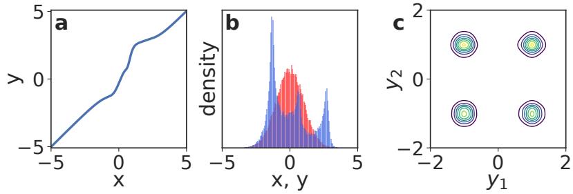
Figure 23.1: Non-linear squared flow (NLSq). Left: an invertible mapping consisting of 4 NLSq layers. Middle: red is the base distribution (Gaussian), blue is the distribution induced by the mapping on the left. Right: density of a 5-layer autoregressive flow using NLSq transformations and a Gaussian base density, trained on a mixture of 4 Gaussians. From Figure 5 of [ZR19b]. Used with kind permission of Zachary Ziegler.

On their own, elementwise flows are limited, since they do not model dependencies between the elements. However, they are useful building blocks for more complex flows, such as coupling flows (Section 23.2.3) and autoregressive flows (Section 23.2.4), as we will see later. In this section, we discuss techniques for constructing scalar-valued bijections h : R ↔︎ R for use in elementwise flows.

23.2.2.1 A”ne scalar bijection

An ^a“ne scalar bijection has the form ^h(u; ^ε) = au ^{+ b}, where ^ε = (a, b) ^{→ R2}. (This is a scalar version of an a”ne flow.) Its derivative dh du is equal to a. It is invertible if and only if a ∈= 0. In practice, we often parameterize a to be positive, for example by making it the exponential or the softplus of an unconstrained parameter. When a = 1, h(u; ε) = u + b is often called an additive scalar bijection.

23.2.2.2 Higher-order perturbations

The a”ne scalar bijection is simple to use, but limited. We can make it more flexible by adding higher-order perturbations, under the constraint that invertibility is preserved. For example, Ziegler and Rush [ZR19b] propose the following, which they term non-linear squared flow:

\[h(u; \theta) = au + b + \frac{c}{1 + (du + e)^2},\tag{23.9}\]

where ^ε = (a, b, c, d, e) ^{→ R5}. When ^c = 0, this reduces to the a”ne case. When ^{c ∈}= 0, it adds an inverse-quadratic perturbation, which can induce multimodality as shown in Figure 23.1. Under the constraints a > ⁹ 8 ^⇒3 cd and d > 0 the function becomes invertible, and its inverse can be computed analytically by solving a quadratic polynomial.

23.2.2.3 Combinations of strictly monotonic scalar functions

A strictly monotonic scalar function is one that is always increasing (has positive derivative everywhere) or always decreasing (has negative derivative everywhere). Such functions are invertible. Many

activation functions, such as the logistic sigmoid ς(u)=1/(1 + exp(↓u)), are strictly monotonic.

Using such activation functions as a starting point, we can build more flexible monotonic functions via conical combination (linear combination with positive coe”cients) and function composition. Suppose h1,…,h^K are strictly increasing; then the following are also strictly increasing:

• a1h¹ + ··· + aKh^K + b with a^k > 0 (conical combination with a bias),
• h¹ ∞ ··· ∞ h^K (function composition).

By repeating the above two constructions, we can build arbitrarily complex increasing functions. For example, a composition of conical combinations of logistic sigmoids is just an MLP where all weights are positive [Hua+18b].

The derivative of such a scalar bijection can be computed by repeatedly applying the chain rule, and in practice can be done with automatic di!erentiation. However, the inverse is not typically computable in closed form. In practice we can compute the inverse using bisection search, since the function is monotonic.

23.2.2.4 Scalar bijections from integration

A simple way to ensure a scalar function is strictly monotonic is to constrain its derivative to be positive. Let h^→ = dh du be this derivative. Wehenkel and Louppe [WL19] directly parameterize h^→ with a neural network whose output is made positive via an ELU activation function shifted up by 1. They then integrate the derivative numerically to get the bijection:

\[h(u) = \int\_0^u h'(t)dt + b,\tag{23.10}\]

where b is a bias. They call this approach unconstrained monotonic neural networks.

The above integral is generally not computable in closed form. It can be, however, if h^→ is constrained appropriately. For example, Jaini, Selby, and Yu [JSY19] take h^→ to be a sum of K squared polynomials of degree L:

\[h'(u) = \sum\_{k=1}^{K} \left(\sum\_{\ell=0}^{L} a\_{k\ell} u^{\ell}\right)^2. \tag{23.11}\]

This makes h^→ a non-negative polynomial of degree 2L. The integral is analytically tractable, and makes h an increasing polynomial of degree 2L + 1. For L = 0, h^→ is constant, so h reduces to an a”ne scalar bijection.

In these approaches, the derivative of the bijection can just be read o!. However, the inverse is not analytically computable in general. In practice, we can use bisection search to compute the inverse numerically.

23.2.2.5 Splines

Another way to construct monotonic scalar functions is using splines. These are piecewise-polynomial or piecewise-rational functions, parameterized in terms of K + 1 knots (uk, xk) through which the spline passes. That is, we set h(uk) = xk, and define h on the interval (u^k↑¹, uk) by interpolating

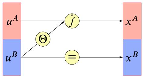
Figure 23.2: Illustration of a coupling layer x = f(u). A bijection, with parameters determined by u^B, is applied to u^A to generate x^A; meanwhile x^B = u^B is passed through unchanged, so the mapping can be inverted. From Figure 3 of [KPB19]. Used with kind permission of Ivan Kobyzev.

from x^k↑¹ to x^k with a polynomial or rational function (ratio of two polynomials). By increasing the number of knots we can create arbitrarily flexible monotonic functions.

Di!erent ways to interpolate between knots give di!erent types of spline. A simple choice is to interpolate linearly [Mül+19a]. However, this makes the derivative discontinuous at the knots. Interpolating with quadratic polynomials [Mül+19a] gives enough flexibility to make the derivative continuous. Interpolating with cubic polynomials [Dur+19], ratios of linear polynomials [DEL20], or ratios of quadratic polynomials [DBP19] allows the derivatives at the knots to be arbitrary parameters.

The spline is strictly increasing if we take u^k↑¹ < uk, x^k↑¹ < xk, and make sure the interpolation between knots is itself increasing. Depending on the flexibility of the interpolating function, more than one interpolation may exist; in practice we choose one that is guaranteed to be always increasing (see references above for details).

An advantage of splines is that they can be inverted analytically if the interpolating functions only contain low-degree polynomials. In this case, we compute u = h↑¹(x) as follows: first, we use binary search to locate the interval (x^k↑¹, xk) in which x lies; then, we analytically solve the resulting low-degree polynomial for u.

23.2.3 Coupling flows

In this section we describe coupling flows, which allow us to model dependencies between dimensions using arbitrary non-linear functions (such as deep neural networks). Consider a partition of the input ^{u → RD} into two subspaces, (u^A,u^B) ^{→ Rd} ↗ ^RD↑^d, where ^d is an integer between 1 and ^{D ↓} 1. Assume a bijection ^ˆf(·; ^ε) : ^{Rd ↔︎ Rd} parameterized by ^ε and acting on the subspace ^Rd. We define the function ^f : ^{RD ↔︎ RD} given by ^{x = f}(u) as follows:

\[\begin{aligned} \mathbf{x}^A &= \hat{\mathbf{f}}(\mathbf{u}^A; \Theta(\mathbf{u}^B)) \\ \mathbf{x}^B &= \mathbf{u}^B. \end{aligned} \tag{23.12}\]

See Figure 23.2 for an illustration. The function f is called a coupling layer [DKB15; DSDB17], because it “couples” u^A and u^B together though ˆf and #. We refer to flows consisting of coupling layers as coupling flows.

The parameters of ˆf are computed by ε = #(u^B), where # is an arbitrary function called the conditioner. Unlike a”ne flows, which mix dimensions linearly, and elementwise flows, which do not mix dimensions at all, coupling flows can mix dimensions with a flexible non-linear conditioner #. In practice we often implement # as a deep neural network; any architecture can be used, including MLPs, CNNs, ResNets, etc.

The coupling layer f is invertible, and its inverse is given by u = f ^↑1(x), where

\[\mathbf{u}^A = \mathbf{\hat{f}}^{-1}(x^A; \Theta(x^B)) \tag{23.14}\]

\[\mathbf{u}^{B} = \mathbf{x}^{B}.\tag{23.15}\]

That is, f ^↑1 is given by simply replacing ˆf with ˆf ^↑1. Because x^B does not depend on u^A, the Jacobian of f is block triangular:

\[\mathbf{J}(\mathbf{f}) = \begin{pmatrix} \partial \mathbf{x}^A / \partial \mathbf{u}^A & \partial \mathbf{x}^A / \partial \mathbf{u}^B\\ \partial \mathbf{x}^B / \partial \mathbf{u}^A & \partial \mathbf{x}^B / \partial \mathbf{u}^B \end{pmatrix} = \begin{pmatrix} \mathbf{J}(\hat{\mathbf{f}}) & \partial \mathbf{x}^A / \partial \mathbf{u}^B\\ \mathbf{0} & \mathbf{I} \end{pmatrix}. \tag{23.16}\]

Thus, det J(f) is equal to det J( ˆf).

We often define ˆf to be an elementwise bijection, so that ˆf ^↑1 and det J( ˆf) are easy to compute. That is, we define:

\[\hat{\mathbf{f}}(\boldsymbol{u}^{A};\boldsymbol{\theta}) = \left(h(u\_1^{A};\boldsymbol{\theta}\_1), \ldots, h(u\_d^{A};\boldsymbol{\theta}\_d)\right),\tag{23.17}\]

where h(·; εi) is a scalar bijection parameterized by εi. Any of the scalar bijections described in Section 23.2.2 can be used here. For example, h(·; εi) can be an a”ne bijection with εⁱ its scale and shift parameters (Section 23.2.2.1); or it can be a monotonic MLP with εⁱ its weights and biases (Section 23.2.2.3); or it can be a monotonic spline with εⁱ its knot coordinates (Section 23.2.2.5).

There are many ways to define the partition of u into (u^A,u^B). A simple way is just to partition u into two halves. We can also exploit spatial structure in the partitioning. For example, if u is an image, we can partition its pixels using a “checkerboard” pattern, where pixels in “black squares” are in u^A and pixels in “white squares” are in u^B [DSDB17]. Since only part of the input is transformed by each coupling layer, in practice we typically employ di!erent partitions along a coupling flow, to ensure all variables get transformed and are given the opportunity to interact.

Finally, if ˆf is an elementwise bijection, we can implement arbitrary partitions easily using a binary mask b as follows:

\[\mathbf{x} = \mathbf{b} \odot \mathbf{u} + (1 - \mathbf{b}) \odot \hat{\mathbf{f}}(\mathbf{u}; \Theta(\mathbf{b} \odot \mathbf{u})),\tag{23.18}\]

where ↙ denotes elementwise multiplication. A value of 0 in b indicates that the corresponding element in u is transformed (belongs to u^A); a value of 1 indicates that it remains unchanged (belongs to u^B).

As an example, we fit a masked coupling flow, created from piecewise rational quadratic splines, to the two moons dataset. Samples from each layer of the fitted model are shown in Figure 23.3.

23.2.4 Autoregressive flows

In this section we discuss autoregressive flows, which are flows composed of autoregressive bijections. Like coupling flows, autoregressive flows allow us to model dependencies between variables with arbitrary non-linear functions, such as deep neural networks.

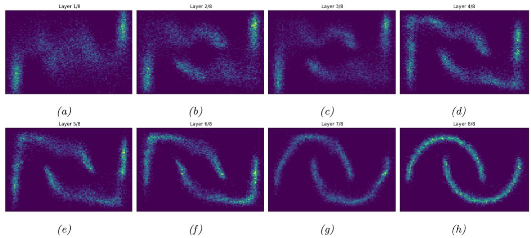
Figure 23.3: (a) Two moons dataset. (b) Samples from a normalizing flow fit to this dataset. Generated by two\_moons\_nsf\_normalizing\_flow.ipynb.

Suppose the input ^u contains ^D scalar elements, that is, ^u = (u1,…,uD) ^{→ RD}. We define an autoregressive bijection ^f : ^{RD ↔︎ RD}, its output denoted by ^x = (x1,…,xD) ^{→ RD}, as follows:

\[x\_i = h(u\_i; \Theta\_i(x\_{1:i-1})), \quad i = 1, \ldots, D. \tag{23.19}\]

Each output xⁱ depends on the corresponding input uⁱ and all previous outputs x1:i↑¹ = (x1,…,xⁱ↑1). The function h(·; ε) : R ↔︎ R is a scalar bijection (for example, one of those described in Section 23.2.2), and is parameterized by ε. The function #ⁱ is a conditioner that outputs the parameters εⁱ that yield xi, given all previous outputs x1:i↑1. Like in coupling flows, #ⁱ can be an arbitrary non-linear function, and is often parameterized as a deep neural network.

Because h is invertible, f is also invertible, and its inverse is given by:

\[u\_i = h^{-1}(x\_i; \Theta\_i(x\_{1:i-1})), \quad i = 1, \ldots, D. \tag{23.20}\]

An important property of f is that each output xⁱ depends on u1:ⁱ = (u1,…,ui), but not on ui+1:^D = (ui+1,…,uD); as a result, the partial derivative ◁xi/◁u^j is identically zero whenever j>i. Therefore, the Jacobian matrix J(f) is triangular, and its determinant is simply the product of its diagonal entries:

\[\det \mathbf{J}(\mathbf{f}) = \prod\_{i=1}^{D} \frac{\partial x\_i}{\partial u\_i} = \prod\_{i=1}^{D} \frac{dh}{du\_i} \,. \tag{23.21}\]

In other words, the autoregressive structure of f leads to a Jacobian determinant that can be computed e”ciently in O(D) time.

Although invertible, autoregressive bijections are computationally asymmetric: evaluating f is inherently sequential, whereas evaluating f ^↑1 is inherently parallel. That is because we need x1:i↑¹ to

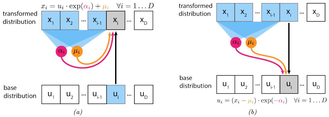
Figure 23.4: (a) A”ne autoregressive flow with one layer. In this figure, u is the input to the flow (sample from the base distribution) and x is its output (sample from the transformed distribution). (b) Inverse of the above. From [Jan18]. Used with kind permission of Eric Jang.

compute xi; therefore, computing the components of x must be done sequentially, by first computing x1, then using it to compute x2, then using x¹ and x² to compute x3, and so on. On the other hand, computing the inverse can be done in parallel for each ui, since u does not appear on the right-hand side of Equation (23.20). Hence, in practice it is often faster to compute f ^↑1 than to compute f, assuming h and h↑¹ have similar computational cost.

23.2.4.1 A”ne autoregressive flows

For a concrete example, we can take h to be an a”ne scalar bijection (Section 23.2.2.1) parameterized by a log scale ↽ and a bias µ. Such autoregressive flows are known as a”ne autoregressive flows. The parameters of the i’th component, ↽ⁱ and µi, are functions of x1:i↑¹, so f takes the following form:

\[x\_i = u\_i \exp(\alpha\_i(x\_{1:i-1})) + \mu\_i(x\_{1:i-1}).\tag{23.22}\]

This is illustrated in Figure 23.4(a). We can invert this by

\[u\_i = (x\_i - \mu\_i(x\_{1:i-1})) \exp(-\alpha\_i(x\_{1:i-1})).\tag{23.23}\]

This is illustrated in Figure 23.4(b). Finally, we can calculate the log absolute Jacobian determinant by

\[\log \left| \det \mathbf{J}(\mathbf{f}) \right| = \log \left| \prod\_{i=1}^{D} \exp(\alpha\_i(\mathbf{z}\_{1:i-1})) \right| = \sum\_{i=1}^{D} \alpha\_i(\mathbf{z}\_{1:i-1}).\tag{23.24}\]

Let us look at an example of an a”ne autoregressive flow on a 2d density estimation problem. Consider an a”ne autoregressive flow x = (x1, x2) = f(u), where u ↑ N (0, I) and f is a single autoregressive bijection. Since x¹ is an a”ne transformation of u¹ ↑ N (0, 1), it is Gaussian with mean µ¹ and standard deviation ς¹ = exp ↽1. Similarly, if we consider x¹ fixed, x² is an a”ne

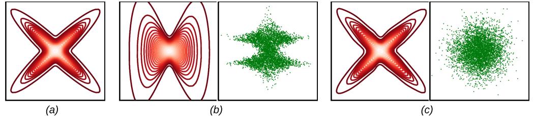
Figure 23.5: Density estimation with a”ne autoregressive flows, using a Gaussian base distribution. (a) True density. (b) Estimated density using a single autoregressive layer with ordering (x1, x2). On the left (contour plot) we show p(x). On the right (green dots) we show samples of u = f ^↑1(x), where x is sampled from the true density. (c) Same as (b), but using 5 autoregressive layers and reversing the variable ordering after each layer. Adapted from Figure 1 of [PPM17]. Used with kind permission of Iain Murray.

transformation of u² ↑ N (0, 1), so it is conditionally Gaussian with mean µ2(x1) and standard deviation ς2(x1) = exp ↽2(x1). Thus, a single a”ne autoregressive bijection will always produce a distribution with Gaussian conditionals, that is, a distribution of the following form:

\[p(x\_1, x\_2) = p(x\_1) \, p(x\_2 | x\_1) = \mathcal{N}(x\_1 | \mu\_1, \sigma\_1^2) \, \mathcal{N}(x\_2 | \mu\_2(x\_1), \sigma\_2(x\_1)^2) \tag{23.25}\]

This result generalizes to an arbitrary number of dimensions D.

A single a”ne bijection is not very powerful, regardless of how flexible the functions ↽2(x1) and µ2(x1) are. For example, suppose we want to fit the cross-shaped density shown in Figure 23.5(a) with such a flow. The resulting maximum-likelihood fit is shown in Figure 23.5(b). The red contours show the predictive distribution, pˆ(x), which clearly fails to capture the true distribution. The green dots show transformed versions of the data samples, p(u); we see that this is far from the Gaussian base distribution.

Fortunately, we can obtain a better fit by composing multiple autoregressive bijections (layers), and reversing the order of the variables after each layer. For example, Figure 23.5(c) shows the results of an a”ne autoregressive flow with 5 layers applied to the same problem. The red contours show that we have matched the empirical distribution, and the green dots show we have matched the Gaussian base distribution.

Note that another way to obtain a better fit is to replace the a”ne bijection h with a more flexible one, such as a monotonic MLP (Section 23.2.2.3) or a monotonic spline (Section 23.2.2.5).

23.2.4.2 Masked autoregressive flows

As we have seen, the conditioners #ⁱ can be arbitrary non-linear functions. The most straightforward way to parameterize them is separately for each i, for example by using D separate neural networks. However, this can be parameter-ine”cient for large D.

In practice, we often share parameters between conditioners by combining them into a single model # that takes in x and outputs (ε1,…, εD). For the bijection to remain autoregressive, we must constrain # so that εⁱ depends only on x1:i↑¹ and not on xi:D. One way to achieve this is to start with an arbitrary neural network (an MLP, a CNN, a ResNet, etc.), and drop connections (for example, by zeroing out weights) until εⁱ is only a function of x1:i↑¹.

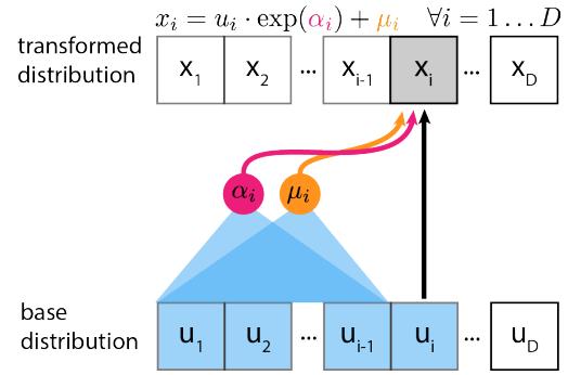
Figure 23.6: Inverse autoregressive flow that uses a”ne scalar bijections. In this figure, u is the input to the flow (sample from the base distribution) and x is its output (sample from the transformed distribution) From [Jan18]. Used with kind permission of Eric Jang.

An example of this approach is the masked autoregressive flow (MAF) model of [PPM17]. This model is an a”ne autoregressive flow combined with permutation layers, as we described in Section 23.2.4.1. MAF implements the combined conditioner # as follows: it starts with an MLP, and then multiplies (elementwise) the weight matrix of each layer with a binary mask of the same size (di!erent masks are used for di!erent layers). The masks are constructed using the method of [Ger+15]. This ensures that all computational paths from x^j to εⁱ are zeroed out whenever j ⇒ i, e!ectively making εⁱ only a function of x1:i↑¹. Still, evaluating the masked conditioner # has the same computational cost as evaluating the original (unmasked) MLP.

The key advantage of MAF (and of related models) is that, given x, all parameters (ε1,…, εD) can be computed e”ciently with one neural network evaluation, so the computation of the inverse f ^↑1 is fast. Thus, we can e”ciently evaluate the probability density of the flow model for arbitrary datapoints. However, in order to compute f, the conditioner # must be called a total of D times, since not all entries of x are available to start with. Thus, generating new samples from the flow is D times more expensive than evaluating its probability density function. This makes MAF suitable for density estimation, but less so for data generation.

23.2.4.3 Inverse autoregressive flows

As we have seen, the parameters εⁱ that yield the i’th output xⁱ are functions of the previous outputs x1:i↑¹. This ensures that the Jacobian J(f) is triangular, and so its determinant is e”cient to compute.

However, there is another possibility: we can make εⁱ a function of the previous inputs instead, that is, a function of u1:i↑¹. This leads to the following bijection, which is known as inverse autoregressive:

\[x\_i = h(u\_i; \Theta\_i(\mathbf{u}\_{1:i-1})), \quad i = 1, \ldots, D. \tag{23.26}\]

Like its autoregressive counterpart, this bijection has a triangular Jacobian whose determinant is also given by det J(f) = ^D i=1 dh duⁱ . Figure 23.6 illustrates an inverse autoregressive flow, for the case where h is a”ne.

To see why this bijection is called “inverse autoregressive”, compare Equation (23.26) with Equation (23.20). The two formulas di!er only notationally: we can get from one to the other by swapping u with x and h with h↑1. In other words, the inverse autoregressive bijection corresponds to a direct parameterization of the inverse of an autoregressive bijection.

Since inverse autoregressive bijections swap the forwards and inverse directions of their autoregressive counterparts, they also swap their computational properties. This means that the forward direction f of an inverse autoregressive flow is inherently parallel and therefore fast, whereas its inverse direction f ^↑1 is inherently sequential and therefore slow.

An example of an inverse autoregressive flow is their namesake IAF model of [Kin+16]. IAF uses a”ne scalar bijections, masked conditioners, and permutation layers, so it is precisely the inverse of the MAF model described in Section 23.2.4.2. Using IAF, we can generate u in parallel from the base distribution (using, for example, a diagonal Gaussian), and then sample each element of x in parallel. However, evaluating p(x) for an arbitrary datapoint x is slow, because we have to evaluate each element of u sequentially. Fortunately, evaluating the likelihood of samples generated from IAF (as opposed to externally provided samples) incurs no additional cost, since in this case the uⁱ terms will already have been computed.

Although not so suitable for density estimation or maximum-likelihood training, IAFs are wellsuited for parameterizing variational posteriors in variational inference. This is because in order to estimate the variational lower bound (ELBO), we only need samples from the variational posterior and their associated probability densities, both of which are e”cient to obtain. See Section 23.1.2.2 for details.

Another useful application of IAFs is training them to mimic models whose probability density is fast to evaluate but which are slow to sample from. A notable example is the parallel wavenet model of [Oor+18]. This model is an IAF p^s that it trained to mimic a pretrained wavenet model p^t by minimizing the KL divergence DKL (p^s ⇐ pt). This KL can be easily estimated by first sampling from p^s and then evaluating log p^s and log p^t at those samples, operations which are all e”cient for these models. After training, we obtain an IAF that can generate audio of similar quality as the original wavenet, but can do so much faster.

23.2.4.4 Connection with autoregressive models

Autoregressive flows can be thought of as generalizing autoregressive models of continuous random variables, discussed in Section 22.1. Specifically, any continuous autoregressive model can be reparameterized as a one-layer autoregressive flow, as we describe below.

Consider a general autoregressive model over a continuous random variable ^x = (x1,…,xD) ^{→ RD} written as

\[p(\mathbf{z}) = \prod\_{i=1}^{D} p\_i(x\_i|\theta\_i) \quad \text{where} \quad \theta\_i = \Theta\_i(x\_{1:i-1}). \tag{23.27}\]

In the above expression, pi(xi|εi) is the i’th conditional distribution of the autoregressive model, whose parameters εⁱ are arbitrary functions of the previous variables x1:i↑1. For example, pi(xi|εi) can be a mixture of one-dimensional Gaussian distributions, with εⁱ representing the collection of its means, variances, and mixing coe”cients.

Now consider sampling a vector x from the autoregressive model, which can be done by sampling

one element at a time as follows:

\[x\_i \sim p\_i(x\_i | \Theta\_i(x\_{1:i-1})) \quad \text{for } i = 1, \ldots, D. \tag{23.28}\]

Each conditional can be sampled from using inverse transform sampling (Section 11.3.1). Let U(0, 1) be the uniform distribution on the interval [0, 1], and let CDFi(xi|εi) be the cumulative distribution function of the i’th conditional. Sampling can be written as:

\[x\_i = \text{CDF}\_i^{-1}(u\_i|\Theta\_i(x\_{1:i-1})) \quad \text{where} \quad u\_i \sim U(0,1). \tag{23.29}\]

Comparing the above expression with the definition of an autoregressive bijection in Equation (23.19), we see that the autoregressive model has been expressed as a one-layer autoregressive flow whose base distribution is uniform on [0, 1]^D and whose scalar bijections correspond to the inverse conditional cdf’s. Viewing autoregressive models as flows this way has an important advantage, namely that it allows us to increase the flexibility of an autoregressive model by composing multiple instances of it in a flow, without sacrificing the overall tractability.

23.2.5 Residual flows

A residual network is a composition of residual connections, which are functions of the form ^f(u) = ^u + F(u). The function F : ^{RD ↔︎ RD} is called the residual block, and it computes the di!erence between the output and the input, f(u) ↓ u.

Under certain conditions on F, the residual connection f becomes invertible. We will refer to flows composed of invertible residual connections as residual flows. In the following, we describe two ways the residual block F can be constrained so that the residual connection f is invertible.

23.2.5.1 Contractive residual blocks

One way to ensure the residual connection is invertible is to choose the residual block to be a contraction. A contraction is a function F whose Lipschitz constant is less than 1; that is, there exists 0 ≃ L < 1 such that for all u¹ and u² we have:

\[\|\mathbf{F}(\mathbf{u}\_1) - \mathbf{F}(\mathbf{u}\_2)\| \le L \|\mathbf{u}\_1 - \mathbf{u}\_2\|. \tag{23.30}\]

The invertibility of f(u) = u+F(u) can be shown as follows. Consider the mapping g(u) = x↓F(u). Because F is a contraction, g is also a contraction. So, by Banach’s fixed-point theorem, g has a unique fixed point u↔︎. Hence we have

\[\mathbf{u}\_{\*} = \mathbf{z} - \mathbf{F}(\mathbf{u}\_{\*}) \tag{23.31}\]

\[\Rightarrow \quad u\_\* + \mathbf{F}(u\_\*) = x \tag{23.32}\]

\[\implies \quad f(u\_\*) = x.\tag{23.33}\]

Because u^↔︎ is unique, it follows that u^↔︎ = f ^↑1(x).

An example of a residual flow with contractive residual blocks is the iResNet model of [Beh+19]. The residual blocks of iResNet are convolutional neural networks, that is, compositions of convolutional layers with non-linear activation functions. Because the Lipschitz constant of a composition is less or equal to the product of the Lipschitz constants of the individual functions, it is enough to ensure the

convolutions are contractive, and to use increasing activation functions with slope less or equal to 1. The iResNet model ensures the convolutions are contractive by applying spectral normalization to their weights [Miy+18a].

In general, there is no analytical expression for the inverse f ^↑1. However, we can approximate f ^↑1(x) using the following iterative procedure:

\[\mathbf{u}\_n = \mathbf{g}(\mathbf{u}\_{n-1}) = \mathbf{z} - \mathbf{F}(\mathbf{u}\_{n-1}).\tag{23.34}\]

Banach’s fixed-point theorem guarantees that the sequence u0,u1,u2,… will converge to u^{↔︎ =} f ^↑1(x) for any choice of u0, and it will do so at a rate of O(Lⁿ), where L is the Lipschitz constant of g (which is the same as the Lipschitz constant of F). In practice, it is convenient to choose u⁰ = x.

In addition, there is no analytical expression for the Jacobian determinant, whose exact computation costs O(D³). However, there is a computationally e”cient stochastic estimator of the log Jacobian determinant. The idea is to express the log Jacobian determinant as a power series. Using the fact that f(x) = x + F(x), we have

\[\log|\det\mathbf{J}(\mathbf{f})| = \log|\det(\mathbf{I} + \mathbf{J}(\mathbf{F}))| = \sum\_{k=1}^{\infty} \frac{(-1)^{k+1}}{k} \text{tr}\left[\mathbf{J}(\mathbf{F})^k\right].\tag{23.35}\]

This power series converges when the matrix norm of J(F) is less than 1, which here is guaranteed exactly because F is a contraction. The trace of J(F)^k can be e”ciently approximated using Jacobian-vector products via the Hutchinson trace estimator [Ski89; Hut89; Mey+21]:

\[\operatorname{tr}\left[\mathbf{J}(\mathbf{F})^k\right] \approx \mathbf{v}^\top \mathbf{J}(\mathbf{F})^k \mathbf{v},\tag{23.36}\]

where v is a sample from a distribution with zero mean and unit covariance, such as N (0, I). Finally, the infinite series can be approximated by a finite one either by truncation [Beh+19], which unfortunately yields a biased estimator, or by employing the Russian-roulette estimator [Che+19], which is unbiased.

23.2.5.2 Residual blocks with low-rank Jacobian

There is an e”cient way of computing the determinant of a matrix which is a low-rank perturbation of an identity matrix. Suppose A and B are matrices, where A is D ↗ M and B is M ↗ D. The following formula is known as the Weinstein-Aronszajn identity2, and is a special case of the more general matrix determinant lemma:

\[\det(\mathbf{I}\_D + \mathbf{A}\mathbf{B}) = \det(\mathbf{I}\_M + \mathbf{B}\mathbf{A}).\tag{23.37}\]

We write I^D and I^M for the D ↗ D and M ↗ M identity matrices respectively. The significance of this formula is that it turns a ^D ↗ ^D determinant that costs ^O(D³) into an ^M ↗ ^M determinant that costs O(M³). If M is smaller than D, this saves computation.

With some restrictions on the residual block ^F : ^{RD ↔︎ RD}, we can apply this formula to compute the determinant of a residual connection e”ciently. The trick is to create a bottleneck inside F. We do that by defining F = F^{2 ∞} F1, where F¹ : ^{RD ↔︎ RM}, F² : ^{RM ↔︎ RD} and ^M ↖ ^D. The chain

^2. See https://en.wikipedia.org/wiki/Weinstein-Aronszajn\_identity.

rule gives J(F) = J(F2)J(F1), where J(F2) is D ↗ M and J(F1) is M ↗ D. Now we can apply our determinant formula as follows:

\[\det \mathbf{J}(\mathbf{f}) = \det(\mathbf{I}\_D + \mathbf{J}(\mathbf{F})) = \det(\mathbf{I}\_D + \mathbf{J}(\mathbf{F}\_2)\mathbf{J}(\mathbf{F}\_1)) = \det(\mathbf{I}\_M + \mathbf{J}(\mathbf{F}\_1)\mathbf{J}(\mathbf{F}\_2)). \tag{23.38}\]

Since the final determinant costs O(M3), we can make the Jacobian determinant e”cient by reducing M, that is, by narrowing the bottleneck.

An example of the above is the planar flow of [RM15]. In this model, each residual block is an MLP with one hidden layer and one hidden unit. That is,

\[f(\mathbf{u}) = \mathbf{u} + \mathbf{v}\sigma(\mathbf{w}^\top \mathbf{u} + b),\tag{23.39}\]

where ^{v → RD}, ^{w → RD} and ^{b → R} are the parameters, and ^ς is the activation function. The residual block is the composition of F1(u) = w⇓u + b and F2(z) = vς(z), so M = 1. Their Jacobians are J(F1)(u) = w⇓ and J(F2)(z) = vς^→ (z). Substituting these in the formula for the Jacobian determinant we obtain:

\[\det \mathbf{J}(f)(\mathbf{u}) = 1 + \mathbf{w}^{\top} \mathbf{v} \sigma'(\mathbf{w}^{\top} \mathbf{u} + b), \tag{23.40}\]

which can be computed e”ciently in O(D). Other examples include the circular flow of [RM15] and the Sylvester flow of [Ber+18].

This technique gives an e”cient way of computing determinants of residual connections with bottlenecks, but in general there is no guarantee that such functions are invertible. This means that invertibility must be satisfied on a case-by-case basis. For example, the planar flow is invertible when ς is the hyperbolic tangent and w⇓v > ↓1, but otherwise it may not be.

23.2.6 Continuous-time flows

So far we have discussed flows that consist of a sequence of bijections f1,…, f^N . Starting from some input x⁰ = u, this creates a sequence of outputs x1,…, x^N where xⁿ = fn(xⁿ↑1). However, we can also have flows where the input is transformed into the final output in a continuous way. That is, we start from x⁰ = x(0), create a continuously-indexed sequence x(t) for t → [0, T] with some fixed T, and take x(T) to be the final output. Thinking of t as analogous to time, we refer to these as continuous-time flows.

The sequence x(t) is defined as the solution to a first-order ordinary di!erential equation (ODE) of the form:

\[\frac{dx}{dt}(t) = \mathbf{F}(x(t), t). \tag{23.41}\]

The function ^F : ^RD ↗ [0, T] ^{↔︎ RD} is a time-dependent vector field that parameterizes the ODE. If we think of x(t) as the position of a particle in D dimensions, the vector F(x(t), t) determines the particle’s velocity at time t.

The flow (for time ^T) is a function ^f : ^{RD ↔︎ RD} that takes in an input ^x0, solves the ODE with initial condition x(0) = x0, and returns x(T). The function f is a well-defined bijection if the solution to the ODE exists for all t → [0, T] and is unique. These conditions are not generally satisfied for arbitrary F, but they are if F(·, t) is Lipschitz continuous with a Lipschitz constant that does not

depend on t. That is, f is a well-defined bijection if there exists a constant L such that for all x1, x² and t → [0, T] we have:

\[\|\mathbf{F}(\mathbf{x}\_1, t) - \mathbf{F}(\mathbf{x}\_2, t)\| \le L \|\mathbf{x}\_1 - \mathbf{x}\_2\|. \tag{23.42}\]

This result is a consequence of the Picard-Lindelöf theorem for ODEs.3 In practice, we can parameterize F using any choice of model, provided the Lipschitz condition is met.

Usually the ODE cannot be solved analytically, but we can solve it approximately by discretizing it. A simple example is Euler’s method, which corresponds to the following discretization for some small step size ϖ > 0:

\[ \mathbf{x}(t+\epsilon) = \mathbf{x}(t) + \epsilon \mathbf{F}(\mathbf{x}(t), t). \tag{23.43} \]

This is equivalent to a residual connection with residual block ϖF(·, t), so the ODE solver can be thought of as a deep residual network with O(T /ϖ) layers. A smaller step size leads to a more accurate solution, but also to more computation. There are several other solution methods varying in accuracy and sophistication, such as those in the broader Runge-Kutta family, some of which use adaptive step sizes.

The inverse of f can be easily computed by solving the ODE in reverse. That is, to compute f ^↑1(x^T ) we solve the ODE with initial condition x(T) = x^T , and return x(0). Unlike some other flows (such as autoregressive flows) which are more expensive to compute in one direction than in the other, continuous-time flows require the same amount of computation in either direction.

In general, there is no analytical expression for the Jacobian determinant of f. However, we can express it as the solution to a separate ODE, which we can then solve numerically. First, we define ^ft : ^{RD ↔︎ RD} to be the flow for time ^t, that is, the function that takes ^x0, solves the ODE with initial condition x(0) = x⁰ and returns x(t). Clearly, f⁰ is the identity function and f^T = f. Let us define L(t) = log | det J(ft)(x0)|. Because f⁰ is the identity function, L(0) = 0, and because f^T = f, L(T) gives the Jacobian determinant of f that we are interested in. It can be shown that L satisfies the following ODE:

\[\frac{dL}{dt}(t) = \text{tr}\Big[\mathbf{J}(\mathbf{F}(\cdot, t))(\mathbf{z}(t))\Big].\tag{23.44}\]

That is, the rate of change of L at time t is equal to the Jacobian trace of F(·, t) evaluated at x(t). So we can compute L(T) by solving the above ODE with initial condition L(0) = 0. Moreover, we can compute x(T) and L(T) simultaneously, by combining their two ODEs into a single ODE operating on the extended space (x, L).

An example of a continuous-time flow is the neural ODE model of [Che+18c], which uses a neural network to parameterize F. To avoid backpropagating gradients through the ODE solver, which can be computationally demanding, they use the adjoint sensitivity method to express the time evolution of the gradient with respect to x(t) as a separate ODE. Solving this ODE gives the required gradients, and can be thought of as the continuous-time analog of backpropagation.

Another example is the FFJORD model of [Gra+19]. This is similar to the neural ODE model, except that it uses the Hutchinson trace estimator to approximate the Jacobian trace of F(·, t).

^3. See https://en.wikipedia.org/wiki/Picard-Lindel%C3%B6f\_theorem

This usage of the Hutchinson trace estimator is analogous to that in contractive residual flows (Section 23.2.5.1), and it speeds up computation in exchange for a stochastic (but unbiased) estimate.

Unfortunately, the above approaches are slow and complicated. The flow matching technique of Section 25.4.7 provides a simpler approach to training continuous time normalizing flows, using a fast nonlinear least squares formulation.

23.3 Applications

In this section, we highlight some applications of flows for canonical probabilistic machine learning tasks.

23.3.1 Density estimation

Flow models allow exact density computation and can be used to fit multi-modal densities to observed data. (see Figure 23.3 for an example). An early example is Gaussianization [CG00] who applied this idea to fit low-dimensional densities. Tabak and Vanden-Eijnden [TVE10] and Tabak and Turner [TT13] introduced the modern idea of flows (including the term ‘normalizing flows’), describing a flow as a composition of simpler maps. Deep density models [RA13] was one of the first to use neural networks for flows to parameterize high-dimensional densities. There has been a rich line of follow-up work including NICE [DKB15] and Real NVP [DSDB17]. (NVP stands for “non-volume-preserving”, which refers to the fact that the Jacobian of the transform is not unity.) Masked autoregressive flows (Section 23.2.4.2) further improved performance on unconditional and conditional density estimation tasks.

Flows can be used for hybrid models which model the joint density of inputs and targets p(x, y), as opposed to discriminative classification models which just model the conditional p(y|x) and density models which just model the marginal p(x). Nalisnick et al. [Nal+19b] proposed a flow-based hybrid model using invertible mappings for representation learning and showed that the joint density p(x, y) can be computed e”ciently, which can be useful for downstream tasks such as anomaly detection, semi-supervised learning and selective classification. Flow-based hybrid models are memory-e”cient since most of the parameters are in the invertible representation which are shared between the discriminative and generative models; furthermore, the density p(x, y) can be computed in a single forwards pass leading to computational savings. Residual flows [Che+19] use invertible residual mappings [Beh+19] for hybrid modeling which further improves performance. Flows have also been used to fit densities to embeddings [Zha+20b; CZG20] for anomaly detection tasks.

23.3.2 Generative modeling

Another task is generation, which involves generating novel samples from a fitted model p↔︎(x). Generation is a popular downstream task for normalizing flows, which have been applied for di!erent data modalities including images, video, audio, text, and structured objects such as graphs and point clouds. Images are arguably the most popular modality for deep generative models: GLOW [KD18b] was one of the first flow-based models to generate compelling high-dimensional images, and has been extended to video to produce RGB frames [Kum+19b]; residual flows [Che+19] have also been shown to produce sharp images.

Oord et al. [Oor+18] used flows for audio synthesis by distilling WaveNet into an IAF (Section 23.2.4.3), which enables faster sampling than WaveNet. Other flow models for audio include WaveFLOW [PVC19] and FlowWaveNet [Kim+19], which directly speed up WaveNet using coupling layers.

Flows have been also used for text. Tran et al. [Tra+19] define a discrete flow over a vocabulary for language-modeling tasks. Another popular approach is to define a latent variable model with discrete observation space but a continuous latent space. For example, Ziegler and Rush [ZR19a] use normalizing flows in latent space for language modeling.

23.3.3 Inference

Normalizing flows have been used for probabilistic inference. Rezende and Mohamed [RM15] popularized normalizing flows in machine learning, and showed how they can be used for modeling variational posterior distributions in latent variable models. Various extensions such as Householder flows [TW16], inverse autoregressive flows [Kin+16], multiplicative normalizing flows [LW17], and Sylvester flows [Ber+18] have been proposed for modeling the variational posterior for latent variable models, as well as posteriors for Bayesian neural networks.

Flows have been used as complex proposal distributions for importance sampling; examples include neural importance sampling [Mül+19b] and Boltzmann generators [Noé+19]. Ho!man et al. [Hof+19] used flows to improve the performance of Hamiltonian Monte Carlo (Section 12.5) by defining bijective transformations to transform random variables to simpler distributions and performing HMC in that space instead.

Finally, flows can be used in the context of simulation-based inference, where the likelihood function of the parameters is not available, but simulating data from the model is possible. The main idea is to train a flow on data simulated from the model in order to approximate the posterior distribution or the likelihood function. The flow model can also be used to guide simulations in order to make inference more e”cient [PSM19; GNM19]. This approach has been used for inference of simulation models in cosmology [Als+19] and computational neuroscience [Gon+20].

24 Energy-based models

This chapter is co-authored with Yang Song and Durk Kingma.

24.1 Introduction

We have now seen several ways of defining deep generative models, including VAEs (Chapter 21), autoregressive models (Chapter 22), and normalizing flows (Chapter 23). All of the above models can be formulated in terms of directed graphical models (Chapter 4), where we generate the data one step at a time, using locally normalized distributions. In some cases, it is easier to specify a distribution in terms of a set of constraints that valid samples must satisfy, rather than a generative process. This can be done using an undirected graphical model (Chapter 4).

Energy-based models or EBM can be written as a Gibbs distribution as follows:

\[p\_{\theta}(\mathbf{x}) = \frac{\exp(-\mathcal{E}\_{\theta}(\mathbf{x}))}{Z\_{\theta}} \tag{24.1}\]

where Eω(x) is known as the energy function with parameters ε, and Z^ω is the partition function:

\[Z\_{\theta} = \int \exp(-\mathcal{E}\_{\theta}(\mathbf{x})) \, \mathrm{d}\mathbf{x} \tag{24.2}\]

This is constant wrt x but is a function of ε. Since EBMs do not usually make any Markov assumptions (unlike graphical models), evaluating this integral is usually intractable. Consequently we usually need to use approximate methods, such as annealed importance sampling, discussed in Section 11.5.4.1.

The advantage of an EBM over other generative models is that the energy function can be any kind of function that returns a non-negative scalar; it does not need to integrate to 1. This allows one to use a variety of neural network architectures for defining the energy. As such, EBMs have found wide applications in many fields of machine learning, including image generation [Ngi+11; Xie+16; DM19b], discriminative learning [Gra+20b], natural processing [Mik+13; Den+20], density estimation [Wen+19a; Son+19], and reinforcement learning [Haa+17; Haa+18b], to list a few. (More examples can be found at https://github.com/yataobian/awesome-ebm.)

24.1.1 Example: products of experts (PoE)

As an example of why energy based models are useful, suppose we want to create a generative model of proteins that are thermally stable at room temperature, and which bind to the COVID-19 spike

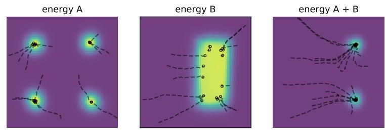
Figure 24.1: Combining two energy functions in 2d by summation, which is equivalent to multiplying the corresponding probability densities. We also illustrate some sampled trajectories towards high probability (low energy) regions. From Figure 14 of [DM19a]. Used with kind permission of Yilun Du.

receptor. Suppose p1(x) can generate stable proteins and p2(x) can generate proteins that bind. (For example, both of these models could be autoregressive sequence models, trained on di!erent datasets.) We can view each of these models as “experts” about a particular aspect of the data. On their own, they are not an adequate model of the data that we have (or want to have), but we can then combine them, to represent the conjunction of features, by computing a product of experts (PoE) [Hin02]:

\[p\_{12}(\mathbf{z}) = \frac{1}{Z\_{12}} p\_1(\mathbf{z}) p\_2(\mathbf{z}) \tag{24.3}\]

This will assign high probability to proteins that are stable and which bind, and low probability to all others. By contrast, a mixture of experts would either generate from p¹ or from p2, but would not combine features from both.

If the experts are represented as energy based models (EBM), then the PoE model is also an EBM, with an energy given by

\[\mathcal{E}\_{12}(x) = \mathcal{E}\_1(x) + \mathcal{E}\_2(x) \tag{24.4}\]

Intuitively, we can think of each component of energy as a “soft constraint” on the data. This idea is illustrated in Figure 24.1.

24.1.2 Computational di!culties

Although the flexibility of EBMs can provide significant modeling advantages, computation of the likelihood and drawing samples from the model are generally intractable. In this chapter, we will discuss a variety of approximate methods to solve these problems.

24.2 Maximum likelihood training

The de facto standard for learning probabilistic models from iid data is maximum likelihood estimation (MLE). Let pω(x) be a probabilistic model parameterized by ε, and pD(x) be the underlying data

distribution of a dataset. We can fit pω(x) to pD(x) by maximizing the expected log-likelihood function over the data distribution, defined by

\[\ell(\boldsymbol{\theta}) = \mathbb{E}\_{\mathbf{x} \sim p\_{\mathcal{D}}(\mathbf{x})} [\log p\_{\boldsymbol{\theta}}(\mathbf{x})] \tag{24.5}\]

as a function of ε. Here the expectation can be easily estimated with samples from the dataset. Maximizing likelihood is equivalent to minimizing the KL divergence between pD(x) and pω(x), because

\[\ell(\boldsymbol{\theta}) = -D\_{\mathbb{KL}}\left(p\_{\mathcal{D}}(\mathbf{x}) \parallel p\_{\boldsymbol{\theta}}(\mathbf{x})\right) + \text{const} \tag{24.6}\]

where the constant is equal to E^x↗pD(x)[log pD(x)] which does not depend on ε.

We cannot usually compute the likelihood of an EBM because the normalizing constant Z^ω is often intractable. Nevertheless, we can still estimate the gradient of the log-likelihood with MCMC approaches, allowing for likelihood maximization with stochastic gradient ascent [You99]. In particular, the gradient of the log-probability of an EBM decomposes as a sum of two terms:

\[ \nabla\_{\theta} \log p\_{\theta}(\mathbf{x}) = -\nabla\_{\theta} \mathcal{E}\_{\theta}(\mathbf{x}) - \nabla\_{\theta} \log Z\_{\theta}.\tag{24.7} \]

The first gradient term, ↓∝ωEω(x), is straightforward to evaluate with automatic di!erentiation. The challenge is in approximating the second gradient term, ∝^ω log Zω, which is intractable to compute exactly. This gradient term can be rewritten as the following expectation:

\[\nabla\_{\theta} \log Z\_{\theta} = \nabla\_{\theta} \log \int \exp(-\mathcal{E}\_{\theta}(\mathbf{x})) d\mathbf{x} \tag{24.8}\]

\[\stackrel{\text{(i)}}{=} \left( \int \exp(-\mathcal{E}\_{\theta}(\mathbf{x})) d\mathbf{x} \right)^{-1} \nabla\_{\theta} \int \exp(-\mathcal{E}\_{\theta}(\mathbf{x})) d\mathbf{x} \tag{24.9}\]

\[\mathbf{x} = \left(\int \exp(-\mathcal{E}\_{\theta}(\mathbf{x}))d\mathbf{x}\right)^{-1} \int \nabla\_{\theta} \exp(-\mathcal{E}\_{\theta}(\mathbf{x}))d\mathbf{x} \tag{24.10}\]

\[\stackrel{\text{(ii)}}{=} \left( \int \exp(-\mathcal{E}\_{\theta}(\mathbf{x})) d\mathbf{x} \right)^{-1} \int \exp(-\mathcal{E}\_{\theta}(\mathbf{x})) (-\nabla\_{\theta} \mathcal{E}\_{\theta}(\mathbf{x})) d\mathbf{x} \tag{24.11}\]

\[\mathcal{L} = \int \left( \int \exp(-\mathcal{E}\_{\theta}(\mathbf{x})) d\mathbf{x} \right)^{-1} \exp(-\mathcal{E}\_{\theta}(\mathbf{x})) (-\nabla\_{\theta} \mathcal{E}\_{\theta}(\mathbf{x})) d\mathbf{x} \tag{24.12}\]

\[\stackrel{(iii)}{=} \int \frac{1}{Z\_{\theta}} \exp(-\mathcal{E}\_{\theta}(\mathbf{x})) (-\nabla\_{\theta} \mathcal{E}\_{\theta}(\mathbf{x})) d\mathbf{x} \tag{24.13}\]

\[\stackrel{\text{(iv)}}{=} \int p\_{\theta}(\mathbf{x}) (-\nabla\_{\theta} \mathcal{E}\_{\theta}(\mathbf{x})) d\mathbf{x} \tag{24.14}\]

\[\mathbf{x} = \mathbb{E}\_{\mathbf{x} \sim p\_{\theta}(\mathbf{x})} \left[ -\nabla\_{\theta} \mathcal{E}\_{\theta}(\mathbf{x}) \right],\tag{24.15}\]

where steps (i) and (ii) are due to the chain rule of gradients, and (iii) and (iv) are from definitions in Equations (24.1) and (24.2). Thus, we can obtain an unbiased Monte Carlo estimate of the log-likelihood gradient by using

\[\nabla\_{\theta} \log Z\_{\theta} \simeq -\frac{1}{S} \sum\_{s=1}^{S} \nabla\_{\theta} \mathcal{E}\_{\theta}(\tilde{\mathbf{x}}\_{s}),\tag{24.16}\]

where x˜^s ↑ pω(x), i.e., a random sample from the distribution over x given by the EBM. Therefore, as long as we can draw random samples from the model, we have access to an unbiased Monte Carlo estimate of the log-likelihood gradient, allowing us to optimize the parameters with stochastic gradient ascent.

Much of the literature has focused on methods for e”cient MCMC sampling from EBMs. We discuss some of these methods below.

24.2.1 Gradient-based MCMC methods

Some e”cient MCMC methods, such as Langevin MCMC (Section 12.5.6) or Hamiltonian Monte Carlo (Section 12.5), make use of the fact that the gradient of the log-probability wrt x (known as the Hyvärinen score function, named after [Hyv05a] to distinguish it from the standard score function in Equation (3.39)) is equal to the (negative) gradient of the energy, and is therefore easy to calculate:

\[ \nabla\_{\mathbf{x}} \log p\_{\theta}(\mathbf{x}) = -\nabla\_{\mathbf{x}} \mathcal{E}\_{\theta}(\mathbf{x}) - \underbrace{\nabla\_{\mathbf{x}} \log Z\_{\theta}}\_{=0} = -\nabla\_{\mathbf{x}} \mathcal{E}\_{\theta}(\mathbf{x}).\tag{24.17} \]

For example, when using Langevin MCMC to sample from pω(x), we first draw an initial sample x⁰ from a simple prior distribution, and then simulate an overdamped Langevin di!usion process for K steps with step size ϖ > 0:

\[\mathbf{x}^{k+1} \leftarrow \mathbf{x}^k + \frac{\epsilon^2}{2} \underbrace{\nabla\_\mathbf{x} \log p\_\theta(\mathbf{x}^k)}\_{=-\nabla\_\mathbf{x} \mathcal{E}\_\theta(\mathbf{x})} + \epsilon \mathbf{z}^k, \quad k = 0, 1, \cdots, K - 1. \tag{24.18}\]

where ^{zk ↑ N} (0, ^I) is a Gaussian noise term. We show an example of this process in Figure 25.5d.

When ^{ϖ ↔︎ 0} and ^K ↔︎ ̸, ^xK is guaranteed to distribute as ^pω(x) under some regularity conditions. In practice we have to use a small finite ϖ, but the discretization error is typically negligible, or can be corrected with a Metropolis-Hastings step (Section 12.2), leading to the Metropolis-adjusted Langevin algorithm (Section 12.5.6).

24.2.2 Contrastive divergence

Running MCMC till convergence to obtain a sample x ↑ pω(x) can be computationally expensive. Therefore we typically need approximations to make MCMC-based learning of EBMs practical. One popular method for doing so is contrastive divergence (CD) [Hin02]. In CD, one initializes the MCMC chain from the datapoint x, and proceeds to perform MCMC for a fixed number of steps. One can show that T steps of CD minimizies the following objective:

\[\text{CD}\_{T} = D\_{\text{KL}} \left( p\_{0} \parallel p\_{\infty} \right) - D\_{\text{KL}} \left( p\_{T} \parallel p\_{\infty} \right) \tag{24.19}\]

where p^T is the distribution over x after T MCMC updates, and p⁰ is the data distribution. Typically we can get good results with a small value of T, sometimes just T = 1. We give the details below.

24.2.2.1 Fitting RBMs with CD

CD was initially developed to fit a special kind of latent variable EBM known as a restricted Boltzmann machine (Section 4.3.3.2). This model was specifically designed to support fast block Gibbs sampling, which is required by CD (and can also be exploited by standard MCMC-based learning methods [AHS85].)

For simplicity, we will assume the hidden and visible nodes are binary, and we use 1-step contrastive divergence. As discussed in Supplementary Section 4.3.1, the binary RBM has the following energy function:

\[\mathcal{E}(\mathbf{z}, \mathbf{z}; \boldsymbol{\theta}) = \sum\_{d=1}^{D} \sum\_{k=1}^{K} x\_d z\_k W\_{dk} + \sum\_{d=1}^{D} x\_d b\_d + \sum\_{k=1}^{K} z\_k c\_k \tag{24.20}\]

(Henceforth we will drop the unary (bias) terms, which can be emulated by clamping z^k = 1 or x^d = 1.) This is a loglinear model where we have one binary feature per edge. Thus from Equation (4.135) the gradient of the log-likelihood is given by the clamped expectations minus the unclamped expectations:

\[\frac{\partial \ell}{\partial w\_{dk}} = \frac{1}{N} \sum\_{n=1}^{N} \mathbb{E} \left[ x\_d z\_k | \mathbf{x}\_n, \boldsymbol{\theta} \right] - \mathbb{E} \left[ x\_d z\_k | \boldsymbol{\theta} \right] \tag{24.21}\]

We can rewrite the above gradient in matrix-vector form as follows:

\[\nabla\_{\mathbf{w}} \ell = \mathbb{E}\_{\mathbf{p}\_{\mathcal{D}}(\mathbf{z}) p(\mathbf{z}|\mathbf{z}, \boldsymbol{\theta})} \left[ \mathbf{z} \mathbf{z}^{T} \right] - \mathbb{E}\_{\mathbf{p}(\mathbf{z}, \mathbf{z}|\boldsymbol{\theta})} \left[ \mathbf{z} \mathbf{z}^{T} \right] \tag{24.22}\]

(We can derive a similar expression for the gradient of the bias terms by setting x^d = 1 or z^k = 1.)

The first term in the expression for the gradient in Equation (24.21), when x is fixed to a data case, is sometimes called the clamped phase, and the second term, when x is free, is sometimes called the unclamped phase. When the model expectations match the empirical expectations, the two terms cancel out, the gradient becomes zero and learning stops.

We can also make a connection to the principle of Hebbian learning in neuroscience. In particular, Hebb’s rule says that the strength of connection between two neurons that are simultaneously active should be increased. (This theory is often summarized as “Cells that fire together wire together”.1) The first term in Equation (24.21) is therefore considered a Hebbian term, and the second term an anti-Hebbian term, due to the sign change.

We can leverage the Markov structure of the bipartite graph to approximate the expectations as follows:

\[\mathbf{z}\_n \sim p(\mathbf{z}|\mathbf{x}\_n, \boldsymbol{\theta}) \tag{24.23}\]

\[x\_n' \sim p(x|z\_n, \theta) \tag{24.24}\]

\[\mathbf{z}\_{n}^{\prime} \sim p(\mathbf{z} | \mathbf{x}\_{n}^{\prime}, \boldsymbol{\theta}) \tag{24.25}\]

We can think of x^{→ n} as the model’s best attempt at reconstructing xⁿ after being encoded and then decoded by the model. Such samples are sometimes called fantasy data. See Figure 24.2 for an illustration. Given these samples, we then make the approximation

\[\mathbb{E}\_{p(\cdot|\theta)}\left[\mathbf{z}\mathbf{z}^{\mathsf{T}}\right] \approx \mathbf{z}\_n(\mathbf{z}\_n^{\mathsf{T}})^{\mathsf{T}} \tag{24.26}\]

^1. See https://en.wikipedia.org/wiki/Hebbian\_theory.

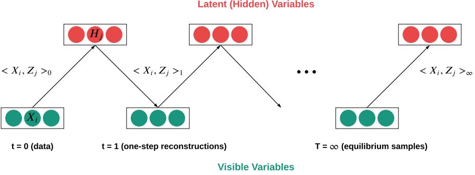
Figure 24.2: Illustration of contrastive divergence sampling for an RBM. The visible nodes are initialized at an example drawn from the dataset. Then we sample a hidden vector, then another visible vector, etc. Eventually (at “infinity”) we will be producing samples from the joint distribution p(x, z|ω).

In practice, it is common to use E [z|x^{→ n}] instead of a sampled value z^{→ n} in the above expression, since this reduces the variance. However, it is not valid to use E [z|xn] instead of sampling zⁿ ↑ p(z|xn) in Equation (24.23), because then each hidden unit would be able to pass more than 1 bit of information, so it would not act as much of a bottleneck.

The whole procedure is summarized in Algorithm 24.1. For more details, see [Hin10; Swe+10].

Algorithm 24.1: CD-1 training for an RBM with binary hidden and visible units

¹ Initialize weights ^{W → RD}⇐^K randomly ² for t = 1, 2,… do ³ for each minibatch of size B do ⁴ Set minibatch gradient to zero, g := 0 ⁵ for each case xⁿ in the minibatch do ⁶ Compute µⁿ = E [z|xn,W] ⁷ Sample zⁿ ↑ p(z|xn,W) ⁸ Sample x^{→ n} ↑ p(x|zn,W) ⁹ Compute µ^{→ n} = E [z|x^{→ n},W] ¹⁰ Compute gradient ∝^W = (xn)(µn) ^{T ↓} (x^→ n)(µ^→ n) T ¹¹ Accumulate g := g + ∝^{W 12} Update parameters W := W + ↼^{t 1 B} g

24.2.2.2 Persistent CD

One variant of CD that sometimes performs better is persistent contrastive divergence (PCD) [Tie08; TH09; You99]. In this approach, a single MCMC chain with a persistent state is employed

to sample from the EBM. In PCD, we do not restart the MCMC chain when training on a new datapoint; rather, we carry over the state of the previous MCMC chain and use it to initialize a new MCMC chain for the next training step. See Algorithm 12 for some pseudocode. Hence there are two dynamical processes running at di!erent time scales: the states x change quickly, and the parameters ε change slowly.

Algorithm 24.2: Persistent MCMC-SGD for fitting an EBM

Initialize parameters ε randomly Initialize chains x˜1:^S randomly Initialize learning rate ↼ for t = 1, 2,… do for x^b in minibatch of size B do g^b = ∝ωEω(xb) for sample s =1: S do Sample x˜^s ↑ MCMC(target = p(·|ε), init = x˜s, nsteps = N) g˜^s = ∝ωEω(x˜s) ^{gt = ↓}( ¹ B *^{B b}=1 ^gb) ^↓ ( ¹ S *^{S s}=1 g˜s) ε := ε + ↼g^t Decrease step size ↼

A theoretical justification for this was given in [You89], who showed that we can start the MCMC chain at its previous value, and just take a few steps, because p(x|εt) is likely to be close to p(x|ε^t↑1), since we only changed the parameters by a small amount in the intervening SGD step.

24.2.2.3 Other methods

PCD can be further improved by keeping multiple historical states of the MCMC chain in a replay bu!er and initialize new MCMC chains by randomly sampling from it [DM19b]. Other variants of CD include mean field CD [WH02], and multi-grid CD [Gao+18].

EBMs trained with CD may not capture the data distribution faithfully, since truncated MCMC can lead to biased gradient updates that hurt the learning dynamics [SMB10; FI10; Nij+19]. There are several methods that focus on removing this bias for improved MCMC training. For example, one line of work proposes unbiased estimators of the gradient through coupled MCMC [JOA17; QZW19]; and Du et al. [Du+20] propose to reduce the bias by di!erentiating through the MCMC sampling algorithm and estimating an entropy correction term.

24.3 Score matching (SM)

If two continuously di!erentiable real-valued functions f(x) and g(x) have equal first derivatives everywhere, then f(x) ≡ g(x) + constant. When f(x) and g(x) are log probability density functions (pdf’s) with equal first derivatives, the normalization requirement (Equation (24.1)) implies that ” exp(f(x))d^{x =} ” exp(g(x))d^x = 1, and therefore ^f(x) ^{≡ g}(x). As a result, one can learn an EBM by (approximately) matching the first derivatives of its log-pdf to the first derivatives of the log

pdf of the data distribution. If they match, then the EBM captures the data distribution exactly. The first-order gradient function of a log pdf wrt its input, ∝^x log pω(x), is called the (Stein) score function. (This is distinct from the Fisher score, ∝^ω log pω(x).) For training EBMs, it is useful to transform the equivalence of distributions to the equivalence of scores, because the score of an EBM can be easily obtained as follows:

\[\mathbf{s}\_{\theta}(\mathbf{z}) \stackrel{\Delta}{=} \nabla\_{\mathbf{x}} \log p\_{\theta}(\mathbf{x}) = -\nabla\_{\mathbf{x}} \mathcal{E}\_{\theta}(\mathbf{x}) \tag{24.27}\]

We see that this does not involve the typically intractable normalizing constant Zω.

Let pD(x) be the underlying data distribution, from which we have a finite number of iid samples but do not know its pdf. The score matching objective [Hyv05b] minimizes a discrepancy between two distributions called the Fisher divergence:

\[D\_F(p\_\mathcal{D}(\mathbf{x}) \parallel p\_\theta(\mathbf{x})) = \mathbb{E}\_{p\_\mathcal{D}(\mathbf{x})} \left[ \frac{1}{2} \left\| \nabla\_\mathbf{x} \log p\_\mathcal{D}(\mathbf{x}) - \nabla\_\mathbf{x} \log p\_\theta(\mathbf{x}) \right\|^2 \right]. \tag{24.28}\]

The expectation wrt pD(x), in this objective and its variants below, admits a trivial unbiased Monte Carlo estimator using the empirical mean of samples x ↑ pD(x). However, the ∝^x log pD(x) term is generally impractical to calculate since it requires knowing the pdf of pD(x). We discuss a solution to this below.

24.3.1 Basic score matching

Hyvärinen [Hyv05b] shows that, under certain regularity conditions, the Fisher divergence can be rewritten using integration by parts, with second derivatives of Eω(x) replacing the unknown first derivatives of pD(x):

\[D\_F(p\_\mathcal{D}(\mathbf{x}) \parallel p\_\theta(\mathbf{x})) = \mathbb{E}\_{p\_\mathcal{D}(\mathbf{x})} \left[ \frac{1}{2} \sum\_{i=1}^d \left( \frac{\partial \mathcal{E}\_\theta(\mathbf{x})}{\partial x\_i} \right)^2 - \frac{\partial^2 \mathcal{E}\_\theta(\mathbf{x})}{\partial x\_i^2} \right] + \text{constant} \tag{24.29}\]

\[\mathbb{E}\_{p\_{\mathcal{D}}(\mathbf{x})} \left[ \frac{1}{2} ||s\_{\theta}(\mathbf{x})||^{2} + \text{tr}(\mathbf{J}\_{\mathbf{x}} s\_{\theta}(\mathbf{x})) \right] + \text{constant} \tag{24.30}\]

where d is the dimensionality of x, and Jxsω(x) is the Jacobian of the score function. The constant does not a!ect optimization and thus can be dropped for training. It is shown by [Hyv05b] that estimators based on score matching are consistent under some regularity conditions, meaning that the parameter estimator obtained by minimizing Equation (24.28) converges to the true parameters in the limit of infinite data. See Figure 25.5 for an example.

An important downside of the objective Equation (24.30) is that it takes O(d²) time to compute the trace of the Jacobian. For this reason, the implicit SM formulation of Equation (24.30) has only been applied to relatively simple energy functions where computation of the second derivatives is tractable.

Score Matching assumes a continuous data distribution with positive density over the space, but it can be generalized to discrete or bounded data distributions [Hyv07b; Lyu12]. It is also possible to consider higher-order gradients of log pdf’s beyond first derivatives [PDL+12].

24.3.2 Denoising score matching (DSM)

The Score Matching objective in Equation (24.30) requires several regularity conditions for log pD(x), e.g., it should be continuously di!erentiable and finite everywhere. However, these conditions may not always hold in practice. For example, a distribution of digital images is typically discrete and bounded, because the values of pixels are restricted to the range {0, 1, ··· , 255}. Therefore, log pD(x) in this case is discontinuous and is negative infinity outside the range, and thus SM is not directly applicable.

To alleviate this, one can add a bit of noise to each datapoint: x˜ = x + ς. As long as the noise distribution ^p(ς) is smooth, the resulting noisy data distribution ^q(x˜) = ” ^q(x˜ ^{| x})pD(x)d^x is also smooth, and thus the Fisher divergence D^F (q(x˜) ⇐ pω(x˜)) is a proper objective. [KL10] showed that the objective with noisy data can be approximated by the noiseless Score Matching objective of Equation (24.30) plus a regularization term; this regularization makes Score Matching applicable to a wider range of data distributions, but still requires expensive second-order derivatives.

[Vin11] proposed an elegant and scalable solution to the above di”culty, by showing that:

\[D\_F(q(\tilde{\mathbf{x}}) \parallel p\_\theta(\tilde{\mathbf{x}})) = \mathbb{E}\_{q(\tilde{\mathbf{x}})} \left[ \frac{1}{2} \left\| \nabla\_{\tilde{\mathbf{x}}} \log p\_\theta(\tilde{\mathbf{x}}) - \nabla\_{\tilde{\mathbf{x}}} \log q(\tilde{\mathbf{x}}) \right\|\_2^2 \right] \tag{24.31}\]

\[=\mathbb{E}\_{q(\mathbf{x},\tilde{\mathbf{x}})} \left[ \frac{1}{2} \left\| \nabla\_{\tilde{\mathbf{x}}} \log p\_{\theta}(\tilde{\mathbf{x}}) - \nabla\_{\tilde{\mathbf{x}}} \log q(\tilde{\mathbf{x}}|\mathbf{x}) \right\|\_{2}^{2} \right] \tag{24.32}\]

\[=\frac{1}{2}\mathbb{E}\_{q(\mathbf{x},\tilde{\mathbf{x}})}\left[\left\|\mathbf{s}\_{\theta}(\tilde{\mathbf{x}})-\frac{(\mathbf{z}-\tilde{\mathbf{x}})}{\sigma^{2}}\right\|\_{2}^{2}\right]+\text{const}\tag{24.33}\]

where sω(x˜) = ∝x˜ log pω(x˜) is the estimated score function, and

\[\nabla\_{\mathbf{x}} \log q(\ddot{\mathbf{x}}|\mathbf{x}) = \nabla\_{\mathbf{x}} \log \mathcal{N}(\ddot{\mathbf{x}}|\mathbf{x}, \sigma^2 \mathbf{I}) = \frac{- (\ddot{\mathbf{x}} - \mathbf{x})}{\sigma^2} \tag{24.34}\]

The directional term x ↓ x˜ corresponds to moving from the noisy input towards the clean input, and we want the score function to approximate this denoising operation. (We will see this idea again in Section 25.3, where we discuss di!usion models.)

To compute the expectation in Equation (24.33), we can sample from pD(x) and then sample the noise term x˜. (The constant term does not a!ect optimization and can be ignored without changing the optimal solution.)

This estimation method is called denoising score matching (DSM) by [Vin11]. Similar formulations were also explored by Raphan and Simoncelli [RS07; RS11] and can be traced back to Tweedie’s formula (Supplementary Section 3.3) and Stein’s unbiased risk estimation [Ste81].

24.3.2.1 Di”culties

The major drawback of adding noise to data arises when pD(x) is already a well-behaved distribution that satisfies the regularity conditions required by score matching. In this case, D^F (q(x˜) ⇐ pω(x˜)) ∈= D^F (pD(x) ⇐ pω(x)), and DSM is not a consistent objective because the optimal EBM matches the noisy distribution q(x˜), not pD(x). This inconsistency becomes non-negligible when q(x˜) significantly di!ers from pD(x).

One way to attenuate the inconsistency of DSM is to choose q ⇓ pD, i.e., use a small noise perturbation. However, this often significantly increases the variance of objective values and hinders optimization. As an example, suppose ^q(x˜ ^{| x}) = ^N (x˜ ^{| x}, ^ς2I) and ^ς ⇓ ⁰. The corresponding DSM objective is

\[D\_F(q(\hat{\mathbf{x}}) \parallel p\_\theta(\hat{\mathbf{x}})) = \mathbb{E}\_{p\_\mathcal{D}(\mathbf{x})} \mathbb{E}\_{\mathbf{z} \sim \mathcal{N}(0, I)} \left[ \frac{1}{2} \left\| \frac{\mathbf{z}}{\sigma} + \nabla\_\mathbf{x} \log p\_\theta(\mathbf{x} + \sigma \mathbf{z}) \right\|\_2^2 \right]\]

\[\simeq \frac{1}{2N} \sum\_{i=1}^N \left\| \frac{\mathbf{z}^{(i)}}{\sigma} + \nabla\_\mathbf{x} \log p\_\theta(\mathbf{x}^{(i)} + \sigma \mathbf{z}^{(i)}) \right\|\_2^2,\tag{24.35}\]

where {x(i) }N i=1 i.i.d. ^{↑ p}D(x), and {z(i) }N i=1 i.i.d. ↑ N (0, I). When ς ↔︎ 0, we can leverage Taylor series expansion to rewrite the Monte Carlo estimator in Equation (24.35) to

\[\frac{1}{2N} \sum\_{i=1}^{N} \left[ \frac{2}{\sigma} (\mathbf{z}^{(i)})^{\mathsf{T}} \nabla\_{\mathbf{x}} \log p\_{\theta}(\mathbf{x}^{(i)}) + \frac{\left\Vert \mathbf{z}^{(i)} \right\Vert\_{2}^{2}}{\sigma^{2}} \right] + \text{constant.} \tag{24.36}\]

When estimating the above expectation with samples, the variances of (z(i) ) ^T∝^x log ^pω(x(i) )/ς and z(i) 2 ² /ς² will both grow unbounded as ^{ς ↔︎ 0} due to division by ^ς and ^ς2. This enlarges the variance of DSM and makes optimization challenging. Various methods have been proposed to reduce this variance (see e.g., [Wan+20d]).

24.3.3 Sliced score matching (SSM)

By adding noise to data, DSM avoids the expensive computation of second-order derivatives. However, as mentioned before, the optimal EBM that minimizes the DSM objective corresponds to the distribution of noise-perturbed data q(x˜), not the original noise-free data distribution pD(x). In other words, DSM does not give a consistent estimator of the data distribution, i.e., one cannot directly obtain an EBM that exactly matches the data distribution even with unlimited data.

Sliced score matching (SSM) [Son+19] is one alternative to Denoising Score Matching that is both consistent and computationally e”cient. Instead of minimizing the Fisher divergence between two vector-valued scores, SSM randomly samples a projection vector v, takes the inner product between v and the two scores, and then compares the resulting two scalars. More specifically, sliced score matching minimizes the following divergence called the sliced Fisher divergence:

\[D\_{SF}(p\_{\mathcal{D}}(\mathbf{x})||p\_{\boldsymbol{\theta}}(\mathbf{x})) = \mathbb{E}\_{p\_{\mathcal{D}}(\mathbf{x})} \mathbb{E}\_{p(\mathbf{v})} \left[ \frac{1}{2} (\mathbf{v}^{\mathsf{T}} \nabla\_{\mathbf{x}} \log p\_{\mathcal{D}}(\mathbf{x}) - \mathbf{v}^{\mathsf{T}} \nabla\_{\mathbf{x}} \log p\_{\mathcal{C}}(\mathbf{x}))^2 \right],\tag{24.37}\]

where p(v) denotes a projection distribution such that Ep(v)[vv^T] is positive definite. Similar to Fisher divergence, sliced Fisher divergence has an implicit form that does not involve the unknown ∝^x log pD(x), which is given by

\[D\_{SF}(p\_{\mathcal{D}}(\mathbf{x})||p\_{\theta}(\mathbf{x})) = \mathbb{E}\_{p\_{\mathcal{D}}(\mathbf{x})}\mathbb{E}\_{p(\mathbf{v})}\left[\frac{1}{2}\sum\_{i=1}^{d}\left(\frac{\partial \mathcal{E}\_{\theta}(\mathbf{x})}{\partial x\_{i}}v\_{i}\right)^{2} + \sum\_{i=1}^{d}\sum\_{j=1}^{d}\frac{\partial^{2}\mathcal{E}\_{\theta}(\mathbf{x})}{\partial x\_{i}\partial x\_{j}}v\_{i}v\_{j}\right] + C.\tag{24.38}\]

All expectations in the above objective can be estimated with empirical means, and again the constant term C can be removed without a!ecting training. The second term involves second-order derivatives of Eω(x), but contrary to SM, it can be computed e”ciently with a cost linear in the dimensionality d. This is because

\[\sum\_{i=1}^{d} \sum\_{j=1}^{d} \frac{\partial^2 \mathcal{E}\_\theta(\mathbf{x})}{\partial x\_i \partial x\_j} v\_i v\_j = \sum\_{i=1}^{d} \frac{\partial}{\partial x\_i} \left( \sum\_{j=1}^{d} \frac{\partial \mathcal{E}\_\theta(\mathbf{x})}{\partial x\_j} v\_j \right) v\_i,\tag{24.39}\]

where f(x) is the same for di!erent values of i. Therefore, we only need to compute it once with O(d) computation, plus another O(d) computation for the outer sum to evaluate Equation (24.39), whereas the original SM objective requires O(d²) computation.

For many choices of p(v), part of the SSM objective (Equation (24.38)) can be evaluated in closed form, potentially leading to lower variance. For example, when p(v) = N (0, I), we have

\[\mathbb{E}\_{p\mathbf{p}\langle\mathbf{x}\rangle}\mathbb{E}\_{p\langle\mathbf{v}\rangle}\left[\frac{1}{2}\sum\_{i=1}^{d}\left(\frac{\partial\mathcal{E}\_{\theta}(\mathbf{x})}{\partial x\_{i}}v\_{i}\right)^{2}\right] = \mathbb{E}\_{p\mathbf{p}\,(\mathbf{x})}\left[\frac{1}{2}\sum\_{i=1}^{d}\left(\frac{\partial\mathcal{E}\_{\theta}(\mathbf{x})}{\partial x\_{i}}\right)^{2}\right] \tag{24.40}\]

and as a result,

\[D\_{SF}(p\_{\mathcal{D}}(\mathbf{x})||p\_{\boldsymbol{\theta}}(\mathbf{x})) = \mathbb{E}\_{p\_{\mathcal{D}}(\mathbf{x})}\mathbb{E}\_{\mathbf{v}\sim\mathcal{N}(\mathbf{0},\boldsymbol{I})} \left[ \frac{1}{2} \sum\_{i=1}^{d} \left( \frac{\partial \mathcal{E}\_{\boldsymbol{\theta}}(\mathbf{x})}{\partial x\_{i}} \right)^{2} + \sum\_{i=1}^{d} \sum\_{j=1}^{d} \frac{\partial^{2} \mathcal{E}\_{\boldsymbol{\theta}}(\mathbf{x})}{\partial x\_{i} \partial x\_{j}} v\_{i} v\_{j} \right] + C \tag{24.41}\]

\[\mathbf{x} = \mathbb{E}\_{\mathbf{p}\mathbf{D}(\mathbf{x})} \mathbb{E}\_{\mathbf{v}\sim\mathcal{N}(\mathbf{0}, I)} \left[ \frac{1}{2} (\mathbf{v}^{\mathsf{T}} \mathbf{s}\_{\theta}(\mathbf{x}))^{2} + \mathbf{v}^{\mathsf{T}} [\mathbf{J} \mathbf{v}] \right] \tag{24.42}\]

where J = Jxsω(x). (Note that Jv can be computed using a Jacobian vector product operation.)

The above objective Equation (24.41) can also be obtained by approximating the sum of second-order gradients in the standard SM objective (Equation (24.30)) with the Hutchinson trace estimator [Ski89; Hut89; Mey+21]. It often (but not always) has lower variance than Equation (24.38), and can perform better in some applications [Son+19].

24.3.4 Connection to contrastive divergence

Though score matching and contrastive divergence (Section 24.2.2) are seemingly very di!erent approaches, they are closely connected to each other. In fact, score matching can be viewed as a special instance of contrastive divergence in the limit of a particular MCMC sampler [Hyv07a]. Moreover, the Fisher divergence optimized by Score Matching is related to the derivative of KL divergence [Cov99], which is the underlying objective of Contrastive Divergence.

Contrastive divergence requires sampling from the EBM Eω(x), and one popular method for doing so is Langevin MCMC. Recall from Section 24.2.1 that given any initial datapoint x0, the Langevin MCMC method executes the following

\[\mathbf{x}^{k+1} \leftarrow \mathbf{x}^k - \frac{\epsilon}{2} \nabla\_\mathbf{x} \mathcal{E}\_\theta(\mathbf{x}^k) + \sqrt{\epsilon} \,\mathbf{z}^k,\tag{24.43}\]

iteratively for ^k = 0, ¹, ··· , K ^{↓ 1}, where ^{zk ↑ N} (0, ^I) and ^{ϖ &}gt; ⁰ is the step size.

Suppose we only run one-step Langevin MCMC for contrastive divergence. In this case, the gradient of the log-likelihood is given by

\[\begin{split} \mathbb{E}\_{p\_{\mathcal{D}}(\mathbf{x})} [\nabla\_{\theta} \log p\_{\theta}(\mathbf{x})] &= -\mathbb{E}\_{p\_{\mathcal{D}}(\mathbf{x})} [\nabla\_{\theta} \mathcal{E}\_{\theta}(\mathbf{x})] + \mathbb{E}\_{\mathbf{x} \sim p\_{\theta}(\mathbf{x})} \left[ \nabla\_{\theta} \mathcal{E}\_{\theta}(\mathbf{x}) \right] \\ &\simeq -\mathbb{E}\_{p\_{\mathcal{D}}(\mathbf{x})} [\nabla\_{\theta} \mathcal{E}\_{\theta}(\mathbf{x})] + \mathbb{E}\_{p\_{\theta}(\mathbf{x}), \mathbf{z} \sim \mathcal{N}(\mathbf{0}, I)} \left[ \nabla\_{\theta} \mathcal{E}\_{\theta} \left( \mathbf{x} - \frac{\epsilon^{2}}{2} \nabla\_{\mathbf{x}} E\_{\theta'}(\mathbf{x}) + \epsilon \mathbf{z} \right) \bigg|\_{\theta'=\theta} \right]. \end{split} \tag{24.44}\]

After Taylor series expansion with respect to ϖ followed by some algebraic manipulations, the above equation can be transformed to the following [Hyv07a]:

\[\frac{\epsilon^2}{2} \nabla\_\theta D\_F(p\_\mathcal{D}(\mathbf{x}) \parallel p\_\theta(\mathbf{x})) + o(\epsilon^2). \tag{24.45}\]

When ϖ is su”ciently small, it corresponds to the re-scaled gradient of the score matching objective.

In general, score matching minimizes the Fisher divergence D^F (pD(x) ⇐ pω(x)), whereas Contrastive Divergence minimizes an objective related to the KL divergence DKL(pD(x) ⇐ pω(x)), as shown in Equation (24.19). The above connection of score matching and Contrastive Divergence is a natural consequence of the connection between those two statistical divergences, as characterized by de Bruijin’s identity [Cov99; Lyu12]:

\[\frac{d}{dt}D\_{KL}(q\_t(\tilde{\mathbf{x}}) \parallel p\_{\theta,t}(\tilde{\mathbf{x}})) = -\frac{1}{2}D\_F(q\_t(\tilde{\mathbf{x}}) \parallel p\_{\theta,t}(\tilde{\mathbf{x}})).\]

Here qt(x˜) and pω,t(x˜) denote smoothed versions of pD(x) and pω(x), resulting from adding Gaussian noise to x with variance t; i.e., x˜ ↑ N (x, tI).

24.3.5 Score-based generative models

We have seen how to use score matching to fit EBMs by learning the scalar energy function Eω(x). We can alternatively directly learn the score function, sω(x) = ∝^x log pω(x); this is called a scorebased generative model, and is discussed in Section 25.3. Such unconstrained score models are not guaranteed to output a conservative vector field, meaning they do not correspond to the gradient of any function. However, both methods seem to give comparable results [SH21].

24.4 Noise contrastive estimation

Another principle for learning the parameters of EBMs is Noise contrastive estimation (NCE), introduced by [GH10]. It is based on the idea that we can learn an EBM by contrasting it with another distribution with known density.

Let pD(x) be our data distribution, and let pn(x) be a chosen distribution with known density, called a noise distribution. This noise distribution is usually simple and has a tractable pdf, like N (0, I), such that we can compute the pdf and generate samples from it e”ciently. Strategies exist to learn the noise distribution, as referenced below. Furthermore, let y be a binary variable with Bernoulli distribution, which we use to define a mixture distribution of noise and data: pn,data(x) =

p(y = 0)pn(x) + p(y = 1)pD(x). According to Bayes’ rule, given a sample x from this mixture, the posterior probability of y = 0 is

\[p\_{\rm n,data}(y=0 \mid \mathbf{x}) = \frac{p\_{\rm n,data}(\mathbf{x} \mid y=0)p(y=0)}{p\_{\rm n,data}(\mathbf{x})} = \frac{p\_{\rm n}(\mathbf{x})}{p\_{\rm n}(\mathbf{x}) + \nu p\_{\mathcal{D}}(\mathbf{x})} \tag{24.46}\]

where 0 = p(y = 1)/p(y = 0).

Let our EBM pω(x) be defined as:

\[p\_{\theta}(\mathbf{x}) = \exp(-\mathcal{E}\_{\theta}(\mathbf{x})) / Z\_{\theta} \tag{24.47}\]

Contrary to most other EBMs, Z^ω is treated as a learnable (scalar) parameter in NCE. Given this model, similar to the mixture of noise and data above, we can define a mixture of noise and the model distribution: pn,ω(x) = p(y = 0)pn(x) + p(y = 1)pω(x). The posterior probability of y = 0 given this noise/model mixture is:

\[p\_{\mathbf{n},\theta}(y=0\mid\mathbf{x}) = \frac{p\_{\mathbf{n}}(\mathbf{x})}{p\_{\mathbf{n}}(\mathbf{x}) + \nu p\_{\theta}(\mathbf{x})} \tag{24.48}\]

In NCE, we indirectly fit pω(x) to pD(x) by fitting pn,ω(y | x) to pn,data(y | x) through a standard conditional maximum likelihood objective:

\[\boldsymbol{\Theta}^{\*} = \underset{\boldsymbol{\Theta}}{\text{argmin}} \, \mathbb{E}\_{\text{p}\_{\text{n,data}}(\mathbf{x})} [D\_{KL}(p\_{\text{n,data}}(y \mid \mathbf{x}) \parallel p\_{\text{n},\theta}(y \mid \mathbf{x}))] \tag{24.49}\]

\[\mathbf{x} = \operatorname\*{argmax}\_{\mathbf{\theta}} \mathbb{E}\_{\mathbf{p}\_{n, \text{data}}(\mathbf{x}, y)} [\log p\_{\mathbf{n}, \mathbf{\theta}}(y \mid \mathbf{x})],\tag{24.50}\]

which can be solved using stochastic gradient ascent. Just like any other deep classifier, when the model is su”ciently powerful, pn,ω^→ (y | x) will match pn,data(y | x) at the optimum. In that case:

\[p\_{\mathbf{n},\theta^\*}(y=0\mid\mathbf{x}) \equiv p\_{\mathbf{n},\text{data}}(y=0\mid\mathbf{x}) \tag{24.51}\]

\[\iff \frac{p\_{\mathbf{n}}(\mathbf{x})}{p\_{\mathbf{n}}(\mathbf{x}) + \nu p\_{\theta^\*}(\mathbf{x})} \equiv \frac{p\_{\mathbf{n}}(\mathbf{x})}{p\_{\mathbf{n}}(\mathbf{x}) + \nu p\_{\mathcal{D}}(\mathbf{x})} \tag{24.52}\]

\[\iff p\_{\mathsf{P}^\*}(\mathbf{x}) \equiv p\_{\mathsf{D}}(\mathbf{x}) \tag{24.53}\]

Consequently, E^ω→ (x) is an unnormalized energy function that matches the data distribution pD(x), and Z^ω→ is the corresponding normalizing constant.

As one unique feature that contrastive divergence and score matching do not have, NCE provides the normalizing constant of an Energy-Based Model as a by-product of its training procedure. When the EBM is very expressive, e.g., a deep neural network with many parameters, we can assume it is able to approximate a normalized probability density and absorb Z^ω into the parameters of Eω(x) [MT12], or equivalently, fixing Z^ω = 1. The resulting EBM trained with NCE will be self-normalized, i.e., having a normalizing constant close to 1.

In practice, choosing the right noise distribution pn(x) is critical to the success of NCE, especially for structured and high-dimensional data. As argued in Gutmann and Hirayama [GH12], NCE works the best when the noise distribution is close to the data distribution (but not exactly the same). Many methods have been proposed to automatically tune the noise distribution, such as Adversarial Contrastive Estimation [BLC18], Conditional NCE [CG18] and Flow Contrastive Estimation [Gao+20]. NCE can be further generalized using Bregman divergences (Section 5.1.10), where the formulation introduced here reduces to a special case.

24.4.1 Connection to score matching

Noise contrastive estimation provides a family of objectives that vary for di!erent pn(x) and 0. This flexibility may allow adaptation to special properties of a task with hand-tuned pn(x) and 0, and may also give a unified perspective for di!erent approaches. In particular, when using an appropriate pn(x) and a slightly di!erent parameterization of pn,ω(y | x), we can recover score matching from NCE [GH12].

Specifically, we choose the noise distribution pn(x) to be a perturbed data distribution: given a small (deterministic) vector v, let pn(x) = pD(x ↓ v). It is e”cient to sample from this pn(x), since we can first draw any datapoint x^→ ↑ pD(x^→ ) and then compute x = x^→ + v. It is, however, di”cult to evaluate the density of pn(x) because pD(x) is unknown. Since the original parameterization of pn,ω(y | x) in NCE (Equation (24.48)) depends on the pdf of pn(x), we cannot directly apply the standard NCE objective. Instead, we replace pn(x) with pω(x ↓ v) and parameterize pn,ω(y = 0 | x) with the following form

\[p\_{\mathbf{n},\theta}(y=0\mid\mathbf{x}) \coloneqq \frac{p\_{\theta}(\mathbf{x}-\mathbf{v})}{p\_{\theta}(\mathbf{x}) + p\_{\theta}(\mathbf{x}-\mathbf{v})} \tag{24.54}\]

In this case, the NCE objective (Equation (24.50)) reduces to:

\[\boldsymbol{\theta}^\* = \underset{\boldsymbol{\theta}}{\operatorname{argmin}} \mathbb{E}\_{p\_{\mathcal{D}}(\mathbf{x})} \left[ \log(1 + \exp(\mathcal{E}\_{\boldsymbol{\theta}}(\mathbf{x}) - \mathcal{E}\_{\boldsymbol{\theta}}(\mathbf{x} - \mathbf{v})) + \log(1 + \exp(\mathcal{E}\_{\boldsymbol{\theta}}(\mathbf{x}) - \mathcal{E}\_{\boldsymbol{\theta}}(\mathbf{x} + \mathbf{v})) \right] \tag{24.55}\]

At ε^↔︎, we have a solution where:

\[p\_{\mathbf{n}, \theta^\*} (y = 0 \mid \mathbf{x}) \equiv p\_{\mathbf{n}, \text{data}} (y = 0 \mid \mathbf{x}) \tag{24.56}\]

\[\implies \frac{p\_{\theta^\*} (\mathbf{x} - \mathbf{v})}{p\_{\theta^\*} (\mathbf{x}) + p\_{\theta^\*} (\mathbf{x} - \mathbf{v})} \equiv \frac{p\_{\mathcal{D}} (\mathbf{x} - \mathbf{v})}{p\_{\mathcal{D}} (\mathbf{x}) + p\_{\mathcal{D}} (\mathbf{x} - \mathbf{v})} \tag{24.57}\]

which implies that p^ω→ (x) ≡ pD(x), i.e., our model matches the data distribution.

As noted in Gutmann and Hirayama [GH12] and Song et al. [Son+19], when ⇐v⇐² ⇓ 0, the NCE objective Equation (24.50) has the following equivalent form by Taylor expansion

\[\underset{\boldsymbol{\Theta}}{\operatorname{argmin}} \frac{1}{4} \mathbb{E}\_{\mathcal{P}\_{\mathcal{D}}(\mathbf{x})} \left[ \frac{1}{2} \sum\_{i=1}^{d} \left( \frac{\partial \mathcal{E}\_{\boldsymbol{\theta}}(\mathbf{x})}{\partial x\_{i}} v\_{i} \right)^{2} + \sum\_{i=1}^{d} \sum\_{j=1}^{d} \frac{\partial^{2} \mathcal{E}\_{\boldsymbol{\theta}}(\mathbf{x})}{\partial x\_{i} \partial x\_{j}} v\_{i} v\_{j} \right] + 2 \log 2 + o(\left\| \mathbf{v} \right\|\_{2}^{2}). \tag{24.58}\]

Comparing against Equation (24.38), we immediately see that the above objective equals that of SSM, if we ignore small additional terms hidden in o(⇐v⇐ 2 ²) and take the expectation with respect to v over a user-specified distribution p(v).

24.5 Other methods

Aside from MCMC-based training, score matching and noise contrastive estimation, there are also other methods for learning EBMs. Below we briefly survey some examples of them. Interested readers can learn more details from references therein.

24.5.1 Minimizing Di”erences/Derivatives of KL Divergences

The overarching strategy for learning probabilistic models from data is to minimize the KL divergence between data and model distributions. However, because the normalizing constants of EBMs are typically intractable, it is hard to directly evaluate the KL divergence when the model is an EBM (see the discussion in Section 24.2.1). One generic idea that has frequently circumvented this di”culty is to consider di!erences/derivatives of KL divergences. It turns out that the unknown partition functions of EBMs are often cancelled out after taking the di!erence of two closely related KL divergences, or computing the derivatives.

Typical examples of this strategy include minimum velocity learning [Mov08; Wan+20d], minimum probability flow [SDBD11], and minimum KL contraction [Lyu11], to name a few. In minimum velocity learning and minimum probability flow, a Markov chain is designed such that it starts from the data distribution pD(x) and converges to the EBM distribution pω(x) = e↑Eω(x) /Zω. Specifically, the Markov chain satisfies p0(x) ≡ pD(x) and p⇑(x) ≡ pω(x), where we denote by pt(x) the state distribution at time t ⇒ 0.

This Markov chain will evolve towards pω(x) unless pD(x) ≡ pω(x). Therefore, we can fit the EBM distribution pω(x) to pD(x) by minimizing the modulus of the “velocity” of this evolution, defined by

\[\left. \frac{d}{dt} \text{D}\_{\text{KL}}(p\_t(\mathbf{x}) \parallel p\_\theta(\mathbf{x})) \right|\_{t=0} \quad \text{or} \quad \left. \frac{d}{dt} \text{D}\_{\text{KL}}(p\_\mathcal{D}(\mathbf{x}) \parallel p\_t(\mathbf{x})) \right|\_{t=0} \tag{24.59}\]

in minimum velocity learning and minimum probability flow respectively. These objectives typically do not require computing the normalizing constant Zω.

In minimum KL contraction [Lyu11], a distribution transformation ! is chosen such that

\[\text{D}\_{\text{KL}}(p(\mathbf{x}) \parallel q(\mathbf{x})) \geq \text{D}\_{\text{KL}}(\Phi\{p(\mathbf{x})\} \parallel \Phi\{q(\mathbf{x})\}) \tag{24.60}\]

with equality if and only if p(x) = q(x). We can leverage this ! to train an EBM, by minimizing

\[\text{D}\_{\text{KL}}(p\_{\mathcal{D}}(\mathbf{x}) \parallel p\_{\theta}(\mathbf{x})) - \text{D}\_{\text{KL}}(\Phi\{p\_{\mathcal{D}}(\mathbf{x})\} \parallel \Phi\{p\_{\theta}(\mathbf{x})\}).\tag{24.61}\]

This objective does not require computing the partition function Z^ω whenever ! is linear.

Minimum velocity learning, minimum probability flow, and minimum KL contraction can all be viewed as generalizations to score matching and noise contrastive estimation [Mov08; SDBD11; Lyu11].

24.5.2 Minimizing the Stein discrepancy

We can train EBMs by minimizing the Stein discrepancy, defined by

\[D\_{\text{Stein}}(p\_{\mathcal{D}}(\mathbf{x}) \parallel p\_{\theta}(\mathbf{x})) := \sup\_{\mathbf{f} \in \mathcal{F}} \mathbb{E}\_{p\_{\mathcal{D}}(\mathbf{x})} [\nabla\_{\mathbf{x}} \log p\_{\theta}(\mathbf{x})^{\mathsf{T}} \mathbf{f}(\mathbf{x}) + \text{trace}(\nabla\_{\mathbf{x}} \mathbf{f}(\mathbf{x}))],\tag{24.62}\]

where F is a family of vector-valued functions, and ∝xf(x) denotes the Jacobian of f(x). (See [Ana+23] for a recent review of Stein’s method.) With some regularity conditions [GM15; LLJ16; CSG16], we have DS(pD(x) ⇐ pω(x)) ⇒ 0, where the equality holds if and only if pD(x) ≡ pω(x). Similar to score matching (Equation (24.30)), the objective Equation (24.62) only involves the score function of pω(x), and does not require computing the EBM’s partition function. Still, the trace term

in Equation (24.62) may demand expensive computation, and does not scale well to high dimensional data.

There are two common methods that sidestep this di”culty. [CSG16] and [LLJ16] discovered that when F is a unit ball in a reproducing kernel Hilbert space (RKHS) with a fixed kernel, the Stein discrepancy becomes kernelized Stein discrepancy, where the trace term is a constant and does not a!ect optimization. Otherwise, trace(∝xf(x)) can be approximated with the Skilling-Hutchinson trace estimator [Ski89; Hut89; Gra+20c].

24.5.3 Adversarial training

Recall from Section 24.2.1 that when training EBMs with maximum likelihood estimation (MLE), we need to sample from the EBM per training iteration. However, sampling using multiple MCMC steps is expensive and requires careful tuning of the Markov chain. One way to avoid this di”culty is to use non-MLE methods that do not need sampling, such as score matching and noise contrastive estimation. Here we introduce another family of methods that sidestep costly MCMC sampling by learning an auxiliary model through adversarial training, which allows fast sampling.

Using the definition of EBMs, we can rewrite the maximum likelihood objective by introducing a variational distribution qε(x) parameterized by ω:

\[\begin{split} \mathbb{E}\_{p\sigma(\mathbf{x})}[\log p\theta\_{\theta}(\mathbf{x})] &= \mathbb{E}\_{p\sigma(\mathbf{x})}[-\mathcal{E}\_{\theta}(\mathbf{x})] - \log Z\_{\theta} \\ &= \mathbb{E}\_{p\sigma(\mathbf{x})}[-\mathcal{E}\_{\theta}(\mathbf{x})] - \log \int e^{-\mathcal{E}\_{\theta}(\mathbf{x})} d\mathbf{x} \\ &= \mathbb{E}\_{p\sigma(\mathbf{x})}[-\mathcal{E}\_{\theta}(\mathbf{x})] - \log \int q\_{\theta}(\mathbf{x}) \frac{e^{-\mathcal{E}\_{\theta}(\mathbf{x})}}{q\_{\theta}(\mathbf{x})} d\mathbf{x} \\ &\stackrel{(i)}{\leq} \mathbb{E}\_{p\sigma(\mathbf{x})}[-\mathcal{E}\_{\theta}(\mathbf{x})] - \int q\_{\theta}(\mathbf{x}) \log \frac{e^{-\mathcal{E}\_{\theta}(\mathbf{x})}}{q\_{\theta}(\mathbf{x})} d\mathbf{x} \\ &= \mathbb{E}\_{p\_{D}(\mathbf{x})}[-\mathcal{E}\_{\theta}(\mathbf{x})] - \mathbb{E}\_{q\_{\theta}(\mathbf{x})}[-\mathcal{E}\_{\theta}(\mathbf{x})] - H(q\_{\theta}(\mathbf{x})), \end{split} \tag{24.63}\]

where H(qε(x)) denotes the entropy of qε(x). Step (i) is due to Jensen’s inequality. Equation (24.63) provides an upper bound to the expected log-likelihood. For EBM training, we can first minimize the upper bound Equation (24.63) with respect to qε(x) so that it is closer to the likelihood objective, and then maximize Equation (24.63) with respect to Eω(x) as a surrogate for maximizing likelihood. This amounts to using the following maximin objective

\[\max\_{\theta} \min\_{\phi} \mathbb{E}\_{q\_{\phi}(\mathbf{x})} [\mathcal{E}\_{\theta}(\mathbf{x})] - \mathbb{E}\_{p\_D(\mathbf{x})} [\mathcal{E}\_{\theta}(\mathbf{x})] - H(q\_{\phi}(\mathbf{x})).\tag{24.64}\]

Optimizing the above objective is similar to training GANs (Chapter 26), and can be achieved by adversarial training. The variational distribution qω(x) should allow both fast sampling and e”cient entropy evaluation to make Equation (24.64) tractable. This limits the model family of qω(x), and usually restricts our choice to invertible probabilistic models, such as inverse autoregressive flow (Section 23.2.4.3). See Dai et al. [Dai+19b] for an example on designing qε(x) and training EBMs with Equation (24.64).

Kim and Bengio [KB16] and Zhai et al. [Zha+16] propose to represent qε(x) with neural samplers, like the generator of GANs. A neural sampler is a deterministic mapping g^ε that maps a random

Gaussian noise z ↑ N (0, I) directly to a sample x = gε(z). When using a neural sampler as qε(x), it is e”cient to draw samples through the deterministic mapping, but H(qε(x)) is intractable since the density of qε(x) is unknown. Kim and Bengio [KB16] and Zhai et al. [Zha+16] propose several heuristics to approximate this entropy function. Kumar et al. [Kum+19c] propose to estimate the entropy through its connection to mutual information: H(qε(z)) = I(gε(z), z), which can be estimated from samples with variational lower bounds [NWJ10b; NCT16b]. Dai et al. [Dai+19a] noticed that when defining pω(x) = p0(x)e↑Eω(x) /Zω, with p0(x) being a fixed base distribution, the entropy term ↓H(qε(x)) in Equation (24.64) can be replaced by DKL(qε(x) ⇐ p0(x)), which can also be approximated with variational lower bounds using samples from qε(x) and p0(x), without requiring the density of qε(x).

Grathwohl et al. [Gra+20a] represent qε(x) as a noisy neural sampler, where samples are obtained via gε(z) + ςς, assuming z, ς ↑ N (0, I). With a noisy neural sampler, ∝εH(qε(x)) becomes particularly easy to estimate, which allows gradient-based optimization for the minimax objective in Equation (24.63). A related approach is proposed in Xie et al. [Xie+18], where authors train a noisy neural sampler with samples obtained from MCMC, and initialize new MCMC chains with samples generated from the neural sampler. This cooperative sampling scheme improves the convergence of MCMC, but may still require multiple MCMC steps for sample generation. It does not optimize the objective in Equation (24.63).

When using both adversarial training and MCMC sampling, Yu et al. [Yu+20] noticed that EBMs can be trained with an arbitrary f-divergence, including KL, reverse KL, total variation, Hellinger, etc. The method proposed by Yu et al. [Yu+20] allows us to explore the trade-o!s and inductive bias of di!erent statistical divergences for more flexible EBM training.

25 Di!usion models

25.1 Introduction

In this chapter, we consider a class of models called di!usion models. This class of models has recently generated a lot of interest, due to its ability to generate diverse, high quality, samples, and the relative simplicity of the training scheme, which allows very large models to be trained at scale. Di!usion models are closely related to VAEs (Chapter 21), normalizing flows (Chapter 23), and EBMs (Chapter 24), as we will see.

The basic idea behind these models is based on the observation that it is hard to convert noise into structured data, but it is easy to convert structured data into noise. In particular, we can use a forwards process or di!usion process to gradually convert the observed data x⁰ into a noisy version x^T by passing the data through T steps of a stochastic encoder q(xt|x^t↑¹). After enough steps, we have x^T ↑ N (0, I), or some other convenient reference distribution. We then learn a reverse process to undo this, by passing the noise through T steps of a decoder pω(x^t↑¹|xt) until we generate x0. See Figure 25.1 for an overall sketch of the approach. In the following sections, we discuss this class of models in more detail. Our presentation is based in part on the excellent tutorial [KGV22]. More details can be found in the recent review papers [Yan+22; Cao+22], as well as specialized papers, such as [Kar+22]. There are also many other excellent resources online, such as https://github.com/heejkoo/Awesome-Diffusion-Models and https: //scorebasedgenerativemodeling.github.io/. For a detailed tutorial on the underlying math, see [McA23; Nak+24; RG24].

25.2 Denoising di!usion probabilistic models (DDPMs)

In this section, we discuss denoising di!usion probabilistic models or DDPMs, introduced in [SD+15b], and then extended in [HJA20; Kin+21] and many other works. We can think of the DDPM as similar to a hierarchical variational autoencoder (Section 21.5), except that all the latent states (denoted x^t for t =1: T) have the same dimensionality as the input x0. (In this respect, a DDPM is similar to a normalizing flow (Chapter 23); however, in a di!usion model, the hidden layers are stochastic, and do not need to use invertible transformations.) In addition, the encoder network q is a simple linear Gaussian model, rather than being learned1, and the decoder network p is shared across all time steps. These restrictions result in a very simple training objective, which

^1. Later we will discuss some extensions in which the noise level of the encoder can also be learned. Nevertheless, the encoder remains simple, by design.

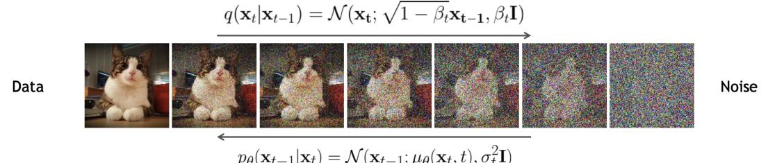
Figure 25.1: Denoising di!usion probabilistic model. The forwards di!usion process, q(xt|x^t↑¹), implements the (non-learned) inference network; this just adds Gaussian noise at each step. The reverse di!usion process, pω(x^t↑¹|xt), implements the decoder; this is a learned Gaussian model. From Slide 16 of [KGV22]. Used with kind permission of Arash Vahdat.

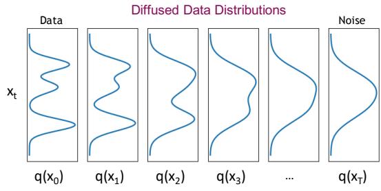
Figure 25.2: Illustration of a di!usion model on 1d data. The forwards di!usion process gradually transforms the empirical data distribution q(x0) into a simple target distribution, here q(x^T ) = N (0, I). To generate from the model, we sample a point x^T ⇐ N (0, I), and then run the Markov chain backwards, by sampling x^t ⇐ pω(xt|xt+1) until we get a sample in the original data space, x0. From Slide 19 of [KGV22]. Used with kind permission of Arash Vahdat.

allows deep models to be easily trained without any risk of posterior collapse (Section 21.4). In particular, in Section 25.2.3, we will see that training reduces to a series of weighted nonlinear least squares problems. We give some of the details below; for even more information, see [RG24].

25.2.1 Encoder (forwards di”usion)

The forwards encoder process is defined to be a simple linear Gaussian model:

\[q(\mathbf{x}\_t|\mathbf{x}\_{t-1}) = \mathcal{N}(\mathbf{x}\_t|\sqrt{1-\beta\_t}\mathbf{x}\_{t-1}, \beta\_t\mathbf{I})\tag{25.1}\]

where the values of ε^t → (0, 1) are chosen according to a noise schedule (see Section 25.2.4). The joint distribution over all the latent states, conditioned on the input, is given by

\[q(\mathbf{x}\_{1:T}|\mathbf{x}\_0) = \prod\_{t=1}^{T} q(\mathbf{x}\_t|\mathbf{x}\_{t-1}) \tag{25.2}\]

Since this defines a linear Gaussian Markov chain, we can compute marginals of it in closed form. In particular, we have

\[q(\mathbf{x}\_t|\mathbf{x}\_0) = N(\mathbf{x}\_t|\sqrt{\overline{\alpha}\_t}\mathbf{x}\_0, (1-\overline{\alpha}\_t)\mathbf{I}) \tag{25.3}\]

where we define

\[\alpha\_t \triangleq 1 - \beta\_t, \overline{\alpha}\_t = \prod\_{s=1}^t \alpha\_s \tag{25.4}\]

We choose the noise schedule such that ↽^T ⇓ 0, so that q(x^T |x0) ⇓ N (0, I).

The distribution q(xt|x0) is known as the di!usion kernel. Applying this to the input data distribution and then computing the result unconditional marginals is equivalent to Gaussian convolution:

\[q(\mathbf{z}\_t) = \int q\_0(\mathbf{z}\_0) q(\mathbf{z}\_t|\mathbf{x}\_0) d\mathbf{x}\_0 \tag{25.5}\]

As t increases, the marginals become simpler, as shown in Figure 25.2. In the image domain, this process will first remove high-frequency content (i.e., low-level details, such as texture), and later will remove low-frequency content (i.e., high-level or “semantic” information, such as shape), as shown in Figure 25.1.

25.2.2 Decoder (reverse di”usion)

In the reverse di!usion process, we would like to invert the forwards di!usion process. If we know the input x0, we can derive the reverse of one forwards step as follows:2

\[q(\mathbf{x}\_{t-1}|\mathbf{x}\_t, \mathbf{x}\_0) = \mathcal{N}(\mathbf{x}\_{t-1}|\bar{\mu}\_t(\mathbf{x}\_t, \mathbf{x}\_0), \bar{\beta}\_t \mathbf{I}) \tag{25.6}\]

\[ \tilde{\mu}\_t(\mathbf{x}\_t, \mathbf{x}\_0) = \frac{\sqrt{\overline{\alpha}\_{t-1}} \beta\_t}{1 - \overline{\alpha}\_t} \mathbf{x}\_0 + \frac{\sqrt{\alpha\_t} (1 - \overline{\alpha}\_{t-1})}{1 - \overline{\alpha}\_t} \mathbf{x}\_t \tag{25.7} \]

\[ \vec{\beta}\_t = \frac{1 - \overline{\alpha}\_{t-1}}{1 - \overline{\alpha}\_t} \beta\_t \tag{25.8} \]

Of course, when generating a new datapoint, we do not know x0, but we will train the generator to approximate the above distribution averaged over x0. Thus we choose the generator to have the form

\[p\_{\theta}(x\_{t-1}|x\_t) = \mathcal{N}(x\_{t-1}|\mu\_{\theta}(x\_t, t), \Sigma\_{\theta}(x\_t, t))\tag{25.9}\]

We often set “ω(xt, t) = ς^{2 t} I. We discuss how to learn ς^{2 t} in Section 25.2.4, but two natural choices are ς^{2 t} = ε^t and ς^{2 t = ε}˜t; these correspond to upper and lower bounds on the reverse process entropy, as shown in [HJA20].

The corresponding joint distribution over all the generated variables is given by pω(x0:^T ) = p(x^T ) ^{T t}=1 pω(x^t↑¹|xt), where we set p(x^T ) = N (0, I). We can sample from this distribution using the pseudocode in Algorithm 25.2.

^2. We just need to use Bayes’ rule for Gaussians. See e.g., https://lilianweng.github.io/posts/ 2021-07-11-diffusion-models/ for a detailed derivation.

25.2.3 Model fitting

We will fit the model by maximizing the evidence lower bound (ELBO), similar to how we train VAEs (see Section 21.2). In particular, for each data example x⁰ we have

\[\log p\_{\theta}(\mathbf{z}\_{0}) = \log \left[ \int dx\_{1:T} q(\mathbf{z}\_{1:T} | x\_{0}) \frac{p\_{\theta}(\mathbf{z}\_{0:T})}{q(\mathbf{z}\_{1:T} | \mathbf{z}\_{0})} \right] \tag{25.10}\]

\[\geq \int dx\_{1:T} q(x\_{1:T}|x\_0) \log \left( p(x\_T) \prod\_{t=1}^T \frac{p\_\theta(x\_{t-1}|x\_t)}{q(x\_t|x\_{t-1})} \right) \tag{25.11}\]

\[\mathbf{x} = \mathbb{E}\_q \left[ \log p(\mathbf{x}\_T) + \sum\_{t=1}^T \log \frac{p\_\theta(\mathbf{x}\_{t-1}|\mathbf{x}\_t)}{q(\mathbf{x}\_t|\mathbf{x}\_{t-1})} \right] \triangleq \mathbf{L}(\mathbf{x}\_0) \tag{25.12}\]

We now discuss how to compute the terms in the ELBO. By the Markov property we have q(xt|x^t↑¹) = q(xt|x^t↑¹, x0), and by Bayes’ rule, we have

\[q(\mathbf{z}\_t|\mathbf{x}\_{t-1}, \mathbf{x}\_0) = \frac{q(\mathbf{x}\_{t-1}|\mathbf{x}\_t, \mathbf{x}\_0)q(\mathbf{x}\_t|\mathbf{x}\_0)}{q(\mathbf{x}\_{t-1}|\mathbf{x}\_0)}\tag{25.13}\]

Plugging Equation (25.13) into the ELBO we get

\[\mathbb{L}(\mathbf{x}\_{0}) = \mathbb{E}\_{q(\mathbf{z}\_{1:T}|\mathbf{x}\_{0})} \left[ \log p(\mathbf{z}\_{T}) + \sum\_{t=2}^{T} \log \frac{p\_{\theta}(\mathbf{z}\_{t-1}|\mathbf{z}\_{t})}{q(\mathbf{z}\_{t-1}|\mathbf{z}\_{t}, \mathbf{z}\_{0})} + \underbrace{\sum\_{t=2}^{T} \log \frac{q(\mathbf{z}\_{t-1}|\mathbf{z}\_{0})}{q(\mathbf{z}\_{t}|\mathbf{z}\_{0})}}\_{\*} + \log \frac{p\_{\theta}(\mathbf{z}\_{0}|\mathbf{z}\_{1})}{q(\mathbf{z}\_{1}|\mathbf{z}\_{0})} \right] \tag{25.14}\]

The term marked * is a telescoping sum, and can be simplified as follows:

\[\ast = \begin{array}{c} \log q(\mathbf{z}\_{T-1}|\mathbf{z}\_0) + \dots + \log q(\mathbf{z}\_2|\mathbf{z}\_0) + \log q(\mathbf{z}\_1|\mathbf{z}\_0) \end{array} \tag{25.15}\]

\[-\log q(\mathbf{z}\_T|\mathbf{z}\_0) - \log q(\mathbf{z}\_{T-1}|\mathbf{z}\_0) - \dots - \log q(\mathbf{z}\_2|\mathbf{z}\_0) \tag{25.16}\]

\[=-\log q(\mathbf{x}\_T|\mathbf{x}\_0) + \log q(\mathbf{x}\_1|\mathbf{x}\_0) \tag{25.17}\]

Hence the negative ELBO (variational upper bound) becomes

\[\mathcal{L}(\mathbf{x}\_{0}) = -\mathbb{E}\_{q(\mathbf{z}\_{t:T}|\mathbf{x}\_{0})} \left[ \log \frac{p(\mathbf{z}\_{T})}{q(\mathbf{z}\_{T}|\mathbf{x}\_{0})} + \sum\_{t=2}^{T} \log \frac{p\_{\theta}(\mathbf{z}\_{t-1}|\mathbf{x}\_{t})}{q(\mathbf{z}\_{t-1}|\mathbf{x}\_{t}, \mathbf{x}\_{0})} + \log p\_{\theta}(\mathbf{z}\_{0}|\mathbf{x}\_{1}) \right] \tag{25.18}\]

\[=\underbrace{D\_{\text{KL}}\left(q(\mathbf{z}\_{T}|\mathbf{x}\_{0})\parallel p(\mathbf{z}\_{T})\right)}\_{L\_{T}(\mathbf{z}\_{0})}\tag{25.19}\]

\[+\sum\_{t=2}^{T} \mathbb{E}\_{q(\boldsymbol{\varpi}\_{t}|\mathbf{x}\_{0})} \underbrace{D\_{\text{KL}}\left(q(\boldsymbol{\varpi}\_{t-1}|\mathbf{x}\_{t},\boldsymbol{\varpi}\_{0}) \parallel p\_{\theta}(\mathbf{z}\_{t-1}|\mathbf{x}\_{t})\right)}\_{L\_{t-1}(\mathbf{z}\_{0})} - \underbrace{\mathbb{E}\_{q(\boldsymbol{\varpi}\_{1}|\mathbf{x}\_{0})} \log p\_{\theta}(\mathbf{z}\_{0}|\mathbf{x}\_{1})}\_{L\_{0}(\mathbf{z}\_{0})} \tag{25.20}\]

Each of these KL terms can be computed analytically, since all the distributions are Gaussian. Below we focus on the ^Lt↑¹ term. Since ^{xt =} ′↽tx^{0 +} (1 ^↓ ↽t)ςt, we can write

\[ \dot{\mu}\_t(x\_t, x\_0) = \frac{1}{\sqrt{\alpha\_t}} \left( x\_t - \frac{\beta\_t}{\sqrt{1 - \overline{\alpha}\_t}} \epsilon \right) \tag{25.21} \]

Thus instead of training the model to predict the mean of the denoised version of x^t↑¹ given its noisy input xt, we can train the model to predict the noise, from which we can compute the mean:

\[ \mu\_{\theta}(x\_t, t) = \frac{1}{\sqrt{\alpha\_t}} \left( x\_t - \frac{\beta\_t}{\sqrt{1 - \overline{\alpha}\_t}} \epsilon\_{\theta}(x\_t, t) \right) \tag{25.22} \]

where the dependence on x⁰ is implicit. With this parameterization, the loss (averaged over the dataset) becomes

\[L\_{t-1} = \mathbb{E}\_{\mathbf{z}\_0 \sim q\_0(\mathbf{z}\_0), \mathbf{c} \sim \mathcal{N}(\mathbf{0}, \mathbf{I})} \left[ \underbrace{\frac{\beta\_t^2}{2\sigma\_t^2 \alpha\_t (1 - \overline{\alpha}\_t)}}\_{\lambda\_t} ||\epsilon - \mathbf{c}\_\theta \left( \underbrace{\sqrt{\overline{\alpha}\_t} \mathbf{z}\_0 + \sqrt{1 - \overline{\alpha}\_t} \mathbf{c}\_\cdot t}\_{\mathbf{z}\_t} \right)||^2 \right] \tag{25.23}\]

The time dependent weight ω^t ensures that the training objective corresponds to maximum likelihood training (assuming the variational bound is tight). However, it has been found empirically that the model produces better looking samples if we set ω^t = 1. The resulting simplified loss (also averaging over time steps t in the model) is given by

\[L\_{\text{simple}} = \mathbb{E}\_{\mathbf{z}\_0 \sim q\_0(\mathbf{z}\_0), \boldsymbol{\epsilon} \sim \mathcal{N}(\mathbf{0}, \mathbf{I}), t \sim \text{Unif}(1, T)} \left[ ||\boldsymbol{\epsilon} - \boldsymbol{\epsilon}\_{\theta} \left( \underbrace{\sqrt{\overline{\alpha}\_t} \boldsymbol{x}\_0 + \sqrt{1 - \overline{\alpha}\_t} \boldsymbol{\epsilon}\_t}\_{\mathbf{z}\_t} t \right)||^2 \right] \tag{25.24}\]

The overall training procedure is shown in Algorithm 25.1. We can improve the perceptual quality of samples using more advanced weighting schemes, are discussed in [Cho+22]. Conversely, if the goal is to improve likelihood scores, we can optimize the noise schedule, as discussed in Section 25.2.4.

Algorithm 25.1: Training a DDPM model with Lsimple.

while not converged do x⁰ ↑ q0(x0) t ↑ Unif({1,…,T}) ς ↑ N (0, I) Take gradient descent step on ∝ω||ς ↓ ς^ω ′↽tx^{0 +} ′^{1 ↓} ↽tς, t ||2

After the model is trained, we can generate data using ancestral sampling, as shown in Algorithm 25.2.

Algorithm 25.2: Sampling from a DDPM model.

¹ x^T ↑ N (0, I) ² foreach t = T,…, 1 do ³ ς^t ↑ N (0, I) ⁴ xt↑¹ = ^⇒ 1 ϱ^t & x^t ↓ ^⇒ 1↑ϱ^t 1↑ϱ^t ςω(xt, t) ’ + ςtς^{t 5} Return x⁰

25.2.4 Learning the noise schedule

In this section, we describe a way to optimize the noise schedule used by the encoder so as to maximize the ELBO; this approach is called a variational di!usion model or VDM [Kin+21].

We will use the following parameterization of the encoder:

\[q(\mathbf{x}\_t|\mathbf{x}\_0) = \mathcal{N}(\mathbf{x}\_t|\alpha\_t\mathbf{x}\_0, \sigma\_t^2\mathbf{I})\tag{25.25}\]

(Note that this ↽^t is di!erent to the one in Equation (25.4).) Rather than working with ↽^t and ς² t separately, we will learn to predict their ratio, which is known as the signal to noise ratio:

\[R(t) = \alpha\_t^2 / \sigma\_t^2 \tag{25.26}\]

This should be monotonically decreasing in t. This can be ensured by defining R(t) = exp(↓γε(t)), where ^γε(t) is a monotonic neural network. We usually set ↽^{t = 1 ↓ ς2 t} , to correspond to the variance preserving SDE discussed in Section 25.4.

Following the derivation in Section 25.2.3, the negative ELBO (variational upper bound) can be written as

\[\mathcal{L}(\mathbf{z}\_{0}) = \underbrace{D\_{\text{KL}}\left(q(\mathbf{z}\_{T}|\mathbf{z}\_{0}) \parallel p(\mathbf{z}\_{T})\right)}\_{\text{prior loss}} + \underbrace{\mathbb{E}\_{q(\mathbf{z}\_{1}|\mathbf{z}\_{0})}[-\log p\_{\theta}(\mathbf{z}\_{0}|\mathbf{z}\_{1})]}\_{\text{reconstruction loss}} + \underbrace{\mathcal{L}\_{D}(\mathbf{z}\_{0})}\_{\text{diffusion loss}} \tag{25.27}\]

where the first two terms are similar to a standard VAE, and the final di!usion loss is given below:3

\[\mathcal{L}\_D(\mathbf{z}\_0) = \frac{1}{2} \mathbb{E}\_{\mathbf{e} \sim \mathcal{N}(\mathbf{0}, \mathbf{I})} \int\_0^1 R'(t) \left\| \mathbf{z}\_0 - \hat{\mathbf{z}}\_\theta(\mathbf{z}\_t, t) \right\|\_2^2 dt \tag{25.28}\]

where R^→ (t) is the derivative of the SNR function, and z^t = ↽tx⁰ + ςtςt. (See [Kin+21] for the derivation.)

Since the SNR function is invertible, due to the monotonicity assumtion, we can perform a change of variables, and make everything a function of v = R(t) instead of t. In particular, let z^v = ↽vx⁰ + ςvς, and x˜ω(z, v) = xˆω(z, R↑¹(v)). Then we can rewrite Equation (25.28) as

\[\mathcal{L}\_D(\mathbf{x}\_0) = \frac{1}{2} \mathbb{E}\_{\mathbf{e} \sim \mathcal{N}(\mathbf{0}, \mathbf{I})} \int\_{R\_{\text{min}}}^{R\_{\text{max}}} \|\mathbf{x}\_0 - \tilde{\mathbf{x}}\_{\theta}(\mathbf{z}\_v, v)\|\_2^2 dv \tag{25.29}\]

^3. We present a simplified form of the loss that uses the continuous time limit, which we discuss in Section 25.4.

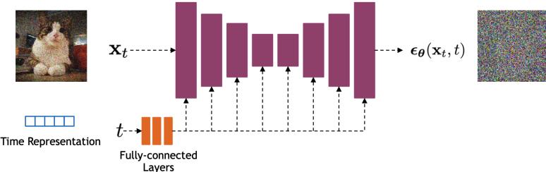
Figure 25.3: Illustration of the U-net architecture used in the denoising step. From Slide 26 of [KGV22]. Used with kind permission of Arash Vahdat.

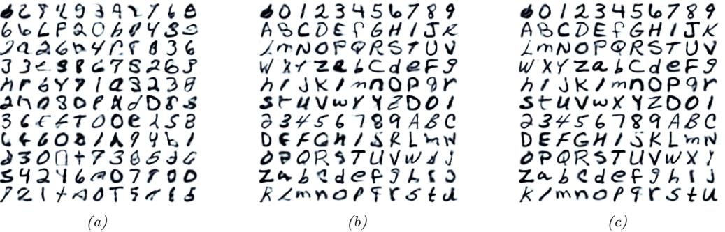
Figure 25.4: Some sample images generated by a small variational di!usion model trained on EMNIST for about 30 minutes on a K40 GPU. (a) Unconditional sampling. (b) Conditioned on class label. (c) Using classifier-free guidance (see Section 25.6.3). Generated by di!usion\_emnist.ipynb. Used with kind permission of Alex Alemi.

where Rmin = R(1) and Rmax = R(0). Thus we see that the shape of the SNR schedule does not matter, except for its value at the two end points.

The integral in Equation (25.29) can be estimated by sampling a timestep uniformly at random. When processing a minibatch of k examples, we can produce a lower variance estimate of the variational bound by using a low-discrepancy sampler (cf., Section 11.6.5). In this approach, instead of sampling the timesteps independently, we sample a single uniform random number u⁰ ↑ Unif(0, 1), and then set t ⁱ = mod (u⁰ + i/k, 1) for the i’th sample. We can also optimize the noise schedule wrt the variance of the di!usion loss.

25.2.5 Example: image generation

Di!usion models are often used to generate images. The most common architecture for image generation is based on the U-net model [RFB15], as shown in Figure 25.3. The time step t is encoded as a vector, using sinusoidal positional encoding or random Fourier features, and is then fed into the residual blocks, using either simple spatial addition or by conditioning the group norm

layers [DN21a]. Of course, other architectures besides U-net are possible. For example, recently [PX22; Li+22; Bao+22a] have proposed the use of transformers, to replace the convolutional and deconvolutional layers.

The results of training a small U-net VDM on EMNIST images are shown in Figure 25.4. By training big models (billions of parameters) for a long time (days) on lots of data (millions of images), di!usion models can be made to generate very high quality images (see Figure 20.2). Results can be further improved by using conditional di!usion models, where guidance is provided about what kinds of images to generate (see Section 25.6).

25.3 Score-based generative models (SGMs)

This section is written with Yang Song and Durk Kingma.

In Section 24.3, we discussed how to fit energy based models (EBMs) using score matching. This adjusts the parameters of the EBM so that the score function of the model, ∝^x log pω(x), matches the score function of the data, ∝^x log pD(x). An alternative to fitting a scalar energy function and computing its score is to directly learn the score function. This is called a score-based generative model or SGM [SE19; SE20b; Son+21b]. We can optimize the score function sω(x) using basic score matching (Section 24.3.1), sliced score matching (Section 24.3.3 or denoising score matching (Section 24.3.2). We discuss this class of models in more detail below. (For a comparison with EBMs, see [SH21].)

25.3.1 Example

In Figure 25.5a, we show the Swiss roll dataset. We estimate the score function by fitting an MLP with 2 hidden layers, each with 128 hidden units, using basic score matching. In Figure 25.5b, we show the output of the network after training for 10,000 steps of SGD. We see that the vector flow field points inwards towards regions where the data density is high, and points outwards from an unstable region with no data density (between the two ‘arms’ on the right). This is easiest to see in Figure 25.5c. In Figure 25.5d, we show some samples from the learned model, generated using Langevin sampling. Better algorithms (e.g., HMC) can produce more plausible samples.

25.3.2 Adding noise at multiple scales

In general, score matching can have di”culty when there are regions of low data density. To see this, suppose pD(x) = φp0(x) + (1 ↓ φ)p1(x). Let S⁰ := {x | p0(x) > 0} and S¹ := {x | p1(x) > 0} be the supports of p0(x) and p1(x) respectively. When they are disjoint from each other, the score of pD(x) is given by

\[\nabla\_{\mathbf{x}} \log p\_{\mathcal{D}}(\mathbf{x}) = \begin{cases} \nabla\_{\mathbf{x}} \log p\_{\mathbf{0}}(\mathbf{x}), & \mathbf{x} \in \mathcal{S}\_{0} \\ \nabla\_{\mathbf{x}} \log p\_{\mathbf{1}}(\mathbf{x}), & \mathbf{x} \in \mathcal{S}\_{1} \end{cases} \tag{25.30}\]

which does not depend on the weight φ. Hence score matching cannot correctly recover the true distribution. Furthermore, Langevin sampling will have di”culty traversing between modes. (In practice this will happen even when the di!erent modes only have approximately disjoint supports.)

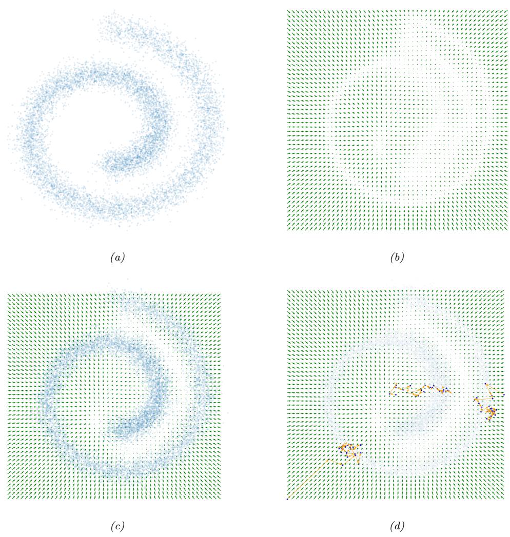
Figure 25.5: Fitting a score-based generative model to the 2d Swiss roll dataset. (a) Training set. (b) Learned score function trained using the basic score matching. (c) Superposition of learned score function and empirical density. (d) Langevin sampling applied to the learned model. We show 3 di!erent trajectories, each of length 25. Generated by score\_matching\_swiss\_roll.ipynb.

Song and Erman [SE19; SE20b] and Song et al. [Son+21b] overcome this difficulty by perturbing training data with different scales of noise. Specifically, they use

\[q\_{\sigma}(\ddot{x}|x) = \mathcal{N}(\ddot{x}|x, \sigma^2 \mathbf{I})\tag{25.31}\]

\[q\_{\sigma}(\ddot{\mathbf{z}}) = \int p\_{\mathcal{D}}(\mathbf{z}) q\_{\sigma}(\ddot{\mathbf{z}}|\mathbf{z}) d\mathbf{z} \tag{25.32}\]

For a large noise perturbation, di!erent modes are connected due to added noise, and the estimated weights between them are therefore accurate. For a small noise perturbation, di!erent modes are more disconnected, but the noise-perturbed distribution is closer to the original unperturbed data distribution. Using a sampling method such as annealed Langevin dynamics [SE19; SE20b; Son+21b] or di!usion sampling [SD+15a; HJA20; Son+21b], we can sample from the most noise-perturbed distribution first, then smoothly reduce the magnitude of noise scales until reaching the smallest one. This procedure helps combine information from all noise scales, and maintains the correct estimation of weights from higher noise perturbations when sampling from smaller ones.

In practice, all score models share weights and are implemented with a single neural network conditioned on the noise scale; this is called a noise conditional score network, and has the form sω(x, ς). Scores of di!erent scales are estimated by training a mixture of score matching objectives, one per noise scale. If we use the denoising score matching objective in Equation (24.33), we get

\[\mathcal{L}(\boldsymbol{\theta};\sigma) = \mathbb{E}\_{\boldsymbol{q}(\mathbf{x},\tilde{\mathbf{x}})} \left[ \frac{1}{2} \left\| \nabla\_{\mathbf{x}} \log p\_{\theta}(\tilde{\mathbf{x}}, \sigma) - \nabla\_{\mathbf{x}} \log q\_{\sigma}(\tilde{\mathbf{x}}|\mathbf{x}) \right\|\_{2}^{2} \right] \tag{25.33}\]

\[\mathbb{E}\_{\mathbf{x}} = \frac{1}{2} \mathbb{E}\_{\mathsf{PD}(\mathbf{x})} \mathbb{E}\_{\tilde{\mathbf{x}} \sim \mathcal{N}(\mathbf{z}, \sigma^2 \mathbf{I})} \left\{ \left\| \mathbf{s}\_{\theta}(\tilde{\mathbf{x}}, \sigma) + \frac{(\tilde{\mathbf{x}} - \mathbf{z})}{\sigma^2} \right\|\_{2}^{2} \right\} \tag{25.34}\]

where we used the fact that, for a Gaussian, the score is given by

\[ \nabla\_{\mathbf{z}} \log \mathcal{N}(\ddot{\mathbf{z}} | \mathbf{z}, \sigma^2 \mathbf{I}) = -\nabla\_{\mathbf{z}} \frac{1}{2\sigma^2} (\mathbf{z} - \ddot{\mathbf{z}})^\mathsf{T} (\mathbf{z} - \ddot{\mathbf{z}}) = \frac{\mathbf{z} - \ddot{\mathbf{z}}}{\sigma^2} \tag{25.35} \]

If we have T di!erent noise scales, we can combine the losses in a weighted fashion using

\[\mathcal{L}(\boldsymbol{\theta}; \sigma\_{1:T}) = \sum\_{t=1}^{T} \lambda\_t \mathcal{L}(\boldsymbol{\theta}; \sigma\_t) \tag{25.36}\]

where we choose ς¹ > ς² > ··· > ς^T , and the weighting term satisfies ω^t > 0.

25.3.3 Equivalence to DDPM

We now show that the above score-based generative model training objective is equivalent to the DDPM loss. To see this, first let us replace pD(x) with q0(x0), x˜ with xt, and sω(x˜, ς) with sω(xt, t). We will also compute a stochastic approximation to Equation (25.36) by sampling a time step uniformly at random. Then Equation (25.36) becomes

\[\mathcal{L} = \mathbb{E}\_{\mathbf{z}\_0 \sim q\_0(\mathbf{z}\_0), \mathbf{z}\_t \sim q(\mathbf{z}\_t | \mathbf{z}\_0), t \sim \text{Unif}(1, T)} \left[ \lambda\_t \left\| \mathbf{s}\_\theta(\mathbf{z}\_t, t) + \frac{(\mathbf{z}\_t - \mathbf{z}\_0)}{\sigma\_t^2} \right\|\_2^2 \right] \tag{25.37}\]

If we use the fact that ^{xt = x0 + ς}tς, and if we define ^sω(xt, t) = ^↓ϑω(xt,t) ^εt , we can rewrite this as

\[\mathcal{L} = \mathbb{E}\_{\mathbf{z}\_0 \sim q\_0(\mathbf{z}\_0), \mathbf{c} \sim \mathcal{N}(\mathbf{0}, \mathbf{I}), t \sim \text{Unif}(1, T)} \left[ \frac{\lambda\_t}{\sigma\_t^2} \left\| \mathbf{c} - \mathbf{c}\_\theta(\mathbf{z}\_t, t) \right\|\_2^2 \right] \tag{25.38}\]

If we set ω^t = ς^{2 t} , we recover Lsimple loss in Equation (25.24).

25.4 Continuous time models using di!erential equations

In this section, we consider a DDPM model in the limit of an infinite number of hidden layers, or equivalently, an SGM in the limit of an infinite number of noise levels. This requires switching from discrete time to continuous time, which complicates the mathematics. The advantage is that we can leverage the large existing literature on solvers for ordinary and stochastic di!erential equations to enable faster generation, as we will see.

25.4.1 Forwards di”usion SDE

Let us first consider a di!usion process where the noise level ε^t gets rewritten as ε(t)“t, where”t is a step size:

\[x\_t = \sqrt{1 - \beta\_t} x\_{t-1} + \sqrt{\beta\_t} \mathcal{N}(\mathbf{0}, \mathbf{I}) = \sqrt{1 - \beta(t)\Delta t} x\_{t-1} + \sqrt{\beta(t)\Delta t} \mathcal{N}(\mathbf{0}, \mathbf{I}) \tag{25.39}\]

If “t is small, we can approximate the first term with a first-order Taylor series expansion to get

\[x\_t \approx x\_{t-1} - \frac{\beta(t)\Delta t}{2} x\_{t-1} + \sqrt{\beta(t)\Delta t} \mathcal{N}(\mathbf{0}, \mathbf{I}) \tag{25.40}\]

Hence for small “t we have

\[\frac{\mathbf{x}\_t - \mathbf{x}\_{t-1}}{\Delta t} \approx -\frac{\beta(t)}{2}\mathbf{x}\_{t-1} + \frac{\sqrt{\beta(t)}}{\sqrt{\Delta t}}N(\mathbf{0}, \mathbf{I})\tag{25.41}\]

We can now switch to the continuous time limit, and write this as the following stochastic di!erential equation or SDE:

\[\frac{dx(t)}{dt} = -\frac{1}{2}\beta(t)x(t) + \sqrt{\beta(t)}\frac{dw(t)}{dt} \tag{25.42}\]

where w(t) represents a standard Wiener process, also called Brownian noise. More generally, we can write such SDEs as follows, where we use Itô calculus notation (see e.g., [SS19]):

\[dx = \underbrace{f(x,t)}\_{\text{drift}}dt + \underbrace{g(t)}\_{\text{diffusion}}dw\tag{25.43}\]

The first term in the above SDE is called the drift coe”cient, and the second term is called the di!usion coe”cient.

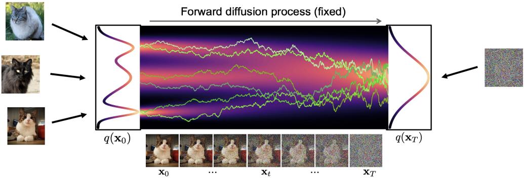
Figure 25.6: Illustration of the forwards di!usion process in continuous time. Yellow lines are sample paths from the SDE. Heat map represents the marginal distribution computed using the probability flow ODE. From Slide 43 of [KGV22]. Used with kind permission of Karsten Kreis.

We can gain some intuition for these processes by looking at the 1d example in Figure 25.6. We can draw multiple paths as follows: sample an initial state from the data distribution, and then integrate over time using Euler-Maruyama integration:

\[x(t + \Delta t) = x(t) + f(x(t), t)\Delta t + g(t)\sqrt{\Delta t}N(\mathbf{0}, \mathbf{I})\tag{25.44}\]

We can see how the data distributiom at t = 0, on the left hand side, gradually gets transformed to a pure noise distribution at t = 1, on the right hand side.

In [Son+21b], they show that the SDE corresponding to DDPMs, in the T ↔︎ ̸ limit, is given by

\[dx = -\frac{1}{2}\beta(t)xdt + \sqrt{\beta(t)}dw\tag{25.45}\]

where ε(t/T) = Tεt. Here the drift term is proportional to ↓x, which encourages the process to return to 0. Consequently, DDPM corresponds to a variance preserving process. By contrast, the SDE corresponding to SGMs is given by the following:

\[d\mathbf{x} = \sqrt{\frac{d[\sigma(t)^2]}{dt}} d\mathbf{w} \tag{25.46}\]

where ς(t/T) = ςt. This SDE has zero drift, so corresponds to a variance exploding process.

25.4.2 Forwards di”usion ODE

Instead of adding Gaussian noise at every step, we can just sample the initial state, and then let it evolve deterministically over time according to the following ordinary di!erential equation or ODE:

\[d\mathbf{x} = \underbrace{\left[f(\mathbf{z}, t) - \frac{1}{2}g(t)^2 \nabla\_{\mathbf{z}} \log p\_t(\mathbf{z})\right]}\_{h(\mathbf{z}, t)} dt \tag{25.47}\]

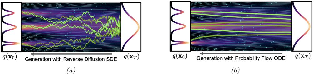
Figure 25.7: Illustration of the reverse di!usion process. (a) Sample paths from the SDE. (b) Deterministic trajectories from the probability flow ODE. From Slide 65 of [KGV22]. Used with kind permission of Karsten Kreis.

This is called the probability flow ODE [Son+21b, Sec D.3]. We can compute the state at any moment in time using any ODE solver:

\[x(t) = x(0) + \int\_0^t h(x, \tau) d\tau \tag{25.48}\]

See Figure 25.7b for a visualization of a sample trajectory. If we start the solver from di!erent random states x(0), then the induced distribution over paths will have the same marginals as the SDE model. See the heatmap in Figure 25.6 for an illustration.

25.4.3 Reverse di”usion SDE

To generate samples from this model, we need to be able to reverse the SDE. In a remarkable result, [And82] showed that any forwards SDE of the form in Equation (25.43) can be reversed to get the following reverse-time SDE:

\[d\mathbf{x} = \left[ f(\mathbf{x}\_t, t) - g(t)^2 \nabla\_\mathbf{x} \log q\_t(\mathbf{x}) \right] dt + g(t) d\overline{\mathbf{w}} \tag{25.49}\]

where w is the standard Wiener process when time flows backwards, dt is an infinitesimal negative time step, and ∝^x log qt(x) is the score function.

In the case of the DDPM, the reverse SDE has the following form:

\[d\mathbf{x}\_t = \left[ -\frac{1}{2}\beta(t)\mathbf{x}\_t - \beta(t)\nabla\_{\mathbf{z}\_t}\log q\_t(\mathbf{z}\_t) \right]dt + \sqrt{\beta(t)}d\overline{\mathbf{w}}\_t \tag{25.50}\]

To estimate the score function, we can use denoising score matching as we discussed in Section 25.3, to get

\[\nabla\_{x\_t} \log q\_t(x\_t) \approx \mathbf{s}\_{\theta}(x\_t, t) \tag{25.51}\]

(In practice, it is advisable to use variance reduction techniques, such as importance sampling, as discussed in [Son+21a].) The SDE becomes

\[d\mathbf{x}\_t = -\frac{1}{2}\beta(t)\left[\mathbf{x}\_t + 2\mathbf{s}\_\theta(\mathbf{x}\_t, t)\right]dt + \sqrt{\beta(t)}d\overline{\mathbf{w}}\_t\tag{25.52}\]

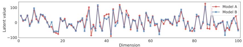
Figure 25.8: Comparing the first 100 dimensions of the latent code obtained for a random CIFAR-100 image. “Model A” and “Model B” are separately trained with di!erent architectures. From Figure 7 of [Son+21b]. Used with kind permission of Yang Song.

After fitting the score network, we can sample from it using ancestral sampling (as in Section 25.2), or we can use the Euler-Maruyama integration scheme in Equation (25.44), which gives

\[x\_{t-1} = x\_t + \frac{1}{2}\beta(t)\left[x\_t + 2s\_\theta(x\_t, t)\right]\Delta t + \sqrt{\beta(t)\Delta t}N(\mathbf{0}, \mathbf{I})\tag{25.53}\]

See Figure 25.7a for an illustration.

25.4.4 Reverse di”usion ODE

Based on the results in Section 25.4.2, we can derive the probability flow ODE from the reverse-time SDE in Equation (25.49) to get

\[d\mathbf{x}\_t = \left[ f(\mathbf{x}\_t, t) - \frac{1}{2} g(t)^2 \mathbf{s}\_\theta(\mathbf{x}\_t, t) \right] dt \tag{25.54}\]

If we set ^f(xt, t) = ^{↓1 2 ε}(t)x^t and ^g(t) = ε(t), as in DDPM, this becomes

\[d\mathbf{x}\_t = -\frac{1}{2}\beta(t)\left[\mathbf{x}\_t + \mathbf{s}\_\theta(\mathbf{x}\_t, t)\right]dt\tag{25.55}\]

See Figure 25.7b for an illustration. A simple way to solve this ODE is to use Euler’s method:

\[x\_{t-1} = x\_t + \frac{1}{2}\beta(t)\left[x\_t + s\_\theta(x\_t, t)\right]\Delta t\tag{25.56}\]

However, in practice one can get better results using higher-order ODE solvers, such as Heun’s method [Kar+22].

This model is a special case of a neural ODE, also called a continuous normalizing flow (see Section 23.2.6). Consequently we can derive the exact log marginal likelihood. However, instead of maximizing this directly (which is expensive), we use score matching to fit the model.

Another advantage of the deterministic ODE approach is that it guarantees that the generative model is identifiable. To see this, note that the ODE (in both forwards and reverse directions) is deterministic, and is uniquely determined by the score function. If the architecture is su”ciently flexible, and if there is enough data, then score matching will recover the true score function of the data generating process. Thus, after training, a given datapoint will map to a unique point in latent space, regardless of the model architecture or initialization (see Figure 25.8).

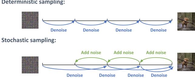
Figure 25.9: Generatng from the reverse di!usion process using 4 steps. (Top) Deterministic sampling. (Bottom) A mix of deterministic and stochastic sampling. Used with kind permission of Ruiqi Gao.

Furthermore, since every point in latent space decodes to a unique image, we can perform “semantic interpolation” in the latent space to generate images with properties that are in between two input examples (cf., Figure 20.9).

25.4.5 Comparison of the SDE and ODE approach

In Section 25.4.3 we described the reverse di!usion process as an SDE, and in Section 25.4.4, we described it as an ODE. We can see the connection between these methods by rewriting the SDE in Equation (25.49) as follows:

\[d\mathbf{x}\_t = \underbrace{-\frac{1}{2}\beta(t)[\mathbf{x}\_t + \mathbf{s}\_\theta(\mathbf{z}\_t, t)]dt}\_{\text{probability flow ODE}} - \underbrace{\frac{1}{2}\beta(t)\mathbf{s}\_\theta(\mathbf{z}\_t, t)dt + \sqrt{\beta(t)}d\overline{\mathbf{w}}\_t}\_{\text{Largevin diffusion SDE}}\tag{25.57}\]

The continuous noise injection can compensate for errors introduced by the numerical integration of the ODE term. Consequently, the resulting samples often look better. However, the ODE approach can be faster. Fortunately it is possible to combine these techniques, as proposed in [Kar+22]. The basic idea is illustrated in Figure 25.9: we alternate between performing a deterministic step using an ODE solver, and then adding a small amount noise to the result. This can be repeated for some number of steps. (We discuss ways to reduce the number of required steps in Section 25.5.)

25.4.6 Example

A simple JAX implementation of the above ideas, written by Winnie Xu, can be found in di!usion\_mnist.ipynb. This fits a small model to MNIST images using denoising score matching. It then generates from the model by solving the probability flow ODE using the di!rax library. By scaling this kind of method up to a much larger model, and training for a much longer time, it is possible to produce very impressive looking results, as shown in Figure 25.10.

25.4.7 Flow matching

In Section 25.4.4, we mentioned that the ODE version of di!usion can be viewed as a continuous-time normalizing flow. From this perspective, we can dispense with the notion of Gaussian noise and

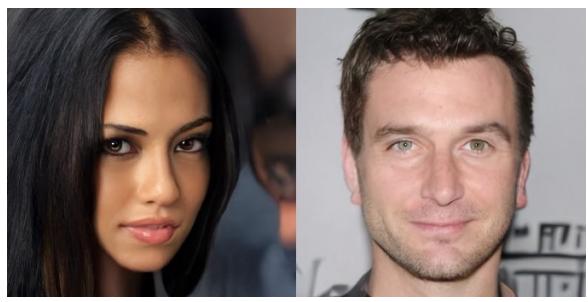
Figure 25.10: Synthetic faces from a score-based generative model trained on CelebA-HQ-256 images. From Figure 12 of [Son+21b]. Used with kind permission of Yang Song.

Brownian motion, used in DDPM, and directly interpret the problem as learning a deterministic mapping from a source distribution p⁰ to a target distribution p¹ via a smooth di!erentiable map. This approach is called flow matching, and was independently proposed in several recent papers [AVE23; Lip+23; LGL23; HBC23].

The basic idea is to train a neural network to approximate the velocity field ^vω(xt, t) ⇓ ^d dtx^{t = d} dt It(x0, x1), where It(x0, x1) = ↽tx⁰ + εtx¹ is the interpolant (e.g., using ↽^t = (1 ↓ t) and ε^t = t); we then use the vector-valued function inside of an ODE solver to compute a sample x¹ = ” ¹ 0 dx^t dt dt starting from x⁰ ↑ p0. The advantage of this approach is that it allows for non-Gaussian source distributions p0, and it provides a way to compute the exact likelihood, namely ^p1(x) = ^p0(x) exp & ^↓ ” ^{1 0} div(vω(xt, t))dt’ . Furthermore, it is possible to optimize the flow so that it solves an optimal transport (Section 6.8) problem (see e.g., [Ton+23]), which can speedup sampling / integration [Lip+23; LGL23].

25.5 Speeding up di!usion models

One of the main disadvantages of di!usion models is that generating from them takes many small steps, which can be slow. While it is possible to just take fewer, larger steps, the results are much worse. In this section, we briefly mention a few techniques that have been proposed to tackle this important problem. Many other techniques are mentioned in the recent review papers [UAP22; Yan+22; Cao+22].

25.5.1 DDIM sampler

In this section, we describe the denoising di!usion implicit model or DDIM of [SME21], which can be used for e”cient deterministic generation. The first step is to use a non-Markovian forwards di!usion process, so it always conditions on the input in addition to the previous step:

\[q(\mathbf{x}\_{t-1}|\mathbf{x}\_t, \mathbf{x}\_0) = \mathcal{N}(\sqrt{\overline{\alpha\_{t-1}}}\mathbf{x}\_0 + \sqrt{1 - \overline{\alpha}\_{t-1} - \hat{\sigma}\_t^2} \frac{\mathbf{z}\_t - \sqrt{\overline{\alpha}\_t}\mathbf{z}\_0}{\sqrt{1 - \overline{\alpha}\_t}}, \bar{\sigma}\_t^2 \mathbf{I}) \tag{25.58}\]

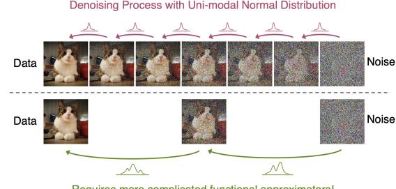
Figure 25.11: Illustration of why taking larger steps in the reverse di!usion process needs more complex, mulit-modal conditional distributions. From Slide 90 of [KGV22]. Used with kind permission of Arash Vahdat.

The corresponding reverse process is

\[p\_{\theta}(\mathbf{z}\_{t-1}|\mathbf{z}\_{t}) = \mathcal{N}(\sqrt{\overline{\alpha}\_{t-1}}\hat{\mathbf{x}}\_{0} + \sqrt{1 - \overline{\alpha}\_{t-1} - \hat{\sigma}\_{t}^{2}}\frac{\mathbf{z}\_{t} - \sqrt{\overline{\alpha}\_{t}}\hat{\mathbf{x}}\_{0}}{\sqrt{1 - \overline{\alpha}\_{t}}}, \hat{\sigma}\_{t}^{2}\mathbf{I}) \tag{25.59}\]

where xˆ⁰ = xˆω(xt, t) is the predicted output from the model. By setting ς˜^{2 t} = 0, the reverse process becomes fully deterministic, given the initial prior sample (whose variance is controlled by ς˜^{2 T} ). The resulting probability flow ODE gives better results when using a small number of steps compared to the methods discussed in Section 25.4.4.

Note that the weighted negative VLB for this model is the same as Lsimple in Section 25.2, so the DDIM sampler can be applied to a trained DDPM model.

25.5.2 Non-Gaussian decoder networks

If the reverse di!usion process takes larger steps, then the induced distribution over clean outputs given a noisy input will become multimodal, as illustrated in Figure 25.11. This requires more complicated forms for the distribution pω(x^t↑¹|xt). In [Gao+21], they use an EBM to fit this distribution. However, this still requires the use of MCMC to draw a sample. In [XKV22], they use a GAN (Chapter 26) to fit this distribution. This enables us to easily draw a sample by passing Gaussian noise through the generator. The benefits over a single stage GAN is that both the generator and discriminator are solving a much simpler problem, resulting in increased mode coverage, and better training stability. The benefit over a standard di!usion model is that we can generate high quality samples in many fewer steps.

25.5.3 Distillation

In this section, we discuss the progressive distillation method of [SH22], which provides a way to create a di!usion model that only needs a small number of steps to create high quality samples. The basic idea is follows. First we train a DDPM model in the usual way, and sample from it using the DDIM method; we treat this as the “teacher” model. We use this to generate intermediate latent states, and train a “student” model to predict the output of the teacher on every second step, as shown in Figure 25.12. After the student has been trained, it can generate results that are as good as

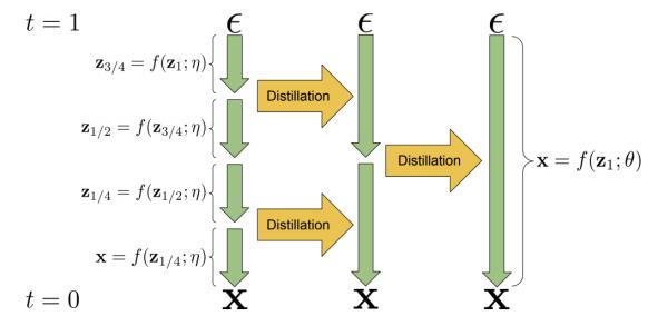
Figure 25.12: Progressive distillation. From Figure 1 of [SH22]. Used with kind permission of Tim Salimans.

the teacher, but in half the number of steps. This student can then teach a new generation of even faster students. See Algorithm 25.4 for the pseudocode, which should be compared to Algorithm 25.3 for the standard training procedure. Note that each round of teaching becomes faster, because the teachers become smaller, so the total time to perform the distillation is relatively small. The resulting model can generate high quality samples in as few as 4 steps.

Algorithm 25.3: Standard training	Algorithm 25.4: Progressive distilla
Input: Model xˆω(zt) to be trained	tion
Input: Dataset D	Input: Trained teacher model xˆϑ(zt)
Input: Loss weight function w	Input: Dataset D
	Input: Loss weight function w
	Input: Student sampling steps N
	1 foreach K iterations do
1 while not converged do	ω := ϑ (Assign student) 2
x ↑ D 2	while not converged do 3
t ↑ Unif(0, 1) 3	x ↑ D 4
ε ↑ N (0, I) 4	t = i/N, i ↑ Cat(1, 2,,N) 5
zt = ωtx + εtε 5	ε ↑ N (0, I) 6
	zt = ωtx + εtε 7
	t→ = t ↔︎ 0.5/N, t→→ = t ↔︎ 1/N 8
	zt↑ = ωt↑xˆϑ(zt) + ωt↑ ωt (zt ↔︎ ωtxˆϑ(zt)) 9
	zt↑↑ = 10
x˜ = x (Clean data is target) 6	ωt↑↑xˆϑ(zt↑ ) + ωt↑↑ ωt↑ (zt↑ ↔︎ ωt↑xˆϑ(zt↑ ))
= log(ω2 t /ε2 ϑt t ) (Log SNR) 7 = w(ϑt) ↓x˜ ↔︎ xˆω(zt)↓2 Lω	x˜ = zt↑↑ ↑(ωt↑↑ /ωt)zt εt↑↑ ↑(ωt↑↑ /ωt)εt (Teacher is target) 11
8 2 ω := ω ↔︎ ϖ↗ωLω 9	= log(ω2 t /ε2 ϑt t ) 12
	= w(ϑt) ↓x˜ ↔︎ xˆω(zt)↓2 Lω 13 2
	ω := ω ↔︎ ϖ↗ωLω 14
	ϑ : ↔︎ = ω (Student becomes next teacher) 15

25.5.4 Latent space di”usion

Another approach to speeding up di!usion models for images is to first embed the images into a lower dimensional space, and then fit the di!usion model to the embeddings. This idea has been

¹⁶ N := N/2 (Halve number of sampling steps)

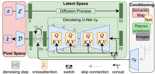
Figure 25.13: Combining a VAE with a di!usion model. Here E and D are the encoder and decoder of the VAE. The di!usion model conditions on the inputs either by using concatentation or by using a cross-attention mechanism. From Figure 3 of [Rom+22]. Used with kind permission of Robin Rombach.

pursued in several papers.

In the latent di!usion model (LDM) of [Rom+22], they adopt a two-stage training scheme, in which they first fit the VAE, augmented with a perceptual loss, and then fit the di!usion model to the embedding. The architecture is illustrated in Figure 25.13. The LDM forms the foundation of the very popular stable di!usion system created by Stability AI. In the latent score-based generative model (LSGM) of [VKK21], they first train a hierarchical VAE, and then jointly train the VAE and a di!usion model.

In addition to speed, an additional advantage of combining di!usion models with autoencoders is that it makes it simple to apply di!usion to many di!erent kinds of data, such as text and graphs: we just need to define a suitable architecture to embed the input domain into a continuous space. Note, however, that it is also possible to define di!usion directly on discrete state spaces, as we discuss in Section 25.7.

So far we have discussed applying di!usion “on top of” a VAE. However, we can also do the reverse, and fit a VAE on top of a DDPM model, where we use the di!usion model to “post process” blurry samples coming from the VAE. See [Pan+22] for details.

25.6 Conditional generation

In this section, we discuss how to generate samples from a di!usion model where we condition on some side information c, such as a class label or text prompt.

25.6.1 Conditional di”usion model

The simplest way to control the generation from a generative model is to train it on (c, x) pairs so as to maximize the conditional likelihood, p(x|c). If the conditioning signal c is a scalar (e.g., a class label), it can be mapped to an embedding vector, and then incorporated into the network by spatial addition, or by using it to modulate the group normalization layers. If the input c is another image, we can simply concatenate it with x^t as an extra set of channels. If the input c is a text prompt, we can embed it, and then use spatial addition or cross-attention (see Figure 25.13 for an illustration).

25.6.2 Classifier guidance

One problem with conditional di!usion models is that we need to retrain them for each kind of conditioning that we want to perform. An alternative approach, known as classifier guidance was proposed in [DN21b], and allows us to leverage pre-trained discriminative classifiers of the form pε(c|x) to control the generation process. The idea is as follows. First we use Bayes’ rule to write

\[\log p(\mathbf{z}|\mathbf{c}) = \log p(\mathbf{c}|\mathbf{z}) + \log p(\mathbf{z}) - \log p(\mathbf{c}) \tag{25.60}\]

from which the score function becomes

\[ \nabla\_{\mathbf{z}} \log p(\mathbf{z}|\mathbf{c}) = \nabla\_{\mathbf{z}} \log p(\mathbf{z}) + \nabla\_{\mathbf{z}} \log p(\mathbf{c}|\mathbf{z}) \tag{25.61} \]

We can now use this conditional score to generate samples, rather than the unconditional score. We can further amplify the influence of the conditioning signal by scaling it by a factor w > 1:

\[ \nabla\_{\mathbf{z}} \log p\_w(\mathbf{z}|\mathbf{c}) = \nabla\_{\mathbf{z}} \log p(\mathbf{z}) + w \nabla\_{\mathbf{z}} \log p(\mathbf{c}|\mathbf{z}) \tag{25.62} \]

In practice, this can be achieved as follows by generating samples from

\[x\_{t-1} \sim \mathcal{N}(\mu + w \Sigma \mathbf{g}, \Sigma), \ \mu = \mu\_{\boldsymbol{\theta}}(\boldsymbol{x}\_{t}, t), \ \Sigma = \Sigma\_{\boldsymbol{\theta}}(\boldsymbol{x}\_{t}, t), \ \boldsymbol{g} = \nabla\_{\mathbf{z}\_{t}} \log p\_{\boldsymbol{\phi}}(\mathbf{c}|\boldsymbol{x}\_{t}) \tag{25.63}\]

25.6.3 Classifier-free guidance

Unfortunately, p(c|xt) is a discriminative model, that may ignore many details of the input xt. Hence optimizing along the directions specified by ∝^xt log p(c|xt) can give poor results, similar to what happens when we create adversarial images. In addition, we need to train a classifier for each time step, since x^t will di!er in its blurriness.

In [HS21], they proposed a technique called classifier-free guidance, which derives the classifier from the generative model, using ^p(c|x) = ^p(x|c)p(c) ^p(x) , from which we get

\[\log p(\mathbf{c}|\mathbf{x}) = \log p(\mathbf{x}|\mathbf{c}) + \log p(\mathbf{c}) - \log p(\mathbf{x}) \tag{25.64}\]

This requires learning two generative models, namely p(x|c) and p(x). However, in practice we can use the same model for this, and simply set c = ¬ to represent the unconditional case. We then use this implicit classifier to get the following modified score function:

\[\nabla\_{\mathbf{z}} \left[ \log p(\mathbf{z}|\mathbf{c}) + w \log p(\mathbf{c}|\mathbf{z}) \right] = \nabla\_{\mathbf{z}} \left[ \log p(\mathbf{z}|\mathbf{c}) + w(\log p(\mathbf{z}|\mathbf{c}) - \log p(\mathbf{z})) \right] \tag{25.65}\]

\[=\nabla\_{\mathbf{z}}\left[(1+w)\log p(\mathbf{z}|\mathbf{c}) - w\log p(\mathbf{z})\right] \tag{25.66}\]

Larger guidance weight usually results in better individual sample quality, but lower diversity.

25.6.4 Generating high resolution images

In order to generate high resolution images, [Ho+21] proposed to use cascaded generation, in which we first train a model to generate 64 ↗ 64 images, and then train a separate super-resolution model to map this to 256 ↗ 256 or 1024 ↗ 1024. This approach is used in Google’s Imagen model [Sah+22b], which is a text-to-image system (see Figure 25.14). Imagen uses large pre-trained text

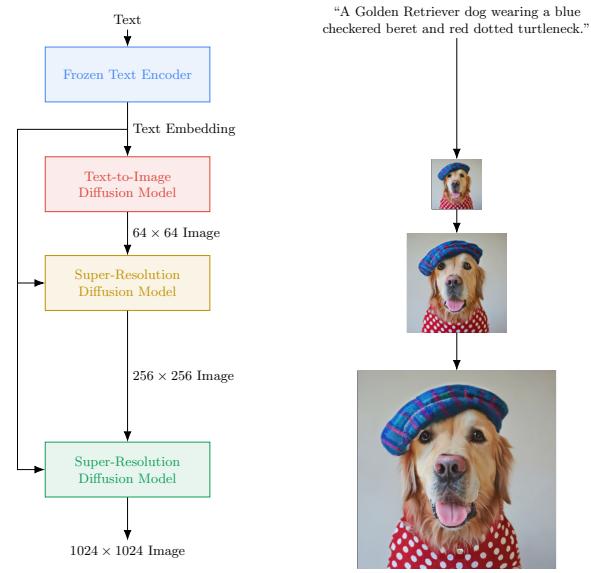
Figure 25.14: Cascaded di!usion model used by the Imagen text-to-image system. From Figure A.5 of [Sah+22b]. Used with kind permission of Saurabh Saxena.

encoder, based on T5-XXL [Raf+20a], combined with a VDM model (Section 25.2.4) based on the U-net architecture, to generate impressive-looking images (see Figure 20.2).

In addition to conditioning on text, it is possible to condition on another image to create a model for image-to-image translation. For example, we can learn map a gray-scale image c to a color image x, or a corrupted or occluded image c to a clean version x. This can be done by training a multi-task conditional di!usion model, as explained in [Sah+22a]. See Figure 20.4 for some sample outputs.

25.7 Di!usion for discrete state spaces

So far in this chapter, we have focused on Gaussian di!usion for generating real-valued data. However it is also possible to define di!usion models for discrete data, such as text or semantic segmentation labels, either by using a continuous latent embedding space (see Section 25.5.4), or by defining di!usion operations directly on the discrete state space, as we discuss beow.

25.7.1 Discrete Denoising Di”usion Probabilistic Models

In this section we discuss the Discrete Denoising Di!usion Probabilistic Model (D3PM) of [Aus+21], which defines a discrete time di!usion process directly on the discrete state space. (This builds on prior work such as multinomial di!usion [Hoo+21], and the original di!usion paper of [SD+15b].)

The basic idea is illustrated in Figure 25.15 in the context of semantic segmentation, which associates a categorical label to each pixel in an image. On the right we illustrate some sample

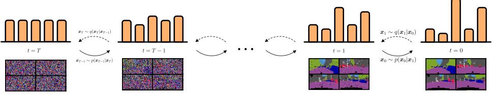
Figure 25.15: Multinomial di!usion model, applied to semantic image segmentation. The input image is on the right, and gets di!used to the noise image on the left. From Figure 1 of [Aus+21]. Used with kind permission of Emiel Hoogeboom.

images, and the corresponding categorical distribution that they induce over a single pixel. We gradually transform these pixel-wise distributions to the uniform distribution, using a stochastic sampling process that we describe below. We then learn a neural network to invert this process, so it can generate discrete data from noise; in the diagram, this corresponds to moving from left to right.

To ensure e”cient training, we require that we can e”ciently sample from q(xt|x0) for an abritrary timestep t, so we can randomly sample time steps when optimizing the variational bound in Equation (25.27). In addition, we require that q(x^t↑¹|xt, x0) have a tractable form, so we can e”ciently compute the KL terms

\[L\_{t-1}(\mathbf{x}\_0) = \mathbb{E}\_{q(\mathbf{z}\_t|\mathbf{z}\_0)} D\_{\text{KL}}\left(q(\mathbf{z}\_{t-1}|\mathbf{z}\_t, \mathbf{z}\_0) \parallel p\_\theta(\mathbf{z}\_{t-1}|\mathbf{z}\_t)\right) \tag{25.67}\]

Finally, it is useful if the forwards process converges to a known stationary distribution, φ(x^T ), which we can use for our generative prior p(x^T ); this ensures DKL (q(x^T |x0) ⇐ p(x^T )) = 0.

To satisfy the above criteria, we assume the state consists of D independent blocks, each representing a categorical variable, x^t → {1,…,K}; we represent this by the one-hot row vector x0. In general, this will represent a vector of probabilities. We then define the forwards di!usion kernel as follows:

\[q(\mathbf{x}\_t|\mathbf{x}\_{t-1}) = \text{Cat}(\mathbf{x}\_t|\mathbf{x}\_{t-1}\mathbf{Q}\_t) \tag{25.68}\]

where [Qt]ij = q(x^t = j|x^t↑¹ = i) is a row stochastic transition matrix. (We discuss how to define Q^t in Section 25.7.2.)

We can derive the t-step marginal of the forwards process as follows:

\[q(\mathbf{x}\_t|\mathbf{x}\_0) = \text{Cat}(\mathbf{x}\_t|\mathbf{x}\_0 \overline{\mathbf{Q}}\_t), \ \overline{\mathbf{Q}}\_t = \mathbf{Q}\_1 \mathbf{Q}\_2 \cdots \mathbf{Q}\_t \tag{25.69}\]

Similarly, we can reverse the forwards process as follows:

\[q(\boldsymbol{x}\_{t-1}|\boldsymbol{x}\_{t},\boldsymbol{x}\_{0}) = \frac{q(\boldsymbol{x}\_{t}|\boldsymbol{x}\_{t-1},\boldsymbol{x}\_{0})q(\boldsymbol{x}\_{t-1}|\boldsymbol{x}\_{0})}{q(\boldsymbol{x}\_{t}|\boldsymbol{x}\_{0})} = \text{Cat}\left(\boldsymbol{x}\_{t-1}|\frac{\boldsymbol{x}\_{t}\mathbf{Q}\_{t}^{\mathsf{T}} \odot \boldsymbol{x}\_{0}\overline{\mathbf{Q}}\_{t-1}}{\boldsymbol{x}\_{0}\overline{\mathbf{Q}}\_{t}\boldsymbol{x}\_{t}^{\mathsf{T}}}\right) \tag{25.70}\]

We discuss how to define the generative process pω(x^t↑¹|xt) in Section 25.7.3. Since both distrbutions factorize, we can easily compute the KL distributions in Equation (25.67) by summing the KL for each dimension.

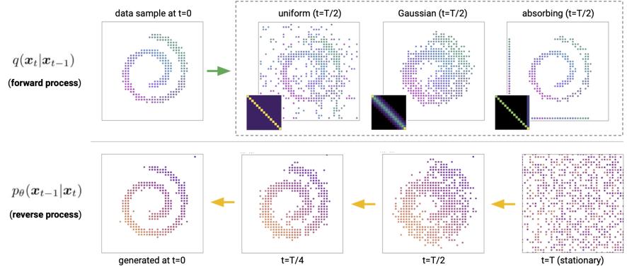
Figure 25.16: D3PM forward and (learned) reverse proccess applied to a quantized Swiss roll. Each dot represents a 2d categorical variable. Top: samples from the uniform, discretized Gaussian, and absorbing state models, along with corresponding transition matrices Q. Bottom: samples from a learned discretized Gaussian reverse process. From Figure 1 of [Aus+21]. Used with kind permission of Jacob Austin.

25.7.2 Choice of Markov transition matrices for the forward processes

In this section, we give some examples of how to represent the transition matrix Qt.

One simple approach is to use Q^t = (1 ↓ εt)I + εt/K, which we can write in scalar form as follows:

\[[\mathbf{Q}\_t]\_{ij} = \begin{cases} 1 - \frac{K-1}{K} \beta\_t & \text{if } i = j \\ \frac{1}{K} \beta\_t & \text{if } i \neq j \end{cases} \tag{25.71}\]

Intuïtively, this adds a little amount of uniform noise over the K classes, and with a large probability, 1 ↓ εt, we sample from x^t↑¹. We call this the uniform kernel. Since this is a doubly stochastic matrix with strictly positive entries, the stationary distributon is uniform. See Figure 25.16 for an illustration.

In the case of the uniform kernel, one can show [Hoo+21] that the marginal distribution is given by

\[q(\mathbf{x}\_t|\mathbf{x}\_0) = \text{Cat}(\mathbf{x}\_t|\overline{\alpha}\_t \mathbf{x}\_0 + (1 - \overline{\alpha}\_t)/K) \tag{25.72}\]

where ↽^t = 1 ^{↓ εt} and ↽^{t = t ς}=1 ↽^ς . This is similar to the Gaussian case discussed in Section 25.2. Furthermore, we can derive the posterior distribution as follows:

\[q(\mathbf{x}\_{t-1}|\mathbf{x}\_t, \mathbf{x}\_0) = \text{Cat}(\mathbf{x}\_{t-1}|\boldsymbol{\theta}\_{\text{post}}(\mathbf{x}\_t, \boldsymbol{\theta}\_0)), \ \boldsymbol{\theta}\_{\text{post}}(\mathbf{x}\_t, \boldsymbol{\theta}\_0) = \boldsymbol{\tilde{\theta}} / \sum\_{k=1}^{K} \boldsymbol{\tilde{\theta}}\_k \tag{25.73}\]

\[\tilde{\boldsymbol{\theta}} = \left[ \alpha\_t \mathbf{x}\_t + (1 - \alpha\_t) / K \right] \odot \left[ \overline{\alpha}\_{t-1} \mathbf{x}\_0 + (1 - \overline{\alpha}\_{t-1}) / K \right] \tag{25.74}\]

Another option is to define a special absorbing state m, representing a MASK token, which we

transition into with probability ^εt. Formally, we have ^Qt = (1 ^{↓ ε}t)^{I + ε}t1e^{T m}, or, in scalar form,

\[[\mathbf{Q}\_t]\_{ij} = \begin{cases} 1 & \text{if } i = j = m \\ 1 - \beta\_t & \text{if } i = j \neq m \\ \beta\_t & \text{if } j = m, i \neq m \end{cases} \tag{25.75}\]

This converges to a point-mass distribution on state m. See Figure 25.16 for an illustration.

Another option, suitable for quantized ordinal values, is to use a discretized Gaussian, that transitions to other nearby states, with a probability that depends on how similar the states are in numerical value. If we ensure the transition matrix is doubly stochastic, the resulting stationary distribution will again be uniform. See Figure 25.16 for an illustration.

25.7.3 Parameterization of the reverse process

While it is possible to directly predict the logits pω(x^t↑¹|xt) using a neural network fω(xt), it is preferable to directly predict the logits of the output, using p˜ω(x˜0|xt); we can then combine this with the analytical expression for q(x^t↑¹|xt, x0) to get

\[p\_{\theta}(\boldsymbol{x}\_{t-1}|\boldsymbol{x}\_{t}) \propto \sum\_{\tilde{\mathbf{x}}\_{0}} q(\boldsymbol{x}\_{t-1}|\boldsymbol{x}\_{t}, \tilde{\mathbf{x}}\_{0}) \tilde{p}\_{\theta}(\bar{\boldsymbol{x}}\_{0}|\boldsymbol{x}\_{t}) \tag{25.76}\]

(The sum over x˜⁰ takes O(DK) time, if there are D dimensions, each with K values.) One advantage of this approach, compared to directly learning pω(x^t↑¹|xt), is that the model will automatically satisfy any sparsity constraints in Qt. In addition, we can perform inference with k steps at a time, by predicting

\[p\_{\theta}(\boldsymbol{x}\_{t-k}|\boldsymbol{x}\_{t}) \propto \sum\_{\tilde{\mathbf{x}}\_{0}} q(\boldsymbol{x}\_{t-k}|\boldsymbol{x}\_{t}, \tilde{\mathbf{x}}\_{0}) \tilde{p}\_{\theta}(\tilde{\mathbf{x}}\_{0}|\boldsymbol{x}\_{t}) \tag{25.77}\]

Note that, in the multi-step Gaussian case, we require more complex models to handle multimodaility (see Section 25.5.2). By contrast, discrete distributions already have this flexibility built in.

25.7.4 Noise schedules

In this section we discuss how to choose the noise schedule for εt. For discretized Gaussian di!usion, [Aus+21] propose to linearly increase the variance of the Gaussian noise before the discretization step. For uniform di!usion, we can use a cosine schedule of the form ↽^t = cos( t/T ^+s 1+s ↽ ² ), where s = 0.08, as proposed in [ND21]. (Recall that ε^t = 1 ↓ ↽t, so the noise increases over time.) For masked di!usion, we can use a schedule of the form ε^t = 1/(T ↓ t + 1), as proposed in [SD+15b].

25.7.5 Connections to other probabilistic models for discrete sequences

There are interesting connections between D3PM and other probabilistic text models. For example, suppose we define the transition matrix as a combination of the unifrom transition matrix and an absorbing MASK state, i.e., Q = ↽1e^{T m + ε}11^T/K + (1 ^↓ ↽ ^{↓ ε})I. For a one-step di!usion process

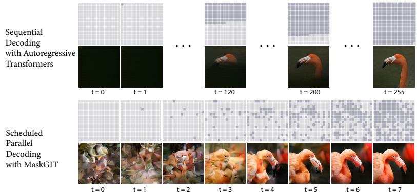
Figure 25.17: Comparison of sequential image generation with a transformer (top) vs parallel generation with MaskGIT (bottom). All pixels start out in the MASK state, denoted by light gray. In the transformer, we generate one pixel at a time, so it takes 256 steps for the whole image. In the MaskGIT method, multiple states are generated in parallel, which only takes 8 steps. From Figure 2 of [Cha+22]. Used with kind permission of Huiwen Chang.

in which q(x1|x0) replaces ↽ = 10% of the tokens with MASK, and ε = 5% uniformly at random, we recover the same objective that is used to train the BERT language model, namely

\[L\_0(\mathbf{z}\_0) = -\mathbb{E}\_{q(\mathbf{z}\_1|\mathbf{z}\_0)} \log p\_\theta(\mathbf{z}\_0|\mathbf{z}\_1) \tag{25.78}\]

(This follows since L^T = 0, and there are no other time steps used in the variational bound in Equation (25.27).)

Now consider a di!usion process that deterministically masks tokens one-by-one. For a sequence of length N = T, we have q([xt]i|x0)=[x0]ⁱ if i<N ↓ t (pass through), else [xt]ⁱ is set to MASK. Because this is a deterministic process, the posterior q(x^t↑¹|xt, x0) is a delta function on the x^t with one fewer mask tokens. One can then show that the KL term becomes DKL (q([xt]i|xt, x0) ⇐ pω([x^t↑¹]i|xt)) = ↓ log pω([x0]i|xt), which is the standard cross-entropy loss for an autoregressive model.

Finally one can show that generative masked language models, such as [WC19; Gha+19], also correspond to discrete di!usion processes: the sequence starts will all locations masked out, and each step, a set of tokens are generated, given the previous sequence. The MaskGIT method of [Cha+22] uses a similar procedure in the image domain, after applying vector quantization to image patches. These parallel, iterative decoders are much faster than sequential autoregressive decoders. See Figure 25.17 for an illustration.

26 Generative adversarial networks

This chapter is written by Mihaela Rosca, Shakir Mohamed, and Balaji Lakshminarayanan.

26.1 Introduction

In this chapter, we focus on implicit generative models, which are a kind of probabilistic model without an explicit likelihood function [ML16]. This includes the family of generative adversarial networks or GANs [Goo16]. In this chapter, we provide an introduction to this topic, focusing on a probabilistic perspective.

To develop a probabilistic formulation for GANs, it is useful to first distinguish between two types of probabilistic models: “prescribed probabilistic models” and “implicit probabilistic models” [DG84]. Prescribed probabilistic models, which we will call explicit probabilistic models, provide an explicit parametric specification of the distribution of an observed random variable x, specifying a log-likelihood function log q⇀(x) with parameters ε. Most models we encountered in this book thus far are of this form, whether they be state-of-the-art classifiers, large-vocabulary sequence models, or fine-grained spatio-temporal models. Alternatively, we can specify an implicit probabilistic model that defines a stochastic procedure to directly generate data. Such models are the natural approach for problems in climate and weather, population genetics, and ecology, since the mechanistic understanding of such systems can be used to directly describe the generative model. We illustrate the di!erence between implicit and explicit models in Figure 26.1.

The form of implicit generative models we focus on in this chapter can be expressed as a probabilistic latent variable model, similar to VAEs (Chapter 21). Implicit generative models use a latent variable ^z and transform it using a deterministic function ^Gω that maps from ^{Rm ↔︎ Rd} using parameters ^ε. Implicit generative models do not include a likelihood function or observation model. Instead, the generating procedure defines a valid density on the output space that forms an e!ective likelihood function:

\[\mathbf{z} = \mathbf{G}\_{\theta}(\mathbf{z}'); \qquad \mathbf{z}' \sim q(\mathbf{z}) \tag{26.1}\]

\[q\_{\theta}(\mathbf{z}) = \frac{\partial}{\partial x\_{1}} \dots \frac{\partial}{\partial x\_{d}} \int\_{\{G\_{\theta}(\mathbf{z}) \le \mathbf{z}\}} q(\mathbf{z}) d\mathbf{z},\tag{26.2}\]

where q(z) is a distribution over latent variables that provides the external source of randomness. Equation (26.2) is the definition of the transformed density q⇀(x) defined as the derivative of a cumulative distribution function, and hence integrates the distribution q(z) over all events defined

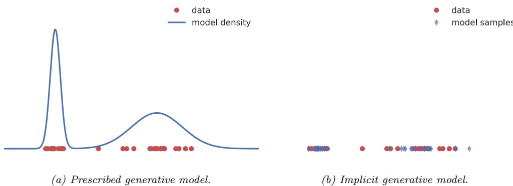
Figure 26.1: Visualizing the di!erence between prescribed and implicit generative models. Prescribed models provide direct access to the learned density (sometimes unnormalized). Implicit models only provide access to a simulator which can be used to generate samples from an implied density. Generated by genmo\_types\_implicit\_explicit.ipynb

by the set {Gω(z) ≃ x}. When the latent and data dimension are equal (m = d) and the function Gω(z) is invertible or has easily characterized roots, we recover the rule for transformations of probability distributions. This transformation of variables property is also used in normalizing flows (Chapter 23). In di!usion models (Chapter 25), we also transform noise into data and vice versa, but the transformation is not strictly invertible.

We can develop more general and flexible implicit generative models where the function G is a non-linear function with d>m, e.g., specified by a deep network. Such models are sometimes called generator networks or generative neural samplers; they can also be throught of as di!erentiable simulators. Unfortunately the integral (26.2) is intractable in these kinds of models, and we may not even be able to determine the set {Gω(z) ≃ x}. Of course, intractability is also a challenge for explicit latent variable models such as VAEs (Chapter 21), but in the GAN case, the lack of a likelihood term makes the learning problem even harder. Therefore this problem is called likelihood-free inference or simulation-based inference.

Likelihood-free inference also forms the basis of the field known as approximate Bayesian computation or ABC, which we briefly discuss in Section 13.6.5. ABC and GANs give us two di!erent algorithmic frameworks for learning in implicit generative models. Both approaches rely on a learning principle based on comparing real and simulated data. This type of learning by comparison instantiates a core principle of likelihood-free inference, and expanding on this idea is the focus of the next section. The subsequent sections will then focus on GANs specifically, to develop a more detailed foundation and practical considerations. (See also https://poloclub.github.io/ganlab/ for an interactive tutorial.)

26.2 Learning by comparison

In most of this book, we rely on the principle of maximum likelihood for learning. By maximizing the likelihood we e!ectively minimize the KL divergence between the model q⇀ (with parameters ε)

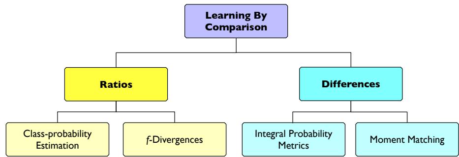
Figure 26.2: Overview of approaches for learning in implicit generative models

and the unknown true data distribution p^↔︎ . Recalling equation (26.2), in implicit models we cannot evaluate q⇀(x), and thus cannot use maximum likelihood training. As implicit models provide a sampling procedure, we instead are searching for learning principles that only use samples from the model.

The task of learning in implicit models is to determine, from two sets of samples, whether their distributions are close to each other and to quantify the distance between them. We can think of this as a ‘two sample’ or likelihood-free approach to learning by comparison. There are many ways of doing this, including using distributional divergences or distances through binary classification, the method of moments, and other approaches. Figure 26.2 shows an overview of di!erent approaches for learning by comparison.

26.2.1 Guiding principles

We are looking for objectives D(p^↔︎ , q) that satisfy the following requirements:

• 1. Provide guarantees about learning the data distribution: argmin^q D(p^↔︎ , q) = p^↔︎ .
• 2. Can be evaluated only using samples from the data and model distribution.
• 3. Are computationally cheap to evaluate.

Many distributional distances and divergences satisfy the first requirement, since by definition they satisfy the following:

\[\mathcal{D}(p^\*,q)\geq 0;\qquad \mathcal{D}(p^\*,q)=0 \iff p^\*=q\tag{26.3}\]

Many distributional distances and divergences, however, fail to satisfy the other two requirements: they cannot be evaluated only using samples — such as the KL divergence, or are computationally intractable — such as the Wasserstein distance. The main approach to overcome these challenges is to approximate the desired quantity through optimization by introducing a comparison model, often called a discriminator or a critic D, such that:

\[\mathcal{D}(p^\*,q) = \operatorname\*{argmax}\_{D} \mathcal{F}(D, p^\*, q) \tag{26.4}\]

where F is a functional that depends on p^↔︎ and q only through samples. For the cases we discuss, both the model and the critic are parametric with parameters ε and ω respectively; instead of optimizing over distributions or functions, we optimize with respect to parameters. For the critic, this results in the optimization problem argmax^ε F(Dε, p^↔︎ , q⇀). For the model parameters ε, the exact objective D(p^↔︎ , q⇀) is replaced with the tractable approximation provided through the use of Dε.

A convenient approach to ensure that F(Dε, p^↔︎ , q⇀) can be estimated using only samples from the model and the unknown data distribution is to depend on the two distributions only in expectation:

\[\mathcal{F}(D\_{\phi}, p^\*, q\_{\theta}) = \mathbb{E}\_{p^\*(\mathfrak{x})} f(\mathfrak{x}, \phi) + \mathbb{E}\_{q\_{\theta}(\mathfrak{x})} g(\mathfrak{x}, \phi) \tag{26.5}\]

where f and g are real valued functions whose choice will define F. In the case of implicit generative models, this can be rewritten to use the sampling path x = Gω(z), z ↑ q(z):

\[\mathcal{F}(D\_{\phi}, p^\*, q\_{\theta}) = \mathbb{E}\_{p^\*(\mathfrak{a})} f(\mathfrak{x}, \phi) + \mathbb{E}\_{\mathfrak{q}(\mathfrak{z})} g(G\_{\theta}(\mathfrak{z}), \phi) \tag{26.6}\]

which can be estimated using Monte Carlo estimation

\[\mathcal{F}(D\_{\Phi}, p^\*, q\_{\theta}) \approx \frac{1}{N} \sum\_{i=1}^{N} f(\hat{x}\_i, \phi) + \frac{1}{M} \sum\_{i=1}^{M} g(G\_{\theta}(\hat{z}\_i), \phi); \qquad \hat{x}\_i \sim p^\*(\mathbf{z}); \qquad \hat{z}\_i \sim q(\mathbf{z}) \tag{26.7}\]

Next, we will see how to instantiate these guiding principles in order to find the functions f and g and thus the objective F which can be used to train implicit models: class probability estimation (Section 26.2.2), bounds on f-divergences (Section 26.2.3), integral probability metrics (Section 26.2.4), and moment matching (Section 26.2.5).

26.2.2 Density ratio estimation using binary classifiers

One way to compare two distributions p^↔︎ and q⇀ is to compute their density ratio r(x) = ^p→ (x) ^qω(x) . The distributions are the same if and only if the ratio is 1 everywhere in the support of qω. Since we cannot evaluate the densities of implicit models, we must instead develop techniques to compute the density ratio from samples alone, following the guiding principles established above.

Fortunately, we can use the trick from Section 2.7.5 which converts density estimation into a binary classification problem to write

\[\frac{p^\*(x)}{q\_\theta(x)} = \frac{D(x)}{1 - D(x)}\tag{26.8}\]

where D(x) is the discriminator or critic which is trained to distinguish samples coming from p^↔︎ vs qω.

For parametric classification, we can learn discriminators Dε(x) → [0, 1] with parameters ω. Using knowledge and insight about probabilistic classification, we can learn the parameters by minimizing any proper scoring rule [GR07] (see also Section 14.2.1). For the familiar Bernoulli log-loss (or binary cross entropy loss), we obtain the objective:

\[V(q\_{\theta}, p^\*) = \arg\max\_{\phi} \mathbb{E}\_{p(\mathbf{z}|y)p(y)}[y \log D\_{\phi}(\mathbf{z}) + (1 - y)\log(1 - D\_{\phi}(\mathbf{z}))]\]

\[= \arg\max\_{\phi} \mathbb{E}\_{p(\mathbf{z}|y=1)p(y=1)} \log D\_{\phi}(\mathbf{z}) + \mathbb{E}\_{p(\mathbf{z}|y=0)p(y=0)} \log(1 - D\_{\phi}(\mathbf{z})) \tag{26.9}\]

\[\mathbf{x} = \arg\max\_{\phi} \frac{1}{2} \mathbb{E}\_{p^\star(\mathfrak{x})} \log D\_{\phi}(\mathfrak{x}) + \frac{1}{2} \mathbb{E}\_{q\_{\theta}(\mathfrak{x})} \log(1 - D\_{\phi}(\mathfrak{x})).\tag{26.10}\]

Loss	Objective Function (D := D(x; ω) → [0, 1])
Bernoulli loss	Ep→(x)[log D] + Eqω(x)[log(1 ↓ D)]
Brier score	↓ D)2] Eqω(x)[↓D2] Ep→(x)[↓(1 +
Exponential loss	+& , ’ 1 O P  1 2 ↓1↑D D 2 + Ep→(x) Eqω(x) ↓ D 1↑D
Misclassification	Ep→(x)[↓I[D ≃ 0.5]] + Eqω(x)[↓I[D > 0.5]]
Hinge loss	O & ’P + O & ’P D D ↓ max 0, 1 ↓ log ↓ max 0, 1 + log Ep→(x) Eqω(x) 1↑D 1↑D
Spherical	2D2)↑ 1 [↽D] + [↽(1 ↓ D)] ; ↽ = (1 ↓ 2D + Ep→(x) Eqω(x) 2

Table 26.1: Proper scoring rules that can be maximized in class probability-based learning of implicit generative models. Based on [ML16].

The same procedure can be extended beyond the Bernoulli log-loss to other proper scoring rules used for binary classification, such as those presented in Table 26.1, adapted from [ML16]. The optimal discriminator D is ^p→ (x) ^p→(x)+qω(x) , since:

\[\frac{p^\*(x)}{q\_\theta(x)} = \frac{D^\*(x)}{1 - D^\*(x)} \implies D^\*(x) = \frac{p^\*(x)}{p^\*(x) + q\_\theta(x)}\tag{26.11}\]

By substituting the optimal discriminator into the scoring rule (26.10), we can show that the objective V can also be interpreted as the the Jensen-Shannon divergence:

\[V^\*(q\_\theta, p^\*) = \frac{1}{2} \mathbb{E}\_{p^\*(\mathbf{z})}[\log \frac{p^\*(\mathbf{z})}{p^\*(\mathbf{z}) + q\_\theta(\mathbf{z})}] + \frac{1}{2} \mathbb{E}\_{q\_\theta(\mathbf{z})}[\log(1 - \frac{p^\*(\mathbf{z})}{p^\*(\mathbf{z}) + q\_\theta(\mathbf{z})})] \tag{26.12}\]

\[=\frac{1}{2}\mathbb{E}\_{p^\*(\mathfrak{x})}[\log\frac{p^\*(\mathfrak{x})}{\frac{p^\*(\mathfrak{x})+q\mathfrak{e}(\mathfrak{x})}{2}}] + \frac{1}{2}\mathbb{E}\_{q\mathfrak{e}(\mathfrak{x})}[\log(\frac{q\_\theta(\mathfrak{x})}{\frac{p^\*(\mathfrak{x})+q\mathfrak{e}(\mathfrak{x})}{2}})] - \log 2\tag{26.13}\]

\[\mathcal{L} = \frac{1}{2} D\_{\text{KL}} \left( p^\* \parallel \frac{p^\* + q\_\theta}{2} \right) + \frac{1}{2} D\_{\text{KL}} \left( q\_\theta \parallel \frac{p^\* + q\_\theta}{2} \right) - \log 2 \tag{26.14}\]

\[=JSD(p^\*,q\theta)-\log 2\tag{26.15}\]

where JSD denotes the Jensen-Shannon divergence:

\[JSD(p^\*, q\_\theta) = \frac{1}{2} D\_{\text{KL}}\left(p^\* \parallel \frac{p^\* + q\_\theta}{2}\right) + \frac{1}{2} D\_{\text{KL}}\left(q\_\theta \parallel \frac{p^\* + q\_\theta}{2}\right) \tag{26.16}\]

This establishes a connection between optimal binary classification and distributional divergences. By using binary classification, we were able to compute the distributional divergence using only samples, which is the important property needed for learning implicit generative models; as expressed in the guiding principles (Section 26.2.1), we have turned an intractable estimation problem — how to estimate the JSD divergence, into an optimization problem — how to learn a classifier which can be used to approximate that divergence.

We would like to train the parameters ε of generative model to minimize the divergence:

\[\min\_{\theta} JSD(p^\*, q\_\theta) = \min\_{\theta} V^\*(q\_\theta, p^\*) + \log 2 \tag{26.17}\]

\[=\underset{\theta}{\text{min}}\,\frac{1}{2}\mathbb{E}\_{p^\*(\mathfrak{x})}\log D^\*(\mathfrak{x}) + \frac{1}{2}\mathbb{E}\_{q\_\theta(\mathfrak{x})}\log(1 - D^\*(\mathfrak{x})) + \log 2\tag{26.18}\]

Since we do not have access to the optimal classifier D^↔︎ but only to the neural approximation D^ε obtained using the optimization in (26.10) , this results in a min-max optimization problem:

\[\min\_{\theta} \max\_{\phi} \frac{1}{2} \mathbb{E}\_{p^\*(\mathfrak{a})} [\log D\_{\phi}(\mathfrak{x})] + \frac{1}{2} \mathbb{E}\_{q \rho(\mathfrak{a})} [\log(1 - D\_{\phi}(\mathfrak{x}))] \tag{26.19}\]

By replacing the generating procedure (26.1) in (26.19) we obtain the objective in terms of the latent variables z of the implicit generative model:

\[\min\_{\theta} \max\_{\phi} \frac{1}{2} \mathbb{E}\_{p^{\mathbf{v}}(\mathbf{z})} [\log D\_{\phi}(\mathbf{z})] + \frac{1}{2} \mathbb{E}\_{q(\mathbf{z})} [\log(1 - D\_{\phi}(G\_{\theta}(\mathbf{z})))],\tag{26.20}\]

which recovers the definition proposed in the original GAN paper [Goo+14]. The core principle behind GANs is to train a discriminator, in this case a binary classifier, to approximate a distance or divergence between the model and data distributions, and to then train the generative model to minimize this approximation of the divergence or distance.

Beyond the use of the Bernoulli scoring rule used above, other scoring rules have been used to train generative models via min-max optimization. The Brier scoring rule, which under discriminator optimality conditions can be shown to correspond to minimizing the Pearson 2² divergence via similar arguments as the ones shown above has lead to LS-GAN [Mao+17]. The hinge scoring rule has become popular [Miy+18b; BDS18], and under discriminator optimality conditions corresponds to minimizing the total variational distance [NWJ+09].

The connection between proper scoring rules and distributional divergences allows the construction of convergence guarantees for the learning criteria above, under infinite capacity of the discriminator and generator: since the minimizer of distributional divergence is the true data distribution (Equation 26.3), if the discriminator is optimal and the generator has enough capacity, it will learn the data distribution. In practice however, this assumption will not hold, as discriminators are rarely optimal; we will discuss this at length in Section 26.3.

26.2.3 Bounds on f-divergences

As we saw with the appearance of the Jensen-Shannon divergence in the previous section, we can consider directly using a measure of distributional divergence to derive methods for learning in implicit models. One general class of divergences are the f-divergences (Section 2.7.1) defined as:

\[\mathcal{D}\_f\left[p^\*(\mathbf{z})|q\_\theta(\mathbf{z})\right] = \int q\_\theta(\mathbf{z}) f\left(\frac{p^\*(\mathbf{z})}{q\_\theta(\mathbf{z})}\right) d\mathbf{z} \tag{26.21}\]

where f is a convex function such that f(1) = 0. For di!erent choices of f, we can recover known distributional divergences such as the KL, reverse KL, and Jensen-Shannon divergence. We discuss such connections in Section 2.7.1, and provide a summary in Table 26.2.

To evaluate Equation (26.21) we will need to evaluate the density of the data p^↔︎ (x) and the model q⇀(x), neither of which are available. In the previous section we overcame the challenge of evaluating the density ratio by transforming it into a problem of binary classification. In this section, we will instead look towards the role of lower bounds on f-divergences, which is an approach for tractability that is also used for variational inference (Chapter 10).

Divergence	f	f †	Optimal Critic
KL	u log u	eu↑1	1 + log r(x)
Reverse KL	↓ log u	↓1 ↓ log(↓u)	↓1/r(x)
JSD	u+1 u log u ↓ (u + 1) log 2	↓ eu) ↓ log(2	2 log( 1+1/r(x) )
22 Pearson	↓ 1)2 (u	1 4u2 + u	2(r(x) ↓ 1)

Table 26.2: Standard divergences as f divergences for various choices of f. The optimal critic is written as a function of the density ratio r(x) = ^p→(x) ^qω(x) .

f-divergences have a widely-developed theory in convex analysis and information theory. Since the function f in Equation (26.21) is convex, we know that we can find a tangent that bounds it from below. The variational formulation of the f-divergence is [NWJ10b; NCT16c]:

\[\mathcal{D}\_f\left[p^\*(\mathbf{z})\|q\_\theta(\mathbf{z})\right] = \int q\_\theta(\mathbf{z}) f\left(\frac{p^\*(\mathbf{z})}{q\_\theta(\mathbf{z})}\right) d\mathbf{z} \tag{26.22}\]

\[=\int q\_{\boldsymbol{\theta}}(\boldsymbol{x})\sup\_{t:\mathcal{X}\to\mathbb{R}}\left[t(\boldsymbol{x})\frac{p^\*(\boldsymbol{x})}{q\_{\boldsymbol{\theta}}(\boldsymbol{x})}-f^\dagger(t(\boldsymbol{x}))\right]d\boldsymbol{x}\tag{26.23}\]

\[=\int\sup\_{t:\mathcal{X}\to\mathbb{R}}p^\*(\mathbf{x})t(\mathbf{x}) - q\_\theta(\mathbf{x})f^\dagger(t(\mathbf{x}))d\mathbf{x}\tag{26.24}\]

\[\geq \sup\_{t \in \mathcal{T}} \mathbb{E}\_{p^\*(\mathfrak{a})}[t(\mathfrak{x})] - \mathbb{E}\_{q\_\theta(\mathfrak{a})}[f^\dagger(t(\mathfrak{x}))].\tag{26.25}\]

In the second line we use the result from convex analysis, discussed Supplementary Section 7.3, that re-expresses the convex function f using f(u) = sup^t ut ↓ f †(t), where f † is the convex conjugate of the function f, and t is a parameter we optimize over. Since we apply f at u = ^p→ (x) ^qω(x) for all x → X , we make the parameter t be a function t(x). The final inequality comes from replacing the supremum over all functions from the data domain X to R with the supremum over a family of functions T (such as the family of functions expressible by a neural network architecture), which might not be able to capture the true supremum. The function t takes the role of the discriminator or critic.

The final expression in Equation (26.25) follows the general desired form of Equation 26.5: it is the di!erence of two expectations, and these expectations can be computed by Monte Carlo estimation using only samples, as in Equation (26.7); despite starting with an objective (Equation 26.21) which contravened the desired principles for training implicit generative models, variational bounds have allowed us to construct an approximation which satisfies all desiderata.

Using bounds on the f-divergence, we obtain an objective (26.25) that allows learning both the generator and critic parameters. We use a critic D with parameters ω to estimate the bound, and then optimize the parameters ε of the generator to minimize the approximation of the f-divergence provided by the critic (we replace t above with Dε, to retain standard GAN notation):

\[\min\_{\theta} \mathcal{D}\_f(p^\*, q\_\theta) \ge \min\_{\theta} \max\_{\phi} \mathbb{E}\_{p^\*(\mathfrak{x})} [D\_\phi(\mathfrak{x})] - \mathbb{E}\_{q\_\theta(\mathfrak{x})} [f^\dagger(D\_\phi(\mathfrak{x}))] \tag{26.26}\]

\[\delta = \min\_{\theta} \max\_{\phi} \mathbb{E}\_{p^\star(\mathbf{z})} [D\_\phi(\mathbf{z})] - \mathbb{E}\_{q(\mathbf{z})} [f^\dagger (D\_\phi(G\_\theta(\mathbf{z})))] \tag{26.27}\]

This approach to train an implicit generative model leads to f-GANs [NCT16c]. It is worth noting that there exists an equivalence between the scoring rules in the previous section and bounds on

f-divergences [RW11]: for each scoring rule we can find an f-divergence that leads to the same training criteria and the same min-max game of Equation 26.27. An intuitive way to grasp the connection between f-divergences and proper scoring rules is through their use of density ratios: in both cases the optimal critic approximates a quantity directly related to the density ratio (see Table 26.2 for f-divergences and Equation (26.11) for scoring rules).

26.2.4 Integral probability metrics

Instead of comparing distributions by using their ratio as we did in the previous two sections, we can instead study their di!erence. A general class of measure of di!erence is given by the Integral Probability Metrics (Section 2.7.2) defined as:

\[I\_F(p^\*(\mathbf{z}), q\_\theta(\mathbf{z})) = \sup\_{f \in \mathcal{F}} \left| \mathbb{E}\_{p^\*(\mathbf{z})} f(\mathbf{z}) - \mathbb{E}\_{q\_\theta(\mathbf{z})} f(\mathbf{z}) \right|. \tag{26.28}\]

The function f is a test or witness function that will take the role of the discriminator or critic. To use IPMs we must define the class of real valued, measurable functions F over which the supremum is taken, and this choice will lead to di!erent distances, just as choosing di!erent convex functions f leads to di!erent f-divergences. Integral probability metrics are distributional distances: beyond satisfying the conditions for distributional divergences D(p^↔︎ , q) ⇒ 0; D(p^↔︎ , q)=0 ∀∋ p^↔︎ = q (Equation (26.3)), they are also symmetric D(p, q) = D(q, p) and satisfy the triangle inequality D(p, q) ≃ D(p, r) + D(r, q).

Not all function families satisfy these conditions of create a valid distance I^F . To see why consider the case where F = {z} where z is the function z(x)=0. This choice of F entails that regardless of the two distributions chosen, the value in Equation 26.28 would be 0, violating the requirement that distance between two distributions be 0 only if the two distributions are the same. A popular choice of F for which I^F satisfies the conditions of a valid distributional distance is the set of 1-Lipschitz functions, which leads to the Wasserstein distance [Vil08]:

\[W\_1(p^\*(\mathbf{z}), q\_\theta(\mathbf{z})) = \sup\_{f: \|f\|\_{\text{Lip}} \le 1} \mathbb{E}\_{p^\*(\mathbf{z})} f(\mathbf{z}) - \mathbb{E}\_{q\rho(\mathbf{z})} f(\mathbf{z}) \tag{26.29}\]

We show an example of a Wasserstein critic in Figure 26.3a. The supremum over the set of 1-Lipschitz functions is intractable for most cases, which again suggests the introduction of a learned critic:

\[W\_1(p^\*(\mathbf{z}), q\_\theta(\mathbf{z})) = \sup\_{f: \|f\|\_{\text{Lip}} \le 1} \mathbb{E}\_{p^\*(\mathbf{z})} f(\mathbf{z}) - \mathbb{E}\_{q\_\theta(\mathbf{z})} f(\mathbf{z}) \tag{26.30}\]

\[\geq \max\_{\phi \colon \|D\_{\Phi}\|\_{\text{Lip}} \leq 1} \mathbb{E}\_{p^\*(\mathfrak{x})} D\_{\phi}(\mathfrak{x}) - \mathbb{E}\_{q\_{\theta}(\mathfrak{x})} D\_{\phi}(\mathfrak{x}),\tag{26.31}\]

where the critic D^ε has to be regularized to be 1-Lipschitz (various techniques for Lipschitz regularization via gradient penalties or spectral normalization methods have been used [ACB17; Gul+17]). As was the case with f-divergences, we replace an intractable quantity which requires a supremum over a class of functions with a bound obtained using a subset of this function class, a subset which can be modeled using neural networks.

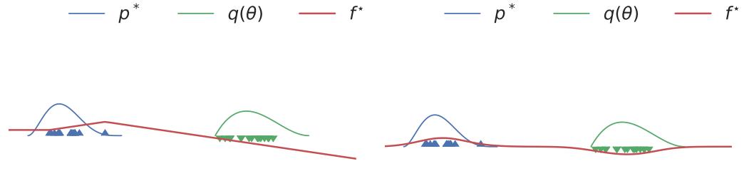
(a) Optimal Wasserstein critic. (b) Optimal MMD critic.

Figure 26.3: Optimal critics in Integral Probability Metrics (IPMs). Generated by ipm\_divergences.ipynb

To train a generative model, we again introduce a min max game:

\[\min\_{\theta} W\_1(p^\*(\mathbf{z}), q\_\theta(\mathbf{z})) \ge \min\_{\theta} \max\_{\phi: \|D\_\phi\|\_{Lip} \le 1} \mathbb{E}\_{p^\*(\mathbf{z})} D\_\phi(\mathbf{z}) - \mathbb{E}\_{q\_\theta(\mathbf{z})} D\_\phi(\mathbf{z}) \tag{26.32}\]

\[\mathfrak{h} = \min\_{\theta} \max\_{\phi: \|D\_{\Phi}\|\_{\text{Lip}} \le 1} \mathbb{E}\_{p^\*(\mathfrak{x})} D\_{\phi}(\mathfrak{x}) - \mathbb{E}\_{q(\mathfrak{z})} D\_{\phi}(G\_{\theta}(\mathfrak{z})) \tag{26.33}\]

This leads to the popular WassersteinGAN [ACB17].

If we replace the choice of function family F to that of functions in an RKHS (Section 18.3.7.1) with norm one, we obtain the maximum mean discrepancy (MMD) discussed in Section 2.7.3:

\[\text{MMD}(p^\*(\mathbf{z}), q\_\theta(\mathbf{z})) = \sup\_{f: \|f\|\_{RKHS} = 1} \mathbb{E}\_{p^\*(\mathbf{z})} f(\mathbf{z}) - \mathbb{E}\_{q\_\theta(\mathbf{z})} f(\mathbf{z}). \tag{26.34}\]

We show an example of an MMD critic in Figure 26.3b. It is often more convenient to use the square MMD loss [LSZ15; DRG15], which can be evaluated using the kernel K (Section 18.3.7.1):

\[\text{MMD}^2(p^\*, q\_\theta) = \mathbb{E}\_{p^\*(\mathbf{z})} \mathbb{E}\_{p^\*(\mathbf{z'})} \mathbb{K}(\mathbf{z}, \mathbf{z'}) - 2\mathbb{E}\_{p^\*(\mathbf{z})} \mathbb{E}\_{q\_\theta(\mathbf{y})} \mathbb{K}(\mathbf{z}, \mathbf{y}) + \mathbb{E}\_{q\_\theta(\mathbf{y})} \mathbb{E}\_{q\_\theta(\mathbf{y'})} \mathbb{K}(\mathbf{y}, \mathbf{y'}) \tag{26.35}\]

\[=\mathbb{E}\_{p^\*(\mathbf{z})}\mathbb{E}\_{p^\*(\mathbf{z'})}\mathbb{K}(\mathbf{z},\mathbf{z'}) - 2\mathbb{E}\_{p^\*(\mathbf{z})}\mathbb{E}\_{q(\mathbf{z})}\mathbb{K}(\mathbf{z},G\_{\boldsymbol{\theta}}(\mathbf{z})) + \mathbb{E}\_{q(\mathbf{z})}\mathbb{E}\_{q(\mathbf{z'})}\mathbb{K}(G\_{\boldsymbol{\theta}}(\mathbf{z}),G\_{\boldsymbol{\theta}}(\mathbf{z'})) \tag{26.36}\]

The MMD can be directly used to learn a generative model, often called a generative matching network [LSZ15]:

\[\min\_{\theta} \text{MMD}^2(p^\*, q\_{\theta}) \tag{26.37}\]

The choice of kernel is important. Using a fixed or predefined kernel such as a radial basis function (RBF) kernel might not be appropriate for all data modalities, such as high dimensional images. Thus we are looking for a way to learn a feature function 3 such that K(3(x), 3(x^→ )) is a valid kernel; luckily, we can use that for any characteristic kernel K(x, x^→ ) and injective function 3, K(3(x), 3(x^→ ))) is also a characteristic kernel. While this tells us that we can use feature functions in the MMD objective, it does not tell us how to learn the features. In order to ensure that the learned features are sensitive to di!erences between the data distribution p^↔︎ (x) and the model distribution q⇀(x), the kernel parameters are trained to maximize the square MMD. This again casts the problem into a

familiar min max objective by learning the projection 3 with parameters ω [Li+17b]:

\[\begin{split} \min\_{\theta} & \text{MinMMD}\_{\zeta}^{-2}(p\_{\mathcal{D}}, q\_{\theta}) \\ &= \min\_{\theta} \max\_{\phi} \mathbb{E}\_{p^{\star}(\mathbf{z})} \mathbb{E}\_{p^{\star}(\mathbf{z}')} \mathcal{K}(\zeta\_{\phi}(\mathbf{z}), \zeta\_{\phi}(\mathbf{z}')) \\ & \quad - 2\mathbb{E}\_{p^{\star}(\mathbf{z})} \mathbb{E}\_{q\_{\phi}(\mathbf{y})} \mathcal{K}(\zeta\_{\phi}(\mathbf{z}), \zeta\_{\phi}(\mathbf{y})) \\ & \quad + \mathbb{E}\_{q\_{\phi}(\mathbf{y})} \mathbb{E}\_{q\_{\phi}(\mathbf{y}')} \mathcal{K}(\zeta\_{\phi}(\mathbf{y}), \zeta\_{\phi}(\mathbf{y}')) \end{split} \tag{26.39}\]

where 3^ε is regularized to be injective, though this is sometimes relaxed [Bin+18]. Unlike the Wasserstein distance and f-divergences, Equation (26.39) can be estimated using Monte Carlo estimation, without requiring a lower bound on the original objective.

26.2.5 Moment matching

More broadly than distances defined by integral probability metrics, for a set of test statistics s, one can define a moment matching criteria [Pea36], also known as the method of moments:

\[\min\_{\theta} \left\| \mathbb{E}\_{p^\*(\mathbf{z})} s(\mathbf{z}) - \mathbb{E}\_{q\_\theta(\mathbf{z})} s(\mathbf{z}) \right\|\_2^2 \tag{26.40}\]

where m(ε) = E^qω(x)s(x) is the moment function. The choice of statistic s(x) is crucial, since as with distributional divergences and distances, we would like to ensure that if the objective is minimized and reaches the minimal value 0, the two distributions are the same p^↔︎ (x) = q⇀(x). To see that not all functions s satisfy this requirement consider the function s(x) = x: simply matching the means of two distributions is not su”cient to match higher moments (such as variance). For likelihood based models the score function s(x) = log q⇀(x) satisfies the above requirement and leads to a consistent estimator [Vaa00], but this choice of s is not available for implicit generative models.

This motivates the search for other approaches of integrating the method of moments for implicit models. The MMD can be seen as a moment matching criteria, by matching the means of the two distributions after lifting the data into the feature space of an RHKS. But moment matching can go beyond integral probability metrics: Ravuri et al. [Rav+18] show that one can learn useful moments by using s as the set of features containing the gradients of a trained discriminator classifier D^ε together with the features of the learned critic: sε(x)=[∝εDε(x), h1(x),…,hn(x)] where h1(x),…,hn(x) are the hidden activations of the learned critic. Both features and gradients are needed: the gradients ∝εDε(x) are required to ensure the estimator for the parameters ε is consistent, since the number of moments s(x) needs to be larger than the number of parameters ε, which will be true if the critic will have more parameters than the model; the features hi(x) are added since they have been shown empirically to improve performance, thus showcasing the importance of the choice of test statistics s used to train implicit models.

26.2.6 On density ratios and di”erences

We have seen how density ratios (Sections 26.2.2 and 26.2.3) and density di!erences (Section 26.2.4) can be used to define training objectives for implicit generative models. We now explore some of the distinctions between using ratios and di!erences for learning by comparison, as well as explore the e!ects of using approximations to these objectives using function classes such as neural networks has on these distinctions.

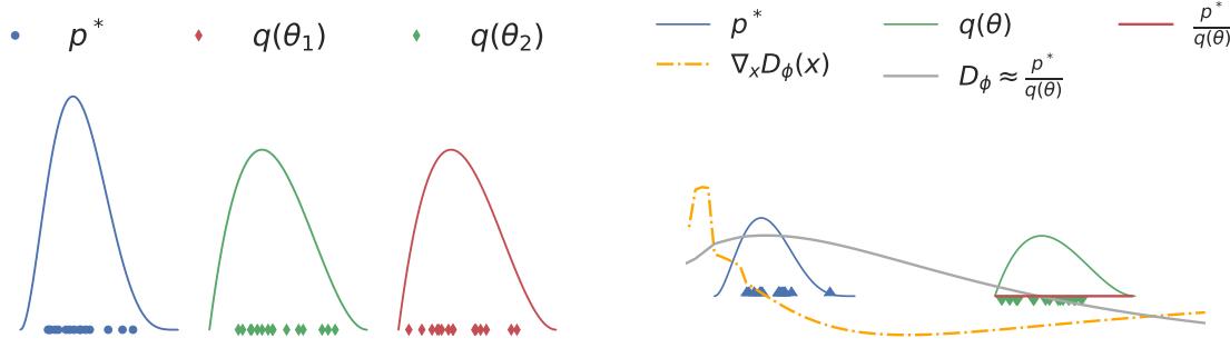
(a) Failure of the KL divergence to distinguish between distributions with non-overlapping support: ^DKL ! p^↓ ↓ qϑ¹ ” ^{= D}KL ! p^↓ ↓ qϑ² ” = ↘, despite qϑ² being closer to p^↓ than qϑ¹ .

(b) The density ratio ^{p→ qω} used by the KL divergence and a smooth estimate given by an MLP, together with the gradient it provides with respect to the input variable.

Figure 26.4: The KL divergence cannot provide learning signal for distributions without overlapping support (left), while the smooth approximation given by a learned decision surface like an MLP can (right). Generated by ipm\_divergences.ipynb

One often stated downside of using divergences that rely on density ratios (such as f-divergences) is their poor behavior when the distributions p^↔︎ and q⇀ do not have overlapping support. For non-overlapping support, the density ratio ^{p→ qω} will be ̸ in the parts of the space where p^↔︎ (x) > 0 but q⇀(x)=0, and 0 otherwise. In that case, the DKL (p^↔︎ ⇐ q⇀) = ̸ and the JSD(p^↔︎ , q⇀) = log 2, regardless of the value of ε. Thus f-divergences cannot distinguish between di!erent model distributions when they do not have overlapping support with the data distribution, as visualized in Figure 26.4a. This is in contrast with di!erence based methods such as IPMs such as the Wasserstein distance and the MMD, which have smoothness requirements built in the definition of the method, by constraining the norm of the critic (Equations (26.29) and (26.34)). We can see the e!ect of these constraints in Figure 26.3: both the Wasserstein distance and the MMD provide useful signal in the case of distributions with non-overlapping support.

While the definition of f-divergences relies on density ratios (Equation (26.21)), we have seen that to train implicit generative models we use approximations to those divergences obtained using a parametric critic Dε. If the function family of the critic used to approximate the divergence (via the bound or class probability estimation) contains only smooth functions, it will not be able to model the sharp true density ratio, which jumps from 0 to ̸, but it can provide a smooth approximation. We show an example in Figure 26.4b, where we show the density ratio for two distributions without overlapping support and an approximation provided by an MLP trained to approximate the KL divergence using Equation 26.25. Here, the smooth decision surface provided by the MLP can be used to train a generative model while the underlying KL divergence cannot be; the learned MLP provides the gradient signal on how to move distribution mass to areas with more density under the data distribution, while the KL divergence provides a zero gradient almost everywhere in the space. This ability of approximations to f-divergences to overcome non-overlapping support issues is a desirable property of generative modeling training criteria, as it allows models to learn the data

distribution regardless of initialization [Fed+18]. Thus while the case of non-overlapping support provides an important theoretical di!erence between IPMs and f-divergences, it is less significant in practice since bounds on f-divergences or class probability estimation are used with smooth critics to approximate the underlying divergence.

Some density ratio and density di!erence based approaches also share commonalities: bounds are used both for f-divergences (variational bounds in Equation 26.25) and for the Wasserstein distance (Equation (26.31)). These bounds to distributional divergence and distances have their own set of challenges: since the generator minimizes a lower bound of the underlying divergence or distance, minimizing this objective provides no guarantees that the divergence will decrease in training. To see this, we can look at Equation 26.26: its RHS can get arbitrarily low without decreasing the LHS, the divergence we are interested in minimizing; this is unlike variational upper bound on the KL divergence used to train variational autoencoders Chapter 21.

26.3 Generative adversarial networks

We have looked at di!erent learning principles that do not require the use of explicit likelihoods, and thus can be used to train implicit models. These learning principles specify training criteria, but do not tell us how to train models or parameterize models. To answer these questions, we now look at algorithms for training implicit models, where the models (both the discriminator and generator) are deep neural networks; this leads us to generative adversarial networks (GANs). We cover how to turn learning principles into loss functions for training GANs (Section 26.3.1); how to train models using gradient descent (Section 26.3.2); how to improve GAN optimization (Section 26.3.4) and how to assess GAN convergence (Section 26.3.5).

26.3.1 From learning principles to loss functions

In Section 26.2 we discussed learning principles for implicit generative models: class probability estimation, bounds on f-divergences, integral probability metrics and moment matching. These principles can be used to formulate loss functions to train the model parameters ε and the critic parameters ω. Many of these objectives use zero-sum losses via a min-max formulation: the generator’s goal is to minimize the same function the discriminator is maximizing. We can formalize this as:

\[\min \max V(\phi, \theta) \tag{26.41}\]

As an example, we recover the original GAN with the Bernoulli log-loss (Equation (26.19)) when

\[V(\phi, \theta) = \frac{1}{2} \mathbb{E}\_{p^\star(\mathfrak{x})} [\log D\_\phi(\mathfrak{x})] + \frac{1}{2} \mathbb{E}\_{q\_\theta(\mathfrak{x})} [\log(1 - D\_\phi(\mathfrak{x}))].\tag{26.42}\]

The reason most of the learning principles we have discussed lead to zero-sum losses is due to their underlying structure: the critic maximizes a quantity in order to approximate a divergence or distance — such as an f-divergence or Integral Probability Metric — and the model minimizes this approximation to the divergence or distance. That need not be the case, however. Intuitively, the discriminator training criteria needs to ensure that the discriminator can distinguish between data and model samples, while the generator loss function needs to ensure that model samples are indistinguishable from data according to the discriminator.

To construct a GAN that is not zero-sum, consider the zero-sum criteria in the original GAN (Equation 26.42), induced by the Bernoulli scoring rule. The discriminator tries to distinguish between data and model samples by classifying the data as real (label 1) and samples as fake (label 0), while the goal of the generator is to minimize the probability that the discriminator classifies its samples as fake: min^ω Eqω(x) log(1 ↓ Dε(x)). An equally intuitive goal for the generator is to maximize the probability that the discriminator classifies its samples as real. While the di!erence might seem subtle, this loss, known as the “nonsaturating loss” [Goo+14], defined as E^qω(x) ↓ log Dε(x), enjoys better gradient properties early in training, as shown in Figure 26.5: the non-saturating loss provides a stronger learning signal (via the gradient) when the generator is performing poorly, and the discriminator can easily distinguish its samples from data, i.e., D(G(z)) is low; more on the gradients properties the saturating and non-saturating losses can be found in [AB17; Fed+18].

There exist many other GAN losses which are not zero-sum, including formulations of LS-GAN [Mao+17], GANs trained using the hinge loss [LY17], and RelativisticGANs [JM18]. We can thus generally write a GAN formulation as follows:

\[\min\_{\phi} L\_D(\phi, \theta); \qquad \min\_{\theta} L\_G(\phi, \theta). \tag{26.43}\]

We recover the zero-sum formulations if ↓LD(ω, ε) = LG(ω, ε) = V (ω, ε). Despite departing from the zero-sum structure, the nested form of the optimization remains in the general formulation, as we will discuss in Section 26.3.2.

The loss functions for the discriminator and generator, L^D and L^G respectively, follow the general form in Equation 26.5, which allows them to be used to e”ciently train implicit generative models. The majority of loss functions considered here can thus be written as follows:

\[L\_D(\phi, \theta) = \mathbb{E}\_{p^\star(\mathbf{z})} g(D\_\phi(\mathbf{z})) + \mathbb{E}\_{q\_\theta(\mathbf{z})} h(D\_\phi(\mathbf{z})) = \mathbb{E}\_{p^\star(\mathbf{z})} g(D\_\phi(\mathbf{z})) + \mathbb{E}\_{q(\mathbf{z})} h(D\_\phi(G\_\theta(\mathbf{z}))) \tag{26.44}\]

\[L\_G(\phi, \theta) = \mathbb{E}\_{q\_{\theta}(\mathbf{z})} l(D\_{\phi}(\mathbf{z})) = \mathbb{E}\_{q(\mathbf{z})} l(D\_{\phi}(G\_{\theta}(\mathbf{z})) \tag{26.45}\]

where g, h, l : R ↔︎ R. We recover the original GAN for g(t) = ↓ log t, h(t) = ↓ log(1 ↓ t) and l(t) = log(1 ↓ t); the non-saturating loss for g(t) = ↓ log t, h(t) = ↓ log(1 ↓ t) and l(t) = ↓ log(t); the Wasserstein distance formulation for g(t) = t, h(t) = ↓t and l(t) = t; for f-divergences g(t) = t, h(t) = ↓f †(t) and l(t) = f †(t).

26.3.2 Gradient descent

GANs employ the learning principles discussed above in conjunction with gradient based learning for the parameters of the discriminator and generator. We assume a general formulation with a discriminator loss function LD(ω, ε) and a generator loss function LG(ω, ε). Since the discriminator is often introduced to approximate a distance or divergence D(p^↔︎ , q⇀) (Section 26.2), for the generator to minimize a good approximation of that divergence one should solve the discriminator optimization fully for each generator update. That would entail that for each generator update one would first find the optimal discriminator parameters ω^↔︎ = argmin^ε LD(ω, ε) in order to perform a gradient update given by ∝ωLG(ω^↔︎, ε). Fully solving the inner optimization problem ω^↔︎ = argmin^ε LD(ω, ε) for each optimization step of the generator is computationally prohibitive, which motivates the use of alternating updates: performing a few gradient steps to update the discriminator parameters, followed by a generator update. Note that when updating the discriminator, we keep the generator

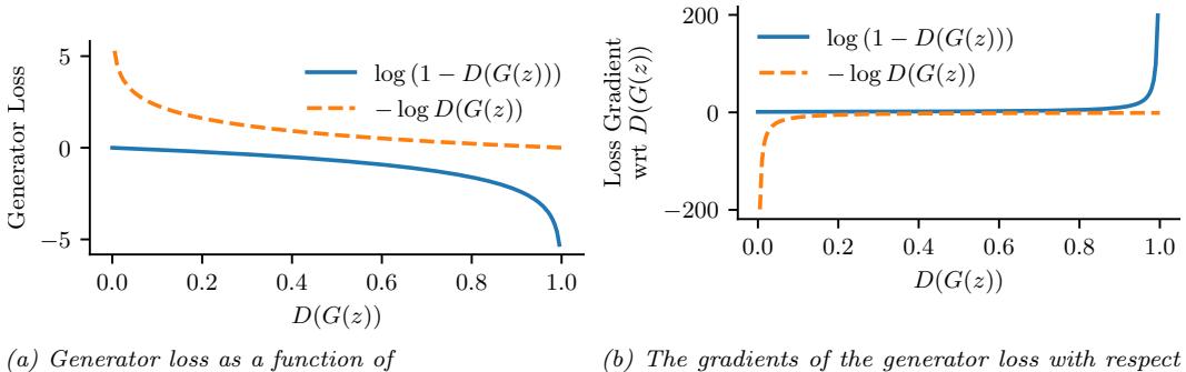
discriminator score.

Figure 26.5: Saturating log(1 ↗ D(G(z))) vs non-saturating ↗ log D(G(z)) loss functions. The non-saturating loss provides stronger gradients when the discriminator is easily detecting that generated samples are fake. Generated by gan\_loss\_types.ipynb

Algorithm 26.1: General GAN training algorithm with alternating updates

• ¹ Initialize ω, ε ² for each training iteration do ³ for K steps do
• ⁴ Update the discriminator parameters ω using the gradient ∝εLD(ω, ε);
• ⁵ Update the generator parameters ε using the gradient ∝ωLG(ω, ε)
• ⁶ Return ω, ε

parameters fixed, and when updating the generator, we keep the discriminator parameters fixed. We show a general algorithm for these alternative updates in Algorithm 26.1.

We are thus interested in computing ∝εLD(ω, ε) and ∝ωLG(ω, ε). Given the choice of loss functions follows the general form in Equations 26.44 and 26.45 both for the discriminator and generator, we can compute the gradients that can be used for training. To compute the discriminator gradients, we write:

\[\nabla\_{\phi} L\_D(\phi, \theta) = \nabla\_{\phi} \left[ \mathbb{E}\_{p^\*(\mathfrak{x})} g(D\_{\phi}(\mathfrak{x})) + \mathbb{E}\_{q \rho(\mathfrak{x})} h(D\_{\phi}(\mathfrak{x})) \right] \tag{26.46}\]

\[\mathbf{x} = \mathbb{E}\_{p^\*(\mathfrak{x})} \nabla\_{\Phi} g(D\_{\Phi}(\mathbf{z})) + \mathbb{E}\_{q\_{\theta}(\mathfrak{x})} \nabla\_{\Phi} h(D\_{\Phi}(\mathbf{z})) \tag{26.47}\]

where ∝εg(Dε(x)) and ∝εh(Dε(x)) can be computed via backpropagation, and each expectation can be estimated using Monte Carlo estimation. For the generator, we would like to compute the gradient:

\[L\_G(\phi, \theta) = \nabla\_{\theta} \mathbb{E}\_{q\_{\theta}(\mathfrak{a})} l(D\_{\phi}(\mathfrak{x})) \tag{26.48}\]

Here we cannot change the order of di!erentiation and integration since the distribution under the integral depends on the di!erentiation parameter ε. Instead, we will use that q⇀(x) is the distribution induced by an implicit generative model (also known as the “reparameterization trick”,

see Section 6.3.5):

\[\nabla\_{\theta} L\_{G}(\phi, \theta) = \nabla\_{\theta} \mathbb{E}\_{q\_{\theta}(\mathbf{z})} l(D\_{\phi}(\mathbf{z})) = \nabla\_{\theta} \mathbb{E}\_{q(\mathbf{z})} l(D\_{\phi}(G\_{\theta}(\mathbf{z}))) = \mathbb{E}\_{q(\mathbf{z})} \nabla\_{\theta} l(D\_{\phi}(G\_{\theta}(\mathbf{z}))) \tag{26.49}\]

and again use Monte Carlo estimation to approximate the gradient using samples from the prior q(z). Replacing the choice of loss functions and Monte Carlo estimation in Algorithm 26.1 leads to Algorithm 26.2, which is often used to train GANs.

Algorithm 26.2: GAN training algorithm

¹ Initialize ω, ε ² for each training iteration do ³ for K steps do ⁴ Sample minibatch of M noise vectors z^m ↑ q(z) ⁵ Sample minibatch of M examples x^m ↑ p^↔︎ (x) 6 Update the discriminator by performing stochastic gradient descent using this gradient: ∝^ε 1 M *^{M m}=1 [g(Dε(xm)) + ∝εh(Dε(Gω(zm)))]. ⁷ Sample minibatch of M noise vectors z^m ↑ q(z) 8 Update the generator by performing stochastic gradient descent using this gradient: ∝^ω 1 M *^{M m}=1 l(Dε(Gω(zm)). ⁹ Return ω, ε

26.3.3 Challenges with GAN training

Due to the adversarial game nature of GANs the optimizing dynamics of GANs are both hard to study in theory, and to stabilize in practice. GANs are known to su!er from mode collapse, a phenomenon where the generator converges to a distribution which does not cover all the modes (peaks) of the data distribution, thus the model underfits the distribution. We show an example in Figure 26.6: while the data is a mixture of Gaussians with 16 modes, the model converges only to a few modes. Alternatively, another problematic behavior is mode hopping, where the generator “hops” between generating di!erent modes of the data distribution. An intuitive explanation for this behavior is as follows: if the generator becomes good at generating data from one mode, it will generate more from that mode. If the discriminator cannot learn to distinguish between real and generated data in this mode, the generator has no incentive to expand its support and generate data from other modes. On the other hand, if the discriminator eventually learns to distinguish between the real and generated data inside this mode, the generator can simply move (hop) to a new mode, and this game of cat and mouse can continue.

While mode collapse and mode hopping are often associated with GANs, many improvements have made GAN training more stable, and these behaviors more rare. These improvements include using large batch sizes, increasing the discriminator neural capacity, using discriminator and generator regularization, as well as more complex optimization methods.

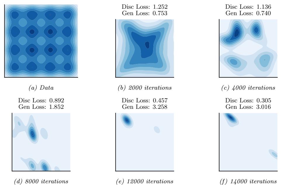
Figure 26.6: Illustration of mode collapse and mode hopping in GAN training. (a) The dataset, a mixture of 16 Gaussians in 2 dimensions. (b-f ) Samples from the model after various amounts of training. Generated by gan\_mixture\_of\_gaussians.ipynb.

26.3.4 Improving GAN optimization

Hyperparameter choices such as the choice of momentum can be crucial when training GANs, with lower momentum values being preferred compared to the usual high momentum used in supervised learning. Algorithms such as Adam [KB14a] provide a great boost in performance [RMC16a]. Many other optimization methods have been successfully applied to GANs, such as those which target variance reduction [Cha+19c]; those which backpropagate through gradient steps, thus ensuring that generator does well against the discriminator after it has been updated [Met+16]; or using a local bilinear approximation of the two player game [SA19]. While promising, these advanced optimization methods tend to have a higher computational cost, making them harder to scale to large models or large datasets compared to less e”cient optimization methods.

26.3.5 Convergence of GAN training

The challenges with GAN optimization make it hard to quantify when convergence has occurred. In Section 26.2 we saw how global convergence guarantees can be provided under optimality conditions for multiple objectives constructed starting with di!erent distributional divergences and distances: if the discriminator is optimal, the generator is minimizing a distributional divergence or distance between the data and model distribution, and thus under infinite capacity and perfect optimization can learn the data distribution. This type of argument has been used since the original GAN paper [Goo+14]

to connect GANs to standard objectives in generative models, and obtain the associated theoretical guarantees. From a game theory perspective, this type of convergence guarantee provides an existence proof of a global Nash equilibrium for the GAN game, though under strong assumptions. A Nash equilibrium is achieved when both players (the discriminator and generator) would incur a loss if they decide to act by changing their parameters. Consider the original GAN defined by the objective in Equation 26.19; then q^ω = p^↔︎ and Dε(x) = ^p→ (x) ^p→(x)+qω(x) ^{= 1 2} is a global Nash equilibrium, since for a given qω, the ratio ^p→ (x) ^p→(x)+qω(x) is the optimal discriminator (Equation 26.11), and given an optimal discriminator, the data distribution is the optimal generator as it is the minimizer of the Jensen-Shannon divergence (Equation 26.15).

While these global theoretical guarantees provide useful insights about the GAN game, they do not account for optimization challenges that arise with accounting for the optimization trajectories of the two players, or for neural network parameterization since they assume infinite capacity both for the discriminator and generator. In practice GANs do not decrease a distance or divergence at every optimization step [Fed+18] and global guarantees are di”cult to obtain when using optimization methods such as gradient descent. Instead, the focus shifts towards local convergence guarantees, such as reaching a local Nash equilibrium. A local Nash equilibrium requires that both players are at a local, not global minimum: a local Nash equilibrium is a stationary point (the gradients of the two loss functions are zero, i.e ∝εLD(ω, ε) = 0 and ∝ωLG(ω, ε) = 0), and the eigenvalues of the Hessian of each player (∝ε∝εLD(ω, ε) and ∝ω∝ωLG(ω, ε)) are non-negative; for a longer discussion on Nash equilibria in continuous games, see [RBS16]. For the general GAN game, it is not guaranteed that a local Nash equilibrium always exists [FO20], and weaker conditions such as stationarity or locally stable stationarity have been studied [Ber+19]; other equilibrium definitions inspired by game theory have also been used [JNJ20; HLC19].

To motivate why convergence analysis is important in the case of GANs, we visualize an example of a GAN that does not converge trained with gradient descent. In DiracGAN [MGN18a] the data distribution p^↔︎ (x) is the Dirac delta distribution with mass at zero. The generator is modeling a Dirac delta distribution with parameter 1: G⇀(z) = 1 and the discriminator is a linear function of the input with learned parameter ϱ: Dω(x) = ϱx. We also assume a GAN formulation where g = h = ↓l in the general loss functions L^D and L^G defined above, see Equations (26.44) and (26.45). This results in the zero-sum game given by:

\[L\_D = \mathbb{E}\_{p^\*(x)} - l(D\_\Phi(x)) + \mathbb{E}\_{q\_\theta(x)} - l(D\_\phi(x)) = -l(0) - l(\theta\phi) \tag{26.50}\]

\[L\_G = \mathbb{E}\_{p^\star(x)} l(D\_\Phi(x)) + \mathbb{E}\_{q\_\theta(x)} l(D\_\Phi(x)) = +l(0) + l(\theta\phi) \tag{26.51}\]

where ^l depends on the GAN formulation used (l(z) = ^↓ log(1 + ^e↑^z) for instance). The unique equilibrium point is 1 = ϱ = 0. We visualize the DiracGAN problem in Figure 26.7 and show that DiracGANs with alternating gradient descent (Algorithm 26.1) do not reach the equilibrium point, but instead takes a circular trajectory around the equilibrium.

There are two main theoretical approaches taken to understand GAN convergence behavior around an equilibrium: by analyzing either the discrete dynamics of gradient descent, or the underlying continuous dynamics of the game using approaches such as stability analysis. To understand the di!erence between the two approaches, consider the discrete dynamics defined by gradient descent

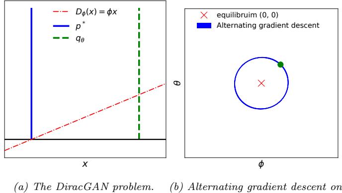
Figure 26.7: Visualizing divergence using a simple GAN: DiracGAN. Generated by dirac\_gan.ipynb

DiracGAN.

with learning rates ↽h and ωh, either via alternating updates (as we have seen in Algorithm 26.1):

\[ \phi\_t = \phi\_{t-1} - \alpha h \nabla\_{\phi} L\_D(\phi\_{t-1}, \theta\_{t-1}), \tag{26.52} \]

\[ \theta\_t = \theta\_{t-1} - \lambda h \nabla\_{\theta} L\_G(\phi\_t, \theta\_{t-1}) \tag{26.53} \]

or simultaneous updates, where instead of alternating the gradient updates between the two players, they are both updated simultaneously:

\[ \phi\_t = \phi\_{t-1} - \alpha h \nabla\_{\phi} L\_D(\phi\_{t-1}, \theta\_{t-1}), \tag{26.54} \]

\[ \theta\_t = \theta\_{t-1} - \lambda h \nabla\_{\theta} L\_G(\phi\_{t-1}, \theta\_{t-1}) \tag{26.55} \]

The above dynamics of gradient descent are obtained using Euler numerical integration from the ODEs that describes the game dynamics of the two players:

\[\dot{\phi} = -\nabla\_{\phi} L\_D(\phi, \theta),\]

\[\dot{\phi} = \nabla\_{\phi} L\_D(\phi, \theta),\]

\[\dot{\theta} = -\nabla\_{\theta} L\_{G}(\phi, \theta) \tag{26.57}\]

One approach to understand the behavior of GANs is to study these underlying ODEs, which, when discretized, result in the gradient descent updates above, rather than directly studying the discrete updates. These ODEs can be used for stability analysis to study the behavior around an equilibrium. This entails finding the eigenvalues of the Jacobian of the game

\[J = \begin{bmatrix} -\nabla\_{\Phi}\nabla\_{\Phi}L\_{D}(\phi,\theta) & -\nabla\_{\theta}\nabla\_{\phi}L\_{D}(\phi,\theta) \\ -\nabla\_{\Phi}\nabla\_{\theta}L\_{G}(\phi,\theta) & -\nabla\_{\theta}\nabla\_{\theta}L\_{G}(\phi,\theta) \end{bmatrix} \tag{26.58}\]

evaluated at a stationary point (i.e., where ∝εLD(ω, ε)=0 and ∝ωLG(ω, ε)=0). If the eigenvalues of the Jacobian all have negative real parts, then the system is asymptotically stable around the equilibrium; if at least one eigenvalue has positive real part, the system is unstable around the

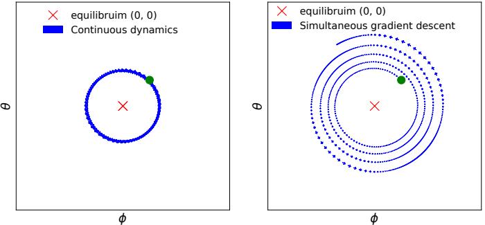
Figure 26.8: Continuous (left) and discrete dynamics (right) take di!erent trajectories in DiracGAN. Generated by dirac\_gan.ipynb

equilibrium. For the DiracGAN, the Jacobian evaluated at the equilibrium 1 = ϱ = 0 is:

\[J = \begin{bmatrix} \nabla\_{\Phi} \nabla\_{\Phi} l(\theta \phi) + l(0) & \nabla\_{\Phi} \nabla\_{\Phi} l(\theta \phi) + l(0) \\ -\nabla\_{\Phi} \nabla\_{\Phi} \left( l(\theta \phi) + l(0) \right) & -\nabla\_{\Phi} \nabla\_{\Phi} \left( l(\theta \phi) + l(0) \right) \end{bmatrix} = \begin{bmatrix} 0 & l'(0) \\ -l'(0) & 0 \end{bmatrix} \tag{26.59}\]

where eigenvalues of this Jacobian are ω^± = ±il^→ (0). This is interesting, as the real parts of the eigenvalues are both 0; this result tells us that there is no asymptotic convergence to an equilibrium, but linear convergence could still occur. In this simple case we can reach the conclusion that convergence does not occur as we observe that there is a preserved quantity in this system, as 1² + ϱ² does not change in time (Figure 26.8, left):

\[\frac{d\left(\theta^2 + \phi^2\right)}{dt} = 2\theta\frac{d\theta}{dt} + 2\phi\frac{d\phi}{dt} = -2\theta l'(\theta\phi)\phi + 2\phi l'(\theta\phi)\theta = 0.1\]

Using stability analysis to understand the underlying continuous dynamics of GANs around an equilibrium has been used to show that explicit regularization can help convergence [NK17; Bal+18]. Alternatively, one can directly study the updates of simultaneous gradient descent shown in Equations 26.54 and 26.55. Under certain conditions, [MNG17b] prove that GANs trained with simultaneous gradient descent reach a local Nash equilibrium. Their approach relies on assessing the convergence of series of the form F^k(x) resulting from the repeated application of gradient descent update of the form F(x) = x + hG(x), where h is the learning rate. Since the function F depends on the learning rate h, their convergence results depend on the size of the learning rate, which is not the case for continuous time approaches.

Both continuous and discrete approaches have been useful in understanding and improving GAN training; however, both approaches still leave a gap between our theoretical understanding and the most commonly used algorithms to train GANs in practice, such as alternating gradient descent or more complex optimizers used in practice, like Adam. Far from only providing di!erent proof techniques, these approaches can reach di!erent conclusions about the convergence of a GAN: we show an example in Figure 26.8, where we see that simultaneous gradient descent and the continuous dynamics behave di!erently when a large enough learning rate is used. In this case, the discretization error — the di!erence between the behavior of the continuous dynamics in Equations 26.56 and 26.57 and the gradient descent dynamics in Equations 26.54 and 26.55 — makes the analysis of gradient descent using continuous dynamics reach the wrong conclusion about DiracGAN [Ros+21]. This di!erence in behavior has been a motivator to train GANs with higher order numerical integrators such as RungeKutta4, which to more closely follow the underlying continuous system compared to gradient descent [Qin+20].

While optimization convergence analysis is an indispensable step in understanding GAN training and has led to significant practical improvements, it is worth noting that ensuring converge to an equilibrium does not ensure the model has learned a good fit of the data distribution. The loss landscape determined by the choice of L^D and LG, as well as the parameterization of the discriminator and generator can lead to equilibria which do not capture the data distribution. The lack of distributional guarantees provided by game equilibria showcases the need to complement convergence analysis with work looking at the e!ect of gradient based learning in this game setting on the learned distribution.

26.4 Conditional GANs

We have thus far discussed how to use implicit generative models to learn a true unconditional distribution p↔︎(x) from which we only have samples. It is often useful, however, to be able to learn conditional distributions of the from p↔︎(x|y). This requires having paired data, where each input xⁿ is paired with a corresponding set of covariates yn, such as a class label, or a set of attributes or words, so D = {(xn, yn) : n =1: N}, as in standard supervised learning. The conditioning variable can be discrete, like a class label, or continuous, such as an embedding which encodes other information. Conditional generative models are appealing since we can specify that we want the generated sample to be associated with conditioning information y, making them very amenable to real world applications, as we discuss in Section 26.7.

To be able to learn implicit conditional distributions q⇀(x|y), we require datasets that specify the conditioning information associated with data, and we have to adapt the model architectures and loss functions. In the GAN case, changing the loss function for the generative model can be done by changing the critic, since the critic is part of the loss function of the generator; it is important for the critic to provide learning signal accounting for conditioning information, by penalizing a generator which provides realistic samples but which ignore the provided conditioning.

If we do not change the form of the min-max game, but provide the conditioning information to the two players, a conditional GAN can be created from the original GAN game [MO14]:

\[\min\_{\theta} \max\_{\phi} \frac{1}{2} \mathbb{E}\_{p(\mathbf{y})} \mathbb{E}\_{p^\*(\mathbf{z}|\mathbf{y})} [\log D\_{\phi}(\mathbf{z}, \mathbf{y})] + \frac{1}{2} \mathbb{E}\_{p(\mathbf{y})} \mathbb{E}\_{q\_{\theta}(\mathbf{z}|\mathbf{y})} [\log(1 - D\_{\phi}(\mathbf{z}, \mathbf{y}))] \tag{26.60}\]

In the case of implicit latent variable models, the embedding information becomes an additional input to the generator, together with the latent variable z:

\[\min\_{\theta} \max\_{\phi} \mathcal{L}(\theta, \phi) = \frac{1}{2} \mathbb{E}\_{p(\mathbf{y})} \mathbb{E}\_{p^\*(\mathbf{z}|\mathbf{y})} [\log D\_{\phi}(\mathbf{z}, \mathbf{y})] + \frac{1}{2} \mathbb{E}\_{p(\mathbf{y})} \mathbb{E}\_{q(\mathbf{z})} [\log(1 - D\_{\phi}(\mathcal{G}\_{\theta}(\mathbf{z}, \mathbf{y}), \mathbf{y}))] \tag{26.61}\]

For discrete conditioning information such as labels, one can also add a new loss function, by training a critic which does not only learn to distinguish between real and fake data, but learns to classify both data and generated samples as pertaining to one of the K classes provided in the

Figure 26.9: Learning an implicit posterior using an adversarial approach, as done in BiGAN. From Figure 1 of [DKD16]. Used with kind permission of Je! Donahue.

dataset [OOS17]:

\[\mathcal{L}\_c(\boldsymbol{\theta}, \phi) = -\left[\frac{1}{2} \mathbb{E}\_{p(\boldsymbol{y})} \mathbb{E}\_{p^\*(\boldsymbol{x}|\boldsymbol{y})} [\log D\_{\phi}(\boldsymbol{y}|\boldsymbol{x})] + \frac{1}{2} \mathbb{E}\_{p(\boldsymbol{y})} \mathbb{E}\_{q\_{\phi}(\boldsymbol{x}|\boldsymbol{y})} [\log(D\_{\phi}(\boldsymbol{y}|\boldsymbol{x}))] \right] \tag{26.62}\]

Note that while we could have two critics, one unsupervised critic and one supervised which maximizes the equation above, in practice the same critic is used, to aid shaping the features used in both decision surfaces. Unlike the adversarial nature of the unsupervised game, it is in the interest of both players to minmize the classification loss Lc. Thus together with the adversarial dynamics provided by L, the two players are trained as follows:

\[\max\_{\phi} \mathcal{L}(\theta, \phi) - \mathcal{L}\_c(\theta, \phi) \tag{26.63} \\ \text{and} \\ \mathcal{L}(\theta, \phi) + \mathcal{L}\_c(\theta, \phi) \tag{26.63}\]

In the case of conditional latent variable models, the latent variable controls the sample variability inside the mode specified by the conditioning information. In early conditional GANs, the conditioning information was provided as additional input to the discriminator and generator, for example by concatenating the conditioning information to the latent variable z in the case of the generator; it has been since observed that it is important to provide the conditioning information at various layers of the model, both for the generator and the discriminator [DV+17; DSK16] or use a projection discriminator [MK18].

26.5 Inference with GANs

Unlike other latent variable models such as variational autoencoders, GANs do not define an inference procedure associated with the generative model. To deploy the principles behind GANs to find a posterior distribution p(z|x), multiple approaches have been taken, from combining GANs and variational autoencoders via hybrid methods [MNG17a; Sri+17; Lar+16; Mak+15b] to constructing inference methods catered to implicit variable models [Dum+16; DKD16; DS19]. An overview of these methods can be found in [Hus17b].

GAN based methods which perform inference and learn implicit posterior distribution p(z|x) introduce changes to the GAN algorithm to do so. An example of such a method is BiGAN (bidirectional GAN) [DKD16] or ALI (adversarialy learned inference) [Dum+16], which trains an

implicit parameterized encoder E^ϖ to map input x to latent variables z. To ensure consistency between the encoder E^ϖ and the generator Gω, an adversarial approach is introduced with a discriminator D^ε learning to distinguish between pairs of data and latent samples: D^ε learns to consider pairs (x, Eϖ(x)) with x ↑ p^↔︎ as real, while (Gω(z), z) with z ↑ q(z) is considered fake. This approach, shown in Figure 26.9, ensures that the joint distributions are matched, and thus the marginal distribution q⇀(x) given by G^ω should learn p^↔︎ (x), while the conditional distribution pϖ(z|x) given by ^Eϖ should learn ^qω(z|x) = ^qω(x,z) ^qω(x) ↘ q⇀(x|z)q(z). This joint GAN loss can be used both to train the generator G^ω and the encoder Eϖ, without requiring a reconstruction loss common in other inference methods. While not using a reconstruction loss, this objective retains the property that under global optimality conditions the encoder and decoder are inverses of each other: Eω(Gϖ(z)) = z and Gϖ(Eω(x)) = x. (See also Section 21.2.4 for a discussion of how VAEs learn to ensure p^↔︎ (x)pϖ(z|x) matches p(z)pω(x|z) using an explicit model of the data.)

26.6 Neural architectures in GANs

We have so far discussed the learning principles, algorithms, and optimization methods that can be used to train implicit generative models parameterized by deep neural networks. We have not discussed, however, the importance of the choice of neural network architectures for the model and the critic, choices which have fueled the progress in GAN generation since their conception. We will look at a few case studies which show the importance of information about data modalities into the critic and the generator (Section 26.6.1), employing the right inductive biases (Section 26.6.2), incorporating attention in GAN models (Section 26.6.3), progressive generation (Section 26.6.4), regularization (Section 26.6.5), and using large scale architectures (Section 26.6.6).

26.6.1 The importance of discriminator architectures

Since the discriminator or critic is rarely optimal — either due to the use of alternating gradient descent or the lack of capacity of the neural discriminator — GANs do not perform distance or divergence minimization in practice. Instead, the critic acts as part of a learned loss function for the model (the generator). Every time the critic is updated, the loss function for the generative model changes; this is in stark contrast with divergence minimization such maximum likelihood estimation, where the loss function stays the same throughout the training of the model. Just as learning features of data instead of handcrafting them is a reason for the success of deep learning methods, learning loss functions advanced the state of the art of generative modeling. Critics that take data modalities into account — such as convolutional critics for images and recurrent critics for sequential data such as text or audio — become part of data modality dependent loss functions. This in turn provides modality-specific learning signal to the model, for example by penalizing blurry images and encouraging sharp edges, which is achieved due to the convolutional parameterization of the critic. Even within the same data modality, changes to critic architectures and regularization have been one of the main drivers in obtaining better GANs, since they a!ect the generator’s loss function, and thus also the gradients of the generator and have a strong e!ect on optimization.

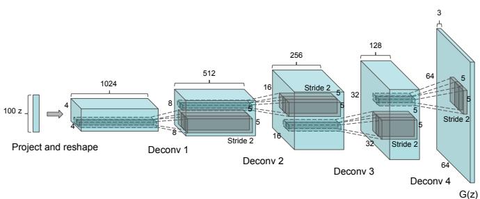
Figure 26.10: DCGAN convolutional generator. From Figure 1 of [RMC15]. Used with kind permission of Alec Radford.

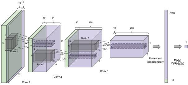
Figure 26.11: DCGAN convolutional discrimiantor. From Figure 1 of [RMC15]. Used with kind permission of Alec Radford.

26.6.2 Architectural inductive biases

While the original GAN paper used convolutions only sparingly, deep convolutional GAN (DC-GAN) [RMC15] performed an extensive study on what architectures are most useful for GAN training, resulting in a set of useful guidelines that led to a substantial boost in performance. Without changing the learning principles behind GANs, DCGAN was able to obtain better results on image data by using convolutional generators (Figure 26.10) and critics, using BatchNormalization for both the generator and critic, replacing pooling layers with strided convolutions, using ReLU activation networks in the generator, and LeakyReLU activations in the discriminator. Many of these principles are still in use today, for larger architectures and with various loss functions. Since DCGAN, residual convolutional layers have become a key staple of both models and critics for image data [Gul+17], and recurrent architectures are used for sequence data such as text [SSG18b; Md+19].

26.6.3 Attention in GANs

Attention mechanisms are explained in detail in Section 16.2.7. In this section, we discuss how to use them for both the GAN generator and discriminator; this is called the self attention GAN or SAGAN model [Zha+19c]. The advantage of self attention is that it ensures that both discriminator and generator have access to a global view of other units of the same layer, unlike convolutional

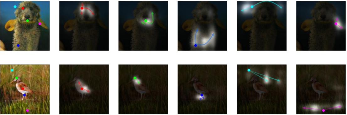
Figure 26.12: Attention queries used by a SAGAN model, showcasing the global span of attention. Each row first shows the input image and a set of color coded query locations in the image. The subsequent images show the attention maps corresponding to each query location in the first image, with the query color coded location being shown, and arrows from it to the attention map are used to highlight the most attended regions. From Figure 1 of [Zha+19c]. Used with kind permission of Han Zhang.

layers. This is illustrated in Figure 26.12, which visualizes the global span of attention: query points can attend to various other areas in the image.

The self-attention mechanism for convolutional features reshaped to ^{h → RC}⇐^N is defined by ^{f = W}fh, ^{g = W}gh, ^{S = fT g}, where ^{Wf → RC↑} ⇐^C , W^{g → RC↑} ⇐^C , where ^{C→ ≃ C} is a hyperparameter. From ^{S → RN}⇐^N , a probability row matrix ^ε is obtained by applying the softmax operator for each row, which is then used to attend to a linear transformation of the features ^{o = W}o(Whh)ε^{T → RC}⇐^N , using learned operators ^{Wh → RC↑} ⇐^C , W^{o → RC}⇐C^↑ . An output is then created by y = γo + h, where γ → R is a learned parameter.

Beyond providing global signal to the players, it is worth noting the flexibility of the self attention mechanism. The learned parameter γ ensures that the model can decide not to use the attention layer, and thus adding self attention does not restrict the set of possible models an architecture can learn. Moreover, self attention significantly increases the number of parameters of the model (each attention layer introduced 4 learned matrices W^f ,Wg,Wh,Wo), an approach that has been observed as a fruitful way to improve GAN training.

26.6.4 Progressive generation

One of the first successful approaches to generating higher resolution, color images from a GAN is via an iterative process, by first generating a lower dimensional sample, and then using that as conditioning information to generate a higher dimensional sample, and repeating the process until the desired resolution is reached. LapGAN [DCF+15] uses a Laplacian pyramid as the iterative building block, by first upsampling the lower dimensional samples using a simple upsampling operation, such as smoothed upsampling, and then using a conditional generator to produce a residual to be added to the upsampled version to produce the higher resolution sample. In turn, this higher resolution sample can then be provided to another LapGAN layer to produce another, even higher resolution

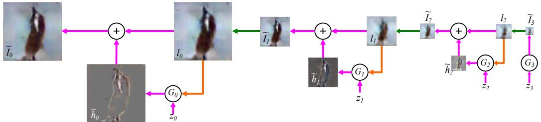
Figure 26.13: LapGAN generation algorithm: the generation process starts with a low dimension sample, which gets upscaled and residually added to the output of a generator at a higher resolution. The process gets repeated multiple times. From Figure 1 of [DCF+15]. Used with kind permission of Emily Denton.

Figure 26.14: ProgressiveGAN training algorithm. The input to the discriminator at the bottom of the figure is either a generated image, or a real image (denotes as ‘Reals’ in the figure) at the corresponding resolution. From Figure 1 of [Kar+18]. Used with kind permission of Tero Karras.

sample, and so on — this process is shown in Figure 26.13. In LapGAN, a di!erent generator and critic are trained for each iterative block of the model; in ProgressiveGAN [Kar+18] the lower resolution generator and critic are “grown”, by becoming part of the generator and critic used to learn to generate higher resolution samples. The higher resolution generator is obtained by adding new layers on top of the last layer of the lower resolution generator. A residual connection between an upscaled version of the lower dimensional sample and the output of the newly created higher resolution generator is added, which is annealed from 0 to 1 in training — transitioning from using the upscaled version of the lower dimensional sample early in training, to only using the sample of the higher resolution generator at the end of training. A similar change is done to the discriminator. Figure 26.14 shows the growing generator and discriminators in ProgressiveGAN training.

26.6.5 Regularization

Regularizing both the discriminator and the generator has by now a long tradition in GAN training. Regularizing GANs can be justified from multiple perspectives: theoretically, as it has been shown to

be tied to convergence analysis [MGN18b]; empirically, as it has been shown to help performance and stability in practice [RMC15; Miy+18c; Zha+19c; BDS18]; and intuitively, as it can be used to avoid overfitting in the discriminator and generator. Regularization approaches include adding noise to the discriminator input [AB17], adding noise to the discriminator and generator hidden features [ZML16], using BatchNorm for the two players [RMC15], adding dropout in the discriminator [RMC15], spectral normalization [Miy+18c; Zha+19c; BDS18], and gradient penalties (penalizing the norm of the discriminator gradient with respect to its input ⇐∝xDε(x)⇐ 2 ) [Arb+18; Fed+18; ACB17; Gul+17]. Often regularization methods help training regardless of the type of loss function used, and have been shown to have e!ects both on training performance as well as the stability of the GAN game. However, improving stability and improving performance in GAN training can be at odds with each other, since too much regularization can make the models very stable but reduce performance [BDS18].

26.6.6 Scaling up GAN models

By combining many of the architectural tricks discussed thus far — very large residual networks, self attention, spectral normalization both in the discriminator and the generator, BatchNormalization in the generator — one can train GANs to generate diverse, high quality data, as done with BigGAN [BDS18], StyleGAN [Kar+20c], and alias-free GAN [Kar+21]. Beyond combining carefully chosen architectures and regularization, creating large scale GANs also require changes in optimization, with large batch sizes being a key component. This furthers the view that the key components of the GAN game — the losses, the parameterization of the models, and the optimization method — have to be viewed collectively rather than in isolation.

26.7 Applications

The ability to generate new plausible data enables a wide range of applications for GANs. This section will look at a set of applications that aim to demonstrate the breadth of GANs across di!erent data modalities, such as images (Section 26.7.1), video (Section 26.7.2), audio (Section 26.7.3), and text (Section 26.7.4), and include applications such as imitation learning (Section 26.7.5), domain adapation (Section 26.7.6), and art (Section 26.7.7).

26.7.1 GANs for image generation

The most widely studied application area is in image generation. We focus on the translation of one image to another using either paired or unpaired datasets. There are many other topics related to image GANs that we do not cover, and a more complete overview can be found in other sources, such as [Goo16] for the theory and [Bro19] for the practice. A JAX notebook which uses a small pretrained GAN to generate some face images can be found at GAN\_JAX\_CelebA\_demo.ipynb. We show the progression of quality in sample generation of faces using GANs in Figure 26.15. There is also increasing need to consider the generation of images with regards to the potential risks they can have when used in other domains, which involve discussions of synthetic media and deep fakes, and sources for discussion include [Bru+18; Wit].

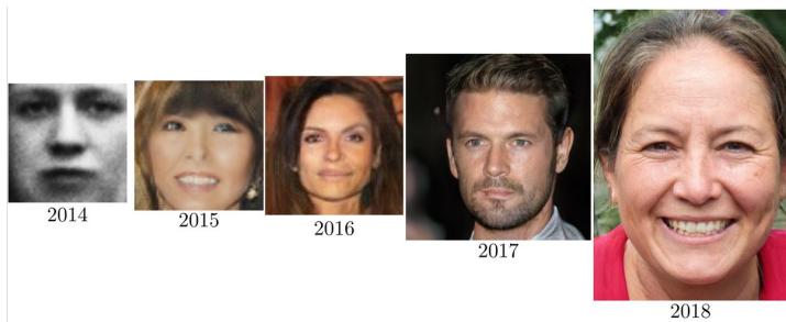
Figure 26.15: Increasingly realistic synthetic faces generated by di!erent kinds of GAN, specifically (from left to right): original GAN [Goo+14], DCGAN [RMC15], CoupledGAN [LT16], ProgressiveGAN [Kar+18], StyleGAN [KLA19]. Used with kind permission of Ian Goodfellow. An online demo, which randomly generates face images using StyleGAN, can be found at https: // thispersondoesnotexist. com .

26.7.1.1 Conditional image generation

Class-conditional image generation using GANs has become a very fruitful endeavor. BigGAN [BDS18] carries out class-conditional generation of ImageNet samples across a variety of categories, from dogs and cats to volcanoes and hamburgers. StyleGAN [KLA19] is able to generate high quality images of faces at high resolution by learning a conditioning style vector and the ProgressiveGAN architecture discussed in Section 26.6.4. By learning the conditioning vector they are able to generate samples which interpolate between the styles of other samples, for example by preserving coarser style elements such as pose or face shape from one sample, and smaller scale style elements such as hair style from another; this provides fine grained control over the style of the generated images.

26.7.1.2 Paired image-to-image generation

We have discussed in Section 26.4 how using paired data of the form (xn, yn) can be used to build conditional generative models of p(x|y). In some cases, the conditioning variable y has the same size and shape as the output variable x. The resulting model pω(x|y) can then be used to perform image to image translation, as illustrated in Figure 26.16, where y is drawn from the source domain, and x from the target domain. Collecting paired data of this form can be expensive, but in some cases, we can acquire it automatically. One such example is image colorization, where a paired dataset can easily be obtained by processing color images into grayscale images (see e.g., [Jas]).

A conditional GAN used for paired image-to-image translation was proposed in [Iso+17], and is known as the pix2pix model. It uses a U-net style architecture for the generator, as used for semantic segmentation tasks. However, they replace the batch normalization layers with instance normalization, as in neural style transfer.

For the discriminator, pix2pix uses a patchGAN model, that tries to classify local patches as being real or fake (as opposed to classifying the whole image). Since the patches are local, the discriminator is forced to focus on the style of the generated patches, and ensure they match the statistics of the target domain. A patch-level discriminator is also faster to train than a whole-image discriminator, and gives a denser feedback signal. This can produce results similar to Figure 26.16

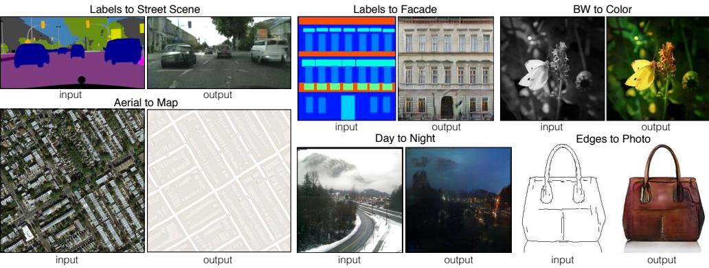
Figure 26.16: Example results on several image-to-image translation problems as generated by the pix2pix conditional GAN. From Figure 1 of [Iso+17]. Used with kind permission of Phillip Isola.

(depending on the dataset).

26.7.1.3 Unpaired image-to-image generation

A major drawback of conditional GANs is the need to collect paired data. It is often much easier to collect unpaired data of the form D^x = {xⁿ : n =1: Nx} and D^y = {yⁿ : n =1: Ny}. For example, D^x might be a set of daytime images, and D^y a set of night-time images; it would be impossible to collect a paired dataset in which exactly the same scene is recorded during the day and night (except using a computer graphics engine, but then we wouldn’t need to learn a generator).

We assume that the datasets D^x and D^y come from the marginal distributions p(x) and p(y) respectively. We would then like to fit a joint model of the form p(x, y), so that we can compute conditionals p(x|y) and p(y|x) and thus translate from one domain to another. This is called unsupervised domain translation.

In general, this is an ill-posed problem, since there are an infinite number of di!erent joint distributions that are consistent with a set of marginals p(x) and p(y). We can try, however, to learn a joint distribution such that samples from it satisfy additional constraints. For example, if G is a conditional generator that maps a sample from X to Y, and F maps a sample from Y to X , it is reasonable to require that these be inverses of each other, i.e., F(G(x)) = x and G(F(y)) = y. This is called a cycle consistency loss [Zhu+17]. We can encourage G and F to satisfy this constraint by using a penalty term on the di!erence between the starting image and the image we get after going through this cycle:

\[\mathcal{L}\_{\text{cycle}} = \mathbb{E}\_{p(\mathbf{z})} ||F(G(\mathbf{z})) - \mathbf{z}||\_1 + \mathbb{E}\_{p(\mathbf{y})} ||G(F(\mathbf{y})) - \mathbf{y}||\_1 \tag{26.64}\]

To ensure that the outputs of G are samples from p(y) and those of F are samples from p(x), we use a standard GAN approach, introducing discriminators D^X and D^Y , which can be done using any choice of GAN loss LGAN, as visualized in Figure 26.17. Finally, we can optionally check that applying the conditional generator to images from its own domain does not change them:

\[\mathcal{L}\_{\text{identity}} = \mathbb{E}\_{p(\mathbf{z})} \| \mathbf{z} - F(\mathbf{z}) \|\_{1} + \mathbb{E}\_{p(\mathbf{y})} \| \mathbf{y} - G(\mathbf{y}) \|\_{1} \tag{26.65}\]

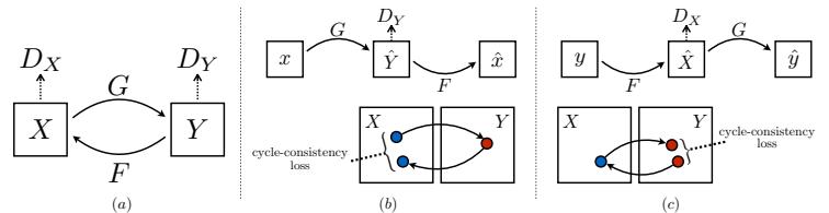
Figure 26.17: Illustration of the CycleGAN training scheme. (a) Illustration of the 4 functions that are trained. (b) Forwards cycle consistency from X back to X . (c) Backwards cycle consistency from Y back to Y. From Figure 3 of [Zhu+17]. Used with kind permission of Jun-Yan Zhu.

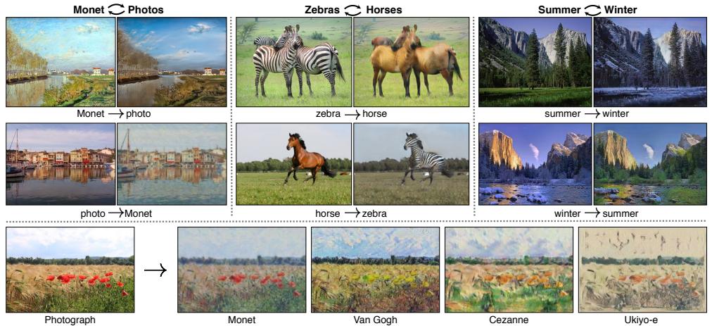
Figure 26.18: Some examples of unpaired image-to-image translation generated by the CycleGAN model. From Figure 1 of [Zhu+17]. Used with kind permission of Jun-Yan Zhu.

We can combine all three of these consistency losses to train the translation mappings F and G, using hyperparameters ω¹ and ω2:

\[\mathcal{L} = \mathcal{L}\_{\text{GAN}} + \lambda\_1 \mathcal{L}\_{\text{cycle}} + \lambda\_2 \mathcal{L}\_{\text{identity}} \tag{26.66}\]

CycleGAN results on various datasets are shown in Figure 26.18. The bottom row shows how CycleGAN can be used for style transfer.

26.7.2 Video generation

The GAN framework can be expanded from individual images (frames) to videos; the techniques used to generate realistic images can also be applied to generate videos, with additional techniques required to ensure spatio-temporal consistency. Spatio-temporal consistency is obtained by ensuring that the discriminator has access to the real data and generated sequences in order, thus penalizing the generator when generating realistic individual frames without respecting temporal order [SMS17;

Sai+20; CDS19; Tul+18]. Another discriminator can be employed to additionally ensure each frame is realistic [Tul+18; CDS19]. The generator itself needs to have a temporal element, which is often implemented through a recurrent component. As with images, the generation framework can be expanded to video-to-video translation [Ban+18; Wan+18], encompassing applications such as motion transfer [Cha+19a].

26.7.3 Audio generation

Generative models have been demonstrated in the tasks of generating audio waveforms, as well as for the task of text-to-speech (TTS) generation. Other types of generative models, such as autoregressive models, such as WaveNet [Oor+16a] and WaveRNN [Kal+18b] have been developed for these applications, although autoregressive models are di”cult to parallelize over time since they predict each time step of the audio sequentially and can be computationally expensive and too slow to be used in practice. GANs provide an alternative approach for these tasks and other paths for addressing these concerns.

Many di!erent GAN architectures have been developed for audio-only generation, including generation of single note recordings from instruments by GANSynth, a vocoder model that uses GANs to generate magnitude spectrograms from mel-spectrograms [Eng+18], in voice conversion using a modified CycleGAN discussed above [Kan+20], and the direct generation of raw audio in WaveGAN [DMP18].

Initial work on GANs for TTS was developed [Yan+17] whose approach is similar to conditional GANs for image generation (see Section 26.7.1.2), but uses 1d convolution instead of 2d. More recent GANs such as GAN-TTS [Bi%+19] use more advanced architectures and discriminators that operate at multiple frequency scales that have performance that now matches the best performing autoregressive models when assessed using mean opinion scores. In both the direct-audio generation, the ability of GANs to allow faster generation and di!erent types of context is the advantage that makes them advantageous compared to other models.

26.7.4 Text generation

Similar to image and audio domains, there are several tasks for text data for which GAN-based approaches have been developed, including conditional text generation and text-style transfer. Text data are often represented as discrete values, at either the character level or the word-level, indicating membership within a set of a particular vocabulary size (alphabet size, or number of words). Due to the discrete nature of text, GAN models trained on text are explicit, since they explicitly model the probability distribution of the output, rather than modeling the sampling path. This is unlike most GAN models of continuous data such as images that we have discussed in the chapter so far, though explicit GANs of continuous data do exist [Die+19b].

The discrete nature of text is why maximum likelihood is one of the most common methods of learning generative models of text. However, models trained with maximum likelihood are often limited to autoregressive models, while like in the audio case, GANs make it possible to generate text in a non-autoregressive manner, making other tasks possible, such as one-shot feedforward generation [Gul+17].

The di”culty of generating discrete data such as text using GANs can be seen looking at their loss function, such as in Equations (26.19), (26.21) and (26.28). GAN losses contain terms of

the form Eqω(x)f(x), which we not only need to evaluate, but also backpropagate through, by computing ∝⇀Eqω(x)f(x). In the case of implicit distributions given by latent variable models, we used the reparameterization trick to compute this gradient (Equation 26.49). In the discrete case, the reparameterization trick is not available and we have to look for other ways to estimate the desired gradient. One approach is to use the score function estimator, discussed in Section 6.3.4. However, the score function estimator exhibits high gradient variance, which can destabilize training. One common approach to avoid this issue is to pre-train the language model generator using maximum likelihood, and then to fine-tune with a GAN loss which gets backpropagated into the generator using the score-function estimator, as done by Sequence GAN [Yu+17], MaliGAN [Che+17], and RankGAN [Lin+17a]. While these methods spearheaded the use of GANs for text, they do not address the inherent instabilities of score function estimation and thus have to limit the amount of adversarial fine tuning to a small number of epochs and often use a small learning rate, keeping their performance close to that of the maximum-likelihood solution [SSG18a; Cac+18].

An alternative to maximum likelihood pretraining is to use other approaches to stabilize the score function estimator or to use continuous relaxations for backpropagation. ScratchGAN is a word-level model that uses large batch sizes and discriminator regularization to stabilize score function training (these techniques are the same that we have seen as stabilizers for training image GANs) [Md+19]. [Pre+17b] completely avoid the score function estimator and develop a character level model without pre-training, by using continuous relaxations and curriculum learning. These training approaches can also benefit from other architectural advances, e.g., [NNP19] showed that language GANs can benefit from complex architectures such as relation networks [San+17].

Finally, unsupervised text style transfer, mimicking image style transfer, have been proposed by [She+17; Fu+17] using adversarial classifiers to decode to a di!erent style/language, or like [Pra+18] who trains di!erent encoders, one per style, by combining the encoder of a pre-trained NMT and style classifiers, among other approaches.

26.7.5 Imitation learning

Imitation learning takes advantage of observations of expert demonstrations to learn action policies and reward functions of unknown environments by minimizing some form of discrepancy between the learned and the expert behaviors. There are many approaches available, including behavioral cloning [PPG91] that treats this problem as one of supervised learning, and inverse reinforcement learning [NR00b]. GANs are appealing for imitation learning since they provide a way to avoid the di”culty of designing good discrepancy functions for behaviors, and instead learn these discrepancy functions using a discriminator between trajectories generated by a learned agent and observed demonstrations.

This approach, known as generative adversarial imitation learning (GAIL) [HE16a] demonstrates the ability to use GANs for complex behaviors in high-dimensional environments. GAIL jointly learns a generator, which forms a stochastic policy, along with a discriminator that acts as a reward signal. Like we saw in the probabilistic development of GANs in the earlier sections, GAIL can also be generalized to multiple f-divergences, rather than the standard Jensen-Shannon divergence used as the standard loss in GANs. This has led to a family of other GAIL variants that use other f-divergences [Ke+19a; Fin+16; Bro+20c], including f-GAIL that aims to also learn the best f-divergence to use [Zha+20f], as well as new analytical insight into the computation and generalization of such approaches [Che+20b].

26.7.6 Domain adaptation

An important task in machine learning is to correct for shifts in the data distribution over time, minimizing some measure of domain shift, as we discuss in Section 19.5.3. Like with the other applications, GANs are popular as ways of avoiding the choice of distance or degree of shift. Both the supervised and unsupervised approaches for image generation we reviewed earlier looked at pixellevel domain adaptation models that perform distribution alignment in raw pixel space, translating source data to the style of a target domain, as with pix2pix and CycleGAN. Extensions of these approaches for the general problem of domain adaptation seek to do this not only in the observed data space (e.g., with pixels), but also at the feature level. One general approach is domainadversarial training of neural networks [Gan+16b] or adversarial discriminative domain adaptation (ADDA) [Tze+17]. The CyCADA approach of [Hof+18] extends CycleGAN by enforcing both structural and semantic consistency during adaptation using a cycle-consistency loss and semantics losses based on a particular visual recognition task. There are also many extensions that include class conditional information [Tsa+18; Lon+18] or adaptation when the modes to be matched have di!erent frequencies in the source and target domains [BHC19].

26.7.7 Design, art and creativity

Generative models, particularly of images, have added to approaches in the more general area of algorithmic art. The applications in image and audio generation with transfer can also be considered aspects of artistic image generation. In these cases, the goal of training is not generalization, but to create appealing images across di!erent types of visual aesthetics [Sar18]. One example takes style transfer GANs to create visual experiences, in which objects placed under a video are re-rendered using other visual styles in real time [AFG19]. The generation ability has been used to explore alternative designs and fabrics in fashion [Kat+19], and have now also become part of major drawing software to provide new tools to support designers [Ado]. And beyond images, creative and artistic expression using GANs include areas in music, voice, dance, and typography [AI 19].

Part V

Discovery

27 Discovery methods: an overview

27.1 Introduction

We have seen in Part III how to create probabilistic models that can make predictions about outputs given inputs, using supervised learning methods (conditional likelihood maximization). And we have seen in Part IV how to create probabilistic models that can generate outputs unconditionally, using unsupervised learning methods (unconditional likelihood maximization). However, in some settings, our goal is to try to understand a given dataset. That is, we want to discover something “interesting”, and possibly “actionable”. Prediction and generation are useful subroutines for discovery, but are not su”cient on their own. In particular, although neural networks often implicitly learn useful features from data, they are often hard to interpret, and the results can be unstable and sensitive to arbitrary details of the training protocol (e.g., SGD learning rates, or random seeds).

In this part of the book, we focus on learning models that create an interpretable representation of high dimensional data. A common approach is to use a latent variable model, in which we make the assumption that the observed data x was caused by, or generated by, some underlying (often low dimensional) latent factors z, which represents the “true” state of the world. Crucially, these latent variables are assumed to be meaningful to the end user of the model. (Thus evaluating such models will generally require domain expertise.)

For example, suppose we want to interpret an image x in terms of an underlying 3d scene, z, which is represented in terms of objects and surfaces. The forwards mapping from z to x is often many-to-one, i.e., di!erent latent values, say z and z^→ , may give rise to the same observation x, due to limitations of the sensor. (This is called perceptual aliasing.) Consequently the inverse mapping, from x to z, is ill-posed. In such cases, we need to impose a prior, p(z), to make our estimate well-defined. In simple settings, we can use a point estimate, such as the MAP estimate

\[\hat{\mathbf{z}}(\mathbf{z}) = \operatorname\*{argmax}\_{\mathbf{z}} p(\mathbf{z}|\mathbf{z}) = \operatorname\*{argmax}\_{\mathbf{z}} \log p(\mathbf{z}) + \log p(\mathbf{z}|\mathbf{z}) \tag{27.1}\]

In the context of computer vision, this approach is known as vision as inverse graphics or analysis by synthesis [KMY04; YK06; Doy+07; MC19]. See Figure 27.1 for an illustration.

This approach to inverse modeling is widely used in science and engineering, where z represents the underlying state of the world which we want to estimate, and x is just a noisy or partial manifestation of this true state. In some cases, we know both the prior p(z|ε) and the likelihood p(x|z, ε), and we just need to solve the inference problem for z. But more commonly, the model parameters ε are also (partially) unknown, and need to be inferred from observable samples D = {xⁿ : n =1: N}. In some cases, the structure of the model itself is unknown and needs to be learned.

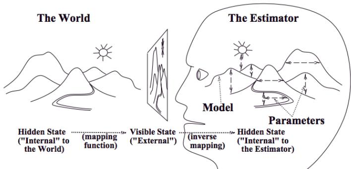
Figure 27.1: Vision as inverse graphics. The agent (here represented by a human head) has to infer the scene z given the image x using an estimator. From Figure 1 of [Rao99]. Used with kind permission of Rajesh Rao.

27.2 Overview of Part V

In Chapter 28, we discuss simple latent variable models where typically the observed data is a fixeddimensional vector such as ^{x → RD}. In Chapter 29 we extend these models to work with sequences of correlated vectors, x = x1:^T , such as speech, video, genomics data, etc. It is straightforward to make parts of these model be nonlinear (“deep”), as we discuss. These models can also be extended to the spatio-temporal setting. In Chapter 30, we extend these models to work with general graphs.

In Chapter 31, we discuss non-parametric Bayesian models, which allow us to represent uncertainty about many aspects of a model, such as the number of hidden states, the structure of the model, the form of a functional dependency, etc. Thus the complexity of the learned representation can grow dynamically, depending on the quantity and quality (informativeness) of the data. This is important when performing discovery tasks, and helps us maintain flexibility while still retaining interpretability.

In Chapter 32, we discuss representation learning using neural networks. This can be tackled using latent variable modeling, but there are also a variety of other estimation methods one can use. Finally, in Chapter 33, we discuss how to interpret the behavior of a predictive model (typically a neural network).

28 Latent factor models

28.1 Introduction

A latent variable model (LVM) is any probabilistic model in which some variables are always latent or hidden. A simple example is a mixture model (Section * 28.2), which has the form p(x) = ^k p(x|z = k)p(z = k), where z is an indicator variable that specifies which mixture component to use for generating x. However, we can also use continuous latent variables, or a mixture of discrete and continuous. And we can also have multiple latent variables, which are interconnected in complex ways.

In this chapter, we discuss a very simple kind of LVM that has the following form:

\[\mathbf{z} \sim p(\mathbf{z})\tag{28.1}\]

\[\mathbf{z}|\mathbf{z}\sim\text{Exp}\mathbf{f}\mathbf{a}(\mathbf{z}|f(\mathbf{z}))\tag{28.2}\]

where f(z) is known as the decoder, and p(z) is some kind of prior. We assume that z is a single “layer” of hidden random variables, corresponding to a set of “latent factors”. We call these latent factor models. In this chapter, we assume the decoder f is a simple linear model; we consider nonlinear extensions in Chapter 21. Thus the overall model is similar to a GLM (Section 15.1), except the input to the model is hidden.

We can create a large variety of di!erent “classical” models by changing the form of the prior p(z) and/or the likelihood p(x|z), as we show in Table 28.1. We will give the details in the following sections. (Note that, although we are discussing generative models, our focus is on posterior inference of meaningful latents (discovery), rather than generating realistic samples of data.)

28.2 Mixture models

One way to create more complex probability models is to take a convex combination of simple distributions. This is called a mixture model. This has the form

\[p(x|\theta) = \sum\_{k=1}^{K} \pi\_k p\_k(x) \tag{28.3}\]

where p^k is the k’th mixture component, and φ^k are the mixture weights which satisfy 0 ≃ φ^k ≃ 1 and *^{K k}=1 φ^k = 1.

We can re-express this model as a hierarchical model, in which we introduce the discrete latent variable z → {1,…,K}, which specifies which distribution to use for generating the output x. The

Model	p(z)	p(x z)	Section
FA/PCA	N (z 0, I)	N (x Wz, $)	Section 28.3.1
GMM	* c Cat(c ↼)N (z µc, “c)	N (x Wz, $)	Section 28.2.4
MixFA	Cat(c ↼)N (z 0, I)	N (x Wcz + µc, $c)	Section 28.3.3.5
NMF	 k Ga(zk ↽k, εk)	 exp(wT d Poi(xd dz)))	Section 28.4.1
Simplex FA (mPCA)	Dir(z ↽)	 d Cat(xd Wdz)	Section 28.4.2
LDA	Dir(z ↽)	 d Cat(xd Wz)	Section 28.5
ICA	 d Laplace(zd ω)	 ↓ wT d ϑ(xd dz)	Section 28.6
Sparse coding	 k Laplace(zk ω)	 d N (xd wT ς2) dz,	Section 28.6.5

Table 28.1: Some popular “shallow” latent factor models. Abbreviations: FA = factor analysis, PCA = principal components analysis, GMM = Gaussian mixture model, NMF = non-negative matrix factorization, mPCA = multinomial PCA, LDA = latent Dirichlet allocation, ICA = independent components analysis. k =1: L ranges over latent dimensions, d =1: D ranges over observed dimensions. (For ICA, we have the constraint that L = D.)

prior on this latent variable is p(z = k) = φk, and the conditional is p(x|z = k) = pk(x) = p(x|εk). That is, we define the following joint model:

\[p(z|\theta) = \text{Cat}(z|\pi) \tag{28.4}\]

\[p(\mathbf{z}|z=k,\mathbf{\theta}) = p(\mathbf{z}|\theta\_k) \tag{28.5}\]

The “generative story” for the data is that we first sample a specific component z, and then we generate the observations x using the parameters chosen according to the value of z. By marginalizing out z, we recover Equation (28.3):

\[p(\mathbf{z}|\boldsymbol{\theta}) = \sum\_{k=1}^{K} p(z=k|\boldsymbol{\theta})p(\mathbf{z}|z=k, \boldsymbol{\theta}) = \sum\_{k=1}^{K} \pi\_k p(\mathbf{z}|\boldsymbol{\theta}\_k) \tag{28.6}\]

We can create di!erent kinds of mixture model by varying the base distribution pk, as we illustrate below.

28.2.1 Gaussian mixture models (GMMs)

A Gaussian mixture model or GMM, also called a mixture of Gaussians (MoG), is defined as follows:

\[p(\mathbf{z}) = \sum\_{k=1}^{K} \pi\_k \mathcal{N}(\mathbf{z}|\boldsymbol{\mu}\_k, \boldsymbol{\Sigma}\_k) \tag{28.7}\]

In Figure 28.1 we show the density defined by a mixture of 3 Gaussians in 2d. Each mixture component is represented by a di!erent set of elliptical contours. If we let the number of mixture components grow su”ciently large, a GMM can approximate any smooth distribution over R^D.

GMMs are often used for unsupervised clustering of real-valued data samples ^{xn → RD}. This works in two stages. First we fit the model, usually by computing the MLE ^{εˆ =} argmax log ^p(D|ε),

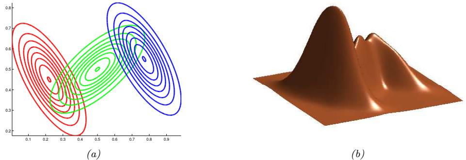
Figure 28.1: A mixture of 3 Gaussians in 2d. (a) We show the contours of constant probability for each component in the mixture. (b) A surface plot of the overall density. Adapted from Figure 2.23 of [Bis06]. Generated by gmm\_plot\_demo.ipynb.

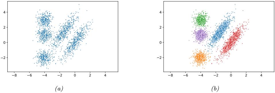
Figure 28.2: (a) Some data in 2d. (b) A possible clustering using K = 5 clusters computed using a GMM. Generated by gmm\_2d.ipynb.

where D = {xⁿ : n =1: N} (e.g., using EM or SGD). Then we associate each datapoint xⁿ with a discrete latent or hidden variable zⁿ → {1,…,K} which specifies the identity of the mixture component or cluster which was used to generate xn. These latent identities are unknown, but we can compute a posterior over them using Bayes’ rule:

\[r\_{nk} \triangleq p(z\_n = k | \mathbf{x}\_n, \boldsymbol{\theta}) = \frac{p(z\_n = k | \boldsymbol{\theta}) p(\mathbf{x}\_n | z\_n = k, \boldsymbol{\theta})}{\sum\_{k'=1}^{K} p(z\_n = k' | \boldsymbol{\theta}) p(\mathbf{x}\_n | z\_n = k', \boldsymbol{\theta})} \tag{28.8}\]

The quantity rnk is called the responsibility of cluster k for datapoint n. Given the responsibilities, we can compute the most probable cluster assignment as follows:

\[\hat{z}\_n = \arg\max\_k r\_{nk} = \arg\max\_k \left[ \log p(\mathbf{z}\_n | z\_n = k, \boldsymbol{\theta}) + \log p(z\_n = k | \boldsymbol{\theta}) \right] \tag{28.9}\]

This is known as hard clustering. (If we use the responsibilities to fractionally assign each datapoint to di!erent clusters, it is called soft clustering.) See Figure 28.2 for an example.

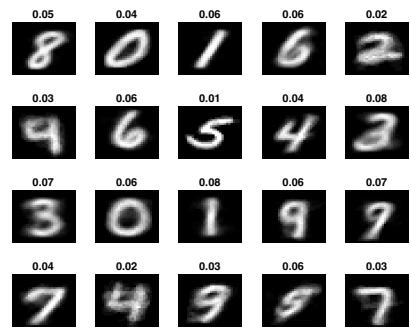
Figure 28.3: We fit a mixture of 20 Bernoullis to the binarized MNIST digit data. We visualize the estimated cluster means µˆk. The numbers on top of each image represent the estimated mixing weights ϑˆk. No labels were used when training the model. Generated by mix\_bernoulli\_em\_mnist.ipynb.

If we have a uniform prior over zn, and we use spherical Gaussians with “^k = I, the hard clustering problem reduces to

\[z\_n = \underset{k}{\text{argmin}} \, ||\boldsymbol{x}\_n - \hat{\boldsymbol{\mu}}\_k||\_2^2 \tag{28.10}\]

In other words, we assign each datapoint to its closest centroid, as measured by Euclidean distance. This is the basis of the K-means clustering algorithm (see the prequel to this book).

28.2.2 Bernoulli mixture models

If the data is binary valued, we can use a Bernoulli mixture model (BMM), also called a mixture of Bernoullis, where each mixture component has the following form:

\[p(\mathbf{z}|z=k,\boldsymbol{\theta}) = \prod\_{d=1}^{D} \text{Ber}(y\_d|\mu\_{dk}) = \prod\_{d=1}^{D} \mu\_{dk}^{y\_d} (1-\mu\_{dk})^{1-y\_d} \tag{28.11}\]

Here µdk is the probability that bit d turns on in cluster k.

For example, consider fitting a mixture of Bernoullis using K = 20 components to the MNIST dataset. The resulting parameters for each mixture component (i.e., µ^k and φk) are shown in Figure 28.3. We see that the model has “discovered” a representation of each type of digit. (Some digits are represented multiple times, since the model does not know the “true” number of classes. See Section 3.8.1 for information on how to choose the number K of mixture components.)

28.2.3 Gaussian scale mixtures (GSMs)

A Gaussian scale mixture or GSM [AM74; Wes87] is like an “infinite” mixture of Gaussians, each with a di!erent scale (variance). More precisely, let ^{x = ϖ}z, where ^{z ↑ N} (0, ^{ς2 0}) and ϖ ↑ p(ϖ). We can

think of this as multiplicative noise being applied to the Gaussian rv ^z. We have ^x|^{ϖ ↑ N} (0, ^ϖ2ς² 0). Marginalizing out the scale ϖ gives

\[p(x) = \int \mathcal{N}(x|0, \sigma\_0^2 \epsilon^2) p(\epsilon) d\epsilon \tag{28.12}\]

By changing the prior p(ϖ), we can create various interesting distributions. We give some examples below.

The main advantage of this approach is that it is often computationally more convenient to work with the expanded parameterization, in which we explicitly include the scale term ϖ, since, conditional on that, the distribution is Gaussian. We use this formulation in Section 6.5.5, where we discuss robust regression.

28.2.3.1 Student-t distribution as a GSM

We can represent the Student distribution as a GSM as follows:

\[\mathcal{T}(x|0,\sigma^2,\nu) = \int\_0^\infty \mathcal{N}(x|0,z\sigma^2) \text{IG}(z|\frac{\nu}{2},\frac{\nu}{2}) dz = \int\_0^\infty \mathcal{N}(x|0,z\sigma^2) \chi^{-2}(z|\nu,1) dz \tag{28.13}\]

where IG is the inverse Gamma distribution (Section 2.2.3.4). Thus we can think of the Student as an infinite superposition of Gaussians of di!erent widths; marginalizing this out induces a distribution with wider tails than a Gaussian with the same variance. This result also explains why the Student distribution approaches a Gaussian as the dof gets large, since when 0 = ̸, the inverse Gamma distribution becomes a delta function.

28.2.3.2 Laplace distribution as a GSM

Similarly one can show that the Laplace distribution is an infinite weighted sum of Gaussians, where the precision comes from a gamma distribution:

\[\text{Laplace}(x|0,\lambda) = \int \mathcal{N}(x|0,\tau^2) \text{Ga}(\tau^2|1, \frac{\lambda^2}{2}) d\tau^2 \tag{28.14}\]

28.2.3.3 Spike and slab distribution

Suppose ^{ϖ ↑} Ber(φ). (Note that ^{ϖ2 = ϖ}, since ^{ϖ →} {0, ¹}.) In this case we have

\[x = \sum\_{\epsilon \in \{0, 1\}} N(x|0, \sigma\_0^2 \epsilon) p(\epsilon) = \pi N(x|0, \sigma\_0^2) + (1 - \pi)\delta\_0(x) \tag{28.15}\]

This is known as the spike and slab distribution, since the ^ϑ0(x) is a “spike” at 0, and the ^N (x|0, ^ς2 0) acts like a uniform “slab” for large enough ς0. This distribution is useful in sparse modeling.

28.2.3.4 Horseshoe distribution

Suppose ϖ ↑ C+(1), which is the half-Cauchy distribution (see Section 2.2.2.4). Then the induced distribution p(x) is called the horseshoe distribution [CPS10]. This has a spike at 0, like the

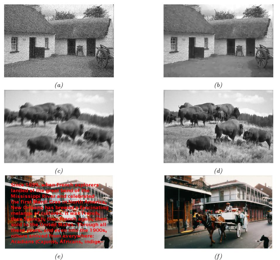
Figure 28.4: Example of recovering a clean image (right) from a corrupted version (left) using MAP estimation with a GMM patch prior and Gaussian likelihood. First row: image denoising. Second row: image deblurring. Third row: image inpainting. From [RW15] and [ZW11]. Used with kind permission of Dan Rosenbaum and Daniel Zoran.

Student and Laplace distributions, but has heavy tails that do not asymptote to zero. This makes it useful as a sparsity promoting prior, that “kills o!” small parameters, but does not overregularize large parameters.

28.2.4 Using GMMs as a prior for inverse imaging problems

In this section, we consider using GMMs as a blackbox density model to regularize the inversion of a many-to-one mapping. Specifically, we consider the problem of inferring a “clean” image x from a corrupted version y. We use a linear-Gaussian forwards model of the form

\[p(\mathbf{y}|\mathbf{x}) = \mathcal{N}(\mathbf{y}|\mathbf{W}\mathbf{x}, \sigma^2\mathbf{I})\tag{28.16}\]

where ς² is the variance of the measurement noise. The form of the matrix W depends on the nature of the corruption, which we assume is known, for simplicity. Here are some common examples of di!erent kinds of corruption we can model in our approach:

• If the corruption is due to additive noise (as in Figure 28.4a), we can set W = I. The resulting MAP estimate can be used for image denoising, as in Figure 28.4b.
• If the corruption is due to blurring (as in Figure 28.4c), we can set W to be a fixed convolutional kernel [KF09b]. The resulting MAP estimate can be used for image deblurring, as in Figure 28.4d.
• If the corruption is due to occlusion (as in Figure 28.4e), we can set W to be a diagonal matrix, with 0s in the locations corresponding to the occluders. The resulting MAP estimate can be used for image inpainting, as in Figure 28.4f.
• If the corruption is due to downsampling, we can set W to a convolutional kernel. The resulting MAP estimate can be used for image super-resolution.

Thus we see that the linear-Gaussian likelihood model is surprisingly flexible. Given the model, our goal is to invert it, by computing the MAP estimate xˆ = argmax p(x|y). However, the problem of inverting this model is ill-posed, since there are many possible latent images x that map to the same observed image y. Therefore we need to use a prior to regularize the inversion process.

In [ZW11], they propose to partition the image into patches, and to use a GMM prior of the form p(xi) = * ^k p(cⁱ = k)N (xi|µk, “k) for each patch i. They use K = 200 mixture components, and they fit the GMM on a dataset of 2M clean image patches.

To compute the MAP mixture component, c^{↔︎ i} , we can marginalize out xⁱ and use Equation (2.129) to compute the marginal likelihood

\[c\_i^\* = \underset{c}{\text{argmax}} \, p(c)p(y\_i|c) = \underset{c}{\text{argmax}} \, p(c) \mathcal{N}(y\_i|\mathbf{W}\mu\_c, \sigma^2\mathbf{I} + \mathbf{W}\Sigma\_c\mathbf{W}^\top) \tag{28.17}\]

We can then approximate the MAP for the latent patch xⁱ by using the approximation

\[p(x\_i|y\_i) \approx p(x\_i|y\_i, c\_i^\*) \propto \mathcal{N}(x\_i|\mu\_{c\_i^\*}, \Sigma\_{c\_i^\*})\mathcal{N}(y\_i|\mathbf{W}x\_i, \sigma^2\mathbf{I})\tag{28.18}\]

If we know c^{↔︎ i} , we can compute the above using Bayes’ rule for Gaussians in Equation (2.121).

To apply this method to full images, [ZW11] optimize the following objective

\[E(x|y) = \frac{1}{2\sigma^2} ||\mathbf{W}x - y||^2 - \text{EPLL}(x) \tag{28.19}\]

where EPLL is the “expected patch log likelihood”, given by

\[\text{EPLL}(\mathbf{z}) = \sum\_{i} \log p(\mathbf{P}\_i \mathbf{z}) \tag{28.20}\]

where xⁱ = Pix is the i’th patch computed by projection matrix Pi. Since these patches overlap, this is not a valid likelihood, since it overcounts the pixels. Nevertheless, optimizing this objective (using a method called “half quadratic splitting”) works well empirically. See Figure 28.4 for some examples of this process in action.

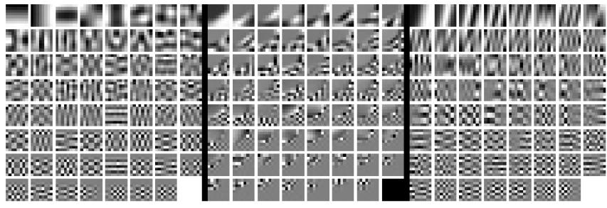
Figure 28.5: Illustration of the parameters learned by a GMM applied to image patches. Each of the 3 panels corresponds to a di!erent mixture component k. Within each panel, we show the eigenvectors (reshaped as images) of the covariance matrix “^k in decreasing order of eigenvalue. We see various kinds of patterns, including ones that look like the ones learned from PCA (see Figure 28.34), but also ones that look like edges and texture. From Figure 6 of [ZW11]. Used with kind permission of Daniel Zoran.

A more principled solution to the overlapping patch problem is to use a multiscale model, as proposed in [PE16]. Another approach, proposed in [FW21], uses Gibbs sampling to combine samples from overlapping patches. This approach has the additional advantage of computing posterior samples from p(x|y), which can look much better than the posterior mean or mode computed by optimization methods. (For example, if the corruption process removes the color from the latent image x to create a gray scale y, then the posterior MAP estimate of x will also be a gray scale image, whereas posterior samples will be color images.) See also Section 28.3.3.5 where we show how to extend the GMM model to a mixture of low rank Gaussians, which lets us directly model images instead of image patches.

28.2.4.1 Why does the method work?

To understand why such a simple model of image patches works so well, note that the log prior for a single latent image patch xⁱ using mixture component k can be written as follows:

\[\log p(\mathbf{z}\_i | c\_i = k) = \log \mathcal{N}(\mathbf{z}\_i | \mathbf{0}, \Sigma\_k) = -\mathbf{z}\_i^\mathsf{T} \Sigma\_k^{-1} \mathbf{z}\_i + a\_k \tag{28.21}\]

where a^k is a constant that depends on k but is independent of xi. Let “^k = Vk#kV^{T k} be an eigendecomposition of”k, where ωk,d is the d’th eigenvalue of “k, and vk,d is the d’th eigenvector. Then we can rewrite the above as follows:

\[\log p(\mathbf{z}\_i | c\_i = k) = -\sum\_{d=1}^{D} \frac{1}{\lambda\_{k,d}} (\mathbf{v}\_{k,d}^T \mathbf{z}\_i)^2 + a\_k \tag{28.22}\]

Thus we see that the eigenvectors are acting like templates. Each mixture component has a di!erent set of templates, each with their own weight (eigenvalue), as illustrated in Figure 28.5. By mixing these together, we get a powerful model for the statistics of natural image patches. (See [ZW12] for more analysis of why this simple model works so well, based on the “dead leaves” model of image formation.)

28.2.4.2 Speeding up inference using discriminative models

Although simple and e!ective, computing f(y) = argmax^x p(x|y) for each image patch can be slow if the image is large. However, every time we solve this problem, we can store the result, and build up a dataset of (y, f(y)) pairs. We can then train an amortized inference network (Section 10.1.5) to learn this y ↔︎ f(y) mapping, to speed up future inferences, as proposed in [RW15]. (See also [Par+19] for further speedup tricks.)

An alternative approach is to dispense with the generative model, and to train on an artificially created dataset of the form (y, x), where x is a clean natural image, and y = C(x) is an artificial corruption of it. We can then train a discriminative model ˆf(y) directly from (y, x) pairs. This technique works very well (see e.g., [Luc+18]), but is limited by the form of corruptions C it is trained on. This means we need to train a di!erent network for every linear operator W, and sometimes even for every di!erent noise level ς².

28.2.4.3 Blind inverse problems

In the discussion above, we assumed the forwards model had the form ^p(y|x, ^ε) = ^N (y|Wx, ^ς2I), where W is known. If W is not known, then computing p(x|y) is known as a blind inverse problem.

Such problems are much harder to solve. One approach is to estimate the parameters of the forwards model, W, and the latent image, x, using an EM-like method from a set of images coming from the same likelihood function. That is, we alternate between estimating ^{xˆ =} argmax^{x p}(x|y,W^ˆ ) in the E step, and estimating ^{Wˆ =} argmax^{W p}(y|xˆ,W) in the M step. Some encouraging results of this approach are shown in [Ani+18]. (They use a GAN prior for p(x) rather than a GMM.)

In cases where we get two independent noisy samples, y¹ and y2, generated from the same underlying image x, then we can avoid having to explicitly learn an image prior p(x), and can instead directly learn an estimator for the posterior mode, f(y) = argmax^x p(x|y), without needing access to the latent image x, by exploiting a form of cycle consistency; see [XC19] for details.

28.2.5 Using mixture models for classification problems

It is possible to use mixture models to define the class-conditional density p(x|y = c) in a generative classifier. We can then derive the class posterior using Bayes’ rule:

\[p(y=c|\mathbf{z}) = \frac{p(y=c)p(\mathbf{z}|y=c)}{\sum\_{c'} p(y=c)p(\mathbf{z}|y=c)} = \frac{p(y=c)p(\mathbf{z}|y=c)}{Z} \tag{28.23}\]

where p(y = c) = φ^c is the prior on class label c, Z is the normalization constant, and the form of p(x|y = c) depends on the kind of data we have. For real-valued features, it is common to use a GMM:

\[p(\mathbf{z}|y=c) = \sum\_{k=1}^{K\_c} \alpha\_{c,k} \mathcal{N}(\mathbf{z}|\mu\_{c,k}, \mathbf{\Sigma}\_{c,k}) \tag{28.24}\]

Using a generative model to perform classification can be useful when we have missing data, since we can compute ^p(x^v|^{y = c}) = * ^{xm p}(x^m, ^xv|^y = ^c) to compute the marginal likelihood of the visible features x^v. It is also useful for semi-supervised learning, since we can optimize the model to fit * ⁿ log p(x^l n, y^{l n}) on the labeled data and * ⁿ log p(x^{u n}) on the unlabeled data.

28.2.5.1 Hybrid generative/discriminative training

Unfortunately the classification accuracy of generative models of the form p(x, y) can be much worse than discriminative (conditional) models of the form p(y|x), since the latter are directly optimized to predict the labels given the features, and don’t “waste” capacity on modeling irrelevant details of the inputs. (For a more in-depth discussion of generative vs discriminative classifiers, see e.g., [Mur22, Sec 9.4].)

Fortunately it is possible to train generative models in a discriminative fashion, which can close the performance gap with conditional models, while maintaining the advantages of generative models. In particular, we can optimize the following hybrid objective, proposed in [BT04; Rot+18]:

\[\mathcal{L}(\boldsymbol{\theta}) = -\lambda \underbrace{\sum\_{n=1}^{N} \log p(\boldsymbol{x}\_n, y\_n|\boldsymbol{\theta})}\_{\mathcal{L}\_{\text{gen}}(\boldsymbol{\theta})} - (1 - \lambda) \underbrace{\sum\_{n=1}^{N} \log p(y\_n|\boldsymbol{x}\_n, \boldsymbol{\theta})}\_{\mathcal{L}\_{\text{div}}(\boldsymbol{\theta})} \tag{28.25}\]

where 0 ≃ ω ≃ 1 controls the tradeo! between generative and discriminative modeling.

If we have unlabeled data, we can modify the generative loss as shown below:

\[\mathcal{L}\_{\text{gen}}(\boldsymbol{\theta}) = \kappa \sum\_{n=1}^{N^{l}} \log p(\mathbf{z}\_{n}^{l}, y\_{n}^{l} | \boldsymbol{\theta}) + (1 - \kappa) \sum\_{n=1}^{N^{u}} \log p(\mathbf{z}\_{n}^{u} | \boldsymbol{\theta}) \tag{28.26}\]

Here we have introduced an extra trade-o! parameter 0 ≃ ⇁ ≃ 1 to prevent the unlabeled data from overwhelming the labeled data (if N^u ⇑ Nl), as proposed in [Nig+00].

An alternative to changing the objective function is to change the model itself, so that we parameterize the joint using ^p(x, y) = ^p(y|x, ^ε)p(x|ε˜), and then define di!erent kinds of joint priors p(ε, ε˜); see [LBM06; BL07a] for details.

28.2.5.2 Optimization issues

To optimize the loss, we need to reparameterize the model into unconstrained form. For the class prior, we can use φ1:^C = softmax(φ˜1:^C ), and optimize wrt the logits φ˜1:^C . Similarly for the mixture weights ↽c,1:K. The means µck are already unconstrained. For the covariance matrices, we will use a diagonal plus low-rank representation, to reduce the number of parameters:

\[\mathbf{\dot{\Sigma}}\_{c,k} = \text{diag}(\mathbf{d}\_{c,k}) + \mathbf{S}\_{c,k} \mathbf{S}\_{c,k}^{\sf T} \tag{28.27}\]

where Sc,k is an unconstrained D ↗ R matrix, where R ↖ D is the rank of the approximation. (For numerical stability, we usually add ϖI to the above expression, to ensure “c,k is positive definite for all parameter settings.) To ensure positivity of the diagonal term, we can use the softplus transform, dc,k = log(1 + exp( ˜ dc,k)), and optimize wrt the ˜ dc,k terms.

28.2.5.3 Numerical issues

To compute the class conditional log likelihood, ▷^c = log p(x|y = c), we can use the log-sum-exp trick to avoid numerical underflow. Define ↽˜ck = log ↽ck, and ▷ck = log N (x|µck, “ck) and let

εck = ˜↽ck + ▷ck. Then we have

\[\ell\_c = \log p(\mathbf{z}|y=c) = \log \left(\sum\_k p(z\_k|y=c)p(\mathbf{z}|y=c, z=k)\right) = \log \left(\sum\_k \alpha\_{ck} \mathcal{N}(\mathbf{z}|\boldsymbol{\mu}\_{ck}, \boldsymbol{\Sigma}\_{ck})\right) \tag{28.28}\]

\[\mathcal{L} = \log\left(\sum\_{k} e^{\beta\_{ck}}\right) = \log\left(e^M \sum\_{k} e^{\beta\_{ck} - M}\right) = M + \log\left(\sum\_{k} e^{\beta'\_{ck}}\right) \stackrel{\Delta}{=} \log\text{sumexp}(\{\beta\_{ck}\}\_k) \tag{28.29}\]

where M = max^k εck and ε^→ ck = ^εck ^{↓ M}. Note that we can safely compute each ^eϑ↑ ck without underflow.

We can use a similar method to compute the posterior over classes. We have

\[p(y=c|\mathbf{x}) = \frac{\pi\_c e^{l\_c}}{Z} = \frac{\pi\_c e^{l\_c - L}}{e^{-L}Z} = \frac{\pi\_c e^{\tilde{l}\_c}}{\tilde{Z}} \tag{28.30}\]

where ^{L =} max^{c l}c, ˜l^{c = lc ↓ L}, and ^Z˜ ⁼ * ^c φce ˜l^c . This lets us combine the class prior probability φ^c with the scaled class conditional log likelihood ˜l^c to get the class posterior in a stable way. (We can also compute the log normalization constant, log p(x) = log Z = log(Z˜) + L.)

To compute a single Gaussian log density, ▷ck = log N (x|µck, “ck), we need to evaluate log det(”ck) and “^↑1 ck . To make this e”cient, we can use the matrix determinant lemma to compute

\[\det(\mathbf{A} + \mathbf{S}\mathbf{S}^{\mathsf{T}}) = \det(\mathbf{I} + \mathbf{S}^{\mathsf{T}}\mathbf{A}^{-1}\mathbf{S})\det(\mathbf{A})\tag{28.31}\]

where A = diag(d) + ϖI, and the matrix inversion lemma to compute

\[(\mathbf{A} + \mathbf{S} \mathbf{S}^{\mathsf{T}})^{-1} = \mathbf{A}^{-1} - \mathbf{A}^{-1} \mathbf{S} (\mathbf{I} + \mathbf{S}^{\mathsf{T}} \mathbf{A}^{-1} \mathbf{S})^{-1} \mathbf{S}^{\mathsf{T}} \mathbf{A}^{-1} \tag{28.32}\]

(See also the discussion of mixture of factor analyzers in Section 28.3.3.)

28.2.6 Unidentifiability

The parameters of a mixture model are unidentifiable, due to the label switching problem. To see this, consider fitting a GMM with 2 clusters (with parameters εˆ) to a dataset which is generated from the true distribution p^↔︎ which we assume is also a GMM with 2 clusters (with parameters ε↔︎). The MLE will converge to the estimated parameters ^εˆ which minimizes ^DKL & ^p(x|ε↔︎) ⇐ ^p(x|εˆ) ’ . However, there are 2 equally likely modes to the likelihood surface, (µˆ ¹ = µ^{↔︎ 1}, µˆ ² = µ^{↔︎ 2}) and (µˆ ² = µ^↔︎ 1, µˆ ¹ = µ^{↔︎ 2}), since the identify of the clusters is irrelevant. Hence computing the posterior mean of the cluster parameters µ^k from some Bayesian inference procedure is meaningless. Instead, [Ste00] proposes a decision theoretic approach, in which the action space allows the user to ask questions about the clustering assignment (or parameters) after performing a suitable permutation of the labels. See also [Pap16] for an R library that implements this and other related algorithms.

28.3 Factor analysis

In this section, we discuss a simple latent factor model in which the prior p(z) is Gaussian, and the likelihood p(x|z) is also Gaussian, using a linear decoder for the mean. This family includes many important special cases, such as PCA, as we discuss below. We also briefly discuss some simple extensions.

28.3.1 Factor analysis: the basics

Factor analysis corresponds to the following linear-Gaussian latent variable generative model:

\[p(\mathbf{z}) = \mathcal{N}(\mathbf{z}|\boldsymbol{\mu}\_0, \boldsymbol{\Sigma}\_0) \tag{28.33}\]

\[p(x|z, \theta) = N(x|\mathbf{W}z + \mu, \Psi) \tag{28.34}\]

where W is a D ↗ L matrix, known as the factor loading matrix, and $ is a diagonal D ↗ D covariance matrix.

28.3.1.1 FA as a Gaussian with low-rank plus diagonal covariance

FA can be thought of as a low-rank version of a Gaussian distribution. To see this, note that the induced marginal distribution p(x|ε) is a Gaussian (see Equation (2.129) for the derivation):

\[p(x|\theta) = \int \mathcal{N}(x|\mathbf{W}z + \mu, \Psi) \mathcal{N}(z|\mu\_0, \Sigma\_0) dz \tag{28.35}\]

\[= \mathcal{N}(x|\mathbf{W}\mu\_0 + \mu, \Psi + \mathbf{W}\Sigma\_0 \mathbf{W}^\top) \tag{28.36}\]

The first and second moments can be derived as follows:

\[\begin{aligned} \mathbb{E}\left[x\right] &= \mathbf{W}\mu\_0 + \mu\\ \text{Cov}\left[x\right] &= \mathbf{W}\text{Cov}\left[z\right]\mathbf{W}^\top + \Psi = \mathbf{W}\boldsymbol{\Sigma}\_0\mathbf{W}^\top + \Psi \end{aligned} \tag{28.37}\]

From this, we see that we can set µ⁰ = 0 without loss of generality, since we can always absorb Wµ⁰ into µ. Similarly, we can set “⁰ = I without loss of generality, since we can always absorb a correlated prior by using a new weight matrix, ^W˜ ^{= W}”^{↑ 1} 2 ⁰ , since then

\[\text{Cov}\left[\mathbf{z}\right] = \mathbf{W}\boldsymbol{\Sigma}\_0\mathbf{W}^\mathsf{T} + \boldsymbol{\Psi} = \dot{\mathbf{W}}\dot{\mathbf{W}}^\mathsf{T} + \boldsymbol{\Psi} \tag{28.38}\]

Finally, we see that we should restrict $ to be diagonal, otherwise we could set W˜ = 0, thus ignoring the latent factors, while still being able to model any covariance. After these simplifications we have the final model:

\[p(\mathbf{z}) = N(\mathbf{z}|\mathbf{0}, \mathbf{I})\tag{28.39}\]

\[p(x|\mathbf{z}) = \mathcal{N}(x|\mathbf{W}z + \mu, \Psi) \tag{28.40}\]

from which we get

\[p(x) = \mathcal{N}(x|\mu, \mathbf{W}\mathbf{W}^{\top} + \Psi) \tag{28.41}\]

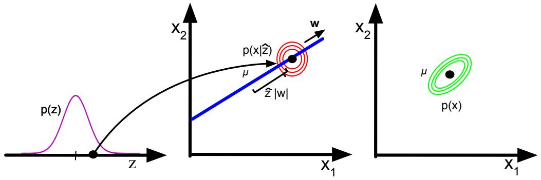
Figure 28.6: Illustration of the FA generative process, where we have L = 1 latent dimension generating ^D = 2 observed dimensions; we assume # ^{= ε2}I. The latent factor has value ^{z ↔︎ R}, sampled from ^p(z); this gets mapped to a 2d o!set ^{ε = z}w, where ^{w ↔︎ R2}, which gets added to ^µ to define a Gaussian ^p(x|z) = ^N (x|^{µ + ε}, ^ε2I). By integrating over ^z, we “slide” this circular Gaussian “spray can” along the principal component axis w, which induces elliptical Gaussian contours in x space centered on µ. Adapted from Figure 12.9 of [Bis06].

For example, suppose where L = 1, D = 2 and $ = ς²I. We illustrate the generative process in this case in Figure 28.6. We can think of this as taking an isotropic Gaussian “spray can”, representing the likelihood p(x|z), and “sliding it along” the 1d line defined by wz + µ as we vary the 1d latent prior z. This induces an elongated (and hence correlated) Gaussian in 2d. That is, the induced distribution has the form ^p(x) = ^N (x|µ, ww^{T + ς2}I).

In general, FA approximates the covariance matrix of the visible vector using a low-rank decomposition:

\[\mathbf{C} = \text{Cov}\left[x\right] = \mathbf{W}\mathbf{W}^{\mathsf{T}} + \Psi \tag{28.42}\]

This only uses O(LD) parameters, which allows a flexible compromise between a full covariance Gaussian, with O(D²) parameters, and a diagonal covariance, with O(D) parameters.

28.3.1.2 Computing the posterior

We can compute the posterior over the latent codes, p(z|x), using Bayes’ rule for Gaussians. In particular, from Equation (2.121), we have

\[p(\mathbf{z}|\mathbf{x}) = \mathcal{N}(\mathbf{z}|\boldsymbol{\mu}\_{z|x}, \boldsymbol{\Sigma}\_{z|x}) \tag{28.43}\]

\[\boldsymbol{\Sigma}\_{z|x} = \left(\mathbf{I} + \mathbf{W}^{\mathsf{T}} \boldsymbol{\Psi}^{-1} \mathbf{W}\right)^{-1} = \mathbf{I} - \mathbf{W}^{\mathsf{T}} (\mathbf{W} \mathbf{W}^{\mathsf{T}} + \boldsymbol{\Psi})^{-1} \mathbf{W} \tag{28.44}\]

\[ \mu\_{z|x} = \Sigma\_{z|x} [\mathbf{W}^\mathsf{T} \Psi^{-1}(x - \mu)] = \mathbf{W}^\mathsf{T} (\mathbf{W} \mathbf{W}^\mathsf{T} + \Psi)^{-1} (x - \mu) \tag{28.45} \]

We can avoid inverting the ^D ↗ ^D matrix ^{C =} WW^{T +} $ by using the matrix inversion lemma:

\[\mathbf{C}^{-1} = (\mathbf{W}\mathbf{W}^{\mathsf{T}} + \boldsymbol{\Psi})^{-1} \tag{28.46}\]

\[=\Psi^{-1} - \Psi^{-1}\mathbf{W}\underbrace{(\mathbf{I} + \mathbf{W}^{\mathrm{T}}\Psi^{-1}\mathbf{W})^{-1}}\_{\mathbf{L}^{-1}}\mathbf{W}^{\mathrm{T}}\Psi^{-1} \tag{28.47}\]

where ^{L = I + WT}$^↑1W is ^L ↗ ^L.

28.3.1.3 Computing the likelihood

In this section, we discuss how to e”ciently compute the log (marginal) likelihood, which is given by

\[\log p(\mathbf{z}|\boldsymbol{\mu}, \mathbf{C}) = -\frac{1}{2} \left[ D \log(2\pi) + \log \det(\mathbf{C}) + \hat{\mathbf{z}}^{\mathsf{T}} \mathbf{C}^{-1} \hat{\mathbf{z}} \right] \tag{28.48}\]

where ^x˜ = ^{x ↓ µ}, and C = WW^T + $. Using Equation (28.47), the Mahalanobis distance can be computed using

\[ \bar{x}^{\mathsf{T}}\mathbf{C}^{-1}\bar{x} = \bar{x}^{\mathsf{T}} \left[ \Psi^{-1}\bar{x} - \Psi^{-1}\mathbf{W}\mathbf{L}^{-1}(\mathbf{W}^{\mathsf{T}}\Psi^{-1}\bar{x}) \right] \tag{28.49} \]

which takes O(L³ + LD) to compute. From the matrix determinant lemma, the log determinant is given by

\[\log \det(\mathbf{C}) = \log \det(\mathbf{L}) + \log \det(\Psi) \tag{28.50}\]

which takes O(L³ + D) to compute. (See also Section 28.2.5, where we discuss fitting low-rank GMM classifiers discriminatively, which requires similar computations.)

28.3.1.4 Model fitting using EM

We can compute the MLE for the FA model either by performing gradient ascent on the log likelihood in Equation (28.48), or by using the EM algorithm [RT82; GH96b]. The latter can converge faster, and automatically satisfies positivity constraints on $. We give the details below, assuming that the observed data is standardized, so µ = 0 for notational simplicity.

In the E step, we compute the following expected su”cient statistics:

\[\mathbf{E}\_{\mathbf{z},\mathbf{z}} = \sum\_{n=1}^{N} \mathbf{z}\_n \mathbb{E}\left[\mathbf{z}|\mathbf{z}\_n\right]^\top \tag{28.51}\]

\[\mathbf{E}\_{\mathbf{z},\mathbf{z}} = \sum\_{n=1}^{N} \mathbb{E}\left[\mathbf{z}\mathbf{z}^{\mathsf{T}}|\mathbf{x}\_{n}\right] \tag{28.52}\]

\[\mathbf{E}\_{x,x} = \sum\_{n=1}^{N} x\_n \mathbf{x}\_n^\top \tag{28.53}\]

where

\[\mathbf{E}\left[\mathbf{z}|\mathbf{x}\right] = \mathbf{B}\mathbf{z} \tag{28.54}\]

\[\mathbb{E}\left[\mathbf{z}\mathbf{z}^{\mathsf{T}}|\mathbf{z}\right] = \text{Cov}\left[\mathbf{z}|\mathbf{z}\right] + \mathbb{E}\left[\mathbf{z}|\mathbf{z}\right]\mathbb{E}\left[\mathbf{z}|\mathbf{z}\right]^{\mathsf{T}} = \mathbf{I} - \mathbf{B}\mathbf{W} + \mathbf{B}\mathbf{z}\mathbf{z}^{\mathsf{T}}\mathbf{B}^{\mathsf{T}}\tag{28.55}\]

B ↫ W^T($ + WW^T) ^↑1 = W^TC↑¹ (28.56)

In the M step, we have

\[\mathbf{W}^{\text{new}} = \mathbf{E}\_{\mathbf{z},\mathbf{z}} \mathbf{E}\_{\mathbf{z},\mathbf{z}}^{-1} \tag{28.57}\]

\[\Psi^{\text{new}} = \frac{1}{N} \text{diag} \left( \mathbf{E}\_{\mathbf{z},\mathbf{z}} - \mathbf{W}^{\text{new}} \mathbf{E}\_{\mathbf{z},\mathbf{z}}^{\text{T}} \right) \tag{28.58}\]

28.3.1.5 Handling missing data

We can also perform posterior inference in the presence of missing data (if we make the missing at random assumption — see Section 3.11 for discussion). In particular, let us partition x = (x1, x2), W = [W1,W2], and µ = [µ1, µ2], and suppose x² is missing (unknown). From Supplementary Section 2.1.1, we have

\[p(\mathbf{z}|\mathbf{x}\_1) = N(\mathbf{z}|\boldsymbol{\mu}\_{z|1}, \boldsymbol{\Sigma}\_{z|1}) \tag{28.59}\]

\[ \boldsymbol{\Sigma}\_{z|1}^{-1} = \mathbf{I} + \mathbf{W}\_1^T \boldsymbol{\Sigma}\_{11}^{-1} \mathbf{W}\_1 \tag{28.60} \]

\[ \mu\_{z|1} = \Sigma\_{z|1} [\mathbf{W}\_1^\mathsf{T} \Sigma\_{11}^{-1} \left(x\_1 - \mu\_1\right)] \tag{28.61} \]

where “¹¹ is the top left block of $.

We can modify the EM algorithm to fit the model in the presence of missing data in the obvious way.

28.3.1.6 Unidentifiability of the parameters

The parameters of a FA model are unidentifiable. To see this, consider a model with weights W and observation covariance $. We have

\[\text{Cov}\left[\boldsymbol{x}\right] = \mathbf{W} \mathbb{E}\left[\boldsymbol{z}\boldsymbol{z}^{\mathsf{T}}\right] \mathbf{W}^{\mathsf{T}} + \mathbb{E}\left[\boldsymbol{\epsilon}\boldsymbol{\epsilon}^{\mathsf{T}}\right] = \mathbf{W}\mathbf{W}^{\mathsf{T}} + \boldsymbol{\Psi} \tag{28.62}\]

where ^{ς ↑ N} (0, $) is the observation noise. Now consider a di!erent model with weights ^W˜ ⁼ WR, where R is an arbitrary orthogonal rotation matrix, satisfying RR^T = I. This has the same likelihood, since

\[\text{Cov}\left[\mathbf{z}\right] = \check{\mathbf{W}} \mathbb{E}\left[\mathbf{z}\mathbf{z}^{\mathsf{T}}\right] \check{\mathbf{W}}^{\mathsf{T}} + \mathbb{E}\left[\epsilon\boldsymbol{\epsilon}^{\mathsf{T}}\right] = \mathbf{W} \mathbf{R} \mathbf{R}^{\mathsf{T}} \mathbf{W}^{\mathsf{T}} + \boldsymbol{\Psi} = \mathbf{W} \mathbf{W}^{\mathsf{T}} + \boldsymbol{\Psi} \tag{28.63}\]

Geometrically, multiplying W by an orthogonal matrix is like rotating z before generating x; but since z is drawn from an isotropic Gaussian, this makes no di!erence to the likelihood. Consequently, we cannot uniquely identify W, and therefore cannot uniquely identify the latent factors, either. This is called the “factor rotations problem” (see e.g., [Dar80]).

To break this symmetry, several solutions can be used, as we discuss below.

• Forcing W to have orthogonal columns.. In (P)PCA, we force W to have orthogonal columns. and to sort the dimensions in order of decreasing eigenvalue (of WWT). However, this still does not ensure identifiability, since we can always multiply W by another orthogonal matrix without changing the likelihood.
• Forcing W to be lower triangular. One way to resolve permutation unidentifiability, which is popular in the Bayesian community (e.g., [LW04]), is to ensure that the first visible feature is only generated by the first latent factor, the second visible feature is only generated by the first

two latent factors, and so on. For example, if L = 3 and D = 4, the correspond factor loading matrix is given by

\[\mathbf{W} = \begin{pmatrix} w\_{11} & 0 & 0 \\ w\_{21} & w\_{22} & 0 \\ w\_{31} & w\_{32} & w\_{33} \\ w\_{41} & w\_{42} & w\_{43} \end{pmatrix} \tag{28.64}\]

We also require that wkk > 0 for k =1: L. The total number of parameters in this constrained matrix is D + DL ↓ L(L ↓ 1)/2, which is equal to the number of uniquely identifiable parameters in FA (excluding the mean).1 The disadvantage of this method is that the first L visible variables, known as the founder variables, a!ect the interpretation of the latent factors, and so must be chosen carefully.

• Sparsity promoting priors on the weights. Instead of pre-specifying which entries in W are zero, we can encourage the entries to be zero, using ▷¹ regularization [ZHT06], ARD [Bis99; AB08], or spike-and-slab priors [Rat+09]. This is called sparse factor analysis. This does not necessarily ensure a unique MAP estimate, but it does encourage interpretable solutions.
• Choosing an informative rotation matrix. There are a variety of heuristic methods that try to find rotation matrices R which can be used to modify W (and hence the latent factors) so as to try to increase the interpretability, typically by encouraging them to be (approximately) sparse. One popular method is known as varimax [Kai58].
• Use of non-Gaussian priors for the latent factors. If we replace the prior on the latent variables, p(z), with a non-Gaussian distribution, we can sometimes uniquely identify W, as well as the latent factors. See e.g., [KKH20] for details.

28.3.2 Probabilistic PCA

In this section, we consider a special case of the factor analysis model in which W has orthogonal columns and $ = ^ς2I, so ^p(x) = ^N (x|µ, C) where C = WW^T + ^ς2I. This model is called probabilistic principal components analysis (PPCA) [TB99], or sensible PCA [Row97].

The advantage of PPCA over factor analysis is that the MLE has a closed form solution, as we show in Section 28.3.2.2. The advantage of PPCA over non-probabilistic PCA is that the model defines a proper likelihood function, which makes it easier to extend in various ways e.g., by creating mixtures of PPCA models (see Section 28.3.3).

28.3.2.1 Derivation of the MLE

The log likelihood for PPCA is given by

\[\log p(\mathbf{X}|\mu, \mathbf{W}, \sigma^2) = -\frac{ND}{2}\log(2\pi) - \frac{N}{2}\log|\mathbf{C}| - \frac{1}{2}\sum\_{n=1}^{N}(x\_n - \mu)^\top \mathbf{C}^{-1}(x\_n - \mu) \tag{28.65}\]

^1. We get D parameters for ! and DL for W, but we need to remove L(L ↔︎ 1)/2 degrees of freedom coming from R, since that is the dimensionality of the space of orthogonal matrices of size L → L. To see this, note that there are L ↔︎ 1 free parameters in R in the first column (since the column vector must be normalized to unit length), there are L ↔︎ 2 free parameters in the second column (which must be orthogonal to the first), and so on.

The MLE for µ is x. Plugging in gives

\[\log p(\mathbf{X}|\mu, \mathbf{W}, \sigma^2) = -\frac{N}{2} \left[ D \log(2\pi) + \log|\mathbf{C}| + \text{tr}(\mathbf{C}^{-1}\mathbf{S}) \right] \tag{28.66}\]

where S = ¹ N *^{N n}=1(xⁿ ↓ x)(xⁿ ↓ x) ^T is the empirical covariance matrix.

In [TB99; Row97] they show that the maximum of this objective must satisfy

\[\hat{\mathbf{W}} = \mathbf{U}\_L (\mathbf{A}\_L - \sigma^2 \mathbf{I})^{\frac{1}{2}} \mathbf{R} \tag{28.67}\]

where U^L is a D ↗ L matrix whose columns are given by the L eigenvectors of S with largest eigenvalues, #^L is the L ↗ L diagonal matrix of corresponding eigenvalues, and R is an arbitrary L ↗ L orthogonal matrix, which (WLOG) we can take to be R = I.

If we plug in the MLE for W, we find the covariance for the predictive distribution to be

\[\mathbf{C} = \mathbf{W}\mathbf{W}^{\mathsf{T}} + \sigma^2 \mathbf{I} = \mathbf{U}\_L(\mathbf{A}\_L - \sigma^2 \mathbf{I})\mathbf{U}\_L^{\mathsf{T}} + \sigma^2 \mathbf{I} \tag{28.68}\]

The MLE for the observation variance is

\[ \sigma^2 = \frac{1}{D - L} \sum\_{i=L+1}^{D} \lambda\_i \tag{28.69} \]

which is the average distortion associated with the discarded dimensions. If L = D, then the estimated noise is 0, since the model collapses to z = x.

28.3.2.2 PCA is recovered in the noise-free limit

In the noise-free limit, where ς² = 0, we see that the MLE (for R = I) is

\[ \hat{\mathbf{W}} = \mathbf{U}\_L \boldsymbol{\Lambda}\_L^{\frac{1}{2}} \tag{28.70} \]

so

\[\mathbf{\hat{C}} = \mathbf{\hat{W}}\mathbf{\hat{W}}^{\mathrm{T}} = \mathbf{U}\_{L}\boldsymbol{\Lambda}\_{L}^{\frac{1}{2}}\boldsymbol{\Lambda}\_{L}^{\frac{1}{2}}\mathbf{U}\_{L}^{\mathrm{T}} = \mathbf{S}\_{L} \tag{28.71}\]

where S^L is the rank L approximation to S. This is the same as standard PCA.

28.3.2.3 Computing the posterior

To use PPCA as an alternative to PCA, we need to compute the posterior mean E [z|x], which is the equivalent of the PCA encoder model. Using the factor analysis results from Section 28.3.1.2, we have

\[p(\mathbf{z}|\mathbf{z}) = \mathcal{N}(\mathbf{z}|\sigma^{-2}\Sigma\mathbf{W}^{\mathrm{T}}(\mathbf{z}-\boldsymbol{\mu}), \boldsymbol{\Sigma}) \tag{28.72}\]

where

\[\mathbf{\dot{\Sigma}}^{-1} = \mathbf{I} + \sigma^{-2} \mathbf{W}^{\mathsf{T}} \mathbf{W} = \frac{1}{\sigma^2} (\underbrace{\sigma^2 \mathbf{I} + \mathbf{W}^{\mathsf{T}} \mathbf{W}}\_{\mathbf{M}}) \tag{28.73}\]

Hence

\[p(\mathbf{z}|\mathbf{x}) = \mathcal{N}(\mathbf{z}|\mathbf{M}^{-1}\mathbf{W}^{\mathrm{T}}(\mathbf{z}-\boldsymbol{\mu}), \sigma^{2}\mathbf{M}^{-1})\tag{28.74}\]

In the ς² = 0 limit, we have M = WTW and so

\[\mathbb{E}\left[z|x\right] = (\mathbf{W}^{\mathsf{T}}\mathbf{W})^{-1}\mathbf{W}^{\mathsf{T}}(x-\overline{x})\tag{28.75}\]

This is the orthogonal projection of the data into the latent space, as in standard PCA.

28.3.2.4 Model fitting using EM

In Section 28.3.2.2, we showed how to fit the PCA model using an eigenvector method. We can also use EM, by leveraging the probabilistic formulation of PPCA in the zero noise limit, ς² = 0, as shown by [Row97].

In particular, let Z˜ ^{= ZT} be an ^L ↗ ^N matrix storing the posterior means (low-dimensional representations) along its columns. Similarly, let x˜ⁿ = xⁿ ↓ µˆ be the centered examples stored along the columns of X˜ . From Equation (28.75), when ς² = 0, we have

\[\tilde{\mathbf{Z}} = (\mathbf{W}^{\mathrm{T}} \mathbf{W})^{-1} \mathbf{W}^{\mathrm{T}} \tilde{\mathbf{X}} \tag{28.76}\]

This constitutes the E step. Notice that this is just an orthogonal projection of the data.

From Equation (28.57), the M step is given by

\[\hat{\mathbf{W}} = \left[\sum\_{n} \tilde{\boldsymbol{x}}\_{n} \mathbb{E}\left[\boldsymbol{z}\_{n} | \tilde{\boldsymbol{x}}\_{n}\right]^{\mathsf{T}}\right] \left[\sum\_{n} \mathbb{E}\left[\boldsymbol{z}\_{n} | \tilde{\boldsymbol{x}}\_{n}\right] \mathbb{E}\left[\boldsymbol{z}\_{n} | \tilde{\boldsymbol{x}}\_{n}\right]^{\mathsf{T}}\right]^{-1} \tag{28.77}\]

where we exploited the fact that ” = Cov [z|x˜]=0^I when ^ς2 = 0.

In summary, here is the entire algorithm:

\[\tilde{\mathbf{Z}} = (\mathbf{W}^{\mathsf{T}} \mathbf{W})^{-1} \mathbf{W}^{\mathsf{T}} \tilde{\mathbf{X}} \text{ (E step)}\tag{28.78}\]

\[\mathbf{W} = \tilde{\mathbf{X}} \tilde{\mathbf{Z}}^{\mathsf{T}} (\tilde{\mathbf{Z}} \tilde{\mathbf{Z}}^{\mathsf{T}})^{-1} \text{ (M step)} \tag{28.79}\]

It is worth comparing this expression to the MLE for multi-output linear regression, which has the form W = (* ⁿ ynx^T n)(* ⁿ xnx^{T n})↑1. Thus we see that the M step is like linear regression where we replace the observed inputs by the expected values of the latent variables.

[TB99] showed that the only stable fixed point of the EM algorithm is the globally optimal solution. That is, the EM algorithm converges to a solution where W spans the same linear subspace as that defined by the first L eigenvectors of S. However, if we want W to be orthogonal, and to contain the eigenvectors in descending order of eigenvalue, we have to orthogonalize the resulting matrix (which can be done quite cheaply). Alternatively, we can modify EM to give the principal basis directly [AO03].

28.3.3 Mixture of factor analyzers

The factor analysis model (Section 28.3.1) assumes the observed data can be modeled as arising from a linear mapping from a low-dimensional set of Gaussian factors. One way to relax this assumption is

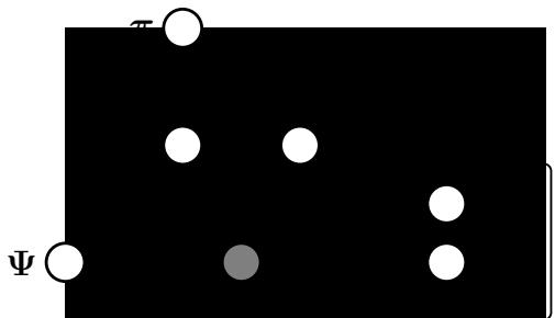
Figure 28.7: Mixture of factor analyzers as a PGM.

to assume the model is only locally linear, so the overall model becomes a (weighted) combination of FA models; this is called a mixture of factor analyzers or MFA [GH96b]. The overall model for the data is a mixture of linear manifolds, which can be used to approximate an overall curved manifold. Another way to think of this model is a mixture of Gaussians, where each mixture component has a covariance matrix which is diagonal plus low-rank.

28.3.3.1 Model definition

The generative story is as follows. First we sample a discrete latent indicator mⁿ → {1,…,K} from discrete distribution Cat(·|↼) to specify which subspace (cluster) we should use to generate the data. If mⁿ = k, we sample zⁿ from a Gaussian prior and pass it through the W^k matrix, where W^k maps from the L-dimensional subspace to the D-dimensional visible space.2 Finally we add Gaussian observation noise sampled from N (µk, $). Thus the model is as follows:

\[p(\mathbf{z}\_n | \mathbf{z}\_n, m\_n = k, \boldsymbol{\theta}) = \mathcal{N}(\boldsymbol{x}\_n | \boldsymbol{\mu}\_k + \mathbf{W}\_k \mathbf{z}\_n, \boldsymbol{\Psi}) \tag{28.80}\]

\[p(\mathbf{z}\_n|\boldsymbol{\theta}) = \mathcal{N}(\mathbf{z}\_n|\mathbf{0}, \mathbf{I})\tag{28.81}\]

\[p(m\_n|\theta) = \text{Cat}(m\_n|\pi) \tag{28.82}\]

The corresponding distribution in the visible space is given by

\[p(\mathbf{z}|\boldsymbol{\theta}) = \sum\_{k} p(m=k) \int p(\mathbf{z}|\boldsymbol{c}) p(\mathbf{z}|\boldsymbol{z}, m) \, d\mathbf{z} \tag{28.83}\]

\[\sigma\_k = \sum\_k \pi\_k \int \mathcal{N}(\mathbf{z}|\mathbf{0}, \mathbf{I}) \mathcal{N}(\mathbf{z}|\mathbf{W}\_k \mathbf{z} + \boldsymbol{\mu}\_k, \boldsymbol{\Psi}) \, d\mathbf{z} \tag{28.84}\]

\[=\sum\_{k}\pi\_{k}\mathcal{N}(x|\mu\_{k},\Psi+\mathbf{W}\_{k}\mathbf{W}\_{k}^{\mathrm{T}})\tag{28.85}\]

In the special case that $ = ς²I, we get a mixture of PPCA models. See Figure 28.8 for an example of the method applied to some 2d data.

^2. If we allow zn to depend on mn, we can let each subspace have a di!erent dimensionality, as suggested in [KS15].

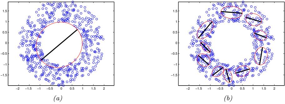
Figure 28.8: Mixture of PPCA models fit to a 2d dataset, using L = 1 latent dimensions. (a) K = 1 mixture components. (b) K = 10 mixture components. Generated by mix\_ppca\_demo.ipynb.

We can think of this as a low-rank version of a mixture of Gaussians. In particular, this model needs O(KLD) parameters instead of the O(KD²) parameters needed for a mixture of full covariance Gaussians. This can reduce overfitting.

28.3.3.2 Model fitting using EM

We can fit this model using EM, extending the results of Section 28.3.1.4 (see [GH96b] for the derivation, and [ZY08] for a faster ECM version). In the E step, we compute the posterior responsibility of cluster j for datapoint i using

\[\tau\_{ij} \triangleq p(m\_i = j | \boldsymbol{x}\_i, \boldsymbol{\theta}) \propto \pi\_j \mathcal{N}(\boldsymbol{x}\_i | \boldsymbol{\mu}\_j, \mathbf{W}\_j \mathbf{W}\_j^\mathsf{T} + \boldsymbol{\Psi}) \tag{28.86}\]

We also compute the following expected su”cient statistics, where we define w^j = I(m = j) and B^j = W^{T j} ($ + WjW^{T j} )↑¹:

\[\mathbb{E}\left[w\_j \mathbf{z} | \mathbf{z}\_i\right] = \mathbb{E}\left[w\_j | \mathbf{z}\_i\right] \mathbb{E}\left[\mathbf{z} | w\_j, \mathbf{z}\_i\right] = r\_{ij} \mathbf{B}\_j(\mathbf{z}\_i - \boldsymbol{\mu}\_j) \tag{28.87}\]

\[\mathbb{E}\left[w\_{j}\mathbf{z}\mathbf{z}^{\mathsf{T}}|\mathbf{z}\_{i}\right] = \mathbb{E}\left[w\_{j}|\mathbf{z}\_{i}\right]\mathbb{E}\left[\mathbf{z}\mathbf{z}^{\mathsf{T}}|w\_{j},\mathbf{z}\_{i}\right] = r\_{ij}(\mathbf{I}-\mathbf{B}\_{j}\mathbf{W}\_{j}+\mathbf{B}\_{j}(\mathbf{z}-\boldsymbol{\mu}\_{j})(\mathbf{z}-\boldsymbol{\mu}\_{j})^{\mathsf{T}}\mathbf{B}\_{j}^{\mathsf{T}}) \tag{28.88}\]

In the M step, we compute the following parameter update for the augmented factor loading matrix:

\[\mathbb{E}\left[\mathbf{W}\_{j}^{\text{new}}\,\mu\_{j}^{\text{new}}\right] \stackrel{\Delta}{=} \tilde{\mathbf{W}}\_{j}^{\text{new}} = \left(\sum\_{i} r\_{ij} \boldsymbol{x}\_{i} \mathbb{E}\left[\tilde{\mathbf{z}} \, | \boldsymbol{x}\_{i}, \boldsymbol{w}\_{j}\right]^{\mathsf{T}}\right) \left(\sum\_{i} r\_{ij} \mathbb{E}\left[\tilde{\mathbf{z}} \, \tilde{\mathbf{z}}^{\mathsf{T}} \, | \boldsymbol{x}\_{i}, \boldsymbol{w}\_{j}\right]\right)^{-1} \tag{28.89}\]

where z˜ = [z; 1],

\[\mathbb{E}\left[\bar{\mathbf{z}}|x\_i, w\_j\right] = \begin{pmatrix} \mathbb{E}\left[\mathbf{z}|x\_i, w\_j\right] \\ 1 \end{pmatrix} \tag{28.90}\]

\[\mathbb{E}\left[\bar{\mathbf{z}}\bar{\mathbf{z}}^{\mathsf{T}}|\boldsymbol{x}\_{i},\boldsymbol{w}\_{j}\right] = \begin{pmatrix} \mathbb{E}\left[\bar{\mathbf{z}}\bar{\mathbf{z}}^{\mathsf{T}}|\boldsymbol{x}\_{i},\boldsymbol{w}\_{j}\right] & \mathbb{E}\left[\bar{\mathbf{z}}|\boldsymbol{x}\_{i},\boldsymbol{w}\_{j}\right] \\ \mathbb{E}\left[\bar{\mathbf{z}}|\boldsymbol{x}\_{i},\boldsymbol{w}\_{j}\right]^{\mathsf{T}} & 1 \end{pmatrix} \tag{28.91}\]

The new covariance matrix is given by

\[\Psi^{\rm new} = \frac{1}{N} \text{diag} \left( \sum\_{ij} r\_{ij} (\mathbf{z}\_i - \mathbf{\bar{W}}\_j^{\rm new} \mathbb{E}\left[\bar{\mathbf{z}} | \mathbf{z}\_i, w\_j\right]) \mathbf{z}\_i^{\rm T} \right) \tag{28.92}\]

And the new mixing weights are given by

\[ \pi\_j^{\text{new}} = \frac{1}{N} \sum\_{i=1}^{N} r\_{ij} \tag{28.93} \]

28.3.3.3 Model fitting using SGD

We can also fit mixture models using SGD, as shown in [RW18]. This idea can be combined with an inference network (see Section 10.1.5) to e”ciently approximate the posterior over the latent variables. [Zon+18] use this approach to jointly learn a GMM applied to a deep autoencoder to provide a nonlinear extension of MFA; they show good results on anomaly detection.

28.3.3.4 Model selection

To choose the number of mixture components K, and the number of latent dimensions L, we can use discrete search combined with objectives such as the marginal likelihood or validation likelihood. However, we can also use numerical optimization methods to optimize L, which can be faster. We initially assume that N^c is known. To estimate L, we set the model to its maximal size, and then use a technique called automatic relevance determination or ARD to automatically prune out irrelevant weights (see Section 15.2.8). This can be implemented using variational Bayes EM (Section 10.3.5); for details, see [Bis99; GB00].

Figure 28.9 illustrates this approach applied to a mixture of FA models fit to a small synthetic dataset. The figures visualize the weight matrices for each cluster, using Hinton diagrams, where where the size of the square is proportional to the value of the entry in the matrix. We see that many of them are sparse. Figure 28.10 shows that the degree of sparsity depends on the amount of training data, in accord with the Bayesian Occam’s razor. In particular, when the sample size is small, the method automatically prefers simpler models, but as the sample size gets su”ciently large, the method converges on the “correct” solution, which is one with 6 subspaces of dimensionality 1, 2, 2, 3, 4 and 7.

Although the ARD method can estimate the number of latent dimensions L, it still needs to perform discrete search over the number of mixture components Nc. This is done using “birth” and “death” moves [GB00]. An alternative approach is to perform stochastic sampling in the space of models. Traditional approaches, such as [LW04], are based on reversible jump MCMC, and also use birth and death moves. However, this can be slow and di”cult to implement. More recent approaches use non-parametric priors, combined with Gibbs sampling, see e.g., [PC09].

28.3.3.5 MixFA for image generation

In this section, we use the MFA model as a generative model for images, following [RW18]. This is equivalent to using a mixture of Gaussians, where each mixture component has a low-rank covariance

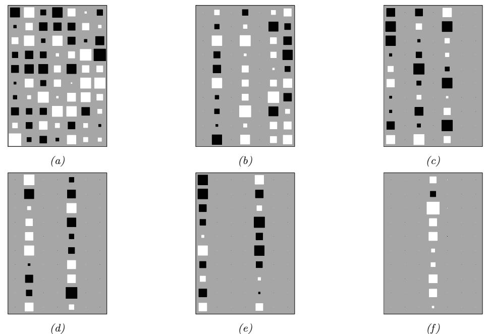
Figure 28.9: Illustration of estimating the e!ective dimensionalities in a mixture of factor analysers using variational Bayes EM with an ARD prior. Black are negative values, white are positive, gray is 0. The blank columns have been forced to 0 via the ARD mechanism, reducing the e!ective dimensionality. The data was generated from 6 clusters with intrinsic dimensionalities of 7, 4, 3, 2, 2, 1, which the method has successfully estimated. From Figure 4.4 of [Bea03]. Used with kind permission of Matt Beal.

number of points	intrinsic dimensionalities
per cluster	1	7	4	3	2	2
8			2			1
8	1 2
16	1 4				2
32	1	6	3	3	2	2
64	1	7	4	3	2	2
128	1	7	4	3	2	2

Figure 28.10: We show the estimated number of clusters, and their estimated dimensionalities, as a function of sample size. The ARD algorithm found two di!erent solutions when N = 8. Note that more clusters, with larger e!ective dimensionalities, are discovered as the sample sizes increases. From Table 4.1 of [Bea03]. Used with kind permission of Matt Beal.

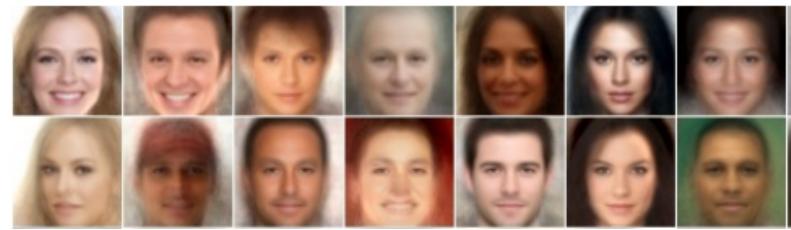
Figure 28.11: Random samples from the MixFA model fit to CelebA. Generated by mix\_ppca\_celebA.ipynb. Adapted from Figure 4 of [RW18]. Used with kind permission of Yair Weiss.

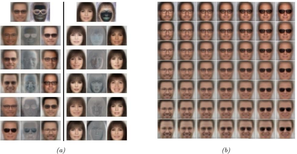
Figure 28.12: (a) Visualization of the parameters learned by the MFA model. The top row shows the mean µ^k and noise variance #k, reshaped from 12,288-dimensional vectors to 64 ↓ 64 ↓ 3 images, for two mixture components k. The next 5 rows show the first 5 (of 10) basis functions (columns of Wk) as images. On row i, left column, we show µ^k ↗ Wk[:, i]; in the middle, we show 0.5 + Wk[:, i], and on the right we show µ^k + Wk[:, i]. (b) Images generated by computing µ^k + z1Wk[:, i] + z2Wk[:, j], for some component k and dimensions i, j, where (z1, z2) are drawn from the grid [↗1:1, ↗1 : 1], so the central image is just µk. From Figure 6 of [RW18]. Used with kind permission of Yair Weiss.

matrix. Surprisingly, the results are competitive with deep generative models such as those in Part IV, despite the fact that no neural networks are used in the model.

In [RW18], they fit the MFA model to the CelebA dataset, which is a dataset of faces of celebrities (movie stars). They use K = 300 components, each of latent dimension L = 10; the observed data has dimension D = 64 ↗ 64 ↗ 3 = 12, 288. They fit the model using SGD, using the methods from Section 28.3.1.3 to e”ciently compute the log likelihood, despite the high dimensionality. The µ^k parameters are initialized using K-means clustering, and the W^k parameters are initialized using factor analysis for each component separately. Then the model is fine-tuned end-to-end.

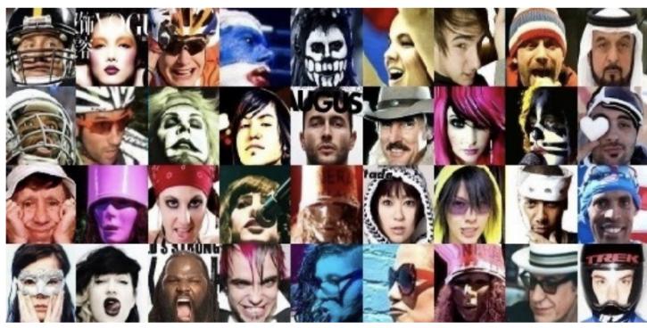
Figure 28.13: Samples from the 100 CelebA images with lowest likelihood under the MFA model. Generated by mix\_ppca\_celebA.ipynb. Adapted from Figure 7a of [RW18]. Used with kind permission of Yair Weiss.

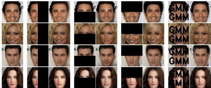
Figure 28.14: Illustration of image imputation using an MFA. Left column shows 4 original images. Subsequent pairs of columns show an occluded input, and a predicted output. Generated by mix\_ppca\_celebA.ipynb. Adapted from Figure 7b of [RW18]. Used with kind permission of Yair Weiss.

Figure 28.11 shows some images generated from the fitted model. The results are suprisingly good for such a simple locally linear model. The reason the method works is similar to the discussion in Section 28.2.4.1: essentially the W^k matrix learns a set of L-dimensional basis functions for the subset of face images that get mapped to cluster k. See Figure 28.12 for an illustration.

There are several advantages to this model compared to VAEs and GANs. First, [RW18], showed that this MixFA model captures more of the modes of the data distribution than more sophisticated generative models, such as VAEs (Section 21.2) and GANs (Chapter 26). Second, we can compute the exact likelihood p(x), so we can compute outliers or unusual images. This is illustrated in Figure 28.13.

Third, we can perform image imputation from partially observed images given arbitrary missingness patterns. To see this, let us partition x = (x1, x2), where x¹ (of size D1) is observed and x² (of size

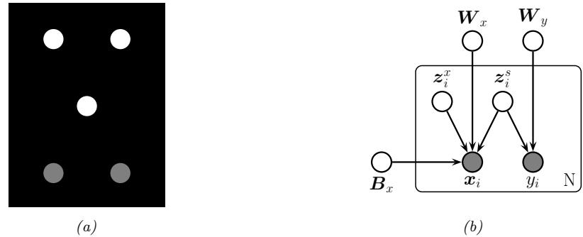
Figure 28.15: Gaussian latent factor models for paired data. (a) Supervised PCA. (b) Partial least squares.

D² = D ↓ D1) is missing. We can compute the most probable cluster using

\[k^\* = \underset{k=1}{\text{argmax}} \, p(c=k)p(\mathbf{z}\_1|c=k) \tag{28.94}\]

where

\[\log p(\mathbf{x}\_1|\mu\_k, \mathbf{C}\_k) = -\frac{1}{2} \left[ D\_1 \log(2\pi) + \log \det(\mathbf{C}\_{k,11}) + \tilde{\mathbf{x}}\_1^\mathsf{T} \mathbf{C}\_{k,11}^{-1} \tilde{\mathbf{x}}\_1 \right] \tag{28.95}\]

where ^Ck,¹¹ is the top left ^D1 ↗ ^D1 block of ^WkW^{T k} + $k, and x˜¹ = x¹ ↓ µk[1 : D1]. Once we know which discrete mixture component to use, we can compute the Gaussian posterior p(z|x1, k↔︎) using Equation (28.59). Let zˆ = E [z|x1, k↔︎]. Given this, we can compute the predicted output for the full image:

\[ \hat{\mathbf{z}} = \mathbf{W}\_{k^\*} \hat{\mathbf{z}} + \mu\_{k^\*} \tag{28.96} \]

We then use the estimate x^→ = [x1, xˆ2], so the observed pixels are not changed. This is an example of image imputation, and is illustrated in Figure 28.14. Note that we can condition on an arbitrary subset of pixels, and fill in the rest, whereas some other models (e.g., autoregressive models) can only predict the bottom right given the top left (since they assume a generative model which works in raster-scan order).

28.3.4 Factor analysis models for paired data

In this section, we discuss linear-Gaussian factor analysis models when we have two kinds of observed variables, ^{x → RDx} and ^{y → RDy} , which are paired. These often correspond to di!erent sensors or modalities (e.g., images and sound). We follow the presentation of [Vir10].

28.3.4.1 Supervised PCA

If we have two observed signals, we can model the joint p(x, y) using a shared low-dimensional representation using the following linear Gaussian model:

\[p(\mathbf{z}\_n) = N(\mathbf{z}\_n | \mathbf{0}, \mathbf{I}\_L) \tag{28.97}\]

\[p(\mathbf{z}\_n|\mathbf{z}\_n, \theta) = N(\mathbf{z}\_n|\mathbf{W}\_x \mathbf{z}\_n, \sigma\_x^2 \mathbf{I}\_{D\_x}) \tag{28.98}\]

\[p(y\_n|z\_n, \theta) = N(y\_n|\mathbf{W}\_y z\_n, \sigma\_y^2 \mathbf{I}\_{D\_y}) \tag{28.99}\]

This is illustrated as a graphical model in Figure 28.15a. The intuition is that zⁿ is a shared latent subspace, that captures features that xⁿ and yⁿ have in common. The variance terms ς^x and ς^y control how much emphasis the model puts on the two di!erent signals.

The above model is called supervised PCA [Yu+06]. If we put a prior on the parameters ε = (Wx,Wy, ςx, ςy), it is called Bayesian factor regression [Wes03].

We can marginalize out zⁿ to get p(yn|xn, ε). If yⁿ is a scalar, this becomes

\[p(y\_n|\mathbf{x}\_n, \boldsymbol{\theta}) = N(y\_n|\mathbf{x}\_n^\mathsf{T}\boldsymbol{v}, \boldsymbol{w}\_y^\mathsf{T}\mathbf{C}\boldsymbol{w}\_y + \sigma\_y^2) \tag{28.100}\]

\[\mathbf{C} = (\mathbf{I} + \sigma\_x^{-2} \mathbf{W}\_x^\mathsf{T} \mathbf{W}\_x)^{-1} \tag{28.101}\]

\[w = \sigma\_x^{-2} \mathbf{C} \mathbf{W}\_x w\_y \tag{28.102}\]

To apply this to the classification setting, we can replace the Gaussian p(y|z) with a logistic regression model:

\[p(y\_n|\mathbf{z}\_n, \theta) = \text{Ber}(y\_n|\sigma(\mathbf{w}\_y^\mathsf{T}\mathbf{z}\_n))\tag{28.103}\]

In this case, we can no longer compute the marginal posterior predictive p(yn|xn, ε) in closed form, but we can use techniques similar to exponential family PCA (see [Guo09] for details).

The above model is completely symmetric in x and y. If our goal is to predict y from x via the latent bottleneck z, then we might want to upweight the likelihood term for y, as proposed in [Ris+08]. This gives

\[p(\mathbf{X}, \mathbf{Y}, \mathbf{Z} | \theta) = p(\mathbf{Y} | \mathbf{Z}, \mathbf{W}\_y) p(\mathbf{X} | \mathbf{Z}, \mathbf{W}\_x)^\alpha p(\mathbf{Z}) \tag{28.104}\]

where ↽ ≃ 1 controls the relative importance of modeling the two sources. The value of ↽ can be chosen by cross-validation.

28.3.4.2 Partial least squares

We now consider an asymmetric or more “discriminative” form of supervised PCA. The key idea is to allow some of the (co)variance in the input features to be explained by its own subspace, z^{x i} , and to let the rest of the subspace, z^{s i} , be shared between input and output. The model has the form

\[p(\mathbf{z}\_i) = \mathcal{N}(z\_i^s | \mathbf{0}, \mathbf{I}\_{L\_s}) \mathcal{N}(z\_i^x | \mathbf{0}, \mathbf{I}\_{L\_x}) \tag{28.105}\]

\[p(y\_i|\mathbf{z}\_i) = \mathcal{N}(\mathbf{W}\_y \mathbf{z}\_i^s + \mu\_y, \sigma^2 \mathbf{I}\_{D\_y}) \tag{28.106}\]

\[p(\mathbf{z}\_i|\mathbf{z}\_i) = \mathcal{N}(\mathbf{W}\_x \mathbf{z}\_i^s + \mathbf{B}\_x \mathbf{z}\_i^x + \mu\_x, \sigma^2 \mathbf{I}\_{D\_x}) \tag{28.107}\]

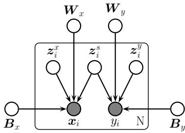
Figure 28.16: Canonical correlation analysis as a PGM.

See Figure 28.15b. The corresponding induced distribution on the visible variables has the form

\[p(\boldsymbol{v}\_{i}|\boldsymbol{\theta}) = \int \mathcal{N}(\boldsymbol{v}\_{i}|\mathbf{W}\boldsymbol{z}\_{i} + \boldsymbol{\mu}, \sigma^{2}\mathbf{I}) \mathcal{N}(\boldsymbol{z}\_{i}|\mathbf{0}, \mathbf{I}) d\boldsymbol{z}\_{i} = \mathcal{N}(\boldsymbol{v}\_{i}|\boldsymbol{\mu}, \mathbf{W}\mathbf{W}^{\mathsf{T}} + \sigma^{2}\mathbf{I}) \tag{28.108}\]

where vⁱ = (yi; xi), µ = (µy; µx) and

\[\mathbf{W} = \begin{pmatrix} \mathbf{W}\_y & \mathbf{0} \\ \mathbf{W}\_x & \mathbf{B}\_x \end{pmatrix} \tag{28.109}\]

\[\mathbf{W}\mathbf{W}^{\top} = \begin{pmatrix} \mathbf{W}\_{y}\mathbf{W}\_{y}^{\top} & \mathbf{W}\_{y}\mathbf{W}\_{x}^{\top} \\ \mathbf{W}\_{x}\mathbf{W}\_{y}^{\top} & \mathbf{W}\_{x}\mathbf{W}\_{x}^{\top} + \mathbf{B}\_{x}\mathbf{B}\_{x}^{\top} \end{pmatrix} \tag{28.110}\]

We should choose L large enough so that the shared subspace does not capture covariate-specific variation.

MLE in this model is equivalent to the technique of partial least squares (PLS) [Gus01; Nou+02; Sun+09]. This model can be also be generalized to discrete data using the exponential family [Vir10].

28.3.4.3 Canonical correlation analysis

We now consider a symmetric unsupervised version of PLS, in which we allow each view to have its own “private” subspace, but there is also a shared subspace. If we have two observed variables, xⁱ and yi, then we have three latent variables, z^{s i → RLs} which is shared, ^{zx i → RLx} and ^{zy i → RLy} which are private. We can write the model as follows [BJ05]:

\[p(\mathbf{z}\_i) = \mathcal{N}(z\_i^s | \mathbf{0}, \mathbf{I}\_{L\_s}) \mathcal{N}(z\_i^x | \mathbf{0}, \mathbf{I}\_{L\_x}) \mathcal{N}(z\_i^y | \mathbf{0}, \mathbf{I}\_{L\_y}) \tag{28.111}\]

\[p(\mathbf{z}\_i|\mathbf{z}\_i) = \mathcal{N}(\mathbf{z}\_i|\mathbf{B}\_x\mathbf{z}\_i^x + \mathbf{W}\_x\mathbf{z}\_i^s + \boldsymbol{\mu}\_x, \sigma^2\mathbf{I}\_{D\_x}) \tag{28.112}\]

\[p(y\_i|\mathbf{z}\_i) = N(y\_i|\mathbf{B}\_y\mathbf{z}\_i^y + \mathbf{W}\_y\mathbf{z}\_i^s + \boldsymbol{\mu}\_y, \sigma^2\mathbf{I}\_{D\_y}) \tag{28.113}\]

See Figure 28.16 The corresponding observed joint distribution has the form

\[p(v\_i|\theta) = \int \mathcal{N}(v\_i|\mathbf{W}z\_i + \mu, \sigma^2 \mathbf{I}) \mathcal{N}(z\_i|\mathbf{0}, \mathbf{I}) dz\_i = \mathcal{N}(v\_i|\mu, \mathbf{W}\mathbf{W}^\mathsf{T} + \sigma^2 \mathbf{I}\_D) \tag{28.114}\]

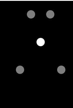
Figure 28.17: Exponential family PCA model as a DPGM.

where

\[\mathbf{W} = \begin{pmatrix} \mathbf{W}\_x & \mathbf{B}\_x & \mathbf{0} \\ \mathbf{W}\_y & \mathbf{0} & \mathbf{B}\_y \end{pmatrix} \tag{28.115}\]

\[\mathbf{W}\mathbf{W}^{\mathsf{T}} = \begin{pmatrix} \mathbf{W}\_{x}\mathbf{W}\_{x}^{\mathsf{T}} + \mathbf{B}\_{x}\mathbf{B}\_{x}^{\mathsf{T}} & \mathbf{W}\_{x}\mathbf{W}\_{y}^{\mathsf{T}}\\ \mathbf{W}\_{y}\mathbf{W}\_{x}^{\mathsf{T}} & \mathbf{W}\_{y}\mathbf{W}\_{y}^{\mathsf{T}} + \mathbf{B}\_{y}\mathbf{B}\_{y}^{\mathsf{T}} \end{pmatrix} \tag{28.116}\]

[BJ05] showed that MLE for this model is equivalent to a classical statistical method known as canonical correlation analysis or CCA [Hot36]. However, the PGM perspective allows us to easily generalize to multiple kinds of observations (this is known as generalized CCA [Hor61]) or to nonlinear models (this is known as deep CCA [WLL16; SNM16]), or exponential family CCA [KVK10]. See [Uur+17] for further discussion of CCA and its extensions, and Section 32.2.2.2 for more details.

28.3.5 Factor analysis with exponential family likelihoods

So far we have assumed the observed data is real-valued, so ^{xn → RD}. If we want to model other kinds of data (e.g., binary or categorical), we can simply replace the Gaussian output distribution with a suitable member of the exponential family, where the natural parameters are given by a linear function of zn. That is, we use

\[p(\mathbf{z}\_n|\mathbf{z}\_n) = \exp(\mathcal{T}(\mathbf{z})^\mathsf{T}\boldsymbol{\theta} + h(\mathbf{z}) - g(\boldsymbol{\theta})) \tag{28.117}\]

where the N ↗ D matrix of natural parameters is assumed to be given by the low rank decomposition % = ZW, where Z is N ↗ L and W is L ↗ D. The resulting model is called exponential family factor analysis

Unlike the linear-Gaussian FA, we cannot compute the exact posterior p(zn|xn,W) due to the lack of conjugacy between the expfam likelihood and the Gaussian prior. Furthermore, we cannot compute the exact marginal likelihood either, which prevents us from finding the optimal MLE.

[CDS02] proposed a coordinate ascent method for a deterministic variant of this model, known as exponential family PCA. This alternates between computing a point estimate of zⁿ and W. This

can be regarded as a degenerate version of variational EM, where the E step uses a delta function posterior for zn. [GS08] present an improved algorithm that finds the global optimum, and [Ude+16] presents an extension called generalized low rank models, that covers many di!erent kinds of loss function.

However, it is often preferable to use a probabilistic version of the model, rather than computing point estimates of the latent factors. In this case, we must represent the posterior using a nondegenerate distribution to avoid overfitting, since the number of latent variables is proportional to the number of data cases [WCS08]. Fortunately, we can use a non-degenerate posterior, such as a Gaussian, by optimizing the variational lower bound. We give some examples of this below.

28.3.5.1 Example: binary PCA

Consider a factored Bernoulli likelihood:

\[p(\mathbf{z}|\mathbf{z}) = \prod\_{d} \text{Ber}(x\_d | \sigma(\mathbf{w}\_d^\top \mathbf{z})) \tag{28.118}\]

Suppose we observe N = 150 bit vectors of length D = 16. Each example is generated by choosing one of three binary prototype vectors, and then by flipping bits at random. See Figure 28.18(a) for the data. We can fit this using the variational EM algorithm (see [Tip98] for details). We use L = 2 latent dimensions to allow us to visualize the latent space. In Figure 28.18(b), we plot E O ^zn|xn,W^{ˆ P} . We see that the projected points group into three distinct clusters, as is to be expected. In Figure 28.18(c), we plot the reconstructed version of the data, which is computed as follows:

\[p(\hat{x}\_{nd} = 1 | \mathbf{z}\_n) = \int d\mathbf{z}\_n \, p(\mathbf{z}\_n | \mathbf{z}\_n) p(\hat{x}\_{nd} | \mathbf{z}\_n) \tag{28.119}\]

If we threshold these probabilities at 0.5 (corresponding to a MAP estimate), we get the “denoised” version of the data in Figure 28.18(d).

28.3.5.2 Example: categorical PCA

We can generalize the model in Section 28.3.5.1 to handle categorical data by using the following likelihood:

\[p(\mathbf{z}|\mathbf{z}) = \prod\_{d} \text{Cat}(x\_d | \text{softmax}(\mathbf{W}\_d \mathbf{z})) \tag{28.120}\]

We call this categorical PCA (CatPCA). A variational EM algorithm for fitting this is described in [Kha+10].

28.3.6 Factor analysis with DNN likelihoods (VAEs)

The FA model assumes the observed data can be modeled as arising from a linear mapping from a low-dimensional set of Gaussian factors. One way to relax this assumption is to let the mapping from z to x be a nonlinear model, such as a neural network. That is, the likelihood becomes

\[p(\mathbf{z}|\mathbf{z}) = \mathcal{N}(\mathbf{z}|f(w;\theta), \sigma^2 \mathbf{I})\tag{28.121}\]

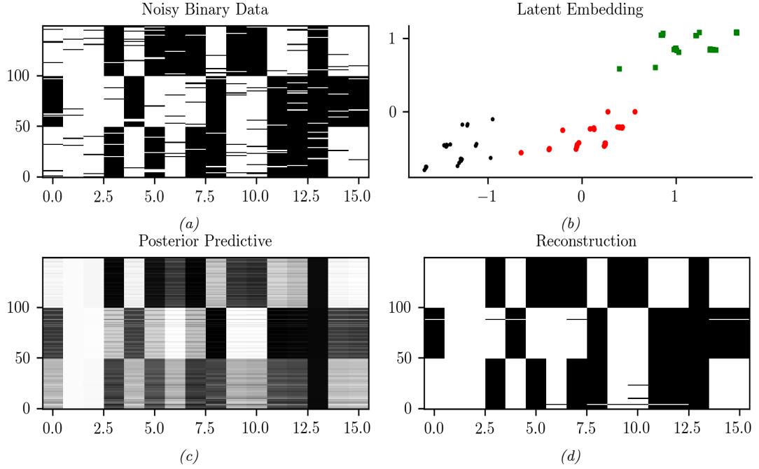
Figure 28.18: (a) 150 synthetic 16 dimensional bit vectors. (b) The 2d embedding learned by binary PCA, fit using variational EM. We have color coded points by the identity of the true “prototype” that generated them. (c) Predicted probability of being on. (d) Thresholded predictions. Generated by binary\_fa\_demo.ipynb.

We call this “nonlinear factor analysis”. (We can of course replace the Gaussian likelihood with other distributions, such as categorical, in which case we get nonlinear exponential family factor analysis.) Unfortunately we can no longer compute the posterior or the MLE exactly, so we need to use approximate methods. In Chapter 21, we discuss the variational autoencoder, which fits this nonlinear FA model using amortized variational inference. However, it is also possible to fit the same model using other inference methods, such as MCMC (see e.g., [Hof17]).

28.3.7 Factor analysis with GP likelihoods (GP-LVM)

In this section we discuss a nonlinear version of factor analysis in which we replace the linear decoder ^f(z) = ^Wz used in the likelihood ^p(y|z) = ^N (y|f(z), ^ς2I) with a nonlinear function, represented by a Gaussian process (Chapter 18), one per output dimension. This is known as a GP-LVM, which stands for “Gaussian process latent variable model” [Law05]. (Note that we switch notation a bit from standard FA and define the observed output variable by y, to be consistent with standard supervised GP notation; the inputs to the GP will be latent variables z.)

To explain the method in more detail, we start with PPCA (Section 28.3.2). Recall that the PPCA

model is as follows:

\[p(\mathbf{z}\_i) = \mathcal{N}(\mathbf{z}\_i | \mathbf{0}, \mathbf{I}) \tag{28.122}\]

\[p(y\_i|\mathbf{z}\_i, \boldsymbol{\theta}) = \mathcal{N}(y\_i|\mathbf{W}\mathbf{z}\_i, \sigma^2\mathbf{I})\tag{28.123}\]

We can fit this model by maximum likelihood, by integrating out the zⁱ and maximizing wrt W (and ς²). The objective is given by

\[p(\mathbf{Y}|\mathbf{W}, \sigma^2) = (2\pi)^{-DN/2} |\mathbf{C}|^{-N/2} \exp\left(-\frac{1}{2} \text{tr}(\mathbf{C}^{-1}\mathbf{Y}^\mathsf{T}\mathbf{Y})\right) \tag{28.124}\]

where C = WW^T + ς²I. As we showed in Section 28.3.2, the MLE for W can be computed in terms of the eigenvectors of Y^TY.

Now we consider the dual problem, whereby we maximize wrt Z and integrate out W. We will use a prior of the form p(W) = ^j N (w^j |0, I). The corresponding likelihood becomes

\[p(\mathbf{Y}|\mathbf{Z}, \sigma^2) = \prod\_{d=1}^{D} N(\mathbf{Y}\_{:,d}|\mathbf{0}, \mathbf{Z}\mathbf{Z}^\top + \sigma^2 \mathbf{I})\tag{28.125}\]

\[= (2\pi)^{-DN/2} |\mathbf{K}\_z|^{-D/2} \exp\left(-\frac{1}{2} \text{tr}(\mathbf{K}\_\sigma^{-1} \mathbf{Y} \mathbf{Y}^\mathsf{T})\right) \tag{28.126}\]

where K^ε = K + ς²I, and K = ZZT. The MLE for Z can be computed in terms of the eigenvectors of Kε, and gives the same results as PPCA (see [Law05] for the details).

To understand what this process is doing, consider modeling the prior on f : Z ↔︎ Y with a GP with a linear kernel:

\[\mathcal{K}(\mathbf{z}\_i, \mathbf{z}\_j) = \mathbf{z}\_i^\mathsf{T} \mathbf{z}\_j + \sigma^2 \delta\_{ij} \tag{28.127}\]

The corresponding covariance matrix has the form K = ZZ^T + ς²I. Thus Equation (28.126) is equivalent to the likelihood of a product of independent GPs. Just as factor analysis is like linear regression with unknown inputs, so GP-LVM is like GP regression with unknown inputs. The goal is then to compute a point estimate of these unknown inputs, i.e., Zˆ. (We can also use Bayesian inference.)

The advantage of the dual formulation is that we can use a more general kernel for K instead of the linear kernel. That is, we can set Kij = K(zi, z^j ) for any Mercer kernel. The MLE for Z is no longer be available via eigenvalue methods, but can be computed using gradient-based optimization.

In Figure 28.19, we illustrate the model (with an ARD kernel) applied to some motion capture data, from the CMU mocap database at http://mocap.cs.cmu.edu/. Each person has 41 markers, whose motion in 3d is tracked using 12 infrared cameras. Each datapoint corresponds to a di!erent body pose. When projected to 2d, we see that similar poses are clustered nearby.

28.4 LFMs with non-Gaussian priors

In this section, we discuss (linear) latent factor models with non-Gaussian priors. See Table 28.1 for a summary of the models we will discuss.

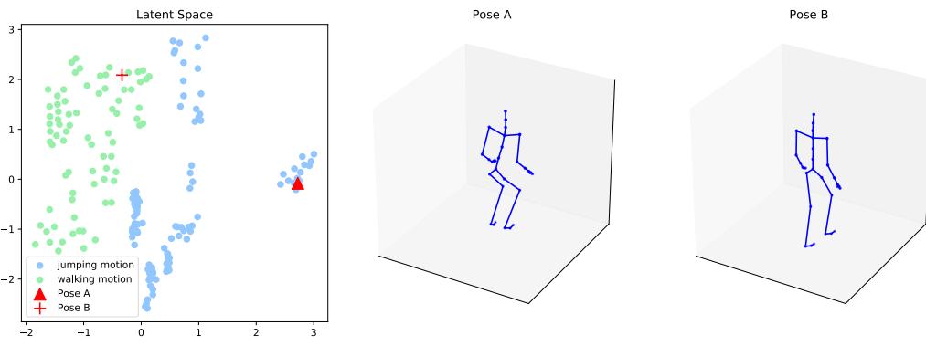
Figure 28.19: Illustration of a 2d embedding of human motion-capture data using a GP-LVM. We show two poses and their corresponding embeddings. Generated by gplvm\_mocap.ipynb. Used with kind permission of Aditya Ravuri.

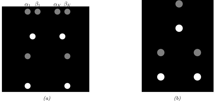
Figure 28.20: (a) Gaussian-Poisson (GAP) model as a DPGM. Here ^zn,k ^{↔︎ R+} and ^xn,d ^{↔︎ Z}↔︎⁰. (b) Simplex FA model as a DPGM. Here zⁿ ↔︎ S^K and xn,d ↔︎ {1,…,V }.

28.4.1 Non-negative matrix factorization (NMF)

Suppose that we use a gamma distribution for the latents: p(z) = ^k Ga(zk|↽k, εk). This results in a sparse, non-negative hidden representation, which can help interpretability. This is particularly useful when the data is also sparse and non-negative, such as word counts. In this case, it makes sense to use a Poisson likelihood: ^p(x|z) = ^{D d}=1 Poi(xd|w^{T d}z). The overall model has the form

\[p(\mathbf{z}, \mathbf{z}) = p(\mathbf{z})p(\mathbf{z}|\mathbf{z}) = \left[\prod\_{k} \text{Ga}(z\_k|\alpha\_k, \beta\_k)\right] \left[\prod\_{d=1}^{D} \text{Poi}(x\_d|\mathbf{w}\_d^\top \mathbf{z})\right] \tag{28.128}\]

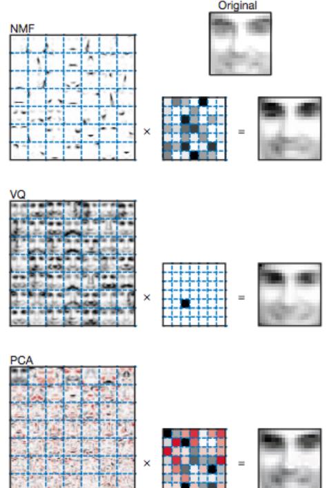
Figure 28.21: Illustrating the di!erence between non-negative matrix factorization (NMF), vector quantization (VQ), and principal components analysis (PCA). Left column: filters (columns of W) learned from a set of 2429 faces images, each of size 19 ↓ 19. There are 49 basis functions in total, shown in a 7 ↓ 7 montage; each filter is reshaped to a 19 ↓ 19 image for display purposes. (For PCA, negative weights are red, positive weights are black.) Middle column: the 49 latent factors z when the model is applied to the original face image shown at the top. Right column: reconstructed face image. From Figure 1 of [LS99].

The resulting model is called the GaP (gamma-Poisson) model [Can04]. See Figure 28.20a for the graphical model.

The parameters ↽^k and ε^k control the sparsity of the latent representation zn. If we set ↽^k = ε^k = 0, and compute the MLE for W, we recover non-negative matrix factorization (NMF) [PT94; LS99; LS01], as shown in [BJ06].

Figure 28.21 illustrates the result of applying NMF to a dataset of image patches of faces, where the data correspond to non-negative pixel intensities. We see that the learned basis functions are small localized parts of faces. Also, the coe”cient vector z is sparse and positive. For PCA, the coe”cient vector has negative values, and the resulting basis functions are global, not local. For vector quantization (i.e., GMM model), z is a one-hot vector, with a single mixture component turned on; the resulting weight vectors correspond to entire image prototypes. The reconstruction quality is similar in each case, but the nature of the learned latent representation is quite di!erent.

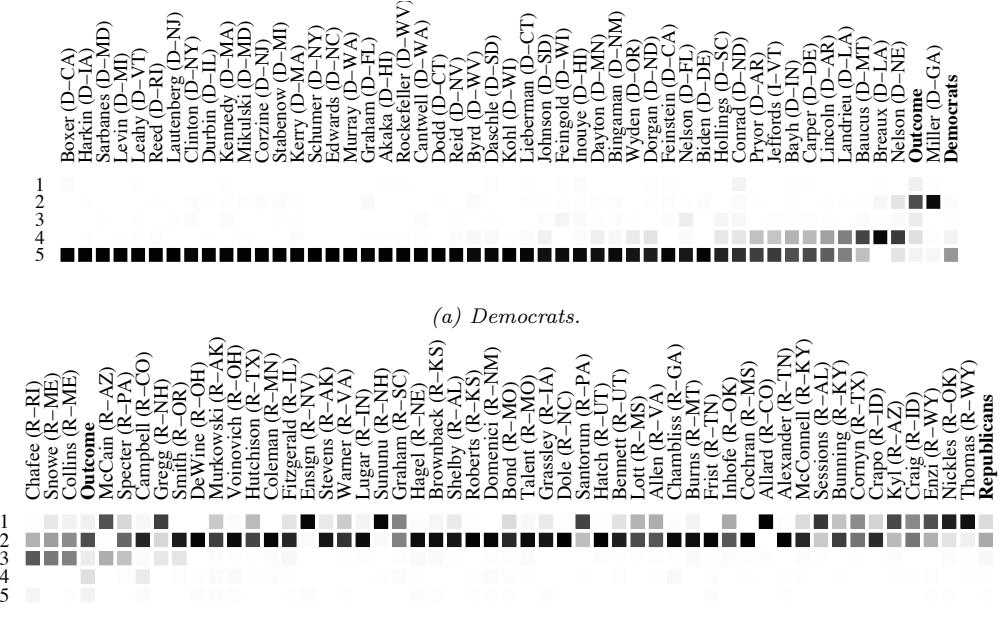
(b) Republicans.

Figure 28.22: The simplex factor analysis model applied to some roll call data from the US Senate collected in 2003. The senators have been sorted from left to right using the binary PCA method of [Lee06]. See text for details. From Figures 8–9 of [BJ06]. Used with kind permission of Wray Buntine.

28.4.2 Multinomial PCA

Suppose we use a Dirichlet prior for the latents, p(z) = Dir(z|↽), so z → SK, which is the Kdimensional probability simplex. As in Section 28.4.1, the vector z will be sparse and non-negative, but in addition it will satsify the constraint *^{K k}=1 z^k = 1, so the components are not independent. Now suppose our data is categorical, x^d → {1,…,V }, so our likelihood has the form p(x|z) = ^d Cat(xd|Wdz). The overall model is therefore

\[p(\mathbf{z}, \mathbf{z}) = \text{Dir}(\mathbf{z}|\mathbf{\alpha}) \prod\_{d=1}^{D} \text{Cat}(x\_d | \mathbf{W}\_d \mathbf{z}) \tag{28.129}\]

See Figure 28.20b for the DPGM. This model (or small variants of it) has multiple names: user rating profile model [Mar03], admixture model [PSD00], mixed membership model [EFL04], multinomial PCA (mPCA) [BJ06], or simplex factor analysis (sFA) [BD11].

28.4.2.1 Example: roll call data

Let us consider the example from [BJ06], who applied this model to analyze some roll call data from the US Senate in 2003. Specifically, the data has the form xn,d → {+1, ↓1, 0} for n = 1 : 100

and d = 1 : 459, where xnd is the vote of the n’th senator on the d’th bill, where +1 means in favor, ↓1 means against, and 0 means not voting. In addition, we have the overall outcome, which we denote by x101,d → {+1, ↓1}, where +1 means the bill was passed, and -1 means it was rejected.

We fit the mPCA model to this data using 5 latent factors using variational EM. Figure 28.22 plots E [znk|xn] → [0, 1], which is the degree to which senator n belongs to latent component or “bloc” k. We see that component 5 is the Democractic majority, and block 2 is the Republican majority. See [BJ06] for further details.

28.4.2.2 Advantage of Dirichlet prior over Gaussian prior

The main advantage of using a Dirichlet prior compared to a Gaussian prior is that the latent factors are more interpretable. To see this, note that the mean parameters for d’th output distribution have the form µnd = W^dzn, and hence

\[p(x\_{nd} = v | \mathbf{z}\_n) = \sum\_{k} z\_{nk} w\_{vk}^d \tag{28.130}\]

Thus the latent variables can be additively combined to compute the mean parameters, aiding interpretability. By contrast, the CatPCA model in Section 28.3.5.2 uses a Gaussian prior, so W^dzⁿ can be negative; consequently it must pass this vector through a softmax, to convert from natural parameters to mean parameters; this makes zⁿ harder to interpret.

28.4.2.3 Connection to mixture models

If zⁿ were a one-hot vector, rather than any point in the probability simplex, then the mPCA model would be equivalent to selecting a single column from W^d corresponding to the discrete hidden state. This is equivalent to a finite mixture of categorical distributions (see Section 28.2.2), and corresponds to the assumption that x is generated by a single cluster. However, the mPCA model does not require that zⁿ be one-hot, and instead allows xⁿ to partially belong to multiple clusters. For this reason, this model is also known as an admixture mixture or mixed membership model [EFL04].

28.5 Topic models

In this section, we show how to modify the multinomial PCA model of Section 28.4.2 to create latent variable models for sequences of discrete tokens, such as words in text documents, or genes in a DNA sequence. The basic idea is to assume that the words are conditionally independent given a latent topic vector z. Rather than being a single discrete cluster label, z is a probability distribution over clusters, and each word is sampled from its own “local” cluster. In the NLP community, this kind of model is called a topic model (see e.g., [BGHM17]).

28.5.1 Latent Dirichlet allocation (LDA)

In this section, we discuss the most common kind of topic model known as latent Dirichlet allocation or LDA [BNJ03a; Ble12]. (This usage of the term “LDA” is not to be confused with linear discriminant analysis.) In the genetic community, this model is known as an admixture model [PSD00].

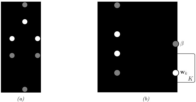
Figure 28.23: Latent Dirichlet allocation (LDA) as a DPGM. (a) Unrolled form. (b) Plate form.

28.5.1.1 Model definition

We can define the LDA model as follows. Let xnl → {1,…,V } be the identity of the l’th word in document n, where l can now range from 1 to Ln, the length of the document, and V is the size of the vocabulary. The probability of word v at location l is given by

\[p(x\_{nl} = v | \mathbf{z}\_n) = \sum\_{k} z\_{nk} w\_{kv} \tag{28.131}\]

where 0 ≃ znk ≃ 1 is the proportion of “topic” k in document n, and zⁿ ↑ Dir(↽).

We can rewrite this model by associating a discrete latent variable mnl → {1,…,Nz} with each word in each document, with distribution p(mnl|zn) = Cat(mnl|zn). Thus mnl specifies the topic to use for word l in document n. The full joint model becomes

\[p(\mathbf{z}\_n, \mathbf{z}\_n, \mathbf{m}\_n) = \text{Dir}(\mathbf{z}\_n | \alpha) \prod\_{l=1}^{L\_n} \text{Cat}(m\_{nl} | \mathbf{z}\_n) \text{Cat}(x\_{nl} | \mathbf{W}[m\_{nl}, :]) \tag{28.132}\]

where W[k, :] = w^k is the distribution over words for the k’th topic. See Figure 28.23 for the corresponding DPGM.

We typically use a Dirichlet prior the topic parameters, p(wk) = Dir(wk|ε1^V ); by setting ε small enough, we can encourage these topics to be sparse, so that each topic only predicts a subset of the words. In addition, we use a Dirichlet prior on the latent factors, p(zn) = Dir(zn|↽1^Nz ). If we set ↽ small enough, we can encourage the topic distribution for each document to be sparse, so that each document only contains a subset of the topics. See Figure 28.24 for an illustration.

Note that an earlier version of LDA, known as probabilistic LSA, was proposed in [Hof99]. (LSA stands for “latent semantic analysis”, and refers to the application of PCA to text data; see [Mur22, Sec 20.5.1.2] for details.) The likelihood function, p(x|z), is the same as in LDA, but pLSA does not specify a prior for z, since it is designed for posterior analysis of a fixed corpus (similar to LSA), rather than being a true generative model.

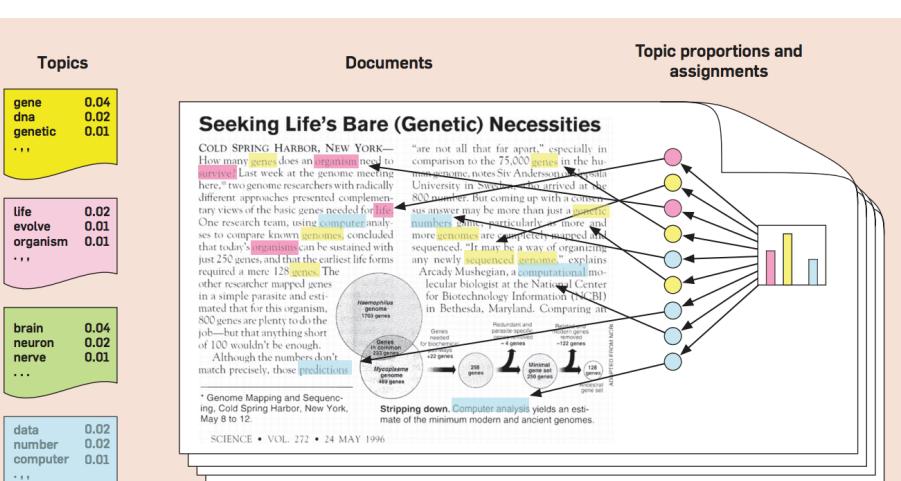
Figure 28.24: Illustration of latent Dirichlet allocation (LDA). We have color coded certain words by the topic they have been assigned to: yellow represents the genetics cluster, pink represents the evolution cluster, blue represent the data analysis cluster, and green represents the neuroscience cluster. Each topic is in turn defined as a sparse distribution over words. This article is not related to neuroscience, so no words are assigned to the green topic. The overall distribution over topic assignments for this document is shown in the right as a sparse histogram. Adapted from Figure 1 of [Ble12]. Used with kind permission of David Blei.

28.5.1.2 Polysemy

Each topic is a distribution over words that co-occur, and which are therefore semantically related. For example, Figure 28.25 shows 3 topics which were learned from an LDA model fit to the TASA corpus3. These seem to correspond to 3 di!erent senses of the word “play”: playing an instrument, a theatrical play, and playing a sports game.

We can use the inferred document-level topic distribution to overcome polysemy, i.e., to disambiguate the meaning of a particular word. This is illustrated in Figure 28.26, where a subset of the words are annotated with the topic to which they were assigned (i.e., we show argmax^k p(mnl = k|xn). In the first document, the word “music” makes it clear that the musical topic (number 77) is present in the document, which in turn makes it more likely that mnl = 77 where l is the index corresponding to the word “play”.

^3. The TASA corpus is an untagged collection of educational materials consisting of 37,651 documents and 12,190,931 word tokens. Words appearing in fewer than 5 documents were replaced with an asterisk, but punctuation was included. The combined vocabulary was of size 37,202 unique words.

Topic 77			Topic 82			Topic 166
	word prob.			word prob.			word prob.
MUSIC	.090		LITERATURE	.031		PLAY	.136
DANCE	.034		POEM	.028		BALL	.129
SONG	.033		POETRY	.027		GAME	.065
PLAY	.030		POET	.020		PLAYING	.042
SING	.026		PLAYS	.019		HIT	.032
SINGING	.026		POEMS	.019		PLAYED	.031
BAND	.026		PLAY	.015		BASEBALL	.027
PLAYED	.023		LITERARY	.013		GAMES	.025
SANG	.022		WRITERS	.013		BAT	.019
SONGS	.021		DRAMA	.012		RUN	.019
DANCING	.020		WROTE	.012		THROW	.016
PIANO	.017		POETS	.011		BALLS	.015
PLAYING	.016		WRITER	.011		TENNIS	.011
RHYTHM	.015		SHAKESPEARE	.010		HOME	.010
ALBERT	.013		WRITTEN	.009		CATCH	.010
MUSICAL	.013		STAGE	.009		FIELD	.010

Figure 28.25: Three topics related to the word play. From Figure 9 of [SG07]. Used with kind permission of Tom Gri”ths.

Figure 28.26: Three documents from the TASA corpus containing di!erent senses of the word play. Grayed out words were ignored by the model, because they correspond to uninteresting stop words (such as “and”, “the”, etc.) or very low frequency words. From Figure 10 of [SG07]. Used with kind permission of Tom Gri”ths.

28.5.1.3 Posterior inference

Many algorithms have been proposed to perform approximate posterior inference in the LDA model. In the original LDA paper, [BNJ03a], they use variational mean field inference (see Section 10.3). In [HBB10], they use stochastic VI (see Supplementary Section 28.1.2). In [GS04], they use collapsed Gibbs sampling, which marginalizes out the discrete latents (see Supplementary Section 28.1.1). In [MB16; SS17b] they discuss how to learned amortized inference networks to perform VI for the collapsed model.

Recently, there has been considerable interest in spectral methods for fitting LDA-like models

which are fast and which come with provable guarantees about the quality of the solution they obtain (unlike MCMC and variational methods, where the solution is just an approximation of unknown quality). These methods make certain (reasonable) assumptions beyond the basic model, such as the existence of some anchor words, which uniquely identify the topic for a document. See [Aro+13] for details.

28.5.1.4 Determining the number of topics

Choosing Nz, the number of topics, is a standard model selection problem. Here are some approaches that have been taken:

• Use annealed importance sampling (Section 11.5.4) to approximate the evidence [Wal+09].
• Cross validation, using the log likelihood on a test set.
• Use the variational lower bound as a proxy for log p(D|Nz).
• Use non-parametric Bayesian methods [Teh+06].

28.5.2 Correlated topic model

One weakness of LDA is that it cannot capture correlation between topics. For example, if a document has the “business” topic, it is reasonable to expect the “finance” topic to co-occcur. The source of the problem is the use of a Dirichlet prior for zn. The problem with the Dirichlet it that it is characterized by just a mean vector ↽, but its covariance is fixed ($ij = ↓↽i↽^j ), rather than being a free parameter.

One way around this is to replace the Dirichlet prior with the logistic normal distribution, which is defined as follows:

\[p(\mathbf{z}) = \int \text{Cat}(\mathbf{z}|\text{softmax}(\mathbf{e})) \mathcal{N}(\mathbf{e}|\mu, \mathbf{E}) d\mathbf{e} \tag{28.133}\]

This is known as the correlated topic model [BL07b];

The di!erence from categorical PCA discussed in Section 28.3.5.2 is that CTM uses a logistic normal to model the mean parameters, so zⁿ is sparse and non-negative, whereas CatPCA uses a normal to model the natural parameters, so zⁿ is dense and can be negative. More precisely, the CTM defines xnl ↑ Cat(Wsoftmax(ςn)), but CatPCA defines xnd ↑ Cat(softmax(Wdzn)).

Fitting the CTM model is tricky, since the prior for ςⁿ is no longer conjugate to the multinomial likelihood for mnl. However, we can derive a variational mean field approximation, as described in [BL07b].

Having fit the model, one can then convert “ˆ to a sparse precision matrix”ˆ ^↑1 by pruning low-strength edges, to get a sparse Gaussian graphical model. This allows you to visualize the correlation between topics. Figure 28.27 shows the result of applying this procedure to articles from Science magazine, from 1990–1999.

28.5.3 Dynamic topic model

In LDA, the topics (distributions over words) are assumed to be static. In some cases, it makes sense to allow these distributions to evolve smoothly over time. For example, an article might use the topic “neuroscience”, but if it was written in the 1900s, it is more likely to use words like “nerve”, whereas if

Figure 28.27: Output of the correlated topic model (with K = 50 topics) when applied to articles from Science. Nodes represent topics, with the 5 most probable phrases from each topic shown inside. Font size reflects overall prevalence of the topic. From Figure 2 of [BL07b]. Used with kind permission of David Blei.

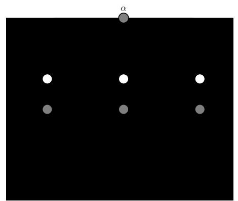
Figure 28.28: The dynamic topic model as a DPGM.

it was written in the 2000s, it is more likely to use words like “calcium receptor” (this reflects the general trend of neuroscience towards molecular biology).

One way to model this is to assume the topic distributions evolve according to a Gaussian random walk, as in a state space model (see Section 29.1). We can map these Gaussian vectors to probabilities

1881 force energy motion differ light measure magnet direct matter result

1890 motion force magnet energy measure differ direct line result light

“Atomic Physics”

1900 magnet electric measure force theory system motion line point differ

1910 force magnet theory electric atom system measure line energy body

matter

1920 atom theory electron energy measure ray electr line force value

electron

1930 ray measure energy theory light wave radiat atom electric value

quantum

1940 energy measure electron light atom particle ray radiat point theory

1950 energy radiat ray electron measure atom particle two light absorpt

1881 On Matter as a form of Energy 1892 Non-Euclidean Geometry

1960 radiat energy electron measure ray atom field two particle observe

1917 ``Keep Your Eye on the Ball’’

1933 Studies in Nuclear Physics 1943 Aristotle, Newton, Einstein. II 1950 Instrumentation for Radioactivity

1965 Lasers

1900 On Kathode Rays and Some Related Phenomena

1970 electron energy atom measure radiat field ray model particle magnet

1980 electron energy particle field radiat model atom two ray measure

1990 electron atom energy structur field model state two magnet ray

2000 state energy electron magnet field atom system two quantum physic

1920 The Arrangement of Atoms in Some Common Metals

1975 Particle Physics: Evidence for Magnetic Monopole Obtained

Figure 28.29: Part of the output of the dynamic topic model when applied to articles from Science. At the top, we show the top 10 words for the neuroscience topic over time. On the bottom left, we show the probability of three words within this topic over time. On the bottom right, we list paper titles from di!erent years that contained this topic. From Figure 4 of [BL06]. Used with kind permission of David Blei.

via the softmax function, resulting in the following model:

\[ \omega\_k^t | \boldsymbol{w}\_k^{t-1} \sim \mathcal{N}(\boldsymbol{w}\_{t-1,k}, \sigma^2 \mathbf{1}\_{N\_w}) \tag{28.134} \]

\[\mathbf{z}\_n^t \sim \text{Dir}(\alpha \mathbf{1}\_{N\_z}) \tag{28.135}\]

\[m\_{nl}^t | \mathbf{z}\_n^t \sim \text{Cat}(\mathbf{z}\_n^t) \tag{28.136}\]

\[x\_{nl}^t | m\_{nl}^t = k, \mathbf{W}^t \sim \text{Cat}(\text{softmax}(w\_k^t)) \tag{28.137}\]

This is known as a dynamic topic model [BL06]. See Figure 28.28 for the DPGM.

One can perform approximate inference in this model using a structured mean field method (Section 10.4.1), that exploits the Kalman smoothing algorithm (Section 8.2.2) to perform exact inference on the linear-Gaussian chain between the w^{t k} nodes (see [BL06] for details). Figure 28.29 illustrates a typical output of the system when applied to 100 years of articles from Science.

It is also possible to use amortized inference, and to learn embeddings for each word, which works much better with rare words. This is called the dynamic embedded topic model [DRB19].

28.5.4 LDA-HMM

The Latent dirichlet allocation (LDA) model of Section 28.5.1 assumes words are exchangeable, and thus ignores word order. A simple way to model sequential dependence between words is to use an HMM. The trouble with HMMs is that they can only model short-range dependencies, so they cannot capture the overall gist of a document. Hence they can generate syntactically correct sentences, but not semantically plausible ones.

It is possible to combine LDA with HMM to create a model called LDA-HMM [Gri+04]. This model uses the HMM states to model function or syntactic words, such as “and” or “however”, and uses the LDA to model content or semantic words, which are harder to predict. There is a distinguished HMM state which specifies when the LDA model should be used to generate the word; the rest of

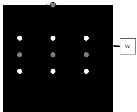
Figure 28.30: LDA-HMM model as a DPGM.

the time, the HMM generates the word.

More formally, for each document n, the model defines an HMM with states hnl → {0,…,H}. In addition, each document has an LDA model associated with it. If hnl = 0, we generate word xnl from the semantic LDA model, with topic specified by mnl; otherwise we generate word xnl from the syntactic HMM model. The DPGM is shown in Figure 28.30. The CPDs are as follows:

\[p(\mathbf{z}\_n) = \text{Dir}(\mathbf{z}\_n | \alpha \mathbf{1}\_{N\_\mathbf{z}}) \tag{28.138}\]

\[p(m\_{nl} = k | \mathbf{z}\_n) = z\_{nk} \tag{28.139}\]

\[p(h\_{n,l} = j | h\_{n,l-1} = i) = A\_{ij} \tag{28.140}\]

\[p(x\_{nl} = d | m\_{nl} = k, h\_{nl} = j) = \begin{cases} \ W\_{kd} & \text{if } j = 0 \\\ B\_{jd} & \text{if } j > 0 \end{cases} \tag{28.141}\]

where W is the usual topic-word matrix, B is the state-word HMM emission matrix, and A is the state-state HMM transition matrix.

Inference in this model can be done with collapsed Gibbs sampling, analytically integrating out all the continuous quantities. See [Gri+04] for the details.

The results of applying this model (with N^z = 200 LDA topics and H = 20 HMM states) to the combined Brown and TASA corpora4 are shown in Table 28.2. We see that the HMM generally is responsible for syntactic words, and the LDA for semantics words. If we did not have the HMM, the LDA topics would get “polluted” by function words (see top of figure), which is why such words are normally removed during preprocessing.

The model can also help disambiguate when the same word is being used syntactically or semantically. Figure 28.31 shows some examples when the model was applied to the NIPS corpus.5 We see

^4. The Brown corpus consists of 500 documents and 1,137,466 word tokens, with part-of-speech tags for each token. The TASA corpus is an untagged collection of educational materials consisting of 37,651 documents and 12,190,931 word tokens. Words appearing in fewer than 5 documents were replaced with an asterisk, but punctuation was included. The combined vocabulary was of size 37,202 unique words.

^5. NIPS stands for “Neural Information Processing Systems”. It is one of the top machine learning conferences. The NIPS corpus volumes 1–12 contains 1713 documents.

the	the	the	the	the	a	the	the	the
blood	,	,	of	a	the	,	,	,
,	and	and	,	of	of	of	a	a
of	of	of	to	,	,	a	of	in
body	a	in	in	in	in	and	and	game
heart	in	land	and	to	water	in	drink	ball
and	trees	to	classes	picture	is	story	alcohol	and
in	tree	farmers	government	film	and	is	to	team
to	with	for	a	image	matter	to	bottle	to
is	on	farm	state	lens	are	as	in	play
blood	forest	farmers	government	light	water	story	drugs	ball
heart	trees	land	state	eye	matter	stories	drug	game
pressure	forests	crops	federal	lens	molecules	poem	alcohol	team
body	land	farm	public	image	liquid	characters	people	*
lungs	soil	food	local	mirror	particles	poetry	drinking	baseball
oxygen	areas	people	act	eyes	gas	character	person	players
vessels	park	farming	states	glass	solid	author	e!ects	football
arteries	wildlife	wheat	national	object	substance	poems	marijuana	player
*	area	farms	laws	objects	temperature	life	body	field
breathing	rain	corn	department	lenses	changes	poet	use	basketball
the	in	he	*	be	said	can	time	,
a	for	it	new	have	made	would	way	;
his	to	you	other	see	used	will	years	(
this	on	they	first	make	came	could	day	:
their	with	i	same	do	went	may	part	)
these	at	she	great	know	found	had	number
your	by	we	good	get	called	must	kind
her	from	there	small	go		do	place
my	as	this	little	take		have
some	into	who	old	find		did

Table 28.2: Upper row: topics extracted by the LDA model when trained on the combined Brown and TASA corpora. Middle row: topics extracted by LDA part of LDA-HMM model. Bottom row: topics extracted by HMM part of LDA-HMM model. Each column represents a single topic/class, and words appear in order of probability in that topic/class. Since some classes give almost all probability to only a few words, a list is terminated when the words account for 90% of the probability mass. From Figure 2 of [Gri+04]. Used with kind permission of Tom Gri”ths.

that the roles of words are distinguished, e.g., “we require the algorithm to return a matrix” (verb) vs “the maximal expected return” (noun). In principle, a part of speech tagger could disambiguate these two uses, but note that (1) the LDA-HMM method is fully unsupervised (no POS tags were used), and (2) sometimes a word can have the same POS tag, but di!erent senses, e.g., “the left graph” (a synactic role) vs “the graph G” (a semantic role).

More recently, [Die+17] proposed topic-RNN, which is similar to LDA-HMM, but replaces the HMM model with an RNN, which is a much more powerful model.

28.6 Independent components analysis (ICA)

Consider the following situation. You are in a crowded room and many people are speaking. Your ears essentially act as two microphones, which are listening to a linear combination of the di!erent speech signals in the room. Your goal is to deconvolve the mixed signals into their constituent parts. This is known as the cocktail party problem, or the blind source separation (BSS) problem, where “blind” means we know “nothing” about the source of the signals. Besides the obvious

In contrast to this approach, we study here how the overall network activity can control single cell parameters such as input resistance, as well as time and space constants, parameters that are crucial for excitability and spariotemporal (sic) integration.

Figure 3: Topics and classes from the composite model on the NIPS corpus.

image data state membrane chip experts kernel network images gaussian policy synaptic analog expert support neural object mixture value cell neuron gating vector networks objects likelihood function * digital hme svm output feature posterior action current synapse architecture kernels input recognition prior reinforcement dendritic neural mixture # training views distribution learning potential hardware learning space inputs # em classes neuron weight mixtures function weights pixel bayesian optimal conductance # function machines # visual parameters * channels vlsi gate set outputs in is see used model networks however # with was show trained algorithm values also * for has note obtained system results then i on becomes consider described case models thus x from denotes assume given problem parameters therefore t at being present found network units first n using remains need presented method data here into represents propose defined approach functions now c over exists describe generated paper problems hence r

The integrated architecture in this paper combines feed forward control and error feedback adaptive control using neural networks.

In other words, for our proof of convergence, we require the softassign algorithm to return a doubly stochastic matrix as *sinkhorn theorem guarantees that it will instead of a matrix which is merely close to being doubly stochastic based on some reasonable metric.

The aim is to construct a portfolio with a maximal expected return for a given risk level and time horizon while simultaneously obeying *institutional or *legally required constraints.

\[\begin{array}{c|c} \text{The left } \texttt{graph} & \texttt{is the standard experiment the right from a training with } \texttt{samsple}. \\\\ \text{3.} & \text{The } \texttt{graph} \parallel G \text{ is called the } \texttt{"gausst} \box{\texttt{graph}.} \end{array}\]

Figure 4: Function and content words in the NIPS corpus. Graylevel indicates posterior probability of assignment to LDA component, with black being highest. The boxed word appears as a function word and a content word in one element of each pair of sentences. Asterisked words had low frequency, and were treated as a single word type by the model. Figure 28.31: Function and content words in the NIPS corpus, as distinguished by the LDA-HMM model. Graylevel indicates posterior probability of assignment to LDA component, with black being highest. The boxed word appears as a function word in one sentence, and as a content word in another sentence. Asterisked words had low frequency, and were treated as a single word type by the model. From Figure 4 of [Gri+04]. Used with kind permission of Tom Gri”ths.

being assigned to syntactic HMM classes produces templates for writing NIPS papers, into which content words can be inserted. For example, replacing the content words that the model identifies in the second sentence with content words appropriate to the topic of the present paper, we could write: The integrated architecture in this paper combines simple applications to acoustic signal processing, this problem also arises when analyzing EEG and MEG signals, financial data, and any other dataset (not necessarily temporal) where latent sources or factors get mixed together in a linear way. See Figure 28.32 for an example.

probabilistic syntax and topic-based semantics using generative models. 28.6.1 Noiseless ICA model

3.3 Marginal probabilities We assessed the marginal probability of the data under each model, P(w), using the har-We can formalize the problem as follows. Let ^{xn → RD} be the vector of observed responses, at “time” ⁿ, where ^D is the number of sensors/microphones. Let ^{zn → RD} be the hidden vector of source signals at time n, of the same dimensionality as the observed signal. We assume that

\[\mathbf{z}\_n = \mathbf{A}\mathbf{z}\_n\tag{28.142}\]

for evaluating Bayes factors via MCMC [11]. This probability takes into account the complexity of the models, as more complex models are penalized by integrating over a latent space with larger regions of low probability. The results are shown in Figure 5. LDA outperforms the HMM on the Brown corpus, but the HMM out-performs LDA on the larger Brown+TASA corpus. The composite model provided the best account of both corpora, where A is an invertible D ↗ D matrix known as the mixing matrix or the generative weights. The prior has the form p(zn) = ^{D j}=1 p^j (z^j ). Typically we assume this is a sparse prior, so only a subset of the signals are active at any one time (see Section 28.6.2 for further discussion of priors for this model). This model is called independent components analysis or ICA, since we assume that each observation xⁿ is a linear combination of independent components represented by sources zn, i.e,

\[x\_{nj} = \sum\_{i} A\_{ij} z\_{nj} \tag{28.143}\]

“Probabilistic Machine Learning: Advanced Topics”. Online version. April 18, 2025

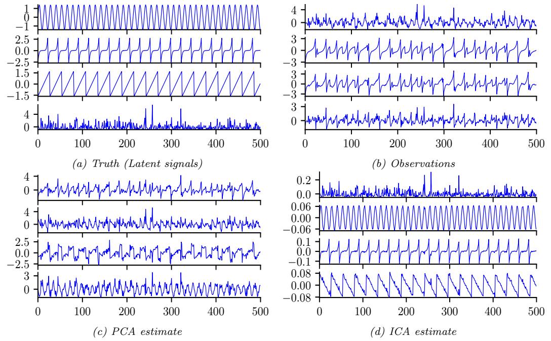
Figure 28.32: Illustration of ICA applied to 500 iid samples of a 4d source signal. This matches the true sources, up to permutation of the dimension indices. Generated by ica\_demo.ipynb.

Our goal is to infer the source signals, p(zn|xn, A). Since the model is noiseless, we have

\[p(\mathbf{z}\_n|\mathbf{z}\_n, \mathbf{A}) = \delta(\mathbf{z}\_n - \mathbf{B}\mathbf{z}\_n) \tag{28.144}\]

where B = A↑¹ are the recognition weights. (We discuss how to estimate these weights in Section 28.6.3.)

28.6.2 The need for non-Gaussian priors

Since x = Az, we have E [x] = AE [z] and Cov [x] = Cov [Az] = ACov [z] A^T. Without loss of generality, we can assume E [z] = 0, since we can always center the data. Similarly, we can assume Cov [z] = I, since AA^T can capture any correlation in x. Thus z is a set of D unit variance, uncorrelated variables, as in factor analysis (Section 28.3.1).

However, this is not su”cient to uniquely identify A and hence z, as we explained in Section 28.3.1.6. So we need to go beyond an uncorrelated prior and enforce an independent, and non-Gaussian, prior.

To illustrate this, suppose we have two independent sources with uniform distributions, as shown in Figure 28.33(a). Now suppose we have the following mixing matrix

\[\mathbf{A} = 0.3 \begin{pmatrix} 2 & 3 \\ 2 & 1 \end{pmatrix} \tag{28.145}\]

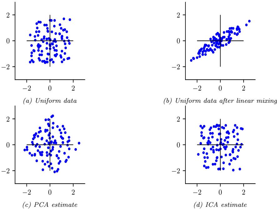
Figure 28.33: Illustration of ICA and PCA applied to 100 iid samples of a 2d source signal with a uniform distribution. Generated by ica\_demo\_uniform.ipynb.

Then we observe the data shown in Figure 28.33(b) (assuming no noise). The full-rank PCA model (where K = D) is equivalent to ICA, except it uses a factored Gaussian prior for z. The result of using PCA is shown in Figure 28.33(c). This corresponds to a whitening or sphering of the data, in which Cov [z] = I. To uniquely recover the sources, we need to perform an additional rotation. The trouble is, there is no information in the symmetric Gaussian posterior to tell us which angle to rotate by. In a sense, PCA solves “half” of the problem, since it identifies the linear subspace; all that ICA has to do is then to identify the appropriate rotation. To do this, ICA uses an independent, but non-Gaussian, prior. The result is shown in Figure 28.33(d). This shows that ICA can recover the source variables, up to a permutation of the indices and possible sign change.

We typically use a prior which is a super-Gaussian distribution, meaning it has heavy tails; this helps with identifiability. One option is to use a Laplace prior. For mean zero and variance 1, this has a log pdf given by

\[\log p(z) = -\sqrt{2}|z| - \log(\sqrt{2})\tag{28.146}\]

However, since the Laplace prior is not di!erentiable at the origin, in ICA it is more common to use the logistic distribution, discussed in Section 15.4.1. If we set the mean to 0 and the variance to 1, we have ^µ = 0 and ^{s = ⇒3} ↽ , so the log pdf becomes the following (using the relationship

sech(x)=1/ cosh(x)):

\[\log p(z) = \log \text{sech}^2(z/2s) - \log(4s) = -2\log \cosh(\frac{\pi}{2\sqrt{3}}z) - \log \frac{4\sqrt{3}}{\pi} \tag{28.147}\]

28.6.3 Maximum likelihood estimation

In this section, we discuss how to estimate the mixing matrix A using maximum likelohood. By the change of variables formula we have

\[p\_x(\mathbf{z}) = p\_z(\mathbf{z}) |\det(\mathbf{A}^{-1})| = p\_z(\mathbf{B}\mathbf{z}) |\det(\mathbf{B})| \tag{28.148}\]

where B = A↑¹. We can simplify the problem by first whitening the data by computing x˜ = S^{↑ 1 2} U^T(^{x ↓ x}), where ” = USU^T is the SVD of the covariance matrix. We can now replace the general matrix B with an orthogonal matrix V. Hence the likelihood becomes

\[p\_x(\hat{\mathbf{z}}) = p\_z(\mathbf{V}\hat{\mathbf{z}})|\det(\mathbf{V})|\tag{28.149}\]

Since we are constraining V to be orthogonal, the | det(V)| term is a constant, so we can drop it. In addition, we drop the tilde symbol, for brevity. Thus the average negative log likelihood can be written as

\[\text{NLL}(\mathbf{V}) = -\frac{1}{N} \log p(\mathbf{X}|\mathbf{V}) = -\frac{1}{N} \sum\_{j=1}^{L} \sum\_{n=1}^{N} \log p\_j(\mathbf{v}\_j^\top \mathbf{z}\_n) \tag{28.150}\]

where v^j is the j’th row of V, and the prior is factored, so p(z) = ^j p^j (z^j ). We can also replace the sum over n with an expectation wrt the empirical distribution to get the following objective

\[\text{NLL}(\mathbf{V}) = \sum\_{j} \mathbb{E}\left[G\_{j}(z\_{j})\right] \tag{28.151}\]

where z^j = v^{T j} x and G^j (z^j ) ↫ ↓ log p^j (z^j ). We want to minimize this (nonconvex) objective subject to the constraint that V is an orthogonal matrix.

It is straightforward to derive a (projected) gradient descent algorithm to fit this model. (For some JAX code, see https://github.com/tuananhle7/ica). One can also derive a faster algorithm that follows the natural gradient; see e.g., [Mac03, ch 34] for details. However, the most popular method is to use an approximate Newton method, known as fast ICA [HO00]. This was used to produce Figure 28.32.

28.6.4 Alternatives to MLE

In this section, we discuss various alternatives estimators for ICA that have been proposed over the years. We will show that they are equivalent to MLE. However, they bring interesting perspectives to the problem.

28.6.4.1 Maximizing non-Gaussianity

An early approach to ICA was to find a matrix V such that the distribution z = Vx is as far from Gaussian as possible. (There is a related approach in statistics called projection pursuit [FT74].) One measure of non-Gaussianity is kurtosis, but this can be sensitive to outliers. Another measure is the negentropy, defined as

\[\text{Ingenentropy}(z) \triangleq \mathbb{H}\left(\mathcal{N}(\mu, \sigma^2)\right) - \mathbb{H}(z) \tag{28.152}\]

where µ = E [z] and ς² = V [z]. Since the Gaussian is the maximum entropy distribution (for a fixed variance), this measure is always non-negative and becomes large for distributions that are highly non-Gaussian.

We can define our objective as maximizing

\[J(\mathbf{V}) = \sum\_{j} \text{negentropy}(z\_j) = \sum\_{j} \mathbb{H}\left(\mathcal{N}(\mu\_j, \sigma\_j^2)\right) - \mathbb{H}\left(z\_j\right) \tag{28.153}\]

where z = Vx. Since we assume E [z] = 0 and Cov [z] = I, the first term is a constant. Hence

\[J(\mathbf{V}) = \sum\_{j} -\mathbb{H}\left(z\_{j}\right) + \text{const} = \sum\_{j} \mathbb{E}\left[\log p(z\_{j})\right] + \text{const} \tag{28.154}\]

which we see is equal (up to a sign change, and irrelevant constants) to the log-likelihood in Equation (28.151).

28.6.4.2 Minimizing total correlation

In Section 5.3.5.1, we show that the total correlation of z is given by

\[\text{TC}(\mathbf{z}) = \sum\_{j} \mathbb{H}(z\_{j}) - \mathbb{H}(\mathbf{z}) = D\_{\text{KL}}\left(p(\mathbf{z}) \parallel \prod\_{j} p\_{k}(z\_{j})\right) \tag{28.155}\]

This is zero i! the components of z are all mutually independent. In Section 21.3.1.1, we show that minimizing this results in a representation that is disentangled.

Now since z = Vx, we have

\[\text{TC}(\mathbf{z}) = \sum\_{j} \mathbb{H}(z\_{j}) - \mathbb{H}(\mathbf{V}x) \tag{28.156}\]

Since we constrain V to be orthogonal, we can drop the last term, since H(Vx) = H(x) = const, since multiplying by V does not change the shape of the distribution. Hence we have TC(z) = * ^k H(zk). Minimizing this is equivalent to maximizing the negentropy, which is equivalent to maximum likelihood.

28.6.4.3 Maximizing mutual information (InfoMax)

Let z^j = ϱ(v^{T j} x) + ϖ be the noisy output of an encoder, where ϱ is some nonlinear scalar function, and ϖ ↑ N (0, 1). It seems reasonable to try to maximize the information flow through this system, a

principle known as infomax [Lin88b; BS95a]. That is, we want to maximize the mutual information between z (the internal neural representation) and x (the observed input signal). We have I(x; z) = H(z) ↓ H(z|x), where the latter term is constant if we assume the noise has constant variance. One can show that we can approximate the former term as follows

\[\mathbb{E}\left(\mathbf{z}\right) = \sum\_{j} \mathbb{E}\left[\log \phi'(\mathbf{v}\_j^{\mathsf{T}} \mathbf{z})\right] + \log|\det(\mathbf{V})|\tag{28.157}\]

where, as usual, we can drop the last term if V is orthogonal. If we define ϱ(z) to be a cdf, then ϱ→ (z) is its pdf, and the above expression is equivalent to the log likelihood. In particular, if we use a logistic nonlinearity, ϱ(z) = ς(z), then the corresponding pdf is the logistic distribution, and log ϱ^→ (z) = log cosh(z), which matches Equation (28.147) (ignoring irrelevant constants). Thus we see that infomax is equivalent to maximum likelihood.

28.6.5 Sparse coding

In this section, we consider an extension of ICA to the case where we allow for observation noise (using a Gaussian likelihood), and we allow for a non-square mixing matrix W. We also use a Laplace prior for z. The resulting model is as follows:

\[p(\mathbf{z}, \mathbf{z}) = p(\mathbf{z})p(\mathbf{z}|\mathbf{z}) = \left[\prod\_{k} \text{Laplace}(z\_k|0, 1/\lambda)\right] \mathcal{N}(\mathbf{z}|\mathbf{W}\mathbf{z}, \sigma^2 \mathbf{I})\tag{28.158}\]

Thus each observation x is approximated by a sparse combination of columns of W, known as basis functions; the sparse vector of weights is given by z. (This can be thought of as a form of sparse factor analysis, except the sparsity is in the latent code z, not the weight matrix W.)

Not all basis functions will be active for any given observation, due to the sparsity penalty. Hence we can allow for more latent factors K than observations D. This is called overcomplete representation.

If we have a batch of N examples, stored in the rows of X, the negative log joint becomes

\[-\log p(\mathbf{X}, \mathbf{Z}|\mathbf{W}) = \frac{1}{2\sigma^2} \sum\_{n=1}^{N} ||\mathbf{x}\_n - \mathbf{W}\mathbf{z}\_n||\_2^2 + \lambda ||\mathbf{z}\_n||\_1 + \text{const} \tag{28.159}\]

\[=\frac{1}{2\sigma^2}||\mathbf{X}-\mathbf{WZ}||\_F^2+\lambda||\mathbf{Z}||\_{1,1}+\text{const}\tag{28.160}\]

The MAP inference problem consists of estimating Z for a fixed W; this is known as sparse coding, and can be solved using standard algorithms for sparse linear regression (see Section 15.2.6).6,

The learning problem consists of estimating W, marginalizing out Z. This is called dictionary learning. Since this is computationally di”cult, it is common to jointly optimize W and Z (thus “maxing out” wrt Z instead of marginalizing it out). We can do this by applying alternating optimization to Equation (28.160): estimating Z given W is a sparse linear regression problem, and estimating W given Z is a simple least squares problem. (For faster algorithms, see [Mai+10].)

^6. Solving an ϱ¹ optimization problem for each data example can be slow. However, it is possible to train a neural network to approximate the outcome of this process; this is known as predictive sparse decomposition [KRL08; GL10].

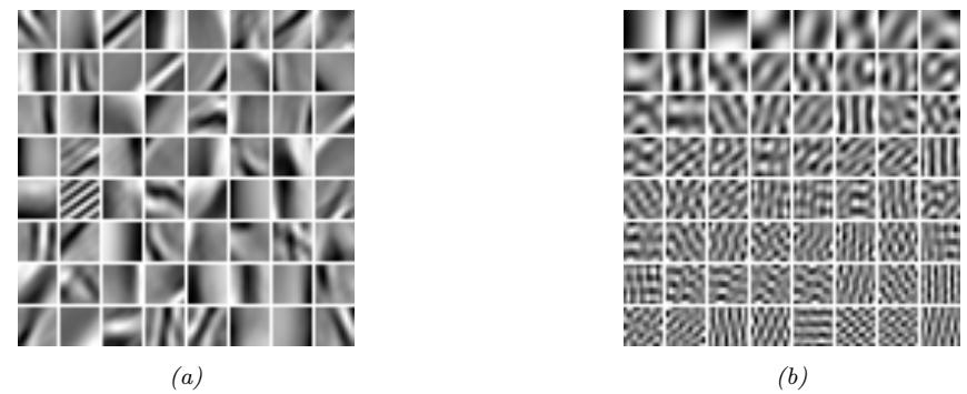
Figure 28.34: Illustration of the filters learned by various methods when applied to natural image patches. (a) Sparse coding. (b) PCA. Generated by sparse\_dict\_demo.ipynb.

Figure 28.34(a) illustrates the results of dictionary learning when applied to a dataset of natural image patches. (Each patch is first centered and normalized to unit norm.) We see that the method has learned bar and edge detectors that are similar to the simple cells in the primary visual cortex of the mammalian brain [OF96]. By contrast, PCA results in sinusoidal gratings, as shown in Figure 28.34(b).7

28.6.6 Nonlinear ICA

There are various ways to extend ICA to the nonlinear case. The resulting methods are similar to variational autoencoders (Chapter 21). For details, see e.g., [KKH20].

^7. The reason PCA discovers sinusoidal grating patterns is because it is trying to model the covariance of the data, which, in the case of image patches, is translation invariant. This means Cov [I(x, y), I(x→ , y→ )] = f # (x ↔︎ x^→ )² + (^{y ↔︎ y→} )2$ for some function f, where I(x, y) is the image intensity at location (x, y). One can show (see e.g., [HHH09, p125]) that the eigenvectors of a matrix of this kind are always sinusoids of di!erent phases, i.e., PCA discovers a Fourier basis.

29 State-space models

29.1 Introduction

A state-space model (SSM) is a partially observed Markov model, in which the hidden state, zt, evolves over time according to a Markov process (Section 2.6), and each hidden state generates some observations y^t at each time step. (We focus on discrete time systems.) The main goal is to infer the hidden states given the observations. However, we may also be interested in using the model to predict future observations (e.g., for time-series forecasting).

An SSM can be represented as a stochastic discrete time nonlinear dynamical system of the form

\[\mathbf{z}\_t = \mathbf{f}(\mathbf{z}\_{t-1}, \mathbf{u}\_t, \mathbf{q}\_t) \tag{29.1}\]

\[y\_t = h(z\_t, u\_t, y\_{1:t-1}, r\_t) \tag{29.2}\]

where ^{zt → RNz} are the hidden states, ^{ut → RNu} are optional observed inputs, ^{yt → RNy} are observed outputs, f is the transition function, q^t is the process noise, h is the observation function, and r^t is the observation noise.

Rather than writing this as a deterministic function of random noise, we can represent it as a probabilistic model as follows:

\[p(\mathbf{z}\_t | \mathbf{z}\_{t-1}, \mathbf{u}\_t) = p(\mathbf{z}\_t | \mathbf{f}(\mathbf{z}\_{t-1}, \mathbf{u}\_t)) \tag{29.3}\]

\[p(y\_t | \mathbf{z}\_t, \mathbf{u}\_t, y\_{1:t-1}) = p(y\_t | \mathbf{h}(\mathbf{z}\_t, \mathbf{u}\_t, y\_{1:t-1})) \tag{29.4}\]

where p(zt|z^t↑¹,ut) is the transition model, and p(yt|zt,ut, y1:t↑¹) is the observation model. Unrolling over time, we get the following joint distribution:

\[p(\mathbf{y}\_{1:T}, \mathbf{z}\_{1:T} | \mathbf{u}\_{1:T}) = \left[ p(\mathbf{z}\_1 | \mathbf{u}\_1) \prod\_{t=2}^{T} p(\mathbf{z}\_t | \mathbf{z}\_{t-1}, \mathbf{u}\_t) \right] \left[ \prod\_{t=1}^{T} p(\mathbf{y}\_t | \mathbf{z}\_t, \mathbf{u}\_t, \mathbf{y}\_{1:t-1}) \right] \tag{29.5}\]

If we assume the current observation y^t only depends on the current hidden state, zt, and the previous observation, y^t↑¹, we get the graphical model in Figure 29.1(a). (This is called an autoregressive state-space model.) However, by using a su”cient expressive hidden state zt, we can implicitly represent all the past observations, y1:t↑¹. Thus it is more common to assume that the observations are conditionally independent of each other (rather than having Markovian dependencies) given the hidden state. In this case the joint simplifies to

\[p(\mathbf{y}\_{1:T}, \mathbf{z}\_{1:T} | \mathbf{u}\_{1:T}) = \left[ p(\mathbf{z}\_1 | \mathbf{u}\_1) \prod\_{t=2}^{T} p(\mathbf{z}\_t | \mathbf{z}\_{t-1}, \mathbf{u}\_t) \right] \left[ \prod\_{t=1}^{T} p(\mathbf{y}\_t | \mathbf{z}\_t, \mathbf{u}\_t) \right] \tag{29.6}\]

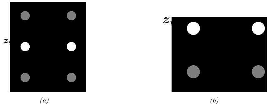
Figure 29.1: State-space model represented as a graphical model. (a) Generic form, with inputs ut, hidden state zt, and observations yt. We assume the observation likelihood is first-order auto-regressive. (b) Simplified form, with no inputs, and Markovian observations.

Sometimes there are no external inputs, so the model further simplifies to the following unconditional generative model:

\[p(\mathbf{y}\_{1:T}, \mathbf{z}\_{1:T}) = \left[ p(\mathbf{z}\_1) \prod\_{t=2}^{T} p(\mathbf{z}\_t | \mathbf{z}\_{t-1}) \right] \left[ \prod\_{t=1}^{T} p(\mathbf{y}\_t | \mathbf{z}\_t) \right] \tag{29.7}\]

See Figure 29.1(b) for the simplified graphical model.

29.2 Hidden Markov models (HMMs)

In this section, we discuss the hidden Markov model or HMM, which is an SSM in which the hidden states are discrete, so z^t → {1,…,K}. The observations may be discrete, y^t → {1,…,Ny}, or continuous, ^{yt → RNy} , or some combination, as we illustrate below. More details on HMMs can be found in Supplementary Chapter 29, as well as other references, such as [Rab89; Fra08; CMR05]. For an interactive introduction, see https://nipunbatra.github.io/hmm/.

29.2.1 Conditional independence properties

The HMM graphical model is shown in Figure 29.1(b). This encodes the assumption that the hidden states are Markovian, and the observations are iid conditioned on the hidden states. All that remains is to specify the form of the conditional probability distributions of each node.

29.2.2 State transition model

The initial state distribution is denoted by

\[p(z\_1 = j) = \pi\_j \tag{29.8}\]

where ↼ is a discrete distribution over the K states.

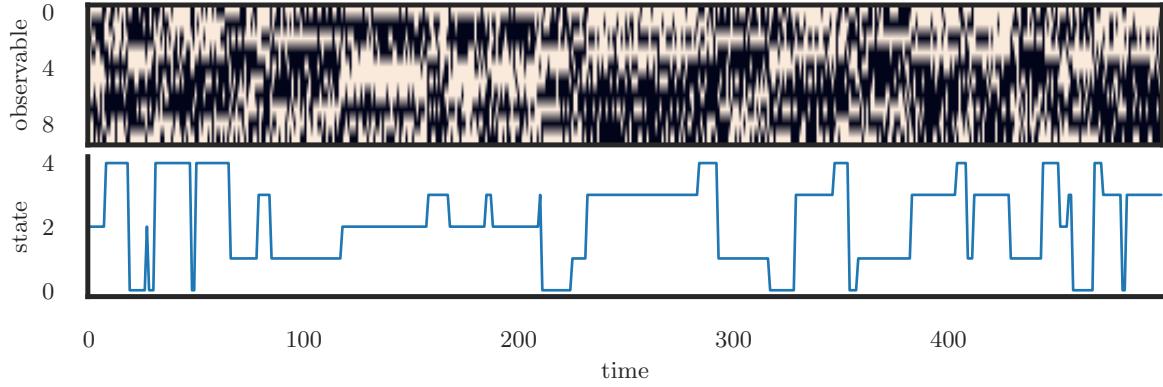
Figure 29.2: Some samples from an HMM with 10 Bernoulli observables. Generated by bernoulli\_hmm\_example.ipynb.

The transition model is denoted by

\[p(z\_t = j | z\_{t-1} = i) = A\_{ij} \tag{29.9}\]

Here the i’th row of A corresponds to the outgoing distribution from state i. This is a row stochastic matrix, meaning each row sums to one. We can visualize the non-zero entries in the transition matrix by creating a state transition diagram, as shown in Figure 2.15.

29.2.3 Discrete likelihoods

The observation model p(yt|z^t = j) can take multiple forms, depending on the type of data. For discrete observations we can use

\[p(y\_t = k | z\_t = j) = y\_{jk} \tag{29.10}\]

For example, see the casino HMM example in Section 9.2.1.1.

If we have D discrete observations per time step, we can use a factorial model of the form

\[p(y\_t | z\_t = j) = \prod\_{d=1}^{D} \text{Cat}(y\_{td} | y\_{d,j,:}) \tag{29.11}\]

In the special case of binary observations, this becomes

\[p(y\_t | z\_t = j) = \prod\_{d=1}^{D} \text{Ber}(y\_{td} | y\_{d,j}) \tag{29.12}\]

In Figure 29.2, we give an example of an HMM with 5 hidden states and 10 Bernoulli observables.

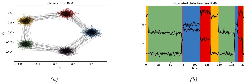
Figure 29.3: (a) Some 2d data sampled from a 5 state HMM. Each state emits from a 2d Gaussian. (b) The hidden state sequence is shown by the colors. We superimpose the observed 2d time series (note that we have shifted the vertical scale so the values don’t overlap). Generated by gaussian\_hmm\_2d.ipynb.

29.2.4 Gaussian likelihoods

If y^t is continuous, it is common to use a Gaussian observation model:

\[p(\mathbf{y}\_t | z\_t = j) = \mathcal{N}(y\_t | \mu\_j, \Sigma\_j) \tag{29.13}\]

As a simple example, suppose we have an HMM with 3 hidden states, each of which generates a 2d Gaussian. We can represent these Gaussian distributions as 2d ellipses, as shown in Figure 29.3(a). We call these “lily pads”, because of their shape. We can imagine a frog hopping from one lily pad to another. (This analogy is due to the late Sam Roweis.) It will stay on a pad for a while (corresponding to remaining in the same discrete state zt), and then jump to a new pad (corresponding to a transition to a new state). See Figure 29.3(b). The data we see are just the 2d points (e.g., water droplets) coming from near the pad that the frog is currently on. Thus this model is like a Gaussian mixture model (Section 28.2.1), in that it generates clusters of observations, except now there is temporal correlation between the datapoints.

We can also use more flexible observation models. For example, if we use an M-component GMM, then we have

\[p(\mathfrak{y} | z\_t = j) = \sum\_{k=1}^{M} w\_{jk} \mathcal{N}(y\_t | \mu\_{jk}, \Sigma\_{jk}) \tag{29.14}\]

This is called a GMM-HMM.

29.2.5 Autoregressive likelihoods

The standard HMM assumes the observations are conditionally independent given the hidden state. In practice this is often not the case. However, it is straightforward to have direct arcs from y^t↑¹ to y^t as well as from z^t to yt, as in Figure 29.1(a). This is known as an auto-regressive HMM.

For continuous data, we can use an observation model of the form

\[p(y\_t | y\_{t-1}, z\_t = j, \boldsymbol{\theta}) = N(y\_t | \mathbf{E}\_j y\_{t-1} + \boldsymbol{\mu}\_j, \boldsymbol{\Sigma}\_j) \tag{29.15}\]

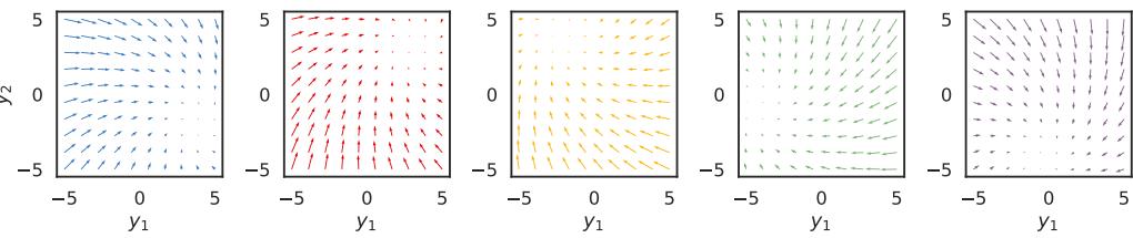
Figure 29.4: Illustration of the observation dynamics for each of the 5 hidden states. The attractor point corresponds to the steady state solution for the corresponding autoregressive process. Generated by hmm\_ar.ipynb.

This is a linear regression model, where the parameters are chosen according to the current hidden state. (We could also use a nonlinear model, such as a neural network.) Such models are widely used in econometrics, where they are called regime switching Markov model [Ham90]. Similar models can be defined for discrete observations (see e.g., [SJ99]).

We can also consider higher-order extensions, where we condition on the last L observations:

\[p(y\_t | y\_{t-L:t-1}, z\_t = j, \boldsymbol{\theta}) = \mathcal{N}(y\_t | \sum\_{\ell=1}^{L} \mathbf{W}\_{j,\ell} y\_{t-\ell} + \boldsymbol{\mu}\_j, \boldsymbol{\Sigma}\_j) \tag{29.16}\]

The AR-HMM essentially combines two Markov chains, one on the hidden variables, to capture long range dependencies, and one on the observed variables, to capture short range dependencies [Ber99]. Since all the visible nodes are observed, adding connections between them just changes the likelihood, but does not complicate the task of posterior inference (see Section 9.2.3).

Let us now consider a 2d example of this, due to Scott Linderman. We use a left-to-right transition matrix with 5 states. In addition, the final state returns to first state, so we just cycle through the states. Let ^{yt → R}2, and suppose we set ^Ej to a rotation matrix with a small angle of 7 degrees, and we set each µ^j to 72-degree separated points on a circle about the origin, so each state rotates 1/5 of the way around the circle. If the model stays in the same state j for a long time, the observed dynamics will converge to the steady state y↔︎,j , which satisfies y↔︎,j = Ejy↔︎,j + µ^j ; we can solve for the steady state vector using ^y↔︎,j = (^{I ↓ Ej} )↑¹µ^j . We can visualize the induced 2d flow for each of the 5 states as shown in Figure 29.4.

In Figure 29.5(a), we show a trajectory sampled from this model. We see that the two components of the observation vector undergo di!erent dynamics, depending on the underlying hidden state. In Figure 29.5(b), we show the same data in a 2d scatter plot. The first observation is the yellow dot (from state 2) at (↓0.8, 0.5). The dynamics converge to the stationary value of y↔︎,² = (↓2.0, 3.8). Then the system jumps to the green state (state 3), so it adds an o!set of µ³ to the last observation, and then converges to the stationary value of y↔︎,³ = (↓4.3, ↓0.8). And so on.

29.2.6 Neural network likelihoods

For higher dimensional data, such as images, it can be useful to use a normalizing flow (Chapter 23), one per latent state (see e.g., [HNBK18; Gho+21]), as the class-conditional generative model. However, it is also possible to use discriminative neural network classifiers, which are much easier to train. In

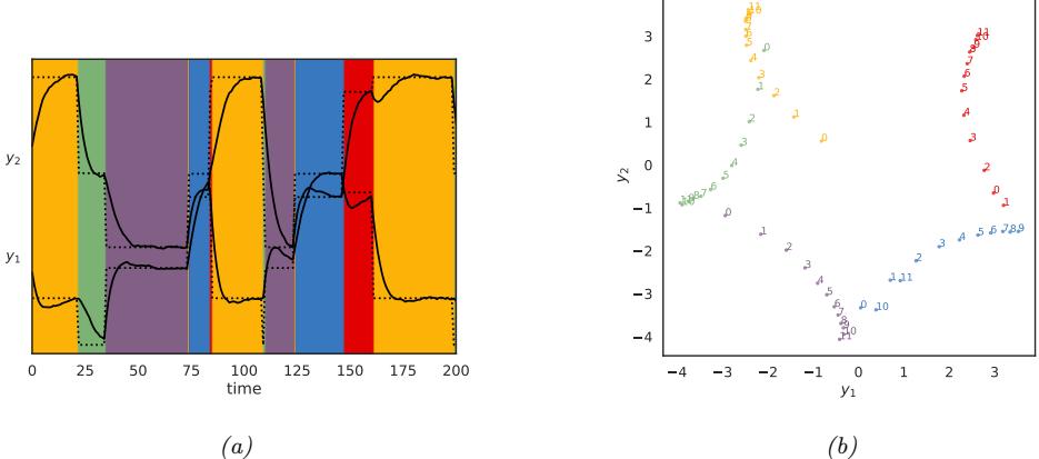
Figure 29.5: Samples from the 2d AR-HMM. (a) Time series plot of yt,¹ and yt,2. (The latter are shifted up vertically by 4.7) The background color is the generating state. The dotted lines represent the stationary value for that component of the observation. (b) Scatter plot of observations. Colors denote the generating state. We show the first 12 samples from each state. Generated by hmm\_ar.ipynb.

particular, note that the likelihood per state can be rewritten as follows:

\[p(y\_t|z\_t=j) = \frac{p(z\_t=j|y\_t)p(y\_t)}{p(z\_t=j)} \propto \frac{p(z\_t=j|y\_t)}{p(z\_t=j)}\tag{29.17}\]

where we have dropped the p(yt) term since it is independent of the state zt. Here p(z^t = j|yt) is the output of a classifier, and p(z^t = j) is the probability of being in state j, which can be computed from the stationary distribution of the Markov chain (or empirically, if the state sequence is known). We can thus use discriminative classifiers to define the likelihood function when using gradient-based training. This is called the scaled likelihood trick [BM93; Ren+94]. [Guo+14] used this to create a hybrid CNN-HMM model for estimating sequences of digits based on street signs.

29.3 HMMs: applications

In this section, we discuss some applications of HMMs.

29.3.1 Time series segmentation

In this section, we give a variant of the casino example from Section 9.2.1.1, where our goal is to segment a time series into di!erent regimes, each of which corresponds to a di!erent statistical distribution. In Figure 29.6a we show the data, corresponding to counts generated from some process (e.g., visits to a web site, or number of infections). We see that the count rate seems to be roughly constant for a while, and then changes at certain points. We would like to segment this data stream into K di!erent regimes or states, each of which is associated with a Poisson observation model with

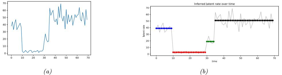
Figure 29.6: (a) A sample time series dataset of counts. (b) A segmentation of this data using a 4 state HMM. Generated by poisson\_hmm\_changepoint.ipynb.

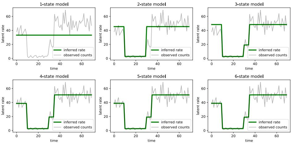
Figure 29.7: Segmentation of the time series using HMMs with 1–6 states. Generated by poisson\_hmm\_changepoint.ipynb.

rate ωk:

\[p(y\_t | z\_t = k) = \text{Poi}(y\_t | \lambda\_k) \tag{29.18}\]

We use a uniform prior over the initial states. For the transition matrix, we assume the Markov chain stays in the same state with probability p = 0.95, and otherwise transitions to one of the other K ↓ 1 states uniformly at random:

\[z\_1 \sim \text{Categorical}\left(\left\{\frac{1}{4}, \frac{1}{4}, \frac{1}{4}, \frac{1}{4}\right\}\right) \tag{29.19}\]

\[z\_t | z\_{t-1} \sim \text{Categorical}\left(\left\{ \begin{array}{cc} p & \text{if } z\_t = z\_{t-1} \\ \frac{1-p}{4-1} & \text{otherwise} \end{array} \right\} \right) \tag{29.20}\]

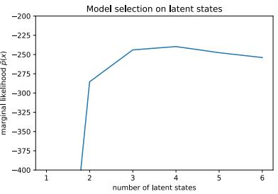
Figure 29.8: Marginal likelihood vs number of states K in the Poisson HMM. Generated by poisson\_hmm\_changepoint.ipynb.

We compute a MAP estimate for the parameters ⇀1:^K using a log-Normal(5,5) prior. We optimize the log of the Poisson rates using gradient descent, initializing the parameters at a random value centered on the log of the overall count means. We show the results in Figure 29.6b. See that the method has successfully partitioned the data into 4 regimes, which is in fact how it was generated. (The generating rates are ⇀ = (40, 3, 20, 50), with the changepoints happening at times (10, 30, 35).)

In general we don’t know the optimal number of states K. To solve this, we can fit many di!erent models, as shown in Figure 29.7, for K =1:6. We see that after K ⇒ 3, the model fits are very similar, since multiple states get associated to the same regime. We can pick the “best” K to be the one with the highest marginal likelihood. Rather than summing over both discrete latent states and integrating over the unknown parameters ⇀, we just maximize over the parameters (empirical Bayes approximation):

\[p(\mathbf{y}\_{1:T}|K) \approx \max\_{\lambda} \sum\_{\mathbf{z}} p(\mathbf{y}\_{1:T}, \mathbf{z}\_{1:T} | \lambda, K) \tag{29.21}\]

We show this plot in Figure 29.8. We see the peak is at K = 3 or K = 4; after that it starts to go down, due to the Bayesian Occam’s razor e!ect.

29.3.2 Protein sequence alignment

An important application of HMMs is to the problem of protein sequence alignment [Dur+98]. Here the goal is to determine if a test sequence y1:^T belongs to a protein family or not, and if so, how it aligns with the canonical representation of that family. (Similar methods can be used to align DNA and RNA sequences.)

To solve the alignment problem, let us initially assume we have a set of aligned sequences from a protein family, from which we can generate a consensus sequence. This defines a probability distribution over symbols at each location t in the string; denote each position-specific scoring matrix (PSSM) by 1t(v) = p(y^t = v). These parameters can be estimated by counting.

Now we turn the PSSM into an HMM with 3 hidden states, representing the events that the location t matches the consensus sequence, z^t = M, or inserts its own unique symbol, z^t = I, or deletes (skips) the corresponding consensus symbol, z^t = D. We define the observation models for these 3 events as follows. For matches, we use the PSSM p(y^t = v|z^t = M) = 1t(v). For insertions

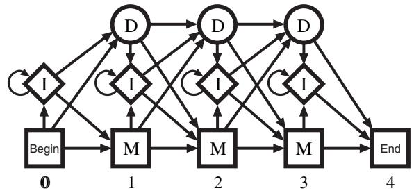
20. . . x

AG- - - C A- AG- C AG- AA- - - AAAC AG- - - C

1 3 2. . .

(a) Multiple alignment:

bat rat cat gnat goat

Figure 29.9: State transition diagram for a profile HMM. From Figure 5.7 of [Dur+98]. Used with kind permission of Richard Durbin.

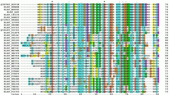
Figure 29.10: Example of multiple sequence alignment. We show the first 90 positions of the acidic ribosomal protein P0 from several organisms. Colors represent functional properties of the corresponding amino acid. Dashes represent insertions or deletions. From https: // en. wikipedia. org/ wiki/ Multiple\_ sequence\_ alignment . Used with kind permission of Wikipedia author Miguel Andrade.

we use the uniform distribution p(y^t = v|z^t = I)=1/V , where V is the size of the vocabulary. For deletions, we use p(y^t = ↓|z^t = D), where “-” is a special deletion symbol used to pad the generated sequence to the correct length. The corresponding state transition matrix is shown in Figure 29.9: we see that matches and deletions advance one location along the consensus sequence, but insertions stay in the same location (represented by the self-transition from I to I). This model is known as a profile HMM.

Given a profile HMM with consensus parameters ε, we can compute p(y1:^T |ε) in O(T) time using the forwards algorithm, as described in Section 9.2.2. This can be used to decide if the sequence belongs to this family or not, by thresholding the log-odds score, L(y) = log p(y|ε)/p(y|M0), where M⁰ is a baseline model, such as the uniform distribution. If the string matches, we can compute an alignment to the consensus using the Viterbi algorithm, as described in Section 9.2.6. See Figure 29.10 for an illustration of such a multiple sequence alignment. If we don’t have an initial set of aligned sequences from which to compute the consensus sequence ε, we can use the Baum-Welch algorithm

Author: Kevin P. Murphy. (C) MIT Press. CC-BY-NC-ND license

0

4 1 0

0 0 0

---

• • • • 0

(c) Observed emission/transition counts

A C G T A C G T M-M M-D M-I I-M I-D I-I D-M D-D D-I

match emissions

insert emissions

state transitions 0123

model position

2 0 1

2 1

0 0 2

4 0 0

0 0 0

1 0 0

3 1 0

0 1 0 (Section 29.4.1) to compute the MLE for the parameters ε from a set of unaligned sequences. For details, see e.g., [Dur+98, Ch.6].

29.3.3 Spelling correction

In this section, we illustrate how to use an HMM for spelling correction. The goal is to infer the sequence of words z1:^T that the user meant to type, given observations of what they actually did type, y1:^T .

29.3.3.1 Baseline model

We start by using a simple unigram language model, so p(z1:^T ) = 1:^T p(zt), where p(z^t = k) is the prior probability of word k being used. These probabilities can be estimated by simply normalizing word frequency counts from a large training corpus. We ignore any Markov structure.

Now we turn to the observation model, p(y^t = v|z^t = k), which is the probability the user types word v when they meant to type word k. For this, we use a noisy channel model, in which the “message” z^t gets corrupted by one of four kinds of error: substitution error, where we swap one letter for another (e.g., “government” mistyped as “govermment”); transposition errors, where we swap the order of two adjacent letters (e.g., “government” mistyped as “govermnent”); deletion errors, where we omit one letter (e.g., “government” mistyped as “goverment”); and insertion errors, where we add an extra latter (e.g., “government” mistyped as “governmennt”). If y di!ers from z by d such errors, we say that y and z have an edit distance of d. Let D(y, d) be the set of words that are edit distance d away from y. We can then define the following likelihood function:

\[p(y|z) = \begin{cases} p\_1 & y = z \\ p\_2 & y \in \mathcal{D}(z, 1) \\ p\_3 & y \in \mathcal{D}(z, 2) \\ p\_4 & \text{otherwise} \end{cases} \tag{29.22}\]

where p¹ > p² > p³ > p4.

We can combine the likelihood with the prior to get the overall score for each hypothesis (i.e., candidate correction). This simple model, which was proposed by Peter Norvig1, can work can quite well. However, it also has some flaws. For example, the error model assumes that the smaller the edit distance, the more likely the word, but this is not always valid. For example, “reciet” gets corrected to “recite” instead of “receipt”, and “adres” gets corrected to “acres” not “address”. We can fix this problem by learning the parameters of the noise model based on a labeled corpus of (z, x) pairs derived from actual spelling errors. One possible way to get such a corpus is to look at web search behavior: if a user types query q¹ and then quickly changes it to q² followed by a click on a link, it suggests that q² is a manual correction for q1, so we can set (z = q2, y = q1). This heuristic has been used in the Etsy search engine.2 It is also possible to manually collect such data (see e.g., [Hag+17]), or to algorithmically create (z, y) pairs, where y is an automatically generated misspelling of z (see e.g., [ECM18]).

^1. See his excellent tutorial at http://norvig.com/spell-correct.html.

^2. See this blogpost by Mohit Nayyar for details: https://codeascraft.com/2017/05/01/ modeling-spelling-correction-for-search-at-etsy/.

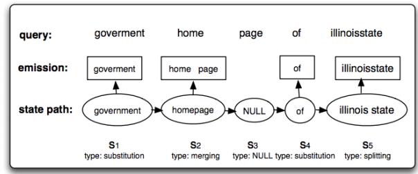
Figure 29.11: Illustration of an HMM applied to spelling correction. The top row, labeled “query”, represents the search query y1:^T typed by the user, namely “goverment home page of illinoisstate”. The bottom row, labeled “state path”, represents the most probable assignment to the hidden states, z1:^T , namely “government homepage of illinois state”. (The NULL state is a silent state, that is needed to handle the generation of two tokens from a single hidden state.) The middle row, labeled “emission”, represents the words emitted by each state, which match the observed data. From Figure 1 of [LDZ11].

29.3.3.2 HMM model

The baseline model can work well, but has room for improvement. In particular, many errors will be hard to correct without context. For example, suppose the user typed “advice”: did they mean “advice” or “advise”? It depends on whether they intended to use a noun or a verb, which is hard to tell without looking at the sequence of words. To do this, we will “upgrade” our model to an HMM. We just have to replace our independence prior p(z1:^T ) = ^t p(zt) by a standard first-order language model on words, p(z1:^T ) = ^t p(zt|z^t↑¹). The parameters of this model can be estimated by counting bigrams in a large corpus of “clean” text (see Section 2.6.3.1). The observation model p(yt|zt) can remain unchanged.

Given this model, we can compute the top N most likely hidden sequences in O(NTK²) time, where K is the number of hidden states, and T is the length of the sequence, as explained in Section 9.2.6.5. In a naive implementation, the number of hidden states K is the number of words in the vocabulary, which would make the method very slow. However, we can exploit sparsity of the likelihood function (i.e., the fact that p(y|z) is 0 for most values of z) to generate small candidate lists of hidden states for each location in the sequence. This gives us a sparse belief state vector ↽t.

29.3.3.3 Extended HMM model

We can extend the HMM model to handle higher level errors, in addition to misspellings of individual words. In particular, [LDZ11; LDZ12] proposed modeling the following kinds of errors:

• Two words merged into one, e.g., “home page” ↔︎ “homepage”.
• One word split into two, e.g., “illinoisstate” ↔︎ “illinois state”.
• Within-word errors, such as substitution, transposition, insertion and deletion of letters, as we discussed in Section 29.3.3.2.

We can model this with an HMM, where we augment the state space with a silent state, that does not emit any symbols. Figure 29.11 illustrates how this model can “denoise” the observed query “goverment home page of illinoisstate” into the correctly formulated query “government homepage of illinois state”.

An alternative to using HMMs is to use supervised learning to fit a sequence-to-sequence translation model, using RNNs or transformers. This can work very well, but often needs much more training data, which can be problematic for low-resource languages [ECM18].

29.4 HMMs: parameter learning

In this section, we discuss how to compute a point estimate or the full posterior over the model parameters of an HMM given a set of partially observed sequences.

29.4.1 The Baum-Welch (EM) algorithm

In this section, we discuss how to compute an approximate MLE for the parameters of an HMM using the EM algorithm which is an iterative bound optimization algorithm (see Section 6.5.3 for details). When applied to HMMs, the resulting method is known as the Baum-Welch algorithm [Bau+70].

29.4.1.1 Log likelihood

The joint probability of a single sequence is given by

\[p(y\_{1:T}, z\_{1:T} | \boldsymbol{\theta}) = [p(z\_1 | \boldsymbol{\pi})] \left[ \prod\_{t=2}^{T} p(z\_t | z\_{t-1}, \mathbf{A}) \right] \left[ \prod\_{t=1}^{T} p(y\_t | z\_t, \mathbf{B}) \right] \tag{29.23}\]

\[=\left[\prod\_{k=1}^{K}\pi\_{k}^{\mathbb{I}(z\_{1}=k)}\right]\left[\prod\_{t=2}^{T}\prod\_{j=1}^{K}\prod\_{k=1}^{K}A\_{jk}^{\mathbb{I}(z\_{t-1}=j,z\_{t}=k)}\right]\left[\prod\_{t=1}^{T}\prod\_{k=1}^{K}p(y\_{t}|\mathbf{B}\_{k})^{\mathbb{I}(z\_{t}=k)}\right] \tag{29.24}\]

where ε = (↼, A, B). Of course, we cannot compute this objective, since z1:^T is hidden. So instead we will optimize the expected complete data log likelihood, where expectations are taken using the parameters from the previous iteration of the algorithm:

\[Q(\theta, \theta^{\text{old}}) = \mathbb{E}\_{p(\mathbf{z}\_{1:T} | \mathbf{y}\_{1:T}, \theta^{\text{old}})} \left[ \log p(\mathbf{y}\_{1:T}, \mathbf{z}\_{1:T} | \theta) \right] \tag{29.25}\]

This can be easily summed over N sequences. See Figure 29.12 for the graphical model.

The above objective is a lower bound on the observed data log likelihood, log p(y1:^T |ε), so the entire procedure is a bound optimization method that is guaranteed to converge to a local optimum. (In fact, if suitably initialized, the method can be shown to converge to (close to) one of the global optima [YBW15].)

29.4.1.2 E step

Let Ajk = p(z^t = k|z^t↑¹ = j) be the K ↗ K transition matrix. For the first time slice, let φ^k = p(z¹ = k) be the initial state distribution. Let ε^k represent the parameters of the observation model for state k.

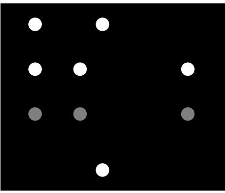
Figure 29.12: HMM with plate notation. A are the parameters for the state transition matrix p(zt|z^t↑¹) and B are the parameters for the discrete observation model p(xt|zt). Tⁿ is the length of the n’th sequence.

To compute the expected su”cient statistics, we first run the forwards-backwards algorithm on each sequence (see Section 9.2.3). This returns the following node and edge marginals:

\[p\_{n,t}(j) \triangleq p(z\_t = j | \mathbf{y}\_{n,1:T\_n}, \theta^{old}) \tag{29.26}\]

\[\xi\_{n,t}(j,k) \triangleq p(z\_{t-1}=j, z\_t=k|y\_{n,1:T\_n}, \theta^{\text{old}}) \tag{29.27}\]

where Tⁿ is the length of sequence n. We can then derive the expected counts as follows (note that we pool the su”cient statistics across time, since the parameters are tied, as well as across sequences):

\[\mathbb{E}\left[N\_k^1\right] = \sum\_{n=1}^N \gamma\_{n,1}(k), \mathbb{E}\left[N\_k\right] = \sum\_{n=1}^N \sum\_{t=2}^{T\_n} \gamma\_{n,t}(k), \mathbb{E}\left[N\_{jk}\right] = \sum\_{n=1}^N \sum\_{t=2}^{T\_n} \xi\_{n,t}(j,k) \tag{29.28}\]

Given the above quantities, we can compute the expected complete data log likelihood as follows:

\[\begin{split} Q(\boldsymbol{\theta},\boldsymbol{\theta}^{\text{old}}) &= \sum\_{k=1}^{K} \mathbb{E}\left[N\_{k}^{1}\right] \log \pi\_{k} + \sum\_{j=1}^{K} \sum\_{k=1}^{K} \mathbb{E}\left[N\_{jk}\right] \log A\_{jk} \\ &+ \sum\_{n=1}^{N} \sum\_{t=1}^{T\_{n}} \sum\_{k=1}^{K} p(z\_{t} = k | \mathbf{y}\_{n,1:T\_{n}}, \boldsymbol{\theta}^{\text{old}}) \log p(\mathbf{y}\_{n,t} | \boldsymbol{\theta}\_{k}) \end{split} \tag{29.29}\]

29.4.1.3 M step

We can estimate the transition matrix and initial state probabilities by maximizing the objective subject to the sum to one constraint. The result is just a normalized version of the expected counts:

\[\hat{A}\_{jk} = \frac{\mathbb{E}\left[N\_{jk}\right]}{\sum\_{k'} \mathbb{E}\left[N\_{jk'}\right]}, \ \hat{\pi}\_k = \frac{\mathbb{E}\left[N\_k^1\right]}{N} \tag{29.30}\]

This result is quite intuitive: we simply add up the expected number of transitions from j to k, and divide by the expected number of times we transition from j to anything else.

For a categorical observation model, the expected su”cient statistics are

\[\mathbb{E}\left[M\_{kv}\right] = \sum\_{n=1}^{N} \sum\_{t=1}^{T\_n} \gamma\_{n,t}(k)\mathbb{I}\left(y\_{n,t} = v\right) = \sum\_{n=1}^{N} \sum\_{t:y\_{n,t} = v} \gamma\_{n,t}(k) \tag{29.31}\]

The M step has the form

\[ \hat{B}\_{kv} = \frac{\mathbb{E}\left[M\_{kv}\right]}{\mathbb{E}\left[N\_k\right]} \tag{29.32} \]

This result is quite intuitive: we simply add up the expected number of times we are in state k and we see a symbol v, and divide by the expected number of times we are in state k. See Algorithm 11 for the pseudocode.

For a Gaussian observation model, the expected su”cient statistics are given by

\[\overline{\mathbf{y}}\_k = \sum\_{n=1}^N \sum\_{t=1}^{T\_n} \gamma\_{n,t}(k) y\_{n,t}, \ \overline{\mathbf{y} \mathbf{y}^T}\_k = \sum\_{n=1}^N \sum\_{t=1}^{T\_n} \gamma\_{n,t}(k) y\_{n,t} \mathbf{y}\_{n,t}^T \tag{29.33}\]

The M step becomes

\[ \hat{\mu}\_k = \frac{\overline{y}\_k}{\mathbb{E}\left[N\_k\right]} \tag{29.34} \]

\[ \hat{\Sigma}\_k = \frac{\overline{\mathbf{y}\mathbf{y}^\mathsf{T}\_k} - \mathbb{E}\left[N\_k\right]\hat{\boldsymbol{\mu}}\_k\hat{\boldsymbol{\mu}}\_k^\mathsf{T}}{\mathbb{E}\left[N\_k\right]} \tag{29.35} \]

In practice, we often need to add a log prior to these estimates to ensure the resulting “ˆ ^k estimate is well-conditioned. See [Mur22, Sec 4.5.2] for details.

Algorithm 29.1: Baum-Welch algorithm for (discrete observation) HMMs

Initialize parameters ε for each iteration do // E step Initialize expected counts: E [Nk]=0, E [Njk]=0, E [Mkv]=0 for each datacase n do Use forwards-backwards algorithm on yⁿ to compute γn,t and 4n,t (Equations 29.26–29.27) E [Nk] := E [Nk] + *^{Tn t}=2 γn,t(k) E [Njk] := E [Njk] + *^{Tn t}=2 4n,t(j, k) E [Mkv] := E [Mkv] + * ^t:xn,t=^v γn,t(k) // M step Compute new parameters ε = (A, B,↼) using Equations 29.30

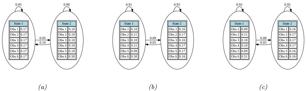
Figure 29.13: Illustration of the casino HMM. (a) True parameters used to generate the data. (b) Estimated parameters using EM. (c) Estimated parameters using SGD. Note that in the learned models (b-c), states 1 and 2 are switched compared to the generating model (a), due to unidentifiability. Generated by casino\_hmm\_training.ipynb.

29.4.1.4 Initialization

As usual with EM, we must take care to ensure that we initialize the parameters carefully, to minimize the chance of getting stuck in poor local optima. There are several ways to do this, such as:

• Use some fully labeled data to initialize the parameters.
• Initially ignore the Markov dependencies, and estimate the observation parameters using the standard mixture model estimation methods, such as K-means or EM.
• Randomly initialize the parameters, use multiple restarts, and pick the best solution.

Techniques such as deterministic annealing [UN98; RR01a] can help mitigate the e!ect of local minima. Also, just as K-means is often used to initialize EM for GMMs, so it is common to initialize EM for HMMs using Viterbi training. The Viterbi algorithm is explained in Section 9.2.6, but basically it is an algorithm to compute the single most probable path. As an approximation to the E step, we can replace the sum over paths with the statistics computed using this single path. Sometimes this can give better results [AG11].

29.4.1.5 Example: casino HMM

In this section, we fit the casino HMM from Section 9.2.1.1. The true generative model is shown in Figure 29.13a. We used this to generate 4 sequences of length 5000, totalling 20,000 observations. We initialized the model with random parameters. We ran EM for 200 iterations and got the results in Figure 29.13b. We see that the learned parameters are close to the true parameters, modulo label switching of the states (see Section 28.2.6).

29.4.2 Parameter estimation using SGD

Although the EM algorithm is the “traditional” way to fit HMMs, it is inherently a batch algorithm, so it does not scale well to large datasets (with many sequences). Although it is possible to extend

Figure 29.14: Average negative log likelihood per learning step the casino HMM. (a) EM. (b) SGD with minibatch size 1. (b) Full batch gradient descent. Generated by casino\_hmm\_training.ipynb.

bound optimization to the online case (see e.g., [Mai15]), this can take a lot of memory.

A simple alternative is to optimize log p(y1:^T |ε) using SGD. We can compute this objective using the forwards algorithm, as shown in Equation (8.7):

\[\log p(y\_{1:T}|\theta) = \sum\_{t=1}^{T} \log p(y\_t|y\_{1:t-1}, \theta) = \sum\_{t=1}^{T} \log Z\_t \tag{29.36}\]

where the normalization constant for each time step is given by

\[Z\_t \triangleq p(y\_t | y\_{1:t-1}) = \sum\_{j=1}^{K} p(z\_t = j | y\_{1:t-1}) p(y\_t | z\_t = j) \tag{29.37}\]

Of course, we need to ensure the transition matrix remains a valid row stochastic matrix, i.e., that ^{0 ≃ A}ij ^{≃ 1} and * ^j Aij = 1. Similarly, if we have categorical observations, we need to ensure Bjk is a valid row stochastic matrix, and if we have Gaussian observations, we need to ensure “^k is a valid psd matrix. These constraints are automatically taken care of in EM. When using SGD, we can reparameterize to an unconstrained form, as proposed in [BC94].

29.4.2.1 Example: casino HMM

In this section, we use SGD to fit the casino HMM using the same data as in Section 29.4.1.5. We show the learning the learning curves in Figure 29.14. We see that SGD converges slightly more slowly than EM, and is not monotonic in how it decreases the NLL loss, even in the full batch case. However, the final parameters are similar, as shown in Figure 29.13.

29.4.3 Parameter estimation using spectral methods

Fitting HMMs using maximum likelihood is di”cult, because the log likelihood is not convex. Thus there are many local optima, and EM and SGD can give poor results. An alternative approach is to marginalize out the hidden variables, and work instead with predictive distributions in the visible space. For discrete observation HMMs, with observation matrix Bjk = p(y^t = k|z^t = j), such a

distribution has the form

\[p[y\_t]\_k \triangleq p(y\_t = k | y\_{1:t-1})\tag{29.38}\]

This is called a predictive state representation [SJR04].

Suppose there are m possible hidden states, and n possible visible symbols, where n ⇒ m. One can show [HKZ12; Joh12] that the PSR vectors lie in a subspace in ^Rn with a dimensionality of ^{m ≃ n}. Intuitively this is because the linear operator A defining the hidden state update in Equation (9.8), combined with the mapping to observables via B, induces low rank structure in the output space. Furthermore, we can estimate a basis for this low rank subspace using SVD applied to the observable matrix of co-occurrence counts:

\[[\mathbf{P}\_2]\_{ij} = p(y\_t = i, y\_{t-1} = j) \tag{29.39}\]

We also need to estimate the third order statistics

\[[\mathbf{P}\_3]\_{ijk} = p(y\_t = i, y\_{t-1} = j, y\_{t-2} = k) \tag{29.40}\]

Using these quantities, it possible to perform recursive updating of our predictions while working entirely in visible space. This is called spectral estimation, or tensor decomposition [HKZ12; AHK12; Rod14; Ana+14; RSG17].

We can use spectral methods to get a good initial estimate of the parameters for the latent variable model, which can then be refined using EM (see e.g., [Smi+00]). Alternatively, we can use them “as is”, without needing EM at all. See [Mat14] for a comparison of these methods. See also Section 29.8.2 where we discuss spectral methods for fitting linear dynamical systems.

29.4.4 Bayesian HMMs

MLE methods can easily overfit, and can su!er from numerical problems, especially when sample sizes are small. In this section, we briefly discuss some approaches to inferring the posterior over the parameters, p(ε|D). By adopting a Bayesian approach, we can also allow the number of states to be unbounded by using a hierarchical Dirichlet process (Supplementary Section 31.1) to get a HDP-HMM [Fox+08].

There are various algorithms we can use to perform posterior inference, such as variational Bayes EM [Bea03] or blocked Gibbs sampling (see Section 29.4.4.1), that alternates between sampling latent sequences z^s 1:T ,1:^N using the forwards filtering backwards sampling algorithm (Section 9.2.7) and sampling the parameters from their full conditionals, ^p(ε|y1:^T , ^zs 1:T ,1:^N ). Unfortuntely, the high correlation between z and ε makes this coordinate-wise approach rather slow.

A faster approach is to marginalize out the discrete latents (using the forwards algorithm), and then to use MCMC [Fot+14] or SVI [Obe+19] to sample from the following log posterior:

\[\log p(\boldsymbol{\theta}, \mathcal{D}) = \log p(\boldsymbol{\theta}) + \sum\_{n=1}^{N} \log p(\boldsymbol{y}\_{1:T,n} | \boldsymbol{\theta}) \tag{29.41}\]

This is a form of “collapsed” inference.

29.4.4.1 Blocked Gibbs sampling for HMMs

This section is written by Xinglong Li.

In this section, we discuss Bayesian inference for HMMs using blocked Gibbs sampling [Sco02]. For the observation model, we consider the first-order auto-regressive HMM model in Section 29.2.5, so p(yt|yt↑1, z^t = j, ε) = N (yt|Ejyt↑¹ + µ^j , “^j ). For a model with K hidden states, the unknown parameters are ε = {↼, A, E1,…, EK,”1,…, “K}, where we assume (for notational simplicity) that µ^j of each autoregressive model is known, and that we condition the observations on y1.

We alternate between sampling from p(z1:^T |y1:^T , ε) using the forwards filtering backwards sampling algorithm (Section 9.2.7), and sampling from p(ε|z1:^T , y1:^T ). Sampling from p(ε|z1:^T , y1:^T ) is easy if we use conjugate priors. Here we use a Dirichlet prior for ↼ and each row A^j· of the transition matrix, and choose the matrix normal inverse Wishart distribution as the prior for {E^j , “j} of each autoregressive model, similar to Bayesian multivariate linear regression Section 15.2.9. In particular, the prior distributions of ε are:

\[ \pi \sim \text{Dir}(\mathfrak{\alpha}\_{\pi}) \tag{29.42} \]

\[\begin{aligned} \mathbf{E}\_j \sim \text{IW}(\boldsymbol{\vartheta}\_j, \check{\boldsymbol{\Psi}}\_j) \end{aligned} \qquad \qquad \qquad \mathbf{E}\_j | \boldsymbol{\Sigma}\_j \sim \mathcal{M} \mathcal{N}(\check{\mathbf{M}}\_j, \boldsymbol{\Sigma}\_j, \check{\mathbf{V}}\_j) \tag{29.43}\]

where ↭↽↽,k=↭↽↽ /K and ↭↽A,k=↭↽^A /K. The log prior probability is

\[\begin{split} \log p(\boldsymbol{\theta}) = & c + \sum\_{k=1}^{K} \frac{\mathbb{M}\_{\pi}}{K} \log \pi\_{k} + \sum\_{j=1}^{K} \sum\_{k=1}^{K} \frac{\mathbb{M}\_{A}}{K} \log A\_{jk} - \sum\_{j=1}^{K} \left( \frac{\mathbb{M}\_{j} + \mathbb{N}\_{y} + 1}{2} \log |\boldsymbol{\Sigma}\_{j}| + \frac{1}{2} \text{tr} \left( \check{\boldsymbol{\Psi}}\_{j} \, \boldsymbol{\Sigma}\_{j}^{-1} \right) \right) \\ & - \sum\_{j=1}^{K} \left( \frac{1}{2} \log |\boldsymbol{\Sigma}\_{j}| + \frac{1}{2} \text{tr} ( (\boldsymbol{\mathsf{E}}\_{j} - \check{\mathbf{M}}\_{j})^{\mathsf{T}} \boldsymbol{\Sigma}\_{j}^{-1} (\boldsymbol{\mathsf{E}}\_{j} - \check{\mathbf{M}}\_{j}) \, \check{\mathbf{V}}\_{j}) \right) \end{split} \tag{29.44}\]

Given y1:^T and z1:^T we denote N^j = *^{T t}=2 ^I(z^{t = j}) and ^Njk ⁼ *^{T ↑1 t}=1 I(z^t = j, zt+1 = k). The joint likelihood is

\[\begin{aligned} \log p(y\_{1:T}, \mathbf{z}\_{1:T} | \boldsymbol{\theta}) &= c + \sum\_{k=1}^{K} \mathbb{I} \left( z\_{1} = k \right) \log \pi\_{k} + \sum\_{j=1}^{K} \sum\_{k=1}^{K} N\_{jk} \log A\_{jk} \\ &- \sum\_{j=1}^{K} \sum\_{z\_{t} = j} \left( \frac{1}{2} \log |\boldsymbol{\Sigma}\_{j}| + \frac{1}{2} (y\_{t} - \mathbf{E}\_{j} y\_{t-1} - \boldsymbol{\mu}\_{j})^{\mathsf{T}} \boldsymbol{\Sigma}\_{j}^{-1} (y\_{t} - \mathbf{E}\_{j} y\_{t-1} - \boldsymbol{\mu}\_{j}) \right) \end{aligned} \tag{29.45}\]

\[\begin{aligned} \mathbf{x} &= c + \sum\_{k=1}^{K} \mathbb{I}\left(z\_1 = k\right) \log \pi\_k + \sum\_{j=1}^{K} \sum\_{k=1}^{K} N\_{jk} \log A\_{jk} \\ &- \sum\_{j=1}^{K} \left(\frac{N\_j}{2} \log |\mathbf{E}\_j| + \frac{1}{2} (\hat{\mathbf{Y}}\_j - \mathbf{E}\_j \hat{\mathbf{Y}}\_j)^\top \mathbf{E}\_j^{-1} (\hat{\mathbf{Y}}\_j - \mathbf{E}\_j \hat{\mathbf{Y}}\_j) \right) \end{aligned} \tag{29.46}\]

where ^{Yˆ j} = [yt↓µ^j ]zt=^j and ^Y˜ ^j = [y^t↑1]zt=^j , and it can be seen that ^{Yˆ j ↑} MN & ^{Yˆ j |}EjY˜ ^j , “^j , ^INj ’ .

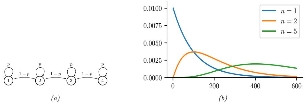
Figure 29.15: (a) A Markov chain with n = 4 repeated states and self loops. (b) The resulting distribution over sequence lengths, for p = 0.99 and various n. Generated by hmm\_self\_loop\_dist.ipynb.

It is obvious from log p(ε) + log p(y1:^T , z1:^T |ε) that the posteriors of ↼ and A^j· are both still Dirichlet distributions. It can also be shown that the posterior distributions of {E^j , “j} are still matrix normal inverse Wishart distributions, whose hyperparameters can be directly obtained by replacing Y, A, X in Equation (15.105) with Yˆ ^j , E^j and Y˜ ^j respectively. To summarize, the posterior distribution p(ε|z1:^T , y1:^T ) is:

\[ \pi | \mathbf{z}\_{1:T} \sim \text{Dir}(\hat{\alpha}\_{\pi}), \tag{2.47} \\ \widehat{\alpha}\_{\pi,k} = \mathbb{X}\_{\pi} \,/K + \mathbb{T} \,(z\_1 = k) \tag{29.47} \]

\[\mathbf{A}\_{j\cdot}|\mathbf{z}\_{1:T} \sim \text{Dir}(\hat{\mathbf{a}}\_A),\tag{2.45} \\ \text{and} \\ \qquad \qquad \hat{\alpha}\_{A\_j,k} = \mathbb{X}\_A/K + N\_{jk}\tag{29.48}\]

\[\mathbf{E}\_{j}|\mathbf{z}\_{1:T},\mathbf{y}\_{1:T} \sim \text{IW}(\boldsymbol{\vartheta}\_{j},\boldsymbol{\hat{\Psi}}\_{j}) \qquad\qquad\qquad \mathbf{E}\_{j}|\boldsymbol{\Sigma}\_{j},\mathbf{z}\_{1:T},\mathbf{y}\_{1:T} \sim \mathcal{M}\mathcal{N}(\boldsymbol{\hat{\mathbf{M}}}\_{j},\boldsymbol{\Sigma}\_{j},\boldsymbol{\hat{\Psi}}\_{j}) \tag{29.49}\]

29.5 HMMs: generalizations

In this section, we discuss various extensions of the vanilla HMM introduced in Section 29.2.

29.5.1 Hidden semi-Markov model (HSMM)

In a standard HMM (Section 29.2), the probability we remain in state i for exactly d steps is

\[p(d\_i = d) = (1 - A\_{ii})A\_{ii}^d \propto \exp(d \log A\_{ii}) \tag{29.50}\]

where Aii is the self-loop probability. This is called the geometric distribution. However, this kind of exponentially decaying function of d is sometimes unrealistic.

A simple way to model non-geometric waiting times is to replace each state with n new states, each with the same emission probabilities as the original state. For example, consider the model in Figure 29.15(a). Obviously the smallest sequence this can generate is of length n = 4. Any path of length ^d through the model has probability ^pd↑ⁿ(1 ^{↓ p})ⁿ; multiplying by the number of possible paths we find that the total probability of a path of length d is

\[p(d) = \binom{d-1}{n-1} p^{d-n} (1-p)^n \tag{29.51}\]

This is equivalent to the negative binomial distribution. By adjusting n and the self-loop probabilities p of each state, we can model a wide range of waiting times: see Figure 29.15(b).

A more general solution is to use a semi-Markov model, in which the next state not only depends on the previous state, but also on how how long we’ve been in that state. When the state-space is not observed directly, the result is called a hidden semi-Markov model (HSMM), a variable duration HMM, or an explicit duration HMM [Yu10].

One way to represent a HSMM is to use the graphical model shown in Figure 29.16(a). The d^t → {1,…,D} node is a state duration counter, where D is the maximum duration of any state. When we first enter state j, we sample d^t from the duration distribution for that state, d^t ↑ p^j (·). Thereafter, d^t deterministically counts down until d^t = 1. More precisely, we define the following CPD:

\[p(d\_t = d' | d\_{t-1} = d, z\_t = j) = \begin{cases} \ D\_j(d') & \text{if } d = 1 \\ 1 & \text{if } d' = d - 1 \text{ and } d > 1 \\ 0 & \text{otherwise} \end{cases} \tag{29.52}\]

Note that D^j (d) could be represented as a table (a non-parametric approach) or as some kind of parametric distribution, such as a gamma distribution. If D^j (d) is a (truncated) geometric distribution, this emulates a standard HMM.

While d^t > 1, the state z^t is not allowed to change. When d^t = 1, we make a stochastic transition to a new state. (We assume Ajj = 0.) More precisely, we define the state CPD as follows:

\[p(z\_t = k | z\_{t-1} = j, d\_{t-1} = d) = \begin{cases} 1 & \text{if } d > 1 \text{ and } j = k \\ A\_{jk} & \text{if } d = 1 \\ 0 & \text{otherwise} \end{cases} \tag{29.53}\]

This ensures that the model stays in the same state for the entire duration of the segment. At each step within this segment, an observation is generated.

HSMMs are useful not only because they can model the duration of each state explicitly, but also because they can model the distribution of a whole subsequence of observations at once, instead of assuming all observations are generated independently at each time step. That is, they can use likelihood models of the form p(yt:t+l↑¹|z^t = k, d^t = l), which generate l correlated observations if the duration in state k is for l time steps. This approach, known as a segmental HMM, is useful for modeling data that is piecewise linear, or shows other local trends [ODK96]. We can also use an RNN to model each segment, resulting in an RNN-HSMM model [Dai+17].

More precisely, we can define a segmental HMM as follows:

\[p(\mathbf{y}, \mathbf{z}, \mathbf{d}) = \left[ p(z\_1) p(d\_1 | z\_1) \prod\_{t=2}^{T} p(z\_t | z\_{t-1}, d\_{t-1}) p(d\_t | z\_t, d\_{t-1}) \right] p(\mathbf{y} | \mathbf{z}, \mathbf{d}) \tag{29.54}\]

In a standard HSMM, we assume

\[p(\mathbf{y}|\mathbf{z}, \mathbf{d}) = \prod\_{t=1}^{T} p(y\_t|z\_t) \tag{29.55}\]

so the duration variables only determine the hidden state dynamics. To define p(y|z, d) for a segmental HMM, let us use sⁱ and eⁱ to denote the start and end times of segment i. This sequence

Figure 29.16: Encoding a hidden semi-Markov model as a DPGM. (a) d^t is a deterministic down counter (duration variable). Each observation is generated independently. (b) Similar to (a), except now we generate the observations within each segment as a block. In this figure, we represent the non-Markovian dependencies between the observations within each segment by using undirected edges. We represent the conditional independence between the observations across di!erent segments by disconnecting y1:3 from y4:5; this can be enforced by “breaking the link” whenever d^t = 1 (representing the end of a segment).

can be computed deterministically from d using s¹ = 1, sⁱ = sⁱ↑¹ + d^si↓¹ , and eⁱ = sⁱ + d^si ↓ 1. We now define the observation model as follows:

\[p(y|\mathbf{z}, \mathbf{d}) = \prod\_{i=1}^{|\mathbf{s}|} p(y\_{s\_i; \mathbf{c}\_i} | z\_{s\_i}, d\_{s\_i}) \tag{29.56}\]

See Figure 29.16(b) for the DPGM.

If we use an RNN for each segment, we have

\[p(y\_{s\_i:s\_i}|z\_{s\_i},d\_{s\_i}) = \prod\_{t=s\_i}^{e\_i} p(y\_t|y\_{s\_i:t-1}, z\_{s\_i}) = \prod\_{t=s\_i}^{e\_i} p(y\_t|h\_t, z\_{s\_i}) \tag{29.57}\]

where h^t is the hidden state that is deterministically updated given the previous observations in this sequence.

As shown in [Chi14], it is possible to compute ^p(zt, dt|y1:^T ) in ^O(TK^{2 +} TKD) time, where ^T is the sequence length, K is the number of states, and D is the maximum duration of any segment. In [Dai+17], they show how to train an approximate inference algorithm, based on a mean field approximation ^q(z, ^d|y) = ^t q(zt|y)q(dt|y), to compute the posterior in O(TK + T D) time.

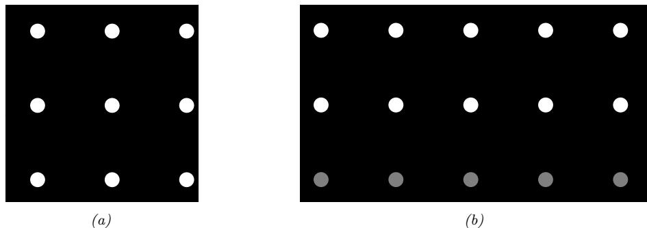
29.5.2 Hierarchical HMMs

A hierarchical HMM (HHMM) [FST98] is an extension of the HMM that is designed to model domains with hierarchical structure. Figure 29.17 gives an example of an HHMM used in automatic speech recognition, where words are composed of phones which are composed of subphones. We can always “flatten” an HHMM to a regular HMM, but a factored representation is often easier to interpret, and allows for more e”cient inference and model fitting.

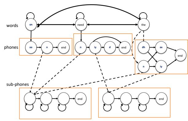
Figure 29.17: An example of an HHMM for an ASR system which can recognize 3 words. The top level represents bigram word probabilities. The middle level represents the phonetic spelling of each word. The bottom level represents the subphones of each phone. (It is traditional to represent a phone as a 3 state HMM, representing the beginning, middle and end; these are known as subphones.) Adapted from Figure 7.5 of [JM00].

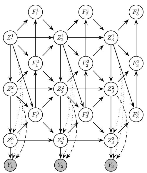
Figure 1: A 3-level HHMM represented as a DBN. Q^{d t} is the state at time t, level d; Fd ^t = 1 if the HMM at level d has finished (entered its exit state), otherwise F^{d t} = 0. Shaded nodes are observed; the remaining nodes are hidden. In some applications, the dotted arcs from Q¹ and the dashed arcs from Q² may be omitted. Figure 29.18: An HHMM represented as a DPGM. Z^{ϖ t} is the state at time t, level ϖ; F^{ϖ t} = 1 if the HMM at level ϖ has finished (entered its exit state), otherwise F^{ϖ t} = 0. Shaded nodes are observed; the remaining nodes are hidden. We may optionally clamp F^{ϖ T} = 1, where T is the length of the observation sequence, to ensure all models have finished by the end of the sequence. From Figure 2 of [MP01].

1

HHMMs have been used in many application domains, e.g., speech recognition [Bil01], gene finding [Hu+00], plan recognition [BVW02], monitoring transportation patterns [Lia+07], indoor robot localization [TMK04], etc. HHMMs are less expressive than stochastic context free grammars (SCFGs) since they only allow hierarchies of bounded depth, but they support more e”cient inference. In particular, inference in SCFGs (using the inside outside algorithm, [JM08]) takes O(T³) whereas inference in an HHMM takes O(T) time [MP01; WM12].

We can represent an HHMM as a directed graphical model as shown in Figure 29.18. Z↼ ^t represents the state at time t and level ▷. A state transition at level ▷ is only “allowed” if the chain at the level below has “finished”, as determined by the F↼↑^{1 t} node. (The chain below finishes when it chooses to enter its end state.) This mechanism ensures that higher level chains evolve more slowly than lower level chains, i.e., lower levels are nested within higher levels.

A variable duration HMM can be thought of as a special case of an HHMM, where the top level is a deterministic counter, and the bottom level is a regular HMM, which can only change states once the counter has “timed out”. See [MP01] for further details.

29.5.3 Factorial HMMs

An HMM represents the hidden state using a single discrete random variable z^t → {1,…,K}. To represent 10 bits of information would require K = 2¹⁰ = 1024 states. By contrast, consider a distributed representation of the hidden state, where each zt,m → {0, 1} represents the m’th bit of the t’th hidden state. Now we can represent 10 bits using just 10 binary variables. This model is called a factorial HMM [GJ97].

More precisely, the model is defined as follows:

\[p(\mathbf{z}, \mathbf{y}) = \prod\_{t} \left[ \prod\_{m} p(z\_{tm} | z\_{t-1, m}) \right] p(\mathbf{y}\_t | \mathbf{z}\_t) \tag{29.58}\]

where p(ztm = k|z^t↑1,m = j) = Amjk is an entry in the transition matrix for chain m, p(z1^m = k|z0m) = p(z1^m = k) = φmk, is the initial state distribution for chain m, and

\[p(y\_t | \mathbf{z}\_t) = \mathcal{N}\left(y\_t | \sum\_{m=1}^{M} \mathbf{W}\_m \mathbf{z}\_{tm}, \boldsymbol{\Sigma}\right) \tag{29.59}\]

is the observation model, where ztm is a 1-of-K encoding of ztm and W^m is a D↗K matrix (assuming ^{yt → RD}). Figure 29.19a illustrates the model for the case where ^M = 3.

An interesting application of FHMMs is to the problem of energy disaggregation [KJ12]. In this problem, we observe the total energy usage of a house at each moment in time, i.e., the observation model has the form

\[p(y\_t | \mathbf{z}\_t) = \mathcal{N}(y\_t | \sum\_{m=1}^{M} w\_m z\_{tm}, \sigma^2) \tag{29.60}\]

where w^m is the amount of energy used by device m, and ztm = 1 if device m is being used at time t and ztm = 0 otherwise. The transition model is assumed to be

\[p(z\_{t,m} = 1 | z\_{t-1,m}) = \begin{cases} A\_{01} & \text{if } z\_{t-1,m} = 0 \\ A\_{11} & \text{if } z\_{t-1,m} = 1 \end{cases} \tag{29.61}\]

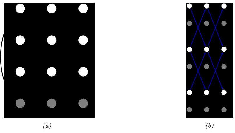
Figure 29.19: (a) A factorial HMM with 3 chains. (b) A coupled HMM with 3 chains.

We do not know which devices are turned on at each time step (i.e., the ztm are hidden), but by applying inference in the FHMM over time, we can separate the total energy into its parts, and thereby determine which devices are using the most electricity.

Unfortunately, conditioned on yt, all the hidden variables are correlated (due to explaining away the common observed child yt). This make exact state estimation intractable. However, we can derive e”cient approximate inference algorithms, as we discuss in Supplementary Section 10.3.2.

29.5.4 Coupled HMMs

If we have multiple related data streams, we can use a coupled HMM [Bra96]. This is a series of HMMs where the state transitions depend on the states of neighboring chains. That is, we represent the conditional distribution for each time slice as

\[p(\mathbf{z}\_t, y\_t | \mathbf{z}\_{t-1}) = \prod\_m p(y\_{tm} | z\_{tm}) p(z\_{tm} | \mathbf{z}\_{t-1, m-1:m+1}) \tag{29.62}\]

with boundary conditions defined in the obvious way. See Section 29.5.4 for an illustration with M = 3 chains.

Coupled HMMs have been used for various tasks, such as audio-visual speech recognition [Nef+02], modeling freeway tra”c flows [KM00], and modeling conversational interactions between people [Bas+01].

However, there are two drawbacks to this model. First, exact inference takes O(T(K^M)2), as in a factorial HMM; however, in practice this is not usually a problem, since M is often small. Second, the model requires O(MK⁴) parameters to specify, if there are M chains with K states per chain, because each state depends on its own past plus the past of its two neighbors. There is a closely related model, known as the influence model [Asa00], which uses fewer parameters, by computing a convex combination of pairwise transition matrices.

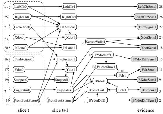
Figure 29.20: The BATnet DBN. The transient nodes are only shown for the second slice, to minimize clutter. The dotted lines are used to group related variables. Used with kind permission of Daphne Koller.

29.5.5 Dynamic Bayes nets (DBN)

A dynamic Bayesian network (DBN) is a way to represent a stochastic process using a directed graphical model [Mur02]. (Note that the network is not dynamic (the structure and parameters are fixed), rather it is a network representation of a dynamical system.) A DBN can be considered as a natural generalization of an HMM.

An example is shown in Figure 29.20, which is a DBN designed to monitor the state of a simulated autonomous car known as the “Bayesian automated taxi”, or “BATmobile” [For+95]. To define the model, you just need to specify the structure of the first time-slice, the structure between two time-slices, and the form of the CPDs. For details, see [KF09a].

29.5.6 Changepoint detection

In this section, we discuss changepoint detection, which is the task of detecting when there are “abrupt” changes in the distribution of the observed values in a time series. We focus on the online case. (For a review of o$ine methods to this problem, see e.g., [AC17; TOV18]. (See also [BW20] for a recent empirical evaluation of various methods, focused on the 1d time series case.)

The methods we discuss can (in principle) be used for high-dimensional time series segmentation. Our starting point is the hidden semi-Markov models (HSMM) discussed in Section 29.5.1. This is like an HMM in which we explicitly model the duration spent in each state. This is done by augmenting the latent state z^t with a duration variable d^t which is initialized according to a duration distribution, d^t ↑ D^zt (·), and which then counts down to 1. An alternative approach is to add a variable rt{0, 1,…, } which encodes the run length for the current state; this starts at 0 whenever a new segment is created, and then counts up by one at each step. The transition dynamics is specified by

\[p(r\_t|r\_{t-1}) = \begin{cases} H(r\_{t-1} + 1) & \text{if } r\_t = 0\\ 1 - H(r\_{t-1} + 1) & \text{if } r\_t = r\_{t-1} + 1\\ 0 & \text{otherwise} \end{cases} \tag{29.63}\]

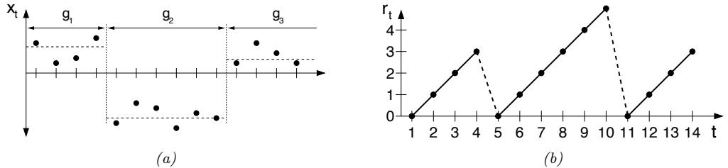
Figure 29.21: Illustration of Bayesian online changepoint detection (BOCPD). (a) Hypothetical segmentation of a univariate time series divided by changepoints on the mean into three segments of lengths g¹ = 4, g² = 6, and an undetermined length for g³ (since it the third segment has not yet ended). From Figure 1 of [AM07]. Used with kind permission of Ryan Adams.

where H(⇀ ) is a hazard function:

\[H(\tau) = \frac{p\_g(\tau)}{\sum\_{t=\tau}^{\infty} p\_g(t)}\tag{29.64}\]

where pg(t) is the probability of a segment of length t. See Figure 29.21 for an illustration. If we set p^g to be a geometric distribution with parameter ω, then the hazard function is the constant H(⇀ )=1/ω.

The advantage of the run-length representation is that we can define the observation model for a segment in a causal way (that only depends on past data):

\[p(y\_t | y\_{1:t-1}, r\_t = r, z\_t = k) = p(y\_t | y\_{t-r:t-1}, z\_t = k) = \int p(y\_t | \eta) p(\eta | y\_{t-r:t-1}, z\_t = k) d\eta \tag{29.65}\]

where ϑ are the parameters that are “local” to this segment. This called the underlying predictive model or UPM for the segment. The posterior over the UPM parameters is given by

\[p(\eta|y\_{t-r:t-1}, z\_t = k) \propto p(\eta|z\_t = k) \prod\_{i=t-r}^{t-1} p(y\_i|\eta) \tag{29.66}\]

where we initialize the prior for ϑ using hyper-parameters chosen by state k. If the model is conjugate exponential, we can compute this marginal likelihood in closed form, and we have

\[\pi\_t^{r,k} = p(y\_t | y\_{t-r:t-1}, z\_t = k) = p(y\_t | \psi\_t^{r,k}) \tag{29.67}\]

where ⇁r,k ^t are the parameters of the posterior predictive distribution at time t based on the last r observations (and using a prior from state k).

In the special case in which we have K = 1 hidden states, then each segment is modeled independently, and we get a product partition model [BH92]:

\[p(y|r) = p(y\_{s\_1:e\_1}) \dots p(y\_{s\_N:e\_N}) \tag{29.68}\]

where sⁱ and eⁱ are the start and end of segment i, which can be computed from the run lengths r. (We initialize with r⁰ = 0.) Thus there is no information sharing between segments. This can be

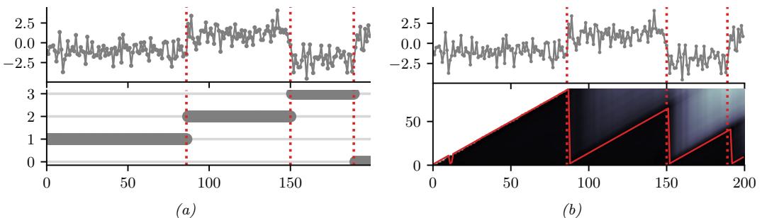
Figure 29.22: Illustration of BOCPD. (a) Synthetic data from a GMM with 4 states. Top row is the data, bottom row is the generating state. (b) Output of algorithm. Top row: Estimated changepoint locations. Bottom row: posterior predicted probability of a changepoint at each step. Generated by changepoint\_detection.ipynb.

useful for time series in which there are abrupt changes, and where the new parameters are unrelated to the old ones.

Detecting the locations of these changes is called changepoint detection. An exact online algorithm for solving this task was proposed in [FL07] and independently in [AM07]; in the latter paper, they call the method Bayesian online changepoint detection or BOCPD. We can compute a posterior over the current run length recursively as follows:

\[p(r\_t | \mathbf{y}\_{1:t}) \propto p(\mathbf{y}\_t | \mathbf{y}\_{1:t-1}, r\_t) p(r\_t | \mathbf{y}\_{1:t-1}) \tag{29.69}\]

where we initialize with p(r⁰ = 0) = 1. The marginal likelihood p(yt|y1:t↑¹, rt) is given by Equation (29.65) (with z^t = 1 dropped, since there is just one state). The prior predictive is given by

\[p(r\_t | \mathbf{y}\_{1:t-1}) = \sum\_{r\_{t-1}} p(r\_t | r\_{t-1}) p(r\_{t-1} | \mathbf{y}\_{1:t-1}) \tag{29.70}\]

The one step ahead predictive distribution is given by

\[p(\mathbf{y}\_{t+1}|\mathbf{y}\_{1:t}) = \sum\_{r\_t} p(\mathbf{y}\_{t+1}|\mathbf{y}\_{1:t}, r\_t) p(r\_t|\mathbf{y}\_{1:t}) \tag{29.71}\]

29.5.6.1 Example

We give an example of the method in Figure 29.22 applied to a synthetic 1d dataset generated from a 4 state GMM. The likelihood is a univariate Gaussian, ^p(yt|µ) = ^N (yt|µ, ^ς2), where ^ς2 = 1 is fixed, and µ is inferred using a Gaussian prior. The hazard function is set to a geometric distribution with rate N/T, where N = 4 is the true number of change points and T = 200 is the length of the sequence.

29.5.6.2 Extensions

Although the above method is exact, each update step takes O(t) time, so the total cost of the algorithm is O(T²). We can reduce this by pruning out states with low probability. In particular, we

can use particle filtering (Section 13.2) with N particles, together with a stratified optimal resampling method, to reduce the cost to O(T N). See [FL07] for details.

In addition, the above method relies on a conjugate exponential model in order to compute the marginal likelihood, and update the posterior parameters for each r, in O(1) time. For more complex models, we need to use approximations. In [TBS13], they use variational Bayes (Section 10.3.3), and in [Mav16], they use particle filtering (Section 13.2), which is more general, but much slower.

It is possible to extend the model in various other ways. In [FL11], they allow for Markov dependence between the parameters of neighboring segments. In [STR10], they use a Gaussian process (Chapter 18) to represent the UPM, which captures correlations between observations within the same segment. In [KJD18], they use generalized Bayesian inference (Section 14.1.3) to create a method that is more robust to model misspecification.

In [Gol+17], they extend the model by modeling the probability of a sequence of observations, rather than having to make the decision about whether to insert a changepoint or not based on just the likelihood ratio of a single time step.

In [AE+20], they extend the model by allowing for multiple discrete states, as in an HSMM. In addition, they add both the run length r^t and the duration d^t to the state space. This allows the method to specify not just when the current segment started, but also when it is expected to end. In addition, it allows the UPM to depend on the duration of the segment, and not just on past observations. For example, we can use

\[p(y\_t | r\_t, d\_t, \eta) = \mathcal{N}(y\_t | \phi(r\_t/d\_t)^\mathsf{T}\eta, \sigma^2) \tag{29.72}\]

where 0 ≃ rt/d^t ≃ 1, and ω() is a set of learned basis functions. This allows observation sequences for the same hidden state to have a common functional shape, even if the time spent in each state is di!erent.

29.6 Linear dynamical systems (LDSs)

In this section, we discuss linear-Gaussian state-space model (LG-SSM), also called linear dynamical system (LDS). This is a special case of an SSM in which the transition function and observation function are both linear, and the process noise and observation noise are both Gaussian.

29.6.1 Conditional independence properties

The LDS graphical model is shown in Figure 29.1(a). This encodes the assumption that the hidden states are Markovian, and the observations are iid conditioned on the hidden states. All that remains is to specify the form of the conditional probability distributions of each node.

29.6.2 Parameterization

An LDS model is defined as follows:

\[p(\mathbf{z}\_t | \mathbf{z}\_{t-1}, \mathbf{u}\_t) = \mathcal{N}(\mathbf{z}\_t | \mathbf{F}\_t \mathbf{z}\_{t-1} + \mathbf{B}\_t \mathbf{u}\_t + \mathbf{b}\_t, \mathbf{Q}\_t) \tag{29.73}\]

p(yt|zt,ut) = N (yt|Htz^t + Dtu^t + dt, Rt) (29.74)

We often assume the bias (o!set) terms are zero, in which case the model simplifies to

\[p(\mathbf{z}\_t | \mathbf{z}\_{t-1}, \mathbf{u}\_t) = \mathcal{N}(\mathbf{z}\_t | \mathbf{F}\_t \mathbf{z}\_{t-1} + \mathbf{B}\_t \mathbf{u}\_t, \mathbf{Q}\_t) \tag{29.75}\]

\[p(y\_t|\mathbf{z}\_t, \mathbf{u}\_t) = \mathcal{N}(y\_t|\mathbf{H}\_t\mathbf{z}\_t + \mathbf{D}\_t\mathbf{u}\_t, \mathbf{R}\_t) \tag{29.76}\]

Furthermore, if there are no inputs, the model further simplifies to

\[p(\mathbf{z}\_t|\mathbf{z}\_{t-1}) = \mathcal{N}(\mathbf{z}\_t|\mathbf{F}\_t\mathbf{z}\_{t-1}, \mathbf{Q}\_t) \tag{29.77}\]

\[p(y\_t|\mathbf{z}\_t) = \mathcal{N}(y\_t|\mathbf{H}\_t\mathbf{z}\_t, \mathbf{R}\_t) \tag{29.78}\]

We can also write this as a structural equation model (Section 4.7.2):

\[\mathbf{z}\_{t} = \mathbf{F}\_{t}\mathbf{z}\_{t-1} + \mathbf{q}\_{t} \tag{29.79}\]

\[y\_t = \mathbf{H}\_t \mathbf{z}\_t + r\_t \tag{29.80}\]

where q^t ↑ N (0, Qt) is the process noise, and r^t ↑ N (0, Rt) is the observation noise.

Typically we assume the parameters ε^t = (Ft, Ht, Bt, Dt, Qt, Rt) are independent of time, so the model is stationary. (We discuss how to learn the parameters in Section 29.8.) Given the parameters, we discuss how to perform online posterior inference of the latent states using the Kalman filter in Section 8.2.2, and o$ine inference using the Kalman smoother in Section 8.2.3.

29.7 LDS: applications

In this section, we discuss some applications of LDS models.

29.7.1 Object tracking and state estimation

Consider an object moving in R². Let the state at time t be the position and velocity of the object, z^t = u^t v^t u˙ ^t v˙^t . (We use u and v for the two coordinates, to avoid confusion with the state and observation variables.) We assume this evolves in continuous time according to a linear stochastic di!erential equation or SDE, in which the dynamics are given by Newton’s law of motion, and where the random acceleration corresponds to a white noise process (aka Brownian motion). However, since the observations occur at discrete time steps tk, we will only evaluate the system at discrete time points; this is called a continuous-discrete SSM [SS19, p199]. (We shall henceforth write t instead of tk, since in this book we only consider discrete time.) The corresponding discrete time SSM is given by the following [SS19, p82]:

\[ \underbrace{\begin{pmatrix} u\_t \\ v\_t \\ \dot{u}\_t \\ \dot{v}\_t \end{pmatrix}}\_{\mathbf{z}\_t} = \underbrace{\begin{pmatrix} 1 & 0 & \Delta & 0 \\ 0 & 1 & 0 & \Delta \\ 0 & 0 & 1 & 0 \\ 0 & 0 & 0 & 1 \end{pmatrix}}\_{\mathbf{F}} \underbrace{\begin{pmatrix} u\_{t-1} \\ v\_{t-1} \\ \dot{u}\_{t-1} \\ \dot{v}\_{t-1} \end{pmatrix}}\_{\mathbf{z}\_{t-1}} + q\_t \tag{29.81} \]

where ” is the step size between consecutive discrete measurement times, q^t ↑ N (0, Q) is the process noise, and the noise covariance matrix Q is given by

\[\mathbf{Q} = \begin{pmatrix} \frac{q\_1 \Delta^3}{3} & 0 & \frac{q\_1 \Delta^2}{2} & 0\\ 0 & \frac{q\_2 \Delta^3}{3} & 0 & \frac{q\_2 \Delta^2}{2} \\ \frac{q\_1 \Delta^2}{2} & 0 & q\_1 \Delta & 0 \\ 0 & \frac{q\_2 \Delta^2}{2} & 0 & q\_2 \Delta \end{pmatrix}\]

where qⁱ are the di!usion coe”cients of the white noise process for dimension i (see [SS19, p44] for details).

Now suppose that at each discrete time point we observe the location, corrupted by Gaussian noise. Thus the observation model becomes

\[ \underbrace{\begin{pmatrix} y\_{1,t} \\ y\_{2,t} \end{pmatrix}}\_{\mathbf{y}\_t} = \underbrace{\begin{pmatrix} 1 & 0 & 0 & 0 \\ 0 & 0 & 1 & 0 \end{pmatrix}}\_{\mathbf{H}} \begin{pmatrix} u\_t \\ \dot{u}\_t \\ v\_t \\ \dot{v}\_t \end{pmatrix} + r\_t \tag{29.82} \]

where r^t ↑ N (0, R) is the observation noise. We see that the observation matrix H simply “extracts” the relevant parts of the state vector.

Suppose we sample a trajectory and corresponding set of noisy observations from this model, (z1:^T , ^y1:^T ) ^{↑ p}(z, ^y|ε). (We use diagonal observation noise, R = diag(ς^{2 1}, ς^{2 2}).) The results are shown in Figure 29.23(a). We can use the Kalman filter (Section 8.2.2) to compute p(zt|y1:t, ε) for each ^t,. (We initialize the filter with a vague prior, namely ^p(z0) = ^N (z0|0, ¹⁰⁵I).) The results are shown in Figure 29.23(b). We see that the posterior mean (red line) is close to the ground truth, but there is considerable uncertainty (shown by the confidence ellipses). To improve results, we can use the Kalman smoother (Section 8.2.3) to compute p(zt|y1:^T , ε), where we condition on all the data, past and future. The results are shown in Figure 29.23(c). Now we see that the resulting estimate is smoother, and the uncertainty is reduced. (The uncertainty is larger at the edges because there is less information in the neighbors to condition on.)

29.7.2 Online Bayesian linear regression (recursive least squares)

In Section 15.2.2, we discuss how to compute ^p(w|ς², ^D) for a linear regression model in batch mode, using a Gaussian prior of the form p(w) = N (w|µ, “). In this section, we discuss how to compute this posterior online, by repeatedly performing the following update:

\[p(w|\mathcal{D}\_{1:t}) \propto p(\mathcal{D}\_t|w)p(w|\mathcal{D}\_{1:t-1}) \tag{29.83}\]

\[\propto p(\mathcal{D}\_t|\boldsymbol{w})p(\mathcal{D}\_{t-1}|\boldsymbol{w})\dots p(\mathcal{D}\_1|\boldsymbol{w})p(\boldsymbol{w})\tag{29.84}\]

where D^t = (ut, yt) is the t’th labeled example, and D1:t↑¹ are the first t ↓ 1 examples. (For brevity, we drop the conditioning on ^ς2.) We see that the previous posterior, ^p(w|D1:t↑¹), becomes the current prior, which gets updated by D^t to become the new posterior, p(w|D1:t). This is an example of sequential Bayesian updating or online Bayesian inference. In the case of linear regression, this process is known as the recursive least squares or RLS algorithm.

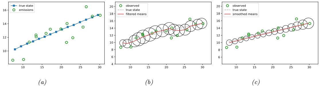
Figure 29.23: Illustration of Kalman filtering and smoothing for a linear dynamical system. (Repeated from Figure 8.2.) (a) Observations (green circles) are generated by an object moving to the right (true location denoted by blue squares). (b) Results of online Kalman filtering. Circles are 95% confidence ellipses, whose center is the posterior mean, and whose shape is derived from the posterior covariance. (c) Same as (b), but using o#ine Kalman smoothing. The MSE in the trajectory for filtering is 3.13, and for smoothing is 1.71. Generated by kf\_tracking\_script.ipynb.

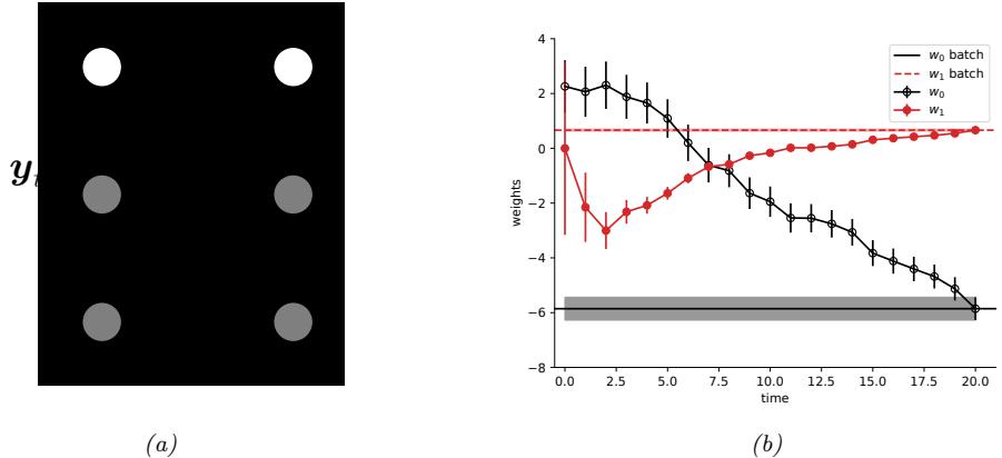
Figure 29.24: (a) A dynamic generalization of linear regression. (b) Illustration of the recursive least squares algorithm applied to the model ^p(y|x, ^w) = ^N (y|w^{0 + w}1x, ^ε2). We plot the marginal posterior of ^w0 and ^w1 vs number of datapoints. (Error bars represent ^E [w^{j |}y1:t, ^x1:t] ^± !^V [w^{j |}y1:t, ^x1:t].) After seeing all the data, we converge to the o#ine (batch) Bayes solution, represented by the horizontal lines. (Shading represents the marginal posterior variance.) Generated by kf\_linreg.ipynb.

We can implement this method by using a linear Gaussian state-space model(Section 29.6). The basic idea is to let the hidden state represent the regression parameters, and to let the (time-varying) observation model H^t represent the current feature vector xt. 3 That is, the observation model has the form

\[p(y\_t|\mathbf{w}\_t) = \mathcal{N}(y\_t|\mathbf{H}\_t\mathbf{z}\_t, \mathbf{R}\_t) = \mathcal{N}(y\_t|\mathbf{x}\_t^\mathsf{T}w\_t, \sigma^2) \tag{29.85}\]

If we assume the regression parameters do not change, the dynamics model becomes

\[p(\boldsymbol{w}\_{t}|\boldsymbol{w}\_{t-1}) = N(\boldsymbol{w}\_{t}|\boldsymbol{w}\_{t-1},0) = \delta(\boldsymbol{w}\_{t} - \boldsymbol{w}\_{t-1})\tag{29.86}\]

(If we do let the parameters change over time, we get a so-called dynamic linear model [Har90; WH97; PPC09].) See Figure 29.24a for the model, and Supplementary Section 8.1.2 for a simplification of the Kalman filter equations when applied to this special case.

We show a 1d example in Figure 29.24b. We see that online inference converges to the exact batch (o$ine) posterior in a single pass over the data.

If we approximate the Kalman gain matrix by K^t ⇓ ↼t1, we recover the least mean squares or LMS algorithm, where ↼^t is the learning rate. In LMS, we need to adapt the learning rate to ensure convergence to the MLE. Furthermore, the algorithm may require multiple passes through the data to converge to this global optimum. By contrast, the RLS algorithm automatically performs step-size adaptation, and converges to the optimal posterior in a single pass over the data.

In Section 8.6.3, we extend this approach to perform online parameter estimation for logistic regression, and in Section 17.5.2, we extend this approach to perform online parameter estimation for MLPs.

29.7.3 Adaptive filtering

Consider an autoregressive model of order D:

\[y\_t = w\_1 y\_{t-1} + \dots + w\_D y\_{t-D} + \epsilon\_t \tag{29.87}\]

where ϖ^t ↑ N (0, 1). The problem of adaptive filtering is to estimate the parameters w1:^D given the observations y1:t.

We can cast this as inference in an LG-SSM by defining the observation matrix to be H^t = (y^t↑¹ …y^t↑^D) and defining the state as z^t = w. We can also allow the parameters to evolve over time, similar to Section 29.7.2.

29.7.4 Time series forecasting

In Section 29.12 we discuss how to use LDS models to perform time series forecasting.

^3. It is tempting to think we can just set the input ut to the covariates xt. Unfortunately this will not work, since the e!ect of the inputs is to add an o!set term to the output in a way which is independent of the hidden state (parameters). That is, since we have yt = Htzt + Dtut + d + rt, if we set ut = xt then the features get multiplied by the constant LDS parameter Dt instead of the hidden state zt containing the regression weights.

29.8 LDS: parameter learning

There are many approaches for estimating the parameters of state-space models. (In the control theory community, this is known as systems identification [Lju87].) In the case of linear dynamical systems, many of the methods are similar to techniques used to fit HMMs, discussed in Section 29.4. For example, we can use EM, SGD, spectral methods, or Bayesian methods, as we discuss below. (For more details, see [Sar13, Ch 12].)

29.8.1 EM for LDS

This section is coauthored with Xinglong Li.

If we only observe the output sequence, we can compute ML or MAP estimates of the parameters using EM. The method is conceptually quite similar to the Baum-Welch algorithm for HMMs (Section 29.4.1), except we use Kalman smoothing (Section 8.2.3) instead of forwards-backwards in the E step, and use di!erent calculations in the M step. The details can be found in [SS82; GH96a]. Here we extend these results to consider the case where the HMM may have an optional input sequence u1:^T .

Our goal is to maximize the expected complete data log likelihood

\[Q(\theta, \theta\_{k-1}) = \mathbb{E}\left[\log p(\mathbf{z}\_{1:T}, \mathbf{y}\_{1:T} | \theta) | \mathbf{y}\_{1:T}, \mathbf{u}\_{1:T}, \theta\_{k-1}\right] \tag{29.88}\]

where the expectations are taken wrt the parameters at the previous iteration k ↓ 1 of the algorithm. (We initialize with random parameters, or by first fitting a simpler model, such as factor analysis.) For brevity of notations, we assume that the bias terms are included in D and B (i.e., the last entry of u^t is 1).

The log joint is given by the following:

\[\log p(\mathbf{z}\_{1:T}, \mathbf{y}\_{1:T} | \boldsymbol{\theta}) = -\sum\_{t=1}^{T} \left( \frac{1}{2} (\mathbf{y}\_t - \mathbf{H}\mathbf{z}\_t - \mathbf{D}\mathbf{u}\_t)^\mathsf{T} \mathbf{R}^{-1} (\mathbf{y}\_t - \mathbf{H}\mathbf{z}\_t - \mathbf{D}\mathbf{u}\_t) \right) - \frac{T}{2} \log |\mathbf{R}| \tag{29.89}\]

\[-\sum\_{t=2}^{T} \left( \frac{1}{2} (\mathbf{z}\_t - \mathbf{F}\mathbf{z}\_{t-1} - \mathbf{B}\mathbf{u}\_t)^\mathsf{T} \mathbf{Q}^{-1} (\mathbf{z}\_t - \mathbf{F}\mathbf{z}\_{t-1} - \mathbf{B}\mathbf{u}\_t) \right) - \frac{T-1}{2} \log |\mathbf{Q}| \tag{29.90}\]

\[-\frac{1}{2}(\mathbf{z}\_1 - m\_1)^\mathsf{T} \mathbf{V}\_1^{-1} (\mathbf{z}\_1 - m\_1) - \frac{1}{2}\log|\mathbf{V}\_1| + \text{const} \tag{29.91}\]

where the prior on the initial state is p(z1) = N (z1|m1, V1).

In the E step, we can run the Kalman smoother to compute µ^t|^T = E [zt|y1:^T ], and “^t|^T = Cov [zt|y1:^T ], from which we can compute zˆ^t = µ^t|^T and

\[\mathbf{P}\_t = \mathbb{E}\left[\mathbf{z}\_t \mathbf{z}\_t^\mathsf{T} | \mathbf{y}\_{1:T}\right] = \boldsymbol{\Sigma}\_{t|T} + \mu\_{t|T} \boldsymbol{\mu}\_{t|T}^\mathsf{T} \tag{29.92}\]

We also need to compute the cross term

\[\mathbf{P}\_{t,t-1} = \mathbb{E}\left[\mathbf{z}\_t \mathbf{z}\_{t-1}^\mathsf{T} | y\_{1:T} \right] = \mathbf{E}\_{t,t-1|T} + \mu\_{t|T} \mu\_{t-1|T}^\mathsf{T} \tag{29.93}\]

where

\[\boldsymbol{\Sigma}\_{t-1,t-2|T} = \boldsymbol{\Sigma}\_{t-1|t-1} \mathbf{J}\_{t-2}^{\mathsf{T}} + \mathbf{J}\_{t-1} (\boldsymbol{\Sigma}\_{t,t-1|T} - \mathbf{F} \boldsymbol{\Sigma}\_{t-1|t-1}) \mathbf{J}\_{t-2}^{\mathsf{T}} \tag{29.94}\]

where J^t is the backwards Kalman gain matrix defined in Equation (8.67). We initialize this using “T ,T ^↑1|^T = (I ↓ K^T H)F”^{T ↑}1|^{T ↑1}, where K^T is the forwards Kalman gain matrix defined in Equation (8.28).

We can derive the M step as follows, using standard matrix calculus. We denote Aout = [H, D], xˆout,t = [zˆ^{T t} ,u^T t ] ^T , Adyn = [F, B], ,xˆdyn,t = [zˆ^{T t}↑¹,u^T t ] ^T , and

\[\mathbf{P}\_{\rm out,t} = \begin{pmatrix} \mathbf{P}\_{t} & \hat{\mathbf{z}}\_{t} \mathbf{u}\_{t}^{\rm T} \\ \mathbf{u}\_{t} \hat{\mathbf{z}}\_{t}^{\rm T} & \mathbf{u}\_{t} \mathbf{u}\_{t}^{\rm T} \end{pmatrix}, \tag{2.65} \\ \mathbf{P}\_{\rm dyn,t} = \begin{pmatrix} \mathbf{P}\_{t-1} & \hat{\mathbf{z}}\_{t-1} \mathbf{u}\_{t}^{\rm T} \\ \mathbf{u}\_{t} \hat{\mathbf{z}}\_{t-1}^{\rm T} & \mathbf{u}\_{t} \mathbf{u}\_{t}^{\rm T} \end{pmatrix}. \tag{29.95}\]

• Output matrices:

\[\frac{\partial \mathcal{Q}}{\partial \mathbf{A}\_{\rm out}} = \sum\_{t=1}^{T} \mathbf{R}^{-1} y\_t \hat{\mathbf{x}}\_{\rm out,t}^T - \sum\_{t=1}^{T} \mathbf{R}^{-1} \mathbf{A}\_{\rm out} \mathbf{P}\_{\rm out,t} = \mathbf{0} \tag{29.96}\]

\[\mathbf{A}\_{\text{out}}^{\text{new}} = \left(\sum\_{t=1}^{T} \mathbf{y}\_{t} \hat{\mathbf{x}}\_{\text{out},t}^{\text{T}}\right) \left(\sum\_{t=1}^{T} \mathbf{P}\_{\text{out},t}\right)^{-1} \tag{29.97}\]

• Output noise covariance:

\[\frac{\partial \mathcal{Q}(\mathbf{A}\_{\rm out} = \mathbf{A}\_{\rm out}^{\rm new})}{\partial \mathbf{R}^{-1}} = \frac{T}{2}\mathbf{R} - \frac{1}{2} \sum\_{t=1}^{T} \left( y\_t \mathbf{y}\_t^\top - 2\mathbf{A}\_{\rm out}^{\rm new} \hat{x}\_{\rm out,t} \mathbf{y}\_t^\top + \mathbf{A}\_{\rm out}^{\rm new} \mathbf{P}\_{\rm out,t} \mathbf{A}\_{\rm out}^{\rm new,T} \right) = \mathbf{0} \quad (29.98)\]

\[\mathbf{R}^{\text{new}} = \frac{1}{T} \sum\_{t=1}^{T} (y\_t \mathbf{y}\_t^\top - \mathbf{A}\_{\text{out}}^{\text{new}} \hat{x}\_{\text{out},t} \mathbf{y}\_t^\top) \tag{29.99}\]

• System dynamics matrices:

\[\frac{\partial \mathcal{Q}}{\partial \mathbf{A}\_{\text{dyn}}} = -\sum\_{t=2}^{T} \mathbf{Q}^{-1} \left[ \mathbf{P}\_{t, t-1}, \hat{\mathbf{z}}\_{t} \mathbf{u}\_{t}^{\text{T}} \right] + \sum\_{t=2}^{T} \mathbf{Q}^{-1} \mathbf{A}\_{\text{dyn}} \mathbf{P}\_{\text{dyn}, t} = \mathbf{0} \tag{29.100}\]

\[\mathbf{A}\_{\text{dyn}}^{\text{new}} = \left(\sum\_{t=2}^{T} [\mathbf{P}\_{t, t-1}, \hat{\mathbf{z}}\_t \mathbf{u}\_t^\top] \right) \left(\sum\_{t=2}^{T} \mathbf{P}\_{\text{dyn}, t} \right)^{-1} \tag{29.101}\]

• State noise covariance:

\[\frac{\partial \mathcal{Q}(\mathbf{A}\_{\mathrm{dyn}} = \mathbf{A}\_{\mathrm{dyn}}^{\mathrm{new}})}{\partial \mathbf{Q}^{-1}} = \frac{T - 1}{2} \mathbf{Q} - \frac{1}{2} \sum\_{t=2}^{T} (\mathbf{P}\_{t} - 2\mathbf{A}\_{\mathrm{dyn}}^{\mathrm{new}} \left[ \mathbf{P}\_{t-1,t}, \mathbf{u}\_{t} \hat{\mathbf{z}}\_{t}^{\mathrm{T}} \right] + \mathbf{A}\_{\mathrm{dyn}}^{\mathrm{new}} \mathbf{P}\_{\mathrm{dyn},t} \mathbf{A}\_{\mathrm{dyn}}^{\mathrm{new}, \mathrm{T}}) \tag{29.102}\]

\[\mathbf{Q} = \frac{T - 1}{2} \mathbf{Q} - \frac{1}{2} \sum\_{t=2}^{T} \left( \mathbf{P}\_t - \mathbf{A}\_{\text{dyn}}^{\text{new}} \left[ \mathbf{P}\_{t-1,t}, u\_t \hat{z}\_t^\top \right] \right) = \mathbf{0} \tag{29.103}\]

\[\mathbf{Q}^{\text{new}} = \frac{1}{T - 1} \sum\_{t=2}^{T} \left( \mathbf{P}\_t - \mathbf{A}\_{\text{dyn}}^{\text{new}} \left[ \mathbf{P}\_{t-1, t}, \mathbf{u}\_t \hat{\mathbf{z}}\_t^\top \right] \right) \tag{29.104}\]

• Initial state mean:

\[\frac{\partial \mathcal{Q}}{\partial m} = (\hat{\mathbf{z}}\_1 - m)\mathbf{V}\_1^{-1} = \mathbf{0} \tag{29.105}\]

\[m^{\text{new}} = \hat{\mathbf{z}}\_1 \tag{29.106}\]

• Initial state covariance:

\[\frac{\partial \mathcal{Q}}{\partial \mathbf{V}\_1^{-1}} = \frac{\mathbf{V}\_1}{2} - \frac{1}{2} (\mathbf{P}\_1 - \hat{\mathbf{z}}\_1 \mathbf{m}\_1^\top - m\_1 \hat{\mathbf{z}}\_1^\top + m\_1 m\_1^\top) = \mathbf{0} \tag{29.107}\]

\[\mathbf{V}\_1^{\text{new}} = \mathbf{P}\_1 - \hat{\mathbf{z}}\_1 \hat{\mathbf{z}}\_1^\top \tag{29.108}\]

Note that computing these expected su”cient statistics in the inner loop of EM takes O(T) time, which can be expensive for long sequences. In [Mar10b], a faster method, known as ASOS (approximate second order statistics), is proposed. In this approach, various statistics are precomputed in a single pass over the sequence, and from then on, all iterations take constant time (independent of T). Alternatively, if we have multiple processors, we can perform Kalman smoothing in O(log T) time using parallel scan operations (Section 8.2.3.4).

29.8.2 Subspace identification methods

EM does not always give satisfactory results, because it is sensitive to the initial parameter estimates. One way to avoid this is to use a di!erent approach known as a subspace identification (SSID) [OM96; Kat05].

To understand this approach, let us initially assume there is no observation noise and no system noise. In this case, we have z^t = Fz^t↑¹ and y^t = Hzt, and hence y^t = HF^t↑¹z1. Consequently all the observations must be generated from a dim(zt)-dimensional linear manifold or subspace. We can identify this subspace using PCA. Once we have an estimate of the zt’s, we can fit the model as if it were fully observed. We can either use these estimates in their own right, or use them to initialize EM. Several papers (e.g., [Smi+00; BK15]) have shown that initializing EM this way gives much better results than initializing EM at random, or just using SSID without EM.

Although the theory only works for noise-free data, we can try to estimate the system noise covariance Q from the residuals in predicting z^t from z^t↑¹, and to estimate the observation noise covariance R from the residuals in predicting y^t from zt. We can either use these estimates in their own right, or use them to initialize EM. Because this method relies on taking an SVD, it is called a spectral estimation method. Similar methods can also be used for HMMs (see Section 29.4.3).

29.8.3 Ensuring stability of the dynamical system

When estimating the dynamics matrix F, it is very useful to impose a constraint on its eigenvalues. To see why this is important, consider the case of no system noise. In this case, the hidden state at time t is given by

\[\mathbf{z}\_t = \mathbf{F}^t \mathbf{z}\_1 = \mathbf{U} \boldsymbol{\Lambda}^t \mathbf{U}^{-1} \mathbf{z}\_1 \tag{29.109}\]

where U is the matrix of eigenvectors for F, and # = diag(ωi) contains the eigenvalues. If any ωⁱ > 1, then for large t, z^t will blow up in magnitude. Consequently, to ensure stability, it is useful to require

that all the eigenvalues are less than 1 [SBG07]. Of course, if all the eigenvalues are less than 1, then E [zt] = 0 for large t, so the state will return to the origin. Fortunately, when we add noise, the state becomes non-zero, so the model does not degenerate.

29.8.4 Bayesian LDS

SSMs can be quite sensitive to their parameter values, which is a particular concern when they are used for forecasting applications (see Section 29.12.1), or when the latent states or parameters are interpreted for scientific purposes (see e.g., [AM+16]). In such cases, it is wise to represent our uncertainty about the parameters by using Bayesian inference.

There are various algorithms we can use to perform this task. For linear-Gaussian SSMs, it is possible to use variational Bayes EM [Bea03; BC07] (see Section 10.3.5), or blocked Gibbs sampling (see Section 29.8.4.1). Note, however, that ε and z are highly correlated, so the mean field approximation can be inaccurate, and the blocked Gibbs method can mix slowly. It is also possible to use collapsed MCMC in which we marginalize out z1:^T and just work with p(ε|y1:^T ), which we can sample using HMC.

29.8.4.1 Blocked Gibbs sampling for LDS

This section is written by Xinglong Li.

In this section, we discuss blocked Gibbs sampling for LDS [CK94b; CMR05; FS07]. We alternate between sampling from p(z1:^T |y1:^T , ε) using the forwards-filter backwards-sampling algorithm (Section 8.2.3.5), and sampling from p(ε|z1:^T , y1:^T ), which is easy to do if we use conjugate priors.

In more detail, we will consider the following linear Gaussian state space model with homogeneous parameters:

\[p(\mathbf{z}\_t | \mathbf{z}\_{t-1}, \mathbf{u}\_t) = \mathcal{N}(\mathbf{z}\_t | \mathbf{F} \mathbf{z}\_{t-1} + \mathbf{B} \mathbf{u}\_t, \mathbf{Q}) \tag{29.110}\]

\[p(y\_t | \mathbf{z}\_t, \mathbf{u}\_t) = \mathcal{N}(y\_t | \mathbf{H} \mathbf{z}\_t + \mathbf{D} \mathbf{u}\_t, \mathbf{R}) \tag{29.111}\]

The set of all the parameters is ε = {F, H, B, D, Q, R}. For the sake of simplicity, we assume that the regression coe”cient matrix B and D include the intercept term (i.e., the last entry of u^t = 1).

We use conjugate MNIW priors, as in Bayesian multivariate linear regression Section 15.2.9. Specifically,

\[p(\mathbf{Q}, [\mathbf{F}, \mathbf{B}]) = \text{MNIW}(\mathbf{M}\_{z0}, \mathbf{V}\_{z0}, \nu\_{q0}, \Psi\_{q0}) \tag{29.112}\]

\[p(\mathbf{R}, [\mathbf{H}, \mathbf{D}]) = \text{MNIW}(\mathbf{M}\_{y0}, \mathbf{V}\_{y0}, \nu\_{r0}, \Psi\_{r0}) \tag{29.113}\]

Given z1:^T , u1:^T and y1:^T , the posteriors are also MNIW. Specifically,

\[\mathbf{Q}|\mathbf{z}\_{1:T}, \mathbf{u}\_{1:T} \sim \text{IW}(\nu\_{q1}, \Psi\_{q1}) \tag{29.114}\]

\[[\mathbf{F}, \mathbf{B}][\mathbf{Q}, \mathbf{z}\_{1:T}, \mathbf{u}\_{1:T} \sim \mathcal{M}\mathcal{N}(\mathbf{M}\_{z1}, \mathbf{Q}, \mathbf{V}\_{z1}) \tag{29.115}\]

where the set of hyperparameters {Mz1, Vz1, 0^q1 , $q1} of the posterior MNIW can be obtained by replacing Y, A, X in Equation (15.105) with z2:^T , [F, B], and [z^{T t}↑¹,u^T t ] T ^t=2:^T , respectively. Similarly,

\[\mathbf{R}|\mathbf{z}\_{1:T}, \mathbf{u}\_{1:T}, \mathbf{y}\_{1:T} \sim \text{IW}(\nu\_{r1}, \Psi\_{r1}) \tag{29.116}\]

\[[\mathbf{H}, \mathbf{D}][\mathbf{R}, \mathbf{z}\_{1:T}, \mathbf{u}\_{1:T}, \mathbf{y}\_{1:T} \sim \mathcal{M}\mathcal{N}(\mathbf{M}\_{y1}, \mathbf{R}, \mathbf{V}\_{y1}), \tag{29.117}\]

and the hyperparameters {My1, Vy1, 0r1, $r1} of the posterior MNIW can be obtained by replacing Y, A, X in Equation (15.105) with y1:^T , [H, D], and [y^{T t} ,u^T t ] T 1;^T .

29.8.5 Online parameter learning for SSMs

For many applications, we need to estimate the parameters of the SSM (such as the transition noise Q and observation noise R) online, so that we can track non-stationary environments, etc. This problem is known as adaptive filtering. For some classical methods (based on moment matching), see [JB67; Meh72]. For an online, recursive MLE method based on the derivative of the particle filter, see [ADT12]. For a recent online variational Bayes approach, see [Cam+21; Hua+18c; VW21] and the references therein.

29.9 Switching linear dynamical systems (SLDSs)

Consider a state-space model in which the latent state has both a discrete latent variable, m^t → {1,…,K}, and a continuous latent variable, ^{zt → RNz} . (A model with discrete and continuous latent variables is known as a hybrid system in control theory.) We assume the observed responses are continuous, ^{yt → RNy} . We may also have continuous observed inputs ^{ut → RNu} . The discrete variable can be used to represent di!erent kinds of system dynamics or operating regimes (e.g., normal or abnormal), or di!erent kinds of observation models (e.g., to handle outliers due to sensor noise or failures). If the system is linear-Gaussian, it is called a switching linear dynamical system (SLDS), a regime switching Markov model [Ham90; KN98], or a jump Markov linear system (JMLS) [DGK01].

29.9.1 Parameterization

An SLDS model is defined as follows:

\[p(m\_t = k | m\_{t-1} = j) = A\_{jk} \tag{29.118}\]

\[p(\mathbf{z}\_t | \mathbf{z}\_{t-1}, m\_t = k, \mathbf{u}\_t) = \mathcal{N}(\mathbf{z}\_t | \mathbf{F}\_k \mathbf{z}\_{t-1} + \mathbf{B}\_k \mathbf{u}\_t + \mathbf{b}\_k, \mathbf{Q}\_k) \tag{29.119}\]

\[p(\mathbf{y}\_t | \mathbf{z}\_t, m\_t = k, \mathbf{u}\_t) = \mathcal{N}(\mathbf{y}\_t | \mathbf{H}\_k \mathbf{z}\_t + \mathbf{D}\_k \mathbf{u}\_t + \mathbf{d}\_k, \mathbf{R}\_k) \tag{29.120}\]

See Figure 29.25a for the DPGM representation. It is straightforward to make a nonlinear version of this model.

29.9.2 Posterior inference

Unfortunately exact inference in such switching models is intractable, even in the linear Gaussian case. To see why, suppose for simplicity that the latent discrete switching variable m^t is binary, and that only the dynamics matrix F depend on mt, not the observation matrix H. Our initial belief state will be a mixture of 2 Gaussians, corresponding to p(z1|y1, m¹ = 1) and p(z1|y1, m¹ = 2). The one-step-ahead predictive density will be a mixture of 4 Gaussians p(z2|y1, m¹ = 1, m² = 1), p(z2|y1, m¹ = 1, m² = 2), p(z2|y1, m¹ = 2, m² = 1), and p(z2|y1, m¹ = 2, m² = 2), obtained by passing each of the prior modes through the 2 possible transition models. The belief state at step 2 will also be a mixture of 4 Gaussians, obtained by updating each of the above distributions with

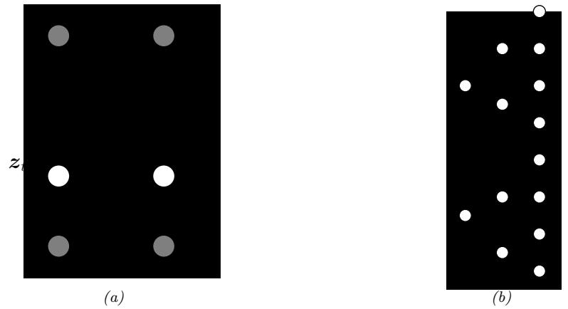
Figure 29.25: (a) A switching SSM. Squares represent discrete random variables, circles represent continuous random variables. (b) Illustration of how the number of modes in the belief state of a switching SSM grows exponentially over time. We assume there are two binary states.

y2. At step 3, the belief state will be a mixture of 8 Gaussians. And so on. So we see there is an exponential explosion in the number of modes. Each sequence of discrete values corresponds to a di!erent hypothesis (sometimes called a track), which can be represented as a tree, as shown in Figure 29.25b.

Various methods for approximate online inference have been proposed for this model, such as the following:

• Prune o! low probability trajectories in the discrete tree. This is widely used in multiple hypothesis tracking methods (see Section 29.9.3).
• Use particle filtering (Section 13.2) where we sample discrete trajectories, and apply the Kalman filter to the continuous variables. See Section 13.4.1 for details.
• Use ADF (Section 8.6), where we approximate the exponentially large mixture of Gaussians with a smaller mixture of Gaussians. See Section 8.6.2 for details.
• Use structured variational inference, where we approximate the posterior as a product of chainstructured distributions, one over the discrete variables and one over the continuous variables, with variational “coupling” terms in between (see e.g., [GH98; PJD21; Wan+22]).

29.9.3 Application: Multitarget tracking

The problem of multi-target tracking frequently arises in engineering applications (especially in aerospace and defence). This is a very large topic (see e.g., [BSF88; BSL93; Vo+15] for details), but in this section, we show how switching LDS models (or their nonlinear extensions) can be used to tackle the problem.

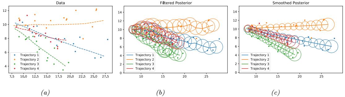
Figure 29.26: Illustration of Kalman filtering and smoothing for tracking multiple moving objects. Generated by kf\_parallel.ipynb.

Figure 29.27: A model for tracking two objects in the presence of data-association ambiguity. We observe 3, 1 and 2 detections at time steps t ↗ 1, t and t + 1. The m^t hidden variable encodes the association between the observations and the hidden causes.

29.9.3.1 Warm-up

In the simplest setting, we know there are N objects we want to track, and each one generates its own uniquely identified observation. If we assume the objects are independent, we can apply Kalman filtering and smoothing in parallel, as shown in Figure 29.26. (In this example, each object follows a linear dynamical model with di!erent initial random velocities, as in Section 29.7.1.)

29.9.3.2 Data association

More generally, at each step we may observe M measurements, e.g., “blips” on a radar screen. We can have M<N due to occlusion or missed detections. We can have M>N due to clutter or false alarms. Or we can have M = N. In any case, we need to figure out the correspondence between the M detections x^{m t} and the N objects z^{i t}. This is called the problem of data association, and it arises in many application domains.

We can model this problem by augmenting the state space with discrete variables m^t that represent the association matrix between the observations, yt,1:M, and the sources, zt,1:^N . See Figure 29.27 for an illustration, where we have N = 2 objects, but a variable number M^t of observations per time step.

As we mentioned in Section 29.9.2, inference in such hybrid (discrete-continouus) models is intractable, due to the exponential number of posterior modes. In the sections below, we briefly mention a few approximate inference methods.

29.9.3.3 Nearest neighbor approximation using Hungarian algorithm

A common way to perform approximate inference in this model is to compute an N ↗ M weight matrix, where Wim measures the “compatibility” between object i and measurement m, typically based on how close m is to where the model thinks i is (the so-called nearest neighbor data association heuristic).

We can make this into a square matrix by adding dummy background objects, which can explain all the false alarms, and adding dummy observations, which can explain all the missed detections. We can then compute the maximal weight bipartite matching using the Hungarian algorithm, which takes O(max(N,M)³) time (see e.g., [BDM09]).

Conditional on knowing the assignments of measurements to tracks, we can perform the usual Bayesian state update procedure (e.g., based on Kalman filtering). Note that objects that are assigned to dummy observations do not perform a measurement update, so their state estimate is just based on forwards prediction from the dynamics model.

29.9.3.4 Other approximate inference schemes

The Hungarian algorithm can be slow (since it is cubic in the number of measurements), and can give poor results since it relies on hard assignment. Better performance can be obtained by using loopy belief propagation (Section 9.4). The basic idea is to approximately marginalize out the unknown assignment variables, rather than perform a MAP estimate. This is known as the SPADA method (sum-product algorithm for data association) [WL14b; Mey+18].

The cost of each iteration of the iterative procedure is O(NM). Furthermore, [WL14b] proved this will always converge in a finite number of steps, and [Von13] showed that the corresponding solution will in fact be the global optimum. The SPADA method is more e”cient, and more accurate, than earlier heuristic methods, such as JPDA (joint probabilistic data association) [BSWT11; Vo+15].

It is also possible to use sequential Monte Carlo methods to solve data association and tracking. See Section 13.2 for a general discussion of SMC, and [RAG04; Wan+17b] for a review of specific techniques for this model family.

29.9.3.5 Handling an unknown number of targets

In general, we do not know the true number of targets N, so we have to deal with variable-sized state space. This is an example of an open world model (see Section 4.6.5), which di!ers from the standard closed world assumption where we know how many objects of interest there are.

For example, suppose at each time step we get two “blips” on our radar screen, representing the presence of an object at a given location. These measurements are not tagged with the source of the object that generated them, so the data looks like Figure 29.28(a). In Figure 29.28(b-c) we show two

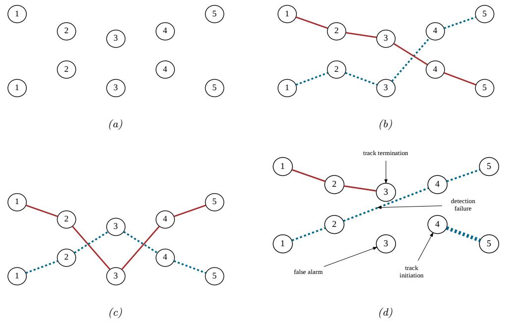
Figure 29.28: Illustration of multi-target tacking in 2d over 5 time steps. (a) We observe 2 measurements per time step. (b-c) Possible hypotheses about the underlying object tracks. (d) A more complex hypothesis in which the red track stops at step 3, the dashed red track starts at step 4, the dotted blue track has a detection failure at step 3, and one of the measurements at step 3 is a false alarm. Adapted from Figure 15.8 of [RN19].

di!erent hypotheses about the underlying object trajectories that could have generated this data. However, how can we know there are two objects? Maybe there are more, but some are just not detected. Maybe there are fewer, and some observations are false alarms due to background clutter. One such more complex hypothesis is shown in Figure 29.28(d). Figuring out what is going on in problems such as this is known as multiple hypothesis tracking.

A common approximate solution to this is to create new objects whenever an observation cannot be “explained” (i.e., generated with high likelihood) by any existing objects, and to prune out old objects that have not been detected in a while (in order to keep the computational cost bounded). Sets whose size and content are both random are called random finite sets. An elegant mathematical framework for dealing with such objects is described in [Mah07; Mah13; Vo+15].

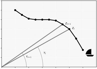
Figure 29.29: Illustration of a bearings-only tracking problem. Adapted from Figure 2.1 of [CP20b].

29.10 Nonlinear SSMs

In this section, we consider SSMs with nonlinear transition and/or observation functions, and additive Gaussian noise. That is, we assume the model has the following form

\[\mathbf{z}\_t = \mathbf{f}(\mathbf{z}\_{t-1}, \mathbf{u}\_t) + \mathbf{q}\_t \tag{29.121}\]

\[\mathbf{q}\_t \sim N(\mathbf{0}, \mathbf{Q}\_t) \tag{29.122}\]

\[y\_t = h(z\_t, u\_t) + r\_t \tag{29.123}\]

\[ \sigma\_t \sim N(\mathbf{0}, \mathbf{R}\_t) \tag{29.124} \]

This is called a nonlinear dynamical system (NLDS), or nonlinear Gaussian SSM (NLG-SSM).

29.10.1 Example: object tracking and state estimation

In Section 8.3.2.3 we give an example of a 2d tracking problem where the motion model is nonlinear, but the observation model is linear.

Here we consider an example where the motion model is linear, but the observation model is nonlinear. In particular, suppose we use the same 2d linear dynamics as in Section 29.7.1, where the state space contains the position and velocity of the object, z^t = u^t v^t u˙ ^t v˙^t . (We use u and v for the two coordinates, to avoid confusion with the state and observation variables.) Instead of directly observing the location, suppose we have a bearings only tracking problem, in which we just observe the angle to the target:

\[y\_t = \tan^{-1} \left( \frac{v\_t - s\_y}{u\_t - s\_x} \right) + r\_t \tag{29.125}\]

where (sx, sy) is the position of the measurement sensor. See Figure 29.29 for an illustration. This nonlinear observation model prevents the use of the Kalman filter, but we can still apply approximate inference methods, as we discuss below.

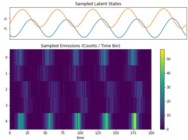
Figure 29.30: Samples from a 2d LDS with 5 Poisson likelihood terms. Generated by poisson\_lds.ipynb.

29.10.2 Posterior inference

Inferring the states of an NLDS model is in general computationally di”cult. Fortunately, there are a variety of approximate inference schemes that can be used, such as the extended Kalman filter (Section 8.3.2), the unscented Kalman filter (Section 8.4.2), etc.

29.11 Non-Gaussian SSMs

In this section, we consider SSMs in which the transition and observation noise is non-Gaussian. The transition and observation functions can be linear or nonlinear. We can represent this as a probabilistic model as follows:

\[p(\mathbf{z}\_t | \mathbf{z}\_{t-1}, \mathbf{u}\_t) = p(\mathbf{z}\_t | f(\mathbf{z}\_{t-1}, \mathbf{u}\_t)) \tag{29.126}\]

\[p(y\_t|\mathbf{z}\_t, \mathbf{u}\_t) = p(y\_t|\mathbf{h}(\mathbf{z}\_t, \mathbf{u}\_t)) \tag{29.127}\]

This is called a non-Gaussian SSM (NSSM).

29.11.1 Example: spike train modeling

In this section we consider an SSM with linear-Gaussian latent dynamics and a Poisson likelihood. Such models are widely used in neuroscience for modeling neural spike trains. (see e.g., [Pan+10; Mac+11]). This is an example of an exponential family state-space model (see e.g., [Vid99; Hel17]).

We consider a simple example where the model has 2 continuous latent variables, and we set the

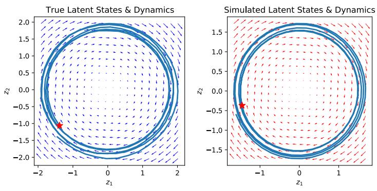
Figure 29.31: Latent state trajectory (blue lines) and dynamics matrix A (arrows) for (left) true model and (right) estimated model. The star marks the start of the trajectory. Generated by poisson\_lds.ipynb.

dynamics matrix A to a random rotation matrix. The observation model has the form

\[p(y\_t|\mathbf{z}\_t) = \prod\_{d=1}^{D} \text{Poi}(y\_{td}|\exp(\mathbf{w}\_d^\mathsf{T}\mathbf{z}\_t))\tag{29.128}\]

where w^d is a random vector, and we use D = 5 observations per time step. Some samples from this model are shown in Figure 29.30.

We can fit this model by using EM, where in the E step we approximate p(yt|zt) using a Laplace approximation, after which we can use the Kalman smoother to compute p(z1:^T |y1:^T ). In the M step, we optimize the expected complete data log likelihood, similar to Section 29.8.1. We show the result in Figure 29.31, where we compare the parameters A and the posterior trajectory E [zt|y1:^T ] using the true model and the estimated model. We see good agreement.

29.11.2 Example: stochastic volatility models

In finance, it is common to model the log-returns, y^t = log(pt/p^t↑1), where p^t is the price of some asset at time t. A common model for this problem, known as a stochastic volatility model, (see e.g., [KSC98]), has the following form:

\[y\_t = \mathbf{u}\_t^\mathsf{T} \boldsymbol{\beta} + \exp(z\_t/2)r\_t\tag{29.129}\]

\[z\_t = \mu + \rho(z\_{t-1} - \mu) + \sigma q\_t \tag{29.130}\]

\[r\_t \sim \mathcal{N}(0, 1) \tag{29.131}\]

\[q\_t \sim \mathcal{N}(0, 1) \tag{29.132}\]

We see that the dynamical model is a first-order autoregressive process. We typically require that |5| < 1, to ensure the system is stationary. The observation model is Gaussian, but can be replaced by a heavy-tailed distribution such as a Student.

We can capture longer range temporal correlation by using a higher order auto-regressive process. To do this, we just expand the state-space to contain the past K values. For example, if K = 2 we

have

\[ \begin{pmatrix} z\_t - \mu \\ z\_{t-1} - \mu \end{pmatrix} = \begin{pmatrix} \rho\_1 & \rho\_2 \\ 1 & 0 \end{pmatrix} \begin{pmatrix} z\_{t-1} - \mu \\ z\_{t-2} - \mu \end{pmatrix} + \begin{pmatrix} q\_t \\ 0 \end{pmatrix} \tag{29.133} \]

where ^{qt ↑ N} (0, ^{ς2 z} ). Thus we have

\[z\_t = \mu + \rho\_1(z\_{t-1} - \mu) + \rho\_2(z\_{t-2} - \mu) + q\_t \tag{29.134}\]

29.11.3 Posterior inference

Inferring the states of an NGSSM model is in general computationally di”cult. Fortunately, there are a variety of approximate inference schemes that can be used, which we discuss in Chapter 8 and Chapter 13.

29.12 Structural time series models

In this section, we discuss time series forecasting, which is the problem of computing the predictive distribution over future observations given the data up until the present, i.e., computing p(yt+h|y1:t). (The model may optionally be conditioned on known future inputs, to get p(yt+h|y1:t,u1:t+h).) There are many approaches to this problem (see e.g., [HA21]), but in this section, we focus on structural time series (STS) models, which are defined in terms of linear-Gaussian SSMs.

Many classical time series methods, such as the ARMA (autoregressive moving average) method, can be represented as STS models (see e.g., [Har90; CK07; DK12; PFW21]). However, the STS approach has much more flexibility. For example, we can create nonlinear, non-Gaussian, and even hierarchical extensions, as we discuss below.

29.12.1 Introduction

The basic idea of an STS model is to represent the observed scalar time series as a sum of C individual components:

\[f(t) = f\_1(t) + f\_2(t) + \dots + f\_C(t) + \epsilon\_t \tag{29.135}\]

where ^{ϖt ↑ N} (0, ^ς2). For example, we might have a seasonal component that causes the observed values to oscillate up and down, and a growth component, that causes the observed values to get larger over time. Each latent process fc(t) is modeled by a linear Gaussian state-space model, which (in this context) is also called a dynamic linear model (DLM). Since these are linear, we can combine them altogether into a single LG-SSM. In particular, in the case of scalar observations, the model has the form

\[p(\mathbf{z}\_t | \mathbf{z}\_{t-1}, \boldsymbol{\theta}) = \mathcal{N}(\mathbf{z}\_t | \mathbf{F} \mathbf{z}\_{t-1}, \mathbf{Q}) \tag{29.136}\]

\[p(y\_t | \mathbf{z}\_t, \boldsymbol{\theta}) = \mathcal{N}(y\_t | \mathbf{H} \mathbf{z}\_t + \boldsymbol{\beta}^\top \mathbf{u}\_t, \sigma\_y^2) \tag{29.137}\]

where F and Q are block structured matrices, with one block per component. The vector H then adds up all the relevant pieces from each component to generate the overall mean. Note that the

matrices F and H are fixed sparse matrices which can be derived from the form of the corresponding components of the model, as we discuss below. So the only model parameters are the variance terms, Q and ς^{2 y}, and the optional regression coe”cients φ. 4 We can generalize this to vector-valued observations as follows:

\[p(\mathbf{z}\_t | \mathbf{z}\_{t-1}, \boldsymbol{\theta}) = \mathcal{N}(\mathbf{z}\_t | \mathbf{F} \mathbf{z}\_{t-1}, \mathbf{Q}) \tag{29.138}\]

\[p(y\_t|\mathbf{z}\_t, \boldsymbol{\theta}) = \mathcal{N}(y\_t|\mathbf{H}\mathbf{z}\_t + \mathbf{D}u\_t, \mathbf{R})\tag{29.139}\]

29.12.2 Structural building blocks

In this section, we discuss the building blocks of common STS models.

29.12.2.1 Local level model

The simplest latent dynamical process is known as the local level model. It assumes the observations y^t → R are generated by a Gaussian with (latent) mean µt, which evolves over time according to a random walk:

\[y\_t = \mu\_t + \epsilon\_{y,t} \quad \epsilon\_{y,t} \sim N(0, \sigma\_y^2) \tag{29.140}\]

\[ \mu\_t = \mu\_{t-1} + \epsilon\_{\mu, t}, \quad \epsilon\_{\mu, t} \sim \mathcal{N}(0, \sigma\_{\mu}^2) \tag{29.141} \]

We also assume ^{µ1 ↑ N} (0, ^{ς2 µ}). Hence the latent mean at any future step has distribution ^{µt ↑ N} (0, tς^{2 µ}), so the variance grows with time. We can also use an autoregressive (AR) process, ^{µt = 5}µ^t↑^{1 + ϖ}µ,t, where ^|5^{| &}lt; ¹. This has the stationary distribution ^µ⇑ ^{↑ N} (0, ^ε2 µ ¹↑ρ² ), so the uncertainty grows to a finite asymptote instead of unboundedly.

29.12.2.2 Local linear model

Many time series exhibit linear trends upwards or downwards, at least locally. We can model this by letting the level µ^t change by an amount ϑ^t↑¹ (representing the slope of the line over an interval “t = 1) at each step

\[ \mu\_t = \mu\_{t-1} + \delta\_{t-1} + \epsilon\_{\mu,t} \tag{29.142} \]

The slope itself also follows a random walk,

\[ \delta\_t = \delta\_{t-1} + \epsilon\_{\delta, t} \tag{29.143} \]

and ^ϖ▷,t ^{↑ N} (0, ^{ς2 ▷} ). This is called a local linear trend model.

We can combine these two processes by defining the following dynamics model:

\[ \underbrace{\begin{pmatrix} \mu\_t \\ \delta\_t \end{pmatrix}}\_{\mathbf{z}\_t} = \underbrace{\begin{pmatrix} 1 & 1 \\ 0 & 1 \end{pmatrix} \begin{pmatrix} \mu\_{t-1} \\ \delta\_{t-1} \end{pmatrix}}\_{\mathbf{F}} + \underbrace{\begin{pmatrix} \epsilon\_{\mu,t} \\ \epsilon\_{\delta,t} \end{pmatrix}}\_{\mathbf{e}\_t} \tag{29.144} \]

^4. In the statistics community, the notation often follows that used in [DK12], who write the dynamics as ϖ^t = ^Ttϖt↑^{1 + c}tRtϑ^t and the observations as ^{yt = Z}tϖ^{t + ϱ}Tx^{t + H}tςt, where ^{ϑt ↑ N} (0, ^I) and ^{ςt ↑ N} (0, 1).

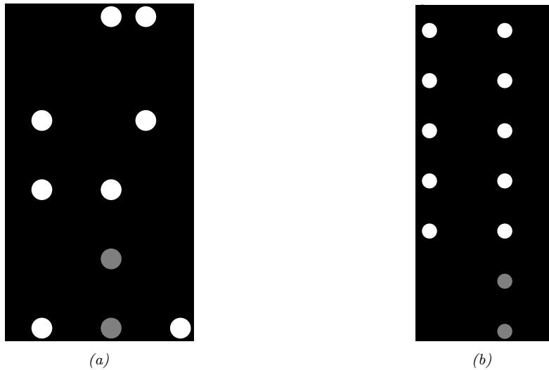
Figure 29.32: (a) A BSTS model with local linear trend and linear regression on inputs. The observed output is yt. The latent state vector is defined by z^t = (µt, ϱt). The (static) parameters are ω = (εy, εµ, εϱ, ϑ). The covariates are ut. (b) Adding a latent seasonal process (with S = 4 seasons). Parameter nodes are omitted for clarity.

For the emission model we have

\[y\_t = \underbrace{\begin{pmatrix} 1 & 0 \\ \end{pmatrix}}\_{\mathbf{H}} \underbrace{\begin{pmatrix} \mu\_t \\ \delta\_t \\ \end{pmatrix}}\_{\mathbf{z}\_t} + \epsilon\_{y,t} \tag{29.145} \tag{29.145}\]

We can also use an autoregressive model for the slope, i.e.,

\[ \delta\_t \delta\_t = D + \rho(\delta\_{t-1} - D) + \epsilon\_{\delta, t} \tag{29.146} \]

where D is the long run slope to which ϑ will revert. This is called a “semilocal linear trend” model, and is useful for longer term forecasts.

29.12.2.3 Adding covariates

We can easily include covariates u^t into the model, to increase prediction accuracy. If we use a linear model, we have

\[y\_t = \mu\_t + \mathcal{B}^{\top} u\_t + \epsilon\_{y,t} \tag{29.147}\]

See Figure 29.32a for an illustration of the local level model with covariates. Note that, when forecasting into the future, we will need some way to predict the input values of future ut+h; a simple approach is just to assume future inputs are the same as the present, ut+^h = ut.

29.12.2.4 Modelling seasonality

Many time series also exhibit seasonality, i.e., they fluctuate periodically. This can be modeled by creating a latent process consisting of a series o!set terms, st. To model cyclicity, we ensure that these sum to zero (on average) over a complete cycle of S steps:

\[s\_t = -\sum\_{k=1}^{S-1} s\_{t-k} + \epsilon\_{s,t}, \; \epsilon\_{s,t} \sim \mathcal{N}(0, \sigma\_s^2) \tag{29.148}\]

For example, for S = 4, we have s^t = ↓(s^t↑¹ +s^t↑² +s^t↑3) +ϖs,t. We can convert this to a first-order model by stacking the last S ↓ 1 seasons into the state vector, as shown in Figure 29.32b.

29.12.2.5 Adding it all up

We can combine the various latent processes (local level, linear trend, and seasonal cycles) into a single linear-Gaussian SSM, because the sparse graph structure can be encoded by sparse matrices. More precisely, the transition model becomes

\[ \underbrace{\begin{pmatrix} s\_t \\ s\_{t-1} \\ s\_{t-2} \\ \mu\_t \\ \delta\_t \end{pmatrix}}\_{\mathbf{z}\_t} = \underbrace{\begin{pmatrix} -1 & -1 & -1 & 0 & 0 \\ 1 & 0 & 0 & 0 & 0 \\ 0 & 1 & 0 & 0 & 0 \\ 0 & 0 & 0 & 1 & 1 \\ 0 & 0 & 0 & 0 & 1 \end{pmatrix}}\_{\mathbf{F}} \begin{pmatrix} s\_{t-1} \\ s\_{t-2} \\ s\_{t-3} \\ \mu\_{t-1} \\ \delta\_{t-1} \end{pmatrix} + \mathcal{N}\left(\mathbf{0}, \text{diag}\left[ (\sigma\_s^2, 0, 0, \sigma\_\mu^2, \sigma\_\delta^2) \right] \right) \tag{29.149} \]

Having defined the model, we can use the Kalman filter to compute p(zt|y1:t), and then make predictions forwards in time by rolling forwards in latent space, and then predicting the outputs:

\[p(y\_{t+1}|y\_{1:t}) = \int p(y\_{t+1}|z\_{t+1})p(z\_{t+1}|z\_t)p(z\_t|y\_{1:t})dz\_t\tag{29.150}\]

This can be computed in closed form, as explained in Section 8.2.2.

29.12.3 Model fitting

Once we have specified the form of the model, we need to learn the model parameters, ε = (D, R, Q), since F and H fixed to the values specified by the structural blocks, and B = 0. Common approaches are based on maximum likelihood estimation (see Section 29.8), and Bayesian inference (see Section 29.8.4). The latter approach is known as Bayesian structural time series or BSTS modeling [SV14; QRJN18], and often uses the following conjugate prior:

\[p(\boldsymbol{\theta}) = \text{MNW}(\mathbf{R}, \mathbf{D})\text{IW}(\mathbf{Q})\tag{29.151}\]

Alternatively, if there are a large number of covariates, we may use a sparsity-promoting prior (e.g., spike and slab, Section 15.2.5) for the regression coe”cients D.

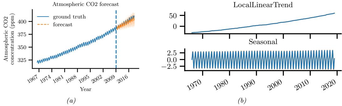
Figure 29.33: (a) CO² levels from Mauna Loa. In orange plot we show predictions for the most recent 10 years. (b) Underlying components for the STS mode which was fit to Figure 29.33a. Generated by sts.ipynb.

29.12.4 Forecasting

Once the parameters have been estimated on an historical dataset, we can perform inference on a new time series to compute p(zt|y1:t,u1:t, ε) using the Kalman filter (Section 8.2.2). Given the current posterior, we can then “roll forwards” in time to forecast future observations h steps ahead by computing p(yt+h|y1:t,u1:t+h, ε), as in Section 8.2.2.3. If the parameters are uncertain, we can sample from the posterior, p(ε|y1:t,u1:t), and then perform Monte Carlo averaging of the forecasts.

29.12.5 Examples

In this section, we give various examples of STS models.

29.12.5.1 Example: forecasting CO² levels from Mauna Loa

In this section, we fit an STS model to the monthly atmospheric CO² readings from the Mauna Loa observatory in Hawaii.5 The data is from January 1966 to February 2019. We combine a local linear trend model with a seasonal model, where we assume the periodicity is S = 12, since the data is monthly (see Figure 29.33a). We fit the model to all the data except for the last 10 years using variational Bayes. The resulting posterior mean and standard deviations for the parameters are ς^y = 0.169 ± 0.008, ς^µ = 0.159 ± 0.017, ς^▷ = 0.009 ± 0.003, ς^s = 0.038 ± 0.008. We can sample 10 parameter vectors from the posterior and then plug them it to create a distribution over forecasts. The results are shown in orange in Figure 29.33a. Finally, in Figure 29.33b, we plot the posterior mean values of the two latent components (linear trend and current seasonal value) over time. We see how the model has successfully decomposed the observed signal into a sum of two simpler signals. (See also Section 18.8.1 where we model this data using a GP.)

^5. For details, see https://blog.tensorflow.org/2019/03/structural-time-series-modeling-in.html.

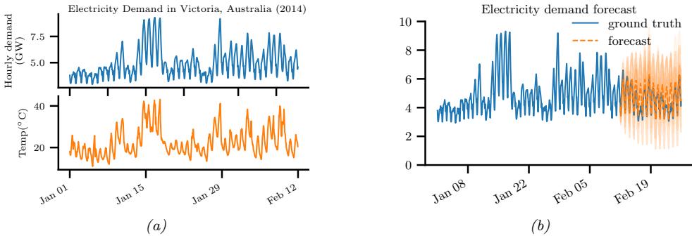
Figure 29.34: (a) Hourly temperature and electricity demand in Victoria, Australia in 2014. (b) Electricity forecasts using an STS. Generated by sts.ipynb.

29.12.5.2 Example: forecasting (real-valued) electricity usage

In this section, we consider a more complex example: forecasting electricity demand in Victoria, Australia, as a function of the previous value and the external temperature. (Remember that January is summer in Australia!) The hourly data from the first six weeks of 2014 is shown in Figure 29.34a. 6

We fit an STS to this using 4 components: a seasonal hourly e!ect (period 24), a seasonal daily e!ect (period 7, with 24 steps per season), a linear regression on the temperature, and an autoregressive term on the observations themselves. We fit the model with variational inference. (This takes about a minute on a GPU.) We then draw 10 posterior samples and show the posterior predictive forecasts in Figure 29.34b. We see that the results are reasonable, but there is also considerable uncertainty.

We plot the individual components in Figure 29.35. Note that they have di!erent vertical scales, reflecting their relative importance. We see that the regression on the external temperature is the most important e!ect. However, the hour of day e!ect is also quite significant, even after accounting for external temperature. The autoregressive e!ect is the most uncertain one, since it is responsible for modeling all of the residual variation in the data beyond what is accounted for by the observation noise.

We can also use the model for anomaly detection. To do this, we compute the one-step-ahead predictive distributions, p(yt|y1:t↑¹,u1:t), for each time step t, and then flag all time steps where the observation is improbable. The results are shown in Figure 29.36.

29.12.5.3 Example: forecasting (integer valued) sales

In Section 29.12.5.2, we used a linear Gaussian STS model to forecast electricity demand. However, for some problems, we have integer valued observations, e.g., for neural spike data (see Section 29.11.1), RNA-Seq data [LJY19], sales data, etc. Here we focus on the case of sales data, where y^t → {0, 1, 2,…} is the number of units of some item that are sold on a given day. Predicting future values of y^t is important for many businesses. (This problem is known as demand forecasting.)

We assume the observed counts are due to some latent demand, z^t → R. Hence we can use a model similar to Section 29.11.1, with a Poisson likelihood, except the linear dynamics are given

^6. The data is from https://github.com/robjhyndman/fpp2-package.

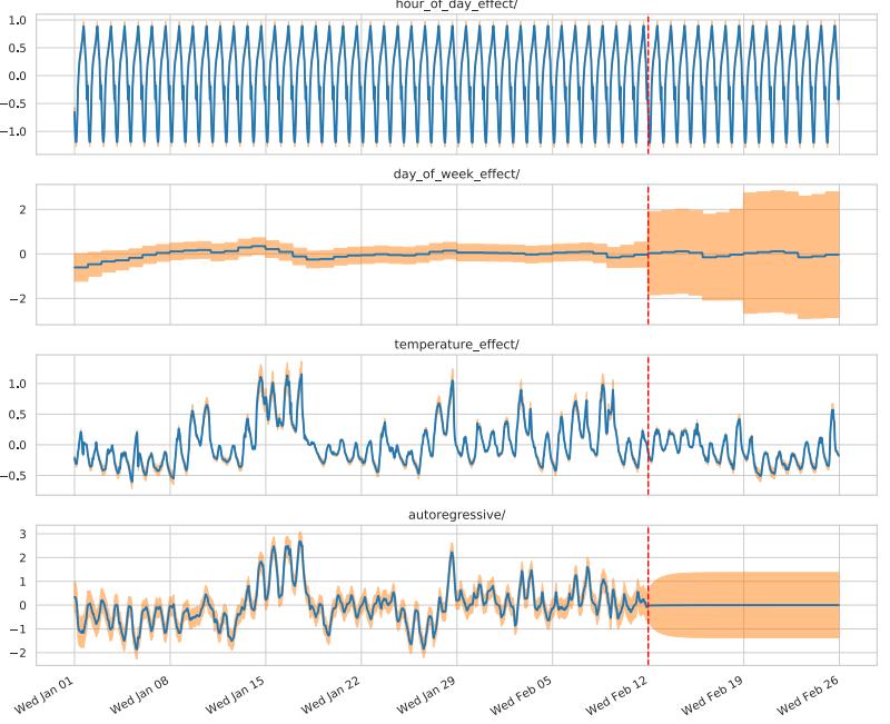
Figure 29.35: Components of the electricity forecasts. Generated by sts.ipynb.

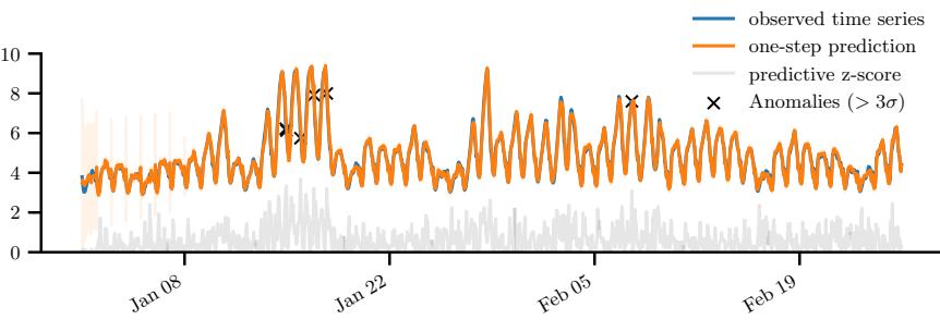
Figure 29.36: Anomaly detection in a time series. We plot the observed electricity data in blue and the predictions in orange. In gray, we plot the z-score at time t , given by (y^t ↗ µt)/εt, where p(yt|y1:t↑¹, u1:t) = ^N (µt, ^{ε2 t} ). Anomalous observations are defined as points where z^t > 3 and are marked with black crosses. Generated by sts.ipynb.

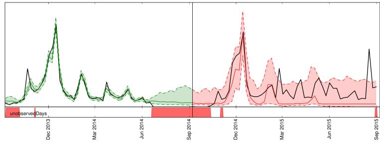
Figure 29.37: Visualization of a probabilistic demand forecast for a hypothetical product. Note the sudden spike near the Christmas holiday in December 2013. The black line denotes the actual demand. Green lines denote the model samples in the training range, while the red lines show the actual probabilistic forecast on data unseen by the model. The red bars at the bottom indicate out-of-stock events which can explain the observed zeros. From Figure 1 of [Bös+17]. Used with kind permission of Tim Januschowski.

by an STS model. In [SSF16; See+17], they consider a likelihood of the form ^{yt ↑} Poi(yt|g(d^{y t} )), where d^t = z^t + u^{T t} w is the instantaneous latent demand, u^t are the covariates that encode seasonal indicators (e.g., temporal distance from holidays), and g(d) = e^d or log(1+e^d) is the transfer function. The dynamics model is a local random walk term, and z^t = z^t↑¹ + ↽N (0, 1), to capture serial correlation in the data.

However, sometimes we observe zero counts, y^t = 0, not because there is no demand, but because there is no supply (i.e., we are out of stock). If we do not model this properly, we may incorrectly infer that z^t = 0, thus underestimating demand, which may result in not ordering enough inventory for the future, further compounding the error.

One solution is to use a zero-inflated Poisson (ZIP) model [Lam92] for the likelihood. This is a mixture model of the form ^p(yt|dt) = ^p0I(y^t = 0) + (1 ^{↓ p}0)Poi(yt|e^dt ), where ^p0 is the probability of the first mixture component. It is also common to use a (possibly zero-inflated) negative binomial model (Section 2.2.1.4) as the likelihood. This is used in [Cha14; Sal+19b] for the demand forecasting problem. The disadvantage of these likelihoods is that they are not log-concave for d^t = 0, which complicates posterior inference. In particular, the Laplace approximation is a poor choice, since it may find a saddle point. In [SSF16], they tackle this using a log-concave multi-stage likelihood, in which y^t = 0 is emitted with probability ς(d^{0 t} ); otherwise y^t = 1 is emitted with probability ς(d¹ t ); otherwise y^t = is emitted with probability Poi(d^{2 t} ). This generalizes the scheme in [SOB12].

29.12.5.4 Example: hierarchical SSM for electoral panel data

Suppose we perform a survey for the US presidential elections. Let N^{j t} be the number of people who vote at time t in state j, and let y^{j t} be the number of those people who vote Democrat. (We assume Nj ^{t ↓ yj t} vote Republican.) It is natural to want to model the dependencies in this data both across time (longitudinally) and across space (this is an example of panel data).

We can do this using a hierarchical SSM, as illustrated in Figure 29.38. The top level Markov chain, z^{0 t} , models national-level trends, and the state-specific chains, z^{j t} , model local “random e!ects”. In practice we would usually also include covariates at the national level, u^{0 t} and state level, u^j t .

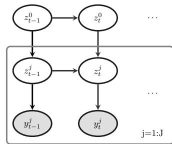
Figure 29.38: Illustration of a hierarchical state-space model.

Thus the model becomes

\[y\_t^j \sim \text{Bin}(y\_t^j | \pi\_t^j, N\_t^j) \tag{29.152}\]

\[\boldsymbol{\pi}\_{t}^{j} = \sigma \left[ (\mathbf{z}\_{t}^{0})^{\mathsf{T}} \mathbf{u}\_{t}^{0} + (\mathbf{z}\_{t}^{j})^{\mathsf{T}} \mathbf{u}\_{t}^{j} \right] \tag{29.153}\]

\[\mathbf{z}\_{t}^{0} = \mathbf{z}\_{t-1}^{0} + \mathcal{N}(\mathbf{0}, \sigma^{2}\mathbf{I}) \tag{29.154}\]

\[\mathbf{z}\_{t}^{j} = \mathbf{z}\_{t-1}^{j} + \mathcal{N}(\mathbf{0}, \tau^{2}\mathbf{I}) \tag{29.155}\]

For more details, see [Lin13b].

29.12.6 Causal impact of a time series intervention

In this section, we discuss how to estimate the causal e!ect on an intervention given some quasiexperimental time series data. (The term “quasi-experimental” means the data was collected under an intervention but without using random assignment.) For example, suppose y^t is the click through rate (CTR) of the web page of some company at time t. The company launches an ad campaign at time n, and observes outcomes y1:ⁿ before the intervention and yn+1:^m after the intervention. (This is an example of an interrupted time series, since the “natural” process was perturbed at some point.) A natural question to ask is: what would the CTR have been had the company not run the ad campaign? This is a counterfactual question. (We discuss counterfactuals in Section 4.7.4.) If we can predict this counterfactual time series, y˜n+1:m, then we compare the actual y^t to the predicted y˜t, and use this to estimate the causal impact of the intervention.

To predict the counterfactual outcome, we will use a structural time series (STS) model (see Section 29.12), following [Bro+15]. An STS model is a linear-Gaussian state-space model, where arrows have a natural causal interpretation in terms of the arrow of time; thus a STS is a kind of structural equation model, and hence a structural causal model (see Section 4.7). The use of an SCM allows us to infer the latent state of the noise variables given the observed data; we can then “roll back time” to the point of intervention, where we explore an alternative “fork in the road” from the one we actually took by “rolling forwards in time” in a new version of the model, using the twin network approach to counterfactual inference (see Section 4.7.4).

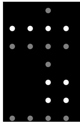
Figure 29.39: Twin network state-space model for estimating causal impact of an intervention that occurs just after time step n = 2. We have m = 4 actual observations, denoted y1:4. We cut the incoming arcs to z³ since we assume z3:^T comes from a di!erent distribution, namely the post-intervention distribution. However, in the counterfactual world, shown at the bottom of the figure (with tilde symbols), we assume the distributions are the same as in the past, so information flows along the chain uninterrupted.

29.12.6.1 Computing the counterfactual prediction

To explain the method in more detail, consider the twin network in Figure 29.39. The intervention occurs after time n = 2, and there are m = 4 observations in total. We observe 2 datapoints before the intervention, y1:2, and 2 datapoints afterwards, y3:4. We assume observations are generated by latent states z1:4, which evolve over time. The states are subject to exogeneous noise terms, which can represent any set of unmodeled factors, such as the state of the economy. In addition, we have exogeneous covariates, x1:m.

To predict what would have happened if we had not performed the intervention, (an event denoted by a˜ = 0), we replicate the part of the model that occurs after the intervention, and use it to make forecasts. The goal is to compute the counterfactual distribution, p(y˜n+1:m|y1:n, x1:m), where y˜^t represents counterfactual outcomes if the action had been a˜ = 0. We can compute this counterfactual distribution as follows:

\[p(\ddot{y}\_{n+1:m}|y\_{1:n}, \mathbf{z}\_{1:m}) = \int p(\ddot{y}\_{n+1:m}|\ddot{z}\_{n+1:m}, \mathbf{z}\_{n+1:m}, \theta) p(\ddot{z}\_{n+1:m}|z\_n, \theta) \times \tag{29.156}\]

\[p(\mathbf{z}\_n, \theta | \mathbf{z}\_{1:n}, \mathbf{y}\_{1:n}) d\theta d\mathbf{z}\_n d\mathbf{\bar{z}}\_{n+1:m} \tag{29.157}\]

where

\[p(\mathbf{z}\_n, \theta | x\_{1:n}, y\_{1:n}) = p(z\_n | x\_{1:n}, y\_{1:n}, \theta) p(\theta | x\_{1:n}, y\_{1:n}) \tag{29.158}\]

For linear Gaussian SSMs, the term p(zn|x1:n, y1:n, ε) can be computed using Kalman filtering (Section 8.2.2), and the term p(ε|y1:n, x1:n), can be computed using MCMC or variational inference.

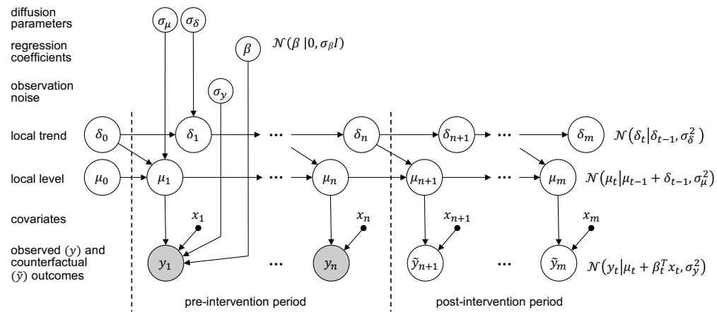
Figure 29.40: A graphical model representation of the local level causal impact model. The dotted line represents the time n at which an intervention occurs. Adapted from Figure 2 of [Bro+15]. Used with kind permission of Kay Brodersen.

We can use samples from the above posterior predictive distribution to compute a Monte Carlo approximation to the distribution of the treatment e!ect per time step, ⇀ ^{i t} = ^{yt ↓ y}˜^{i t}, where the i index refers to posterior samples. We can also approximate the distribution of the cumulative causal impact using ς^{i t =} *^{t s}=n+1 ⇀ ^{i t} . (There will be uncertainty in these quantities arising both from epistemic uncertainty, about the true parameters controlling the model, and aleatoric uncertainty, due to system and observation noise.)

29.12.6.2 Assumptions needed for the method to work

The validity of the method is based on 3 assumptions: (1) Predictability: we assume that the outcome can be adequately predicted by our model given the data at hand. (We can check this by using backcasting, in which we make predictions on part of the historical data.) (2) Una!ectedness: we assume that the intervention does not change future covariates xn+1:m. (We can potentially check this by running the method with each of the covariates as an outcome variable.) (3) Stability: we assume that, had the intervention not taken place, the model for the outcome in the pre-treatment period would have continued in the post-treatment period. (We can check this by seeing if we predict an e!ect if the treatment is shifted earlier in time.)

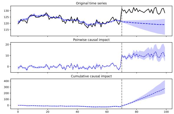
Figure 29.41: Some simulated time series data which we use to estimate the causal impact of some intervention, which occurs at time n = 70, Generated by causal\_impact\_jax.ipynb.

29.12.6.3 Example

As a concrete example, let us assume we have a local level model and we use linear regression to model the dependence on the covariates, as in Section 29.12.2.3. That is,

\[y\_t = \mu\_t + \boldsymbol{\beta}^{\mathrm{T}} \boldsymbol{x}\_t + \boldsymbol{\mathcal{N}}(\boldsymbol{0}, \sigma\_y^2) \tag{29.159}\]

\[ \mu\_t = \mu\_{t-1} + \delta\_{t-1} + N(0, \sigma\_\mu^2) \tag{29.160} \]

\[ \delta\_t \delta\_t = \delta\_{t-1} + \mathcal{N}(0, \sigma\_\delta^2) \tag{29.161} \]

See the graphical model in Figure 29.40. The static parameters of the model are ε = (φ, ς^{2 y}, ς^{2 µ}, ς² ▷ ), the other terms are state or observation variables. (Note that we are free to use any kind of STS model; the local level model is just a simple default.)

For simplicity, let us assume we have a single scalar input xt, in addition to the scalar output yt. We create some synthetic data using an autoregressive process on xt, and then set y^t = 1.2x^t + ϖt. We then manually intervene at timestep t = 70 by increasing the y^t values by 10. In Figure 29.41, we show the output of the causal impact procedure when applied to this dataset. In the top row, we see that the forecasted output y˜^t (blue line) at times t ⇒ 70 follows the general AR trend learned by the model on the pre-interventional period, whereas the actual observations y^t (black line) are quite di!erent. Thus the posterior over the pointwise causal impact, ⇀^t = y^t ↓ y˜t, has a value of about 10 for t ⇒ 70.

29.12.6.4 Comparison to synthetic control

The use of a linear combination of other “donor” time series φ^Tx^t is similar in spirit to the concept of a “synthetic control” [Aba; Shi+21]. However we do not restrict ourselves to a convex combination of donors. Indeed, when we have many covariates, we can use a spike-and-slab prior (Section 15.2.5) or horseshoe prior (Section 15.2.7) to select the relevant ones. Furthermore, the STS method can be applied even if we just observe the outcome series yt, without any other parallel time series.

29.12.7 Prophet

Prophet [TL18a] is a popular time series forecasting library from Facebook. It fits a generalized additive model of the form

\[y(t) = g(t) + s(t) + h(t) + w^\top x(t) + \epsilon\_t \tag{29.162}\]

where g(t) is a trend function, s(t) is a seasonal fluctuation (modeled using linear regression applied to a sinusoidal basis set), h(t) is an optional set of sparse “holiday e!ects”, x(t) are an optional set of (possibly lagged) covariates, w are the regression coe”cients, and ϖ(t) is the residual noise term, assumed to be iid Gaussian.

Prophet is a regression model, not an auto-regressive model, since it predicts the time series y1:^T given the time stamp t and the covariates x1:^T , but without conditioning on past observations of y. To model the dependence on time, the trend function is assumed to be a piecewise linear trend with S changepoints, uniformly spaced in time. (See Section 29.5.6 for a discussion of changepoint detection.) That is, the model has the form

\[g(t) = (k + \mathbf{a}(t)^T \boldsymbol{\delta})t + (m + \mathbf{a}(t)^T \boldsymbol{\gamma})\tag{29.163}\]

where k is the growth rate, m is the o!set, a^j (t) = I(t ⇒ s^j ), where s^j is the time of the j’th changepoint, ϑ^t ↑ Laplace(⇀ ) is the magnitude of the change, and γ^j = ↓s^j ϑ^j to make the function continuous. The Laplace prior on ϑ ensures the MAP parameter estimate is sparse, so the di!erence across change point boundaries is usually 0.

For an interactive visualization of how Prophet works, see https://github.com/MBrouns/timeseers.

29.12.8 Neural forecasting methods

Classical time series methods work well when there is little data (e.g., short sequences, or few covariates). However, in some cases, we have a lot of data. For example, we might have a single, but very long sequence, such as in anomaly detection from real-time sensors [Ahm+17]. Or we may have multiple, related sequences, such as sales of related products [Sal+19b]. In both cases, larger data means we can a!ord to fit more complex parametric models. Neural networks are a natural choice, because of their flexibility. Until recently, their performance in forecasting tasks was not competitive with classical methods, but this has recently started to change, as described in [Ben+22; LZ20].

A common benchmark in the univariate time series forecasting literature is the M4 forecasting competition [MSA18], which requires participants to make forecasts on many di!erent kinds of (univariate) time series (without covariates). This was recently won by a neural method [Smy20]. More precisely, the winner of the 2019 M4 competition was a hybrid RNN-classical method called ES-RNN [Smy20]. The exponential smoothing (ES) part allows data-e”cient adaptation to the observed past of the current time series; the recurrent neural network (RNN) part allows for learning of nonlinear components from multiple related time series. (This is known as a local+global model, since the ES part is “trained” just on the local time series, whereas the RNN is trained on a global dataset of related time series.)

In [Ran+18] they adopt a di!erent approach for combining RNNs and classical methods, called DeepSSM. In particular, they train a single RNN to predict the parameters of a state-space model (see Main Section 29.1). In more detail, let xⁿ 1:^T represent the n’th time series, and let ε^{n t} represent the non-stationary parameters of a linear-trend SSM model (see Section 29.12.1). We train an RNN to compute ε^{n t} = f(cⁿ 1:^T ; ω), where ω are the RNN parameters shared across all sequences. We can use the predicted parameters to compute the log likelihood of the sequence, Lⁿ = log p(xⁿ 1:^{T |}cⁿ 1:^T , εⁿ 1:^T ), using the Kalman filter. These two modules can be combined to allow for end-to-end training of ω to maximize *^{N n}=1 Ln.

In [Wan+19c], they propose a di!erent hybrid model known as Deep Factors. The idea is to represent each time series (or its latent function, for non-Gaussian data) as a weighted sum of a global time series, coming from a neural model, and a stochastic local model, such as an SSM or GP. The DeepGLO (global-local) approach of [SYD19] proposes a related hybrid method, where the global model uses matrix factorization to learn shared factors. This is then combined with temporal convolutional networks.

It is also possible to train a purely neural model, without resorting to classical methods. For example, the N-BEATS model of [Ore+20] trains a residual network to predict the weights of a set of basis functions, corresponding to a polynomial trend and a periodic signal. The weights for the basis functions are predicted for each window of input using the neural network. Another approach is the DeepAR model of [Sal+19b], which fits a single RNN to a large number of time series. The original paper used integer (count) time series, modeled with a negative binomial likelihood function. This is a unimodal distribution, which may not be suitable for all tasks. More flexible forms, such as mixtures of Gaussians, have also been proposed [Muk+18].

A popular alternative is to use quantile regression [Koe05], in which the model is trained to predict quantiles of the distribution, which can be done by optimizing the pinball loss (see Section 14.3.2.1). For example, [Gas+19] proposed SQF-RNN, which uses splines to represent the quantile function. They used CRPS or continuous-ranked probability score as the loss function, which trains the model to predict all the quantiles. In particular, for a quantile predictor F ^↑1(↽), the CRPS loss is defined as

\[\text{CRPS}(F^{-1}, y) = \int\_0^1 2\ell\_\alpha(y, F^{-1}(\alpha)) d\alpha\]

where the inner loss function is the pinball loss defined in Equation (14.53). CRPS is a proper scoring rule, but is less sensitive to outliers, and is more “distance aware”, than log loss. For determiistic predictions, the CRPS reduces to the absolute error.

The above methods all predict a single output (per time step). If there are multiple simultaneous observations, it is best to try to model their interdependencies. In [Sal+19a], they use a (low-rank) Gaussian copula for this, and in [Tou+19], they use a nonparametric copula.

In [Wen+17], they simultaneously predict quantiles for multiple steps ahead using dilated causal convolution (or an RNN). They call their method MQ-CNN. In [WT19], they extend this to predict the full quantile function, taking as input the desired quantile level ↽, rather than prespecifying a fixed set of levels. They also use a copula to learn the dependencies among multiple univariate marginals.

29.13 Deep SSMs

Traditional state-space model assume linear dynamics and linear observation models, both with additive Gaussian noise. This is obviously very limiting. In this section, we allow the dynamics and/or observation model to be modeled by nonlinear and/or non-Markovian deep neural networks;

we call these deep state-space model, also known as dynamical variational autoencoders. (To be consistent with the literature on VAEs, we denote the observations by x^t instead of yt.) For a detailed review, see [Ged+20; Gir+21].

29.13.1 Deep Markov models

Suppose we create a SSM in which we use a deep neural network for the dynamics model and/or observation model; the result is called a deep Markov model [KSS17] or stochastic RNN [BO14; Fra+16]. (This is not quite the same as a variational RNN, which we explain in Section 29.13.4.)

We can fit a DMM using SVI (Section 10.1.4). The key is to infer the posterior over the latents. From the first-order Markov properties, the exact posterior is given by

\[p(\mathbf{z}\_{1:T}|\mathbf{z}\_{1:T}) = \prod\_{t=1}^{T} p(\mathbf{z}\_t|\mathbf{z}\_{t-1}, \mathbf{z}\_{1:T}) = \prod\_{t=1}^{T} p(\mathbf{z}\_t|\mathbf{z}\_{t-1}, \mathbf{z}\_{t:t} \mathbf{z}\_t^\prime, \mathbf{z}\_{t:T}) \tag{29.164}\]

where we define p(z1|z0, x1:^T ) = p(z1|x1:^T ), and the cancelation follows since z^t ∅ x1:t↑¹|z^t↑¹, as pointed out in [KSS17].

In general, it is intractable to compute p(z1:^T |x1:^T ), so we approximate it with an inference network. There are many choices for ^q. A simple one is a fully factorized model, ^q(z1:^{T |}x1:^T ) = ^t q(zt|x1:t). This is illustrated in Figure 29.42a. Since z^t only depends on past data, x1:^t (which is accumulated in the RNN hidden state ht), we can use this inference network at run time for online inference. However, for training the model o$ine, we can use a more accurate posterior by using

\[q(\mathbf{z}\_{1:T}|\mathbf{z}\_{1:T}) = \prod\_{t=1}^{T} q(\mathbf{z}\_t|\mathbf{z}\_{t-1}, \mathbf{z}\_{1:T}) = \prod\_{t=1}^{T} q(\mathbf{z}\_t|\mathbf{z}\_{t-1}, \mathbf{z}\_{1:t} \mathbf{z}\_t = \mathbf{f}, \mathbf{z}\_{t:T}) \tag{29.165}\]

Note that the dependence on past observation x1:t↑¹ is already captured by z^t↑¹, as in Equation (29.164). The dependencies on future observations, xt:^T , can be summarized by a backwards RNN, as shown in Figure 29.42b. Thus

\[q(\mathbf{z}\_{1:T}, \boldsymbol{h}\_{1:T} | \boldsymbol{x}\_{1:T}) = \prod\_{t=T}^{1} \mathbb{I}\left(\boldsymbol{h}\_{t} = f(\boldsymbol{h}\_{t+1}, \boldsymbol{x}\_{t})\right) \prod\_{t=1}^{T} q(\boldsymbol{z}\_{t} | \boldsymbol{z}\_{t-1}, \boldsymbol{h}\_{t}) \tag{29.166}\]

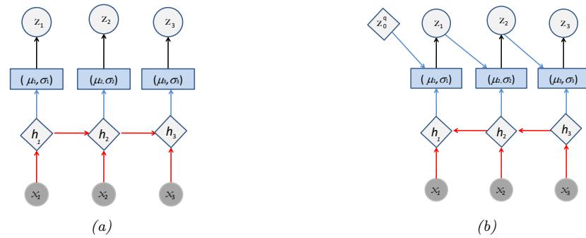
Figure 29.42: Inference networks for deep Markov model. (a) Fully factorized causal posterior ” q(z1:^T |x1:^T ) = ^t q(zt|x1:t). The past observations x1:^t are stored in the RNN hidden state ht. (b) Markovian posterior ^q(z1:^{T |}x1:^T ) = ” ^t q(zt|z^t↑¹, xt:^T ). The future observations xt:^T are stored in the RNN hidden state ht.

Given a fully factored q(z1:^T ), we can compute the ELBO as follows.

\[\log p(\mathbf{z}\_{1:T}) = \log \left[ \sum\_{\mathbf{z}\_{1:T}} p(\mathbf{z}\_{1:T} | \mathbf{z}\_{1:T}) p(\mathbf{z}\_{1:T}) \right] \tag{29.167}\]

\[=\log \mathbb{E}\_{q(\mathbf{z}\_{1:T})} \left[ p(\mathbf{z}\_{1:T}|\mathbf{z}\_{1:T}) \frac{p(\mathbf{z}\_{1:T})}{q(\mathbf{z}\_{1:T})} \right] \tag{29.168}\]

\[\mathbf{y} = \log \mathbb{E}\_{q(\mathbf{z}\_{1:T})} \left[ \prod\_{t=1}^{T} \frac{p(\mathbf{z}\_t | \mathbf{z}\_t) p(\mathbf{z}\_t | \mathbf{z}\_{t-1})}{q(\mathbf{z}\_t)} \right] \tag{29.169}\]

\[\geq \mathbb{E}\_{q(\mathbf{z}\_{t:T})} \left[ \sum\_{t=1}^{T} \log p(\mathbf{z}\_t | \mathbf{z}\_t) + \log p(\mathbf{z}\_t | \mathbf{z}\_{t-1}) - \log q(\mathbf{z}\_t) \right] \tag{29.170}\]

\[=\sum\_{t=1}^{T} \mathbb{E}\_{q(\mathbf{z}\_t)} \left[ \log p(\mathbf{z}\_t | \mathbf{z}\_t) \right] - \mathbb{E}\_{q(\mathbf{z}\_{t-1})} \left[ D\_{\text{KL}} \left( q(\mathbf{z}\_t) \parallel p(\mathbf{z}\_t | \mathbf{z}\_{t-1}) \right) \right] \tag{29.171}\]

If we assume that the variational posteriors are jointly Gaussian, we can use the reparameterization trick to use posterior samples to compute stochastic gradients of the ELBO. Furthermore, since we assumed a Gaussian prior, the KL term can be computed analytically.

29.13.2 Recurrent SSM

In a DMM, the observation model p(xt|zt) is first-order Markov, as is the dynamics model p(zt|z^t↑1). We can modify the model so that it captures long-range dependencies by adding deterministic hidden states as well. We can make the observation model depend on z1:^t instead of just z^t by using p(xt|ht), where h^t = f(h^t↑¹, zt), so h^t records all the stochastic choices. This is illustrated in Figure 29.43a. We can also make the dynamical prior depend on z1:t↑¹ by replacing p(zt|z^t↑1) with p(zt|h^t↑1). as is illustrated in Figure 29.43b. This is known as a recurrent SSM.

We can derive an inference network for an RSSM similar to the one we used for DMMs, except now we use a standard forwards RNN to compute q(zt|x1:t↑¹, x1:t).

Figure 29.43: Recurrent state-space models. (a) Prior is first-order Markov, p(zt|z^t↑¹), but observation model is not Markovian, p(xt|ht) = p(xt|z1:t), where h^t summarizes z1:t. (b) Prior model is no longer first-order Markov either, p(zt|h^t↑¹) = p(zt|z1:t↑¹). Diamonds are deterministic nodes, circles are stochastic.

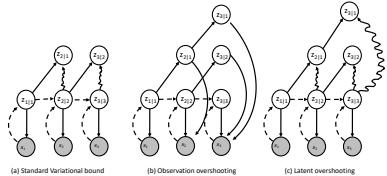
Figure 29.44: Unrolling schemes for SSMs. The labels zⁱ|^j is shorthand for p(zi|x1:^j ). Solid lines denote the generative process, dashed lines the inference process. Arrows pointing at shaded circles represent log-likelihood loss terms. Wavy arrows indicate KL divergence loss terms. (a) Standard 1 step reconstruction of the observations. (b) Observation overshooting tries to predict future observations by unrolling in latent space. (c) Latent overshooting predicts future latent states and penalizes their KL divergence, but does need to care about future observations. Adapted from Figure 3 of [Haf+19].

29.13.3 Improving multistep predictions

In Figure 29.44(a), we show the loss terms involved in the ELBO. In particular, the wavy edge z^t|^t ↔︎ z^t|t↑¹ corresponds to Eq(zt↓1) [DKL (q(zt) ⇐ p(zt|z^t↑¹))], and the solid edge z^t|^t ↔︎ x^t corresponds to Eq(zt) [log p(xt|zt)]. We see that the dynamics model, p(zt|z^t↑¹), is only ever penalized in terms of how it di!ers from the one-step-ahead posterior q(zt), which can hurt the ability of the model to make long-term predictions.

One solution to this is to make multistep forwards predictions using the dynamics model, and use these to reconstruct future observations, and add these errors as extra loss terms. This is called observation overshooting [Amo+18], and is illustrated in Figure 29.44(b).

A faster approach, proposed in [Haf+19], is to apply a similar idea but in latent space. More precisely, let us compute the multi-step prediction model, by repeatedly applying the transition model and integrating out the intermediate states to get p(zt|z^t↑d). We can then compute the ELBO

Figure 29.45: Variational RNN. (a) Generative model. (b) Inference model. The diamond-shaped nodes are deterministic.

for this as follows:

\[\log p\_d(\mathbf{z}\_{1:T}) \stackrel{\Delta}{=} \log \int \prod\_{t=1}^{T} p(\mathbf{z}\_t | \mathbf{z}\_{t-d}) p(\mathbf{z}\_t | \mathbf{z}\_t) d\mathbf{z}\_{1:T} \tag{29.172}\]

\[\geq \sum\_{t}^{T} \mathbb{E}\_{q(\mathbf{z}\_t)} \left[ \log p(\mathbf{z}\_t | \mathbf{z}\_t) \right] - \mathbb{E}\_{p(\mathbf{z}\_{t-1} | \mathbf{z}\_{t-d}) q(\mathbf{z}\_{t-d})} \left[ D\_{\mathbb{KL}}(q(\mathbf{z}\_t) \parallel p(\mathbf{z}\_t | \mathbf{z}\_{t-1})) \right] \tag{29.173}\]

To train the model so it is good at predicting at different future horizon depths \(d\) , we can average the above over all \(1 \le d \le D\) . However, for computational reasons, we can instead just average the KL terms, using weights \(\beta\_d\) . This is called **latent** **overshoot [Hz+19]**, and is illustrated in Figure 29.44(c). The new objective becomes

\[\frac{1}{D} \sum\_{d=1}^{D} \log p\_d(\mathbf{z}\_{1:T}) \ge \sum\_{t=1}^{T} \mathbb{E}\_{q(\mathbf{z}\_t)} \left[ \log p(\mathbf{z}\_t | \mathbf{z}\_t) \right] \tag{29.174}\]

\[-\frac{1}{D} \sum\_{d=1}^{D} \beta\_d \mathbb{E}\_{p(\mathbf{z}\_{t-1}|\mathbf{z}\_{t-d})q(\mathbf{z}\_{t-d})} \left[ D\_{\mathbb{KL}} \left( q(\mathbf{z}\_t) \parallel p(\mathbf{z}\_t|\mathbf{z}\_{t-1}) \right) \right] \tag{29.175}\]

29.13.4 Variational RNNs

t=1

A variational RNN (VRNN) [Chu+15] is similar to a recurrent SSM except the hidden states are generated conditional on all past hidden states and all past observations, rather than just the past hidden states. This is a more expressive model, but is slower to use for forecasting, since unrolling into the future requires generating observations xt+1, xt+2,… to “feed into” the hidden states, which controls the dynamics. This makes the model less useful for forecasting and model-based RL (see Section 35.4.5.2).

More precisely, the generative model is as follows:

\[p(\mathbf{z}\_{1:T}, \mathbf{z}\_{1:T}, h\_{1:T}) = \prod\_{t=1}^{T} p(\mathbf{z}\_t | h\_{t-1}, \mathbf{z}\_{t-1}) \mathbb{I}\left(h\_t = f(h\_{t-1}, \mathbf{z}\_{t-1}, \mathbf{z}\_t)\right) p(\mathbf{z}\_t | h\_t) \tag{29.176}\]

where p(z1|h0, x0) = p(z0) and h¹ = f(h0, x0, z1) = f(z1). Thus h^t = (z1:t, x1:t↑¹) is a summary of the past observations and past and current stochastic latent samples. If we marginalize out these deterministic hidden nodes, we see that the dynamical prior on the stochastic latents is p(zt|ht↑1, xt↑¹) = p(zt|z1:t↑1, x1:t↑¹), whereas in a DMM, it is p(zt|zt↑¹), and in an RSSM, it is p(zt|z1:t↑1). See Figure 29.45a for an illustration.

We can train VRNNs using SVI. In [Chu+15], they use the following inference network:

\[q(\mathbf{z}\_{1:T}, h\_{1:T} | \mathbf{x}\_{1:T}) = \prod\_{t=1}^{T} \mathbb{I}\left(h\_t = f(h\_{t-1}, \mathbf{z}\_{t-1}, \mathbf{z}\_t) \, q(\mathbf{z}\_t | h\_t) \right) \tag{29.177}\]

Thus h^t = (z1:t↑¹, x1:t). Marginalizing out these deterministic nodes, we see that the filtered posterior has the form ^q(z1:^{T |}x1:^T ) = ^t q(zt|z1:t↑¹, x1:t). See Figure 29.45b for an illustration. (We can also optionally replace x^t with the output of a bidirectional RNN to get the smoothed posterior, ^q(z1:^{T |}x1:^T ) = ^t q(zt|z1:t↑¹, x1:^T ).)

This approach was used in [DF18] to generate simple videos of moving objects (e.g., a robot pushing a block); they call their method stochastic video generation or SVG. This was scaled up in [Vil+19], using simpler but larger architectures.

30 Graph learning

30.1 Introduction

Graphs are a very common way to represent data. In this chapter we discuss probability models for graphs. In Section 30.2, we assume the graph structure G is known, but we want to “explain” it in terms of a set of meaningful latent features; for this we use various kinds of latent variable models. In Section 30.3, we assume the graph structure G is unknown and needs to be inferred from correlated data, ^{xn → RD}; for this, we will use probabilistic graphical models with unknown topology. See also Section 16.3.6, where we discuss graph neural networks, for performing supervised learning using graph-structured data.

30.2 Latent variable models for graphs

Graphs arise in many application areas, such as modeling social networks, protein-protein interaction networks, or patterns of disease transmission between people or animals. To try to find “interesting structure” in such graphs, such as clusters or communities, it is common to fit latent variable generative models of various forms, such as the stochastic blocks model.

More details on this topic can be found in online Supplementary Section 30.1.

30.3 Graphical model structure learning

In this section, we discuss how to learn the structure of a probabilistic graphical model given sample observations of some or all of its nodes. That is, the input is an N ↗ D data matrix, and the output is a graph G (directed or undirected) with N^G nodes. (Usually N^G = D, but we also consider the case where we learn extra latent nodes that are not present in the input.)

30.3.1 Methods

There are many di!erent methods for learning PGM graph structures. See e.g., [VCB22] for a recent review. More details on this topic can be found in Supplementary Chapter 30.

30.3.2 Applications

In terms of applications, there are three main reasons to perform structure learning for PGMs: understanding, prediction, and causal inference (which involves both understanding and prediction),

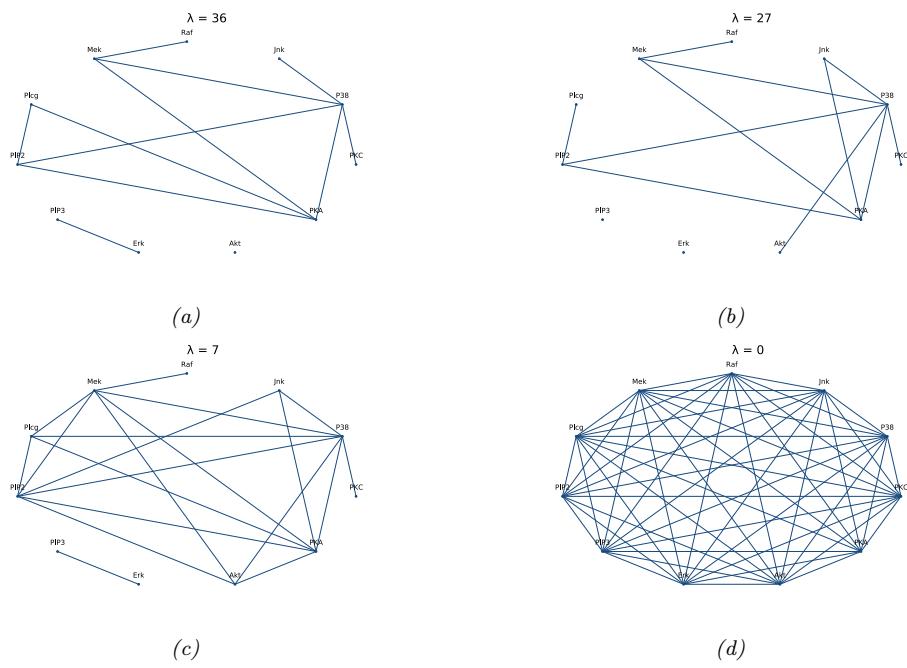
Figure 30.1: A sparse undirected Gaussian graphical model learned using graphical lasso applied to some flow cytometry data (from [Sac+05]), which measures the phosphorylation status of 11 proteins. The sparsity level is controlled by ς. (a) ς = 36. (b) ς = 27. (c) ς = 7. (d) ς = 0. Adapted from Figure 17.5 of [HTF09]. Generated by ggm\_lasso\_demo.ipynb.

as we summarize below.

Learning sparse PGMs can be useful for gaining an understanding of multiple interacting variables. For example, consider a problem that arises in systems biology: we measure the phosphorylation status of some proteins in a cell [Sac+05] and want to infer how they interact. Figure 30.1 gives an example of a graph structure that was learned from this data, using a method called graphical lasso [FHT08; MH12], which is explained in Supplementary Section 30.4.2. As another example, [Smi+06] showed that one can recover the neural “wiring diagram” of a certain kind of bird from multivariate time-series EEG data. The recovered structure closely matched the known functional connectivity of this part of the bird brain.

In some cases, we are not interested in interpreting the graph structure, we just want to use it to make predictions. One example of this is in financial portfolio management, where accurate models of the covariance between large numbers of di!erent stocks is important. [CW07] show that by learning a sparse graph, and then using this as the basis of a trading strategy, it is possible to outperform (i.e., make more money than) methods that do not exploit sparse graphs. Another example is predicting tra”c jams on the freeway. [Hor+05] describe a deployed system called JamBayes for predicting tra”c flow in the Seattle area, using a directed graphical model whose structure was learned from data.

Structure learning is also an important pre-requisite for causal inference. In particular, to predict the e!ects of interventions on a system, or to perform counterfactual reasoning, we need to know the structural causal model (SCM), as we discuss in Section 4.7. An SCM is a kind of directed graphical model where the relationships between nodes are deterministic (functional), except for stochastic root (exogeneous) variables. Consequently one can use techniques for learning DAG structures as a way to learn SCMs, if we make some assumptions about (lack of) confounders. This is called causal discovery. See Supplementary Section 30.5 in the online supplementary material for details.

31 Nonparametric Bayesian models

This chapter is written by Vinayak Rao.

31.1 Introduction

The defining characteristic of a parametric model is that the objects being modeled, whether regression or classification functions, probability densities, or something more modern like graphs or shapes, are indexed by a finite-dimensional parameter vector. For instance, neural networks have a fixed number of parameters, independent of the dataset. In a parametric Bayesian model, a prior probability distribution on these parameters is used to define a prior distribution on the objects of interest. By contrast, in a Bayesian nonparametric (BNP) model (also called a non-parametric Bayesian model) we directly place prior distributions on the objects of interest, such as functions, graphs, probability distributions, etc. This is usually done via some kind of stochastic process, which is a probability distribution over a potentially infinite set of random variables.

One example is a Gaussian process. As explained in Chapter 18, this defines a probability distribution over an unknown function f : X ↔︎ R, such that the joint distribution of f(X) = (f(x1),…,f(x^N )) is jointly Gaussian for any finite set of values ^{X =} {x^{n →} X }^{N n}=1 i.e., p(f(X)) = N (f(X)|µ(X), K(X)) where µ(X)=[µ(x1),…,µ(x^N )] is the mean, K(X)=[K(xi), K(x^j )] is the N ↗ N Gram matrix, and K is a positive definite kernel function. The complexity of the posterior over functions can grow with the amount of data, avoiding underfitting, since we maintain a full posterior distribution over the infinite set of unknown “parameters” (i.e., function evaluations at all points x → X ). But by taking a Bayesian approach, we avoid overfitting this infinitely flexible model. Despite involving infinite-parameter objects, practitioners are often only interested in inferences on a finite training dataset and predictions on a finite test dataset. This often allows these models to be surprisingly tractable. We can also define probability distributions over probability distributions, as well as other kinds of objects.

We discuss these topics in more detail in Supplementary Chapter 31. For even more information, see e.g., [Hjo+10; GV17].

32 Representation learning

This chapter is written by Ben Poole and Simon Kornblith.

32.1 Introduction

Representation learning is a paradigm for training machine learning models to transform raw inputs into a form that makes it easier to solve new tasks. Unlike supervised learning, where the task is known at training time, representation learning often assumes that we do not know what task we wish to solve ahead of time. Without this knowledge, are there transformations of the input we can learn that are useful for a variety of tasks we might care about?

One point of evidence that representation learning is possible comes from us. Humans can rapidly form rich representations of new classes [LST15] that can support diverse behaviors: finding more instances of that class, decomposing that instance into parts, and generating new instances from that class. However, it is hard to directly specify what representations we would like our machine learning systems to learn. We may want it make it easy to solve new tasks with small amounts of data, we may want to construct novel inputs or answer questions about similarities between inputs, and we may want the representation to encode certain information while discarding other information.

In building methods for representation learning, the goal is to design a task whose solution requires learning an improved representation of the input instead of directly specifying what the representation should do. These tasks can vary greatly, from building generative models of the dataset to learning to cluster datapoints. Di!erent methods often involve di!erent assumptions on the dataset, di!erent kinds of data, and induce di!erent biases on the learned representation. In this chapter we first discuss methods for evaluating learned representations, then approaches for learning representations based on supervised learning, generative modeling, and self-supervised learning, and finally the theory behind when representation learning is possible.

32.2 Evaluating and comparing learned representations

How can we make sense of representations learned by di!erent neural networks, or of the di!erences between representations learned in di!erent layers of the same network? Although it is tempting to imagine representations of neural networks as points in a space, this space is high-dimensional. In order to determine the quality of representations and how di!erent representations di!er, we need ways to summarize these high-dimensional representations or their relationships with a few

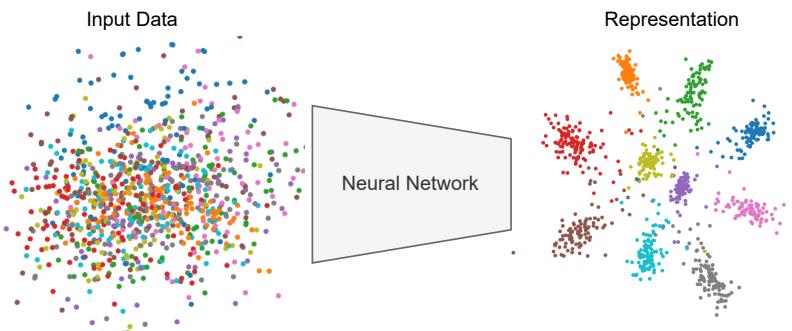
Figure 32.1: Representation learning transforms input data (left) where data from di!erent classes (color) are mixed together to a representation (right) where attributes like class are more easily distinguished. Generated by vib\_demo.ipynb.

relevant scalars. Doing so requires making assumptions about what structure in the representations is important.

32.2.1 Downstream performance

The most common way to evaluate the quality of a representation is to adapt it to one or more downstream tasks thought to be representative of real-world scenarios. In principle, one could choose any strategy to adapt the representation, but a small number of adaptation strategies dominate the literature. We discuss these strategies below.

Clearly, downstream performance can only di!er from pretraining performance if the downstream task is di!erent from the pretraining task. Downstream tasks can di!er from the pretraining task in their input distributions, target distributions, or both. The downstream tasks used to evaluate unsupervised or self-supervised representation learning often involve the same distribution of inputs as the pretraining task, but require predicting targets that were not provided during pretraining. For example, in self-supervised visual representation learning, representations learned on the ImageNet dataset without using the accompanying labels are evaluated on ImageNet using labels, either by performing linear evaluation with all the data or by fine-tuning using subsets of the data. By contrast, in transfer learning (Section 19.5.1), the input distribution of the downstream task di!ers from the distribution of the pretraining task. For example, we might pretrain the representation on a large variety of natural images and then ask how the representation performs at distinguishing di!erent species of birds not seen during pretraining.

32.2.1.1 Linear classifiers and linear evaluation

Linear evaluation treats the trained neural network as a fixed feature extractor and trains a linear classifier on top of fixed features extracted from a chosen network layer. In earlier work, this linear classifier was often a support vector machine [Don+14; SR+14; Cha+14], but in more recent work, it is typically an L²-regularized multinomial logistic regression classifier [ZIE17; KSL19; KZB19]. The process of training this classifier is equivalent to attaching a new layer to the chosen

representation layer and training only this new layer, with the rest of the network’s weights frozen and any normalization/regularization layers set to “inference mode” (see Figure 32.2).

Although linear classifiers are conceptually simple compared to deep neural networks, they are not necessarily simple to train. Unlike deep neural network training, objectives associated with commonly-used linear classifiers are convex and thus it is possible to find global minima, but it can be challenging to do so with stochastic gradient methods. When using SGD, it is important to tune both the learning rate schedule and weight decay. Even with careful tuning, SGD may still require substantially more epochs to converge when training the classifier than when training the original neural network [KZB19]. Nonetheless, linear evaluation with SGD remains a commonly used approach in the representation learning literature.

When it is possible to maintain all features in memory simultaneously, it is possible to use full-batch optimization method with line search such as L-BFGS in place of SGD [KSL19; Rad+21]. These optimization methods ensure that the loss decreases at every iteration of training, and thus do not require manual tuning of learning rates. To obtain maximal accuracy, it is still important to tune the amount of regularization, but this can be done e”ciently by sweeping this hyperparameter and using the optimal weights for the previous value of the hyperparameter as a warm start. Using a full-batch optimizer typically implies precomputing the features before performing the optimization, rather than recomputing features on each minibatch. Precomputing features can save a substantial amount of computation, since the forwards passes through the frozen model are typically much more expensive than computing the gradient of the linear classifier. However, precomputing features also limits the number of augmentations of each example that can be considered.

It is important to keep in mind that the accuracy obtainable by training a linear classifier on a finite dataset is only a lower bound on the accuracy of the Bayes-optimal linear classifier. The datasets used for linear evaluation are often small relative to the number of parameters to be trained, and the classifier typically needs to be regularized to obtain maximal accuracy. Thus, linear evaluation accuracy depends not only on whether it is possible to linearly separate di!erent classes in the representation, but also on how much data is required to find a good decision boundary with a given training objective and regularizer. In practice, even an invertible linear transformation of a representation can a!ect linear evaluation accuracy.

32.2.1.2 Fine-tuning

It is also possible to adapt all layers from the pretraining task to the downstream task. This process is typically referred to as fine-tuning [HS06b; Gir+14]. In its simplest form, fine-tuning, like linear evaluation, involves attaching a new layer to a chosen representation layer, but unlike linear evaluation, all network parameters, and not simply those of the new layer, are updated according to gradients computed on the downstream task. The new layer may be initialized with zeros or using the solution obtained by training it with all other parameters frozen. Typically, the best results are obtained when the network is fine-tuned at a lower learning rate than was used for pretraining.

Fine-tuning is substantially more expensive than training a linear classifier on top of fixed feature representations, since each training step requires backpropagating through multiple layers. However, fine-tuned networks typically outperform linear classifiers, especially when the pretraining and downstream tasks are very di!erent [KSL19; AGM14; Cha+14; Azi+15]. Linear classifiers perform better only when the number of training examples is very small (~5 per class) [KSL19].

Fine-tuning can also involve adding several new network layers. For detection and segmentation

tasks, which require fine-grained knowledge of spatial position, it is common to add a feature pyramid network (FPN) [Lin+17b] that incorporates information from di!erent feature maps in the pretrained network. Alternatively, new layers can be interspersed between old layers and initialized to preserve the network’s output. Net2Net [CGS15] follows this approach to construct a higher-capacity network that makes use of representations contained in the pretrained weights of a smaller network, whereas adapter modules [Hou+19] incorporate new, parameter-e”cient modules into a pretrained network and freeze the old ones to reduce the number of parameters that need to be stored when adapting models to di!erent tasks.

32.2.1.3 Disentanglement

Given knowledge about how a dataset was generated, for example that there are certain factors of variation such as position, shape, and color that generated the data, we often wish to estimate how well we can recover those factors in our learned representation. This requires using disentangled representation learning methods (see Section 21.3.1.1). While there are a variety of metrics for disentanglement, most measure to what extent there is a one-to-one correspondence between latent factors and dimensions of the learned representation.

32.2.2 Representational similarity

Rather than measure compatibility between a representation and a downstream task, we might seek to directly examine relationships between two fixed representations without reference to a task. In this section, we assume that we have two sets of fixed representations corresponding to the same n examples. These representations could be extracted from di!erent layers of the same network or layers of di!erent neural networks, and need not have the same dimensionality. For notational convenience, we assume that each set of representations has been stacked row-wise to form matrices ^{X → Rn}⇐p¹ and ^{Y → Rn}⇐p² such that ^Xi,: and ^Yi,: are two di!erent representations of the same example.

32.2.2.1 Representational similarity analysis and centered kernel alignment

Representational similarity analysis (RSA) is the dominant technique for measuring similarity of representations in neuroscience [KMB08], but has also been applied in machine learning. RSA reduces the problem of measuring similarity between representation matrices to measuring the similarities between representations of individual examples. RSA begins by forming representational similarity matrices (RSMs) from each representation. Given functions k : X ↗ X ℜ↔︎ R and k^→ : Y ↗ Y ℜ↔︎ R that measure the similarity between pairs of representations of individual examples ^x, ^{x→ → X} , and ^y, ^{y→ → Y}, the corresponding representational similarity matrices ^K, ^{K→ → Rn}⇐ⁿ contain the similarities between the representations of all pairs of examples Kij = k(Xi,:, Xj,:) and K^→ ij = k^→ (Yi,:,Yj,:). These representational similarity matrices are transformed into a scalar similarity value by applying a matrix similarity function s(K, K^→ ).

The RSA framework can encompass many di!erent forms of similarity through the selection of the similarity functions k(·, ·), k^→ (·, ·), and s(·, ·). How these functions should be selected is a contentious topic [BS+20; Kri19]. In practice, it is common to choose k(x, x^→ ) = k^→ (x, x^→ ) = corr[x, x^→ ], the Pearson correlation coe”cient between examples. s(·, ·) is often chosen to be the Spearman rank correlation between the representational similarity matrices, which is computed by reshaping K and

K^→ to vectors, computing the rankings of their elements, and measuring the Pearson correlation between these rankings.

Centered kernel alignment (CKA) is a technique that was first proposed in machine learning literature [Cri+02; CMR12] but that can be interpreted as a form of RSA. In centered kernel alignment, the per-example similarity functions k and k^→ are chosen to be positive semi-definite kernels so that K and K^→ are kernel matrices. The matrix similarity function s is the cosine similarity between centered kernel matrices

\[s(K, K') = \frac{\langle HKH, HK'H \rangle\_{\mathcal{F}}}{\|HKH\|\_{\mathcal{F}} \|HK'H\|\_{\mathcal{F}}},\tag{32.1}\]

where ^ℑA, ^B⊤^{F =} vec(A)⇓vec(B) = tr(A⇓B) is the Frobenius product, and ^{H = I ↓ 1 n} 11⇓ is the centering matrix. As it is applied above, the centering matrix subtracts the means from the rows and columns of the similarity index.

A special case of centered kernel alignment arises when k and k^→ are chosen to be the linear kernel k(x, x^→ ) = k^→ (x, x^→ ) = x⇓x^→ . In this case, K = XX⇓ and K^→ = Y Y ⇓, allowing for an alternative expression for CKA in terms of the similarities between pairs of features rather than pairs of examples. The representations themselves must first be centered by subtracting the means from their columns, yielding X˜ = HX and Y˜ = HY . Then, so-called linear centered kernel alignment is given by

\[s(K, K') = \frac{\langle \hat{X}\hat{X}^\top, \hat{Y}\hat{Y}^\top \rangle\_\mathcal{F}}{\|\hat{X}\hat{X}^\top\|\_\mathcal{F} \|\hat{Y}\hat{Y}^\top\|\_\mathcal{F}} = \frac{\|\hat{X}^\top\hat{Y}\|\_\mathcal{F}^2}{\|\hat{X}^\top\hat{X}\|\_\mathcal{F} \|\hat{Y}^\top\hat{Y}\|\_\mathcal{F}}.\tag{32.2}\]

Linear centered kernel alignment is equivalent to the RV coe”cient [RE76] between centered features, as shown in [Kor+19].

32.2.2.2 Canonical correlation analysis and related methods

Given two datasets (in this case, the representation matrices X and Y ), canonical correlation analysis or CCA (Section 28.3.4.3) seeks to map both datasets to a shared latent space such that they are maximally correlated in this space. The i th pair of canonical weights (wi, w^{→ i}) maximize the correlation between the corresponding canonical vectors 5ⁱ = corr[Xwi,Y w^{→ i}] subject to the constraint that the new canonical vectors are orthogonal to previous canonical vectors,

\[\begin{aligned} \text{maximize } & \text{corr}[\mathbf{X}\,\mathbf{w}\_i, \mathbf{Y}\,\mathbf{w}\_i']\\ \text{subject to} & \quad \forall\_{j\]

The maximum number of non-zero canonical correlations is the minimum of the ranks, p = min(rk(X),rk(Y )).

The standard algorithm for computing the canonical weights and correlations [BG73] first decomposes the individual representations as the product of an orthogonal matrix and a second matrix, X˜ = QR : Q⇓Q = I and Y˜ = Q^→ R^→ : Q→⇓Q^→ = I. These decompositions can be obtained either by QR factorization or singular value decomposition. A second singular value decomposition of Q⇓Q^→ = U”V ⇓ provides the quantities needed to determine the canonical weights and correlations. Specifically, the canonical correlations are the singular values ▷ = diag(“); the canonical vectors are the columns of XW = QU and Y W^→ = Q^→ V ; and the canonical weights are W = R↑1U and W^→ = R→↑1V .

Two common strategies to turn the resulting vector of canonical correlations into a scalar are to take the mean squared canonical correlation,

\[R\_{\rm CCA}^2(\mathbf{X}, \mathbf{Y}) = \|\boldsymbol{\rho}\|\_2^2 / p = \|\mathbf{Q}^\top \mathbf{Q}^\prime\|\_\mathbb{F}^2 / p,\tag{32.4}\]

or the mean canonical correlation,

\[\bar{\rho} = \sum\_{i=1}^{p} \rho\_i / p = ||\mathbf{Q}^\top \mathbf{Q}^\prime||\_\* / p,\tag{32.5}\]

where ⇐ · ⇐^↔︎ denotes the nuclear norm. The mean squared canonical correlation has several alternative names, including Yanai’s GCD [Yan74; RBS84], Pillai’s trace, or the eigenspace overlap score [May+19].

Although CCA is a powerful tool, it su!ers from the curse of dimensionality. If at least one representation has more neurons than examples and each neuron is linearly independent of the others, then all canonical correlations are 1. In practice, because neural network representations are high-dimensional, we can find ourselves in the regime where there are not enough data to accurately estimate the canonical correlations. Moreover, even when we can accurately estimate the canonical correlations, it may be desirable for a similarity measure to place less emphasis on the similarity of low-variance directions.

Singular vector CCA (SVCCA) mitigates these problems by retaining only the largest principal components of X˜ and Y˜ when performing CCA. Given the singular value decomposition of the representations X˜ = U”V ⇓ and Y˜ = U^→ “^→ V →⇓, SVCCA retains only the first k columns of U corresponding to the largest k singular values of ϱ = diag(”) (i.e., the k largest principal components) and the first k^→ columns of U^→ corresponding to the largest k^→ singular values ϱ^→ = diag(“^→ ). With these singular value decompositions, the canonical correlations, vectors, and weights can then be computed using the algorithm of Björck and Golub [BG73] described above, by setting

\[\mathbf{Q} = \mathbf{U}\_{:,1:k}, \qquad \mathbf{R} = \Sigma\_{1:k,1:k} \mathbf{V}\_{:,1:k}^{\top}, \qquad \mathbf{Q}' = \mathbf{U}\_{:,1:k}', \qquad \mathbf{R}' = \Sigma\_{1:k,1:k}' \mathbf{V}\_{:,1:k}^{\top}.\tag{32.6}\]

Raghu et al. [Rag+17] suggest retaining enough components to explain 99% of the variance, i.e., setting ^k to the minimum value such that ⇐ϱ1:k⇐²/⇐ϱ⇐² = 0.99 and ^k→ to the minimum value such that ⇐ϱ^→ 1:k↑⇐²/⇐ϱ^→ ⇐² = 0.99. However, for a fixed value of min(k, k^→ ), CCA-based similarity measures increase with the value of max(k, k^→ ). Representations that require more components to explain 99% of the variance of representations may thus appear “more similar” to all other representations than representations with more rapidly decaying singular value spectra. In practice, it is often better to set k and k^→ to the same fixed value.

Projection-weighted CCA (PWCCA) [MRB18] instead weighs the correlations by a measure of the variability in the original representation that they explain. The resulting similarity measure is

\[\text{PWCCA}(\mathbf{X}, \mathbf{Y}) = \frac{\sum\_{i=1}^{p} \alpha\_{i} \rho\_{i}}{\sum\_{i=1}^{p} \alpha\_{i}}, \tag{2.7} \\ \tag{32.7} \\ \tag{32.7} \\ \tag{32.7}\]

PWCCA enjoys somewhat widespread use in representational similarity literature, but it has potentially undesirable properties. First, it is asymmetric; its value depends on which of the two representations is used for the weighting. Second, it is unclear why weightings should be determined using the L¹ norm, which is not invariant to rotations of the representation. It is arguably more intuitive to weight the correlations directly by the amount of variance in the representation that the canonical component explains, which corresponds to replacing the L¹ norm with the squared L² norm. The resulting similarity measure is

\[R\_{\rm LR}^2(\mathbf{X}, \mathbf{Y}) = \frac{\sum\_{i=1}^p \alpha\_i' \rho\_i^2}{\sum\_{i=1}^p \alpha\_i'}, \tag{2.8} = \sum\_{j=1}^{p\_2} \|(\mathbf{Y} \,\mathbf{w}\_i')^\top \mathbf{Y}\|\_2^2. \tag{32.8}\]

As shown by Kornblith et al. [Kor+19], when p² ⇒ p1, this alternative similarity measure is equivalent to the overall variance explained by using linear regression to fit every neuron in Y˜ using the representation X˜ ,

\[R\_{\rm LR}^2(X,Y) = 1 - \sum\_{i=1}^{p\_2} \min\_{\beta} \| |\bar{Y}\_{:,i} - \bar{X}\beta\|^2 / \|\bar{Y}\|\_{\rm F}^2. \tag{32.9}\]

Finally, there is also a close relationship between CCA and linear CKA. This relationship can be clarified by writing similarity indexes directly in terms of the singular value decompositions X˜ = U”V ⇓ and Y˜ = U^→ “^→ V →⇓. The left-singular vectors uⁱ = U:,i correspond to the principal components of X normalized to unit length, and the squared singular values ωⁱ = $² ii are the amount of variance that those principal components explain (up to a factor of 1/n). Given these singular value decompositions, R² CCA, R² LR, and linear CKA become:

\[R\_{\rm CCA}^2(\mathbf{X}, \mathbf{Y}) = \sum\_{i=1}^{p\_1} \sum\_{j=1}^{p\_2} \left( \mathbf{u}\_i^\top \mathbf{u}\_j' \right)^2 / p\_1 \tag{32.10}\]

\[R\_{\rm LR}^2(X,Y) = \sum\_{i=1}^{p\_2} \sum\_{j=1}^{p\_2} \lambda\_j' \left(\mathbf{u}\_i^\top \mathbf{u}\_j'\right)^2 / \sum\_{j=1}^{p\_2} \lambda\_j' \tag{32.11}\]

\[\text{CKA}\_{\text{linear}}(\mathbf{X}, \mathbf{Y}) = \frac{\sum\_{i=1}^{p\_1} \sum\_{j=1}^{p\_2} \lambda\_i \lambda\_j' \left(\mathbf{u}\_i^\top \mathbf{u}\_j'\right)^2}{\sqrt{\sum\_{i=1}^{p\_1} \lambda\_i^2} \sqrt{\sum\_{j=1}^{p\_2} \lambda\_j'^2}}. \tag{32.12}\]

Thus, these similarity indexes all involve the similarities between all pairs of principal components from X and Y , but place di!erent weightings on these similarities according to the fraction of variance that these principal components explain.

32.2.2.3 Comparing representational similarity measures

What properties are desirable in a representational similarity measure is an open question, and this question may not have a unique answer. Whereas evaluations of downstream accuracy approximate real-world use cases for neural network representations, the goal of representational similarity is instead to develop understanding of how representations evolve across neural networks, or how they di!er between neural networks with di!erent architectures or training settings.

One way to taxonomize di!erent similarity measures is through the transformations of a representation that they are invariant to. The minimum form of invariance is invariance to permutation of a representation’s constituent neurons, which is needed because neurons in neural networks generally have no canonical ordering: for commonly-used initialization strategies, any permutation of a given initialization is equiprobable, and nearly all architectures and optimizers produce training trajectories that are equivariant under permutation. On the other hand, invariance to arbitrary invertible transformations, as provided by mutual information, is clearly undesirable, since many realistic neural networks are injective functions of the input [Gol+19] and thus there always exists an invertible transformation between any pair of representations. In practice, most similarity measures in common use are invariant to rotations (orthogonal transformations) of representations, which implies invariance to permutation. Similarity measures based solely on CCA correlations, such as R² CCA and 5¯, are invariant to all invertible linear transformations of representations. However, SVCCA and PWCCA are not.

A di!erent way to distinguish similarity measures is to investigate situations where we know the relationships among representations and to empirically evaluate their ability to recover these relationships. Kornblith et al. [Kor+19] propose a simple “sanity check”: Given two architecturally identical networks A and B trained from di!erent random initializations, any layer in network A should be more similar to the architecturally corresponding layer in network B than to any other layer. They show that, when considering flattened representations of CNNs, similarity measures based on centered kernel alignment satisfy this sanity check whereas other similarity measures do not. By contrast, when considering representations of individual tokens in Transformers, all similarity measures perform reasonably well. However, Maheswaranathan et al. [Mah+19] show that both CCA and linear CKA are highly sensitive to seemingly innocuous RNN design choices such as the activation function, even though analysis of the fixed points of the dynamics of di!erent networks suggests they all operate similarly.

32.3 Approaches for learning representations

The goal of representation learning is to learn a transformation of the inputs that makes it easier to solve future tasks. Typically the tasks we want the representation to be useful for are not known when learning the representation, so we cannot directly train to improve performance on the task. Learning such generic representations requires collecting large-scale unlabeled or weakly-labeled datasets, and identifying tasks or priors for the representations that one can solve without direct access to the downstream tasks. Most methods focus on learning a parametric mapping z = f⇀(x) that takes an input x and transforms it into a representation z using a neural network with parameters 1.

The main challenge in representation learning is coming up with a task that requires learning a good representation to solve. If the task is too easy, then it can be solved without learning an interesting transformation of the inputs, or by learning a shortcut. If a task is too di!erent from the downstream task that the representation will be evaluated on, then the representation may also not be useful. For example, if the downstream task is object detection, then the representation needs to encode both the identity and location of objects in the image. However, if we only care about classification, then the representation can discard information about position. This leads to approaches for learning representations that are often not generic: di!erent training tasks may perform better for di!erent downstream tasks.

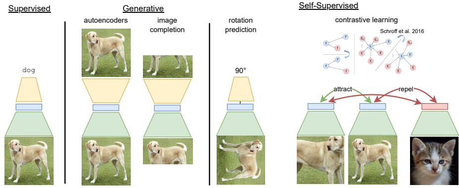
Figure 32.2: Approaches for representation learning from images. An input image is encoded through a deep neural network (green) to produce a representation (blue). An additional shallow or deep neural network (yellow) is often used to train the representation, but is thrown out after the representation is learned when solving downstream tasks. In the supervised case, the mapping from the representation to logits is typically linear, while for autoencoders the mapping from representation to images can be highly complex and stochastic. Unlike supervised or generative approaches, contrastive methods rely on other datapoints in the form of positive pairs (often created through data augmentation) and negative pairs (typically other datapoints) to learn a representation.

In Figue 32.2, we outline three approaches we will discuss for representation learning. Supervised approaches train on large-scale supervised or weakly-supervised data using standard supervised losses. Generative approaches aim to learn generative models of the dataset or parts of a dataset. Self-supervised approaches are based on transformation prediction or multi-view learning, where we design a task that where labels can be easily synthesized without needing human input.

32.3.1 Supervised representation learning and transfer

The first major successes in visual representation learning with deep learning came from networks trained on large labeled datasets. Following the discovery that supervised deep neural networks could outperform classical computer vision models for natural image classification [KSH12b; CMS12], it became clear that the representations learned by these networks could outperform handcrafted features used across a wide variety of tasks [Don+14; SR+14; Oqu+14; Gir+14]. Although unsupervised visual representation learning has recently achieved competitive results on many domains, supervised representation learning remains the dominant approach.

Larger networks trained on larger datasets generally achieve better performance on both pretraining and downstream tasks. When other design choices are held fixed, architectures that achieve higher accuracy during pretraining on natural image datasets such as ImageNet also learn better representations for downstream natural image tasks, as measured by both linear evaluation and fine-tuned accuracy [KSL19; TL19; Zha+19a; Zha+21; Abn+21]. However, when the domain shift from the pretraining task to the downstream task becomes larger (e.g., from ImageNet to medical imaging), the correlation between pretraining and downstream accuracy can be much lower [Rag+19; Ke+21; Abn+21]. Studies that vary pretraining dataset size generally find that larger pretraining datasets yield better representations for downstream tasks [HAE16; Mah+18; Kol+20; Zha+21; Abn+21], although there is an interaction between model size and dataset. When training small models with the intention of transferring to a specific downstream task, it is sometimes preferable to pretrain on a smaller dataset that is more closely related to that task rather than a larger dataset that is less closely related [Cui+18; Mah+18; Ngi+18; Kol+20], but larger models seem to derive greater benefit from larger, more diverse datasets [Mah+18; Kol+20].

Whereas scaling the architecture and dataset size generally improves both pretraining and downstream accuracy, other design choices can improve pretraining accuracy at the expense of transfer, or vice versa. Regularizers such as penultimate layer dropout and label smoothing improve accuracy on pretraining tasks but produce worse representations for downstream tasks [KSL19; Kor+21]. Although most convolutional neural networks are trained with batch normalization, Kolesnikov et al. [Kol+20] find that the combination of group normalization and weight standardization leads to networks that perform similarly on pretraining tasks but substantially better on transfer tasks. Adversarial training produces networks that perform worse on pretraining tasks as compared to standard training, but these representations transfer better to other tasks [Sal+20]. For certain combinations of pretraining and downstream datasets, increasing the amount of weight decay on the network’s final layer can improve transferability at the cost of pretraining accuracy [Zha+21; Abn+21].

The challenge of collecting ever-larger pretraining datasets has led to the emergence of weaklysupervised representation learning, which eschews the expensive human annotations of datasets such as ImageNet and instead relies on data that can be readily collected from the Internet, but which may have greater label noise. Supervision sources include hashtags accompanying images on websites such as Instagram and Flickr [CG15; Iza+15; Jou+16; Mah+18], image labels obtained automatically using proprietary algorithms involving user feedback signals [Sun+17; Kol+20], or image captions/alt text [Li+17a; SPL20; DJ21; Rad+21; Jia+21]. Hashtags and automatic labeling give rise to image classification problems that closely resemble their more strongly supervised counterparts. The primary di!erence versus standard supervised representation learning is that the data are noisier, but in practice, the benefits of more data often outweigh the detrimental e!ects of the noise.

Image-text supervision has provided more fertile ground for innovation, as there are many di!erent ways of jointly processing text and images. The simplest approach is again to convert the data into an image classification problem, where the network is trained to predict which words or n-grams appear in the text accompanying a given image [Li+17a]. More sophisticated approaches train image-conditional language models [DJ21] or masked language models [SPL20], which can make better use of the structure of the text. Recently, there has been a surge in interest in contrastive image/text pretraining models such as CLIP [Rad+21] and ALIGN [Jia+21], details of which we discuss in Section 32.3.4. These models process images and text independently using two separate “towers”, and learn an embedding space where embeddings of images lie close to the embeddings of the corresponding text. As shown by Radford et al. [Rad+21], contrastive image/text pretraining learns high-quality representations faster than alternative approaches.

Beyond simply learning good visual representations, pretrained models that embed image and text in a common space enable zero-shot transfer of learned representations. In zero-shot transfer, an image classifier is constructed using only textual descriptions of the classes of interest, without any images from the downstream task. Early co-embedding models relied on pretrained image models and word embeddings that were then adapted to a common space [Fro+13], but contrastive image/text pretraining provides a means to learn co-embedding models end-to-end. Compared to linear classifiers trained using image embeddings, zero-shot classifiers typically perform worse, but zero-shot classifiers are far more robust to distribution shift [Rad+21].

32.3.2 Generative representation learning

Supervised representation learning often fails to learn representations for tasks that di!er significantly from the task the representation was trained on. How can we learn representations when the task we wish to solve di!ers a lot from tasks where we have large labeled datasets?

Generative representation learning aims to model the entire distribution of a dataset q(x) with a parametric model p⇀(x). The hope of generative representation learning is that, if we can build models that can create all the data that we have seen, then we implicitly may learn a representation that can be used to answer any question about the data, not just the questions that are related to a supervised task for which we have labels. For example, in the case of digit classification, it is hard to collect labels for the style of a handwritten digit, but if the model has to produce all possible handwritten digits in our dataset it needs to learn to produce digits with di!erent styles. On the other hand, supervised learning to classify digits aims to learn a representation that is invariant to style.

There are two main approaches for learning representations with generative models: (1) latentvariable models that aim to capture the underlying factors of variation in data with latent variables z that act as the representation (see the chapter on VAEs, Chapter 21), and (2) fully-observed models where a neural architecture is trained with a tractable generative objective (see the chapters on AR models, Chapter 22, and flow models, Chapter 23), and then a representation is extracted from the learned architecture.

32.3.2.1 Latent-variable models

One criterion for learning a good representation of the world is that it is useful for synthesizing observed data. If we can build a model that can create new observations, and has a simple set of latent variables, then hopefully this model will learn variables that are related to the underlying physical process that created the observations. For example, if we are trying to model a dataset of 2d images of shapes, knowing the position, size, and type of the shape would enable easy synthesis of the image. This approach to learning is known as analysis-by-synthesis, and is a theory of perception that aims at identifying a set of underlying latent factors (analysis) that could be used to synthesize observations [Rob63; Bau74; LM03]. Our goal is to learn a generative model p⇀(x, z) over the observations x and latents z, with parameters 1. Given an observation x, performing the analysis step to extract a representation requires running inference to sample or compute the posterior mean of p⇀(z|x). Di!erent choices for the model p⇀(x, z) and inference procedure for p⇀(z|x) represent di!erent ways of learning representations from a dataset.

Early work on deep latent-variable generative models aimed to learn stacks of features often based on training simple energy-based models or directed sparse coding models, each of which could explain the previous set of latent factors, and which learned increasingly abstract representation [HOT06b; Lee+09; Ran+06]. Bengio, Courville, and Vincent [BCV13] provide an overview of several methods based on stacking latent-variable generative modeling approaches to learn increasingly abstract representation. However greedy approaches to generative representation learning have failed to scale

to larger natural datasets.

If the generative process that created the data is simple and can be described, then encoding that structure into a generative model is a tremendously powerful way of learning useful and robust representations. Lake, Salakhutdinov, and Tenenbaum [LST15] and George et al. [Geo+17] use knowledge of how characters are composed of strokes to build hierarchical generative models with representations that excel at several downstream tasks. However, for many real-world datasets the generative structure is not known, and the generative model must also be learned. There is often a tradeo! between imposing structure in the generative process (such as sparsity) vs. learning that structure from data.

Directed latent-variable generative models have proven easier to train and scale to natural datasets. Variational autoencoders (Chapter 21) train a directed latent-variable generative model with variational inference, and learn a prior p⇀(z), decoder p⇀(x|z), and an amortized inference network qω(z|x) that can be used to extract a representation on new datapoints. Higgins et al. [Hig+17b] show ε-VAEs (Section 21.3.1) are capable of learning latent variables that correspond to factors of variation on simple synthetic datasets. Kingma et al. [Kin+14b] and Rasmus et al. [Ras+15] demonstrate improved performance on semi-supervised learning with VAEs. While there have been several recent advances to scale up VAEs to natural datasets [VK20b; Chi21b], none of these methods have yet led to representations that are competitive for downstream tasks such as classification or segmentation.

Adversarial methods for training directed latent-variable models have also proven useful for representation learning. In particular, GANs (Chapter 26) trained with encoders such as BiGAN [DKD17], ALI [Dum+17], and [Che+16] were able to learn representations on small scale datasets that performed well at object classification. The discriminators from GANs have also proven useful for learning representations [RMC16b]. More recently, these methods were scaled up to ImageNet in BigBiGAN [DS19], with learned representations that performed strongly on classification and segmentation tasks.

32.3.2.2 Fully observed models

The neural network architectures used in fully observed generative models can also learn useful representations without the presence of latent-variables. ImageGPT [Che+20a] demonstrate that an autoregressive model trained on pixels can learn internal representations that excel at image classification. Unlike with latent-variable models where the representation is often thought of as the latent variables, ImageGPT extracted representations from the deterministic layers of the transformer architecture used to compute future tokens. Similar approaches have shown progress for learning features in language modeling [Raf+20b], however alternative objectives, based on masked training (as in BERT, [Dev+19]), often leads to better performance.

32.3.2.3 Autoencoders

A related set of methods for representation learning are based on learning a representation from which the original data can be reconstructed. These methods are often called autoencoders (see Section 16.3.3), as the data is encoded in a way such that the input data itself can be recreated. However, unlike generative models, they cannot typically be used to synthesize observations from scratch or assign likelihoods to observations. Autoencoders learn an encoder that outputs a representation z = f⇀(x), and a decoder gω(z) that takes the representation z and tries to recreate the

input data, x. The quality of the approximate reconstruction , xˆ = gω(z) is often measured using a domain-specific loss, for example mean-squared error for images:

\[\mathcal{L}(\theta, \phi) = \frac{1}{|\mathcal{D}|} \sum\_{x \in \mathcal{D}} \|x - g\_{\phi}(f\_{\theta}(x))\|\_{2}^{2}. \tag{32.13}\]

If there are no constraints on the encoder or decoder, and the dimensionality of the representation z matches the dimensionality of the input x, then there exists a trivial solution to minimize the autoencoding objective: set both f⇀ and g^ω to identity functions. In this case the representation has not learned anything interesting, and thus in practice an additional regularizer is often placed on the learned representation.

Reducing the dimensionality of the representation z is one e!ective mechanism to avoid trivial solutions to the autoencoding objective. If both the encoder and decoder networks are linear, and the loss is mean-squared-error, then the resulting linear autoencoder model can learn the principal components of a dataset [Pla18].

Other methods maintain higher-dimensional representations by adding sparsity (for example, penalties on ⇐z⇐¹ in Ng et al. [Ng+11]) or smoothness regularizers [Rif+11], or adding noise to the input [Vin+08] or intermediate layers of the network [Sri+14b; PSDG14]. These added regularizers aim to bias the encoder and decoder to learn representations that are not just the identity function, but instead are nonlinear transformations of the input that may be useful for downstream tasks. See Bengio, Courville, and Vincent [BCV13] for a more detailed discussion of regularized autoencoders and their applications. A recent re-evaluation of several algorithms based on iteratively learning features by stacked regularized autoencoders have been shown to degrade performance versus training end-to-end from scratch [Pai+14]. However, we will see in Section 32.3.3.1 that denoising autoencoders have shown promise for representation learning in discrete domains and when applied with more complex noise and masking patterns.

32.3.2.4 Challenges in generative representation learning

Despite several success in generative representation learning, they have empirically fallen behind. Generative methods for representation learning have to learn to match complex high-dimensional and diverse training datasets, which requires modeling all axis of variation of the inputs, regardless of whether they are semantically relevant for downstream tasks. For example, the exact pattern of blades of grass in an image matter for generation quality, but are unlikely to be useful for many of the semantic evaluations that are typically used. Ways to bias generative models to focus on the semantic features and ignore “noise” in the input is an open area of research.

32.3.3 Self-supervised representation learning

When given large amounts of labeled data, standard supervised learning is a powerful mechanism for training deep neural networks. When only presented with unlabeled data, building generative models requires modeling all variations in a dataset, and is often not explicit about what is the signal and noise that we aim to capture in a representation. The methods and architectures for building these generative models also di!ers substantially from those of supervised learning, where largely feedforward architectures are used to predict low-dimensional representations. Instead of trying to model all aspects of variation, self-supervised learning aims to design tasks where labels can be generated cheaply, and help to encode the structure of what we may care about for other downstream tasks. Self-supervised learning methods allow us to apply the tools and techniques of supervised learning to unlabeled data by designing a task for which we can cheaply produce labels.

In the image domain, several self-supervised tasks, also known as pretext tasks, have been proven e!ective for learning representations. Models are trained to perform these tasks in a supervised fashion using data generated by the pretext task, and then the learned representation is transferred to a target task of interest (such as object recognition), by training a linear classifier or fine-tuning the model in a supervised fashion.

32.3.3.1 Denoising and masked prediction

Generative representation learning is challenging because generative models must learn to produce the entire data distribution. A simpler option is denoising, in which some variety of noise is added to the input and the model is trained to reconstruct the noiseless input. A particularly successful variant of denoising is masked prediction, in which input patches or tokens are replaced with uninformative masks and the network is trained to predict only these missing patches or tokens.

The denoising autoencoder [Vin+08; Vin+10a] was the first deep model to exploit denoising for representation learning. A denoising autoencoder resembles a standard autoencoder architecturally, but it is trained to perform a di!erent task. Whereas a standard autoencoder attempts to reconstruct its input exactly, a denoising autoencoder attempts to produce a noiseless output from a noisy input. Vincent et al. [Vin+08] argue that the network must learn the structure of the data manifold in order to solve the denoising task.

Newer approaches retain the conceptual approach of the denoising autoencoder, but adjust the masking strategy and objective. BERT [Dev+18] introduced the masked language modeling task, where 15% of the input tokens are selected for masking and the network is trained to predict them. 80% of the time, these tokens are replaced with an uninformative [MASK] token. However, the [MASK] token does not appear at fine-tuning time, producing some domain shift between pretraining and fine-tuning. Thus, 10% of the time, tokens are replaced with random tokens, and 10% of the time, they are left intact. BERT and the masked language modeling task have been extremely influential for representation learning in natural language processing, inspiring substantial follow-up work [Liu+19c; Jos+20].

Although denoising-based approaches to representation learning were first employed for computer vision, they received little attention for the decade that followed. Vincent et al. [Vin+08] greedily trained stacks of up to three denoising autoencoders that were then fine-tuned end-to-end to perform digit classification, but greedy unsupervised pretraining was abandoned as it was shown that it was possible to attain good performance using CNNs and other architectures trained end-to-end. Context encoders [Pat+16] mask contiguous image regions and train models to perform inpainting, achieving transfer learning performance competitive with other contemporary unsupervised visual representation learning methods. The use of image colorization as a pretext task [ZIE16; ZIE17] is also related to denoising in that colorization involves reconstructing the original image from a corrupted input, although generally color is dropped in a deterministic fashion rather than stochastically.

Recently, the success of BERT in NLP has inspired new approaches to visual representation learning based on masked prediction. Image GPT [Che+20a] trained a transformer directly upon pixels to perform a BERT-style masked image modeling task. While the resulting model achieves very high accuracy when fine-tuned CIFAR-10, the cost of self-attention is quadratic in the number of pixels,

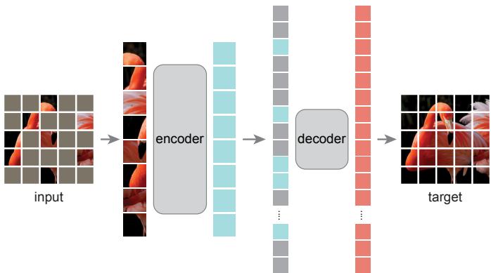
Figure 32.3: Masked autoencoders learn a representation of images by randomly masking out input patches and trying to predict them (from He et al. [He+21]).

limiting applicability to larger image sizes. BEiT [Bao+22b] addresses this challenge by combining the idea of masked image modeling with the patch-based architecture of vision transformers [Dos+21]. BEiT splits images into 16↗16 pixel image patches and then discretizes these patches using a discrete VAE [Ram+21b]. At training time, 40% of tokens are masked. The network receives continuous patches as input and is trained to predict the discretized missing tokens using a softmax over all possible tokens.

The masked autoencoder or MAE [He+22] further simplifies the masked image modeling task (see Figure 32.3). The MAE eliminates the need to discretize patches and instead predicts the constituent pixels of each patch directly using a shallow decoder trained with L² loss. Because the MAE encoder operates only on the unmasked tokens, it can be trained e”ciently even while masking most (75%) of the tokens. Models pretrained using masked prediction and then fine-tuned with labels currently hold the top positions on the ImageNet leaderboard among models trained without additional data [He+22; Don+21].

32.3.3.2 Transformation prediction

An even simpler approach to representation learning involves applying a transformation to the input image and then predicting the transformation that was applied (see Figure 32.4). This prediction task is usually formulated as a classification problem. For visual representation learning, transformation prediction is appealing because it allows reusing exactly the same training pipelines as standard supervised image classification. However, it is not clear that networks trained to perform transformation prediction tasks learn rich visual representations. Transformation prediction tasks are potentially susceptible to “shortcut” solutions, where networks learn trivial features that are nonetheless su”cient to solve the task with high accuracy. For many years, self-supervised learning methods based on transformation prediction were among the top-performing methods, but they have since been displaced by newer methods based on contrastive learning and masked prediction.

Some pretext tasks operate by cutting images into patches and training networks to recover the spatial arrangement of the patches. In context prediction [DGE15], a network receives two adjacent

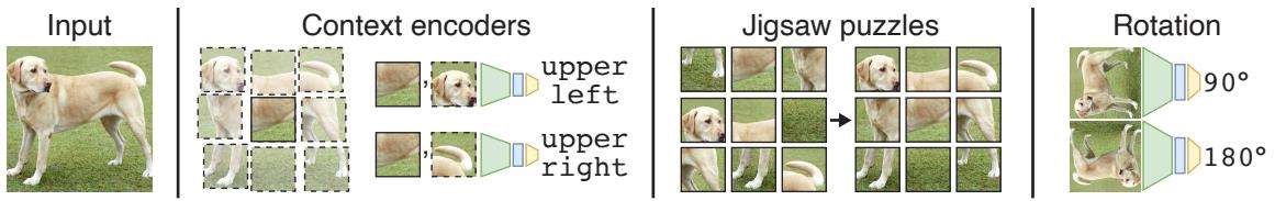
Figure 32.4: Transformation prediction involves training neural networks to predict a transformation applied to the input. Context encoders predict the position of a second crop relative to the first. The jigsaw puzzle task involves predicting the way in which patches have been permuted. Rotation prediction involves predicting the rotation that was applied to the input.

image patches as input and is trained to recover their spatial relationship by performing an eight-class classification problem. To prevent the network from directly matching the pixels at the patch borders, the two patches must be separated by a small variable gap. In addition, to prevent networks from using chromatic aberration to localize the patches relative to the lens, color channels must be distorted or stochastically dropped. Other work has trained networks to solve jigsaw puzzles by splitting images into a 3 ↗ 3 grid of patches [NF16]. The network receives shu$ed patches as input and learns to predict how they were permuted. By limiting the permutations to a subset of all possibilities, the jigsaw puzzle task can be formulated as a standard classification task [NF16].

Another widely used pretext task is rotation prediction [GSK18], where input images are rotated 0, 90, 180, or 270 degrees and networks are trained to classify which rotation was applied. Although this task is extremely simple, the learned representations often perform better than those learned using patch-based methods [GSK18; KZB19]. However, all approaches based on transformation prediction currently underperform masked prediction and multiview approaches on standard benchmark datasets such as CIFAR-10 and ImageNet.

32.3.4 Multiview representation learning

The field of multiview representation learning aims to learn a representation where “similar” inputs or views of an input are mapped nearby in the representation space, and “dissimilar” inputs are mapped further apart. This representation space is often high-dimensional, and relies on collecting data or designing a task where one can generative “positive” pairs of examples that are similar, and “negative” pairs of examples that are dissimilar. There are many motivations and objectives for multiview representation learning, but all rely on coming up with sets of positive pairs, and a mechanism to prevent all representations from collapsing to the same point. Here we use the term multiview representation learning to encompass contrastive learning which combines positive and negative pairs, metric learning, and “non-contrastive” learning which eliminates the need for negative pairs.

Unlike generative methods for representation learning, multiview representation learning makes it easy to incorporate prior knowledge about what inputs should be closer in the embedding space. Furthermore, these inputs need not be from the same modality, and thus multiview representation learning can be applied with rich multimodal datasets. The simplicity of the way in which prior knowledge can be incorporated into a model through data has made multiview representation learning one of the most powerful and performant methods for learning representations.

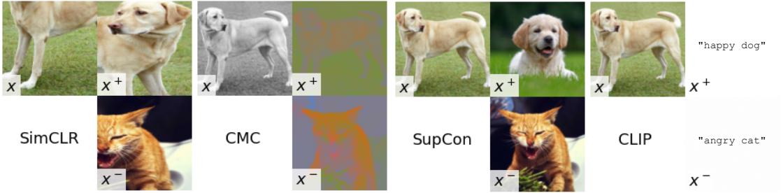
Figure 32.5: Positive and negative pairs used by di!erent multiview representation learning methods.

While there are a variety of methods for multiview representation learning, they all involve a repulsion component that pulls positive pairs closer together in embedding space, and a mechanism to prevent collapse of the representation to a single point in embedding space. We begin by describing loss functions for multiview representation learning and how they combine attractive and repulsive terms to shape the representation, then discuss the role of view generation, and finally practical considerations in deploying multiview representation learning.

32.3.4.1 View selection

Multiview representation learning depends on a datapoint or “anchor” x, a positive example x⁺ that x will be attracted to, and zero or more negative examples x^↑ that x is repelled from. We assume access to a data-generating process for the positive pair: p⁺(x, x⁺), and a process that generates the negative examples given the datapoint ^x: ^p↑(x^↑|x). Typically ^p+(x, x⁺) generate (x, x⁺) that are di!erent augmentations of an underlying image from the dataset, and x^↑ represents an augmented view of a di!erent random image from the dataset. The generative process for x^↑ is then independent of x, i.e., p↑(x^↑|x) = p↑(x↑).

The choice of views used to generate positive and negative pairs is critical to the success of representation learning. Figure 32.5 shows the positive pair (x, x⁺) and negative x^↑ for several methods which we discuss below: SimCLR, CMC, SupCon, and CLIP.

SimCLR [Che+20c] creates positive pairs by applying two di!erent data augmentations defined by transformations t and t ^→ to an initial image x⁰ twice: x = t(x0), x⁺ = t → (x0). The data augmentations used are random crops (with horizontal flips and resize), color distortion, and Gaussian blur. The strengths of these augmentations (e.g., the amount of blur) impact performance and are typically treated as a hyperparameter.

If we access to additional information, such as a categorical label, we can use this to select positive pairs with the same label, and negative pairs with di!erent labels. The resulting objective, when used with a contrastive loss, is called SupCon [Kho+20], and resembles neighborhood component analysis [Gol+04]. It was shown to improve robustness when compared to standard supervised learning.

Contrastive multiview coding (CMC) [TKI20] generates views by splitting an initial image into orthogonal dimensions, such as the luma and chroma dimensions. These views are now no longer in the same space (or same dimensionality), and thus we must learn di!erent encoders for the di!erent inputs. However, the output of these encoders all live in the same-dimensional embedding space, and

can be used in contrastive losses. At test-time, we can then combine embeddings from these di!erent views through averaging or concatenation.

Views do not need to be from the same modality. CLIP [Rad+21] uses contrastive learning on image-text pairs, where x is an image, and x⁺ and x^↑ are text descriptions. When applied to massive datasets of image-text pairs scraped from the Internet, CLIP is able to learn robust representations without any of the additional data augmentation needed by SimCLR or other image-only contrastive methods.

In most contrastive methods, negative examples are selected by randomly choosing x⁺ from other elements in a minibatch. However, if the batch size is small it may be the case that none of the negative examples are close in embedding space to the positive example, and so learning may be slow. Instead of randomly choosing negatives, they may be chosen more intelligently through hard negative mining that selects negative examples that are close to the positive example in embedding space [Fag+18]. This typically requires maintaining and updating a database of negative examples over the course of training; this incurs enough computational overhead that the technique is infrequently used. However, reweighting examples within a minibatch can also lead to improved performance [Rob+21].

The choice of positive and negative views directly impacts what features are learned and what invariances are encouraged. Tian et al. [Tia+20] discusses the role of view selection on the learned representations, showing how choosing positives based on shared attributes (as in SupCon) can lead to learning those attributes or ignoring them. They also present a method for learning views (whereas all prior approaches fix views) based on targeting a “sweet spot” in the level of mutual information between the views that is neither too high or too low. However, understanding what views will work well for what downstream tasks remains an open area of study.

32.3.4.2 Contrastive losses

Given p⁺ and p↑, we seek loss functions that learn an embedding f⇀(x) where x and x⁺ are close in the embedding space, while x and x^↑ are far apart. This is called metric learning.

Chopra, Hadsell, LeCun, et al. [CHL+05] present a family of objectives that implements this intuition by enforcing the distance between negative pairs to always be at least ϖ bigger than the distance between positive pairs. The contrastive loss as instantiated in [HCL06] is:

\[\mathcal{L}\_{\text{contrative}} = \mathbb{E}\_{x, x^+, x^-} \left[ \|f\_\theta(x) - f\_\theta(x^+)\|^2 + \max(0, \epsilon - \|f\_\theta(x) - f\_\theta(x^-)\|^2 \right]. \tag{32.14}\]

This loss pulls together the positive pairs by making the squared ▷² distance between them small, and tries to ensure that negative pairs are at least a distance of ϖ apart. One challenge with using the contrastive loss in practice is tuning the hyperparameter ϖ.

Similarly, the triplet loss [SKP15] tries to ensure that the positive pair (x, x⁺) is always at least some distance ϖ closer to each other than the negative pair (x, x↑):

\[\mathcal{L}\_{\text{triplet}} = \mathbb{E}\_{x, x^+, x^-} \left[ \max(0, \|f\_\theta(x) - f\_\theta(x^+)\|^2 - \|f\_\theta(x) - f\_\theta(x^-)\|^2 + \epsilon) \right]. \tag{32.15}\]

A downside to the triplet loss approach is that one has to be careful about choosing hard negatives: if the negative pair is already su”ciently far away then the objective function is zero and no learning occurs.

An alternative contrastive loss which has gained popularity due to its lack of hyperparameters and empirical e!ectiveness is known as the InfoNCE loss [OLV18b] or the multiclass N-pair loss

[Soh16]:

\[\mathcal{L}\_{\text{InfoNCE}} = -\mathbb{E}\_{x, x^{+}, x^{-}\_{1:M}} \left[ \log \frac{\exp f\_{\theta}(x)^{T} g\_{\phi}(x^{+})}{\exp f\_{\theta}(x)^{T} g\_{\phi}(x^{+}) + \sum\_{i=1}^{M} \exp f\_{\theta}(x)^{T} g\_{\phi}(x^{-}\_{i})} \right],\tag{32.16}\]

where M are the number of negative examples. Typically the embeddings f(x) and g(x^→ ) are ▷2 normalized, and an additional hyperparameter ⇀ can be introduced to rescale the inner products [Che+20c]. Unlike the triplet loss, which uses a hard threshold of ϖ, LInfoNCE can always be improved by pushing negative examples further away. Intuitively, the InfoNCE loss ensures that the positive pair is closer together than any of the M negative pairs in the minibatch. The InfoNCE loss can be related to a lower bound on the mutual information between the input x and the learned representation z [OLV18b; Poo+19a]:

\[I(X;Z)\geq\log M-\mathcal{L}\_{\text{InfoNCE}},\tag{32.17}\]

and has also been motivated as a way of learning representations through the InfoMax principle [OLV18b; Hje+18; BHB19]. When applying the InfoNCE loss to parallel views that are the same modality and dimension, the encoder f⇀ for the anchor x and the positive and negative examples g^ω can be shared.

32.3.4.3 Negative-free losses

Negative-free representation learning (sometimes called non-contrastive representation learning) learns representations using only positive pairs, without explicitly constructing negative pairs. Whereas contrastive methods prevent collapse by enforcing that positive pairs are closer together than negative pairs, negative-free methods make use of other mechanisms. One class of negative-free objectives includes both attractive terms and terms that prevent collapse. Another class of methods uses objectives that include only attractive terms, and instead relies on the learning dynamics to prevent collapse.

The Barlow Twins loss [Zbo+21] is

\[\mathcal{L}\_{\rm BT} = \sum\_{i=1}^{p} (1 - \mathcal{C}\_{ii})^2 + \lambda \sum\_{i=1}^{p} \sum\_{j \neq i} \mathcal{C}\_{ij}^2 \tag{32.18}\]

where C is the cross-correlation matrix between two batches of features that arise from the two views. The first term is an attractive term that encourages high similarity between the representations of the two views, whereas the second term prevents collapse to a low-rank representation. The loss is minimized when C is the identity matrix. The VICreg loss, based on ensuring the variance of features being non-zero, has also been useful for preventing collapse [BPL22]. The Barlow Twins loss can be related to kernel-based independence criterion such as HSIC which have also been useful as losses for representation learning [Li+21; Tsa+21].

BYOL (bootstrap your own latents) [Gri+20] and SimSiam [Che+20c] simply minimize the mean squared error between two representations:

\[\mathcal{L}\_{\text{BYOL}} = \mathbb{E}\_{\mathbf{z}, \mathbf{z}^+} \left[ \|g\_{\phi}(f\_{\theta}(\mathbf{z})) - f\_{\theta^\prime}(\mathbf{z}^+)\|^2 \right]. \tag{32.19}\]

Following Grill et al. [Gri+20], g^ω is known as the predictor, f⇀ is the online network, and f⇀^↑ is the target network. When optimizing this loss function, weights are backpropagated to update ϱ and 1, but optimizing 1^→ directly leads the representation to collapse [Che+20c]. Instead, BYOL sets 1^→ as an exponential moving average of 1, and SimSiam sets 1^→ ▽ 1 at each iteration of training. The reasons why BYOL and SimSiam avoid collapse are not entirely clear, but Tian, Chen, and Ganguli [TCG21] analyze the gradient flow dynamics of a simplified linear BYOL model and show that collapse can indeed be avoided given properly set hyperparameters.

DINO (self-distillation with no labels) [Car+21] is another non-contrastive loss that relies on the dynamics of learning to avoid collapse. Like BYOL, DINO uses a loss that consists only of an attractive term between an online network and a target network formed by an exponential moving average of the online network weights. Unlike BYOL, DINO uses a cross-entropy loss where the target network produces the targets for the online network, and avoids the need for a predictor network. The DINO loss is:

\[\mathcal{L}\_{\text{DINO}} = \mathbb{E}\_{\mathbf{z}, \mathbf{z}^+} \left[ H(f\_{\theta'}(\mathbf{z}) / \tau, \text{center}(f\_{\theta}(\mathbf{z}^+)) / \tau') \right]. \tag{32.20}\]

where, with some abuse of notation, center is a mean-centering operation applied across the minibatch that contains x⁺. Centering the output of the target network is necessary to prevent collapse to a single “class”, whereas using a lower temperature ⇀ ^→ < ⇀ for the target network is necessary to prevent collapse to a uniform distribution. The DINO loss provides marginal gains over the BYOL loss when performing self-supervised representation learning with vision transformers on ImageNet [Car+21].

In [LeC22], Yann LeCun outlines a general roadmap for AI, part of which relies on non-contrastive representation learning. For each set of paired inputs x, x^→ , the model must learn an embedding z = f(x) and z^→ = f(x^→ ) and a prediction function zˆ^→ = g(z) such that zˆ^→ is close to z^→ ; he calls this the Joint Embedding Prediction Architecture or JEPA. (It is similar to BYOL, except the notion of “close” can be more general than small squared distance.) See e.g., [Ass+23] for a recent implementation of this idea for images.

32.3.4.4 Tricks of the trade

Beyond view selection and losses, there are a number of useful architectures and modifications that enable more e!ective multiview representation learning.

Normalizing the output of the encoders and computing cosine similarity instead of predicting unconstrained representations has shown to improve performance [Che+20c]. This normalization bounds the similarity between points between ↓1 and 1, so an additional temperature parameter ⇀ is typically introduced and fixed or annealed over the course of learning.

While the learned representation with multiview learning are often useful for downstream tasks, the losses when combined with data augmentation typically lead to too much invariance for some tasks. Instead, one can extract an earlier layer in the encoder as the representation, or alternatively, add an additional layer known as a projection head to the encoder before computing the loss [Che+20c]. When training we compute the loss on the output of the projection head, but when evaluating the quality of the representation we discard this additional layer.

Given the summation over negative examples in the denominator of the InfoNCE loss, it is often sensitive to the batch size used for training. In practice, large batch sizes of 4096 or more are needed to achieve good performance with this loss, which can be computationally burdensome. MoCo (momentum contrast) [He+20] introduced a memory queue to store negative examples from previous minibatches to expand the size of negatives at each iteration. Additionally, they use a momentum encoder, where the encoder for the positive and negative examples uses an exponential moving average of the anchor encoder parameters. This momentum encoder approach was also found useful in BYOL to prevent collapse. As in BYOL, adding an extra predictor network that maps from the online network to the target network has shown to improve the performance of MoCo, and removes the requirement of a memory queue [CXH21].

The backbone architectures of the encoder networks play a large role in the quality of representations. For representation learning in vision, recent work has switched from ConvNet-based backbones to vision transformers, resulting in larger-scale models with improved performance on several downstream tasks [CXH21].

32.4 Theory of representation learning

While deep representation learning has replaced hand-designed features for most applications, the theory behind what features are learned and what guarantees these methods provide are limited. Here we review several theoretical directions in understanding representation learning: identifiability, information maximization, and transfer bounds.

32.4.1 Identifiability

In this section, we assume a latent-variable generative model that generated the data, where z ↑ p(z) are the latent variables, and x = g(z) is a deterministic generator that maps from the latent variables to observations. Our goal is to learn a representation h = f⇀(x) that inverts the generative model and recovers h = z. If we can do this, we say the model is identifiable. Oftentimes we are not able to recover the true latent variables exactly, for example the dimensions of the latent variables may be permuted, or individual dimensions may be transformed version of an underlying latent variable: hⁱ = fi(zi). Thus most theoretical work on identifiability focuses on the case of learning a representation that can be permuted and elementwise transformed to match the true latent variables. Such representations are referred to as disentangled as the dimensions of the learned representation do not mix together multiple dimensions of the true latent variables.

Methods for recovering are typically based around latent-variable models such as VAEs combined with various regularizers (see Section 21.3.1.1). While several publications showed promising empirical progress, a large-scale study by Locatello et al. [Loc+20a] on disentangled representation learning methods showed that several existing approaches cannot work without additional assumptions on the data or model. Their argument relies on the observation that we can form a bijection f that takes samples from a factorial prior p(z) = ⁱ pi(zi) and maps to z^→ = f(z) that (1) preservers the marginal distribution, and (2) has entirely entangled latents (each dimension of z influences every dimension of z^→ ). Transforming the marginal in this way changes the representation, but preserves the marginal likelihood of the data, and thus one cannot use marginal likelihood alone to identify or distinguish between the entangled and disentangled model. Empirically, they show that past methods largely succeeded due to careful hyperparameter selection on the target disentanglement metrics that require supervised labels. While further work has developed unsupervised methods for hyperparameter that address several of these issues [Dua+20], at this point there are no known robust methods for learning disentangled representations without further assumptions.

To address the empirical and theoretical gap in learning disentangled representations, several papers

have proposed using additional sources of information in the form of weakly-labeled data to provide guarantees. In theoretical work on nonlinear ICA [RMK21; Khe+20; Häl+21], this information comes in the form of additional observations for each datapoint that are related to the underlying latent variable through an exponential family. Work on causal representation learning has expanded the applicability of these methods and highlighted the settings where such strong assumptions on weakly-labeled data may be attainable [Sch+21c; WJ21; Rei+22]

Alternatively, one can assume access to pairs of observations where the relationship between latent variables is known. In Shu et al. [Shu+19b], they show that one can provably learn a disentangled representation of data when given access to pairs of data where only one of the latent variables is changed at a time. In real world datasets, having access to pairs of data like this is challenging, as not all the latent-variables of the model may be under the control of the data collector, and covering the full space of settings of the latent variable may be prohibitively expensive. Locatello et al. [Loc+20b] develops this method further but leverages a heuristic to detect which latent variable has changed, and shows this performs empirically well, and under some restricted settings may lead to learning disentangled representations.

More recently, [Kiv+21; Kiv+22] showed that it is possible to identify deep latent variable models, such as VAEs, without any side information, provided the latent space prior has the form of a mixture. It is also possible to provably identify some latent causal structure if you have data from multiple related environments [Kü24].

32.4.2 Information maximization

When learning representations of an input x, one desideratum is to preserve as much information about x as possible. Any information we discard cannot be recovered, and if that information is useful for a downstream task then performance will decrease. Early work on understanding biological learning by Linsker [Lin88c] and Bell and Sejnowski [BS95b] argued that information maximization or InfoMax is a good learning principle for biological systems as it enables the downstream processing systems access to as much sensory input as possible. However, these biological systems aim to communicate information subject to strong constraints, and these constraints can likely be tuned over time by evolution to sculpt the kinds of representations that are learned.

When applying information maximization to neural networks, we are often able to realize trivial solutions which biological systems may not face: being able to losslessly copy the input. Information theory does not “color” the bits, it does not tell us which bits of an input are more important than others. Simply sending the image losslessly maximizes information, but does not provide a transformation of the input that can improve performance according to the metrics in Section 32.2. Architectural and optimization constraints can guide the bits we learn and the bits we dispose of, but we can also leverage additional sources of information, for example labels, to identify which bits to extract.

The information bottleneck method (Section 5.6) aims to learn representations Z of an input X that are predictive of another observed variable Y , while being as compressed as possible. The observed variable Y guides the bits learned in the representation Z towards those that are predictive, and penalizes content that does not predict Y . We can formalize the information bottleneck as an optimization problem [TPB00]:

\[\text{maximize}\_{\theta} I(Z;Y) - \beta I(X;Z). \tag{32.21}\]

Estimating mutual information in high dimensions is challenging, but we can form variational bounds on mutual information that are amenable to optimization with modern neural networks, such as variational information bottleneck (VIB, see Section 5.6.2). Approaches built on VIB have shown improved robustness to adversarial examples and natural variations [FA20].

Unlike information bottleneck methods, many recent approaches motivated by InfoMax have no explicit compression objective [Hje+18; BHB19; OLV18b]. They aim to maximize information subject to constraints, but without any explicit penalty on the information contained in the representation.

In spite of the appeal of explaining representation learning with information theory, there are a number of challenges. One of the greatest challenges in applying information theory to understand the content in learned representations is that most learned representations have determinstic encoders, z = f⇀(x) that map from a continuous input x to a continuous representation z. These mappings can typically preserve infinite information about the input. As mutual information estimators scale poorly with the true mutual information, estimating MI in this setting is di”cult and typically results in weak lower bounds.

In the absence of constraints, maximizing information between an input and a learned representation has trivial solutions that do not result in any interesting transformation of the input. For example, the identity mapping z = x maximizes information but does not alter the input. Tschannen et al. [Tsc+19] show that for invertible networks where the true mutual information between the input and representation is infinite, maximizing estimators of mutual information can result in meaningful learned represenations. This highlights that the geometric dependence and bias of these estimators may have more to do with their success for representation learning than the information itself (as it is infinite throughout training).

There have been several proposed methods for learning stochastic representations that constrain the amount of information in learned representations [Ale+17]. However, these approaches have not yet resulted in improved performance on most downstream tasks. Fischer and Alemi [FA20] shows that constraining information can improve robustness on some benchmarks, but scaling up models and datasets with determinstic representations currently presents the best results [Rad+21]. More work is needed to identify whether constraining information can improve learned representations.

33 Interpretability

This chapter is written by Been Kim and Finale Doshi-Velez.1

33.1 Introduction

As machine learning models become increasingly commonplace, there exists increasing pressure to ensure that these models’ behaviors align with our values and expectations. It is essential that models that automate even mundane tasks (e.g., processing paperwork, flagging potential fraud) do not harm their users or society at large. Models with large impacts on health and welfare (e.g., recommending treatment, driving autonomously) must not only be safe but often also function collaboratively with their users.

However, determining whether a model is harmful is not easy. Specific performance metrics may be too narrowly focused—e.g., just because an autonomous car stays in lane does not mean it is safe. Indeed, the narrow objectives used in common decision formalisms such as Bayesian decision theory (Section 34.1), multi-step decision problems (Chapter 34), and reinforcement learning (Chapter 35) can often be easily exploited (e.g.” reward hacking). Incomplete sets of metrics also result in models that learn shortcuts that do not generalize to new situations (e.g., [Gei+20b]). Even when one knows the desired metrics, those metrics can be hard to estimate with limited data or a distribution shift (Chapter 19). Finally, normative concepts, such as fairness, may be impossible to fully formalize. As a result, not only may unexpected and irreversible harms occur (e.g., an adverse drug reaction) but more subtle harms may go unnoticed until su”cient reporting data accrues [Amo+16].

Interpretability allows human experts to inspect a model. Alongside traditional statistical measures of performance, this human inspection can help expose issues and thus mitigate potential harms. Exposing the workings of a model can also help people identify ways to incorporate information they have into a final decision. More broadly, even when we are satisfied with a model’s performance, we may be interested in understanding why they work to gain scientific and operational insights. For example, one might gain insights in language structure by asking why a language model performs so well; understanding why patient data cluster along particular axes may result in a better

^1. After publication of this chapter, some theoretical results have been derived in [Bil+24] which show that several popular interpretability methods, such as integrated gradients and SHAP, can provably fail to do better than random guessing at explaining model behaviour. Various other negative results pertaining to popular interpretability methods have also been shown. Indeed, some people (e.g., [LWS18; Mil23]) have raised doubts about the validity of the whole field of interpretability — and this was before the widespread adoption of LLMs, which raises a host of di!erent questions [Sin+24]. So the reader should exercise caution when reading this chapter.

understanding of disease and the common treatment pathways. Ultimately, interpretation helps humans to communicate better with machines to accomplish our tasks better.

In this chapter, we lay out the role and terminologies in interpretable ML before introducing methods, properties, and evaluation of interpretability methods.

33.1.1 The role of interpretability: unknowns and under-specifications

As noted above, ensuring that models behave as desired is challenging. In some cases, the desired behavior can be guaranteed by design, such as certain notions of privacy via di!erentially-private learning algorithms or some chosen mathematical metric of fairness. In other cases, tracking various metrics, such as adverse events or subgroup error rates, may be the appropriate and su”cient way to identify concerns. Much of this textbook deals with uncertainty quantification: basic models in Chapter 3, Bayesian neural networks in Chapter 17, Gaussian processes in Chapter 18). When well-calibrated uncertainties can be computed, they may provide su”cient warning that a model’s output may be suspect.

However, in many cases, the ultimate goal may be fundamentally impossible to fully specify and thus formalize. For example, Section 20.4.8 discusses the challenge of evaluating the quality of samples from a generative model. In such cases, human inspection of the machine learning model may be necessary. Below we describe several examples.

Blindspot discovery. Inspection may reveal blindspots in our modeling, objective, or data [Bad+18; Zec+18b; Gur+18]. For example, suppose a company has trained a machine learning system for credit scoring. The model was trained on a relatively a$uent, middle-aged population, and now the company is considering using it on a di!erent, college-aged population. Suppose that inspection of the model reveals that it relies heavily on the applicant’s mortgage payments. Not only might this suggest that the model might not transfer well to the college population, but it might encourage us to check for bias in the existing application because we know historical biases have prevented certain populations from achieving home ownership (something that a purely quantitative definition of fairness may not be able to recognize). Indeed, the most common application of interpretability in industry settings is for engineers to debug models and make deployment decisions [Pai].

Novel insights. Inspection may catalyze the discovery of novel insights. For example, suppose an algorithm determines that surgical procedures fall into three clusters. The surgeries in one of the clusters of patients seem to consistently take longer than expected. A human inspecting these clusters may determine that a common factor in the cluster with the delays is that those surgeries occur in a di!erent part of the hospital, a feature not in the original dataset. This insight may result in ideas to improve on-time surgery performance.

Human+ML teaming. Inspection may empower e!ective human+ML interaction and teaming. For example, suppose an anxiety treatment recommendation algorithm reveals the patient’s comorbid insomnia constrained its recommendations. If the patient reports that they no longer have trouble sleeping, the algorithm could be re-run with that constraint removed to get additional treatment options. More broadly, inspection can reveal places where people may wish to adjust the model, such as correcting an incorrect input or assumption. It can also help people use only part of a model in their own decision-making, such as using a model’s computation of which treatments

unsafe vs. which treatments are best. In these ways, the human+ML team may be able to produce better combined performance than either alone (e.g., [Ame+19; Kam16]).

Individual-level recourse. Inspection can help determine whether a specific harm or error happened in a specific context. For example, if a loan applicant knows what features were used to deny them a loan, they have a starting point to argue that an error might have been made, or that the algorithm denied them unjustly. For this reason, inspectability is sometimes a legal requirement [Zer+19; GF17; Cou16].

As we look at the examples above, we see that one common element is that interpretability is needed when we need to combine human insights with the ML algorithm to achieve the ultimate goal. 2 However, looking at the list above also emphasizes that beyond this very basic commonality, each application and task represents very di!erent needs. A scientist seeking to glean insights from a clustering on molecules may be interested in global patterns — such as all molecules with certain loop structures are more stable — and be willing to spend hours puzzling over a model’s outputs. In contrast, a clinician seeking to make a specific treatment decision may only care about aspects of the model relevant to the specific patient; they must also reach their decision within the time-pressure of an o”ce visit. This brings us to our most important point: the best form of explanation depends on the context; interpretability is a means to an end.

33.1.2 Terminology and framework

In broad strokes, “to interpret means to explain or present in understandable terms” [Mer]. Understanding, in turn, involves an alignment of mental models. In interpretable machine learning, that alignment is between what (perhaps part of) the machine learning model is doing and what the user thinks the model is doing.

As a result, interpretable machine learning ecosystem includes not only standard machine learning (e.g.” a prediction task) but also what information is provided to the human user, in what context, and the user’s ultimate goal. The broader socio-technical system — the collection of interactions between human, social, organizational, and technical (hardware and software) factors — cannot be ignored [Sel+19]. The goal of interpretable machine learning is to help a user do their task, with their cognitive strengths and weaknesses, with their focus and distractions [Mil19]. Below we define the key terms of this expanded ecosystem and describe how they relate to each other. Before continuing, however, we note that the field of interpretable machine learning is relatively new, and a consensus around terminology is still evolving. Thus, it is always important to define terms.

Two core social or human factors elements in interpretable machine learning are the context and the end-task.

Context. We use the term context to describe the setting in which an interpretable machine learning system will be used. Who is the user? What information do they have? What constraints are present on their time, cognition, or attention? We will use the terms context and application interchangeably [Sta].

^2. We emphasize that interpretability is di!erent from manipulation or persuasion, where the goal is to intentionally deceive or convince users of a predetermined choice.

End-task. We use the term end-task to refer to the user’s ultimate goal. What are they ultimately trying to achieve? We will use the terms end-task and downstream tasks interchangeably.

Three core technical elements in interpretable machine learning are the method, the metrics, and the properties of the methods.

Method. How does the interpretability happen? We use the term explanation to mean the output provided by the method to the user: interpretable machine learning methods provide explanations to the users. If the explanation is the model itself, we call the method inherently interpretable or interpretable by design. In other cases, the model may be too complex for a human to inspect it in its entirety: perhaps it is a large neural network that no human could expect to comprehend; perhaps it is a medium-sized decision tree that could be inspected if one had twenty minutes but not if one needs to make a decision in two minutes. In such cases, the explanation may be a partial view of the model, one that is ideally suited for performing the end-task in the given context. Finally, we note that even inherently interpretable models do not reveal everything: one might be able to fully inspect the function (e.g., a two-node decision tree) but not know what data it was trained on or which datapoints were most influential.

Metrics. How is the interpretability method evaluated? Evaluation is one of the most essential and challenging aspects of interpretable machine learning, because we are interested in the end-task performance of the human, when explanation is provided. We call this the downstream performance. Just as di!erent goals in ML require di!erent metrics (e.g., positive predictive value, log likelihood, AUC), di!erent contexts and end-tasks will have di!erent metrics. For example, the model with the best predictive performance (e.g., log likelihood loss) may not be the model that results in the best downstream performance.

Properties. What characteristics does the explanation have in relation to the model, the context and the end-tasks? Di!erent contexts and di!erent end-tasks might require di!erent properties. For example, suppose that an explanation is being used to identify ways in which a denied loan applicant could improve their application. Then, it may be important that the explanation only include factors that, if changed, would change the outcome. In contrast, suppose the explanation is being used to determine if the denial was fair. Then, it may be important that the explanation does not leave out any relevant factors. In this way, properties serve as a glue between interpretability methods, contexts and end-tasks: properties allow us to specify and quantify aspects of the explanation relevant to our ultimate end-task goals. Then we can make sure that our interpretability method has those properties.

How they all relate. Formulating an interpretable machine learning problem generally starts by specifying the context and the end-task. Together the context and the end-task imply what metrics are appropriate to evaluate the downstream performance on the end-task and suggest what properties will be important in the explanation. Meanwhile, the context also determines the data and training metric for the ML model. The appropriate choice of explanation methods will depend on the model and properties desired, and it will be evaluated with respect to the end-task metric to determine the downstream performance. Figure 33.1 shows these relationships.

Interpretable machine learning involves many challenges, from computing explanations and optimizing interpretable models and creating explanations with certain properties to understanding

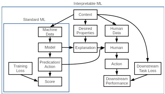
Figure 33.1: The interpretable machine learning ecosystem. While standard machine learning can often abstract away elements of the context and consider only the process of learning models given a data distribution and a loss, interpretable machine is inextricably tied to a socio-technical context.

the associated human factors. That said, the grand challenge is to (1) understand what properties are needed for di!erent contexts and end-tasks and (2) identify and create interpretable machine learning methods that have those properties.

A simple example In the following sections, we will expand upon methods for interpretability, metrics for evaluation, and types of properties. First, however, we provide a simple example connecting all of the concepts we discussed above.

Suppose our context is that we have a lemonade stand, and our end-task is to understand when the stand is most successful in order to prioritize which days it is worth setting it up. (We have heard that sometimes machine learning models latch on to incorrect mechanisms and want to check the model before using it to inform our business strategy.) Our metric for the downstream performance is whether we correctly determine if the model can be trusted; this could be quantified as the amount of profit that we make by opening on busy days and being closed on quiet days.

To train our model, we collect data on two input features — the average temperature for the day (measured in degrees Fahrenheit) and the cleanliness of the sidewalk near our stand (measured as a proportion of the sidewalk that is free of litter, between 0 and 1) — and the output feature of whether the day was profitable. Two models seem to fit the data approximately equally well:

Model 1:

\[p(\texttt{profit}) = .9 \ast (\texttt{tensile} \times \texttt{75}) + .1(\texttt{howClea} \texttt{Sidew1k}) \tag{33.1}\]

Model 2:

\[p(\texttt{profit}) = \sigma(.9(\texttt{temperature} - 75) / \texttt{maxTemperature} + .1(\texttt{hourTalesDiswa1k} - .5)) \tag{33.2}\]

These models are illustrated in Figure 33.2. Both of these models are inherently interpretable in the sense that they are easy to inspect and understand. While we were not explicitly seeking causal models (for that, see Chapter 36), both rely mostly on the temperature, which seems reasonable.

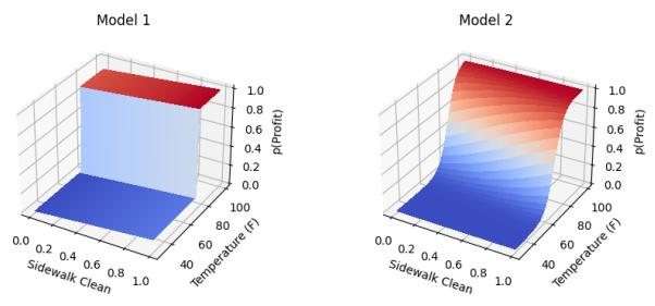
Figure 33.2: Models described in the simple example. Both of these models have the same qualitative characteristics, but di!erent explanation methods will describe these models quite di!erently, potentially causing confusion.

For the sake of this example, suppose that the models above were black boxes, and we could only request partial views of it. We decide to ask the model for the most important features. Let us see what happens when we consider two di!erent ways of computing important features.3

Our first (feature-based) explanation method computes, for each training point, whether individually changing each feature to its max or min value changes the prediction. Important features are those that change the prediction for many training points. One can think of this explanation method as a variant of computing feature importance based on how important a feature is to the coalition that produces the prediction. In this case, both models will report temperature to be the dominating feature. If we used this explanation to vet our models, we would correctly conclude that both models use the features in a sensible way (and thus may be worth considering for deciding when to open our lemonade stand).

Our second (feature-based) explanation method computes the magnitude of the derivatives of the output with respect to the inputs for each training point. Important features are those that have a large sum of absolute derivatives across the training set. One can think of this explanation method as a variant of computing feature importances based on local geometry. In this case, Model 2 will still report that temperature has higher derivatives. However, Model 1, which has very similar behavior to Model 2, will report that sidewalk cleanliness is the dominating feature because the derivative with respect to temperature is zero nearly everywhere. If we used this explanation to vet our models, we would incorrectly conclude that Model 1 relies on an unimportant feature (and that Model 1 and 2 rely on di!erent features).

What happened? The di!erent explanations had di!erent properties. The first explanation had the property of fidelity with respect to identifying features that, if changed, will a!ect the prediction, whereas the second explanation had the property of correctly identifying features that have the most local curvature. In this example, the first property is more important for the task of determining whether our model can be used to determine our business strategy. 4

^3. In the remainder of the chapter we will describe many other ways of creating and computing explanations.

^4. Other properties may be important for this end-task. This example is just the simplest one.

33.2 Methods for interpretable machine learning

There exist many methods for interpretable machine learning. Each method has di!erent properties and the right choice will depend on context and end-tasks. As we noted in Section 33.1.2, the grand challenge in interpretable machine learning is determining what kinds of properties are needed for what contexts, and what explanation methods satisfy those properties. Thus, one should consider this section a high-level snapshot of the rapidly changing options of methods that one may want to choose for interpretable machine learning.

33.2.1 Inherently interpretable models: the model is its explanation

We consider certain classes of models inherently interpretable: a person can inspect the full model and, with reasonable e!ort, understand how inputs become outputs.5 Specifically, we define inherently interpretable models as those that require no additional process or proxies in order for them to be used as explanation for the end-task. For example, suppose a model consists of a relatively small set of rules. Then, those rules might su”ce as the explanation for end-tasks that do not involve extreme time pressure. (Note: in this way, a model might be inherently interpretable for one end-task and not another.)

Inherently interpretable models fall into two main categories: sparse (or otherwise compact) models and logic-based models.

Compact or sparse feature-based models include various kinds of sparse regressions. Earlier in this textbook, we discussed simple models such as HMMs (Section 29.2), generalized linear models (Chapter 15), and various latent variable models (Chapter 28). When small enough, these are generally inherently interpretable. More advanced models in this category include super-sparse linear integer models and other checklist models [DMV15; UTR14].

While simple functionally, sparsity has its drawbacks when it comes to inspection and interpretation. For example, if a model picks only one of several correlated features, it may be harder to identify what signal is actually driving the prediction. A model might also assign correlated features di!erent signs that ultimately cancel, rendering an interpretion of weights meaningless.

To handle these issues, as well as to express more complex functions, some models in this category impose hierarchical or modular structures in which each component is still relatively compact and can be inspected. Examples include topic models (e.g., [BNJ03b], (small) discrete time series models (e.g., [FHDV20]), generalized additive models (e.g., [HT17]) and monotonicity-enforced models (e.g., [Gup+16]).

Logic-based models use logical statements as basis. Models in this category include decisiontrees [Bre+17], decision lists [Riv87; WR15; Let+15a; Ang+18; DMV15] , decision tables, decision sets [Hau+10; Wan+17a; LBL16; Mal+17; Bén+21], and logic programming [MDR94]. A broader discussion, as well as a survey of user studies on these methods, can be found in [Fre14]. Logic-based models easily model non-linear relationships but can have trouble modeling continuous relationships between the input and output (e.g., expressing a linear function vs. a step-wise constant function). Like the compact models, hierarchies and other forms of modularity can be used to extend the expressivity of the model while keeping it human-inspectable. For example, one can define a new

^5. There may be other questions, such as how training data influenced the model, which may still require additional computation or information.

concept as a formula based on some literals, and then use the new concept to build more complex rules.

When using inherently interpretable models, three key decisions need to be made: the choice of the model class, how to manage uninterpretable input features, and the choice of optimization method.

Decision: model class. Since the model is its own explanation, the decision on the model class becomes the decision on the form of explanation. Thus, we need to consider both whether the model class is a good choice for modeling the data as well as providing the necessary information to the user. For example, if one chooses to use a linear model to describe one’s data, then it is important that the intended users can understand or manipulate the linear model. Moreover, if the fitting process produces a model that is too large to be human-inspectable, then it is no longer inherently interpretable, even if it belongs to one of the model classes described above.

Decision: optimization methods for training. The kinds of model classes that are typically inherently interpretable often require more advanced methods for optimization: compact, sparse, and logic-based models all involve learning discrete parameters. Fortunately, there is a long and continuing history of research for optimizing such models, including directly via optimization programs, relaxation and rounding techniques, and search-based approaches. Another popular optimization approach is via distillation or mimics: one first trains a complex model (e.g., a neural network) and then uses the complex model’s output to train a simpler model to mimic the more complex model. The more complex model is then discarded. These optimization techniques are beyond the scope of this chapter but covered in optimization textbooks.

Decision: how to manage uninterpretable input features. Sometimes the input features themselves are not directly interpretable (e.g., pixels of an image or individual amplitudes spectrogram); only collections of inputs have semantic meaning for human users. This situation challenges our ability not only to create inherently interpretable models but also explanations in general.

To address this issue, more advanced methods attempt to add a “concept” layer that first converts the uninterpretable raw input to a set of human-interpretable concept features. Next, these concepts are mapped to the model’s output [Kim+18a; Bau+17]. This second stage can still be inherently interpretable. For example, one could first map a pattern of spectrogram to a semantically meaningful sound (e.g., people chatting, cups clinking) and then from those sounds to a scene classification (e.g., in a cafe). While promising, one must ensure that the initial data-to-concept mapping truly maps the raw data to concepts as the user understands them, no more and no less. Creating and validating that machine-derived concepts correspond to a semantically meaningful human concepts remains an open research challenge.

When might we want to consider inherently interpretable models? When not? Inherently interpretable models have several advantages over other approaches. When the model is its explanation, one need not worry about whether the explanation is faithful to the model or whether it provides the right partial view of the model for the intended task. Relatedly, if a person vets the model and finds nothing amiss, they might feel more confident about avoiding surprises. For all these reasons, inherently interpretable models have been advocated for in high-stakes scenarios, as well as generally being the first go-to to try [Rud19].

That said, these models do have their drawbacks. They typically require more specialized

optimization approaches. With appropriate optimization, inherently interpretable models can often match the performance of more complex models, but there are domains — in particular, images, waveforms, and language — in which deep models or other more complex models typically give significantly higher performance. Trying to fit complex behavior with a simple function may result not only in high bias in the trained model but also invite people to (incorrectly) rationalize why that highly biased model is sensible [Lun+20]. In an industry setting, seeking a migration away from a legacy, uninterpretable, business-critical model that has been tuned over decades would run into resistance.

Lastly, we note that just because a model is inherently interpretable, it does not guard against all kinds of surprises: as noted in Section 33.1, interpretability is just one form of validation mechanism. For example, if the data distribution shifts, then one may observe unexpected model behavior.

33.2.2 Semi-inherently interpretable models: example-based methods

Example-based models use examples as their basis for their predictions. For example, an examplebased classifier might predict the class of a new input by first identifying the outputs for similar instances in the training set and next taking a vote. K-nearest neighbors is one of the best known models in this class. Extensions include methods to identify exemplars for predicted classes and clusters (e.g., [KRS14; KL17b; JL15a; FD07b; RT16; Arn+10]), to generate exemplars (e.g., [Li+17d]), to define similarities between instances via sophisticated embeddings (e.g.,[PM18a]), and to first decompose an instance into parts and then find neighbors or exemplars between the parts (e.g., [Che+18b]). Like logic-based models, example-based models can describe highly non-linear boundaries.

On one hand, individual decisions made by example-based methods seem fully inspectable: one can provide the user with exactly the training instances (including their output labels) that were used to classify a particular input in a particular way. However, it may be di”cult to convey a potentially complex distance metric used to define “similarity”. As a result, the user may incorrectly infer what features or patterns made examples similar. It is also often di”cult to convey the intuition behind the global decision boundary using examples.

33.2.3 Post-hoc or joint training: the explanation gives a partial view of the model

Inherently interpretable models are a subset of all machine learning models, and circumstances may require working with a model that is not inherently interpretable. As noted above, large neural models (Chapter 16) have demonstrated large performance benefits for certain kinds of data (e.g., images, waveform, and text); one might have to work with a legacy, business critical model that has been tuned for decades; one might be trying to understand a system of interconnected models.

In these cases, the view that the explanation gives into the model will necessarily be partial: the explanation may only be an approximation of the model or be otherwise incomplete. Thus, more decisions have to be made. Below, we split these decisions into two broad categories — what the explanation should consist of to best serve the context and how the explanation should be computed from the trained model. More detail on the abilities and limitations of these partial explanation methods can be found in [Sla+20; Yeh+19a; Kin+19; Ade+20a].

33.2.3.1 What does the explanation consist of ?

One set of decisions center around the content of the explanation and what properties it should have. One choice is the form: Should the explanation be a list of important features? The top interactions? One must also choose the scope of the explanation: Is it trying to explain the whole model (global)? The model’s behavior near a specific input (local)? Something else? Determining what properties the explanation must have will help answer these and other questions. We expand on each of these points below; the right choice, as always, will depend on the user — whom the explanation is for —and their end-task.

Decision: form of the explanation. In the case of inherently interpretable models, the model class used to fit the data was also the explanation. Now, the model class and the explanation are two di!erent entities. For example, the model could be a deep network and the explanation a decision tree.

Works in interpretable machine learning have used a large variety of forms of explanations. The form could be a list of “important” input features [RSG16b; Lun+20; STY17; Smi+17; FV17] or “important” concepts [Kim+18a; Bau+20; Bau+18]. Or it could be a simpler model that approximates the complex model (e.g., a local linear approximation, an approximating rule set)[FH17; BKB17; Aga+21; Yin+19c]. Another choice could be a set of similar or prototypical examples [KRS14; AA18; Li+17d; JL15a; JL15b; Arn+10]. Finally, one can choose whether the explanation should include a contrast against an alternative (also sometimes described as a counterfactual explanation) [Goy+19; WMR18; Kar+20a] or include or influential examples [KL17b].

Di!erent forms of explanations will facilitate di!erent tasks in di!erent contexts. For example, a contrastive explanation of why treatment A is better than treatment B may help a clinician decide between treatments A and B. However, a contrast between treatments A and B may not be useful when comparing treatments A and C. Given the large number of choices, literature on how people communicate in the desired context can often provide some guidance. For example, if the domain involves making quick, high-stakes decisions, one might turn to how trauma nurses and firefighters explain their decisions (known as recognition-primed decision making, [Kle17]).

Decision: scope of the explanation: global or local. Another major decision regarding the parameters of the explanation is its scope.

Local explanation: In some cases, we may only need to interrogate an existing model about a specific decision. For example, why was this image predicted as a bird? Why was this patient predicted to have diabetes? Local explanations can help see if a consequential decision was made incorrectly or determine what could have been done di!erently to produce a di!erent outcome (i.e., provide a recourse).

Local explanations can take many forms. A family of methods called saliency maps or attribution maps [STY17; Smi+17; ZF14; Sel+17; Erh+09; Spr+14; Shr+16] estimate the importances of each input dimension (e.g., via first-order derivatives with respect to the input). More generally, one might locally-fit simpler model in the neighborhood of the input of interest (e.g., LIME [RSG16b]). A local explanation may also consist of representative examples, including identifying which training points were most influential for a particular decision [KL17b] or identifying nearby datapoints with di!erent predictions [MRW19; LHR20; Kar+20a].

All local explanation methods are partial views because they only attempt to explain the model around an input of interest. A key risk is that the user may overgeneralize the explanation to a wider region than it applies. They may also interpolate an incorrect mental model of the model based on a few local explanations.

Global explanation: In other cases, we may desire insight into the model as a whole or for a collection of datapoints (e.g., all inputs predicted to one class). For example, suppose that our end-task is to decide whether to deploy a model. Then, we care about understanding the entire model.

Global explanations can take many forms. One choice is to fit a simpler model (e.g., an inherently interpretable model) that approximates the original model (e.g., [HVD14]). One can also identify concepts or features that a!ect decisions across many inputs (e.g., [Kim+18b]). Another approach is to provide a carefully chosen set of representative examples [Yeh+18]. These examples might be chosen to be somehow characteristic of, or providing coverage of, a class (e.g., [AA18]), to draw attention to decision boundaries (e.g., [Zhu+18]), or to identify inputs particularly influential in training the model.

Unless a model is inherently interpretable, it is still important to remember that a global explanation is still a partial view. To make a complex model accessible to the user, the global explanation will need to leave some things out.

Decision: determining what properties the context needs. Di!erent forms of explanations have di!erent levels of expressivity. For example, an explanation listing important features, or fitting a local linear model around a particular input, does not expose interactions—but fitting a local decision tree would. For each form, there will also be many ways to compute an explanation of that form (more on this in Section 33.2.3.2). How do we choose amongst all of these di!erent ways to compute the explanation? We suggest that the first step in determining the form and computation of an explanation should be to determine what properties are needed from it.

Specifying properties is especially important because not only may di!erent forms of explanations have di!erent intrinsic properties—e.g., can it model interactions?—but the properties may depend on the model being explained. For example, if the model is relatively smooth, then a feature-based explanation relying on local gradients may be fairly faithful to the original model. However if the model has spiky contours, the same explanation may not adequately capture the model’s behavior. Once the desired properties are determined, one can determine what kind of computation is necessary to achieve them. We will list commonly desirable properties in Section 33.3.

33.2.3.2 How the explanation is computed

Another set of decisions has to do with how the explanation is computed.

Decision: computation of explanation. Once we make the decisions above, we must decide how the explanation will actually be computed. This choice will have a large impact on the explanation’s properties. Thus, it is crucial to carefully choose a computational approach that provides the properties needed for the context and end-task.

For example, suppose one is seeking to identify the most “important” input features that change a prediction. Di!erent computations correspond to di!erent definitions of importance. One definition of importance might be the smallest region in an image that, when changed, changes the prediction a perturbation-based analysis. Even within this definition, we would need to specify how that

perturbation will be computed: Do we keep the pixel values within the training distribution? Do we preserve correlations between pixels? Di!erent works take di!erent approaches [SVZ13; DG17; FV17; DSZ16; Adl+18; Bac+15a].

A related approach is to define importance in terms of sensitivity (e.g., largest gradients of the output with respect to the input feature). Even then, there are many computational decisions to be made [STY17; Smi+17; Sel+17; Erh+09; Shr+16]. Yet another common definition of importance is how often the input feature is part of a “winning coalition” that drives the prediction, e.g., a Shapley or Banzhaf score [LL17]. Each of these definitions have di!erent properties, as well as require di!erent amounts of computation.

Similar issues come up with other forms of explanations. For example, for an example-based explanation, one has to define what it means to be similar or otherwise representative: Is it the cosine similarity between activations? A uniform L2 ball of a certain size between inputs? Likewise, there are many di!erent ways to obtain counterfactuals. One can rely on distance functions to identify nearby inputs that with di!erent outputs [WMR17; LHR20], causal frameworks [Kus+18], or SAT formulations [Kar+20a], among other choices.

Decision: joint training vs. post-hoc application. So far, we have described our partial explanation techniques as extracting some information from an already-trained model. This approach is called deriving a post-hoc explanation. As noted above, post-hoc, partial explanations may have some limitations: for example, an explanation based on a local linear approximation may be great if the model is generally smooth, but provide little insight if the model has high curvature. Note that this limitation is not because the partial explanation is wrong, but because the view that local gradients provide isn’t su”cient if the true decision boundary is curvy.

One approach to getting explanations to have desired properties we is to train the model and the explanation jointly. For example, a regularizer that penalizes violations of desired properties can help steer the overall optimization process towards learning models that both perform well and are amenable to the desired explanation [Plu+20]. It is often possible to find such a model because most complex model classes have multiple high-performing optima [Bre01].

The choice of regularization will depend on the desired properties, the form of the explanation, and its computation. For example, in some settings, we may desire the explanation use the same features that people do for the task (e.g., lower frequency vs. higher frequency features in image classifiers [Wan+20b]) — and still be faithful to the model. In other settings, we may want to control the input dimensions used or not used in the explanation, or for the explanation to be somehow compact (e.g., a small decision tree) while still being faithful to the underlying model, [RHDV17; Shu+19a; Vel+17; Nei+18; Wu+19b; Plu+20]. (Certain attention models fall into this category [JW19; WP19].) We may also have constraints on the properties of concepts or other intermediate features [AMJ18b; Koh+20a; Hen+16; BH20; CBR20; Don+17b]. In all of these cases, these desired properties could be included as a regularizer when training the model.

When choosing between a post-hoc explanation or joint training, one key consideration is that joint training assumes that one can re-train the model or the system of interest. In many cases in practice, this may not be possible. Replacing a complex and well-validated system in deployment for a decade may not be possible or take a prohibitively long time. In that case, one can still extract approximated explanations using post-hoc methods. Finally, a joint optimization, even when it can be performed, is not a panacea: optimization for some properties may result in unexpected violations of other (unspecified but desired) properties. For this reason, explanations from jointly trained models are still partial.

When might we want to consider post-hoc methods, and when not?. The advantage of post-hoc interpretability methods is that they can be applied to any model. This family of methods is especially useful in real-world scenarios where one needs to work with a system that contains many models as its parts, where one cannot expect to replace the whole system with one model. These approaches can also provide at least some broader knowledge about the model to identify unexpected concerns.

That said, post-hoc explanations, as approximations of the true model, may not be fully faithful to the model nor cover the model completely. As such, an explanation method tailored for one context may not be transferable in another; even in the intended context, there may be blindspots about the model that the explanation misses completely. For these reasons, in high stakes situations, one should attempt to use an inherently interpretable model first if possible [Rud19]. In all situations when post-hoc explanations are used, one must keep in mind that they are only one tool in a broader accountability toolkit and warn users appropriately.

33.2.4 Transparency and visualization

The scope of interpretable machine learning is around methods that expose the process by which a trained model makes a decision. However, the behavior of a model also depends on the objective function, the training data, how the training data were collected and processed, and how the model was trained and tested. Conveying to a human these other aspects of what goes into the creation of a model can be as important as explaining the trained model itself. While a full discussion of transparency and visualization is outside the scope of this chapter, we provide a brief discussion here to describe these important adjacent concepts.

Transparency is an umbrella term for the many things that one could expose about the modeling process and its context. Interpreting models is one aspect. However, one could also be transparent about other aspects, such as the data collection process or the training process (e.g., [Geb+21; Mit+19; Dnp]). There are also situations in which a trained model is released (whether or not it is inherently interpretable), and thus the software can be inspected and run directly.

Visualization is one way to create transparency. One can visualize the data directly or various aspects of the model’s process (e.g., [Str+17]). Interactive visualizations can convey more than text or code descriptions [ZF14; OMS17; MOT15; Ngu+16; Hoh+20]. Finally, in the specific context of interpretable machine learning, how the explanation is presented — the visualization — can make a large di!erence in how easily users can consume it. Even something as simple as a rule list has many choices of layout, highlighting, and other organization.

When might we want to consider transparency and visualization? When not? In many cases, the trouble with a model comes not from the model itself, but parts of its training pipeline. The problem might be the training data. For example, since policing data contain historical bias, predictions of crime hot spots based on that data will be biased. Similarly, if clinicians only order tests when they are concerned about a patient’s condition, then a model trained to predict risk based on tests ordered will only recapitulate what the clinicians already know. Transparency about the properties of the data, and how training and testing were performed, can help identify these issues.

Of course, inspecting the data and the model generation process is something that takes time and attention. Thus, visualizations of this kind and other descriptions to increase transparency are best-suited to situations in which a human inspector is not under time pressure to sift through potentially complex patterns for sources of trouble. These methods are not well-suited for situations

in which a specific decision must be made in a relatively short amount of time, e.g., providing decision-support to a clinician at the bedside.

Finally, transparency in the form of making code available can potentially assist in understanding how a model works, identifying bugs, and allowing independent testing by a third party (e.g., testing with a new set of inputs, evaluating counterfactuals in di!erent testing distributions). However, if a model is su”ciently complex, as many modern models are, then simply having access to the code is likely not be enough for a human to gain su”cient understanding for their task.

33.3 Properties: the abstraction between context and method

Recall from the terminology and framework in Section 33.1.2 that the context and end-task determine what properties are needed for the explanation. For example, in a high-stakes setting — such as advising on interventions for an unstable patient — it may be important that the explanation completely and accurately reflects the model (fidelity). In contrast, in a discovery-oriented setting, it might be more important for any explanation to allow for e”cient iterative refinement, revealing di!erent aspects of the model in turn (interactivity). Not all contexts and end-tasks need all properties, and the lack of a key property may result in poor downstream performance.

While the research is still evolving, there exists a growing informal understanding about how properties may work as an abstraction between methods and contexts. Many interpretability methods from Section 33.2 share the same properties, and methods with the same properties may have similar downstream performance in a specific end-task and context. If two contexts and end-tasks require the same properties, then a method that works well for one may work well for the other. A method with properties well-matched for one context could miserably fail in another context.

How to find desired properties? Of course, identifying what properties are important for a particular context and end-task is not trivial. Indeed, identifying what properties are important for what contexts, end-tasks, and downstream performance metrics is one facet of the grand challenge of interpretable machine learning. For the present, the process of identifying the correct properties will likely require iteration via user studies. However, iterating over properties is still a much smaller space than iterating over methods. For example, if one wants to test whether the sparsity of the explanation is key to good downstream performance, one could intentionally create explanations of varying levels of sparsity to test that hypothesis. This is a much more precise knob to test than exhaustively trying out di!erent explanation methods with di!erent hyperparameters.

Below, we first describe examples of properties that have been discussed in the interpretable machine learning literature. Many of these properties are purely computational — that is, they can be determined purely from the model and the explanation. A few have some user-centric elements. Next we list examples of properties of explanation from cognitive science (on human to human explanations) and human-computer interaction (on machine to human explanations). Some of these properties have analogs in the machine learning list, while others may serve as inspiration for areas to formalize.

33.3.1 Properties of explanations from interpretable machine learning

Many lists of potentially-important properties of interpretable machine learning models have been compiled, sometimes using di!erent terms for similar concepts and sometimes using the similar terms

for di!erent concepts. Below we list some commonly-described properties of explanations, knowing that this list will evolve over time as the field advances.

Faithfulness, fidelity (e.g., as described in [JG20; JG21]). When the explanation is only a partial view of the model, how well does it match the model? There are many ways to make this notion precise. For example, suppose a mimic (simple model) is used to provide a global explanation of a more complex model. One possible measure of faithfulness could be how often the mimic gives the same outputs as the original. Another could be how often the mimic has the same first derivatives (local slope) as the original. In the context of a local explanation consisting of the ‘key’ features for a prediction, one could measure faithfulness by whether the prediction changes if the supposedly important features are flipped. Another measure could check to make sure the prediction does not change if a supposedly unimportant feature is flipped. The appropriate formalization will depend on the context.

Compactness, sparsity (e.g., as described in [Lip18; Mur+19] ). In general, an explanation must be small enough such that the user can process it within the constraints of the task (e.g., how quickly a decision must be made). Sparsity generally corresponds to some notion of smallness (a few features, a few parameters, L1 norm etc.). Compactness generally carries an additional notion of not including anything irrelevant (that is, even if the explanation is small enough, it could be made smaller). Each must be formalized for the context

Completeness (e.g., as described in [Yeh+19b]). If the explanation is not the model, does it still include all of the relevant elements? For example, if an explanation consists of important features for a prediction, does it include all of them, or leave some out? Moreover, if the explanation uses derived quantities that are not the raw input features — for example, some notion of higher-level concepts — are they expressive enough to explain all possible directions of variation that could change the prediction? Note that one can have a faithful explanation in certain ways but not complete in others: Fore example, an explanation may be faithful in the sense that flipping features considered important flips the prediction and flipping features considered unimportant does not. However, the explanation may fail to include that flipping a set of unimportant features does change the prediction.

Stability (e.g., as described in [AMJ18a]) To what extent are the explanations similar for similar inputs? Note that the underlying model will naturally a!ect whether the explanation can be stable. For example, if the underlying model has high curvature and the explanation has limited expressiveness, then it may not be possible to have a stable explanation.

Actionability (e.g., as described in [Kar+20b; Poy+20]). Actionability implies filtering the content of the explanation to focus on only aspects of the model that the user might be able to intervene on. For example, if a patient is predicted to be at high risk of heart disease, an actionable explanation might only include mutable factors such as exercise and not immutable factors such as age or genetics. The notion of recourse corresponds to actionability in a justice context.

Modularity (e.g., as described in [Lip18; Mur+19]). Modularity implies that the explanation can be broken down into understandable parts. While modularity does not guarantee that the user can explain the system as a whole, for more complex models, modular explanations — where the user can inspect each part — can be an e!ective way to provide a reasonable level of insight into the model’s workings.

Interactivity (e.g., [Ten+20]) Does the explanation allow the user to ask questions, such as how the explanation changes for a related input, or how an output changes given a change in input? In some contexts, providing everything that a user might want or need to know from the start might be overwhelming, but it might be possible to provide a way for the user to navigate the information

about the model in their own way.

Translucence (e.g., as described in [SF20; Lia+19]). Is the explanation clear about its limitations? For example, if a linear model is locally fit to a deep model at a particular input, is there a mechanism that reports that this explanation may be limited if there are strong feature interactions around that input? We emphasize that translucence is about exposing limitations in the explanation, rather than the model. As with all accountability methods, the goal of the explanation is to expose the limitations of the model.

Simulability (e.g., as described in [Lip18; Mur+19]). A model is simulable if a user can take the model and an input and compute the output (within any constraints of time and cognition). A simulable explanation is an explanation that is a simulable model. For example, a list of features is not simulable, because a list of features alone does not tell us how to compute the output. In contrast, an explanation in the form of a decision tree does include a computation process: the user can follow the logic of the tree, as long as it is not too deep. This example also points out an important di!erence between compactness and simulability: if an explanation is too large, it may not be simulable. However, just because an explanation is compact — such as a short list of features does not mean that a person can compute the model’s output with it.

It may seem that simulability is di!erent from the other properties because its definition involves human input. However, in practice, we often know what kinds of explanations are easy for people to simulate (e.g., decision trees with short path lengths, rule lists with small formulas, etc.). This knowledge can be turned into a purely computational training constraint where we seek simulatable explanations.

Alignment to the user’s vocabulary and mental model. (e.g., as described in [Kim+18a]). Is the content of the explanation designed for the user’s vocabulary? For example, the explanation could be given in the semantics a user knows, such as medical conditions vs. raw sensor readings. Doing so can help the user more easily connect the explanation to their knowledge and existing decision-making guidelines [Clo+19]. Of course, the right vocabulary will depend on the user: an explanation in terms of parameter variances and influential points may be comprehensible to an engineer debugging a lending model but not to a loan applicant.

Like simulability, mental-model alignment is more human-centric. However, just as before, we can imagine an abstraction between eliciting vocabulary and mental models from users (i.e., determining how they define their terms and how to think), and ensuring that an explanation is provided in alignment with whatever that elicited user vocabulary and mental model is.

Once desired properties are identified, we need to operationalize them. For example, if sparsity is a desired property, would using the L1 norm be enough? Or does a more sophisticated loss term need to be designed? This decision will necessarily be human-centric: how small an explanation needs to be, or in what ways it needs to be small, is a decision that needs to consider how people will be using the explanation. Once operationalized, most properties can be optimized computationally. That said, the properties should be evaluated with the context, end-task, model, and chosen explanation methods. Once evaluated, one may revisit the choice of the explanation and model.

Finally, we emphasize that the ability to achieve a particular property will depend on the intrinsic characteristics of the model. For example, the behavior of a highly nonlinear model with interactions between the inputs will, in general, be harder to understand than a linear model. No matter how we try to explain it, if we are trying to explain something complicated, then users will have a harder time understanding it.

33.3.2 Properties of explanations from cognitive science

Above we focused on computational properties between models and explanations. The fields of cognitive science and human-computer interaction have long examined what people consider good properties of an explanation. These more human-centered properties may be ones that researchers in machine learning may be less aware of, yet essential for communicating information to people.

Unsurprisingly, the literature on human explanation concurs that the explanation must fit the context [VF+80]; di!erent contexts require di!erent properties and di!erent explanations. That said, human explanations are also social constructs, often including post-hoc rationalizations and other biases. We should focus on properties that help users achieve their goals, not ones simply “because people sometimes do it”.

Below we list several of these properties.

Soundness (e.g., as described in [Kul+13]). Explanations should contain nothing but the truth with respect to whatever they are describing. Soundness corresponds to notions of compactness and faithfulness above.

Completeness (e.g., as described in [Kul+13]). Explanations should contain the whole truth with respect to whatever they are describing. Completeness corresponds to notions of completeness and faithfulness above.

Generality (e.g., as described in [Mil19]). Overall, people understand that an explanation for one context may not apply in another. That said, there is an expectation that an explanation should reflect some underlying mechanism or principle and will thus apply to similar cases — for whatever notion of similarity is in the person’s mental model. Explanations that do not generalize to similar cases may be misinterpreted. Generality corresponds to notions of stability above.

Simplicity (e.g., as described in [Mil19]). All of the above being equal, simpler explanations are generally preferred. Simplicity relates to notions of sparsity and complexity above.

Contrastiveness (e.g., as described in [Mil19]). Contrastive explanations provide information of how something di!ers from an alternate decision or prediction. For example, instead of providing a list of features for why a particular drug is recommended, it might provide a list of features that explain why one drug is recommended over another. Contrastiveness relates to notions of actionability above, and more generally explanation types that include counterfactuals.

Finally, the cognitive science literature also notes that explanations are often goal directed. This matches the notion of explanation in ML as information that helps a person improve performance on their end-task. Di!erent information may help with di!erent goals, and thus human explanations take many forms. Examples include deductive-nomological forms (i.e. a logical proofs) [HO48], forms that provide a sense of an underlying mechanism [BA05; Gle02; CO06], and forms that convey understanding [Kei06]. Knowing these forms can help us consider what options might be best among di!erent sets of interpretable machine learning methods.

33.4 Evaluation of interpretable machine learning models

One cannot formalize the notion of interpretability without specifying the context, the end-task, and the downstream performance metric [VF+80]. If one explanation empowers the human to get better performance on their end-task over another explanation, then it is more useful. While the grand challenge of interpretable machine learning is to develop a general understanding of what properties are needed for good downstream performance on di!erent end-tasks in di!erent contexts, in this section, we will focus on rigorous evaluation within one context [DVK17].

Specifically, we describe two major categories for evaluating interpretable machine learning methods:

Computational evaluations of properties (without people). Computational evaluations of whether explanations have desired properties that do not involve user studies. For example, one can computationally measure whether a particular explanation satisfies a definition of faithfulness under di!erent training and test data distributions or whether the outputs of one explanation are more sparse than another. Such measures are valuable when one already knows that certain properties may be important for certain contexts. Computational evaluations also serve as intermediate evaluations and sanity checks to identify undesirable explanation behavior prior to a more expensive user study-based evaluation.

User studies (with people). Ultimately, user studies are needed to measure how well an interpretable machine learning method enables the user to complete their end-task in a given context. Performing a rigorous, well-designed user study in a real context is significant work — much more so than computing a test likelihood on benchmark datasets. It requires significant asks of not only the researchers but also the target users. Methods for di!erent contexts will also have di!erent evaluation challenges: while a system designed to assist with optimizing music recommendations might be testable on a wide population, a system designed to help a particle physicist identify new kinds of interactions might only be tested with one or two physicists because people with that expertise are hard to find. In all cases, the evaluation can be done rigorously given careful attention to experimental design.

33.4.1 Computational evaluation: does the method have desired properties?

While the ultimate measure of interpretability is whether the method successfully empowers the user to perform their task, properties can serve as a valuable abstraction. Checking whether an explanation has the right computational and desired properties can ensure that the method works as expected (e.g., no implementation errors, no obviously odd behaviors). One can iterate on novel, computationally-e”cient methods to optimize the quantitative formalization of a property before conducting expensive human experiments. Computational checks can also ensure whether properties that held for one model continue to hold when applied to another model. Finally, checking for specific properties can also help pinpoint in what way an explanation is falling short, which may be less clear from a user study due to confounding.

In some cases, one might be able to prove mathematically that an explanation has certain properties, while in others the test must be empirical. For empirical testing, one umbrella strategy is to use a hypothesis-based sanity check; if we think a phenomenon X should never occur (hypothesis), we can test whether we can create situations where X may occur. If it does, then the method fails

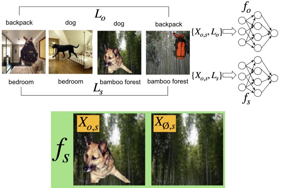
Figure 33.3: An example of computational evaluation using (semi-)synthetic datasets from [YK19]: foreground images (e.g., dogs, backpacks) are placed on di!erent backgrounds (e.g., indoors, outdoors) to test what an explanation is looking for.

this sanity check. Another umbrella strategy is to create datasets with known characteristics or ground truth explanations. These could be purely synthetic constructions (e.g., generated tables with intentionally correlated features), semi-synthetic approaches (e.g., intentionally changing the labels on an image dataset), or taking slices of a real dataset (e.g., introduce intentional bias by only selecting real image, label pairs that are of outdoor environments). Note that these tests can only tell us if something is wrong; if a method passes a check, there may still be missing blindspots.

Examples of sanity checks. One strategy is to come up with statements of the form “if this explanation is working, then phenomenon X should not be occurring” and then try to create a situation in which phenomenon X occurs. If we succeed, then the sanity check fails. By asking about out-of-the-box phenomena, this strategy can reveal some surprising failure modes of explanation methods.

For example, [Ade+20a] operates under the assumption that a faithful explanation should be a function of a model’s prediction. The hypothesis is that the explanation should significantly change when comparing a trained model to an untrained model (where prediction is random). They show that many existing methods fail to pass this sanity check (Figure 33.4).

In another example, [Kin+19] hypothesize that a faithful explanation should be invariant to input transformations that do not a!ect model predictions or weights, such as constant shift of inputs (e.g., all inputs are added by 10). This hypothesis can be seen as testing both faithfulness and stability

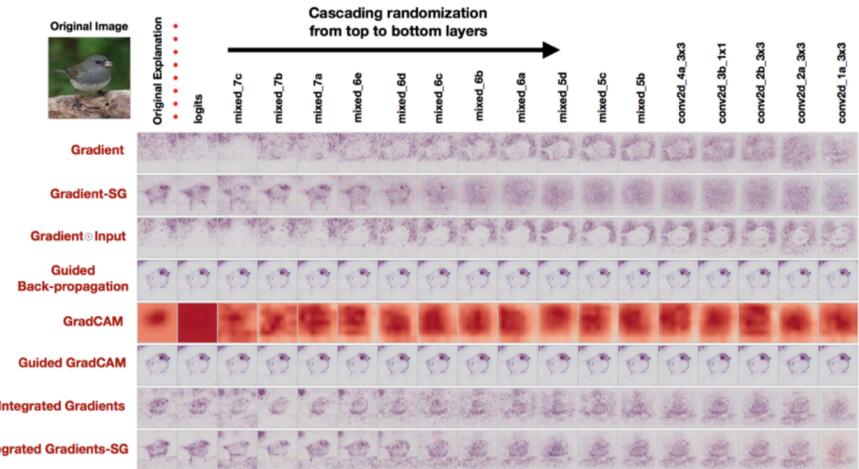
Figure 33.4: Interpretability methods (each row) and their explanations as we randomize layers starting from the logits, and cumulatively to the bottom layer (each column), in the context of image classification task. The rightmost column is showing a completely randomized network. Most methods output similar explanations for the first two columns; one predicts the bird, and the other predicts randomly. This sanity check tests the hypothesis that the explanation should significantly change (quantitatively and qualitatively) when comparing a trained model and an untrained model [Ade+20a].

properties. Their work shows that some methods fail this sanity check.

Adversarial attacks on explanations also fall into this category. For example, [GAZ19] shows that two perceptively indistinguishable inputs with the same predicted label can be assigned very di!erent explanations.

Examples using (semi)synthetic datasets. Constructed datasets can also help score properties of various methods. We use the work of [YK19] as an example. Here, the authors were interested in explanations with the properties of compactness and faithfulness: it should not identify features as important if they are not. To test for these properties, the authors generate images with known correlations. Specifically, they generate multiple datasets, each with a di!erent rate of how often each particular foreground object co-occurs with each particular background (see Figure 33.3). Each dataset comes with two labels per image: for the object and the background.

Now, the authors compare two models: one trained to classify objects and one trained to classify backgrounds (left, Figure 33.3). If a model is trained to classify objects and they all happen to have the same background, the background should be less important than in a model trained to classify backgrounds ([YK19] call this ‘model contrast score’). They also checked that the model trained to predict backgrounds was not providing attributions to the foreground objects (see right Figure 33.3). Other works using similar strategies include [Wil+20b; Gha+21; PMT18; KPT21; Yeh+19b; Kim+18b].

Examples with real datasets. While more di”cult, it is possible to at least partially check for

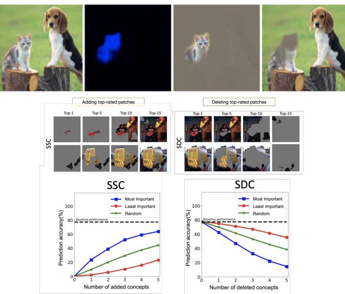
Figure 33.5: Examples of computational evaluation with real datasets. Top row is from Figure 1 of [DG17], used with kind permission of Yarin Gal. Bottom row is from Figure 4 of [Gho+19a]. One would expect that adding or deleting patches rated as most ‘relevant’ for an image classification would have a large e!ect on the classification compared to patches not rated as important.

certain kinds of properties on real datasets that have no ground-truth.

For example, suppose an explanation ranks features from most to least important. We want to determine if this ranking is faithful. Further, suppose we can assume that the features do not interact. Then, one can attempt to make the prediction just with the top-1 most important feature, just the top-2 ranked features, etc. and observe if the change in prediction accuracy exhibits diminishing returns as more features are added. (If the features do interact, this test will not work. For example, if features A, B, C are the top-3 features, but C is only important if feature B is present, the test above would over-estimate the importance of the feature C.)

Figure 33.5 shows an example of this kind of test [Gho+19a]. Their method outputs a set of image patches (e.g., a set of connected pixels) that correlates with the prediction. They add top-n image patches provided by the explanation one by one and observe the desired trend in accuracy. A similar experiment in reverse direction (i.e., deleting top-n most important image patches one by one) provides additional evidence. Similar experiments are also conducted in [FV17; RSG16a].

For example, in [DG17], authors define properties in plain English first: smallest su”cient region (smallest region of the image that alone allows a confident classification) and smallest destroying region (smallest region of the image that when removed, prevents a confident classification), followed by careful operationalization of these properties such that they become the objective for optimization. Then, separately, an evaluation metric of saliency is defined to be “the tightest rectangular crop that contains the entire salient region and to feed that rectangular region to the classifier to directly verify whether it is able to recognise the requested class”. While the “rectangular” constraint may introduce

artifacts, it is a neat trick to make evaluation possible. By checking expected behavior as described above, authors confirm that methods’ behavior on the real data is aligned with the defined property compared to baselines.

Evaluating the evaluations. As we have seen so far, there are many ways to formalize a given property and many empirical tests to determine whether a property is present. Each empirical test will have di!erent qualities. As an illustration, in [Tom+20], the authors ask whether popular saliency metrics give consistent results across literature. They tested whether di!erent metrics for assessing the quality of saliency-based explanations (explanations that identify important pixels or regions in images) is evaluating similar properties. In other words, this work tests consistency and stability properties of metrics. They show many metrics are statistically unreliable and inconsistent. While each metric may still have a particular use [Say+19], knowing this inconsistency exists helps us better understand the landscape and limitations of evaluation approaches. Developing good evaluations for computational properties is an ongoing area of research.

33.4.2 User study-based evaluation: does the method help a user perform a target task?

User study-based evaluations measure whether an interpretable machine learning method helps a human perform some task. This task could be the ultimate end-task of interest (e.g., does a method help a doctor make better treatment decisions) or a synthetic task that mirrors contexts of interest (e.g., a simplified situation with artificial diseases and symptoms). In both cases, rigorous experimental design is critical to ensuring that the experiment measures what we want it to measure. Understanding experimental design for user studies is essential for research in interpretable machine learning.

33.4.2.1 User studies in real contexts.

The gold standard for testing whether an explanation is useful is to test it in the intended context: Do clinicians make better decisions with a certain kind of decision support? Do programmers debug code faster with a certain kind of explanation about model errors? Do product teams create more fair models for their businesses? A complete guide on how to design and conduct user studies is out of scope for this chapter; below we point out some basic considerations.

33.4.2.2 Basic elements of user studies

Performing a high-quality user study is a nuanced and non-trivial endeavor. There are many sources of bias, some obvious (e.g., learning and fatigue e!ects during a study) and some less obvious (e.g., participants willing to work with us are more optimistic about AI technology than those we could not recruit, or di!erent participants may have di!erent needs for cognition).

Interface design. The explanation must be presented to the user. Unlike the intrinsic di”culty of explaining a model (i.e., complex models are harder to explain than simple ones), the design of the interface is an extrinsic source of di”culty that can confound the experimental results. For example, it may be easier, in general, to scan a list of features ordered by importance rather than alphabetically.

When we perform an evaluation with respect to an end-task, intrinsic and extrinsic di”culties can get conflated. Does one explanation type work better because it does a better job of explaining the complex system? Or does it work better simply because it was presented in a way that was easier for people to use? Especially if the goal is to test the di!erence between one explanation and another in the experiment, it is important that the interface for each is designed to tease out the e!ect from the explanations and their presentations. (Note that good presentations and visualization are an important but di!erent object of study.) Moreover, if using the interface requires training, it is important to deliver the training to users in a way that is neutral in each testing condition. For example, how the end-task and goals of the study are described during training (e.g., with practice questions) will have a large impact on how users approach the task.

Baselines. Simply the presence of an explanation may change the way in which people interact with an ML system. Thus, it is often important to consider how a human performs with no ML system, with an ML system and no explanation, with an ML system and a placebo explanation (an explanation that provides no information), and with an ML system and hand-crafted explanations (manually generated by humans who are presumably good communicators).

Experimental design and hypothesis testing. Independent and dependent variables, hypotheses, and inclusion and exclusion criteria must be clearly defined prior to the start of the study. For example, suppose that one hypothesizes that a particular explanation will help a developer debug an image classifier. In this case, the independent variable would be a form of assistance: the particular explanation, competing explanation methods, and the baselines above. The dependent variable would be whether the developer can identify bugs. Inclusion and exclusion criteria might include a requirement that the developer has su”cient experience training image classifiers (as determined by an initial survey, or a pre-test), demonstrates engagement (as measured by a base level of performance on practice rounds), and does not have prior experience with the particular explanation types (as determined by an initial survey). Other exclusion criteria could be removing outliers. For example, one could decide, in advance, to exclude data from any participant that takes an unusually long or short time to perform task as a proxy for engagement.

As noted in Section 33.2, there are many decisions that go into any interpretable machine learning method, and each context is nuanced. Studies of the form “Does explanation X (computed via some pipeline Y ) help users in context Z compared to explanation X^→ ?” may not provide much insight as to why that particular explanation is better or worse — making it harder not only to iterate on a particular explanation but also to generalize to other explanations or contexts. There are many factors of potential variation in the results, ranging from the properties of the explanation and its presentation to the di”culty of the task.

To reduce this variance, and to get more useful and generalizable insights, we can manipulate some factors of variation directly. For example, suppose the research question is whether complete explanations are better than incomplete explanations in a particular context. One might write out hand-crafted explanations that are complete in what features they implicate, explanations in which one important feature is missing, and explanations in which several important features are missing. Doing so ensures even coverage of the di!erent experimental regimes of interest, which may not occur if the explanations were simply output from a pipeline. As another example, one might intentionally create an image classifier with known bugs, or simply pretend to have an image classifier that makes certain predictions (as done in [Ade+20b]). These kinds of studies are called wizard-of-Oz studies, and they can help us more precisely uncover the science of why an explanation is useful (e.g., as done in [Jac+21]).

Once the independent and dependent variables, hypotheses, and participant criteria (including how the independent and dependent variables may be manipulated) are determined, the next step is setting up the study design itself. Broadly speaking, randomization marginalizes over potential confounds. For example, randomization in assigning subjects to tasks marginalizes the subject’s prior knowledge; randomization in the order of tasks marginalizes out learning e!ects. Matching and repeated measures reduce variance. An example of matching would be asking the same subject to perform the same end-task with two di!erent explanations. An example of repeated measures would be asking the subject to perform the end-task for several di!erent inputs.

Other techniques for designing user studies include block randomized designs/Latin square designs that randomize the order of explanation types while keeping tasks associated with each explanation type grouped together. This can be used to marginalize the e!ects of learning and fatigue without too much context switching. Careful consideration should be given to what will be compared within subjects and across subjects. Comparisons of task performance within subjects will have lower variance but a potential bias from learning e!ects from the first task to the second. Comparisons across subjects will have higher variance and also potential bias from population shift during experimental recruitment. Finally, each of these study designs, as well as the choice of independent and dependent variables, will imply an appropriate significance test. It is essential to choose the right test and multiple hypothesis correction to avoid inflated significance values while retaining power.

Qualitative studies. So far, we have described the standard approach for the design of a quantitative user study–one in which the dependent variable is numerically measured (e.g., time taken to correctly identify a bug, % bugs detected). While quantitative studies provide value by demonstrating that there is a consistent, quantifiable e!ect across many users, they usually do not tell us why a certain explanation worked. In contrast, qualitative studies, often performed with a “think-aloud” or other discussion-based protocol in which users expose their thought process as they perform the experiment, can help identify why a particular form of explanation seems to be useful or not. The experimenter can gain insights by hearing how the user was using the information, and depending on the protocol, can ask for clarifications.

For example, suppose one is interested in how people use an example-based explanation to understand a video-game agent’s policy. The idea is to show a few video clips of an automated agent in the video game, and then ask the user what the agent might do in novel situations. In a think-aloud study, the user would perform this task while talking through how they are connecting the videos they have seen to the new situation. By hearing these thoughts, a researcher might not only gain deeper insight into how users make these connections — e.g., users might see the agent collect coins in one video and presume that the agent will always go after coins — but they might also identify surprising bugs: for example, a user might see the agent fall into a pit and attribute it to a one-o! sloppy fingers, not internalizing that an automated agent might make that mistake every time.

While a participant in a think-aloud study is typically more engaged in the study than they might be otherwise (because they are describing their thinking), knowing their thoughts can provide insight into the causal process between what information is being provided by the explanation and the action that the human user takes, ultimately helping advance the science of how people interact with machine-provided information.

Pilot studies: The above descriptions are just a very high-level overview of the many factors that must be designed properly for a high-quality evaluation. In practice, one does not typically get all of these right the first time. Small scale pilot studies are essential to checking factors such as whether participants attend to the provided information in unexpected ways or whether instructions are clear and well-designed. Modifying the experiments after iterative small scale pilot studies can save a lot of time and energy down the road. In these pilots, one should collect not only the usual information about users and the dependent variables, but also discuss with the participants how they approached the study tasks and whether any aspects of the study were confusing. These discussions will lead to insights and confidence that the study is testing what it is intended to test. The results from pilot studies should not be included in the final results.

Finally, as the number of factors to test increases (e.g., baselines, independent variables), the study design becomes more complex and may require more participants and longer participation times to determine if the results are significant — which can in turn increase costs and e!ects of fatigue. Pilots, think-aloud studies, and careful thinking about what aspects of the evaluation require user studies and what can be completed computationally can all help distill down a user-based evaluation to the most important factors.

33.4.2.3 User studies in synthetic contexts

It is not always appropriate or possible to test an interpretable machine learning method in the real context: for example, it would be unethical to test a prototype explanation system on patients each time one has a new way to convey information about a treatment recommendation. In such cases, we might want to run an experiment in which clinicians perform a task on made-up patients, or in some analogous non-medical context where the participant pool is bigger and more a!ordable. Similarly, one might create a relatively accessible image classification debugging context where one can control the incorrect labels, distribution shifts, etc. (e.g., [Ade+20b]) and see what explanations help users detect problems in this simpler setting. The convenience and scalability of using a simpler setting could shed light on what properties of explanations are important generally (e.g., for debugging image classification). For example, we can test how di!erent forms of explanation have di!erent cognitive loads or how a particular property a!ects performance with a relatively large pool of subjects (e.g., [Lag+19]). The same principles we outlined above for user studies in real contexts continue to apply, but there are some important cautions.

Cautions regarding synthetic contexts: While user studies with synthetic contexts can be valuable for identifying scientific principles, one must be cautious. For example, experimental subjects in a synthetic high-stakes context may not treat the stakes of the problem as seriously, may be relatively unburdened with respect to distractions or other demands on their time and attention (e.g., a quiet study environment vs. a chaotic hospital floor), and ignore important factors of the task (e.g., clicking through to complete the task as quickly as possible). Moreover, small di!erences in task definition can have big e!ects: even the di!erence between asking users to simply perform a task with an explanation available vs. asking users to answer some questions about the explanation first, may create very di!erent results as the latter forces the user to pay attention to the explanation and the former does not. Priming users by giving them a specific scenario where they can put themselves into a mindset could help. For example: “Imagine now you are an engineer at a company selling a

risk calculator. A deadline is approaching and your boss wants to make sure the product will work for a new client. Describe how you would use the following explanation”.

33.5 Discussion: how to think about interpretable machine learning

Interpretable machine learning is a young, interdisciplinary field of study. As a result, consensus on definitions, evaluation methods, and appropriate abstractions is still forming. The goal of this section is to lay out a core set of principles about interpretable machine learning. While specifics in the previous sections may change, the principles below will be durable.

There is no universal, mathematical definition of interpretability, and there never will be. Defining a downstream performance metric (and justifying it) for each context is a must. The information that best communicates to the human what is needed to perform a task will necessarily vary: for example, what a clinical expert needs to determine whether to try a new treatment policy is very di!erent than what a person needs to determine how to get a denied loan approved. Similarly, methods to communicate characteristics of models built on pixel data may not be appropriate for communicating characteristics of models built on language data. We may hope to identify desired properties in explanations to maximize downstream task performance for di!erent classes of end tasks — that is the grand challenge of interpretable machine learning — but there will never be one metric for all contexts.

While this lack of a universal metric may feel disappointing, other areas of machine learning also lack universal metrics. For example, not only is it impossible to satisfy the many metrics on fairness at the same time [KMR16], but also in a particular situation, none may exactly match the desires of the stakeholders. Even in a standard classification setting, there are many metrics that correspond to making the predicted and true labels as close as possible. Does one care about overall accuracy? Precision? Recall? It is unlikely that one objective captures everything that is needed in one situation, much less across di!erent contexts. Evaluation can still be rigorous as long as assumptions and requirements are made precise.

What sets interpretable machine learning apart from other areas of machine learning, however, is that a large class of evaluations require human input. As a necessarily interdisciplinary area, rigorous work in interpretable machine learning requires not only knowledge of computation and statistics but also experimental design and user studies.

Interpretability is only a part of the solution for fairness, calibrated trust, accountability, causality, and other important problems. Learning models that are fair, safe, causal, or engender calibrated trust are all goals, whereas interpretability is one means towards that goal.

In some cases, we don’t need interpretability. For example, if the goal can be fully formalized in mathematical terms (e.g., a regulatory requirement may mandate a model satisfy certain fairness metrics), we do not need any human input. If a model behaves as expected across an exhaustive set of pre-defined inputs, then it may be less important to understand how it produced its outputs. Similarly, if a model performs well across a variety of regimes, that might (appropriately) increase one’s trust in it; if it makes errors, that might (appropriately) decrease trust without an inspection of any of the system’s internals.

In other cases, human input is needed to achieve the end-task. For example, while there is much

work in the identification of causal models (see Chapter 36), under many circumstances, it is not possible to learn a model that is guaranteed to be causal from a dataset alone. Here, interpretability could assist the end-task of “Is the model causal?” by allowing a human to inspect the model’s prediction process.

As another example, one could measure the safety of a clinical decision support system by tracking how often its recommendations causes harm to patients — and stop using the system if it causes too much harm. However, if we use this approach to safety, we will only discover that the system is unsafe after a significant number of patients have been harmed. Here, interpretability could support the end-task of safety by allowing clinical experts to inspect the model’s decision process for red flags prior to deployment.

In general, complex contexts and end-tasks will require a constellation of methods (and people) to achieve them. For example, formalizing a complex notion such as accountability will require a broad collection of people — from policy makers and ethicists to corporations, engineers, and users unifying vocabularies, exchanging domain knowledge, and identifying goals. Evaluating or monitoring it will involve various empirical measures of quality and insights from interpretability.

Interpretability is not about understanding everything about the model; it is about understanding enough to do the end-task. The ultimate measure of an interpretable machine learning method is whether it helps the user perform their end-task. Suppose the end-task is to fix an overheating laptop. An explanation that lists the likely sources of heat is probably su”cient to address the issue, even if one does not know the chemical properties of its components. On the other hand, if the laptop keeps freezing up, knowing about the sources of heat may not be the right information. Importantly, both end-tasks have clear downstream performance metrics: we can observe whether the information helped the user perform actions that make the laptop overheat or freeze up less.

As another example, consider AlphaGo, Google DeepMind’s AI go player that beat the human world champion, Lee SeDol. The model is so complex that one cannot fully understand its decision process, including surprising moves like its famous move 37[Met16]. That said, partial probes (e.g., does AlphaGo believe the same move would have made a di!erent impact if it was made earlier but similar position in the game) might still help a go expert gain insights on the rationale for the move in the context of what they already know about the game.

Relatedly, interpretability is distinct from full transparency into the model or knowing the model’s code. Staring at the weights of every neuron in a large network is likely to be as e!ective as taking one’s laptop apart to understand a bug in your code. There are many good reasons for open source projects and models, but open source code itself may or may not be su”cient for a user to accomplish their end-task. For example, a typical user will not be able to reason through 100K lines of parameters despite having all the pieces available.

That said, any partial view of a model is, necessarily, only a partial view; it does not tell the full story. While we just argued that many end-tasks do not require knowing everything about a model, we also must acknowledge that a partial view does not convey the full model. For example, the set of features needed to change a loan decision may be the right partial view for a denied applicant, but convey nothing about whether the model is discriminatory. Any probe will only return what it is designed to compute (e.g., an approximation of a complex function with a simpler one). Di!erent probes may be able to reveal di!erent properties at di!erent levels of quality. Incorrectly believing

the partial view is the full story could result in incorrect insights.

Partial views can lack stability and enable attacks. Relatedly, any explanation that reveals only certain parts of a model can lack stability (e.g., [AMJ18a]) and can be more easily attacked (e.g., see [Yeh+19a; GAZ19; Dom+19; Sla+20]). Especially when models are overparameterized such as neural networks, it is possible to learn models whose explanations say one thing (e.g., a feature is not important, according to some formalization of feature importance) while the model does another (e.g., uses the prohibited feature). Joint training can also exacerbate the issue, as it allows the model to learn boundaries that pass some partial-view test while in reality violating the underlying constraint. Other adversarial approaches can work on the input, minimally perturbing it to change the explanation’s partial view while keeping the prediction constant or to change the prediction while keeping the explanation constant.

These concerns highlight an important open area: We need to improve ways to endow explanations with the property of translucence, that is, explanations that communicate what they can and cannot say about the model. Translucence is important because misinterpreted explanations that happen to favor a user’s views create false basis for trust.

Trade-o!s between inherently interpretable models and performance often do not exist; partial views can help when they do. While some have claimed that there exists an inherent trade-o! between using an inherently-interpretable model and performance (defined as a model’s performance on some test data), this trade-o! does not always exist in practice for several reasons [Rud19].

First, in many cases, the data can be surprisingly well-fit by a fairly simple model (due to high noise, for example) or a model that can be decomposed into interpretable parts. One can often find a combination of architecture, regularizer, and optimizer that produces inherently interpretable models with performance comparable to, or sometimes even better than, blackbox approaches [Wan+17a; LCG12; Car+15; Let+15b; UR16; FHDV20; KRS14]. In fact, interpretability and performance can be synergistic: methods for encoding a preference for simpler models (e.g., L1 regularizer for sparsity property) were initially developed to increase performance and avoid overfitting, and interpretable models are often more robust [RDV18].

Second, a narrow focus on the trade-o! between using inherently interpretable models and a predefined metric of performance, as usually measured on a validation set, overlooks a broader issue: that predefined metric of performance may not tell the full story about the quality of the model. For example, using an inherently interpretable model may enable a person to realize that a prediction is based on confounding, not causation—or other ways it might fail in deployment. In this way, one might get better performance with an inherently interpretable model in practice even if a blackbox appears to have better performance numbers in validation. An inherently interpretable model may also enable better human+model teaming by allowing the human user to step in and override the system appropriately.

Human factors are essential. All machine learning systems ultimately connect to broader sociotechnical contexts. However, in many cases, many aspects of model construction and optimization can be performed in a purely computational setting: there are techniques to check for appropriate model capacity, techniques for tuning a gradient descent or convex optimization. In contrast, interpretable machine learning must consider human factors from the beginning: there is no point optimizing an explanation to have various properties if it still fails to improve the user’s performance on the

end-task.

Over-reliance. Just because an explanation is present, does not mean that the user will analytically and reasonably incorporate the information provided into their ultimate decision-making task. The presence of any explanation can increase a user’s trust in the model, exacerbating the general issue of over-trust in human+ML teams. Recent studies have found that even data scientists over-trust explanations in unintended ways [Kau+20]; their excitement about the tool led them to take it at face-value rather than dig deeper. [LM20] reports a similar finding, noting that inaccurate but evocative presentations can create a feeling of comprehension.

Over-reliance can be combated with explicit measures to force the user to engage analytically and skeptically with the information in the explanation. For example, one could ask the user to submit their decision first and only then show the recommendation and accompanying explanation to pique their interest in why their choice and the recommendation might disagree (and prompting whether they want to change their choice). Another option is to ask the user some basic questions about the explanation prior to submitting their decision to force them to look at the explanation carefully. Yet another option is to provide only the relevant information (the explanation) without the recommendation, forcing the user to synthesize the additional information on their own. However, in all these cases, there is a delicate balance: users will often be amenable to expending additional cognitive e!ort if they can see it achieves better results, but if they feel the e!ort is too much, they may start ignoring the information entirely.

Potential for misuse. A malicious version of over-reliance is when explanations are used to manipulate a user rather than facilitating the user’s end-task. Further, users may report that they like explanations that are simple, require little cognitive e!ort, etc. even when those explanations do not help them perform their end-task. As creators of interpretable machine learning methods, one must be on alert to ensure that the explanations help the user achieve what they want to (ideally in a way that they also like).

Misunderstandings from a lack of understanding of machine learning. Even when correctly engaged, users in di!erent contexts will have di!erent levels of knowledge about machine learning. For example, not everyone may understand concepts such as additive factors or Shapley values [Sha16]. Users may also attribute more understanding to a model than it actually has. For example, if they see a set of pixels highlighted around a beak, or a set of topic model terms about a disease, they may mistakenly believe that the machine learning model has some notion of concepts that matches theirs, when the truth might be quite di!erent.

Related: perception issues in image explanations. The nature of our visual processing system adds another layer of nuance when it comes to interpreting and misinterpreting explanations. In Figure 33.6, two explanations (in terms of important pixels in a bird image) seem to communicate a similar message; for most people, both explanations seem to suggest that the belly and cheek of the bird are the important parts for this prediction. However, one of them is generated from a trained network (left), but the other one is from a network that returns random predictions (right). While the two saliency maps aren’t identical to machines, they look similar because humans don’t parse an image as pixel values, but as whole, they see a bird in both pictures.

Another common issue with pixel-based explanations is that explanation creators often multiply the original image with an importance “mask” (black and clear saliency mask, where black pixel represents

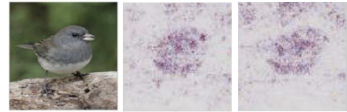
Figure 33.6: (Potential) perception issues: an explanation from a trained network (left) is visually indistinguishable to humans from one from an untrained network (right)—even if they are not exactly identical.

no importance and a clear pixel represents maximum importance), introducing the arbitrary artifact that black objects never appear important [Smi+17]. In addition, this binary mask is produced by clipping important pixels in a certain percentile (e.g., only taking 99↓th percentile), which can also introduce another artifact [Sun+19c]. The balancing act between artifacts introduced by visualization for the ease of understanding and faithfully representing the explanation remains a challenge.

Together, all of these points on human factors emphasize what we said from the start: we cannot divorce the study and practice of interpretable machine learning from its intended socio-technical context