Probabilistic Machine Learning: Advanced Topics

Chapter 7 ~ 19

Part II

Inference

7 Inference algorithms: an overview

7.1 Introduction

In the probabilistic approach to machine learning, all unknown quantities — be they predictions about the future, hidden states of a system, or parameters of a model — are treated as random variables, and endowed with probability distributions. The process of inference corresponds to computing the posterior distribution over these quantities, conditioning on whatever data is available.

In more detail, let ω represent the unknown variables, and D represent the known variables. Given a likelihood p(D|ω) and a prior p(ω), we can compute the posterior p(ω|D) using Bayes’ rule:

\[p(\boldsymbol{\theta}|\mathcal{D}) = \frac{p(\boldsymbol{\theta})p(\mathcal{D}|\boldsymbol{\theta})}{p(\mathcal{D})} \tag{7.1}\]

The main computational bottleneck is computing the normalization constant in the denominator, which requires solving the following high dimensional integral:

\[p(\mathcal{D}) = \int p(\mathcal{D}|\theta)p(\theta)d\theta \tag{7.2}\]

This is needed to convert the unnormalized joint probability of some parameter value, p(ω, D), to a normalized probability, p(ω|D), which takes into account all the other plausible values that ω could have.

Once we have the posterior, we can use it to compute posterior expectations of some function of the unknown variables, i.e.,

\[\mathbb{E}\left[g(\theta)|\mathcal{D}\right] = \int g(\theta)p(\theta|\mathcal{D})d\theta\tag{7.3}\]

By defining g in the appropriate way, we can compute many quantities of interest, such as the following:

\[\text{mean: } g(\theta) = \theta\]

\[\text{covariance: } g(\theta) = (\theta - \mathbb{E}\left[\theta | \mathcal{D}\right])(\theta - \mathbb{E}\left[\theta | \mathcal{D}\right])^{\mathsf{T}} \tag{7.5}\]

\[\text{marginals: } g(\theta) = p(\theta\_1 = \theta\_1^\* | \theta\_{2:D}) \tag{7.6}\]

\[\text{preactive: } g(\theta) = p(\mathbf{y}\_{N+1}|\theta) \tag{7.7}\]

\[\text{expected loss: } g(\theta) = \ell(\theta, a) \tag{7.8}\]

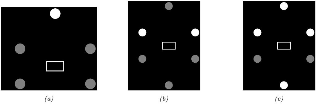
Figure 7.1: Graphical models with (a) global hidden variables for representing the Bayesian discriminative model p(y1:^N , ωy|x1:^N ) = p(ωy) !^{N n}=1 p(yn|xn; ωy); (b) local hidden variables for representing the generative model ^p(x1:^N , ^z1:^{N |}ω) = !^{N n}=1 p(zn|ωz)p(xn|zn, ωx); (c) local and global hidden variables for representing the Bayesian generative model p(x1:^N , z1:^N , ω) = p(ωz)p(ωx) !^{N n}=1 p(zn|ωz)p(xn|zn, ωx). Shaded nodes are assumed to be known (observed), unshaded nodes are hidden.

where yN+1 is the next observation after seeing the N examples in D, and the posterior expected loss is computing using loss function ε and action a (see Section 34.1.3). Finally, if we define g(ω) = p(D|ω, M) for model M, we can also phrase the marginal likelihood (Section 3.8.3) as an expectation wrt the prior:

\[\mathbb{E}\left[g(\theta)|M\right] = \int g(\theta)p(\theta|M)d\theta = \int p(\mathcal{D}|\theta,M)p(\theta|M)d\theta = p(\mathcal{D}|M) \tag{7.9}\]

Thus we see that integration (and computing expectations) is at the heart of Bayesian inference, whereas di!erentiation is at the heart of optimization.

In this chapter, we give a high level summary of algorithmic techniques for computing (approximate) posteriors, and/or their corresponding expectations. We will give more details in the following chapters. Note that most of these methods are independent of the specific model. This allows problem solvers to focus on creating the best model possible for the task, and then relying on some inference engine to do the rest of the work — this latter process is sometimes called “turning the Bayesian crank”. For more details on Bayesian computation, see e.g., [Gel+14a; MKL21; MFR20].

7.2 Common inference patterns

There are kinds of posterior we may want to compute, but we can identify 3 main patterns, as we discuss below. These give rise to di!erent types of inference algorithm, as we will see in later chapters.

7.2.1 Global latents

The first pattern arises when we need to perform inference in models which have global latent variables, such as parameters of a model ω, which are shared across all N observed training cases. This is shown in Figure 7.1a, and corresponds to the usual setting for supervised or discriminative

learning, where the joint distribution has the form

\[p(\mathbf{y}\_{1:N}, \boldsymbol{\theta} | \boldsymbol{x}\_{1:N}) = p(\boldsymbol{\theta}) \left[ \prod\_{n=1}^{N} p(\mathbf{y}\_n | \boldsymbol{x}\_n, \boldsymbol{\theta}) \right] \tag{7.10}\]

The goal is to compute the posterior p(ω|x1:^N , y1:^N ). Most of the Bayesian supervised learning models discussed in Part III follow this pattern.

7.2.2 Local latents

The second pattern arises when we need to perform inference in models which have local latent variables, such as hidden states z1:^N ; we assume the model parameters ω are known. This is shown in Figure 7.1b. Now the joint distribution has the form

\[p(\mathbf{z}\_{1:N}, \mathbf{z}\_{1:N} | \boldsymbol{\theta}) = \left[ \prod\_{n=1}^{N} p(\mathbf{z}\_n | \mathbf{z}\_n, \boldsymbol{\theta}\_x) p(\mathbf{z}\_n | \boldsymbol{\theta}\_z) \right] \tag{7.11}\]

The goal is to compute p(zn|xn, ω) for each n. This is the setting we consider for most of the PGM inference methods in Chapter 9.

If the parameters are not known (which is the case for most latent variable models, such as mixture models), we may choose to estimate them by some method (e.g., maximum likelihood), and then plug in this point estimate. The advantage of this approach is that, conditional on ω, all the latent variables are conditionally independent, so we can perform inference in parallel across the data. This lets us use methods such as expectation maximization (Section 6.5.3), in which we infer p(zn|xn, ωt) in the E step for all n simultaneously, and then update ω^t in the M step. If the inference of zⁿ cannot be done exactly, we can use variational inference, a combination known as variational EM (Section 6.5.6.1).

Alternatively, we can use a minibatch approximation to the likelihood, marginalizing out zⁿ for each example in the minibatch to get

\[\log p(\mathcal{D}\_t | \theta\_t) = \sum\_{n \in \mathcal{D}\_t} \log \left[ \sum\_{\mathbf{z}\_n} p(\mathbf{z}\_n, \mathbf{z}\_n | \theta\_t) \right] \tag{7.12}\]

where D^t is the minibatch at step t. If the marginalization cannot be done exactly, we can use variational inference, a combination known as stochastic variational inference or SVI (Section 10.1.4). We can also learn an inference network qω(z|x; ω) to perform the inference for us, rather than running an inference engine for each example n in each batch t; the cost of learning ε can be amortized across the batches. This is called amortized SVI (see Section 10.1.5).

7.2.3 Global and local latents

The third pattern arises when we need to perform inference in models which have local and global latent variables. This is shown in Figure 7.1c, and corresponds to the following joint distribution:

\[p(\mathbf{z}\_{1:N}, \mathbf{z}\_{1:N}, \boldsymbol{\theta}) = p(\boldsymbol{\theta}\_x) p(\boldsymbol{\theta}\_z) \left[ \prod\_{n=1}^N p(\mathbf{z}\_n | \mathbf{z}\_n, \boldsymbol{\theta}\_x) p(\mathbf{z}\_n | \boldsymbol{\theta}\_z) \right] \tag{7.13}\]

This is essentially a Bayesian version of the latent variable model in Figure 7.1b, where now we model uncertainty in both the local variables zⁿ and the shared global variables ω. This approach is less common in the ML community, since it is often assumed that the uncertainty in the parameters ω is negligible compared to the uncertainty in the local variables zn. The reason for this is that the parameters are “informed” by all N data cases, whereas each local latent zⁿ is only informed by a single datapoint, namely xn. Nevertheless, there are advantages to being “fully Bayesian”, and modeling uncertainty in both local and global variables. We will see some examples of this later in the book.

7.3 Exact inference algorithms

In some cases, we can perform example posterior inference in a tractable manner. In particular, if the prior is conjugate to the likelihood, the posterior will be analytically tractable. In general, this will be the case when the prior and likelihood are from the same exponential family (Section 2.4). In particular, if the unknown variables are represented by ω, then we assume

\[p(\boldsymbol{\theta}) \propto \exp(\boldsymbol{\lambda}\_0^\mathsf{T} \boldsymbol{\tau}(\boldsymbol{\theta})) \tag{7.14}\]

\[p(y\_i|\theta) \propto \exp(\tilde{\lambda}\_i(y\_i)^\mathsf{T}\mathcal{T}(\theta))\tag{7.15}\]

where T (ω) are the su”cient statistics, and ϑ are the natural parameters. We can then compute the posterior by just adding the natural parameters:

\[p(\boldsymbol{\theta}|\boldsymbol{y}\_{1:N}) = \exp(\boldsymbol{\lambda}\_{\*}^{\mathsf{T}}\mathcal{T}(\boldsymbol{\theta})) \tag{7.16}\]

\[ \lambda\_\* = \lambda\_0 + \sum\_{n=1}^N \bar{\lambda}\_n(y\_n) \tag{7.17} \]

See Section 3.4 for details.

Another setting where we can compute the posterior exactly arises when the D unknown variables are all discrete, each with K states; in this case, the integral for the normalizing constant becomes a sum with K^D terms. In many cases, K^D will be too large to be tractable. However, if the distribution satisfies certain conditional independence properties, as expressed by a probabilistic graphical model (PGM), then we can write the joint as a product of local terms (see Chapter 4). This lets us use dynamic programming to make the computation tractable (see Chapter 9).

7.4 Approximate inference algorithms

For most probability models, we will not be able to compute marginals or posteriors exactly, so we must resort to using approximate inference. There are many di!erent algorithms, which trade o! speed, accuracy, simplicity, and generality. We briefly discuss some of these algorithms below, and give more detail in the following chapters. (See also [Alq22; MFR20] for a review of various methods.)

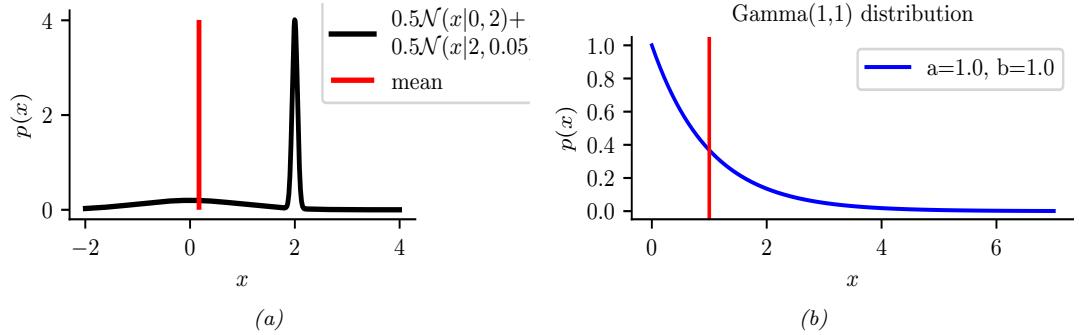
Figure 7.2: Two distributions in which the mode (highest point) is untypical of the distribution; the mean (vertical red line) is a better summary. (a) A bimodal distribution. Generated by bimodal\_dist\_plot.ipynb. (b) A skewed Ga(1, 1) distribution. Generated by gamma\_dist\_plot.ipynb.

7.4.1 The MAP approximation and its problems

The simplest approximate inference method is to compute the MAP estimate

\[\hat{\boldsymbol{\theta}} = \operatorname{argmax} p(\boldsymbol{\theta}|\mathcal{D}) = \operatorname{argmax} \log p(\boldsymbol{\theta}) + \log p(\mathcal{D}|\boldsymbol{\theta}) \tag{7.18}\]

and then to assume that the posterior puts 100% of its probability on this single value:

\[p(\boldsymbol{\theta}|\mathcal{D}) \approx \delta(\boldsymbol{\theta} - \hat{\boldsymbol{\theta}}) \tag{7.19}\]

The advantage of this approach is that we can compute the MAP estimate using a variety of optimization algorithms, which we discuss in Chapter 6. However, the MAP estimate also has various drawbacks, some of which we discuss below.

7.4.1.1 The MAP estimate gives no measure of uncertainty

In many statistical applications (especially in science) it is important to know how much one can trust a given parameter estimate. Obviously a point estimate does not convey any notion of uncertainty. Although it is possible to derive frequentist notions of uncertainty from a point estimate (see Section 3.3.1), it is arguably much more natural to just compute the posterior, from which we can derive useful quantities such as the standard error (see Section 3.2.1.6) and credible regions (see Section 3.2.1.7).

In the context of prediction (which is the main focus in machine learning), we saw in Section 3.2.2 that plugging in a point estimate can underestimate the predictive uncertainty, which can result in predictions which are not just wrong, but confidently wrong. It is generally considered very important for a predictive model to “know what it does not know”, and the Bayesian approach is a good strategy for achieving this goal.

7.4.1.2 The MAP estimate is often untypical of the posterior

In some cases, we may not be interested in uncertainty, and instead we just want a single summary of the posterior. However, the mode of a posterior distribution is often a very poor choice as a

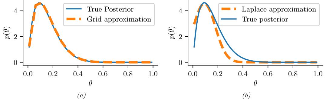
Figure 7.3: Approximating the posterior of a beta-Bernoulli model. (a) Grid approximation using 20 grid points. (b) Laplace approximation. Generated by laplace\_approx\_beta\_binom.ipynb.

summary statistic, since the mode is usually quite untypical of the distribution, unlike the mean or median. This is illustrated in Figure 7.2(a) for a 1d continuous space, where we see that the mode is an isolated peak (black line), far from most of the probability mass. By contrast, the mean (red line) is near the middle of the distribution.

Another example is shown in Figure 7.2(b): here the mode is 0, but the mean is non-zero. Such skewed distributions often arise when inferring variance parameters, especially in hierarchical models. In such cases the MAP estimate (and hence the MLE) is obviously a very bad estimate.

7.4.1.3 The MAP estimate is not invariant to reparameterization

A more subtle problem with MAP estimation is that the result we get depends on how we parameterize the probability distribution, which is not very desirable. For example, when representing a Bernoulli distribution, we should be able to parameterize it in terms of probability of success, or in terms of the log-odds (logit), without that a!ecting our beliefs.

For example, let xˆ = argmax^x px(x) be the MAP estimate for x. Now let y = f(x) be a transformation of x. In general it is not the case that yˆ = argmax^y py(y) is given by f(xˆ). For example, let ^{x ↔︎ N} (6, 1) and ^{y = f}(x), where ^f(x) = ¹ 1+exp(↓x+5) . We can use the change of variables (Section 2.5.1) to conclude ^py(y) = ^px(^{f ↓}1(y))^| df→1(y) dy |. Alternatively we can use a Monte Carlo approximation. The result is shown in Figure 2.12. We see that the original Gaussian for p(x) has become “squashed” by the sigmoid nonlinearity. In particular, we see that the mode of the transformed distribution is not equal to the transform of the original mode.

We have seen that the MAP estimate depends on the parameterization. The MLE does not su!er from this since the likelihood is a function, not a probability density. Bayesian inference does not su!er from this problem either, since the change of measure is taken into account when integrating over the parameter space.

7.4.2 Grid approximation

If we want to capture uncertainty, we need to allow for the fact that ω may have a range of possible values, each with non-zero probability. The simplest way to capture this property is to partition the

space of possible values into a finite set of regions, call them r1,…, rK, each representing a region of parameter space of volume ! centered on ωk. This is called a grid approximation. The probability of being in each region is given by p(ω ↗ rk|D) ↓ pk!, where

\[p\_k = \frac{\tilde{p}\_k}{\sum\_{k'=1}^K \tilde{p}\_{k'}} \tag{7.20}\]

\[ \bar{p}\_k = p(\mathcal{D}|\boldsymbol{\theta}\_k)p(\boldsymbol{\theta}\_k) \tag{7.21} \]

As K increases, we decrease the size of each grid cell. Thus the denominator is just a simple numerical approximation of the integral

\[p(\mathcal{D}) = \int p(\mathcal{D}|\theta)p(\theta)d\theta \approx \sum\_{k=1}^{K} \Delta \bar{p}\_k \tag{7.22}\]

As a simple example, we will use the problem of approximating the posterior of a beta-Bernoulli model. Specifically, the goal is to approximate

\[p(\theta|\mathcal{D}) \propto \left[ \prod\_{n=1}^{N} \text{Ber}(y\_n|\theta) \right] \text{Beta}(1, 1) \tag{7.23}\]

where D consists of 10 heads and 1 tail (so the total number of observations is N = 11), with a uniform prior. Although we can compute this posterior exactly using the method discussed in Section 3.4.1, this serves as a useful pedagogical example since we can compare the approximation to the exact answer. Also, since the target distribution is just 1d, it is easy to visualize the results.

In Figure 7.3a, we illustrate the grid approximation applied to our 1d problem. We see that it is easily able to capture the skewed posterior (due to the use of an imbalanced sample of 10 heads and 1 tail). Unfortunately, this approach does not scale to problems in more than 2 or 3 dimensions, because the number of grid points grows exponentially with the number of dimensions.

7.4.3 Laplace (quadratic) approximation

In this section, we discuss a simple way to approximate the posterior using a multivariate Gaussian; this known as a Laplace approximation or quadratic approximation (see e.g., [TK86; RMC09]).

Suppose we write the posterior as follows:

\[p(\boldsymbol{\theta}|\mathcal{D}) = \frac{1}{Z}e^{-\mathcal{E}(\boldsymbol{\theta})} \tag{7.24}\]

where E(ω) = → log p(ω, D) is called an energy function, and Z = p(D) is the normalization constant. Performing a Taylor series expansion around the mode ωˆ (i.e., the lowest energy state) we get

\[\mathcal{E}(\boldsymbol{\theta}) \approx \mathcal{E}(\hat{\boldsymbol{\theta}}) + (\boldsymbol{\theta} - \hat{\boldsymbol{\theta}})^{\mathsf{T}} \boldsymbol{g} + \frac{1}{2} (\boldsymbol{\theta} - \hat{\boldsymbol{\theta}})^{\mathsf{T}} \mathbf{H} (\boldsymbol{\theta} - \hat{\boldsymbol{\theta}}) \tag{7.25}\]

where g is the gradient at the mode, and H is the Hessian. Since ωˆ is the mode, the gradient term is

zero. Hence

\[\hat{p}(\boldsymbol{\theta}, \mathcal{D}) = e^{-\mathcal{E}(\boldsymbol{\theta})} \exp\left[ -\frac{1}{2} (\boldsymbol{\theta} - \hat{\boldsymbol{\theta}})^{\mathsf{T}} \mathbf{H}(\boldsymbol{\theta} - \hat{\boldsymbol{\theta}}) \right] \tag{7.26}\]

\[\hat{p}(\boldsymbol{\theta}|\mathcal{D}) = \frac{1}{Z}\hat{p}(\boldsymbol{\theta}, \mathcal{D}) = \mathcal{N}(\boldsymbol{\theta}|\boldsymbol{\theta}, \mathbf{H}^{-1})\tag{7.27}\]

\[Z = e^{-\mathcal{E}(\dot{\hat{\theta}})} (2\pi)^{D/2} |\mathbf{H}|^{-\frac{1}{2}} \tag{7.28}\]

The last line follows from normalization constant of the multivariate Gaussian.

The Laplace approximation is easy to apply, since we can leverage existing optimization algorithms to compute the MAP estimate, and then we just have to compute the Hessian at the mode. (In high dimensional spaces, we can use a diagonal approximation.)

In Figure 7.3b, we illustrate this method applied to our 1d problem. Unfortunately we see that it is not a particularly good approximation. This is because the posterior is skewed, whereas a Gaussian is symmetric. In addition, the parameter of interest lies in the constrained interval ω ↗ [0, 1], whereas the Gaussian assumes an unconstrained space, ^ω ↗ ^RD. Fortunately, we can solve this latter problem by using a change of variable. For example, in this case we can apply the Laplace approximation to ϱ = logit(ω). This is a common trick to simplify the job of inference.

See Section 15.3.5 for an application of Laplace approximation to Bayesian logistic regression, Section 17.3.2 for an application of Laplace approximation to Bayesian neural networks, and Section 4.3.5.3 for an application to Gaussian Markov random fields.

7.4.4 Variational inference

In Section 7.4.3, we discussed the Laplace approximation, which uses an optimization procedure to find the MAP estimate, and then approximates the curvature of the posterior at that point based on the Hessian. In this section, we discuss variational inference (VI), also called variational Bayes (VB). This is another optimization-based approach to posterior inference, but which has much more modeling flexibility (and thus can give a much more accurate approximation).

VI attempts to approximate an intractable probability distribution, such as p(ω|D), with one that is tractable, q(ω), so as to minimize some discrepancy D between the distributions:

\[q^\* = \operatorname\*{argmin}\_{q \in \mathcal{Q}} D(q, p) \tag{7.29}\]

where Q is some tractable family of distributions (e.g., fully factorized distributions). Rather than optimizing over functions q, we typically optimize over the parameters of the function q; we denote these variational parameters by ϖ.

It is common to use the KL divergence (Section 5.1) as the discrepancy measure, which is given by

\[D(q, p) = D\_{\mathbb{KL}}\left(q(\boldsymbol{\theta}|\boldsymbol{\psi}) \parallel p(\boldsymbol{\theta}|\mathcal{D})\right) = \int q(\boldsymbol{\theta}|\boldsymbol{\psi}) \log \frac{q(\boldsymbol{\theta}|\boldsymbol{\psi})}{p(\boldsymbol{\theta}|\mathcal{D})} d\boldsymbol{\theta} \tag{7.30}\]

where p(ω|D) = p(D|ω)p(ω)/p(D). The inference problem then reduces to the following optimization

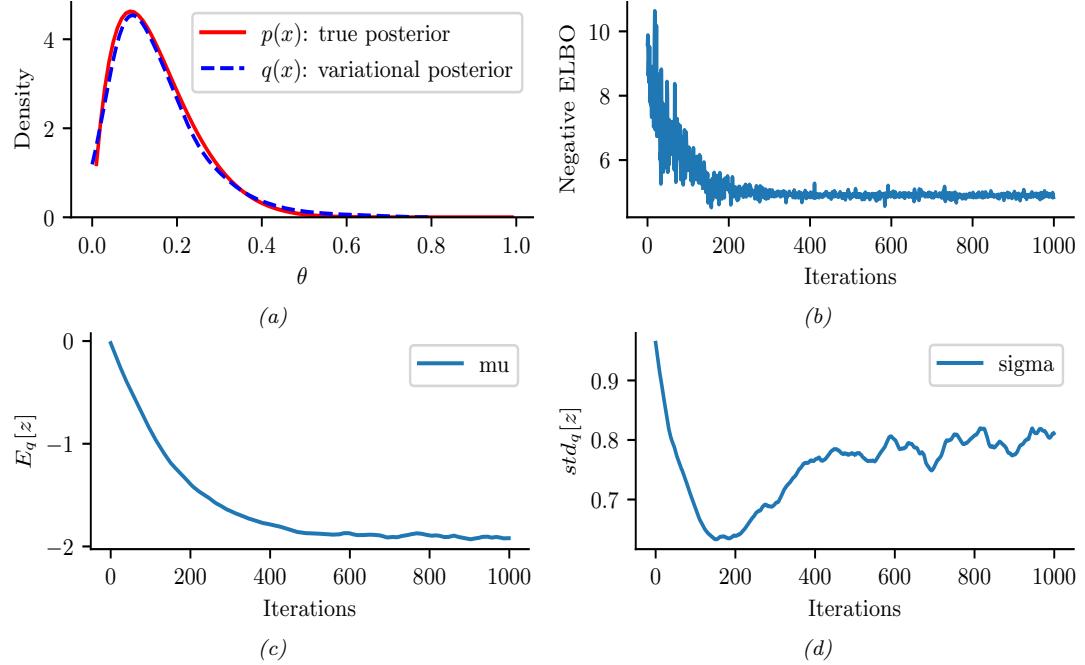
Figure 7.4: ADVI applied to the beta-Bernoulli model. (a) Approximate vs true posterior. (b) Negative ELBO over time. (c) Variational µ parameter over time. (d) Variational ω parameter over time. Generated by advi\_beta\_binom.ipynb.

problem:

\[\psi^\* = \operatorname\*{argmin}\_{\psi} D\_{\text{KL}}\left(q(\theta|\psi) \parallel p(\theta|\mathcal{D})\right) \tag{7.31}\]

\[\mathbb{E}\_{\theta} = \operatorname\*{argmin}\_{\boldsymbol{\Psi}} \mathbb{E}\_{q(\boldsymbol{\theta}|\boldsymbol{\Psi})} \left[ \log q(\boldsymbol{\theta}|\boldsymbol{\psi}) - \log \left( \frac{p(\mathcal{D}|\boldsymbol{\theta})p(\boldsymbol{\theta})}{p(\mathcal{D})} \right) \right] \tag{7.32}\]

\[\Psi = \operatorname\*{argmin}\_{\boldsymbol{\Psi}} \underbrace{\mathbb{E}\_{q(\boldsymbol{\theta}|\boldsymbol{\Psi})} \left[ -\log p(\mathcal{D}|\boldsymbol{\theta}) - \log p(\boldsymbol{\theta}) + \log q(\boldsymbol{\theta}|\boldsymbol{\psi}) \right]}\_{-L(\boldsymbol{\psi})} + \log p(\mathcal{D}) \tag{7.33}\]

Note that log p(D) is independent of ϖ, so we can ignore it when fitting the approximate posterior, and just focus on maximizing the term

\[\mathbb{E}(\psi) \stackrel{\Delta}{=} \mathbb{E}\_{q(\boldsymbol{\theta}|\boldsymbol{\psi})} \left[ \log p(\mathcal{D}|\boldsymbol{\theta}) + \log p(\boldsymbol{\theta}) - \log q(\boldsymbol{\theta}|\boldsymbol{\psi}) \right] \tag{7.34}\]

Since we have DKL (q ↘ p) ≃ 0, we have #(ϖ) ⇐ log p(D). The quantity log p(D), which is the log marginal likelihood, is also called the evidence. Hence #(ϖ) is known as the evidence lower bound or ELBO. By maximizing this bound, we are making the variational posterior closer to the true posterior. (See Section 10.1 for details.)

We can choose any kind of approximate posterior that we like. For example, we may use a Gaussian, q(ω|ϖ) = N (ω|µ, !). This is di!erent from the Laplace approximation, since in VI, we optimize

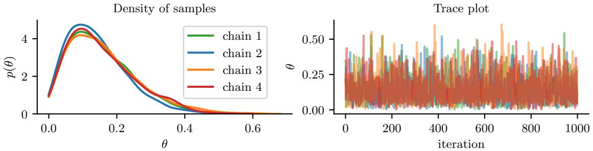
Figure 7.5: Approximating the posterior of a beta-Bernoulli model using MCMC. (a) Kernel density estimate derived from samples from 4 independent chains. (b) Trace plot of the chains as they generate posterior samples. Generated by hmc\_beta\_binom.ipynb.

!, rather than equating it to the Hessian. If ! is diagonal, we are assuming the posterior is fully factorized; this is called a mean field approximation.

A Gaussian approximation is not always suitable for all parameters. For example, in our 1d example we have the constraint that ω ↗ [0, 1]. We could use a variational approximation of the form q(ω|ϖ) = Beta(ω|a, b), where ϖ = (a, b). However choosing a suitable form of variational distribution requires some level of expertise. To create a more easily applicable, or “turn-key”, method, that works on a wide range of models, we can use a method called automatic di!erentiation variational inference or ADVI [Kuc+16]. This uses the change of variables method to convert the parameters to an unconstrained form, and then computes a Gaussian variational approximation. The method also uses automatic di!erentiation to derive the Jacobian term needed to compute the density of the transformed variables. See Section 10.2.2 for details.

We now apply ADVI to our 1d beta-Bernoulli model. Let ω = ς(z), where we replace p(ω|D) with q(z|ϖ) = N (z|µ, ς), where ϖ = (µ, ς). We optimize a stochastic approximation to the ELBO using SGD. The results are shown in Figure 7.4 and seem reasonable.

7.4.5 Markov chain Monte Carlo (MCMC)

Although VI is fast, it can give a biased approximation to the posterior, since it is restricted to a specific function form q ↗ Q. A more flexible approach is to use a non-parametric approximation in terms of a set of samples, ^q(ω) ^{↓ 1} S &^{S s}=1 ^ϑ(^{ω → ωs}). This is called a Monte Carlo approximation. The key issue is how to create the posterior samples ^{ωs ↔︎ p}(ω|D) e”ciently, without having to evaluate the normalization constant ^p(D) = / ^p(ω, ^D)dω.

For low dimensional problems, we can use methods such as importance sampling, which we discuss in Section 11.5. However, for high dimensional problems, it is more common to use Markov chain Monte Carlo or MCMC. We give the details in Chapter 12, but give a brief introduction here.

The most common kind of MCMC is known as the Metropolis-Hastings algorithm. The basic idea behind MH is as follows: we start at a random point in parameter space, and then perform a random walk, by sampling new states (parameters) from a proposal distribution q(ω^↔︎ |ω). If q is chosen carefully, the resulting Markov chain distribution will satisfy the property that the fraction of

time we visit each point in space is proportional to the posterior probability. The key point is that to decide whether to move to a newly proposed point ω^↔︎ or to stay in the current point ω, we only need to evaluate the unnormalized density ratio

\[\frac{p(\boldsymbol{\theta}|\mathcal{D})}{p(\boldsymbol{\theta}'|\mathcal{D})} = \frac{p(\mathcal{D}|\boldsymbol{\theta})p(\boldsymbol{\theta})/p(\mathcal{D})}{p(\mathcal{D}|\boldsymbol{\theta}')p(\boldsymbol{\theta}')/p(\mathcal{D})} = \frac{p(\mathcal{D},\boldsymbol{\theta})}{p(\mathcal{D},\boldsymbol{\theta}')}\tag{7.35}\]

This avoids the need to compute the normalization constant p(D). (In practice we usually work with log probabilities, instead of joint probabilities, to avoid numerical issues.)

We see that the input to the algorithm is just a function that computes the log joint density, log p(ω, D), as well as a proposal distribution q(ω^↔︎ |ω) for deciding which states to visit next. It is common to use a Gaussian distribution for the proposal, q(ω^↔︎ |ω) = N (ω^↔︎ |ω, ςI); this is called the random walk Metropolis algorithm. However, this can be very ine”cient, since it is blindly walking through the space, in the hopes of finding higher probability regions.

In models that have conditional independence structure, it is often easy to compute the full conditionals p(ωd|ω↓^d, D) for each variable d, one at a time, and then sample from them. This is like a stochastic analog of coordinate ascent, and is called Gibbs sampling (see Section 12.3 for details).

For models where all unknown variables are continuous, we can often compute the gradient of the log joint, ⇒^ε log p(ω, D). We can use this gradient information to guide the proposals into regions of space with higher probability. This approach is called Hamiltonian Monte Carlo or HMC, and is one of the most widely used MCMC algorithms due to its speed. For details, see Section 12.5.

We apply HMC to our beta-Bernoulli model in Figure 7.5. (We use a logit transformation for the parameter.) In panel b, we show samples generated by the algorithm from 4 parallel Markov chains. We see that they oscillate around the true posterior, as desired. In panel a, we compute a kernel density estimate from the posterior samples from each chain; we see that the result is a good approximation to the true posterior in Figure 7.3.

7.4.6 Sequential Monte Carlo

MCMC is like a stochastic local search algorithm, in that it makes moves through the state space of the posterior distribution, comparing the current value to proposed neighboring values. An alternative approach is to use perform inference using a sequence of di!erent distributions, from simpler to more complex, with the final distribution being equal to the target posterior. This is called sequential Monte Carlo or SMC. This approach, which is more similar to tree search than local search, has various advantages over MCMC, which we discuss in Chapter 13.

A common application of SMC is to sequential Bayesian inference, in which we recursively compute (i.e., in an online fashion) the posterior p(ωt|D1:t), where D1:^t = {(xn, yn) : n =1: t} is all the data we have seen so far. This sequence of distributions converges to the full batch posterior p(ω|D) once all the data has been seen. However, the approach can also be used when the data is arriving in a continual, unending stream, as in state-space models (see Chapter 29). The application of SMC to such dynamical models is known as particle filtering. See Section 13.2 for details.

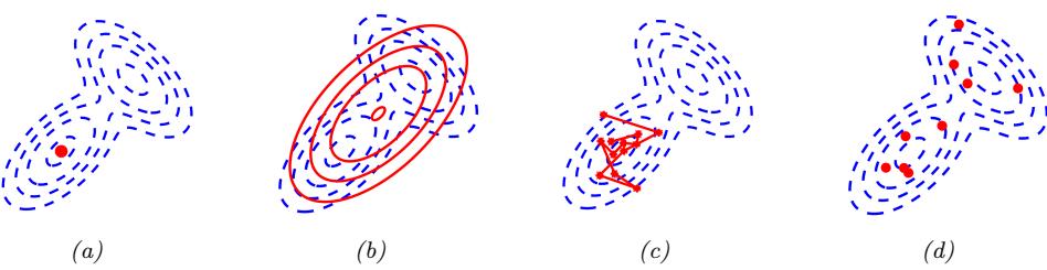
Figure 7.6: Di!erent approximations to a bimodal 2d distribution. (a) Local MAP estimate. (b) Parametric Gaussian approximation. (c) Correlated samples from near one mode. (d) Independent samples from the distribution. Adapted from Figure 2 of [PY14]. Used with kind permission of George Panadreou.

7.4.7 Challenging posteriors

In many applications, the posterior can be high dimensional and multimodal. Approximating such distributions can be quite challenging. In Figure 7.6, we give a simple 2d example. We compare MAP estimation (which does not capture any uncertainty), a Gaussian parametric approximation such as the Laplace approximation or variational inference (see panel b), and a nonparametric approximation in terms of samples. If the samples are generated from MCMC, they are serially correlated, and may only explore a local model (see panel c). However, ideally we can draw independent samples from the entire support of the distribution, as shown in panel d. We may also be able to fit a local parametric approximation around each such sample (see Section 17.3.9.1), to get a semi-parametric approximation to the posterior.

7.5 Evaluating approximate inference algorithms

There are many di!erent approximate inference algorithms, each of which make di!erent tradeo!s between speed, accuracy, generality, simplicity, etc. This makes it hard to compare them on an equal footing.

One approach is to evaluate the accuracy of the approximation q(ω) by comparing to the “true” posterior p(ω|D), computed o$ine with an “exact” method. We are usually interested in accuracy vs speed tradeo!s, which we can compute by evaluating DKL (p(ω|D) ↘ qt(ω)), where qt(ω) is the approximate posterior after t units of compute time. Of course, we could use other measures of distributional similarity, such as Wasserstein distance.

Unfortunately, it is usually impossible to compute the true posterior p(ω|D). A simple alternative is to evaluate the quality in terms of its prediction abilities on out of sample observed data, similar to cross validation. More generally, we can compare the expected loss or Bayesian risk (Section 34.1.3) of di!erent posteriors, as proposed in [KPS98; KPS99]:

\[R = \mathbb{E}\_{p^\*(x,y)}\left[\ell(y, q(y|x, \mathcal{D}))\right] \text{ where } q(y|x, \mathcal{D}) = \int p(y|x, \theta)q(\theta|\mathcal{D})d\theta \tag{7.36}\]

where ε(y, q(y)) is some loss function, such as log-loss. Alternatively, we can measure performance of the posterior when it is used in some downstream task, such as continual or active learning, as proposed in [Far22].

For some specialized methods for assessing variational inference, see [Yao+18b; Hug+20], and for Monte Carlo methods, see [CGR06; CTM17; GAR16].

8 Gaussian filtering and smoothing

8.1 Introduction

In this chapter, we consider the task of posterior inference in state-space models (SSMs). We discuss SSMs in more detail in Chapter 29, but we can think of them as latent variable sequence models with the conditional independencies shown by the chain-structured graphical model Figure 8.1. The corresponding joint distribution has the form

\[p(\mathbf{y}\_{1:T}, \mathbf{z}\_{1:T} | \mathbf{u}\_{1:T}) = \left[ p(\mathbf{z}\_1 | \mathbf{u}\_1) \prod\_{t=2}^{T} p(\mathbf{z}\_t | \mathbf{z}\_{t-1}, \mathbf{u}\_t) \right] \left[ \prod\_{t=1}^{T} p(\mathbf{y}\_t | \mathbf{z}\_t, \mathbf{u}\_t) \right] \tag{8.1}\]

where z^t are the hidden variables at time t, y^t are the observations (outputs), and u^t are the optional inputs. The term p(zt|z^t↓¹,ut) is called the dynamics model or transition model, p(yt|zt,ut) is called the observation model or measurement model, and p(z1|u1) is the prior or initial state distribution.1

8.1.1 Inferential goals

Given the sequence of observations, and a known model, one of the main tasks with SSMs is to perform posterior inference about the hidden states; this is also called state estimation.

For example, consider an airplane flying in the sky. (For simplicity, we assume the world is 2d, not 3d.) We would like to estimate its location and velocity ^zt ↗ ^R4 given noisy sensor measurements of its location ^yt ↗ ^R2, as illustrated in Figure 8.2(a). (We ignore the inputs ^ut for simplicity.)

We discuss a suitable SSM for this problem, that embodies Newton’s laws of motion, in Section 8.2.1.1. We can use the model to compute the belief state p(zt|y1:t); this is called Bayesian filtering. If we represent the belief state using a Gaussian, then we can use the Kalman filter to solve this task, as we discuss in Section 8.2.2. In Figure 8.2(b) we show the results of this algorithm. The green dots are the noisy observations, the red line shows the posterior mean estimate of the location, and the black circles show the posterior covariance. (The posterior over the velocity is not shown.) We see that the estimated trajectory is less noisy than the raw data, since it incorporates prior knowledge about how the data was generated.

Another task of interest is the smoothing problem where we want to compute p(zt|y1:^T ) using an o$ine dataset. We can compute these quantities using the Kalman smoother described in

^1. In some cases, the initial state distribution is denoted by p(z0), and then we derive p(z1|u1) by passing p(z0) through the dynamics model. In this case, the joint distribution represents p(y1:^T , z0:^T |u1:^T ).

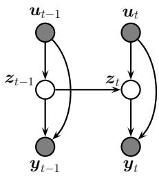
Figure 8.1: A state-space model represented as a graphical model. z^t are the hidden variables at time t, y^t are the observations (outputs), and u^t are the optional inputs.

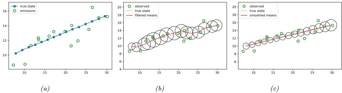
Figure 8.2: Illustration of Kalman filtering and smoothing for a linear dynamical system. (a) Observations (green cirles) are generated by an object moving to the right (true location denoted by blue squares). (b) Results of online Kalman filtering. Circles are 95% confidence ellipses, whose center is the posterior mean, and whose shape is derived from the posterior covariance. (c) Same as (b), but using o”ine Kalman smoothing. The MSE in the trajectory for filtering is 3.13, and for smoothing is 1.71. Generated by kf\_tracking\_script.ipynb.

Section 8.2.3. In Figure 8.2(c) we show the result of this algorithm. We see that the resulting estimate is smoother compared to filtering, and that the posterior uncertainty is reduced (as visualized by the smaller confidence ellipses).

To understand this behavior intuitively, consider a detective trying to figure out who committed a crime. As they move through the crime scene, their uncertainty is high until he finds the key clue; then they have an “aha” moment, the uncertainty is reduced, and all the previously confusing observations are, in hindsight, easy to explain. Thus we see that, given all the data (including finding the clue), it is much easier to infer the state of the world.

A disadvantage of the smoothing method is that we have to wait until all the data has been observed before we start performing inference, so it cannot be used for online or realtime problems. Fixed lag smoothing is a useful compromise between online and o$ine estimation; it involves computing p(z^t↓^ω|y1:t), where ε > 0 is called the lag. This gives better performance than filtering, but incurs a slight delay. By changing the size of the lag, we can trade o! accuracy vs delay. See Figure 8.3 for an illustration.

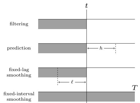
Figure 8.3: The main kinds of inference for state-space models. The shaded region is the interval for which we have data. The arrow represents the time step at which we want to perform inference. t is the current time, T is the sequence length, ε is the lag, and h is the prediction horizon. Used with kind permission of Peter Chang.

In addition to infering the latent state, we may want to predict future observations. We can compute the observed predictive distribution h steps into the future as follows:

\[p(\mathbf{y}\_{t+h}|\mathbf{y}\_{1:t}) = \sum\_{\mathbf{z}\_{t+h}} p(\mathbf{y}\_{t+h}|\mathbf{z}\_{t+h}) p(\mathbf{z}\_{t+h}|\mathbf{y}\_{1:t}) \tag{8.2}\]

where the hidden state predictive distribution is obtained by pushing the current belief state through the dynamics model

\[p(\mathbf{z}\_{t+h}|\mathbf{y}\_{1:t}) = \sum\_{\mathbf{z}\_{t:t+h-1}} p(\mathbf{z}\_t|\mathbf{y}\_{1:t}) p(\mathbf{z}\_{t+1}|\mathbf{z}\_t) p(\mathbf{z}\_{t+2}|\mathbf{z}\_{t+1}) \cdots p(\mathbf{z}\_{t+h}|\mathbf{z}\_{t+h-1}) \tag{8.3}\]

(When the states are continuous, we need to replace the sums with integrals.)

8.1.2 Bayesian filtering equations

The Bayes filter is an algorithm for recursively computing the belief state p(zt|y1:t) given the prior belief from the previous step, p(z^t↓¹|y1:t↓1), the new observation yt, and the model. This can be done using sequential Bayesian updating, and requires a constant amount of computation per time step (independent of t). For a dynamical model, this reduces to the predict-update cycle described below.

The prediction step is just the Chapman-Kolmogorov equation:

\[p(\mathbf{z}\_t|\mathbf{y}\_{1:t-1}) = \int p(\mathbf{z}\_t|\mathbf{z}\_{t-1}) p(\mathbf{z}\_{t-1}|\mathbf{y}\_{1:t-1}) d\mathbf{z}\_{t-1} \tag{8.4}\]

The prediction step computes the one-step-ahead predictive distribution for the latent state, which

updates the posterior from the previous time step into the prior for the current step.2

The update step is just Bayes’ rule:

\[p(\mathbf{z}\_t|\mathbf{y}\_{1:t}) = \frac{1}{Z\_t} p(\mathbf{y}\_t|\mathbf{z}\_t) p(\mathbf{z}\_t|\mathbf{y}\_{1:t-1}) \tag{8.5}\]

where the normalization constant is

\[Z\_t = \int p(y\_t|\mathbf{z}\_t) p(\mathbf{z}\_t|\mathbf{y}\_{1:t-1}) d\mathbf{z}\_t = p(y\_t|\mathbf{y}\_{1:t-1}) \tag{8.6}\]

We can use the normalization constants to compute the log likelihood of the sequence as follows:

\[\log p(\mathbf{y}\_{1:T}) = \sum\_{t=1}^{T} \log p(\mathbf{y}\_t | \mathbf{y}\_{1:t-1}) = \sum\_{t=1}^{T} \log Z\_t \tag{8.7}\]

where we define p(y1|y0) = p(y1). This quantity is useful for computing the MLE of the parameters.

8.1.3 Bayesian smoothing equations

In the o$ine setting, we want to compute p(zt|y1:^T ), which is the belief about the hidden state at time t given all the data, both past and future. This is called (fixed interval) smoothing. We first perform the forwards or filtering pass, and then compute the smoothed belief states by working backwards, from right (time t = T) to left (t = 1), as we explain below. Hence this method is also called forwards filtering backwards smoothing or FFBS.

Suppose, by induction, that we have already computed p(zt+1|y1:^T ). We can convert this into a joint smoothed distribution over two consecutive time steps using

\[p(\mathbf{z}\_t, \mathbf{z}\_{t+1} | y\_{1:T}) = p(\mathbf{z}\_t | \mathbf{z}\_{t+1}, y\_{1:T}) p(\mathbf{z}\_{t+1} | y\_{1:T}) \tag{8.8}\]

To derive the first term, note that from the Markov properties of the model, and Bayes’ rule, we have

\[p(\mathbf{z}\_t | \mathbf{z}\_{t+1}, \mathbf{y}\_{1:T}) = p(\mathbf{z}\_t | \mathbf{z}\_{t+1}, \mathbf{y}\_{1:t}, \mathbf{y}\_{t+T:T}) \tag{8.9}\]

\[\mathbf{y} = \frac{p(\mathbf{z}\_t, \mathbf{z}\_{t+1} | \mathbf{y}\_{1:t})}{p(\mathbf{z}\_{t+1} | \mathbf{y}\_{1:t})} \tag{8.10}\]

\[\dot{\mathbf{y}} = \frac{p(\mathbf{z}\_{t+1}|\mathbf{z}\_t)p(\mathbf{z}\_t|\mathbf{y}\_{1:t})}{p(\mathbf{z}\_{t+1}|\mathbf{y}\_{1:t})} \tag{8.11}\]

Thus the joint distribution over two consecutive time steps is given by

\[p(\mathbf{z}\_t, \mathbf{z}\_{t+1} | y\_{1:T}) = p(\mathbf{z}\_t | \mathbf{z}\_{t+1}, y\_{1:t}) p(\mathbf{z}\_{t+1} | y\_{1:T}) = \frac{p(\mathbf{z}\_{t+1} | \mathbf{z}\_t) p(\mathbf{z}\_t | y\_{1:t}) p(\mathbf{z}\_{t+1} | y\_{1:T})}{p(\mathbf{z}\_{t+1} | y\_{1:t})} \tag{8.12}\]

^2. The prediction step is not needed at t = 1 if p(z1) is provided as input to the model. However, if we just provide p(z0), we need to compute p(z1|y1:0) = p(z1) by applying the prediction step.

from which we get the new smoothed marginal distribution:

\[p(\mathbf{z}\_t|\mathbf{y}\_{1:T}) = p(\mathbf{z}\_t|\mathbf{y}\_{1:t}) \int \left[ \frac{p(\mathbf{z}\_{t+1}|\mathbf{z}\_t)p(\mathbf{z}\_{t+1}|\mathbf{y}\_{1:T})}{p(\mathbf{z}\_{t+1}|\mathbf{y}\_{1:t})} \right] d\mathbf{z}\_{t+1} \tag{8.13}\]

\[=\int p(\mathbf{z}\_t, \mathbf{z}\_{t+1}|\mathbf{y}\_{1:t}) \frac{p(\mathbf{z}\_{t+1}|\mathbf{y}\_{1:T})}{p(\mathbf{z}\_{t+1}|\mathbf{y}\_{1:t})} d\mathbf{z}\_{t+1} \tag{8.14}\]

Intuitively we can interpret this as follows: we start with the two-slice filtered distribution, p(zt, zt+1|y1:t), and then we divide out the old p(zt+1|y1:t) and multiply in the new p(zt+1|y1:^T ), and then marginalize out zt+1.

8.1.4 The Gaussian ansatz

In general, computing the integrals required to implement Bayesian filtering and smoothing is intractable. However, there are two notable exceptions: if the state space is discrete, as in an HMM, we can represent the belief states as discrete distributions (histograms), which we can update using the forwards-backwards algorithm, as discussed in Section 9.2; and if the SSM is a linear-Gaussian model, then we can represent the belief states by Gaussians, which we can update using the Kalman filter and smoother, which we discuss in Section 8.2.2 and Section 8.2.3. In the nonlinear and/or non-Gaussian setting, we can still use a Gaussian to represent an approximate belief state, as we discuss in Section 8.3, Section 8.4, Section 8.5 and Section 8.6. We discuss some non-Gaussian approximations in Section 8.7.

For most of this chapter, we assume the SSM can be written as a nonlinear model subject to additive Gaussian noise:

\[\begin{aligned} z\_t &= f(z\_{t-1}, u\_t) + \mathcal{N}(\mathbf{0}, \mathbf{Q}\_t) \\ y\_t &= h(z\_t, u\_t) + \mathcal{N}(\mathbf{0}, \mathbf{R}\_t) \end{aligned} \tag{8.15}\]

where f is the transition or dynamics function, and h is the observation function. In some cases, we will further assume that these functions are linear.

8.2 Inference for linear-Gaussian SSMs

In this section, we discuss inference in SSMs where all the distributions are linear Gaussian. This is called a linear Gaussian state space model (LG-SSM) or a linear dynamical system (LDS). We discuss such models in detail in Section 29.6, but in brief they have the following form:

\[p(\mathbf{z}\_t | \mathbf{z}\_{t-1}, \mathbf{u}\_t) = \mathcal{N}(\mathbf{z}\_t | \mathbf{F}\_t \mathbf{z}\_{t-1} + \mathbf{B}\_t \mathbf{u}\_t + \mathbf{b}\_t, \mathbf{Q}\_t) \tag{8.16}\]

\[p(y\_t|\mathbf{z}\_t, \mathbf{u}\_t) = \mathcal{N}(y\_t|\mathbf{H}\_t\mathbf{z}\_t + \mathbf{D}\_t\mathbf{u}\_t + \mathbf{d}\_t, \mathbf{R}\_t) \tag{8.17}\]

where ^zt ↗ ^RNz is the hidden state, ^yt ↗ ^RNy is the observation, and ^ut ↗ ^RNu is the input. (We have allowed the parameters to be time-varying, for later extensions that we will consider.) We often assume the means of the process noise and observation noise (i.e., the bias or o!set terms) are zero, so b^t = 0 and d^t = 0. In addition, we often have no inputs, so B^t = D^t = 0. In this case, the model

simplifies to the following:3

\[p(\mathbf{z}\_t|\mathbf{z}\_{t-1}) = \mathcal{N}(\mathbf{z}\_t|\mathbf{F}\_t\mathbf{z}\_{t-1}, \mathbf{Q}\_t) \tag{8.18}\]

\[p(y\_t|\mathbf{z}\_t) = \mathcal{N}(y\_t|\mathbf{H}\_t\mathbf{z}\_t, \mathbf{R}\_t) \tag{8.19}\]

See Figure 8.1 for the graphical model.4

Note that an LG-SSM is just a special case of a Gaussian Bayes net (Section 4.2.3), so the entire joint distribution p(y1:^T , z1:^T |u1:^T ) is a large multivariate Gaussian with NyNzT dimensions. However, it has a special structure that makes it computationally tractable to use, as we show below. In particular, we will discuss the Kalman filter and Kalman smoother, that can perform exact filtering and smoothing in O(T N^{3 z} ) time.

8.2.1 Examples

Before diving into the theory, we give some motivating examples.

8.2.1.1 Tracking and state estimation

A common application of LG-SSMs is for tracking objects, such as airplanes or animals, from noisy measurements, such as radar or cameras. For example, suppose we want to track an object moving in 2d. (We discuss this example in more detail in Section 29.7.1.) The hidden state z^t encodes the location, (xt1, xt2), and the velocity, (x˙ ^t1, x˙ ^t1), of the moving object. The observation y^t is a noisy version of the location. (The velocity is not observed but can be inferred from the change in location.) We assume that we obtain measurements with a sampling period of !. The new location is the old location plus ! times the velocity, plus noise added to all terms:

\[\mathbf{z}\_{t} = \underbrace{\begin{pmatrix} 1 & 0 & \Delta & 0 \\ 0 & 1 & 0 & \Delta \\ 0 & 0 & 1 & 0 \\ 0 & 0 & 0 & 1 \end{pmatrix}}\_{\mathbf{F}} \mathbf{z}\_{t-1} + \mathbf{q}\_{t} \tag{8.20}\]

where q^t ↔︎ N (0, Qt). The observation extracts the location and adds noise:

\[\mathbf{y}\_t = \underbrace{\begin{pmatrix} 1 & 0 & 0 & 0 \\ 0 & 1 & 0 & 0 \end{pmatrix}}\_{\mathbf{H}} \mathbf{z}\_t + \mathbf{r}\_t \tag{8.21}\]

where r^t ↔︎ N (0, Rt).

Our goal is to use this model to estimate the unknown location (and velocity) of the object given the noisy observations. In particular, in the filtering problem, we want to compute p(zt|y1:t) in

^3. Our notation is similar to [SS23], except he writes p(xk|xk→1) = N (xk|Ak→1xk→1, Qk→1) instead of p(zt|zt→1) = N (zt|Ftzt→1, Qt), and p(yk|xk) = N (yk|Hkxk, Rk) instead of p(yt|zt) = N (yt|Htzt, Rt).

^4. Note that, for some problems, the evolution of certain components of the state vector is deterministic, in which case the corresponding noise terms must be zero. To avoid singular covariance matrices, we can replace the dynamics noise ^{wt → N} (0, ^Qt) with ^Gtw˜ ^t, where ^w˜ ^{t → N} (0, ^Q˜ ^t), where ^Q˜ ^t is a smaller ^{Nq ↑ Nq} psd matrix, and ^Gt is a ^{Ny ↑ N}q. In this case, the covariance of the noise becomes Q^t = GtQ˜ ^tG^T t .

a recursive fashion. Figure 8.2(b) illustrates filtering for the linear Gaussian SSM applied to the noisy tracking data in Figure 8.2(a) (shown by the green dots). The filtered estimates are computed using the Kalman filter algorithm described in Section 8.2.2. The red line shows the posterior mean estimate of the location, and the black circles show the posterior covariance. We see that the estimated trajectory is less noisy than the raw data, since it incorporates prior knowledge about how the data was generated.

Another task of interest is the smoothing problem where we want to compute p(zt|y1:^T ) using an o$ine dataset. Figure 8.2(c) illustrates smoothing for the LG-SSM, implemented using the Kalman smoothing algorithm described in Section 8.2.3. We see that the resulting estimate is smoother, and that the posterior uncertainty is reduced (as visualized by the smaller confidence ellipses).

8.2.1.2 Online Bayesian linear regression (recursive least squares)

In Section 29.7.2 we discuss how to use the Kalman filter to recursively compute the exact posterior p(w|D1:t) for a linear regression model in an online fashion. This is known as the recursive least squares algorithm. The basic idea is to treat the latent state to be the parameter values, z^t = w, and to define the non-stationary observation model as ^p(yt|zt) = ^N (yt|x^{T t} zt, ς²), and the dynamics model as p(zt|z^t↓¹) = N (zt|z^t↓¹, 0I).

8.2.1.3 Time series forecasting

In Section 29.12, we discuss how to use Kalman filtering to perform time series forecasting.

8.2.2 The Kalman filter

The Kalman filter (KF) is an algorithm for exact Bayesian filtering for linear Gaussian state space models. The resulting algorithm is the Gaussian analog of the HMM filter in Section 9.2.2. The belief state at time t is now given by p(zt|y1:t) = N (zt|µ^t|^t, !^t|t), where we use the notation µ^t|t^↑ and !^t|t^↑ to represent the posterior mean and covariance given y1:t^↑ . 5 Since everything is Gaussian, we can perform the prediction and update steps in closed form, as we explain below (see Section 8.2.2.4 for the derivation).

8.2.2.1 Predict step

The one-step-ahead prediction for the hidden state, also called the time update step, is given by the following:

\[p(\mathbf{z}\_t | \mathbf{y}\_{1:t-1}, \mathbf{u}\_{1:t}) = \mathcal{N}(\mathbf{z}\_t | \boldsymbol{\mu}\_{t|t-1}, \boldsymbol{\Sigma}\_{t|t-1}) \tag{8.22}\]

\[ \mu\_{t|t-1} = \mathbf{F}\_t \mu\_{t-1|t-1} + \mathbf{B}\_t u\_t + \mathbf{b}\_t \tag{8.23} \]

\[\mathbf{E}\_{t|t-1} = \mathbf{F}\_t \boldsymbol{\Sigma}\_{t-1|t-1} \mathbf{F}\_t^\top + \mathbf{Q}\_t \tag{8.24}\]

^5. We represent the mean and covariance of the filtered belief state by µt|^t and !t|t, but some authors use the notation m^t and P^t instead. We represent the mean and covariance of the smoothed belief state by µt|^T and !t|^T , but some authors use the notation m^{s t} and P^{s t} instead. Finally, we represent the mean and covariance of the one-step-ahead posterior predictive distribution, ^p(zt|y1:t→1), by ^µt|t→¹ and !t|t→1, whereas some authors use ^{m→ t} and P^{→ t} instead.

8.2.2.2 Update step

The update step (also called the measurement update step) can be computed using Bayes’ rule, as follows:

\[p(\mathbf{z}\_t | \mathbf{y}\_{1:t}, \mathbf{u}\_{1:t}) = N(\mathbf{z}\_t | \boldsymbol{\mu}\_{t|t}, \boldsymbol{\Sigma}\_{t|t}) \tag{8.25}\]

\[ \hat{y}\_t = \mathbf{H}\_t \boldsymbol{\mu}\_{t|t-1} + \mathbf{D}\_t \mathbf{u}\_t + \mathbf{d}\_t \tag{8.26} \]

\[\mathbf{S}\_{t} = \mathbf{H}\_{t} \boldsymbol{\Sigma}\_{t|t-1} \mathbf{H}\_{t}^{\mathsf{T}} + \mathbf{R}\_{t} \tag{8.27}\]

\[\mathbf{K}\_t = \mathbf{E}\_{t|t-1} \mathbf{H}\_t^\mathsf{T} \mathbf{S}\_t^{-1} \tag{8.28}\]

\[ \mu\_{t|t} = \mu\_{t|t-1} + \mathbf{K}\_t (y\_t - \hat{y}\_t) \tag{8.29} \]

\[ \Sigma\_{t|t} = \Sigma\_{t|t-1} - \mathbf{K}\_t \mathbf{H}\_t \Sigma\_{t|t-1} \tag{8.30} \]

\[\mathbf{K} = \boldsymbol{\Sigma}\_{t|t-1} - \mathbf{K}\_t \mathbf{S}\_t \mathbf{K}\_t^\top \tag{8.31}\]

where K^t is the Kalman gain matrix. Note that yˆ^t is the expected observation, so e^t = y^t → yˆ^t is the residual error, also called the innovation term. The covariance of the observation is denoted by ^St, and the cross covariance bwteen the observation and state is denoted by ^{Ct =} !^t|t↓¹H^{T t} . In practice, to compute the Kalman gain, we do not use K^t = CtS↓^{1 t} , but instead we solve the linear system KtS^t = Ct. 6

To understand the update step intuitively, note that the update for the latent mean, µ^t|^t = µ^t|t↓¹ + Ktet, is the predicted new latent mean plus a correction factor, which is K^t times the error signal ^et. If ^{Ht = I}, then ^{Kt =} !^t|t↓¹S↓^{1 t} ; in the scalar case, this becomes k^t = “^t|t↓¹/St, which is the ratio between the variance of the prior (from the dynamics model) and the variance of the measurement, which we can interpret as an inverse signal to noise ratio. If we have a strong prior and/or very noisy sensors, |Kt| will be small, and we will place little weight on the correction term. Conversely, if we have a weak prior and/or high precision sensors, then |Kt| will be large, and we will place a lot of weight on the correction term. Similarly, the new covariance is the old covariance minus a positive definite matrix, which depends on how informative the measurement is.

Note that, by using the matrix inversion lemma, the Kalman gain matrix can also be written as

\[\mathbf{K}\_{t} = \boldsymbol{\Sigma}\_{t|t-1} \mathbf{H}\_{t}^{\mathsf{T}} (\mathbf{H}\_{t} \boldsymbol{\Sigma}\_{t|t-1} \mathbf{H}\_{t}^{\mathsf{T}} + \mathbf{R}\_{t})^{-1} = (\boldsymbol{\Sigma}\_{t|t-1}^{-1} + \mathbf{H}\_{t}^{\mathsf{T}} \mathbf{R}\_{t}^{-1} \mathbf{H}\_{t})^{-1} \mathbf{H}\_{t}^{\mathsf{T}} \mathbf{R}\_{t}^{-1} \tag{8.32}\]

This is useful if R↓^{1 t} is precomputed (e.g., if it is constant over time) and N^y ⇑ Nz. In addition, in Equation (8.97), we give the information form of the filter, which shows that the posterior precision has the form !^{↓1 t} = !^{↓1 t}|t↓^{1 + HT t} R↓^{1 t} Ht, so we can also write the gain matrix as K^t = !tH^{T t} R↓^{1 t} .

8.2.2.3 Posterior predictive

The one-step-ahead posterior predictive density for the observations can be computed as follows. (We ignore inputs and bias terms, for notational brevity.) First we compute the one-step-ahead predictive density for latent states:

\[p(\mathbf{z}\_t | \mathbf{y}\_{1:t-1}) = \int p(\mathbf{z}\_t | \mathbf{z}\_{t-1}) p(\mathbf{z}\_{t-1} | \mathbf{y}\_{1:t-1}) d\mathbf{z}\_{t-1} \tag{8.33}\]

\[=\mathcal{N}(\mathbf{z}\_t|\mathbf{F}\_t\mu\_{t-1\mid t-1}, \mathbf{F}\_t\Sigma\_{t-1\mid t-1}\mathbf{F}\_t^\top + \mathbf{Q}\_t) = \mathcal{N}(\mathbf{z}\_t|\mu\_{t\mid t-1}, \Sigma\_{t\mid t-1})\tag{8.34}\]

6. Equivalently we have S^{T t} K^{T t} = C^{T t} , so we can compute K^t in JAX using K = jnp.linalg.lstq(S.T, C.T)[0].T. Then we convert this to a prediction about observations by marginalizing out zt:

\[p(y\_t|y\_{1:t-1}) = \int p(y\_t, z\_t|y\_{1:t-1})dz\_t = \int p(y\_t|z\_t)p(z\_t|y\_{1:t-1})dz\_t = \mathcal{N}(y\_t|\dot{y}\_t, \mathbf{S}\_t) \tag{8.35}\]

This can also be used to compute the log-likelihood of the observations: The normalization constant of the new posterior can be computed as follows:

\[\log p(\mathbf{y}\_{1:T}) = \sum\_{t=1}^{T} \log p(\mathbf{y}\_t | \mathbf{y}\_{1:t-1}) = \sum\_{t=1}^{T} \log Z\_t \tag{8.36}\]

where we define p(y1|y0) = p(y1). This is just a sum of the log probabilities of the one-step-ahead measurement predictions, and is a measure of how “surprised” the model is at each step.

We can generalize the prediction step to predict observations K steps into the future by first forecasting K steps in latent space, and then “grounding” the final state into predicted observations. (This is in contrast to an RNN (Section 16.3.4), which requires generating observations at each step, in order to update future hidden states.)

8.2.2.4 Derivation

In this section we derive the Kalman filter equations, following [SS23, Sec 6.3]. The results are a straightforward application of the rules for manipulating linear Gaussian systems, discussed in Section 2.3.2.

First we derive the prediction step. From Equation (2.120), the joint predictive distribution for states is given by

\[p(\mathbf{z}\_{t-1}, \mathbf{z}\_t | \mathbf{y}\_{1:t-1}) = p(\mathbf{z}\_t | \mathbf{z}\_{t-1}) p(\mathbf{z}\_{t-1} | \mathbf{y}\_{1:t-1}) \tag{8.37}\]

\[\mathbf{y}^{\*} = \mathcal{N}(\mathbf{z}\_{t}|\mathbf{F}\_{t}\mathbf{z}\_{t-1}, \mathbf{Q}\_{t})\mathcal{N}(\mathbf{z}\_{t-1}|\boldsymbol{\mu}\_{t-1|t-1}, \boldsymbol{\Sigma}\_{t-1|t-1})\tag{8.38}\]

\[=\mathcal{N}\left(\begin{pmatrix}\mathbf{z}\_{t-1}\\\mathbf{z}\_{t}\end{pmatrix}|\mu',\Sigma'\right)\tag{8.39}\]

where

\[\boldsymbol{\mu}' = \begin{pmatrix} \mu\_{t-1|t-1} \\ \mathbf{F}\_t \mu\_{t-1|t-1} \end{pmatrix}, \ \boldsymbol{\Sigma}' = \begin{pmatrix} \boldsymbol{\Sigma}\_{t-1|t-1} & \boldsymbol{\Sigma}\_{t-1|t-1} \mathbf{F}\_t^\top \\ \mathbf{F}\_t \boldsymbol{\Sigma}\_{t-1|t-1} & \mathbf{F}\_t \boldsymbol{\Sigma}\_{t-1|t-1} \mathbf{F}\_t^\top + \mathbf{Q}\_t \end{pmatrix} \tag{8.40}\]

Hence the marginal predictive distribution for states is given by

\[p(\mathbf{z}\_t|\mathbf{y}\_{1:t-1}) = \mathcal{N}(\mathbf{z}\_t|\mathbf{F}\_t\mu\_{t-1\mid t-1}, \mathbf{F}\_t\Sigma\_{t-1\mid t-1}\mathbf{F}\_t^\top + \mathbf{Q}\_t) = \mathcal{N}(\mathbf{z}\_t|\mu\_{t\mid t-1}, \Sigma\_{t\mid t-1}) \tag{8.41}\]

Now we derive the measurement update step. The joint distribution for state and observation is given by

\[p(\mathbf{z}\_t, y\_t | \mathbf{y}\_{1:t-1}) = p(\mathbf{y}\_t | \mathbf{z}\_t) p(\mathbf{z}\_t | \mathbf{y}\_{1:t-1}) \tag{8.42}\]

\[=\mathcal{N}(y\_t|\mathbf{H}\_t\mathbf{z}\_t, \mathbf{R}\_t)\mathcal{N}(z\_t|\boldsymbol{\mu}\_{t|t-1}, \boldsymbol{\Sigma}\_{t|t-1})\tag{8.43}\]

\[\mathbf{y}^{\prime} = \mathcal{N}\left( \begin{pmatrix} \mathbf{z}\_{t} \\ \mathbf{y}\_{t} \end{pmatrix} \big| \boldsymbol{\mu}^{\prime\prime}, \boldsymbol{\Sigma}^{\prime\prime} \right) \tag{8.44}\]

where

\[\boldsymbol{\mu}^{\prime\prime} = \begin{pmatrix} \boldsymbol{\mu}\_{t|t-1} \\ \mathbf{H}\_{t}\boldsymbol{\mu}\_{t|t-1} \end{pmatrix}, \ \boldsymbol{\Sigma}^{\prime\prime} = \begin{pmatrix} \boldsymbol{\Sigma}\_{t|t-1} & \boldsymbol{\Sigma}\_{t|t-1} \mathbf{H}\_{t}^{\top} \\ \mathbf{H}\_{t}\boldsymbol{\Sigma}\_{t|t-1} & \mathbf{H}\_{t}\boldsymbol{\Sigma}\_{t|t-1}^{-1}\mathbf{H}\_{t}^{\top} + \mathbf{R}\_{t} \end{pmatrix} \tag{8.45}\]

Finally, we convert this joint into a conditional using Equation (2.78) as follows:

\[p(\mathbf{z}\_t | y\_t, y\_{1:t-1}) = \mathcal{N}(\mathbf{z}\_t | \mu\_{t|t}, \Sigma\_{t|t}) \tag{8.46}\]

\[ \mu\_{t|t} = \mu\_{t|t-1} + \Sigma\_{t|t-1} \mathbf{H}\_t^\mathsf{T} (\mathbf{H}\_t \Sigma\_{t|t-1} \mathbf{H}\_t^\mathsf{T} + \mathbf{R}\_t)^{-1} [y\_t - \mathbf{H}\_t \mu\_{t|t-1}] \tag{8.47} \]

\[\mathbf{y} = \boldsymbol{\mu}\_{t|t-1} + \mathbf{K}\_t[\mathbf{y}\_t - \mathbf{H}\_t \boldsymbol{\mu}\_{t|t-1}] \tag{8.48}\]

\[ \Sigma\_{t|t} = \Sigma\_{t|t-1} - \Sigma\_{t|t-1} \mathbf{H}\_t^\mathsf{T} (\mathbf{H}\_t \Sigma\_{t|t-1} \mathbf{H}\_t^\mathsf{T} + \mathbf{R}\_t)^{-1} \mathbf{H}\_t \Sigma\_{t|t-1} \tag{8.49} \]

\[\mathbf{x} = \boldsymbol{\Sigma}\_{t|t-1} - \mathbf{K}\_t \mathbf{H}\_t \boldsymbol{\Sigma}\_{t|t-1} \tag{8.50}\]

where

\[\mathbf{S}\_t = \mathbf{H}\_t \boldsymbol{\Sigma}\_{t|t-1} \mathbf{H}\_t^\top + \mathbf{R}\_t \tag{8.51}\]

\[\mathbf{K}\_{t} = \boldsymbol{\Sigma}\_{t|t-1} \mathbf{H}\_{t}^{\mathrm{T}} \mathbf{S}\_{t}^{-1} \tag{8.52}\]

8.2.2.5 Abstract formulation

We can represent the Kalman filter equations much more compactly by defining various functions that create and manipulate jointly Gaussian systems, as in Section 2.3.2. In particular, suppose we have the following linear Gaussian system:

\[p(\mathbf{z}) = \mathcal{N}(\mathfrak{p}, \mathfrak{P}) \tag{8.53}\]

\[p(y|\mathbf{z}) = \mathcal{N}(\mathbf{A}\mathbf{z} + \mathbf{b}, \boldsymbol{\Omega})\tag{8.54}\]

Then the joint is given by

\[p(\mathbf{z}, \mathbf{y}) = \mathcal{N}\left(\left(\frac{\check{\boldsymbol{\mu}}}{\overline{\boldsymbol{\mu}}}\right), \begin{pmatrix} \check{\boldsymbol{\Sigma}} & \mathbf{C} \\ \mathbf{C}^{\mathsf{T}} & \mathbf{S} \end{pmatrix}\right) = \mathcal{N}\left(\left(\mathbf{A}\,\check{\boldsymbol{\mu}} + \mathbf{b}\right), \begin{pmatrix} \check{\boldsymbol{\Sigma}} & \check{\boldsymbol{\Sigma}}\,\mathbf{A}^{\mathsf{T}} \\ \mathbf{A}\,\check{\boldsymbol{\Sigma}} & \mathbf{A}\,\check{\boldsymbol{\Sigma}}\,\mathbf{A}^{\mathsf{T}} + \boldsymbol{\Omega} \end{pmatrix}\right) \tag{8.55}\]

and the posterior is given by

\[p(\mathbf{z}|\mathbf{y}) = \mathcal{N}(\mathbf{z}|\,\hat{\boldsymbol{\mu}}, \hat{\boldsymbol{\Sigma}}) = \mathcal{N}\left(\mathbf{z}|\,\check{\boldsymbol{\mu}} + \mathbf{K}(\boldsymbol{y} - \overline{\boldsymbol{\mu}}), \check{\boldsymbol{\Sigma}} - \mathbf{K}\mathbf{S}\mathbf{K}^{\mathsf{T}}\right) \tag{8.56}\]

where K = CS↓¹. See Algorithm 8.1 for the pseudocode.

We can now apply these functions to derive Kalman filtering as follows. In the prediction step, we compute

\[p(\mathbf{z}\_{t-1}, \mathbf{z}\_t | y\_{1:t-1}) = \mathcal{N}\left( \begin{pmatrix} \mu\_{t-1|t-1} \\ \mu\_{t|t-1} \end{pmatrix}, \begin{pmatrix} \Sigma\_{t-1|t-1} & \Sigma\_{t-1,t|t-1} \\ \Sigma\_{t,t-1|t-1} & \Sigma\_{t|t-1} \end{pmatrix} \right) \tag{8.57}\]

\[\mathbf{u}\_t(\mu\_{t|t-1}, \Sigma\_{t|t-1}, \Sigma\_{t-1,t|t}) = \mathbf{LinGaussJoint}(\mu\_{t-1|t-1}, \Sigma\_{t-1|t-1}, \mathbf{F}\_t, \mathbf{B}\_t \mathbf{u}\_t + \mathbf{b}\_t, \mathbf{Q}\_t) \tag{8.58}\]

Algorithm 8.1: Functions for a linear Gaussian system.

¹ def LinGaussJoint( ↭µ, ↭ !, A, b, “) : ² µ = A ↭µ +b ³ S =” + A ↭ ! A^{T 4} C =↭ ! A^{T 5} Return (µ, S, C) ⁶ def GaussCondition( ↭µ, ↭ !, µ, S, C, y) : ⁷ K = CS↓^{1 8} ↫µ=↭^{µ +}K(^{y → µ}) ⁹ ↫ !=↭ ! ^→KSK^{T 10} ε = log N (y|µ, S) ¹¹ Return ( ↫µ, ↫ !, ε)

from which we get the marginal distribution

\[p(z\_t | y\_{1:t-1}) = \mathcal{N}(\mu\_{t|t-1}, \Sigma\_{t|t-1}) \tag{8.59}\]

In the update step, we compute the joint distribution

\[p(\mathbf{z}\_t, y\_t | y\_{1:t-1}) = \mathcal{N}\left( \begin{pmatrix} \mu\_{t \mid t-1} \\ \overline{\mu}\_t \end{pmatrix}, \begin{pmatrix} \Sigma\_{t \mid t-1} & \mathbf{C}\_t \\ \mathbf{C}\_t^\top & \mathbf{S}\_t \end{pmatrix} \right) \tag{8.60}\]

\[(\hat{y}\_t, \mathbf{S}\_t, \mathbf{C}\_t) = \text{Lin}\text{Gauss}\text{Joint}(\mu\_{t|t-1}, \Sigma\_{t|t-1}, \mathbf{H}\_t, \mathbf{D}\_t u\_t + \mathbf{d}\_t, \mathbf{R}\_t) \tag{8.61}\]

We then condition this on the observations to get the posterior distribution

\[p(\mathbf{z}\_t | y\_t, y\_{1:t-1}) = p(\mathbf{z}\_t | y\_{1:t}) = N(\mu\_{t|t}, \Sigma\_{t|t}) \tag{8.62}\]

\[(\mu\_{t|t}, \Sigma\_{t|t}, \ell\_t) = \mathbf{GuessCondition}(\mu\_{t|t-1}, \Sigma\_{t|t-1}, \hat{y}\_t, \mathbf{S}\_t, \mathbf{C}\_t, y\_t) \tag{8.63}\]

The overall KF algorithm is shown in Algorithm 8.2.

Algorithm 8.2: Kalman filter.

def KF(F1:^T , B1:^T , b1:^T , Q1:^T , H1:^T , D1:^T , d1:^T , R1:^T ,u1:^T , y1:^T , µ⁰|⁰, !⁰|⁰) : foreach t =1: T do // Predict: (µ^t|t↓¹, !^t|t↓¹, →) = LinGaussJoint(µ^t↓1|t↓¹, !^t↓1|t↓¹, Ft, Btu^t + bt, Qt) // Update: (µ, S, C) = LinGaussJoint(µ^t|t↓¹, !^t|t↓¹, Ht, Dtu^t + dt, Rt) (µ^t|^t, !^t|^t, εt) = GaussCondition(µ^t|t↓¹, !^t|t↓¹, µ, S, C, y) Return (µ^t|^t, !^t|^t)^{T t}=1, &^{T t}=1 ε^t

8.2.2.6 Numerical issues

In practice, the Kalman filter can encounter numerical issues. One solution is to use the information filter, which recursively updates the natural parameters of the Gaussian, #t|^{t =} !↓^{1 t}|^t and ^ϱt|^{t =} #tµt|t, instead of the mean and covariance (see Section 8.2.4). Another solution is the square root filter, which works with the Cholesky or QR decomposition of !t|t, which is much more numerically stable than directly updating !^t|^t. These techniques can be combined to create the square root information filter (SRIF) [May79]. (According to [Bie06], the SRIF was developed in 1969 for use in JPL’s Mariner 10 mission to Venus.) In [Tol22] they present an approach which uses QR decompositions instead of matrix inversions, which can also be more stable.

8.2.2.7 Continuous-time version

The Kalman filter can be extended to work with continuous time dynamical systems; the resulting method is called the Kalman Bucy filter. See [SS19, p208] for details. q

8.2.3 The Kalman (RTS) smoother

In Section 8.2.2, we described the Kalman filter, which sequentially computes p(zt|y1:t) for each t. This is useful for online inference problems, such as tracking. However, in an o$ine setting, we can wait until all the data has arrived, and then compute p(zt|y1:^T ). By conditioning on past and future data, our uncertainty will be significantly reduced. This is illustrated in Figure 8.2(c), where we see that the posterior covariance ellipsoids are smaller for the smoothed trajectory than for the filtered trajectory.

We now explain how to compute the smoothed estimates, using an algorithm called the RTS smoother or RTSS, named after its inventors, Rauch, Tung, and Striebel [RTS65]. It is also known as the Kalman smoothing algorithm. The algorithm is the linear-Gaussian analog to the forwards-filtering backwards-smoothing algorithm for HMMs in Section 9.2.4.

8.2.3.1 Algorithm

In this section, we state the Kalman smoother algorithm. We give the derivation in Section 8.2.3.2. The key update equations are as follows: From this, we can extract the smoothed marginal

\[p(\mathbf{z}\_t | \mathbf{y}\_{1:T}) = \mathcal{N}(\mathbf{z}\_t | \boldsymbol{\mu}\_{t|T}, \boldsymbol{\Sigma}\_{t|T}) \tag{8.64}\]

\[ \mu\_{t+1|t} = \mathbf{F}\_t \mu\_{t|t} \tag{8.65} \]

\[\boldsymbol{\Sigma}\_{t+1|t} = \mathbf{F}\_t \boldsymbol{\Sigma}\_{t|t} \mathbf{F}\_t^\top + \mathbf{Q}\_{t+1} \tag{8.66}\]

\[\mathbf{J}\_t = \boldsymbol{\Sigma}\_{t|t} \mathbf{F}\_t^\top \boldsymbol{\Sigma}\_{t+1|t}^{-1} \tag{8.67}\]

\[ \mu\_{t|T} = \mu\_{t|t} + \mathbf{J}\_t (\mu\_{t+1|T} - \mu\_{t+1|t}) \tag{8.68} \]

\[\boldsymbol{\Sigma}\_{t|T} = \boldsymbol{\Sigma}\_{t|t} + \mathbf{J}\_t (\boldsymbol{\Sigma}\_{t+1|T} - \boldsymbol{\Sigma}\_{t+1|t}) \mathbf{J}\_t^T \tag{8.69}\]

8.2.3.2 Derivation

In this section, we derive the RTS smoother, following [SS23, Sec 12.2]. As in the derivation of the Kalman filter in Section 8.2.2.4, we make heavy use of the rules for manipulating linear Gaussian

systems, discussed in Section 2.3.2.

The joint filtered distribution for two consecutive time slices is

\[p(\mathbf{z}\_t, \mathbf{z}\_{t+1} | y\_{1:t}) = p(\mathbf{z}\_{t+1} | \mathbf{z}\_t) p(\mathbf{z}\_t | y\_{1:t}) = \mathcal{N}(\mathbf{z}\_{t+1} | \mathbf{F}\_t \mathbf{z}\_t, \mathbf{Q}\_{t+1}) \mathcal{N}(\mathbf{z}\_t | \boldsymbol{\mu}\_{t|t}, \boldsymbol{\Sigma}\_{t|t}) \tag{8.70}\]

\[=N\left(\left(\begin{array}{c}\mathbf{z}\_{t}\\\mathbf{z}\_{t+1}\end{array}\right)|\mathbf{m}\_{1},\mathbf{V}\_{1}\right)\tag{8.71}\]

where

\[\boldsymbol{\mu}\_{1} = \begin{pmatrix} \mu\_{t|t} \\ \mathbf{F}\_{t}\mu\_{t|t} \end{pmatrix}, \ \mathbf{V}\_{1} = \begin{pmatrix} \boldsymbol{\Sigma}\_{t|t} & \boldsymbol{\Sigma}\_{t|t}\mathbf{F}\_{t}^{\top} \\ \mathbf{F}\_{t}\boldsymbol{\Sigma}\_{t|t} & \mathbf{F}\_{t}\boldsymbol{\Sigma}\_{t|t}\mathbf{F}\_{t}^{\top} + \mathbf{Q}\_{t+1} \end{pmatrix} \tag{8.72}\]

By the Markov property for the hidden states we have

\[p(\mathbf{z}\_t | \mathbf{z}\_{t+1}, \mathbf{y}\_{1:T}) = p(\mathbf{z}\_t | \mathbf{z}\_{t+1}, \mathbf{y}\_{1:t}, \mathbf{y}\_{t+1:T}) = p(\mathbf{z}\_t | \mathbf{z}\_{t+1}, \mathbf{y}\_{1:t}) \tag{8.73}\]

and hence by conditioning the joint distribution p(zt, zt+1|y1:t) on the future state we get

\[p(\mathbf{z}\_t | \mathbf{z}\_{t+1}, \mathbf{y}\_{1:T}) = \mathcal{N}(\mathbf{z}\_t | \mathbf{m}\_2, \mathbf{V}\_2) \tag{8.74}\]

\[ \mu\_{t+1|t} = \mathbf{F}\_t \mu\_{t|t} \tag{8.75} \]

\[\mathbf{E}\_{t+1|t} = \mathbf{F}\_t \boldsymbol{\Sigma}\_{t|t} \mathbf{F}\_t^\top + \mathbf{Q}\_{t+1} \tag{8.76}\]

\[\mathbf{J}\_t = \boldsymbol{\Sigma}\_{t|t} \mathbf{F}\_t^\mathsf{T} \boldsymbol{\Sigma}\_{t+1|t}^{-1} \tag{8.77}\]

\[m\_2 = \mu\_{t|t} + \mathbf{J}\_t(\mathbf{z}\_{t+1} - \mu\_{t+1|t}) \tag{8.78}\]

\[\mathbf{V}\_2 = \boldsymbol{\Sigma}\_{t|t} - \mathbf{J}\_t \boldsymbol{\Sigma}\_{t+1|t} \mathbf{J}\_t^\top \tag{8.79}\]

where J^t is the backwards Kalman gain matrix.

\[\mathbf{J}\_t = \boldsymbol{\Sigma}\_{t, t+1|t} \boldsymbol{\Sigma}\_{t+1|t}^{-1} \tag{8.80}\]

where !t,t+1|^{t =} !^t|^tF^{T t} is the cross covariance term in the upper right block of V1.

The joint distribution of two consecutive time slices given all the data is

\[p(\mathbf{z}\_{t+1}, \mathbf{z}\_t | \mathbf{y}\_{1:T}) = p(\mathbf{z}\_t | \mathbf{z}\_{t+1}, \mathbf{y}\_{1:T}) p(\mathbf{z}\_{t+1} | \mathbf{y}\_{1:T}) \tag{8.81}\]

\[\mathbf{y} = \mathcal{N}(\mathbf{z}\_t | \mathbf{m}\_2(\mathbf{z}\_{t+1}), \mathbf{V}\_2) \mathcal{N}(\mathbf{z}\_{t+1} | \boldsymbol{\mu}\_{t+1|T}, \boldsymbol{\Sigma}\_{t+1|T}) \tag{8.82}\]

\[\mathbf{y} = \mathcal{N}\left(\begin{pmatrix} \mathbf{z}\_{t+1} \\ \mathbf{z}\_t \end{pmatrix} \, \big|\, m\_3, \mathbf{V}\_3\right) \tag{8.83}\]

where

\[\boldsymbol{\mu}\_{3} = \begin{pmatrix} \boldsymbol{\mu}\_{t+1|T} \\ \boldsymbol{\mu}\_{t|t} + \mathbf{J}\_{t}(\boldsymbol{\mu}\_{t+1|T} - \boldsymbol{\mu}\_{t+1|t}) \end{pmatrix}, \ \mathbf{V}\_{3} = \begin{pmatrix} \boldsymbol{\Sigma}\_{t+1|T} & \boldsymbol{\Sigma}\_{t+1|T} \mathbf{J}\_{t}^{\mathsf{T}} \\ \mathbf{J}\_{t} \boldsymbol{\Sigma}\_{t+1|T} & \mathbf{J}\_{t} \boldsymbol{\Sigma}\_{t+1|T} \mathbf{J}\_{t}^{\mathsf{T}} + \mathbf{V}\_{2} \end{pmatrix} \tag{8.84}\]

From this, we can extract p(zt|y1:^T ), with the mean and covariance given by Equation (8.68) and Equation (8.69).

8.2.3.3 Two-filter smoothing

Note that the backwards pass of the Kalman smoother does not need access to the observations, y1:^T , but does need access to the filtered belief states from the forwards pass, p(zt|y1:t) = N (zt|µt|t, !t|t). There is an alternative version of the algorithm, known as two-filter smoothing [FP69; Kit04], in which we compute the forwards pass as usual, and then separately compute backwards messages ^p(yt+1:^{T |}zt) ^{↑ N} (zt|µ^{b t}|t, !^{b t}|t), similar to the backwards filtering algorithm in HMMs (Section 9.2.3).

However, these backwards messages are conditional likelihoods, not posteriors, which can cause numerical problems. For example, consider t = T; in this case, we need to set the initial covariance matrix to be !^{b T} = ⇓I, so that the backwards message has no e!ect on the filtered posterior (since there is no evidence beyond step T). This problem can be resolved by working in information form. An alternative approach is to generalize the two-filter smoothing equations to ensure the likelihoods are normalizable by multiplying them by artificial distributions [BDM10].

In general, the RTS smoother is preferred to the two-filter smoother, since it is more numerically stable, and it is easier to generalize it to the nonlinear case.

8.2.3.4 Time and space complexity

In general, the Kalman smoothing algorithm takes O(N^{3 y} + N^{2 z} + NyNz) per step, where there are T steps. This can be slow when applied to long sequences. In [SGF21], they describe how to reduce this to O(log T) steps using a parallel prefix scan operator that can be run e”ciently on GPUs. In addition, we can reduce the space from O(T), to O(log T) using the same algorithm as in Section 9.2.5.

8.2.3.5 Forwards filtering backwards sampling

To draw posterior samples from the LG-SSM, we can leverage the following result:

\[p(\mathbf{z}\_t | \mathbf{z}\_{t+1}, \mathbf{y}\_{1:T}) = \mathcal{N}(\mathbf{z}\_t | \bar{\mu}\_t, \bar{\Sigma}\_t) \tag{8.85}\]

\[ \tilde{\mu}\_t = \mu\_{t|t} + \mathbf{J}\_t (\mathbf{z}\_{t+1} - \mathbf{F}\_t \mu\_{t|t}) \tag{8.86} \]

\[\tilde{\boldsymbol{\Sigma}}\_{t} = \boldsymbol{\Sigma}\_{t|t} - \mathbf{J}\_{t} \boldsymbol{\Sigma}\_{t+1|t} \mathbf{J}\_{t}^{\mathsf{T}} = \boldsymbol{\Sigma}\_{t|t} - \boldsymbol{\Sigma}\_{t|t} \mathbf{F}\_{t}^{\mathsf{T}} \boldsymbol{\Sigma}\_{t+1|t}^{-1} \boldsymbol{\Sigma}\_{t+1|t} \mathbf{J}\_{t}^{\mathsf{T}} \tag{8.87}\]

\[\mathbf{I} = \boldsymbol{\Sigma}\_{t|t} (\mathbf{I} - \mathbf{F}\_t^{\mathrm{T}} \mathbf{J}\_t^{\mathrm{T}}) \tag{8.88}\]

where J^t is the backwards Kalman gain defined in Equation (8.67).

8.2.4 Information form filtering and smoothing

This section is written by Giles Harper-Donnelly.

In this section, we derive the Kalman filter and smoother algorithms in information form. We will see that this is the “dual” of Kalman filtering/smoothing in moment form. In particular, while computing marginals in moment form is easy, computing conditionals is hard (requires a matrix inverse). Conversely, for information form, computing marginals is hard, but computing conditionals is easy.

8.2.4.1 Filtering: algorithm

The predict step has a similar structure to the update step in moment form. We start with the prior p(zt↓1|y1:t↓1,u1:t↓1) = Nc(zt↓1|ϱt↓1|t↓1, #t↓1|t↓1) and then compute

\[p(\mathbf{z}\_t | y\_{1:t-1}, \mathbf{u}\_{1:t}) = \mathcal{N}\_c(\mathbf{z}\_t | \eta\_{t|t-1}, \mathbf{A}\_{t|t-1}) \tag{8.89}\]

\[\mathbf{M}\_t = \mathbf{A}\_{t-1|t-1} + \mathbf{F}\_t^\mathsf{T} \mathbf{Q}\_t^{-1} \mathbf{F}\_t \tag{8.90}\]

\[\mathbf{J}\_t = \mathbf{Q}\_t^{-1} \mathbf{F}\_t \mathbf{M}\_t^{-1} \tag{8.91}\]

\[\mathbf{A}\_{t|t-1} = \mathbf{Q}\_t^{-1} - \mathbf{Q}\_t^{-1} \mathbf{F}\_t (\mathbf{A}\_{t-1|t-1} + \mathbf{F}\_t^{\mathrm{T}} \mathbf{Q}\_t^{-1} \mathbf{F}\_t)^{-1} \mathbf{F}\_t^{\mathrm{T}} \mathbf{Q}\_t^{-1} \tag{8.92}\]

\[\mathbf{Q} = \mathbf{Q}\_t^{-1} - \mathbf{J}\_t \mathbf{F}\_t^T \mathbf{Q}\_t^{-1} \tag{8.93}\]

\[\mathbf{Q} = \mathbf{Q}\_t^{-1} - \mathbf{J}\_t \mathbf{M}\_t \mathbf{J}\_t^{\mathsf{T}} \tag{8.94}\]

\[ \eta\_{t|t-1} = \mathbf{J}\_t \eta\_{t-1|t-1} + \boldsymbol{\Lambda}\_{t|t-1} (\mathbf{B}\_t \boldsymbol{u}\_t + \mathbf{b}\_t), \tag{8.95} \]

where J^t is analogous to the Kalman gain matrix in moment form Equation (8.28). From the matrix inversion lemma, Equation (2.93), we see that Equation (8.92) is the inverse of the predicted covariance !^t|t↓¹ given in Equation (8.24).

The update step in information form is as follows:

\[p(\mathbf{z}\_t | y\_{1:t}, \mathbf{u}\_{1:t}) = \mathcal{N}\_c(\mathbf{z}\_t | \boldsymbol{\eta}\_{t|t}, \mathbf{A}\_{t|t}) \tag{8.96}\]

\[\mathbf{A}\_{t|t} = \mathbf{A}\_{t|t-1} + \mathbf{H}\_t^\mathrm{T} \mathbf{R}\_t^{-1} \mathbf{H}\_t \tag{8.97}\]

\[ \eta\_{t|t} = \eta\_{t|t-1} + \mathbf{H}\_t^\mathsf{T} \mathbf{R}\_t^{-1} (y\_t - \mathbf{D}\_t u\_t - d\_t). \tag{8.98} \]

8.2.4.2 Filtering: derivation

For the predict step, we first derive the joint distribution over hidden states at t, t → 1:

\[p(\mathbf{z}\_{t-1}, \mathbf{z}\_t | \mathbf{y}\_{1:t-1}, \mathbf{u}\_{1:t}) = p(\mathbf{z}\_t | \mathbf{z}\_{t-1}, \mathbf{u}\_t) p(\mathbf{z}\_{t-1} | \mathbf{y}\_{1:t-1}, \mathbf{u}\_{1:t-1}) \tag{8.99}\]

\[=\boldsymbol{\mathcal{N}}\_{c}(\mathbf{z}\_{t}, \boldsymbol{|\mathbf{Q}|}^{-1}(\mathbf{F}\_{t}\mathbf{z}\_{t-1} + \mathbf{B}\_{t}\boldsymbol{u}\_{t} + \mathbf{b}\_{t}), \mathbf{Q}\_{t}^{-1})\tag{8.100}\]

\[\times \mathcal{N}\_c(\mathbf{z}\_{t-1}, |\boldsymbol{\eta}\_{t-1|t-1}, \mathbf{A}\_{t-1|t-1}) \tag{8.101}\]

\[=\mathcal{N}\_c(z\_{t-1}, z\_t | \eta\_{t-1,t|t}, \Lambda\_{t-1,t|t}) \tag{8.102}\]

where

\[\eta\_{t-1,t|t-1} = \begin{pmatrix} \eta\_{t-1|t-1} - \mathbf{F}\_t^\mathsf{T} \mathbf{Q}\_t^{-1} (\mathbf{B}\_t u\_t + b\_t) \\ \mathbf{Q}\_t^{-1} (\mathbf{B}\_t u\_t + b\_t) \end{pmatrix} \tag{8.103}\]

\[ \boldsymbol{\Lambda}\_{t-1,t|t-1} = \begin{pmatrix} \mathbf{A}\_{t-1|t-1} + \mathbf{F}\_t^\mathsf{T} \mathbf{Q}\_t^{-1} \mathbf{F}\_t & -\mathbf{F}\_t^\mathsf{T} \mathbf{Q}\_t^{-1} \\ -\mathbf{Q}\_t^{-1} \mathbf{F}\_t & \mathbf{Q}\_t^{-1} \end{pmatrix} \tag{8.104} \]

The information form predicted parameters ϱ^t|t↓¹, #^t|t↓¹ can then be derived using the marginalisation formulae in Section 2.3.1.4.

For the update step, we start with the joint distribution over the hidden state and the observation

at t:

\[p(\mathbf{z}\_t, y\_t | y\_{1:t-1}, \mathbf{u}\_{1:t}) = p(y\_t | \mathbf{z}\_t, \mathbf{u}\_t) p(\mathbf{z}\_t | y\_{1:t-1}, \mathbf{u}\_{1:t-1}) \tag{8.105}\]

\[\mathbf{y} = \mathcal{N}\_c(\mathbf{y}\_t, |\mathbf{R}\_t^{-1}(\mathbf{H}\_t z\_t + \mathbf{D} u\_t + \mathbf{d}\_t), \mathbf{R}\_t^{-1}) \mathcal{N}\_c(z\_t | \eta\_{t|t-1}, \mathbf{A}\_{t|t-1}) \tag{8.106}\]

\[=\mathcal{N}\_c(\mathbf{z}\_t, \mathbf{y}|\eta\_{\mathbf{z},\mathbf{y}|t}, \mathbf{A}\_{\mathbf{z},\mathbf{y}|t})\tag{8.107}\]

where

\[\eta\_{x,y|t} = \begin{pmatrix} \eta\_{t|t-1} - \mathbf{H}\_t^\mathrm{T} \mathbf{R}\_t^{-1} (\mathbf{D}\_t u\_t + \mathbf{d}\_t) \\ \mathbf{R}\_t^{-1} (\mathbf{D}\_t u\_t + \mathbf{d}\_t) \end{pmatrix} \tag{8.108}\]

\[\mathbf{A}\_{\mathbf{z},\mathbf{y}|t} = \begin{pmatrix} \mathbf{A}\_{t|t-1} + \mathbf{H}\_t^\mathrm{T} \mathbf{R}\_t^{-1} \mathbf{H}\_t & -\mathbf{H}\_t^\mathrm{T} \mathbf{R}\_t^{-1} \\ -\mathbf{R}\_t^{-1} \mathbf{H}\_t & \mathbf{R}\_t^{-1} \end{pmatrix} \tag{8.109}\]

The information form filtered parameters ϱ^t|^t, #^t|^t are then derived using the conditional formulae in 2.3.1.4.

8.2.4.3 Smoothing: algorithm

The smoothing equations are as follows:

\[p(\mathbf{z}\_t | \mathbf{y}\_{1:T}) = \mathcal{N}\_c(\mathbf{z}\_t | \boldsymbol{\eta}\_{t|T}, \boldsymbol{\Lambda}\_{t|T}) \tag{8.110}\]

\[\mathbf{U}\_t = \mathbf{Q}\_t^{-1} + \boldsymbol{\Lambda}\_{t+1|T} - \boldsymbol{\Lambda}\_{t+1|t} \tag{8.111}\]

\[\mathbf{L}\_t = \mathbf{F}\_t^\mathsf{T} \mathbf{Q}\_t^{-1} \mathbf{U}\_t^{-1} \tag{8.112}\]

\[\mathbf{A}\_{t|T} = \mathbf{A}\_{t|t} + \mathbf{F}\_t^\mathsf{T} \mathbf{Q}\_t^{-1} \mathbf{F}\_t - \mathbf{L}\_t \mathbf{Q}\_t^{-1} \mathbf{F} \tag{8.113}\]

\[=\mathbf{A}\_{t|t} + \mathbf{F}\_t^\mathrm{T} \mathbf{Q}\_t^{-1} \mathbf{F}\_t - \mathbf{L}\_t \mathbf{U}\_t \mathbf{L}\_t^\mathrm{T} \tag{8.114}\]

\[ \eta\_{t|T} = \eta\_{t|t} + \mathbf{L}\_t (\eta\_{t+1|T} - \eta\_{t+1|t}).\tag{8.115} \]

The parameters ϱ^t|^t and #^t|^t are the filtered values from Equations (8.98) and (8.97) respectively. Similarly, ϱt+1|^t and #t+1|^t are the predicted parameters from Equations (8.95) and (8.92). The matrix L^t is the information form analog to the backwards Kalman gain matrix in Equation (8.67).

8.2.4.4 Smoothing: derivation

From the generic forwards-filtering backwards-smoothing equation, Equation (8.14), we have

\[p(\mathbf{z}\_t | y\_{1:T}) = p(\mathbf{z}\_t | y\_{1:t}) \int \left[ \frac{p(\mathbf{z}\_{t+1} | \mathbf{z}\_t) p(\mathbf{z}\_{t+1} | y\_{1:T})}{p(\mathbf{z}\_{t+1} | y\_{1:t})} \right] d\mathbf{z}\_{t+1} \tag{8.116}\]

\[=\int p(\mathbf{z}\_t, \mathbf{z}\_{t+1}|\mathbf{y}\_{1:t}) \frac{p(\mathbf{z}\_{t+1}|\mathbf{y}\_{1:T})}{p(\mathbf{z}\_{t+1}|\mathbf{y}\_{1:t})} d\mathbf{z}\_{t+1} \tag{8.117}\]

\[\mathcal{N} = \int \mathcal{N}\_c(\mathbf{z}\_t, \mathbf{z}\_{t+1} | \eta\_{t, t+1|t}, \Lambda\_{t, t+1|t}) \frac{\mathcal{N}\_c(\mathbf{z}\_{t+1} | \eta\_{t+1|T}, \Lambda\_{t+1|T})}{\mathcal{N}\_c(\mathbf{z}\_{t+1} | \eta\_{t+1|t}, \Lambda\_{t+1|t})} d\mathbf{z}\_{t+1} \tag{8.118}\]

\[\mathcal{I}\_t = \int \mathcal{N}\_c(\mathbf{z}\_t, \mathbf{z}\_{t+1} | \eta\_{t, t+1 \mid T}, \Lambda\_{t, t+1 \mid T}) d\mathbf{z}\_{t+1}. \tag{8.119}\]

The parameters of the joint filtering predictive distribution, p(zt, zt+1|y1:t), take precisely the same form as those in the filtering derivation described in Section 8.2.4.2:

\[\boldsymbol{\eta}\_{t,t+1|t} = \begin{pmatrix} \boldsymbol{\eta}\_{t|t} \\ \mathbf{0} \end{pmatrix}, \quad \boldsymbol{\Lambda}\_{t,t+1|t} = \begin{pmatrix} \boldsymbol{\Lambda}\_{t|t} + \mathbf{F}\_{t+1}^{\mathrm{T}} \mathbf{Q}\_{t+1}^{-1} \mathbf{F}\_{t+1} & -\mathbf{F}\_{t+1}^{\mathrm{T}} \mathbf{Q}\_{t+1}^{-1} \\ -\mathbf{Q}\_{t+1}^{-1} \mathbf{F}\_{t+1} & \mathbf{Q}\_{t+1}^{-1} \end{pmatrix}, \tag{8.120}\]

We can now update this potential function by subtracting out the filtered information and adding in the smoothing information, using the rules for manipulating Gaussian potentials described in Section 2.3.3:

\[ \boldsymbol{\eta}\_{t,t+1|T} = \boldsymbol{\eta}\_{t,t+1|t} + \begin{pmatrix} \mathbf{0} \\ \eta\_{t+1|T} \end{pmatrix} - \begin{pmatrix} \mathbf{0} \\ \eta\_{t+1|t} \end{pmatrix} = \begin{pmatrix} \eta\_{t|t} \\ \eta\_{t+1|T} - \eta\_{t+1|t} \end{pmatrix},\tag{8.121} \]

and

\[ \boldsymbol{\Lambda}\_{t,t+1|T} = \boldsymbol{\Lambda}\_{t,t+1|t} + \begin{pmatrix} \mathbf{0} & \mathbf{0} \\ \mathbf{0} & \boldsymbol{\Lambda}\_{t+1|T} \end{pmatrix} - \begin{pmatrix} \mathbf{0} & \mathbf{0} \\ \mathbf{0} & \boldsymbol{\Lambda}\_{t+1|t} \end{pmatrix}\_{\perp} \tag{8.122} \]

\[\mathbf{A} = \begin{pmatrix} \mathbf{A}\_{t|t} + \mathbf{F}\_{t+1}^{\mathrm{T}} \mathbf{Q}\_{t+1}^{-1} \mathbf{F}\_{t+1} & -\mathbf{F}\_{t+1}^{\mathrm{T}} \mathbf{Q}\_{t+1}^{-1} \\ -\mathbf{Q}\_{t+1}^{-1} \mathbf{F}\_{t+1} & \mathbf{Q}\_{t+1}^{-1} + \Lambda\_{t+1|T} - \Lambda\_{t+1|t} \end{pmatrix} \tag{8.123}\]

Applying the information form marginalization formula Equation (2.85) leads to Equation (8.115) and Equation (8.113).

8.3 Inference based on local linearization

In this section, we extend the Kalman filter and smoother to the case where the system dynamics and/or the observation model are nonlinear. (We continue to assume that the noise is additive Gaussian, as in Equation (8.15).) The basic idea is to linearize the dynamics and observation models about the previous state estimate using a first order Taylor series expansion, and then to apply the standard Kalman filter equations from Section 8.2.2. Intuitively we can think of this as approximating a stationary non-linear dynamical system with a non-stationary linear dynamical system. This approach is called the extended Kalman filter or EKF.

8.3.1 Taylor series expansion

Suppose ^{x ↔︎ N} (µ, !) and ^{y = g}(x), where ^g : ^Rn ↖ ^Rm is a di!erentiable and invertible function. The pdf for y is given by

\[p(\mathbf{y}) = |\det \text{Jac}(\mathbf{g}^{-1})(\mathbf{y})| \, N(\mathbf{g}^{-1}(\mathbf{y}) | \boldsymbol{\mu}, \boldsymbol{\Sigma}) \tag{8.124}\]

In general this is intractable to compute, so we seek an approximation.

Suppose x = µ + ς, where ς ↔︎ N (0, !). Then we can form a first order Taylor series expansion of the function g as follows:

\[\mathbf{g}(\mathbf{z}) = \mathbf{g}(\mu + \delta) \approx \mathbf{g}(\mu) + \mathbf{G}(\mu)\delta \tag{8.125}\]

where G(µ) = Jac(g)(µ) is the Jacobian of g at µ:

\[[\mathbf{G}(\mu)]\_{jj'} = \frac{\partial g\_j(\mathbf{z})}{\partial x\_{j'}}|\_{\mathbf{z}=\mu} \tag{8.126}\]

We now derive the induced Gaussian approximation to y = g(x). The mean is given by

\[\mathbb{E}\left[y\right] \approx \mathbb{E}\left[g(\mu) + \mathbf{G}(\mu)\delta\right] = \mathbf{g}(\mu) + \mathbf{G}(\mu)\mathbb{E}\left[\delta\right] = \mathbf{g}(\mu)\tag{8.127}\]

The covariance is given by

\[\text{Cov}\left[y\right] = \mathbb{E}\left[ (\mathbf{g}(x) - \mathbb{E}\left[\mathbf{g}(x)\right])(\mathbf{g}(x) - \mathbb{E}\left[\mathbf{g}(x)\right])^{\mathsf{T}} \right] \tag{8.128}\]

\[\approx \mathbb{E}\left[ (\mathbf{g}(x) - \mathbf{g}(\mu))(\mathbf{g}(x) - \mathbf{g}(\mu))^{\mathsf{T}} \right] \tag{8.129}\]

\[\approx \mathbb{E}\left[ (\mathbf{g}(\mu) + \mathbf{G}(\mu)\boldsymbol{\delta} - \mathbf{g}(\mu))(\mathbf{g}(\mu) + \mathbf{G}(\mu)\boldsymbol{\delta} - \mathbf{g}(\mu))^{\mathsf{T}} \right] \tag{8.130}\]

\[\mathbf{E} = \mathbb{E}\left[ (\mathbf{G}(\mu)\boldsymbol{\delta})(\mathbf{G}(\mu)\boldsymbol{\delta})^{\mathsf{T}} \right] \tag{8.131}\]

\[\mathbf{G} = \mathbf{G}(\mu) \mathbb{E}\left[\boldsymbol{\delta}\boldsymbol{\delta}^{\mathsf{T}}\right] \mathbf{G}(\mu)^{\mathsf{T}} \tag{8.132}\]

\[\mathbf{g} = \mathbf{G}(\boldsymbol{\mu}) \,\,\boldsymbol{\Sigma}\,\mathbf{G}(\boldsymbol{\mu})^{\mathsf{T}} \,\tag{8.133}\]

Algorithm 8.3: Linearized approximation to a joint Gaussian distribution.

def LinearizedGaussJoint(µ, !, g, “) : yˆ = g(µ) G = Jac(g)(µ) S = G!G^T +” ⁵ C = !G^T Return (yˆ, S, C)

When deriving the EKF, we need to compute the joint distribution p(x, y) where

\[x \sim \mathcal{N}(\mu, \Sigma), \ y = g(x) + q, \ q \sim \mathcal{N}(\mathbf{0}, \Omega) \tag{8.134}\]

where q is independent of x. We can compute this by defining the augmented function g˜(x)=[x, g(x)] and following the procedure above. The resulting linear approximation to the joint is

\[ \begin{pmatrix} x \\ y \end{pmatrix} \sim N\left( \begin{pmatrix} \mu \\ \hat{y} \end{pmatrix}, \begin{pmatrix} \Sigma & \mathbf{C} \\ \mathbf{C}^{\top} & \mathbf{S} \end{pmatrix} \right) = N\left( \begin{pmatrix} \mu \\ g(\mu) \end{pmatrix}, \begin{pmatrix} \Sigma & \Sigma \mathbf{G}^{\top} \\ \mathbf{G}\Sigma & \mathbf{G}\Sigma \mathbf{G}^{\top} + \mathbf{O} \end{pmatrix} \right) \tag{8.135} \]

where the parameters are computed using Algorithm 8.3. We can then condition this joint Gaussian on the observed value y to get the posterior.

It is also possible to derive an approximation for the case of non-additive Gaussian noise, where y = g(x, q). See [SS23, Sec 7.1] for details.

8.3.2 The extended Kalman filter (EKF)

We now derive the extended Kalman filter for performing approximate inference in the model given by Equation (8.15). We first linearize the dynamics model around µ^t↓1|t↓¹ to get an approximation to the one-step-ahead predictive distribution p(zt|y1:t↓¹,u1:t) = N (zt|µ^t|t↓¹, !^t|t↓1). We then linearize the observation model around µ^t|t↓¹, and then perform a Gaussian update. (In Section 8.3.2.2, we consider linearizing around a di!erent point that gives better accuracy.)

We can write one step of the EKF algorithm using the notation from Section 8.2.2.5 as follows:

\[(\mu\_{t|t-1}, \Sigma\_{t|t-1}, -) = \text{LinearizedGaussJoint}(\mu\_{t-1|t-1}, \Sigma\_{t-1|t-1}, f(\cdot, \mu\_t), \mathbf{Q}\_t) \tag{8.136}\]

\[(\hat{y}\_t, \mathbf{S}\_t, \mathbf{C}\_t) = \text{LinearizedGaussJoint}(\mu\_{t|t-1}, \Sigma\_{t|t-1}, h(\cdot, u\_t), \mathbf{R}\_t) \tag{8.137}\]

\[\mathbf{u}(\mu\_{t|t}, \Sigma\_{t|t}, \ell\_t) = \mathbf{GuessConditional}(\mu\_{t|t-1}, \Sigma\_{t|t-1}, \hat{y}\_t, \mathbf{S}\_t, \mathbf{C}\_t, y\_t) \tag{8.138}\]

Spelling out the details more explicitly, we can write the predict step as follows:

\[ \mu\_{t|t-1} = f(\mu\_{t-1}, u\_t) \tag{8.139} \]

\[\mathbf{E}\_{t|t-1} = \mathbf{F}\_t \mathbf{E}\_{t-1} \mathbf{F}\_t^\top + \mathbf{Q}\_t \tag{8.140}\]

where F^t ↙ Jac(f(·,ut))(µ^t|t↓1) is the N^z ⇔ N^z Jacobian matrix of the dynamics model. The update step is as follows:

\[\hat{y}\_t = h(\mu\_{t|t-1}, \mathbf{u}\_t) \tag{8.141}\]

\[\mathbf{S}\_{t} = \mathbf{H}\_{t} \boldsymbol{\Sigma}\_{t|t-1} \mathbf{H}\_{t}^{\mathsf{T}} + \mathbf{R}\_{t} \tag{8.142}\]

\[\mathbf{K}\_{t} = \boldsymbol{\Sigma}\_{t|t-1} \mathbf{H}\_{t}^{\mathrm{T}} \mathbf{S}\_{t}^{-1} \tag{8.143}\]

\[ \mu\_{t|t} = \mu\_{t|t-1} + \mathbf{K}\_t (y\_t - \hat{y}\_t) \tag{8.144} \]

\[ \Delta \Sigma\_{t|t} = \Sigma\_{t|t-1} - \mathbf{K}\_t \mathbf{H}\_t \\ \Sigma\_{t|t-1} = \Sigma\_{t|t-1} - \mathbf{K}\_t \mathbf{S}\_t \mathbf{K}\_t^\top \tag{8.145} \]

where H^t ↙ Jac(h(·,ut))(µ^t|t↓1) is the N^y ⇔ N^z Jacobian matrix of the observation model and K^t is the N^z ⇔ N^y Kalman gain matrix. See Supplementary Section 8.2.1 for the details of the derivation.

8.3.2.1 Accuracy

The EKF is widely used because it is simple and relatively e”cient. However, there are two cases when the EKF works poorly [IX00; VDMW03]. The first is when the prior covariance is large. In this case, the prior distribution is broad, so we end up sending a lot of probability mass through di!erent parts of the function that are far from µ^t↓1|t↓¹, where the function has been linearized. The other setting where the EKF works poorly is when the function is highly nonlinear near the current mean (see Figure 8.5a).

A more accurate approach is to use a second-order Taylor series approximation, known as the second order EKF. The resulting updates can still be computed in closed form (see [SS23, Sec 7.3] for details). We can further improve performance by repeatedly re-linearizing the equations around µ^t instead of µ^t|t↓¹; this is called the iterated EKF (see Section 8.3.2.2). In Section 8.4.2, we will discuss an algorithm called the unscented Kalman filter (UKF) which is even more accurate, and is derivative free (does not require computing Jacobians).

8.3.2.2 Iterated EKF

Another way to improve the accuracy of the EKF is by repeatedly re-linearizing the measurement model around the current posterior, µ^t|t, instead of µ^t|t↓1; this is called the iterated EKF [BC93]. See Algorithm 8.4 for the pseudocode. (If we set the number of iterations to J = 1, we recover the standard EKF.)

Algorithm 8.4: Iterated extended Kalman filter.

def IEKF(f, Q, h, R, y1:^T , µ0|0, !0|0, J) : foreach t =1: T do Predict step: (µt|t↓1, !t|t↓1, →) = LinearizedGaussJoint(µt↓1|t↓1, !t↓1|t↓1, f(·,ut), Qt) Update step: µ^t|^t = µ^t|t↓¹, !^t|^t = !^t|t↓¹ foreach j =1: J do (yˆt, St, Ct) = LinearizedGaussJoint(µ^t|^t, !^t|^t, h(·,ut), Rt) (µ^t|^t, !^t|^t, εt) = GaussCondition(µ^t|t↓¹, !^t|t↓¹, yˆt, St, Ct, yt)

\[\mathfrak{o} \text{ Return } (\mu\_{t|t}, \Sigma\_{t|t})\_{t=1}^T\]

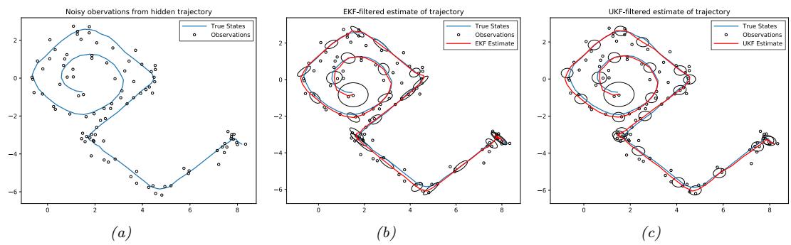
Figure 8.4: Illustration of filtering applied to a 2d nonlinear dynamical system. (a) True underlying state and observed data. (b) Extended Kalman filter estimate. Generated by ekf\_spiral.ipynb. (c) Unscented Kalman filter estimate. Generated by ukf\_spiral.ipynb.

The IEKF can be interpreted as a Gauss–Newton method for finding MAP estimate of the state at each step [BC93]. Specifically it minimizes the following objective:

\[\mathcal{L}(\mathbf{z}\_t) = \frac{1}{2} (\mathbf{y}\_t - \mathbf{h}(\mathbf{z}\_t))^\mathsf{T} \mathbf{R}\_t^{-1} (\mathbf{y}\_t - \mathbf{h}(\mathbf{z}\_t)) + \frac{1}{2} (\mathbf{z}\_t - \boldsymbol{\mu}\_{t|t-1})^\mathsf{T} \boldsymbol{\Sigma}\_{t|t-1}^{-1} (\mathbf{z}\_t - \boldsymbol{\mu}\_{t|t-1}) \tag{8.146}\]

See [SS23, Sec 7.4] for details.

Unfortunately the Gauss-Newton method can sometimes diverge. Various robust extensions including Levenberg-Marquardt, line search, and quasi-Newton methods — have been proposed in [SHA15; SS20a]. See [SS23, Sec 7.5] for details.

8.3.2.3 Example: Tracking a point spiraling in 2d

In Section 8.2.1.1, we considered an example of state estimation and tracking of an object moving in 2d under a linear dynamics model with a linear observation model. However, motion and observation models are often nonlinear. For example, consider an object that is moving along a curved trajectory,

such as this:

\[\mathbf{f}(\mathbf{z}) = (z\_1 + \Delta \sin(z\_2), z\_2 + \Delta \cos(z\_1))\tag{8.147}\]

where ! is the discrete step size (see [SS19, p221] for the continuous time version). For simplicity, we assume full visibility of the state vector (modulo observation noise), so h(z) = z.

Despite the simplicity of this model, exact inference is intractable. However, we can easily apply the EKF. The results are shown in Figure 8.4b.

8.3.2.4 Example: Neural network training

In Section 17.5.2, we show how to use the EKF to perform online parameter inference for an MLP regression model.

8.3.3 The extended Kalman smoother (EKS)

We can extend the EKF to the o$ine smoothing case, resulting in the extended Kalman smoother, also called the extended RTS smoother. We just need to linearize the dynamics around the filtered mean when computing Ft, and then we can apply the standard Kalman smoother update. See [SS23, Sec 13.1] for more details.

For improved accuracy, we can use the iterated EKS, which relinearizes the model at the previous MAP estimate. In [Bel94], they show that IEKS is equivalent to a Gauss-Newton method for computing the MAP estimate of the smoothing posterior. Unfortunately the IEKS can diverge in some cases. A robust IEKS method, that uses line search and Levenberg-Marquardt to update the parameters, is presented in [SS20a].

8.4 Inference based on the unscented transform

In this section, we replace the local linearization of the model with a di!erent approximation. The key idea is this: instead of computing a linear approximation to the dynamics and measurement functions, and then passing a Gaussian distribtution through the linearized functions, we instead approximate the joint distributions p(z^t↓¹, zt|y1:t↓¹) and p(zt, yt|y1:t↓¹) by Gaussians, where the moments are computed using numerical integration; we can then compute the marginal and conditional of these distributions to perform the time and measurement updates.

There are many methods to compute the Gaussian moments, as we discuss in Section 8.5.1. Here we use a method based on the unscented transform (see Section 8.4.1). Using the unscented transform for the transition and observation models gives the the overall method, known as the unscented Kalman filter or UKF, [JU97; JUDW00], also called the sigma point filter [VDMW03].

The main advantage of the UKF over the EKF is that it can be more accurate, and more stable. (Indeed, [JU97; JUDW00] claim the term “unscented” was invented because the method “doesn’t stink”.) In addition, the UKF does not need to compute Jacobians of the observation and dynamics models, so it can be applied to non-di!erentiable models, or ones with hard constraints. However, the UKF can be slower, since it requires N^z evaluations of the dynamics and observation models. In addition, it has 3 hyper-parameters that need to be set.

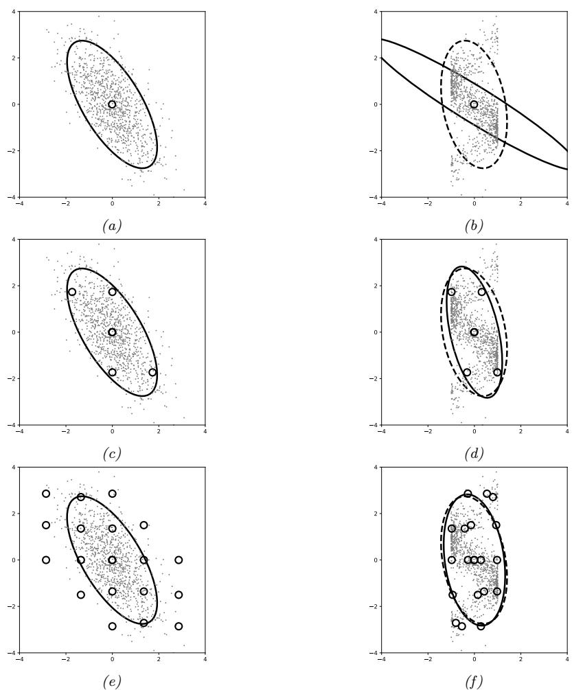
Figure 8.5: Illustration of di!erent ways to approximate the distribution induced by a nonlinear transformation ^f : ^{R2 → R2}. (a) Data from the source distribution, ^{D =} {x^{i ↑ p}(x)}, with Gaussian approximation superimposed. (b) The dots show a Monte Carlo approximation to p(f(x)) derived from D^↑ = {f(xi)}. The dotted ellipse is a Gaussian approximation to this target distribution, computed from the empirical moments. The solid ellipse is a Taylor transform. (c) Unscented sigma points. (d) Unscented transform. (e) Gauss-Hermite points (order 5). (f ) GH transform. Adapted from Figures 5.3–5.4 of [Sar13]. Generated by gaussian\_transforms.ipynb.

Algorithm 8.5: Computing sigma points using unscented transform.

¹ def SigmaPoints(µ, !; ϱ, ↼, ↽) : ² n = dimensionality of µ ³ ⇀ ^{= ϱ}2(^{n +} ↽) ^{→ n 4} Compute a set of 2n + 1 sigma points: ^{X0 = µ}, ^{Xi = µ + ∝n +} ⇀ [ ∝ !]:i, ^Xi+^{n = µ → ∝n +} ⇀ [ ∝ !]:^{i 5} Compute a set of 2n + 1 weights for the mean and covariance: w^{m 0} = ^{ε n}+^ε , w^{c 0} = ^{ε n}+^ε + (1 ^{→ ϱ2 +} ↼), w^{m i} = w^{c i} = ¹ 2(n+ε) ⁶ Return (X0:2n, w^m 0:2n, w^c 0:2n)

Algorithm 8.6: Unscented approximation to a joint Gaussian distribution.

¹ def UnscentedGaussJoint(µ, !, g, “; ϱ, ↼, ↽) : ² (X0:2n, w^m 0:2n, w^c 0:2n) = SigmaPoints(µ, !; ϱ, ↼, ↽) ³ Yⁱ = g(Xi), i =0:2n ⁴ yˆ = &^{2n i}=0 w^{m i} Y^{i 5} S = &^{2n i}=0 w^{c i} (Yⁱ → µ^U )(Yⁱ → µ^U ) ^T +” ⁶ C = &^{2n i}=0 w^{c i} (Xⁱ → µ)(Yⁱ → µ^U ) T ⁷ Return (yˆ, S, C)

8.4.1 The unscented transform

Suppose we have two random variables ^{x ↔︎ N} (µ, !) and ^y = ^g(x), where ^g : ^Rn ↖ ^Rm. The unscented transform forms a Gaussian approximation to p(y) using the following process. First we compute a set of ²n+ 1 sigma points, ^Xi, and corresponding weights, ^{wm i} and w^{c i} , using Algorithm 8.5, for i =0:2n. (The notation M:ⁱ means the i’th column of matrix M, ∝ ! is the matrix square root, so ^∝ ! ∝ !^{T =} !.) Next we propagate the sigma points through the nonlinear function to get the following 2n + 1 outputs:

\[\mathcal{Y}\_i = \mathbf{g}(\mathcal{X}\_i), \ i = 0:2n\tag{8.148}\]

Finally we estimate the mean and covariance of the resulting set of points:

\[\mathbb{E}\left[\mathbf{g}(\mathbf{z})\right] \approx \hat{\mathbf{y}} = \sum\_{i=0}^{2n} w\_i^m \mathcal{Y}\_i \tag{8.149}\]

\[\text{Cov}\left[\mathbf{g}(\mathbf{z})\right] \approx \mathbf{S}' = \sum\_{i=0}^{2n} w\_i^c (\mathcal{Y}\_i - \hat{\mathbf{y}}) (\mathcal{Y}\_i - \hat{\mathbf{y}})^\mathsf{T} \tag{8.150}\]

Now suppose we want to approximate the joint distribution p(x, y), where y = g(x) + e, and e ↔︎ N (0, “). By defining the augmented function g˜(x)=(x, g(x)), and applying the above

procedure (and adding extra noise), we get

\[ \begin{pmatrix} x \\ y \end{pmatrix} \sim \mathcal{N} \left( \begin{pmatrix} \mu \\ \hat{y} \end{pmatrix}, \begin{pmatrix} \Sigma & \mathbf{C} \\ \mathbf{C}^{\top} & \mathbf{S} \end{pmatrix} \right) \tag{8.151} \]

where the parameters are computed using Algorithm 8.6.

The sigma points and their weights depend on three hyperparameters, ϱ, ↼, and ↽, which determine the spread of the sigma points around the mean. A typical recommended setting for these is ϱ = 1, ↼ = 0, ↽ = n/2 [Bit16].

In Figure 8.5(a-b), we show the linearized Taylor transform discussed in Section 8.3.1 applied to a nonlinear function. In Figure 8.5(c-d), we show the corresponding unscented transform, which we can see is more accurate. In fact, the unscented transform (which uses 2n + 1 sigma points) is a third-order method in the sense that the mean of y is exact for polynomials up to order 3. However the covariance is only exact for linear functions (first order polynomials), because the square of a second order polynomial is already order 4. However, the UT idea can be extended to order 5 using 2n² + 1 sigma points [MS67]; this can capture covariance terms exactly for quadratic functions. We discuss even more accurate approximations, based on numerical integration methods, in Section 8.5.1.4.

8.4.2 The unscented Kalman filter (UKF)

The UKF applies the unscented transform twice, once to approximate passing through the system model f, and once to approximate passing through the measurement model h. By analogy to Section 8.2.2.5, we can derive the UKF algorithm as follows:

\[(\mu\_{t|t-1}, \Sigma\_{t|t-1}, -) = \text{UnscentedGaussJoint}(\mu\_{t-1|t-1}, \Sigma\_{t-1|t-1}, f(\cdot, \mathbf{u}\_t), \mathbf{Q}\_t) \tag{8.152}\]

\[(\hat{y}\_t, \mathbf{S}\_t, \mathbf{C}\_t) = \mathbf{Unconnected} \mathbf{Guuss} \mathbf{Joint}(\mu\_{t|t-1}, \Sigma\_{t|t-1}, h(\cdot, u\_t), \mathbf{R}\_t) \tag{8.153}\]

\[\mathbf{u}\_{t|t}(\mu\_{t|t}, \Sigma\_{t|t}, \ell\_t) = \mathbf{GuessConditional}(\mu\_{t|t-1}, \Sigma\_{t|t-1}, \hat{y}\_t, \mathbf{S}\_t, \mathbf{C}\_t, y\_t) \tag{8.154}\]

See [SS23, Sec 8.8] and [Arg24] for more details.

In Figure 8.4c, we illustrate the UKF algorithm (with ϱ = 1, ↼ = 0, ↽ = 2) applied to the 2d nonlinear tracking problem from Section 8.3.2.3.

8.4.3 The unscented Kalman smoother (UKS)

The unscented Kalman smoother, also called the unscented RTS smoother [Sar08], is a simple modification of the usual Kalman smoothing method, where we approximate the nonlinearity by the unscented transform. The key insight is to notice that the reverse Kalman gain matrix J^t in Equation (8.80) can be defined in terms of the predicted covariance and cross covariance, both of which can be estimated using the UT. Once we have computed this, we can use the RTS equations in the usual way. See [SS23, Sec 14.4] for the details.

An interesting application of unscented Kalman smoothing was its use by the UK government as part of its COVID-19 contact tracing app [Lov+20; BCH20]. The app used the UKS to estimate the distance between (anonymized) people based on bluetooth signal strength between their mobile phones; the distance was then combined with other signals, such as contact duration and infectiousness level of the index case, to estimate the risk of transmission. (See also [MKS21] for a way to learn the risk score.)

8.5 Other variants of the Kalman filter

In this section, we briefly mention some other variants of Kalman filtering. For a more extensive review, see [Sar13; SS23; Li+17e].

8.5.1 General Gaussian filtering

This section is co-authored with Peter Chang.

Let p(z) = N (z|µ, !) and p(y|z) = N (y|hµ(z), “) for some function hµ. Let p(z, y) = p(z)p(y|z) be the exact joint distribution. The best Gaussian approximation to the joint can be computed by solving

\[q(\mathbf{z}, \mathbf{y}) = \operatorname\*{argmin}\_{q \in \mathcal{N}} D\_{\text{KL}}\left(p(\mathbf{z}, \mathbf{y}) \parallel q(\mathbf{z}, \mathbf{y})\right) \tag{8.155}\]

As we explain in Section 5.1.4.2, this can be obtained by moment matching, i.e.,

\[q(\mathbf{z}, \mathbf{y}) = N\left( \begin{pmatrix} \mathbf{z} \\ \mathbf{y} \end{pmatrix} \mid \begin{pmatrix} \mu \\ \hat{\mathbf{y}} \end{pmatrix}, \begin{pmatrix} \Sigma & \mathbf{C} \\ \mathbf{C}^{\mathsf{T}} & \mathbf{S} \end{pmatrix} \right) \tag{8.156}\]

where

\[ \hat{y} = \mathbb{E}\left[y\right] = \int h\_{\mu}(z) N(z|\mu, \Sigma) dz \tag{8.157} \]

\[\mathbf{S} = \mathbb{V}\left[y\right] = \boldsymbol{\Omega} + \int (\boldsymbol{h}\_{\mu}(\boldsymbol{z}) - \hat{\boldsymbol{y}})(\boldsymbol{h}\_{\mu}(\boldsymbol{z}) - \hat{\boldsymbol{y}})^{\mathrm{T}} \boldsymbol{N}(\boldsymbol{z}|\mu, \boldsymbol{\Sigma}) d\boldsymbol{z} \tag{8.158}\]

\[\mathbf{C} = \text{Cov}\left[z, y\right] = \int (z - \mu)(h\_{\mu}(z) - \hat{y})^{\text{T}} \mathcal{N}(z|\mu, \Sigma) dz \tag{8.159}\]

We can use the above Gaussian approximation either for the time update (i.e., going from p(z^t↓¹|y1:t↓1) to p(zt|y1:t↓1) via p(z^t↓¹, zt|y1:t↓1)), or for the measurement update, (i.e., going from p(zt|y1:t↓¹) to p(zt|y1:t) via p(zt, yt|y1:t↓¹)). For example, if the prior from the time update is p(zt) = N (zt|µ^t|t↓¹, !^t|t↓¹), then the measurement update becomes

\[\mathbf{K}\_t = \mathbf{C}\_t \mathbf{S}\_t^{-1} \tag{8.160}\]

\[ \mu\_{t|t} = \mu\_{t|t-1} + \mathbf{K}\_t (y\_t - \hat{y}\_t) \tag{8.161} \]

\[\boldsymbol{\Sigma}\_{t|t} = \boldsymbol{\Sigma}\_{t|t-1} - \mathbf{K}\_t \mathbf{S}\_t \mathbf{K}\_t^\top \tag{8.162}\]

The resulting method is called general Gaussian filtering or GGF [IX00; Wu+06].

8.5.1.1 Statistical linear regression

An alternative perspective on the above method is that we are approximating the likelihood by q(y|z) = N (y|Az + b, “), where we define

\[\begin{aligned} \mathbf{A} &= \mathbf{C}^{\mathsf{T}} \boldsymbol{\Sigma}^{-1} \\ \mathbf{b} &= \boldsymbol{\hat{y}} - \mathbf{A}\boldsymbol{\mu} \\ \boldsymbol{\Omega} &= \mathbf{S} - \mathbf{A}\boldsymbol{\Sigma}\mathbf{A}^{\mathsf{T}} \end{aligned} \tag{8.163}\]

This is called statistical linear regression or SLR [LBS01; AHE07], and ensures that we minimize

\[\mathcal{L}(\mathbf{A}, \mathbf{b}, \Omega) = \mathbb{E}\_{\mathcal{N}(\mathbf{z}|\mu, \Sigma)} \left[ D\_{\text{KL}} \left( p(\mathbf{y}|\mathbf{z}) \parallel q(\mathbf{y}|\mathbf{z}; \mathbf{A}, \mathbf{b}, \Omega) \right) \right] \tag{8.164}\]

For the proof, see [GF+15; Kam+22].

Equivalently, one can show that the above parameters minimize the following mean squared error

\[\mathcal{L}(\mathbf{A}, \mathbf{b}) = \mathbb{E}\left[ (\mathbf{y} - \mathbf{A}\mathbf{x} - \mathbf{b})^{\mathsf{T}} (\mathbf{y} - \mathbf{A}\mathbf{x} - \mathbf{b}) \right] \tag{8.165}\]

with ” given by the residual noise

\[\Omega = \mathbb{E}\left[ (y - \mathbf{A}x - \mathbf{b})(y - \mathbf{A}x - \mathbf{b})^{\top} \right] \tag{8.166}\]

See [SS23, Sec 9.4] for the proof.

Note that although SLR results in a linear model, it is di!erent than the Taylor series approximation of Section 8.3.1, since the linearization is chosen to be optimal wrt a distribution of points (averaged over N (z|µ, !)), instead of just being optimal at a single point µ.

8.5.1.2 Approximating the moments

To implement GGF, we need a way to compute yˆ, S and C. To help with this, we define two functions to compute Gaussian first and second moments:

\[g\_e(\mathbf{f}, \mu, \Sigma) \stackrel{\Delta}{=} \int \mathbf{f}(\mathbf{z}) \mathcal{N}(\mathbf{z}|\mu, \Sigma) d\mathbf{z} \tag{8.167}\]

\[g\_c(\mathbf{f}, \mathbf{g}, \boldsymbol{\mu}, \boldsymbol{\Sigma}) \triangleq \int (\mathbf{f}(z) - \overline{\mathbf{f}}) (\mathbf{g}(z) - \overline{\mathbf{g}})^\mathsf{T} \mathcal{N} (z | \boldsymbol{\mu}, \boldsymbol{\Sigma}) dz \tag{8.168}\]

where f = ge(f, µ, !) and g = ge(g, µ, !). There are several ways to compute these integrals, as we discuss below.

8.5.1.3 Approximation based on linearization

The simplest approach to approximating the moments is to linearize the functions f and g around µ, which yields the following (see Section 8.3.1):

^fˆ(z) = ^{µ + F}(^{z → µ}) (8.169)

\[ \hat{\mathbf{g}}(z) = \mu + \mathbf{G}(z - \mu) \tag{8.170} \]

where F and G are the Jacobians of f and g. Thus we get the following implementation of the moment functions:

\[g\_e(\hat{\mathbf{f}}, \boldsymbol{\mu}, \boldsymbol{\Sigma}) = \mathbb{E}\left[\boldsymbol{\mu} + \mathbf{F}(\boldsymbol{z} - \boldsymbol{\mu})\right] = \boldsymbol{\mu} \tag{8.171}\]

\[g\_c(\hat{\mathbf{f}}, \hat{\mathbf{g}}, \boldsymbol{\mu}, \boldsymbol{\Sigma}) = \mathbb{E}\left[ (\hat{\mathbf{f}}(\mathbf{z}) - \overline{\mathbf{f}})(\hat{\mathbf{g}}(\mathbf{z}) - \overline{\mathbf{g}})^{\mathsf{T}} \right] \tag{8.172}\]

\[=\mathbb{E}\left[\hat{f}(z)\hat{g}(z)^{\mathsf{T}}+\overline{f}\overline{g}^{\mathsf{T}}-\hat{f}(z)\overline{g}^{\mathsf{T}}-\overline{f}\hat{g}(z)^{\mathsf{T}}\right] \tag{8.173}\]

\[\mathbf{E} = \mathbb{E}\left[ (\mu + \mathbf{F}(z - \mu))(\mu + \mathbf{G}(z - \mu))^{\mathsf{T}} + \mu\mu^{\mathsf{T}} - \mu\mu^{\mathsf{T}} - \mu\mu^{\mathsf{T}} \right] \tag{8.174}\]

\[\mathbf{H} = \mathbb{E}\left[\boldsymbol{\mu}\boldsymbol{\mu}^{\mathsf{T}} + \mathbf{F}(\boldsymbol{z} - \boldsymbol{\mu})(\boldsymbol{z} - \boldsymbol{\mu})^{\mathsf{T}}\mathbf{G}^{\mathsf{T}} + \mathbf{F}(\boldsymbol{z} - \boldsymbol{\mu})\boldsymbol{\mu}^{\mathsf{T}} + \boldsymbol{\mu}(\boldsymbol{z} - \boldsymbol{\mu})^{\mathsf{T}}\mathbf{G}^{\mathsf{T}} - \boldsymbol{\mu}\boldsymbol{\mu}^{\mathsf{T}}\right] \quad (8.175)\]

\[=\mathbf{F}\mathbb{E}\left[(z-\mu)(z-\mu)^{\mathsf{T}}\right]\mathbf{G}^{\mathsf{T}}=\mathbf{F}\Sigma\mathbf{G}^{\mathsf{T}}\tag{8.176}\]

Using this inside the GGF is equivalent to the EKF in Section 8.3.2. However, this approach can lead to large errors and sometimes divergence of the filter [IX00; VDMW03].

8.5.1.4 Approximation based on Gaussian quadrature (sigma points)

Since we are computing integrals wrt a Gaussian measure, we can use Gaussian quadrature methods of the following form:

\[\int h(\mathbf{z}) \mathcal{N}(\mathbf{z}|\boldsymbol{\mu}, \boldsymbol{\Sigma}) d\mathbf{z} \approx \sum\_{k=1}^{K} w^{k} h(\mathbf{z}^{k}) \tag{8.177}\]

for a suitable set of evaluation points z^k (sometimes called sigma points) and weights w^k. (Note that one-dimensional integrals are called quadratures, and multi-dimensional integrals are called cubatures.)

One way to compute the sigma points is to use the unscented transform described in Section 8.4.1. Using this inside the GGF is equivalent to the UKF in Section 8.4.2.

Alternatively, we can use spherical cubature integration, which gives rise to the cubature Kalman filter or CKF [AH09]. This turns out (see [SS23, Sec 8.7]) to be a special case of the UKF, with 2n^z + 1 sigma points, and hyperparameter values of ϱ = 1 and ↼ = 0 (with ↽ left free).

A more accurate approximation uses Gauss-Hermite integration, which allows the user to select more sigma points. In particular, an order p approximation will be exact for polynomials of order up to 2p → 1. See [SS23, Sec 8.3] for details, and Figure 8.5(e-f) for an illustration. However, this comes at a price: the number of sigma points is now pⁿ. Using Gauss-Hermite integration for GGF gives rise to the Gauss-Hermite Kalman filter or GHKF [IX00], also known as the quadrature Kalman filter or QKF [AHE07].

8.5.1.5 Approximation based on Monte Carlo integration

We can also approximate the integrals with Monte Carlo (see Section 11.2). Note, however, that this is not the same as particle filtering (Section 13.2), which approximates the conditional p(zt|y1:t) rather than the joint p(zt, yt|y1:t↓¹) (see Section 8.6.1 for discussion of this di!erence).

8.5.2 Conditional moment Gaussian filtering

We can go beyond the Gaussian likelihood assumption by approximating the actual likelihood by a linear Gaussian model, as proposed in [TGFS18]. The only requirement is that we can compute the first and second conditional moments of the likelihood:

\[h\_{\mu}(z) = \mathbb{E}\left[y|z\right] = \int yp(y|z)dy\tag{8.178}\]

\[h\_{\Sigma}(\mathbf{z}) = \text{Cov}\left[y|\mathbf{z}\right] = \int (y - h\_{\mu}(\mathbf{z}))(y - h\_{\mu}(\mathbf{z}))^{\mathsf{T}} p(y|\mathbf{z}) dy \tag{8.179}\]

Note that these integrals may be wrt a non-Gaussian measure p(y|z). Also, y may be discrete, in which case these integrals become sums.

Next we compute the unconditional moments. By the law of iterated expecations we have

\[\hat{y} = \mathbb{E}\left[y\right] = \mathbb{E}\left[\mathbb{E}\left[y|z\right]\right] = \int \mathbf{h}\_{\mu}(z)\mathcal{N}(z|\mu, \Sigma)dz = g\_{e}(\mathbf{h}\_{\mu}(z), \mu, \Sigma) \tag{8.180}\]

Similarly

\[\mathbf{C} = \text{Cov}\left[\mathbf{z}, \mathbf{y}\right] = \mathbb{E}\left[\mathbb{E}\left[(\mathbf{z} - \boldsymbol{\mu})(\mathbf{y} - \hat{\mathbf{y}})|\mathbf{z}\right]\right] = \mathbb{E}\left[(\mathbf{z} - \boldsymbol{\mu})(\mathbf{h}\_{\boldsymbol{\mu}}(\mathbf{z}) - \hat{\mathbf{y}})\right] \tag{8.181}\]

\[f\_{\boldsymbol{\mu}} = \begin{array}{c} \dots & \dots & \dots & \dots & \dots & \dots & \dots \end{array} \tag{8.182}\]

\[\hat{\mathbf{y}} = \int (\mathbf{z} - \mu)(\hbar\_{\mu}(\mathbf{z}) - \hat{\mathbf{y}})^{\mathsf{T}} \mathcal{N}(\mathbf{z}|\mu, \boldsymbol{\Sigma}) d\mathbf{z} = g\_{c}(\mathbf{z}, \hbar\_{\mu}(\mathbf{z}), \mu, \boldsymbol{\Sigma}) \tag{8.182}\]

Finally

\[\mathbf{S} = \mathbb{V}\left[\mathbf{y}\right] = \mathbb{E}\left[\mathbb{V}\left[\mathbf{y}|\mathbf{z}\right]\right] + \mathbb{V}\left[\mathbb{E}\left[\mathbf{y}|\mathbf{z}\right]\right] \tag{8.183}\]

\[I = \int h\_{\Sigma}(z) \mathcal{N}(z|\mu, \Sigma) dz + \int (h\_{\mu}(z) - \hat{y})(h\_{\mu}(z) - \hat{y})^{\mathsf{T}} \mathcal{N}(z|\mu, \Sigma) dz \tag{8.184}\]

\[=g\_e(\boldsymbol{h}\_\Sigma(\boldsymbol{z}), \boldsymbol{\mu}, \boldsymbol{\Sigma}) + g\_c(\boldsymbol{h}\_\mu(\boldsymbol{z}), \boldsymbol{h}\_\mu(\boldsymbol{z}), \boldsymbol{\mu}, \boldsymbol{\Sigma})\tag{8.185}\]

Note that the equation for yˆ is the same in Equation (8.157) and Equation (8.180), and the equation for C is the same in Equation (8.159) and Equation (8.182). Furthermore, if h!(z) = “, then the equation for S is the same in Equation (8.158) and Equation (8.185).

We can approximate the unconditional moments using linearization or numerical integration. We can then plug them into the GGF algorithm. We call this conditional moments Gaussian filtering or CMGF.

We can use CMGF to perform approximate inference in SSMs with Poisson likelihoods. For example, if ^p(y|z) = Poisson(y|ce^z), we have

\[\hbar\_{\mu}(z) = \hbar\_{\Sigma}(z) = ce^{z} \tag{8.186}\]

This method can be used to perform (extended) Kalman filtering with more general exponential family likelihoods, as described in [TGFS18; Oll18]. For example, suppose we have a categorical likelihood:

\[p(y\_t | \mathbf{z}\_t) = \text{Cat}(y\_t | \mathbf{p}\_t) = \text{Cat}(y\_t | \text{softmax}(\eta\_t)) = \text{Cat}(y\_t | \text{softmax}(h(\mathbf{z}\_t))) \tag{8.187}\]

where ϱ^t = h(zt) are the predicted logits. Then the conditional mean and covariance are given by

\[h\_{\mu}(\mathbf{z}\_{t}) = \mathbf{p}\_{t} = \text{softmax}(h(\mathbf{z}\_{t})), \ h\_{\Sigma}(\mathbf{z}\_{t}) = \text{diag}(\mathbf{p}\_{t}) - \mathbf{p}\_{t}\mathbf{p}\_{t}^{\mathsf{T}} \tag{8.188}\]

(We can drop one of the classes from the vector p^t to ensure the covariance is full rank.) This approach can be used for online inference in neural network classifiers [CMJ22], as well as Gaussian process classifiers [GFTS19] and recommender systems [GU16; GUK21]. We can also use this method as a proposal distribution inside of a particle filtering algorithm (Section 13.2), as discussed in [Hos+20b]. Finally, for a variational interpretation of CMGF, see [JCM24].

8.5.3 Iterated filters and smoothers

The GGF method in Section 8.5.1, and the CMGF method in Section 8.5.2, both require computing moments wrt the predictive distribution N (zt|µ^t|t↓¹, !^t|t↓¹) before performing the measurement update. It is possible to do one step of GGF to compute the posterior given the new observation, N (zt|µ^t|^t, !^t|^t), and then to use this revised posterior to compute new moments in an iterated fashion. This is called iterated posterior linearization filter or IPLF [GF+15]. (This is similar to the iterated EKF which we discussed in Section 8.3.2.2.) See Algorithm 8.7 for the pseudocode, and [SS23, Sec 10.4] for more details.

Algorithm 8.7: Iterated conditional moments Gaussian filter. def Iterated-CMGF(f, Q, hµ, h!, y1:^T , µ⁰|⁰, !⁰|⁰, J, ge, gc) : foreach t =1: T do Predict step: (µ^t|t↓¹, !^t|t↓¹, →) = MomentsGaussJoint(µ^t↓1|t↓¹, !^t↓1|t↓¹, f, Q, ge, gc) Update step: µ^t|^t = µ^t|t↓¹, !^t|^t = !^t|t↓¹ foreach j =1: J do (yˆt, St, Ct) = MomentsGaussJoint(µ^t|^t, !^t|^t, hµ, h!, ge, gc) (µ^t|^t, !^t|^t, εt) = GaussCondition(µ^t|t↓¹, !^t|t↓¹, yˆt, St, Ct, yt) Return (µ^t|^t, !^t|^t)^T t=1 def MomentsGaussJoint(µ, !, hµ, h!, ge, gc) : yˆ = ge(hµ(z), µ, !) S = ge(h!(z), µ, !) + gc(hµ(z), hµ(z), µ, !) C = gc(z, hµ(z), µ, !) Return (yˆ, S, C)

In a similar way, we can derive the iterated posterior linearization smoother or IPLS [GFSS17]. This is similar to the iterated EKS which we discussed in Section 8.3.3.

Unfortunately the IPLF and IPLS can diverge. A more robust version of IPLF, that uses line search to perform damped (partial) updates, is presented in [Rai+18b]. Similarly, a more robust version of IPLS, that uses line search and Levenberg-Marquardt to update the parameters, is presented in [Lin+21c].

Various extensions of the above methods have been proposed. For example, in [HPR19] they extend IPLS to belief propagation in Forney factor graphs (Section 4.6.1.2), which enables the method to be applied to a large class of graphical models beyond SSMs. In particular, they give a general linearization formulation (including explicit message update rules) for nonlinear approximate Gaussian BP (Section 9.4.3) where the linearization can be Jacobian-based (“EKF-style”), statistical (moment matching), or anything else. They also show how any such linearization method can benefit from iterations.

In [Kam+22], they present a method based on approximate expectation propagation (Section 10.7), that is very similar to IPLS, except that the distributions that are used to compute the SLR terms, needed to compute the Gaussian messages, are di!erent. In particular, rather than using the smoothed posterior from the last iteration, it uses the “cavity” distribution, which is the current posterior minus the incoming message that was sent at the last iteration, similar to Section 8.2.4.4. The advantage of this is that the outgoing message does not double count the evidence. The disadvantage is that this may be numerically unstable.

In [WSS21], they propose a variety of “Bayes-Newton” methods for approximately computing Gaussian posteriors to probabilistic models with nonlinear and/or non-Gaussian likelihoods. This generalizes all of the above methods, and can be applied to SSMs and GPs.

8.5.4 Ensemble Kalman filter

The ensemble Kalman filter (EnKF) is a technique developed in the geoscience (meteorology) community to perform approximate online inference in large nonlinear systems. In particular, it is mostly used for problems where the hidden state represents an unknown physical quantity (e.g., temperature or pressure) at each point on a spatial grid, and the measurements are sparse and spatially localized. Combining this information over space and time is called data assimilation.

The canonical reference is [Eve09], but a more accessible tutorial (using the same Bayesian signal processing approach we adopt in this chapter) is in [Rot+17].

The key idea is to represent the belief state ^p(zt|y1:t) by a finite number of samples {z^{s t}|^t : ^{s =} 1 : ^Ns}, where each sample ^{zs t}|^t ↗ ^RNz , which we collect into an ^{Nz ⇔ Ns} matrix ^Zt|^t. In contrast to particle filtering (Section 13.2), the samples are updated in a manner that closely resembles the Kalman filter, so there is no importance sampling or resampling step. The downside is that the posterior does not converge to the true Bayesian posterior even as N^s ↖ ⇓ [LGMT11], except in the linear-Gaussian case. However, sometimes the performance of EnKF can be better for small number of samples (although this depends of course on the PF proposal distribution).

The posterior mean and covariance can be derived from the ensemble of samples as follows:

\[\mathbf{\tilde{z}}\_{t|t} = \frac{1}{N\_s} \sum\_{s=1}^{N\_s} \mathbf{z}\_{t|t}^s = \frac{1}{N\_s} \mathbf{Z}\_{t|t} \mathbf{1} \tag{8.189}\]

\[\bar{\Sigma}\_{t|t} = \frac{1}{N\_s - 1} \sum\_{s=1}^{N\_s} (\mathbf{z}\_t^s - \bar{\mathbf{z}}\_{t|t})(\mathbf{z}\_t^s - \bar{\mathbf{z}}\_{t|t})^\top = \frac{1}{N\_s - 1} \bar{\mathbf{Z}}\_{t|t} \bar{\mathbf{Z}}\_{t|t}^\top \tag{8.190}\]

where ^Z˜^t|^{t = Zt}|^{t → z}˜^t|^t1^{T = Zt}|^t(I^{Ns → 1 Ns 11T}) are the centered particles, on per column.

We update the samples as follows. For the time update, we first draw N^s system noise variables qs ^t ↔︎ N (0, Qt), and then we pass these, and the previous state estimate, through the dynamics

model to get the one-step-ahead state predictions, z^{s t}|t↓^{1 = f}(z^{s t}↓1|t↓1, ^{qs t} ), from which we get Z^t|t↓¹ = {z^{s t}|t↓1}. Next we draw ^Ns observation noise variables ^{rs t} ↔︎ N (0, Rt), and use them to compute the one-step-ahead observation predictions, y^{s t}|t↓^{1 = h}(z^{s t}|t↓1, ^{rs t} ) and Y^t|t↓¹ = {y^{s t}|t↓1}, which has size N^y ⇔ Ns. Finally we compute the measurement update using

\[\mathbf{Z}\_{t|t} = \mathbf{Z}\_{t|t-1} + \mathbf{\bar{K}}\_{t} (y\_t \mathbf{1}^{\mathsf{T}} - \mathbf{Y}\_{t|t-1}) \tag{8.191}\]

which is the analog of Equation (8.29).

We now discuss how to compute K˜ ^t, which is the analog of the Kalman gain matrix in Equation (8.28). First note that we can write the exact Kalman gain matrix (in the linear-Gaussian case) as ^{Kt =} !^t|t↓¹H^TS↓^{1 t} = CtS↓^{1 t} , where S^t is the covariance of the predictive distribution for the observation vector at time t, and C^t is the cross-covariance of the joint predictive distribution for the next state and next observation. In the EnKF, we approximate S^t and C^t empirically as follows. First we compute the anomalies

\[\bar{\mathbf{Z}}\_{t|t-1} = \mathbf{Z}\_{t|t-1} - \bar{\mathbf{z}}\_{t|t-1} \mathbf{1}^{\mathsf{T}}, \ \bar{\mathbf{Y}}\_{t|t-1} = \mathbf{Y}\_{t|t-1} - \bar{y}\_{t|t-1} \mathbf{1}^{\mathsf{T}} \tag{8.192}\]

Then we compute the sample covariance matrices

\[\bar{\mathbf{C}}\_{t} = \frac{1}{N\_s - 1} \bar{\mathbf{Z}}\_{t|t-1} \bar{\mathbf{Y}}\_{t|t-1}^{\mathsf{T}}, \quad \bar{\mathbf{S}}\_{t} = \frac{1}{N\_s - 1} \bar{\mathbf{Y}}\_{t|t-1} \bar{\mathbf{Y}}\_{t|t-1}^{\mathsf{T}} \tag{8.193}\]

Finally we compute

\[ \tilde{\mathbf{K}}\_t = \tilde{\mathbf{C}}\_t \tilde{\mathbf{S}}\_t^{-1} \tag{8.194} \]

which has the same form as a multivariate least squares problem. For models with additive noise, we can reduce the variance of this procedure by eliminating the sampling of the predicted observations. Thus we replace ^Y˜ ^t|t↓¹ with its deterministic version, ^O˜ ^t|t↓^{1 =} HZ˜^t|t↓¹ (assuming a linear observation model for notational simplicity). We then use C˜ ^t = ^{1 N}s↓1Z˜^t|t↓1O˜^{T t}|t↓1, and ^S˜^{t = 1 N}s↓1O˜ ^t|t↓1O˜^{T t}|t↓^{1 +} Rt. (It is also possible to eliminate the sampling for the latent states, by using the ensemble square root filter [Tip+03], although this may be less robust.)

We now compare the computational complexity of EnKF and KF algorithms. Recall that N^z is the number of latent dimensions, N^y is the number of observed dimensions, and N^s is the number of samples. We will assume N^z > N^s > Ny, as occurs in most geospatial problems. The EnKF time update takes O(N^{2 z} Ns) time to propagate the samples though the model (assuming that f is a linear model), whereas the KF takes O(N^{3 z} ) time to compute Ft!^t↓¹F^t + Qt. If the transition matrix is sparse (e.g., diagonal), the EnKF time reduces to O(NzNs) and the EKF time reduces to O(N^{2 z} ).

Now we discuss the cost of the measurement update. The EnKF measurement update takes O(NzNyNs) time to compute C˜ ^t, O(N^{2 y} Ns) time to compute S˜t, O(N^{3 y} ) time to compute S˜↓^{1 t} , O(NzN^{2 y} ) to compute ^K˜ ^t, and ^O(NzNyNs) time to compute ^Zt|t, for a total of ^O(NzNyNs), where we have dropped terms that don’t depend on N^z for notational simplicity, and assumed N^z ⇑ Ny. By contrast, in the EKF, the measurement update takes O(N^{2 z} Ny) to compute Ct, O(N^{2 z} Ny) to compute St, O(N^{3 y} ) to compute S↓^{1 t} , O(NzN^{2 y} ) to compute Kt, and O(NzNy) to compute µ^t|t, for a total of O(N^{2 z} Ny).

In summary, for sparse (e.g., diagonal) F, EnKF is O(NzNs+NzNsNy) and EKF is O(N^{2 z} +N^{2 z} Ny), whereas for dense F, EnKF is O(N^{2 z} N^s + NzNsNy) and EKF is O(N^{3 z} + N^{2 z} Ny).

Unfortunately, if N^s is too small, the EnKF can be become overconfident, and the filter can diverge. A common heuristic to reduce this is known as covariance inflation, in which we replace ^Z˜t|t↓¹ with ^Z˜t|t↓^{1 =} ↼(Zt|t↓^{1 → z}˜t|t↓11T) for some fudge factor ↼ ^> ¹.

Unlike the particle filter, the EnKF is not guaranteed to converge to the correct posterior. However, hybrid PF/EnKF approaches have been developed (see e.g., [LGMT11; FK13b; Rei13]) with better theoretical foundations.

8.5.5 Robust Kalman filters

In practice we often have noise that is non-Gaussian. A common example is when we have clutter, or outliers, in the observation model, or sudden changes in the process model. In this case, we might use the Laplace distribution [Ara+09] or the Student t-distribution [Ara10; RÖG13; Ara+17] as noise models.

[Hua+17b] proposes a variational Bayes (Section 10.3.3) approach, that allows the dynamical prior and the observation model to both be (linear) Student distributions, but where the posterior is approximated at each step using a Gaussian, conditional on the noise scale matrix, which is modeled using an inverse Wishart distribution. An extension of this, to handle mixture distributions, can be found in [Hua+19].

In addition to robustness to non-Gaussian noise, it is useful to ensure robustness to approximations such as those used by EKF (namely local linearization), by adapting the step size, etc. For details, see e.g., [SHA15; SS20a].

8.5.6 Dual EKF

In this section, we briefly discuss one approach to estimating the parameters of an SSM. In an o$ine setting, we can use EM, SGD, or Bayesian inference to compute an approximation to p(ω|y1:^T ) (see Section 29.8). In the online setting, we want to compute p(ωt|y1:t). We can do this by adding the parameters to the state space, possibly with an artificial dynamics, p(ωt|ω^t↓¹) = N (ωt|ω^t↓¹, ⇁I), and then performing joint inference of states and parameters. The latent variables at each step now contain the latent states, zt, and the latent parameters, ωt. One approach to performing approximating inference in such a model is to use the dual EKF, in which one EKF performs state estimation and the other EKF performs parameter estimation [WN01].

8.5.7 Normalizing flow KFs

Normalizing flows, as discussed in Chapter 23, are a kind of deep generative model with a tractable exact likelihood. These can be used to “upgrade” the observation model of a linear Gaussian SSM, while still retaining tractable exact Gaussian inference, as shown in [Béz+20]. In particular, instead of observing y^t = Htz^t + rt, where r^t ↔︎ N (0, Rt), we observe y^t = ft(ht), where h^t = Htz^t + rt, and ^ft : ^RNy ↖ ^RNy is an invertible function with a tractable Jacobian. In this case, the exact posterior, ^p(zt|y1:t), is given by the usual Kalman filter equations applied to ^{ht = f ↓1 t} (yt) instead of yt, which we denote by pLGSSM(zt|h1:t).

This result can be shown by induction. First note that, by the change of variable formula, p(yt|zt) = ^p(ht|zt)Df ^{↓1 t} (yt), where Dg(a) ↭ ^| det Jac(g)(a)|. By induction, we have ^p(z^t↓¹|y1:t↓1) = ^pLGSSM(z^t↓¹|h1:t↓1), and hence by the linear Gaussian assumptions for the dynamics model, p(zt|y1:t↓1) = pLGSSM(zt|h1:t↓1).

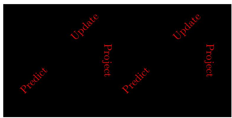
Figure 8.6: Illustration of the predict-update-project cycle of assumed density filtering. q^t ↓ Q is a tractable distribution, whereas we may have p^t|t→¹ ↔︎↓ Q and p^t ↔︎↓ Q.

Thus the filtering posterior is given by

\[p(\mathbf{z}\_t|\mathbf{y}\_{1:t}) = \frac{p(\mathbf{y}\_t|\mathbf{z}\_t)p(\mathbf{z}\_t|\mathbf{y}\_{1:t-1})}{\int p(\mathbf{y}\_t|\mathbf{z}\_t')p(\mathbf{z}\_t'|\mathbf{y}\_{1:t-1})d\mathbf{z}\_t'} = \frac{Df\_t^{-1}(\mathbf{y}\_t)p(\mathbf{h}\_t|\mathbf{z}\_t)p(\mathbf{z}\_t|\mathbf{y}\_{1:t-1})}{\int Df\_t^{-1}(\mathbf{y}\_t)p(\mathbf{h}\_t|\mathbf{z}\_t')p(\mathbf{z}\_t'|\mathbf{y}\_{1:t-1})}\]

\[= \frac{p(\mathbf{h}\_t|\mathbf{z}\_t)p\_{\text{LGSSM}}(\mathbf{z}\_t|\mathbf{h}\_{1:t-1})}{\int p(\mathbf{h}\_t|\mathbf{z}\_t')p\_{\text{LGSSM}}(\mathbf{z}\_t'|\mathbf{h}\_{1:t-1})} = p\_{\text{LGSSM}}(\mathbf{z}\_t|\mathbf{h}\_{1:t})\]

Similar reasoning applies to the smoothing distribution.

8.6 Assumed density filtering

In this section, we discuss assumed density filtering or ADF [May79]. In this approach, we assume the posterior has a specific form (e.g., a Gaussian). At each step, we update the previous posterior with the new likelihood; the result will often not have the desired form (e.g., will no longer be Gaussian), so we project it to the closest approximating distribution of the required type.

In more detail, we assume (by induction) that our prior q^t↓¹(z^t↓¹) ↓ p(z^t↓¹|y1:t↓¹) satisfies q^t↓¹ ↗ Q, where Q is a family of tractable distributions. We can update the prior with the new measurement to get the approximate posterior as follows. First we compute the one-step-ahead predictive distribution

\[p\_{t|t-1}(\mathbf{z}\_t | \mathbf{y}\_{1:t-1}) = \int p(\mathbf{z}\_t | \mathbf{z}\_{t-1}) q\_{t-1}(\mathbf{z}\_{t-1}) d\mathbf{z}\_{t-1} \tag{8.195}\]

Then we update this prior with the likelihood for step t to get the posterior

\[p\_t(\mathbf{z}\_t|\mathbf{y}\_{1:t}) = \frac{1}{Z\_t} p(\mathbf{y}\_t|\mathbf{z}\_t) p\_{t|t-1}(\mathbf{z}\_t) \tag{8.196}\]

where

\[Z\_t = \int p(y\_t|\mathbf{z}\_t) p\_{t|t-1}(\mathbf{z}\_t) d\mathbf{z}\_t \tag{8.197}\]

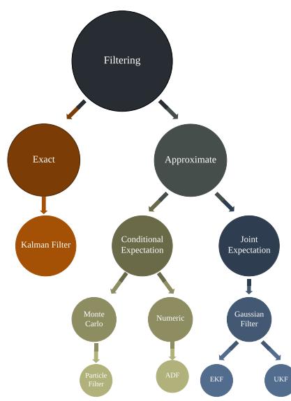
Figure 8.7: A taxonomy of filtering algorithms. Adapted from Figure 2 of [Wüt+16].

is the normalization constant. Unfortunately, we often find that the resulting posterior is no longer in our tractable family, p(zt) ′↗ Q. So after Bayesian updating we seek the best tractable approximation by computing

\[q\_t(\mathbf{z}\_t | \mathbf{y}\_{1:t}) = \underset{q \in \mathcal{Q}}{\operatorname{argmin}} \, D\_{\text{KL}}\left(p\_t(\mathbf{z}\_t | \mathbf{y}\_{1:t}) \parallel q(\mathbf{z}\_t)\right) \tag{8.198}\]

This minimizes the Kullback-Leibler divergence from the approximation q(zt) to the “exact” posterior pt(zt), and can be thought of as projecting p onto the space of tractable distributions. Thus the overall algorithm consists of three steps — predict, update, and project — as sketched in Figure 8.6.

Computing min^q DKL (p ↘ q) is known as moment projection, since the optimal q should have the same moments as p (see Section 5.1.4.2). So in the Gaussian case, we just need to set the mean and covariance of q^t so they are the same as the mean and covariance of pt. We will give some examples of this below. By contrast, computing min^q DKL (q ↘ p), as in variational inference (Section 10.1), is known as information projection, and will result in mode seeking behavior (see Section 5.1.4.1), rather than trying to capture overall moments.

8.6.1 Connection with Gaussian filtering

When Q is the set of Gaussian distributions, there is a close connection between ADF and Gaussian filtering, which we discussed in Section 8.5.1. GF corresponds to solving the following optimization problem

\[q\_{t|t-1}(\mathbf{z}\_t, \tilde{y}\_t) = \operatorname\*{argmin}\_{q \in \mathcal{Q}} D\_{\mathbb{KL}}\left(p(\mathbf{z}\_t, \tilde{y}\_t | \mathbf{y}\_{1:t-1}) \parallel q(\mathbf{z}\_t, \tilde{y}\_t | \mathbf{y}\_{1:t-1})\right) \tag{8.199}\]

^{pj =} !

pij

b i,j

where

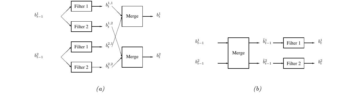
^t = P(Xt, S^t−¹ = i, S^t = j|y1:t), is the joint posterior, and b j ^t = P(Xt, S^t = y|y1:t) is the marginal posterior. The filter box implements the Kalman filter equations. The merge box implements the moment matching equations. 5.4 Belief state = set of samples (particle filtering) The basic idea behind particle filtering⁶ is to approximate the belief state by a set of weighted particles or samples: Figure 8.8: ADF for a switching linear dynamical system with 2 discrete states. (a) GPB2 method. (b) IMM method.

^P(Xt|y1:t) ^≈ !N^s

q(xⁱ t|xⁱ

q(xⁱ t|xⁱ

^{= P}(yt|xⁱ

def

1:t−1, ^y1:t)q(xⁱ

1:t−¹, ^y1:t) ^wi

t)P(xⁱ t|x^{i t}−1) 1:t−1|y1:t−1)

t−1

wi ^tδ(Xt, Xⁱ t )

i ^pj|^{i =} “pij ^j pij ^{µj =} ! i µijp^j|^{i Σj =} ! i ^Σijp^j|^{i +}! i (µij − µ^j )(µij − µ^j ) ^{T pj}|ⁱ In the junction tree literature, this is called”weak marginalization”. It can be applied to any conditionally Gaussian model, not just switching SSMs. i=1 (In this section, X^{i t} means the i’th sample of Xt, and Xt,i means the i’th component of Xt.) This is a non-parametric approach, and hence can handle non-linearities, multi-modal distributions, etc. The advantage over discretization is that the method is adaptive, placing more particles (corresponding to a finer discretization) in places where the probability density is higher. Given a prior of this form, we can compute the posterior using importance sampling. In importance sampling, we assume the target distribution, π(x), is hard to sample from; instead, we sample from a proposal or importance distribution ^q(x), and weight the sample according to ^{wi ∝ π}(x)/q(x). (After we have finished sampling, we can normalize all the weights so ” ⁱ wⁱ = 1). We can use this to sample paths with weights which can be solved by moment matching (see Section 8.5.1). We then condition this joint distribution on the event y˜^t = yt, where y˜^t is the unknown random variable and y^t is its observed value. This gives pt(zt|y1:t), which is easy to compute, due to the Gaussian assumption. By contrast, in Gaussian ADF, we first compute the (locally) exact posterior pt(zt|y1:t), and then approximate it with qt(zt|y1:t) by projecting into Q. Thus ADF approximates the conditional pt(zt|y1:t), whereas GF approximates the joint p^t|t↓¹(zt, y˜t|y1:t↓¹), from which we derive pt(zt|y1:t) by conditioning.

The GPB2 algorithm requires running M² Kalman filters at each step. A cheaper alternative, known as interacting multiple models (IMM), can be obtained by first collapsing the prior to a single Gaussian (by moment matching), and then updating it using M different Kalman filters, one per value of St: see Figure 40. Unfortunately, it is hard to extend IMM to the smoothing case, unlike GPB2, a smoothing version of which is discussed in Section 6.1.3. 5.3.2 Viterbi approximation If there are a large number of discrete variables, it may be too slow to perform M² or even M KF updates, as required wi ^{t ∝ P}(xⁱ 1:t|y1:t) q(xⁱ 1:t|y1:t) The probability of a sample path, P(xⁱ 1:t|y1:t), can be computed recursively using Bayes rule. Typically we will want the proposal distribution to be recursive also, i.e., q(x1:t|y1:t) = q(xt|x1:t−1, y1:t)q(x1:t−1|y1:t−1). In this case we have wi ^{t ∝ P}(yt|xⁱ t)P(xⁱ t|x^{i t}−1)P(xⁱ 1:t−1|y1:t−1) ADF is more accurate than GF, since it directy approximates the posterior, but it is more computationally demanding, for reasons explained in [Wüt+16]. However, in [Kam+22] they propose an approximate form of expectation propagation (which is a generalization of ADF) in which the messages are computed using the same local joint Gaussian approximation as used in Gaussian filtering. See Figure 8.7 for a summary of how these di!erent methods relate.

there is a natural ordering on the discrete values: one fault is much more likely than two faults, etc. However, it would not be applicable to the data association DBN in Figure 23, where there is no such ordering. 8.6.2 ADF for SLDS (Gaussian sum filter)

by GPB2 and IMM. Instead, one can enumerate the discrete values in a priori order of probability. (Computing their posterior probability is as expensive as an exact update step.) This makes sense for a DBN for fault diagnosis, where

= wˆ^{i t × wi} t−1 where we have defined wˆ^{i t} to be the incremental weight. For filtering, we usually only care about the posterior marginal P(Xt|y1:t), as opposed to the full posterior ^P(X1:t|y1:t). Hence we use the following proposal: ^q(xt|xⁱ 1:t−¹, ^y1:t) ^{= q}(xt|x^{i t}−¹, yt). This means we only need to In this section, we apply ADF to inference in switching linear dynamical systems (SLDS, Section 29.9), which are a combination of HMM and LDS models. The resulting method is known as the Gaussian sum filter (see e.g., [Cro+11; Wil+17]).

33 6Particle filtering is also known as sequential Monte Carlo, sequential importance sampling with resampling (SISR), the bootstrap filter, the condensation algorithm, survival of the fittest, etc. 34 A Gaussian sum filter approximates the belief state at each step by a mixture of K Gaussians. This can be implemented by running K Kalman filters in parallel. This is particularly well suited to switching SSMs. We now describe one version of this algorithm, known as the “second order generalized pseudo-Bayes filter” (GPB2) [BSF88]. We assume that the prior belief state b^t↓¹ is a mixture of K Gaussians, one per discrete state:

\[b\_{t-1}^i \triangleq p(\mathbf{z}\_{t-1}, m\_{t-1} = i | y\_{1:t-1}) = \pi\_{t-1|t-1}^i \mathcal{N}(\mathbf{z}\_{t-1} | \mu\_{t-1|t-1}^i, \Sigma\_{t-1|t-1}^i) \tag{8.200}\]

where i ↗ {1,…,K}. We then pass this through the K di!erent linear models to get

\[b\_t^{ij} \triangleq p(\mathbf{z}\_t, m\_{t-1} = i, m\_t = j | \mathbf{y}\_{1:t}) = \pi\_{t|t}^{ij} \mathcal{N}(\mathbf{z}\_t | \boldsymbol{\mu}\_{t|t}^{ij}, \boldsymbol{\Sigma}\_{t|t}^{ij}) \tag{8.201}\]

where ϖij ^t|^{t = ϖi t}↓1|t↓¹Aij , where ^Aij ^{= p}(m^{t = j}|m^t↓^{1 = i}). Finally, for each value of ^j, we collapse

the K Gaussian mixtures down to a single mixture to give

\[b\_t^j \triangleq p(\mathbf{z}\_t, m\_t = j | \mathbf{y}\_{1:t}) = \pi\_{t|t}^j \mathcal{N}(\mathbf{z}\_t | \boldsymbol{\mu}\_{t|t}^j, \boldsymbol{\Sigma}\_{t|t}^j) \tag{8.202}\]

See Figure 8.8a for a sketch.

The optimal way to approximate a mixture of Gaussians with a single Gaussian is given by ^{q =} arg min^{q D}KL (^q ↘ ^p), where ^p(z) = & ^{k ϖkN} (z|µ^k, !^k) and ^q(z) = ^N (z|µ, !). This can be solved by moment matching, that is,

\[\mu = \mathbb{E}\left[\mathbf{z}\right] = \sum\_{k} \pi^{k} \mu^{k} \tag{8.203}\]

\[\Delta = \text{Cov}\left[\mathbf{z}\right] = \sum\_{k} \pi^{k} \left(\boldsymbol{\Sigma}^{k} + (\boldsymbol{\mu}^{k} - \boldsymbol{\mu})(\boldsymbol{\mu}^{k} - \boldsymbol{\mu})^{\mathsf{T}}\right) \tag{8.204}\]

In the graphical model literature, this is called weak marginalization [Lau92], since it preserves the first two moments. Applying these equations to our model, we can go from b ij ^t to b j ^t as follows (where we drop the t subscript for brevity):

\[ \pi^j = \sum\_i \pi^{ij} \tag{8.205} \]

\[ \pi^{j|i} = \frac{\pi^{ij}}{\sum\_{j'} \pi^{ij'}} \tag{8.206} \]

\[ \mu^j = \sum\_i \pi^{j|i} \mu^{ij} \tag{8.207} \]

\[\Delta^j = \sum\_i \pi^{j|i} \left( \Sigma^{ij} + (\mu^{ij} - \mu^j)(\mu^{ij} - \mu\_j)^\top \right) \tag{8.208}\]

This algorithm requires running K² filters at each step. A cheaper alternative, known as interactive multiple models or IMM [BSF88], can be obtained by first collapsing the prior to a single Gaussian (by moment matching), and then updating it using K di!erent Kalman filters, one per value of mt. See Figure 8.8b for a sketch.

8.6.3 ADF for online logistic regression

In this section we discuss the application of ADF to online Bayesian parameter inference for a binary logistic regression model, based on [Zoe07]. The overall approach is similar to the online linear regression case (discussed in Section 29.7.2), but approximates the posterior after each update step, which is necessary since the likelihood is not conjugate to the prior.

We assume our model has the following form:

\[p(y\_t | \mathbf{z}\_t, \mathbf{w}\_t) = \text{Ber}(y\_t | \sigma(\mathbf{z}\_t^\mathsf{T} \mathbf{w}\_t)) \tag{8.209}\]

\[p(w\_t | w\_{t-1}) = \mathcal{N}(w\_t | w\_{t-1}, \mathbf{Q}) \tag{8.210}\]

where Q is the covariance of the process noise, which allows the parameters to change slowly over time. We will assume Q = ⇁I; we can also set ⇁ = 0, as in the recursive least squares method

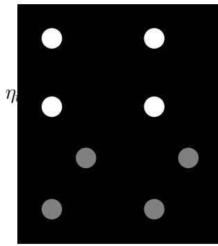
Figure 8.9: A dynamic logistic regression model. w^t are the regression weights at time t, and ϑ^t = w^{T t} xt. Compare to Figure 29.24a.

(Section 29.7.2), if we believe the parameters will not change. See Figure 8.9 for an illustration of the model.

As our approximating family, we will use diagonal Gaussians, for computational e”ciency. Thus the prior is the posterior from the previous time step, and has the form

\[p(\boldsymbol{w}\_{t-1}|\mathcal{D}\_{1:t-1}) \approx p\_{t-1}(\boldsymbol{w}\_{t-1}) = \prod\_{j} N(\boldsymbol{w}\_{t-1}^{j}|\boldsymbol{\mu}\_{t-1\mid t-1}^{j}, \boldsymbol{\tau}\_{t-1\mid t-1}^{j}) \tag{8.211}\]

where µ^{j t}↓1|t↓¹ and ^{τ j t}↓1|t↓¹ are the posterior mean and variance for parameter ^j given past data. Now we discuss how to update this prior.

First we compute the one-step-ahead predictive density p^t|t↓¹(wt) using the standard linear-Gaussian update, i.e., µ^t|t↓¹ = µ^t↓1|t↓¹ and φ ^t|t↓¹ = φ ^t↓1|t↓¹ + Q, where we can set Q = 0I if there is no drift.

Now we concentrate on the measurement update step. Define the scalar sum (corresponding to the logits, if we are using binary classification) as η^t = w^{T t x}t. If ^pt|t↓¹(wt) = ^{j N} (w^{j t |}µ^{j t}|t↓¹, ^{τ j t}|t↓¹), then we can compute the 1d prior predictive distribution for η^t as follows:

\[p(\eta\_t | \mathcal{D}\_{1:t-1}, \mathbf{z}\_t) \approx p\_{t|t-1}(\eta\_t) = \mathcal{N}(\eta\_t | m\_{t|t-1}, v\_{t|t-1}) \tag{8.212}\]

\[m\_{t|t-1} = \sum\_{j} x\_{t,j} \mu\_{t|t-1}^j \tag{8.213}\]

\[v\_{t|t-1} = \sum\_{j} x\_{t,j}^2 \tau\_{t|t-1}^j \tag{8.214}\]

The posterior for the 1d η^t is given by

\[p(\eta\_t | \mathcal{D}\_{1:t}) \approx p\_t(\eta\_t) = \mathcal{N}(\eta\_t | m\_t, v\_t) \tag{8.215}\]

\[m\_t = \int \eta\_t \frac{1}{Z\_t} p(y\_t|\eta\_t) p\_{t|t-1}(\eta\_t) d\eta\_t \tag{8.216}\]

\[v\_t = \int \eta\_t^2 \frac{1}{Z\_t} p(y\_t|\eta\_t) p\_{t|t-1}(\eta\_t) d\eta\_t - m\_t^2 \tag{8.217}\]

\[Z\_t = \int p(y\_t|\eta\_t) p\_{t|t-1}(\eta\_t) d\eta\_t \tag{8.218}\]

where p(yt|ηt) = Ber(yt|ηt). These integrals are one dimensional, and so can be e”ciently computed using Gaussian quadrature, as explained in [Zoe07; KB00].

Having inferred pt(ηt), we need to compute pt(w|ηt). This can be done as follows. Define ϑ^m as the change in the mean and ϑ^v as the change in the variance:

\[m\_t = m\_{t|t-1} + \delta\_m, \ v\_t = v\_{t|t-1} + \delta\_v \tag{8.219}\]

Using the fact that ^p(ηt|w) = ^N (ηt|w^Tηt, 0) is a linear Gaussian system, with prior ^p(w) = p(w|µ^t|t↓¹, φ ^t|t↓1) and “soft evidence” p(ηt) = N (mt, vt), we can derive the posterior for p(w|Dt) as follows:

\[p\_t(w\_t^i) = \mathcal{N}(w\_t^i | \mu\_{t|t}^i, \tau\_{t|t}^i) \tag{8.220}\]

\[ \mu\_{t|t}^i = \mu\_{t|t-1}^i + a\_i \delta\_m \tag{8.221} \]

\[ \tau\_{t|t}^i = \tau\_{t|t-1}^i + a\_i^2 \delta\_v \tag{8.222} \]

\[a\_i \triangleq \frac{x\_t^i \tau\_{t|t-1}^i}{\sum\_j (x\_t^j)^2 + \tau\_{t|t-1}^j} \tag{8.223}\]

Thus we see that the parameters which correspond to inputs ⁱ with larger magnitude (big ^|x^{i t}|) or larger uncertainty (big τ ^{i t}|t↓1) get updated most, due to a large ^ai factor, which makes intuitive sense.

As an example, we consider a 2d binary classification problem. We sequentially compute the posterior using the ADF, and compare to the o$ine estimate computed using a Laplace approximation. In Figure 8.10 we plot the posterior marginals over the 3 parameters as a function of “time” (i.e., after conditioning on each training example one). We see that we converge to the o$ine MAP estimate. In Figure 8.11, we show the results of performing sequential Bayesian updating in a di!erent ordering of the data. We still converge to approximate the same answer. In Figure 8.12, we see that the resulting posterior predictive distributions from the Laplace estimate and ADF estimate (at the end of training) are similar.

Note that the whole algorithm only takes O(D) time and space per step, the same as SGD. However, unlike SGD, there are no step-size parameters, since the diagonal covariance implicitly specifies the size of the update for each dimension. Furthermore, we get a posterior approximation, not just a point estimate.

The overall approach is very similar to the generalized posterior linearization filter of Section 8.5.3, which uses quadrature (or the unscented transform) to compute a Gaussian approximation to the joint p(yt, wt|D1:t↓¹), from which we can easily compute p(wt|D1:t). However, ADF approximates the posterior rather than the joint, as explained in Section 8.6.1.

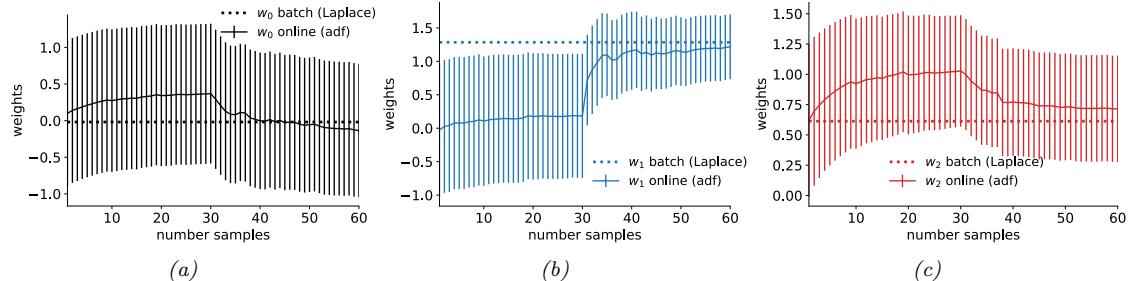
Figure 8.10: Bayesian inference applied to a 2d binary logistic regression problem, p(y = 1|x) = ω(w⁰ + w1x¹ + w2x2). We show the marginal posterior mean and variance for each parameter vs time as computed by ADF. The dotted horizontal line is the o”ine Laplace approximation. Generated by adf\_logistic\_regression\_demo.ipynb.

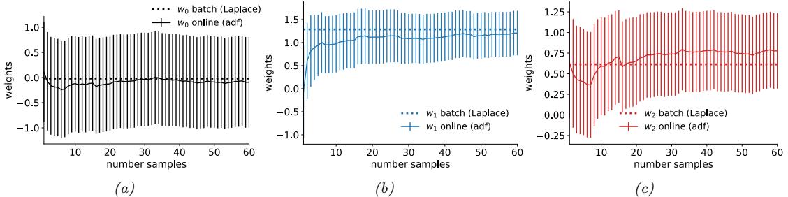
Figure 8.11: Same as Figure 8.10, except the order in which the data is visited is di!erent. Generated by adf\_logistic\_regression\_demo.ipynb.

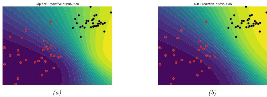
Figure 8.12: Predictive distribution for the binary logistic regression problem. (a) Result from Laplace approximation. (b) Result from ADF at the final step. Generated by adf\_logistic\_regression\_demo.ipynb.

8.6.4 ADF for online DNNs

In Section 17.5.3, we show how to use ADF to recursively approximate the posterior over the parameters of a deep neural network in an online fashion. This generalizes Section 8.6.3 to the case of nonlinear models.

8.7 Other inference methods for SSMs

There are a variety of other inference algorithms that can be applied to SSMs. We give a very brief summary below. For more details, see e.g., [Dau05; Sim06; Fra08; Sar13; SS23; Tri21].

8.7.1 Grid-based approximations

A very simple approach to approximate inference in SSMs is to discretize the state space, and then to apply the HMM filter and smoother (see Section 9.2.3), as proposed in [RG17]. This is called a grid-based approximation. (See also the discretization filter of [Far21].) Unfortunately, this approach will not scale to higher dimensional problems, due to the curse of dimensionality. In particular, we know that the HMM filter takes O(K²) operations per time step, if there are K states. If we have N^z dimensions, each discretized into B bins, then we have K = B^Nz , so the approach quickly becomes intractable.

However, this approach can be useful in 1d or 2d. As an illustration, consider a simple 1d SSM with linear dynamics corrupted by additive Student noise:

\[z\_t = z\_{t-1} + \mathcal{T}\_2(0, 1) \tag{8.224}\]

The observations are also linear, and are also corrupted by additive Student noise:

\[y\_t = z\_t + \overline{T\_2}(0, 1) \tag{8.225}\]

This robust observation model is useful when there are potential outliers in the observed data, such as at time t = 20 in Figure 8.13a. (See also Section 8.5.5 for discussion of robust Kalman filters.)

Unfortunately the use of a non-Gaussian likelihood means that the resulting posterior can become multimodal. Fortunately, this is not a problem for the grid-based approach. We show the results for filtering and smoothing in Figure 8.14a and in Figure 8.14b. We see that at t = 20, the filtering distribution, p(zt|y1:20), is bimodal, with a mean that is quite far from the true state (see Figure 8.13b for a detailed plot). Such a multimodal distribution can be approximated by a suitably fine discretization. (See [Far21] for details on how to choose the discretization and control the error.)

8.7.2 Expectation propagation

In Section 10.7 we discuss the expectation propagation (EP) algorithm, which can be viewed as an iterative version of ADF (Section 8.6). In particular, at each step we combine each exact local likelihood factor with approximate factors from both the past filtering distribution and the future smoothed posterior; these factors are combined to compute the locally exact posterior, which is then projected back to the tractable family (e.g., Gaussian), before moving to the next time step. This process can be iterated for increased accuracy. In many cases the local EP update is intractable, but we can make a local Gaussian approximation, similar to the one in general Gaussian filtering (Section 8.5.1), as explained in [Kam+22].

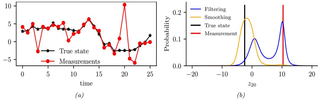
Figure 8.13: (a) Observations and true and estimated state. (b) Marginal distributions for time step t = 20. Generated by discretized\_ssm\_student.ipynb.

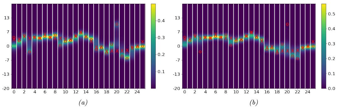
Figure 8.14: Discretized posterior of the latent state at each time step. Red cross is the true latent state. Red circle is observation. (a) Filtering. (b) Smoothing. Generated by discretized\_ssm\_student.ipynb.

8.7.3 Variational inference

EP can be viewed as locally minimizing the inclusive KL, DKL (p(zt|y1:^T ) ↘ q(zt|y1:^T )), for each time step t. An alternative approach is to globally minimize the exclusive KL, DKL (q(z1:^T |y1:^T ) ↘ p(z1:^T |y1:^T )); this is called variational inference, and is explained in Chapter 10. The di!erence between these two objectives is discussed in more detail in Section 5.1.4.1, but from a practical point of view, the main advantage of VI is that we can derive a tractable lower bound to the objective, and can then optimize it using stochastic optimization. This method is guaranteed to converge, unlike EP. For more details on VI applied to SSMs (both state estimation and parameter estimation), see e.g., [CWS21; Cou+20; Cou+21; BFY20; FLMM21; Cam+21].

8.7.4 MCMC

In Chapter 12 we discuss Markov chain Monte Carlo (MCMC) methods, which can be used to draw samples from intractable posteriors. In the case of SSMs, this includes both the distribution over states, p(z1:^T |y1:^T ), and the distribution over parameters, p(ω|y1:^T ). In some cases, such as when

using HMMs or linear-Gaussian SSMs, we can perform blocked Gibbs sampling, in which we use forwards filtering backwards sampling to sample an entire sequence from p(z1:^T |y1:^T , ω), followed by sampling the parameters, p(ω|z1:^T , y1:^T ) (see e.g., [CK96; Sco02; CMR05] for details.) Alternatively we can marginalize out the hidden states and just compute the parameter posterior p(ω|y1:^T ). When state inference is intractable, we can use gradient-based HMC methods (assuming the states are continuous), although this does not scale well to long sequences.

8.7.5 Particle filtering

In Section 13.2 we discuss particle filtering, which is a form of sequential Bayesian inference for SSMs which replaces the assumption that the posterior is (approximately) Gaussian with a more flexible representation, namely a set of weighted samples called “particles” (see e.g., [Aru+02; DJ11; NLS19]). Essentially the technique amounts to a form of importance sampling, combined with steps to prevent “particle impoverishment”, which refers to some samples receiving negligible weight because they are too improbable in the posterior (which grows with time). Particle filtering is widely used because it is very flexible, and has good theoretical properties. In practice it may require many samples to get a good approximation, but we can use heuristic methods, such as the extended or unscented Kalman filters, as proposal distributions, which can improve the e”ciency significantly. In the o$ine setting, we can use particle smoothing (Section 13.5) or SMC (sequential Monte Carlo) samplers (Section 13.6).

9 Message passing algorithms

9.1 Introduction

In this chapter we consider posterior inference (i.e., computing marginals, modes, samples, etc) for probability distributions that can be represented by a probabilistic graphical model (PGM, Chapter 4) with some kind of sparse graph structure (i.e., it is not a fully connected graph). The algorithms we discuss will leverage the conditional independence properties encoded in the graph structure (discussed in Chapter 4) in order to perform e”cient inference. In particular, we will use the principle of dynamic programming (DP), which finds an optimal solution by solving subproblems and then combining them.

DP can be implemented by computing local quantities for each node (or clique) in the graph, and then sending messages to neighboring nodes (or cliques) so that all nodes (cliques) can come to an overall consensus about the global solutions. Hence these are known as message passing algorithms. Each message can be intepreted as probability distribution about the value of a node given evidence from part of the graph. These distributions are often called belief states, so these algorithms are also called belief propagation (BP) algorithms.

In Section 9.2, we consider the special case where the graph structure is a 1d chain, which is an important special case. (For a chain, a natural approach is to send messages forwards in time, and then backwards in time, so this method can also be used for inference in state space models, as we discuss in Chapter 8.) In Section 9.3, we can generalize this approach to work with trees, and in Section 9.4, we generalize it work with any graph, including ones with cycles or loops. However, sending messages on loopy graphs may give incorrect answers. In such cases, we may wish to convert the graph to a tree, and then send messages on it, using the methods discussed in Section 9.5 and Section 9.6. We can also pose the inference problem as an optimization problem, as we discuss in Section 9.7.

9.2 Belief propagation on chains

In this section, we consider inference for PGMs where the graph structure is a 1d chain. For notational simplicity, we focus on the case where the graphical model is directed rather than undirected, although the resulting methods are easy to generalize. In addition, we only consider the case where all the hidden variables are discrete; we discuss generalizations to handle continuous latent variables in Chapter 8 and Chapter 13.

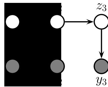
Figure 9.1: An HMM represented as a graphical model. z^t are the hidden variables at time t, y^t are the observations (outputs).

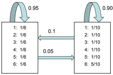
Figure 9.2: The state transition matrix A and observation matrix B for the casino HMM. Adapted from [Dur+98, p54].

9.2.1 Hidden Markov Models

In this section we assume the graphical model can be represented as a state space model, as shown in Figure 9.1. We discuss SSMs in more detail in Chapter 29, but we can think of them as latent variable sequence models with the conditional independencies shown by the chain-structured graphical model Figure 8.1. The corresponding joint distribution has the form

\[p(\mathbf{y}\_{1:T}, \mathbf{z}\_{1:T}) = \left[ p(\mathbf{z}\_1) \prod\_{t=2}^{T} p(\mathbf{z}\_t | \mathbf{z}\_{t-1}) \right] \left[ \prod\_{t=1}^{T} p(\mathbf{y}\_t | \mathbf{z}\_t) \right] \tag{9.1}\]

where z^t are the hidden variables at time t, and y^t are the observations (outputs). If all the latent variables are discrete (as we assume in this section), the resulting model is called a hidden Markov model or HMM. We consider SSMs with continuous latent variables in Chapter 8.

9.2.1.1 Example: casino HMM

As a concrete example from [Dur+98], we consider the occasionally dishonest casino. We assume we are in a casino and observe a series of die rolls, y^t ↗ {1, 2,…, 6}. Being a keen-eyed statistician, we notice that the distribution of values is not what we expect from a fair die: it seems that there

are occasional “streaks”, in which 6s seem to show up more often than other values. We would like to estimate the underlying state, namely whether the die is fair or loaded, so that we make predictions about the future.

To formalize this, let z^t ↗ {1, 2} represent the unknown hidden state (fair or loaded) at time t, and let y^t ↗ {1,…, 6} represent the observed outcome (die roll). Let Ajk = p(z^t = k|zt↓¹ = j) be the state transition matrix. Most of the time the casino uses a fair die, z = 1, but occasionally it switches to a loaded die, z = 2, for a short period, as shown in the state transition diagram in Figure 9.2.

Let Bkl = p(y^t = l|z^t = k) be the observation matrix corresponding to a categorical distribution over values of the die face. If z = 1 the observation distribution is a uniform categorical distribution over the symbols {1,…, 6}. If z = 2, the observation distribution is skewed towards face 6. That is,

\[p(y\_t | z\_t = 1) = \text{Cat}(y\_t | [1/6, \dots, 1/6]) \tag{9.2}\]

\[p(y\_t | z\_t = 2) = \text{Cat}(y\_t | [1/10, 1/10, 1/10, 1/10, 1/10, 5/10])\tag{9.3}\]

If we sample from this model, we may generate data such as the following:

hid: 1111111111222211111111111111111111112222222221222211111111111111111111 obs: 1355534526553366316351551526232112113462221263264265422344645323242361

Here obs refers to the observation and hid refers to the hidden state (1 is fair and 2 is loaded). In the full sequence of length 300, we find the empirical fraction of times that we observe a 6 in hidden state 1 to be 0.149, and in state 2 to be 0.472, which are very close to the expected fractions. (See casino\_hmm.ipynb for the code.)

9.2.1.2 Posterior inference

Our goal is to infer the hidden states by computing the posterior over all the hidden nodes in the model, p(zt|y1:^T ). This is called the smoothing distribution. By the Markov property, we can break this into two terms:

\[p(\mathbf{z}\_t = j | \mathbf{y}\_{t+1:T}, \mathbf{y}\_{1:t}) \propto p(\mathbf{z}\_t = j, \mathbf{y}\_{t+1:T} | \mathbf{y}\_{1:t}) = p(\mathbf{z}\_t = j | \mathbf{y}\_{1:t}) p(\mathbf{y}\_{t+1:T} | \mathbf{z}\_t = j, \mathbf{y}\_{\mathbf{x}:\mathbf{f}}) \tag{9.4}\]

We will first compute the filtering distribution p(z^t = j|y1:t) by working forwards in time. We then compute the p(yt+1:^T |z^t = j) terms by working backwards in time, and then we finally combine both terms. Both passes take (TK²) time, where K is the number of discrete hidden states. We give the details below.

9.2.2 The forwards algorithm

As we discuss in Section 8.1.2, the Bayes filter is an algorithm for recursively computing the belief state p(zt|y1:t) given the prior belief from the previous step, p(z^t↓¹|y1:t↓1), the new observation yt, and the model. In the HMM literature, this is known as the forwards algorithm.

In an HMM, the latent states z^t are discrete, so we can define the belief state as a vector, ϱt(j) ↭ p(z^t = j|y1:t), the local evidence as another vector, ⇀t(j) ↭ p(yt|z^t = j), and the transition matrix as Ai,j = p(z^t = j|z^t↓¹ = i). Then the predict step becomes

\[\alpha\_{t|t-1}(j) \triangleq p(z\_t = j | \mathbf{y}\_{1:t-1}) = \sum\_{i} p(z\_t = j | z\_{t-1} = i) p(z\_{t-1} = i | \mathbf{y}\_{1:t-1}) = \sum\_{i} A\_{i,j} \alpha\_{t-1}(i) \tag{9.5}\]

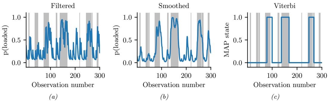
Figure 9.3: Inference in the dishonest casino. Vertical gray bars denote times when the hidden state corresponded to the loaded die. Blue lines represent the posterior probability of being in that state given di!erent subsets of observed data. If we recover the true state exactly, the blue curve will transition at the same time as the gray bars. (a) Filtered estimates. (b) Smoothed estimates. (c) MAP trajectory. Generated by casino\_hmm.ipynb.

and the update step becomes

\[\alpha\_t(j) = \frac{1}{Z\_t} p(y\_t | z\_t = j) p(z\_t = j | y\_{1:t-1}) = \frac{1}{Z\_t} \lambda\_t(j) \alpha\_{t|t-1}(j) = \frac{1}{Z\_t} \lambda\_t(j) \left[ \sum\_i \alpha\_{t-1}(i) A\_{i,j} \right] \tag{9.6}\]

where the normalization constant for each time step is given by

\[Z\_t \triangleq p(y\_t | y\_{1:t-1}) = \sum\_{j=1}^{K} p(y\_t | \mathbf{z}\_t = j) p(\mathbf{z}\_t = j | y\_{1:t-1}) = \sum\_{j=1}^{K} \lambda\_t(j) \alpha\_{t|t-1}(j) \tag{9.7}\]

We can write the update equation in matrix-vector notation as follows:

\[\alpha\_t = \text{normalize}\left(\lambda\_t \odot (\mathbf{A}^{\mathsf{T}} \alpha\_{t-1})\right) \tag{9.8}\]

where ∞ represents elementwise vector multiplication, and the normalize function just ensures its argument sums to one. (See Section 9.2.3.4 for more discussion on normalization.)

Figure 9.3(a) illustrates filtering for the casino HMM, applied to a random sequence y1:^T of length T = 300. In blue, we plot the probability that the die is in the loaded (vs fair) state, based on the evidence seen so far. The gray bars indicate time intervals during which the generative process actually switched to the loaded die. We see that the probability generally increases in the right places.

9.2.3 The forwards-backwards algorithm

In this section, we present the most common approach to smoothing in HMMs, known as the forwardsbackwards or FB algorithm [Rab89]. In the forwards pass, we compute ϱt(j) = p(z^t = j|y1:t) as before. In the backwards pass, we compute the conditional likelihood

\[\beta\_t(j) \triangleq p(y\_{t+1:T} | \mathbf{z}\_t = j) \tag{9.9}\]

We then combine these using

\[p(j) = p(\mathbf{z}\_t = j | \mathbf{y}\_{t+1:T}, \mathbf{y}\_{1:t}) \propto p(\mathbf{z}\_t = j, \mathbf{y}\_{t+1:T} | \mathbf{y}\_{1:t}) \tag{9.10}\]

\[\mathbf{z} = p(\mathbf{z}\_t = j | \mathbf{y}\_{1:t}) p(\mathbf{y}\_{t+1:T} | \mathbf{z}\_t = j, \mathbf{y}\_{\mathbf{x}:t}) = \alpha\_t(j)\beta\_t(j) \tag{9.11}\]

In matrix notation, this becomes

\[ \gamma\_t = \text{normalize}(\alpha\_t \odot \beta\_t) \tag{9.12} \]

Note that the forwards and backwards passes can be computed independently, but both need access to the local evidence p(yt|zt). The results are only combined at the end. This is therefore called two-filter smoothing [Kit04].

9.2.3.1 Backwards recursion

We can recursively compute the ↼’s in a right-to-left fashion as follows:

\[\mathbf{x}\_{t-1}(i) = p(\mathbf{y}\_{t:T} | \mathbf{z}\_{t-1} = i) \tag{9.13}\]

\[\mathbf{z}\_{t} = \sum\_{j} p(\mathbf{z}\_{t} = j, \mathbf{y}\_{t}, \mathbf{y}\_{t+1:T} | \mathbf{z}\_{t-1} = i) \tag{9.14}\]

\[\mathbf{x} = \sum\_{j} p(y\_{t+1:T} | \mathbf{z}\_t = j, \mathbf{y} \mathbf{y} , \mathbf{z}\_{t-T} = \mathbf{f} ) p(\mathbf{z}\_t = j, \mathbf{y}\_t | \mathbf{z}\_{t-1} = i) \tag{9.15}\]

\[\mathbf{z} = \sum\_{j} p(y\_{t+1:T} | \mathbf{z}\_t = j) p(y\_t | \mathbf{z}\_t = j, \mathbf{z}\_{t-\mathbf{T}} = \mathbf{\tilde{z}} \mathbf{\tilde{}}) p(\mathbf{z}\_t = j | \mathbf{z}\_{t-1} = i) \tag{9.16}\]

\[\lambda = \sum\_{j} \beta\_{t}(j)\lambda\_{t}(j)A\_{i,j} \tag{9.17}\]

We can write the resulting equation in matrix-vector form as

\[ \boldsymbol{\beta}\_{t-1} = \mathbf{A}(\lambda\_t \odot \boldsymbol{\beta}\_t) \tag{9.18} \]

The base case is

\[ \beta\_T(i) = p(\mathbf{y}\_{T+1:T} | \mathbf{z}\_T = i) = p(\emptyset | \mathbf{z}\_T = i) = 1\tag{9.19} \]

which is the probability of a non-event.

Note that ⇀^t & is not a probability distribution over states, since it does not need to satisfy ^j ↼t(j)=1. However, we usually normalize it to avoid numerical underflow (see Section 9.2.3.4).

9.2.3.2 Example

In Figure 9.3(a-b), we compare filtering and smoothing for the casino HMM. We see that the posterior distributions when conditioned on all the data (past and future) are indeed smoother than when just conditioned on the past (filtering).

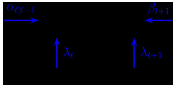
Figure 9.4: Computing the two-slice joint distribution for an HMM from the forwards messages, backwards messages, and local evidence messages.

9.2.3.3 Two-slice smoothed marginals

We can compute the two-slice marginals using the output of the forwards-backwards algorithm as follows:

\[p(\mathbf{z}\_t, \mathbf{z}\_{t+1}|\mathbf{y}\_{1:T}) = p(\mathbf{z}\_t, \mathbf{z}\_{t+1}|\mathbf{y}\_{1:t}, \mathbf{y}\_{t+1:T}) \tag{9.20}\]

\[\propto p(y\_{t+1:T}|z\_t, z\_{t+1}, y\_{1:t}) p(z\_t, z\_{t+1}|y\_{1:t}) \tag{9.21}\]

\[\mathbf{y} = p(\mathbf{y}\_{t+1:T}|\mathbf{z}\_{t+1})p(\mathbf{z}\_t, \mathbf{z}\_{t+1}|\mathbf{y}\_{1:t}) \tag{9.22}\]

\[=p(y\_{t+1:T}|z\_{t+1})p(z\_t|y\_{1:t})p(z\_{t+1}|z\_t)\tag{9.23}\]

\[=p(y\_{t+1}, y\_{t+2:T}|z\_{t+1})p(z\_t|y\_{1:t})p(z\_{t+1}|z\_t)\tag{9.24}\]

\[=p(\mathbf{y}\_{t+1}|\mathbf{z}\_{t+1})p(\mathbf{y}\_{t+2:T}|\mathbf{z}\_{t+1},\mathbf{y}\_{t+1})p(\mathbf{z}\_t|\mathbf{y}\_{1:t})p(\mathbf{z}\_{t+1}|\mathbf{z}\_t)\tag{9.25}\]

\[=p(\mathbf{y}\_{t+1}|\mathbf{z}\_{t+1})p(\mathbf{y}\_{t+2:T}|\mathbf{z}\_{t+1})p(\mathbf{z}\_t|\mathbf{y}\_{1:t})p(\mathbf{z}\_{t+1}|\mathbf{z}\_t)\tag{9.26}\]

We can rewrite this in terms of the already computed quantities as follows:

\[ \lambda \xi\_{t, t+1}(i, j) \propto \lambda\_{t+1}(j) \beta\_{t+1}(j) \alpha\_t(i) A\_{i, j} \tag{9.27} \]

Or in matrix-vector form:

\[\mathbf{f}\_{t,t+1} \propto \mathbf{A} \odot \left[ \alpha\_t (\lambda\_{t+1} \odot \boldsymbol{\beta}\_{t+1})^{\mathsf{T}} \right] \tag{9.28}\]

Since ↼^t ↑ ϑ^t ∞ ↼^t|t↓¹, we can also write the above equation as follows:

\[\mathbf{f}\_{t,t+1} \propto \mathbf{A} \odot \left[ (\lambda\_t \odot \alpha\_{t|t-1}) \odot (\lambda\_{t+1} \odot \beta\_{t+1})^\top \right] \tag{9.29}\]

This can be interpreted as a product of incoming messages and local factors, as shown in Figure 9.4. In particular, we combine the factors ↼^t|t↓¹ = p(zt|y1:t↓¹), A = p(zt+1|zt), ϑ^t ↑ p(yt|zt), ϑt+1 ↑ p(yt+1|zt+1), and ⇀t+1 ↑ p(yt+2:^T |zt+1) to get p(zt, zt+1, yt, yt+1, yt+2:^T |y1:t↓1), which we can then normalize.

9.2.3.4 Numerically stable implementation

In most publications on HMMs, such as [Rab89], the forwards message is defined as the following unnormalized joint probability:

\[\alpha\_t'(j) = p(\mathbf{z}\_t = j, \mathbf{y}\_{1:t}) = \lambda\_t(j) \left[ \sum\_i \alpha\_{t-1}'(i) A\_{i,j} \right] \tag{9.30}\]

We instead define the forwards message as the normalized conditional probability

\[p(\alpha\_t(j) = p(\mathbf{z}\_t = j | \mathbf{y}\_{1:t}) = \frac{1}{Z\_t} \lambda\_t(j) \left[ \sum\_i \alpha\_{t-1}(i) A\_{i,j} \right] \tag{9.31}\]

The unnormalized (joint) form has several problems. First, it rapidly su!ers from numerical underflow, since the probability of the joint event that (z^t = j, y1:t) is vanishingly small.1 Second, it is less interpretable, since it is not a distribution over states. Third, it precludes the use of approximate inference methods that try to approximate posterior distributions (we will see such methods later). We therefore always use the normalized (conditional) form.

Of course, the two definitions only di!er by a multiplicative constant, since p(z^t = j|y1:t) = p(z^t = j, y1:t)/p(y1:t) [Dev85]. So the algorithmic di!erence is just one line of code (namely the presence or absence of a call to the normalize function). Nevertheless, we feel it is better to present the normalized version, since it will encourage readers to implement the method properly (i.e., normalizing after each step to avoid underflow).

In practice it is more numerically stable to compute the log probabilities εt(j) = log p(yt|z^t = j) of the evidence, rather than the probabilities ⇀t(j) = p(yt|z^t = j). We can combine the state conditional log likelihoods ⇀t(j) with the state prior p(z^t = j|y1:t↓1) by using the log-sum-exp trick, as in Equation (28.30).

9.2.4 Forwards filtering backwards smoothing

An alternative way to perform o$ine smoothing is to use forwards filtering/backwards smoothing, as discussed in Section 8.1.3. In this approach, we first perform the forwards or filtering pass, and then compute the smoothed belief states by working backwards, from right (time t = T) to left (t = 1). This approach is widely used for SSMs with continuous latent states, since the backwards likelihood ↼t(i) used in Section 9.2.3 is not always well defined when the state space is not discrete.

We assume by induction that we have already computed

\[ \gamma\_{t+1}(j) \triangleq p(\mathbf{z}\_{t+1} = j | \mathbf{y}\_{1:T}) \tag{9.32} \]

^1. For example, if the observations are independent of the states, we have p(z^t = j, y1:t) = p(z^t = j) !t ⁱ=1 p(yi), which becomes exponentially small with t.

We then compute the smoothed joint distribution over two consecutive time steps:

\[\xi\_{t,t+1}(i,j) \triangleq p(\mathbf{z}\_t = i, \mathbf{z}\_{t+1} = j | \mathbf{y}\_{1:T}) = p(\mathbf{z}\_t = i | \mathbf{z}\_{t+1} = j, \mathbf{y}\_{1:t}) p(\mathbf{z}\_{t+1} = j | \mathbf{y}\_{1:T}) \tag{9.33}\]

\[p(\mathbf{z}\_t = -i | \mathbf{z}\_t = j) p(\mathbf{z}\_t = i | \mathbf{z}\_t = j | \mathbf{z}\_t = -i | \mathbf{z}\_t = )\]

\[\mathbf{z} = \frac{p(\mathbf{z}\_{t+1} = j | \mathbf{z}\_t = i)p(\mathbf{z}\_t = i | \mathbf{y}\_{1:t})p(\mathbf{z}\_{t+1} = j | \mathbf{y}\_{1:T})}{p(\mathbf{z}\_{t+1 = j} | \mathbf{y}\_{1:t})} \tag{9.34}\]

\[ \lambda = \alpha\_t(i) A\_{i,j} \frac{\gamma\_{t+1}(j)}{\alpha\_{t+1\mid t}(j)} \tag{9.35} \]

where

\[\alpha\_{t+1|t}(j) = p(\mathbf{z}\_{t+1} = j | \mathbf{y}\_{1:t}) = \sum\_{i'} A(i', j)\alpha\_t(i') \tag{9.36}\]

is the one-step-ahead predictive distribution. We can interpret the ratio in Equation (9.35) as dividing out the old estimate of zt+1 given y1:t, namely ϱt+1|^t, and multiplying in the new estimate given y1:^T , namely ▷t+1.

Once we have the two sliced smoothed distribution, we can easily get the marginal one slice smoothed distribution using

\[\gamma\_t(i) = p(\mathbf{z}\_t = i | \mathbf{y}\_{1:T}) = \sum\_j \xi\_{t, t+1}(i, j) = \alpha\_t(i) \sum\_j \left[ A\_{i, j} \frac{\gamma\_{t+1}(j)}{\alpha\_{t+1 \mid t}(j)} \right] \tag{9.37}\]

We initialize the recursion using ▷^T (j) = ϱ^T (j) = p(z^T = j|y1:^T ).

9.2.5 Time and space complexity

It is clear that a straightforward implementation of the forwards-backwards algorithm takes O(K²T) time, since we must perform a K ⇔ K matrix multiplication at each step. For some applications, such as speech recognition, K is very large, so the O(K²) term becomes prohibitive. Fortunately, if the transition matrix is sparse, we can reduce this substantially. For example, in a sparse left-to-right transition matrix (e.g., Figure 9.6(a)), the algorithm takes O(TK) time.

In some cases, we can exploit special properties of the state space, even if the transition matrix is not sparse. In particular, suppose the states represent a discretization of an underlying continuous state-space, and the transition matrix has the form Ai,j ↑ 0(z^j → zi), where zⁱ is the continuous vector represented by state i and 0(u) is some scalar cost function, such as Euclidean distance. Then one can implement the forwards-backwards algorithm in O(TK log K) time. The key is to rewrite Equation (9.5) as a convolution,

\[\alpha\_{t|t-1}(j) = p(z\_t = j | \mathbf{y}\_{1:t-1}) = \sum\_{i} \alpha\_{t-1}(i) A\_{i,j} = \sum\_{i} \alpha\_{t-1}(i)\rho(j-i) \tag{9.38}\]

and then to apply the Fast Fourier Transform. (A similar transformation can be applied in the backwards pass.) This is very useful for models with large state spaces. See [FHK03] for details.

We can also reduce inference to O(log T) time by using a parallel prefix scan operator that can be run e”ciently on GPUs. For details, see [HSGF21].

In some cases, the bottleneck is memory, not time. In particular, to compute the posteriors ↽t, we must store the fitered distributions ↼^t for t = 1,…,T until we do the backwards pass. It is possible

Figure 9.5: The trellis of states vs time for a Markov chain. Adapted from [Rab89].

to devise a simple divide-and-conquer algorithm that reduces the space complexity from O(KT) to O(K log T) at the cost of increasing the running time from O(K²T) to O(K²T log T). The basic idea is to store ↼^t and ⇀^t vectors at a logarithmic number of intermediate checkpoints, and then recompute the missing messages on demand from these checkpoints. See [BMR97; ZP00] for details.

9.2.6 The Viterbi algorithm

The MAP estimate is (one of) the sequences with maximum posterior probability:

\[\mathbf{z}\_{1:T}^{\*} = \underset{\mathbf{z}\_{1:T}}{\operatorname{argmax}} \, p(\mathbf{z}\_{1:T} | \mathbf{y}\_{1:T}) = \underset{\mathbf{z}\_{1:T}}{\operatorname{argmax}} \, \log p(\mathbf{z}\_{1:T} | \mathbf{y}\_{1:T}) \tag{9.39}\]

\[= \underset{\mathbf{z}\_{1:T}}{\operatorname{argmax}} \, \log \pi\_1(\mathbf{z}\_1) + \log \lambda\_1(\mathbf{z}\_1) + \sum\_{t=2}^{T} \left[ \log A(\mathbf{z}\_{t-1}, \mathbf{z}\_t) + \log \lambda\_t(\mathbf{z}\_t) \right] \tag{9.40}\]

This is equivalent to computing a shortest path through the trellis diagram in Figure 9.5, where the nodes are possible states at each time step, and the node and edge weights are log probabilities. This can be computed in O(TK²) time using the Viterbi algorithm [Vit67], as we explain below.

t=2

9.2.6.1 Forwards pass

Recall the (unnormalized) forwards equation

\[\alpha'\_t(j) = p(\mathbf{z}\_t = j, \mathbf{y}\_{1:t}) = \sum\_{\mathbf{z}\_1, \dots, \mathbf{z}\_{t-1}} p(\mathbf{z}\_{1:t-1}, \mathbf{z}\_t = j, \mathbf{y}\_{1:t}) \tag{9.41}\]

Now suppose we replace sum with max to get

\[\delta\_t(j) \triangleq \max\_{\mathbf{z}\_1, \dots, \mathbf{z}\_{t-1}} p(\mathbf{z}\_{1:t-1}, \mathbf{z}\_t = j, \mathbf{y}\_{1:t}) \tag{9.42}\]

This is the maximum probability we can assign to the data so far if we end up in state j. The key insight is that the most probable path to state j at time t must consist of the most probable path to

some other state i at time t → 1, followed by a transition from i to j. Hence

\[\delta\_t(j) = \lambda\_t(j) \left[ \max\_i \delta\_{t-1}(i) A\_{i,j} \right] \tag{9.43}\]

We initialize by setting ϑ1(j) = ϖj⇀1(j).

We often work in the log domain to avoid numerical issues. Let ϑ^{↔︎ t}(j) = → log ϑt(j), ⇀^{↔︎ t}(j) = → log p(yt|z^t = j), A^↔︎ (i, j) = → log p(z^t = j|z^t↓¹ = i). Then we have

\[ \delta\_t'(j) = \lambda\_t'(j) + \left[ \min\_i \delta\_{t-1}'(i) + A'(i, j) \right] \tag{9.44} \]

We also need to keep track of the most likely previous (ancestor) state, for each possible state that we end up in:

\[a\_t(j) \triangleq \operatorname\*{argmax}\_i \delta\_{t-1}(i) A\_{i,j} = \operatorname\*{argmin}\_i \delta'\_{t-1}(i) + A'(i,j) \tag{9.45}\]

That is, at(j) stores the identity of the previous state on the most probable path to z^t = j. We will see why we need this in Section 9.2.6.2.

9.2.6.2 Backwards pass

In the backwards pass, we compute the most probable sequence of states using a traceback procedure, as follows: z^{→ t} = at+1(z^{→ t}+1), where we initialize using z^{→ T} = arg maxⁱ ϑ^T (i). This is just following the chain of ancestors along the MAP path.

If there is a unique MAP estimate, the above procedure will give the same result as picking zˆ^t = argmax^j ▷t(j), computed by forwards-backwards, as shown in [WF01b]. However, if there are multiple posterior modes, the latter approach may not find any of them, since it chooses each state independently, and hence may break ties in a manner that is inconsistent with its neighbors. The traceback procedure avoids this problem, since once z^t picks its most probable state, the previous nodes condition on this event, and therefore they will break ties consistently.

9.2.6.3 Example

In Figure 9.3(c), we show the Viterbi trace for the casino HMM. We see that, most of the time, the estimated state corresponds to the true state.

In Figure 9.6, we give a detailed worked example of the Viterbi algorithm, based on [Rus+95]. Suppose we observe the sequence of discrete observations y1:4 = (C1, C3, C4, C6), representing codebook entries in a vector-quantized version of a speech signal. The model starts in state z¹ = S1. The probability of generating x¹ = C¹ in z¹ is 0.5, so we have ϑ1(1) = 0.5, and ϑ1(i)=0 for all other states. Next we can self-transition to S¹ with probability 0.3, or transition to S² with proabability 0.7. If we end up in S1, the probability of generating x² = C³ is 0.3; if we end up in S2, the probability of generating x² = C³ is 0.2. Hence we have

\[ \delta\_2(1) = \delta\_1(1) A(1,1) \lambda\_2(1) = 0.5 \cdot 0.3 \cdot 0.3 = 0.045 \tag{9.46} \]

\[ \delta\_2(2) = \delta\_1(1)A(1,2)\lambda\_2(2) = 0.5 \cdot 0.7 \cdot 0.2 = 0.07\tag{9.47} \]

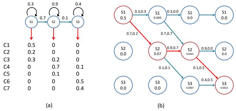
Figure 9.6: Illustration of Viterbi decoding in a simple HMM for speech recognition. (a) A 3-state HMM for a single phone. We are visualizing the state transition diagram. We assume the observations have been vector quantized into 7 possible symbols, C1,…,C7. Each state S1, S2, S³ has a di!erent distribution over these symbols. Adapted from Figure 15.20 of [RN02]. (b) Illustration of the Viterbi algorithm applied to this model, with data sequence C1, C3, C4, C6. The columns represent time, and the rows represent states. The numbers inside the circles represent the ϖt(j) value for that state. An arrow from state i at t ↗ 1 to state j at t is annotated with two numbers: the first is the probability of the i → j transition, and the second is the probability of generating observation y^t from state j. The red lines/circles represent the most probable sequence of states. Adapted from Figure 24.27 of [RN95].

Thus state 2 is more probable at t = 2; see the second column of Figure 9.6(b). The algorithm continues in this way until we have reached the end of the sequence. One we have reached the end, we can follow the red arrows back to recover the MAP path (which is 1,2,2,3).

For more details on HMMs for automatic speech recognition (ASR) see e.g., [JM08].

9.2.6.4 Time and space complexity

The time complexity of Viterbi is clearly O(K²T) in general, and the space complexity is O(KT), both the same as forwards-backwards. If the transition matrix has the form Ai,j ↑ 0(z^j → zi), where zⁱ is the continuous vector represented by state i and 0(u) is some scalar cost function, such as Euclidean distance, we can implement Viterbi in O(TK) time, by using the generalized distance transform to implement Equation (9.44). See [FHK03; FH12] for details.

9.2.6.5 N-best list

There are often multiple paths which have the same likelihood. The Viterbi algorithm returns one of them, but can be extended to return the top N paths [SC90; NG01]. This is called the N-best list. Computing such a list can provide a better summary of the posterior uncertainty.

In addition, we can perform discriminative reranking [CK05] of all the sequences in L^N , based on global features derived from (y1:^T , z1:^T ). This technique is widely used in speech recognition. For example, consider the sentence “recognize speech”. It is possible that the most probable interpretation by the system of this acoustic signal is “wreck a nice speech”, or maybe “wreck a nice beach” (see

Figure 34.3). Maybe the correct interpretation is much lower down on the list. However, by using a re-ranking system, we may be able to improve the score of the correct interpretation based on a more global context.

One problem with the N-best list is that often the top N paths are very similar to each other, rather than representing qualitatively di!erent interpretations of the data. Instead we might want to generate a more diverse set of paths to more accurately represent posterior uncertainty. One way to do this is to sample paths from the posterior, as we discuss in Section 9.2.7. Another way is to use a determinantal point process (Supplementary Section 31.8.5) which encourages points to be diverse [Bat+12; ZA12].

9.2.7 Forwards filtering backwards sampling

Rather than computing the single most probable path, it is often useful to sample multiple paths from the posterior: z^s 1:^T ↔︎ p(z1:^T |y1:^T ). We can do this by modifying the forwards filtering backwards smoothing algorithm from Section 9.2.4, so that we draw samples on the backwards pass, rather than computing marginals. This is called forwards filtering backwards sampling (also sometimes unfortunately abbreviated to FFBS). In particular, note that we can write the joint from right to left using

\[p(\mathbf{z}\_{1:T}|\mathbf{y}\_{1:T}) = p(\mathbf{z}\_T|\mathbf{y}\_{1:T})p(\mathbf{z}\_{T-1}|\mathbf{z}\_T, \mathbf{y}\_{1:T})p(\mathbf{z}\_{T-2}|\mathbf{z}\_{T-1}, \mathbf{z}\_T; \mathbf{y}\_{1:T}) \cdots p(\mathbf{z}\_1|\mathbf{z}\_2, \mathbf{z}\_3; \mathbf{y}\_{1:T}) \tag{9.48}\]

\[=p(\mathbf{z}\_T|\mathbf{y}\_{1:T})\prod\_{t=T-1}^{1}p(\mathbf{z}\_t|\mathbf{z}\_{t+1},\mathbf{y}\_{1:T})\tag{9.49}\]

Thus at step t we sample z^{s t} from ^p(zt|z^{s t}+1, y1:^T ) given in Equation (9.49).

9.3 Belief propagation on trees

The forwards-backwards algorithm for HMMs discussed in Section 9.2.3 (and the Kalman smoother algorithm for LDS which we discuss in Section 8.2.3) can be interpreted as a message passing algorithm applied to a chain structured graphical model. In this section, we generalize these algorithms to work with trees.

9.3.1 Directed vs undirected trees

Consider a pairwise undirected graphical model, which can be written as follows:

\[p^\*(\mathbf{z}) \triangleq p(\mathbf{z}|\mathbf{y}) \propto \prod\_{s \in \mathcal{V}} \psi\_s(z\_s|\mathbf{y}\_s) \prod\_{(s,t) \in \mathcal{E}} \psi\_{s,t}(z\_s, z\_t) \tag{9.50}\]

where 1s,t(zs, zt) are the pairwise clique potential, one per edge, 1s(zs|ys) are the local evidence potentials, one per node, V is the set of nodes, and E is the set of edges. (We will henceforth drop the conditioning on the observed values y for brevity.)

Now suppose the corresponding graph structure is a tree, such as the one in Figure 9.7a. We can always convert this into a directed tree by picking an arbitrary node as the root, and then “picking

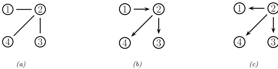
Figure 9.7: An undirected tree and two equivalent directed trees.

the tree up by the root” and orienting all the edges away from the root. For example, if we pick node 1 as the root we get Figure 9.7b. This corresponds to the following directed graphical model:

\[p^\*(\mathbf{z}) \propto p^\*(z\_1) p^\*(z\_2|z\_1) p^\*(z\_3|z\_2) p^\*(z\_4|z\_2) \tag{9.51}\]

However, if we pick node 2 as the root, we get Figure 9.7c. This corresponds to the following directed graphical model:

\[p^\*(\mathbf{z}) \propto p^\*(z\_2) p^\*(z\_1|z\_2) p^\*(z\_3|z\_2) p^\*(z\_4|z\_2) \tag{9.52}\]

Since these graphs express the same conditional independence properties, they represent the same family of probability distributions, and hence we are free to use any of these parameterizations.

To make the model more symmetric, it is preferable to use an undirected tree. If we define the potentials as (possibly unnnormalized) marginals (i.e., 1s(zs) ↑ p→(zs) and 1s,t(zs, zt) = p→(zs, zt)), then we can write

\[p^\*(\mathbf{z}) \propto \prod\_{s \in \mathcal{V}} p^\*(z\_s) \prod\_{(s,t) \in \mathcal{E}} \frac{p^\*(z\_s, z\_t)}{p^\*(z\_s)p^\*(z\_t)}\tag{9.53}\]

For example, for Figure 9.7a we have

\[p^\*(z\_1, z\_2, z\_3, z\_4) \propto p^\*(z\_1)p^\*(z\_2)p^\*(z\_3)p^\*(z\_4)\frac{p^\*(z\_1, z\_2)p^\*(z\_2, z\_3)p^\*(z\_2, z\_4)}{p^\*(z\_1)p^\*(z\_2)p^\*(z\_2)p^\*(z\_3)p^\*(z\_2)p^\*(z\_4)}\tag{9.54}\]

To see the equivalence with the directed representation, we can cancel terms to get

\[p^\*(z\_1, z\_2, z\_3, z\_4) \propto p^\*(z\_1, z\_2) \frac{p^\*(z\_2, z\_3)}{p^\*(z\_2)} \frac{p^\*(z\_2, z\_4)}{p^\*(z\_2)}\tag{9.55}\]

\[=p^\*(z\_1)p^\*(z\_2|z\_1)p^\*(z\_3|z\_2)p^\*(z\_4|z\_2)\tag{9.56}\]

\[=p^\*(z\_2)p^\*(z\_1|z\_2)p^\*(z\_3|z\_2)p^\*(z\_4|z\_2)\tag{9.57}\]

where p→(zt|zs) = p→(zs, zt)/p→(zs).

Thus a tree can be represented as either an undirected or directed graph. Both representations can be useful, as we will see.

// Collect to root for each node s in post-order bels(zs) ↘ ϱs(zs) ! ^t↓ch^s m^t↔︎^s(zs) t = parent(s) ^ms↔︎^t(zt) = ” ^zs ϱst(zs, zt)bels(zs)

// Distribute from root for each node t in pre-order s = parent(t) ^ms↔︎^t(zt) = ” ^{zs ϱ}st(zs, zt) bels(zs) mt↔︎s(zs) belt(zt) ↘ belt(zt)m^s↔︎^t(zt)

Figure 9.8: Belief propagation on a pairwise, rooted tree.

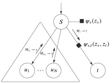
Figure 9.9: Illustration of how the top-down message from s to t is computed during BP on a tree. The uⁱ nodes are the other children of s, besides t. Square nodes represent clique potentials.

9.3.2 Sum-product algorithm

In this section, we assume that our model is an undirected tree, as in Equation (9.50). However, we will pick an arbitrary node as a root, and orient all the edges downwards away from this root, so that each node has a unique parent. For a directed, rooted tree, we can compute various node orderings. In particular, in a pre-order, we traverse from the root to the left subtree and then to right subtree, top to bottom. In a post-order, we traverse from the left subtree to the right subtree and then to the root, bottom to top. We will use both of these below.

We now present the sum-product algorithm for trees. We first send messages from the leaves to the root. This is the generalization of the forwards pass from Section 9.2.2. Let m^s↗t(zt) denote the message from node s to node t. This summarizes the belief state about z^t given all the evidence in the tree below the s → t edge. Consider a node s in the ordering. We update its belief state by

combining the incoming messages from all its children with its own local evidence:

\[\text{bel}\_s(z\_s) \propto \psi\_s(z\_s) \prod\_{t \in \text{ch}\_s} m\_{t \to s}(z\_s) \tag{9.58}\]

To compute the outgoing message that s should send to its parent t, we pass the local belief through the pairwise potential linking s and t, and then marginalize out s to get

\[m\_{s \to t}(z\_t) = \sum\_{z\_s} \psi\_{st}(z\_s, z\_t) \text{bel}\_s(z\_s) \tag{9.59}\]

At the root of the tree, belt(zt) = p(zt|y) will have seen all the evidence. It can then send messages back down to the leaves. The message that s sends to its child t should be the product of all the messages that s received from all its other children u, passed through the pairwise potential, and then marginalized:

\[m\_{s \to t}(z\_t) = \sum\_{z\_s} \left( \psi\_s(z\_s) \psi\_{st}(z\_s, z\_t) \prod\_{u \in \text{ch}\_s \backslash t} m\_{u \to s}(z\_s) \right) \tag{9.60}\]

See Figure 9.9. Instead of multiplying all-but-one of the messages that s has received, we can multiply all of them and then divide out by the t ↖ s message from child t. The advantage of this is that the product of all the messages has already been computed in Equation (9.58), so we don’t need to recompute that term. Thus we get

\[m\_{s \to t}(z\_t) = \sum\_{z\_s} \psi\_{st}(z\_s, z\_t) \frac{\text{bel}\_s(z\_s)}{m\_{t \to s}(z\_s)}\tag{9.61}\]

We can think of bels(zs) as the new updated posterior p(zs|y) given all the evidence, and m^t↗s(zs) as the prior predictive p(zs|y^{↓ t} ), where y^{↓ t} is all the evidence in the subtree rooted at t. Thus the ratio contains the new evidence that t did not already know about from its own subtree. We use this to update the belief state at node t to get:

\[\text{bel}\_{t}(z\_{t}) \propto \text{bel}\_{t}(z\_{t}) m\_{s \to t}(z\_{t}) \tag{9.62}\]

(Note that Equation (9.58) is a special case of this where we don’t divide out by m^s↗t, since in the upwards pass, there is no incoming message from the parent.) This is analogous to the backwards smoothing equation in Equation (9.37), with ϱt(i) replaced by belt(z^t = i), A(i, j) replaced by 1st(z^s = i, z^t = j), ▷t+1(j) replaced by bels(z^s = j), and ϱt+1|^t(j) replaced by m^t↗^s(z^s = j).

See Figure 9.8 for the overall pseudocode. This can be generalized to directed trees with multiple root nodes (known as polytrees) as described in Supplementary Section 9.1.1.

9.3.3 Max-product algorithm

In Section 9.3.2 we described the sum-product algorithm, that computes the posterior marginals:

\[\text{bel}\_i(k) = \gamma\_i(k) = p(z\_i = k | \mathbf{y}) = \sum\_{\mathbf{z}\_{-i}} p(z\_i = k, \mathbf{z}\_{-i} | \mathbf{y}) \tag{9.63}\]

We can replace the sum operation with the max operation to get max-product belief propagation. The result of this computation are a set of max marginals for each node:

\[ \zeta\_i(k) = \max\_{\mathbf{z}\_{-i}} p(z\_i = k, \mathbf{z}\_{-i}|\mathbf{y}) \tag{9.64} \]

We can derive two di!erent kinds of “MAP” estimates from these local quantities. The first is zˆⁱ = argmax^k ▷i(k); this is known as the maximizer of the posterior marginal or MPM estimate (see e.g., [MMP87; SM12]); let zˆ = [zˆ1,…, zˆ^Nz ] be the sequence of such estimates. The second is z˜ⁱ = argmax^k 2i(k); we call this the maximizer of the max marginal or MMM estimate; let z˜ = [˜z1,…, z˜^Nz ].

An interesting question is: what, if anything, do these estimates have to do with the “true” MAP estimate, z^→ = argmax^z p(z|y)? We discuss this below.

9.3.3.1 Connection between MMM and MAP

In [YW04], they showed that, if the max marginals are unique and computed exactly (e.g., if the graph is a tree), then z˜ = z→. This means we can recover the global MAP estimate by running max product BP and then setting each node to its local max (i.e., using the MMM estimate).

However, if there are ties in the max marginals (corresponding to the case where there is more than one globally optimal solution), this “local stitching” process may result in global inconsistencies.

If we have a tree-structured model, we can use a traceback procedure, analogous to the Viterbi algorithm (Section 9.2.6), in which we clamp nodes to their optimal values while working backwards from the root. For details, see e.g., [KF09a, p569].

Unfortunately, traceback does not work on general graphs. An alternative, iterative approach, proposed in [YW04], is follows. First we run max product BP, and clamp all nodes which have unique max marginals to their optimal values; we then clamp a single ambiguous node to an optimal value, and condition on all these clamped values as extra evidence, and perform more rounds of message passing, until all ties are broken. This may require many rounds of inference, although the number of non-clamped (hidden) variables gets reduced at each round.

9.3.3.2 Connection between MPM and MAP

In this section, we discuss the MPM estimate, zˆ, which computes the maximum of the posterior marginals. In general, this does not correspond to the MAP estimate, even if the posterior marginals are exact. To see why, note that MPM just looks at the belief state for each node given all the visible evidence, but ignores any dependencies or constraints that might exist in the prior.

To illustrate why this could be a problem, consider the error correcting code example from Section 5.5, where we defined p(z, y) = p(z1)p(z2)p(z3|z1, z2) ^{3 i}=1 p(yi|zi), where all variables are binary. The priors p(z1) and p(z2) are uniform. The conditional term p(z3|z1, z2) is deterministic, and computes the parity of (z1, z2). In particular, we have p(z³ = 1|z1, z2) = I(odd(z1, z2)), so that the total number of 1s in the block z1:3 is even. The likelihood terms p(yi|zi) represent a bit flipping noisy channel model, with noise level ϱ = 0.2.

Suppose we observe y = (1, 0, 0). In this case, the exact posterior marginals are as follows:2 ▷¹ = [0.3469, 0.6531], ▷² = [0.6531, 0.3469], ▷³ = [0.6531, 0.3469]. The exact max marginals are all the same,

^2. See error\_correcting\_code\_demo.ipynb for the code.

namely 2ⁱ = [0.3265, 0.3265]. Finally, the 3 global MAP estimates are z^→ ↗ {[0, 0, 0], [1, 1, 0], [1, 0, 1]}, each of which corresponds to a single bit flip from the observed vector. The MAP estimates are all valid code words (they have an even number of 1s), and hence are sensible hypotheses about the value of z. By contrast, the MPM estimate is zˆ = [1, 0, 0], which is not a legal codeword. (And in this example, the MMM estimate is not well defined, since the max marginals are not unique.)

So, which method is better? This depends on our loss function, as we discuss in Section 34.1. If we want to minimize the prediction error of each zi, also called bit error, we should compute the MPM. If we want to minimize the prediction error for the entire sequence z, also called word error, we should use MAP, since this can take global constraints into account.

For example, suppose we are performing speech recognition and someones says “recognize speech”. MPM decoding may return “wreck a nice beach”, since locally it may be that “beach” is the most probable interpretation of “speech” when viewed in isolation (see Figure 34.3). However, MAP decoding would infer that “recognize speech” is the more likely overall interpretation, by taking into account the language model prior, p(z).

On the other hand, if we don’t have strong constraints, the MPM estimate can be more robust [MMP87; SM12], since it marginalizes out the other nodes, rather than maxing them out. For example, in the casino HMM example in Figure 9.3, we see that the MPM method makes 49 bit errors (out of a total possible of T = 300), and the MAP path makes 60 errors.

9.3.3.3 Connection between MPE and MAP

In the graphical models literature, computing the jointly most likely setting of all the latent variables, z^→ = argmax^z p(z|y), is known as the most probable explanation or MPE [Pea88]. In that literature, the term “MAP” is used to refer to the case where we maximize some of the hidden variables, and marginalize (sum out) the rest. For example, if we maximize a single node, zi, but sum out all the others, z↓ⁱ, we get the MPM zˆⁱ = argmax^zi & ^z→ⁱ p(z|y).

We can generalize the MPM estimate to compute the best guess for a set of query variables Q, given evidence on a set of visible variables V , marginalizing out the remaining variables R, to get

\[\mathbf{z}\_Q^\* = \arg\max\_{\mathbf{z}\_Q} \sum\_{\mathbf{z}\_R} p(\mathbf{z}\_Q, \mathbf{z}\_R | \mathbf{z}\_V) \tag{9.65}\]

(Here z^R are called nuisance variables, since they are not of interest, and are not observed.) In [Pea88], this is called a MAP estimate, but we will call it an MPM estimate, to avoid confusion with the ML usage of the term “MAP” (where we maximize everything jointly).

9.4 Loopy belief propagation

In this section, we extend belief propagation to work on graphs with cycles or loops; this is called loopy belief propagation or LBP. Unfortunately, this method may not converge, and even if it does, it is not clear if the resulting estimates are valid. Indeed, Judea Pearl, who invented belief propagation for trees, wrote the following about loopy BP in 1988:

When loops are present, the network is no longer singly connected and local propagation schemes will invariably run into trouble … If we ignore the existence of loops and permit the nodes to continue communicating with each other as if the network were singly connected,

messages may circulate indefinitely around the loops and the process may not converge to a stable equilibrium … Such oscillations do not normally occur in probabilistic networks … which tend to bring all messages to some stable equilibrium as time goes on. However, this asymptotic equilibrium is not coherent, in the sense that it does not represent the posterior probabilities of all nodes of the network. — [Pea88, p.195]

Despite these reservations, Pearl advocated the use of belief propagation in loopy networks as an approximation scheme (J. Pearl, personal communication). [MWJ99] found empirically that it works on various graphical models, and it is now used in many real world applications, some of which we discuss below. In addition, there is now some theory justifying its use in certain cases, as we discuss below. (For more details, see e.g., [Yed11].)

9.4.1 Loopy BP for pairwise undirected graphs

In this section, we assume (for notational simplicity) that our model is an undirected pairwise PGM, as in Equation (9.50). However, unlike Section 9.3.2, we do not assume the graph is a tree. We can apply the same message passing equations as before. However, since there is no natural node ordering, we will do this in a parallel, asynchronous way. The basic idea is that all nodes receive messages from their neighbors in parallel, they then update their belief states, and finally they send new messages back out to their neighbors. This message passing process repeats until convergence. This kind of computing architecture is called a systolic array, due to its resemblance to a beating heart.

More precisely, we initialize all messages to the all 1’s vector. Then, in parallel, each node absorbs messages from all its neighbors using

\[\text{bel}\_s(z\_s) \propto \psi\_s(z\_s) \prod\_{t \in \text{nbr}\_s} m\_{t \to s}(z\_s) \tag{9.66}\]

Then, in parallel, each node sends messages to each of its neighbors:

\[m\_{s \to t}(z\_t) = \sum\_{z\_s} \left( \psi\_s(z\_s) \psi\_{st}(z\_s, z\_t) \prod\_{u \in \text{nbr}\_s \backslash t} m\_{u \to s}(z\_s) \right) \tag{9.67}\]

The m^s↗^t message is computed by multiplying together all incoming messages, except the one sent by the recipient, and then passing through the 1st potential. We continue this process until convergence. If the graph is a tree, the method is guaranteed to converge after D(G) iterations, where D(G) is the diameter of the graph, that is, the largest distance between any two nodes.

9.4.2 Loopy BP for factor graphs

To implement loopy BP for general graphs, including those with higher-order clique potentials (beyond pairwise), it is useful to use a factor graph representation described in Section 4.6.1. In this section, we summarize the BP equations for the bipartite version of factor graphs, as derived in [KFL01].3 For a version that works for Forney factor graphs, see [Loe+07].

^3. For an e!cient JAX implementation of these equations for discrete factor graphs, see https://github.com/deepmind/ PGMax. For the Gaussian case, see https://github.com/probml/pgm-jax.

502 IEEE TRANSACTIONS ON INFORMATION THEORY, VOL. 47, NO. 2, FEBRUARY 2001

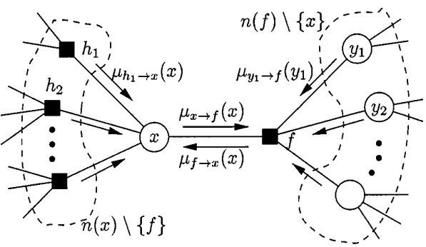
Fig. 5. Local substitutions that transform a rooted cycle-free factor graph to an expression tree for a marginal function at (a) a variable node and (b) a factor algorithm. single- algorithm, once these messages have arrived, is able Figure 9.10: Message passing on a bipartite factor graph. Square nodes represent factors, and circles represent variables. The yⁱ nodes correspond to the neighbors x^{↑ i} of f other than x. From Figure 6 of [KFL01]. Used with kind permission of Brendan Frey.

to compute a message to be sent on the one remaining edge to its neighbor (temporarily regarded as the parent), just as in

Fig. 6. A factor-graph fragment, showing the update rules of the sum-product

The computation terminates at the root node , where the the single- algorithm, i.e., according to Fig. 5. Let us denote this temporary parent as vertex . After sending a message to In the case of bipartite factor graphs, we have two kinds of messages: variables to factors

\[m\_{x \to f}(x) = \prod\_{h \in \text{hrt}(x) \backslash \{f\}} m\_{h \to x}(x) \tag{9.68}\]

, either from variable to factor , or vice versa, is a single-argument function of , the variable associated with the bors (other than ), each being regarded, in turn, as a parent. The algorithm terminates once two messages have been passed and factors to variables

product of the messages. Similarly, the summary operator is applied to the functions, not necessarily literally to the messages

node.

themselves.

sages received at .

product of these messages.

C. Computing All Marginal Functions

neighbors of were children.

as a root vertex, so there is no fixed parent/child relationship among neighboring vertices. Instead, each neighbor of any given vertex is at some point regarded as a parent of . The message passed from to is computed just as in the singlealgorithm, i.e., as if were indeed the parent of and all other

As in the single- algorithm, message passing is initiated at the leaves. Each vertex remains idle until messages have arrived on all but one of the edges incident on . Just as in the

the message.

\[m\_{f \to x}(x) = \sum\_{\mathfrak{a}'} f(x, x') \prod\_{x' \in \text{hrt}(f) \backslash \{x\}} m\_{x' \to f}(x') \tag{9.69}\]

node, all messages are functions of that variable, and so is any The message passed on an edge during the operation of the single- sum-product algorithm can be interpreted as follows. If erates by computing various sums and products, we refer to it as the sum-product algorithm. The sum-product algorithm operates according to the following simple rule: Here nbr(x) are all the factors that are connected to variable x, and nbr(f) are all the variables that are connected to factor f. These messages are illustrated in Figure 9.10. At convergence, we can compute the final beliefs as a product of incoming messages:

\[\text{bel}(x) \propto \prod\_{f \in \text{adv}(x)} m\_{f \to x}(x) \tag{9.70}\]

product algorithm is simply a summary for of the product of the local functions descending from the vertex that originates if is a variable node) with all messages received at on edges than , summarized for the variable associated with . Let denote the message sent from node to node The order in which the messages are sent can be determined using various heuristics, such as computing a spanning tree, and picking an arbitrary node as root. Alternatively, the update ordering can be chosen adaptively using residual belief propagation [EMK06]. Or fully parallel, asynchronous implementations can be used.

In many circumstances, we may be interested in computing for more than one value of . Such a computation might in the operation of the sum-product algorithm, let denote the message sent from node to node . Also, let 9.4.3 Gaussian belief propagation

be accomplished by applying the single- algorithm separately for each desired value of , but this approach is unlikely to be efficient, since many of the subcomputations performed for different values of will be the same. Computation of for all simultaneously can be efficiently accomplished by esdenote the set of neighbors of a given node in a factor graph. Then, as illustrated in Fig. 6, the message computations performed by the sum-product algorithm may be expressed as follows: It is possible to genereralize (loopy) belief propagation to the Gaussian case, by using the “calculus for linear Gaussian models” in Section 2.3.3 to compute the messages and beliefs. Note that computing the posterior mean in a linear-Gaussian system is equivalent to solving a linear system, so these methods are also useful for linear algebra. See e.g., [PL03; Bic09; Du+18] for details.

where is the set of arguments of the function . The update rule at a variable node takes on the particularly simple form given by (5) because there is no local function to include, and the summary for of a product of functions of is

sentially “overlaying” on a single factor graph all possible instances of the single- algorithm. No particular vertex is taken Author: Kevin P. Murphy. (C) MIT Press. CC-BY-NC-ND license

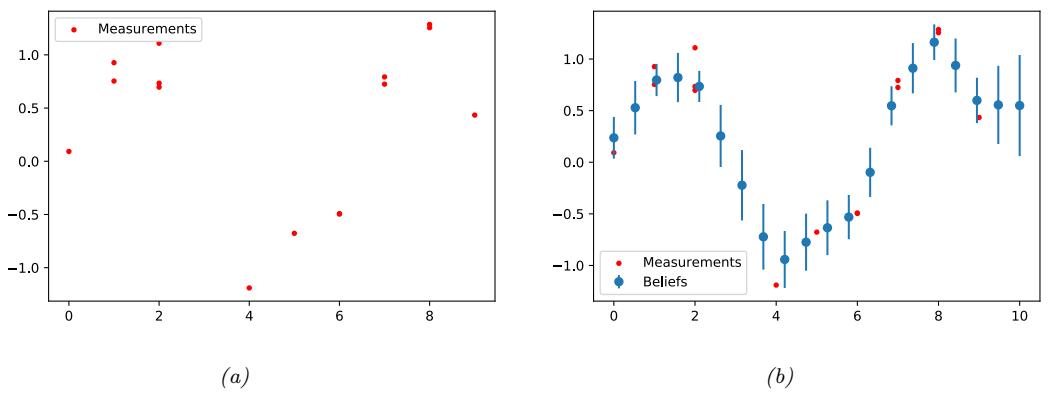
Figure 9.11: Interpolating noisy data using Gaussian belief propagation applied to a 1d MRF. Generated by gauss-bp-1d-line.ipynb.

As an example of Gaussian BP, consider the problem of interpolating noisy data in 1d, as discussed in [OED21]. In particular, let f : R ↖ R be an unknown function for which we get N noisy measurements yⁱ at locations xi. We want to estimate zⁱ = f(gi) at G grid locations gi. Let xⁱ be the closest location to gi. Then we assume the measurement factor is as follows:

\[ \psi\_i(z\_{i-1}, z\_i) = \frac{1}{\sigma^2} (\hat{y}\_i - y\_i)^2 \tag{9.71} \]

\[ \hat{y}\_i = (1 - \gamma\_i)z\_{i-1} + \gamma\_i z\_i \tag{9.72} \]

\[\gamma\_i = \frac{x\_i - g\_i}{g\_i - g\_{i-1}} \tag{9.73}\]

Here yˆⁱ is the predicted measurement. The potential function makes the unknown function values zⁱ↓¹ and zⁱ move closer to the observation, based on how far these grid points are from where the measurement was taken. In addition, we add a pairwise smoothness potential, that encodes the prior that zⁱ should be close to zⁱ↓¹ and zi+1:

\[ \phi\_i(z\_{i-1}, z\_i) = \frac{1}{\tau^2} \delta\_i^2 \tag{9.74} \]

\[ \delta\_i = z\_i - z\_{i-1} \tag{9.75} \]

The overall model is

\[p(\mathbf{z}|\mathbf{x}, \mathbf{y}, \mathbf{g}, \sigma^2, \tau^2) \propto \prod\_{i=1}^{G} \psi\_i(z\_{i-1}, z\_i) \phi\_i(z\_{i-1}, z\_i) \tag{9.76}\]

Suppose the true underlying function is a sine wave. We show some sample data in Figure 9.11(a). We then apply Gaussian BP. Since this model is a chain, and the model is linear-Gaussian, the resulting posterior marginals, shown in Figure 9.11(b), are exact. We see that the method has inferred the underlying sine shape just based on a smoothness prior.

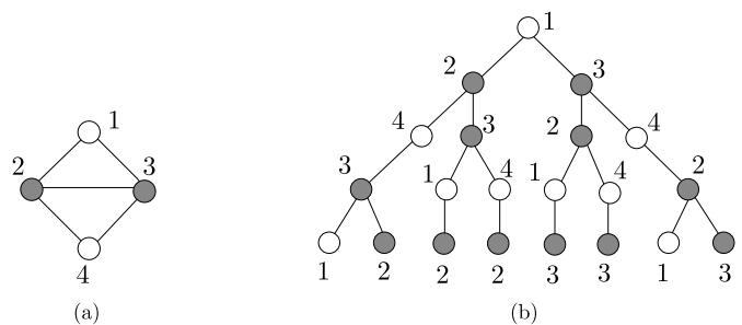
Figure 9.12: (a) A simple loopy graph. (b) The computation tree, rooted at node 1, after 4 rounds of message passing. Nodes 2 and 3 occur more often in the tree because they have higher degree than nodes 1 and 2. From Figure 8.2 of [WJ08]. Used with kind permission of Martin Wainwright.

To perform message passing in models with non-linear (but Gaussian) potentials, we can generalize the extended Kalman filter techniques from Section 8.3.2 and the moment matching techniques (based on quadrature/sigma points) from Section 8.5.1 and Section 8.5.1.1 from chains to general factor graphs (see e.g., [MHH14; PHR18; HPR19]). To extend to the non-Gaussian case, we can use non-parametric BP or particle BP (see e.g., [Sud+03; Isa03; Sud+10; Pac+14]), which uses ideas from particle filtering (Section 13.2).

9.4.4 Convergence

Loopy BP may not converge, or may only converge slowly. In this section, we discuss some techniques that increase the chances of convergence, and the speed of convergence.

9.4.4.1 When will LBP converge?

The details of the analysis of when LBP will converge are beyond the scope of this chapter, but we briefly sketch the basic idea. The key analysis tool is the computation tree, which visualizes the messages that are passed as the algorithm proceeds. Figure 9.12 gives a simple example. In the first iteration, node 1 receives messages from nodes 2 and 3. In the second iteration, it receives one message from node 3 (via node 2), one from node 2 (via node 3), and two messages from node 4 (via nodes 2 and 3). And so on.

The key insight is that T iterations of LBP is equivalent to exact computation in a computation tree of height T + 1. If the strengths of the connections on the edges is su”ciently weak, then the influence of the leaves on the root will diminish over time, and convergence will occur. See [MK05; WJ08] and references therein for more information.

9.4.4.2 Making LBP converge

Although the theoretical convergence analysis is very interesting, in practice, when faced with a model where LBP is not converging, what should we do?

One simple way to increase the chance of convergence is to use damping. That is, at iteration k,

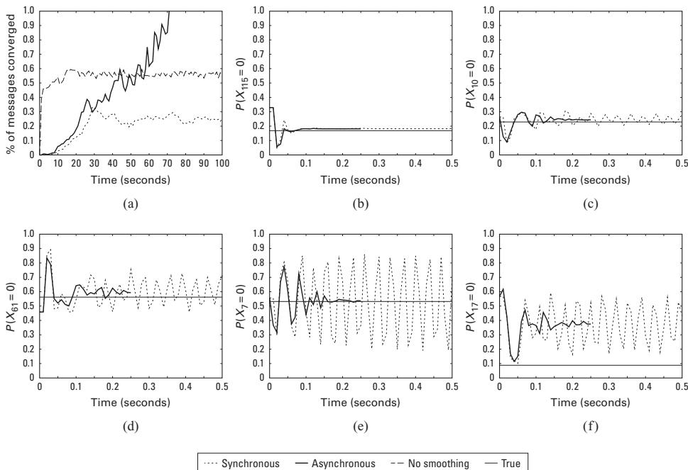
Figure 9.13: Illustration of the behavior of loopy belief propagation on an 11 ≃ 11 Ising grid with random potentials, wij ↑ Unif(↗C, C), where C = 11. For larger C, inference becomes harder. (a) Percentage of messages that have converged vs time for 3 di!erent update schedules: Dotted = damped synchronous (few nodes converge), dashed = undamped asychnronous (half the nodes converge), solid = damped asychnronous (all nodes converge). (b-f) Marginal beliefs of certain nodes vs time. Solid straight line = truth, dashed = sychronous, solid = damped asychronous. From Figure 11.C.1 of [KF09a]. Used with kind permission of Daphne Koller.

we use an update of the form

\[m\_{t \to s}^{k}(x\_s) = \lambda m\_{t \to s}(x\_s) + (1 - \lambda)m\_{t \to s}^{k-1}(x\_s) \tag{9.77}\]

where m^t↗s(xs) is the standard undamped message, where 0 ⇐ ⇀ ⇐ 1 is the damping factor. Clearly if ⇀ = 1 this reduces to the standard scheme, but for ⇀ < 1, this partial updating scheme can help improve convergence. Using a value such as ⇀ ↔︎ 0.5 is standard practice. The benefits of this approach are shown in Figure 9.13, where we see that damped updating results in convergence much more often than undamped updating (see [ZLG20] for some analysis of the benefits of damping).

It is possible to devise methods, known as double loop algorithms, which are guaranteed to converge to a local minimum of the same objective that LBP is minimizing [Yui01; WT01]. Unfortunately, these methods are rather slow and complicated, and the accuracy of the resulting marginals is usually not much greater than with standard LBP. (Indeed, oscillating marginals is sometimes a sign that the LBP approximation itself is a poor one.) Consequently, these techniques are not very widely used (although see [GF21] for a newer technique).

9.4.4.3 Increasing the convergence rate with adaptive scheduling

The standard approach when implementing LBP is to perform synchronous updates, where all nodes absorb messages in parallel, and then send out messages in parallel. That is, the new messages at iteration k + 1 are computed in parallel using

\[\mathbf{m}\_{1:E}^{k+1} = \left( f\_1(\mathbf{m}^k), \dots, f\_E(\mathbf{m}^k) \right) \tag{9.78}\]

where E is the number of edges, and fi(m) is the function that computes the message for edge i given all the old messages. This is analogous to the Jacobi method for solving linear systems of equations.

It is well known [Ber97b] that the Gauss-Seidel method, which performs asynchronous updates in a fixed round-robin fashion, converges faster when solving linear systems of equations. We can apply the same idea to LBP, using updates of the form

\[m\_i^{k+1} = f\_i\left(\{\mathbf{m}\_j^{k+1} : j < i\}, \{\mathbf{m}\_j^k : j > i\}\right) \tag{9.79}\]

where the message for edge i is computed using new messages (iteration k + 1) from edges earlier in the ordering, and using old messages (iteration k) from edges later in the ordering.

This raises the question of what order to update the messages in. One simple idea is to use a fixed or random order. The benefits of this approach are shown in Figure 9.13, where we see that (damped) asynchronous updating results in convergence much more often than synchronous updating.

However, we can do even better by using an adaptive ordering. The intuition is that we should focus our computational e!orts on those variables that are most uncertain. [EMK06] proposed a technique known as residual belief propagation, in which messages are scheduled to be sent according to the norm of the di!erence from their previous value. That is, we define the residual of new message m^s↗^t at iteration k to be

\[|r(s,t,k) = || \log m\_{s \to t} - \log m\_{s \to t}^k||\_{\infty} = \max\_j |\log \frac{m\_{s \to t}(j)}{m\_{s \to t}^k(j)}|\tag{9.80}\]

We can store messages in a priority queue, and always send the one with highest residual. When a message is sent from s to t, all of the other messages that depend on m^s↗^t (i.e., messages of the form m^t↗^u where u ↗ nbr(t)  s) need to be recomputed; their residual is recomputed, and they are added back to the queue. In [EMK06], they showed (experimentally) that this method converges more often, and much faster, than using sychronous updating, or asynchronous updating with a fixed order.

A refinement of residual BP was presented in [SM07]. In this paper, they use an upper bound on the residual of a message instead of the actual residual. This means that messages are only computed if they are going to be sent; they are not just computed for the purposes of evaluating the residual. This was observed to be about five times faster than residual BP, although the quality of the final results are similar.

9.4.5 Accuracy

For a graph with a single loop, one can show that the max-product version of LBP will find the correct MAP estimate, if it converges [Wei00]. For more general graphs, one can bound the error in the approximate marginals computed by LBP, as shown in [WJW03; IFW05; Vin+10b].

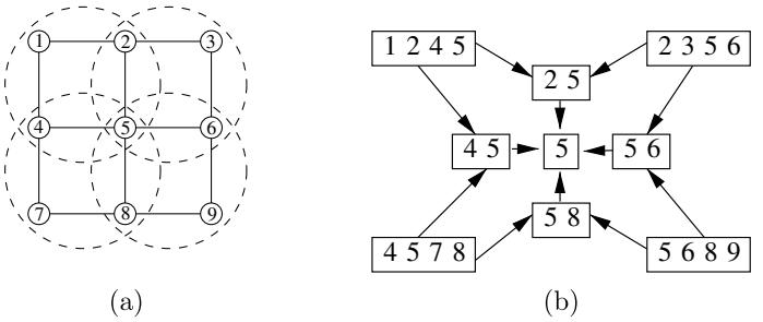
Figure 9.14: (a) Clusters superimposed on a 3 ≃ 3 lattice graph. (b) Corresponding hyper-graph. Nodes represent clusters, and edges represent set containment. From Figure 4.5 of [WJ08]. Used with kind permission of Martin Wainwright.

Much stronger results are available in the case of Gaussian models. In particular, it can be shown that, if the method converges, the means are exact, although the variances are not (typically the beliefs are over confident). See e.g., [WF01a; JMW06; Bic09; Du+18] for details.

9.4.6 Generalized belief propagation

We can improve the accuracy of loopy BP by clustering together nodes that form a tight loop. This is known as the cluster variational method, or generalized belief propagation [YFW00].

The result of clustering is a hyper-graph, which is a graph where there are hyper-edges between sets of vertices instead of between single vertices. Note that a junction tree (Section 9.6) is a kind of hyper-graph. We can represent a hyper-graph using a poset (partially ordered set) diagram, where each node represents a hyper-edge, and there is an arrow e¹ ↖ e² if e² ∋ e1. See Figure 9.14 for an example.

If we allow the size of the largest hyper-edge in the hyper-graph to be as large as the treewidth of the graph, then we can represent the hyper-graph as a tree, and the method will be exact, just as LBP is exact on regular trees (with treewidth 1). In this way, we can define a continuum of approximations, from LBP all the way to exact inference. See Supplementary Section 10.4.3.3 for more information.

9.4.7 Convex BP

In Supplementary Section 10.4.3 we analyze LBP from a variational perspective, and show that the resulting optimization problem, for both standard and generalized BP, is non-convex. However it is possible to create a version of convex BP, as we explain in Supplementary Section 10.4.4, which has the advantage that it will always converge.

9.4.8 Application: error correcting codes

LBP was first proposed by Judea Pearl in his 1988 book [Pea88]. He recognized that applying BP to loopy graphs might not work, but recommended it as a heuristic.

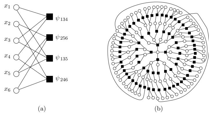
Figure 9.15: (a) A simple factor graph representation of a (2,3) low-density parity check code. Each message bit (hollow round circle) is connected to two parity factors (solid black squares), and each parity factor is connected to three bits. Each parity factor has the form ϱstu(xs, xt, xu) = I(x^s ⇐ x^t ⇐ x^u = 1), where ⇐ is the xor operator. The local evidence factors for each hidden node are not shown. (b) A larger example of a random LDPC code. We see that this graph is “locally tree-like”, meaning there are no short cycles; rather, each cycle has length ↑ log m, where m is the number of nodes. This gives us a hint as to why loopy BP works so well on such graphs. (Note, however, that some error correcting code graphs have short loops, so this is not the full explanation.) From Figure 2.9 from [WJ08]. Used with kind permission of Martin Wainwright.

However, the main impetus behind the interest in LBP arose when McEliece, MacKay, and Cheng [MMC98] showed that a popular algorithm for error correcting codes, known as turbocodes [BGT93], could be viewed as an instance of LBP applied to a certain kind of graph.

We introduced error correcting codes in Section 5.5. Recall that the basic idea is to send the source message ^x ↗ {0, 1}^m over a noisy channel, and for the receiver to try to infer it given noisy measurements ^y ↗ {0, ¹}^m or ^y ↗ ^Rm. That is, the receiver needs to compute ^{x→ =} argmax^{x p}(x|y) = argmax^x p˜(x).

It is standard to represent p˜(x) as a factor graph (Section 4.6.1), which can easily represent any deterministic relationships (parity constraints) between the bits. A factor graph is a bipartite graph with xⁱ nodes on one side, and factors on the other. A graph in which each node is connected to n factors, and in which each factor is connected to k nodes, is called an (n, k) code. Figure 9.15(a) shows a simple example of a (2, 3) code, where each bit (hollow round circle) is connected to two parity factors (solid black squares), and each parity factor is connected to three bits. Each parity factor has the form

\[ \psi\_{\rm stu}(x\_s, x\_t, x\_u) \stackrel{\Delta}{=} \begin{cases} 1 & \text{if } x\_s \otimes x\_t \otimes x\_u = 1 \\ 0 & \text{otherwise} \end{cases} \tag{9.81} \]

If the degrees of the parity checks and variable nodes remain bounded as the blocklength m increases, this is called a low-density parity check code, or LDPC code. (Turbocodes are constructed in a similar way.)

Figure 9.15(b) shows an example of a randomly constructed LDPC code. This graph is “locally tree-like”, meaning there are no short cycles; rather, each cycle has length ↔︎ log m. This fact is important to the success of LBP, which is only guaranteed to work on tree-structured graphs. Using

ˆ

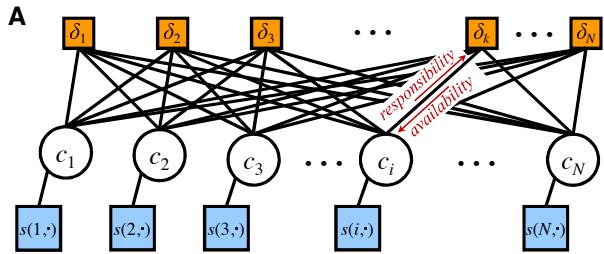
k B … k α^{k i} C … D Figure 9.16: Factor graphs for a#nity propagation. Circles are variables, squares are factors. Each cⁱ node has N possible states. From Figure S2 of [FD07a]. Used with kind permission of Brendan Frey.

ci s(i, ) … ci ci s(i, ) Figure S2: Factor Graph for Affinity Propagation methods such as these, people have been able to approach the lower bound in Shannon’s channel coding theorem, meaning they have produced codes with very little redundancy for a given amount of noise in the channel. See e.g., [MMC98; Mac03] for more details. Such codes are widely used, e.g., in modern cellphones.

9.4.9 Application: a!nity propagation

N numbers can be reduced to a single number, making affinity propagation efficient as a message-passing algorithm. The message sent from δk(c) to cⁱ also consists of N real numbers and can be denoted αⁱ←^k(j) (Fig. S2C). At any time, the value of cⁱ can be estimated by summing together all incoming availability and similarity messages (Fig. S2D). Since the ρ-messages are outgoing from variables, they are computed as the element-In this section, we discuss a”nity propagation [FD07a], which can be seen as an improvement to K-medoids clustering, which takes as input a pairwise similarity matrix. The idea is that each datapoint must choose another datapoint as its exemplar or centroid; some datapoints will choose themselves as centroids, and this will automatically determine the number of clusters. More precisely, let cⁱ ↗ {1,…,N} represent the centroid for datapoint i. The goal is to maximize the following function

\[J(\mathbf{c}) = \sum\_{i=1}^{N} S(i, c\_i) + \sum\_{k=1}^{N} \delta\_k(\mathbf{c}) \tag{9.82}\]

Messages sent from functions to variables are computed by summing incoming messages and then maximizing over all variables except the variable the message is being sent to. where S(i, ci) is the similarity between datapoint i and its centroid ci. The second term is a penalty term that is →⇓ if some datapoint i has chosen k as its exemplar (i.e., cⁱ = k), but k has not chosen itself as an exemplar (i.e., we do not have c^k = k). More formally,

\[\delta\_k(\mathbf{c}) = \begin{cases} -\infty & \text{if } c\_k \neq k \text{ but } \exists i: c\_i = k\\ 0 & \text{otherwise} \end{cases} \tag{9.83}\]

10 This encourages “representative” samples to vote for themselves as centroids, thus encouraging clustering behavior.

The objective function can be represented as a factor graph. We can either use N nodes, each with N possible values, as shown in Figure 9.16, or we can use N² binary nodes (see [GF09] for the details). We will assume the former representation.

We can find a strong local maximum of the objective by using max-product loopy belief propagation (Section 9.4). Referring to the model in Figure 9.16, each variable node cⁱ sends a message to each factor node ϑk. It turns out that this vector of N numbers can be reduced to a scalar message,

A

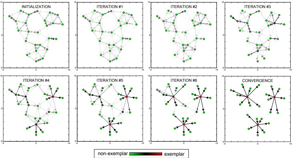
B C Sending responsibilities Candidate exemplar k Competing candidate Sending availabilities Candidate exemplar k Figure 9.17: Example of a#nity propagation. Each point is colored coded by how much it wants to be an exemplar (red is the most, green is the least). This can be computed by summing up all the incoming availability messages and the self-similarity term. The darkness of the i → k arrow reflects how much point i wants to belong to exemplar k. From Figure 1 of [FD07a]. Used with kind permission of Brendan Frey.

r(i%,k)

r(i,k) Data point i a(i,k%) a(i,k) Data point i Supporting data point i% denoted rⁱ↗k, known as the responsibility. This is a measure of how much i thinks k would make a good exemplar, compared to all the other exemplars i has looked at. In addition, each factor node ϑ^k sends a message to each variable node ci. Again this can be reduced to a scalar message, aⁱ≃^k, known as the availability. This is a measure of how strongly k believes it should an exemplar for i, based on all the other datapoints k has looked at.

D 25 20 As usual with loopy BP, the method might oscillate, and convergence is not guaranteed. However, by using damping, the method is very reliable in practice. If the graph is densely connected, message passing takes O(N²) time, but with sparse similarity matrices, it only takes O(E) time, where E is the number of edges or non-zero entries in S.

-1000 -100 -1 -10 -0.1 15 10 5 0 Number of clustersSee (A) The number of clusters can be controlled by scaling the diagonal terms S(i, i), which reflect how much each datapoint wants to be an exemplar. Figure 9.17 gives a simple example of some 2d data, where the negative Euclidean distance was used to measured similarity. The S(i, i) values were set to be the median of all the pairwise similarities. The result is 3 clusters. Many other results are reported in [FD07a], who show that the method significantly outperforms K-medoids.

Fig 1, Frey & Dueck

9.4.10 Emulating BP with graph neural nets

Value of shared preference

exemplar k%

There is a close connection between message passing in PGMs and message passing in graph neural networks (GNNs), which we discuss in Section 16.3.6. However, for PGMs, the message computations are computing using (non-learned) update equations that work for any model; all that is needed

is the graph structure G, model parameters ω, and evidence v. By contrast, GNNs are trained to emulate specific functions using labeled input-output pairs.

It is natural to wonder what happens if we train a GNN on the exact posterior marginals derived from a small PGM, and then apply that trained GNN to a di!erent test PGM. In [Yoo+18; Zha+19d], they show this method can work quite well if the test PGM is similar in structure to the one used for training.

An alternative approach is to start with a known PGM, and then “unroll” the BP message passing algorithm to produce a layered feedforward model, whose connectivity is derived from the graph. The resulting network can then be trained discriminatively for some end-task (not necessarily computing posterior marginals). Thus the BP procedure applied to the PGM just provides a way to design the neural network structure. This method is called deep unfolding (see e.g., [HLRW14]), and can often give very good results. (See also [SW20] for a more recent version of this approach, called “neural enhanced BP”.)

These neural methods are useful if the PGM is fixed, and we want to repeatedly perform inference or prediction with it, using di!erent values of the evidence, but where the set of nodes which are observed is always the same. This is an example of amortized inference, where we train a model to emulate the results of running an iterative optimization scheme (see Section 10.1.5 for more discussion).

9.5 The variable elimination (VE) algorithm

In this section, we discuss an algorithm to compute a posterior marginal p(zQ|y) for any query set Q, assuming p is defined by a graphical model. Unlike loopy BP, it is guaranteed to give the correct answers even if the graph has cycles. We assume all the hidden nodes are discrete, although a version of the algorithm can be created for the Gaussian case by using the rules for sum and product defined in Section 2.3.3.

9.5.1 Derivation of the algorithm

We will explain the algorithm by applying it to an example. Specifically, we consider the student network from Section 4.2.2.2. Suppose we want to compute p(J = 1), the marginal probability that a person will get a job. Since we have 8 binary variables, we could simply enumerate over all possible assignments to all the variables (except for J), adding up the probability of each joint instantiation:

\[p(J) = \sum\_{L} \sum\_{S} \sum\_{G} \sum\_{H} \sum\_{I} \sum\_{D} \sum\_{C} p(C, D, I, G, S, L, J, H) \tag{9.84}\]

However, this would take O(27) time. We can be smarter by pushing sums inside products. This is the key idea behind the variable elimination algorithm [ZP96], also called bucket elimination [Dec96], or, in the context of genetic pedigree trees, the peeling algorithm [CTS78].

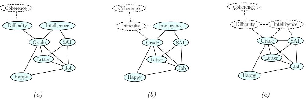
Figure 9.18: Example of the elimination process, in the order C, D, I, H, G, S, L. When we eliminate I (figure c), we add a fill-in edge between G and S, since they are not connected. Adapted from Figure 9.10 of [KF09a].

In our example, we get

\[\begin{aligned} p(J) &= \sum\_{L,S,G,H,I,D,C} p(C,D,I,G,S,L,J,H) \\ &= \sum\_{L,S,G,H,I,D,C} \psi\_C(C)\psi\_D(D,C)\psi\_I(I)\psi\_G(G,I,D)\psi\_S(S,I)\psi\_L(L,G) \\ &\times \psi\_J(J,L,S)\psi\_H(H,G,J) \\ &= \sum\_{L,S} \psi\_J(J,L,S)\sum\_G \psi\_L(L,G)\sum\_H \psi\_H(H,G,J)\sum\_I \psi\_S(S,I)\psi\_I(I) \\ &\times \sum\_D \psi\_G(G,I,D)\sum\_C \psi\_C(C)\psi\_D(D,C) \end{aligned}\]

We now evaluate this expression, working right to left as shown in Table 9.1. First we multiply together all the terms in the scope of the & ^C operator to create the temporary factor

\[ \tau\_1'(C, D) = \psi\_C(C)\psi\_D(D, C) \tag{9.85} \]

Then we marginalize out C to get the new factor

\[\tau\_1(D) = \sum\_C \tau\_1'(C, D) \tag{9.86}\]

Next we multiply together all the terms in the scope of the & ^D operator and then marginalize out to create

\[ \tau\_2'(G, I, D) = \psi\_G(G, I, D)\tau\_1(D) \tag{9.87} \]

\[\tau\_2(G, I) = \sum\_D \tau'\_2(G, I, D) \tag{9.88}\]

And so on.

” L ” S ω^J (J, L, S) ” G ωL(L, G) ” H ωH(H, G, J) ” I ωS(S, I)ω^I (I) ” D ωG(G, I, D) ” C ω^C (C)ωD(D, C) # $% & ^ω1(D) ” L ” S ω^J (J, L, S) ” G ωL(L, G) ” H ωH(H, G, J) ” I ωS(S, I)ω^I (I) ” D ωG(G, I, D)ε1(D) # $% & ^ω2(G,I) ” L ” S ω^J (J, L, S) ” G ωL(L, G) ” H ωH(H, G, J) ” I ωS(S, I)ω^I (I)ε2(G, I) # $% & ^ω3(G,S) ” L ” S ω^J (J, L, S) ” G ωL(L, G) ” H ωH(H, G, J) # $% & ^ω4(G,J) ε3(G, S) ” L ” S ω^J (J, L, S) ” G ωL(L, G)ε4(G, J)ε3(G, S) # $% & ^ω5(J,L,S) ” L ” S ω^J (J, L, S)ε5(J, L, S) # $% & ^ω6(J,L) ” L ε6(J, L) # $% & ^ω7(J)

Table 9.1: Eliminating variables from Figure 4.38 in the order C, D, I, H, G, S, L to compute P(J).

The above technique can be used to compute any marginal of interest, such as p(J) or p(J, H). To compute a conditional, we can take a ratio of two marginals, where the visible variables have been clamped to their known values (and hence don’t need to be summed over). For example,

\[p(J=j|I=1, H=0) = \frac{p(J=j, I=1, H=0)}{\sum\_{j'} p(J=j', I=1, H=0)} \tag{9.89}\]

9.5.2 Computational complexity of VE

The running time of VE is clearly exponential in the size of the largest factor, since we have to sum over all of the corresponding variables. Some of the factors come from the original model (and are thus unavoidable), but new factors may also be created in the process of summing out. For example, in Table 9.1, we created a factor involving G, I, and S; but these nodes were not originally present together in any factor.

The order in which we perform the summation is known as the elimination order. This can have a large impact on the size of the intermediate factors that are created. For example, consider the ordering in Table 9.1: the largest created factor (beyond the original ones in the model) has size 3, corresponding to τ5(J, L, S). Now consider the ordering in Table 9.2: now the largest factors are τ1(I, D, L, J, H) and τ2(D, L, S, J, H), which are much bigger.

\[\begin{aligned} \sum\_{D} \sum\_{C} \psi\_{D}(D,C) \sum\_{H} \sum\_{S} \psi\_{J}(I,L,S) \sum\_{I} \psi\_{I}(I) \psi\_{S}(S,I) \underbrace{\sum\_{G} \psi\_{G}(G,I,D) \psi\_{L}(L,G) \psi\_{H}(H,G,J)}\_{\tau\_{1}(L,L,L,J,H)} \\ \sum\_{D} \sum\_{C} \psi\_{D}(D,C) \sum\_{H} \sum\_{L} \sum\_{S} \psi\_{J}(J,L,S) \underbrace{\sum\_{I} \psi\_{I}(I) \psi\_{S}(S,I) \tau\_{1}(I,D,L,J,H)}\_{\tau\_{2}(D,L,S,J,H)} \\ \sum\_{D} \sum\_{C} \psi\_{D}(D,C) \sum\_{H} \sum\_{L} \sum\_{S} \psi\_{J}(J,L,S) \tau\_{2}(D,L,S,J,H) \\ \sum\_{D} \sum\_{C} \psi\_{D}(D,C) \sum\_{H} \sum\_{L} \tau\_{3}(D,L,J,H) \\ \sum\_{D} \sum\_{C} \psi\_{D}(D,C) \sum\_{H} \tau\_{4}(D,L,H) \\ \sum\_{D} \sum\_{C} \psi\_{D}(D,C) \sum\_{H} \psi\_{D}(D,L,S,J,H) \\ \sum\_{D} \sum\_{C} \psi\_{D}(D,C) \tau\_{5}(D,L,S,J,H) \\ \sum\_{D} \sum\_{C} \psi\_{D}(D,D,L,S,J,H) \\ \sum\_{D} \sum\_{D} \tau\_{6}(D,D,S,J,H) \end{aligned}\]

Table 9.2: Eliminating variables from Figure 4.38 in the order G, I, S, L, H, C, D.

We can determine the size of the largest factor graphically, without worrying about the actual numerical values of the factors, by running the VE algorithm “symbolically”. When we eliminate a variable zt, we connect together all variables that share a factor with z^t (to reflect the new temporary factor τ ^{↔︎ t} ). The edges created by this process are called fill-in edges. For example, Figure 9.18 shows the fill-in edges introduced when we eliminate in the C, D, I, . . . order. The first two steps do not introduce any fill-ins, but when we eliminate I, we connect G and S, to capture the temporary factor

\[ \tau\_3'(G, S, I) = \psi\_S(S, I)\psi\_I(I)\tau\_2(G, I) \tag{9.90} \]

Let G⇐ be the (undirected) graph induced by applying variable elimination to G using elimination ordering ̸. The temporary factors generated by VE correspond to maximal cliques in the graph G⇐. For example, with ordering (C, D, I, H, G, S, L), the maximal cliques are as follows:

\[\{C, D\}, \{D, I, G\}, \{G, L, S, J\}, \{G, J, H\}, \{G, I, S\} \tag{9.91}\]

It is clear that the time complexity of VE is

\[\sum\_{c \in \mathcal{C}(G\_{\prec})} K^{|c|} \tag{9.92}\]

where C(G) are the (maximal) cliques in graph G, |c| is the size of the clique c, and we assume for notational simplicity that all the variables have K states each.

Let us define the induced width of a graph given elimination ordering ̸, denoted w⇐, as the size of the largest factor (i.e., the largest clique in the induced graph ) minus 1. Then it is easy to see that the complexity of VE with ordering ̸ is ^O(Kw↗+1). The smallest possible induced width for a graph is known as its treewidth. Unfortunately finding the corresponding optimal elimination order is an NP-complete problem [Yan81; ACP87]. See Section 9.5.3 for a discussion of some approximate methods for finding good elimination orders.

9.5.3 Picking a good elimination order

Many algorithms take time (or space) which is exponential in the tree width of the corresponding graph. For example, this applies to Cholesky decompositions of sparse matrices, as well as to einsum contractions (see https://github.com/dgasmith/opt\_einsum). Hence we would like to find an elimination ordering that minimizes the width. We say that an ordering ϖ is a perfect elimination ordering if it does not introduce any fill-in edges. Every graph that is already triangulated (e.g., a tree) has a perfect elimination ordering. We call such graphs decomposable.

In general, we will need to add fill-in edges to ensure the resulting graph is decomposable. Di!erent orderings can introduce di!erent numbers of fill-in edges, which a!ects the width of the resulting chordal graph; for example, compare Table 9.1 to Table 9.2.

Choosing an elimination ordering with minimal width is NP-complete [Yan81; ACP87]. It is common to use greedy approximation known as the min-fill heuristic, which works as follows: eliminate any node which would not result in any fill-ins (i.e., all of whose uneliminated neighbors already form a clique); if there is no such node, eliminate the node which would result in the minimum number of fill-in edges. When nodes have di!erent weights (e.g., representing di!erent numbers of states), we can use the min-weight heuristic, where we try to minimize the weight of the created cliques at each step.

Of course, many other methods are possible. See [Heg06] for a general survey. [Kja90; Kja92] compared simulated annealing with the above greedy method, and found that it sometimes works better (although it is much slower). [MJ97] approximate the discrete optimization problem by a continuous optimization problem. [BG96] present a randomized approximation algorithm. [Gil88] present the nested dissection order, which is always within O(log N) of optimal. [Ami01] discuss various constant-factor appoximation algorithms. [Dav+04] present the AMD or approximate minimum degree ordering algorithm, which is implemented in Matlab.4 The METIS library can be used for finding elimination orderings for large graphs; this implements the nested dissection algorithm [GT86]. For a planar graph with N nodes, the resulting treewidth will have the optimal size of O(N³/²).

9.5.4 Computational complexity of exact inference

We have seen that variable elimination takes O(NK^w+1) time to compute the marginals for a graph with N nodes, and treewidth w, where each variable has K states. If the graph is densely connected, then w = O(N), and so inference will take time exponential in N.

^4. See the description of the symamd command at https://bit.ly/31N6E2b. (“sym” stands for symbolic, “amd” stands approximate minimum degree.)

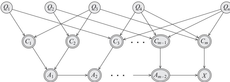
Figure 9.19: Encoding a 3-SAT problem on n variables and m clauses as a DGM. The Q^s variables are binary random variables. The C^t variables are deterministic functions of the Qs’s, and compute the truth value of each clause. The A^t nodes are a chain of AND gates, to ensure that the CPT for the final x node has bounded size. The double rings denote nodes with deterministic CPDs. From Figure 9.1 of [KF09a]. Used with kind permission of Daphne Koller.

Of course, just because some particular algorithm is slow doesn’t mean that there isn’t some smarter algorithm out there. Unfortunately, this seems unlikely, since it is easy to show that exact inference for discrete graphical models is NP-hard [DL93]. The proof is a simple reduction from the satisfiability problem. In particular, note that we can encode any 3-SAT problem as a DPGM with deterministic links, as shown in Figure 9.19. We clamp the final node, x, to be on, and we arrange the CPTs so that p(x = 1) > 0 i! there is a satisfying assignment. Computing any posterior marginal requires evaluating the normalization constant, p(x = 1), so inference in this model implicitly solves the SAT problem.

In fact, exact inference is #P-hard [Rot96], which is even harder than NP-hard. The intuitive reason for this is that to compute the normalizing constant, we have to count how many satisfying assignments there are. (By contrast, MAP estimation is provably easier for some model classes [GPS89], since, intuitively speaking, it only requires finding one satisfying assignment, not counting all of them.) Furthermore, even approximate inference is computationally hard in general [DL93; Rot96].

The above discussion was just concerned with inferring the states of discrete hidden variables. When we have continuous hidden variables, the problem can be even harder, since even a simple two-node graph, of the form z ↖ y, can be intractable to invert if the variables are high dimensional and do not have a conjugate relationship (Section 3.4). Inference in mixed discrete-continuous models can also be hard [LP01].

As a consequence of these hardness results, we often have to resort to approximate inference methods, such as variational inference (Chapter 10) and Monte Carlo inference (Chapter 11).

9.5.5 Drawbacks of VE

Consider using VE to compute all the marginals in a chain-structured graphical model, such as an HMM. We can easily compute the final marginal p(z^T |y) by eliminating all the nodes z¹ to z^{T ↓1} in order. This is equivalent to the forwards algorithm, and takes O(K²T) time, as we discussed in Section 9.2.3. But now suppose we want to compute p(z^{T ↓1}|y). We have to run VE again, at a cost

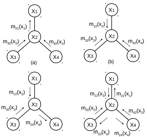
Figure 9.20: Sending multiple messages along a tree. (a) z¹ is root. (b) z² is root. (c) z⁴ is root. (d) All of the messages needed to compute all singleton marginals. Adapted from Figure 4.3 of [Jor07].

of O(K²T) time. So the total cost to compute all the marginals is O(K²T²). However, we know that we can solve this problem in O(K²T) using the forwards-backwards, as we discussed in Section 9.2.3. The di!erence is that FB caches the messages computed on the forwards pass, so it can reuse them later. (Caching previously computed results is the core idea behind dynamic programming.)

The same problem arises when applying VE to trees. For example, consider the 4-node tree in Figure 9.20. We can compute p(z1|y) by eliminating z2:4; this is equivalent to sending messages up to z¹ (the messages correspond to the τ factors created by VE). Similarly we can compute p(z2|y), p(z3|y) and then p(z4|y). We see that some of the messages used to compute the marginal on one node can be re-used to compute the marginals on the other nodes. By storing the messages for later re-use, we can compute all the marginals in O(K²T) time, as we show in Section 9.3.

The question is: how do we get these benefits of message passing on a tree when the graph is not a tree? We give the answer in Section 9.6.

9.6 The junction tree algorithm (JTA)

The junction tree algorithm or JTA is a generalization of variable elimination that lets us e”ciently compute all the posterior marginals without repeating redundant work, by using dynamic programming, thus avoiding the problems mentioned in Section 9.5.5. The basic idea is to convert the graph into a special kind of tree, known as a junction tree (also called a join tree, or clique tree), and then to run belief propagation (message passing) on this tree. We can create the join tree by running variable elimination “symbolically”, as discussed in Section 9.5.2, and adding the generated fill-in edges to the graph. The resulting chordal graph can then be converted to a tree, as explained in Supplementary Section 9.2.1. Once we have a tree, we can perform message passing on it, using a variant of the method Section 9.3.2. See Supplementary Section 9.2.2 for details.

9.7 Inference as optimization

In this section, we discuss how to perform posterior inference by solving an optimization problem, which is often computationally simpler. See also Supplementary Section 9.3.

9.7.1 Inference as backpropagation

In this section, we discuss how to compute posterior marginals in a graphical model using automatic di!erentiation. For notational simplicity, we focus on undirected graphical models, where the joint can be represented as an exponential family (Section 2.4) follows:

\[p(\mathbf{z}) = \frac{1}{Z} \prod\_{c} \psi\_{c}(\mathbf{z}\_{c}) = \exp(\sum\_{c} \eta\_{c}^{\mathsf{T}} \mathcal{T}(\mathbf{z}\_{c}) - \log A(\eta)) = \exp(\eta^{\mathsf{T}} \mathcal{T}(\mathbf{z}) - \log A(\eta))\tag{9.93}\]

where 1^c is the potential function for clique c, ϱ^c are the natural parameters for clique c, T (xc) are the corresponding su”cient statistics, and A = log Z is the log partition function.

We will consider pairwise models (with node and edge potentials), and discrete variables. The natural parameters are the node and edge log potentials, ϱ = ({ηs;j}, {ηs,t;j,k}), and the su”cient statistics are node and edge indicator functions, T (x)=({I(x^s = j)}, {I(x^s = j, x^t = k)}). (Note: we use s, t ↗ V to index nodes and j, k ↗ X to index states.)

The mean of the su”cient statistics are given by

\[\mu = \mathbb{E}\left[\mathcal{T}(x)\right] = \left(\{p(x\_s = j)\}\_s, \{p(x\_s = j, x\_t = k)\}\_{s \neq t}\right) = \left(\{\mu\_{s;j}\}\_s, \{\mu\_{st;jk}\}\_{s \neq t}\right) \tag{9.94}\]

The key result, from Equation (2.236), is that µ = ⇒ϖA(ϱ). Thus as long as we have a function that computes A(ϱ) = log Z(ϱ), we can use automatic di!erentiation (Section 6.2) to compute gradients, and then we can extract the corresponding node marginals from the gradient vector. If we have evidence (known values) on some of the variables, we simply “clamp” the corresponding entries to 0 or 1 in the node potentials.

The observation that probabilistic inference can be performed using automatic di!erentiation has been discovered independently by several groups (e.g., [Dar03; PD03; Eis16; ASM17]). It also lends itself to the development of di!erentiable approximations to inference (see e.g., [MB18]).

9.7.1.1 Example: inference in a small model

As a concrete example, consider a small chain structured model x¹ → x² → x3, where each node has K states. We can represent the node potentials as K ⇔ 1 tensors (table of numbers), and the edge potentials by K ⇔ K tensors. The partition function is given by

\[Z(\psi) = \sum\_{x\_1, x\_2, x\_3} \psi\_1(x\_1)\psi\_2(x\_2)\psi\_3(x\_3)\psi\_{12}(x\_1, x\_2)\psi\_{23}(x\_2, x\_3) \tag{9.95}\]

Let ϱ = log(ϖ) be the log potentials, and A(ϱ) = log Z(ϱ) be the log partition function. We can compute the single node marginals µ^s = p(x^s =1: K) using µ^s = ⇒^ϖsA(ϱ), and the pairwise marginals µs,t(j, k) = p(x^s = j, x^t = k) using µs,t = ⇒^ϖs,tA(ϱ).

We can compute the partition function Z e”ciently use numpy’s einsum function, which implements tensor contraction using Einstein summation notation. We label each dimension of the tensors

by A, B, and C, so einsum knows how to match things up. We then compute gradients using an auto-di! library.5 The result is that inference can be done in two lines of Python code, as shown in Listing 9.1:

Listing 9.1: Computing marginals from derivative of log partition function import jax.numpy as jnp from jax import grad logZ_fun = lambda logpots: np.log(jnp.einsum(“A,B,C,AB ,BC”, *[jnp.exp(lp) for lp in logpots])) probs = grad(logZ_fun)(logpots)

To perform conditional inference, such as p(x^s = k|x^t = e), we multiply in one-hot indicator vectors to clamp x^t to the value e so that the unnormalized joint only assigns non-zero probability to state combinations that are valid. We then sum over all values of the unclamped variables to get the constrained partition function Ze. The gradients will now give us the marginals conditioned on the evidence [Dar03].

9.7.2 Perturb and MAP

In this section, we discuss how to draw posterior samples from a graphical model by leveraging optimization as a subroutine. The basic idea is to make S copies of the model, each of which has slightly perturbed versions of the parameters, ω^s = ω^s + ,s, and then to compute the MAP estimate, x^s = argmax p(x|y; ωs). For a suitably chosen noise distribution for ,s, this technique — known as perturb-and-MAP — can be shown that to give exact posterior samples [PY10; PY11; PY14].

9.7.2.1 Gaussian case

We first consider the case of a Gaussian MRF. Let ^x ↗ ^RN be the vector of hidden states with prior

\[p(\mathbf{z}) \propto \mathcal{N}(\mathbf{G}x|\boldsymbol{\mu}\_p, \boldsymbol{\Sigma}\_p) \propto \exp(-\frac{1}{2}\boldsymbol{x}^\mathsf{T}\mathbf{K}\_x\boldsymbol{x} + \boldsymbol{h}\_x^\mathsf{T}\boldsymbol{x})\tag{9.96}\]

where G ↗ ^RK⇑^N is a matrix that represents prior dependencies (e.g., pairwise correlations), K^x = G^T!^{↓1 p} G, and h^x = G^T!^{↓1 p µ}p. Let ^y ↗ ^RM be the measurements with likelihood

\[p(y|x) = \mathcal{N}(y|\mathbf{H}x + \mathbf{c}, \boldsymbol{\Sigma}\_n) \propto \exp(-\frac{1}{2}\boldsymbol{x}^\mathsf{T}\mathbf{K}\_{y|x}\boldsymbol{x} + \boldsymbol{h}\_{y|x}^\mathsf{T}\boldsymbol{x} - \frac{1}{2}\boldsymbol{y}^\mathsf{T}\boldsymbol{\Sigma}\_n^{-1}y) \tag{9.97}\]

where ^H ↗ ^RM⇑^N represents dependencies between the hidden and visible variables, ^Ky|^{x = HT}!^{↓1 n} H and ^hy|^{x = HT}!^{↓1 n} (y → c). The posterior is given by the following (cf. one step of the information filter in Section 8.2.4)

\[p(x|\mathbf{y}) = \mathcal{N}(x|\boldsymbol{\mu}, \boldsymbol{\Sigma})\tag{9.98}\]

\[\mathbf{E}^{-1} = \mathbf{K} = \mathbf{G}^{\mathsf{T}} \boldsymbol{\Sigma}\_p^{-1} \mathbf{G} + \mathbf{H}^{\mathsf{T}} \boldsymbol{\Sigma}\_n^{-1} \mathbf{H} \tag{9.99}\]

\[\boldsymbol{\mu} = \mathbf{K} (\mathbf{G}^{\mathsf{T}} \boldsymbol{\Sigma}\_p^{-1} \boldsymbol{\mu}\_p + \mathbf{H}^{\mathsf{T}} \boldsymbol{\Sigma}\_n^{-1} (\boldsymbol{y} - \mathbf{c})) \tag{9.100}\]

^5. See ugm\_inf\_autodi“.py for the full (JAX) code, and see https://github.com/srush/ProbTalk for a (PyTorch) version by Sasha Rush.

where we have assumed K = K^x + Ky|^x is invertible (although the prior or likelihood on their own may be singular).

The K rows of G = [g^{T 1} ; … ; g^{T K}] and the M rows of H = [h^{T 1}; … ; h^{T M}] can be combined into the L rows of F = [f^{T 1} ; … ; fL], which define the linear constraints of the system. If we assume that !^p and !ⁿ are diagonal, then the structure of the graphical model is uniquely determined by the sparsity of F. The resulting posterior factorizes as a product of L Gaussian “experts”:

\[p(\mathbf{x}|\mathbf{y}) \propto \prod\_{l=1}^{L} \exp(-\frac{1}{2}\mathbf{x}^{\mathsf{T}}\mathbf{K}\_{l}\mathbf{z} + \boldsymbol{\mathsf{h}}\_{l}^{\mathsf{T}}\mathbf{z}) \propto \prod\_{l=1}^{L} \mathcal{N}(\mathbf{f}\_{l}^{\mathsf{T}}\mathbf{z}; \boldsymbol{\mu}\_{l}, \boldsymbol{\Sigma}\_{l}) \tag{9.101}\]

where “^l equals !p,l,l for l =1: K and equals !n,l↑,l^↑ for l = K +1: L where l ^↔︎ = l → K. Similarly µ^l = µp,l for l =1: K and µ^l = (y^l↑ → c^l↑ ) for l = K +1: L.

To apply perturb and MAP, we proceed as follows. First perturb the prior mean by sampling µ˜ ^p ↔︎ N (µp, !p), and perturb the measurements by sampling y˜ ↔︎ N (y, !n). (Note that this is equivalent to first perturbing the linear term in each information form potential, using ^h˜^{l = hl + f}l!^{↓ 1} 2 ^l ⇁l, where ⇁^l ↔︎ N (0, 1).) Then compute the MAP estimate for x using the perturbed parameters:

\[\ddot{x} = \mathbf{K}^{-1} \mathbf{G}^{\mathsf{T}} \Sigma\_p^{-1} \ddot{\boldsymbol{\mu}}\_p + \mathbf{K}^{-1} \mathbf{H}^{\mathsf{T}} \Sigma\_n^{-1} (\ddot{y} - \mathbf{c}) \tag{9.102}\]

\[\mathbf{K} = \underbrace{\mathbf{K}^{-1}\mathbf{G}^{\mathrm{T}}\boldsymbol{\Sigma}\_{p}^{-1}}\_{\mathbf{A}}(\boldsymbol{\mu}\_{p} + \boldsymbol{\epsilon}\_{\boldsymbol{\mu}}) + \underbrace{\mathbf{K}^{-1}\mathbf{H}^{\mathrm{T}}\boldsymbol{\Sigma}\_{n}^{-1}}\_{\mathbf{B}}(\boldsymbol{y} + \boldsymbol{\epsilon}\_{\boldsymbol{y}} - \mathbf{c})\tag{9.103}\]

\[\mathbf{H} = \mu + \mathbf{A}\epsilon\_{\mu} + \mathbf{B}\epsilon\_{y} \tag{9.104}\]

We see that E [x˜] = µ and E (x˜ → µ)(x˜ → µ) T = K↓¹ = !, so the method produces exact samples.

This approach is very scalable, since compute the MAP estimate of sparse GMRFs (i.e., posterior mean) can be done e”ciently using conjugate gradient solvers. Alternatively we can use loopy belief propagation (Section 9.4), which can often compute the exact posterior mean (see e.g., [WF01a; JMW06; Bic09; Du+18]).

9.7.2.2 Discrete case

In [PY11; PY14] they extend perturb-and-MAP to the case of discrete graphical models. This setup is more complicated, and requires the use of Gumbel noise, which can be sampled using ⇁ = → log(→ log(u)), where u ↔︎ Unif(0, 1). This noise should be added to all the potentials in the model, but as a simple approximation, it can just be added to the unary terms, i.e., the local evidence potentials. Let the score, or unnormalized log probability, of configuration x given inputs c be

\[\log S(\mathbf{z}; \mathbf{c}) = \log p(\mathbf{z}|\mathbf{c}) + \text{const} = \sum\_{i} \log \phi\_{i}(x\_{i}) + \sum\_{ij} \log \psi\_{ij}(x\_{i,j}) \tag{9.105}\]

where we have assumed a pairwise CRF for notational simplicity. If we perturb the local evidence potentials 3i(k) by adding ⇁ik to each entry, where k indexes the discrete latent states, we get S˜(x; c). We then compute a sample x˜ by solving x˜ = argmax S˜(x; c). The advantage of this approach is that it can leverage e”cient MAP solvers for discrete models, such as those discussed in Supplementary Section 9.3. This can in turn be used for parameter learning, and estimating the partition function [HJ12; Erm+13].

10 Variational inference

10.1 Introduction

In this chapter, we discuss variational inference, which reduces posterior inference to optimization. Note that VI is a large topic; this chapter just gives a high level overview. For more details, see e.g., [Jor+98; JJ00; Jaa01; WJ08; SQ05; TLG08; Zha+19b; Bro18].

10.1.1 The variational objective

Consider a model with unknown (latent) variables z, known variables x, and fixed parameters ω. (If the parameters are unknown, they can be added to z, as we discuss later.) We assume the prior is pε(z) and the likelihood is pε(x|z), so the unnormalized joint is pε(x, z) = pε(x|z)pε(z), and the posterior is pε(z|x) = pε(x, z)/pε(x). We assume that it is intractable to compute the normalization constant, pε(x) = / pε(x, z)dz, and hence intractable to compute the normalized posterior. We therefore seek an approximation to the posterior, which we denote by q(z), such that we minimize the following loss:

\[q = \operatorname\*{argmin}\_{q \in \mathcal{Q}} D\_{\text{KL}}\left(q(\mathbf{z}) \parallel p\_{\theta}(\mathbf{z}|\mathbf{z})\right) \tag{10.1}\]

Since we are minimizing over functions (namely distributions q), this is called a variational method.

In practice we pick a parametric family Q, where we use ϖ, known as the variational parameters, to specify which member of the family we are using. We can compute the best variational parameters (for given x) as follows:

\[\Psi^\* = \operatorname\*{argmin}\_{\psi} D\_{\text{KL}}\left(q\_{\psi}(\mathbf{z}) \parallel p\_{\theta}(\mathbf{z}|\mathbf{z})\right) \tag{10.2}\]

\[=\operatorname\*{argmin}\_{\psi} \mathbb{E}\_{q\_{\theta}(\mathbf{z})} \left[ \log q\_{\psi}(\mathbf{z}) - \log \left( \frac{p\_{\theta}(\mathbf{z}|\mathbf{z}) p\_{\theta}(\mathbf{z})}{p\_{\theta}(\mathbf{z})} \right) \right] \tag{10.3}\]

\[\mathbf{x} = \operatorname\*{argmin}\_{\boldsymbol{\Psi}} \underbrace{\mathbb{E}\_{q\_{\boldsymbol{\Psi}}(\mathbf{z})} \left[ \log q\_{\boldsymbol{\Psi}}(\mathbf{z}) - \log p\_{\boldsymbol{\theta}}(\mathbf{z}|\mathbf{z}) - \log p\_{\boldsymbol{\theta}}(\mathbf{z}) \right]}\_{\mathcal{L}(\boldsymbol{\theta}, \boldsymbol{\psi}|\mathbf{z})} + \log p\_{\boldsymbol{\theta}}(\mathbf{z}) \tag{10.4}\]

The final term log pε(x) = log( / pε(x, z)dz) is generally intractable to compute. Fortunately, it is independent of ϖ, so we can drop it. This leaves us with the first term, which we write as follows:

\[\mathcal{L}(\theta, \psi|x) = \mathbb{E}\_{q\_{\psi}(\mathbf{z})} \left[ -\log p\_{\theta}(\mathbf{z}, \mathbf{z}) + \log q\_{\psi}(\mathbf{z}) \right] \tag{10.5}\]

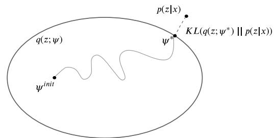
Figure 10.1: Illustration of variational inference. The large oval represents the set of variational distributions Q = {qω(z) : ε ↓ ⇒}, where ⇒ is the set of possible variational parameters. The true distribution is the point p(z|x), which we assume lies outside the set. Our goal is to find the best approximation to p within our variational family; this is the point ε↗ which is closest in KL divergence. We find this point by starting an optimization procedure from the random initial point εinit. Adapted from a figure by David Blei.

Minimizing this objective will minimize the KL divergence, causing our approximation to approach the true posterior. See Figure 10.1 for an illustration. In the sections below, we give two di!erent interpretations of this objective function.

10.1.1.1 The view from physics: minimize the variational free energy

If we define Eε(z) = → log pε(z, x) as the energy, then we can rewrite the loss in Equation (10.5)

\[\mathcal{L}(\theta, \psi|x) = \mathbb{E}\_{q\_{\psi}(\mathbf{z})} \left[ \mathcal{E}\_{\theta}(\mathbf{z}) \right] - \mathbb{H}(q\_{\psi}) = \text{expected energy} - \text{entropy} \tag{10.6}\]

In physics, this is known as the variational free energy (VFE). This is an upper bound on the free energy (FE), → log pε(x), which follows from the fact that

\[D\_{\mathbb{KL}}\left(q\_{\psi}(\mathbf{z}) \parallel p\_{\theta}(\mathbf{z}|\mathbf{x})\right) = \mathcal{L}(\theta, \psi|\mathbf{x}) + \log p\_{\theta}(\mathbf{z}) \geq 0 \tag{10.7}\]

\[\underbrace{\mathcal{L}(\boldsymbol{\theta},\psi|\boldsymbol{x})}\_{\text{VFE}} \ge \underbrace{-\log p\_{\boldsymbol{\theta}}(\boldsymbol{x})}\_{\text{FE}}\tag{10.8}\]

Variational inference is equivalent to minimizing the VFE. If we reach the minimum value of → log pε(x), then the KL divergence term will be 0, so our approximate posterior will be exact.

10.1.1.2 The view from statistics: maximize the evidence lower bound (ELBO)

The negative of the VFE is known as the evidence lower bound or ELBO function [BKM16]:

\[\operatorname{EL}(\theta, \psi | x) \stackrel{\Delta}{=} \operatorname{E}\_{q\_{\phi}(\mathbf{z})} \left[ \log p\_{\theta}(x, \mathbf{z}) - \log q\_{\psi}(\mathbf{z}) \right] = \operatorname{ELBO} \tag{10.9}\]

The name “ELBO” arises because

\[\mathbb{E}(\theta, \psi | x) \le \log p\_{\theta}(x) \tag{10.10}\]

where log pε(x) is called the “evidence”. The inequality follows from Equation (10.8). Therefore maximizing the ELBO wrt ϖ will minimize the original KL, since log pε(x) is a constant wrt ϖ.

(Note: we use the symbol # for the ELBO, rather than L, since we want to maximize # but minimize L.)

We can rewrite the ELBO as follows:

\[\mathbb{L}(\theta, \psi|x) = \mathbb{E}\_{q\_{\psi}(\mathbf{z})} \left[ \log p\_{\theta}(x, \mathbf{z}) \right] + \mathbb{H}(q\_{\psi}(\mathbf{z})) \tag{10.11}\]

We can interpret this

\[\text{ELBO} = \text{expected log joint} + \text{entropy} \tag{10.12}\]

The second term encourages the posterior to be maximum entropy, while the first term encourages it to be a joint MAP configuration.

We can also rewrite the ELBO as

\[\mathcal{L}(\psi|\theta,\mathbf{z}) = \mathbb{E}\_{q\_{\psi}(\mathbf{z})} \left[ \log p\_{\theta}(\mathbf{z}|\mathbf{z}) + \log p\_{\theta}(\mathbf{z}) - \log q\_{\psi}(\mathbf{z}) \right] \tag{10.13}\]

\[=\mathbb{E}\_{q\_{\boldsymbol{\Psi}}(\mathbf{z})}\left[\log p\_{\boldsymbol{\theta}}(\mathbf{z}|\mathbf{z})\right] - D\_{\text{KL}}\left(q\_{\boldsymbol{\Psi}}(\mathbf{z}) \parallel p\_{\boldsymbol{\theta}}(\mathbf{z})\right) \tag{10.14}\]

We can interpret this as follows:

ELBO = expected log likelihood → KL from posterior to prior (10.15)

The KL term acts like a regularizer, preventing the posterior from diverging too much from the prior.

10.1.2 Form of the variational posterior

There are two main approaches for choosing the form of the variational posterior, qϑ(z|x). In the first approach, we pick a convenient functional form, such as multivariate Gaussian, and then optimize the ELBO using gradient-based methods. This is called fixed-form VI, and is discussed in Section 10.2. An alternative is to make the mean field assumption, namely that the posterior factorizes:

\[q\_{\psi}(\mathbf{z}) = \prod\_{j=1}^{J} q\_{j}(\mathbf{z}\_{j}) \tag{10.16}\]

where q^j (z^j ) = q^ϑj (z^j ) is the posterior over the j’th group of variables. We don’t need to specify the functional form for each q^j . Instead, the optimal distributional form can be derived by maximizing the ELBO wrt each group of variational parameters one at a time, in a coordinate ascent manner. This is therefore called free-form VI, and is discussed in Section 10.3.

We now give a simple example of variational inference applied to a 2d latent vector z, representing the mean of a Gaussian. The prior is ^N (z^{| m}↭ , ↭ V), and the likelihood is

\[p(\mathcal{D}|\mathbf{z}) = \prod\_{n=1}^{N} \mathcal{N}(x\_n|\mathbf{z}, \boldsymbol{\Sigma}) \propto \mathcal{N}(\overline{\boldsymbol{x}}|\mathbf{z}, \frac{1}{N}\boldsymbol{\Sigma}) \tag{10.17}\]

The exact posterior, ^p(z|D) = ^N (z^{| m}↫ , ↫ V), can be computed analytically, as discussed in Section 3.4.4.1. In Figure 10.2, we compare three Gaussian variational approximations to the posterior. If q uses a full covariance matrix, it matches the exact posterior; however, this is intractable in high

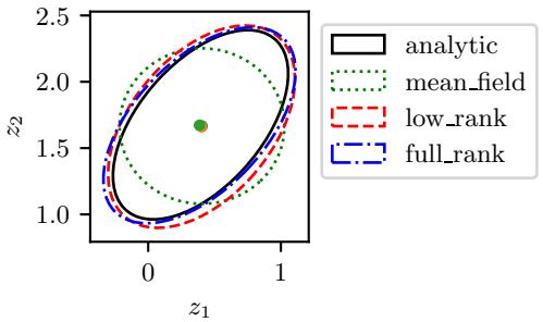
Figure 10.2: Variational approximation to the exact (Gaussian) posterior for the mean of a 2d Gaussian likelihood with a Gaussian prior. We show 3 Gaussian approximations to the posterior, using a full covariance (blue), a diagonal covariance (green), and a diagonal plus rank one covariance (red). Generated by gaussian\_2d\_vi.ipynb.

dimensions. If q uses a diagonal covariance matrix (corresponding to the mean field approximation), we see that the approximation is over confident, which is a well-known flaw of variational inference, due to the mode-seeking nature of minimizing DKL (q ↘ p) (see Section 5.1.4.3 for details). Finally, if q uses a rank-1 plus diagonal approximation, we get a much better approximation; furthermore, this can be computed quite e”ciently, as we discuss in Section 10.2.1.3.

10.1.3 Parameter estimation using variational EM

So far, we have assumed the model parameters ω are known. However, we can try to estimate them by maximing the log marginal likelihood of the dataset, D = {xⁿ : n =1: N},

\[\log p(\mathcal{D}|\boldsymbol{\theta}) = \sum\_{n=1}^{N} \log p(\boldsymbol{x}\_n|\boldsymbol{\theta}) \tag{10.18}\]

In general, this is intractable to compute, but we discuss approximations below.

10.1.3.1 MLE for latent variable models

Suppose we have a latent variable model of the form

\[p(\mathcal{D}, \mathbf{z}\_{1:N} | \boldsymbol{\theta}) = \prod\_{n=1}^{N} p(\mathbf{z}\_n | \boldsymbol{\theta}) p(\mathbf{z}\_n | \mathbf{z}\_n, \boldsymbol{\theta}) \tag{10.19}\]

as shown in Figure 10.3a. Furthermore, suppose we want to compute the MLE for ω given the dataset D = {xⁿ : n =1: N}. Since the local latent variables zⁿ are hidden, we must marginalize them out to get the local (per example) log marginal likelihood:

\[\log p(\mathbf{z}\_n|\boldsymbol{\theta}) = \log \left[ \int p(\mathbf{z}\_n|\mathbf{z}\_n, \boldsymbol{\theta}) p(\mathbf{z}\_n|\boldsymbol{\theta}) d\mathbf{z}\_n \right] \tag{10.20}\]

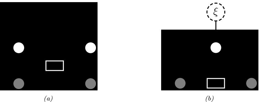
Figure 10.3: Graphical models with: (a) Local stochastic latent variables zⁿ and global deterministic latent parameter ω. (b) Global stochastic latent parameter ω and global deterministic latent hyper-parameter ϑ. The observed variables xⁿ are shown by shaded circles.

Unfortunately, computing this integral is usually intractable, since it corresponds to the normalization constant of the exact posterior. Fortunately, the ELBO is a lower bound on this:

\[\mathbb{E}(\theta, \psi\_n | x\_n) \le \log p(x\_n | \theta) \tag{10.21}\]

We can thus optimize the model parameters by maximizing

\[\mathbb{E}\left(\boldsymbol{\theta},\psi\_{1:N}|\mathcal{D}\right) \triangleq \sum\_{n=1}^{N} \mathbb{E}(\boldsymbol{\theta},\psi\_{n}|\boldsymbol{x}\_{n}) \leq \log p(\mathcal{D}|\boldsymbol{\theta}) \tag{10.22}\]

This is the basis of the variational EM algorithm. We discuss this in more detail in Section 6.5.6.1, but the basic idea is to alternate between maximizing the ELBO wrt the variational parameters {ϖn} in the E step, to give us q^ϑn (zn), and then maximizing the ELBO (using the new ϖn) wrt the model parameters ω in the M step. (We can also use SGD and amortized inference to speed this up, as we explain in Sections 10.1.4 to 10.1.5.)

10.1.3.2 Empirical Bayes for fully observed models

Suppose we have a fully observed model (with no local latent variables) of the form

\[p(\mathcal{D}, \theta | \xi) = p(\theta | \xi) \prod\_{n=1}^{N} p(x\_n | \theta) \tag{10.23}\]

as shown in Figure 10.3b. In the context of Bayesian parameter inference, our goal is to compute the parameter posterior:

\[p(\boldsymbol{\theta}|\mathcal{D},\boldsymbol{\xi}) = \frac{p(\mathcal{D}|\boldsymbol{\theta})p(\boldsymbol{\theta}|\boldsymbol{\xi})}{p(\mathcal{D}|\boldsymbol{\xi})} \tag{10.24}\]

where ω are the global unknown model parameters (latent variables), and ⇁ are the hyper-parameters for the prior. If the hyper-parameters are unknown, we can estimate them using empirical Bayes (see

Section 3.7) by computing

\[\hat{\boldsymbol{\xi}} = \operatorname\*{argmax}\_{\boldsymbol{\xi}} \log p(\mathcal{D} | \boldsymbol{\xi}) \tag{10.25}\]

We can use variational EM to compute this, similar to Section 10.1.3.1, except now the parameters to be estimated are ⇁, the latent variables are the shared global parameters ω, and the observations are the entire dataset, D. We then get the lower bound

\[\log p(\mathcal{D}|\boldsymbol{\xi}) \ge \mathcal{L}(\boldsymbol{\xi}, \boldsymbol{\psi}|\mathcal{D}) = \mathbb{E}\_{q\_{\boldsymbol{\psi}}(\boldsymbol{\theta})} \left[ \sum\_{n=1}^{N} \log p(\boldsymbol{x}\_{n}|\boldsymbol{\theta}) \right] - D\_{\text{KL}} \left( q\_{\boldsymbol{\psi}}(\boldsymbol{\theta}) \parallel p(\boldsymbol{\theta}|\boldsymbol{\xi}) \right) \tag{10.26}\]

We optimize this wrt the parameters of the variational posterior, ϖ, and wrt the prior hyper-parameters ⇁.

If the prior ⇁ is fixed, we just need to optimize the variational parameters ϖ to compute the posterior, qϑ(ω|D). This is known as variational Bayes. See Section 10.3.3 for more details.

10.1.4 Stochastic VI

In Section 10.1.3, we saw that parameter estimation requires optimizing the ELBO for the entire dataset, which is defined as the sum of the ELBOs for each of the N data samples xn. Computing this objective can be slow if N is large. Fortunately, we can replace this objective with a stochastic approximation, which is faster to compute, and provides an unbiased estimate. In particular, at each step, we can draw a random minibatch of B = |B| examples from the dataset, and then make the approximation

\[\mathbb{E}(\boldsymbol{\theta}, \boldsymbol{\psi}\_{1:N} | \mathcal{D}) = \sum\_{n=1}^{N} \mathbb{E}(\boldsymbol{\theta}, \boldsymbol{\psi}\_{n} | \boldsymbol{x}\_{n}) \approx \frac{N}{B} \sum\_{\mathbf{z}\_{n} \in \mathcal{B}} \left[ \mathbb{E}\_{q\_{\boldsymbol{\Psi}\_{n}}(\mathbf{z}\_{n})} \left[ \log p\_{\boldsymbol{\theta}}(\mathbf{z}\_{n} | \mathbf{z}\_{n}) + \log p\_{\boldsymbol{\theta}}(\mathbf{z}\_{n}) - \log q\_{\boldsymbol{\Psi}\_{n}}(\mathbf{z}\_{n}) \right] \right] \tag{10.27}\]

This can be used inside of a stochastic optimization algorithm, such as SGD. This is called stochastic variational inference or SVI [Hof+13], and allows VI to scale to large datasets.

10.1.5 Amortized VI

In Section 10.1.4, we saw that in each iteration of SVI, we need to optimize the local variational parameters ϖⁿ for each example n in the minibatch. This nested optimization can be quite slow.

An alternative approach is to train a model, known as an inference network or recognition network, to predict ϖⁿ from the observed data, xn, using ϖⁿ = finf ^ω (xn). This technique is known as amortized variational inference [GG14; GJW23], or inference compilation [LBW17], since we are reducing the cost of per-example time inference by training a model that is shared across all examples. (See also [Amo22] for a general discussion of amortized optimization.) For brevity, we will write the amortized posterior as

\[q(\mathbf{z}\_n|\boldsymbol{\psi}\_n) = q(\mathbf{z}\_n|f\_\Phi^{\mathrm{inf}}(\mathbf{z}\_n)) = q\_\Phi(\mathbf{z}\_n|\mathbf{z}\_n) \tag{10.28}\]

The corresponding ELBO becomes

\[\text{KL}(\boldsymbol{\theta}, \phi | \mathcal{D}) = \sum\_{n=1}^{N} \left[ \mathbb{E}\_{q\_{\boldsymbol{\theta}}(\mathbf{z}\_{n} | \mathbf{z}\_{n})} \left[ \log p\_{\boldsymbol{\theta}}(\mathbf{z}\_{n}, \mathbf{z}\_{n}) - \log q\_{\boldsymbol{\phi}}(\mathbf{z}\_{n} | \mathbf{z}\_{n}) \right] \right] \tag{10.29}\]

If we combine this with SVI we get an amortized version of Equation (10.27). For example, if we use a minibatch of size 1, we get

\[\mathcal{L}(\theta, \phi | \mathbf{z}\_n) \approx N \left[ \mathbb{E}\_{q\_{\phi}(\mathbf{z}\_n | \mathbf{z}\_n)} \left[ \log p\_{\theta}(\mathbf{z}\_n, \mathbf{z}\_n) - \log q\_{\phi}(\mathbf{z}\_n | \mathbf{z}\_n) \right] \right] \tag{10.30}\]

We can optimize this as shown in Algorithm 10.1. Note that the (partial) maximization wrt ω in the M step is usually done with a gradient update, but the maximization wrt ε in the E step is trickier, since the loss uses ε to define an expectation operator, so we can’t necessarily push the gradient operator inside; we discuss ways to optimize the variational parameters in Section 10.2 and Section 10.3.

Algorithm 10.1: Amortized stochastic variational EM

Initialize ω, ε ² repeat Sample xⁿ ↔︎ p^D E step: ε = argmax^ω #(ω, ε|xn) M step: ω = argmax^ε #(ω, ε|xn) until converged

10.1.6 Semi-amortized inference

Amortized SVI is widely used for fitting LVMs, e.g., for VAEs (see Section 21.2), for topic models [SS17a], for probabilistic programming [RHG16], for CRFs [TG18], etc. However, the use of an inference network can result in a suboptimal setting of the local variational parameters ϖn. This is called the amortization gap [CLD18]. We can close this gap by using the inference network to warm-start an optimizer for ϖn; this is known as semi-amortized VI [Kim+18c]. (See also [MYM18], who propose a closely related method called iterative amortized inference.)

An alternative approach is to use the inference network as a proposal distribution. If we combine this with importance sampling, we get the IWAE bound of Section 10.5.1. If we use this with Metropolis-Hastings, we get a VI-MCMC hybrid (see Section 10.4.5).

10.2 Gradient-based VI

In this section, we will choose some convenient form for qϑ(z), such as a Gaussian for continuous z, or a product of categoricals for discrete z, and then optimize the ELBO using gradient based methods.

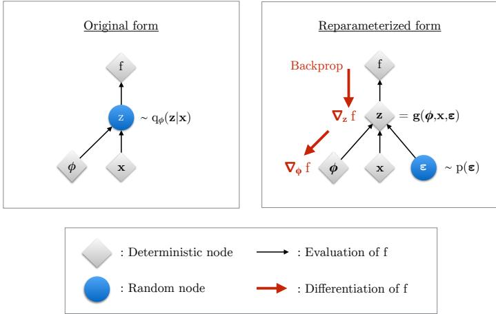
Figure 10.4: Illustration of the reparameterization trick. The objective f depends on the variational parameters ϖ, the observed data x, and the latent random variable z ↑ qε(z|x). On the left, we show the standard form of the computation graph. On the right, we show a reparameterized form, in which we move the stochasticity into the noise source ϱ, and compute z deterministically, z = g(ϖ, x, ϱ). The rest of the graph is deterministic, so we can backpropagate the gradient of the scalar f wrt ϖ through z and into ϖ. From Figure 2.3 of [KW19a]. Used with kind permission of Durk Kingma.

The gradient wrt the generative parameters ω is easy to compute, since we can push gradients inside the expectation, and use a single Monte Carlo sample:

\[\nabla\_{\theta} \mathbb{L}(\theta, \phi | x) = \nabla\_{\theta} \mathbb{E}\_{q\_{\phi}(\mathbf{z}|\mathbf{x})} \left[ \log p\_{\theta}(\mathbf{z}, \mathbf{z}) - \log q\_{\phi}(\mathbf{z}|\mathbf{x}) \right] \tag{10.31}\]

\[=\mathbb{E}\_{q\_{\phi}(\mathbf{z}|\boldsymbol{\pi})} \left[ \nabla\_{\theta} \left\{ \log p\_{\theta}(\boldsymbol{x}, \mathbf{z}) - \log q\_{\phi}(\boldsymbol{z}|\boldsymbol{x}) \right\} \right] \tag{10.32}\]

\[\approx \nabla\_{\theta} \log p\_{\theta}(\mathbf{z}, \mathbf{z}^{s}) \tag{10.33}\]

where ^{zs ↔︎ q}ω(z|x). This is an unbiased estimate of the gradient, so can be used with SGD.

The gradient wrt the inference parameters ε is harder to compute since

\[\nabla\_{\phi} \mathcal{L}(\theta, \phi | \mathbf{z}) = \nabla\_{\phi} \mathbb{E}\_{q\_{\phi}(\mathbf{z}|\mathbf{z})} \left[ \log p\_{\theta}(\mathbf{z}, \mathbf{z}) - \log q\_{\phi}(\mathbf{z}|\mathbf{z}) \right] \tag{10.34}\]

\[\neq \mathbb{E}\_{q\_{\phi}(\mathbf{z}|\mathbf{z})} \left[ \nabla\_{\phi} \left\{ \log p\_{\theta}(\mathbf{z}, \mathbf{z}) - \log q\_{\phi}(\mathbf{z}|\mathbf{x}) \right\} \right] \tag{10.35}\]

However, we can often use the reparameterization trick, which we discuss in Section 10.2.1. If not, we can use blackbox VI, which we discuss in Section 10.2.3.

10.2.1 Reparameterized VI

In this section, we discuss the reparameterization trick for taking gradients wrt distributions over continuous latent variables z ↔︎ qω(z|x). We explain this in detail in Section 6.3.5, but we summarize the basic idea here.

The key trick is to rewrite the random variable z ↔︎ qω(z|x) as some di!erentiable (and invertible) transformation g of another random variable , ↔︎ p(,), which does not depend on ε, i.e., we assume we can write

\[\mathbf{z} = g(\phi, \mathbf{z}, \mathbf{e})\tag{10.36}\]

For example,

\[\mathbf{z} \sim \mathcal{N}(\mu, \text{diag}(\sigma)) \iff \mathbf{z} = \mu + \mathbf{e} \odot \sigma, \ \mathbf{e} \sim \mathcal{N}(\mathbf{0}, \mathbf{I}) \tag{10.37}\]

Using this, we have

\[\mathbb{E}\_{q\_{\phi}(\mathbf{z}|\mathbf{z})} \left[ f(\mathbf{z}) \right] = \mathbb{E}\_{p(\mathbf{e})} \left[ f(\mathbf{z}) \right] \quad \text{s.t.} \quad \mathbf{z} = g(\phi, \mathbf{z}, \mathbf{e}) \tag{10.38}\]

where we define

\[f\_{\theta,\phi}(\mathbf{z}) = \log p\_{\theta}(\mathbf{z}, \mathbf{z}) - \log q\_{\phi}(\mathbf{z}|\mathbf{z}) \tag{10.39}\]

Hence

\[\nabla\_{\phi} \mathbb{E}\_{q\_{\phi}(\mathbf{z}|\mathbf{z})} \left[ f(\mathbf{z}) \right] = \nabla\_{\phi} \mathbb{E}\_{p(\mathbf{e})} \left[ f(\mathbf{z}) \right] = \mathbb{E}\_{p(\mathbf{e})} \left[ \nabla\_{\phi} f(\mathbf{z}) \right] \tag{10.40}\]

which we can approximate with a single Monte Carlo sample. This lets us propagate gradients back through the f function. See Figure 10.4 for an illustration. This is called reparameterized VI or RVI.

Since we are now working with the random variable ,, we need to use the change of variables formula to compute

\[\log q\_{\phi}(\mathbf{z}|\mathbf{x}) = \log p(\epsilon) - \log \left| \det \left( \frac{\partial \mathbf{z}}{\partial \epsilon} \right) \right| \tag{10.41}\]

where ^{ϑz ϑς} is the Jacobian:

\[\frac{\partial \mathbf{z}}{\partial \mathbf{e}} = \begin{pmatrix} \frac{\partial z\_1}{\partial e\_1} & \cdots & \frac{\partial z\_1}{\partial e\_k} \\ \vdots & \ddots & \vdots \\ \frac{\partial z\_k}{\partial e\_1} & \cdots & \frac{\partial z\_k}{\partial e\_k} \end{pmatrix} \tag{10.42}\]

We design the transformation z = g(,) such that this Jacobian is tractable to compute. We give some examples below.

10.2.1.1 Gaussian with diagonal covariance (mean field)

Suppose we use a fully factorized Gaussian posterior. Then the reparameterization process becomes

\[ \epsilon \sim \mathcal{N}(\mathbf{0}, \mathbf{I})\tag{10.43} \]

\[\mathbf{z} = \mu + \boldsymbol{\sigma} \odot \boldsymbol{\epsilon} \tag{10.44}\]

where the inference network generates the parameters of the transformation:

\[f(\mu, \log \sigma) = f\_{\phi}^{\inf}(x) \tag{10.45}\]

Thus to sample from the posterior qω(z|x), we sample , ↔︎ N (0, I), and then compute z.

Given the sample, we need to evaluate the ELBO:

\[f(\mathbf{z}) = \log p\_{\theta}(\mathbf{z}|\mathbf{z}) + \log p\_{\theta}(\mathbf{z}) - \log q\_{\phi}(\mathbf{z}|\mathbf{z}) \tag{10.46}\]

To evaluate the pε(x|z) term, we can just plug z into the likelihood. To evaluate the log qω(z|x) term, we need to use the change of variables formula from Equation (10.41). The Jacobian is given by ^{ϑz ϑς} = diag(σ). Hence

\[\log q\_{\phi}(\mathbf{z}|\mathbf{z}) = \sum\_{k=1}^{K} \left[ \log \mathcal{N}(\epsilon\_k | 0, 1) - \log \sigma\_k \right] = -\sum\_{k=1}^{K} \left[ \frac{1}{2} \log(2\pi) + \frac{1}{2} \epsilon\_k^2 + \log \sigma\_k \right] \tag{10.47}\]

Finally, to evaluate the p(z) term, we can use the transformation z = 0 + 1 ∞ ,, so the Jacobian is the identity and we get

\[\log p(\mathbf{z}) = -\sum\_{k=1}^{K} \left[ \frac{1}{2} z\_k^2 + \frac{1}{2} \log(2\pi) \right] \tag{10.48}\]

An alternative is to use the objective

\[f'(\mathbf{z}) = \log p\_{\theta}(\mathbf{z}|\mathbf{z}) + D\_{\text{KL}}\left(q\_{\phi}(\mathbf{Z}|x) \parallel p\_{\theta}(\mathbf{Z})\right) \tag{10.49}\]

In some cases, we evaluate the second term analytically, without needing Monte Carlo. For example, if we assume a diagonal Gaussian prior, p(z) = N (z|0, I), and diagonal gaussian posterior, q(z|x) = N (z|µ, diag(σ)), we can use Equation (5.78) to compute the KL in closed form:

\[D\_{\rm KL}\left(q \parallel p\right) = \sum\_{k=1}^{K} \left[ -\log \sigma\_k + \frac{1}{2} \sigma\_k^2 + \frac{1}{2} \mu\_k^2 \right] \tag{10.50}\]

The objective f^↔︎ (z) is often lower variance than f(z), since it computes the KL analytically. However, it is harder to generalize this objective to settings where the prior and/or posterior are not Gaussian.

10.2.1.2 Gaussian with full covariance

Now consider using a full covariance Gaussian posterior. We will compute a Cholesky decomposition of the covariance, ! = LL^T, where L is a lower triangular matrix with non-zero entries on the diagonal. Hence the reparameterization becomes

\[ \epsilon \sim \mathcal{N}(\mathbf{0}, \mathbf{I})\tag{10.51} \]

\[\mathbf{z} = \mu + \mathbf{L}\epsilon \tag{10.52}\]

The Jacobian of this a”ne transformation is ^{ϑz ϑς} = L. Since L is a triangular matrix, its determinant is the product of its main diagonal, so

\[\log \left| \det \frac{\partial z}{\partial \epsilon} \right| = \sum\_{k=1}^{K} \log |L\_{kk}| \tag{10.53}\]

We can compute L using

\[\mathbf{L} = \mathbf{M} \odot \mathbf{L}' + \text{diag}(\sigma) \tag{10.54}\]

where M is a masking matrix with 0s on and above the diagonal, and 1s below the diagonal, and where (µ, log σ,L^↔︎ ) is predicted by the inference network. With this construction, the diagonal entries of L are given by σ, so

\[\log \left| \det \frac{\partial z}{\partial \epsilon} \right| = \sum\_{k=1}^{K} \log |L\_{kk}| = \sum\_{k=1}^{K} \log \sigma\_k \tag{10.55}\]

10.2.1.3 Gaussian with low-rank plus diagonal covariance

In high dimensions, an e”cient alternative to using a Cholesky decomposition is the factor decomposition

\[\mathbf{E} = \mathbf{B}\mathbf{B}^{\mathsf{T}} + \mathbf{C}^{2} \tag{10.56}\]

where B is the factor loading matrix of size d ⇔ f, where f ∃ d is the number of factors, d is the dimensionality of z, and C = diag(c1,…,cd). This reduces the total number of variational parameters from d + d(d + 1)/2 to (f + 2)d. In [ONS18], they called this approach VAFC (short for variational approximation with factor covariance).

In the special case where f = 1, the covariance matrix becomes

\[ \Delta \Sigma = \mathbf{b} \mathbf{b}^{\mathsf{T}} + \text{diag}(\mathbf{c}^2) \tag{10.57} \]

In this case, it is possible to compute the natural gradient (Section 6.4) of the ELBO in closed form in O(d) time, as shown in [Tra+20b; TND21], who call the approach NAGVAC-1 (natural gradient Gaussian variational approximation). This can result in much faster convergence than following the normal gradient.

In Section 10.1.2, we show that this low rank approximation is much better than a diagonal approximation. See Supplementary Section 10.1 for more examples.

10.2.1.4 Other variational posteriors

Many other kinds of distribution can be written in a reparameterizable way, as described in [Moh+20]. This includes standard exponential family distributions, such as the gamma and Dirichlet, as well as more exotic forms, such as inverse autoregressive flows (see Section 10.4.3).

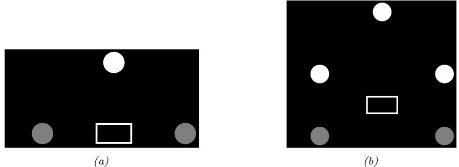
Figure 10.5: Graphical models with (a) Global latent parameter ω and observed variables x1:^N . (b) Local latent variables z1:^N , global latent parameter ω, and observed variables x1:^N .

10.2.1.5 Example: Bayesian parameter inference

In this section, we use reparameterized SVI to infer the posterior for the parameters of a Gaussian mixture model (GMM). We will marginalize out the discrete latent variables, so just need to approximate the posterior over the global latent, p(ω|D). This is sometimes called a “collapsed” model, since we have marginalized out all the local latent variables. That is, we have converted the model in Figure 10.5b to the one in Figure 10.5a. We choose a factored (mean field) variational posterior that is conjugate to the likelihood, but is also reparameterizable. This lets us fit the posterior with SGD.

For simplicity, we assume diagonal covariance matrices for each Gaussian mixture component. Thus the likelihood for one datapoint, ^x ↗ ^RD, is

\[p(x|\theta) = \sum\_{k=1}^{K} \pi\_k \mathcal{N}(x|\mu\_k, \text{diag}(\lambda\_k)^{-1}) \tag{10.58}\]

where µ^k = (µk1,…,µkD) are the means, ϑ^k = (⇀k1,…, ⇀kD) are the precisions, and ▷ = (ϖ1,…, ϖK) are the mixing weights. We use the following prior for these parameters:

\[p\_{\xi}(\theta) = \left[ \prod\_{k=1}^{K} \prod\_{d=1}^{D} \mathcal{N}(\mu\_{kd}|0, 1) \text{Ga}(\lambda\_{kd}|5, 5) \right] \text{Dir}(\pi|\mathbf{1}) \tag{10.59}\]

where ⇁ are the hyperparameters. We assume the following mean field posterior:

\[q\_{\boldsymbol{\Psi}}(\boldsymbol{\theta}) = \left[ \prod\_{k=1}^{K} \prod\_{d=1}^{D} \mathcal{N}(\mu\_{kd}|m\_{kd}, s\_{kd}) \text{Ga}(\lambda\_{kd}|\alpha\_{kd}, \beta\_{kd}) \right] \text{Dir}(\boldsymbol{\pi}|\mathbf{c}) \tag{10.60}\]

where ϖ = (m1:K,1:D, s1:K,1:D, ↼1:K,1:D, ⇀1:K,1:D, c) are the variational parameters for ω. We can compute the ELBO using

\[\mathcal{L}(\boldsymbol{\xi}, \boldsymbol{\psi} | \mathcal{D}) = \mathbb{E}\_{q\_{\boldsymbol{\Psi}}(\boldsymbol{\theta})} \left[ \log p(\mathcal{D} | \boldsymbol{\theta}) + \log p\_{\boldsymbol{\xi}}(\boldsymbol{\theta}) - \log q\_{\boldsymbol{\Psi}}(\boldsymbol{\theta}) \right] \tag{10.61}\]

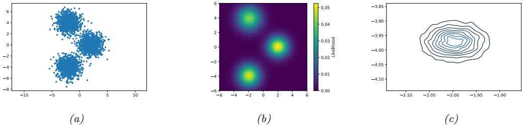
Figure 10.6: SVI for fitting a mixture of 3 Gaussians in 2d. (a) 3000 training points. (b) Fitted density, plugging in the posterior mean parameters. (c) Kernel density estimate fit to 10,000 samples from q(µ1|ε). Generated by svi\_gmm\_demo\_2d.ipynb.

Since the distributions are reparameterizable, we can push gradients inside this expression. We can approximate the expectation by drawing a single posterior sample, and can approximate the log likelihood using minibatching. We can then update the variational parameters, (and optionally the hyperparameters of the prior, as we discussed in Section 10.1.3.2) using the pseudcode in Algorithm 10.2.

Algorithm 10.2: Reparameterized SVI for Bayesian parameter inference

Initialize ϖ, ⇁ ² repeat Sample minibatch B = {x^b ↔︎ D : b =1: B} Sample , ↔︎ q⁰ Compute ω˜ = g(ϖ, ,) Compute ^L(ϖ|D, ^ω˜) = ^{→ N} B & ^xn↑^B log ^p(xn|ω˜) ^→ log ^pϱ(ω˜) + log ^qϑ(ω˜) Update ⇁ := ⇁ ^{→ η}⇒ϱL(⇁, ^ϖ|D, ^ω˜) Update ^ϖ := ^{ϖ → η}⇒ϑL(⇁, ^ϖ|D, ^ω˜) until converged

Figure 10.6 gives an example of this in practice. We generate a dataset from a mixture of 3 Gaussians in 2d, using µ^{→ 1} = [2, 0], µ^{→ 2} = [→2, →4], µ^{→ 3} = [→2, 4], precisions ⇀^→ dk = 1, and uniform mixing weights, ▷^→ = [1/3, 1/3, 1/3]. Figure 10.6a shows the training set of 3000 points. We fit this using SVI, with a batch size of 500, for 1000 epochs, using the Adam optimizer. Figure 10.6b shows the predictions of the fitted model. More precisely, it shows p(x|ω), where ω = Eq(ε|ϑ) [ω]. Figure 10.6c shows a kernel density estimate fit to 10,000 samples from q(µ1|ϖ). We see that the posterior mean is E [µ1] ↓ [→2, →4]. Due to label switching unidentifiability, we see this matches µ^→ 2 rather than µ^→ 1.

10.2.1.6 Example: MLE for LVMs

In this section, we consider reparameterized SVI for computing the MLE for latent variable models (LVMs) with continuous latents, such as variational autoencoders (Section 21.2). Unlike Section 10.2.1.5, we cannot analytically marginalize out the local latents. Instead we will use amortized inference, as in Section 10.1.5, which means we learn an inference network (with parameters ε) to predict the local variational parameters ϖⁿ given input xn. If we sample a single example xⁿ from the dataset at each iteration, and a single latent variable zⁿ from the variational posterior, then we get the pseudocode in Algorithm 10.3.

Algorithm 10.3: Reparameterized amortized SVI for MLE of an LVM

1 Initialize ω, ε
2 repeat
3 Sample xn ↔ pD
4 Sample ,n ↔ q0
5 Compute zn = g(ε, xn, ,n)
6 Compute L(ω, ε|xn, zn) = → log pε(xn, zn) + log qω(zn|xn)
7 Update ω := ω → η⇒εL(ε, ω|xn, zn)
8 Update ε := ε → η⇒ωL(ε, ω|xn, zn)
9 until converged

10.2.2 Automatic di”erentiation VI

To apply Gaussian VI, we need to transform constrained parameters (such as variance terms) to unconstrained form, so they live in R^D. This technique can be used for any distribution for which we can define a bijection to R^D. This approach is called automatic di!erentiation variational inference or ADVI [Kuc+16]. We give the details below.

10.2.2.1 Basic idea

Our goal is to approximate the posterior p(ω|D) ↑ p(ω)p(D|ω), where ω ↗ # lives in some Ddimensional constrained parameter space. Let ^T : # ↖ ^RD be a bijective mapping that maps from the constrained space # to the unconstrained space ^RD. with inverse ^{T ↓1} : ^RD ↖ #. Let ^{u = T}(ω) be the unconstrained latent variables. We will use a Gaussian variational approximation to the posterior for u, i.e.,: qϑ(u) = N (u|µd, !), where ϖ = (µ, !).

By the change of variable formula Equation (2.257), we have

\[p(\mathbf{u}) = p(T^{-1}(\mathbf{u})) |\det(\mathbf{J}\_{T^{-1}}(\mathbf{u}))|\tag{10.62}\]

where J^{T →1} is the Jacobian of the inverse mapping u ↖ ω. Hence the ELBO becomes

\[\mathbb{E}(\boldsymbol{\Psi}) = E\_{\mathbf{u} \sim q\_{\Psi}(\mathbf{u})} \left[ \log p(\mathcal{D} | T^{-1}(\mathbf{u})) + \log p(T^{-1}(\mathbf{u})) + \log \left| \det(\mathbf{J}\_{T^{-1}}(\mathbf{u})) \right| \right] + \mathbb{E}(\boldsymbol{\psi}) \tag{10.63}\]

This is a tractable objective, assuming the Jacobian is tractable, since the final entropy term is available in closed form, and we can use a Monte Carlo approximation of the expectation over u.

Since the objective is stochastic, and reparamterizable, we can use SGD to optimize it. However, [Ing20] propose deterministic ADVI, in which the samples ,^s ↔︎ N (0, I) are held fixed during the optimization process. This is called the common random numbers trick (Section 11.6.1), and makes the objective a deterministic function; this allows for the use of more powerful second-order optimization methods, such as BFGS. (Of course, if the dataset is large, we might need to use minibatch subsampling, which reintroduces stochasticity.)

10.2.2.2 Example: ADVI for beta-binomial model

To illustrate ADVI, we consider the 1d beta-binomial model from Section 7.4.4. We want to approximate ^p(ω|D) using the prior ^p(ω) = Beta(ω|a, b) and likelihood ^p(D|ω) = ⁱ Ber(yi|ω), where the su”cient statistics are N¹ = 10, N⁰ = 1, and the prior is uninformative, a = b = 1. We use the transformation ω = T ^↓1(z) = ς(z), and optimize the ELBO with SGD. The results of this method are shown in Figure 7.4 and show that the Gaussian fit is a good approximation, despite the skewed nature of the posterior.

10.2.2.3 Example: ADVI for GMMs

In this section, we use ADVI to approximate the posterior of the parameters of a mixture of Gaussians. The di!erence from the VBEM algorithm of Section 10.3.6 is that we use ADVI combined with a Gaussian variational posterior, rather than using a mean field approximation defined by a product of conjugate distributions.

To apply ADVI, we marginalize out the discrete local discrete latents mⁿ ↗ {1,…,K} analytically, so the likelihood has the form

\[p(\mathcal{D}|\boldsymbol{\theta}) = \prod\_{n=1}^{N} \left[ \sum\_{k=1}^{K} \pi\_k \mathcal{N}(y\_n | \mu\_k, \text{diag}(\boldsymbol{\Sigma}\_k)) \right] \tag{10.64}\]

We use an uniformative Gaussian prior for the µk, a uniform LKJ prior for the Lk, a log-normal prior for the σk, and a uniform Dirichlet prior for the mixing weights ▷. (See [Kuc+16, Fig 21] for a definition of the model in STAN syntax.) The posterior approximation for the unconstrained parameters is a block-diagonal gaussian. q(u) = N (u|ϖµ, ϖ!), where the unconstrained parameters are computed using suitable bijections (see code for details).

We apply this method to the Old Faithful dataset from Figure 10.12, using K = 10 mixture components. The results are shown in Figure 10.7. In the top left, we show the special case where we constrain the posterior to be a MAP estimate, by setting ϖ! = 0. We see that there is no sparsity in the posterior, since there is no Bayesian “Occam factor” from marginalizing out the parameters. In panels c–d, we show 3 samples from the posterior. We see that the Bayesian method strongly prefers just 2 mixture components, although there is a small amount of support for some other Gaussian components (shown by the faint ellipses).

10.2.2.4 More complex posteriors

We can combine ADVI with any of the improved posterior approximations that we discuss in Section 10.4 — such as Gaussian mixtures [Mor+21b] or normalizing flows [ASD20] — to create a high-quality, automatic approximate inference scheme.

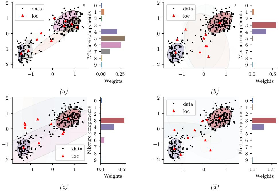
Figure 10.7: Posterior over the mixing weights (histogram) and the means and covariances of each Gaussian mixture component, using K = 10, when fitting the model to the Old Faithful dataset from Figure 10.12. (a) MAP approximation. (b-d) 3 samples from the Gaussian approximation. The intensity of the shading is proportional to the mixture weight. Generated by gmm\_advi\_bijax.ipynb.

10.2.3 Blackbox variational inference

In this section, we assume that we can evaluate ^L˜(ϖ, ^z) = log ^p(z, ^x) ^→ log ^qϑ(z) pointwise, but we do not assume we can take gradients of this function. (For example, z may contain discrete variables.) We are thus treating the model as a “blackbox”. Hence this approach is called blackbox variational inference or BBVI [RGB14; ASD20].

10.2.3.1 Estimating the gradient using REINFORCE

To estimate the gradient of the ELBO, we will use the score function estimator, also called the REINFORCE estimator (Section 6.3.4). In particular, suppose we write the ELBO as

\[\mathbb{E}(\psi) = \mathbb{E}\_{q(\mathbf{z}|\psi)} \left[ \tilde{\mathcal{L}}(\psi, \mathbf{z}) \right] = \mathbb{E}\_{q(\mathbf{z}|\psi)} \left[ \log p(\mathbf{z}, \mathbf{z}) - \log q(\mathbf{z}|\psi) \right] \tag{10.65}\]

Then from Equation (6.58) we have

\[\nabla\_{\psi} \mathbb{E}(\psi) = \mathbb{E}\_{q(\mathbf{z}|\psi)} \left[ \tilde{\mathcal{L}}(\psi, \mathbf{z}) \nabla\_{\psi} \log q(\mathbf{z}|\psi) \right] \tag{10.66}\]

We can then compute a Monte Carlo approximation to this:

\[\widehat{\nabla\_{\psi}L(\psi\_t)} = \frac{1}{S} \sum\_{s=1}^{S} \check{L}(\psi, \mathbf{z}\_s) \nabla\_{\psi} \log q\_{\psi}(\mathbf{z}\_s)|\_{\psi = \psi\_t} \tag{10.67}\]

We can pass this to any kind of gradient optimizer, such as SGD or Adam.

10.2.3.2 Reducing the variance using control variates

In practice, the variance of this estimator is quite large, so it is important to use methods such as control variates or CV (Section 6.3.4.1). To see how this works, consider the naive gradient estimator in Equation (10.67), which for the i’th component we can write as

\[\left(\widehat{\nabla\_{\psi\_i}\mathcal{L}}(\overline{\boldsymbol{\psi}}\_t)\right)^{\text{naive}} = \frac{1}{S} \sum\_{s=1}^{S} \tilde{g}\_i(\mathbf{z}\_s) \tag{10.68}\]

\[ \tilde{g}\_i(\mathbf{z}\_s) = g\_i(\mathbf{z}\_s) \times \tilde{\mathcal{L}}(\boldsymbol{\psi}, \mathbf{z}\_s) \tag{10.69} \]

\[g\_i(\mathbf{z}\_s) = \nabla\_{\psi\_i} \log q\_{\psi}(\mathbf{z}\_s) \tag{10.70}\]

The control variate version of this can be obtained by replacing g˜i(zs) with

\[ \hat{g}\_i^{cv}(\mathbf{z}) = \tilde{g}\_i(\mathbf{z}) + c\_i(\mathbb{E}\left[b\_i(\mathbf{z})\right] - b\_i(\mathbf{z})) \tag{10.71} \]

where bi(z) is a baseline function and cⁱ is some constant, to be specified below. A convenient baseline is the score function, bi(z) = ⇒^ϑi log q^ϑi (z) = gi(z), since this is correlated with g˜i(z), and has the property that E [bi(z)] = 0, since the expected value of the score function is zero, as we showed in Equation (3.44). Hence

\[ \tilde{g}\_i^{cv}(\mathbf{z}) = \tilde{g}\_i(\mathbf{z}) - c\_i g\_i(\mathbf{z}) = g\_i(\mathbf{z}) (\tilde{\mathcal{L}}(\psi, \mathbf{z}) - c\_i) \tag{10.72} \]

so the CV estimator is given by

\[\left(\widehat{\nabla\_{\psi\_i}L(\bar{\psi\_t})}^{\text{cv}}\right)^{\text{cv}} = \frac{1}{S} \sum\_{s=1}^{S} g\_i(\mathbf{z}\_s) \times \left(\bar{\mathcal{L}}(\psi, \mathbf{z}\_s) - c\_i\right) \tag{10.73}\]

One can show that the optimal cⁱ that minimizes the variance of the CV estimator is

\[c\_i = \frac{\text{Cov}\left[g\_i(\mathbf{z})\vec{\mathcal{L}}(\boldsymbol{\psi}, \mathbf{z}), g\_i(\mathbf{z})\right]}{\mathbb{V}\left[g\_i(\mathbf{z})\right]}\tag{10.74}\]

For more details, see e.g., [TND21].

10.3 Coordinate ascent VI

A common approximation in variational inference is to assume that all the latent variables are independent, i.e.,

\[q\_{\psi}(\mathbf{z}) = \prod\_{j=1}^{J} q\_{j}(z\_{j}) \tag{10.75}\]

where J is the number of hidden variables, and q^j (z^j ) is shorthand for qϑ^j (z^j ), where ϖ^j are the variational parameters for the j’th distribution. This is called the mean field approximation.

From Equation (10.11), the ELBO becomes

\[\mathbb{L}(\psi) = \int q\_{\psi}(\mathbf{z}) \log p\_{\theta}(\mathbf{z}, \mathbf{z}) d\mathbf{z} + \sum\_{j=1}^{J} \mathbb{H}(q\_{j}) \tag{10.76}\]

since the entropy of a product distribution is the sum of entropies of each component in the product. The first term also often decomposes according to the Markov properties of the graphical model. This allows us to use a coordinate ascent optimization scheme to estimate each ϖ^j , as we explain in Section 10.3.1. This is called coordinate ascent variational inference or CAVI, and is an alternative to gradient-based VI.

10.3.1 Derivation of CAVI algorithm

In this section, we derive the coordinate ascent variational inference (CAVI) procedure.

To derive the update equations, we initially assume there are just 3 discrete latent variables, to simplify notation. In this case the ELBO is given by

\[\mathbb{L}(q\_1, q\_2, q\_3) = \sum\_{z\_1} \sum\_{z\_2} \sum\_{z\_3} q\_1(z\_1) q\_2(z\_2) q\_3(z\_3) \log \tilde{p}(z\_1, z\_2, z\_3) + \sum\_{j=1}^3 \mathbb{H}(q\_j) \tag{10.77}\]

where we define p˜(z) = pε(z, x) for brevity. We will optimize this wrt each qi, one at a time, keeping the others fixed.

Let us look at the objective for q3:

\[\mathcal{L}\_3(q\_3) = \sum\_{z\_3} q\_3(z\_3) \left[ \sum\_{z\_1} \sum\_{z\_2} q\_1(z\_1) q\_2(z\_2) \log \tilde{p}(z\_1, z\_2, z\_3) \right] + \mathbb{H}(q\_3) + \text{const} \tag{10.78}\]

\[=\sum\_{z\_3} q\_3(z\_3) \left[ g\_3(z\_3) - \log q\_3(z\_3) \right] + \text{const} \tag{10.79}\]

where

\[g\_3(z\_3) \triangleq \sum\_{z\_1} \sum\_{z\_2} q\_1(z\_1) q\_2(z\_2) \log \tilde{p}(z\_1, z\_2, z\_3) = \mathbb{E}\_{\mathbf{z}\_{-3}} \left[ \log \tilde{p}(z\_1, z\_2, z\_3) \right] \tag{10.80}\]

where z↓³ = (z1, z2) is all variables except z3. Here g3(z3) can be interpreted as an expected negative energy (log probability). We can convert this into an unnormalized probability distribution by defining

\[f\_3(z\_3) = \exp(g\_3(z\_3))\tag{10.81}\]

which we can normalize to get

\[f\_3(z\_3) = \frac{\tilde{f}\_3(z\_3)}{\sum\_{z\_3'} \tilde{f}\_3(z\_3')} \propto \exp(g\_3(z\_3))\tag{10.82}\]

Since g3(z3) ↑ log f3(z3) we get

\[\mathrm{KL}\_3(q\_3) = \sum\_{z\_3} q\_3(z\_3) \left[ \log f\_3(z\_3) - \log q\_3(z\_3) \right] + \text{const} = -D\_{\mathrm{KL}} \left( q\_3 \parallel f\_3 \right) + \text{const} \tag{10.83}\]

Since DKL (q³ ↘ f3) achieves its minimal value of 0 when q3(z3) = f3(z3) for all z3, we see that q→ ³(z3) = f3(z3).

Now suppose that the joint distribution is defined by a Markov chain, where z¹ ↖ z² ↖ z3, so z¹ ¬ z3|z2. Hence log ˜p(z1, z2, z3) = log ˜p(z2, z3|z1) + log ˜p(z1), where the latter term is independent of q3(z3). Thus the ELBO simplifies to

\[\mathbb{H}\_3(q\_3) = \sum\_{z\_3} q\_3(z\_3) \left[ \sum\_{z\_2} q\_2(z\_2) \log \tilde{p}(z\_2, z\_3) \right] + \mathbb{H}(q\_3) + \text{const} \tag{10.84}\]

\[=\sum\_{z\_3} q\_3(z\_3) \left[ \log f\_3(z\_3) - \log q\_3(z\_3) \right] + \text{const} \tag{10.85}\]

where

\[\log f\_3(z\_3) \propto \exp\left[\sum\_{z\_2} q\_2(z\_2) \log \tilde{p}(z\_2, z\_3)\right] = \exp\left[\mathbb{E}\_{\mathbf{z}\_{\text{mb}\_3}}\left[\log \tilde{p}(z\_2, z\_3)\right]\right] \tag{10.86}\]

where zmb³ = z² is the Markov blanket (Section 4.2.4.3) of z3. As before, the optimal variational distribution is given by q3(z3) = f3(z3).

In general, when we have J groups of variables, the optimal variational distribution for the j’th group is given by

\[q\_j(\mathbf{z}\_j) \propto \exp\left[\mathbb{E}\_{\mathbf{z}\_{\rm{mb}\_j}}\left[\log \tilde{p}(\mathbf{z}\_j, \mathbf{z}\_{\rm{mb}\_j})\right]\right] \tag{10.87}\]

(Compare to the equation for Gibbs sampling in Equation (12.19).) The CAVI method simply computes q^j for each dimension j in turn, in an iterative fashion (see Algorithm 10.4). Convergence is guaranteed since the bound is concave wrt each of the factors qⁱ [Bis06, p. 466].

Algorithm 10.4:	Coordinate ascent	variational	inference	(CAVI).
——————–	———————-	————-	———–	———

Initialize q^j (z^j ) for j =1: J foreach t =1: T do foreach j =1: J do Compute g^j (z^j ) = E^zmbⁱ [log ˜p(zi, zmbⁱ )] Compute q^j (z^j ) ↑ exp(g^j (z^j ))

Note that the functional form of the qⁱ distributions does not need to be specified in advance, but will be determined by the form of the log joint. This is therefore called free-form VI, as opposed to fixed-form, where we explicitly choose a convenient distributional type for q (we discuss fixed-form VI in Section 10.2). We give some examples below that will make this clearer.

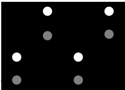
Figure 10.8: A grid-structured MRF with hidden nodes zⁱ and local evidence nodes xi. The prior p(z) is an undirected Ising model, and the likelihood ^p(x|z) = ! ⁱ p(xi|zi) is a directed fully factored model.

10.3.2 Example: CAVI for the Ising model

In this section, we apply CAVI to perform mean field inference in an Ising model (Section 4.3.2.1), which is a kind of Markov random field defined on binary random variables, zⁱ ↗ {→1, +1}, arranged in a 2d grid.

Originally Ising models were developed as models of atomic spins for magnetic materials, although we will apply them to an image denoising problem. Specifically, let zⁱ be the hidden value of pixel i, and xⁱ ↗ R be the observed noisy value. See Figure 10.8 for the graphical model.

Let Li(zi) ↭ log p(xi|zi) be the log likelihood for the i’th pixel (aka the local evidence for node i in the graphical model). The overall likelihood has the form

\[p(\mathbf{z}|\mathbf{z}) = \prod\_{i} p(x\_i|z\_i) = \exp(\sum\_{i} L\_i(z\_i)) \tag{10.88}\]

Our goal is to approximate the posterior p(z|x). We will use an Ising model for the prior:

\[p(\mathbf{z}) = \frac{1}{Z\_0} \exp(-\mathcal{E}\_0(\mathbf{z})) \tag{10.89}\]

\[\mathcal{E}\_0(\mathbf{z}) = -\sum\_{i \sim j} W\_{ij} z\_i z\_j \tag{10.90}\]

where we sum over each i → j edge. Therefore the posterior has the form

\[p(\mathbf{z}|\mathbf{x}) = \frac{1}{Z(\mathbf{z})} \exp(-\mathcal{E}(\mathbf{z})) \tag{10.91}\]

\[\mathcal{E}(\mathbf{z}) = \mathcal{E}\_0(\mathbf{z}) - \sum\_{i} L\_i(z\_i) \tag{10.92}\]

We will now make the following fully factored approximation:

\[q(\mathbf{z}) = \prod\_{i} q\_i(z\_i) = \prod\_{i} \text{Ber}(z\_i|\mu\_i) \tag{10.93}\]

where µⁱ = E^qi [zi] is the mean value of node i. To derive the update for the variational parameter µi, we first compute the unnormalized log joint, log ˜p(z) = →E(z), dropping terms that do not involve

zi:

\[\log \hat{p}(\mathbf{z}) = z\_i \sum\_{j \in \text{nbr}\_i} W\_{ij} z\_j + L\_i(z\_i) + \text{const} \tag{10.94}\]

This only depends on the states of the neighboring nodes. Hence

\[q\_i(z\_i) \propto \exp(\mathbb{E}\_{q\_{-i}(\mathbf{z})} \left[ \log \tilde{p}(\mathbf{z}) \right]) = \exp\left(z\_i \sum\_{j \in \text{nbr}\_i} W\_{ij} \mu\_j + L\_i(z\_i)\right) \tag{10.95}\]

where ^q↓ⁱ(z) = ^j⇒=^{i q}(z^j ). Thus we replace the states of the neighbors by their average values. (Note that this replaces binary variables with continuous ones.)

We now simplify this expression. Let mⁱ = & ^j↑nbr^{i W}ijµ^j be the mean field influence on node ⁱ. Also, let L^{+ i} ↭ Li(+1) and L^{↓ i} ↭ Li(→1). The approximate marginal posterior is given by

\[q\_i(z\_i = 1) = \frac{e^{m\_i + L\_i^+}}{e^{m\_i + L\_i^+} + e^{-m\_i + L\_i^-}} = \frac{1}{1 + e^{-2m\_i + L\_i^- - L\_i^+}} = \sigma(2a\_i) \tag{10.96}\]

\[a\_i \stackrel{\Delta}{=} m\_i + 0.5(L\_i^+ - L\_i^-) \tag{10.97}\]

Similarly, we have qi(zⁱ = →1) = ς(→2ai). From this we can compute the new mean for site i:

\[\mu\_i = \mathbb{E}\_{q\_i} \left[ z\_i \right] = q\_i(z\_i = +1) \cdot (+1) + q\_i(z\_i = -1) \cdot (-1) \tag{10.98}\]

\[\frac{1}{1+e^{-2a\_i}} - \frac{1}{1+e^{2a\_i}} = \frac{e^{a\_i}}{e^{a\_i}+e^{-a\_i}} - \frac{e^{-a\_i}}{e^{-a\_i}+e^{a\_i}} = \tanh(a\_i) \tag{10.99}\]

We can turn the above equations into a fixed point algorithm by writing

\[\mu\_i^t = \tanh\left(\sum\_{j \in \text{nbr}\_i} W\_{ij} \mu\_j^{t-1} + 0.5(L\_i^+ - L\_i^-)\right) \tag{10.100}\]

Following [MWJ99], we can use damped updates of the following form to improve convergence:

\[\mu\_i^t = (1 - \lambda)\mu\_i^{t-1} + \lambda \tanh\left(\sum\_{j \in \text{nbr}\_i} W\_{ij}\mu\_j^{t-1} + 0.5(L\_i^+ - L\_i^-)\right) \tag{10.101}\]

for 0 < ⇀ < 1. We can update all the nodes in parallel, or update them asynchronously.

Figure 10.9 shows the method in action, applied to a 2d Ising model with homogeneous attractive potentials, Wij = 1. We use parallel updates with a damping factor of ⇀ = 0.5. (If we don’t use damping, we tend to get “checkerboard” artifacts.)

10.3.3 Variational Bayes

In Bayesian modeling, we treat the parameters ω as latent variables. Thus our goal is to approximate the parameter posterior p(ω|D) ↑ p(ω)p(D|ω). Applying VI to this problem is called variational Bayes [Att00].

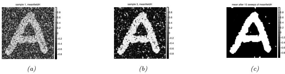
Figure 10.9: Example of image denoising using mean field (with parallel updates and a damping factor of 0.5). We use an Ising prior with Wij = 1 and a Gaussian noise model with ω = 2. We show the results after 1, 3 and 15 iterations across the image. Compare to Figure 12.3, which shows the results of using Gibbs sampling. Generated by ising\_image\_denoise\_demo.ipynb.

In this section, we assume there are no latent variables except for the shared global parameters, so the model has the form

\[p(\boldsymbol{\theta}, \mathcal{D}) = p(\boldsymbol{\theta}) \prod\_{n=1}^{N} p(\mathcal{D}\_n | \boldsymbol{\theta}) \tag{10.102}\]

These conditional independencies are illustrated in Figure 10.5a.

We will fit the variational posterior by maximizing the ELBO

\[\mathbb{E}\left(\psi\_{\boldsymbol{\theta}}|\mathcal{D}\right) = \mathbb{E}\_{q(\boldsymbol{\theta}|\psi\_{\boldsymbol{\theta}})}\left[\log p(\boldsymbol{\theta}, \mathcal{D})\right] + \mathbb{E}(q(\boldsymbol{\theta}|\psi\_{\boldsymbol{\theta}})) \tag{10.103}\]

We will assume the variational posterior factorizes over the parameters:

\[q(\boldsymbol{\theta}|\boldsymbol{\psi}\_{\boldsymbol{\theta}}) = \prod\_{j} q(\boldsymbol{\theta}\_{j}|\boldsymbol{\psi}\_{\boldsymbol{\theta}\_{j}}) \tag{10.104}\]

We can then update each ϖ^ϱj using CAVI (Section 10.3.1).

10.3.4 Example: VB for a univariate Gaussian

Consider inferring the parameters of a 1d Gaussian. The likelihood is given by ^p(D|ω) = ^{N n}=1 ^N (xn|µ, ⇀↓1), where µ is the mean and ⇀ is the precision. Suppose we use a conjugate prior of the form

\[p(\mu, \lambda) = \mathcal{N}(\mu | \mu\_0, (\kappa\_0 \lambda)^{-1}) \text{Ga}(\lambda | a\_0, b\_0) \tag{10.105}\]

It is possible to derive the posterior p(µ, ⇀|D) for this model exactly, as shown in Section 3.4.3.3. However, here we use the VB method with the following factored approximate posterior:

\[q(\mu,\lambda) = q(\mu|\psi\_{\mu})q(\lambda|\psi\_{\lambda})\tag{10.106}\]

We do not need to specify the forms for the distributions q(µ|ϖµ) and q(⇀|ϖε); the optimal forms will “fall out” automatically during the derivation (and conveniently, they turn out to be Gaussian and gamma respectively). Our presentation follows [Mac03, p429].

10.3.4.1 Target distribution

The unnormalized log posterior has the form

\[\log \bar{p}(\mu, \lambda) = \log p(\mu, \lambda, \mathcal{D}) = \log p(\mathcal{D} | \mu, \lambda) + \log p(\mu | \lambda) + \log p(\lambda) \tag{10.107}\]

\[= \frac{N}{2} \log \lambda - \frac{\lambda}{2} \sum\_{n=1}^{N} (x\_n - \mu)^2 - \frac{\kappa\_0 \lambda}{2} (\mu - \mu\_0)^2\]

\[+ \frac{1}{2} \log (\kappa\_0 \lambda) + (a\_0 - 1) \log \lambda - b\_0 \lambda + \text{const} \tag{10.108}\]

10.3.4.2 Updating q(µ|ϖµ)

The optimal form for q(µ|ϖµ) is obtained by averaging over ⇀:

\[\log q(\mu|\psi\_{\mu}) = \mathbb{E}\_{q(\lambda|\psi\_{\lambda})} \left[ \log p(\mathcal{D}|\mu, \lambda) + \log p(\mu|\lambda) \right] + \text{const} \tag{10.109}\]

\[\hat{\mu}\_{\lambda} = -\frac{\mathbb{E}\_{q(\lambda|\psi\_{\lambda})}\left[\lambda\right]}{2} \left\{ \kappa\_0 (\mu - \mu\_0)^2 + \sum\_{n=1}^{N} (x\_n - \mu)^2 \right\} + \text{const} \tag{10.110}\]

By completing the square one can show that ^q(µ|ϖµ) = ^N (µ|µ^N , ↽↓^{1 N} ), where

\[ \mu\_N = \frac{\kappa\_0 \mu\_0 + N\overline{x}}{\kappa\_0 + N}, \ \kappa\_N = (\kappa\_0 + N)\mathbb{E}\_{q(\lambda|\psi\_\lambda)}\left[\lambda\right] \tag{10.111} \]

At this stage we don’t know what q(⇀|ϖε) is, and hence we cannot compute E [⇀], but we will derive this below.

10.3.4.3 Updating q(ϑ|ϖφ)

The optimal form for q(⇀|ϖε) is given by

\[\log q(\lambda|\psi\_{\lambda}) = \mathbb{E}\_{q(\mu|\psi\_{\mu})} \left[ \log p(\mathcal{D}|\mu, \lambda) + \log p(\mu|\lambda) + \log p(\lambda) \right] + \text{const} \tag{10.112}\]

\[= (a\_0 - 1)\log \lambda - b\_0 \lambda + \frac{1}{2}\log \lambda + \frac{N}{2}\log \lambda\]

\[- \frac{\lambda}{2} \mathbb{E}\_{q(\mu|\psi\_{\mu})} \left[ \kappa\_0 (\mu - \mu\_0)^2 + \sum\_{n=1}^{N} (x\_n - \mu)^2 \right] + \text{const} \tag{10.113}\]

We recognize this as the log of a gamma distribution, hence q(⇀|ϖε) = Ga(⇀|a^N , b^N ), where

\[a\_N = a\_0 + \frac{N+1}{2} \tag{10.114}\]

\[b\_N = b\_0 + \frac{1}{2} \mathbb{E}\_{q(\mu | \Phi\_\mu)} \left[ \kappa\_0 (\mu - \mu\_0)^2 + \sum\_{n=1}^N (x\_n - \mu)^2 \right] \tag{10.115}\]

10.3.4.4 Computing the expectations

To implement the updates, we have to specify how to compute the various expectations. Since ^q(µ) = ^N (µ|µ^N , ↽↓^{1 N} ), we have

\[\mathbb{E}\_{\mathbf{q}(\mu)}\left[\mu\right] = \mu\_N \tag{10.116}\]

\[\mathbb{E}\_{q(\mu)}\left[\mu^2\right] = \frac{1}{\kappa\_N} + \mu\_N^2 \tag{10.117}\]

Since q(⇀) = Ga(⇀|a^N , b^N ), we have

\[\mathbb{E}\_{q(\lambda)}\left[\lambda\right] = \frac{a\_N}{b\_N} \tag{10.118}\]

We can now give explicit forms for the update equations. For q(µ) we have

\[ \mu\_N = \frac{\kappa\_0 \mu\_0 + N \overline{x}}{\kappa\_0 + N} \tag{10.119} \]

\[ \kappa\_N = (\kappa\_0 + N) \frac{a\_N}{b\_N} \tag{10.120} \]

and for q(⇀) we have

\[a\_N = a\_0 + \frac{N+1}{2} \tag{10.121}\]

\[b\_N = b\_0 + \frac{1}{2} \kappa\_0 (\mathbb{E}\left[\mu^2\right] + \mu\_0^2 - 2\mathbb{E}\left[\mu\right]\mu\_0) + \frac{1}{2} \sum\_{n=1}^N \left(x\_n^2 + \mathbb{E}\left[\mu^2\right] - 2\mathbb{E}\left[\mu\right]x\_n\right) \tag{10.122}\]

We see that µ^N and a^N are in fact fixed constants, and only ↽^N and b^N need to be updated iteratively. (In fact, one can solve for the fixed points of ↽^N and b^N analytically, but we don’t do this here in order to illustrate the iterative updating scheme.)

10.3.4.5 Illustration

Figure 10.10 gives an example of this method in action. The green contours represent the exact posterior, which is Gaussian-gamma. The dotted red contours represent the variational approximation over several iterations. We see that the final approximation is reasonably close to the exact solution. However, it is more “compact” than the true distribution. It is often the case that mean field inference underestimates the posterior uncertainty, for reasons explained in Section 5.1.4.1.

10.3.4.6 Lower bound

In VB, we maximize a lower bound on the log marginal likelihood:

\[\mathbb{L}(\psi\_{\theta}|\mathcal{D}) \le \log p(\mathcal{D}) = \log \iint p(\mathcal{D}|\mu, \lambda) p(\mu, \lambda) d\mu d\lambda \tag{10.123}\]

It is very useful to compute the lower bound itself, for three reasons. First, it can be used to assess convergence of the algorithm. Second, it can be used to assess the correctness of one’s code: as with

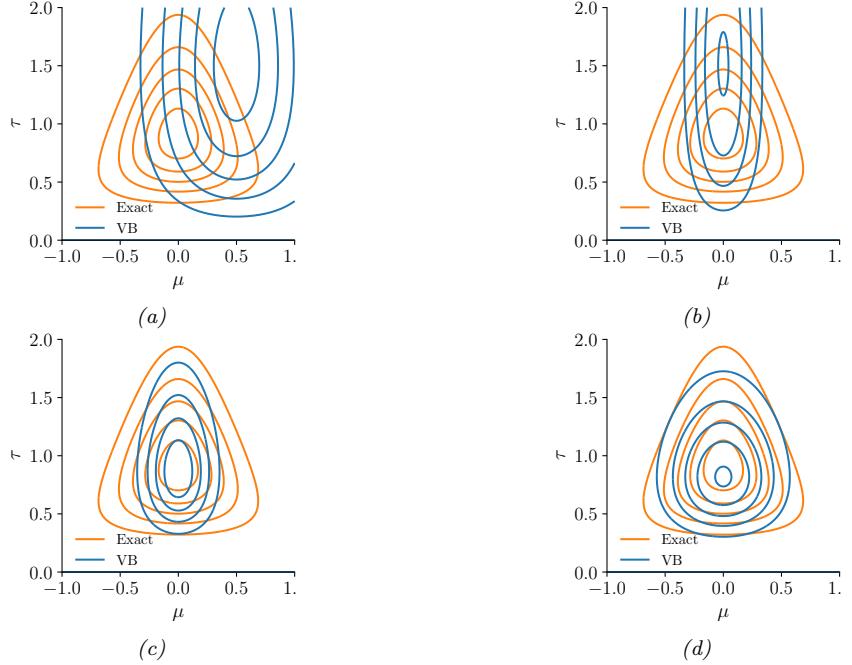
Figure 10.10: Factored variational approximation (orange) to the Gaussian-gamma distribution (blue). (a) Initial guess. (b) After updating q(µ|εµ). (c) After updating q(ς|εε). (d) At convergence (after 5 iterations). Adapted from Fig. 10.4 of [Bis06]. Generated by unigauss\_vb\_demo.ipynb.

EM, if we use CAVI to optimize the objective, the bound should increase monotonically at each iteration, otherwise there must be a bug. Third, the bound can be used as an approximation to the marginal likelihood, which can be used for Bayesian model selection or empirical Bayes (see Section 10.1.3). In the case of the current model, one can show that the lower bound has the following form:

\[\mathcal{L} = \text{const} + \frac{1}{2} \ln \frac{1}{\kappa\_N} + \ln \Gamma(a\_N) - a\_N \ln b\_N \tag{10.124}\]

10.3.5 Variational Bayes EM

In Bayesian latent variable models, we have two forms of hidden variables: local (or per example) hidden variables zn, and global (shared) hidden variables ω, which represent the parameters of the model. See Figure 10.5b for an illustration. (Note that the parameters, which are fixed in number, are sometimes called intrinsic variables, whereas the local hidden variables are called extrinsic variables.) If h = (ω, z1:^N ) represents all the hidden variables, then the joint distribution is given by

\[p(\mathbf{h}, \mathcal{D}) = p(\theta, \mathbf{z}\_{1:N}, \mathcal{D}) = p(\theta) \prod\_{n=1}^{N} p(\mathbf{z}\_n | \theta) p(\mathbf{z}\_n | \mathbf{z}\_n, \theta) \tag{10.125}\]

We will make the following mean field assumption:

\[q(\theta, z\_{1:N} | \psi\_{1:N}, \psi\_{\theta}) = q(\theta | \psi\_{\theta}) \prod\_{n=1}^{N} q(z\_n | \psi\_n) \tag{10.126}\]

where ϖ = (ϖ1:^N , ϖε).

We will use VI to maximize the ELBO:

\[\mathcal{L}(\psi|\mathcal{D}) = \mathbb{E}\_{\mathbf{q}(\boldsymbol{\theta}, \mathbf{z}\_{1:N} | \boldsymbol{\psi}\_{1:N}, \boldsymbol{\psi}\_{\boldsymbol{\theta}})} \left[ \log p(\mathbf{z}\_{1:N}, \boldsymbol{\theta}, \mathcal{D}) - \log q(\boldsymbol{\theta}, \mathbf{z}\_{1:N}) \right] \tag{10.127}\]

If we use the mean field assumption, then we can apply the CAVI approach to optimize each set of variational parameters. In particular, we can alternate between optimizing the qn(zn) in parallel, independently of each other, with q(ω) held fixed, and then optimizing q(ω) with the qⁿ held fixed. This is known as variational Bayes EM [BG06]. It is similar to regular EM, except in the E step, we infer an approximate posterior for zⁿ averaging out the parameters (instead of plugging in a point estimate), and in the M step, we update the parameter posterior parameters using the expected su”cient statistics.

Now suppose we approximate ^q(ω) by a delta function, ^q(ω) = ^ϑ(^{ω → ω}ˆ). The Bayesian LVM ELBO objective from Equation (10.127) simplifies to the “LVM ELBO”:

\[\mathbb{E}(\boldsymbol{\theta}, \psi\_{1:N} | \mathcal{D}) = \mathbb{E}\_{q(\mathbf{z}\_{1:N} | \psi\_{1:N})} \left[ \log p(\boldsymbol{\theta}, \mathcal{D}, \mathbf{z}\_{1:N}) - \log q(\mathbf{z}\_{1:N} | \psi\_{1:N}) \right] \tag{10.128}\]

We can optimize this using the variational EM algorithm, which is a CAVI algorithm which updates the ϖⁿ in parallel in the variational E step, and then updates ω in the M step.

VEM is simpler than VBEM since in the variational E step, we compute ^q(zn|xn, ^ωˆ), instead of Eε[q(zn|xn, ω)]; that is, we plug in a point estimate of the model parameters, rather than averaging over the parameters. For more details on VEM, see Section 10.1.3.

10.3.6 Example: VBEM for a GMM

Consider a standard Gaussian mixture model (GMM):

\[p(\mathbf{z}, x | \theta) = \prod\_{n} \prod\_{k} \pi\_k^{z\_{nk}} \mathcal{N}(\mathbf{z}\_n | \boldsymbol{\mu}\_k, \boldsymbol{\Lambda}\_k^{-1})^{z\_{nk}} \tag{10.129}\]

where znk = 1 if datapoint n belongs to cluster k, and znk = 0 otherwise. Our goal is to approximate the posterior p(z, ω|x) under the following conjugate prior

\[p(\boldsymbol{\theta}) = \text{Dir}(\boldsymbol{\pi} | \check{\boldsymbol{\alpha}}) \prod\_{k} \mathcal{N}(\boldsymbol{\mu}\_{k} | \boldsymbol{\pi}, (\mathbb{X} \,\boldsymbol{\Lambda}\_{k})^{-1}) \text{Wi}(\boldsymbol{\Lambda}\_{k} | \check{\mathbf{L}}, \mathcal{V}) \tag{10.130}\]

where #^k is the precision matrix for cluster k. For the mixing weights, we usually use a symmetric prior, ↭↼= ϱ01.

The exact posterior ^p(z, ^ω|D) is a mixture of ^KN distributions, corresponding to all possible labelings z, which is intractable to compute. In this section, we derive a VBEM algorithm, which will approximate the posterior around a local mode. We follow the presentation of [Bis06, Sec 10.2]. (See also Section 10.2.1.5 and Section 10.2.2.3, where we discuss variational approximations based on stochastic gradient descent, which can scale better to large datasets compared to VBEM.)

10.3.6.1 The variational posterior

We will use the standard mean field approximation to the posterior: q(ω, z1:^N ) = q(ω) ⁿ qn(zn). At this stage we have not specified the forms of the q functions; these will be determined by the form of the likelihood and prior. Below we will show that the optimal forms are as follows:

\[q\_n(z\_n) = \text{Cat}(\mathbf{z}\_n | \mathbf{r}\_n) \tag{10.131}\]

\[q(\boldsymbol{\theta}) = \text{Dir}(\boldsymbol{\pi}|\,\hat{\boldsymbol{\alpha}}) \prod\_{k} \mathcal{N}(\boldsymbol{\mu}\_{k}|\,\hat{\boldsymbol{m}}\_{k}, (\mathbb{k}\_{k}\,\mathbf{A}\_{k})^{-1}) \text{Wi}(\mathbf{A}\_{k}|\,\hat{\mathbf{L}}\_{k}, \boldsymbol{\beta}\_{k}) \tag{10.132}\]

where rⁿ are the posterior responsibilities, and the parameters with hats on them are the hyperparameters from the prior updated with data.

10.3.6.2 Derivation of q(ω) (variational M step)

Using the mean field recipe in Algorithm 10.4, we write down the log joint, and take expectations over all variables except ω, so we average out the zⁿ wrt q(zn) = Cat(zn|rn):

\[\begin{split} \log q(\boldsymbol{\theta}) &= \underbrace{\log p(\boldsymbol{\pi}) + \sum\_{n} \mathbb{E}\_{q(z\_n)} \left[ \log p(\mathbf{z}\_n | \boldsymbol{\pi}) \right]}\_{L\_{\boldsymbol{\pi}}} \\ &+ \sum\_{k} \underbrace{\left[ \log p(\boldsymbol{\mu}\_k, \mathbf{A}\_k) \sum\_{n} \mathbb{E}\_{q(z\_n)} \left[ z\_{nk} \right] \log \mathcal{N}(\boldsymbol{x}\_n | \boldsymbol{\mu}\_k, \mathbf{A}\_k^{-1}) \right]}\_{L\_{\boldsymbol{\mu}\_k}, \mathbf{A}\_k} \Bigg] + \text{const} \end{split} \tag{10.133}\]

Since the expected log joint factorizes into a term involving ▷ and terms involving (µk, #k), we see that the variational posterior also factorizes into the form

\[q(\boldsymbol{\theta}) = q(\boldsymbol{\pi}) \prod\_{k} q(\boldsymbol{\mu}\_k, \mathbf{A}\_k) \tag{10.134}\]

For the ▷ term, we have

\[\log q(\pi) = (\alpha\_0 - 1) \sum\_{k} \log \pi\_k + \sum\_{k} \sum\_{n} r\_{nk} \log \pi\_k + \text{const} \tag{10.135}\]

Exponentiating, we recognize this as a Dirichlet distribution:

\[q(\pi) = \text{Dir}(\pi \mid \hat{\alpha}) \tag{10.136}\]

\[ \hat{\alpha}\_k = \alpha\_0 + N\_k \tag{10.137} \]

\[N\_k = \sum\_{n} r\_{nk} \tag{10.138}\]

For the µ^k and #^k terms, we have

\[q(\boldsymbol{\mu}\_k, \boldsymbol{\Lambda}\_k) = \mathcal{N}(\boldsymbol{\mu}\_k | \boldsymbol{\mathcal{m}}\_k, (\mathbb{k}\_k \, \boldsymbol{\Lambda}\_k)^{-1}) \text{Wi}(\boldsymbol{\Lambda}\_k | \, \hat{\mathbf{L}}\_k, \boldsymbol{\mathcal{\boldsymbol{\beta}}}\_k) \tag{10.139}\]

\[\mathcal{R}\_k = \mathbb{K} + N\_k \tag{10.140}\]

\[ \hat{\mathfrak{m}}\_k = \left(\mathbb{k}\,\,\mathfrak{M} + N\_k \overline{x}\_k\right) / \,\,\hat{\mathfrak{k}}\_k \tag{10.141} \]

\[\hat{\mathbf{L}}\_{k}^{-1} = \check{\mathbf{L}}^{-1} + N\_{k}\mathbf{S}\_{k} + \frac{\mathbb{K}}{\mathbb{K}} \frac{N\_{k}}{+N\_{k}} (\overline{\mathbf{z}}\_{k} - \mathfrak{M})(\overline{\mathbf{z}}\_{k} - \mathfrak{M})^{\mathsf{T}} \tag{10.142}\]

\[ \hat{\nu}\_k = \check{\nu} + N\_k \tag{10.143} \]

\[ \overline{x}\_k = \frac{1}{N\_k} \sum\_n r\_{nk} x\_n \tag{10.144} \]

\[\mathbf{S}\_{k} = \frac{1}{N\_{k}} \sum\_{n} r\_{nk} (\mathbf{z}\_{n} - \overline{\mathbf{z}}\_{k}) (\mathbf{z}\_{n} - \overline{\mathbf{z}}\_{k})^{\mathsf{T}} \tag{10.145}\]

This is very similar to the M step for MAP estimation for GMMs, except here we are computing the parameters of the posterior for ω rather than a point estimate ωˆ.

10.3.6.3 Derivation of q(z) (variational E step)

The variational E step is more interesting, since it is quite di!erent from the E step in regular EM, because we need to average over the parameters, rather than condition on them. In particular, we have

\[\log q(\mathbf{z}) = \sum\_{n} \sum\_{k} z\_{nk} \left( \mathbb{E}\_{q(\boldsymbol{\pi})} \left[ \log \pi\_k \right] + \frac{1}{2} \mathbb{E}\_{q(\mathbf{A}\_k)} \left[ \log |\mathbf{A}\_k| \right] - \frac{D}{2} \log(2\pi)\]

\[-\frac{1}{2} \mathbb{E}\_{q(\boldsymbol{\theta})} \left[ (\boldsymbol{x}\_n - \boldsymbol{\mu}\_k)^\mathsf{T} \boldsymbol{\Lambda}\_k (\boldsymbol{x}\_n - \boldsymbol{\mu}\_k) \right] \right) + \text{const} \tag{10.146}\]

Using the fact that ^q(▷) = Dir(▷^| ↫↼), one can show that

\[\exp(\mathbb{E}\_{q(\pi)}\left[\log \pi\_k\right]) = \frac{\exp(\psi(\hat{\alpha}\_k))}{\exp(\psi(\sum\_{k'} \hat{\alpha}\_{k'}))} \stackrel{\Delta}{=} \tilde{\pi}\_k \tag{10.147}\]

where 1 is the digamma function:

\[ \psi(x) = \frac{d}{dx} \log \Gamma(x) \tag{10.148} \]

This takes care of the first term.

For the second term, one can show

\[\mathbb{E}\_{q(\mathbf{A}\_k)}\left[\log|\Lambda\_k|\right] = \sum\_{j=1}^D \psi\left(\frac{\hat{\nu}\_k + 1 - j}{2}\right) + D \log 2 + \log|\hat{\mathbf{L}}\_k| \tag{10.149}\]

Finally, for the expected value of the quadratic form, one can show

\[\mathbb{E}\_{q(\boldsymbol{\mu}\_{k},\boldsymbol{\Lambda}\_{k})}\left[ (\boldsymbol{x}\_{n}-\boldsymbol{\mu}\_{k})^{\mathsf{T}}\boldsymbol{\Lambda}\_{k}(\boldsymbol{x}\_{n}-\boldsymbol{\mu}\_{k}) \right] = D\,\widehat{\kappa}\_{k}^{-1} + \widehat{\boldsymbol{\nu}}\_{k}\left(\boldsymbol{x}\_{n}-\widehat{\boldsymbol{m}}\_{k}\right)^{\mathsf{T}}\widehat{\boldsymbol{\Lambda}}\_{k}\left(\boldsymbol{x}\_{n}-\widehat{\boldsymbol{m}}\_{k}\right) \triangleq \boldsymbol{\Lambda}\_{k} \tag{10.150}\]

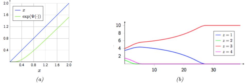
Figure 10.11: (a) We plot exp(ϱ(x)) vs x. We see that this function performs a form of shrinkage, so that small values get set to zero. (b) We plot N^k vs time for 4 di!erent states (z values), starting from random initial values. We perform a series of VBEM updates, ignoring the likelihood term. We see that states that initially had higher counts get reinforced, and sparsely populated states get killed o!. From [LK07]. Used with kind permission of Percy Liang.

Thus we get that the posterior responsibility of cluster k for datapoint n is

\[r\_{nk} \propto \tilde{\pi}\_k \tilde{\Lambda}\_k^{\frac{1}{2}} \exp\left(-\frac{D}{2\beta\_k} - \frac{\vartheta\_k}{2} (\mathbf{z}\_n - \hat{m}\_k)^\top \hat{\Lambda}\_k \ (\mathbf{z}\_n - \hat{m}\_k)\right) \tag{10.151}\]

Compare this to the expression used in regular EM:

\[r r\_{nk}^{EM} \propto \hat{\pi}\_k |\hat{\Lambda}\_k|^{\frac{1}{2}} \exp\left(-\frac{1}{2} (\boldsymbol{x}\_n - \boldsymbol{\hat{\mu}}\_k)^{\mathsf{T}} \hat{\Lambda}\_k (\boldsymbol{x}\_n - \boldsymbol{\hat{\mu}}\_k)\right) \tag{10.152}\]

where ϖˆ^k is the MAP estimate for ϖk. The significance of this di!erence is discussed in Section 10.3.6.4.

10.3.6.4 Automatic sparsity inducing e!ects of VBEM

In regular EM, the E step has the form given in Equation (10.152), whereas in VBEM, the E step has the form given in Equation (10.151). Although they look similar, they di!er in an important way. To understand this, let us ignore the likelihood term, and just focus on the prior. From Equation (10.147) we have

\[r\_{nk}^{VB} = \tilde{\pi}\_k = \frac{\exp(\psi(\hat{\alpha}\_k))}{\exp(\psi(\sum\_{k'} \hat{\alpha}\_{k'}))} \tag{10.153}\]

And from the usual EM MAP estimation equations for GMM mixing weights (see e.g., [Mur22, Sec 8.7.3.4]) we have

\[r\_{nk}^{EM} = \hat{\pi}\_k = \frac{\hat{\alpha}\_k - 1}{\sum\_{k'} (\hat{\alpha}\_{k'} - 1)} \tag{10.154}\]

where ↫ϱk= ϱ⁰ + Nk, and N^k = & ⁿ rnk is the expected number of assignments to cluster k.

We know from Figure 2.6 that using ϱ⁰ ∃ 1 causes ▷ to be sparse, which will encourage rⁿ to be sparse, which will “kill o!” unnecessary mixture components (i.e., ones for which N^k ∃ N, meaning very few datapoints are assigned to cluster k). To encourage this sparsity promoting e!ect, let us set ϱ⁰ = 0. In this case, the updated parameters for the mixture weights are given by the following:

\[\tilde{\pi}\_k = \frac{\exp(\psi(N\_k))}{\exp(\psi(\sum\_{k'} N\_{k'}))} \tag{10.155}\]

\[ \hat{\pi}\_k = \frac{N\_k - 1}{\sum\_{k'} (N\_{k'} - 1)} \tag{10.156} \]

Now consider a cluster which has no assigned data, so N^k = 0. In regular EM, ϖˆ^k might end up negative, as pointed out in [FJ02]. (This will not occur if we use maximum likelihood training, which corresponds to ϱ⁰ = 1, but this will not induce any sparsity, either.) This problem does not arise in VBEM, since we use the digamma function, which is always positive, as shown in Figure 10.11(a).

More interestingly, let us consider the e!ect of these updates on clusters that have unequal, but non-zero, number of assignments. Suppose we start with a random assignment of counts to 4 clusters, and iterate the VBEM algorithm, ignoring the contribution from the likelihood for simplicity. Figure 10.11(b) shows how the counts N^k evolve over time. We notice that clusters that started out with small counts end up with zero counts, and clusters that started out with large counts end up with even larger counts. In other words, the initially popular clusters get more and more members. This is called the rich get richer phenomenon; we will encounter it again in Supplementary Section 31.2, when we discuss Dirichlet process mixture models.

The reason for this e!ect is shown in Figure 10.11(a): we see that exp(1(Nk)) < Nk, and is zero if N^k is su”ciently small, similar to the soft-thresholding behavior induced by ε1-regularization (see Section 15.2.6). Importantly, this e!ect of reducing N^k is greater on clusters with small counts.

We now demonstrate this automatic pruning method on a real example. We fit a mixture of 6 Gaussians to the Old Faithful dataset, using ϱ⁰ = 0.001. Since the data only really “needs” 2 clusters, the remaining 4 get “killed o!”, as shown in Figure 10.12. In Figure 10.13, we plot the initial and final values of ϱk; we see that ↫ϱk= 0 for all but two of the components k.

Thus we see that VBEM for GMMs with a sparse Dirichlet prior provides an e”cient way to choose the number of clusters. Similar techniques can be used to choose the number of states in an HMM and other latent variable models. However, this variational pruning e!ect (also called posterior collapse), is not always desirable, since it can cause the model to “ignore” the latent variables z if the likelihood function p(x|z) is su”ciently powerful. We discuss this more in Section 21.4.

10.3.6.5 Lower bound on the marginal likelihood

The VBEM algorithm is maximizing the following lower bound

\[\mathcal{L} = \sum\_{\mathbf{z}} \int d\theta \, q(\mathbf{z}, \theta) \log \frac{p(\mathbf{z}, \mathbf{z}, \theta)}{q(\mathbf{z}, \theta)} \le \log p(\mathbf{z}) \tag{10.157}\]

This quantity increases monotonically with each iteration, as shown in Figure 10.14.

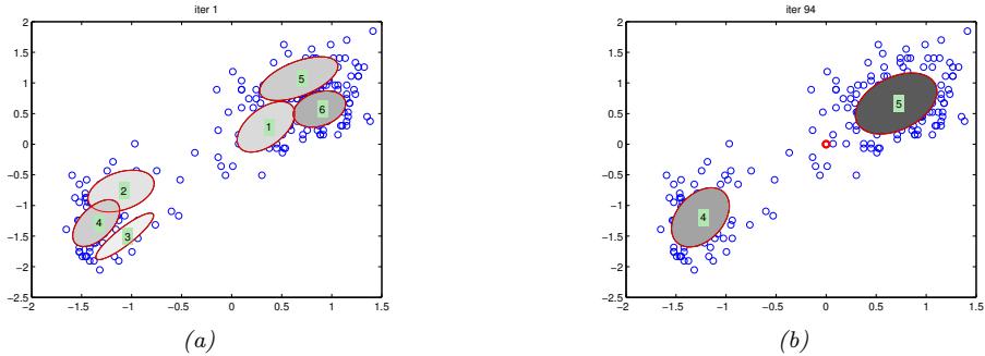
Figure 10.12: We visualize the posterior mean parameters at various stages of the VBEM algorithm applied to a mixture of Gaussians model on the Old Faithful data. Shading intensity is proportional to the mixing weight. We initialize with K-means and use φ⁰ = 0.001 as the Dirichlet hyper-parameter. (The red dot on the right panel represents all the unused mixture components, which collapse to the prior at 0.) Adapted from Figure 10.6 of [Bis06]. Generated by gmm\_vb\_em.ipynb.

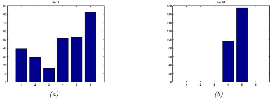
Figure 10.13: We visualize the posterior values of ς^k for the model in Figure 10.12 after the first and last iteration of the algorithm. We see that unnecessary components get “killed o!”. (Interestingly, the initially large cluster 6 gets “replaced” by cluster 5.) Generated by gmm\_vb\_em.ipynb.

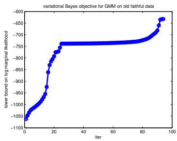
Figure 10.14: Lower bound vs iterations for the VB algorithm in Figure 10.12. The steep parts of the curve correspond to places where the algorithm figures out that it can increase the bound by “killing o!” unnecessary mixture components, as described in Section 10.3.6.6. The plateaus correspond to slowly moving the clusters around. Generated by gmm\_vb\_em.ipynb.

10.3.6.6 Model selection using VBEM

Section 10.3.6.4 discusses a way to choose K automatically, during model fitting, by “killing o!” unneeded clusters. An alternative approach is to fit several models, and then to use the variational lower bound to the log marginal likelihood, L(K) ⇐ log p(D|K), to approximate p(K|D). In particular, if we have a uniform prior, we get the posterior

\[p(K|\mathcal{D}) = \frac{p(\mathcal{D}|K)}{\sum\_{K'} p(\mathcal{D}|K')} \approx \frac{e^{\mathcal{L}(K)}}{\sum\_{K'} e^{\mathcal{L}(K')}}\tag{10.158}\]

It is shown in [BG06] that the VB approximation to the marginal likelihood is more accurate than BIC [BG06]. However, the lower bound needs to be modified somewhat to take into account the lack of identifiability of the parameters. In particular, although VB will approximate the volume occupied by the parameter posterior, it will only do so around one of the local modes. With K components, there are K! equivalent modes, which di!er merely by permuting the labels. Therefore a more accurate approximation to the log marginal likelihood is to use log p(D|K) ↓ L(K) + log(K!).

10.3.7 Variational message passing (VMP)

In this section, we describe the CAVI algorithm for a generic model in which each complete conditional, p(z^j |z↓^j , x), is in the exponential family, i.e.,

\[p(\mathbf{z}\_j|\mathbf{z}\_{-j}, \mathbf{z}) = h(\mathbf{z}\_j) \exp[\eta\_j(\mathbf{z}\_{-j}, \mathbf{z})^\mathsf{T} \mathcal{T}(\mathbf{z}\_j) - A\_j(\eta\_j(\mathbf{z}\_{-j}, \mathbf{z}))] \tag{10.159}\]

where T (z^j ) is the vector of su”cient statistics, ϱ^j are the natural parameters, A^j is the log partition function, and h(z^j ) is the base distribution. This assumption holds if the prior p(z^j ) is conjugate to the likelihood, p(z↓^j , x|z^j ).

If Equation (10.159) holds, the mean field update node j becomes

\[q\_j(\mathbf{z}\_j) \propto \exp\left[\mathbb{E}\left[\log p(\mathbf{z}\_j|\mathbf{z}\_{-j}, \mathbf{z})\right]\right] \tag{10.160}\]

\[=\exp\left[\log h(\mathbf{z}\_j) + \mathbb{E}\left[\eta\_j(\mathbf{z}\_{-j}, \mathbf{z})\right]^\top \mathcal{T}(\mathbf{z}\_j) - \mathbb{E}\left[A\_j(\eta\_j(\mathbf{z}\_{-j}, \mathbf{z}))\right]\right] \tag{10.161}\]

\[\times h(\mathbf{z}\_j) \exp\left[\mathbb{E}\left[\eta\_j(\mathbf{z}\_{-j}, \mathbf{z})\right]^\mathsf{T} \mathcal{T}(\mathbf{z}\_j)\right] \tag{10.162}\]

Thus we update the local natural parameters using the expected values of the other nodes. These become the new variational parameters:

\[\psi\_j = \mathbb{E}\left[\eta\_j(\mathbf{z}\_{-j}, \mathbf{z})\right] \tag{10.163}\]

We can generalize the above approach to work with any model where each full conditional is conjugate. The resulting algorithm is known as variational message passing or VMP [WB05] that works for any directed graphical model. VMP is similar to belief propagation (Section 9.3): at each iteration, each node collects all the messages from its parents, and all the messages from its children (which might require the children to get messages from their co-parents), and combines them to compute the expected value of the node’s su”cient statistics. The messages that are sent are the expected su”cient statistics of a node, rather than just a discrete or Gaussian distribution (as in BP). Several software libraries have implemented this framework (see e.g., [Win; Min+18; Lut16; Wan17]).

VMP can be extended to the case where each full conditional is conditionally conjugate using the CVI framework in Supplementary Section 10.3.1. See also [ABV21], where they use local Laplace approximations to intractable factors inside of a message passing framework.

10.3.8 Autoconj

The VMP method requires the user to manually specify a graphical model; the corresponding node update equations are then computed for each node using a lookup table, for each possible combination of node types. It is possible to automatically derive these update equations for any conditionally conjugate directed graphical model using a technique called autoconj [HJT18]. This is analogous to the use of automatic di!erentiation (autodi!) to derive the gradient for any di!erentiable function. (Note that autoconj uses autodi! internally.) The resulting full conditionals can be used for CAVI, and also for Gibbs sampling (Section 12.3).

10.4 More accurate variational posteriors

In general, we can improve the tightness of the ELBO lower bound, and hence reduce the KL divergence of our posterior approximation, if we use more flexible posterior families (although optimizing within more flexible families may be slower, and can incur statistical error if the sample size is low [Bha+21]). In this section, we give several examples of more accurate variational posteriors, going beyond fully factored mean field approximations, or simple unimodal Gaussian approximations.

10.4.1 Structured mean field

The mean field assumption is quite strong, and can sometimes give poor results. Fortunately, sometimes we can exploit tractable substructure in our problem, so that we can e”ciently handle some kinds of dependencies between the variables in the posterior in an analytic way, rather than assuming they are all independent. This is called the structured mean field approach [SJ95].

A common example arises when appling VI to time series models, such as HMMs, where the latent variables within each sequence are usually highly correlated across time. Rather than assuming a fully factorized posterior, we can treat each sequence zn,1:^T as a block, and just assume independence between blocks and the parameters: q(z1:N,1:^T , ω) = q(ω) ^{N n}=1 q(zn,1:^T ), where q(zn,1:^T ) = ^t q(zn,t|zn,t↓¹). We can compute the joint distribution q(zn,1:^T ), taking into account the dependence between time steps, using the forwards-backwards algorithm. For details, see [JW14; Fot+14]. A similar approach was applied to the factorial HMM model, as we discuss in Supplementary Section 10.3.2.

An automatic way to derive a structured variational approximation to a probabilistic model, specified by a probabilistic programming language, is discussed in [AHG20].

10.4.2 Hierarchical (auxiliary variable) posteriors

Suppose ^qω(z|x) = ^k qω(zk|x) is a factorized distribution, such as a diagonal Gaussian. This does not capture dependencies between the latent variables (components of z). We could of course use a full covariance matrix, but this might be too expensive.

An alternative approach is to use a hierarchical model, in which we add auxiliary latent variables a, which are used to increase the flexibility of the variational posterior. In particular, we can still assume qω(z|x, a) is conditionally factorized, but when we marginalize out a, we induce dependencies between the elements of z, i.e.,

\[q\_{\phi}(z|\mathbf{z}) = \int q\_{\phi}(z|x, \mathbf{a}) q\_{\phi}(\mathbf{a}|x) d\mathbf{a} \neq \prod\_{k} q\_{\phi}(z\_{k}|x) \tag{10.164}\]

This is called a hierarchical variational model [Ran16], or an auxiliary variable deep generative model [Maa+16].

In [TRB16], they model qω(z|x, a) as a Gaussian process, which is a flexible nonparametric distribution (see Chapter 18), where a are the inducing points. This combination is called a variational GP.

10.4.3 Normalizing flow posteriors

Normalizing flows are a class of probability models which work by passing a simple source distribution, such as a diagonal Gaussian, through a series of nonlinear, but invertible, mappings f to create a more complex distribution. This can be used to get more accurate posterior approximations than standard Gaussian VI, as we discuss in Section 23.1.2.2.

10.4.4 Implicit posteriors

In Chapter 26, we discuss implicit probability distributions, which are models which we can sample from, but which we cannot evaluate pointwise. For example, consider passing a Gaussian noise term, z⁰ ↔︎ N (0, I), through a nonlinear, non-invertible mapping f to create z = f(z0); it is easy to sample from q(z), but it is intractable to evaluate the density q(z) (unlike with flows). This makes it hard to evaluate the log density ratio log pε(z)/qϑ(z|x), which is needed to compute the ELBO. However, we can use the same method as is used in GANs (generative adversarial networks, Chapter 26), in which we train a classifier that discriminates prior samples from samples from the variational posterior by evaluating T(x, z) = log qϑ(z|x) → log pε(z). See e.g., [TR19] for details.

10.4.5 Combining VI with MCMC inference

There are various ways to combine variational inference with MCMC to get an improved approximate posterior. In [SKW15], they propose Hamiltonian variational inference, in which they train an inference network to initialize an HMC sampler (Section 12.5). The gradient of the log posterior (wrt the latents), which is needed by HMC, is given by

\[\nabla\_{\mathbf{z}} \log p\_{\theta}(\mathbf{z}|\mathbf{z}) = \nabla\_{\mathbf{z}} \log \left[ p\_{\theta}(\mathbf{z}, \mathbf{z}) - \log p\_{\theta}(\mathbf{z}) \right] = \nabla\_{\mathbf{z}} \log p\_{\theta}(\mathbf{z}, \mathbf{z}) \tag{10.165}\]

This is easy to compute. They use the final sample to approximate the posterior qω(z|x). To compute the entropy of this distribution, they also learn an auxiliary inverse inference network to reverse the HMC Markov chain.

A simpler approach is proposed in [Hof17]. Here they train an inference network to initialize an HMC sampler, using the standard ELBO for ε, but they optimize the generative parameters ω using

a stochastic approximation to the log marginal likelihood, given by log pε(z, x) where z is a sample from the HMC chain. This does not require learning a reverse inference network, and avoids problems with variational pruning, since it does not use the ELBO for training the generative model.

10.5 Tighter bounds

Another way to improve the quality of the posterior approximation is to optimize q wrt a bound that is a tighter approximation to the log marginal likelihood compared to the standard ELBO. We give some examples below.

10.5.1 Multi-sample ELBO (IWAE bound)

In this section, we discuss a method known as the importance weighted autoencoder or IWAE [BGS16], which is a way to tighten the variational lower bound by using self-normalized importance sampling (Section 11.5.2). (It can also be interpreted as standard ELBO maximization in an expanded model, where we add extra auxiliary variables [CMD17; DS18; Tuc+19].)

Let the inference network qω(z|x) be viewed as a proposal distribution for the target posterior pε(z|x). Define w^{→ s} = ^pϑ(x,zs) ^qε(zs|x) as the unnormalized importance weight for a sample, and ^{ws =} w^{→ s} /( &^{S s}↑=1 w^{→ s↑} ) as the normalized importance weights. From Equation (11.43) we can compute an estimate of the marginal likelihood p(x) using

\[\hat{p}\_S(\mathbf{z}|\mathbf{z}\_{1:S}) \stackrel{\Delta}{=} \frac{1}{S} \sum\_{k=1}^{S} \frac{p\_\theta(\mathbf{z}, \mathbf{z}\_s)}{q\_\phi(\mathbf{z}\_s|\mathbf{z})} = \frac{1}{S} \sum\_{k=1}^{S} w\_s \tag{10.166}\]

This is unbiased, i.e., ^Eqε(z1:^{S |}x) [ˆpS(x|z1:S)] ^{= p}(x), where ^qω(z1:S|x) = ^{S s}=1 qω(zs|x). In addition, since the estimator is always positive, we can take logarithms, and thus obtain a stochastic lower bound on the log likelihood:

\[\mathbb{E}\_S(\phi, \theta | \mathbf{z}) \triangleq \mathbb{E}\_{q\_\phi(\mathbf{z}\_{1:S} | \mathbf{z})} \left[ \log \left( \frac{1}{S} \sum\_{s=1}^S w\_s \right) \right] = \mathbb{E}\_{q\_\phi(\mathbf{z}\_{1:S} | \mathbf{z})} \left[ \log \hat{p}\_S(\mathbf{z}\_{1:S}) \right] \tag{10.167}\]

\[0 \le \log \mathbb{E}\_{q\_{\phi}(\mathbf{z}\_{1:S} \mid \mathbf{z})} \left[ \hat{p}\_S(\mathbf{z}\_{1:S}) \right] = \log p(\mathbf{z}) \tag{10.168}\]

where we used Jensen’s inequality in the penultimate line, and the unbiased property in the last line. This is called the multi-sample ELBO or IWAE bound [BGS16]. The gradients of this expression wrt ω and ε are given in Equation (10.179). If S = 1, #^S reduces to the standard ELBO:

\[\mathcal{L}\_1(\phi, \theta | x) = \mathbb{E}\_{q(\mathbf{z}|\mathbf{z})} \left[ \log w \right] = \int q\_\phi(\mathbf{z}|\mathbf{z}) \log \frac{p\_\theta(\mathbf{z}, \mathbf{z})}{q\_\phi(\mathbf{z}|\mathbf{z})} d\mathbf{z} \tag{10.169}\]

One can show [BGS16] that increasing the number of samples S is guaranteed to make the bound tighter, thus making it a better proxy for the log likelihood. Intuitively, averaging the S samples inside the log removes the need for every sample z^s to explain the data x. This encourages the proposal distribution q to be less concentrated than the single-sample variational posterior.

10.5.1.1 Pathologies of optimizing the IWAE bound

Unfortunately, increasing the number of samples in the IWAE bound can decrease the signal to noise ratio, resulting in learning a worse model [Rai+18a]. Intuitively, the reason this happens is that increasing S reduces the dependence of the bound on the quality of the inference network, which makes the gradient of the ELBO wrt ε less informative (higher variance).

One solution to this is to use the doubly reparameterized gradient estimator [TL18b]. Another approach is to use alternative estimation methods that avoid ELBO maximization, such as using the thermodynamic variational objective (see Section 10.5.2) or the reweighted wake-sleep algorithm (see Section 10.6).

10.5.2 The thermodynamic variational objective (TVO)

In [MLW19; Bre+20b], they present the thermodynamic variational objective or TVO. This is an alternative to IWAE for creating tighter variational bounds, which has certain advantages, particularly for posteriors that are not reparameterizable (e.g., discrete latent variables). The framework also has close connections with the reweighted wake-sleep algorithm from Section 10.6, as we will see in Section 10.5.3.

The TVO technique uses thermodynamic integration, also called path sampling, which is a technique used in physics and phylogenetics to approximate intractable normalization constants of high dimensional distributions (see e.g., [GM98; LP06; FP08]). This is based on the insight that it is easier to calculate the ratio of two unknown constants than to calculate the constants themselves. This is similar to the idea behind annealed importance sampling (Section 11.5.4), but TI is deterministic. For details, see [MLW19; Bre+20b].

10.5.3 Minimizing the evidence upper bound

Recall that the evidence lower bound or ELBO is given by

\[\operatorname{KL}(\theta, \phi | \mathbf{z}) = \log p\_{\theta}(\mathbf{z}) - D\_{\text{KL}}\left(q\_{\phi}(\mathbf{z}|\mathbf{z})\right) \parallel p\_{\theta}(\mathbf{z}|\mathbf{z}) \tag{10.170} \\ \leq \log p\_{\theta}(\mathbf{z}) \tag{10.170}\]

By analogy, we can define the evidence upper bound or EUBO as follows:

\[\text{EUBO}(\theta, \phi | \mathbf{z}) = \log p\_{\theta}(\mathbf{z}) + D\_{\text{KL}} \left( p\_{\theta}(\mathbf{z} | \mathbf{z}) \parallel q\_{\phi}(\mathbf{z} | \mathbf{z}) \right) \geq \log p\_{\theta}(\mathbf{z}) \tag{10.171}\]

Minimizing this wrt the variational parameters ε, as an alternative to maxmimizing the ELBO, was proposed in [MLW19], where they showed that it can sometimes converge to the true log pε(x) faster.

The above bound is for a specific input x. If we sample x from the generative model, and minimize E^pϑ(x) [EUBO(ω, ε|x)] wrt ε, we recover the sleep phase of the wake-sleep algorithm (see Section 10.6.2).

Now suppose we sample x from the empirical distribution, and minimize E^pD(x) [EUBO(ω, ε|x)] wrt ε. To approximate the expectation, we can use self-normalized importance sampling, as in Equation (10.188), to get

\[\nabla\_{\phi} \text{EUBO}(\theta, \phi | \mathbf{z}) = \sum\_{s=1}^{S} \overline{w}\_{s} \nabla\_{\phi} \log q\_{\phi}(\mathbf{z}^{s} | \mathbf{z}) \tag{10.172}\]

where w^s = w(s) /( & ^s↑ w(s^↑ ) ), and w(s) ^{= p}(x,zs) ^q(zs|ωt) . This is equivalent to the “daydream” update (aka “wake-phase ε update”) of the wake-sleep algorithm (see Section 10.6.3).

10.6 Wake-sleep algorithm

So far in this chapter we have focused on fitting latent variable models by maximizing the ELBO. This has two main drawbacks. First, it does not work well when we have discrete latent variables, because in such cases we cannot use the reparameterization trick; thus we have to use higher variance estimators, such as REINFORCE (see Section 10.2.3). Second, even in the case where we can use the reparameterization trick, the lower bound may not be very tight. We can improve the tightness by using the IWAE multi-sample bound (Section 10.5.1), but paradoxically this may not result in learning a better model, for reasons discussed in Section 10.5.1.1.

In this section, we discuss a di!erent way to jointly train generative and inference models, which avoids some of the problems with ELBO maximization. The method is known as the wake-sleep algorithm [Hin+95; BB15b; Le+19; FT19]. because it alternates between two steps: in the wake phase, we optimize the generative model parameters ω to maximize the marginal likelihood of the observed data (we approximate log pε(x) by drawing importance samples from the inference network), and in the sleep phase, we optimize the inference model parameters ε to learn to invert the generative model by training the inference network on labeled (x, z) pairs, where x are samples generated by the current model parameters. This can be viewed as a form of adaptive importance sampling, which iteratively improves its proposal, while simultaneously optimizing the model. We give further details below.

10.6.1 Wake phase

In the wake phase, we minimize the KL divergence from the empirical distribution to the model’s distribution:

\[\mathcal{L}(\boldsymbol{\theta}) = D\_{\text{KL}}\left(p\_{\mathcal{D}}(\mathbf{z}) \parallel p\_{\boldsymbol{\theta}}(\mathbf{z})\right) = \mathbb{E}\_{p\_{\mathcal{D}}(\mathbf{z})}\left[-\log p\_{\boldsymbol{\theta}}(\mathbf{z})\right] + \text{const} \tag{10.173}\]

where ^pε(x) = / ^pε(z)pε(x|z)dz. This is equivalent to maximizing the likelihood of the observed data:

\[\ell(\theta) = \mathbb{E}\_{p \circ (x)} \left[ \log p\_{\theta}(x) \right] \tag{10.174}\]

Since the log marginal likelihood log pε(x) cannot be computed exactly, we will approximate it. In the original wake-sleep paper, they proposed to use the ELBO lower bound. In the reweighted wake-sleep (RWS) algorithm of [BB15b; Le+19], they propose to use the IWAE bound from Section 10.5.1 instead. In particular, if we draw S samples from the inference network, z^s ↔︎ qς(z|x), we get the following estimator:

\[\ell(\boldsymbol{\theta}|\boldsymbol{\phi}, \boldsymbol{x}) = \log \left( \frac{1}{S} \sum\_{s=1}^{S} w\_s \right) \tag{10.175}\]

where w^s = ^pϑ(x,zs) ^qε(zs|x) . Note that this is the same as the IWAE bound in Equation (10.168).

We now discuss how to compute the gradient of this objective wrt ω or ε. Using the log-derivative trick, we have that

\[ \nabla \log w\_s = \frac{1}{w\_s} \nabla w\_s \tag{10.176} \]

Hence

\[\nabla \ell(\boldsymbol{\theta} | \boldsymbol{\phi}, \boldsymbol{x}) = \frac{1}{\frac{1}{S} \sum\_{s=1}^{S} w\_{s}} \left( \frac{1}{S} \sum\_{s=1}^{S} \nabla w\_{s} \right)\_{\boldsymbol{\phi}} \tag{10.177}\]

\[\hat{\lambda} = \frac{1}{\sum\_{s=1}^{S} w\_s} \left( \sum\_{s=1}^{S} w\_s \nabla \log w\_s \right) \tag{10.178}\]

\[=\sum\_{s=1}^{S} \overline{w}\_{s} \nabla \log w\_{s} \tag{10.179}\]

where w^s = ws/( &^{S s}↑=1 w^s↑ ).

In the case of the derivatives wrt ω, we have

\[\nabla\_{\theta} \log w\_s = \frac{1}{w\_s} \nabla\_{\theta} w\_s = \frac{q\_{\phi}(z\_s|x)}{p\_{\theta}(x, z\_s)} \nabla\_{\theta} \frac{p\_{\theta}(x, z\_s)}{q\_{\phi}(z\_s|x)} = \frac{1}{p\_{\theta}(x, z\_s)} \nabla\_{\theta} p\_{\theta}(x, z\_s) = \nabla\_{\theta} \log p\_{\theta}(x, z\_s) \tag{10.180}\]

and hence we get

\[\nabla\_{\theta}\ell(\theta|\phi,x)\sum\_{s=1}^{S}\overline{w}\_{s}\nabla\log p\_{\theta}(x,z\_{s})\tag{10.181}\]

10.6.2 Sleep phase

In the sleep phase, we try to minimize the KL divergence between the true posterior (under the current model) and the inference network’s approximation to that posterior:

\[\mathcal{L}(\phi) = \mathbb{E}\_{p\mathfrak{o}(\mathfrak{x})} \left[ D\_{\mathbb{KL}} \left( p\_{\theta}(\mathfrak{z}|\mathfrak{x}) \parallel q\_{\phi}(\mathfrak{z}|\mathfrak{x}) \right) \right] = \mathbb{E}\_{p\mathfrak{o}(\mathfrak{z},\mathfrak{x})} \left[ -\log q\_{\phi}(\mathfrak{z}|\mathfrak{x}) \right] + \text{const} \tag{10.182}\]

Equivalently, we can maximize the following log likelihood objective:

\[\ell(\phi|\theta) = \mathbb{E}\_{\langle \mathbf{z}, \mathbf{z} \rangle \sim p\_{\theta}(\mathbf{z}, \mathbf{z})} \left[ \log q\_{\phi}(\mathbf{z}|\mathbf{z}) \right] \tag{10.183}\]

where pε(z, x) = pε(z)pε(x|z). We see that the sleep phase amounts to maximum likelihood training of the inference network based on samples from the generative model. These “fantasy samples”, created while the network “dreams”, can be easily generated using ancestral sampling (Section 4.2.5). If we use S such samples, the objective becomes

\[\ell(\phi|\theta) = \frac{1}{S} \sum\_{s=1}^{S} \log q\_{\phi}(\mathbf{z}\_{s}^{\prime}|\mathbf{x}\_{s}^{\prime}) \tag{10.184}\]

where (z^{↔︎ s}, x^{↔︎ s}) ↔︎ pε(z, x). The gradient of this is given by

\[\nabla\_{\Phi}\ell(\phi|\theta) = \frac{1}{S} \sum\_{s=1}^{S} \nabla\_{\Phi} \log q\_{\phi}(\mathbf{z}\_{s}^{\prime}|\mathbf{x}\_{s}^{\prime}) \tag{10.185}\]

We do not require qω(z^↔︎ |x) to be reparameterizable, since the samples are drawn from a distribution that is independent of ε. This means it is easy to apply this method to models with discrete latent variables.

10.6.3 Daydream phase

The disadvantage of the sleep phase is that the inference network, qω(z|x), is trying to follow a moving target, pε(z|x). Furthermore, it is only being trained on synthetic data from the model, not on real data. The reweighted wake-sleep algorithm of [BB15b] proposed to learn the inference network by using real data from the empirical distribution, in addition to fantasy data. They call the case where you use real data the “wake-phase q update”, but we will call it the “daydream phase”, since, unlike sleeping, the system uses real data x to update the inference model, instead of fantasies.1 [Le+19] went further, and proposed to only use the wake and daydream phases, and to skip the sleep phase entirely.

In more detail, the new objective which we want to minimize becomes

\[\mathcal{L}(\phi|\theta) = \mathbb{E}\_{\mathcal{D}\mathcal{D}}\left[D\_{\text{KL}}\left(p\_{\theta}(\mathbf{z}|\mathbf{x}) \parallel q\_{\phi}(\mathbf{z}|\mathbf{x})\right)\right] \tag{10.186}\]

We can compute a single sample approximation to the negative of the above expression as follows:

\[\ell(\phi|\theta, x) = \mathbb{E}\_{p\_{\theta}(\mathbf{z}|\mathbf{x})} \left[ \log q\_{\phi}(\mathbf{z}|x) \right] \tag{10.187}\]

where x ↔︎ pD. We can approximate this expectation using importance sampling, with q^ω as the proposal. This results in the following estimator of the gradient for each datapoint:

\[\nabla\_{\Phi}\ell(\phi|\theta,x) = \int p\_{\theta}(\mathbf{z}|x)\nabla\_{\phi}\log q\_{\phi}(\mathbf{z}|x)dz \approx \sum\_{s=1}^{S} \overline{w}\_{s}\nabla\_{\phi}\log q\_{\phi}(\mathbf{z}\_{s}|x) \tag{10.188}\]

where z^s ↔︎ qω(zs|x) and w^s are the normalized weights.

We see that Equation (10.188) is very similar to Equation (10.185). The key di!erence is that in the daydream phase, we sample from (x, zs) ↔︎ pD(x)qω(z|x), where x is a real datapoint, whereas in the sleep phase, we sample from (x^{↔︎ s}, z^{↔︎ s}) ↔︎ pε(z, x), where x^{↔︎ s} is generated datapoint.

10.6.4 Summary of algorithm

We summarize the RWS algorithm in Algorithm 10.5. The disadvantage of the RWS algorithm is that it does not optimize a single well-defined objective, so it is not clear if the method will converge, in contrast to ELBO maximization. On the other hand, the method is fairly simple, since it consists of two alternating weighted maximum likelihood problems. It can also be shown to “sandwich” a

^1. We thank Rif A. Saurous for suggesting this term.

Algorithm 10.5: One SGD update using wake-sleep algorithm.

• ¹ Sample xⁿ from dataset
• ² Draw S samples from inference network: z^s ↔︎ q(z|xn)
• ³ Compute unnormalized weights: w^s = ^p(xn,zs) q(zs|xn)
• ⁴ Compute normalized weights: w^s = ! ^{ws S s}↑=1 ws^↑
• ⁵ Optional: Compute estimate of log likelihood: log p(xn) = log( ¹ S &^{S s}=1 ws)
• ⁶ Wake phase: Update ω using &^{S s}=1 ws⇒^ε log pε(zs, xn)
• ⁷ Daydream phase: Update ε using &^{S s}=1 ws⇒^ω log qω(zs|xn)
• ⁸ Optional sleep phase: Draw S samples from model, (x^{↔︎ s}, z^{↔︎ s}) ↔︎ pε(x, z) and update ε using 1 S &^{S s}=1 ⇒^ω log qω(z^↔︎ s|x^↔︎ s)

\(\mathbf{o}\) \(\mathbf{b}\)

lower and upper bound of the log marginal likelihood. We can think of this in terms of the two joint distributions pε(x, z) = pε(z)pε(x|z) and qD,ω(x, z) = pD(x)qω(z|x):

wake phase min ε DKL (qD,ω(x, z) ↘ pε(x, z)) (10.189)

daydream phase min ω DKL (pε(x, z) ↘ qD,ω(x, z)) (10.190)

10.7 Expectation propagation (EP)

One problem with lower bound maximization (i.e., standard VI) is that we are minimizing DKL (q ↘ p), which induces zero-forcing behavior, as we discussed in Section 5.1.4.1. This means that q(z|x) tends to be too compact (over-confident), to avoid the situation in which q(z|x) > 0 but p(z|x)=0, which would incur infinite KL penalty.

Although zero-forcing can be desirable behavior for some multi-modal posteriors (e.g., mixture models), it is not so reasonable for many unimodal posteriors (e.g., Bayesian logistic regression, or GPs with log-concave likelihoods). One way to avoid this problem is to minimize DKL (p ↘ q), which is zero-avoiding, as we discussed in Section 5.1.4.1. This tends to result in broad posteriors, which avoids overconfidence. In this section, we discuss expectation propagation or EP [Min01b], which can be seen as a local approximation to DKL (p ↘ q).

10.7.1 Algorithm

We assume the exact posterior can be written as follows:

\[p(\boldsymbol{\theta}|\mathcal{D}) = \frac{1}{Z\_p}\hat{p}(\boldsymbol{\theta}), \ \hat{p}(\boldsymbol{\theta}) = p\_0(\boldsymbol{\theta})\prod\_{k=1}^{K}f\_k(\boldsymbol{\theta})\tag{10.191}\]

where pˆ(ω) is the unnormalized posterior, p⁰ is the prior, f^k corresponds to the k’th likelihood term or local factor (also called a site potential). Here Z^p = p(D)Z⁰ is the normalization constant

for the posterior, where Z⁰ is the normalization constant for the prior. To simplify notation, we let f0(ω) = p0(ω) be the prior.

We will approximate the posterior as follows:

\[q(\theta) = \frac{1}{Z\_q}\hat{q}(\theta), \ \hat{q}(\theta) = p\_0(\theta) \prod\_{k=1}^{K} \tilde{f}\_k(\theta) \tag{10.192}\]

where ˜f^k ↗ ^Q is the approximate local factor, and ^Q is some tractable family in the exponential family, usually a Gaussian [Gel+14b].

We will optimize each ˜fⁱ in turn, keeping the others fixed. We initialize each ˜fⁱ using an uninformative distribution from the family Q. so q(ω) = p0(ω).

To compute the new local factor ˜fnew ⁱ , we proceed as follows. First we compute the cavity distribution by deleting the ˜fⁱ from the approximate posterior by dividing it out:

\[q\_{-i}^{\text{cavity}}(\boldsymbol{\theta}) = \frac{q(\boldsymbol{\theta})}{\hat{f}\_i(\boldsymbol{\theta})} \propto \prod\_{k \neq i} \check{f}\_k(\boldsymbol{\theta}) \tag{10.193}\]

This division operation can be implemented by subtracting the natural parameters, as explained in Section 2.3.3.2. The cavity distribution represents the e!ect of all the factors except for fⁱ (which is approximated by ˜fi).

Next we (conceptually) compute the tilted distribution by multiplying the exact factor fⁱ onto the cavity distribution:

\[q\_i^{\text{tilted}}(\theta) = \frac{1}{Z\_i} f\_i(\theta) q\_{-i}^{\text{cavity}}(\theta) \tag{10.194}\]

where Zⁱ = / qcavity ^↓i (ω)fi(ω)dω is the normalization constant for the tilted distribution. This is the result of combining the current approximation, excluding factor i, with the exact fⁱ term.

Unfortunately, the resulting tilted distribution may be outside of our model family (e.g., if we combine a Gaussian prior with a non-Gaussian likelihood). So we will approximate the tilted distribution as follows:

\[q\_i^{\text{proj}}(\theta) = \text{proj}(q\_i^{\text{tilt}}) \triangleq \underset{\tilde{q} \in \mathfrak{Q}}{\text{argmin}} \, D(q\_i^{\text{tilt}} || \tilde{q}) \tag{10.195}\]

This can be thought of as projecting the tilted distribution into the approximation family. If D(qtilted ⁱ ||q) = ^DKL qtilted ⁱ ↘ q , this can be done by moment matching, as shown in Section 5.1.4.2. For example, suppose the cavity distribution is Gaussian, qcavity ^↓i (ω) = Nc(ω|r↓ⁱ, Q↓ⁱ), using the canonical parameterization. Then the log of the tilted distribution is given by

\[\log q\_i^{\text{titeded}}(\theta) = \alpha \log f\_i(\theta) - \frac{1}{2} \theta^\text{T} \mathbf{Q}\_{-i} \theta + r\_{-i}^\text{T} \theta + \text{const} \tag{10.196}\]

Let ^ωˆ be a local maximum of this objective. If ^Q is the set of Gaussians, we can compute the projected tilted distribution as a Gaussian with the following parameters:

\[\mathbf{Q}\_{\rangle i} = -\nabla\_{\theta}^{2} \log q\_{i}^{\text{tited}}(\theta)|\_{\theta = \hat{\theta}}, \ r\_{\rangle i} = \mathbf{Q}\_{\rangle i} \hat{\theta} \tag{10.197}\]

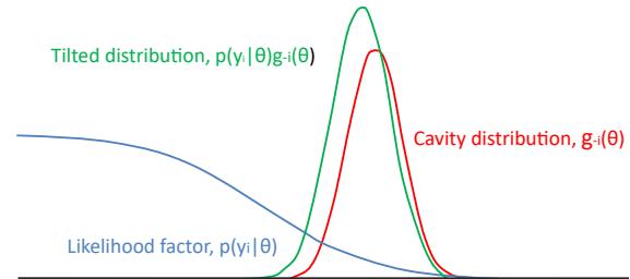
Figure 10.15: Combining a logistic likelihood factor ^{fi = p}(yi|ω) with the cavity prior, ^qcavity ^→i = g→ⁱ(ω), to get the tilted distribution, qtilted ⁱ = p(yi|ω)g→ⁱ(ω). Adapted from Figure 2 of [Gel+14b].

This is called Laplace propagation [SVE04]. For more general distributions, we can use Monte Carlo approximations; this is known as blackbox EP [HL+16a; Li+18c].

Finally, we compute a local factor that, if combined with the cavity distribution, would give the same results as this projected distribution:

\[\tilde{f}\_i^{\text{new}}(\theta) = \frac{q\_i^{\text{proj}}(\theta)}{q\_{-i}^{\text{cavity}}(\theta)} \tag{10.198}\]

We see that qcavity ^↓i (ω) ˜fnew ⁱ (ω) = ^qproj ⁱ (ω), so combining this approximate factor with the cavity distribution results in a distribution which is the best possible approximation (within Q) to the results of using the exact factor.

10.7.2 Example

Figure 10.15 illustrates the process of combining a very non-Gaussian likelihood fⁱ with a Gaussian cavity prior qcavity ^↓i to yield a nearly Gaussian tilted distribution ^qtilted ⁱ , which can then be approximated by a Gaussian using projection.

Thus instead of trying to “Gaussianize” each likelihood term fⁱ in isolation (as is done, e.g., in EKF), we try to find the best local factor ˜fⁱ (within some family) that achieves approximately the same e!ect, when combined with all the other terms (represented by the cavity distribution, q↓i), as using the exact factor fi. That is, we choose a local factor that works well in the context of all the other factors.

10.7.3 EP as generalized ADF

We can view EP as a generalization of the ADF algorithm discussed in Section 8.6. ADF is a form of sequential Bayesian inference. At each step, it maintains a tractable approximation to the posterior, qt(z) ↗ Q, updates it with the likelihood from the next observation, pˆt+1(z) ↑ qt(z)p(xt|z), and then projects the resulting updated posterior back to the tractable family using qt+1 = argmin^q↑^Q DKL (ˆpt+1 ↘ q). ADF minimizes KL in the desired direction. However, it is a sequential algorithm, designed for the online setting. In the batch setting, the method can given

di!erent results depending on the order in which the updates are performed. In addition, if we perform multiple passes over the data, we will include the same likelihood terms multiple times, resulting in an overconfident posterior. EP overcomes this problem.

10.7.4 Optimization issues

In practice, EP can be numerically unstable. For example, if we use Gaussians as our local factors, we might end up with negative variance when we subtract the natural parameters. To reduce the chance of this, it is common to use damping, in which we perform a partial update of each factor with a step size of ϑ. More precisely, we change the final step to be the following:

\[\tilde{f}\_i^{\text{new}}(\theta) = \left(\tilde{f}\_i(\theta)\right)^{1-\delta} \left(\frac{q\_i^{\text{proj}}(\theta)}{q\_{-i}^{\text{cavity}}}\right)^{\delta} \tag{10.199}\]

This can be implemented by scaling the natural parameters by ϑ. [ML02] suggest ϑ = 1/K as a safe strategy (where K is the number of factors), but this results in very slow convergence. [Gel+14b] suggest starting with ϑ = 0.5, and then reducing to ϑ = 1/K over K iterations.

In addition to numerical stability, there is no guarantee that EP will converge in its vanilla form, although empirically it can work well, especially with log-concave factors fⁱ (e.g., as in GP classifiers).

10.7.5 Power EP and ↼-divergence

We also have a choice about what divergence measure D(qtilted ⁱ ||q) to use when we approximate the tilted distribution. If we use DKL qtilted ⁱ ↘ q , we recover classic EP, as described above. If we use DKL ^q ↘ ^qtilted i , we recover the reverse KL used in standard variational inference. We can generalize the above results by using ϱ-divergences (Section 2.7.1.2), which allow us to interpolate between mode seeking and mode covering behavior, as shown in Figure 2.20. We can optimize the ϱ-divergence by using the power EP method of [Min04].

Algorithmically, this is a fairly small modification to regular EP. In particular, we first compute the cavity distribution, qcavity ^{↓i ↑ q} f ˜ε i ; we then approximate the tilted distribution, qproj ^{i =} proj(qcavity ^{↓i f} ↼ ⁱ );

and finally we compute the new factor ˜fnew ⁱ ↑ ) ^qproj i qcavity →i *¹/↼ .

10.7.6 Stochastic EP

The main disadvantage of EP in the big data setting is that we need to store the ˜fn(ω) terms for each datapoint n, so we can compute the cavity distribution. If ω has D dimensions, and we use full covariance Gaussians, this requires O(ND²) memory.

The idea behind stochastic EP [LHLT15] is to approximate the local factors with a shared factor that acts like an aggregated likelihood, i.e.,

\[\prod\_{n=1}^{N} f\_n(\theta) \approx \tilde{f}(\theta)^N \tag{10.200}\]

where typically fn(ω) = p(xn|ω). This exploits the fact that the posterior only cares about approximating the product of the likelihoods, rather than each likelihood separately. Hence it su”ces for ˜f(ω) to approximate the average likelihood.

We can modify EP to this setting as follows. First, when computing the cavity distribution, we use

\[q\_{-1}(\theta) \propto q(\theta) / \bar{f}(\theta) \tag{10.201}\]

We then compute the tilted distribution

\[q\_{\lfloor n \rfloor}(\theta) \propto f\_n(\theta) q\_{-1}(\theta) \tag{10.202}\]

Next we derive the new local factor for this datapoint using moment matching:

\[\begin{cases} \bar{f}\_n(\theta) = \text{proj}(q\_{\lfloor n \rfloor}(\theta)) / q\_{-1}(\theta) \end{cases} \tag{10.203}\]

Finally, we perform a damped update of the average likelihood ˜f(ω) using this new local factor:

\[\bar{f}\_{\text{new}}(\theta) = \bar{f}\_{\text{old}}(\theta)^{1 - 1/N} \bar{f}\_{n}(\theta)^{1/N} \tag{10.204}\]

The ADF algorithm is similar to SEP, in that we compute the tilted distribution q<sup>t ↑ ftq^t↓¹ and then project it, without needing to keep the f^t factors. The di!erence is that instead of using the cavity distribution q↓¹(ω) as a prior, it uses the posterior from the previous time step, q^t↓¹. This avoids the need to compute and store ˜f, but results in overconfidence in the batch setting.

11 Monte Carlo methods

11.1 Introduction

In this chapter, we discuss Monte Carlo methods, which are a stochastic approach to solving numerical integration problems. The name refers to the “Monte Carlo” casino in Monaco; this was used as a codename by von Neumann and Ulam, who invented the technique while working on the atomic bomb during WWII. Since then, the technique has become widely adopted in physics, statistics, machine learning, and many areas of science and engineering.

In this chapter, we give a brief introduction to some key concepts. In Chapter 12, we discuss MCMC, which is the most widely used MC method for high-dimensional problems. In Chapter 13, we discuss SMC, which is widely used for MC inference in state space models, but can also be applied more generally. For more details on MC methods, see e.g., [Liu01; RC04; KTB11; BZ20; SAAG24].

11.2 Monte Carlo integration

We often want to compute the expected value of some function of a random variable, E [f(X)]. This requires computing the following integral:

\[\mathbb{E}\left[f(\mathbf{z})\right] = \int f(\mathbf{z})p(\mathbf{z})d\mathbf{z} \tag{11.1}\]

where ^x ↗ ^Rn, ^f : ^Rn ↖ ^Rm, and ^p(x) is the target distribution of ^X. 1 In low dimensions (up to, say, 3), we can compute the above integral e”ciently using numerical integration, which (adaptively) computes a grid, and then evaluates the function at each point on the grid.2 But this does not scale to higher dimensions.

An alternative approach is to draw multiple random samples, xⁿ ↔︎ p(x), and then to compute

\[\mathbb{E}\left[f(\mathbf{z})\right] \approx \frac{1}{N\_s} \sum\_{n=1}^{N\_s} f(\mathbf{z}\_n) \tag{11.2}\]

This is called Monte Carlo integration. It has the advantage over numerical integration that the function is only evaluated in places where there is non-negligible probability, so it does not

^1. In many cases, the target distribution may be the posterior p(x|y), which can be hard to compute; in such problems, we often work with the unnormalized distribution, p˜(x) = p(x, y), instead, and then normalize the results using Z = ’ p(x, y)dx = p(y).

^2. In 1d, numerical integration is called quadrature; in higher dimensions, it is called cubature [Sar13].

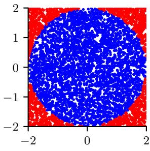
Figure 11.1: Estimating ↼ by Monte Carlo integration using 5000 samples. Blue points are inside the circle, red points are outside. Generated by mc\_estimate\_pi.ipynb.

need to uniformly cover the entire space. In particular, it can be shown that the accuracy is in principle independent of the dimensionality of x, and only depends on the number of samples N^s (see Section 11.2.2 for details). The catch is that we need a way to generate the samples xⁿ ↔︎ p(x) in the first place. In addition, the estimator may have high variance. We will discuss this topic at length in the sections below.

11.2.1 Example: estimating ▷ by Monte Carlo integration

MC integration can be used for many applications, not just in ML and statistics. For example, suppose we want to estimate ϖ. We know that the area of a circle with radius r is ϖr², but it is also equal to the following definite integral:

\[I = \int\_{-r}^{r} \int\_{-r}^{r} \mathbb{I}\left(x^2 + y^2 \le r^2\right) dx dy \tag{11.3}\]

Hence ϖ = I/(r2). Let us approximate this by Monte Carlo integration. Let f(x, y) = I ^{x2 + y2} ⇐ ^r2 be an indicator function that is 1 for points inside the circle, and 0 outside, and let p(x) and p(y) be uniform distributions on [→r, r], so p(x) = p(y)=1/(2r). Then

\[I = (2r)(2r) \int \int f(x, y)p(x)p(y)dxdy \tag{11.4}\]

\[I = 4r^2 \int \int f(x,y)p(x)p(y)dxdy dy\tag{11.5}\]

\[\approx 4r^2 \frac{1}{N\_s} \sum\_{n=1}^{N\_s} f(x\_n, y\_n) \tag{11.6}\]

Using 5000 samples, we find ϖˆ = 3.10 with standard error 0.09 compared to the true value of ϖ = 3.14. We can plot the points that are accepted or rejected as in Figure 11.1.

11.2.2 Accuracy of Monte Carlo integration

The accuracy of an MC approximation increases with sample size. This is illustrated in Figure 11.2. On the top line, we plot a histogram of samples from a Gaussian distribution. On the bottom line,

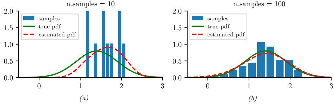
Figure 11.2: 10 and 100 samples from a Gaussian distribution, ^N (^µ = 1.5, ^ω2 = 0.25). A dotted red line denotes kernel density estimate derived from the samples. Generated by mc\_accuracy\_demo.ipynb.

we plot a smoothed version of these samples, created using a kernel density estimate. This smoothed distribution is then evaluated on a dense grid of points and plotted. Note that this smoothing is just for the purposes of plotting, it is not used for the Monte Carlo estimate itself.

If we denote the exact mean by µ = E [f(X)], and the MC approximation by µˆ, one can show that, with independent samples,

\[\mathcal{N}(\hat{\mu} - \mu) \to \mathcal{N}(0, \frac{\sigma^2}{N\_s}) \tag{11.7}\]

where

\[\sigma^2 = \mathbb{V}\left[f(X)\right] = \mathbb{E}\left[f(X)^2\right] - \mathbb{E}\left[f(X)\right]^2\tag{11.8}\]

This is a consequence of the central limit theorem. Of course, ς² is unknown in the above expression, but it can be estimated by MC:

\[ \hat{\sigma}^2 = \frac{1}{N\_s} \sum\_{n=1}^{N\_s} (f(x\_n) - \hat{\mu})^2 \tag{11.9} \]

Thus for large enough N^s we have

\[P\left\{\hat{\mu} - 1.96\frac{\hat{\sigma}}{\sqrt{N\_s}} \le \mu \le \hat{\mu} + 1.96\frac{\hat{\sigma}}{\sqrt{N\_s}}\right\} \approx 0.95\tag{11.10}\]

The term ^L ↽ˆ^{2 Ns} is called the (numerical or empirical) standard error, and is an estimate of our uncertainty about our estimate of µ.

If we want to report an answer which is accurate to within ±⇁ with probability at least 95%, we need to use a number of samples ^Ns which satisfies ¹.96Mςˆ²/N^s ⇐ ⇁. We can approximate the 1.96 factor by 2, yielding ^{Ns ≃} 4ˆ↽^{2 ϖ2} .

The remarkable thing to note about the above results is that the error in the estimate, ς²/Ns, is theoretically independent of the dimensionality of the integral. The catch is that sampling from high dimensional distributions can be hard. We turn to that topic next.

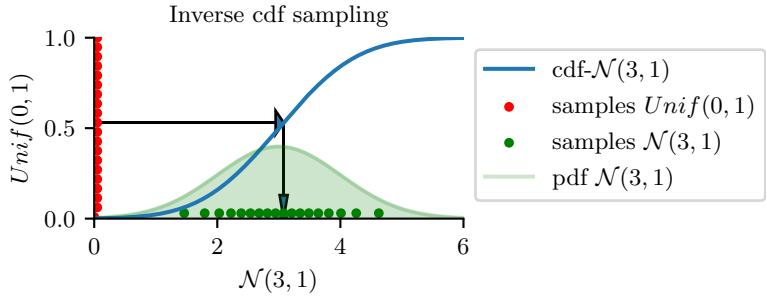
Figure 11.3: Sampling from N (3, 1) using an inverse cdf.

11.3 Generating random samples from simple distributions

We saw in Section 11.2 how we can evaluate E [f(X)] for di!erent functions f of a random variable X using Monte Carlo integration. The main computational challenge is to e”ciently generate samples from the probability distribution p→(x) (which may be a posterior, p→(x) ↑ p(x|D)). In this section, we discuss sampling methods that are suitable for parametric univariate distributions. These can be used as building blocks for sampling from more complex multivariate distributions.

11.3.1 Sampling using the inverse cdf

The simplest method for sampling from a univariate distribution is based on the inverse probability transform. Let F be a cdf of some distribution we want to sample from, and let F ^↓1 be its inverse. Then we have the following result.

Theorem 11.3.1. If ^{U ↔︎ U}(0, 1) is a uniform rv, then ^{F ↓1}(U) ^{↔︎ F}.

Proof.

\[\Pr(F^{-1}(U)\le x) = \Pr(U\le F(x)) \quad \text{(aplying } F \text{ to both sides)} \tag{11.11}\]

\[y = F(x) \quad \text{(because } \Pr(U \le y) = y) \tag{11.12}\]

where the first line follows since F is a monotonic function, and the second line follows since U is uniform on the unit interval.

Hence we can sample from any univariate distribution, for which we can evaluate its inverse cdf, as follows: generate a random number u ↔︎ U(0, 1) using a pseudorandom number generator (see e.g., [Pre+88] for details). Let u represent the height up the y axis. Then “slide along” the x axis until you intersect the F curve, and then “drop down” and return the corresponding x value. This corresponds to computing x = F ^↓1(u). See Figure 11.3 for an illustration.

For example, consider the exponential distribution

\[\text{Expon}(x|\lambda) \triangleq \lambda e^{-\lambda x} \,\, \mathbb{I}\left(x \ge 0\right) \tag{11.13}\]

The cdf is

\[F(x) = 1 - e^{-\lambda x} \text{ } \mathbb{I}\left(x \ge 0\right) \tag{11.14}\]

whose inverse is the quantile function

\[F^{-1}(p) = -\frac{\ln(1-p)}{\lambda} \tag{11.15}\]

By the above theorem, if ^{U ↔︎} Unif(0, 1), we know that ^{F ↓}1(U) ^↔︎ Expon(⇀). So we can sample from the exponential distribution by first sampling from the uniform and then transforming the results using → ln(1 → u)/⇀. (In fact, since 1 → U ↔︎ Unif(0, 1), we can just use → ln(u)/⇀.)

11.3.2 Sampling from a Gaussian (Box-Muller method)

In this section, we describe a method to sample from a Gaussian. The idea is we sample uniformly from a unit radius circle, and then use the change of variables formula to derive samples from a spherical 2d Gaussian. This can be thought of as two samples from a 1d Gaussian.

In more detail, sample ^z1, z² ↗ (→1, 1) uniformly, and then discard pairs that do not satisfy ^z2 1+z^{2 2} ⇐ 1. The result will be points uniformly distributed inside the unit circle, so p(z) = ¹ ⇀ I(z inside circle). Now define

\[x\_i = z\_i \left(\frac{-2\ln r^2}{r^2}\right)^{\frac{1}{2}} \tag{11.16}\]

for i =1:2, where r² = z^{2 1} + z^{2 2}. Using the multivariate change of variables formula, we have

\[p(x\_1, x\_2) = p(z\_1, z\_2) |\frac{\partial(z\_1, z\_2)}{\partial(x\_1, x\_2)}| = \left[\frac{1}{\sqrt{2\pi}} \exp(-\frac{1}{2}x\_1^2)\right] \left[\frac{1}{\sqrt{2\pi}} \exp(-\frac{1}{2}x\_2^2)\right] \tag{11.17}\]

Hence x¹ and x² are two independent samples from a univariate Gaussian. This is known as the Box-Muller method.

To sample from a multivariate Gaussian, we first compute the Cholesky decomposition of its covariance matrix, ! = LL^T, where L is lower triangular. Next we sample ^{x ↔︎ N} (0, I) using the Box-Muller method. Finally we set y = Lx + µ. This is valid since

\[\text{Cov}\left[y\right] = \text{L}\text{Cov}\left[x\right]\mathbf{L}^{\mathsf{T}} = \text{L}\text{ L}\mathbf{L}^{\mathsf{T}} = \Sigma\]

11.4 Rejection sampling

Suppose we want to sample from the target distribution

\[p(\mathbf{z}) = \bar{p}(\mathbf{z}) / Z\_p \tag{11.19}\]

where p˜(x) is the unnormalized version, and

\[Z\_p = \int \tilde{p}(\mathbf{x}) \, d\mathbf{x} \tag{11.20}\]

is the (possibly unknown) normalization constant. One of the simplest approaches to this problem is rejection sampling, which we now explain.

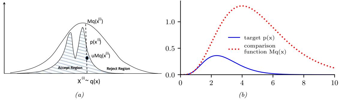
Figure 11.4: (a) Schematic illustration of rejection sampling. From Figure 2 of [And+03]. Used with kind permission of Nando de Freitas. (b) Rejection sampling from a Ga(φ = 5.7, ς = 2) distribution (solid blue) using a proposal of the form MGa(k, ς↗1) (dotted red), where k = ⇑5.7⇓ = 5. The curves touch at φ↗k = 0.7. Generated by rejection\_sampling\_demo.ipynb.

11.4.1 Basic idea

In rejection sampling, we require access to a proposal distribution q(x) which satisfies Cq(x) ≃ p˜(x), for some constant C. The function Cq(x) provides an upper envelope for p˜.

We can use the proposal distribution to generate samples from the target distribution as follows. We first sample x⁰ ↔︎ q(x), which corresponds to picking a random x location, and then we sample u⁰ ↔︎ Unif(0,Cq(x0)), which corresponds to picking a random height (y location) under the envelope. If u⁰ > p˜(x0), we reject the sample, otherwise we accept it. This process is illustrated in 1d in Figure 11.4(a): the acceptance region is shown shaded, and the rejection region is the white region between the shaded zone and the upper envelope.

We now prove this procedure is correct. First note that the probability of any given sample x⁰ being accepted equals the probability of a sample u⁰ ↔︎ Unif(0,Cq(x0)) being less than or equal to p˜(x0), i.e.,

\[q(\text{accept}|\mathbf{x}\_0) = \int\_0^{\tilde{p}(\mathbf{x}\_0)} \frac{1}{Cq(\mathbf{x}\_0)} \, du = \frac{\tilde{p}(\mathbf{x}\_0)}{Cq(\mathbf{x}\_0)} \tag{11.21}\]

Therefore

\[q(\text{propose and accept } x\_0) = q(\mathbf{x}\_0) q(\text{accept}|\mathbf{x}\_0) = q(\mathbf{x}\_0) \frac{\tilde{p}(\mathbf{x}\_0)}{Cq(\mathbf{x}\_0)} = \frac{\tilde{p}(\mathbf{x}\_0)}{C} \tag{11.22}\]

Integrating both sides give

\[\int q(\mathbf{x}\_0) q(\text{accept}|\mathbf{x}\_0) \, d\mathbf{x}\_0 = q(\text{accept}) = \frac{\int \bar{p}(\mathbf{x}\_0) \, d\mathbf{x}\_0}{C} = \frac{Z\_p}{C} \tag{11.23}\]

Hence we see that the distribution of accepted points is given by the target distribution:

\[q(\mathbf{z}\_0|\text{accept}) = \frac{q(\mathbf{z}\_0, \text{accept})}{q(\text{accept})} = \frac{\bar{p}(\mathbf{z}\_0)}{C} \frac{C}{Z\_p} = \frac{\bar{p}(\mathbf{z}\_0)}{Z\_p} = p(\mathbf{z}\_0) \tag{11.24}\]

How e”cient is this method? If p˜ is a normalized target distribution, the acceptance probability is 1/C. Hence we want to choose C as small as possible while still satisfying Cq(x) ≃ p˜(x).

11.4.2 Example

For example, suppose we want to sample from a gamma distribution:3

\[\text{Ga}(x|\alpha,\lambda) = \frac{1}{\Gamma(\alpha)} x^{\alpha - 1} \lambda^{\alpha} \exp(-\lambda x) \tag{11.25}\]

where $(ϱ) is the gamma function. One can show that if Xⁱ iid ↔︎ Expon(⇀), and Y = X¹ + ··· + Xk, then Y ↔︎ Ga(k, ⇀). For non-integer shape parameters ϱ, we cannot use this trick. However, we can use rejection sampling using a Ga(k, ⇀ → 1) distribution as a proposal, where k = ∅ϱℜ. The ratio has the form

\[\frac{p(x)}{q(x)} = \frac{\text{Ga}(x|\alpha, \lambda)}{\text{Ga}(x|k, \lambda - 1)} = \frac{x^{\alpha - 1} \lambda^{\alpha} \exp(-\lambda x) / \Gamma(\alpha)}{x^{k - 1} (\lambda - 1)^k \exp(-(\lambda - 1)x) / \Gamma(k)}\tag{11.26}\]

\[\alpha = \frac{\Gamma(k)\lambda^{\alpha}}{\Gamma(\alpha)(\lambda - 1)^{k}} x^{\alpha - k} \exp(-x) \tag{11.27}\]

This ratio attains its maximum when x = ϱ → k. Hence

\[C = \frac{\text{Ga}(\alpha - k|\alpha, \lambda)}{\text{Ga}(\alpha - k|k, \lambda - 1)} \tag{11.28}\]

See Figure 11.4(b) for a plot.

11.4.3 Adaptive rejection sampling

We now describe a method that can automatically come up with a tight upper envelope q(x) to any log concave 1d density p(x). The idea is to upper bound the log density with a piecewise linear function, as illustrated in Figure 11.5(a). We choose the initial locations for the pieces based on a fixed grid over the support of the distribution. We then evaluate the gradient of the log density at these locations, and make the lines be tangent at these points.

Since the log of the envelope is piecewise linear, the envelope itself is piecewise exponential:

\[q(x) = C\_i \lambda\_i \exp(-\lambda\_i (x - x\_{i-1})), \quad x\_{i-1} < x \le x\_i \tag{11.29}\]

where xⁱ are the grid points. It is relatively straightforward to sample from this distribution. If the sample x is rejected, we create a new grid point at x, and thereby refine the envelope. As the number of grid points is increased, the tightness of the envelope improves, and the rejection rate goes down. This is known as adaptive rejection sampling (ARS) [GW92]. Figure 11.5(b-c) gives an example of the method in action. As with standard rejection sampling, it can be applied to unnormalized distributions.

^3. This section is based on notes by Ioana A. Cosma, available at http://users.aims.ac.za/~ioana/cp2.pdf.

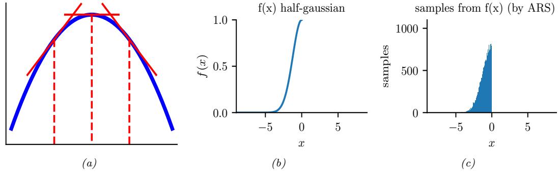
Figure 11.5: (a) Idea behind adaptive rejection sampling. We place piecewise linear upper (and lower) bounds on the log-concave density. Adapted from Figure 1 of [GW92]. Generated by ars\_envelope.ipynb. (b-c) Using ARS to sample from a half-Gaussian. Generated by ars\_demo.ipynb.

11.4.4 Rejection sampling in high dimensions

It is clear that we want to make our proposal q(x) as close as possible to the target distribution p(x), while still being an upper bound. But this is quite hard to achieve, especially in high dimensions. To see this, consider sampling from ^p(x) = ^N (0, ^{ς2 p}I) using as a proposal ^q(x) = ^N (0, ^{ς2 q} I). Obviously we must have ς^{2 q ≃ ς2 p} in order to be an upper bound. In D dimensions, the optimum value is given by C = (ςq/ςp)D. The acceptance rate is 1/C (since both p and q are normalized), which decreases exponentially fast with dimension. For example, if ς^q exceeds ς^p by just 1%, then in 1000 dimensions the acceptance ratio will be about 1/20,000. This is a fundamental weakness of rejection sampling.

11.5 Importance sampling

In this section, we describe a Monte Carlo method known as importance sampling for approximating integrals of the form

\[\mathbb{E}\left[\varphi(x)\right] = \int \varphi(x)\pi(x)dx\tag{11.30}\]

where 5 is called a target function, and ϖ(x) is the target distribution, often a conditional distribution of the form ϖ(x) = p(x|y). Since in general it is di”cult to draw from the target distribution, we will instead draw from some proposal distribution q(x) (which will usually depend on y). We then adjust for the inaccuracies of this by associating weights with each sample, so we end up with a weighted MC approximation:

\[\mathbb{E}\left[\varphi(\mathbf{z})\right] \approx \sum\_{n=1}^{N} W\_n \varphi(\mathbf{z}\_n) \tag{11.31}\]

We discuss two cases, first when the target is normalized, and then when it is unnormalized. This will a!ect the ways the weights are computed, as well as statistical properties of the estimator.

11.5.1 Direct importance sampling

In this section, we assume that we can evaluate the normalized target distribution ϖ(x), but we cannot sample from it. So instead we will sample from the proposal q(x). We can then write

\[\int \varphi(x)\pi(x)dx = \int \varphi(x)\frac{\pi(x)}{q(x)}q(x)dx\tag{11.32}\]

We require that the proposal be non-zero whenever the target is non-zero, i.e., the support of q(x) needs to be greater or equal to the support of ϖ(x). If we draw N^s samples xⁿ ↔︎ q(x), we can write

\[\mathbb{E}\left[\varphi(\mathbf{z})\right] \approx \frac{1}{N\_s} \sum\_{n=1}^{N\_s} \frac{\pi(\mathbf{z}\_n)}{q(\mathbf{z}\_n)} \varphi(\mathbf{z}\_n) = \frac{1}{N\_s} \sum\_{n=1}^{N\_s} \tilde{w}\_n \varphi(\mathbf{z}\_n) \tag{11.33}\]

where we have defined the importance weights as follows:

\[ \hat{w}\_n = \frac{\pi(x\_n)}{q(x\_n)}\tag{11.34} \]

The result is an unbiased estimate of the true mean E [5(x)].

11.5.2 Self-normalized importance sampling

The disadvantage of direct importance sampling is that we need a way to evaluate the normalized target distribution ϖ in order to compute the weights. It is often much easier to evaluate the unnormalized target distribution

\[ \ddot{\gamma}(\mathbf{z}) = Z\pi(\mathbf{z})\tag{11.35} \]

where

\[Z = \int \ddot{\gamma}(\mathbf{x})d\mathbf{z} \tag{11.36}\]

is the normalization constant. (For example, if ϖ(x) = p(x|y), then ▷˜(x) = p(x, y) and Z = p(y).) The key idea is to also approximate the normalization constant Z with importance sampling. This method is called self-normalized importance sampling. The resulting estimate is a ratio of two estimates, and hence is biased. However as N^s ↖ ⇓, the bias goes to zero, under some weak assumptions (see e.g., [RC04] for details).

In more detail, SNIS is based on this approximation:

\[\mathbb{E}\left[\varphi(\mathbf{z})\right] = \int \varphi(\mathbf{z})\pi(\mathbf{z})d\mathbf{x} = \frac{\int \varphi(\mathbf{z})\bar{\gamma}(\mathbf{z})d\mathbf{x}}{\int \bar{\gamma}(\mathbf{z})d\mathbf{x}} = \frac{\int \left[\frac{\bar{\gamma}(\mathbf{z})}{q(\mathbf{z})}\varphi(\mathbf{z})\right]q(\mathbf{x})d\mathbf{x}}{\int \left[\frac{\bar{\gamma}(\mathbf{z})}{q(\mathbf{z})}\right]q(\mathbf{z})d\mathbf{x}} \tag{11.37}\]

\[\approx \frac{\frac{1}{N\_s} \sum\_{n=1}^{N\_s} \tilde{w}\_n \varphi(\mathbf{z}\_n)}{\frac{1}{N\_s} \sum\_{n=1}^{N\_s} \tilde{w}\_n} \tag{11.38}\]

where we have defined the unnormalized weights

\[ \tilde{w}\_n = \frac{\tilde{\gamma}(\mathbf{z}\_n)}{q(\mathbf{z}\_n)} \tag{11.39} \]

We can write Equation (11.38) more compactly as

\[\mathbb{E}\left[\varphi(\mathbf{z})\right] \approx \sum\_{n=1}^{N\_s} W\_n \varphi(\mathbf{z}\_n) \tag{11.40}\]

where we have defined the normalized weights by

\[W\_n = \frac{\tilde{w}\_n}{\sum\_{n'=1}^{N\_s} \tilde{w}\_{n'}} \tag{11.41}\]

This is equivalent to approximating the target distribution using a weighted sum of delta functions:

\[\pi(\mathbf{x}) \approx \sum\_{n=1}^{N\_s} W\_n \delta(\mathbf{x} - \mathbf{x}\_n) \stackrel{\Delta}{=} \hat{\pi}(\mathbf{x}) \tag{11.42}\]

As a byproduct of this algorithm we get the following appoximation to the normalization constant:

\[Z \approx \frac{1}{N\_s} \sum\_{n=1}^{N\_s} \tilde{w}\_n \stackrel{\Delta}{=} \hat{Z} \tag{11.43}\]

11.5.3 Choosing the proposal

The performance of importance sampling depends crucially on the quality of the proposal distribution. As we mentioned, we require that the support of q cover the support of the target (i.e., ▷˜(x) > 0 =∀ q(x) > 0). However, we also want the proposal to not be too “loose” of a “covering”. Ideally it should also take into account properties of the target function 5 as well, as shown in Figure 11.6. This can yield subsantial benefits, as shown in the “target aware Bayesian inference” scheme of [Rai+20]. However, usually the target function 5 is unknown or ignored, so we just try to find a “generally useful” approximation to the target.

One way to come up with a good proposal is to learn one, by optimizing the variational lower bound or ELBO (see Section 10.1.1.2). Indeed, if we fix the parameters of the generative model, we can think of importance weighted autoencoders (Section 10.5.1) as learning a good IS proposal. More details on this connection can be found in [DS18].

11.5.4 Annealed importance sampling (AIS)

In this section, we describe a method known as annealed importance sampling [Nea01] for sampling from complex, possibly multimodal distributions. Assume we want to sample from some target distribution p0(x) ↑ f0(x) (where f0(x) is the unnormalized version), but we cannot easily do so, because p⁰ is complicated in some way (e.g., high dimensional and/or multi-modal). However, suppose that there is an easier distribution which we can sample from, call it pn(x) ↑ fn(x); for

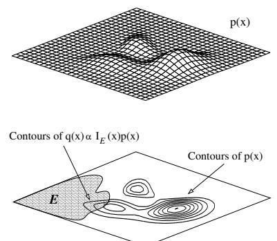
Figure 11.6: In importance sampling, we should sample from a distribution that takes into account regions where ↼(x) has high probability and where ↽(x) is large. Here the function to be evaluated is an indicator function of a set, corresponding to a set of rare events in the tail of the distribution. From Figure 3 of [And+03]. Used with kind permission of Nando de Freitas.

example, this might be the prior. We now construct a sequence of intermediate distributions that move slowly from pⁿ to p⁰ as follows:

\[f\_j(\mathbf{z}) = f\_0(\mathbf{z})^{\beta\_j} f\_n(\mathbf{z})^{1-\beta\_j} \tag{11.44}\]

where 1 = ↼⁰ > ↼¹ > ··· > ↼ⁿ = 0, where ↼^j is an inverse temperature. We will sample a set of points from fn, and then from fⁿ↓¹, and so on, until we eventually sample from f0.

To sample from each f^j , suppose we can define a Markov chain T^j (x, x^↔︎ ) = p^j (x^↔︎ |x), which leaves p⁰ invariant (i.e., / p^j (x^↔︎ |x)p0(x)dx = p0(x^↔︎ )). (See Chapter 12 for details on how to construct such chains.) Given this, we can sample x from p⁰ as follows: sample vⁿ ↔︎ pn; sample vⁿ↓¹ ↔︎ Tⁿ↓1(vn, ·); and continue in this way until we sample v⁰ ↔︎ T0(v1, ·); finally we set x = v⁰ and give it weight

\[w = \frac{f\_{n-1}(\mathbf{v}\_{n-1})}{f\_n(\mathbf{v}\_{n-1})} \frac{f\_{n-2}(\mathbf{v}\_{n-2})}{f\_{n-1}(\mathbf{v}\_{n-2})} \cdots \frac{f\_1(\mathbf{v}\_1)}{f\_2(\mathbf{v}\_1)} \frac{f\_0(\mathbf{v}\_0)}{f\_1(\mathbf{v}\_0)} \tag{11.45}\]

This can be shown to be correct by viewing the algorithm as a form of importance sampling in an extended state space v = (v0,…, vn). Consider the following distribution on this state space:

\[p(\mathbf{v}) \propto \varphi(\mathbf{v}) = f\_0(\mathbf{v}\_0) \tilde{T}\_0(\mathbf{v}\_0, \mathbf{v}\_1) \tilde{T}\_2(\mathbf{v}\_1, \mathbf{v}\_2) \cdots \tilde{T}\_{n-1}(\mathbf{v}\_{n-1}, \mathbf{v}\_n) \tag{11.46}\]

\[\propto p(\mathbf{v}\_0) p(\mathbf{v}\_1|\mathbf{v}\_0) \cdots p(\mathbf{v}\_n|\mathbf{v}\_{n-1}) \tag{11.47}\]

where T˜ ^j is the reversal of T^j :

\[\tilde{T}\_j(\mathbf{v}, \mathbf{v}') = T\_j(\mathbf{v}', \mathbf{v}) p\_j(\mathbf{v}') / p\_j(\mathbf{v}) = T\_j(\mathbf{v}', \mathbf{v}) f\_j(\mathbf{v}') / f\_j(\mathbf{v}) \tag{11.48}\]

It is clear that & ^v1,…,vⁿ 5(v) = f0(v0), so by sampling from p(v), we can e!ectively sample from p0(x).

We can sample on this extended state space using the above algorithm, which corresponds to the following proposal:

\[q(\mathbf{v}) \propto g(\mathbf{v}) = f\_n(\mathbf{v}\_n) T\_{n-1}(\mathbf{v}\_n, \mathbf{v}\_{n-1}) \cdots T\_2(\mathbf{v}\_2, \mathbf{v}\_1) T\_0(\mathbf{v}\_1, \mathbf{v}\_0) \tag{11.49}\]

\[\propto p(\mathbf{v}\_n) p(\mathbf{v}\_{n-1}|\mathbf{v}\_n) \cdots p(\mathbf{v}\_1|\mathbf{v}\_0) \tag{11.50}\]

One can show that the importance weights w = ^ϕ(v0,…,vn) ^g(v0,…,vn) are given by Equation (11.45). Since marginals of the sampled sequences from this extended model are equivalent to samples from p0(x), we see that we are using the correct weights.

11.5.4.1 Estimating normalizing constants using AIS

An important application of AIS is to evaluate a ratio of partition functions. Notice that ^{Z0 =} / ^f0(x)d^{x =} / ⁵(v)dv, and ^{Zn =} / ^fn(x)d^{x =} / ^g(v)dv. Hence

\[\frac{Z\_0}{Z\_n} = \frac{\int \varphi(\mathbf{v})d\mathbf{v}}{\int g(\mathbf{v})d\mathbf{v}} = \frac{\int \frac{\varphi(\mathbf{v})}{g(\mathbf{v})}g(\mathbf{v})d\mathbf{v}}{\int g(\mathbf{v})d\mathbf{v}} = \mathbb{E}\_g\left[\frac{\varphi(\mathbf{v})}{g(\mathbf{v})}\right] \approx \frac{1}{S}\sum\_{s=1}^S w\_s\tag{11.51}\]

where w^s = 5(vs)/g(vs). If f⁰ is a prior and fⁿ is the posterior, we can estimate Zⁿ = p(D) using the above equation, provided the prior has a known normalization constant Z0. This is generally considered the method of choice for evaluating di”cult partition functions. See e.g., [GM98] for more details.

11.6 Controlling Monte Carlo variance

As we mentioned in Section 11.2.2, the standard error in a Monte Carlo estimate is O(1/ ∝ S), where S is the number of (independent) samples. Consequently it may take many samples to reduce the variance to a su”ciently small value. In this section, we discuss some ways to reduce the variance of sampling methods. For more details, see e.g., [KTB11].

11.6.1 Common random numbers

When performing Monte Carlo optimization, we often want to compare Ep(z) [f(ω, z)] to Ep(z) [f(ω^↔︎ , z)] for di!erent values of the parameters ω and ω^↔︎ . To reduce the variance of this comparison, we can use the same random samples z^s for evaluating both functions. In this way, di!erences in the outcome can be ascribed to di!erences in the parameters ω, rather than to the noise terms. This is called the common random numbers trick, and is widely used in ML (see e.g., [GBJ18; NJ00]), since it can often convert a stochastic optimization problem into a deterministic one, enabling the use of more powerful optimization methods. For more details on CRN, see e.g., https://en.wikipedia.org/wiki/Variance\_reduction#Common\_Random\Numbers\(CRN).

11.6.2 Rao-Blackwellization

In this section, we discuss a useful technique for reducing the variance of MC estimators known as Rao-Blackwellization. To explain the method, suppose we have two rv’s, X and Y , and we want

to estimate f = E [f(X, Y )]. The naive approach is to use an MC approximation

\[\hat{f}\_{MC} = \frac{1}{S} \sum\_{s=1}^{S} f(X\_s, Y\_s) \tag{11.52}\]

where (Xs, Ys) ↔︎ p(X, Y ). This is an unbiased estimator of f. However, it may have high variance.

Now suppose we can analytically marginalize out Y , provided we know X, i.e., we can tractably compute

\[f\_X(X\_s) = \int dY p(Y|X\_s) f(X\_s, Y) = \mathbb{E}\left[f(X, Y)|X = X\_s\right] \tag{11.53}\]

Let us define the Rao-Blackwellized estimator

\[\hat{f}\_{RB} = \frac{1}{S} \sum\_{s=1}^{S} f\_X(X\_s) \tag{11.54}\]

where X^s ↔︎ p(X). This is an unbiased estimator, since E ^ˆfRB = E [E [f(X, Y )|X]] = f. However, this estimate can have lower variance than the naive estimator. The intuitive reason is that we are now sampling in a reduced dimensional space. Formally we can see this by using the law of iterated variance to get

\[\mathbb{V}\left[\mathbb{E}\left[f(X,Y)|X\right]\right] = \mathbb{V}\left[f(X,Y)\right] - \mathbb{E}\left[\mathbb{V}\left[f(X,Y)\right]|X\right] \le \mathbb{V}\left[f(X,Y)\right] \tag{11.55}\]

For some examples of this in practice, see Section 6.3.4.2, Section 13.4, and Section 12.3.8.

11.6.3 Control variates

Suppose we want to estimate ^{µ = E} [f(X)] using an unbiased estimator ^m(^X ) = ¹ S &^{S s}=1 m(xs), where x^s ↔︎ p(X) and E [m(X)] = µ. (We abuse notation slightly and use m to refer to a function of a single random variable as well as a set of samples.) Now consider the alternative estimator

\[m^\*(\mathcal{X}) = m(\mathcal{X}) + c\left(b(\mathcal{X}) - \mathbb{E}\left[b(\mathcal{X})\right]\right) \tag{11.56}\]

This is called a control variate, and b is called a baseline. (Once again we abuse notation and use ^b(^X ) = ¹ S &^{S s}=1 ^b(xs) and ^m→(^X ) = ¹ S &^{S s}=1 m→(xs).)

It is easy to see that m→(X ) is an unbiased estimator, since E [m→(X)] = E [m(X)] = µ. However, it can have lower variance, provided b is correlated with m. To see this, note that

\[\mathbb{V}\left[m^\*(X)\right] = \mathbb{V}\left[m(X)\right] + c^2\mathbb{V}\left[b(X)\right] + 2c\text{Cov}\left[m(X), b(X)\right] \tag{11.57}\]

By taking the derivative of V [m→(X)] wrt c and setting to 0, we find that the optimal value is

\[c^\* = -\frac{\text{Cov}\left[m(X), b(X)\right]}{\mathbb{V}\left[b(X)\right]}\tag{11.58}\]

The corresponding variance of the new estimator is now

\[\mathbb{V}\left[m^\*(X)\right] = \mathbb{V}\left[m(X)\right] - \frac{\text{Cov}\left[m(X), b(X)\right]^2}{\mathbb{V}\left[b(X)\right]} = (1 - \rho\_{m,b}^2)\mathbb{V}\left[m(X)\right] \le \mathbb{V}\left[m(X)\right] \tag{11.59}\]

where 0² m,b is the correlation of the basic estimator and the baseline function. If we can ensure this correlation is high, we can reduce the variance. Intuitively, the CV estimator is exploiting information about the errors in the estimate of a known quantity, namely E [b(X)], to reduce the errors in estimating the unknown quantity, namely µ.

We give a simple worked example in Section 11.6.3.1. See Section 10.2.3 for an example of this technique applied to blackbox variational inference.

11.6.3.1 Example

We now give a simple worked example of control variates.4 Consider estimating µ = E [f(X)] where f(X)=1/(1 + X) and X ↔︎ Unif(0, 1). The exact value is

\[ \mu = \int\_0^1 \frac{1}{1+x} dx = \ln 2 \approx 0.693\tag{11.60} \]

The naive MC estimate, using ^S samples, is ^m(^X ) = ¹ S &^{S s}=1 f(xs). Using S = 1500, we find E [m(X )] = 0.6935 with standard error se = 0.0037.

Now let us use b(X)=1+ X as a baseline, so b(X ) = (1/S) & ^s(1 + xs). This has expectation E [b(X)] = / ^{1 0} (1 + ^x)dx ^{= 3 2} . The control variate estimator is given by

\[m^\*(\mathcal{X}) = \frac{1}{S} \sum\_{s=1}^S f(x\_s) + c\left(\frac{1}{S} \sum\_{s=1}^S b(x\_s) - \frac{3}{2}\right) \tag{11.61}\]

The optimal value can be estimated from the samples of m(xs) and b(xs), and plugging into Equation (11.58) to get c^→ ↓ 0.4773. Using S = 1500, we find E [m→(X )] = 0.6941 and se = 0.0007.

See also Section 11.6.4.1, where we analyze this example using antithetic sampling.

11.6.4 Antithetic sampling

In this section, we discuss antithetic sampling, which is a simple way to reduce variance.5 Suppose we want to estimate ω = E [Y ]. Let Y¹ and Y² be two samples. An unbiased estimate of ω is given by ˆω = (Y¹ + Y2)/2. The variance of this estimate is

\[\mathbb{V}\left[\hat{\theta}\right] = \frac{\mathbb{V}\left[Y\_1\right] + \mathbb{V}\left[Y\_2\right] + 2\text{Cov}\left[Y\_1, Y\_2\right]}{4} \tag{11.62}\]

so the variance is reduced if Cov [Y1, Y2] < 0. So whenever we sample Y1, we should set Y² to be its “opposite”, but with the same mean.

For example, suppose Y ↔︎ Unif(0, 1). If we let y1,…,yⁿ be iid samples from Unif(0, 1), then we can define y^{↔︎ i} = 1 → yi. The distribution of y^{↔︎ i} is still Unif(0, 1), but Cov [yi, y^{↔︎ i}] < 1.

^4. The example is from https://en.wikipedia.org/wiki/Control\_variates, with modified notation. See control\_variates.ipynb for some code.

^5. Our presentation is based on https://en.wikipedia.org/wiki/Antithetic\_variates. See antithetic\_sampling.ipynb for the code.

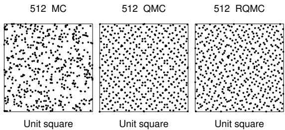
Figure 11.7: Illustration of Monte Carlo (MC), Quasi-MC (QMC) from a Sobol sequence, and randomized QMC using a scrambling method. Adapted from Figure 1 of [OR20]. Used with kind permission of Art Owen.

11.6.4.1 Example

To see why this can be useful, consider the example from Section 11.6.3.1. Let µˆmc be the classic MC estimate using 2N samples from Unif(0, 1), and let µˆanti be the MC estimate using the above antithetic sampling scheme applied to N base samples from Unif(0, 1). The exact value is µ = ln 2 ↓ 0.6935. For the classical method, with N = 750, we find E [ˆµmc] = 0.69365 with a standard error of 0.0037. For the antithetic method, we find E [ˆµanti] = 0.6939 with a standard error of 0.0007, which matches the control variate method of Section 11.6.3.1.

11.6.5 Quasi-Monte Carlo (QMC)

Quasi-Monte Carlo (see e.g., [Lem09; Owe13]) is an approach to numerical integration that replaces random samples with low discrepancy sequences, such as the Halton sequence (see e.g., [Owe17]) or Sobol sequence. Intuitively, these are space filling sequences of points, constructed to reduce the unwanted gaps and clusters that would arise among randomly chosen inputs. See Figure 11.7 for an example.6

More precisely, consider the problem of evaluating the following D-dimensional integral:

\[\overline{f} = \int\_{[0,1]^D} f(\mathbf{z})d\mathbf{z} \approx \hat{f}\_N = \frac{1}{N} \sum\_{n=1}^N f(\mathbf{z}\_n) \tag{11.63}\]

Let ⇁^{N = |f → ˆ}f^{N |} be the error. In standard Monte Carlo, if we draw ^N independent samples, then we have ⇁^N ↔︎ O ⇔ 1 N . In QMC, it can be shown that ⇁^N ↔︎ O (log ^N)^D N . For N > 2^D, the latter is smaller than the former.

One disadvantage of QMC is that it just provides a point estimate of f, and does not give an uncertainty estimate. By contrast, in regular MC, we can estimate the MC standard error, discussed in Section 11.2.2. Randomized QMC (see e.g., [L’E18]) provides a solution to this problem. The basic idea is to repeat the QMC method R times, by perturbing the sequence of N points by a

^6. More details on QMC can be found at http://roth.cs.kuleuven.be/wiki/Main\_Page. For connections to Bayesian quadrature, see e.g., [DKS13; HKO22].

random amount. In particular, define

\[y\_{i,r} = x\_i + \mu\_r \pmod{1} \tag{11.64}\]

where ^x1,…, ^xN is a low-discrepancy sequence, and ^{ur ↔︎} Unif(0, 1)^D is a random perturbation. The set {yj} is low discrepancy, and satisfies that each ^{yj ↔︎} Unif(0, 1)^D, for ^j =1: ^{N ⇔ R}. This has much lower variance than standard MC. (Typically we take R to be a power of 2.) Recently, [OR20] proved a strong law of large numbers for RQMC.

QMC and RQMC can be used inside of MCMC inference (see e.g., [OT05]) and variational inference (see e.g., [BWM18]). It is also commonly used to select the initial set of query points for Bayesian optimization (Section 6.6).

Another technique that can be used is orthogonal Monte Carlo, where the samples are conditioned to be pairwise orthogonal, but with the marginal distributions matching the original ones (see e.g., [Lin+20]).

12 Markov chain Monte Carlo

12.1 Introduction

In Chapter 11, we considered non-iterative Monte Carlo methods, including rejection sampling and importance sampling, which generate independent samples from some target distribution. The trouble with these methods is that they often do not work well in high dimensional spaces. In this chapter, we discuss a popular method for sampling from high-dimensional distributions known as Markov chain Monte Carlo or MCMC. In a survey by SIAM News1, MCMC was placed in the top 10 most important algorithms of the 20th century.

The basic idea behind MCMC is to construct a Markov chain (Section 2.6) on the state space X whose stationary distribution is the target density p→(x) of interest. (In a Bayesian context, this is usually a posterior, p→(x) ↑ p(x|D), but MCMC can be applied to generate samples from any kind of distribution.) That is, we perform a random walk on the state space, in such a way that the fraction of time we spend in each state x is proportional to p→(x). By drawing (correlated) samples x0, x1, x2,…, from the chain, we can perform Monte Carlo integration wrt p→.

Note that the initial samples from the chain do not come from the stationary distribution, and should be discarded; the amount of time it takes to reach stationarity is called the mixing time or burn-in time; reducing this is one of the most important factors in making the algorithm fast, as we will see.

The MCMC algorithm has an interesting history. It was discovered by physicists working on the atomic bomb at Los Alamos during World War II, and was first published in the open literature in [Met+53] in a chemistry journal. An extension was published in the statistics literature in [Has70], but was largely unnoticed. A special case (Gibbs sampling, Section 12.3) was independently invented in [GG84] in the context of Ising models (Section 4.3.2.1). But it was not until [GS90] that the algorithm became well-known to the wider statistical community. Since then it has become wildly popular in Bayesian statistics, and is becoming increasingly popular in machine learning.

In the rest of this chapter, we give a brief introduction to MCMC methods. For more details on the theory, see e.g., [GRS96; BZ20]. For more details on the implementation side, see e.g., [Lao+20]. And for an interactive visualization of many of these algorithsm in 2d, see http://chi-feng.github. io/mcmc-demo/app.html.

^1. Source: http://www.siam.org/pdf/news/637.pdf.

12.2 Metropolis-Hastings algorithm

In this section, we describe the simplest kinds of MCMC algorithm known as the Metropoli-Hastings or MH algorithm.

12.2.1 Basic idea

The basic idea in MH is that at each step, we propose to move from the current state x to a new state x^↔︎ with probability q(x^↔︎ |x), where q is called the proposal distribution (also called the kernel). The user is free to use any kind of proposal they want, subject to some conditions which we explain below. This makes MH quite a flexible method.

Having proposed a move to x^↔︎ , we then decide whether to accept this proposal, or to reject it, according to some formula, which ensures that the long-term fraction of time spent in each state is proportional to p→(x). If the proposal is accepted, the new state is x^↔︎ , otherwise the new state is the same as the current state, x (i.e., we repeat the sample).

If the proposal is symmetric, so q(x^↔︎ |x) = q(x|x^↔︎ ), the acceptance probability is given by the following formula:

\[A = \min\left(1, \frac{p^\*(x')}{p^\*(x)}\right) \tag{12.1}\]

We see that if x^↔︎ is more probable than x, we definitely move there (since ^p↓(x^↑ ) ^p↓(x) > 1), but if x^↔︎ is less probable, we may still move there anyway, depending on the relative probabilities. So instead of greedily moving to only more probable states, we occasionally allow “downhill” moves to less probable states. In Section 12.2.2, we prove that this procedure ensures that the fraction of time we spend in each state x is equal to p→(x).

If the proposal is asymmetric, so q(x^↔︎ |x) ′= q(x|x^↔︎ ), we need the Hastings correction, given by the following:

\[A = \min(1, \alpha) \tag{12.2}\]

\[\alpha = \frac{p^\*(\mathbf{x'})q(\mathbf{x}|\mathbf{x'})}{p^\*(\mathbf{x})q(\mathbf{x'}|\mathbf{x})} = \frac{p^\*(\mathbf{x'})/q(\mathbf{x'}|\mathbf{x})}{p^\*(\mathbf{x})/q(\mathbf{x}|\mathbf{x'})} \tag{12.3}\]

This correction is needed to compensate for the fact that the proposal distribution itself (rather than just the target distribution) might favor certain states. (In addition we see that the algorithm is more likely to take an an exploratory step into a low-probability region, where p→(x^↔︎ ) is small, if it knows it can easily get back to where it came from, i.e., if q(x|x^↔︎ ) is large.)

An important reason why MH is a useful algorithm is that, when evaluating ϱ, we only need to know the target density up to a normalization constant. In particular, suppose p→(x) = ^{1 Z} p˜(x), where p˜(x) is an unnormalized distribution and Z is the normalization constant. Then

\[\alpha = \frac{\left(\bar{p}(\mathbf{x'})/Z\right)q(\mathbf{z}|\mathbf{x'})}{\left(\bar{p}(\mathbf{x})/Z\right)q(\mathbf{x'}|\mathbf{x})} \tag{12.4}\]

so the Z’s cancel. Hence we can sample from p^→ even if Z is unknown.

A proposal distribution q is valid or admissible if it “covers” the support of the target. Formally, we can write this as

\[\text{supp}(p^\*) \subseteq \cup\_x \text{supp}(q(\cdot|x)) \tag{12.5}\]

With this, we can state the overall algorithm as in Algorithm 12.1.

Algorithm 12.1: Metropolis-Hastings algorithm

¹ Initialize x^{0 2} for s = 0, 1, 2,… do ³ Define x = x^{s 4} Sample x^↔︎ ↔︎ q(x^↔︎ |x) 5 Compute acceptance probability ^{ϱ = p}˜(x^↔︎ )q(x|x^↔︎ ) p˜(x)q(x^↔︎ |x) ⁶ Compute A = min(1, ϱ) ⁷ Sample u ↔︎ U(0, 1) 8 Set new sample to x^s+1 = ^x↔︎ if ^u ⇐ ^A (accept) x^s if u>A (reject)

12.2.2 Why MH works

To prove that the MH procedure generates samples from p→, we need a bit of Markov chain theory, as discussed in Section 2.6.4.

The MH algorithm defines a Markov chain with the following transition matrix:

\[p(\mathbf{z'}|\mathbf{x}) = \begin{cases} q(\mathbf{z'}|\mathbf{x})A(\mathbf{z'}|\mathbf{x}) & \text{if } \mathbf{z'} \neq \mathbf{z} \\ q(\mathbf{z}|\mathbf{x}) + \sum\_{\mathbf{z}' \neq \mathbf{z}} q(\mathbf{z'}|\mathbf{x})(1 - A(\mathbf{z'}|\mathbf{x})) & \text{otherwise} \end{cases} \tag{12.6}\]

This follows from a case analysis: if you move to x^↔︎ from x, you must have proposed it (with probability q(x^↔︎ |x)) and it must have been accepted (with probability A(x^↔︎ |x)); otherwise you stay in state x, either because that is what you proposed (with probability q(x|x)), or because you proposed something else (with probability q(x^↔︎ |x)) but it was rejected (with probability 1 → A(x^↔︎ |x)).

Let us analyze this Markov chain. Recall that a chain satisfies detailed balance if

\[p(\boldsymbol{x}'|\boldsymbol{x})p^\*(\boldsymbol{x}) = p(\boldsymbol{x}|\boldsymbol{x}')p^\*(\boldsymbol{x}') \tag{12.7}\]

This means in the in-flow to state x^↔︎ from x is equal to the out-flow from state x^↔︎ back to x, and vice versa. We also showed that if a chain satisfies detailed balance, then p^→ is its stationary distribution. Our goal is to show that the MH algorithm defines a transition function that satisfies detailed balance

and hence that p^→ is its stationary distribution. (If Equation (12.7) holds, we say that p^→ is an invariant distribution wrt the Markov transition kernel q.)

Theorem 12.2.1. If the transition matrix defined by the MH algorithm (given by Equation (12.6)) is ergodic and irreducible, then p^→ is its unique limiting distribution.

Proof. Consider two states x and x^↔︎ . Either

\[p^\*(x)q(x'|x) < p^\*(x')q(x|x') \tag{12.8}\]

or

\[p^\*(x)q(x'|x) \ge p^\*(x')q(x|x') \tag{12.9}\]

Without loss of generality, assume that p→(x)q(x^↔︎ |x) > p→(x^↔︎ )q(x|x^↔︎ ). Hence

\[\alpha(x'|x) = \frac{p^\*(x')q(x|x')}{p^\*(x)q(x'|x)} < 1\tag{12.10}\]

Hence we have A(x^↔︎ |x) = ϱ(x^↔︎ |x) and A(x|x^↔︎ )=1.

Now to move from x to x^↔︎ we must first propose x^↔︎ and then accept it. Hence

\[p(x'|x) = q(x'|x)A(x'|x) = q(x'|x)\frac{p^\*(x')q(x|x')}{p^\*(x)q(x'|x)} = \frac{p^\*(x')}{p^\*(x)}q(x|x') \tag{12.11}\]

Hence

\[p^\*(x)p(x'|x) = p^\*(x')q(x|x')\tag{12.12}\]

The backwards probability is

\[p(x|x') = q(x|x')A(x|x') = q(x|x') \tag{12.13}\]

since A(x|x^↔︎ )=1. Inserting this into Equation (12.12) we get

\[p^\*(x)p(x'|x) = p^\*(x')p(x|x')\tag{12.14}\]

so detailed balance holds wrt p→. Hence, from Theorem 2.6.3, p^→ is a stationary distribution. Furthermore, from Theorem 2.6.2, this distribution is unique, since the chain is ergodic and irreducible.

12.2.3 Proposal distributions

In this section, we discuss some common proposal distributions. Note, however, that good proposal design is often intimately dependent on the form of the target distribution (most often the posterior).

12.2.3.1 Independence sampler

If we use a proposal of the form q(x^↔︎ |x) = q(x^↔︎ ), where the new state is independent of the old state, we get a method known as the independence sampler, which is similar to importance sampling (Section 11.5). The function q(x^↔︎ ) can be any suitable distribution, such as a Gaussian. This has non-zero probability density on the entire state space, and hence is a valid proposal for any unconstrained continuous state space.

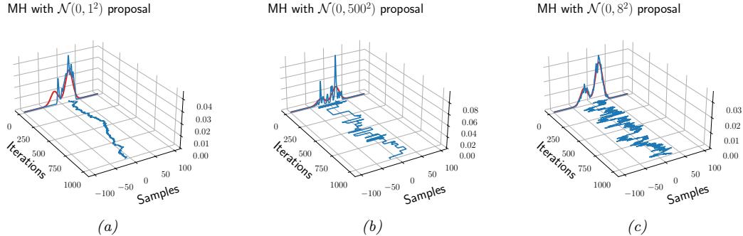
Figure 12.1: An example of the Metropolis-Hastings algorithm for sampling from a mixture of two 1d Gaussians (µ = (↗20, 20), φ = (0.3, 0.7), ! = (100, 100)), using a Gaussian proposal with standard deviation of ⇀ ↓ {1, 8, 500}. (a) When ⇀ = 1, the chain gets trapped near the starting state and fails to sample from the mode at µ = ↗20. (b) When ⇀ = 500, the chain is very “sticky”, so its e!ective sample size is low (as reflected by the rough histogram approximation at the end). (c) Using a variance of ⇀ = 8 is just right and leads to a good approximation of the true distribution (shown in red). Compare to Figure 12.4. Generated by mcmc\_gmm\_demo.ipynb.

12.2.3.2 Random walk Metropolis (RWM) algorithm

The random walk Metropolis algorithm corresponds to MH with the following proposal distribution:

\[q(x'|x) = \mathcal{N}(x'|x, \tau^2 \mathbf{I})\tag{12.15}\]

Here τ is a scale factor chosen to facilitate rapid mixing. [RR01b] prove that, if the posterior is Gaussian, the asymptotically optimal value is to use τ ² = 2.38²/D, where D is the dimensionality of x; this results in an acceptance rate of 0.234, which (in this case) is the optimal tradeo! between exploring widely enough to cover the distribution without being rejected too often. (See [Béd08] for a more recent account of optimal acceptance rates for random walk Metropolis methods.)

Figure 12.1 shows an example where we use RWM to sample from a mixture of two 1D Gaussians. This is a somewhat tricky target distribution, since it consists of two somewhat separated modes. It is very important to set the variance of the proposal τ ² correctly: if the variance is too low, the chain will only explore one of the modes, as shown in Figure 12.1(a), but if the variance is too large, most of the moves will be rejected, and the chain will be very sticky, i.e., it will stay in the same state for a long time. This is evident from the long stretches of repeated values in Figure 12.1(b). If we set the proposal’s variance just right, we get the trace in Figure 12.1(c), where the samples clearly explore the support of the target distribution.

12.2.3.3 Composing proposals

If there are several proposals that might be useful, one can combine them using a mixture proposal, which is a convex combination of base proposals:

\[q(\mathbf{z}'|\mathbf{x}) = \sum\_{k=1}^{K} w\_k q\_k(\mathbf{z}'|\mathbf{x}) \tag{12.16}\]

where w^k are the mixing weights that sum to one. As long as each q^k is an individually valid proposal, and each w^k > 0, then the overall mixture proposal will also be valid. In particular, if each proposal is reversible, so it satisfies detailed balance (Section 2.6.4.4), then so does the mixture.

It is also possible to compose individual proposals by chaining them together to get

\[q(\mathbf{z}'|\mathbf{x}) = \sum\_{\mathbf{x}\_1} \cdots \sum\_{\mathbf{x}\_{K-1}} q\_1(\mathbf{x}\_1|\mathbf{z}) q\_2(\mathbf{x}\_2|\mathbf{x}\_1) \cdots q\_K(\mathbf{z}|\mathbf{x}\_{K-1}) \tag{12.17}\]

A common example is where each base proposal only updates a subset of the variables (see e.g., Section 12.3).

12.2.3.4 Data-driven MCMC

In the case where the target distribution is a posterior, p→(x) = p(x|D), it is helpful to condition the proposal not just on the previous hidden state, but also the visible data, i.e., to use q(x^↔︎ |x, D). This is called data-driven MCMC (see e.g., [TZ02; Jih+12]).

One way to create such a proposal is to train a recognition network to propose states using q(x^↔︎ |x, D) = f(x). If the state space is high-dimensional, it might be hard to predict all the hidden components, so we can alternatively train individual “experts” to predict specific pieces of the hidden state. For example, in the context of estimating the 3d pose of a person from an image, we might combine a face detector with a limb detector. We can then use a mixture proposal of the form

\[q(\mathbf{z}'|\mathbf{z}, \mathcal{D}) = \pi\_0 q\_0(\mathbf{z}'|\mathbf{z}) + \sum\_k \pi\_k q\_k(x\_k'|f\_k(\mathcal{D})) \tag{12.18}\]

where q⁰ is a standard data-independent proposal (e.g., random walk), and q^k updates the k’th component of the state space.

The overall procedure is a form of generate and test: the discriminative proposals q(x^↔︎ |x, D) generate new hypotheses, which are then “tested” by computing the posterior ratio ^p(x^↑ |D) ^p(x|D) , to see if the new hypothesis is better or worse. (See also Section 13.3, where we discuss learning proposal distributions for particle filters.)

12.2.3.5 Adaptive MCMC

One can change the parameters of the proposal as the algorithm is running to increase e”ciency. This is called adaptive MCMC. This allows one to start with a broad covariance (say), allowing large moves through the space until a mode is found, followed by a narrowing of the covariance to ensure careful exploration of the region around the mode.

However, one must be careful not to violate the Markov property; thus the parameters of the proposal should not depend on the entire history of the chain. It turns out that a su”cient condition to ensure this is that the adaption is “faded out” gradually over time. See e.g., [AT08] for details.

12.2.4 Initialization

It is necessary to start MCMC in an initial state that has non-zero probability. A natural approach is to first use an optimizer to find a local mode. However, at such points the gradients of the log joint are zero, which can cause problems for some gradient-based MCMC methods, such as HMC (Section 12.5), so it can be better to start “close” to a MAP estimate (see e.g., [HFM17, Sec 7.]).

12.3 Gibbs sampling

The major problems with MH are the need to choose the proposal distribution, and the fact that the acceptance rate may be low. In this section, we describe an MH method that exploits conditional independence properties of a graphical model to automatically create a good proposal, with acceptance probability 1. This method is known as Gibbs sampling. 2 (In physics, this method is known as Glauber dynamics or the heat bath method.) This is the MCMC analog of coordinate descent.3

12.3.1 Basic idea

The idea behind Gibbs sampling is to sample each variable in turn, conditioned on the values of all the other variables in the distribution. For example, if we have D = 3 variables, we use

• x^s+1 ^{1 ↔︎ p}(x1|x^s 2, x^s 3)

\[\bullet \ x\_2^{s+1} \sim p(x\_2 | x\_1^{s+1}, x\_3^s)\]

\[\bullet \ x\_3^{s+1} \sim p(x\_3 | x\_1^{s+1}, x\_2^{s+1})\]

This readily generalizes to D variables. (Note that if xⁱ is a known variable, we do not sample it, but it may be used as input to another conditional distribution.)

The expression p(xi|x↓ⁱ) is called the full conditional for variable i. In general, xⁱ may only depend on some of the other variables. If we represent p(x) as a graphical model, we can infer the dependencies by looking at i’s Markov blanket, which are its neighbors in the graph (see Section 4.2.4.3), so we can write

\[x\_i^{s+1} \sim p(x\_i | \mathbf{x}\_{-i}^s) = p(x\_i | \mathbf{x}\_{\text{mb(i)}}^s) \tag{12.19}\]

(Compare to the equation for mean field variational inference in Equation (10.87).)

We can sample some of the nodes in parallel, without a!ecting correctness. In particular, suppose we can create a coloring of the (moralized) undirected graph, such that no two neighboring nodes have the same color. (In general, computing an optimal coloring is NP-complete, but we can use e”cient heuristics such as those in [Kub04].) Then we can sample all the nodes of the same color in parallel, and cycle through the colors sequentially [Gon+11].

^2. Josiah Willard Gibbs, 1839–1903, was an American physicist.

^3. Several software libraries exist for applying Gibbs sampling to general graphical models, including Nimble, which is a C++ library with an R wrapper, and which replaces older programs such as BUGS and JAGS.

12.3.2 Gibbs sampling is a special case of MH

It turns out that Gibbs sampling is a special case of MH where we use a sequence of proposals of the form

\[q\_i(\boldsymbol{x}'|\boldsymbol{x}) = p(\boldsymbol{x}'\_i|\boldsymbol{x}\_{-i})\mathbb{I}\left(\boldsymbol{x}'\_{-i} = \boldsymbol{x}\_{-i}\right) \tag{12.20}\]

That is, we move to a new state where xⁱ is sampled from its full conditional, but x↓ⁱ is left unchanged.

We now prove that the acceptance rate of each such proposal is 100%, so the overall algorithm also has an acceptance rate of 100%. We have

\[\alpha = \frac{p(x')q\_i(x|x')}{p(x)q\_i(x'|x)} = \frac{p(x'\_i|x'\_{-i})p(x'\_{-i})p(x\_i|x'\_{-i})}{p(x\_i|x\_{-i})p(x\_{-i})p(x'\_i|x\_{-i})} \tag{12.21}\]

\[\dot{x}\_i = \frac{p(x\_i'|x\_{-i})p(x\_{-i})p(x\_i|x\_{-i})}{p(x\_i|x\_{-i})p(x\_{-i})p(x\_i'|x\_{-i})} = 1\tag{12.22}\]

where we exploited the fact that x^{↔︎ ↓i} = x↓ⁱ.

The fact that the acceptance rate is 100% does not necessarily mean that Gibbs will converge rapidly, since it only updates one coordinate at a time (see Section 12.3.7). However, if we can group together correlated variables, then we can sample them as a group, which can significantly help mixing.

12.3.3 Example: Gibbs sampling for Ising models

In Section 4.3.2.1, we discuss Ising models and Potts models, which are pairwise MRFs with a 2d grid structure. The joint distribution has the form

\[p(\mathbf{x}) = \frac{1}{Z} \prod\_{i \sim j} \psi\_{ij}(x\_i, x\_j | \boldsymbol{\theta}) \tag{12.23}\]

where i ↔︎ j means i and j are neighbors in the graph.

To apply Gibbs sampling to such a model, we just need to iteratively sample from each full conditional:

\[p(x\_i|x\_{-i}) \propto \prod\_{j \in \text{nbr}(i)} \psi\_{ij}(x\_i, x\_j) \tag{12.24}\]

Note that although Gibbs sampling is a sequential algorithm, we can sometimes exploit conditional independence properties to perform parallel updates [RS97a]. In the case of a 2d grid, we can color code nodes using a checkerboard pattern shown in Figure 12.2. This has the property that the black nodes are conditionally independent of each other given the white nodes, and vice versa. Hence we can sample all the black nodes in parallel (as a single group), and then sample all the white nodes, etc.

To perform the sampling, we need to compute the full conditional in Equation (12.24). In the case of an Ising model with edge potentials 1(xi, x^j ) = exp(Jxix^j ), where xⁱ ↗ {→1, +1}, the full

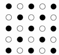
Figure 12.2: Illustration of checkerboard pattern for a 2d MRF. This allows for parallel updates.

conditional becomes

\[p(x\_i = +1 | x\_{-i}) = \frac{\prod\_{j \in \text{nbr}(i)} \psi\_{ij}(x\_i = +1, x\_j)}{\prod\_{j \in \text{nbr}(i)} \psi(x\_i = +1, x\_j) + \prod\_{j \in \text{nbr}(i)} \psi(x\_i = -1, x\_i)} \tag{12.25}\]

\[=\frac{\exp[J\sum\_{j\in\text{nbr}(i)} x\_j]}{\exp[J\sum\_{j\in\text{nbr}(i)} x\_j] + \exp[-J\sum\_{j\in\text{nbr}(i)} x\_j]}\tag{12.26}\]

\[=\frac{\exp[J\eta\_i]}{\exp[J\eta\_i] + \exp[-J\eta\_i]} = \sigma(2J\eta\_i) \tag{12.27}\]

where J is the coupling strength, ηⁱ ↭ & ^j↑nbr(i) ^xj , and ^ς(u)=1/(1 + ^e↓u) is the sigmoid function. Some samples from this model are shown in Figure 4.17.

It is easy to see that ηⁱ = xi(aⁱ → di), where aⁱ is the number of neighbors that agree with (have the same sign as) node i, and d^t is the number of neighbors who disagree. If this number is equal, the “forces” on xⁱ cancel out, so the full conditional is uniform. (Another way to see this is as follows: if we use xⁱ ↗ {0, 1}, this becomes p(xⁱ = +1|x↓ⁱ) = ς(J(aⁱ → di)), so if aⁱ = di, then we get 0.5 probability for each state.)

One application of Ising models is as a prior for binary image denoising problems. In particular, suppose y is a noisy version of x, and we wish to compute the posterior p(x|y) ↑ p(x)p(y|x), where ^p(x) is an Ising prior, and ^p(y|x) = ⁱ p(yi|xi) is a per-site likelihood term. Suppose this is a Gaussian. Let ¹i(xi) = ^N (yi|xi, ^ς2) be the corresponding “local evidence” term. The full conditional becomes

\[p(x\_i = +1 | \boldsymbol{x}\_{-i}, \boldsymbol{y}) = \frac{\exp[J\eta\_i]\psi\_i(+1)}{\exp[J\eta\_i]\psi\_i(+1) + \exp[-J\eta\_i]\psi\_i(-1)}\tag{12.28}\]

\[\dot{\lambda} = \sigma \left( 2J\eta\_i + \log \frac{\psi\_i(+1)}{\psi\_i(-1)} \right) \tag{12.29}\]

Now the probability of xⁱ entering each state is determined both by compatibility with its neighbors (the Ising prior) and compatibility with the data (the local likelihood term).

See Figure 12.3 for an example of this algorithm applied to a simple image denoising problem. The results are similar to the mean field results in Figure 10.9.

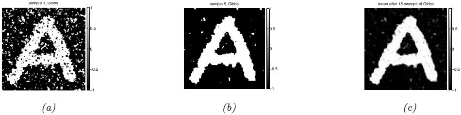
Figure 12.3: Example of image denoising using Gibbs sampling. We use an Ising prior with J = 1 and a Gaussian noise model with ω = 2. (a) Sample from the posterior after one sweep over the image. (b) Sample after 5 sweeps. (c) Posterior mean, computed by averaging over 15 sweeps. Compare to Figure 10.9 which shows the results of mean field inference. Generated by ising\_image\_denoise\_demo.ipynb.

12.3.4 Example: Gibbs sampling for Potts models

We can extend Section 12.3.3 to the Potts models as follows. Recall that the model has the following form:

\[p(\mathbf{z}) = \frac{1}{Z} \exp(-\mathcal{E}(\mathbf{z})) \tag{12.30}\]

\[\mathcal{E}(\mathbf{z}) = -J \sum\_{i \sim j} \mathbb{I}\left(x\_i = x\_j\right) \tag{12.31}\]

For a node i with neighbors nbr(i), the full conditional is thus given by

\[p(x\_i = k | \mathbf{x}\_{-i}) = \frac{\exp(J \sum\_{n \in \text{nbr}(i)} \mathbb{I}\left(x\_n = k\right))}{\sum\_{k'} \exp(J \sum\_{n \in \text{nbr}(i)} \mathbb{I}\left(x\_n = k'\right))}\tag{12.32}\]

So if J > 0, a node i is more likely to enter a state k if most of its neighbors are already in state k, corresponding to an attractive MRF. If J < 0, a node i is more likely to enter a di!erent state from its neighbors, corresponding to a repulsive MRF. See Figure 4.18 for some samples from this model created using this method.

12.3.5 Example: Gibbs sampling for GMMs

In this section, we consider sampling from a Bayesian Gaussian mixture model of the form

\[p(z=k, x|\theta) = \pi\_k \mathcal{N}(x|\mu\_k, \Sigma\_k) \tag{12.33}\]

\[p(\boldsymbol{\theta}) = \text{Dir}(\boldsymbol{\pi}|\boldsymbol{\alpha}) \prod\_{k=1}^{K} \mathcal{N}(\boldsymbol{\mu}\_k|\boldsymbol{m}\_0, \mathbf{V}\_0) \text{IW}(\boldsymbol{\Sigma}\_k, \mathbf{S}\_0, \boldsymbol{\nu}\_0) \tag{12.34}\]

12.3.5.1 Known parameters

Suppose, initially, that the parameters ω are known. We can easily draw independent samples from p(x|ω) by using ancestral sampling: first sample z and then x. However, for illustrative purposes, we

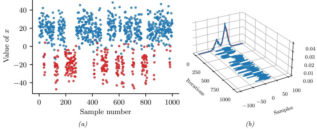
Figure 12.4: (a) Some samples from a mixture of two 1d Gaussians generated using Gibbs sampling. Color denotes the value of z, vertical location denotes the value of x. Horizontal axis represents time (sample number). (b) Traceplot of x over time, and the resulting empirical distribution is shown in blue. The true distribution is shown in red. Compare to Figure 12.1. Generated by mcmc\_gmm\_demo.ipynb.

will use Gibbs sampling to draw correlated samples. The full conditional for p(x|z = k, ω) is just N (x|µk, !k), and the full conditional for p(z = k|x) is given by Bayes’ rule:

\[p(z=k|\mathbf{x}, \boldsymbol{\theta}) = \frac{\pi\_k \mathcal{N}(\boldsymbol{x}|\boldsymbol{\mu}\_k, \boldsymbol{\Sigma}\_k)}{\sum\_{k'} \pi\_{k'} \mathcal{N}(\boldsymbol{x}|\boldsymbol{\mu}\_{k'}, \boldsymbol{\Sigma}\_{k'})} \tag{12.35}\]

An example of this procedure, applied to a mixture of two 1d Gaussians with means at →20 and +20, is shown in Figure 12.4. We see that the samples are auto correlated, meaning that if we are in state 1, we will likely stay in that state for a while, and generate values near µ1; then we will stochastically jump to state 2, and stay near there for a while, etc. (See Section 12.6.3 for a way to measure this.) By contrast, independent samples from the joint would not be correlated at all.

In Section 12.3.5.2, we modify this example to sample the parameters of the GMM from their posterior, p(ω|D), instead of sampling from p(D|ω).

12.3.5.2 Unknown parameters

Now suppose the parameters are unknown, so we want to fit the model to data. If we use a conditionally conjugate factored prior, then the full joint distribution is given by

\[p(\mathbf{z}, \mathbf{z}, \boldsymbol{\mu}, \boldsymbol{\Sigma}, \boldsymbol{\pi}) = p(\mathbf{z}|\mathbf{z}, \boldsymbol{\mu}, \boldsymbol{\Sigma}) p(\mathbf{z}|\boldsymbol{\pi}) p(\boldsymbol{\pi}) \prod\_{k=1}^{K} p(\mu\_k) p(\boldsymbol{\Sigma}\_k) \tag{12.36}\]

\[= \left(\prod\_{i=1}^{N} \prod\_{k=1}^{K} \left(\pi\_k \mathcal{N}(x\_i|\mu\_k, \Sigma\_k)\right)^{\mathbb{I}(z\_i=k)}\right) \times \tag{12.37}\]

\[\text{Dir}(\pi|\alpha)\prod\_{k=1}^{K}\mathcal{N}(\mu\_k|m\_0,\mathbf{V}\_0)\text{IW}(\Sigma\_k|\mathbf{S}\_0,\nu\_0)\tag{12.38}\]

We use the same prior for each mixture component.

The full conditionals are as follows. For the discrete indicators, we have

\[p(z\_i = k | \mathbf{x}\_i, \boldsymbol{\mu}, \boldsymbol{\Sigma}, \boldsymbol{\pi}) \propto \pi\_k \mathcal{N}(\boldsymbol{x}\_i | \boldsymbol{\mu}\_k, \boldsymbol{\Sigma}\_k) \tag{12.39}\]

For the mixing weights, we have (using results from Section 3.4.2)

\[p(\boldsymbol{\pi}|\boldsymbol{z}) = \text{Dir}(\{\alpha\_k + \sum\_{i=1}^{N} \mathbb{I}\left(z\_i = k\right)\}\_{k=1}^{K}) \tag{12.40}\]

For the means, we have (using results from Section 3.4.4.1)

\[p(\mu\_k | \Sigma\_k, \mathbf{z}, \mathbf{z}) = \mathcal{N}(\mu\_k | m\_k, \mathbf{V}\_k) \tag{12.41}\]

\[\mathbf{V}\_k^{-1} = \mathbf{V}\_0^{-1} + N\_k \boldsymbol{\Sigma}\_k^{-1} \tag{12.42}\]

\[\mathbf{m}\_k = \mathbf{V}\_k (\boldsymbol{\Sigma}\_k^{-1} N\_k \overline{\boldsymbol{x}}\_k + \mathbf{V}\_0^{-1} \boldsymbol{m}\_0) \tag{12.43}\]

\[N\_k \triangleq \sum\_{i=1}^N \mathbb{I}\left(z\_i = k\right) \tag{12.44}\]

\[\overline{x}\_k \stackrel{\Delta}{=} \frac{\sum\_{i=1}^N \mathbb{I}\left(z\_i = k\right) x\_i}{N\_k} \tag{12.45}\]

For the covariances, we have (using results from Section 3.4.4.2)

\[p(\Sigma\_k | \boldsymbol{\mu}\_k, \boldsymbol{z}, \boldsymbol{x}) = \text{IW}(\Sigma\_k | \mathbf{S}\_k, \boldsymbol{\nu}\_k) \tag{12.46}\]

\[\mathbf{S}\_{k} = \mathbf{S}\_{0} + \sum\_{i=1}^{N} \mathbb{I}\left(z\_{i} = k\right) (\boldsymbol{x}\_{i} - \boldsymbol{\mu}\_{k}) (\boldsymbol{x}\_{i} - \boldsymbol{\mu}\_{k})^{\mathsf{T}} \tag{12.47}\]

\[ \nu\_k = \nu\_0 + N\_k \tag{12.48} \]

12.3.6 Metropolis within Gibbs

When implementing Gibbs sampling, we have to sample from the full conditionals. If the distributions are conjugate, we can compute the full conditional in closed form, but in the general case, we will need to devise special algorithms to sample from the full conditionals.

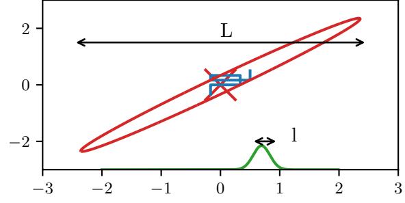
Figure 12.5: Illustration of potentially slow sampling when using Gibbs sampling for a skewed 2d Gaussian. Adapted from Figure 11.11 of [Bis06]. Generated by gibbs\_gauss\_demo.ipynb.

One approach is to use the MH algorithm; this is called Metropolis within Gibbs. In particular, to sample from x^s+1 ^{i ↔︎ p}(xi|x^s+1 1:i↓¹, ^{xs i}+1:D), we proceed in 3 steps:

1. Propose x^{↔︎ i} ↔︎ q(x^↔︎ i|x^s i )

2. Compute the acceptance probability Aⁱ = min(1, ϱi) where

\[\alpha\_i = \frac{p(\mathbf{x}\_{1:i-1}^{s+1}, \mathbf{x}\_i^\prime, \mathbf{x}\_{i+1:D}^s) / q(x\_i^\prime | x\_i^s)}{p(\mathbf{x}\_{1:i-1}^{s+1}, \mathbf{x}\_i^s, \mathbf{x}\_{i+1:D}^s) / q(x\_i^s | x\_i^\prime)}\tag{12.49}\]

3. Sample ^{u ↔︎ U}(0, 1) and set ^xs+1 ⁱ = x^{↔︎ i} if u<Ai, and set x^s+1 ⁱ = x^{s i} otherwise.

12.3.7 Blocked Gibbs sampling

Gibbs sampling can be quite slow, since it only updates one variable at a time (so-called single site updating). If the variables are highly correlated, the chain will move slowly through the state space. This is illustrated in Figure 12.5, where we illustrate sampling from a 2d Gaussian. The ellipse represents the covariance matrix. The size of the moves taken by Gibbs sampling is controlled by the variance of the conditional distributions. If the variance is ε along some coordinate direction, but the support of the distribution is L along this dimension, then we need O((L/ε)²) steps to obtain an independent sample.

In some cases we can e”ciently sample groups of variables at a time. This is called blocked Gibbs sampling [JKK95; WY02], and can make much bigger moves through the state space.

As an example, suppose we want to perform Bayesian inference for a state-space model, such as an HMM, i.e., we want to sample from

\[p(\theta, z | \mathbf{z}) \propto p(\theta) \prod\_{t=1}^{T} p(x\_t | z\_t, \theta) p(z\_t | z\_{t-1}, \theta) \tag{12.50}\]

We can use blocked Gibbs sampling, where we alternate between sampling from p(ω|z, x) and p(z|x, ω). The former is easy to do (assuming conjugate priors), since all variables in the model are observed (see Section 29.8.4.1). The latter can be done using forwards-filtering backwards-sampling (Section 9.2.7).

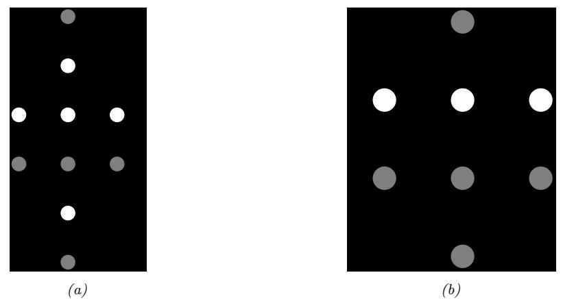
Figure 12.6: (a) A mixture model represented as an “unrolled” DPGM. (b) After integrating out the continuous latent parameters.

12.3.8 Collapsed Gibbs sampling

We can sometimes gain even greater speedups by analytically integrating out some of the unknown quantities. This is called a collapsed Gibbs sampler, and it tends to be more e”cient, since it is sampling in a lower dimensional space. This can result in lower variance, as discussed in Section 11.6.2.

As an example, consider a GMM with a fully conjugate prior. This can be represented as a DPGM as shown in Figure 12.6a. Since the prior is conjugate, we can analytically integrate out the model parameters µk, !k, and ▷, so the only remaining hidden variables are the discrete indicator variables z. However, once we integrate out ▷, all the zⁱ nodes become inter-dependent. Similarly, once we integrate out ω^k = (µk, !k), all the xⁱ nodes become inter-dependent, as shown in Figure 12.6b. Nevertheless, we can easily compute the full conditionals, and hence implement a Gibbs sampler, as we explain below. In particular, the full conditional for the latent indicators is given by

\[p(z\_i = k | \mathbf{z}\_{-i}, \mathbf{z}, \alpha, \beta) \propto p(z\_i = k | \mathbf{z}\_{-i}, \alpha, \beta) p(\mathbf{z} | z\_i = k, \mathbf{z}\_{-i}, \mathbf{z} | \beta) \tag{12.51}\]

\[\propto p(z\_i = k | \mathbf{z}\_{-i}, \alpha) p(x\_i | \mathbf{z}\_{-i}, z\_i = k, \mathbf{z}\_{-i}, \beta)\]

\[p(\mathbf{z}\_{-i}|z\_{i}=\pi; \mathbb{K}, \mathbf{z}\_{-i}, \beta) \tag{12.52}\]

\[\mathbf{x} \propto p(z\_i = k | \mathbf{z}\_{-i}, \mathbf{a}) p(\mathbf{z}\_i | \mathbf{z}\_{-i}, z\_i = k, \mathbf{z}\_{-i}, \boldsymbol{\beta}) \tag{12.53}\]

where ⇀ = (m0, V0, S0, 40) are the hyper-parameters for the class-conditional densities. We now discuss how to compute these terms.

Suppose we use a symmetric prior of the form ▷ ↔︎ Dir(↼), where ϱ^k = ϱ/K, for the mixing weights. Then we can obtain the first term in Equation (12.53), from Equation (3.96), where

\[p(z\_1, \ldots, z\_N | \alpha) = \frac{\Gamma(\alpha)}{\Gamma(N + \alpha)} \prod\_{k=1}^{K} \frac{\Gamma(N\_k + \alpha/K)}{\Gamma(\alpha/K)} \tag{12.54}\]

Hence

\[p(z\_i = k | \mathbf{z}\_{-i}, \alpha) = \frac{p(\mathbf{z}\_{1:N} | \alpha)}{p(\mathbf{z}\_{-i} | \alpha)} = \frac{\frac{1}{\Gamma(N + \alpha)}}{\frac{1}{\Gamma(N + \alpha - 1)}} \times \frac{\Gamma(N\_k + \alpha/K)}{\Gamma(N\_{k,-i} + \alpha/K)} \tag{12.55}\]

\[=\frac{\Gamma(N+\alpha-1)}{\Gamma(N+\alpha)}\frac{\Gamma(N\_{k,-i}+1+\alpha/K)}{\Gamma(N\_{k,-i}+\alpha/K)}=\frac{N\_{k,-i}+\alpha}{N+\alpha-1}\tag{12.56}\]

where ^Nk,↓ⁱ ↭ & ⁿ⇒=^{i I}(z^{n = k}) = ^{Nk → 1}, and where we exploited the fact that $(^x + 1) = ^x$(x).

To obtain the second term in Equation (12.53), which is the posterior predictive distribution for xⁱ given all the other data and all the assignments, we use the fact that

\[p(x\_i | x\_{-i}, x\_{-i}, z\_i = k, \beta) = p(x\_i | \mathcal{D}\_{-i,k}, \beta) \tag{12.57}\]

where D↓i,k = {x^j : z^j = k, j ′= i} is all the data assigned to cluster k except for xi. If we use a conjugate prior for ωk, we can compute p(xi|D↓i,k, ⇀) in closed form. Furthermore, we can e”ciently update these predictive likelihoods by caching the su”cient statistics for each cluster. To compute the above expression, we remove xi’s statistics from its current cluster (namely zi), and then evaluate xⁱ under each cluster’s posterior predictive distribution. Once we have picked a new cluster, we add xi’s statistics to this new cluster.

Some pseudo-code for one step of the algorithm is shown in Algorithm 12.2, based on [Sud06, p94]. (We update the nodes in random order to improve the mixing time, as suggested in [RS97b].) We can initialize the sample by sequentially sampling from p(zi|z1:i↓¹, x1:i). In the case of GMMs, both the naive sampler and collapsed sampler take O(NKD) time per step.

	Algorithm 12.2: Collapsed Gibbs sampler for a mixture model
1 for each i =1: N in random order do
2	Remove xi’s su”cient statistics from old cluster zi
3	for each k =1: K do
4	Compute pk(xi ⇀) = p(xi {xj : zj = k, j ′= i}, ⇀)
5	Compute p(zi = k z↓i, ϱ) ↑ (Nk,↓i + ϱ/K)pk(xi)
6	Sample zi ↔︎ p(zi ·)
7	Add xi’s su”cient statistics to new cluster zi

The primary advantage of using the collapsed sampler is that it extends to the case where we have an “infinite” number of mixture components, as in the Dirichlet process mixture model of Supplementary Section 31.2.2.

12.4 Auxiliary variable MCMC

Sometimes we can dramatically improve the e”ciency of sampling by introducing auxiliary variables, in order to reduce correlation between the original variables. If the original variables are denoted by x, and the auxiliary variables by v, then the augmented distribution becomes p(x, v). We assume it is easier to sample from this than the marginal distribution p(x). If so, we can draw joint samples (x^s, ^vs) ^{↔︎ p}(x, ^v), and then just “throw away” the ^vs, and the result will be samples from the desired marginal, ^{xs ↔︎} & ^v p(x, v). We give some examples of this below.

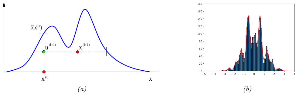
Figure 12.7: Slice sampling. (a) Illustration of one step of the algorithm in 1d. Given a previous sample xⁱ , we sample uⁱ+1 uniformly on [0, f(xⁱ )], where f = p˜ is the (unnormalized) target density. We then sample xⁱ+1 along the slice where ^f(x) ^{⇔ ui}+1. From Figure 15 of [And+03]. Used with kind permission of Nando de Freitas. (b) Output of slice sampling applied to a 1d distribution. Generated by slice\_sampling\_demo\_1d.ipynb.

Figure 12.8: Posterior for binomial regression for 1d data. Left: slice sampling approximation. Right: grid approximation. Generated by slice\_sampling\_demo\_2d.ipynb.

12.4.1 Slice sampling

Consider sampling from a univariate, but multimodal, distribution p(x) = p˜(x)/Zp, where p˜(x) is unnormalized, and Z^p = / p˜(x)dx. We can sometimes improve the ability to make large moves by adding a uniform auxiliary variable v. We define the joint distribution as follows:

\[\hat{p}(x,v) = \begin{cases} 1/Z\_p & \text{if } 0 \le v \le \tilde{p}(x) \\ 0 & \text{otherwise} \end{cases} \tag{12.58}\]

The marginal distribution over x is given by

\[\int \widehat{p}(x,v)dv = \int\_0^{\widetilde{p}(x)} \frac{1}{Z\_p} dv = \frac{\widetilde{p}(x)}{Z\_p} = p(x) \tag{12.59}\]

so we can sample from p(x) by sampling from pˆ(x, v) and then ignoring v. To do this, we will use a technique called slice sampling [Nea03].

This works as follows. Given previous sample xⁱ , we sample vi+1 from

\[p(v|x^i) = U\_{[0, \tilde{p}(x^i)]}(v) \tag{12.60}\]

This amounts to uniformly picking a point on the vertical line between 0 and p˜(xⁱ ), We use this to construct a “slice” of the density at or above this height, by computing ^Ai+1 = {^x : ^p˜(x) ^{≃ vi}+1}. We then sample xⁱ+1 uniformly from ths set. See Figure 12.7(a) for an illustration.

To compute the level set A, we can use an iterative search procedure called stepping out, in which we start with an interval ^xmin ⇐ ^x ⇐ ^xmax around the current point ^xi of some width, and then we keep extending it until the endpoints fall outside the slice. We can then use rejection sampling to sample from the interval. For the details, see [Nea03].

To apply the method to multivariate distributions, we sample one extra auxiliary variable for each dimension. Thus we perfom 2D sampling operations to draw a single joint sample, where D is the number of random variables. The advantage of this over Gibbs sampling applied to the original (non-augmented) distribution is that it only needs access to the unnormalized joint, not the full-conditionals.

Figure 12.7(b) illustrates the algorithm in action on a synthetic 1d problem. Figure 12.8 illustrates its behavior on a slightly harder problem, namely binomial logistic regression. The model has the form yⁱ ↔︎ Bin(ni, logit(↼¹ + ↼2xi)). We use a vague Gaussian prior for the ↼^j ’s. On the left we show the slice sampling approximation to the posterior, and on the right we show a grid-based approximation, as a simple deteterministic proxy for the true posterior. We see a close correspondence.

12.4.2 Swendsen-Wang

Consider an Ising model of the following form: p(x) = ¹ Z ^e &(xe), where x^e = (xi, x^j ) for edge ^e = (i, j), ^xi ↗ {+1, ^→1}, and the edge potential is defined by ) ^{eJ e}↓^J e↓^J e^J * , where J is the edge strength. In Section 12.3.3, we discussed how to apply Gibbs sampling to this model. However, this can be slow when J is large in absolute value, because neighboring states can be highly correlated. The Swendsen-Wang algorithm [SW87b] is an auxiliary variable MCMC sampler which mixes much faster, at least for the case of attractive or ferromagnetic models, with J > 0.

Suppose we introduce auxiliary binary variables, one per edge.4 These are called bond variables, and will be denoted by v. We then define an extended model p(x, v) of the form p(x, v) = 1 Z↑ ^e &(xe, ve), where v^e ↗ {0, 1}, and we define the new edge potentials as follows:

\[ \Psi(\mathbf{z}\_e, v\_e = 0) = \begin{pmatrix} e^{-J} & e^{-J} \\ e^{-J} & e^{-J} \end{pmatrix}, \\ \Psi(\mathbf{z}\_e, v\_e = 1) = \begin{pmatrix} e^J - e^{-J} & 0 \\ 0 & e^J - e^{-J} \end{pmatrix} \tag{12.61} \]

It is clear that &^{1 v}e=0 &(xe, ve) = &(xe), and hence that & ^v p(x, v) = p(x), as required.

Fortunately, it is easy to apply Gibbs sampling to this extended model. The full conditional p(v|x) factorizes over the edges, since the bond variables are conditionally independent given the node

^4. Our presentation of the method is based on notes by David MacKay, available from http://www.inference.phy. cam.ac.uk/mackay/itila/swendsen.pdf.

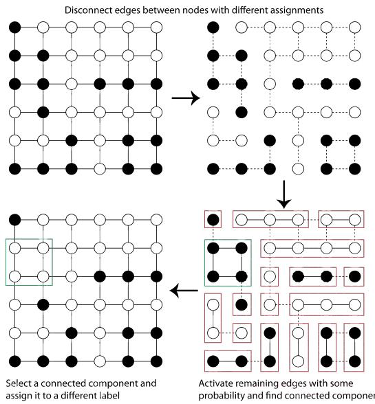
Figure 12.9: Illustration of the Swendsen-Wang algorithm on a 2d grid. Used with kind permission of Kevin Tang.

variables. Furthermore, the full conditional p(ve|xe) is simple to compute: if the nodes on either end of the edge are in the same state (xⁱ = ^xj ), we set the bond ^ve to 1 with probability ^p = 1 ^{→ e}↓2^J , otherwise we set it to 0. In Figure 12.9 (top right), the bonds that could be turned on (because their corresponding nodes are in the same state) are represented by dotted edges. In Figure 12.9 (bottom right), the bonds that are randomly turned on are represented by solid edges.

To sample p(x|v), we proceed as follows. Find the connected components defined by the graph induced by the bonds that are turned on. (Note that a connected component may consist of a singleton node.) Pick one of these components uniformly at random. All the nodes in each such component must have the same state. Pick a state ±1 uniformly at random, and set all the variables in this component to adopt this new state. This is illustrated in Figure 12.9 (bottom right), where the green square denotes the selected connected component; we set all the nodes within this square to white, to get the bottom left configuration.

It should be intuitively clear that Swendsen-Wang makes much larger moves through the state space than Gibbs sampling. The gains are exponentially large for certain settings of the edge parameter. More precisely, let the edge strength be parameterized by J/T, where T > 0 is a computational temperature. For large T, the nodes are roughly independent, so both methods work equally well. However, as T approaches a critical temperature Tc, the typical states of the system have very long correlation lengths, and Gibbs sampling takes a very long time to generate independent samples. As the temperature continues to drop, the typical states are either all on or all o!. The frequency with which Gibbs sampling moves between these two modes is exponentially small. By contrast, SW mixes rapidly at all temperatures.

Unfortunately, if any of the edge weights are negative, J < 0, the system is frustrated, and there

are exponentially many modes, even at low temperature. SW does not work very well in this setting, since it tries to force many neighboring variables to have the same state. In fact, sampling from these kinds of frustrated systems is provably computationally hard for any algorithm [JS93; JS96].

12.5 Hamiltonian Monte Carlo (HMC)

Many MCMC algorithms perform poorly in high dimensional spaces, because they rely on a form of random search based on local perturbations. In this section, we discuss a method known as Hamiltonian Monte Carlo or HMC, that leverages gradient information to guide the local moves. This is an auxiliary variable method (Section 12.4) derived from physics [Dua+87; Nea93; Mac03; Nea10; Bet17].5 In particular, the method builds on Hamiltonian mechanics, which we describe below.

12.5.1 Hamiltonian mechanics

Consider a particle rolling around an energy landscape. We can characterize the motion of the particle in terms of its position ^ω ↗ ^RD (often denoted by ^q) and its momentum ^v ↗ ^RD (often denoted by p). The set of possible values for (ω, v) is called the phase space. We define the Hamiltonian function for each point in phase space as follows:

\[\mathcal{H}(\theta, \mathbf{v}) \triangleq \mathcal{E}(\theta) + \mathcal{K}(\mathbf{v}) \tag{12.62}\]

where E(ω) is the potential energy, K(v) is the kinetic energy, and the Hamiltonian is the total energy. In a physical setting, the potential energy is due to the pull of gravity, and the momentum is due to the motion of the particle. In a statistical setting, we often take the potential energy to be

\[\mathcal{E}(\boldsymbol{\theta}) = -\log \bar{p}(\boldsymbol{\theta})\tag{12.63}\]

where p˜(ω) is a possibly unnormalized distribution, such as p(ω, D), and the kinetic energy to be

\[\mathcal{K}(\mathbf{v}) = \frac{1}{2} \mathbf{v}^{\mathsf{T}} \boldsymbol{\Sigma}^{-1} \mathbf{v}\]

where ! is a positive definite matrix, known as the inverse mass matrix.

Stable orbits are defined by trajectories in phase space that have a constant energy. The trajectory of a particle within an energy level set can be obtained by solving the following continuous time di!erential equations, known as Hamilton’s equations:

\[\begin{aligned} \frac{d\theta}{dt} &= \frac{\partial \mathcal{H}}{\partial \mathbf{v}} = \frac{\partial \mathcal{K}}{\partial \mathbf{v}}\\ \frac{d\mathbf{v}}{dt} &= -\frac{\partial \mathcal{H}}{\partial \boldsymbol{\theta}} = -\frac{\partial \mathcal{E}}{\partial \boldsymbol{\theta}} \end{aligned} \tag{12.65}\]

To see why energy is conserved, note that

\[\frac{d\mathcal{H}}{dt} = \sum\_{i=1}^{D} \left[ \frac{\partial \mathcal{H}}{\partial \theta\_i} \frac{d\theta\_i}{dt} + \frac{\partial \mathcal{H}}{\partial \mathbf{v}\_i} \frac{d\mathbf{v}\_i}{dt} \right] = \sum\_{i=1}^{D} \left[ \frac{\partial \mathcal{H}}{\partial \theta\_i} \frac{\partial \mathcal{H}}{\partial \mathbf{v}\_i} - \frac{\partial \mathcal{H}}{\partial \theta\_i} \frac{\partial \mathcal{H}}{\partial \mathbf{v}\_i} \right] = 0 \tag{12.66}\]

^5. The method was originally called hybrid MC [Dua+87]. It was introduced to the statistics community in [Nea93], and was renamed to Hamiltonian MC in [Mac03].

Intuitively, we can understand this result as follows: a satellite in orbit around a planet will “want” to continue in a straight line due to its momentum, but will get pulled in towards the planet due to gravity, and if these forces cancel, the orbit is stable. If the satellite starts spiraling towards the planet, its kinetic energy will increase but its potential energy will decrease.

Note that the mapping from (ω(t), v(t)) to (ω(t+s), v(t+s)) for some time increment s is invertible for small enough time steps. Furthermore, this mapping is volume preserving, so has a Jacobian determinant of 1. (See e.g., [BZ20, p287] for a proof.) These facts will be important later when we turn this system into an MCMC algorithm.

12.5.2 Integrating Hamilton’s equations

In this section, we discuss how to simulate Hamilton’s equations in discrete time.

12.5.2.1 Euler’s method

The simplest way to model the time evolution is to update the position and momentum simultaneously by a small amount, known as the step size η:

\[\mathbf{v}\_{t+1} = \mathbf{v}\_t + \eta \frac{dv}{dt}(\boldsymbol{\theta}\_t, \mathbf{v}\_t) = \mathbf{v}(t) - \eta \frac{\partial \mathcal{E}(\boldsymbol{\theta}\_t)}{\partial \boldsymbol{\theta}} \tag{12.67}\]

\[\theta\_{t+1} = \theta\_t + \eta \frac{d\theta}{dt}(\theta\_t, v\_t) = \theta\_t + \eta \frac{\partial \mathcal{K}(v\_t)}{\partial v} \tag{12.68}\]

If the kinetic energy has the form in Equation (12.64) then the second expression simplifies to

\[ \theta\_{t+1} = \theta\_t + \eta \Sigma^{-1} v\_{t+1} \tag{12.69} \]

This is known as Euler’s method.

12.5.2.2 Modified Euler’s method

The modified Euler’s method is slightly more accurate, and works as follows: First update the momentum, and then update the position using the new momentum:

\[\mathbf{v}\_{t+1} = \mathbf{v}\_t + \eta \frac{d\mathbf{v}}{dt}(\theta\_t, \mathbf{v}\_t) = \mathbf{v}\_t - \eta \frac{\partial \mathcal{E}(\theta\_t)}{\partial \theta} \tag{12.70}\]

\[\theta\_{t+1} = \theta\_t + \eta \frac{d\theta}{dt}(\theta\_t, v\_{t+1}) = \theta\_t + \eta \frac{\partial \mathbb{K}(v\_{t+1})}{\partial v} \tag{12.71}\]

Unfortunately, the asymmetry of this method can cause some theoretical problems (see e.g., [BZ20, p287]) which we resolve below.

12.5.2.3 Leapfrog integrator

In this section, we discuss the leapfrog integrator, which is a symmetrized version of the modified Euler method. We first perform a “half” update of the momentum, then a full update of the position,

and then finally another “half” update of the momentum:

\[v\_{t+1/2} = v\_t - \frac{\eta}{2} \frac{\partial \mathcal{E}(\boldsymbol{\theta}\_t)}{\partial \boldsymbol{\theta}}\tag{12.72}\]

\[\boldsymbol{\theta}\_{t+1} = \boldsymbol{\theta}\_t + \eta \frac{\partial \mathbb{C}(\boldsymbol{v}\_{t+1/2})}{\partial \boldsymbol{v}} \tag{12.73}\]

\[\mathbf{v}\_{t+1} = \mathbf{v}\_{t+1/2} - \frac{\eta}{2} \frac{\partial \mathcal{E}(\boldsymbol{\theta}\_{t+1})}{\partial \boldsymbol{\theta}} \tag{12.74}\]

If we perform multiple leapfrog steps, it is equivalent to performing a half step update of v at the beginning and end of the trajectory, and alternating between full step updates of ω and v in between.

12.5.2.4 Higher order integrators

It is possible to define higher order integrators that are more accurate, but take more steps. For details, see [BRSS18].

12.5.3 The HMC algorithm

We now describe how to use Hamiltonian dynamics to define an MCMC sampler in the expanded state space (ω, v). The target distribution has the form

\[p(\theta, \boldsymbol{v}) = \frac{1}{Z} \exp\left[-\mathcal{H}(\theta, \boldsymbol{v})\right] = \frac{1}{Z} \exp\left[-\mathcal{E}(\theta) - \frac{1}{2}\boldsymbol{v}^{\mathsf{T}}\boldsymbol{\Sigma}\boldsymbol{v}\right] \tag{12.75}\]

The marginal distribution over the latent variables of interest has the form

\[p(\boldsymbol{\theta}) = \int p(\boldsymbol{\theta}, \boldsymbol{v}) d\boldsymbol{v} = \frac{1}{Z\_q} e^{-\mathcal{E}(\boldsymbol{\theta})} \int \frac{1}{Z\_p} e^{-\frac{1}{2} \boldsymbol{v}^T \boldsymbol{\Sigma} \boldsymbol{v}} d\boldsymbol{v} = \frac{1}{Z\_q} e^{-\mathcal{E}(\boldsymbol{\theta})} \tag{12.76}\]

Suppose the previous state of the Markov chain is (ω^t↓¹, v^t↓¹). To sample the next state, we proceed as follows. We set the initial position to ω^{↔︎ 0} = ω^t↓¹, and sample a new random momentum, v↔︎ ⁰ ↔︎ N (0, !). We then initialize a random trajectory in the phase space, starting at (ω^{↔︎ 0}, v^{↔︎ 0}), and followed for L leapfrog steps, until we get to the final proposed state (ω→, v→)=(ω^{↔︎ L}, v^{↔︎ L}). If we have simulated Hamiltonian mechanics correctly, the energy should be the same at the start and end of this process; if not, we say the HMC has diverged, and we reject the sample. If the energy is constant, we compute the MH acceptance probability

\[\alpha = \min\left(1, \frac{p(\boldsymbol{\theta}^\*, \boldsymbol{v}^\*)}{p(\boldsymbol{\theta}\_{t-1}, \boldsymbol{v}\_{t-1})}\right) = \min\left(1, \exp\left[-\mathcal{H}(\boldsymbol{\theta}^\*, \boldsymbol{v}^\*) + \mathcal{H}(\boldsymbol{\theta}\_{t-1}, \boldsymbol{v}\_{t-1})\right]\right) \tag{12.77}\]

(The transition probabilities cancel since the proposal is reversible.) Finally, we accept the proposal by setting (ωt, vt)=(ω→, v→) with probability ϱ, otherwise we set (ωt, vt)=(ω^t↓¹, v^t↓1). (In practice we don’t need to keep the momentum term, it is only used inside of the leapfrog algorithm.) See Algorithm 12.3 for the pseudocode.6

^6. There are many high-quality implementations of HMC. For example, BlackJAX in JAX.

Algorithm 12.3: Hamiltonian Monte Carlo

¹ for t =1: T do ² Generate random momentum vt↓¹ ↔︎ N (0, !) ³ Set (ω^{↔︎ 0}, v^{↔︎ 0})=(ωt↓1, vt↓1) ⁴ Half step for momentum: v^↔︎ 1 2 = v↔︎ ^{0 → ▷ 2} ⇒E(ω^↔︎ 0) ⁵ for l =1: L → 1 do ⁶ ω^{↔︎ l} = ω^{↔︎ l}↓^{1 + η}!^↓1v^↔︎ l↓1/2 ⁷ v^{↔︎ l}+1/² = v^{↔︎ l}↓1/^{2 → η}⇒E(ω^↔︎ l) ⁸ Full step for location: ω^{↔︎ L} = ω^{↔︎ L}↓^{1 + η}!^↓1v^↔︎ L↓1/2 ⁹ Half step for momentum: v^{↔︎ L} = v^{↔︎ L}↓1/^{2 → ▷ 2} ⇒E(ω^↔︎ L) ¹⁰ Compute proposal (ω→, v→)=(ω^{↔︎ L}, v^↔︎ L) ¹¹ Compute ϱ = min (1, exp[→H(ω→, v→) + H(ω^t↓¹, v^t↓¹)]) ¹² Set ω^t = ω^→ with probability ϱ, otherwise ω^t = ω^t↓¹.

We need to sample a new momentum at each iteration to satisfy ergodicity. To see why, recall that ^H(ω, ^v) stays approximately constant as we move through phase space. If ^H(ω, ^v) = ^E(ω) + ^{1 2} v^T!v, then clearly E(ω) ⇐ H(ω, v) = h for all locations ω along the trajectory. Thus the sampler cannot reach states where E(ω) > h. To ensure the sampler explores the full space, we must pick a random momentum at the start of each iteration.

12.5.4 Tuning HMC

We need to specify three hyperparameters for HMC: the number of leapfrog steps L, the step size η, and the covariance !.

12.5.4.1 Choosing the number of steps using NUTS

We want to choose the number of leapfrog steps L to be large enough that the algorithm explores the level set of constant energy, but without doubling back on itself, which would waste computation, due to correlated samples. Fortunately, there is an algorithm, known as the no-U-turn sampler or NUTS algorithm [HG14], which can adaptively choose L for us.

12.5.4.2 Choosing the step size

When ! = I, the ideal step size η should be roughly equal to the width of E(ω) in the most constrained direction of the local energy landscape. For a locally quadratic potential, this corresponds to the square root of the smallest marginal standard deviation of the local covariance matrix. (If we think of the energy surface as a valley, this corresponds to the direction with the steepest sides.) A step size much larger than this will cause moves that are likely to be rejected because they move to places which increase the potential energy too much. On the other hand, if the step size is too low, the proposal distribution will not move much from the starting position, and the algorithm will be very slow.

In [BZ20, Sec 9.5.4] they recommend the following heuristic for picking η: set ! = I and L = 1, and then vary η until the acceptance rates are in the range of 40%–80%. Of course, di!erent step sizes might be needed in di!erent parts of the state space. In this case, we can use learning rate schedules from the optimization literature, such as cyclical schedules [Zha+20e].

12.5.4.3 Choosing the covariance (inverse mass) matrix

To allow for larger step sizes, we can use a smarter choice for !, also called the inverse mass matrix. One way to estimate a fixed ! is to run HMC with ! = I for a warm-up period, until the chain is “burned in” (see Section 12.6); then we run for a few more steps, so we can compute the empirical covariance matrix using ! = E (ω → ω)(ω → ω) T . In [Hof+19] they propose a method called the NeuTra HMC algorithm which “neutralizes” bad geometry by learning an inverse autoregressive flow model (Section 23.2.4.3) in order to map the warped distribution to an isotropic Gaussian. This is often an order of magnitude faster than vanilla HMC.

12.5.5 Riemann manifold HMC

If we let the covariance matrix change as we move position, so ! is a function of ω, the method is known as Riemann manifold HMC or RM-HMC [GC11; Bet13], since the moves follow a curved manifold, rather than the flat manifold induced by a constant !.

A natural choice for the covariance matrix is to use the Hessian at the current location, to capture the local geometry:

\[ \Delta(\theta) = \nabla^2 \mathcal{E}(\theta) \tag{12.78} \]

Since this is not always positive definite, an alternative, that can be used for some problems, is to use the Fisher information matrix (Section 3.3.4), given by

\[\Sigma(\boldsymbol{\theta}) = -\mathbb{E}\_{p(\boldsymbol{x}|\boldsymbol{\theta})} \left[ \nabla^2 \log p(\boldsymbol{x}|\boldsymbol{\theta}) \right] \tag{12.79}\]

Once we have computed !(ω), we can compute the kinetic energy as follows:

\[\mathcal{K}(\boldsymbol{\theta}, \boldsymbol{v}) = \frac{1}{2} \log((2\pi)^{D} |\boldsymbol{\Sigma}(\boldsymbol{\theta})|) + \frac{1}{2} \boldsymbol{v}^{\mathsf{T}} \boldsymbol{\Sigma}(\boldsymbol{\theta}) \boldsymbol{v} \tag{12.80}\]

Unfortunately the Hamiltonian updates of ω and v are no longer separable, which makes the RM-HMC algorithm more complex to implement, so it is not widely used.

12.5.6 Langevin Monte Carlo (MALA)

A special case of HMC occurs when we take L = 1 leapfrog steps. This is known as Langevin Monte Carlo (LMC), or the Metropolis adjusted Langevin algorithm (MALA) [RT96]. This gives rise to the simplified algorithm shown in Algorithm 12.4.

A further simplification is to eliminate the MH acceptance step. In this case, the update becomes

\[\theta\_t = \theta\_{t-1} - \frac{\eta^2}{2} \Sigma^{-1} \nabla \mathcal{E}(\theta\_{t-1}) + \eta \Sigma^{-1} \upsilon\_{t-1} \tag{12.81}\]

\[\mathbf{f}\_t = \theta\_{t-1} - \frac{\eta^2}{2} \boldsymbol{\Sigma}^{-1} \boldsymbol{\nabla} \mathcal{E}(\theta\_{t-1}) + \eta \sqrt{\boldsymbol{\Sigma}^{-1}} \mathbf{c}\_{t-1} \tag{12.82}\]

Algorithm 12.4: Langevin Monte Carlo

¹ for t =1: T do

• ² Generate random momentum vt↓¹ ↔︎ N (0, !)
• ^{3 ω→ = ω}t↓^{1 → ▷2 2} !↓1⇒E(ωt↓1) + ^η!↓1vt↓^{1 4 v→ = v}t↓^{1 → ▷ 2 ⇒}E(ωt↓1) ^{→ ▷ 2} ⇒E(ω→)
• ⁵ Compute ϱ = min (1, exp[→H(ω→, v→)]/ exp[→H(ω^t↓¹, v^t↓¹)])
• ⁶ Set ω^t = ω^→ with probability ϱ, otherwise ω^t = ω^t↓¹.

where v^t↓¹ ↔︎ N (0, !) and ,^t↓¹ ↔︎ N (0, I). This is just like gradient descent with added noise. If we set ! to be the Fisher information matrix, this becomes natural gradient descent (Section 6.4) with added noise. If we approximate the gradient with a stochastic gradient, we get a method known as SGLD, or stochastic gradient Langevin descent (see Section 12.7.1 for details).

Now suppose ! ^{= I}, and we set ^{η = ∝}2. In continuous time, we get the following stochastic di!erential equation (SDE), known as Langevin di!usion:

\[d\theta\_t = -\nabla \mathcal{E}(\theta\_t)dt + \sqrt{2}d\mathbf{B}\_t \tag{12.83}\]

where B^t represents D-dimensional Brownian motion. If we use this to generate the samples, the method is known as the unadjusted Langevin algorithm or ULA [Par81; RT96].

12.5.7 Connection between SGD and Langevin sampling

In this section, we discuss a deep connection between stochastic gradient descent (SGD) and Langevin sampling, following the presentation of [BZ20, Sec 10.2.3].

Consider the minimization of the additive loss

\[\mathcal{L}(\boldsymbol{\theta}) = \sum\_{n=1}^{N} \mathcal{L}\_n(\boldsymbol{\theta}) \tag{12.84}\]

For example, we may define Ln(ω) = → log p(yn|xn, ω.) We will use a minibatch approximation to the gradients:

\[\nabla\_B \mathcal{L}(\boldsymbol{\theta}) = \frac{1}{B} \sum\_{n \in \mathcal{S}} \nabla \mathcal{L}\_n(\boldsymbol{\theta}) \tag{12.85}\]

where S = {i1,…,iB} is a randomly chosen set of indices of size B. For simplicity of analysis, we assume the indices are chosen with replacement from {1,…,N}.

Let us define the (scaled) error (due to minibatching) in the estimated gradient by

\[w\_t \triangleq \sqrt{\eta} (\nabla \mathcal{L}(\theta\_t) - \nabla\_B \mathcal{L}(\theta\_t)) \tag{12.86}\]

This is called the di!usion term. Then we can rewrite the SGD update as

\[\theta\_{t+1} = \theta\_t - \eta \nabla\_B \mathcal{L}(\theta\_t) = \theta\_t - \eta \nabla \mathcal{L}(\theta\_t) + \sqrt{\eta} \mathbf{v}\_t \tag{12.87}\]

The di!usion term v^t has mean 0, since

\[\mathbb{E}\left[\nabla\_B \mathcal{L}(\boldsymbol{\theta})\right] = \frac{1}{B} \sum\_{j=1}^{B} \mathbb{E}\left[\nabla \mathcal{L}\_{i\_j}(\boldsymbol{\theta})\right] = \frac{1}{B} \sum\_{j=1}^{B} \nabla \mathcal{L}(\boldsymbol{\theta}) = \nabla \mathcal{L}(\boldsymbol{\theta}) \tag{12.88}\]

To compute the variance of the di!usion term, note that

\[\mathbb{V}\left[\nabla\_B \mathcal{L}(\boldsymbol{\theta})\right] = \frac{1}{B^2} \sum\_{j=1}^{B} \mathbb{V}\left[\nabla \mathcal{L}\_{i\_j}(\boldsymbol{\theta})\right] \tag{12.89}\]

where

\[\mathbb{E}\left[\nabla\mathcal{L}\_{i\_j}(\boldsymbol{\theta})\right] = \mathbb{E}\left[\nabla\mathcal{L}\_{i\_j}(\boldsymbol{\theta})\nabla\mathcal{L}\_{i\_j}(\boldsymbol{\theta})^\mathsf{T}\right] - \mathbb{E}\left[\nabla\mathcal{L}\_{i\_j}(\boldsymbol{\theta})\right]\mathbb{E}\left[\nabla\mathcal{L}\_{i\_j}(\boldsymbol{\theta})^\mathsf{T}\right] \tag{12.90}\]

\[= \left(\frac{1}{N} \sum\_{n=1}^{N} \nabla \mathcal{L}\_n(\boldsymbol{\theta}) \nabla \mathcal{L}\_n(\boldsymbol{\theta})^\mathsf{T}\right) - \nabla \mathcal{L}(\boldsymbol{\theta}) \nabla \mathcal{L}(\boldsymbol{\theta})^\mathsf{T} \triangleq \mathbf{D}(\boldsymbol{\theta}) \tag{12.91}\]

where D(ω) is called the di!usion matrix. Hence V [vt] = ^{▷ B} D(ωt).

[LTW15] prove that the following continuous time stochastic di!erential equation is a first-order approximation of minibatch SGD (assuming the loss function is Lipschitz continuous):

\[d\theta(t) = -\nabla \mathcal{L}(\theta(t))dt + \sqrt{\frac{\eta}{B} \mathbf{D}(\theta\_t)} d\mathbf{B}(t) \tag{12.92}\]

where B(t) is Brownian motion. Thus the noise from minibatching causes SGD to act like a Langevin sampler. (See [Hu+17] for more information.)

The scale factor for the noise, τ = ^{▷ B} , plays the role of temperature. Thus we see that using a smaller batch size is like using a larger temperature; the added noise ensures that SGD avoids going into narrow ravines, and instead spends most of its time in flat minima which have better generalization performance [Kes+17]. See Section 17.4.1 for more discussion of this point.

12.5.8 Applying HMC to constrained parameters

To apply HMC, we require that all the latent quantities be continuous (real-valued) and have unconstrained support, i.e., ^ω ↗ ^RD, so discrete latent variables need to be marginalized out (although some recent work, such as [NDL20; Zho20], relaxes this requirement).

As an example of how this can be done, consider a GMM. We can easily write the likelihood without discrete latents as follows:

\[p(x\_n|\theta) = \sum\_{k=1}^{K} \pi\_k \mathcal{N}(x\_n|\mu\_k, \Sigma\_k) \tag{12.93}\]

The corresponding “collapsed” model is shown in Figure 12.10(b). (Note that this is the opposite of Section 12.3.8, where we integrated out the continuous parameters in order to apply Gibbs sampling to the discrete latents.) We can apply similar techniques to other discrete latent variable models. For

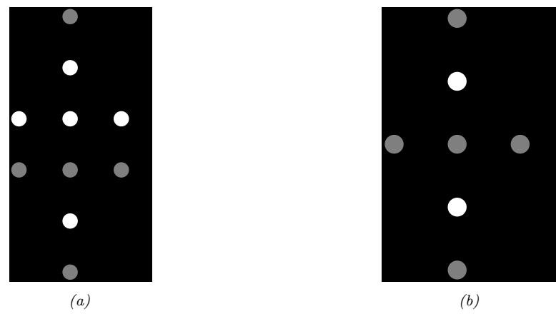
Figure 12.10: (a) A mixture model. (b) After integrating out the discrete latent variables.

example, to apply HMC to HMMs, we can use the forwards algorithm (Section 9.2.2) to e”ciently compute ^p(xn|ω) = & ^z1:^T p(xn, zn,1:^T |ω).

In addition to marginalizing out any discrete latent variables, we need to ensure the remaining continuous latent variables are unconstrained. This often requires performing a change of variables using a bijector. For example, instead of sampling the discrete probability vector from the probability simplex ^▷ ↗ ^SK, we should sample the logits ^ϱ ↗ ^RK. After sampling, we can transform back, since bijectors are invertible. (For a practical example, see change\_of\_variable\_hmc.ipynb.)

12.5.9 Speeding up HMC

Although HMC uses gradient information to explore the typical set, sometimes the geometry of the typical set can be di”cult to sample from. See Section 12.5.4.3 for ways to estimate the mass matrix, which can help with such di”cult cases.

Another issue is the cost of evaluating the target distribution, E(ω) = → log ˜p(ω). For many ML applications, this has the form log ˜p(ω) = log p0(ω) + &^{N n}=1 log p(ωn|ω). This takes O(N) time to compute. We can speed this up by using stochastic gradient methods; see Section 12.7 for details.

12.6 MCMC convergence

We start MCMC from an arbitrary initial state. As we explained in Section 2.6.4, the samples will be coming from the chain’s stationary distribution only when the chain has “forgotten” where it started from. The amount of time it takes to enter the stationary distribution is called the mixing time (see Section 12.6.1 for details). Samples collected before the chain has reached its stationary distribution do not come from p→, and are usually thrown away. The initial period, whose samples will be ignored, is called the burn-in phase.

For example, consider a uniform distribution on the integers {0, 1,…, 20}. Suppose we sample from this using a symmetric random walk. In Figure 12.11, we show two runs of the algorithm. On

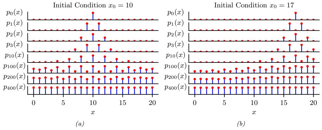
Figure 12.11: Illustration of convergence to the uniform distribution over {0, 1,…, 20} using a symmetric random walk starting from (left) state 10, and (right) state 17. Adapted from Figures 29.14 and 29.15 of [Mac03]. Generated by random\_walk\_integers.ipynb.

the left, we start in state 10; on the right, we start in state 17. Even in this small problem it takes over 200 steps until the chain has “forgotten” where it started from. Proposal distributions that make larger changes can converge faster. For example, [BD92; Man] prove that it takes about 7 ri$e shu$es to properly mix a deck of 52 cards (i.e., to ensure the distribution is uniform).

In Section 12.6.1 we discuss how to compute the mixing time theoretically. In practice, this can be very hard [BBM10] (this is one of the fundamental weaknesses of MCMC), so in Section 12.6.2, we discuss practical heurstics.

12.6.1 Mixing rates of Markov chains

The amount of time it takes for a Markov chain to converge to the stationary distribution, and forget its initial state, is called the mixing time. More formally, we say that the mixing time from state x⁰ is the minimal time such that, for any constant ⇁ > 0, we have that

\[\forall \tau\_{\epsilon}(x\_0) \triangleq \min \{ t : ||\delta\_{x\_0}(x)T^t - p^\*||\_1 \le \epsilon \} \tag{12.94}\]

where ϑ^x0 (x) is a distribution with all its mass in state x0, T is the transition matrix of the chain (which depends on the target p^→ and the proposal q), and ϑ^x0 (x)T^t is the distribution after t steps. The mixing time of the chain is defined as

\[\forall \tau\_{\epsilon} \stackrel{\Delta}{=} \max\_{x\_0} \tau\_{\epsilon}(x\_0) \tag{12.95}\]

This is the maximum amount of time it takes for the chain’s distribution to get ⇁ close to p^→ from any starting state.

The mixing time is determined by the eigengap ▷ = ⇀¹ → ⇀2, which is the di!erence between the first and second eigenvalues of the transition matrix. For a finite state chain, one cans show τ^ϖ = O( ¹ ⇁ log ^{n ϖ} ), where n is the number of states.

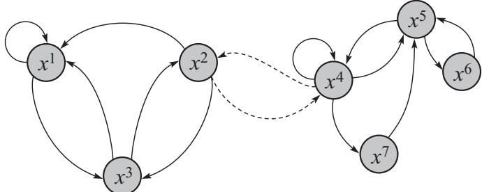
Figure 12.12: A Markov chain with low conductance. The dotted arcs represent transitions with very low probability. From Figure 12.6 of [KF09a]. Used with kind permission of Daphne Koller.

We can also study the problem by examining the geometry of the state space. For example, consider the chain in Figure 12.12. We see that the state space consists of two “islands”, each of which is connected via a narrow “bottleneck”. (If they were completely disconnected, the chain would not be ergodic, and there would no longer be a unique stationary distribution, as discussed in Section 2.6.4.3.) We define the conductance 3 of a chain as the minimum probability, over all subsets S of states, of transitioning from that set to its complement:

\[\phi \triangleq \min\_{S:0 \le p^\*(S) \le 0.5} \frac{\sum\_{x \in S, x' \in S^c} T(x \to x')}{p^\*(S)},\tag{12.96}\]

One can show that τ^ϖ ⇐ O ^{1 ς2} log ⁿ ϖ . Hence chains with low conductance have high mixing time. For example, distributions with well-separated modes usually have high mixing time. Simple MCMC methods, such as MH and Gibbs, often do not work well in such cases, and more advanced algorithms, such as parallel tempering, are necessary (see e.g., [ED05; Kat+06; BZ20]).

12.6.2 Practical convergence diagnostics

Computing the mixing time of a chain is in general quite di”cult, since the transition matrix is usually very hard to compute. Furthermore, diagnosing convergence is computationally intractable in general [BBM10]. Nevertheless, various heuristics have been proposed — see e.g., [Gey92; CC96; BR98; Veh+19]. We discuss some of the current recommended approaches below, following [Veh+19].

12.6.2.1 Trace plots

One of the simplest approaches to assessing if the method has converged is to run multiple chains (typically 3 or 4) from very di!erent overdispersed starting points, and to plot the samples of some quantity of interest, such as the value of a certain component of the state vector, or some event such as the value taking on an extreme value. This is called a trace plot. If the chain has mixed, it should have “forgotten” where it started from, so the trace plots should converge to the same distribution, and thus overlap with each other.

To illustrate this, we will consider a very simple, but enlightening, example from [McE20, Sec 9.5]. The model is a univariate Gaussian, yⁱ ↔︎ N (ϱ, ς), with just 2 observations, y¹ = →1 and y² = +1.

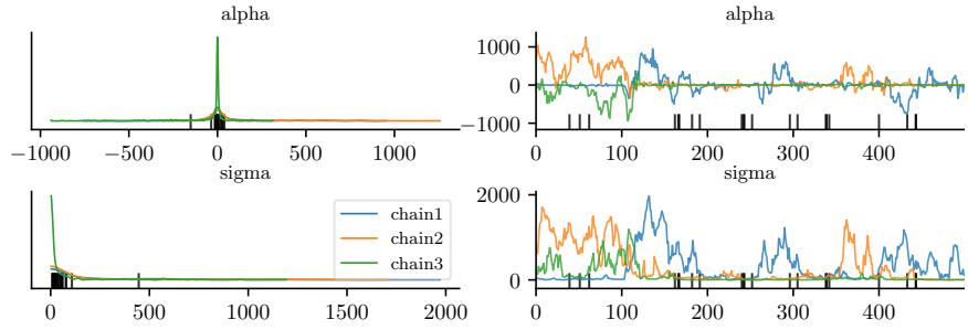
Figure 12.13: Marginals (left) and trace plot (right) for the univariate Gaussian using the di!use prior. Black vertical lines indicate HMC divergences. Adapted from Figures 9.9–9.10 of [McE20]. Generated by mcmc\_traceplots\_unigauss.ipynb.

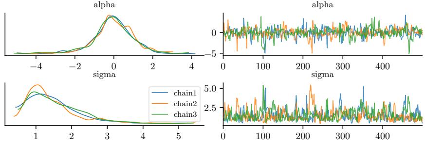
Figure 12.14: Marginals (left) and trace plot (right) for the univariate Gaussian using the sensible prior. Adapted from Figures 9.9–9.10 of [McE20]. Generated by mcmc\_traceplots\_unigauss.ipynb.

We first consider a very di!use prior, ϱ ↔︎ N (0, 1000) and ς ↔︎ Expon(0.0001), both of which allow for very large values of ϱ and ς. We fit the model using HMC using 3 chains and 500 samples. The result is shown in Figure 12.13. On the right, we show the trace plots for ϱ and ς for 3 di!erent chains. We see that they do not overlap much with each other. In addition, the numerous black vertical lines at the bottom of the plot indicate that HMC had many divergences.

The problem is caused by the overly di!use priors, which do not get overwhelmed by the likelihood because we only have 2 datapoints. Thus the posterior is also di!use. We can fix this by using slightly stronger priors, that keep the parameters close to more sensible values. For example, suppose we use ϱ ↔︎ N (1, 10) and ς ↔︎ Expon(1). Now we get the results in Figure 12.14. On the right we see that the traceplots overlap. On the left, we see that the marginal distributions from each chain have support over a reasonable interval, and have a peak at the “right” place (the MLE for ϱ is 0, and for ς is 1). And we don’t see any divergence warnings (vertical black markers in the plot).

Since trace plots of converging chains correspond to overlapping lines, it can be hard to distinguish success from failure. An alternative plot, known as a trace rank plot, was recently proposed in [Veh+19]. (In [McE20], this is called a trankplot, a term we borrow.) The idea is to compute the rank of each sample based on all the samples from all the chains, after burnin. We then plot a histogram of the ranks for each chain separately. If the chains have converged, the distribution

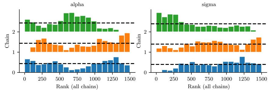
Figure 12.15: Trace rank plot for the univariate Gaussian using the di!use prior. Adapted from Figures 9.9–9.10 of [McE20]. Generated by mcmc\_traceplots\_unigauss.ipynb.

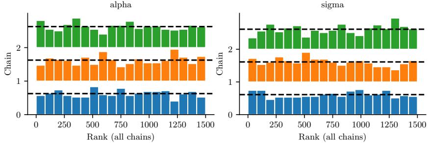
Figure 12.16: Trace rank plot for the univariate Gaussian using the sensible prior. Adapted from Figures 9.9–9.10 of [McE20]. Generated by mcmc\_traceplots\_unigauss.ipynb.

over ranks should be uniform, since there should be no preference for high or low scoring samples amongst the chains.

The trankplot for the model with the di!use prior is shown in Figure 12.15. (The x-axis is from 1 to the total number of samples, which in this example is 1500, since we use 3 chains and draw 500 samples from each.) We can see that the di!erent chains are clearly not mixing. The trankplot for the model with the sensible prior is shown in Figure 12.16; this looks much better.

12.6.2.2 Estimated potential scale reduction (EPSR)

In this section, we discuss a way to assess convergence more quantitatively. The basic idea is this: if one or more chains has not mixed well, then the variance of all the chains combined together will be higher than the variance of the individual chains. So we will compare the variance of the quantity of interest computed between and within chains.

More precisely, suppose we have M chains, and we draw N samples from each. Let xnm denote the quantity of interest derived from the n’th sample from the m’th chain. We compute the between-

and within-sequence variances as follows:

\[B = \frac{N}{M-1} \sum\_{m=1}^{M} \left(\overline{x}\_m - \overline{x}\_{..}\right)^2, \text{ where } \overline{x}\_m = \frac{1}{N} \sum\_{n=1}^{N} x\_{nm}, \text{ } \overline{x}\_{..} = \frac{1}{M} \sum\_{m=1}^{M} \overline{x}\_{.m} \tag{12.97}\]

\[W = \frac{1}{M} \sum\_{m=1}^{M} s\_m^2, \text{ where } s\_m^2 = \frac{1}{N-1} \sum\_{n=1}^{N} (x\_{nm} - \mathbb{Z}\_{\cdot m})^2 \tag{12.98}\]

The formula for s^{2 m} is the usual unbiased estimate for the variance from a set of N samples; W is just the average of this. The formula for B is similar, but scaled up by N since it is based on the variance of x·^m, which are averaged over N values.

Next we compute the following average variance:

\[ \hat{V}^{+} \stackrel{\Delta}{=} \frac{N-1}{N}W + \frac{1}{N}B\tag{12.99} \]

Finally, we compute the following quantity, known as the estimated potential scale reduction or R-hat:

\[ \hat{R} \triangleq \sqrt{\frac{\hat{V}^+}{W}} \tag{12.100} \]

In [Veh+19], they recommend checking if R <ˆ 1.01 before declaring convergence.

For example, consider the Rˆ values for various samplers for our univariate GMM example. In particular, consider the 3 MH samplers in Figure 12.1, and the Gibbs sampler in Figure 12.4. The Rˆ values are 1.493, 1.039, 1.005, and 1.007. So this diagnostic has correctly identified that the first two samplers are unreliable, which evident from the figure.

In practice, it is recommended to use a slightly di!erent quantity, known as split-Rˆ. This can be computed by splitting each chain into the first and second halves, thus doubling the number of chains M (but halving the number of samples N from each), before computing Rˆ. This can detect non-stationarity within a single chain.

12.6.3 E”ective sample size

Although MCMC lets us draw samples from a target distribution (assuming it has converged), the samples are not independent, so we may need to draw a lot of them to get a reliable estimate. In this section, we discuss how to compute the e!ective sample size or ESS from a set of (possibly correlated) samples.

To start, suppose we draw N independent samples from the target distribution, and let xˆ = 1 N &^{N n}=1 xⁿ be our empirical estimate of the mean of the quantity of interest. The variance of this estimate is given by

\[\mathbb{V}\left[\hat{x}\right] = \frac{1}{N^2}\mathbb{V}\left[\sum\_{n=1}^{N} x\_n\right] = \frac{1}{N^2}\sum\_{n=1}^{N} \mathbb{V}\left[x\_n\right] = \frac{1}{N}\sigma^2\tag{12.101}\]

where ς² = V [X]. If the samples are correlated, the variance of the estimate will be higher, as we show below.

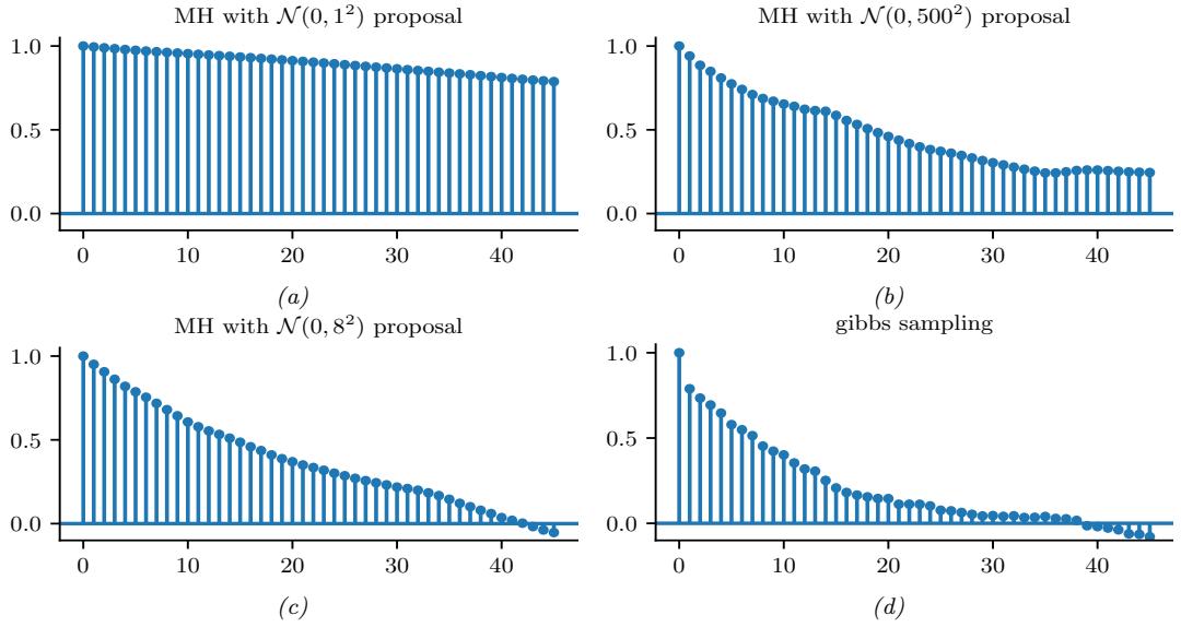
Figure 12.17: Autocorrelation functions for various MCMC samplers for the mixture of two 1d Gaussians. (a-c) These are the MH samplers in Figure 12.1. (d) This is the Gibbs sampler in Figure 12.4. Generated by mcmc\_gmm\_demo.ipynb.

Recall that for N (not necessarily independent) random variables we have

\[\mathbb{V}\left[\sum\_{n=1}^{N} x\_n\right] = \sum\_{i=1}^{N} \sum\_{j=1}^{N} \text{Cov}\left[x\_i, x\_j\right] = \sum\_{i=1}^{N} \mathbb{V}\left[x\_i\right] + 2 \sum\_{1 \le i < j \le N} \text{Cov}\left[x\_i, x\_j\right] \tag{12.102}\]

Let x = ¹ N &^{N n}=1 xⁿ be our estimate based on these correlated samples. The variance of this estimate is given by

\[\mathbb{V}\left[\overline{x}\right] = \frac{1}{N^2} \sum\_{i=1}^{N} \sum\_{j=1}^{N} \text{Cov}\left[x\_i, x\_j\right] \tag{12.103}\]

We now rewrite this in a more convenient form. First recall that the correlation of xⁱ and x^j is given by

\[\text{corr}\left[x\_i, x\_j\right] = \frac{\text{Cov}\left[x\_i, x\_j\right]}{\sqrt{\mathbb{V}\left[x\_i\right]\mathbb{V}\left[x\_j\right]}}\tag{12.104}\]

Since we assume we are drawing samples from the target distribution, we have V [xi] = ς², where ς² is the true variance. Hence

\[\mathbb{V}\left[\overline{x}\right] = \frac{\sigma^2}{N^2} \sum\_{i=1}^{N} \sum\_{j=1}^{N} \text{corr}\left[x\_i, x\_j\right] \tag{12.105}\]

For a fixed i, we can think of corr [xi, x^j ] as a function of j. This will usually decay as j gets further from i. As N ↖ ⇓ we can approximate the sum of correlations by

\[\sum\_{j=1}^{N} \text{corr}\left[x\_i, x\_j\right] \to \sum\_{\ell=-\infty}^{\infty} \text{corr}\left[x\_i, x\_{i+\ell}\right] = 1 + 2\sum\_{\ell=1}^{\infty} \text{corr}\left[x\_i, x\_{i+\ell}\right] \tag{12.106}\]

since corr [xi, xi] = 1 and corr [xi, xⁱ↓^ω] = corr [xi, xi+ω] for lag ε > 0. Since we assume the samples are coming from a stationary distribution, the index i does not matter. Thus we can define the autocorrelation time as

\[\rho = 1 + 2\sum\_{\ell=1}^{\infty} \rho(\ell) \tag{12.107}\]

where 0(ε) is the autocorrelation function (ACF), defined as

\[\rho(\ell) \stackrel{\Delta}{=} \text{corr}\left[x\_0, x\_\ell\right] \tag{12.108}\]

The ACF can be approximated e”ciently by convolving the signal x with itself. In Figure 12.17, we plot the ACF for our four samplers for the GMM. We see that the ACF of the Gibbs sampler (bottom right) dies o! to 0 much more rapidly than the MH samplers. Intuitively this indicates that each Gibbs sample is “worth” more than each MH sample. We quantify this below.

From Equation (12.105), we can compute the variance of our estimate in terms of the ACF as follows: V [x] = ↽² N² &^{N i}=1 ^{0 =} ↽^{2 N} 0. By contrast, the variance of the estimate from independent samples is V [ˆx] = ↽^{2 N} . So we see that the variance is a factor 0 larger when there is correlation. We therefore define the e!ective sample size of our set of samples to be

\[N\_{\text{eff}} \triangleq \frac{N}{\rho} = \frac{N}{1 + 2\sum\_{\ell=1}^{\infty} \rho(\ell)}\tag{12.109}\]

In practice, we truncate the sum at lag L, which is the last integer at which 0(L) is positive. Also, if we run M chains, the numerator should be NM, so we get the following estimate:

\[\hat{N}\_{\text{eff}} = \frac{NM}{1 + 2\sum\_{\ell=1}^{L} \hat{\rho}(\ell)}\tag{12.110}\]

In [Veh+19], they propose various extensions of the above estimator, such as using rank statistics, to make the estimate more robust.

12.6.4 Improving speed of convergence

There are many possible things you could try if the Rˆ value is too large, and/or the e!ective sample size is too low. Here is a brief list:

• Try using a non-centered parameterization (see Section 12.6.5).
• Try sampling variables in groups or blocks (see Section 12.3.7).

Figure 12.18: Neal’s funnel. (a) Joint density. (b) HMC samples from centered representation. (c) HMC samples from non-centered representation. Generated by neals\_funnel.ipynb.

• Try using Rao-Blackwellization, i.e., analytically integrating out some of the variables (see Section 12.3.8).
• Try adding auxiliary variables (see Section 12.4).
• Try using adaptive proposal distributions (see Section 12.2.3.5).

More details can be found in [Rob+18].

12.6.5 Non-centered parameterizations and Neal’s funnel

A common problem that arises when applying sampling to hierarchical Bayesian models is when a set of parameters at one level of the model have a tight depenendence on parameters at the level above. We show some practical examples of this in the hierarchical Gaussian 8-schools example in Section 3.6.2.2 and the hierarchical radon regression example in Section 15.5.2.2. Here, we focus on the following simple toy model that captures the essence of the problem:

\[ \nu \sim \mathcal{N}(0, 3) \tag{12.111} \]

\[x \sim \mathcal{N}(0, \exp(\nu))\tag{12.112}\]

The corresponding joint density p(x, 4) is shown in Figure 12.18a. This is known Neal’s funnel, named after [Nea03]. It is hard for a sampler to “descend” in the narrow “neck” of the distribution, corresponding to areas where the variance 4 is small [BG13].

Fortunately, we can represent this model in an equivalent way that makes it easier to sample from, providing we use a non-centered parameterization [PR03]. This has the form

\[ \nu \sim \mathcal{N}(0, 3) \tag{12.113} \]

\[z \sim \mathcal{N}(0, 1)\tag{12.114}\]

\[x = z \exp(\nu) \tag{12.115}\]

This is easier to sample from, since p(z, 4) is a product of 2 independent Gaussians, and we can derive x deterministically from these Gaussian samples. The advantage of this reparameterization is

shown in Figure 12.18. A method to automatically derive such reparameterizations is discussed in [GMH20].

12.7 Stochastic gradient MCMC

Consider an unnormalized target distribution of the following form:

\[p(\boldsymbol{\theta}) \propto p(\boldsymbol{\theta}, \mathcal{D}) = p\_0(\boldsymbol{\theta}) \prod\_{n=1}^{N} p(\boldsymbol{x}\_n | \boldsymbol{\theta}) \tag{12.116}\]

where D = (x1,…, x^N ). Alternatively we can define the target distribution in terms of an energy function (negative log joint) as follows:

\[p(\theta, \mathcal{D}) \propto \exp(-\mathcal{E}(\theta))\tag{12.117}\]

The energy function can be decomposed over data samples:

\[\mathcal{E}(\boldsymbol{\theta}) = \sum\_{n=1}^{N} \mathcal{E}\_n(\boldsymbol{\theta}) \tag{12.118}\]

\[\mathcal{E}\_n(\theta) = -\log p(x\_n|\theta) - \frac{1}{N} \log p\_0(\theta) \tag{12.119}\]

Evaluating the full energy (e.g., to compute an acceptance probability in the Metropolis-Hastings algorithm, or to compute the gradient in HMC) takes O(N) time, which does not scale to large data. In this section, we discuss some solutions to this problem.

12.7.1 Stochastic gradient Langevin dynamics (SGLD)

Recall from Equation (12.83) that the Langevin di!usion SDE has the following form

\[d\theta\_t = -\nabla \mathcal{E}(\theta\_t)dt + \sqrt{2}d\mathbf{W}\_t\tag{12.120}\]

where dW^t is a Wiener noise (also called Brownian noise) process. In discrete time, we can use the following Euler approximation:

\[ \boldsymbol{\theta}\_{t+1} \approx \boldsymbol{\theta}\_t - \eta\_t \nabla \mathcal{E}(\boldsymbol{\theta}\_t) + \sqrt{2\eta\_t} \mathcal{N}(\mathbf{0}, \mathbf{I}) \tag{12.121} \]

Computing the gradient g(ωt) = ⇒E(ωt) at each step takes O(N) time. We can compute an unbiased minibatch approximation to the gradient term in O(B) time using

\[\hat{\mathbf{g}}(\boldsymbol{\theta}\_{t}) = \frac{N}{B} \sum\_{n \in \mathcal{B}\_{t}} \nabla \mathcal{E}\_{n}(\boldsymbol{\theta}\_{t}) = -\frac{N}{B} \left( \sum\_{n \in \mathcal{B}\_{t}} \nabla \log p(\boldsymbol{x}\_{n}|\boldsymbol{\theta}\_{t}) + \frac{B}{N} \nabla \log p\_{0}(\boldsymbol{\theta}\_{t}) \right) \tag{12.122}\]

where B^t is the minibatch at step t. This gives rise to the following approximate update:

\[ \theta\_{t+1} = \theta\_t - \eta\_t \hat{\mathbf{g}}(\theta\_t) + \sqrt{2\eta\_t} N(\mathbf{0}, \mathbf{I}) \tag{12.123} \]

This is called stochastic gradient Langevin dynamics or SGLD [Wel11]. The resulting update step is identical to SGD, except for the addition of a Gaussian noise term. (See [Neg+21] for some recent analysis of this method; they also suggest setting ^{ηt ↑ N ↓}2/³.)

12.7.2 Preconditionining

As in SGD, we can get better results (especially for models such as neural networks) if we use preconditioning to scale the gradient updates. In [PT13], they use the Fisher information matrix (FIM) as the preconditioner; this method is known as stochastic gradient Riemannian Langevin dynamics or SGRLD.

Unfortunately, computing the FIM is often hard. In [Li+16], they propose to use the same kind of diagonal approximation as used by RMSprop; this is called preconditioned SGLD. An alternative is to use an Adam-like preconditioner, as proposed in [KSL21]. This is called SGLD-Adam. For more details, see [CSN21].

12.7.3 Reducing the variance of the gradient estimate

The variance of the noise introduced by minibatching can be quite large, which can hurt the performance of methods such as SGLD [BDM18]. In [Bak+17], they propose to reduce the variance of this estimate by using a control variate estimator; this method is therefore called SGLD-CV. Specifically they use the following gradient approximation:

\[\hat{\nabla}\_{cv}\mathcal{E}(\boldsymbol{\theta}\_t) = \nabla \mathcal{E}(\hat{\boldsymbol{\theta}}) + \frac{N}{B} \sum\_{n \in \mathcal{S}\_t} \left( \nabla \mathcal{E}\_n(\boldsymbol{\theta}\_t) - \nabla \mathcal{E}\_n(\hat{\boldsymbol{\theta}}) \right) \tag{12.124}\]

Here ωˆ is any fixed value, but it is often taken to be an approximate MAP estimate (e.g., based on one epoch of SGD). The reason Equation (12.124) is valid is because the terms we add and subtract are equal in expectation, and hence we get an unbiased estimate:

\[\mathbb{E}\left[\hat{\nabla}\_{cv}\mathcal{E}(\boldsymbol{\theta}\_{t})\right] = \nabla\mathcal{E}(\boldsymbol{\hat{\theta}}) + \mathbb{E}\left[\frac{N}{B}\sum\_{n\in\mathcal{S}\_{t}}\left(\nabla\mathcal{E}\_{n}(\boldsymbol{\theta}\_{t}) - \nabla\mathcal{E}\_{n}(\boldsymbol{\hat{\theta}})\right)\right] \tag{12.125}\]

\[\hat{\mathbf{e}} = \nabla \mathcal{E}(\hat{\boldsymbol{\theta}}) + \nabla \mathcal{E}(\boldsymbol{\theta}\_t) - \nabla \mathcal{E}(\hat{\boldsymbol{\theta}}) = \nabla \mathcal{E}(\boldsymbol{\theta}\_t) \tag{12.126}\]

Note that the first term, ^⇒E(ωˆ) = &^{N n}=1 ^⇒En(ωˆ), requires a single pass over the entire dataset, but only has to be computed once (e.g., while estimating ωˆ).

One disadvantage of SGLD-CV is that the reference point ωˆ has to be precomputed, and is then fixed. An alternative is to update the reference point online, by performing periodic full batch estimates. This is called SVRG-LD [Dub+16; Cha+18], where SVRG stands for stochastic variance reduced gradient, and LD stands for Langevin dynamics. If we use ω˜^t to denote the most recent snapshot (reference point), the corresponding gradient estimate is given by

\[\hat{\nabla}\_{swrg} \mathcal{E}(\boldsymbol{\theta}\_t) = \nabla \mathcal{E}(\boldsymbol{\tilde{\theta}}\_t) + \frac{N}{B} \sum\_{n \in \mathcal{S}\_t} \left( \nabla \mathcal{E}\_n(\boldsymbol{\theta}\_t) - \nabla \mathcal{E}\_n(\boldsymbol{\tilde{\theta}}\_t) \right) \tag{12.127}\]

We recompute the snapshot every τ steps (known as the epoch length). See Algorithm 12.5 for the pseudo-code.

The disadvantage of SVRG is that it needs to perform a full pass over the data every τ steps. An alternative approach, called SAGA-LD [Dub+16; Cha+18] (which stands for stochastic averaged gradient acceleration), avoids this by storing all N gradient vectors, and then doing incremental updates. Unfortunately the memory requirements of this algorithm usually make it impractical.

Algorithm 12.5: SVRG Langevin descent

¹ Initialize ω^{0 2} for t =1: T do ³ if t mod τ = 0 then ⁴ ω˜ = ω^{t 5} g˜ = &^{N n}=1 ^En(ω˜) ⁶ Sample minibatch B^t ↗ {1,…,N} ⁷ g^t = g˜ + ^N B & n↑B^{t ⇒}En(ωt) → ⇒En(ω˜) ^{8 ω}t+1 ^{= ωt → η}tg^{t + ∝}2ηt^N (0, ^I)

12.7.4 SG-HMC

We discussed Hamiltonian Monte Carlo (HMC) in Section 12.5, which uses auxiliary momentum variables to improve performance over Langevin MC. In this section, we discuss a way to speed it up by approximating the gradients using minibatches. This is called SG-HMC [CFG14; ZG21], where SG stands for “stochastic gradient”.

Recall that the leapfrog updates have the following form:

\[\mathbf{v}\_{t+1/2} = \mathbf{v}\_t - \frac{\eta}{2} \nabla \mathcal{E}(\theta\_t) \tag{12.128}\]

\[\boldsymbol{\theta}\_{t+1} = \boldsymbol{\theta}\_t + \eta \boldsymbol{v}\_{t+1/2} = \boldsymbol{\theta}\_t + \eta \boldsymbol{v}\_t - \frac{\eta}{2} \nabla \mathcal{E}(\boldsymbol{\theta}\_t) \tag{12.129}\]

\[\mathbf{v}\_{t+1} = \mathbf{v}\_{t+1/2} - \frac{\eta}{2} \nabla \mathcal{E}(\boldsymbol{\theta}\_{t+1}) = \mathbf{v}\_t - \frac{\eta}{2} \nabla \mathcal{E}(\boldsymbol{\theta}\_t) - \frac{\eta}{2} \nabla \mathcal{E}(\boldsymbol{\theta}\_{t+1}) \tag{12.130}\]

We can replace the full batch gradient with a stochastic approximation, to get

\[\boldsymbol{\theta}\_{t+1} = \boldsymbol{\theta}\_t + \eta \boldsymbol{v}\_t - \frac{\eta^2}{2} \boldsymbol{g}(\boldsymbol{\theta}\_t, \boldsymbol{\xi}\_t) \tag{12.131}\]

\[v\_{t+1} = v\_t - \frac{\eta}{2}g(\theta\_t, \xi\_t) - \frac{\eta}{2}g(\theta\_{t+1}, \xi\_{t+1/2}) \tag{12.132}\]

where ⇁^t and ⇁t+1/² are independent sources of randomness (e.g., batch indices). In [ZG21], they show that this algorithm (even without the MH rejection step) provides a good approximation to the posterior (in the sense of having small Wasserstein-2 distance) for the case where the energy functon is strongly convex. Furthermore, performance can be considerably improved if we use the variance reduction methods discussed in Section 12.7.3.

12.7.5 Underdamped Langevin dynamics

The underdamped Langevin dynamics (ULD) has the form of the following SDE [CDC15; LMS16; Che+18a; Che+18d]:

\[\begin{aligned} d\theta\_t &= v\_t dt\\ d\upsilon\_t &= -\mathbf{g}(\theta\_t)dt - \gamma v\_t dt + \sqrt{2\gamma} d\mathbf{W}\_t \end{aligned} \tag{12.133}\]

where g(ωt) = ⇒E(ωt) is the gradient or force acting on the particle, ▷ > 0 is the friction parameter, and dW^t is Wiener noise.

Equation (12.133) is like the Langevin dynamics of Equation (12.83) but with an added momentum term vt. We can solve the dynamics using various integration methods. It can be shown (see e.g., [LMS16]) that these methods are accurate to second order, whereas solving standard (overdamped) Langevin is only accurate to first order, and thus will require more sampling steps to achieve a given accuracy.

12.8 Reversible jump (transdimensional) MCMC

Suppose we have a set of models with di!erent numbers of parameters, e.g., mixture models in which the number of mixture components is unknown. Let the model be denoted by m, and let its unknowns (e.g., parameters) be denoted by ^xm ↗ ^Xm (e.g., ^Xm = ^Rnm, where ^nm is the dimensionality of model m). Sampling in spaces of di!ering dimensionality is called trans-dimensional MCMC. We could sample the model indicator m ↗ {1,…,M} and sample all the parameters from the product space ^{M m}=1 Xm, but this is very ine”cient, and only works if M is finite. It is more parsimonious to sample in the union space ^X = ^{⊤M m}=1{m} ⇔ Xm, where we only worry about parameters for the currently active model.

The di”culty with this approach arises when we move between models of di!erent dimensionality. The trouble is that when we compute the MH acceptance ratio, we are comparing densities defined on spaces of di!erent dimensionality, which is not well defined. For example, comparing densities on two points of a sphere makes sense, but comparing a density on a sphere to a density on a circle does not, as there is a dimensional mismatch in the two concepts. The solution, proposed by [Gre95] and known as reversible jump MCMC or RJMCMC, is to augment the low dimensional space with extra random variables so that the two spaces have a common measure. This is illustrated in Figure 12.19.

We give a sketch of the algorithm below. For more details, see e.g., [Gre03; HG12].

12.8.1 Basic idea

To explain the method in more detail, we follow the presentation of [And+03]. To ensure a common measure, we need to define a way to extend each pair of subspaces X^m and Xⁿ to Xm,n = X^m ⇔ Um,n and Xn,m = Xⁿ ⇔ Un,m. We also need to define a deterministic, di!erentiable and invertible mapping

\[f\_n(x\_m, \mathfrak{u}\_{m,n}) = f\_{n \to m}(x\_n, \mathfrak{u}\_{n,m}) = (f\_{n \to m}^x(x\_n, \mathfrak{u}\_{n,m}), f\_{n \to m}^u(x\_n, \mathfrak{u}\_{n,m})) \tag{12.134}\]

Invertibility means that

\[f\_{m \to n}(f\_{n \to m}(x\_n, u\_{n,m})) = (x\_n, u\_{n,m}) \tag{12.135}\]

Finally, we need to define proposals qⁿ↗^m(un,m|n, xn) and q^m↗ⁿ(um,n|m, xm).

Suppose we are in state (n, xn). We move to (m, xm) by generating un,m ↔︎ qⁿ↗^m(·|n, xn), and then computing (xm,um,n) = fⁿ↗^m(xn,un,m). We then accept the move with probability

\[A\_{n \to m} = \min\left\{1, \frac{p(m, \mathbf{x}\_m^\*)}{p(n, \mathbf{z}\_n)} \times \frac{q(n|m)}{q(m|n)} \times \frac{q\_{m \to n}(\mathbf{u}\_{m,n}|m, \mathbf{z}\_m^\*)}{q\_{n \to m}(\mathbf{u}\_{n,m}|n, \mathbf{z}\_n)} \times |\det \mathbf{J}\_{f\_{m \to n}}|\right\} \tag{12.136}\]

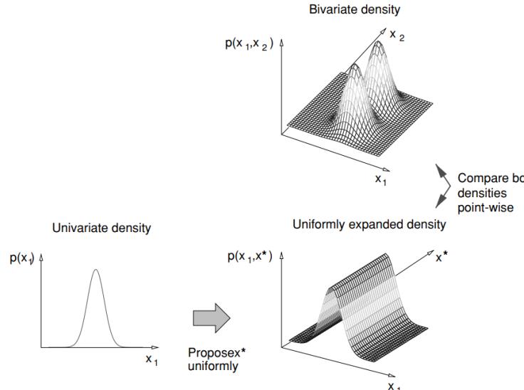
Figure 12.19: To compare a 1d model against a 2d model, we first have to map the 1d model to 2d space so the two have a common measure. Note that we assume the ridge has finite support, so it is integrable. From Figure 17 of [And+03]. Used with kind permission of Nando de Freitas.

where x^{→ m} = f^{x n}↗^m(xn,un,m), J^fm↔︎ⁿ is the Jacobian of the transformation

\[J\_{f\_m \to n} = \frac{\partial f\_{n \to m}(x\_m, u\_{m,n})}{\partial(x\_m, u\_{m,n})} \tag{12.137}\]

and | det J| is the absolute value of the determinant of the Jacobian.

12.8.2 Example

Let us consider an example from [AFD01]. They consider an RBF network for nonlinear regression of the form

\[f(x) = \sum\_{j=1}^{k} a\_j \mathcal{K}(||x - \mu\_j||) + \boldsymbol{\beta}^{\mathsf{T}} x + \beta\_0 + \epsilon \tag{12.138}\]

where K() is some kernel function (e.g., a Gaussian), k is the number of such basis functions, and ⇁ is a Gaussian noise term. If k = 0, the model corresponds to linear regression.

They fit this model to the data in Figure 12.20(a). The predictions on the test set are shown in Figure 12.20(b). Estimates of p(k|D), the (distribution over the) number of basis functions, are shown in Figure 12.20(c) as a function of the iteration number; the posterior at the final iteration is shown in Figure 12.20(d). There is clearly the most posterior support for k = 2, which makes sense given the two “bumps” in the data.

⁰ 0.2 0.4 0.6 0.8 ^{1 −3} −2 −1 0 1 2 3 4 Train output Train input (a) ⁰ 0.2 0.4 0.6 0.8 ^{1 −4} −3 −2 −1 0 1 2 3 4 Test output Test input True function Test data Prediction (b) ^{0 500 1000 1500 2000 0} 0.1 0.2 0.3 0.4 0.5 0.6 0.7 0.8 0.9 1 Chain length p(k|y) 1 2 3 4 (c) ^{1 2 3 4 0} 0.1 0.2 0.3 0.4 0.5 0.6 0.7 p(k|data) (d)

Figure 12.20: Fitting an RBF network to some 1d data using RJMCMC. (a) Prediction on train set. (b) Prediction on test set. (c) Plot of p(k|D) vs iteration. (d) Final posterior p(k|D). Adapted from Figure 4 of [AFD01]. Generated by rjmcmc\_rbf, written by Nando de Freitas.

To generate these results, they consider several kinds of proposal. One of them is to split a current basis function µ into two new ones using

\[ \mu\_1 = \mu - u\_{n,n+1}\beta,\ \mu\_2 = \mu + u\_{n,n+1}\beta,\tag{12.139} \]

where ↼ is a parameter of the proposal, and un,m is sampled from some distribution (e.g., uniform). To ensure reversibility, they define a corresponding merge move

\[ \mu = \frac{\mu\_1 + \mu\_2}{2} \tag{12.140} \]

where µ¹ is chosen at random, and µ² is its nearest neighbor. To ensure these moves are reversible, we require ||µ¹ → µ2|| < 2↼.

The acceptance ratio for the split move is given by

\[A\_{split} = \min\left\{1, \frac{p(k+1, \mu\_{k+1})}{p(k, \mu\_{k+1})} \times \frac{1/(k+1)}{1/k} \times \frac{1}{p(u\_{n,m})} \times |\det \mathbf{J}\_{split}|\right\} \tag{12.141}\]

where 1/k is the probability of choosing one of the k bases uniformly at random. The Jacobian is

\[\mathbf{J}\_{split} = \frac{\partial(\mu\_1, \mu\_2)}{\partial(\mu, u\_{n,m})} = \det\begin{pmatrix} 1 & 1\\ -\beta & \beta \end{pmatrix} \tag{12.142}\]

so |det Jsplit| = 2↼. The acceptance ratio for the merge move is given by

\[A\_{merge} = \min\left\{1, \frac{p(k-1, \mu\_{k-1})}{p(k, \mu\_k)} \times \frac{1/(k-1)}{1/k} \times |\det \mathbf{J}\_{merge}|\right\} \tag{12.143}\]

where |det Jmerge| = 1/(2↼).

Algorithm 12.6: Generic reversible jump MCMC (single step)

Sample u ↔︎ U(0, 1) If u ⇐ b^k then birth move else if u ⇐ (b^k + dk) then death move else if u ⇐ (b^k + d^k + sk) then split move else if u ⇐ (b^k + d^k + s^k + mk) then merge move else update parameters

The overall pseudo-code for the algorithm, assuming the current model has index k, is given in Algorithm 12.6. Here b^k is the probability of a birth move, d^k is the probability of a death move, s^k is the probability of a split move, and m^k is the probability of a merge move. If we don’t make a dimension-changing move, we just update the parameters of the current model using random walk MH.

12.8.3 Discussion

RJMCMC algorithms can be quite tricky to implement. If, however, the continuous parameters can be integrated out (resulting in a method called collapsed RJMCMC), much of the di”culty goes away, since we are just left with a discrete state space, where there is no need to worry about change of measure. For example, if we fix the centers µ^j in Equation (12.138) (e.g., using samples from the data, or using K-means clustering), we are left with a linear model, where we can integrate out the parameters. All that is left to do is sample which of these fixed basis functions to include in the model, which is a discrete variable selection problem. See e.g., [Den+02] for details.

In Chapter 31, we discuss Bayesian nonparametric models, which allow for an infinite number of di!erent models. Surprisingly, such models are often easier to deal with computationally (as well as more realistic, statistically) than working with a finite set of di!erent models.

12.9 Annealing methods

Many distributions are multimodal and hence hard to sample from. However, by analogy to the way metals are heated up and then cooled down in order to make the molecules align, we can imagine using a computational temperature parameter to “smooth out” a distribution, gradually cooling it to recover the original “bumpy” distribution. We first explain this idea in more detail in the context of an algorithm for MAP estimation. We then discuss extensions to the sampling case.

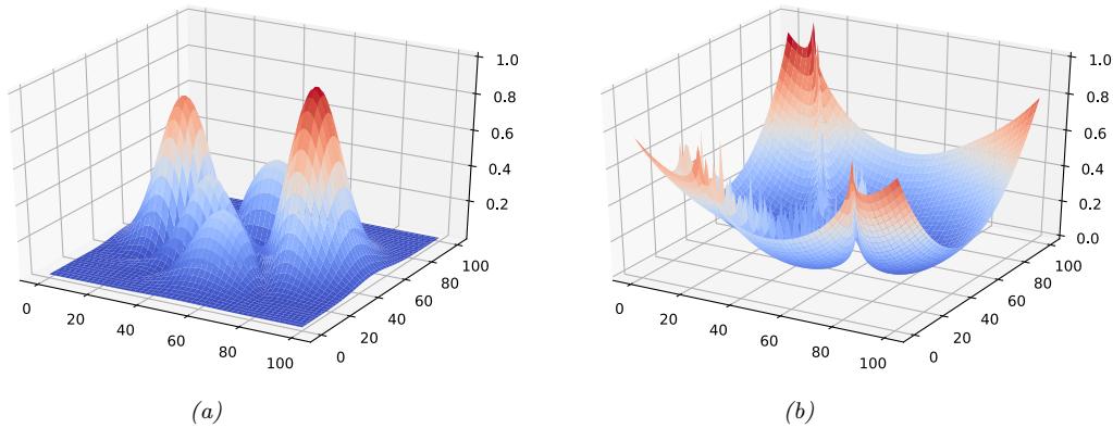
Figure 12.21: (a) A peaky distribution. (b) Corresponding energy function. Generated by simulated\_annealing\_2d\_demo.ipynb.

12.9.1 Simulated annealing

In this section, we discuss the simulated annealing algorithm [KJV83; LA87], which is a variant of the Metropolis-Hastings algorithm which is designed to find the global optimum of blackbox function. (Other approaches to blackbox optimization are discussed in Section 6.7.)

Annealing is a physical process of heating a solid until thermal stresses are released, then cooling it very slowly until the crystals are perfectly arranged, acheiving a minimum energy state. Depending on how fast or slow the temperature is cooled, the results will have better or worse quality. We can apply this approach to probability distributions, to control the number of modes (low energy states) that they have, by defining

\[p\_T(\mathbf{z}) = \exp(-\mathcal{E}(\mathbf{z})/T) \tag{12.144}\]

where T is the temperature, which is reduced over time. As an example, consider the peaks function:

\[p(x,y) \propto |3(1-x)^2e^{-x^2-(y+1)^2} - 10(\frac{x}{5}-x^3-y^5)e^{-x^2-y^2} - \frac{1}{3}e^{-(x+1)^2-y^2}|\tag{12.145}\]

This is plotted in Figure 12.21a. The corresponding energy is in Figure 12.21b. We plot annealed versions of this distribution in Figure 12.22. At high temperatures, T ⇑ 1, the surface is approximately flat, and hence it is easy to move around (i.e., to avoid local optima). As the temperature cools, the largest peaks become larger, and the smallest peaks disappear. By cooling slowly enough, it is possible to “track” the largest peak, and thus find the global optimum (minimum energy state). This is an example of a continuation method.

In more detail, at each step, we sample a new state according to some proposal distribution x^↔︎ ↔︎ q(·|xt). For real-valued parameters, this is often simply a random walk proposal centered on the current iterate, x^↔︎ = x^t + ,t+1, where ,t+1 ↔︎ N (0, !). (The matrix ! is often diagonal, and may be updated over time using the method in [Cor+87].) Having proposed a new state, we compute

Figure 12.22: Annealed version of the distribution in Figure 12.21a at di!erent temperatures. Generated by simulated\_annealing\_2d\_demo.ipynb.

the acceptance probability

\[\alpha\_{t+1} = \exp\left(-\left(\mathcal{E}(\mathbf{x'}) - \mathcal{E}(\mathbf{x}\_t)\right)/T\_t\right) \tag{12.146}\]

where T^t is the temperature of the system. We then accept the new state (i.e., set xt+1 = x^↔︎ ) with probability min(1, ϱt+1), otherwise we stay in the current state (i.e., set xt+1 = xt). This means that if the new state has lower energy (is more probable), we will definitely accept it, but if it has higher energy (is less probable), we might still accept, depending on the current temperature. Thus the algorithm allows “downhill” moves in probability space (uphill in energy space), but less frequently as the temperature drops.

The rate at which the temperature changes over time is called the cooling schedule. It has been shown [Haj88] that if one cools according to a logarithmic schedule, T^t ↑ 1/ log(t + 1), then the method is guaranteed to find the global optimum under certain assumptions. However, this schedule is often too slow. In practice it is common to use an exponential cooling schedule of the form

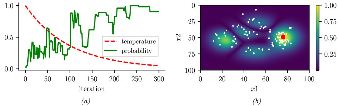
Figure 12.23: Simulated annealing applied to the distribution in Figure 12.21a. (a) Temperature vs iteration and probability of each visited point vs iteration. (b) Visited samples, superimposed on the target distribution. The big red dot is the highest probability point found. Generated by simulated\_annealing\_2d\_demo.ipynb.

Tt+1 = ▷Tt, where ▷ ↗ (0, 1] is the cooling rate. Cooling too quickly means one can get stuck in a local maximum, but cooling too slowly just wastes time. The best cooling schedule is di”cult to determine; this is one of the main drawbacks of simulated annealing.

In Figure 12.23a, we show a cooling schedule using ▷ = 0.9. If we combine this with a Gaussian random walk proposal with ς = 10 to the peaky distribution in Figure 12.21a, we get the results shown in Figure 12.23b. We see that the algorithm concentrates its samples near the global optimum (the peak on the middle right).

12.9.2 Parallel tempering

Another way to combine MCMC and annealing is to run multiple chains in parallel at di!erent temperatures, and allow one chain to sample from another chain at a neighboring temperature. In this way, the high temperature chain can make long distance moves through the state space, and have this influence lower temperature chains. This is known as parallel tempering. See e.g., [ED05; Kat+06] for details.

13 Sequential Monte Carlo

13.1 Introduction

In this chapter, we discuss sequential Monte Carlo or SMC algorithms, which can be used to sample from a sequence of related probability distributions. SMC is most commonly used to solve filtering in state-space models (SSM, Chapter 29), but it can also be applied to other problems, such as sampling from a static (but possibly multi-modal) distribution, or for sampling rare events from some process.

Our presentation is based on the excellent tutorial [NLS19], and di!ers from traditional presentations, such as [Aru+02], by emphasizing the fact that we are sampling sequences of related variables, not just computing the filtering distribution of an SSM. This more general perspective will let us tackle static estimation problems, as we will see. For another good introduction to SMC, see [DJ11]. For a more formal (measure theoretic) treatment of SMC, using the Feynman-Kac formalism, see [CP20b].

13.1.1 Problem statement

In SMC, the goal is to sample from a sequence of related distributions of the form

\[\pi\_t(\mathbf{z}\_{1:t}) = \frac{1}{Z\_t} \bar{\gamma}\_t(\mathbf{z}\_{1:t}) \tag{13.1}\]

for t =1: T, where ▷˜^t is the unnormalized target distribution, ϖ^t is the normalized version, and z1:^t are the random variables of interest. In some applications (e.g., filtering in an SSM), we care about each intermediate marginal distribution, ϖt(zt), for t =1: T; this is called particle filtering. (The word “particle” just means “sample”.) In other applications, we only care about the final distribution, ϖ^T (z^T ), and the intermediate steps are introduced just for computational reasons; this is called an SMC sampler. We briefly review both of these below, and go into more detail in later sections.

13.1.2 Particle filtering for state-space models

An important application of SMC is to sequential (online) inference (state estimation) in SSMs. As an example, consider a Markovian state-space model with the following joint distribution:

\[ \pi\_T(\mathbf{z}\_{1:T}) \propto p(\mathbf{z}\_{1:T}, \mathbf{y}\_{1:T}) = p(\mathbf{z}\_1) p(\mathbf{y}\_1 | \mathbf{z}\_1) \prod\_{t=1}^T p(\mathbf{z}\_t | \mathbf{z}\_{t-1}) p(\mathbf{y}\_t | \mathbf{z}\_t) \tag{13.2} \]

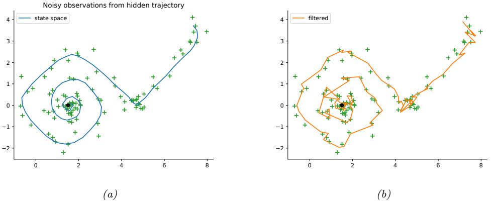
Figure 13.1: Illustration of particle filtering (using the dynamical prior as the proposal) applied to a 2d nonlinear dynamical system. (a) True underlying state and observed data. (b) PF estimate of the posterior mean. Generated by bootstrap\_filter\_spiral.ipynb.

A common choice is to define the unnormalized target distribution at step t to be

\[\hat{\gamma}\_t(\mathbf{z}\_{1:t}) = p(\mathbf{z}\_{1:t}, \mathbf{y}\_{1:t}) = p(\mathbf{z}\_1)p(\mathbf{y}\_1|\mathbf{z}\_1) \prod\_{s=1}^t p(\mathbf{z}\_s|\mathbf{z}\_{s-1})p(\mathbf{y}\_s|\mathbf{z}\_s) \tag{13.3}\]

Note that this a distribution over an (ever growing) sequence of latent variables. However, we often only care about the most recent marginal of this distribution, in which case we just need to compute ▷˜t(zt), which avoids having to store the full history.

For example, consider the following 2d nonlinear tracking problem (the same one as in Section 8.3.2.3):

\[\begin{aligned} p(\mathbf{z}\_t | \mathbf{z}\_{t-1}) &= \mathcal{N}(\mathbf{z}\_t | f(\mathbf{z}\_{t-1}), q\mathbf{I})\\ p(\mathbf{y}\_t | \mathbf{z}\_t) &= \mathcal{N}(\mathbf{y}\_t | \mathbf{z}\_t, r\mathbf{I})\\ f(\mathbf{z}) &= (z\_1 + \Delta \sin(z\_2), z\_2 + \Delta \cos(z\_1)) \end{aligned} \tag{13.4}\]

where ! is the step size of the underlying continuous system, q is the variance of the system noise, and r is the variance of the observation noise. (We treat !, q, and r as fixed constants; see Supplementary Section 13.1.3 for a discussion of joint state and parameter estimation.) The true underlying state trajectory, and the corresponding noisy measurements, are shown in Figure 13.1a. The posterior mean estimate of the state, computed using 2000 samples in a simple form of SMC called the bootstrap filter (Section 13.2.3.1), is shown in Figure 13.1b.

Particle filtering can also be applied to non-Markovian models, where z^t may depend on all the past hidden states, z1:t↓¹, and y^t depends on the current z^t and possibly also all the past hidden states, z1:t↓¹, and optionally the past observatiobns, y1:t↓¹. In this case, the unnormalized target

distribution at step t is

\[\hat{\gamma}\_t(\mathbf{z}\_{1:t}) = p(\mathbf{z}\_1)p(y\_1|\mathbf{z}\_1)\prod\_{s=1}^t p(\mathbf{z}\_s|\mathbf{z}\_{1:s-1})p(y\_s|\mathbf{z}\_{1:s})\tag{13.5}\]

For example, consider a 1d Gaussian sequence model where the dynamics are first-order Markov, but the observations depend on the entire past sequence (this is example 1.2.1 from [NLS19]):

\[\begin{aligned} p(z\_t|\mathbf{z}\_{1:t-1}) &= \mathcal{N}(z\_t|\phi z\_{t-1}, q) \\ p(y\_t|\mathbf{z}\_{1:t}) &= \mathcal{N}(y\_t|\sum\_{s=1}^t \beta^{t-s} z\_s, r) \end{aligned} \tag{13.6}\]

If we set ↼ = 0, we get ^p(yt|z1:t) = ^N (yt|zt, r) (where we define 0⁰ = 1), so the model becomes a linear-Gaussian SSM. As ↼ gets larger, the dependence on the past increases, making the inference problem harder. (We will revisit this example below.)

13.1.3 SMC samplers for static parameter estimation

Now consider the problem of parameter estimation from a fixed dataset, D = {yⁿ : n =1: N}. We suppose the observations are conditionally iid, so the posterior has the form p(z|D) ↑ p(z) ^{N n}=1 p(yn|z), where z is the unknown parameter. It is not immediately obvious how to approximate p(z|D) using SMC, since we just have one distribution. However, we can convert this into a sequential inference problem in several di!erent ways. One approach, known as data tempering, defines the (marginal) target distribution at step t as ▷˜t(zt) = p(zt)p(y1:t|zt). In this case, the number of time steps T is the same as the number of data samples, N. Another approach, known as likelihood tempering, defines the (marginal) target distribution at step t as ^▷˜t(zt) = ^p(zt)p(D|zt)^◁t , where 0 = ^{τt &}lt; ··· ^&lt; ^τT = 1 is a temperature parameter. In this case, the number of steps T depends on how quickly we anneal the distibution from the initial prior p(z1) to the final target p(z^T )p(D|z^T ).

Once we have defined the marginal target distributions ▷˜t(zt), we need a way to expand this to a joint target distribution over a sequence of variables, ▷˜t(z1:t), so the distributions become connected to each other. We explain how to do this in Section 13.6. We can then treat the model as an SSM and apply particle filtering. At the end, we extract the final joint target distribution, ▷˜^T (z1:^T ) = p(z1:^T )p(D|z^T ), from which we can compute the marginal target distribution ▷˜^T (z^T ) = p(z^T , D), from which we can get the posterior p(z|D) by normalizing. We give the details in Section 13.6.

13.2 Particle filtering

In this section, we cover the basics of SMC for state space models, culiminating in a method known as the particle filter.

13.2.1 Importance sampling

We start by reviewing the self-normalized importance sampling method (SNIS), which is the foundation of the particle filter. (See also Section 11.5.)

Suppose we are interested in estimating the expectation of some function 5^t with respect to a target distribution ϖt, which we denote by

\[\mathbb{E}\_t(\varphi) \stackrel{\Delta}{=} \mathbb{E}\_{\pi\_t}[\varphi\_t(\mathbf{z}\_{1:t})] = \int \frac{\tilde{\gamma}\_t(\mathbf{z}\_{1:t})}{Z\_t} \varphi\_t(\mathbf{z}\_{1:t}) d\mathbf{z}\_{1:t} \tag{13.7}\]

where Z^t = / ▷˜t(z1:t)dz1:t. Suppose we use SNIS with proposal qt(z1:t). We then get the following approximation:

\[\pi\_t(\varphi) \approx \frac{1}{\hat{Z}\_t} \frac{1}{N\_s} \sum\_{i=1}^{N\_s} \tilde{w}\_t(\mathbf{z}\_{1:t}^i) \varphi\_t(\mathbf{z}\_{1:t}^i) \tag{13.8}\]

where zⁱ 1:t iid ^{↔︎ qt} are independent samples from the proposal, ^w˜^{i t} are the unnormalized weights defined by

\[ \bar{w}\_t^i = \frac{\bar{\gamma}\_t(\mathbf{z}\_{1:t}^i)}{q\_t(\mathbf{z}\_{1:t}^i)} \tag{13.9} \]

and Zˆ^t is the approximate normalization constant defined by

\[\hat{Z}\_t \triangleq \frac{1}{N\_s} \sum\_{i=1}^{N\_s} \bar{w}\_t^i \tag{13.10}\]

To simplify notation, let us define the normalized weights by

\[W\_t^i = \frac{\bar{w}\_t^i}{\sum\_j \bar{w}\_t^j} \tag{13.11}\]

Then we can write

\[\mathbb{E}\_{\pi\_t} \left[ \varphi\_t(\mathbf{z}\_{1:t}) \right] \approx \sum\_{i=1}^{N\_s} W\_t^i \varphi\_t(\mathbf{z}\_{1:t}^i) \tag{13.12}\]

Alternatively, instead of computing the expectation of a specific target function, we can just approximate the target distribution itself, using a sum of weighted samples:

\[\pi\_t(\mathbf{z}\_{1:t}) \approx \sum\_{i=1}^{N\_s} W\_t^i \delta(\mathbf{z}\_{1:t} - \mathbf{z}\_{1:t}^i) \stackrel{\Delta}{=} \widehat{\pi}\_t(\mathbf{z}\_{1:t}) \tag{13.13}\]

The problem with importance sampling when applied in the context of sequential models is that the dimensionality of the state space is very large, and increases with t. This makes it very hard to define a good proposal that covers the high probability regions, resulting in most samples getting negligible weight. In the sections below, we discuss solutions to this problem.

13.2.2 Sequential importance sampling

In this section, we discuss sequential importance sampling or SIS, in which the proposal has the following autoregressive structure:

\[q\_t(\mathbf{z}\_{1:t}) = q\_{t-1}(\mathbf{z}\_{1:t-1})q\_t(\mathbf{z}\_t|\mathbf{z}\_{1:t-1})\tag{13.14}\]

We can obtain samples from q^t↓¹(z1:t↓¹) by reusing the zⁱ 1:t↓¹ samples, which we then extend by one step by sampling from the conditional ^qt(zt|zⁱ 1:t↓1). We can think of this as “growing” the chain (sequence of states). The unnormalized weights can be computed recursively as follows:

\[\ddot{w}\_t(\mathbf{z}\_{1:t}) = \frac{\ddot{\gamma}\_t(\mathbf{z}\_{1:t})}{q\_t(\mathbf{z}\_{1:t})} = \frac{\ddot{\gamma}\_{t-1}(\mathbf{z}\_{1:t-1})}{\ddot{\gamma}\_{t-1}(\mathbf{z}\_{1:t-1})} \frac{\ddot{\gamma}\_t(\mathbf{z}\_{1:t})}{q\_t(\mathbf{z}\_t|\mathbf{z}\_{1:t-1})q\_{t-1}(\mathbf{z}\_{1:t-1})} \tag{13.15}\]

\[=\frac{\widetilde{\gamma}\_{t-1}(\mathbf{z}\_{1:t-1})}{q\_{t-1}(\mathbf{z}\_{1:t-1})}\frac{\widetilde{\gamma}\_{t}(\mathbf{z}\_{1:t})}{\widetilde{\gamma}\_{t-1}(\mathbf{z}\_{1:t-1})q\_{t}(\mathbf{z}\_{t}|\mathbf{z}\_{1:t-1})}\tag{13.16}\]

\[\dot{\gamma} = \tilde{w}\_{t-1}(\mathbf{z}\_{1:t-1}) \frac{\tilde{\gamma}\_t(\mathbf{z}\_{1:t})}{\tilde{\gamma}\_{t-1}(\mathbf{z}\_{1:t-1}) q\_t(\mathbf{z}\_t | \mathbf{z}\_{1:t-1})} \tag{13.17}\]

The ratio factors are sometimes called the incremental importance weights:

\[\alpha\_t(\mathbf{z}\_{1:t}) = \frac{\bar{\gamma}\_t(\mathbf{z}\_{1:t})}{\bar{\gamma}\_{t-1}(\mathbf{z}\_{1:t-1}) q\_t(\mathbf{z}\_t | \mathbf{z}\_{1:t-1})} \tag{13.18}\]

See Algorithm 13.1 for pseudocode for the resulting SIS algorithm. (In practice we compute the weights in log-space, and convert back using the log-sum-exp trick.)

Note that, in the special case of state space models, the weight computation can be further simplified. In particular, suppose we have

\[\bar{\gamma}\_t(\mathbf{z}\_{1:t}) = p(\mathbf{z}\_{1:t}, \mathbf{y}\_{1:t}) = p(\mathbf{y}\_t | \mathbf{z}\_{1:t}) p(\mathbf{z}\_t | \mathbf{z}\_{1:t-1}) p(\mathbf{z}\_{1:t-1}, \mathbf{y}\_{1:t-1}) \tag{13.19}\]

\[=p(y\_t|\mathbf{z}\_{1:t})p(\mathbf{z}\_t|\mathbf{z}\_{1:t-1})\ddot{\gamma}\_{t-1}(\mathbf{z}\_{1:t-1})\tag{13.20}\]

Then the incremental weight is given by

\[\alpha\_t(\mathbf{z}\_{1:t}) = \frac{p(\mathbf{y}\_t|\mathbf{z}\_{1:t})p(\mathbf{z}\_t|\mathbf{z}\_{1:t-1})\bar{\gamma}\_{t-1}(\mathbf{z}\_{1:t-1})}{\bar{\gamma}\_{t-1}(\mathbf{z}\_{1:t-1})q\_t(\mathbf{z}\_t|\mathbf{z}\_{1:t-1})} = \frac{p(\mathbf{y}\_t|\mathbf{z}\_{1:t})p(\mathbf{z}\_t|\mathbf{z}\_{1:t-1})}{q\_t(\mathbf{z}\_t|\mathbf{z}\_{1:t-1})}\tag{13.21}\]

Unfortunately SIS su!ers from a problem known as weight degeneracy or particle impoverishment, in which most of the weights become very small (near zero), so the posterior ends up being approximated by a single particle. This is illustrated in Figure 13.2a, where we apply SIS to the non-Markovian example in Equation (13.6) using N^s = 5 particles. The reason for degeneracy is that each particle has to “explain” (generate) the entire sequence of observations. Each sequence of guessed states becomes increasingly improbable over time, due to the product of likelihood terms, and the di!erences between the weights of each hypothesis will grow exponentally. Of course, there has to be a best sequence amongst the set of candidates, so when we normalize the weights, the best one will get weight 1 and the rest will get weight 0. But this is a waste of most of the particles. We discuss a solution to this in Section 13.2.3.

Algorithm 13.1: Sequential importance sampling (SIS)

¹ Initialization: z^{i 1 ↔︎ q}1(z1), ^w˜^{i 1 =} ⇁˜1(zⁱ 1) q1(z^{i 1}) , ^{Wi 1 = w}˜ⁱ ! ^{1 j w}˜^j 1 , ϖˆ1(z1) = &N^{s i}=1 W^{i 1}ϑ(z^{1 → zi} 1) ² for t =2: T do ³ for i =1: N^s do ⁴ Sample z^{i t ↔︎ q}t(zt|zⁱ 1:t↓¹) ⁵ Compute incremental weight ϱ^{i t =} ⇁˜t(zⁱ 1:t) ⇁˜t→1(zⁱ 1:t→1)qt(zⁱ t|zⁱ 1:t→1) ⁶ Compute unnormalized weight w˜^{i t} = ˜w^{i t}↓¹ϱⁱ t ⁷ Compute normalized weights W^{i t = w}˜ⁱ ! ^{t j w}˜^j t for i =1: N^{s 8} Compute MC posterior ϖˆt(z1:t) = &^{Ns i}=1 W^{i t ϑ}(z1:^{t → zi} 1:t)

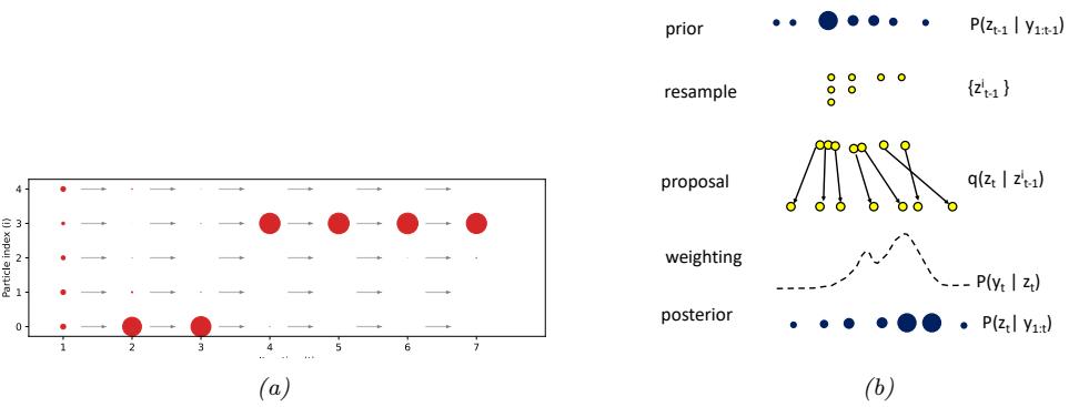
Figure 13.2: (a) Illustration of weight degeneracy for SIS applied to the model in Equation (13.6). with parameters (⇁, q, β, r) = (0.9, 10.0, 0.5, 1.0). We use T = 6 steps and N^s = 5 samples. We see that as t increases, almost all the probability mass concentrates on particle 3. Generated by sis\_vs\_smc.ipynb. Adapted from Figure 2 of [NLS19]. (b) Illustration of the bootstrap particle filtering algorithm.

13.2.3 Sequential importance sampling with resampling

In this section, we describe sequential importance sampling with resampling (SISR). The basic idea is this: instead of “growing” all of the old particle sequences by one step, we first select the N^s “fittest” particles, by sampling from the old posterior, and then we let these survivors grow by one step.

In more detail, at step t, we sample from

\[q\_t^{\text{SISR}}(\mathbf{z}\_{1:t}) = \hat{\pi}\_{t-1}(\mathbf{z}\_{1:t-1}) q\_t(\mathbf{z}\_t | \mathbf{z}\_{1:t-1}) \tag{13.22}\]

where ϖˆ^t↓1(z1:t↓1) is the previous weighted posterior approximation. By contrast, in SIS, we sample from

\[q\_t^{\rm SIS}(\mathbf{z}\_{1:t}) = q\_{t-1}^{\rm SIS}(\mathbf{z}\_{1:t-1}) q\_t(\mathbf{z}\_t | \mathbf{z}\_{1:t-1}) \tag{13.23}\]

Algorithm 13.2: Sequential importance sampling with resampling (SISR)

¹ Initialization: z^{i 1 ↔︎ q}1(z1), ^w˜^{i 1 =} ⇁˜1(zⁱ 1) q1(z^{i 1}) , ^{Wi 1 = w}˜ⁱ ! ^{1 j w}˜^j 1 , ϖˆ1(z1) = &N^{s i}=1 W^{i 1}ϑ(z^{1 → zi 2} for t =2: T do ³ Compute ancestors a1:N^{s t}↓¹ = resample( ˜w 1:N^{s t}↓¹ ) ⁴ Select z1:N^{s t}↓^{1 =} permute(a1:N^{s t}↓¹ , ^z1:N^{s t}↓¹ ) ⁵ Reset unnormalized weights w˜1:N^{s t}↓¹ = 1/N^{s 6} for i =1: N^s do ⁷ Sample z^{i t ↔︎ q}t(zt|zⁱ 1:t↓¹) ⁸ Compute unnormalized weight w˜^{i t} = ϱ^{i t =} ⇁˜t(zⁱ 1:t) ⇁˜t→1(zⁱ 1:t→1)qt(zⁱ t|zⁱ 1:t→1) ⁹ Compute normalized weights W^{i t = w}˜ⁱ ! ^{t j w}˜^j t for i =1: N^{s 10} Compute MC posterior ϖˆt(z1:t) = &^{Ns i}=1 W^{i t ϑ}(z1:^{t → zi} 1:t)

We can sample from Equation (13.22) in two steps. First we resample N^s samples from ϖˆ^t↓1(z1:t↓1) to get a uniformly weighted set of new samples zⁱ 1:t↓¹. (See Section 13.2.4 for details on how to do this.) Then we extend each sample using z^{i t ↔︎ q}t(zt|zⁱ 1:t↓¹), and concatenate ^{zi t} to zⁱ 1:t↓¹,

After making a proposal, we compute the unnormalized weights. We use the standard SNIS method, except we “pretend” that the proposal is given by ▷˜^t↓¹(zⁱ 1:t↓¹)qt(zⁱ t|zⁱ 1:t↓¹) even though we used ϖˆ^t↓¹(zⁱ 1:t↓¹)qt(zⁱ t|zⁱ 1:t↓¹). The intuitive reason why this is valid is because the previous weighted approximation, ϖˆ^t↓1(zⁱ 1:t↓1), was an unbiased estimate of the previous target distribution, ▷˜^t↓¹(z1:t↓¹). (See e.g., [CP20b] for more theoretical details.) We then compute the unnormalized weights, which are the same as the incremental weights, since the resampling step sets w˜^{i t}↓¹ = 1. We then normalize these weights and compute the new approximation to the target posterior ϖˆt(z1:t). See Algorithm 13.2 for the pseudocode.

13.2.3.1 Bootstrap filter

We now consider a special case of SISR, in which the model is an SSM, and the proposal distribution is equal to the dynamical prior:

\[q\_t(\mathbf{z}\_t | \mathbf{z}\_{1:t-1}) = p(\mathbf{z}\_t | \mathbf{z}\_{1:t-1}) \tag{13.24}\]

In this case, the corresponding incremental weight in Equation (13.21) simplifies to

\[\alpha\_t(\mathbf{z}\_{1:t}) = \frac{p(\mathbf{y}\_t|\mathbf{z}\_{1:t})p(\mathbf{z}\_t|\mathbf{z}\_{1:t-1})}{q(\mathbf{z}\_t|\mathbf{z}\_{1:t-1})} = \frac{p(\mathbf{y}\_t|\mathbf{z}\_t)p(\mathbf{z}\_t|\mathbf{z}\_{t-1})}{p(\mathbf{z}\_t|\mathbf{z}\_{t-1})} = p(\mathbf{y}\_t|\mathbf{z}\_{1:t}) \tag{13.25}\]

This special case is called the bootstrap filter [Gor93] or the survival of the fittest algorithm [KKR95]. (In the computer vision literature, this is called the condensation algorithm, which stands for “conditional density propagation” [IB98].) See Figure 13.2b for an illustration of how this algorithm works, and Figure 13.1b for some sample results on real data.

Author: Kevin P. Murphy. (C) MIT Press. CC-BY-NC-ND license

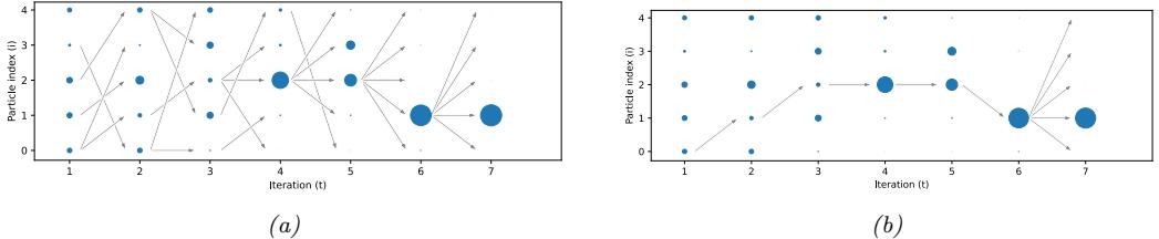
Figure 13.3: (a) Illustration of diversity of samples in SMC applied to the model in Equation (13.6). (b) Illustration of the path degeneracy problem. Generated by sis\_vs\_smc.ipynb. Adapted from Figure 3 of [NLS19].

The bootstrap filter is useful for models where we can sample from the dynamics, but cannot evaluate the transition model pointwise. This occurs in certain implicit dynamical models, such as those defined using di!erential equations (see e.g., [IBK06]); such models are often used in epidemiology. However, in general it is much more e”cient to use proposals that take the current evidence y^t into account. We discuss ways to approximate such “locally optimal” proposals in Section 13.3.

13.2.3.2 Path degeneracy problem

In Figure 13.3a we show how particle filtering can result in a much more diverse set of active particles, with more balanced weights when applied to the non-Markovian example in Equation (13.6).

While particle filtering does not su!er from weight degeneracy, it does su!er from another problem known as path degeneracy. This refers to the fact that the number of particles that “survive” (have non-negligible weight) over many steps may drop rapidly over time, resulting in a loss of diversity when we try to represent the distribution over the past. We illustrate this in Figure 13.3b, where we only include arrows for samples that have been resampled at each step up until the final step. We see that we have N^s = 5 identical copies of z^{1 1} in the final set of surviving sequences. (The time at which all the paths meet at a common ancestor, when tracing backwards in time, is known as the coalescence time.) We discuss some ways to ameliorate this issue in Section 13.2.4 and Section 13.2.5.

13.2.3.3 Estimating the normalizing constant

We can use particle filtering to approximate the normalization constant Z^T = p(y1:^T ) = ^{T t}=1 p(yt|y1:t↓1) as follows:

\[ \hat{Z}\_T = \prod\_{t=1}^T \hat{Z}\_t \tag{13.26} \]

where, from Equation (13.10), we have

\[\hat{Z}\_t = \frac{1}{N\_s} \sum\_{i=1}^{N\_s} \bar{w}\_t^i = \hat{Z}\_{t-1} \left( \widehat{Z\_t / Z\_{t-1}} \right) \tag{13.27}\]

where

\[\widehat{Z\_t/Z\_{t-1}} = \frac{\sum\_{i=1}^{N\_s} \bar{w}\_t^i}{\sum\_{i=1}^{N\_s} \bar{w}\_{t-1}^i} \tag{13.28}\]

This estimate of the marginal likelihood is very useful for tasks such as parameter estimation.

13.2.4 Resampling methods

Importance sampling gives a weighted set of particles, {(W^{i t} , z^{i t}) : i =1: N}, which we can use to approximate posterior expectations using

\[\mathbb{E}\left[f(\mathbf{z}\_t)|\mathbf{y}\_{1:t}\right] \approx \sum\_{i=1}^{N} W\_t^i f(\mathbf{z}\_t^i) \tag{13.29}\]

Suppose we sample a single index ^A ↗ {1,…,N} with probabilities (W^{1 t} ,…,W^{N t} ). Then the expected value evaluated at this index is

\[\mathbb{E}\left[f(\mathbf{z}\_t^A)|\mathbf{y}\_{1:t}\right] = \sum\_{i=1}^N p(A=i)f(\mathbf{z}\_t^i) = \sum\_{i=1}^N W\_t^i f(\mathbf{z}\_t^i) \tag{13.30}\]

If we sample N indices independently and compute their average, we get

\[\mathbb{E}\left[f(\mathbf{z}\_t)|y\_{1:t}, A\_{1:N}\right] \approx \frac{1}{N} \sum\_{i=1}^N f(\mathbf{z}\_t^{A\_i})\tag{13.31}\]

which is a standard unweighted Monte Carlo estimate, with weights W^{i t} = 1/N. Averaging over the indices gives

\[\mathbb{E}\_{A\_{1:N}}\left[\frac{1}{N}\sum\_{i=1}^{N}f(\mathbf{z}\_t^{A\_i})\right] = \sum\_{i=1}^{N}W\_t^i f(\mathbf{z}\_t^i) \tag{13.32}\]

Thus using the output from the resampling procedure — which drops particles with low weight, and duplicates particles with high weight — will give the same result in expectation as the original weighted estimate. However, to reduce the variance of the method, we need to pick the resampling method carefully, as we discuss below.

13.2.4.1 Inverse cdf

Most of the common resampling methods work as follows. First we form the cumulative distribution from the weights W1:^N , as illustrated by the staircase in Figure 13.4. (We drop the t index for brevity.) Then, given a set of ^N uniform random variables, ^{Ui ↔︎} Unif(0, 1), we check to see which bin (interval) Uⁱ lands in; if it falls in bin a, we return index a, i.e., sample i gets mapped to index a if

\[\sum\_{j=1}^{a-1} W^j \le U^i < \sum\_{j=1}^a W^j \tag{13.33}\]

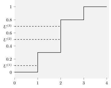
Figure 13.4: Illustration of how to sample from the empirical cdf P(x) = “^{N n}=1 ^WnI(^{x ⇔ n}) shown in black. The height of step n is Wn. If U^m picks step n, then we set the ancestor of m to be n, i.e., A^m = n. In this example, A1:3 = (1, 2, 2). Adapted from Figure 9.3 of [CP20b].

It would seem that each index would take O(N) time to compute, for a total time of O(N²), but if the Uⁱ are ordered from smallest to largest, we can implement it in O(N) time. We denote this function A1:^N = icdf(W1:^N , U1:^N ). See Listing 13.1 for some JAX code.1

def icdf(weights , u):
  n = weights.shape[0]
  cumsum = jnp.cumsum(weights)
  idx = jnp.searchsorted(cumsum , u)
  return jnp.clip(idx , 0, n - 1)

13.2.4.2 Multinomial resampling

In multinomial resampling, we set U1:^N to be an ordered set of N samples from the uniform distribution. We then compute the ancestor indices using A1:^N = icdf(W1:^N , U1:^N ).

Although this is a simple method, it can introduce a lot of variance into the representation of the distribution. For example, suppose all the weights are equal, ^Wn = 1/N. Let ^{Wn =} &^{N m}=1 I(A^m = n) be the number of “o!spring” for particle n (i.e., the number of times this particle is chosen in the resampling step). We have ^{Wn ↔︎} Bin(N, ¹/N), so ^P(Wⁿ = 0) = (1 ^{→ 1}/N)^{N ↓ e}↓^{1 ↓ 0}.37. So there is a 37% chance that any given particle will disappear even though they all had the same initial weight. In the sections below, we discuss some low variance resampling methods.

13.2.4.3 Stratified resampling

A simple approach to improve on multinomial resampling is to use stratified resampling, in which we divide the unit interval into N^s strata, (0, 1/Ns), (1/Ns, 2/Ns), up to (1 → 1/Ns, 1). We then generate

\[U^i \sim \text{Unif}((i-1)/N\_s, i/N\_s) \tag{13.34}\]

and compute A1:^N = icdf(W1:^N , U1:^N ). 2

^1. Modified from https://github.com/blackjax-devs/blackjax/blob/main/blackjax/smc/resampling.py.

^2. To compute the U1:^N , we can use v = jr.uniform(rngkey, (n,)) and u = (jnp.arange(n) + v) / n.

13.2.4.4 Systematic resampling

We can further reduce the variance by forcing all the samples to be deterministically generated from a shared random source, u ↔︎ Unif(0, 1), by computing

\[U^i = \frac{i-1}{N\_s} + \frac{u}{N\_s} \tag{13.35}\]

We then compute A1:^N = icdf(W1:^N , U1:^N ). 3

13.2.4.5 Comparison

It can be proved that all of the above methods are unbiased. Empirically it seems that systematic resampling is lower variance than other methods [HSG06], although stratified resampling, and the more complex method of [GCW19], have better theoretical properties. Multinomial resampling is not recommended, since it has provably higher variance than the other methods.

13.2.5 Adaptive resampling

The resampling step can result in loss of diversity, since each ancestor may generate multiple children, and some may generate no children, since the ancestor indices A^{n t} are sampled independently; this is the path degeneracy problem mentioned above. On the other hand, if we never resample, we end up with SIS, which su!ers from weight degeneracy (particles with negligible weight). A compromise is to use adaptive resampling, in which we resample whenever the e!ective sample size or ESS drops below some minimum, such as N/2. A common way to define the ESS is as follows:4

\[\text{ESS}(W^{1:N}) = \frac{1}{\sum\_{n=1}^{N} (W^n)^2} \tag{13.36}\]

Alternatively we can compute the ESS using the unnormalized weights:

\[\text{ESS}(\bar{w}^{1:N}) = \frac{\left(\sum\_{n=1}^{N} \bar{w}^n\right)^2}{\sum\_{n=1}^{N} (\bar{w}^n)^2} \tag{13.37}\]

Note that if we have ^k weights with ^w˜ⁿ = 1 and ^{N → k} weights with ^w˜ⁿ = 0, then the ESS is ^k; thus ESS is between 1 and N.

The pseudocode for SISR with adaptive resampling is given in Algorithm 13.3. (We use the notation of [Law+22, App. B], in which we first sample new extensions of the sequences, and then optionally resample the sequences at the end of each step.)

13.3 Proposal distributions

The e”ciency of PF is crucially dependent on the quality of the proposal distribution. We discuss some options below.

^3. To compute the U1:^N , we can use v = jr.uniform(rngkey, ()) and u = (jnp.arange(n) + v) / n.

^4. Note that the ESS used in SMC is di”erent than the ESS used in MCMC (Section 12.6.3); the latter takes into account auto-correlation of the MCMC samples.

Algorithm 13.3: SISR with adaptive resampling (generic SMC)

¹ Initialization: w˜1:N^{s 0} = 1, ^Zˆ⁰ = 1 ² for t =1: T do ³ for i =1: N^s do ⁴ Sample particle z^{i t ↔︎ q}t(zt|zⁱ 1:t↓1) ⁵ Compute incremental weight ϱ^{i t =} ⇁˜t(zⁱ 1:t) ⇁˜t→1(zⁱ 1:t→1)qt(zⁱ t|zⁱ 1:t→1) ⁶ Compute unnormalized weight w˜^{i t} = ˜w^{i t}↓¹ϱⁱ t ⁷ Estimate normalization constant: ^Z⊋t/Z^t↓^{1 =} !Ns ⁱ=1 ^w˜ⁱ ! ^t Ns ⁱ=1 ^w˜ⁱ t→1 , ^Zˆ^{t = Z}ˆ^t↓¹(Z⊋t/Z^t↓¹) ⁸ if ESS( ˜w1:Nt↓¹) ^&lt; ESSmin then ⁹ Compute ancestors a1:N^{s t} = resample( ˜w 1:N^{s t} ) ¹⁰ Select z1:N^{s t} = permute(a1:N^{s t} , z1:N^{s t} ) ¹¹ Reset unnormalized weights w˜1:N^{s t} = 1/N^{s 12} Compute normalized weights W^{i t = w}˜ⁱ ! ^{t j w}˜^j t for i =1: N^{s 13} Compute MC posterior ϖˆt(z1:t) = &^{Ns i}=1 W^{i t ϑ}(z1:^{t → zi} 1:t)

13.3.1 Locally optimal proposal

We define the (one-step) locally optimal proposal distribution q^{→ t} (zt|z1:t↓1) to be the one that minimizes

\[D\_{\rm KL} \left( \pi\_{t-1}(\mathbf{z}\_{1:t-1}) q\_t(\mathbf{z}\_t | \mathbf{z}\_{1:t-1}) \parallel \pi\_t(\mathbf{z}\_{1:t}) \right) \tag{13.38}\]

\[\mathbf{x} = \mathbb{E}\_{\pi\_{t-1}q\_t} \left[ \log \left\{ \pi\_{t-1}(\mathbf{z}\_{1:t-1}) q\_t(\mathbf{z}\_t | \mathbf{z}\_{1:t-1}) \right\} - \log \pi\_t(\mathbf{z}\_{1:t}) \right] \tag{13.39}\]

\[\mathbf{z} = \mathbb{E}\_{\pi\_{t-1}q\_t} \left[ \log q\_t(\mathbf{z}\_t | \mathbf{z}\_{1:t-1}) - \log \pi\_t(\mathbf{z}\_t | \mathbf{z}\_{1:t-1}) \right] + \text{const} \tag{13.40}\]

\[\mathbf{E} = \mathbb{E}\_{\pi\_{t-1}q\_t} \left[ D\_{\text{KL}} \left( q\_t(\mathbf{z}\_t | \mathbf{z}\_{1:t-1}) \parallel \pi\_t(\mathbf{z}\_t | \mathbf{z}\_{1:t-1}) \right) \right] + \text{const} \tag{13.41}\]

The KL is minimized by choosing

\[q\_t^\*(\mathbf{z}\_t|\mathbf{z}\_{1:t-1}) = \pi\_t(\mathbf{z}\_t|\mathbf{z}\_{1:t-1}) = \frac{\bar{\gamma}\_t(\mathbf{z}\_{1:t})}{\bar{\gamma}\_t(\mathbf{z}\_{1:t-1})} \tag{13.42}\]

where ^▷˜t(z1:t↓¹) = / ^▷˜t(z1:t)dz^t is the probability of the past sequence under the current target distribution.

Note that the subscript t specifies the t’th distribution, so in the context of SSMs, we have ϖt(zt|z1:t↓¹) = p(zt|z1:t↓¹, y1:t). Thus we see that when proposing zt, we should condition on all the data, including the most recent observation, yt; this is called a guided particle filter, and will be better than the bootstrap filter, which proposes from the prior.

In general, it is intractable to compute the locally optimal proposal, so we consider various approximations below.

13.3.2 Proposals based on the extended and unscented Kalman filter

One way to approximate the locally optimal proposal distribution is based on the extended Kalman filter (Section 8.3.2) or the unscented Kalman filter (Section 13.3.2), which gives rise to the extended particle filter [DGA00] and unscented particle filter [Mer+00] respectively. To explain these methods, we follow the presentation of [NLS19, p36]. As usual, we assume the dynamical system can be written as z^t = f(z^t↓¹) + q^t and y^t = h(zt) + rt, where q^t is the system noise and r^t is the observation noise. The EKF and UKF approximations assume that the joint distribution over neighboring time steps, given the i’th history, is Gaussian:

\[p(\mathbf{z}\_t, y\_t | \mathbf{z}\_{1:t-1}^i) \approx \mathcal{N}\left(\begin{pmatrix} \mathbf{z}\_t \\ y\_t \end{pmatrix} | \hat{\mu}^i, \hat{\Sigma}^i \right) \tag{13.43}\]

where

\[\hat{\boldsymbol{\mu}}^{i} = \begin{pmatrix} \hat{\mu}^{i}\_{z} \\ \hat{\mu}^{i}\_{y} \end{pmatrix}, \hat{\Sigma}^{i} = \begin{pmatrix} \hat{\Sigma}^{i}\_{zz} & \hat{\Sigma}^{i}\_{zy} \\ \hat{\Sigma}^{i}\_{yz} & \hat{\Sigma}^{i}\_{yy} \end{pmatrix} \tag{13.44}\]

(See Section 8.5.1 for details.)

The EKF and UKF compute µˆⁱ and !ˆ ⁱ di!erently. In the EKF, we linearize f and h, and assume the noise terms are Gaussian. We then compute ^p(zt, ^yt|zⁱ 1:t↓¹) exactly for this linearized model (see Section 8.3.1). In the UKF, we propagate sigma points through f and h, and approximate the resulting means and covariances using the unscented transform, which can be more accurate (see Section 8.4). Once we have computed µˆⁱ and !ˆ ⁱ , we can use standard rules for Gaussian conditioning to compute the approximate proposal as follows:

\[q(\mathbf{z}\_t | \mathbf{z}\_{1:t-1}^i, y\_t) \approx \mathcal{N}(\mathbf{z}\_t | \boldsymbol{\mu}\_t^i, \boldsymbol{\Sigma}\_t^i) \tag{13.45}\]

\[ \mu\_t^i = \hat{\mu}\_z^i + \hat{\Sigma}\_{zy}^i (\hat{\Sigma}\_{yy}^i)^{-1} (y\_t - \hat{\mu}\_y^i) \tag{13.46} \]

\[ \hat{\Sigma}\_t^i = \hat{\Sigma}\_{zz}^i - \hat{\Sigma}\_{zy}^i \left(\hat{\Sigma}\_{yy}^i\right)^{-1} \hat{\Sigma}\_{yz}^i \tag{13.47} \]

Note that the linearization (or sigma point) approximation needs to be performed for each particle sepatately.

13.3.3 Proposals based on the Laplace approximation

To handle non-Gaussian likelihoods in an SSM, we can use the Laplace approximation (Section 7.4.3), as suggested in [DGA00]. In particular, consider an SSM with linear-Gaussian latent dynamics and a GLM likelihood. At each step, we compute the maximum z^{→ t} = argmax log p(yt|zt) as step t (e.g., using Newton-Raphson), and then approximate the likelihood using

\[p(y\_t|\mathbf{z}\_t) \approx \mathcal{N}(\mathbf{z}\_t|\mathbf{z}\_t^\*, -\mathbf{H}\_t^\*) \tag{13.48}\]

where H→ ^t is the Hessian of the log-likelihood at the mode. We now compute ^p(zt|z^{i t}↓¹, yt) using the update step of the Kalman filter, using the same equations as in Section 13.3.2. This combination is called the Laplace Gaussian filter [Koy+10]. We give an example in Section 13.3.3.1.

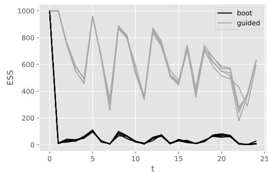
Figure 13.5: E!ective sample size at each step for the bootstrap particle filter and a guided particle filter for a Gaussian SSM with Poisson likelihood. Adapted from Figure 10.4 of [CP20b]. Generated by pf\_guided\_neural\_decoding.ipynb.

13.3.3.1 Example: neural decoding

In this section, we give an example where we apply the Laplace approximation to an SSM with linear-Gaussian dynamics and a Poisson likelihood. The application arises from neuroscience. In particular, assume we record the neural spike trains as a monkey moves its hand around in space. Let ^zt ↗ ^R6 represent the 3d location and velocity of the hand. We model the dynamics of the hand using a simple Brownian random walk model [CP20b, p157]:

\[\begin{pmatrix} z\_t(i) \\ z\_t(i+3) \end{pmatrix} | \mathbf{z}\_{t-1} \sim \mathcal{N}\_2 \left( \begin{pmatrix} 1 & \Delta \\ 0 & 1 \end{pmatrix} \begin{pmatrix} z\_{t-1}(i) \\ z\_{t-1}(i+3) \end{pmatrix}, \sigma^2 \mathbf{Q} \right), \ i = 1:3 \tag{13.49}\]

where the covariance of the noise is given by the following, assuming a discretization step of !:

\[\mathbf{Q} = \begin{pmatrix} \Delta^3/3 & \Delta^2/2\\ \Delta^2/2 & \Delta \end{pmatrix} \tag{13.50}\]

We assume the k’th observation at time t is the number of spikes for neuron k in this sensing interval:

\[p(y\_t(k)|\mathbf{z}\_t) = \text{Poi}(\lambda\_k(\mathbf{z}\_t)) \tag{13.51}\]

\[\log \lambda\_k(\mathbf{z}\_t) = \alpha\_k + \beta\_k^\top \mathbf{z}\_t \tag{13.52}\]

Our goal is to compute p(zt|y1:t), which lets us infer the position of the hand from the neural code. (Apart from its value for furthering basic science, this can be useful for applications such as helping disabled people control their arms using “mind control”.)

To illustrate this, we sample a synthetic dataset from the model, to simulate a “monkey” moving its arm for T = 25 time steps; this generates K = 50 neuronal counts per time step. We then apply particle filtering to this dataset (using the true model), using either the bootstrap filter (i.e., proposal is the random walk prior) or the guided filter (i.e., proposal is the Laplace approximation mentioned above). In Figure 13.5, we see that the e!ective sample size of the guided filter is much higher than for the bootstrap filter.

13.3.4 Proposals based on SMC (nested SMC)

It is possible to use SMC as a subroutine to compute a proposal distribution for SMC: at each step t, for each particle i, we run an SMC algorithm where the target distribution is the optimal proposal, ^p(zt|zⁱ 1:t↓1, y1:t). This is called nested SMC [NLS15; NLS19].

This method can approximate the locally optimal proposal arbitrarily well, since it does not make any limiting parametric assumptions. However, the method can be slow, although the inner SMC algorithm can be run in parallel for each outer sample [NLS15; NLS19].

13.4 Rao-Blackwellized particle filtering (RBPF)

In some models, we can partition the hidden variables into two kinds, m^t and zt, such that we can analytically integrate out z^t provided we know the values of m1:t. This means we only have to sample m1:t, and can represent p(zt|m1:t, y1:t) parametrically. These hybrid particles are sometimes called distributional particles or collapsed particles [KF09a, Sec 12.4]. This combines techniques from particle filtering (Section 13.2) with deterministic methods such as Kalman filtering (Section 8.2.2).

The advantage of this approach is that we reduce the dimensionality of the space in which we are sampling, which reduces the variance of our estimate. This technique is known as Rao-Blackwellized particle filtering or RBPF for short. (See Section 11.6.2 for more details on Rao-Blackwellization.) In Section 13.4.1 we give an example of RBPF for inference in a switching linear dynamical systems. In Section 13.4.3 we illustrate RBPF for inference in the SLAM model for a mobile robot.

13.4.1 Mixture of Kalman filters

In this section, we consider the application of RBPF to a switching linear dynamical system (Section 29.9). This model has both continuous and discrete latent variables. This can be used to track a system that switches between discrete modes or operating regimes, represented by the discrete variable mt.

For notational simplicity, we ignore the control inputs ut. Thus the model is given by

\[p(\mathbf{z}\_t | \mathbf{z}\_{t-1}, m\_t = k) = \mathcal{N}(\mathbf{z}\_t | \mathbf{F}\_k \mathbf{z}\_{t-1}, \mathbf{Q}\_k) \tag{13.53}\]

\[p(y\_t | \mathbf{z}\_t, m\_t = k) = \mathcal{N}(y\_t | \mathbf{H}\_k \mathbf{z}\_t, \mathbf{R}\_k) \tag{13.54}\]

\[p(m\_t = k | m\_{t-1} = j) = A\_{jk} \tag{13.55}\]

We let ω^k = (Fk, Hk, Qk, Rk, A:,k) represent all the parameters for state k.

Exact inference is intractable, but if we sample the discrete variables, we can infer the continuous variables conditoned on the discretes exactly, making this a good candidate for RBPF. In particular, if we sample trajectories mⁿ 1:t, we can apply a Kalman filter to each particle. This can be thought of as a mixture of Kalman filters [CL00]. The resulting belief state is represented by

\[p(\mathbf{z}\_t, m\_t | \mathbf{y}\_{1:t}) \approx \sum\_{n=1}^{N} W\_t^n \delta(m\_t - m\_t^n) \mathcal{N}(\mathbf{z}\_t | \boldsymbol{\mu}\_t^n, \boldsymbol{\Sigma}\_t^n) \tag{13.56}\]

To derive the filtering algorithm, note that the full posterior at time t can be written as follows:

\[p(m\_{1:t}, z\_{1:t} | y\_{1:t}) = p(z\_{1:t} | m\_{1:t}, y\_{1:t}) p(m\_{1:t} | y\_{1:t}) \tag{13.57}\]

The second term is given by the following:

\[p(m\_{1:t}|y\_{1:t}) \propto p(y\_t|m\_{1:t}, y\_{1:t-1})p(m\_{1:t}|y\_{1:t-1})\tag{13.58}\]

\[=p(y\_t|m\_{1:t},y\_{1:t-1})p(m\_t|m\_{1:t-1},y\_{1:t-1})p(m\_{1:t-1}|y\_{1:t-1})\tag{13.59}\]

\[=p(y\_t|m\_{1:t}, y\_{1:t-1})p(m\_t|m\_{t-1})p(m\_{1:t-1}|y\_{1:t-1})\tag{13.60}\]

Note that, unlike the case of standard particle filtering, we cannot write p(yt|m1:t, y1:t↓1) = p(yt|mt), since m^t does not d-separate the past observations from yt, as is evident from Figure 29.25a.

Suppose we use the following recursive proposal distribution:

\[q(m\_{1:t}|y\_{1:t}) = q(m\_t|m\_{1:t-1}, y\_{1:t})q(m\_{1:t-1}|y\_{1:t})\tag{13.61}\]

Then we get the unnormalized importance weights

\[ \tilde{w}\_t^n \propto \frac{p(\mathbf{y}\_t | m\_t^n, m\_{1:t-1}^n, \mathbf{y}\_{1:t-1}) p(m\_t^n | m\_{t-1}^n)}{q(m\_t^n | m\_{1:t-1}^n, \mathbf{y}\_{1:t})} \tilde{w}\_{t-1}^n \tag{13.62} \]

As a special case, suppose we propose from the prior, ^q(mt|m^{n t}↓¹, ^y1:t) = ^p(mt|m^{n t}↓1). If we sample discrete state k, the weight update becomes

\[ \hat{w}\_t^n \propto \hat{w}\_{t-1}^n p(y\_t | m\_t^n = k, m\_{1:t-1}^n, y\_{1:t-1}) = \hat{w}\_{t-1}^n L\_{tk}^n \tag{13.63} \]

where

\[L\_{tk}^{n} = p(y\_t | m\_t = k, m\_{1:t-1}^{n}, y\_{1:t-1}) = \int p(y\_t | m\_t = k, \mathbf{z}\_t) p(\mathbf{z}\_t | m\_t = k, y\_{1:t-1}, m\_{1:t-1}^{n}) d\mathbf{z}\_t \tag{13.64}\]

The quantity Lⁿ tk is the predictive density for the new observation y^t conditioned on m^t = k and the history of previous latents, mⁿ 1:t↓¹. In the case of SLDS models, this can be computed using the normalization constant of the Kalman filter, Equation (8.35). The resulting algorithm is shown in Algorithm 13.4. The step marked “KFupdate” refers to the Kalman filter update equations in Section 8.2.2, and is applied to each particle separately.

Algorithm 13.4: One step of RBPF for SLDS using prior as proposal

¹ for n =1: N do ^{2 k ↔︎ p}(mt|m^{n t}↓¹) ³ m^{n t} := k ⁴ (µ^{n t} , !^{n t} , Lⁿ tk) = KFupdate(µ^{n t}↓¹, !^{n t}↓¹, yt, ωk) ⁵ w˜^{n t} = ˜w^{n t}↓¹Lⁿ tk ⁶ Compute ESS = ESS( ˜w 1:N^{s t} ) ⁷ if ESS < ESSmin then ⁸ a1:Nt = Resample( ˜w1:Nt ) ⁹ (m1:N^{s t} , µ1:N^{s t} , !1:N^{s t} ) = permute(at,m1:N^{s t} , µ1:N^{s t} , !1:N^{s t} ) ¹⁰ w˜^{n t} = 1/N^s

13.4.1.1 Improvements

An improved version of the algorithm can be developed based on the fact that we are sampling a discrete state space. At each step, we propagate each of the N old particles through all K possible transition models. We then compute the weight for all NK new particles, and sample from this to get the final set of N particles. This latter step can be done using the optimal resampling method of [FC03], which will stochastically select the particles with the largest weight, while also ensuring the result is an unbiased approximation. In addition, this approach ensures that we do not have duplicate particles, which is wasteful and unnecessary when the state space is discrete.

13.4.2 Example: tracking a maneuvering object

In this section we give an example of RBPF for an SLDS from [DGK01]. Our goal is to track an object that has the following motion model:

\[p(\mathbf{z}\_t | \mathbf{z}\_{t-1}, m\_t = k) = \mathcal{N}(\mathbf{z}\_t | \mathbf{F} \mathbf{z}\_{t-1} + \mathbf{b}\_k, \mathbf{Q}) \tag{13.65}\]

where z^t = (x1t, x˙ ¹t, x2t, x˙ ²t) contains the 2d position and velocity. We define the observaton matrix by H = I and the observation covariance by R = 10 diag(2, 1, 2, 1). We define the dynamics matrix by

\[\mathbf{F} = \begin{pmatrix} 1 & \Delta & 0 & 0 \\ 0 & 1 & 0 & 0 \\ 0 & 0 & 1 & \Delta \\ 0 & 0 & 0 & 1 \end{pmatrix} \tag{13.66}\]

where ! = 0.1,. We set the noise covariance to Q = 0.2I and the input bias vectors for each state to b¹ = (0, 0, 0, 0), b² = (→1.225, →0.35, 1.225, 0.35) and b³ = (1.225, 0.35, →1.225, →0.35). Thus the system will turn in di!erent directions depending on the discrete state. The discrete state transition matrix is given by

\[\mathbf{A} = \begin{pmatrix} 0.8 & 0.1 & 0.1 \\ 0.1 & 0.8 & 0.1 \\ 0.1 & 0.1 & 0.8 \end{pmatrix} \tag{13.67}\]

Figure 13.6a shows some observations, and the true state of the system, from a sample run, for 100 steps. The colors denote the discrete state, and the location of the symbol denotes the (x, y) location. The small dots represent noisy observations. Figure 13.6b shows the estimate of the state computed using RBPF with the optimal proposal with 1000 particles. In Figure 13.6c, we show the analogous estimate using the boostrap filter, which does much worse.

In Figure 13.7a and Figure 13.7b, we show the posterior marginals of the (x, y) locations over time. In Figure 13.7c we show the true discrete state, and in Figure 13.7d we show the posterior marginal over discrete states. The overall state classification error rate is 29%, but it seems that occasionally misclassifying isolated time steps does not significantly hurt estimation of the continuous states, as we can see from Figure 13.6b.

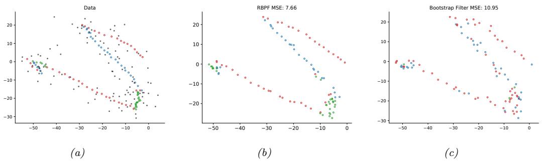
Figure 13.6: Illustration of state estimation for a switching linear model. (a) Black dots are observations, hollow circles are the true location, colors represent the discrete state. (b) Estimate from RBPF. Generated by rbpf\_maneuver.ipynb. (c) Estimate from bootstrap filter. Generated by bootstrap\_filter\_maneuver.ipynb.

13.4.3 Example: FastSLAM

Consider a robot moving around an environment, such as a maze or indoor o”ce environment. It needs to learn a map of the environment, and keep track of its location (pose) within that map. This problem is known as simultaneous localization and mapping, or SLAM for short. SLAM is widely used in mobile robotics (see e.g., [SC86; CN01; TBF06] for details). It is also useful in augmented reality, where the task is to recursively estimate the 3d pose of a handheld camera with respect to a set of 2d visual landmarks (this is known as visual SLAM, [TUI17; SMT18; Cza+20; DH22]).

Let us assume we can represent the map as the 2d locations of a set of K landmarks, denote them by l ¹,…,l ^K (each is a vector in R²). (We can use data association to figure out which landmark generated each observation, as discussed in Section 29.9.3.2.) Let r^t represent the unknown location of the robot at time t. Let z^t = (rt,l 1:Kt ) be the combined state space. We can then perform online inference so that the robot can update its estimate of its own location, and the landmark locations.

The state transition model is defined as

\[p(\mathbf{z}\_t | \mathbf{z}\_{t-1}, \mathbf{u}\_t) = p(\mathbf{r}\_t | \mathbf{r}\_{t-1}, \mathbf{l}\_{t-1}^{1:K}, \mathbf{u}\_t) \prod\_{k=1}^{K} p(\mathbf{l}\_t^k | \mathbf{l}\_{t-1}^k) \tag{13.68}\]

where p(rt|r^t↓¹,l 1:Kt↓¹,ut) specifies how the robot moves given the control signal ^ut and the location of the obstacles l 1:Kt↓¹. (Note that in this section, we assume that a human is joysticking the robot through the environment, so u1:^t is given as input, i.e., we do not address the decision-theoretic issue of choosing where to move.)

If the obstacles (landmarks) are static, we can define p(l k t |l k ^t↓1) = ϑ(l k ^t → l k ^t↓1), which is equivalent to treating the map as an unknown parameter that is shared globally across all time steps. More generally, we can let the landmark locations evolve over time [Mur00a].

The observations y^t measure the distance from r^t to the set of closest landmarks. Figure 13.8 shows the corresponding graphical model for the case where K = 2, and where on the first step it sees landmarks 1 and 2, then just landmark 2, then just landmark 1, etc.

If all the CPDs are linear-Gaussian, then we can use a Kalman filter to maintain our belief state

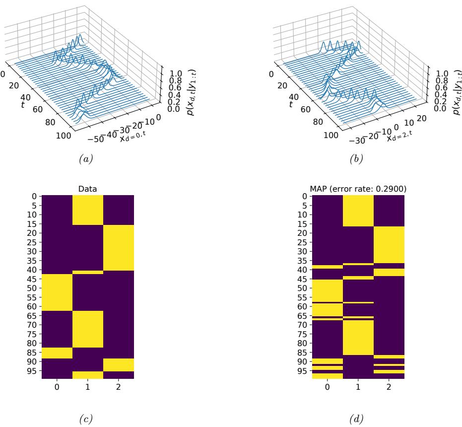
Figure 13.7: Visualizing the posterior from the RBPF algorithm. Top row: Posterior marginals of the location of the object over time, derived from the mixture of Gaussian representation for (a) x location (dimension 0), (b) y location (dimension 2). Bottom row: visualization of the true (c) and predicted (d) discrete states. Generated by rbpf\_maneuver.ipynb.

about the location of the robot and the location of the landmarks, p(zt|y1:t,u1:t). In the more general case of a nonlinear model, we can use the EKF (Section 8.3.2) or UKF (Section 8.4.2).

Over time, the uncertainty in the robot’s location will increase, due to wheel slippage, etc., but when the robot returns to a familiar location, its uncertainty will decrease again. This is called closing the loop, and is illustrated in Figure 13.9(a), where we see the uncertainty ellipses, representing Cov [zt|y1:t,u1:t], grow and then shrink.

In addition to visualizing the uncertainty of the robot’s location, we can visualize the uncertainty about the map. To do this, consider the posterior precision matrix, #^t = !^{↓1 t} . Zeros in the precision

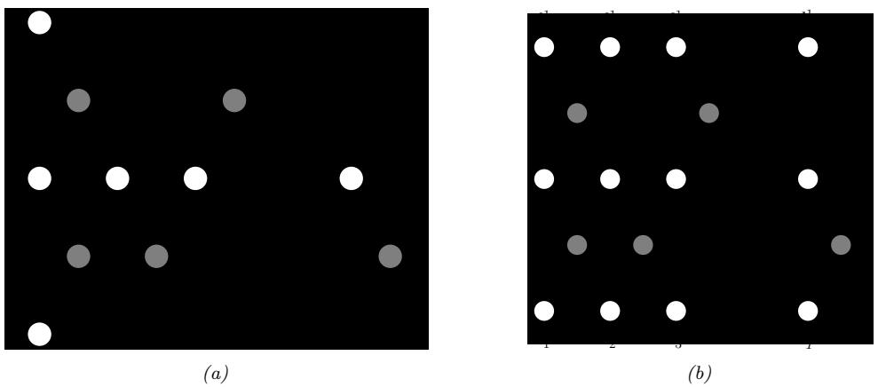
Figure 13.8: Graphical model representing the SLAM problem. l k ^t is the location of landmark k at time t, r^t is the location of the robot at time t, and y^t is the observation vector. In the model on the left, the landmarks are static (so they act like global shared parameters), on the right, their location can change over time. The robot’s observations are based on the distance to the nearest landmarks from the current state, denoted f(rt,l k ^t ). The number of observations per time step is variable, depending on how many landmarks are within the range of the sensor. Adapted from Figure 15.A.3 of [KF09a].

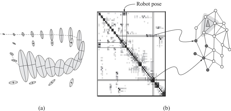
Figure 13.9: Illustration of the SLAM problem. (a) A robot starts at the top left and moves clockwise in a circle back to where it started. We see how the posterior uncertainty about the robot’s location increases and then decreases as it returns to a familar location, closing the loop. If we performed smoothing, this new information would propagate backwards in time to disambiguate the entire trajectory. (b) We show the precision matrix, representing sparse correlations between the landmarks, and between the landmarks and the robot’s position (pose). The conditional independencies encoded by the sparse precision matrix can be visualized as a Gaussian graphical model, as shown on the right. From Figure 15.A.3 of [KF09a]. Used with kind permission of Daphne Koller.

matrix correspond to absent edges in the corresponding undirected Gaussian graphical model (GGM, see Section 4.3.5). Initially all the beliefs about landmark locations are uncorrelated (by assumption), so the GGM is a disconnected graph, and #^t is diagonal. However, as the robot moves about, it will induce correlation between nearby landmarks. Intuitively this is because the robot is estimating its position based on distance to the landmarks, but the landmarks’ locations are being estimated based on the robot’s position, so they all become interdependent. This can be seen more clearly from the graphical model in Figure 13.8: it is clear that l ¹ and l ² are not d-separated by y1:t, because there is a path between them via the unknown sequence of r1:^t nodes. Consequently, the precision matrix becomes denser over time. As a consequence of the precision matrix becoming denser, each inference step takes O(K³) time. This prevents the method from being applied to large maps.

One way to speed this up is based on the following observation: conditional on knowing the robot’s path, ^r1:t, the landmark locations are independent, i.e., ^p(lt|r1:t, ^y1:t) = ^{K k}=1 p(l k ^t |r1:t, y1:t). This can be seen by looking at the DGM in Figure 13.8. We can therefore sample the trajectory using some proposal, and apply (2d) Kalman filtering to each landmark independently. This is an example of RBPF, and reduces the inference cost to O(NK), where N is the number of particles and K is the number of landmarks.

The overall cost of this technique is O(NK) per step. Fortunately, the number of particles N needed for good performance is quite small, so the algorithm is essentially linear in the number of landmarks, making it quite scalable. This idea was first suggested in [Mur00a], who applied it to grid-structured occupancy grids (and used the HMM filter for each particle). It was subsequently extended to landmark-based maps in [Thr+04], using the Kalman filter for each particle; they called the technique FastSLAM.

13.5 Extensions of the particle filter

There are many extensions to the basic particle filtering algorithm, such as the following:

• We can increase particle diversity by applying one or more steps of MCMC sampling (Section 12.2) at each PF step using ϖt(zt) as the target distribution. This is called the resample-move algorithm [DJ11]. It is also possible to use SMC instead of MCMC to diversify the samples [GM17].
• We can extend PF to the case of o$ine inference; this is called particle smoothing (see e.g., [Kla+06]).
• We can extend PF to inference in general graphical models (not just chains) by combining PF with loopy belief propagation (Section 9.4); this is called non-parametric BP or particle BP (see e.g., [Sud+03; Isa03; Sud+10; Pac+14]).
• We can extend PF to perform inference in static models (e.g., for parameter inference), as we discuss in Section 13.6.

13.6 SMC samplers

In this section, we discuss SMC samplers (sequential Monte Carlo samplers), which are a way to apply particle filters to sample from a generic target distribution, ϖ(z) = ▷˜(z)/Z, rather than

requiring the model to be an SSM. Thus SMC is an alternative to MCMC.

The advantages of SMC samplers over MCMC are as follows: we can estimate the normalizing constant Z; we can more easily develop adaptive versions that tune the transition kernel using the current set of samples; and the method is easier to parallelize (see e.g., [CCS22; Gre+22]).

The method works by defining a sequence of intermediate distributions, ϖt(zt), which we expand to a sequence of distributions over all the past variables, ϖt(z1:t). We then use the particle filtering algorithm to sample from each of these intermediate distributions. By marginalizing all but the final state, we recover samples from the target distribution, ϖ(z) = & ^z1:T→¹ ϖ^T (z1:^T ), as we explain below. (For more details, see e.g., [Dai+20a; CP20b].)

13.6.1 Ingredients of an SMC sampler

To define an SMC sampler, we need to specify several ingredients:

• A sequence of distributions defined on the same state space, ϖt(zt)=˜▷t(zt)/Zt, for t =0: T;
• ^A forwards kernel ^Mt(zt|z^t↓1) (often written as ^Mt(z^t↓¹, ^zt)), which satisfies & ^zt Mt(zt|z^t↓1) = 1. This can be used to propose new samples from our current estimate when we apply particle filtering.
• ^A backwards kernel ^Lt(zt|zt+1) (often written as ^L(zt, ^zt+1)), which satisfies & ^zt Lt(zt|zt+1) = 1. This allows us to create a sequence of variables by working backwards in time from the final target value to the first time step. In particular, we create the following joint distribution:

\[\pi\_t(\mathbf{z}\_{1:t}) = \pi\_t(\mathbf{z}\_t) \prod\_{s=1}^{t-1} L\_s(\mathbf{z}\_s | \mathbf{z}\_{s+1}) \tag{13.69}\]

This satisfies & ^z1:t→¹ ϖt(z1:t) = ϖt(zt), so if we apply particle filtering to this for t =1: T, then samples from the “end” of such sequences will be from the target distribution ϖt.

With the above ingredients, we can compute the incremental weight at step t using

\[\alpha\_{t} = \frac{\overline{\pi}\_{t}(\mathbf{z}\_{1:t})}{\overline{\pi}\_{t-1}(\mathbf{z}\_{1:t-1})M\_{t}(\mathbf{z}\_{t}|\mathbf{z}\_{t-1})} \propto \frac{\bar{\gamma}\_{t}(\mathbf{z}\_{t})}{\bar{\gamma}\_{t-1}(\mathbf{z}\_{t-1})} \frac{L\_{t-1}(\mathbf{z}\_{t-1}|\mathbf{z}\_{t})}{M\_{t}(\mathbf{z}\_{t}|\mathbf{z}\_{t-1})} \tag{13.70}\]

This can be plugged into the generic SMC algorithm, Algorithm 13.3.

We still have to specify the forwards and backwards kernels. We will assume the forwards kernel M^t is an MCMC kernel that leaves ϖ^t invariant. We can then define the backwards kernel to be the time reversal of the forwards kernel. More precisely, suppose we define L^t↓¹ so it satisfies

\[ \pi\_t(\mathbf{z}\_t) L\_{t-1}(\mathbf{z}\_{t-1}|\mathbf{z}\_t) = \pi\_t(\mathbf{z}\_{t-1}) M\_t(\mathbf{z}\_t|\mathbf{z}\_{t-1}) \tag{13.71} \]

In this case, the incremental weight simplifies as follows:

\[\alpha\_t = \frac{Z\_t \pi\_t(\mathbf{z}\_t) L\_{t-1}(\mathbf{z}\_{t-1}|\mathbf{z}\_t)}{Z\_{t-1} \pi\_{t-1}(\mathbf{z}\_{t-1}) M\_t(\mathbf{z}\_t|\mathbf{z}\_{t-1})} \tag{13.72}\]

\[\tau\_t = \frac{Z\_t \pi\_t(\mathbf{z}\_{t-1}) M\_t(\mathbf{z}\_t | \mathbf{z}\_{t-1})}{Z\_{t-1} \pi\_{t-1}(\mathbf{z}\_{t-1}) M\_t(\mathbf{z}\_t | \mathbf{z}\_{t-1})} \tag{13.73}\]

\[\dot{\tilde{\gamma}}\_{t} = \frac{\tilde{\gamma}\_{t}(z\_{t-1})}{\tilde{\gamma}\_{t-1}(z\_{t-1})} \tag{13.74}\]

We can use any kind of MCMC kernel for Mt. For example, if the parameters are real valued and unconstrained, we can use a Markov kernel that corresponds to K steps of a random walk Metropolis-Hastings sampler. We can set the covariance of the proposal to ^ϑ2!^{ˆ t}↓1, where !^{ˆ t}↓¹ is the empirical covariance of the weighted samples from the previous step, (W1:^{N t}↓¹ , ^z1:Nt↓¹ ), and ^ϑ = 2.38D↓3/² (which is the optimal scaling parameter for RWMH). In high dimensional problems, we can use gradient based Markov kernels, such as HMC [BCJ20] and NUTS [Dev+21]. For binary state spaces, we can use the method of [SC13].

13.6.2 Likelihood tempering (geometric path)

There are many ways to specify the intermediate target distributions. In the geometric path method, we specify the intermediate distributions to be

\[ \hat{\gamma}\_t(\mathbf{z}) = \hat{\gamma}\_0(\mathbf{z})^{1-\lambda\_t} \hat{\gamma}(\mathbf{z})^{\lambda\_t} \tag{13.75} \]

where 0 = ⇀⁰ < ⇀¹ < ··· < ⇀^T = 1 are inverse temperature parameters, and ▷˜⁰ is the initial proposal. If we apply particle filtering to this model, but “turn o!” the resampling step, the method becomes equivalent to annealed importance sampling (Section 11.5.4).

In the context of Bayesian parameter inference, we often denote the latent variable z by ω, we define ▷˜0(ω) ↑ ϖ0(ω) as the prior, and ▷˜(z) = ϖ0(ω)p(D|ω) as the posterior. We can then define the intermediate distributions to be

\[\hat{\gamma}\_t(\theta) = \pi\_0(\theta)^{1-\lambda\_t} \pi\_0(\theta)^{\lambda\_t} p(\mathcal{D}|\theta)^{\lambda\_t} = \pi\_0(\theta)^{1-\lambda\_t} \exp[-\lambda\_t \mathcal{E}(\theta)] \tag{13.76}\]

where E(ω) = → log p(D, ω) is the energy (potential) function. The incremental weights are given by

\[\alpha\_t(\boldsymbol{\theta}) = \frac{\pi\_0(\boldsymbol{\theta})^{1-\lambda\_t} \exp[-\lambda\_t \mathcal{E}(\boldsymbol{\theta})]}{\pi\_0(\boldsymbol{\theta})^{1-\lambda\_t} \exp[-\lambda\_{t-1} \mathcal{E}(\boldsymbol{\theta})]} = \exp[-\delta\_t \mathcal{E}(\boldsymbol{\theta})] \tag{13.77}\]

where ⇀^t = ⇀^t↓¹ + ϑt.

For this method to work well, it is important to choose the ⇀^t so that the successive distributions are “equidistant”; this is called adaptive tempering. In the case of a Gaussian prior and Gaussian energy, one can show [CP20b] that this can be achieved by picking ⇀^t = (1 + ^▷)t+1 ^{→ 1}, where ^{▷ &}gt; ⁰ is some constant. Thus we should increase ⇀ slowly at first, and then make bigger and bigger steps.

In practice we can estimate ⇀^t by setting ⇀^t = ⇀^t↓¹ + ϑ^t , where

\[\delta\_t = \operatorname\*{argmin}\_{\delta \in [0, 1 - \lambda\_{t-1}]} \left( \operatorname\*{ESSLW}(\{-\delta \: \mathcal{E}(\theta\_t^n)\}) - \operatorname\*{ESS}\_{\text{min}} \right) \tag{13.78}\]

where ESSLW({ln}) = ESS({e^ln }) computes the ESS (Equation (13.37)) from the log weights, lⁿ = log ˜wⁿ. This ensures the change in the ESS across steps is close to the desired minimum ESS, typically 0.5N. (If there is no solution for ϑ in the interval, we set ϑ^t = 1→⇀^t↓1.) See Algorithm 13.5 for the overall algorithm.

13.6.2.1 Example: sampling from a 1d bimodal distribution

Consider the simple distribution

\[p(\boldsymbol{\theta}) \propto N(\boldsymbol{\theta}|\mathbf{0}, \mathbf{I}) \exp(-\mathcal{E}(\boldsymbol{\theta})) \tag{13.79}\]

Algorithm 13.5: SMC with adaptive tempering

¹ ⇀↓¹ = 0, ^{t = →}1, ^{Wn ↓1} = 1 ² while ⇀^t < 1 do 3 t = t + 1 ⁴ if t = 0 then ⁵ ω^{n 0} ↔︎ ϖ0(ω) ⁶ else ^{7 A}1:Nt ⁼ Resample(W1:^{N t}↓¹ ) ⁸ ω^{n t ↔︎ Mε}t→¹ (ω^An t ^t↓¹, ·) ⁹ Compute ϑ^t using Equation (13.78) ¹⁰ ⇀^t = ⇀^t↓¹ + ϑ^{t 11} w˜^{n t} = exp[→ϑE(ω^{n t} )] ¹² W^{n t} = ˜w^{n t} /( &^{N m}=1 w˜^{m t} ) 2 1 0 1 2 0.0 0.5 ¹.^{0 1} (a) 2 1 0 1 2 0.0 0.5 ¹.⁰ 0.0 0.25 0.5 0.75 1.0 (b)

Figure 13.10: (a) Illustration of a bimodal target distribution. (b) Tempered versions of the target at di!erent inverse temperatures, from ς^T = 1 down to ς¹ = 0. Generated by smc\_tempered\_1d\_bimodal.ipynb.

where ^E(ω) = ^c(||ω||^{2 →} 1)². We plot this in 1d in Figure 13.10a for ^c = 5; we see that it has a bimodal shape, since the low energy states correspond to parameter vectors whose norm is close to 1.

SMC is particularly useful for sampling from multimodal distributions, which can be provably hard to e”ciently sample from using other methods, including HMC [MPS18], since gradients only provide local information about the curvature. As an example, in Figure 13.11a and Figure 13.11b we show the result of applying HMC (Section 12.5) and NUTS (Section 12.5.4.1) to this problem. We see that both algorithms get stuck near the initial state of ω⁰ = 1.

In Figure 13.10b, we show tempered versions of the target distribution at 5 di!erent temperatures, chosen uniformly in the interval [0, 1]. We see that at ⇀¹ = 0, the tempered target is equal to the Gaussian prior (blue line), which is easy to sample from. Each subsequent distribution is close to the previous one, so SMC can track the change until it ends up at the target distribution with ⇀^T = 1, as shown in Figure 13.11c.

These SMC results were obtained using the adaptive tempering scheme described above. In Figure 13.11d we see that initially the temperature is small, and then it increases exponentially. The algorithm takes 8 steps until ⇀^T ≃ 1.

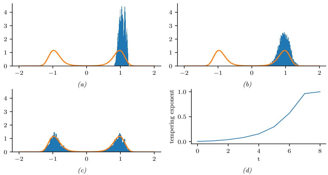
Figure 13.11: Sampling from the bimodal distribution in Figure 13.10a. (a) HMC. (b) NUTS. (c) Tempered SMC with HMC kernel (single step). (d) Adaptive inverse temperature schedule. Generated by smc\_tempered\_1d\_bimodal.ipynb.

13.6.3 Data tempering

If we have a set of iid observations, we can define the t’th target to be

\[\bar{\gamma}\_t(\theta) = p(\theta)p(y\_{1:t}|\theta) \tag{13.80}\]

We can now apply SMC to this model. From Equation (13.74), the incremental weight becomes

\[p(\boldsymbol{\theta}) = \frac{\tilde{\gamma}\_t(\mathbf{z}\_{t-1})}{\tilde{\gamma}\_{t-1}(\mathbf{z}\_{t-1})} = \frac{p(\boldsymbol{\theta})p(\mathbf{y}\_{1:t}|\boldsymbol{\theta})}{p(\boldsymbol{\theta})p(\mathbf{y}\_{1:t-1}|\boldsymbol{\theta})} = p(\mathbf{y}\_t|\mathbf{y}\_{1:t-1}, \boldsymbol{\theta})\tag{13.81}\]

This can be plugged into the generic SMC algorithm in Algorithm 13.3.

Unfortunately, to sample from the MCMC kernel will typically take O(t) time, since the MH accept/reject step requires computing p(ω^↔︎ ) ^{t i}=1 p(y1i|ω^↔︎ ) for any proposed ω^↔︎ . Hence the total cost is O(T²) if there are T observations. To reduce this, we can only sample parameters at times t when the ESS drops below a certain level; in the remaining steps, we just grow the sequence deterministically by repeating the previously sampled value. This technique was proposed in [Cho02], who called it the iterated batch importance sampling or IBIS algorithm.

13.6.3.1 Example: IBIS for a 1d Gaussian

In this section, we give a simple example of IBIS applied to data from a 1d Gaussian, y^t ↔︎ N (µ = 3.14, ς = 1) for t = 1 : 30. The unknowns are ω = (µ, ς). The prior is p(ω) = N (µ|0, 1)Ga(ς|a =

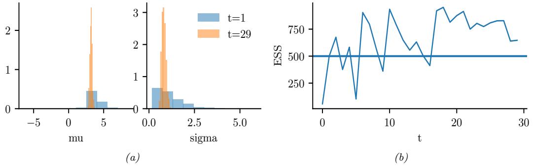
Figure 13.12: Illustration of IBIS applied to 30 samples from N (µ = 3.14, ω = 1). (a) Posterior approximation after t = 1 and t = 29 observations. (b) E!ective sample size over time. The sudden jumps up occur whenever resampling is triggered, which happens when the ESS drops below 500. Generated by smc\_ibis\_1d.ipynb.

1, b = 1). We use IBIS with an adaptive RWMH kernel. We use N = 20 particles, each updated for K = 50 MCMC steps, so we collect 1000 samples per time step.

Figure 13.12a shows the approximate posterior after t = 1 and t = 29 time steps. We see that the posterior concentrates on the true values of µ = 3.14 and ς = 1.

Figure 13.12b plots the ESS vs time. The number of particles is 1000, and resampling (and MCMC moves) is triggered whenever this drops below 500. We see that we only need to invoke MCMC updates 3 times.

13.6.4 Sampling rare events and extrema

Suppose we want to sample values from ϖ0(ω) conditioned on the event that S(ω) > ⇀→, where S is some score or “fitness” function. If ⇀^→ is in the tail of the score distribution, this corresponds to sampling a rare event, which can be hard.

One approach is to use SMC to sample from a sequence of distributions with gradually increasing thresholds:

\[\pi\_t(\boldsymbol{\theta}) = \frac{1}{Z\_t} \mathbb{I}\left(S(\boldsymbol{\theta}) \ge \lambda\_t\right) \pi\_0(\boldsymbol{\theta}) \tag{13.82}\]

with ⇀⁰ < ··· < ⇀^T = ⇀→. We can then use likelihood tempering, where the “likelihood” is the function

\[G\_t(\theta\_t) = \mathbb{I}\left(S(\theta\_t) \ge \lambda\_t\right) \tag{13.83}\]

We can use SMC to generate samples from the final distribution ϖ^T . We may also be interested in estimating

\[Z\_T = p(S(\theta) \ge \lambda\_T) \tag{13.84}\]

where the probability is taken wrt ϖ0(ω).

We can adaptively set the thresholds ⇀^t as follows: at each step, sort the samples by their score, and set ⇀^t to the ϱ’th highest quantile. For example, if we set ϱ = 0.5, we keep the top 50% fittest particles. This ensures the ESS equals the minimum threshold at each step. For details, see [Cér+12].

Note that this method is very similar to the cross-entropy method (Section 6.7.5). The di!erence is that CEM fits a parametric distribution (e.g., a Gaussian) to the particles at each step and samples from that, rather than using a Markov kernel.

13.6.5 SMC-ABC and likelihood-free inference

The term likelihood-free inference refers to estimating the parameters ω of a blackbox from which we can sample data, y ↔︎ p(·|ω), but where we cannot evaluate p(y|ω) pointwise. Such models are called simulators, so this approach to inference is also called simulation-based inference (see e.g., [Nea+08; CBL20; Gou+96]). These models are also called implicit models (see Section 26.1).

If we want to approximate the posterior of a model with no known likelihood, we can use approximate Bayesian computation or ABC (see e.g., [Bea19; SFB18; Gut+14; Pes+21]). In this setting, we sample both parameters ω and synthetic data y such that the synthetic data (generated from ω) is su”ciently close to the observed data y→, as judged by some distance score, d(y, y→) < ⇁. (For high dimensional problems, we typically require d(s(y), s(y→)) < ⇁, where s(y) is a low-dimensionary summary statistic of the data.)

In SMC-ABC, we gradually decrease the discrepancy ⇁ to get a series of distributions as follows:

\[\pi\_t(\theta, y) = \frac{1}{Z\_t} \pi\_0(\theta) p(y|\theta) \mathbb{I}\left(d(y, y^\*) < \epsilon\_t\right) \tag{13.85}\]

where ⇁⁰ > ⇁¹ > ··· . This is similar to the rare event SMC samplers in Section 13.6.4, except that we can’t directly evaluate the quality of a candidate, ω. Instead we must first convert it to data space and make the comparison there. For details, see [DMDJ12].

Although SMC-ABC is popular in some fields, such as genetics and epidemiology, this method is quite slow and does not scale to high dimensional problems. In such settings, a more e”cient approach is to train a generative model to emulate the simulator; if this model is parametric with a tractable likelihood (e.g., a flow model), we can use the usual methods for posterior inference of its parameters (including gradient based methods like HMC). See e.g., [Bre+20a] for details.

13.6.6 SMC²

We have seen how SMC can be a useful alternative to MCMC. However it requires that we can e”ciently evaluate the likelihood ratio terms ⇁t(εt) ⇁t→1(εt) . In cases where this is not possible (e.g., for latent variable models), we can use SMC (specifically the estimate Zˆ^t in Equation (13.10)) as a subroutine to approximate these likelihoods. This is called SMC2. For details, see [CP20b, Ch. 18].

13.6.7 Variational filtering SMC

One way to improve SMC is to learn a proposal distribution (e.g., using a neural network) such that the approximate posterior, ϖˆ^T (z1:^T ; ε, ω), is close to the target posterior, ϖ^T (z1:^T ; ω), where ω are the model parameters, and ε are the proposal parameters (which may depend on ω). One can show

[Nae+18] that the KL divergence between these distributions can be bounded as follows:

\[0 \le D\_{\rm KL} \left( \mathbb{E} \left[ \hat{\pi}\_T(\mathbf{z}\_{1:T}) \right] \parallel \pi\_T(\mathbf{z}\_{1:T}) \right) \le -\mathbb{E} \left[ \log \frac{\hat{Z}\_T}{Z\_T} \right] \tag{13.86}\]

where

\[Z\_T(\boldsymbol{\theta}) = p\_{\boldsymbol{\theta}}(\boldsymbol{y}\_{1:T}) = \int p\_{\boldsymbol{\theta}}(\boldsymbol{z}\_{1:T}, \boldsymbol{y}\_{1:T}) d\boldsymbol{z}\_{1:T} \tag{13.87}\]

Hence

\[\mathbb{E}\left[\log \hat{Z}\_T(\theta, \phi)\right] \le \mathbb{E}\left[\log Z\_T(\theta)\right] = \log Z\_T(\theta) \tag{13.88}\]

Thus we can use SMC sampling to compute an unbiased approximation to E log Zˆ^T (ω, ε) , which is a lower bound on the evidence (log marginal likelihood).

We can now maximize this lower bound wrt ω and ε using SGD, as a way to learn both proposals and the model. Unfortunately, computing the gradient of the bound is tricky, since the resampling step is non-di!erentiable. However, in practice one can ignore the dependence of the resampling operator on the parameters, or one can use di!erentiable approximations (see e.g., [Ros+22]). This overall approach was independently proposed in several papers: the FIVO (filtering variational objective) paper [Mad+17], the variational SMC paper [Nae+18] and the auto-encoding SMC paper [Le+18].

13.6.8 Variational smoothing SMC

The methods in Section 13.6.7 use SMC in which the target distributions are defined to be the filtered distributions, ϖt(z1:t) = pε(z1:t|y1:t); this is called filtering SMC. Unfortunately, this can work poorly when fitting models to o$ine sequence data, since at time t, all future observations are ignored in the objective, no matter how good the proposal. This can create situations where future observations are unlikely given the current set of sampled trajectories, which can result in particle impoverishment and high variance in the estimate of the lower bound.

Recently, a new method called SIXO (smoothing inference with twisted objectives) was proposed in [Law+22] that uses the smoothing distributions as targets, ϖt(z1:t) = pε(z1:t|y1:^T ), to create a much lower variance variational lower bound. Of course it is impossible to directly compute this posterior, but we can approximate it using twisted particle filters [WL14a; AL+16]. In this approach, we approximate the (unnormalized) posterior using

\[p\_{\theta}(\mathbf{z}\_{1:t}, \mathbf{y}\_{1:T}) = p\_{\theta}(\mathbf{z}\_{1:t}, \mathbf{y}\_{1:t}) p\_{\theta}(\mathbf{y}\_{t+1:T} | \mathbf{z}\_{1:t}, \mathbf{y}\_{1:t}) \tag{13.89}\]

\[\mathbf{y}\_t = p\_\theta(\mathbf{z}\_{1:t}, \mathbf{y}\_{1:t}) p\_\theta(\mathbf{y}\_{t+1:T} | \mathbf{z}\_t) \tag{13.90}\]

\[\approx p\_{\theta}(\mathbf{z}\_{1:t}, \mathbf{y}\_{1:t}) r\_{\psi}(\mathbf{y}\_{t+1:T}, \mathbf{z}\_{t}) \tag{13.91}\]

where rϑ(yt+1:^T , zt) ↓ pε(yt+1:^T |zt) is the twisting function, which acts as a “lookahead function”.

One way to approximate the twisting function is to note that

\[p\_{\theta}(y\_{t+1:T}|z\_t) = \frac{p\_{\theta}(z\_t|y\_{t+1:T})p\_{\theta}(y\_{t+1:T})}{p\_{\theta}(z\_t)} \propto \frac{p\_{\theta}(z\_t|y\_{t+1:T})}{p\_{\theta}(z\_t)}\tag{13.92}\]

where we drop terms that are independent of z^t since such terms will cancel out when we normalize the sampling weights. We can approximate the density ratio using the binary classifier method of Section 2.7.5. To do this, we define one distribution to be p¹ = pε(zt, yt+1:^T ) and the other to be p² = pε(zt)pε(yt+1:^T ), so that p1/p² = ^pϑ(zt|yt+1:^T ) ^pϑ(zt) . We can easily draw a sample (z1:^T , y1:^T ) ↔︎ p^ε using ancestral sampling, from which we can compute (zt, yt+1:^T ) ↔︎ p¹ by marginalization. We can also sample a fresh sequence from (z˜1:^T , y˜1:^T ) ↔︎ p^ε from which we can compute (z˜t, y˜t+1:^T ) ↔︎ p² by marginalization. We then use (zt, yt+1:^T ) as a positive example and (z˜t, y˜t+1:^T ) as a negative example when training the binary classifier, rϑ(yt+1:^T , zt).

Once we have updated the twisting parameters ϖ, we can rerun SMC to get a tighter lower bound on the log marginal likelihood, which we can then optimize wrt the model parameters ω and proposal parameters ε. Thus the overall method is a stochastic variational EM-like method for optimziing the bound

\[\mathcal{L}\_{\text{SIXO}}(\theta,\phi,\psi,y\_{1:T}) \stackrel{\Delta}{=} \mathbb{E}\left[\log \hat{Z}\_{\text{SIXO}}(\theta,\phi,\psi,y\_{1:T})\right] \tag{13.93}\]

\[\leq \log \mathbb{E}\left[\hat{Z}\_{\text{SIXO}}(\theta, \phi, \psi, y\_{1:T})\right] = \log p\_{\theta}(y\_{1:T}) \tag{13.94}\]

In [Law+22] they prove the following: suppose the true model p^→ is an SSM in which the optimal proposal function for the model satisfies p→(zt|z1:t↓¹, y1:^T ) ↗ Q, and the optimal lookahead function for the model satisfies p→(yt+1:^T |zt) ↗ R. Furthermore, assume the SIXO objective has a unique maximizer. Then, at the optimum, we have that the learned proposal q^ω↓ (zt|z1:t↓¹, y1:^T ) ↗ Q is equal to the optimal proposal, the learned twisting function r^ϑ↓ (yt+1:^T , zt) ↗ R is equal to the optimal lookahead, and the lower bound is tight (i.e., LSIXO(ω→, ε^→, ϖ^→) = p→(y1:^T )) for any number of samples N^s ≃ 1 and for any kind of SSM p→. (This is in contrast to the FIVO bound, whiere the bound does not usually become tight.)

Part III

Prediction

14 Predictive models: an overview

14.1 Introduction

The vast majority of machine learning is concerned with tackling a single problem, namely learning to predict outputs y from inputs x using some function f that is estimated from a labeled training set ^{D =} {(xn, ^yn) : ⁿ =1: ^N}, for ^xn ↗ ^{X ℑ RD} and ^yn ↗ ^{Y ℑ RC} . We can model our uncertainty about the correct output for a given input using a conditional probability model of the form p(y|f(x)). When Y is a discrete set of labels, this is called (in the ML literature) a discriminative model, since it lets us discriminate (distinguish) between the di!erent possible values of y. If the output is real-valued, Y = R, this is called a regression model. (In the statistics literature, the term “regression model” is used in both cases, even if Y is a discrete set.) We will use the more generic term “predictive model” to refer to such models.

A predictive model can be considered as a special case of a conditional generative model (discussed in Chapter 20). In a predictive model, the output is usually low dimensional, and there is a single best answer that we want to predict. However, in most generative models, the output is usually high dimensional, such as images or sentences, and there may be many correct outputs for any given input. We will discuss a variety of types of predictive model in Section 14.1.1, but we defer the details to subsequent chapters. The rest of this chapter then discusses issues that are relevant to all types of predictive model, regardless of the specific form, such as evaluation.

14.1.1 Types of model

There are many di!erent kinds of predictive model p(y|x). The biggest distinction is between parametric models, that have a fixed number of parameters independent of the size of the training set, and non-parametric models that have a variable number of parameters that grows with the size of the training set. Non-parametric models are usually more flexible, but can be slower to use for prediction. Parametric models are usually less flexible, but are faster to use for prediction.

Most non-parametric models are based on comparing a test input x to some or all of the stored training examples {xn, n =1: N}, using some form of similarity, sⁿ = K(x, xn) ≃ 0, and then predicting the output using some weighted combination of the training labels, such as yˆ = &^{N n}=1 snyn. A typical example is a Gaussian process, which we discuss in Chapter 18. Other examples, such as K-nearest neighbor models, are discussed in the prequel to this book, [Mur22].

Most parametric models have the form p(y|x) = p(y|f(x; ω)), where f is some kind of function that predicts the parameters (e.g., the mean, or logits) of the output distribution (e.g., Gaussian or categorical). There are many kinds of function we can use. If f is a linear function of ω (i.e., f(x; ω) = ωTε(x) for some fixed feature transformation ε), then the model is called a generalized linear model or GLM, which we discuss in Chapter 15. If f is a non-linear, but di!erentiable, function of ω (e.g., f(x; ω) = ω^{T 2}ε(x; ω1) for some learnable function ε(x; ω1)), then it is common to represent f using a neural network (Chapter 16). Other types of predictive model, such as decision trees and random forests, are discussed in the prequel to this book, [Mur22].

14.1.2 Model fitting using ERM, MLE, and MAP

In this section, we briefly discuss some methods used for fitting (parametric) models. The most common approach is to use maximum likelihood estimation or MLE, which amounts to solving the following optimization problem:

\[\hat{\boldsymbol{\theta}} = \underset{\boldsymbol{\theta} \in \Theta}{\operatorname{argmax}} \, p(\mathcal{D} | \boldsymbol{\theta}) = \underset{\boldsymbol{\theta} \in \Theta}{\operatorname{argmax}} \log p(\mathcal{D} | \boldsymbol{\theta}) \tag{14.1}\]

If the dataset is N iid data samples, the likelihood decomposes into a product of terms, p(D|ω) = ^{N n}=1 p(yn|xn, ω). Thus we can instead minimize the following (scaled) negative log likelihood:

\[\hat{\boldsymbol{\theta}} = \underset{\boldsymbol{\theta} \in \Theta}{\operatorname{argmin}} \frac{1}{N} \sum\_{n=1}^{N} [-\log p(\boldsymbol{y}\_n | \boldsymbol{x}\_n, \boldsymbol{\theta})] \tag{14.2}\]

We can generalize this by replacing the log loss εn(ω) = → log p(yn|xn, ω) with a more general loss function to get

\[\hat{\boldsymbol{\theta}} = \operatorname\*{argmin}\_{\boldsymbol{\theta} \in \boldsymbol{\Theta}} r(\boldsymbol{\theta}) \tag{14.3}\]

where r(ω) is the empirical risk

\[r(\theta) = \frac{1}{N} \sum\_{n=1}^{N} \ell\_n(\theta) \tag{14.4}\]

This approach is called empirical risk minimization or ERM.

ERM can easily result in overfitting, so it is common to add a penalty or regularizer term to get

\[\dot{\theta} = \operatorname\*{argmin}\_{\theta \in \Theta} r(\theta) + \lambda C(\theta) \tag{14.5}\]

where ⇀ ≃ 0 controls the degree of regularization, and C(ω) is some complexity measure. If we use log loss, and we define C(ω) = → log ϖ0(ω), where ϖ0(ω) is some prior distribution, and we use ⇀ = 1, we recover the MAP estimate

\[\hat{\boldsymbol{\theta}} = \operatorname\*{argmax}\_{\boldsymbol{\theta} \in \Theta} \log p(\mathcal{D} | \boldsymbol{\theta}) + \log \pi\_0(\boldsymbol{\theta}) \tag{14.6}\]

This can be solved using standard optimization methods (see Chapter 6).

14.1.3 Model fitting using Bayes, VI, and generalized Bayes

Another way to prevent overfitting is to estimate a probability distribution over parameters, q(ω), instead of a point estimate. That is, we can try to estimate the ERM in expectation:

\[\hat{q} = \operatorname\*{argmin}\_{q \in \mathcal{P}(\Theta)} \mathbb{E}\_{q(\theta)} \left[ r(\theta) \right] \tag{14.7}\]

If P(#) is the space of all probability distributions over parameters, then the solution will converge to a delta function that puts all its probability on the MLE. Thus this approach, on its own, will not prevent overfitting. However, we can regularize the problem by preventing the distribution from moving too far from the prior. If we measure the divergence between q and the prior using KL divergence, we get

\[\hat{q} = \operatorname\*{argmin}\_{q \in \mathcal{P}(\Theta)} \mathbb{E}\_{q(\theta)} \left[ r(\theta) \right] + \frac{1}{\lambda} D\_{\text{KL}} \left( q \parallel \pi\_0 \right) \tag{14.8}\]

The solution to this problem is known as the Gibbs posterior, and is given by the following:

\[\hat{q}(\theta) = \frac{e^{-\lambda r(\theta)}\pi\_0(\theta)}{\int e^{-\lambda r(\theta')}\pi\_0(\theta')d\theta'} \tag{14.9}\]

This is widely used in the PAC-Bayes community (see e.g., [Alq21].

Now suppose we use log loss, and set ⇀ = N, to get

\[\hat{q}(\theta) = \frac{e^{\sum\_{n=1}^{N} \log p(y\_n | \mathbf{z}\_n, \theta)} \pi\_0(\theta)}{\int e^{\sum\_{n=1}^{N} \log p(y\_n | \mathbf{z}\_n, \theta')} \pi\_0(\theta') d\theta'} \tag{14.10}\]

Then the resulting distribution is equivalent to the Bayes posterior:

\[\hat{q}(\theta) = \frac{p(\mathcal{D}|\theta)\pi\_0(\theta)}{\int p(\mathcal{D}|\theta')\pi\_0(\theta')d\theta'} \tag{14.11}\]

Often computing the Bayes posterior is intractable. We can simplify the problem by restricting attention to a limited family of distributions, Q(#) ∋ P(#). This gives rise to the following objective:

\[\hat{q} = \operatorname\*{argmin}\_{q \in \mathcal{Q}(\Theta)} \mathbb{E}\_{q(\theta)} \left[ -\log p(\mathcal{D}|\theta) \right] + D\_{\text{KL}} \left( q \parallel \pi\_0 \right) \tag{14.12}\]

This is known as variational inference; see Chapter 10 for details.

We can generalize this by replacing the negative log likelihood with a general risk, r(ω). Furthermore, we can replace the KL with a general divergence, D(q||ϖ0), which we can weight using a general ⇀. This gives rise to the following objective:

\[\hat{q} = \operatorname\*{argmin}\_{q \in \mathfrak{Q}(\Theta)} \mathbb{E}\_{q(\theta)} \left[ r(\theta) \right] + \lambda D(q || \pi\_0) \tag{14.13}\]

This is called generalized Bayesian inference [BHW16; KJD19; KJD21].

14.2 Evaluating predictive models

In this section we discuss how to evaluate the quality of a trained discriminative model.

14.2.1 Proper scoring rules

It is common to measure performance of a predictive model using a proper scoring rule [GR07], which is defined as follows. Let S(pε,(y, x)) be the score for predictive distribution pε(y|x) when given an event y|x ↔︎ p→(y|x), where p^→ is the true conditional distribution. (If we want to evaluate a Bayesian model, where we marginalize out ω rather than condition on it, we just replace pε(y|x) with ^p(y|x) = / ^pε(y|x)p(ω|D)dω.) The expected score is defined by

\[S(p\_\theta, p^\*) = \int p^\*(x)p^\*(y|x)S(p\_\theta, (y, x))dydx \tag{14.14}\]

A proper scoring rule is one where S(pε, p→) ⇐ S(p→, p→), with equality i! pε(y|x) = p→(y|x). Thus maximizing such a proper scoring rule will force the model to match the true probabilities.

The log-likelihood, S(pε,(y, x)) = log pε(y|x), is a proper scoring rule. This follows from Gibbs inequality:

\[\mathbb{E}\left(p\_{\theta}, p^\*\right) = \mathbb{E}\_{p^\*(\mathfrak{a})p^\*(y|\mathfrak{a})}\left[\log p\_{\theta}(y|\mathfrak{a})\right] \le \mathbb{E}\_{p^\*(\mathfrak{a})p^\*(y|\mathfrak{a})}\left[\log p^\*(y|\mathfrak{a})\right] \tag{14.15}\]

Therefore minimizing the NLL (aka log loss) should result in well-calibrated probabilities. However, in practice, log-loss can over-emphasize tail probabilities [QC+06].

A common alternative is to use the Brier score [Bri50], which is defined as follows:

\[S(p\_{\theta}, (y, x)) \stackrel{\Delta}{=} \frac{-1}{C} \sum\_{c=1}^{C} (p\_{\theta}(y = c | x) - \mathbb{I}(y = c))^{2} \tag{14.16}\]

This is prortional to the squared error of the predictive distribution p = p(1 : C|x) compared to the one-hot label distribution y. (We add a negative sign to the original definition so that larger values (less negative) are better, to be consistent with the conventions above.) Since it based on squared error, the Brier score is less sensitive to extremely rare or extremely common classes. The Brier score is also a proper scoring rule.

14.2.2 Calibration

A model whose predicted probabilities match the empirical frequencies is said to be calibrated [Daw82; NMC05; Guo+17]. For example, if a classifier predicts p(y = c|x)=0.9, then we expect this to be the true label about 90% of the time. A well-calibrated model is useful to avoid making the wrong decision when the outcome is too uncertain. In the sections below, we discuss some ways to measure and improve calibration.

14.2.2.1 Expected calibration error

To assess calibration, we divide the predicted probabilities into a finite set of bins or buckets, and then assess the discrepancy between the empirical probability and the predicted probability by counting.

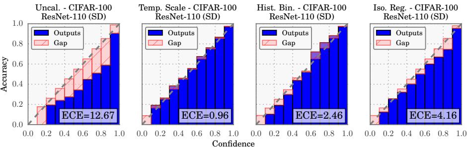
Figure 14.1: Reliability diagrams for the ResNet CNN image classifier [He+16b] applied to CIFAR-100 dataset. ECE is the expected calibration error, and measures the size of the red gap. Methods from left to right: original probabilities; after temperature scaling; after histogram binning; after isotonic regression. From Figure 4 of [Guo+17]. Used with kind permission of Chuan Guo.

More precisely, suppose we have B bins. Let B^b be the set of indices of samples whose prediction confidence falls into the interval I^b = ( ^b↓^{1 B} , ^{b B} ]. Here we use uniform bin widths, but we could also define the bins so that we can get an equal number of samples in each one.

Let f(x)^c = p(y = c|x), yˆⁿ = argmax^c↑{1,…,C} f(xn)c, and pˆⁿ = max^c↑{1,…,C} f(xn)c. The accuracy within bin b is defined as

\[\text{acc}(\mathcal{B}\_b) = \frac{1}{|\mathcal{B}\_b|} \sum\_{n \in \mathcal{B}\_b} \mathbb{I}\left(\hat{y}\_n = y\_n\right) \tag{14.17}\]

The average confidence within this bin is defined as

\[\text{conf}(\mathcal{B}\_b) = \frac{1}{|\mathcal{B}\_b|} \sum\_{n \in \mathcal{B}\_b} \hat{p}\_n \tag{14.18}\]

If we plot accuracy vs confidence, we get a reliability diagram, as shown in Figure 14.1. The gap between the accuracy and confidence is shown in the red bars. We can measure this using the expected calibration error (ECE) [NCH15]:

\[\text{ECE}(f) = \sum\_{b=1}^{B} \frac{|\mathcal{B}\_b|}{B} |\text{acc}(\mathcal{B}\_b) - \text{conf}(\mathcal{B}\_b)| \tag{14.19}\]

In the multiclass case, the ECE only looks at the error of the MAP (top label) prediction. We can extend the metric to look at all the classes using the marginal calibration error, proposed in [KLM19]:

\[\text{MCE} = \sum\_{c=1}^{C} w\_c \mathbb{E}\left[ \left( p(Y = c | f(\mathbf{z})\_c) - f(\mathbf{z})\_c \right)^2 \right] \tag{14.20}\]

\[=\sum\_{c=1}^{C} w\_c \sum\_{b=1}^{B} \frac{|\mathcal{B}\_{b,c}|}{B} \left( \text{acc}(\mathcal{B}\_{b,c}) - \text{conf}(\mathcal{B}\_{b,c}) \right)^2 \tag{14.21}\]

where Bb,c is the b’th bin for class c, and w^c ↗ [0, 1] denotes the importance of class c. (We can set w^c = 1/C if all classes are equally important.) In [Nix+19], they call this metric static calibration error; they show that certain methods that have good ECE may have poor MCE. Other multi-class calibration metrics are discussed in [WLZ19].

14.2.2.2 Improving calibration

In principle, training a classifier so it optimizes a proper scoring rule (such as NLL) should automatically result in a well-calibrated classifier. In practice, however, unbalanced datasets can result in poorly calibrated predictions. Below we discuss various ways for improving the calibration of probabilistic classifiers, following [Guo+17].

14.2.2.3 Platt scaling

Let z be the log-odds, or logit, and p = ς(z), produced by a probabilistic binary classifier. We wish to convert this to a more calibrated value q. The simplest way to do this is known as Platt scaling, and was proposed in [Pla00]. The idea is to compute q = ς(az + b), where a and b are estimated via maximum likelihood on a validation set.

In the multiclass case, we can extend Platt scaling by using matrix scaling: q = softmax(Wz + b), where we estimate W and b via maximum likelihood on a validation set. Since W has K ⇔ K parameters, where K is the number of classes, this method can easily overfit, so in practice we restrict W to be diagonal.

14.2.2.4 Nonparametric (histogram) methods

Platt scaling makes a strong assumption about the shape of the calibration curve. A more flexible, nonparametric, method is to partition the predicted probabilities into bins, pm, and to estimate an empirical probability q^m for each such bin; we then replace p^m with qm; this is known as histogram binning [ZE01a]. We can regularize this method by requiring that q = f(p) be a piecewise constant, monotonically non-decreasing function; this is known as isotonic regression [ZE01a]. An alternative approach, known as the scaling-binning calibrator, is to apply a scaling method (such as Platt scaling), and then to apply histogram binning to that. This has the advantage of using the average of the scaled probabilities in each bin instead of the average of the observed binary labels (see Figure 14.2). In [KLM19], they prove that this results in better calibration, due to the lower variance of the estimator.

In the multiclass case, z is the vector of logits, and p = softmax(z) is the vector of probabilities. We wish to convert this to a better calibrated version, q. [ZE01b] propose to extend histogram binning and isotonic regression to this case by applying the above binary method to each of the K one-vs-rest problems, where K is the number of classes. However, this requires K separate calibration models, and results in an unnormalized probability distribution.

14.2.2.5 Temperature scaling

In [Guo+17], they noticed empirically that the diagonal version of Platt scaling, when applied to a variety of DNNs, often ended learning a vector of the form w = (c, c, . . . , c), for some constant c. This suggests a simpler form of scaling, which they call temperature scaling: q = softmax(z/T),

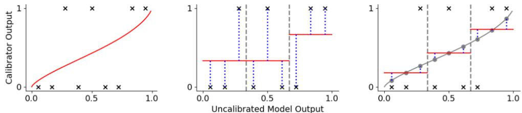
Figure 14.2: Visualization of 3 di!erent approaches to calibrating a binary probabilistic classifier. Black crosses are the observed binary labels, red lines are the calibrated outputs. (a) Platt scaling. (b) Histogram binning with 3 bins. The output in each bin is the average of the binary labels in each bin. (c) The scaling-binning calibrator. This first applies Platt scaling, and then computes the average of the scaled points (gray circles) in each bin. From Figure 1 of [KLM19]. Used with kind permission of Ananya Kumar.

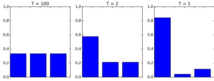
Figure 14.3: Softmax distribution softmax(a/T), where a = (3, 0, 1), at temperatures of T = 100, T = 2 and T = 1. When the temperature is high (left), the distribution is uniform, whereas when the temperature is low (right), the distribution is “spiky”, with most of its mass on the largest element. Generated by softmax\_plot.ipynb.

where T > 0 is a temperature parameter, which can be estimated by maximum likelihood on the validation set. The e!ect of this temperature parameter is to make the distribution less peaky, as shown in Figure 14.3. [Guo+17] show empirically that this method produces the lowest ECE on a variety of DNN classification problems (see Figure 14.1 for a visualization). Furthermore, it is much simpler and faster than the other methods.

Note that Platt scaling and temperature scaling do not a!ect the identity of the most probable class label, so these methods have no impact on classification accuracy. However, they do improve calibration performance. A more recent multi-class calibration method is discussed in [Kul+19].

14.2.2.6 Label smoothing

When training classifiers, we usually represent the true target label as a one-hot vector, say y = (0, 1, 0) to represent class 2 out of 3. We can improve results if we “spread” some of the probability mass across all the bins. For example we may use y = (0.1, 0.8, 0.1). This is called label smoothing and

often results in better-calibrated models [MKH19].

14.2.2.7 Bayesian methods

Bayesian approaches to fitting classifiers often result in more calibrated predictions, since they represent uncertainty in the parameters. See Section 17.3.8 for an example. However, [Ova+19] shows that well-calibrated models (even Bayesian ones) often become mis-calibrated when applied to inputs that come from a di!erent distribution (see Section 19.2 for details).

14.2.3 Beyond evaluating marginal probabilities

Calibration (Section 14.2.2) focuses on assessing properties of the marginal predictive distribution p(y|x). But this can sometimes be insu”cient to distinguish between a good and bad model, especially in the context of online learning and sequential decision making, as pointed out in [Lu+22; Osb+21; WSG21; KKG22]. For example, consider two learning agents who observe a sequence of coin tosses. Let the outcome at time t be Y^t ↔︎ Ber(ω), where ω is the unknown parameter. Agent 1 believes ω = 2/3, whereas agent 2 believes either ω = 0 or ω = 1, but is not sure which, and puts probabilities 1/3 and 2/3 on these events. Thus both agents, despite having di!erent models, make identical predictions for the next outcome: p(Y ^{i 1} = 0) = 1/3 for agents i = 1, 2. However, the predictions of the two agents about a sequence of τ future outcomes is very di!erent: In particular, agent 1 predicts each individual coin toss is a random Bernoulli event, where the probability is due to irreducible noise or aleatoric uncertainty:

\[p(Y\_1^1 = 0, \dots, Y\_\tau^1 = 0) = \frac{1}{3^\tau} \tag{14.22}\]

By contrast, agent 2 predicts that the sequence will either be all heads or all tails, where the probability is induced by epistemic uncertainty about the true parameters:

\[p(Y\_1^2 = y\_1, \dots, Y\_\tau^2 = y\_\tau) = \begin{cases} 1/3 & \text{if } y\_1 = \dots = y\_\tau = 0 \\ 2/3 & \text{if } y\_1 = \dots = y\_\tau = 1 \\ 0 & \text{otherwise} \end{cases} \tag{14.23}\]

(See Section 3.2.2 for more discussion of epistemic uncertainty.) The di!erence in beliefs between these agents will impact their behavior. For example, in a casino, agent 1 incurs little risk on repeatedly betting on heads in the long run, but for agent 2, this would be a very unwise strategy, and some initial information gathering (exploration) would be worthwhile.

Based on the above, we see that it is useful to evaluate joint predictive distributions when assessing predictive models. In [Lu+22; Osb+21] they propose to evaluate the posterior predictive distributions over τ outcomes y = Y^T +1:^{T +◁} , given a set of τ inputs x = XT:^{T +}◁↓1, and the past T data samples, D^T = {(Xt, Yt+1) : t = 0, 1,…,T → 1}. The Bayes optimal predictive distribution is

\[P\_T^B = p(\mathbf{y}|\mathbf{x}, \mathcal{D}\_T) \tag{14.24}\]

This is usually intractable to compute. Instead the agent will use an approximate distribution, known as a belief state, which we denote by

\[Q\_T = q(\mathbf{y}|\mathbf{x}, \mathcal{D}\_T) \tag{14.25}\]

The natural performance metric is the KL between these distributions. Since this depends on the inputs x and D^T = (X0:^{T ↓}1, Y1:^T ), we will average the KL over these values, which are drawn iid from the true data generating distribution, which we denote by

\[P(X,Y,\mathcal{E}) = P(X|\mathcal{E})P(Y|X,\mathcal{E})P(\mathcal{E})\tag{14.26}\]

where E is the true but unknown environment. Thus we define our metric as

\[d\_{B,Q}^{KL} = \mathbb{E}\_{P(\mathbf{z}, \mathcal{D}\_T)} \left[ D\_{\text{KL}} \left( P^B(\mathbf{y}|\mathbf{z}, \mathcal{D}\_T) \parallel Q(\mathbf{y}|\mathbf{z}, \mathcal{D}\_T) \right) \right] \tag{14.27}\]

where

\[P(\mathbf{z}, \mathcal{D}\_T, \mathcal{E}) = P(\mathcal{E}) \underbrace{\left[ \prod\_{t=0}^{T-1} P(X\_t|\mathcal{E}) P(Y\_{t+1}|X\_t, \mathcal{E}) \right]}\_{P(\mathcal{D}\_T|\mathcal{E})} \underbrace{\left[ \prod\_{t=T}^{T+\tau-1} P(x\_t|\mathcal{E}) \right]}\_{P(\mathbf{z}|\mathcal{E})} \tag{14.28}\]

and P(x, D^T ) marginalizes this over environments.

Unfortunately, it is usually intractable to compute the exact Bayes posterior, P ^{B T} , so we cannot evaluate dKL B,Q. However, in Section 14.2.3.1, we show that

\[d\_{B,Q}^{KL} = d\_{\mathcal{E},Q}^{KL} - \mathbb{I}(\mathcal{E}; \mathbf{y} | \mathcal{D}\_T, \mathbf{z}) \tag{14.29}\]

where the second term is a constant wrt the agent, and the first term is given by

\[d\_{\mathcal{E},Q}^{KL} = \mathbb{E}\_{P(\mathbf{z}, \mathcal{D}\_T, \mathcal{E})} \left[ D\_{\mathbb{KL}} \left( P(\mathbf{y}|\mathbf{z}, \mathcal{E}) \parallel Q(\mathbf{y}|\mathbf{z}, \mathcal{D}\_T) \right) \right] \tag{14.30}\]

\[=\mathbb{E}\_{P(\mathbf{y}|\mathbf{z},\mathcal{E})P(\mathbf{z},\mathcal{D}\_T,\mathcal{E})}\left[\log\frac{P(\mathbf{y}|\mathbf{z},\mathcal{E})}{Q(\mathbf{y}|\mathbf{z},\mathcal{D}\_T)}\right] \tag{14.31}\]

Hence if we rank agents in terms of dKL ^E,Q, it will give the same results as ranking them by ^dKL B,Q.

To compute dKL ^E,Q in practice, we can use a Monte Carlo approximation: we just have to sample ^J environments, ^{Ej ↔︎ P}(E), sample a training set ^DT from each environment, ^{Dj T ↔︎ P}(D^T |E^j ), and then sample N data vectors of length τ , (x^{j n}, y^{j n}) ^{↔︎ P}(XT:^{T +}◁↓¹, Y^T +1:^{T +◁} |E^j ). We can then compute

\[\hat{d}\_{\mathcal{E},Q}^{KL} = \frac{1}{JN} \sum\_{j=1}^{J} \sum\_{n=1}^{N} \left[ \log P(\mathbf{y}\_n^j | \mathbf{z}\_n^j, \mathcal{E}^j) - \log Q(\mathbf{y}\_n^j | \mathbf{z}\_n^j, \mathcal{D}\_T^j) \right] \tag{14.32}\]

where

\[p\_{jn} = P(y\_n^j | \mathbf{x}\_n^j, \mathcal{E}^j) = \prod\_{t=T}^{T+\tau-1} P(Y\_{n,t+1}^j | X\_{n,t}^j, \mathcal{E}^j) \tag{14.33}\]

\[q\_{jn} = Q(y\_n^j | \mathbf{x}\_n^j, \mathcal{D}\_T^j) = \int Q(y\_n^j | \mathbf{x}\_n^j, \boldsymbol{\theta}) Q(\boldsymbol{\theta} | \mathcal{D}\_T^j) d\boldsymbol{\theta} \tag{14.34}\]

\[\approx \frac{1}{M} \sum\_{m=1}^{M} \prod\_{t=T}^{T+\tau-1} Q(Y\_{n,t+1}^{j} | X\_{n,t}^{j}, \theta\_{m}^{j}) \tag{14.35}\]

where ω^{j m ↔︎ Q}(ω|D^{j T} ) is a sample from the agent’s posterior over the environment.

The above assumes that P(Y |X) is known; this will be the case if we use a synthetic data generator, as in the “neural testbed” in [Osb+21]. If we just have J empirical distributions for P^j (X, Y ), we can replace the KL with the cross entropy, which only di!ers by an additive constant:

\[d\_{\mathcal{E},Q}^{KL} = \mathbb{E}\_{P(\mathbf{z}, \mathcal{D}\_T, \mathcal{E})} \left[ D\_{\mathbb{KL}} \left( P(\mathbf{y}|\mathbf{z}, \mathcal{E}) \parallel Q(\mathbf{y}|\mathbf{z}, \mathcal{D}\_T) \right) \right] \tag{14.36}\]

\[= \mathbb{E}\_{P(\mathbf{z}, \mathbf{y}, \mathcal{E})} \left[ \log P(\mathbf{y}|\mathbf{z}, \mathcal{E}) \right] - \mathbb{E}\_{P(\mathbf{z}, \mathbf{y}, \mathcal{D}\_T|\mathcal{E})P(\mathcal{E})} \left[ \log Q(\mathbf{y}|\mathbf{z}, \mathcal{D}\_T) \right] \tag{14.37}\]

• ,- . const + ,- . ^dCE E,Q where the latter term is just the empirical negative log likelihood (NLL) of the agent on samples from the environment. Hence if we rank agents in terms of their NLL or cross entropy dCE ^E,Q we will get the same results as ranking them by dKL ^E,Q, which will in turn give the same results as ranking

them by dKL B,Q. In practice we can approximate the cross entropy as follows:

\[\hat{d}\_{\mathcal{E},Q}^{CE} = -\frac{1}{JN} \sum\_{j=1}^{J} \sum\_{n=1}^{N} \log Q(\mathbf{y}\_n^j | \mathbf{x}\_n^j, \mathcal{D}\_T^j) \tag{14.38}\]

where ^{Dj T ↔︎ Pj} , and (x^{j n}, y^{j n}) ^{↔︎ Pj} .

An alternative to estimating the KL or NLL is to evaluate the joint predictive accuracy by using it in a downstream task. In [Osb+21], they show that good predictive accuracy (for τ > 1) correlates with good performance on a bandit problem (see Section 34.4). In [WSG21] they show that good predictive accuracy (for τ > 1) results in good performance on a transductive active learning task.

14.2.3.1 Proof of claim

We now prove Equation (14.29), based on [Lu+21]. First note that

\[d\_{\mathcal{E},Q}^{KL} = \mathbb{E}\_{P(\mathbf{z}, \mathcal{D}\_T, \mathcal{E})P(\mathbf{y}|\mathbf{z}, \mathcal{E})} \left[ \log \frac{P(\mathbf{y}|\mathbf{z}, \mathcal{E})}{Q(\mathbf{y}|\mathbf{z}, \mathcal{D}\_T)} \right] \tag{14.39}\]

\[=\mathbb{E}\left[\log\frac{P(\mathbf{y}|\mathbf{z},\mathcal{D}\_T)}{Q(\mathbf{y}|\mathbf{z},\mathcal{D}\_T)}\right] + \mathbb{E}\left[\log\frac{P(\mathbf{y}|\mathbf{z},\mathcal{E})}{P(\mathbf{y}|\mathbf{z},\mathcal{D}\_T)}\right] \tag{14.40}\]

For the first term in Equation (14.40) we have

\[\mathbb{E}\left[\log\frac{P(\mathbf{y}|\mathbf{z},\mathcal{D}\_T)}{Q(\mathbf{y}|\mathbf{z},\mathcal{D}\_T)}\right] = \sum P(\mathbf{z},\mathbf{y},\mathcal{D}\_T)\log\frac{P(\mathbf{y}|\mathbf{z},\mathcal{D}\_T)}{Q(\mathbf{y}|\mathbf{z},\mathcal{D}\_T)}\tag{14.41}\]

\[=\sum P(\mathbf{x},\mathcal{D}\_T)\sum P(\mathbf{y}|\mathbf{x},\mathcal{D}\_T)\log\frac{P(\mathbf{y}|\mathbf{x},\mathcal{D}\_T)}{Q(\mathbf{y}|\mathbf{x},\mathcal{D}\_T)}\tag{14.42}\]

\[\mathbb{E}\_{\mathbf{x}} = \mathbb{E}\_{P(\mathbf{z}, \mathcal{D}\_T)} \left[ D\_{\text{KL}} \left( P(\mathbf{y} | \mathbf{z}, \mathcal{D}\_T) \parallel Q(\mathbf{y} | \mathbf{z}, \mathcal{D}\_T) \right) \right] = d\_{B,Q}^{KL} \tag{14.43}\]

We now show that the second term in Equation (14.40) reduces to the mutual information. We exploit the fact that

\[P(y|\mathbf{z}, \mathcal{E}) = P(y|\mathcal{D}\_T, \mathbf{z}, \mathcal{E}) = \frac{P(\mathcal{E}, y|\mathcal{D}\_T, \mathbf{z})}{P(\mathcal{E}|\mathcal{D}\_T, \mathbf{z})} \tag{14.44}\]

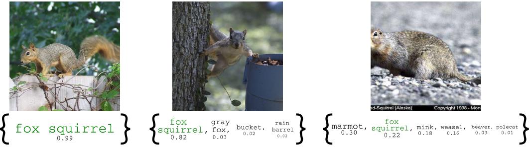
Figure 14.4: Prediction set examples on Imagenet. We show three progressively more di#cult examples of the class fox squirrel and the prediction sets generated by conformal prediction. (Compare to Figure 17.9.) From Figure 1 of [AB21]. Used with kind permission of Anastasios Angelopoulos.

since D^T has no new information in beyond E. From this we get

\[\mathbb{E}\left[\log\frac{P(\mathbf{y}|\mathbf{z},\mathcal{E})}{P(\mathbf{y}|\mathbf{z},\mathcal{D}\_T)}\right] = \mathbb{E}\left[\log\frac{P(\mathcal{E},\mathbf{y}|\mathcal{D}\_T,\mathbf{z})/P(\mathcal{E}|\mathcal{D}\_T,\mathbf{z})}{P(\mathbf{y}|\mathcal{D},\mathcal{D}\_T)}\right] \tag{14.45}\]

\[\hat{\rho} = \sum P(\mathcal{D}\_T, x) \sum P(\mathcal{E}, y | \mathcal{D}\_T, x) \log \frac{P(\mathcal{E}, y | \mathcal{D}\_T, x)}{P(y | \mathcal{D}\_T, x) P(\mathcal{E} | \mathcal{D}\_T, x)} \tag{14.46}\]

\[= \mathbb{I}(\mathcal{E}; \mathcal{y} | \mathcal{D}\_T, \mathbf{z}) \tag{14.47}\]

Hence

\[d\_{\mathcal{E},Q}^{KL} = d\_{B,Q}^{KL} + \mathbb{I}(\mathcal{E}; \boldsymbol{y} | \mathcal{D}\_T, \mathbf{z}) \tag{14.48}\]

as claimed.

14.3 Conformal prediction

In this section, we briefly discuss conformal prediction [VGS05; SV08; ZFV20; AB21; KSB21; Man22b; ABB24]. This is a simple but e!ective way to create prediction intervals or sets with guaranteed frequentist coverage probability from any predictive method p(y|x). This can be seen as a form of distribution free uncertainty quantification, since it works without making assumptions (beyond exchangeability of the data) about the true data generating process or the form of the model.1 Our presentation is based on the excellent tutorial of [AB21].2

In conformal prediction, we start with some heuristic notion of uncertainty — such as the softmax score for a classification problem, or the variance for a regression problem — and we use it to define a conformal score s(x, y) ↗ R, which measures how badly the output y “conforms” to x. (Large

^1. The exchangeability assumption rules out time series data, which is serially correlated. However, extensions to conformal prediction have been developed for the time series case, see e.g., [Zaf+22; Bha+23]. The exchangeability assumption also rules out distribution shift, although extensions to this case have also been developed [Tib+19].

^2. See also the easy-to-use MAPIE Python library at https://mapie.readthedocs.io/en/latest/index.html, and the list of papers at [Man22a].

values of the score are less likely, so it is better to think of it as a non-conformity score.) Next we apply this score to a calibration set of n labeled examples, that was not used to train f, to get S = {sⁱ = s(xi, yi) : i =1: n}. 3 The user specifies a desired confidence threshold ϱ, say 0.1, and we then compute the (1 ^{→ ϱ}) quantile ^qˆ of ^S. (In fact, we should replace ^{1 → ϱ} with ↙(n+1)(1↓↼)^{∝ n} , to account for the finite size of S.) Finally, given a new test input, xn+1, we compute the prediction set to be

\[\mathcal{T}(\mathbf{z}\_{n+1}) = \{ y : s(\mathbf{z}\_{n+1}, y) \le \hat{q} \}\tag{14.49}\]

Intuitively, we include all the outputs y that are plausible given the input. See Figure 14.4 for an illustration.

Remarkably, one can show the following general result

\[1 - \alpha \le P^\*(y^{n+1} \in \mathcal{T}(\mathbf{z}\_{n+1})) \le 1 - \alpha + \frac{1}{n+1} \tag{14.50}\]

where the probability is wrt the true distribution P→(x1, y1,…, xn+1, yn+1). We say that the prediction set has a coverage level of 1 → ϱ. This holds for any value of n ≃ 1 and ϱ ↗ [0, 1]. The only assumption is that the values (xi, yi) are exchangeable, and hence the calibration scores sⁱ are also exchangeable.

To see why this is true, let us sort the scores so ^{s1 &}lt; ··· ^sn, so ^{qˆ = s}i, where ^{i =} ↙(n+1)(1↓↼)^{∝ n} . (We assume the scores are distinct, for simplicity.) The score sn+1 is equally likely to fall in anywhere between the calibration points s1,…,sn, since the points are exchangeable. Hence

\[P^\*(s\_{n+1} \le s\_k) = \frac{k}{n+1} \tag{14.51}\]

for any k ↗ {1,…,n + 1}. The event {yn+1 ↗ T (xn+1)} is equivalent to {sn+1 ⇐ qˆ}. Hence

\[P^\*(y\_{n+1} \in T(x\_{n+1})) = P^\*(s\_{n+1} \le \hat{q}) = \frac{\lceil (n+1)(1-\alpha) \rceil}{n+1} \ge 1-\alpha \tag{14.52}\]

For the proof of the upper bound, see [Lei+18].

Although this result may seem like a “free lunch”, it is worth noting that we can always achieve a desired coverage level by defining the prediction set to be all possible labels. In this case, the prediction set will be independent of the input, but it will cover the true label 1 → ϱ of the time. To rule out such degenerate cases, we seek prediction sets that are as small as possible (although we allow for the set to be larger for harder examples), while meeting the coverage requirement. Achieving this goal requires that we define suitable conformal scores. Below we give some examples of how to compute conformal scores s(x, y) for di!erent kinds of problem.4 It is also important to note that the coverage guarantees are frequentist in nature, and refer to average behavior, rather than representing per-instance uncertainty, as in the Bayesian approach.

^3. Using a calibration set is called split conformal prediction. If we don’t have enough data to adopt this splitting approach, we can use full conformal prediction [VGS05], which requires fitting the model n times using a leave-one-out type procedure.

^4. It is also possible to learn conformal scores in an end-to-end way, jointly with the predictive model, as discussed in [Stu+22].

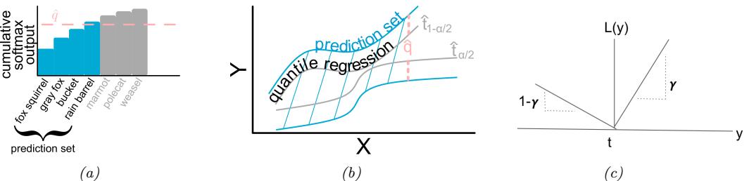
Figure 14.5: (a) Illusration of adaptive prediction set. From Figure 5 of [AB21]. Used with kind permission of Anastasios Angelopoulos. (b) Illustration of conformalized quantile regression. From Figure 6 of [AB21]. Used with kind permission of Anastasios Angelopoulos. (c) Illustration of pinball loss function.

14.3.1 Conformalizing classification

The simplest way to apply conformal prediction to multiclass classification is to derive the conformal score from the softmax score assigned to the label using s(x, y)=1 → f(x)y, so large values are considered less likely than small values. We compute the threshold qˆ as described above, and then we define the prediction set to be T (x) = {y : f(x)^y ≃ 1 → qˆ}, which matches Equation (14.49). That is, we take the set of all class labels above the specified threshold, as illustrated in Figure 14.4.

Although the above approach produces prediction sets with the smallest average size (as proved in [SLW19]), the size of the set tends to be too large for easy examples and too small for hard examples. We now present an improved method, known as adaptive prediction sets, due to [RSC20], which solves this problem. The idea is simple: we sort all the softmax scores, f(x)^c for c =1: C, to get permutation ϖ1:^C , and then we define s(x, y) to be the cumulative sum of the scores up until we reach label y: s(x, y) = &^{k c}=1 f(x)⇀^c , where k = ϖy. We now compute qˆ as before, and define the prediction set T (x) to be the set of all labels, sorted in order of decreasing probability, until we cover qˆ of the probability mass. See Figure 14.5a for an illustration. This uses all the softmax scores output by the model, rather than just the top score, which accounts for its improved performance.

14.3.2 Conformalizing regression

In this section, we consider conformalized regression problems. Since now y ↗ R, computing the prediction set in Equation (14.49) is expensive, so instead we will compute a prediction interval, specified by a lower and upper bound.

14.3.2.1 Conformalizing quantile regression

In this section, we use quantile regression to compute the lower and upper bounds. We first fit a function of the form t⇁(x), which predicts the ▷ quantile of the cdf P^Y (Y ) = p(Y |x). For example, if we set ▷ = 0.5, we get the median. If we use ▷ = 0.05 and ▷ = 0.95, we can get an approximate 90% prediction interval using [t0.05(x), t0.95(x)], as illustrated by the gray lines in Figure 14.5b.

To fit the quantile regression model, we just replace squared loss with the quantile loss, also called the pinball loss, which is defined as

\[\ell\_{\gamma}(y,\hat{t}) = (\gamma - \mathbb{I}\left(y < \hat{t}\right))(y - \hat{t}) = (y - \hat{t})\gamma\mathbb{I}\left(y > \hat{t}\right) + (\hat{t} - y)(1 - \gamma)\mathbb{I}\left(y < \hat{t}\right) \tag{14.53}\]

where y is the true output and t ˆ is the predicted value at quantile ▷. See Figure 14.5c for an illustration. The key property of this loss function is that its minimizer is the ▷-quantile of the distribution P^Y , i.e.,

\[\underset{\delta}{\text{argmin}} \, \mathbb{E}\_{\mathbf{y}\mathbf{y}} \left[ \ell\_{\gamma}(y, \hat{t}) \right] = P\_{\mathbf{y}}^{-1}(\gamma)\]

However, the regression quantiles are usually only approximately a 90% interval because the model may be mismatched to the true distribution. Fortunately we can use conformal prediction to fix this. In particular, let us define the conformal score to be

\[s(x, y) = \max\left(\hat{t}\_{\alpha/2}(x) - y, y - \hat{t}\_{\alpha/2}(x)\right) \tag{14.54}\]

In other words, s(x, y) is a positive measure of how far the value y is outside the prediction interval, or is a negative measure if y is inside the prediction interval. We compute qˆ as before, and define the conformal prediction interval to be

\[\mathcal{T}(\mathbf{z}) = [\hat{t}\_{\alpha/2}(\mathbf{z}) - \hat{q}, \hat{t}\_{\alpha/2}(\mathbf{z}) + \hat{q}] \tag{14.55}\]

This makes the quantile regression interval wider if qˆ is positive (if the base method was overconfident), and narrower if qˆ is negative (if the base method was underconfident). See Figure 14.5b for an illustration. This approach is called conformalized quantile regression or CQR [RPC19].

14.3.2.2 Conformalizing predicted variances

There are many ways to define uncertainty scores u(x), such as the predicted standard deviation, from which we can derive a prediction interval using

\[\mathcal{T}(\mathbf{z}) = [f(\mathbf{z}) - u(\mathbf{z})\hat{q}, f(\mathbf{z}) + u(\mathbf{z})\hat{q}] \tag{14.56}\]

Here qˆ is derived from the quantiles of the following conformal scores

\[s(x, y) = \frac{|y - f(x)|}{u(x)}\tag{14.57}\]

The interval produced by this method tends to be wider than the one computed by CQR, since it extends an equal amount above and below the predicted value f(x). In addition, the uncertainty measure u(x) may not scale properly with ϱ. Nevertheless, this is a simple post-hoc method that can be applied to many regression methods without needing to retrain them.

14.3.3 Conformalizing Bayes

Suppose we can compute the posterior predictive distribution f(x)^y = p(y|x). If this is a perfect model, then the following prediction set would be optimal:

\[\mathcal{S}(\mathbf{x}) = \{ y : f(\mathbf{z})\_y > t \}, \text{ where } t \text{ is chosen so } \int\_{y \in \mathcal{S}(\mathbf{z})} f(\mathbf{z})\_y dy = 1 - \alpha \tag{14.58}\]

This set will not have the desired coverage if our modeling assumptions are wrong. However, we can conformalize it by defining s(x, y) = →f(x)^y and T (x) = {y : f(x)^y > →qˆ }. That is, we include all outputs above the chosen threshold. In [Hof21] they prove that this procedure has the smallest average size (Bayes risk) of any conformal procedure with 1 → ϱ coverage. Thus it is optimal in both the Bayesian and frequentist sense.

14.3.4 What do we do if we don’t have a calibration set?

So far we have assumed access to a separate calibration set, which makes things simple. This is called split conformal prediction. If we don’t have enough data to adopt this splitting approach, we can use full conformal prediction [VGS05], which requires fitting the model n times using a leave-one-out type procedure. Alternatively we can use the more e”cient Bayesian add-one-in importance sampling procedure of [FH21], or the jackknife+ procedure of [Bar+19].

14.3.5 General conformal prediction/ decision problems

It is possible to generalize conformal prediction to the case where the output set is more general than just a set of class labels, or an interval of the real line [Ang+24], greatly expanding the applicability. For example, [Yad+24] uses “conformal abstention” to decide when an LLM should not answer a question if it is not su”ciently confident.

15 Generalized linear models

15.1 Introduction

A generalized linear model or GLM [MN89] is a conditional version of an exponential family distribution (Section 2.4). More precisely, the model has the following form:

\[p(y\_n|\mathbf{x}\_n, w, \sigma^2) = \exp\left[\frac{y\_n \eta\_n - A(\eta\_n)}{\sigma^2} + \log h(y\_n, \sigma^2)\right] \tag{15.1}\]

where ^{ηn = wT}xⁿ is the natural parameter for the distribution, ^A(ηn) is the log normalizer, ^T (y) = ^y is the su”cient statistic, and ς² is the dispersion term. Based on the results in Section 2.4.3, we can show that the mean and variance of the response variable are as follows:

\[\mu\_n \triangleq \mathbb{E}\left[y\_n | \mathbf{x}\_n, \mathbf{w}, \sigma^2\right] = A'(\eta\_n) \triangleq \ell^{-1}(\eta\_n) \tag{15.2}\]

\[\mathbb{V}\left[y\_n|x\_n, w, \sigma^2\right] = A''(\eta\_n)\,\sigma^2 \tag{15.3}\]

We will denote the mapping from the linear inputs to the mean of the output using µⁿ = ε↓1(ηn), where the function ε is known as the link function, and ε↓¹ is known as the mean function. This relationship is usually written as follows:

\[\ell(\mu\_n) = \eta\_n = \mathbf{w}^{\mathsf{T}} \mathbf{z}\_n \tag{15.4}\]

GLMs are quite limited in their predictive power, due to the assumption of linearity (although we can always use basis function expansion on xⁿ to improve the flexibility). However, the main use of GLMs in the statistics literature is not for prediction, but for hypothesis testing, as we explain in Section 3.10.3. This relies on the ability to compute the posterior, p(w|D), which we discuss in Section 15.1.4. We can use this to draw conclusions about whether any of the inputs (e.g., representing di!erent groups) have a significant e!ect on the output.

15.1.1 Some popular GLMs

In this section, we give some examples of widely used GLMs.

15.1.1.1 Linear regression

Recall that linear regression has the form

\[p(y\_n|\mathbf{x}\_n, \mathbf{w}, \sigma^2) = \frac{1}{\sqrt{2\pi\sigma^2}} \exp(-\frac{1}{2\sigma^2}(y\_n - \mathbf{w}^\mathsf{T}\mathbf{x}\_n)^2) \tag{15.5}\]

Hence

\[\log p(y\_n|\mathbf{x}\_n, \mathbf{w}, \sigma^2) = -\frac{1}{2\sigma^2} (y\_n - \eta\_n)^2 - \frac{1}{2} \log(2\pi\sigma^2) \tag{15.6}\]

where ηⁿ = wTxn. We can write this in GLM form as follows:

\[\log p(y\_n|\mathbf{x}\_n, \mathbf{w}, \sigma^2) = \frac{y\_n \eta\_n - \frac{\eta\_n^2}{2}}{\sigma^2} - \frac{1}{2} \left(\frac{y\_n^2}{\sigma^2} + \log(2\pi\sigma^2)\right) \tag{15.7}\]

We see that A(ηn) = η^{2 n}/2 and hence

\[\mathbb{E}\left[y\_n\right] = \eta\_n = \mathbf{w}^{\mathsf{T}} \mathbf{z}\_n \tag{15.8}\]

\[\mathbb{V}\left[y\_n\right] = \sigma^2\tag{15.9}\]

See Section 15.2 for details on linear regression.

15.1.1.2 Binomial regression

If the response variable is the number of successes in Nⁿ trials, yⁿ ↗ {0,…,Nn}, we can use binomial regression, which is defined by

\[p(y\_n | \mathbf{x}\_n, N\_n, \mathbf{w}) = \text{Bin}(y\_n | \sigma(\mathbf{w}^\mathsf{T} \mathbf{x}\_n), N\_n) \tag{15.10}\]

We see that binary logistic regression is the special case when Nⁿ = 1.

The log pdf is given by

\[\log p(y\_n|\mathbf{x}\_n, N\_n, \mathbf{w}) = y\_n \log \mu\_n + (N\_n - y\_n) \log(1 - \mu\_n) + \log \binom{N\_n}{y\_n} \tag{15.11}\]

\[=y\_n \log(\frac{\mu\_n}{1-\mu\_n}) + N\_n \log(1-\mu\_n) + \log\binom{N\_n}{y\_n} \tag{15.12}\]

where µⁿ = ς(ηn). To rewrite this in GLM form, let us define

\[\eta\_n \triangleq \log \left[ \frac{\mu\_n}{(1 - \mu\_n)} \right] = \log \left[ \frac{1}{1 + e^{-\mathbf{w}^\mathsf{T} \mathbf{z}\_n}} \frac{1 + e^{-\mathbf{w}^\mathsf{T} \mathbf{z}\_n}}{e^{-\mathbf{w}^\mathsf{T} \mathbf{z}\_n}} \right] = \log \frac{1}{e^{-\mathbf{w}^\mathsf{T} \mathbf{z}\_n}} = \mathbf{w}^\mathsf{T} \mathbf{z}\_n \tag{15.13}\]

Hence we can write binomial regression in GLM form as follows

\[\log p(y\_n|\mathbf{x}\_n, N\_n, \mathbf{w}) = y\_n \eta\_n - A(\eta\_n) + h(y\_n) \tag{15.14}\]

\[\text{where } h(y\_n) = \log\binom{N\_n}{y\_n} \text{ and }\]

\[A(\eta\_n) = -N\_n \log(1 - \mu\_n) = N\_n \log(1 + e^{\eta\_n}) \tag{15.15}\]

Hence

\[\mathbb{E}\left[y\_n\right] = \frac{dA}{d\eta\_n} = \frac{N\_n e^{\eta\_n}}{1 + e^{\eta\_n}} = \frac{N\_n}{1 + e^{-\eta\_n}} = N\_n \mu\_n \tag{15.16}\]

and

\[\mathbb{V}\left[y\_n\right] = \frac{d^2A}{d\eta\_n^2} = N\_n\mu\_n(1-\mu\_n) \tag{15.17}\]

See Section 15.3.9 for an example of binomial regression.

15.1.1.3 Poisson regression

If the response variable is an integer count, yⁿ ↗ {0, 1,…}, we can use Poisson regression, which is defined by

\[p(y\_n|\mathbf{x}\_n, \mathbf{w}) = \text{Poi}(y\_n|\exp(\mathbf{w}^\mathsf{T}\mathbf{x}\_n))\tag{15.18}\]

where

\[\text{Poi}(y|\mu) = e^{-\mu} \frac{\mu^y}{y!} \tag{15.19}\]

is the Poisson distribution. Poisson regression is widely used in bio-statistical applications, where yⁿ might represent the number of diseases of a given person or place, or the number of reads at a genomic location in a high-throughput sequencing context (see e.g., [Kua+09]).

The log pdf is given by

\[\log p(y\_n|\mathbf{x}\_n, \mathbf{w}) = y\_n \log \mu\_n - \mu\_n - \log(y\_n!) \tag{15.20}\]

where µⁿ = exp(w^Txn). Hence in GLM form we have

\[\log p(y\_n|\mathbf{x}\_n, \mathbf{w}) = y\_n \eta\_n - A(\eta\_n) + h(y\_n) \tag{15.21}\]

where ^ηn = log(µn) = ^wTxn, ^A(ηn) = ^{µn = e▷n} , and ^h(yn) = ^→ log(yn!). Hence

\[\mathbb{E}\left[y\_n\right] = \frac{dA}{d\eta\_n} = e^{\eta\_n} = \mu\_n \tag{15.22}\]

and

\[\mathbb{V}\left[y\_n\right] = \frac{d^2A}{d\eta\_n^2} = e^{\eta\_n} = \mu\_n \tag{15.23}\]

15.1.1.4 Zero-inflated Poisson regression

In many forms of count data, the number of observed 0s is larger than what a model might expect, even after taking into account the predictors. Intuitively, this is because there may be many ways to produce no outcome. For example, consider predicting sales data for a product. If the sales are 0, does it mean the product is unpopular (so the demand is very low), or was it simply sold out (implying the demand is high, but supply is zero)? Similar problems arise in genomics, epidemiology, etc.

To handle such situations, it is common to use a zero-inflated Poisson or ZIP model. The likelihood for this model is a mixture of two distributions: a spike at 0, and a standard Poisson. Formally, we define

\[\text{ZIP}(y|\rho,\lambda) = \begin{cases} \rho + (1 - \rho)\exp(-\lambda) & \text{if } y = 0\\ (1 - \rho)\frac{\lambda^y \exp(-\lambda)}{y!} & \text{if } y > 0 \end{cases} \tag{15.24}\]

Here 0 is the prior probability of picking the spike, and ⇀ is the rate of the Poisson. We see that there are two “mechanisms” for generating a 0: either (with probability 0) we choose the spike, or (with probability 1 → 0) we simply generate a zero count just because the rate of the Poisson is so low. (This latter event has probability ⇀⁰e↓^ε/0! = e↓^ε.)

15.1.2 GLMs with noncanonical link functions

We have seen how the mean parameters of the output distribution are given by µ = ε↓¹(η), where the function ε is the link function. There are several choices for this function, as we now discuss.

The canonical link function ε satisfies the property that ω = ε(µ), where ω are the canonical (natural) parameters. Hence

\[\theta = \ell(\mu) = \ell(\ell^{-1}(\eta)) = \eta \tag{15.25}\]

This is what we have assumed so far. For example, for the Bernoulli distribution, the canonical parameter is the log-odds η = log(µ/(1 → µ)), which is given by the logit transform

\[\eta = \ell(\mu) = \text{logit}(\mu) = \log\left(\frac{\mu}{1-\mu}\right) \tag{15.26}\]

The inverse of this is the sigmoid or logistic funciton

\[\mu = \ell^{-1}(\eta) = \sigma(\eta) = 1/(1 + e^{-\eta})\tag{15.27}\]

However, we are free to use other kinds of link function. For example, in Section 15.4 we use

\[ \eta = \ell(\mu) = \Phi^{-1}(\mu) \tag{15.28} \]

\[ \mu = \ell^{-1}(\eta) = \Phi(\eta) \tag{15.29} \]

This is known as the probit link function.

Another link function that is sometimes used for binary responses is the complementary log-log function

\[\eta = \ell(\mu) = \log(-\log(1-\mu))\tag{15.30}\]

This is used in applications where we either observe 0 events (denoted by y = 0) or one or more (denoted by y = 1), where events are assumed to be governed by a Poisson distribution with rate ⇀. Let E be the number of events. The Poisson assumption means p(E = 0) = exp(→⇀) and hence

\[p(y=0) = (1 - \mu) = p(E=0) = \exp(-\lambda)\tag{15.31}\]

Thus ⇀ = → log(1 → µ). When ⇀ is a function of covariates, we need to ensure it is positive, so we use ⇀ = e^▷, and hence

\[\eta = \log(\lambda) = \log(-\log(1-\mu))\tag{15.32}\]

15.1.3 Maximum likelihood estimation

GLMs can be fit using similar methods to those that we used to fit logistic regression. In particular, the negative log-likelihood has the following form (ignoring constant terms):

\[\text{NLL}(\boldsymbol{w}) = -\log p(\mathcal{D}|\boldsymbol{w}) = -\frac{1}{\sigma^2} \sum\_{n=1}^{N} \ell\_n \tag{15.33}\]

where

\[\ell\_n \triangleq \eta\_n y\_n - A(\eta\_n) \tag{15.34}\]

where ηⁿ = w^Txn. For notational simplicity, we will assume ς² = 1.

We can compute the gradient for a single term as follows:

\[\mathbf{g}\_n \triangleq \frac{\partial \ell\_n}{\partial \mathbf{w}} = \frac{\partial \ell\_n}{\partial \eta\_n} \frac{\partial \eta\_n}{\partial \mathbf{w}} = (y\_n - A'(\eta\_n))\mathbf{x}\_n = (y\_n - \mu\_n)\mathbf{x}\_n \tag{15.35}\]

where µⁿ = f(w^Txn), and f is the inverse link function that maps from canonical parameters to mean parameters. (For example, in the case of logistic regression, we have µⁿ = ς(w^Tx).)

The Hessian is given by

\[\mathbf{H} = \frac{\partial^2}{\partial \mathbf{w} \partial \mathbf{w}^\mathrm{T}} \mathrm{NLL}(\boldsymbol{w}) = -\sum\_{n=1}^N \frac{\partial \mathbf{g}\_n}{\partial \mathbf{w}^\mathrm{T}} \tag{15.36}\]

where

\[\frac{\partial \mathbf{g}\_n}{\partial \mathbf{w}^\mathsf{T}} = \frac{\partial \mathbf{g}\_n}{\partial \mu\_n} \frac{\partial \mu\_n}{\partial \mathbf{w}^\mathsf{T}} = -\boldsymbol{x}\_n f'(\mathbf{w}^\mathsf{T} \boldsymbol{x}\_n) \mathbf{x}\_n^\mathsf{T} \tag{15.37}\]

Hence

\[\mathbf{H} = \sum\_{n=1}^{N} f'(\eta\_n) \mathbf{x}\_n \mathbf{z}\_n^\top \tag{15.38}\]

For example, in the case of logistic regression, f(ηn) = ς(ηn) = µn, and f^↔︎ (ηn) = µn(1 → µn). In general, we see that the Hessian is positive definite, since f^↔︎ (ηn) > 0; hence the negative log likelihood is convex, so the MLE for a GLM is unique (assuming f(ηn) > 0 for all n).

For small datasets, we can use the iteratively reweighted least squares or IRLS algorithm, which is a form of Newton’s method, to compute the MLE (see e.g., [Mur22, Sec 10.2.6]). For large datsets, we can use SGD. (In practice it is often useful to combine SGD with methods that automatically tune the step size, such as [Loi+21].)

15.1.4 Bayesian inference

Maximum likelihood estimation provides a point estimate of the parameters, but does not convey any notion of uncertainty, which is important for hypothesis testing, as we explain in Section 3.10.3,

as well as for avoiding overfitting. To compute the uncertainty, we will perform Bayesian inference of the parameters. To do this, we we first need to specify a prior. Choosing a suitable prior depends on the form of link function. For example, a “flat” or “uninformative” prior on the o!set term ϱ ↗ R will not translate to an uninformative prior on the probability scale if we pass ϱ through a sigmoid, as we discuss in Section 15.3.4.

Once we have chosen the prior, we can compute the posterior using a variety of approximate inference methods. For small datasets, HMC (Section 12.5) is the easiest to use, since you just need to write down the log likelihood and log prior; we can then use autograd to compute derivatives which can be passed to the HMC engine (see e.g., [BG13] for details).

There are many standard software packages for HMC analysis of (hierarchical) GLMs, such as Bambi (https://github.com/bambinos/bambi), which is a Python wrapper on top of PyMC/Black-JAX, RStanARM (https://cran.r-project.org/web/packages/rstanarm/index.html), which is an R wrapper on top of Stan, and BRMS (https://cran.r-project.org/web/packages/brms/ index.html), which is another R wrapper on top of Stan. These libraries support a convenient formula syntax, initially created in the R language, for compactly specifying the form of the model, including possible interaction terms between the inputs.

For large datasets, HMC can be slow, since it is a full batch algorithm. In such settings, variational Bayes (see e.g., [HOW11; TN13]), expectation propagation (see e.g., [KW18]), or more specialized algorithms (e.g., [HAB17]) are the best choice.

15.2 Linear regression

Linear regression is the simplest case of a GLM, and refers to the following model:

\[p(y|\mathbf{z}, \theta) = \mathcal{N}(y|w\_0 + \mathbf{w}^\mathsf{T}\mathbf{z}, \sigma^2) \tag{15.39}\]

where ω = (w0, w, ς²) are all the parameters of the model. (In statistics, the parameters w⁰ and w are usually denoted by ↼⁰ and ⇀.) We gave a detailed introduction to this model in the prequel to this book, [Mur22]. In this section, we briefly discuss maximum likelihood estimation, and then focus on a Bayesian analysis.

15.2.1 Ordinary least squares

From Equation (15.39), we can derive the negative log likelihood of the data as follows:

\[\text{NLL}(\mathbf{w}, \sigma^2) = -\sum\_{n=1}^{N} \log \left[ \left( \frac{1}{2\pi\sigma^2} \right)^{\frac{1}{2}} \exp \left( -\frac{1}{2\sigma^2} (y\_n - \mathbf{w}^\mathsf{T} \mathbf{x}\_n)^2 \right) \right] \tag{15.40}\]

\[=\frac{1}{2\sigma^2}\sum\_{n=1}^{N}(y\_n-\hat{y}\_n)^2+\frac{N}{2}\log(2\pi\sigma^2)\tag{15.41}\]

where we have defined the predicted response yˆⁿ ↭ w^Txn. In [Mur22, Sec 11.2.2] we show that the MLE is given by

\[ \hat{w}\_{\text{mle}} = (\mathbf{X}^{\mathsf{T}}\mathbf{X})^{-1}\mathbf{X}^{\mathsf{T}}\mathbf{y} \tag{15.42} \]

This is called the ordinary least squares (OLS) solution.

The MLE for the observation noise is given by

\[\hat{\sigma}\_{\text{mle}}^2 = \underset{\sigma^2}{\text{argmin}} \, \text{NLL}(\hat{\boldsymbol{w}}, \sigma^2) = \frac{1}{N} \sum\_{n=1}^N (y\_n - \mathbf{z}\_n^\mathsf{T} \hat{\boldsymbol{w}})^2 \tag{15.43}\]

This is just the mean squared error of the residuals, which is an intuitive result.

15.2.2 Conjugate priors

In this section, we derive the posterior for the parameters using a conjugate prior. We first consider the case where just w is unknown (so the observation noise variance parameter ς² is fixed), and then we consder the general case, where both ς² and w are unknown.

15.2.2.1 Noise variance is known

The conjugate prior for linear regression has the following form:

\[p(w) = \mathcal{N}(w \mid \check{w}, \check{\Sigma}) \tag{15.44}\]

We often use ↭w= 0 as the prior mean and ↭ != τ ²I^D as the prior covariance. (We assume the bias term is included in the weight vector, but often use a much weaker prior for it, since we typically do not want to regularize the overall mean level of the output.)

To derive the posterior, let us first rewrite the likelihood in terms of an MVN as follows:

\[\ell(\mathbf{w}) = p(\mathcal{D}|\mathbf{w}, \sigma^2) = \prod\_{n=1}^{N} p(y\_n|\mathbf{w}^\top \mathbf{x}, \sigma^2) = \mathcal{N}(\mathbf{y}|\mathbf{X}\mathbf{w}, \sigma^2 \mathbf{I}\_N) \tag{15.45}\]

where I^N is the N ⇔ N identity matrix. We can then use Bayes’ rule for Gaussians (Equation (2.121)) to derive the posterior, which is as follows:

\[p(w|\mathbf{X}, y, \sigma^2) \propto \mathcal{N}(w|\,\acute{w}, \breve{\Sigma}) \mathcal{N}(y|\mathbf{X}w, \sigma^2 \mathbf{I}\_N) = \mathcal{N}(w|\,\hat{w}, \widehat{\Sigma}) \tag{15.46}\]

\[ \hat{\boldsymbol{w}} \triangleq \hat{\boldsymbol{\Sigma}} \left( \check{\boldsymbol{\Sigma}}^{-1} \check{\boldsymbol{w}} + \frac{1}{\sigma^2} \mathbf{X}^{\mathsf{T}} \boldsymbol{y} \right) \tag{15.47} \]

\[ \hat{\boldsymbol{\Sigma}} \stackrel{\scriptstyle \boldsymbol{\Delta}}{=} (\check{\boldsymbol{\Sigma}}^{-1} + \frac{1}{\sigma^2} \mathbf{X}^{\mathsf{T}} \mathbf{X})^{-1} \tag{15.48} \]

where ↫w is the posterior mean, and ↫ ! is the posterior covariance.

Now suppose ↭w= 0 and ↭ != τ ²I. In this case, the posterior mean becomes

\[ \hat{w} = \frac{1}{\sigma^2} \sum \mathbf{X}^{\mathsf{T}} y = (\frac{\sigma^2}{\tau^2} \mathbf{I} + \mathbf{X}^{\mathsf{T}} \mathbf{X})^{-1} \mathbf{X}^{\mathsf{T}} y \tag{15.49} \]

If we define ⇀ = ↽^{2 ◁2} , we see this is equivalent to ridge regression, which optimizes

\[\mathcal{L}(\mathbf{w}) = \text{RSS}(\mathbf{w}) + \lambda ||\mathbf{w}||^2 \tag{15.50}\]

where RSS is the residual sum of squares:

\[\text{RSS}(w) = \frac{1}{2} \sum\_{n=1}^{N} (y\_n - w^\top x\_n)^2 = \frac{1}{2} ||\mathbf{X}w - y||\_2^2 = \frac{1}{2} (\mathbf{X}w - y)^\top (\mathbf{X}w - y) \tag{15.51}\]

15.2.2.2 Noise variance is unknown

In this section, we assume w and ς² are both unknown. The likelihood is given by

\[\ell(\boldsymbol{w}, \sigma^2) = p(\mathcal{D}|\boldsymbol{w}, \sigma^2) \propto (\sigma^2)^{-N/2} \exp\left(-\frac{1}{2\sigma^2} \sum\_{n=1}^N (y\_n - \boldsymbol{w}^\top \boldsymbol{x}\_n)^2\right) \tag{15.52}\]

Since the regression weights now depend on ς² in the likelihood, the conjugate prior for w has the form

\[p(w|\sigma^2) = \mathcal{N}(w|\,\check{w}, \sigma^2 \,\,\check{\Sigma})\tag{15.53}\]

For the noise variance ς², the conjugate prior is based on the inverse gamma distrbution, which has the form

\[\text{IG}(\sigma^2 \mid \mathbb{A}, \check{b}) = \frac{\check{b}^{\check{a}}}{\Gamma(\check{a})} (\sigma^2)^{-(\mathbb{A}^\prime + 1)} \exp(-\frac{\check{b}}{\sigma^2}) \tag{15.54}\]

(See Section 2.2.3.4 for more details.) Putting these two together, we find that the joint conjugate prior is the normal inverse gamma distribution:

\[\begin{split} \text{NIG}(\boldsymbol{w}, \sigma^{2} | \check{\boldsymbol{w}}, \check{\boldsymbol{\Sigma}}, \check{\boldsymbol{a}}, \check{\boldsymbol{b}}) \triangleq & \mathcal{N}(\boldsymbol{w} \mid \check{\boldsymbol{w}}, \sigma^{2} \check{\boldsymbol{\Sigma}}) \text{IG}(\sigma^{2} | \check{\boldsymbol{a}}, \check{\boldsymbol{b}}) \\ &= \frac{\boldsymbol{b}^{\mathsf{id}}}{(2\pi)^{D/2} | \check{\boldsymbol{\Sigma}}|^{\frac{1}{2}} \Gamma(\boldsymbol{\hat{a}})} (\sigma^{2})^{-(\mathsf{id} + (D/2) + 1)} \\ & \times \exp\left[ -\frac{(\boldsymbol{w} - \check{\boldsymbol{w}})^{\mathsf{T}} \check{\boldsymbol{\Sigma}}^{\mathsf{T}} (\boldsymbol{w} - \check{\boldsymbol{w}}) + 2 \, \check{\boldsymbol{b}}}{2\sigma^{2}} \right] \end{split} \tag{15.56}\]

This results in the following posterior:

\[p(\mathbf{w}, \sigma^2 | \mathcal{D}) = \text{NIG}(\mathbf{w}, \sigma^2 | \: \hat{\mathbf{w}}, \hat{\mathbf{S}}, \hat{a}, \hat{b}) \tag{15.57}\]

\[ \hat{\boldsymbol{w}} = \hat{\boldsymbol{\Sigma}} \left( \check{\boldsymbol{\Sigma}}^{-1} \check{\boldsymbol{w}} + \mathbf{X}^{\mathsf{T}} \boldsymbol{y} \right) \tag{15.58} \]

\[ \hat{\boldsymbol{\Sigma}} = (\check{\boldsymbol{\Sigma}}^{-1} + \mathbf{X}^{\mathsf{T}} \mathbf{X})^{-1} \tag{15.59} \]

\[ \hat{a} = \check{a} + N/2\tag{15.60} \]

\[ \hat{b} = \check{b} + \frac{1}{2} \left( \check{\boldsymbol{w}}^{\mathsf{T}} \check{\boldsymbol{\Sigma}}^{-1} \check{\boldsymbol{w}} + \boldsymbol{y}^{\mathsf{T}} \boldsymbol{y} - \hat{\boldsymbol{w}}^{\mathsf{T}} \hat{\boldsymbol{\Sigma}}^{-1} \hat{\boldsymbol{w}} \right) \tag{15.61} \]

The expressions for ↫w and ↫ ! are similar to the case where ς² is known. The expression for ↫a is also intuitive, since it just updates the counts. The expression for ↫ b can be interpreted as follows: it is the prior sum of squares, ↭ b, plus the empirical sum of squares, y^Ty, plus a term due to the error in the prior on w.

The posterior marginals are as follows. For the variance, we have

\[p(\sigma^2|\mathcal{D}) = \int p(w|\sigma^2, \mathcal{D}) p(\sigma^2|\mathcal{D}) dw = \text{IG}(\sigma^2|\: \partial, \: \hat{b}) \tag{15.62}\]

For the regression weights, it can be shown that

\[p(\boldsymbol{w}|\mathcal{D}) = \int p(\boldsymbol{w}|\sigma^2, \mathcal{D}) p(\sigma^2|\mathcal{D}) d\sigma^2 = \mathcal{T}(\boldsymbol{w}|\:\hat{\boldsymbol{w}}, \frac{\hat{b}}{\hat{a}}, \hat{\Sigma}, 2\:\hat{a}) \tag{15.63}\]

15.2.2.3 Posterior predictive distribution

In machine learning we usually care more about uncertainty (and accuracy) of our predictions, not our parameter estimates. Fortunately, one can derive the posterior predictive distribution in closed form. In particular, one can show that, given N^↔︎ new test inputs X˜ , we have

\[p(\ddot{\mathbf{y}}|\ddot{\mathbf{X}}, \mathcal{D}) = \int \int p(\ddot{\mathbf{y}}|\ddot{\mathbf{X}}, \mathbf{w}, \sigma^2) p(\boldsymbol{w}, \sigma^2|\mathcal{D}) d\mathbf{w} d\sigma^2 \tag{15.64}\]

\[=\int\int \mathcal{N}(\check{\mathbf{y}}|\hat{\mathbf{X}}\boldsymbol{w},\sigma^{2}\mathbf{I}\_{N'})\mathrm{NIG}(\boldsymbol{w},\sigma^{2}|\,\,\hat{\mathbf{w}},\hat{\mathbf{S}},\hat{a},\hat{b})d\boldsymbol{w}d\sigma^{2}\tag{15.65}\]

\[\mathbf{T} = \mathcal{T}(\hat{\mathbf{y}}|\hat{\mathbf{X}}\ \hat{\mathbf{w}}, \frac{\hat{b}}{\hat{a}}(\mathbf{I}\_{N'} + \hat{\mathbf{X}}\ \hat{\mathbf{Z}}\ \hat{\mathbf{X}}^{\mathsf{T}}), 2\ \mathsf{d} \ \text{(}\tag{15.66}\]

The posterior predictive mean is equivalent to “normal” linear regression, but where we plug in ^{wˆ = E} [w|D] instead of the MLE. The posterior predictive variance has two components: ↭ ^b/ ↭aI^N↑ due to the measurement noise, and ↭ ^b/ ↭aX˜ ↫ ! X˜^T due to the uncertainty in w. This latter term varies depending on how close the test inputs are to the training data. If we plug in a point estimate for ς², and just integrate out ^w, we get the simpler expression ^p(y˜|X˜ , ^D) = ^N (y˜|X˜ ↫w, ^ςˆ²I^{N↑ + X}˜ ↫ ! X˜ ^T). This has narrower variance than the Student distribution.

15.2.3 Uninformative priors

A common criticism of Bayesian inference is the need to use a prior. This is sometimes thought to “pollute” the inferences one makes from the data. We can minimize the e!ect of the prior by using an uninformative prior, as we discussed in Section 3.5. Below we discuss various uninformative priors for linear regression.

15.2.3.1 Je!reys prior

From Section 3.5.3.1, we know that the Je!reys prior for the location parameter has the form p(w) ↑ 1, and from Section 3.5.3.2, we know that the Je!reys prior for the scale factor has the form ^p(ς) ^{↑ ς}↓¹. We can emulate these priors using an improper NIG prior with ↭w^{= 0}, ↭ !⁼ ⇓I, ↭a^{= →}D/² and ↭ b= 0. The corresponding posterior is given by

\[p(\mathbf{w}, \sigma^2 | \mathcal{D}) = \text{NIG}(\mathbf{w}, \sigma^2 | \:\hat{\mathbf{w}}, \hat{\Sigma}, \hat{a}, \hat{b}) \tag{15.67}\]

\[ \hat{\boldsymbol{w}} = \hat{\boldsymbol{w}}\_{\text{mle}} = (\mathbf{X}^{\mathsf{T}} \mathbf{X})^{-1} \mathbf{X}^{\mathsf{T}} \boldsymbol{y} \tag{15.68} \]

\[ \hat{\mathbf{X}} = (\mathbf{X}^{\mathsf{T}} \mathbf{X})^{-1} \stackrel{\Delta}{=} \mathbf{C} \tag{15.69} \]

\[ \hat{a} = \frac{\nu}{2} \tag{15.70} \]

\[ \hat{b} = \frac{s^2 \nu}{2} \tag{15.71} \]

\[s^2 \triangleq \frac{||\hat{y} - \hat{y}||^2}{\nu} \tag{15.72}\]

\[ \nu = N - D \tag{15.73} \]

Hence the posterior distribution of the weights is given by

\[p(w|\mathcal{D}) = \mathcal{T}(w|\hat{w}, s^2 \mathbf{C}, \nu) \tag{15.74}\]

where wˆ is the MLE. The marginals for each weight therefore have the form

\[p(w\_d|\mathcal{D}) = \mathcal{T}(w\_d|\hat{w}\_d, s^2 C\_{dd}, \nu) \tag{15.75}\]

15.2.3.2 Connection to frequentist statistics

Interestingly, the posterior when using Je!reys prior is formally equivalent to the frequentist sampling distribution of the MLE, which has the form

\[p(\hat{w}\_d|\mathcal{D}^\*) = \mathcal{T}(\hat{w}\_d|w\_d, s^2C\_{dd}, \nu) \tag{15.76}\]

where D^→ = (X, y→) is hypothetical data generated from the true model given the fixed inputs X. In books on frequentist statistics, this is more commonly written in the following equivalent way (see e.g., [Ric95, p542]):

\[\frac{\hat{w}\_d - w\_d}{s\sqrt{C\_{dd}}} \sim t\_{N-D} \tag{15.77}\]

The sampling distribution is numerically the same as the posterior distribution in Equation (15.75) because ^T (w|µ, ^ς2, ⁴) = ^T (µ|w, ^ς2, ⁴). However, it is semantically quite di!erent, since the sampling distribution does not condition on the observed data, but instead is based on hypothetical data drawn from the model. See [BT73, p117] for more discussion of the equivalences between Bayesian and frequentist analysis of simple linear models when using uninformative priors.

15.2.3.3 Zellner’s g-prior

It is often reasonable to assume an uninformative prior on ς², since that is just a scalar that does not have much influence on the results, but using an uninformative prior for w can be dangerous, since the strength of the prior controls how well regularized the model is, as we know from ridge regression.

A common compromise is to use an NIG prior with ↭a^{= →}D/2, ↭ ^b= 0 (to ensure ^p(ς²) ^{↑ 1}) and ↭w^{= 0} and ↭ != g(X^TX)↓¹, where g > 0 plays a role analogous to 1/⇀ in ridge regression. This is called Zellner’s g-prior [Zel86].1 We see that the prior covariance is proportional to (XTX)↓¹ rather than I; this ensures that the posterior is invariant to scaling of the inputs, e.g., due to a change in the units of measurement [Min00a].

^1. Note this prior is conditioned on the inputs X, but not the outputs y; this is totally valid in a conditional (discriminative) model, where all calculations are conditioned on X, which is treated like a fixed constant input.

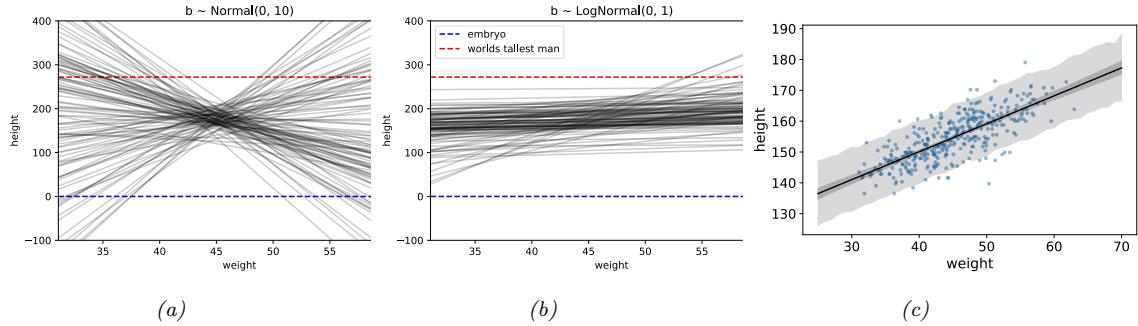
Figure 15.1: Linear regression for predicting height given weight, ^{y ↑ N} (^{φ + β}x, ^ω2). (a) Prior predictive samples using a Gaussian prior for β. (b) Prior predictive samples using a log-Gaussian prior for β. (c) Posterior predictive samples using the log-Gaussian prior. The inner shaded band is the 95% credible interval for µ, representing epistemic uncertainty. The outer shaded band is the 95% credible interval for the observations y, which also adds data uncertainty due to ω. Adapted from Figures 4.5 and 4.10 of [McE20]. Generated by linreg\_height\_weight.ipynb.

With this prior, the posterior becomes

\[p(\mathbf{w}, \sigma^2 | g, \mathcal{D}) = \text{NIG}(\mathbf{w}, \sigma^2 | \mathbf{w}\_N, \mathbf{V}\_N, a\_N, b\_N) \tag{15.78}\]

\[\mathbf{V}\_N = \frac{g}{g+1} (\mathbf{X}^T \mathbf{X})^{-1} \tag{15.79}\]

\[ \hat{w}\_N = \frac{g}{g+1} \hat{w}\_{mle} \tag{15.80} \]

\[a\_N = N/2\tag{15.81}\]

\[b\_N = \frac{s^2}{2} + \frac{1}{2(g+1)}\hat{w}\_{mle}^T \mathbf{X}^T \mathbf{X} \hat{w}\_{mle} \tag{15.82}\]

Various approaches have been proposed for setting g, including cross validation, empirical Bayes [Min00a; GF00], hierarchical Bayes [Lia+08], etc.

15.2.4 Informative priors

In many problems, it is possible to use domain knowledge to come up with plausible priors. As an example, we consider the problem of predicting the height of a person given their weight. We will use a dataset collected from Kalahari foragers by the anthropologist Nancy Howell (this example is from [McE20, p93]).

Let xⁱ be the weight (in kg) and yⁱ be height (in cm) of the i’th person, and let x be the mean of the inputs. The observation model is given by

\[y\_i \sim \mathcal{N}(\mu\_i, \sigma) \tag{15.83}\]

\[ \mu\_i = \alpha + \beta (x\_i - \overline{x}) \tag{15.84} \]

We see that the intercept ϱ is the predicted output if xⁱ = x, and the slope ↼ is the predicted change in height per unit change in weight above or below the average weight.

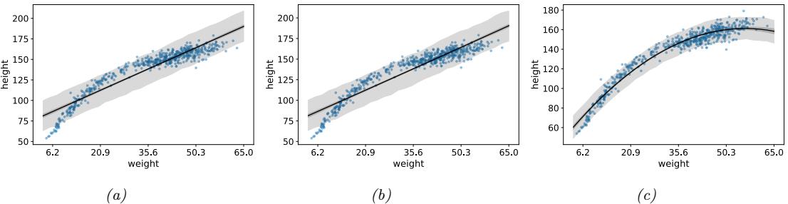
Figure 15.2: Linear regression for predicting height given weight for the full dataset (including children) using polynomial regression. (a) Posterior fit for linear model with log-Gaussian prior for β1. (b) Posterior fit for quadratic model with log-Gaussian prior for β2. (c) Posterior fit for quadratic model with Gaussian prior for β2. Adapted from Figure 4.11 of [McE20]. Generated by linreg\_height\_weight.ipynb.

The question is: what priors should we use? To be truly Bayesian, we should set these before looking at the data. A sensible prior for ϱ is the height of a “typical person”, with some spread. We use ϱ ↔︎ N (178, 20), since the author of the book from which this example is taken is 178cm. By using a standard deviation of 20, the prior puts 95% probability on the broad range of 178 ± 40.

What about the prior for ↼? It is tempting to use a vague prior, or weak prior, such as ↼ ↔︎ N (0, 10), which is similar to a flat (uniform) prior, but more concentrated at 0 (a form of mild regularization). To see if this is reasonable, we can compute samples from the prior predictive distribution, i.e., we sample (ϱs, ↼s) ↔︎ p(ϱ)p(↼), and then plot ϱsx + ↼^s for a range of x values, for di!erent samples s =1: S. The results are shown in Figure 15.1a. We see that this is not a very sensible prior. For example, we see that it suggests that it is just as likely for the height to decrease with weight as increase with weight, which is not plausible. In addition, it predicts heights which are larger than the world’s tallest person (272 cm) and smaller than the world’s shortest person (an embryo, of size 0).

We can encode the monotonically increasing relationship between weight and height by restricting ↼ to be positive. An easy way to do this is to use a log-normal or log-Gaussian prior. (If ↼˜ = log(↼) is Gaussian, then ^eβ˜ must be positive.) Specifically, we will assume ↼ ^↔︎ LN (0, 1). Samples from this prior are shown in Figure 15.1b. This is much more reasonable.

Finally we must choose a prior over ς. In [McE20] they use ς ↔︎ Unif(0, 50). This ensures that ς is positive, and that the prior predictive distribution for the output is within 100cm of the average height. However, it is usually easier to specify the expected value for ς than an upper bound. To do this, we can use ς ↔︎ Expon(⇀), where ⇀ is the rate. We then set E [ς] = 1/⇀ to the value of the standard deviation that we expect. For example, we can use the empirical standard deviation of the data.

Since these priors are no longer conjugate, we cannot compute the posterior in closed form. However, we can use a variety of approximate inference methods. In this simple example, it su”ces to use a quadratic (Laplace) approximation (see Section 7.4.3). The results are shown in Figure 15.1c, and look sensible.

So far, we have only considered a subset of the data, corresponding to adults over the age of 18. If we include children, we find that the mapping from weight to height is nonlinear. This is illustrated

in Figure 15.2a. We can fix this problem by using polynomial regression. For example, consider a quadratic expansion of the standardized features xi:

\[ \mu\_i = \alpha + \beta\_1 x\_i + \beta\_2 x\_i^2 \tag{15.85} \]

If we use a log-Gaussian prior for ↼2, we find that the model is too constrained, and it underfits. This is illustrated in Figure 15.2b. The reason is that we need to use an inverted quadratic with a negative coe”cient, but since this is disallowed by the prior, the model ends up not using this degree of freedom (we find E [↼2|D] ↓ 0.08). If we use a Gaussian prior on ↼2, we avoid this problem, illustrated in Figure 15.2c.

This example shows that it can be useful to think about the functional form of the mapping from inputs to outputs in order to specify sensible priors.

15.2.5 Spike and slab prior

It is often useful to be able to select a subset of the input features when performing prediction, either to reduce overfitting, or to improve interpretability of the model. This can be achieved if we ensure that the weight vector w is sparse (i.e., has many zero elements), since if w^d = 0, then x^d plays no role in the inner product w^Tx.

The canonical way to achieve sparsity when using Bayesian inference is to use a spike-and-slab (SS) prior [MB88], which has the form of a 2 component mixture model, with one component being a “spike” at 0, and the other being a uniform “slab” between →a and a:

\[p(\mathbf{w}) = \prod\_{d=1}^{D} (1 - \pi)\delta(w\_d) + \pi \text{Unif}(w\_d|-a, a) \tag{15.86}\]

where ϖ is the prior probability that each coe”cient is non-zero. The corresponding log prior on the coe”cients is thus

\[\log p(\mathbf{w}) = ||\mathbf{w}||\_0 \log(1 - \pi) + (D - ||\mathbf{w}||\_0) \log \pi = -\lambda ||\mathbf{w}||\_0 + \text{const} \tag{15.87}\]

where ⇀ = log ⇀ ¹↓⇀ controls the sparsity of the model, and ||w||^{0 =} &^{D d}=1 I(w^d ′= 0) is the ε⁰ norm of the weights. Thus MAP estimation with a spike and slab prior is equivalent ε⁰ regularization; this penalizes the number of non-zero coe”cients. Interestingly, posterior samples will also be sparse.

By contrast, consider using a Laplace prior. The lasso estimator uses MAP estimation, which results in a sparse estimate. However, posterior samples are not sparse. Interestingly, [EY09] show theoretically (and [SPZ09] confirm experimentally) that using the posterior mean with a spike-andslab prior also results in better prediction accuracy than using the posterior mode with a Laplace prior.

In practice, we often approximate the uniform slab with a broad Gaussian distribution,

\[p(\mathbf{w}) = \prod\_{d} (1 - \pi)\delta(w\_d) + \pi \mathcal{N}(w\_d | 0, \sigma\_w^2) \tag{15.88}\]

As ς^{2 w} ↖ ⇓, the second term approaches a uniform distribution over [→⇓, +⇓]. We can implement the mixture model by associating a binary random variable, s^d ↔︎ Ber(ϖ), with each coe”cient, to indicate if the coe”cient is “on” or “o!”.

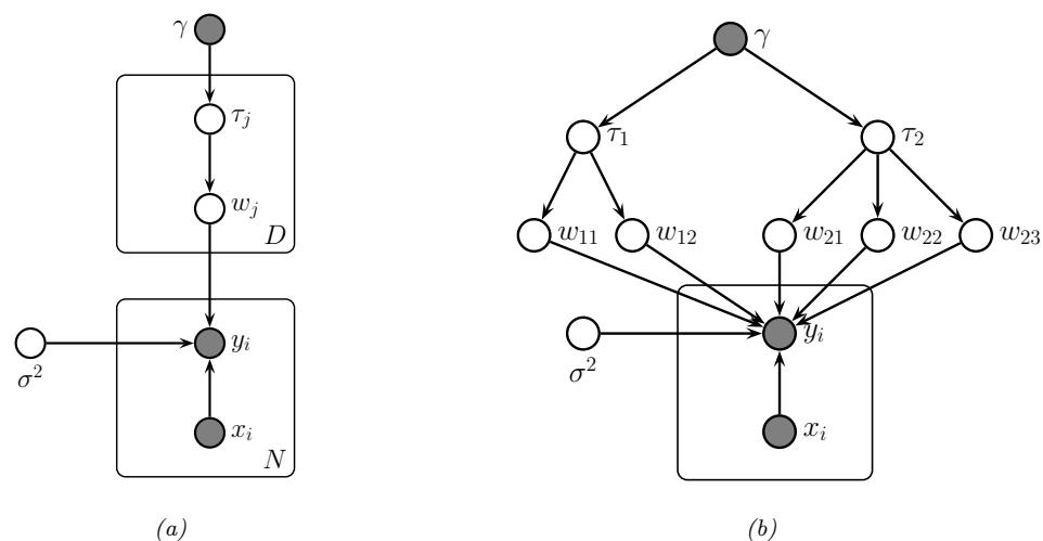
Figure 15.3: (a) Representing lasso using a Gaussian scale mixture prior. (b) Graphical model for group lasso with 2 groups, the first has size G¹ = 2, the second has size G² = 3.

Unfortunately, MAP estimation (not to mention full Bayesian inference) with such discrete mixture priors is computationally di”cult. Various approximate inference methods have been proposed, including greedy search (see e.g., [SPZ09]) or MCMC (see e.g., [HS09]).

15.2.6 Laplace prior (Bayesian lasso)

A computationally cheap way to achieve sparsity is to perform MAP estimation with a Laplace prior by minimizing the penalized negative log likelihood:

\[\text{PNLL}(\mathbf{w}) = -\log p(\mathcal{D}|\mathbf{w}) - \log p(\mathbf{w}|\lambda) = ||\mathbf{X}\mathbf{w} - \mathbf{y}||\_2^2 + \lambda ||\mathbf{w}||\_1 + \text{const} \tag{15.89}\]

where ||w||¹ ↭ &^{D d}=1 |wd| is the ε¹ norm of w. This method is called lasso, which stands for “least absolute shrinkage and selection operator” [Tib96]. See Section 11.4 of the prequel to this book, [Mur22], for details.

In this section, we discuss posterior inference with this prior; this is known as the Bayesian lasso [PC08]. In particular, we assume the following prior:

\[p(w|\sigma^2) = \prod\_j \frac{\gamma}{2\sqrt{\sigma^2}} e^{-\gamma|w\_j|/\sqrt{\sigma^2}} \tag{15.90}\]

where ^{▷ ↑ ▷}. (Note that conditioning the prior on ^ς2 is important to ensure that the full posterior is unimodal.)

To simplify inference, we will represent the Laplace prior as a Gaussian scale mixture, which we discussed in Section 28.2.3.2. In particular, one can show that the Laplace distribution is an infinite

weighted sum of Gaussians, where the precision comes from a gamma distribution:

\[\text{Laplace}(w|0,\gamma) = \int \mathcal{N}(w|0,\tau^2) \text{Ga}(\tau^2|1,\frac{\gamma^2}{2}) d\tau^2 \tag{15.91}\]

We can therefore represent the Bayesian lasso model as a hierarchical latent variable model, as shown in Figure 15.3a. The corresponding joint distribution has the following form:

\[p(\mathbf{y}, \mathbf{w}, \tau, \sigma^2 | \mathbf{X}) = \mathcal{N}(\mathbf{y} | \mathbf{X} \mathbf{w}, \sigma^2 \mathbf{I}\_N) \left[ \prod\_j \mathcal{N}(w\_j | 0, \sigma^2 \tau\_j^2) \text{Ga}(\tau\_j^2 | 1, \gamma^2 / 2) \right] p(\sigma^2) \tag{15.92}\]

We can also create a GSM to match the group lasso prior, which sets multiple coe”cients to zero at the same time:

\[\mathbf{w}\_g | \sigma^2, \tau\_g^2 \sim \mathcal{N}(\mathbf{0}, \sigma^2 \tau\_g^2 \mathbf{I}\_{d\_g}) \tag{15.93}\]

\[ \tau\_g^2 \sim \text{Ga}(\frac{d\_g+1}{2}, \frac{\gamma^2}{2})\tag{15.94} \]

where d^g is the size of group g. So we see that there is one variance term per group, each of which comes from a gamma prior, whose shape parameter depends on the group size, and whose rate parameter is controlled by ▷.

Figure 15.3b gives an example, where we have 2 groups, one of size 2 and one of size 3. This picture makes it clearer why there should be a grouping e!ect. For example, suppose w1,¹ is small; then τ ² 1 will be estimated to be small, which will force w1,² to be small, due to shrinkage (cf. Section 3.6). Conversely, suppose w1,¹ is large; then τ ^{2 1} will be estimated to be large, which will allow w1,² to be become large as well.

Given these hierachical models, we can easily derive a Gibbs sampling algorithm (Section 12.3) to sample from the posterior (see e.g., [PC08]). Unfortunately, these posterior samples are not sparse, even though the MAP estimate is sparse. This is because the prior puts infinitessimal probability on the event that each coe”cient is zero.

15.2.7 Horseshoe prior

The Laplace prior is not suitable for sparse Bayesian models, because posterior samples are not sparse. The spike and slab prior does not have this problem but is often too slow to use (although see [BRG20]). Fortunately, it is possible to devise continuous priors (without discrete latent variables) that are both sparse and computationally e”cient. One popular prior of this type is the horseshoe prior [CPS10], so-named because of the shape of its density function.

In the horseshoe prior, instead of using a Laplace prior for each weight, we use the following Gaussian scale mixture:

\[w\_j \sim \mathcal{N}(0, \gamma\_j^2 \tau^2) \tag{15.95}\]

\[ \gamma\_j \sim \mathcal{C}\_+ (0, 1) \tag{15.96} \]

\[ \tau^2 \sim \mathcal{C}\_+(0, 1) \tag{15.97} \]

where ^C+(0, 1) is the half-Cauchy distribution (Section 2.2.2.4), ^▷j is a local shrinkage factor, and ^{τ 2} is a global shrinkage factor. The Cauchy distribution has very fat tails, so w^j is likely to be either 0 or very far from 0, which emulates the spike and slab prior, but in a continuous way. For more details, see e.g., [Bha+19].

15.2.8 Automatic relevancy determination

An alternative to using posterior inference with a sparsity promoting prior is to use posterior inference with a Gaussian prior, w^j ↔︎ N (0, 1/ϱ^j ), but where we use empirical Bayes to optimize the precisions ^ϱj . That is, we first compute ↼^{ˆ =} argmax↽ ^p(y|X, ↼), and then compute ^{wˆ =} argmax^{w N} (w|0, ↼^{ˆ ↓}1). Perhaps surprisingly, we will see that this results in a sparse estimate, for reasons we explain in Section 15.2.8.2.

This technique is known as sparse Bayesian learning [Tip01] or automatic relevancy determination (ARD) [Mac95; Nea96]. It has also been called NUV estimation, which stands for “normal prior with unknown variance” [Loe+16]. It was originally developed for neural networks (where sparsity is applied to the first layer weights), but here we apply it to linear models.

15.2.8.1 ARD for linear models

In this section, we explain ARD in more detail, by applying it to linear regression. The likelihood is ^p(y|x, ^w, ↼) = ^N (y|w^Tx, 1/↼), where ↼ = 1/ς². The prior is ^p(w) = ^N (w|0, A↓¹), where A = diag(↼). The marginal likelihood can be computed analytically (using Equation (2.129)) as follows:

\[p(\mathbf{y}|\mathbf{X},\alpha,\beta) = \int \mathcal{N}(\mathbf{y}|\mathbf{X}w,(1/\beta)\mathbf{I}\_N)\mathcal{N}(w|\mathbf{0},\mathbf{A}^{-1})dw\tag{15.98}\]

\[\mathbf{y} = \mathcal{N}(y|\mathbf{0}, \beta^{-1}\mathbf{I}\_N + \mathbf{X}\mathbf{A}^{-1}\mathbf{X}^\top) \tag{15.99}\]

\[=\mathcal{N}(y|\mathbf{0}, \mathbf{C}\_{\alpha})\tag{15.100}\]

where C↽ ↭ ↼↓1I^N + XA↓1XT. This is very similar to the marginal likelihood under the spike-andslab prior (Section 15.2.5), which is given by

\[p(\boldsymbol{y}|\mathbf{X}, \mathbf{s}, \sigma\_w^2, \sigma\_y^2) = \int \mathcal{N}(\boldsymbol{y}|\mathbf{X}\_{\mathbf{s}} w\_{\mathbf{s}}, \sigma\_y^2 \mathbf{I}) \mathcal{N}(w\_{\mathbf{s}}|\mathbf{0}\_{\mathbf{s}}, \sigma\_w^2 \mathbf{I}) dw\_{\mathbf{s}} = \mathcal{N}(\boldsymbol{y}|\mathbf{0}, \mathbf{C}\_{\mathbf{s}}) \tag{15.101}\]

where C^s = ς^{2 y}I^N + ς² wXsX^{T s}. (Here X^s refers to the design matrix where we select only the columns of X where s^d = 1.) The di!erence is that we have replaced the binary s^j ↗ {0, 1} variables with continuous ^ϱj ↗ ^R+, which makes the optimization problem easier.

The objective is the log marginal likelihood, given by

\[\ell(\alpha, \beta) = -2 \log p(\mathbf{y} | \mathbf{X}, \alpha, \beta) = \log |\mathbf{C}\_{\alpha}| + \mathbf{y}^{\mathsf{T}} \mathbf{C}\_{\alpha}^{-1} \mathbf{y} \tag{15.102}\]

There are various algorithms for optimizing ε(↼, ↼), some of which we discuss in Section 15.2.8.3.

ARD can be used as an alternative to ε¹ regularization. Although the ARD objective is not convex, it tends to give much sparser results [WW12]. In addition, it can be shown [WRN10] that the ARD objective has many fewer local optima than the ε0-regularized objective, and hence is much easier to optimize.

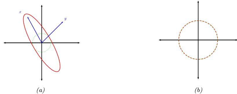
Figure 15.4: Illustration of why ARD results in sparsity. The vector of inputs x does not point towards the vector of outputs y, so the feature should be removed. (a) For finite φ, the probability density is spread in directions away from y. (b) When φ = ↖, the probability density at y is maximized. Adapted from Figure 8 of [Tip01].

15.2.8.2 Why does ARD result in a sparse solution?

Once we have estimated ↼ and ↼, we can compute the posterior over the parameters using Bayes’ rule for Gaussians, to get ^p(w|D, ↼^ˆ , ↼ˆ) = ^N (w^| ↫w, ↫ !), where ↫ !^↓1 = ↼ˆX^TX + A and ↫w= ↼ˆ ↫ ! X^Ty. If we have ^ϱˆ^d ↓ ⇓, then ↫wd^{↓ 0}, so the solution vector will be sparse.

We now give an intuitive argument, based on [Tip01], about when such a sparse solution may be optimal. We shall assume ↼ = 1/ς² is fixed for simplicity. Consider a 1d linear regression with 2 training examples, so X = x = (x1, x2), and y = (y1, y2). We can plot x and y as vectors in the plane, as shown in Figure 15.4. Suppose the feature is irrelevant for predicting the response, so x points in a nearly orthogonal direction to y. Let us see what happens to the marginal likelihood as we change ^ϱ. The marginal likelihood is given by ^p(y|x, ^ϱ, ↼) = ^N (y|0, ^C↼), where ^C↼ ^{= 1 β} I + ¹ ↼ xx^T. If ϱ is finite, the posterior will be elongated along the direction of x, as in Figure 15.4(a). However, if ^{ϱ =} ⇓, we have ^C↼ ^{= 1 β} I, which is spherical, as in Figure 15.4(b). If |C↼| is held constant, the latter assigns higher probability density to the observed response vector y, so this is the preferred solution. In other words, the marginal likelihood “punishes” solutions where ϱ^d is small but X:,d is irrelevant, since these waste probability mass. It is more parsimonious (from the point of view of Bayesian Occam’s razor) to eliminate redundant dimensions.

Another way to understand the sparsity properties of ARD is as approximate inference in a hierarchical Bayesian model [BT00]. In particular, suppose we put a conjugate prior on each precision, ϱ^d ↔︎ Ga(a, b), and on the observation precision, ↼ ↔︎ Ga(c, d). Since exact inference with a Student prior is intractable, we can use variational Bayes (Section 10.3.3), with a factored posterior approximation of the form

\[q(w, \alpha) = q(w)q(\alpha) \approx \mathcal{N}(w|\mu, \Sigma) \prod\_{d} \text{Ga}(\alpha\_d | \, \hat{a}\_d, \hat{b}\_d) \tag{15.103}\]

ARD approximates q(↼) by a point estimate. However, in VB, we integrate out ↼; the resulting

posterior marginal q(w) on the weights is given by

\[p(\boldsymbol{w}|\mathcal{D}) = \int \mathcal{N}(\boldsymbol{w}|\mathbf{0}, \text{diag}(\boldsymbol{\alpha})^{-1}) \prod\_{d} \text{Ga}(\alpha\_d | \, \partial\_d, \widehat{b}) d\boldsymbol{\alpha} \tag{15.104}\]

This is a Gaussian scale mixture, and can be shown to be the same as a multivariate Student distribution (see Section 28.2.3.1), with non-diagonal covariance. Note that the Student has a large spike at 0, which intuitively explains why the posterior mean (which, for a Student distribution, is equal to the posterior mode) is sparse.

Finally, we can also view ARD as a MAP estimation problem with a non-factorial prior [WN07]. Intuitively, the dependence between the w^j parameters arises, despite the use of a diagonal Gaussian prior, because the prior precision ϱ^j is estimated based after marginalizing out all w, and hence depends on all the features. Interestingly, [WRN10] prove that MAP estimation with non-factorial priors is strictly better than MAP estimation with any possible factorial prior in the following sense: the non-factorial objective always has fewer local minima than factorial objectives, while still satisfying the property that the global optimum of the non-factorial objective corresponds to the global optimum of the ε⁰ objective — a property that ε¹ regularization, which has no local minima, does not enjoy.

15.2.8.3 Algorithms for ARD

There are various algorithms for optimizing ε(↼, ↼). One approach is to use EM, in which we compute p(w|D, ↼) in the E step and then maximize ↼ in the M step. In variational Bayes, we infer both w and ↼ (see [Dru08] for details). In [WN10], they present a method based on iteratively reweighted ε¹ estimation.

Recently, [HXW17] showed that the nested iterative computations performed these methods can emulated by a recurrent neural network (Section 16.3.4). Furthermore, by training this model, it is possible to achieve much faster convergence than manually designed optimization algorithms.

15.2.8.4 Relevance vector machines

Suppose we create a linear regression model of the form ^p(y|x; ^ω) = ^N (y|w^Tε(x), ^ς2), where ε(x)=[K(x, x1),…, K(x, x^N )], where K() is a kernel function (Section 18.2) and x1,…, x^N are the N training points. This is called kernel basis function expansion, and transforms the input from ^x ↗ ^X to ^ε(x) ↗ ^RN . Obviously this model has ^O(N) parameters, and hence is nonparametric. However, we can use ARD to select a small subset of the exemplars. This technique is called the relevance vector machine (RVM) [Tip01; TF03].

15.2.9 Multivariate linear regression

This section is written by Xinglong Li.

In this section, we consider the multivariate linear regression model, which has the form

\[\mathbf{Y} = \mathbf{W}\mathbf{X} + \mathbf{E} \tag{15.105}\]

where ^W ↗ ^RNy⇑N^x is the matrix of regression coe”cient, ^X ↗ ^RNx⇑^N is the matrix of input features (with each row being an input variable and each column being an observation), Y ↗ ^RNy⇑^N is the

matrix of responses (with each row being an output variable and each column being an observation), and E = [e1, ··· , e^N ] is the matrix of residual errors, where eⁱ iid ↔︎ N (0, !). It can be seen from the definition that given !, W and X, columns of Y are independently random variables following multivariate normal distributions. So the likelihood of the observation is

\[p(\mathbf{Y}|\mathbf{W}, \mathbf{X}, \boldsymbol{\Sigma}) = \frac{1}{(2\pi)^{N\_y \times N} |\boldsymbol{\Sigma}|^{N/2}} \exp\left(\sum\_{i=1}^{N} -\frac{1}{2} (y\_i - \mathbf{W}\boldsymbol{x}\_i)^\mathsf{T} \boldsymbol{\Sigma}^{-1} (y\_i - \mathbf{W}\boldsymbol{x}\_i)\right) \tag{15.106}\]

\[=\frac{1}{(2\pi)^{N\_y \times N} |\mathbf{E}|^{N/2}} \exp\left(-\frac{1}{2} \text{tr}\left( (\mathbf{Y} - \mathbf{W}\mathbf{X})^\mathsf{T} \boldsymbol{\Sigma}^{-1} (\mathbf{Y} - \mathbf{W}\mathbf{X}) \right)\right) \tag{15.107}\]

\[=\mathcal{MN}(\mathbf{Y}|\mathbf{WX}, \boldsymbol{\Sigma}, \mathbf{I}\_{N \times N}),\tag{15.108}\]

The conjugate prior for this is the matrix normal inverse Wishart distribution,

\[\mathbf{W}, \boldsymbol{\Sigma} \sim \text{MNIW}(\mathbf{M}\_0, \mathbf{V}\_0, \boldsymbol{\nu}\_0, \boldsymbol{\Psi}\_0) \tag{15.109}\]

where the MNIW is defined by

\[\mathbf{W}|\boldsymbol{\Sigma} \sim \mathcal{M}\boldsymbol{\mathbb{V}}(\mathbf{M}\_0, \boldsymbol{\Sigma}\_0, \mathbf{V}\_0) \tag{15.110}\]

\[ \Sigma \sim \text{IW}(\nu\_0, \Psi\_0), \tag{15.111} \]

where ^V0 ↗ ^RNx⇑N^x ++ , $⁰ ↗ ^RNy⇑N^y ++ and 4⁰ > N^x → 1 is the degree of freedom of the inverse Wishart distribution.

The posterior distribution of {W, !} still follows a matrix normal inverse Wishart distribution. We follow the derivation in [Fox09, App.F]. Tthe density of the joint distribution is

\[p(\mathbf{Y}, \mathbf{W}, \boldsymbol{\Sigma}) \propto |\boldsymbol{\Sigma}|^{-(\nu\_0 + N\_y + 1 + N\_x + N)/2} \times \exp\left\{-\frac{1}{2} \text{tr}(\boldsymbol{\Omega}\_0)\right\} \tag{15.112}\]

\[\boldsymbol{\Omega}\_0 \triangleq \boldsymbol{\Psi}\_0 \boldsymbol{\Sigma}^{-1} + (\mathbf{Y} - \mathbf{W}\mathbf{X})^\mathsf{T} \mathbf{S}^{-1} (\mathbf{Y} - \mathbf{W}\mathbf{X}) + (\mathbf{W} - \mathbf{M}\_0)^\mathsf{T} \mathbf{S}^{-1} (\mathbf{W} - \mathbf{M}\_0) \mathbf{V}\_0 \tag{15.113}\]

We first aggregate items including W in the exponent so that it takes the form of a matrix normal distribution. This is similar to the “completing the square” technique that we used in deriving the conjugate posterior for multivariate normal distributions in Section 3.4.4.3. Specifically,

\[\operatorname{tr}\left[\left(\mathbf{Y} - \mathbf{W}\mathbf{X}\right)^{\mathsf{T}}\boldsymbol{\Sigma}^{-1}(\mathbf{Y} - \mathbf{W}\mathbf{X}) + \left(\mathbf{W} - \mathbf{M}\_0\right)^{\mathsf{T}}\boldsymbol{\Sigma}^{-1}(\mathbf{W} - \mathbf{M}\_0)\mathbf{V}\_0\right] \tag{15.114}\]

\[=\text{tr}\left(\boldsymbol{\Sigma}^{-1}[(\mathbf{Y}-\mathbf{WX})(\mathbf{Y}-\mathbf{WX})^{\mathsf{T}}+(\mathbf{W}-\mathbf{M}\_{0})\mathbf{V}\_{0}(\mathbf{W}-\mathbf{M}\_{0})^{\mathsf{T}}]\right)\tag{15.115}\]

\[=\text{tr}\left(\boldsymbol{\Sigma}^{-1}[\mathbf{W}\mathbf{S}\_{xx}\mathbf{W}^{\mathsf{T}} - 2\mathbf{S}\_{yx}\mathbf{W}^{\mathsf{T}} + \mathbf{S}\_{yy}]\right)\tag{15.116}\]

\[=\text{tr}\left(\boldsymbol{\Sigma}^{-1}[(\mathbf{W}-\mathbf{S}\_{yx}\mathbf{S}\_{xx}^{-1})\mathbf{S}\_{xx}(\mathbf{W}-\mathbf{S}\_{yx}\mathbf{S}\_{xx}^{-1})^{\mathsf{T}}+\mathbf{S}\_{y|x}]\right).\tag{15.117}\]

where

\[\mathbf{S}\_{xx} = \mathbf{X}\mathbf{X}^{\mathsf{T}} + \mathbf{V}\_{0},\tag{15.18}\]

\[\mathbf{S}\_{yx} = \mathbf{Y}\mathbf{X}^{\mathsf{T}} + \mathbf{M}\_{0}\mathbf{V}\_{0},\tag{15.118}\]

\[\mathbf{S}\_{yy} = \mathbf{Y}\mathbf{Y}^{\mathsf{T}} + \mathbf{M}\_0 \mathbf{V}\_0 \mathbf{M}\_0^{\mathsf{T}},\tag{15.19}\]

\[\mathbf{S}\_{y|x} = \mathbf{S}\_{yy} - \mathbf{S}\_{yx} \mathbf{S}\_{xx}^{-1} \mathbf{S}\_{yx}^{\mathsf{T}}.\tag{15.119}\]

Therefore, it can be see from Equation (15.117) that given !, W follows a matrix normal distribution

\[\mathbf{W}|\boldsymbol{\Sigma}, \mathbf{X}, \mathbf{Y} \sim \mathcal{M}\mathcal{N}(\mathbf{S}\_{yx}\mathbf{S}\_{xx}^{-1}, \boldsymbol{\Sigma}, \mathbf{S}\_{xx}).\tag{15.120}\]

Marginalizing out W (which corresponds to removing the terms including W in the exponent in Equation (15.113)), it can be shown that the posterior distribution of ! is an inverse Wishart distribution. In fact, by replacing Equation (15.117) to the corresponding terms in Equation (15.113), it can be seen that the only terms left after integrating out ^W are !^↓1$ and !^↓1S^y|^x, which indicates that the scale matrix of the posterior inverse Wishart distribution is $⁰ + S^y|^x.

In conclusion, the joint posterior distribution of {W, !} given the observation is

\[\mathbf{W}, \boldsymbol{\Sigma} | \mathbf{X}, \mathbf{Y} \sim \text{MNN}(\mathbf{M}\_1, \mathbf{V}\_1, \nu\_1, \Psi\_1) \tag{15.121}\]

\[\mathbf{M}\_1 = \mathbf{S}\_{yx}\mathbf{S}\_{xx}^{-1} \tag{15.122}\]

\[\mathbf{V}\_1 = \mathbf{S}\_{xx} \tag{15.123}\]

\[ \nu\_1 = N + \nu\_0 \tag{15.124} \]

\[ \Psi\_1 = \Psi\_0 + \mathbf{S}\_{y|x} \tag{15.125} \]

The MAP estimate of W and ! are the mode of the posterior matrix normal inverse Wishart distribution. To derive this, notice that W only appears in the matrix normal density function in the posterior, so the matrix W maximizing the posterior density of {W, !} is the matrix W that maximizes the matrix normal posterior of ^W. So the MAP estimate of ^W is ^Wˆ ^{= M1 = S}yxS↓¹ xx , and this holds for any value of !. By plugging ^{W = Wˆ} into the joint posterior of {W, !}, and taking derivatives over !, it can be seen that the matrix maximizing the density is (4¹ + N^y + N^x + 1)↓¹$1. Since $¹ is positive definite, it is the MAP estimate of !.

In conclusion, the MAP estimate of {W, !} are

\[ \hat{\mathbf{W}} = \mathbf{S}\_{yx}\mathbf{S}\_{xx}^{-1} \tag{15.126} \]

\[\hat{\Delta} = \frac{1}{\nu\_1 + N\_y + N\_x + 1} (\Psi\_0 + \mathbf{S}\_{y|x}) \tag{15.127}\]

15.3 Logistic regression

Logistic regression is a very widely used discriminative classification model that maps input vectors ^x ↗ ^RD to a distribution over class labels, ^y ↗ {1,…,C}. If ^C = 2, this is known as binary logistic regression, and if C > 2, it is known as multinomial logistic regression, or alternatively, multiclass logistic regression.

15.3.1 Binary logistic regression

In the binary case, where y ↗ {0, 1}, the model has the following form

\[p(y|x; \theta) = \text{Ber}(y|\sigma(w^\top x + b))\tag{15.128}\]

where w are the weights, b is the bias (o!set), and ς is the sigmoid or logistic function, defined by

\[ \sigma(a) \stackrel{\Delta}{=} \frac{1}{1 + e^{-a}} \tag{15.129} \]

Let ^ηn = ^wTxⁿ + ^b be the logits for example ⁿ, and ^µn = ^ς(ηn) = ^p(^y = 1|xn) be the mean of the output. Then we can write the log likelihood as the negative cross entropy:

\[\log p(\mathcal{D}|\boldsymbol{\theta}) = \log \prod\_{n=1}^{N} \mu\_n^{y\_n} (1 - \mu\_n)^{1 - y\_n} = \sum\_{n=1}^{N} y\_n \log \mu\_n + (1 - y\_n) \log(1 - \mu\_n) \tag{15.130}\]

We can expand this equation into a more explicit form (that is commonly seen in implementations) by performing some simple algebra. First note that

\[\mu\_n = \frac{1}{1 + e^{-\eta\_n}} = \frac{e^{\eta\_n}}{1 + e^{\eta\_n}}, \ 1 - \mu\_n = 1 - \frac{e^{\eta\_n}}{1 + e^{\eta\_n}} = \frac{1}{1 + e^{\eta\_n}} \tag{15.131}\]

Hence

\[\log p(\mathcal{D}|\boldsymbol{\theta}) = \sum\_{n=1}^{N} y\_n [\log e^{\eta\_n} - \log(1 + e^{\eta\_n})] + (1 - y\_n)[\log 1 - \log(1 + e^{\eta\_n})] \tag{15.132}\]

\[\hat{y}\_n = \sum\_{n=1}^{N} y\_n [\eta\_n - \log(1 + e^{\eta\_n})] + (1 - y\_n)[-\log(1 + e^{\eta\_n})] \tag{15.133}\]

\[\hat{\eta} = \sum\_{n=1}^{N} y\_n \eta\_n - \sum\_{n=1}^{N} \log(1 + e^{\eta\_n}) \tag{15.134}\]

Note that the log(1 + e^a) function is often implemented using np.log1p(np.exp(a)).

15.3.2 Multinomial logistic regression

Multinomial logistic regression is a discriminative classification model of the following form:

\[p(y|x; \theta) = \text{Cat}(y|\text{softmax}(\mathbf{W}x + \mathbf{b})) \tag{15.135}\]

where ^x ↗ ^RD is the input vector, ^y ↗ {1,…,C} is the class label, ^W is a ^{C ⇔ D} weight matrix, ^b is C-dimensional bias vector, and softmax() is the softmax function, defined as

\[\text{softmax}(\mathbf{a}) \triangleq \left[ \frac{e^{a\_1}}{\sum\_{c'=1}^{C} e^{a\_{c'}}}, \dots, \frac{e^{a\_C}}{\sum\_{c'=1}^{C} e^{a\_{c'}}} \right] \tag{15.136}\]

If we define the logits as ϱⁿ = Wxⁿ + b, the probabilities as µⁿ = softmax(ϱn), and let yⁿ be the one-hot encoding of the label yn, then the log likelihood can be written as the negative cross entropy:

\[\log p(\mathcal{D}|\boldsymbol{\theta}) = \log \prod\_{n=1}^{N} \prod\_{c=1}^{C} \mu\_{nc}^{y\_{nc}} = \sum\_{n=1}^{N} \sum\_{c=1}^{C} y\_{nc} \log \mu\_{nc} \tag{15.137}\]

15.3.3 Dealing with class imbalance and the long tail

In many problems, some classes are much rarer than others; this problem is called class imbalance. In such a setting, standard maximum likelihood training may not work well, since it designed to minimize (a bound on) the 0-1 loss, which can be dominated by the most frequent classes. A natural alternative is to consider the balanced error rate, which computes the average of the per-class error rates of classifier f:

\[\text{BER}(f) = \frac{1}{C} \sum\_{y=1}^{C} p\_{\pi|y}^{\*} \left( y \notin \text{argmax}\_{y' \in \mathcal{Y}} f\_{y'}(x) \right) \tag{15.138}\]

where p^→ is the true distribution. The classifier that optimizes this loss, f ^→, must satisfy

\[\underset{y \in \mathcal{Y}}{\operatorname{argmax}} \, f\_y^\*(\boldsymbol{x}) = \underset{y \in \mathcal{Y}}{\operatorname{argmax}} \, p\_{\text{bal}}^\*(y|\boldsymbol{x}) = \underset{y \in \mathcal{Y}}{\operatorname{argmax}} \, p^\*(\boldsymbol{x}|\boldsymbol{y}) \tag{15.139}\]

where p^→ bal(y|x) ^{↑ 1 C} p→(x|y) is the predictor when using balanced classes. Thus to minimize the BER, we should use the class-conditional likelihood, p(x|y), rather than the class posterior, p(y|x).

In [Men+21], they propose a simple scheme called logit adjustment that can achieve this optimal classifier. We assume the model computes logits using fy(x) = w^{T y}ε(x), where ε(x) = x for a GLM. In the post-hoc version, the model is trained in the usual way, and then at prediction time, we use

\[\underset{y \in \mathcal{Y}}{\operatorname{argmax}} \, p(\mathbf{z}|y) = \underset{y \in \mathcal{Y}}{\operatorname{argmax}} \frac{p(y|\mathbf{z})p(\mathbf{z})}{p(y)} = \underset{y \in \mathcal{Y}}{\operatorname{argmax}} \frac{\exp(\mathbf{w}\_y^\mathsf{T}\phi(\mathbf{z}))}{\pi\_y} \tag{15.140}\]

where ϖ^y = p(y) is the empirical label prior. In practice, it is helpful to inroduce a tuning parameter τ > 0 and to use the predictor

\[\hat{f}(\mathbf{x}) = \operatorname\*{argmax}\_{y \in \mathcal{Y}} f\_y(\mathbf{x}) - \tau \log \pi\_y \tag{15.141}\]

Alternatively, we can change the loss function used during training, by using the following logit adjusted softmax cross-entropy loss:

\[\ell(y, f(x)) = -\log \frac{e^{f\_y(x) + \tau \log \pi\_y}}{\sum\_{y'=1}^C e^{f\_{y'}(x) + \tau \log \pi\_{y'}}} \tag{15.142}\]

This is like training with a predictor of the form gy(x) = fy(x) + τ log ϖy, and then at test time using argmax^y fy(x) = argmax^y gy(x) → τ log ϖy, as above.

We can also combine the above loss with a prior on the parameters and perform Bayesian inference, as we discuss below. (The use of a non-standard likelihood can be justifed using the generalized Bayesian inference framework, as discussed in Section 14.1.3.)

15.3.4 Parameter priors

As with linear regression, it is standard to use Gaussian priors for the weights in a logistic regression model. It is natural to set the prior mean to 0, to reflect the fact that the output could either

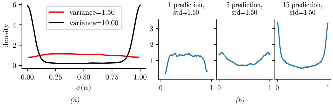
Figure 15.5: (a) Prior on logistic regression output when using N (0, ω) prior for the o!set term, for ω = 10 or ω = 1.5. Adapted from Figure 11.3 of [McE20]. Generated by logreg\_prior\_o!set.ipynb. (b) Distribution over the fraction of 1s we expect to see when using binary logistic regression applied to random binary feature vectors of increasing dimensionality. We use a N (0, 1.5) prior on the regression coe#cients. Adapted from Figure 3 of [Gel+20]. Generated by logreg\_prior.ipynb.

increase or decrease in probability depending on the input. But how do we set the prior variance? It is tempting to use a large value, to approximate a uniform distribution, but this is a bad idea. To see why, consider a binary logistic regression model with just an o!set term and no features:

\[p(y|\theta) = \text{Ber}(y|\sigma(\alpha))\tag{15.143}\]

\[p(\alpha) = \mathcal{N}(\alpha|0, \omega) \tag{15.144}\]

If we set the prior to the large value of 6 = 10, the implied prior for y is an extreme distribution, with most of its density near 0 or 1, as shown in Figure 15.5a. By contrast, if we use the smaller value of 6 = 1.5, we get a flatter distribution, as shown.

If we have input features, the problem gets a little trickier, since the magnitude of the logits will now depend on the number and distribution of the input variables. For example, suppose we generate N random binary vectors xn, each of dimension D, where xnd ↔︎ Ber(p), where p = 0.8. We then compute ^p(yⁿ = 1|xn) = ^ς(⇀^Txn), where ⇀ ^{↔︎ N} (0, ¹.5I). We sample ^S values of ⇀, and for each one, we sample a vector of labels, y1:N,s from the above distribution. We then compute the fraction of positive labels, f^s = ¹ N &^{N n}=1 I(yn,s = 1). We plot the distribution of {fs} as a function of D in Figure 15.5b. We see that the induced prior is initially flat, but eventually becomes skewed towards the extreme values of 0 and 1. To avoid this, we should standardize the inputs, and scale the variance of the prior by 1/ ∝ D. We can also use a heavier tailed distribution, such as a Cauchy or Student [Gel+08; GLM15], instead of the Gaussian prior.

15.3.5 Laplace approximation to the posterior

Unfortunately, we cannot compute the posterior analytically, unlike with linear regression, since there is no corresponding conjugate prior. (This mirrors the case with MLE, where we have a closed form solution for linear regression, but not for logistic regression.) Fortunately, there are a range of approximate inference methods we can use.

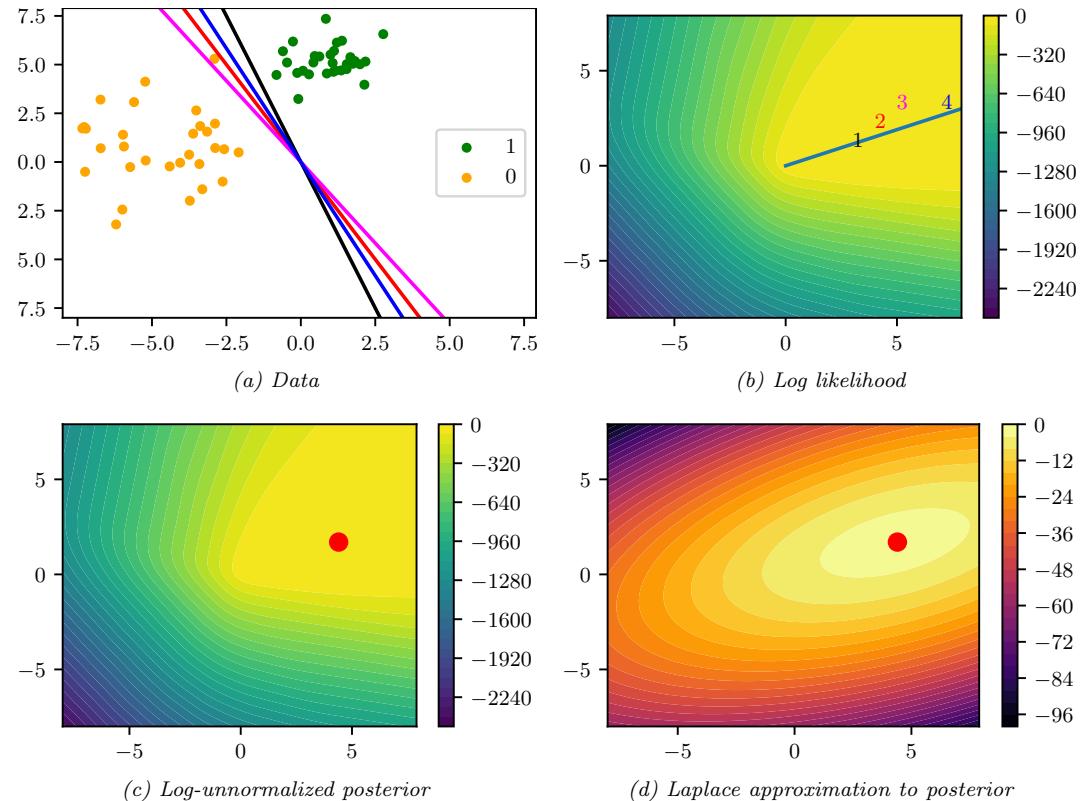
Figure 15.6: (a) Illustration of the data and some decision boundaries. (b) Log-likelihood for a logistic regression model. The line is drawn from the origin in the direction of the MLE (which is at infinity). The numbers correspond to 4 points in parameter space, corresponding to the colored lines in (a). (c) Unnormalized log posterior (assuming vague spherical prior). (d) Laplace approximation to posterior. Adapted from a figure by Mark Girolami. Generated by logreg\_laplace\_demo.ipynb.

In this section, we use the Laplace approximation. As we explain in Section 7.4.3, this approximates the posterior using a Gaussian. The mean of the Gaussian is equal to the MAP estimate wˆ , and the covariance is equal to the inverse Hessian H computed at the MAP estimate, i.e.,

\[p(\boldsymbol{w}|\mathcal{D}) \approx \mathcal{N}(\boldsymbol{w}|\hat{\boldsymbol{w}}, \mathbf{H}^{-1}),\\\hat{\boldsymbol{w}} = \arg\min - \log p(\boldsymbol{w}, \mathcal{D}),\\\mathbf{H} = -\nabla\_{\mathbf{w}}^{2} \log p(\boldsymbol{w}, \mathcal{D})|\_{\hat{\mathbf{w}}} \tag{15.145}\]

We can find the mode using a standard optimization method, and we can then compute the Hessian at the mode analytically or using automatic di!erentiation.

As an example, consider the binary data illustrated in Figure 15.6(a). There are many parameter settings that correspond to lines that perfectly separate the training data; we show 4 example lines. For each decision boundary in Figure 15.6(a), we plot the corresponding parameter vector as point in the log likelihood surface in Figure 15.6(b). These parameters values are w¹ = (3, 1), w² = (4, 2), w³ = (5, 3), and w⁴ = (7, 3). These points all approximately satisfy wi(1)/wi(2) ↓ wˆ mle(1)/wˆ mle(2), and hence are close to the orientation of the maximum likelihood decision boundary. The points are ordered by increasing weight norm (3.16, 4.47, 5.83, and 7.62). The unconstrained MLE has ||w|| = ⇓, so is infinitely far to the top right.

To ensure a unique solution, we use a (spherical) Gaussian prior centered at the origin, ^N (w|0, ^ς2I). The value of ^ς2 controls the strength of the prior. If we set ^ς2 = ⇓, we force the MAP estimate to be w = 0; this will result in maximally uncertain predictions, since all points x will produce a predictive distribution of the form ^p(^y = 1|x)=0.5. If we set ^ς2 = 0, the MAP estimate becomes the MLE, resulting in minimally uncertain predictions. (In particular, all positively labeled points will have p(y = 1|x)=1.0, and all negatively labeled points will have p(y = 1|x)=0.0, since the data is separable.) As a compromise (to make a nice illustration), we pick the value ς² = 100.

Multiplying this prior by the likelihood results in the unnormalized posterior shown in Figure 15.6(c). The MAP estimate is shown by the red dot. The Laplace approximation to this posterior is shown in Figure 15.6(d). We see that it gets the mode correct (by construction), but the shape of the posterior is somewhat distorted. (The southwest-northeast orientation captures uncertainty about the magnitude of w, and the southeast-northwest orientation captures uncertainty about the orientation of the decision boundary.)

15.3.6 Approximating the posterior predictive distribution

Next we need to convert the posterior over the parameters into a posterior over predictions, as follows:

\[p(y|\mathbf{z}, \mathcal{D}) = \int p(y|\mathbf{z}, \mathbf{w}) p(\mathbf{w}|\mathcal{D}) d\mathbf{w} \tag{15.146}\]

The simplest way to evaluate this integral is to use a Monte Carlo approximation. For example, in the case of binary logistic regression, we have

\[p(y=1|\mathbf{x}, \mathcal{D}) \approx \frac{1}{S} \sum\_{s=1}^{S} \sigma(w\_s^{\mathsf{T}} \mathbf{x}) \tag{15.147}\]

where w^s ↔︎ p(w|D) are posterior samples.

However, we can also use deterministic approximations to the integral, which are often faster. Let f^→ = f(x→, w) be the predicted logits, before the sigmoid/softmax layer, given test point x→. If the posterior over the parameters is Gaussian, p(w|D) = N (µ, !), then the predictive distribution over logits is also Gaussian:

\[p(\mathbf{f}\_\*|\mathbf{x}\_\*, \mathcal{D}) = \int \delta(\mathbf{f}\_\* - f(\mathbf{x}\_\*, w)) \mathcal{N}(w|\mathcal{D}) dw = \mathcal{N}(\mathbf{f}\_\*|\boldsymbol{\mu}^\mathsf{T}\boldsymbol{x}\_\*, \boldsymbol{x}\_\*^\mathsf{T}\boldsymbol{\Sigma}\boldsymbol{x}\_\*) \stackrel{\scriptstyle\Delta}{=} \mathcal{N}(\mathbf{f}\_\*|\boldsymbol{\mu}\_\*, \boldsymbol{\Sigma}\_\*) \quad (15.148)\]

In the case of binary logistic regression, we can approximate the sigmoid with the probit function ’ (see Section 15.4), which allows us to solve the integral analytically:

\[p(y\_\*|x\_\*) \approx \int \Phi(f\_\*) \mathcal{N}(f\_\*|\mu\_\*, \sigma\_\*^2) df\_\* = \sigma \left(\frac{\mu\_\*}{\sqrt{1 + \frac{\pi}{8}\sigma\_\*^2}}\right) \tag{15.149}\]

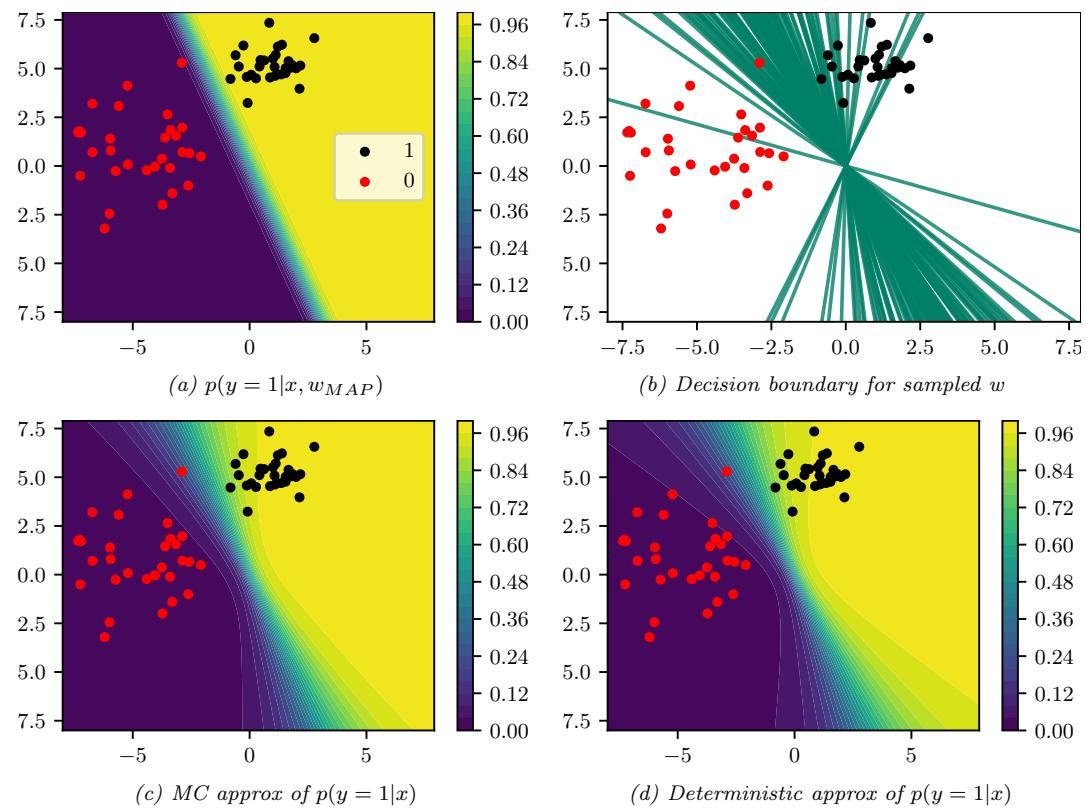
Figure 15.7: Posterior predictive distribution for a logistic regression model in 2d. (a) Contours of p(y = |x, wˆ map). (b) Samples from the posterior predictive distribution. (c) Averaging over these samples. (d) Moderated output (probit approximation). Generated by logreg\_laplace\_demo.ipynb.

This is called the probit approximation [SL90]. In [Gib97], a generalization to the multiclass case was provided. This is known as the generalized probit approximation, and has the form

\[p(y\_\*|x\_\*) \approx \int \text{softmax}(\mathbf{f}\_\*) \mathcal{N}(\mathbf{f}\_\*|\mu\_\*, \Sigma\_\*) d\mathbf{f}\_\* = \text{softmax}\left(\{\frac{\mu\_{\*,c}}{\sqrt{1 + \frac{\pi}{8}\Sigma\_{\*,cc}}}\}\right) \tag{15.150}\]

This ignores the correlations between the logits, because it only depends on the diagonal elements of !→. Nevertheless it can work well, even in the case of neural net classifiers [LIS20]. Another deterministic approximation, known as the Laplace bridge, is discussed in Section 17.3.10.2.

We now illustrate the posterior predictive for our binary example. Figure 15.7(a) shows the plugin approximation using the MAP estimate. We see that there is no uncertainty about the location of the decision boundary, even though we are generating probabilistic predictions over the labels. Figure 15.7(b) shows what happens when we plug in samples from the Gaussian posterior. Now we see that there is considerable uncertainty about the orientation of the “best” decision boundary. Figure 15.7(c) shows the average of these samples. By averaging over multiple predictions, we see

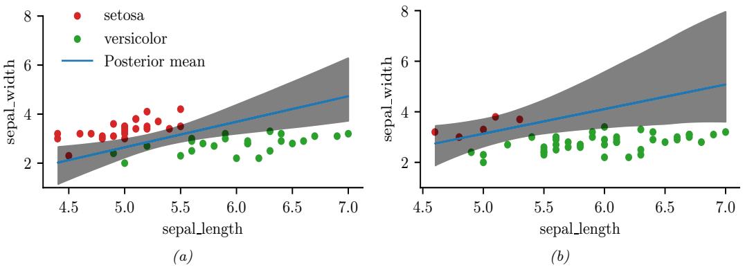
Figure 15.8: Illustration of the posterior over the decision boundary for classifying iris flowers (setosa vs versicolor) using 2 input features. (a) 25 examples per class. Adapted from Figure 4.5 of [Mar18]. (b) 5 examples of class 0, 45 examples of class 1. Adapted from Figure 4.8 of [Mar18]. Generated by logreg\_iris\_bayes\_2d.ipynb.

that the uncertainty in the decision boundary “splays out” as we move further from the training data. Figure 15.7(d) shows that the probit approximation gives very similar results to the Monte Carlo approximation.

15.3.7 MCMC inference

Markov chain Monte Carlo, or MCMC, is often considered the “gold standard” for approximate inference, since it makes no explicit assumptions about the form of the posterior. It is explained in depth in Chapter 12, but the output is a set of (correlated) samples from the posterior, which gives the following non-parametric approximation:

\[q(\boldsymbol{\theta}|\mathcal{D}) \approx \frac{1}{S} \sum\_{s=1}^{S} \delta(\boldsymbol{\theta} - \boldsymbol{\theta}^{s}) \tag{15.151}\]

where ^{ωs ↔︎ p}(ω|D). Once we have the samples, we can plug them into Equation (15.147) to approximate the posterior predictive distribution.

A common MCMC method is known as Hamiltonian Monte Carlo (Section 12.5); this can leverage our ability to compute the gradient of the log joint, ⇒^ε log p(D, ω), for improved e”ciency. Let us apply HMC to a 2-dimensional, 2-class version of the iris classification problem, where we just use two input features, sepal length and sepal width, and two classes, Virginica and non-Virginica. The decision boundary is the set of points (x^→ 1, x^{→ 2}) such that ς(b + w1x^{→ 1} + w2x^{→ 2})=0.5. Such points must lie on the following line:

\[x\_2^\* = -\frac{b}{w\_2} + \left(-\frac{w\_1}{w\_2}x\_1^\*\right) \tag{15.152}\]

We can therefore compute an MC approximation to the posterior over decision boundaries by sampling the parameters from the posterior, (w1, w2, b) ↔︎ p(ω|D), and plugging them into the above equation,

Di Dept.	Gi Gender	Ai # Admitted	Ri # Rejected	Ni # Applications
A	male	512	313	825
A	female	89	19	108
B	male	353	207	560
B	female	17	8	25
C	male	120	205	325
C	female	202	391	593
D	male	138	279	417
D	female	131	244	375
E	male	53	138	191
E	female	94	299	393
F	male	22	351	373
F	female	24	317	341

Table 15.1: Admissions data for UC Berkeley from [BHO75].

to get p(x^→ 1, x^{→ 2}|D). The results of this method (using a vague Gaussian prior for the parameters) are shown in Figure 15.8a. The solid line is the posterior mean, and the shaded interval is a 95% credible interval. As before, we see that the uncertainty about the location of the boundary is higher as we move away from the training data.

In Figure 15.8b, we show what happens to the decision boundary when we have unbalanced classes. We notice two things. First, the posterior uncertainty increases, because we have less data from the red class. Second, we see that the posterior mean of the decision boundary shifts towards the class with less data. This follows from linear discriminant analysis, where one can show that changing the class prior changes the location of the decision boundary, so that more of the input space gets mapped to the class which is higher a priori. (See [Mur22, Sec 9.2] for details.)

15.3.8 Other approximate inference methods

There are many other approximate inference methods we can use, as we discuss in Part II. A common approach is variational inference (Section 10.1), which converts approximate inference into an optimization problem. It does this by choosing an approximate distribution q(w; ϖ) and optimizing the variational parameters ϖ to maximize the evidence lower bound (ELBO). This has the e!ect of making q(w; ϖ) ↓ p(w|D) in the sense that the KL divergence is small. There are several ways to tackle this: use a stochastic estimate of the ELBO (see Section 10.2.1), use the conditionally conjugate VI method of Supplementary Section 10.3.1.2, or use a “local” VI method that creates a quadratic lower bound to the logistic function (see Supplementary Section 15.1).

In the online setting, we can use assumed density filtering (ADF) to recursively compute a Gaussian approximate posterior p(w|D1:t), as we discuss in Section 8.6.3.

15.3.9 Case study: is Berkeley admissions biased against women?

In this section, we consider a simple but interesting example of logistic regression from [McE20, Sec 11.1.4]. The question of interest is whether admission to graduate school at UC Berkeley is biased against women. The dataset comes from a famous paper [BHO75], which collected statistics for 6 departments for men and women. The data table only has 12 rows, shown in Table 15.1, although the total sample size (number of observations) is 4526. We conduct a regression analysis to try to determine if gender “causes” imbalanced admissions rates.

An obvious way to attempt to answer the question of interest is to fit a binomial logistic regression model, in which the outcome is the admissions rate, and the input is a binary variable representing the gender of each sample (make or female). One way to write this model is as follows:

\[A\_i \sim \text{Bin}(N\_i, \mu\_i) \tag{15.153}\]

\[\text{logit}(\mu\_i) = \alpha + \beta \text{MAE}[i] \tag{15.154}\]

\[ \alpha \sim \mathcal{N}(0, 10) \tag{15.155} \]

\[ \beta \sim \mathcal{N}(0, 1.5) \tag{15.156} \]

Here Aⁱ is the number of admissions for sample i, Nⁱ is the nunber of applications, and MALE[i]=1 i! the sample is male. So the log odds is ϱ for female cases, and ϱ + ↼ for male candidates. (The choice of prior for these parameters is discussed in Section 15.3.4.)

The above formulation is asymmetric in the genders. In particular, the log odds for males has two random variables associated with it, and hence is a-priori more uncertain. It is often better to rewrite the model in the following symmetric way:

\[A\_i \sim \text{Bin}(N\_i, \mu\_i) \tag{15.157}\]

\[\text{logit}(\mu\_i) = \alpha\_{\text{GENDER}[i]} \tag{15.158}\]

\[ \alpha\_j \sim \mathcal{N}(0, 1.5), \; j \in \{1, 2\} \tag{15.159} \]

Here GENDER[i] is the gender (1 for male, 2 for female), so the log odds is ϱ¹ for males and ϱ² for females.

We can perform posterior inference using a variety of methods (see Chapter 7). Here we use HMC (Section 12.5). We find the 89% credible interval for ϱ¹ is [→0.29, 0.16] and for ϱ² is [→0.91, 0.75]. 2 The corresponding distribution for the di!erence in probability, ς(ϱ1) → ς(ϱ2), is [0.12, 0.16], with a mean of 0.14. So it seems that Berkeley is biased in favor of men.

However, before jumping to conclusions, we should check if the model is any good. In Figure 15.9a, we plot the posterior predictive distribution, along with the original data. We see the model is a very bad fit to the data (the blue data dots are often outside the black predictive intervals). In particular, we see that the empirical admissions rate for women is actually higher in all the departments except for C and E, yet the model says that women should have a 14% lower chance of admission.

The trouble is that men and women did not apply to the same departments in equal amounts. Women tended not to apply to departments, like A and B, with high admissions rates, but instead applied more to departments, like F, with low admissions rates. So even though less women were accepted overall, within in each department, women tended to be accepted at about the same rate.

^2. McElreath uses 89% interval instead of 95% to emphasize the arbitrary nature of these values. The di”erence is insignificant.

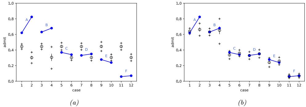
Figure 15.9: Blue dots are admission rates for each of the 6 departments (A-F) for males (left half of each dyad) and females (right half ). The circle is the posterior mean of µi, the small vertical black lines indicate 1 standard deviation of µi. The + marks indicate 95% predictive interval for Ai. (a) Basic model, only taking gender into account. (b) Augmented model, adding department specific o!sets. Adapted from Figure 11.5 of [McE20]. Generated by logreg\_ucb\_admissions\_numpyro.ipynb.

We can get a better understanding if we consider the DAG in Figure 15.10a. This is intended to be a causal model of the relevant factors. We discuss causality in more detail in Chapter 36, but the basic idea should be clear from this picture. In particular, we see that there is an indirect causal path G ↖ D ↖ A from gender to acceptance, so to infer the direct a!ect G ↖ A, we need to condition on D and close the indirect path. We can do this by adding department id as another feature:

\[A\_i \sim \text{Bin}(N\_i, \mu\_i) \tag{15.160}\]

\[\text{logit}(\mu\_i) = \alpha\_{\text{GENDER}[i]} + \gamma\_{\text{DEPT}[i]} \tag{15.161}\]

\[ \alpha\_j \sim \mathcal{N}(0, 1.5), j \in \{1, 2\} \tag{15.162} \]

\[ \gamma\_k \sim \mathcal{N}(0, 1.5), k \in \{1, \ldots, 6\} \tag{15.163} \]

Here j ↗ {1, 2} (for gender) and k ↗ {1,…, 6} (for department). Note that there 12 parameters in this model, but each combination (slice of the data) has a fairly large sample size of data associated with it, as we see in Table 15.1.

In Figure 15.9b, we plot the posterior predictive distribution for this new model; we see the fit is now much better. We find the 89% credible interval for ϱ¹ is [→1.38, 0.35] and for ϱ² is [→1.31, 0.42]. The corresponding distribution for the di!erence in probability, ς(ϱ1) → ς(ϱ2), is [→0.05, 0.01]. So it seems that there is no bias after all.

However, the above conclusion is based on the correctness of the model in Figure 15.10a. What if there are unobserved confounders U, such as academic ability, influencing both admission rate and department choice? This hypothesis is shown in Figure 15.10b. In this case, conditioning on the collider D opens up a non-causal path between gender and admissions, G ↖ D A U ↖ A. This invalidates any causal conclusions we may want to draw.

The point of this example is to serve as a cautionary tale to those trying to draw causal conclusions from predictive models. See Chapter 36 for more details.

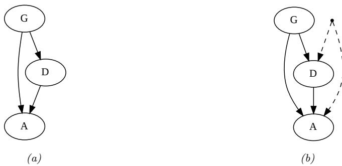
Figure 15.10: Some possible causal models of admissions rates. G is gender, D is department, A is acceptance rate. (a) No hidden confounders. (b) Hidden confounder (small dot) a!ects both D and A. Generated by logreg\_ucb\_admissions\_numpyro.ipynb.

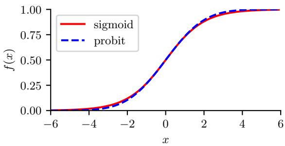
Figure 15.11: The logistic (sigmoid) function ω(x) in solid red, with the Gaussian cdf function !(ςx) in dotted blue superimposed. Here ς = #↼/8, which was chosen so that the derivatives of the two curves match at x = 0. Adapted from Figure 4.9 of [Bis06]. Generated by probit\_plot.ipynb.

15.4 Probit regression

In this section, we discuss probit regression, which is similiar to binary logistic regression except it uses µⁿ = ‘(an) instead of µⁿ = ς(an) as the mean function, where’ is the cdf of the standard normal, and aⁿ = w^Txn. The corresponding link function is therefore aⁿ = ε(µn) = ’↓¹(µn); the inverse of the Gaussian cdf is known as the probit function.

The Gaussian cdf ’ is very similar to the logistic function, as shown in Figure 15.11. Thus probit regression and “regular” logistic regression behave very similarly. However, probit regression has some advantages. In particular, it has a simple interpretation as a latent variable model (see Section 15.4.1), which arises from the field of choice theory as studied in economics (see e.g., [Koo03]). This also simplifies the task of Bayesian parameter inference.

15.4.1 Latent variable interpretation

We can interpret aⁿ = w^Txⁿ as a factor that is proportional to how likely a person is respond positively (generate yⁿ = 1) given input xn. However, typically there are other unobserved factors that

influence someone’s response. Let us model these hidden factors by Gaussian noise, ⇁ⁿ ↔︎ N (0, 1). Let the combined preference for positive outcomes be represented by the latent variable zⁿ = wTxⁿ + ⇁n. We assume that the person will pick the positive label i! this latent factor is positive rather than negative, i.e.,

\[y\_n = \mathbb{I}\left(z\_n \ge 0\right) \tag{15.164}\]

When we marginalize out zn, we recover the probit model:

\[p(y\_n = 1 | \mathbf{x}\_n, \mathbf{w}) = \int \mathbb{I}(z\_n \ge 0) \mathcal{N}(z\_n | \mathbf{w}^\mathsf{T} \mathbf{x}\_n, 1) dz\_n \tag{15.165}\]

\[\epsilon\_n = p(\boldsymbol{\omega}^\mathsf{T} \boldsymbol{x}\_n + \epsilon\_n \ge 0) = p(\epsilon\_n \ge -\boldsymbol{w}^\mathsf{T} \boldsymbol{x}\_n) \tag{15.166}\]

\[\Phi = 1 - \Phi(-\boldsymbol{w}^{\mathsf{T}}\boldsymbol{x}\_n) = \Phi(\boldsymbol{w}^{\mathsf{T}}\boldsymbol{x}\_n) \tag{15.167}\]

Thus we can think of probit regression as a threshold function applied to noisy input.

We can interpret logistic regression in the same way. However, in that case the noise term ⇁ⁿ comes from a logistic distribution, defined as follows:

\[f(y|\mu, s) \triangleq \frac{e^{-\frac{y-\mu}{s}}}{s(1 + e^{-\frac{y-\mu}{s}})^2} = \frac{1}{4s} \text{sech}^2(\frac{y-\mu}{s^2}) \tag{15.168}\]

where the mean is µ and the variance is ^s2⇀^{2 3} . The cdf of this distribution is given by

\[F(y|\mu, s) = \frac{1}{1 + e^{-\frac{y - \mu}{s}}} \tag{15.169}\]

It is clear that if we use logistic noise with µ = 0 and s = 1 we recover logistic regression. However, it is computationally easier to deal with Gaussian noise, as we show below.

15.4.2 Maximum likelihood estimation

In this section, we discuss some methods for fitting probit regression using MLE.

15.4.2.1 MLE using SGD

We can find the MLE for probit regression using standard gradient methods. Let µⁿ = w^Txn, and let y˜ⁿ ↗ {→1, +1}. Then the gradient of the log-likelihood for a single example n is given by

\[g\_n \triangleq \frac{d}{dw} \log p(\check{y}\_n | w^\mathsf{T} x\_n) = \frac{d\mu\_n}{dw} \frac{d}{d\mu\_n} \log p(\check{y}\_n | w^\mathsf{T} x\_n) = x\_n \frac{\check{y}\_n \phi(\mu\_n)}{\Phi(\check{y}\_n \mu\_n)} \tag{15.170}\]

where 3 is the standard normal pdf, and ’ is its cdf. Similarly, the Hessian for a single case is given by

\[\mathbf{H}\_n = \frac{d}{dw^2} \log p(\ddot{y}\_n | \mathbf{w}^\mathsf{T} x\_n) = -\mathbf{x}\_n \left( \frac{\phi(\mu\_n)^2}{\Phi(\ddot{y}\_n \mu\_n)^2} + \frac{\ddot{y}\_n \mu\_n \phi(\mu\_n)}{\Phi(\ddot{y}\_n \mu\_n)} \right) \mathbf{x}\_n^\mathsf{T} \tag{15.171}\]

This can be passed to any gradient-based optimizer.

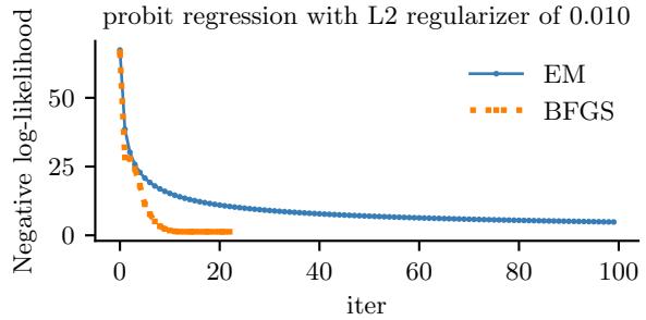
Figure 15.12: Fitting a probit regression model in 2d using a quasi-Newton method or EM. Generated by probit\_reg\_demo.ipynb.

15.4.2.2 MLE using EM

We can use the latent variable interpretation of probit regression to derive an elegant EM algorithm for fitting the model. The complete data log likelihood has the following form, assuming a N (0, V0) prior on w:

\[\ell(\mathbf{z}, w | \mathbf{V}\_0) = \log p(\mathbf{y} | \mathbf{z}) + \log \mathcal{N}(\mathbf{z} | \mathbf{X}w, \mathbf{I}) + \log \mathcal{N}(w | \mathbf{0}, \mathbf{V}\_0) \tag{15.172}\]

\[=\sum\_{n}\log p(y\_n|z\_n) - \frac{1}{2}(\mathbf{z}-\mathbf{X}w)^\mathrm{T}(\mathbf{z}-\mathbf{X}w) - \frac{1}{2}w^\mathrm{T}\mathbf{V}\_0^{-1}w\tag{15.173}\]

The posterior in the E step is a truncated Gaussian:

\[p(z\_n|y\_n, x\_n, w) = \begin{cases} \mathcal{N}(z\_n|w^\top x\_n, 1)\mathbb{I}(z\_n > 0) & \text{if } y\_n = 1\\ \mathcal{N}(z\_n|w^\top x\_n, 1)\mathbb{I}(z\_n < 0) & \text{if } y\_n = 0 \end{cases} \tag{15.174}\]

In Equation (15.173), we see that w only depends linearly on z, so we just need to compute E [zn|yn, xn, w], so we just need to compute the posterior mean. One can show that this is given by

\[\mathbb{E}\left[z\_n|\mathbf{w}, \mathbf{z}\_n\right] = \begin{cases} \mu\_n + \frac{\phi(\mu\_n)}{1 - \Phi(-\mu\_n)} = \mu\_n + \frac{\phi(\mu\_n)}{\Phi(\mu\_n)} & \text{if } y\_n = 1\\ \mu\_n - \frac{\phi(\mu\_n)}{\Phi(-\mu\_n)} = \mu\_n - \frac{\phi(\mu\_n)}{1 - \Phi(\mu\_i)} & \text{if } y\_n = 0 \end{cases} \tag{15.175}\]

where µⁿ = w^Txn.

In the M step, we estimate w using ridge regression, where µ = E [z] is the output we are trying to predict. Specifically, we have

\[ \hat{\boldsymbol{w}} = (\mathbf{V}\_0^{-1} + \mathbf{X}^{\mathsf{T}} \mathbf{X})^{-1} \mathbf{X}^{\mathsf{T}} \boldsymbol{\mu} \tag{15.176} \]

The EM algorithm is simple, but can be much slower than direct gradient methods, as illustrated in Figure 15.12. This is because the posterior entropy in the E step is quite high, since we only observe that z is positive or negative, but are given no information from the likelihood about its magnitude. Using a stronger regularizer can help speed convergence, because it constrains the range of plausible z values. In addition, one can use various speedup tricks, such as data augmentation [DM01].

15.4.3 Bayesian inference

It is possible to use the latent variable formulation of probit regression in Section 15.4.2.2 to derive a simple Gibbs sampling algorithm for approximating the posterior p(w|D) (see e.g., [AC93; HH06]).

The key idea is to use an auxiliary latent variable, which, when conditioned on, makes the whole model a conjugate linear-Gaussian model. The full conditional for the latent variables is given by

\[p(z\_i|y\_i, x\_i, w) = \begin{cases} \mathcal{N}(z\_i|w^T x\_i, 1) \mathbb{I}(z\_i > 0) & \text{if } y\_i = 1\\ \mathcal{N}(z\_i|w^T x\_i, 1) \mathbb{I}(z\_i < 0) & \text{if } y\_i = 0 \end{cases} \tag{15.177}\]

Thus the posterior is a truncated Gaussian. We can sample from a truncated Gaussian, N (z|µ, ς)I(a ⇐ z ⇐ b) in two steps: first sample ^{u ↔︎ U}(‘((^{a → µ})/ς),’((^{b → µ})/ς)), then set ^{z = µ + ς}’↓¹(u) [Rob95a].

The full conditional for the parameters is given by

\[p(w|\mathcal{D}, \mathbf{z}, \lambda) = \mathcal{N}(w\_N, \mathbf{V}\_N) \tag{15.178}\]

\[\mathbf{V}\_N = (\mathbf{V}\_0^{-1} + \mathbf{X}^T \mathbf{X})^{-1} \tag{15.179}\]

\[\mathbf{w}\_{N} = \mathbf{V}\_{N}(\mathbf{V}\_{0}^{-1}w\_{0} + \mathbf{X}^{T}\mathbf{z})\tag{15.180}\]

For further details, see e.g., [AC93; FSF10]. It is also possible to use variational Bayes, which tends to be much faster (see e.g., [GR06a; FDZ19]).

15.4.4 Ordinal probit regression

One advantage of the latent variable interpretation of probit regression is that it is easy to extend to the case where the response variable is ordered in some way, such as the outputs low, medium, and high. This is called ordinal regression. The basic idea is as follows. If there are C output values, we introduce C + 1 thresholds ▷^j and set

\[y\_n = j \quad \text{if} \quad \gamma\_{j-1} < z\_n \le \gamma\_j \tag{15.181}\]

where ▷⁰ ⇐ ··· ⇐ ▷^C . For identifiability reasons, we set ▷⁰ = →⇓, ▷¹ = 0 and ▷^C = ⇓. For example, if C = 2, this reduces to the standard binary probit model, whereby zⁿ < 0 produces yⁿ = 0 and zⁿ ≃ 0 produces yⁿ = 1. If C = 3, we partition the real line into 3 intervals: (→⇓, 0], (0, ▷2], (▷2, ⇓). We can vary the parameter ▷² to ensure the right relative amount of probability mass falls in each interval, so as to match the empirical frequencies of each class label. See e.g., [AC93] for further details.

Finding the MLEs for this model is a bit trickier than for binary probit regression, since we need to optimize for w and ↽, and the latter must obey an ordering constraint. See e.g., [KL09] for an approach based on EM. It is also possible to derive a simple Gibbs sampling algorithm for this model (see e.g., [Hof09, p216]).

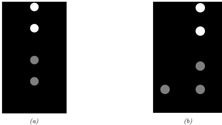
Figure 15.13: Hierarchical Bayesian discriminative models with J groups. (a) Nested formulation. (b) Non-nested formulation, with group indicator gⁿ ↓ {1,…,J}.

15.4.5 Multinomial probit models

Now consider the case where the response variable can take on C unordered categorical values, yⁿ ↗ {1,…,C}. The multinomial probit model is defined as follows:

\[z\_{nc} = w\_c^\mathsf{T} x\_{nc} + \epsilon\_{nc} \tag{15.182}\]

\[ \epsilon \sim \mathcal{N}(\mathbf{0}, \mathbf{R}) \tag{15.183} \]

\[y\_n = \arg\max\_c z\_{nc} \tag{15.184}\]

See e.g., [DE04; GR06b; Sco09; FSF10] for more details on the model and its connection to multinomial logistic regression.

If instead of setting yⁿ = argmax^c zic we use ync = I(znc > 0), we get a model known as multivariate probit, which is one way to model C correlated binary outcomes (see e.g., [TMD12]).

15.5 Multilevel (hierarchical) GLMs

Suppose we have a set of J related datasets, each of which contains a series of N^j datapoints ^{Dj =} {(x^{j n}, y^{j n}) : n =1: Nj}. There are 3 main ways to fit models in such a setting: we could fit J separate models, p(y|x; D^j ), which might result in overfitting if some D^j are small; we could pool all the data to get ^{D = ⊤J j}=1D^j and fit a single model, p(y|x; D), which might result in underfitting; or we can use a hierarchical Bayesian model, also called a multilevel model or partially pooled model, in which we assume each group has its own parameters, ω^j , but that these have something in common, as modeled by a shared global prior p(ω⁰). (Note that each group could be a single individual.) The overall model has the form

\[p(\boldsymbol{\theta}^{0:J}, \mathcal{D}) = p(\boldsymbol{\theta}^0) \prod\_{j=1}^J \left[ p(\boldsymbol{\theta}^j | \boldsymbol{\theta}^0) \prod\_{n=1}^{N\_j} p(\boldsymbol{y}^j\_n | \boldsymbol{x}^j\_n, \boldsymbol{\theta}^j) \right] \tag{15.185}\]

See Figure 15.13a, which represents the model using nested plate notation.

It is often more convenient to represent the model as in Figure 15.13b, which eliminates the nested plates (and hence the double indexing of variables) by associating a group indicator variable gⁿ ↗ {1,…,J}, which specifies which set of parameters to use for each datapoint. Thus the model now has the form

\[p(\boldsymbol{\theta}^{0:J}, \mathcal{D}) = p(\boldsymbol{\theta}^0) \left[ \prod\_{j=1}^J p(\theta^j | \boldsymbol{\theta}^0) \right] \left[ \prod\_{n=1}^N p(y\_n | \boldsymbol{x}\_n, g\_n, \boldsymbol{\theta}) \right] \tag{15.186}\]

where

\[p(y\_n | x\_n, g\_n, \theta) = \prod\_{j=1}^{J} p(y\_n | x\_n, \theta^j)^{\mathbb{I}(g\_n=j)} \tag{15.187}\]

If the likelihood function is a GLM, this hierarchical model is called a hierarchical GLM [LN96]. This class of models is very widely used in applied statistics. For much more details, see e.g., [GH07; GHV20b; Gel+22].

15.5.1 Generalized linear mixed models (GLMMs)

Suppose that the prior on the per-group parameters is Gaussian, so ^p(ω^{j |}ω⁰) = ^N (ω^{j |}ω⁰, !^j ). If we have a GLM likelihood, the model becomes

\[p(\mathbf{y}\_n | \mathbf{x}\_n, g\_n = j, \boldsymbol{\theta}) = p(\mathbf{y}\_n | \boldsymbol{\ell}(\boldsymbol{\eta}\_n)) \tag{15.188}\]

\[\eta\_n = \mathbf{x}\_n^\mathsf{T} \boldsymbol{\theta}^j = \mathbf{x}\_n^\mathsf{T} (\boldsymbol{\theta}^0 + \boldsymbol{\epsilon}^j) = \mathbf{x}\_n^\mathsf{T} \boldsymbol{\theta}^0 + \mathbf{x}\_n^\mathsf{T} \boldsymbol{\epsilon}^j \tag{15.189}\]

where ^ε is the link function, and ,^{j ↔︎ N} (0, !). This is known as a generalized linear mixed model (GLMM) or mixed e!ects model. The shared (common) parameters ω⁰ are called fixed e!ects, and the group-specific o!sets ,^j are called random e!ects. 3 We can see that the random e!ects model group-specific deviations or idiosyncracies away from the shared fixed parameters. Furthermore, we see that the random e!ects are correlated, which allows us to model dependencies between the observations that would not be captured by a standard GLM.

For model fitting, we can use any of the Bayesian inference methods that we discussed in Section 15.1.4.

15.5.2 Example: radon regression

In this section, we give an example of a hierarchical Bayesian linear regression model. We apply it to a simplified version of the radon example from [Gel+14a, Sec 9.4].

Radon is known to be the highest cause of lung cancer in non-smokers, so reducing it where possible is desirable. To help with this, we fit a regression model, that predicts the (log) radon level as a function of the location of the house, as represented by a categorical feature indicating its county, and

^3. Note that there are multiple definitions of the terms “fixed e”ects” and random e”ects”, as explained in this blog post by Andrew Gelman: https://statmodeling.stat.columbia.edu/2005/01/25/why\_i\_dont\_use/.

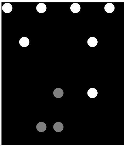
Figure 15.14: A hierarchical Bayesian linear regression model for the radon problem.

a binary feature representing whether the house has a basement or not. We use a dataset consisting of J = 85 counties in Minnesota; each county has between 2 and 80 measurements.

We assume the following likelihood:

\[p(y\_n | x\_n, g\_n = j, \boldsymbol{\theta}) = \mathcal{N}(y\_n | \alpha\_j + \beta\_j x\_n, \sigma\_y^2) \tag{15.190}\]

where gⁿ ↗ {1,…,J} is the county for house i, and xⁿ ↗ {0, 1} indicates if the floor is at level 0 (i.e., in the basement) or level 1 (i.e., above ground). Intuitively we expect the radon levels to be lower in houses without basements, since they are more insulated from the earth which is the source of the radon.

Since some counties have very few datapoints, we use a hierarchical prior in which we assume ^{ϱj ↔︎ N} (µ↼, ^ς2 ↼), and ↼^{j ↔︎ N} (µβ, ^{ς2 β}). We use weak priors for the parameters: µ↼ ↔︎ N (0, 1), µ^β ↔︎ N (0, 1), ς↼ ↔︎ C+(1), ς^β ↔︎ C+(1), ς^y ↔︎ C+(1). See Figure 15.14 for the graphical model.

15.5.2.1 Posterior inference

Figure 15.15 shows the posterior marginals for µ↼, µβ, ϱ^j and ↼^j . We see that µ^β is close to →0.6 with high probability, which confirms our suspicion that having x = 1 (i.e., no basement) decreases the amount of radon in the house. We also see that the distribution of the ϱ^j parameters is quite variable, due to di!erent base rates across the counties.

Figure 15.16 shows predictions from the hierarchical and non-hierarchical model for 3 di!erent counties. We see that the predictions from the hierarchical model are more consistent across counties, and work well even if there are no examples of certain feature combinations for a given county (e.g., there are no houses without basements in the sample from Cass county). If we sample data from the posterior predictive distribution, and compare it to the real data, we find that the RMSE is 0.13 for the non-hierarchical model and 0.08 for the hierarchical model, indicating that the latter fits better.

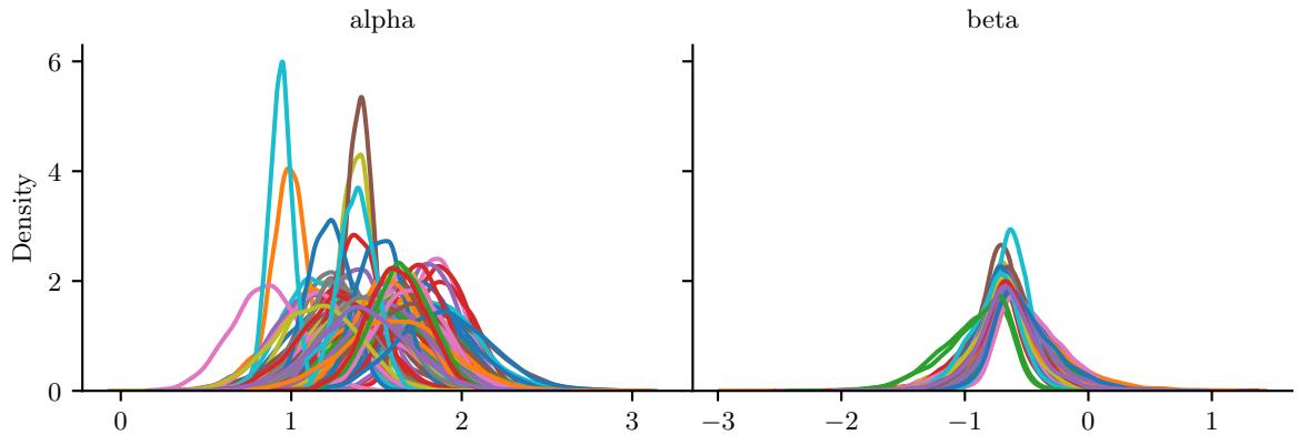
Figure 15.15: Posterior marginals for φ^j and β^j for each county j in the radon model. Generated by linreg\_hierarchical\_non\_centered.ipynb.

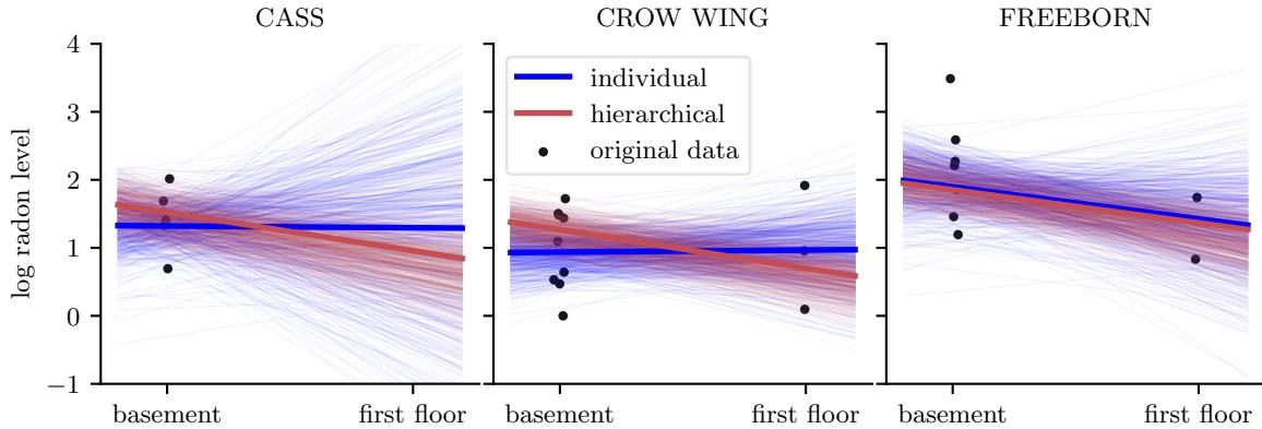
Figure 15.16: Predictions from the radon model for 3 di!erent counties in Minnesota. Black dots are observed datapoints. Red represents results of hierarchical (shared) prior, blue represents results of non-hierarchical prior. Thick lines are the result of using the posterior mean, thin lines are the result of using posterior samples. Generated by linreg\_hierarchical\_non\_centered.ipynb.

15.5.2.2 Non-centered parameterization

One problem that frequently arises in hierarchical models is that the parameters be very correlated. This can cause computational problems when performing inference.

Figure 15.17a gives an example where we plot p(↼^j , ςβ|D) for some specific county j. If we believe that ς^β is large, then ↼^c is “allowed” to vary a lot, and we get the broad distribution at the top of the figure. However, if we believe that ς^β is small, then ↼^j is constrained to be close to the global prior mean of µβ, so we get the narrow distribution at the bottom of the figure. This is often called Neal’s funnel, after a paper by Radford Neal [Nea03]. It is di”cult for many algorithms (especially sampling algorithms) to explore parts of parameter space at the bottom of the funnel. This is evident from the marginal posterior for ς^β shown (as a histogram) on the right hand side of the plot: we see

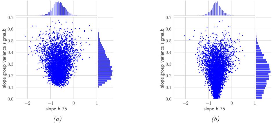
Figure 15.17: (a) Bivariate posterior p(β^j , ωϑ|D) for the hierarchical radon model for county j = 75 using centered parameterization. (b) Similar to (a) except we plot ^p(β˜^j , ^ωϑ|D) for the non-centered parameterization. Generated by linreg\_hierarchical\_non\_centered.ipynb.

that it excludes the interval [0, 0.1], thus ruling out models in which we shrink ↼^j all the way to 0. In cases where a covariate has no useful predictive role, we would like to be able to induce sparsity, so we need to overcome this problem.

A simple solution to this is to use a non-centered parameterization [PR03]. That is, we replace ↼^{j ↔︎ N} (µβ, ^{ς2 β}) with ↼^{j = µβ +} ↼˜jςβ, where ↼˜^{j ↔︎ N} (0, 1) represents the ^o!set from the global mean, µβ. The correlation between ↼˜^j and ς^β is much less, as shown in Figure 15.17b. See Section 12.6.5 for more details.

16 Deep neural networks

16.1 Introduction

The term “deep neural network” or DNN, in its modern usage, refers to any kind of di!erentiable function that can be expressed as a computation graph, where the nodes are primitive operations (like matrix mulitplication), and edges represent numeric data in the form of vectors, matrices, or tensors. In its simplest form, this graph can be constructed as a linear series of nodes or “layers”. The term “deep” refers to models with many such layers.

In Section 16.2 we discuss some of the basic building blocks (node types) that are used in the field. In Section 16.3 we give examples of common architectures which are constructed from these building blocks. In Section 6.2 we show how we can e”ciently compute the gradient of functions defined on such graphs. If the function computes the scalar loss of the model’s predictions given a training set, we can pass this gradient to an optimization routine, such as those discussed in Chapter 6, in order to fit the model. Fitting such models to data is called “deep learning”.

We can combine DNNs with probabilistic models in two di!erent ways. The first is to use them to define nonlinear functions which are used inside conditional distributions. For example, we may construct a classifier using p(y|x, ω) = Cat(y|softmax(f(x; ω))), where f(x; ω) is a neural network that maps inputs x and parameters ω to output logits. Or we may construct a joint probability distribution over multiple variables using a directed graphical model (Chapter 4) where each CPD p(xi|pa(xi)) is a DNN. This lets us construct expressive probability models.

The other way we can combine DNNs and probabilistic models is to use DNNs to approximate the posterior distribution, i.e., we learn a function f to compute q(z|f(D; ε)), where z are the hidden variables (latents and/or parameters), D are the observed variables (data), f is an inference network, and ε are its parameters; for details, see Section 10.1.5. Note that in the latter setting, the joint model p(z, D) may be a “traditional” model without any “neural” components. For example, it could be a complex simulator. Thus the DNN is just used for computational purposes, not statistical/modeling purposes. (This is sometimed called deep Bayesian learning, as opposed to Bayesian deep learning which we discuss in Chapter 17.)

More details on DNNs can be found in such books as [Zha+20a; Cho21; Gér19; GBC16; Raf22], as well as a multitude of online courses. For a more theoretical treatment, see e.g., [Ber+21; Cal20; Aro+21; RY21].

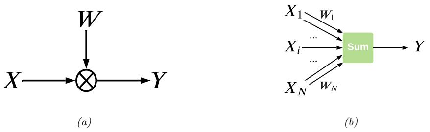
Figure 16.1: An artificial “neuron”, the most basic building block of a DNN. (a) The output y is a weighted combination of the inputs x, where the weights vector is denoted by w. (b) Alternative depiction of the neuron’s behavior. The bias term b can be emulated by defining w^N = b and X^N = 1.

16.2 Building blocks of di!erentiable circuits

In this section we discuss some common building blocks used in constructing neural networks. We denote the input to a block as x and the output as y.

16.2.1 Linear layers

The most basic building block of a DNN is a single “neuron”, which corresponds to a real-valued signal y computed by multiplying a vector-valued input signal x by a weight vector w, and then adding a bias term b. That is,

\[y = f(\mathbf{x}; \boldsymbol{\theta}) = \mathbf{w}^{\mathsf{T}} \boldsymbol{x} + b \tag{16.1}\]

where ω = (w, b) are the parameters for the function f. This is depicted in Figure 16.1. (The bias term is omitted for clarity.)

It is common to group a set of neurons together into a layer. We can then represent the activations of a layer with ^D units as a vector ^z ↗ ^RD. We can transform an input vector of activations ^x into an output vector y by multiplying by a weight matrix W, an adding an o!set vector or bias term b to get

\[y = f(x; \theta) = \mathbf{W}x + b \tag{16.2}\]

where ω = (W, b) are the parameters for the function f. This is called a linear layer, or fully connected layer.

It is common to prepend the bias vector onto the first column of the weight matrix, and to append a 1 to the vector x, so that we can write this more compactly as x = W˜ ^Tx˜, where W˜ = [W, b] and x˜ = [x, 1]. This allows us to ignore the bias term from our notation if we want to.

16.2.2 Nonlinearities

A stack of linear layers is equivalent to a single linear layer where we multliply together all the weight matrices. To get more expressive power we can transform each layer by passing it elementwise

Name	Definition	Range	Reference
Sigmoid	1 ς(a) = 1+e→a	[0, 1]
Hyperbolic tangent	tanh(a)=2ς(2a) → 1	[→1, 1]
Softplus	ea) ς+(a) = log(1 +	[0, ⇓]	[GBB11]
Rectified linear unit	ReLU(a) = max(a, 0)	[0, ⇓]	[GBB11; KSH12a]
Leaky ReLU	max(a, 0) + ϱ min(a, 0)	[→⇓, ⇓]	[MHN13]
Exponential linear unit	min(ϱ(ea → max(a, 0) + 1), 0)	[→⇓, ⇓]	[CUH16]
Swish	aς(a)	[→⇓, ⇓]	[RZL17]
GELU	a’(a)	[→⇓, ⇓]	[HG16]
Sine	sin(a)	[→1, 1]	[Sit+20]

Table 16.1: List of some popular activation functions for neural networks.

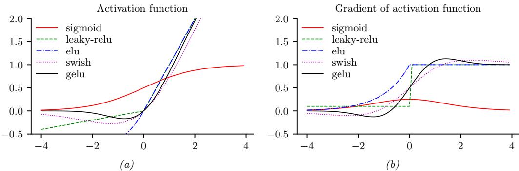
Figure 16.2: (a) Some popular activation functions. “ReLU” stands for “restricted linear unit”. “GELU” stands for “Gaussian error linear unit”. (b) Plot of their gradients. Generated by activation\_fun\_deriv.ipynb.

(pointwise) through a nonlinear function called an activation function. This is denoted by

\[\varphi = \varphi(x) = [\varphi(x\_1), \dots, \varphi(x\_D)] \tag{16.3}\]

See Table 16.1 for a list of some common activation functions, and Figure 16.2 for a visualization. For more details, see e.g., [Mur22, Sec 13.2.3].

16.2.3 Convolutional layers

When dealing with image data, we can apply the same weight matrix to each local patch of the image, in order to reduce the number of parameters. If we “slide” this weight matrix over the image and add up the results, we get a technique known as convolution; in this case the weight matrix is often called a “kernel” or “filter”.

More precisely, let ^X ↗ ^RH⇑^W be the input image, and ^W ↗ ^Rh⇑^w be the kernel. The output is

1 0 -1 1 0 -1 1 0 -1 4 9 2 5 8 3 5 6 2 4 0 3 2 4 5 4 5 2 5 6 5 4 7 8 5 7 7 9 2 1 5 8 5 3 8 4 4 9 2 5 8 3 5 6 2 4 0 3 2 4 5 4 5 2 5 6 5 4 7 8 5 7 7 9 2 1 5 8 5 3 8 4 4 9 2 5 8 3 5 6 24 03 2 4 54 52 5 6 5 4 7 8 5 7 79 21 5 8 5 3 8 4 1 0 -1 1 0 -1 1 0 -1 1 0 -1 1 0 -1 1 0 -1 1 0 -1 1 0 -1 1 0 -1 1 0 -1 1 0 -1 1 0 -1 0 0 0 1 1 1 -1 -1 -1 Input Filter 1 * Filter 2 = = Output 6 x 6 x 3 3 x 3 x 3 3 x 3 x 3 4 x 4 4 x 4 4 x 4 x 2

Figure 16.3: A 2d convolutional layer with 3 input channels and 2 output channels. The kernel has size 3 ≃ 3 and we use stride 1 with 0 padding, so the 6 ≃ 6 input gets mapped to the 4 ≃ 4 output.

denoted by Z = X ↫W, where (ignoring boundary conditions) we have the following:1

\[Z\_{i,j} = \sum\_{u=0}^{h-1} \sum\_{v=0}^{w-1} x\_{i+u,j+v} w\_{u,v} \tag{16.4}\]

Essentially we compare a local patch of x, of size h ⇔ w and centered at (i, j), to the filter w; the output just measures how similar the input patch is to the filter. We can define convolution in 1d or 3d in an analogous manner. Note that the spatial size of the outputs may be smaller than inputs, due to boundary e!ects, although this can be solved by using padding. See [Mur22, Sec 14.2.1] for more details.

We can repeat this process for multiple layers of inputs, and by using multiple filters, we can generate multiple layers of output. In general, if we have C input channels, and we want to map it to D output (feature) channels, then we define D kernels, each of size h ⇔ w ⇔ C, where h, w are the height and width of the kernel. The d’th output feature map is obtained by convolving all C input feature maps with the d’th kernel, and then adding up the results elementwise:

\[z\_{i,j,d} = \sum\_{u=0}^{h-1} \sum\_{v=0}^{w-1} \sum\_{c=0}^{C-1} x\_{i+u,j+v,c} w\_{u,v,c,d} \tag{16.5}\]

This is called a convolutional layer, and is illustrated in Figure 16.3.

The advantage of a convolutional layer compared to using a linear layer is that the weights of the kernel are shared across locations in the input. Thus if a pattern in the input shifts locations, the corresponding output activation will also shift. This is called shift equivariance. In some cases, we want the output to be the same, no matter where the input pattern occurs; this is called shift invariance, and can be obtained by using a pooling layer, which computes the maximum or

^1. Note that, technically speaking, we are using cross correlation rather than convolution. However, these terms are used interchangeably in deep learning.

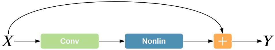
Figure 16.4: A residual connection around a convolutional layer.

average value in each local patch of the input. (Note that pooling layers have no free (learnable) parameters.) Other forms of invariance can also be captured by neural networks (see e.g., [CW16; FWW21]).

16.2.4 Residual (skip) connections

If we stack a large number of nonlinear layers together, the signal may get squashed to zero or may blow up to infinity, depending on the magnitude of the weights, and the nature of the nonlinearities. Similar problems can plague gradients that are passed backwards through the network (see Section 6.2). To reduce the e!ect of this we can add skip connections, also called residual connections, which allow the signal to skip one or more layers, which prevents it from being modified. For example, Figure 16.4 illustrates a network that computes

\[y = f(x; \mathbf{W}) = \varphi(\text{conv}(x; \mathbf{W})) + x \tag{16.6}\]

Now the convolutional layer only needs to learn an o!set or residual to add (or subtract) to the input to match the desired output, rather than predicting the output directly. Such residuals are often small in size, and hence are easier to learn using neurons with weights that are bounded (e.g., close to 1).

16.2.5 Normalization layers

To learn an input-output mapping, it is often best if the inputs are standardized, meaning that they have zero mean and unit standard deviation. This ensures that the required magnitude of the weights is small, and comparable across dimensions. To ensure that the internal activations have this property, it is common to add normalization layers.

The most common approach is to use batch normalization (BN) [IS15]. However this relies on having access to a batch of B > 1 input examples. Various alternatives have been proposed to overcome the need of having an input batch, such as layer normalization [BKH16], instance normalization [UVL16], group normalization [WH18], filter response normalization [SK20], etc. More details can be found in [Mur22, Sec 14.2.4].

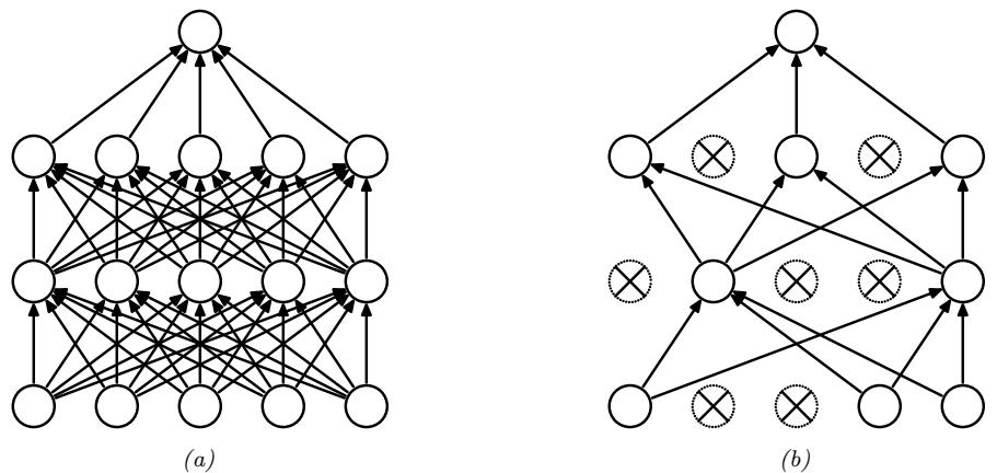
Figure 16.5: Illustration of dropout. (a) A standard neural net with 2 hidden layers. (b) An example of a thinned net produced by applying dropout with p = 0.5. Units that have been dropped out are marked with an x. From Figure 1 of [Sri+14a]. Used with kind permission of Geo! Hinton.

16.2.6 Dropout layers

Neural networks often have millions of parameters, and thus can sometimes overfit, especially when trained on small datasets. There are many ways to ameliorate this e!ect, such as applying regularizers to the weights, or adopting a fully Bayesian approach (see Chapter 17). Another common heuristic is known as dropout [Sri+14a], in which edges are randomly omitted each time the network is used, as illustrated in Figure 16.5. More precisely, if wlij is the weight of the edge from node i in layer l → 1 to node j in layer l + 1, then we replace it with ωlij = wlij ⇁li, where ⇁li ↔︎ Ber(1 → p), where p is the drop probability, and 1 → p is the keep probability. Thus if we sample ⇁li = 0, then all of the weights going out of unit i in layer l → 1 into any j in layer l will be set to 0.

During training, the gradients will be zero for the weights connected to a neuron which has been switched “o!”. However, since we resample ⇁lij every time the network is used, di!erent combinations of weights will be updated on each step. The result is an ensemble of networks, each with slightly di!erent sparse graph structures.

At test time, we usually turn the dropout noise o!, so the model acts deterministically. To ensure the weights have the same expectation at test time as they did during training (so the input activation to the neurons is the same, on average), at test time we should use E [ωlij ] = wlijE [⇁li]. For Bernoulli noise, we have E [⇁] = 1 → p, so we should multiply the weights by the keep probability, 1 → p, before making predictions. We can, however, use dropout at test time if we wish. This is called Monte Carlo dropout (see Section 17.3.1).

16.2.7 Attention layers

In all of the neural networks we have considered so far, the hidden activations are a linear combination of the input activations, followed by a nonlinearity: Z = ⁵(XW), where X ↗ ^Rn⇑^d are the hidden feature vectors, and W ↗ ^Rd⇑d^v are a fixed set of weights that are learned on a training set to

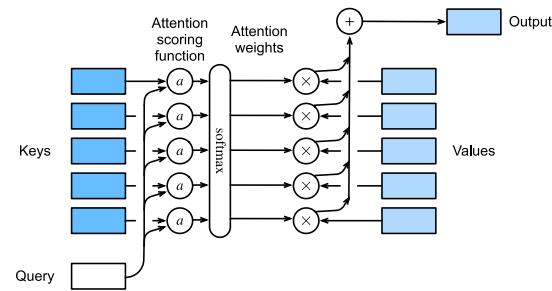
Figure 16.6: Attention layer. (a) Mapping a single query q to a single output, given a set of keys and values. From Figure 10.3.1 of [Zha+20a]. Used with kind permission of Aston Zhang.

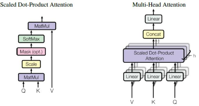
Figure 16.7: (a) Scaled dot-product attention in matrix form. (b) Multi-head attention. From Figure 2 of [Vas+17b]. Used with kind permission of Ashish Vaswani.

produce Z ↗ ^Rn⇑d^v outputs. However, we can imagine a more flexible model in which the weights depend on the inputs, i.e., Z = 5(XW(X)), where W(X) is a function to be defined below. This kind of multiplicative interaction is called attention.

We can better understand attention by comparing it to non-parametric kernel based prediction methods, such as Gaussian processes (Chapter 18). In this approach we compare the input query ^x ↗ ^Rd to each of the training examples ^X = (x1,…, ^xn) using a kernel to get a vector of similarity scores, ↼ = [K(x, ^xi)]^{n i}=1. We then use this to retrieve a weighted combination of the corresponding ^m target values ^yi ↗ ^Rdv to compute the predicted output, as follows:

\[ \hat{y} = \sum\_{i=1}^{n} \alpha\_i y\_i \tag{16.7} \]

See Section 18.3.7 for details.

We can make a di!erentiable and parametric version of this as follows (see [Tsa+19] for details). First we replace the stored examples matrix X with a learned embedding, to create a set of stored keys, K = XW^k ↗ ^Rn⇑d^k . Similarly we replace the stored output matrix Y with a learned

embedding, to create a set of stored values, V = YW^v ↗ ^Rn⇑d^v . Finally we embed the input to create a query, ^{q = W}q^x ↗ ^Rd^k . The parameters to be learned are the three embedding matrices.

Next, we replace fixed kernel function with a soft attention layer. More precisely, we define the weighted output for query q to be

\[\text{Attn}(\mathbf{q}, (\mathbf{k}\_1, \mathbf{v}\_1), \dots, (\mathbf{k}\_n, \mathbf{v}\_n)) = \text{Attn}(\mathbf{q}, (\mathbf{k}\_{1:n}, \mathbf{v}\_{1:n})) = \sum\_{i=1}^n \alpha\_i(\mathbf{q}, \mathbf{k}\_{1:n}) v\_i \tag{16.8}\]

where ϱi(q, k1:n) is the i’th attention weight; these weights satisfy 0 ⇐ ϱi(q, k1:n) ⇐ 1 for each i and & ⁱ ϱi(q, k1:n)=1.

The attention weights can be computed from an attention score function a(q, ki) ↗ R, that computes the similarity of query q to key ki. For example, we can use (scaled) dot product attention, which has the form

\[a(\mathbf{q}, \mathbf{k}) = \mathbf{q}^{\mathrm{T}} \mathbf{k} / \sqrt{d\_{\mathbf{k}}} \tag{16.9}\]

(The scaling by ^∝d^k is to reduce the dependence of the output on the dimensionality of the vectors.) Given the scores, we can compute the attention weights using the softmax function:

\[\alpha\_i(\mathbf{q}, k\_{1:n}) = \text{softmax}\_i([a(\mathbf{q}, k\_1), \dots, a(\mathbf{q}, k\_n)]) = \frac{\exp(a(\mathbf{q}, k\_i))}{\sum\_{j=1}^n \exp(a(\mathbf{q}, k\_j))}\tag{16.10}\]

See Figure 16.6 for an illustration.

In some cases, we want to restrict attention to a subset of the dictionary, corresponding to valid entries. For example, we might want to pad sequences to a fixed length (for e”cient minibatching), in which case we should “mask out” the padded locations. This is called masked attention. We can implement this e”ciently by setting the attention score for the masked entries to a large negative number, such as ^→10⁶, so that the corresponding softmax weights will be 0.

For e”ciency, we usually compute all n vectors in parallel. Let the corresponding matrices of queries, keys and values be denoted by ^Q ↗ ^Rn⇑d^k , ^K ↗ ^Rn⇑d^k , ^V ↗ ^Rn⇑d^v . Let

\[\mathbf{z}\_{j} = \sum\_{i=1}^{n} \alpha\_{i}(\mathbf{q}\_{j}, \mathbf{K}) \mathbf{z}\_{i} \tag{16.11}\]

be the ^j’th output corresponding to the ^j’th query. We can compute all outputs Z ↗ ^Rn⇑d^v in parallel using

\[\mathbf{Z} = \text{Attn}(\mathbf{Q}, \mathbf{K}, \mathbf{V}) = \text{softmax}(\frac{\mathbf{Q}\mathbf{K}^{\text{T}}}{\sqrt{d\_k}})\mathbf{V} \tag{16.12}\]

where the softmax function softmax is applied row-wise. See Figure 16.7 (left) for an illustration.

To increase the flexibility of the model, we often use a multi-head attention layer, as illustrated in Figure 16.7 (right). Let the i’th head be

\[h\_i = \text{Attn}(\mathbf{QW}\_i^Q, \mathbf{KW}\_i^K, \mathbf{VW}\_i^V) \tag{16.13}\]

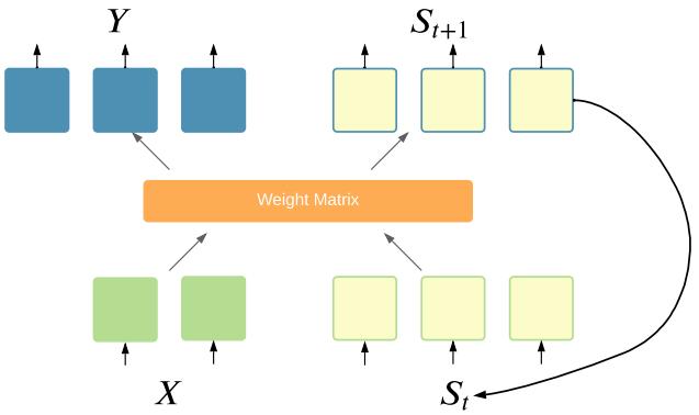
Figure 16.8: Recurrent layer.

where W^{Q i} ↗ ^Rd⇑d^k , W^{K i} ↗ ^Rd⇑d^k and W^{V i} ↗ ^Rd⇑d^v are linear projection matrices. We define the output of the MHA layer to be

\[\mathbf{Z} = \text{MHA}(\mathbf{Q}, \mathbf{K}, \mathbf{V}) = \text{Concat}(\mathbf{h}\_1, \dots, \mathbf{h}\_h) \mathbf{W}^O \tag{16.14}\]

where ^h is the number of heads, and ^WO ↗ ^Rhdv⇑d. Having multiple heads can increase performance of the layer, in the event that some of the weight matrices are poorly initialized; after training, we can often remove all but one of the heads [MLN19].

When the output of one attention layer is used as input to another, the method is called selfattention. This is the basis of the transformer model, which we discuss in Section 16.3.5.

16.2.8 Recurrent layers

We can make the model be stateful by augmenting the input x with the current state st, and then computing the output and the new state using some kind of function:

\[f(y, s\_{t+1}) = f(x, s\_t) \tag{16.15}\]

This is called a recurrent layer, as shown in Figure 16.8. This forms the basis of recurrent neural networks, discussed in Section 16.3.4. In a vanilla RNN, the function f is a simple MLP, but it may also use attention (Section 16.2.7).

16.2.9 Multiplicative layers

In this section, we discuss multiplicative layers, which are useful for combining di!erent information sources. Our presentation follows [Jay+20].

Suppose we have inputs ^x ↗ ^Rn and ^z ↗ ^Rm, In a linear layer (and, by extension, convolutional layers), it is common to concatenate the inputs to get ^f(x, ^z) = ^W[x; ^z] + ^b, where ^W ↗ ^Rk⇑(m+n) and ^b ↗ ^Rk. We can increase the expressive power of the model by using multiplicative interactions, such as the following bilinear form:

\[f(\mathbf{z}, \mathbf{z}) = \mathbf{z}^{\mathsf{T}} \mathbb{W}\mathbf{z} + \mathbf{U}\mathbf{z} + \mathbf{V}\mathbf{z} + \mathbf{b} \tag{16.16}\]

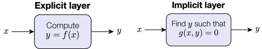
Figure 16.9: Explicit vs implicit layers.

where ^W ↗ ^Rm⇑n⇑^k is a weight tensor, defined such that

\[\mathbb{E}\left(\mathbf{z}^{\mathsf{T}}\mathbb{W}\mathbf{z}\right)\_{k} = \sum\_{ij} \mathbf{z}\_{i}\mathbb{W}\_{ijk}\mathbf{z}\_{j} \tag{16.17}\]

That is, the k’th entry of the output is the weighted inner product of z and x, where the weight matrix is the ^k’th “slice” of ^W. The other parameters have size ^U ↗ ^Rk⇑^m, ^V ↗ ^Rk⇑ⁿ, and ^b ↗ ^Rk.

This formulation includes many interesting special cases. In particular, a hypernetwork [HDL17] can be viewed in this way. A hypernetwork is a neural network that generates parameters for another neural network. In particular, we replace f(x; ω) with f(x; g(z; ε)). If f and g are a”ne, this is equivalent to a multiplicative layer. To see this, let W^↔︎ = z^TW + V and b^↔︎ = Uz + b. If we define g(z; %)=[W^↔︎ , b^↔︎ ], and f(x; ω) = W^↔︎ x + b^↔︎ , we recover Equation (16.16).

We can also view the gating layers used in RNNs (Section 16.3.4) as a form of multiplicative interaction. In particular, if the hypernetwork computes the diagonal matrix W^↔︎ = ς(z^TW + V) = diag(a1,…,an), then we can define f(x, z; ω) = a(z) ∞ x, which is the standard gating mechanism. Attention mechanisms (Section 16.2.7) are also a form of multiplicative interaction, although they involve three-way interactions, between query, key, and value.

Another variant arises if the hypernetwork just computes a scalar weight for each channel of a convolutional layer, plus a bias term:

\[f(\mathbf{z}, \mathbf{z}) = a(\mathbf{z}) \odot \mathbf{z} + \mathbf{b}(\mathbf{z}) \tag{16.18}\]

This is called FiLM, which stands for “feature-wise linear modulation” [Per+18]. For a detailed tutorial on the FiLM layer and its many applications, see https://distill.pub/2018/ feature-wise-transformations.

16.2.10 Implicit layers

So far we have focused on explicit layers, which specify how to transform the input to the output using y = f(x). We can also define implicit layers, which specify the output indirectly, in terms of a constraint function:

\[\begin{aligned} \boldsymbol{y} \in \operatorname\*{argmin}\_{\boldsymbol{y}} f(\boldsymbol{x}, \boldsymbol{y}) \text{ such that } \boldsymbol{g}(\boldsymbol{x}, \boldsymbol{y}) = \boldsymbol{0} \end{aligned} \tag{16.19}\]

The details on how to find a solution to this constrained optimization problem can vary depending on the problem. For example, we may need to run an inner optimization routine, or call a di!erential

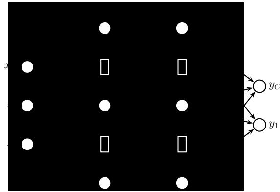
Figure 16.10: A feedforward neural network with D inputs, K¹ hidden units in layer 1, K² hidden units in layer 2, and C outputs. w(l) jk is the weight of the connection from node j in layer l ↗ 1 to node k in layer l.

equation solver. The main advantage of this approach is that the inner computations do not need to be stored explicitly, which saves a lot of memory. Furthermore, once the solution has been found, we can propagate gradients through the whole layer, by leveraging the implicit function theorem. This lets us use higher level primitives inside an end-to-end framework. For more details, see [GHC21] and http://implicit-layers-tutorial.org/.

16.3 Canonical examples of neural networks

In this section, we give several “canonical” examples of neural network architectures that are widely used for di!erent tasks.

16.3.1 Multilayer perceptrons (MLPs)

A multilayer perceptron (MLP), also called a feedforward neural network (FFNN), is one of the simplest kinds of neural networks. It consists of a series of L linear layers, combined with elementwise nonlinearities:

\[f(x; \theta) = \mathbf{W}\_L \varphi\_L(\mathbf{W}\_{L-1} \varphi\_{L-1}(\cdots \varphi\_1(\mathbf{W}\_1 x) \cdots)) \tag{16.20}\]

For example, Figure 16.10 shows an MLP with 1 input layer of D units, 2 hidden layers of K¹ and K² units, and 1 output layer with C units. The k’th hidden unit in layer l is given by

\[h\_k^{(l)} = \varphi\_l \left( b\_k^{(l)} + \sum\_{j=1}^{K\_{l-1}} w\_{jk}^{(l)} h\_j^{(l-1)} \right) \tag{16.21}\]

where 5^l is the nonlinear activation function at layer l.

For a classification problem, the final nonlinearity is usually the softmax function. However, it is also common for the final layer to have linear activations, in which case the outputs are interpreted as logits; the loss function used during training then converts to (log) probabilities internally.

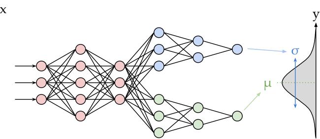
Figure 16.11: Illustration of an MLP with a shared “backbone” and two output “heads”, one for predicting the mean and one for predicting the variance. From https: // brendanhasz. github. io/ 2019/ 07/ 23/ bayesian-density-net. html . Used with kind permission of Brendan Hasz.

We can also use MLPs for regression. Figure 16.11 shows how we can make a model for heteroskedastic nonlinear regression. (The term “heteroskedastic” just means that the predicted output variance is input-dependent, rather than a constant.) This function has two outputs which compute ^fµ(x) = ^E [y|x, ^ω] and ^f↽(x) = ^MV [y|x, ^ω]. We can share most of the layers (and hence parameters) between these two functions by using a common “backbone” and two output “heads”, as shown in Figure 16.11. For the µ head, we use a linear activation, 5(a) = a. For the ς head, we use a softplus activation, 5(a) = ς+(a) = log(1 + e^a). If we use linear heads and a nonlinear backbone, the overall model is given by

\[p(y|\mathbf{z},\boldsymbol{\theta}) = \mathcal{N}\left(y|\mathbf{w}\_{\mu}^{\mathrm{T}}f(\boldsymbol{x};\boldsymbol{w}\_{\mathrm{shareel}}), \sigma\_{+}(\boldsymbol{w}\_{\sigma}^{\mathrm{T}}f(\boldsymbol{x};\boldsymbol{w}\_{\mathrm{shareel}}))\right) \tag{16.22}\]

16.3.2 Convolutional neural networks (CNNs)

A vanilla convolutional neural network or CNN consists of a series of convolutional layers, pooling layers, linear layers, and nonlinearities. See Figure 16.12 for an example. More sophisticated architectures, such as the ResNet model [He+16a; He+16b], add skip (residual) connections, normalization layers, etc. The ConvNeXt model of [Liu+22b] is considered the current (as of February 2022) state of the art CNN architecture for a wide variety of vision tasks. See e.g., [Mur22, Ch.14] for more details on CNNs.

16.3.3 Autoencoders

An autoencoder is a neural network that maps inputs x to a low-dimensional latent space using an encoder, z = fe(x), and then attempts to reconstruct the inputs using a decoder, xˆ = fd(z). The model is trained to minimize

\[\mathcal{L}(\theta) = ||r(x) - x||\_2^2 \tag{16.23}\]

where r(x) = fd(fe(x)). (We can also replace squared error with more general conditional log likelihoods.) See Figure 16.13 for an illustration of a 3 layer AE.

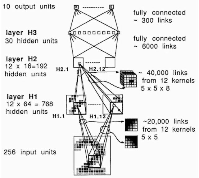
Figure 16.12: One of the first CNNs ever created, for classifying MNIST images. From Figure 3 of [LeC+89]. For a “modern” implementation, see lecun1989.ipynb.

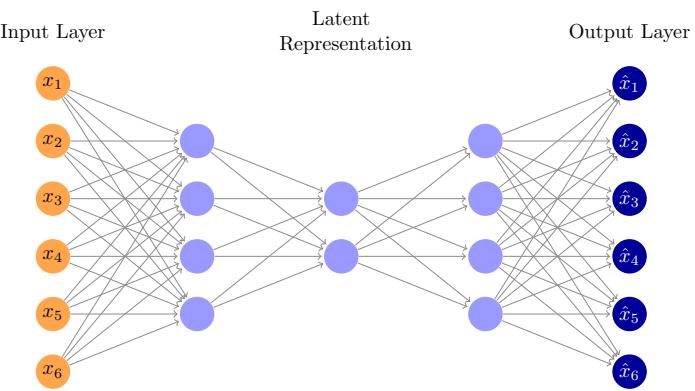
Figure 16.13: Illustration of an autoencoder with 3 hidden layers.

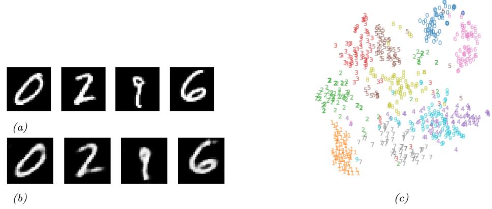
Figure 16.14: (a) Some MNIST digits. (b) Reconstruction of these images using a convolutional autoencoder. (c) t-SNE visualization of the 20-d embeddings. The colors correspond to class labels, which were not used during training. Generated by ae\_mnist\_conv\_jax.ipynb.

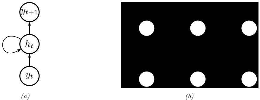
Figure 16.15: Illustration of a recurrent neural network (RNN). (a) With self-loop. (b) Unrolled in time.

For image data, we can make the encoder be a convolutional network, and the decoder be a transpose convolutional network. We can use this to compute low dimensional embeddings of image data. For example, suppose we fit such a model to some MNIST digits. We show the reconstruction abilities of such a model in Figure 16.14b. In Figure 16.14c, we show a 2d visualization of the 20-dimensional embedding space computed using t-SNE. The colors correspond to class labels, which were not used during training. We see fairly good separation, showing that images which are visually similar are placed close to each other in the embedding space, as desired. (See also Section 21.2.3, where we compare AEs with variational AEs.)

16.3.4 Recurrent neural networks (RNNs)

A recurrent neural network (RNN) is a network with a recurrent layer, as in Equation (16.15). This is illustrated in Figure 16.15. Formally this defines the following probability distribution over

1

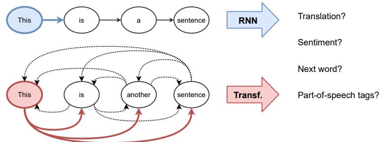
Figure 16.16: Visualizing the di!erence between an RNN and a transformer. From [Jos20]. Used with kind permission of Chaitanya Joshi.

sequences:

\[p(\mathbf{y}\_{1:T}) = \sum\_{\mathbf{h}\_{1:T}} p(\mathbf{y}\_{1:T}, \mathbf{h}\_{1:T}) = \sum\_{\mathbf{h}\_{1:T}} \mathbb{I}\left(\mathbf{h}\_1 = \mathbf{h}\_1^\*\right) p(\mathbf{y}\_1|\mathbf{h}\_1) \prod\_{t=2}^T p(\mathbf{y}\_t|\mathbf{h}\_t) \mathbb{I}\left(\mathbf{h}\_t = f(\mathbf{h}\_{t-1}, \mathbf{y}\_{t-1})\right) \tag{16.24}\]

where h^t is the deterministic hidden state, computed from the last hidden state and last output using f(h^t↓¹, y^t↓¹). (At training time, y^t↓¹ is observed, but at prediction time, it is generated.)

In a vanilla RNN, the function f is a simple MLP. However, we can also use attention to selectively update parts of the state vector based on similarity between the input the previous state, as in the GRU (gated recurrent unit) model, and the LSTM (long short term memory) model. We can also make the model into a conditional sequence model, by feeding in extra inputs to the f function. See e.g., [Mur22, Ch. 15] for more details on RNNs.

16.3.5 Transformers

Consider the problem of classifying each word in a sentence, for example with its part of speech tag (noun, verb, etc). That is, we want to learn a mapping ^f : ^X ↖ ^Y, where ^X = ^VT is the set of input sequences defined over (word) vocabulary ^V, ^T is the length of the sentence, and ^Y = ^{T T} is the set of output sequences, defined over (tag) vocabulary T . To do well at this task, we need to learn a contextual embedding of each word. RNNs process one token at a time, so the embedding of the word at location t, zt, depends on the hidden state of the network, st, which may be a lossy summary of all the previously seen words. We can create bidirectional RNNs so that future words can also a!ect the embedding of zt, but this dependence is still mediated via the hidden state. An alternative approach is to compute z^t as a direct function of all the other words in the sentence, by using the attention operator discussed in Section 16.2.7 rather than using hidden state. This is called an (encoder-only) transformer, and is used by models such as BERT [Dev+19]. This idea is sketched in Figure 16.16.

It is also possible to create a decoder-only transformer, in which each output y^t only attends to all the previously generated outputs, y1:t↓¹. This can be implemented using masked attention, and is useful for generative language models, such as GPT (see Section 22.4.1). We can combine the encoder and decoder to create a conditional sequence-to-sequence model, p(y1:T^y |x1:T^x ), as proposed in the original transformer paper [Vas+17c]. See Supplementary Section 16.1.1 and [PH22] for more details.

It has been found that large transformers are very flexible sequence-to-sequence function approximators, if trained on enough data (see e.g., [Lin+21a] for a review in the context of NLP, and [Kha+21; Han+20; Zan21] for reviews in the context of computer vision). The reasons why they work so well are still not very clear. However, some initial insights can be found in, e.g., [Rag+21; WGY21; Nel21; BP21]. See also Supplementary Section 16.1.2.5 where we discuss the connection with graph neural networks, and [Tur23] for a more general discussion.

16.3.6 Graph neural networks (GNNs)

It is possible to define neural networks for working with graph-structured data. These are called graph neural networks or GNNs. See Supplementary Section 16.1.2 for details.

17 Bayesian neural networks

This chapter is coauthored with Andrew Wilson.

17.1 Introduction

Deep neural networks (DNNs) are usually trained using a (penalized) maximum likelihood objective to find a single setting of parameters. However, large flexible models like neural networks can represent many functions, corresponding to di!erent parameter settings, which fit the training data well, yet generalize in di!erent ways. (This phenomenon is known as underspecification (see e.g., [D’A+20]; see Figure 17.11 for an illustration.) Considering all of these di!erent models together can lead to improved accuracy and uncertainty representation. This can be done by computing the posterior predictive distribution using Bayesian model averaging:

\[p(\mathbf{y}|\mathbf{z}, \mathcal{D}) = \int p(\mathbf{y}|\mathbf{z}, \boldsymbol{\theta}) p(\boldsymbol{\theta}|\mathcal{D}) d\boldsymbol{\theta} \tag{17.1}\]

where p(ω|D) ↑ p(ω)p(D|ω).

The main challenges in applying Bayesian inference to DNNs are specifying suitable priors, and e”ciently computing the posterior, which is challenging due to the large number of parameters and the large datasets. The application of Bayesian inference to DNNs is sometimes called Bayesian deep learning or BDL. By contrast, the term deep Bayesian learning or DBL refers to the use of deep models to help speed up Bayesian inference of “classical” models, usually by training amortized inference networks that can be used as part of a variational inference or importance sampling algorithm, as discussed in Section 10.1.5.) For more details on the topic of BDL, see e.g., [PS17; Wil20; WI20; Jos+22; Kha20; Arb+23].

17.2 Priors for BNNs

To perform Bayesian inference for the parameters of a DNN, we need to specify a prior p(ω). [Nal18; WI20; For22] discusses the issue of prior selection at length. Here we just give a brief summary of common approaches.

17.2.1 Gaussian priors

Consider an MLP with one hidden layer with activation function 5 and a linear output:

\[f(x; \theta) = \mathbf{W}\_2 \varphi(\mathbf{W}\_1 x + \mathbf{b}\_1) + \mathbf{b}\_2 \tag{17.2}\]

(If the output is nonlinear, such as a softmax transform, we can fold it into the loss function during training.) If we have two hidden layers this becomes

\[f(\mathbf{z}; \boldsymbol{\theta}) = \mathbf{W}\_3 \left( \varphi \left( \mathbf{W}\_2 \varphi (\mathbf{W}\_1 \mathbf{z} + \mathbf{b}\_1) + \mathbf{b}\_2 \right) \right) + \mathbf{b}\_3 \tag{17.3}\]

In general, with L → 1 hidden layers and a linear output, we have

\[f(x; \theta) = \mathbf{W}\_L \left( \cdots \varphi(\mathbf{W}\_1 x + \mathbf{b}\_1) \right) + \mathbf{b}\_L \tag{17.4}\]

We need to specify the priors for W^l and b^l for l =1: L. The most common choice is to use a factored Gaussian prior:

\[\mathbf{W}\_{\ell} \sim \mathcal{N}(\mathbf{0}, \alpha\_{\ell}^{2} \mathbf{I}), \ \mathbf{b}\_{\ell} \sim \mathcal{N}(\mathbf{0}, \beta\_{\ell}^{2} \mathbf{I}) \tag{17.5}\]

The Xavier initialization or Glorot initialization, named after the first author of [GB10], is to set

\[\alpha\_{\ell}^{2} = \frac{2}{n\_{\text{in}} + n\_{\text{out}}} \tag{17.6}\]

where nin is the fan-in of a node in level ε (number of weights coming into a neuron), and nout is the fan-out (number of weights going out of a neuron). LeCun initialization, named after Yann LeCun, corresponds to using

\[ \alpha\_{\ell}^{2} = \frac{1}{n\_{\text{in}}} \tag{17.7} \]

We can get a better understanding of these priors by considering the e!ect they have on the corresponding distribution over functions that they define. To help understand this correspondence, let us reparameterize the model as follows:

\[\mathbf{W}\_{\ell} = \alpha\_{\ell} \boldsymbol{\eta}\_{\ell}, \ \boldsymbol{\eta}\_{\ell} \sim \mathcal{N}(\mathbf{0}, \mathbf{I}), \ \mathbf{b}\_{\ell} = \beta\_{\ell} \boldsymbol{\epsilon}\_{\ell}, \ \boldsymbol{\epsilon}\_{\ell} \sim \mathcal{N}(\mathbf{0}, \mathbf{I}) \tag{17.8}\]

Hence every setting of the prior hyperparameters specifies the following random function:

\[f(\mathbf{z}; \alpha, \beta) = \alpha\_L \eta\_L (\cdots \varphi(\alpha\_1 \eta\_1 \mathbf{z} + \beta\_1 \mathbf{e}\_1)) + \beta\_L \mathbf{e}\_L \tag{17.9}\]

To get a feeling for the e!ect of these hyperparameters, we can sample MLP parameters from this prior and plot the resulting random functions. We use a sigmoid nonlinearity, so 5(a) = ς(a). We consider L = 2 layers, so W¹ are the input-to-hidden weights, and W² are the hidden-to-output weights. We assume the input and output are scalars, so we are generating random nonlinear 1d mappings f : R ↖ R.

Figure 17.1(a) shows some sampled functions where ϱ¹ = 5, ↼¹ = 1, ϱ² = 1, ↼² = 1. In Figure 17.1(b) we increase ϱ1; this allows the first layer weights to get bigger, making the sigmoid-like

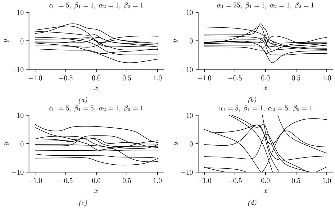
Figure 17.1: The e!ects of changing the hyperparameters on an MLP with one hidden layer. (a) Random functions sampled from a Gaussian prior with hyperparameters φ¹ = 5, β¹ = 1, φ² = 1, β² = 1. (b) Increasing φ¹ by a factor of 5. (c) Increasing β¹ by a factor of 5. (d) Increasing φ² by a factor of 5. Generated by mlp\_priors\_demo.ipynb.

shape of the functions steeper. In Figure 17.1(c), we increase ↼1; this allows the first layer biases to get bigger, which allows the center of the sigmoid to shift left and right more, away from the origin. In Figure 17.1(d), we increase ϱ2; this allows the second layer linear weights to get bigger, making the functions more “wiggly” (greater sensitivity to change in the input, and hence larger dynamic range).

The above results are specific to the case of sigmoidal activation functions. ReLU units can behave di!erently. For example, [WI20, App. E] show that for MLPs with ReLU units, if we set ↼^ω = 0, so the bias terms are all zero, the e!ect of changing ϱ^ω is just to rescale the output. To see this, note that Equation (17.9) simplifies to

\[f(\mathbf{z}; \alpha, \beta = \mathbf{0}) = \alpha\_L \eta\_L(\cdots \varphi(\alpha\_1 \eta\_1 \mathbf{z})) = \alpha\_L \cdots \alpha\_1 \eta\_L(\cdots \varphi(\eta\_1 \mathbf{z})) \tag{17.10}\]

\[\alpha = \alpha\_L \cdots \alpha\_1 f(x; (\alpha = 1, \beta = 0)) \tag{17.11}\]

where we used the fact that for ReLU, 5(ϱz) = ϱ5(z) for any positive ϱ, and 5(ϱz)=0 for any negative ϱ (since the preactivation z ≃ 0). In general, it is the ratio of ϱ and ↼ that matters for determining what happens to input signals as they propagate forwards and backwards through a randomly initialized model; for details, see e.g., [Bah+20].

We see that initializing the model’s parameters at a particular random value is like sampling a

point from this prior over functions. In the limit of infinitely wide neural networks, we can derive this prior distribution analytically: this is known as a neural network Gaussian process, and is explained in Section 18.7.

17.2.2 Sparsity-promoting priors

Although Gaussian priors are simple and widely used, they are not the only option. For some applications, it is useful to use sparsity promoting priors, such as the Laplace, which encourage most of the weights (or channels in a CNN) to be zero (cf. Section 15.2.6). For details, see [Hoe+21].

17.2.3 Learning the prior

We have seen how di!erent priors for the parameters correspond to di!erent priors over functions. We could in principle set the hyperparameters (e.g., the ↼ and ⇀ parameters of the Gaussian prior) using grid search to optimize cross-validation loss. However, cross-validation can be slow, particularly if we allow di!erent priors for each layer of the network, as our grid search will grow exponentially with the number of hyperparameters we wish to determine.

An alternative is to use gradient based methods to optimize the marginal likelihood

\[\log p(\mathcal{D}|\alpha, \mathcal{B}) = \int \log p(\mathcal{D}|\theta) p(\theta|\alpha, \mathcal{B}) d\theta \tag{17.12}\]

This approach is known as empirical Bayes (Section 3.7) or evidence maximization, since log p(D|↼, ⇀) is also called the evidence [Mac92a; WS93; Mac99]. This can give rise to sparse models, as we discussed in the context of automatic relevancy determination (Section 15.2.8). Unfortunately, computing the marginal likelihood is computationally di”cult for large neural networks.

Learning the prior is more meaningful if we can do it on a separate, but related dataset. In [SZ+22] they propose to train a model on an initial, large dataset D¹ (possibly unsupervised) to get a point estimate, ωˆ1, from which they can derive an approximate low-rank Gaussian posterior, using the SWAG method (Section 17.3.8). They then use this informative prior when fine-tuning the model on a downstream dataset ^D2. The fine-tuning can either be a MAP estimate ^ωˆ² or some approximate posterior, p(ω2|D2, D1), e.g., computed using MCMC (Section 17.3.7). They call this technique “Bayesian transfer learning”. (See Section 19.5.1 for more details on transfer learning.)

17.2.4 Priors in function space

Typically, the relationship between the prior distribution over parameters and the functions preferred by the prior is not transparent. In some cases, it can be possible to pick more informative priors based on principles such as desired invariances that we want the function to satisfy (see e.g., [Nal18]). [FBW21] introduces residual pathway priors, providing a mechanism for encoding high level concepts into prior distributions, such as locality, independencies, and symmetries, without constraining model flexibility. A di!erent approach to encoding interpretable priors over functions leverages kernel methods such as Gaussian processes (e.g., [Sun+19a]), as we discuss in Section 18.1.

17.2.5 Architectural priors

Beyond specifying the parametric prior, it is important to note that the architecture of the model can have an even larger e!ect on the induced distribution over functions, as argued in Wilson and Izmailov [WI20] and Izmailov et al. [Izm+21b]. For example, a CNN architecture encodes prior knowledge about translation equivariance, due to its use of convolution, and hierarchical structure, due to its use of multiple layers. Other forms of inductive bias are induced by di!erent architectures, such as RNNs. (Models such as transformers have weaker inductive bias, but consequently often need more data to perform well.) Thus we can think of the field of neural architecture search (reviewed in [EMH19]) as a form of structural prior learning.

In fact, with a suitable architecture, we can often get good results using random (untrained) models. For example, Ulyanov, Vedaldi, and Lempitsky [UVL18] showed that an untrained CNN with random parameters (sampled from a Gaussian) often works very well for low-level image processing tasks, such as image denoising, super-resolution, and image inpainting. The resulting prior over functions has been called the deep image prior. Similarly, Pinto and Cox [PC12] showed that untrained CNNs with the right structure can do well at face recognition. Moreover, Zhang et al. [Zha+17] show that randomly initialized CNNs can process data to provide features that greatly improve the performance of other models, such as kernel methods.

17.3 Posteriors for BNNs

There are a large number of di!erent approximate inference schemes that have been applied to Bayesian neural networks, with di!erent strengths and limitations. In the sections below, we briefly describe some of these.

17.3.1 Monte Carlo dropout

Monte Carlo dropout (MCD) [GG16; KG17] is a very simple and widely used method for approximating the Bayesian predictive distribution. Usually stochastic dropout layers are added as a form of regularization, and are “turned o!” at test time, as described in Section 16.2.6, However, the idea in MCD is to also perform random sampling at test time. More precisely, we drop out each hidden unit by sampling from a Bernoulli(p) distribution; we repeat this procedure S times, to create S distinct models. We then create an equally weighted average of the predictive distributions for each of these models:

\[p(y|\mathbf{z}, \mathcal{D}) \approx \frac{1}{S} \sum\_{s=1}^{S} p(y|\mathbf{z}, \mathbf{\theta}^s) \tag{17.13}\]

where ω^s is a version of the MAP parameter estimate where we randomly drop out some connections.

We give an example of this process in action in Figure 17.2. We see that it succesfully captures uncertainty due to “out of distribution” inputs. (See Section 19.3.2 for more discussion of OOD detection.)

One drawback of MCD is that it is slow at test time. However this can be overcome by “distilling” the model’s predictions into a deterministic “student” network, as we discuss in Section 17.3.10.3.

A more fundamental problem is that MCD does not give proper uncertainty estimates, as argued in [Osb16; LF+21]. The problem is the following. Although MCD can be viewed as a form of variational

Figure 17.2: Illustration of MC dropout applied to the LeNet architecture. The inputs are some rotated images of the digit 1 from the MNIST dataset. (a) Softmax inputs (logits). (b) Softmax outputs (proabilities). We see that the inputs are classified as digit 7 for the last three images (as shown by the probabilities), even though the model has high uncertainty (as shown by the logits). Adapted from Figure 4 of [GG16]. Generated by mnist\_classification\_mc\_dropout.ipynb

inference [GG16], this is only true under a degenerate posterior approximation, corresponding to a mixture of two delta functions, one at 0 (for dropped out nodes) and one at the MLE. This posterior will not converge to the true posterior (which is a delta function at the MLE) even as the training set size goes to infinity, since we are always dropping out hidden nodes with a constant probability p [Osb16]. Fortunately this pathology can be fixed if the noise rate is optimized [GHK17]. For more details, see e.g., [HGMG18; NHLS19; LF+21].

17.3.2 Laplace approximation

In Section 7.4.3, we introduced the Laplace approximation, which computes a Gaussian approximation to the posterior, p(ω|D), centered at the MAP estimate, ω→. The posterior prediction matrix is equal to the Hessian of the negative log joint computed at the mode. The benefits of this approach are that it is simple, and it can be used to derive a Bayesian estimate from a pretrained model. The main disadvantage is that computing the Hessian can be expensive. In addition, it may not be positive definite, since the log likelihood of DNNs is non-convex. It is therefore common to use a Gauss-newton approximation to the Hessian instead, as we explain below.

Following the notation of [Dax+21], let ^f(xn, ^ω) ↗ ^RC be the prediction function with ^C outputs, and ^ω ↗ ^RP be the parameter vector. Let ^r(y; ^f) = ^⇒f log ^p(y|f) be the residual1, and %(y; ^f) = →⇒^{2 f} log ^p(y|f) be the per-input noise term. In addition, let ^J ↗ ^RC⇑^P be the Jacobian, [Jε(x)]ci ⁼ ϑfc(x,ε) ϑϱⁱ , and ^H ↗ ^RC⇑^P ⇑^P be the Hessian, [Hε(x)]cij ^{= ϑ}2fc(x,ε) ϑϱiϑϱ^j . Then the gradient and Hessian

^1. In the Gaussian case, this term becomes ^↓f ||^{y ↔︎ f}||² = 2||^{y ↔︎ f}||, so it can be interpreted as a residual error.

of the log likelihood are given by the following [IKB21]:

\[\nabla\_{\theta} \log p(y|f(x,\theta)) = \mathbf{J}\_{\theta}(x)^{\mathsf{T}} r(y;f) \tag{17.14}\]

\[\nabla^2\_{\theta} \log p(y|f(x,\theta)) = \mathbf{H}\_{\theta}(x)^\top r(y;f) - \mathbf{J}\_{\theta}(x)^\top \Lambda(y;f)\mathbf{J}\_{\theta}(\theta) \tag{17.15}\]

Since the network Hessian H is usually intractable to compute, it is usually dropped, leaving only the Jacobian term. This is called the generalized Gauss-Newton or GGN approximation [Sch02; Mar20]. The GGN approximation is guaranteed to be positive definite. By contrast, this is not true for the original Hessian in Equation (17.15), since the objective is not convex. Furthermore, computing the Jacobian term is cheaper to compute than the Hessian.

Putting it all together, for a Gaussian prior, p(ω) = N (ω|m0, S0), the Laplace approximation becomes p(ω|D) ↓ (N |ω→, !GGN), where

\[\Sigma\_{\rm GGN}^{-1} = \sum\_{n=1}^{N} \mathbf{J}\_{\theta^\*} (x\_n)^{\mathsf{T}} \Lambda(y\_n; f\_n) \mathbf{J}\_{\theta^\*} (x\_n) + \mathbf{S}\_0^{-1} \tag{17.16}\]

Unfortunately inverting this matrix takes O(P³) time, so for models with many parameters, further approximations are usually used. The simplest is to use a diagonal approximation, which takes O(P) time and space. A more sophisticated approach is presented in [RBB18a], which leverages the KFAC (Kronecker factored curvature) approximation of [MG15]. This approximates the covariance of each layer using a Kronecker product.

A limitation of the Laplace approximation is that the posterior covariance is derived from the Hessian evaluated at the MAP parameters. This means Laplace forms a highly local approximation: even if the non-Gaussian posterior could be well-described by a Gaussian distribution, the Gaussian distribution formed using Laplace only captures the local characteristics of the posterior at the MAP parameters — and may therefore su!er badly from local optima, providing overly compact or di!use representations. In addition, the curvature information is only used after the model has been estimated, and not during the model optimization process. By contrast, variational inference (Section 17.3.3) can provide more accurate approximations for comparable cost.

17.3.3 Variational inference

In fixed-form variational inference (Section 10.2), we choose a distribution for the posterior approximation qϑ(ω)and minimize DKL (q ↘ p), with respect to ϖ. We often choose a Gaussian approximate posterior, qϑ(ω) = N (ω|µ, !), which lets us use the reparameterization trick to create a low variance estimator of the gradient of the ELBO (see Section 10.2.1). Despite the use of a Gaussian, the parameters that minimize the KL objective are often di!erent from what we would find with the Laplace approximation (Section 17.3.2).

Variational methods for neural networks date back to at least Hinton and Camp [HC93]. In deep learning, [Gra11] revisited variational methods, using a Gaussian approximation with a diagonal covariance matrix. This approximates the distribution of every parameter in the model by a univariate Gaussian, where the mean is the point estimate, and the variance captures the uncertainty, as shown in Figure 17.3. This approach was improved further in [Blu+15], who used the reparameterization trick to compute lower variance estimates of the ELBO; they called their method Bayes by backprop (BBB). This is essentially identical to the SVI algorithm in Algorithm 10.2, except the likelihood becomes p(yn|xn, ω) from the DNN, and the prior pϱ(ω) and variational posterior qϑ(ω) are Gaussians.

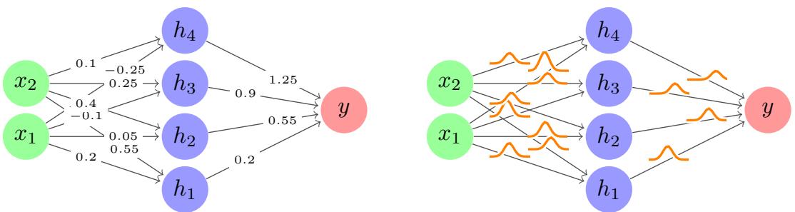
Figure 17.3: Illustration of an MLP with (left) a point estimate for each weight, (right) a marginal distribution for each weight, corresponding to a fully factored posterior approximation.

Many extensions of the BBB have been proposed. In [KSW15], they propose the local reparameterization trick, that samples the activations a = Wz at each layer, instead of the weights W, which results in a lower variance estimate of the ELBO gradient. In [Osa+19a], they used the variational online Gauss-Newton (VOGN) method of [Kha+18], for improved scalability. VOGN is a noisy version of natural gradient descent, where the extra noise emulates the e!ect of variational inference. In [Mis+18], they replaced the diagonal approximation with a low-rank plus diagonal approximation, and used VOGN for fitting. In [Tra+20b], they use a rank-one plus diagonal approximation known as NAGVAC (see Section 10.2.1.3). In this case, there are only 3 times as many parameters as when computing a point estimate (for the variational mean, variance, and rank-one vector), making the approach very scalable. In addition, in this case it is possible to analytically compute the natural gradient, which speeds up model fitting (see Section 6.4). Many other variational methods have also been proposed (see e.g., [LW16; Zha+18; Wu+19a; HHK19]). See also Section 17.5.4 for a discussion of online VI for DNNs.

17.3.4 Expectation propagation

Expectation propagation (EP) is similar to variational inference, except it locally optimizes DKL (p ↘ q) instead of DKL (q ↘ p), where p is the exact posterior and q is the approximate posterior. For details, see Section 10.7.

A special case of EP is the assumed density filtering (ADF) algorithm of Section 8.6, which is equivalent to the first pass of ADF. In Section 8.6.3 we show how to apply ADF to online logistic regression. In [HLA15a], they extend ADF to the case of BNNs; they called their method probabilistic backpropagation or PBP. They approximate every parameter in the model by a Gaussian factor, as in Figure 17.3. See Section 17.5.3 for the details.

17.3.5 Last layer methods

A very simple approximation to the posterior is to only “be Bayesian” about the weights in the final layer, and to use MAP estimates for all the other parameters. This is called the neural-linear approximation [RTS18]. In more detail, let z = f(x, ω) be the predicted outputs (e.g., logits) of the model before any optional final nonlinearity. We assume this has the form z = w^{T L}ε(x; ω),

where ε(x) are the features extracted by the first L → 1 layers. This gives us a Bayesian GLM. We can use standard techniques, such as the Laplace approximation (Section 15.3.5), to compute p(wL|D) = N (µL, !L), given ε(). To estimate the parameters of the feature extractor, we can optimize the log-likelihood in the usual way. Given the posterior over the last layer weights, we can compute the posterior predictive distribution over the logits using

\[p(\mathbf{z}|\mathbf{z}, \mathcal{D}) = \mathcal{N}(\mathbf{z}|\boldsymbol{\mu}\_L \phi(\mathbf{z}), \phi(\mathbf{z}) \Sigma\_L \phi(\mathbf{z})^\top) \tag{17.17}\]

This can be passed through the final softmax layer to compute p(y|x, D) as described in Section 15.3.6.

In [KHH20] they show this can reduce overconfidence in predictions for inputs that are far from the training data. However, this approach ignores uncertainty introduced by the earlier feature extraction layers, where most of the parameters reside. We discuss a solution to this in Section 17.3.6.

17.3.6 SNGP

It is possible to combine DNNs with Gaussian process (GP) models (Chapter 18), by using the DNN to act as a feature extractor, which is then fed into the kernel in the final layer. This is called “deep kernel learning” (see Section 18.6.6).

One problem with this is that the feature extractor may lose information which is not needed for classification accuracy, but which is needed for robust performance on out-of-distribution inputs (see Section 17.4.6.2). The basic problem is that, in a classification problem, there is no reduction in training accuracy (log likelihood) if points which are far away are projected close together, as long as they are on the correct side of the decision boundary. Thus the distances between two inputs can be erased by the feature extraction layers, so that OOD inputs appear to the final layer to be close to the training set.

One solution to this is to use the SNGP (spectrally normalized Gaussian process) method of [Liu+20d; Liu+22a]. This constrains the feature extraction layers to be “distance preserving”, so that two inputs that are far apart in input space remain far apart after many layers of feature extraction, by using spectral normalization of the weights to bound the Lipschitz constant of the feature extractor. The overall approach ensures that information that is relevant for computing the confidence of a prediction, but which might be irrelevant to computing the label of a prediction, is not lost. This can help performance in tasks such as out-of-distribution detection (Section 17.4.6.2).

17.3.7 MCMC methods

Some of the earliest work on inference for BNNs was done by Radford Neal, who proposed to use Hamiltonian Monte Carlo (Section 12.5) to approximate the posterior [Nea96]. This is generally considered the gold standard method, since it does not make strong assumptions about the form of the posterior. For more recent work on scaling up HMC for BNNs, see e.g., [Izm+21b; CJ21].

We give a simple example of vanilla HMC in Figure 17.4, where we fit a shallow MLP to a small 2d binary dataset. We plot the mean and standard deviation of the posterior predictive distribution, p(y = 1|x; D). We see that the uncertainty is higher as we move away from the training data. (Compare to Bayesian logistic regression in 1d in Figure 15.8a.)

However, a significant limitation of standard MCMC procedures, including HMC, is that they require access to the full training set at each step. Stochastic gradient MCMC methods, such as

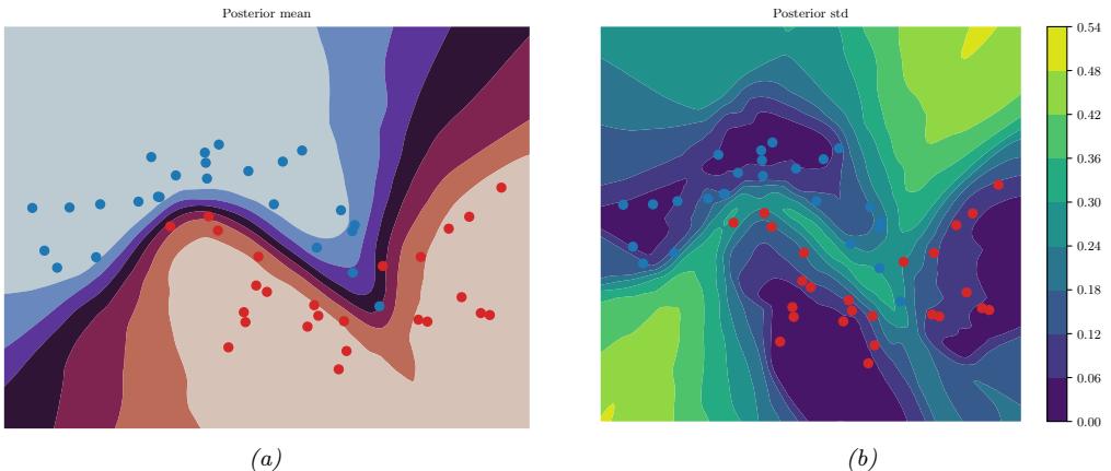
Figure 17.4: Illustration of an MLP fit to the two-moons dataset using HMC. (a) Posterior mean. (b) Posterior standard derivation. The uncertainty increases as we move away from the training data. Generated by bnn\_mlp\_2d\_hmc.ipynb.

SGLD, operate instead using mini-batches of data, o!ering a scalable alternative, as we discuss in Section 12.7.1. For an example of SGLD applied to an MLP, see Section 19.3.3.1.

17.3.8 Methods based on the SGD trajectory

In [MHB17; SL18; CS18], it was shown that, under some assumptions, the iterates produced by stochastic gradient descent (SGD), when run at a fixed learning rate, correspond to samples from a Gaussian approximation to the posterior centered at a local mode, ^p(ω|D) ^{↓ N} (ω|ωˆ, !). We can therefore use SGD to generate approximate posterior samples. This is similar to SG-MCMC methods, except we do not add explicit gradient noise, and the learning rate is held constant.

In [Izm+18], they noted that these SGD solutions (with fixed learning rate) surround the periphery of points of good generalization, as shown in Figure 17.5. This is in part because SGD does not converge to a local optimum unless the learning rate is annealed to 0. They therefore proposed to compute the average of several SGD samples, each one collected after a certain interval (e.g., one epoch of training), to get ω = ¹ S &^{S s}=1 ωs. They call this stochastic weight averaging (SWA). They showed that the resulting point tends to correspond to a broader local minimum than the SGD solutions (see Figure 17.10), resulting in better generalization performance.

The SWA approach is related to Polyak-Ruppert averaging, which is often used in convex optimization. The di!erence is that Polyak-Ruppert typically assumes the learning rate decays to zero, and uses an exponential moving average (EMA) of iterates, rather than an equal average; Polyak-Ruppert averaging is mainly used to reduce variance in the SGD estimate, rather than as a method to find points of better generalization.

The SWA approach is also related to snapshot ensembles [Hua+17a], and fast geometric ensembles [Gar+18c]; these methods save the parameters ω^s after increasing and decreasing the learning rate multiple times in a cyclical fashion, and then computing the average of the predictions using ^p(y|x, ^D) ^{↓ 1} S &^{S s}=1 p(y|x, ωs), rather than computing the average of the parameters and

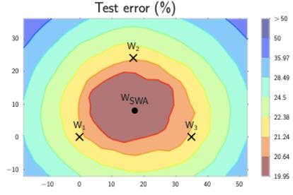
Figure 17.5: Illustration of stochastic weight averaging (SWA). The three crosses represent di!erent SGD solutions. The star in the middle is the average of these parameter values. From Figure 1 of [Izm+18]. Used with kind permission of Andrew Wilson.

predicting with a single model (which is faster). Moreover, by finding a flat region, representing a “center or mass” in the posterior, SWA can be seen as approximating the Bayesian model average in Equation 17.1 with a single model.

In [Mad+19], they proposed to fit a Gaussian distribution to the set of samples produced by SGD near a local mode. They use the SWA solution as the mean of the Gaussian. For the covariance matrix, they use a low-rank plus diagonal approximation of the form p(ω|D) = N (ω|ω, !), where ! = (!diag ⁺ !lr)/2, !diag ⁼ diag(ω^{2 →} (ω)²), ^{ω = 1} S &^{S s}=1 ωs, ω² = ¹ S &^{S s}=1 ω^{2 s} , and !lr = ¹ S&&^T is the sample covariance matrix of the last K samples of &ⁱ = (ωⁱ → ωi), where ωⁱ is the running average of the parameters from the first i samples. They call this method SWAG, which stands for “stochastic weight averaging with Gaussian posterior”. This can be used to generate an arbitrary number of posterior samples at prediction time. They show that SWAG scales to large residual networks with millions of parameters, and large datasets such as ImageNet, with improved accuracy and calibration over conventional SGD training, and no additional training overhead.

17.3.9 Deep ensembles

Many conventional approximate inference methods focus on approximating the posterior p(ω|D) in a local neighborhood around one of the posterior modes. While this is often not a major limitation in classical machine learning, modern deep neural networks have highly multi-modal posteriors, with parameters in di!erent modes giving rise to very di!erent functions. On the other hand, the functions in a neighborhood of a single mode may make fairly similar predictions. So using such a local approximation to compute the posterior predictive will underestimate uncertainty and generalize more poorly.

A simple alternative method is to train multiple models, and then to approximate the posterior using an equally weighted mixture of delta functions,

\[p(\boldsymbol{\theta}|\mathcal{D}) \approx \frac{1}{M} \sum\_{m=1}^{M} \delta(\boldsymbol{\theta} - \hat{\boldsymbol{\theta}}\_{m}) \tag{17.18}\]

where M is the number of models, and ωˆ^m is the MAP estimate for model m. See Figure 17.6 for a

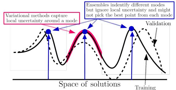
Figure 17.6: Cartoon illustration of the NLL as it varies across the parameter space. Subspace methods (red) model the local neighborhood around a local mode, whereas ensemble methods (blue) approximate the posterior using a set of distinct modes. From Figure 1 of [FHL19]. Used with kind permission of Balaji Lakshminarayanan.

sketch. This approach is called deep ensembles [LPB17; FHL19].

The models can di!er in terms of their random seed used for initialization [LPB17], or hyperparameters [Wen+20c], or architecture [Zai+20], or all of the above. In addition, [DF21; TB22] discusses how to add an explicit repulsive term to ensure functional diversity between the ensemble members. This way, each member corresponds to a distinct prediction function. Combining these is more e!ective than combining multiple samples from the same basin of attraction, especially in the presence of dataset shift [Ova+19].

17.3.9.1 Multi-SWAG

We can further improve on this approach by fitting a Gaussian to each local mode using the SWAG method from Section 17.3.8 to get a mixture of Gaussians approximation:

\[p(\boldsymbol{\theta}|\mathcal{D}) \approx \frac{1}{M} \sum\_{m=1}^{M} N(\boldsymbol{\theta}|\hat{\boldsymbol{\theta}}\_{m}, \boldsymbol{\Sigma}\_{m}) \tag{17.19}\]

This approach is known as MultiSWAG [WI20]. MultiSWAG performs a Bayesian model average both across multiple basins of attraction, like deep ensembles, but also within each basin, and provides an easy way to generate an arbitrary number of posterior samples, S>M, in an any-time fashion.

17.3.9.2 Deep ensembles with random priors

The standard way to fit each member of a deep ensemble is to initialize them each with a di!erent random set of parameters, but them to train them all on the same data. Unfortunately this can result in the predictions from each ensemble member being rather similar, which reduces the benefit of the approach. One way to increase diversity is to train each member on a di!erent subset of the data; this is called bootstrap sampling. Another approach is to define the i’th ensemble member gi(x) to be the addition of a trainable model ti(x) and a fixed, but random, prior network, pi(x), to get

\[g\_i(x; \theta\_i) = t\_i(x; \theta\_i) + \beta p\_i(x) \tag{17.20}\]

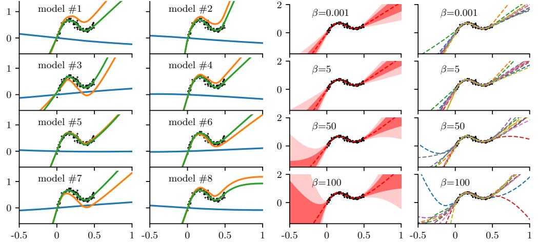
Figure 17.7: Deep ensemble with random priors. (a) Individual predictions from each member. Blue is the fixed random prior function, orange is the trainable function, green is the combination of the two. (b) Overall prediction from the ensemble, for increasingly large values of β. On the left we show (in red) the posterior mean and pointwise standard deviation, and on the right we show samples from the posterior. As β increases, we trust the random priors more, and pay less attention to the data, thus getting a more di!use posterior. Generated by randomized\_priors.ipynb.

where ↼ ≃ 0 controls the amount of data-independent variation between the members. The trainable network learns to model the residual error between the true output and the value predicted by the prior. This is called a random prior deep ensemble [OAC18]. See Figure 17.7 for an illustration.

17.3.9.3 Deep ensembles as approximate Bayesian inference

The posterior predictive distribution for a Bayesian neural network cannot be expressed in closed form. Therefore all Bayesian inference approaches in deep learning are approximate. In this context, all approximate inference procedures fall onto a spectrum, representing how closely they approximate the true posterior predictive distribution. Deep ensembles can provide better approximations to a Bayesian model average than a single basin marginalization approach, because point masses from di!erent basins of attraction represent greater functional diversity than standard Bayesian approaches which sample within a single basin.

17.3.9.4 Deep ensembles vs classical ensembles

Note that deep ensembles are slightly di!erent from classical ensemble methods (see e.g., [Die00]), such as bagging and random forests, which obtain diversity of their predictors by training them on di!erent subsets of the data (created using bootstrap resampling), or on di!erent features. This data perturbation is necessary to get diversity when the base learner is a convex problem (such as a linear model, or shallow decision tree). In the deep ensemble approach, every model is trained on the same data, and the same input features. The diversity arises due to di!erent starting parameters, di!erent

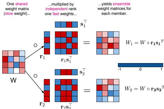
Figure 17.8: Illustration of batch ensemble with 2 ensemble members. From Figure 2 of [WTB20]. Used with kind permission of Paul Vicol.

random seeds, and SGD noise, which induces di!erent solutions due to the nonconvex loss. It is also possible to explicitly enforce diversity of the ensemble members, which can provably improve performance [TB22].

17.3.9.5 Deep ensembles vs mixtures of experts and stacking

If we use weighted combinations of the models, ^p(ω|D) = &^{M m}=1 p(m|D)p(ω|m, D), where p(m|D) is the marginal likelihood of model m, then, in the large sample limit, this mixture will concentrate on the MAP model, so only one component will be selected. By contrast, in deep ensembles, we always use M equally weighted models. Thus we see that Bayes model averaging is not the same as model ensembling [Min00b]. Indeed, ensembling can enlarge the expressive power of the posterior predictive distribution compared to BMA [OCM21].

We can also make the mixing weights be conditional on the inputs:

\[p(y|\mathbf{z}, \mathcal{D}) = \sum\_{m} w\_{m}(\mathbf{z}) p(y|\mathbf{z}, \theta\_{m}) \tag{17.21}\]

If we constrain the weights to be non-zero and sum to one, this is called a mixture of experts. However, if we allow a general positive weighted combination, the approach is called stacking [Wol92; Bre96; Yao+18a; CAII20]. In stacking, the weights wm(x) are usually estimated on hold-out data, to make the method more robust to model misspecification.

17.3.9.6 Batch ensemble

Deep ensembles require M times more memory and time than a single model. One way to reduce the memory cost is to share most of the parameters — which we call slow weights, W — and then let each ensemble member m estimate its own local perturbation, which we will call fast weights, Fm. We then define W^m = W∞ Fm. For e”ciency, we can define F^m to be a rank-one matrix, F^m = smr^{T m}, as illustrated in Figure 17.8. This is called batch ensemble [WTB20].

It is clear that the memory overhead is very small compared to naive ensembles, since we just need to store 2M vectors (s^{l m} and r^{l m}) for every layer l, which is negligible compared to the quadratic cost of storing the shared weight matrix W^l .

In addition to memory savings, batch ensemble can reduce the inference time by a constant factor by leveraging within-device parallelism. To see this, consider the output of one layer using ensemble m on example n:

\[y\_n^m = \varphi\left(\mathbf{W}\_m^\mathsf{T} x\_n\right) = \varphi\left((\mathbf{W} \odot \mathbf{s}\_m \mathbf{r}\_m^\mathsf{T})^\mathsf{T} x\_n\right) = \varphi\left((\mathbf{W}^\mathsf{T} (x\_n \odot \mathbf{s}\_m) \odot \mathbf{r}\_m)\right) \tag{17.22}\]

We can vectorize this for a minibatch of inputs X by replicating r^m and s^m along the B rows in the batch to form matrices, giving

\[\mathbf{Y}\_m = \varphi\left( ( (\mathbf{X} \odot \mathbf{S}\_m)\mathbf{W}) \odot \mathbf{R}\_m \right) \tag{17.23}\]

This applies the same ensemble parameters m to every example in the minibatch of size B. To achieve diversity during training, we can divide the minibatch into M sub-batches, and use sub-batch m to train Wm. (Note that this reduces the batch size for training each ensemble to B/M.) At test time, when we want to average over M models, we can replicate each input M times, leading to a batch size of BM.

In [WTB20], they show that this method outperforms MC dropout at negligible extra memory cost. However, the best combination was to combine batch ensemble with MC dropout; in some cases, this approached the performance of naive ensembles.

17.3.10 Approximating the posterior predictive distribution

Once we have approximated the parameter posterior, q(ω) ↓ p(ω|D), we can use it to approximate the posterior predictive distribution:

\[p(\mathbf{y}|\mathbf{z}, \mathcal{D}) = \int q(\theta) p(\mathbf{y}|\mathbf{z}, \theta) d\theta \tag{17.24}\]

We often approximate this integral using Monte Carlo:

\[p(\mathbf{y}|\mathbf{z}, \mathcal{D}) \approx \frac{1}{S} \sum\_{s=1}^{S} p(\mathbf{y}|\mathbf{f}(\mathbf{z}, \theta^s)) \tag{17.25}\]

where ^{ωs ↔︎ q}(ω|D). We discuss some extensions of this approach below.

17.3.10.1 A linearized approximation

In [IKB21] they point out that samples from an approximate posterior, q(ω), can result in bad predictions when plugged into the model if the posterior puts probability density “in the wrong places”. This is because f(x; ω) is a highly nonlinear function of ω that might behave quite di!erently when ω is far from the MAP estimate on which q(ω) is centered. To avoid this problem, they propose to replace f(x; ω) with a linear approximation centered at the MAP estimate ω→:

\[f\_{\rm lin}^{\theta^\*} (x, \theta) = f(x, \theta^\*) + \mathbf{J}(x)(\theta - \theta^\*) \tag{17.26}\]

where Jε^↓ (x) = ^ϑf(x;ε) ^ϑε |ε^↓ is the P ⇔ C Jacobian matrix, where P is the number of parameters, and C is the number of outputs. Such a model is well behaved around ω→, and so the approximation

\[p(\mathbf{y}|\mathbf{z}, \mathcal{D}) \approx \frac{1}{S} \sum\_{s=1}^{S} p(\mathbf{y}|\mathbf{f}\_{\text{lin}}^{\boldsymbol{\theta}^\*}(\mathbf{z}, \boldsymbol{\theta}^s)) \tag{17.27}\]

often works better than Equation (17.25).

Note that z = f ^ε↓ lin (x, ω) is a linear function of the parameters ω, but a nonlinear function of the inputs ^x. Thus ^p(y|^{f ε↓} lin (x, ω)) is a generalized linear model (Section 15.1), so [IKB21] call this approximation the GLM predictive distribution.

If we have a Gaussian approximation to the parameter, p(ω|D) ↓ N (ω|µ, !), then we can “push this through” the linear approximation to get

\[p(z|x,\mathcal{D}) \approx \mathcal{N}(z|\mathbf{f}(x,\mu),\mathbf{J}(x)^{\mathsf{T}}\Sigma\mathbf{J}(x))\tag{17.28}\]

where z are the logits. (Alternatively, we can use the last layer method of Equation (17.17) to get a Gaussian approximation to p(z|x, D).) If we approximate the final softmax layer with a probit function, we can analytically pass this Gaussian through the final softmax layer to deterministically compute the predictive probabilities p(y = c|x, D), using Equation (15.150). Alternatively, we can use the Laplace bridge approximation in Section 17.3.10.2.

17.3.10.2 The Laplace bridge approximation

Just using a point estimate of the probability of each class label, p^c = p(y = c|x, D), can be unreliable, since it does not convey any sense of uncertainty in the probability value, even though we may have taken the uncertainty of the parameters into account (e.g., using the methods of Section 17.3.10.1). An alternative is to represent the output over labels as a Dirichlet distribution, Dir(▷|↼), rather than a categorical distribution, Cat(y|p), where p = softmax(z). This is more appropriate if we view each datapoint as being annotated with a “soft” vector of probabilities (e.g., representing consensus votes from human raters), rather than a one-hot encoding with a single “ground truth” value. This can be useful for settings where the true label is ambiguous (see e.g., [Bey+20; Dum+18]).

We can either train the model to predict the Dirichlet parameters directly (as in the prior network approach of [MG18]), or we can train the model to predict softmax outputs in the usual way, and then derive the Dirichlet parameters from a Gaussian approximation to the posterior. The latter approach is known as the Laplace bridge [HKH22], and has the advantage that it can be used as a post-processing method. It works as follows. First we compute a Gaussian approximation to the logits, p(z|x, D) = N (z|m, V) using Equation (17.28) or Equation (17.17). Then we compute

\[\alpha\_i = \frac{1}{V\_{ii}} \left( 1 - \frac{2}{C} + \frac{\exp(m\_i)}{C^2} \sum\_{j=1}^{C} \exp(-m\_j) \right) \tag{17.29}\]

where C is the number of classes. We can then derive the probabilities of each class label using p^c = E [ϖc] = ϱc/ϱ0, where ϱ⁰ = &^{C c}=1 ϱc.

Note that the derivation of the above result assumes that the Gaussian terms sum to zero, since the Gaussian has one less degree of freedom compared to the Dirichlet. To ensure this, it is necessary

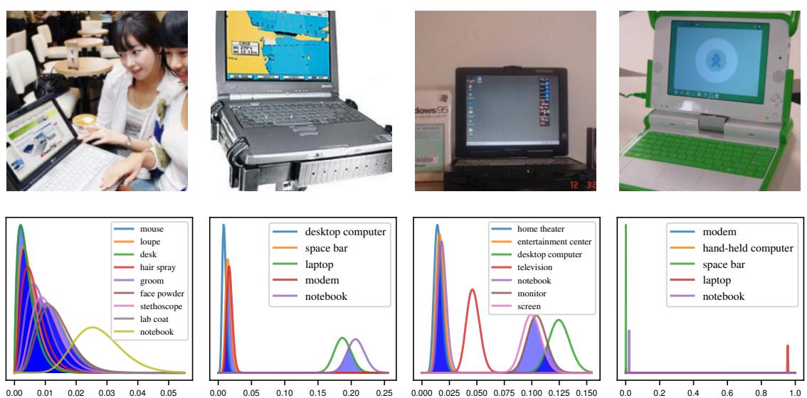
Figure 17.9: Illustration of uncertainty about individual labels in an image classification problem. Top row: images from the “laptop” class of ImageNet. Bottom row: beta marginals for the top-k predtions for the respective image. First column: high uncertainty about all the labels. Second column: “notebook” and “laptop” have high confidence. Third column: “desktop”, “screen” and “monitor” have high confidence. Fourth column: only “laptop” has high confidence. (Compare to Figure 14.4.) From Figure 6 of [HKH22]. Used with kind permission of Philipp Hennig.

to first project the Gaussian distribution onto this constraint surface, yielding

\[p(\mathbf{z}|\mathbf{z}, \mathcal{D}) = \mathcal{N}\left(\mathbf{z}|m - \frac{\mathbf{V}\mathbf{1}\mathbf{1}^{\mathsf{T}}m}{\mathbf{1}^{\mathsf{T}}\mathbf{V}\_{\ast}\mathbf{1}}, \mathbf{V} - \frac{\mathbf{V}\mathbf{1}\mathbf{1}^{\mathsf{T}}\mathbf{V}}{\mathbf{1}^{\mathsf{T}}\mathbf{V}\mathbf{1}}\right) = \mathcal{N}(\mathbf{z}|m', \mathbf{V}') \tag{17.30}\]

where 1 is the ones vector of size C. To avoid potential problems where ↼ is sparse, [HKH22] propose to also scale the posterior (after the zero-sum constraint) by using m↔︎↔︎ = m^↔︎ / ∝c and V↔︎↔︎ = V^↔︎ /c, where c = (& ii V ^↔︎ ii)/ MC/2.

One useful property of the Laplace bridge approximation, compared to the probit approximation, is that we can easily compute a marginal distribution over the probablility of each label being present. This is because the marginals of a Dirichlet are beta distributions. We can use this to adaptively compute a top-k prediction set; this is similar in spirit to conformal prediction (Section 14.3.1), but is Bayesian, in the sense that it represents per-instance uncertainty. The method works as follows. First we sort the class labels in decreasing order of expected probability, to get ↼˜ ; next we compute the marginal distribution over the probability for the top label,

\[p(\pi\_1|\mathbf{z}, \mathcal{D}) = \text{Beta}(\ddot{\alpha}\_1, \alpha\_0 - \ddot{\alpha}\_1) \tag{17.31}\]

where ϱ⁰ = & ^c ϱc. We then compute the marginal distributions for the other labels in a similar way,

and return all labels that have significant overlap with the top label. As we see from the examples in Figure 17.9, this approach can return variable-sized outputs, reflecting uncertainty in a natural way.

17.3.10.3 Distillation

The MC approximation to the posterior predictive is S times slower than a standard, deterministic plug-in approximation. One way to speed this up is to use distillation to approximate the semi-parametric “teacher” model p^t from Equation (17.25) by a parametric “student” model p^s by minimizing E [DKL (pt(y|x) ↘ ps(y|x))] wrt ps. This approach was first proposed in [HVD14], who called the technique “dark knowledge”, because the teacher has “hidden” information in its predictive probabilities (logits) than is not apparent in the raw one-hot labels.

In [Kor+15], this idea was used to distill the predictions from a teacher whose parameter posterior was computed using HMC; this is called “Bayesian dark knowledge”. A similar idea was used in [BPK16; GBP18], who distilled the predictive distribution derived from MC dropout (Section 17.3.1).

Since the parametric student is typically less flexible than the semi-parametric teacher, it may be overconfident, and lack diversity in its predictions. To avoid this overconfidence, it is safer to make the student be a mixture distribution [SG05; Tra+20a].

17.3.11 Tempered and cold posteriors

When working with BNNs for classification problems, the likelihood is usually taken to be

\[p(y|x,\theta) = \text{Cat}(y|\text{softmax}(f(x;\theta)))\tag{17.32}\]

where ^f(x; ^ω) ↗ ^RC returns the logits over the ^C class labels. This is the same as in multinomial logistic regression (Section 15.3.2); the only di!erence is that f is a nonlinear function of ω.

However, in practice, it is often found (see e.g., [Zha+18; Wen+20b; LST21; Noc+21]) that BNNs give better predictive accuracy if the likelihood function is scaled by some power ϱ. That is, instead of targeting the posterior p(ω|D) ↑ p(y|x, ω)p(ω), these methods target the tempered posterior, ^ptempered(ω|D) ^{↑ p}(y|X, ^ω)↼p(ω). In log space, we have

\[\log p\_{\text{temporal}}(\boldsymbol{\theta}|\mathcal{D}) = \alpha \log p(\boldsymbol{y}|\mathbf{X}, \boldsymbol{\theta}) + \log p(\boldsymbol{\theta}) + \text{const} \tag{17.33}\]

This is also called an ϱ-posterior or power posterior [Med+21].

Another common method is to target the cold posterior, ^pcold(ω|D) ^{↑ p}(ω|X, ^y)¹/T , or, in log space,

\[\log p\_{\text{cold}}(\boldsymbol{\theta}|\mathcal{D}) = \frac{1}{T} \log p(\boldsymbol{y}|\mathbf{X}, \boldsymbol{\theta}) + \frac{1}{T} \log p(\boldsymbol{\theta}) + \text{const} \tag{17.34}\]

If T < 1, we say that the posterior is “cold”. Note that, in the case of a Gaussian prior, using the cold posterior is the same as using the tempered posterior with a di!erent hyperparameter, since 1 ^T log pcold(ω) is given by

\[\frac{1}{T}\log\mathcal{N}(\boldsymbol{\theta}|0,\sigma\_{\text{cold}}^{2}\mathbf{I}) = -\frac{1}{2T\sigma\_{\text{cold}}^{2}}\sum\_{i}\theta\_{i}^{2} + \text{const} = \mathcal{N}(\boldsymbol{\theta}|0,\sigma\_{\text{temporal}}^{2}\mathbf{I}) + \text{const} \tag{17.35}\]

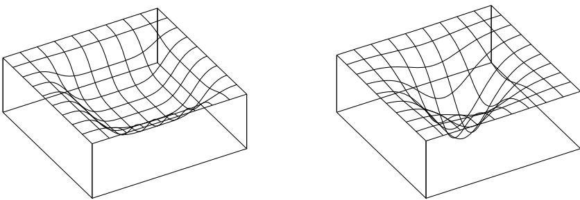
Figure 17.10: Flat vs sharp minima. From Figures 1 and 2 of [HS97]. Used with kind permission of Jürgen Schmidhuber.

which equals log ptempered(ω) if we set ς² tempered = Tς² cold. Thus both methods are e!ectively the same, and just reweight the likelihood by ϱ = 1/T.

Cold posteriors in Bayesian neural network classifiers are a consequence of underrepresenting aleatoric (label) uncertainty, as shown by [Kap+22]. On benchmarks such as CIFAR-100, we should have essentially no uncertainty about the labels of the training images, yet Bayesian classifiers with softmax likelihoods have very high uncertainty for these points. Moreover, [Izm+21b] showed that the cold posterior e!ect in all the examples of [Wen+20b] when data augmentation is removed. [Kap+22] show that with the SGLD inference in [Wen+20b], data augmentation has the e!ect of raising the likelihood to a power 1/K for minibatches of size K. Cold posteriors exactly counteract this e!ect, more honestly representing our beliefs about aleatoric uncertainty, by sharpening the likelihood. However, tempering is not required, and [Kap+22] show that by using a Dirichlet observation model to explicitly represent (lack of) label noise, there is no cold posterior e!ect, even with data augmentation. The curation hypotheses of [Ait21] can be considered a special case of the above explanation, where curation has the e!ect of increasing our confidence about training labels.

In Section 14.1.3, we discuss generalized variational inference, which gives a general framework for understanding whether and how the likelihood or prior could benefit from tempering. Tempering is particularly useful if (as is usually the case) the model is misspecified [KJD21].

17.4 Generalization in Bayesian deep learning

In this section, we discuss why “being Bayesian” can improve predictive accuracy and generalization performance.

17.4.1 Sharp vs flat minima

Some optimization methods (in particular, second-order batch methods) are able to find “needles in haystacks”, corresponding to narrow but deep “holes” in the loss landscape, corresponding to parameter settings with very low loss. These are known as sharp minima, see Figure 17.10(right). From the point of view of minimizing the empirical loss, the optimizer has done a good job. However, such solutions generally correspond to a model that has overfit the data. It is better to find points that correspond to flat minima, as shown in Figure 17.10(left); such solutions are more robust and

generalize better. To see why, note that flat minima correspond to regions in parameter space where there is a lot of posterior uncertainty, and hence samples from this region are less able to precisely memorize irrelevant details about the training set [AS17]. Put another way, the description length for sharp minima is large, meaning you need to use many bits of precision to specify the exact location in parameter space to avoid incurring large loss, whereas the description length for flat minima is less, resulting in better generalization [Mac03].

SGD often finds such flat minima by virtue of the addition of noise, which prevents it from “entering” narrow regions of the loss landscape (see Section 12.5.7). In addition, in higher dimensional spaces, flat regions occupy a much greater volume, and are thus much more easily discoverable by optimization procedures. More precisely, the analysis in [SL18] shows that the probability of entering any given basin of attraction ^A around a minimum is given by ^pSGD(^ω ↗ ^A) ^↑ / ^{A e}↓L(ε) dω. Note that this is integrating over the volume of space corresponding to A, and hence is proportional to the model evidence (marginal likelihood) for that region, as explained in Section 3.8.1. Since the evidence is parameterization invariant (since we marginalize out the parameters), this means that SGD will avoid regions that have low evidence (corresponding to sharp minima) regardless of how we parameterize the model (contrary to the claims in [Din+17]).

In fact, several papers have shown that we can view SGD as approximately sampling from the Bayesian posterior (see Section 17.3.8). The SWA method (Section 17.3.8) can be seen as finding a center of mass in the posterior based on these SGD samples, finding solutions that generalize better than picking a single SGD point.

If we must use a single solution, a flat one will help us better approximate the Bayesian model average in the integral of Equation (17.1). However, by attempting to perform a more complete Bayesian model average, we will select for flatness without having to deal with the messiness of having to worry about flatness definitions, or the e!ects of reparameterization, or unknown implicit regularization, as the model average will automatically weight regions with the greatest volume.

17.4.2 Mode connectivity and the loss landscape

In DNNs there are often many low-loss solutions, which provide complementary explanations of the data. Moreover, in [Gar+18c] they showed that two independently trained SGD solutions can be connected by a curve in a subspace, along which the training loss remains near-zero, known as mode connectivity. Despite having the same training loss, these di!erent parameter settings give rise to very di!erent functions, as illustrated in Figure 17.11, where we show predictions on a 1d regression problem coming from di!erent points in parameter space obtained by interpolating along a mode connecting curve between two distinct MAP estimates. Using a Bayesian model average, we can combine these functions together to provide much better performance over a single flat solution [Izm+19].

Recently, it has been discovered [Ben+21b] that there are in fact large multidimensional simplexes of low loss solutions, which can be combined together for significantly improved performance. These results further motivate the Bayesian approach (Equation (17.1)), where we perform a posterior weighted model average.

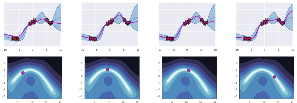
Figure 17.11: Diversity of high performing functions sampled from the posterior. Top row: we show predictions on the 1d input domain for 4 di!erent functions. We see that they extrapolate in di!erent ways outside of the support of the data. Bottom row: we show a 2d subspace spanning two distinct modes (MAP estimates), and connected by a low-loss curved path computed as in [Gar+18c]. From Figure 8 of [WI20]. Used with kind permission of Andrew Wilson.

17.4.3 E”ective dimensionality of a model

Modern DNNs have millions of parameters, but these parameters are often not well-determined by the data, i.e., there can be a lot of posterior uncertainty. By averaging over the posterior, we reduce the chance of overfitting, because we do not use “degrees of freedom” that are not needed or warranted.

To quantify the number of degrees of freedom, or e!ective dimensionality [Mac92b], we follow [MBW20] and define

\[N\_{\text{eff}}(\mathbf{H}, c) = \sum\_{i=1}^{k} \frac{\lambda\_i}{\lambda\_i + c},\tag{17.36}\]

where ⇀ⁱ are the eigenvalues of the Hessian matrix H computed at a local mode, and c > 0 is a regularization parameter. Intuitively, the e!ective dimension counts the number of well-determined parameters. A “flat minimum” will have many directions in parameter space that are not welldetermined, and hence will have low e!ective dimensionality. This means that we can perform Bayesian inference in a low dimensional subspace [Izm+19]: Since there is functional homogeneity in all directions but those defining the e!ective dimension, neural networks can be significantly compressed.

This compression perspective can also be used to understand why the e!ective dimension can be a good proxy for generalization. If two models have similar training loss, but one has lower e!ective dimension, then it is providing a better compression for the data at the same fidelity. In Figure 17.12 we show that for CNNs with low training loss (above the green partition), the e!ective dimensionality closely tracks generalization performance. We also see that the number of parameters alone is not a strong determinant of generalization. Indeed, models with more parameters can have a lower number of e!ective parameters. We also see that wide but shallow models overfit, while depth helps provide

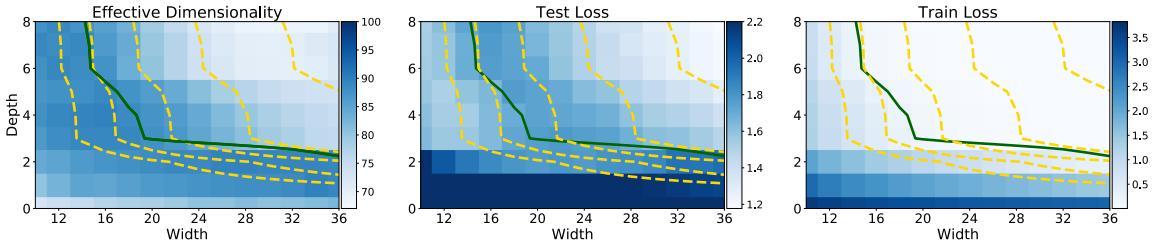
Figure 17.12: Left: e!ective dimensionality as a function of model width and depth for a CNN on CIFAR-100. Center: test loss as a function of model width and depth. Right: train loss as a function of model width and depth. Yellow level curves represent equal parameter counts (1e5, 2e5, 4e5, 1.6e6). The green curve separates models with near-zero training loss. E!ective dimensionality serves as a good proxy for generalization for models with low train loss. We see wide but shallow models overfit, providing low train loss, but high test loss and high e!ective dimensionality. For models with the same train loss, lower e!ective dimensionality can be viewed as a better compression of the data at the same fidelity. Thus depth provides a mechanism for compression, which leads to better generalization. From Figure 2 of [MBW20]. Used with kind permission of Andrew Wilson.

lower e!ective dimensionality, leading to a better compression of the data. It is depth that makes modern neural networks distinctive, providing hierarchical inductive biases making it possible to discover more regularity in the data.

17.4.4 The hypothesis space of DNNs

Zhang et al. [Zha+17] showed that CNNs can fit CIFAR-10 images with random labels with zero training error, but can still generalize well on the noise-free test set. It has been claimed that this result contradicts a classical understanding of generalization, because it shows that neural networks are capable of significantly overfitting the data, but can still generalize well on structured inputs.

We can resolve this paradox by taking a Bayesian perspective. In particular, we know that modern CNNs are very flexible, so they can fit almost any pattern (since they are in fact universal approximators). However, their architecture encodes a prior over what kinds of patterns they expect to see in the data (see Section 17.2.5). Image datasets with random labels can be represented by this function class, but such solutions receive very low marginal likelihood, since they strongly violate the prior assumptions [WI20]. By contrast, image datasets where the output labels are consistent with patterns in the input get much higher marginal likelihood.

This phenomenon is not unique to DNNs. For example, it also occurs with Gaussian processes (Chapter 18). Such models are also universal approximators, but they allocate most of their probability mass to a small range of solutions (depending on the chosen kernel). They can also fit image datasets with random labels, but such data receives a low marginal likelihood [WI20].

In general, we can distinguish the support of a model, i.e., the set of functions it can represent, from the distribution over that support, i.e., the inductive bias which leads it to prefer some functions over others. We would like to use models where the support is large, so we can capture the complexity of real-world data, but also where the inductive bias places probability mass on the kinds of functions we expect to see. If we succeed at this, the posterior will quickly converge on the true function after

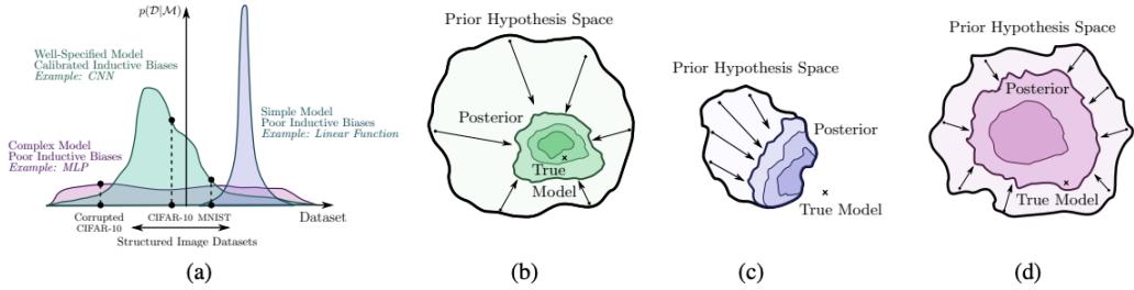
Figure 17.13: Illustration of the behavior of di!erent kinds of model families and the prior distributions they induce over datasets. (a) The purple model is a simple linear model that has small support, and can only represent a few kinds of datasets. The pink model is an unstructured MLP: this has support over a large range of datasets with a fairly uninformative (broad) prior. Finally the green model is a CNN; this has support over a large range of datasets but the prior is more concentrated on certain kinds of datasets that have compositional structure. (b) The posterior for the green model (CNN) rapidly collapses to the true model, since it is consistent with the data. (c) The posterior for the purple model (linear) also rapidly collapses, but to a solution which cannot represent the true model. (d) The posterior for the pink model (MLP) collapses very slowly (as a function of dataset size). From Figure 2 of [WI20]. Used with kind permission of Andrew Wilson.

seeing a small amount of data. This idea is sketched in Figure 17.13.

17.4.5 PAC-Bayes

PAC-Bayes [McA99; LC02; Gue19; Alq21; GSZ21] provides a promising mechanism to derive non-vacuous generalization bounds for large stochastic networks [Ney+17; NBS18; DR17], with parameters sampled from a probability distribution. In particular, the di!erence between the train error and the generalization error can be expressed as

\[\sqrt{\frac{D\_{\rm KL}(Q \parallel P) + c}{2(N - 1)}},\tag{17.37}\]

where c is a constant, N is the number of training points, P is the prior distribution over the parameters, and Q is an arbitrary distribution, which can be chosen to optimize the bound.

The perspective in this chapter is largely complementary, and in some ways orthogonal, to the PAC-Bayes literature. Our focus has been on Bayesian marginalization, particularly multi-modal marginalization, and a prescriptive approach to model construction. In contrast, PAC-Bayes bounds are about bounding the empirical risk of a single sample, rather than marginalization, and are not currently prescriptive: what we would do to improve the bounds, such as reducing the number of model parameters, or using highly compact priors, does not typically improve generalization. Moreover, while we have seen Bayesian model averaging over multimodal posteriors has a significant e!ect on generalization, it has a minimal logarithmic e!ect on PAC-Bayes bounds. In general, because the bounds are loose, albeit non-vacuous in some cases, there is often room to make modeling choices that improve PAC-Bayes bounds without improving generalization, making it hard to derive a prescription for model construction from the bounds.

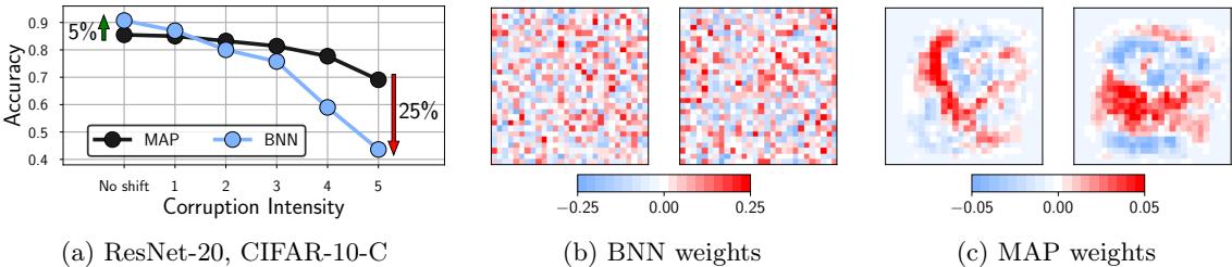
Figure 17.14: Bayesian neural networks under covariate shift. a: Performance of a ResNet-20 on the pixelate corruption in CIFAR-10-C. For the highest degree of corruption, a Bayesian model average underperforms a MAP solution by 25% (44% against 69%) accuracy. See Izmailov et al. [Izm+21b] for details. b: Visualization of the weights in the first layer of a Bayesian fully-connected network on MNIST sampled via HMC. c: The corresponding MAP weights. We visualize the weights connecting the input pixels to a neuron in the hidden layer as a 28 ≃ 28 image, where each weight is shown in the location of the input pixel it interacts with. This is Figure 1 of Izmailov et al. [Izm+21a].

17.4.6 Out-of-distribution generalization for BNNs

Bayesian methods are often assumed to be more robust in the context of distribution shift (discussed in Chapter 19), because they capture more uncertainty than methods based on point estimation. However, there are some subtleties, some of which we discuss below.

17.4.6.1 BMA can give poor results with default priors

Many approximate inference methods, especially deep ensembles, are significantly less overconfident (more well calibrated) in the presence of some kinds of covariate shifts [Ova+19]. However, in [Izm+21b], it was noted that HMC, which arguably o!ers the most accurate approximation to the posterior, often works poorly under distribution shift.

Rather than an idiosyncracy of HMC, Izmailov et al. [Izm+21a] show this lack of robustness is a foundational issue of Bayesian model averaging under covariate shift, caused by degeneracies in the training data, and a poor choice of prior. As an illustrative special case, MNIST digits all have black corner pixels. Weights in the first layer of a neural network connected to these pixels are multiplied by zero, and thus can take any value without a!ecting the outputs of the network. Classical MAP training or deep ensembles of MAP solutions with a Gaussian prior will therefore drive these parameters to zero, since they don’t help with the data fit, and the resulting network will be robust to corruptions on these pixels. On the other hand, the posterior for these parameters will be the same as the prior, and so a Bayesian model average will multiply corruptions by random numbers sampled from the prior, leading to degraded predictive performance.

Figure 17.14(b, c) visualizes this example, showing the first-layer weights of a fully-connected network for the MAP solution and a BNN posterior sample, on MNIST. The MAP weights corresponding to zero intensity pixels near the boundary are near zero, while the BNN weights look noisy, sampled from a Gaussian prior.

Izmailov et al. [Izm+21a] prove that this issue is a special case of a much more general problem, whenever there are linear dependencies in the input features of the training data, both for fully-

connected and convolutional networks. In this case, the data live on a hyperplane. If a covariate or domain shift, moves orthogonal to this hyperplane, the posterior will be the same as the prior in the direction of the shift. The posterior model average will thus be highly vulnerable to shifts that do not particularly a!ect the underlying semantic structure of the problem (such as corruptions), whereas the MAP solution will be entirely robust to such shifts.

By introducing a prior over parameters which is aligned with the principal components of the training inputs, we can substantially improve the generalization accuracy of Bayesian neural networks in out-of-distribution settings. Izmailov et al. [Izm+21a] propose the following EmpCov prior: ^p(w¹) = ^N (0, ^ϱ” ⁺ ⇁I), where ^w1 are the first layer weights, ” ^{= 1} n↓1 &^{n i}=1 xix^{T i} is the empirical covariance of the training input features xi, ϱ > 0 determines the scale of the prior, and ⇁ is a small positive constant to ensure the covariance matrix is positive definite. With this improved prior they are able to obtain a method that is much more robust to distribution shift.

17.4.6.2 BNNs can be overconfident on OOD inputs

An important problem in practice is how a predictive model will behave when it is given an input that is “out of distribution” or OOD. Ideally we would like the model to express that it is not confident in its prediction, so that the system can abstain from predicting (see Section 19.3.3). Using “exact” inference methods, such as MCMC, for BNNs can give this behavior in some cases. For example, in Section 19.3.3.1 we showed that an MLP which was fit to MNIST using SGLD would be less overconfident than a point estimate (computed using SGD) when presented with inputs from fashion MNIST. However, this behavior does not always occur reliably.

To illustrate the problem, consider the 2d nonlinear binary classification dataset shown in Figure 17.15. In addition to the two training classes, we have highlighted (in green) a set of OOD inputs that are far from the support of the training set. Intuitively we would expect the model to predict a probability of 0.5 (corresponding to “don’t know”) for such inputs that are far from the training set. However we see that the only methods that do so are the Gaussian process (GP) classifier (see Section 18.4) and the SNGP model (Section 17.3.6), which contains a GP layer on top of the feature extractor.

The lesson we learn from this simple example is that “being Bayesian” only helps if we are using a good hypothesis class. If we only consider a single MLP classifier, with standard Gaussian priors on the weights, it is extremely unlikely that we will learn the kind of compact decision boundary shown in Figure 17.15g, because that function has negligible support under our prior (c.f. Section 17.4.4). Instead we should embrace the power of Bayes to avoid overfitting and use as complex a model class as we can a!ord.

17.4.7 Model selection for BNNs

Historically, the marginal likelihood (aka Bayesian evidence) has been used for model selection problems, such as choosing neural architectures or hyperparameter values [Mac92a]. Recent methods based on the Laplace approximation, such as [Imm+21; Dax+21], have made this scalable to large BNNs. However, [Lot+22] argue that it is much better to use the conditional marginal likelihood, which we discuss in Section 3.8.5.

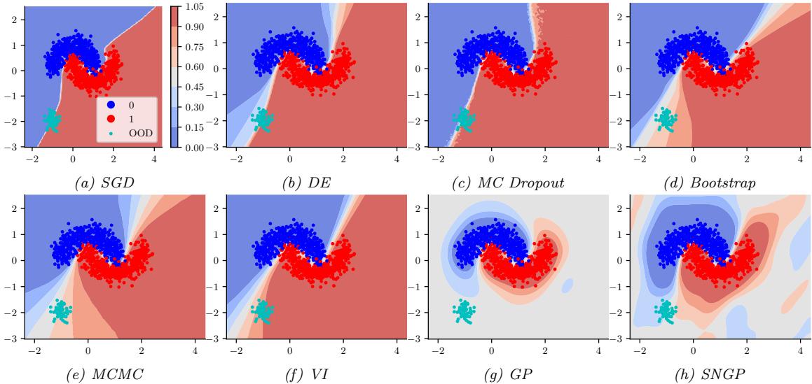
Figure 17.15: Predictions made by various (B)NNs when presented with the training data shown in blue and red. The green blob is an example of some OOD inputs. Methods are: (a) standard SGD; (b) deep Ensemble of 10 models with di!erent random initializations; (c) MC dropout with 50 samples; (d) bootstrap training, where each of the 10 models is initialized identically but given di!erent versions of the data, obtained by resampling with replacement; (e) MCMC using NUTS algorithm with 3000 warmup steps and 3000 samples; (f ) variational inference; (g) Gaussian process classifier using RBF kernel; (h) SNGP. The model is an MLP with 8,16,16,8 units in the hidden layers and ReLu activation. The output layer has 1 neuron with sigmoid activation. Generated by makemoons\_comparison.ipynb

17.5 Online inference

In Section 17.3, we have focused on batch or o$ine inference. However, an important application of Bayesian inference is in sequential settings, where the data arrives in a continuous stream, and the model has to “keep up”. This is called sequential Bayesian inference, and is one approach to online learning (see Section 19.7.5). In this section, we discuss some algorithmic approaches to this problem in the context of DNNs. These methods are widely used for continual learning, which we discuss Section 19.7.

17.5.1 Sequential Laplace for DNNs

In [RBB18b], they extended the Laplace method of Section 17.3.2 to the sequential setting. Specifically, let ^p(ω|D1:t↓1) ^{↓ N} (ω|µ^t↓¹, #^{↓1 t}↓1) be the approximate posterior from the previous step; we assume the precision matrix is Kronecker factored. We now compute the new mean by solving the MAP

problem

\[\mu\_t = \operatorname\*{argmax}\log p(\mathcal{D}\_t|\boldsymbol{\theta}) + \log p(\boldsymbol{\theta}|\mathcal{D}\_{1:t-1}) \tag{17.38}\]

\[\hat{\theta} = \operatorname{argmax} \log p(\mathcal{D}\_t | \theta) - \frac{1}{2} (\theta - \mu\_{t-1}) \Lambda\_{t-1}^{-1} (\theta - \mu\_{t-1}) \tag{17.39}\]

Once we have computed µt, we compute the approximate Hessian at this point, and get the new posterior precision

\[ \Lambda\_t = \lambda \mathbf{H}(\mu\_t) + \Lambda\_{t-1} \tag{17.40} \]

where ⇀ ≃ 0 is a weighting factor that trades o! how much the model pays attention to the new data vs old data.

Now suppose we use a diagonal approximation to the posterior prediction matrix. From Equation (17.39), we see that this amounts to adding a quadratic penalty to each new MAP estimate, to encourage it to remain close to the parameters from previous tasks. This approach is called elastic weight consolidation (EWC) [Kir+17].

17.5.2 Extended Kalman filtering for DNNs

In Section 29.7.2, we showed how Kalman filtering can be used to incrementally compute the exact posterior for the weights of a linear regression model with known variance, i.e., we compute ^p(ω|D1:t, ^ς2), where ^D1:^{t =} {(ui, yi) : ⁱ =1: ^t} is the data seen so far, and

\[p(y\_t | \mathbf{u}\_t, \boldsymbol{\theta}, \sigma^2) = \mathcal{N}(y\_t | \boldsymbol{\theta}^\top \mathbf{u}\_t, \sigma^2) \tag{17.41}\]

is the linear regression likelihood. The application of KF to this model is known as recursive least squares.

Now consider the case of nonlinear regression:

\[p(y\_t | \mathbf{u}\_t, \theta, \sigma^2) = \mathcal{N}(y\_t | f(\theta, \mathbf{u}\_t), \sigma^2) \tag{17.42}\]

where f(ω,ut) is some nonlinear function, such as an MLP. We can use the extended Kalman filter (Section 8.3.2) to approximately compute ^p(ωt|D1:t, ^ς2), where ^ωt is the hidden state (see e.g., [SW89; PF03]). To see this, note that we can set the dynamics model to the identity function, f(ωt) = ωt, so the parameters are propagated through unchanged, and the observation model to the input-dependent function f(ωt) = f(ωt,ut). We set the observation noise to R^t = ς², and the dynamics noise to Q^t = qI, where q is a small constant, to allow the parameters to slowly drift according to artificial process noise. (In practice it can be useful to anneal q from a large initial value to something near 0.)

17.5.2.1 Example

We now give an example of this process in action. We sample a synthetic dataset from the true function

\[h^\*(u) = x - 10\cos(u)\sin(u) + u^3\tag{17.43}\]

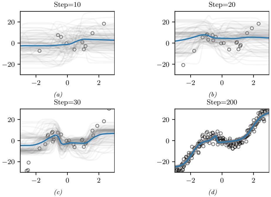
Figure 17.16: Sequential Bayesian inference for the parameters of an MLP using the extended Kalman filter. We show results after seeing the first 10, 20, 30 and 200 observations. (For a video of this, see https: // bit. ly/ 3wXnWaM .) Generated by ekf\_mlp.ipynb.

and add Gaussian noise with ς = 3. We then fit this with an MLP with one hidden layer with H hidden units, so the model has the form

\[f(\theta, \mathbf{u}) = \mathbf{W}\_2 \tanh(\mathbf{W}\_1 \mathbf{u} + \mathbf{b}\_1) + \mathbf{b}\_2 \tag{17.44}\]

where ^W1 ↗ ^RH⇑1, ^b1 ↗ ^RH, ^W2 ↗ ^R1⇑H, ^b2 ↗ ^R1. We set ^H = 6, so there are ^D = 19 parameters in total.

Given the data, we sequentially compute the posterior, starting from a vague Gaussian prior, p(ω) = N (ω|0, !0), where !⁰ = 100I. (In practice we cannot start from the prior mean, which is ω⁰ = 0, since linearizing the model around this point results in a zero gradient, so we use an initial random sample for ω0.) The results are shown in Figure 17.16. We can see that the model adapts to the data, without having to specify any learning rate. In addition, we see that the predictions become gradually more confident, as the posterior concentrates on the MLE.

17.5.2.2 Setting the variance terms

In the above example, we set the variance terms by hand. In general we need to estimate the noise variance ς, which determines R^t and hence the learning rate, as well as the strength of the prior !0, which controls the amount of regularization. Some methods for doing this are discussed in [FNG00].

17.5.2.3 Reducing the computational complexity

The naive EKF method described above takes O(N^{3 z} ) time, which is prohibitive for large neural networks. A simple approximation, known as the decoupled EKF, was proposed in [PF91; SPD92] (see [PF03] for a review). This partitions the weights into G groups or blocks, and estimates the relevant matrices for each group g independently. If G = 1, this reduces the standard global EKF. If we put each weight into its own group, we get a fully diagonal approximation. In practice this does not work any better than SGD, since it ignores correlations between the parameters. A useful compromise is to put all the weights corresponding to each neuron into its own group; this is called node decoupled EKF, which has been used in [Sim02] to train RBF networks and [GUK21] to train exponential family matrix factorization models (widely used in recommender systems). For more details on DEKF, Supplementary Section 17.1.

Another approach to increasing computational e”ciency is to leverage the fact that the e!ective dimensionality of a DNN is often quite low (see Section 17.4.3). Indeed we can approximate the model parameters by using a low dimensional vector of coe”cients that specify the point in a linear manifold corresponding to weight space; the basis set defining this linear manifold can either be chosen randomly [Li+18b; GARD18; Lar+22], or can be estimated using PCA applied to the SGD iterates [Izm+19]. We can exploit this observation to perform EKF in this low-dimensional subspace, which significantly speeds up inference, as discussed in [DMKM22].

17.5.3 Assumed density filtering for DNNs

In Section 8.6.3, we discussed how to use assumed density filtering (ADF) to perform online (binary) logistic regression. In this section, we generalize this to nonlinear predictive models, such as DNNs. The key is to perform Gaussian moment matching of the hidden activations at each layer of the model. This provides an alternative to the EKF approach in Section 17.5.2, which is based on linearization of the network.

We will assume the following likelihood:

\[p(\mathbf{y}\_t | \mathbf{u}\_t, \mathbf{w}\_t) = \text{Exp}\{\mathbf{w}\_t | \ell^{-1}(f(\mathbf{u}\_t; \mathbf{w}\_t))\}\tag{17.45}\]

where f(x; w) is the DNN, ε↓¹ is the inverse link function, and Expfam() is some exponential family distribution. For example, if f is linear and we are solving a binary classification problem, we can write

\[p(y\_t | \mathbf{u}\_t, \mathbf{w}\_t) = \text{Ber}(y\_t | \sigma(\mathbf{u}\_t^\mathsf{T} \mathbf{w}\_t)) \tag{17.46}\]

We discussed using ADF to fit this model in Section 8.6.3.

In [HLA15b], they propose probabilistic backpropagation (PBP), which is an instance of ADF applied to MLPs. The basic idea is to approximate the posterior over the weights in each layer using a fully factorized distribution

\[p(\boldsymbol{w}\_{l}|\mathcal{D}\_{1:t}) \approx p\_{l}(\boldsymbol{w}\_{l}) = \prod\_{l=1}^{L} \prod\_{i=1}^{D\_{l}} \prod\_{j=1}^{D\_{l-1}+1} N(w\_{ijl}|\boldsymbol{\mu}\_{ijl}^{t}, \boldsymbol{\tau}\_{ijl}^{t}) \tag{17.47}\]

where L is the number of layers, and D^l is the number of neurons in layer l. (The expectation backpropagation algorithm of [SHM14] is a special case of this, where the variances are fixed to τ = 1.)

Suppose the parameters are static, so w^t = wt↓¹. Then the new posterior, after conditioning on the t’th observation, is given by

\[\hat{p}\_t(\mathbf{w}) = \frac{1}{Z\_t} p(y\_t|\mathbf{u}\_t, \mathbf{w}) \mathcal{N}(\mathbf{w}|\boldsymbol{\mu}^{t-1}, \boldsymbol{\Sigma}^{t-1}) \tag{17.48}\]

where !^t↓¹ = diag(φ ^t↓¹). We then project pˆt(w) onto the space of factored Gaussians to compute the new (approximate) posterior, pt(w). This can be done by computing the following means and variances [Min01a]:

\[ \mu\_{ijl}^t = \mu\_{ijl}^{t-1} + \tau\_{ijl}^{t-1} \frac{\partial \ln Z\_t}{\partial \mu\_{ijl}^{t-1}} \tag{17.49} \]

\[\tau\_{ijl}^t = \tau\_{ijl}^{t-1} - (\tau\_{ijl}^{t-1})^2 \left[ \left( \frac{\partial \ln Z\_t}{\partial \mu\_{ijl}^{t-1}} \right)^2 - 2 \frac{\partial \ln Z\_t}{\partial \tau\_{ijl}^{t-1}} \right] \tag{17.50}\]

In the forwards pass, we compute Z^t by propagating the input u^t through the model. Since we have a Gaussian distribution over the weights, instead of a point estimate, this induces an (approximately) Gaussian distribution over the values of the hidden units. For certain kinds of activation functions (such as ReLU), the relevant integrals (to compute the means and variances) can be solved analytically, as in GP-neural networks (Section 18.7). The result is that we get a Gaussian distribution over the final layer of the form N (ϱt|µ, !), where ϱ^t = f(ut; wt) is the output of the neural network before the GLM link function induced by pt(wt). Hence we can approximate the partition function using

\[Z\_t \approx \int p(y\_t|\eta\_t) \mathcal{N}(\eta\_t|\mu, \Sigma) d\eta\_t \tag{17.51}\]

We now discuss how to compute this integral. In the case of probit classification, with y ↗ {→1, +1}, we have p(y|x, w) = ‘(yη), where’ is the cdf of the standard normal. We can then use the following analytical result

\[\int \Phi(y\eta) \mathcal{N}(h|\mu, \sigma) d\eta = \Phi\left(\frac{y\mu}{\sqrt{1+\sigma}}\right) \tag{17.52}\]

In the case of logistic classification, with y ↗ {0, 1}, we have p(y|x, w) = Ber(y|ς(η)); in this case, we can use the probit approximation from Section 15.3.6. For the multiclass case, where ^y ↗ {0, ¹}^C (one-hot encoding), we have p(y|x, w) = Cat(y|softmax(ϱ)). A variational lower bound to log Z^t for this case is given in [GDFY16].

Once we have computed Zt, we can take gradients and update the Gaussian posterior moments, before moving to the next step.

17.5.4 Online variational inference for DNNs

A natural approach to online learning is to use variational inference, where the prior is the posterior from the previous step. This is known as streaming variational Bayes [Bro+13]. In more detail,

at step t, we compute

\[\psi\_t = \operatorname\*{argmin}\_{\psi} \underbrace{\operatorname\*{argmin}\_{q(\boldsymbol{\theta}|\boldsymbol{\psi})} \left[ \ell\_t(\boldsymbol{\theta}) \right] + D\_{\text{KL}} \left( q(\boldsymbol{\theta}|\boldsymbol{\psi}) \parallel q(\boldsymbol{\theta}|\boldsymbol{\psi}\_{t-1}) \right)}\_{-L\_t(\boldsymbol{\psi})} \tag{17.53}\]

\[\hat{\mathbf{x}}\_{t} = \operatorname\*{argmin}\_{\boldsymbol{\Psi}} \mathbb{E}\_{q(\boldsymbol{\theta}|\boldsymbol{\Psi})} \left[ \ell\_{t}(\boldsymbol{\theta}) + \log q(\boldsymbol{\theta}|\boldsymbol{\psi}) - \log q(\boldsymbol{\theta}|\boldsymbol{\psi}\_{t-1}) \right] \tag{17.54}\]

where εt(ω) = → log p(Dt|ω) is the negative log likelihood (or, more generally, some loss function) of the data batch at step t.

When applied to DNNs, this approach is called variational continual learning or VCL [Ngu+18]. (We discuss continual learning in Section 19.7.) An e”cient implementation of this, known as FOO-VB (“fixed-point operator for online variational Bayes”) is given in [Zen+21].

One problem with the VCL objective in Equation (17.53) is that the KL term can cause the model to become too sparse, which can prevent the model from adapting or learning new tasks. This problem is called variational overpruning [TT17]. More precisely, the reason this happens is as follows: some weights might not be needed to fit a given dataset, so their posterior will be equal to the prior, but sampling from these high-variance weights will add noise to the likeilhood; to reduce this, the optimization method will prefer to set the bias term to a large negative value, so the corresponding unit is “turned o!”, and thus has no e!ect on the likelihood. Unfortunately, these “dead units” become stuck, so there is not enough network capacity to learn the next task.

In [LST21], they propose a solution to this, known as generalized variational continual learning or GVCL. The first step is to downweight the KL term by a factor ↼ < 1 to get

\[\mathcal{L}\_t = \mathbb{E}\_{q(\boldsymbol{\theta}|\boldsymbol{\psi})} \left[ \ell\_t(\boldsymbol{\theta}) \right] + \beta D\_{\text{KL}} \left( q(\boldsymbol{\theta}|\boldsymbol{\psi}) \parallel q(\boldsymbol{\theta}|\boldsymbol{\psi}\_{t-1}) \right) \tag{17.55}\]

Interestingly, one can show that in the limit of ↼ ↖ 0, this recovers several standard methods that use a Laplace approximation based on the Hessian. In particular if we use a diagonal variational posterior, this reduces to online EWC method of [Sch+18]; if we use a block-diagonal and Kronecker factored posterior, this reduces to the online structured Laplace method of [RBB18b]; and if we use a low-rank posterior precision matrix, this reduces to the SOLA method of [Yin+20].

The second step is to replace the prior and posterior by using tempering, which is useful when the model is misspecified, as discussed in Section 17.3.11. In the case of Gaussians, raising the distribution to the power ⇀ is equivalent to tempering with a temperature of τ = 1/⇀, which is the same as scaling the covariance by ⇀↓¹. Thus the GVCL objective becomes

\[\mathcal{L}\_t = \mathbb{E}\_{q(\boldsymbol{\theta}|\boldsymbol{\psi})} \left[ \ell\_t(\boldsymbol{\theta}) \right] + \beta D\_{\text{KL}} \left( q(\boldsymbol{\theta}|\boldsymbol{\psi})^\lambda \parallel q(\boldsymbol{\theta}|\boldsymbol{\psi}\_{t-1})^\lambda \right) \tag{17.56}\]

This can be optimized using SGD, assuming the posterior is reparameterizable (see Section 10.2.1).

17.6 Hierarchical Bayesian neural networks

In some problems, we have multiple related datasets, such as a set of medical images from di!erent hospitals. Some aspects of the data (e.g., the shape of healthy vs diseased cells) is generally the same across datasets, but other aspects may be unique or idiosyncractic (e.g., each hospital may use a di!erent colored die for staining). To model this, we can use a hierarchical Bayesian model, in which we allow the parameters for each dataset to be di!erent (to capture random e!ects), while coming from

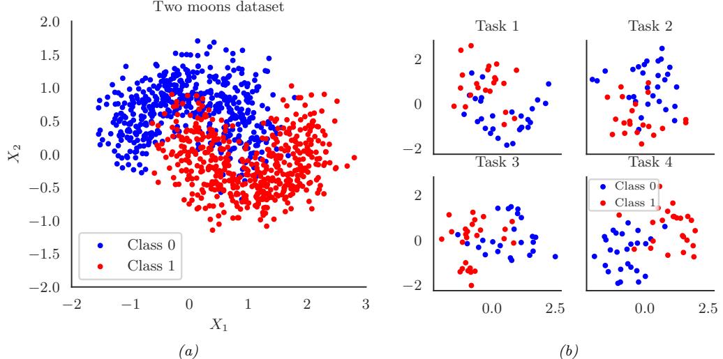
Figure 17.17: (a) Two moons synthetic dataset. (b) Multi-task version, where we rotate the data to create 18 related tasks (groups). Each dataset has 50 training and 50 test points. Here we show the first 4 tasks. Generated by bnn\_hierarchical.ipynb.

a common prior (to capture shared e!ects). This is the setup we considered in Section 15.5, where we discuss hierarchical Bayesian GLMs. In this section, we extend this to nonlinear predictors based on neural networks. (The setup is very similar to domain generalization, discussed in Section 19.6.2, except here we care about performance on all the domains, not just a held-out target domain.)

17.6.1 Example: multimoons classification

In this section, we consider an example2 where we want to solve multiple related nonlinear binary classification problems coming from J di!erent environments or distributions. We assume that each environment has its own unique decision boundary ^p(y|x, ^wj ), so this is a form of concept shift (see Section 19.2.3). However we assume the overall shape of each boundary is similar to a common shared boundary, denote ^p(y|x, ^w0). We only have a small number ^Nj of examples from each environment, ^{Dj =} {(x^j n, y^{j n}) : n =1: Nj}, but we can utilize their common structure to do better than fitting J separate models.

To illustrate this, we create some synthetic 2d data for the J = 18 tasks. We start with the two-moons dataset, illustrated in Figure 17.17a. Each task is obtained by rotating the 2d inputs by a di!erent amount, to create 18 related classification problems (see Figure 17.17b). See Figure 17.17b for the training data for 4 tasks.

To handle the nonlinear decision boundary, we use a multilayer perceptron. Since the dataset is low-dimensional (2d input), we use a shallow model with just 2 hidden layers, each with 5 neurons. We could fit a separate MLP to each task, but since we have limited data per task (N^j = 50 examples

^2. This example is from https://twiecki.io/blog/2018/08/13/hierarchical\_bayesian\_neural\_network/. For a real-world example of a similar approach applied to a gesture recognition task, see [Jos+17].

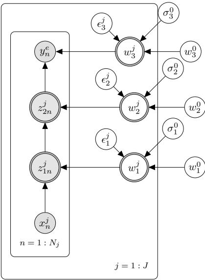
Figure 17.18: Illustration of a hierarchical Bayesian MLP with 2 hidden layers. There are J di!erent models, each with N^j observed samples, and a common set of global shared parent parameters denoted with the 0 superscript. Nodes which are shaded are observed. Nodes with double ringed circles are deterministic functions of their parents.

for training), this works poorly, as we show below. We could also pool all the data and fit a single model, but this does even worse, since the datasets come from di!erent underlying distributions, so mixing the data together from di!erent “concepts” confuses the model. Instead we adopt a hierarchical Bayesian approach.

Our modeling assumptions are shown in Figure 17.18. In particular, we assume the weight from unit i to unit k in layer l for environment j, denoted w^j i,k,l, comes from a common prior value w⁰ i,k,l, with a random o!set. We use the non-centered parameterization from Section 12.6.5 to write

\[w\_{i,k,l}^{j} = w\_{i,k,l}^{0} + \epsilon\_{i,k,l}^{j} \times \sigma\_{l}^{0} \tag{17.57}\]

where ⇁ j i,k,l ^{↔︎ N} (0, 1). By allowing a di!erent ^{ς0 l} per layer l, we let the model control the degree of shrinkage to the prior for each layer separately. (We could also make the ς^{j l} parameters be environment specific, which would allow for di!erent amounts of distribution shift from the common parent.) For the hyper-parameters, we put ^N (0, 1) priors on ^w0 i,k,l, and ^N+(1) priors on ^ς0 l .

We compute the posterior p(,1:^J 1:L, w⁰ 1:L,σ⁰ 1:L|D) using HMC (Section 12.5). We then evaluate this model using a fresh set of labeled samples from each environment. The average classification accuracy on the train and test sets for the non-hierarchical model (one MLP per environment, fit separately) is 86% and 83%. For the hierarchical model, this improves to 91% and 89% respectively.

To see why the hierarchical model works better, we will plot the posterior predictive distribution in 2d. Figure 17.19(top) shows the results for the nonhierarchical models; we see that the method

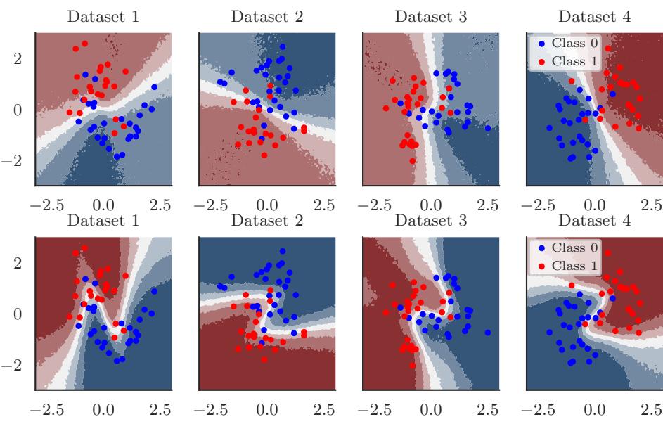
Figure 17.19: Top: Results of fitting separate MLPs on each dataset. Bottom: Results of fitting hierarchical MLP on all datasets jointly. Generated by bnn\_hierarchical.ipynb.

fails to learn the common underlying Z-shaped decision boundary. By contrast, Figure 17.19(bottom) shows that the hierarchical method has correctly recovered the common pattern, while still allowing group variation.

18 Gaussian processes

This chapter is coauthored with Andrew Wilson.

18.1 Introduction

Deep neural networks are a family of flexible function approximators of the form f(x; ω), where the dimensionality of ω (i.e., the number of parameters) is fixed, and independent of the size N of the training set. However, such parametric models can overfit when N is small, and can underfit when N is large, due to their fixed capacity. In order to create models whose capacity automatically adapts to the amount of data, we turn to nonparametric models.

There are many approaches to building nonparametric models for classification and regression (see e.g., [Was06]). In this chapter, we consider a Bayesian approach in which we represent uncertainty about the input-output mapping f by defining a prior distribution over functions, and then updating it given data. In particular, we will use a Gaussian process to represent the prior p(f); we then use Bayes’ rule to derive the posterior p(f|D), which is another GP, as we explain below. More details on GPs can be found the excellent book [RW06], as well as the interactive tutorial at https://distill.pub/2019/visual-exploration-gaussian-processes. See also Chapter 31 for other examples of Bayesian nonparametric models.

18.1.1 GPs: what and why?

To explain GPs in more detail, recall that a Gaussian random vector of length N, f = [f1,…,f^N ], is defined by its mean µ = E [f] and its covariance ! = Cov [f]. Now consider a function f : X ↖ R evaluated at a set of inputs, ^{X =} {xⁿ ↗ X }^{N n}=1. Let f^X = [f(x1),…,f(x^N )] be the set of unknown function values at these points. If f^X is jointly Gaussian for any set of N ≃ 1 points, then we say that f : X ↖ R is a Gaussian process. Such a process is defined by its mean function m(x) ↗ R and a covariance function, K(x, x^↔︎ ) ≃ 0, which is any positive definite Mercer kernel (see Section 18.2). For example, we might use an RBF kernel of the form K(x, x^↔︎ ) ↑ exp(→||x→x^↔︎ ||2) (see Section 18.2.1.1 for details).

We denote the corresponding GP by

\[f(\mathbf{x}) \sim GP(m(\mathbf{x}), \mathbb{K}(\mathbf{x}, \mathbf{z}')) \tag{18.1}\]

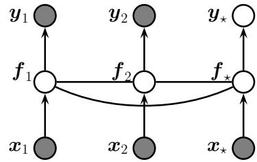
Figure 18.1: A Gaussian process for 2 training points, x¹ and x2, and 1 testing point, x↗, represented as a graphical model representing ^p(y, ^fX|X) = ^N (fX|m(X), ^K(X)) ! ⁱ p(yi|fi). The hidden nodes fⁱ = f(xi) represent the value of the function at each of the datapoints. These hidden nodes are fully interconnected by undirected edges, forming a Gaussian graphical model; the edge strengths represent the covariance terms “ij = K(xi, x^j ). If the test point x↗ is similar to the training points x¹ and x2, then the value of the hidden function f↗ will be similar to f¹ and f2, and hence the predicted output y↗ will be similar to the training values y¹ and y2.

where

\[m(\mathbf{x}) = \mathbb{E}\left[f(\mathbf{x})\right] \tag{18.2}\]

\[\mathcal{K}(\mathbf{x}, \mathbf{z}') = \mathbb{E}\left[ (f(\mathbf{z}) - m(\mathbf{z}))(f(\mathbf{z}') - m(\mathbf{z}'))^\top \right] \tag{18.3}\]

This means that, for any finite set of points X = {x1,…, x^N }, we have

\[p(\mathbf{f}\_X|\mathbf{X}) = \mathcal{N}(\mathbf{f}\_X|\mu\_X, \mathbf{K}\_{X,X}) \tag{18.4}\]

where µ^X = (m(x1),…,m(x^N )) and KX,X(i, j) ↭ K(xi, x^j ).

A GP can be used to define a prior over functions. We can evaluate this prior at any set of points we choose. However, to learn about the function from data, we have to update this prior with a likelihood function. We typically assume we have a set of N iid observations D = {(xi, yi) : i =1: N}, where yⁱ ↔︎ p(y|f(xi)), as shown in Figure 18.1. If we use a Gaussian likelihood, we can compute the posterior p(f|D) in closed form, as we discuss in Section 18.3. For other kinds of likelihoods, we will need to use approximate inference, as we discuss in Section 18.4. In many cases f is not directly observed, and instead forms part of a latent variable model, both in supervised and unsupervised settings such as in Section 28.3.7.

The generalization properties of a Gaussian process are controlled by its covariance function (kernel), which we describe in Section 18.2. These kernels live in a reproducing kernel Hilbert space (RKHS), described in Section 18.3.7.1.

GPs were originally designed for spatial data analysis, where the input is 2d. This special case is called kriging. However, they can be applied to higher dimensional inputs. In addition, while they have been traditionally limited to small datasets, it is now possible to apply GPs to problems with millions of points, with essentially exact inference. We discuss these scalability advances in Section 18.5.

Moreover, while Gaussian processes have historically been considered smoothing interpolators, GPs now routinely perform representation learning, through covariance function learning, and multilayer

models. These advances have clearly illustrated that GPs and neural networks are not competing, but complementary, and can be combined for better performance than would be achieved by deep learning alone. We describe GPs for representation learning in Section 18.6.

The connections between Gaussian processes and neural networks can also be further understood by considering infinite limits of neural networks that converge to Gaussian processes with particular covariance functions, which we describe in Section 18.7.

So Gaussian processes are nonparametric models which can scale and do representation learning. But why, in the age of deep learning, should we want to use a Gaussian process? There are several compelling reasons to prefer a GP, including:

• Gaussian processes typically provide well-calibrated predictive distributions, with a good characterization of epistemic (model) uncertainty — uncertainty arising from not knowing which of many solutions is correct. For example, as we move away from the data, there are a greater variety of consistent solutions, and so we expect greater uncertainty.
• Gaussian processes are often state-of-the-art for continuous regression problems, especially spatiotemporal problems, such as weather interpolation and forecasting. In regression, Gaussian process inference can also typically be performed in closed form.
• The marginal likelihood of a Gaussian process provides a powerful mechanism for flexible kernel learning. Kernel learning enables us to provide long-range extrapolations, but also tells us interpretable properties of the data that we didn’t know before, towards scientific discovery.
• Gaussian processes are often used as a probabilistic surrogate for optimizing expensive objectives, in a procedure known as Bayesian optimization (Section 6.6).

18.2 Mercer kernels

The generalization properties of Gaussian processes boil down to how we encode prior knowledge about the similarity of two input vectors. If we know that xⁱ is similar to x^j , then we can encourage the model to make the predicted output at both locations (i.e., f(xi) and f(x^j )) to be similar.

To define similarity, we introduce the notion of a kernel function. The word “kernel” has many di!erent meanings in mathematics; here we consider a Mercer kernel, also called a positive definite kernel. This is any symmetric function ^K : ^{X ⇔ X} ↖ ^R+ such that

\[\sum\_{i=1}^{N} \sum\_{j=1}^{N} \mathcal{K}(\mathbf{z}\_i, \mathbf{z}\_j) c\_i c\_j \ge 0 \tag{18.5}\]

for any set of N (unique) points xⁱ ↗ X , and any choice of numbers cⁱ ↗ R. We assume K(xi, x^j ) > 0, so that we can only achieve equality in the above equation if cⁱ = 0 for all i.

Another way to understand this condition is the following. Given a set of N datapoints, let us define the Gram matrix as the following N ⇔ N similarity matrix:

\[\mathbf{K} = \begin{pmatrix} \mathcal{K}(\mathbf{z}\_1, \mathbf{z}\_1) & \cdots & \mathcal{K}(\mathbf{z}\_1, \mathbf{z}\_N) \\ & \vdots \\ \mathcal{K}(\mathbf{z}\_N, \mathbf{z}\_1) & \cdots & \mathcal{K}(\mathbf{z}\_N, \mathbf{z}\_N) \end{pmatrix} \tag{18.6}\]

We say that K is a Mercer kernel i! the Gram matrix is positive definite for any set of (distinct) inputs {xi}^{N i}=1.

We discuss several popular Mercer kernels below. More details can be found at [Wil14] and https://www.cs.toronto.edu/~duvenaud/cookbook/. See also Section 18.6 where we discuss how to learn kernels from data.

18.2.1 Stationary kernels

For real-valued inputs, ^{X = RD}, it is common to use stationary kernels (also called shift-invariant kernels), which are functions of the form K(x, x^↔︎ ) = K(r), where r = x → x^↔︎ ; thus the output only depends on the relative di!erence between the inputs. (See Section 18.2.2 for a discussion of non-stationary kernels.) Furthermore, in many cases, all that matters is the magnitude of the di!erence:

\[r = ||r||\_2 = ||x - x'||\tag{18.7}\]

We give some examples below. (See also Figure 18.3 and Figure 18.4 for some visualizations of these kernels.)

18.2.1.1 Squared exponential (RBF) kernel

The squared exponential (SE) kernel, also sometimes called the exponentiated quadratic kernel or the radial basis function (RBF) kernel, is defined as

\[\mathcal{K}(r;\ell) = \exp\left(-\frac{r^2}{2\ell^2}\right) \tag{18.8}\]

Here ε corresponds to the length-scale of the kernel, i.e., the distance over which we expect di!erences to matter.

From Equation (18.7) we can rewrite this kernel as

\[\mathcal{K}(\mathbf{x}, \mathbf{z}'; \ell) = \exp\left(-\frac{||\mathbf{z} - \mathbf{z}'||^2}{2\ell^2}\right) \tag{18.9}\]

This is the RBF kernel we encountered earlier. It is also sometimes called the Gaussian kernel.

See Figure 18.3(f) and Figure 18.4(f) for a visualization in 1D.

18.2.1.2 ARD kernel

We can generalize the RBF kernel by replacing Euclidean distance with Mahalanobis distance, as follows:

\[\mathcal{K}(r; \Sigma, \sigma^2) = \sigma^2 \exp\left(-\frac{1}{2}r^\top \Sigma^{-1} r\right) \tag{18.10}\]

where r = x → x^↔︎ . If ! is diagonal, this can be written as

\[\mathcal{K}(r;\ell,\sigma^2) = \sigma^2 \exp\left(-\frac{1}{2}\sum\_{d=1}^D \frac{1}{\ell\_d^2} r\_d^2\right) = \prod\_{d=1}^D \mathcal{K}(r\_d; \ell\_d, \sigma^{2/d}) \tag{18.11}\]

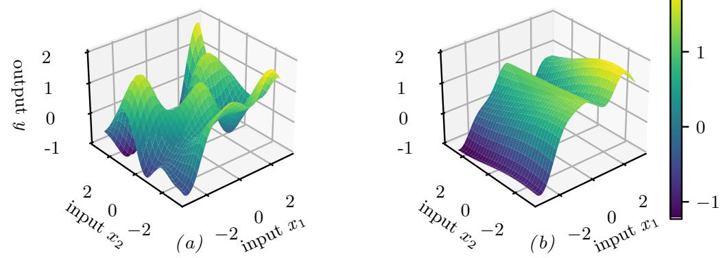
Figure 18.2: Function samples from a GP with an ARD kernel. (a) ε¹ = ε² = 1. Both dimensions contribute to the response. (b) ε¹ = 1, ε² = 5. The second dimension is essentially ignored. Adapted from Figure 5.1 of [RW06]. Generated by gpr\_demo\_ard.ipynb.

where

\[\mathcal{K}(r;\ell,\tau^2) = \tau^2 \exp\left(-\frac{1}{2}\frac{1}{\ell^2}r^2\right) \tag{18.12}\]

We can interpret ς² as the overall variance, and ε^d as defining the characteristic length scale of dimension d. If d is an irrelevant input dimension, we can set ε^d = ⇓, so the corresponding dimension will be ignored. This is known as automatic relevance determination or ARD (Section 15.2.8). Hence the corresponding kernel is called the ARD kernel. See Figure 18.2 for an illustration of some 2d functions sampled from a GP using this prior.

18.2.1.3 Matérn kernels

The SE kernel gives rise to functions that are infinitely di!erentiable, and therefore are very smooth. For many applications, it is better to use the Matérn kernel, which gives rise to “rougher” functions, which can better model local “wiggles” without having to make the overall length scale very small.

The Matérn kernel has the following form:

\[\mathcal{K}(r;\nu,\ell) = \frac{2^{1-\nu}}{\Gamma(\nu)} \left(\frac{\sqrt{2\nu}r}{\ell}\right)^{\nu} K\_{\nu}\left(\frac{\sqrt{2\nu}r}{\ell}\right) \tag{18.13}\]

where K⁰ is a modified Bessel function and ε is the length scale. Functions sampled from this GP are k-times di!erentiable i! 4 > k. As 4 ↖ ⇓, this approaches the SE kernel.

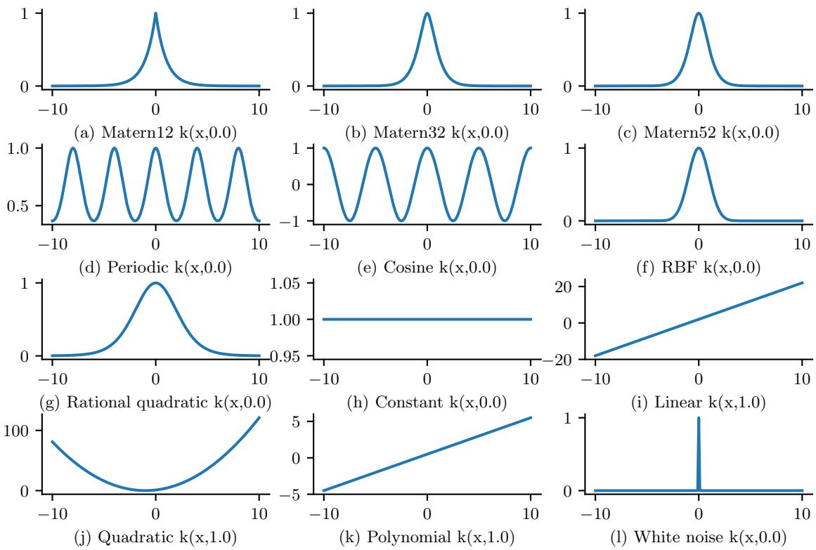
Figure 18.3: GP kernels evaluated at k(x, 0) as a function of x. Generated by gpKernelPlot.ipynb.

For values ⁴ ↗ { ^{1 2} , ^{3 2} , ^{5 2} }, the function simplifies as follows:

\[\mathcal{K}(r; \frac{1}{2}, \ell) = \exp(-\frac{r}{\ell}) \tag{18.14}\]

\[\mathcal{K}(r; \frac{3}{2}, \ell) = \left(1 + \frac{\sqrt{3}r}{\ell}\right) \exp\left(-\frac{\sqrt{3}r}{\ell}\right) \tag{18.15}\]

\[\mathcal{K}(r; \frac{5}{2}, \ell) = \left( 1 + \frac{\sqrt{5}r}{\ell} + \frac{5r^2}{3\ell^2} \right) \exp\left( -\frac{\sqrt{5}r}{\ell} \right) \tag{18.16}\]

See Figure 18.3(a-c) and Figure 18.4(a-c) for a visualization.

The value 4 = ^{1 2} corresponds to the Ornstein-Uhlenbeck process, which describes the velocity of a particle undergoing Brownian motion. The corresponding function is continuous but not di!erentiable, and hence is very “jagged”.

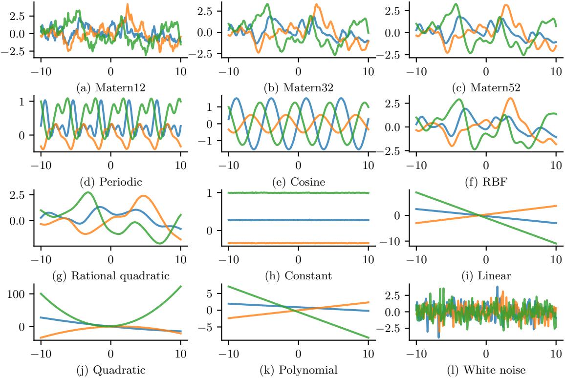
Figure 18.4: GP samples drawn using di!erent kernels. Generated by gpKernelPlot.ipynb.

18.2.1.4 Periodic kernels

One way to create a periodic 1d random function is to map x to the 2d space u(x)=(cos(x),sin(x)), and then use an SE kernel in u-space:

\[\mathcal{K}(x, x') = \exp\left(-\frac{2\sin^2((x - x')/2)}{\ell^2}\right) \tag{18.17}\]

which follows since (cos(x) → cos(x^↔︎ ))² + (sin(x) ^→ sin(x^↔︎ ))² = 4 sin²((^{x → x↔︎} )/2). We can generalize this by specifying the period p to get the periodic kernel, also called the exp-sine-squared kernel:

\[\mathcal{K}\_{\text{per}}(r;\ell,p) = \exp\left(-\frac{2}{\ell^2}\sin^2(\pi\frac{r}{p})\right) \tag{18.18}\]

where p is the period and ε is the length scale. See Figure 18.3(d-e) and Figure 18.4(d-e) for a visualization.

A related kernel is the cosine kernel:

\[\mathcal{K}(r;p) = \cos\left(2\pi \frac{r}{p}\right) \tag{18.19}\]

18.2.1.5 Rational quadratic kernel

We define the rational quadratic kernel to be

\[\mathcal{K}\_{RQ}(r;\ell,\alpha) = \left(1 + \frac{r^2}{2\alpha\ell^2}\right)^{-\alpha} \tag{18.20}\]

We recognize this is proportional to a Student t density. Hence it can be interpreted as a scale mixture of SE kernels of di!erent characteristic lengths. In particular, let τ = 1/ε², and assume ^{τ ↔︎} Ga(ϱ, ^ε2). Then one can show that

\[\mathcal{K}\_{RQ}(r) = \int p(\tau|\alpha, \ell^2) \mathcal{K}\_{SE}(r|\tau) d\tau \tag{18.21}\]

As ϱ ↖ ⇓, this reduces to a SE kernel.

See Figure 18.3(g) and Figure 18.4(g) for a visualization.

18.2.1.6 Kernels from spectral densities

Consider the case of a stationary kernel which satisfies K(x, x^↔︎ ) = K(ς), where ς = x → x^↔︎ , for ^x, ^x↔︎ ↗ ^Rd. Let us further assume that ^K(ς) is positive definite. In this case, Bochner’s theorem tells us that we can represent K(ς) by its Fourier transform:

\[\mathcal{K}(\boldsymbol{\delta}) = \int\_{\mathbb{R}^d} p(\omega) e^{j\omega^\top \boldsymbol{\delta}} d\omega \tag{18.22}\]

where ^{j =} ∝→1, ^{ejϱ =} cos(ω) + ^j sin(ω), ⁰ is the frequency, and ^p(0) is the spectral density (see [SS19, p93, p253] for details).

We can easily derive and gain intuitions into several kernels from spectral densities. If we take the Fourier transform of an RBF kernel we find the spectral density ^p(0) = ^∝ 2ϖε² exp →2ϖ²0²ε² . Thus the spectral density is also Gaussian, but with a bandwidth inversely proportional to the length-scale hyperparameter ε. That is, as ε becomes large, the spectral density collapses onto a point mass. This result is intuitive: as we increase the length-scale, our model treats points as correlated over large distances, and becomes very smooth and slowly varying, and thus low-frequency. In general, since the Gaussian distribution has relatively light tails, we can see that RBF kernels won’t generally support high frequency solutions.

We can instead use a Student t spectral density, which has heavy tails that will provide greater support for higher frequencies. Taking the inverse Fourier transform of this spectral density, we recover the Matérn kernel, with degrees of freedom 4 corresponding to the degrees of freedom in the spectral density. Indeed, the smaller we make 4, the less smooth and higher frequency are the associated fits to data using a Matérn kernel.

We can also derive spectral mixture kernels by modelling the spectral density as a scale-location mixture of Gaussians and taking the inverse Fourier transform [WA13]. Since scale-location mixtures of Gaussians are dense in the set of distributions, and can therefore approximate any spectral density, this kernel can approximate any stationary kernel to arbitrary precision. The spectral mixture kernel thus forms a powerful approach to kernel learning, which we discuss further in Section 18.6.5.

18.2.2 Nonstationary kernels

A stationary kernel assumes the measure of similarity between two inputs is independent of their location, i.e., K(x, x^↔︎ ) only depends on r = x→x^↔︎ . A nonstationary kernel relaxes this assumption. This is useful for a variety of problems, such as environmental modeling (see e.g., [GSR12; Pat+22]), where correlations between locations can change depending on latent factors in the environment.

18.2.2.1 Polynomial kernels

A simple form of non-stationary kernel is the polynomial kernel (also called dot product kernel) of order M, defined by

\[\mathcal{K}(\mathbf{x}, \mathbf{z}') = (\mathbf{z}^{\mathsf{T}} \mathbf{z}')^M \tag{18.23}\]

This contains all monomials of order M. For example, if M = 2, we get the quadratic kernel; in 2d, this becomes

\[(x^\top x')^2 = (x\_1 x\_1' + x\_2 x\_2')^2 = (x\_1 x\_1')^2 + (x\_2 x\_2')^2 + 2(x\_1 x\_1')(x\_2 x\_2') \tag{18.24}\]

We can generalize this to contain all terms up to degree M by using the inhomogeneous polynomial kernel

\[\mathcal{K}(\mathbf{x}, \mathbf{z}') = (\mathbf{z}^{\mathsf{T}} \mathbf{z}' + c)^{M} \tag{18.25}\]

For example, if M = 2 and the inputs are 2d, we have

\[\begin{aligned} (x^\mathsf{T}x' + 1)^2 &= (x\_1x\_1')^2 + (x\_1x\_1')(x\_2x\_2') + (x\_1x\_1')\\ &+ (x\_2x\_2)(x\_1x\_1') + (x\_2x\_2')^2 + (x\_2x\_2')\\ &+ (x\_1x\_1') + (x\_2x\_2') + 1 \end{aligned} \tag{18.26}\]

18.2.2.2 Gibbs kernel

Consider an RBF kernel where the length scale hyper-parameter, and the signal variance hyperparameter, are both input dependent; this is called the Gibbs kernel [Gib97], and is defined by

\[\mathcal{K}(\mathbf{z}, \mathbf{z}') = \sigma(\mathbf{z})\sigma(\mathbf{z}') \sqrt{\frac{2\ell(\mathbf{z})\ell(\mathbf{z}')}{\ell(\mathbf{z})^2 + \ell(\mathbf{z}')^2}} \exp\left(-\frac{||\mathbf{z} - \mathbf{z}'||^2}{\ell(\mathbf{z})^2 + \ell(\mathbf{z}')^2}\right) \tag{18.27}\]

If ε(x) and ς(x) are constants, this reduces to the standard RBF kernel. We can model the functional dependency of these kernel parameters on the input by using another GP (see e.g., [Hei+16]).

18.2.2.3 Other non-stationary kernels

Other ways to induce non-stationarity include using a neural network kernel (Section 18.7.1), nonstationary spectral kernels [RHK17], or a deep GP (Section 18.7.3).

18.2.3 Kernels for nonvectorial (structured) inputs

Kernels are particularly useful when the inputs are structured objects, such as strings and graphs, since it is often hard to “featurize” variable-sized inputs. For example, we can define a string kernel which compares strings in terms of the number of n-grams they have in common [Lod+02; BC17].

We can also define kernels on graphs [KJM19]. For example, the random walk kernel conceptually performs random walks on two graphs simultaneously, and then counts the number of paths that were produced by both walks. This can be computed e”ciently as discussed in [Vis+10]. For more details on graph kernels, see [KJM19].

For a review of kernels on structured objects, see e.g., [Gär03].

18.2.4 Making new kernels from old

Given two valid kernels K1(x, x^↔︎ ) and K2(x, x^↔︎ ), we can create a new kernel using any of the following methods:

\[\mathcal{K}(\mathbf{z}, \mathbf{z}') = c \mathcal{K}\_1(\mathbf{z}, \mathbf{z}'), \text{ for any constant } c > 0 \tag{18.28}\]

\[\mathcal{K}(\mathbf{x}, \mathbf{z}') = f(\mathbf{z}) \mathcal{K}\_1(\mathbf{z}, \mathbf{z}') f(\mathbf{z}'), \text{ for any function } f \tag{18.29}\]

\[\mathcal{K}(\mathbf{z}, \mathbf{z}') = q(\mathcal{K}\_1(\mathbf{z}, \mathbf{z}')) \text{ for any polynomial function } q \text{ with nonnegative. coef.} \tag{18.30}\]

\[\mathcal{K}(\mathbf{x}, \mathbf{z}') = \exp(\mathcal{K}\_1(\mathbf{z}, \mathbf{z}')) \tag{18.31}\]

\[\mathcal{K}(\mathbf{x}, \mathbf{z}') = \mathbf{z}^{\mathsf{T}} \mathbf{A} \mathbf{z}', \text{ for any psd matrix } \mathbf{A} \tag{18.32}\]

For example, suppose we start with the linear kernel K(x, x^↔︎ ) = xx^↔︎ . We know this is a valid Mercer kernel, since the corresponding Gram matrix is just the (scaled) covariance matrix of the data. From the above rules, we can see that the polynomial kernel K(x, x^↔︎ )=(x^Tx^↔︎ )^M from Section 18.2.2.1 is a valid Mercer kernel.

We can also use the above rules to establish that the Gaussian kernel is a valid kernel. To see this, note that

\[||\mathbf{x} - \mathbf{z}'||^2 = \mathbf{z}^\mathsf{T}\mathbf{z} + (\mathbf{z}')^\mathsf{T}\mathbf{z}' - 2\mathbf{z}^\mathsf{T}\mathbf{z}'\tag{18.33}\]

and hence

\[\mathcal{K}(\mathbf{x}, \mathbf{z}') = \exp(-||\mathbf{z} - \mathbf{z}'||^2 / 2\sigma^2) = \exp(-\mathbf{z}^\mathsf{T}\mathbf{z} / 2\sigma^2)\exp(\mathbf{z}^\mathsf{T}\mathbf{z}' / \sigma^2)\exp(-(\mathbf{z}')^\mathsf{T}\mathbf{z}' / 2\sigma^2) \tag{18.34}\]

is a valid kernel.

We can also combine kernels using addition or multiplication:

\[ \lambda \mathcal{K}(x, x') = \mathcal{K}\_1(x, x') + \mathcal{K}\_2(x, x') \tag{18.35} \]

\[ \mathcal{K}(\mathbf{x}, \mathbf{z}') = \mathcal{K}\_1(\mathbf{x}, \mathbf{z}') \times \mathcal{K}\_2(\mathbf{z}, \mathbf{z}') \tag{18.36} \]

Multiplying two positive-definite kernels together always results in another positive definite kernel. This is a way to get a conjunction of the individual properties of each kernel, as illustrated in Figure 18.5.

In addition, adding two positive-definite kernels together always results in another positive definite kernel. This is a way to get a disjunction of the individual properties of each kernel, as illustrated in Figure 18.6.

For an example of combining kernels to forecast some time series data, see Section 18.8.1.

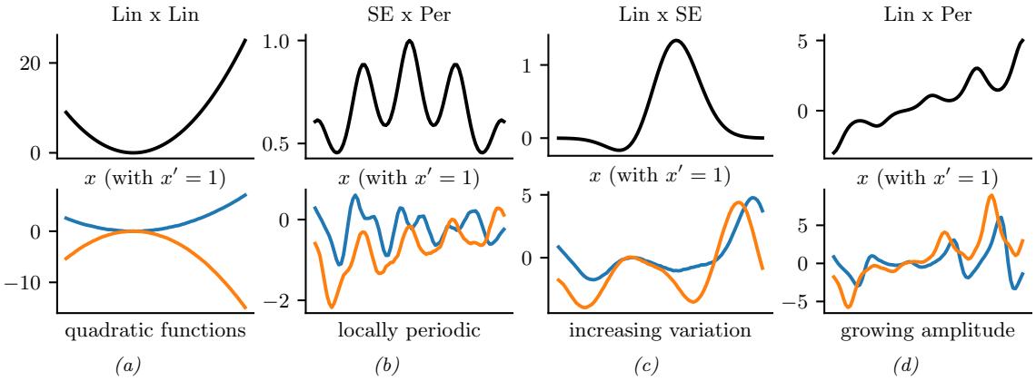
Figure 18.5: Examples of 1d structures obtained by multiplying elementary kernels. Top row shows K(x, x^↑ = 1). Bottom row shows some functions sampled from GP(f|0, K). Adapted from Figure 2.2 of [Duv14]. Generated by combining\_kernels\_by\_multiplication.ipynb.

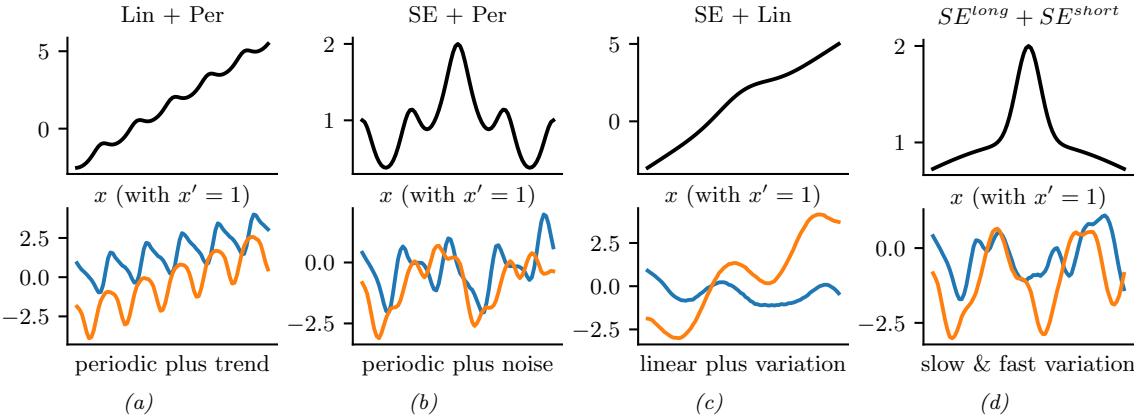
Figure 18.6: Examples of 1d structures obtained by summing elementary kernels. Top row shows K(x, x^↑ = 1). Bottom row shows some functions sampled from GP(f|0, K). Adapted from Figure 2.2 of [Duv14]. Generated by combining\_kernels\_by\_summation.ipynb.

18.2.5 Mercer’s theorem

Recall that any positive definite matrix K can be represented using an eigendecomposition of the form K = U^T#U, where # is a diagonal matrix of eigenvalues ⇀ⁱ > 0, and U is a matrix containing the eigenvectors. Now consider element (i, j) of K:

\[k\_{ij} = (\mathbf{A}^{\frac{1}{2}} \mathbf{U}\_{:i})^{\mathrm{T}} (\mathbf{A}^{\frac{1}{2}} \mathbf{U}\_{:j}) \tag{18.37}\]

where U:ⁱ is the i’th column of U. If we define ε(xi) = U:i, then we can write

\[k\_{ij} = \sum\_{m=1}^{M} \lambda\_m \phi\_m(\mathbf{z}\_i) \phi\_m(\mathbf{z}\_j) \tag{18.38}\]

where M is the rank of the kernel matrix. Thus we see that the entries in the kernel matrix can be computed by performing an inner product of some feature vectors that are implicitly defined by the eigenvectors of the kernel matrix.

This idea can be generalized to apply to kernel functions, not just kernel matrices, as we now show. First, we define an eigenfunction 3() of a kernel K with eigenvalue ⇀ wrt measure µ as a function that satisfies

\[\int \mathcal{K}(\mathbf{x}, \mathbf{x}') \phi(\mathbf{x}) d\mu(\mathbf{x}) = \lambda \phi(\mathbf{x}') \tag{18.39}\]

We usually sort the eigenfunctions in order of decreasing eigenvalue, ⇀¹ ≃ ⇀² ≃ ··· . The eigenfunctions are orthogonal wrt µ:

\[\int \phi\_i(\mathbf{x})\phi\_j(\mathbf{x})d\mu(\mathbf{x}) = \delta\_{ij} \tag{18.40}\]

where ϑij is the Kronecker delta. With this definition in hand, we can state Mercer’s theorem. Informally, it says that any positive definite kernel function can be represented as the following infinite sum:

\[\mathcal{K}(\mathbf{z}, \mathbf{z}') = \sum\_{m=1}^{\infty} \lambda\_m \phi\_m(\mathbf{z}) \phi\_m(\mathbf{z}') \tag{18.41}\]

where 3^m are eigenfunctions of the kernel, and ⇀^m are the corresponding eigenvalues. This is the functional analog of Equation (18.38).

A degenerate kernel has only a finite number of non-zero eigenvalues. In this case, we can rewrite the kernel function as an inner product between two finite-length vectors. For example, consider the quadratic kernel K(x, x^↔︎ ) = Bx, x^{↔︎ C2} from Equation (18.24). If we define ^ε(x1, x2) = [x² 1, ^∝2x1x2, x^{2 2}] ↗ ^R3, then we can write this as ^K(x, ^x↔︎ ) = ε(x) ^Tε(x^↔︎ ). Thus we see that this kernel is degenerate.

Now consider the RBF kernel. In this case, the corresponding feature representation is infinite dimensional (see Section 18.2.6 for details). However, by working with kernel functions, we can avoid having to deal with infinite dimensional vectors.

From the above, we see that we can replace inner product operations in an explicit (possibly infinite dimensional) feature space with a call to a kernel function, i.e., we replace ε(x) ^Tε(x) with K(x, x^↔︎ ). This is called the kernel trick.

18.2.6 Approximating kernels with random features

Although the power of kernels resides in the ability to avoid working with featurized representations of the inputs, such kernelized methods can take O(N³) time, in order to invert the Gram matrix K, as we will see in Section 18.3. This can make it di”cult to use such methods on large scale data.

Fortunately, we can approximate the feature map for many kernels using a randomly chosen finite set of M basis functions, thus reducing the cost to O(NM + M3).

We will show how to do this for shift-invariant kernels by returning to Bochner’s theorem in Eq. (18.22). In the case of a Gaussian RBF kernel, we have seen that the spectral density is a Gaussian distribution. Hence we can easily compute a Monte Carlo approximation to this integral by sampling random Gaussian vectors. This yields the following approximation: K(x, x^↔︎ ) ↓ ε(x) ^Tε(x), where the (real-valued) feature vector is given by

\[\boldsymbol{\phi}(\mathbf{z}) = \sqrt{\frac{1}{D}} \begin{bmatrix} \sin(\mathbf{z}\_1^\mathsf{T} \mathbf{z}), \cdots, \sin(\mathbf{z}\_D^\mathsf{T} \mathbf{z}), \cos(\mathbf{z}\_1^\mathsf{T} \mathbf{z}), \cdots, \cos(\mathbf{z}\_D^\mathsf{T} \mathbf{z}) \end{bmatrix} \tag{18.42}\]

\[=\sqrt{\frac{1}{D}}\left[\sin(\mathbf{Z}^{\mathsf{T}}\mathbf{z}), \cos(\mathbf{Z}^{\mathsf{T}}\mathbf{z})\right] \tag{18.43}\]

Here Z = (1/ς)G, and G ↗ ^Rd⇑^D is a random Gaussian matrix, where the entries are sampled iid from N (0, 1). The representation in Equation (18.43) are called random Fourier features (RFF) [SS15; RR08] or “weighted sums of random kitchen sinks” [RR09]. (One can obtain an even better approximation by ensuring that the rows of Z are random but orthogonal; this is called orthogonal random features [Yu+16].)

One can create similar random feature representations for other kinds of kernels. We can then use such features for supervised learning by defining f(x; ω) = W5(Zx) + b, where Z is a random Gaussian matrix, and the form of 5 depends on the chosen kernel. This is equivalent to a one layer MLP with random input-to-hidden weights; since we only optimize the hidden-to-output weights ω = (W, b), the model is equivalent to a linear model with fixed random features. If we use enough random features, we can approximate the performance of a kernelized prediction model, but the computational cost is now O(N) rather than O(N²).

Unfortunately, random features can result in worse performance than using a non-degenerate kernel, since they don’t have enough expressive power. We discuss other ways to scale GPs to large datasets in Section 18.5.

18.3 GPs with Gaussian likelihoods

In this section, we discuss GPs for regression, using a Gaussian likelihood. In this case, all the computations can be performed in closed form, using standard linear algebra methods. We extend this framework to non-Gaussian likelihoods later in the chapter.

18.3.1 Predictions using noise-free observations

Suppose we observe a training set D = {(xn, yn) : n =1: N}, where yⁿ = f(xn) is the noise-free observation of the function evaluated at xn. If we ask the GP to predict f(x) for a value of x that it has already seen, we want the GP to return the answer f(x) with no uncertainty. In other words, it should act as an interpolator of the training data. Here we assume the observed function values are noiseless. We will consider the case of noisy observations shortly.

Now we consider the case of predicting the outputs for new inputs that may not be in D. Specifically, given a test set X^→ of size N^→ ⇔ D, we want to predict the function outputs f^→ = [f(x1),…,f(x^N↓ )].

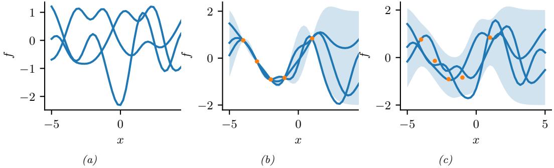
Figure 18.7: Left: some functions sampled from a GP prior with RBF kernel. Middle: some samples from a GP posterior, after conditioning on 5 noise-free observations. Right: some samples from a GP posterior, after conditioning on 5 noisy observations. The shaded area represents E [f(x)] ± 2 #V[f(x)]. Adapted from Figure 2.2 of [RW06]. Generated by gpr\_demo\_noise\_free.ipynb.

By definition of the GP, the joint distribution p(fX, f→|X, X→) has the following form

\[N\begin{pmatrix}f\_X\\f\_\*\end{pmatrix} \sim N\left(\begin{pmatrix}\mu\_X\\\mu\_\*\end{pmatrix}, \begin{pmatrix}\mathbf{K}\_{X,X} & \mathbf{K}\_{X,\*}\\\mathbf{K}\_{X,\*}^\top & \mathbf{K}\_{\*,\*}\end{pmatrix}\right) \tag{18.44}\]

where µ^X = (m(x1),…,m(x^N )), µ^→ = (m(x^→ 1),…,m(x^{→ N↓} )), KX,X = K(X, X) is N ⇔ N, KX,^→ = K(X, X→) is N ⇔ N→, and K→,^→ = K(X→, X→) is N^→ ⇔ N→. See Figure 18.7 for a static illustration, and http://www.infinitecuriosity.org/vizgp/ for an interactive visualization.

By the standard rules for conditioning Gaussians (Section 2.3.1.4), the posterior has the following form

\[p(\mathbf{f}\_\*|\mathbf{X}\_\*, \mathcal{D}) = \mathcal{N}(\mathbf{f}\_\*|\boldsymbol{\mu}\_{\*|X}, \boldsymbol{\Sigma}\_{\*|X}) \tag{18.45}\]

\[ \mu\_{\*|X} = \mu\_\* + \mathbf{K}\_{X,\*}^{\mathsf{T}} \mathbf{K}\_{X,X}^{-1} (f\_X - \mu\_X) \tag{18.46} \]

\[\mathbf{E}\_{\*|X} = \mathbf{K}\_{\*,\*} - \mathbf{K}\_{X,\*}^{\mathsf{T}} \mathbf{K}^{-1} \mathbf{K}\_{X,\*} \tag{18.47}\]

This process is illustrated in Figure 18.7. On the left we show some samples from the prior, p(f), where we use an RBF kernel (Section 18.2.1.1) and a zero mean function. On the right, we show samples from the posterior, p(f|D). We see that the model perfectly interpolates the training data, and that the predictive uncertainty increases as we move further away from the observed data.

Note that the cost of the above method for sampling N^→ points is O(N^{3 →} ). This can be reduced to O(N→) time using the methods in [Ple+18; Wil+20a].

18.3.2 Predictions using noisy observations

In Section 18.3.1, we showed how to do GP regression when the training data was noiseless. Now let us consider the case where what we observe is a noisy version of the underlying function, yⁿ = f(xn)+⇁n, where ⇁^{n ↔︎ N} (0, ^{ς2 y}). In this case, the model is not required to interpolate the data, but it must come “close” to the observed data. The covariance of the observed noisy responses is

\[\text{Cov}\left[y\_i, y\_j\right] = \text{Cov}\left[f\_i, f\_j\right] + \text{Cov}\left[\epsilon\_i, \epsilon\_j\right] = \mathcal{K}(\mathbf{x}\_i, \mathbf{x}\_j) + \sigma\_y^2 \delta\_{ij} \tag{18.48}\]

where ϑij = I(i = j). In other words

\[\text{Cov}\left[y|\mathbf{X}\right] = \mathbf{K}\_{X,X} + \sigma\_y^2 \mathbf{I}\_N \tag{18.49}\]

The joint density of the observed data and the latent, noise-free function on the test points is given by

\[N\begin{pmatrix}\mathbf{y} \\ \mathbf{f}\_{\*}\end{pmatrix} \sim N\left(\begin{pmatrix}\mu\_{X} \\ \mu\_{\*}\end{pmatrix}, \begin{pmatrix}\mathbf{K}\_{X,X} + \sigma\_{y}^{2}\mathbf{I} & \mathbf{K}\_{X,\*} \\ \mathbf{K}\_{X,\*}^{\mathrm{T}} & \mathbf{K}\_{\*,\*}\end{pmatrix}\right) \tag{18.50}\]

Hence the posterior predictive density at a set of test points X^→ is

\[p(f\_\*|\mathcal{D}, \mathbf{X}\_\*) = \mathcal{N}(f\_\*|\mu\_{\*|X}, \Sigma\_{\*|X}) \tag{18.51}\]

\[ \mu\_{\*|X} = \mu\_\* + \mathbf{K}\_{X,\*}^{\mathsf{T}} (\mathbf{K}\_{X,X} + \sigma\_y^2 \mathbf{I})^{-1} (y - \mu\_X) \tag{18.52} \]

\[\mathbf{E}\_{\*\mid X} = \mathbf{K}\_{\*,\*} - \mathbf{K}\_{X,\*}^{\mathsf{T}} (\mathbf{K}\_{X,X} + \sigma\_y^2 \mathbf{I})^{-1} \mathbf{K}\_{X,\*} \tag{18.53}\]

In the case of a single test input, this simplifies as follows

\[p(f\_\*|\mathcal{D}, \mathbf{x}\_\*) = \mathcal{N}(f\_\*|m\_\* + \mathbf{k}\_\*^\mathsf{T}(\mathbf{K}\_{X,X} + \sigma\_y^2 \mathbf{I})^{-1}(\mathbf{y} - \mu\_X), \ k\_{\*\*} - \mathbf{k}\_\*^\mathsf{T}(\mathbf{K}\_{X,X} + \sigma\_y^2 \mathbf{I})^{-1}\mathbf{k}\_\*) \tag{18.54}\]

where k^→ = [K(x→, x1),…, K(x→, x^N )] and k→→ = K(x→, x→). If the mean function is zero, we can write the posterior mean as follows:

\[\mu\_{\*\mid X} = \mathbf{k}\_\*^\mathrm{T} \underbrace{\mathbf{K}\_\sigma^{-1} y}\_{\alpha} = \sum\_{n=1}^N \mathcal{K}(x\_\*, x\_n) \alpha\_n \tag{18.55}\]

where

\[\mathbf{K}\_{\sigma} = \mathbf{K}\_{X,X} + \sigma\_y^2 \mathbf{I} \tag{18.56}\]

\[\alpha = \mathbf{K}\_{\sigma}^{-1} y\]

Fitting this model amounts to computing ↼ in Equation (18.57). This is usually done by computing the Cholesky decomposition of K↽, as described in Section 18.3.6. Once we have computed ↼, we can compute predictions for each test point in O(N) time for the mean, and O(N²) time for the variance.

18.3.3 Weight space vs function space

In this section, we show how Bayesian linear regression is a special case of a GP.

Consider the linear regression model ^{y = f}(x) + ⇁, where ^f(x) = ^wTε(x) and ⇁ ^{↔︎ N} (0, ^{ς2 y}). If we use a Gaussian prior p(w) = N (w|0, !w), then the posterior is as follows (see Section 15.2.2 for the derivation):

\[p(w|\mathcal{D}) = \mathcal{N}(w|\frac{1}{\sigma\_y^2}\mathbf{A}^{-1}\Phi^T\mathbf{y}, \mathbf{A}^{-1})\tag{18.58}\]

where % is the N ⇔ D design matrix, and

\[\mathbf{A} = \sigma\_y^{-2} \Phi^\mathsf{T} \Phi + \Sigma\_w^{-1} \tag{18.59}\]

The posterior predictive distribution for f^→ = f(x→) is therefore

\[p(f\_\*|\mathcal{D}, x\_\*) = N(f\_\*|\frac{1}{\sigma\_y^2} \boldsymbol{\phi}\_\*^\mathsf{T} \mathbf{A}^{-1} \boldsymbol{\Phi}^\mathsf{T} \boldsymbol{y}, \ \boldsymbol{\phi}\_\*^\mathsf{T} \mathbf{A}^{-1} \boldsymbol{\phi}\_\*) \tag{18.60}\]

where ε^→ = ε(x→). This views the problem of inference and prediction in weight space.

We now show that this is equivalent to the predictions made by a GP using a kernel of the form K(x, x^↔︎ ) = ε(x) ^T!wε(x^↔︎ ). To see this, let ^{K =} %!w%^T, ^{k→ =} %!wε→, and ^k→→ ^{= εT →}!wε→. Using this notation, and the matrix inversion lemma, we can rewrite Equation (18.60) as follows

\[p(f\_\*|\mathcal{D}, \mathcal{x}\_\*) = \mathcal{N}(f\_\*|\mu\_{\*|X}, \Sigma\_{\*|X}) \tag{18.61}\]

\[ \mu\_{\*\mid X} = \boldsymbol{\phi}\_{\*}^{\mathsf{T}} \boldsymbol{\Sigma}\_{w} \boldsymbol{\Phi}^{\mathsf{T}} (\mathbf{K} + \sigma\_{y}^{2} \mathbf{I})^{-1} \boldsymbol{y} = \boldsymbol{k}\_{\*}^{\mathsf{T}} (\mathbf{K} \boldsymbol{\chi}, \boldsymbol{x} + \sigma\_{y} \mathbf{I})^{-1} \boldsymbol{y} \tag{18.62} \]

\[\boldsymbol{\Sigma}\_{\*|X} = \boldsymbol{\phi}\_{\*}^{\mathsf{T}} \boldsymbol{\Sigma}\_{w} \boldsymbol{\phi}\_{\*} - \boldsymbol{\phi}\_{\*}^{\mathsf{T}} \boldsymbol{\Sigma}\_{w} \boldsymbol{\Phi}^{\mathsf{T}} (\mathbf{K} + \boldsymbol{\sigma}\_{y}^{2} \mathbf{I})^{-1} \boldsymbol{\Phi} \boldsymbol{\Sigma}\_{w} \boldsymbol{\phi}\_{\*} = \boldsymbol{k}\_{\*\*} - \boldsymbol{k}\_{\*}^{\mathsf{T}} (\mathbf{K}\_{X,X} + \boldsymbol{\sigma}\_{y}^{2} \mathbf{I})^{-1} \boldsymbol{k}\_{\*} \tag{18.63}\]

which matches the results in Equation (18.54), assuming m(x)=0. A non-zero mean can be captured by adding a constant feature with value 1 to ε(x).

Thus we can derive a GP from Bayesian linear regression. Note, however, that linear regression assumes ε(x) is a finite length vector, whereas a GP allows us to work directly in terms of kernels, which may correspond to infinite length feature vectors (see Section 18.2.5). That is, a GP works in function space.

18.3.4 Semiparametric GPs

So far, we have mostly assumed the mean of the GP is 0, and have relied on its interpolation abilities to model the mean function. Sometimes it is useful to fit a global linear model for the mean, and use the GP to model the residual errors, as follows:

\[g(x) = f(x) + \boldsymbol{\beta}^{\mathsf{T}} \boldsymbol{\phi}(x) \tag{18.64}\]

where f(x) ↔︎ GP(0, K(x, x^↔︎ )), and ε() are some fixed basis functions. This combines a parametric and a non-parametric model, and is known as a semi-parametric model.

If we assume ⇀ ↔︎ N (b, B), we can integrate these parameters out to get a new GP [O’H78]:

\[g(\mathbf{z}) \sim \text{GP}\left(\phi(\mathbf{z})^{\mathsf{T}} \mathbf{b}, \,\,\mathcal{K}(\mathbf{z}, \mathbf{z}') + \phi(\mathbf{z})^{\mathsf{T}} \mathbf{B}\phi(\mathbf{z}')\right) \tag{18.65}\]

Let H^X = ε(X) ^T be the ^{D ⇔N} matrix of training examples, and ^{H→ = ε}(X→) ^T be the ^{D ⇔}N^→ matrix of test examples. The corresponding predictive distribution for test inputs X^→ has the following form [RW06, p28]:

\[\mathbb{E}\left[g(\mathbf{X}\_{\ast})|\mathcal{D}\right] = \mathbf{H}\_{\ast}^{\mathsf{T}}\overline{\boldsymbol{\beta}} + \mathbf{K}\_{X,\ast}^{\mathsf{T}}\mathbf{K}\_{\sigma}^{-1}(y - \mathbf{H}\_{X}^{\mathsf{T}}\overline{\boldsymbol{\beta}}) = \mathbb{E}\left[f(\mathbf{X}\_{\ast})|\mathcal{D}\right] + \mathbf{R}^{\mathsf{T}}\overline{\boldsymbol{\beta}}\tag{18.66}\]

\[\text{Cov}\left[g(\mathbf{X}\_{\ast})|\mathcal{D}\right] = \text{Cov}\left[f(\mathbf{X}\_{\ast})|\mathcal{D}\right] + \mathbf{R}^{\mathsf{T}}(\mathbf{B}^{-1} + \mathbf{H}\_{X}\mathbf{K}\_{\sigma}^{-1}\mathbf{H}\_{X}^{\mathsf{T}})^{-1}\mathbf{R} \tag{18.67}\]

\[\overline{\beta} = (\mathbf{B}^{-1} + \mathbf{H}\_X \mathbf{K}\_\sigma^{-1} \mathbf{H}\_X^\top)^{-1} (\mathbf{H}\_X \mathbf{K}\_\sigma^{-1} y + \mathbf{B}^{-1} b) \tag{18.68}\]

\[\mathbf{R} = \mathbf{H}\_{\*} - \mathbf{H}\_{X}\mathbf{K}\_{\sigma}^{-1}\mathbf{K}\_{X,\*} \tag{18.69}\]

These results can be interpreted as follows: the mean is the usual mean from the GP, plus a global o!set from the linear model, using ⇀; and the covariance is the usual covariance from the GP, plus an additional positive term due to the uncertainty in ⇀.

In the limit of an uninformative prior for the regression parameters, as B ↖ ⇓I, this simplifies to

\[\mathbb{E}\left[g(\mathbf{X}\_{\ast})|\mathcal{D}\right] = \mathbb{E}\left[f(\mathbf{X}\_{\ast})|\mathcal{D}\right] + \mathbf{R}^{\mathsf{T}}(\mathbf{H}\_{X}\mathbf{K}\_{\sigma}^{-1}\mathbf{H}\_{X}^{\mathsf{T}})^{-1}\mathbf{H}\_{X}\mathbf{K}\_{\sigma}^{-1}\mathbf{y} \tag{18.70}\]

\[\text{Cov}\left[g(\mathbf{X}\_{\ast})|\mathcal{D}\right] = \text{Cov}\left[f(\mathbf{X}\_{\ast})|\mathcal{D}\right] + \mathbf{R}^{\mathsf{T}}(\mathbf{H}\_{X}\mathbf{K}\_{\sigma}^{-1}\mathbf{H}\_{X}^{\mathsf{T}})^{-1}\mathbf{R} \tag{18.71}\]

18.3.5 Marginal likelihood

Most kernels have some free parameters. For example, the RBF-ARD kernel (Section 18.2.1.2) has the form

\[\mathcal{K}(\mathbf{x}, \mathbf{z}') = \exp\left(-\frac{1}{2} \sum\_{d=1}^{D} \frac{1}{\ell\_d^2} (x\_d - x\_d')^2\right) = \prod\_{d=1}^{D} \mathcal{K}\_{\ell\_d}(x\_d, x\_d') \tag{18.72}\]

where each ε^d is a length scale for feature dimension d. Let these (and the observation noise variance ς2 ^y, if present) be denoted by ω. We can compute the likelihood of these parameters as follows:

\[p(\boldsymbol{y}|\mathbf{X},\boldsymbol{\theta}) = p(\mathcal{D}|\boldsymbol{\theta}) = \int p(\boldsymbol{y}|\mathbf{f}\_{X},\boldsymbol{\theta}) p(\mathbf{f}\_{X}|\mathbf{X},\boldsymbol{\theta}) d\boldsymbol{f}\_{X} \tag{18.73}\]

Since we are integrating out the function f, we often call ω hyperparameters, and the quantity p(D|ω) the marginal likelihood.

Since f is a GP, we can compute the above integral using the marginal likelihood for the corresponding Gaussian. This gives

\[\log p(\mathcal{D}|\boldsymbol{\theta}) = -\frac{1}{2}(\boldsymbol{y} - \boldsymbol{\mu}\_{\boldsymbol{X}})^{\mathsf{T}} \mathbf{K}\_{\sigma}^{-1} (\boldsymbol{y} - \boldsymbol{\mu}\_{\boldsymbol{X}}) - \frac{1}{2} \log |\mathbf{K}\_{\sigma}| - \frac{N}{2} \log(2\pi) \tag{18.74}\]

The first term is the square of the Mahalanobis distance between the observations and the predicted values: better fits will have smaller distance. The second term is the log determinant of the covariance matrix, which measures model complexity: smoother functions will have smaller determinants, so → log |K↽| will be larger (less negative) for simpler functions. The marginal likelihood measures the tradeo! between fit and complexity.

In Section 18.6.1, we discuss how to learn the kernel parameters from data by maximizing the marginal likelihood wrt ω.

18.3.6 Computational and numerical issues

In this section, we discuss computational and numerical issues which arise when implementing the above equations. For notational simplicity, we assume the prior mean is zero, m(x)=0.

The posterior predictive mean is given by µ^→ = k^{T →}K↓¹ ↽ ^y. For reasons of numerical stability, it is unwise to directly invert K↽. A more robust alternative is to compute a Cholesky decomposition, K↽ = LL^T, which takes O(N³) time. Given this, we can compute

\[\boldsymbol{\mu}\_{\*} = \boldsymbol{k}\_{\*}^{\mathsf{T}} \mathbf{K}\_{\sigma}^{-1} \boldsymbol{y} = \boldsymbol{k}\_{\*}^{\mathsf{T}} \mathbf{L}^{-\mathsf{T}} (\mathbf{L}^{-1} \boldsymbol{y}) = \boldsymbol{k}\_{\*}^{\mathsf{T}} \boldsymbol{\alpha} \tag{18.75}\]

Here ↼ ^{= LT} * (^{L  y}*), where we have used the backslash operator to represent backsubstitution.

We can compute the variance in O(N2) time for each test case using

\[ \sigma\_s^2 = k\_{ss} - k\_s^\mathrm{T} \mathbf{L}^{-T} \mathbf{L}^{-1} \mathbf{k}\_s = k\_{ss} - \mathbf{v}^\mathrm{T} \mathbf{v} \tag{18.76} \]

where v = L  k→.

Finally, the log marginal likelihood (needed for kernel learning, Section 18.6) can be computed using

\[\log p(y|\mathbf{X}) = -\frac{1}{2}y^\mathsf{T}\alpha - \sum\_{n=1}^{N} \log L\_{nn} - \frac{N}{2}\log(2\pi) \tag{18.77}\]

We see that overall cost is dominated by O(N³). We discuss faster, but approximate, methods in Section 18.5.

18.3.7 Kernel ridge regression

The term ridge regression refers to linear regression with an ε² penalty on the regression weights:

\[\mathbf{w}^\* = \underset{\mathbf{w}}{\operatorname{argmin}} \sum\_{n=1}^N (y\_n - f(\mathbf{z}\_n; \mathbf{w}))^2 + \lambda ||\mathbf{w}||\_2^2 \tag{18.78}\]

where f(x; w) = w^Tx. The solution for this is

\[\mathbf{w}^\* = (\mathbf{X}^\mathsf{T}\mathbf{X} + \lambda\mathbf{I})^{-1}\mathbf{X}^\mathsf{T}\mathbf{y} = (\sum\_{n=1}^N x\_n \mathbf{x}\_n^\mathsf{T} + \lambda\mathbf{I})^{-1}(\sum\_{n=1}^N x\_n y\_n) \tag{18.79}\]

In this section, we consider a function space version of this:

\[f^\* = \underset{f \in \mathcal{F}}{\text{argmin}} \sum\_{n=1}^N (y\_n - f(\mathbf{z}\_n))^2 + \lambda ||f||^2 \tag{18.80}\]

For this to make sense, we have to define the function space F and the norm ||f||. If we use a function space derived from a positive definite kernel function K, the resulting method is called kernel ridge regression (KRR). We will see that the resulting estimate f ^→(x→) is equivalent to the posterior mean of a GP. We give the details below.

18.3.7.1 Reproducing kernel Hilbert spaces

In this section, we briefly introduce the relevant mathematical “machinery” needed to explain KRR.

Let F = {f : X ↖ R} be a space of real-valued functions. Elements of this space (i.e., functions) can be added and scalar multiplied as if they were vectors. That is, if f ↗ F and g ↗ F, then ϱf +↼g ↗ F for ϱ, ↼ ↗ R. We can also define an inner product for F, which is a mapping Bf,gC ↗ R which satisfies the following:

\[ \langle \alpha f\_1 + \beta f\_2, g \rangle = \alpha \langle f\_1, g \rangle + \beta \langle f\_2, g \rangle \tag{18.81} \]

\[ \langle f, g \rangle = \langle g, f \rangle \tag{18.82} \]

\[<\langle f, f \rangle \ge 0 \tag{18.83}\]

\[\langle f, f \rangle = 0 \text{ iff } f(x) = 0 \text{ for all } x \in \mathcal{X} \tag{18.84}\]

We define the norm of a function using

\[||f|| \triangleq \sqrt{\langle f, f \rangle} \tag{18.85}\]

A function space H with an inner product operator is called a Hilbert space. (We also require that the function space be complete, which means that every Cauchy sequence of functions fⁱ ↗ H has a limit that is also in H.)

The most common Hilbert space is the space known as L². To define this, we need to specify a measure µ on the input space X ; this is a function that assigns any (suitable) subset A of X to a positive number, such as its volume. This can be defined in terms of the density function w : X ↖ R, as follows:

\[ \mu(A) = \int\_A w(x)dx\tag{18.86} \]

Thus we have ^µ(dx) = ^w(x)dx. We can now define ^L2(^X , µ) to be the space of functions ^f : ^X ↖ ^R that satisfy

\[\int\_{X} f(x)^2 w(x) dx < \infty \tag{18.87}\]

This is known as the set of square-integrable functions. This space has an inner product defined by

\[ \langle f, g \rangle = \int\_{\mathcal{X}} f(x)g(x)w(x)dx \tag{18.88} \]

We define a Reproducing Kernel Hilbert Space or RKHS as follows. Let H be a Hilbert space of functions f : X ↖ R. We say that H is an RKHS endowed with inner product B·, ·C^H if there exists a (symmetric) kernel function K : X ⇔ X ↖ R with the following properties:

• For every x ↗ X , K(x, ·) ↗ H.
• K satisfies the reproducing property:

\[<\langle f(\cdot), \mathcal{K}(\cdot, x') \rangle = f(x') \tag{18.89}\]

The reason for the term “reproducing property” is as follows. Let f(·) = K(x, ·). Then we have that

\[ \langle \mathcal{K}(x, \cdot), \mathcal{K}(\cdot, x') \rangle = \mathcal{K}(x, x') \tag{18.90} \]

18.3.7.2 Complexity of a function in an RKHS

The main utility of RKHS from the point of view of machine learning is that it allows us to define a notion of a function’s “smoothness” or “complexity” in terms of its norm, as we now discuss.

Suppose we have a positive definite kernel function K. From Mercer’s theorem we have K(x, x^↔︎ & ) = ↘ ⁱ=1 ⇀i3i(x)3i(x^↔︎ & ). Now consider a Hilbert space ^H defined by functions of the form ^f(x) = ↘ ⁱ=1 ^fi3(x), with &↘ ⁱ=1 f ^{2 i} /⇀ < ⇓. The inner product of two functions in this space is

\[<\langle f, g \rangle\_{\mathcal{U}} = \sum\_{i=1}^{\infty} \frac{f\_i g\_i}{\lambda\_i} \tag{18.91}\]

Hence the (squared) norm is given by

\[||f||\_{\mathcal{H}}^2 = \langle f, f \rangle\_{\mathcal{H}} = \sum\_{i=1}^{\infty} \frac{f\_i^2}{\lambda\_i} \tag{18.92}\]

This is analogous to the quadratic form f^TK↓1f which occurs in some GP objectives (see Equation (18.101)). Thus the smoothness of the function is controlled by the properties of the corresponding kernel.

18.3.7.3 Representer theorem

In this section, we consider the problem of (regularized) empirical risk minimization in function space. In particular, consider the following problem:

\[f^\* = \operatorname\*{argmin}\_{f \in \mathcal{H}\_{\mathcal{K}}} \sum\_{n=1}^N \ell(y\_n, f(x\_n)) + \frac{\lambda}{2} ||f||\_{\mathcal{H}}^2 \tag{18.93}\]

where H^K is an RKHS with kernel K and ε(y, yˆ) ↗ R is a loss function. Then one can show [KW70; SHS01] the following result:

\[f^\*(x) = \sum\_{n=1}^N \alpha\_n \mathcal{K}(x, x\_n) \tag{18.94}\]

where ϱⁿ ↗ R are some coe”cients that depend on the training data. This is called the representer theorem.

Now consider the special case where the loss function is squared loss, and ⇀ = ς^{2 y}. We want to minimize

\[\mathcal{L}(f) = \frac{1}{2\sigma\_y^2} \sum\_{n=1}^{N} (y\_n - f(x\_n))^2 + \frac{1}{2}||f||\_{\mathcal{H}}^2 \tag{18.95}\]

Substituting in Equation (18.94), and using the fact that BK(·, xi), K(·, x^j )C = K(xi, x^j ), we obtain

\[\mathcal{L}(f) = \frac{1}{2}\boldsymbol{\alpha}^{\mathsf{T}}\mathbf{K}\boldsymbol{\alpha} + \frac{1}{2\sigma\_y^2}||\boldsymbol{y} - \mathbf{K}\boldsymbol{\alpha}||^2\tag{18.96}\]

\[\mathbf{K} = \frac{1}{2}\boldsymbol{\alpha}^{\mathsf{T}}(\mathbf{K} + \frac{1}{\sigma\_y^2}\mathbf{K}^2)\boldsymbol{\alpha} - \frac{1}{\sigma\_y^2}\mathbf{y}^{\mathsf{T}}\mathbf{K}\boldsymbol{\alpha} + \frac{1}{2\sigma\_y^2}\mathbf{y}^{\mathsf{T}}\mathbf{y} \tag{18.97}\]

Minimizing this wrt ↼ gives ↼ˆ = (K + ς^{2 y}I)↓¹y, which is the same as Equation (18.57). Furthermore, the prediction for a test point is

\[\hat{f}(\mathbf{x}\_{\*}) = \mathbf{k}\_{\*}^{\mathrm{T}} \boldsymbol{\alpha} = \mathbf{k}\_{\*}^{\mathrm{T}} (\mathbf{K} + \sigma\_{y}^{2} \mathbf{I})^{-1} \mathbf{y} \tag{18.98}\]

This is known as kernel ridge regression [Vov13]. We see that the result matches the posterior predictive mean of a GP in Equation (18.55).

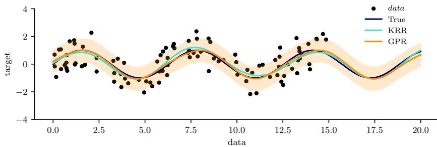
Figure 18.8: Kernel ridge regression (KRR) compared to Gaussian process regression (GPR) using the same kernel. Generated by krr\_vs\_gpr.ipynb.

Model	Likelihood	Section
Regression	ς2 N (fi, y)	Section 18.3.2
Robust regression	ς2 T0(fi, y)	Section 18.4.4
Binary classification	Ber(ς(fi))	Section 18.4.1
Multiclass classification	Cat(softmax(fi))	Section 18.4.2
Poisson regression	Poi(exp(fi))	Section 18.4.3

Table 18.1: Summary of GP models with a variety of likelihoods.

18.3.7.4 Example of KRR vs GPR

In this section, we compare KRR with GP regression on a simple 1d problem. Since the underlying function is believed to be periodic, we use the periodic kernel from Equation (18.18). To capture the fact that the observations are noisy, we add to this a white noise kernel

\[\mathcal{K}(\mathbf{x}, \mathbf{z}') = \sigma\_y^2 \delta(\mathbf{z} - \mathbf{z}') \tag{18.99}\]

as in Equation (18.48). Thus there are 3 GP hyper-parameters: the kernel length scale ε, the kernel periodicity p, and the noise level ς^{2 y}. We can optimize these by maximizing the marginal likelihood using gradient descent (see Section 18.6.1). For KRR, we also have 3 hyperparameters (ε, p, and ⇀ = ς^{2 y}); we optimize these using grid search combined with cross validation (which in general is slower than gradient based optimization). The resulting model fits are shown in Figure 18.8, and are very similar, as is to be expected.

18.4 GPs with non-Gaussian likelihoods

So far, we have focused on GPs for regression using Gaussian likelihoods. In this case, the posterior is also a GP, and all computation can be performed analytically. However, if the likelihood is non-Gaussian, we can no longer compute the posterior exactly. We can create a variety of di!erent “classical” models by changing the form of the likelihood, as we show in Table 18.1. In the sections below, we briefly discuss some approximate inference methods. (For more details, see e.g., [WSS21].)

log p(yi fi)	ϑ ϑfi log p(yi fi)	ϑ2 log p(yi fi) ϑf2 i
log ς(yifi)	ti → ϖi	→ϖi(1 → ϖi)
log ’(yifi)	yiς(fi) #(yifi)	ς2 #(yifi)2 → yifiς(fi) i → #(yifi)

Table 18.2: Likelihood, gradient, and Hessian for binary logistic/probit GP regression. We assume yⁱ ↓ {↗1, +1} and define tⁱ = (yⁱ + 1)/2 ↓ {0, 1} and ↼ⁱ = ω(fi) for logistic regression, and ↼ⁱ = !(fi) for probit regression. Also, ⇁ and ! are the pdf and cdf of N (0, 1). From [RW06, p43].

18.4.1 Binary classification

In this section, we consider binary classification using GPs. If we use the sigmoid link function, we have p(yⁿ = 1|xn) = ς(ynf(xn)). If we assume yⁿ ↗ {→1, +1}, then we have p(yn|xn) = ς(ynfn), since ς(→z)=1 → ς(z). If we use the probit link, we have p(yⁿ = 1|xn) = ‘(ynf(xn)), where’(z) is the cdf of the standard normal. More generally, let p(yn|xn) = Ber(yn|5(fn)). The overall log joint has the form

\[\mathcal{L}(\mathbf{f}\_X) = \log p(\mathbf{y}|\mathbf{f}\_X) + \log p(\mathbf{f}\_X|\mathbf{X}) \tag{18.100}\]

\[=\log p(\mathbf{y}|\mathbf{f}\_X) - \frac{1}{2}\mathbf{f}\_X^\top \mathbf{K}\_{X,X}^{-1} \mathbf{f}\_X - \frac{1}{2}\log|\mathbf{K}\_{X,X}| - \frac{N}{2}\log 2\pi\tag{18.101}\]

The simplest approach to approximate inference is to use a Laplace approximation (Section 7.4.3). The gradient and Hessian of the log joint are given by

\[\nabla \mathcal{L} = \nabla \log p(\mathbf{y}|f\_X) - \mathbf{K}\_{X,X}^{-1} f\_X \tag{18.102}\]

\[ \nabla^2 \mathcal{L} = \nabla^2 \log p(\mathbf{y}|\mathbf{f}\_X) - \mathbf{K}\_{X,X}^{-1} = -\mathbf{A} - \mathbf{K}\_{X,X}^{-1} \tag{18.103} \]

where # ↭ →⇒² log ^p(y|fX) is a diagonal matrix, since the likelihood factorizes across examples. Expressions for the gradient and Hessian of the log likelihood for the logit and probit case are shown in Table 18.2. At convergence, the Laplace approximation of the posterior takes the following form:

\[p(\mathbf{f}\_X|\mathcal{D}) \approx q(\mathbf{f}\_X) = \mathcal{N}(\hat{\mathbf{f}}, (\mathbf{K}\_{X,X}^{-1} + \mathbf{A})^{-1}) \tag{18.104}\]

where fˆ is the MAP estimate. See [RW06, Sec 3.4] for further details.

For improved accuracy, we can use variational inference, in which we assume q(fX) = N (fX|m, S); we then optimize m and S using (stochastic) gradient descent, rather than assuming S is the Hessian at the mode. See Section 18.5.4 for the details.

Once we have a Gaussian posterior q(fX|D), we can then use standard GP prediction to compute q(f→|x→, D). Finally, we can approximate the posterior predictive distribution over binary labels using

\[ \pi\_\* = p(y\_\* = 1 | x\_\*, \mathcal{D}) = \int p(y\_\* = 1 | f\_\*) q(f\_\* | x\_\*, \mathcal{D}) df\_\* \tag{18.105} \]

This 1d integral can be computed using the probit approximation from Section 15.3.6. In this case we have ^{ϖ→ ↓ ς}(↽(v)^E [f→]), where ^{v = V} [f→] and ↽²(v) = (1 + ^ϖv/8)↓¹.

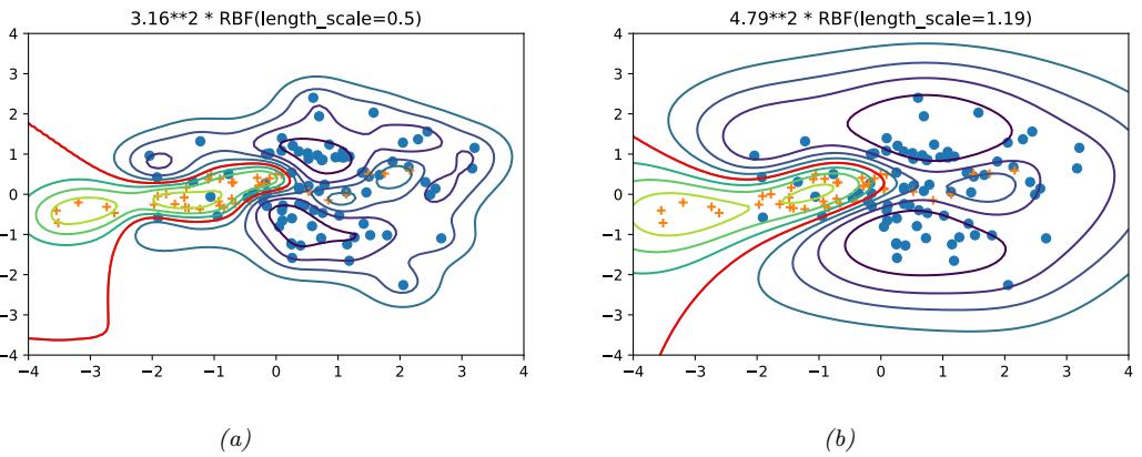
Figure 18.9: Contours of the posterior predictive probability for a binary classifier generated by a GP with an SE kernel. (a) Manual kernel parameters: short length scale, ^ε = 0.5, variance ³.16² ↙ ⁹.98. (b) Learned kernel parameters: long length scale, ^ε = 1.19, variance ⁴.79² ↙ ²².9. Generated by gpc\_demo\_2d.ipynb.

In Figure 18.9, we show a synthetic binary classification problem in 2d. We use an SE kernel. On the left, we show predictions using hyper-parameters set by hand; we use a short length scale, hence the very sharp turns in the decision boundary. On the right, we show the predictions using the learned hyper-parameters; the model favors more parsimonious explanation of the data.

18.4.2 Multiclass classification

The multi-class case is somewhat harder, since the function now needs to return a vector of C logits to get ^p(yn|xn) = Cat(yn|softmax(fn)), where ^fn = (^{f 1 n},…,f ^{C n} ), It is standard to assume that ^{f c ↔︎} GP(0, ^Kc). Thus we have one latent function per class, which are a priori independent, and which may use di!erent kernels.

We can derive a Laplace approximation for this model as discussed in [RW06, Sec 3.5]. Alternatively, we can use a variational approach, using the local variational bound to the multinomial softmax in [Cha12]. An alternative variational method, based on data augmentation with auxiliary variables, is described in [Wen+19b; Liu+19a; GFWO20]. More recently, some simple closed form Gaussian variational approximations for both the Bernoulli and softmax likelihoods has been derived in [Mil+18; Bui24]. For example, if 1^k = f(x, ω)^k is the logit for class k, and we use a Ga(6k; ϱ, ↼) for 6^k = exp(1k), then we replace the original likelihood with N (1k|mk, vk), where for the moment matching approximation of [Mil+18] we have ^mk = log(ϱ/↼) ^{→ 0}.5ς² and ^{vk = ς2} = log(1 + ^β ↼ ).

18.4.3 GPs for Poisson regression (Cox process)

In this section, we illustrate Poisson regression where the underlying log rate function is modeled by a GP. This is known as a Cox process. We can perform approximate posterior inference in this model using Laplace, MCMC, or SVI (stochastic variational inference). In Figure 18.10 we give a 1d example, where we use a Matérn ^{5 2} kernel. We apply MCMC and SVI. In the VI case, we additionally

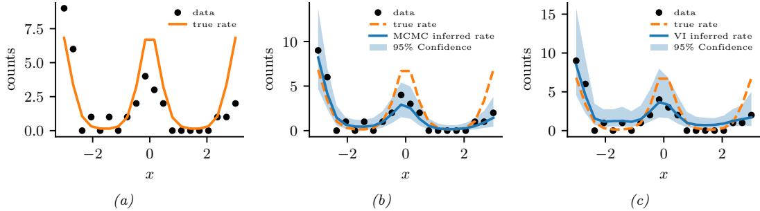
Figure 18.10: Poisson regression with a GP. (a) Observed data (black dots) and true log rate function (yellow line). (b) Posterior predictive distribution (shading shows 1 and 2 ω bands) from MCMC. (c) Posterior predictive distribution from SVI. Generated by gp\_poisson\_1d.ipynb.

have to specify the form of the posterior; we use a Gaussian approximation for the variational GP posterior p(f|X, y), and a point estimate for the kernel parameters.

An interesting application of this is to spatial disease mapping. For example, [VPV10] discuss the problem of modeling the relative risk of heart attack in di!erent regions in Finland. The data consists of the heart attacks in Finland from 1996–2000 aggregated into 20km ⇔ 20km lattice cells. The likelihood has the following form: yⁿ ↔︎ Poi(enrn), where eⁿ is the known expected number of deaths (related to the population of cell n and the overall death rate), and rⁿ is the relative risk of cell n which we want to infer. Since the data counts are small, we regularize the problem by sharing information with spatial neighbors. Hence we assume f ↭ log(r) ↔︎ GP(0, K). We use a Matérn kernel (Section 18.2.1.3) with 4 = 3/2, and a length scale and magnitude that are estimated from data.

Figure 18.11 gives an example of this method in action (using Laplace approximation). On the left we plot the posterior mean relative risk (RR), and on the right, the posterior variance. We see that the RR is higher in eastern Finland, which is consistent with other studies. We also see that the variance in the north is higher, since there are fewer people living there.

18.4.4 Other likelihoods

Many other likelihoods are possible. For example, [VJV09] uses a Student t likelihood in order to perform robust regression. A general method for performing approximate variational inference in GPs with such non-conjugate likelihoods is discussed in [WSS21].

18.5 Scaling GP inference to large datasets

In Section 18.3.6, we saw that the best way to perform GP inference and training is to compute a Cholesky decomposition of the ^{N ⇔ N} Gram matrix. Unfortunately, this takes ^O(N³) time. In this section, we discuss methods to scale up GPs to handle large N. See Table 18.3 for a summary, and

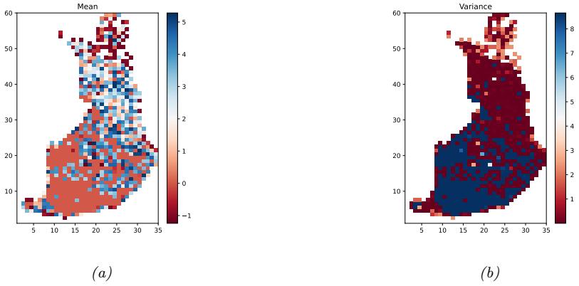
Figure 18.11: We show the relative risk of heart disease in Finland using a Poisson GP fit to 911 data points. Left: posterior mean. Right: posterior variance. Generated by gp\_spatial\_demo.ipynb.

Method	Cost	Section
Cholesky	O(N3)	Section 18.3.6
Conj. Grad.	O(CN2)	Section 18.5.5
Inducing	O(NM2 + M3 + DNM)	Section 18.5.3
Variational	O(NM2 + M3 + DNM)	Section 18.5.4
SVGP	O(BM2 + M3 + DNM)	Section 18.5.4.3
KISS-GP	CDMD log O(CN + M)	Section 18.5.5.3
SKIP	L3N CL2N) O(DLN + DLM log M + log D +	Section 18.5.5.3

Table 18.3: Summary of time to compute the log marginal likelihood of a GP regression model. Notation: N is number of training examples, M is number of inducing points, B is size of minibatch, D is dimensionality of input vectors (assuming ^{X = RD}), ^C is number of conjugate gradient iterations, and ^L is number of Lanczos iterations. Based on Table 2 of [Gar+18a].

[Liu+20c] for more details.1

18.5.1 Subset of data

The simplest approach to speeding up GP inference is to throw away some of the data. Suppose we keep a subset of M examples. In this case, exact inference will take O(M³) time. This is called the subset-of-data approach.

The key question is: how should we choose the subset? The simplest approach is to pick random examples (this method was recently analyzed in [HIY19]). However, intuitively it makes more sense to try to pick a subset that in some sense “covers” the original data, so it contains approximately the same information (up to some tolerance) without the redundancy. Clustering algorithms are

^1. We focus on e!cient methods for evaluating the marginal likelihood and the posterior predictive distribution. For an e!cient method for sampling a function from the posterior, see [Wil+20a].

one heuristic approach, but we can also use coreset methods, which can provably find such an information-preserving subset (see e.g., [Hug+19] for an application of this idea to GPs).

18.5.1.1 Informative vector machine

Clustering and coreset methods are unsupervised, in that they only look at the features xⁱ and not the labels yi, which can be suboptimal. The informative vector machine [HLS03] uses a greedy strategy to iteratively add the labeled example (x^j , y^j ) that maximally reduces the entropy of the function’s posterior, !^j = ^H (p(f^j )) ^{→ H} (pnew(f^j )), where ^pnew(f^j ) is the posterior of ^f at x^j after conditioning on y^j . (This is very similar to active learning.) To compute !^j , let ^p(f^j ) = ^N (µ^j , v^j ), and ^p(f^{j |}y^j ) ^{↑ p}(f^j )^N (y^{j |}f^j , ^ς2) = ^N (f^{j |}µnew ^j , vnew ^j ), where (vnew ^j )↓¹ = v↓^{1 j} +ς↓2. Since ^H (^N (µ, v)) ⁼ log(2ϖev)/2, we have !^j = 0.⁵ log(1 +vj/ς²). Since this is a monotonic function of v^j , we can maximize it by choosing the site with the largest variance. (In fact, entropy is a submodular function, so we can use submodular optimization algorithms to improve on the IVM, as shown in [Kra+08].)

18.5.1.2 Discussion

The main problem with the subset of data approach is that it ignores some of the data, which can reduce predictive accuracy and increase uncertainty about the true function. Fortunately there are other scalable methods that avoid this problem, essentially by approximately representing (or compressing) the training data, as we discuss below.

18.5.2 Nyström approximation

Suppose we had a rank M approximation to the N ⇔ N matrix gram matrix of the following form:

\[\mathbf{K}\_{X,X} \approx \mathbf{U} \boldsymbol{\Lambda} \mathbf{U}^{\top} \tag{18.106}\]

where # is a diagonal matrix of the M leading eigenvalues, and U is the matrix of the corresponding M eigenvectors, each of size N. In this case, we can use the matrix inversion lemma to write

\[\mathbf{K}\_{\sigma}^{-1} = (\mathbf{K}\_{X,X} + \sigma^2 \mathbf{I}\_N)^{-1} \approx \sigma^{-2} \mathbf{I}\_N + \sigma^{-2} \mathbf{U} (\sigma^2 \mathbf{A}^{-1} + \mathbf{U}^\top \mathbf{U})^{-1} \mathbf{U}^\top \tag{18.107}\]

which takes O(NM²) time. Similarly, one can show (using the Sylvester determinant lemma) that

\[|\mathbf{K}\_{\sigma}| \approx |\boldsymbol{\Lambda}| |\sigma^2 \boldsymbol{\Lambda}^{-1} + \mathbf{U}^{\mathsf{T}} \mathbf{U}|\tag{18.108}\]

which also takes O(NM²) time.

Unfortunately, directly computing such an eigendecomposition takes O(N³) time, which does not help. However, suppose we pick a subset Z of M<N points. We can partition the Gram matrix as follows (where we assume the chosen points come first, and then the remaining points):

\[\mathbf{K}\_{X,X} = \begin{pmatrix} \mathbf{K}\_{Z,Z} & \mathbf{K}\_{Z,X-Z} \\ \mathbf{K}\_{X-Z,Z} & \mathbf{K}\_{X-Z,X-Z} \end{pmatrix} \stackrel{\scriptstyle \Delta}{=} \begin{pmatrix} \mathbf{K}\_{Z,Z} & \mathbf{K}\_{Z,\tilde{X}} \\ \mathbf{K}\_{\tilde{X},Z} & \mathbf{K}\_{\tilde{X},\tilde{X}} \end{pmatrix} \tag{18.109}\]

where ^X˜ ^{= X → Z}. We now compute an eigendecomposition of ^KZ,Z to get the eigenvalues {⇀i}^M i=1 and eigenvectors {ui}^{M i}=1. We now use these to approximate the full matrix as shown below, where

the scaling constants are chosen so that ↘u˜i↘ ↓ 1:

\[ \tilde{\lambda}\_i \triangleq \frac{N}{M} \lambda\_i \tag{18.110} \]

\[ \bar{\mathbf{u}} \triangleq \sqrt{\frac{M}{N}} \frac{1}{\lambda\_i} \mathbf{K}\_{\bar{\mathbf{X}}, Z} \mathbf{u}\_i \tag{18.111} \]

\[\mathbf{K}\_{X,X} \approx \sum\_{i=1}^{M} \vec{\lambda}\_i \vec{u}\_i \vec{u}\_i^T \tag{18.112}\]

\[=\sum\_{i=1}^{M}\frac{N}{M}\lambda\_{i}\sqrt{\frac{M}{N}}\frac{1}{\lambda\_{i}}\mathbf{K}\_{\tilde{X},Z}u\_{i}\ \sqrt{\frac{M}{N}}\frac{1}{\lambda\_{i}}\mathbf{u}\_{i}^{\mathsf{T}}\mathbf{K}\_{\tilde{X},Z}^{\mathsf{T}}\tag{18.113}\]

\[=\mathbf{K}\_{\hat{\mathcal{X}},Z}\left(\sum\_{i=1}^{M}\frac{1}{\lambda\_{i}}u\_{i}u\_{i}^{\mathrm{T}}\right)\mathbf{K}\_{\hat{\mathcal{X}},Z}\tag{18.114}\]

\[\mathbf{K} = \mathbf{K}\_{\tilde{X},Z} \mathbf{K}\_{Z,Z}^{-1} \mathbf{K}\_{\tilde{X},Z}^{\mathsf{T}} \tag{18.115}\]

This is known as the Nyström approximation [WS01]. If we define

\[\mathbf{Q}\_{A,B} \triangleq \mathbf{K}\_{A,Z} \mathbf{K}\_{Z,Z}^{-1} \mathbf{K}\_{Z,B} \tag{18.116}\]

then we can write the approximate Gram matrix as QX,X. We can then replace K↽ with Qˆ X,X = QX,X + ς²I^N . Computing the eigendecomposition takes O(M³) time, and computing Qˆ ^↓1 X,X takes O(NM²) time. Thus complexity is now linear in N instead of cubic.

If we are approximating only ^Kˆ X,X in ^µ→|^X in Equation (18.52) and !→|^X in Equation (18.53), then this is inconsistent with the other un-approximated kernel function evaluations in these formulae, and can result in the predictive variance being negative. One solution to this is to use the same Q approximation for all terms.

18.5.3 Inducing point methods

In this section, we discuss an approximation method based on inducing points, also called pseudoinputs, which are like a learned summary of the training data that we can condition on, rather than conditioning on all of it.

Let X be the observed inputs, and f^X = f(X) be the unknown vector of function values (for which we have noisy observations y). Let f^→ be the unknown function values at one or more test points X→. Finally, let us assume we have M additional inputs, Z, with unknown function values f^Z (often denoted by u). The exact joint prior has the form

\[p(\mathbf{f}\_X, \mathbf{f}\_\*) = \int p(\mathbf{f}\_\*, \mathbf{f}\_X, \mathbf{f}\_Z) d\mathbf{f}\_Z = \int p(\mathbf{f}\_\*, \mathbf{f}\_X | \mathbf{f}\_Z) p(\mathbf{f}\_Z) d\mathbf{f}\_Z = N\left(\mathbf{0}, \begin{pmatrix} \mathbf{K}\_{X,X} & \mathbf{K}\_{X,\*} \\ \mathbf{K}\_{\*,X} & \mathbf{K}\_{\*,\*} \end{pmatrix} \right) \tag{18.117}\]

(We write p(fX, f→) instead of p(fX, f→|X, X→), since the inputs can be thought of as just indices into the random function f.)

We will choose f^Z in such a way that it acts as a su”cient statistic for the data, so that we can predict f^→ just using f^Z instead of fX, i.e., we assume f^→ ¬ fX|fZ. Thus we approximate the prior

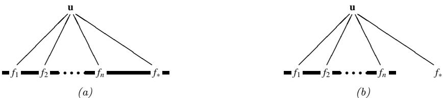
Figure 18.12: Illustration of the graphical model for a GP on n observations, f1:n, and one test case, f↗, with inducing variables u. The thick lines indicate that all variables are fully interconnected. The observations yⁱ (not shown) are locally connected to each fi. (a) no approximations are made. (b) we assume f↗ is conditionally independent of f^X given u. From Figure 1 of [QCR05]. Used with kind permission of Joaquin Quiñonero Candela.

as follows:

\[p(\mathbf{f}\_\*, \mathbf{f}\_X, \mathbf{f}\_Z) = p(\mathbf{f}\_\* | \mathbf{f}\_X, \mathbf{f}\_Z) p(\mathbf{f}\_X | \mathbf{f}\_Z) p(\mathbf{f}\_Z) \approx p(\mathbf{f}\_\* | \mathbf{f}\_Z) p(\mathbf{f}\_X | \mathbf{f}\_Z) p(\mathbf{f}\_Z) \tag{18.118}\]

See Figure 18.12 for an illustration of this assumption, and Section 18.5.3.4 for details on how to choose the inducing set Z. (Note that this method is often called a “sparse GP”, because it makes predictions for f^→ using a subset of the training data, namely fZ, instead of all of it, fX.)

From this, we can derive the following train and test conditionals

\[p(\mathbf{f}\_X|\mathbf{f}\_Z) = \mathcal{N}(\mathbf{f}\_X|\mathbf{K}\_{X,Z}\mathbf{K}\_{Z,Z}^{-1}\mathbf{f}\_Z, \mathbf{K}\_{X,X} - \mathbf{Q}\_{X,X})\tag{18.119}\]

\[p(f\_\*|f\_Z) = \mathcal{N}(f\_\*|\mathbf{K}\_{\*,Z}\mathbf{K}\_{Z,Z}^{-1}f\_Z, \mathbf{K}\_{\*,\*} - \mathbf{Q}\_{\*,\*})\tag{18.120}\]

The above equations can be seen as exact inference on noise-free observations fZ. To gain computational speedups, we will make further approximations to the terms ^Q˜ X,X ^{= K}X,X ^{→ Q}X,X and ^Q˜ ^→,^{→ = K}→,^{→ → Q}→,→, as we discuss below. We can then derive the approximate prior ^q(fX, ^f→) = / ^q(fX|fZ)q(f→|fZ)p(fZ)dfZ, which we then condition on the observations in the usual way.

All of the approximations we discuss below result in an initial training cost of O(M³ + NM²), and then take O(M) time for the predictive mean for each test case, and O(M²) time for the predictive variance. (Compare this to O(N³) training time and O(N) and O(N²) testing time for exact inference.)

18.5.3.1 SOR/DIC

Suppose we assume ^Q˜ X,X ^{= 0} and ^Q˜ ^→,^{→ = 0}, so the conditionals are deterministic. This is called the deterministic inducing conditional (DIC) approximation [QCR05], or the subset of regressors (SOR) approximation [Sil85; SB01]. The corresponding joint prior has the form

\[q\_{\rm SOR}(\mathbf{f}\_X, \mathbf{f}\_\*) = \mathcal{N}(\mathbf{0}, \begin{pmatrix} \mathbf{Q}\_{X,X} & \mathbf{Q}\_{X,\*} \\ \mathbf{Q}\_{\*,X} & \mathbf{Q}\_{\*,\*} \end{pmatrix} \tag{18.121}\]

Let us define Qˆ X,X = QX,X + ς²I^N , and ! = (ς↓²KZ,XKX,Z + KZ,Z)↓¹. Then the predictive distribution is

\[q\_{\rm SOR}(\mathbf{f}\_\*|\mathbf{y}) = \mathcal{N}(\mathbf{f}\_\*|\mathbf{Q}\_{\*,X}\hat{\mathbf{Q}}\_{X,X}^{-1}\mathbf{y}, \ \mathbf{Q}\_{\*,\*} - \mathbf{Q}\_{\*,X}\hat{\mathbf{Q}}\_{X,X}^{-1}\mathbf{Q}\_{X,\*})\tag{18.122}\]

\[\mathbf{y} = \mathcal{N}(\mathbf{f}\_\* | \sigma^{-2} \mathbf{K}\_{\*,Z} \Sigma \mathbf{K}\_{Z,X} \mathbf{y}, \, \mathbf{K}\_{\*,Z} \Sigma \mathbf{K}\_{Z,\*}) \tag{18.123}\]

This is equivalent to the usual one for GPs except we have replaced KX,X by QX,X. This is equivalent to performing GP inference with the following kernel function

\[ \boldsymbol{\kappa}\_{\text{SOR}}(\mathbf{z}\_i, \mathbf{z}\_j) = \boldsymbol{\kappa}(\mathbf{z}\_i, \mathbf{Z}) \, \mathbf{K}\_{\text{Z}, \mathbf{Z}}^{-1} \, \boldsymbol{\kappa}(\mathbf{Z}, \mathbf{z}\_j) \tag{18.124} \]

The kernel matrix has rank M, so the GP is degenerate. Furthermore, the kernel will be near 0 when xⁱ or x^j is far from one of the chosen points Z, which can result in an underestimate of the predictive variance.

18.5.3.2 DTC

One way to overcome the overconfidence of DIC is to only assume ^Q˜ X,X ^{= 0}, but let ^Q˜ ^→,^{→ = K}→,→→Q→,^→ be exact. This is called the deterministic training conditional or DTC method [SWL03].

The corresponding joint prior has the form

\[q\_{\rm dtc}(f\_X, f\_\*) = \mathcal{N}(\mathbf{0}, \begin{pmatrix} \mathbf{Q}\_{X,X} & \mathbf{Q}\_{X,\*} \\ \mathbf{Q}\_{\*,X} & \mathbf{K}\_{\*,\*} \end{pmatrix} \tag{18.125}\]

Hence the predictive distribution becomes

\[q\_{\rm dc}(f\_\*|y) = N(f\_\*|\mathbf{Q}\_{\*,X}\hat{\mathbf{Q}}\_{X,X}^{-1}y, \; \mathbf{K}\_{\*,\*} - \mathbf{Q}\_{\*,X}\hat{\mathbf{Q}}\_{X,X}^{-1}\mathbf{Q}\_{X,\*})\tag{18.126}\]

\[\mathbf{K} = \mathcal{N}(\mathbf{f}\_\* | \sigma^{-2} \mathbf{K}\_{\*,Z} \Sigma \mathbf{K}\_{Z,X} \mathbf{y}, \mathbf{K}\_{\*,\*} - \mathbf{Q}\_{\*,\*} + \mathbf{K}\_{\*,Z} \Sigma \mathbf{K}\_{Z,\*}) \tag{18.127}\]

The predictive mean is the same as in SOR, but the variance is larger (since K→,^→ → Q→,^→ is positive definite) due to the uncertainty of f^→ given fZ.

18.5.3.3 FITC

A widely used approximation assumes q(fX|fZ) is fully factorized, i.e,

\[q(\mathbf{f}\_X|\mathbf{f}\_Z) = \prod\_{n=1}^N p(f\_n|\mathbf{f}\_Z) = \mathcal{N}(\mathbf{f}\_X|\mathbf{K}\_{X,Z}\mathbf{K}\_{Z,Z}^{-1}\mathbf{f}\_Z, \text{diag}(\mathbf{K}\_{X,X} - \mathbf{Q}\_{X,X})) \tag{18.128}\]

This is called the fully independent training conditional or FITC assumption, and was first proposed in [SG06a]. This throws away less uncertainty than the SOR and DTC methods, since it does not make any deterministic assumptions about the relationship between f^X and fZ.

The joint prior has the form

\[q\_{\rm fric}(\mathbf{f}\_{X}, \mathbf{f}\_{\*}) = \mathcal{N}(\mathbf{0}, \begin{pmatrix} \mathbf{Q}\_{X,X} - \text{diag}(\mathbf{Q}\_{X,X} - \mathbf{K}\_{X,X}) & \mathbf{Q}\_{X,\*} \\ \mathbf{Q}\_{\*,X} & \mathbf{K}\_{\*,\*} \end{pmatrix} \tag{18.129}\]

The predictive distribution for a single test case is given by

\[q\_{\rm fitc}(f\_\*|\mathbf{y}) = \mathcal{N}(f\_\*|k\_{\*,Z}\Sigma\mathbf{K}\_{Z,X}\Lambda^{-1}\mathbf{y}, k\_{\*\*} - q\_{\*\*} + k\_{\*,Z}\Sigma k\_{Z,\*})\tag{18.130}\]

where % ↭ diag(KX,X ^{→ Q}X,X ^{+ ς2}I^N ), and ! ↭ (KZ,Z ^{+ K}Z,X#↓¹KX,Z)↓¹. If we have a batch of test cases, we can assume they are conditionally independent (an approach known as fully independent conditional or FIC), and multiply the above equation.

The computational cost is the same as for SOR and DTC, but the approach avoids some of the pathologies due to a non-degenerate kernel. In particular, one can show that the FIC method is equivalent to exact GP inference with the following non-degenerate kernel:

\[\mathcal{K}\_{\text{fic}}(\mathbf{z}\_i, \mathbf{z}\_j) = \begin{cases} \mathcal{K}(\mathbf{z}\_i, \mathbf{z}\_j) & \text{if } i = j \\ \mathcal{K}\_{\text{SOR}}(\mathbf{z}\_i, \mathbf{z}\_j) & \text{if } i \neq j \end{cases} \tag{18.131}\]

18.5.3.4 Learning the inducing points

So far, we have not specified how to choose the inducing points or pseudoinputs Z. We can treat these like kernel hyperparameters, and choose them so as to maximize the log marginal likelihood, given by

\[\log q(\mathbf{y}|\mathbf{X}, \mathbf{Z}) = \log \int \int p(\mathbf{y}|\mathbf{f}\_X) q(\mathbf{f}\_X|\mathbf{X}, \mathbf{f}\_Z) p(\mathbf{f}\_Z|\mathbf{Z}) d\mathbf{f}\_Z d\mathbf{f} \tag{18.132}\]

\[=\log\int p(y|\mathbf{f}\_X)q(\mathbf{f}\_X|\mathbf{X},\mathbf{Z})d\mathbf{f}\_X\tag{18.133}\]

\[= -\frac{1}{2}\log|\mathbf{Q}\_{X,X} + \mathbf{A}| - \frac{1}{2}\mathbf{y}^{\mathsf{T}}(\mathbf{Q}\_{X,X} + \mathbf{A})^{-1}\mathbf{y} - \frac{n}{2}\log(2\pi) \tag{18.134}\]

where the definition of # depends on the method, namely #SOR = #dtc = ς²I^N , and #fitc = diag(KX,X ^{→ Q}X,X) + ^ς2I^N .

If the input domain is ^Rd, we can optimize Z ↗ ^RMd using gradient methods. However, one of the appeals of kernel methods is that they can handle structured inputs, such as strings and graphs (see Section 18.2.3). In this case, we cannot use gradient methods to select the inducing points. A simple approach is to select the inducing points from the training set, as in the subset of data approach in Section 18.5.1, or using the e”cient selection mechanism in [Cao+15]. However, we can also use discrete optimization methods, such as simulated annealing (Section 12.9.1), as discussed in [For+18a]. See Figure 18.13 for an illustration.

18.5.4 Sparse variational methods

In this section, we discuss a variational approach to GP inference called the sparse variational GP or SVGP approximation, also known as the variational free energy or VFE approach [Tit09; Mat+16]. This is similar to the inducing point methods in Section 18.5.3, except it approximates the posterior, rather than approximating the prior. The variational approach can also easily handle non-conjugate likelihoods, as we will see. For more details, see e.g., [BWR16; Lei+20]. (See also [WKS21] for connections between SVGP and the Nyström method.)

To explain the idea behind SVGP/ VFE, let us assume, for simplicity, that the function f is defined over a finite set X of possible inputs, which we partition into three subsets: the training set X, a set

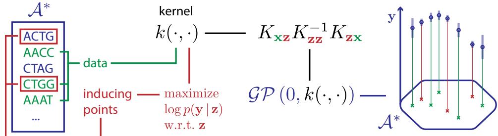
Figure 18.13: Illustration of how to choose inducing points from a discrete input domain (here DNA sequences of length 4) to maximize the log marginal likelihood. From Figure 1 of [For+18a]. Used with kind permission of Vincent Fortuin.

of inducing points Z, and all other points (which we can think of as the test set), X→. (We assume these sets are disjoint.) Let fX, f^Z and f^→ represent the corresponding unknown function values on these points, and let f = [fX, fZ, f→] be all the unknowns. (Here we work with a fixed-length vector f, but the result generalizes to Gaussian processes, as explained in [Mat+16].) We assume the function is sampled from a GP, so p(f) = N (m(X ), K(X , X )).

The inducing point methods in Section 18.5.3 approximates the GP prior by assuming p(f→, fX, fZ) ↓ p(f→|fZ)p(fX|fZ)p(fZ). The inducing points f^Z are chosen to maximize the likelihood of the observed data. We then perform exact inference in this approximate model. By contrast, in this section, we will keep the model unchanged, but we will instead approximate the posterior p(f|y) using variational inference.

In the VFE view, the inducing points Z and inducing variables f^Z (often denoted by u) are variational parameters, rather than model parameters, which avoids the risk of overfitting. Furthermore, one can show that as the number of inducing points m increases, the quality of the posterior consistently improves, eventually recovering exact inference. By contrast, in the classical inducing point method, increasing m does not always result in better performance [BWR16].

In more detail, the VFE approach tries to find an approximate posterior q(f) to minimize DKL (q(f) ↘ p(f|y)). The key assumption is that q(f) = q(f→, fX, fZ) = p(f→, fX|fZ)q(fZ), where p(f→, fX|fZ) is computed exactly using the GP prior, and q(fZ) is learned, by minimizing K(q) = DKL (q(f) ↘ p(f|y)). 2 Intuitively, q(fZ) acts as a “bottleneck” which “absorbs” all the observations from y; posterior predictions for elements of f^X or f^→ are then made via their dependence on fZ, rather than their dependence on each other.

^2. One can show that DKL (q(f) ↗ p(f|y)) = DKL (q(fX, f^Z ) ↗ p(fX, f^Z |y)), which is the original objective from [Tit09].

We can derive the form of the loss, which is used to compute the posterior q(fZ), as follows:

\[\mathcal{K}(q) = D\_{\text{KL}}\left(q(\mathbf{f}\_\*, \mathbf{f}\_X, \mathbf{f}\_Z) \parallel p(\mathbf{f}\_\*, \mathbf{f}\_X, \mathbf{f}\_Z|\mathbf{y})\right) \tag{18.135}\]

\[=\int q(\mathbf{f}\_\*, \mathbf{f}\_X, \mathbf{f}\_Z) \log \frac{q(\mathbf{f}\_\*, \mathbf{f}\_X, \mathbf{f}\_Z)}{p(\mathbf{f}\_\*, \mathbf{f}\_X, \mathbf{f}\_Z|y)} d\mathbf{f}\_\* \, d\mathbf{f}\_X \, d\mathbf{f}\_Z \tag{18.136}\]

\[=\int p(\mathbf{f}\_{\*},\mathbf{f}\_{X}|\mathbf{f}\_{Z})q(\mathbf{f}\_{Z})\log\frac{p(\mathbf{f}\_{\*}|\mathbf{f}\_{X};\mathbf{f}\_{Z}^{\star}\mathbf{\widehat{z}})\underline{p}(\mathbf{f}\_{X}|\mathbf{f}\_{Z}^{\star}\mathbf{\widehat{z}})q(\mathbf{f}\_{Z})p(\mathbf{y})}{p(\mathbf{f}\_{\*}|\mathbf{f}\_{X};\mathbf{f}\_{X}^{\star}\mathbf{\widehat{z}})\underline{p}(\mathbf{f}\_{X}|\mathbf{f}\_{Z}^{\star}\mathbf{\widehat{z}})p(\mathbf{f}\_{X})p(\mathbf{y}|\mathbf{f}\_{X})}d\mathbf{f}\_{\*}\,d\mathbf{f}\_{X}\,d\mathbf{f}\_{Z}\tag{18.137}\]

\[=\int p(\mathbf{f}\_\*, \mathbf{f}\_X|\mathbf{f}\_Z) q(\mathbf{f}\_Z) \log \frac{q(\mathbf{f}\_Z) p(\mathbf{y})}{p(\mathbf{f}\_Z) p(\mathbf{y}|\mathbf{f}\_X)} d\mathbf{f}\_\* \, d\mathbf{f}\_X \, d\mathbf{f}\_Z \tag{18.138}\]

\[=\int q(\mathbf{f}\_Z)\log\frac{q(\mathbf{f}\_Z)}{p(\mathbf{f}\_Z)}d\mathbf{f}\_Z - \int p(\mathbf{f}\_X|\mathbf{f}\_Z)q(\mathbf{f}\_Z)\log p(\mathbf{y}|\mathbf{f}\_X)d\mathbf{f}\_X \,d\mathbf{f}\_Z + C\tag{18.139}\]

\[\mathbb{E} = D\_{\mathbb{KL}}\left(q(\mathbf{f}\_Z) \parallel p(\mathbf{f}\_Z)\right) - \mathbb{E}\_{q(\mathbf{f}\_X)}\left[\log p(\mathbf{y}|\mathbf{f}\_X)\right] + C \tag{18.140}\]

where C = log p(y) is an irrelevant constant.

We can alternatively write the objective as an evidence lower bound that we want to maximize:

\[\log p(\mathbf{y}) = \mathcal{K}(q) + \mathbb{E}\_{q(\mathbf{f}\_X)} \left[ \log p(\mathbf{y}|\mathbf{f}\_X) \right] - D\_{\text{KL}} \left( q(\mathbf{f}\_Z) \parallel p(\mathbf{f}\_Z) \right) \tag{18.141}\]

\[\geq \mathbb{E}\_{q(\mathbf{f}\_{X})} \left[ \log p(\mathbf{y}|\mathbf{f}\_{X}) \right] - D\_{\mathbb{KL}} \left( q(\mathbf{f}\_{Z}) \parallel p(\mathbf{f}\_{Z}) \right) \triangleq \mathcal{L}(q) \tag{18.142}\]

Now suppose we choose a Gaussian posterior approximation, q(fZ) = N (fZ|m, S). Since p(fZ) = N (fZ|0, K(Z, Z)), we can compute the KL term in closed form using the formula for KL divergence between Gaussians (Equation (5.77)). To compute the expected log-likelihood term, we first need to compute the induced posterior over the latent function values at the training points:

\[q(\mathbf{f}\_X|\mathbf{m}, \mathbf{S}) = \int p(\mathbf{f}\_X|\mathbf{f}\_Z, \mathbf{X}, \mathbf{Z}) q(\mathbf{f}\_Z|\mathbf{m}, \mathbf{S}) d\mathbf{f}\_Z = \mathcal{N}(\mathbf{f}\_X|\bar{\mu}, \bar{\Sigma}) \tag{18.143}\]

\[ \tilde{\mu}\_i = m(\mathbf{x}\_i) + \alpha(\mathbf{x}\_i)^\mathsf{T}(\mathbf{m} - m(\mathbf{Z})) \tag{18.144} \]

\[ \tilde{\Sigma}\_{ij} = \mathcal{K}(\boldsymbol{x}\_i, \boldsymbol{x}\_j) - \alpha(\boldsymbol{x}\_i)^\mathsf{T}(\mathcal{K}(\mathbf{Z}, \mathbf{Z}) - \mathbf{S})\alpha(\boldsymbol{x}\_j) \tag{18.145} \]

\[\alpha(x\_i) = \mathbb{X}(\mathbf{Z}, \mathbf{Z})^{-1} \mathbb{X}(\mathbf{Z}, x\_i) \tag{18.146}\]

Hence the marginal at a single point is ^q(fn) = ^N (fn|µ˜n, “˜ nn), which we can use to compute the expected log likelihood:

\[\mathbb{E}\_{q(\mathbf{f}\_X)}\left[\log p(\mathbf{y}|\mathbf{f}\_X)\right] = \sum\_{n=1}^{N} \mathbb{E}\_{q(f\_n)}\left[\log p(y\_n|f\_n)\right] \tag{18.147}\]

We discuss how to compute these expectations below.

18.5.4.1 Gaussian likelihood

If we have a Gaussian observation model, we can compute the expected log likelihood in closed form. In particular, if we assume m(x) = 0, we have

\[\mathbb{E}\_{q(f\_n)}\left[\log \mathcal{N}(y\_n|f\_n, \beta^{-1})\right] = \log \mathcal{N}(y\_n|\mathbf{k}\_n^\mathrm{T}\mathbf{K}\_{Z,Z}^{-1}\mathbf{m}, \beta^{-1}) - \frac{1}{2}\beta \tilde{k}\_{nn} - \frac{1}{2}\text{tr}(\mathbf{S}\mathbf{A}\_n) \tag{18.148}\]

where ˜ ^knn ^{= k}nn ^{→ kT} nK↓¹ Z,Zkn, kⁿ is the n’th column of KZ,X and #ⁿ = ↼K↓¹ Z,Zknk^T nK↓¹ Z,Z. Hence the overall ELBO has the form

\[\mathcal{L}(q) = \log \mathcal{N}(y|\mathbf{K}\_{X,Z}\mathbf{K}\_{Z,Z}^{-1}\mathbf{m}, \beta^{-1}\mathbf{I}\_N) - \frac{1}{2}\beta \text{tr}(\mathbf{K}\_{X,Z}\mathbf{K}\_{Z,Z}^{-1}\mathbf{S}\mathbf{K}\_{Z,Z}^{-1}\mathbf{K}\_{Z,X}) \tag{18.149}\]

\[-\frac{1}{2}\beta \text{tr}(\mathbf{K}\_{X,X} - \mathbf{Q}\_{X,X}) - D\_{\mathbb{KL}}\left(q(\mathbf{f}\_Z) \parallel p(\mathbf{f}\_Z)\right) \tag{18.150}\]

where QX,X = KX,ZK↓¹ Z,ZKZ,X.

To compute the gradients of this, we leverage the following result [OA09]:

\[\frac{\partial}{\partial \mu} \mathbb{E}\_{\mathcal{N}(x|\mu, \sigma^2)} \left[ h(x) \right] = \mathbb{E}\_{\mathcal{N}(x|\mu, \sigma^2)} \left[ \frac{\partial}{\partial x} h(x) \right] \tag{18.151}\]

\[\frac{\partial}{\partial \sigma^2} \mathbb{E}\_{\mathcal{N}(x|\mu, \sigma^2)} \left[ h(x) \right] = \frac{1}{2} \mathbb{E}\_{\mathcal{N}(x|\mu, \sigma^2)} \left[ \frac{\partial^2}{\partial x^2} h(x) \right] \tag{18.152}\]

We then substitute h(x) with log p(yn|fn). Using this, one can show

^⇒mL(q) = ↼K↓¹ Z,ZKZ,Xy → #m (18.153)

\[\nabla \mathbf{S} \mathcal{L}(q) = \frac{1}{2} \mathbf{S}^{-1} - \frac{1}{2} \mathbf{A} \tag{18.154}\]

Setting the derivatives to zero gives the optimal solution:

\[\mathbf{S} = \boldsymbol{\Lambda}^{-1} \tag{18.155}\]

\[ \Lambda = \beta \mathbf{K}\_{Z,Z}^{-1} \mathbf{K}\_{Z,X} \mathbf{K}\_{X,Z} \mathbf{K}\_{Z,Z}^{-1} + \mathbf{K}\_{Z,Z}^{-1} \tag{18.156} \]

\[\mathbf{m} = \beta \mathbf{A}^{-1} \mathbf{K}\_{Z,Z}^{-1} \mathbf{K}\_{Z,X} \mathbf{y} \tag{18.157}\]

This is called sparse GP regression or SGPR [Tit09].

With these parameters, the lower bound on the log marginal likelihood is given by

\[\log p(\mathbf{y}) \ge \log N(\mathbf{y}|\mathbf{0}, \mathbf{K}\_{X,Z}\mathbf{K}\_{Z,Z}^{-1}\mathbf{K}\_{Z,X} + \beta^{-1}\mathbf{I}) - \frac{1}{2}\beta \text{tr}(\mathbf{K}\_{X,X} - \mathbf{Q}\_{X,X}) \tag{18.158}\]

(This is called the “collapsed” lower bound, since we have marginalized out fZ.) If Z = X, then ^KZ,Z ^{= K}Z,X ^{= K}X,X, so the bound becomes tight, and we have log ^p(y) = log ^N (y|0, ^KX,X ⁺↼↓1I).

Equation (18.158) is almost the same as the log marginal likelihood for the DTC model in Equation (18.134), except for the trace term; it is this latter term that prevents overfitting, due to the fact that we treat f^Z as variational parameters of the posterior rather than model parameters of the prior.

18.5.4.2 Non-Gaussian likelihood

In this section, we briefly consider the case of non-Gaussian likelihoods, which arise when using GPs for classification or for count data (see Section 18.4). We can compute the gradients of the expected log likelihood by defining h(fn) = log p(yn|fn) and then using a Monte Carlo approximation to Equation (18.151) and Equation (18.152). In the case of a binary classifier, we can use the results in Table 18.2 to compute the inner ^{ϑ ϑ}f^{n h}(fn) and ^ϑ2 ϑf² n h(fn) terms. Alternatively, we can use numerical integration techniques, such as those discussed in Section 8.5.1.4. (See also [WSS21].)

18.5.4.3 Minibatch SVI

Computing the optimal variational solution in Section 18.5.4.1 requires solving a batch optimization problem, which takes O(M³ + NM²) time. This may still be too slow if N is large, unless M is small, which compromises accuracy.

An alternative approach is to perform stochastic optimization of the VFE objective, instead of batch optimization. This is known as stochastic variational inference (see Section 10.1.4). The key observation is that the log likelihood in Equation (18.147) is a sum of N terms, which we can approximate with minibatch sampling to compute noisy estimates of the gradient, as proposed in [HFL13].

In more detail, the objective becomes

\[\mathcal{L}(q) = \left[ \frac{N}{B} \sum\_{b=1}^{B} \frac{1}{|\mathcal{B}\_b|} \sum\_{n \in \mathcal{B}\_b} \mathbb{E}\_{q(f\_n)} \left[ \log p(y\_n | f\_n) \right] \right] - D\_{\text{KL}} \left( q(f\_Z) \parallel (p(f\_Z)) \right) \tag{18.159}\]

where B^b is the b’th batch, and B is the number of batches. Since the GP model (with Gaussian likelihoods) is in the exponential family, we can e”ciently compute the natural gradient (Section 6.4) of Equation (18.159) wrt the canonical parameters of q(fZ); this converges much faster than following the standard gradient. See [HFL13] for details.

18.5.5 Exploiting parallelization and structure via kernel matrix multiplies

It takes O(N³) time to compute the Cholesky decomposition of KX,X, which is needed to solve the linear system K↽↼ = y and to compute |KX,X|. An alternative to Cholesky decomposition is to use linear algebra methods, often called Krylov subspace methods based just on matrix vector multiplication or MVM. These approaches are often much faster.

In short, if the kernel matrix KX,X has special algebraic structure, which is often the case through either the choice of kernel or the structure of the inputs, then it is typically easier to exploit this structure in performing fast matrix multiplies. Moreover, even if the kernel matrix does not have special structure, matrix multiplies are trivial to parallelize, and can thus be greatly accelerated by GPUs, unlike Cholesky based methods which are largely sequential. Algorithms based on matrix multiplies are in harmony with modern hardware advances, which enable significant parallelization.

18.5.5.1 Using conjugate gradient and Lanczos methods

We can solve the linear system K↽↼ = y using conjugate gradients (CG). The key computational step in CG is the ability to perform MVMs. Let τ (K↽) be the time complexity of a single MVM with K↽. For a dense ^{n ⇔ n} matrix, we have ^τ (K↽) = ⁿ²; however, we can speed this up if K↽ is sparse or structured, as we discuss below.

Even if K↽ is dense, we may still be able to save time by solving the linear system approximately. In particular, if we perform C iterations, CG will take O(Cτ (K↽)) time. If we run for C = n, and τ (K↽) = n², it gives the exact solution in O(n³) time. However, often we can use fewer iterations and still get good accuracy, depending on the condition number of K↽.

We can compute the log determinant of a matrix using the MVM primitive with a similar iterative method known as stochastic Lanczos quadrature [UCS17; Don+17a]. This takes O(Lτ (K↽)) time for L iterations.

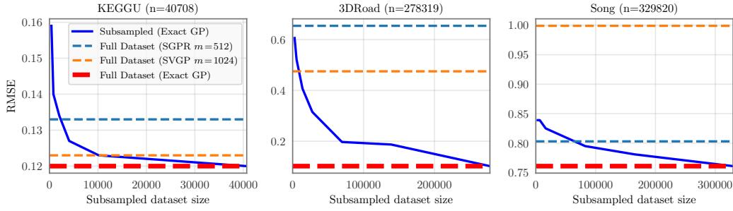
Figure 18.14: RMSE on test set as a function of training set size using a GP with Matern 3/2 kernel with shared lengthscale across all dimensions. Solid lines: exact inference. Dashed blue: SGPR method (closed-form batch solution to the Gaussian variational approximation) of Section 18.5.4.1 with M = 512 inducing points. Dashed orange: SVGP method (SGD on Gaussian variational approxiation) of Section 18.5.4.3 with M = 1024 inducing points. Number of input dimensions: KEGGU D = 27, 3DRoad D = 3, Song D = 90. From Figure 4 of [Wan+19a]. Used with kind permission of Andrew Wilson.

These methods have been used in the blackbox matrix-matrix multiplication (BBMM) inference procedure of [Gar+18a], which formulates a batch approach to CG that can be e!ectively parallelized on GPUs. Using 8 GPUs, this enabled the authors of [Wan+19a] to perform exact inference for a GP regression model on ^{N ↔︎} 10⁴ datapoints in seconds, ^{N ↔︎} 10⁵ datapoints in minutes, and ^{N ↔︎ 106} datapoints in hours.

Interestingly, Figure 18.14 shows that exact GP inference on a subset of the data can often outperform approximate inference on the full data. We also see that performance of exact GPs continues to significantly improve as we increase the size of the data, suggesting that GPs are not only useful in the small-sample setting. In particular, the BBMM is an exact method, and so will preserve the non-parametric representation of a GP with a non-degenerate kernel. By contrast, standard scalable approximations typically operate by replacing the exact kernel with an approximation that corresponds to a parametric model. The non-parametric GPs are able to grow their capacity with more data, benefiting more significantly from the structure present in large datasets.

18.5.5.2 Kernels with compact support

Suppose we use a kernel with compact support, where K(x, x^↔︎ )=0 if ↘x → x^↔︎ ↘ > ⇁ for some threshold ⇁ (see e.g., [MR09]), then K↽ will be sparse, so τ (K↽) will be O(N). We can also induce sparsity and structure in other ways, as we discuss in Section 18.5.5.3.

18.5.5.3 KISS

One way to ensure that MVMs are fast is to force the kernel matrix to have structure. The structured kernel interpolation (SKI) method of [WN15] does this as follows. First it assumes we have a set of inducing points, with Gram matrix KZ,Z. It then interpolates these values to predict the entries of the full kernel matrix using

\[\mathbf{K}\_{X,X} \approx \mathbf{W}\_{\mathbf{X}} \mathbf{K}\_{Z,Z} \mathbf{W}\_{\mathbf{X}}^{\top} \tag{18.160}\]

where W^X is a sparse matrix containing interpolation weights. If we use cubic interpolation, each row only has 4 nonzeros. Thus we can compute (WXKZ,ZW^{T X})v for any vector v in O(N + M²) time.

Note that the SKI approach generalizes all inducing point methods. For example, we can recover the subset of regressors method (SOR) method by setting the interpolation weights to W = KX,ZK↓¹ Z,Z. We can identify this procedure as performing a global Gaussian process interpolation strategy on the user specified kernel. See [WN15] and [WDN15] for more details.

In 1d, we can further reduce the running time by choosing the inducing points to be on a regular grid, so that KZ,Z is a Toeplitz matrix. In higher dimensions, we need to use a multidimensional grid of points, resulting in KZ,Z being a Kronecker product of Toeplitz matrices. This enables matrix vector multiplication in O(N + M log M) time and O(N + M) space. The resulting method is called KISS-GP [WN15], which stands for “kernel interpolation for scalable, structured GPs”.

Unfortunately, the KISS method can take exponential time in the input dimensions D when exploiting Kronecker structure in KZ,Z, due to the need to create a fully connected multidimensional lattice. In [Gar+18b], they propose a method called SKIP, which stands for “SKI for products”. The idea is to leverage the fact that many kernels (including ARD) can be written as a product of 1d kernels: K(x, x^↔︎ ) = ^{D d}=1 ^Kd(x, ^x↔︎ ). This can be combined with the 1d SKI method to enable fast MVMs. The overall running time to compute the log marginal likelihood (which is the bottleneck for kernel learning) using C iterations of CG and a Lanczos decomposition of rank L, becomes ^O(DL(^{N + M} log ^M) + ^L3N log ^{D +} CL²N). Typical values are ^{L ↔︎ 101} and ^{C ↔︎ 102}.

18.5.5.4 Tensor train methods

Consider the Gaussian VFE approach in Section 18.5.4. We have to estimate the covariance S and the mean m. We can represent S e”ciently using Kronecker structure, as used by KISS. Additionally, we can represent m e”ciently using the tensor train decomposition [Ose11] in combination with SKI [WN15]. The resulting TT-GP method can scale e”ciently to billions of inducing points, as explained in [INK18].

18.5.6 Converting a GP to an SSM

Consider a function defined on a 1d scalar input, such as a time index. For many stationary 1d kernels, the corresponding GP can be modeled using a linear time invariant (LTI) stochastic di!erential equation (SDE)3; this SDE can then be converted to a linear-Gaussian state space model (Section 29.1) as first proposed in [HS10]. For example, consider the exponential kernel in Equation (18.14), K(t, t^↔︎ ) = ^{q 2ε} exp(→⇀|t → t ↔︎ |), which corresponds to a Matérn kernel with 4 = 1/2. The corresponding SDE is the Orstein-Uhlenbeck process which has the form dx(t) dt = →⇀x(t) + w(t), where w(t) is a white noise process with spectral density q [SS19, p258].4 For other kernels (such as Matérn with 4 = 3/2), we need to use multiple latent states in order to capture higher order

^3. The condition is that the spectral density of the covariance function has to be a rational function. This includes many kernels, such as the Matérn kernel, but excludes the squared exponential (RBF) kernel. However the latter can be approximated by an SDE, as explained in [SS19, p261].

^4. This is sometimes written as dx ^{= ↔︎}ϑx dt ^{+ d}ϖ, where ^ϖ(t) is a Brownian noise process, and ^w(t) = ^dϑ(t) dt , as explained in [SS19, p45].

derivative terms (see Supplementary Section 18.2 for details). Furthermore, for higher dimensional inputs, we need to use even more latent states, to enforce the Markov property [DSP21].

Once we have converted the GP to LG-SSM form, we can perform exact inference in O(N) time using Kalman smoothing, as explained in Section 8.2.3. Furthermore, if we have access to a highly parallel processor, such as a GPU, we can reduce the time to log(N) [CZS22], as explained in Section 8.2.3.4.

18.6 Learning the kernel

In [Mac98], David MacKay asked: “How can Gaussian processes replace neural networks? Have we thrown the baby out with the bathwater?” This remark was made in the late 1990s, at the end of the second wave of neural networks. Researchers and practitioners had grown weary of the design decisions associated with neural networks — such as activation functions, optimization procedures, architecture design — and the lack of a principled framework to make these decisions. Gaussian processes, by contrast, were perceived as flexible and principled probabilistic models, which naturally followed from Radford Neal’s results on infinite neural networks [Nea96], which we discuss in more depth in Section 18.7.

However, MacKay [Mac98] noted that neural networks could discover rich representations of data through adaptive hidden basis functions, while Gaussian processes with standard kernel functions, such as the RBF kernel, are essentially just smoothing devices. Indeed, the generalization properties of Gaussian processes hinge on the suitability of the kernel function. Learning the kernel is how we do representation learning with Gaussian processes, and in many cases will be crucial for good performance — especially when we wish to perform extrapolation, making predictions far away from the data [WA13; Wil+14].

As we will see, learning a kernel is in many ways analogous to training a neural network. Moreover, neural networks and Gaussian processes can be synergistically combined through approaches such as deep kernel learning (see Section 18.6.6) and NN-GPs (Section 18.7.2).

18.6.1 Empirical Bayes for the kernel parameters

Suppose, as in Section 18.3.2, we are performing 1d regression using a GP with an RBF kernel. Since the data has observation noise, the kernel has the following form:

\[\mathcal{K}\_y(x\_p, x\_q) = \sigma\_f^2 \exp(-\frac{1}{2\ell^2}(x\_p - x\_q)^2) + \sigma\_y^2 \delta\_{pq} \tag{18.161}\]

Here ε is the horizontal scale over which the function changes, ς^{2 f} controls the vertical scale of the function, and ς^{2 y} is the noise variance. Figure 18.15 illustrates the e!ects of changing these parameters. We sampled 20 noisy datapoints from the SE kernel using (ε, ς^f , ςy) = (1, 1, 0.1), and then made predictions various parameters, conditional on the data. In Figure 18.15(a), we use (ε, ς^f , ςy) = (1, 1, 0.1), and the result is a good fit. In Figure 18.15(b), we increase the length scale to ε = 3; now the function looks smoother, but we are arguably underfitting.

To estimate the kernel parameters ω (sometimes called hyperparameters), we could use exhaustive search over a discrete grid of values, with validation loss as an objective, but this can be quite slow. (This is the approach used by nonprobabilistic methods, such as SVMs, to tune kernels.) Here we

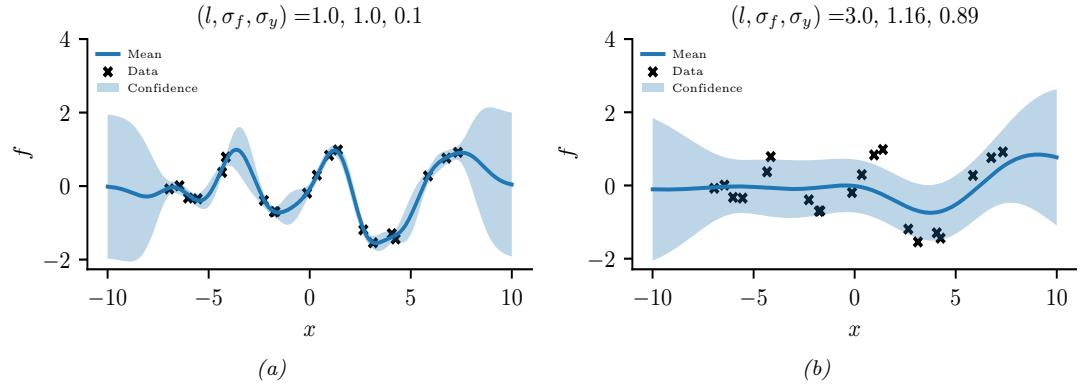
Figure 18.15: Some 1d GPs with RBF kernels but di!erent hyper-parameters fit to 20 noisy observations. The hyper-parameters (ε, ω^f , ωy) are as follows: (a) (1, 1, 0.1) (b) (3.0, 1.16, 0.89). Adapted from Figure 2.5 of [RW06]. Generated by gpr\_demo\_change\_hparams.ipynb.

consider an empirical Bayes approach, which will allow us to use continuous optimization methods, which are much faster. In particular, we will maximize the marginal likelihood

\[p(\mathbf{y}|\mathbf{X},\boldsymbol{\theta}) = \int p(\mathbf{y}|\mathbf{f},\mathbf{X})p(\mathbf{f}|\mathbf{X},\boldsymbol{\theta})d\mathbf{f} \tag{18.162}\]

(The reason it is called the marginal likelihood, rather than just likelihood, is because we have marginalized out the latent Gaussian vector ^f.) Since ^p(f|X) = ^N (f|0, ^K), and ^p(y|f) = ^{N n}=1 ^N (yn|fn, ^ς2 y), the marginal likelihood is given by

\[\log p(y|\mathbf{X}, \theta) = \log N(y|0, \mathbf{K}\_{\sigma}) = -\frac{1}{2}y\mathbf{K}\_{\sigma}^{-1}y - \frac{1}{2}\log|\mathbf{K}\_{\sigma}| - \frac{N}{2}\log(2\pi) \tag{18.163}\]

where the dependence of K↽ on ω is implicit. The first term is a data fit term, the second term is a model complexity term, and the third term is just a constant. To understand the tradeo! between the first two terms, consider a SE kernel in 1d, as we vary the length scale ε and hold ς^{2 y} fixed. Let ^J(ε) = ^→ log ^p(y|X, ^ε). For short length scales, the fit will be good, so ^yTK↓¹ ↽ ^y will be small. However, the model complexity will be high: K will be almost diagonal, since most points will not be considered “near” any others, so the log |K↽| will be large. For long length scales, the fit will be poor but the model complexity will be low: K will be almost all 1’s, so log |K↽| will be small.

We now discuss how to maximize the marginal likelihood. One can show that

\[\frac{\partial}{\partial \theta\_j} \log p(y|\mathbf{X}, \theta) = \frac{1}{2} y^\mathsf{T} \mathbf{K}\_\sigma^{-1} \frac{\partial \mathbf{K}\_\sigma}{\partial \theta\_j} \mathbf{K}\_\sigma^{-1} y - \frac{1}{2} \text{tr}(\mathbf{K}\_\sigma^{-1} \frac{\partial \mathbf{K}\_\sigma}{\partial \theta\_j}) \tag{18.164}\]

\[\mathbf{H} = \frac{1}{2} \text{tr}\left( (\boldsymbol{\alpha} \boldsymbol{\alpha}^{\mathsf{T}} - \mathbf{K}\_{\sigma}^{-1}) \frac{\partial \mathbf{K}\_{\sigma}}{\partial \theta\_{j}} \right) \tag{18.165}\]

where ↼ = K↓¹ ↽ y. It takes O(N³) time to compute K↓¹ ↽ , and then O(N²) time per hyper-parameter to compute the gradient.

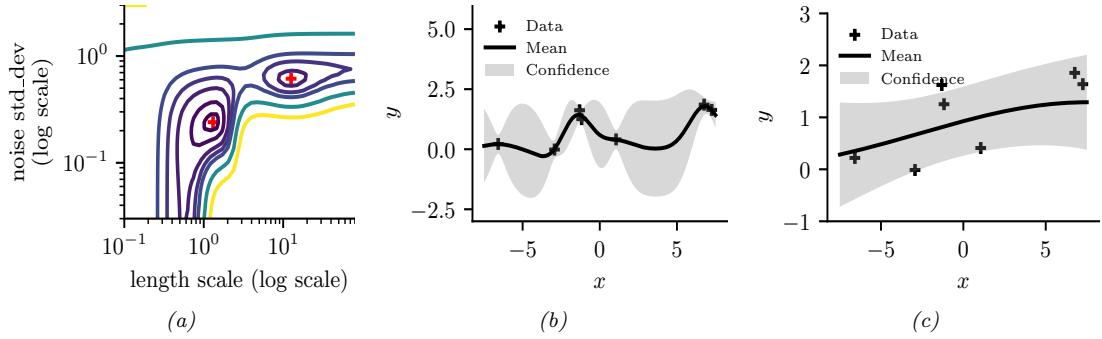
Figure 18.16: Illustration of local minima in the marginal likelihood surface. (a) We plot the log marginal likelihood vs ω^{2 y} and ε, for fixed ω^{2 f} = 1, using the 7 datapoints shown in panels b and c. (b) The function corresponding to the lower left local minimum, (ε, ω^{2 n}) ↙ (1, 0.2). This is quite “wiggly” and has low noise. (c) The function corresponding to the top right local minimum, (ε, ω^{2 n}) ↙ (10, 0.8). This is quite smooth and has high noise. The data was generated using (ε, ω^{2 n}) = (1, 0.1). Adapted from Figure 5.5 of [RW06]. Generated by gpr\_demo\_marglik.ipynb.

The form of ^ϑK^ϑ ϑϱ^j depends on the form of the kernel, and which parameter we are taking derivatives with respect to. Often we have constraints on the hyper-parameters, such as ς^{2 y} ≃ 0. In this case, we can define ω = log(ς^{2 y}), and then use the chain rule.

Given an expression for the log marginal likelihood and its derivative, we can estimate the kernel parameters using any standard gradient-based optimizer. However, since the objective is not convex, local minima can be a problem, as we illustrate below, so we may need to use multiple restarts.

18.6.1.1 Example

Consider Figure 18.16. We use the SE kernel in Equation (18.161) with ς^{2 f} = 1, and plot log ^p(y|X, ^ε, ^{ς2 y}) (where X and y are the 7 datapoints shown in panels b and c as we vary ε and ς^{2 y}. The two local optima are indicated by + in panel a. The bottom left optimum corresponds to a low-noise, short-length scale solution (shown in panel b). The top right optimum corresponds to a high-noise, long-length scale solution (shown in panel c). With only 7 datapoints, there is not enough evidence to confidently decide which is more reasonable, although the more complex model (panel b) has a marginal likelihood that is about 60% higher than the simpler model (panel c). With more data, the more complex model would become even more preferred.

Figure 18.16 illustrates some other interesting (and typical) features. The region where ς^{2 y} ↓ 1 (top of panel a) corresponds to the case where the noise is very high; in this regime, the marginal likelihood is insensitive to the length scale (indicated by the horizontal contours), since all the data is explained as noise. The region where ε ↓ 0.5 (left hand side of panel a) corresponds to the case where the length scale is very short; in this regime, the marginal likelihood is insensitive to the noise level (indicated by the vertical contours), since the data is perfectly interpolated. Neither of these regions would be chosen by a good optimizer.

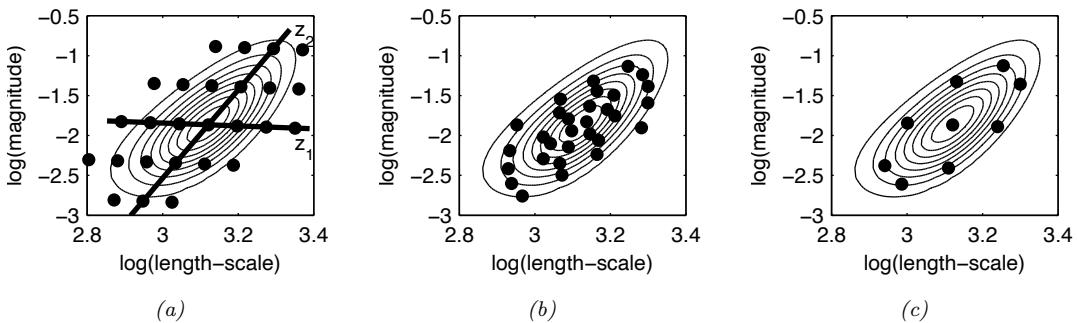
Figure 18.17: Three di!erent approximations to the posterior over hyper-parameters: grid-based, Monte Carlo, and central composite design. From Figure 3.2 of [Van10]. Used with kind permission of Jarno Vanhatalo.

18.6.2 Bayesian inference for the kernel parameters

When we have a small number of datapoints (e.g., when using GPs for blackbox optimization, as we discuss in Section 6.6), using a point estimate of the kernel parameters can give poor results [Bul11; WF14]. As a simple example, if the function values that have been observed so far are all very similar, then we may estimate ^{ςˆ ↓ 0}, which will result in overly confident predictions.5

To overcome such overconfidence, we can compute a posterior over the kernel parameters. If the dimensionality of ω is small, we can compute a discrete grid of possible values, centered on the MAP estimate ωˆ (computed as above). We can then approximate the posterior using

\[p(\boldsymbol{f}|\mathcal{D}) = \sum\_{s=1}^{S} p(\boldsymbol{f}|\mathcal{D}, \boldsymbol{\theta}\_s) p(\boldsymbol{\theta}\_s|\mathcal{D}) \boldsymbol{w}\_s \tag{18.166}\]

where w^s denotes the weight for grid point s.

In higher dimensions, a regular grid su!ers from the curse of dimensionality. One alternative is place grid points at the mode, and at a distance ±1sd from the mode along each dimension, for a total of 2|ω| + 1 points. This is called a central composite design [RMC09]. See Figure 18.17 for an illustration.

In higher dimensions, we can use Monte Carlo inference for the kernel parameters when computing Equation (18.166). For example, [MA10] shows how to use slice sampling (Section 12.4.1) for this task, [Hen+15] shows how to use HMC (Section 12.5), and [BBV11a] shows how to use SMC (Chapter 13).

In Figure 18.18, we illustrate the di!erence between kernel optimization vs kernel inference. We fit a 1d dataset using a kernel of the form

\[\mathcal{K}(r) = \sigma\_1^2 \mathcal{K}\_{\text{SE}}(r;\tau) \mathcal{K}\_{\text{cos}}(r;\rho\_1) + \sigma\_2^s \mathcal{K}\_{\text{32}}(r;\rho\_2) \tag{18.167}\]

where KSE(r; ε) is the squared exponential kernel (Equation (18.12)), Kcos(r; 01) is the cosine kernel (Equation (18.19)), and ^K32(r; ⁰2) is the Matérn ^{3 2} kernel (Equation (18.15)). We then compute a

^5. In [WSN00; BBV11b], they show how we can put a conjugate prior on ϱ² and integrate it out, to generate a Student version of the GP, which is more robust.

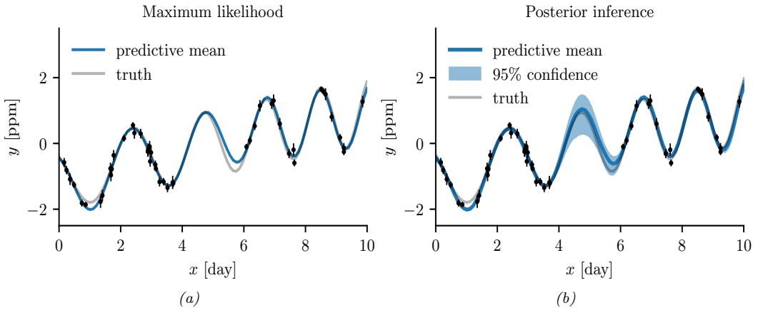
Figure 18.18: Di!erence between estimation and inference for kernel hyper-parameters. (a) Empirical Bayes approach based on optimization. We plot the posterior predicted mean given a plug-in estimate, E $ ^f(x)|D, ^ωˆ % . (b) Bayesian approach based on HMC. We plot the posterior predicted mean, marginalizing over hyperparameters, E [f(x)|D]. Generated by gp\_kernel\_opt.ipynb.

point-estimate of the kernel parameters using empirical Bayes, and posterior samples using HMC. We can predict the posterior mean of f on a 1d test set by plugging in the MLE or averaging over samples. We see that the latter captures more uncertainty (beyond the uncertainty captured by the Gaussian itself).

18.6.3 Multiple kernel learning for additive kernels

A special case of kernel learning arises when the kernel is a sum of B base kernels

\[\mathcal{K}(\mathbf{z}, \mathbf{z}') = \sum\_{b=1}^{B} w\_b \mathcal{K}\_b(\mathbf{z}, \mathbf{z}') \tag{18.168}\]

Optimizing the weights w^b > 0 using structural risk minimization is known as multiple kernel learning; see e.g., [Rak+08] for details.

Now suppose we constrain the base kernels to depend on a subset of the variables. Furthermore, suppose we enforce a hierarchical inclusion property (e.g., including the kernel k¹²³ means we must also include k12, k¹³ and k23), as illustrated in Figure 18.19(left). This is called hierarchical kernel learning. We can find a good subset from this model class using convex optimization [Bac09]; however, this requires the use of cross validation to estimate the weights. A more e”cient approach is to use the empirical Bayes approach described in [DNR11].

In many cases, it is common to restrict attention to first order additive kernels:

\[\mathcal{K}(\mathbf{z}, \mathbf{z}') = \sum\_{d=1}^{D} \mathcal{K}\_d(x\_d, x'\_d) \tag{18.169}\]

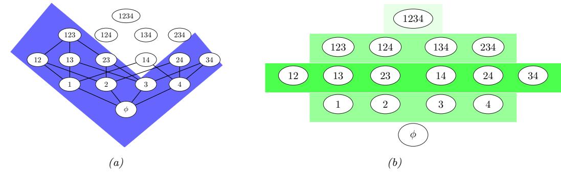
Figure 18.19: Comparison of di!erent additive model classes for a 4d function. Circles represent di!erent interaction terms, ranging from first-order to fourth-order. Left: hierarchical kernel learning uses a nested hierarchy of terms. Right: additive GPs use a weighted sum of additive kernels of di!erent orders. Color shades represent di!erent weighting terms. Adapted from Figure 6.2 of [Duv14].

The resulting function then has the form

\[f(\mathbf{x}) = f\_1(x\_1) + \dots + f\_D(x\_D) \tag{18.170}\]

This is called a generalized additive model or GAM.

Figure 18.20 shows an example of this, where each base kernel has the form Kd(xd, x^{↔︎ d}) = ς2 dSE(xd, x^{↔︎ d}|εd), In Figure 18.20, we see that the ^{ς2 d} terms for the coarse and fine features are set to zero, indicating that these inputs have no impact on the response variable.

[DBW20] considers additive kernels operating on di!erent linear projections of the inputs:

\[\mathcal{K}(\mathbf{z}, \mathbf{z}') = \sum\_{b=1}^{B} w\_b \mathcal{K}\_b(\mathbf{P}\_b \mathbf{z}, \mathbf{P}\_b \mathbf{z}') \tag{18.171}\]

Surprisingly, they show that these models can match or exceed the performance of kernels operating on the original space, even when the projections are into a single dimension, and not learned. In other words, it is possible to reduce many regression problems to a single dimension without loss in performance. This finding is particularly promising for scalable inference, such as KISS (see Section 18.5.5.3), and active learning, which are greatly simplified in a low dimensional setting.

More recently, [LBH22] has proposed the orthogonal additive kernel (OAK), which imposes an orthogonality constraint on the additive functions. This ensures an identifiable, low-dimensional representation of the functional relationship, and results in improved performance.

18.6.4 Automatic search for compositional kernels

Although the above methods can estimate the hyperparameters of a specified set of kernels, they do not choose the kernels themselves (other than the special case of selecting a subset of kernels from a set). In this section, we describe a method, based on [Duv+13], for sequentially searching through the space of increasingly complex GP models so as to find a parsiminous description of the data. (See also [BHB22] for a review.)

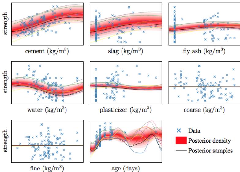
Figure 18.20: Predictive distribution of each term in a GP-GAM model applied to a dataset with 8 continuous inputs and 1 continuous output, representing the strength of some concrete. From Figure 2.7 of [Duv14]. Used with kind permission of David Duvenaud.

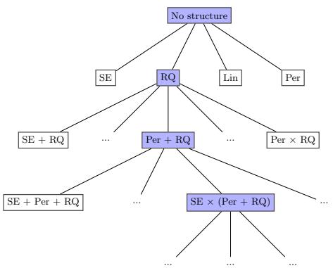
Figure 18.21: Example of a search tree over kernel expressions. Adapted from Figure 3.2 of [Duv14].

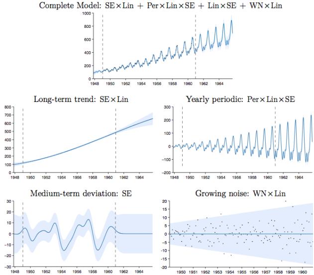
Figure 18.22: Top row: airline dataset and posterior distribution of the model discovered after a search of depth 10. Subsequent rows: predictions of the individual components. From Figure 3.5 of [Duv14], based on [Llo+14]. Used with kind permission of David Duvenaud.

We start with a simple kernel, such as the white noise kernel, and then consider replacing it with a set of possible alternative kernels, such as an SE kernel, RQ kernel, etc. We use the BIC score (Section 3.8.7.2) to evaluate each candidate model (choice of kernel) m. This has the form BIC(m) = log ^p(D|m)^{→ 1 2} |m| log N, where p(D|m) is the marginal likelihood, and |m| is the number of parameters. The first term measures fit to the data, and the second term is a complexity penalty. We can also consider replacing a kernel by the addition of two kernels, k ↖ (k + k^↔︎ ), or the multiplication of two kernels, k ↖ (k ⇔ k^↔︎ ). See Figure 18.21 for an illustration of the search space.

Searching through this space is similar to what a human expert would do. In particular, if we find structure in the residuals, such as periodicity, we can propose a certain “move” through the space. We can also start with some structure that is assumed to hold globally, such as linearity, but if we find this only holds locally, we can multiply the kernel by an SE kernel. We can also add input dimensions incrementally, to capture higher order interactions.

Figure 18.22 shows the output of this process applied to a dataset of monthly totals of international airline passengers. The input to the GP is the set of time stamps, x =1: t; there are no other features.

The observed data lies in between the dotted vertical lines; curves outside of this region are extrapolations. We see that the system has discovered a fairly interpretable set of patterns in the data. Indeed, it is possible to devise an algorithm to automatically convert the output of this search process to a natural language summary, as shown in [Llo+14]. In this example, it summarizes the data as being generated by the addition of 4 underlying trends: a linearly increasing function; an approximately periodic function with a period of 1.0 years, and with linearly increasing amplitude; a

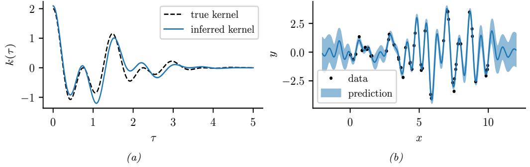
Figure 18.23: Illustration of a GP with a spectral mixture kernel in 1d. (a) Learned vs true kernel. (b) Predictions using learned kernel. Generated by gp\_spectral\_mixture.ipynb.

smooth function; and uncorrelated noise with linearly increasing standard deviation.

Recently, [Sun+18] showed how to create a DNN which learns the kernel given two input vectors. The hidden units are defined as sums and products of elementary kernels, as in the above search based approach. However, the DNN can be trained in a di!erentiable way, so is much faster.

18.6.5 Spectral mixture kernel learning

Any shift-invariant (stationary) kernel can be converted via the Fourier transform to its dual form, known as its spectral density. This means that learning the spectral density is equivalent to learning any shift-invariant kernel. For example, if we take the Fourier transform of an RBF kernel, we get a Gaussian spectral density centered at the origin. If we take the Fourier transform of a Matérn kernel, we get a Student spectral density centred at the origin. Thus standard approaches to multiple kernel learning, which typically involve additive compositions of RBF and Matérn kernels with di!erent length-scale parameters, amount to density estimation with a scale mixture of Gaussian or Student distributions at the origin. Such models are very inflexible for density estimation, and thus also very limited in being able to perform kernel learning.

On the other hand, scale-location mixture of Gaussians can model any density to arbitrary precision. Moreover, with even a small number of components these mixtures of Gaussians are highly flexible. Thus a spectral density corresponding to a scale-location mixture of Gaussians forms an expressive basis for all shift-invariant kernels. One can evaluate the inverse Fourier transform for a Gaussian mixture analytically, to derive the spectral mixture kernel [WA13], which we can express for one-dimensional inputs x as:

\[\mathcal{K}(x, x') = \sum\_{i} w\_i \cos((x - x')(2\pi\mu\_i)) \exp(-2\pi^2(x - x')^2 v\_i) \tag{18.172}\]

The mixture weights wi, as well as the means µⁱ and variances vⁱ of the Gaussians in the spectral density, can be learned by empirical Bayes optimization (Section 18.6.1) or in a fully-Bayesian procedure (Section 18.6.2) [Jan+17]. We illustrate the former approach in Figure 18.23.

By learning the parameters of the spectral mixture kernel, we can discover representations that enable extrapolation — to make reasonable predictions far away from the data. For example, in

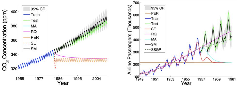
Figure 18.24: Extrapolations (point predictions and 95% credible set) on CO² and airline datasets using Gaussian processes with Matérn, rational quadratic, periodic, RBF (SE), and spectral mixture kernels, each with hyperparameters learned using empirical Bayes. From [Wil14].

Section 18.8.1, compositions of kernels are carefully hand-crafted to extrapolate CO² concentrations. But in this instance, the human statistician is doing all of the interesting representation learning. Figure 18.24 shows Gaussian processes with learned spectral mixture kernels instead automatically extrapolating on CO² and airline passenger problems.

These kernels can also be used to extrapolate higher dimensional large-scale spatio-temporal patterns. Large datasets can provide relatively more information for expressive kernel learning. However, scaling an expressive kernel learning approach poses di!erent challenges than scaling a standard Gaussian process model. One faces additional computational constraints, and the need to retain significant model structure for expressing the rich information available in a large dataset. Indeed, in Figure 18.24 we can separately understand the e!ects of the kernel learning approach and scalable inference procedure, in being able to discover structure necessary to extrapolate textures. An expressive kernel model and a scalable inference approach that preserves a non-parametric representation are needed for good performance.

Structure exploiting inference procedures, such as Kronecker methods, as well as KISS-GP and conjugate gradient based approaches, are appropriate for these tasks — since they generally preserve or exploit existing structure, rather than introducing approximations that corrupt the structure. Spectral mixture kernels combined with these scalable inference techniques have been used to great e!ect for spatiotemporal extrapolation problems, including land-surface temperature forecasting, epidemiological modeling, and policy-relevant applications.

18.6.6 Deep kernel learning

Deep kernel learning [SH07; Wil+16] combines the structural properties of neural networks with the non-parametric flexibility and uncertainty representation provided by Gaussian processes. For example, we can define a “deep RBF kernel” as follows:

\[\mathcal{K}\_{\theta}(x, x') = \exp\left[ -\frac{1}{2\sigma^2} ||h^L\_{\theta}(x) - h^L\_{\theta}(x')||^2 \right] \tag{18.173}\]

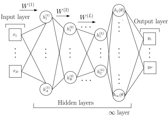
Figure 18.25: Deep kernel learning: a Gaussian process with a deep kernel maps D dimensional inputs x through L parametric hidden layers followed by a hidden layer with an infinite number of basis functions, with base kernel hyperparameters ω. Overall, a Gaussian process with a deep kernel produces a probabilistic mapping with an infinite number of adaptive basis functions parameterized by ↼ = {w, ω}. All parameters ↼ are learned through the marginal likelihood of the Gaussian process. From Figure 1 of [Wil+16].

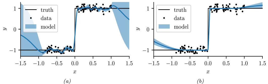
Figure 18.26: Modeling a discontinuous function with (a) a GP with a “shallow” Matérn ^{3 2} kernel, and (b) a GP with a “deep” MLP + Matérn kernel. Generated by gp\_deep\_kernel\_learning.ipynb.

where h^{L ε} (x) are the outputs of layer L from a DNN. We can then learn the parameters ω by maximizing the marginal likelihood of the Gaussian processes.

This framework is illustrated in Figure 18.25. We can understand the neural network features as inputs into a base kernel. The neural network can either be (1) pre-trained, (2) learned jointly with the base kernel parameters, or (3) pre-trained and then fine-tuned through the marginal likelihood. This approach can be viewed as a “last-layer” Bayesian model, where a Gaussian process is applied to the final layer of a neural network. The base kernel often provides a good measure of distance in feature space, desirably encouraging predictions to have high uncertainty as we move far away from the data.

We can use deep kernel learning to help the GP learn discontinuous functions, as illustrated in Figure 18.26. On the left we show the results of a GP with a standard Matérn ^{3 2} kernel. It is clear

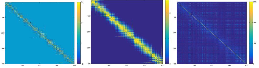
Figure 18.27: Left: the learned covariance matrix of a deep kernel with spectral mixture base kernel on a set of test cases for the Olivetti faces dataset, where the test samples are ordered according to the orientations of the input faces. Middle: the respective covariance matrix using a deep kernel with RBF base kernel. Right: the respective covariance matrix using a standard RBF kernel. From Figure 5 of [Wil+16].

that the out-of-sample predictions are poor. On the right we show the results of the same model where we first transform the input through a learned 2 layer MLP (with 15 and 10 hidden units). It is clear that the model is working much better.

As a more complex example, we consider a regression problem where we wish to map faces (vectors of pixel intensities) to a continuous valued orientation angle. In Figure 18.27, we evaluate the deep kernel matrix (with RBF and spectral mixture base kernels, discussed in Section 18.6.5) on data ordered by orientation angle. We can see that the learned deep kernels, in the left two panels, have a pronounced diagonal band, meaning that they have discovered that faces with similar orientation angles are correlated. On the other hand, in the right panel we see that the entries even for a learned RBF kernel are highly di!use. Since the RBF kernel essentially uses Euclidean distance as a metric for similarity, it is unable to learn a representation that e!ectively solves this problem. In this case, one must do highly non-Euclidean metric learning.

However, [ORW21] show that the approach to DKL based on maximizing the marginal likelihood can result in overfitting that is worse than standard DNN learning. They propose a fully Bayesian approach, in which they use SGLD (Section 12.7.1) to sample the DNN weights as well as the GP hyperparameters.

18.7 GPs and DNNs

In Section 18.6.6, we showed how we can combine the structural properties of neural networks with GPs. In Section 18.7.1 we show that, in the limit of infinitely wide networks, a neural network defines a GP with a certain kernel. These kernels are fixed, so the method is not performing representation learning, as a standard neural network would (see e.g., [COB18; Woo+19]). Nonetheless, these kernels are interesting in their own right, for example in modelling non-stationary covariance structure. In Section 18.7.2, we discuss the connection between SGD training of DNNs and GPs. And in Section 18.7.3, we discuss deep GPs, which are similar to DNNs in that they consist of many layers of functions which are composed together, but each layer is a nonparametric function.

18.7.1 Kernels derived from infinitely wide DNNs (NN-GP)

In this section, we show that an MLP with one hidden layer, whose width goes to infinity, and which has a Gaussian prior on all the parameters, converges to a Gaussian process with a well-defined kernel.6 This result was first shown for in [Nea96; Wil98], and was later extended to deep MLPs in [DFS16; Lee+18], to CNNs in [Nov+19], and to general DNNs in [Yan19]. The resulting kernel is called the NN-GP kernel [Lee+18].

We will consider the following model:

\[f\_k(\mathbf{z}) = b\_k + \sum\_{j=1}^{H} v\_{jk} h\_j(\mathbf{z}), \ h\_j(\mathbf{z}) = \varphi(u\_{0j} + \mathbf{z}^\mathsf{T} u\_j) \tag{18.174}\]

where H is the number of hidden units, and 5() is some nonlinear activation function, such as ReLU. We will assume Gaussian priors on the parameters:

\[b\_k \sim \mathcal{N}(0, \sigma\_b),\\ v\_{jk} \sim \mathcal{N}(0, \sigma\_v),\\ u\_{0j} \sim \mathcal{N}(0, \sigma\_0),\\ \mathbf{u}\_j \sim \mathcal{N}(0, \Sigma) \tag{18.175}\]

Let ω = {bk, vjk, u0^j ,uj} be all the parameters. The expected output from unit k when applied to one input vector is given by

\[\mathbb{E}\_{\theta} \left[ f\_k(\mathbf{z}) \right] = \mathbb{E}\_{\theta} \left[ b\_k + \sum\_{j=1}^{H} v\_{jk} h\_j(\mathbf{z}) \right] = \underbrace{\mathbb{E}\_{\theta} \left[ b\_k \right]}\_{=0} + \sum\_{j=1}^{H} \underbrace{\mathbb{E}\_{\theta} \left[ v\_{jk} \right]}\_{=0} \mathbb{E}\_{\mathbf{u}} \left[ h\_j(\mathbf{z}) \right] = 0 \tag{18.176}\]

The covariance in the output for unit k when the function is applied to two di!erent inputs is given by the following:7

\[\mathbb{E}\_{\theta} \left[ f\_k(\mathbf{z}) f\_k(\mathbf{z}') \right] = \mathbb{E}\_{\theta} \left[ \left( b\_k + \sum\_{j=1}^{H} v\_{jk} h\_j(\mathbf{z}) \right) \left( b\_k + \sum\_{j=1}^{H} v\_{jk} h\_j(\mathbf{z}) \right) \right] \tag{18.177}\]

\[\sigma = \sigma\_b^2 + \sum\_{j=1} \mathbb{E}\_\theta \left[ v\_{jk}^2 \right] \mathbb{E}\_\mathbf{u} \left[ h\_j(\mathbf{z}) h\_j(\mathbf{z}') \right] = \sigma\_b^2 + \sigma\_v^2 H \mathbb{E}\_\mathbf{u} \left[ h\_j(\mathbf{z}) h\_j(\mathbf{z}') \right] \tag{18.178}\]

Now consider the limit ^H ↖ ⇓. We scale the magnitude of the output by defining ^{ς2 v} = 6/H. Since the input to k’th output unit is an infinite sum of random variables (from the hidden units h^j (x)), we can use the central limit theorem to conclude that the output converges to a Gaussian with mean and variance given by

\[\mathbb{E}\left[f\_k(\mathbf{z})\right] = 0, \ \mathbb{V}\left[f\_k(\mathbf{z})\right] = \sigma\_b^2 + \omega \mathbb{E}\_\mathbf{u}\left[h(\mathbf{z})^2\right] \tag{18.179}\]

Furthermore, the joint distribution over {fk(xn) : n =1: N} for any N ≃ 2 converges to a multivariate Gaussian with covariance given by

\[\mathbb{E}\left[f\_k(\mathbf{z})f\_k(\mathbf{z}')\right] = \sigma\_b^2 + \omega \mathbb{E}\_\mathbf{u}\left[h(\mathbf{z})h(\mathbf{z}')\right] \stackrel{\Delta}{=} \mathcal{K}(\mathbf{z}, \mathbf{z}') \tag{18.180}\]

7. We are using the fact that ^{u → N} (0, ^ϱ2) implies ^E ( u2) = V [u] = ϱ2.

^6. Our presentation is based on http://cbl.eng.cam.ac.uk/pub/Intranet/MLG/ReadingGroup/presentation\_ matthias.pdf.

\[\begin{array}{ll} \frac{h(\tilde{x})}{\operatorname{erf}(\tilde{x}^{\mathsf{T}}\tilde{u})} & \frac{C(\tilde{x},\tilde{x}')}{\frac{2}{\pi}\arcsin(f\_{1}(\tilde{x},\tilde{x}'))} \\ \frac{1}{\mathsf{L}\left(\tilde{x}^{\mathsf{T}}\tilde{u}\geq 0\right)} & \pi-\theta(\tilde{x},\tilde{x}') \\ \operatorname{ReLU}(\tilde{x}^{\mathsf{T}}\tilde{u}) & \frac{f\_{2}(\tilde{x},\tilde{x}')}{\pi}\sin(\theta(\tilde{x},\tilde{x}'))+\frac{\pi-\theta(\tilde{x},\tilde{x}')}{\pi}\tilde{x}^{\mathsf{T}}\tilde{\Sigma}\tilde{x}' \end{array}\]

Table 18.4: Some neural net GP kernels. Here we define f1(x˜, x˜^↑ ) = ²x˜T!˜ ^x˜^↑ ∝(1+2x˜T!˜ ^x˜)(1+2(x˜↑)T!˜ ^x˜↑) , f2(x˜, x˜^↑ ) = ||!˜ ^{1 2 x}˜|| ||!˜ ^{1 2} x˜^↑ ||, f3(x˜, x˜^↑ ) = & (x˜^T!˜ x˜)((x˜↑)^T!˜ x˜↑), and ▷(x˜, x˜^↑ ) = arccos(f3(x˜, x˜^↑ )). Results are derived in [Wil98; CS09].

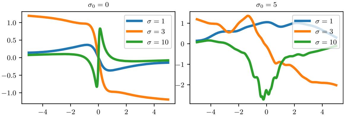
Figure 18.28: Sample output from a GP with an NNGP kernel derived from an infinitely wide one layer MLP with activation function of the form h(x) = erf(x · u + u0) where u ↑ N (0, ω) and u⁰ ↑ N (0, ω0). Generated by nngp\_1d.ipynb. Used with kind permission of Matthias Bauer.

Thus the MLP converges to a GP. To compute the kernel function, we need to evaluate

\[C(\mathbf{z}, \mathbf{z}') = \mathbb{E}\_{\mathbf{u}} \left[ h(u\_0 + \mathbf{u}^{\mathsf{T}} \mathbf{z}) h(u\_0 + \mathbf{u}^{\mathsf{T}} \mathbf{z}') \right] = \mathbb{E}\_{\mathbf{u}} \left[ h(\tilde{\mathbf{u}}^{\mathsf{T}} \tilde{\mathbf{z}}) h(\tilde{\mathbf{u}}^{\mathsf{T}} \tilde{\mathbf{z}}') \right] \tag{18.181}\]

where we have defined x˜ = (1, x) and u˜ = (u0,u). Let us define

\[ \bar{\Sigma} = \begin{pmatrix} \sigma\_0^2 & 0 \\ 0 & \Sigma \end{pmatrix} \tag{18.182} \]

Then we have

\[C(\boldsymbol{x}, \boldsymbol{x}') = \int h(\boldsymbol{\bar{u}}^{\mathsf{T}} \boldsymbol{\bar{x}}) h(\boldsymbol{\bar{u}}^{\mathsf{T}} \boldsymbol{\bar{x}'}) \mathcal{N}(\boldsymbol{\bar{u}} | \mathbf{0}, \boldsymbol{\bar{\Sigma}}) d\boldsymbol{\bar{u}} \tag{18.183}\]

This can be computed in closed form for certain activation functions, as shown in Table 18.4.

This is sometimes called the neural net kernel. Note that this is a non-stationary kernel, and sample paths from it are nearly discontinuous and tend to constant values for large positive or negative inputs, as illustrated in Figure 18.28.

18.7.2 Neural tangent kernel (NTK)

In Section 18.7.1 we derived the NN-GP kernel, under the assumption that all the weights are random. A natural question is: can we derive a kernel from a DNN after it has been trained, or more generally, while it is being trained. It turns out that this can be done, as we show below.

Let f = [f(xn; ω)]^{N n}=1 be the ^{N ⇔ 1} prediction vector, let ^⇒f^L = [ ^{ϑL ϑ}f(xn) ] N ⁿ=1 be the N ⇔ 1 loss gradient vector, let ω = [ωp] P ^p=1 be the ^{P ⇔ 1} vector of parameters, and let ^⇒ε^f = [ ^ϑf(xn) ϑϱ^p ] be the P ⇔ N matrix of partials. Suppose we perform continuous time gradient descent with fixed learning rate η. The parameters evolve over time as follows:

\[ \partial\_t \theta\_t = -\eta \nabla\_\theta \mathcal{L}(f\_t) = -\eta \nabla\_\theta \mathbf{f}\_t \cdot \nabla\_f \mathcal{L}(\mathbf{f}\_t) \tag{18.184} \]

Thus the function evolves over time as follows:

\[ \partial\_t \mathbf{f}\_t = \nabla\_\theta \mathbf{f}\_t^\top \partial\_t \theta\_t = -\eta \nabla\_\theta \mathbf{f}\_t^\top \nabla\_\theta \mathbf{f}\_t \cdot \nabla\_f \mathcal{L}(\mathbf{f}\_t) = -\eta \nabla\_t \cdot \nabla\_f \mathcal{L}(\mathbf{f}\_t) \tag{18.185} \]

where T^t is the N ⇔ N kernel matrix

\[\mathcal{T}\_t(x, x') \triangleq \nabla\_{\theta} f\_t(x) \cdot \nabla\_{\theta} f\_t(x') = \sum\_{p=1}^P \frac{\partial f(x; \theta)}{\partial \theta\_p} \Big|\_{\theta\_t} \frac{\partial f(x'; \theta)}{\partial \theta\_p} \Big|\_{\theta\_t} \tag{18.186}\]

If we let the learning rate η become infinitesimally small, and the widths go to infinity, one can show that this kernel converges to a constant matrix, this is known as the neural tangent kernel or NTK [JGH18]:

\[\mathcal{T}(x, x') \triangleq \nabla\_{\theta} f(x; \theta\_{\infty}) \cdot \nabla\_{\theta} f(x'; \theta\_{\infty}) \tag{18.187}\]

Details on how to compute this kernel for various models, such as CNNs, graph neural nets, and general neural nets, can be found in [Aro+19; Du+19; Yan19]. A software libary to compute the NN-GP kernel and NTK is available in [Ano19].

The assumptions behind the NTK results in the parameters barely changing from their initial values (which is why a linear approximation around the starting parameters is valid). This can still lead to a change in the final predictions (and zero final training error), because the final layer weights can learn to use the random features just like in kernel regression. However, this phenomenon — which has been called “lazy training” [COB18] — is not representative of DNN behavior in practice [Woo+19], where parameters often change a lot. Fortunately it is possible to use a di!erent parameterization which does result in feature learning in the infinite width limit [YH21].

18.7.3 Deep GPs

A deep Gaussian process or DGP is a composition of GPs [DL13]. More formally, a DGP of L layers is a hierachical model of the form

\[\text{DGP}(\mathbf{z}) = f\_L \circ \cdots \circ \mathbf{f}\_1(\mathbf{z}),\\\ f\_i(\cdot) = [f\_i^{(1)}(\cdot), \dots, f\_i^{(H\_i)}(\cdot)],\\f\_i^{(j)} \sim \text{GP}(0, \mathcal{K}\_i(\cdot, \cdot)) \tag{18.188}\]

This is similar to a deep neural network, except the hidden nodes are now hidden functions.

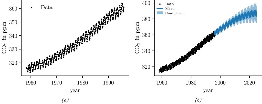
Figure 18.29: (a) The observed Mauna Loa CO² time series. (b) Forecasts from a GP. Generated by gp\_mauna\_loa.ipynb.

A natural question is: what is gained by this approach compared to a standard GP? Although conventional single-layer GPs are nonparametric, and can model any function (assuming the use of a non-degenerate kernel) with enough data, in practice their performance is limited by the choice of kernel. It is tempting to think that deep kernel learning (Section 18.6.6) can solve this problem, but in theory a GP on top of a DNN is still just a GP. However, one can show that a composition of GPs is strictly more general. Unfortunately, inference in deep GPs is rather complicated, so we leave the details to Supplementary Section 18.1. See also [Jak21] for a recent survey on this topic.

18.8 Gaussian processes for time series forecasting

It is possible to use Gaussian processes to perform time series forecasting (see e.g., [Rob+13]). The basic idea is to model the unknown output as a function of time, f(t), and to represent a prior about the form of f as a GP; we then update this prior given the observed evidence, and forecast into the future. Naively this would take O(T³) time. However, for certain stationary kernels, it is possible to reformulate the problem as a linear-Gaussian state space model, and then use the Kalman smoother to perform inference in O(T) time, as explained in [SSH13; SS19; Ada+20]. This conversion can be done exactly for Matérn kernels and approximately for Gaussian (RBF) kernels (see [SS19, Ch. 12]). In [SGF21], they describe how to reduce the linear dependence on T to log(T) time using a parallel prefix scan operator, that can be run e”ciently on GPUs (see Section 8.2.3.4).

18.8.1 Example: Mauna Loa

In this section, we use the Mauna Loa CO² dataset from Section 29.12.5.1. We show the raw data in Figure 18.29(a). We see that there is periodic (or quasi-periodic) signal with a year-long period superimposed on a long term trend. Following [RW06, Sec 5.4.3], we will model this with a

composition of kernels:

\[ \mathcal{K}(r) = \mathcal{K}\_1(r) + \mathcal{K}\_2(r) + \mathcal{K}\_3(r) + \mathcal{K}\_4(r) \tag{18.189} \]

where Ki(t, t^↔︎ ) = Ki(t → t ↔︎ ) for the i’th kernel.

To capture the long term smooth rising trend, we let K¹ be a squared exponential (SE) kernel, where ω⁰ is the amplitude and ω¹ is the length scale:

\[\mathcal{K}\_1(r) = \theta\_0^2 \exp\left(-\frac{r^2}{2\theta\_1^2}\right) \tag{18.190}\]

To model the periodicity, we can use a periodic or exp-sine-squared kernel from Equation (18.18) with a period of 1 year. However, since it is not clear if the seasonal trend is exactly periodic, we multiply this periodic kernel with another SE kernel to allow for a decay away from periodicity; the result is K2, where ω² is the magnitude, ω³ is the decay time for the periodic component, ω⁴ = 1 is the period, and ω⁵ is the smoothness of the periodic component.

\[\mathcal{K}\_2(r) = \theta\_2^2 \exp\left(-\frac{r^2}{2\,\theta\_3^2} - \theta\_5 \sin^2\left(\frac{\pi}{\theta\_4}\right)\right) \tag{18.191}\]

To model the (small) medium term irregularities, we use a rational quadratic kernel (Equation (18.20)):

\[\mathcal{K}\_3(r) = \theta\_6^2 \left[ 1 + \frac{r^2}{2\theta\_7^2 \theta\_8} \right]^{-\theta\_8} \tag{18.192}\]

where ω⁶ is the magnitude, ω⁷ is the typical length scale, and ω⁸ is the shape parameter.

The magnitude of the independent noise can be incorporated into the observation noise of the likelihood function. For the correlated noise, we use another SE kernel:

\[\mathcal{K}\_4(r) = \theta\_9^2 \exp\left(-\frac{r^2}{2\theta\_{10}^2}\right) \tag{18.193}\]

where ω⁹ is the magnitude of the correlated noise, and ω¹⁰ is the length scale. (Note that the combination of K¹ and K⁴ is non-identifiable, but this does not a!ect predictions.)

We can fit this model by optimizing the marginal likelihood wrt ω (see Section 18.6.1). The resulting forecast is shown in Figure 18.29(b).

19 Beyond the iid assumption

19.1 Introduction

The standard approach to supervised ML assumes the training and test sets both contain independent and identically distributed (iid) samples from the same distribution. However, there are many settings in which the test distribution may be di!erent from the training distribution; this is known as distribution shift, as we discuss in Section 19.2.

In some cases, we may have data from multiple related distributions, not just train and test, as we discuss in Section 19.6. We may also encounter data in a streaming setting, where the data distribution may be changing continuously, or in a piecewise constant fashion, as we discuss in Section 19.7. Finally, in Section 19.8, we discuss settings in which the test distribution is chosen by an adversary to minimize performance of a prediction system.

19.2 Distribution shift

Suppose we have a labeled training set from a source distribution p(x, y) which we use to fit a predictive model p(y|x). At test time we encounter data from the target distribution q(x, y). If p ′= q, we say that there has been a distribution shift or dataset shift [QC+08; BD+10]. This can adversely a!ect the performance of predictive models, as we illustrate in Section 19.2.1. In Section 19.2.2 we give a taxonomy of some kinds of distribution shift using the language of causal graphical models. We then proceed to discuss a variety of strategies that can be adopted to ameliorate the harm caused by distribution shift. In particular, in Section 19.3, we discuss techniques for detecting shifts, so that we can abstain from giving an incorrect prediction if the model is not confident. In Section 19.4, we discuss techniques to improve robustness to shifts; in particular, given labeled data from p(x, y), we aim to create a model that approximates q(y|x). In Section 19.5, we discuss techniques to adapt the model to the target distribution given some labeled or unlabeled data from the target.

19.2.1 Motivating examples

Figure 19.1 shows how shifting the test distribution slightly, by adding a small amount of Gaussian noise, can hurt performance of an otherwise high accuracy image classifier. Similar e!ects occur with other kinds of common corruptions, such as image blurring [HD19]. Analogous problems can also occur in the text domain [Ryc+19], and the speech domain (see e.g., male vs female speakers in

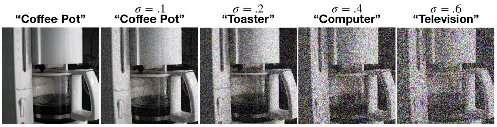
Figure 19.1: E!ect of Gaussian noise of increasing magnitude on an image classifier. The model is a ResNet-50 CNN trained on ImageNet. From Figure 23 of [For+19]. Used with kind permission of Justin Gilmer.

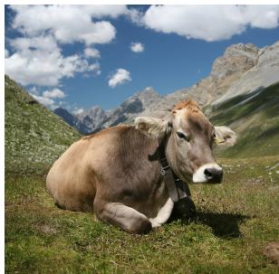
1. Cow: 0.99, Pasture: 0.99, Grass: 0.99, No Person: 0.98, Mammal: 0.98

3. No Person: 0.97, Mammal: 0.96, Water: 0.94, Beach: 0.94, Two: 0.94

Figure 19.2: Illustration of how image classifiers generalize poorly to new environments. (a) In the training data, most cows ocur on grassy backgrounds. (b-c) In these test image, the cow occurs “out of context”, namely on a beach. The background is considered a “spurious correlation”. In (b), the cow is not detected. In (c), it is classified with a generic “mammal” label. Top five labels and their confidences are produced by ClarifAI.com, which is a state of the art commerical vision system. From Figure 1 of [BVHP18]. Used with kind permission of Sara Beery.

Seashore: 0.97

Figure 34.3). These examples illustrate that high performing predictive models can be very sensitive to small changes in the input distribution.

Performance can also drop on “clean” images, but which exhibit other kinds of shift. Figure 19.2 gives an amusing example of this. In particular, it illustrates how the performance of a CNN image classifier can be very accurate on in-domain data, but can be very inaccurate on out-of-domain data, such as images with a di!erent background, or taken at a di!erent time or location (see e.g., [Koh+20b]) or from a novel viewing angle (see e.g., [KH22])).

The root cause of many of these problems is the fact that discriminative models often leverage features that are predictive of the output in the training set, but which are not reliable in general. For example, in an image classification dataset, we may find that green grass in the background is very predictive of the class label “cow”, but this is not a feature that is stable across di!erent distributions; these are called spurious correlations or shortcut features. Unfortunately, such features are often easier for models to learn, for reasons explained in [Gei+20a; Xia+21b; Sha+20; Pez+21].

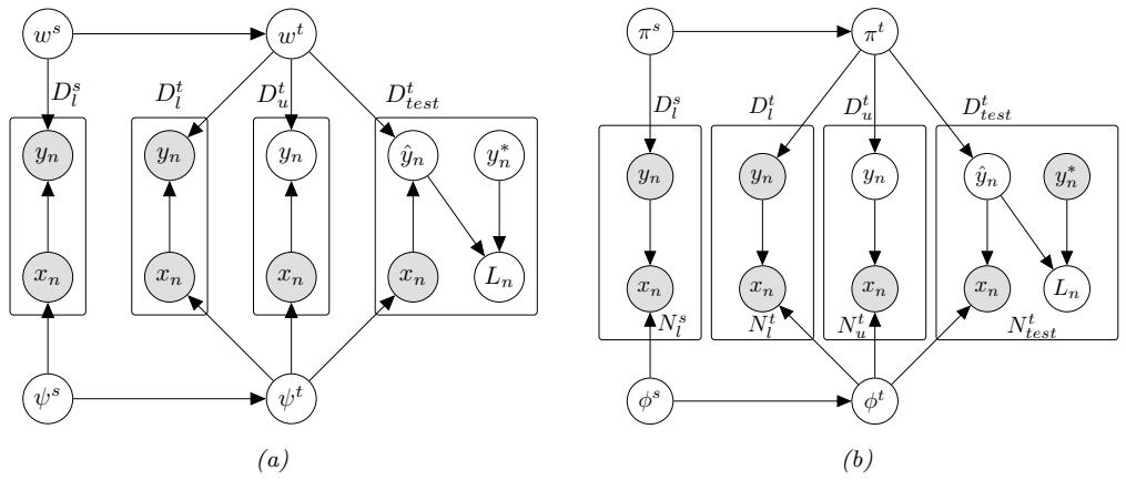
Figure 19.3: Models for distribution shift from source ^s to target ^t. Here ^{Ds L} is the labeled training set from the source, ^{Dt L} is an optional labeled training set from the target, ^{Dt U} is an optional unlabeled training set from the target, and ^Dt test is a labeled test set from the target. In the latter case, yˆⁿ is the prediction on the n’th test case (generated by the model), y↗ ⁿ is the true value, and εⁿ = ε(y↗ ⁿ, yˆn) is the corresponding loss. (Note that we don’t evaluate the loss on the source distribution.) (a) Discriminative (causal) model. (b) Generative (anticausal).

Relying on these shortcuts can have serious real-world consequences. For example, [Zec+18a] found that a CNN trained to recognize pneumonia was relying on hospital-specific metal tokens in the chest X-ray scans, rather than focusing on the lungs themselves, and thus the model did not generalize to new hospitals.

Analogous problems arise with other kinds of ML models, as well as other data types, such as text (e.g., changing “he” to “she” can flip the output of a sentiment analysis system), audio (e.g., adding background noise can easily confuse speech recognition systems), and medical records [Ros22]. Furthermore, the changes to the input needed to change the output can often be imperceptible, as we discuss in the section on adversarial robustness (Section 19.8).

19.2.2 A causal view of distribution shift

In the sections below, we briefly summarize some canonical kinds of distribution shift. We adopt a causal view of the problem, following [Sch+12a; Zha+13b; BP16; Mei18a; CWG20; Bud+21; SCS22]).1 (See Section 4.7 for a brief discussion of causal DAGs, and Chapter 36 for more details.)

We assume the inputs to the model (the covariates) are X and the outputs to be predicted (the labels) are Y . If we believe that X causes Y , denoted X ↖ Y , we call it causal prediction or discriminative prediction. If we believe that Y causes X, denoted Y ↖ X, we call it anticausal prediction or generative prediction. [Sch+12a].

The decision about which model to use depends on our assumptions about the underlying data

^1. In the causality literature, the question of whether a model can generalize to a new distribution is called the question of external validity. If a model is externally valid, we say that it is transportable from one distribution to another [BP16].

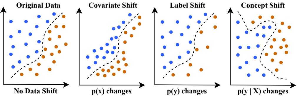
Figure 19.4: Illustration of some kinds of distribution shift for a 2d binary classification problem. Adapted from Figure 1 of [al21].

generating process. For example, suppose X is a medical image, and Y is an image segmentation created by a human expert or an algorithm. If we change the image, we will change the annotation, and hence X ↖ Y . Now suppose X is a medical image and Y is the ground truth disease state of the patient, as estimated by some other means (e.g., a lab test). In this case, we have Y ↖ X, since changing the disease state will change the appearance of the image. As another example, suppose X is a text review of a movie, and Y is a measure of how informative the review is. Clearly we have X ↖ Y . Now suppose Y is the star rating of the movie, representing the degree to which the user liked it; this will a!ect the words that they write, and hence Y ↖ X.

Based on the above discussion, we can factor the joint distribution in two possible ways. One way is to define a discriminative model:

\[p\_{\theta}(x, y) = p\_{\psi}(x) p\_{w}(y|x) \tag{19.1}\]

See Figure 19.3a. Alternatively we can define a generative model:

\[p\_{\theta}(x, y) = p\_{\pi}(y) p\_{\phi}(x|y) \tag{19.2}\]

See Figure 19.3b. For each of these 2 model types, di!erent parts of the distribution may change from source to target. This gives rise to 4 canonical type of shift, as we discuss in Section 19.2.3.

19.2.3 The four main types of distribution shift

The four main types of distribution shift are summarized in Section 19.2 and are illustrated in Figure 19.4. We give more details below (see also [LP20]).

19.2.3.1 Covariate shift

In a causal (discriminative) model, if ^pϑ(x) changes (so ^ϖs ′^{= ϖt} ), we call it covariate shift, also called domain shift. For example, the training distribution may be clean images of co!ee pots, and the test distribution may be images of co!ee pots with Gaussian noise, as shown in Figure 19.1; or the

Name	Source	Target	Joint
Covariate/domain	p(X)p(Y	q(X)p(Y	Discriminative
shift	X)	X)
Concept	p(X)p(Y	p(X)q(Y	Discriminative
shift	X)	X)
Label	p(Y	q(Y	Generative
(prior)	)p(X Y	)p(X Y
shift	)	)
Manifestation shift	p(Y )p(X Y )	p(Y )q(X Y )	Generative

Table 19.1: The 4 main types of distribution shift.

training distribution may be photos of objects in a catalog, with uncluttered white backgrounds, and the test distribution may be photos of the same kinds of objects collected “in the wild”; or the training data may be synthetically generated images, and the test distribution may be real images. Similar shifts can occur in the text domain; for example, the training distribution may be movie reviews written in English, and the test distribution may be translations of these reviews into Spanish.

Some standard strategies to combat covariate shift include importance weighting (Section 19.5.2) and domain adaptation (Section 19.5.3).

19.2.3.2 Concept shift

In a causal (discriminative) model, if ^pw(y|x) changes (so ^ws ′^{= wt} ), we call it concept shift, also called annotation shift. For example, consider the medical imaging context: the conventions for annotating images might be di!erent between the training distribution and test distribution. Another example of concept shift occurs when a new label can occur in the target distribution that was not part of the source distribution. This is related to open world recognition, discussed in Section 19.3.4.

Since concept shift is a change in what we “mean” by a label, it is impossible to fix this problem without seeing labeled examples from the target distribution, which defines each label by means of examples.

19.2.3.3 Label/prior shift

In a generative model, if ^p↼(y) changes (i.e., ^▷s ′^{= ▷t} ), we call it label shift, also called prior shift or prevalence shift. For example, consider the medical imaging context, where Y = 1 if the patient has some disease and Y = 0 otherwise. If the training distribution is an urban hospital and the test distribution is a rural hospital, then the prevalence of the disease, represented by p(Y = 1), might very well be di!erent.

Some standard strategies to combat label shift are to reweight the output of a discriminative classifier using an estimate of the new label distribution, as we discuss in Section 19.5.4.

19.2.3.4 Manifestation shift

In a generative model, if ^pω(x|y) changes (i.e., ^εs ′^{= εt} ), we call it manifestation shift [CWG20], or conditional shift [Zha+13b]. This is, in some sense, the inverse of concept shift. For example, consider the medical imaging context: the way that the same disease Y manifests itself in the shape of a tumor X might be di!erent. This is usually due to the presence of a hidden confounding factor that has changed between source and target (e.g., di!erent age of the patients).

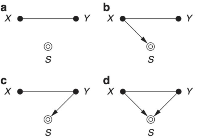
Figure 19.5: Causal diagrams for di!erent sample selection strategies. Undirected edges can be oriented in either direction. The selection variable S is set to 1 its parent nodes match the desired criterion; only these samples are included in the dataset. (a) No selection. (b) Selection on X. (c) Selection on Y . (d) Selection on X and Y . Adapted from Figure 4 of [CWG20].

19.2.4 Selection bias

In some cases, we may induce a shift in the distribution just due to the way the data is collected, without any changes to the underlying distributions. In particular, let S = 1 if a sample from the population is included in the training set, and S = 0 otherwise. Thus the source distribution is p(X, Y ) = p(X, Y |S = 1) but the target distribution is q(X, Y ) = p(X, Y |S ↗ {0, 1}) = p(X, Y ), so there is no selection.

In Figure 19.5 we visualize the four kinds of selection. For example, suppose we select based on X meeting certain criteria, e.g., images of a certain quality, or exhibiting a certain pattern; this can induce domain shift or covariate shift. Now suppose we select based on Y meeting certain criteria, e.g., we are more likely to select rare examples where Y = 1, in order to balance the dataset (for reasons of computational e”ciency); this can induce label shift. Finally, suppose we select based on both X and Y ; this can induce non-causal dependencies between X and Y , a phenomenon known as selection bias (see Section 4.2.4.2 for details).

19.3 Detecting distribution shifts

In general it will not be possible to make a model robust to all of the ways a distribution can shift at test time, nor will we always have access to test samples at training time. As an alternative, it may be su”cient for the model to detect that a shift has happened, and then to respond in the appropriate way. There are several ways of detecting distribution shift, some of which we summarize below. (See also Section 29.5.6, where we discuss changepoint detection in time series data.) The main distinction between methods is based on whether we have a set of samples from the target distribution, or just a single sample, and whether the test samples are labeled or unlabeled. We discuss these di!erent scenarios below.

19.3.1 Detecting shifts using two-sample testing

Suppose we collect a set of samples from the source and target distribution. We can then use standard techniques for two-sample testing to estimate if the null hypothesis, p(x, y) = q(x, y), is true or not. (If we have unlabeled samples, we just test if p(x) = q(x).) For example, we can use MMD (Section 2.7.3) to measure the distance between the set of input samples (see e.g., [Liu+20a]). Or we can measure (Euclidean) distances in the embedding space of a classifier trained on the source (see e.g., [KM22]).

In some cases it may be possible to just test if the distribution of the labels p(y) has changed, which is an easier problem than testing for changes in the distribution of inputs p(x). In particular, if the label shift assumption (Section 19.2.3.3) holds (i.e., q(x|y) = p(x|y)), plus some other assumptions, then we can use the blackbox shift estimation technique from Section 19.5.4 to estimate q(y). If we find that q(y) = p(y), then we can conclude that q(x, y) = p(x, y). In [RGL19], they showed experimentally that this method worked well for detecting distribution shifts even when the label shift assumption does not hold.

It is also possible to use conformal prediction (Section 14.3) to develop “distribution free” methods for detecting covariate shift, given only acccess to a calibration set and some conformity scoring function [HL20].

19.3.2 Detecting single out-of-distribution (OOD) inputs

Now suppose we just have one unlabeled sample from the target distribution, x ↔︎ q, and we want to know if x is in-distribution (ID) or out-of-distribution (OOD). We will call this problem out-of-distribution detection, although it is also called anomaly detection, and novelty detection. 2

The OOD detection problem requires making a binary decision about whether the test sample is ID or OOD. If it is ID, we may optionally require that we return its class label, as shown in Figure 19.6. In the sections below, we give a brief overview of techniques that have been proposed for tackling this problem, but for more details, see e.g., [Pan+21; Ruf+21; Bul+20; Yan+21; Sal+21; Hen+19b].

19.3.2.1 Supervised ID/OOD methods (outlier exposure)

The simplest method for OOD detection assumes we have access to labeled ID and OOD samples at training time. Then we just fit a binary classifier to distinguish the OOD or background class (called “known unknowns”) from the ID class (called “known knowns”) This technique is called outlier exposure (see e.g., [HMD19; Thu+21; Bit+21]) and can work well. However, in most cases we will not have enough examples from the OOD distribution, since the OOD set is basically the set of all possible inputs except for the ones of interest.

^2. The task of outlier detection is somewhat di”erent from anomaly or OOD detection, despite the similar name. In the outlier detection literature, the assumption is that there is a single unlabeled dataset, and the goal is to identify samples which are “untypical” compared to the majority. This is often used for data cleaning. (Note that this is a transductive learning task, where the model is trained and evaluated on the same data. We focus on inductive tasks, where we train a model on one dataset, and then test it on another.)

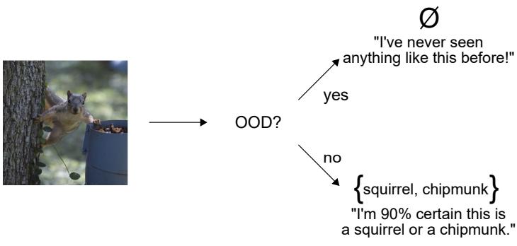
Figure 19.6: Illustration of a two-stage decision problem. First we must decide if the input image is out-ofdistribution (OOD) or not. If it is not, we must return the set of class labels that have high probabilitiy. From [AB21]. Used with kind permission of Anastasios Angelopoulos.

19.3.2.2 Classification confidence methods

Instead of trying to solve the binary ID/OOD classification problem, we can directly try to predict the class of the input. Let the probabilities over the C labels be p^c = p(y = c|x), and let the logits be ε^c = log pc. We can derive a confidence score or uncertainty metric in a variety of ways from these quantities, e.g., the max probability ^s = max^{c p}c, the margin ^s = max^{c εc →} max^{2 c} ε^c (where max² means the second largest element), the entropy s = H(p1:^C )3, the “energy score” s = & ^c ε^c [Liu+21b], etc. In [Mil+21; Vaz+22] they show that the simple max probability baseline performs very well in practice.

19.3.2.3 Conformal prediction

It is possible to create a method for OOD detection and ID classification that has provably bounded risk using conformal prediction (Section 14.3). The details are in [Ang+21], but we sketch the basic idea here.

We want to solve the two-stage decision problems illustrated in Figure 19.6. We define the prediction set as follows:

\[\mathcal{T}\_{\lambda}(x) = \begin{cases} \emptyset & \text{if } \text{OOD}(x) > \lambda\_1 \\ \text{APS} & \text{otherwise} \end{cases} \tag{19.3}\]

where OOD(x) is some heuristic OOD score (such as max class probability), and APS(x) is the adaptive prediction set method of Section 14.3.1, which returns the set of the top K class labels, such that the sum of their probabilities exceeds threshold ⇀2. (Formally, APS(x) = {ϖ1,…, ϖK} where ϖ sorts f(x)1:^C in descending order, and K = min{K^↔︎ : &^{K↑ c}=1 f(x)^c > ⇀2}.)

We choose the thresholds ⇀¹ and ⇀² using a calibration set and a frequentist hypothesis testing

^3. [Kir+21] argues against using entropy, since it confuses uncertainty about which of the C labels to use with uncertainty about whether any of the labels is suitable, compared to a “none-of-the-above” option.

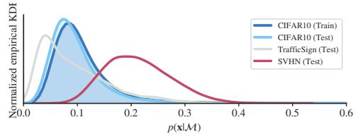
Figure 19.7: Likelihoods from a Glow normalizing flow model (Section 23.2.1) trained on CIFAR10 and evaluated on di!erent test sets. The SVHN street sign dataset has lower visual complexity, and hence higher likelihood. Qualitatively similar results are obtained for other generative models and datasets. From Figure 1 of [Ser+20]. Used with kind permission of Joan Serrà.

method (see [Ang+21]). The resulting thresholds will jointly minimize the following risks:

\[R\_1(\lambda) = p(\mathcal{T}\_\lambda(x) = \emptyset) \tag{19.4}\]

\[R\_2(\lambda) = p(y \notin \mathcal{T}\_\lambda(x) | \mathcal{T}\_\lambda(x) \neq \emptyset) \tag{19.5}\]

where p(x, y) is the true but unknown source distribution (of ID samples, no OOD samples required), R¹ is the chance that an ID sample will be incorrectly rejected as OOD (type-I error), and R² is the chance (conditional on the decision to classify) that the true label is not in the predicted set. The goal is to set ⇀¹ as large as possible (so we can detect OOD examples when they arise) while controlling the type-I error (e.g., we may want to ensure that we falsely flag (as OOD) no more than 10% of in-distribution samples). We then set ⇀² in the usual way for the APS method in Section 14.3.1.

19.3.2.4 Unsupervised methods

If we don’t have labeled examples, a natural approach to OOD detection is to fit an unconditional density model (such as a VAE) to the ID samples, and then to evaluate the likelihood p(x) and compare this to some threshold value. Unfortunately for many kinds of deep model and datasets, we sometimes find that p(x) is lower for samples that are from the source distribution than from a novel target distribution. For example, if we train a pixel-CNN model (Section 22.3.2) or a normalizing-flow model (Chapter 23) on Fashion-MNIST and evaluate it on MNIST, we find it gives higher likelihood to the MNIST samples [Nal+19a; Ren+19; KIW20; ZGR21]. This phenomenon occurs for several other models and datasets (see Figure 19.7), and can be explained by the fact that the natural data usually lies on a low-dimensional manifold, and simpler distributions (which need fewer dimensions) get assigned higher density by many models which are defined over the entire ambient space [Kam+24].

One solution to this is to use a log likelihood ratio relative to a baseline density model, R(x) = log p(x)/q(x), as opposed to the raw log likelihood, L(x) = log p(x). (This technique was explored in [Ren+19], amongst other papers.) An important advantage of this is that the ratio is invariant to transformations of the data. To see this, let x^↔︎ = ε(x) be some invertible, but possibly nonlinear, transformation. By the change of variables, we have p(x^↔︎ ) = ^p(x)^| det Jac(ε^↓1)(x)|. Thus L(x^↔︎ ) will di!er from L(x) in a way that depends on the transformation. By contrast, we have R(x) = R(x^↔︎ ), regardless of ε, since

\[R(\mathbf{z}') = \log p(\mathbf{z}') - \log q(\mathbf{z}') = \log p(\mathbf{z}) + \log|\det \text{Jac}(\boldsymbol{\phi}^{-1})(\mathbf{z})| - \log q(\mathbf{z}) - \log|\det \text{Jac}(\boldsymbol{\phi}^{-1})(\mathbf{z})|\]

(19.6)

Various other strategies have been proposed, such as computing the log-likelihood adjusted by a measure of the complexity (coding length computed by a lossless compression algorithm) of the input [Ser+20], computing the likelihood of model features instead of inputs [Mor+21a], etc.

A closely related technique relies on reconstruction error. The idea is to fit an autoencoder or VAE (Section 21.2) to the ID samples, and then measure the reconstruction error of the input: a sample that is OOD is likely to incur larger error (see e.g., [Pol+19]). However, this su!ers from the same problems as density estimation methods.

An alternative to trying to estimate the likelihood, or reconstruct the output, is to use a GAN (Chapter 26) that is trained to discriminate “real” from “fake” data. This has been extended to the open set recognition setting in the OpenGAN method of [KR21b].

19.3.3 Selective prediction

Suppose the system has a confidence level of p that an input is OOD (see Section 19.3.4 for a discussion of some ways to compute such confidence scores). If p is below some threshold, the system may choose to abstain from classifying it with a specific label. By varying the threshold, we can control the tradeo! between accuracy and abstention rate. This is called selective prediction (see e.g., [EW10; GEY19; Ziy+19; JKG18]), and is useful for applications where an error can be more costly than asking a human expert for help (e.g., medical image classification).

19.3.3.1 Example: SGLD vs SGD for MLPs

One way to improve performance of OOD detection is to “be Bayesian” about the parameters of the model, so that the uncertainty in their values is reflected in the posterior predictive distribution. This can result in better performance in selective prediction tasks.

In this section, we give a simple example of this, where we fit a shallow MLP to the MNIST dataset using either standard SGD (specifically RMSprop) or stochastic gradient Langevin dynamics (see Section 12.7.1), which is a form of MCMC inference. We use 6,000 training steps, where each step uses a minibatch of size 1,000. After fitting the model to the training set, we evaluate its predictions on the test set. To assess how well calibrated the model is, we select a subset of predictions whose confidence is above a threshold t. (The confidence value is just the probability assigned to the MAP class.) As we increase the threshold t from 0 to 1, we make predictions on fewer examples, but the accuracy should increase. This is shown in Figure 19.8: the green curve is the fraction of the test set for which we make a prediction, and the blue curve is the accuracy. On the left we show SGD, and on the right we show SGLD. In this case, performance is quite similar, although SGD has slightly higher accuracy. However, the story changes somewhat when there is distribution shift.

To study the e!ects under distribution shift, we apply both models to FashionMNIST data. We show the results in Figure 19.9. The accuracy of both models is very low (less than the chance level of 10%), but SGD remains quite confident in many more of its predictions than SGLD, which is more conservative. To see this, consider a confidence threshold of 0.5: the SGD approach predicts on about 97% of the examples (recall that the green curve corresponds to the right hand axis), whereas the SGLD only predicts on about 70% of the examples.

More details on the behavior of Bayesian neural networks under distribution shift can be found in Section 17.4.6.2.

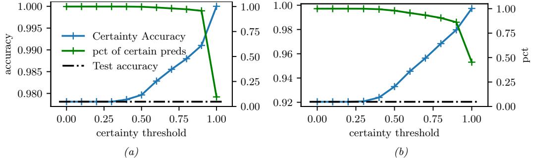
Figure 19.8: Accuracy vs confidence plots for an MLP fit to the MNIST training set, and then evaluated on one batch from the MNIST test set. Scale for blue accuracy curve is on the left, scale for green percentage predicted curve is on the right. (a) Plugin approach, computed using SGD. (b) Bayesian approach, computed using 10 samples from SGLD. Generated by bnn\_mnist\_sgld.ipynb.

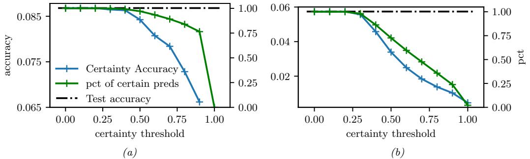
Figure 19.9: Similar to Figure 19.8, except that performance is evaluated on the Fashion MNIST dataset. (a) SGD. (b) SGLD. Generated by bnn\_mnist\_sgld.ipynb.

19.3.4 Open set and open world recognition

In Section 19.3.3, we discussed methods that “refuse to classify” if the system is not confident enough about its predicted output. If the system detects that this lack of confidence is due to the input coming from a novel class, rather than just being a novel instance of an existing class, we call the problem open set recognition (see e.g., [GHC20] for a review).

Rather than “flagging” novel classes as OOD, we can instead allow the set of classes to grow over time; this is called open world classification [BB15a]. Note that open world classification is most naturally tackled in the context of a continual learning system, which we discuss in Section 19.7.3.

For a survey article that connects open set learning with OOD detection, see [Sal+22].

19.4 Robustness to distribution shifts

In this section, we discuss techniques to improve the robustness of a model to distribution shifts. In particular, given labeled data from p(x, y), we aim to create a model that approximates q(y|x).

19.4.1 Data augmentation

A simple approach to potentially increasing the robustness of a predictive model to distribution shifts is to simulate samples from the target distribution by modifying the source data. This is called data augmentation, and is widely used in the deep learning community. For example, it is standard to apply small perturbations to images (e.g., shifting them or rotating them), while keeping the label the same (assuming that the label should be invariant to such changes); see e.g., [SK19; Hen+20] for details. Similarly, in NLP (natural language processing), it is standard to change words that should not a!ect the label (e.g., replacing “he” with “she” in a sentiment analysis system), or to use back translation (from a source language to a target language and back) to generate paraphrases; see e.g., [Fen+21] for a review of such techniques. For a causal perspective on data augmentation, see e.g., [Kau+21].

19.4.2 Distributionally robust optimization

We can make a discriminative model that is robust to (some forms of) covariate shift by solving the following distributionally robust optimization (DRO) problem:

\[\min\_{f \in \mathcal{F}} \max\_{\mathbf{w} \in \mathcal{W}} \frac{1}{N} \sum\_{n=1}^{N} w\_n \ell(f(x\_n), y\_n) \tag{19.7}\]

where the samples are from the source distribution, (xn, yn) ↔︎ p. This is an example of a min-max optimization problem, in which we want to minimize the worst case risk. The specification of the robustness set, W, is a key factor that determines how well the method works, and how di”cult the optimization problem is. Typically it is specified in terms of an ε² ball around the inputs, but this could also be defined in a feature (embedding space) It is also possible to define the robustness set in terms of local changes to a structural causal model [Mei18a]. For more details on DRO, see e.g., [CP20a; LFG21; Sag+20; RM22].

19.5 Adapting to distribution shifts

In this section, we discuss techniques to adapt the model to the target distribution. If we have some labeled data from the target distribution, we can use transfer learning, as we discuss in Section 19.5.1. However, getting labeled data from the target distribution is often not an option. Therefore, in the other sections, we discuss techniques that just rely on unlabeled data from the target distribution.

19.5.1 Supervised adaptation using transfer learning

Suppose we have labeled training data from a source distribution, ^{Ds =} {(xn, ^yn) ^{↔︎ p} : ⁿ =1: ^Ns}, and also some labeled data from the target distribution, ^{Dt =} {(xn, ^yn) ^{↔︎ q} : ⁿ =1: ^Nt}. Our goal is to minimize the risk on the target distibution q, which can be computed using

\[R(f, q) = \mathbb{E}\_{q(\mathbf{z}, \mathbf{y})} \left[ \ell(\mathbf{y}, f(\mathbf{z})) \right] \tag{19.8}\]

We can approximate the risk empirically using

\[\hat{R}(f, \mathcal{D}^t) = \frac{1}{|\mathcal{D}^t|} \sum\_{(\mathfrak{x}\_n, \mathfrak{y}\_n) \in \mathcal{D}^t} \ell(\mathfrak{y}\_n, f(\mathfrak{x}\_n)) \tag{19.9}\]

If ^Dt is large enough, we can directly optimize this using standard empirical risk minimization (ERM). However, if ^Dt is small, we might want to use ^Ds somehow as a regularizer. This is called transfer learning, since we hope to “transfer knowledge” from p to q. There are many approaches to transfer learning (see e.g., [Zhu+21] for a review). We briefly mention a few below.

19.5.1.1 Pre-train and fine-tune

The simplest and most widely used approach to transfer learning is the pre-train and fine-tune approach. We first fit a model to the source distribution by computing ^{f s =} argmin^{f R}ˆ(f, ^Ds). (Note that the source data may be unlabeled, in which case we can use self-supervised learning methods.) We then adapt the model to work on the target distribution by computing

\[f^t = \operatorname\*{argmin}\_f \hat{R}(f, \mathcal{D}^t) + \lambda ||f - f^s|| \tag{19.10}\]

where ||^{f →f s}|| is some distance between the functions, and ⇀ ^{≃ 0} controls the degree of regularization.

Since we assume that we have very few samples from the target distribution, we typically “freeze” most of the parameters of the source model. (This makes an implicit assumption that the features that are useful for the source distribution also work well for the target.) We can then solve Equation (19.10) by “chopping o! the head” from f ^s and replacing it with a new linear layer, to map to the new set of labels for the target distribution, and then compute a new MAP estimate for the parameters on the target distribution. (We can also compute a prior for the parameters of the source model, and use it to compute a posterior for the parameters of the target model, as discussed in Section 17.2.3.)

This approach is very widely used in practice, since it is simple and e!ective. In particular, it is common to take a large pre-trained model, such as a transformer, that has been trained (often using self supervised learning, Section 32.3.3) on a lot of data, such as the entire web, and then to use this model as a feature extractor (see e.g., [Kol+20]). The features are fed to the downstream model, which may be a linear classifier or a shallow MLP, which is trained on the target distribution.

19.5.1.2 Prompt tuning (in-context learning)

Recently another approach to transfer learning has been developed, that leverages large models, such as transformers (Section 22.4), which are trained on massive web datasets, usually in an unsupervised way, and then adapted to a small, task-specific target distribution. The interesting thing about this approach is the parameters of the original model are not changed; instead, the model is simply “conditioned” on new training data, usually in the form of a text prompt z. That is, we compute

\[f^t(\mathbf{z}) = f^s(\mathbf{z} \cup \mathbf{z}) \tag{19.11}\]

where we (manually or automatically) optimize z while keeping f ^s frozen. This approach is called prompt tuning or in-context learning (see e.g., [Liu+21a]), and is an instance of few-shot learning (see Figure 22.4 for an example).

Here z acts like a small training dataset, and f ^s uses attention (Section 16.2.7) to “look at” all its inputs, comparing x with the examples in z, and uses this to make a prediction. This works because the text training data often has a similar hierarchical structure (see [Xie+22] for a Bayesian interpretation).

19.5.2 Weighted ERM for covariate shift

In this section we reconsider the risk minimization objective in Equation (19.8), but leverage unlabeled data from the target distribution to estimate it. If we make the covariate shift assumption (i.e., q(x, y) = q(x)p(y|x)), then we have

\[R(f,q) = \int q(\mathbf{x})q(\mathbf{y}|\mathbf{x})\ell(\mathbf{y},f(\mathbf{z}))d\mathbf{x}d\mathbf{y} \tag{19.12}\]

\[=\int q(x)p(y|x)\ell(y,f(x))dxdy\tag{19.13}\]

\[\hat{\rho} = \int \frac{q(x)}{p(x)} p(x) p(y|x) \ell(y, f(x)) dx dy \tag{19.14}\]

\[\approx \frac{1}{N} \sum\_{(\mathfrak{x}\_n, \mathfrak{y}\_n) \in \mathcal{D}\_L^s} w\_n \ell(\mathfrak{y}\_n, f(\mathfrak{x}\_n)) \tag{19.15}\]

where the weights are given by the ratio

\[w\_n = w(\mathbf{z}\_n) = \frac{q(\mathbf{z}\_n)}{p(\mathbf{z}\_n)}\tag{19.16}\]

Thus we can solve the covariate shift problem by using weighted ERM [Shi00a; SKM07].

However, this raises two questions. First, why do we need to use this technique, since a discriminative model p(y|x) should work for any input x, regardless of which distribution it comes from? Second, given that we do need to use this method, in practice how should we estimate the weights wⁿ = w(xn) = ^q(xn) ^p(xn) ? We discuss these issues below.

19.5.2.1 Why is covariate shift a problem for discriminative models?

For a discriminative model of the form p(y|x), it might seem that such a change in p(x) will not a!ect the predictions. If the predictor p(y|x) is the correct model for all parts of the input space x, then this conclusion is warranted. However, most models will only be accurate in certain parts of the input space. This is illustrated in Figure 19.10b, where we show that a linear model fit to the source distribution may perform much worse on the target distribution than a model that weights target points more heavily during training.

19.5.2.2 How should we estimating the ERM weights?

One approach to estimating the ERM weights wⁿ = w(xn) = ^q(xn) ^p(xn) is to learn a density model for the source and target. However, density esimation is di”cult for high dimensional features. An alternative approach is to try to approximate the density ratio, by fitting a binary classifier to distinguish the two distributions, as discussed in Section 2.7.5. In particular, suppose we have an equal number of samples from p(x) and q(x). Let us label the first set with c = →1 and the second set with c = 1. Then we have

\[p(c=1|x) = \frac{q(x)}{q(x) + p(x)}\tag{19.17}\]

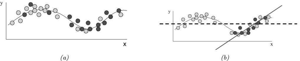
Figure 19.10: (a) Illustration of covariate shift. Light gray represents training distribution, dark gray represents test distribution. We see the test distribution has shifted to the right but the underlying input-output function is constant. (b) Dashed line: fitting a linear model across the full support of X. Solid black line: fitting the same model only on parts of input space that have high likelihood under the test distribution. From Figures 1–2 of [Sto09]. Used with kind permission of Amos Storkey.

and hence ^p(c=1|x) ^p(c=↓1|x) ^{= q}(x) ^p(x) . If the classifier has the form ^f(x) = ^p(^c = 1|x) = ^ς(h(x)) = ¹ 1+exp(↓h(x)) , where h(x) is the prediction function that returns the logits, then the importance weights are given by

\[w\_n = \frac{1/(1 + \exp(-h(x\_n)))}{\exp(-h(x\_n))/(1 + \exp(-h(x\_n)))} = \exp(h(x\_n))\tag{19.18}\]

Of course this method requires that x values that may occur in the test distribution should also be possible in the training distribution, i.e., q(x) > 0 =∀ p(x) > 0. Hence there are no guarantees about this method being able to interpolate beyond the training distribution.

19.5.3 Unsupervised domain adaptation for covariate shift

We now turn to methods that only need access to unlabeled examples from the target distribution.

The technique of unsupervised domain adaptation or UDA assumes access to a labeled dataset from the source distribution, ^D1 = ^{Ds L} ↔︎ p(x, y) and an unlabeled dataset from the target distribution, ^D2 = ^{Dt U} ↔︎ q(x). It then uses the unlabeled target data to improve robustness or invariance of the predictor, rather than using a weighted ERM method.

There are many forms of UDA (see e.g., [KL21; CB20] for reviews). Here we just focus on one method, called domain adversarial learning [Gan+16a]. Let f↽ : X¹ ⊤ X² ↖ H be a feature extractor defined on the two input domains, let c^β : H ↖ {1, 2} be a classifier that maps from the feature space to the domain from which the input was taken, either domain 1 or 2 (source or target), and let g^▷ : H ↖ Y be a classifier that maps from the feature space to the label space. We want to train the feature extractor so that it cannot distinguish whether the input is coming from the source or target distribution; in this case, it will only be able to use features that are common to both domains. Hence we optimize

\[\min\_{\gamma} \max\_{\alpha, \beta} \frac{1}{N\_1 + N\_2} \sum\_{\mathbf{z}\_n \in \mathcal{D}\_1, \mathcal{D}\_2} \ell(d\_n, c\_{\beta}(f\_{\mathbf{z}}(\mathbf{z}\_n))) + \frac{1}{N\_1} \sum\_{(\mathbf{z}\_n, y\_n) \in \mathcal{D}\_1} \ell(y\_n, g\_{\gamma}(f\_{\mathbf{z}}(\mathbf{z}\_n))) \tag{19.19}\]

The objective in Equation (19.19) minimizes the loss on the desired task of classifying y, but maximizes

the loss on the auxiliary task of classifying the domain label d. This can be implemented by the gradient sign reversal trick, and is related to GANs (Section 26.7.6).

19.5.4 Unsupervised techniques for label shift

In this section, we describe an approach known as blackbox shift estimation, due to [LWS18], which can be used to tackle the label shift problem in an unsupervised way. We assume that the only thing that changes in the target distribution is the label prior, i.e., if the source distribution is denoted by p(x, y) and target distribution is denoted by q(x, y), we assume q(x, y) = p(x|y)q(y).

First note that, for any deterministic function f : X ↖ Y, we have

\[p(\mathbf{z}|y) = q(\mathbf{z}|y) \implies p(f(\mathbf{z})|y) = q(f(\mathbf{z})|y) \implies p(\hat{y}|y) = q(\hat{y}|y) \tag{19.20}\]

where yˆ = f(x) is the predicted label. Let µⁱ = q(yˆ = i) be the empirical fraction of times the model predicts class i on the test set, and let q(y = i) be the true but unknown label distribution on the test set, and let Cij = p(yˆ = i|y = j) be the class confusion matrix estimated on the training set. Then we have

\[\mu\_{\hat{y}} = \sum\_{y} q(\hat{y}|y)q(y) = \sum\_{y} p(\hat{y}|y)q(y) = \sum\_{y} p(\hat{y}, y) \frac{q(y)}{p(y)}\tag{19.21}\]

We can write this in matrix-vector form as follows:

\[ \mu\_i = \sum\_i C\_{ij} q\_j, \implies \mu = \mathbf{C} \mathbf{q} \tag{19.22} \]

Hence we can solve q = C↓¹µ, providing that C is not singular (this will be the case if C is strongly diagonal, i.e., the model predicts class yⁱ correctly more often than any other class y^j ). We also require that for every q(y) > 0 we have p(y) > 0, which means we see every label at training time.

Once we know the new label distribution, q(y), we can adjust our discriminative classifier to take the new label prior into account as follows:

\[q(y|\mathbf{z}) = \frac{q(\mathbf{z}|y)q(y)}{q(\mathbf{z})} = \frac{p(\mathbf{z}|y)q(y)}{q(\mathbf{z})} = \frac{p(y|\mathbf{z})p(\mathbf{z})}{p(y)}\frac{q(y)}{q(\mathbf{z})} = p(y|\mathbf{z})\frac{q(y)}{p(y)}\frac{p(\mathbf{z})}{q(\mathbf{z})}\tag{19.23}\]

We can safely ignore the ^p(x) ^q(x) term, which is constant wrt y, and we can plug in our estimates of the label distributions to compute the ^q(y) ^p(y) .

In summary, there are three requirements for this method: (1) the confusion matrix is invertible; (2) no new labels at test time; (3) the only thing that changes is the label prior. If these three conditions hold, the above approach is a valid estimator. See [LWS18] for more details, and [Gar+20] for an alternative approach, based on maximum likelihood (rather than moment matching) for estimating the new marginal label distribution.

19.5.5 Test-time adaptation

In some settings, it is possible to continuously update the model parameters. This allows the model to adapt to changes in the input distribution. This is called test time adaptation or TTA. The

di!erence from the unsupervised domain adaptation methods of Section 19.5.3 is that, in the online setting, we just have the model which was trained on the source, and not the source distribution.

In [Sun+20] they proposed an approach called TTT (“test-time training”) for adapting a discriminative model. In this approach, a self-supervised proxy task is used to create proxy-labels, which can then be used to adapt the model at run time. In more detail, suppose we create a Y-structured network, where we first perform feature extraction, x ↖ h, and then use h to predict the output y and some proxy output r, such as the angle of rotation of the input image. The rotation angle is known if we use data augmentation. Hence we can apply this technique at test time, even if y is unknown, and update the x ↖ h ↖ r part of the network, which influences the prediction for y via the shared bottleneck (feature layer) h.

Of course, if the proxy output, such as the rotation angle, is not known, we cannot use proxysupervised learning methods such as TTT. In [Wan+20a], they propose an approach, inspired by semi-supervised learning methods, which they call TENT, which stands for “test-time adaptation by entropy minimization”. The idea is to update the classifier parameters to minimize the entropy of the predictive distribution on a batch of test examples. In [Goy+22], they give a justification for this heuristic from the meta-learning perspective. In [ZL21], they present a Bayesian version of TENT, which they call BACS, which stands for “Bayesian adaptation under covariate shift”. In [ZLF21], they propose a method called MEMO (“marginal entropy minimization with one test point”) that can be used for any architecture. The idea is, once again, to apply data augmentation at test time to the input x, to create a set of inputs, x˜1,…, x˜B. Now we update the parameters so as to minimize the predictive entropy produced by the averaged distribution

\[\overline{p}(\mathbf{y}|x,w) = \frac{1}{B} \sum\_{b=1}^{B} p(\mathbf{y}|\bar{x}\_b, w) \tag{19.24}\]

This ensures that the model gives the same predictions for each perturbation of the input, and that the predictions are confident (low entropy).

An alternative to entropy based methods is to use pseudolabels (predicted outputs on the unlaneled target generated by the source model), and then to self-train on these (see e.g., [KML20; LHF20; Che+22]), often with additional regularizers to prevent over-fitting.

19.6 Learning from multiple distributions

In Section 19.2, we discussed the setting in which a model is trained on a single source distribution, and then evaluated on a distinct target distribution. In this section, we generalize this to a setting in which the model is trained on data from J ≃ 2 source distributions, before being tested on data from a target distribution. This includes a variety of di!erent problem settings, depending on the value of J, as we summarize in Figure 19.11.

19.6.1 Multitask learning

In multi-task learning (MTL) [Car97], we have labeled data from J di!erent distributions, ^Dj = {(x^{j n}, y^{j n}) : n =1: Nj}, and the goal is to learn a model that predicts well on all J of them simultaneously, where f(x, j) : X ↖ Y^j is the output for the j’th task. For example, we might want to map a color image of size ^{H ⇔ W ⇔ 3} to a set of semantic labels per pixel, ^{Y1 =} {1,…,C}HW , as

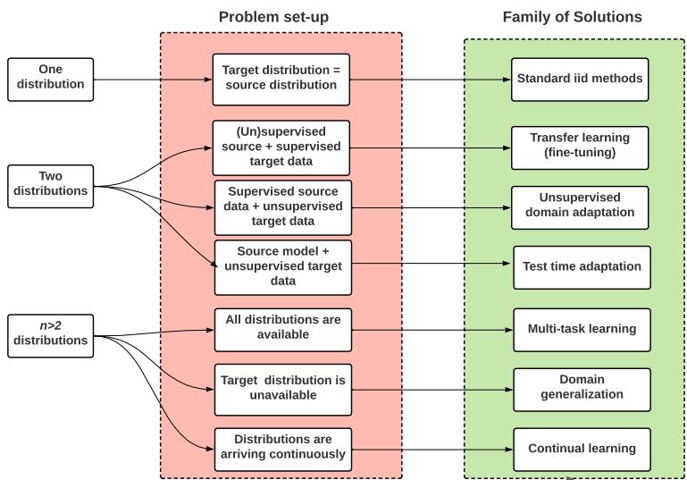
Figure 19.11: Schematic overview of techniques for learning from 1 or more di!erent distributions. Adapted from slide 3 of [Sca21].

well as a set of predicted depth values per pixel, ^{Y2 = R}HW . We can do this using ERM where we have multiple samples for each task:

\[f^\* = \operatorname\*{argmin}\_f \sum\_{j=1}^J \sum\_{n=1}^{N\_j} \ell\_j(y\_n^j, f(\mathbf{z}\_n^j, j)) \tag{19.25}\]

where ε^j is the loss function for task j (suitably scaled).

There are many approaches to solving MTL. The simplest is to fit a single model with multiple “output heads”, as illustrated in Figure 19.12. This is called a “shared trunk network”. Unfortunately this often leads to worse performance than training J single task networks. In [Mis+16], they propose to take a weighted combination of the activations of each single task network, an approach they called “cross-stitch networks”. See [ZY21] for a more detailed review of neural approaches, and [BLS11] for a theoretical analysis of this problem.

Note that multi-task learning does not always help performance on each task because sometimes there can be “task interference” or “negative transfer” (see e.g., [MAP17; Sta+20; WZR20]). In such cases, we should use separate networks, rather than using one model with multiple output heads.

19.6.2 Domain generalization

The problem of domain generalization assumes we train on J di!erent labeled source distributions or “environments” (also called “domains”), and then test on a new target distribution (denoted by

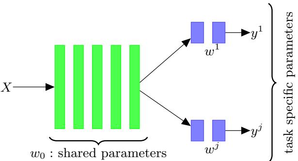
Figure 19.12: Illustration of multi-headed network for multi-task learning.

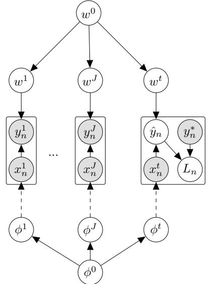
Figure 19.13: Hierarchical Bayesian discriminative model for learning from J di!erent environments (distributions), and then testing on a new target distribution t = J + 1. Here yˆⁿ is the prediction for test example xn, y↗ ⁿ is the true output, and εⁿ = ε(y^{t n}, y↗ ⁿ) is the associated loss. The parameters of the distribution over input features pε(x) are shown with dotted edges, since these distributions do not need to be learned in a discriminative model.

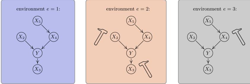
Figure 19.14: Illustration of invariant causal prediction. The hammer symbol represents variables whose distribution is perturbed in the given environment. An invariant predictor must use features {X2, X4}. Considering indirect causes instead of direct ones (e.g. {X2, X5}) or an incomplete set of direct causes (e.g., {X4}) may not be su#cient to guarantee invariant prediction. From Figure 1 of [PBM16b]. Used with kind permission of Jonas Peters.

t = J + 1). In some cases each environment is just identified with a meaningless integer id. In more realistic settings, each di!erent distribution has associated meta-data or context variables that characterizes the environment in which the data was collected, such as the time, location, imaging device, etc.

Domain generalization (DG) is similar to multi-task learning, but di!ers in what we want to predict. In particular, in DG, we only care about prediction accuracy on the target distribution, not the J training distribution. Furthermore, we assume we don’t have any labeled data from the target distribution. We therefore have to make some assumptions about how p^t (x, y) relates to p^j (x, y) for j =1: J.

One way to formalize this is to create a hierarchical Bayesian model, as proposed in [Bax00], and illustrated in Figure 19.13. This encodes the assumption that p^t (x, ^y) = ^p(x|ε^t )p(y|x, ^wt ) where w^t is derived from a common “population level” model w⁰, shared across all distributions, and similarly for ε^t . (Note, however, that in a discriminative model, we don’t need to model ^p(x|ε^t ).) See Section 15.5 for discussion of hierarchical Bayesian GLMs, and Section 17.6 for discussion of hierarchical Bayesian MLPs.

Many other techniques have been proposed for DG. Note, however, that [GLP21] found that none of these methods worked consistently better than the baseline approach of performing empirical risk minimization across all the provided datasets. For more information, see e.g., [GLP21; She+21; Wan+21; Chr+21].

19.6.3 Invariant risk minimization

One approach to domain generalization that has received a lot of attention is called invariant risk minimization or IRM [Arj+19]. The goal is to learn a predictor that works well across all environments, yet is less prone to depending on the kinds of “spurious features” we discussed in Section 19.2.1.

IRM is an extension of an earlier method called invariant causal prediction (ICP) [PBM16b]. This uses hypothesis testing methods to find the set of predictors (features) that directly cause the

outcome in each environment, rather than features that are indirect causes, or are just correlated with the outcome. See Figure 19.14 for an illustration.

In [Arj+19], they proposed an extension of ICP to handle the case of high dimensional inputs, where the individual variables do not have any causal meaning (e.g., they correspond to pixels). Their approach requires finding a predictor that works well on average, across all environments, while also being optimal for each individual environment. That is, we want to find

\[f^\* = \operatorname\*{argmin}\_{f \in \mathcal{F}} \sum\_{j=1}^J \frac{1}{N\_j} \sum\_{n=1}^{N\_j} \ell(\mathbf{y}\_n^j, f(\mathbf{z}\_n^j)) \tag{19.26}\]

\[\text{Is such that } f \in \arg\min\_{g \in \mathcal{F}} \frac{1}{N\_j} \sum\_{n=1}^{N\_j} \ell(y\_n^j, g(x\_n^j)) \text{ for all } j \in \mathcal{E} \tag{19.27}\]

where E is the set of environments, and F is the set of prediction functions. The intuition behind this is as follows: there may be many functions that achieve low empirical loss on any given environment, since the problem may be underspecified, but if we pick the one that also works well on all environments, it is more likely to rely on causal features rather than spurious features.

Unfortunately, more recent work has shown that the IRM principle often does not work well for covariate shift, both in theory [RRR21] and practice [GLP21], although it can work well in some anti-causal (generative) models [Ahu+21].

19.6.4 Meta learning

The goal of meta-learning is to “learn the learning algorithm” [TP97]. A common way to do this is to provide the meta-learner with a set of datasets from di!erent distributions. This is very similar to domain generalization (Section 19.6.2), except that we partition each training distribution into training and test, so we can “practice” learning to generalize from a training set to a test set. A general review of meta-learning can be found in [Hos+20a]. Here we present a unifying summary based on the hierarchical Bayesian framework proposed in [Gor+19].

19.6.4.1 Meta-learning as probabilistic inference for prediction

We assume there are ^J tasks (distributions), each of which has a training set ^Dj train = {(x^{j n}, y^{j n}) : ⁿ =1: ^Nj} and a test set ^Dj test = {(x˜^{j m}, y˜^{j m}) : ^m =1: ^Mj}. In addition, ^wj are the task specific parameters, and w⁰ are the shared parameters, as shown in Figure 19.15. This is very similar to the domain generalization model in Figure 19.13, except for two di!erences: first there is the trivial di!erence due to the use of plate notation; second, in meta learning, we have both training and test partitions for all distributions, whereas in DG, we only have a test set for the target distribution.

We will learn a point estimate for the global parameters w⁰, since it is shared across all datasets, and thus has little uncertainty. However, we will compute an approximate posterior for w^j , since each task often has little data. We denote this posterior by ^p(w^j |D^j train, w⁰). From this, we can compute the posterior predictive distribution for each task:

\[p(\ddot{y}^j|\ddot{x}^j, \mathcal{D}\_{\text{train}}^j, \mathbf{w}^0) = \int p(\ddot{y}^j|\ddot{x}^j, \mathbf{w}^j) p(\mathbf{w}^j|\mathcal{D}\_{\text{train}}^j, \mathbf{w}^0) dw^j \tag{19.28}\]

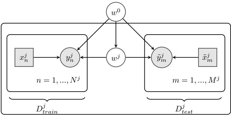
Figure 19.15: Hierarchical Bayesian model for meta-learning. There are J tasks, each of which has a training set ^{Dj =} {(x^{j n}, y^{j n}) : ⁿ =1: ^Nj} and a test set ^Dj test ⁼ {(x˜^{j m}, y˜^{j m}) : ^m =1: ^Mj}. ^wj are the task specific parameters, and ω are the shared parameters. Adapted from Figure 1 of [Gor+19].

Since computing the posterior is in general intractable, we will learn an amortized approximation (see Section 10.1.5) to the predictive distribution, denoted by ^qω(y˜^{j |}x˜^j , ^Dj train, w⁰). We choose the parameters of the prior w⁰ and the inference network ε to make this predictive posterior as accurate as possible for any given input dataset:

\[\boldsymbol{\phi}^{\*} = \operatorname\*{argmin}\_{\boldsymbol{\phi}} \mathbb{E}\_{\mathcal{P}(\mathcal{D}\_{\text{train}}, \hat{\mathbf{z}})} \left[ D\_{\text{KL}} \left( p(\check{\mathbf{y}} | \hat{\mathbf{z}}, \mathcal{D}\_{\text{train}}, \mathbf{w}^{0}) \parallel q\_{\phi}(\check{\mathbf{y}} | \hat{\mathbf{z}}, \mathcal{D}\_{\text{train}}, \mathbf{w}^{0}) \right) \right] \tag{19.29}\]

\[\mathbf{x}^{0} = \operatorname\*{argmin}\_{\phi} \mathbb{E}\_{\mathcal{P}(\mathcal{D}\_{\text{train}}, \tilde{\mathbf{z}})} \left[ \mathbb{E}\_{\mathcal{P}(\tilde{\mathbf{y}}|\tilde{\mathbf{z}}, \mathcal{D}\_{\text{train}}, \mathbf{w}^{0})} \left[ \log q\_{\phi}(\tilde{\mathbf{y}}|\tilde{\mathbf{z}}, \mathcal{D}\_{\text{train}}, \mathbf{w}^{0}) \right] \right] \tag{19.30}\]

\[\hat{\mathbf{x}} = \operatorname\*{argmin}\_{\phi} \mathbb{E}\_{p(\mathcal{D}\_{\text{train}}, \tilde{\mathbf{z}}, \tilde{\mathbf{y}})} \left[ \log \int p(\tilde{\mathbf{y}} | \tilde{\mathbf{z}}, \mathbf{w}) q\_{\phi}(\mathbf{w} | \mathcal{D}\_{\text{train}}, \mathbf{w}^{0}) d\mathbf{w} \right] \tag{19.31}\]

where we made the approximation ^p(y˜|x˜, ^Dtrain, ^w0) ^{↓ p}(y˜|x˜, ^Dtrain). We can then make a Monte Carlo approximation to the outer expectation by sampling J tasks (distributions) from p(D), each of which gets partitioned into a train and test set, {(D^j train, ^Dj test) ↔︎ p(D) : j =1: J}, where Dj test = {(x˜m, y˜m}. We can make an MC approximation to the inner expectation (the integral) by drawing S samples from the task-specific parameter posterior w^{j s ↔︎ q}ω(w^j |D^j , ^w0). The resulting objective has the following form (where we assume each test set has M samples for notational simplicity):

\[\mathcal{L}\_{\text{meta}}(\boldsymbol{w}^{0}, \boldsymbol{\phi}) = \frac{1}{MJ} \sum\_{m=1}^{M} \sum\_{j=1}^{J} \log \left( \frac{1}{S} \sum\_{s=1}^{S} p(\bar{y}\_{m}^{j} | \bar{x}\_{m}^{j}, \boldsymbol{w}\_{s}^{j}) \right) \tag{19.32}\]

Note that this is di!erent from standard (amortized) variational inference, that focuses on approximating the expected accuracy of the parameter posterior given all of the data for a task, Dj all ^{= Dj} train ^{⊤ Dj} test, rather than focusing on predictive accuracy of a test set given a training set.

Indeed, the standard objective has the form

\[\mathcal{L}\_{\text{VI}}(\boldsymbol{w}^{0}, \boldsymbol{\phi}) = \frac{1}{J} \sum\_{j=1}^{J} \left( \sum\_{(\boldsymbol{x}, \boldsymbol{y}) \in \mathcal{D}\_{\text{all}}^{j}} \left[ \frac{1}{S} \sum\_{s=1}^{S} \log p(\bar{\mathbf{y}}^{j} | \bar{\mathbf{z}}^{j}, \boldsymbol{w}\_{s}^{j}) \right] - D\_{\text{KL}} \left( q\_{\phi}(\boldsymbol{w}^{j} | \mathcal{D}\_{\text{all}}^{j}, \boldsymbol{w}^{0}) \parallel p(\boldsymbol{w}^{j} | \boldsymbol{w}^{0}) \right) \right) \tag{19.33}\]

where w^{j s ↔︎ q}ω(w^j |D^j all). We see that the standard formulation takes the average of a log, but the meta-learning formulation takes the log of an average. The latter can give provably better predictive accuracy, as pointed out in [MAD20]. Another di!erence is that the meta-learning formulation optimizes the forward KL, not reverse KL. Finally, in the meta-learning formulation, we do not have the KL penalty term on the parameter posterior.

Below we show how this framework includes several common approaches to meta-learning.

19.6.4.2 Neural processes

In the special case that the task-specific inference network computes a point estimate, ^q(w^j |D^j , ^w0) = ^ϑ(w^{j → A}ω(D^j , ^w0)), the posterior predictive distribution becomes

\[q(\check{y}^j|\bar{\bf}^j, \mathcal{D}^j, w^0) = \int p(\check{y}^j|\bar{\bf}^j, w^j) q(w^j|\mathcal{D}^j, w^0) dw^j = p(\check{y}^j|\bar{\bf}^j, \mathcal{A}\_\Phi(\mathcal{D}^j, w^0), w^0) \tag{19.34}\]

where ^Aω(D^j , ^w0) is a function that takes in a set, and returns some parameters. We can evaluate this predictive distribution empirically, and directly optimize it (wrt ε and w⁰) using standard supervised maximum likelihood methods. This approach is called a neural process [Gar+18e; Gar+18d; Dub20; Jha+22]).

19.6.4.3 Gradient-based meta-learning (MAML)

In gradient-based meta-learning, we define the task specific inference procedure as follows:

\[\dot{\boldsymbol{w}}^{j} = \mathcal{A}(\mathcal{D}^{j}, \boldsymbol{w}^{0}) = \boldsymbol{w}^{0} + \eta \nabla\_{\mathbf{w}} \log \sum\_{n=1}^{N^{j}} p(\mathbf{y}\_{n}^{j} | \boldsymbol{x}\_{n}^{j}, \boldsymbol{w}) |\_{\mathbf{w}^{0}} \tag{19.35}\]

That is, we set the task specific parameters to be shared parameters w⁰, modified by one step along the gradient of the log conditional likelihood. This approach is called model-agnostic meta-learning or MAML [FAL17]. It is also possible to take multiple gradient steps, by feeding the gradient into an RNN [RL17].

19.6.4.4 Metric-based few-shot learning (prototypical networks)

Now suppose w⁰ correspond to the parameters of a shared neural feature extractor, hw⁰ (x), and the task specific parameters are the weights and biases of the last linear layer of a classifier, ^wj = {w^{j c} , b^j c}^{C c}=1. Let us compute the average of the feature vectors for each class in each task’s training set:

\[\mu\_c^j = \frac{1}{|\mathcal{D}\_c^j|} \sum\_{\mathbf{w}\_n^c \in \mathcal{D}\_c^j} h\_{\mathbf{w}^0}(\mathbf{z}\_n^c) \tag{19.36}\]

Now define the task specific inference procedure as follows. We first compute the vector containing the centroid and norm for each class:

\[ \hat{\boldsymbol{w}}^j = \mathcal{A}(\mathcal{D}^j, \boldsymbol{w}^0) = [\mu\_c^j, \quad -\frac{1}{2}||\mu\_c^j||^2]\_{c=1}^C \tag{19.37} \]

The predictive distribution becomes

\[q(\check{y}^j = c|\check{\mathbf{z}}^j, \mathcal{D}^j, \boldsymbol{w}^0) \propto \exp\left(-d(h\_{\mathbf{w}^0}(\check{\mathbf{z}}), \boldsymbol{\mu}^j\_c)\right) = \exp\left(h\_{\mathbf{w}^0}(\check{\mathbf{z}})^\mathsf{T}\boldsymbol{\mu}^j\_c - \frac{1}{2}||\boldsymbol{\mu}^j\_c||^2\right) \tag{19.38}\]

where d(u, v) is the Euclidean distance. This is equivalent to the technique known as prototypical networks [SSZ17].

19.7 Continual learning

In this section, we discuss continual learning (see e.g., [Had+20; Del+21; Qu+21; LCR21; Mai+22; Wan+23]), also called life-long learning (see e.g., [Thr98; CL18]), in which the system learns from a sequence of di!erent distributions, p1, p2,…. In particular, at each time step t, the model receives a batch of labeled data,

\[\mathcal{D}\_t = \{(x\_n, y\_n) \sim p\_t(x, \mathbf{y}) : n = 1 : N\_t\} \tag{19.39}\]

where pt(x, y) is the unknown data distribution, which we represent as pt(x, y) = pt(x)p(y|ft(x)), where f^t : X^t ↖ Y^t is the unknown prediction function. Each distribution defines a di!erent task. The learner is then expected to update its belief state about the underlying distribution, and to use its beliefs to make predictions on an independent test set,

\[\mathcal{D}\_t^{\text{test}} = \{ (\mathbf{x}\_n, \mathbf{y}\_n) \sim p\_t^{\text{test}}(\mathbf{z}, \mathbf{y}) : n = 1 : N\_t^{\text{test}} \} \tag{19.40}\]

Depending on how we assume pt(x, y) evolve over time, and how the test set is defined, we can create a variety of di!erent CL scenarios. In particular, if the test distribution at time t contains samples from all the tasks up to (and including) time t, then we require that the model not “forget” past data, which can be tricky for many methods, as discussed in Section 19.7.4. By contrast, if the test distribution at time t is same as the current distribution, as in online learning (Section 19.7.5), then we just require that the learner adapt to changes, but it need not remember the past. (Note that we focus on supervised problems, but non-stationarity also arises in reinforcement learning; in particular, the input distribution changes due to the agent’s changing policy, and the desired prediction function changes due to the value function for that policy being updated.)

19.7.1 Domain drift

The problem of domain drift refers to the setting in which pt(x) changes over time (i.e., covariate shift), but the functional mapping f^t : X ↖ Y is constant. For example, the vision system of a self driving car may have to classify cars vs pedestrians under shifting lighting conditions (see e.g., [Sun+22]).

To evaluate such a model, we assume ftest ^t = f^t and define ptest ^t (x) to be the current input distribution p^t (e.g., if it is currently night time, we want the detector to work well on dark images).

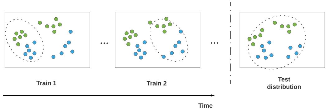
Figure 19.16: An illustration of domain drift.

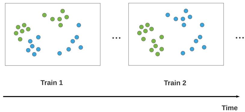
Figure 19.17: An illustration of concept drift.

Alternatively we can define ptest ^t (x) to be the union of all the input distributions seen so far, ptest ^t = ^{⊤T s}=1p^s (e.g., we want the detector to work well on dark and light images)/ This latter assumption is illustrated in Figure 19.16.

19.7.2 Concept drift

The problem of concept drift refers to the setting where the functional mapping f^t : X ↖ Y changes over time, but the input distribution pt(x) is constant [WK96]. For example, we can imagine a setting in which people engage in certain behaviors, and at step t some of these are classified as illegal, and at step t ^↔︎ > t, the definition of what is legal changes, and hence the decision boundary changes. This is illustrated in Figure 19.17.

As another example, we might initially be faced with a sort-by-color task, where red objects go on the left and blue objects on the right, and then a sort-by-shape task, where square objects go on the

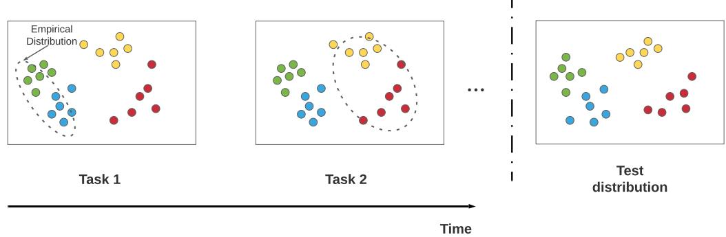
Figure 19.18: An illustration of class incremental learning. Adapted from Figure 1 of [LCR21].

left and circular objects go on the right.4 We can think of this as a problem where ^p(y|x,task) is stationary, but the task is unobserved, so p(y|x) changes.

In the concept drift scenario, we see that the prediction for the same underlying input point x ↗ X will change depending on when the prediction is performed. This means that the test distribution also needs to change over time for meaningful identification. Alternatively, we can “tag” each input with the corresponding time stamp or task id.

19.7.3 Class incremental learning

A very widely studied form of continual learning focuses on the setting in which new class labels are “revealed” over time. That is, there is assumed to be a true static prediction function f : X ↖ Y, but at step t, the learner only sees samples from (X , Yt), where Y^t ∋ Y. For example, consider the problem of digit classification from images. Y¹ might be {0, 1}, and Y² might be {2,…, 9}. Learning to classify with an increasing number of categories is called class incremental learning (see e.g., [Mas+20]). See Figure 19.18 for an illustration.

The problem of class incremental learning has been studied under a variety of di!erent assumptions, as discussed in [Hsu+18; VT18; FG18; Del+21]. The most common scenarios are shown in Figure 19.19. If we assume there are no well defined boundaries between tasks, we have continuous task-agnostic learning (see e.g., [SKM21; Zen+21]). If there are well defined boundaries (i.e., discontinuous changes of the training distribution), then we can distinguish two subcases. If the boundaries are not known during training (similar to detecting distribution shift), we have discrete task-agnostic learning. Finally, if the boundaries are given to the training algorithm, we have a task-aware learning problem.

A common experimental setup in the task-aware setting is to define each task to be a di!erent version of the MNIST dataset, e.g., with all 10 classes present but with the pixels randomly permuted (this is called permuted MNIST) or with a subset of 2 classes present at each step (this is called split MNIST).5 In the task-aware setting, the task label may or may not be known at test time.

^4. This example is from Mike Mozer.

^5. In the split MNIST setup, for task 1, digits (0,1) get labeled as (0,1), but in task 2, digits (2,3) get labeled as (0,1).

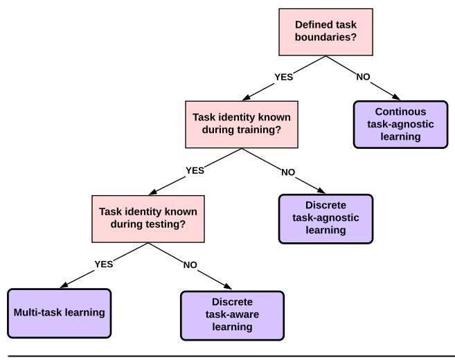
Generally more challenging scenario(less information)

Figure 19.19: Di!erent kinds of incremental learning. Adapted from Figure 1 of [Zen+18].

If it is, the problem is essentially equivalent to multi-task learning (see Section 19.6.1). If it is not, the model must predict the task and corresponding class label within that task (which is a standard supervised problem with a hierarchical label space); this is commonly done by using a multi-headed DNN, with CT outputs, where C is the number of classes, and T is the number of tasks.

In the multi-headed approach, the number of “heads” is usually specified as input to the algorithm, because the softmax imposes a sum-to-one constraint that prevents incremental estimation of the output weights in the open-class setting. An alternative approach is to wait until a new class label is encountered for the first time, and then train the model with an enlarged output head. This requires storing past data from each class, as well as data for the new class (see e.g., [PTD20]). Alternatively, we can use generative classifiers where we do not need to worry about “output heads”. If we use a “deep” nearest neighbor classifier, with a shared feature extractor (embedding function), the main challenge is to e”ciently update the stored prototypes for past classes as the feature extractor parameters change (see e.g., [DLT21]). If we fit a separate generative model per class (e.g., a VAE, as in [VLT21]), then online learning becomes easier, but the method may be less sample e”cient.

At the time of writing, most of the CL literature focuses on the task-aware setting. However, from a practical point of view, the assumption that task boundaries are provided at training or test time is very unrealistic. For example, consider the problem of training a robot to perform various activities: The data just streams in, and the robot must learn what to do, without anyone telling it that it is now being given an example from a new task or distribution (see e.g., [Fon+21; Wo%+21]). Thus future research should focus on the task-agnostic setting, with either discrete or continuous changes.

So the “meaning” of the output label depends on what task we are solving. Thus the output space is really hierarchical, namely the cross product of task id and class label.

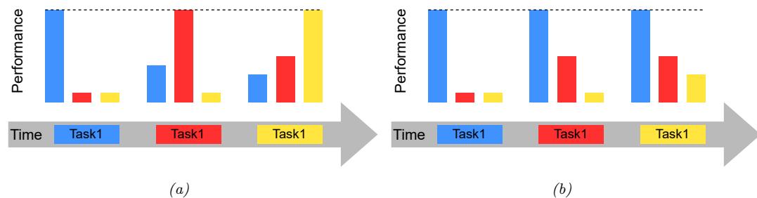
Figure 19.20: Some failure modes in class incremental learning. We train on task 1 (blue) and evaluate on tasks 1–3 (blue, orange, yellow); we then train on task 2 and evaluate on tasks 1–3; etc. (a) Catastrophic forgetting refers to the phenomenon in which performance on a previous task drops when trained on a new task. (b) Too little plasticity (e.g., due to too much regularization) refers to the phenomenon in which only the first task is learned. Adapted from Figure 2 of [Had+20].

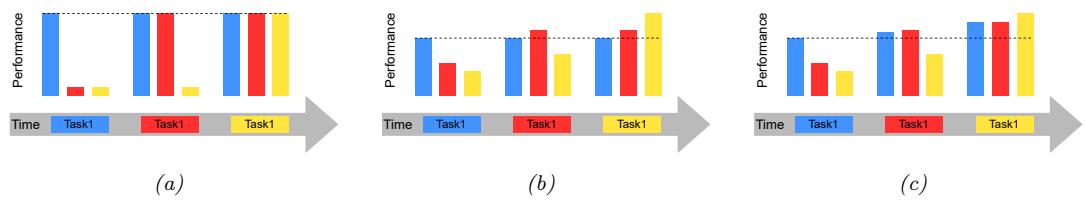
Figure 19.21: What success looks like for class incremental learning. We train on task 1 (blue) and evaluate on tasks 1–3 (blue, orange, yellow); we then train on task 2 and evaluate on tasks 1–3; etc. (a) No forgetting refers to the phenomenon in which performance on previous tasks does not degrade over time. (b) Forwards transfer refers to the phenomenon in which training on past tasks improves performance on future tasks beyond what would have been obtained by training from scratch. (c) Backwards transfer refers to the phenomenon in which training on future tasks improves performance on past tasks beyond what would have been obtained by training from scratch. Adapted from Figure 2 of [Had+20].

19.7.4 Catastrophic forgetting

In the class incremental learning literature, it is common to train on a sequence of tasks, but to test (at each step) on all tasks. In this scenario, there are two main possible failure modes. The first possible problem is called “catastrophic forgetting” (see e.g., [Rob95b; Fre99; Kir+17]). This refers to the phenomenon in which performance on a previous task drops when trained on a new task (see Figure 19.20(a)). Another possible problem is that only the first task is learned, and the model does not adapt to new tasks (see Figure 19.20(b)).

If we avoid these problems, we should expect to see the performance profile in Figure 19.21(a), where performance of incremental training is equal to training on each task separately. However, we might hope to do better by virtue of the fact that we are training on multiple tasks, which are often assumed to be related. In particular, we might hope to see forwards transfer, in which training on past tasks improves performance on future tasks beyond what would have been obtained by training from scratch (see Figure 19.21(b)). Additionally, we might hope to see backwards transfer, in which training on future tasks improves performance on past tasks (see Figure 19.21(c)).

We can quantify the degree of transfer as follows, following [LPR17]. If Rij is the performance on task j after it was trained on task i, Rind ^j is the performance on task j when trained just on j, and there are T tasks, then the amount of forwards transfer is

\[\text{FWT} = \frac{1}{T} \sum\_{j=1}^{T} R\_{j,j} - R\_j^{\text{ind}} \tag{19.41}\]

and the amount of backwards transfer is

\[\text{BWT} = \frac{1}{T} \sum\_{j=1}^{T} R\_{T,j} - R\_{j,j} \tag{19.42}\]

There are many methods that have been devised to overcome the problem of catastrophic forgetting, but we can group them into three main types. The first is regularization methods, which add a loss to preserve information that is relevant to old tasks. (For example, online Bayesian inference is of this type, since the posterior for the parameters is derived from the new data and the past prior; see e.g., the elastic weight consolidation method discussed in Section 17.5.1, or the variational continual learning method discussed in Supplementary Section 10.2). The second is memory methods, which rely on some kind of experience replay or rehearsal of past data (see e.g., [Hen+21]), or some kind of generative model of past data. The third is architectural methods, that add capacity to the network whenever a task boundary is encountered, such as a new class label (see e.g., [Rus+16]).

Of course, these techniques can be combined. For example, we can create a semi-parametric model, in which we store some past data (exemplars) while also learning parameters online in a Bayesian (regularized) way (see e.g., [Kur+20]). The “right” method depends, as usual, on what inductive bias you want to use, and what your computational budget is in terms of time and memory.

19.7.5 Online learning

The problem of online learning is similar to continual learning, except the loss metric is di!erent, and we usually assume that learning and evaluation occur at each step. More precisely, we assume the data generating distribution, p^{→ t} (x, y) = p(x|εt)p(y|x, wt), evolves over time, as shown in Figure 19.22. At each step t nature generates a data sample, (xt, yt) ↔︎ p^{→ t} . The agent sees x^t and is asked to predict y^t by computing the posterior predictive distribution

\[ \hat{p}\_{t|t-1} = p(\mathbf{y}|x\_t, \mathcal{D}\_{1:t-1}) \tag{19.43} \]

where D1:t↓¹ = {(xs, ys) : s =1: t → 1} is all past data. It then incurs a loss of

\[\mathcal{L}\_t = \ell(\hat{p}\_{t|t-1}, \mathbf{y}\_t) \tag{19.44}\]

See Figure 19.22. This approach is called prequential prediction [DV99; GSR13], and also forms the basis of online conformal prediction [VGS22].

In contrast to the continual learning scenarios studied above, the loss incurred at each step is what matters, rather than loss on a fixed test set. That is, we want to minimize ^{L =} &^{T t}=1 Lt. In the case of log-loss, this is equal to the (conditional) log marginal likelihood of the data, log p(D1:^T ) =

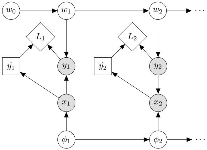
Figure 19.22: Online learning illustrated as an influence diagram (Section 34.2). Here yˆ^t = argmax^y p(y|xt, D1:t→¹) is the action (MAP predicted output) at time t, and L^t = ε(yt, yˆt) is the corresponding loss (utility) function. We then update the parameters of the model, ω^t = (wt, ϖt), given the input and true output (xt, yt). The parameters of the world model can change arbitrarily over time.

log p(y1:^T |x1:^T ). This can be used to compute the prequential minimum description length (MDL) of a model [BLH22], which is useful for model selection.

Another metric that is widely used, especially if it assumed that the distributions can be generated by an adversary, is to compare the cumulative loss to the optimal value one could have obtained in hindsight. This yields a quantity called the regret:

\[\text{rereget} = \sum\_{t=1}^{T} \left[ \ell(\hat{p}\_{t|t-1}, \mathbf{y}\_t) - \ell(\hat{p}\_{t|T}, \mathbf{y}\_t) \right] \tag{19.45}\]

where pˆ^t|t↓¹ = p(y|xt, D1:t↓¹) is the online prediction, and pˆ^t|^T = p(y|xt, D1:^T ) is the optimal estimate at the end of training. Bounds on the regret can be derived when the loss is convex [Ora19; Haz22]. It is possible to convert bounds on regret, which are backwards looking, into bounds on risk (i.e., expected future loss), which is forwards looking. See [HT15] for details.

Online learning is very useful for decision and control problems, such as multi-armed bandits (Section 34.4) and reinforcement learning (see Chapter 35), where the agent “lives forever”, and where there is no fixed training phase followed by a test phase. (See e.g., Section 17.5 where we discuss online Bayesian inference for neural networks.)

The previous continual learning scenarios can be derived as special cases of online learning: we use a di!erent distribution (task) per time step, and provide a set of examples as input, instead of a single example. On odd time steps, we train on the data from the current distribution, and incur a loss of 0; and on even time steps, we evaluate on the test distribution, which may consist of the union of all previously seen tasks, and return the empirical loss. (Thus doing well on old distributions is relevant because we assume such distributions keep recurring.) Typically in CL the amount of

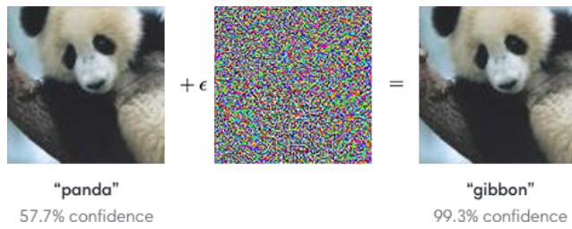
Figure 19.23: Example of an adversarial attack on an image classifier. Left column: original image which is correctly classified. Middle column: small amount of structured noise which is added to the input (magnitude of noise is magnified by 10≃). Right column: new image, which is confidently misclassified as a “gibbon”, even though it looks just like the original “panda” image. Here ◁ = 0.007. From Figure 1 of [GSS15]. Used with kind permission of Ian Goodfellow.

data per task is large, whereas online learning is more concerned with fast adaptation to slowly (or piecewise continuously) changing distributions using small amounts of data per time step.

19.8 Adversarial examples

This section is coauthored with Justin Gilmer.

In Section 19.2, we discussed what happens to a predictive model when the input distribution shifts for some reason. In this section, we consider the case where an adversary deliberately chooses inputs to minimize the performance of a predictive model. That is, suppose an input x is classified as belonging to class c. We then choose a new input xadv which minimizes the probability of this label, subject to the constraint that xadv is “perceptually similar” to the original input x. This gives rise to the following objective:

\[\mathbf{x}\_{\text{adv}} = \operatorname\*{argmin}\_{\mathbf{z}' \in \Delta(\mathbf{z})} \log p(y = c | \mathbf{z}') \tag{19.46}\]

where !(x) is the set of images that are “similar” to x (we discuss di!erent notions of similarity below).

Equation (19.46) is an example of an adversarial attack. We illustrate this in Figure 19.23. The input image x is on the left, and is predicted to be a panda with probability 57%. By adding a tiny amount of carefully chosen noise (shown in the middle) to the input, we generate the adversarial image xadv on the right: this “looks like” the input, but is now classified as a gibbon with probability 99%.

The ability to create adversarial images was first noted in [Sze+14]. It is suprisingly easy to create such examples, which seems paradoxical, given the fact that modern classifiers seem to work so well on normal inputs, and the perturbed images “look” the same to humans. We explain this paradox in Section 19.8.5.

The existence of adversarial images also raises security concerns. For example, [Sha+16] showed they could force a face recognition system to misclassify person A as person B, merely by asking person A to wear a pair of sunglasses with a special pattern on them, and [Eyk+18] show that is

possible to attach small “adversarial stickers” to tra”c signs to classify stop signs as speed limit signs.

Below we briefly discuss how to create adversarial attacks, why they occur, and how we can try to defend against them. We focus on the case of deep neural nets for images, although it is important to note that many other kinds of models (including logistic regression and generative models) can also su!er from adversarial attacks. Furthermore, this is not restricted to the image domain, but occurs with many kinds of high dimensional inputs. For example, [Li+19] contains an audio attack and [Dal+04; Jia+19] contains a text attack. More details on adversarial examples can be found in e.g., [Wiy+19; Yua+19].

19.8.1 Whitebox (gradient-based) attacks

To create an adversarial example, we must find a “small” perturbation ς to add to the input x to create xadv = x + ς so that f(xadv) = y^↔︎ , where f() is the classifier, and y^↔︎ is the label we want to force the system to output. This is known as a targeted attack. Alternatively, we may just want to find a perturbation that causes the current predicted label to change from its current value to any other value, so that f(x + ς) ′= f(x), which is known as untargeted attack.

In general, we define the objective for the adversary as maximizing the following loss:

\[\mathbf{x}\_{\text{adv}} = \underset{\mathbf{z}' \in \Delta(\mathfrak{a})}{\text{argmax}} \mathcal{L}(\mathbf{z}', y; \boldsymbol{\theta}) \tag{19.47}\]

where y is the true label. For the untargeted case, we can define L(x^↔︎ , y; ω) = → log p(y|x^↔︎ ), so we minimize the probability of the true label; and for the targeted case, we can define L(x^↔︎ , y; ω) = log p(y^↔︎ |x↔︎ ), where we maximize the probability of the desired label y^↔︎ ′= y.

To define what we mean by “small” perturbation, we impose the constraint that xadv ↗ !(x), which is the set of “perceptually similar” images to the input x. Most of the literature has focused on a simplistic setting in which the adversary is restricted to making bounded l^p perturbations of a clean input x, that is

\[\Delta(\mathbf{z}) = \{ \mathbf{z}' : ||\mathbf{z}' - \mathbf{z}||\_p < \epsilon \}\tag{19.48}\]

Typically people assume p = 1 or p = 0. We will discuss more realistic threat models in Section 19.8.3.

In this section, we assume that the attacker knows the model parameters ω; this is called a whitebox attack, and lets us use gradient based optimization methods. We relax this assumption in Section 19.8.2.)

To solve the optimization problem in Equation (19.47), we can use any kind of constrained optimization method. In [Sze+14] they used bound-constrained BFGS. [GSS15] proposed the more e”cient fast gradient sign (FGS) method, which performs iterative updates of the form

\[x\_{t+1} = x\_t + \delta\_t \tag{19.49}\]

\[\boldsymbol{\delta}\_t = \epsilon \operatorname{sign}(\nabla\_\mathbf{z} \log p(y'|x, \boldsymbol{\theta})|\_{\mathfrak{w}\_t}) \tag{19.50}\]

where ⇁ > 0 is a small learning rate. (Note that this gradient is with respect to the input pixels, not the model parameters.) Figure 19.23 gives an example of this process.

More recently, [Mad+18] proposed the more powerful projected gradient descent (PGD) attack; this can be thought of as an iterated version of FGS. There is no “best” variant of PGD for

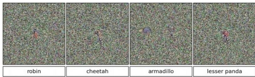
Figure 19.24: Images that look like random noise but which cause the CNN to confidently predict a specific class. From Figure 1 of [NYC15]. Used with kind permission of Je! Clune.

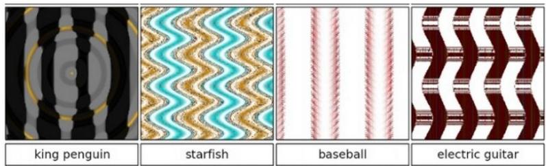
Figure 19.25: Synthetic images that cause the CNN to confidently predict a specific class. From Figure 1 of [NYC15]. Used with kind permission of Je! Clune.

solving 19.47. Instead, what matters more is the implementation details, e.g. how many steps are used, the step size, and the exact form of the loss. To avoid local minima, we may use random restarts, choosing random points in the constraint space ! to initialize the optimization. The algorithm should be carefully tuned to the specific problem, and the loss should be monitored to check for optimization issues. For best practices, see [Car+19].

19.8.2 Blackbox (gradient-free) attacks

In this section, we no longer assume that the adversary knows the parameters ω of the predictive model f. This is known as a black box attack. In such cases, we must use derivative-free optimization (DFO) methods (see Section 6.7).

Evolutionary algorithms (EA) are one class of DFO solvers. These were used in [NYC15] to create blackbox attacks. Figure 19.24 shows some images that were generated by applying an EA to a random noise image. These are known as fooling images, as opposed to adversarial images, since they are not visually realistic. Figure 19.25 shows some fooling images that were generated by applying EA to the parameters of a compositional pattern-producing network (CPPN) [Sta07].6 By suitably perturbing the CPPN parameters, it is possible to generate structured images with high fitness (classifier score), but which do not look like natural images [Aue12].

^6. A CPPN is a set of elementary functions (such as linear, sine, sigmoid, and Gaussian) which can be composed in order to specify the mapping from each coordinate to the desired color value. CPPN was originally developed as a way to encode abstract properties such as symmetry and repetition, which are often seen during biological development.

Figure 19.26: An adversarially modified image to evade spam detectors. The image is constructed from scratch, and does not involve applying a small perturbation to any given image. This is an illustrative example of how large the space of possible adversarial inputs # can be when the attacker has full control over the input. From [Big+11]. Used with kind permission of Battista Biggio.

In [SVK19], they used di!erential evolution to attack images by modifying a single pixel. This is equivalent to bounding the ε⁰ norm of the perturbation, so that ||xadv → x||⁰ = 1.

In [Pap+17], they learned a di!erentiable surrogate model of the blackbox, by just querying its predictions y for di!erent inputs x. They then used gradient-based methods to generate adversarial attacks on their surrogate model, and then showed that these attacks transferred to the real model. In this way, they were able to attack various the image classification APIs of various cloud service providers, including Google, Amazon, and MetaMind.

19.8.3 Real world adversarial attacks

Typically, the space of possible adversarial inputs ! can be quite large, and will be di”cult to exactly define mathematically as it will depend on semantics of the input based on the attacker’s goals [BR18]. (The set of variations ! that we want the model to be invariant to is called the threat model.)

Consider for example of the content constrained threat model discussed in [Gil+18a]. One instance of this threat model involves image spam, where the attacker wishes to upload an image attachment in an email that will not be classified as spam by a detection model. In this case ! is incredibly large as it consists of all possible images which contain some semantic concept the attacker wishes to upload (in this case an advertisement). To explore !, spammers can utilize di!erent fonts, word orientations or add random objects to the background as is the case of the adversarial example in Figure 19.26 (see [Big+11] for more examples). Of course, optimization based methods may still be used here to explore parts of !. However, in practice it may be preferable to design an adversarial input by hand as this can be significantly easier to execute with only limited-query black-box access to the underlying classifier.

19.8.4 Defenses based on robust optimization

As discussed in Section 19.8.3, securing a system against adversarial inputs in more general threat models seems extraordinarily di”cult, due to the vast space of possible adversarial inputs !. However, there is a line of research focused on producing models which are invariant to perturbations within a small constraint set !(x), with a focus on lp-robustness where !(x) = {x^↔︎ : ||x → x^↔︎ ||^p < ⇁}. Although solving this toy threat model has little application to security settings, enforcing smoothness priors has in some cases improved robustness to random image corruptions [SHS], led to models which transfer better [Sal+20], and has biased models towards di!erent features in the data [Yin+19a].

Perhaps the most straightforward method for improving lp-robustness is to directly optimize for it through robust optimization [BTEGN09], also known as adversarial training [GSS15]. We define the adversarial risk to be

\[\min\_{\theta} \mathbb{E}\_{(\mathbf{z}, \mathbf{y}) \sim p(\mathbf{z}, \mathbf{y})} \left[ \max\_{\mathbf{z}' \in \Delta(\mathbf{z})} L(\mathbf{z}', \mathbf{y}; \theta) \right] \tag{19.51}\]

The min max formulation in equation 19.51 poses unique challenges from an optimization perspective — it requires solving both the non-concave inner maximization and the non-convex outer minimization problems. Even worse, the inner max is NP-hard to solve in general [Kat+17]. However, in practice it may be su”cient to compute the gradient of the outer objective ⇒ϱL(xadv, y, ; ω) at an approximately maximal point in the inner problem xadv ↓ argmax^x↑ L(x^↔︎ , y; ω) [Mad+18]. Currently, best practice is to approximate the inner problem using a few steps of PGD.

Other methods seek to certify that a model is robust within a given region !(x). One method for certification uses randomized smoothing [CRK19] — a technique for converting a model robust to random noise into a model which is provably robust to bounded worst-case perturbations in the l2-metric. Another class of methods applies specifically for networks with ReLU activations, leveraging the property that the model is locally linear, and that certifying in region defined by linear constraints reduces to solving a series of linear programs, for which standard solvers can be applied [WK18].

19.8.5 Why models have adversarial examples

The existence of adversarial inputs is paradoxical, since modern classifiers seem to do so well on normal inputs. However, the existence of adversarial examples is a natural consequence of the general lack of robustness to distribution shift discussed in Section 19.2. To see this, suppose a model’s accuracy drops on some shifted distribution of inputs pte(x) that di!ers from the training distribution ptr(x); in this case, the model will necessarily be vunerable to an adversarial attack: if errors exist, there must be a nearest such error. Furthermore, if the input distribution is high dimensional, then we should expect the nearest error to be significantly closer than errors which are sampled randomly from some out-of-distribution pte(x).

A cartoon illustration of what is going on is shown in Figure 19.27a, where x⁰ is the clean input image, B is an image corrupted by Gaussian noise, and A is an adversarial image. If we assume a linear decision boundary, then the error set E is a half space a certain distance from x0. We can relate the distance to the decision boundary d(x0, E) with the error rate in noise at some input x0, denoted by µ = P^φ⇓N(0,↽I) [x⁰ + ϑ ↗ E]. With a linear decision boundary the relationship between

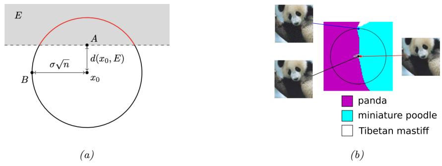
Figure 19.27: (a) When the input dimension n is large and the decision boundary is locally linear, even a small error rate in random noise will imply the existence of small adversarial perturbations. Here, d(x0, E) denotes the distance from a clean input x⁰ to an adversarial example (A) while the distance from x⁰ to a random sample N(0; ω²I (B) will be approximately ω ^∝n. As ⁿ → ↖ the ratio of ^d(x0, A) to ^d(x0, B) goes to 0. (b) A 2d slice of the InceptionV3 decision boundary through three points: a clean image (black), an adversarial example (red), and an error in random noise (blue). The adversarial example and the error in noise lie in the same region of the error set which is misclassified as “miniature poodle”, which closely resembles a halfspace as in a. Used with kind permission of Justin Gilmer.

these two quantities is determined by

\[d(\mathbf{x}\_0, E) = -\sigma \Phi^{-1}(\mu) \tag{19.52}\]

where ’↓¹ denotes the inverse cdf of the gaussian distribution. When the input dimension is large, this distance will be significantly smaller than the distance to a randomly sampled noisy image x⁰ + ϑ for ϑ ↔︎ N(0, ςI), as the noise term will with high propbability have norm ||ϑ||² ↓ ς ∝ d. As a concrete example consider the ImageNet dataset, where d = 224 ⇔ 224 ⇔ 3 and suppose we set ς = .2. Then if the error rate in noise is just µ = .01, equation 19.52 will imply that d(x0, E) = .5. Thus the distance to an adversarial example will be more than 100 times closer than the distance to a typical noisy images, which will be ς ∝ d ↓ 77.6. This phenomenon of small volume error sets being close to most points in a data distribution p(x) is called concentration of measure, and is a property common among many high dimensional data distributions [MDM19; Gil+18b].

In summary, although the existence of adversarial examples is often discussed as an unexpected phenomenon, there is nothing special about the existence of worst-case errors for ML classifiers they will always exist as long as errors exist.