Probabilistic Machine Learning: Advanced Topics

Chapter 1 ~ 6

Probabilistic Machine Learning

Adaptive Computation and Machine Learning

Francis Bach, editor

A complete list of titles can be found online at https://mitpress.mit.edu/search-result-list/ ?series=adaptive-computation-and-machine-learning-series.

Probabilistic Machine Learning Advanced Topics

Kevin P. Murphy

The MIT Press Cambridge, Massachusetts London, England

© 2023 Kevin P. Murphy

This work is subject to a Creative Commons CC-BY-NC-ND license.

Subject to such license, all rights are reserved.

The MIT Press would like to thank the anonymous peer reviewers who provided comments on drafts of this book. The generous work of academic experts is essential for establishing the authority and quality of our publications. We acknowledge with gratitude the contributions of these otherwise uncredited readers.

Printed and bound in the United States of America.

Library of Congress Cataloging-in-Publication Data

Names: Murphy, Kevin P., author.

Title: Probabilistic machine learning : advanced topics / Kevin P. Murphy. Description: Cambridge, Massachusetts : The MIT Press, [2023] | Series: Adaptive computation and machine learning series | Includes bibliographical references and index. Identifiers: LCCN 2022045222 (print) | LCCN 2022045223 (ebook) | ISBN 9780262048439 (hardcover) | ISBN 9780262376006 (epub) | ISBN 9780262375993 (pdf) Subjects: LCSH: Machine learning. | Probabilities. Classification: LCC Q325.5 .M873 2023 (print) | LCC Q325.5 (ebook) | DDC 006.3/1015192–dc23/eng20230111 LC record available at https://lccn.loc.gov/2022045222 LC ebook record available at https://lccn.loc.gov/2022045223

This book is dedicated to my wife Margaret, who has been the love of my life for 20+ years.

Brief Contents

1 Introduction 1

I Fundamentals 3

• 2 Probability 5
• 3 Statistics 63
• 4 Graphical models 143
• 5 Information theory 219
• 6 Optimization 261

II Inference 343

• 7 Inference algorithms: an overview 345
• 8 Gaussian filtering and smoothing 359
• 9 Message passing algorithms 401
• 10 Variational inference 439
• 11 Monte Carlo methods 483
• 12 Markov chain Monte Carlo 499
• 13 Sequential Monte Carlo 543

III Prediction 573

• 14 Predictive models: an overview 575
• 15 Generalized linear models 591
• 16 Deep neural networks 631
• 17 Bayesian neural networks 647
• 18 Gaussian processes 681
• 19 Beyond the iid assumption 735

IV Generation 771

• 20 Generative models: an overview 773
• 21 Variational autoencoders 791
• 22 Autoregressive models 821
• 23 Normalizing flows 829
• 24 Energy-based models 849
• 25 Di 867
• 26 Generative adversarial networks 893

V Discovery 925

• 27 Discovery methods: an overview 927
• 28 Latent factor models 929
• 29 State-space models 979
• 30 Graph learning 1043
• 31 Nonparametric Bayesian models 1047
• 32 Representation learning 1049
• 33 Interpretability 1073

VI Action 1103

• 34 Decision making under uncertainty 1105
• 35 Reinforcement learning 1145
• 36 Causality 1185

Contents

Preface xxxi

1 Introduction 1

I Fundamentals 3

2 Probability 5

2.1	Introduction	5
	2.1.1	Probability space 5
	2.1.2	Discrete random variables 5
	2.1.3	Continuous random variables 6
	2.1.4	Probability axioms 7
	2.1.5	Conditional probability 7
	2.1.6	Bayes’ rule 8
2.2		Some common probability distributions 8
	2.2.1	Discrete distributions 9
	2.2.2	Continuous distributions on R 10
	2.2.3	Continuous distributions on R+ 13
	2.2.4	Continuous distributions on [0, 1] 17
	2.2.5	Multivariate continuous distributions 17
2.3		Gaussian joint distributions 22
	2.3.1	The multivariate normal 22
	2.3.2	Linear Gaussian systems 28
	2.3.3	A general calculus for linear Gaussian systems 30
2.4		The exponential family 33
	2.4.1	Definition 34
	2.4.2	Examples 34
	2.4.3	Log partition function is cumulant generating function 39
	2.4.4	Canonical (natural) vs mean (moment) parameters 41
	2.4.5	MLE for the exponential family 42
	2.4.6	Exponential dispersion family 43
	2.4.7	Maximum entropy derivation of the exponential family 43
2.5		Transformations of random variables 44
	2.5.1	Invertible transformations (bijections) 44
	2.5.2	Monte Carlo approximation 45
	2.5.3	Probability integral transform 45
2.6		Markov chains 46
	2.6.1	Parameterization 47
	2.6.2	Application: language modeling 49

2.6.3 Parameter estimation 49 2.6.4 Stationary distribution of a Markov chain 51 2.7 Divergence measures between probability distributions 55 2.7.1 f-divergence 55 2.7.2 Integral probability metrics 57 2.7.3 Maximum mean discrepancy (MMD) 58 2.7.4 Total variation distance 61 2.7.5 Density ratio estimation using binary classifiers 61 3 Statistics 63 3.1 Introduction 63 3.2 Bayesian statistics 63 3.2.1 Tossing coins 64 3.2.2 Modeling more complex data 70 3.2.3 Selecting the prior 71 3.2.4 Computational issues 71 3.2.5 Exchangeability and de Finetti’s theorem 72 3.3 Frequentist statistics 72 3.3.1 Sampling distributions 73 3.3.2 Bootstrap approximation of the sampling distribution 73 3.3.3 Asymptotic normality of the sampling distribution of the MLE 75 3.3.4 Fisher information matrix 75 3.3.5 Counterintuitive properties of frequentist statistics 80 3.3.6 Why isn’t everyone a Bayesian? 82 3.4 Conjugate priors 83 3.4.1 The binomial model 84 3.4.2 The multinomial model 84 3.4.3 The univariate Gaussian model 85 3.4.4 The multivariate Gaussian model 90 3.4.5 The exponential family model 96 3.4.6 Beyond conjugate priors 99 3.5 Noninformative priors 102 3.5.1 Maximum entropy priors 102 3.5.2 Je!reys priors 103 3.5.3 Invariant priors 106 3.5.4 Reference priors 107 3.6 Hierarchical priors 108 3.6.1 A hierarchical binomial model 108 3.6.2 A hierarchical Gaussian model 111 3.6.3 Hierarchical conditional models 114 3.7 Empirical Bayes 114 3.7.1 EB for the hierarchical binomial model 115 3.7.2 EB for the hierarchical Gaussian model 116 3.7.3 EB for Markov models (n-gram smoothing) 116 3.7.4 EB for non-conjugate models 118 3.8 Model selection 118 3.8.1 Bayesian model selection 119 3.8.2 Bayes model averaging 121 3.8.3 Estimating the marginal likelihood 121 3.8.4 Connection between cross validation and marginal likelihood 122 3.8.5 Conditional marginal likelihood 123 3.8.6 Bayesian leave-one-out (LOO) estimate 124 3.8.7 Information criteria 125 3.9 Model checking 128 3.9.1 Posterior predictive checks 128

3.10 Hypothesis testing 131 3.10.1 Frequentist approach 131 3.10.2 Bayesian approach 132 3.10.3 Common statistical tests correspond to inference in linear models 136 3.11 Missing data 141 4 Graphical models 143 4.1 Introduction 143 4.2 Directed graphical models (Bayes nets) 143 4.2.1 Representing the joint distribution 143 4.2.2 Examples 144 4.2.3 Gaussian Bayes nets 148 4.2.4 Conditional independence properties 149 4.2.5 Generation (sampling) 154 4.2.6 Inference 155 4.2.7 Learning 155 4.2.8 Plate notation 161 4.3 Undirected graphical models (Markov random fields) 164 4.3.1 Representing the joint distribution 165 4.3.2 Fully visible MRFs (Ising, Potts, Hopfield, etc.) 166 4.3.3 MRFs with latent variables (Boltzmann machines, etc.) 172 4.3.4 Maximum entropy models 174 4.3.5 Gaussian MRFs 177 4.3.6 Conditional independence properties 179 4.3.7 Generation (sampling) 181 4.3.8 Inference 182 4.3.9 Learning 182 4.4 Conditional random fields (CRFs) 186 4.4.1 1d CRFs 187 4.4.2 2d CRFs 190 4.4.3 Parameter estimation 193 4.4.4 Other approaches to structured prediction 194 4.5 Comparing directed and undirected PGMs 194 4.5.1 CI properties 194 4.5.2 Converting between a directed and undirected model 196 4.5.3 Conditional directed vs undirected PGMs and the label bias problem 197 4.5.4 Combining directed and undirected graphs 198 4.5.5 Comparing directed and undirected Gaussian PGMs 200 4.6 PGM extensions 202 4.6.1 Factor graphs 202 4.6.2 Probabilistic circuits 205 4.6.3 Directed relational PGMs 206 4.6.4 Undirected relational PGMs 208 4.6.5 Open-universe probability models 211 4.6.6 Programs as probability models 211 4.7 Structural causal models 212 4.7.1 Example: causal impact of education on wealth 213 4.7.2 Structural equation models 214 4.7.3 Do operator and augmented DAGs 214 4.7.4 Counterfactuals 215 5 Information theory 219 5.1 KL divergence 219 5.1.1 Desiderata 220 5.1.2 The KL divergence uniquely satisfies the desiderata 221 5.1.3 Thinking about KL 224 5.1.4 Minimizing KL 225

• 5.1.5 Properties of KL 228
• 5.1.6 KL divergence and MLE 230
• 5.1.7 KL divergence and Bayesian inference 231
• 5.1.8 KL divergence and exponential families 232
• 5.1.9 Approximating KL divergence using the Fisher information matrix 233
• 5.1.10 Bregman divergence 233
• 5.2 Entropy 234
  • 5.2.1 Definition 235
  • 5.2.2 Di 235
  • 5.2.3 Typical sets 236
  • 5.2.4 Cross entropy and perplexity 237
• 5.3 Mutual information 238
  • 5.3.1 Definition 238
    • 5.3.2 Interpretation 239
    • 5.3.3 Data processing inequality 239
  • 5.3.4 Su”cient statistics 240
  • 5.3.5 Multivariate mutual information 241
  • 5.3.6 Variational bounds on mutual information 244
  • 5.3.7 Relevance networks 246
• 5.4 Data compression (source coding) 247
  • 5.4.1 Lossless compression 247
  • 5.4.2 Lossy compression and the rate-distortion tradeo! 248
  • 5.4.3 Bits back coding 250
• 5.5 Error-correcting codes (channel coding) 251
• 5.6 The information bottleneck 252
  • 5.6.1 Vanilla IB 252
    • 5.6.2 Variational IB 253
  • 5.6.3 Conditional entropy bottleneck 254
• 5.7 Algorithmic information theory 256
  • 5.7.1 Kolmogorov complexity 256
    • 5.7.2 Solomono! induction 257

6 Optimization 261

• 6.1 Introduction 261 6.2 Automatic di!erentiation 261 6.2.1 Di 261 6.2.2 Di 266 6.3 Stochastic optimization 271 6.3.1 Stochastic gradient descent 271 6.3.2 SGD for optimizing a finite-sum objective 273 6.3.3 SGD for optimizing the parameters of a distribution 273 6.3.4 Score function estimator (REINFORCE) 274 6.3.5 Reparameterization trick 275 6.3.6 Gumbel softmax trick 277 6.3.7 Stochastic computation graphs 278 6.3.8 Straight-through estimator 279 6.4 Natural gradient descent 279 6.4.1 Defining the natural gradient 280 6.4.2 Interpretations of NGD 281 6.4.3 Benefits of NGD 282 6.4.4 Approximating the natural gradient 282 6.4.5 Natural gradients for the exponential family 284 6.5 Bound optimization (MM) algorithms 287 6.5.1 The general algorithm 287
  • 6.5.2 Example: logistic regression 288
  • 6.5.3 The EM algorithm 289

6.5.4 Example: EM for an MVN with missing data 291 6.5.5 Example: robust linear regression using Student likelihood 293 6.5.6 Extensions to EM 295 6.6 Bayesian optimization 297 6.6.1 Sequential model-based optimization 298 6.6.2 Surrogate functions 298 6.6.3 Acquisition functions 300 6.6.4 Other issues 303 6.7 Derivative-free optimization 304 6.7.1 Local search 304 6.7.2 Simulated annealing 307 6.7.3 Evolutionary algorithms 307 6.7.4 Estimation of distribution (EDA) algorithms 310 6.7.5 Cross-entropy method 312 6.7.6 Evolutionary strategies 312 6.7.7 LLMs for DFO 314 6.8 Optimal transport 314 6.8.1 Warm-up: matching optimally two families of points 314 6.8.2 From optimal matchings to Kantorovich and Monge formulations 316 6.8.3 Solving optimal transport 318 6.9 Submodular optimization 322 6.9.1 Intuition, examples, and background 323 6.9.2 Submodular basic definitions 325 6.9.3 Example submodular functions 327 6.9.4 Submodular optimization 329 6.9.5 Applications of submodularity in machine learning and AI 333 6.9.6 Sketching, coresets, distillation, and data subset and feature selection 334 6.9.7 Combinatorial information functions 337 6.9.8 Clustering, data partitioning, and parallel machine learning 339 6.9.9 Active and semi-supervised learning 339 6.9.10 Probabilistic modeling 340 6.9.11 Structured norms and loss functions 341 6.9.12 Conclusions 342

II Inference 343

7 Inference algorithms: an overview 345

• 7.1 Introduction 345
• 7.2 Common inference patterns 346
  • 7.2.1 Global latents 346
  • 7.2.2 Local latents 347
  • 7.2.3 Global and local latents 347
• 7.3 Exact inference algorithms 348
• 7.4 Approximate inference algorithms 348
  • 7.4.1 The MAP approximation and its problems 349
  • 7.4.2 Grid approximation 350
  • 7.4.3 Laplace (quadratic) approximation 351
  • 7.4.4 Variational inference 352
  • 7.4.5 Markov chain Monte Carlo (MCMC) 354
  • 7.4.6 Sequential Monte Carlo 355
  • 7.4.7 Challenging posteriors 356
• 7.5 Evaluating approximate inference algorithms 356

8 Gaussian filtering and smoothing 359

8.1 Introduction 359 8.1.1 Inferential goals 359

8.1.2 Bayesian filtering equations 361 8.1.3 Bayesian smoothing equations 362 8.1.4 The Gaussian ansatz 363 8.2 Inference for linear-Gaussian SSMs 363 8.2.1 Examples 364 8.2.2 The Kalman filter 365 8.2.3 The Kalman (RTS) smoother 370 8.2.4 Information form filtering and smoothing 372 8.3 Inference based on local linearization 375 8.3.1 Taylor series expansion 375 8.3.2 The extended Kalman filter (EKF) 376 8.3.3 The extended Kalman smoother (EKS) 379 8.4 Inference based on the unscented transform 379 8.4.1 The unscented transform 381 8.4.2 The unscented Kalman filter (UKF) 382 8.4.3 The unscented Kalman smoother (UKS) 382 8.5 Other variants of the Kalman filter 383 8.5.1 General Gaussian filtering 383 8.5.2 Conditional moment Gaussian filtering 386 8.5.3 Iterated filters and smoothers 387 8.5.4 Ensemble Kalman filter 388 8.5.5 Robust Kalman filters 390 8.5.6 Dual EKF 390 8.5.7 Normalizing flow KFs 390 8.6 Assumed density filtering 391 8.6.1 Connection with Gaussian filtering 392 8.6.2 ADF for SLDS (Gaussian sum filter) 393 8.6.3 ADF for online logistic regression 394 8.6.4 ADF for online DNNs 398 8.7 Other inference methods for SSMs 398 8.7.1 Grid-based approximations 398 8.7.2 Expectation propagation 398 8.7.3 Variational inference 399 8.7.4 MCMC 399 8.7.5 Particle filtering 400 9 Message passing algorithms 401 9.1 Introduction 401 9.2 Belief propagation on chains 401 9.2.1 Hidden Markov Models 402 9.2.2 The forwards algorithm 403 9.2.3 The forwards-backwards algorithm 404 9.2.4 Forwards filtering backwards smoothing 407 9.2.5 Time and space complexity 408 9.2.6 The Viterbi algorithm 409 9.2.7 Forwards filtering backwards sampling 412 9.3 Belief propagation on trees 412 9.3.1 Directed vs undirected trees 412 9.3.2 Sum-product algorithm 414 9.3.3 Max-product algorithm 415 9.4 Loopy belief propagation 417 9.4.1 Loopy BP for pairwise undirected graphs 418 9.4.2 Loopy BP for factor graphs 418 9.4.3 Gaussian belief propagation 419 9.4.4 Convergence 421 9.4.5 Accuracy 423

9.4.6 Generalized belief propagation 424 9.4.7 Convex BP 424 9.4.8 Application: error correcting codes 424 9.4.9 Application: a“nity propagation 426 9.4.10 Emulating BP with graph neural nets 427 9.5 The variable elimination (VE) algorithm 428 9.5.1 Derivation of the algorithm 428 9.5.2 Computational complexity of VE 430 9.5.3 Picking a good elimination order 432 9.5.4 Computational complexity of exact inference 432 9.5.5 Drawbacks of VE 433 9.6 The junction tree algorithm (JTA) 434 9.7 Inference as optimization 435 9.7.1 Inference as backpropagation 435 9.7.2 Perturb and MAP 436 10 Variational inference 439 10.1 Introduction 439 10.1.1 The variational objective 439 10.1.2 Form of the variational posterior 441 10.1.3 Parameter estimation using variational EM 442 10.1.4 Stochastic VI 444 10.1.5 Amortized VI 444 10.1.6 Semi-amortized inference 445 10.2 Gradient-based VI 445 10.2.1 Reparameterized VI 446 10.2.2 Automatic di!erentiation VI 452 10.2.3 Blackbox variational inference 454 10.3 Coordinate ascent VI 455 10.3.1 Derivation of CAVI algorithm 456 10.3.2 Example: CAVI for the Ising model 458 10.3.3 Variational Bayes 459 10.3.4 Example: VB for a univariate Gaussian 460 10.3.5 Variational Bayes EM 463 10.3.6 Example: VBEM for a GMM 464 10.3.7 Variational message passing (VMP) 470 10.3.8 Autoconj 471 10.4 More accurate variational posteriors 471 10.4.1 Structured mean field 471 10.4.2 Hierarchical (auxiliary variable) posteriors 471 10.4.3 Normalizing flow posteriors 472 10.4.4 Implicit posteriors 472 10.4.5 Combining VI with MCMC inference 472 10.5 Tighter bounds 473 10.5.1 Multi-sample ELBO (IWAE bound) 473 10.5.2 The thermodynamic variational objective (TVO) 474 10.5.3 Minimizing the evidence upper bound 474 10.6 Wake-sleep algorithm 475 10.6.1 Wake phase 475 10.6.2 Sleep phase 476 10.6.3 Daydream phase 477 10.6.4 Summary of algorithm 477 10.7 Expectation propagation (EP) 478 10.7.1 Algorithm 478 10.7.2 Example 480 10.7.3 EP as generalized ADF 480

	10.7.4	Optimization issues 481
	10.7.5	Power EP and ω-divergence 481
	10.7.6	Stochastic EP 481
		11 Monte Carlo methods 483
11.1	Introduction	483
11.2		Monte Carlo integration 483
	11.2.1	Example: estimating ε by Monte Carlo integration 484
	11.2.2	Accuracy of Monte Carlo integration 484
11.3		Generating random samples from simple distributions 486
	11.3.1	Sampling using the inverse cdf 486
	11.3.2	Sampling from a Gaussian (Box-Muller method) 487
11.4		Rejection sampling 487
	11.4.1	Basic idea 488
	11.4.2	Example 489
	11.4.3	Adaptive rejection sampling 489
	11.4.4	Rejection sampling in high dimensions 490
11.5		Importance sampling 490
	11.5.1	Direct importance sampling 491
	11.5.2	Self-normalized importance sampling 491
	11.5.3	Choosing the proposal 492
	11.5.4	Annealed importance sampling (AIS) 492
11.6		Controlling Monte Carlo variance 494
	11.6.1	Common random numbers 494
	11.6.2	Rao-Blackwellization 494
	11.6.3	Control variates 495
	11.6.4	Antithetic sampling 496
	11.6.5	Quasi-Monte Carlo (QMC) 497
		12 Markov chain Monte Carlo 499
12.1	Introduction	499
12.2		Metropolis-Hastings algorithm 500
	12.2.1	Basic idea 500
	12.2.2	Why MH works 501
	12.2.3	Proposal distributions 502
	12.2.4	Initialization 505
12.3		Gibbs sampling 505
	12.3.1	Basic idea 505
	12.3.2	Gibbs sampling is a special case of MH 506
	12.3.3	Example: Gibbs sampling for Ising models 506
	12.3.4	Example: Gibbs sampling for Potts models 508
	12.3.5	Example: Gibbs sampling for GMMs 508
	12.3.6	Metropolis within Gibbs 510
	12.3.7	Blocked Gibbs sampling 511
	12.3.8	Collapsed Gibbs sampling 512
12.4		Auxiliary variable MCMC 513
	12.4.1	Slice sampling 514
	12.4.2	Swendsen-Wang 515
12.5		Hamiltonian Monte Carlo (HMC) 517
	12.5.1	Hamiltonian mechanics 517
	12.5.2	Integrating Hamilton’s equations 518
	12.5.3	The HMC algorithm 519
	12.5.4	Tuning HMC 520
	12.5.5	Riemann manifold HMC 521
	12.5.6	Langevin Monte Carlo (MALA) 521
	12.5.7	Connection between SGD and Langevin sampling 522
	12.5.8	Applying HMC to constrained parameters 523

	12.5.9	Speeding up HMC 524
12.6		MCMC convergence 524
	12.6.1	Mixing rates of Markov chains 525
	12.6.2	Practical convergence diagnostics 526
	12.6.3	E!ective sample size 529
	12.6.4	Improving speed of convergence 531
	12.6.5	Non-centered parameterizations and Neal’s funnel 532
12.7		Stochastic gradient MCMC 533
	12.7.1	Stochastic gradient Langevin dynamics (SGLD) 533
	12.7.2	Preconditionining 534
	12.7.3	Reducing the variance of the gradient estimate 534
	12.7.4	SG-HMC 535
	12.7.5	Underdamped Langevin dynamics 535
12.8		Reversible jump (transdimensional) MCMC 536
	12.8.1	Basic idea 536
	12.8.2	Example 537
	12.8.3	Discussion 539
12.9		Annealing methods 539
	12.9.1	Simulated annealing 540
	12.9.2	Parallel tempering 542
		13 Sequential Monte Carlo 543
13.1	Introduction	543
	13.1.1	Problem statement 543
	13.1.2	Particle filtering for state-space models 543
	13.1.3	SMC samplers for static parameter estimation 545
13.2		Particle filtering 545
	13.2.1	Importance sampling 545
	13.2.2	Sequential importance sampling 547
	13.2.3	Sequential importance sampling with resampling 548
	13.2.4	Resampling methods 551
	13.2.5	Adaptive resampling 553
13.3		Proposal distributions 553
	13.3.1	Locally optimal proposal 554
	13.3.2	Proposals based on the extended and unscented Kalman filter 555
	13.3.3	Proposals based on the Laplace approximation 555
	13.3.4	Proposals based on SMC (nested SMC) 557
13.4		Rao-Blackwellized particle filtering (RBPF) 557
	13.4.1	Mixture of Kalman filters 557
	13.4.2	Example: tracking a maneuvering object 559
	13.4.3	Example: FastSLAM 560
13.5		Extensions of the particle filter 563
13.6	SMC samplers	563
	13.6.1	Ingredients of an SMC sampler 564
	13.6.2	Likelihood tempering (geometric path) 565
	13.6.3	Data tempering 567
	13.6.4	Sampling rare events and extrema 568
	13.6.5	SMC-ABC and likelihood-free inference 569
	13.6.6	SMC2 569
	13.6.7	Variational filtering SMC 569
	13.6.8	Variational smoothing SMC 570

III Prediction 573

14 Predictive models: an overview 575

14.1	Introduction	575
	14.1.1	Types of model 575
	14.1.2	Model fitting using ERM, MLE, and MAP 576
	14.1.3	Model fitting using Bayes, VI, and generalized Bayes 577
14.2		Evaluating predictive models 578
	14.2.1	Proper scoring rules 578
	14.2.2	Calibration 578
	14.2.3	Beyond evaluating marginal probabilities 582
14.3		Conformal prediction 585
	14.3.1	Conformalizing classification 587
	14.3.2	Conformalizing regression 587
	14.3.3	Conformalizing Bayes 588
	14.3.4	What do we do if we don’t have a calibration set? 589
	14.3.5	General conformal prediction/ decision problems 589
		15 Generalized linear models 591
15.1	Introduction	591
	15.1.1	Some popular GLMs 591
	15.1.2	GLMs with noncanonical link functions 594
	15.1.3	Maximum likelihood estimation 595
	15.1.4	Bayesian inference 595
15.2		Linear regression 596
	15.2.1	Ordinary least squares 596
	15.2.2	Conjugate priors 597
	15.2.3	Uninformative priors 599
	15.2.4	Informative priors 601
	15.2.5	Spike and slab prior 603
	15.2.6	Laplace prior (Bayesian lasso) 604
	15.2.7	Horseshoe prior 605
	15.2.8	Automatic relevancy determination 606
	15.2.9	Multivariate linear regression 608
15.3		Logistic regression 610
	15.3.1	Binary logistic regression 610
	15.3.2	Multinomial logistic regression 611
	15.3.3	Dealing with class imbalance and the long tail 612
	15.3.4	Parameter priors 612
	15.3.5	Laplace approximation to the posterior 613
	15.3.6	Approximating the posterior predictive distribution 615
	15.3.7	MCMC inference 617
	15.3.8	Other approximate inference methods 618
	15.3.9	Case study: is Berkeley admissions biased against women? 619
15.4		Probit regression 621
	15.4.1	Latent variable interpretation 621
	15.4.2	Maximum likelihood estimation 622
	15.4.3	Bayesian inference 624
	15.4.4	Ordinal probit regression 624
	15.4.5	Multinomial probit models 625
15.5		Multilevel (hierarchical) GLMs 625
	15.5.1	Generalized linear mixed models (GLMMs) 626
	15.5.2	Example: radon regression 626
		16 Deep neural networks 631
16.1	Introduction	631
16.2		Building blocks of di!erentiable circuits 632

• 16.2.1 Linear layers 632
• 16.2.2 Nonlinearities 632
• 16.2.3 Convolutional layers 633
• 16.2.4 Residual (skip) connections 635 16.2.5 Normalization layers 635 16.2.6 Dropout layers 636 16.2.7 Attention layers 636 16.2.8 Recurrent layers 639 16.2.9 Multiplicative layers 639 16.2.10 Implicit layers 640 16.3 Canonical examples of neural networks 641 16.3.1 Multilayer perceptrons (MLPs) 641 16.3.2 Convolutional neural networks (CNNs) 642 16.3.3 Autoencoders 642 16.3.4 Recurrent neural networks (RNNs) 644 16.3.5 Transformers 645 16.3.6 Graph neural networks (GNNs) 646 17 Bayesian neural networks 647 17.1 Introduction 647 17.2 Priors for BNNs 647 17.2.1 Gaussian priors 648 17.2.2 Sparsity-promoting priors 650 17.2.3 Learning the prior 650 17.2.4 Priors in function space 650 17.2.5 Architectural priors 651 17.3 Posteriors for BNNs 651 17.3.1 Monte Carlo dropout 651 17.3.2 Laplace approximation 652 17.3.3 Variational inference 653 17.3.4 Expectation propagation 654 17.3.5 Last layer methods 654 17.3.6 SNGP 655 17.3.7 MCMC methods 655 17.3.8 Methods based on the SGD trajectory 656 17.3.9 Deep ensembles 657 17.3.10 Approximating the posterior predictive distribution 661 17.3.11 Tempered and cold posteriors 664 17.4 Generalization in Bayesian deep learning 665 17.4.1 Sharp vs flat minima 665 17.4.2 Mode connectivity and the loss landscape 666 17.4.3 E 667 17.4.4 The hypothesis space of DNNs 668 17.4.5 PAC-Bayes 669 17.4.6 Out-of-distribution generalization for BNNs 670 17.4.7 Model selection for BNNs 671 17.5 Online inference 672 17.5.1 Sequential Laplace for DNNs 672 17.5.2 Extended Kalman filtering for DNNs 673 17.5.3 Assumed density filtering for DNNs 675 17.5.4 Online variational inference for DNNs 676 17.6 Hierarchical Bayesian neural networks 677 17.6.1 Example: multimoons classification 678 18 Gaussian processes 681 18.1 Introduction 681 18.1.1 GPs: what and why? 681 18.2 Mercer kernels 683
  • 18.2.1 Stationary kernels 684 18.2.2 Nonstationary kernels 689

18.2.3 Kernels for nonvectorial (structured) inputs 690 18.2.4 Making new kernels from old 690 18.2.5 Mercer’s theorem 691 18.2.6 Approximating kernels with random features 692 18.3 GPs with Gaussian likelihoods 693 18.3.1 Predictions using noise-free observations 693 18.3.2 Predictions using noisy observations 694 18.3.3 Weight space vs function space 695 18.3.4 Semiparametric GPs 696 18.3.5 Marginal likelihood 697 18.3.6 Computational and numerical issues 697 18.3.7 Kernel ridge regression 698 18.4 GPs with non-Gaussian likelihoods 701 18.4.1 Binary classification 702 18.4.2 Multiclass classification 703 18.4.3 GPs for Poisson regression (Cox process) 703 18.4.4 Other likelihoods 704 18.5 Scaling GP inference to large datasets 704 18.5.1 Subset of data 705 18.5.2 Nyström approximation 706 18.5.3 Inducing point methods 707 18.5.4 Sparse variational methods 710 18.5.5 Exploiting parallelization and structure via kernel matrix multiplies 714 18.5.6 Converting a GP to an SSM 716 18.6 Learning the kernel 717 18.6.1 Empirical Bayes for the kernel parameters 717 18.6.2 Bayesian inference for the kernel parameters 720 18.6.3 Multiple kernel learning for additive kernels 721 18.6.4 Automatic search for compositional kernels 722 18.6.5 Spectral mixture kernel learning 725 18.6.6 Deep kernel learning 726 18.7 GPs and DNNs 728 18.7.1 Kernels derived from infinitely wide DNNs (NN-GP) 729 18.7.2 Neural tangent kernel (NTK) 731 18.7.3 Deep GPs 731 18.8 Gaussian processes for time series forecasting 732 18.8.1 Example: Mauna Loa 732 19 Beyond the iid assumption 735 19.1 Introduction 735 19.2 Distribution shift 735 19.2.1 Motivating examples 735 19.2.2 A causal view of distribution shift 737 19.2.3 The four main types of distribution shift 738 19.2.4 Selection bias 740 19.3 Detecting distribution shifts 740 19.3.1 Detecting shifts using two-sample testing 741 19.3.2 Detecting single out-of-distribution (OOD) inputs 741 19.3.3 Selective prediction 744 19.3.4 Open set and open world recognition 745 19.4 Robustness to distribution shifts 745 19.4.1 Data augmentation 746 19.4.2 Distributionally robust optimization 746 19.5 Adapting to distribution shifts 746 19.5.1 Supervised adaptation using transfer learning 746 19.5.2 Weighted ERM for covariate shift 748

• 19.5.3 Unsupervised domain adaptation for covariate shift 749
• 19.5.4 Unsupervised techniques for label shift 750
• 19.5.5 Test-time adaptation 750
• 19.6 Learning from multiple distributions 751
  • 19.6.1 Multitask learning 751
  • 19.6.2 Domain generalization 752
  • 19.6.3 Invariant risk minimization 754
  • 19.6.4 Meta learning 755
• 19.7 Continual learning 758
  • 19.7.1 Domain drift 758
    • 19.7.2 Concept drift 759
  • 19.7.3 Class incremental learning 760
  • 19.7.4 Catastrophic forgetting 762
  • 19.7.5 Online learning 763
• 19.8 Adversarial examples 765
  • 19.8.1 Whitebox (gradient-based) attacks 766
  • 19.8.2 Blackbox (gradient-free) attacks 767
  • 19.8.3 Real world adversarial attacks 768
  • 19.8.4 Defenses based on robust optimization 769
  • 19.8.5 Why models have adversarial examples 769

IV Generation 771

20 Generative models: an overview 773 20.1 Introduction 773 20.2 Types of generative model 773 20.3 Goals of generative modeling 775 20.3.1 Generating data 775 20.3.2 Density estimation 777 20.3.3 Imputation 778 20.3.4 Structure discovery 779 20.3.5 Latent space interpolation 780 20.3.6 Latent space arithmetic 781 20.3.7 Generative design 782 20.3.8 Model-based reinforcement learning 782 20.3.9 Representation learning 782 20.3.10 Data compression 782 20.4 Evaluating generative models 782 20.4.1 Likelihood-based evaluation 783 20.4.2 Distances and divergences in feature space 784 20.4.3 Precision and recall metrics 785 20.4.4 Statistical tests 786 20.4.5 Challenges with using pretrained classifiers 787 20.4.6 Using model samples to train classifiers 787 20.4.7 Assessing overfitting 787 20.4.8 Human evaluation 788 20.5 Training objectives 788 21 Variational autoencoders 791

21.1 Introduction 791

• 21.2 VAE basics 791
  • 21.2.1 Modeling assumptions 792
  • 21.2.2 Model fitting 793
  • 21.2.3 Comparison of VAEs and autoencoders 793
  • 21.2.4 VAEs optimize in an augmented space 794

21.3	VAE generalizations 796
	21.3.1 ϑ-VAE 797
	21.3.2 InfoVAE 799
	21.3.3 Multimodal VAEs 800
	21.3.4 Semisupervised VAEs 803
	21.3.5 VAEs with sequential encoders/decoders 804
21.4	Avoiding posterior collapse 806
	21.4.1 KL annealing 807
	21.4.2 Lower bounding the rate 808
	21.4.3 Free bits 808
	21.4.4 Adding skip connections 808
	21.4.5 Improved variational inference 808
	21.4.6 Alternative objectives 809
21.5	VAEs with hierarchical structure 809
	21.5.1 Bottom-up vs top-down inference 810
	21.5.2 Example: very deep VAE 811
	21.5.3 Connection with autoregressive models 812
	21.5.4 Variational pruning 814
	21.5.5 Other optimization di”culties 814
21.6	Vector quantization VAE 815
	21.6.1 Autoencoder with binary code 815
	21.6.2 VQ-VAE model 815
	21.6.3 Learning the prior 817
	21.6.4 Hierarchical extension (VQ-VAE-2) 817
	21.6.5 Discrete VAE 818
	21.6.6 VQ-GAN 819
	22 Autoregressive models 821
22.1	Introduction 821
22.2	Neural autoregressive density estimators (NADE) 822
22.3	Causal CNNs 822
	22.3.1 1d causal CNN (convolutional Markov models) 823
	22.3.2 2d causal CNN (PixelCNN) 823
22.4	Transformers 824
	22.4.1 Text generation (GPT, etc.) 825
	22.4.2 Image generation (DALL-E, etc.) 826
	22.4.3 Other applications 828
22.5	Large Language Models (LLMs) 828
	23 Normalizing flows 829
23.1	Introduction 829
	23.1.1 Preliminaries 829
	23.1.2 How to train a flow model 831
23.2	Constructing flows 832
	23.2.1 A”ne flows 832
	23.2.2 Elementwise flows 832
	23.2.3 Coupling flows 835
	23.2.4 Autoregressive flows 836
	23.2.5 Residual flows 842
	23.2.6 Continuous-time flows 844
23.3	Applications 846
	23.3.1 Density estimation 846
	23.3.2 Generative modeling 846
	23.3.3 Inference 847
	24 Energy-based models 849

24.1 Introduction 849

	24.1.1 Example: products of experts (PoE) 849
	24.1.2 Computational di”culties 850
24.2	Maximum likelihood training 850
	24.2.1 Gradient-based MCMC methods 852
	24.2.2 Contrastive divergence 852
24.3	Score matching (SM) 855
	24.3.1 Basic score matching 856
	24.3.2 Denoising score matching (DSM) 857
	24.3.3 Sliced score matching (SSM) 858
	24.3.4 Connection to contrastive divergence 859
	24.3.5 Score-based generative models 860
24.4	Noise contrastive estimation 860
	24.4.1 Connection to score matching 862
24.5	Other methods 862
	24.5.1 Minimizing Di!erences/Derivatives of KL Divergences 863
	24.5.2 Minimizing the Stein discrepancy 863
	24.5.3 Adversarial training 864
	25 Di!usion models 867
25.1	Introduction 867
25.2	Denoising di!usion probabilistic models (DDPMs) 867
	25.2.1 Encoder (forwards di!usion) 868
	25.2.2 Decoder (reverse di!usion) 869
	25.2.3 Model fitting 870
	25.2.4 Learning the noise schedule 872
	25.2.5 Example: image generation 873
25.3	Score-based generative models (SGMs) 874
	25.3.1 Example 874
	25.3.2 Adding noise at multiple scales 874
	25.3.3 Equivalence to DDPM 876
25.4	Continuous time models using di!erential equations 877
	25.4.1 Forwards di!usion SDE 877
	25.4.2 Forwards di!usion ODE 878
	25.4.3 Reverse di!usion SDE 879
	25.4.4 Reverse di!usion ODE 880
	25.4.5 Comparison of the SDE and ODE approach 881
	25.4.6 Example 881
	25.4.7 Flow matching 881
25.5	Speeding up di!usion models 882
	25.5.1 DDIM sampler 882
	25.5.2 Non-Gaussian decoder networks 883
	25.5.3 Distillation 883
	25.5.4 Latent space di!usion 884
25.6	Conditional generation 885
	25.6.1 Conditional di!usion model 885
	25.6.2 Classifier guidance 886
	25.6.3 Classifier-free guidance 886
	25.6.4 Generating high resolution images 886
25.7	Di!usion for discrete state spaces 887
	25.7.1 Discrete Denoising Di!usion Probabilistic Models 887
	25.7.2 Choice of Markov transition matrices for the forward processes	889
	25.7.3 Parameterization of the reverse process 890
	25.7.4 Noise schedules 890
	25.7.5 Connections to other probabilistic models for discrete sequences	890
	26 Generative adversarial networks 893

26.1 Introduction 893

26.2		Learning by comparison 894
	26.2.1	Guiding principles 895
	26.2.2	Density ratio estimation using binary classifiers 896
	26.2.3	Bounds on f-divergences 898
	26.2.4	Integral probability metrics 900
	26.2.5	Moment matching 902
	26.2.6	On density ratios and di!erences 902
26.3		Generative adversarial networks 904
	26.3.1	From learning principles to loss functions 904
	26.3.2	Gradient descent 905
	26.3.3	Challenges with GAN training 907
	26.3.4	Improving GAN optimization 908
	26.3.5	Convergence of GAN training 908
26.4		Conditional GANs 912
26.5		Inference with GANs 913
26.6		Neural architectures in GANs 914
	26.6.1	The importance of discriminator architectures 914
	26.6.2	Architectural inductive biases 915
	26.6.3	Attention in GANs 915
	26.6.4	Progressive generation 916
	26.6.5	Regularization 917
	26.6.6	Scaling up GAN models 918
26.7	Applications	918
	26.7.1	GANs for image generation 918
	26.7.2	Video generation 921
	26.7.3	Audio generation 922
	26.7.4	Text generation 922
	26.7.5	Imitation learning 923
	26.7.6	Domain adaptation 924
	26.7.7	Design, art and creativity 924

V Discovery 925

27 Discovery methods: an overview 927

• 27.1 Introduction 927
• 27.2 Overview of Part V 928

28 Latent factor models 929

• 28.1 Introduction 929
  • 28.2 Mixture models 929
    • 28.2.1 Gaussian mixture models (GMMs) 930
    • 28.2.2 Bernoulli mixture models 932
    • 28.2.3 Gaussian scale mixtures (GSMs) 932
    • 28.2.4 Using GMMs as a prior for inverse imaging problems 934
    • 28.2.5 Using mixture models for classification problems 937
    • 28.2.6 Unidentifiability 939
  • 28.3 Factor analysis 940
    • 28.3.1 Factor analysis: the basics 940
    • 28.3.2 Probabilistic PCA 944
    • 28.3.3 Mixture of factor analyzers 946
    • 28.3.4 Factor analysis models for paired data 953
    • 28.3.5 Factor analysis with exponential family likelihoods 956
    • 28.3.6 Factor analysis with DNN likelihoods (VAEs) 957
    • 28.3.7 Factor analysis with GP likelihoods (GP-LVM) 958
  • 28.4 LFMs with non-Gaussian priors 959

28.4.1 Non-negative matrix factorization (NMF) 960 28.4.2 Multinomial PCA 962 28.5 Topic models 963 28.5.1 Latent Dirichlet allocation (LDA) 963 28.5.2 Correlated topic model 967 28.5.3 Dynamic topic model 967 28.5.4 LDA-HMM 969 28.6 Independent components analysis (ICA) 971 28.6.1 Noiseless ICA model 972 28.6.2 The need for non-Gaussian priors 973 28.6.3 Maximum likelihood estimation 975 28.6.4 Alternatives to MLE 975 28.6.5 Sparse coding 977 28.6.6 Nonlinear ICA 978 29 State-space models 979 29.1 Introduction 979 29.2 Hidden Markov models (HMMs) 980 29.2.1 Conditional independence properties 980 29.2.2 State transition model 980 29.2.3 Discrete likelihoods 981 29.2.4 Gaussian likelihoods 982 29.2.5 Autoregressive likelihoods 982 29.2.6 Neural network likelihoods 983 29.3 HMMs: applications 984 29.3.1 Time series segmentation 984 29.3.2 Protein sequence alignment 986 29.3.3 Spelling correction 988 29.4 HMMs: parameter learning 990 29.4.1 The Baum-Welch (EM) algorithm 990 29.4.2 Parameter estimation using SGD 993 29.4.3 Parameter estimation using spectral methods 994 29.4.4 Bayesian HMMs 995 29.5 HMMs: generalizations 997 29.5.1 Hidden semi-Markov model (HSMM) 997 29.5.2 Hierarchical HMMs 999 29.5.3 Factorial HMMs 1001 29.5.4 Coupled HMMs 1002 29.5.5 Dynamic Bayes nets (DBN) 1003 29.5.6 Changepoint detection 1003 29.6 Linear dynamical systems (LDSs) 1006 29.6.1 Conditional independence properties 1006 29.6.2 Parameterization 1006 29.7 LDS: applications 1007 29.7.1 Object tracking and state estimation 1007 29.7.2 Online Bayesian linear regression (recursive least squares) 1008 29.7.3 Adaptive filtering 1010 29.7.4 Time series forecasting 1010 29.8 LDS: parameter learning 1011 29.8.1 EM for LDS 1011 29.8.2 Subspace identification methods 1013 29.8.3 Ensuring stability of the dynamical system 1013 29.8.4 Bayesian LDS 1014 29.8.5 Online parameter learning for SSMs 1015 29.9 Switching linear dynamical systems (SLDSs) 1015 29.9.1 Parameterization 1015

29.9.2 Posterior inference 1015 29.9.3 Application: Multitarget tracking 1016 29.10 Nonlinear SSMs 1020 29.10.1 Example: object tracking and state estimation 1020 29.10.2 Posterior inference 1021 29.11 Non-Gaussian SSMs 1021 29.11.1 Example: spike train modeling 1021 29.11.2 Example: stochastic volatility models 1022 29.11.3 Posterior inference 1023 29.12 Structural time series models 1023 29.12.1 Introduction 1023 29.12.2 Structural building blocks 1024 29.12.3 Model fitting 1026 29.12.4 Forecasting 1027 29.12.5 Examples 1027 29.12.6 Causal impact of a time series intervention 1031 29.12.7 Prophet 1035 29.12.8 Neural forecasting methods 1035 29.13 Deep SSMs 1036 29.13.1 Deep Markov models 1037 29.13.2 Recurrent SSM 1038 29.13.3 Improving multistep predictions 1039 29.13.4 Variational RNNs 1040

30 Graph learning 1043

• 30.1 Introduction 1043
• 30.2 Latent variable models for graphs 1043
• 30.3 Graphical model structure learning 1043 30.3.1 Methods 1043 30.3.2 Applications 1043

31 Nonparametric Bayesian models 1047

31.1 Introduction 1047

32 Representation learning 1049

• 32.1 Introduction 1049
• 32.2 Evaluating and comparing learned representations 1049 32.2.1 Downstream performance 1050
  • 32.2.2 Representational similarity 1052
• 32.3 Approaches for learning representations 1056
  • 32.3.1 Supervised representation learning and transfer 1057
  • 32.3.2 Generative representation learning 1059
  • 32.3.3 Self-supervised representation learning 1061
  • 32.3.4 Multiview representation learning 1064
• 32.4 Theory of representation learning 1069
  • 32.4.1 Identifiability 1069
  • 32.4.2 Information maximization 1070

33 Interpretability 1073

• 33.1 Introduction 1073
  • 33.1.1 The role of interpretability: unknowns and under-specifications 1074
  • 33.1.2 Terminology and framework 1075
• 33.2 Methods for interpretable machine learning 1079
  • 33.2.1 Inherently interpretable models: the model is its explanation 1079
  • 33.2.2 Semi-inherently interpretable models: example-based methods 1081
  • 33.2.3 Post-hoc or joint training: the explanation gives a partial view of the model 1081
  • 33.2.4 Transparency and visualization 1085
• 33.3 Properties: the abstraction between context and method 1086
  • 33.3.1 Properties of explanations from interpretable machine learning 1086
  • 33.3.2 Properties of explanations from cognitive science 1089
• 33.4 Evaluation of interpretable machine learning models 1090
  • 33.4.1 Computational evaluation: does the method have desired properties? 1090
    • 33.4.2 User study-based evaluation: does the method help a user perform a target task? 1094
• 33.5 Discussion: how to think about interpretable machine learning 1098

VI Action 1103

		34 Decision making under uncertainty 1105
34.1		Statistical decision theory 1105
	34.1.1	Basics 1105
	34.1.2	Frequentist decision theory 1106
	34.1.3	Bayesian decision theory 1106
	34.1.4	Frequentist optimality of the Bayesian approach 1107
	34.1.5	Examples of one-shot decision making problems 1107
34.2		Decision (influence) diagrams 1112
	34.2.1	Example: oil wildcatter 1112
	34.2.2	Information arcs 1113
	34.2.3	Value of information 1114
	34.2.4	Computing the optimal policy 1115
34.3	A/B testing	1115
	34.3.1	A Bayesian approach 1115
	34.3.2	Example 1119
34.4		Contextual bandits 1120
	34.4.1	Types of bandit 1120
	34.4.2	Applications 1122
	34.4.3	Exploration-exploitation tradeo! 1122
	34.4.4	The optimal solution 1122
	34.4.5	Upper confidence bounds (UCBs) 1124
	34.4.6	Thompson sampling 1126
	34.4.7	Regret 1127
34.5		Markov decision problems 1128
	34.5.1	Basics 1128
	34.5.2	Partially observed MDPs 1130
	34.5.3	Episodes and returns 1130
	34.5.4	Value functions 1131
	34.5.5	Optimal value functions and policies 1132
34.6		Planning in an MDP 1134
	34.6.1	Value iteration 1134
	34.6.2	Policy iteration 1135
	34.6.3	Linear programming 1136
34.7		Active learning 1137
	34.7.1	Active learning scenarios 1138
	34.7.2	Relationship to other forms of sequential decision making	1138
	34.7.3	Acquisition strategies 1139
	34.7.4	Batch active learning 1141
		35 Reinforcement learning 1145
35.1	Introduction	1145
	35.1.1	Overview of methods 1145
	35.1.2	Value-based methods 1147
	35.1.3	Policy search methods 1147
	35.1.4	Model-based RL 1147

35.1.5 Exploration-exploitation tradeo! 1148 35.2 Value-based RL 1150 35.2.1 Monte Carlo RL 1150 35.2.2 Temporal di 1150 35.2.3 TD learning with eligibility traces 1151 35.2.4 SARSA: on-policy TD control 1152 35.2.5 Q-learning: o!-policy TD control 1153 35.2.6 Deep Q-network (DQN) 1154 35.3 Policy-based RL 1156 35.3.1 The policy gradient theorem 1157 35.3.2 REINFORCE 1158 35.3.3 Actor-critic methods 1158 35.3.4 Bound optimization methods 1160 35.3.5 Deterministic policy gradient methods 1162 35.3.6 Gradient-free methods 1163 35.4 Model-based RL 1164 35.4.1 Model predictive control (MPC) 1164 35.4.2 Combining model-based and model-free 1166 35.4.3 MBRL using Gaussian processes 1166 35.4.4 MBRL using DNNs 1168 35.4.5 MBRL using latent-variable models 1168 35.4.6 Robustness to model errors 1171 35.5 O 1171 35.5.1 Basic techniques 1171 35.5.2 The curse of horizon 1175 35.5.3 The deadly triad 1176 35.5.4 Some common o!-policy methods 1177 35.6 Control as inference 1177 35.6.1 Maximum entropy reinforcement learning 1178 35.6.2 Other approaches 1180 35.6.3 Imitation learning 1182 36 Causality 1185 36.1 Introduction 1185 36.2 Causal formalism 1187 36.2.1 Structural causal models 1187 36.2.2 Causal DAGs 1188 36.2.3 Identification 1190 36.2.4 Counterfactuals and the causal hierarchy 1192 36.3 Randomized control trials 1194 36.4 Confounder adjustment 1195 36.4.1 Causal estimand, statistical estimand, and identification 1195 36.4.2 ATE estimation with observed confounders 1198 36.4.3 Uncertainty quantification 1203 36.4.4 Matching 1203 36.4.5 Practical considerations and procedures 1204 36.4.6 Summary and practical advice 1207 36.5 Instrumental variable strategies 1208 36.5.1 Additive unobserved confounding 1210 36.5.2 Instrument monotonicity and local average treatment e!ect 1212 36.5.3 Two stage least squares 1215 36.6 Di!erences 1216 36.6.1 Estimation 1219 36.7 Credibility checks 1219 36.7.1 Placebo checks 1220 36.7.2 Sensitivity analysis to unobserved confounding 1221

36.8 The do-calculus 1228 36.8.1 The three rules 1228 36.8.2 Revisiting backdoor adjustment 1229 36.8.3 Frontdoor adjustment 1230 36.9 Further reading 1232

Index 1235

Bibliography 1253

Preface

I am writing a longer [book] than usual because there is not enough time to write a short one. (Blaise Pascal, paraphrased.)

This book is a sequel to [Mur22]. and provides a deeper dive into various topics in machine learning (ML). The previous book mostly focused on techniques for learning functions of the form f : X → Y, where f is some nonlinear model, such as a deep neural network, X is the set of possible inputs (typically ^X = ^RD), and ^Y = {1,…,C} represents the set of labels for classification problems or Y = R for regression problems. Judea Pearl, a well known AI researcher, has called this kind of ML a form of “glorified curve fitting” (quoted in [Har18]).

In this book, we expand the scope of ML to encompass more challenging problems. For example, we consider training and testing under di!erent distributions; we consider generation of high dimensional outputs, such as images, text, and graphs, so the output space is, say, ^Y = ^R3→256→²⁵⁶ for image generation or ^Y = {1,…,K}^T for text generation (this is sometimes called generative AI); we discuss methods for discovering “insights” about data, based on latent variable models; and we discuss how to use probabilistic models for causal inference and decision making under uncertainty.

We assume the reader has some prior exposure to ML and other relevant mathematical topics (e.g., probability, statistics, linear algebra, optimization). This background material can be found in the prequel to this book, [Mur22], as well several other good books (e.g., [Lin+21b; DFO20]).

Python code (mostly in JAX) to reproduce nearly all of the figures can be found online. In particular, if a figure caption says “Generated by gauss_plot_2d.ipynb”, then you can find the corresponding Jupyter notebook at probml.github.io/notebooks#gauss\_plot\_2d.ipynb. Clicking on the figure link in the pdf version of the book will take you to this list of notebooks. Clicking on the notebook link will open it inside Google Colab, which will let you easily reproduce the figure for yourself, and modify the underlying source code to gain a deeper understanding of the methods. (Colab gives you access to a free GPU, which is useful for some of the more computationally heavy demos.)

In addition to the online code, probml.github.io/supp contains some additional supplementary online content which was excluded from the main book for space reasons. For exercises (and solutions) related to the topics in this book, see [Gut22].

Contributing authors

This book is the result of a lot of e!ort from a lot of people. I would especially like to thank the following people who wrote or cowrote various sections or chapters:

• Alex Alemi (Google), who co-wrote Section 5.1 (KL divergence) (with Murphy).
• Je! Bilmes (U. Washington), who wrote Section 6.9 (Submodular optimization).
• Peter Chang, who co-wrote Section 8.5.1 (General Gaussian filtering) (with Murphy).
• Marco Cuturi (Apple, work done at Google), who wrote Section 6.8 (Optimal transport).
• Alexander D’Amour (Google), who co-wrote Chapter 36 (Causality) (with Veitch).
• Finale Doshi-Velez (Harvard), who co-wrote Chapter 33 (Interpretability) (with Kim).
• Roy Frostig (Google), who wrote Section 6.2 (Automatic di!erentiation).
• Justin Gilmer (Google), who wrote Section 19.8 (Adversarial examples).
• Giles Harper-Donnelly, who wrote Section 8.2.4 (Information form filtering and smoothing).
• Been Kim (Google), who co-wrote Chapter 33 (Interpretability) (with Doshi-Velez).
• Durk Kingma (Google), who co-wrote Chapter 24 (Energy-based models) (with Song).
• Simon Kornblith (Google), who co-wrote Chapter 32 (Representation learning) (with Poole).
• Balaji Lakshminarayanan (Google), who co-wrote Chapter 23 (Normalizing flows) (with Papamakarios) and Chapter 26 (Generative adversarial networks) (with Mohamed and Rosca).
• Lihong Li (Amazon, work done at Google), who co-wrote Section 34.4 (Contextual bandits) and Chapter 35 (Reinforcement learning) (with Murphy).
• Xinglong Li (UBC), who wrote Section 15.2.9 (Multivariate linear regression), Section 29.4.4.1 (Blocked Gibbs sampling for HMMs), Section 29.8.4.1 (Blocked Gibbs sampling for LDS), and Supplementary Section 31.2.3.
• Shakir Mohamed (Deepmind), who co-wrote Chapter 26 (Generative adversarial networks) (with Lakshminarayanan and Rosca).
• George Papamakarios (Deepmind), who cowrote Chapter 23 (Normalizing flows) (with Lakshminarayanan).
• Zeel Patel (IIT Gandhinagar), who cowrote Section 34.7 (Active learning) (with Murphy).
• Ben Poole (Google), who co-wrote Chapter 32 (Representation learning) (with Kornblith).
• Mihaela Rosca (Deepmind/UCL), who co-wrote Chapter 26 (Generative adversarial networks).
• Vinayak Rao (Purdue), who wrote Chapter 31 (Nonparametric Bayesian models).
• Yang Song (Stanford), who co-wrote Chapter 24 (Energy-based models) (with Kingma).
• Victor Veitch (Google/U. Chicago), who co-wrote Chapter 36 (Causality) (with D’Amour).
• Andrew Wilson (NYU), who co-wrote Chapter 17 (Bayesian neural networks) and Chapter 18 (Gaussian processes) (with Murphy).

Other contributors

I would also like to thank the following people who helped in various other ways:

• Many people who helped make or improve the figures, including: Aman Atman, Vibhuti Bansal, Shobhit Belwal, Aadesh Desai, Vishal Ghoniya, Anand Hegde, Ankita Kumari Jain, Madhav Kanda, Aleyna Kara, Rohit Khoiwal, Taksh Panchal, Dhruv Patel, Prey Patel, Nitish Sharma, Hetvi Shastri, Mahmoud Soliman, and Gautam Vashishtha. A special shout out to Zeel B Patel

and Karm Patel for their significant e!orts in improving the figure quality.

• Participants in the Google Summer of Code (GSOC) for 2021, including Ming Liang Ang, Aleyna Kara, Gerardo Duran-Martin, Srikar Reddy Jilugu, Drishti Patel, and co-mentor Mahmoud Soliman.
• Participants in the Google Summer of Code (GSOC) for 2022, including Peter Chang, Giles Harper-Donnelly, Xinglong Li, Zeel B Patel, Karm Patel, Qingyao Sun, and co-mentors Nipun Batra and Scott Linderman.
• Many other people who contributed code (see autogenerated list at https://github.com/probml/ pyprobml#acknowledgements).
• Many people who proofread parts of the book, including: Aalto Seminar students, Bill Behrman, Kay Brodersen, Peter Chang, Krzysztof Choromanski, Adrien Corenflos, Tom Dietterich, Gerardo Duran-Martin, Lehman Krunoslav, Ruiqi Gao, Amir Globerson, Giles Harper-Donnelly, Ravin Kumar, Junpeng Lao, Stephen Mandt, Norm Matlo!, Simon Prince, Rif Saurous, Erik Sudderth, Donna Vakalis, Hal Varian, Chris Williams, Raymond Yeh, and others listed at https://github. com/probml/pml2-book/issues?q=is:issue. A special shout out to John Fearns who proofread almost all the math, and the MIT Press editor who ensured I use “Oxford commas” in all the right places.

About the cover

The cover illustrates a variational autoencoder (Chapter 21) being used to map from a 2d Gaussian to image space.

Changelog

All changes listed at https://github.com/probml/pml2-book/issues?q=is%3Aissue+is%3Aclosed.

• August, 2023. First printing.

1 Introduction

“Intelligence is not just about pattern recognition and function approximation. It’s about modeling the world”. — Josh Tenenbaum, NeurIPS 2021.

Much of current machine learning focuses on the task of mapping inputs to outputs (i.e., approximating functions of the form f : X → Y), often using “deep learning” (see e.g., [LBH15; Sch14; Sej20; BLH21]). Judea Pearl, a well known AI researcher, has called this “glorified curve fitting” (quoted in [Har18]). This is a little unfair, since when X and/or Y are high-dimensional spaces — such as images, sentences, graphs, or sequences of decisions/actions — then the term “curve fitting” is rather misleading, since one-dimensional intuitions often do not work in higher-dimensional settings (see e.g., [BPL21]). Nevertheless, the quote gets at what many feel is lacking in current attempts to “solve AI” using machine learning techniques, namely that they are too focused on prediction of observable patterns, and not focused enough on “understanding” the underlying latent structure behind these patterns.

Gaining a “deep understanding” of the structure behind the observed data is necessary for advancing science, as well as for certain applications, such as healthcare (see e.g., [DD22]), where identifying the root causes or mechanisms behind various diseases is the key to developing cures. In addition, such “deep understanding” is necessary in order to develop robust and e!cient systems. By “robust” we mean methods that work well even if there are unexpected changes to the data distribution to which the system is applied, which is an important concern in many areas, such as robotics (see e.g., [Roy+21]). By “e”cient” we generally mean data or statistically e”cient, i.e., methods that can learn quickly from small amounts of data (cf., [Lu+23]). This is important since data can be limited in some domains, such as healthcare and robotics, even though it is abundant in other domains, such as language and vision, due to the ability to scrape the internet. We are also interested in computationally e”cient methods, although this is a secondary concern as computing power continues to grow. (We also note that this trend has been instrumental to much of the recent progress in AI, as noted in [Sut19].)

To develop robust and e”cient systems, this book adopts a model-based approach, in which we try to learn parsimonious representations of the underlying “data generating process” (DGP) given samples from one or more datasets (c.f., [Lak+17; Win+19; Sch20; Ben+21a; Cun22; MTS22]). This is in fact similar to the scientific method, where we try to explain (features of) the observations by developing theories or models. One way to formalize this process is in terms of Bayesian inference applied to probabilistic models, as argued in [Jay03; Box80; GS13]. We discuss inference algorithms in detail in Part II of the book.1 But before we get there, in Part I we cover some relevant background

^1. Note that, in the deep learning community, the term “inference” means applying a function to some inputs to

material that will be needed. (This part can be skipped by readers who are already familiar with these basics.)

Once we have a set of inference methods in our toolbox (some of which may be as simple as computing a maximum likelihood estimate using an optimization method, such as stochastic gradient descent) we can turn our focus to discussing di!erent kinds of models. The choice of model depends on our task, the kind and amount of data we have, and our metric(s) of success. We will broadly consider four main kinds of task: prediction (e.g., classification and regression), generation (e.g., of images or text), discovery (of “meaningful structure” in data), and control (optimal decision making). We give more details below.

In Part III, we discuss models for prediction. These models are conditional distributions of the form p(y|x), where x ↑ X is some input (often high dimensional), and y ↑ Y is the desired output (often low dimensional). In this part of the book, we assume there is one right answer that we want to predict, although we may be uncertain about it.

In Part IV, we discuss models for generation. These models are distributions of the form p(x) or p(x|c), where c are optional conditioning inputs, and where there may be multiple valid outputs. For example, given a text prompt c, we may want to generate a diverse set of images x that “match” the caption. Evaluating such models is harder than in the prediction setting, since it is less clear what the desired output should be.

In Part V, we discuss latent variable models, which are joint models of the form p(z, x) = p(z)p(x|z), where z is the hidden state and x are the observations that are assumed to be generated from z. The goal is to compute p(z|x), in order to uncover some (hopefully meaningful/useful) underlying state or patterns in the observed data. We also consider methods for trying to discover patterns learned implicitly by predictive models of the form p(y|x), without relying on an explicit generative model of the data.

Finally, in Part VI, we discuss models and algorithms which can be used to make decisions under uncertainty. This naturally leads into the very important topic of causality, with which we close the book.

In view of the broad scope of the book, we cannot go into detail on every topic. However, we have attempted to cover all the basics. In some cases, we also provide a “deeper dive” into the research frontier (as of 2022). We hope that by bringing all these topics together, you will find it easier to make connections between all these seemingly disparate areas, and can thereby deepen your understanding of the field of machine learning.

compute the output. This is unrelated to Bayesian inference, which is concerned with the much harder task of inverting a function, and working backwards from observed outputs to possible hidden inputs (causes). The latter is more closely related to what the deep learning community calls “training”.

Part I Fundamentals

2 Probability

2.1 Introduction

In this section, we formally define what we mean by probability, following the presentation of [Cha21, Ch. 2]. Other good introductions to this topic can be found in e.g., [GS97; BT08; Bet18; DFO20].

2.1.1 Probability space

We define a probability space to be a triple (!, F, P), where ! is the sample space, which is the set of possible outcomes from an experiment; F is the event space, which is the set of all possible subsets of !; and P is the probability measure, which is a mapping from an event E ↓ ! to a number in [0, 1] (i.e., P : F → [0, 1]), which satisfies certain consistency requirements, which we discuss in Section 2.1.4.

2.1.2 Discrete random variables

The simplest setting is where the outcomes of the experiment constitute a countable set. For example, consider throwing a 3-sided die, where the faces are labeled “A”, “B”, and “C”. (We choose 3 sides instead of 6 for brevity.) The sample space is ! = {A, B, C}, which represents all the possible outcomes of the “experiment”. The event space is the set of all possible subsets of the sample space, so F = {↔︎, {A}, {B}, {C}, {A, B}, {A, C}, {B,C}, {A, B, C}}. An event is an element of the event space. For example, the event E¹ = {A, B} represents outcomes where the die shows face A or B, and event E² = {C} represents the outcome where the die shows face C.

Once we have defined the event space, we need to specify the probability measure, which provides a way to compute the “size” or “weight” of each set in the event space. In the 3-sided die example, suppose we define the probability of each outcome (atomic event) as ^P[{A}] = ^{2 6} , ^P[{B}] = ^{1 6} , and ^P[{C}] = ^{3 6} . We can derive the probability of other events by adding up the measures for each outcome, e.g., ^P[{A, B}] = ^{2 6 + 1 6 = 1 2} . We formalize this in Section 2.1.4.

To simplify notation, we will assign a number to each possible outcome in the sample space. This can be done by defining a random variable or rv, which is a function X : ! → R that maps an outcome ω ↑ ! to a number X(ω) on the real line. For example, we can define the random variable X for our 3-sided die using X(A)=1, X(B)=2, X(C)=3. As another example, consider an experiment where we flip a fair coin twice. The sample space is ! = {ω¹ = (H, H), ω² = (H, T), ω³ = (T,H), ω⁴ = (T,T)}, where H stands for head, and T for tail. Let X be the random variable that represents the number of heads. Then we have X(ω1)=2, X(ω2)=1, X(ω3)=1, and X(ω4)=0.

We define the set of possible values of the random variable to be its state space, denoted X(!) = X . We define the probability of any given state using

\[p\_X(a) = \mathbb{P}[X = a] = \mathbb{P}[X^{-1}(a)] \tag{2.1}\]

where ^X↑1(a) = {^{ω ↑} !|X(ω) = ^a} is the pre-image of ^a. Here ^pX is called the probability mass function or pmf for random variable X. In the example where we flip a fair coin twice, the pmf is ^pX(0) = ^P[{(T,T)}] = ^{1 4} , ^pX(1) = ^P[{(T,H),(H, T)}] = ^{2 4} , and ^pX(2) = ^P[{(H, H)}] = ^{1 4} . The pmf can be represented by a histogram, or some parametric function (see Section 2.2.1). We call p^X the probability distribution for rv X. We will often drop the X subscript from p^X where it is clear from context.

2.1.3 Continuous random variables

We can also consider experiments with continuous outcomes. In this case, we assume the sample space is a subset of the reals, ! ↓ R, and we define each continuous random variable to be the identify function, X(ω) = ω.

For example, consider measuring the duration of some event (in seconds). We define the sample space to be ! = {t : 0 ↗ t ↗ Tmax}. Since this is an uncountable set, we cannot define all possible subsets by enumeration, unlike the discrete case. Instead, we need to define event space in terms of a Borel sigma-field, also called a Borel sigma-algebra. We say that F is a ε-field if (1) ↔︎ ↑ ^F and ! ^{↑ F}; (2) ^F is closed under complement, so if ^{E ↑ F} then ^{Ec ↑ F}; and (3) ^F is closed under countable unions and intersections, meaning that ↘^{↓ i}=1Eⁱ ↑ F and ≃^{↓ i}=1Eⁱ ↑ F, provided E1, E2,… ↑ F. Finally, we say that B is a Borel ε-field if it is a ε-field generated from semi-closed intervals of the form (⇐⇒, b] = {x : ⇐⇒ < x ↗ b}. By taking unions, intersections and complements of these intervals, we can see that B contains the following sets:

\[\{(a,b), [a,b], (a,b], [a,b], \{b\}, \ -\infty \le a \le b \le \infty\tag{2.2}\]

In our duration example, we can further restrict the event space to only contain intervals whose lower bound is 0 and whose upper bound is ↗ Tmax.

To define the probability measure, we assign a weighting function pX(x) ⇑ 0 for each x ↑ ! known as a probability density function or pdf. See Section 2.2.2 for a list of common pdf’s. We can then derive the probability of an event E = [a, b] using

\[\mathbb{P}([a,b]) = \int\_{E} d\mathbb{P} = \int\_{a}^{b} p(x) dx \tag{2.3}\]

We can also define the cumulative distribution function or cdf for random variable X as follows:

\[P\_X(x) \triangleq \mathbb{P}[X \le x] = \int\_{-\infty}^{x} p\_X(x') dx' \tag{2.4}\]

From this we can compute the probability of an interval using

\[\mathbb{P}([a,b]) = p(a \le X \le b) = P\_X(b) - P\_X(a) \tag{2.5}\]

The term “probability distribution” could refer to the pdf p^X or the cdf P^X or even the probabiliy measure P.

We can generalize the above definitions to multidimensional spaces, ! ^{↓ Rn}, as well as more complex sample spaces, such as functions.

2.1.4 Probability axioms

The probability law associated with the event space must follow the axioms of probability, also called the Kolmogorov axioms, which are as follows:1

• Non-negativity: P[E] ⇑ 0 for any E ↓ !.
• Normalization: P[!] = 1.
• Additivity: for any countable sequence of pairwise disjoint sets {E1, E2,…, }, we have

\[\mathbb{P}\left[\cup\_{i=1}^{\infty} E\_i\right] = \sum\_{i=1}^{\infty} \mathbb{P}[E\_i] \tag{2.6}\]

In the finite case, where we just have two disjoint sets, E¹ and E2, this becomes

\[\mathbb{P}[E\_1 \cup E\_2] = \mathbb{P}[E\_1] + \mathbb{P}[E\_2] \tag{2.7}\]

This corresponds to the probability of event E¹ or E2, assuming they are mutually exclusive (disjoint sets).

From these axioms, we can derive the complement rule:

\[\mathbb{P}[E^c] = 1 - \mathbb{P}[E] \tag{2.8}\]

where ^{Ec =} !  ^E is the complement of ^E. (This follows since ^P[!] = 1 = ^P[^E ↘ ^Ec] = ^P[E] + ^P[E^c].) We can also show that P[E] ↗ 1 (proof by contradiction), and P[↔︎]=0 (which follows from first corollary with E = !).

We can also show the following result, known as the addition rule:

\[\mathbb{P}[E\_1 \cup E\_2] = \mathbb{P}[E\_1] + \mathbb{P}[E\_2] - \mathbb{P}[E\_1 \cap E\_2] \tag{2.9}\]

This holds for any pair of events, even if they are not disjoint.

2.1.5 Conditional probability

Consider two events E¹ and E2. If P[E2] ⇓= 0, we define the conditional probability of E¹ given E² as

\[\mathbb{P}[E\_1|E\_2] \stackrel{\Delta}{=} \frac{\mathbb{P}[E\_1 \cap E\_2]}{\mathbb{P}[E\_2]} \tag{2.10}\]

From this, we can get the multiplication rule:

\[\mathbb{P}[E\_1 \cap E\_2] = \mathbb{P}[E\_1|E\_2]\mathbb{P}[E\_2] = \mathbb{P}[E\_2|E\_1]\mathbb{P}[E\_1] \tag{2.11}\]

^1. These laws can be shown to follow from a more basic set of assumptions about reasoning under uncertainty, a result known as Cox’s theorem [Cox46; Cox61].

Conditional probability measures how likely an event E¹ is given that event E² has happened. However, if the events are unrelated, the probability will not change. Formally, We say that E¹ and E² are independent events if

\[\mathbb{P}[E\_1 \cap E\_2] = \mathbb{P}[E\_1]\mathbb{P}[E\_2] \tag{2.12}\]

If both P[E1] > 0 and P[E2] > 0, this is equivalent to requiring that P[E1|E2] = P[E1] or equivalently, P[E2|E1] = P[E2]. Similarly, we say that E¹ and E² are conditionally independent given E³ if

\[\mathbb{P}[E\_1 \cap E\_2 | E\_3] = \mathbb{P}[E\_1 | E\_3] \mathbb{P}[E\_2 | E\_3] \tag{2.13}\]

From the definition of conditional probability, we can derive the law of total probability, which states the following: if {A1,…,An} is a partition of the sample space !, then for any event B ↓ !, we have

\[\mathbb{P}[B] = \sum\_{i=1}^{n} \mathbb{P}[B|A\_i] \mathbb{P}[A\_i] \tag{2.14}\]

2.1.6 Bayes’ rule

From the definition of conditional probability, we can derive Bayes’ rule, also called Bayes’ theorem, which says that, for any two events E¹ and E² such that P[E1] > 0 and P[E2] > 0, we have

\[\mathbb{P}[E\_1|E\_2] = \frac{\mathbb{P}[E\_2|E\_1]\mathbb{P}[E\_1]}{\mathbb{P}[E\_2]} \tag{2.15}\]

For a discrete random variable X with K possible states, we can write Bayes’ rule as follows, using the law of total probability:

\[p(X=k|E) = \frac{p(E|X=k)p(X=k)}{p(E)} = \frac{p(E|X=k)p(X=k)}{\sum\_{k'=1}^{K} p(E|X=k')p(X=k')}\tag{2.16}\]

Here p(X = k) is the prior probability, p(E|X = k) is the likelihood, p(X = k|E) is the posterior probability, and p(E) is a normalization constant, known as the marginal likelihood.

Similarly, for a continuous random variable X, we can write Bayes’ rule as follows:

\[p(X=x|E) = \frac{p(E|X=x)p(X=x)}{p(E)} = \frac{p(E|X=x)p(X=x)}{\int p(E|X=x')p(X=x')dx'} \tag{2.17}\]

2.2 Some common probability distributions

There are a wide variety of probability distributions that are used for various kinds of models. We summarize some of the more commonly used ones in the sections below. See Supplementary Chapter 2 for more information, and https://ben18785.shinyapps.io/distribution-zoo/ for an interactive visualization.

2.2.1 Discrete distributions

In this section, we discuss some discrete distributions defined on subsets of the (non-negative) integers.

2.2.1.1 Bernoulli and binomial distributions

Let x ↑ {0, 1,…,N}. The binomial distribution is defined by

\[\operatorname{Bin}(x|N,\mu) \triangleq \binom{N}{x} \mu^x (1-\mu)^{N-x} \tag{2.18}\]

where ’^N k ( ↭ ^N! (N↑k)!k! is the number of ways to choose ^k items from ^N (this is known as the binomial coe!cient, and is pronounced “N choose k”).

If N = 1, so x ↑ {0, 1}, the binomial distribution reduces to the Bernoulli distribution:

\[\text{Ber}(x|\mu) = \begin{cases} 1 - \mu & \text{if } x = 0 \\ \mu & \text{if } x = 1 \end{cases} \tag{2.19}\]

where µ = E [x] = p(x = 1) is the mean.

2.2.1.2 Categorical and multinomial distributions

If the variable is discrete-valued, x ↑ {1,…,K}, we can use the categorical distribution:

\[\text{Cat}(x|\theta) \triangleq \prod\_{k=1}^{K} \theta\_k^{\mathbb{I}(x=k)} \tag{2.20}\]

Alternatively, we can represent the K-valued variable x with the one-hot binary vector x, which lets us write

\[\text{Cat}(x|\theta) \stackrel{\Delta}{=} \prod\_{k=1}^{K} \theta\_k^{x\_k} \tag{2.21}\]

If the k’th element of x counts the number of times the value k is seen in N = #^{K k}=1 x^k trials, then we get the multinomial distribution:

\[\mathcal{M}(\mathbf{x}|N,\boldsymbol{\theta}) \triangleq \binom{N}{x\_1 \dots x\_K} \prod\_{k=1}^K \theta\_k^{x\_k} \tag{2.22}\]

where the multinomial coe!cient is defined as

\[\binom{N}{k\_1 \dots k\_m} \stackrel{\Delta}{=} \frac{N!}{k\_1! \dots k\_m!} \tag{2.23}\]

2.2.1.3 Poisson distribution

Suppose X ↑ {0, 1, 2,…}. We say that a random variable has a Poisson distribution with parameter ϖ > 0, written X ⇔ Poi(ϖ), if its pmf (probability mass function) is

\[\text{Poi}(x|\lambda) = e^{-\lambda} \frac{\lambda^x}{x!} \tag{2.24}\]

where ϖ is the mean (and variance) of x.

2.2.1.4 Negative binomial distribution

Suppose we have an “urn” with N balls, R of which are red and B of which are blue. Suppose we perform sampling with replacement until we get n ⇑ 1 balls. Let X be the number of these that are blue. It can be shown that X ⇔ Bin(n, p), where p = B/N is the fraction of blue balls; thus X follows the binomial distribution, discussed in Section 2.2.1.1.

Now suppose we consider drawing a red ball a “failure”, and drawing a blue ball a “success”. Suppose we keep drawing balls until we observe r failures. Let X be the resulting number of successes (blue balls); it can be shown that X ⇔ NegBinom(r, p), which is the negative binomial distribution defined by

\[\text{NegBinom}(x|r, p) \triangleq \binom{x+r-1}{x} (1-p)^r p^x \tag{2.25}\]

for ^{x ↑} {0, ¹, ²,…}. (If ^r is real-valued, we replace ’^x+r↑¹ x ( with !(x+r) ^x!!(r) , exploiting the fact that (x ⇐ 1)! = “(x).)

This distribution has the following moments:

\[\mathbb{E}\left[x\right] = \frac{p\left[r\right]}{1-p}, \; \mathbb{V}\left[x\right] = \frac{p\left[r\right]}{(1-p)^2} \tag{2.26}\]

This two parameter family has more modeling flexibility than the Poisson distribution, since it can represent the mean and variance separately. This is useful, e.g., for modeling “contagious” events, which have positively correlated occurrences, causing a larger variance than if the occurrences were independent. In fact, the Poisson distribution is a special case of the negative binomial, since it can be shown that Poi(ϖ) = lim^r↗↓ NegBinom(r, ^ω 1+^ω ). Another special case is when r = 1; this is called the geometric distribution.

2.2.2 Continuous distributions on R

In this section, we discuss some univariate distributions defined on the reals, p(x) for x ↑ R.

2.2.2.1 Gaussian (Normal)

The most widely used univariate distribution is the Gaussian distribution, also called the normal distribution. (See [Mur22, Sec 2.6.4] for a discussion of these names.) The pdf (probability density function) of the Gaussian is given by

\[\mathcal{N}(x|\mu, \sigma^2) \triangleq \frac{1}{\sqrt{2\pi\sigma^2}} \ e^{-\frac{1}{2\sigma^2}(x-\mu)^2} \tag{2.27}\]

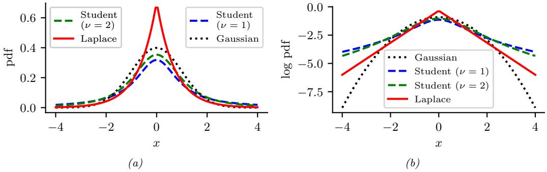
Figure 2.1: (a) The pdf ’s for a N (0, 1), T1(0, 1) and Laplace(0, 1/ ^→2). The mean is 0 and the variance is 1 for both the Gaussian and Laplace. The mean and variance of the Student distribution is undefined when ω = 1. (b) Log of these pdf ’s. Note that the Student distribution is not log-concave for any parameter value, unlike the Laplace distribution. Nevertheless, both are unimodal. Generated by student\_laplace\_pdf\_plot.ipynb.

where ↖ 2ϱε² is the normalization constant needed to ensure the density integrates to 1. The parameter µ encodes the mean of the distribution, which is also equal to the mode. The parameter ε² encodes the variance. Sometimes we talk about the precision of a Gaussian, by which we mean the inverse variance: ϖ = 1/ε². A high precision means a narrow distribution (low variance) centered on µ.

The cumulative distribution function or cdf of the Gaussian is defined as

\[\Phi(x;\mu,\sigma^2) \triangleq \int\_{-\infty}^{x} \mathcal{N}(z|\mu,\sigma^2) dz \tag{2.28}\]

If µ = 0 and ε = 1 (known as the standard normal distribution), we just write #(x).

2.2.2.2 Half-normal

For some problems, we want a distribution over non-negative reals. One way to create such a distribution is to define ^{Y = |}X|, where ^{X ⇔ N} (0, ^ε2). The induced distribution for ^Y is called the half-normal distribution, which has the pdf

\[\mathcal{N}\_{+}(y|\sigma) \triangleq 2\mathcal{N}(y|0, \sigma^{2}) = \frac{\sqrt{2}}{\sigma\sqrt{\pi}} \exp\left(-\frac{y^{2}}{2\sigma^{2}}\right) \quad y \ge 0 \tag{2.29}\]

This can be thought of as the ^N (0, ^ε2) distribution “folded over” onto itself.

2.2.2.3 Student t-distribution

One problem with the Gaussian distribution is that it is sensitive to outliers, since the probability decays exponentially fast with the (squared) distance from the center. A more robust distribution is the Student t-distribution, which we shall call the Student distribution for short. Its pdf is as

follows:

\[\mathcal{T}\_{\nu}(x|\mu,\sigma^2) = \frac{1}{Z} \left[ 1 + \frac{1}{\nu} \left( \frac{x-\mu}{\sigma} \right)^2 \right]^{-\left(\frac{\nu+1}{2}\right)} \tag{2.30}\]

\[Z = \frac{\sqrt{\nu \pi \sigma^2} \Gamma(\frac{\nu}{2})}{\Gamma(\frac{\nu+1}{2})} = \sqrt{\nu} \sigma B(\frac{1}{2}, \frac{\nu}{2}) \tag{2.31}\]

where µ is the mean, ε > 0 is the scale parameter (not the standard deviation), and ς > 0 is called the degrees of freedom (although a better term would be the degree of normality [Kru13], since large values of ς make the distribution act like a Gaussian). Here “(a) is the gamma function defined by

\[ \Gamma(a) \triangleq \int\_0^\infty x^{a-1} e^{-x} dx\tag{2.32} \]

and B(a, b) is the beta function, defined by

\[B(a,b) \triangleq \frac{\Gamma(a)\Gamma(b)}{\Gamma(a+b)}\tag{2.33}\]

2.2.2.4 Cauchy distribution

If ς = 1, the Student distribution is known as the Cauchy or Lorentz distribution. Its pdf is defined by

\[\mathcal{L}(x|\mu,\gamma) = \frac{1}{Z} \left[ 1 + \left(\frac{x-\mu}{\gamma}\right)^2 \right]^{-1} \tag{2.34}\]

where Z = φ↼( ^{1 2} , ^{1 2} ) = φϱ. This distribution is notable for having such heavy tails that the integral that defines the mean does not converge.

The half Cauchy distribution is a version of the Cauchy (with mean 0) that is “folded over” on itself, so all its probability density is on the positive reals. Thus it has the form

\[\mathcal{L}\_{+}(x|\gamma) \triangleq \frac{2}{\pi \gamma} \left[ 1 + \left(\frac{x}{\gamma}\right)^{2} \right]^{-1} \tag{2.35}\]

2.2.2.5 Laplace distribution

Another distribution with heavy tails is the Laplace distribution, also known as the double sided exponential distribution. This has the following pdf:

\[\text{Laplace}(x|\mu, b) \triangleq \frac{1}{2b} \exp\left(-\frac{|x-\mu|}{b}\right) \tag{2.36}\]

Here µ is a location parameter and b > 0 is a scale parameter. See Figure 2.1 for a plot.

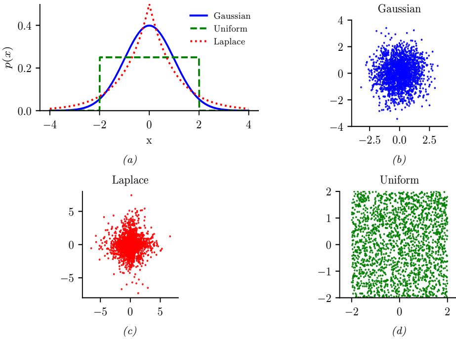
Figure 2.2: Illustration of Gaussian (blue), sub-Gaussian (uniform, green), and super-Gaussian (Laplace, red) distributions in 1d and 2d. Generated by sub\_super\_gauss\_plot.ipynb.

2.2.2.6 Sub-Gaussian and super-Gaussian distributions

There are two main variants of the Gaussian distribution, known as super-Gaussian or leptokurtic (“Lepto” is Greek for “narrow”) and sub-Gaussian or platykurtic (“Platy” is Greek for “broad”). These distributions di!er in terms of their kurtosis, which is a measure of how heavy or light their tails are (i.e., how fast the density dies o! to zero away from its mean). More precisely, the kurtosis is defined as

\[\text{kurt}(z) \triangleq \frac{\mu\_4}{\sigma^4} = \frac{\mathbb{E}\left[ (Z - \mu)^4 \right]}{(\mathbb{E}\left[ (Z - \mu)^2 \right])^2} \tag{2.37}\]

where ε is the standard deviation, and µ⁴ is the 4th central moment. (Thus µ¹ = µ is the mean, and µ² = ε² is the variance.) For a standard Gaussian, the kurtosis is 3, so some authors define the excess kurtosis as the kurtosis minus 3.

A super-Gaussian distribution (e.g., the Laplace) has positive excess kurtosis, and hence heavier tails than the Gaussian. A sub-Gaussian distribution, such as the uniform, has negative excess kurtosis, and hence lighter tails than the Gaussian. See Figure 2.2 for an illustration.

2.2.3 Continuous distributions on R⁺

In this section, we discuss some univariate distributions defined on the positive reals, ^p(x) for ^{x ↑ R+}.

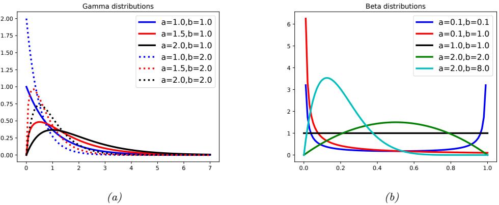
Figure 2.3: (a) Some gamma distributions. If a ↑ 1, the mode is at 0; otherwise the mode is away from 0. As we increase the rate b, we reduce the horizontal scale, thus squeezing everything leftwards and upwards. Generated by gamma\_dist\_plot.ipynb. (b) Some beta distributions. If a < 1, we get a “spike” on the left, and if b < 1, we get a “spike” on the right. If a = b = 1, the distribution is uniform. If a > 1 and b > 1, the distribution is unimodal. Generated by beta\_dist\_plot.ipynb.

2.2.3.1 Gamma distribution

The gamma distribution is a flexible distribution for positive real valued rv’s, x > 0. It is defined in terms of two parameters, called the shape a > 0 and the rate b > 0:

\[\text{Ga}(x|\text{shape}=a, \text{rate}=b) \triangleq \frac{b^a}{\Gamma(a)} x^{a-1} e^{-xb} \tag{2.38}\]

Sometimes the distribution is parameterized in terms of the rate a and the scale s = 1/b:

\[\text{Ga}(x|\text{shape}=a,\text{scale}=s) \stackrel{\Delta}{=} \frac{1}{s^a \Gamma(a)} x^{a-1} e^{-x/s} \tag{2.39}\]

See Figure 2.3a for an illustration.

2.2.3.2 Exponential distribution

The exponential distribution is a special case of the gamma distribution and is defined by

\[\text{Expon}(x|\lambda) \triangleq \text{Ga}(x|\text{shape}=1, \text{rate}=\lambda) \tag{2.40}\]

This distribution describes the times between events in a Poisson process, i.e., a process in which events occur continuously and independently at a constant average rate ϖ.

2.2.3.3 Chi-squared distribution

The chi-squared distribution is a special case of the gamma distribution and is defined by

\[ \chi^2\_\nu(x) \stackrel{\Delta}{=} \text{Ga}(x|\text{shape}=\frac{\nu}{2}, \text{rate}=\frac{1}{2})\tag{2.41} \]

where ς is called the degrees of freedom. This is the distribution of the sum of squared Gaussian random variables. More precisely, if ^{Zi ⇔ N} (0, 1), and ^{S =} #^{ε i}=1 Z^{2 i} , then ^{S ⇔} ↽^{2 ε}. Hence if ^{X ⇔ N} (0, ^ε2) then ^{X2 ⇔ ε}2↽^{2 1}. Since ^E - ↽2 1 . = 1 and V - ↽2 1 . = 2, we have

\[\mathbb{E}\left[X^{2}\right] = \sigma^{2}, \mathbb{V}\left[X^{2}\right] = 2\sigma^{4} \tag{2.42}\]

2.2.3.4 Inverse gamma

The inverse gamma distribution, denoted Y ⇔ IG(a, b), is the distribution of Y = 1/X assuming X ⇔ Ga(a, b). This pdf is defined by

\[\text{IG}(x|\text{shape}=a,\text{scale}=b) \triangleq \frac{b^a}{\Gamma(a)} x^{-(a+1)} e^{-b/x} \tag{2.43}\]

The mean only exists if a > 1. The variance only exists if a > 2.

The scaled inverse chi-squared distribution is a reparameterization of the inverse gamma distribution:

\[\chi^{-2}(x|\nu,\sigma^2) = \text{IG}(x|\text{shape}=\frac{\nu}{2}, \text{scale}=\frac{\nu\sigma^2}{2}) \tag{2.44}\]

\[=\frac{1}{\Gamma(\nu/2)}\left(\frac{\nu\sigma^2}{2}\right)^{\nu/2}x^{-\frac{\nu}{2}-1}\exp\left(-\frac{\nu\sigma^2}{2x}\right)\tag{2.45}\]

The regular inverse chi-squared distribution, written ↽↑^{2 ε} (x), is the special case where ςε² = 1 (i.e., ^ε2 = 1/ς). This corresponds to IG(x|shape ^{= ς}/2,scale ^{= 1} 2 ).

2.2.3.5 Pareto distribution

The Pareto distribution has the following pdf:

\[\text{Pareto}(x|m,\kappa) = \kappa m^{\kappa} \frac{1}{x^{(\kappa+1)}} \mathbb{I}\left(x \ge m\right) \tag{2.46}\]

See Figure 2.4(a) for some plots. We see that x must be greater than the minimum value m, but then the pdf rapidly decays after that. If we plot the distribution on a log-log scale, it forms the straight line log ^p(x) = ⇐^a log ^x + log(c), where ^a = (⇀ + 1) and ^c = ⇀m^ϑ: see Figure 2.4(b) for an illustration.

When m = 0, the distribution has the form p(x) = ⇀x↑^a. This is known as a power law. If a = 1, the distribution has the form p(x) ↙ 1/x; if we interpret x as a frequency, this is called a 1/f function.

The Pareto distribution is useful for modeling the distribution of quantities that exhibit heavy tails or long tails, in which most values are small, but there are a few very large values. Many forms of data exhibit this property. ([ACL16] argue that this is because many datasets are generated by a variety of latent factors, which, when mixed together, naturally result in heavy tailed distributions.) We give some examples below.

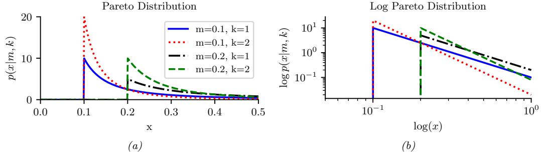
Figure 2.4: (a) The Pareto pdf Pareto(x|k,m). (b) Same distribution on a log-log plot. Generated by pareto\_dist\_plot.ipynb.

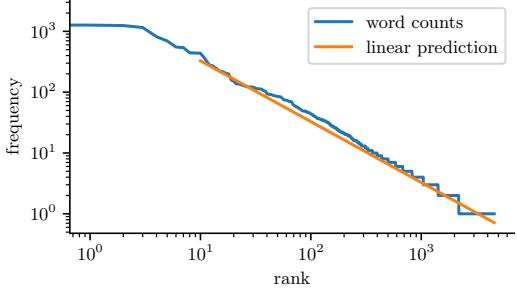
Figure 2.5: A log-log plot of the frequency vs the rank for the words in H. G. Wells’ The Time Machine. Generated by zipfs\_law\_plot.ipynb. Adapted from a figure from [Zha+20a, Sec 8.3].

Modeling wealth distributions

The Pareto distribution is named after the Italian economist and sociologist Vilfredo Pareto. He created it in order to model the distribution of wealth across di!erent countries. Indeed, in economics, the parameter ⇀ is called the Pareto index. If we set ⇀ = 1.16, we recover the 80-20 rule, which states that 80% of the wealth of a society is held by 20% of the population.2

Zipf ’s law

Zipf ’s law says that the most frequent word in a language (such as “the”) occurs approximately twice as often as the second most frequent word (“of”), which occurs twice as often as the fourth most frequent word, etc. This corresponds to a Pareto distribution of the form

\[p(x=r) \propto \kappa r^{-a} \tag{2.47}\]

^2. In fact, wealth distributions are even more skewed than this. For example, as of 2014, 80 billionaires now have as much wealth as 3.5 billion people! (Source: http://www.pbs.org/newshour/making-sense/ wealthiest-getting-wealthier-lobbying-lot.) Such extreme income inequality exists in many plutocratic countries, including the USA (see e.g., [HP10]).

where r is the rank of word x when sorted by frequency, and ⇀ and a are constants. If we set a = 1, we recover Zipf’s law.3 Thus Zipf’s law predicts that if we plot the log frequency of words vs their log rank, we will get a straight line with slope ⇐1. This is in fact true, as illustrated in Figure 2.5. 4 See [Ada00] for further discussion of Zipf’s law, and Section 2.6.2 for a discussion of language models.

2.2.4 Continuous distributions on [0, 1]

In this section, we discuss some univariate distributions defined on the [0, 1] interval.

2.2.4.1 Beta distribution

The beta distribution has support over the interval [0, 1] and is defined as follows:

\[\text{Beta}(x|a,b) = \frac{1}{B(a,b)} x^{a-1} (1-x)^{b-1} \tag{2.48}\]

where B(a, b) is the beta function, which is given by B(a, b) = !(a)!(b) !(a+b) , where “(z) = $ ^{↓ 0} t ^z↑¹e↑^t dt is the gamma function.

We require a, b > 0 to ensure the distribution is integrable (i.e., to ensure B(a, b) exists). If a = b = 1, we get the uniform distribution. If a and b are both less than 1, we get a bimodal distribution with “spikes” at 0 and 1; if a and b are both greater than 1, the distribution is unimodal. See Figure 2.3b.

2.2.5 Multivariate continuous distributions

In this section, we summarize some other widely used multivariate continuous distributions.

2.2.5.1 Multivariate normal (Gaussian)

The multivariate normal (MVN), also called the multivariate Gaussian, is by far the most widely used multivariate distribution. As such, the whole of Section 2.3 is dedicated to it.

2.2.5.2 Multivariate Student distribution

One problem with Gaussians is that they are sensitive to outliers. Fortunately, we can easily extend the Student distribution, discussed in Main Section 2.2.2.3, to D dimensions. In particular, the pdf of the multivariate Student distribution is given by

\[\mathcal{T}\_{\nu}(x|\mu, \Sigma) = \frac{1}{Z} \left[ 1 + \frac{1}{\nu} (x - \mu)^{\mathsf{T}} \Sigma^{-1} (x - \mu) \right]^{-\left(\frac{\nu + D}{2}\right)} \tag{2.49}\]

\[Z = \frac{\Gamma(\nu/2)}{\Gamma(\nu/2 + D/2)} \frac{\nu^{D/2} \pi^{D/2}}{|\Sigma|^{-1/2}}\tag{2.50}\]

where ! is called the scale matrix.

3. For example, p(x = 2) = ϖ2→¹ = 2ϖ4→¹ = 2p(x = 4).

4. We remove the first 10 words from the plot, since they don’t fit the prediction as well.

The Student has fatter tails than a Gaussian. The smaller ς is, the fatter the tails. As ς → ⇒, the distribution tends towards a Gaussian. The distribution has these properties:

\[\text{mean} = \mu, \text{ mode} = \mu, \text{cov} = \frac{\nu}{\nu - 2} \Sigma \tag{2.51}\]

The mean is only well defined (finite) if ς > 1. Similarly, the covariance is only well defined if ς > 2.

2.2.5.3 Circular normal (von Mises Fisher) distribution

Sometimes data lives on the unit sphere, rather than being any point in Euclidean space. For example, any ^D dimensional vector that is ⇁2-normalized lives on the unit (^D ⇐ 1) sphere embedded in ^RD.

There is an extension of the Gaussian distribution that is suitable for such angular data, known as the von Mises-Fisher distribution, or the circular normal distribution. It has the following pdf:

\[\text{vMF}(x|\mu,\kappa) \triangleq \frac{1}{Z} \exp(\kappa \mu^{\mathsf{T}} x) \tag{2.52}\]

\[Z = \frac{(2\pi)^{D/2} I\_{D/2 - 1}(\kappa)}{\kappa^{D/2 - 1}}\tag{2.53}\]

where µ is the mean (with ||µ|| = 1), ⇀ ⇑ 0 is the concentration or precision parameter (analogous to 1/ε for a standard Gaussian), and Z is the normalization constant, with Ir(·) being the modified Bessel function of the first kind and order r. The vMF is like a spherical multivariate Gaussian, parameterized by cosine distance instead of Euclidean distance.

The vMF distribution can be used inside of a mixture model to cluster ⇁2-normalized vectors, as an alternative to using a Gaussian mixture model [Ban+05]. If ⇀ → 0, this reduces to the spherical K-means algorithm. It can also be used inside of an admixture model (Main Section 28.4.2); this is called the spherical topic model [Rei+10].

If D = 2, an alternative is to use the von Mises distribution on the unit circle, which has the form

\[\text{vMF}(x|\mu,\kappa) = \frac{1}{Z} \exp(\kappa \cos(x-\mu))\tag{2.54}\]

\[Z = 2\pi I\_0(\kappa)\tag{2.55}\]

2.2.5.4 Matrix normal distribution (MN)

The matrix normal distribution is defined by the following probability density function over matrices ^{X ↑ Rn}→^p:

\[\mathcal{LM}(\mathbf{X}|\mathbf{M}, \mathbf{U}, \mathbf{V}) \triangleq \frac{|\mathbf{V}|^{n/2}}{2\pi^{np/2}|\mathbf{U}|^{p/2}} \exp\left\{-\frac{1}{2} \text{tr}\left[ (\mathbf{X} - \mathbf{M})^{\mathsf{T}} \mathbf{U}^{-1} (\mathbf{X} - \mathbf{M}) \mathbf{V} \right] \right\} \tag{2.56}\]

where ^{M ↑ Rn}→^p is the mean value of ^X, ^{U ↑ Sn}→ⁿ ++ is the covariance among rows, and ^{V ↑ Sp}→^p ++ is the precision among columns. It can be seen that

\[\text{vec}(\mathbf{X}) \sim \mathcal{N}(\text{vec}(\mathbf{M}), \mathbf{V}^{-1} \otimes \mathbf{U}). \tag{2.57}\]

Note that there is another version of the definition of the matrix normal distribution using the column-covariance matrix V˜ = V↑¹ instead of V, which leads to the density

\[\frac{1}{2\pi^{np/2}|\mathbf{U}|^{p/2}|\tilde{\mathbf{V}}|^{n/2}}\exp\left\{-\frac{1}{2}\text{tr}\left[(\mathbf{X}-\mathbf{M})^{\mathsf{T}}\mathbf{U}^{-1}(\mathbf{X}-\mathbf{M})\tilde{\mathbf{V}}^{-1}\right]\right\}.\tag{2.58}\]

These two versions of definition are obviously equivalent, but we will see that the definition we adopt in Equation (2.56) will lead to a neat update of the posterior distribution (just as the precision matrix is more convenient to use than the covariance matrix in analyzing the posterior of the multivariate normal distribution with a conjugate prior).

2.2.5.5 Wishart distribution

The Wishart distribution is the generalization of the gamma distribution to positive definite matrices. Press [Pre05, p107] has said, “The Wishart distribution ranks next to the normal distribution in order of importance and usefulness in multivariate statistics”. We will mostly use it to model our uncertainty when estimating covariance matrices (see Section 3.4.4).

The pdf of the Wishart is defined as follows:

\[\text{Wi}(\mathbf{S}|\mathbf{S},\nu) \triangleq \frac{1}{Z} |\mathbf{S}|^{(\nu - D - 1)/2} \exp\left(-\frac{1}{2} \text{tr}(\mathbf{S}^{-1}\mathbf{E})\right) \tag{2.59}\]

\[Z \triangleq |\mathbf{S}|^{-\nu/2} 2^{\nu D/2} \Gamma\_D(\nu/2) \tag{2.60}\]

Here ς is called the “degrees of freedom” and S is the “scale matrix”. (We shall get more intuition for these parameters shortly.) The normalization constant only exists (and hence the pdf is only well defined) if ς > D ⇐ 1.

The distribution has these properties:

\[\text{mean} = \nu \mathbf{S}, \text{ mode} = (\nu - D - 1)\mathbf{S} \tag{2.61}\]

Note that the mode only exists if ς > D + 1.

If D = 1, the Wishart reduces to the gamma distribution:

\[\text{Wi}(\lambda|s^{-1}, \nu) = \text{Ga}(\lambda|\text{shape} = \frac{\nu}{2}, \text{rate} = \frac{1}{2s}) \tag{2.62}\]

If s = 2, this reduces to the chi-squared distribution.

There is an interesting connection between the Wishart distribution and the Gaussian. In particular, let ^{xn ⇔ N} (0, !). One can show that the scatter matrix, ^{S =} #^{N n}=1 xnx^{T n}, has a Wishart distribution: S ⇔ Wi(!, N).

2.2.5.6 Inverse Wishart distribution

If ^{ϖ ⇔} Ga(a, b), then that ^{1 ω ⇔} IG(a, b). Similarly, if !^{↑1 ⇔} Wi(S↑¹, ^ς) then ! ^⇔ IW(S, ^ς), where IW is the inverse Wishart, the multidimensional generalization of the inverse gamma. It is defined as follows, for ς > D ⇐ 1 and S ′ 0:

\[\text{IW}(\boldsymbol{\Sigma}|\mathbf{S}^{-1},\nu) = \frac{1}{Z} |\boldsymbol{\Sigma}|^{-(\nu+D+1)/2} \exp\left(-\frac{1}{2} \text{tr}(\mathbf{S}\boldsymbol{\Sigma}^{-1})\right) \tag{2.63}\]

\[Z\_{\rm IW} = |\mathbf{S}|^{\nu/2} 2^{\nu D/2} \Gamma\_D(\nu/2) \tag{2.64}\]

One can show that the distribution has these properties:

\[\text{mean} = \frac{\mathbf{S}}{\nu - D - 1}, \text{ mode} = \frac{\mathbf{S}}{\nu + D + 1} \tag{2.65}\]

If D = 1, this reduces to the inverse gamma:

\[\text{I}\,\text{I}\,\text{W}(\sigma^2|s^{-1},\nu) = \text{IG}(\sigma^2|\nu/2, s/2) \tag{2.66}\]

If s = 1, this reduces to the inverse chi-squared distribution.

2.2.5.7 Dirichlet distribution

A multivariate generalization of the beta distribution is the Dirichlet5 distribution, which has support over the probability simplex, defined by

\[S\_K = \{x : 0 \le x\_k \le 1, \sum\_{k=1}^K x\_k = 1\} \tag{2.67}\]

The pdf is defined as follows:

\[\text{Dir}(x|\alpha) \triangleq \frac{1}{B(\alpha)} \prod\_{k=1}^{K} x\_k^{\alpha\_k - 1} \mathbb{I} \left( x \in S\_K \right) \tag{2.68}\]

where B(ε) is the multivariate beta function,

\[B(\alpha) \stackrel{\Delta}{=} \frac{\prod\_{k=1}^{K} \Gamma(\alpha\_k)}{\Gamma(\sum\_{k=1}^{K} \alpha\_k)}\tag{2.69}\]

Figure 2.6 shows some plots of the Dirichlet when K = 3. We see that α⁰ = # ^k α^k controls the strength of the distribution (how peaked it is), and the α^k control where the peak occurs. For example, Dir(1, 1, 1) is a uniform distribution, Dir(2, 2, 2) is a broad distribution centered at (1/3, 1/3, 1/3), and Dir(20, 20, 20) is a narrow distribution centered at (1/3, 1/3, 1/3). Dir(3, 3, 20) is an asymmetric distribution that puts more density in one of the corners. If α^k < 1 for all k, we get “spikes” at the corners of the simplex. Samples from the distribution when α^k < 1 are sparse, as shown in Figure 2.7.

For future reference, here are some useful properties of the Dirichlet distribution:

\[\mathbb{E}\left[x\_k\right] = \frac{\alpha\_k}{\alpha\_0}, \text{ mode}\left[x\_k\right] = \frac{\alpha\_k - 1}{\alpha\_0 - K}, \text{ V}\left[x\_k\right] = \frac{\alpha\_k(\alpha\_0 - \alpha\_k)}{\alpha\_0^2(\alpha\_0 + 1)}\tag{2.70}\]

where α⁰ = # ^k αk.

Often we use a symmetric Dirichlet prior of the form α^k = α/K. In this case, we have E [xk] = 1/K, and V [xk] = ^K↑^{1 K}2(ϖ+1) . So we see that increasing α increases the precision (decreases the variance) of the distribution.

^5. Johann Dirichlet was a German mathematician, 1805–1859.

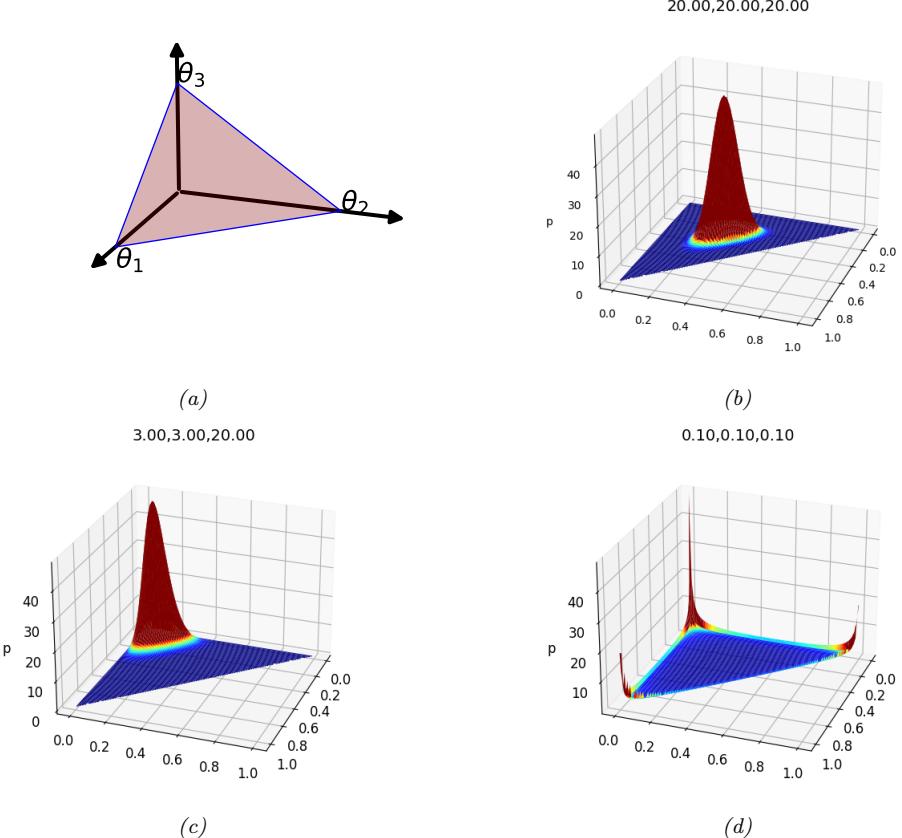
Figure 2.6: (a) The Dirichlet distribution when K = 3 defines a distribution over the simplex, which can be represented by the triangular surface. Points on this surface satisfy ^{0 ↑ εc ↑ 1} and !^{3 c}=1 ε^c = 1. Generated by dirichlet\_3d\_triangle\_plot.ipynb. (b) Plot of the Dirichlet density for ω = (20, 20, 20). (c) Plot of the Dirichlet density for ω = (3, 3, 20). (d) Plot of the Dirichlet density for ω = (0.1, 0.1, 0.1). Generated by dirichlet\_3d\_spiky\_plot.ipynb.

The Dirichlet distribution is useful for distinguishing aleatoric (data) uncertainty from epistemic uncertainty. To see this, consider a 3-sided die. If we know that each outcome is equally likely, we can use a “peaky” symmetric Dirichlet, such as Dir(20, 20, 20), shown in Figure 2.6(b); this reflects the fact that we are sure the outcomes will be unpredictable. By contrast, if we are not sure what the outcomes will be like (e.g., it could be a biased die), then we can use a “flat” symmetric Dirichlet, such as Dir(1, 1, 1), which can generate a wide range of possible outcome distributions. We can make the Dirichlet distribution be conditional on inputs, resulting in what is called a prior network [MG18], since it encodes p(ϑ|x) (output is a distributon) rather than p(y|x) (output is a label).

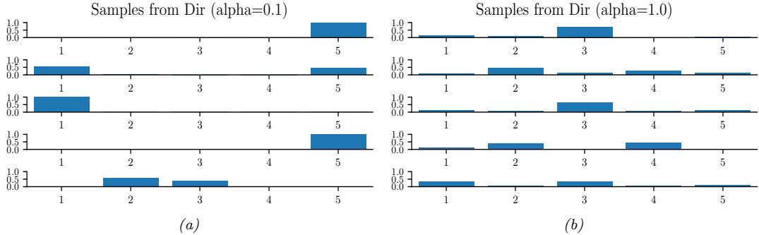
Figure 2.7: Samples from a 5-dimensional symmetric Dirichlet distribution for di!erent parameter values. (a) ω = (0.1,…, 0.1). This results in very sparse distributions, with many 0s. (b) ω = (1,…, 1). This results in more uniform (and dense) distributions. Generated by dirichlet\_samples\_plot.ipynb.

2.3 Gaussian joint distributions

The most widely used joint probability distribution for continuous random variables is the multivariate Gaussian or multivariate normal (MVN). The popularity is partly because this distribution is mathematically convenient, but also because the Gaussian assumption is fairly reasonable in many cases. Indeed, the Gaussian is the distribution with maximum entropy subject to having specified first and second moments (Section 2.4.7). In view of its importance, this section discusses the Gaussian distribution in detail.

2.3.1 The multivariate normal

In this section, we discuss the multivariate Gaussian or multivariate normal in detail.

2.3.1.1 Definition

The MVN density is defined by the following:

\[\mathcal{N}(x|\mu, \Sigma) \triangleq \frac{1}{(2\pi)^{D/2} |\Sigma|^{1/2}} \, \exp\left[ -\frac{1}{2} (x - \mu)^{\mathsf{T}} \Sigma^{-1} (x - \mu) \right] \tag{2.71}\]

where ^µ = ^E [x] ^{↑ RD} is the mean vector, and ! = Cov [x] is the ^{D ∞ D} covariance matrix. The normalization constant ^Z = (2ϱ)D/²|!^{| 1}/² just ensures that the pdf integrates to 1. The expression inside the exponential (ignoring the factor of ⇐0.5) is the squared Mahalanobis distance between the data vector x and the mean vector µ, given by

\[d\_{\Sigma}(x,\mu)^2 = (x-\mu)^{\mathsf{T}}\Sigma^{-1}(x-\mu) \tag{2.72}\]

In 2d, the MVN is known as the bivariate Gaussian distribution. Its pdf can be represented as ^{x ⇔ N} (µ, !), where ^{x ↑ R2}, ^{µ ↑ R2} and

\[ \Sigma = \begin{pmatrix} \sigma\_1^2 & \sigma\_{12}^2 \\ \sigma\_{21}^2 & \sigma\_2^2 \end{pmatrix} = \begin{pmatrix} \sigma\_1^2 & \rho \sigma\_1 \sigma\_2 \\ \rho \sigma\_1 \sigma\_2 & \sigma\_2^2 \end{pmatrix} \tag{2.73} \]

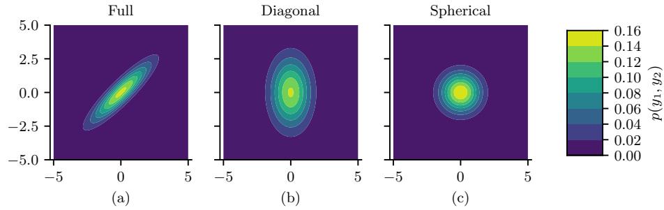
Figure 2.8: Visualization of a 2d Gaussian density in terms of level sets of constant probability density. (a) A full covariance matrix has elliptical contours. (b) A diagonal covariance matrix is an axis aligned ellipse. (c) A spherical covariance matrix has a circular shape. Generated by gauss\_plot\_2d.ipynb.

where the correlation coe”cient is given by ^ρ ↭ ^ϱ2 12 ^ϱ1ϱ² .

Figure 2.8 plots some MVN densities in 2d for three di!erent kinds of covariance matrices. A full covariance matrix has D(D + 1)/2 parameters, where we divide by 2 since ! is symmetric. A diagonal covariance matrix has D parameters, and has 0s in the o!-diagonal terms. A spherical covariance matrix, also called isotropic covariance matrix, has the form ! = ε²ID, so it only has one free parameter, namely ε².

2.3.1.2 Gaussian shells

Multivariate Gaussians can behave rather counterintuitively in high dimensions. In particular, we can ask: if we draw samples x ⇔ N (0, ID), where D is the number of dimensions, where do we expect most of the x to lie? Since the peak (mode) of the pdf is at the origin, it is natural to expect most samples to be near the origin. However, in high dimensions, the typical set of a Gaussian is a thin shell or annulus with a distance from origin given by r = ε ↖ D and a thickness of O(εD ^{1 4} ). The intuitive reason for this is as follows: although the density decays as e↑r2/², meaning density decreases from the origin, the volume of a sphere grows as r^D, meaning volume increases from the origin, and since mass is density times volume, the majority of points end up in this annulus where these two terms “balance out”. This is called the “Gaussian soap bubble” phenomenon, and is illustrated in Figure 2.9. 6

To see why the typical set for a Gaussian is concentrated in a thin annulus at radius ↖ D, consider the squared distance of a point ^x from the origin, ^d(x) = #^{D i}=1 x^{2 i} , where xⁱ ⇔ N (0, 1). The expected squared distance is given by E d². = #^{D i}=1 ^E x2 i . = D, and the variance of the squared distance is given by V d². = #^{D i}=1 ^V x2 i . = D. As D grows, the coe”cient of variation (i.e., the SD relative to the mean) goes to zero:

\[\lim\_{D \to \infty} \frac{\text{std}\left[d^2\right]}{\mathbb{E}\left[d^2\right]} = \lim\_{D \to \infty} \frac{\sqrt{D}}{D} = 0 \tag{2.74}\]

^6. For a more detailed explanation, see this blog post by Ferenc Huszar: https://www.inference.vc/ high-dimensional-gaussian-distributions-are-soap-bubble/.

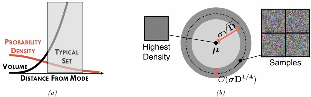
Figure 2.9: (a) Cartoon illustration of why the typical set of a Gaussian is not centered at the mode of the distribution. (b) Illustration of the typical set of a Gaussian, which is concentrated in a thin annulus of thickness ϑD¹/⁴ and distance ϑD¹/² from the origin. We also show an image with the highest density (the all gray image on the left). as well as some high probability samples (the speckle noise images on the right). From Figure 1 of [Nal+19a]. Used with kind permission of Eric Nalisnick.

Thus the expected square distance concentrates around D, so the expected distance concentrates around ^E [d(x)] ⁼ ↖ D. See [Ver18] for a more rigorous proof, and Section 5.2.3 for a discussion of typical sets.

To see what this means in the context of images, in Figure 2.9b, we show some grayscale images that are sampled from a Gaussian of the form ^N (µ, ^ε2I), where ^µ corresponds to the all-gray image. However, it is extremely unlikely that randomly sampled images would be close to all-gray, as shown in the figure.

2.3.1.3 Marginals and conditionals of an MVN

Let us partition our vector of random variables x into two parts, x¹ and x2, so

\[ \mu = \begin{pmatrix} \mu\_1 \\ \mu\_2 \end{pmatrix}, \quad \Sigma = \begin{pmatrix} \Sigma\_{11} & \Sigma\_{12} \\ \Sigma\_{21} & \Sigma\_{22} \end{pmatrix} \tag{2.75} \]

The marginals of this distribution are given by the following (see Section 2.3.1.5 for the proof):

\[p(\mathbf{x}\_1) = \int \mathcal{N}(\mathbf{x}|\boldsymbol{\mu}, \boldsymbol{\Sigma}) d\boldsymbol{x}\_2 \stackrel{\scriptstyle \Delta}{=} \mathcal{N}(\boldsymbol{x}\_1|\boldsymbol{\mu}\_1^m, \boldsymbol{\Sigma}\_1^m) = \mathcal{N}(\boldsymbol{x}\_1|\boldsymbol{\mu}\_1, \boldsymbol{\Sigma}\_{11}) \tag{2.76}\]

\[p(\mathbf{x}\_2) = \int \mathcal{N}(\mathbf{x}|\boldsymbol{\mu}, \boldsymbol{\Sigma}) d\boldsymbol{x}\_1 \stackrel{\scriptstyle \Delta}{=} \mathcal{N}(\boldsymbol{x}\_2|\boldsymbol{\mu}\_2^m, \boldsymbol{\Sigma}\_2^m) = \mathcal{N}(\boldsymbol{x}\_2|\boldsymbol{\mu}\_2, \boldsymbol{\Sigma}\_{22}) \tag{2.77}\]

The conditional distributions can be shown to have the following form (see Section 2.3.1.5 for the proof):

\[p(\mathbf{x}\_1|\mathbf{x}\_2) = \mathcal{N}(\mathbf{x}\_1|\mu\_{1|2}^c, \Sigma\_{1|2}^c) = \mathcal{N}(\mathbf{x}\_1|\mu\_1 + \Sigma\_{12}\Sigma\_{22}^{-1}(\mathbf{x}\_2 - \mu\_2), \ \Sigma\_{11} - \Sigma\_{12}\Sigma\_{22}^{-1}\Sigma\_{21})\tag{2.78}\]

\[p(\mathbf{x}\_2|\mathbf{x}\_1) = \mathcal{N}(\mathbf{x}\_2|\boldsymbol{\mu}\_{2|1}^c, \boldsymbol{\Sigma}\_{2|1}^c) = \mathcal{N}(\mathbf{x}\_2|\boldsymbol{\mu}\_2 + \boldsymbol{\Sigma}\_{21}\boldsymbol{\Sigma}\_{11}^{-1}(\mathbf{x}\_1 - \boldsymbol{\mu}\_1), \,\boldsymbol{\Sigma}\_{22} - \boldsymbol{\Sigma}\_{21}\boldsymbol{\Sigma}\_{11}^{-1}\boldsymbol{\Sigma}\_{12})\tag{2.79}\]

Note that the posterior mean of p(x1|x2) is a linear function of x2, but the posterior covariance is independent of x2; this is a peculiar property of Gaussian distributions.

2.3.1.4 Information (canonical) form

It is common to parameterize the MVN in terms of the mean vector µ and the covariance matrix !. However, for reasons which are explained in Section 2.4.2.5, it is sometimes useful to represent the Gaussian distribution using canonical parameters or natural parameters, defined as

\[ \Lambda \triangleq \Sigma^{-1}, \quad \eta \triangleq \Sigma^{-1}\mu \tag{2.80} \]

The matrix ” = !^↑1 is known as the precision matrix, and the vector ϖ is known as the precision-weighted mean. We can convert back to the more familiar moment parameters using

\[ \mu = \boldsymbol{\Lambda}^{-1} \boldsymbol{\eta}, \quad \boldsymbol{\Sigma} = \boldsymbol{\Lambda}^{-1} \tag{2.81} \]

Hence we can write the MVN in canonical form (also called information form) as follows:

\[\mathcal{N}\_c(x|\eta,\Lambda) \triangleq c \exp\left(x^\top \eta - \frac{1}{2} x^\top \Lambda x\right) \tag{2.82}\]

\[c \stackrel{\triangle}{=} \frac{\exp(-\frac{1}{2}\eta^{\mathsf{T}}\Lambda^{-1}\eta)}{(2\pi)^{D/2}\sqrt{\det(\Lambda^{-1})}}\tag{2.83}\]

where we use the notation Nc() to distinguish it from the standard parameterization N (). For more information on moment and natural parameters, see Section 2.4.2.5.

It is also possible to derive the marginalization and conditioning formulas in information form (see Section 2.3.1.6 for the derivation). For the marginals we have

\[p(\mathbf{x}\_1) = \mathcal{N}\_c(\mathbf{x}\_1|\boldsymbol{\eta}\_1^m, \boldsymbol{\Lambda}\_1^m) = \mathcal{N}\_c(\mathbf{x}\_1|\boldsymbol{\eta}\_1 - \boldsymbol{\Lambda}\_{12}\boldsymbol{\Lambda}\_{22}^{-1}\boldsymbol{\eta}\_2, \boldsymbol{\Lambda}\_{11} - \boldsymbol{\Lambda}\_{12}\boldsymbol{\Lambda}\_{22}^{-1}\boldsymbol{\Lambda}\_{21})\tag{2.84}\]

\[p(\mathbf{x}\_2) = \mathcal{N}\_c(\mathbf{x}\_2|\boldsymbol{\eta}\_2^m, \boldsymbol{\Lambda}\_2^m) = \mathcal{N}\_c(\mathbf{x}\_2|\boldsymbol{\eta}\_2 - \boldsymbol{\Lambda}\_{21}\boldsymbol{\Lambda}\_{11}^{-1}\boldsymbol{\eta}\_1, \boldsymbol{\Lambda}\_{22} - \boldsymbol{\Lambda}\_{21}\boldsymbol{\Lambda}\_{11}^{-1}\boldsymbol{\Lambda}\_{12})\tag{2.85}\]

For the conditionals we have

\[p(\mathbf{x}\_1|\mathbf{x}\_2) = \mathcal{N}\_c(\mathbf{x}\_1|\eta\_{1|2}^c, \Lambda\_{1|2}^c) = \mathcal{N}\_c(\mathbf{x}\_1|\eta\_1 - \Lambda\_{12}\mathbf{x}\_2, \Lambda\_{11})\tag{2.86}\]

\[p(\mathbf{x}\_2|\mathbf{x}\_1) = \mathcal{N}\_c(\mathbf{x}\_2|\eta\_{2\mid 1}^c, \Lambda\_{2\mid 1}^c) = \mathcal{N}\_c(\mathbf{x}\_2|\eta\_2 - \Lambda\_{21}\mathbf{x}\_1, \Lambda\_{22}) \tag{2.87}\]

Thus we see that marginalization is easier in moment form, and conditioning is easier in information form.

2.3.1.5 Derivation: moment form

In this section, we derive Equation (2.77) and Equation (2.78) for marginalizing and conditioning an MVN in moment form.

Before we dive in, we need to introduce the following result, for the inverse of a partitioned matrix of the form

\[\mathbf{M} = \begin{pmatrix} \mathbf{E} & \mathbf{F} \\ \mathbf{G} & \mathbf{H} \end{pmatrix} \tag{2.88}\]

where we assume E and H are invertible. One can show (see e.g., [Mur22, Sec 7.3.2] for the proof) that

\[\mathbf{M}^{-1} = \begin{pmatrix} (\mathbf{M}/\mathbf{H})^{-1} & -(\mathbf{M}/\mathbf{H})^{-1}\mathbf{F}\mathbf{H}^{-1} \\ -\mathbf{H}^{-1}\mathbf{G}(\mathbf{M}/\mathbf{H})^{-1} & \mathbf{H}^{-1} + \mathbf{H}^{-1}\mathbf{G}(\mathbf{M}/\mathbf{H})^{-1}\mathbf{F}\mathbf{H}^{-1} \end{pmatrix} \tag{2.89}\]

\[\begin{aligned} \mathbf{E} &= \begin{pmatrix} \mathbf{E}^{-1} + \mathbf{E}^{-1} \mathbf{F} (\mathbf{M}/\mathbf{E})^{-1} \mathbf{G} \mathbf{E}^{-1} & -\mathbf{E}^{-1} \mathbf{F} (\mathbf{M}/\mathbf{E})^{-1} \\ -(\mathbf{M}/\mathbf{E})^{-1} \mathbf{G} \mathbf{E}^{-1} & (\mathbf{M}/\mathbf{E})^{-1} \end{pmatrix} \end{aligned} \tag{2.90}\]

where

\[\mathbf{M}/\mathbf{H} \stackrel{\Delta}{=} \mathbf{E} - \mathbf{F}\mathbf{H}^{-1}\mathbf{G} \tag{2.91}\]

\[\mathbf{M}/\mathbf{E} \stackrel{\Delta}{=} \mathbf{H} - \mathbf{G}\mathbf{E}^{-1}\mathbf{F} \tag{2.92}\]

We say that M/H is the Schur complement of M wrt H, and M/E is the Schur complement of M wrt E.

From the above, we also have the following important result, known as the matrix inversion lemma or the Sherman-Morrison-Woodbury formula:

\[\left(\mathbf{M}/\mathbf{H}\right)^{-1} = \left(\mathbf{E} - \mathbf{F}\mathbf{H}^{-1}\mathbf{G}\right)^{-1} = \mathbf{E}^{-1} + \mathbf{E}^{-1}\mathbf{F}(\mathbf{H} - \mathbf{G}\mathbf{E}^{-1}\mathbf{F})^{-1}\mathbf{G}\mathbf{E}^{-1} \tag{2.93}\]

Now we return to the derivation of the MVN conditioning equation. Let us factor the joint p(x1, x2) as p(x2)p(x1|x2) as follows:

\[p(\mathbf{x}\_1, \mathbf{x}\_2) \propto \exp\left\{ -\frac{1}{2} \begin{pmatrix} \mathbf{x}\_1 - \boldsymbol{\mu}\_1 \\ \mathbf{x}\_2 - \boldsymbol{\mu}\_2 \end{pmatrix}^{\mathsf{T}} \begin{pmatrix} \boldsymbol{\Sigma}\_{11} & \boldsymbol{\Sigma}\_{12} \\ \boldsymbol{\Sigma}\_{21} & \boldsymbol{\Sigma}\_{22} \end{pmatrix}^{-1} \begin{pmatrix} \boldsymbol{x}\_1 - \boldsymbol{\mu}\_1 \\ \boldsymbol{x}\_2 - \boldsymbol{\mu}\_2 \end{pmatrix} \right\} \tag{2.94}\]

Using the equation for the inverse of a block structured matrix, the above exponent becomes

\[p(\mathbf{z}\_1, \mathbf{z}\_2) \propto \exp\left\{ -\frac{1}{2} \begin{pmatrix} \mathbf{z}\_1 - \mu\_1 \\ \mathbf{z}\_2 - \mu\_2 \end{pmatrix}^{\mathsf{T}} \begin{pmatrix} \mathbf{I} & \mathbf{0} \\ -\Sigma\_{22}^{-1} \Sigma\_{21} & \mathbf{I} \end{pmatrix} \begin{pmatrix} (\Sigma/\Sigma\_{22})^{-1} & \mathbf{0} \\ \mathbf{0} & \Sigma\_{22}^{-1} \end{pmatrix} \right\} \tag{2.95}\]

\[\times \begin{pmatrix} \mathbf{I} & -\Sigma\_{12}\Sigma\_{22}^{-1} \\ \mathbf{0} & \mathbf{I} \end{pmatrix} \begin{pmatrix} x\_1 - \mu\_1 \\ x\_2 - \mu\_2 \end{pmatrix} \end{pmatrix} \tag{2.96}\]

\[=\exp\left\{-\frac{1}{2}(\mathbf{z}\_1-\boldsymbol{\mu}\_1-\boldsymbol{\Sigma}\_{12}\boldsymbol{\Sigma}\_{22}^{-1}(\mathbf{z}\_2-\boldsymbol{\mu}\_2))^\top(\boldsymbol{\Sigma}/\boldsymbol{\Sigma}\_{22})^{-1}\tag{2.97}\]

\[\left\{ (\mathbf{x}\_1 - \boldsymbol{\mu}\_1 - \boldsymbol{\Sigma}\_{12} \boldsymbol{\Sigma}\_{22}^{-1} (\mathbf{x}\_2 - \boldsymbol{\mu}\_2)) \right\} \times \exp\left\{ -\frac{1}{2} (\mathbf{x}\_2 - \boldsymbol{\mu}\_2)^\mathsf{T} \boldsymbol{\Sigma}\_{22}^{-1} (\mathbf{x}\_2 - \boldsymbol{\mu}\_2) \right\} \tag{2.98}\]

This is of the form

\[\exp(\text{quadratic form in } \mathbf{z}\_1, \mathbf{z}\_2) \times \exp(\text{quadratic form in } \mathbf{z}\_2) \tag{2.99}\]

Hence we have successfully factorized the joint as

\[p(\mathbf{x}\_1, \mathbf{x}\_2) = p(\mathbf{x}\_1 | \mathbf{x}\_2) p(\mathbf{x}\_2) \tag{2.100}\]

\[=\mathcal{N}(x\_1|\mu\_{1|2}, \Sigma\_{1|2})\mathcal{N}(x\_2|\mu\_2, \Sigma\_{22})\tag{2.101}\]

where

\[ \mu\_{1|2} = \mu\_1 + \Sigma\_{12} \Sigma\_{22}^{-1} (x\_2 - \mu\_2) \tag{2.102} \]

\[ \Delta\_{1|2} = \Sigma / \Sigma\_{22} \stackrel{\Delta}{=} \Sigma\_{11} - \Sigma\_{12} \Sigma\_{22}^{-1} \Sigma\_{21} \tag{2.103} \]

where !/!²² is as the Schur complement of ! wrt !22.

2.3.1.6 Derivation: information form

In this section, we derive Equation (2.85) and Equation (2.86) for marginalizing and conditioning an MVN in information form.

First we derive the conditional formula.7 Let us partition the information form parameters as follows:

\[\boldsymbol{\eta} = \begin{pmatrix} \eta\_1 \\ \eta\_2 \end{pmatrix}, \quad \boldsymbol{\Lambda} = \begin{pmatrix} \boldsymbol{\Lambda}\_{11} & \boldsymbol{\Lambda}\_{12} \\ \boldsymbol{\Lambda}\_{21} & \boldsymbol{\Lambda}\_{22} \end{pmatrix} \tag{2.104}\]

We can now write the joint log probabilty of x1, x² as

\[\ln p(\mathbf{z}\_1, \mathbf{z}\_2) = -\frac{1}{2} \begin{pmatrix} \mathbf{z}\_1 \\ \mathbf{z}\_2 \end{pmatrix}^{\mathsf{T}} \begin{pmatrix} \mathbf{A}\_{11} & \mathbf{A}\_{12} \\ \mathbf{A}\_{21} & \mathbf{A}\_{22} \end{pmatrix} \begin{pmatrix} \mathbf{x}\_1 \\ \mathbf{x}\_2 \end{pmatrix} + \begin{pmatrix} \mathbf{z}\_1 \\ \mathbf{z}\_2 \end{pmatrix}^{\mathsf{T}} \begin{pmatrix} \eta\_1 \\ \eta\_2 \end{pmatrix} + \text{const.} \tag{2.105}\]

\[\begin{aligned} \mathbf{x} &= -\frac{1}{2} \mathbf{x}\_1^\mathsf{T} \mathbf{A}\_{11} \mathbf{x}\_1 - \frac{1}{2} \mathbf{x}\_2^\mathsf{T} \mathbf{A}\_{22} \mathbf{x}\_2 - \frac{1}{2} \mathbf{x}\_1^\mathsf{T} \mathbf{A}\_{12} \mathbf{x}\_2 - \frac{1}{2} \mathbf{x}\_2^\mathsf{T} \mathbf{A}\_{21} \mathbf{x}\_1 \\ &+ \mathbf{x}\_1^\mathsf{T} \boldsymbol{\eta}\_1 + \mathbf{x}\_2^\mathsf{T} \boldsymbol{\eta}\_2 + \text{const.} \end{aligned} \tag{2.106}\]

where the constant term does not depend on x¹ or x2.

To calculate the parameters of the conditional distribution p(x1|x2), we fix the value of x² and collect the terms which are quadratic in x¹ for the conditional precision and then linear in x¹ for the conditional precision-weighted mean. The terms which are quadratic in ^x1 are just ⇐¹ 2x^{T 1}“11x1, and hence

\[ \Lambda\_{1|2}^c = \Lambda\_{11} \tag{2.107} \]

The terms which are linear in x¹ are

\[-\frac{1}{2}x\_1^\mathsf{T}\Lambda\_{12}x\_2 - \frac{1}{2}x\_2^\mathsf{T}\Lambda\_{21}x\_1 + x\_1^\mathsf{T}\eta\_1 = x\_1^\mathsf{T}(\eta\_1 - \Lambda\_{12}x\_2) \tag{2.108}\]

since “^{T 21} =”12. Thus the conditional precision-weighted mean is

\[ \eta\_{1|2}^c = \eta\_1 - \Lambda\_{12} x\_2. \tag{2.109} \]

We will now derive the results for marginalizing in information form. The marginal, p(x2), can be calculated by integrating the joint, p(x1, x2), with respect to x1:

\[\begin{split} p(\mathbf{x}\_{2}) &= \int p(\mathbf{x}\_{1}, \mathbf{x}\_{2}) d\mathbf{x}\_{1} \\ &\propto \int \exp\left\{ -\frac{1}{2} \mathbf{x}\_{1}^{\mathsf{T}} \boldsymbol{\Lambda}\_{11} \boldsymbol{x}\_{1} - \frac{1}{2} \mathbf{x}\_{2}^{\mathsf{T}} \boldsymbol{\Lambda}\_{22} \boldsymbol{x}\_{2} - \frac{1}{2} \mathbf{x}\_{1}^{\mathsf{T}} \boldsymbol{\Lambda}\_{12} \boldsymbol{x}\_{2} - \frac{1}{2} \mathbf{x}\_{2}^{\mathsf{T}} \boldsymbol{\Lambda}\_{21} \boldsymbol{x}\_{1} + \mathbf{x}\_{1}^{\mathsf{T}} \boldsymbol{\eta}\_{1} + \mathbf{x}\_{2}^{\mathsf{T}} \boldsymbol{\eta}\_{2} \right\} d\mathbf{x}\_{1}, \end{split} \tag{2.110}\]

Author: Kevin P. Murphy. (C) MIT Press. CC-BY-NC-ND license

(2.111)

^7. This derivation is due to Giles Harper-Donnelly.

where the terms in the exponent have been decomposed into the partitioned structure in Equation (2.104) as in Equation (2.106). Next, collecting all the terms involving x1,

\[p(\mathbf{z}\_2) \propto \exp\left\{-\frac{1}{2}\mathbf{z}\_2^\mathsf{T}\boldsymbol{\Lambda}\_{22}\mathbf{z}\_2 + \mathbf{z}\_2^\mathsf{T}\boldsymbol{\eta}\_2\right\} \int \exp\left\{-\frac{1}{2}\mathbf{z}\_1^\mathsf{T}\boldsymbol{\Lambda}\_{11}\mathbf{z}\_1 + \mathbf{z}\_1^\mathsf{T}(\boldsymbol{\eta}\_1 - \boldsymbol{\Lambda}\_{12}\mathbf{z}\_2)\right\} d\boldsymbol{x}\_1,\tag{2.112}\]

we can recognize the integrand as an exponential quadratic form. Therefore the integral is equal to the normalizing constant of a Gaussian with precision, “11, and precision weighted mean, ϖ¹ ⇐”12x2, which is given by the reciprocal of Equation (2.83). Substituting this in to our equation we have,

\[p(\mathbf{z}\_2) \propto \exp\left\{-\frac{1}{2}\mathbf{z}\_2^\mathsf{T}\boldsymbol{\Lambda}\_{22}\boldsymbol{x}\_2 + \mathbf{z}\_2^\mathsf{T}\boldsymbol{\eta}\_2\right\} \exp\left\{\frac{1}{2}(\boldsymbol{\eta}\_1 - \boldsymbol{\Lambda}\_{12}\boldsymbol{x}\_2)^\mathsf{T}\boldsymbol{\Lambda}\_{11}^{-1}(\boldsymbol{\eta}\_1 - \boldsymbol{\Lambda}\_{12}\boldsymbol{x}\_2)\right\} \tag{2.113}\]

\[\propto \exp\left\{ -\frac{1}{2} \mathbf{x}\_2^\mathsf{T} \boldsymbol{\Lambda}\_{22} \boldsymbol{x}\_2 + \mathbf{x}\_2^\mathsf{T} \boldsymbol{\eta}\_2 + \frac{1}{2} \mathbf{x}\_2^\mathsf{T} \boldsymbol{\Lambda}\_{21} \boldsymbol{\Lambda}\_{11}^{-1} \boldsymbol{\Lambda}\_{12} \boldsymbol{x}\_2 - \mathbf{x}\_2^\mathsf{T} \boldsymbol{\Lambda}\_{21} \boldsymbol{\Lambda}\_{11}^{-1} \boldsymbol{\eta}\_1 \right\} \tag{2.114}\]

\[=\exp\left\{-\frac{1}{2}x\_2^\mathsf{T}(\boldsymbol{\Lambda}\_{22}-\boldsymbol{\Lambda}\_{21}\boldsymbol{\Lambda}\_{11}^{-1}\boldsymbol{\Lambda}\_{12})\boldsymbol{x}\_2+x\_2^\mathsf{T}(\eta\_2-\boldsymbol{\Lambda}\_{21}\boldsymbol{\Lambda}\_{11}^{-1}\boldsymbol{\eta}\_1)\right\},\tag{2.115}\]

which we now recognise as an exponential quadratic form in x2. Extract the quadratic terms to get the marginal precision,

\[ \Lambda\_{22}^m = \Lambda\_{22} - \Lambda\_{21} \Lambda\_{11}^{-1} \Lambda\_{12}, \tag{2.116} \]

and the linear terms to get the marginal precision-weighted mean,

\[ \eta\_2^m = \eta\_2 - \Lambda\_{21} \Lambda\_{11}^{-1} \eta\_1. \tag{2.117} \]

2.3.2 Linear Gaussian systems

Consider two random vectors ^{y ↑ RD} and ^{z ↑ RL}, which are jointly Gaussian with the following joint distribution:

\[p(\mathbf{z}) = \mathcal{N}(\mathbf{z}|\check{\boldsymbol{\mu}}, \check{\boldsymbol{\Sigma}}) \tag{2.118}\]

\[p(y|z) = N(y|\mathbf{W}z + b, \Omega) \tag{2.119}\]

where W is a matrix of size D ∞ L. This is an example of a linear Gaussian system.

2.3.2.1 Joint distribution

The corresponding joint distribution, p(z, y) = p(z)p(y|z), is itself a D + L dimensional Gaussian, with mean and covariance given by the following (this result can be obtained by moment matching):

\[p(\mathbf{z}, \mathbf{y}) = \mathcal{N}(\mathbf{z}, \mathbf{y} | \bar{\mu}, \bar{\Sigma}) \tag{2.120a}\]

\[ \check{\mu} \triangleq \begin{pmatrix} \check{\mu} \\ m \end{pmatrix} \triangleq \begin{pmatrix} \check{\mu} \\ \mathbf{W} \ \check{\mu} + \mathbf{b} \end{pmatrix} \tag{2.120b} \]

\[ \begin{aligned} \boldsymbol{\tilde{\Sigma}} \triangleq \begin{pmatrix} \boldsymbol{\breve{\Sigma}} & \mathbf{C}^{\mathsf{T}} \\ \mathbf{C} & \mathbf{S} \end{pmatrix} \triangleq \begin{pmatrix} \boldsymbol{\breve{\Sigma}} & \boldsymbol{\breve{\Sigma}} \,\mathbf{W}^{\mathsf{T}} \\ \mathbf{W} \,\boldsymbol{\breve{\Sigma}} & \mathbf{W} \,\boldsymbol{\breve{\Sigma}} \,\mathbf{W}^{\mathsf{T}} + \boldsymbol{\Omega} \end{pmatrix} \tag{2.120c} \\ \tag{2.120c} \end{aligned} \]

See Algorithm 8.1 on page 369 for some pseudocode to compute this joint distribution.

2.3.2.2 Posterior distribution (Bayes’ rule for Gaussians)

Now we consider computing the posterior p(z|y) from a linear Gaussian system. Using Equation (2.78) for conditioning a joint Gaussian, we find that the posterior is given by

\[p(\mathbf{z}|\mathbf{y}) = \mathcal{N}(\mathbf{z}|\,\hat{\mathbf{p}}, \hat{\mathbf{z}}) \tag{2.121a}\]

\[ \hat{\boldsymbol{\mu}} = \check{\boldsymbol{\mu}} + \check{\boldsymbol{\Sigma}} \,\,\mathbf{W}^{\mathsf{T}} (\boldsymbol{\Omega} + \mathbf{W} \,\,\check{\boldsymbol{\Sigma}} \,\,\mathbf{W}^{\mathsf{T}})^{-1} (\boldsymbol{y} - (\mathbf{W} \,\,\check{\boldsymbol{\mu}} + \boldsymbol{b})) \tag{2.121b} \]

\[ \hat{\Sigma} = \check{\Sigma} - \check{\Sigma}^{\prime} \mathbf{W}^{\dagger} (\mathbf{\Omega} + \mathbf{W}^{\prime} \check{\Sigma}^{\prime} \mathbf{W}^{\dagger})^{-1} \mathbf{W}^{\prime} \check{\Sigma} \tag{2.121c} \]

This is known as Bayes’ rule for Gaussians. We see that if the prior p(z) is Gaussian, and the likelihood p(y|z) is Gaussian, then the posterior p(z|y) is also Gaussian. We therefore say that the Gaussian prior is a conjugate prior for the Gaussian likelihood, since the posterior distribution has the same type as the prior. (In other words, Gaussians are closed under Bayesian updating.)

We can simplify these equations by defining S = W ↭ ! W^T + #, C =↭ ! W^T, and m = W ↭µ +b, as in Equation (2.120). We also define the Kalman gain matrix: 8

\[\mathbf{K} = \mathbf{C} \mathbf{S}^{-1} \tag{2.122}\]

From this, we get the posterior

\[ \hat{\mu} = \check{\mu} + \mathbf{K}(y - m) \tag{2.123} \]

\[ \hat{\boldsymbol{\Sigma}} = \check{\boldsymbol{\Sigma}} - \mathbf{K} \mathbf{C}^{\mathsf{T}} \tag{2.124} \]

Note that

\[\mathbf{K}\mathbf{S}\mathbf{K}^{\mathsf{T}} = \mathbf{C}\mathbf{S}^{-1}\mathbf{S}\mathbf{S}^{-\mathsf{T}}\mathbf{C}^{\mathsf{T}} = \mathbf{C}\mathbf{S}^{-1}\mathbf{C}^{\mathsf{T}} = \mathbf{K}\mathbf{C}^{\mathsf{T}} \tag{2.125}\]

and hence we can also write the posterior covariance as

\[ \hat{\Delta} = \check{\Sigma} - \mathbf{K} \mathbf{S} \mathbf{K}^{\mathsf{T}} \tag{2.126} \]

Using the matrix inversion lemma from Equation (2.93), we can also rewrite the posterior in the following form [Bis06, p93], which takes O(L³) time instead of O(D³) time:

\[ \hat{\mathbf{E}} = (\breve{\mathbf{E}}^{-1} + \mathbf{W}^{\mathsf{T}} \Omega^{-1} \mathbf{W})^{-1} \tag{2.127} \]

\[ \hat{\boldsymbol{\mu}} = \hat{\boldsymbol{\Sigma}} \left[ \mathbf{W}^{\mathsf{T}} \boldsymbol{\Omega}^{-1} \left( \boldsymbol{y} - \mathbf{b} \right) + \check{\boldsymbol{\Sigma}}^{-1} \check{\boldsymbol{\mu}} \right] \tag{2.128} \]

Finally, note that the corresponding normalization constant for the posterior is just the marginal on y evaluated at the observed value:

\[p(y) = \int \mathcal{N}(z \mid \boldsymbol{\mu}, \check{\mathbf{X}}) \mathcal{N}(y \mid \mathbf{W}z + \mathbf{b}, \boldsymbol{\Omega}) dz\]

\[= \mathcal{N}(y \mid \mathbf{W} \nmid +\mathbf{b}, \boldsymbol{\Omega} + \mathbf{W} \not\to \mathbf{W}^{\mathsf{T}}) = \mathcal{N}(y \mid m, \mathbf{S}) \tag{2.129}\]

From this, we can easily compute the log marginal likelihood. We summarize all these equations in Algorithm 8.1.

^8. The name comes from the Kalman filter algorithm, which we discuss in Section 8.2.2.

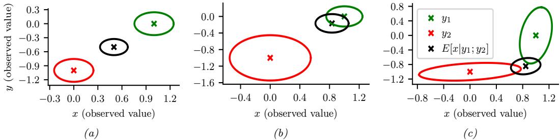
Figure 2.10: We observe x = (0, ↓1) (red cross) and y = (1, 0) (green cross) and estimate E [z|x, y, ε] (black cross). (a) Equally reliable sensors, so the posterior mean estimate is in between the two circles. (b) Sensor 2 is more reliable, so the estimate shifts more towards the green circle. (c) Sensor 1 is more reliable in the vertical direction, Sensor 2 is more reliable in the horizontal direction. The estimate is an appropriate combination of the two measurements. Generated by sensor\_fusion\_2d.ipynb.

2.3.2.3 Example: Sensor fusion with known measurement noise

Suppose we have an unknown quantity of interest, z ⇔ N (µz, !z), from which we get two noisy measurements, x ⇔ N (z, !x) and y ⇔ N (z, !y). Pictorially, we can represent this example as x ∈ z → y. This is an example of a linear Gaussian system. Our goal is to combine the evidence together, to compute p(z|x, y; ω). This is known as sensor fusion. (In this section, we assume ω = (!x, !y) is known. See Supplementary Section 2.1.2 for the general case.)

We can combine x and y into a single vector v, so the model can be represented as z → v, where p(v|z) = N (v|Wz, !v), where W = [I; I] and !^v = [!x, 0; 0, !y] are block-structured matrices. We can then apply Bayes’ rule for Gaussians (Section 2.3.2.2) to compute p(z|v).

Figure 2.10(a) gives a 2d example, where we set !^x = !^y = 0.01I2, so both sensors are equally reliable. In this case, the posterior mean is halfway between the two observations, x and y. In Figure 2.10(b), we set !^x = 0.05I² and !^y = 0.01I2, so sensor 2 is more reliable than sensor 1. In this case, the posterior mean is closer to y. In Figure 2.10(c), we set

\[ \Sigma\_x = 0.01 \begin{pmatrix} 10 & 1 \\ 1 & 1 \end{pmatrix}, \quad \Sigma\_y = 0.01 \begin{pmatrix} 1 & 1 \\ 1 & 10 \end{pmatrix} \tag{2.130} \]

so sensor 1 is more reliable in the second component (vertical direction), and sensor 2 is more reliable in the first component (horizontal direction). In this case, the posterior mean is vertically closer to x and horizontally closer to y.

2.3.3 A general calculus for linear Gaussian systems

In this section, we discuss a general method for performing inference in linear Gaussian systems. The key is to define joint distributions over the relevant variables in terms of a potential function, represented in information form. We can then easily derive rules for marginalizing potentials, multiplying and dividing potentials, and conditioning them on observations. Once we have defined these operations, we can use them inside of the belief propagation algorithm (Section 9.3) or junction tree algorithm (Supplementary Section 9.2) to compute quantities of interest. We give the details on how to perform these operations below; our presentation is based on [Lau92; Mur02].

2.3.3.1 Moment and canonical parameterization

We can represent a Gaussian distribution in moment form or in canonical (information) form. In moment form we have

\[\phi(x; p, \mu, \Sigma) = p \times \exp\left(-\frac{1}{2}(x - \mu)^{\mathsf{T}}\Sigma^{-1}(x - \mu)\right) \tag{2.131}\]

where ^p = (2ϱ)↑n/²|!^{| ↑ 1 2} is the normalizing constant that ensures $ ^x ▷(x; p, µ, !)=1. (n is the dimensionality of x.) Expanding out the quadratic form and collecting terms we get the canonical form:

\[\phi(\mathbf{x}; g, \hbar, \mathbf{K}) = \exp\left(g + \mathbf{x}^{\mathsf{T}}\hbar - \frac{1}{2}\mathbf{x}^{\mathsf{T}}\mathbf{K}\mathbf{x}\right) = \exp\left(g + \sum\_{i} h\_{i}x\_{i} - \frac{1}{2}\sum\_{i}\sum\_{k} K\_{ij}x\_{i}x\_{j}\right) \tag{2.132}\]

where

\[\mathbf{K} = \boldsymbol{\Sigma}^{-1} \tag{2.133}\]

\[h = \Sigma^{-1} \mu \tag{2.134}\]

\[g = \log p - \frac{1}{2} \mu^{\mathsf{T}} \mathbf{K} \mu \tag{2.135}\]

K is often called the precision matrix.

Note that potentials need not be probability distributions, and need not be normalizable (integrate to 1). We keep track of the constant terms (p or g) so we can compute the likelihood of the evidence.

2.3.3.2 Multiplication and division

We can define multiplication and division in the Gaussian case by using canonical forms, as follows. To multiply ▷1(x1,…,xk; g1, h1, K1) by ▷2(xk+1,…,xn; g2, h2, K2), we extend them both to the same domain x1,…,xⁿ by adding zeros to the appropriate dimensions, and then computing

\[(g\_1, \mathbf{h}\_1, \mathbf{K}\_1) \* (g\_2, \mathbf{h}\_2, \mathbf{K}\_2) = (g\_1 + g\_2, \mathbf{h}\_1 + \mathbf{h}\_2, \mathbf{K}\_1 + \mathbf{K}\_2) \tag{2.136}\]

Division is defined as follows:

\[((g\_1, \mathbf{h}\_1, \mathbf{K}\_1) / (g\_2, \mathbf{h}\_2, \mathbf{K}\_2) = (g\_1 - g\_2, \mathbf{h}\_1 - \mathbf{h}\_2, \mathbf{K}\_1 - \mathbf{K}\_2) \tag{2.137}\]

2.3.3.3 Marginalization

Let ▷^W be a potential over a set W of variables. We can compute the potential over a subset V △ W of variables by marginalizing, denoted ▷^V = # ^W<sup>V ^▷W . Let

\[\mathbf{x} = \begin{pmatrix} x\_1 \\ x\_2 \end{pmatrix}, \qquad \boldsymbol{h} = \begin{pmatrix} \boldsymbol{h}\_1 \\ \boldsymbol{h}\_2 \end{pmatrix}, \qquad \mathbf{K} = \begin{pmatrix} \mathbf{K}\_{11} & \mathbf{K}\_{12} \\ \mathbf{K}\_{21} & \mathbf{K}\_{22} \end{pmatrix}, \tag{2.138}\]

with x¹ having dimension n¹ and x² having dimension n2. It can be shown that

\[\int\_{\mathfrak{w}\_1} \phi(\mathbf{x}\_1, \mathbf{x}\_2; g, \hbar, \mathbf{K}) = \phi(\mathbf{x}\_2; \hat{g}, \hat{\hbar}, \hat{\mathbf{K}}) \tag{2.139}\]

where

\[\hat{g} = g + \frac{1}{2} \left( n\_1 \log(2\pi) - \log|\mathbf{K}\_{11}| + h\_1^\mathrm{T} \mathbf{K}\_{11}^{-1} h\_1 \right) \tag{2.140}\]

\[ \hat{h} = h\_2 - \mathbf{K}\_{21}\mathbf{K}\_{11}^{-1}h\_1 \tag{2.141} \]

\[ \hat{\mathbf{K}} = \mathbf{K}\_{22} - \mathbf{K}\_{21} \mathbf{K}\_{11}^{-1} \mathbf{K}\_{12} \tag{2.142} \]

2.3.3.4 Conditioning on evidence

Consider a potential defined on (x, y). Suppose we observe the value y. The new potential is given by the following reduced dimensionality object:

\[\phi^\*(\mathbf{x}) = \exp\left[g + \begin{pmatrix} \mathbf{z}^T & \mathbf{y}^T \end{pmatrix} \begin{pmatrix} \mathbf{h}\_X \\ \mathbf{h}\_Y \end{pmatrix} - \frac{1}{2} \begin{pmatrix} \mathbf{z}^T & \mathbf{y}^T \end{pmatrix} \begin{pmatrix} \mathbf{K}\_{XX} & \mathbf{K}\_{XY} \\ \mathbf{K}\_{YX} & \mathbf{K}\_{YY} \end{pmatrix} \begin{pmatrix} \mathbf{z} \\ \mathbf{y} \end{pmatrix}\right] \tag{2.143}\]

\[=\exp\left[\left(g+h\_Y^Ty-\frac{1}{2}y^T\mathbf{K}\_{YY}y\right)+x^T(h\_X-\mathbf{K}\_{XY}y)-\frac{1}{2}x^T\mathbf{K}\_{XX}x\right]\tag{2.144}\]

This generalizes the corresponding equation in [Lau92] to the vector-valued case.

2.3.3.5 Converting a linear-Gaussian CPD to a canonical potential

Finally we discuss how to create the initial potentials, assuming we start with a directed Gaussian graphical model. In particular, consider a node with a linear-Gaussian conditional probability distribution (CPD):

\[p(\mathbf{z}|\mathbf{u}) = c \exp\left[ -\frac{1}{2} \left( (\mathbf{z} - \boldsymbol{\mu} - \mathbf{B}^T \mathbf{u})^T \boldsymbol{\Sigma}^{-1} (\mathbf{z} - \boldsymbol{\mu} - \mathbf{B}^T \mathbf{u}) \right) \right] \tag{2.145}\]

\[\mathbf{x} = \exp\left[-\frac{1}{2}\begin{pmatrix} x & u \end{pmatrix} \begin{pmatrix} \Sigma^{-1} & -\Sigma^{-1}\mathbf{B}^{T} \\ -\mathbf{B}\Sigma^{-1} & \mathbf{B}\Sigma^{-1}\mathbf{B}^{T} \end{pmatrix} \begin{pmatrix} x \\ u \end{pmatrix} \tag{2.146}\]

\[+\begin{pmatrix} x & u \end{pmatrix} \begin{pmatrix} \Sigma^{-1}\mu \\ -\mathbf{B}\Sigma^{-1}\mu \end{pmatrix} -\frac{1}{2}\mu^T\Sigma^{-1}\mu + \log c \bigg|\tag{2.147}\]

where ^c = (2ϱ)↑n/²|!^{| ↑ 1 2} . Hence we set the canonical parameters to

\[g = -\frac{1}{2}\mu^T \Sigma^{-1} \mu - \frac{n}{2}\log(2\pi) - \frac{1}{2}\log|\Sigma|\tag{2.148}\]

\[h = \begin{pmatrix} \Sigma^{-1}\mu \\ -\mathbf{B}\Sigma^{-1}\mu \end{pmatrix} \tag{2.149}\]

\[\mathbf{K} = \begin{pmatrix} \boldsymbol{\Sigma}^{-1} & -\boldsymbol{\Sigma}^{-1} \mathbf{B}^{T} \\ -\mathbf{B} \boldsymbol{\Sigma}^{-1} & \mathbf{B} \boldsymbol{\Sigma}^{-1} \mathbf{B}^{T} \end{pmatrix} = \begin{pmatrix} \mathbf{I} \\ -\mathbf{B} \end{pmatrix} \boldsymbol{\Sigma}^{-1} \begin{pmatrix} \mathbf{I} & -\mathbf{B} \end{pmatrix} \tag{2.150}\]

In the special case that x is a scalar, the corresponding result can be found in [Lau92]. In particular

we have $↑¹ = 1/ε² , B = b and n = 1, so the above becomes

\[g = \frac{-\mu^2}{2\sigma^2} - \frac{1}{2}\log(2\pi\sigma^2) \tag{2.151}\]

\[h = \frac{\mu}{\sigma^2} \begin{pmatrix} 1 \\ -b \end{pmatrix} \tag{2.152}\]

\[\mathbf{K} = \frac{1}{\sigma} \begin{pmatrix} 1 & -b^T \\ -b & bb^T \end{pmatrix}. \tag{2.153}\]

2.3.3.6 Example: Product of Gaussians

As an application of the above results, we can derive the (unnormalized) product of two Gaussians, as follows (see also [Kaa12, Sec 8.1.8]):

\[\mathcal{N}(x|\mu\_1, \Sigma\_1) \times \mathcal{N}(x|\mu\_2, \Sigma\_2) \propto \mathcal{N}(x|\mu\_3, \Sigma\_3) \tag{2.154}\]

where

\[ \Delta \Sigma\_3 = \left(\Sigma\_1^{-1} + \Sigma\_2^{-1}\right)^{-1} \tag{2.155} \]

\[ \mu\_3 = \Sigma\_3(\Sigma\_1^{-1}\mu\_1 + \Sigma\_2^{-1}\mu\_2) \tag{2.156} \]

We see that the posterior precision is a sum of the individual precisions, and the posterior mean is a precision-weighted combination of the individual means. We can also rewrite the result in the following way, which only requires one matrix inversion:

\[ \Sigma\_3 = \Sigma\_1 \left(\Sigma\_1 + \Sigma\_2\right)^{-1} \Sigma\_2 \tag{2.157} \]

\[ \mu\_3 = \Sigma\_2 (\Sigma\_1 + \Sigma\_2)^{-1} \mu\_1 + \Sigma\_1 (\Sigma\_1 + \Sigma\_2)^{-1} \mu\_2 \tag{2.158} \]

In the scalar case, this becomes

\[\mathcal{N}(x|\mu\_1, \sigma\_1^2)\mathcal{N}(x|\mu\_2, \sigma\_2^2) \propto \mathcal{N}\left(x|\frac{\mu\_1\sigma\_2^2 + \mu\_2\sigma\_1^2}{\sigma\_1^2 + \sigma\_2^2}, \frac{\sigma\_1^2\sigma\_2^2}{\sigma\_1^2 + \sigma\_2^2}\right) \tag{2.159}\]

2.4 The exponential family

In this section, we define the exponential family, which includes many common probability distributions. The exponential family plays a crucial role in statistics and machine learning, for various reasons, including the following:

• The exponential family is the unique family of distributions that has maximum entropy (and hence makes the least set of assumptions) subject to some user-chosen constraints, as discussed in Section 2.4.7.

• The exponential family is at the core of GLMs, as discussed in Section 15.1.

• The exponential family is at the core of variational inference, as discussed in Chapter 10.

• Under certain regularity conditions, the exponential family is the only family of distributions with finite-sized su”cient statistics, as discussed in Section 2.4.5.

• All members of the exponential family have a conjugate prior [DY79], which simplifies Bayesian inference of the parameters, as discussed in Section 3.4.

2.4.1 Definition

Consider a family of probability distributions parameterized by ^{ϖ ↑ RK} with fixed support over ^{X D ↓ RD}. We say that the distribution ^p(x|ϖ) is in the exponential family if its density can be written in the following way:

\[p(x|\eta) \triangleq \frac{1}{Z(\eta)} h(x) \exp[\eta^{\mathsf{T}} \mathcal{T}(x)] = h(x) \exp[\eta^{\mathsf{T}} \mathcal{T}(x) - A(\eta)] \tag{2.160}\]

where ^h(x) is a scaling constant (also known as the base measure, often 1), ^T (x) ^{↑ RK} are the su!cient statistics, ϖ are the natural parameters or canonical parameters, Z(ϖ) is a normalization constant known as the partition function, and A(ϖ) = log Z(ϖ) is the log partition function. In Section 2.4.3, we show that A is a convex function over the convex set ! ↭ {^{ϖ ↑ RK} : ^A(ϖ) ^&lt; ^⇒}.

It is convenient if the natural parameters are independent of each other. Formally, we say that an exponential family is minimal if there is no ^{ϖ ↑ RK}  {0} such that ^ϖTT (x)=0. This last condition can be violated in the case of multinomial distributions, because of the sum to one constraint on the parameters; however, it is easy to reparameterize the distribution using K ⇐ 1 independent parameters, as we show below.

Equation (2.160) can be generalized by defining ϖ = f(ϱ), where ϱ is some other, possibly smaller, set of parameters. In this case, the distribution has the form

\[p(\mathbf{z}|\phi) = h(\mathbf{z}) \exp[f(\phi)^\mathsf{T}\mathcal{T}(\mathbf{z}) - A(f(\phi))] \tag{2.161}\]

If the mapping from ϱ to ϖ is nonlinear, we call this a curved exponential family. If ϖ = f(ϱ) = ϱ, the model is said to be in canonical form. If, in addition, T (x) = x, we say this is a natural exponential family or NEF. In this case, it can be written as

\[p(\mathbf{z}|\boldsymbol{\eta}) = h(\mathbf{z}) \exp[\boldsymbol{\eta}^{\mathsf{T}}\boldsymbol{x} - A(\boldsymbol{\eta})] \tag{2.162}\]

We define the moment parameters as the mean of the su”cient statistics vector:

\[m = \mathbb{E}\left[\mathcal{T}(x)\right] \tag{2.163}\]

We will see some examples below.

2.4.2 Examples

In this section, we consider some common examples of distributions in the exponential family. Each corresponds to a di!erent way of defining h(x) and T (x) (since Z and hence A are derived from knowing h and T ).

2.4.2.1 Bernoulli distribution

The Bernoulli distribution can be written in exponential family form as follows:

\[\text{Ber}(x|\mu) = \mu^x (1-\mu)^{1-x} \tag{2.164}\]

\[=\exp[x\log(\mu)+(1-x)\log(1-\mu)]\tag{2.165}\]

\[\hat{\eta}\_t = \exp[\mathcal{T}(x)^\mathsf{T}\eta] \tag{2.166}\]

where T (x)=[I(x = 1),I(x = 0)], ϖ = [log(µ), log(1 ⇐ µ)], and µ is the mean parameter. However, this is an over-complete representation since there is a linear dependendence between the features. We can see this as follows:

\[\mathbb{1}^{\mathsf{T}}\mathcal{T}(x) = \mathbb{1}(x=0) + \mathbb{1}(x=1) = 1\tag{2.167}\]

If the representation is overcomplete, ϖ is not uniquely identifiable. It is common to use a minimal representation, which means there is a unique ϖ associated with the distribution. In this case, we can just define

\[\text{Ber}(x|\mu) = \exp\left[x \log\left(\frac{\mu}{1-\mu}\right) + \log(1-\mu)\right] \tag{2.168}\]

We can put this into exponential family form by defining

\[\eta = \log\left(\frac{\mu}{1-\mu}\right) \tag{2.169}\]

\[\mathcal{T}(x) = x^{\frac{1}{2}} \tag{2.170}\]

\[A(\eta) = -\log(1 - \mu) = \log(1 + e^{\eta})\tag{2.171}\]

\[h(x) = 1\tag{2.172}\]

We can recover the mean parameter µ from the canonical parameter ◁ using

\[ \mu = \sigma(\eta) = \frac{1}{1 + e^{-\eta}} \tag{2.173} \]

which we recognize as the logistic (sigmoid) function.

2.4.2.2 Categorical distribution

We can represent the discrete distribution with K categories as follows (where x^k = I(x = k)):

\[\text{Cat}(x|\mu) = \prod\_{k=1}^{K} \mu\_k^{x\_k} = \exp\left[\sum\_{k=1}^{K} x\_k \log \mu\_k\right] \tag{2.174}\]

\[\hat{\mu} = \exp\left[\sum\_{k=1}^{K-1} x\_k \log \mu\_k + \left(1 - \sum\_{k=1}^{K-1} x\_k\right) \log(1 - \sum\_{k=1}^{K-1} \mu\_k)\right] \tag{2.175}\]

\[\hat{\mu} = \exp\left[\sum\_{k=1}^{K-1} x\_k \log\left(\frac{\mu\_k}{1 - \sum\_{j=1}^{K-1} \mu\_j}\right) + \log(1 - \sum\_{k=1}^{K-1} \mu\_k)\right] \tag{2.176}\]

\[=\exp\left[\sum\_{k=1}^{K-1} x\_k \log\left(\frac{\mu\_k}{\mu\_K}\right) + \log \mu\_K\right] \tag{2.177}\]

where ^µK = 1 ⇐ #^K↑^{1 k}=1 µk. We can write this in exponential family form as follows:

\[\text{Cat}(x|\eta) = \exp(\eta^{\mathsf{T}}\mathcal{T}(x) - A(\eta))\tag{2.178}\]

\[\eta = [\log \frac{\mu\_1}{\mu\_K}, \dots, \log \frac{\mu\_{K-1}}{\mu\_K}] \tag{2.179}\]

\[A(\eta) = -\log(\mu\_K) \tag{2.180}\]

\[\mathcal{T}(x) = [\mathbb{I}\left(x = 1\right), \dots, \mathbb{I}\left(x = K - 1\right)] \tag{2.181}\]

\[h(x) = 1\tag{2.182}\]

We can recover the mean parameters from the canonical parameters using

\[\mu\_k = \frac{e^{\eta\_k}}{1 + \sum\_{j=1}^{K-1} e^{\eta\_j}} \tag{2.183}\]

If we define ◁^K = 0, we can rewrite this as follows:

\[\mu\_k = \frac{e^{\eta\_k}}{\sum\_{j=1}^K e^{\eta\_j}} \tag{2.184}\]

for k =1: K. Hence µ = softmax(ϖ), where softmax is the softmax or multinomial logit function in Equation (15.136). From this, we find

\[\mu\_K = 1 - \frac{\sum\_{k=1}^{K-1} e^{\eta\_k}}{1 + \sum\_{k=1}^{K-1} e^{\eta\_k}} = \frac{1}{1 + \sum\_{k=1}^{K-1} e^{\eta\_k}} \tag{2.185}\]

and hence

\[A(\eta) = -\log(\mu\_K) = \log\left(\sum\_{k=1}^{K} e^{\eta\_k}\right) \tag{2.186}\]

2.4.2.3 Univariate Gaussian

The univariate Gaussian is usually written as follows:

\[\mathcal{N}(x|\mu,\sigma^2) = \frac{1}{(2\pi\sigma^2)^{\frac{1}{2}}} \exp[-\frac{1}{2\sigma^2}(x-\mu)^2] \tag{2.187}\]

\[=\frac{1}{(2\pi)^{\frac{1}{2}}}\exp[\frac{\mu}{\sigma^2}x-\frac{1}{2\sigma^2}x^2-\frac{1}{2\sigma^2}\mu^2-\log\sigma] \tag{2.188}\]

We can put this in exponential family form by defining

\[\eta = \begin{pmatrix} \mu/\sigma^2\\ -\frac{1}{2\sigma^2} \end{pmatrix} \tag{2.189}\]

\[\mathcal{T}(x) = \begin{pmatrix} x \\ x^2 \end{pmatrix} \tag{2.190}\]

\[A(\eta) = \frac{\mu^2}{2\sigma^2} + \log \sigma = \frac{-\eta\_1^2}{4\eta\_2} - \frac{1}{2}\log(-2\eta\_2) \tag{2.191}\]

\[h(x) = \frac{1}{\sqrt{2\pi}}\tag{2.192}\]

The moment parameters are

\[\mathbf{m} = [\mu, \mu^2 + \sigma^2] \tag{2.193}\]

2.4.2.4 Univariate Gaussian with fixed variance

If we fix ε² = 1, we can write the Gaussian as a natural exponential family, by defining

\[ \eta = \mu \tag{2.194} \]

\[T(x) = x \tag{2.195}\]

\[A(\mu) = \frac{\mu^2}{2\sigma^2} + \log \sigma = \frac{\mu^2}{2} \tag{2.196}\]

\[h(x) = \frac{1}{\sqrt{2\pi}} \exp[-\frac{x^2}{2}] = \mathcal{N}(x|0, 1) \tag{2.197}\]

Note that this in example, the base measure h(x) is not constant.

2.4.2.5 Multivariate Gaussian

It is common to parameterize the multivariate normal (MVN) in terms of the mean vector µ and the covariance matrix !. The corresponding pdf is given by

\[\mathcal{N}(x|\mu, \Sigma) = \frac{1}{(2\pi)^{D/2}\sqrt{\det(\Sigma)}} \exp\left(-\frac{1}{2}x^{\mathsf{T}}\Sigma^{-1}x + x^{\mathsf{T}}\Sigma^{-1}\mu - \frac{1}{2}\mu^{\mathsf{T}}\Sigma^{-1}\mu\right) \tag{2.198}\]

\[\hat{\mu} = c \exp\left(\boldsymbol{x}^{\mathsf{T}} \boldsymbol{\Sigma}^{-1} \boldsymbol{\mu} - \frac{1}{2} \boldsymbol{x}^{\mathsf{T}} \boldsymbol{\Sigma}^{-1} \boldsymbol{x}\right) \tag{2.199}\]

\[c \stackrel{\Delta}{=} \frac{\exp(-\frac{1}{2}\mu^T \Sigma^{-1} \mu)}{(2\pi)^{D/2} \sqrt{\det(\Sigma)}}\tag{2.200}\]

However, we can also represent the Gaussian using canonical parameters or natural parameters, also called the information form:

\[ \Lambda = \Sigma^{-1} \tag{2.201} \]

\[ \xi = \Sigma^{-1} \mu \tag{2.202} \]

\[\mathcal{N}\_c(x|\xi,\Lambda) \triangleq c' \exp\left(x^\mathsf{T}\xi - \frac{1}{2}x^\mathsf{T}\Lambda x\right) \tag{2.203}\]

\[c' = \frac{\exp(-\frac{1}{2}\boldsymbol{\xi}^{\mathsf{T}}\boldsymbol{\Lambda}^{-1}\boldsymbol{\xi})}{(2\pi)^{D/2}\sqrt{\det(\boldsymbol{\Lambda}^{-1})}}\tag{2.204}\]

where we use the notation Nc() to distinguish it from the standard parameterization N (). Here ” is called the precision matrix and ς is the precision-weighted mean vector.

We can convert this to exponential family notation as follows:

\[\mathcal{N}\_c(x|\xi,\Lambda) = \underbrace{(2\pi)^{-D/2}}\_{h(\mathfrak{a})} \underbrace{\exp\left[\frac{1}{2}\log|\Lambda| - \frac{1}{2}\xi^T\Lambda^{-1}\xi\right]}\_{g(\mathfrak{n})} \exp\left[-\frac{1}{2}x^\top\Lambda x + x^\top\xi\right] \tag{2.205}\]

\[\mathbf{x} = h(\boldsymbol{x})g(\boldsymbol{\eta})\exp\left[-\frac{1}{2}\boldsymbol{x}^{\mathsf{T}}\boldsymbol{\Lambda}\boldsymbol{x} + \boldsymbol{x}^{\mathsf{T}}\boldsymbol{\xi}\right]\_{\mathsf{T}}\tag{2.206}\]

\[\mathbf{x} = h(\mathbf{x})g(\boldsymbol{\eta})\exp\left[-\frac{1}{2}(\sum\_{ij}x\_ix\_j\Lambda\_{ij}) + \mathbf{z}^\top\boldsymbol{\xi}\right] \tag{2.207}\]

\[=h(x)g(\eta)\exp\left[-\frac{1}{2}\text{vec}(\boldsymbol{\Lambda})^{\mathsf{T}}\text{vec}(\boldsymbol{x}\boldsymbol{x}^{\mathsf{T}}) + \boldsymbol{x}^{\mathsf{T}}\boldsymbol{\xi}\right] \tag{2.208}\]

\[=h(\mathbf{z})\exp\left[\boldsymbol{\eta}^{\mathsf{T}}\mathcal{T}(\mathbf{z}) - A(\boldsymbol{\eta})\right] \tag{2.209}\]

where

\[h(\mathbf{z}) = (2\pi)^{-D/2} \tag{2.210}\]

\[\eta = [\xi; -\frac{1}{2}\text{vec}(\Lambda)] = [\Sigma^{-1}\mu; -\frac{1}{2}\text{vec}(\Sigma^{-1})] \tag{2.211}\]

\[\mathcal{T}(\mathbf{x}) = [\mathbf{x}; \text{vec}(\mathbf{x}\mathbf{x}^{\mathsf{T}})] \tag{2.212}\]

\[A(\eta) = -\log g(\eta) = -\frac{1}{2}\log|\Lambda| + \frac{1}{2}\xi^T \Lambda^{-1} \xi \tag{2.213}\]

From this, we see that the mean (moment) parameters are given by

\[m = \mathbb{E}\left[\mathcal{T}(x)\right] = \left[\mu; \mu\mu^{\mathsf{T}} + \Sigma\right] \tag{2.214}\]

(Note that the above is not a minimal representation, since ” is a symmetric matrix. We can convert to minimal form by working with the upper or lower half of each matrix.)

2.4.2.6 Non-examples

Not all distributions of interest belong to the exponential family. For example, the Student distribution (Section 2.2.2.3) does not belong, since its pdf (Equation (2.30)) does not have the required form. (However, there is a generalization, known as the ▷-exponential family [Nau04; Tsa88] which does include the Student distribution.)

As a more subtle example, consider the uniform distribution, Y ⇔ Unif(ϑ1, ϑ2). The pdf has the form

\[p(y|\theta) = \frac{1}{\theta\_2 - \theta\_1} \mathbb{I}\left(\theta\_1 \le y \le \theta\_2\right) \tag{2.215}\]

It is tempting to think this is in the exponential family, with h(y)=1, T (y) = 0, and Z(ω) = ϑ² ⇐ ϑ1. However, the support of this distribution (i.e., the set of values Y = {y : p(y) > 0}) depends on the parameters ω, which violates an assumption of the exponential family.

2.4.3 Log partition function is cumulant generating function

The first and second cumulants of a distribution are its mean E [X] and variance V [X], whereas the first and second moments are E [X] and E - X². . We can also compute higher order cumulants (and moments). An important property of the exponential family is that derivatives of the log partition function can be used to generate all the cumulants of the su”cient statistics. In particular, the first and second cumulants are given by

\[\nabla\_{\eta}A(\eta) = \mathbb{E}\left[\mathcal{T}(x)\right] \tag{2.216}\]

\[\nabla^2\_{\eta} A(\eta) = \text{Cov}\left[\mathcal{T}(x)\right] \tag{2.217}\]

We prove this result below.

2.4.3.1 Derivation of the mean

For simplicity, we focus on the 1d case. For the first derivative we have

\[\frac{dA}{d\eta} = \frac{d}{d\eta} \left( \log \int \exp(\eta \mathcal{T}(x)) h(x) dx \right) \tag{2.218}\]

\[\eta = \frac{\frac{d}{d\eta} \int \exp(\eta \mathcal{T}(x)) h(x) dx}{\int \exp(\eta \mathcal{T}(x)) h(x) dx} \tag{2.219}\]

\[=\frac{\int \mathcal{T}(x) \exp(\eta \mathcal{T}(x)) h(x) dx}{\exp(A(\eta))}\tag{2.220}\]

\[=\int \mathcal{T}(x) \exp(\eta \mathcal{T}(x) - A(\eta)) h(x) dx \tag{2.221}\]

\[=\int \mathcal{T}(x)p(x)dx = \mathbb{E}\left[\mathcal{T}(x)\right] \tag{2.222}\]

For example, consider the Bernoulli distribution. We have A(◁) = log(1 + e^ς), so the mean is given by

\[\frac{dA}{d\eta} = \frac{e^{\eta}}{1 + e^{\eta}} = \frac{1}{1 + e^{-\eta}} = \sigma(\eta) = \mu \tag{2.223}\]

2.4.3.2 Derivation of the variance

For simplicity, we focus on the 1d case. For the second derivative we have

\[\frac{d^2A}{d\eta^2} = \frac{d}{d\eta} \int \mathcal{T}(x) \exp(\eta \mathcal{T}(x) - A(\eta)) h(x) dx \tag{2.224}\]

\[=\int \mathcal{T}(x) \exp\left(\eta \mathcal{T}(x) - A(\eta)\right) h(x) (\mathcal{T}(x) - A'(\eta)) dx \tag{2.225}\]

\[I = \int \mathcal{T}(x) p(x) (\mathcal{T}(x) - A'(\eta)) dx \tag{2.226}\]

\[I = \int \mathcal{T}^2(x)p(x)dx - A'(\eta)\int \mathcal{T}(x)p(x)dx\tag{2.227}\]

\[=\mathbb{E}\left[\mathcal{T}^2(X)\right] - \mathbb{E}\left[\mathcal{T}(x)\right]^2 = \mathbb{V}\left[\mathcal{T}(x)\right] \tag{2.228}\]

where we used the fact that A^↔︎ (◁) = dA ^dς = E [T (x)]. For example, for the Bernoulli distribution we have

\[\frac{d^2A}{d\eta^2} = \frac{d}{d\eta}(1 + e^{-\eta})^{-1} = (1 + e^{-\eta})^{-2}e^{-\eta} \tag{2.229}\]

\[=\frac{e^{-\eta}}{1+e^{-\eta}}\frac{1}{1+e^{-\eta}}=\frac{1}{e^{\eta}+1}\frac{1}{1+e^{-\eta}}=(1-\mu)\mu\tag{2.230}\]

2.4.3.3 Connection with the Fisher information matrix

In Section 3.3.4, we show that, under some regularity conditions, the Fisher information matrix is given by

\[\mathbf{F}(\eta) \triangleq \mathbb{E}\_{p(\mathbf{z}|\eta)} \left[ \nabla \log p(\mathbf{z}|\eta) \nabla \log p(\mathbf{z}|\eta)^{\mathsf{T}} \right] = -\mathbb{E}\_{p(\mathbf{z}|\eta)} \left[ \nabla\_{\eta}^{2} \log p(\mathbf{z}|\eta) \right] \tag{2.231}\]

Hence for an exponential family model we have

\[\mathbf{F}(\eta) = -\mathbb{E}\_{\mathbf{p}(\mathbf{z}|\eta)} \left[ \nabla\_{\eta}^{2} (\eta^{\mathsf{T}} \mathcal{T}(\mathbf{z}) - A(\eta)) \right] = \nabla\_{\eta}^{2} A(\eta) = \text{Cov} \left[ \mathcal{T}(\mathbf{z}) \right] \tag{2.232}\]

Thus the Hessian of the log partition function is the same as the FIM, which is the same as the covariance of the su”cient statistics. See Section 3.3.4.6 for details.

2.4.4 Canonical (natural) vs mean (moment) parameters

Let ! be the set of normalizable natural parameters:

\[\Omega \stackrel{\Delta}{=} \{ \eta \in \mathbb{R}^{K} : Z(\eta) < \infty \} \tag{2.233}\]

We say that an exponential family is regular if ! is an open set. It can be shown that ! is a convex set, and A(ϖ) is a convex function defined over this set.

In Section 2.4.3, we prove that the derivative of the log partition function is equal to the mean of the su”cient statistics, i.e.,

\[m = \mathbb{E}\left[\mathcal{T}(x)\right] = \nabla\_{\eta}A(\eta) \tag{2.234}\]

The set of valid moment parameters is given by

\[\mathcal{M} = \{ \mathbf{m} \in \mathbb{R}^{K} : \mathbb{E}\_{p} \left[ \mathcal{T}(\mathbf{z}) \right] = \mathbf{m} \} \tag{2.235}\]

for some distribution p.

We have seen that we can convert from the natural parameters to the moment parameters using

\[m = \nabla\_{\eta} A(\eta) \tag{2.236}\]

If the family is minimal, one can show that

\[ \eta = \nabla\_m A^\*(m) \tag{2.237} \]

where A↘(m) is the convex conjugate of A:

\[A^\*(\mathfrak{m}) \stackrel{\Delta}{=} \sup\_{\eta \in \Omega} \mu^\mathsf{T}\eta - A(\eta) \tag{2.238}\]

Thus the pair of operators (▽A, ▽A↘) lets us go back and forth between the natural parameters ϖ ↑ ! and the mean parameters m ↑ M.

For future reference, note that the Bregman divergences (Section 5.1.10) associated with A and A↘ are as follows:

\[B\_A(\lambda\_1 || \lambda\_2) = A(\lambda\_1) - A(\lambda\_2) - (\lambda\_1 - \lambda\_2)^T \nabla\_\lambda A(\lambda\_2) \tag{2.239}\]

\[B\_{A^\*} (\mu\_1 || \mu\_2) = A(\mu\_1) - A(\mu\_2) - (\mu\_1 - \mu\_2)^\top \nabla\_\mu A(\mu\_2) \tag{2.240}\]

(2.241)

2.4.5 MLE for the exponential family

The likelihood of an exponential family model has the form

\[p(\mathcal{D}|\boldsymbol{\eta}) = \left[\prod\_{n=1}^{N} h(\mathbf{z}\_n)\right] \exp\left(\boldsymbol{\eta}^{\mathsf{T}}[\sum\_{n=1}^{N} \mathcal{T}(\mathbf{z}\_n)] - NA(\boldsymbol{\eta})\right) \propto \exp\left[\boldsymbol{\eta}^{\mathsf{T}}\mathcal{T}(\mathcal{D}) - NA(\boldsymbol{\eta})\right] \tag{2.242}\]

where T (D) are the su”cient statistics:

\[\mathcal{T}(\mathcal{D}) = \left[ \sum\_{n=1}^{N} \mathcal{T}\_1(x\_n), \dots, \sum\_{n=1}^{N} \mathcal{T}\_K(x\_n) \right] \tag{2.243}\]

For example, for the Bernoulli model we have ^T (D)=[# ⁿ I(xⁿ = 1)], and for the univariate Gaussian, we have ^T (D)=[# ⁿ xn, # ⁿ x² n].

The Pitman-Koopman-Darmois theorem states that, under certain regularity conditions, the exponential family is the only family of distributions with finite su”cient statistics. (Here, finite means a size independent of the size of the dataset.) In other words, for an exponential family with natural parameters ϖ, we have

\[p(\mathcal{D}|\boldsymbol{\eta}) = p(\mathcal{T}(\mathcal{D})|\boldsymbol{\eta})\tag{2.244}\]

We now show how to use this result to compute the MLE. The log likelihood is given by

\[\log p(\mathcal{D}|\boldsymbol{\eta}) = \boldsymbol{\eta}^{\mathsf{T}} \boldsymbol{\mathcal{T}}(\mathcal{D}) - NA(\boldsymbol{\eta}) + \text{const} \tag{2.245}\]

Since ⇐A(ϖ) is concave in ^ϖ, and ^ϖTT (D) is linear in ^ϖ, we see that the log likelihood is concave, and hence has a unique global maximum. To derive this maximum, we use the fact (shown in Section 2.4.3) that the derivative of the log partition function yields the expected value of the su”cient statistic vector:

\[N\nabla\_{\eta}\log p(\mathcal{D}|\eta) = \nabla\_{\eta}\eta^{\mathsf{T}}\mathcal{T}(\mathcal{D}) - N\nabla\_{\eta}A(\eta) = \mathcal{T}(\mathcal{D}) - N\mathbb{E}\left[\mathcal{T}(x)\right] \tag{2.246}\]

For a single data case, this becomes

\[\nabla\_{\eta} \log p(x|\eta) = \mathcal{T}(x) - \mathbb{E}\left[\mathcal{T}(x)\right] \tag{2.247}\]

Setting the gradient in Equation (2.246) to zero, we see that at the MLE, the empirical average of the su”cient statistics must equal the model’s theoretical expected su”cient statistics, i.e., ϖˆ must satisfy

\[\mathbb{E}\left[\mathcal{T}(\mathbf{x})\right] = \frac{1}{N} \sum\_{n=1}^{N} \mathcal{T}(\mathbf{x}\_n) \tag{2.248}\]

This is called moment matching. For example, in the Bernoulli distribution, we have T (x) = I(X = 1), so the MLE satisfies

\[\mathbb{E}\left[\mathcal{T}(x)\right] = p(X=1) = \mu = \frac{1}{N} \sum\_{n=1}^{N} \mathbb{I}\left(x\_n = 1\right) \tag{2.249}\]

2.4.6 Exponential dispersion family

In this section, we consider a slight extension of the natural exponential family known as the exponential dispersion family. This will be useful when we discuss GLMs in Section 15.1. For a scalar variable, this has the form

\[p(x|\eta, \sigma^2) = h(x, \sigma^2) \exp\left[\frac{\eta x - A(\eta)}{\sigma^2}\right] \tag{2.250}\]

Here ε² is called the dispersion parameter. For fixed ε², this is a natural exponential family.

2.4.7 Maximum entropy derivation of the exponential family

Suppose we want to find a distribution p(x) to describe some data, where all we know are the expected values (Fk) of certain features or functions fk(x):

\[\int d\mathbf{x} \, p(\mathbf{x}) f\_k(\mathbf{x}) = F\_k\]

For example, f¹ might compute x, f² might compute x², making F¹ the empirical mean and F² the empirical second moment. Our prior belief in the distribution is q(x).

To formalize what we mean by “least number of assumptions”, we will search for the distribution that is as close as possible to our prior q(x), in the sense of KL divergence (Section 5.1), while satisfying our constraints.

If we use a uniform prior, q(x) ↙ 1, minimizing the KL divergence is equivalent to maximizing the entropy (Section 5.2). The result is called a maximum entropy model.

To minimize KL subject to the constraints in Equation (2.251), and the constraint that p(x) ⇑ 0 and # ^x p(x)=1, we need to use Lagrange multipliers. The Lagrangian is given by

\[J(p, \lambda) = -\sum\_{\mathbf{z}} p(\mathbf{z}) \log \frac{p(\mathbf{z})}{q(\mathbf{z})} + \lambda\_0 \left(1 - \sum\_{\mathbf{z}} p(\mathbf{z})\right) + \sum\_k \lambda\_k \left(F\_k - \sum\_{\mathbf{z}} p(\mathbf{z}) f\_k(\mathbf{z})\right) \tag{2.252}\]

We can use the calculus of variations to take derivatives wrt the function p, but we will adopt a simpler approach and treat p as a fixed length vector (since we are assuming that x is discrete). Then we have

\[\frac{\partial J}{\partial p\_c} = -1 - \log \frac{p(x=c)}{q(x=c)} - \lambda\_0 - \sum\_k \lambda\_k f\_k(x=c) \tag{2.253}\]

Setting ^{φJ φ}p^c = 0 for each c yields

\[p(\mathbf{z}) = \frac{q(\mathbf{z})}{Z} \exp\left(-\sum\_{k} \lambda\_k f\_k(\mathbf{z})\right) \tag{2.254}\]

where we have defined Z ↭ e1+ω⁰ . Using the sum-to-one constraint, we have

\[11 = \sum\_{\mathbf{x}} p(\mathbf{x}) = \frac{1}{Z} \sum\_{\mathbf{x}} q(\mathbf{x}) \exp\left(-\sum\_{k} \lambda\_k f\_k(\mathbf{x})\right) \tag{2.255}\]

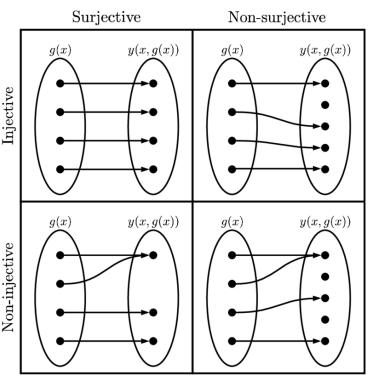
Figure 2.11: Illustration of injective and surjective functions.

Hence the normalization constant is given by

\[Z = \sum\_{x} q(x) \exp\left(-\sum\_{k} \lambda\_k f\_k(x)\right) \tag{2.256}\]

This has exactly the form of the exponential family, where f(x) is the vector of su”cient statistics, ⇐φ are the natural parameters, and q(x) is our base measure.

For example, if the features are f1(x) = x and f2(x) = x², and we want to match the first and second moments, we get the Gaussian disribution.

2.5 Transformations of random variables

Suppose x ⇔ px(x) is some random variable, and y = f(x) is some deterministic transformation of it. In this section, we discuss how to compute py(y).

2.5.1 Invertible transformations (bijections)

Let f be a bijection that maps Rⁿ to Rⁿ. (A bijection is a function that is injective, or one-to-one, and surjective, as illustrated in Figure 2.11; this means that the function has a well-defined inverse.) Suppose we want to compute the pdf of y = f(x). The change of variables formula tells us that

\[p\_y(\mathbf{y}) = p\_x\left(f^{-1}(\mathbf{y})\right) \left| \det\left[\mathbf{J}\_{f^{-1}}(\mathbf{y})\right] \right| \tag{2.257}\]

where ^Jf↓¹ (y) is the Jacobian of the inverse mapping ^{f ↑1} evaluated at ^y, and ^| det ^J| is the absolute value of the determinant of J. In other words,

\[\mathbf{J}\_{f^{-1}}(\mathbf{y}) = \begin{pmatrix} \frac{\partial x\_1}{\partial y\_1} & \cdots & \frac{\partial x\_1}{\partial y\_n} \\ & \vdots \\ \frac{\partial x\_n}{\partial y\_1} & \cdots & \frac{\partial x\_n}{\partial y\_n} \end{pmatrix} \tag{2.258}\]

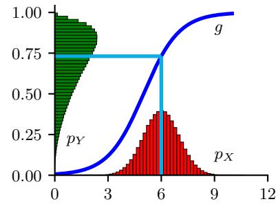
Figure 2.12: Example of the transformation of a density under a nonlinear transform. Note how the mode of the transformed distribution is not the transform of the original mode. Adapted from Exercise 1.4 of [Bis06]. Generated by bayes\_change\_of\_var.ipynb.

If the Jacobian matrix is triangular, the determinant reduces to a product of the terms on the main diagonal:

\[\det(\mathbf{J}) = \prod\_{i=1}^{n} \frac{\partial x\_i}{\partial y\_i} \tag{2.259}\]

2.5.2 Monte Carlo approximation

Sometime it is di”cult to compute the Jacobian. In this case, we can make a Monte Carlo approximation, by drawing ^S samples ^{xs ⇔ p}(x), computing ^{ys = f}(x^s), and then constructing the empirical pdf

\[p\_{\mathcal{D}}(\mathbf{y}) = \frac{1}{S} \sum\_{s=1}^{S} \delta(\mathbf{y} - \mathbf{y}^{s}) \tag{2.260}\]

For example, let ^{x ⇔ N} (6, 1) and ^{y = f}(x), where ^f(x) = ¹ 1+exp(↑x+5) . We can approximate ^p(y) using Monte Carlo, as shown in Figure 2.12.

2.5.3 Probability integral transform

Suppose that X is a random variable with cdf PX. Let Y (X) = PX(X) be a transformation of X. We now show that Y has a uniform distribution, a result known as the probability integral transform (PIT):

\[P\_Y(y) = \Pr(Y \le y) = \Pr(P\_X(X) \le y) \tag{2.261}\]

\[=\Pr(X \le P\_X^{-1}(y)) = P\_X(P\_X^{-1}(y)) = y \tag{2.262}\]

For example, in Figure 2.13, we show various distributions with pdf’s p^X on the left column. We sample from these, to get xⁿ ⇔ px. Next we compute the empirical cdf of Y = PX(X), by computing yⁿ = PX(xn) and then sorting the values; the results, shown in the middle column, show that this

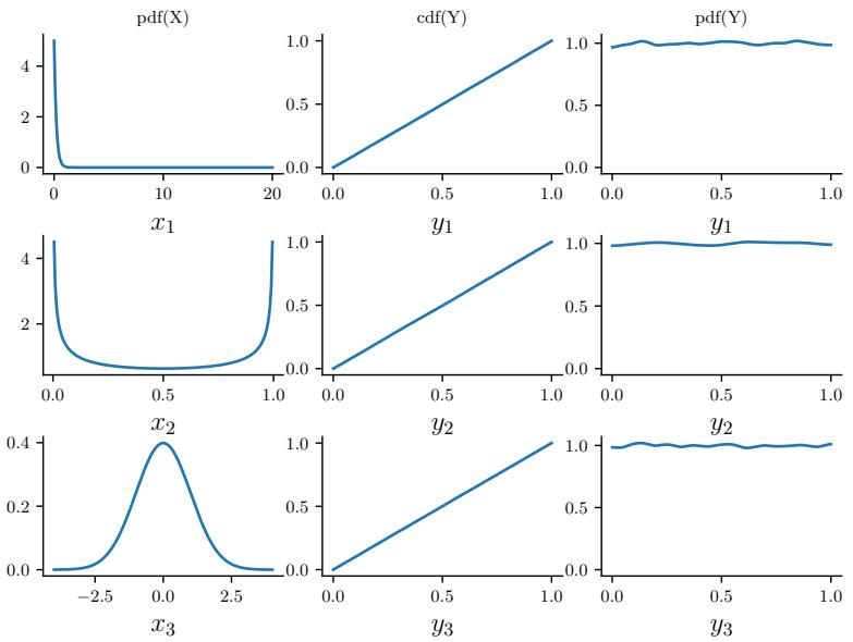
Figure 2.13: Illustration of the probability integral transform. Left column: 3 di!erent pdf ’s for p(X) from which we sample xⁿ ↔︎ p(x). Middle column: empirical cdf of yⁿ = PX(xn). Right column: empirical pdf of p(yn) using a kernel density estimate. Adapted from Figure 11.17 of [MKL11]. Generated by ecdf\_sample.ipynb.

distribution is uniform. We can also approximate the pdf of Y by using kernel density estimation; this is shown in the right column, and we see that it is (approximately) flat.

We can use the PIT to test if a set of samples come from a given distribution using the Kolmogorov–Smirnov test. To do this, we plot the empirical cdf of the samples and the theoretical cdf of the distribution, and compute the maximum distance between these two curves, as illustrated in Figure 2.14. Formally, the KS statistic is defined as

\[D\_n = \max\_x |P\_n(x) - P(x)|\tag{2.263}\]

where n is the sample size, Pⁿ is the empirical cdf, and P is the theoretical cdf. The value Dⁿ should approach 0 (as n → ⇒) if the samples are drawn from P.

Another application of the PIT is to generate samples from a distribution: if we have a way to sample from a uniform distribution, uⁿ ⇔ Unif(0, 1), we can convert this to samples from any other distribution with cdf P^X by setting xⁿ = P ^{↑1 X} (un).

2.6 Markov chains

Suppose that x^t captures all the relevant information about the state of the system. This means it is a su!cient statistic for predicting the future given the past, i.e.,

\[p(x\_{t+\tau}|x\_t, x\_{1:t-1}) = p(x\_{t+\tau}|x\_t) \tag{2.264}\]

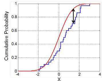
Figure 2.14: Illustration of the Kolmogorov–Smirnov statistic. The red line is a model cdf, the blue line is an empirical cdf, and the black arrow is the K–S statistic. From https: // en. wikipedia. org/ wiki/ Kolmogorov\_ Smirnov\_ test . Used with kind permission of Wikipedia author Bscan.

for any 2 ⇑ 0. This is called the Markov assumption. In this case, we can write the joint distribution for any finite length sequence as follows:

\[p(\mathbf{x}\_{1:T}) = p(\mathbf{x}\_1)p(\mathbf{x}\_2|\mathbf{x}\_1)p(\mathbf{x}\_3|\mathbf{x}\_2)p(\mathbf{x}\_4|\mathbf{x}\_3)\dots = p(\mathbf{x}\_1)\prod\_{t=2}^T p(\mathbf{x}\_t|\mathbf{x}\_{t-1})\tag{2.265}\]

This is called a Markov chain or Markov model. Below we cover some of the basics of this topic; more details on the theory can be found in [Kun20].

2.6.1 Parameterization

In this section, we discuss how to represent a Markov model parametrically.

2.6.1.1 Markov transition kernels

The conditional distribution p(xt|x^t↑¹) is called the transition function, transition kernel, or Markov kernel. This is just a conditional distribution over the states at time t given the state at time ^t ⇐ ¹, and hence it satisfies the conditions ^p(xt|x^t↑¹) ⇑ ⁰ and $ ^x≃^X dx p(x^{t = x}|x^t↑¹)=1.

If we assume the transition function p(xt|x1:t↑¹) is independent of time, then the model is said to be homogeneous, stationary, or time-invariant. This is an example of parameter tying, since the same parameter is shared by multiple variables. This assumption allows us to model an arbitrary number of variables using a fixed number of parameters. We will make the time-invariant assumption throughout the rest of this section.

2.6.1.2 Markov transition matrices

In this section, we assume that the variables are discrete, so X^t ↑ {1,…,K}. This is called a finite-state Markov chain. In this case, the conditional distribution p(Xt|X^t↑¹) can be written as a K ∞ K matrix A, known as the transition matrix, where Aij = p(X^t = j|X^t↑¹ = i) is the probability of going from state i to state j. Each row of the matrix sums to one, # ^j Aij = 1, so this is called a stochastic matrix.

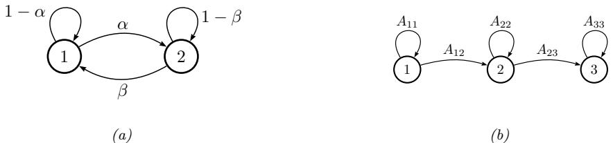
Figure 2.15: State transition diagrams for some simple Markov chains. Left: a 2-state chain. Right: a 3-state left-to-right chain.

A stationary, finite-state Markov chain is equivalent to a stochastic automaton. It is common to visualize such automata by drawing a directed graph, where nodes represent states and arrows represent legal transitions, i.e., non-zero elements of A. This is known as a state transition diagram. The weights associated with the arcs are the probabilities. For example, the following 2-state chain

\[\mathbf{A} = \begin{pmatrix} 1 - \alpha & \alpha \\ \beta & 1 - \beta \end{pmatrix} \tag{2.266}\]

is illustrated in Figure 2.15(a). The following 3-state chain

\[\mathbf{A} = \begin{pmatrix} A\_{11} & A\_{12} & 0 \\ 0 & A\_{22} & A\_{23} \\ 0 & 0 & 1 \end{pmatrix} \tag{2.267}\]

is illustrated in Figure 2.15(b). This is called a left-to-right transition matrix.

1 The Aij element of the transition matrix specifies the probability of getting from i to j in one step. The n-step transition matrix A(n) is defined as

\[A\_{ij}(n) \triangleq p(X\_{t+n} = j | X\_t = i) \tag{2.268}\]

which is the probability of getting from i to j in exactly n steps. Obviously A(1) = A. The Chapman-Kolmogorov equations state that

\[A\_{ij}(m+n) = \sum\_{k=1}^{K} A\_{ik}(m)A\_{kj}(n)\tag{2.269}\]

In words, the probability of getting from i to j in m + n steps is just the probability of getting from i to k in m steps, and then from k to j in n steps, summed up over all k. We can write the above as a matrix multiplication

\[\mathbf{A}(m+n) = \mathbf{A}(m)\mathbf{A}(n)\tag{2.270}\]

Hence

\[\mathbf{A}(n) = \mathbf{A}\,\mathbf{A}(n-1) = \mathbf{A}\,\mathbf{A}\,\mathbf{A}(n-2) = \dots = \mathbf{A}^n \tag{2.271}\]

Thus we can simulate multiple steps of a Markov chain by “powering up” the transition matrix.

christians first inhabit wherein thou hast forgive if a man childless and of laying of core these are the heavens shall reel to and fro to seek god they set their horses and children of israel

Figure 2.16: Example output from an 10-gram character-level Markov model trained on the King James Bible. The prefix “christians” is given to the model. Generated by ngram\_character\_demo.ipynb.

2.6.1.3 Higher-order Markov models

The first-order Markov assumption is rather strong. Fortunately, we can easily generalize first-order models to depend on the last n observations, thus creating a model of order (memory length) n:

\[p(\mathbf{x}\_{1:T}) = p(\mathbf{x}\_{1:n}) \prod\_{t=n+1}^{T} p(\mathbf{x}\_t | \mathbf{x}\_{t-n:t-1}) \tag{2.272}\]

This is called a Markov model of order n. If n = 1, this is called a bigram model, since we need to represent pairs of characters, p(xt|x^t↑1). If n = 2, this is called a trigram model, since we need to represent triples of characters, p(xt|x^t↑¹, x^t↑²). In general, this is called an n-gram model.

Note, however, we can always convert a higher order Markov model to a first order one by defining an augmented state space that contains the past n observations. For example, if n = 2, we define x˜^t = (x^t↑¹, xt) and use

\[p(\check{\mathbf{x}}\_{1:T}) = p(\check{\mathbf{x}}\_2) \prod\_{t=3}^{T} p(\check{\mathbf{x}}\_t | \check{\mathbf{x}}\_{t-1}) = p(\mathbf{x}\_1, \mathbf{x}\_2) \prod\_{t=3}^{T} p(\mathbf{x}\_t | \mathbf{x}\_{t-1}, \mathbf{x}\_{t-2}) \tag{2.273}\]

Therefore we will just focus on first-order models throughout the rest of this section.

2.6.2 Application: language modeling

One important application of Markov models is to create language models (LM), which are models which can generate (or score) a sequence of words. When we use a finite-state Markov model with a memory of length m = n ⇐ 1, it is called an n-gram model. For example, if m = 1, we get a unigram model (no dependence on previous words); if m = 2, we get a bigram model (depends on previous word); if m = 3, we get a trigram model (depends on previous two words); etc. See Figure 2.16 for some generated text.

These days, most LMs are built using recurrent neural nets (see Section 16.3.4), which have unbounded memory. However, simple n-gram models can still do quite well when trained with enough data [Che17].

Language models have various applications, such as priors for spelling correction (see Section 29.3.3) or automatic speech recognition. In addition, conditional language models can be used to generate sequences given inputs, such as mapping one language to another, or an image to a sequence, etc.

2.6.3 Parameter estimation

In this section, we discuss how to estimate the parameters of a Markov model.

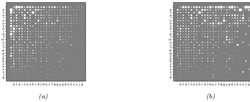
Figure 2.17: (a) Hinton diagram showing character bigram counts as estimated from H. G. Wells’s book The Time Machine. Characters are sorted in decreasing unigram frequency; the first one is a space character. The most frequent bigram is ‘e-’, where - represents space. (b) Same as (a) but each row is normalized across the columns. Generated by bigram\_hinton\_diagram.ipynb.

2.6.3.1 Maximum likelihood estimation

The probability of any particular sequence of length T is given by

\[p(x\_{1:T}|\theta) = \pi(x\_1)A(x\_1, x\_2)\dots A(x\_{T-1}, x\_T) \tag{2.274}\]

\[=\prod\_{j=1}^{K} (\pi\_j)^{\mathbb{I}(x\_1=j)} \prod\_{t=2}^{T} \prod\_{j=1}^{K} \prod\_{k=1}^{K} (A\_{jk})^{\mathbb{I}(x\_t=k, x\_{t-1}=j)} \tag{2.275}\]

Hence the log-likelihood of a set of sequences D = (x1,…, x^N ), where xⁱ = (xi1,…,xi,Tⁱ ) is a sequence of length Ti, is given by

\[\log p(\mathcal{D}|\boldsymbol{\theta}) = \sum\_{i=1}^{N} \log p(\boldsymbol{x}\_i|\boldsymbol{\theta}) = \sum\_{j} N\_j^1 \log \pi\_j + \sum\_{j} \sum\_{k} N\_{jk} \log A\_{jk} \tag{2.276}\]

where we define the following counts:

\[N\_j^\triangleq \sum\_{i=1}^N \mathbb{I}\left(x\_{i1} = j\right), \ N\_{jk} \triangleq \sum\_{i=1}^N \sum\_{t=1}^{T\_i - 1} \mathbb{I}\left(x\_{i,t} = j, x\_{i,t+1} = k\right), \ N\_j = \sum\_k N\_{jk} \tag{2.277}\]

By adding Lagrange multipliers to enforce the sum to one constraints, one can show (see e.g., [Mur22, Sec 4.2.4]) that the MLE is given by the normalized counts:

\[ \hat{\pi}\_j = \frac{N\_j^1}{\sum\_{j'} N\_{j'}^1}, \quad \hat{A}\_{jk} = \frac{N\_{jk}}{N\_j} \tag{2.278} \]

We often replace N^{1 j} , which is how often symbol j is seen at the start of a sequence, by N^j , which is how often symbol j is seen anywhere in a sequence. This lets us estimate parameters from a single sequence.

The counts N^j are known as unigram statistics, and Njk are known as bigram statistics. For example, Figure 2.17 shows some 2-gram counts for the characters {a, . . . , z, ⇐} (where - represents space) as estimated from H. G. Wells’s book The Time Machine.

2.6.3.2 Sparse data problem

When we try to fit n-gram models for large n, we quickly encounter problems with overfitting due to data sparsity. To see that, note that many of the estimated counts Njk will be 0, since now j indexes over discrete contexts of size Kⁿ↑¹, which will become increasingly rare. Even for bigram models (n = 2), problems can arise if K is large. For example, if we have K ⇔ 50, 000 words in our vocabulary, then a bi-gram model will have about 2.5 billion free parameters, corresponding to all possible word pairs. It is very unlikely we will see all of these in our training data. However, we do not want to predict that a particular word string is totally impossible just because we happen not to have seen it in our training text — that would be a severe form of overfitting.9

A “brute force” solution to this problem is to gather lots and lots of data. For example, Google has fit n-gram models (for n =1:5) based on one trillion words extracted from the web. Their data, which is over 100GB when uncompressed, is publically available.10 Although such an approach can be surprisingly successful (as discussed in [HNP09]), it is rather unsatisfying, since humans are able to learn language from much less data (see e.g., [TX00]).

2.6.3.3 MAP estimation

A simple solution to the sparse data problem is to use MAP estimation with a uniform Dirichlet prior, Aj: ⇔ Dir(α1). In this case, the MAP estimate becomes

\[ \hat{A}\_{jk} = \frac{N\_{jk} + \alpha}{N\_j + K\alpha} \tag{2.279} \]

If α = 1, this is called add-one smoothing.

The main problem with add-one smoothing is that it assumes that all n-grams are equally likely, which is not very realistic. We discuss a more sophisticated approach, based on hierarchical Bayes, in Section 3.7.3.

2.6.4 Stationary distribution of a Markov chain

Suppose we continually draw consecutive samples from a Markov chain. In the case of a finite state space, we can think of this as “hopping” from one state to another. We will tend to spend more time in some states than others, depending on the transition graph. The long term distribution over states is known as the stationary distribution of the chain. In this section, we discuss some of the relevant theory. In Chapter 12, we discuss an important application, known as MCMC, which is a way to generate samples from hard-to-normalize probability distributions. In Supplementary Section 2.2

^9. A famous example of an improbable, but syntactically valid, English word string, due to Noam Chomsky [Cho57], is “colourless green ideas sleep furiously”. We would not want our model to predict that this string is impossible. Even ungrammatical constructs should be allowed by our model with a certain probability, since people frequently violate grammatical rules, especially in spoken language.

^10. See http://googleresearch.blogspot.com/2006/08/all-our-n-gram-are-belong-to-you.html for details.

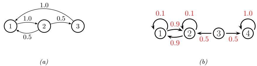
Figure 2.18: Some Markov chains. (a) A 3-state aperiodic chain. (b) A reducible 4-state chain.

we consider Google’s PageRank algorithm for ranking web pages, which also leverages the concept of stationary distributions.

2.6.4.1 What is a stationary distribution?

Let Aij = p(X^t = j|X^t↑¹ = i) be the one-step transition matrix, and let ϱt(j) = p(X^t = j) be the probability of being in state j at time t.

If we have an initial distribution over states of ϑ0, then at time 1 we have

\[ \pi\_1(j) = \sum\_i \pi\_0(i) A\_{ij} \tag{2.280} \]

or, in matrix notation, ϑ¹ = ϑ0A, where we have followed the standard convention of assuming ϑ is a row vector, so we post-multiply by the transition matrix.

1 Now imagine iterating these equations. If we ever reach a stage where ϑ = ϑA, then we say we have reached the stationary distribution (also called the invariant distribution or equilibrium distribution). Once we enter the stationary distribution, we will never leave.

For example, consider the chain in Figure 2.18(a). To find its stationary distribution, we write

\[\begin{pmatrix} \pi\_1 & \pi\_2 & \pi\_3 \end{pmatrix} = \begin{pmatrix} \pi\_1 & \pi\_2 & \pi\_3 \end{pmatrix} \begin{pmatrix} 1 - A\_{12} - A\_{13} & A\_{12} & A\_{13} \\ A\_{21} & 1 - A\_{21} - A\_{23} & A\_{23} \\ A\_{31} & A\_{32} & 1 - A\_{31} - A\_{32} \end{pmatrix} \tag{2.281}\]

Hence ϱ1(A¹² + A13) = ϱ2A²¹ + ϱ3A31. In general, we have

\[ \pi\_i \sum\_{j \neq i} A\_{ij} = \sum\_{j \neq i} \pi\_j A\_{ji} \tag{2.282} \]

In other words, the probability of being in state i times the net flow out of state i must equal the probability of being in each other state j times the net flow from that state into i. These are called the # global balance equations. We can then solve these equations, subject to the constraint that ^j ϱ^j = 1, to find the stationary distribution, as we discuss below.

2.6.4.2 Computing the stationary distribution

To find the stationary distribution, we can just solve the eigenvector equation A^Tv = v, and then to set ϑ = v^T, where v is an eigenvector with eigenvalue 1. (We can be sure such an eigenvector

exists, since A is a row-stochastic matrix, so A1 = 1; also recall that the eigenvalues of A and A^T are the same.) Of course, since eigenvectors are unique only up to constants of proportionality, we must normalize v at the end to ensure it sums to one.

Note, however, that the eigenvectors are only guaranteed to be real-valued if all entries in the matrix are strictly positive, Aij > 0 (and hence Aij < 1, due to the sum-to-one constraint). A more general approach, which can handle chains where some transition probabilities are 0 or 1 (such as Figure 2.18(a)), is as follows. We have K constraints from ϑ(I ⇐ A) = 0^K→¹ and 1 constraint from ϑ1^K→¹ = 1. Hence we have to solve ϑM = r, where M = [I ⇐ A, 1] is a K ∞ (K + 1) matrix, and r = [0, 0,…, 0, 1] is a 1 ∞ (K + 1) vector. However, this is overconstrained, so we will drop the last column of I ⇐ A in our definition of M, and drop the last 0 from r. For example, for a 3 state chain we have to solve this linear system:

\[ \begin{pmatrix} \pi\_1 & \pi\_2 & \pi\_3 \end{pmatrix} \begin{pmatrix} 1 - A\_{11} & -A\_{12} & 1 \\ -A\_{21} & 1 - A\_{22} & 1 \\ -A\_{31} & -A\_{32} & 1 \end{pmatrix} = \begin{pmatrix} 0 & 0 & 1 \end{pmatrix} \tag{2.283} \]

For the chain in Figure 2.18(a) we find ϑ = [0.4, 0.4, 0.2]. We can easily verify this is correct, since ϑ = ϑA.

Unfortunately, not all chains have a stationary distribution, as we explain below.

2.6.4.3 When does a stationary distribution exist?

Consider the 4-state chain in Figure 2.18(b). If we start in state 4, we will stay there forever, since 4 is an absorbing state. Thus ϑ = (0, 0, 0, 1) is one possible stationary distribution. However, if we start in 1 or 2, we will oscillate between those two states forever. So ϑ = (0.5, 0.5, 0, 0) is another possible stationary distribution. If we start in state 3, we could end up in either of the above stationary distributions with equal probability. The corresponding transition graph has two disjoint connected components.

We see from this example that a necessary condition to have a unique stationary distribution is that the state transition diagram be a singly connected component, i.e., we can get from any state to any other state. Such chains are called irreducible.

Now consider the 2-state chain in Figure 2.15(a). This is irreducible provided α, ↼ > 0. Suppose α = ↼ = 0.9. It is clear by symmetry that this chain will spend 50% of its time in each state. Thus ϑ = (0.5, 0.5). But now suppose α = ↼ = 1. In this case, the chain will oscillate between the two states, but the long-term distribution on states depends on where you start from. If we start in state 1, then on every odd time step (1,3,5,…) we will be in state 1; but if we start in state 2, then on every odd time step we will be in state 2.

This example motivates the following definition. Let us say that a chain has a limiting distribution if ϱ^{j =} limⁿ↗↓ Aⁿ ij exists and is independent of the starting state i, for all j. If this holds, then the long-run distribution over states will be independent of the starting state:

\[p(X\_t = j) = \sum\_i p(X\_0 = i) A\_{ij}(t) \to \pi\_j \text{ as } t \to \infty \tag{2.284}\]

Let us now characterize when a limiting distribution exists. Define the period of state i to be d(i) ↭ gcd{t : Aii(t) > 0}, where gcd stands for greatest common divisor, i.e., the largest integer

that divides all the members of the set. For example, in Figure 2.18(a), we have d(1) = d(2) = gcd(2, 3, 4, 6, …)=1 and d(3) = gcd(3, 5, 6, …)=1. We say a state i is aperiodic if d(i)=1. (A su”cient condition to ensure this is if state i has a self-loop, but this is not a necessary condition.) We say a chain is aperiodic if all its states are aperiodic. One can show the following important result:

Theorem 2.6.1. Every irreducible (singly connected), aperiodic finite state Markov chain has a limiting distribution, which is equal to ϑ, its unique stationary distribution.

A special case of this result says that every regular finite state chain has a unique stationary distribution, where a regular chain is one whose transition matrix satisfies Aⁿ ij > 0 for some integer n and all i, j, i.e., it is possible to get from any state to any other state in n steps. Consequently, after n steps, the chain could be in any state, no matter where it started. One can show that su”cient conditions to ensure regularity are that the chain be irreducible (singly connected) and that every state have a self-transition.

To handle the case of Markov chains whose state space is not finite (e.g, the countable set of all integers, or all the uncountable set of all reals), we need to generalize some of the earlier definitions. Since the details are rather technical, we just briefly state the main results without proof. See e.g., [GS92] for details.

For a stationary distribution to exist, we require irreducibility (singly connected) and aperiodicity, as before. But we also require that each state is recurrent, which means that you will return to that state with probability 1. As a simple example of a non-recurrent state (i.e., a transient state), consider Figure 2.18(b): state 3 is transient because one immediately leaves it and either spins around state 4 forever, or oscillates between states 1 and 2 forever. There is no way to return to state 3.

It is clear that any finite-state irreducible chain is recurrent, since you can always get back to where you started from. But now consider an example with an infinite state space. Suppose we perform a random walk on the integers, X = {…, ⇐2, ⇐1, 0, 1, 2,…}. Let Ai,i+1 = p be the probability of moving right, and Ai,i↑¹ = 1 ⇐ p be the probability of moving left. Suppose we start at X¹ = 0. If p > 0.5, we will shoot o! to +⇒; we are not guaranteed to return. Similarly, if p < 0.5, we will shoot o! to ⇐⇒. So in both cases, the chain is not recurrent, even though it is irreducible. If p = 0.5, we can return to the initial state with probability 1, so the chain is recurrent. However, the distribution keeps spreading out over a larger and larger set of the integers, so the expected time to return is infinite. This prevents the chain from having a stationary distribution.

More formally, we define a state to be non-null recurrent if the expected time to return to this state is finite. We say that a state is ergodic if it is aperiodic, recurrent, and non-null. We say that a chain is ergodic if all its states are ergodic. With these definitions, we can now state our main theorem:

Theorem 2.6.2. Every irreducible, ergodic Markov chain has a limiting distribution, which is equal to ϑ, its unique stationary distribution.

This generalizes Theorem 2.6.1, since for irreducible finite-state chains, all states are recurrent and non-null.

2.6.4.4 Detailed balance

Establishing ergodicity can be di”cult. We now give an alternative condition that is easier to verify.

We say that a Markov chain A is time reversible if there exists a distribution ϑ such that

\[ \pi\_i A\_{ij} = \pi\_j A\_{ji} \tag{2.285} \]

These are called the detailed balance equations. This says that the flow from i to j must equal the flow from j to i, weighted by the appropriate source probabilities.

We have the following important result.

Theorem 2.6.3. If a Markov chain with transition matrix A is regular and satisfies the detailed balance equations wrt distribution ϑ, then ϑ is a stationary distribution of the chain.

Proof. To see this, note that

\[\sum\_{i} \pi\_i A\_{ij} = \sum\_{i} \pi\_j A\_{ji} = \pi\_j \sum\_{i} A\_{ji} = \pi\_j \tag{2.286}\]

and hence ϑ = Aϑ.

Note that this condition is su”cient but not necessary (see Figure 2.18(a) for an example of a chain with a stationary distribution which does not satisfy detailed balance).

2.7 Divergence measures between probability distributions

In this section, we discuss various ways to compare two probability distributions, P and Q, defined on the same space. For example, suppose the distributions are defined in terms of samples, X = {x1,…, x^N } ⇔ P and X ^↔︎ = {x˜1,…, x˜M} ⇔ Q. Determining if the samples come from the same distribution is known as a two-sample test (see Figure 2.19 for an illustration). This can be computed by defining some suitable divergence metric D(P, Q) and comparing it to a threshold. (We use the term “divergence” rather than distance since we will not require D to be symmetric.) Alternatively, suppose P is an empirical distribution of data, and Q is the distribution induced by a model. We can check how well the model approximates the data by comparing D(P, Q) to a threshold; this is called a goodness-of-fit test.

There are two main ways to compute the divergence between a pair of distributions: in terms of their di!erence, P ⇐ Q (see e.g., [Sug+13]) or in terms of their ratio, P/Q (see e.g., [SSK12]). We briefly discuss both of these below. (Our presentation is based, in part, on [GSJ19].)

2.7.1 f-divergence

In this section, we compare distributions in terms of their density ratio r(x) = p(x)/q(x). In particular, consider the f-divergence [Mor63; AS66; Csi67; LV06; CS04], which is defined as follows:

\[D\_f(p||q) = \int q(\mathbf{x}) f\left(\frac{p(\mathbf{x})}{q(\mathbf{x})}\right) d\mathbf{x} \tag{2.287}\]

where f : R⁺ → R is a convex function satisfying f(1) = 0. From Jensen’s inequality (Section 5.1.2.2), it follows that D^f (p||q) ⇑ 0, and obviously D^f (p||p)=0, so D^f is a valid divergence. Below we discuss some important special cases of f-divergences. (Note that f-divergences are also called ▷-divergences.)

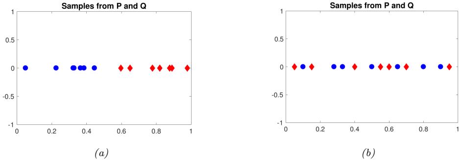
Figure 2.19: Samples from two distributions which are (a) di!erent and (b) similar. From a figure from [GSJ19]. Used with kind permission of Arthur Gretton.

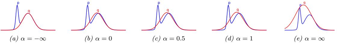
Figure 2.20: The Gaussian q which minimizes ϖ-divergence to p (a mixture of two Gaussians), for varying ϖ. From Figure 1 of [Min05]. Used with kind permission of Tom Minka.

2.7.1.1 KL divergence

Suppose we compute the f-divergence using f(r) = r log(r). In this case, we get a quantity called the Kullback Leibler divergence, defined as follows:

\[D\_{\text{KL}}\left(p \parallel q\right) = \int p(\mathbf{x}) \log \frac{p(\mathbf{x})}{q(\mathbf{x})} d\mathbf{x} \tag{2.288}\]

See Section 5.1 for more details.

2.7.1.2 Alpha divergence

If f(x) = ^{4 1}↑ϖ² (1 ⇐ ^x 1+^{ϑ 2} ), the f-divergence becomes the alpha divergence [Ama09], which is as follows:

\[D\_{\alpha}^{A}(p||q) \stackrel{\Delta}{=} \frac{4}{1-\alpha^{2}} \left(1 - \int p(\mathbf{x})^{(1+\alpha)/2} q(\mathbf{x})^{(1-\alpha)/2} d\mathbf{x}\right) \tag{2.289}\]

where we assume α ⇓= ±1. Another common parameterization, and the one used by Minka in [Min05], is as follows:

\[D\_{\alpha}^{M}(p||q) = \frac{1}{\alpha(1-\alpha)} \left(1 - \int p(\mathbf{x})^{\alpha} q(\mathbf{x})^{1-\alpha} d\mathbf{x}\right) \tag{2.290}\]

This can be converted to Amari’s notation using D^{A ϖ→} = D^{M ϖ} where α^↔︎ = 2α ⇐ 1. (We will use the Minka convention.)

We see from Figure 2.20 that as α → ⇐⇒, q prefers to match one mode of p, whereas when α → ⇒, q prefers to cover all of p. More precisely, one can show that as α → 0, the alpha divergence tends towards DKL (q ̸ p), and as α → 1, the alpha divergence tends towards DKL (p ̸ q). Also, when α = 0.5, the alpha divergence equals the Hellinger distance (Section 2.7.1.3).

2.7.1.3 Hellinger distance

The (squared) Hellinger distance is defined as follows:

\[D\_H^2(p||q) \stackrel{\Delta}{=} \frac{1}{2} \int \left(p(\mathbf{x})^{\frac{1}{2}} - q(\mathbf{x})^{\frac{1}{2}}\right)^2 d\mathbf{x} = 1 - \int \sqrt{p(\mathbf{x})q(\mathbf{x})}d\mathbf{x} \tag{2.291}\]

This is a valid distance metric, since it is symmetric, nonnegative, and satisfies the triangle inequality.

We see that this is equal (up to constant factors) to the ^f-divergence with ^f(r)=(↖^r ⇐ 1)2, since

\[\int dx \, q(x) \left( \frac{p^{\frac{1}{2}}(x)}{q^{\frac{1}{2}}(x)} - 1 \right)^2 = \int dx \, q(x) \left( \frac{p^{\frac{1}{2}}(x) - q^{\frac{1}{2}}(x)}{q^{\frac{1}{2}}(x)} \right)^2 = \int dx \, \left( p^{\frac{1}{2}}(x) - q^{\frac{1}{2}}(x) \right)^2 \quad (2.292)\]

2.7.1.4 Chi-squared distance

The chi-squared distance ↽² is defined by

\[\chi^2(p,q) \triangleq \frac{1}{2} \int \frac{(q(x) - p(x))^2}{q(x)} dx \tag{2.293}\]

This is equal (up to constant factors) to an ^f-divergence where ^f(r)=(^r ⇐ 1)², since

\[\int dx \,\, q(x) \left(\frac{p(x)}{q(x)} - 1\right)^2 = \int dx \,\, q(x) \left(\frac{p(x) - q(x)}{q(x)}\right)^2 = \int dx \,\, \frac{1}{q(x)} \left(p(x) - q(x)\right)^2\tag{2.294}\]

2.7.2 Integral probability metrics

In this section, we compute the divergence between two distributions in terms of P ⇐ Q using an integral probability metric or IPM [Sri+09]. This is defined as follows:

\[\sup D\_{\mathcal{F}}(P, Q) \stackrel{\Delta}{=} \sup\_{f \in \mathcal{F}} |\mathbb{E}\_{p(\mathbf{z})} \left[ f(\mathbf{z}) \right] - \mathbb{E}\_{q(\mathbf{z}')} \left[ f(\mathbf{z}') \right]| \tag{2.295}\]

where F is some class of “smooth” functions. The function f that maximizes the di!erence between these two expectations is called the witness function. See Figure 2.21 for an illustration.

There are several ways to define the function class F. One approach is to use an RKHS, defined in terms of a positive definite kernel function; this gives rise to the method known as maximum mean discrepancy or MMD. See Section 2.7.3 for details.

Another approach is to define F to be the set of functions that have bounded Lipschitz constant, i.e., F = {||f||^L ↗ 1}, where

\[||f||\_L = \sup\_{\mathbf{x} \neq \mathbf{x}'} \frac{|f(\mathbf{x}) - f(\mathbf{x}')|}{||\mathbf{x} - \mathbf{x}'||} \tag{2.296}\]

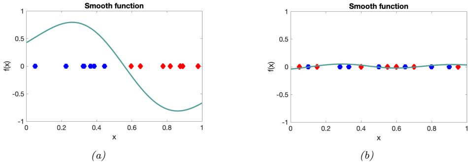
Figure 2.21: A smooth witness function for comparing two distributions which are (a) di!erent and (b) similar. From a figure from [GSJ19]. Used with kind permission of Arthur Gretton.

The IPM in this case is equal to the Wasserstein-1 distance

\[W\_1(P, Q) \stackrel{\Delta}{=} \sup\_{||f||\_2 \le 1} |\mathbb{E}\_{p(\mathbf{z})} \left[ f(\mathbf{z}) \right] - \mathbb{E}\_{q(\mathbf{z}')} \left[ f(\mathbf{z}') \right]| \tag{2.297}\]

See Section 6.8.2.4 for details.

2.7.3 Maximum mean discrepancy (MMD)

In this section, we describe the maximum mean discrepancy or MMD method of [Gre+12], which defines a discrepancy measure D(P, Q) using samples from the two distributions. The samples are compared using positive definite kernels (Section 18.2), which can handle high-dimensional inputs. This approach can be used to define two-sample tests, and to train implicit generative models (Section 26.2.4).

2.7.3.1 MMD as an IPM

The MMD is an integral probability metric (Section 2.7.2) of the form

\[\text{MMD}(P, Q; \mathcal{F}) = \sup\_{f \in \mathcal{F} : ||f|| \le 1} \left[ \mathbb{E}\_{p(\mathbf{z})} \left[ f(\mathbf{z}) \right] - \mathbb{E}\_{q(\mathbf{z'})} \left[ f(\mathbf{z'}) \right] \right] \tag{2.298}\]

where F is an RKHS (Section 18.3.7.1) defined by a positive definite kernel function K. We can represent functions in this set as an infinite sum of basis functions

\[f(\mathbf{x}) = \langle f, \phi(\mathbf{x}) \rangle\_{\mathcal{F}} = \sum\_{l=1}^{\infty} f\_l \phi\_l(\mathbf{x}) \tag{2.299}\]

We restrict the set of witness functions f to be those that are in the unit ball of this RKHS, so ||f||^{2 F =} #^{↓ l}=1 f ^{2 l} ↗ 1. By the linearity of expectation, we have

\[\mathbb{E}\_{p(\mathbf{z})}\left[f(\mathbf{z})\right] = \langle f, \mathbb{E}\_{p(\mathbf{z})}\left[\phi(\mathbf{z})\right] \rangle\_{\mathcal{F}} = \langle f, \mu\_P \rangle\_{\mathcal{F}}\tag{2.300}\]

where µ^P is called the kernel mean embedding of distribution P [Mua+17]. Hence

\[\text{MMD}(P, Q; \mathcal{F}) = \sup\_{||f|| \le 1} \langle f, \mu\_P - \mu\_Q \rangle\_{\mathcal{F}} = ||\mu\_P - \mu\_Q|| \tag{2.301}\]

since the unit vector f that maximizes the inner product is parallel to the di!erence in feature means.

To get some intuition, suppose ϱ(x)=[x, x²]. In this case, the MMD computes the di!erence in the first two moments of the two distributions. This may not be enough to distinguish all possible distributions. However, using a Gaussian kernel is equivalent to comparing two infinitely large feature vectors, as we show in Section 18.2.6, and hence we are e!ectively comparing all the moments of the two distributions. Indeed, one can show that MMD=0 i! P = Q, provided we use a non-degenerate kernel.

2.7.3.2 Computing the MMD using the kernel trick

In this section, we describe how to compute Equation (2.301) in practice, given two sets of samples, ^X = {xn}^{N n}=1 and X ^↔︎ = {x^↔︎ m}^{M m}=1, where xⁿ ⇔ P and x^{↔︎ m ⇔ Q}. Let ^{µP = 1} N #^{N n}=1 ϱ(xn) and µ^Q = ¹ M #^{M m}=1 ϱ(x^{↔︎ m}) be empirical estimates of the kernel mean embeddings of the two distributions. Then the squared MMD is given by

\[\begin{split} \text{MMD}^2(X, X') & \stackrel{\scriptstyle \!^1}{=} ||\frac{1}{N} \sum\_{n=1}^N \phi(\mathbf{z}\_n) - \frac{1}{M} \sum\_{m=1}^M \phi(\mathbf{z}'\_m)||^2 \\ &= \frac{1}{N^2} \sum\_{n=1}^N \sum\_{n'=1}^N \phi(\mathbf{z}\_n)^\sf T} \phi(\mathbf{z}\_{n'}) - \frac{2}{NM} \sum\_{n=1}^N \sum\_{m=1}^M \phi(\mathbf{z}\_n)^\sf T} \phi(\mathbf{z}\_n)^\sf T \phi(\mathbf{z}'\_m) \\ &+ \frac{1}{M^2} \sum\_{m=1}^M \sum\_{n'=1}^M \phi(\mathbf{z}'\_{m'})^\sf T \phi(\mathbf{z}'\_m) \end{split} \tag{2.303}\]

Since Equation (2.303) only involves inner products of the feature vectors, we can use the kernel trick (Section 18.2.5) to rewrite the above as follows:

\[\text{MMD}^2(\mathcal{X}, \mathcal{X}') = \frac{1}{N^2} \sum\_{n=1}^N \sum\_{n'=1}^N \mathcal{K}(\mathbf{x}\_n, \mathbf{z}\_{n'}) - \frac{2}{NM} \sum\_{n=1}^N \sum\_{m=1}^M \mathcal{K}(\mathbf{z}\_n, \mathbf{z}'\_m) + \frac{1}{M^2} \sum\_{m=1}^M \sum\_{n'=1}^M \mathcal{K}(\mathbf{z}'\_m, \mathbf{z}'\_{n'}) \tag{2.304}\]

2.7.3.3 Linear time computation

The MMD takes O(N²) time to compute, where N is the number of samples from each distribution. In [Chw+15], they present a di!erent test statistic called the unnormalized mean embedding or UME, that can be computed in O(N) time.

The key idea is to notice that evaluating

\[\text{witness}^2(\mathbf{v}) = (\mu\_Q(\mathbf{v}) - \mu\_P(\mathbf{v}))^2 \tag{2.305}\]

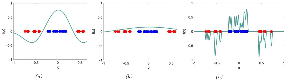
Figure 2.22: E!ect of decreasing the bandwidth parameter ϑ on the witness function defined by a Gaussian kernel. From a figure from [GSJ19]. Used with kind permission of Dougal Sutherland.

at a set of test locations v1,…, v^J is enough to detect a di!erence between P and Q. Hence we define the (squared) UME as follows:

\[\text{UME}^2(P, Q) = \frac{1}{J} \sum\_{j=1}^{J} \left[ \mu\_P(v\_j) - \mu\_Q(v\_j) \right]^2 \tag{2.306}\]

where µ^P (v) = Ep(x) [K(x, v)] can be estimated empirically in O(N) time, and similarly for µQ(v).

A normalized version of UME, known as NME, is presented in [Jit+16]. By maximizing NME wrt the locations v^j , we can maximize the statistical power of the test, and find locations where P and Q di!er the most. This provides an interpretable two-sample test for high dimensional data.

2.7.3.4 Choosing the right kernel

The e!ectiveness of MMD (and UME) obviously crucially depends on the right choice of kernel. Even for distiguishing 1d samples, the choice of kernel can be very important. For example, consider a Gaussian kernel, Kϱ(x, x^↔︎ ) = exp(⇐ ^{1 2}ϱ² ||x ⇐ x^↔︎ ||²). The e!ect of changing ^ε in terms of the ability to distinguish two di!erent sets of 1d samples is shown in Figure 2.22. Fortunately, the MMD is di!erentiable wrt the kernel parameters, so we can choose the optimal ε² so as to maximize the power of the test [Sut+17]. (See also [Fla+16] for a Bayesian approach, which maximizes the marginal likelihood of a GP representation of the kernel mean embedding.)

For high-dimensional data such as images, it can be useful to use a pre-trained CNN model as a way to compute low-dimensional features. For example, we can define K(x, x^↔︎ ) = Kϱ(h(x), h(x^↔︎ )), where h is some hidden layer of a CNN. such as the “inception” model of [Sze+15a]. The resulting MMD metric is known as the kernel inception distance [Bi#+18]. This is similar to the Fréchet inception distance [Heu+17a], but has nicer statistical properties, and is better correlated with human perceptual judgement [Zho+19a].

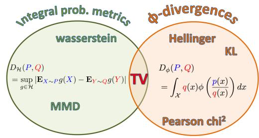
Figure 2.23: Summary of the two main kinds of divergence measures between two probability distributions P and Q. From a figure from [GSJ19]. Used with kind permission of Arthur Gretton.

2.7.4 Total variation distance

The total variation distance between two probability distributions is defined as follows:

\[D\_{\rm TV}(p,q) \triangleq \frac{1}{2}||\mathbf{p} - \mathbf{q}||\_1 = \frac{1}{2} \int |p(\mathbf{x}) - q(\mathbf{x})|d\mathbf{x} \tag{2.307}\]

This is equal to an f-divergence where f(r) = |r ⇐ 1|/2, since

\[\frac{1}{2}\int q(\mathbf{x})|\frac{p(\mathbf{x})}{q(\mathbf{x})} - 1|d\mathbf{x} = \frac{1}{2}\int q(\mathbf{x})|\frac{p(\mathbf{x}) - q(\mathbf{x})}{q(\mathbf{x})}|d\mathbf{x} = \frac{1}{2}\int |p(\mathbf{x}) - q(\mathbf{x})|d\mathbf{x} \tag{2.308}\]

One can also show that the TV distance is an integral probability measure. In fact, it is the only divergence that is both an IPM and an f-divergence [Sri+09]. See Figure 2.23 for a visual summary.

2.7.5 Density ratio estimation using binary classifiers

In this section, we discuss a simple approach for comparing two distributions that turns out to be equivalent to IPMs and f-divergences.

Consider a binary classification problem in which points from P have label y = 1 and points from Q have label y = 0, i.e., P(x) = p(x|y = 1) and Q(x) = p(x|y = 0). Let p(y = 1) = ϱ be the class prior. By Bayes’ rule, the density ratio r(x) = P(x)/Q(x) is given by

\[\frac{P(x)}{Q(x)} = \frac{p(x|y=1)}{p(x|y=0)} = \frac{p(y=1|x)p(x)}{p(y=1)} / \frac{p(y=0|x)p(x)}{p(y=0)}\tag{2.309}\]

\[y = \frac{p(y=1|x)}{p(y=0|x)} \frac{1-\pi}{\pi} \tag{2.310}\]

If we assume ϱ = 0.5, then we can estimate the ratio r(x) by fitting a binary classifier or discriminator h(x) = p(y = 1|x) and then computing r = h/(1 ⇐ h). This is called the density ratio estimation or DRE trick.

We can optimize the classifer h by minimizing the risk (expected loss). For example, if we use

log-loss, we have

\[R(h) = \mathbb{E}\_{p(\mathbf{z}|y)p(y)}\left[ -y \log h(\mathbf{z}) - (1 - y) \log(1 - h(\mathbf{z})) \right] \tag{2.311}\]

\[=\pi \mathbb{E}\_{P(\mathfrak{x})}\left[-\log h(\mathfrak{x})\right] + (1-\pi)\mathbb{E}\_{Q(\mathfrak{x})}\left[-\log(1-h(\mathfrak{x}))\right] \tag{2.312}\]

We can also use other loss functions ⇁(y, h(x)) (see Section 26.2.2).

Let R↽ ^h↑ = inf^h≃^F R(h) be the minimum risk achievable for loss function ⇁, where we minimize over some function class F. 11 In [NWJ09], they show that for every f-divergence, there is a loss function ⇁ such that ⇐D^f (P, Q) = ^R↽ ^h↑ . For example (using the notation y˜ ↑ {⇐1, 1} instead of y ↑ {0, 1}), total-variation distance corresponds to hinge loss, ⇁(y, h ˜ ) = max(0, 1 ⇐ yh˜ ); Hellinger distance corresponds to exponential loss, ⇁(y, h ˜ ) = exp(⇐yh˜ ); and ↽² divergence corresponds to logistic loss, ⇁(˜y, h) = log(1 + exp(⇐yh˜ )).

We can also establish a connection between binary classifiers and IPMs [Sri+09]. In particular, let ⇁(˜y, h) = ⇐2˜yh, and p(˜y = 1) = p(˜y = ⇐1) = 0.5. Then we have

\[R\_{h^\*} = \inf\_h \int \ell(\ddot{y}, h(x)) p(x|\ddot{y}) p(\ddot{y}) dx d\ddot{y} \tag{2.313}\]

\[\hat{y} = \inf\_{h} 0.5 \int \ell(1, h(\mathbf{x})) p(\mathbf{x} | \tilde{y} = 1) d\mathbf{x} + 0.5 \int \ell(-1, h(\mathbf{x})) p(\mathbf{x} | \tilde{y} = -1) d\mathbf{x} \tag{2.314}\]

\[0 = \inf\_{h} \int h(\mathbf{x}) Q(\mathbf{x}) d\mathbf{x} - \int h(\mathbf{x}) P(\mathbf{x}) d\mathbf{x} \tag{2.315}\]

\[=\sup\_{h} - \int h(\mathbf{x})Q(\mathbf{x})d\mathbf{x} + \int h(\mathbf{x})P(\mathbf{x})d\mathbf{x} \tag{2.316}\]

which matches Equation (2.295). Thus the classifier plays the same role as the witness function.

^11. If P is a fixed distribution, and we minimize the above objective wrt h, while also maximizing it wrt a model Q(x), we recover a technique known as a generative adversarial network for fitting an implicit model to a distribution of samples P (see Chapter 26 for details). However, in this section, we assume Q is known.

3 Statistics

3.1 Introduction

Probability theory (which we discussed in Chapter 2) is concerned with modeling the distribution over observed data outcomes D given known parameters ω by computing p(D|ω). By contrast, statistics is concerned with the inverse problem, in which we want to infer the unknown parameters ω given observations, i.e., we want to compute p(ω|D). Indeed, statistics was originally called inverse probability theory. Nowadays, there are two main approaches to statistics, frequentist statistics and Bayesian statistics, as we discuss below. (See also Section 34.1, where we compare the frequentist and Bayesian approaches to decision theory.) Note, however, that most of this book focuses on the Bayesian approach, for reasons that will become clear.

3.2 Bayesian statistics

In the Bayesian approach to statistics, we treat the parameters ω as unknown, and the data D as fixed and known. (This is the opposite of the frequentist approach, which we discuss in Section 3.3.) We represent our uncertainty about the parameters, after (posterior to) seeing the data, by computing the posterior distribution using Bayes’ rule:

\[p(\boldsymbol{\theta}|\mathcal{D}) = \frac{p(\boldsymbol{\theta})p(\mathcal{D}|\boldsymbol{\theta})}{p(\mathcal{D})} = \frac{p(\boldsymbol{\theta})p(\mathcal{D}|\boldsymbol{\theta})}{\int p(\boldsymbol{\theta}')p(\mathcal{D}|\boldsymbol{\theta}')d\boldsymbol{\theta}'} \tag{3.1}\]

Here p(ω) is called the prior, and represents our beliefs about the parameters before seeing the data; p(D|ω) is called the likelihood, and represents our beliefs about what data we expect to see for each setting of the parameters; p(ω|D) is called the posterior, and represents our beliefs about the parameters after seeing the data; and p(D) is called the marginal likelihood or evidence, and is a normalization constant that we will use later.

The task of computing this posterior is called Bayesian inference, posterior inference, or just inference. We will give many examples in the following sections of this chapter, and will discuss algorithmic issues in Part II. For more details on Bayesian statistics, see e.g., [Ber97a; Hof09; Lam18; Kru15; McE20] for introductory level material, [Gel+14a; MKL21; GHV20a] for intermediate level material, and [BS94; Ber85b; Rob07] for more advanced theory. For applications to cognitive science and neuroscience, see e.g., [Ten+06; Doy+07; Has+17; MKG23].

3.2.1 Tossing coins

It is common to explain the key ideas behind Bayesian inference by considering a coin tossing experiment. We shall follow this tradition (although also see Supplementary Section 3.1 for an alternative gentle introduction to Bayes using the example of Bayesian concept learning).

Let ϑ ↑ [0, 1] be the chance that some coin comes up heads, an event we denote by Y = 1. Suppose we toss a coin N times, and we record the outcomes as D = {yⁿ ↑ {0, 1} : n =1: N}. We want to compute p(ϑ|D), which represents our beliefs about the parameter after doing collecting the data. To compute the posterior, we can use Bayes’ rule, as in Equation (3.1). We give the details below.

3.2.1.1 Likelihood

We assume the data are iid or independent and identically distributed. Thus the likelihood has the form

\[p(\mathcal{D}|\theta) = \prod\_{n=1}^{N} \theta^{y\_n} (1-\theta)^{1-y\_n} = \theta^{N\_1} (1-\theta)^{N\_0} \tag{3.2}\]

where we have defined N¹ = #^{N n}=1 ^I(yⁿ = 1) and ^{N0 =} #^{N n}=1 I(yⁿ = 0), representing the number of heads and tails. These counts are called the su!cient statistics of the data, since this is all we need to know about D to infer ϑ. The total count, N = N⁰ + N1, is called the sample size.

Note that we can also consider a Binomial likelihood model, in which we perform N trials and observe the number of heads, y, rather than observing a sequence of coin tosses. Now the likelihood has the following form:

\[p(\mathcal{D}|\theta) = \text{Bin}(y|N, \theta) = \binom{N}{y} \theta^y (1-\theta)^{N-y} \tag{3.3}\]

The scaling factor ’^N y ( is independent of ϑ, so we can ignore it. Thus this likelihood is proportional to the Bernoulli likelihood in Equation (3.2), so our inferences about ϑ will be the same for both models.

3.2.1.2 Prior

We also need to specify a prior. Let us assume we know nothing about the parameter, except that it lies in the interval [0, 1]. We can represent this uninformative prior using a uniform distribution,

\[p(\theta) = \text{Unif}(\theta|0, 1) \tag{3.4}\]

More generally, we will write the prior using a beta distribution (Section 2.2.4.1), for reasons that will become clear shortly. That is, we assume

\[p(\theta) = \text{Beta}(\theta | \check{\alpha}, \check{\beta}) \propto \theta^{\check{\alpha} - 1} (1 - \theta)^{\check{\beta} - 1} \tag{3.5}\]

Here ↭α and ↭ ↼ are called hyper-parameters, since they are parameters of the prior which determine our beliefs about the “main” parameter ϑ. If we set ↭α=↭ ↼= 1, we recover the uniform prior as a special case.

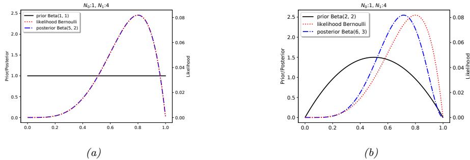
Figure 3.1: Updating a Beta prior with a Bernoulli likelihood with su”cient statistics N¹ = 4, N⁰ = 1. (a) Uniform Beta(1,1) prior. (a) Beta(2,2) prior. Generated by beta\_binom\_post\_plot.ipynb.

We can think of these hyper-parameters as pseudocounts, which play a role analogous to the empirical counts ^N1 and ^N0 derived from the real data. The strength of the prior is controlled by ↭ ^N=↭^{α +} ↭ ↼; this is called the equivalent sample size, since it plays a role analogous to the observed sample size, N = N¹ + N0.

3.2.1.3 Posterior

We can compute the posterior by multiplying the likelihood by the prior:

\[p(\boldsymbol{\theta}|\mathcal{D}) \propto \theta^{N\_1} (1-\theta)^{N\_0} \theta^{\mathbb{X}-1} (1-\theta)^{\overset{\succ}{\boldsymbol{\beta}}-1} \propto \text{Beta}(\boldsymbol{\theta}|\operatorname{\check{\alpha}} + N\_1, \check{\boldsymbol{\beta}} + N\_0) = \text{Beta}(\boldsymbol{\theta}|\operatorname{\check{\alpha}}, \widehat{\boldsymbol{\beta}}) \tag{3.6}\]

where ↫α↭↭^{α +}N¹ and ↫ ↼↭↭ ↼ +N⁰ are the parameters of the posterior. Since the posterior has the same functional form as the prior, we say that it is a conjugate prior (see Section 3.4 for more details).

For example, suppose we observe N¹ = 4 heads and N⁰ = 1 tails. If we use a uniform prior, we get the posterior shown in Figure 3.1a. Not surprisingly, this has exactly the same shape as the likelihood (but is scaled to integrate to 1 over the range [0, 1]).

Now suppose we use a prior that has a slight preference for values of ϑ near to 0.5, reflecting our prior belief that it is more likely than not that the coin is fair. We will make this a weak prior by setting ↭α=↭ ↼= 2. The e!ect of using this prior is illustrated in Figure 3.1b. We see the posterior (blue line) is a “compromise” between the prior (black line) and the likelihood (red line).

3.2.1.4 Posterior mode (MAP estimate)

The most probable value of the parameter is given by the MAP estimate

\[\hat{\theta}\_{\text{map}} = \arg\max\_{\theta} p(\theta | \mathcal{D}) = \arg\max\_{\theta} \log p(\theta | \mathcal{D}) = \arg\max\_{\theta} \log p(\theta) + \log p(\mathcal{D} | \theta) \tag{3.7}\]

Using calculus, one can show that this is given by

\[ \hat{\theta}\_{\text{map}} = \frac{\check{\alpha} + N\_1 - 1}{\check{\alpha} + N\_1 - 1 + \check{\beta} + N\_0 - 1} \tag{3.8} \]

If we use a uniform prior, p(ϑ) ↙ 1, the MAP estimate becomes the MLE, since log p(ϑ)=0:

\[\hat{\theta}\_{\text{mle}} = \arg\max\_{\theta} \log p(\mathcal{D}|\theta) = \frac{N\_1}{N\_1 + N\_0} = \frac{N\_1}{N} \tag{3.9}\]

This is intuitive and easy to compute. However, the MLE can be very misleading in the small sample setting. For example, suppose we toss the coins N times, but never see any heads, so N¹ = 0. In this case, we would estimate that ˆϑ = 0, which means we would not predict any future observations to be heads either. This is a very extreme estimate, that is likely due to insu”cient data. We can solve this problem using a MAP estimate with a stronger prior. For example, if we use a Beta(ϑ|2, 2) prior, we get the estimate

\[\hat{\theta}\_{\text{map}} = \frac{N\_1 + 1}{N\_1 + 1 + N\_0 + 1} = \frac{N\_1 + 1}{N + 2} \tag{3.10}\]

This is called add-one smoothing.

3.2.1.5 Posterior mean

The posterior mode can be a poor summary of the posterior, since it corresponds to picking a single point from the entire distribution. The posterior mean is a more robust estimate, since it is a summary statistic derived by integrating over the distribution, ^{ϑ =} $ ^ϑp(ϑ|D)dϑ. In the case of a beta posterior, ^p(ϑ|D) = Beta(ϑ^| ↫α, ↫ ↼), the posterior mean is given by

\[\overline{\theta} \triangleq \mathbb{E}\left[\theta | \mathcal{D}\right] = \frac{\widehat{\alpha}}{\widehat{\beta} + \widehat{\alpha}} = \frac{\widehat{\alpha}}{\widehat{N}} \tag{3.11}\]

where ↫ N=↫ ↼ + ↫α is the strength (equivalent sample size) of the posterior.

We will now show that the posterior mean is a convex combination of the prior mean, m =↭α / ↭ N and the MLE, ˆϑmle = ^N1 N :

\[\mathbb{E}\left[\theta|\mathcal{D}\right] = \frac{\check{\alpha} + N\_1}{\check{\alpha} + N\_1 + \check{\beta} + N\_0} = \frac{\check{N}\,m + N\_1}{N + \check{N}}\tag{3.12}\]

\[=\frac{\check{N}}{N+\check{N}}m+\frac{N}{N+\check{N}}\frac{N\_1}{N}=\lambda m+(1-\lambda)\hat{\theta}\_{\text{mle}}\tag{3.13}\]

where ^{ϖ =} ↭ N↫ ^N is the ratio of the prior to posterior equivalent sample size. We see that the weaker the prior is, the smaller ϖ is, and hence the closer the posterior mean is to the MLE.

3.2.1.6 Posterior variance

To capture some notion of uncertainty in our estimate, a common approach is to compute the standard error of our estimate, which is just the posterior standard deviation:

\[\text{se}(\theta) = \sqrt{\mathbb{V}\left[\theta|\mathcal{D}\right]} \tag{3.14}\]

In the case of the Bernoulli model, we showed that the posterior is a beta distribution. The variance of the beta posterior is given by

\[\mathbb{V}\left[\theta|\mathcal{D}\right] = \frac{\widehat{\alpha}\widehat{\beta}}{(\widehat{\alpha}+\widehat{\beta})^2(\widehat{\alpha}+\widehat{\beta}+1)} = \frac{(\check{\alpha}+N\_1)(\check{\beta}+N\_0)}{(\check{\alpha}+N\_1+\check{\beta}+N\_0)^2(\check{\alpha}+N\_1+\check{\beta}+N\_0+1)}\tag{3.15}\]

If ^{N ∃}↭^{α +} ↭ ↼, this simplifies to

\[\mathbb{V}\left[\theta|\mathcal{D}\right] \approx \frac{N\_1 N\_0}{(N\_1 + N\_0)^2 (N\_1 + N\_0)} = \frac{N\_1}{N} \frac{N\_0}{N} \frac{1}{N} = \frac{\hat{\theta}(1 - \hat{\theta})}{N} \tag{3.16}\]

where ˆϑ = N1/N is the MLE. Hence the standard error is given by

\[ \sigma = \sqrt{\mathbb{V}\left[\theta|\mathcal{D}\right]} \approx \sqrt{\frac{\hat{\theta}(1-\hat{\theta})}{N}}\tag{3.17} \]

We see that the uncertainty goes down at a rate of 1/ ↖ N. We also see that the uncertainty (variance) is maximized when ˆϑ = 0.5, and is minimized when ˆϑ is close to 0 or 1. This makes sense, since it is easier to be sure that a coin is biased than to be sure that it is fair.

3.2.1.7 Credible intervals

A posterior distribution is (usually) a high dimensional object that is hard to visualize and work with. A common way to summarize such a distribution is to compute a point estimate, such as the posterior mean or mode, and then to compute a credible interval, which quantifies the uncertainty associated with that estimate. (A credible interval is not the same as a confidence interval, which is a concept from frequentist statistics which we discuss in Section 3.3.5.1.)

More precisely, we define a 100(1 ⇐ α)% credible interval to be a (contiguous) region C = (⇁, u) (standing for lower and upper) which contains 1 ⇐ α of the posterior probability mass, i.e.,

\[C\_{\alpha}(\mathcal{D}) = (\ell, u) : P(\ell \le \theta \le u | \mathcal{D}) = 1 - \alpha \tag{3.18}\]

There may be many intervals that satisfy Equation (3.18), so we usually choose one such that there is (1⇐α)/2 mass in each tail; this is called a central interval. If the posterior has a known functional form, we can compute the posterior central interval using ⇁ ^{= F ↑}1(α/2) and ^{u = F ↑}1(1⇐α/2), where F is the cdf of the posterior, and F ^↑1 is the inverse cdf. For example, if the posterior is Gaussian, ^p(ϑ|D) = ^N (0, 1), and ^α = 0.05, then we have ⇁ ⁼ #↑1(α/2) = ⇐1.96, and ^{u =} #↑1(1 ⇐ ^α/2) = 1.96, where # denotes the cdf of the Gaussian. This justifies the common practice of quoting a credible interval in the form of µ ± 2ε, where µ represents the posterior mean, ε represents the posterior standard deviation, and 2 is a good approximation to 1.96.

A problem with central intervals is that there might be points outside the central interval which have higher probability than points that are inside, as illustrated in Figure 3.2(a). This motivates an alternative quantity known as the highest posterior density or HPD region, which is the set of points which have a probability above some threshold. More precisely we find the threshold p↘ on the pdf such that

\[1 - \alpha = \int\_{\theta: p(\theta|\mathcal{D}) > p^\*} p(\theta|\mathcal{D}) d\theta \tag{3.19}\]

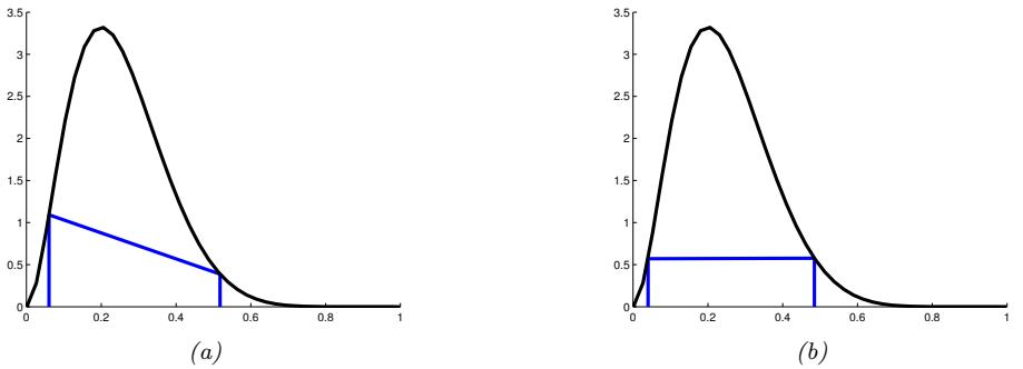
Figure 3.2: (a) Central interval and (b) HPD region for a Beta(3,9) posterior. The CI is (0.06, 0.52) and the HPD is (0.04, 0.48). Adapted from Figure 3.6 of [Hof09]. Generated by betaHPD.ipynb.

and then define the HPD as

\[C\_{\alpha}(\mathcal{D}) = \{ \theta : p(\theta | \mathcal{D}) \ge p^\* \} \tag{3.20}\]

In 1d, the HPD region is sometimes called a highest density interval or HDI. For example, Figure 3.2(b) shows the 95% HDI of a Beta(3, 9) distribution, which is (0.04, 0.48). We see that this is narrower than the central interval, even though it still contains 95% of the mass; furthermore, every point inside of it has higher density than every point outside of it.

3.2.1.8 Posterior predictive distribution

Suppose we want to predict future observations. The optimal Bayesian approach is to compute the posterior predictive distribution, by marginalizing out all the unkown parameters:

\[p(\mathbf{y}|\mathcal{D}) = \int p(\mathbf{y}|\boldsymbol{\theta})p(\boldsymbol{\theta}|\mathcal{D})d\boldsymbol{\theta} \tag{3.21}\]

Sometimes computing this integral can be di”cult (even if we already have access to the posterior). A common approximation is to just “plug in” a point estimate of the parameters, ^{ωˆ = 1}(D), where 1() is some estimator such as a method to compute the MLE or MAP, which gives

\[p(y|\mathcal{D}) \approx p(y|\hat{\theta})\tag{3.22}\]

This is called a plugin approximation. This is equivalent to modeling the posterior with a degenerate distribution centered at the point estimate

\[p(\boldsymbol{\theta}|\mathcal{D}) \approx \delta(\boldsymbol{\theta} - \hat{\boldsymbol{\theta}}) \tag{3.23}\]

where 1 is the Dirac delta function. This follows from the sifting property of delta functions:

\[p(\boldsymbol{y}|\mathcal{D}) = \int p(\boldsymbol{y}|\boldsymbol{\theta})p(\boldsymbol{\theta}|\mathcal{D})d\boldsymbol{\theta} = \int p(\boldsymbol{y}|\boldsymbol{\theta})\delta(\boldsymbol{\theta}-\hat{\boldsymbol{\theta}})d\boldsymbol{\theta} = p(\boldsymbol{y}|\hat{\boldsymbol{\theta}})\tag{3.24}\]

3.2. Bayesian statistics 69

Unfortunately, the plugin approximation can result in overfitting. For example, consider the coin tossing example, and suppose we have seen N = 3 heads in a row. The MLE is ˆϑ = 3/3=1. However, if we use this estimate for prediction, we would predict that tails are impossible, and would be very surprised if one ever showed up.1

Instead of the plugin approximation, we can marginalize over all parameter values to compute the exact posterior predictive, as follows:

\[p(y=1|\mathcal{D}) = \int\_0^1 p(y=1|\theta)p(\theta|\mathcal{D})d\theta\tag{3.25}\]

\[=\int\_0^1 \theta \, \text{Beta}(\theta | \, \hat{\alpha}, \hat{\beta}) d\theta = \mathbb{E}\left[\theta | \mathcal{D}\right] = \frac{\hat{\alpha}}{\hat{\alpha} + \hat{\beta}}\tag{3.26}\]

If we use a uniform prior, p(ϑ) = Beta(ϑ|1, 1), the predictive distribution becomes

\[p(y=1|\mathcal{D}) = \frac{N\_1 + 1}{N\_1 + N\_0 + 2} \tag{3.27}\]

This is known as Laplace’s rule of succession. Note that this is equivalent to plugging in the add-one smoothing estimate from Equation (3.10); however, that relied on the rather unnatural Beta(2,2) prior, whereas Laplace smoothing uses a uniform prior.

3.2.1.9 Marginal likelihood

The marginal likelihood or evidence for a model M is defined as

\[p(\mathcal{D}|\mathcal{M}) = \int p(\boldsymbol{\theta}|\mathcal{M}) p(\mathcal{D}|\boldsymbol{\theta}, \mathcal{M}) d\boldsymbol{\theta} \tag{3.28}\]

When performing inference for the parameters of a specific model, we can ignore this term, since it is constant wrt ω. However, this quantity plays a vital role when choosing between di!erent models, as we discuss in Section 3.8.1. It is also useful for estimating the hyperparameters from data (an approach known as empirical Bayes), as we discuss in Section 3.7.

In general, computing the marginal likelihood can be hard. However, in the case of the beta-Bernoulli model, the marginal likelihood is proportional to the ratio of the posterior normalizer to the prior normalizer. To see this, recall that the posterior is given by ^p(ϑ|D) = Beta(ϑ^| ↫α, ↫ ↼), where ↫α=↭^{α +}N¹ and ↫ ↼=↭ ↼ +N0. We know the normalization constant of the posterior is B( ↫α, ↫ ↼), where B is the beta function. Hence

\[p(\boldsymbol{\theta}|\mathcal{D}) = \frac{p(\mathcal{D}|\boldsymbol{\theta})p(\boldsymbol{\theta})}{p(\mathcal{D})} = \frac{1}{p(\mathcal{D})} \left[ \theta^{N\_1} (1-\theta)^{N\_0} \right] \left[ \frac{1}{B(\boldsymbol{\lambda}, \check{\boldsymbol{\beta}})} \theta^{\check{\boldsymbol{\alpha}}-1} (1-\theta)^{\check{\boldsymbol{\beta}}-1} \right] \tag{3.29}\]

\[\hat{\theta}\_{1} = \frac{1}{p(\mathcal{D})} \frac{1}{B(\mathbb{X}, \check{\beta})} \left[ \theta^{\mathbb{X} + N\_{1} - 1} (1 - \theta)^{\mathbb{X} + N\_{0} - 1} \right] = \frac{1}{B(\widehat{\alpha}, \widehat{\beta})} \left[ \theta^{\widehat{\alpha}} (1 - \theta)^{\widehat{\beta}} \right] \tag{3.30}\]

^1. This is analogous to a black swan event, which refers to the discovery of black swans by Dutch explorers when they first arrived in Australia in 1697, after only ever having seen white swans their entire lives (see https: //en.wikipedia.org/wiki/Black\_swan\_theory for details).

So the marginal likelihood is given by the ratio of normalization constants for the posterior and prior, ^p(D) = ^B(↫ϖ, ↫⇀) B(↭ϖ, ↭⇀) . For the special case where we use the Je!rey’s prior in Equation (3.225) (i.e., ^p(ϑ) = Beta(ϑ^| ↭α^{= 1} 2 , ↭ ↼= ^{1 2} )), the marginal likelihood reduces to the Krichevski-Trofimov estimator or KT estimator [WST96]:

\[p(\mathcal{D}) = \frac{B(\widehat{\alpha}, \widehat{\beta})}{B(\widetilde{\alpha}, \widetilde{\beta})} = \frac{\Gamma(N\_1 + \frac{1}{2})\Gamma(N\_0 + \frac{1}{2})}{\Gamma(N\_1 + N\_0 + \frac{1}{2} + \frac{1}{2})} \frac{\Gamma(\frac{1}{2} + \frac{1}{2})}{\Gamma(\frac{1}{2})\Gamma(\frac{1}{2})} = \frac{1}{\pi}B\left(N\_1 + \frac{1}{2}, N\_0 + \frac{1}{2}\right) \tag{3.31}\]

where we used the facts that B(a, b) = !(a)!(b) !(a+b) , “(1) = 1 and”( ^{1 2} ) = ↖ϱ.

3.2.2 Modeling more complex data

In Section 3.2.1, we showed how the Bayesian approach can be applied to analyse a very simple model, namely a Bernoulli distribution for representing binary events such as coin tosses. The same basic ideas can be applied to more complex models. For example, in machine learning, we are often very interested in predicting outcomes y given input features x. For this, we can use a conditional probability distribution of the form p(y|x, ω), which can be a generalized linear model (Chapter 15), or a neural network (Chapter 16), etc.

The main quantity of interest is the posterior predictive distribution, given by

\[p(\mathbf{y}|\mathbf{z}, \mathcal{D}) = \int p(\mathbf{y}|\mathbf{z}, \boldsymbol{\theta}) p(\boldsymbol{\theta}|\mathcal{D}) d\boldsymbol{\theta} \tag{3.32}\]

By integrating out, or marginalizing out, the unknown parameters, we reduce the chance of overfitting, since we are e!ectively computing the weighted average of predictions from an infinite number of models. This act of integrating over uncertainty is at the heart of the Bayesian approach to machine learning. (Of course, the Bayesian approach requires a prior, but so too do methods that rely on regularization, so the prior is not so much the distinguishing aspect.)

It is worth contrasting the Bayesian approach to the more common plugin approximation, in which we compute a point estimate ωˆ of the parameters (such as the MLE), and then plug them into the model to make predictions using ^p(y|x, ^ωˆ). As we explained in Section 3.2.1.8, this is equivalent to approximate the posterior by a delta function, ^p(ω|D) ^{¬ 1}(^ω ⇐ ^ωˆ), since

\[p(\mathbf{y}|\mathbf{z}, \mathcal{D}) \approx \int p(\mathbf{y}|\mathbf{z}, \boldsymbol{\theta}) \delta(\boldsymbol{\theta} - \boldsymbol{\hat{\theta}}) d\boldsymbol{\theta} = p(\mathbf{y}|\boldsymbol{x}, \boldsymbol{\hat{\theta}}) \tag{3.33}\]

The plugin approximation is simple and widely used. However, it ignores uncertainty in the parameter estimates, which can result in an underestimate of the predictive uncertainty. For example, Figure 3.3a plots the plugin approximation ^p(y|x, ^ωˆ) for a linear regression model ^p(y|x, ^ω) = ^N (y|w^{ˆ T} mlex, εˆ² mle), where we plug in the MLEs for w and ε². (See Section 15.2.1 for details on how to compute these MLEs.) We see that the size of the predicted variance is a constant (namely εˆ²).

The uncertainty captured by εˆmle is called aleatoric uncertainty or intrinsic uncertainty, and would persist even if we knew the true model and true parameters. However, since we don’t know the parameters, we have an additional, and orthogonal, source of uncertainty, called epistemic

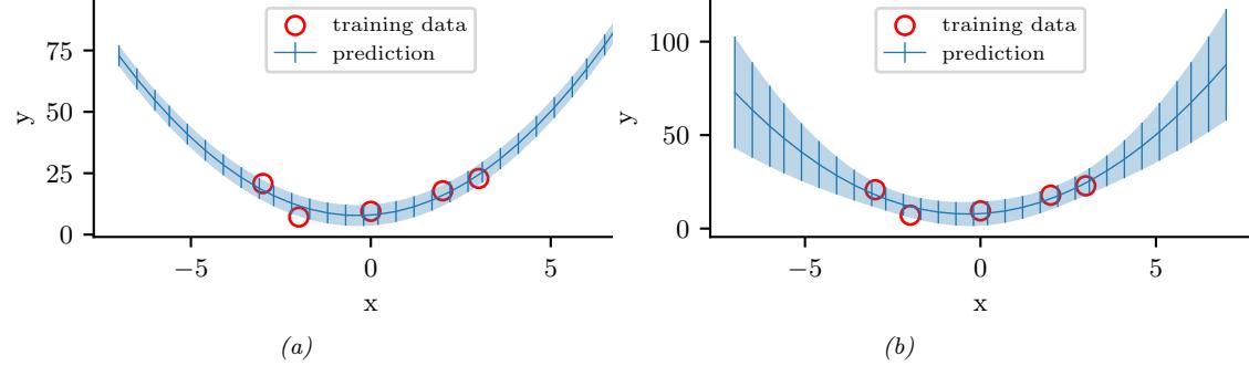
Figure 3.3: Predictions made by a polynomial regression model fit to a small dataset. (a) Plugin approximation to predictive density using the MLE. The curves shows the posterior mean, E [y|x], and the error bars show the posterior standard deviation, std [y|x], around this mean. (b) Bayesian posterior predictive density, obtained by integrating out the parameters. Generated by linreg\_post\_pred\_plot.ipynb.

uncertainty (since it arises due to a lack of knowledge about the truth).2 In the Bayesian approach, we take this into account, which can be useful for applications such as active learning (Section 34.7), Bayesian optimization (Section 6.6), and risk-sensitive decision making (Section 34.1.3). The resulting Bayesian posterior predictive distribution for this example is shown in Figure 3.3b. We see that now the error bars get wider as we move away from the training data. For more details on Bayesian linear regression, see Section 15.2.

We can use similiar Bayesian methods for more complex nonlinear models such as neural nets, as we discuss in Section 17.1, as well as for unconditional generative models, as we discuss in Part IV.

3.2.3 Selecting the prior

A challenge with the Bayesian approach is that it requires the user to specify a prior, which may be di”cult in large models, such as neural networks. We discuss the topic of prior selection at length later in this chapter. In particular, in Section 3.4, we discuss conjugate priors, which are computationally convenient; in Section 3.5, we discuss uninformative priors, which often correspond to a limit of a conjugate prior where we “know nothing”; in Section 3.6, we discuss hierarchical priors, which are useful when we have multiple related datasets; and in Section 3.7, we discuss empirical priors, which can be learned from the data.

3.2.4 Computational issues

Another challenge with the Bayesian approach is that it can be computationally expensive to compute the posterior and/or posterior predictive. We give an overview of suitable approximate posterior

^2. Formally, we can define epistemic uncertainty as the mutual information (Section 5.3) between the (random) observation y and the unknown quantity of interest ω. This is given by I(ω; y) = H(y) → H(y|ω). Intuitively, this says the epistemic uncertainty is the total uncertainty minus the aleatoric uncertainty. (Note that we can also condition everything on the fixed inputs x and D, but we omitted this for notational simplicity.) See e.g., [KD09] for more details.

inference methods in Section 7.4, and discuss the topic at length in Part II. (See also [MFR20] for a historical review of this topic.)

3.2.5 Exchangeability and de Finetti’s theorem

An interesting philosophical question is: where do priors come from, given that they refer to parameters which are just abstract quantities in a model, and not directly observable. A fundamental result, known as de Finetti’s theorem, explains how they are related to our beliefs about observable outcomes.

To explain the result, we first need a definition. We say that a sequence of random variables (x1, x2,…) is infinitely exchangeable if, for any n, the joint probability p(x1,…, xn) is invariant to permutation of the indices. That is, for any permutation ϱ, we have

\[p(x\_1, \ldots, x\_n) = p(x\_{\pi\_1}, \ldots, x\_{\pi\_n}) \tag{3.34}\]

Exchangeability is a more general concept compared to the more familiar concept of a sequence of independent, identically distributed or iid variables. For example, suppose D = (x1,…, xn) is a sequence of images, where each xⁱ ⇔ p↘ is generated independently from the same “true distribution” p↘. We see that this is an iid sequence. Now suppose x⁰ is a background image. The sequence (x⁰ + x1,…, x⁰ + xn) is infinitely exchangeable but not iid, since all the variables share a hidden common factor, namely the background x0. Thus the more examples we see, the better we will be able to estimate the shared x0, and thus the better we can predict future elements.

More generally, we can view an exchangeable sequence as coming from a hidden common cause, which we can treat as an unknown random variable ω. This is formalized by de Finetti’s theorem:

Theorem 3.2.1 (de Finetti’s theorem). A sequence of random variables (x1, x2,…) is infinitely exchangeable i”, for all n, we have

\[p(\mathbf{x}\_1, \dots, \mathbf{x}\_n) = \int \prod\_{i=1}^n p(\mathbf{x}\_i | \boldsymbol{\theta}) p(\boldsymbol{\theta}) d\boldsymbol{\theta} \tag{3.35}\]

where ω is some hidden common random variable (possibly infinite dimensional). That is, xⁱ are iid conditional on ω.

We often interpret ω as a parameter. The theorem tells us that, if our data is exchangeable, then there must exist a parameter ω, and a likelihood p(xi|ω), and a prior p(ω). Thus the Bayesian approach follows automatically from exchangeability [O’N09]. (The approach can also be extended to conditional probability models using a concept called partially exchangeable [Dia88a].)

3.3 Frequentist statistics

Bayesian statistics, which we discussed in Section 3.2, treats parameters of models just like any other unknown random variable, and applies the rules of probability theory to infer them from data. Attempts have been made to devise approaches to statistical inference that avoid treating parameters like random variables, and which thus avoid the use of priors and Bayes rule. This alternative approach is known as frequentist statistics, classical statistics or orthodox statistics.

The basic idea (formalized in Section 3.3.1) is to represent uncertainty by calculating how a quantity estimated from data (such as a parameter or a predicted label) would change if the data were changed. It is this notion of variation across repeated trials that forms the basis for modeling uncertainty used by the frequentist approach. By contrast, the Bayesian approach views probability in terms of information rather than repeated trials. This allows the Bayesian to compute the probability of one-o! events, such as the probability that the polar ice cap will melt by 2030. In addition, the Bayesian approach avoids certain paradoxes that plague the frequentist approach (see Section 3.3.5), and which are a source of much confusion.

Despite the disadvantages of frequentist statistics, it is a widely used approach, and it has some concepts (such as cross validation, model checking and conformal prediction) that are useful even for Bayesians [Rub84]. Thus it is important to know some of the basic principles. We give a brief summary of these principles below. For more details, see other texbooks, such as [Was04; Cox06; YS10; EH16].

3.3.1 Sampling distributions

In frequentist statistics, uncertainty is not represented by the posterior distribution of a random variable, but instead by the sampling distribution of an estimator. (We define these two terms below.)

As explained in the section on decision theory in Section 34.1.2, an estimator is a decision procedure that specifies what action to take given some observed data. In the context of parameter estimation, where the action space is to return a parameter vector, we will denote this by ^{ωˆ =} &^ˆ (D). For example, ωˆ could be the maximum likelihood estimate, the MAP estimate, or the method of moments estimate.

The sampling distribution of an estimator is the distribution of results we would see if we applied the estimator multiple times to di!erent datasets sampled from some distribution; in the context of parameter estimation, it is the distribution of ωˆ, viewed as a random variable that depends on the random sample D. In more detail, imagine sampling S di!erent data sets, each of size N, from some true model p(x|ω↘) to generate

\[\hat{\mathcal{D}}^{(s)} = \{ \mathbf{x}\_n \sim p(\mathbf{x}\_n | \theta^\*) : n = 1 : N \} \tag{3.36}\]

We denote this by ^D˜ (s) ^{⇔ ω}↘ for brevity. Now apply the estimator to each ^D˜ (s) to get a set of estimates, {ωˆ(D˜ (s) )}. As we let S → ⇒, the distribution induced by this set is the sampling distribution of the estimator. More precisely, we have

\[p(\hat{\Theta}(\bar{\mathcal{D}}) = \theta | \bar{\mathcal{D}} \sim \theta^\*) \approx \frac{1}{S} \sum\_{s=1}^{S} \delta(\theta - \hat{\Theta}(\bar{\mathcal{D}}^{(s)})) \tag{3.37}\]

We often approximate this by Monte Carlo, as we discuss in Section 3.3.2, although in some cases we can compute it analytically, as we discuss in Section 3.3.3.

3.3.2 Bootstrap approximation of the sampling distribution

In cases where the estimator is a complex function of the data, or when the sample size is small, it is often useful to approximate its sampling distribution using a Monte Carlo technique known as the bootstrap [ET93].

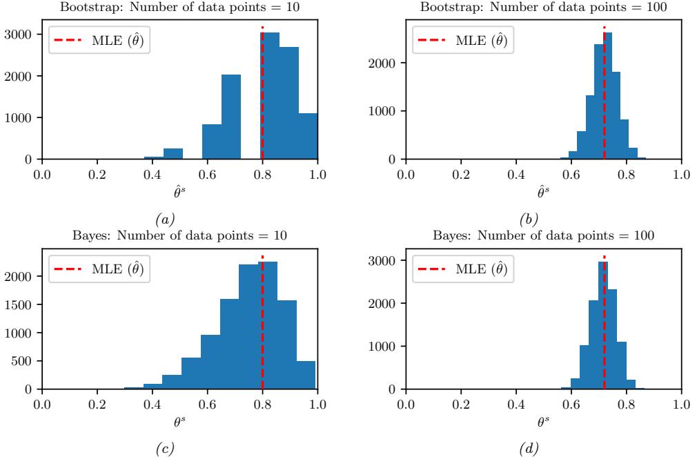
Figure 3.4: Bootstrap (top row) vs Bayes (bottom row). The N data cases were generated from Ber(ε = 0.7). Left column: N = 10. Right column: N = 100. (a-b) A bootstrap approximation to the sampling distribution of the MLE for a Bernoulli distribution. We show the histogram derived from B = 10, 000 bootstrap samples. (c-d) Histogram of 10,000 samples from the posterior distribution using a uniform prior. Generated by bootstrap\_demo\_bernoulli.ipynb.

The idea is simple. If we knew the true parameters ω↘, we could generate many (say S) fake datasets, each of size ^N, from the true distribution, using ^D˜ (s) ⁼ {x^{n ⇔ p}(xn|ω↘) : ⁿ =1: ^N}. We could then compute our estimate from each sample, ^ωˆ^{s =} &^ˆ (D˜ (s) ) and use the empirical distribution of the resulting ωˆ^s as our estimate of the sampling distribution, as in Equation (3.37). Since ω↘ is unknown, the idea of the parametric bootstrap is to generate each sampled dataset using ^{ωˆ =} &ˆ(D) instead of ^ω↘, i.e., we use ^D˜ (s) ⁼ {x^{n ⇔ p}(xn|ωˆ) : ⁿ =1: ^N} in Equation (3.37). This is a plug-in approximation to the sampling distribution.

The above approach requires that we have a parametric generative model for the data, p(x|ω). An alternative, called the non-parametric bootstrap, is to sample N data points from the original dataset with replacement. This creates a new distribution ^D(s) which has the same size as the original. However, the number of unique data points in a bootstrap sample is just 0.632 ∞ N, on average. (To see this, note that the probability an item is picked at least once is (1 ⇐ (1 ⇐ 1/N)^N ), which approaches 1 ⇐ ^e↑^{1 ¬} 0.632 for large ^N.) Fortunately, various improved versions of the bootstrap have been developed (see e.g., [ET93]).

Figure 3.4(a-b) shows an example where we compute the sampling distribution of the MLE for a Bernoulli using the parametric bootstrap. (Results using the non-parametric bootstrap are essentially

the same.) When N = 10, we see that the sampling distribution is asymmetric, and therefore quite far from Gaussian, but when N = 100, the distribution looks more Gaussian, as theory suggests (see Section 3.3.3).

A natural question is: what is the connection between the parameter estimates ^ωˆ^{s =} &ˆ(D(s) ) computed by the bootstrap and parameter values sampled from the posterior, ^{ωs ⇔ p}(·|D)? Conceptually they are quite di!erent. But in the common case that the estimator is MLE and the prior is not very strong, they can be quite similar. For example, Figure 3.4(c-d) shows an example where we compute the posterior using a uniform Beta(1,1) prior, and then sample from it. We see that the posterior and the sampling distribution are quite similar. So one can think of the bootstrap distribution as a “poor man’s” posterior [HTF01, p235].

However, perhaps surprisingly, bootstrap can be slower than posterior sampling. The reason is that the bootstrap has to generate S sampled datasets, and then fit a model to each one. By contrast, in posterior sampling, we only have to “fit” a model once given a single dataset. (Some methods for speeding up the bootstrap when applied to massive data sets are discussed in [Kle+11].)

3.3.3 Asymptotic normality of the sampling distribution of the MLE

The most common estimator is the MLE. When the sample size becomes large, the sampling distribution of the MLE for certain models becomes Gaussian. This is known as the asymptotic normality of the sampling distribution. More formally, we have the following result:

Theorem 3.3.1. Under various technical conditions, we have

\[ \sqrt{N}(\hat{\boldsymbol{\theta}} - \boldsymbol{\theta}^\*) \to \mathcal{N}(\mathbf{0}, \mathbf{F}(\boldsymbol{\theta}^\*)^{-1}) \tag{3.38} \]

where F(ω↘) is the Fisher information matrix, defined in Equation (3.40), ω↘ are the parameters of the data generating process to which the estimator will be applied, and → means convergence in distribution.

The Fisher information matrix equals the Hessian of the log likelihood, as we show in Section 3.3.4, so F(ω↘) measures the amount of curvature of the log-likelihood surface at the true parameter value. Thus we can intepret this theorem as follows: as the sample size goes to infinity, the sampling distribution of the MLE will converge to a Gaussian centered on the true parameter, with a precision equal to the Fisher information. Thus a problem with an informative (peaked) likelihood will ensure that the parameters are “well determined” by the data, and hence there will be little variation in the estimates ^ωˆ around ^ω↘ as this estimator is applied across di!erent datasets ^D˜ .

3.3.4 Fisher information matrix

In this section, we discuss an important quantity called the Fisher information matrix, which is related to the curvature of the log likelihood function. This plays a key role in frequentist statistics, for characterizing the sampling distribution of the MLE, discussed in Section 3.3.3. However, it is also used in Bayesian statistics (to derive Je!reys’ uninformative priors, discussed in Section 3.5.2), as well as in optimization (as part of the natural gradient descent, procedure, discussed in Section 6.4).

3.3.4.1 Definition

The score function is defined to be the gradient of the log likelihood wrt the parameter vector:

\[s(\theta) \triangleq \nabla\_{\theta} \log p(x|\theta) \tag{3.39}\]

The Fisher information matrix (FIM) is defined to be the covariance of the score function:

\[\mathbf{F}(\boldsymbol{\theta}) \triangleq \mathbb{E}\_{\mathbf{z} \sim p(\boldsymbol{x}|\boldsymbol{\theta})} \left[ \nabla\_{\boldsymbol{\theta}} \log p(\boldsymbol{x}|\boldsymbol{\theta}) \nabla\_{\boldsymbol{\theta}} \log p(\boldsymbol{x}|\boldsymbol{\theta})^{\mathsf{T}} \right] \tag{3.40}\]

so the (i, j)’th entry has the form

\[F\_{ij} = \mathbb{E}\_{\mathbf{x} \sim \boldsymbol{\theta}} \left[ \left( \frac{\partial}{\partial \theta\_i} \log p(\mathbf{x}|\boldsymbol{\theta}) \right) \left( \frac{\partial}{\partial \theta\_j} \log p(\mathbf{x}|\boldsymbol{\theta}) \right) \right] \tag{3.41}\]

We give an interpretation of this quantity below.

3.3.4.2 Equivalence between the FIM and the Hessian of the NLL

In this section, we prove that the Fisher information matrix equals the expected Hessian of the negative log likelihood (NLL)

\[\text{NLL}(\boldsymbol{\theta}) = -\log p(\mathcal{D}|\boldsymbol{\theta}) \tag{3.42}\]

Since the Hessian measures the curvature of the likelihood, we see that the FIM tells us how well the likelihood function can identify the best set of parameters. (If a likelihood function is flat, we cannot infer anything about the parameters, but if it is a delta function at a single point, the best parameter vector will be uniquely determined.) Thus the FIM is intimately related to the frequentist notion of uncertainty of the MLE, which is captured by the variance we expect to see in the MLE if we were to compute it on multiple di!erent datasets drawn from our model.

More precisely, we have the following theorem.

Theorem 3.3.2. If log p(x|ω) is twice di”erentiable, and under certain regularity conditions, the FIM is equal to the expected Hessian of the NLL, i.e.,

\[\mathbf{F}(\boldsymbol{\theta})\_{ij} \triangleq \mathbb{E}\_{\mathbf{z} \sim \boldsymbol{\theta}} \left[ \left( \frac{\partial}{\partial \theta\_i} \log p(\mathbf{z}|\boldsymbol{\theta}) \right) \left( \frac{\partial}{\partial \theta\_j} \log p(\mathbf{z}|\boldsymbol{\theta}) \right) \right] = -\mathbb{E}\_{\mathbf{z} \sim \boldsymbol{\theta}} \left[ \frac{\partial^2}{\partial \theta\_i \theta\_j} \log p(\mathbf{z}|\boldsymbol{\theta}) \right] \tag{3.43}\]

Before we prove this result, we establish the following important lemma.

Lemma 3.3.1. The expected value of the score function is zero, i.e.,

\[\mathbb{E}\_{p(\mathbf{z}|\boldsymbol{\theta})} \left[ \nabla \log p(\mathbf{z}|\boldsymbol{\theta}) \right] = \mathbf{0} \tag{3.44}\]

We prove this lemma in the scalar case. First, note that since $ ^p(x|ϑ)dx = 1, we have

\[\frac{\partial}{\partial \theta} \int p(x|\theta) dx = 0\tag{3.45}\]

Combining this with the identity

\[\frac{\partial}{\partial \theta} p(x|\theta) = \left[ \frac{\partial}{\partial \theta} \log p(x|\theta) \right] p(x|\theta) \tag{3.46}\]

we have

\[0 = \int \frac{\partial}{\partial \theta} p(x|\theta) dx = \int \left[ \frac{\partial}{\partial \theta} \log p(x|\theta) \right] p(x|\theta) dx = \mathbb{E} \left[ s(\theta) \right] \tag{3.47}\]

Now we return to the proof of our main theorem. For simplicity, we will focus on the scalar case, following the presentation of [Ric95, p263].

Proof. Taking derivatives of Equation (3.47), we have

\[0 = \frac{\partial}{\partial \theta} \int \left[ \frac{\partial}{\partial \theta} \log p(x|\theta) \right] p(x|\theta) dx \tag{3.48}\]

\[I = \int \left[\frac{\partial^2}{\partial\theta^2} \log p(x|\theta)\right] p(x|\theta) dx + \int \left[\frac{\partial}{\partial\theta} \log p(x|\theta)\right] \frac{\partial}{\partial\theta} p(x|\theta) dx \tag{3.49}\]

\[I = \int \left[\frac{\partial^2}{\partial\theta^2} \log p(x|\theta)\right] p(x|\theta) dx + \int \left[\frac{\partial}{\partial\theta} \log p(x|\theta)\right]^2 p(x|\theta) dx \tag{3.50}\]

and hence

\[-\mathbb{E}\_{x\sim\theta}\left[\frac{\partial^2}{\partial\theta^2}\log p(x|\theta)\right] = \mathbb{E}\_{x\sim\theta}\left[\left(\frac{\partial}{\partial\theta}\log p(x|\theta)\right)^2\right] \tag{3.51}\]

as claimed.

Now consider the Hessian of the NLL given N iid samples D = {xⁿ : n =1: N}:

\[H\_{ij} \triangleq -\frac{\partial^2}{\partial \theta\_i \theta\_j} \log p(\mathcal{D}|\boldsymbol{\theta}) = -\sum\_{n=1}^N \frac{\partial^2}{\partial \theta\_i \theta\_j} \log p(\boldsymbol{x}\_n|\boldsymbol{\theta}) \tag{3.52}\]

From the above theorem, we have

\[\mathbb{E}\_{p(\mathcal{D}|\boldsymbol{\theta})} \left[ \mathbf{H}(\mathcal{D}) | \boldsymbol{\theta} \right] = N \mathbf{F}(\boldsymbol{\theta}) \tag{3.53}\]

This is useful when deriving the sampling distribution of the MLE, as discussed in Section 3.3.3.

3.3.4.3 Example: FIM for the binomial

Suppose x ⇔ Bin(n, ϑ). The log likelihood for a single sample is

\[l(\theta|x) = x \log \theta + (n - x) \log(1 - \theta) \tag{3.54}\]

The score function is just the gradient of the log-likelihood:

\[s(\theta|x) \triangleq \frac{d}{d\theta}l(\theta|x) = \frac{x}{\theta} - \frac{n-x}{1-\theta} \tag{3.55}\]

The gradient of the score function is

\[s'(\theta|x) = -\frac{x}{\theta^2} - \frac{n-x}{(1-\theta)^2} \tag{3.56}\]

Hence the Fisher information is given by

\[F(\theta) = \mathbb{E}\_{x \sim \theta} \left[ -s'(\theta|x) \right] = \frac{n\theta}{\theta^2} + \frac{n - n\theta}{(1 - \theta)^2} = \frac{n}{\theta} + \frac{n}{1 - \theta} = \frac{n}{\theta(1 - \theta)}\tag{3.57}\]

3.3.4.4 Example: FIM for the univariate Gaussian

Consider a univariate Gaussian p(x|ω) = N (x|µ, v). We have

\[\ell(\boldsymbol{\theta}) = \log p(\boldsymbol{x}|\boldsymbol{\theta}) = -\frac{1}{2v}(\boldsymbol{x} - \boldsymbol{\mu})^2 - \frac{1}{2}\log(v) - \frac{1}{2}\log(2\pi) \tag{3.58}\]

The partial derivatives are given by

\[\frac{\partial \ell}{\partial \mu} = (x - \mu)v^{-1}, \ \frac{\partial^2 \ell}{\partial \mu^2} = -v^{-1} \tag{3.59}\]

\[\frac{\partial \ell}{\partial v} = \frac{1}{2}v^{-2}(x-\mu)^2 - \frac{1}{2}v^{-1},\\\frac{\partial \ell}{\partial v^2} = -v^{-3}(x-\mu)^2 + \frac{1}{2}v^{-2} \tag{3.60}\]

\[\frac{\partial \ell}{\partial \mu \partial v} = -v^{-2}(x - \mu) \tag{3.61}\]

and hence

\[\mathbf{F}(\boldsymbol{\theta}) = \begin{pmatrix} \mathbb{E}\left[v^{-1}\right] \\ \mathbb{E}\left[v^{-2}(x-\mu)\right] & \mathbb{E}\left[v^{-3}(x-\mu)^2 - \frac{1}{2}v^{-2}\right] \end{pmatrix} = \begin{pmatrix} \frac{1}{v} & 0 \\ 0 & \frac{1}{2v^2} \end{pmatrix} \tag{3.62}\]

3.3.4.5 Example: FIM for logistic regression

Consider ⇁2-regularized binary logistic regression. The negative log joint has the following form:

\[\mathcal{L}(w) = -\log[p(\mathbf{y}|\mathbf{X}, w)p(w|\lambda)] = -w^\mathsf{T}\mathbf{X}^\mathsf{T}\mathbf{y} + \sum\_{n=1}^{N} \log(1 + e^{\mathbf{w}^\mathsf{T}\mathbf{z}\_n}) + \frac{\lambda}{2}w^\mathsf{T}w \tag{3.63}\]

The derivative has the form

\[\nabla\_{\mathbf{w}} \mathcal{L}(w) = -\mathbf{X}^{\mathsf{T}}y + \mathbf{X}^{\mathsf{T}}s + \lambda w \tag{3.64}\]

where sⁿ = ε(w^Txn). The FIM is given by

\[\mathbf{F}(\mathbf{w}) = \mathbb{E}\_{p(\mathbf{y}|\mathbf{X}, \mathbf{w}, \lambda)} \left[ \nabla^2 \mathcal{L}(\mathbf{w}) \right] = \mathbf{X}^\mathsf{T} \mathbf{A} \mathbf{X} + \lambda \mathbf{I} \tag{3.65}\]

where ” is the N ∞ N diagonal matrix with entries

\[ \Lambda\_{nn} = \sigma(\boldsymbol{w}^{\mathsf{T}} \boldsymbol{x}\_n)(1 - \sigma(\boldsymbol{w}^{\mathsf{T}} \boldsymbol{x}\_n))\tag{3.66} \]

3.3.4.6 FIM for the exponential family

In this section, we discuss how to derive the FIM for an exponential family distribution with natural parameters ϖ, which generalizes many of the previous examples. Recall from Equation (2.216) that the gradient of the log partition function is the expected su”cient statistics

\[\nabla\_{\eta}A(\eta) = \mathbb{E}\left[\mathcal{T}(x)\right] = m \tag{3.67}\]

and from Equation (2.247) that the gradient of the log likelihood is the statistics minus their expected value:

\[\nabla\_{\eta} \log p(x|\eta) = \mathcal{T}(x) - \mathbb{E}\left[\mathcal{T}(x)\right] \tag{3.68}\]

Hence the FIM wrt the natural parameters F^ω is given by

\[\mathbb{E}\_{\mathbf{y}}(\mathbf{F}\_{\eta})\_{ij} = \mathbb{E}\_{p(\mathbf{z}|\eta)} \left[ \frac{\partial \log p(\mathbf{z}|\eta)}{\partial \eta\_i} \frac{\partial \log p(\mathbf{z}|\eta)}{\partial \eta\_j} \right] \tag{3.69}\]

\[\mathbb{E}\_{\mathbf{x}} = \mathbb{E}\_{p(\mathbf{z}|\eta)} \left[ (\mathcal{T}(\mathbf{z})\_i - m\_i)(\mathcal{T}(\mathbf{z})\_j - m\_j) \right] \tag{3.70}\]

\[=\text{Cov}\left[\mathcal{T}(\mathbf{z})\_i, \mathcal{T}(\mathbf{z})\_j\right] \tag{3.71}\]

or, in short,

\[\mathbf{F}\_{\eta} = \text{Cov}\left[\mathcal{T}(\mathbf{x})\right] \tag{3.72}\]

Sometimes we need to compute the Fisher wrt the moment parameters m:

\[\mathbb{E}\_{\mathbf{f}}(\mathbf{F}\_{m})\_{ij} = \mathbb{E}\_{p(\mathbf{z}|\mathbf{m})} \left[ \frac{\partial \log p(\mathbf{z}|\boldsymbol{\eta})}{\partial m\_{i}} \frac{\partial \log p(\mathbf{z}|\boldsymbol{\eta})}{\partial m\_{j}} \right] \tag{3.73}\]

From the chain rule we have

\[\frac{\partial \log p(x)}{\partial \alpha} = \frac{\partial \log p(x)}{\partial \beta} \frac{\partial \beta}{\partial \alpha} \tag{3.74}\]

and hence

\[\mathbf{F}\_{\alpha} = \frac{\partial \beta}{\partial \alpha}^{\uparrow} \mathbf{F}\_{\beta} \frac{\partial \beta}{\partial \alpha} \tag{3.75}\]

Using the log trick

\[\nabla \mathbb{E}\_{p(\mathbf{z})} \left[ f(\mathbf{z}) \right] = \mathbb{E}\_{p(\mathbf{z})} \left[ f(\mathbf{z}) \nabla \log p(\mathbf{z}) \right] \tag{3.76}\]

and Equation (3.68) we have

\[\frac{\partial m\_i}{\partial \eta\_j} = \frac{\partial \mathbb{E}\left[\mathcal{T}(\mathbf{x})\_i\right]}{\partial \eta\_j} = \mathbb{E}\left[\mathcal{T}(\mathbf{x})\_i \frac{\partial \log p(\mathbf{x}|\eta)}{\partial \eta\_j}\right] = \mathbb{E}\left[\mathcal{T}(\mathbf{x})\_i(\mathcal{T}(\mathbf{x})\_j - m\_j)\right] \tag{3.77}\]

\[=\mathbb{E}\left[\mathcal{T}(\mathbf{z})\_i\mathcal{T}(\mathbf{z})\_j\right] - \mathbb{E}\left[\mathcal{T}(\mathbf{z})\_i\right]m\_j = \text{Cov}\left[\mathcal{T}(\mathbf{z})\_i\mathcal{T}(\mathbf{z})\_j\right] = (\mathbf{F}\_\eta)\_{ij} \tag{3.78}\]

and hence

\[\frac{\partial \eta}{\partial m} = \mathbf{F}\_{\eta}^{-1} \tag{3.79}\]

so

\[\mathbf{F}\_m = \frac{\partial \boldsymbol{\eta}}{\partial m}^{\mathsf{T}} \mathbf{F}\_{\boldsymbol{\eta}} \frac{\partial \boldsymbol{\eta}}{\partial m} = \mathbf{F}\_{\boldsymbol{\eta}}^{-1} \mathbf{F}\_{\boldsymbol{\eta}} \mathbf{F}\_{\boldsymbol{\eta}}^{-1} = \mathbf{F}\_{\boldsymbol{\eta}}^{-1} = \text{Cov} \left[ \boldsymbol{\mathcal{T}}(\boldsymbol{x}) \right]^{-1} \tag{3.80}\]

3.3.5 Counterintuitive properties of frequentist statistics

Although the frequentist approach to statistics is widely taught, it su!ers from certain pathological properties, resulting in its often being misunderstood and/or misused, as has been pointed out in multiple articles (see e.g., [Bol02; Bri12; Cla21; Gel16; Hoe+14; Jay03; Kru10; Lav00; Lyu+20; Min99; Mac03; WG17]). We give some examples below.

3.3.5.1 Confidence intervals

In frequentist statistics, we use the variability induced by the sampling distribution as a way to estimate uncertainty of a parameter estimate. In particular, we define a 100(1 ⇐ α)% confidence interval as any interval ^I(D˜ )=(⇁(D˜ ), u(D˜ )) derived from a hypothetical dataset ^D˜ such that

\[\Pr(\theta \in I(\tilde{\mathcal{D}}) | \tilde{\mathcal{D}} \sim \theta) = 1 - \alpha \tag{3.81}\]

It is common to set α = 0.05, which yields a 95% CI. This means that, if we repeatedly sampled data, and compute ^I(D˜ ) for each such dataset, then about 95% of such intervals will contain the true parameter ϑ. We say that the CI has 95% coverage.

Note, however, that Equation (3.81) does not mean that for any particular dataset that ϑ ↑ I(D) with 95% probability, which is what a Bayesian credible interval computes (Section 3.2.1.7), and which is what most people are usually interested in. So we see that the concept of frequentist CI and Bayesian CI are quite di!erent: In the frequentist approach, ϑ is treated as an unknown fixed constant, and the data is treated as random. In the Bayesian approach, we treat the data as fixed (since it is known) and the parameter as random (since it is unknown).

This counter-intuitive definition of confidence intervals can lead to bizarre results. Consider the following example from [Ber85a, p11]. Suppose we draw two integers D = (y1, y2) from

\[p(y|\theta) = \begin{cases} \begin{array}{ll} 0.5 & \text{if } y = \theta \\ 0.5 & \text{if } y = \theta + 1 \\ 0 & \text{otherwise} \end{array} \end{cases} \tag{3.82}\]

If ϑ = 39, we would expect the following outcomes each with probability 0.25:

\[(39, 39), (39, 40), (40, 39), (40, 40) \tag{3.83}\]

Let m = min(y1, y2) and define the following interval:

\[[\ell(\mathcal{D}), u(\mathcal{D})] = [m, m] \tag{3.84}\]

For the above samples this yields

\[[39, 39], \ [39, 39], \ [39, 39], \ [40, 40] \tag{3.85}\]

Hence Equation (3.84) is clearly a 75% CI, since 39 is contained in 3/4 of these intervals. However, if we observe D = (39, 40) then p(ϑ = 39|D)=1.0, so we know that ϑ must be 39, yet we only have 75% “confidence” in this fact. We see that the CI will “cover” the true parameter 75% of the time, if we compute multiple CIs from di!erent randomly sampled datasets, but if we just have a single observed dataset, and hence a single CI, then the frequentist “coverage” probability can be very misleading.

Several more interesting examples, along with Python code, can be found at [Van14]. See also [Hoe+14; Mor+16; Lyu+20; Cha+19b], who show that many people, including professional statisticians, misunderstand and misuse frequentist confidence intervals in practice, whereas Bayesian credible intervals do not su!er from these problems.

3.3.5.2 p-values

The frequentist approach to hypothesis testing, known as null hypothesis significance testing or NHST, is to define a decision procedure for deciding whether to accept or reject the null hypothesis H⁰ based on whether some observed test statistic t(D) is likely or not under the sampling distribution of the null model. We describe this procedure in more detail in Section 3.10.1.

Rather than accepting or rejecting the null hypothesis, we can compute a quantity related to how likely the null hypothesis is to be true. In particular, we can compute a quantity called a p-value, which is defined as

\[\mathbb{P}\left[\text{vap}(t(\mathcal{D})) \triangleq \Pr(t(\tilde{\mathcal{D}}) \ge t(\mathcal{D}) | \tilde{\mathcal{D}} \sim H\_0) \right.\tag{3.86}\]

where ^D˜ ^{⇔ H0} is hypothetical future data. That is, the p-value is just the tail probability of observing the value t(D) under the sampling distribution. (Note that the p-value does not explicitly depend on a model of the data, but most common test statistics implicitly define a model, as we discuss in Section 3.10.3.)

A p-value is often interpreted as the likelihood of the data under the null hypothesis, so small values are interpreted to mean that H⁰ is unlikely, and therefore that H¹ is likely. The reasoning is roughly as follows:

If H⁰ is true, then this test statistic would probably not occur. This statistic did occur. Therefore H⁰ is probably false.

However, this is invalid reasoning. To see why, consider the following example (from [Coh94]):

If a person is an American, then he is probably not a member of Congress. This person is a member of Congress. Therefore he is probably not an American.

This is obviously fallacious reasoning. By contrast, the following logical argument is valid reasoning:

If a person is a Martian, then he is not a member of Congress. This person is a member of Congress. Therefore he is not a Martian.

The di!erence between these two cases is that the Martian example is using deduction, that is, reasoning forward from logical definitions to their consequences. More precisely, this example uses a rule from logic called modus tollens, in which we start out with a definition of the form P ∅ Q; when we observe ¬Q, we can conclude ¬P. By contrast, the American example concerns induction, that is, reasoning backwards from observed evidence to probable (but not necessarily true) causes using statistical regularities, not logical definitions.

To perform induction, we need to use probabilistic inference (as explained in detail in [Hac01; Jay03]). In particular, to compute the probability of the null hypothesis, we should use Bayes rule, as follows:

\[p(H\_0|\mathcal{D}) = \frac{p(\mathcal{D}|H\_0)p(H\_0)}{p(\mathcal{D}|H\_0)p(H\_0) + p(\mathcal{D}|H\_1)p(H\_1)}\tag{3.87}\]

If the prior is uniform, so p(H0) = p(H1)=0.5, this can be rewritten in terms of the likelihood ratio LR = p(D|H0)/p(D|H1) as follows:

\[p(H\_0|\mathcal{D}) = \frac{LR}{LR+1} \tag{3.88}\]

In the American Congress example, D is the observation that the person is a member of Congress. The null hypothesis H⁰ is that the person is American, and the alternative hypothesis H¹ is that the person is not American. We assume that p(D|H0) is low, since most Americans are not members of Congress. However, p(D|H1) is also low — in fact, in this example, it is 0, since only Americans can be members of Congress. Hence LR = ⇒, so p(H0|D)=1.0, as intuition suggests.

Note, however, that NHST ignores p(D|H1) as well as the prior p(H0), so it gives the wrong results, not just in this problem, but in many problems. Indeed, even most scientists misinterpret p-values.3. Consequently the journal The American Statistician published a whole special issue warning about the use of p-values and NHST [WSL19], and several journals have even banned p-values [TM15; AGM19].

3.3.5.3 Discussion

The above problems stem from the fact that frequentist inference is not conditional on the actually observed data, but instead is based on properties derived from the sampling distribution of the estimator. However, conditional probability statements are what most people want. As Jim Berger writes in [Ber85a]:

Users of statistics want to know the probability (after seeing the data) that a hypothesis is true, or the probability that ϑ is in a given interval, and yet classical statistics does not allow one to talk of such things. Instead, artificial concepts such as error probabilities and coverage probabilites are introduced as substitutes. It is ironic that non-Bayesians often claim that the Bayesians form a dogmatic unrealistic religion, when instead it is the non-Bayesian methods that are often founded on elaborate and artificial structures. Unfortunately, those who become used to these artificial structures come to view them as natural, and hence this line of argument tends to have little e!ect on the established non-Bayesian. – Jim Berger, [Ber85a].

3.3.6 Why isn’t everyone a Bayesian?

I believe that it would be very di”cult to persuade an intelligent person that current [frequentist] statistical practice was sensible, but that there would be much less di”culty with an approach via likelihood and Bayes’ theorem. — George Box, 1962 (quoted in [Jay76]).

In Section 3.3.5 we showed that inference based on frequentist principles can exhibit various forms of counterintuitive behavior that can sometimes contradict common sense. Given these problems of frequentist statistics, an obvious question to ask is: “Why isn’t everyone a Bayesian?” The statistician Bradley Efron wrote a paper with exactly this title [Efr86]. His short paper is well worth reading for anyone interested in this topic. Below we quote his opening section:

^3. See e.g., https://fivethirtyeight.com/features/not-even-scientists-can-easily-explain-p-values/.

The title is a reasonable question to ask on at least two counts. First of all, everyone used to be a Bayesian. Laplace wholeheartedly endorsed Bayes’s formulation of the inference problem, and most 19th-century scientists followed suit. This included Gauss, whose statistical work is usually presented in frequentist terms.

A second and more important point is the cogency of the Bayesian argument. Modern statisticians, following the lead of Savage and de Finetti, have advanced powerful theoretical arguments for preferring Bayesian inference. A byproduct of this work is a disturbing catalogue of inconsistencies in the frequentist point of view.

Nevertheless, everyone is not a Bayesian. The current era (1986) is the first century in which statistics has been widely used for scientific reporting, and in fact, 20th-century statistics is mainly non-Bayesian. However, Lindley (1975) predicts a change for the 21st century.

Time will tell whether Lindley was right. However, the trends seem to be going in this direction. Traditionally, computation has been a barrier to using Bayesian methods, but this is less of an issue these days, due to faster computers and better algorithms, which we discuss in Part II.

Another, more fundamental, concern is that the Bayesian approach is only as correct as its modeling assumptions. In particular, it is important to check sensitivity of the conclusions to the choice of prior (and likelihood), using techniques such as Bayesian model checking (Section 3.9.1). In particular, as Donald Rubin wrote in his paper called “Bayesianly Justifiable and Relevant Frequency Calculations for the Applied Statistician” [Rub84]:

The applied statistician should be Bayesian in principle and calibrated to the real world in practice. [They] should attempt to use specifications that lead to approximately calibrated procedures under reasonable deviations from [their assumptions]. [They] should avoid models that are contradicted by observed data in relevant ways — frequency calculations for hypothetical replications can model a model’s adequacy and help to suggest more appropriate models.

A final issue is more practical. Most users of statistical methods are not experts in statistics, but instead are experts in their own domain, such as psychology or social science. They often just want a simple (and fast!) method for testing a hypothesis, and so they turn to standard “cookie cutter” frequentist procedures, such as t-tests and ↽²-tests. Fortunately there are simple Bayesian alternatives to these tests, as we discuss in Section 3.10, which avoid the conceptual problems we discussed in Section 3.3.5, and which can also be easily “upgraded” to use more complex (and realistic) modeling assumptions when necessary. Furthermore, by using an empirical Bayes approach, it is possible to derive automatic and robust Bayesian methods that have good frequentist properties but which are also conditional on the data, thus providing the best of both worlds.

For a more detailed discussion of the pros and cons of the Bayesian approach, in the context of machine learning, see https://bit.ly/3Rbd4lo and https://bit.ly/3j8miSR.

3.4 Conjugate priors

In this section, we consider Bayesian inference for a class of models with a special form of prior, known as a conjugate prior, which simplifies the computation of the posterior. Formally, we say that a prior p(ω) ↑ F is a conjugate prior for a likelihood function p(D|ω) if the posterior is in the same parameterized family as the prior, i.e., p(ω|D) ↑ F. In other words, F is closed under

Bayesian updating. If the family F corresponds to the exponential family (defined in Section 2.4), then the computations can be performed in closed form. In more complex settings, we cannot perform closed-form inference, but we can often leverage these results as tractable subroutines inside of a larger computational pipeline.

3.4.1 The binomial model

One of the simplest examples of conjugate Bayesian analysis is the beta-binomial model. This is covered in detail in Section 3.2.1.

3.4.2 The multinomial model

In this section, we generalize the results from Section 3.4.1 from binary variables (e.g., coins) to K-ary variables (e.g., dice). Let y ⇔ Cat(ω) be a discrete random variable drawn from a categorical distribution. The likelihood has the form

\[p(\mathcal{D}|\boldsymbol{\theta}) = \prod\_{n=1}^{N} \text{Cat}(y\_n|\boldsymbol{\theta}) = \prod\_{n=1}^{N} \prod\_{c=1}^{C} \theta\_c^{\mathbb{I}(y\_n=c)} = \prod\_{c=1}^{C} \theta\_c^{N\_c} \tag{3.89}\]

where N^c = # ⁿ I(yⁿ = c). We can generalize this to the multinomial distribution by defining y ⇔ M(N, ω), where N is the number of trials, and y^c = N^c is the number of times value c is observed. The likelihood becomes

\[p(\mathbf{y}|N, \boldsymbol{\theta}) = \binom{N}{N\_1 \dots N\_C} \prod\_{c=1}^C \theta\_c^{N\_c} \tag{3.90}\]

This is the same as the categorical likelihood modulo a scaling factor. Going forwards, we will work with the categorical model, for notational simplicity.

The conjugate prior for a categorical distribution is the Dirichlet distribution, which we discussed in Section 2.2.5.7. We denote this by ^p(ω) = Dir(ω^| ↭ε), where ↭^ε is the vector of prior pseudo-counts. Often we use a symmetric Dirichlet prior of the form ↭αk=↭α /K. In this case, we have E [ϑk] = 1/K, and V [ϑk] = ^K↑^{1 K}2(↭ϖ+1) . Thus we see that increasing the prior sample size ↭^α decreases the variance of the prior, which is equivalent to using a stronger prior.

We can combine the multinomial likelihood and Dirichlet prior to compute the Dirichlet posterior, as follows:

\[p(\boldsymbol{\theta}|\mathcal{D}) \propto p(\mathcal{D}|\boldsymbol{\theta}) \text{Dir}(\boldsymbol{\theta}|\operatorname{\boldsymbol{\alpha}}) \propto \left[\prod\_{k} \theta\_{k}^{N\_{k}}\right] \left[\prod\_{k} \theta\_{k}^{\mathbb{X}\_{k}-1}\right] \tag{3.91}\]

\[<\text{Dir}(\boldsymbol{\theta}|\,\check{\boldsymbol{\alpha}}\_{1}+N\_{1},\ldots,\check{\boldsymbol{\alpha}}\_{K}+N\_{K}) = \text{Dir}(\boldsymbol{\theta}|\,\hat{\boldsymbol{\alpha}})\tag{3.92}\]

where ↫αk=↭α^k +N^k are the parameters of the posterior. So we see that the posterior can be computed by adding the empirical counts to the prior counts. In particular, the posterior mode is given by

\[\hat{\theta}\_{k} = \frac{\hat{\alpha}\_{k} - 1}{\sum\_{k'=1}^{K} \hat{\alpha}\_{k} - 1} = \frac{N\_{k} + \check{\alpha}\_{k} - 1}{\sum\_{k'=1}^{K} N\_{k} + \check{\alpha}\_{k} - 1} \tag{3.93}\]

If we set α^k = 1 we recover the MLE; if we set α^k = 2, we recover the add-one smoothing estimate. The marginal likelihood for the Dirichlet-categorical model is given by the following:

\[p(\mathcal{D}) = \frac{B(\mathbf{N} + \alpha)}{B(\alpha)}\tag{3.94}\]

where

\[B(\alpha) = \frac{\prod\_{k=1}^{K} \Gamma(\alpha\_k)}{\Gamma(\sum\_k \alpha\_k)} \tag{3.95}\]

Hence we can rewrite the above result in the following form, which is what is usually presented in the literature:

\[p(\mathcal{D}) = \frac{\Gamma(\sum\_{k} \alpha\_{k})}{\Gamma(N + \sum\_{k} \alpha\_{k})} \prod\_{k} \frac{\Gamma(N\_{k} + \alpha\_{k})}{\Gamma(\alpha\_{k})} \tag{3.96}\]

For more details on this model, see [Mur22, Sec 4.6.3].

3.4.3 The univariate Gaussian model

In this section, we derive the posterior ^p(µ, ^ε2|D) for a univariate Gaussian. For simplicity, we consider this in three steps: inferring just µ, inferring just ε², and then inferring both. See Section 3.4.4 for the multivariate case.

3.4.3.1 Posterior of µ given ↽²

If ε² is a known constant, the likelihood for µ has the form

\[p(\mathcal{D}|\mu) \propto \exp\left(-\frac{1}{2\sigma^2} \sum\_{n=1}^{N} (y\_n - \mu)^2\right) \tag{3.97}\]

One can show that the conjugate prior is another Gaussian, N (µ| m ↭ , ↭2 ²). Applying Bayes’ rule for Gaussians (Equation (2.121)), we find that the corresponding posterior is given by

\[p(\mu|\mathcal{D}, \sigma^2) = \mathcal{N}(\mu|\hat{m}, \hat{\tau}^2) \tag{3.98}\]

\[\hat{\tau}^2 = \frac{1}{\frac{N}{\sigma^2} + \frac{1}{\tilde{\tau}^2}} = \frac{\sigma^2 \,\,\breve{\tau}^2}{N \,\,\breve{\tau}^2 + \sigma^2} \tag{3.99}\]

\[ \hat{m} = \hat{\tau}^2 \left( \frac{\check{m}}{\check{\tau}^2} + \frac{N\overline{y}}{\sigma^2} \right) = \frac{\sigma^2}{N \ \check{\tau}^2 + \sigma^2} \stackrel{\check{m}}{\check{m}} + \frac{N \stackrel{\varphi}{\prime}^2}{N \ \check{\tau}^2 + \sigma^2} \overline{y} \tag{3.100} \]

where y ↭ ¹ N #^{N n}=1 yⁿ is the empirical mean.

This result is easier to understand if we work in terms of the precision parameters, which are just inverse variances. Specifically, let ϖ = 1/ε² be the observation precision, and ↭ ϖ= 1/ ↭2 ² be the

precision of the prior. We can then rewrite the posterior as follows:

\[p(\boldsymbol{\mu}|\mathcal{D},\boldsymbol{\lambda}) = \mathcal{N}(\boldsymbol{\mu}|\:\widehat{\boldsymbol{m}},\widehat{\boldsymbol{\lambda}}^{-1})\tag{3.101}\]

\[ \widehat{\lambda} = \check{\lambda} + N\lambda \tag{3.102} \]

\[\boldsymbol{\mathcal{H}} = \frac{N\lambda\overline{y} + \check{\lambda}\dot{\boldsymbol{m}}}{\widehat{\lambda}} = \frac{N\lambda}{N\lambda + \check{\lambda}}\overline{y} + \frac{\check{\lambda}}{N\lambda + \check{\lambda}}\ \boldsymbol{\mathcal{H}} \tag{3.103}\]

These equations are quite intuitive: the posterior precision ↫ ϖ is the prior precision ↭ ϖ plus N units of measurement precision ϖ. Also, the posterior mean m ↫ is a convex combination of the empirical mean y and the prior mean m ↭ . This makes it clear that the posterior mean is a compromise between the empirical mean and the prior. If the prior is weak relative to the signal strength (↭ ϖ is small relative to ϖ), we put more weight on the empirical mean. If the prior is strong relative to the signal strength ( ↭ ϖ is large relative to ϖ), we put more weight on the prior. This is illustrated in Figure 3.5. Note also that the posterior mean is written in terms of Nϖx, so having N measurements each of precision ϖ is like having one measurement with value x and precision Nϖ.

To gain further insight into these equations, consider the posterior after seeing a single datapoint y (so N = 1). Then the posterior mean can be written in the following equivalent ways:

\[ \hat{\boldsymbol{m}} = \underset{\widetilde{\lambda}}{\overset{\textstyle \vec{\lambda}}{\overset{\textstyle \vec{\lambda}}{\boldsymbol{\lambda}}}}{\overset{\textstyle \vec{\lambda}}{\overset{\textstyle \vec{\lambda}}{\boldsymbol{\lambda}}}}{\overset{\textstyle \vec{\lambda}}{\overset{\textstyle \vec{\lambda}}{\boldsymbol{\lambda}}}} + \underset{\widetilde{\lambda}}{\overset{\textstyle \vec{\lambda}}{\overset{\textstyle \vec{\lambda}}{\boldsymbol{\lambda}}}}{\overset{\textstyle \vec{\lambda}}{\overset{\textstyle \vec{\lambda}}{\boldsymbol{\lambda}}}}{\overset{\textstyle \vec{\lambda}}{\boldsymbol{\lambda}}} \tag{3.104} \]

\[ \dot{\lambda} = \check{m} + \frac{\lambda}{\check{\lambda}} (y - \check{m}) \tag{3.105} \]

\[y = y - \frac{\check{\lambda}}{\check{\lambda}}(y - \check{m})\tag{3.106}\]

The first equation is a convex combination of the prior mean and the data. The second equation is the prior mean adjusted towards the data y. The third equation is the data adjusted towards the prior mean; this is called a shrinkage estimate. This is easier to see if we define the weight w = ↭ ^ω/ ↫ ^ω. Then we have

\[ \hat{m} = y - w(y - \dot{m}) = (1 - w)y + w \,\,\forall\,\,\tag{3.107} \]

Note that, for a Gaussian, the posterior mean and posterior mode are the same. Thus we can use the above equations to perform MAP estimation.

3.4.3.2 Posterior of ↽² given µ

If µ is a known constant, the likelihood for ε² has the form

\[p(\mathcal{D}|\sigma^2) \propto (\sigma^2)^{-N/2} \exp\left(-\frac{1}{2\sigma^2} \sum\_{n=1}^N (y\_n - \mu)^2\right) \tag{3.108}\]

where we can no longer ignore the 1/(ε²) term in front. The standard conjugate prior is the inverse gamma distribution (Section 2.2.3.4), given by

\[\mathrm{IG}(\sigma^2 \mid \mathbb{X}, \check{b}) = \frac{\check{b}^{\mathsf{nd}}}{\Gamma(\mathsf{d})} (\sigma^2)^{-(\mathsf{d} + 1)} \exp(-\frac{\check{b}}{\sigma^2}) \tag{3.109}\]

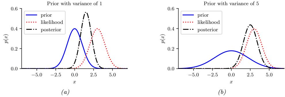
Figure 3.5: Inferring the mean of a univariate Gaussian with known ϑ². (a) Using strong prior, p(µ) = N (µ|0, 1). (b) Using weak prior, p(µ) = N (µ|0, 5). Generated by gauss\_infer\_1d.ipynb.

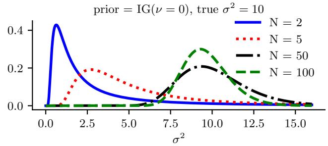
Figure 3.6: Sequential updating of the posterior for ϑ² starting from an uninformative prior. The data was generated from a Gaussian with known mean µ = 5 and unknown variance ϑ² = 10. Generated by gauss\_seq\_update\_sigma\_1d.ipynb

Multiplying the likelihood and the prior, we see that the posterior is also IG:

\[p(\sigma^2 | \mu, \mathcal{D}) = \text{IG}(\sigma^2 | \:^\partial, \hat{b}) \tag{3.110}\]

\[ \partial \mathbf{u} = \mathbf{\not\!u} + \mathbf{N}/2 \tag{3.111} \]

\[\hat{b} = \check{b} + \frac{1}{2} \sum\_{n=1}^{N} (y\_n - \mu)^2 \tag{3.112}\]

See Figure 3.6 for an illustration.

One small annoyance with using the IG( ↭a, ↭ b) distribution is that the strength of the prior is encoded in both ↭a and ↭ b. Therefore, in the Bayesian statistics literature it is common to use an alternative parameterization of the IG distribution, known as the (scaled) inverse chi-squared distribution:

\[\chi^{-2}(\sigma^2|\check{\nu}, \check{\tau}^2) = \text{IG}(\sigma^2|\frac{\check{\nu}}{2}, \frac{\check{\nu} \, \check{\tau}^2}{2}) \propto (\sigma^2)^{-\not\nu/2 - 1} \exp(-\frac{\check{\nu} \, \check{\tau}^2}{2\sigma^2}) \tag{3.113}\]

Here ↭ς (called the degrees of freedom or dof parameter) controls the strength of the prior, and ↭2 ²

encodes the prior mean. With this prior, the posterior becomes

\[p(\sigma^2|\mathcal{D}, \mu) = \chi^{-2}(\sigma^2|\hat{\nu}, \hat{\tau}^2) \tag{3.114}\]

\[\mathcal{V} = \mathcal{V} + N\tag{3.115}\]

\[\hat{\tau}^2 = \frac{\check{\nu}\,\check{\tau}^2 + \sum\_{n=1}^{N} (y\_n - \mu)^2}{\hat{\nu}} \tag{3.116}\]

We see that the posterior dof ↫ς is the prior dof ↭ς plus N, and the posterior sum of squares ↫ς ↫2 ² is the prior sum of squares ↭ς ↭2 ² plus the data sum of squares.

3.4.3.3 Posterior of µ and ↽²: conjugate prior

Now suppose we want to infer both the mean and variance. The corresponding conjugate prior is the normal inverse gamma:

\[\text{NIG}(\mu, \sigma^2 | \nmid \mathbb{K}, \mathbb{K}, \check{b}) \triangleq \mathcal{N}(\mu | \nmid \mathbb{K}, \sigma^2 / \aleph) \text{IG}(\sigma^2 | \nmid \mathbb{K}, \check{b}) \tag{3.117}\]

However, it is common to use a reparameterization of this known as the normal inverse chi-squared or NIX distribution [Gel+14a, p67], which is defined by

\[N I \chi^2(\mu, \sigma^2 \vert \not\equiv, \vec{\kappa}, \vec{\nu}, \vec{\tau}^2) \stackrel{\Delta}{=} N(\mu \vert \not\equiv, \sigma^2 \vert \not\equiv) \chi^{-2}(\sigma^2 \vert \not\equiv, \vec{\tau}^2) \tag{3.118}\]

\[\propto (\frac{1}{\sigma^2})^{(\check{\nu}+3)/2} \exp\left(-\frac{\check{\nu}\check{\tau}^2 + \check{\kappa}\left(\mu - \check{m}\right)^2}{2\sigma^2}\right) \tag{3.119}\]

See Figure 3.7 for some plots. Along the µ axis, the distribution is shaped like a Gaussian, and along the ε² axis, the distribution is shaped like a ↽↑2; the contours of the joint density have a “squashed egg” appearance. Interestingly, we see that the contours for µ are more peaked for small values of ε², which makes sense, since if the data is low variance, we will be able to estimate its mean more reliably.

One can show (based on Section 3.4.4.3) that the posterior is given by

\[p(\mu, \sigma^2 | \mathcal{D}) = NI\chi^2(\mu, \sigma^2 | \hat{m}, \hat{\kappa}, \hat{\nu}, \hat{\tau}^2) \tag{3.120}\]

\[ \hat{m} = \frac{\hbar \hat{m} + N\overline{x}}{\hbar} \tag{3.121} \]

\[ \widehat{\kappa} = \widecheck{\kappa} + N\tag{3.122} \]

\[ \hat{\nu} = \check{\nu} + N\tag{3.123} \]

\[\mathcal{V}\dot{\mathcal{T}}^2 = \mathcal{V}\dot{\mathcal{T}}^2 + \sum\_{n=1}^{N} (y\_n - \overline{y})^2 + \frac{N}{\mathcal{K}} \frac{\mathbb{K}}{+N} (\mathbb{M} - \overline{y})^2 \tag{3.124}\]

The interpretation of this is as follows. For µ, the posterior mean m ↫ is a convex combination of the prior mean m ↭ and the MLE x; the strength of this posterior, ↫⇀, is the prior strength ↭⇀ plus the number of datapoints N. For ε², we work instead with the sum of squares: the posterior sum of squares, ↫ς ↫2 ², is the prior sum of squares ↭ς ↭2 ² plus the data sum of squares, #^{N n}=1(yⁿ ⇐ ^y)², plus a term due to the discrepancy between the prior mean m ↭ and the MLE y. The strength of this posterior, ↫ς, is the prior strength ↭ς plus the number of datapoints N;

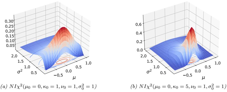
Figure 3.7: The NIϱ²(µ, ^ϑ2|m, ^ς, ^ω, ^ϑ2) distribution. ^m is the prior mean and ^ς is how strongly we believe this; ϑ² is the prior variance and ω is how strongly we believe this. (a) m = 0, ς = 1, ω = 1, ϑ² = 1. Notice that the contour plot (underneath the surface) is shaped like a “squashed egg”. (b) We increase the strength of our belief in the mean by setting ς = 5, so the distribution for µ around m = 0 becomes narrower. Generated by nix\_plots.ipynb.

The posterior marginal for ε² is just

\[p(\sigma^2|\mathcal{D}) = \int p(\mu, \sigma^2|\mathcal{D})d\mu = \chi^{-2}(\sigma^2|\mathcal{V}, \hat{\tau}^2) \tag{3.125}\]

with the posterior mean given by E ^ε2|D. ⁼ ↫^ε ↫^{ε ↑2} ↫2 ².

The posterior marginal for µ has a Student distribution, which follows from the fact that the Student distribution is a (scaled) mixture of Gaussians:

\[p(\mu|\mathcal{D}) = \int p(\mu, \sigma^2|D) d\sigma^2 = \mathcal{T}(\mu|\,\hat{m}, \hat{\tau}^2 \;/\,\hat{\mathbb{K}}, \mathcal{V}) \tag{3.126}\]

with the posterior mean given by E [µ|D] =m ↫ .

3.4.3.4 Posterior of µ and ↽²: uninformative prior

If we “know nothing” about the parameters a priori, we can use an uniformative prior. We discuss how to create such priors in Section 3.5. A common approach is to use a Je!reys prior. In Section 3.5.2.3, we show that the Je!reys prior for a location and scale parameter has the form

\[p(\mu, \sigma^2) \propto p(\mu)p(\sigma^2) \propto \sigma^{-2} \tag{3.127}\]

We can simulate this with a conjugate prior by using

\[p(\mu, \sigma^2) = NI\chi^2(\mu, \sigma^2 \mid \check{m} = 0, \check{\kappa} = 0, \check{\nu} = -1, \check{\tau}^2 = 0) \tag{3.128} \]

With this prior, the posterior has the form

\[p(\mu, \sigma^2 | \mathcal{D}) = N I \chi^2(\mu, \sigma^2 | \,\hat{m} = \overline{y}, \hat{\aleph} = N, \hat{\nu} = N - 1, \hat{\tau}^2 = s^2) \tag{3.129}\]

where

\[s^2 \triangleq \frac{1}{N-1} \sum\_{n=1}^{N} (y\_n - \overline{y})^2 = \frac{N}{N-1} \hat{\sigma}\_{\text{mle}}^2 \tag{3.130}\]

s is known as the sample standard deviation. Hence the marginal posterior for the mean is given by

\[p(\mu|\mathcal{D}) = \mathcal{T}(\mu|\overline{y}, \frac{s^2}{N}, N - 1) = \mathcal{T}(\mu|\overline{y}, \frac{\sum\_{n=1}^{N} (y\_n - \overline{y})^2}{N(N - 1)}, N - 1) \tag{3.131}\]

Thus the posterior variance of µ is

\[\mathbb{V}\left[\mu|\mathcal{D}\right] = \frac{\hat{\nu}}{\hat{\nu}-2} \quad \hat{\tau}^2 = \frac{N-1}{N-3} \frac{s^2}{N} \to \frac{s^2}{N} \tag{3.132}\]

The square root of this is called the standard error of the mean:

\[\text{se}(\mu) \triangleq \sqrt{\mathbb{V}[\mu|\mathcal{D}]} \approx \frac{s}{\sqrt{N}}\tag{3.133}\]

Thus we can approximate the 95% credible interval for µ using

\[I\_{.95}(\mu|\mathcal{D}) = \overline{y} \pm 2\frac{s}{\sqrt{N}}\tag{3.134}\]

3.4.4 The multivariate Gaussian model

In this section, we derive the posterior p(µ, !|D) for a multivariate Gaussian. For simplicity, we consider this in three steps: inferring just µ, inferring just !, and then inferring both.

3.4.4.1 Posterior of µ given !

The likelihood has the form

\[p(\mathcal{D}|\mu) = \mathcal{N}(\overline{\mathfrak{y}}|\mu, \frac{1}{N}\Sigma) \tag{3.135}\]

For simplicity, we will use a conjugate prior, which in this case is a Gaussian. In particular, if ^p(µ) = ^N (µ^{| m}↭ , ↭ V) then we can derive a Gaussian posterior for µ based on the results in Section 2.3.2.2 We get

\[p(\boldsymbol{\mu}|\mathcal{D}, \boldsymbol{\Sigma}) = \mathcal{N}(\boldsymbol{\mu}|\,\hat{\boldsymbol{m}}, \hat{\mathbf{V}}) \tag{3.136}\]

\[ \hat{\mathbf{V}}^{-1} = \check{\mathbf{V}}^{-1} + N\boldsymbol{\Sigma}^{-1} \tag{3.137} \]

\[ \hat{m} = \hat{\mathbf{V}} \left( \Sigma^{-1} (N \overline{\mathbf{y}}) + \check{\mathbf{V}}^{-1} \check{\mathbf{m}} \right) \tag{3.138} \]

Figure 3.8 gives a 2d example of these results.

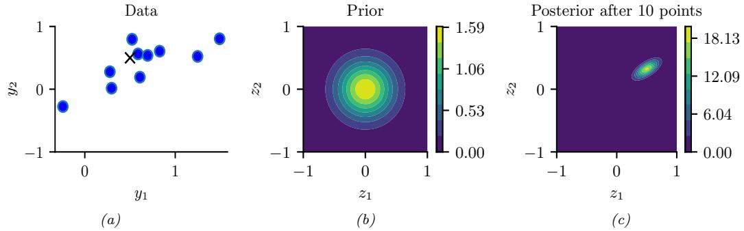
Figure 3.8: Illustration of Bayesian inference for a 2d Gaussian random vector z. (a) The data is generated from ^{yn ↔︎ N} (z, !y), where ^z = [0.5, ⁰.5]^T and !^y = 0.1([2, 1; 1, 1]). We assume the sensor noise covariance !^y is known but z is unknown. The black cross represents z. (b) The prior is p(z) = N (z|0, 0.1I2). (c) We show the posterior after 10 datapoints have been observed. Generated by gauss\_infer\_2d.ipynb.

3.4.4.2 Posterior of ! given µ

We now discuss how to compute p(!|D, µ).

Likelihood

We can rewrite the likelihood as follows:

\[p(\mathcal{D}|\mu, \Sigma) \propto |\Sigma|^{-\frac{N}{2}} \exp\left(-\frac{1}{2} \text{tr}(\mathbf{S}\_{\mu}\Sigma^{-1})\right) \tag{3.139}\]

where

\[\mathbf{S}\_{\mu} \triangleq \sum\_{n=1}^{N} (y\_n - \mu)(y\_n - \mu)^{\mathsf{T}} \tag{3.140}\]

is the scatter matrix around µ.

Prior

The conjugate prior is known as the inverse Wishart distribution, which is a distribution over positive definite matrices, as we explained in Section 2.2.5.5. This has the following pdf:

\[\mathrm{IW}(\boldsymbol{\Sigma}|\,\check{\boldsymbol{\Psi}}^{-1},\check{\boldsymbol{\nu}}) \propto |\boldsymbol{\Sigma}|^{-(\boldsymbol{\mathcal{V}}+\boldsymbol{D}+1)/2} \exp\left(-\frac{1}{2} \mathrm{tr}(\check{\boldsymbol{\Psi}}\,\boldsymbol{\Sigma}^{-1})\right) \tag{3.141}\]

Here ↭ς> D ⇐ ¹ is the degrees of freedom (dof), and ↭ $ is a symmetric pd matrix. We see that ↭ $ plays the role of the prior scatter matrix, and N⁰ ↭↭ς +D + 1 controls the strength of the prior, and hence plays a role analogous to the sample size N.

Posterior

Multiplying the likelihood and prior we find that the posterior is also inverse Wishart:

\[p(\mathbf{E}|\mathcal{D},\mu) \propto |\Sigma|^{-\frac{N}{2}} \exp\left(-\frac{1}{2} \text{tr}(\Sigma^{-1} \mathbf{S}\_{\mu})\right) |\Sigma|^{-(\mathcal{V}+D+1)/2}\]

\[\exp\left(-\frac{1}{2} \text{tr}(\Sigma^{-1} \check{\Psi})\right) \tag{3.142}\]

\[\mathbf{S} = |\boldsymbol{\Sigma}|^{-\frac{N + (\mathcal{V} + D + 1)}{2}} \exp\left(-\frac{1}{2} \text{tr}\left[\boldsymbol{\Sigma}^{-1} (\mathbf{S}\_{\mu} + \check{\boldsymbol{\Psi}})\right]\right) \tag{3.143}\]

\[\mathbf{H} = \text{IW}(\boldsymbol{\Sigma} | \boldsymbol{\hat{\Psi}}, \boldsymbol{\hat{\mathcal{V}}}) \tag{3.144}\]

\[\mathcal{V} = \mathbb{M} + N \tag{3.145}\]

\[ \hat{\Psi} = \check{\Psi}^{\prime} + \mathbf{S}\_{\mu} \tag{3.146} \]

In words, this says that the posterior strength ↫ς is the prior strength ↭ς plus the number of observations N, and the posterior scatter matrix ↫ $ is the prior scatter matrix ↭ $ plus the data scatter matrix Sµ.

3.4.4.3 Posterior of ! and µ

In this section, we compute p(µ, !|D) using a conjugate prior.

Likelihood

The likelihood is given by

\[p(\mathcal{D}|\boldsymbol{\mu}, \boldsymbol{\Sigma}) \propto |\boldsymbol{\Sigma}|^{-\frac{N}{2}} \exp\left(-\frac{1}{2} \sum\_{n=1}^{N} (\boldsymbol{y}\_n - \boldsymbol{\mu})^\mathsf{T} \boldsymbol{\Sigma}^{-1} (\boldsymbol{y}\_n - \boldsymbol{\mu})\right) \tag{3.147}\]

One can show that

\[\sum\_{n=1}^{N} (y\_n - \mu)^\mathsf{T} \Sigma^{-1} (y\_n - \mu) = \mathrm{tr}(\Sigma^{-1} \mathbf{S}) + N(\overline{y} - \mu)^\mathsf{T} \Sigma^{-1} (\overline{y} - \mu) \tag{3.148}\]

where

\[\mathbf{S} \triangleq \mathbf{S}\_{\overline{\mathbf{y}}} = \sum\_{n=1}^{N} (y\_n - \overline{y})(y\_n - \overline{y})^\top = \mathbf{Y}^\top \mathbf{C}\_N \mathbf{Y} \tag{3.149}\]

is empirical scatter matrix, and C^N is the centering matrix

\[\mathbf{C}\_{N} \triangleq \mathbf{I}\_{N} - \frac{1}{N} \mathbf{1}\_{N} \mathbf{1}\_{N}^{\mathsf{T}} \tag{3.150}\]

Hence we can rewrite the likelihood as follows:

\[p(\mathcal{D}|\boldsymbol{\mu}, \boldsymbol{\Sigma}) \propto |\boldsymbol{\Sigma}|^{-\frac{N}{2}} \exp\left(-\frac{N}{2} (\boldsymbol{\mu} - \overline{\boldsymbol{y}})^{\mathsf{T}} \boldsymbol{\Sigma}^{-1} (\boldsymbol{\mu} - \overline{\boldsymbol{y}})\right) \exp\left(-\frac{1}{2} \text{tr}(\boldsymbol{\textbf{S}} \boldsymbol{\Sigma}^{-1})\right) \tag{3.151}\]

We will use this form below.

3.4. Conjugate priors 93

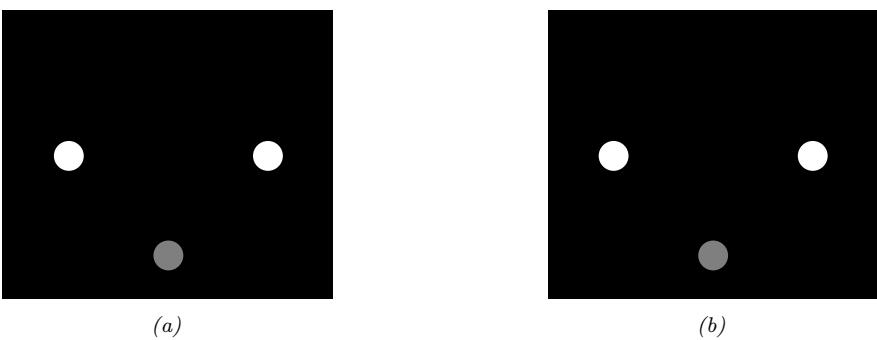
Figure 3.9: Graphical models representing di!erent kinds of assumptions about the parameter priors. (a) A semi-conjugate prior for a Gaussian. (b) A conjugate prior for a Gaussian.

Prior

The obvious prior to use is the following

\[p(\boldsymbol{\mu}, \boldsymbol{\Sigma}) = \mathcal{N}(\boldsymbol{\mu} | \check{\boldsymbol{m}}, \check{\mathbf{V}}) \text{IW}(\boldsymbol{\Sigma} | \check{\boldsymbol{\Psi}}^{-1}, \check{\boldsymbol{\nu}}) \tag{3.152}\]

where IW is the inverse Wishart distribution. Unfortunately, µ and ! appear together in a nonfactorized way in the likelihood in Equation (3.151) (see the first exponent term), so the factored prior in Equation (3.152) is not conjugate to the likelihood.4

The above prior is sometimes called conditionally conjugate, since both conditionals, p(µ|!) and p(!|µ), are individually conjugate. To create a fully conjugate prior, we need to use a prior where µ and ! are dependent on each other. We will use a joint distribution of the form p(µ, !) = p(µ|!)p(!). Looking at the form of the likelihood equation, Equation (3.151), we see that a natural conjugate prior has the form of a normal-inverse-Wishart or NIW distribution, defined as follows:

\[\begin{split} \text{NIV}(\boldsymbol{\mu}, \boldsymbol{\Sigma} | \widecheck{\boldsymbol{m}}, \widecheck{\kappa}, \widecheck{\Psi}, \widecheck{\Psi}) &\triangleq \mathcal{N}(\boldsymbol{\mu} | \widecheck{\boldsymbol{m}}, \frac{1}{\widecheck{\kappa}} \boldsymbol{\Sigma}) \times \text{IW}(\boldsymbol{\Sigma} | \widecheck{\Psi}^{-1}, \boldsymbol{\mathcal{V}}) \\ &= \frac{1}{Z\_{\text{NIW}}} |\boldsymbol{\Sigma}|^{-\frac{1}{2}} \exp\left(-\frac{\mathbb{K}}{2} (\boldsymbol{\mu} - \widecheck{\boldsymbol{m}})^{\mathsf{T}} \boldsymbol{\Sigma}^{-1} (\boldsymbol{\mu} - \widecheck{\boldsymbol{m}})\right) \\ &\times |\boldsymbol{\Sigma}|^{-\frac{\mathsf{V} + D + 1}{2}} \exp\left(-\frac{1}{2} \text{tr}(\widecheck{\Psi} \,\boldsymbol{\Sigma}^{-1})\right) \end{split} \tag{3.154}\]

where the normalization constant is given by

\[Z\_{\rm NIW} \triangleq 2^{\circ D/2} \Gamma\_D(\check{\nu}/2) (2\pi/\check{\kappa})^{D/2} |\check{\Psi}|^{\circ \prime/2} \tag{3.155}\]

The parameters of the NIW can be interpreted as follows: m↭ is our prior mean for µ, and ↭⇀ is how strongly we believe this prior; ↭ $ is (proportional to) our prior mean for !, and ↭ς is how strongly we believe this prior.5

^4. Using the language of directed graphical models, we see that µ and ! become dependent when conditioned on D due to explaining away. See Figure 3.9(a).

^5. Note that our uncertainty in the mean is proportional to the covariance. In particular, if we believe that the variance

Posterior

To derive the posterior, let us first rewrite the scatter matrix as follows:

\[\mathbf{S} = \mathbf{Y}^{\mathsf{T}} \mathbf{Y} - \frac{1}{N} (\sum\_{n=1}^{N} y\_n) (\sum\_{n=1}^{N} y\_n)^{\mathsf{T}} = \mathbf{Y}^{\mathsf{T}} \mathbf{Y} - N \overline{y} \overline{y}^{\mathsf{T}} \tag{3.156}\]

where Y^TY = #^{N n}=1 yny^{T n} is the sum of squares matrix.

Now we can multiply the likelihood and the prior to give

\[p(\boldsymbol{\mu}, \boldsymbol{\Sigma} | \mathcal{D}) \propto |\boldsymbol{\Sigma}|^{-\frac{N}{2}} \exp\left(-\frac{N}{2} (\boldsymbol{\mu} - \overline{\boldsymbol{y}})^{\mathsf{T}} \boldsymbol{\Sigma}^{-1} (\boldsymbol{\mu} - \overline{\boldsymbol{y}})\right) \exp\left(-\frac{1}{2} \text{tr}(\boldsymbol{\Sigma}^{-1} \mathbf{S})\right) \tag{3.157}\]

\[\times |\boldsymbol{\Sigma}|^{-\frac{\mathsf{V}\_{+}D+2}{2}} \exp\left(-\frac{\check{\boldsymbol{\kappa}}}{2}(\boldsymbol{\mu}-\check{\boldsymbol{m}})^{\mathsf{T}}\boldsymbol{\Sigma}^{-1}(\boldsymbol{\mu}-\check{\boldsymbol{m}})\right) \exp\left(-\frac{1}{2}\text{tr}(\boldsymbol{\Sigma}^{-1}\check{\boldsymbol{\Psi}})\right) \tag{3.158}\]

\[\hat{\mathbf{x}} = |\boldsymbol{\Sigma}|^{-(N+\mathbb{M}+D+2)/2} \exp(-\frac{1}{2} \text{tr}(\boldsymbol{\Sigma}^{-1} \mathbf{M})) \tag{3.159}\]

where

\[\mathbf{M} \triangleq N(\boldsymbol{\mu} - \overline{\boldsymbol{y}})(\boldsymbol{\mu} - \overline{\boldsymbol{y}})^{\mathsf{T}} + \check{\kappa} \,(\boldsymbol{\mu} - \check{\boldsymbol{m}})(\boldsymbol{\mu} - \check{\boldsymbol{m}})^{\mathsf{T}} + \mathbf{S} + \boldsymbol{\Psi} \tag{3.160}\]

\[\mathbf{y}^{\top} = (\breve{\kappa} + N)\mu\mu^{\sf T} - \mu(\breve{\kappa}\breve{m} + N\overline{y})^{\sf T} - (\breve{\kappa}\breve{m} + N\overline{y})\mu^{\sf T} + \breve{\kappa}\breve{m}\breve{m}^{\sf T} + \mathbf{Y}^{\sf T}\mathbf{Y} + \breve{\Psi} \tag{3.161}\]

We can simplify the M matrix as follows:

\[(\check{\kappa} + N)\mu\mu^{\mathsf{T}} - \mu(\check{\kappa}\check{m} + N\overline{y})^{\mathsf{T}} - (\check{\kappa}\check{m} + N\overline{y})\mu^{\mathsf{T}} \tag{3.162}\]

\[\mathbf{H} = (\mathbb{X} + N) \left( \mu - \frac{\mathbb{X}\mathbb{M} + N\overline{\mathbf{y}}}{\mathbb{X} + N} \right) \left( \mu - \frac{\mathbb{X}\mathbb{M} + N\overline{\mathbf{y}}}{\mathbb{X} + N} \right)^{\mathsf{T}} \tag{3.163}\]

\[-\frac{(\check{\kappa}\check{m}+N\overline{y})(\check{\kappa}\check{m}+N\overline{y})^{\mathsf{T}}}{\check{\kappa}+N}\tag{3.164}\]

\[=\hat{\kappa}\left(\mu-\hat{m}\right)(\mu-\hat{m})^{\mathsf{T}}-\hat{\kappa}\hat{m}\hat{m}^{\mathsf{T}}\tag{3.165}\]

Hence we can rewrite the posterior as follows:

\[p(\boldsymbol{\mu}, \boldsymbol{\Sigma} | \mathcal{D}) \propto |\boldsymbol{\Sigma}|^{(\mathcal{O} + D + 2)/2} \exp\left( -\frac{1}{2} \text{tr} \left[ \boldsymbol{\Sigma}^{-1} \left( \hat{\boldsymbol{\kappa}} \left( \boldsymbol{\mu} - \hat{\boldsymbol{m}} \right) (\boldsymbol{\mu} - \hat{\boldsymbol{m}})^{\mathsf{T}} + \hat{\boldsymbol{\Psi}} \right) \right] \right) \tag{3.166}\]

\[\hat{\rho} = \text{NIW}(\mu, \Sigma | \,\hat{m}, \hat{\kappa}, \hat{\nu}, \hat{\Psi}) \tag{3.167}\]

is large, then our uncertainty in µ must be large too. This makes sense intuitively, since if the data has large spread, it will be hard to pin down its mean.

where

\[ \hat{\boldsymbol{m}} = \frac{\check{\boldsymbol{\kappa}} \check{\boldsymbol{m}} + N \overline{\boldsymbol{y}}}{\hat{\boldsymbol{\kappa}}} = \frac{\check{\boldsymbol{\kappa}}}{\check{\boldsymbol{\kappa}} + N} \check{\boldsymbol{m}} + \frac{N}{\check{\boldsymbol{\kappa}} + N} \overline{\boldsymbol{y}} \tag{3.168} \]

\[ \widehat{\kappa} = \check{\kappa} + N\tag{3.169} \]

\[ \hat{\nu} = \check{\nu}' + N \tag{3.170} \]

\[ \hat{\Psi} = \check{\Psi} + \mathcal{S} + \frac{\check{\kappa}}{\check{\kappa} + N} (\overline{y} - \check{m}) (\overline{y} - \check{m})^{\mathsf{T}} \tag{3.171} \]

\[\mathbf{y} = \check{\mathbf{Y}} + \mathbf{Y}^{\mathsf{T}}\mathbf{Y} + \check{\kappa}\check{\mathbf{m}}\check{\mathbf{m}}^{\mathsf{T}} - \hat{\kappa}\hat{\mathbf{m}}\hat{\mathbf{m}}^{\mathsf{T}} \tag{3.172}\]

This result is actually quite intuitive: the posterior mean m↫ is a convex combination of the prior mean and the MLE; the posterior scatter matrix ↫ $ is the prior scatter matrix ↭ $ plus the empirical scatter matrix S plus an extra term due to the uncertainty in the mean (which creates its own virtual scatter matrix); and the posterior confidence factors ↫⇀ and ↫ς are both incremented by the size of the data we condition on.

Posterior marginals

We have computed the joint posterior

\[p(\boldsymbol{\mu}, \boldsymbol{\Sigma} | \mathcal{D}) = \mathcal{N}(\boldsymbol{\mu} | \boldsymbol{\Sigma}, \mathcal{D}) p(\boldsymbol{\Sigma} | \mathcal{D}) = \mathcal{N}(\boldsymbol{\mu} | \hat{\boldsymbol{m}}, \frac{1}{\hat{\boldsymbol{\kappa}}} \boldsymbol{\Sigma}) \text{IW}(\boldsymbol{\Sigma} | \hat{\boldsymbol{\Psi}}^{-1}, \hat{\boldsymbol{\nu}}) \tag{3.173}\]

We now discuss how to compute the posterior marginals, p(!|D) and p(µ|D).

It is easy to see that the posterior marginal for ! is

\[p(\boldsymbol{\Sigma}|\mathcal{D}) = \int p(\boldsymbol{\mu}, \boldsymbol{\Sigma}|\mathcal{D})d\boldsymbol{\mu} = \text{IW}(\boldsymbol{\Sigma}|\,\,\widehat{\boldsymbol{\Psi}}^{-1}, \boldsymbol{\mathcal{V}}) \tag{3.174}\]

For the mean, one can show that

\[p(\boldsymbol{\mu}|\mathcal{D}) = \int p(\boldsymbol{\mu}, \boldsymbol{\Sigma}|\mathcal{D})d\boldsymbol{\Sigma} = \mathcal{T}(\boldsymbol{\mu} \mid \boldsymbol{\hat{\mu}}, \frac{\boldsymbol{\hat{\Psi}}}{\boldsymbol{\hat{\kappa}}\boldsymbol{\mathcal{V}}}, \boldsymbol{\hat{\nu}}) \tag{3.175}\]

where ↫ς^↔︎ ↭↫^ς ⇐^D + 1. Intuitively this result follows because ^p(µ|D) is an infinite mixture of Gaussians, where each mixture component has a value of ! drawn from the IW distribution; by mixing these altogether, we induce a Student distribution, which has heavier tails than a single Gaussian.

Posterior mode

The maximum a posteriori (MAP) estimate of µ and ! is the mode of the posterior NIW distribution with density

\[p(\boldsymbol{\mu}, \boldsymbol{\Sigma} | \mathbf{Y}) = \mathcal{N}(\boldsymbol{\mu} | \hat{\boldsymbol{\mu}}, \hat{\boldsymbol{\kappa}}^{-1}, \boldsymbol{\Sigma}) \text{IW}(\boldsymbol{\Sigma} | \hat{\boldsymbol{\Psi}}^{-1}, \hat{\boldsymbol{\nu}}) \tag{3.176}\]

To find the mode, we firstly notice that ^µ only appears in the conditional distribution ^N (µ^| ↫µ, ↫⇀↑¹ !), and the mode of this normal distribution equals its mean, i.e., µ =↫µ. Also notice that this holds for any choice of !. So we can plug µ =↫µ in Equation (3.176) and derive the mode of !. Notice that

\[-2\*\log p(\mu=\widehat{\mu}, \Sigma|\mathbf{Y}) = (\mathcal{V} + D + 2)\log(|\Sigma|) + \text{tr}(\widehat{\Psi}|\Sigma^{-1}) + c \tag{3.177}\]

where c is a constant irrelevant to !. We then take the derivative over !:

\[\frac{\partial \log p(\mu = \hat{\mu} \, \, \Sigma | \mathbf{Y})}{\partial \Sigma} = (\hat{\nu} + D + 2)\Sigma^{-1} - \Sigma^{-1} \hat{\Psi} \, \Sigma^{-1} \tag{3.178}\]

By setting the derivative to 0 and solving for !, we see that ( ↫ς +D + 2)↑¹ ↫ $ is the matrix that maximizes Equation (3.177). By checking that ↫ $ is a positive definite matrix, we conclude that ↫ $ is the MAP estimate of the covariance matrix !.

In conclusion, the MAP estimate of {µ, !} are

\[ \hat{\mu} = \frac{\check{\kappa}\check{\mu} + N\bar{\mathfrak{y}}}{\check{\kappa} + N} \tag{3.179} \]

\[ \hat{\mathbf{E}} = \frac{1}{\hat{\nu} + D + 2} \hat{\Psi} \tag{3.180} \]

Posterior predictive

We now discuss how to predict future data by integrating out the parameters. If y ⇔ N (µ, !), where (µ, !|D) ^⇔ NIW(m↫ , ↫⇀, ↫ς, ↫ $), then one can show that the posterior predictive distribution, for a single observation vector, is as follows:

\[p(\mathbf{y}|\mathcal{D}) = \int \mathcal{N}(\mathbf{z}|\boldsymbol{\mu}, \boldsymbol{\Sigma}) \text{NIV}(\boldsymbol{\mu}, \boldsymbol{\Sigma}|\,\hat{\boldsymbol{m}}, \hat{\kappa}, \hat{\nu}, \hat{\Psi}) d\boldsymbol{\mu} d\boldsymbol{\Sigma} \tag{3.181}\]

\[\hat{\sigma} = \mathcal{T}(\boldsymbol{y}|\,\hat{\boldsymbol{m}}, \frac{\hat{\Psi}\left(\hat{\kappa} + 1\right)}{\hat{\kappa}\hat{\nu}'}, \hat{\nu}') \tag{3.182}\]

where ↫ς^{↔︎ =}↫^ς ⇐^D + 1.

3.4.5 The exponential family model

We have seen that exact Bayesian analysis is considerably simplified if the prior is conjugate to the likelihood. Since the posterior must have the same form as the prior, and hence the same number of parameters, the likelihood function must have fixed-sized su”cient statistics, so that we can write p(D|ω) = p(s(D)|ω). This suggests that the only family of distributions for which conjugate priors exist is the exponential family, a result proved in [DY79].6 In the sections below, we show how to perform conjugate analysis for a generic exponential family model.

3.4.5.1 Likelihood

Recall that the likelihood of the exponential family is given by

\[p(\mathcal{D}|\boldsymbol{\eta}) = h(\mathcal{D}) \exp(\boldsymbol{\eta}^{\mathsf{T}} \mathbf{s}(\mathcal{D}) - NA(\boldsymbol{\eta})) \tag{3.183}\]

\[\text{where } \mathbf{s}(\mathcal{D}) = \sum\_{n=1}^{N} \mathbf{s}(\boldsymbol{x}\_{n}) \text{ and } h(\mathcal{D}) \triangleq \prod\_{n=1}^{N} h(\boldsymbol{x}\_{n}).\]

^6. There are some exceptions. For example, the uniform distribution Unif(x|0, ↼) has finite su”cient statistics (N,m = maxⁱ xi), as discussed in Section 2.4.2.6; hence this distribution has a conjugate prior, namely the Pareto distribution (Section 2.2.3.5), p(↼) = Pareto(↼|↼0, ϖ), yielding the posterior p(↼|x) = Pareto(max(↼0, m), ϖ + N).

3.4.5.2 Prior

Let us write the prior in a form that mirrors the likelihood:

\[p(\boldsymbol{\eta} \mid \check{\boldsymbol{\tau}}, \boldsymbol{\mathcal{V}}) = \frac{1}{Z(\check{\boldsymbol{\tau}}, \boldsymbol{\mathcal{V}})} \exp(\check{\boldsymbol{\tau}}^{\mathsf{T}} \boldsymbol{\eta} - \boldsymbol{\mathcal{V}} \, A(\boldsymbol{\eta})) \tag{3.184}\]

where ↭ς is the strength of the prior, and ↭⇀ / ↭ς is the prior mean, and Z( ↭⇀ , ↭ς) is a normalizing factor. The parameters ↭⇀ can be derived from virtual samples representing our prior beliefs.

3.4.5.3 Posterior

The posterior is given by

\[p(\eta|\mathcal{D}) = \frac{p(\mathcal{D}|\eta)p(\eta)}{p(\mathcal{D})} \tag{3.185}\]

\[=\frac{h(\mathcal{D})}{Z(\check{\boldsymbol{\tau}},\check{\boldsymbol{\nu}})p(\mathcal{D})}\exp\left((\check{\boldsymbol{\tau}}+\mathsf{s}(\mathcal{D}))^{\mathsf{T}}\boldsymbol{\eta}-(\mathbb{V}+N)A(\boldsymbol{\eta})\right)\tag{3.186}\]

\[\hat{\boldsymbol{\mu}} = \frac{1}{Z(\hat{\boldsymbol{\tau}}, \hat{\boldsymbol{\nu}})} \exp\left(\hat{\boldsymbol{\tau}}^{\mathsf{T}} \boldsymbol{\eta} - \hat{\boldsymbol{\nu}}^{\mathsf{T}} A(\boldsymbol{\eta})\right) \tag{3.187}\]

where

\[ \hat{\tau} = \check{\tau} + \mathbf{s}(\mathcal{D})\tag{3.188} \]

\[\mathcal{V} = \mathcal{V} + N\tag{3.189}\]

\[Z(\hat{\boldsymbol{\tau}}, \mathcal{V}) = \frac{Z(\check{\boldsymbol{\tau}}, \mathcal{V})}{h(\mathcal{D})} p(\mathcal{D}) \tag{3.190}\]

We see that this has the same form as the prior, but where we update the su”cient statistics and the sample size.

The posterior mean is given by a convex combination of the prior mean and the empirical mean (which is the MLE):

\[\mathbb{E}\left[\eta|\mathcal{D}\right] = \frac{\hat{\tau}}{\hat{\nu}} = \frac{\check{\tau} + \mathsf{s}(\mathcal{D})}{\check{\nu} + N} = \frac{\mathbb{V}}{\check{\nu} + N} \frac{\check{\tau}}{\check{\nu}} + \frac{N}{\check{\nu} + N} \frac{\mathsf{s}(\mathcal{D})}{N} \tag{3.191}\]

\[=\lambda \mathbb{E}\left[\eta\right] + (1-\lambda)\hat{\eta}\_{\text{mle}} \tag{3.192}\]

where ^{ϖ =} ↭^ε ↭^{ε +N} .

3.4.5.4 Marginal likelihood

From Equation (3.190) we see that the marginal likelihood is given by

\[p(\mathcal{D}) = \frac{Z(\hat{\boldsymbol{\tau}}, \hat{\boldsymbol{\nu}})h(\mathcal{D})}{Z(\check{\boldsymbol{\tau}}, \hat{\boldsymbol{\nu}})} \tag{3.193}\]

See Section 3.2.1.9 for a detailed example in the case of the beta-Bernoulli model.

3.4.5.5 Posterior predictive density

We now derive the predictive density for future observables D^↔︎ = (x˜1,…, x˜N^→ ) given past data D = (x1,…, x^N ):

\[p(\mathcal{D}'|\mathcal{D}) = \int p(\mathcal{D}'|\eta)p(\eta|\mathcal{D})d\eta\tag{3.194}\]

\[=\int h(\mathcal{D}')\exp(\eta^{\mathsf{T}}\mathbf{s}(\mathcal{D}') - N'A(\eta))\frac{1}{Z(\widehat{\boldsymbol{\tau}},\boldsymbol{\delta})}\exp(\eta^{\mathsf{T}}\,\widehat{\boldsymbol{\tau}}-\boldsymbol{\mathcal{V}}\,A(\eta))d\eta\tag{3.195}\]

\[\dot{\lambda} = h(\mathcal{D}') \frac{Z(\check{\tau} + \mathbf{s}(\mathcal{D}) + \mathbf{s}(\mathcal{D}'), \check{\nu} + N + N')}{Z(\check{\tau} + \mathbf{s}(\mathcal{D}), \mathcal{V} + N)} \tag{3.196}\]

3.4.5.6 Example: Bernoulli distribution

As a simple example, let us revisit the Beta-Bernoulli model in our new notation.

The likelihood is given by

\[p(\mathcal{D}|\theta) = (1-\theta)^N \exp\left(\log(\frac{\theta}{1-\theta}) \sum\_{i} x\_n\right) \tag{3.197}\]

Hence the conjugate prior is given by

\[p(\theta|\nu\_0, \tau\_0) \propto (1 - \theta)^{\nu\_0} \exp\left(\log(\frac{\theta}{1 - \theta})\tau\_0\right) \tag{3.198}\]

\[= \theta^{\tau\_0} (1 - \theta)^{\nu\_0 - \tau\_0} \tag{3.199}\]

If we define α = 2⁰ + 1 and ↼ = ς⁰ ⇐ 2⁰ + 1, we see that this is a beta distribution.

We can derive the posterior as follows, where s = # ⁱ I(xⁱ = 1) is the su”cient statistic:

\[p(\theta|\mathcal{D}) \propto \theta^{\tau\_0 + s} (1 - \theta)^{\nu\_0 - \tau\_0 + n - s} \tag{3.200}\]

\[\theta = \theta^{\tau\_n} (1 - \theta)^{\nu\_n - \tau\_n} \tag{3.201}\]

We can derive the posterior predictive distribution as follows. Assume p(ϑ) = Beta(ϑ|α, ↼), and let s = s(D) be the number of heads in the past data. We can predict the probability of a given sequence of future heads, ^D↔︎ = (x˜1,…, ^x˜m), with su”cient statistic ^{s↔︎ =} #^{m n}=1 I(˜xⁱ = 1), as follows:

\[p(\mathcal{D}'|\mathcal{D}) = \int\_0^1 p(\mathcal{D}'|\theta) \text{Beta}(\theta|\alpha\_n, \beta\_n) d\theta \tag{3.202}\]

\[=\frac{\Gamma(\alpha\_n + \beta\_n)}{\Gamma(\alpha\_n)\Gamma(\beta\_n)} \int\_0^1 \theta^{\alpha\_n + t' - 1} (1 - \theta)^{\beta\_n + m - t' - 1} d\theta \tag{3.203}\]

\[=\frac{\Gamma(\alpha\_n + \beta\_n)}{\Gamma(\alpha\_n)\Gamma(\beta\_n)} \frac{\Gamma(\alpha\_{n+m})\Gamma(\beta\_{n+m})}{\Gamma(\alpha\_{n+m} + \beta\_{n+m})} \tag{3.204}\]

where

\[ \alpha\_{n+m} = \alpha\_n + s' = \alpha + s + s' \tag{3.205} \]

\[ \beta\_{n+m} = \beta\_n + (m - s') = \beta + (n - s) + (m - s') \tag{3.206} \]

3.4.6 Beyond conjugate priors

We have seen various examples of conjugate priors, all of which have come from the exponential family (see Section 2.4). These priors have the advantages of being easy to interpret (in terms of su”cient statistics from a virtual prior dataset), and being easy to compute with. However, for most models, there is no prior in the exponential family that is conjugate to the likelihood. Furthermore, even where there is a conjugate prior, the assumption of conjugacy may be too limiting. Therefore in the sections below, we briefly discuss various other kinds of priors. (We defer the question of posterior inference with these priors until Section 7.1, where we discuss algorithmic issues, since we can no longer use closed-form solutions when the prior is not conjugate.)

3.4.6.1 Mixtures of conjugate priors

In this section, we show how we can create a mixture of conjugate priors for increased modeling flexibility. Fortunately, the resulting mixture prior is still conjugate.

As an example, suppose we want to predict the outcome of a coin toss at a casino, and we believe that the coin may be fair, but it may also be biased towards heads. This prior cannot be represented by a beta distribution. Fortunately, it can be represented as a mixture of beta distributions. For example, we might use

\[p(\theta) = 0.5 \text{Beta}(\theta | 20, 20) + 0.5 \text{Beta}(\theta | 30, 10) \tag{3.207}\]

If ϑ comes from the first distribution, the coin is fair, but if it comes from the second, it is biased towards heads.

We can represent a mixture by introducing a latent indicator variable h, where h = k means that ϑ comes from mixture component k. The prior has the form

\[p(\theta) = \sum\_{k} p(h=k)p(\theta|h=k) \tag{3.208}\]

where each p(ϑ|h = k) is conjugate, and p(h = k) are called the (prior) mixing weights. One can show that the posterior can also be written as a mixture of conjugate distributions as follows:

\[p(\theta|\mathcal{D}) = \sum\_{k} p(h=k|\mathcal{D})p(\theta|\mathcal{D}, h=k) \tag{3.209}\]

where p(h = k|D) are the posterior mixing weights given by

\[p(h=k|\mathcal{D}) = \frac{p(h=k)p(\mathcal{D}|h=k)}{\sum\_{k'} p(h=k')p(\mathcal{D}|h=k')}\tag{3.210}\]

Here the quantity p(D|h = k) is the marginal likelihood for mixture component k (see Section 3.2.1.9).

Returning to our example above, if we have the prior in Equation (3.207), and we observe N¹ = 20 heads and N⁰ = 10 tails, then, using Equation (3.31), the posterior becomes

\[p(\theta|\mathcal{D}) = 0.346 \operatorname{Beta}(\theta|40, 30) + 0.654 \operatorname{Beta}(\theta|50, 20) \tag{3.211}\]

See Figure 3.10 for an illustration.

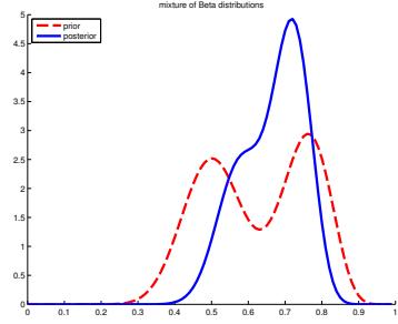
Figure 3.10: A mixture of two Beta distributions. Generated by mixbetademo.ipynb.

We can compute the posterior probability that the coin is biased towards heads as follows:

\[\Pr(\theta > 0.5 | \mathcal{D}) = \sum\_{k} \Pr(\theta > 0.5 | \mathcal{D}, h = k) p(h = k | \mathcal{D}) = 0.9604 \tag{3.212}\]

If we just used a single Beta(20,20) prior, we would get a slightly smaller value of Pr(ϑ > 0.5|D) = 0.8858. So if we were “suspicious” initially that the casino might be using a biased coin, our fears would be confirmed more quickly than if we had to be convinced starting with an open mind.

3.4.6.2 Robust (heavy-tailed) priors

The assessment of the influence of the prior on the posterior is called sensitivity analysis, or robustness analysis. There are many ways to create robust priors. (see e.g., [IR00]). Here we consider a simple approach, namely the use of a heavy-tailed distribution.

To motivate this, let us consider an example from [Ber85a, p7]. Suppose x ⇔ N (ϑ, 1). We observe that x = 5 and we want to estimate ϑ. The MLE is of course ˆϑ = 5, which seems reasonable. The posterior mean under a uniform prior is also ϑ = 5. But now suppose we know that the prior median is 0, and that there is 25% probability that ϑ lies in any of the intervals (⇐⇒, ⇐1), (⇐1, 0), (0, 1), (1, ⇒). Let us also assume the prior is smooth and unimodal.

One can show that a Gaussian prior of the form ^N (ϑ|0, ².192) satisfies these prior constraints. But in this case the posterior mean is given by 3.43, which doesn’t seem very satisfactory. An alternative distribution that captures the same prior information is the Cauchy prior T1(ϑ|0, 1). With this prior, we find (using numerical method integration: see robust\_prior\_demo.ipynb for the code) that the posterior mean is about 4.6, which seems much more reasonable. In general, priors with heavy tails tend to give results which are more sensitive to the data, which is usually what we desire.

Heavy-tailed priors are usually not conjugate. However, we can often approximate a heavy-tailed prior by using a (possibly infinite) mixture of conjugate priors. For example, in Section 28.2.3, we show that the Student distribution (of which the Cauchy is a special case) can be written as an infinite mixture of Gaussians, where the mixing weights come from a gamma distribution. This is an example of a hierarchical prior; see Section 3.6 for details.

3.4.6.3 Priors for scalar variances

In this section, we discuss some commonly used priors for variance parameters. Such priors play an important role in determining how much regularization a model exhibits. For example, consider a linear regression model, ^p(y|x, ^w, ^ε2) = ^N (y|wTx, ^ε2). Suppose we use a Gaussian prior on the weights, ^p(w) = ^N (w|0, ^{2 2}I). The value of ^{2 2} (relative to ^ε2) plays a role similar to the strength of an ⇁2-regularization term in ridge regression. In the Bayesian setting, we need to ensure we use sensible priors for the variance parameters, 2 ² and ε². This becomes even more important when we discuss hierarchical models, in Section 3.6.

We start by considering the simple problem of inferting a variance parameter ε² from a Gaussian likelihood with known mean, as in Section 3.4.3.2. The uninformative prior is ^p(ε²) = IG(ε²|0, 0), which is improper, meaning it does not integrate to 1. This is fine as long as the posterior is proper. This will be the case if the prior is on the variance of the noise of N ⇑ 2 observable variables. Unfortunately the posterior is not proper, even if N → ⇒, if we use this prior for the variance of the (non observable) weights in a regression model [Gel06; PS12], as we discuss in Section 3.6.

One solution to this is to use a weakly informative proper prior such as IG(3, 3) for small 3. However, this turns out to not work very well, for reasons that are explained in [Gel06; PS12]. Instead, it is recommended to use other priors, such as uniform, exponential, half-normal, half-Student-t, or half-Cauchy; all of these are bounded below by 0, and just require 1 or 2 hyperparameters. (The term “half” refers to the fact that the distribution is “folded over” onto itself on the positive side of the real axis.)

3.4.6.4 Priors for covariance matrices

The conjugate prior for a covariance matrix is the inverse Wishart (Section 2.2.5.6). However, it can be hard to set the parameters for this in an uninformative way. One approach, discussed in [HW13], is to use a scale mixture of inverse Wisharts, where the scaling parameters have inverse gamma distributions. It is possible to choose shape and scale parameters to ensure that all the correlation parameters have uniform (⇐1, 1) marginals, and all the standard deviations have half-Student distributions.

Unfortunately, the Wishart distribution has heavy tails, which can lead to poor performance when used in a sampling algorithm.7 A more common approach, following Equation (3.213), is to represent the D ∞ D covariance matrix ! in terms of a product of the marginal standard deviations, ↽ = (ε1,…, εD), and the D ∞ D correlation matrix R, as follows:

\[\Delta = \text{diag}(\sigma) \text{ R } \text{diag}(\sigma) \tag{3.213}\]

For example, if D = 2 ,we have

\[ \Sigma = \begin{pmatrix} \sigma\_1 & 0 \\ 0 & \sigma\_2 \end{pmatrix} \begin{pmatrix} 1 & \rho \\ \rho & 1 \end{pmatrix} \begin{pmatrix} \sigma\_1 & 0 \\ 0 & \sigma\_2 \end{pmatrix} = \begin{pmatrix} \sigma\_1^2 & \rho \sigma\_1 \sigma\_2 \\ \rho \sigma\_1 \sigma\_2 & \sigma\_2^2 \end{pmatrix} \tag{3.214} \]

We can put a factored prior on the standard deviations, following the recommendations of Sec-

^7. See comments from Michael Betancourt at https://github.com/pymc-devs/pymc/issues/538.

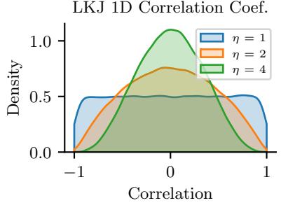
Figure 3.11: Distribution on the correlation coe”cient φ induced by a 2d LKJ distribution with varying parameter. Adapted from Figure 14.3 of [McE20]. Generated by lkj\_1d.ipynb.

tion 3.4.6.3. For example,

\[p(\boldsymbol{\sigma}) = \prod\_{d=1}^{D} \text{Expon}(\sigma\_d | 1) \tag{3.215}\]

For the correlation matrix, it is common to use as a prior the LKJ distribution, named after the authors of [LKJ09]. This has the form

\[\text{LKJ}(\mathbf{R}|\eta) \propto |\mathbf{R}|^{\eta - 1} \tag{3.216}\]

so it only has one free parameter. When ◁ = 1, it is a uniform prior; when ◁ = 2, it is a “weakly regularizing” prior, that encourages small correlations (close to 0). See Figure 3.11 for a plot.

In practice, it is more common to define R in terms of its Cholesky decomposition, R = LL^T, where L is an unconstrained lower triangular matrix. We then represent the prior using

\[\text{LKJ} \text{chol}(\mathbf{L}|\eta) \propto |\mathbf{L}|^{-\eta - 1} \tag{3.217}\]

3.5 Noninformative priors

When we have little or no domain specific knowledge, it is desirable to use an uninformative, noninformative, or objective priors, to “let the data speak for itself”. Unfortunately, there is no unique way to define such priors, and they all encode some kind of knowledge. It is therefore better to use the term di”use prior, minimally informative prior, or default prior.

In the sections below, we briefly mention some common approaches for creating default priors. For further details, see e.g., [KW96] and the Stan website.8

3.5.1 Maximum entropy priors

A natural way to define an uninformative prior is to use one that has maximum entropy, since it makes the least commitments to any particular value in the state space (see Section 5.2 for a

^8. https://github.com/stan-dev/stan/wiki/Prior-Choice-Recommendations.

discussion of entropy). This is a formalization of Laplace’s principle of insu!cient reason, in which he argued that if there is no reason to prefer one prior over another, we should pick a “flat” one.

For example, in the case of a Bernoulli distribution with rate ϑ ↑ [0, 1], the maximum entropy prior is the uniform distribution, p(ϑ) = Beta(ϑ|1, 1), which makes intuitive sense.

However, in some cases we know something about our random variable ω, and we would like our prior to match these constraints, but otherwise be maximally entropic. More precisely, suppose we want to find a distribution p(ω) with maximum entropy, subject to the constraints that the expected values of certain features or functions fk(ω) match some known quantities Fk. This is called a maxent prior. In Section 2.4.7, we show that such distributions must belong to the exponential family (Section 2.4).

For example, suppose ϑ ↑ {1, 2,…, 10}, and let p^c = p(ϑ = c) be the corresponding prior. Suppose we know that the prior mean is 1.5. We can encode this using the following constraint

\[\mathbb{E}\left[f\_1(\theta)\right] = \mathbb{E}\left[\theta\right] = \sum\_{c} c \ p\_c = 1.5\tag{3.218}\]

In addition, we have the constraint # ^c p^c = 1. Thus we need to solve the following optimization problem:

\[\min\_{\mathbf{p}} \mathbb{H}(\mathbf{p}) \quad \text{s.t.} \quad \sum\_{c} c \; p\_{c} = 1.5, \; \sum\_{c} p\_{c} = 1.0 \tag{3.219}\]

This gives the decaying exponential curve in Figure 3.12. Now suppose we know that ϑ is either 3 or 4 with probability 0.8. We can encode this using

\[\mathbb{E}\left[f\_1(\theta)\right] = \mathbb{E}\left[\mathbb{1}\left(\theta \in \{3, 4\}\right)\right] = \Pr(\theta \in \{3, 4\}) = 0.8 \tag{3.220}\]

This gives the inverted U-curve in Figure 3.12. We note that this distribution is flat in as many places as possible.

3.5.2 Je!reys priors

Let ϑ be a random variable with prior p⇁(ϑ), and let ▷ = f(ϑ) be some invertible transformation of ϑ. We want to choose a prior that is invariant to this function f, so that the posterior does not depend on how we parameterize the model.

For example, consider a Bernoulli distribution with rate parameter ϑ. Suppose Alice uses a binomial likelihood with data D, and computes p(ϑ|D). Now suppose Bob uses the same likelihood and data, but parameterizes the model in terms of the odds parameter, ▷ = ⇁ ¹↑⇁ . He converts Alice’s prior to p(▷) using the change of variables formula, and them computes p(▷|D). If he then converts back to the ϑ parameterization, he should get the same result as Alice.

We can achieve this goal that provided we use a Je”reys prior, named after Harold Je!reys.9 In 1d, the Je!reys prior is given by ^p(ϑ) ↙ F(ϑ), where ^F is the Fisher information (Section 3.3.4). In multiple dimensions, the Je!reys prior has the form ^p(ω) ↙ det ^F(ω), where ^F is the Fisher information matrix (Section 3.3.4).

^9. Harold Je!reys, 1891–1989, was an English mathematician, statistician, geophysicist, and astronomer. He is not to be confused with Richard Je!rey, a philosopher who advocated the subjective interpretation of probability [Jef04].

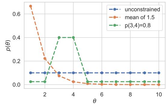
Figure 3.12: Illustration of 3 di!erent maximum entropy priors. Adapted from Figure 1.10 of [MKL11]. Generated by maxent\_priors.ipynb.

To see why the Je!reys prior is invariant to parameterization, consider the 1d case. Suppose ^p⇁(ϑ) ↙ F(ϑ). Using the change of variables, we can derive the corresponding prior for ^▷ as follows:

\[p\_{\phi}(\phi) = p\_{\theta}(\theta) \left| \frac{d\theta}{d\phi} \right| \tag{3.221}\]

\[\propto \sqrt{F(\theta) \left(\frac{d\theta}{d\phi}\right)^2} = \sqrt{\mathbb{E}\left[\left(\frac{d\log p(x|\theta)}{d\theta}\right)^2\right] \left(\frac{d\theta}{d\phi}\right)^2} \tag{3.222}\]

\[\mathcal{E} = \sqrt{\mathbb{E}\left[\left(\frac{d\log p(x|\theta)}{d\theta}\frac{d\theta}{d\phi}\right)^2\right]} = \sqrt{\mathbb{E}\left[\left(\frac{d\log p(x|\phi)}{d\phi}\right)^2\right]}\tag{3.223}\]

\[=\sqrt{F(\phi)}\tag{3.224}\]

Thus the prior distribution is the same whether we use the ϑ parameterization or the ▷ parameterization.

We give some examples of Je!reys priors below.

3.5.2.1 Je”reys prior for binomial distribution

Let us derive the Je!reys prior for the binomial distribution using the rate parameterization ϑ. From Equation (3.57), we have

\[p(\theta) \propto \theta^{-\frac{1}{2}} (1 - \theta)^{-\frac{1}{2}} = \frac{1}{\sqrt{\theta (1 - \theta)}} \propto \text{Beta}(\theta | \frac{1}{2}, \frac{1}{2}) \tag{3.225}\]

Now consider the odds parameterization, ^{▷ = ϑ}/(1 ⇐ ^ϑ), so ^{ϑ = φ φ}+1 . The likelihood becomes

\[p(x|\phi) \propto \left(\frac{\phi}{\phi+1}\right)^x \left(1 - \frac{\phi}{\phi+1}\right)^{n-x} = \phi^x(\phi+1)^{-x}(\phi+1)^{-n+x} = \phi^x(\phi+1)^{-n} \tag{3.226}\]

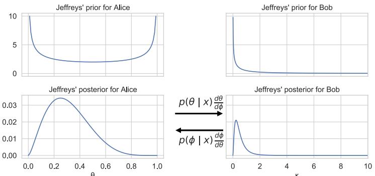
Figure 3.13: Illustration of Je!reys prior for Alice (who uses the rate ε) and Bob (who uses the odds ↼ = ε/(1 ↓ ε)). Adapted from Figure 1.9 of [MKL11]. Generated by je!reys\_prior\_binomial.ipynb.

Thus the log likelihood is

\[\ell = x \log \phi - n \log \phi + 1 \tag{3.227}\]

The first and second derivatives are

\[\frac{d\ell}{d\phi} = \frac{x}{\phi} - \frac{n}{\phi + 1} \tag{3.228}\]

\[\frac{d^2\ell}{d\phi^2} = -\frac{x}{\phi^2} + \frac{n}{(\phi+1)^2} \tag{3.229}\]

Since E [x] = nϑ = n ^{φ φ}+1 , the Fisher information matrix is given by

\[F(\phi) = -\mathbb{E}\left[\frac{d^2\ell}{d\phi^2}\right] \frac{n}{\phi(\phi+1)} - \frac{n}{(\phi+1)^2} \tag{3.230}\]

\[\eta = \frac{n(\phi + 1) - n\phi}{\phi(\phi + 1)^2} = \frac{n}{\phi(\phi + 1)^2} \tag{3.231}\]

Hence

\[p\_{\phi}(\phi) \propto \phi^{-0.5} (1+\phi)^{-1} \tag{3.232}\]

See Figure 3.13 for an illustration.

3.5.2.2 Je”reys prior for multinomial distribution

For a categorical random variable with K states, one can show that the Je!reys prior is given by

\[p(\boldsymbol{\theta}) \propto \text{Dir}(\boldsymbol{\theta}|\frac{1}{2}, \dots, \frac{1}{2}) \tag{3.233}\]

Note that this is di!erent from the more obvious choices of Dir( ^{1 K} ,…, ^{1 K} ) or Dir(1,…, 1).

3.5.2.3 Je”reys prior for the mean and variance of a univariate Gaussian

Consider a 1d Gaussian ^{x ⇔ N} (µ, ^ε2) with both parameters unknown, so ^ω = (µ, ^ε). From Equation (3.62), the Fisher information matrix is

\[\mathbf{F}(\boldsymbol{\theta}) = \begin{pmatrix} 1/\sigma^2 & 0\\ 0 & 1/(2\sigma^4) \end{pmatrix} \tag{3.234}\]

so det(F(ω)) = ⇓ 1 ²ϱ³ . However, the standard Je!reys uninformative prior for the Gaussian is defined as the product of independent uninformative priors (see [KW96]), i.e.,

\[p(\mu, \sigma^2) \propto p(\mu)p(\sigma^2) \propto 1/\sigma^2 \tag{3.235}\]

It turns out that we can emulate this prior with a conjugate NIX prior:

\[p(\mu, \sigma^2) = NI\chi^2(\mu, \sigma^2 | \mu\_0 = 0, \check{\kappa} = 0, \check{\nu} = -1, \check{\sigma}^2 = 0) \tag{3.236}\]

This lets us easily reuse the results for conjugate analysis of the Gaussian in Section 3.4.3.3, as we showed in Section 3.4.3.4.

3.5.3 Invariant priors

If we have “objective” prior knowledge about a problem in the form of invariances, we may be able to encode this into a prior, as we show below.

3.5.3.1 Translation-invariant priors

A location-scale family is a family of probability distributions parameterized by a location µ and scale ε. If x is an rv in this family, then y = a + bx is also an rv in the same family.

When inferring the location parameter µ, it is intuitively reasonable to want to use a translationinvariant prior, which satisfies the property that the probability mass assigned to any interval, [A, B] is the same as that assigned to any other shifted interval of the same width, such as [A⇐c, B⇐c]. That is,

\[\int\_{A-c}^{B-c} p(\mu)d\mu = \int\_{A}^{B} p(\mu)d\mu \tag{3.237}\]

This can be achieved using

\[p(\mu) \propto 1\tag{3.238}\]

since

\[\int\_{A-c}^{B-c} 1 d\mu = (B-c) - (A-c) = (B-A) = \int\_{A}^{B} 1 d\mu \tag{3.239}\]

This is the same as the Je!reys prior for a Gaussian with unknown mean µ and fixed variance. This follows since ^F(µ)=1/ε² ↙ ¹, from Equation (3.62), and hence ^p(µ) ↙ ¹.

3.5.3.2 Scale-invariant prior

When inferring the scale parameter ε, we may want to use a scale-invariant prior, which satisfies the property that the probability mass assigned to any interval [A, B] is the same as that assigned to any other interval [A/c, B/c], where c > 0. That is,

\[\int\_{A/c}^{B/c} p(\sigma)d\sigma = \int\_{A}^{B} p(\sigma)d\sigma \tag{3.240}\]

This can be achieved by using

p(ε) ↙ 1/ε (3.241)

since then

\[\int\_{A/c}^{B/c} \frac{1}{\sigma} d\sigma = [\log \sigma]\_{A/c}^{B/c} = \log(B/c) - \log(A/c) = \log(B) - \log(A) = \int\_{A}^{B} \frac{1}{\sigma} d\sigma \tag{3.242}\]

This is the same as the Je!reys prior for a Gaussian with fixed mean µ and unknown scale ε. This follows since ^F(ε)=2/ε², from Equation (3.62), and hence ^p(ε) ↙ ¹/ε.

3.5.3.3 Learning invariant priors

Whenever we have knowledge of some kind of invariance we want our model to satisfy, we can use this to encode a corresponding prior. Sometimes this is done analytically (see e.g., [Rob07, Ch.9]). When this is intractable, it may be possible to learn invariant priors by solving a variational optimization problem (see e.g., [NS18]).

3.5.4 Reference priors

One way to define a noninformative prior is as a distribution which is maximally far from all possible posteriors, when averaged over datasets. This is the basic idea behind a reference prior [Ber05; BBS09]. More precisely, we say that p(ω) is a reference prior if it maximizes the expected KL divergence between posterior and prior:

\[p^\*(\boldsymbol{\theta}) = \underset{p(\boldsymbol{\theta})}{\text{argmax}} \int\_{\mathcal{D}} p(\mathcal{D}) D\_{\text{KL}} \left( p(\boldsymbol{\theta}|\mathcal{D}) \parallel p(\boldsymbol{\theta}) \right) d\mathcal{D} \tag{3.243}\]

where ^p(D) = $ ^p(D|ω)p(ω)dω. This is the same as maximizing the mutual information ^I(ω, ^D). We can eliminate the integral over datasets by noting that

\[\text{We can eliminate one image over } \mathfrak{h} \text{ as a } \mathfrak{h}\text{-module.}\]

\[\int p(\mathcal{D}) \int p(\boldsymbol{\theta} | \mathcal{D}) \log \frac{p(\boldsymbol{\theta} | \mathcal{D})}{p(\boldsymbol{\theta})} = \int p(\boldsymbol{\theta}) \int p(\mathcal{D} | \boldsymbol{\theta}) \log \frac{p(\mathcal{D} | \boldsymbol{\theta})}{p(\mathcal{D})} = \mathbb{E}\_{\boldsymbol{\theta}} \left[ D\_{\text{KL}} \left( p(\mathcal{D} | \boldsymbol{\theta}) \parallel p(\mathcal{D}) \right) \right] \tag{3.244}\]

where we used the fact that ^p(ϑ|D) ^p(ϑ) ^{= p}(D|ϑ) ^p(D) .

One can show that, in 1d, the corresponding prior is equivalent to the Je!reys prior. In higher dimensions, we can compute the reference prior for one parameter at a time, using the chain rule. However, this can become computationally intractable. See [NS17] for a tractable approximation based on variational inference (Section 10.1).

3.6 Hierarchical priors

Bayesian models require specifying a prior p(ω) for the parameters. The parameters of the prior are called hyperparameters, and will be denoted by ς. If these are unknown, we can put a prior on them; this defines a hierarchical Bayesian model, or multi-level model, which can visualize like this: ς → ω → D. We assume the prior on the hyper-parameters is fixed (e.g., we may use some kind of minimally informative prior), so the joint distribution has the form

\[p(\xi, \theta, \mathcal{D}) = p(\xi)p(\theta|\xi)p(\mathcal{D}|\theta) \tag{3.245}\]

The hope is that we can learn the hyperparameters by treating the parameters themselves as datapoints.

A common setting in which such an approach makes sense is when we have J > 1 related datasets, D^j , each with their own parameters ω^j . Inferring p(ω^j |D^j ) independently for each group j can give poor results if D^j is a small dataset (e.g., if condition j corresponds to a rare combination of features, or a sparsely population region). We could of course pool all the data to compute a single model, p(ω|D), but that would not let us model the subpopulations. A hierarchical Bayesian model lets us borrow statistical strength from groups with lots of data (and hence well-informed posteriors p(ω^j |D)) in order to help groups with little data (and hence highly uncertain posteriors p(ω^j |D)). The idea is that well-informed groups j will have a good estimate of ω^j , from which we can infer ς, which can be used to help estimate ω^k for groups k with less data. (Information is shared via the hidden common parent node ς in the graphical model, as shown in Figure 3.14.) We give some examples of this below.

After fitting such models, we can compute two kinds of posterior predictive distributions. If we want to predict observations for an existing group j, we need to use

\[p(y\_j|\mathcal{D}) = \int p(y\_j|\theta\_j)p(\theta\_j|\mathcal{D})d\theta\_j \tag{3.246}\]

However, if we want to predict observations for a new group ∋ that has not yet been measured, but which is comparable to (or exchangeable with) the existing groups 1 : J, we need to use

\[p(y\_\*|\mathcal{D}) = \int p(y\_\*|\theta\_\*)p(\theta\_\*|\xi)p(\xi|\mathcal{D})d\theta\_\* d\xi\tag{3.247}\]

We give some examples below. (More information can be found in e.g., [GH07; Gel+14a].)

3.6.1 A hierarchical binomial model

Suppose we want to estimate the prevalence of some disease amongst di!erent group of individuals, either people or animals. Let N^j be the size of the j’th group, and let y^j be the number of positive cases for group j =1: J. We assume y^j ⇔ Bin(N^j , ϑ^j ), and we want to estimate the rates ϑ^j . Since some groups may have small population sizes, we may get unreliable results if we estimate each ϑ^j separately; for example we may observe y^j = 0 resulting in ˆϑ^j = 0, even though the true infection rate is higher.

One solution is to assume all the ϑ^j are the same; this is called parameter tying. The resulting pooled MLE is just ˆϑpooled = ! ^j ! ^{yj j Nj} . But the assumption that all the groups have the same rate is a

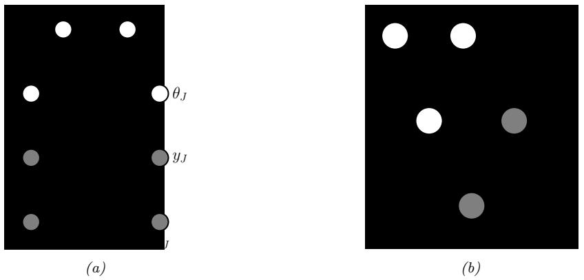
Figure 3.14: PGM for a hierarchical binomial model. (a) “Unrolled” model. (b) Same model, using plate notation.

rather strong one. A compromise approach is to assume that the ϑ^j are similar, but that there may be group-specific variations. This can be modeled by assuming the ϑ^j are drawn from some common distribution, say ϑ^j ⇔ Beta(a, b). The full joint distribution can be written as

\[p(\mathcal{D}, \boldsymbol{\theta}, \boldsymbol{\xi}) = p(\boldsymbol{\xi}) p(\boldsymbol{\theta} | \boldsymbol{\xi}) p(\mathcal{D} | \boldsymbol{\theta}) = p(\boldsymbol{\xi}) \left[ \prod\_{j=1}^{J} \text{Beta}(\theta\_j | \boldsymbol{\xi}) \right] \left[ \prod\_{j=1}^{J} \text{Bin}(y\_j | N\_j, \theta\_j) \right] \tag{3.248}\]

where ς = (a, b). In Figure 3.14 we represent these assumptions using a directed graphical model (see Section 4.2.8 for an explanation of such diagrams).

It remains to specify the prior p(ς). Following [Gel+14a, p110], we use

\[p(a,b) \propto (a+b)^{-5/2} \tag{3.249}\]

3.6.1.1 Posterior inference

We can perform approximate posterior inference in this model using a variety of methods. In Section 3.7.1 we discuss an optimization based approach, but here we discuss one of the most popular methods in Bayesian statistics, known as HMC or Hamiltonian Monte Carlo. This is described in Section 12.5, but in short it is a form of MCMC (Markov chain Monte Carlo) that exploits information from the gradient of the log joint to guide the sampling process. This algorithm generates samples in an unconstrained parameter space, so we need to define the log joint over all the parameters ⇁ = (ω˜, ˜ ^ς) ^{↑ RD} as follows:

\[\log p(\mathcal{D}, \omega) = \log p(\mathcal{D}|\theta) + \log p(\theta|\xi) + \log p(\xi) \tag{3.250}\]

\[+\sum\_{j=1}^{J} \log|\text{Jac}(\sigma)(\ddot{\theta}\_{j})| + \sum\_{i=1}^{2} \log|\text{Jac}(\sigma\_{+})(\ddot{\xi}\_{i})|\tag{3.251}\]

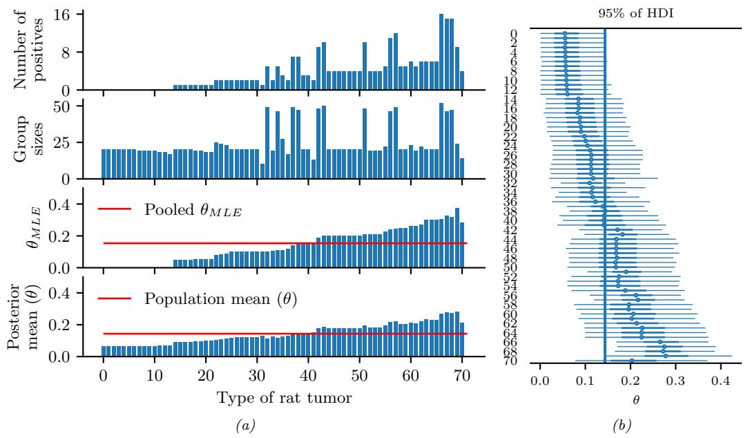
Figure 3.15: Data and inferences for the hierarchical binomial model fit using HMC. Generated by hierarchical\_binom\_rats.ipynb.

where ϑ^j = ε(˜ϑ^j ) is the sigmoid transform, and 4ⁱ = ε+(˜4i) is the softplus transform. (We need to add the Jacobian terms to account for these deterministic transformations.) We can then use automatic di!erentation to compute ▽^ϱ log p(D, ⇁), which we pass to the HMC algorithm. This algorithm returns a set of (correlated) samples from the posterior, (˜ ςs , ^ω˜^s) ^{⇔ p}(⇁|D), which we can back transform to (ς^s , ω^s). We can then estimate the posterior over quantities of interest by using a Monte Carlo approximation to p(f(ω)|D) for suitable f (e.g., to compute the posterior mean rate for group j, we set f(ω) = ϑ^j ).

3.6.1.2 Example: the rats dataset

In this section, we apply this model to analyze the number of rats that develop a certain kind of tumor during a particular clinical trial (see [Gel+14a, p102] for details). We show the raw data in rows 1–2 of Figure 3.15a. In row 3, we show the MLE ˆϑ^j for each group. We see that some groups have ˆϑ^j = 0, which is much less than the pooled MLE ˆϑpooled (red line). In row 4, we show the posterior mean E[ϑ^j |D] estimated from all the data, as well as the population mean E[ϑ|D] = E[a/(a + b)|D] shown in the red lines. We see that groups that have low counts have their estimates increased towards the population mean, and groups that have large counts have their estimates decreased towards the population mean. In other words, the groups regularize each other; this phenomenon is called shrinkage. The amount of shrinkage is controlled by the prior on (a, b), which is inferred from the data.

In Figure 3.15b, we show the 95% credible intervals for each parameter, as well as the overall

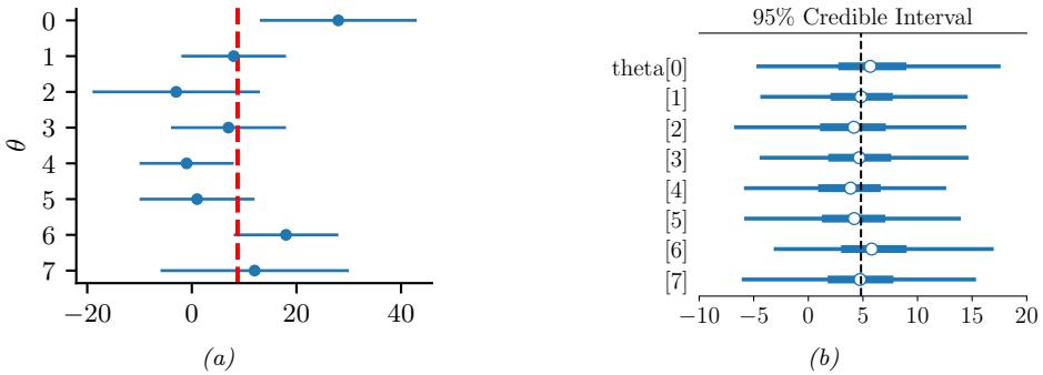
Figure 3.16: Eight schools dataset. (a) Raw data. Each row plots y^j ± ϑ^j . Vertical line is the pooled estimate. (b) Posterior 95% credible intervals for ε^j . Vertical line is posterior mean E [µ|D]. Generated by schools8.ipynb.

population mean. (This is known as a forest plot.) We can use this to decide if any group is significantly di!erent than any specified target value (e.g., the overall average).

3.6.2 A hierarchical Gaussian model

In this section, we consider a variation of the model in Section 3.6.1, where this time we have real-valued data instead of binary count data. More specificially we assume ^yij ^{⇔ N} (ϑ^j , ^ε2), where ϑ^j is the unknown mean for group j, and ε² is the observation variance (assumed to be shared across groups and fixed, for simplicity). Note that having N^j observations yij each with variance ε² is like having one measurement y^j ↭ ¹ N^j #^{Nj i}=1 yij with variance ε^{2 j} ↭ ε²/N^j . This lets us simplify notation and use one observation per group, with likelihood ^{yj ⇔ N} (ϑ, ^{ε2 j} ), where we assume the ε^j ’s are known.

We use a hierarchical model by assuming each group’s parameters come from a common distribution, ^{ϑj ⇔ N} (µ, ^{2 2}). The model becomes

\[p(\mu, \tau^2, \theta\_{1:J} | \mathcal{D}) \propto p(\mu) p(\tau^2) \prod\_{j=1}^{J} \mathcal{N}(\theta\_j | \mu, \tau^2) \mathcal{N}(y\_j | \theta\_j, \sigma\_j^2) \tag{3.252}\]

where p(µ)p(2 ²) is some kind of prior over the hyper-parameters. See Figure 3.19a for the graphical model.

3.6.2.1 Example: the eight schools dataset

Let us now apply this model to some data. We will consider the eight schools dataset from [Gel+14a, Sec 5.5]. The goal is to estimate the e!ects on a new coaching program on SAT scores. Let ynj be the observed improvement in score for student n in school j compared to a baseline. Since each school has multiple students, we summarize its data using the empirical mean ^y·^{j = 1} N^j #^{Nj n}=1 ynj and standard deviation ε^j . See Figure 3.16a for an illustration of the data. We also show the pooled

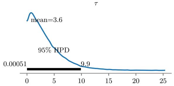
Figure 3.17: Marginal posterior density p(↽ |D) for the 8-schools dataset. Generated by schools8.ipynb.

MLE for ϑ, which is a precision weighted average of the data:

\[\overline{y}\_{..} = \frac{\sum\_{j=1}^{J} \frac{1}{\sigma\_j^2} \overline{y}\_{.j}}{\sum\_{j=1}^{J} \frac{1}{\sigma\_j^2}}\tag{3.253}\]

We see that school 0 has an unusually large improvement (28 points) compared to the overall mean, suggesting that the estimating ϑ⁰ just based on D⁰ might be unreliable. However, we can easily apply our hierarchical model. We will use HMC to do approximate inference. (See Section 3.7.2 for a faster approximate method.)

After computing the (approximate) posterior, we can compute the marginal posteriors p(ϑ^j |D) for each school. These distributions are shown in Figure 3.16b. Once again, we see shrinkage towards the global mean µ = E [µ|D], which is close to the pooled estimate y... In fact, if we fix the hyper-parameters to their posterior mean values, and use the approximation

\[p(\mu, \tau^2 | \mathcal{D}) = \delta(\mu - \overline{\mu}) \delta(\tau^2 - \overline{\tau}^2) \tag{3.254}\]

then we can use the results from Section 3.4.3.1 to compute the marginal posteriors

\[p(\theta\_j|\mathcal{D}) \approx p(\theta\_j|\mathcal{D}\_j, \overline{\mu}, \overline{\tau}^2) \tag{3.255}\]

In particular, we can show that the posterior mean ^E [ϑ^j |D] is in between the MLE ^ˆϑ^{j = yj} and the global mean µ = E [µ|D]:

\[\mathbb{E}\left[\theta\_j|\mathcal{D}, \mathbb{Z}, \mathbb{Z}^2\right] = w\_j \mathbb{Z} + (1 - w\_j)\hat{\theta}\_j \tag{3.256}\]

where the amount of shrinkage towards the global mean is given by

\[w\_j = \frac{\sigma\_j^2}{\sigma\_j^2 + \tau^2} \tag{3.257}\]

Thus we see that there is more shrinkage for groups with smaller measurement precision (e.g., due to smaller sample size), which makes intuitive sense. There is also more shrinkage if 2 ² is smaller; of course 2 ² is unknown, but we can compute a posterior for it, as shown in Figure 3.17.

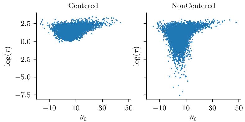
Figure 3.18: Posterior p(ε0, log(↽ )|D) for the eight schools model using (a) centered parameterization and (b) non-centered parameterization. Generated by schools8.ipynb.

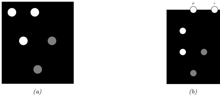
Figure 3.19: A hierarchical Gaussian Bayesian model. (a) Centered parameterization. (b) Non-centered parameterization.

3.6.2.2 Non-centered parameterization

It turns out that posterior inference in this model is di”cult for many algorithms because of the tight dependence between the variance hyperparameter 2 ² and the group means ϑ^j , as illustrated by the funnel shape in Figure 3.18. In particular, consider making local moves through parameter space. The algorithm can only “visit” the place where 2 ² is small (corresponding to strong shrinkage to the prior) if all the ϑ^j are close to the prior mean µ. It may be hard to move into the area where 2 ² is small unless all groups simultaneously move their ϑ^j estimates closer to µ.

A standard solution to this problem is to rewrite the model using the following non-centered parameterization:

\[ \theta\_j = \mu + \tau \eta\_j \tag{3.258} \]

\[ \eta\_j \sim \mathcal{N}(0, 1) \tag{3.259} \]

See Figure 3.19b for the corresponding graphical model. By writing ϑ^j as a deterministic function of

its parents plus a local noise term, we have reduced the dependence between ϑ^j and 2 and hence the other ϑ^k variables, which can improve the computational e”ciency of inference algorithms, as we discuss in Section 12.6.5. This kind of reparameterization is widely used in hierarchical Bayesian models.

3.6.3 Hierarchical conditional models

In Section 15.5, we discuss hierarchical Bayesian GLM models, which learn conditional distributions p(y|x, ω^j ) for each group j, using a prior of the form p(ω^j |ς). In Section 17.6, we discuss hierarchical Bayesian neural networks, which generalize this idea to nonlinear predictors.

3.7 Empirical Bayes

In Section 3.6, we discussed hierarchical Bayes as a way to infer parameters from data. Unfortunately, posterior inference in such models can be computationally challenging. In this section, we discuss a computationally convenient approximation, in which we first compute a point estimate of the hyperparameters, ˆ ^ς, and then compute the conditional posterior, ^p(ω|^ˆ ς, D), rather than the joint posterior, p(ω, ς|D).

To estimate the hyper-parameters, we can maximize the marginal likelihood:

\[\hat{\boldsymbol{\xi}}\_{\text{mmol}}(\mathcal{D}) = \underset{\boldsymbol{\xi}}{\text{argmax}} \, p(\mathcal{D}|\boldsymbol{\xi}) = \underset{\boldsymbol{\xi}}{\text{argmax}} \int p(\mathcal{D}|\boldsymbol{\theta}) p(\boldsymbol{\theta}|\boldsymbol{\xi}) d\boldsymbol{\theta} \tag{3.260}\]

This technique is known as type II maximum likelihood, since we are optimizing the hyperparameters, rather than the parameters. (In the context of neural networks, this is sometimes called the evidence procedure [Mac92a; WS93; Mac99].) Once we have estimated ˆ ς, we compute the posterior ^p(ω|^ˆ ς, D) in the usual way.

Since we are estimating the prior parameters from data, this approach is empirical Bayes (EB) [CL96]. This violates the principle that the prior should be chosen independently of the data. However, we can view it as a computationally cheap approximation to inference in the full hierarchical Bayesian model, just as we viewed MAP estimation as an approximation to inference in the one level model ω → D. In fact, we can construct a hierarchy in which the more integrals one performs, the “more Bayesian” one becomes, as shown below.

Method	Definition
Maximum likelihood	ωˆ = argmaxϑ p(D ω)
MAP estimation	ωˆ = argmaxϑ p(D ω)p(ω ς)
ML-II (empirical Bayes)	ˆ $ p(D ω)p(ω ς)dω ς = argmaxς
MAP-II	ˆ $ p(D ω)p(ω ς)p(ς)dω ς = argmaxς
Full Bayes	p(ω, ς D) ↙ p(D ω)p(ω ς)p(ς)

Note that ML-II is less likely to overfit than “regular” maximum likelihood, because there are typically fewer hyper-parameters ς than there are parameters ω. We give some simple examples below, and will see more applications later in the book.

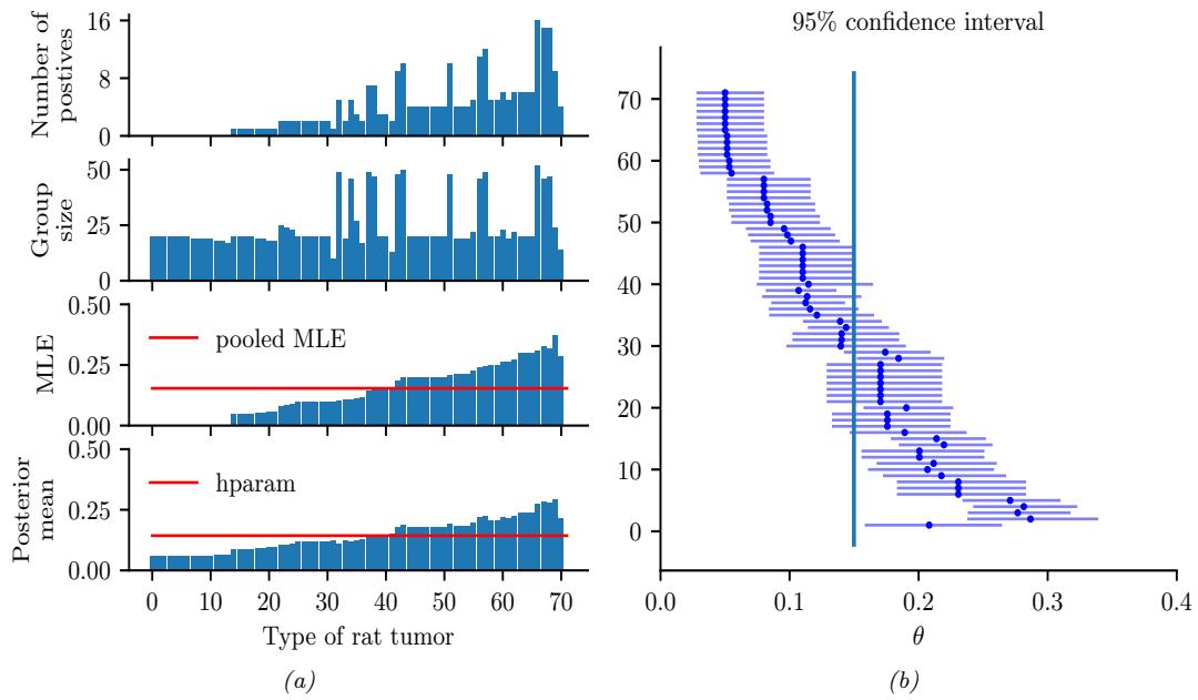
Figure 3.20: Data and inferences for the hierarchical binomial model fit using empirical Bayes. Generated by eb\_binom.ipynb.

3.7.1 EB for the hierarchical binomial model

In this section, we revisit the hierarchical binomial model from Section 3.6.1, but we use empirical Bayes instead of full Bayesian inference. We can analytically integrate out the ϑ^j ’s, and write down the marginal likelihood directly: The resulting expression is

\[p(\mathcal{D}|\boldsymbol{\xi}) = \prod\_{j} \int \text{Bin}(y\_j|N\_j, \theta\_j) \text{Beta}(\theta\_j|a, b) d\theta\_j \tag{3.261}\]

\[\propto \prod\_{j} \frac{B(a+y\_j, b+N\_j-y\_j)}{B(a,b)}\tag{3.262}\]

\[=\prod\_{j} \frac{\Gamma(a+b)}{\Gamma(a)\Gamma(b)} \frac{\Gamma(a+y\_j)\Gamma(b+N\_j-y\_j)}{\Gamma(a+b+N\_j)}\tag{3.263}\]

Various ways of maximizing this marginal likelihood wrt a and b are discussed in [Min00c].

Having estimated the hyper-parameters a and b, we can plug them in to compute the posterior ^p(ϑ^{j |}a, ^{ˆ ˆ}b, ^D) for each group, using conjugate analysis in the usual way. We show the results in Figure 3.20; they are very similar to the full Bayesian analysis shown in Figure 3.15, but the EB method is much faster.

3.7.2 EB for the hierarchical Gaussian model

In this section, we revisit the hierarchical Gaussian model from Section 3.6.2.1. However, we fit the model using empirical Bayes.

For simplicity, we will assume that ε^{2 j} = ε² is the same for all groups. When the variances are equal, we can derive the EB estimate in closed form, as we now show. We have

\[p(y\_j|\mu, \tau^2, \sigma^2) = \int \mathcal{N}(y\_j|\theta\_j, \sigma^2) \mathcal{N}(\theta\_j|\mu, \tau^2) d\theta\_j = \mathcal{N}(y\_j|\mu, \tau^2 + \sigma^2) \tag{3.264}\]

Hence the marginal likelihood is

\[p(\mathcal{D}|\mu, \tau^2, \sigma^2) = \prod\_{j=1}^{J} \mathcal{N}(y\_j|\mu, \tau^2 + \sigma^2) \tag{3.265}\]

Thus we can estimate the hyper-parameters using the usual MLEs for a Gaussian. For µ, we have

\[ \hat{\mu} = \frac{1}{J} \sum\_{j=1}^{J} y\_j = \overline{y} \tag{3.266} \]

which is the overall mean. For 2 ², we can use moment matching, which is equivalent to the MLE for a Gaussian. This means we equate the model variance to the empirical variance:

\[ \hat{\tau}^2 + \sigma^2 = \frac{1}{J} \sum\_{j=1}^{J} (y\_j - \overline{y})^2 \triangleq v \tag{3.267} \]

so ²ˆ^{2 = v} ⇐ε². Since we know ^{2 2} must be positive, it is common to use the following revised estimate:

\[ \hat{\tau}^2 = \max\{0, v - \sigma^2\} = (v - \sigma^2)\_+ \tag{3.268} \]

Given this, the posterior mean becomes

\[ \hat{\theta}\_j = \lambda \mu + (1 - \lambda) y\_j = \mu + (1 - \lambda)(y\_j - \mu) \tag{3.269} \]

where ϖ^j = ϖ = ε²/(ε² + 2 ²).

Unfortunately, we cannot use the above method on the 8-schools dataset in Section 3.6.2.1, since it uses unequal ε^j . However, we can still use the EM algorithm or other optimization based methods.

3.7.3 EB for Markov models (n-gram smoothing)

The main problem with add-one smoothing, discussed in Section 2.6.3.3, is that it assumes that all n-grams are equally likely, which is not very realistic. A more sophisticated approach, called deleted interpolation [CG96], defines the transition matrix as a convex combination of the bigram frequencies fjk = Njk/N^j and the unigram frequencies f^k = Nk/N:

\[A\_{jk} = (1 - \lambda)f\_{jk} + \lambda f\_k = (1 - \lambda)\frac{N\_{jk}}{N\_j} + \lambda \frac{N\_k}{N} \tag{3.270}\]

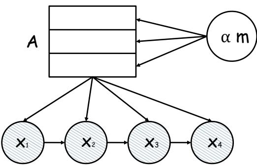
Figure 3.21: A Markov chain in which we put a di!erent Dirichlet prior on every row of the transition matrix A, but the hyperparameters of the Dirichlet are shared.

The term ϖ is usually set by cross validation. There is also a closely related technique called backo” smoothing; the idea is that if fjk is too small, we “back o!” to a more reliable estimate, namely fk.

We now show that this heuristic can be interpreted as an empirical Bayes approximation to a hierarchical Bayesian model for the parameter vectors corresponding to each row of the transition matrix A. Our presentation follows [MP95].

First, let us use an independent Dirichlet prior on each row of the transition matrix:

\[\mathbf{A}\_{j} \sim \text{Dir}(\alpha\_{0} m\_{1}, \dots, \alpha\_{0} m\_{K}) = \text{Dir}(\alpha\_{0} \boldsymbol{m}) = \text{Dir}(\boldsymbol{\alpha}) \tag{3.271}\]

where A^j is row j of the transition matrix, m is the prior mean (satisfying # ^k m^k = 1) and α⁰ is the prior strength (see Figure 3.21). In terms of the earlier notation, we have ω^j = A^j and ς = (α,m).

The posterior is given by A^j ⇔ Dir(ε+ N^j ), where N^j = (Nj1,…,NjK) is the vector that records the number of times we have transitioned out of state j to each of the other states. The posterior predictive density is

\[p(X\_{t+1} = k | X\_t = j, \mathcal{D}) = \frac{N\_{jk} + \alpha\_j m\_k}{N\_j + \alpha\_0} = \frac{f\_{jk} N\_j + \alpha\_j m\_k}{N\_j + \alpha\_0} \tag{3.272}\]

\[ \lambda = (1 - \lambda\_j) f\_{jk} + \lambda\_j m\_k \tag{3.273} \]

where

\[ \lambda\_j = \frac{\alpha\_j}{N\_j + \alpha\_0} \tag{3.274} \]

This is very similar to Equation (3.270) but not identical. The main di!erence is that the Bayesian model uses a context-dependent weight ϖ^j to combine m^k with the empirical frequency fjk, rather than a fixed weight ϖ. This is like adaptive deleted interpolation. Furthermore, rather than backing o! to the empirical marginal frequencies fk, we back o! to the model parameter mk.

The only remaining question is: what values should we use for α and m? Let’s use empirical Bayes. Since we assume each row of the transition matrix is a priori independent given ε, the marginal

likelihood for our Markov model is given by

\[p(\mathcal{D}|\boldsymbol{\alpha}) = \prod\_{j} \frac{B(\mathbf{N}\_j + \boldsymbol{\alpha})}{B(\boldsymbol{\alpha})} \tag{3.275}\]

where N^j = (Nj1,…,NjK) are the counts for leaving state j and B(ε) is the generalized beta function.

We can fit this using the methods discussed in [Min00c]. However, we can also use the following approximation [MP95, p12]:

\[m\_k \propto |\{j : N\_{jk} > 0\}|\,\tag{3.276}\]

This says that the prior probability of word k is given by the number of di!erent contexts in which it occurs, rather than the number of times it occurs. To justify the reasonableness of this result, MacKay and Peto [MP95] give the following example.

Imagine, you see, that the language, you see, has, you see, a frequently occuring couplet ‘you see’, you see, in which the second word of the couplet, see, follows the first word, you, with very high probability, you see. Then the marginal statistics, you see, are going to become hugely dominated, you see, by the words you and see, with equal frequency, you see.

If we use the standard smoothing formula, Equation (3.270), then P(you|novel) and P(see|novel), for some novel context word not seen before, would turn out to be the same, since the marginal frequencies of ‘you’ and ‘see’ are the same (11 times each). However, this seems unreasonable. ‘You’ appears in many contexts, so P(you|novel) should be high, but ‘see’ only follows ‘you’, so P(see|novel) should be low. If we use the Bayesian formula Equation (3.273), we will get this e!ect for free, since we back o! to m^k not fk, and m^k will be large for ‘you’ and small for ‘see’ by Equation (3.276).

Although elegant, this Bayesian model does not beat the state-of-the-art language model, known as interpolated Kneser-Ney [KN95; CG98]. By using ideas from nonparametric Bayes, one can create a language model that outperforms such heuristics, as discussed in [Teh06; Woo+09]. However, one can get even better results using recurrent neural nets (Section 16.3.4); the key to their success is that they don’t treat each symbol “atomically”, but instead learn a distributed embedding representation, which encodes the assumption that some symbols are more similar to each other than others.

3.7.4 EB for non-conjugate models

For more complex models, we cannot compute the EB estimate exactly. However, we can use the variational EM method to compute an approximate EB estimate, as we explain in Section 10.1.3.2.

3.8 Model selection

All models are wrong, but some are useful. — George Box [BD87, p424].10

^10. George Box is a retired statistics professor at the University of Wisconsin.

In this section, we assume we have a set of di!erent models M, each of which may fit the data to di!erent degrees, and each of which may make di!erent assumptions. We discuss how to pick the best model from this set. or to average over all of them.

We assume the “true” model is in the set M; this is known as the M-complete assumption [BS94]. Of course, in reality, none of the models may be adequate; this is known as the M-open scenario [BS94; CI13]. We can check how well a model fits (or fails to fit) the data using the procedures in Section 3.9. If none of the models are a good fit, we need to expand our hypothesis space.

3.8.1 Bayesian model selection

The natural way to pick the best model is to pick the most probable model according to Bayes’ rule:

\[\hat{m} = \underset{m \in \mathcal{M}}{\text{argmax}} \, p(m|\mathcal{D}) \tag{3.277}\]

where

\[p(m|\mathcal{D}) = \frac{p(\mathcal{D}|m)p(m)}{\sum\_{m \in \mathcal{M}} p(\mathcal{D}|m)p(m)}\tag{3.278}\]

is the posterior over models. This is called Bayesian model selection. If the prior over models is uniform, p(m)=1/|M|, then the MAP model is given by

\[ \hat{m} = \underset{m \in \mathcal{M}}{\text{argmax}} \, p(\mathcal{D}|m) \tag{3.279} \]

The quantity p(D|m) is given by

\[p(\mathcal{D}|m) = \int p(\mathcal{D}|\theta, m)p(\theta|m)d\theta\tag{3.280}\]

This is known as the marginal likelihood, or the evidence for model m. (See Section 3.8.3 for details on how to compute this quantity.) If the model assigns high prior predictive density to the observed data, then we deem it a good model. If, however, the model has too much flexibility, then some prior settings will not match the data; this probability mass will be “wasted”, lowering the expected likelihood. This implicit regularization e!ect is called the Bayesian Occam’s razor. See Figure 3.22 for an illustration.

3.8.1.1 Example: is the coin fair?

As an example, suppose we observe some coin tosses, and want to decide if the data was generated by a fair coin, ϑ = 0.5, or a potentially biased coin, where ϑ could be any value in [0, 1]. Let us denote the first model by M⁰ and the second model by M1. The marginal likelihood under M⁰ is simply

\[p(\mathcal{D}|M\_0) = \left(\frac{1}{2}\right)^N\tag{3.281}\]

where N is the number of coin tosses. From Equation (3.31), the marginal likelihood under M1, using a Beta prior, is

\[p(\mathcal{D}|M\_1) = \int p(\mathcal{D}|\theta)p(\theta)d\theta = \frac{B(\alpha\_1 + N\_1, \alpha\_0 + N\_0)}{B(\alpha\_1, \alpha\_0)}\tag{3.282}\]

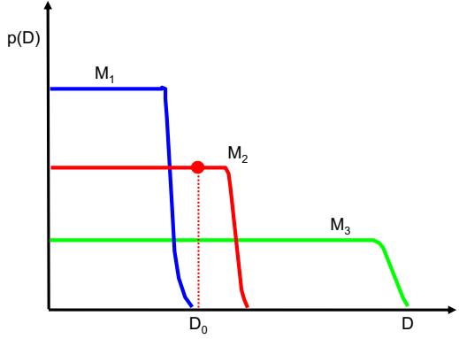
Figure 3.22: A schematic illustration of the Bayesian Occam’s razor. The broad (green) curve corresponds to a complex model, the narrow (blue) curve to a simple model, and the middle (red) curve is just right. Adapted from Figure 3.13 of [Bis06]. See also [MG05, Figure 2] for a similar plot produced on real data.

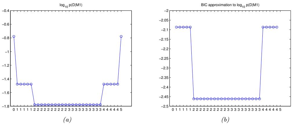
Figure 3.23: (a) Log marginal likelihood vs number of heads for the coin tossing example. (b) BIC approximation. (The vertical scale is arbitrary, since we are holding N fixed.) Generated by coins\_model\_sel\_demo.ipynb.

We plot log p(D|M1) vs the number of heads N¹ in Figure 3.23(a), assuming N = 5 and a uniform prior, α¹ = α⁰ = 1. (The shape of the curve is not very sensitive to α¹ and α0, as long as the prior is symmetric, so α⁰ = α1.) If we observe 2 or 3 heads, the unbiased coin hypothesis M⁰ is more likely than M1, since M⁰ is a simpler model (it has no free parameters) — it would be a suspicious coincidence if the coin were biased but happened to produce almost exactly 50/50 heads/tails. However, as the counts become more extreme, we favor the biased coin hypothesis.

In Figure 3.23(b), we show a similar result, where we approximate the log marginal likelihood with the BIC score (see Section 3.8.7.2).

3.8.2 Bayes model averaging

If our goal is to perform predictions, we are better o! averaging over all models, rather than predicting using just one single model. That is, we should compute the posterior predictive distribution using

\[p(y|\mathcal{D}) = \sum\_{m \in \mathcal{M}} p(y|m)p(m|\mathcal{D})\tag{3.283}\]

This is called Bayes model averaging [Hoe+99]. This is similar to the machine learning technique of ensembling, in which we take a weighted combination of predictors. However, it is not the same, as pointed out in [Min00b], since the weights in an ensemble do not need to sum to 1. In particular, in BMA, if there is a single best model, call it m↘, then in the large sample limit, p(m|D) will become a degenerate distribution with all its weight on m↘, and the other members of M will be ignored. This does not happen with an ensemble.

3.8.3 Estimating the marginal likelihood

To perform Bayesian model selection or averaging, we need to be able to compute the marginal likelihood in Equation (3.280), also called the evidence. Below we give a brief summary of some suitable methods. For more details, see e.g., [FW12].

3.8.3.1 Analytic solution for conjugate models

If we use a conjugate prior, we can compute the marginal likelihood analytically, as we discussed in Section 3.4.5.4. We give a worked example in Section 3.8.1.1.

3.8.3.2 Harmonic mean estimator

A particularly simple estimator, known as the harmonic mean estimator, was proposed in [NR94]. It is defined as follows:

\[p(\mathcal{D}) \approx \left(\frac{1}{S} \sum\_{s=1}^{S} \frac{1}{p(\mathcal{D}|\theta\_s)}\right)^{-1} \tag{3.284}\]

where ω^s ⇔ p(ω) are samples from the posterior. This follows from the following identity:

\[\mathbb{E}\left[\frac{1}{p(\mathcal{D}|\boldsymbol{\theta})}\right] = \int \frac{1}{p(\mathcal{D}|\boldsymbol{\theta})} p(\boldsymbol{\theta}|\mathcal{D}) d\boldsymbol{\theta} \tag{3.285}\]

\[=\int \frac{1}{p(\mathcal{D}|\boldsymbol{\theta})} \frac{p(\mathcal{D}|\boldsymbol{\theta})p(\boldsymbol{\theta})}{p(\mathcal{D})} d\boldsymbol{\theta} \tag{3.286}\]

\[\mathcal{I} = \frac{1}{p(\mathcal{D})} \int p(\theta) d\theta = \frac{1}{p(\mathcal{D})} \tag{3.287}\]

Unfortunately, Radford Neal (in a blog post in 2008) described this method as “The Worst Monte Carlo Method Ever”.11 In particular, he said:

^11. https://bit.ly/3t7id0k.

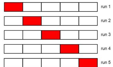
Figure 3.24: Schematic of 5-fold cross validation.

It’s easy to see why this estimator can’t possibly work well in practice. As is well-known, the posterior distribution for a Bayesian model is often much narrower than the prior, and it is often not very sensitive to what the prior is, as long as the prior is broad enough to encompass the region with high likelihood. […] Since the prior a!ects the harmonic mean estimate of the marginal likelihood only through its e!ect on the posterior distribution, it follows that the harmonic mean estimate is very likely to be virtually the same for the two priors, for any reasonable size sample from the posterior. […] The harmonic mean method is clearly hopelessly inaccurate.

3.8.3.3 Other Monte Carlo methods

The marginal likelihood can be more reliably estimated using annealed importance sampling, as discussed in Section 11.5.4.1. An extension of this, known as sequential Monte Carlo sampling, as discussed in Section 13.2.3.3. Another method that is well suited to estimate the normalization constant is known as nested sampling [Ski06; Buc21].

3.8.3.4 Variational Bayes

An e”cient way to compute an approximation to the evidence is to use variational Bayes, which we discuss in Section 10.3.3. This computes a tractable approximation to the posterior, q(ω|D), by optimizing the evidence lower bound or ELBO, log q(D|ω), which can be used to approximate the evidence.

3.8.4 Connection between cross validation and marginal likelihood

A standard approach to model evaluation is to estimate its predictive performance (in terms of log likelihood) on a validation set, which is distinct from the training set which is used to fit the model If we don’t have such a separate validation set, we can make one by partitioning the training set into K subsets or “folds”, and then training on K ⇐ 1 and testing on the K’th; we repeat this K times, as shown in Figure 3.24. This is known as cross validation.

If we set K = N, the method is known as leave-one-out cross validation or LOO-CV, since we train on N ⇐ 1 points and test on the remaining one, and we do this N times. More precisely, we

have

\[L\_{\rm LOO}(m) \triangleq \sum\_{n=1}^{N} \log p(\mathcal{D}\_n | \hat{\theta}(\mathcal{D}\_{-n}), m) \tag{3.288}\]

where ^ωˆ↑ⁿ is the parameter estimate computing when we omit ^Dn from the training set. (We discuss fast approxmations to this in Section 3.8.6.)

Interestingly, the LOO-CV version of log likelihood is closely related to the log marginal likelihood. To see this, let us write the log marginal likelihood (LML) in sequential form as follows:

\[\text{LML}(m) \triangleq \log p(\mathcal{D}|m) = \log \prod\_{n=1}^{N} p(\mathcal{D}\_n | \mathcal{D}\_{1:n-1}, m) = \sum\_{n=1}^{N} \log p(\mathcal{D}\_n | \mathcal{D}\_{1:n-1}, m) \tag{3.289}\]

where

\[p(\mathcal{D}\_n|\mathcal{D}\_{1:n-1},m) = \int p(\mathcal{D}\_n|\theta)p(\theta|\mathcal{D}\_{1:n-1},m)d\theta\tag{3.290}\]

Note that we evaluate the posterior on the first n ⇐ 1 datapoints and use this to predict the n’th; this is called prequential analysis [DV99].

Suppose we use a point estimate for the parameters at time n, rather than the full posterior. We can then use a plugin approximation to the n’th predictive distribution:

\[p(\mathcal{D}\_n|\mathcal{D}\_{1:n-1}, m) \approx \int p(\mathcal{D}\_n|\theta) \delta(\theta - \hat{\theta}\_m(\mathcal{D}\_{1:n-1})) d\theta = p(\mathcal{D}\_n|\hat{\theta}\_m(\mathcal{D}\_{1:n-1})) \tag{3.291}\]

Then Equation (3.289) simplifies to

\[\log p(\mathcal{D}|m) \approx \sum\_{n=1}^{N} \log p(\mathcal{D}\_n|\hat{\theta}(\mathcal{D}\_{1:n-1}), m) \tag{3.292}\]

This is very similar to Equation (3.288), except it is evaluated sequentially. A complex model will overfit the “early” examples and will then predict the remaining ones poorly, and thus will get low marginal likelihood as well as a low cross-validation score. See [FH20] for further discussion.

3.8.5 Conditional marginal likelihood

The marginal likelihood answers the question “what is the likelihood of generating the training data from my prior?”. This can be suitable for hypothesis testing between di!erent fixed priors, but is less useful for selecting models based on their posteriors. In the latter case, we are more interested in the question “what is the probability that the posterior could generate withheld points from the data distribution?”, which is related to the generalization performance of the (fitted) model. In fact [Lot+22] showed that the marginal likelihood can sometimes be negatively correlated with the generalization performance, because the first few terms in the LML decomposition may be large and negative for a model that has a poor prior but which otherwise adapts quickly to the data (by virtue of the prior being weak).

A better approach is to use the conditional log marginal likelihood, which is defined as follows [Lot+22]:

\[\text{CLML}(m) = \sum\_{n=K}^{N} \log p(\mathcal{D}\_n | \mathcal{D}\_{1:n-1}, m) \tag{3.293}\]

where K ↑ {1,…,N} is a parameter of the algorithm. This evaluates the LML of the last N ⇐ K datapoints, under the posterior given by the first K datapoints. We can reduce the dependence on the ordering of the datapoints by averaging over orders; if we set K = N ⇐ 1 and average over all orders, we get the LOO estimate.

The CLML is much more predictive of generalization performance than the LML, and is much less sensitive to prior hyperparameters. Furthermore, it is easier to calculuate, since we can use a straightforward Monte Carlo estimate of the integral, where we sample from the posterior p(ω|D<n); this does not su!er from the same problems as the harmonic mean estimator in Section 3.8.3.2 which samples from the prior.

3.8.6 Bayesian leave-one-out (LOO) estimate

In this section we discuss a computationally e”cient method, based on importance sampling, to approximate the leave-one-out (LOO) estimate without having to fit the model N times. We focus on conditional (supervised) models, so p(D|ω) = p(y|x, ω).

Suppose we have computed the posterior given the full dataset for model m. We can use this to evaluate the resulting predictive distribution p(yn|xn, D, m) for each datapoint n in the dataset. This gives the log-pointwise predictive-density or LPPD score:

\[\text{LPPD}(m) \triangleq \sum\_{n=1}^{N} \log p(\mathbf{y}\_n | \mathbf{x}\_n, \mathcal{D}, m) = \sum\_{n=1}^{N} \log \int p(\mathbf{y}\_n | \mathbf{x}\_n, \boldsymbol{\theta}, m) p(\boldsymbol{\theta} | \mathcal{D}, m) d\boldsymbol{\theta} \tag{3.294}\]

We can approximate LPPD with Monte Carlo:

\[\text{LPPD}(m) \approx \sum\_{n=1}^{N} \log \left( \frac{1}{S} \sum\_{s=1}^{S} p(\mathbf{y}\_n | x\_n, \boldsymbol{\theta}\_s, m) \right) \tag{3.295}\]

where ω^s ⇔ p(ω|D, m) is a posterior sample.

The trouble with LPPD is that it predicts the n’th datapoint yⁿ using all the data, including yn. What we would like to compute is the expected LPPD (ELPD) on future data, (x↘, y↘):

\[\text{ELPD}(m) \stackrel{\Delta}{=} \mathbb{E}\_{\mathbf{z}\_{\ast}, \mathbf{y}\_{\ast}} \log p(\mathbf{y}\_{\ast} | \mathbf{z}\_{\ast}, \mathcal{D}, m) \tag{3.296}\]

Of course, the future data is unknown, but we can use a LOO approximation:

\[\text{ELPD}\_{\text{LOO}}(m) \triangleq \sum\_{n=1}^{N} \log p(y\_n | x\_n, \mathcal{D}\_{-n}, m) = \sum\_{n=1}^{N} \log \int p(y\_n | x\_n, \theta, m) p(\theta | \mathcal{D}\_{-n}, m) d\theta \tag{3.297}\]

This is a Bayesian version of Equation (3.288). We can approximate this integral using Monte Carlo:

\[\text{ELPD}\_{\text{LOO}}(m) \approx \sum\_{n=1}^{N} \log \left( \frac{1}{S} \sum\_{s=1}^{S} p(y\_n | \mathbf{x}\_n, \boldsymbol{\theta}\_{s,-n}, m) \right) \tag{3.298}\]

where ωs,↑ⁿ ⇔ p(ω|D↑ⁿ, m).

The above procedure requires computing N di!erent posteriors, leaving one datapoint out at a time, which is slow. A faster alternative is to compute p(ω|D, m) once, and then use importance sampling (Section 11.5) to approximate the above integral. More precisely, let f(ω) = p(ω|D↑ⁿ, m) be the target distribution of interest, and let g(ω) = p(ω|D, m) be the proposal. Define the importance weight for each sample s when leaving out example n to be

\[w\_{s,-n} = \frac{f(\boldsymbol{\theta}\_s)}{g(\boldsymbol{\theta}\_s)} = \frac{p(\boldsymbol{\theta}\_s|\mathcal{D}\_{-n})}{p(\boldsymbol{\theta}\_s|\mathcal{D})} = \frac{p(\mathcal{D}\_{-n}|\boldsymbol{\theta}\_s)p(\boldsymbol{\theta}\_s)}{p(\mathcal{D}\_{-n})} \frac{p(\mathcal{D})}{p(\mathcal{D}|\boldsymbol{\theta}\_s)p(\boldsymbol{\theta}\_s)}\tag{3.299}\]

\[\propto \frac{p(\mathcal{D}\_{-n}|\theta\_s)}{p(\mathcal{D}|\theta\_s)} = \frac{p(\mathcal{D}\_{-n}|\theta\_s)}{p(\mathcal{D}\_{-n}|\theta)p(\mathcal{D}\_n|\theta\_s)} = \frac{1}{p(\mathcal{D}\_n|\theta\_s)}\tag{3.300}\]

We then normalize the weights to get

\[ \hat{w}\_{s,-n} = \frac{w\_{s,-n}}{\sum\_{s'=1}^{S} w\_{s',-n}} \tag{3.301} \]

and use them to get the estimate

\[\text{ELPD}\_{\text{IS-LOO}}(m) = \sum\_{n=1}^{N} \log \left( \sum\_{s=1}^{S} \hat{w}\_{s,-n} p(\mathbf{y}\_n | \mathbf{x}\_n, \mathbf{e}\_s, m) \right) \tag{3.302}\]

Unfortunately, the importance weights may have high variance, where some weights are much larger than others. To reduce this e!ect, we fit a Pareto distribution (Section 2.2.3.5) to each set of weights for each sample, and use this to smooth the weights. This technique is called Pareto smoothed importance sampling or PSIS [Veh+15; VGG17]. The Pareto distribution has the form

\[p(r|u,\sigma,k) = \sigma^{-1}(1+k(r-u)\sigma^{-1})^{-1/k-1} \tag{3.303}\]

where u is the location, ε is the scale, and k is the shape. The parameter values kⁿ (for each datapoint n) can be used to assess how well this approximation works. If we find kⁿ > 0.5 for any given point, it is likely an outlier, and the resulting LOO estimate is likely to be quite poor. See [Siv+20] for further discussion, and [Kel21] for a general tutorial on PSIS-LOO-CV.

3.8.7 Information criteria

An alternative approach to cross validation is to score models using the negative log likelihood (or LPPD) on the training set plus a complexity penalty term:

\[\mathcal{L}(m) = -\log p(\mathcal{D}|\hat{\theta}, m) + C(m) \tag{3.304}\]

This is called an information criterion. Di!erent methods use di!erent complexity terms C(m), as we discuss below. See e.g., [GHV14] for further details.

A note on notation: it is conventional, when working with information criteria, to scale the NLL by ⇐2 to get the deviance:

\[\text{deviance}(m) = -2\log p(\mathcal{D}|\hat{\theta}, m) \tag{3.305}\]

This makes the math “prettier” for certain Gaussian models.

3.8.7.1 Minimum description length (MDL)

We can think about the problem of scoring di!erent models by using tools from information theory (Chapter 5). In particular, suppose we want to choose a model so that the sender can send some dataa to the receiver using the fewest number of bits. Choosing models this way is known as the minimum description length or MDL principle (see e.g., [HY01; Gru07; GR19] for details, and see [Wal05] for the closely related minimum message length criterion).

We now derive an approximation to the MDL objective. First, the sender needs to specify which model to use. Let ^{ωˆ ↑ RDm} be the parameters estimated using ^N data samples. Since we can only reliably estimate each parameter to an accuracy of O(1/ ↖ N) (see Section 4.7.2), we only need to use log2(1/ ↖ N) = ^{1 2} log2(N) bits to encode each parameter.

Second, the sender needs to use this model to encode the data, which takes

\[L(m) = -\log p(\mathcal{D}|\hat{\theta}, m) = -\sum\_{n} \log p(y\_n|\hat{\theta}, m) \tag{3.306}\]

bits. The total cost is

\[\mathcal{L}\_{\text{MDL}}(m) = -\log p(\mathcal{D}|\hat{\theta}, m) + \frac{D\_m}{2} \log N \tag{3.307}\]

We see that this two-part code has the same basic form as BIC, discussed in Section 3.8.7.2.

3.8.7.2 The Bayesian information criterion (BIC)

The Bayesian information criterion or BIC [Sch78] is similar to the MDL, and has the form

\[\mathcal{L}\_{\text{BIC}}(m) = -2\log p(\mathcal{D}|\hat{\theta}, m) + D\_m \log N \tag{3.308}\]

where D^m is the degrees of freedom of model m.

We can derive the BIC score as a simple approximation to the log marginal likelihood. In particular, suppose we make a Gaussian approximation to the posterior, as discussed in Section 7.4.3. Then we get (from Equation (7.28)) the following:

\[\log p(\mathcal{D}|m) \approx \log p(\mathcal{D}|\hat{\theta}\_{\text{map}}) + \log p(\hat{\theta}\_{\text{map}}) - \frac{1}{2} \log |\mathbf{H}| \tag{3.309}\]

where ^H is the Hessian of the negative log joint log ^p(D, ^ω) evaluated at the MAP estimate ^ωˆmap. We see that Equation (3.309) is the log likelihood plus some penalty terms. If we have a uniform prior, ^p(ω) ↙ ¹, we can drop the prior term, and replace the MAP estimate with the MLE, ^ωˆ, yielding

\[\log p(\mathcal{D}|m) \approx \log p(\mathcal{D}|\hat{\theta}) - \frac{1}{2} \log |\mathbf{H}| \tag{3.310}\]

We now focus on approximating the log |H| term, which is sometimes called the Occam factor, since it is a measure of model complexity (volume of the posterior distribution). We have H = #^{N i}=1 Hi, where ^{Hi =} ▽▽ log ^p(Di|ω). Let us approximate each ^Hi by a fixed matrix ^Hˆ . Then we have

\[\log|\mathbf{H}| = \log|N\hat{\mathbf{H}}| = \log(N^{D\_m}|\hat{\mathbf{H}}|) = D\_m \log N + \log|\hat{\mathbf{H}}|\tag{3.311}\]

where ^{Dm =} dim(ω) and we have assumed ^H is full rank. We can drop the log ^|H^{ˆ |} term, since it is independent of N, and thus will get overwhelmed by the likelihood. Putting all the pieces together, we get the BIC score that we want to maximize:

\[J\_{\rm BIC}(m) = \log p(\mathcal{D}|\hat{\theta}, m) - \frac{D\_m}{2} \log N \tag{3.312}\]

We can also define the BIC loss, that we want to minimize, by multiplying by ⇐2:

\[\mathcal{L}\_{\text{BIC}}(m) = -2\log p(\mathcal{D}|\hat{\theta}, m) + D\_m \log N\tag{3.313}\]

3.8.7.3 Akaike information criterion

The Akaike information criterion [Aka74] is closely related to BIC. It has the form

\[\mathcal{L}\_{\text{AIC}}(m) = -2\log p(\mathcal{D}|\hat{\theta}, m) + 2D\_m \tag{3.314}\]

This penalizes complex models less heavily than BIC, since the regularization term is independent of N. This estimator can be derived from a frequentist perspective.

3.8.7.4 Widely applicable information criterion (WAIC)

The main problem with MDL, BIC, and AIC is that it can be hard to compute the degrees of a freedom of a model, needed to define the complexity term, since most parameters are highly correlated and not uniquely identifiable from the likelihood. In particular, if the mapping from parameters to the likelihood is not one-to-one, then the model known as a singular statistical model, since the corresponding Fisher information matrix (Section 3.3.4), and hence the Hessian H above, may be singular. (Similar problems arise in over-parameterized models [Dwi+23].) An alternative criterion that works even in the singular case is known as the widely applicable information criterion (WAIC), also known as the Watanabe–Akaike information criterion [Wat10; Wat13].

WAIC is like other information criteria, except it is more Bayesian. First it replaces the log likelihood L(m), which uses a point estimate of the parameters, with the LPPD, which marginalizes them out. (see Equation (3.295)). For the complexity term, WAIC uses the variance of the predictive distribution:

\[C(m) = \sum\_{n=1}^{N} \mathbb{V}\_{\theta \mid \mathcal{D}, m} [\log p(y\_n | x\_n, \theta, m)] \approx \sum\_{n=1}^{N} \mathbb{V} \{ \log p(y\_n | x\_n, \theta\_s, m) : s = 1 : S \} \tag{3.315}\]

The intuition for this is as follows: if, for a given datapoint n, the di!erent posterior samples ω^s make very di!erent predictions, then the model is uncertain, and likely too flexible. The complexity term essentially counts how often this occurs. The final WAIC loss is

\[\mathcal{L}\_{\text{WAIC}}(m) = -2\text{LPDD}(m) + 2C(m) \tag{3.316}\]

Interestingly, it can be shown that the PSIS LOO estimate in Section 3.8.6 is asymptotically equivalent to WAIC [VGG17].

3.9 Model checking

Bayesian inference and decision making is optimal, but only if the modeling assumptions are correct. In this section, we discuss some ways to assess if a model is reasonable. From a Bayesian perspective, this can seem a bit odd, since if we knew there was a better model, why don’t we just use that? Here we assume that we do not have a specific alternative model in mind (so we are not performing model selection, unlike Section 3.8.1). Instead we are just trying to see if the data we observe is “typical” of what we might expect if our model were correct. This is called model checking.

3.9.1 Posterior predictive checks

Suppose we are trying to estimate the probability of heads for a coin, ϑ ↑ [0, 1]. We have two candidate models or hypotheses, M¹ which corresponds to ϑ = 0.99 and M² which corresponds to ϑ = 0.01. Suppose we flip the coin 40 times and it comes up heads 30 times. Obviously we have p(M = M1|D) ∃ p(M = M2|D). However model M¹ is still a very bad model for the data. (This example is from [Kru15, p331].)

To evaluate how good a candidate model M is, after seeing some data D, we can imagine using the model to generate synthetic future datasets, by drawing from the posterior predictive distribution:

\[ \tilde{\mathcal{D}}^s \sim p(\tilde{\mathcal{D}}|M, \mathcal{D}) = \{ y\_{1:N}^s \sim p(\cdot|M, \theta^s), \theta^s \sim p(\theta|\mathcal{D}, M) \}\tag{3.317} \]

These represent “plausible hallucinations” of the model. To assess the quality of our model, we can compute how “typical” our observed data D is compared to the model’s hallucinations. To perform this comparison, we create one or more scalar test statistics, test(D˜ ^s), and compare them to the test statistics on the actual data, test(D). These statistics should measure features of interest (since it will not, in general, be possible to capture every aspect of the data with a given model). If there is a large di!erence between the distribution of test(D˜ ^s) across di!erent ^s and the value of test(D), it suggests the model is not a good one. This approach called a posterior predictive check [Rub84].

3.9.1.1 Example: 1d Gaussian

To make things clearer, let us consider an example from [Gel+04]. In 1882, Newcomb measured the speed of light using a certain method and obtained N = 66 measurements, shown in Figure 3.25(a). There are clearly two outliers in the left tails, suggesting that the distribution is not Gaussian. Let us nonetheless fit a Gaussian to it. For simplicity, we will just compute the MLE, and use a plug-in approximation to the posterior predictive density:

\[p(\bar{y}|\mathcal{D}) \approx \mathcal{N}(\bar{y}|\hat{\mu}, \hat{\sigma}^2), \quad \hat{\mu} = \frac{1}{N} \sum\_{n=1}^{N} y\_n, \quad \hat{\sigma}^2 = \frac{1}{N} \sum\_{n=1}^{N} (y\_n - \hat{\mu})^2 \tag{3.318}\]

Let ^D˜ ^s be the ^s’th dataset of size ^N = 66 sampled from this distribution, for ^s = 1 : 1000. The histogram of ^D˜ ^s for some of these samples is shown in Figure 3.25(b). It is clear that none of the

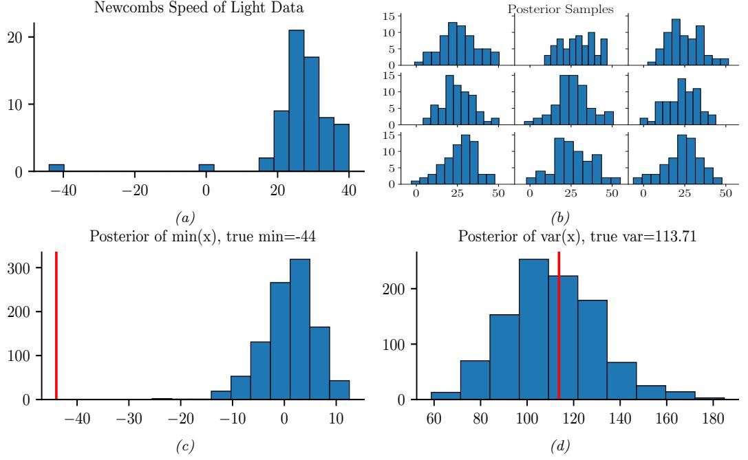
Figure 3.25: (a) Histogram of Newcomb’s data. (b) Histograms of data sampled from Gaussian model. (c) Histogram of test statistic on data sampled from the model, which represents ^p(test(D˜ ^s)|D), where test(D) = min{y ↗ D}. The vertical line is the test statistic on the true data, test(D). (d) Same as (c) except test(D) = V{y ↗ D}. Generated by newcomb\_plugin\_demo.ipynb.

samples contain the large negative examples that were seen in the real data. This suggests the model cannot capture the long tails present in the data. (We are assuming that these extreme values are scientifically interesting, and something we want the model to capture.)

A more formal way to test fit is to define a test statistic. Since we are interested in small values, let us use

\[\text{test}(\mathcal{D}) = \min\{y : y \in \mathcal{D}\} \tag{3.319}\]

The empirical distribution of test(D˜ ^s) for ^s = 1 : 1000 is shown in Figure 3.25(c). For the real data, test(D) = ⇐44, but the test statistics of the generated data, test(D˜ ), are much larger. Indeed, we see that ⇐⁴⁴ is in the left tail of the predictive distribution, ^p(test(D˜ )|D).

3.9.1.2 Example: linear regression

When fitting conditional models, p(y|x), we will have a di!erent prediction for each input x. We can compare the predictive distribution p(y|xn) to the observed yⁿ to detect places where the model does poorly.

As an example of this, we consider the “wa$e divorce” dataset from [McE20, Sec 5.1]. This contains the divorce rate Dn, marriage rate Mn, and age Aⁿ at first marriage for 50 di!erent US states. We use

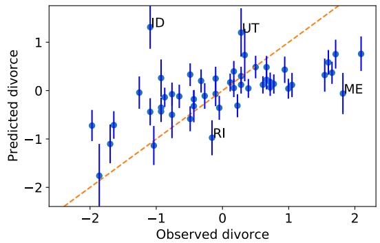
Figure 3.26: Posterior predictive distribution for divorce rate vs actual divorce rate for 50 US states. Both axes are standardized (i.e., z-scores). A few outliers are annotated. Adapted from Figure 5.5 of [McE20]. Generated by linreg\_divorce\_ppc.ipynb.

a linear regression model to predict the divorce rate, ^p(^{y = d}|^x = (a, m)) = ^N (d|^{α +} ↼a^{a +} ↼mm, ^ε2), using vague priors for the parameters. (In this example, we use a Laplace approximation to the posterior, discussed in Section 7.4.3.) We then compute the posterior predictive distribution p(y|xn, D), which is a 1d Gaussian, and plot this vs each observed outcome yn.

The result is shown in Figure 3.26. We see several outliers, some of which have been annotated. In particular, we see that both Idaho (ID) and Utah (UT) have a much lower divorce rate than predicted. This is because both of these states have an unusually large proportion of Mormons.

Of course, we expect errors in our predictive models. However, ideally the predictive error bars for the inputs where the model is wrong would be larger, rather than the model confidently making errors. In this case, the overconfidence arises from our incorrect use of a linear model.

3.9.2 Bayesian p-values

If some test statistic of the observed data, test(D), occurs in the left or right tail of the predictive distribution, then it is very unlikely under the model. We can quantify this using a Bayesian p-value, also called a posterior predictive p-value:

\[p\_B = \Pr(\text{test}(\tilde{\mathcal{D}}) \ge \text{test}(\mathcal{D}) | M, \mathcal{D}) \tag{3.320}\]

where ^M represents the model we are using, and ^D˜ is a hypothetical future dataset. In contrast, a classical or frequentist p-value is defined as

\[p\_C = \Pr(\text{test}(\tilde{\mathcal{D}}) \ge \text{test}(\mathcal{D}) | M) \tag{3.321}\]

where M represents the null hypothesis. The key di!erence is that the Bayesian compares what was observed to what one would expect after conditioning the model on the data, whereas the frequentist compares what was observed to the sampling distribution of the null hypothesis, which is independent of the data.

We can approximate the Bayesian p-value using Monte Carlo integration, as follows:

\[p\_B = \int \mathbb{I}\left(\text{test}(\bar{\mathcal{D}}) > \text{test}(\mathcal{D})\right) p(\bar{\mathcal{D}}|\theta) p(\theta|\mathcal{D}) d\theta \approx \frac{1}{S} \sum\_{s=1}^{S} \mathbb{I}\left(\text{test}(\bar{\mathcal{D}}^s) > \text{test}(\mathcal{D})\right) \tag{3.322}\]

Any extreme value for p^B (i.e., a value near 0 or 1) means that the observed data is unlikely under the model, as assessed via test statistic test. However, if test(D) is a su”cient statistic of the model, it is likely to be well estimated, and the p-value will be near 0.5. For example, in the speed of light example, if we define our test statistic to be the variance of the data, test(D) = V{y : y ↑ D}, we get a p-value of 0.48. (See Figure 3.25(d).) This shows that the Gaussian model is capable of representing the variance in the data, even though it is not capable of representing the support (range) of the data.

The above example illustrates the very important point that we should not try to assess whether the data comes from a given model (for which the answer is nearly always that it does not), but rather, we should just try to assess whether the model captures the features we care about. See [Gel+04, ch.6] for a more extensive discussion of this topic.

3.10 Hypothesis testing

Suppose we have collected some coin tossing data, and we want to know if there if the coin is fair or not. Or, more interestingly, we have collected some clinical trial data, and want to know if there is a non-zero e!ect of the treatment on the outcome (e.g., di!erent survival rates for the treatment and control groups). These kinds of problems can be solved using hypothesis testing. In the sections below, we summarize several common approaches to hypothesis testing.

3.10.1 Frequentist approach

In this section, we summarize the approach to hypothesis testing that is used in classical or frequentist statistics, which is known as null hypothesis significance testing or NHST. The basic idea is to define a binary decision rule of the form 1(D) = I(t(D) ⇑ t ↘), where t(D) is some scalar test statistic derived from the data, and t ↘ is some critical value. If the test statistic exceeds the critical value, we reject the null hypothesis.

There is a large “zoo” of possible test statistics one can use (e.g., [Ken93] lists over 100 di!erent tests), but a simple example is a t-statistic, defined as

\[t(\mathcal{D}) = \frac{\overline{x} - \mu}{\hat{\sigma}/\sqrt{N}}\tag{3.323}\]

where where x is the empirical mean of D, εˆ is the empirical standard deviation, N is the sample size, and µ is the population mean, corresponding to the mean value of the null hypothesis (often 0).

To compute the critical value t ↘, we pick a significance level α, often 0.05, which controls the type I error rate of the decision procedure (i.e., the probability of accidentally rejecting the null hypothesis when it is true). We then find the value t ↘ whose tail probability, under the sampling distribution of the test statistic given the null hypothesis, matches the significance level:

\[p(t|\tilde{\mathcal{D}}) \ge t^\*|H\_0\rangle = \alpha \tag{3.324}\]

Bayes factor BF(1, 0)	Interpretation
1 BF < 100	Decisive evidence for M0
1 BF < 10	Strong evidence for M0
1 1 10 < BF < 3	Moderate evidence for M0
1 3 < BF < 1	Weak evidence for M0
1 < BF < 3	Weak evidence for M1
3 < BF < 10	Moderate evidence for M1
BF > 10	M1 Strong evidence for
BF > 100	Decisive evidence for M1

Table 3.1: Je!reys scale of evidence for interpreting Bayes factors.

This construction guarantees that ^p(1(D˜ )=1|H0) = ^α.

Rather than comparing t(D) to t ↘, a more common (but equivalent) approach is to compute the p-value of t(D), which is defined in Equation (3.86). We can then reject the null hypothesis is p < α.

Unfortunately, despite its widespread use, p-values and NHST have many problems, some of which are discussed in Section 3.3.5.2. We shall therefore avoid using this approach in this book.

3.10.2 Bayesian approach

In this section, we discucss the Bayesian approach to hypothesis testing. There are in fact two approaches, one based on model comparison using Bayes factors (Section 3.10.2.1), and one based on parameter estimation (Section 3.10.2.3).

3.10.2.1 Model comparison approach

Bayesian hypothesis testing is a special case of Bayesian model selection (discussed in Section 3.8.1) when we just have two models, commonly called the null hypothesis, M0, and the alternative hypothesis, M1. Let us define the Bayes factor as the ratio of marginal likelihoods:

\[B\_{1,0} \triangleq \frac{p(\mathcal{D}|M\_1)}{p(\mathcal{D}|M\_0)} = \frac{p(M\_1|\mathcal{D})}{p(M\_0|\mathcal{D})} / \frac{p(M\_1)}{p(M\_0)}\tag{3.325}\]

(This is like a likelihood ratio, except we integrate out the parameters, which allows us to compare models of di!erent complexity.) If B1,⁰ > 1 then we prefer model 1, otherwise we prefer model 0 (see Table 3.1).

We give a worked example of how to compute Bayes factors for a binomial test in Section 3.8.1.1. For examples of computing Bayes factors for more complex tests, see e.g. [Etz+18; Ly+20].

3.10.2.2 Improper priors cause problems for Bayes factors

Problems can arise when we use improper priors (i.e., priors that do not integrate to 1) for Bayesian model selection, even though such priors may be acceptable for other purposes, such as parameter inference. For example, consider testing the hypotheses M⁰ : ϑ ↑ &⁰ vs M¹ : ϑ ↑ &1. The posterior

probability of M⁰ is given by

\[p(M\_0|\mathcal{D}) = \frac{p(M\_0)L\_0}{p(M\_0)L\_0 + p(M\_1)L\_1} \tag{3.326}\]

where ^{Li = p}(D|Mi) = $ #ⁱ p(D|ϑ)p(ϑ|Mi)dϑ is the marginal likelihood for model i.

Suppose (for simplicity) that p(M0) = p(M1)=0.5, and we use a uniform but improper prior over the model parameters, ^p(ϑ|M0) ↙ ^c0 and ^p(ϑ|M1) ↙ ^c1. Define ⇁^{i =} $ #ⁱ p(D|ϑ)dϑ, so Lⁱ = ci⇁i. Then

\[p(M\_0|\mathcal{D}) = \frac{c\_0 \ell\_0}{c\_0 \ell\_0 + c\_1 \ell\_1} = \frac{\ell\_0}{\ell\_0 + (c\_1/c\_0)\ell\_1} \tag{3.327}\]

Thus the posterior (and hence Bayes factor) depends on the arbitrary constants c⁰ and c1. This is known as the marginalization paradox. For this reason, we should avoid using improper priors when performing Bayesian model selection. (However, if the same improper prior is used for common parameters that are shared between the two hypotheses, then the paradox does not arise.)

More generally, since the marginal likelihood is the likelihood averaged wrt the prior, results can be quite sensitive to the form of prior that is used. (See also Section 3.8.5, where we discuss conditional marginal likelihood.)

3.10.2.3 Parameter estimation approach

There are several drawbacks of the Bayesian hypothesis testing approach in Section 3.10.2.1, such as computational di”culty of computing the marginal likelihood (see Section 3.8.3), and the sensitivity to the prior (see Section 3.10.2.2). An alternative approach is to estimate the parameters of the model in the usual way, and then to see how much posterior probability is assigned to the parameter value corresponding to the null hypothesis. For example, to “test” if a coin is fair, we can first compute the posterior p(ϑ|D), and then we can evaluate the plausibility of the null hypothesis by computing p(0.5 ⇐ 3 < ϑ < 0.5 + 3|D), where (0.5 ⇐ 3, 0.5 + 3) is called the region of practical equivalence or ROPE [Kru15; KL17c]. This is not only computationally simpler, but is also allows us to quantify the e!ect size (i.e., the expected deviation of ϑ from the null value of 0.5), rather than merely accepting or rejecting a hypothesis. This approach is therefore called Bayesian estimation. We give some examples below, following https://www.sumsar.net/blog/2014/01/bayesian-first-aid/. (See also Section 3.10.3 for ways to perform more general tests usings GLMs.)

3.10.2.4 One sample test of a proportion (Binomial test)

Suppose we perform N coin tosses and observe y heads, where the frequency of heads is ϑ. We want to test the null hypothesis that ϑ = 0.5. In frequentist statistics, we can use a binomial test. We now present a Bayesian alternative.

First we compute the posterior, p(ϑ|D) ↙ p(ϑ)Bin(x|ϑ, N). To do this, we need to specify a prior. We will use a noninformative prior. Following Section 3.5.2.1, the Je!reys prior is ^p(ϑ) ↙ Beta(ϑ^{| 1 2} , ^{1 2} ), but [Lee04] argues that the uniform or flat prior, p(ϑ) ↙ Beta(ϑ|1, 1), is the least informative when we know that both heads and tails are possible. The posterior then becomes p(ϑ|D) = Beta(ϑ|y + 1, N ⇐ y + 1). From this, we can compute the credible interval ^I = (⇁, u) using ⇁ ^{= P ↑}1(α/2) and ^{u = P ↑}1(1⇐α/2), where P is the cdf of the posterior. We can also easily compute the probability that the frequency

exceeds the null value using

\[p(\theta > 0.5 | \mathcal{D}) = \int\_{0.5}^{1} p(\theta | \mathcal{D}) d\theta \tag{3.328}\]

We can compute this quantity using numerical integration or analytically [Coo05].

3.10.2.5 Two sample test of relative proportions (χ² test)

Now consider the setting where we have J groups, and in each group j we observe y^j successes in N^j trials. We denote the success rate by ϑ^j , and we are interested in testing the hypothesis that ϑ^j is the same for all the groups. In frequentist statistics, we can use a ↽² test. Here we present a Bayesian alternative.

We will use an extension of Section 3.10.2.4, namely y^j ⇔ Bin(ϑ^j , N^j ), where ϑ^j ⇔ Beta(1, 1), for j =1: J. To simplify notation, assume we J = 2 groups. The posterior is given by

\[p(\theta\_1, \theta\_2 | \mathcal{D}) = \text{Beta}(\theta\_1 | y\_1 + 1, N\_1 - y\_1 + 1) \text{Beta}(\theta\_2 | y\_2 + 1, N\_2 - y\_2 + 1) \tag{3.329}\]

We can then compute the posterior of the group di!erence, 1 = ϑ¹ ⇐ ϑ2, using

\[p(\delta|\mathcal{D}) = \int\_0^1 \int\_0^1 \mathbb{I}\left(\delta = \theta\_1 - \theta\_2\right) p(\theta\_1|\mathcal{D}\_1) p(\theta\_2|\mathcal{D}\_2) \tag{3.330}\]

\[=\int\_{0}^{1} \text{Beta}(\theta\_1 | y\_1 + 1, N\_1 - y\_1 + 1) \text{Beta}(\theta\_1 - \delta | y\_2 + 1, N\_2 - y\_2 + 1) d\theta\_1 \tag{3.331}\]

We can then use p(1 > 0|D) to decide if the relative proportions between the two groups are significantly di!erent or not.

3.10.2.6 One sample test of a mean (t-test)

Consider a dataset where we have N real-valued observations yⁿ which we assume come from a Gaussian, ^{yn ⇔ N} (µ, ^ε2). We would like to test the hypothesis that ^µ = 0. In frequentist statistics, the standard approach to this is to use a t-test, which is based on the sampling distribution of the standardized estimated mean. Here we develop a Bayesian alternative.

If we use a noninformative prior (which is a limiting case of the conjugate Gaussian-gamma prior), then the posterior for ^p(µ|D), after marginalizing out ^ε2, is the same as the sampling distribution of the MLE, µˆ, as we show in Section 15.2.3.2. In particular, both have a Student t distribution. Consequently, the Bayesian credible interval will be the same as the frequentist confidence interval in this simple setting.

However, a flat or noninformative prior for p(µ) ↙ 1 and p(ε) ↙ 1 can give poor results, since we usually do not expect arbitrarily large values. According to [GHV20a], it is generally better to use weakly informative priors, whose hyperparameters can be derived from statistics of the data. For example, for the mean, we can use p(µ) = N (µ = 0, ε = 2.5sd(Y )) (assuming the data is centered), and for the standard deviation, we can use p(ε) = Half-Student-t(µ = 0, ε = sd(y), ς = 4). 12 These

^12. This default prior is used by the Python bambi library [Cap+22], as well as the R rstanarm library (see https://mc-stan.org/rstanarm/articles/priors.html).

priors are no longer conjugate, but we can easily perform approximate posterior inference using MCMC or other algorithms discussed in Part II. We call this approach BTT, for “Bayesian t-test”.

[Kru13] proposes to use a Student likelihood yⁿ ⇔ T (µ, ε, ς) instead of a Gaussian likelihood, since it is more robust to outliers. He calls the method BEST method (“Bayesian Estimation Supersedes the t-test”), but we call it robust BTT. In addition to a di!erent likelihood, robust BTT uses a di!erent weakly informative prior, namely µ ⇔ N (µ = Mµ, ε = Sµ), ε ↑ Unif(εlow, εhigh), and ς ⇐ 1 ⇔ Expon(1/29). 13

3.10.2.7 Paired sample test of relative means (paired t-test)

Now suppose we have paired data from two groups, D = {(y1n, y2n) : n =1: N}, where we assume ^yjn ^{⇔ N} (µ^j , ^ε2). We are interested in testing whether ^µ1 = ^µ2. A simpler alternative is to define ^{yn = y}2n⇐y1n, which we model using ^{yn ⇔ N} (µ, ^ε2). We can then test whether ^µ = 0 using the t-test; this is called a paired sample t-test. In the Bayesian setting, we can just pass {yⁿ = y2ⁿ ⇐ y1n} to the BTT procedure of Section 3.10.2.6.

3.10.2.8 Two sample test of relative means (two sample t-test)

In this section, we consider the setting in which we have two datasets, ^{D1 =} {y1^{n ⇔ N} (µ1, ^{ε2 1}) : n = 1 : ^N1} and ^D2 = {y2^{n ⇔ N} (µ2, ^{ε2 2}) : n =1: N2}, and we want to test the null hypothesis that µ¹ = µ2. If we assume ε^{2 1} = ε^{2 2}, we can use a two-sample t-test, also called an independent t-test or unpaired t-test. If we allow the variance of the observations to vary by group, then we can use Welch’s t-test.

In the Bayesian setting, we can tackle this by generalizing the BTT model of Section 3.10.2.6 to two groups by defining ^yjn ^{⇔ N} (µ^j , ^{ε2 j} ), for j = 1, 2. (We can also use a robust likelihood.) Once we have specified the model, we can perform posterior inference in the usual way, and compute quantities such as p(µ¹ ⇐ µ² > 0|D). See Figure 3.27 for an example.

3.10.2.9 Testing a correlation coe!cient

In this section, we consider the setting in which we have some data D = {(xn, yn) : n =1: N}, where (x, y) be may be correlated with a Pearson correlation coe!cient of ρ. We are interested in testing the null hypothesis that ρ = 0.

In the Bayesian setting, we can do this by generalizing the two-sample BTT approach of Section 3.10.2.8. Specifically, we assume

\[ \Lambda(x\_n, y\_n) \sim \mathcal{N}(\mu, \Sigma) \tag{3.332} \]

where µ = [µ1, µ2], and

\[ \Sigma = \begin{pmatrix} \sigma\_1^2 & \rho \sigma\_1 \sigma\_2 \\ \rho \sigma\_a \sigma\_2 & \sigma\_2^2 \end{pmatrix} \tag{3.333} \]

^13. The prior for ς is an exponential distribution with mean 29 shifted 1 to the right, which keeps ς away from zero. According to [Kru13], “This prior was selected because it balances nearly normal distributions (ς > 30) with heavy tailed distributions (ς < 30)”. To avoid contamination from outliers, the prior for µ uses M^µ = M, where M is the trimmed mean, and S^µ = 103D, where D is the mean absolute deviation . The prior for φ uses φlow = D/1000 and φhigh = D ↓ 1000.

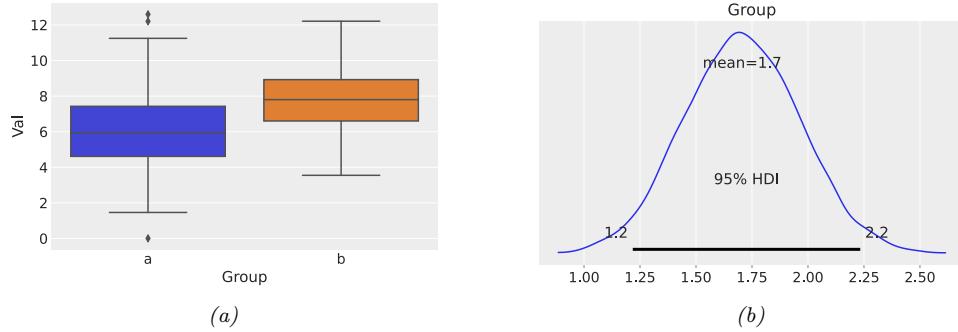
Figure 3.27: Illustration of Bayesian two-sample t-test. (a) Some synthetic data from two groups. (b) Posterior distribution of the di!erence, p(µ² ↓ µ1|D). Generated by ttest\_bambi.ipynb.

We use the same (data-driven) priors for µ^j and ε^j , and use a uniform prior for the correlation, p(ρ) = Unif(⇐1, 1), following [BMM00]. Once we have specified the model, we can perform posterior inference in the usual way, and compute quantities such as p(ρ > 0|D).

3.10.3 Common statistical tests correspond to inference in linear models

We have now seen many di!erent tests, and it may be unclear what test to use when. Fortunately, [Lin19] points out that many of the most common tests can be represented exactly (or approximately) in terms of inference (either Bayesian or frequentist) about the parameters of a generalized linear model or GLM (see Chapter 15 for details on GLMs). This approach is easier to understand and more flexible, as discussed at length in e.g., [Kru15; GHV20b]. We summarize some of these results in Table 3.2 and the discussion below.

3.10.3.1 Approximating nonparametric tests using the rank transform

It is common to use “nonparametric tests”, which generalize standard tests to settings where the data do not necessarily follow a Gaussian or Student distribution. A simple way to approximate such tests is to replace the original data with its order statistics, and then to apply a standard parametric test, as proposed in [CI81]. This gives a good approximation to the standard nonparametric tests for sample sizes of N ⇑ 10.

Concretely, we can compute a rank transform, in which the data points (assumed to be scalar) are sorted, and then replaced by their integer value in the ordering. For example, the rank transform of D = (3.6, 3.4, ⇐5.0, 8.2) is R(D) = (3, 2, 1, 4). Alternatively we may use the signed ranked, which first sorts the values according to their absolute size, and then attaches the corresponding sign. For example, the signed rank transform of D = (3.6, 3.4, ⇐5.0, 8.2) is SR(D) = (2, 1, ⇐3, 4).

We can now easily fit a parametric model, such as a GLM, to the rank-transformed data, as illustrated in Figure 3.28. (In [Doo+17], they propose a Bayesian interpretation of this, where the order statistics are viewed as observations of an underyling latent continuous quantity, on which inference is performed.) We will use this trick in the sections below.

Y	X	P/N	Name	Model	Exact
R	-	P	One-sample t-test	ε2) y ⇔ N (µ,	↫
R	-	N	Wilcoxon signed-ranked	ε2) SR(y) ⇔ N (µ,	N > 14
(R, R)	-	P	Paired-sample t-test	ε2) y2 ⇐ y1 ⇔ N (µ,	↫
(R, R)	-	N	Wilcoxon matched pairs	ε2) SR(y2 ⇐ y1) ⇔ N (µ,	↫
R	R	P	Pearson correlation	ε2) y ⇔ N (↼0 + ↼1x,	↫
R	R	N	Spearman correlation	ε2) R(y) ⇔ N (↼0 + ↼1R(x),	N > 10
R	{0, 1}	P	Two-sample t-test	ε2) y ⇔ N (↼0 + ↼1x,	↫
R	{0, 1}	P	Welch’s t-test	ε2 y ⇔ N (↼0 + ↼1x, x)	↫
R	{0, 1}	N	Mann-Whitney U	ε2 SR(y) ⇔ N (↼0 + ↼1x, x)	N > 11
R	[J]	P	One-way ANOVA	ε2) y ⇔ N (faov(x; ↼),	↫
R	[J]	N	Kruskal-Wallis	ε2) R(y) ⇔ N (faov(x; ↼),	N > 11
R	[J] ∞ [K]	N	Two-way ANOVA	ε2) y ⇔ N (faov2(x1, x2; ↼),	↫

Table 3.2: Many common statistical tests are equivalent to performing inference for the parameters of simple linear models. Here P/N represents parametric vs nonparametric test; we approximate the latter by using the rank function R(y) or the signed rank function SR(y). The last column, labeled “exact”, specifies the sample size for which this approximation becomes accurate enough to be indistinguishable from the exact result. When the input variable is categorical, x¹ ↗ [J], where [J] = {1,…,J}, we define the mean of the output using the analysis of variance function faov(x1, ϑ). When we have two categorical inputs, x¹ ↗ [J] and x² ↗ [K], we use faov2(x1, x2; ϑ). Adapted from the crib sheet at https: // lindeloev. github. io/ tests-as-linear/ .

3.10.3.2 Metric-predicted variable on one or two groups (t-test)

Suppose we have some data ^D = {y^{n ⇔ N} (µ, ^ε2) : ⁿ =1: ^N}, and we are interested in testing the null hypothesis that µ = 0. We can model this as a linear regression model with a constant input (bias term), and no covariates: ^p(yn|ω) = ^N (yn|↼0, ^ε2), where ↼^{0 = µ}. We can now perform inference on ↼⁰ in the usual way for GLMs, and then perform hypothesis testing. This is equivalent to the one sample t-test discussed in Section 3.10.2.6. For a nonparametric version, we can transform the data using the signed rank transform, thus fitting SR(yn) ^{⇔ N} (µ, ^ε2). The results are very close to the Wilcoxon signed-ranked test.

Now suppose we have paired data from two groups, D = {(y1n, y2n) : n =1: N}, where we assume ^yjn ^{⇔ N} (µ^j , ^ε2). We are interested in testing whether ^µ1 = ^µ2. A simpler alternative is to define ^yn = ^y2ⁿ ⇐ ^y1n, which we model using ^{yn ⇔ N} (µ, ^ε2). We can then test whether ^µ = 0 using the paired sample t-test, discussed in Section 3.10.2.6. Alternatively we can do inference on SR(yn), to get the Wilcoxon matched pairs test.

To handle the setting in which we have unpaired data from two groups, we can represent the data as D = {(xn, yn) : n =1: N}, where xⁿ ↑ {0, 1} represents whether the input belongs to group 0 or group 1. We assume the data comes from the following linear regression model: ^p(yn|xn) ^{⇔ N} (↼⁰ + ↼1xn, ^ε2). We can now perform inference on ↼ in the usual way for GLMs, and then perform hypothesis testing. This is equivalent to the two-sample t-test discussed in Section 3.10.2.8. In the nonparametric setting, we can replace y with its signed ranked transform and use the model SR(y) ^{⇔ N} (↼^{0 +} ↼1x, ^ε2). This is approximately the same as the Mann-Whitney U test.

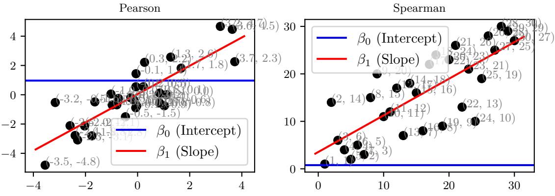
Figure 3.28: Illustration of 1d linear regression applied to some data (left) and its rank-transformed version (right). Generated by linreg\_rank\_stats.ipynb.

3.10.3.3 Metric-predicted variable with metric predictors (correlation test)

In this section, we assume the data has the form D = {(xn, yn) : n =1: N}, where xⁿ ↑ R and yⁿ ↑ R are correlated with Pearson correlation coe!cient of ρ. We are interested in testing the hypothesis that ρ = 0.

We can use a “bespoke” Bayesian approach as in Section 3.10.2.9. Alternatively, we can model this using simple linear regression, by writing ^{yn ⇔ N} (↼^{0 +} ↼1x, ^ε2). If we scale the output ^Y so it has a standard deviation of 1, then we find that ↼¹ = ρ, as shown in [Mur22, Sec 11.2.3.3]. Thus we can use p(↼1|D) to make inferences about ρ.

In the nonparametric setting, we compute the rank transform of x and y and then proceed as above. The Spearman rank correlation coe!cient is the Pearson correlation coe”cient on the rank-transformed data. While Pearson’s correlation is useful for assessing the strength of linear relationships, Spearman’s correlation can be used to assess general monotonic relationships, whether linear or not.

If we have multiple metric predictors (i.e., ^{xn ↑ RD}), we can use multiple linear regression instead of simple linear regression. We can then derive the posterior of the partial correlation coe”cient from the posterior of the regression weights.

3.10.3.4 Metric-predicted variable with one nominal predictor (one-way ANOVA)

In this section, we consider the setting in which we have some data D = {(xn, yn) : n =1: N}, where xⁿ ↑ {1,…,J} represents which group the input belongs. (Such a discrete categorical variable is often called a factor.) We assume the data comes from the following linear regression model: ^p(yn|x^{n = j}) ^{⇔ N} (µ^j , ^ε2). We are interested in testing the hypothesis that all the ^µj are the same. This is traditionally performed using a one-way ANOVA test, where ANOVA stands for “analysis of variance”. To derive a nonparametric test, we can first apply a rank transformation to y. This is similar to the Kruskal-Wallis test.

ANOVA assumes that the data are normally distributed, with a common (shared) variance, so that the sampling distribution of the F-statistic can be derived. We can write the corresponding

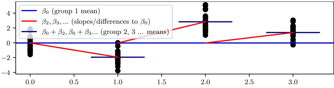
Figure 3.29: Illustration of one-way ANOVA with 4 groups. We are interested in testing whether the red lines have a slope of 0, meaning that all the groups have the same mean. Generated by anova.ipynb.

model as a linear regression model, by using a dummy encoding of xn, where xn[j] = I(xⁿ = j). To avoid overparameterization (which can make the posterior unidentifiable), we drop the first level (this is known as reduced rank encoding). We can then write the model as

\[p(y\_n|x\_n; \theta) \sim \mathcal{N}(f\_{\text{uav}}(x\_n, \beta), \sigma^2) \tag{3.334}\]

where we define the predicted mean using the ANOVA formula:

\[f\_{\rm aov}(x,\beta) = \beta\_0 + \beta\_2 x\_{[2]} + \dots + \beta\_J x\_{[J]} \tag{3.335}\]

We see that ↼⁰ is the overall mean, and also corresponds to the value that will be used for level 1 of the factor (i.e., if xⁿ = 1). The other ↼^j terms represents deviations away from level 1. The null hpothesis corresponds to the assumption that ↼^j = 0 for all j =2: J.

A more symmetric formulation of the model is to write

\[f\_{\rm aov}(x;\beta) = \beta\_0 + \beta\_1 x\_{[1]} + \beta\_2 x\_{[2]} + \dots + \beta\_J x\_{[J]} \tag{3.336}\]

where ↼⁰ is the grand mean, and where we impose the constraint that #^{J j}=1 ↼^j = 0. In this case we can interpret each ↼^j as the amount that group j deviates from the shared baseline ↼0. To satisfy this constraint, we can write the predicted mean as

\[f\_{\text{aov}}(\mathbf{z}, \vec{\beta}) = \vec{\beta}\_0 + \sum\_{j=1}^{J} \vec{\beta}\_j x\_{[j]} = \underbrace{(\vec{\beta}\_0 + \vec{\beta})}\_{\beta\_0} + \sum\_{j=1}^{J} \underbrace{(\vec{\beta}\_j - \vec{\beta})}\_{\beta\_j} x\_{[j]} \tag{3.337}\]

where ↼˜^j are the unconstrained parameters, and ↼ = ¹ J #^{J j}=1 ↼˜^j . This construction satisfies the constraint, since

\[\sum\_{j=1}^{J} \beta\_j = \sum\_{j=1}^{J} \overline{\beta}\_j - \sum\_{j=1}^{J} \overline{\beta} = J\overline{\beta} - J\overline{\beta} = 0 \tag{3.338}\]

In traditional ANOVA, we assume that the data are normally distributed, with a common (shared) variance. In a Bayesian setting, we are free to relax these assumptions. For example, we can use a di!erent likelihood (e.g., Student) and we can allow each group to have its own variance, ε^{2 j} , which can be reliably estimated using a hierarchical Bayesian model (see Section 3.6).

	LH	RH
Male	9	43	N1 = 52
Female	4	44	N2 = 48
Totals	13	87	100

Table 3.3: A 2 ↘ 2 contingency table from http: // en. wikipedia. org/ wiki/ Contingency\_ table .

3.10.3.5 Metric-predicted variable with multiple nominal predictors (multi-way ANOVA)

In this section, we consider the setting in which we have G nominal predictors as input. To simplify notation, we assume we just have G = 2 groups. We assume the mean of y is given by

\[f\_{\rm av2}(x) = \mu + \sum\_{j} \alpha\_j x\_{1,[j]} + \sum\_{k} \beta\_k x\_{2,[k]} + \sum\_{jk} \gamma\_{jk} x\_{1,[j]} x\_{2,[k]} \tag{3.339}\]

where we impose the following sum-to-zero contraints

\[ \sum\_{j} \alpha\_{j} = \sum\_{k} \beta\_{k} = \sum\_{j} \gamma\_{jk} = \sum\_{k} \gamma\_{jk} = 0\tag{3.340} \]

We are interested in testing whether γ = 0, meaning there is no interaction e!ect. This is traditionally done using a two-way ANOVA test. However, we can also use a Bayesian approach and just compute p(ω|D).

3.10.3.6 Count predicted variable with nominal predictors (χ² test)

Consider a situation in which we observed two nominal values for each item measured. For example, the gender of a person (male or female) and whether they are left handed or right handed (LH or RH). If we count the number of outcomes of each type, we can represent the data as a R ∞ C contingency table. See Table 3.3 for an example. We may be interested in testing the null hypothesis that there is no interaction e!ect between the two groups and the outcome (i.e., the two variables are independent). In frequentist statistics, this is often tackled using a ↽²-test, which uses the sampling distribution of the ↽² test statistic, defined as

\[\chi^2 = \sum\_{r=1}^{R} \sum\_{c=1}^{C} \frac{(O\_{r,c} - E\_{r,c})^2}{E\_{r,c}} \tag{3.341}\]

where r indexes the rows, and c the columns, Or,c is the observed count in cell (r, c), and Erc = N pr.p.c is the expected count, where pr. = Oc./N and p.c = O.r/N are the empirical marginal frequencies.

In the Bayesian approach, we can just modify the two-way ANOVA of Section 3.10.3.5, and replace the Gaussian distribution with a Poisson distribution. We also need to pass the predicted natural parameter through an exponential link, since a Poisson distribution requires that the rate parameter is non-negative. Thus the model becomes

\[p(y|x=(r,c),\theta) = \text{Poi}(y|\lambda\_{r,c})\tag{3.342}\]

\[ \lambda\_{rc} = \exp(\beta\_0 + \beta\_r + \beta\_c + \beta\_{r,c}) \tag{3.343} \]

We can now perform posterior inference in the usual way.

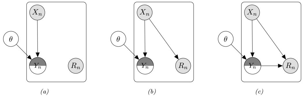
Figure 3.30: Graphical models to represent di!erent patterns of missing data for conditional (discriminative) models. (a) Missing completely at random. (b) Missing at random. (c) Missing not at random. The semi-shaded yⁿ node is observed if rⁿ = 1 and is hidden otherwise. Adapted from Figure 2 of [SG02].

3.10.3.7 Non-metric predicted variables

If the output variable is categorical, yⁿ ↑ {1,…,C}, we can use logistic regression instead of linear regression (see e.g., Section 15.3.9). If the output is ordinal, we can use ordinal regression. If the output is a count variable, we can use Poisson regression. And so on. For more details on GLMs, see Chapter 15.

3.11 Missing data

Sometimes we may have missing data, in which parts of the data vector ^{Xn ↑ RD} may be unknown. (If we have a supervised problem, we append the labels to the feature vector.) We let Xn,mis represent the missing parts, and Xn,obs represent the observed parts. Since the reasons that data are missing may be informative (e.g., declining to answer a survey question such as “Do you have disease X?” may be an indication that the subject does in fact have it), we need to model the missing data mechanism. To do this, we introduce a random variable Rn, to represent which parts of Xⁿ are “revealed” (observed) or not. Specifically, we set Rn,obs = 1 for those indices (components) for which Xⁿ is observed, and set Rn,mis = 0 for the other indices.

There are di!erent kinds of assumptions we can make about the missing data mechanism, as discussed in [Rub76; LR87]. The strongest assumption is to assume the data is missing completely at random or MCAR. This means that p(Rn|Xn) = p(Rn), so the missingness does not depend on the hidden or observed features. A more realistic assumption is known as missing at random or MAR. This means that p(Rn|Xn) = p(Rn|Xn,obs), so the missingness does not depend on the hidden features, but may depend on the visible features. If neither of these assumptions hold, we say the data is missing not at random or MNAR.

Now consider the case of conditional, or discriminative models, in which we model the outcome yⁿ given observed inputs xⁿ using a model of the form p(yn|xn, ω). Since we are conditioning on xn, we assume it is always observed. However, the output labels may or may not be observed, depending on the value of rn. For example, in semi-supervised learning, we have a combination of labeled data, ^{DL =} {(xn, ^yn)}, and unlabeled data, ^{DU =} {(xn)} [CSZ06].

The 3 missing data scenarios for the discriminative setting are shown in Figure 3.30, using graphical model notation (see [MPT13] for details). In the MCAR and MAR cases, we see that we can just ignore the unlabeled data with missing outputs, since the unknown model parameters ω are una!ected by yⁿ if it is a hidden leaf node. However, in the MNAR case, we see that ω depends on yn, even it is hidden, since the value of yⁿ is assumed to a!ect the probability of rn, which is always observed. In such cases, to fit the model, we need to impute the missing values, using methods discussed in Section 20.3.3.

Now consider the case where we use a joint or generative model of the form p(x, y) = p(y)p(x|y), instead of a discriminative model of the form p(y|x). 14 In this case, the unlabeled data can be useful for learning even in the MCAR and MAR scenarios, since ω now depends on both x and y. In particular, information about p(x) can be informative about p(y|x). See e.g., [CSZ06] for details.

^14. In [Sch+12a], they call a model of the form p(y|x) a “causal classifier”, since the features cause the labels, and a model of the form p(x|y) an “anti-causal classifier”, since the features are caused by the labels.

^&quot;Probabilistic Machine Learning: Advanced Topics”. Online version. April 18, 2025

4 Graphical models

4.1 Introduction

I basically know of two principles for treating complicated systems in simple ways: the first is the principle of modularity and the second is the principle of abstraction. I am an apologist for computational probability in machine learning because I believe that probability theory implements these two principles in deep and intriguing ways — namely through factorization and through averaging. Exploiting these two mechanisms as fully as possible seems to me to be the way forward in machine learning. — Michael Jordan, 1997 (quoted in [Fre98]).

Probabilistic graphical models (PGMs) provide a convenient formalism for defining joint distributions on sets of random variables. In such graphs, the nodes represent random variables, and the (lack of) edges represent conditional independence (CI) assumptions between these variables. A better name for these models would be “independence diagrams”, but the term “graphical models” is now entrenched.

There are several kinds of graphical model, depending on whether the graph is directed, undirected, or some combination of directed and undirected, as we discuss in the sections below. More details on graphical models can be found in e.g., [KF09a].

4.2 Directed graphical models (Bayes nets)

In this section, we discuss directed probabilistic graphical models, or DPGM, which are based on directed acyclic graphs or DAGs (graphs that do not have any directed cycles). PGMs based on a DAG are often called Bayesian networks or Bayes nets for short; however, there is nothing inherently “Bayesian” about Bayesian networks: they are just a way of defining probability distributions. They are also sometimes called belief networks. The term “belief” here refers to subjective probability. However, the probabilities used in these models are no more (and no less) subjective than in any other kind of probabilistic model.

4.2.1 Representing the joint distribution

The key property of a DAG is that the nodes can be ordered such that parents come before children. This is called a topological ordering. Given such an order, we define the ordered Markov property to be the assumption that a node is conditionally independent of all its predecessors in

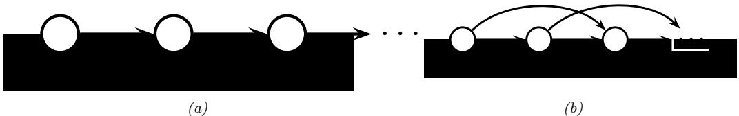
Figure 4.1: Illustration of first and second order Markov models.

the ordering given its parents, i.e.,

\[\begin{array}{l} x\_i \perp \mathbf{z}\_{\text{pred}(i)} \boldsymbol{\upmu}(i) \boldsymbol{\upmu}(i) \, \middle| \, \mathbf{z}\_{\text{pa}(i)} \end{array} \tag{4.1}\]

where pa(i) are the parents of node i, and pred(i) are the predecessors of node i in the ordering. Consequently, we can represent the joint distribution as follows (assuming we use node ordering 1 : NG):

\[p(\mathbf{z}\_{1:N\_G}) = p(x\_1)p(x\_2|x\_1)p(x\_3|x\_1, x\_2)\dots p(x\_{N\_G}|x\_1,\dots,x\_{N\_G-1}) = \prod\_{i=1}^{N\_G} p(x\_i|\mathbf{z}\_{\text{pa}(i)})\tag{4.2}\]

where p(xi|xpa(i)) is the conditional probability distribution or CPD for node i. (The parameters of this distribution are omitted from the notation for brevity.)

The key advantage of the representation used in Equation (4.2) is that the number of parameters used to specify the joint distribution is substantially less, by virtue of the conditional independence assumptions that we have encoded in the graph, than an unstructured joint distribution. To see this, suppose all the variables are discrete and have K states each. Then an unstructured joint distribution needs O(K^NG ) parameters to specify the probability of every configuration. By contrast, with a DAG in which each node has at most N^P parents, we only need O(NGK^NP +1) parameters, which can be exponentially fewer if the DAG is sparse.

We give some examples of DPGM’s in Section 4.2.2, and in Section 4.2.4, we discuss how to read o! other conditional independence properties from the graph.

4.2.2 Examples

In this section, we give several examples of models that can be usefully represented as DPGM’s.

4.2.2.1 Markov chains

We can represent the conditional independence assumptions of a first-order Markov model using the chain-structured DPGM shown in Figure 4.1(a). Consider a variable at a single time step t, which we call the “present”. From the diagram, we see that information cannot flow from the past, x1:t↑1, to the future, xt+1:^T , except via the present, xt. (We formalize this in Section 4.2.4.) This means that the x^t is a su”cient statistic for the past, so the model is first-order Markov. This implies that the corresponding joint distribution can be written as follows:

\[p(\mathbf{z}\_{1:T}) = p(x\_1)p(x\_2|x\_1)p(x\_3|x\_2)\cdots p(x\_T|x\_{T-1}) = p(x\_1)\prod\_{t=2}^{T}p(x\_t|\mathbf{z}\_{1:t-1})\tag{4.3}\]

For discrete random variables, we can represent corresponding CPDs, p(x^t = k|xt↑¹ = j), as a 2d table, known as a conditional probability table or CPT, p(x^t = k|xt↑¹ = j) = ϑjk, where ⁰ ↗ ^ϑjk ↗ ¹ and #^{K k}=1 ϑjk = 1 (i.e., each row sums to 1).

The first-order Markov assumption is quite restrictive. If we want to allow for dependencies two steps into the past, we can create a Markov model of order 2. This is shown in Figure 4.1(b). The corresponding joint distribution has the form

\[p(\mathbf{z}\_{1:T}) = p(x\_1, x\_2)p(x\_3|x\_1, x\_2)p(x\_4|x\_2, x\_3) \cdots p(x\_T|x\_{T-2}, x\_{T-1}) = p(x\_1, x\_2) \prod\_{t=3}^T p(x\_t|x\_{t-2:t-1}) \tag{4.4}\]

As we increase the order of the Markov model, we need to add more edges. In the limit, the DAG becomes fully connected (subject to being acyclic), as shown in Figure 22.1. However, in this case, there are no useful conditional independencies, so the graphical model has no value.

4.2.2.2 The “student” network

Figure 4.2 shows a model for capturing the inter dependencies between 5 discrete random variables related to a hypothetical student taking a class: D = di”culty of class (easy, hard), I = intelligence (low, high), G = grade (A, B, C), S = SAT score (bad, good), L = letter of recommendation (bad, good). (This is a simplification of the “student network” from [KF09a, p.281].) The chain rule tells us that we can represent the joint as follows:

\[p(D, I, G, L, S) = p(L|S, G, D, I) \times p(S|G, D, I) \times p(G|D, I) \times p(D|I) \times p(I) \tag{4.5}\]

where we have ordered the nodes topologically as I, D, G, S, L. Note that L is conditionally independent of all the other nodes earlier in this ordering given its parent G, so we can replace p(L|S, G, D, I) by p(L|G). We can simplify the other terms in a similar way to get

\[p(D, I, G, L, S) = p(L|G) \times p(S|I) \times p(G|D, I) \times p(D) \times p(I) \tag{4.6}\]

The ability to simplify a joint distribution in a product of small local pieces is the key idea behind graphical models.

In addition to the graph structure, we need to specify the conditional probability distributions (CPDs) at each node. For discrete random variables, we can represent the CPD as a table, which means we have a separate row (i.e., a separate categorical distribution) for each conditioning case, i.e., for each combination of parent values. We can represent the i’th CPT as follows:

\[\theta\_{ijk} \triangleq p(x\_i = k | \mathbf{x}\_{\text{pa}(i)} = j) \tag{4.7}\]

The matrix ωi,:,: is a row stochastic matrix, that satisfies the properties 0 ↗ ϑijk ↗ 1 and #^{Ki k}=1 ϑijk = 1 for each row j. Here i indexes nodes, i ↑ [NG]; k indexes node states, k ↑ [Ki], where Kⁱ is the number of states for node i; and j indexes joint parent states, j ↑ [Ji], where Jⁱ = ^p≃pa(i) ^Kp.

The CPTs for the student network are shown next to each node in Figure 4.2. For example, we see that if the class is hard (D = 1) and the student has low intelligence (I = 0), the distribution over grades A, B, and C we expect is p(G|D = 1, I = 0) = [0.05, 0.25, 0.7]; but if the student is intelligent, we get p(G|D = 1, I = 1) = [0.5, 0.3, 0.2].

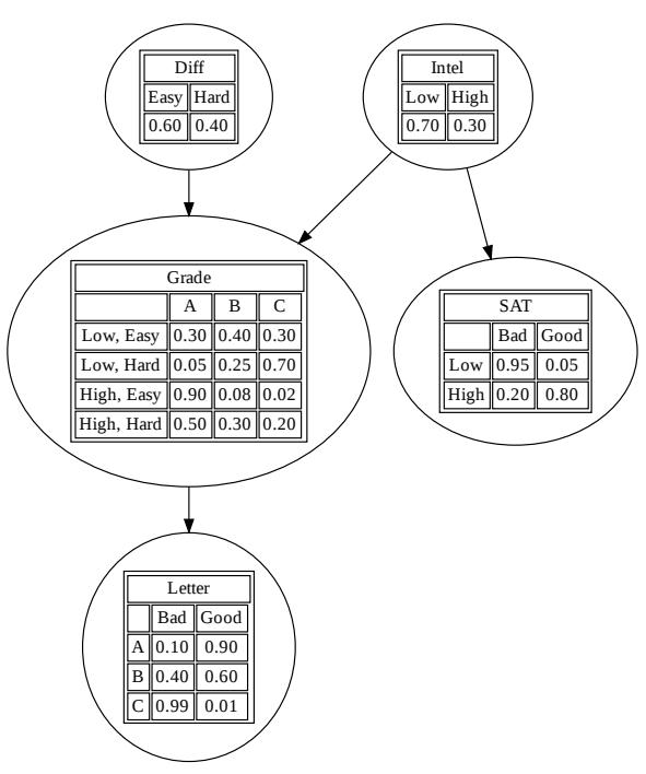
Figure 4.2: The (simplified) student network. “Di!” is the di”culty of the class. “Intel” is the intelligence of the student. “Grade” is the grade of the student in this class. “SAT” is the score of the student on the SAT exam. “Letter” is whether the teacher writes a good or bad letter of recommendation. The circles (nodes) represent random variables, the edges represent direct probabilistic dependencies. The tables inside each node represent the conditional probability distribution of the node given its parents. Generated by student\_pgm.ipynb.

The number of parameters in a CPT is O(K^p+1), where K is the number of states per node, and p is the number of parents. Later we will consider more parsimonious representations, with fewer learnable parameters. (We discuss parameter learning in Section 4.2.7.)

Once we have specified the model, we can use it to answer probabilistic queries, as we discuss in Section 4.2.6. As an example, suppose we observe that the student gets a grade of C. The posterior probability that the student is intelligent is just p(I = High|G = C)=0.08, as shown in Figure 4.8. However, now suppose we also observe that the student gets a good SAT score. Now the posterior probability that the student is intelligent has jumped to p(I = High|G = C, S = Good)=0.58, since we can explain the C grade by inferring it was a di”cult class (indeed, we find p(D = Hard|G = C, S = Good)=0.76). This negative mutual interaction between multiple causes of some observations is called the explaining away e!ect, also known as Berkson’s paradox (see Section 4.2.4.2 for details).

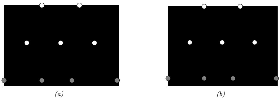
Figure 4.3: (a) Hierarchical latent variable model with 2 layers. (b) Same as (a) but with autoregressive connections within each layer. The observed x variables are the shaded leaf nodes at the bottom. The unshaded nodes are the hidden z variables.

4.2.2.3 Sigmoid belief nets

In this section, we consider a deep generative model of the form shown in Figure 4.3a. This corresponds to the following joint distribution:

\[p(\mathbf{z}, \mathbf{z}) = p(\mathbf{z}\_2) p(\mathbf{z}\_1 | \mathbf{z}\_2) p(\mathbf{z} | \mathbf{z}\_1) = \prod\_{k=1}^{K\_2} p(z\_{2,k}) \prod\_{k=1}^{K\_1} p(z\_{1,k} | \mathbf{z}\_2) \prod\_{d=1}^{D} p(x\_d | \mathbf{z}\_1) \tag{4.8}\]

where x denotes the visible leaf nodes, and z↽ denotes the hidden internal nodes. (We assume there are K↽ hidden nodes at level ⇁, and D visible leaf nodes.)

Now consider the special case where all the latent variables are binary, and all the latent CPDs are logistic regression models. That is,

\[p(\mathbf{z}\_{\ell}|\mathbf{z}\_{\ell+1},\boldsymbol{\theta}) = \prod\_{k=1}^{K\_{\ell}} \text{Ber}(z\_{\ell,k}|\sigma(\mathbf{w}\_{\ell,k}^{\top}\mathbf{z}\_{\ell+1})) \tag{4.9}\]

where ε(u)=1/(1 + e↑^u) is the sigmoid (logistic) function. The result is called a sigmoid belief net [Nea92].

At the bottom layer, p(x|z1, ω), we use whatever observation model is appropriate for the type of data we are dealing with. For example, for real valued data, we might use

\[p(\mathbf{z}|\mathbf{z}\_1, \boldsymbol{\theta}) = \prod\_{d=1}^{D} \mathcal{N}(x\_d | \mathbf{w}\_{1,d,\mu}^{\mathsf{T}} \mathbf{z}\_1, \exp(\mathbf{w}\_{1,d,\sigma}^{\mathsf{T}} \mathbf{z}\_1)) \tag{4.10}\]

where w1,d,µ are the weights that control the mean of the d’th output, and w1,d,^ϱ are the weights that control the variance of the d’th output.

We can also add directed connections between the hidden variables within a layer, as shown in Figure 4.3b. This is called a deep autoregressive network or DARN model [Gre+14], which combines ideas from latent variable modeling and autoregressive modeling.

We discuss other forms of hierarchical generative models in Chapter 21.

4.2.3 Gaussian Bayes nets

Consider a DPGM where all the variables are real-valued, and all the CPDs have the following form, known as a linear Gaussian CPD:

\[p(x\_i | \mathbf{x}\_{\rm pa(i)}) = \mathcal{N}(x\_i | \mu\_i + w\_i^{\rm T} \mathbf{z}\_{\rm pa(i)}, \sigma\_i^2) \tag{4.11}\]

As we show below, multiplying all these CPDs together results in a large joint Gaussian distribution of the form ^p(x) = ^N (x|µ, !), where ^{x ↑ RNG} . This is called a directed Gaussian graphical model or a Gaussian Bayes net.

We now explain how to derive µ and !, following [SK89, App. B]. For convenience, we rewrite the CPDs in the following form:

\[x\_i = \mu\_i + \sum\_{j \in \text{pa}(i)} w\_{i,j} (x\_j - \mu\_j) + \sigma\_i z\_i \tag{4.12}\]

where zⁱ ⇔ N (0, 1), εⁱ is the conditional standard deviation of xⁱ given its parents, wi,j is the strength of the ^{j → i} edge, and ^µi is the local mean.1

It is easy to see that the global mean is just the concatenation of the local means, µ = (µ1,…,µ^NG ). We now derive the global covariance, !. Let S ↭ diag(↽) be a diagonal matrix containing the standard deviations. We can rewrite Equation (4.12) in matrix-vector form as follows:

\[\mathbf{w}(x-\mu) = \mathbf{W}(x-\mu) + \mathbf{S}z \tag{4.13}\]

where W is the matrix of regression weights. Now let e be a vector of noise terms: e ↭ Sz. We can rearrange this to get e = (I ⇐ W)(x ⇐ µ). Since W is lower triangular (because wj,i = 0 if j<i in the topological ordering), we have that I ⇐ W is lower triangular with 1s on the diagonal. Hence

\[ \begin{pmatrix} e\_1 \\ e\_2 \\ \vdots \\ e\_{N\_G} \end{pmatrix} = \begin{pmatrix} 1 \\ -w\_{2,1} & 1 \\ -w\_{3,2} & -w\_{3,1} & 1 \\ \vdots & & \ddots \\ -w\_{N\_G,1} & -w\_{N\_G,2} & \dots & -w\_{N\_G,N\_G-1} & 1 \end{pmatrix} \begin{pmatrix} x\_1 - \mu\_1 \\ x\_2 - \mu\_2 \\ \vdots \\ x\_{N\_G} - \mu\_{N\_G} \end{pmatrix} \tag{4.14} \]

Since I ⇐ W is always invertible, we can write

\[\mathbf{z} - \mu = (\mathbf{I} - \mathbf{W})^{-1} \mathbf{e} \stackrel{\Delta}{=} \mathbf{U} \mathbf{e} = \mathbf{U} \mathbf{S} \mathbf{z} \tag{4.15}\]

where we defined ^U = (^I ⇐ ^W)↑¹. Hence the covariance is given by

\[\mathbf{U}\cdot\mathbf{\Sigma}=\text{Cov}\begin{bmatrix}\mathbf{z}\end{bmatrix}=\text{Cov}\begin{bmatrix}\mathbf{z}-\boldsymbol{\mu}\end{bmatrix}=\text{Cov}\begin{bmatrix}\mathbf{U}\mathbf{S}\mathbf{z}\end{bmatrix}=\mathbf{U}\mathbf{S}\begin{bmatrix}\mathbf{z}\end{bmatrix}\cdot\mathbf{S}\mathbf{U}^{\mathsf{T}}=\mathbf{U}\mathbf{S}^{2}\mathbf{U}^{\mathsf{T}}\tag{4.16}\]

since Cov [z] = I.

^1. If we do not subtract o! the parent’s mean (i.e., if we use xⁱ = µⁱ + ! ^j↑pa(i) ^wi,jx^{j + φ}izi), the derivation of ! is much messier, as can be seen by looking at [Bis06, p370].

4.2.4 Conditional independence properties

We write x^A ℜ^G xB|x^C if A is conditionally independent of B given C in the graph G. (We discuss how to determine whether such a CI property is implied by a given graph in the sections below.) Let I(G) be the set of all such CI statements encoded by the graph, and I(p) be the set of all such CI statements that hold true in some distribution p. We say that G is an I-map (independence map) for p, or that p is Markov wrt G, i! I(G) ↓ I(p). In other words, the graph is an I-map if it does not make any assertions of CI that are not true of the distribution. This allows us to use the graph as a safe proxy for p when reasoning about p’s CI properties. This is helpful for designing algorithms that work for large classes of distributions, regardless of their specific numerical parameters. Note that the fully connected graph is an I-map of all distributions, since it makes no CI assertions at all, as we show below. We therefore say G is a minimal I-map of p if G is an I-map of p, and if there is no G^↔︎ ↓ G which is an I-map of p.

We now turn to the question of how to derive I(G), i.e., which CI properties are entailed by a DAG.

4.2.4.1 Global Markov properties (d-separation)

We say an undirected path P is d-separated by a set of nodes C (containing the evidence) i! at least one of the following conditions hold:

• 1. P contains a chain or pipe, s → m → t or s ∈ m ∈ t, where m ↑ C
• 2. P contains a tent or fork, ^{s ℑm⊤ t}, where ^{m ↑ C}
• 3. P contains a collider or v-structure, s ⊤mℑ t, where m is not in C and neither is any descendant of m.

Next, we say that a set of nodes A is d-separated from a di!erent set of nodes B given a third observed set C i! each undirected path from every node a ↑ A to every node b ↑ B is d-separated by C. Finally, we define the CI properties of a DAG as follows:

\[\mathbf{X}\_A \perp\_G \mathbf{X}\_B | \mathbf{X}\_C \iff \text{A is d-separated from B given C} \tag{4.17}\]

This is called the (directed) global Markov property.

The Bayes ball algorithm [Sha98] is a simple way to see if A is d-separated from B given C, based on the above definition. The idea is this. We “shade” all nodes in C, indicating that they are observed. We then place “balls” at each node in A, let them “bounce around” according to some rules, and then ask if any of the balls reach any of the nodes in B. The three main rules are shown in Figure 4.4. Notice that balls can travel opposite to edge directions. We see that a ball can pass through a chain, but not if it is shaded in the middle. Similarly, a ball can pass through a fork, but not if it is shaded in the middle. However, a ball cannot pass through a v-structure, unless it is shaded in the middle.

We can justify the 3 rules of Bayes ball as follows. First consider a chain structure X → Y → Z, which encodes

\[p(x,y,z) = p(x)p(y|x)p(z|y) \tag{4.18}\]

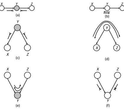
Figure 4.4: Bayes ball rules. A shaded node is one we condition on. If there is an arrow hitting a bar, it means the ball cannot pass through; otherwise the ball can pass through.

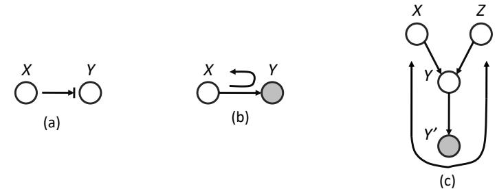
Figure 4.5: (a-b) Bayes ball boundary conditions. (c) Example of why we need boundary conditions. Y ^↓ is an observed child of Y , rendering Y “e!ectively observed”, so the ball bounces back up on its way from X to Z.

When we condition on y, are x and z independent? We have

\[p(x,z|y) = \frac{p(x,y)}{p(y)} = \frac{p(x)p(y|x)p(z|y)}{p(y)} = \frac{p(x,y)p(z|y)}{p(y)} = p(x|y)p(z|y) \tag{4.19}\]

and therefore X ℜ Z | Y . So observing the middle node of chain breaks it in two (as in a Markov chain).

Now consider the tent structure X ∈ Y → Z. The joint is

\[p(x,y,z) = p(y)p(x|y)p(z|y) \tag{4.20}\]

When we condition on y, are x and z independent? We have

\[p(x,z|y) = \frac{p(x,y,z)}{p(y)} = \frac{p(y)p(x|y)p(z|y)}{p(y)} = p(x|y)p(z|y) \tag{4.21}\]

and therefore X ℜ Z | Y . So observing a root node separates its children (as in a naive Bayes classifier: see Section 4.2.8.2).

X	Y	Z
D	I
D	I	S
D	S
D	S	I
D	S	L, I
D	S	G, I
D	S	G, L, I
D	L	G
D	L	G, S
D	L	G, I
D	L	I, G, S

Table 4.1: Conditional independence relationships implied by the student DAG (Figure 4.2). Each line has the form X ≃ Y |Z. Generated by student\_pgm.ipynb.

Finally consider a v-structure X → Y ∈ Z. The joint is

\[p(x,y,z) = p(x)p(z)p(y|x,z) \tag{4.22}\]

When we condition on y, are x and z independent? We have

\[p(x,z|y) = \frac{p(x)p(z)p(y|x,z)}{p(y)}\tag{4.23}\]

so X ⇓ℜ Z|Y . However, in the unconditional distribution, we have

\[p(x,z) = p(x)p(z) \tag{4.24}\]

so we see that X and Z are marginally independent. So we see that conditioning on a common child at the bottom of a v-structure makes its parents become dependent. This important e!ect is called explaining away, inter-causal reasoning, or Berkson’s paradox (see Section 4.2.4.2 for a discussion).

Finally, Bayes ball also needs the “boundary conditions” shown in Figure 4.5(a-b). These rules say that a ball hitting a hidden leaf stops, but a ball hitting an observed leaf “bounces back”. To understand where this rule comes from, consider Figure 4.5(c). Suppose Y ^↔︎ is a (possibly noisy) copy of Y . If we observe Y ^↔︎ , we e!ectively observe Y as well, so the parents X and Z have to compete to explain this. So if we send a ball down X → Y → Y ^↔︎ , it should “bounce back” up along Y ^↔︎ → Y → Z, in order to pass information between the parents. However, if Y and all its children are hidden, the ball does not bounce back.

As an example of the CI statements encoded by a DAG, Table 4.1 shows some properties that follow from the student network in Figure 4.2.

4.2.4.2 Explaining away (Berkson’s paradox)

In this section, we give some examples of the explaining away phenomenon, also called Berkson’s paradox.

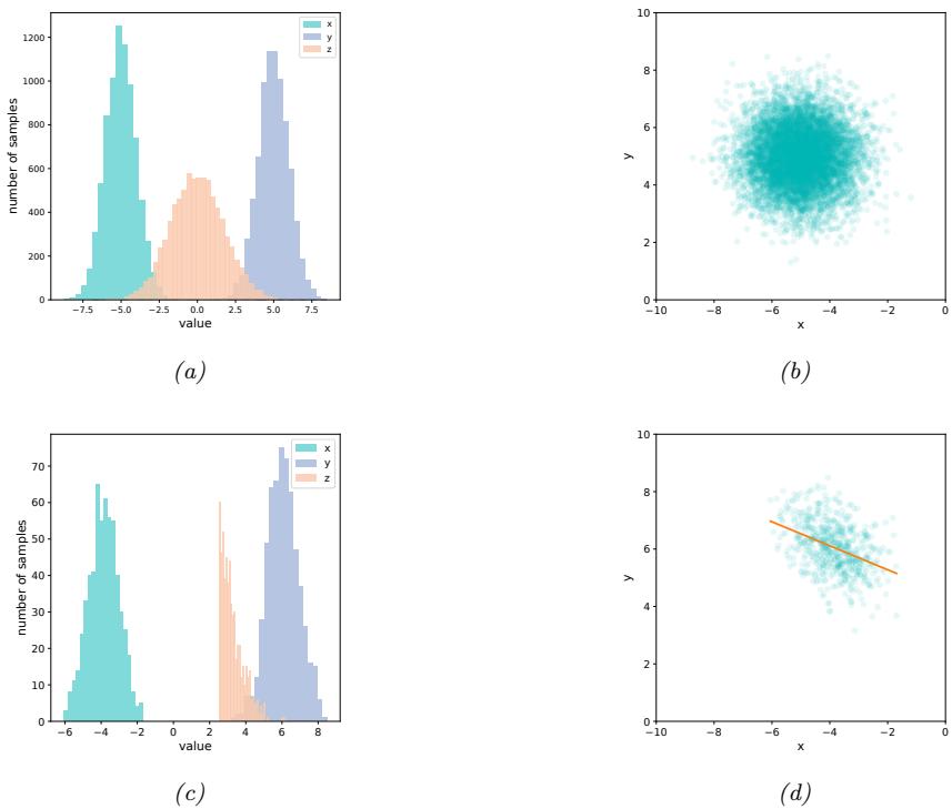
Figure 4.6: Samples from a jointly Gaussian DPGM, p(x, y, z) = N (x| ↓ 5, 1)N (y|5, 1)N (z|x + y, 1). (a) Unconditional marginal distributions, p(x), p(y), p(z). (b) Unconditional joint distribution, p(x, y). (c) Conditional marginal distribution, p(x|z > 2.5), p(y|z > 2.5), p(z|z > 2.5). (d) Conditional joint distribution, p(x, y|z > 2.5). Adapted from [Clo20]. Generated by berksons\_gaussian.ipynb.

As a simple example (from [PM18b, p198]), consider tossing two coins 100 times. Suppose you only record the outcome of the experiment if at least one coin shows up heads. You should expect to record about 75 entries. You will see that every time coin 1 is recorded as tails, coin 2 will be recorded as heads. If we ignore the way in which the data was collected, we might infer from the fact that coins 1 and 2 are correlated that there is a hidden common cause. However, the correct explanation is that the correlation is due to conditioning on a hidden common e!ect (namely the decision of whether to record the outcome or not, so we can censor tail-tail events). This is called selection bias.

As another example of this, consider a Gaussian DPGM of the form

\[p(x,y,z) = N(x|-5,1)N(y|5,1)N(z|x+y,1)\tag{4.25}\]

The graph structure is X → Z ∈ Y , where Z is the child node. Some samples from the unconditional joint distribution p(x, y, z) are shown in Figure 4.6(a); we see that X and Y are uncorrelated. Now suppose we only select samples where z > 2.5. Some samples from the conditional joint distribution

p(x, y|z > 2.5) are shown in Figure 4.6(d); we see that now X and Y are correlated. This could cause us to erroneously conclude that there is a causal relationship, but in fact the dependency is caused by selection bias.

4.2.4.3 Markov blankets

The smallest set of nodes that renders a node i conditionally independent of all the other nodes in the graph is called i’s Markov blanket; we will denote this by mb(i). Below we show that the Markov blanket of a node in a DPGM is equal to the parents, the children, and the co-parents, i.e., other nodes who are also parents of its children:

\[\text{mbi}(i) \stackrel{\alpha}{=} \text{ch}(i) \cup \text{pa}(i) \cup \text{copa}(i) \tag{4.26}\]

See Figure 4.7 for an illustration.

To see why this is true, let us partition all the nodes into the target node Xi, its parents U, its children Y , its coparents Z, and the other variables O. Let X↑ⁱ be all the nodes except Xi. Then we have

\[p(X\_i|X\_{-i}) = \frac{p(X\_i, X\_{-i})}{\sum\_{x} p(X\_i = x, X\_{-i})} \tag{4.27}\]

\[=\frac{p(X\_i, U, Y, Z, O)}{\sum\_{x} p(X\_i = x, U, Y, Z, O)}\tag{4.28}\]

\[=\frac{p(X\_i|U)[\prod\_j p(Y\_j|X\_i, Z\_j)]P(U, Z, O)}{\sum\_{v} n(X\_i - x|U)[\prod\_j v(Y\_j|X\_i - x|Z\_j)]P(U, Z, O)}\tag{4.29}\]

\[=\frac{\sum\_{x}p(X\_{i}=x|U)[\prod\_{j}p(Y\_{j}|X\_{i}=x,Z\_{j})]P(U,Z,O)}{\sum\_{x}p(X\_{i}=x|U)[\prod\_{j}p(Y\_{j}|X\_{i}=x,Z\_{j})]P(U,Z,O)}\tag{4.29}\]

\[=\frac{p(X\_i|U)[\prod\_j p(Y\_j|X\_i, Z\_j)]}{\sum\_x p(X\_i = x|U)[\prod\_j p(Y\_j|X\_i = x, Z\_j)]}\tag{4.30}\]

\[\propto p(X\_i|\text{pa}(X\_i)) \prod\_{Y\_j \in \text{ch}(X\_i)} p(Y\_j|\text{pa}(Y\_j))\tag{4.31}\]

where ch(Xi) are the children of Xⁱ and pa(Y^j ) are the parents of Y^j . We see that the terms that do not involve Xⁱ cancel out from the numerator and denominator, so we are left with a product of terms that include Xⁱ in their “scope”. Hence the full conditional for node i becomes

\[p(x\_i|\mathbf{x}\_{-i}) = p(x\_i|\mathbf{x}\_{\text{mb}(i)}) \propto p(x\_i|\mathbf{x}\_{\text{pa}(i)}) \prod\_{k \in \text{ch}(i)} p(x\_k|\mathbf{x}\_{\text{pa}(k)}) \tag{4.32}\]

We will see applications of this in Gibbs sampling (Equation (12.19)), and mean field variational inference (Equation (10.87)).

4.2.4.4 Other Markov properties

From the d-separation criterion, one can conclude that

\[(i \perp \text{nd}(i) \mid \text{pa}(i) | \text{pa}(i))\]

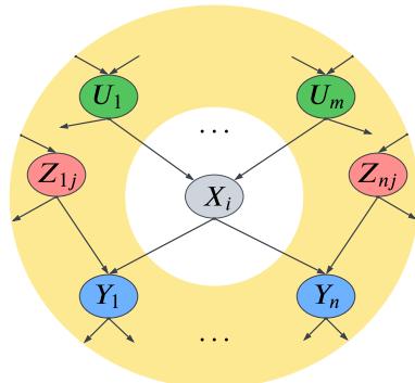
Figure 4.7: Illustration of the Markov blanket of a node in a directed graphical model. The target node Xⁱ is shown in gray, its parents U1:^m are shown in green, its children Y1:ⁿ are shown in blue, and its coparents Z1:n,1:^j are shown in red. Xⁱ is conditionally independent of all the other variables in the model given these variables. Adapted from Figure 13.4b of [RN19].

where the non-descendants of a node nd(i) are all the nodes except for its descendants, nd(i) = {1,…,NG}{i ↘ desc(i)}. Equation (4.33) is called the (directed) local Markov property. For example, in Figure 4.23(a), we have nd(3) = {1, 2, 4}, and pa(3) = 1, so 3 ℜ 2, 4|1.

A special case of this property is when we only look at predecessors of a node according to some topological ordering. We have

\[(i \perp \text{pred}(i) \mid \text{pa}(i) | \text{pa}(i)) \tag{4.34}\]

which follows since pred(i) ↓ nd(i). This is called the ordered Markov property, which justifies Equation (4.2). For example, in Figure 4.23(a), if we use the ordering 1, 2,…, 7. we find pred(3) = {1, 2} and pa(3) = 1, so 3 ℜ 2|1.

We have now described three Markov properties for DAGs: the directed global Markov property G in Equation (4.17), the directed local Markov property L in Equation (4.33), and the ordered Markov property O in Equation (4.34), It is obvious that G =∅ L =∅ O. What is less obvious, but nevertheless true, is that O =∅ L =∅ G (see e.g., [KF09a] for the proof). Hence all these properties are equivalent.

Furthermore, any distribution p that is Markov wrt a graph can be factorized as in Equation (4.2); this is called the factorization property F. It is obvious that O =∅ F, but one can show that the converse also holds (see e.g., [KF09a] for the proof).

4.2.5 Generation (sampling)

It is easy to generate prior samples from a DPGM: we simply visit the nodes in topological order, parents before children, and then sample a value for each node given the value of its parents. This will generate independent samples from the joint, (x1,…,x^NG ) ⇔ p(x|ω). This is called ancestral sampling.

4.2.6 Inference

In the context of PGMs, the term “inference” refers to the task of computing the posterior over a set of query nodes Q given the observed values for a set of visible nodes V , while marginalizing over the irrelevant nuisance variables, R = {1,…,NG}{Q, V }:

\[p\_{\theta}(Q|V) = \frac{p\_{\theta}(Q,V)}{p\_{\theta}(V)} = \frac{\sum\_{R} p\_{\theta}(Q,V,R)}{p\_{\theta}(V)}\tag{4.35}\]

(If the variables are continuous, we should replace sums with integrals.) If Q is a single node, then pϑ(Q|V ) is called the posterior marginal for node Q.

As an example, suppose V = x is a sequence of observed sound waves, Q = z is the corresponding set of unknown spoken words, and R = r are random “non-semantic” factors associated with the signal, such as prosody or background noise. Our goal is to compute the posterior over the words given the sounds, while being invariant to the irrelevant factors:

\[p\_{\theta}(\mathbf{z}|\mathbf{x}) = \sum\_{\mathbf{r}} p\_{\theta}(\mathbf{z}, \mathbf{r}|\mathbf{x}) = \sum\_{\mathbf{r}} \frac{p\_{\theta}(\mathbf{z}, \mathbf{r}, \mathbf{x})}{p\_{\theta}(\mathbf{z})} = \sum\_{\mathbf{r}} \frac{p\_{\theta}(\mathbf{z}, \mathbf{r}, \mathbf{x})}{\sum\_{\mathbf{z}', \mathbf{r}'} p\_{\theta}(\mathbf{z}', \mathbf{r}', \mathbf{x})} \tag{4.36}\]

As a simplification, we can “lump” the random factors R into the query set Q to define the complete set of hidden variables H = Q ↘ R. In this case, the tasks simpifies to

\[p\_{\theta}(h|x) = \frac{p\_{\theta}(h, x)}{p\_{\theta}(x)} = \frac{p\_{\theta}(h, x)}{\sum\_{h'} p\_{\theta}(h', x)}\tag{4.37}\]

The computational complexity of the inference task depends on the CI properties of the graph, as we discuss in Chapter 9. In general it is NP-hard (see Section 9.5.4), but for certain graph structures (such as chains, trees, and other sparse graphs), it can be solved e”ciently (in polynomial) time using dynamic programming (see Chapter 9). For cases where it is intractable, we can use standard methods for approximate Bayesian inference, which we review in Chapter 7.

4.2.6.1 Example: inference in the student network

As an example of inference in PGMs, consider the student network from Section 4.2.2.2. Suppose we observe that the student gets a grade of C. The posterior marginals are shown in Figure 4.8a. We see that the low grade could be explained by the class being hard (since p(D = Hard|G = C)=0.63), but is more likely explained by the student having low intelligence (since p(I = High|G = C)=0.08).

However, now suppose we also observe that the student gets a good SAT score. The new posterior marginals are shown in Figure 4.8b. Now the posterior probability that the student is intelligent has jumped to p(I = High|G = C, SAT = Good)=0.58, since otherwise it would be di”cult to explain the good SAT score. Once we believe the student has high intelligence, we have to explain the C grade by assuming the class is hard, and indeed we find that the probability that the class is hard has increased to p(D = Hard|G = C)=0.76. (This negative mutual interaction between multiple causes of some observations is called the explaining away e!ect, and is discussed in Section 4.2.4.2.)

4.2.7 Learning

So far, we have assumed that the structure G and parameters ω of the PGM are known. However, it is possible to learn both of these from data. For details on how to learn G from data, see Section 30.3.

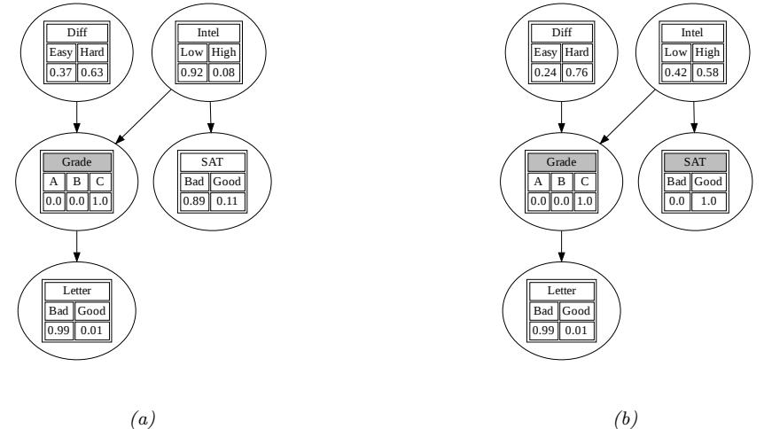
Figure 4.8: Illustration of belief updating in the “Student” PGM. The histograms show the marginal distribution of each node. Nodes with shaded titles are clamped to an observed value. (a) Posterior after conditioning on Grade=C. (b) Posterior after also conditioning on SAT=Good. Generated by student\_pgm.ipynb.

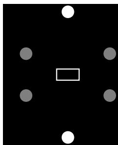
Figure 4.9: A DPGM representing the joint distribution p(y1:^N , x1:^N , εy, εx). Here ε^x and ε^y are global parameter nodes that are shared across the examples, whereas xⁿ and yⁿ are local variables.

Here we focus on parameter learning, i.e., computing the posterior p(ω|D, G). (Henceforth we will drop the conditioning on G, since we assume the graph structure is fixed.)

We can compute the parameter posterior p(ω|D) by treating ω as “just another hidden variable”, and then performing inference. However, in the machine learning community, it is more common to just compute a point estimate of the parameters, such as the posterior mode, ^{ωˆ =} argmax ^p(ω|D). This approximation is often reasonable, since the parameters depend on all the data, rather than just a single datapoint, and are therefore less uncertain than other hidden variables.

4.2.7.1 Learning from complete data

Figure 4.9 represents a graphical model for a typical supervised learning problem. We have N local variables, xⁿ and yn, and 2 global variables, corresponding to the parameters, which are shared across data samples. The local variables are observed (in the training set), so they are represented by solid (shaded) nodes. The global variables are not observed, and hence are represented by empty (unshaded) nodes. (The model represents a generative classifier, so the edge is from yⁿ to xn; if we are fitting a discriminative classifier, the edge would be from xⁿ to yn, and the parameters ω^y would represent the conditional probability p(y|x); there would be no ω^x node in this case.)

From the CI properties of Figure 4.9, it follows that the joint distribution factorizes into a product of terms, one per node:

\[p(\theta, \mathcal{D}) = p(\theta\_x) p(\theta\_y) \left[ \prod\_{n=1}^{N} p(y\_n | \theta\_y) p(x\_n | y\_n, \theta\_x) \right] \tag{4.38}\]

\[\mathbf{x} = \left[ p(\boldsymbol{\theta}\_{y}) \prod\_{n=1}^{N} p(y\_n | \boldsymbol{\theta}\_{y}) \right] \left[ p(\boldsymbol{\theta}\_{x}) \prod\_{n=1}^{N} p(\boldsymbol{x}\_{n} | y\_n, \boldsymbol{\theta}\_{x}) \right] \tag{4.39}\]

\[\propto \left[ p(\theta\_y) p(\mathcal{D}\_y|\theta\_y) \right] \left[ p(\theta\_x) p(\mathcal{D}\_{x|y}|\theta\_x) \right] \tag{4.40}\]

where ^{Dy =} {yn}^{N n}=1 is the data that is su”cient for estimating ^ωy and ^Dx|^{y =} {(xn, yn)}^{N n}=1 is the data that is su”cient for ωx.

From Equation (4.40), we see that the prior, likelihood, and posterior all decompose or factorize according to the graph structure. Thus we can compute the posterior for each parameter independently. In general, we have

\[p(\boldsymbol{\theta}, \mathcal{D}) = \prod\_{i=1}^{N\_G} p(\boldsymbol{\theta}\_i) p(\mathcal{D}\_i | \boldsymbol{\theta}\_i) \tag{4.41}\]

Hence the likelihood and prior factorizes, and thus so does the posterior. If we just want to compute the MLE, we can compute

\[\hat{\boldsymbol{\theta}} = \underset{\boldsymbol{\theta}}{\text{argmax}} \prod\_{i=1}^{N\_G} p(\mathcal{D}\_i | \boldsymbol{\theta}\_i) \tag{4.42}\]

We can solve this for each node independently, as we illustrate in Section 4.2.7.2.

4.2.7.2 Example: computing the MLE for CPTs

In this section, we illustrate how to compute the MLE for tabular CPDs. The likelihood is given by the following product of multinomials:

\[p(\mathcal{D}|\boldsymbol{\theta}) = \prod\_{n=1}^{N} \prod\_{i=1}^{N\_G} p(x\_{ni}|x\_{n, \text{pa}(i)}, \boldsymbol{\theta}\_i) \tag{4.43}\]

\[=\prod\_{n=1}^{N}\prod\_{i=1}^{N\_G}\prod\_{j=1}^{J\_i}\prod\_{k=1}^{K\_i}\theta\_{ijk}^{\mathbb{I}\{x\_{ni}=k,x\_{n,m(i)}=j\}}\tag{4.44}\]

I	D	G	S	L
0	0	2	0	0
0	1	2	0	0
0	0	1	1	1
1	1	1	1	0
1	0	0	1	1
0	0	0	0	1
1	1	2	1	1

Table 4.2: Some fully observed training data for the student network.

I	D	Ni,j,k	ˆϑi,j,k	ϑi,j,k
0	0	[1, 1, 1]	1 1 1 [ 3 , 3 , 3 ]	2 2 2 [ 6 , 6 , 6 ]
0	1	[0, 0, 1]	0 0 1 [ 1 , 1 , 1 ]	1 1 2 [ 4 , 4 , 4 ]
1	0	[1, 0, 0]	1 0 0 [ 1 , 1 , 1 ]	2 1 1 [ 4 , 4 , 4 ]
1	1	[0, 1, 1]	1 1 [0, 2 , 2 ]	1 2 2 [ 5 , 5 , 5 ]

Table 4.3: Su”cient statistics Nijk and corresponding MLE ˆεijk and posterior mean εijk (with Dirichlet (1,1,1) prior) for node i = G in the student network. Each row corresponds to a di!erent joint configuration of its parent nodes, coresponding to state j. The index k refers to the 3 possible values of the child node G.

where

\[\theta\_{ijk} \triangleq p(x\_i = k | \mathbf{x}\_{\text{pa}(i)} = j) \tag{4.45}\]

Let us define the su”cient statistics for node i to be Nijk, which is the number of times that node i is in state k while its parents are in joint state j:

\[N\_{ijk} \triangleq \sum\_{n=1}^{N} \mathbb{I}\left(x\_{n,i} = k, x\_{n, \text{pa}(i)} = j\right) \tag{4.46}\]

The MLE for a multinomial is given by the normalized empirical frequencies:

\[\hat{\theta}\_{ijk} = \frac{N\_{ijk}}{\sum\_{k'} N\_{ijk'}} \tag{4.47}\]

For example, consider the student network from Section 4.2.2.2. In Table 4.2, we show some sample training data. For example, the last line in the tabel encodes a student who is smart (I = 1), who takes a hard class (D = 1), gets a C (G = 2), but who does well on the SAT (S = 1) and gets a good letter of recommendation (L = 1).

In Table 4.3, we list the su”cient statistics Nijk and the MLE ˆϑijk for node i = G, with parents (I,D). A similar process can be used for the other nodes. Thus we see that fitting a DPGM with tabular CPDs reduces to a simple counting problem.

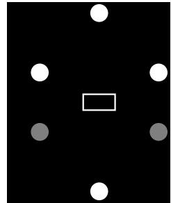
Figure 4.10: A DPGM representing the joint distribution p(z1:^N , x1:^N , εz, εx). The local variables zⁿ are hidden, whereas xⁿ are observed. This is typical for learning unsupervised latent variable models.

However, we notice there are a lot of zeros in the su”cient statistics, due to the small sample size, resulting in extreme estimates for some of the probabilities ˆϑijk. We discuss a (Bayesian) solution to this in Section 4.2.7.3.

4.2.7.3 Example: computing the posterior for CPTs

In Section 4.2.7.2 we discussed how to compute the MLE for the CPTs in a discrete Bayes net. We also observed that this can su!er from the zero-count problem. In this section, we show how a Bayesian approach can solve this problem.

Let us put a separate Dirichlet prior on each row of each CPT, i.e., ωij ⇔ Dir(εij ). Then we can compute the posterior by simply adding the pseudocounts to the empirical counts to get ωij |D ⇔ Dir(Nij + εij ), where Nij = {Nijk : k =1: Ki}, and Nijk is the number of times that node i is in state k while its parents are in state j. Hence the posterior mean estimate is given by

\[\overline{\theta}\_{ijk} = \frac{N\_{ijk} + \alpha\_{ijk}}{\sum\_{k'} (N\_{ijk'} + \alpha\_{ijk'})} \tag{4.48}\]

The MAP estimate has the same form, except we use αijk ⇐ 1 instead of αijk.

In Table 4.3, we illustrate this approach applied to the G node in the student network, where we use a uniform Dirichlet prior, αijk = 1.

4.2.7.4 Learning from incomplete data

In Section 4.2.7.1, we explained that when we have complete data, the likelihood (and posterior) factorizes over CPDs, so we can estimate each CPD independently. Unfortunately, this is no longer the case when we have incomplete or missing data. To see this, consider Figure 4.10. The likelihood of the observed data can be written as follows:

\[p(\mathcal{D}|\boldsymbol{\theta}) = \sum\_{\mathbf{z}\_{1:N}} \left[ \prod\_{n=1}^{N} p(\mathbf{z}\_n|\boldsymbol{\theta}\_z) p(\mathbf{z}\_n|\mathbf{z}\_n, \boldsymbol{\theta}\_x) \right] \tag{4.49}\]

\[=\prod\_{n=1}^{N}\sum\_{\mathbf{z}\_n} p(\mathbf{z}\_n|\boldsymbol{\theta}\_z)p(\mathbf{z}\_n|\mathbf{z}\_n, \boldsymbol{\theta}\_x) \tag{4.50}\]

Thus the log likelihood is given by

\[\ell(\boldsymbol{\theta}) = \sum\_{n} \log \sum\_{\mathbf{z}\_{n}} p(z\_{n}|\boldsymbol{\theta}\_{z}) p(\boldsymbol{x}\_{n}|\boldsymbol{z}\_{n}, \boldsymbol{\theta}\_{z}) \tag{4.51}\]

The log function does not distribute over the # ^zn operation, so the objective does not decompose over nodes.2 Consequently, we can no longer compute the MLE or the posterior by solving separate problems per node.

To solve this, we will resort to optimization methods. (We focus on the MLE case, and leave discussion of Bayesian inference for latent variable models to Part II.) In the sections below, we discuss how to use EM and SGD to find a local optimum of the (non convex) log likelihood objective.

4.2.7.5 Using EM to fit CPTs in the incomplete data case

A popular method for estimating the parameters of a DPGM in the presence of missing data is to the use the expectation maximization (EM) algorithm, as proposed in [Lau95]. We describe EM in detail in Section 6.5.3, but the basic idea is to alternate between inferring the latent variables zⁿ (the E or expectation step), and estimating the parameters given this completed dataset (the M or maximization step). Rather than returning the full posterior ^p(zn|xn, ^ω(t) ) in the E step, we instead return the expected su”cient statistics (ESS), which takes much less space. In the M step, we maximize the expected value of the log likelihood of the fully observed data using these ESS.

As an example, suppose all the CPDs are tabular, as in the example in Section 4.2.7.2. The log-likelihood of the complete data is given by

\[\log p(\mathcal{D}|\boldsymbol{\theta}) = \sum\_{i=1}^{N\_G} \sum\_{j=1}^{J\_i} \sum\_{k=1}^{K\_i} N\_{ijk} \log \theta\_{ijk} \tag{4.52}\]

and hence the expected complete data log-likelihood has the form

\[\mathbb{E}\left[\log p(\mathcal{D}|\boldsymbol{\theta})\right] = \sum\_{i} \sum\_{j} \sum\_{k} \overline{N}\_{ijk} \log \theta\_{ijk} \tag{4.53}\]

where

\[\overline{N}\_{ijk} = \sum\_{n=1}^{N} \mathbb{E}\left[\mathbb{I}\left(x\_{ni} = k, \mathbf{z}\_{n, \text{pa}(i)} = j\right)\right] = \sum\_{n=1}^{N} p(x\_{ni} = k, \mathbf{z}\_{n, \text{pa}(i)} = j | \mathcal{D}\_n, \mathbf{\theta}^{\text{old}}) \tag{4.54}\]

where ^Dn are all the visible variables in case ⁿ, and ^ωold are the parameters from the previous iteration. The quantity ^p(xni, ^xn,pa(i)|Dn, ^ωold) is known as a family marginal, and can be computed using any GM inference algorithm. The Nijk are the expected su!cient statistics (ESS), and constitute the output of the E step.

^2. We can also see this from the graphical model: ω^x is no longer independent of ωz, because there is a path that connects them via the hidden nodes zn. (See Section 4.2.4 for an explanation of how to “read o!” such CI properties from a DPGM.)

Given these ESS, the M step has the simple form

\[ \hat{\theta}\_{ijk} = \frac{\overline{N}\_{ijk}}{\sum\_{k'} \overline{N}\_{ijk'}} \tag{4.55} \]

We can modify this to perform MAP estimation with a Dirichlet prior by simply adding pseudocounts to the expected counts.

The famous Baum-Welch algorithm is a special case of the above equations which arises when the DPGM is an HMM (see Section 29.4.1 for details).

4.2.7.6 Using SGD to fit CPTs in the incomplete data case

The EM algorithm is a batch algorithm. To scale up to large datasets, it is more common to use stochastic gradient descent or SGD (see e.g., [BC94; Bin+97]). To apply this, we need to compute the marginal likelihood of the observed data for each example:

\[p(x\_n|\theta) = \sum\_{z\_n} p(z\_n|\theta\_z) p(x\_n|z\_n, \theta\_x) \tag{4.56}\]

where ω = (ωz, ωx).) (We say that we have “collapsed” the model by marginalizing out zn.) We can then compute the log likelihood using

\[\ell(\boldsymbol{\theta}) = \log p(\mathcal{D}|\boldsymbol{\theta}) = \log \prod\_{n=1}^{N} p(\boldsymbol{x}\_n|\boldsymbol{\theta}) = \sum\_{n=1}^{N} \log p(\boldsymbol{x}\_n|\boldsymbol{\theta}) \tag{4.57}\]

The gradient of this objective can be computed as follows:

\[\nabla \theta \,\ell(\theta) = \sum\_{n} \nabla\_{\theta} \log p(x\_n | \theta) \tag{4.58}\]

\[\dot{\theta} = \sum\_{n} \frac{1}{p(x\_n|\theta)} \nabla\_{\theta} p(x\_n|\theta) \tag{4.59}\]

\[=\sum\_{n}\frac{1}{p(\mathbf{z}\_{n}|\boldsymbol{\theta})}\nabla\_{\boldsymbol{\theta}}\left[\sum\_{\mathbf{z}\_{n}}p(\mathbf{z}\_{n},\boldsymbol{x}\_{n}|\boldsymbol{\theta})\right] \tag{4.60}\]

\[\mathcal{L} = \sum\_{n} \sum\_{\mathbf{z}\_n} \frac{p(\mathbf{z}\_n, \mathbf{z}\_n | \boldsymbol{\theta})}{p(\mathbf{z}\_n | \boldsymbol{\theta})} \nabla\_{\boldsymbol{\theta}} \log p(\mathbf{z}\_n, \mathbf{z}\_n | \boldsymbol{\theta}) \tag{4.61}\]

\[\hat{\mathbf{y}} = \sum\_{n} \sum\_{\mathbf{z}\_{n}} p(\mathbf{z}\_{n} | \mathbf{z}\_{n}, \boldsymbol{\theta}) \nabla\_{\boldsymbol{\theta}} \log p(\mathbf{z}\_{n}, \mathbf{z}\_{n} | \boldsymbol{\theta}) \tag{4.62}\]

We can now apply a minibatch approximation to this in the usual way.

4.2.8 Plate notation

To make the parameters of a PGM explicit, we can add them as nodes to the graph, and treat them as hidden variables to be inferred. Figure 4.11(a) shows a simple example, in which we have N iid

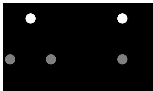
Figure 4.11: Left: datapoints xⁿ are conditionally independent given ε. Right: Same model, using plate notation. This represents the same model as the one on the left, except the repeated xⁿ nodes are inside a box, known as a plate; the number in the lower right hand corner, N, specifies the number of repetitions of the xⁿ node.

random variables, xn, all drawn from the same distribution with common parameter ω. We denote this by

\[x\_n \sim p(x|\theta) \tag{4.63}\]

The corresponding joint distribution over the parameters and data D = {x1,…, x^N } has the form

\[p(\mathcal{D}, \boldsymbol{\theta}) = p(\boldsymbol{\theta}) p(\mathcal{D}|\boldsymbol{\theta}) \tag{4.64}\]

where p(ω) is the prior distribution for the parameters, and p(D|ω) is the likelihood. By virtue of the iid assumption, the likelihood can be rewritten as follows:

\[p(\mathcal{D}|\boldsymbol{\theta}) = \prod\_{n=1}^{N} p(\boldsymbol{x}\_n|\boldsymbol{\theta})\tag{4.65}\]

Notice that the order of the data vectors is not important for defining this model, i.e., we can permute the leaves of the DPGM. When this property holds, we say that the data is exchangeable.

In Figure 4.11(a), we see that the x nodes are repeated N times. (The shaded nodes represent observed values, whereas the unshaded (hollow) nodes represent latent variables or parameters.) To avoid visual clutter, it is common to use a form of syntactic sugar called plates. This is a notational convention in which we draw a little box around the repeated variables, with the understanding that nodes within the box will get repeated when the model is unrolled. We often write the number of copies or repetitions in the bottom right corner of the box. This is illustrated in Figure 4.11(b).

4.2.8.1 Example: factor analysis

In Section 28.3.1, we discuss the factor analysis model, which has the form

\[p(\mathbf{z}) = \mathcal{N}(\mathbf{z}|\mu\_0, \Sigma\_0) \tag{4.66}\]

\[p(x|\mathbf{z}) = \mathcal{N}(x|\mathbf{W}z + \mu, \Psi) \tag{4.67}\]

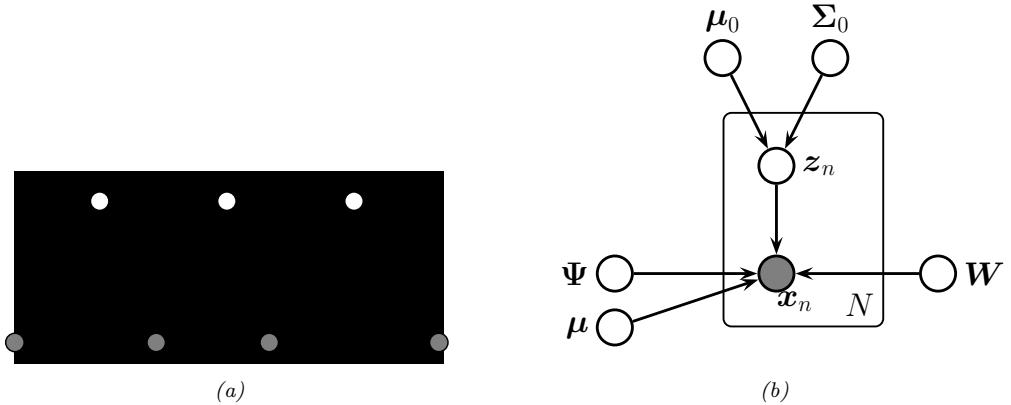
Figure 4.12: (a) Factor analysis model illustrated as a DPGM. We show the components of z (top row) and x (bottom row) as individual scalar nodes. (b) Equivalent model, where z and x are collapsed to vector-valued nodes, and parameters are added, using plate notation.

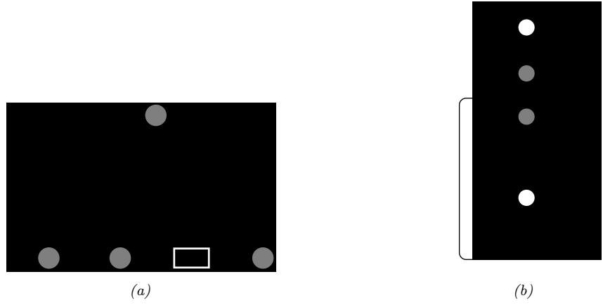
Figure 4.13: (a) Naive Bayes classifier as a DPGM. (b) Model augmented with plate notation.

where W is a D∞L matrix, known as the factor loading matrix, and $ is a diagonal D∞D covariance matrix.

Note that z and x are both vectors. We can explicitly represent their components as scalar nodes as in Figure 4.12a. Here the directed edges correspond to non-zero entries in the W matrix.

We can also explicitly show the parameters of the model, using plate notation, as shown in Figure 4.12b.

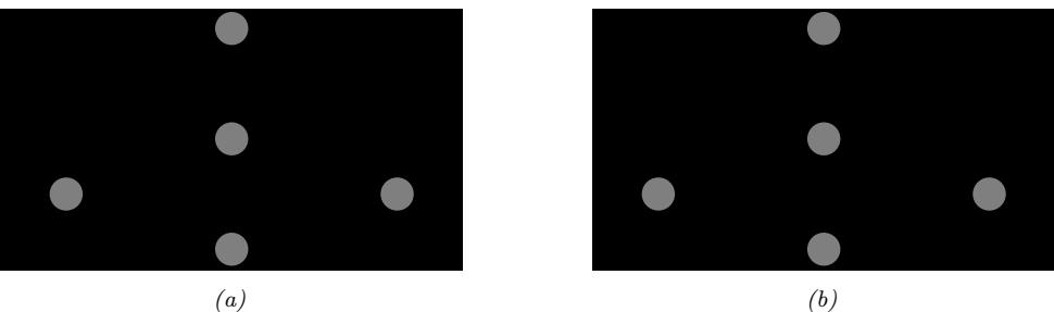
Figure 4.14: Tree-augmented naive Bayes classifier for D = 4 features. The tree topology can change depending on the value of y, as illustrated.

4.2.8.2 Example: naive Bayes classifier

In some models, we have doubly indexed variables. For example, consider a naive Bayes classifier. This is a simple generative classifier, defined as follows:

\[p(\mathbf{z}, y | \boldsymbol{\theta}) = p(y | \boldsymbol{\pi}) \prod\_{d=1}^{D} p(x\_d | y, \boldsymbol{\theta}\_d) \tag{4.68}\]

The fact that the features x1:^D are considered conditionally independent given the class label y is where the term “naive” comes from. Nevertheless, this model often works surprisingly well, and is extremely easy to fit.

We can represent the conditional independence assumption as shown in Figure 4.13a. We can represent the repetition over the dimension d with a plate. When we turn to infering the parameters ω = (ϑ, ω1:D,1:^C ), we also need to represent the repetition over data cases n. This is shown in Figure 4.13b. Note that the parameter ωdc depends on d and c, whereas the feature xnd depends on n and d. This is shown using nested plates to represent the shared d index.

4.2.8.3 Example: relaxing the naive Bayes assumption

We see from Figure 4.13a that the observed features are conditionally independent given the class label. We can of course allow for dependencies between the features, as illustrated in Figure 4.14. (We omit parameter nodes for simplicity.) If we enforce that the edges between the features forms a tree the model is known as a tree-augmented naive Bayes classifier [FGG97], or TAN model. (Trees are a restricted form of graphical model that have various computational advantages that we discuss later.) Note that the topology of the tree can change depending on the value of the class node y; in this case, the model is known as a Bayesian multi net, and can be thought of as a supervised mixture of trees.

4.3 Undirected graphical models (Markov random fields)

Directed graphical models (Section 4.2) are very useful. However, for some domains, being forced to choose a direction for the edges, as required by a DAG, is rather awkward. For example, consider

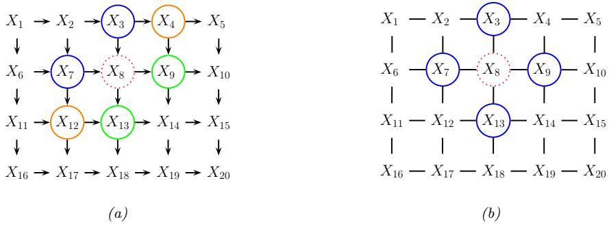
Figure 4.15: (a) A 2d lattice represented as a DAG. The dotted red node X⁸ is independent of all other nodes (black) given its Markov blanket, which include its parents (blue), children (green) and co-parents (orange). (b) The same model represented as a UPGM. The red node X⁸ is independent of the other black nodes given its neighbors (blue nodes).

modeling an image. It is reasonable to assume that the intensity values of neighboring pixels are correlated. We can model this using a DAG with a 2d lattice topology as shown in Figure 4.15(a). This is known as a Markov mesh [AHK65]. However, its conditional independence properties are rather unnatural.

An alternative is to use an undirected probabilistic graphical model (UPGM), also called a Markov random field (MRF) or Markov network. These do not require us to specify edge orientations, and are much more natural for some problems such as image analysis and spatial statistics. For example, an undirected 2d lattice is shown in Figure 4.15(b); now the Markov blanket of each node is just its nearest neighbors, as we show in Section 4.3.6.

Roughly speaking, the main advantages of UPGMs over DPGMs are: (1) they are symmetric and therefore more “natural” for certain domains, such as spatial or relational data; and (2) discriminative UPGMs (aka conditional random fields, or CRFs), which define conditional densities of the form p(y|x), work better than discriminative DGMs, for reasons we explain in Section 4.5.3. The main disadvantages of UPGMs compared to DPGMs are: (1) the parameters are less interpretable and less modular, for reasons we explain in Section 4.3.1; and (2) it is more computationally expensive to estimate the parameters, for reasons we explain in Section 4.3.9.1.

4.3.1 Representing the joint distribution

Since there is no topological ordering associated with an undirected graph, we can’t use the chain rule to represent p(x1:N^G ). So instead of associating CPDs with each node, we associate potential functions or factors with each maximal clique in the graph.3 We will denote the potential function for clique c by 5c(xc; ωc), where ω^c are its parameters. A potential function can be any non-negative function of its arguments (we give some examples below). We can use these functions to define the joint distribution as we explain in Section 4.3.1.1.

^3. A clique is a set of nodes that are all neighbors of each other. A maximal clique is a clique which cannot be made any larger without losing the clique property.

4.3.1.1 Hammersley-Cli”ord theorem

Suppose a joint distribution p satisfies the CI properties implied by the undirected graph G. (We discuss how to derive these properties in Section 4.3.6.) Then the Hammersley-Cli”ord theorem tells us that p can be written as follows:

\[p(\mathbf{z}|\boldsymbol{\theta}) = \frac{1}{Z(\boldsymbol{\theta})} \prod\_{c \in \mathcal{C}} \psi\_c(\mathbf{z}\_c; \boldsymbol{\theta}\_c) \tag{4.69}\]

where C is the set of all the (maximal) cliques of the graph G, and Z(ω) is the partition function given by

\[Z(\boldsymbol{\theta}) \triangleq \sum\_{\mathbf{z}} \prod\_{c \in \mathcal{C}} \psi\_c(\mathbf{z}\_c; \boldsymbol{\theta}\_c) \tag{4.70}\]

Note that the partition function is what ensures the overall distribution sums to 1.4

The Hammersley-Cli!ord theorem was never published, but a proof can be found in [KF09a]. (Note that the theorem only holds for positive distributions, i.e., ones where p(x|ω) > 0 for all configurations x, which rules out some models with hard constraints.)

4.3.1.2 Gibbs distribution

The distribution in Equation (4.69) can be rewritten as follows:

\[p(x|\theta) = \frac{1}{Z(\theta)} \exp(-\mathcal{E}(x;\theta))\tag{4.71}\]

where E(x) > 0 is the energy of state x, defined by

\[\mathcal{E}(x;\theta) = \sum\_{c} \mathcal{E}(x\_c; \theta\_c) \tag{4.72}\]

where x^c are the variables in clique c. We can see the equivalence by defining the clique potentials as

\[\psi\_c(\mathbf{x}\_c; \boldsymbol{\theta}\_c) = \exp(-\mathcal{E}(\mathbf{x}\_c; \boldsymbol{\theta}\_c)) \tag{4.73}\]

We see that low energy is associated with high probability states.

Equation (4.71) is known as the Gibbs distribution. This kind of probability model is also called an energy-based model. These are commonly used in physics and biochemistry. They are also used in ML to define generative models, as we discuss in Chapter 24. (See also Section 4.4, where we discuss conditional random fields (CRFs), which are models of the form p(y|x, ω), where the potential functions are conditioned on input features x.)

4.3.2 Fully visible MRFs (Ising, Potts, Hopfield, etc.)

In this section, we discuss some UPGMs for 2d grids, that are used in statistical physics and computer vision. We then discuss extensions to other graph structures, which are useful for biological modeling and pattern completion.

^4. The partition function is denoted by Z because of the German word Zustandssumme, which means “sum over states”. This reflects the fact that a lot of pioneering working on MRFs was done by German (and Austrian) physicists, such as Boltzmann.

4.3.2.1 Ising models

Consider the 2d lattice in Figure 4.15(b). We can represent the joint distribution as follows:

\[p(x|\theta) = \frac{1}{Z(\theta)} \prod\_{i \sim j} \psi\_{ij}(x\_i, x\_j; \theta) \tag{4.74}\]

where i ⇔ j means i and j are neighbors in the graph. This is called a 2d lattice model.

An Ising model is a special case of the above, where the variables xⁱ are binary. Such models are often used to represent magnetic materials. In particular, each node represents an atom, which can have a magnetic dipole, or spin, which is in one of two states, +1 and ⇐1. In some magnetic systems, neighboring spins like to be similar; in other systems, they like to be dissimilar. We can capture this interaction by defining the clique potentials as follows:

\[\psi\_{ij}(x\_i, x\_j; \theta) = \begin{cases} e^{J\_{ij}} & \text{if } x\_i = x\_j \\ e^{-J\_{ij}} & \text{if } x\_i \neq x\_j \end{cases} \tag{4.75}\]

where Jij is the coupling strength between nodes i and j. This is known as the Ising model. If two nodes are not connected in the graph, we set Jij = 0. We assume that the weight matrix is symmetric, so Jij = Jji. Often we also assume all edges have the same strength, so Jij = J for each (i, j) edge. Thus

\[\psi\_{ij}(x\_i, x\_j; J) = \begin{cases} e^J & \text{if } x\_i = x\_j \\ e^{-J} & \text{if } x\_i \neq x\_j \end{cases} \tag{4.76}\]

It is more common to define the Ising model as an energy-based model, as follows:

\[p(x|\theta) = \frac{1}{Z(J)} \exp(-\mathcal{E}(x;J))\tag{4.77}\]

\[\mathcal{E}(\mathbf{z}; J) = -J \sum\_{i \sim j} x\_i x\_j \tag{4.78}\]

where E(x; J) is the energy, and where we exploited the fact that xix^j = ⇐1 if xⁱ ⇓= x^j , and xix^j = +1 if xⁱ = x^j . The magnitude of J controls the degree of coupling strength between neighboring sites. We can scale the coupling coe”cient J by a temperature term T to get J^↔︎ = J/T, so colder means more tightly coupled (larger J), and hotter means less tightly coupled (smaller J).

If all of the weights are negative, J < 0, then the spins want to be di!erent from their neighbors. This is called an antiferromagnetic system, and results in a frustrated system, since it is not possible for all neighbors to be di!erent from each other in a 2d lattice. In the infinite lattice, this gives rise to the checkerboard pattern shown in Figure 4.16.

If all the edge weights are positive, J > 0, then neighboring spins are likely to be in the same state, since if xⁱ = x^j , the energy term gets a contribution of ⇐J < 0, and lower energy corresponds to higher probability. In the machine learning literature, this is called an associative Markov network. In the physics literature, this is called a ferromagnetic model. If J = 1, the corresponding probability distribution will have two modes, corresponding to the all +1 state and the all -1 state. These are called the ground states of the system.

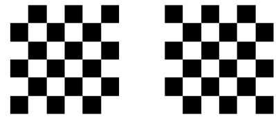
Figure 4.16: The two ground states for a small antiferromagnetic Ising model where J = ↓1. From Figure 31.7 of [Mac03].

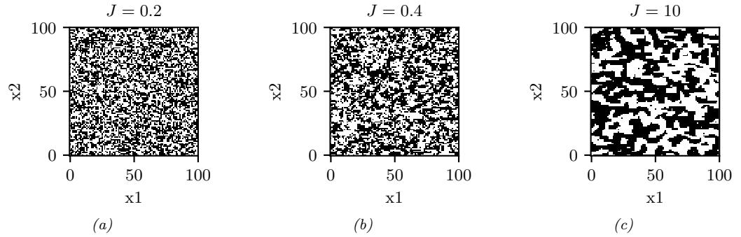
Figure 4.17: Samples from an associative Ising model with varying J > 0. Generated by gibbs\_demo\_ising.ipynb. (Compare to Figure 31.2 of [Mac03].)

In addition to the well-separated configurations of minimum energy, there can be many local minima. The energy surface can become more or less bumpy depending on the temperature T. Figure 4.17 shows some samples from the Ising model for varying J^↔︎ > 0. (The samples were created using the Gibbs sampling method discussed in Section 12.3.3.) As the temperature reduces, the distribution becomes less entropic, and the “clumpiness” of the samples increases. One can show that, as the lattice size goes to infinity, there is a critical temperature J^c below which many large clusters occur, and above which many small clusters occur. In the case of an isotropic square lattice model, one can show [Geo88] that

\[J\_c = \frac{1}{2} \log(1 + \sqrt{2}) \approx 0.44\tag{4.79}\]

This rapid change in global behavior as we vary a parameter of the system is called a phase transition. This can be used to explain how natural systems, such as water, can suddenly go from solid to liquid, or from liquid to gas, when the temperature changes slightly. See e.g., [Mac03, ch 31] for further details on the statistical mechanics of Ising models.

In addition to pairwise terms, it is standard to add unary terms, 5i(xi). In statistical physics, this is called an external field. The resulting model is as follows:

\[p(x|\theta) = \frac{1}{Z(\theta)} \prod\_{i} \psi\_i(x\_i; \theta) \prod\_{i \sim j} \psi\_{ij}(x\_i, x\_j; \theta) \tag{4.80}\]

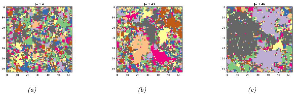
Figure 4.18: Visualizing a sample from a 10-state Potts model of size 128 ↘ 128. The critical value is ^{Jc =} log(1 + ^→10)=1.426. for di!erent association strengths: (a) ^J = 1.40, (b) ^J = 1.43, (c) ^J = 1.46. Generated by gibbs\_demo\_potts.ipynb.

The 5ⁱ terms can be thought of as a local bias term that is independent of the contributions of the neighboring nodes. For binary nodes, we can define this as follows:

\[\psi\_i(x\_i) = \begin{cases} e^{\alpha} & \text{if } x\_i = +1 \\ e^{-\alpha} & \text{if } x\_i = -1 \end{cases} \tag{4.81}\]

If we write this as an energy-based model, we have

\[\mathcal{E}(x|\theta) = -\alpha \sum\_{i} x\_i - J \sum\_{i \sim j} x\_i x\_j \tag{4.82}\]

4.3.2.2 Potts models

In Section 4.3.2.1, we discussed the Ising model, which is a simple 2d MRF for defining distributions over binary variables. It is easy to generalize the Ising model to multiple discrete states, xⁱ ↑ {1, 2,…,K}. If we use the same potential function for every edge, we can write

\[ \psi\_{ij}(x\_i = k, x\_j = k') = e^{J\_{ij}(k, k')} \tag{4.83} \]

where Jij (k, k^↔︎ ) is the energy if one node has state k and its neighbor has state k^↔︎ . A common special case is

\[\psi\_{ij}(x\_i = k, x\_j = k') = \begin{cases} e^J & \text{if } k = k' \\ e^0 & \text{if } k \neq k' \end{cases} \tag{4.84}\]

This is called the Potts model. The Potts model reduces to the Ising model if we define Jpotts = 2Jising.

If J > 0, then neighboring nodes are encouraged to have the same label; this is an example of an associative Markov model. Some samples from this model are shown in Figure 4.18. The phase transition for a 2d Potts model occurs at the following value (see [MS96]):

\[J\_c = \log(1 + \sqrt{K})\tag{4.85}\]

We can extend this model to have local evidence for each node. If we write this as an energy-based model, we have

\[\mathcal{E}\left(\mathbf{z}|\boldsymbol{\theta}\right) = -\sum\_{i}\sum\_{k=1}^{K}\alpha\_{k}\mathbb{I}\left(x\_{i} = k\right) - J\sum\_{i\sim j}\mathbb{I}\left(x\_{i} = x\_{j}\right) \tag{4.86}\]

4.3.2.3 Potts models for protein structure prediction

One interesting application of Potts models arises in the area of protein structure prediction. The goal is to predict the 3d shape of a protein from its 1d sequence of amino acids. A common approach to this is known as direct coupling analysis (DCA). We give a brief summary below; for details, see [Mor+11].

First we compute a multiple sequence alignment (MSA) from a set of related amino acid sequences from the same protein family; this can be done using HMMs, as explained in Section 29.3.2. The MSA can be represented by an N ∞ T matrix X, where N is the number of sequences, T is the length of each sequence, and Xni ↑ {1,…,V } is the identity of the letter at location i in sequence n. For protein sequences, V = 21, representing the 20 amino acids plus the gap character.

Once we have the MSA matrix X, we fit the Potts model using maximum likelihood estimation, or some approximation, such as pseudolikelihood [Eke+13]; see Section 4.3.9 for details.5 After fitting the model, we select the edges with the highest Jij coe”cients, where i, j ↑ {1,…,T} are locations or residues in the protein. Since these locations are highly coupled, they are likely to be in physical contact, since interacting residues must coevolve to avoid destroying the function of the protein (see e.g., [LHF17] for a review). This graph is called a contact map.

Once the contact map is established, it can be used as input to a 3d structural prediction algorithm, such as [Xu18] or the alphafold system [Eva+18], which won the 2018 CASP competition. Such methods use neural networks to learn functions of the form p(d(i, j)|{c(i, j)}), where d(i, j) is the 3d distance between residues i and j, and c(i, j) is the contact map.

4.3.2.4 Hopfield networks

A Hopfield network [Hop82] is a fully connected Ising model (Section 4.3.2.1) with a symmetric weight matrix, W = W^T. The corresponding energy function has the form

\[\mathcal{E}(x) = -\frac{1}{2}x^{\mathsf{T}}\mathbf{W}x\tag{4.87}\]

where xⁱ ↑ {⇐1, +1}.

The main application of Hopfield networks is as an associative memory or content addressable memory. The idea is this: suppose we train on a set of fully observed bit vectors, corresponding to patterns we want to memorize. (We discuss how to do this below). Then, at test time, we present a partial pattern to the network. We would like to estimate the missing variables; this is called pattern completion. That is, we want to compute

\[x^\* = \operatorname\*{argmin}\_{x} \mathcal{E}(x) \tag{4.88}\]

^5. To encourage the model to learn sparse connectivity, we can also compute a MAP estimate with a sparsity promoting prior, as discussed in [IM17].

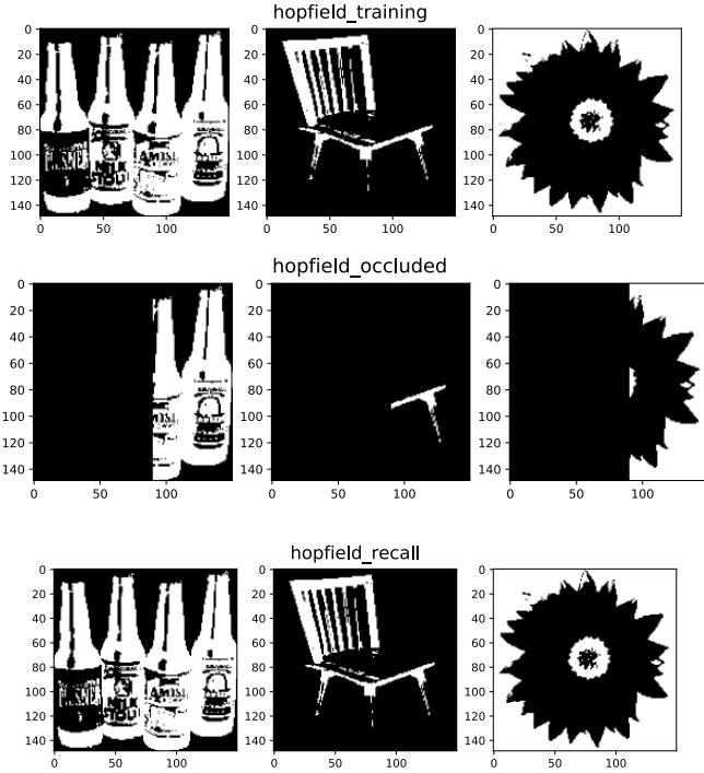
Figure 4.19: Examples of how an associative memory can reconstruct images. These are binary images of size 150 ↘ 150 pixels. Top: training images. Middle row: partially visible test images. Bottom row: final state estimate. Adapted from Figure 2.1 of [HKP91]. Generated by hopfield\_demo.ipynb.

We can solve this optimization problem using iterative conditional modes (ICM), in which we set each hidden variable to its most likely state given its neighbors. Picking the most probable state amounts to using the rule

\[\mathbf{x}^{t+1} = \text{sgn}(\mathbf{W}\mathbf{x}^t) \tag{4.89}\]

This can be seen as a deterministic version of Gibbs sampling (see Section 12.3.3).

We illustrate this process in Figure 4.19. In the top row, we show some training examples. In the middle row, we show a corrupted input, corresponding to the initial state x⁰. In the bottom row, we show the final state after 30 iterations of ICM. The overall process can be thought of as retrieving a complete example from memory based on a piece of the example.

To learn the weights W, we could use the maximum likelihood estimate method described in Section 4.3.9.1. (See also [HSDK12].) However, a simpler heuristic method, proposed in [Hop82], is to use the following outer product method:

\[\mathbf{W} = \left(\frac{1}{N} \sum\_{n=1}^{N} x\_n \mathbf{x}\_n^T \right) - \mathbf{I} \tag{4.90}\]

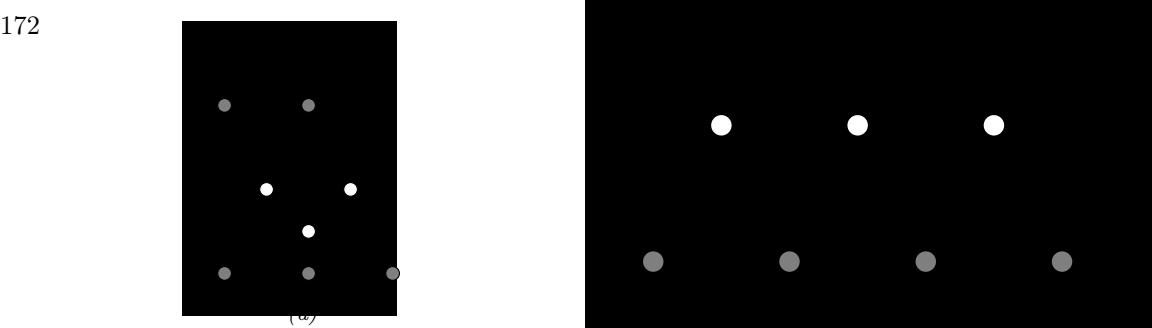
Figure 4.20: (a) A general Boltzmann machine, with an arbitrary graph structure. The shaded (visible) nodes are partitioned into input and output, although the model is actually symmetric and defines a joint distribution on all the nodes. (b) A restricted Boltzmann machine with a bipartite structure. Note the lack of intra-layer connections.

This normalizes the output product matrix by N, and then sets the diagonal to 0. This ensures the energy is low for patterns that match any of the examples in the training set. This is the technique we used in Figure 4.19. Note, however, that this method not only stores the original patterms but also their inverses, and other linear combinations. Consequently there is a limit to how many examples the model can store before they start to “collide” in the memory. Hopfield proved that, for random patterns, the network capacity is ⇔ 0.14N.

4.3.3 MRFs with latent variables (Boltzmann machines, etc.)

In this section, we discuss MRFs which contain latent variables, as a way to represent high dimensional joint distributions in discrete spaces.

4.3.3.1 Vanilla Boltzmann machines

MRFs in which all the variables are visible are limited in their expressive power, since the only way to model correlation between the variables is by directly adding an edge. An alternative approach is to introduce latent variables. A Boltzmann machine [AHS85] is like an Ising model (Section 4.3.2.1) with latent variables. In addition, the graph structure can be arbitrary (not just a lattice), and the binary states are xⁱ ↑ {0, 1} instead of xⁱ ↑ {⇐1, +1}. We usually partition the nodes into hidden nodes z and visible nodes x, as shown in Figure 4.20(a).

4.3.3.2 Restricted Boltzmann machines (RBMs)

Unfortunately, exact inference (and hence learning) in Boltzmann machines is intractable, and even approximate inference (e.g., Gibbs sampling, Section 12.3) can be slow. However, suppose we restrict the architecture so that the nodes are arranged in two layers, and so that there are no connections between nodes within the same layer (see Figure 4.20(b)). This model is known as a restricted Boltzmann machine (RBM) [HT01; HS06a], or a harmonium [Smo86]. The RBM supports e”cient approximate inference, since the hidden nodes are conditionally independent given the visible nodes, i.e., ^p(z|x) = ^{K k}=1 p(zk|x). Note this is in contrast to a directed two-layer models, where the explaining away e!ect causes the latent variables to become “entangled” in the posterior even if they are independent in the prior.

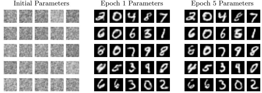
Figure 4.21: Some reconstructed images generated by a binary RBM fit to MNIST. Generated by rbm\_contrastive\_divergence.ipynb.

Visible	Hidden	Name	Reference
Binary	Binary	Binary RBM	[HS06a]
Gaussian	Binary	Gaussian RBM	[WS05]
Categorical	Binary	Categorical RBM	[SMH07]
Multiple categorical	Binary	Replicated softmax/undirected LDA	[SH10]
Gaussian	Gaussian	Undirected PCA	[MM01]
Binary	Gaussian	Undirected binary PCA	[WS05]

Table 4.4: Summary of di!erent kinds of RBM.

Typically the hidden and visible nodes in an RBM are binary, so the energy terms have the form wdkxdzk. If z^k = 1, then the k’th hidden unit adds a term of the form w^{T k}x to the energy; this can be thought of as a “soft constraint”. If z^k = 0, the hidden unit is not active, and does not have an opinion about this data example. By turning on di!erent combinations of constraints, we can create complex distributions on the visible data. This is an example of a product of experts (Section 24.1.1), since ^p(x|z) = ^k:zk=1 exp(w^{T k}x).

This can be thought of as a mixture model with an exponential number of hidden components, corresponding to 2^H settings of z. That is, z is a distributed representation, whereas a standard mixture model uses a localist representation, where z ↑ {1, K}, and each setting of z corresponds to a complete prototype or exemplar w^k to which x is compared, giving rise to a model of the form ^p(x|^{z = k}) ↙ exp(w^{T k}x).

Many di!erent kinds of RBMs have been defined, which use di!erent pairwise potential functions. See Table 4.4 for a summary. (Figure 4.21 gives an example of some images generated from an RBM fit to the binarized MNIST dataset.) All of these are special cases of the exponential family harmonium [WRZH04]. See Supplementary Section 4.3 for more details.

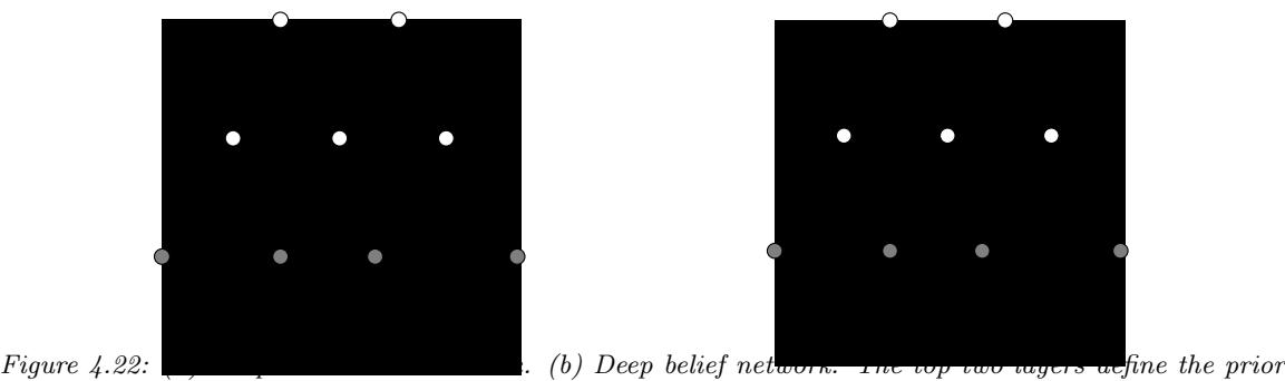
in terms on an RBM. The remaining layers are a directed graphical model that “decodes” the prior into observable data.

4.3.3.3 Deep Boltzmann machines

We can make a “deep” version of an RBM by stacking multiple layers; this is called a deep Boltzmann machine [SH09]. For example, the two layer model in Figure 4.22(a) has the form

\[p(\mathbf{z}, \mathbf{z}\_1, \mathbf{z}\_2 | \boldsymbol{\theta}) = \frac{1}{Z(\mathbf{W}\_1, \mathbf{W}\_2)} \exp\left(\mathbf{z}^\mathsf{T} \mathbf{W}\_1 \mathbf{z}\_1 + \mathbf{z}\_1^\mathsf{T} \mathbf{W}\_2 \mathbf{z}\_2\right) \tag{4.91}\]

where x are the visible nodes at the bottom, and we have dropped bias terms for brevity.

4.3.3.4 Deep belief networks (DBNs)

We can use an RBM as a prior over a latent distributed code, and then use a DPGM “decoder” to convert this into the observed data, as shown in Figure 4.22(b). The corresponding joint distribution has the form

\[p(\mathbf{z}, \mathbf{z}\_1, \mathbf{z}\_2 | \boldsymbol{\theta}) = p(\mathbf{z} | \mathbf{z}\_1, \mathbf{W}\_1) \frac{1}{Z(\mathbf{W}\_2)} \exp\left(\mathbf{z}\_1^\mathsf{T} \mathbf{W}\_2 \mathbf{z}\_2\right) \tag{4.92}\]

In other words, it is an RBM on top of a DPGM. This combination has been called a deep belief network (DBN) [HOT06a]. However, this name is confusing, since it is not actually a belief net. We will therefore call it a deep Boltzmann network (which conveniently has the same DBN abbreviation).

DBNs can be trained in a simple greedy fashion, and support fast bottom-up inference (see [HOT06a] for details). DBNs played an important role in the history of deep learning, since they were one of the first deep models that could be successfully trained. However, they are no longer widely used, since the advent of better ways to train fully supervised deep neural networks (such as using ReLU units and the Adam optimizer), and the advent of e”cient ways to train deep DPGMs, such as the VAE (Section 21.2).

4.3.4 Maximum entropy models

In Section 2.4.7, we show that the exponential family is the distribution with maximum entropy, subject to the constraints that the expected value of the features (su”cient statistics) ϱ(x) match

the empirical expectations. Thus the model has the form

\[p(x|\theta) = \frac{1}{Z(\theta)} \exp\left(\theta^{\mathsf{T}} \phi(x)\right) \tag{4.93}\]

If the features ϱ(x) decompose according to a graph structure, we get a kind of MRF known as a maximum entropy model. We give some examples below.

4.3.4.1 Log-linear models

Suppose the potential functions have the following log-linear form:

\[ \psi\_c(\mathbf{x}\_c; \boldsymbol{\theta}\_c) = \exp(\boldsymbol{\theta}\_c^\top \boldsymbol{\phi}(\mathbf{x}\_c)) \tag{4.94} \]

where ϱ(xc) is a feature vector derived from the variables in clique c. Then the overall model is given by

\[p(x|\theta) = \frac{1}{Z(\theta)} \exp\left(\sum\_{c} \theta\_c^{\mathrm{T}} \phi(x\_c)\right) \tag{4.95}\]

For example, in a Gaussian graphical model (GGM), we have

\[ \phi([x\_i, x\_j]) = [x\_i, x\_j, x\_i x\_j] \tag{4.96} \]

for xⁱ ↑ R. And in an Ising model, we have

\[ \phi([x\_i, x\_j]) = [x\_i, x\_j, x\_i x\_j] \tag{4.97} \]

for xⁱ ↑ {⇐1, +1}. Thus both of these are maxent models. However, there are two key di!erences: first, in a GGM, the variables are real-valued, not binary; second, in a GGM, the partition function Z(ω) can be computed in O(D³) time, whereas in a Boltzmann machine, computing the partition function can take O(2^D) time (see Section 9.5.4 for details).

If the features ϱ are structured in a hierarchical way (capturing first order interactions, and second order interactions, etc.), and all the variables x are categorical, the resulting model is known in statistics as a log-linear model. However, in the ML community, the term “log-linear model” is often used to describe any model of the form Equation (4.95).

4.3.4.2 Feature induction for a maxent spelling model

In some applications, we assume the features ϱ(x) are known. However, it is possible to learn the features in a maxent model in an unsupervised way; this is known as feature induction.

A common approach to feature induction, first proposed in [DDL97; ZWM97], is to start with a base set of features, and then to continually create new feature combinations out of old ones, greedily adding the best ones to the model.

As an example of this approach, [DDL97] describe how to build models to represent English spelling. This can be formalized as a probability distribution over variable length strings, p(x|ω),

where x^t is a letter in the English alphabet. Initially the model has no features, which represents the uniform distribution. The algorithm starts by choosing to add the feature

\[\phi\_1(\mathbf{z}) = \sum\_i \mathbb{I}\left(x\_i \in \{a, \dots, z\}\right) \tag{4.98}\]

which checks if any letter is lowercase or not. After the feature is added, the parameters are (re)-fit by maximum likelihood (a computationally di”cult problem, which we discuss in Section 4.3.9.1). For this feature, it turns out that ˆϑ¹ = 1.944, which means that a word with a lowercase letter in any position is about ^e1.^{944 ¬ 7} times more likely than the same word without a lowercase letter in that position. Some samples from this model, generated using (annealed) Gibbs sampling (described in Section 12.3), are shown below.6

m, r, xevo, ijjiir, b, to, jz, gsr, wq, vf, x, ga, msmGh, pcp, d, oziVlal, hzagh, yzop, io, advzmxnv, ijv_bolft, x, emx, kayerf, mlj, rawzyb, jp, ag, ctdnnnbg, wgdw, t, kguv, cy, spxcq, uzflbbf, dxtkkn, cxwx, jpd, ztzh, lv, zhpkvnu, l^, r, qee, nynrx, atze4n, ik, se, w, lrh, hp+, yrqyka’h, zcngotcnx, igcump, zjcjs, lqpWiqu, cefmfhc, o, lb, fdcY, tzby, yopxmvk, by, fz” t, govyccm, ijyiduwfzo, 6xr, duh, ejv, pk, pjw, l, fl, w

The second feature added by the algorithm checks if two adjacent characters are lowercase:

\[\phi\_2(\mathbf{z}) = \sum\_{i \sim j} \mathbb{I}\left(x\_i \in \{a, \dots, z\}, x\_j \in \{a, \dots, z\}\right) \tag{4.99}\]

Now the model has the form

\[p(\mathbf{z}) = \frac{1}{Z} \exp(\theta\_1 \phi\_1(\mathbf{z}) + \theta\_2 \phi\_2(\mathbf{z})) \tag{4.100}\]

Continuing in this way, the algorithm adds features for the strings s> and ing>, where > represents the end of word, and for various regular expressions such as [0-9], etc. Some samples from the model with 1000 features, generated using (annealed) Gibbs sampling, are shown below.

was, reaser, in, there, to, will, ” was, by, homes, thing, be, reloverated, ther, which, conists, at, fores, anditing, with, Mr., proveral, the, ” ***, on’t, prolling, prothere, ” mento, at, yaou, 1, chestraing, for, have, to, intrally, of, qut, ., best, compers, ***, cluseliment, uster, of, is, deveral, this, thise, of, offect, inatever, thifer, constranded, stater, vill, in, thase, in, youse, menttering, and, ., of, in, verate, of, to

If we define a feature for every possible combination of letters, we can represent any probability distribution. However, this will overfit. The power of the maxent approach is that we can choose which features matter for the domain.

An alternative approach is to introduce latent variables, that implicitly model correlations amongst the visible nodes, rather than explicitly having to learn feature functions. See Section 4.3.3 for an example of such a model.

^6. We thank John La!erty for sharing this example.

4.3.5 Gaussian MRFs

In Section 4.2.3, we showed how to represent a multivariate Gaussian using a DPGM. In this section, we show how to represent a multivariate Gaussian using a UPGM. (For further details on GMRFs, see e.g., [RH05].)

4.3.5.1 Standard GMRFs

A Gaussian graphical model (or GGM), also called a Gaussian MRF, is a pairwise MRF of the following form:

\[p(\mathbf{z}) = \frac{1}{Z(\boldsymbol{\theta})} \prod\_{i \sim j} \psi\_{ij}(x\_i, x\_j) \prod\_i \psi\_i(x\_i) \tag{4.101}\]

\[\psi\_{ij}(x\_i, x\_j) = \exp(-\frac{1}{2}x\_i \Lambda\_{ij} x\_j) \tag{4.102}\]

\[ \psi\_i(x\_i) = \exp(-\frac{1}{2}\Lambda\_{ii}x\_i^2 + \eta\_i x\_i) \tag{4.103} \]

\[Z(\theta) = (2\pi)^{D/2} |\Lambda|^{-\frac{1}{2}} \tag{4.104}\]

The 5ij are edge potentials (pairwise terms), and each the 5ⁱ are node potentials or unary terms. (We could absorb the unary terms into the pairwise terms, but we have kept them separate for clarity.)

The joint distribution can be rewritten in a more familiar form as follows:

\[p(\mathbf{z}) \propto \exp[\eta^{\mathsf{T}} \mathbf{z} - \frac{1}{2} \mathbf{z}^{\mathsf{T}} \mathbf{A} \mathbf{z}] \tag{4.105}\]

This is called the information form of a Gaussian; ” = !^↑1 and ϖ = “µ are called the canonical parameters.

If %ij = 0 , there is no pairwise term connecting xⁱ and x^j , and hence xⁱ ℜ x^j |x↑ij , where x↑ij are all the nodes except for xⁱ and x^j . Hence the zero entries in ” are called structural zeros. This means we can use ⇁¹ regularization on the weights to learn a sparse graph, a method known as graphical lasso (see Supplementary Section 30.4.2).

Note that the covariance matrix ! = “^↑1 can be dense even if the precision matrix” is sparse. For example, consider an AR(1) process with correlation parameter ρ. 7 The precision matrix (for a graph with T = 7 nodes) looks like this:

\[\mathbf{A} = \frac{1}{\tau^2} \begin{pmatrix} 1 & -\rho \\ -\rho & 1+\rho^2 & -\rho \\ & -\rho & 1+\rho^2 & -\rho \\ & & -\rho & 1+\rho^2 & -\rho \\ & & & -\rho & 1+\rho^2 & -\rho \\ & & & & -\rho & 1+\rho^2 & -\rho \\ & & & & & -\rho & 1 \end{pmatrix} \tag{4.106}\]

^7. This example is from https://dansblog.netlify.app/posts/2022-03-22-a-linear-mixed-effects-model/.

But the covariance matrix is fully dense:

\[\mathbf{A}^{-1} = \tau^2 \begin{pmatrix} \rho & \rho^2 & \rho^3 & \rho^4 & \rho^5 & \rho^6 & \rho^7\\ \rho^2 & \rho & \rho^2 & \rho^3 & \rho^4 & \rho^5 & \rho^6\\ \rho^3 & \rho^2 & \rho & \rho^2 & \rho^3 & \rho^4 & \rho^5\\ \rho^4 & \rho^3 & \rho^2 & \rho & \rho^2 & \rho^3 & \rho^4\\ \rho^5 & \rho^4 & \rho^3 & \rho^2 & \rho & \rho^2 & \rho^3\\ \rho^6 & \rho^5 & \rho^4 & \rho^3 & \rho^2 & \rho & \rho^2\\ \rho^7 & \rho^6 & \rho^5 & \rho^4 & \rho^3 & \rho^2 & \rho \end{pmatrix} \tag{4.107}\]

This follows because, in a chain structured UPGM, every pair of nodes is marginally correlated, even if they may be conditionally independent given a separator.

4.3.5.2 Nonlinear Gaussian MRFs

In this section, we consider a generalization of GGMs to handle the case of nonlinear models. Suppose the joint is given by a product of local factors, or clique potentials, 5c, each of which is defined on a set or clique variables x^c as follows:

\[p(\mathbf{z}) = \frac{1}{Z} \prod\_{c} \psi\_{c}(\mathbf{z}\_{c}) \tag{4.108}\]

\[ \psi\_c(\mathbf{x}\_c) = \exp(-E\_c(\mathbf{x}\_c))\tag{4.109} \]

\[E\_c(\mathbf{x}\_c) = \frac{1}{2} (f\_c(\mathbf{x}\_c) - \mathbf{d}\_c)^\mathsf{T} \Sigma\_c^{-1} (f\_c(\mathbf{x}\_c) - \mathbf{d}\_c) \tag{4.110}\]

where d^c is an optional local evidence term for the c’th clique, and f^c is some measurement function. Suppose the measurent function f^c is linear, i.e.,

\[f\_c(\mathbf{x}) = \mathbf{J}\_c \mathbf{x} + \mathbf{b}\_c \tag{4.111}\]

In this case, the energy for clique c becomes

\[E\_c(\mathbf{z}\_c) = \frac{1}{2} \mathbf{z}\_c^\top \underbrace{\mathbf{J}\_c^\top \Sigma\_c^{-1} \mathbf{J}\_c}\_{\mathbf{A}\_c} \mathbf{x}\_c + \mathbf{z}\_c^\top \underbrace{\mathbf{J}\_c^\top \Sigma\_c^{-1} (\mathbf{b}\_c - \mathbf{d}\_c)}\_{-\eta\_c} + \underbrace{\frac{1}{2} (\mathbf{b}\_c - \mathbf{d}\_c) \Sigma\_c^{-1} (\mathbf{b}\_c - \mathbf{d}\_c)}\_{k\_c} \tag{4.112}\]

\[= \frac{1}{2} \mathbf{z}^\top \mathbf{A} \left[ \mathbf{z}\_c - \mathbf{n}^\top \mathbf{z}\_c + k \tag{4.113}\]

\[\mathbf{x}\_c = \frac{1}{2} \mathbf{x}\_c^\mathsf{T} \mathbf{A}\_c \mathbf{x}\_c - \eta\_c^\mathsf{T} \mathbf{x}\_c + k\_c \tag{4.113}\]

which is a standard Gaussian factor. If f^c is nonlinear, it is common to linearize the model around the current estimate x^{0 c} to get

\[f\_c(\mathbf{x}\_c) \approx f\_c(\mathbf{x}\_c^0) + \mathbf{J}\_c(\mathbf{x}\_c - \mathbf{x}\_c^0) = \mathbf{J}\_c \mathbf{x}\_c + \underbrace{(f\_c(\mathbf{x}\_c^0) - \mathbf{J}\_c \mathbf{x}\_c^0)}\_{\mathbf{b}\_c} \tag{4.114}\]

where J^c is the Jacobian of fc(xc) wrt xc. This gives us a “temporary” Gaussian factor that we can use for inference. This process can be iterated for improved accuracy.

4.3.5.3 INLA approximation

GMRFs are often used to represent latent Gaussian models of the form p(y, x|ω) = p(x|ω) ⁱ p(yi|xi, ω), where p(x|ω) is the GMRF prior over the latents, and yⁱ are the observations for node i. (We can optionally condition the model on covariates, which can be used to influence the prior mean of each latent node.) Estimating the parameters by sampling from, or maximizing, p(ω|y), requires marginalizing out the latent x variables, which in general is computationally intractable. The seminal paper [RMC09] introduced the INLA approximation (“integrated nested Laplace approximation”), which we now discuss. (See Section 7.4.3 for an introduction to the Laplace approximation.)

The first observation is that the posterior over the parameters can be written as ^p(ω|y) = ^p(y|ϑ)p(ϑ) ^p(y) , where the likelihood is given by ^p(y|ω) = ^p(y|x↑,ϑ)p(x↑|ϑ) ^p(x↑|y,ϑ) , where ^x↘ is any value. In INLA, the value x↘ is chosen as the mode of a Gaussian approximation to p(x|y, ω). (We discuss how to compute this mode below.) We can then use p(ω, y) to approximate the normalized posterior p(ω|y) using e.g., HMC (assuming the computation of x↘ is di!erentiable). Alternatively, for low dimensional problems, we can use a grid approximation.

We now discuss how to compute the x↘ term. Let f(x) = log p(y|x, ω) be the log likelihood; the Laplace approximation of this, centered at ^x0, has the form ^ˆf(x|x0) = ^f(x0)+(^x ⇐ ^x0) ^Tg⁰ + 1 ² (x ⇐ x0) ^TH0(^x ⇐ ^x0), where ^g0 is the gradient of ^f at ^x0, and H⁰ is the Hessian. Note that H⁰ is diagonal, since we assume the likelihood function factorizes across nodes. The log prior has the form log ^p(x|ω) = ⇐^{1 2} (x ⇐ µ) ^T!^↑1(^x ⇐ ^µ). Hence the log joint is approximated by ^L(x|x0) = log ^p(x|ω) + ^ˆf(x|x0). Grouping the terms which are quadratic and linear in ^x, and dropping constants independent of ^x, we find ^L(x|x0) = ⇐^{1 2}x^T(⇐H^{0 +} !^↑1)^{x + xT}(!^{↑1µ + g0} ⇐ ^H0x0). This corresponds to the log of a Gaussian pdf, with precision “^{0 =} !^↑1 ⇐ ^H0 and precision-weighted mean ^{ϖ0 =} !^{↑1µ + g0} ⇐ ^H0x0. Hence the maximum of ^L(x|x0) is the mean of this Gaussian. given by x¹ =”^{↑1 0} ϖ0, which can be computed by solving the corresponding sparse linear system. We can then iterate this until we find the global maximum x↘. (Note that the sparsity pattern of the posterior precision is the same as the prior precision, since H⁰ is diagonal, so this pattern does not need to be recomputed across iterations.)

Once we have access to an approximation to the posterior over parameters, p(ω|y), we can compute approximate posterior marginals of each latent using ^p(xi|y) = $ ^p(xi|ω, ^y)p(ω|y)dω. In INLA, this integral over ω is performed numerically by summing over a carefully selected set of points, similar to sigma point filtering (see Section 8.4.1); obviously this only works when the dimensionality of ω is small. The p(xi|ω, y) term is computed analytically based on an inner Laplace approximation of p(x|ω, y), which lets us e”ciently marginalize over x↑ⁱ.

4.3.6 Conditional independence properties

In this section, we explain how UPGMs encode conditional independence assumptions.

4.3.6.1 Basic results

UPGMs define CI relationships via simple graph separation as follows: given 3 sets of nodes A, B, and C, we say X^A ℜ^G XB|X^C i! C separates A from B in the graph G. This means that, when we remove all the nodes in C, if there are no paths connecting any node in A to any node in B, then the CI property holds. This is called the global Markov property for UPGMs. For example, in

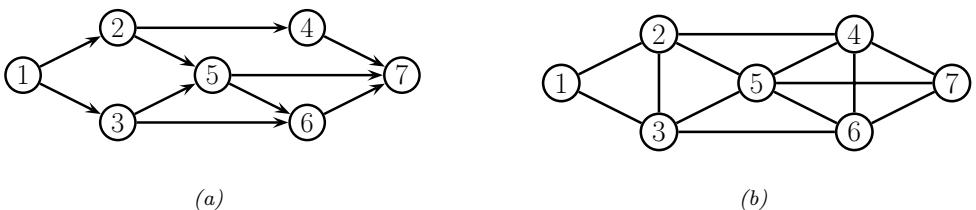
Figure 4.23: (a) A DPGM. (b) Its moralized version, represented as a UPGM.

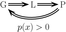
Figure 4.24: Relationship between Markov properties of UPGMs.

Figure 4.23(b), we have that {X1, X2} ℜ {X6, X7}|{X3, X4, X5}.

The smallest set of nodes that renders a node t conditionally independent of all the other nodes in the graph is called t’s Markov blanket; we will denote this by mb(t). Formally, the Markov blanket satisfies the following property:

\[t \perp \mathcal{V} \ll (t) |\text{mb}(t)|\tag{4.115}\]

where cl(t) ↭ mb(t) ↘ {t} is the closure of node t, and V = {1,…,NG} is the set of all nodes. One can show that, in a UPGM, a node’s Markov blanket is its set of immediate neighbors. This is called the undirected local Markov property. For example, in Figure 4.23(b), we have mb(X5) = {X2, X3, X4, X6, X7}.

From the local Markov property, we can easily see that two nodes are conditionally independent given the rest if there is no direct edge between them. This is called the pairwise Markov property. In symbols, this is written as

\[s \perp t | \mathcal{V} \backslash \{s, t\} \iff G\_{st} = 0 \tag{4.116}\]

where Gst = 0 means there is no edge between s and t (so there is a 0 in the adjaceny matrix).

Using the three Markov properties we have discussed, we can derive the following CI properties (amongst others) from the UPGM in Figure 4.23(b): X¹ ℜ X7|rest (pairwise); X¹ ℜ rest|X2, X³ (local); X1, X² ℜ X6, X7|X3, X4, X⁵ (global).

It is obvious that global Markov implies local Markov which implies pairwise Markov. What is less obvious is that pairwise implies global, and hence that all these Markov properties are the same, as illustrated in Figure 4.24 (see e.g., [KF09a, p119] for a proof).8 The importance of this result is that it is usually easier to empirically assess pairwise conditional independence; such pairwise CI statements can be used to construct a graph from which global CI statements can be extracted.

^8. This assumes p(x) > 0 for all x, i.e., that p is a positive density. The restriction to positive densities arises because

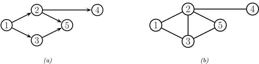
Figure 4.25: (a) The ancestral graph induced by the DAG in Figure 4.23(a) wrt U = {X2, X4, X5}. (b) The moralized version of (a).

4.3.6.2 An undirected alternative to d-separation

We have seen that determinining CI relationships in UPGMs is much easier than in DPGMs, because we do not have to worry about the directionality of the edges. That is, we can use simple graph separation, instead of d-separation.

In this section, we show how to convert a DPGM to a UPGM, so that we can infer CI relationships for the DPGM using simple graph separation. It is tempting to simply convert the DPGM to a UPGM by dropping the orientation of the edges, but this is clearly incorrect, since a v-structure A → B ∈ C has quite di!erent CI properties than the corresponding undirected chain A ⇐ B ⇐ C (e.g., the latter graph incorrectly states that A ℜ C|B). To avoid such incorrect CI statements, we can add edges between the “unmarried” parents A and C, and then drop the arrows from the edges, forming (in this case) a fully connected undirected graph. This process is called moralization. Figure 4.23 gives a larger example of moralization: we interconnect 2 and 3, since they have a common child 5, and we interconnect 4, 5, and 6, since they have a common child 7.

Unfortunately, moralization loses some CI information, and therefore we cannot use the moralized UPGM to determine CI properties of the DPGM. For example, in Figure 4.23(a), using d-separation, we see that X⁴ ℜ X5|X2. Adding a moralization arc X⁴ ⇐X⁵ would lose this fact (see Figure 4.23(b)). However, notice that the 4-5 moralization edge, due to the common child 7, is not needed if we do not observe 7 or any of its descendants. This suggests the following approach to determining if A ℜ B|C. First we form the ancestral graph of DAG G with respect to U = A ↘ B ↘ C. This means we remove all nodes from G that are not in U or are not ancestors of U. We then moralize this ancestral graph, and apply the simple graph separation rules for UPGMs. For example, in Figure 4.25(a), we show the ancestral graph for Figure 4.23(a) using U = {X2, X4, X5}. In Figure 4.25(b), we show the moralized version of this graph. It is clear that we now correctly conclude that X⁴ ℜ X5|X2.

4.3.7 Generation (sampling)

Unlike with DPGMs, it can be quite slow to sample from an UPGM, even from the unconditional prior, because there is no ordering of the variables. Furthermore, we cannot easily compute the probability of any configuration unless we know the value of Z. Consequently it is common to use

deterministic constraints can result in independencies present in the distribution that are not explicitly represented in the graph. See e.g., [KF09a, p120] for some examples. Distributions with non-graphical CI properties are said to be unfaithful to the graph, so I(p) ↔︎= I(G).

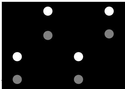
Figure 4.26: A grid-structured MRF with hidden nodes zⁱ and local evidence nodes xi. The prior p(z) is an undirected Ising model, and the likelihood ^p(x|z) = ” ⁱ p(xi|zi) is a directed fully factored model.

MCMC methods for generating from an UPGM (see Chapter 12).

In the special case of UPGMs with low treewidth and discrete or Gaussian potentials, it is possible to use the junction tree algorithm to draw samples using dynamic programming (see Supplementary Section 9.2.3).

4.3.8 Inference

We discuss inference in graphical models in detail in Chapter 9. In this section, we just give an example.

Suppose we have an image composed of binary pixels, zi, but we only observe noisy versions of the pixels, xi. We assume the joint model has the form

\[p(\mathbf{z}, \mathbf{z}) = p(\mathbf{z})p(\mathbf{z}|\mathbf{z}) = \left[\frac{1}{Z} \sum\_{i \sim j} \psi\_{ij}(z\_i, z\_j)\right] \prod\_i p(x\_i|z\_i) \tag{4.117}\]

where ^p(z) is an Ising model prior, and ^p(xi|zi) = ^N (xi|zi, ^ε2), for ^{zi ↑} {⇐1, +1}. This model uses a UPGM as a prior, and has directed edges for the likelihood, as shown in Figure 4.26; such a hybrid undirected-directed model is called a chain graph (even though it is not chain-structured).

The inference task is to compute the posterior marginals p(zi|x), or the posterior MAP estimate, argmax^z p(z|x). The exact computation is intractable for large grids (for reasons explained in Section 9.5.4), so we must use approximate methods. There are many algorithms that we can use, including mean field variational inference (Section 10.3.2), Gibbs sampling (Section 12.3.3), loopy belief propagation (Section 9.4), etc. In Figure 4.27, we show the results of variational inference.

4.3.9 Learning

In this section, we discuss how to estimate the parameters for an MRF. As we will see, computing the MLE can be computationally expensive, even in the fully observed case, because of the need to deal with the partition function Z(ω). And computing the posterior over the parameters, p(ω|D), is even harder, because of the additional normalizing constant p(D) — this case has been called doubly intractable [MGM06]. Consequently we will focus on point estimation methods such as

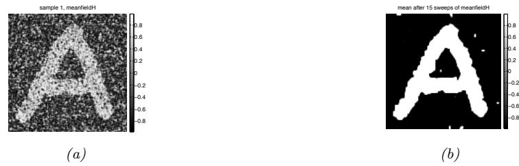
Figure 4.27: Example of image denoising using mean field variational inference. We use an Ising prior with Wij = 1 and a Gaussian noise model with ϑ = 2. (a) Noisy image. (b) Result of inference. Generated by ising\_image\_denoise\_demo.ipynb.

MLE and MAP. (For one approach to Bayesian parameter inference in an MRF, based on persistent variational inference, see [IM17].)

4.3.9.1 Learning from complete data

We will start by assuming there are no hidden variables or missing data during training (this is known as the complete data setting). For simplicity of presentation, we restrict our discusssion to the case of MRFs with log-linear potential functions. (See Section 24.2 for the general nonlinear case, where we discuss MLE for energy-based models.)

In particular, we assume the distribution has the following form:

\[p(x|\theta) = \frac{1}{Z(\theta)} \exp\left(\sum\_{c} \theta\_c^\mathrm{T} \phi\_c(x)\right) \tag{4.118}\]

where c indexes the cliques. The (averaged) log-likelihood of the full dataset becomes

\[\ell(\boldsymbol{\theta}) \triangleq \frac{1}{N} \sum\_{n} \log p(\boldsymbol{x}\_{n}|\boldsymbol{\theta}) = \frac{1}{N} \sum\_{n} \left[ \sum\_{c} \theta\_{c}^{\mathsf{T}} \phi\_{c}(\boldsymbol{x}\_{n}) - \log Z(\boldsymbol{\theta}) \right] \tag{4.119}\]

Its gradient is given by

\[\frac{\partial \ell}{\partial \theta\_c} = \frac{1}{N} \sum\_n \left[ \phi\_c(\mathbf{x}\_n) - \frac{\partial}{\partial \theta\_c} \log Z(\theta) \right] \tag{4.120}\]

We know from Section 2.4.3 that the derivative of the log partition function wrt ω^c is the expectation of the c’th feature vector under the model, i.e.,

\[\frac{\partial \log Z(\theta)}{\partial \theta\_c} = \mathbb{E}\left[\phi\_c(x)|\theta\right] = \sum\_{x} p(x|\theta)\phi\_c(x) \tag{4.121}\]

Hence the gradient of the log likelihood is

\[\frac{\partial \ell}{\partial \theta\_c} = \frac{1}{N} \sum\_n \left[ \phi\_c(\mathbf{z}\_n) \right] - \mathbb{E} \left[ \phi\_c(\mathbf{z}) \right] \tag{4.122}\]

When the expected value of the features according to the data is equal to the expected value of the features according to the model, the gradient will be zero, so we get

\[\mathbb{E}\_{\rm p\mathbb{D}}\left[\phi\_c(\mathbf{z})\right] = \mathbb{E}\_{p(\mathbf{z}|\boldsymbol{\theta})}\left[\phi\_c(\mathbf{z})\right] \tag{4.123}\]

This is called moment matching. Evaluating the Ep^D [ϱc(x)] term is called the clamped phase or positive phase, since x is set to the observed values xn; evaluating the Ep(x|ϑ) [ϱc(x)] term is called the unclamped phase or negative phase, since x is free to vary, and is generated by the model.

In the case of MRFs with tabular potentials (i.e., one feature per entry in the clique table), we can use an algorithm called iterative proportional fitting or IPF [Fie70; BFH75; JP95] to solve these equations in an iterative fashion.9 But in general, we must use gradient methods to perform parameter estimation.

4.3.9.2 Computational issues

The biggest computational bottleneck in fitting MRFs and CRFs using MLE is the cost of computing the derivative of the log partition function, log Z(ω), which is needed to compute the derivative of the log likelihood, as we saw in Section 4.3.9.1. To see why this is slow to compute, note that

\[\nabla\_{\theta} \log Z(\theta) = \frac{\nabla\_{\theta} Z(\theta)}{Z(\theta)} = \frac{1}{Z(\theta)} \nabla\_{\theta} \int \bar{p}(x;\theta) dx = \frac{1}{Z(\theta)} \int \nabla\_{\theta} \bar{p}(x;\theta) dx \tag{4.124}\]

\[=\frac{1}{Z(\boldsymbol{\theta})}\int \bar{p}(\boldsymbol{x};\boldsymbol{\theta})\nabla\_{\boldsymbol{\theta}}\log\bar{p}(\boldsymbol{x};\boldsymbol{\theta})d\boldsymbol{x} = \int \frac{\bar{p}(\boldsymbol{x};\boldsymbol{\theta})}{Z(\boldsymbol{\theta})}\nabla\_{\boldsymbol{\theta}}\log\bar{p}(\boldsymbol{x};\boldsymbol{\theta})d\boldsymbol{x} \tag{4.125}\]

\[\mathbf{E} = \mathbb{E}\_{\mathbf{z} \sim p(\mathbf{z}; \boldsymbol{\theta})} \left[ \nabla \theta \, \log \tilde{p}(\mathbf{z}; \boldsymbol{\theta}) \right] \tag{4.126}\]

where in Equation (4.125) we used the fact that ▽^ϑ log ˜p(x; ^ω) = ^{1 p}˜(x;ϑ)▽ϑp˜(x; ω) (this is known as the log-derivative trick). Thus we see that we need to draw samples from the model at each step of SGD training, just to estimate the gradient.

In Section 24.2.1, we discuss various e”cient sampling methods. However, it is also possible to use alternative estimators which do not use the principle of maximum likelihood. For example, in Section 24.2.2 we discuss the technique of contrastive divergence. And in Section 4.3.9.3, we discuss the technique of pseudolikelihood. (See also [Sto17] for a review of many methods for parameter estimation in MRFs.)

4.3.9.3 Maximum pseudolikelihood estimation

When fitting fully visible MRFs (or CRFs), a simple alternative to maximizing the likelihood is to maximize the pseudo likelihood [Bes75], defined as follows:

\[\ell \, \ell\_{PL}(\boldsymbol{\theta}) \triangleq \frac{1}{N} \sum\_{n=1}^{N} \sum\_{d=1}^{D} \log p(x\_{nd} | \boldsymbol{x}\_{n,-d}, \boldsymbol{\theta}) \tag{4.127}\]

^9. In the case of decomposable graphs, IPF converges in a single iteration. Intuitively, this is because a decomposable graph can be converted to a DAG without any loss of information, as explained in Section 4.5, and we know that we can compute the MLE for tabular CPDs in closed form, just by normalizing the counts.

Figure 4.28: (a) A small 2d lattice. (b) The representation used by pseudo likelihood. Solid nodes are observed neighbors. Adapted from Figure 2.2 of [Car03].

That is, we optimize the product of the full conditionals, also known as the composite likelihood [Lin88a; DL10; VRF11]. Compare this to the objective for maximum likelihood:

\[\ell\_{ML}(\boldsymbol{\theta}) = \frac{1}{N} \sum\_{n=1}^{N} \log p(\boldsymbol{x}\_n | \boldsymbol{\theta}) \tag{4.128}\]

In the case of Gaussian MRFs, PL is equivalent to ML [Bes75], although this is not true in general. Nevertheless, it is a consistent estimator in the large sample limit [LJ08].

The PL approach is illustrated in Figure 4.28 for a 2d grid. We learn to predict each node, given all of its neighbors. This objective is generally fast to compute since each full conditional p(xd|x↑^d, ω) only requires summing over the states of a single node, xd, in order to compute the local normalization constant. The PL approach is similar to fitting each full conditional separately, except that, in PL, the parameters are tied between adjacent nodes.

Experiments in [PW05; HT09] suggest that PL works as well as exact ML for fully observed Ising models, but is much faster. In [Eke+13], they use PL to fitt Potts models to (aligned) protein sequence data. However, when fitting RBMs, [Mar+10] found that PL is worse than some of the stochastic ML methods we discuss in Section 24.2.

Another more subtle problem is that each node assumes that its neighbors have known values during training. If node j ↑ nbr(i) is a perfect predictor for node i (where nbr(i) is the set of neighbors), then j will learn to rely completely on node i, even at the expense of ignoring other potentially useful information, such as its local evidence, say yi. At test time, the neighboring nodes will not be observed, and performance will su!er.10

4.3.9.4 Learning from incomplete data

In this section, we consider parameter estimation for MRFs (and CRFs) with hidden variables. Such incomplete data can arise for several reasons. For example, we may want to learn a model of the form p(z)p(x|z) which lets us infer a “clean” image z from a noisy or corrupted version x. If we only observe x, the model is called a hidden Gibbs random field. See Section 10.3.2 for an

^10. Geo! Hinton has an analogy for this problem. Suppose we want to learn to denoise images of symmetric shapes, such as Greek vases. Each hidden pixel xⁱ depends on its spatial neighbors, as well the noisy observation yi. Since its symmetric counterpart x^j will perfectly predict xi, the model will ignore yⁱ and just rely on x^j , even though x^j will not be available at test time.

example. As another example, we may have a CRF in which the hidden variables are used to encode an unknown alignment between the inputs and outputs [Qua+07], or to model missing parts of the input [SRS10].

We now discuss how to compute the MLE in such cases. For notational simplicity, we focus on unconditional models (MRFs, not CRFs), and we assume all the potentials are log-linear. In this case, the model has the following form:

\[p(x, z | \theta) = \frac{\exp(\theta^{\mathbb{T}} \phi(x, z))}{Z(\theta)} = \frac{\bar{p}(x, z | \theta)}{Z(\theta)}\tag{4.129}\]

\[Z(\boldsymbol{\theta}) = \sum\_{\mathbf{z}, \mathbf{z}} \exp(\boldsymbol{\theta}^{\mathsf{T}} \boldsymbol{\phi}(\boldsymbol{x}, \boldsymbol{z})) \tag{4.130}\]

where p˜(x, z|ω) is the unnormalized distribution. We have dropped the sum over cliques c for brevity.

The log likelihood is now given by

\[\ell(\boldsymbol{\theta}) = \frac{1}{N} \sum\_{n=1}^{N} \log \left( \sum\_{\mathbf{z}\_n} p(\mathbf{z}\_n, \mathbf{z}\_n | \boldsymbol{\theta}) \right) \tag{4.131}\]

\[\hat{\mathbf{z}}\_{n} = \frac{1}{N} \sum\_{n=1}^{N} \log \left( \frac{1}{Z(\boldsymbol{\theta})} \sum\_{\mathbf{z}\_{n}} \bar{p}(\mathbf{z}\_{n}, \mathbf{z}\_{n} | \boldsymbol{\theta}) \right) \tag{4.132}\]

\[\hat{\rho} = \frac{1}{N} \sum\_{n=1}^{N} \left[ \log \sum\_{\mathbf{z}\_n} \bar{p}(\mathbf{z}\_n, \mathbf{z}\_n | \boldsymbol{\theta}) \right] - \log Z(\boldsymbol{\theta}) \tag{4.133}\]

Note that

\[\log \sum\_{\mathbf{z}\_n} \bar{p}(\mathbf{z}\_n, \mathbf{z}\_n | \boldsymbol{\theta}) = \log \sum\_{\mathbf{z}\_n} \exp(\boldsymbol{\theta}^\mathsf{T} \boldsymbol{\phi}(\mathbf{z}\_n, \mathbf{z}\_n)) \stackrel{\scriptstyle \Delta}{=} \log Z(\boldsymbol{\theta}, \mathbf{z}\_n) \tag{4.134}\]

where Z(ω, xn) is the same as the partition function for the whole model, except that x is fixed at xn. Thus the log likelihood is a di!erence of two partition functions, one where x is clamped to xⁿ and z is unclamped, and one where both x and z are unclamped. The gradient of these log partition functions corresponds to the expected features, where (in the clamped case) we condition on x = xn. Hence

\[\frac{\partial \ell}{\partial \theta} = \frac{1}{N} \sum\_{n} \left[ \mathbb{E}\_{\mathbf{z} \sim p(\mathbf{z}|\mathbf{z}, \mathbf{z})} \left[ \phi(x\_n, \mathbf{z}) \right] \right] - \mathbb{E}\_{(\mathbf{z}, \mathbf{z}) \sim p(\mathbf{z}, \mathbf{z}|\theta)} \left[ \phi(\mathbf{z}, \mathbf{z}) \right] \tag{4.135}\]

4.4 Conditional random fields (CRFs)

A conditional random field or CRF [LMP01] is a Markov random field defined on a set of related label nodes y, whose joint probability is predicted conditional on a fixed set of input nodes x. More precisely, it corresponds to a model of the following form:

\[p(y|x,\theta) = \frac{1}{Z(x,\theta)} \prod\_{c} \psi\_c(y\_c; x, \theta) \tag{4.136}\]

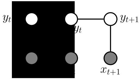
Figure 4.29: A 1d conditional random field (CRF) for sequence labeling.

(Note how the partition function now depends on the inputs x as well as the parameters ω.) Now suppose the potential functions are log-linear and have the form

\[ \psi\_c(\mathbf{y}\_c; \mathbf{z}, \boldsymbol{\theta}) = \exp(\boldsymbol{\theta}\_c^\mathsf{T} \boldsymbol{\phi}\_c(\mathbf{z}, \mathbf{y}\_c)) \tag{4.137} \]

This is a conditional version of the maxent models we discussed in Section 4.3.4. Of course, we can also use nonlinear potential functions, such as DNNs.

CRFs are useful because they capture dependencies amongst the output labels. They can therefore be used for structured prediction, where the output y ↑ Y that we want to predict given the input x lives in some structured space, such as a sequence of labels, or labels associated with nodes on a graph. In such problems, there are often constraints on the set of valid values of the output y. For example, if we want to perform sentence parsing, the output should satisfy the rules of grammar (e.g., noun phrase must precede verb phrase). See Section 4.4.1 for details on the application of CRFs to NLP. In some cases, the “constraints” are “soft”, rather than “hard”. For example, if we want to associate a label with each pixel in an image (a task called semantic segmentation), we might want to “encourage” the label at one location to be the same as its neighbors, unless the visual input strongly suggests a change in semantic content at this location (e.g., at the edge of an object). See Section 4.4.2 for details on the applications of CRFs to computer vision tasks.

4.4.1 1d CRFs

In this section, we focus on 1d CRFs defined on chain-structured graphical models. The graphical model is shown in Figure 4.29. This defines a joint distribution over sequences, y1:^T , given a set of inputs, x1:^T , as follows:

\[p(\mathbf{y}\_{1:T}|x,\boldsymbol{\theta}) = \frac{1}{Z(\mathbf{z},\boldsymbol{\theta})} \prod\_{t=1}^{T} \psi(y\_t, \mathbf{z}\_t; \boldsymbol{\theta}) \prod\_{t=2}^{T} \psi(y\_{t-1}, y\_t; \boldsymbol{\theta}) \tag{4.138}\]

where 5(yt, xt; ω) are the node potentials and 5(yt, yt+1; ω) are the edge potentials. (We have assumed that the edge potentials are independent of the input x, but this assumption is not required.)

Note that one could also consider an alternative way to define this conditional distribution, by

Green chairs the finance committee

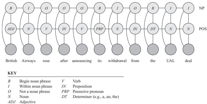
Within location name Not an entitiy

B-PER I-PER OTH OTH OTH B-LOC I-LOC B-PER OTH OTH OTH OTH

Mrs. Green spoke today in New York

I-LOC OTH

2. Figure 4.30: A CRF for joint part of speech tagging and noun phrase segmentation. From Figure 4.E.1 of [KF09a]. Used with kind permission of Daphne Koller.

using a discriminative directed Markov chain:

KEY

B-PER I-PER B-LOC Begin person name Within person name Begin location name

\[p(y\_{1:T}|x,\theta) = p(y\_1|x\_1;\theta) \prod\_{t=2}^{T} p(y\_t|y\_{t-1},x\_t;\theta) \tag{4.139}\]

This is called a maximum entropy Markov model [MFP00]. However, it su!ers from a subtle flaw compared to the CRF. In particular, in the directed model, each conditional p(yt|y^t↑¹, xt; ω), is locally normalized, whereas in the CRF, the model is globally normalized due to the Z(x, ω) term. The latter allows information to propagate through the entire sequence, as we discuss in more detail in Section 4.5.3.

CRFs were widely used in the natural language processing (NLP) community in the 1980s–2010s (see e.g., [Smi11]), although recently they have been mostly replaced by RNNs and transformers (see e.g., [Gol17]). Fortunately, we can get the best of both worlds by combining CRFs with DNNs, which allows us to combine data driven techniques with prior knowledge about constraints on the label space. We give some examples below.

4.4.1.1 Noun phrase chunking

A common task in NLP is information extraction, in which we try to parse a sentence into noun phrases (NP), such as names and addresses of people or businesses, as well as verb phrases, which describe who is doing what to whom (e.g., “British Airways rose”). In order to tackle this task, we can assign a part of speech tag to each word, where the tags correspond to Noun, Verb, Adjective, etc. In addition, to extract the span of each noun phrase, we can annotate words as being at the beginning (B) or inside (I) of a noun phrase, or outside (O) of one. See Figure 4.30 for an example.

The connections between adjacent labels can encode constraints such as the fact that B (begin) must precede I (inside). For example, the sequences OBIIO and OBIOBIO are valid (corresponding to one NP of 3 words, and two adjacent NPs of 2 words), but OIBIO is not. This prior information can be encoded by defining 5(yBIO ^t↑^{1 = ∋}, yBIO ^t = B, xt; ω) to be 0 for any value of * except O. We can encode similar grammatical rules for the POS tags.

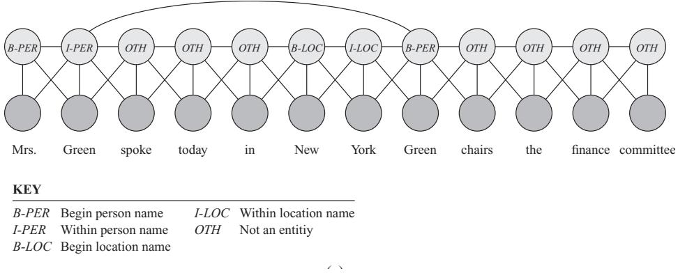
Figure 4.31: A skip-chain CRF for named entity recognition. From Figure 4.E.1 of [KF09a]. Used with kind permission of Daphne Koller.

B I NP

B I O O O B I O I

ADJ N V IN V PRP N IN DT N N POS Given this model, we can compute the MAP sequence of labels, and thereby extract the spans that are labeled as noun phrases. This is called noun phrase chunking.

4.4.1.2 Named entity recognition

Airways rose after announcing its withdrawal from the UAL British deal Begin noun phrase Within noun phrase Not a noun phrase Noun B I O N Verb Preposition Possesive pronoun Determiner (e.g., a, an, the) V IN PRP DT KEY In this section we consider the task of named entity extraction, in which we not only tag the noun phrases, but also classify them into di!erent types. A simple approach to this is to extend the BIO notation to {B-Per, I-Per, B-Loc, I-Loc, B-Org, I-Org, Other}. However, sometimes it is ambiguous whether a word is a person, location, or something else. Proper nouns are particularly di”cult to deal with because they belong to an open class, that is, there is an unbounded number of possible names, unlike the set of nouns and verbs, which is large but essentially fixed. For example, “British Airways” is an organization, but “British Virgin Islands” is a location.

2. Adjective ADJ We can get better performance by considering long-range correlations between words. For example, we might add a link between all occurrences of the same word, and force the word to have the same tag in each occurence. (The same technique can also be helpful for resolving the identity of pronouns.) This is known as a skip-chain CRF. See Figure 4.31 for an illustration, where we show that the word “Green” is interpeted as a person in both occurrences within the same sentence.

We see that the graph structure itself changes depending on the input, which is an additional advantage of CRFs over generative models. Unfortunately, inference in this model is generally more expensive than in a simple chain with local connections because of the larger treewdith (see Section 9.5.2).

4.4.1.3 Natural language parsing

A generalization of chain-structured models for language is to use probabilistic grammars. In particular, a probabilistic context free grammar or PCFG in Chomsky normal form is a set of re-write or production rules of the form ε → ε^↔︎ ε↔︎↔︎ or ε → x, where ε, ε^↔︎ , ε↔︎↔︎ ↑ $ are non-terminals (analogous to parts of speech), and x ↑ X are terminals, i.e., words. Each such rule has an associated probability. The resulting model defines a probability distribution over sequences of words. We can

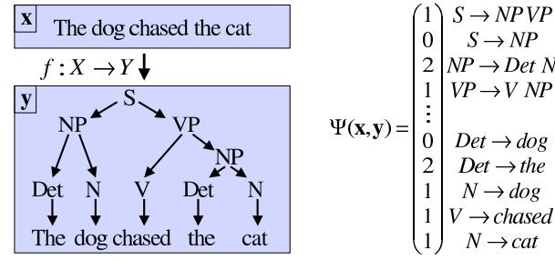
efficient computation of the discriminant function, which in the case of (1.5) is given by ! “lx # ! l”x−1 # Figure 4.32: Illustration of a simple parse tree based on a context free grammar in Chomsky normal form. The feature vector !(x, y) counts the number of times each production rule was used, and is used to define the energy of a particular tree structure, ^E(y|x) = ^↓w^T!(x, ^y). The probability distribution over trees is given by p(y|x) ⇐ exp(↓E(y|x)). From Figure 5.2 of [AHT07]. Used with kind permission of Yasemin Altun.

(y^t )

• η

wll,

Λc (y^t ) ^{⊗ Λ}c(yt+1)

, y¯s)δ(yt+1, ys+1).

). Let us consider a

, (1.6)

(1.7)

Figure 1.2 Natural language parsing.

wol,

1.2.3 Weighted Context-Free Grammars

of grammar rules generating a given sequence x = (x¹, …, x^l

Φ(x^t

F(x, y; w) =

#Ψ(x, y), Ψ(x”

, y”

Figure 4.33: A grid-structured CRF with label nodes yⁱ and local evidence nodes xi.

Parsing is the task of predicting a labeled tree y that is a particular configuration

context-free grammar in Chomsky Normal Form. The rules of this grammar are of

the form σ → σ” σ”“, or σ → x, where σ, σ” , σ”” ∈ Σ are non-terminals, and x ∈ T are terminals. Similar to the sequence case, we define the joint feature map Ψ(x, y) to contain features representing inter-dependencies between labels of the nodes of the compute the probability of observing a particular sequence x = x¹ …x^T by summing over all trees that generate it. This can be done in O(T³) time using the inside-outside algorithm; see e.g., [JM08; MS99; Eis16] for details.

tree (e.g. ^ψσ→σ!σ!! via ^Λc(yrs) ^{⊗ Λc}(yrt ) ^{⊗ Λc}(y(t+1)^s)) and features representing the dependence of labels to observations (e.g. ψ^σ→^τ via Φ^c(x^t ) ^{⊗ Λc}(y^t )). Here yrs denotes the label of the root of a subtree spanning from x^r to x^s. This definition leads to equations similar to (1.5), (1.6) and (1.7). Extensions to this representation is possible, for example by defining higher order features that can be induced using kernel functions over sub-trees (Collins and Duffy, 2002). PCFGs are generative models. It is possible to make discriminative versions which encode the probability of a labeled tree, y, given a sequence of words, x, by using a CRF of the form ^p(y|x) ↙ exp(w^T‘(x, ^y)). For example, we might define’(x, ^y) to count the number of times each production rule was used (which is analogous to the number of state transitions in a chain-structured model), as illustrated in Figure 4.32. We can also use a deep neural net to define the features, as in the neural CRF parser method of [DK15b].

4.4.2 2d CRFs

2006/08/03 14:15

It is also possible to apply CRFs to image processing problems, which are usually defined on 2d grids, as illustrated in Figure 4.33. (Compare this to the generative model in Figure 4.26.) This

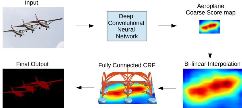
Figure 4.34: A fully connected CRF is added to the output of a CNN, in order to increase the sharpness of the segmentation boundaries. From Figure 3 of [Che+15]. Used with kind permission of Jay Chen.

corresponds to the following conditional model:

\[p(y|x) = \frac{1}{Z(x)} \left[ \sum\_{i \sim j} \psi\_{ij}(y\_i, y\_j) \right] \prod\_i p(y\_i|x\_i) \tag{4.140}\]

In the sections below, we discuss some applications of this and other CRF models in computer vision.

4.4.2.1 Semantic segmentation

The task of semantic segmentation is to assign a label to every pixel in an image. We can easily solve this problem using a CNN with one softmax output node per pixel. However, this may fail to capture long-range dependencies, since convolution is a local operation.

One way to get better results is to feed the output of the CNN into a CRF. Since the CNN already uses convolution, its outputs will usually already be locally smooth, so the benefits from using a CRF with a local grid structure may be quite small. However, we can somtimes get better results if we use a fully connected CRF, which has connections between all the pixels. This can capture long range connections which the grid-structured CRF cannot. See Figure 4.34 for an illustration, and [Che+17a] for details.

Unfortunately, exact inference in a fully connected CRF is intractable, but in the case of Gaussian potentials, it is possible to devise an e”cient mean field algorithm, as described in [KK11]. Interestingly, [Zhe+15] showed how the mean field update equations can be implemented using a recurrent neural network (see Section 16.3.4), allowing end-to-end training. Alternatively, if we are willing to use a finite number of iterations, we can just “unroll” the computation graph and treat it as a fixed-sized feedforward circuit. The result is a graph-structured neural network, where the topology of the GNN is derived from the graphical model (cf., Section 9.4.10). The advantage of this compared to standard CRF methods is that we can train this entire model end-to-end using standard gradient descent methods; we no longer have to worry about the partition function (see Section 4.4.3), or the lack of convergence that can arise when combining approximate inference with standard CRF learning.

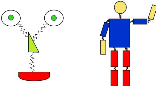
Figure 4.35: Pictorial structures model for a face and body. Each body part corresponds to a node in the CRF whose state space represents the location of that part. The edges (springs) represent pairwise spatial constraints. The local evidence nodes are not shown. Adapted from a figure by Pedro Felzenszwalb.

4.4.2.2 Deformable parts models

Consider the problem of object detection, i.e., finding the location(s) of an object of a given class (e.g., a person or a car) in an image. One way to tackle this is to train a binary classifier that takes as input an image patch and specifies if the patch contains the object or not. We can then apply this to every image patch, and return the locations where the classifier has high confidence detections; this is known as a sliding window detector, and works quite well for rigid objects such as cars or frontal faces. Such an approach can be made e”cient by using convolutional neural networks (CNNs); see Section 16.3.2 for details.

However, such methods can work poorly when there is occlusion, or when the shape is deformable, such as a person’s or animal’s body, because there is too much variation in the overall appearance. A natural strategy to deal with such problems is break the object into parts, and then to detect each part separately. But we still need to enforce spatial coherence of the parts. This can be done using a pairwise CRF, where node yⁱ specifies the location of part i in the image (assuming it is present), and where we connect adjacent parts by a potential function that encourages them to be close together. For example, we can use a pairwise potential of the form 5(yi, y^j |x) = exp(⇐d(yi, y^j )), where yⁱ ↑ {1,…,K} is the location of part i (a discretization of the 2d image plane), and d(yi, y^j ) is the distance between parts i and j. (We can make this “distance” also depend on the inputs x if we want, for example we may relax the distance penalty if we detect an edge.) In addition we will have a local evidence term of the form p(yi|x), which can be any kind of discriminative classifier, such as a CNN, which predicts the distribution over locations for part i given the image x. The overall model has the form

\[p(y|\mathbf{z}) = \frac{1}{Z(\mathbf{z})} \left[ \prod\_{i} p(y\_i|f(\mathbf{z})\_i) \right] \left[ \prod\_{(i,j)\in E} \psi(y\_i, y\_j|\mathbf{z}) \right] \tag{4.141}\]

where E is the set of edges in the CRF, and f(x)ⁱ is the i’th output of the CNN.

We can think of this CRF as a series of parts connected by springs, where the energy of the system increases if the parts are moved too far from their expected relative distance. This is illustrated in Figure 4.35. The resulting model is known as a pictorial structure [FE73], or deformable parts

model [Fel+10]. Furthermore, since this is a conditional model, we can make the spring strengths be image dependent.

We can find the globally optimal joint configuration y↘ = argmax^y p(y|x, ω) using brute force enumeration in O(K^T ) time, where T is the number of nodes and K is the number of states (locations) per node. While T is often small, (e.g., just 10 body parts in Figure 4.35), K is often very large, since there are millions of possible locations in an image. By using tree-structured graphs, exact inference can be done in O(TK²) time, as we explain in Section 9.3.2. Furthermore, by exploiting the fact that the discrete states are ordinal, inference time can be further reduced to O(TK), as explained in [Fel+10].

Note that by “augmenting” standard deep neural network libaries with a dynamic programming inference “module”, we can represent DPMs as a kind of CNN, as shown in [Gir+15]. The key property is that we can backpropagate gradients through the inference algorithm.

4.4.3 Parameter estimation

In this section, we discuss how to perform maximum likelihood estimation for CRFs. This is a small extension of the MRF case in Section 4.3.9.1.

4.4.3.1 Log-linear potentials

In this section we assume the log potential functions are linear in the parameters, i.e.,

\[\psi\_c(y\_c; x, \theta) = \exp(\theta\_c^\top \phi\_c(x, y\_c)) \tag{4.142}\]

Hence the log likelihood becomes

\[\ell(\boldsymbol{\theta}) \triangleq \frac{1}{N} \sum\_{n} \log p(\boldsymbol{y}\_n | \boldsymbol{x}\_n, \boldsymbol{\theta}) = \frac{1}{N} \sum\_{n} \left[ \sum\_{c} \theta\_c^\top \phi\_c(\boldsymbol{y}\_{nc}; \boldsymbol{x}\_n) - \log Z(\boldsymbol{x}\_n; \boldsymbol{\theta}) \right] \tag{4.143}\]

where

\[Z(x\_n; \boldsymbol{\theta}) = \sum\_{\mathbf{y}} \exp(\boldsymbol{\theta}^\top \boldsymbol{\phi}(\boldsymbol{y}, \boldsymbol{x}\_n)) \tag{4.144}\]

is the partition function for example n.

We know from Section 2.4.3 that the derivative of the log partition function yields the expected su”cient statistics, so the gradient of the log likelihood can be written as follows:

\[\frac{\partial \ell}{\partial \theta\_c} = \frac{1}{N} \sum\_n \left[ \phi\_c(y\_{nc}, x\_n) - \frac{\partial}{\partial \theta\_c} \log Z(x\_n; \theta) \right] \tag{4.145}\]

\[=\frac{1}{N}\sum\_{n}\left[\phi\_{c}(y\_{nc},x\_{n})-\mathbb{E}\_{p(\mathbf{y}|\mathbf{z}\_{n},\boldsymbol{\theta})}\left[\phi\_{c}(\mathbf{y},\mathbf{z}\_{n})\right]\right] \tag{4.146}\]

Since the objective is convex, we can use a variety of solvers to find the MLE, such as the stochastic meta descent method of [Vis+06], which is a variant of SGD where the stepsize is adapted automatically.

4.4.3.2 General case

In the general case, a CRF can be written as follows:

\[p(\mathbf{y}|x;\theta) = \frac{\exp(f(x,y;\theta))}{Z(x;\theta)} = \frac{\exp(f(x,y;\theta))}{\sum\_{y'} \exp(f(x,y';\theta))}\tag{4.147}\]

where f(x, y; ω) is a scoring (negative energy) function, where high scores correspond to probable configurations. The gradient of the log likelihood is

\[\nabla\_{\theta}\ell(\theta) = \frac{1}{N} \sum\_{n=1}^{N} \nabla\_{\theta}f(x\_n, y\_n; \theta) - \nabla\_{\theta}\log Z(x\_n; \theta) \tag{4.148}\]

Computing derivatives of the log partition function is tractable provided we can compute the corresponding expectations, as we discuss in Section 4.3.9.2. Note, however, that we need to compute these derivatives for every training example, which is slower than the MRF case, where the log partition function is a constant independent of the observed data (but dependent on the model parameters).

4.4.4 Other approaches to structured prediction

Many other approaches to structured prediction have been proposed, going beyond CRFs. For example, max margin Markov networks [TGK03], and the closely relayed structural support vector machine [Tso+05], can be seen as non-probabilistic alternatives to CRFs. More recently, [BYM17] proposed structured prediction energy networks, which are a form of energy based model (Chapter 24), where we predict using an optimization procedure, yˆ(x) = argmin E(x, y). In addition, it is common to use graph neural networks (Section 16.3.6) and sequence-to-sequence models such as transformers (Section 16.3.5) for this task.

4.5 Comparing directed and undirected PGMs

In this section, we compare DPGMs and UPGMs in terms of their modeling power, we discuss how to convert from one to the other, and we and present a unified representation.

4.5.1 CI properties

Which model has more “expressive power”, a DPGM or a UPGM? To formalize the question, recall from Section 4.2.4 that G is an I-map of a distribution p if I(G) ↓ I(p), meaning that all the CI statements encoded by the graph G are true of the distribution p. Now define G to be perfect map of p if I(G) = I(p), in other words, the graph can represent all (and only) the CI properties of the distribution. It turns out that DPGMs and UPGMs are perfect maps for di!erent sets of distributions (see Figure 4.36). In this sense, neither is more powerful than the other as a representation language.

As an example of some CI relationships that can be perfectly modeled by a DPGM but not a UPGM, consider a v-structure A → C ∈ B. This asserts that A ℜ B, and A ⇓ℜ B|C. If we drop the arrows, we get A ⇐ C ⇐ B, which asserts A ℜ B|C and A ⇓ℜ B, which is not consistent with the independence statements encoded by the DPGM. In fact, there is no UPGM that can precisely

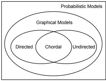
Figure 4.36: DPGMs and UPGMs can perfectly represent di!erent sets of distributions. Some distributions can be perfectly represented by either DPGM’s or UPGMs; the corresponding graph must be chordal.

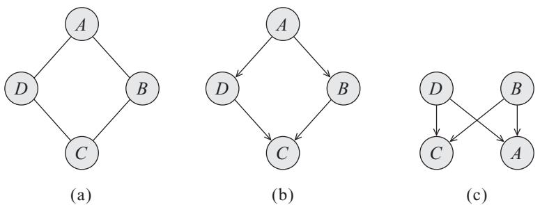
Figure 4.37: A UPGM and two failed attempts to represent it as a DPGM. From Figure 3.10 of [KF09a]. Used with kind permission of Daphne Koller.

represent all and only the two CI statements encoded by a v-structure. In general, CI properties in UPGMs are monotonic, in the following sense: if A ℜ B|C, then A ℜ B|(C ↘ D). But in DPGMs, CI properties can be non-monotonic, since conditioning on extra variables can eliminate conditional independencies due to explaining away.

As an example of some CI relationships that can be perfectly modeled by a UPGM but not a DPGM, consider the 4-cycle shown in Figure 4.37(a). One attempt to model this with a DPGM is shown in Figure 4.37(b). This correctly asserts that A ℜ C|B,D. However, it incorrectly asserts that B ℜ D|A. Figure 4.37(c) is another incorrect DPGM: it correctly encodes A ℜ C|B,D, but incorrectly encodes B ℜ D. In fact there is no DPGM that can precisely represent all and only the CI statements encoded by this UPGM.

Some distributions can be perfectly modeled by either a DPGM or a UPGM; the resulting graphs are called decomposable or chordal. Roughly speaking, this means the following: if we collapse together all the variables in each maximal clique, to make “mega-variables”, the resulting graph will be a tree. Of course, if the graph is already a tree (which includes chains as a special case), it will already be chordal.

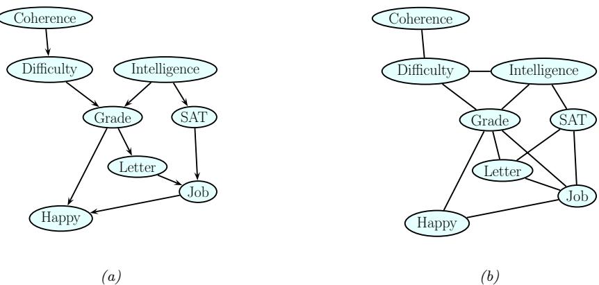
Figure 4.38: Left: the full student DPGM. Right: the equivalent UPGM. We add moralization arcs D-I, G-J, and L-S. Adapted from Figure 9.8 of [KF09a].

4.5.2 Converting between a directed and undirected model

Although DPGMs and UPGMs are not in general equivalent, if we are willing to allow the graph to encode fewer CI properties than may strictly hold, then we can safely convert one to the other, as we explain below.

4.5.2.1 Converting a DPGM to a UPGM

We can easily convert a DPGM to a UPGM as follows. First, any “unmarried” parents that share a child must get “married”, by adding an edge between them; this process is known as moralization. Then we can drop the arrows, resulting in an undirected graph. The reason we need to do this is to ensure that the CI properties of the UGM match those of the DGM, as explained in Section 4.3.6.2. It also ensures there is a clique that can “store” the CPDs of each family.

Let us consider an example from [KF09a]. We will use the (full version of the student network shown in Figure 4.38(a). The corresponding joint has the following form:

\[P(C, D, I, G, S, L, J, H) \tag{4.149}\]

\[0 = P(C)P(D|C)P(I)P(G|I,D)P(S|I)P(L|G)P(J|L,S)P(H|G,J)\tag{4.150}\]

Next, we define a potential or factor for every CPD, yielding

\[p(C, D, I, G, S, L, J, H) = \psi\_C(C)\psi\_D(D, C)\psi\_I(I)\psi\_G(G, I, D) \tag{4.151}\]

\[ \psi\_S(S,I)\psi\_L(L,G)\psi\_J(J,L,S)\psi\_H(H,G,J)\tag{4.152} \]

All the potentials are locally normalized, since they are CPDs, and hence there is no need for a global normalization constant, so Z = 1. The corresponding undirected graph is shown in Figure 4.38(b). We see that we have added D-I, G-J, and L-S moralization edges.11

^11. We will see this example again in Section 9.5, where we use it to illustrate the variable elimination inference algorithm.

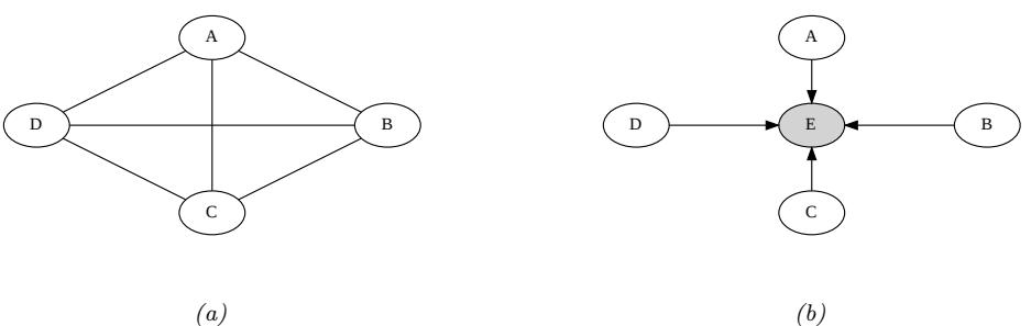
Figure 4.39: (a) An undirected graphical model. (b) A directed equivalent, obtained by adding a dummy observed child node.

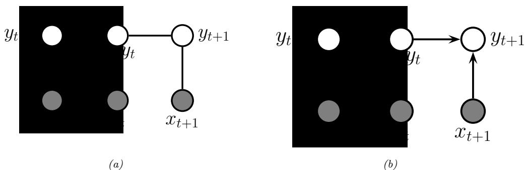
Figure 4.40: Two discriminative models for sequential data. (a) An undirected model (CRF). (b) A directed model (MEMM).

4.5.2.2 Converting a UPGM to a DPGM

To convert a UPGM to a DPGM, we proceed as follows. For each potential function 5c(xc; ωc), we create a “dummy node”, call it Yc, which is “clamped” to a special observed state, call it y↘ ^c . We then define p(Y^c = y↘ ^c |xc) = 5c(xc; ωc). This “local evidence” CPD encodes the same factor as in the DGM. The overall joint has the form pundir(x) ↙ pdir(x, y↘).

As an example, consider the UPGM in Figure 4.39(a), which defines the joint p(A, B, C, D) = 5(A, B, C, D)/Z. We can represent this as a DPGM by adding a dummy E node, which is a child of all the other nodes. We set E = 1 and define the CPD p(E = 1|A, B, C, D) ↙ 5(A, B, C, D). By conditioning on this observed child, all the parents become dependent, as in the UGM.

4.5.3 Conditional directed vs undirected PGMs and the label bias problem

Directed and undirected models behave somewhat di!erently in the conditional (discriminative) setting. As an example of this, let us compare the 1d undirected CRF in Figure 4.40a with the directed Markov chain in Figure 4.40b. (This latter model is called a maximum entropy Markov model

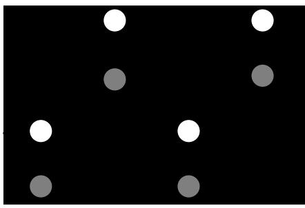
Figure 4.41: A grid-structured MRF with hidden nodes xⁱ and local evidence nodes yi. The prior p(x) is an undirected Ising model, and the likelihood ^p(y|x) = ” ⁱ p(yi|xi) is a directed fully factored model.

(MEMM), which is a reference to the connection with maxent models discussed in Section 4.3.4.) The MEMM su!ers from a subtle problem compared to the CRF known (rather obscurely) as the label bias problem [LMP01]. The problem is that local features at time t do not influence states prior to time t. That is, y^t↑¹ ℜ xt|yt, thus blocking information flow backwards in time.

To understand what this means in practice, consider the part of speech tagging task which we discussed in Section 4.4.1.1. Suppose we see the word “banks”; this could be a verb (as in “he banks at Chase”), or a noun (as in “the river banks were overflowing”). Locally the part of speech tag for the word is ambiguous. However, suppose that later in the sentence, we see the word “fishing”; this gives us enough context to infer that the sense of “banks” is “river banks” and not “financial banks”. However, in an MEMM the “fishing” evidence will not flow backwards, so we will not be able to infer the correct label for “banks”. The CRF does not have this problem.

The label bias problem in MEMMs occurs because directed models are locally normalized, meaning each CPD sums to 1. By contrast, MRFs and CRFs are globally normalized, which means that local factors do not need to sum to 1, since the partition function Z, which sums over all joint configurations, will ensure the model defines a valid distribution.

However, this solution comes at a price: in a CRF, we do not get a valid probability distribution over y1:^T until we have seen the whole sentence, since only then can we normalize over all configurations. Consequently, CRFs are not as useful as directed probabilistic graphical models (DPGM) for online or real-time inference. Furthermore, the fact that Z is a function of all the parameters makes CRFs less modular and much slower to train than DPGM’s, as we discuss in Section 4.4.3.

4.5.4 Combining directed and undirected graphs

We can also define graphical models that contain directed and undirected edges. We discuss a few examples below.

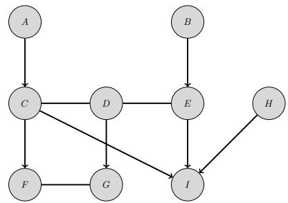
Figure 4.42: A partially directed acyclic graph (PDAG). The chain components are {A}, {B}, {C, D, E}, {F, G}, {H}, and {I}. Adapted from Figure 4.15 of [KF09a].

4.5.4.1 Chain graphs

A chain graph is a PGM which may have both directed and undirected edges, but without any directed cycles. A simple example is shown in Figure 4.41, which defines the following joint model:

\[p(\mathbf{z}\_{1:D}, \mathbf{y}\_{1:D}) = p(\mathbf{z}\_{1:D}) p(\mathbf{y}\_{1:D} | \mathbf{z}\_{1:D}) = \left[ \frac{1}{Z} \prod\_{i \sim j} \psi\_{ij}(x\_i, x\_j) \right] \left[ \prod\_{i=1}^{D} p(y\_i | x\_i) \right] \tag{4.153}\]

In this example, the prior p(x) is specified by a UPGM, and the likelihood p(y|x) is specified as a fully factorized DPGM.

More generally, a chain graph can be defined in terms of a partially directed acyclic graph (PDAG). This is a graph which can be decomposed into a directed graph of chain components, where the nodes within each chain component are connected with each other only with undirected edges. See Figure 4.42 for an example.

We can use a PDAG to define a joint distribution using ⁱ p(Ci|pa(Ci)), where each Cⁱ is a chain component, and each CPD is a conditional random field. For example, referring to Figure 4.42, we have

\[p(A, B, \ldots, I) = p(A)p(B)p(C, D, E | A, B)p(F, G | C, D)p(H)p(I | C, E, H)\tag{4.154}\]

\[p(C, D, E | A, B) = \frac{1}{Z(A, B)} \phi(A, C)\phi(B, E)\phi(C, D)\phi(D, E) \tag{4.155}\]

\[p(F,G|C,D) = \frac{1}{Z(C,D)} \phi(F,C)\phi(G,D)\phi(F,G) \tag{4.156}\]

For more details, see e.g., [KF09a, Sec 4.6.2].

4.5.4.2 Acyclic directed mixed graphs

One can show [Pea09b, p51] that every latent variable DPGM can be rewritten in a way such that every latent variable is a root node with exactly two observed children. This is called the projection of the latent variable PGM, and is observationally indistinguishable from the original model.

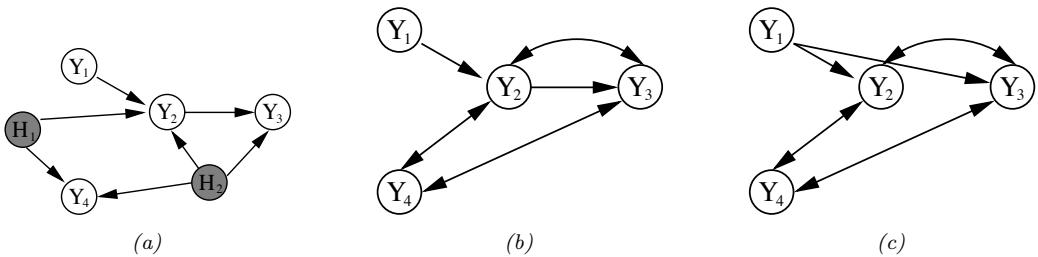
Figure 4.43: (a) A DAG with two hidden variables (shaded). (b) The corresponding ADMG. The bidirected edges reflect correlation due to the hidden variable. (c) A Markov equivalent ADMG. From Figure 3 of [SG09]. Used with kind permission of Ricardo Silva.

Each such latent variable root node induces a dependence between its two children. We can represent this with a directed arc. The resulting graph is called an acyclic directed mixed graph or ADMG. See Figure 4.43 for an example. (A mixed graph is one with undirected, unidirected, and bidirected edges.)

One can determine CI properties of ADMGs using a technique called m-separation [Ric03]. This is equivalent to d-separation in a graph where every bidirected edge Yⁱ ℵ Y^j is replaced by Yⁱ ∈ Xij → Y^j , where Xij is a hidden variable for that edge.

The most common example of ADMGs is when everything is linear-Gaussian. This is known as a structural equation model and is discussed in Section 4.7.2.

4.5.5 Comparing directed and undirected Gaussian PGMs

In this section, we compare directed and undirected Gaussian graphical models. In Section 4.2.3, we saw that directed GGMs correspond to sparse regression matrices. In Section 4.3.5, we saw that undirected GGMs correspond to sparse precision matrices.

The advantage of the DAG formulation is that we can make the regression weights W, and hence !, be conditional on covariate information [Pou04], without worrying about positive definite constraints. The disadavantage of the DAG formulation is its dependence on the order, although in certain domains, such as time series, there is already a natural ordering of the variables.

It is actually possible to combine both directed and undirected representations, resulting in a model known as a (Gaussian) chain graph. For example, consider a discrete-time, second-order Markov chain in which the observations are continuous, ^{xt ↑ RD}. The transition function can be represented as a (vector-valued) linear-Gaussian CPD:

\[p(x\_t | x\_{t-1}, x\_{t-2}, \theta) = \mathcal{N}(x\_t | \mathbf{A}\_1 x\_{t-1} + \mathbf{A}\_2 x\_{t-2}, \Sigma) \tag{4.157}\]

This is called a vector autoregressive or VAR process of order 2. Such models are widely used in econometrics for time series forecasting.

The time series aspect is most naturally modeled using a DPGM. However, if !^↑1 is sparse, then the correlation amongst the components within a time slice is most naturally modeled using a UPGM.

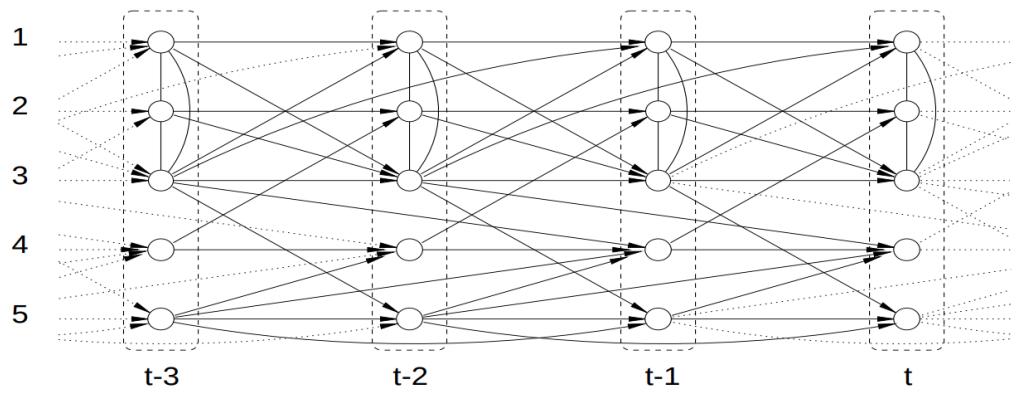
Figure 4.44: A VAR(2) process represented as a dynamic chain graph. From [DE00]. Used with kind permission of Rainer Dahlhaus.

For example, suppose we have

\[\mathbf{A}\_{1} = \begin{pmatrix} \frac{3}{5} & 0 & \frac{1}{5} & 0 & 0\\ 0 & \frac{3}{5} & 0 & -\frac{1}{5} & 0\\ \frac{2}{5} & \frac{1}{5} & \frac{3}{5} & 0 & 0\\ 0 & 0 & 0 & -\frac{1}{2} & \frac{1}{5}\\ 0 & 0 & \frac{1}{5} & 0 & \frac{2}{5} \end{pmatrix}, \quad \mathbf{A}\_{2} = \begin{pmatrix} 0 & 0 & -\frac{1}{5} & 0 & 0\\ 0 & 0 & 0 & 0 & 0\\ 0 & 0 & 0 & 0 & 0\\ 0 & 0 & \frac{1}{5} & 0 & \frac{1}{3}\\ 0 & 0 & 0 & 0 & -\frac{1}{5} \end{pmatrix} \tag{4.158}\]

and

\[ \boldsymbol{\Sigma} = \begin{pmatrix} 1 & \frac{1}{2} & \frac{1}{3} & 0 & 0 \\ \frac{1}{2} & 1 & -\frac{1}{3} & 0 & 0 \\ \frac{1}{3} & -\frac{1}{3} & 1 & 0 & 0 \\ 0 & 0 & 0 & 1 & 0 \\ 0 & 0 & 0 & 0 & 1 \end{pmatrix}, \quad \boldsymbol{\Sigma}^{-1} = \begin{pmatrix} 2.13 & -1.47 & -1.2 & 0 & 0 \\ -1.47 & 2.13 & 1.2 & 0 & 0 \\ -1.2 & 1.2 & 1.8 & 0 & 0 \\ 0 & 0 & 0 & 1 & 0 \\ 0 & 0 & 0 & 0 & 1 \end{pmatrix} \tag{4.159} \]

The resulting graphical model is illustrated in Figure 4.44. Zeros in the transition matrices A¹ and A² correspond to absent directed arcs from x^t↑¹ and x^t↑² into xt. Zeros in the precision matrix !^↑1 correspond to absent undirected arcs between nodes in xt.

4.5.5.1 Covariance graphs

Sometimes we have a sparse covariance matrix rather than a sparse precision matrix. This can be represented using a bi-directed graph, where each edge has arrows in both directions, as in Figure 4.45(a). Here nodes that are not connected are unconditionally independent. For example in Figure 4.45(a) we see that Y¹ ℜ Y3. In the Gaussian case, this means $1,³ = $3,¹ = 0. (A graph representing a sparse covariance matrix is called a covariance graph, see e.g., [Pen13]). By contrast, if this were an undirected model, we would have that Y¹ ℜ Y3|Y2, and %1,³ = %3,¹ = 0, where ” = !^↑1.

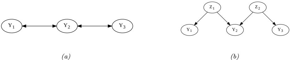
Figure 4.45: (a) A bi-directed graph. (b) The equivalent DAG. Here the z nodes are latent confounders. Adapted from Figures 5.12–5.13 of [Cho11].

A bidirected graph can be converted to a DAG with latent variables, where each bidirected edge is replaced with a hidden variable representing a hidden common cause, or confounder, as illustrated in Figure 4.45(b). The relevant CI properties can then be determined using d-separation.

4.6 PGM extensions

In this section, we discuss some extensions of the basic PGM framework.

4.6.1 Factor graphs

A factor graph [KFL01; Loe04] is a graphical representation that unifies directed and undirected models. They come in two main “flavors”. The original version uses a bipartite graph, where we have nodes for random variables and nodes for factors, as we discuss in Section 4.6.1.1. An alternative form, known as a Forney factor graphs [For01] just has nodes for factors, and the variables are associated with edges, as we explain in Section 4.6.1.2.

4.6.1.1 Bipartite factor graphs

A factor graph is an undirected bipartite graph with two kinds of nodes. Round nodes represent variables, square nodes represent factors, and there is an edge from each variable to every factor that mentions it. For example, consider the MRF in Figure 4.46(a). If we assume one potential per maximal clique, we get the factor graph in Figure 4.46(b), which represents the function

\[f(x\_1, x\_2, x\_3, x\_4) = f\_{124}(x\_1, x\_2, x\_4) f\_{234}(x\_2, x\_3, x\_4) \tag{4.160}\]

We can represent this in a topologically equivalent way as in Figure 4.46(c).

One advantage of factor graphs over UPGM diagrams is that they are more fine-grained. For example, suppose we associate one potential per edge, rather than per clique. In this case, we get the factor graph in Figure 4.46(d), which represents the function

\[f(x\_1, x\_2, x\_3, x\_4) = f\_{14}(x\_1, x\_4) f\_{12}(x\_1, x\_2) f\_{34}(x\_3, x\_4) f\_{23}(x\_2, x\_3) f\_{24}(x\_2, x\_4) \tag{4.161}\]

We can also convert a DPGM to a factor graph: just create one factor per CPD, and connect that factor to all the variables that use that CPD. For example, Figure 4.47 represents the following

0 8

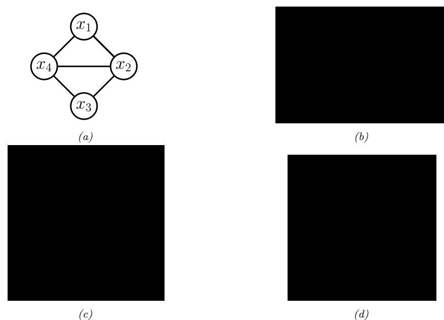
Figure 4.46: (a) A simple UPGM. (b) A factor graph representation assuming one potential per maximal clique. (c) Same as (b), but graph is visualized di!erently. (d) A factor graph representation assuming one potential per edge.

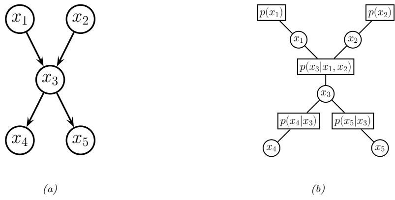
Figure 4.47: (a) A simple DPGM. (b) Its corresponding factor graph.

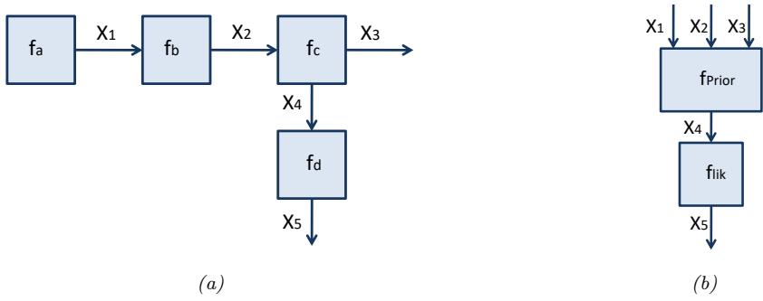
Figure 4.48: A Forney factor graph. (a) Directed version. (b) Hierarchical version.

factorization:

\[f(x\_1, x\_2, x\_3, x\_4, x\_5) = f\_1(x\_1) f\_2(x\_2) f\_{123}(x\_1, x\_2, x\_3) f\_{34}(x\_3, x\_4) f\_{35}(x\_3, x\_5) \tag{4.162}\]

where we define f123(x1, x2, x3) = p(x3|x1, x2), etc. If each node has at most one parent (and hence the graph is a chain or simple tree), then there will be one factor per edge (root nodes can have their prior CPDs absorbed into their children’s factors). Such models are equivalent to pairwise MRFs.

4.6.1.2 Forney factor graphs

A Forney factor graph (FFG), also called a normal factor graph, is a graph in which nodes represent factors, and edges represent variables [For01; Loe04; Loe+07; CLV19]. This is more similar to standard neural network diagrams, and electrical engineering diagrams, where signals (represented as electronic pulses, or tensors, or probability distributions) propagate along wires and are modified by functions represented as nodes.

For example, consider the following factorized function:

\[f(x\_1, \ldots, x\_5) = f\_a(x\_1) f\_b(x\_1, x\_2) f\_c(x\_2, x\_3, x\_4) f\_d(x\_4, x\_5) \tag{4.163}\]

We can visualize this as an FFG as in Figure 4.48a. The edge labeled x³ is called a half-edge, since it is only connected to one node; this is because x³ only participates in one factor. (Similarly for x5.) The directionality associated with the edges is a useful mnemonic device if there is a natural order in which the variables are generated. In addition, associating directions with each edge allows us to uniquely name “messages” that are sent along each edge, which will prove useful when we discuss inference algorithms in Section 9.3.

In addition to being more similar to neural network diagrams, FFGs have the advantage over bipartite FGs in that they support hierarchical (compositional) construction, in which complex dependency structure between variables can be represented as a blackbox, with the input/output interface being represented by edges corresponding to the variables exposed by the blackbox. See Figure 4.48b for an example, which represents the function

\[f(x\_1, \ldots, x\_5) = f\_{\text{prior}}(x\_1, x\_2, x\_3, x\_4) f\_{\text{lik}}(x\_4, x\_5) \tag{4.164}\]

Figure 4.49: An FFG with an equality constraint node (left) and its corresponding simplified form (right).

The factor fprior represents a (potentially complex) joint distribution p(x1, x2, x3, x4), and the factor flik represents the likelihood term p(x5|x4). Such models are widely used to build error-correcting codes (see Section 9.4.8).

To allow for variables to participate in more than 2 factors, equality constraint nodes are introduced, as illustrated in Figure 4.49(a). Formally, this is a factor defined as follows:

\[f\_{=}(x, x\_1, x\_2) = \delta(x - x\_1)\delta(x - x\_2) \tag{4.165}\]

where 1(u) is a Dirac delta if u is continuous, and a Kronecker delta if u is discrete. The e!ect of this factor is to ensure all the variables connected to the factor have the same value; intuitively, this factor acts like a “wire splitter”. Thus the function represented in Figure 4.49(a) is equivalent to the following:

\[f(x, y\_1, y\_2) = f\_x(x) f\_{y|x}(y\_1, x) f\_{y|x}(y\_2, x) \tag{4.166}\]

This simplified form is represented in Figure 4.49(b), where we reuse the x variable across multiple edges. We have chosen the edge orientations to reflect our interpretation of the factors f^y|x(y, x) as likelihood terms, p(y|x). We have also chosen to reuse the same f^y|^x factor for both y variables; this is an example of parameter tying.

4.6.2 Probabilistic circuits

A probabilistic circuit is a kind of graphical model that supports e”cient exact inference. It includes arithmetic circuits [Dar03; Dar09], sum-product networks (SPNs) [PD11; SCPD22]. and other kinds of model.

Here we briefly describe SPNs. An SPN is a probabilistic model, based on a directed tree-structured graph, in which terminal nodes represent univariate probability distributions and non-terminal nodes represent convex combinations (weighted sums) and products of probability functions. SPNs are similar to deep mixture models, in which we combine together dimensions. SPNs leverage contextspecific independence to reduce the complexity of exact inference to time that is proportional to the number of links in the graph, as opposed to the treewidth of the graph (see Section 9.5.2).

SPNs are particularly useful for tasks such as missing data imputation of tabular data (see e.g., [Cla20; Ver+19]). A recent extension of SPNs, known as einsum networks, is proposed in [Peh+20] (see Section 9.7.1 for details on the connection between einstein summation and PGM inference).

4.6.3 Directed relational PGMs

A Bayesian network defines a joint probability distribution over a fixed number of random variables. By using plate notation (Section 4.2.8), we can define models with certain kinds of repetitive structure, and tied parameters, but many models are not expressible in this way. For example, it is not possible to represent even a simple HMM using plate notation (see Figure 29.12). Various notational extensions of plates have been proposed to handle repeated structure (see e.g., [HMK04; Die10]) but have not been widely adopted. The problem becomes worse when we have more complex domains, involving multiple objects which interact via multiple relationships.12 Such models are called relational probability models or RPMs. In this section, we focus on directed RPMs; see Section 4.6.4 for the undirected case.

As in first order logic, RPMs have constant symbols (representing objects), function symbols (mapping one set of constants to another), and predicate symbols (representing relations between objects). We will assume that each function has a type signature. To illustrate this, consider an example from [RN19, Sec 15.1], which concerns online book reviews on sites such as Amazon. Suppose there are two types of objects, Book and Customer, and the following functions and predicates:

\[\text{House} : \text{Customer} \to \{\text{True}, \text{False}\} \tag{4.167}\]

\[\text{Kindess}: \text{Customer} \to \{1, 2, 3, 4, 5\} \tag{4.168}\]

\[\text{Quality}: \text{Book} \to \{1, 2, 3, 4, 5\} \tag{4.169}\]

\[\text{Recommensulation} : \text{Customer} \times \text{Book} \to \{1, 2, 3, 4, 5\} \tag{4.170}\]

The constant symbols refer to specific objects. To keep things simple, we assume there are two books, B¹ and B2, and two customers, C¹ and C2. The basic random variables are obtained by instantiating each function with each possible combination of objects to create a set of ground terms. In this example, these variables are H(C1), Q(B1), R(C1, B2), etc. (We use the abbreviations H, K, Q and R for the functions Honest, Kindness, Quality, and Recommendation.13 )

We now need to specify the (conditional) distribution over these random variables. We define these distributions in terms of the generic indexed form of the variables, rather than the specific ground form. For example, we may use the following priors for the root nodes (variables with no parents):

\[H(c) \sim \text{Cat}(0.99, 0.01) \tag{4.171}\]

\[K(c) \sim \text{Cat}(0.1, 0.1, 0.2, 0.3, 0.3) \tag{4.172}\]

\[Q(b) \sim \text{Cat}(0.05, 0.2, 0.4, 0.2, 0.15) \tag{4.173}\]

For the recommendation nodes, we need to define a conditional distribution of the form

\[R(c,b) \sim \text{RecCPD}(H(c), K(c), Q(b)) \tag{4.174}\]

^12. See e.g., this blog post from Rob Zinkov: https://www.zinkov.com/posts/2013-07-28-stop-using-plates.

^13. A unary function of an object that returns a basic type, such as Boolean or an integer, is often called an attribute of that object.

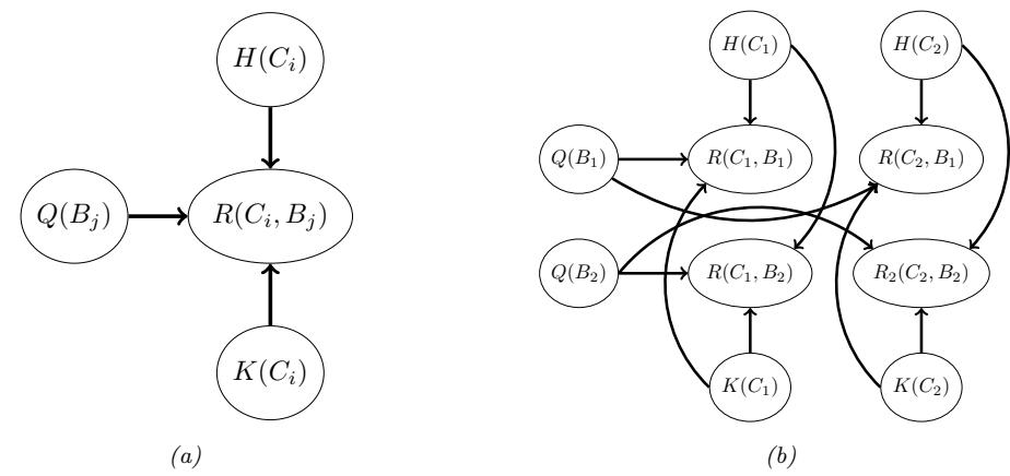
Figure 4.50: RPM for the book review domain. (a) Template for a generic customer Cⁱ and book B^j pair. R is rating, Q is quality, H is honesty, and K is kindness. (b) Unrolled model for 2 books and 2 customers.

where RecCPD is the conditional probability distribution (CPD) for the recommendation node. If represented as a conditional probability table (CPT), this has 2 ∞ 5 ∞ 5 = 50 rows, each with 5 entries. This table can encode our assumptions about what kind of ratings a book receives based on the quality of the book, but also properties of the reviewer, such as their honest and kindness. (More sophisticated models of human raters in the context of crowd-sourced data collection can be found in e.g., [LRC19].)

We can convert the above formulae into a graphical model “template”, as shown in Figure 4.50a. Given a set of objects, we can “unroll” the template to create a “ground network”, as shown in Figure 4.50b. There are C ∞ B + 2C + B random variables, with a corresonding joint state space (set of possible worlds) of size 2^C 5^C+B+BC , which can get quite large. However, if we are only interested in answering specific queries, we can dynamically unroll small pieces of the network that are relevant to that query [GC90; Bre92].

Let us assume that only a subset of the R(c, b) entries are observed, and we would like to predict the missing entries of this matrix. This is essentially a simplified recommender system. (Unfortunately it ignores key aspects of the problem, such as the content/topic of the books, and the interests/preferences of the customers.) We can use standard probabilistic inference methods for graphical models (which we discuss in Chapter 9) to solve this problem.

Things get more interesting when we don’t know which objects are being referred to. For example, customer C¹ might write a review of a book called “Probabilistic Machine Learning”, but do they mean edition 1 (B1) or edition 2 (B2)? To handle this kind of relational uncertainty, we can add all possible referents as parents to each relation. This is illustrated in Figure 4.51, where now Q(B1) and Q(B2) are both parents of R(C1, B1). This is necessary because their review score might either depend on Q(B1) or Q(B2), depending on which edition they are writing about. To disambiguate this, we create a new variable, L(Ci), which specifies which version number of each book customer i is referring to. The new CPD for the recommendation node, p(R(c, b)|H(c), K(c), Q(1 : B), L(c)),

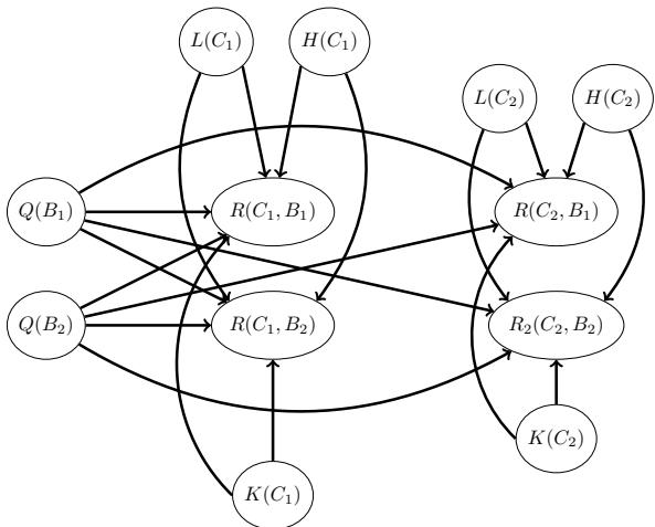
Figure 4.51: An extension of the book review RPM to handle identity uncertainty about which book a given customer is actually reviewing. The R(c, b) node now depends on all books, since we don’t know which one is being referred to. We can select one of these parents based on the mapping specified by the user’s library, L(c).

has the form

\[R(c, b) \sim \text{RecCPT}(H(c), K(c), Q(b')) \text{ where } b' = L(c) \tag{4.175}\]

This CPD acts like a multiplexer, where the L(c) node specifies which of the parents Q(1 : B) to actually use.

Although the above problem may seem contrived, identity uncertainty is a widespread problem in many areas, such as citation analysis, credit card histories, and object tracking (see Section 4.6.5). In particular, the problem of entity resolution or record linkage — which refers to the task of mapping particular strings (such as names) to particular objects (such as people) — is a whole field of research (see e.g., https://en.wikipedia.org/wiki/Record\_linkage for an overview and [SHF15] for a Bayesian approach).

4.6.4 Undirected relational PGMs

We can create relational UGMs in a manner which is analogous to relational DGMs (Section 4.6.3). This is particularly useful in the discriminative setting, for the same reasons that undirected CRFs are preferable to conditional DGMs (see Section 4.4).

4.6.4.1 Collective classification

As an example of a relational UGM, suppose we are interested in the problem of classifying web pages of a university into types (e.g., student, professor, admin, etc.) Obviously we can do this based on the contents of the page (e.g., words, pictures, layout, etc.) However, we might also suppose there is information in the hyper-link structure itself. For example, it might be likely for students to

Fr(A,A)	Fr(B,B)	Fr(B,A)	Fr(A,B)	Sm(A)	Sm(B)	Ca(A)	Ca(B)
1	1	0	1	1	1	1	1
1	1	0	1	1	0	0	0
1	1	0	1	1	1	0	1

Table 4.5: Some possible joint instantiations of the 8 variables in the smoking example.

cite professors, and professors to cite other professors, but there may be no links between admin pages and students/professors. When faced with a web page whose label is ambiguous, we can bias our estimate based on the estimated labels of its neighbors, as in a CRF. This process is known as collective classification (see e.g., [Sen+08]). To specify the CRF structure for a web-graph of arbitrary size and shape, we just specify a template graph and potential functions, and then unroll the template appropriately to match the topology of the web, making use of parameter tying.

4.6.4.2 Markov logic networks

One particularly popular way of specifying relational UGMs is to use first-order logic rather than a graphical description of the template. The result is known as a Markov logic network [RD06; Dom+06; DL09].

For example, consider the sentences “Smoking causes cancer” and “If two people are friends, and one smokes, then so does the other”. We can write these sentences in first-order logic as follows:

\[\forall x. Sm(x) \implies Ca(x) \tag{4.176}\]

\[\forall x.\forall y. Fr(x, y) \land Sm(x) \implies Sm(y) \tag{4.177}\]

where Sm and Ca are predicates, and F r is a relation.

It is convenient to write all formulas in conjunctive normal form (CNF), also known as clausal form. In this case, we get

\[ \neg Sm(x) \lor Ca(x) \tag{4.178} \]

\[ \neg Fr(x, y) \lor \neg Sm(x) \lor Sm(y) \tag{4.179} \]

The first clause can be read as “Either x does not smoke or he has cancer”, which is logically equivalent to Equation (4.176). (Note that in a clause, any unbound variable, such as x, is assumed to be universally quantified.)

Suppose there are just two objects (people) in the world, Anna and Bob, which we will denote by constant symbols A and B. We can then create 8 binary random variables Sm(x), Ca(x), and F r(x, y) for x, y ^↑ {A, B}. This defines ²⁸ possible worlds, some of which are shown in Table 4.5. 14

Our goal is to define a probability distribution over these joint assignments. We can do this by creating a UGM with these variables, and adding a potential function to capture each logical rule or

^14. Note that we have not encoded the fact that F r is a symmetric relation, so F r(A, B) and F r(B,A) might have di!erent values. Similarly, we have the “degenerate” nodes F r(A) and F r(B), since we did not enforce x ↔︎= y in Equation (4.177). (If we add such constraints, then the model compiler, which generates the ground network, should avoid creating redundant nodes.)

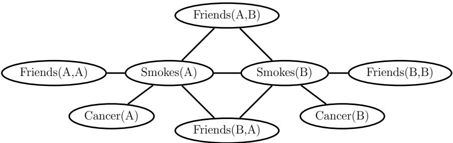
Figure 4.52: An example of a ground Markov logic network represented as a pairwise MRF for 2 people. Adapted from Figure 2.1 from [DL09]. Used with kind permission of Pedro Domingos.

constraint. For example, we can encode the rule ¬Sm(x) C Ca(x) by creating a potential function ’(Sm(x),Ca(x)), where we define

\[\Psi(Sm(x), Ca(x)) = \begin{cases} 1 & \text{if } \neg Sm(x) \lor Ca(x) = T \\ 0 & \text{if } \neg Sm(x) \lor Ca(x) = F \end{cases} \tag{4.180}\]

The result is the UGM in Figure 4.52.

The above approach will assign non-zero probability to all logically valid worlds. However, logical rules may not always be true. For example, smoking does not always cause cancer. We can relax the hard constraints by using non-zero potential functions. In particular, we can associate a weight with each rule, and thus get potentials such as

\[\Psi(Sm(x), Ca(x)) = \begin{cases} e^w & \text{if } \neg Sm(x) \lor Ca(x) = T \\ e^0 & \text{if } \neg Sm(x) \lor Ca(x) = F \end{cases} \tag{4.181}\]

where the value of w > 0 controls strongly we want to enforce the corresponding rule.

The overall joint distribution has the form

\[p(\mathbf{z}) = \frac{1}{Z(\mathbf{w})} \exp(\sum\_{i} w\_i n\_i(\mathbf{z})) \tag{4.182}\]

where ni(x) is the number of instances of clause i which evaluate to true in assignment x.

Given a grounded MLN model, we can then perform inference using standard methods. Of course, the ground models are often extremely large, so more e”cient inference methods, which avoid creating the full ground model (known as lifted inference), must be used. See [DL09; KNP11] for details.

One way to gain tractability is to relax the discrete problem to a continuous one. This is the basic idea behind hinge-loss MRFs [Bac+15b], which support exact inference using scalable convex optimization. There is a template language for this model family known as probabilistic soft logic, which has a similar “flavor” to MLN, although it is not quite as expressive.

Recently MLNs have been combined with DL in various ways. For example, [Zha+20g] uses graph neural networks for inference. And [WP18] uses MLNs for evidence fusion, where the noisy predictions come from DNNs trained using weak supervision.

Finally, it is worth noting one subtlety which arises with undirected models, namely that the size of the unrolled model, which depends on the number of objects in the universe, can a!ect the results of inference, even if we have no data about the new objects. For example, consider an undirected chain of length T, with T hidden nodes z^t and T observed nodes yt; call this model M1. Now suppose we double the length of the chain to 2T, without adding more evidence; call this model M2. We find that p(zt|y1:^T , M1) ⇓= p(zt|y1:^T , M2), for t =1: T, even though we have not added new information, due to the di!erent partition functions. This does not happen with a directed chain, because the newly added nodes can be marginalized out without a!ecting the original nodes, since the model is locally normalized and therefore modular. See [JBB09; Poo+12] for further discussion.

4.6.5 Open-universe probability models

In Section 4.6.3, we discussed relational probability models, as well as the topic of identity uncertainty. However, we also implicitly made a closed world assumption, namely that the set of all objects is fixed and specified ahead of time. In many real world problems, this is an unrealistic assumption. For example, in Section 29.9.3.5, we discuss the problem of tracking an unknown number of objects over time. As another example, consider the problem of enforcing the UN Comprehensive Nuclear Test Ban Treaty (CTBT). This requires monitoring seismic events, and determinining if they were caused by nature or man-made explosions. Thus the number of objects of each type, as well as their source, is uncertain [ARS13],

As another (more peaceful) example, suppose we want to perform citation matching, in which we want to know whether to cite an arxiv version of a paper or the version on some conference website. Are these the same object? It is often hard to tell, since the titles and author might be the same, yet the content may have been updated. It is often necessary to use subtle cues, such as the date stored in the meta-data, to infer if the two “textual measurements” refer to the same underlying object (paper) or not [Pas+02].

In problems such as these, the number of objects of each type, as well as their relationships, is uncertain. This requires the use of open-universe probability models or OUPM, which can generate new objects as well as their properties [Rus15; MR10; LB19]. The first formal language for OUPMs was BLOG [Mil+05], which stands for “Bayesian LOGic”. This used a general purpose, but slow, MCMC inference scheme to sample over possible worlds of variable size and shape. [Las08; LLC20] describes another open-universe modeling language called multi-entity Bayesian networks.

Very recently, Facebook has released the Bean Machine library, available at https://beanmachine. org/, which supports more e”cient inference in OUPMs. Details can be found in [Teh+20], as well as their blog post.15

4.6.6 Programs as probability models

OUPMs, discussed in Section 4.6.5, let us define probability models over complex dynamic state spaces of unbounded and variable size. The set of possible worlds correspond to objects and their

^15. See https://tinyurl.com/2svy5tmh.

attributes and relationships. Another approach is to use a probabilistic programming language or PPL, in which we define the set of possible words as the set of execution traces generated by the program when it is endowed with a random choice mechanism. (This is a procedural approach to the problem, whereas OUPMs are a declarative approach.)

The di!erence between a probabilistic programming language and a standard one was described in [Gor+14] as follows: “Probabilistic programs are usual functional or imperative programs with two added constructs: (1) the ability to draw values at random from distributions, and (2) the abiliy to condition values of variables in a program via observation”. The former is a way to define p(z, y), and the latter is the same as standard Bayesian conditioning p(z|y).

Some recent examples of PPLs include Gen [CT+19], Pyro [Bin+19] and Turing [GXG18]. Inference in such models is often based on SMC, which we discuss in Chapter 13. For more details on PPLs, see e.g. [Mee+18].

4.7 Structural causal models

While probabilities encode our beliefs about a static world, causality tells us whether and how probabilities change when the world changes, be it by intervention or by act of imagination. — Judea Pearl [PM18b].

In this section, we discuss how we can use directed graphical model notation to represent causal models. We discuss causality in greater detail in Chapter 36, but we introduce some basic ideas and notation here, since it is foundational material that we will need in other parts of the book.

The core idea behind causal models is to create a mechanistic model of the world in which we can reason about the e!ects of local changes. The canonical example is an electronic circuit: we can predict the e!ects of any action, such as “knocking out” a particular transistor, or changing the resistance level of a wire, by modifying the circuit locally, and then “re-running” it from the same initial conditions.

We can generalize this idea to create a structural causal models or SCM [PGJ16], also called functional causal model [Sch19]. An SCM is a triple M = (U, V, F), where U = {Uⁱ : i =1: N} is a set of unexplained or exogenous “noise” variables, which are passed as input to the model, V = {Vⁱ : i =1: N} is a set of endogeneous variables that are part of the model itself, and F = {fⁱ : i =1: N} is a set of deterministic functions of the form Vⁱ = fi(Vpaⁱ , Ui), where paⁱ are the parents of variable i, and Uⁱ ↑ U are the external inputs. We assume the equations can be structured in a recursive way, so the dependency graph of nodes given their parents is a DAG. Finally, we assume our model is causally su!cient, which means that V and U are all of the causally relevant factors (although they may not all be observed). This is called the “causal Markov assumption”.

Of course, a model typically cannot represent all the variables that might influence observations or decisions. After all, models are abstractions of reality. The variables that we choose not to model explicitly in a functional way can be lumped into the unmodeled exogenous terms. To represent our ignorance about these terms, we can use a distribution p(U) over their values. By “pushing” this external noise through the deterministic part of the model, we induce a distribution over the endogeneous variables, p(V), as in a probabilistic graphical model. However, SCMs make stronger assumptions than PGMs.

We usually assume p(U) is factorized (i.e., the Uⁱ are independent); this is called a Markovian SCM. If the exogeneous noise terms are not independent, it would break the assumption that

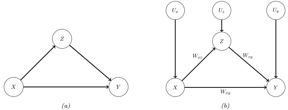
Figure 4.53: (a) PGM for modeling relationship between salary, education and debt. (b) Corresponding SCM.

outcomes can be determined locally using deterministic functions. If there are believed to be dependencies between some of the Ui, we can add extra hidden parents to represent this; this is often depicted as a bidirected or undirected edge connecting the Ui, and is known as a semi-Markovian SCM.

4.7.1 Example: causal impact of education on wealth

We now give a simple example of an SCM, based on [PM18b, p276]. Suppose we are interested in the causal e!ect of education on wealth. Let X represent the level of education of a person (on some numeric scale, say 0 = high school, 1 = college, 2 = graduate school), and Y represent their wealth (at some moment in time). In some cases we might expect that increasing X would increase Y (although it of course depends on the nature of the degree, the nature of the job, etc). Thus we add an edge from X to Y . However, getting more education can cost a lot of money (in certain countries), which is a potentially confounding factor on wealth. Let Z be the debt incurred by a person based on their education. We add an edge from X to Z to reflect the fact that larger X means larger Z (in general), and we add an edge from Z to Y to reflect that larger Z means lower Y (in general).

We can represent our structural assumptions graphically as shown in Figure 4.53b(a). The corresponding SCM has the form:

\[X = f\_X(U\_x) \tag{4.183}\]

\[Z = f\_Z(X, U\_z) \tag{4.184}\]

\[Y = f\_Y(X, Z, U\_y) \tag{4.185}\]

for some set of functions fx, fy, fz, and some prior distribution p(Ux, Uy, Uz). We can also explicitly represent the exogeneous noise terms as shown in Figure 4.53b(b); this makes clear our assumption that the noise terms are a priori independent. (We return to this point later.)

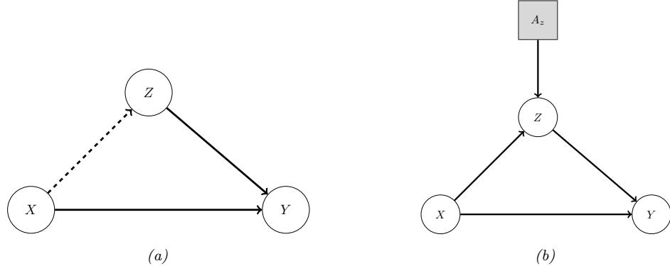
Figure 4.54: An SCM in which we intervene on Z. (a) Hard intervention, in which we clamp Z and thus cut its incoming edges (shown as dotted). (b) Soft intervention, in which we change Z’s mechanism. The square node is an “action” node, using the influence diagram notation from Section 34.2.

4.7.2 Structural equation models

A structural equation model [Bol89; BP13], also known as a path diagram, is a special case of a structural causal model in which all the functional relationships are linear, and the prior on the noise terms is Gaussian. SEMs are widely used in economics and social science, due to the fact that they have a causal interpretation, yet they are computationally tractable.

For example, let us make an SEM version of our education example. We have

\[X = U\_x \tag{4.186}\]

\[Z = c\_z + w\_{xz}X + U\_z \tag{4.187}\]

\[Y = c\_y + w\_{xy}X + w\_{zy}Z + U\_y \tag{4.188}\]

If we assume ^p(Ux) = ^N (Ux|0, ^{ε2 x}), ^p(Uz) = ^N (Ux|0, ^{ε2 z} ), and ^p(Uy) = ^N (Ux|0, ^{ε2 y}), then the model can be converted to the following Gaussian DGM:

\[p(X) = \mathcal{N}(X|\mu\_x, \sigma\_x^2) \tag{4.189}\]

\[p(Z|X) = \mathcal{N}(Z|c\_z + w\_{xz}X, \sigma\_z^2) \tag{4.190}\]

\[p(Y|X,Z) = \mathcal{N}(Y|c\_y + w\_{xy}X + w\_{zy}Z, \sigma\_y^2) \tag{4.191}\]

We can relax the linearity assumption, to allow arbitrarily flexible functions, and relax the Gaussian assumption, to allow any noise distribution. The resulting “nonparametric SEMs” are equivalent to structural causal models. (For a more detailed comparison between SEMs and SCMs, see [Pea12; BP13; Shi00b].)

4.7.3 Do operator and augmented DAGs

One of the main advantages of SCMs is that they let us predict the e!ect of interventions, which are actions that change one or more local mechanisms. A simple intervention is to force a variable to

have a given value, e.g., we can force a gene to be “on” or “o!”. This is called a perfect intervention and is written as do(Xⁱ = xi), where we have introduced new notation for the “do” operator (as in the verb “to do”). This notation means we actively clamp variable Xⁱ to value xⁱ (as opposed to just observing that it has this value). Since the value of Xⁱ is now independent of its usual parents, we should “cut” the incoming edges to node Xⁱ in the graph. This is called the “graph surgery” operation.

In Figure 4.54a we illustrate this for our education SCM, where we force Z to have a given value. For example, we may set Z = 0, by paying o! everyone’s student debt. Note that p(X|do(Z = z)) ⇓= p(X|Z = z), since the intervention changes the model. For example, if we see someone with a debt of 0, we may infer that they probably did not get higher education, i.e., p(X ⇑ 1|Z = 0) is small; but if we pay o! everyone’s college loans, then observing someone with no debt in this modified world should not change our beliefs about whether they got higher education, i.e., p(X ⇑ 1|do(Z = 0)) = p(X ⇑ 1).

In more realistic scenarios, we may not be able to set a variable to a specific value, but we may be able to change it from its current value in some way. For example, we may be able to reduce everyone’s debt by some fixed amount, say ( = ⇐10, 000. Thus we replace Z = fZ(X, Uz) with Z = f^{↔︎ z}(Z, Uz), where f^{↔︎ z}(Z, Uz) = fz(Z, Uz) + (. This is called an additive intervention.

To model this kind of scenario, we can add create an augmented DAG, in which every variable is augmented with an additional parent node, representing whether or not the variable’s mechanism is changed in some way [Daw02; Daw15; CPD17]. These extra variables are represented by square nodes, and correspond to decision variables or actions, as in the influence diagram formalism (Section 34.2). The same formalism is used in MDPs for reinforcement learning (see Section 34.5).

We give an example of this in Figure 4.54b, where we add the A^z ↑ {0, 1} node to specify whether we use the debt reduction policy or not. The modified mechanism for Z becomes

\[Z = f\_Z'(X, U\_x, A\_z) = \begin{cases} f\_Z(X, U\_x) & \text{if } A\_z = 0 \\ f\_Z(X, U\_x) + \Delta & \text{if } A\_z = 1 \end{cases} \tag{4.192}\]

With this new definition, conditioning on the e!ects of an action can be performed using standard probabilistic inference. That is, p(Q|do(A^z = a), E = e) = p(Q|A^z = a, E = e), where Q is the query (e.g., the event X ⇑ 1) and E are the (possibly empty) evidence variables. This is because the A^z node has no parents, so it has no incoming edges to cut when we clamp it.

Although the augmented DAG allows us to use standard notation (no explicit do operators) and inference machinery, the use of “surgical” interventions, which delete incoming edges to a node that is set to a value, results in a simpler graph, which can simplify many calculations, particularly in the non-parametric setting (see [Pea09b, p361] for a discussion). It is therefore a useful abstraction, even if it is less general than the augmented DAG approach.

4.7.4 Counterfactuals

So far we have been focused on predicting the e”ects of causes, so we can choose the optimal action (e.g., if I have a headache, I have to decide should I take an aspirin or not). This can be tackled using standard techniques from Bayesian decision theory, as we have seen (see [Daw00; Daw15; LR19; Roh21; DM22] for more details).

Now suppose we are interested in the causes of e”ects. For example, suppose I took the aspirin and my headache did go away. I might be interested in the counterfactual question “if I had not

Level	Activity	Questions	Examples
1:Association.	Seeing	How would seeing A	Someone took aspirin, how
p(Y a)		change my belief in Y ?	likely is it their headache will
			be cured?
2:Intervention.	Doing	What if I do A?	If I take aspirin, will my
p(Y do(a))			headache be cured?
3:Counterfactuals.	Imagining	Was it A that caused	Would my headache be cured
a do(a↓ p(Y ), y↓ )		Y ?	had I not taken aspirin?

Table 4.6: Pearl’s causal hierarchy. Adapted from Table 1 of [Pea19].

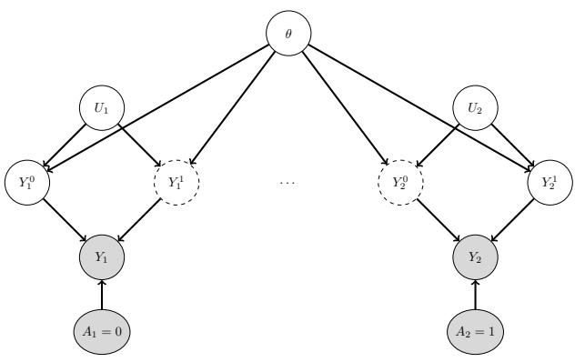
Figure 4.55: Illustration of the potential outcomes framework as a SCM. The nodes with dashed edges are unobserved. In this example, for unit 1, we select action A¹ = 0 and observe Y¹ = Y ^{0 1} = y1, whereas for unit 2, we select action A² = 1 and observe Y² = Y ^{1 2} = y2.

taken the aspirin, would my headache have gone away anyway?“. This kind of reasoning is crucial for legal reasoning (see e.g., [DMM17]), as well as for tasks like explainability and fairness.

Counterfactual reasoning requires strictly more assumptions than reasoning about interventions (see e.g., [DM22]). Indeed, Judea Pearl has proposed what he calls the causal hierarchy [Pea09b; PGJ16; PM18b; Bar+22], which has three levels of analysis, each more powerful than the last. but each making stronger assumptions. See Table 4.6 for a summary.16

In counterfactual reasoning, we want to answer questions of the type p(Y ^a→ |do(a), y), which is read as: “what is the probability distribution over outcomes Y if I were to do a^↔︎ , given that I have already done a and observed outcome y”. (We can also condition on any other evidencee that was observed, such as covariates x.) The quantity Y ^a→ is often called a potential outcome [Rub74], since it is the outcome that would occur in a hypothetical world in which you did a^↔︎ instead of a. (Note that p(Y ^a→ = y) is equivalent to p(Y = y|do(a^↔︎ )), and is an interventional prediction, not a counterfactual one.)

The assumptions behind the potential outcomes framework can be clearly expressed using a

^16. For some Python code that can tell you whether a given causal question (estimand) is identifiable (uniquely answerable) given your modeling assumptions, see https://y0.readthedocs.io/en/latest/ or https://www.pywhy. org/dowhy.

structural causal model. We illustrate this in Figure 4.55 for a simple case where there are two possible actions. We see that we have a set of “units”, such as individual patients, indexed by subscripts. Each unit is associated with a hidden exogeneous random noise source, Ui, that captures everything that is unique about that unit. This noise gets deterministically mapped to two potential outcomes, Y ^{0 i} and Y ^{1 i} , depending on which action is taken. For any given unit, we only get to observe one of the outcomes, namely the one corresponding to the action that was actually chosen. In Figure 4.55, unit 1 chooses action A¹ = 0, so we get to see Y ^{0 1} = y1, whereas unit 2 chooses action A² = 1, so we get to see Y ^{1 2} = y2. The fact that we cannot simultaneously see both outcomes for the same unit is called the “fundamental problem of causal inference” [Hol86].

We will assume the noise sources are independent, which is known as the “stable unit treatment value assumption” or SUTVA. (This would not be true if the treatment on person j could somehow a!ect the outcome of person i, e.g., due to spreading disease or information between i and j.) We also assume that the determinsistic mechanisms that map noise to outcomes are the same across all units (represented by the shared parameter vector ω in Figure 4.55). We need to make one final assumption, namely that the exogeneous noise is not a!ected by our actions. (This is a formalization of the assumption known as “all else being equal”, or (in legal terms) “ceteris paribus”.)

With the above assumptions, we can predict what the outcome for an individual unit would have been in the alternative universe where we picked the other action. The procedure is as follows. First we perform abduction using SCM G, to infer p(Ui|Aⁱ = a, Yⁱ = yi), which is the posterior over the latent factors for unit i given the observed evidence in the actual world. Second we perform intervention, in which we modify the causal mechanisms of G by replacing Aⁱ = a with Aⁱ = a^↔︎ to get G^a→ . Third we perform prediction, in which we propagate the distribution of the latent factors, ^p(Ui|A^{i =} a, Y^{i = y}i), through the modified SCM ^Ga→ to get ^p(^{Y a→ i} |Aⁱ = a, Yⁱ = yi).

In Figure 4.55, we see that we have two copies of every possible outcome variable, to represent the set of possible worlds. Of course, we only get to see one such world, based on the actions that we actually took. More generally, a model in which we “clone” all the deterministic variables, with the noise being held constant between the two branches of the graph for the same unit, is called a twin network [Pea09b]. We will see a more practical example in Section 29.12.6, where we discuss assessing the counterfactual causal impact of an intervention in a time series. See also [RR11; RR13], who propose a related formalism known as single world intervention graph or SWIG. For an implementation of counterfactual inference using the twin network approach, built on top of the Pyro probabilistic programming language, see https://github.com/BasisResearch/chirho.

We see from the above that the potential outcomes framework is mathematically equivalent to structural causal models, but does not use graphical model notation. This has led to heated debate between the founders of the two schools of thought.17. The SCM approach is more popular in computer science (see e.g., [PJS17; Sch19; Sch+21b]), and the PO approach is more popular in economics (see e.g., [AP09; Imb19]). Modern textbooks on causality usually use both formalisms (see e.g., [HR20a; Nea20]).

^17. The potential outcomes framework is based on the work of Donald Rubin, and others, and is therefore sometimes called the Rubin causal model (see e.g., https://en.wikipedia.org/wiki/Rubin\_causal\_model). The structural causal models framework is based on the work of Judea Pearl and others. See e.g., http://causality.cs.ucla.edu/ blog/index.php/2012/12/03/judea-pearl-on-potential-outcomes/ for a discussion of the two.

5 Information theory

Machine learning is fundamentally about information processing. But what is information anyway, and how do we measure it? Ultimately we need a way to quantify the magnitude of an update from one set of beliefs to another. It turns out that with a relatively short list of desiderata there is a unique answer: the Kullback-Leibler (KL) divergence (see Section 5.1). We’ll study the properties of the KL divergence and two special cases: entropy (Section 5.2), and mutual information (Section 5.3). that are useful enough to merit independent study. We then go on to briefly discuss two main applications of information theory. The first application is data compression or source coding, which is the problem of removing redundancy from data so it can be represented more compactly, either in a lossless way (e.g., ZIP files) or a lossy way (e.g., MP3 files). See Section 5.4 for details. The second application is error correction or channel coding, which means encoding data in such a way that it is robust to errors when sent over a noisy channel, such as a telephone line or a satellite link. See Section 5.5 for details.

It turns out that methods for data compression and error correction both rely on having an accurate probabilistic model of the data. For compression, a probabilistic model is needed so the sender can assign shorter codewords to data vectors which occur most often, and hence save space. For error correction, a probabilistic model is needed so the receiver can infer the most likely source message by combining the received noisy message with a prior over possible messages.

It is clear that probabilistic machine learning is useful for information theory. However, information theory is also useful for machine learning. Indeed, we have seen that Bayesian machine learning is about representing and reducing our uncertainty, and so is fundamentally about information. In Section 5.6.2, we explore this direction in more detail, where we discuss the information bottleneck.

For more information on information theory, see e.g., [Mac03; CT06].

5.1 KL divergence

This section is written with Alex Alemi.

To discuss information theory, we need some way to measure or quantify information itself. Let’s say we start with some distribution describing our degrees of belief about a random variable, call it q(x). We then want to update our degrees of belief to some new distribution p(x), perhaps because we’ve taken some new measurements or merely thought about the problem a bit longer. What we seek is a mathematical way to quantify the magnitude of this update, which we’ll denote I[p̸q]. What sort of criteria would be reasonable for such a measure? We discuss this issue below, and then define a quantity that satisfies these criteria.

5.1.1 Desiderata

For simplicity, imagine we are describing a distribution over N possible events. In this case, the probability distribution q(x) consists of N non-negative real numbers that add up to 1. To be even more concrete, imagine we are describing the random variable representing the suit of the next card we’ll draw from a deck: S ↑ {D, E, F, G}. Imagine we initially believe the distributions over suits to be uniform: q = [ ^{1 4} , ^{1 4} , ^{1 4} , ^{1 4} ]. If our friend told us they removed all of the red cards we could update to: q^↔︎ = [ ^{1 2} , ^{1 2} , 0, 0]. Alternatively, we might believe some diamonds changed into clubs and want to update to q↔︎↔︎ = [ ^{3 8} , ^{2 8} , ^{2 8} , ^{1 8} ]. Is there a good way to quantify how much we’ve updated our beliefs? Which is a larger update: q → q^↔︎ or q → q↔︎↔︎?

It seems desireable that any useful such measure would satisfy the following properties:

• 1. continuous in its arguments: If we slightly perturb either our starting or ending distribution, it should similarly have a small e!ect on the magnitude of the update. For example: ^I[p̸ ^{1 4} + 3, ^{1 4} , ^{1 4} , ^{1 4} ⇐ ³] should be close to ^I[p̸q] for small ³, where ^q = [ ^{1 4} , ^{1 4} , ^{1 4} , ¹ 4 ].
• 2. non-negative: I[p̸q] ⇑ 0 for all p(x) and q(x). The magnitude of our updates are non-negative.
• 3. permutation invariant: The magnitude of the update should not depend on the order we choose for the elements of x. For example, it shouldn’t matter if I list my probabilities for the suits of cards in the order D, E, F, G or D, G, F, E, if I keep the order consistent across all of the distributions, I should get the same answer. For example: I[a, b, c, d̸e, f, g, h] = I[a, d, c, b̸e, h, g, f].
• 4. monotonic for uniform distributions: While it’s hard to say how large the updates in our beliefs are in general, there are some special cases for which we have a strong intuition. If our beliefs update from a uniform distribution on N elements to one that is uniform in N^↔︎ elements, the information gain should be an increasing function of N and a decreasing function of N^↔︎ . For instance changing from a uniform distribution on all four suits [ ^{1 4} , ^{1 4} , ^{1 4} , ^{1 4} ] (so N = 4) to only one suit, such as all clubs, [1, 0, 0, 0] where N^↔︎ = 1, is a larger update than if I only updated to the card being black, [ ^{1 2} , ^{1 2} , 0, 0] where N^↔︎ = 2.
• 5. satisfy a natural chain rule: So far we’ve been describing our beliefs in what will happen on the next card draw as a single random variable representing the suit of the next card (S ↑ {D, E, F, G}). We could equivalently describe the same physical process in two steps. First we consider the random variable representing the color of the card (C ↑ {↬, ⊜}), which could be either black (↬ = {D, E}) or red (⊜ = {F, G}). Then, if we draw a red card we describe our belief that it is F versus G. If it was instead black we would assign beliefs to it being D versus E. We can convert any distribution over the four suits into this conditional factorization, for example:

\[p(S) = \left[\frac{3}{8}, \frac{2}{8}, \frac{2}{8}, \frac{1}{8}\right] \tag{5.1}\]

becomes

\[p(C) = \left[\frac{5}{8}, \frac{3}{8}\right] \quad p(\{\clubsuit, \spadesuit\}|C = \blacksquare) = \left[\frac{3}{5}, \frac{2}{5}\right] \quad p(\{\heartsuit, \diamond\}|C = \square) = \left[\frac{2}{3}, \frac{1}{3}\right].\tag{5.2}\]

In the same way we could decompose our uniform distribution q. Obviously, for our measure of information to be of use the magnitude of the update needs to be the same regardless of how we

choose to describe what is ultimately the same physical process. What we need is some way to relate what would be four di!erent invocations of our information function:

\[I\_S \equiv I\left[p(S)\|q(S)\right] \tag{5.3}\]

\[I\_C \equiv I\left[p(C)\|q(C)\right] \tag{5.4}\]

\[I\_{\blacksquare} \equiv I \left[ p(\{\clubsuit, \spadesuit\} | C = \blacksquare) \| q(\{\clubsuit, \spadesuit\} | C = \blacksquare) \right] \tag{5.5}\]

\[I\_{\square} \equiv I \left[ p(\{\heartsuit, \diamond\} | C = \square) \| q(\{\heartsuit, \diamond\} | C = \square) \right]. \tag{5.6}\]

Clearly I^S should be some function of {I^C , I↬, I⊜}. Our last desideratum is that the way we measure the magnitude of our updates will have I^S be a linear combination of I^C , I↬, I⊜. In particular, we will require that they combine as a weighted linear combinations, with weights set by the probability that we would find ourselves in that branch according to the distribution p:

\[I\_S = I\_C + p(C=\blacksquare)I\_{\blacksquare} + p(C=\square)I\_{\square} = I\_C + \frac{5}{8}I\_{\blacksquare} + \frac{3}{8}I\_{\square} \tag{5.7}\]

Stating this requirement more generally: If we partition x into two pieces [xL, xR], so that we can write p(x) = p(xL)p(xR|xL) and similarly for q, the magnitude of the update should be

\[I[p(\mathbf{z}) \| q(\mathbf{z})] = I[p(\mathbf{z}\_L) \| q(\mathbf{z}\_L)] + \mathbb{E}\_{p(\mathbf{z}\_L)} \left[ I[p(\mathbf{z}\_R | \mathbf{z}\_L) \| q(\mathbf{z}\_R | \mathbf{z}\_L)] \right]. \tag{5.8}\]

Notice that this requirement breaks the symmetry between our two distributions: The right hand side asks us to take the expected conditional information gain with respect to the marginal, but we need to decide which of two marginals to take the expectation with respect to.

5.1.2 The KL divergence uniquely satisfies the desiderata

We will now define a quantity that is the only measure (up to a multiplicative constant) that satisfies the above desiderata. The Kullback-Leibler divergence or KL divergence, also known as the information gain or relative entropy, is defined as follows:

\[D\_{\rm KL} \left( p \parallel q \right) \stackrel{\Delta}{=} \sum\_{k=1}^{K} p\_k \log \frac{p\_k}{q\_k}.\tag{5.9}\]

This naturally extends to continuous distributions:

\[D\_{\rm KL}(p \parallel q) \triangleq \int dx \, p(x) \log \frac{p(x)}{q(x)}.\tag{5.10}\]

Next we will verify that this definition satisfies all of our desiderata. (The proof that it is the unique measure which captures these properties can be found in, e.g., [Hob69; Rén61].)

5.1.2.1 Continuity of KL

One of our desiderata was that our measure of information gain should be continuous. The KL divergence is manifestly continuous in its arguments except potentially when p^k or q^k is zero. In the first case, notice that the limit as p → 0 is well behaved:

\[\lim\_{p \to 0} p \log \frac{p}{q} = 0.\tag{5.11}\]

Taking this as the definition of the value of the integrand when p = 0 will make it continuous there. Notice that we do have a problem however if q = 0 in some place that p ⇓= 0. Our information gain requires that our original distribution of beliefs q has some support everywhere the updated distribution does. Intuitively it would require an infinite amount of information for us to update our beliefs in some outcome to change from being exactly 0 to some positive value.

5.1.2.2 Non-negativity of KL divergence

In this section, we prove that the KL divergence as defined is always non-negative. We will make use of Jensen’s inequality, which states that for any convex function f, we have that

\[\int f\left(\sum\_{i=1}^{n} \lambda\_i \mathbf{x}\_i\right) \le \sum\_{i=1}^{n} \lambda\_i f(\mathbf{x}\_i) \tag{5.12}\]

where ^ϖi ⇑ ⁰ and #^{n i}=1 ϖⁱ = 1. This can be proved by induction, where the base case with n = 2 follows by definition of convexity.

Theorem 5.1.1. (Information inequality) DKL (p ̸ q) ⇑ 0 with equality i” p = q.

Proof. We now prove the theorem, following [CT06, p28]. As we noted in the previous section, the KL divergence requires special consideration when p(x) or q(x)=0, the same is true here. Let A = {x : p(x) > 0} be the support of p(x). Using the convexity of the log function and Jensen’s inequality, we have that

\[-D\_{\text{KL}}\left(p \parallel q\right) = -\sum\_{x \in A} p(x) \log \frac{p(x)}{q(x)} = \sum\_{x \in A} p(x) \log \frac{q(x)}{p(x)}\tag{5.13}\]

\[1 \le \log \sum\_{x \in A} p(x) \frac{q(x)}{p(x)} = \log \sum\_{x \in A} q(x) \tag{5.14}\]

\[1 \le \log \sum\_{x \in \mathcal{X}} q(x) = \log 1 = 0 \tag{5.15}\]

Since log(x) is a strictly concave function (⇐ log(x) is convex), we have equality in Equation (5.14) i! p(x) = cq(x) for some c that tracks the fraction of the whole space X contained in A. We have equality in Equation (5.15) i! # ^x≃^{A q}(x) = # ^x≃^{X q}(x)=1, which implies ^c = 1. Hence ^DKL (^p ̸ ^q) = 0 i! p(x) = q(x) for all x.

The non-negativity of KL divergence often feels as though it’s one of the most useful results in information theory. It is a good result to keep in your back pocket. Anytime you can rearrange an expression in terms of KL divergence terms, since those are guaranteed to be non-negative, dropping them immediately generates a bound.

5.1.2.3 KL divergence is invariant to reparameterizations

We wanted our measure of information to be invariant to permutations of the labels. The discrete form is manifestly permutation invariant as summations are. The KL divergence actually satisfies a

much stronger property of reparameterization invariance. Namely, we can transform our random variable through an arbitrary invertible map and it won’t change the value of the KL divergence.

If we transform our random variable from x to some y = f(x) we know that p(x) dx = p(y) dy and q(x) dx = q(y) dy. Hence the KL divergence remains the same for both random variables:

\[D\_{\text{KL}}\left(p(x)\parallel q(x)\right) = \int dx \, p(x) \log \frac{p(x)}{q(x)} = \int dy \, p(y) \log \left(\frac{p(y)\left|\frac{dy}{dx}\right|}{q(y)\left|\frac{dy}{dx}\right|}\right) = D\_{\text{KL}}\left(p(y)\parallel q(y)\right). \tag{5.16}\]

Because of this reparameterization invariance we can rest assured that when we measure the KL divergence between two distributions we are measuring something about the distributions and not the way we choose to represent the space in which they are defined. We are therefore free to transform our data into a convenient basis of our choosing, such as a Fourier bases for images, without a!ecting the result.

5.1.2.4 Montonicity for uniform distributions

Consider updating a probability distribution from a uniform distribution on N elements to a uniform distribution on N^↔︎ elements. The KL divergence is:

\[D\_{\rm KL} \left( p \parallel q \right) = \sum\_{k} \frac{1}{N'} \log \frac{\frac{1}{N'}}{\frac{1}{N}} = \log \frac{N}{N'},\tag{5.17}\]

or the log of the ratio of the elements before and after the update. This satisfies our monotonocity requirement.

We can interpret this result as follows: Consider finding an element of a sorted array by means of bisection. A well designed yes/no question can cut the search space in half. Measured in bits, the KL divergence tells us how many well designed yes/no questions are required on average to move from q to p.

5.1.2.5 Chain rule for KL divergence

Here we show that the KL divergence satisfies a natural chain rule:

\[D\_{\mathbb{KL}}\left(p(x,y)\parallel q(x,y)\right) = \int dx \, dy \, p(x,y) \log \frac{p(x,y)}{q(x,y)}\tag{5.18}\]

\[=\int dx\,dy\,p(x,y)\left[\log\frac{p(x)}{q(x)} + \log\frac{p(y|x)}{q(y|x)}\right] \tag{5.19}\]

\[=D\_{\text{KL}}\left(p(x)\parallel q(x)\right) + \mathbb{E}\_{p(x)}\left[D\_{\text{KL}}\left(p(y|x)\parallel q(y|x)\right)\right].\tag{5.20}\]

We can rest assured that we can decompose our distributions into their conditionals and the KL divergences will just add.

As a notational convenience, the conditional KL divergence is defined to be the expected value of the KL divergence between two conditional distributions:

\[D\_{\text{KL}}\left(p(y|x) \parallel q(y|x)\right) \stackrel{\Delta}{=} \int dx \, p(x) \int dy \, p(y|x) \log \frac{p(y|x)}{q(y|x)}.\tag{5.21}\]

This allows us to drop many expectation symbols.

5.1.3 Thinking about KL

In this section, we discuss some qualitative properties of the KL divergence.

5.1.3.1 Units of KL

Above we said that the desiderata we listed determined the KL divergence up to a multiplicative constant. Because the KL divergence is logarithmic, and logarithms in di!erent bases are the same up to a multiplicative constant, our choice of the base of the logarithm when we compute the KL divergence is a choice akin to choosing which units to measure the information in.

If the KL divergence is measured with the base-2 logarithm, it is said to have units of bits, short for “binary digits”. If measured using the natural logarithm as we normally do for mathematical convenience, it is said to be measured in nats for “natural units”.

To convert between the systems, we use log² y = log ^y log 2 . Hence

\[1\text{ bit} = \log 2\text{ nats} \sim 0.693\text{ nats} \tag{5.22}\]

\[1\text{ nat} = \frac{1}{\log 2}\text{ bits} \sim 1.44\text{ bits}.\tag{5.23}\]

5.1.3.2 Asymmetry of the KL divergence

The KL divergence is not symmetric in its two arguments. While many find this asymmetry confusing at first, we can see that the asymmetry stems from our requirement that we have a natural chain rule. When we decompose the distribution into its conditional, we need to take an expectation with respect to the variables being conditioned on. In the KL divergence we take this expectation with respect to the first argument p(x). This breaks the symmetry between the two distributions.

At a more intuitive level, we can see that the information required to move from q to p is in general di!erent than the information required to move from p to q. For example, consider the KL divergence between two Bernoulli distributions, the first with the probability of success given by 0.443 and the second with 0.975:

\[\text{D}\_{\text{KL}} = 0.975 \log \frac{0.975}{0.443} + 0.025 \log \frac{0.025}{0.557} = 0.692 \text{ nats} \sim 1.0 \text{ bits}. \tag{5.24}\]

So it takes 1 bit of information to update from a [0.443, 0.557] distribution to a [0.975, 0.025] Bernoulli distribution. What about the reverse?

\[\text{D}\_{\text{KL}} = 0.443 \log \frac{0.443}{0.975} + 0.557 \log \frac{0.557}{0.025} = 1.38 \text{ nats} \sim 2.0 \text{ bits},\tag{5.25}\]

so it takes two bits, or twice as much information to move the other way. Thus we see that starting with a distribution that is nearly even and moving to one that is nearly certain takes about 1 bit of information, or one well designed yes/no question. To instead move us from near certainty in an outcome to something that is akin to the flip of a coin requires more persuasion.

5.1.3.3 KL as expected weight of evidence

Imagine you have two di!erent hypotheses you wish to select between, which we’ll label P and Q. You collect some data D. Bayes’ rule tells us how to update our beliefs in the hypotheses being

correct:

\[\Pr(P|D) = \frac{\Pr(D|P)}{\Pr(D)} \Pr(P). \tag{5.26}\]

Normally this requires being able to evaluate the marginal likelihood Pr(D), which is di”cult. If we instead consider the ratio of the probabilities for the two hypotheses:

\[\frac{\Pr(P|D)}{\Pr(Q|D)} = \frac{\Pr(D|P)}{\Pr(D|Q)} \frac{\Pr(P)}{\Pr(Q)},\tag{5.27}\]

the marginal likelihood drops out. Taking the logarithm of both sides, and identifying the probability of the data under the model as the likelihood we find:

\[\log \frac{\Pr(P|D)}{\Pr(Q|D)} = \log \frac{p(D)}{q(D)} + \log \frac{\Pr(P)}{\Pr(Q)}.\tag{5.28}\]

The posterior log probability ratio for one hypothesis over the other is just our prior log probability ratio plus a term that I. J. Good called the weight of evidence [Goo85] D for hypothesis P over Q:

\[w[P/Q; D] \triangleq \log \frac{p(D)}{q(D)}.\tag{5.29}\]

With this interpretation, the KL divergence is the expected weight of evidence for P over Q given by each observation, provided P were correct. Thus we see that data will (on average) add rather than subtract evidence towards the correct hypothesis, since KL divergence is always non-negative in expectation (see Section 5.1.2.2).

5.1.4 Minimizing KL

In this section, we discuss ways to minimize DKL (p ̸ q) or DKL (q ̸ p) wrt an approximate distribution q, given a true distribution p.

5.1.4.1 Forwards vs reverse KL

The asymmetry of KL means that finding a q that is close to p by minimizing DKL (p ̸ q) (also called the inclusive KL or forwards KL) gives di!erent behavior than minimizing DKL (q ̸ p) (also called the exclusive KL or reverse KL). For example, consider the bimodal distribution p shown in blue in Figure 5.1, which we approximate with a unimodal Gaussian q.

To prevent DKL (p ̸ q) from becoming infinite, we must have q > 0 whenever p > 0 (i.e., q must have support everywhere p does), so q tends to cover both modes as it must be nonvanishing everywhere p is; this is called mode-covering or zero-avoiding behavior (orange curve). By contrast, to prevent DKL (q ̸ p) from becoming infinite, we must have q = 0 whenever p = 0, which creates mode-seeking or zero-forcing behavior (green curve).

For an animated visualization (written by Ari Se!) of the di!erence between these two objectives, see https://twitter.com/ari\_seff/status/1303741288911638530.

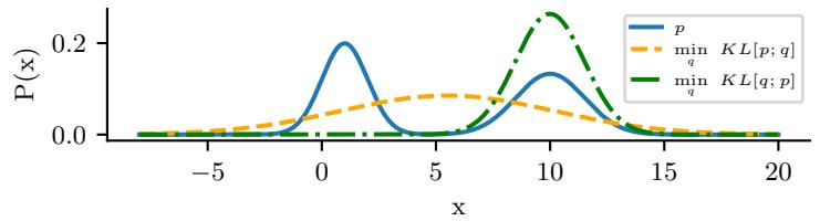
Figure 5.1: Demonstration of the mode-covering or mode-seeking behavior of KL divergence. The original distribution p (shown in blue) is bimodal. When we minimize DKL (p ⇒ q), then q covers the modes of p (orange). When we minimize DKL (q ⇒ p), then q ignores some of the modes of p (green). Generated by minimize\_kl\_divergence.ipynb.

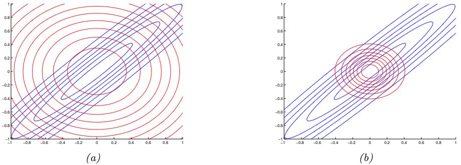
Figure 5.2: Illustrating forwards vs reverse KL on a symmetric Gaussian. The blue curves are the contours of the true distribution p. The red curves are the contours of a factorized approximation q. (a) Minimizing DKL (p ⇒ q). (b) Minimizing DKL (q ⇒ p). Adapted from Figure 10.2 of [Bis06]. Generated by kl\_pq\_gauss.ipynb.

5.1.4.2 Moment projection (mode covering)

Suppose we compute q by minimizing the forwards KL:

\[q = \operatorname\*{argmin}\_{q} D\_{\text{KL}}\left(p \parallel q\right) \tag{5.30}\]

This is called M-projection, or moment projection since the optimal q matches the moments of p, as we show below. The process of computing q is therefore called moment matching.

To see why the optimal q must match the moments of p, let us assume that q is an exponential family distribution of the form

\[q(\mathbf{z}) = h(\mathbf{z}) \exp[\eta^{\mathsf{T}} \mathcal{T}(\mathbf{z}) - \log Z(\eta)] \tag{5.31}\]

where T (x) is the vector of su”cient statistics, and ϖ are the natural parameters. The first order

optimality conditions are as follows:

\[\partial\_{\eta\_i} D\_{\mathbb{KL}} \left( p \parallel q \right) = -\partial\_{\eta\_i} \int\_{\mathfrak{a}} p(\mathbf{z}) \log q(\mathbf{z}) \tag{5.32}\]

\[=-\partial\_{\eta\_i} \int\_{\mathfrak{x}} p(\boldsymbol{x}) \log \left( h(\boldsymbol{x}) \exp[\boldsymbol{\eta}^{\mathsf{T}} \mathcal{T}(\boldsymbol{x}) - \log Z(\boldsymbol{\eta})] \right) \tag{5.33}\]

\[=-\partial\_{\eta\_i} \int\_{\mathfrak{a}} p(\boldsymbol{x}) \left( \boldsymbol{\eta}^{\mathsf{T}} \mathcal{T}(\boldsymbol{x}) - \log Z(\boldsymbol{\eta}) \right) \tag{5.34}\]

\[=-\int\_{\mathfrak{x}} p(\mathbf{z})\mathcal{T}\_i(\mathbf{z}) + \mathbb{E}\_{q(\mathfrak{x})}\left[\mathcal{T}\_i(\mathbf{z})\right] \tag{5.35}\]

\[=-\mathbb{E}\_{p(\mathbf{z})}\left[\mathcal{T}\_i(\mathbf{z})\right] + \mathbb{E}\_{q(\mathbf{z})}\left[\mathcal{T}\_i(\mathbf{z})\right] = 0\tag{5.36}\]

where in the penultimate line we used the fact that the derivative of the log partition function yields the expected su”cient statistics, as shown in Equation (2.216). Hence the expected su”cient statistics (moments of the distribution) must match.

As an example, suppose the true target distribution p is a correlated 2d Gaussian, p(x) = ^N (x|µ, !) = ^N (x|µ, “^↑1), where

\[\boldsymbol{\mu} = \begin{pmatrix} \mu\_1 \\ \mu\_2 \end{pmatrix}, \quad \boldsymbol{\Sigma} = \begin{pmatrix} \Sigma\_{11} & \Sigma\_{12} \\ \Sigma\_{12}^\top & \Sigma\_{22} \end{pmatrix} \quad \boldsymbol{\Lambda} = \begin{pmatrix} \Lambda\_{11} & \Lambda\_{12} \\ \Lambda\_{12}^\top & \Lambda\_{22} \end{pmatrix} \tag{5.37}\]

We will approximate this with a distribution q which is a product of two 1d Gaussians, i.e., a Gaussian with a diagonal covariance matrix:

\[q(\mathbf{z}|\mathbf{m}, \mathbf{V}) = \mathcal{N}(x\_1|m\_1, v\_1)\mathcal{N}(x\_2|m\_2, v\_2) \tag{5.38}\]

If we perform moment matching, the optimal q must therefore have the following form:

\[q(\mathbf{z}) = \mathcal{N}(x\_1|\mu\_1, \Sigma\_{11})\mathcal{N}(x\_2|\mu\_2, \Sigma\_{22}) \tag{5.39}\]

In Figure 5.2(a), we show the resulting distribution. We see that q covers (includes) p, but its support is too broad (under-confidence).

5.1.4.3 Information projection (mode seeking)

Now suppose we compute q by minimizing the reverse KL:

\[q = \operatorname\*{argmin}\_{q} D\_{\text{KL}}\left(q \parallel p\right) \tag{5.40}\]

This is called I-projection, or information projection. This optimization problem is often easier to compute, since the objective requires taking expectations wrt q, which we can choose to be a tractable family.

As an example, consider again the case where the true distribution is a full covariance Gaussian, ^p(x) = ^N (x|µ, “^↑1), and let the approximation be a diagonal Gaussian, ^q(x) = ^N (x|m, diag(v)). Then one can show (see Supplementary Section 5.1.2) that the optimal variational parameters are m = µ and vⁱ =”^↑1 ii . We illustrate this in 2d in Figure 5.2(b). We see that the posterior variance is too narrow, i.e, the approximate posterior is overconfident. Note, however, that minimizing the reverse KL does not always result in an overly compact approximation, as explained in [Tur+08].

5.1.5 Properties of KL

Below are some other useful properties of the KL divergence.

5.1.5.1 Compression lemma

An important general purpose result for the KL divergence is the compression lemma:

Theorem 5.1.2. For any distributions P and Q with a well-defined KL divergence, and for any scalar function ▷ defined on the domain of the distributions we have that:

\[\mathbb{E}\_P\left[\phi\right] \le \log \mathbb{E}\_Q\left[e^{\phi}\right] + D\_{\text{KL}}\left(P \parallel Q\right). \tag{5.41}\]

Proof. We know that the KL divergence between any two distributions is non-negative. Consider a distribution of the form:

\[g(x) = \frac{q(x)}{\mathbb{Z}} e^{\phi(x)}.\tag{5.42}\]

where the partition function is given by:

\[Z = \int dx \, q(x)e^{\phi(x)}.\tag{5.43}\]

Taking the KL divergence between p(x) and g(x) and rearranging gives the bound:

\[D\_{\mathbb{KL}}\left(P \parallel G\right) = D\_{\mathbb{KL}}\left(P \parallel Q\right) - \mathbb{E}\_P\left[\phi(x)\right] + \log(\mathcal{Z}) \ge 0. \tag{5.44}\]

One way to view the compression lemma is that it provides what is termed the Donsker-Varadhan variational representation of the KL divergence:

\[D\_{\mathrm{KL}}\left(P \parallel Q\right) = \sup\_{\phi} \mathbb{E}\_P\left[\phi(x)\right] - \log \mathbb{E}\_Q\left[e^{\phi(x)}\right]. \tag{5.45}\]

In the space of all possible functions ▷ defined on the same domain as the distributions, assuming all of the values above are finite, the KL divergence is the supremum achieved. For any fixed function ▷(x), the right hand side provides a lower bound on the true KL divergence.

Another use of the compression lemma is that it provides a way to estimate the expectation of some function with respect to an unknown distribution P. In this spirit, the compression lemma can be used to power a set of what are known as PAC-Bayes bounds of losses with respect to the true distribution in terms of measured losses with respect to a finite training set. See for example Section 17.4.5 or Banerjee [Ban06].

5.1.5.2 Data processing inequality for KL

We now show that any processing we do on samples from two di!erent distributions makes their samples approach one another. This is called the data processing inequality, since it shows that we cannot increase the information gain from q to p by processing our data and then measuring it.

Theorem 5.1.3. Consider two di”erent distributions p(x) and q(x) combined with a probabilistic channel t(y|x). If p(y) is the distribution that results from sending samples from p(x) through the channel t(y|x) and similarly for q(y) we have that:

\[D\_{\rm KL}\left(p(x) \parallel q(x)\right) \ge D\_{\rm KL}\left(p(y) \parallel q(y)\right) \tag{5.46}\]

Proof. The proof uses Jensen’s inequality from Section 5.1.2.2 again. Call p(x, y) = p(x)t(y|x) and q(x, y) = q(x)t(y|x).

\[D\_{\rm KL}\left(p(x) \parallel q(x)\right) = \int dx \, p(x) \log \frac{p(x)}{q(x)}\tag{5.47}\]

\[=\int dx \int dy \, p(x)t(y|x) \log \frac{p(x)t(y|x)}{q(x)t(y|x)}\tag{5.48}\]

\[= \int dx \int dy \, p(x, y) \log \frac{p(x, y)}{q(x, y)} \tag{5.49}\]

\[=-\int dy\, p(y)\int dx\, p(x|y)\log\frac{q(x,y)}{p(x,y)}\tag{5.50}\]

\[\geq -\int dy \, p(y) \log \left( \int dx \, p(x|y) \frac{q(x,y)}{p(x,y)} \right) \tag{5.51}\]

\[=-\int dy \, p(y) \log\left(\frac{q(y)}{p(y)} \int dx \, q(x|y)\right) \tag{5.52}\]

\[=\int dy \, p(y) \log \frac{p(y)}{q(y)} = D\_{\text{KL}}\left(p(y) \parallel q(y)\right) \tag{5.53}\]

\[\square\]

One way to interpret this result is that any processing done to random samples makes it harder to tell two distributions apart.

As a special form of processing, we can simply marginalize out a subset of random variables.

Corollary 5.1.1. (Monotonicity of KL divergence)

\[D\_{\text{KL}}\left(p(x,y) \parallel q(x,y)\right) \ge D\_{\text{KL}}\left(p(x) \parallel q(x)\right) \tag{5.54}\]

Proof. The proof is essentially the same as the one above.

\[D\_{\text{KL}}\left(p(x,y) \parallel q(x,y)\right) = \int dx \int dy \, p(x,y) \log \frac{p(x,y)}{q(x,y)}\tag{5.55}\]

\[=-\int dy\, p(y)\int dx\, p(x|y)\log\left(\frac{q(y)}{p(y)}\frac{q(x|y)}{p(x|y)}\right) \tag{5.56}\]

\[\geq -\int dy \, p(y) \log \left( \frac{q(y)}{p(y)} \int dx \, q(x|y) \right) \tag{5.57}\]

\[0 = \int dy \, p(y) \log \frac{p(y)}{q(y)} = D\_{\text{KL}}\left(p(y) \parallel q(y)\right) \tag{5.58}\]

(5.59)

One intuitive interpretation of this result is that if you only partially observe random variables, it is harder to distinguish between two candidate distributions than if you observed all of them.

5.1.6 KL divergence and MLE

Suppose we want to find the distribution q that is as close as possible to p, as measured by KL divergence:

\[q^\* = \arg\min\_q D\_{\text{KL}}(p \parallel q) = \arg\min\_q \int p(x) \log p(x) dx - \int p(x) \log q(x) dx \tag{5.60}\]

Now suppose p is the empirical distribution, which puts a probability atom on the observed training data and zero mass everywhere else:

\[p\_{\mathcal{D}}(x) = \frac{1}{N} \sum\_{n=1}^{N} \delta(x - x\_n) \tag{5.61}\]

Using the sifting property of delta functions we get

\[D\_{\rm KL} \left( p\_{\mathcal{D}} \parallel q \right) = - \int p\_{\mathcal{D}}(x) \log q(x) dx + C \tag{5.62}\]

\[I = -\int \left[\frac{1}{N} \sum\_{n} \delta(x - x\_n)\right] \log q(x) dx + C \tag{5.63}\]

\[=-\frac{1}{N}\sum\_{n}\log q(x\_n) + C\tag{5.64}\]

where ^{C =} $ ^pD(x) log ^pD(x) is a constant independent of ^q.

We can rewrite the above as follows

\[D\_{\rm KL} \left( p\_{\mathcal{D}} \parallel q \right) = \mathbb{H}\_{ce}(p\_{\mathcal{D}}, q) - \mathbb{H}(p\_{\mathcal{D}}) \tag{5.65}\]

where

\[\mathbb{H}\_{ce}(p,q) \stackrel{\Delta}{=} -\sum\_{k} p\_k \log q\_k \tag{5.66}\]

is known as the cross entropy. The quantity Hce(pD, q) is the average negative log likelihood of q evaluated on the training set. Thus we see that minimizing KL divergence to the empirical distribution is equivalent to maximizing likelihood.

This perspective points out the flaw with likelihood-based training, namely that it puts too much weight on the training set, a problem known as overfitting. In most applications, we do not really believe that the empirical distribution is a good representation of the true distribution, since it just puts “spikes” on a finite set of points, and zero density everywhere else. Even if the dataset is large (say 1M images), the universe from which the data is sampled is usually even larger (e.g., the set of “all natural images” is much larger than 1M). Thus we need to somehow smooth the empirical distribution by sharing probability mass between “similar” inputs, or we need to regularize the model q so it doesn’t fit the empirical distribution p too closely. (See also Section 20.5.)

5.1.7 KL divergence and Bayesian inference

Bayesian inference itself can be motivated as the solution to a particular minimization problem of KL.

Consider a prior set of beliefs described by a joint distribution q(ϑ, D) = q(ϑ)q(D|ϑ), involving some prior q(ϑ) and some likelihood q(D|ϑ). If we happen to observe some particular dataset D0, how should we update our beliefs? We could search for the joint distribution that is as close as possible to our prior beliefs but that respects the constraint that we now know the value of the data:

\[p(\theta, D) = \operatorname{argmin} D\_{\text{KL}}\left(p(\theta, D) \parallel q(\theta, D)\right) \text{ such that } p(D) = \delta(D - D\_0). \tag{5.67}\]

where 1(D ⇐D0) is a degenerate distribution that puts all its mass on the dataset D that is identically equal to D0. Writing the KL out in its chain rule form:

\[D\_{\mathbb{KL}}\left(p(\theta,D)\parallel q(\theta,D)\right) = D\_{\mathbb{KL}}\left(p(D)\parallel q(D)\right) + D\_{\mathbb{KL}}\left(p(\theta|D)\parallel q(\theta|D)\right),\tag{5.68}\]

makes clear that the solution is given by the joint distribution:

\[p(\theta, D) = p(D)p(\theta|D) = \delta(D - D\_0)q(\theta|D). \tag{5.69}\]

Our updated beliefs have a marginal over the ϑ

\[p(\theta) = \int dD \, p(\theta, D) = \int dD \, \delta(D - D\_0) q(\theta | D) = q(\theta | D = D\_0), \tag{5.70}\]

which is just the usual Bayesian posterior from our prior beliefs evaluated at the data we observed.

By contrast, the usual statement of Bayes’ rule is just a trivial observation about the chain rule of probabilities:

\[q(\theta, D) = q(D)q(\theta|D) = q(\theta)q(D|\theta) \implies q(\theta|D) = \frac{q(D|\theta)}{q(D)}q(\theta). \tag{5.71}\]

Notice that this relates the conditional distribution q(ϑ|D) in terms of q(D|ϑ), q(ϑ) and q(D), but that these are all di!erent ways to write the same distribution. Bayes’ rule does not tell us how we ought to update our beliefs in light of evidence, for that we need some other principle [Cat+11].

One of the nice things about this interpretation of Bayesian inference is that it naturally generalizes to other forms of constraints rather than assuming we have observed the data exactly.

If there was some additional measurement error that was well understood, we ought to instead of picking our updated beliefs to be a delta function on the observed data, simply pick it to be the well understood distribution p(D). For example, we might not know the precise value the data takes, but believe after measuring things that it is a Gaussian distribution with a certain mean and standard deviation.

Because of the chain rule of KL, this has no e!ect on our updated conditional distribution over parameters, which remains the Bayesian posterior: p(ϑ|D) = q(ϑ|D). However, this does change our marginal beliefs about the parameters, which are now:

\[p(\theta) = \int dD \, p(D)q(\theta|D). \tag{5.72}\]

This generalization of Bayes’ rule is sometimes called Je”rey’s conditionalization rule [Cat08].

5.1.8 KL divergence and exponential families

The KL divergence between two exponential family distributions from the same family has a nice closed form, as we explain below.

Consider p(x) with natural parameter ϖ, base measure h(x) and su”cient statistics T (x):

\[p(\mathbf{z}) = h(\mathbf{z}) \exp[\eta^{\mathsf{T}} \mathcal{T}(\mathbf{z}) - A(\eta)] \tag{5.73}\]

where

\[A(\eta) = \log \int h(\mathbf{z}) \exp(\eta^{\mathsf{T}} \mathcal{T}(\mathbf{z})) d\mathbf{z} \tag{5.74}\]

is the log partition function, a convex function of ϖ.

The KL divergence between two exponential family distributions from the same family is as follows:

\[D\_{\mathbb{KL}}\left(p(\mathbf{z}|\boldsymbol{\eta}\_{1})\parallel p(\mathbf{z}|\boldsymbol{\eta}\_{2})\right) = \mathbb{E}\_{\boldsymbol{\eta}\_{1}}\left[\left(\boldsymbol{\eta}\_{1}-\boldsymbol{\eta}\_{2}\right)^{\mathsf{T}}\mathcal{T}(\boldsymbol{x}) - A(\boldsymbol{\eta}\_{1}) + A(\boldsymbol{\eta}\_{2})\right] \tag{5.75}\]

\[\dot{\boldsymbol{\eta}} = \left(\boldsymbol{\eta}\_1 - \boldsymbol{\eta}\_2\right)^{\mathsf{T}} \boldsymbol{\mu}\_1 - A(\boldsymbol{\eta}\_1) + A(\boldsymbol{\eta}\_2) \tag{5.76}\]

where µ^j ↭ E^ωj [T (x)].

5.1.8.1 Example: KL divergence between two Gaussians

An important example is the KL divergence between two multivariate Gaussian distributions, which is given by

\[\begin{aligned} D\_{\text{KL}}\left(\mathcal{N}(x|\mu\_1, \Sigma\_1) \parallel \mathcal{N}(x|\mu\_2, \Sigma\_2)\right) \\ \mathcal{N} = \frac{1}{2} \left[ \text{tr}(\Sigma\_2^{-1} \Sigma\_1) + (\mu\_2 - \mu\_1)^{\mathsf{T}} \Sigma\_2^{-1} (\mu\_2 - \mu\_1) - D + \log \left(\frac{\det(\Sigma\_2)}{\det(\Sigma\_1)}\right) \right] \end{aligned} \tag{5.77}\]

In the scalar case, this becomes

\[D\_{\mathbb{KL}}\left(\mathcal{N}(x|\mu\_1,\sigma\_1)\parallel\mathcal{N}(x|\mu\_2,\sigma\_2)\right) = \log\frac{\sigma\_2}{\sigma\_1} + \frac{\sigma\_1^2 + (\mu\_1 - \mu\_2)^2}{2\sigma\_2^2} - \frac{1}{2} \tag{5.78}\]

5.1.9 Approximating KL divergence using the Fisher information matrix

Let pϑ(x) and p^ϑ→ (x) be two distributions, where ω^↔︎ = ω + ▷. We can measure how close the second distribution is to the first in terms their predictive distribution (as opposed to comparing ω and ω^↔︎ in parameter space) as follows:

\[D\_{\mathbb{KL}}\left(p\_{\theta} \parallel p\_{\theta'}\right) = \mathbb{E}\_{p\_{\theta}(\mathfrak{x})}\left[\log p\_{\theta}(\mathfrak{x}) - \log p\_{\theta'}(\mathfrak{x})\right] \tag{5.79}\]

Let us approximate this with a second order Taylor series expansion:

\[D\_{\mathbb{KL}}\left(p\_{\theta} \parallel p\_{\theta'}\right) \approx -\delta^{\mathsf{T}} \mathbb{E}\left[\nabla \log p\_{\theta}(x)\right] - \frac{1}{2} \delta^{\mathsf{T}} \mathbb{E}\left[\nabla^{2} \log p\_{\theta}(x)\right] \delta \tag{5.80}\]

Since the expected score function is zero (from Equation (3.44)), the first term vanishes, so we have

\[D\_{\mathbb{KL}}\left(p\_{\theta} \parallel p\_{\theta'}\right) \approx \frac{1}{2} \boldsymbol{\delta}^{\mathsf{T}} \mathbf{F}(\theta)\boldsymbol{\delta} \tag{5.81}\]

where F is the FIM

\[\mathbf{F} = -\mathbb{E}\left[\nabla^2 \log p\_{\boldsymbol{\theta}}(\boldsymbol{x})\right] = \mathbb{E}\left[ (\nabla \log p\_{\boldsymbol{\theta}}(\boldsymbol{x})) (\nabla \log p\_{\boldsymbol{\theta}}(\boldsymbol{x}))^\top \right] \tag{5.82}\]

Thus we have shown that the KL divergence is approximately equal to the (squared) Mahalanobis distance using the Fisher information matrix as the metric. This result is the basis of the natural gradient method discussed in Section 6.4.

5.1.10 Bregman divergence

Let f : ! → R be a continuously di!erentiable, strictly convex function defined on a closed convex set !. We define the Bregman divergence associated with f as follows [Bre67]:

\[B\_f(w||\mathbf{v}) = f(w) - f(v) - (w - v)^\top \nabla f(v) \tag{5.83}\]

To understand this, let

\[ \hat{f}\_v(\mathbf{w}) = f(\mathbf{v}) + (\mathbf{w} - \mathbf{v})^\mathsf{T} \nabla f(\mathbf{v}) \tag{5.84} \]

be a first order Taylor series approximation to f centered at v. Then the Bregman divergence is the di!erence from this linear approximation:

\[B\_f(w||v) = f(w) - \hat{f}\_v(w) \tag{5.85}\]

See Figure 5.3a for an illustration. Since ^f is convex, we have ^Bf (w||v) ⇑ ⁰, since ^ˆf^v is a linear lower bound on f.

Below we mention some important special cases of Bregman divergences.

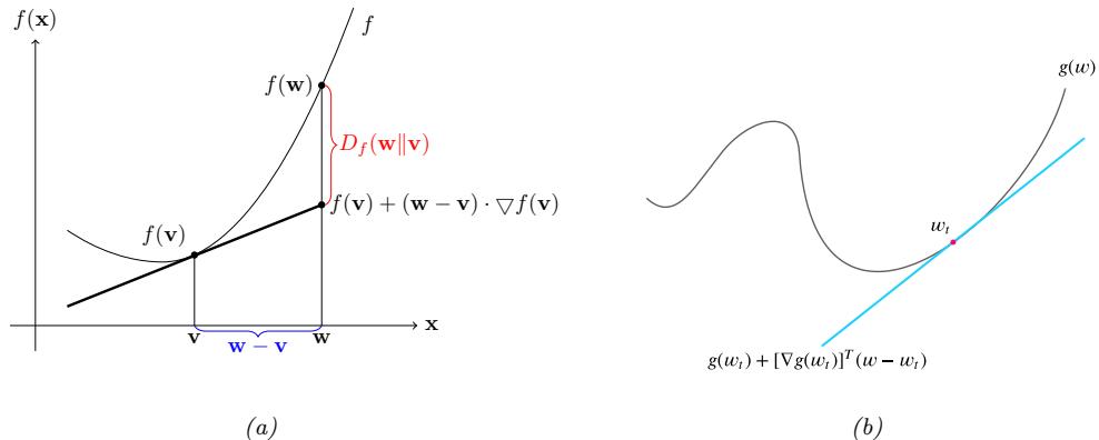
Figure 5.3: (a) Illustration of Bregman divergence. (b) A locally linear approximation to a non-convex function.

• If ^f(w) = ||w||², then ^Bf (w||v) = ||^w ⇐ ^v||² is the squared Euclidean distance.
• If ^f(w) = ^wTQw, then ^Bf (w||v) is the squared Mahalanobis distance.
• If w are the natural parameters of an exponential family distribution, and f(w) = log Z(w) is the log normalizer, then the Bregman divergence is the same as the Kullback-Leibler divergence, as we show in Section 5.1.10.1.

5.1.10.1 KL is a Bregman divergence

Recall that the log partition function A(ϖ) is a convex function. We can therefore use it to define the Bregman divergence (Section 5.1.10) between the two distributions, p and q, as follows:

\[B\_f(\eta\_q||\eta\_p) = A(\eta\_q) - A(\eta\_p) - (\eta\_q - \eta\_p)^\top \nabla\_{\eta\_p} A(\eta\_p) \tag{5.86}\]

\[=A(\eta\_q) - A(\eta\_p) - (\eta\_q - \eta\_p)^\mathsf{T} \mathbb{E}\_p \left[ \mathcal{T}(x) \right] \tag{5.87}\]

\[\mathbf{h} = D\_{\text{KL}}\left(p \parallel q\right) \tag{5.88}\]

where we exploited the fact that the gradient of the log partition function computes the expected su”cient statistics as shown in Section 2.4.3.

In fact, the KL divergence is the only divergence that is both a Bregman divergence and an f-divergence (Section 2.7.1) [Ama09].

5.2 Entropy

In this section, we discuss the entropy of a distribution p, which is just a shifted and scaled version of the KL divergence between the probability distribution and the uniform distribution, as we will see.

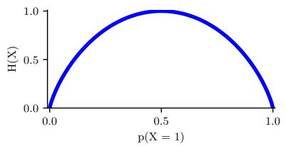
Figure 5.4: Entropy of a Bernoulli random variable as a function of ε. The maximum entropy is log² 2=1. Generated by bernoulli\_entropy\_fig.ipynb.

5.2.1 Definition

The entropy of a discrete random variable X with distribution p over K states is defined by

\[\mathbb{H}(X) \triangleq -\sum\_{k=1}^{K} p(X=k) \log p(X=k) = -\mathbb{E}\_{X} \left[ \log p(X) \right] \tag{5.89}\]

We can use logarithms to any base, but we commonly use log base 2, in which case the units are called bits, or log base e, in which case the units are called nats, as we explained in Section 5.1.3.1.

The entropy is equivalent to a constant minus the KL divergence from the uniform distribution:

\[\mathbb{H}\left(X\right) = \log K - D\_{\text{KL}}\left(p(X) \parallel u(X)\right) \tag{5.90}\]

\[D\_{\text{KL}}\left(p(X) \parallel u(X)\right) = \sum\_{k=1}^{K} p(X=k) \log \frac{p(X=k)}{\frac{1}{K}}\tag{5.91}\]

\[=\log K + \sum\_{k=1}^{K} p(X=k)\log p(X=k) \tag{5.92}\]

If p is uniform, the KL is zero, and we see that the entropy achieves its maximal value of log K.

For the special case of binary random variables, X ↑ {0, 1}, we can write p(X = 1) = ϑ and p(X = 0) = 1 ⇐ ϑ. Hence the entropy becomes

\[\mathbb{H}\left(X\right) = -\left[p(X=1)\log p(X=1) + p(X=0)\log p(X=0)\right] \tag{5.93}\]

\[=-\left[\theta\log\theta+(1-\theta)\log(1-\theta)\right]\tag{5.94}\]

This is called the binary entropy function, and is also written H (ϑ). We plot this in Figure 5.4. We see that the maximum value of 1 bit occurs when the distribution is uniform, ϑ = 0.5. A fair coin requires a single yes/no question to determine its state.

5.2.2 Di!erential entropy for continuous random variables

If X is a continuous random variable with pdf p(x), we define the di”erential entropy as

\[h(X) \stackrel{\Delta}{=} -\int\_{X} dx \, p(x) \log p(x) \tag{5.95}\]

assuming this integral exists.

For example, one can show that the entropy of a d-dimensional Gaussian is

\[h(N(\mu, \Sigma)) = \frac{1}{2} \log |2\pi e\Sigma| = \frac{1}{2} \log [(2\pi e)^d |\Sigma|] = \frac{d}{2} + \frac{d}{2} \log(2\pi) + \frac{1}{2} \log |\Sigma|\tag{5.96}\]

In the 1d case, this becomes

\[h(\mathcal{N}(\mu, \sigma^2)) = \frac{1}{2} \log \left[ 2\pi e \sigma^2 \right] \tag{5.97}\]

Note that, unlike the discrete case, di”erential entropy can be negative. This is because pdf’s can be bigger than 1. For example, suppose X ⇔ U(0, a). Then

\[h(X) = -\int\_0^a dx \, \frac{1}{a} \log \frac{1}{a} = \log a \tag{5.98}\]

If we set a = 1/8, we have h(X) = log2(1/8) = ⇐3 bits.

One way to understand di!erential entropy is to realize that all real-valued quantities can only be represented to finite precision. It can be shown [CT91, p228] that the entropy of an n-bit quantization of a continuous random variable ^X is approximately ^h(X) + ⁿ. For example, suppose ^{X ⇔ U}(0, ¹ 8 ). Then in a binary representation of X, the first 3 bits to the right of the binary point must be 0 (since the number is ↗ 1/8). So to describe X to n bits of accuracy only requires n ⇐ 3 bits, which agrees with h(X) = ⇐3 calculated above.

The continuous entropy also lacks the reparameterization independence of KL divergence (Section 5.1.2.3). In particular, if we transform our random variable y = f(x), the entropy transforms. To see this, note that the change of variables tells us that

\[p(y) \, dy = p(x) \, dx \implies p(y) = p(x) \left| \frac{dy}{dx} \right|^{-1},\tag{5.99}\]

Thus the continuous entropy transforms as follows:

\[h(X) = -\int dx \, p(x) \log p(x) = h(Y) - \int dy \, p(y) \log \left| \frac{dy}{dx} \right|. \tag{5.100}\]

We pick up a factor in the continuous entropy of the log of the determinant of the Jacobian of the transformation. This changes the value for the continuous entropy even for simply rescaling the random variable such as when we change units. For example in Figure 5.5 we show the distribution of adult human heights (it is bimodal because while both male and female heights are normally distributed, they di!er noticeably). The continous entropy of this distribution depends on the units it is measured in. If measured in feet, the continuous entropy is 0.43 bits. Intuitively this is because human heights mostly span less than a foot. If measured in centimeters it is instead 5.4 bits. There are 30.48 centimeters in a foot, log² 30.48 = 4.9 explaining the di!erence. If we measured the continuous entropy of the same distribution measured in meters we would obtain ⇐1.3 bits!

5.2.3 Typical sets

The typical set of a probability distribution is the set whose elements have an information content that is close to that of the expected information content from random samples from the distribution.

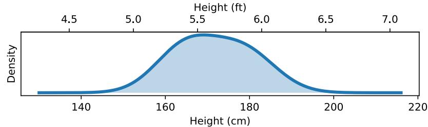
Figure 5.5: Distribution of adult heights. The continuous entropy of the distribution depends on its units of measurement. If heights are measured in feet, this distribution has a continuous entropy of 0.43 bits. If measured in centimeters it’s 5.4 bits. If measured in meters it’s ↓1.3 bits. Data taken from https: // ourworldindata. org/ human-height .

More precisely, for a distribution ^p(x) with support ^{x ↑ X} , the ³-typical set ^{AN ▷ ↑ X N} for ^p(x) is the set of all length N sequences such that

\[\mathbb{H}(p(\mathbf{z})) - \epsilon \le -\frac{1}{N} \log p(\mathbf{z}\_1, \dots, \mathbf{z}\_N) \le \mathbb{H}(p(\mathbf{z})) + \epsilon \tag{5.101}\]

If we assume p(x1,…, x^N ) = ^{N n}=1 p(xn), then we can interpret the term in the middle as the N-sample empirical estimate of the entropy. The asymptotic equipartition property or AEP states that this will converge (in probability) to the true entropy as N → ⇒ [CT06]. Thus the typical set has probability close to 1, and is thus a compact summary of what we can expect to be generated by p(x).

5.2.4 Cross entropy and perplexity

A standard way to measure how close a model q is to a true distribution p is in terms of the KL divergence (Section 5.1), given by

\[D\_{\mathbb{KL}}\left(p \parallel q\right) = \sum\_{x} p(x) \log \frac{p(x)}{q(x)} = \mathbb{H}\_{\text{ce}}\left(p, q\right) - \mathbb{H}\left(p\right) \tag{5.102}\]

where Hce (p, q) is the cross entropy

\[\mathbb{H}\_{ce}\left(p,q\right) = -\sum\_{x} p(x)\log q(x) \tag{5.103}\]

and H (p) = Hce (p, p) is the entropy, which is a constant independent of the model.

In language modeling, it is common to report an alternative performance measure known as the perplexity. This is defined as

\[\text{perplexity}(p,q) \stackrel{\Delta}{=} 2^{\mathbb{H}\_{ce}(p,q)}\tag{5.104}\]

We can compute an empirical approximation to the cross entropy as follows. Suppose we approximate the true distribution with an empirical distribution based on data sampled from p:

\[p\_{\mathcal{D}}(x|\mathcal{D}) = \frac{1}{N} \sum\_{n=1}^{N} \mathbb{I}\left(x = x\_n\right) \tag{5.105}\]

In this case, the cross entropy is given by

\[H = -\frac{1}{N} \sum\_{n=1}^{N} \log p(x\_n) = -\frac{1}{N} \log \prod\_{n=1}^{N} p(x\_n) \tag{5.106}\]

The corresponding perplexity is given by

\[\text{perplexity}(p\_{\mathcal{D}}, p) = 2^{-\frac{1}{N}\log(\prod\_{n=1}^{N} p(x\_n))} = 2^{\log(\prod\_{n=1}^{N} p(x\_n))^{-\frac{1}{N}}} \tag{5.107}\]

\[= (\prod\_{n=1}^{N} p(x\_n))^{-1/N} = \sqrt[N]{\prod\_{n=1}^{N} \frac{1}{p(x\_n)}} \tag{5.108}\]

In the case of language models, we usually condition on previous words when predicting the next word. For example, in a bigram model, we use a second order Markov model of the form p(xn|xⁿ↑1). We define the branching factor of a language model as the number of possible words that can follow any given word. For example, suppose the model predicts that each word is equally likely, regardless of context, so p(xn|xⁿ↑1)=1/K, where K is the number of words in the vocabulary. Then the perplexity is ((1/K)^N )↑1/N = K. If some symbols are more likely than others, and the model correctly reflects this, its perplexity will be lower than K. However, we have H (p↘) ↗ Hce (p↘, p), so we can never reduce the perplexity below 2^{↑ H}(p↑) .

5.3 Mutual information

The KL divergence gave us a way to measure how similar two distributions were. How should we measure how dependent two random variables are? One thing we could do is turn the question of measuring the dependence of two random variables into a question about the similarity of their distributions. This gives rise to the notion of mutual information (MI) between two random variables, which we define below.

5.3.1 Definition

The mutual information between rv’s X and Y is defined as follows:

\[\mathbb{E}\left(X;Y\right) \stackrel{\Delta}{=} D\_{\text{KL}}\left(p(x,y) \parallel p(x)p(y)\right) = \sum\_{y \in Y} \sum\_{x \in X} p(x,y) \log \frac{p(x,y)}{p(x)p(y)}\tag{5.109}\]

(We write I(X; Y ) instead of I(X, Y ), in case X and/or Y represent sets of variables; for example, we can write I(X; Y,Z) to represent the MI between X and (Y,Z).) For continuous random variables, we just replace sums with integrals.

It is easy to see that MI is always non-negative, even for continuous random variables, since

\[\mathbb{L}\left(X;Y\right) = D\_{\text{KL}}\left(p(x,y) \parallel p(x)p(y)\right) \geq 0\tag{5.110}\]

We achieve the bound of 0 i! p(x, y) = p(x)p(y).

5.3.2 Interpretation

Knowing that the mutual information is a KL divergence between the joint and factored marginal distributions tells us that the MI measures the information gain if we update from a model that treats the two variables as independent p(x)p(y) to one that models their true joint density p(x, y).

To gain further insight into the meaning of MI, it helps to re-express it in terms of joint and conditional entropies, as follows:

\[\mathbb{H}(X;Y) = \mathbb{H}(X) - \mathbb{H}(X|Y) = \mathbb{H}(Y) - \mathbb{H}(Y|X) \tag{5.111}\]

Thus we can interpret the MI between X and Y as the reduction in uncertainty about X after observing Y , or, by symmetry, the reduction in uncertainty about Y after observing X. Incidentally, this result gives an alternative proof that conditioning, on average, reduces entropy. In particular, we have 0 ↗ I(X; Y ) = H (X) ⇐ H (X|Y ), and hence H (X|Y ) ↗ H (X).

We can also obtain a di!erent interpretation. One can show that

\[\mathbb{E}\left(X;Y\right) = \mathbb{E}\left(X,Y\right) - \mathbb{E}\left(X|Y\right) - \mathbb{E}\left(Y|X\right) \tag{5.112}\]

Finally, one can show that

\[\mathbb{E}\left(X;Y\right) = \mathbb{E}\left(X\right) + \mathbb{E}\left(Y\right) - \mathbb{E}\left(X,Y\right) \tag{5.113}\]

See Figure 5.6 for a summary of these equations in terms of an information diagram. (Formally, this is a signed measure mapping set expressions to their information-theoretic counterparts [Yeu91a].)

5.3.3 Data processing inequality

Suppose we have an unknown variable X, and we observe a noisy function of it, call it Y . If we process the noisy observations in some way to create a new variable Z, it should be intuitively obvious that we cannot increase the amount of information we have about the unknown quantity, X. This is known as the data processing inequality. We now state this more formally, and then prove it.

Theorem 5.3.1. Suppose X → Y → Z forms a Markov chain, so that X ℜ Z|Y . Then I(X; Y ) ⇑ I(X;Z).

Proof. By the chain rule for mutual information we can expand the mutual information in two di!erent ways:

\[\mathbb{I}\left(X;Y,Z\right) = \mathbb{I}\left(X;Z\right) + \mathbb{I}\left(X;Y|Z\right) \tag{5.114}\]

\[=\mathbb{I}(X;Y) + \mathbb{I}(X;Z|Y) \tag{5.115}\]

Since X ℜ Z|Y , we have I(X;Z|Y )=0, so

\[\mathbb{I}\left(X;Z\right) + \mathbb{I}\left(X;Y|Z\right) = \mathbb{I}\left(X;Y\right) \tag{5.116}\]

Since I(X; Y |Z) ⇑ 0, we have I(X; Y ) ⇑ I(X;Z). Similarly one can prove that I(Y ;Z) ⇑ I(X;Z).

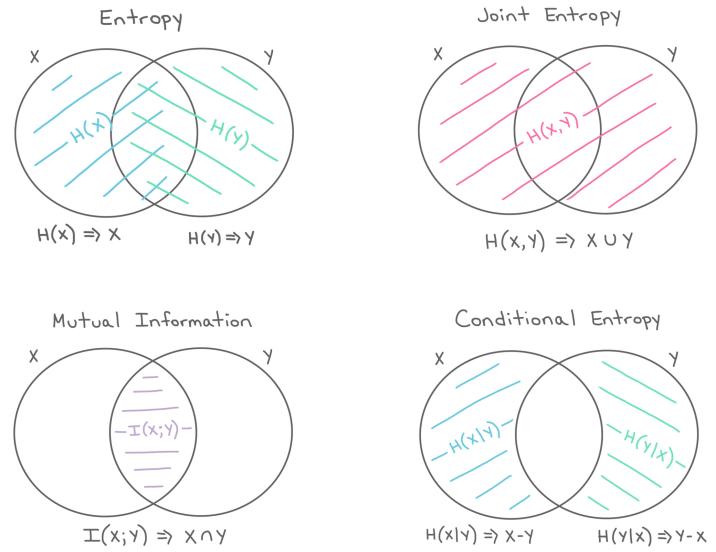
Figure 5.6: The marginal entropy, joint entropy, conditional entropy, and mutual information represented as information diagrams. Used with kind permission of Katie Everett.

5.3.4 Su”cient statistics

An important consequence of the DPI is the following. Suppose we have the chain ϑ → X → s(X). Then

\[\mathbb{E}\left(\theta; s(X)\right) \le \mathbb{E}\left(\theta; X\right) \tag{5.117}\]

If this holds with equality, then we say that s(X) is a su!cient statistic of the data X for the purposes of inferring ϑ. In this case, we can equivalently write ϑ → s(X) → X, since we can reconstruct the data from knowing s(X) just as accurately as from knowing ϑ.

An example of a su”cient statistic is the data itself, s(X) = X, but this is not very useful, since it doesn’t summarize the data at all. Hence we define a minimal su!cient statistic s(X) as one which is su”cient, and which contains no extra information about ϑ; thus s(X) maximally compresses the data X without losing information which is relevant to predicting ϑ. More formally, we say s is a minimal su”cient statistic for X if s(X) = f(s^↔︎ (X)) for some function f and all su”cient statistics s↔︎ (X). We can summarize the situation as follows:

\[ \theta \to s(X) \to s'(X) \to X \tag{5.118} \]

Here s^↔︎ (X) takes s(X) and adds redundant information to it, thus creating a one-to-many mapping.

For example, a minimal su”cient statistic for a set of N Bernoulli trials is simply N and N¹ = ⁿ I(Xⁿ = 1), i.e., the number of successes. In other words, we don’t need to keep track of the entire sequence of heads and tails and their ordering, we only need to keep track of the total number of heads and tails. Similarly, for inferring the mean of a Gaussian distribution with known variance we only need to know the empirical mean and number of samples.

Earlier in Section 5.1.8 we motivated the exponential family of distributions as being the ones that are minimal in the sense that they contain no other information than constraints on some statistics of the data. It makes sense then that the statistics used to generate exponential family distributions are su”cient. It also hints at the more remarkable fact of the Pitman-Koopman-Darmois theorem, which says that for any distribution whose domain is fixed, it is only the exponential family that admits su”cient statistics with bounded dimensionality as the number of samples increases [Dia88b].

5.3.5 Multivariate mutual information

There are several ways to generalize the idea of mutual information to a set of random variables as we discuss below.

5.3.5.1 Total correlation

The simplest way to define multivariate MI is to use the total correlation [Wat60] or multiinformation [SV98], defined as

\[\mathsf{TCC}(\{X\_1, \ldots, X\_D\}) \triangleq D\_{\mathsf{KL}}\left(p(x) \parallel \prod\_d p(x\_d)\right) \tag{5.119}\]

\[\mathbb{E} = \sum\_{\mathbf{x}} p(\mathbf{x}) \log \frac{p(\mathbf{x})}{\prod\_{d=1}^{D} p(x\_d)} = \sum\_{d} \mathbb{H}(x\_d) - \mathbb{H}(\mathbf{x}) \tag{5.120}\]

For example, for 3 variables, this becomes

\[\mathbb{TIC}(X,Y,Z) = \mathbb{H}(X) + \mathbb{H}(Y) + \mathbb{H}(Z) - \mathbb{H}(X,Y,Z) \tag{5.121}\]

where H (X, Y, Z) is the joint entropy

\[\mathbb{H}\left(X,Y,Z\right) = -\sum\_{x}\sum\_{y}\sum\_{z} p(x,y,z)\log p(x,y,z)\tag{5.122}\]

One can show that the multi-information is always non-negative, and is zero i! p(x) = ^d p(xd). However, this means the quantity is non-zero even if only a pair of variables interact. For example, if p(X, Y, Z) = p(X, Y )p(Z), then the total correlation will be non-zero, even though there is no 3 way interaction. This motivates the alternative definition in Section 5.3.5.2.

5.3.5.2 Interaction information (co-information)

The conditional mutual information can be used to give an inductive definition of the multivariate mutual information (MMI) as follows:

\[\mathbb{I}(X\_1; \cdots; X\_D) = \mathbb{I}(X\_1; \cdots; X\_{D-1}) - \mathbb{I}(X\_1; \cdots; X\_{D-1}|X\_D) \tag{5.123}\]

This is called the multiple mutual information [Yeu91b], or the co-information [Bel03]. This definition is equivalent, up to a sign change, to the interaction information [McG54; Han80; JB03; Bro09].

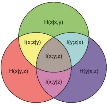
Figure 5.7: Illustration of multivariate mutual information between three random variables. From https: // en. wikipedia. org/ wiki/ Mutual\_ information . Used with kind permission of Wikipedia author PAR.

For 3 variables, the MMI is given by

\[\mathbb{I}\left(X;Y;Z\right) = \mathbb{I}(X;Y) - \mathbb{I}(X;Y|Z) \tag{5.124}\]

\[= \mathbb{I}(X;Z) - \mathbb{I}(X;Z|Y) \tag{5.125}\]

\[= \mathbb{I}(Y;Z) - \mathbb{I}(Y;Z|X) \tag{5.126}\]

This can be interpreted as the change in mutual information between two pairs of variables when conditioning on the third. Note that this quantity is symmetric in its arguments.

By the definition of conditional mutual information, we have

\[\mathbb{I}(X;Z|Y) = \mathbb{I}(Z;X,Y) - \mathbb{I}(Y;Z) \tag{5.127}\]

Hence we can rewrite Equation (5.125) as follows:

\[\mathbb{I}(X;Y;Z) = \mathbb{I}(X;Z) + \mathbb{I}(Y;Z) - \mathbb{I}(X,Y;Z) \tag{5.128}\]

This tells us that the MMI is the di!erence between how much we learn about Z given X and Y individually vs jointly (see also Section 5.3.5.3).

The 3-way MMI is illustrated in the information diagram in Figure 5.7. The way to interpret such diagrams when we have multiple variables is as follows: the area of a shaded area that includes circles A, B, C, . . . and excludes circles F, G, H, . . . represents I(A; B; C; … |F, G, H, . . .); if B = C = ↔︎, this is just H(A|F, G, H, . . .); if F = G = H = ↔︎, this is just I(A; B; C, . . .).

5.3.5.3 Synergy and redundancy

The MMI is I(X; Y ;Z) = I(X;Z) + I(Y ;Z) ⇐ I(X, Y ;Z). We see that this can be positive, zero, or negative. If some of the information about Z that is provided by X is also provided by Y , then there is some redundancy between X and Y (wrt Z). In this case, I(X;Z) + I(Y ;Z) > I(X, Y ;Z), so (from Equation (5.128)) we see that the MMI will be positive. If, by contrast, we learn more about Z when we see X and Y together, we say there is some synergy between them. In this case, I(X;Z) + I(Y ;Z) < I(X, Y ;Z), so the MMI will be negative.

5.3.5.4 MMI and causality

The sign of the MMI can be used to distinguish between di!erent kinds of directed graphical models, which can sometimes be interpreted causally (see Chapter 36 for a general discussion of causality). For example, consider a model of the form X ∈ Z → Y , where Z is a “cause” of X and Y . For example, suppose X represents the event it is raining, Y represents the event that the sky is dark, and Z represents the event that the sky is cloudy. Conditioning on the common cause Z renders the children X and Y independent, since if I know it is cloudy, noticing that the sky is dark does not change my beliefs about whether it will rain or not. Consequently I(X; Y |Z) ↗ I(X; Y ), so I(X; Y ;Z) ⇑ 0.

Now consider the case where Z is a common e!ect, X → Z ∈ Y . In this case, conditioning on Z makes X and Y dependent, due to the explaining away phenomenon (see Section 4.2.4.2). For example, if X and Y are independent random bits, and Z is the XOR of X and Y , then observing Z = 1 means that p(X ⇓= Y |Z = 1) = 1, so X and Y are now dependent (information-theoretically, not causally), even though they were a priori independent. Consequently I(X; Y |Z) ⇑ I(X; Y ), so I(X; Y ;Z) ↗ 0.

Finally, consider a Markov chain, X → Y → Z. We have I(X;Z|Y ) ↗ I(X;Z) and so the MMI must be positive.

5.3.5.5 MMI and entropy

We can also write the MMI in terms of entropies. Specifically, we know that

\[\mathbb{H}(X;Y) = \mathbb{H}(X) + \mathbb{H}(Y) - \mathbb{H}(X,Y) \tag{5.129}\]

and

\[\mathbb{H}(X;Y|Z) = \mathbb{H}(X,Z) + \mathbb{H}(Y,Z) - \mathbb{H}(Z) - \mathbb{H}(X,Y,Z) \tag{5.130}\]

Hence we can rewrite Equation (5.124) as follows:

\[\mathbb{E}(X;Y;Z) = \left[\mathbb{H}(X) + \mathbb{H}(Y) + \mathbb{H}(Z)\right] - \left[\mathbb{H}(X,Y) + \mathbb{H}(X,Z) + \mathbb{H}(Y,Z)\right] + \mathbb{H}(X,Y,Z) \tag{5.131}\]

Contrast this to Equation (5.121).

More generally, we have

\[\mathbb{E}(X\_1, \ldots, X\_D) = -\sum\_{\mathcal{T} \subseteq \{1, \ldots, D\}} (-1)^{|\mathcal{T}|} \mathbb{E}(\mathcal{T}) \tag{5.132}\]

For sets of size 1, 2, and 3 this expands as follows:

\[I\_1 = H\_1 \tag{5.133}\]

\[I\_{12} = H\_1 + H\_2 - H\_{12} \tag{5.134}\]

\[H\_{123} = H\_1 + H\_2 + H\_3 - H\_{12} - H\_{13} - H\_{23} + H\_{123} \tag{5.135}\]

We can use the Möbius inversion formula to derive the following dual relationship:

\[\mathbb{H}\left(\mathcal{S}\right) = -\sum\_{\mathcal{T}\subseteq\mathcal{S}} (-1)^{|\mathcal{T}|} \,\mathbb{I}(\mathcal{T})\tag{5.136}\]

for sets of variables S.

Using the chain rule for entropy, we can also derive the following expression for the 3-way MMI:

\[\mathbb{E}(X;Y;Z) = \mathbb{E}\left(Z\right) - \mathbb{E}\left(Z|X\right) - \mathbb{E}\left(Z|Y\right) + \mathbb{E}\left(Z|X,Y\right) \tag{5.137}\]

5.3.6 Variational bounds on mutual information

In this section, we discuss methods for computing upper and lower bounds on MI that use variational approximations to the intractable distributions. This can be useful for representation learning (Chapter 32). This approach was first suggested in [BA03]. For a more detailed overview of variational bounds on mutual information, see Poole et al. [Poo+19b].

5.3.6.1 Upper bound

Suppose that the joint p(x, y) is intractable to evaluate, but that we can sample from p(x) and evaluate the conditional distribution p(y|x). Furthermore, suppose we approximate p(y) by q(y). Then we can compute an upper bound on the MI as follows:

\[\mathbb{E}(x; y) = \mathbb{E}\_{p(x, y)}\left[\log \frac{p(y|x)q(y)}{p(y)q(y)}\right] \tag{5.138}\]

\[=\mathbb{E}\_{p(\mathbf{z},\mathbf{y})}\left[\log\frac{p(\mathbf{y}|\mathbf{z})}{q(\mathbf{y})}\right]-D\_{\text{KL}}\left(p(\mathbf{y})\parallel q(\mathbf{y})\right)\tag{5.139}\]

\[\leq \mathbb{E}\_{p(\boldsymbol{\mathfrak{x}})} \left[ \mathbb{E}\_{p(\boldsymbol{\mathfrak{y}}|\boldsymbol{\mathfrak{x}})} \left[ \log \frac{p(\boldsymbol{\mathfrak{y}}|\boldsymbol{\mathfrak{x}})}{q(\boldsymbol{\mathfrak{y}})} \right] \right] \tag{5.140}\]

\[=\mathbb{E}\_{p(\mathbf{z})}\left[D\_{\text{KL}}\left(p(\mathbf{y}|\mathbf{z})\parallel q(\mathbf{y})\right)\right] \tag{5.141}\]

This bound is tight if q(y) = p(y).

What’s happening here is that I(Y ; X) = H (Y ) ⇐ H (Y |X) and we’ve assumed we know p(y|x) and so can estimate H (Y |X) well. While we don’t know H (Y ), we can upper bound it using some model q(y). Our model can never do better than p(y) itself (the non-negativity of KL), so our entropy estimate errs too large, and hence our MI estimate will be an upper bound.

5.3.6.2 BA lower bound

Suppose that the joint p(x, y) is intractable to evaluate, but that we can evaluate p(x). Furthermore, suppose we approximate p(x|y) by q(x|y). Then we can derive the following variational lower bound on the mutual information:

\[\mathbb{E}(x; y) = \mathbb{E}\_{p(x, y)}\left[\log \frac{p(x|y)}{p(x)}\right] \tag{5.142}\]

\[=\mathbb{E}\_{p(\mathbf{z},\mathbf{y})}\left[\log\frac{q(\mathbf{z}|\mathbf{y})}{p(\mathbf{z})}\right] + \mathbb{E}\_{p(\mathbf{y})}\left[D\_{\text{KL}}\left(p(\mathbf{z}|\mathbf{y}) \parallel q(\mathbf{z}|\mathbf{y})\right)\right] \tag{5.143}\]

\[\mathbb{E}\_x \ge \mathbb{E}\_{p(\mathbf{z}, \mathbf{y})} \left[ \log \frac{q(\mathbf{z}|\mathbf{y})}{p(\mathbf{z})} \right] = \mathbb{E}\_{p(\mathbf{z}, \mathbf{y})} \left[ \log q(\mathbf{z}|\mathbf{y}) \right] + h(\mathbf{z}) \tag{5.144}\]

where h(x) is the di!erential entropy of x. This is called the BA lower bound, after the authors Barber and Agakov [BA03].

5.3.6.3 NWJ lower bound

The BA lower bound requires a tractable normalized distribution q(x|y) that we can evaluate pointwise. If we reparameterize this distribution in a clever way, we can generate a lower bound that does not require a normalized distribution. Let’s write:

\[q(x|y) = \frac{p(x)e^{f(x,y)}}{Z(y)}\tag{5.145}\]

with Z(y) = Ep(x) e^f(x,y) . the normalization constant or partition function. Plugging this into the BA lower bound above we obtain:

\[\mathbb{E}\_{p(\mathbf{z},\mathbf{y})} \left[ \log \frac{p(\mathbf{z})e^{f(\mathbf{z},\mathbf{y})}}{p(\mathbf{z})Z(\mathbf{y})} \right] = \mathbb{E}\_{p(\mathbf{z},\mathbf{y})} \left[ f(\mathbf{z},\mathbf{y}) \right] - \mathbb{E}\_{p(\mathbf{y})} \left[ \log Z(\mathbf{y}) \right] \tag{5.146}\]

\[=\mathbb{E}\_{p(\boldsymbol{\mathfrak{z}},\boldsymbol{\mathfrak{y}})}\left[f(\boldsymbol{\mathfrak{z}},\boldsymbol{\mathfrak{y}})\right]-\mathbb{E}\_{p(\boldsymbol{\mathfrak{y}})}\left[\log\mathbb{E}\_{p(\boldsymbol{\mathfrak{z}})}\left[e^{f(\boldsymbol{\mathfrak{z}},\boldsymbol{\mathfrak{y}})}\right]\right] \tag{5.147}\]

\[\triangleq I\_{DV}(X;Y).\tag{5.148}\]

This is the Donsker-Varadhan lower bound [DV75].

We can construct a more tractable version of this by using the fact that the log function can be upper bounded by a straight line using

\[ \log x \le \frac{x}{a} + \log a - 1 \tag{5.149} \]

If we set a = e, we get

\[\mathbb{E}(X;Y) \ge \mathbb{E}\_{p(\mathbf{z},\mathbf{y})}[f(\mathbf{z},\mathbf{y})] - e^{-1}\mathbb{E}\_{p(\mathbf{y})}Z(\mathbf{y}) \stackrel{\Delta}{=} I\_{NW}(X;Y) \tag{5.150}\]

This is called the NWJ lower bound (after the authors of Nguyen, Wainwright, and Jordan [NWJ10a]), or the f-GAN KL [NCT16a], or the MINE-f score [Bel+18].

5.3.6.4 InfoNCE lower bound

If we instead explore a multi-sample extension to the DV bound above, we can generate the following lower bound (see [Poo+19b] for the derivation):

\[\mathbb{E}\,\mathbb{I}\_{\text{NCE}} = \mathbb{E}\left[\frac{1}{K}\sum\_{i=1}^{K}\log\frac{e^{f(\mathbf{z}\_{i},y\_{i})}}{\frac{1}{K}\sum\_{j=1}^{K}e^{f(\mathbf{z}\_{i},y\_{j})}}\right] \tag{5.151}\]

\[=\log K - \mathbb{E}\left[\frac{1}{K}\sum\_{i=1}^{K}\log\left(1 + \sum\_{j\neq i}^{K} e^{f(\mathbf{z}\_i, y\_j) - f(\mathbf{z}\_i, y\_i)}\right)\right] \tag{5.152}\]

where the expectation is over paired samples from the joint p(X, Y ). The quantity in Equation (5.152) is called the InfoNCE estimate, and was proposed in [OLV18a; Hen+19a]. (NCE stands for “noise contrastive estimation”, and is discussed in Section 24.4.)

The intuition here is that mutual information is a divergence between the joint p(x, y) and the product of the marginals, p(x)p(y). In other words, mutual information is a measurement of how

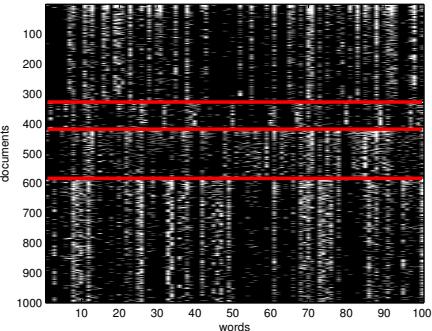
Figure 5.8: Subset of size 16242 x 100 of the 20-newsgroups data. We only show 1000 rows, for clarity. Each row is a document (represented as a bag-of-words bit vector), each column is a word. The red lines separate the 4 classes, which are (in descending order) comp, rec, sci, talk (these are the titles of USENET groups). We can see that there are subsets of words whose presence or absence is indicative of the class. The data is available from http: // cs. nyu. edu/ ~roweis/ data. html . Generated by newsgroups\_visualize.ipynb.

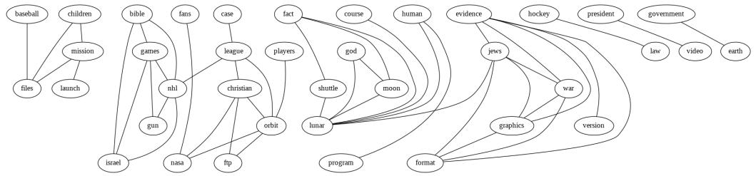
Figure 5.9: Part of a relevance network constructed from the 20-newsgroup data. data shown in Figure 5.8. We show edges whose mutual information is greater than or equal to 20% of the maximum pairwise MI. For clarity, the graph has been cropped, so we only show a subset of the nodes and edges. Generated by relevance\_network\_newsgroup\_demo.ipynb.

distinct sampling pairs jointly is from sampling xs and ys independently. The InfoNCE bound in Equation (5.152) provides a lower bound on the true mutual information by attempting to train a model to distinguish between these two situations.

Although this is a valid lower bound, we may need to use a large batch size K to estimate the MI if the MI is large, since INCE ↗ log K. (Recently [SE20a] proposed to use a multi-label classifier, rather than a multi-class classifier, to overcome this limitation.)

5.3.7 Relevance networks

If we have a set of related variables, we can compute a relevance network, in which we add an i ⇐ j edge if the pairwise mutual information I(Xi; X^j ) is above some threshold. In the Gaussian case, ^I(Xi; ^Xj ) ⁼ ⇐^{1 2} log(1 ⇐ ^ρ2 ij ), where ρij is the correlation coe”cient, and the resulting graph is called a covariance graph (Section 4.5.5.1). However, we can also apply it to discrete random variables.

Relevance networks are quite popular in systems biology [Mar+06], where they are used to visualize

the interaction between genes. But they can also be applied to other kinds of datasets. For example, Figure 5.9 visualizes the MI between words in the 20-newsgroup dataset shown in Figure 5.8. The results seem intuitively reasonable.

However, relevance networks su!er from a major problem: the graphs are usually very dense, since most variables are dependent on most other variables, even after thresholding the MIs. For example, suppose X¹ directly influences X² which directly influences X³ (e.g., these form components of a signalling cascade, X¹ ⇐ X² ⇐ X3). Then X¹ has non-zero MI with X³ (and vice versa), so there will be a 1 ⇐ 3 edge as well as the 1 ⇐ 2 and 2 ⇐ 3 edges; thus the graph may be fully connected, depending on the threshold.

A solution to this is to learn a probablistic graphical model, which represents conditional independence, rather than dependence. In the chain example, there will not be a 1 ⇐ 3 edge, since X¹ ℜ X3|X2. Consequently graphical models are usually much sparser than relevance networks. See Chapter 30 for details.

5.4 Data compression (source coding)

Data compression, also known as source coding, is at the heart of information theory. It is also related to probabilistic machine learning. The reason for this is as follows: if we can model the probability of di!erent kinds of data samples, then we can assign short code words to the most frequently occuring ones, reserving longer encodings for the less frequent ones. This is similar to the situation in natural language, where common words (such as “a”, “the”, “and”) are generally much shorter than rare words. Thus the ability to compress data requires an ability to discover the underlying patterns, and their relative frequencies, in the data. This has led Marcus Hutter to propose that compression be used as an objective way to measure performance towards general purpose AI. More precisely, he is o!ering 50,000 Euros to anyone who can compress the first 100MB of (English) Wikipedia better than some baseline. This is known as the Hutter prize. 1

In this section, we give a brief summary of some of the key ideas in data compression. For details, see e.g., [Mac03; CT06; YMT22].

5.4.1 Lossless compression

Discrete data, such as natural language, can always be compressed in such a way that we can uniquely recover the original data. This is called lossless compression.

Claude Shannon proved that the expected number of bits needed to losslessly encode some data coming from distribution p is at least H (p). This is known as the source coding theorem. Achieving this lower bound requires coming up with good probability models, as well as good ways to design codes based on those models. Because of the non-negativity of the KL divergence, Hce(p, q) ⇑ H(p), so if we use any model q other than the true model p to compress the data, it will take some excess bits. The number of excess bits is exactly DKL (p ̸ q).

Common techniques for realizing lossless codes include Hu!man coding, arithmetic coding, and asymmetric numeral systems [Dud13]. The input to these algorithms is a probability distribution over strings (which is where ML comes in). This distribution is often represented using a latent variable model (see e.g., [TBB19; KAH19]).

^1. For details, see http://prize.hutter1.net.

5.4.2 Lossy compression and the rate-distortion tradeo!

To encode real-valued signals, such as images and sound, as a digital signal, we first have to quantize the signal into a sequence of symbols. A simple way to do this is to use vector quantization. We can then compress this discrete sequence of symbols using lossless coding methods. However, when we uncompress, we lose some information. Hence this approach is called lossy compression.

In this section, we quantify this tradeo! between the size of the representation (number of symbols we use), and the resulting error. We will use the terminology of the variational information bottleneck discussed in Section 5.6.2 (except here we are in the unsupervised setting). In particular, we assume we have a stochastic encoder p(z|x), a stochastic decoder d(x|z) and a prior marginal m(z).

We define the distortion of an encoder-decoder pair (as in Section 5.6.2) as follows:

\[D = -\int d\mathbf{x} \,\, p(\mathbf{x}) \int d\mathbf{z} \,\, e(\mathbf{z}|\mathbf{x}) \log d(\mathbf{z}|\mathbf{z}) \tag{5.153}\]

If the decoder is a deterministic model plus Gaussian noise, ^d(x|z) = ^N (x|fd(z), ^ε2), and the encoder is deterministic, e(z|x) = 1(z ⇐ fe(x)), then this becomes

\[D = \frac{1}{\sigma^2} \mathbb{E}\_{p(\mathbf{z})} \left[ ||f\_d(f\_e(\mathbf{z})) - \mathbf{z}||^2 \right] \tag{5.154}\]

This is just the expected reconstruction error that occurs if we (deterministically) encode and then decode the data using f^e and fd.

We define the rate of our model as follows:

\[ \delta R = \int d\mathbf{z} \, p(\mathbf{z}) \int d\mathbf{z} \, e(\mathbf{z}|\mathbf{z}) \log \frac{e(\mathbf{z}|\mathbf{z})}{m(\mathbf{z})} \tag{5.155} \]

\[\mathbf{E}\_{\mathbf{p}} = \mathbb{E}\_{\mathbf{p}(\mathbf{z})} \left[ D\_{\text{KL}} \left( e(\mathbf{z}|\mathbf{z}) \parallel m(\mathbf{z}) \right) \right] \tag{5.156}\]

\[\rho = \int d\mathbf{z} \int d\mathbf{z} \, p(\mathbf{z}, \mathbf{z}) \log \frac{p(\mathbf{z}, \mathbf{z})}{p(\mathbf{z}) m(\mathbf{z})} \ge \mathbb{I}(\mathbf{z}, \mathbf{z}) \tag{5.157}\]

This is just the average KL between our encoding distribution and the marginal. If we use m(z) to design an optimal code, then the rate is the excess number of bits we need to pay to encode our data using ^m(z) rather than the true aggregate posterior ^p(z) = $ ^{dx p}(x)e(z|x).

There is a fundamental tradeo! between the rate and distortion. To see why, note that a trivial encoding scheme would set e(z|x) = 1(z ⇐ x), which simply uses x as its own best representation. This would incur 0 distortion (and hence maximize the likelihood), but it would incur a high rate, since each e(z|x) distribution would be unique, and far from m(z). In other words, there would be no compression. Conversely, if e(z|x) = 1(z ⇐ 0), the encoder would ignore the input. In this case, the rate would be 0, but the distortion would be high.

We can characterize the tradeo! more precisely using the variational lower and upper bounds on the mutual information from Section 5.3.6. From that section, we know that

\[H - D \le \mathbb{I}(x; z) \le R \tag{5.158}\]

where H is the (di!erential) entropy

\[H = -\int dx \, p(x) \log p(x) \tag{5.159}\]

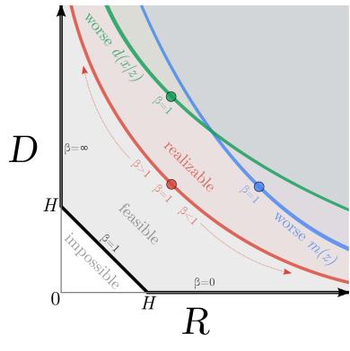
Figure 5.10: Illustration of the rate-distortion tradeo!. See text for details. From Figure 1 of [Ale+18]. Used with kind permission of Alex Alemi.

For discrete data, all probabilities are bounded above by 1, and hence H ⇑ 0 and D ⇑ 0. In addition, the rate is always non-negative, R ⇑ 0, since it is the average of a KL divergence. (This is true for either discrete or continuous encodings z.) Consequently, we can plot the set of achievable values of R and D as shown in Figure 5.10. This is known as a rate distortion curve.

The bottom horizontal line corresponds to the zero distortion setting, D = 0, in which we can perfectly encode and decode our data. This can be achieved by using the trivial encoder where e(z|x) = 1(z ⇐ x). Shannon’s source coding theorem tells us that the minimum number of bits we need to use to encode data in this setting is the entropy of the data, so R ⇑ H when D = 0. If we use a suboptimal marginal distribution m(z) for coding, we will increase the rate without a!ecting the distortion.

The left vertical line corresponds to the zero rate setting, R = 0, in which the latent code is independent of z. In this case, the decoder d(x|z) is independent of z. However, we can still learn a joint probability model p(x) which does not use latent variables, e.g., this could be an autoregressive model. The minimal distortion such a model could achieve is again the entropy of the data, D ⇑ H.

The black diagonal line illustrates solutions that satisfy D = H ⇐ R, where the upper and lower bounds are tight. In practice, we cannot achieve points on the diagonal, since that requires the bounds to be tight, and therefore assumes our models e(z|x) and d(x|z) are perfect. This is called the “non-parametric limit”. In the finite data setting, we will always incur additional error, so the RD plot will trace a curve which is shifted up, as shown in Figure 5.10.

We can generate di!erent solutions along this curve by minimizing the following objective:

\[\Delta J = D + \beta R = \int d\mathbf{z} \, p(\mathbf{z}) \int d\mathbf{z} \, e(\mathbf{z}|\mathbf{z}) \left[ -\log d(\mathbf{z}|\mathbf{z}) + \beta \log \frac{e(\mathbf{z}|\mathbf{z})}{m(\mathbf{z})} \right] \tag{5.160}\]

If we set ↼ = 1, and define q(z|x) = e(z|x), p(x|z) = d(x|z), and p(z) = m(z), this exactly matches the VAE objective in Section 21.2. To see this, note that the ELBO from Section 10.1.1.2 can be written as

\[\mathbb{L} = -(D+R) = \mathbb{E}\_{p(\mathbf{z})} \left[ \mathbb{E}\_{e(\mathbf{z}|\mathbf{z})} \left[ \log d(\mathbf{z}|\mathbf{z}) \right] - \mathbb{E}\_{e(\mathbf{z}|\mathbf{z})} \left[ \log \frac{e(\mathbf{z}|\mathbf{z})}{m(\mathbf{z})} \right] \right] \tag{5.161}\]

which we recognize as the expected reconstruction error minus the KL term DKL (e(z|x) ̸ m(z)).

If we allow ↼ ⇓= 1, we recover the ↼-VAE objective discussed in Section 21.3.1. Note, however, that the ↼-VAE model cannot distinguish between di!erent solutions on the diagonal line, all of which have ↼ = 1. This is because all such models have the same marginal likelihood (and hence same ELBO), although they di!er radically in terms of whether they learn an interesting latent representation or not. Thus likelihood is not a su”cient metric for comparing the quality of unsupervised representation learning methods, as discussed in Section 21.3.1.

For further discussion on the inherent conflict between rate, distortion, and perception, see [BM19]. For techniques for evaluating rate distortion curves for models see [HCG20].

5.4.3 Bits back coding

In the previous section we penalized the rate of our code using the average KL divergence, Ep(x) [R(x)], where

\[R(\mathbf{z}) \triangleq \int d\mathbf{z} \, p(\mathbf{z}|\mathbf{z}) \log \frac{p(\mathbf{z}|\mathbf{z})}{m(\mathbf{z})} = \mathbb{H}\_{ce}(p(\mathbf{z}|\mathbf{z}), m(\mathbf{z})) - \mathbb{H}(p(\mathbf{z}|\mathbf{z})).\tag{5.162}\]

The first term is the cross entropy, which is the expected number of bits we need to encode x; the second term is the entropy, which is the minimum number of bits. Thus we are penalizing the excess number of bits required to communicate the code to a receiver. How come we don’t have to “pay for” the actual (total) number of bits we use, which is the cross entropy?

The reason is that we could in principle get the bits needed by the optimal code given back to us; this is called bits back coding [HC93; FH97]. The argument goes as follows. Imagine Alice is trying to (losslessly) communicate some data, such as an image x, to Bob. Before they went their separate ways, both Alice and Bob decided to share their encoder p(z|x), marginal m(z) and decoder distributions d(x|z). To communicate an image, Alice will use a two part code. First, she will sample a code z ⇔ p(z|x) from her encoder, and communicate that to Bob over a channel designed to e”ciently encode samples from the marginal m(z); this costs ⇐ log² m(z) bits. Next Alice will use her decoder d(x|z) to compute the residual error, and losslessly send that to Bob at the cost of ⇐ log² d(x|z) bits. The expected total number of bits required here is what we naively expected:

\[\mathbb{E}\_{p(\mathbf{z}|\mathbf{z})} \left[ -\log\_2 d(\mathbf{z}|\mathbf{z}) - \log\_2 m(\mathbf{z}) \right] = D + \mathbb{E}\_{ce} (p(\mathbf{z}|\mathbf{z}), m(\mathbf{z})).\tag{5.163}\]

We see that this is the distortion plus cross entropy, not distortion plus rate. So how do we get the bits back, to convert the cross entropy to a rate term?

The trick is that Bob actually receives more information than we suspected. Bob can use the code z and the residual error to perfectly reconstruct x. However, Bob also knows what specific code Alice sent, z, as well as what encoder she used, p(z|x). When Alice drew the sample code z ⇔ p(z|x), she had to use some kind of entropy source in order to generate the random sample. Suppose she did it by picking words sequentially from a compressed copy of Moby Dick, in order to generate a stream of random bits. On Bob’s end, he can reverse engineer all of the sampling bits, and thus recover the compressed copy of Moby Dick! Thus Alice can use the extra randomness in the choice of z to share more information.

While in the original formulation the bits back argument was largely theoretical, o!ering a thought experiment for why we should penalize our models with the KL instead of the cross entropy, recently several practical real world algorithms have been developed that actually achieve the bits back goal. These include [HPHL19; AT20; TBB19; YBM20; HLA19; FHHL20].

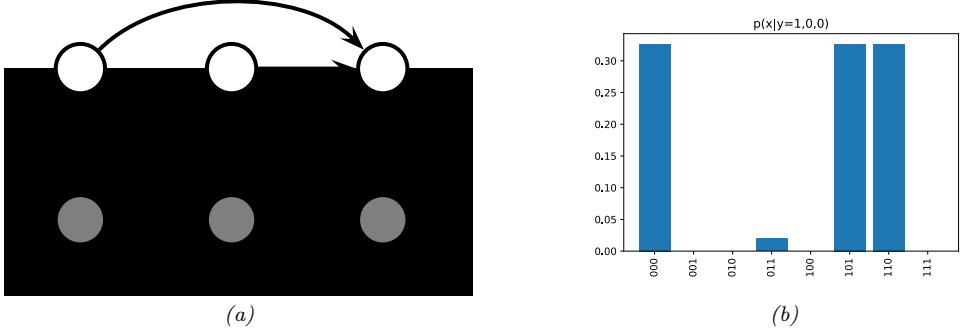
Figure 5.11: (a) A simple error-correcting code DPGM. xⁱ are the sent bits, yⁱ are the received bits. x³ is an even parity check bit computed from x¹ and x2. (b) Posterior over codewords given that y = (1, 0, 0); the probability of a bit flip is 0.2. Generated by error\_correcting\_code\_demo.ipynb.

5.5 Error-correcting codes (channel coding)

The idea behind error correcting codes is to add redundancy to a signal x (which is the result of encoding the original data), such that when it is sent over to the receiver via a noisy transmission line (such as a cell phone connection), the receiver can recover from any corruptions that might occur to the signal. This is called channel coding.

In more detail, let ^{x ↑} {0, 1}^m be the source message, where ^m is called the block length. Let y be the result of sending x over a noisy channel. This is a corrupted version of the message. For example, each message bit may get flipped independently with probability α, in which case ^p(y|x) = ^{m i}=1 p(yi|xi), where p(yi|xⁱ = 0) = [1 ⇐ α, α] and p(yi|xⁱ = 1) = [α, 1 ⇐ α]. Alternatively, we may add Gaussian noise, so ^p(yi|xⁱ = ^b) = ^N (yi|µb, ^ε2). The receiver’s goal is to infer the true message from the noisy observations, i.e., to compute argmax^x p(x|y).

A common way to increase the chance of being able to recover the original signal is to add parity check bits to it before sending it. These are deterministic functions of the original signal, which specify if the sum of the input bits is odd or even. This provides a form of redundancy, so that if one bit is corrupted, we can still infer its value, assuming the other bits are not flipped. (This is reasonable since we assume the bits are corrupted independently at random, so it is less likely that multiple bits are flipped than just one bit.)

For example, suppose we have two original message bits, and we add one parity bit. This can be modeled using a directed graphical model as shown in Figure 5.11(a). This graph encodes the following joint probability distribution:

\[p(x,y) = p(x\_1)p(x\_2)p(x\_3|x\_1, x\_2) \prod\_{i=1}^3 p(y\_i|x\_i) \tag{5.164}\]

The priors p(x1) and p(x2) are uniform. The conditional term p(x3|x1, x2) is deterministic, and computes the parity of (x1, x2). In particular, we have p(x³ = 1|x1, x2)=1 if the total number of 1s in the block x1:2 is odd. The likelihood terms p(yi|xi) represent a bit flipping noisy channel model, with noise level α = 0.2.

Suppose we observe y = (1, 0, 0). We know that this cannot be what the sender sent, since this violates the parity constraint (if x¹ = 1 then we know x³ = 1). Instead, the 3 posterior modes for x are 000 (first bit was flipped), 110 (second bit was flipped), and 101 (third bit was flipped). The only other configuration with non-zero support in the posterior is 011, which corresponds to the much less likely hypothesis that three bits were flipped (see Figure 5.11(b)). All other hypotheses (001, 010, and 100) are inconsistent with the deterministic method used to create codewords. (See Section 9.3.3.2 for further discussion of this point.)

In practice, we use more complex coding schemes that are more e”cient, in the sense that they add less redundant bits to the message, but still guarantee that errors can be corrected. For details, see Section 9.4.8.

5.6 The information bottleneck

In this section, we discuss discriminative models p(y|x) that use a stochastic bottleneck between the input x and the output y to prevent overfitting, and improve robustness and calibration.

5.6.1 Vanilla IB

We say that z is a representation of x if z is a (possibly stochastic) function of x, and hence can be described by the conditional p(z|x). We say that a representation z of x is su!cient for task y if y ℜ x|z, or equivalently, if I(z; y) = I(x; y), i.e., H (y|z) = H (y|x). We say that a representation is a minimal su!cient statistic if z is su”cient and there is no other z with smaller I(z; x) value. Thus we would like to find a representation z that maximizes I(z; y) while minimizing I(z; x). That is, we would like to optimize the following objective:

\[\min \beta \, \mathbb{I}(z; \mathbf{z}) - \mathbb{I}(z; \mathbf{y}) \tag{5.165}\]

where ↼ ⇑ 0, and we optimize wrt the distributions p(z|x) and p(y|z). This is called the information bottleneck principle [TPB99]. This generalizes the concept of minimal su”cient statistic to take into account that there is a tradeo! between su”ciency and minimality, which is captured by the Lagrange multiplier ↼ > 0.

This principle is illustrated in Figure 5.12. We assume Z is a function of X, but is independent of Y , i.e., we assume the graphical model Z ∈ X ℵ Y . This corresponds to the following joint distribution:

\[p(x, y, z) = p(z|x)p(y|x)p(x) \tag{5.166}\]

Thus Z can capture any amount of information about X that it wants, but cannot contain information that is unique to Y , as illustrated in Figure 5.12a. The optimal representation only captures information about X that is useful for Y ; to prevent us “wasting capacity” and fitting irrelevant details of the input, Z should also minimize information about X, as shown in Figure 5.12b.

If all the random variables are discrete, and z = e(x) is a deterministic function of x, then the algorithm of [TPB99] can be used to minimize the IB objective in Section 5.6. The objective can also be solved analytically if all variables are jointly Gaussian [Che+05] (the resulting method can be viewed as a form of supervised PCA). But in general, it is intractable to solve this problem exactly. We discuss a tractable approximation in Section 5.6.2. (More details can be found in e.g., [SZ22].)

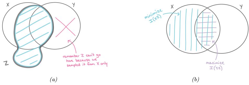
Figure 5.12: Information diagrams for information bottleneck. (a) Z can contain any amount of information about X (whether it useful for predicting Y or not), but it cannot contain information about Y that is not shared with X. (b) The optimal representation for Z maximizes I(Z, Y ) and minimizes I(Z, X). Used with kind permission of Katie Everett.

5.6.2 Variational IB

In this section, we derive a variational upper bound on Equation (5.165), leveraging ideas from Section 5.3.6. This is called the variational IB or VIB method [Ale+16]. The key trick will be to use the non-negativity of the KL divergence to write

\[\int d\mathbf{x} \,\, p(\mathbf{x}) \log p(\mathbf{x}) \ge \int d\mathbf{x} \,\, p(\mathbf{x}) \log q(\mathbf{x}) \tag{5.167}\]

for any distribution q. (Note that both p and q may be conditioned on other variables.)

To explain the method in more detail, let us define the following notation. Let e(z|x) = p(z|x) represent the encoder, b(z|y) ¬ p(z|y) represent the backwards encoder, d(y|z) ¬ p(y|z) represent the classifier (decoder), and m(z) ¬ p(z) represent the marginal. (Note that we get to choose p(z|x), but the other distributions are derived by approximations of the corresponding marginals and conditionals of the exact joint p(x, y, z).) Also, let 7·∀ represent expectations wrt the relevant terms from the p(x, y, z) joint.

With this notation, we can derive a lower bound on I(z; y) as follows:

\[\mathbb{I}(\mathbf{z};\mathbf{y}) = \int d\mathbf{y}d\mathbf{z}\ p(\mathbf{y},\mathbf{z}) \log \frac{p(\mathbf{y},\mathbf{z})}{p(\mathbf{y})p(\mathbf{z})} \tag{5.168}\]

\[=\int dydz\ p(y,z)\log p(y|z) - \int dydz\ p(y,z)\log p(y) \tag{5.169}\]

\[I = \int d\mathbf{y}d\mathbf{z} \, p(\mathbf{z})p(\mathbf{y}|\mathbf{z}) \log p(\mathbf{y}|\mathbf{z}) - \text{const} \tag{5.170}\]

\[\geq \int d\mathbf{y}d\mathbf{z} \ p(\mathbf{y}, \mathbf{z}) \log d(\mathbf{y}|\mathbf{z}) \tag{5.171}\]

\[= \langle \log d(\mathbf{y}|\mathbf{z}) \rangle\]

where we exploited the fact that H (p(y)) is a constant that is independent of our representation.

Note that we can approximate the expections by sampling from

\[p(\mathbf{y}, \mathbf{z}) = \int d\mathbf{x} \, p(\mathbf{x}) p(\mathbf{y}|\mathbf{z}) p(\mathbf{z}|\mathbf{x}) = \int d\mathbf{x} \, p(\mathbf{x}, \mathbf{y}) e(\mathbf{z}|\mathbf{x}) \tag{5.173}\]

This is just the empirical distribution “pushed through” the encoder.

Similarly, we can derive an upper bound on I(z; x) as follows:

\[\mathbb{L}(\mathbf{z};\mathbf{z}) = \int d\mathbf{z}d\mathbf{x}\ p(\mathbf{z},\mathbf{z}) \log \frac{p(\mathbf{z},\mathbf{z})}{p(\mathbf{z})p(\mathbf{z})}\tag{5.174}\]

\[=\int d\mathbf{z}d\mathbf{z}\ p(\mathbf{z},\mathbf{z})\log p(\mathbf{z}|\mathbf{z}) - \int d\mathbf{z}\ p(\mathbf{z})\log p(\mathbf{z})\tag{5.175}\]

\[\leq \int d\mathbf{z}d\mathbf{x} \ p(\mathbf{z}, \mathbf{z}) \log p(\mathbf{z}|\mathbf{x}) - \int d\mathbf{z} \ p(\mathbf{z}) \log m(\mathbf{z}) \tag{5.176}\]

\[\mathbf{x} = \int d\mathbf{z} d\mathbf{x} \ p(\mathbf{z}, \mathbf{z}) \log \frac{e(\mathbf{z}|\mathbf{z})}{m(\mathbf{z})} \tag{5.177}\]

\[= \langle \log e(\mathbf{z}|\mathbf{z}) \rangle - \langle \log m(\mathbf{z}) \rangle \tag{5.178}\]

Note that we can approximate the expectations by sampling from p(x, z) = p(x)p(z|x).

Putting it altogether, we get the following upper bound on the IB objective:

\[ \beta \, \mathbb{I}(\mathbf{z}; \mathbf{z}) - \mathbb{I}(\mathbf{z}; \mathbf{y}) \le \beta \left( \langle \log e(\mathbf{z}|\mathbf{z}) \rangle - \langle \log m(\mathbf{z}) \rangle \right) - \langle \log d(\mathbf{y}|\mathbf{z}) \rangle \tag{5.179} \]

Thus the VIB objective is

\[\mathcal{L}\_{\text{VIB}} = \beta \left( \mathbb{E}\_{p\supset(\mathbf{z})e(\mathbf{z}|\mathbf{z})} \left[ \log e(\mathbf{z}|\mathbf{z}) - \log m(\mathbf{z}) \right] \right) - \mathbb{E}\_{p\supset(\mathbf{z})e(\mathbf{z}|\mathbf{z})d(\mathbf{y}|\mathbf{z})} \left[ \log d(\mathbf{y}|\mathbf{z}) \right] \tag{5.180}\]

\[=-\mathbb{E}\_{p\circ(\mathfrak{z})e(\mathfrak{z}|\mathfrak{z})d(\mathfrak{y}|\mathfrak{z})}\left[\log d(\mathfrak{y}|\mathfrak{z})\right] + \beta \mathbb{E}\_{p\circ(\mathfrak{z})}\left[D\_{\text{KL}}\left(e(\mathfrak{z}|\mathfrak{x}) \parallel m(\mathfrak{z})\right)\right] \tag{5.181}\]

We can now take stochastic gradients of this objective and minimize it (wrt the parameters of the encoder, decoder, and marginal) using SGD. (We assume the distributions are reparameterizable, as discussed in Section 6.3.5.) For the encoder e(z|x), we often use a conditional Gaussian, and for the decoder d(y|z), we often use a softmax classifier. For the marginal, m(z), we should use a flexible model, such as a mixture of Gaussians, since it needs to approximate the aggregated posterior ^p(z) = $ ^dzp(x)e(z|x), which is a mixture of ^N Gaussians (assuming ^p(x) is an empirical distribution with N samples, and e(z|x) is a Gaussian).

We illustrate this in Figure 5.13, where we fit the an MLP model to MNIST. We use a 2d bottleneck layer before passing to the softmax. In panel a, we show the embedding learned by a determinisic encoder. We see that each image gets mapped to a point, and there is little overlap between classes, or between instances. In panels b-c, we show the embedding learned by a stochastic encoder. Each image gets mapped to a Gaussian distribution, we show the mean and the covariance separately. The classes are still well separated, but individual instances of a class are no longer distinguishable, since such information is not relevant for prediction purposes.

5.6.3 Conditional entropy bottleneck

The IB tries to maximize I(Z; Y ) while minimizing I(Z; X). We can write this objective as

\[\min \mathbb{I}(\mathbf{z}; \mathbf{z}) - \lambda \, \mathbb{I}(\mathbf{y}; \mathbf{z}) \tag{5.182}\]

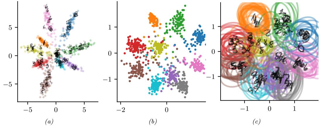
Figure 5.13: 2d embeddings of MNIST digits created by an MLP classifier. (a) Deterministic model. (b-c) VIB model, means and covariances. Generated by vib\_demo.ipynb. Used with kind permission of Alex Alemi.

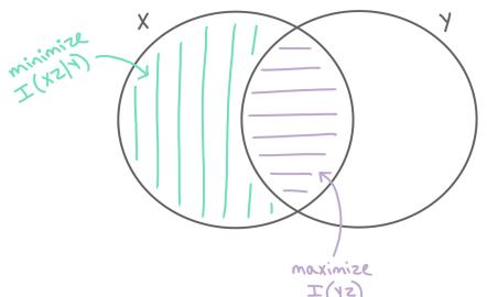
Figure 5.14: Conditional entropy bottleneck (CEB) chooses a representation Z that maximizes I(Z, Y ) and minimizes I(X, Z|Y ). Used with kind permission of Katie Everett.

for ϖ ⇑ 0. However, we see from the information diagram in Figure 5.12b that I(Z; X) contains some information that is relevant to Y . A sensible alternative objective is to minimizes the residual mutual information, I(X;Z|Y ). This gives rise to the following objective:

\[\min \mathbb{I}(x; z | \mathbf{y}) - \lambda^{\prime} \mathbb{I}(y; z) \tag{5.183}\]

for ϖ^↔︎ ⇑ 0. This is known as the conditional entropy bottleck or CEB [Fis20]. See Figure 5.14 for an illustration.

Since I(x; z|y) = I(x; z)⇐I(y; z), we see that the CEB is equivalent to standard IB with ϖ^↔︎ = ϖ+ 1. However, it is easier to upper bound I(x; z|y) than I(x; z), since we are conditioning on y, which

provides information about z. In particular, by leveraging p(z|x, y) = p(z|x) we have

\[\mathbb{I}(\mathbf{z};\mathbf{z}|\mathbf{y}) = \mathbb{I}(\mathbf{z};\mathbf{z}) - \mathbb{I}(\mathbf{y};\mathbf{z}) \tag{5.184}\]

\[=\mathbb{H}(\mathbf{z}) - \mathbb{H}(\mathbf{z}|\mathbf{x}) - \left[\mathbb{H}(\mathbf{z}) - \mathbb{H}(\mathbf{z}|\mathbf{y})\right] \tag{5.185}\]

\[=-\mathbb{H}(z|x) + \mathbb{H}(z|y) \tag{5.186}\]

\[=\int d\mathbf{z}d\mathbf{x}\ p(\mathbf{z},\mathbf{z})\log p(\mathbf{z}|\mathbf{x}) - \int d\mathbf{z}d\mathbf{y}\ p(\mathbf{z},\mathbf{y})\log p(\mathbf{z}|\mathbf{y})\tag{5.187}\]

\[0 \le \int dz dx \, p(\mathbf{z}, \mathbf{z}) \log e(\mathbf{z}|\mathbf{z}) - \int dz dy \, p(\mathbf{z}, \mathbf{y}) \log b(\mathbf{z}|\mathbf{y}) \tag{5.188}\]

\[\mathbf{x} = \langle \log e(\mathbf{z}|\mathbf{z}) \rangle - \langle \log b(\mathbf{z}|\mathbf{y}) \rangle \tag{5.189}\]

Putting it altogether, we get the final CEB objective:

\[\min \beta \left( \left< \log e(\mathbf{z}|\mathbf{z}) \right> - \left< \log b(\mathbf{z}|\mathbf{y}) \right> \right) - \left< \log d(\mathbf{y}|\mathbf{z}) \right> \tag{5.190}\]

Note that it is generally easier to learn the conditional backwards encoder b(z|y) than the unconditional marginal m(z). Also, we know that the tightest upper bound occurs when I(x; z|y) = I(x; z) ⇐ I(y; z)=0. The corresponding value of ↼ corresponds to an optimal representation. By contrast, it is not clear how to measure distance from optimality when using IB.

5.7 Algorithmic information theory

The theory of information we have discussed so far is based on the properties of the underlying stochastic distribution that is assumed to have generated the observed data. However, in many ways it does not capture the intuitive notion of “information” that most people have. For example, consider a sequence of n bits generated independently from a uniform Bernoulli distribution. This distribution has maximum entropy per element of H2(0.5) = 1, so the coding length of a sequence of length ⁿ is ⇐ log^{2 p}(D|ϑ) = ⇐#^{n i}=1 log² Ber(xi|ϑ = 0.5) = n. However, intuitively, such a sequence does not contain very much information at all.

There is an alternative approach to quantifying the degree of information in a given sequence (as opposed to the information content of a stochastic model), known as algorithmic information theory. The roots of this were developed independently by several authors [Sol64; Kol65; Cha66; Cha69]. We give a brief summary below. For more details, see e.g., [Hut07; GV08; LV19].

5.7.1 Kolmogorov complexity

The key concept in algorithmic information theory is the Kolmogorov complexity of a bit string x = x1:n, which is defined as the length of the shortest program p which, when fed as input to a universal Turing machine U, generates the string x: K(x) = min^p≃B^↑ [⇁(p) : U(p) = x], where B↘ is the set of arbitrarily long bit strings, and ⇁(p) is the length of the program. (This definition of complexity can be extended from bit strings x to functions f, but the details are rather complicated.) It can be shown that the Kolmogorov complexity has many properties that are analogous to Shannon entropy. For example, if we ignore additive constants for simplicity, one can show that K(x|y) ↗ K(x) ↗ K(x, y), which is is analogous to H(X|Y ) ↗ H(X) ↗ H(X, Y ).

Unfortunately, Kolmogorov complexity is not a computable function. However, it is possible to add a (logarithmic) time complexity term to the Kolmogorov complexity term, resulting in Levin complexity [Lev73], which can be computed. The Levin complexity is defined as L(x) = minp≃B^↑ [⇁(p) + log(time(p)) : U(p) = x]. where time(p) is the running time of p. This can be computed by running all programs in a time-sliced fashion (allocating time 2↑↽(p) to program p), until the first one halts; this is called Levin search or universal search, and takes time time(LS(x)) = 2L(x) .

Although Levin complexity is computable, it is still ine”cient to compute (although some progress has been made [Sch03]). However, we can also make parametric approximations that enable more e”cient upper bounds to K(x). For example, suppose q is some distribution over bit strings. One can show that K(x) ↗ ⇐ log q(x) + K(q), where K(q) is the K-complexity of the distribution (function) q. If q is a parametric model, we can approximate K(q) by the coding length of q’s parameters; this is equivalent to the MDL objective, discussed in Section 3.8.7.1.

We can use Kolmogorov complexity to give a formal definition of randomness of an individual sequence (or data set), without needing the concept of random variables or communication channels. In particular, we say a string x is compressible if its shortest description is shorter than the string itself (i.e., if K(x) < ⇁(x) = n); otherwise we say the string is algorithmically random. (This is called Martin-Löf randomness [ML66] to distinguish it from other notions of randomness.) For example, x = (10101010 ···) is easily seen to be compressible, since it is just repetitions of the pattern 10; the string x = (11001001 ···) is also compressible (although less so), since it is the binary expansion of ^ϱ2; however, ^x = (10110110 ···) is “truly random”, since it was derived from quantum fluctuations in the vacuum (see [HQC24, Sec 2.7.1]).

Besides its theoretical interest, the above “individual sequence” approach to information theory forms the foundation of (amongst other things) the celebrated Lempel Ziv losssless data compression scheme [ZL77], which forms the basis of zip encoding. (See [Mer24] for further details.) This in turn can be used to implement a universal similarity metric [Li+04]

\[d(x, y) = \frac{\max[K(x|y), K(y|x)]}{\max[K(x), K(y)]} \tag{5.191}\]

where the terms such as K(x) can be approximated by the coding cost of some universal compressor such as LZ; this gives rise to the normalized compression distance [CV05]. Recently [Jia+23] showed that NCD, combined with K-nearest neighbors, can outperform the BERT language model at the task of text classification in the “low-resource” setting (although bag-of-word classifiers also do well in this setting, and are faster [Opi23]).

5.7.2 Solomono! induction

Now consider the (online) prediction problem. Suppose we have observed x1:^t drawn from some unknown distribution µ(x1:t); we want to approximate µ with some model ς, so we can predict the future using ς(xt+1|x1:t). This is called the problem of induction. We assume ς ↑ M, where M is

^2. See https://oeis.org/A004601 for the binary expansion of ε. Note that the length of the program to generate ε depends on the programming language which we use. For example, if the language supports integration as a primitive, the program can be expressed concisely as ε = 4 ” ¹ 0 ↗^{1 → x}2dx. More elementary Turing machines will require longer programs. However, the extra program length corresponds to an additive constant term, which becomes negligible in the limit that n ↘ ↑.

a countable set of models (distributions). Let w^ε be the prior probability of model ς. In the approach known as Solomono” induction [Sol64], we assume M is the set of all computable functions, and we define the prior to be w^ε = 2↑K(ε) . This is a “universal prior”, since it can model any computable distribution µ. Furthermore, the particular weighting term is motivated by Occam’s razor, which says we should prefer the simplest model that explains the data.

Given this prior (or in fact any other prior), we can compute the prior predictive distribution over sequences using the following Bayesian mixture model:

\[\xi(\mathbf{z}\_{1:t}) = \sum\_{\nu \in \mathcal{M}} w\_{\nu} \nu(\mathbf{z}\_{1:t}) \tag{5.192}\]

From this, we can compute the posterior predictive distribution at step t as follows:

\[\xi(x\_{t}|\mathbf{z}\_{\]

\[=\sum\_{\nu\in\mathcal{M}} w\_{\nu} \frac{\nu(\mathbf{z}\_{\]

where in the last line we exploited the fact that the posterior weight over each model is given by

\[w(\nu|\mathbf{x}\_{1:t}) = p(\nu|\mathbf{x}\_{1:t}) = \frac{p(\nu)p(\mathbf{x}\_{1:t}|\nu)}{p(\mathbf{x}\_{1:t})} = \frac{w\_{\nu}\nu(\mathbf{x}\_{1:t})}{\xi(\mathbf{x}\_{1:t})} \tag{5.195}\]

Now consider comparing the accuracy of this predictive distribution to the truth at each step t. We will use the squared error

\[s\_t(\boldsymbol{x}\_{\]

Consider the expected total error up to time n:

\[S\_n = \sum\_{t=1}^n \sum\_{\substack{\mathfrak{x}\_{\]

In [Sol78], Solomono! proved the following remarkable bound on the total error (in the limit) of his predictor:

\[S\_{\infty} \le \ln(w\_{\mu}^{-1}) = K(\mu)\ln 2\tag{5.198}\]

This shows that the total error is bounded by the complexity of the environment that generated the data. Thus simple environments are easy to learn (in a sample complexity sense), so predictions of an optimal predictor rapidly approach the truth.

We can also consider the setting in which we assume the data is generated from some unknown deterministic program p. This must satisfy U(p) = x∋, where x∋ is the infinite extension of the observed prefix x = x1:t. Suppose we define the prior over programs to be Pr(p)=2↑↽(p) . Then the prior predictive distribution over sequences is given by the following [Sol64]:

\[M(\mathbf{z}) = \sum\_{p:U(p)=\mathbf{z}\*} 2^{-\ell(p)}\tag{5.199}\]

Remarkably, one can show (see e.g., [WSH13]) that M(x) = 4(x). From this, we can then compute the posterior predictive distribution M(xt|x<t) = M(x1:t)/M(x<t). Since this is a convex combination of deterministic distributions, it can also be used to model stochastic environments.

Since Solomono! induction relies on Kolmogorov complexity to define its prior, it is uncomputable. However, it is possible to approximate this scheme in various ways. For example recently [GM+24] showed that it is possible to use meta learning (see Section 19.6.4) to train a generic sequence predictor, such as a transformer or LSTM, on data generated by random Turing machines, so that the transformer learns to approximate a universal predictor.

In [HQC24], they show how to apply Solomono! induction to design optimal online decision making agents, resulting a universal artificial general intelligence or AGI known as AIXI.

6 Optimization

6.1 Introduction

In this chapter, we consider solving optimization problems of various forms. Abstractly these can all be written as

\[\theta^\* \in \underset{\theta \in \Theta}{\operatorname{argmin}} \mathcal{L}(\theta) \tag{6.1}\]

where L : & → R is the objective or loss function, and & is the parameter space we are optimizing over. However, this abstraction hides many details, such as whether the problem is constrained or unconstrained, discrete or continuous, convex or non-convex, etc. In the prequel to this book, [Mur22], we discussed some simple optimization algorithms for some common problems that arise in machine learning. In this chapter, we discuss some more advanced methods. For more details on optimization, please consult some of the many excellent textbooks, such as [KW19b; BV04; NW06; Ber15; Ber16] as well as various review articles, such as [BCN18; Sun+19b; PPS18; Pey20].

6.2 Automatic di!erentiation

This section is written by Roy Frostig.

This section is concerned with computing (partial) derivatives of complicated functions in an automatic manner. By “complicated” we mean those expressed as a composition of an arbitrary number of more basic operations, such as in deep neural networks. This task is known as automatic di”erentiation (AD), or autodi”. AD is an essential component in optimization and deep learning, and is also used in several other fields across science and engineering. See e.g., Baydin et al. [Bay+15] for a review focused on machine learning and Griewank and Walther [GW08] for a classical textbook.

6.2.1 Di!erentiation in functional form

Before covering automatic di!erentiation, it is useful to review the mathematics of di!erentiation. We will use a particular functional notation for partial derivatives, rather than the typical one used throughout much of this book. We will refer to the latter as the named variable notation for the moment. Named variable notation relies on associating function arguments with names. For instance, given a function ^f : ^{R2 → R}, the partial derivative of ^f with respect to its first scalar argument, at a

point a = (a1, a2), might be written:

\[\left.\frac{\partial f}{\partial x\_1}\right|\_{x=a} \tag{6.2}\]

This notation is not entirely self-contained. It refers to a name x = (x1, x2), implicit or inferred from context, suggesting the argument of f. An alternative expression is:

\[\frac{\partial}{\partial a\_1} f(a\_1, a\_2) \tag{6.3}\]

where now a¹ serves both as an argument name (or a symbol in an expression) and as a particular evaluation point. Tracking names can become an increasingly complicated endeavor as we compose many functions together, each possibly taking several arguments.

A functional notation instead defines derivatives as operators on functions. If a function has multiple arguments, they are identified by position rather than by name, alleviating the need for auxiliary variable definitions. Some of the following definitions draw on those in Spivak’s Calculus on Manifolds [Spi71] and in Sussman and Wisdom’s Functional Di”erential Geometry [SW13], and generally appear more regularly in accounts of di!erential calculus and geometry. These texts are recommended for a more formal treatment, and a more mathematically general view, of the material briefly covered in this section.

Beside notation, we will rely on some basic multivariable calculus concepts. This includes the notion of (partial) derivatives, the di!erential or Jacobian of a function at a point, its role as a linear approximation local to the point, and various properties of linear maps, matrices, and transposition. We will focus on a finite-dimensional setting and write {e1,…, ^en} for the standard basis in ^Rn.

Linear and multilinear functions. We use ^F : ^{Rn ≿ Rm} to denote a function ^F : ^{Rn → Rm} that is linear, and by ^F[x] its application to ^{x ↑ Rn}. Recall that such a linear map corresponds to a matrix in R^m→ⁿ whose columns are F[e1],…,F[en]; both interpretations will prove useful. Conveniently, function composition and matrix multiplication expressions look similar: to compose two linear maps F and G we can write F I G or, barely abusing notation, consider the matrix F G. Every linear map F : Rⁿ ≿ R^m has a transpose F : R^m ≿ Rⁿ, which is another linear map identified with transposing the corresponding matrix.

Repeatedly using the linear arrow symbol, we can denote by:

\[T: \underbrace{\mathbb{R}^n \colon \cdots \circ \cdots \circ \mathbb{R}^n}\_{k \text{ times}} \to \mathbb{R}^m \tag{6.4}\]

a multilinear, or more specifically k-linear, map:

\[T: \underbrace{\mathbb{R}^n \times \cdots \times \mathbb{R}^n}\_{k \text{ times}} \to \mathbb{R}^m \tag{6.5}\]

which corresponds to an array (or tensor) in ^Rm→n→···→ⁿ. We denote by ^T[x1,…, ^xk] ^{↑ Rm} the application of such a ^k-linear map to vectors ^x1,…, ^{xk ↑ Rn}.

The derivative operator. For an open set ^U △ ^Rn and a di!erentiable function ^f : ^{U → Rm}, denote its derivative function:

\[\{\partial f: U \to \left(\mathbb{R}^n \rightharpoonup \mathbb{R}^m\right)\}\tag{6.6}\]

or equivalently ^0f : ^{U → R}m→ⁿ. This function maps a point ^{x ↑ U} to the Jacobian of all partial derivatives evaluated at x. The symbol 0 itself denotes the derivative operator, a function mapping functions to their derivative functions. When m = 1, the map 0f(x) recovers the standard gradient ▽f(x) at any x ↑ U, by considering the matrix view of the former. Indeed, the nabla symbol ▽ is sometimes described as an operator as well, such that ▽f is a function. When n = m = 1, the Jacobian is scalar-valued, and 0f is the familiar derivative f^↔︎ .

In the expression 0f(x)[v], we will sometimes refer to the argument x as the linearization point for the Jacobian, and to v as the perturbation. We call the map:

\[f(x,v) \mapsto \partial f(x)[v] \tag{6.7}\]

over linearization points ^{x ↑ U} and input perturbations ^{v ↑ Rn} the Jacobian-vector product (JVP). We similarly call its transpose:

\[\phi(x, u) \mapsto \partial f(x)^{\dagger}[u] \tag{6.8}\]

over linearization points ^{x ↑ U} and output perturbations ^{u ↑ Rm} the vector-Jacobian product (VJP).

Thinking about maps instead of matrices can help us define higher-order derivatives recursively, as we proceed to do below. It separately suggests how the action of a Jacobian is commonly written in code. When we consider writing 0f(x) in a program for a fixed x, we often implement it as a function that carries out multiplication by the Jacobian matrix, i.e., v J→ 0f(x)[v], instead of explicitly representing it as a matrix of numbers in memory. Going a step further, for that matter, we often implement 0f as an entire JVP at once, i.e., over any linearization point x and perturbation v. As a toy example with scalars, consider the cosine:

\[\cos(x,v)\mapsto\partial\cos(x)v=-v\sin(x)\tag{6.9}\]

If we express this at once in code, we can, say, avoid computing sin(x) whenever v = 0. 1

Higher-order derivatives. Suppose the function f above remains arbitrarily di!erentiable over its domain ^U △ ^Rn. To take another derivative, we write:

\[ \partial^2 f: U \to \left(\mathbb{R}^n \multimap \mathbb{R}^n \multimap \mathbb{R}^m\right) \tag{6.10} \]

where 0²f(x) is a bilinear map representing all second-order partial derivatives. In named variable notation, one might write ^φf(x) ^φxiφx^j to refer to ⁰²f(x)[ei, ^ej ], for example.

^1. This example ignores that such an optimization might be done (best) by a compiler. Then again, for more complex examples, implementing (x, v) ≃↘ ↽f(x)[v] as a single subroutine can help guide compiler optimizations all the same.

The second derivative function 02f can be treated coherently as the outcome of applying the derivative operator twice. That is, it makes sense to say that ^{02 = 0 I 0}. This observation extends recursively to cover arbitrary higher-order derivatives. For k ⇑ 1:

\[\partial^k f: U \to \underbrace{(\mathbb{R}^n \multimap \dots \multimap \mathbb{R}^n \multimap \mathbb{R}^m)}\_{k \text{ times}} \multimap \mathbb{R}^m) \tag{6.11}\]

is such that 0^kf(x) is a k-linear map.

With ^m = 1, the map ⁰²f(x) corresponds to the Hessian matrix at any ^{x ↑ U}. Although Jacobians and Hessians su”ce to make sense of many machine learning techniques, arbitrary higher-order derivatives are not hard to come by either (e.g., [Kel+20]). As an example, they appear when writing down something as basic as a function’s Taylor series approximation, which we can express with our derivative operator as:

\[f(\mathbf{z} + \mathbf{v}) \approx f(\mathbf{z}) + \partial f(\mathbf{z})[\mathbf{v}] + \frac{1}{2!} \partial^2 f(\mathbf{z})[\mathbf{v}, \mathbf{v}] + \dots + \frac{1}{k!} \partial^k f(\mathbf{z})[\mathbf{v}, \dots, \mathbf{v}] \tag{6.12}\]

Multiple inputs. Now consider a function of two arguments:

\[g: U \times V \to \mathbb{R}^m.\]

where ^U △ ^Rn1 and ^V △ ^Rn2 . For our purposes, a product domain like ^{U ∞ V} mainly serves to suggest a convenient partitioning of a function’s input components. It is isomorphic to a subset of Rⁿ1+n² , corresponding to a single-input function. The latter tells us how the derivative functions of g ought to look, based on previous definitions, and we will swap between the two views with little warning. Multiple inputs tend to arise in the context of computational circuits and programs: many functions in code are written to accept multiple arguments, and many basic operations (such as +) do the same.

With multiple inputs, we can denote by 0ig the derivative function with respect to the i’th argument:

\[\partial\_1 g : \mathbb{R}^{n\_1} \times \mathbb{R}^{n\_2} \to \left( \mathbb{R}^{n\_1} \multimap \mathbb{R}^m \right), \text{ and} \tag{6.14}\]

\[ \partial\_2 g : \mathbb{R}^{n\_1} \times \mathbb{R}^{n\_2} \to \left( \mathbb{R}^{n\_2} \to \mathbb{R}^m \right). \tag{6.15} \]

Under the matrix view, the function ⁰1^g maps a pair of points ^{x ↑ Rn1} and ^{y ↑ Rn2} to the matrix of all partial derivatives of g with respect to its first argument, evaluated at (x, y). We take 0g with no subscript to simply mean the concatenation of 01g and 02g:

\[\partial g: \mathbb{R}^{n\_1} \times \mathbb{R}^{n\_2} \to \left(\mathbb{R}^{n\_1} \times \mathbb{R}^{n\_2} \to \mathbb{R}^m\right) \tag{6.16}\]

where, for every linearization point (x, ^y) ^{↑ U ∞ V} and perturbations ^x˙ ^{↑ Rn1} , ^y˙ ^{↑ Rn2} :

\[ \partial g(x,y)[\dot{x},\dot{y}] = \partial\_1 g(x,y)[\dot{x}] + \partial\_2 g(x,y)[\dot{y}].\tag{6.17} \]

Alternatively, taking the matrix view:

\[ \partial g(\mathbf{x}, \mathbf{y}) = \begin{pmatrix} \partial\_1 g(\mathbf{x}, \mathbf{y}) & \partial\_2 g(\mathbf{x}, \mathbf{y}) \end{pmatrix} \tag{6.18} \]

This convention will simplify our chain rule statement below. When n¹ = n² = m = 1, both sub-matrices are scalar, and 0g1(x, y) recovers the partial derivative that might otherwise be written in named variable notation as:

\[\frac{\partial}{\partial x}g(x,y) \,. \tag{6.19}\]

However, the expression 0g¹ bears a meaning on its own (as a function) whereas the expression ^φg φx may be ambiguous without further context. Again composing operators lets us write higher-order derivatives. For instance, ⁰201g(x, ^y) ^{↑ Rm}→n1→n² , and if ^m = 1, the Hessian of ^g at (x, ^y) is:

\[ \begin{pmatrix} \partial\_1 \partial\_1 g(\mathbf{z}, \mathbf{y}) & \partial\_1 \partial\_2 g(\mathbf{z}, \mathbf{y}) \\ \partial\_2 \partial\_1 g(\mathbf{z}, \mathbf{y}) & \partial\_2 \partial\_2 g(\mathbf{z}, \mathbf{y}) \end{pmatrix}. \tag{6.20} \]

Composition and fan-out. If ^{f = g I h} for some ^h : ^{Rn → Rp} and ^g : ^{Rp → Rm}, then the chain rule of calculus observes that:

\[\partial f(\mathbf{x}) = \partial g(h(\mathbf{x})) \circ \partial h(\mathbf{x}) \text{ for all } \mathbf{x} \in \mathbb{R}^n \tag{6.21}\]

How does this interact with our notation for multi-argument functions? For one, it can lead us to consider expressions with fan-out, where several sub-expressions are functions of the same input. For instance, assume two functions ^a : ^{Rn → Rm1} and ^b : ^{Rn → Rm2} , and that:

\[f(\mathbf{x}) = g(a(\mathbf{x}), b(\mathbf{x})) \tag{6.22}\]

for some function g. Abbreviating h(x)=(a(x), b(x)) so that f(x) = g(h(x)), Equations (6.16) and (6.21) tell us that:

\[ \partial f(\mathbf{x}) = \partial g(h(\mathbf{x})) \diamond \partial h(\mathbf{x}) \tag{6.23} \]

\[0 = \partial\_1 g(a(x), b(x)) \diamond \partial a(x) + \partial\_2 g(a(x), b(x)) \diamond \partial b(x) \tag{6.24}\]

Note that + is meant pointwise here. It also follows from the above that if instead:

\[f(x, y) = g(a(x), b(y))\tag{6.25}\]

in other words, if we write multiple arguments but exhibit no fan-out, then:

\[ \partial\_1 f(x, y) = \partial\_1 g(a(x), b(y)) \diamond \partial a(x) \,, \text{ and} \tag{6.26} \]

\[ \partial\_2 f(x, y) = \partial\_2 g(a(x), b(y)) \diamond \partial b(y) \tag{6.27} \]

Composition and fan-out rules for derivatives are what let us break down a complex derivative calculation into simpler ones. This is what automatic di!erentiation techniques rely on when processing the sort of elaborate numerical computations that turn up in modern machine learning and numerical programming.

6.2.2 Di!erentiating chains, circuits, and programs

The purpose of automatic di!erentiation is to compute derivatives of arbitrary functions provided as input. Given a function ^f : ^U △ ^{Rn → Rm} and a linearization point ^{x ↑ U}, AD computes either:

• the JVP ⁰f(x)[v] for an input perturbation ^{v ↑ R}n, or
• the VJP 0f(x) ^T[u] for an output perturbation ^{u ↑ Rm}.

In other words, JVPs and VJPs capture the two essential tasks of AD.2

Deciding what functions f to handle as input, and how to represent them, is perhaps the most load-bearing aspect of this setup. Over what language of functions should we operate? By a language, we mean some formal way of describing functions by composing a set of basic primitive operations. For primitives, we can think of various di!erentiable array operations (elementwise arithmetic, reductions, contractions, indexing and slicing, concatenation, etc.), but we will largely consider primitives and their derivatives as a given, and focus on how elaborately we can compose them. AD becomes increasingly challenging with increasingly expressive languages. Considering this, we introduce it in stages.

6.2.2.1 Chain compositions and the chain rule

To start, take only functions that are chain compositions of basic operations. Chains are a convenient class of function representations because derivatives decompose along the same structure according to the aptly-named chain rule.

As a toy example, consider ^f : ^{Rn → Rm} composed of three operations in sequence:

\[f = c \diamond b \diamond a \tag{6.28}\]

By the chain rule, its derivatives are given by

\[ \partial f(\mathbf{x}) = \partial c(b(a(\mathbf{x}))) \diamond \partial b(a(\mathbf{x})) \diamond \partial a(\mathbf{x}) \tag{6.29} \]

Now consider the JVP against an input perturbation ^{v ↑ Rn}:

\[\partial f(\mathbf{z})[\mathbf{v}] = \partial c(b(a(\mathbf{z}))) \left[\partial b(a(\mathbf{z})) \left[\partial a(\mathbf{z})[\mathbf{v}]\right] \right] \tag{6.30}\]

This expression’s bracketing highlights a right-to-left evaluation order that corresponds to forwardmode automatic di”erentiation. Namely, to carry out this JVP, it makes sense to compute prefixes of the original chain:

\[x, \ a(x), \ b(a(x))\tag{6.31}\]

alongside the partial JVPs, because each is then immediately used as a subsequent linearization point, respectively:

\[\begin{array}{ccccc}\partial a(\underline{x}), \ \partial b(\underline{a(x)}), \ \partial c(\underline{b(a(x))}) & \\ \end{array} \tag{6.32}\]

Extending this idea to arbitrary chain compositions gives Algorithm 6.1.

^2. Materalizing the Jacobian as a numerical array, as is commonly required in an optimization context, is a special case of computing a JVP or VJP against the standard basis vectors in Rⁿ or R^m respectively.

Algorithm 6.1: Forward-mode automatic di!erentiation (JVP) on chains

input: ^f : ^{Rn → Rm} as a chain composition ^{f = fT I} ··· ^{I f1} input: linearization point ^{x ↑ Rn} and input perturbation ^{v ↑ Rn} x0, v⁰ := x, v for t := 1,…,T do x^t := ft(x^t↑¹) v^t := 0ft(x^t↑¹)[v^t↑¹] output: x^T , equal to f(x) output: v^T , equal to 0f(x)[v]

By contrast, we can transpose Equation (6.29) to consider a VJP against an output perturbation ^{u ↑ Rm}:

\[ \partial f(\mathbf{x})^{\mathsf{T}}[\mathbf{u}] = \partial a(\mathbf{x})^{\mathsf{T}} \left[ \partial b(a(\mathbf{x}))^{\mathsf{T}} \left[ \partial c(b(a(\mathbf{x})))^{\mathsf{T}}[\mathbf{u}] \right] \right] \tag{6.33} \]

Transposition reverses the Jacobian maps relative to their order in Equation (6.29), and now the bracketed evaluation corresponds to reverse-mode automatic di”erentiation. To carry out this VJP, we can compute the original chain prefixes x, a(x), and b(a(x)) first, and then read them in reverse as successive linearization points:

\[\begin{bmatrix} \partial \underline{c}(b(a(\mathbf{x}))) \end{bmatrix}^{\mathsf{T}}, \ \partial b \underline{(a(\mathbf{x}))}^{\mathsf{T}}, \ \partial \underline{a(\mathbf{x})}^{\mathsf{T}} \tag{6.34}\]

Extending this idea to arbitrary chain compositions gives Algorithm 6.2.

Algorithm 6.2:	Reverse-mode	automatic	di!erentiation	(VJP)	on chains
——————-	————–	———–	—————-	——-	————–

input: ^f : ^{Rn → Rm} as a chain composition ^{f = fT I} ··· ^{I f1} input: linearization point ^{x ↑ Rn} and output perturbation ^{u ↑ Rm 3} x⁰ := x for t := 1,…,T do x^t := ft(x^t↑¹) ⁶ u^T := u for t := T,…, 1 do u^t↑¹ := 0ft(x^t↑¹) ^T[ut] output: x^T , equal to f(x) output: u0, equal to 0f(x) ^T[u]

Although chain compositions impose a very specific structure, they already capture some deep neural network models, such as multi-layer perceptrons (provided matrix multiplication is a primitive operation), as covered in this book’s prequel [Mur22, Ch.13].

Reverse-mode AD is faster than forward-mode when the output is scalar valued (as often arises in deep learning, where the output is a loss function). However, reverse-mode AD stores all chain

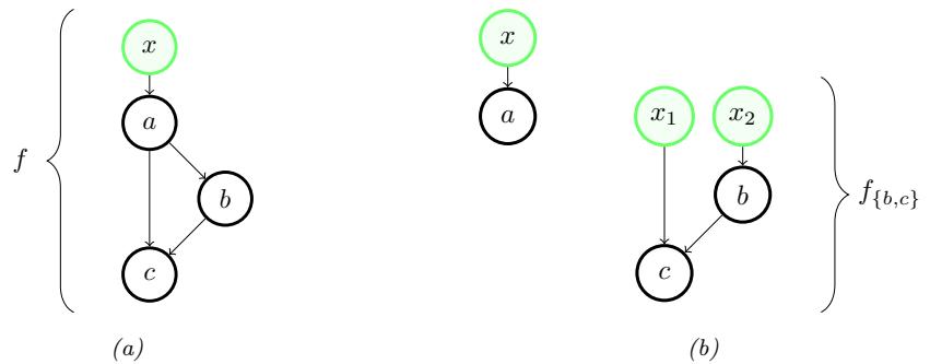
Figure 6.1: A circuit for a function f over three primitives, and its decomposition into two circuits without fan-out. Input nodes are drawn in green.

prefixes before its backwards traversal, so it consumes more memory than forward-mode. There are ways to combat this memory requirement in special-case scenarios, such as when the chained operations are each reversible [MDA15; Gom+17; KKL20]. One can also trade o! memory for computation by discarding some prefixes and re-computing them as needed.

6.2.2.2 From chains to circuits

When primitives can accept multiple inputs, we can naturally extend chains to circuits — directed acyclic graphs over primitive operations, sometimes also called computation graphs. To set up for this section, we will distinguish between (1) input nodes of a circuit, which symbolize a function’s arguments, and (2) primitive nodes, each of which is labeled by a primitive operation. We assume that input nodes have no incoming edges and (without loss of generality) exactly one outgoing edge each, and that the graph has exactly one sink node. The overall function of the circuit is composition of operations from the input nodes to the sink, where the output of each operation is input to others according to its outgoing edges.

What made AD work in Section 6.2.2.1 is the fact that derivatives decompose along chains thanks to the aptly-named chain rule. When moving from chains to directed acyclic graphs, do we need some sort of “graph rule” in order to decompose our calculation along the circuit’s structure? Circuits introduce two new features: fan-in and fan-out. In graphical terms, fan-in simply refers to multiple edges incoming to a node, and fan-out refers to multiple edges outgoing.

What do these mean in functional terms? Fan-in happens when a primitive operation accepts multiple arguments. We observed in Section 6.2.1 that multiple arguments can be treated as one, and how the chain rule then applies. Fan-out requires slightly more care, specifically for reverse-mode di!erentiation.

The gist of an answer can be illustrated with a small example. Consider the circuit in Figure 6.1a. The operation a precedes b and c topologically, with an outgoing edge to each of both. We can cut a away from {b, c} to produce two new circuits, shown in Figure 6.1b. The first corresponds to a and the second corresponds to the remaining computation, given by:

\[f\_{\{b,c\}}(x\_1, x\_2) = c(x\_1, b(x\_2))\,. \tag{6.35}\]

We can recover the complete function f from a and f{b,c} with the help of a function dup given by:

\[\text{dup}(x) = (x, x) \equiv \begin{pmatrix} I \\ I \end{pmatrix} x \tag{6.36}\]

so that f can be written as a chain composition:

\[f = f\_{\{b,c\}} \diamond \text{dup} \diamond a \,. \tag{6.37}\]

The circuit for f{b,c} contains no fan-out, and composition rules such as Equation (6.25) tell us its derivatives in terms of b, c, and their derivatives, all via the chain rule. Meanwhile, the chain rule applied to Equation (6.37) says that:

\[ \partial f(\mathbf{x}) = \partial f\_{\{b,c\}}(\text{dup}(a(\mathbf{x}))) \circ \partial \text{dup}(a(\mathbf{x})) \circ \partial a(\mathbf{x}) \tag{6.38} \]

\[=\partial f\_{\{b,c\}}(a(\mathbf{z}),a(\mathbf{z})) \circ \begin{pmatrix} I \\ I \end{pmatrix} \circ \partial a(\mathbf{z}) \,. \tag{6.39}\]

The above expression suggests calculating a JVP of f by right-to-left evaluation. It is similar to the JVP calculation suggested by Equation (6.30), but with a duplication operation ’ I I(^T in the middle that arises from the Jacobian of dup.

Transposing the derivative of f at x:

\[\partial f(\mathbf{x})^{\mathsf{T}} = \partial a(\mathbf{x})^{\mathsf{T}} \circ \left(I \quad I\right) \circ \partial f\_{\{b,c\}}(a(\mathbf{x}), a(\mathbf{x}))^{\mathsf{T}}.\tag{6.40}\]

Considering right-to-left evaluation, this too is similar to the VJP calculation suggested by Equation (6.33), but with a summation operation ’ I I( in the middle that arises from the transposed Jacobian of dup. The lesson of using dup in this small example is that, more generally, in order to handle fan-out in reverse mode AD, we can process operations in topological order — first forward and then in reverse — and then sum partial VJPs along multiple outgoing edges.

Algorithm 6.3: Foward-mode circuit di!erentiation (JVP)

input: ^f : ^{Rn → Rm} composing ^f1,…,f^T in topological order, where ^f1 is identity input: linearization point ^{x ↑ Rn} and perturbation ^{v ↑ Rn} x1, v¹ := x, v for t := 2,…,T do let [q1,…,qr] = Pa(t) x^t := ft(x^q1 ,…, x^qr ) ⁷ v^t := #^{r i}=1 0ift(x^q1 ,…, x^qr )[v^qi ] output: x^T , equal to f(x) output: v^T , equal to 0f(x)[v]

Algorithms 6.3 and 6.4 give a complete description of forward- and reverse-mode di!erentiation on circuits. For brevity they assume a single argument to the entire circuit function. Nodes are indexed 1,…,T. The first is the input node, and the remaining T ⇐ 1 are labeled by their operation f2,…,f^T . We take f¹ to be the identity. For each t, if f^t takes k arguments, let Pa(t) be the ordered

Algorithm 6.4: Reverse-mode circuit di!erentiation (VJP)

input: ^f : ^{Rn → Rm} composing ^f1,…,f^T in topological order, where ^f1, f^T are identity input: linearization point ^{x ↑ Rn} and perturbation ^{u ↑ Rm 3} x¹ := x for t := 2,…,T do let [q1,…,qr] = Pa(t) x^t := ft(x^q1 ,…, x^qr ) u(^{T ↑}1)↗^T := u for t := T ⇐ 1,…, 2 do let [q1,…,qr] = Pa(t) ¹⁰ u^{↔︎ t} := # ^c≃Ch(t) ^ut↗^c u^qi↗^t := 0ift(x^q1 ,…, x^qr ) ^Tu^{↔︎ t} for i = 1,…,r output: x^T , equal to f(x) output: u¹↗², equal to 0f(x) ^Tu

list of k indices of its parent nodes (possibly containing duplicates, due to fan-out), and let Ch(t) be the indices of its children (again possibly duplicate). Algorithm 6.4 takes a few more conventions: that f^T is the identity, that node T has T ⇐ 1 as its only parent, and that the child of node 1 is node 2.

Fan-out is a feature of graphs, but arguably not an essential feature of functions. One can always remove all fan-out from a circuit representation by duplicating nodes. Our interest in fan-out is precisely to avoid this, allowing for an e”cient representation and, in turn, e”cient memory use in Algorithms 6.3 and 6.4.

Reverse-mode AD on circuits has appeared under various names and formulations over the years. The algorithm is precisely the backpropagation algorithm in neural networks, a term introduced in the 1980s [RHW86b; RHW86a], and has separately come up in the context of control theory and sensitivity, as summarized in historical notes by Goodfellow, Bengio, and Courville [GBC16, Section 6.6].

6.2.2.3 From circuits to programs

Graphs are useful for introducing AD algorithms, and they might align well enough with neural network applications. But computer scientists have spent decades formalizing and studying various “languages for expressing functions compositionally”. Simply put, this is what programming languages are for! Can we automatically di!erentiate numerical functions expressed in, say, Python, Haskell, or some variant of the lambda calculus? These o!er a far more widespread — and intuitively more expressive — way to describe an input function.3

In the previous sections, our approach to AD became more complex as we allowed for more complex graph structure. Something similar happens when we introduce grammatical constructs in a

^3. In Python, what the language calls a “function” does not always describe a pure function of the arguments listed in its syntactic definition; its behavior may rely on side e!ects or global state, as allowed by the language. Here, we specifically mean a Python function that is pure and functional. JAX’s documentation details this restriction [Bra+18].

programming language. How do we adapt AD to handle a language with loops, conditionals, and recursive calls? What about parallel programming constructs? We have partial answers to questions like these today, although they invite a deeper dive into language details such as type systems and implementation concerns [Yu+18; Inn20; Pas+21b].

One example language construct that we already know how to handle, due to Section 6.2.2.2, is a standard let expression. In languages with a means of name or variable binding, multiple appearances of the same variable are analogous to fan-out in a circuit. Figure 6.1a corresponds to a function f that we could write in a functional language as:

f(x) = let ax = a(x) in c(ax, b(ax))

in which ax indeed appears twice after it is bound.

Understanding the interaction between language capacity and automatic di!erentiability is an ongoing topic of computer science research [PS08a; AP19; Vyt+19; BMP19; MP21]. In the meantime, functional languages have proven quite e!ective in recent AD systems, both widely-used and experimental. Systems such as JAX, Dex, and others are designed around pure functional programming models, and internally rely on functional program representations for di!erentiation [Mac+15; BPS16; Sha+19; FJL18; Bra+18; Mac+19; Dex; Fro+21; Pas+21a].

6.3 Stochastic optimization

In this section, we consider optimization of stochastic objectives of the form

\[\mathcal{L}(\boldsymbol{\theta}) = \mathbb{E}\_{q\boldsymbol{\theta}\left(\mathbf{z}\right)} \left[ \boldsymbol{\tilde{\mathcal{L}}}(\boldsymbol{\theta}, \mathbf{z}) \right] \tag{6.41}\]

where ω are the parameters we are optimizing, and z is a random variable, such as an external noise.

6.3.1 Stochastic gradient descent

Suppose we have a way of computing an unbiased estimate g^t of the gradient of the objective function, i.e.,

\[\mathbb{E}\left[\mathfrak{g}\_{\mathfrak{t}}\right] = \nabla\_{\theta} \mathcal{L}(\theta)|\_{\mathfrak{G}\_{\mathfrak{t}}} \tag{6.42}\]

Then we can use this inside of a gradient descent procedure:

\[ \theta\_{t+1} = \theta\_t - \eta\_t g\_t \tag{6.43} \]

where ◁^t is the learning rate or step size. This is called stochastic gradient descent or SGD.

6.3.1.1 Choosing the step size

When using SGD, we need to be careful in how we choose the learning rate in order to achieve convergence. Rather than choosing a single constant learning rate, we can use a learning rate

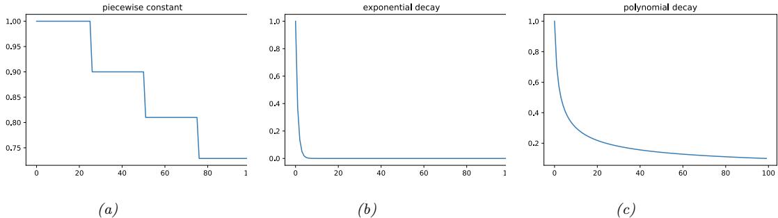
Figure 6.2: Illustration of some common learning rate schedules. (a) Piecewise constant. (b) Exponential decay. (c) Polynomial decay. Generated by learning\_rate\_plot.ipynb.

schedule, in which we adjust the step size over time. Theoretically, a su”cient condition for SGD to achieve convergence is if the learning rate schedule satisfies the Robbins-Monro conditions:

\[\eta\_t \to 0, \ \frac{\sum\_{t=1}^{\infty} \eta\_t^2}{\sum\_{t=1}^{\infty} \eta\_t} \to 0 \tag{6.44}\]

Some common examples of learning rate schedules are listed below:

\[ \eta\_t = \eta\_i \text{ if } t\_i \le t \le t\_{i+1} \quad \text{piecewise constant} \tag{6.45} \]

\[ \eta\_t = \eta\_0 e^{-\lambda t} \text{ exponential decay} \tag{6.46} \]

\[ \eta\_t = \eta\_0 (\beta t + 1)^{-\alpha} \text{ polynomial decay} \tag{6.47} \]

In the piecewise constant schedule, tⁱ are a set of time points at which we adjust the learning rate to a specified value. For example, we may set ◁ⁱ = ◁0φⁱ , which reduces the initial learning rate by a factor of φ for each threshold (or milestone) that we pass. Figure 6.2a illustrates this for ◁⁰ = 1 and φ = 0.9. This is called step decay. Sometimes the threshold times are computed adaptively, by estimating when the train or validation loss has plateaued; this is called reduce-on-plateau. Exponential decay is typically too fast, as illustrated in Figure 6.2b. A common choice is polynomial decay, with α = 0.5 and ↼ = 1, as illustrated in Figure 6.2c; this corresponds to a square-root schedule, ◁^t = ◁⁰ ⇓ 1 ^t+1 . For more details, see [Mur22, Sec 8.4.3].

6.3.1.2 Variance reduction

SGD can be slow to converge because it relies on a stochastic estimate of the gradient. Various methods have been proposed for reducing the variance of the parameter estimates generated at each step, which can speedup convergence. For more details, see [Mur22, Sec 8.4.5].

6.3.1.3 Preconditioned SGD

In many cases, the gradient magnitudes can be very di!erent along each dimension, corresponding to the loss surface being steep along some directions and shallow along others, similar to a valley

floor. In such cases, one can get faster convergence by scaling the gradient vector by a conditioning matrix C^t as follows:

\[ \boldsymbol{\theta}\_{t+1} = \boldsymbol{\theta}\_t - \eta\_t \mathbf{C}\_t \mathbf{g}\_t \tag{6.48} \]

This is called preconditioned SGD. For more details, see [Mur22, Sec 8.4.6].

6.3.2 SGD for optimizing a finite-sum objective

In the simplest case, the distribution used to compute the expectation, qϑ(z), does not depend on the parameters being optimized, ω. In this case, we can push gradients inside the expectation operator, and then use Monte Carlo sampling for z to approximate the gradient:

\[\nabla\_{\boldsymbol{\theta}} \mathcal{L}(\boldsymbol{\theta}) = \nabla\_{\boldsymbol{\theta}} \mathbb{E}\_{\mathbf{q}(\mathbf{z})} \left[ \boldsymbol{\tilde{\mathcal{L}}}(\boldsymbol{\theta}, \mathbf{z}) \right] = \mathbb{E}\_{\mathbf{q}(\mathbf{z})} \left[ \nabla\_{\boldsymbol{\theta}} \boldsymbol{\tilde{\mathcal{L}}}(\boldsymbol{\theta}, \mathbf{z}) \right] \approx \frac{1}{S} \sum\_{s=1}^{S} \nabla\_{\boldsymbol{\theta}} \boldsymbol{\tilde{\mathcal{L}}}(\boldsymbol{\theta}, \mathbf{z}\_{s}) \tag{6.49}\]

For example, consider the problem of empirical risk minimization or ERM, which requires minimizing

\[\mathcal{L}(\boldsymbol{\theta}) = \frac{1}{N} \sum\_{n=1}^{N} \bar{\mathcal{L}}(\boldsymbol{\theta}, \boldsymbol{z}\_n) = \frac{1}{N} \sum\_{n=1}^{N} \ell(y\_n, f(\boldsymbol{x}\_n; \boldsymbol{\theta})) \tag{6.50}\]

where zⁿ = (xn, yn) is the n’th labeled example, and f is a prediction function. This kind of objective is called a finite sum objective. We can write this as an expected loss wrt the empirical distrbution pD(x, y):

\[\mathcal{L}(\boldsymbol{\theta}) = \mathbb{E}\_{\mathcal{P}\_{\mathcal{D}}(\mathbf{z})} \left[ \boldsymbol{\tilde{\mathcal{L}}}(\boldsymbol{\theta}, \mathbf{z}) \right] \tag{6.51}\]

Since the expectation depends on the data, and not on the parameters, we can approximate the gradient by using a minibatch of B = |B| datapoints from the full dataset D at each iteration:

\[\mathfrak{g}\_t = \nabla \mathcal{L}(\boldsymbol{\theta}\_t) = \frac{1}{B} \sum\_{n \in \mathcal{B}} \nabla \ell(\boldsymbol{y}\_n, f(\boldsymbol{x}\_n; \boldsymbol{\theta})) \tag{6.52}\]

These noisy gradients can then be passed to SGD. When the dataset is large, this method is much faster than full batch gradient descent, since it does not require evaluating the loss on all N examples before updating the model [BB08; BB11].

6.3.3 SGD for optimizing the parameters of a distribution

Now suppose the stochasticity depends on the parameters we are optimizing. For example, z could be an action sampled from a stochastic policy qϑ, as in RL (Section 35.3.2), or z could be a latent variable sampled from an inference network qϑ, as in stochastic variational inference (see Section 10.2). In this case, the gradient is given by

\[ \nabla\_{\theta} \mathbb{E}\_{q\_{\theta}(\mathbf{z})} \left[ \bar{\mathcal{L}}(\theta, \mathbf{z}) \right] = \nabla\_{\theta} \int \bar{\mathcal{L}}(\theta, \mathbf{z}) q\_{\theta}(\mathbf{z}) d\mathbf{z} = \int \nabla\_{\theta} \bar{\mathcal{L}}(\theta, \mathbf{z}) q\_{\theta}(\mathbf{z}) d\mathbf{z} \tag{6.53} \]

\[=\int \left[\nabla\_{\theta}\vec{\mathcal{L}}(\theta,\mathbf{z})\right]q\_{\theta}(\mathbf{z})d\mathbf{z}+\int \vec{\mathcal{L}}(\theta,\mathbf{z})\left[\nabla\_{\theta}q\_{\theta}(\mathbf{z})\right]d\mathbf{z}\tag{6.54}\]

In the first line, we have assumed that we can swap the order of integration and di!erentiation (see [Moh+20] for discussion). In the second line, we use the product rule for derivatives.

The first term can be approximated by Monte Carlo sampling:

\[\int \left[\nabla\_{\theta} \vec{\mathcal{L}}(\theta, z)\right] q\_{\theta}(z) dz \approx \frac{1}{S} \sum\_{s=1}^{S} \nabla\_{\theta} \vec{\mathcal{L}}(\theta, z\_{s}) \tag{6.55}\]

where ^{zs ⇔ q}ϑ. Note that if ^L˜() is independent of ^ω, this term vanishes.

Now consider the second term, that takes the gradients of the distribution itself:

\[I \triangleq \int \bar{\mathcal{L}}(\theta, z) \left[ \nabla\_{\theta} q\_{\theta}(z) \right] dz \tag{6.56}\]

We can no longer use vanilla Monte Carlo sampling to approximate this integral. However, there are various other ways to approximate this (see [Moh+20] for an extensive review). We briefly describe the two main methods in Section 6.3.4 and Section 6.3.5.

6.3.4 Score function estimator (REINFORCE)

The simplest way to approximate Equation (6.56) is to exploit the log derivative trick, which is the following identity:

\[ \nabla\_{\theta} q\_{\theta}(\mathbf{z}) = q\_{\theta}(\mathbf{z}) \nabla\_{\theta} \log q\_{\theta}(\mathbf{z}) \tag{6.57} \]

With this, we can rewrite Equation (6.56) as follows:

\[I = \int \ddot{\mathcal{L}}(\theta, \mathbf{z}) [q\_{\theta}(\mathbf{z}) \nabla\_{\theta} \log q\_{\theta}(\mathbf{z})] d\mathbf{z} = \mathbb{E}\_{q\_{\theta}(\mathbf{z})} \left[ \tilde{\mathcal{L}}(\theta, \mathbf{z}) \nabla\_{\theta} \log q\_{\theta}(\mathbf{z}) \right] \tag{6.58}\]

This is called the score function estimator or SFE [Fu15]. (The term “score function” refers to the gradient of a log probability distribution, as explained in Section 3.3.4.1.) It is also called the likelihood ratio gradient estimator, or the REINFORCE estimator (the reason for this latter name is explained in Section 35.3.2). We can now easily approximate this with Monte Carlo:

\[I \approx \frac{1}{S} \sum\_{s=1}^{S} \vec{\mathcal{L}}(\theta, \mathbf{z}\_s) \nabla\_{\theta} \log q\_{\theta}(\mathbf{z}\_s) \tag{6.59}\]

where z^s ⇔ qϑ. We only require that the sampling distribution is di!erentiable, not the objective ^L˜(ω, ^z) itself. This allows the method to be used for blackbox stochastic optimization problems, such as variational optimization (Supplementary Section 7.4.3), black-box variational inference (Section 10.2.3), reinforcement learning (Section 35.3.2), etc.

6.3.4.1 Control variates

The score function estimate can have high variance. One way to reduce this is to use control variates, in which we replace ^L˜(ω, ^z) with

\[ \hat{\vec{\mathcal{L}}}(\theta, \mathbf{z}) = \bar{\mathcal{L}}(\theta, \mathbf{z}) - c \left( b(\theta, \mathbf{z}) - \mathbb{E} \left[ b(\theta, \mathbf{z}) \right] \right) \tag{6.60} \]

where ^b(ω, ^z) is a baseline function that is correlated with ^L˜(ω, ^z), and c > ⁰ is a coe”cient. Since E L ˆ˜(ω, ^z) = E ^L˜(ω, ^z) , we can use L ˆ˜ to compute unbiased gradient estimates of ^L˜. The advantage is that this new estimate can result in lower variance, as we show in Section 11.6.3.

6.3.4.2 Rao-Blackwellization

Suppose ^qϑ(z) is a discrete distribution. In this case, our objective becomes ^L(ω) = # ^{z L}˜(ω, ^z)qϑ(z). We can now easily compute gradients using ▽ϑL(ω) = # ^{z L}˜(ω, ^z)▽ϑqϑ(z). Of course, if ^z can take on exponentially many values (e.g., we are optimizing over the space of strings), this expression is intractable. However, suppose we can partition this sum into two sets, a small set S¹ of high probability values and a large set S² of all other values. Then we can enumerate over S¹ and use the score function estimator for S2:

\[\nabla \theta \mathcal{L}(\theta) = \sum\_{\mathbf{z} \in S\_1} \ddot{\mathcal{L}}(\theta, \mathbf{z}) \nabla \theta \eta \theta(\mathbf{z}) + \mathbb{E}\_{\eta \theta(\mathbf{z}|\mathbf{z} \in S\_2)} \left[ \ddot{\mathcal{L}}(\theta, \mathbf{z}) \nabla \theta \log q \theta(\mathbf{z}) \right] \tag{6.61}\]

To compute the second expectation, we can use rejection sampling applied to samples from qϑ(z). This procedure is a form of Rao-Blackwellization as shown in [Liu+19b], and reduces the variance compared to standard SFE (see Section 11.6.2 for details on Rao-Blackwellization).

6.3.5 Reparameterization trick

The score function estimator can have high variance, even when using a control variate. In this section, we derive a lower variance estimator, which can be applied if ^L˜(ω, ^z) is di!erentiable wrt ^z. We additionally require that we can compute a sample from qϑ(z) by first sampling ◁ from some noise distribution q⁰ which is independent of ω, and then transforming to z using a deterministic and di!erentiable function ^z = ^g(ω, ^◁). For example, instead of sampling ^{z ⇔ N} (µ, ^ε2), we can sample ◁ ⇔ N (0, 1) and compute

\[\mathbf{z} = g(\theta, \epsilon) = \mu + \sigma \epsilon \tag{6.62}\]

where ω = (µ, ε). This allows us to rewrite our stochastic objective as follows:

\[\mathcal{L}(\boldsymbol{\theta}) = \mathbb{E}\_{q\_{\boldsymbol{\theta}}(\mathbf{z})} \left[ \boldsymbol{\tilde{\mathcal{L}}}(\boldsymbol{\theta}, \mathbf{z}) \right] = \mathbb{E}\_{q\_{\boldsymbol{0}}(\mathbf{e})} \left[ \boldsymbol{\tilde{\mathcal{L}}}(\boldsymbol{\theta}, g(\boldsymbol{\theta}, \boldsymbol{\epsilon})) \right] \tag{6.63}\]

Since q0(◁) is independent of ω, we can push the gradient operator inside the expectation, which we can approximate with Monte Carlo:

\[\nabla\_{\theta} \mathcal{L}(\theta) = \mathbb{E}\_{\theta\_0(\epsilon)} \left[ \nabla\_{\theta} \vec{\mathcal{L}}(\theta, g(\theta, \epsilon)) \right] \approx \frac{1}{S} \sum\_{s=1}^{S} \nabla\_{\theta} \vec{\mathcal{L}}(\theta, g(\theta, \epsilon\_s)) \tag{6.64}\]

where ◁^s ⇔ q0. This is called the reparameterization gradient or the pathwise derivative [Gla03; Fu15; KW14; RMW14a; TLG14; JO18; FMM18], and is widely used in variational inference (Section 10.2.1). For a review of such methods, see [Moh+20].

Note that the tensorflow probability library (which also has a JAX interface) supports reparameterizable distributions. Therefore you can just write code in a straightforward way, as shown in the code snippet below.

Listing 6.1: Derivative of a stochastic function

def expected_loss(params):
   zs = dist.sample(N, key)
   return jnp.mean(loss(params , zs))
g = jax.grad(expected_loss)(params)

6.3.5.1 Example

As a simple example, suppose we define some arbitrary function, such as ^L˜(z) = ^z2 ⇐ ³z, and then define its expected value as L(ω) = EN(z|µ,v) ^L˜(z) , where ω = (µ, v) and v = ε². Suppose we want to compute

\[\nabla\_{\theta} \mathcal{L}(\theta) = \left[ \frac{\partial}{\partial \mu} \mathbb{E} \left[ \bar{\mathcal{L}}(z) \right], \frac{\partial}{\partial v} \mathbb{E} \left[ \bar{\mathcal{L}}(z) \right] \right] \tag{6.65}\]

Since the Gaussian distribution is reparameterizable, we can sample z ⇔ N (z|µ, v), and then use automatic di!erentiation to compute each of these gradient terms, and then average.

However, in the special case of Gaussian distributions, we can also compute the gradient vector directly. In particular, in Section 6.4.5.1 we present Bonnet’s theorem, which states that

\[\frac{\partial}{\partial \mu} \mathbb{E}\left[\tilde{\mathcal{L}}(z)\right] = \mathbb{E}\left[\frac{\partial}{\partial z}\tilde{\mathcal{L}}(z)\right] \tag{6.66}\]

Similarly, Price’s theorem states that

\[\frac{\partial}{\partial v} \mathbb{E}\left[\bar{\mathcal{L}}(z)\right] = 0.5 \mathbb{E}\left[\frac{\partial^2}{\partial z^2} \bar{\mathcal{L}}(z)\right] \tag{6.67}\]

In gradient\_expected\_value\_gaussian.ipynb we show that these two methods are numerically equivalent, as theory suggests.

6.3.5.2 Total derivative

To compute the gradient term inside the expectation in Equation (6.64) we need to use the total derivative, since the function ^L˜ depends on ^ω directly and via the noise sample ^z. Recall that, for a function of the form ^L˜(ϑ1,…, ^ϑdϱ , z1(ω),…,z^dz (ω)), the total derivative wrt ^ϑi is given by the chain rule as follows:

\[\frac{\partial \vec{\mathcal{L}}^{\text{TD}}}{\partial \theta\_i} \quad = \frac{\partial \vec{\mathcal{L}}}{\partial \theta\_i} + \sum\_j \frac{\partial \vec{\mathcal{L}}}{\partial z\_j} \frac{\partial z\_j}{\partial \theta\_i} \tag{6.68}\]

and hence

\[ \nabla\_{\theta} \bar{\mathcal{L}}(\theta, z)^{\text{TD}} = \nabla\_{z} \bar{\mathcal{L}}(\theta, z) \mathbf{J} + \nabla\_{\theta} \bar{\mathcal{L}}(\theta, z) \tag{6.69} \]

where J = ^φz^{T φϑ} is the d^z ∞ d^◁ Jacobian matrix of the noise transformation:

\[\mathbf{J} = \begin{pmatrix} \frac{\partial \mathbf{z}\_1}{\partial \theta\_1} & \cdots & \frac{\partial \mathbf{z}\_1}{\partial \theta\_{d\_\psi}} \\ \vdots & \ddots & \vdots \\ \frac{\partial \mathbf{z}\_{d\_x}}{\partial \theta\_{d\_\psi}} & \cdots & \frac{\partial \mathbf{z}\_{d\_x}}{\partial \theta\_{d\_\psi}} \end{pmatrix} \tag{6.70}\]

We leverage this decomposition in Section 6.3.5.3, where we derive a lower variance gradient estimator in the special case of variational inference.

6.3.5.3 “Sticking the landing” estimator

In this section we consider the special case which arises in variational inference (Section 10.2). The ELBO objective (for a single latent sample z) has the form

\[\tilde{\mathcal{L}}(\mathbf{\theta}, \mathbf{z}) = \log p(\mathbf{z}, \mathbf{z}) - \log q(\mathbf{z}|\mathbf{\theta}) \tag{6.71}\]

where ω are the parameters of the variational posterior. The gradient becomes

\[\nabla\_{\theta} \tilde{\mathcal{L}}(\theta, z) = \nabla\_{\theta} \left[ \log p(z, x) - \log q(z | \theta) \right] \tag{6.72}\]

\[=\underbrace{\nabla\_{\mathbf{z}}\left[\log p(\mathbf{z},\mathbf{z})-\log q(\mathbf{z}|\boldsymbol{\theta})\right]\mathbf{J}}\_{\text{path derivative}}-\underbrace{\nabla\_{\boldsymbol{\theta}}\log q(\mathbf{z}|\boldsymbol{\theta})}\_{\text{score function}}\tag{6.73}\]

\[\begin{array}{ccc}\hline\multicolumn{3}{c}{\text{path derivative}} & & \multicolumn{3}{c}{\text{ccore function}}\\\hline\end{array}\]

The first term is the indirect e!ect of ω on the objective via the generated samples z. The second term is the direct e!ect of ω on the objective. The second term is zero in expectation since it is the score function (see Equation (3.44)), but it may be non-zero for a finite number of samples, even if q(z|ω) = p(z|x) is the true posterior. In [RWD17], they propose to drop the second term to create a lower variance estimator. This can be achieved by using log q(z|ω^↔︎ ), where ω^↔︎ is a “disconnected” copy of ω that does not a!ect the gradient. In pseudocode, this looks like the following:

\[ \mathfrak{e} \sim q\_0(\mathfrak{e})\tag{6.74} \]

\[\mathbf{z} = g(\boldsymbol{\epsilon}, \boldsymbol{\theta})\tag{6.75}\]

\[ \theta' = \text{stop-gradient}(\theta) \tag{6.76} \]

\[\mathbf{g} = \nabla\_{\theta} \left[ \log p(\mathbf{z}, \mathbf{z}) - \log q(\mathbf{z}|\theta') \right] \tag{6.77}\]

They call this the sticking the landing or STL estimator.4 Note that the STL estimator is not always better than the “standard” estimator, without the stop gradient term. In [GD20], they propose to use a weighted combination of estimators, where the weights are optimized so as to reduce variance for a fixed amount of compute.

6.3.6 Gumbel softmax trick

When working with discrete variables, we cannot use the reparameterization trick. However, we can often relax the discrete variables to continuous ones in a way which allows the trick to be used, as we explain below.

Consider a one-hot vector ^d with ^K bits, so ^{dk ↑} {0, ¹} and #^{K k}=1 d^k = 1. This can be used to represent a K-ary categorical variable d. Let P(d) = Cat(d|ϑ), where ϱ^k = P(d^k = 1), so 0 ↗ ϱ^k ↗ 1. Alternatively we can parameterize the distribution in terms of (α1,…, αk), where ϱ^k = αk/( #^{K k}→=1 α^k→ ). We will denote this by d ⇔ Cat(d|ε).

^4. The expression “to stick a landing” means to land firmly on one’s feet after performing a gymnastics move. In the current context, the analogy is this: if the variational posterior is optimal, then we want our objective to be 0, and not to “wobble” with Monte Carlo noise.

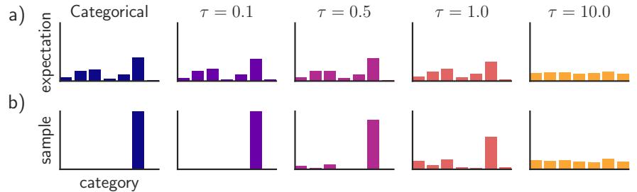
Figure 6.3: Illustration of the Gumbel-softmax (concrete) distribution with K = 7 states at di!erent temperatures ↽ . The top row shows E [z], and the bottom row shows samples z ↔︎ GumbelSoftmax(ω, ↽ ). The left column shows a discrete (categorical) distribution, which always produces one-hot samples. From Figure 1 of [JGP17]. Used with kind permission of Ben Poole.

We can sample a one-hot vector d from this distribution by computing

\[\mathbf{d} = \text{onehot}(\underset{k}{\text{argmax}} [\epsilon\_k + \log \alpha\_k])\tag{6.78}\]

where 3^k ⇔ Gumbel(0, 1) is sampled from the Gumbel distribution [Gum54]. We can draw such samples by first sampling u^k ⇔ Unif(0, 1) and then computing 3^k = ⇐ log(⇐ log(uk)). This is called the Gumbel-max trick [MTM14], and gives us a reparameterizable representation for the categorical distribution.

Unfortunately, the derivative of the argmax is 0 everywhere except at the boundary of transitions from one label to another, where the derivative is undefined. However, suppose we replace the argmax with a softmax, and replace the discrete one-hot vector ^d with a continuous relaxation ^{x ↑} (^K↑¹, where (^K↑¹ = {^{x ↑ RK} : ^{xk ↑} [0, 1], #^{K k}=1 x^k = 1} is the K-dimensional simplex. Then we can write

\[x\_k = \frac{\exp((\log \alpha\_k + \epsilon\_k)/\tau)}{\sum\_{k'=1}^K \exp((\log \alpha\_{k'} + \epsilon\_{k'})/\tau)}\tag{6.79}\]

where 2 > 0 is a temperature parameter. This is called the Gumbel-softmax distribution [JGP17] or the concrete distribution [MMT17]. This smoothly approaches the discrete distribution as 2 → 0, as illustrated in Figure 6.3.

We can now replace f(d) with f(x), which allows us to take reparameterized gradients wrt x.

6.3.7 Stochastic computation graphs

We can represent an arbitrary function containing both deterministic and stochastic components as a stochastic computation graph. We can then generalize the AD algorithm (Section 6.2) to leverage score function estimation (Section 6.3.4) and reparameterization (Section 6.3.5) to compute Monte Carlo gradients for complex nested functions. For details, see [Sch+15a; Gaj+19].

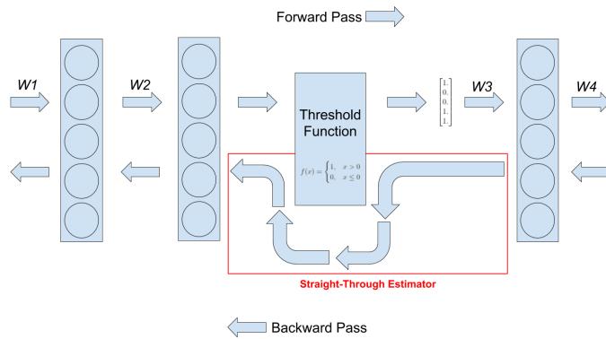
Figure 6.4: Illustration of straight-through estimator when applied to a binary threshold function in the middle of an MLP. From https: // www. hassanaskary. com/ python/ pytorch/ deep% 20learning/ 2020/ 09/ 19/ intuitive-explanation-of-straight-through-estimators. html . Used with kind permission of Hassan Askary.

6.3.8 Straight-through estimator

In this section, we discuss how to approximate the gradient of a quantized version of a signal. For example, suppose we have the following thresholding function, that binarizes its output:

\[f(x) = \begin{cases} 1 & \text{if } x > 0 \\ 0 & \text{if } x \le 0 \end{cases} \tag{6.80}\]

This does not have a well-defined gradient. However, we can use the straight-through estimator proposed in [Ben13] as an approximation. The basic idea is to replace g(x) = f^↔︎ (x), where f^↔︎ (x) is the derivative of f wrt input, with g(x) = x when computing the backwards pass. See Figure 6.4 for a visualization, and [Yin+19b] for an analysis of why this is a valid approximation.

In practice, we sometimes replace g(x) = x with the hard tanh function, defined by

\[\text{HardTanh}(x) = \begin{cases} x & \text{if } -1 \le x \le 1 \\ 1 & \text{if } x > 1 \\ -1 & \text{if } x < -1 \end{cases} \tag{6.81}\]

This ensures the gradients that are backpropagated don’t get too large. See Section 21.6 for an application of this approach to discrete autoencoders.

6.4 Natural gradient descent

In this section, we discuss natural gradient descent (NGD) [Ama98], which is a second order method for optimizing the parameters of (conditional) probability distributions pϑ(y|x). The key idea is to compute parameter updates by measuring distances between the induced distributions, rather than comparing parameter values directly.

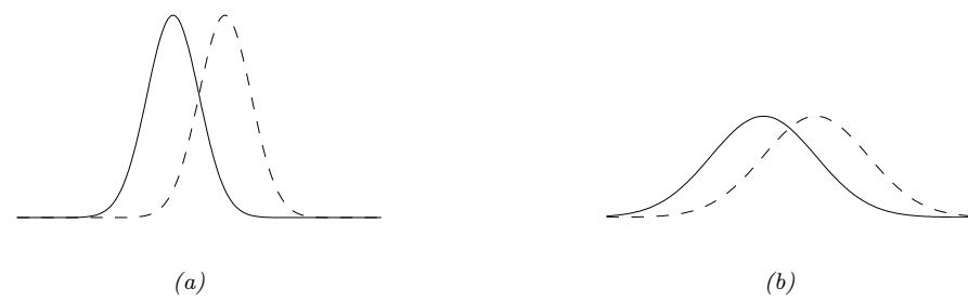
Figure 6.5: Changing the mean of a Gaussian by a fixed amount (from solid to dotted curve) can have more impact when the (shared) variance is small (as in a) compared to when the variance is large (as in b). Hence the impact (in terms of prediction accuracy) of a change to µ depends on where the optimizer is in (µ, ϑ) space. From Figure 3 of [Hon+10], reproduced from [Val00]. Used with kind permission of Antti Honkela.

For example, consider comparing two Gaussians, p^ϑ = p(y|µ, ε) and p^ϑ→ = p(y|µ^↔︎ , ε^↔︎ ). The (squared) Euclidean distance between the parameter vectors decomposes as ||ω ⇐ ω^↔︎ ||² = (^µ ⇐ ^µ↔︎ )² + (^ε ⇐ ^ε↔︎ )2. However, the predictive distribution has the form exp(⇐ ^{1 2}ϱ² (^y ⇐ ^µ)²), so changes in ^µ need to be measured relative to ε. This is illustrated in Figure 6.5(a-b), which shows two univariate Gaussian distributions (dotted and solid lines) whose means di!er by 1. In Figure 6.5(a), they share the same small variance ε², whereas in Figure 6.5(b), they share the same large variance. It is clear that the value of 1 matters much more (in terms of the e!ect on the distribution) when the variance is small. Thus we see that the two parameters interact with each other, which the Euclidean distance cannot capture. This problem gets much worse when we consider more complex models, such as deep neural networks. By modeling such correlations, NGD can converge much faster than other gradient methods.

6.4.1 Defining the natural gradient

The key to NGD is to measure the notion of distance between two probability distributions in terms of the KL divergence. As we show in Section 5.1.9, this can be approximated in terms of the Fisher information matrix (FIM). In particular, for any given input x, we have

\[D\_{\rm KL} \left( p\_{\theta}(y|x) \parallel p\_{\theta+\delta}(y|x) \right) \approx \frac{1}{2} \delta^{\mathsf{T}} \mathbf{F}\_{\mathfrak{x}} \delta \tag{6.82}\]

where F^x is the FIM

\[\mathbb{E}\_{\mathbf{z}}(\theta) = -\mathbb{E}\_{p\_{\theta}(\mathbf{y}|\mathbf{z})} \left[ \nabla^{2} \log p\_{\theta}(\mathbf{y}|\mathbf{z}) \right] = \mathbb{E}\_{p\_{\theta}(\mathbf{y}|\mathbf{z})} \left[ (\nabla \log p\_{\theta}(\mathbf{y}|\mathbf{z})) (\nabla \log p\_{\theta}(\mathbf{y}|\mathbf{z}))^{\mathsf{T}} \right] \tag{6.83}\]

We can compute the average KL between the current and updated distributions using ^{1 2 ▷T}F▷, where F is the averaged FIM:

\[\mathbf{F}(\theta) = \mathbb{E}\_{\mathrm{p}\circ(\mathfrak{a})} \left[ \mathbf{F}\_{\mathfrak{a}}(\theta) \right] \tag{6.84}\]

NGD uses the inverse FIM as a preconditioning matrix, i.e., we perform updates of the following form:

\[\boldsymbol{\theta}\_{t+1} = \boldsymbol{\theta}\_t - \eta\_t \mathbf{F}(\boldsymbol{\theta}\_t)^{-1} \mathbf{g}\_t \tag{6.85}\]

The term

\[\mathbf{F}^{-1}\mathbf{g}\_t = \mathbf{F}^{-1}\nabla \mathcal{L}(\boldsymbol{\theta}\_t) \triangleq \tilde{\nabla} \mathcal{L}(\boldsymbol{\theta}\_t) \tag{6.86}\]

is called the natural gradient.

6.4.2 Interpretations of NGD

6.4.2.1 NGD as a trust region method

In Supplementary Section 7.1.3.1 we show that we can interpret standard gradient descent as optimizing a linear approximation to the objective subject to a penalty on the ⇁² norm of the change in parameters, i.e., if ωt+1 = ω^t + ▷, then we optimize

\[M\_t(\boldsymbol{\delta}) = \mathcal{L}(\boldsymbol{\theta}\_t) + \mathbf{g}\_t^\mathsf{T}\boldsymbol{\delta} + \eta||\boldsymbol{\delta}||\_2^2 \tag{6.87}\]

Now let us replace the squared distance with the squared FIM-based distance, ||▷||^{2 F =} ▷^TF▷. This is equivalent to squared Euclidean distance in the whitened coordinate system ϱ = F^{1 2} ω, since

\[||\phi\_{t+1} - \phi\_t||\_2^2 = ||\mathbf{F}^{\frac{1}{2}}(\theta\_t + \delta) - \mathbf{F}^{\frac{1}{2}}\theta\_t||\_2^2 = ||\mathbf{F}^{\frac{1}{2}}\delta||\_2^2 = ||\delta||\_F^2\tag{6.88}\]

The new objective becomes

\[M\_t(\boldsymbol{\delta}) = \mathcal{L}(\boldsymbol{\theta}\_t) + \boldsymbol{g}\_t^\mathsf{T}\boldsymbol{\delta} + \eta \boldsymbol{\delta}^\mathsf{T} \mathbf{F} \boldsymbol{\delta} \tag{6.89}\]

Solving ▽↼Mt(▷) = 0 gives the update

\[\delta\_t = -\eta \mathbf{F}^{-1} \mathbf{g}\_t \tag{6.90}\]

This is the same as the natural gradient direction. Thus we can view NGD as a trust region method, where we use a first-order approximation to the objective, and use FIM-distance in the constraint.

In the above derivation, we assumed F was a constant matrix. Im most problems, it will change at each point in space, since we are optimizing in a curved space known as a Riemannian manifold. For certain models, we can compute the FIM e”ciently, allowing us to capture curvature information, even though we use a first-order approximation to the objective.

6.4.2.2 NGD as a Gauss-Newton method

If p(y|x, ω) is an exponential family distribution with natural parameters computed by ϖ = f(x, ω), then one can show [Hes00; PB14] that NGD is identical to the generalized Gauss-Newton (GGN) method (Section 17.3.2). Furthermore, in the online setting, these methods are equivalent to performing sequential Bayesian inference using the extended Kalman filter, as shown in [Oll18].

6.4.3 Benefits of NGD

The use of the FIM as a preconditioning matrix, rather than the Hessian, has two advantages. First, F is always positive definite, whereas H can have negative eigenvalues at saddle points, which are prevalent in high dimensional spaces. Second, it is easy to approximate F online from minibatches, since it is an expectation (wrt the empirical distribution) of outer products of gradient vectors. This is in contrast to Hessian-based methods [Byr+16; Liu+18a], which are much more sensitive to noise introduced by the minibatch approximation.

In addition, the connection with trust region optimization makes it clear that NGD updates parameters in a way that matter most for prediction, which allows the method to take larger steps in uninformative regions of parameter space, which can help avoid getting stuck on plateaus. This can also help with issues that arise when the parameters are highly correlated.

For example, consider a 2d Gaussian with an unusual, highly coupled parameterization, proposed in [SD12]:

\[p(\mathbf{z}; \boldsymbol{\theta}) = \frac{1}{2\pi} \exp\left[ -\frac{1}{2} \left( x\_1 - \left[ 3\theta\_1 + \frac{1}{3}\theta\_2 \right] \right)^2 - \frac{1}{2} \left( x\_2 - \left[ \frac{1}{3}\theta\_1 \right] \right)^2 \right] \tag{6.91}\]

The objective is the cross entropy loss:

\[\mathcal{L}(\boldsymbol{\theta}) = -\mathbb{E}\_{p^\*(\boldsymbol{\pi})} \left[ \log p(\boldsymbol{x}; \boldsymbol{\theta}) \right] \tag{6.92}\]

The gradient of this objective is given by

\[\nabla\_{\theta} \mathcal{L}(\theta) \begin{pmatrix} = \mathbb{E}\_{p^\*(\mathfrak{x})} \left[ 3(x\_1 - \left[ 3\theta\_1 + \frac{1}{3}\theta\_2 \right]) + \frac{1}{3}(x\_2 - \left[ \frac{1}{3}\theta\_1 \right]) \right] \\ \mathbb{E}\_{p^\*(\mathfrak{x})} \left[ \frac{1}{3}(x\_1 - \left[ 3\theta\_1 + \frac{1}{3}\theta\_2 \right]) \right] \end{pmatrix} \tag{6.93}\]

Suppose that p↘(x) = p(x; [0, 0]). Then the Fisher matrix is a constant matrix, given by

\[\mathbf{F} = \begin{pmatrix} 3^2 + \frac{1}{3^2} & 1\\ 1 & \frac{1}{3^2} \end{pmatrix} \tag{6.94}\]

Figure 6.6 compares steepest descent in ω space with the natural gradient method, which is equivalent to steepest descent in ϱ space. Both methods start at ω = (1, ⇐1). The global optimum is at ω = (0, 0). We see that the NG method (blue dots) converges much faster to this optimum and takes the shortest path, whereas steepest descent takes a very circuitous route. We also see that the gradient field in the whitened parameter space is more “spherical”, which makes descent much simpler and faster.

Finally, note that since NGD is invariant to how we parameterize the distribution, we will get the same results even for a standard parameterization of the Gaussian. This is particularly useful if our probability model is more complex, such as a DNN (see e.g., [SSE18]).

6.4.4 Approximating the natural gradient

The main drawback of NGD is the computational cost of computing (the inverse of) the Fisher information matrix (FIM). To speed this up, several methods make assumptions about the form of F, so it can be inverted e”ciently. For example, [LeC+98] uses a diagonal approximation for

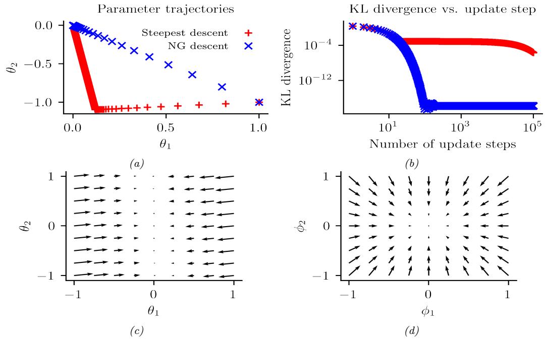
Figure 6.6: Illustration of the benefits of natural gradient vs steepest descent on a 2d problem. (a) Trajectories of the two methods in parameter space (red = steepest descent, blue = NG). They both start in the bottom right, at (1, ↓1). (b) Objective vs number of iterations. (c) Gradient field in the ε parameter space. (d) Gradient field in the whitened ϖ = F^{1 2} ε parameter space used by NG. Generated by nat\_grad\_demo.ipynb.

neural net training; [RMB08] uses a low-rank plus block diagonal approximation; and [GS15] assumes the covariance of the gradients can be modeled by a directed Gaussian graphical model with low treewidth (i.e., the Cholesky factorization of F is sparse).

[MG15] propose the KFAC method, which stands for “Kronecker factored approximate curvature”; this approximates the FIM of a DNN as a block diagonal matrix, where each block is a Kronecker product of two small matrices. This method has shown good results on supervised learning of neural nets [GM16; BGM17; Geo+18; Osa+19b] as well as reinforcement learning of neural policy networks [Wu+17]. The KFAC approximation can be justified using the mean field analysis of [AKO18]. In addition, [ZMG19] prove that KFAC will converge to the global optimum of a DNN if it is overparameterized (i.e., acts like an interpolator).

A simpler approach is to approximate the FIM by replacing the model’s distribution with the empirical distribution. In particular, define ^pD(x, ^y) = ¹ N #^{N n}=1 ^1xn (x)1^yn (y), ^pD(x) = ¹ N #^{N n}=1 1^xn (x) and pϑ(x, y) = pD(x)p(y|x, ω). Then we can compute the empirical Fisher [Mar16] as follows:

\[\mathbf{F} = \mathbb{E}\_{p\_{\boldsymbol{\theta}}(\boldsymbol{x}, \boldsymbol{y})} \left[ \nabla \log p(\boldsymbol{y}|\boldsymbol{x}, \boldsymbol{\theta}) \nabla \log p(\boldsymbol{y}|\boldsymbol{x}, \boldsymbol{\theta})^{\mathsf{T}} \right] \tag{6.95}\]

\[\approx \mathbb{E}\_{p\_{\mathcal{D}}(\mathbf{z}, \mathbf{y})} \left[ \nabla \log p(\mathbf{y}|\mathbf{z}, \boldsymbol{\theta}) \nabla \log p(\mathbf{y}|\mathbf{z}, \boldsymbol{\theta})^{\mathsf{T}} \right] \tag{6.96}\]

\[\hat{\rho} = \frac{1}{|\mathcal{D}|} \sum\_{(\mathfrak{x}, \mathfrak{y}) \in \mathcal{D}} \nabla \log p(\mathfrak{y}|\mathfrak{x}, \mathfrak{A}) \nabla \log p(\mathfrak{y}|\mathfrak{x}, \mathfrak{A})^{\mathsf{T}} \tag{6.97}\]

This approximation is widely used, since it is simple to compute. In particular, we can compute a diagonal approximation using the squared gradient vector. (This is similar to AdaGrad, but only uses the current gradient instead of a moving average of gradients; the latter is a better approach when performing stochastic optimization.)

Unfortunately, the empirical Fisher does not work as well as the true Fisher [KBH19; Tho+19]. To see why, note that when we reach a flat part of parameter space where the gradient vector goes to zero, the empirical Fisher will become singular, and hence the algorithm will get stuck on this plateau. However, the true Fisher takes expectations over the outputs, i.e., it marginalizes out y. This will allow it to detect small changes in the output if we change the parameters. This is why the natural gradient method can “escape” plateaus better than standard gradient methods.

An alternative strategy is to use exact computation of F, but solve for F↑¹g approximately using truncated conjugate gradient (CG) methods, where each CG step uses e”cient methods for Hessian-vector products [Pea94]. This is called Hessian free optimization [Mar10a]. However, this approach can be slow, since it may take many CG iterations to compute a single parameter update.

6.4.5 Natural gradients for the exponential family

In this section, we asssume L is an expected loss of the following form:

\[\mathcal{L}(\mu) = \mathbb{E}\_{q\_{\mu}(\mathbf{z})} \left[ \bar{\mathcal{L}}(\mathbf{z}) \right] \tag{6.98}\]

where qµ(z) is an exponential family distribution with moment parameters µ. This is the basis of variational optimization (discussed in Supplementary Section 7.4.3) and natural evolutionary strategies (discussed in Section 6.7.6).

It turns out the gradient wrt the moment parameters is the same as the natural gradient wrt the natural parameters φ. This follows from the chain rule:

\[\frac{d}{d\lambda}\mathcal{L}(\lambda) = \frac{d\mu}{d\lambda}\frac{d}{d\mu}\mathcal{L}(\mu) = \mathbf{F}(\lambda)\nabla\_{\mu}\mathcal{L}(\mu) \tag{6.99}\]

where L(µ) = L(φ(µ)), and where we used Equation (2.232) to write

\[\mathbf{F}(\lambda) = \nabla\_{\lambda} \mu(\lambda) = \nabla\_{\lambda}^{2} A(\lambda) \tag{6.100}\]

Hence

\[ \bar{\nabla}\_{\lambda} \mathcal{L}(\lambda) = \mathbf{F}(\lambda)^{-1} \nabla\_{\lambda} \mathcal{L}(\lambda) = \nabla\_{\mu} \mathcal{L}(\mu) \tag{6.101} \]

It remains to compute the (regular) gradient wrt the moment parameters. The details on how to do this will depend on the form of the q and the form of L(φ). We discuss some approaches to this problem below.

6.4.5.1 Analytic computation for the Gaussian case

In this section, we assume that q(z) = N (z|m, V). We now show how to compute the relevant gradients analytically.

Following Section 2.4.2.5, the natural parameters of q are

\[ \lambda^{(1)} = \mathbf{V}^{-1} m, \; \lambda^{(2)} = -\frac{1}{2} \mathbf{V}^{-1} \tag{6.102} \]

and the moment parameters are

\[ \mu^{(1)} = m,\ \mu^{(2)} = \mathbf{V} + m\mathbf{m}^{\mathsf{T}} \tag{6.103} \]

For simplicity, we derive the result for the scalar case. Let ^{m = µ}(1) and ^{v = µ}(2) ⇐ (µ(1))2. By using the chain rule, the gradient wrt the moment parameters are

\[\frac{\partial \mathcal{L}}{\partial \mu^{(1)}} = \frac{\partial \mathcal{L}}{\partial m} \frac{\partial m}{\partial \mu^{(1)}} + \frac{\partial \mathcal{L}}{\partial v} \frac{\partial v}{\partial \mu^{(1)}} = \frac{\partial \mathcal{L}}{\partial m} - 2 \frac{\partial \mathcal{L}}{\partial v} m \tag{6.104}\]

\[\frac{\partial \mathcal{L}}{\partial \mu^{(2)}} = \frac{\partial \mathcal{L}}{\partial m} \frac{\partial m}{\partial \mu^{(2)}} + \frac{\partial \mathcal{L}}{\partial v} \frac{\partial v}{\partial \mu^{(2)}} = \frac{\partial \mathcal{L}}{\partial v} \tag{6.105}\]

It remains to compute the derivatives wrt m and v. If z ⇔ N (m, V), then from Bonnet’s theorem [Bon64] we have

\[\frac{\partial}{\partial m\_i} \mathbb{E}\left[\tilde{\mathcal{L}}(\mathbf{z})\right] = \mathbb{E}\left[\frac{\partial}{\partial \theta\_i} \tilde{\mathcal{L}}(\mathbf{z})\right] \tag{6.106}\]

And from Price’s theorem [Pri58] we have

\[\frac{\partial}{\partial V\_{ij}} \mathbb{E}\left[\vec{\mathcal{L}}(\mathbf{z})\right] = c\_{ij} \mathbb{E}\left[\frac{\partial^2}{\partial \theta\_i \theta\_j} \vec{\mathcal{L}}(\mathbf{z})\right] \tag{6.107}\]

where cij = ^{1 2} if i = j and cij = 1 otherwise. (See gradient\_expected\_value\_gaussian.ipynb for a “proof by example” of these claims.)

In the multivariate case, the result is as follows [OA09; KR21a]:

\[ \nabla\_{\mu^{(1)}} \mathbb{E}\_{q(\mathbf{z})} \left[ \vec{\mathcal{L}}(\mathbf{z}) \right] = \nabla\_{\mathbf{m}} \mathbb{E}\_{q(\mathbf{z})} \left[ \vec{\mathcal{L}}(\mathbf{z}) \right] - 2 \nabla\_{\mathbf{V}} \mathbb{E}\_{q(\mathbf{z})} \left[ \vec{\mathcal{L}}(\mathbf{z}) \right] \mathbf{m} \tag{6.108} \]

\[\mathbb{E}\_{q(\mathbf{z})} \left[ \nabla\_{\mathbf{z}} \tilde{\mathcal{L}}(\mathbf{z}) \right] - \mathbb{E}\_{q(\mathbf{z})} \left[ \nabla\_{\mathbf{z}}^{2} \tilde{\mathcal{L}}(\mathbf{z}) \right] m \tag{6.109}\]

\[ \nabla\_{\mu^{(2)}} \mathbb{E}\_{q(\mathbf{z})} \left[ \begin{matrix} \tilde{\mathcal{L}}(\mathbf{z}) \\ \end{matrix} \right] = \nabla \mathbf{v} \mathbb{E}\_{q(\mathbf{z})} \left[ \tilde{\mathcal{L}}(\mathbf{z}) \right] \tag{6.110} \]

\[\mathcal{L} = \frac{1}{2} \mathbb{E}\_{q(\mathbf{z})} \left[ \nabla\_{\mathbf{z}}^2 \tilde{\mathcal{L}}(\mathbf{z}) \right] \tag{6.111}\]

Thus we see that the natural gradients rely on both the gradient and Hessian of the loss function ^L˜(z). We will see applications of this result in Supplementary Section 7.4.2.2.

6.4.5.2 Stochastic approximation for the general case

In general, it can be hard to analytically compute the natural gradient. However, we can compute a Monte Carlo approximation. To see this, let us assume L is an expected loss of the following form:

\[\mathcal{L}(\mu) = \mathbb{E}\_{q\_{\mu}(\mathbf{z})} \left[ \tilde{\mathcal{L}}(\mathbf{z}) \right] \tag{6.112}\]

From Equation (6.101) the natural gradient is given by

\[\nabla\_{\mu} \mathcal{L}(\mu) = \mathbf{F}(\lambda)^{-1} \nabla\_{\lambda} \mathcal{L}(\lambda) \tag{6.113}\]

For exponential family distributions, both of these terms on the RHS can be written as expectations, and hence can be approximated by Monte Carlo, as noted by [KL17a]. To see this, note that

\[\mathbf{F}(\lambda) = \nabla\_{\lambda} \mu(\lambda) = \nabla\_{\lambda} \mathbb{E}\_{q\lambda} \left[ \mathcal{T}(\mathbf{z}) \right] \tag{6.114}\]

\[ \nabla\_{\lambda} \mathcal{L}(\lambda) = \nabla\_{\lambda} \mathbb{E}\_{q\_{\lambda}(\mathbf{z})} \left[ \tilde{\mathcal{L}}(\mathbf{z}) \right] \tag{6.115} \]

If q is reparameterizable, we can apply the reparameterization trick (Section 6.3.5) to push the gradient inside the expectation operator. This lets us sample z from q, compute the gradients, and average; we can then pass the resulting stochastic gradients to SGD.

6.4.5.3 Natural gradient of the entropy function

In this section, we discuss how to compute the natural gradient of the entropy of an exponential family distribution, which is useful when performing variational inference (Chapter 10). The natural gradient is given by

\[ \tilde{\nabla}\_{\lambda} \mathbb{H}(\lambda) = -\nabla\_{\mu} \mathbb{E}\_{q\_{\mu}(\mathbf{z})} \left[ \log q(\mathbf{z}) \right] \tag{6.116} \]

where, from Equation (2.160), we have

\[\log q(\mathbf{z}) = \log h(\mathbf{z}) + \mathcal{T}(\mathbf{z})^{\mathsf{T}} \lambda - A(\lambda) \tag{6.117}\]

Since E [T (z)] = µ, we have

\[ \nabla\_{\mu} \mathbb{E}\_{q\_{\mu}(\mathbf{z})} \left[ \log q(\mathbf{z}) \right] = \nabla\_{\mu} \mathbb{E}\_{q(\mathbf{z})} \left[ \log h(\mathbf{z}) \right] + \nabla\_{\mu} \mu^{\mathsf{T}} \lambda(\mu) - \nabla\_{\mu} A(\lambda) \tag{6.118} \]

where h(z) is the base measure. Since φ is a function of µ, we have

\[ \nabla\_{\mu} \mu^{\mathsf{T}} \lambda = \lambda + (\nabla\_{\mu} \lambda)^{\mathsf{T}} \mu = \lambda + (\mathsf{F}\_{\lambda}^{-1} \nabla\_{\lambda} \lambda)^{\mathsf{T}} \mu = \lambda + \mathsf{F}\_{\lambda}^{-1} \mu \tag{6.119} \]

and since µ = ▽εA(φ) we have

\[\nabla\_{\mu}A(\lambda) = \mathbf{F}\_{\lambda}^{-1}\nabla\_{\lambda}A(\lambda) = \mathbf{F}\_{\lambda}^{-1}\mu \tag{6.120}\]

Hence

\[-\nabla\_{\mu}\mathbb{E}\_{q\_{\mu}(\mathbf{z})}\left[\log q(\mathbf{z})\right] = -\nabla\_{\mu}\mathbb{E}\_{q(\mathbf{z})}\left[\log h(\mathbf{z})\right] - \lambda\tag{6.121}\]

If we assume that h(z) = const, as is often the case, we get

\[ \bar{\nabla}\_{\lambda} \boxplus (\lambda) = -\lambda \tag{6.122} \]

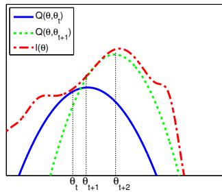
Figure 6.7: Illustration of a bound optimization algorithm. Adapted from Figure 9.14 of [Bis06]. Generated by em\_log\_likelihood\_max.ipynb.

6.5 Bound optimization (MM) algorithms

In this section, we consider a class of algorithms known as bound optimization or MM algorithms. In the context of minimization, MM stands for majorize-minimize. In the context of maximization, MM stands for minorize-maximize. There are many examples of MM algorithms, such as EM (Section 6.5.3), proximal gradient methods (Section 4.1), the mean shift algorithm for clustering [FH75; Che95; FT05], etc. For more details, see e.g., [HL04; Mai15; SBP17; Nad+19],

6.5.1 The general algorithm

In this section, we assume our goal is to maximize some function ⇁(ω) wrt its parameters ω. The basic approach in MM algorithms is to construct a surrogate function Q(ω, ω^t ) which is a tight lowerbound to ⇁(ω) such that Q(ω, ω^t ) ↗ ⇁(ω) and ^Q(ω^t , ω^t ) = ⇁(ω^t ). If these conditions are met, we say that Q minorizes ⇁. We then perform the following update at each step:

\[\theta^{t+1} = \underset{\theta}{\text{argmax}} \, Q(\theta, \theta^t) \tag{6.123}\]

This guarantees us monotonic increases in the original objective:

\[\ell(\boldsymbol{\theta}^{t+1}) \ge Q(\boldsymbol{\theta}^{t+1}, \boldsymbol{\theta}^t) \ge Q(\boldsymbol{\theta}^t, \boldsymbol{\theta}^t) = \ell(\boldsymbol{\theta}^t) \tag{6.124}\]

where the first inequality follows since Q(ω^t , ω^↔︎ ) is a lower bound on ⇁(ω^t ) for any ω^↔︎ ; the second inequality follows from Equation (6.123); and the final equality follows the tightness property. As a consequence of this result, if you do not observe monotonic increase of the objective, you must have an error in your math and/or code. This is a surprisingly powerful debugging tool.

This process is sketched in Figure 6.7. The dashed red curve is the original function (e.g., the log-likelihood of the observed data). The solid blue curve is the lower bound, evaluated at ω^t ; this touches the objective function at ω^t . We then set ω^t+1 to the maximum of the lower bound (blue curve), and fit a new bound at that point (dotted green curve). The maximum of this new bound becomes ω^t+2, etc.

6.5.2 Example: logistic regression

If ⇁(ω) is a concave function we want to maximize, then one way to obtain a valid lower bound is to use a bound on its Hessian, i.e., to find a negative definite matrix B such that H(ω) ′ B. In this case, one can show (see [BCN18, App. B]) that

\[\ell(\boldsymbol{\theta}) \ge \ell(\boldsymbol{\theta}^t) + (\boldsymbol{\theta} - \boldsymbol{\theta}^t)^\mathsf{T} \boldsymbol{g}(\boldsymbol{\theta}^t) + \frac{1}{2} (\boldsymbol{\theta} - \boldsymbol{\theta}^t)^\mathsf{T} \mathbf{B} (\boldsymbol{\theta} - \boldsymbol{\theta}^t) \tag{6.125}\]

where g(ω^t ) = ▽⇁(ω^t ). Therefore the following function is a valid lower bound:

\[Q(\theta, \theta^t) = \theta^\mathsf{T}(g(\theta^t) - \mathbf{B}\theta^t) + \frac{1}{2}\theta^\mathsf{T}\mathbf{B}\theta\tag{6.126}\]

The corresponding update becomes

\[\boldsymbol{\theta}^{t+1} = \boldsymbol{\theta}^{t} - \mathbf{B}^{-1} \boldsymbol{g}(\boldsymbol{\theta}^{t}) \tag{6.127}\]

This is similar to a Newton update, except we use B, which is a fixed matrix, rather than H(ω^t ), which changes at each iteration. This can give us some of the advantages of second order methods at lower computational cost.

For example, let us fit a multi-class logistic regression model using MM. (We follow the presentation of [Kri+05], who also consider the more interesting case of sparse logistic regression.) The probability that example n belongs to class c ↑ {1,…,C} is given by

\[p(y\_n = c | \mathbf{x}\_n, \mathbf{w}) = \frac{\exp(\mathbf{w}\_c^\mathsf{T} \mathbf{x}\_n)}{\sum\_{i=1}^C \exp(\mathbf{w}\_i^\mathsf{T} \mathbf{x}\_n)} \tag{6.128}\]

Because of the normalization condition #^{C c}=1 p(yⁿ = c|xn, w)=1, we can set w^C = 0. (For example, in binary logistic regression, where C = 2, we only learn a single weight vector.) Therefore the parameters ^ω correspond to a weight matrix ^w of size ^D(^C ⇐ 1), where ^{xn ↑ RD}.

If we let pn(w)=[p(yⁿ = 1|xn, w),…,p(yⁿ = C⇐1|xn, w)] and yⁿ = [I(yⁿ = 1),…,I(yⁿ = C ⇐ 1)], we can write the log-likelihood as follows:

\[\ell(w) = \sum\_{n=1}^{N} \left[ \sum\_{c=1}^{C-1} y\_{nc} w\_c^\top x\_n - \log \sum\_{c=1}^{C} \exp(w\_c^\top x\_n) \right] \tag{6.129}\]

The gradient is given by the following:

\[\mathbf{g}(\mathbf{w}) = \sum\_{n=1}^{N} (\mathbf{y}\_n - \mathbf{p}\_n(\mathbf{w})) \otimes \mathbf{z}\_n \tag{6.130}\]

where ∝ denotes Kronecker product (which, in this case, is just outer product of the two vectors). The Hessian is given by the following:

\[\mathbf{H}(\boldsymbol{w}) = -\sum\_{n=1}^{N} (\text{diag}(\mathbf{p}\_n(\boldsymbol{w})) - \mathbf{p}\_n(\boldsymbol{w})\mathbf{p}\_n(\boldsymbol{w})^\mathsf{T}) \otimes (\mathbf{z}\_n \mathbf{z}\_n^\mathsf{T})\tag{6.131}\]

We can construct a lower bound on the Hessian, as shown in [Boh92]:

\[\mathbf{H}(\mathbf{w}) \succ -\frac{1}{2} [\mathbf{I} - \mathbf{1}\mathbf{1}^{\mathsf{T}} / C] \otimes (\sum\_{n=1}^{N} x\_n \mathbf{z}\_n^{\mathsf{T}}) \triangleq \mathbf{B} \tag{6.132}\]

where I is a (C ⇐ 1)-dimensional identity matrix, and 1 is a (C ⇐ 1)-dimensional vector of all 1s. In the binary case, this becomes

\[\mathbf{H}(\mathbf{w}) \succ -\frac{1}{2}(1-\frac{1}{2})\sum\_{n=1}^{N} x\_n^{\mathbb{T}} x\_n) = -\frac{1}{4}\mathbf{X}^{\mathbb{T}}\mathbf{X} \tag{6.133}\]

This follows since ^pn ↗ ⁰.⁵ so ⇐(pⁿ ⇐ ^{p2 n}) ⇑ ⇐0.25.

We can use this lower bound to construct an MM algorithm to find the MLE. The update becomes

\[\mathbf{w}^{t+1} = \mathbf{w}^t - \mathbf{B}^{-1} \mathbf{g}(\mathbf{w}^t) \tag{6.134}\]

For example, let us consider the binary case, so ^{gt =} ▽⇁(w^t ) = ^XT(^y ⇐µ^t ), where µ^t = [pn(w^t ),(1⇐ pn(w^t ))]^{N n}=1. The update becomes

\[\mathbf{w}^{t+1} = \mathbf{w}^t - 4(\mathbf{X}^\mathsf{T}\mathbf{X})^{-1}\mathbf{g}^t\tag{6.135}\]

The above is faster (per step) than the IRLS (iteratively reweighted least squares) algorithm (i.e., Newton’s method), which is the standard method for fitting GLMs. To see this, note that the Newton update has the form

\[w^{t+1} = w^t - \mathbf{H}^{-1} g(w^t) = w^t - (\mathbf{X}^\mathsf{T} \mathbf{S}^t \mathbf{X})^{-1} g^t \tag{6.136}\]

where S^t = diag(µ^{t K}(1 ⇐ ^µt )). We see that Equation (6.135) is faster to compute, since we can precompute the constant matrix (X^TX)↑¹.

6.5.3 The EM algorithm

In this section, we discuss the expectation maximization (EM) algorithm [DLR77; MK07], which is an algorithm designed to compute the MLE or MAP parameter estimate for probability models that have missing data and/or hidden variables. It is a special case of an MM algorithm.

The basic idea behind EM is to alternate between estimating the hidden variables (or missing values) during the E step (expectation step), and then using the fully observed data to compute the MLE during the M step (maximization step). Of course, we need to iterate this process, since the expected values depend on the parameters, but the parameters depend on the expected values.

In Section 6.5.3.1, we show that EM is a bound optimization algorithm, which implies that this iterative procedure will converge to a local maximum of the log likelihood. The speed of convergence depends on the amount of missing data, which a!ects the tightness of the bound [XJ96; MD97; SRG03; KKS20].

We now describe the EM algorithm for a generic model. We let yⁿ be the visible data for example n, and zⁿ be the hidden data.

6.5.3.1 Lower bound

The goal of EM is to maximize the log likelihood of the observed data:

\[\ell(\boldsymbol{\theta}) = \sum\_{n=1}^{N} \log p(y\_n|\boldsymbol{\theta}) = \sum\_{n=1}^{N} \log \left[ \sum\_{\mathbf{z}\_n} p(y\_n, z\_n|\boldsymbol{\theta}) \right] \tag{6.137}\]

where yⁿ are the visible variables and zⁿ are the hidden variables. Unfortunately this is hard to optimize, since the log cannot be pushed inside the sum.

EM gets around this problem as follows. First, consider a set of arbitrary distributions qn(zn) over each hidden variable zn. The observed data log likelihood can be written as follows:

\[\ell(\boldsymbol{\theta}) = \sum\_{n=1}^{N} \log \left[ \sum\_{\mathbf{z}\_n} q\_n(\mathbf{z}\_n) \frac{p(\mathbf{y}\_n, \mathbf{z}\_n | \boldsymbol{\theta})}{q\_n(\mathbf{z}\_n)} \right] \tag{6.138}\]

Using Jensen’s inequality, we can push the log (which is a concave function) inside the expectation to get the following lower bound on the log likelihood:

\[\ell(\boldsymbol{\theta}) \ge \sum\_{n} \sum\_{\mathbf{z}\_n} q\_n(\mathbf{z}\_n) \log \frac{p(\mathbf{y}\_n, \mathbf{z}\_n | \boldsymbol{\theta})}{q\_n(\mathbf{z}\_n)} \tag{6.139}\]

\[\mathbb{E}\_{n} = \sum\_{n} \underbrace{\mathbb{E}\_{q\_n} \left[ \log p(\mathbf{y}\_n, \mathbf{z}\_n | \boldsymbol{\theta}) \right] + \mathbb{H}(q\_n)}\_{\text{L}(\boldsymbol{\theta}, q\_n | \mathbf{y}\_n)} \tag{6.140}\]

\[\mathbf{y} = \sum\_{n} \mathbf{L}(\boldsymbol{\theta}, q\_n | \boldsymbol{y}\_n) \stackrel{\scriptstyle \mathbf{x}}{=} \mathbf{L}(\boldsymbol{\theta}, \{q\_n\} | \mathcal{D}) \tag{6.141}\]

where H(q) is the entropy of probability distribution q, and %(ω, {qn}|D) is called the evidence lower bound or ELBO, since it is a lower bound on the log marginal likelihood, log p(y1:^N |ω), also called the evidence. Optimizing this bound is the basis of variational inference, as we discuss in Section 10.1.

6.5.3.2 E step

We see that the lower bound is a sum of N terms, each of which has the following form:

\[\text{EL}(\theta, q\_n | \mathbf{y}\_n) = \sum\_{\mathbf{z}\_n} q\_n(\mathbf{z}\_n) \log \frac{p(\mathbf{y}\_n, \mathbf{z}\_n | \theta)}{q\_n(\mathbf{z}\_n)} \tag{6.142}\]

\[=\sum\_{\mathbf{z}\_n} q\_n(\mathbf{z}\_n) \log \frac{p(\mathbf{z}\_n|\mathbf{y}\_n, \boldsymbol{\theta}) p(\mathbf{y}\_n|\boldsymbol{\theta})}{q\_n(\mathbf{z}\_n)} \tag{6.143}\]

\[=\sum\_{\mathbf{z}\_n} q\_n(\mathbf{z}\_n) \log \frac{p(\mathbf{z}\_n|\mathbf{y}\_n, \boldsymbol{\theta})}{q\_n(\mathbf{z}\_n)} + \sum\_{\mathbf{z}\_n} q\_n(\mathbf{z}\_n) \log p(\mathbf{y}\_n|\boldsymbol{\theta}) \tag{6.144}\]

\[=-D\_{\rm KL}\left(q\_n(\mathbf{z}\_n)\parallel p(\mathbf{z}\_n|\mathbf{y}\_n,\boldsymbol{\theta})\right)+\log p(\mathbf{y}\_n|\boldsymbol{\theta})\tag{6.145}\]

where ^DKL (^q ̸ ^p) ↭ # ^{z q}(z)log ^q(z) ^p(z) is the Kullback-Leibler divergence (or KL divergence for short) between probability distributions q and p. We discuss this in more detail in Section 5.1, but the key

property we need here is that DKL (q ̸ p) ⇑ 0 and DKL (q ̸ p) = 0 i! q = p. Hence we can maximize the lower bound %(ω, {qn}|D) wrt {qn} by setting each one to q↘ ⁿ = p(zn|yn, ω). This is called the E step. This ensures the ELBO is a tight lower bound:

\[\mathbb{E}\left(\boldsymbol{\theta}, \{q\_n^\*\} | \mathcal{D}\right) = \sum\_n \log p(y\_n | \boldsymbol{\theta}) = \ell(\boldsymbol{\theta} | \mathcal{D}) \tag{6.146}\]

To see how this connects to bound optimization, let us define

\[Q(\theta, \theta^t) = \mathbb{L}(\theta, \{p(z\_n | y\_n; \theta^t)\}) \tag{6.147}\]

Then we have Q(ω, ω^t ) ↗ ⇁(ω) and ^Q(ω^t , ω^t ) = ⇁(ω^t ), as required.

However, if we cannot compute the posteriors ^p(zn|yn; ^ωt ) exactly, we can still use an approximate distribution ^q(zn|yn; ^ωt ); this will yield a non-tight lower-bound on the log-likelihood. This generalized version of EM is known as variational EM [NH98b]. See Section 6.5.6.1 for details.

6.5.3.3 M step

In the M step, we need to maximize %(ω, {q^{t n}}) wrt ^ω, where the ^{qt n} are the distributions computed in the E step at iteration t. Since the entropy terms H(qn) are constant wrt ω, we can drop them in the M step. We are left with

\[\ell^t(\boldsymbol{\theta}) = \sum\_{n} \mathbb{E}\_{q\_n^t(\mathbf{z}\_n)} \left[ \log p(\mathbf{y}\_n, \mathbf{z}\_n | \boldsymbol{\theta}) \right] \tag{6.148}\]

This is called the expected complete data log likelihood. If the joint probability is in the exponential family (Section 2.4), we can rewrite this as

\[\boldsymbol{\ell}^{t}(\boldsymbol{\theta}) = \sum\_{n} \mathbb{E}\left[\boldsymbol{\mathcal{T}}(\boldsymbol{y}\_{n}, \boldsymbol{z}\_{n})^{\mathsf{T}}\boldsymbol{\theta} - A(\boldsymbol{\theta})\right] = \sum\_{n} \left(\mathbb{E}\left[\boldsymbol{\mathcal{T}}(\boldsymbol{y}\_{n}, \boldsymbol{z}\_{n})\right]^{\mathsf{T}}\boldsymbol{\theta} - A(\boldsymbol{\theta})\right) \tag{6.149}\]

where E [T (yn, zn)] are called the expected su!cient statistics.

In the M step, we maximize the expected complete data log likelihood to get

\[\boldsymbol{\Theta}^{t+1} = \arg\max\_{\boldsymbol{\Theta}} \sum\_{n} \mathbb{E}\_{q\_n^t} \left[ \log p(\boldsymbol{y}\_n, \boldsymbol{z}\_n | \boldsymbol{\theta}) \right] \tag{6.150}\]

In the case of the exponential family, the maximization can be solved in closed-form by matching the moments of the expected su”cient statistics (Section 2.4.5).

We see from the above that the E step does not in fact need to return the full set of posterior distributions # {q(zn)}, but can instead just return the sum of the expected su”cient statistics, ⁿ Eq(zn) [T (yn, zn)].

A common application of EM is for fitting mixture models; we discuss this in the prequel to this book, [Mur22]. Below we give a di!erent example.

6.5.4 Example: EM for an MVN with missing data

It is easy to compute the MLE for a multivariate normal when we have a fully observed data matrix: we just compute the sample mean and covariance. In this section, we consider the case where we have

missing data or partially observed data. For example, we can think of the entries of Y as being answers to a survey; some of these answers may be unknown. There are many kinds of missing data, as we discuss in Section 3.11. In this section, we make the missing at random (MAR) assumption, for simplicity. Under the MAR assumption, the log likelihood of the visible data has the form

\[\log p(\mathbf{X}|\boldsymbol{\theta}) = \sum\_{n} \log p(\boldsymbol{x}\_n|\boldsymbol{\theta}) = \sum\_{n} \log \left[ \int p(\boldsymbol{x}\_n, \boldsymbol{z}\_n|\boldsymbol{\theta}) d\boldsymbol{z}\_n \right] \tag{6.151}\]

where xⁿ are the visible variables in case n, zⁿ are the hidden variables, and yⁿ = (zn, xn) are all the variables. Unfortunately, this objective is hard to maximize. since we cannot push the log inside the expectation. Fortunately, we can easily apply EM, as we explain below.

6.5.4.1 E step

Suppose we have the parameters ω^t↑¹ from the previous iteration. Then we can compute the expected complete data log likelihood at iteration t as follows:

\[Q(\theta, \theta^{t-1}) = \mathbb{E}\left[\sum\_{n=1}^{N} \log \mathcal{N}(y\_n|\mu, \Sigma) | \mathcal{D}, \theta^{t-1}\right] \tag{6.152}\]

\[=-\frac{N}{2}\log|2\pi\Sigma|-\frac{1}{2}\sum\_{n}\mathbb{E}\left[\left(y\_{n}-\mu\right)^{\mathsf{T}}\Sigma^{-1}(y\_{n}-\mu)\right]\tag{6.153}\]

\[=-\frac{N}{2}\log|2\pi\Sigma|-\frac{1}{2}\text{tr}(\Sigma^{-1}\sum\_{n}\mathbb{E}\left[(y\_n-\mu)(y\_n-\mu)^\top\right]\tag{6.154}\]

\[=-\frac{N}{2}\log|\boldsymbol{\Sigma}| - \frac{ND}{2}\log(2\pi) - \frac{1}{2}\text{tr}(\boldsymbol{\Sigma}^{-1}\boldsymbol{\Sigma}\left[\mathbf{S}(\boldsymbol{\mu})\right])\tag{6.155}\]

where

\[\mathbb{E}\left[\mathbf{S}(\boldsymbol{\mu})\right] \stackrel{\Delta}{=} \sum\_{n} \left( \mathbb{E}\left[\boldsymbol{y}\_{n}\boldsymbol{y}\_{n}^{\mathsf{T}}\right] + \boldsymbol{\mu}\boldsymbol{\mu}^{\mathsf{T}} - 2\boldsymbol{\mu}\mathbb{E}\left[\boldsymbol{y}\_{n}\right]^{\mathsf{T}} \right) \tag{6.156}\]

(We drop the conditioning of the expectation on ^D and ^ωt↑¹ for brevity.) We see that we need to compute # ^{n E} [yn] and # ^{n E} yny^T n . ; these are the expected su”cient statistics.

To compute these quantities, we use the results from Section 2.3.1.3. We have

\[p(\mathbf{z}\_n|\mathbf{z}\_n, \theta) = \mathcal{N}(\mathbf{z}\_n|m\_n, \mathbf{V}\_n) \tag{6.157}\]

\[m\_n \stackrel{\Delta}{=} \mu\_h + \Sigma\_{hv} \Sigma\_{vv}^{-1} (x\_n - \mu\_v) \tag{6.158}\]

\[\mathbf{V}\_n \stackrel{\Delta}{=} \boldsymbol{\Sigma}\_{hh} - \boldsymbol{\Sigma}\_{hv} \boldsymbol{\Sigma}\_{vv}^{-1} \boldsymbol{\Sigma}\_{vh} \tag{6.159}\]

where we partition µ and ! into blocks based on the hidden and visible indices h and v. Hence the expected su”cient statistics are

\[\mathbb{E}\left[\mathfrak{y}\_{n}\right] = \left(\mathbb{E}\left[\mathfrak{z}\_{n}\right]; \mathfrak{x}\_{n}\right) = \left(\mathfrak{m}\_{n}; \mathfrak{x}\_{n}\right) \tag{6.160}\]

To compute E yny^T n . , we use the result that Cov [y] = E yyT. ⇐ ^E [y] ^E yT. . Hence

\[\mathbb{E}\left[\boldsymbol{y}\_{n}\boldsymbol{y}\_{n}^{\mathsf{T}}\right] = \mathbb{E}\left[\begin{pmatrix}\boldsymbol{z}\_{n}\\\boldsymbol{x}\_{n}\end{pmatrix}\begin{pmatrix}\boldsymbol{z}\_{n}^{\mathsf{T}} & \boldsymbol{x}\_{n}^{\mathsf{T}}\end{pmatrix}\right] = \begin{pmatrix}\mathbb{E}\left[\boldsymbol{z}\_{n}\boldsymbol{z}\_{n}^{\mathsf{T}}\right] & \mathbb{E}\left[\boldsymbol{z}\_{n}\right]\boldsymbol{x}\_{n}^{\mathsf{T}}\\\boldsymbol{x}\_{n}\mathbb{E}\left[\boldsymbol{z}\_{n}\right]^{\mathsf{T}} & \boldsymbol{x}\_{n}\boldsymbol{x}\_{n}^{\mathsf{T}}\end{pmatrix} \tag{6.161}\]

\[\mathbb{E}\left[\mathbf{z}\_n\mathbf{z}\_n^\top\right] = \mathbb{E}\left[\mathbf{z}\_n\right]\mathbb{E}\left[\mathbf{z}\_n\right]^\top + \mathbf{V}\_n\tag{6.162}\]

6.5.4.2 M step

By solving ▽Q(ω, ^ω(t↑1)) = ⁰, we can show that the M step is equivalent to plugging these ESS into the usual MLE equations to get

\[\mu^t = \frac{1}{N} \sum\_{n} \mathbb{E}\left[y\_n\right] \tag{6.163}\]

\[\Delta^t = \frac{1}{N} \sum\_{n} \mathbb{E}\left[y\_n y\_n^\top\right] - \mu^t(\mu^t)^\top \tag{6.164}\]

Thus we see that EM is not equivalent to simply replacing variables by their expectations and applying the standard MLE formula; that would ignore the posterior variance and would result in an incorrect estimate. Instead we must compute the expectation of the su”cient statistics, and plug that into the usual equation for the MLE.

6.5.4.3 Initialization

To get the algorithm started, we can compute the MLE based on those rows of the data matrix that are fully observed. If there are no such rows, we can just estimate the diagonal terms of ! using the observed marginal statistics. We are then ready to start EM.

6.5.4.4 Example

As an example of this procedure in action, let us consider an imputation problem, where we have N = 100 10-dimensional data cases, which we assume to come from a Gaussian. We generate synthetic data where 50% of the observations are missing at random. First we fit the parameters using EM. Call the resulting parameters ωˆ. We can now use our model for predictions by computing E ^zn|xn, ^ωˆ . Figure 6.8 indicates that the results obtained using the learned parameters are almost as good as with the true parameters. Not surprisingly, performance improves with more data, or as the fraction of missing data is reduced.

6.5.5 Example: robust linear regression using Student likelihood

In this section, we discuss how to use EM to fit a linear regression model that uses the Student distribution for its likelihood, instead of the more common Gaussian distribution, in order to achieve robustness, as first proposed in [Zel76]. More precisely, the likelihood is given by

\[p(y|\mathbf{x}, \mathbf{w}, \sigma^2, \nu) = \mathcal{T}(y|\mathbf{w}^\mathsf{T}\mathbf{x}, \sigma^2, \nu) \tag{6.165}\]

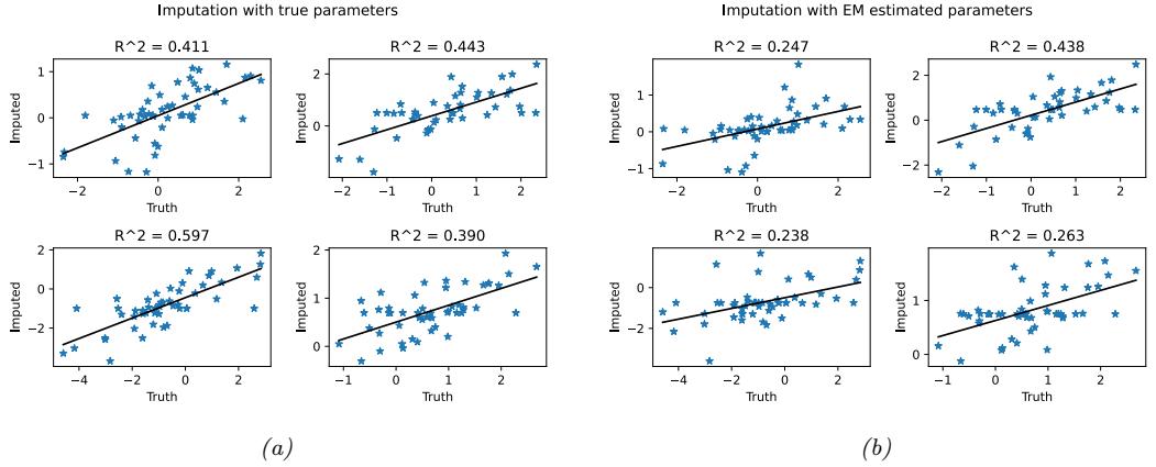
Figure 6.8: Illustration of data imputation using a multivariate Gaussian. (a) Scatter plot of true values vs imputed values using true parameters. (b) Same as (a), but using parameters estimated with EM. We just show the first four variables, for brevity. Generated by gauss\_imputation\_em\_demo.ipynb.

At first blush it may not be apparent how to do this, since there is no missing data, and there are no hidden variables. However, it turns out that we can introduce “artificial” hidden variables to make the problem easier to solve; this is a common trick. The key insight is that we can represent the Student distribution as a Gaussian scale mixture, as we discuss in Section 28.2.3.1.

We can apply the GSM version of the Student distribution to our problem by associating a latent scale zⁿ ↑ R⁺ with each example. The complete data log likelihood is therefore given by

\[\log p(\mathbf{y}, \mathbf{z} | \mathbf{X}, \mathbf{w}, \sigma^2, \nu) = \sum\_{n} -\frac{1}{2} \log(2\pi z\_n \sigma^2) - \frac{1}{2z\_n \sigma^2} (y\_i - \mathbf{w}^T \mathbf{x}\_i)^2 \tag{6.166}\]

\[+\left(\frac{\nu}{2} - 1\right)\log(z\_n) - z\_n \frac{\nu}{2} + \text{const} \tag{6.167}\]

Ignoring terms not involving w, and taking expectations, we have

\[Q(\theta, \theta^t) = -\sum\_{n} \frac{\lambda\_n}{2\sigma^2} (y\_n - \mathbf{w}^T \mathbf{x}\_n)^2 \tag{6.168}\]

where ϖ^{t n} ↭ ^E [1/zn|yn, ^xn, ^wt ]. We recognize this as a weighted least squares objective, with weight ϖt ⁿ per datapoint.

We now discuss how to compute these weights. Using the results from Section 2.2.3.4, one can show that

\[p(z\_n | y\_n, \mathbf{x}\_n, \boldsymbol{\theta}) = \text{IG}(\frac{\nu + 1}{2}, \frac{\nu + \delta\_n}{2}) \tag{6.169}\]

where ^{1n =} (yn↑x^{T x}n)^{2 ϱ2} is the standardized residual. Hence

\[\lambda\_n = \mathbb{E}\left[1/z\_n\right] = \frac{\nu^t + 1}{\nu^t + \delta\_n^t} \tag{6.170}\]

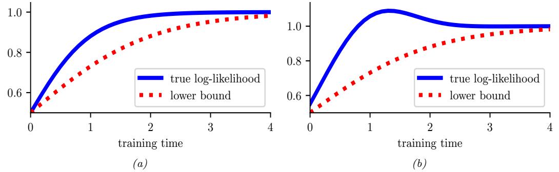
Figure 6.9: Illustration of possible behaviors of variational EM. (a) The lower bound increases at each iteration, and so does the likelihood. (b) The lower bound increases but the likelihood decreases. In this case, the algorithm is closing the gap between the approximate and true posterior. This can have a regularizing e!ect. Adapted from Figure 6 of [SJJ96]. Generated by var\_em\_bound.ipynb.

So if the residual 1^{t n} is large, the point will be given low weight ϖ^{t n}, which makes intuitive sense, since it is probably an outlier.

6.5.6 Extensions to EM

There are many variations and extensions of the EM algorithm, as discussed in [MK97]. We summarize a few of these below.

6.5.6.1 Variational EM

Suppose in the E step we pick q↘ ⁿ = argmin^qn≃^Q DKL (qⁿ ̸ p(zn|xn, ω)). Because we are optimizing over the space of functions, this is called variational inference (see Section 10.1 for details). If the family of distributions Q is rich enough to contain the true posterior, qⁿ = p(zn|xn, ω), then we can make the KL be zero. But in general, we might choose a more restrictive class for computational reasons. For example, we might use qn(zn) = N (zn|µn, diag(↽n)) even if the true posterior is correlated.

The use of a restricted posterior family Q inside the E step of EM is called variational EM [NH98a]. Unlike regular EM, variational EM is not guaranteed to increase the actual log likelihood itself (see Figure 6.9), but it does monotonically increase the variational lower bound. We can control the tightness of this lower bound by varying the variational family Q; in the limit in which qⁿ = pn, corresponding to exact inference, we recover the same behavior as regular EM. See Section 10.1.3 for further discussion.

6.5.6.2 Hard EM

Suppose we use a degenerate posterior approximation in the context of variational EM, corresponding to a point estimate, q(z|xn) = 1zˆⁿ (z), where zˆⁿ = argmax^z p(z|xn). This is equivalent to hard EM, where we ignore uncertainty about zⁿ in the E step.

The problem with this degenerate approach is that it is very prone to overfitting, since the number of latent variables is proportional to the number of datacases [WCS08].

6.5.6.3 Monte Carlo EM

Another approach to handling an intractable E step is to use a Monte Carlo approximation to the expected su”cient statistics. That is, we draw samples from the posterior, z^{s n ⇔ p}(zn|xn, ^ωt ); then we compute the su”cient statistics for each completed vector, (xn, z^{s n}); and finally we average the results. This is called Monte Carlo EM or MCEM [WT90; Nea12; Rut24].

One way to draw samples is to use MCMC (see Chapter 12). However, if we have to wait for MCMC to converge inside each E step, the method becomes very slow. An alternative is to use stochastic approximation, and only perform “brief” sampling in the E step, followed by a partial parameter update. This is called stochastic approximation EM [DLM99] and tends to work better than MCEM.

6.5.6.4 Generalized EM

Sometimes we can perform the E step exactly, but we cannot perform the M step exactly. However, we can still monotonically increase the log likelihood by performing a “partial” M step, in which we merely increase the expected complete data log likelihood, rather than maximizing it. For example, we might follow a few gradient steps. This is called the generalized EM or GEM algorithm [MK07]. (This is an unfortunate term, since there are many ways to generalize EM, but it is the standard terminology.) For example, [Lan95a] proposes to perform one Newton-Raphson step:

\[\theta\_{t+1} = \theta\_t - \eta\_t \mathbf{H}\_t^{-1} \mathbf{g}\_t \tag{6.171}\]

where 0 < ◁^t ↗ 1 is the step size, and

\[g\_t = \frac{\partial}{\partial \theta} Q(\theta, \theta\_t)|\_{\theta = \theta\_t} \tag{6.172}\]

\[\mathbf{H}\_t = \frac{\partial^2}{\partial \theta \partial \theta^\mathrm{T}} Q(\theta, \theta\_t)|\_{\theta = \theta\_t} \tag{6.173}\]

If ◁^t = 1, [Lan95a] calls this the gradient EM algorithm. However, it is possible to use a larger step size to speed up the algorithm, as in the quasi-Newton EM algorithm of [Lan95b]. This method also replaces the Hessian in Equation (6.173), which may not be negative definite (for non exponential family models), with a BFGS approximation. This ensures the overall algorithm is an ascent algorithm. Note, however, when the M step cannot be computed in closed form, EM loses some of its appeal over directly optimizing the marginal likelihood with a gradient based solver.

6.5.6.5 ECM algorithm

The ECM algorithm stands for “expectation conditional maximization”, and refers to optimizing the parameters in the M step sequentially, if they turn out to be dependent. The ECME algorithm, which stands for “ECM either” [LR95], is a variant of ECM in which we maximize the expected complete data log likelihood (the Q function) as usual, or the observed data log likelihood, during one or more of the conditional maximization steps. The latter can be much faster, since it ignores

the results of the E step, and directly optimizes the objective of interest. A standard example of this is when fitting the Student distribution. For fixed ς, we can update ! as usual, but then to update ς, we replace the standard update of the form ςt+1 = arg max^ε Q((µt+1, !t+1, ς), ω^t ) with ^ςt+1 = arg max^ε log ^p(D|µt+1, !t+1, ^ς). See [MK97] for more information.

6.5.6.6 Online EM

When dealing with large or streaming datasets, it is important to be able to learn online, as we discussed in Section 19.7.5. There are two main approaches to online EM in the literature. The first approach, known as incremental EM [NH98a], optimizes the lower bound Q(ω, q1,…,q^N ) one qⁿ at a time; however, this requires storing the expected su”cient statistics for each data case.

The second approach, known as stepwise EM [SI00; LK09; CM09], is based on stochastic gradient descent. This optimizes a local upper bound on ⇁n(ω) = log p(xn|ω) at each step. (See [Mai13; Mai15] for a more general discussion of stochastic and incremental bound optimization algorithms.)

6.6 Bayesian optimization

In this section, we discuss Bayesian optimization or BayesOpt, which is a model-based approach to black-box optimization, designed for the case where the objective function f : X → R is expensive to evaluate (e.g., if it requires running a simulation, or training and testing a particular neural net architecture).

Since the true function f is expensive to evaluate, we want to make as few function calls (i.e., make as few queries x to the oracle f) as possible. This suggests that we should build a surrogate function (also called a response surface model) based on the data collected so far, Dⁿ = {(xi, yi) : i =1: n}, which we can use to decide which point to query next. There is an inherent tradeo! between picking the point x where we think f(x) is large (we follow the convention in the literature and assume we are trying to maximize f), and picking points where we are uncertain about f(x) but where observing the function value might help us improve the surrogate model. This is another instance of the exploration-exploitation dilemma.

In the special case where the domain we are optimizing over is finite, so X = {1,…,A}, the BayesOpt problem becomes similar to the best arm identification problem in the bandit literature (Section 34.4). An important di!erence is that in bandits, we care about the cost of every action we take, whereas in optimization, we usually only care about the cost of the final solution we find. In other words, in bandits, we want to minimize cumulative regret, whereas in optimization we want to minimize simple or final regret.

Another related topic is active learning. Here the goal is to identify the whole function f with as few queries as possible, whereas in BayesOpt, the goal is just to identify the maximum of the function.

Bayesian optimization is a large topic, and we only give a brief overview below. For more details, see e.g., [Sha+16; Fra18; Gar23]. (See also https://distill.pub/2020/bayesian-optimization/ for an interactive tutorial.)

6.6.1 Sequential model-based optimization

BayesOpt is an instance of a strategy known as sequential model-based optimization (SMBO) [HHLB11]. In this approach, we alternate between querying the function at a point, and updating our estimate of the surrogate based on the new data. More precisely, at each iteration n, we have a labeled dataset Dⁿ = {(xi, yi) : i =1: n}, which records points xⁱ that we have queried, and the corresponding function values, yⁱ = f(xi) + 3i, where 3ⁱ is an optional noise term. We use this dataset to estimate a probability distribution over the true function f; we will denote this by p(f|Dn). We then choose the next point to query xn+1 using an acquisition function α(x; Dn), which computes the expected utility of querying x. (We discuss acquisition functions in Section 6.6.3). After we observe yn+1 = f(xn+1) + 3n+1, we update our beliefs about the function, and repeat. See Algorithm 6.5 for some pseudocode.

Algorithm 6.5: Bayesian optimization

• ¹ Collect initial dataset D⁰ = {(xi, yi)} from random queries xⁱ or a space-filling design
• ² Initialize model by computing p(f|D0)
• ³ for n = 1, 2,… until convergence do
• ⁴ Choose next query point xn+1 = argmax^x≃^X α(x; Dn)
• ⁵ Measure function value, yn+1 = f(xn+1) + 3ⁿ
• ⁶ Augment dataset, Dn+1 = {Dn,(xn+1, yn+1)}
• ⁷ Update model by computing p(f|Dn+1)

This method is illustrated in Figure 6.10. The goal is to find the global optimum of the solid black curve. In the first row, we show the 2 previously queried points, x¹ and x2, and their corresponding function values. y¹ = f(x1) and y² = f(x2). Our uncertainty about the value of f at those locations is 0 (if we assume no observation noise), as illustrated by the posterior credible interval (shaded blue are) becoming “pinched”. Consequently the acquisition function (shown in green at the bottom) also has value 0 at those previously queried points. The red triangle represents the maximum of the acquisition function, which becomes our next query, x3. In the second row, we show the result of observing y³ = f(x3); this further reduces our uncertainty about the shape of the function. In the third row, we show the result of observing y⁴ = f(x4). This process repeats until we run out of time, or until we are confident there are no better unexplored points to query.

The two main “ingredients” that we need to provide to a BayesOpt algorithm are (1) a way to represent and update the posterior surrogate p(f|Dn), and (2) a way to define and optimize the acquisition function α(x; Dn). We discuss both of these topics below.

6.6.2 Surrogate functions

In this section, we discuss ways to represent and update the posterior over functions, p(f|Dn).

6.6.2.1 Gaussian processes

In BayesOpt, it is very common to use a Gaussian process or GP for our surrogate. GPs are explained in detail in Chapter 18, but the basic idea is that they represent p(f(x)|Dn) as a Gaussian,

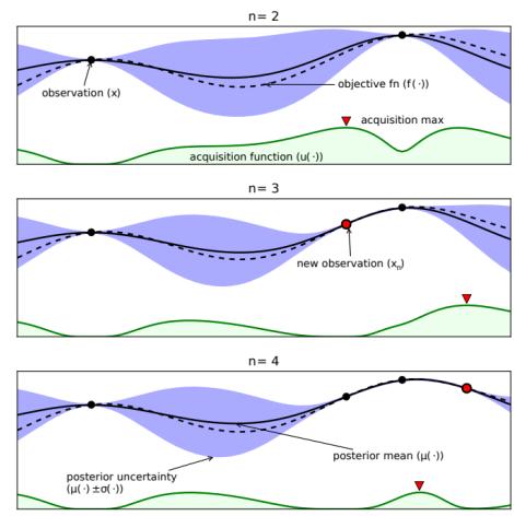
Figure 6.10: Illustration of sequential Bayesian optimization over three iterations. The rows correspond to a training set of size t = 2, 3, 4. The dotted black line is the true, but unknown, function f(x). The solid black line is the posterior mean, µ(x). The shaded blue intervals are the 95% credible interval derived from µ(x) and ϑ(x). The solid black dots correspond to points whose function value has already been computed, i.e., xⁿ for which f(xn) is known. The green curve at the bottom is the acquisition function. The red dot is the proposed next point to query, which is the maximum of the acquisition function. From Figure 1 of [Sha+16]. Used with kind permission of Nando de Freitas.

^p(f(x)|Dn) = ^N (f|µn(x), ^{ε2 n}(x)), where µn(x) and εn(x) are functions that can be derived from the training data Dⁿ = {(xi, yi) : i =1: n} using a simple closed-form equation. The GP requires specifying a kernel function Kϑ(x, x^↔︎ ), which measures similarities between input points x, x^↔︎ . The intuition is that if two inputs are similar, so Kϑ(x, x^↔︎ ) is large, then the corresponding function values are also likely to be similar, so f(x) and f(x^↔︎ ) should be positively correlated. This allows us to interpolate the function between the labeled training points; in some cases, it also lets us extrapolate beyond them.

GPs work well when we have little training data, and they support closed form Bayesian updating. However, exact updating takes O(N³) for N samples, which becomes too slow if we perform many function evaluations. There are various methods (Section 18.5.3) for reducing this to O(NM²) time, where M is a parameter we choose, but this sacrifices some of the accuracy.

In addition, the performance of GPs depends heavily on having a good kernel. We can estimate the kernel parameters ω by maximizing the marginal likelihood, as discussed in Section 18.6.1. However, since the sample size is small (by assumption), we can often get better performance by marginalizing out ω using approximate Bayesian inference methods, as discussed in Section 18.6.2. See e.g., [WF16] for further details.

6.6.2.2 Bayesian neural networks

A natural alternative to GPs is to use a parametric model. If we use linear regression, we can e”ciently perform exact Bayesian inference, as shown in Section 15.2. If we use a nonlinear model,

such as a DNN, we need to use approximate inference methods. We discuss Bayesian neural networks in detail in Chapter 17. For their application to BayesOpt, see e.g., [Spr+16; PPR22; Kim+22].

6.6.2.3 Other models

We are free to use other forms of regression model. [HHLB11] use an ensemble of random forests; such models can easily handle conditional parameter spaces, as we discuss in Section 6.6.4.2, although bootstrapping (which is needed to get uncertainty estimates) can be slow.

6.6.3 Acquisition functions

In BayesOpt, we use an acquisition function (also called a merit function) to evaluate the expected utility of each possible point we could query: α(x|Dn) = Ep(y|x,Dn) [U(x, y; Dn)], where y = f(x) is the unknown value of the function at point x, and U() is a utility function. Di!erent utility functions give rise to di!erent acquisition functions, as we discuss below. We usually choose functions so that the utility of picking a point that has already been queried is small (or 0, in the case of noise-free observations), in order to encourage exploration.

6.6.3.1 Probability of improvement

Let us define Mⁿ = max^{n i}=1 yⁱ to be the best value observed so far (known as the incumbent). (If the observations are noisy, using the highest mean value maxⁱ Ep(f|Dn) [f(xi)] is a reasonable alternative [WF16].) Then we define the utility of some new point x using U(x, y; Dn) = I(y>Mn). This gives reward i! the new value is better than the incumbent. The corresponding acquisition function is then given by the expected utility, αP I (x; Dn) = p(f(x) > Mn|Dn). This is known as the probability of improvement [Kus64]. If p(f|Dn) is a GP, then this quantity can be computed in closed form, as follows:

\[ \alpha\_{PI}(\mathbf{z}; \mathcal{D}\_n) = p(f(\mathbf{z}) > M\_n | \mathcal{D}\_n) = \Phi(\gamma\_n(\mathbf{z}, M\_n)) \tag{6.174} \]

where # is the cdf of the N (0, 1) distribution and

\[\gamma\_n(\mathbf{x}, \tau) = \frac{\mu\_n(\mathbf{x}) - \tau}{\sigma\_n(\mathbf{x})} \tag{6.175}\]

6.6.3.2 Expected improvement

The problem with PI is that all improvements are considered equally good, so the method tends to exploit quite aggressively [Jon01]. A common alternative takes into account the amount of improvement by defining U(x, y; Dn)=(y ⇐ Mn)I(y>Mn) and

\[\alpha\_{EI}(\mathbf{z}; \mathcal{D}\_n) = \mathbb{E}\_{\mathcal{D}\_n} \left[ U(\mathbf{z}, y) \right] = \mathbb{E}\_{\mathcal{D}\_n} \left[ (f(\mathbf{z}) - M\_n) \mathbb{I} (f(\mathbf{z}) > M\_n) \right] \tag{6.176}\]

This acquisition function is known as the expected improvement (EI) criterion [Moc+96]. In the case of a GP surrogate, this has the following closed form expression:

\[\alpha\_{EI}(\mathbf{z}; \mathcal{D}\_n) = (\mu\_n(\mathbf{z}) - M\_n)\Phi(\gamma) + \sigma\_n(\mathbf{z})\phi(\gamma) = \sigma\_n(\mathbf{z})[\gamma\_n\Phi(\gamma) + \phi(\gamma)]\tag{6.177}\]

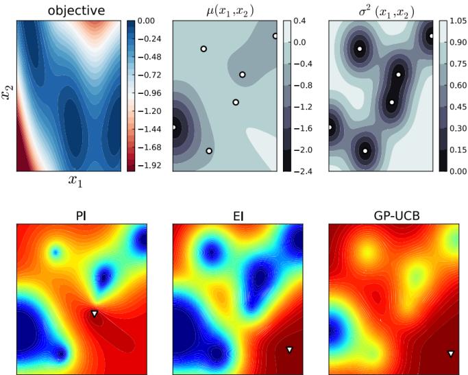
Figure 6.11: The first row shows the objective function, (the Branin function defined on R²), and its posterior mean and variance using a GP estimate. White dots are the observed data points. The second row shows 3 di!erent acquisition functions (probability of improvement, expected improvement, and upper confidence bound); the white triangles are the maxima of the corresponding acquisition functions. From Figure 6 of [BCF10]. Used with kind permission of Nando de Freitas.

where ▷() is the pdf of the N (0, 1) distribution, # is the cdf, and φ = φn(x, Mn). The first term encourages exploitation (evaluating points with high mean) and the second term encourages exploration (evaluating points with high variance). This is illustrated in Figure 6.10.

If we cannot compute the predictive variance analytically, but can draw posterior samples, then we can compute a Monte Carlo approximation to the EI, as proposed in [Kim+22]:

\[\alpha\_{EI}(\mathbf{z}; \mathcal{D}\_n) \approx \frac{1}{S} \sum\_{s=1}^{S} \max(\mu\_n^s(\mathbf{z}) - M\_n, 0) \tag{6.178}\]

6.6.3.3 Upper confidence bound (UCB)

An alternative approach is to compute an upper confidence bound or UCB on the function, at some confidence level ↼n, and then to define the acquisition function as follows: αUCB(x; Dn) = µn(x) + ↼nεn(x). This is the same as in the contextual bandit setting, discussed in Section 34.4.5, except we are optimizing over x ↑ X , rather than a finite set of arms a ↑ {1,…,A}. If we use a GP for our surrogate, the method is known as GP-UCB [Sri+10].

6.6.3.4 Thompson sampling

We discuss Thompson sampling in Section 34.4.6 in the context of multiarmed bandits, where the state space is finite, X = {1,…,A}, and the acquisition function α(a; Dn) corresponds to the probability that arm a is the best arm. We can generalize this to real-valued input spaces X using

\[\alpha(\mathbf{x}; \mathcal{D}\_n) = \mathbb{E}\_{p(\boldsymbol{\theta} | \mathcal{D}\_n)} \left[ \mathbb{I} \left( \mathbf{x} = \underset{\mathbf{x}'}{\operatorname{argmax}} \, f\_{\boldsymbol{\theta}}(\mathbf{x}') \right) \right] \tag{6.179}\]

We can compute a single sample approximation to this integral by sampling ^ω˜ ^{⇔ p}(ω|Dn). We can then pick the optimal action as follows:

\[\mathbf{x}\_{n+1} = \underset{\mathbf{z}}{\operatorname{argmax}} \, \alpha(\mathbf{z}; \mathcal{D}\_n) = \underset{\mathbf{z}}{\operatorname{argmax}} \, \mathbb{I}\left(\mathbf{z} = \underset{\mathbf{z}'}{\operatorname{argmax}} \, f\_\theta(\mathbf{z}')\right) = \underset{\mathbf{z}}{\operatorname{argmax}} \, f\_\theta(\mathbf{z}) \tag{6.180}\]

In other words, we greedily maximize the sampled surrogate.

For continuous spaces, Thompson sampling is harder to apply than in the bandit case, since we can’t directly compute the best “arm” xn+1 from the sampled function. Furthermore, when using GPs, there are some subtle technical di”culties with sampling a function, as opposed to sampling the parameters of a parametric surrogate model (see [HLHG14] for discussion).

6.6.3.5 Entropy search

Since our goal in BayesOpt is to find x↘ = argmax^x f(x), it makes sense to try to directly minimize our uncertainty about the location of x↘, which we denote by p↘(x|Dn). We will therefore define the utility as follows:

\[U(\mathbf{x}, y; \mathcal{D}\_n) = \mathbb{H}\left(\mathbf{x}^\* | \mathcal{D}\_n\right) - \mathbb{H}\left(\mathbf{x}^\* | \mathcal{D}\_n \cup \{(\mathbf{x}, y)\}\right) \tag{6.181}\]

where H (x↘|Dn) = H (p↘(x|Dn)) is the entropy of the posterior distribution over the location of the optimum. This is known as the information gain criterion; the di!erence from the objective used in active learning is that here we want to gain information about x↘ rather than about f for all x. The corresponding acquisition function is given by

\[\alpha\_{ES}(\mathbf{z}; \mathcal{D}\_n) = \mathbb{E}\_{p(y|\mathbf{z}, \mathcal{D}\_n)} \left[ U(\mathbf{z}, y; \mathcal{D}\_n) \right] = \mathbb{H} \left( \mathbf{z}^\* | \mathcal{D}\_n \right) - \mathbb{E}\_{p(y|\mathbf{z}, \mathcal{D}\_n)} \left[ \mathbb{H} \left( \mathbf{z}^\* | \mathcal{D}\_n \cup \{ (\mathbf{z}, y) \} \right) \right] \tag{6.182}\]

This is known as entropy search [HS12].

Unfortunately, computing H (x↘|Dn) is hard, since it requires a probability model over the input space. Fortunately, we can leverage the symmetry of mutual information to rewrite the acquisition function in Equation (6.182) as follows:

\[\alpha\_{PES}(\mathbf{z}; \mathcal{D}\_n) = \mathbb{H}\left(y|\mathcal{D}\_n, \mathbf{z}\right) - \mathbb{E}\_{\mathbf{z}^\* \mid \mathcal{D}\_n} \left[\mathbb{H}\left(y|\mathcal{D}\_n, \mathbf{z}, \mathbf{z}^\*\right)\right] \tag{6.183}\]

where we can approximate the expectation from p(x↘|Dn) using Thompson sampling. Now we just have to model uncertainty about the output space y. This is known as predictive entropy search [HLHG14].

6.6.3.6 Knowledge gradient

So far the acquisition functions we have considered are all greedy, in that they only look one step ahead. The knowledge gradient acquisition function, proposed in [FPD09], looks two steps ahead by considering the improvement we might expect to get if we query x, update our posterior, and then exploit our knowledge by maximizing wrt our new beliefs. More precisely, let us define the best value we can find if we query one more point:

\[\mathbb{E}\,V\_{n+1}(\mathbf{z},y) = \max\_{\mathbf{z}'} \mathbb{E}\_{p(f|\mathbf{z},y,\mathcal{D}\_n)} \left[ f(\mathbf{z}') \right] \tag{6.184}\]

\[V\_{n+1}(\mathbf{z}) = \mathbb{E}\_{p(y|\mathbf{z}, \mathcal{D}\_n)} \left[ V\_{n+1}(\mathbf{z}, y) \right] \tag{6.185}\]

We define the KG acquisition function as follows:

\[\alpha\_{KG}(\mathbf{z}; \mathcal{D}\_n) = \mathbb{E}\_{\mathcal{D}\_n} \left[ (V\_{n+1}(\mathbf{z}) - M\_n) \mathbb{I} \left( V\_{n+1}(\mathbf{z}) > M\_n \right) \right] \tag{6.186}\]

Compare this to the EI function in Equation (6.176).) Thus we pick the point xn+1 such that observing f(xn+1) will give us knowledge which we can then exploit, rather than directly trying to find a better point with better f value.

6.6.3.7 Optimizing the acquisition function

The acquisition function α(x) is often multimodal (see e.g., Figure 6.11), since it will be 0 at all the previously queried points (assuming noise-free observations). Consequently maximizing this function can be a hard subproblem in itself [WHD18; Rub+20].

In the continuous setting, it is common to use multirestart BFGS or grid search. We can also use the cross-entropy method (Section 6.7.5), using mixtures of Gaussians [BK10] or VAEs [Fau+18] as the generative model over x. In the discrete, combinatorial setting (e.g., when optimizing biological sequences), [Bel+19] use regularized evolution, (Section 6.7.3), and [Ang+20] use proximial policy optimization (Section 35.3.4). Many other combinations are possible.

6.6.4 Other issues

There are many other issues that need to be tackled when using Bayesian optimization, a few of which we briefly mention below.

6.6.4.1 Parallel (batch) queries

In some cases, we want to query the objective function at multiple points in parallel; this is known as batched Bayesian optimization. Now we need to optimize over a set of possible queries, which is computationally even more di”cult than the regular case. See [WHD18; DBB20] for some recent papers on this topic.

6.6.4.2 Conditional parameters

BayesOpt is often applied to hyper-parameter optimization. In many applications, some hyperparameters are only well-defined if other ones take on specific values. For example, suppose we are trying to automatically tune a classifier, as in the Auto-Sklearn system [Feu+15], or the Auto-WEKA

system [Kot+17]. If the method chooses to use a neural network, it also needs to specify the number of layers, and number of hidden units per layer; but if it chooses to use a decision tree, it instead should specify di!erent hyperparameters, such as the maximum tree depth.

We can formalize such problems by defining the search space in terms of a tree or DAG (directed acyclic graph), where di!erent subsets of the parameters are defined at each leaf. Applying GPs to this setting requires non-standard kernels, such as those discussed in [Swe+13; Jen+17]. Alternatively, we can use other forms of Bayesian regression, such as ensembles of random forests [HHLB11], which can easily handle conditional parameter spaces.

6.6.4.3 Multifidelity surrogates

In some cases, we can construct surrogate functions with di!erent levels of accuracy, each of which may take variable amounts of time to compute. In particular, let f(x, s) be an approximation to the true function at x with fidelity s. The goal is to solve max^x f(x, 0) by observing f(x, s) at a sequence of (xi, si) values, such that the total cost #^{n i}=1 c(si) is below some budget. For example, in the context of hyperparameter selection, s may control how long we run the parameter optimizer for, or how large the validation set is.

In addition to choosing what fidelity to use for an experiment, we may choose to terminate expensive trials (queries) early, if the results of their cheaper proxies suggest they will not be worth running to completion (see e.g., [Str19; Li+17c; FKH17]). Alternatively, we may choose to resume an earlier aborted run, to collect more data on it, as in the freeze-thaw algorithm [SSA14].

6.6.4.4 Constraints

If we want to maximize a function subject to known constraints, we can simply build the constraints into the acquisition function. But if the constraints are unknown, we need to estimate the support of the feasible set in addition to estimating the function. In [GSA14], they propose the weighted EI criterion, given by αwEI (x; Dn) = αEI (x; Dn)h(x; Dn), where h(x; Dn) is a GP with a Bernoulli observation model that specifies if x is feasible or not. Of course, other methods are possible. For example, [HL+16b] propose a method based on predictive entropy search.

6.7 Derivative-free optimization

Derivative-free optimization or DFO refers to a class of techniques for optimizing functions without using derivatives. This is useful for blackbox function optimization as well as discrete optimization. If the function is expensive to evaliate, we can use Bayesian optimization (Section 6.6). If the function is cheap to evaluate, we can use stochastic local search methods or evolutionary search methods, as we discuss below.

6.7.1 Local search

In this section, we discuss heuristic optimization algorithms that try to find the global maximum in a discrete, unstructured search space. These algorithms replace the local gradient based update, which has the form ωt+1 = ω^t + ◁tdt, with the following discrete analog:

\[x\_{t+1} = \underset{x \in \text{nbr}(\pi\_t)}{\text{argmax}} \mathcal{L}(x) \tag{6.187}\]

where nbr(xt) ↓ X is the set of neighbors of xt. This is called hill climbing, steepest ascent, or greedy search.

If the “neighborhood” of a point contains the entire space, Equation (6.187) will return the global optimum in one step, but usually such a global neighborhood is too large to search exhaustively. Consequently we usually define local neighborhoods. For example, consider the 8-queens problem. Here the goal is to place queens on an 8 ∞ 8 chessboard so that they don’t attack each other (see Figure 6.14). The state space has the form ^X = 64⁸, since we have to specify the location of each queen on the grid. However, due to the constraints, there are only 8^{8 ¬} 17M feasible states. We define the neighbors of a state to be all possible states generated by moving a single queen to another square in the same column, so each node has 8 ∞ 7 = 56 neighbors. According to [RN10, p.123], if we start at a randomly generated 8-queens state, steepest ascent gets stuck at a local maximum 86% of the time, so it only solves 14% of problem instances. However, it is fast, taking an average of 4 steps when it succeeds and 3 when it gets stuck.

In the sections below, we discuss slightly smarter algorithms that are less likely to get stuck in local maxima.

6.7.1.1 Stochastic local search

Hill climbing is greedy, since it picks the best point in its local neighborhood, by solving Equation (6.187) exactly. One way to reduce the chance of getting stuck in local maxima is to approximately maximize this objective at each step. For example, we can define a probability distribution over the uphill neighbors, proportional to how much they improve, and then sample one at random. This is called stochastic hill climbing. If we gradually decrease the entropy of this probability distribution (so we become greedier over time), we get a method called simulated annealing, which we discuss in Section 12.9.1.

Another simple technique is to use greedy hill climbing, but then whenever we reach a local maximum, we start again from a di!erent random starting point. This is called random restart hill climbing. To see the benefit of this, consider again the 8-queens problem. If each hill-climbing search has a probability of p ¬ 0.14 of success, then we expect to need R = 1/p ¬ 7 restarts until we find a valid solution. The expected number of total steps can be computed as follows. Let N¹ = 4 be the average number of steps for successful trials, and N⁰ = 3 be the average number of steps for failures. Then the total number of steps on average is N¹ + (R ⇐ 1)N⁰ =4+6 ∞ 3 = 22. Since each step is quick, the overall method is very fast. For example, it can solve an n-queens problem with n =1M in under a minute.

Of course, solving the n-queens problem is not the most useful task in practice. However, it is typical of several real-world boolean satisfiability problems, which arise in problems ranging from AI planning to model checking (see e.g., [SLM92]). In such problems, simple stochastic local search (SLS) algorithms of the kind we have discussed work surprisingly well (see e.g., [HS05]).

6.7.1.2 Tabu search

Hill climbing will stop as soon as it reaches a local maximum or a plateau. Obviously one can perform a random restart, but this would ignore all the information that had been gained up to this point. A more intelligent alternative is called tabu search [GL97]. This is like hill climbing, except it allows moves that decrease (or at least do not increase) the scoring function, provided the move is to a new

Algorithm 6.6: Tabu search.

t := 0 // counts iterations c := 0 // counts number of steps with no progress Initialize x⁰ x↘ := x⁰ // current best incumbent while c<cmax do xt+1 = argmax^x≃nbr(xt){xt↓^ς ,…,xt↓1} f(x) if f(xt+1) > f(x↘) then x↘ := xt+1 ⁹ c := 0 ¹⁰ else c := c + 1 t := t + 1 return x↘

state that has not been seen before. We can enforce this by keeping a tabu list which tracks the 2 most recently visited states. This forces the algorithm to explore new states, and increases the chances of escaping from local maxima. We continue to do this for up to cmax steps (known as the “tabu tenure”). The pseudocode can be found in Algorithm 6.6. (If we set cmax = 1, we get greedy hill climbing.)

For example, consider what happens when tabu search reaches a hill top, xt. At the next step, it will move to one of the neighbors of the peak, xt+1 ↑ nbr(xt), which will have a lower score. At the next step, it will move to the neighbor of the previous step, xt+2 ↑ nbr(xt+1); the tabu list prevents it cycling back to x^t (the peak), so it will be forced to pick a neighboring point at the same height or lower. It continues in this way, “circling” the peak, possibly being forced downhill to a lower level-set (an inverse basin flooding operation), until it finds a ridge that leads to a new peak, or until it exceeds a maximum number of non-improving moves.

According to [RN10, p.123], tabu search increases the percentage of 8-queens problems that can be solved from 14% to 94%, although this variant takes an average of 21 steps for each successful instance and 64 steps for each failed instance.

6.7.1.3 Random search

A surprisingly e!ective strategy in problems where we know nothing about the objective is to use random search. In this approach, each iterate xt+1 is chosen uniformly at random from X . This should always be tried as a baseline.

In [BB12], they applied this technique to the problem of hyper-parameter optimization for some ML models, where the objective is performance on a validation set. In their examples, the search space is continuous, & = [0, 1]D. It is easy to sample from this at random. The standard alternative approach is to quantize the space into a fixed set of values, and then to evaluate them all; this is known as grid search. (Of course, this is only feasible if the number of dimensions D is small.) They found that random search outperformed grid search. The intuitive reason for this is that many

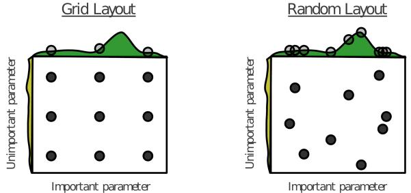
Figure 6.12: Illustration of grid search (left) vs random search (right). From Figure 1 of [BB12]. Used with kind permission of James Bergstra.

hyper-parameters do not make much di!erence to the objective function, as illustrated in Figure 6.12. Consequently it is a waste of time to place a fine grid along such unimportant dimensions.

RS has also been used to optimize the parameters of MDP policies, where the objective has the form f(x) = E↽⇑π^x [R(⇀ )] is the expected reward of trajectories generated by using a policy with parameters x. For policies with few free parameters, RS can outperform more sophisticated reinforcement learning methods described in Chapter 35, as shown in [MGR18]. In cases where the policy has a large number of parameters, it is sometimes possible to project them to a lower dimensional random subspace, and perform optimization (either grid search or random search) in this subspace [Li+18a].

6.7.2 Simulated annealing

Simulated annealing [KJV83; LA87] is a stochastic local search algorithm (Section 6.7.1.1) that attempts to find the global minimum of a black-box function E(x), where E() is known as the energy function. The method works by converting the energy to an (unnormalized) probability distribution over states by defining p(x) = exp(⇐E(x)), and then using a variant of the Metropolis-Hastings algorithm to sample from a set of probability distributions, designed so that at the final step, the method samples from one of the modes of the distribution, i.e., it finds one of the most likely states, or lowest energy states. This approach can be used for both discrete and continuous optimization. See Section 12.9.1 for more details.

6.7.3 Evolutionary algorithms

Stochastic local search (SLS) maintains a single “best guess” at each step, xt. If we run this for T steps, and restart K times, the total cost is TK. A natural alternative is to maintain a set or population of K good candidates, St, which we try to improve at each step. This is called an evolutionary algorithm (EA). If we run this for T steps, it also takes TK time; however, it can often get better results than multi-restart SLS, since the search procedure explores more of the space in parallel, and information from di!erent members of the population can be shared. Many versions of EA are possible, as we discuss below.

Since EA algorithms draw inspiration from the biological process of evolution, they also borrow

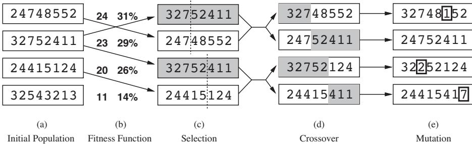
Figure 6.13: Illustration of a genetic algorithm applied to the 8-queens problem. (a) Initial population of 4 strings. (b) We rank the members of the population by fitness, and then compute their probability of mating. Here the integer numbers represent the number of nonattacking pairs of queens, so the global maximum has a value of 28. We pick an individual ^ε with probability ^p(ε) = ^L(ε)/Z, where ^{Z =} ! ^ω↑^P L(ε) sums the total fitness of the population. For example, we pick the first individual with probability 24/78 = 0.31, the second with probability 23/78 = 0.29, etc. In this example, we pick the first individual once, the second twice, the third one once, and the last one does not get to breed. (c) A split point on the “chromosome” of each parent is chosen at random. (d) The two parents swap their chromosome halves. (e) We can optionally apply pointwise mutation. From Figure 4.6 of [RN10]. Used with kind permission of Peter Norvig.

a lot of its terminology. The fitness of a member of the population is the value of the objective function (possibly normalized across population members). The members of the population at step t + 1 are called the o”spring. These can be created by randomly choosing a parent from S^t and applying a random mutation to it. This is like asexual reproduction. Alternatively we can create an o!spring by choosing two parents from St, and then combining them in some way to make a child, as in sexual reproduction; combining the parents is called recombination. (It is often followed by mutation.)

The procedure by which parents are chosen is called the selection function. In truncation selection, each parent is chosen from the fittest K members of the population (known as the elite set). In tournament selection, each parent is the fittest out of K randomly chosen members. In fitness proportionate selection, also called roulette wheel selection, each parent is chosen with probability proportional to its fitness relative to the others. We can also “kill o!” the oldest members of the population, and then select parents based on their fitness; this is called regularized evolution [Rea+19]).

In addition to the selection rule for parents, we need to specify the recombination and mutation rules. There are many possible choices for these heuristics. We briefly mention a few of them below.

• In a genetic algorithm (GA) [Gol89; Hol92], we use mutation and a particular recombination method based on crossover. To implement crossover, we assume each individual is represented as a vector of integers or binary numbers, by analogy to chromosomes. We pick a split point along the chromosome for each of the two chosen parents, and then swap the strings, as illustrated in Figure 6.13.
• In genetic programming [Koz92], we use a tree-structured representation of individuals, instead of a bit string. This representation ensures that all crossovers result in valid children, as illustrated

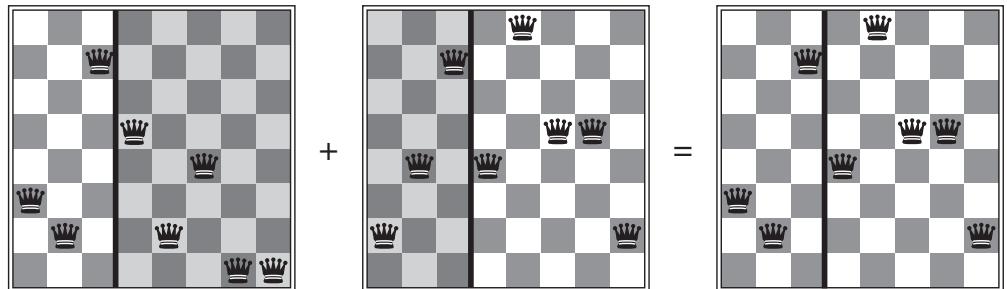
Figure 6.14: The 8-queens states corresponding to the first two parents in Figure 6.13(c) and their first child in Figure 6.13(d). We see that the encoding 32752411 means that the first queen is in row 3 (counting from the bottom left), the second queen is in row 2, etc. The shaded columns are lost in the crossover, but the unshaded columns are kept. From Figure 4.7 of [RN10]. Used with kind permission of Peter Norvig.

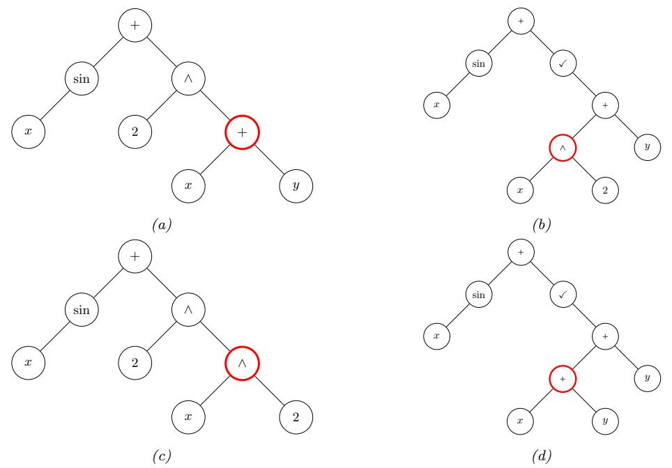
Figure 6.15: Illustration of crossover operator in a genetic program. (a-b) the two parents, representing sin(x)+(x + y) ² and sin(x) + #x² + y. The red circles denote the two crossover points. (c-d) the two children, representing sin(x)+(x²) ² and sin(x) + →x + y + y. Adapted from Figure 9.2 of [Mit97]

in Figure 6.15. Genetic programming can be useful for finding good programs as well as other structured objects, such as neural networks. In evolutionary programming, the structure of the tree is fixed and only the numerical parameters are evolved.

• In surrogate assisted EA, a surrogate function ˆf(s) is used instead of the true objective function f(s) in order to speed up the evaluation of members of the population (see [Jin11] for a survey). This is similar to the use of response surface models in Bayesian optimization (Section 6.6), except it does not deal with the explore-exploit tradeo!.
• In a memetic algorithm [MC03], we combine mutation and recombination with standard local search.

Evolutionary algorithms have been applied to a large number of applications, including training neural networks (this combination is known as neuroevolution [Sta+19]). An e”cient JAX-based library for (neuro)-evolution can be found at https://github.com/google/evojax.

6.7.4 Estimation of distribution (EDA) algorithms

EA methods maintain a population of good candidate solutions, which can be thought of as an implicit (nonparametric) density model over states with high fitness. [BC95] proposed to “remove the genetics from GAs”, by explicitly learning a probabilistic model over the configuration space that puts its mass on high scoring solutions. That is, the population becomes the set of parameters of a generative model, ωt.

One way to learn such as model is as follows. We start by creating a sample of K^↔︎ > K candidate solutions from the current model, S^t = {x^k ⇔ p(x|ωt)}. We then rank the samples using the fitness function, and then pick the most promising subset S↘ ^t of size K using a selection operator (this is known as truncation selection). Finally, we fit a new probabilistic model p(x|ωt+1) to S↘ ^t using maximum likelihood estimation. This is called the estimation of distribution or EDA algorithm (see e.g., [LL02; PSCP06; Hau+11; PHL12; Hu+12; San17; Bal17]).

Note that EDA is equivalent to minimizing the cross entropy between the empirical distribution defined by S↘ ^t and the model distribution p(x|ωt+1). Thus EDA is related to the cross entropy method, as described in Section 6.7.5, although CEM usually assumes the special case where p(x|ω) = N (x|µ, !). EDA is also closely related to the EM algorithm, as discussed in [Bro+20a].

As a simple example, suppose the configuration space is bit strings of length D, and the fitness function is f(x) = #^{D d}=1 xd, where x^d ↑ {0, 1} (this is called the one-max function in the EA literature). A simple probabilistic model for this is a fully factored model of the form p(x|ω) = ^{D d}=1 Ber(xd|ϑd). Using this model inside of DBO results in a method called univariate marginal distribution algorithm or UMDA.

We can estimate the parameters of the Bernoulli model by setting ϑ^d to the fraction of samples in S↘ ^t that have bit d turned on. Alternatively, we can incrementally adjust the parameters. The population-based incremental learning (PBIL) algorithm [BC95] applies this idea to the factored Bernoulli model, resulting in the following update:

\[ \hat{\theta}\_{d,t+1} = (1 - \eta\_t)\hat{\theta}\_{d,t} + \eta\_t \overline{\theta}\_{d,t} \tag{6.188} \]

where ϑd,t = ¹ N^t #^{K k}=1 I(xk,d = 1) is the MLE estimated from the K = |S↘ ^t | samples generated in the current iteration, and ◁^t is a learning rate.

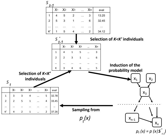
Figure 6.16: Illustration of the BOA algorithm (EDA applied to a generative model structured as a Bayes net). Adapted from Figure 3 of [PHL12].

It is straightforward to use more expressive probability models that capture dependencies between the parameters (these are known as building blocks in the EA literature). For example, in the case of real-valued parameters, we can use a multivariate Gaussian, p(x) = N (x|µ, !). The resulting method is called the estimation of multivariate normal algorithm or EMNA, [LL02]. (See also Section 6.7.5.)

For discrete random variables, it is natural to use probabilistic graphical models (Chapter 4) to capture dependencies between the variables. [BD97] learn a tree-structured graphical model using the Chow-Liu algorithm (Supplementary Section 30.2.1); [BJV97] is a special case of this where the graph is a tree. We can also learn more general graphical model structures (see e.g., [LL02]). We typically use a Bayes net (Section 4.2), since we can use ancestral sampling (Section 4.2.5) to easily generate samples; the resulting method is therefore called the Bayesian optimization algorithm (BOA) [PGCP00].5 The hierarchical BOA (hBOA) algorithm [Pel05] extends this by using decision trees and decision graphs to represent the local CPTs in the Bayes net (as in [CHM97]), rather than using tables. In general, learning the structure of the probability model for use in EDA is called linkage learning, by analogy to how genes can be linked together if they can be co-inherited as a building block.

We can also use deep generative models to represent the distribution over good candidates. For example, [CSF16] use denoising autoencoders and NADE models (Section 22.2), [Bal17] uses a DNN regressor which is then inverted using gradient descent on the inputs, [PRG17] uses RBMs

^5. This should not be confused with the Bayesian optimization methods we discuss in Section 6.6, that use response surface modeling to model p(f(x)) rather than p(x↔︎).

(Section 4.3.3.2), [GSM18] uses VAEs (Section 21.2), etc. Such models might take more data to fit (and therefore more function calls), but can potentially model the probability landscape more faithfully. (Whether that translates to better optimization performance is not clear, however.)

6.7.5 Cross-entropy method

The cross-entropy method [Rub97; RK04; Boe+05] is a special case of EDA (Section 6.7.4) in which the population is represented by a multivariate Gaussian. In particular, we set µt+1 and !t+1 to the empirical mean and covariance of S↘ ^t+1, which are the top K samples. This is closely related to the SMC algorithm for sampling rare events discussed in Section 13.6.4.

The CEM is sometimes used for optimizing the action sequence for model predictive control systems (Section 35.4.1), since it is simple and can find reasonably good optima of multimodal objectives. It is also sometimes used inside of Bayesian optimization (Section 6.6), to optimize the multi-modal acquisition function (see [BK10]).

6.7.5.1 Di”erentiable CEM

The di”erentiable CEM method of [AY20] replaces the top K operator with a soft, di!erentiable approximation, which allows the optimizer to be used as part of an end-to-end di!erentiable pipeline. For example, we can use this to create a di!erentiable model predictive control (MPC) algorithm (Section 35.4.1), as described in Section 35.4.5.2.

The basic idea is as follows. Let S^t = {xt,i ⇔ p(x|ωt) : i =1: K^↔︎ } represent the current population, with fitness values vt,i = f(xt,i). Let v↘ t,K be the K’th smallest value. In CEM, we compute the set of top K samples, S↘ ^t = {i : vt,i ⇑ v↘ t,K}, and then update the model based on these: ωt+1 = argmax^ϑ # ⁱ≃S^{t p}t(i)log ^p(xt,i|ω), where ^pt(i) = ^I(^{i ↑ S}↘ ^t ) /|S↘ ^t |. In the di!erentiable version, we replace the sparse distribution p^t with the “soft” dense distribution q^t = )(pt; 2, K), where

\[\Pi(\mathbf{p}; \tau, K) = \operatorname\*{argmin}\_{\mathbf{0} \le \mathbf{q} \le \mathbf{1}} - \mathbf{p}^{\mathsf{T}} \mathbf{q} - \tau \,\mathsf{H}(\mathbf{q}) \quad \text{s.t.} \quad \mathbf{1}^{\mathsf{T}} \mathbf{q} = K \tag{6.189}\]

projects the distribution p onto the polytope of distributions which sum to K. (Here H(q) = ⇐# ⁱ qⁱ log(qi) + (1 ⇐ qi)log(1 ⇐ qi) is the entropy, and 2 > 0 is a temperature parameter.) This projection operator (and hence the whole DCEM algorithm) can be backpropagated through using implicit di!erentiation [AKZK19].

6.7.6 Evolutionary strategies

Evolution strategies [Wie+14] are a form of distribution-based optimization in which the distribution over the population is represented by a Gaussian, p(x|ωt) (see e.g., [Sal+17b]). Unlike CEM, the parameters are updated using gradient ascent applied to the expected value of the objective, rather than using MLE on a set of elite samples. More precisely, consider the smoothed objective L(ω) = Ep(x|ϑ) [f(x)]. We can use the REINFORCE estimator (Section 6.3.4) to compute the gradient of this objective as follows:

\[\nabla\_{\theta} \mathcal{L}(\theta) = \mathbb{E}\_{p(\mathbf{z}|\theta)} \left[ f(\mathbf{z}) \nabla\_{\theta} \log p(\mathbf{z}|\theta) \right] \tag{6.190}\]

We then perform the update

ωk+1 = ω^k + ◁▽ϑL(ωk)

The expectation in Equation (6.190) can be approximated by drawing Monte Carlo samples. The computation of the gradient depends on the form of p(x|ω). A common choice is a Gaussian. We can then use the following results:

\[\begin{aligned} \nabla\_{\mu} \log p(x|\mu, \Sigma) &= \Sigma^{-1} (x - \mu) \\ \nabla\_{\Sigma} \log p(x|\mu, \Sigma) &= \frac{1}{2} \Sigma^{-1} (x - \mu) (x - \mu)^{\top} \Sigma^{-1} - \frac{1}{2} \Sigma^{-1} \end{aligned}\]

A gradient based update of ! may not ensure it remains positive definite. Therefore it is common to use a Cholesky factor representation, ! = A^TA. We then use the result

\[\nabla\_{\mathbf{A}} \log p(\mathbf{z}|\boldsymbol{\mu}, \mathbf{A}) = \mathbf{A} \left[ \nabla\_{\Sigma} \log p(\mathbf{z}|\boldsymbol{\mu}, \boldsymbol{\Sigma}) + \nabla\_{\Sigma} \log p(\mathbf{z}|\boldsymbol{\mu}, \boldsymbol{\Sigma})^{\mathsf{T}} \right]\]

6.7.6.1 Natural evolutionary strategies

If the probability model is in the exponential family, we can compute the natural gradient (Section 6.4), rather than the “vanilla” gradient, which can result in faster convergence. Such methods are called natural evolution strategies [Wie+14].

6.7.6.2 CMA-ES

The CMA-ES method of [Han16], which stands for “covariance matrix adaptation evolution strategy” is a kind of NES. It is very similar to CEM (Section 6.7.5) except it updates the parameters in a special way. In particular, instead of computing the new mean and covariance using unweighted MLE on the elite set, we attach weights to the elite samples based on their rank. We then set the new mean to the weighted MLE of the elite set.

The update equations for the covariance are more complex. In particular, “evolutionary paths” are also used to accumulate the search directions across successive generations, and these are used to update the covariance. It can be shown that the resulting updates approximate the natural gradient of L(ω) without explicitly modeling the Fisher information matrix [Oll+17].

Figure 6.17 illustrates the method in action.

6.7.6.3 Isotropic evolutionary strategies

If we use a Gaussian distribution with a (fixed) spherical covariance, then we have p(x|ω) = ^N (x|µ, ^ε2I), where ^ω = ^µ. In this case, the gradient can be written as follows, where we define ◁ = x ⇐ µ:

\[\nabla\_{\boldsymbol{\mu}} \mathcal{L}(\boldsymbol{\mu}) = \mathbb{E}\_{\mathcal{N}(\boldsymbol{x}|\boldsymbol{\mu}, \sigma^{2}\mathbf{I})} \left[ f(\boldsymbol{x}) \nabla\_{\boldsymbol{\mu}} \log \mathcal{N}(\boldsymbol{x}|\boldsymbol{\mu}, \sigma^{2}\mathbf{I}) \right] = \mathbb{E}\_{\mathcal{N}(\boldsymbol{x}|\boldsymbol{\mu}, \sigma^{2}\mathbf{I})} \left[ f(\boldsymbol{x}) \frac{1}{\sigma^{2}} (\boldsymbol{x} - \boldsymbol{\mu}) \right]\]

\[= \mathbb{E}\_{\mathcal{N}(\boldsymbol{\epsilon}|\mathbf{0}, \mathbf{I})} \left[ f(\boldsymbol{x} + \sigma \boldsymbol{\epsilon}) \frac{1}{\sigma^{2}} (\sigma \boldsymbol{\epsilon}) \right] \\ = \frac{1}{\sigma} \mathbb{E}\_{\mathcal{N}(\boldsymbol{\epsilon}|\mathbf{0}, \mathbf{I})} \left[ f(\boldsymbol{x} + \sigma \boldsymbol{\epsilon}) \boldsymbol{\epsilon} \right]\]

We can reduce the variance of this estimate by drawing m/2 samples of ◁ and then using ⇐◁ as the remaining m/2; this is called mirror sampling [Sal+17c], and is related to antithetic sampling (see Section 11.6.4).

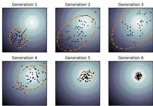
Figure 6.17: Illustration of the CMA-ES method applied to a simple 2d function. The dots represent members of the population, and the dashed orange ellipse represents the multivariate Gaussian. From https: // en. wikipedia. org/ wiki/ CMA-ES . Used with kind permission of Wikipedia author Sentewolf.

6.7.7 LLMs for DFO

Recently it has become popular to use large language models or LLMs to help optimize black-box functions, represented either in a domain-specific language, such as symbolic expressions, or as Python code. One approach is to provide a set of (x, y) inputs, and prompt the LLM to generate the corresponding function f; this is called zero-shot learning. Usually it is necessary to iterate this process, by feeding incorrect predictions back into the LLM context, and asking the model to improve its output; this is called in-context learning. We can also use the LLM as a mutation operator inside of an evolutionary search algorithm, as in the FunSearch system [RP+24].

6.8 Optimal transport

This section is written by Marco Cuturi.

In this section, we focus on optimal transport theory, a set of tools that have been proposed, starting with work by [Mon81], to compare two probability distributions. We start from a simple example involving only matchings, and work from there towards various extensions.

6.8.1 Warm-up: matching optimally two families of points

Consider two families (x1,…, xn) and (y1,…, yn), each consisting in n > 1 distinct points taken from a set X . A matching between these two families is a bijective mapping that assigns to each point ^xi another point ^yj . Such an assignment can be encoded by pairing indices (i, j) ^↑ {1,…,n}² such that they define a permutation ε in the symmetric group Sn. With that convention and given a permuation ε, xⁱ would be assigned to y^ϱi , the εi’th element in the second family.

Matchings costs. When matching a family with another, it is natural to consider the cost incurred when pairing any point ^xi with another point ^yj , for all possible pairs (i, j) ^↑ {1,…,n}². For instance, xⁱ might contain information on the current location of a taxi driver i, and y^j that

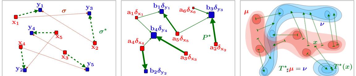
Figure 6.18: Left: Matching a family of 5 points to another is equivalent to considering a permutation in {1,…,n}. When to each pair (xi, ^yj ) ↗ ^R2 is associated a cost equal to the distance ^⇒x^{i ↓ y}j⇒, the optimal matching problem involves finding a permutation ϑ that minimizes ⇒xⁱ ↓ y^ωi ⇒ for i in {1, 2, 3, 4, 5}. Middle: The Kantorovich formulation of optimal transport generalizes optimal matchings, and arises when comparing discrete measures, that is, families of weighted points that do not necessarily share the same size but do share the same total mass. The relevant variable is a matrix P of size n ↘ m, which must satisfy row-sum and column-sum constraints, and which minimizes its dot product with matrix Cij . Right: another direct extension of the matching problem lies when, intuitively, the number n of points that is described is such that the considered measures become continuous densities. In that setting, and unlike the Kantorovich setting, the goal is to seek a map T : X ⇑ X which, to any point x in the support of the input measure µ is associated a point y = T(x) in the support of ω. The push-forward constraint Tεµ = ω ensures that ω is recovered by applying map T to all points in the support of µ; the optimal map T ^ϑ is that which minimizes the distance between x and T(x), averaged over µ.

of a user j who has just requested a taxi; in that case, Cij ↑ R may quantify the cost (in terms of time, fuel or distance) required for taxi driver i to reach user j. Alternatively, xⁱ could represent a vector of skills held by a job seeker i and y^j a vector quantifying desirable skills associated with a job posting j; in that case Cij could quantify the number of hours required for worker i to carry out job j. We will assume without loss of generality that the values Cij are obtained by evaluating a cost function c : X ∞ X → R on the pair (xi, y^j ), namely Cij = c(xi, y^j ). In many applications of optimal transport, such cost functions have a geometric interpretation and are typically distance functions on ^X as in Fig. 6.18, in which ^{X = R2}, or as will be later discussed in Section 6.8.2.4.

Least-cost matchings. Equipped with a cost function c, the optimal matching (or assignment) problem is that of finding a permutation that reaches the smallest total cost, as defined by the function

\[\min\_{\sigma} E(\sigma) = \sum\_{i=1}^{n} c(\mathbf{x}\_i, \mathbf{y}\_{\sigma\_i}) \,. \tag{6.191}\]

The optimal matching problem is arguably one of the simplest combinatorial optimization problems, tackled as early as the 19th century [JB65]. Although a naive enumeration of all permutations would require evaluating objective E a total of n! times, the Hungarian algorithm [Kuh55] was shown to provide the optimal solution in polynomial time [Mun57], and later refined to require in the worst case O(n³) operations.

6.8.2 From optimal matchings to Kantorovich and Monge formulations

The optimal matching problem is relevant to many applications, but it su!ers from a few limitations. One could argue that most of the optimal transport literature arises from the necessity to overcome these limitations and extend (6.191) to more general settings. An obvious issue arises when the number of points available in both familites is not the same. The second limitation arises when considering a continuous setting, namely when trying to match (or morph) two probability densities, rather than families of atoms (discrete measures).

6.8.2.1 Mass splitting

Suppose again that all points xⁱ and y^j describe skills, respectively held by a worker i and needed for a task j to be fulfilled in a factory. Since finding a matching is equivalent to finding a permutation in {1,…,n}, problem (6.191) cannot handle cases in which the number of workers is larger (or smaller) than the number of tasks. More problematically, the assumption that every single task is indivisible, or that workers are only able to dedicate themselves to a single task, is hardly realistic. Indeed, certain tasks may require more (or less) dedication than that provided by a single worker, whereas some workers may only be able to work part-time, or, on the contrary, be willing to put in extra hours. The rigid machinery of permutations falls short of handling such cases, since permutations are by definition one-to-one associations. The Kantorovich formulation allows for mass-splitting, the idea that the e!ort provided by a worker or needed to complete a given task can be split. In practice, to each of the n workers is associated, in addition to xi, a positive number aⁱ > 0. That number represents the amount of time worker i is able to provide. Similarly, we introduce numbers b^j > 0 describing the amount of time needed to carry out each of the m tasks (n and m do not necessarily coincide). Worker i is therefore described as a pair (ai, xi), mathematically equivalent to a weighted Dirac measure ai1^xi . The overall workforce available to the factory is described as a discrete measure # ^{i a}i1^xi , whereas its tasks are described in # ^j b^j 1^yj . If one assumes further that the factory has a balanced workload, namely that # ⁱ aⁱ = # ^j b^j , then the Kantorovich [Kan42] formulation of optimal transport is:

\[\text{OPT}\_C(\mathbf{a}, \mathbf{b}) \triangleq \min\_{P \in \mathbf{R}\_+^{n \times m}, P \mathbf{1}\_n = \mathbf{a}, P^T \mathbf{1}\_m = \mathbf{b}} \langle P, C \rangle \triangleq \sum\_{i, j} P\_{ij} C\_{ij}. \tag{6.192}\]

The interpretation behind such matrices is simple: each coe”cient Pij describes an allocation of time for worker i to spend on task j. The i’th row-sum must be equal to the total aⁱ for the time constraint of worker i to be satisfied, whereas the j’th column-sum must be equal to b^j , reflecting that the time needed to complete task j has been budgeted.

6.8.2.2 Monge formulation and optimal push forward maps

By introducing mass-splitting, the Kantorovich formulation of optimal transport allows for a far more general comparison between discrete measures of di!erent sizes and weights (middle plot of Fig. 6.18). Naturally, this flexibility comes with a downside: one can no longer associate to each point xⁱ another point y^j to which it is uniquely associated, as was the case with the classical matching problem. Interestingly, this property can be recovered in the limit where the measures become densities. Indeed, the Monge [Mon81] formulation of optimal transport allows us to recover precisely that property, on the condition (loosely speaking) that measure µ admits a density. In

that setting, the analogous mathematical object guaranteeing that µ is mapped onto ς is that of push forward maps morphing µ to ς, namely maps T such that for any measurable set A △ X , µ(T ^↑1(A)) = ς(A). When T is di!erentiable, and µ, ς have densities p and q wrt the Lebesgue measure in R^d, this statement is equivalent, thanks to the change of variables formula, to ensuring almost everywhere that:

\[q(T(x)) = p(x)|J\_T(x)|\,,\tag{6.193}\]

where |J^T (x)| stands for the determinant of the Jacobian matrix of T evaluated at x.

Writing T0µ = ς when T does satisfy these conditions, the Monge [Mon81] problem consists in finding the best map T that minimizes the average cost between x and its displacement T(x),

\[\inf\_{T:T:\mathcal{I}\mu=\nu} \int\_{\mathcal{X}} c(\mathbf{x}, T(\mathbf{x})) \,\mu(d\mathbf{x}).\tag{6.194}\]

T is therefore a map that pushes µ forwards to ς globally, but which results, on average, in the smallest average cost. While very intuitive, the Monge problem turns out to be extremely di”cult to solve in practice, since it is non-convex. Indeed, one can easily check that the constraint {T0µ = ς} is not convex, since one can easily find counter-examples for which T0µ = ς and T^{↔︎ 0}ς yet ( ^{1 2T + 1} 2T^↔︎ )0µ ⇓= ς. Luckily, Kantorovich’s approach also works for continuous measures, and yields a comparatively much simpler linear program.

6.8.2.3 Kantorovich formulation

The Kantovorich problem (6.192) can also be extended to a continuous setting: Instead of optimizing over a subset of matrices in Rⁿ→^m, consider )(µ, ς), the subset of joint probability distributions P(X ∞ X ) with marginals µ and ς, namely

\[\Pi(\mu, \nu) \triangleq \{ \pi \in \mathcal{P}(\mathcal{X}^2) : \forall A \subset \mathcal{X}, \pi(A \times \mathcal{X}) = \mu(A) \text{ and } \pi(\mathcal{X} \times A) = \nu(A) \}. \tag{6.195}\]

Note that )(µ, ς) is not empty since it always contains the product measure µ ∝ ς. With this definition, the continuous formulation of (6.192) can be obtained as

\[\text{OTr}\_c(\mu, \nu) \triangleq \inf\_{\pi \in \Pi(\mu, \nu)} \int\_{\mathcal{X}^2} c \text{ d}\pi \,. \tag{6.196}\]

Notice that (6.196) subsumes directly (6.192), since one can check that they coincide when µ, ς are discrete measures, with respective probability weights a, b and locations (x1,…, xn) and (y1,…, ym).

6.8.2.4 Wasserstein distances

When c is equal to a metric d exponentiated by an integer, the optimal value of the Kantorovich problem is called the Wasserstein distance between µ and ς:

\[W\_{\mathbb{P}}(\mu,\nu) \triangleq \left( \inf\_{\pi \in \Pi(\mu,\nu)} \int\_{\mathcal{X}^2} d(\mathbf{x},\mathbf{y})^p \, \mathrm{d}\pi(\mathbf{x},\mathbf{y}) \right)^{1/p} \,. \tag{6.197}\]

While the symmetry and the fact that Wp(µ, ς)=0 ∅ µ = ς are relatively easy to prove provided d is a metric, proving the triangle inequality is slightly more challenging, and builds on a result known as the gluing lemma ([Vil08, p.23]). The p’th power of Wp(µ, ς) is often abbreviated as W^{p p} (µ, ς).

6.8.3 Solving optimal transport

6.8.3.1 Duality and cost concavity

Both (6.192) and (6.196) are linear programs: their constraints and objective functions only involve summations. In that sense they admit a dual formulation (here, again, (6.199) subsumes (6.198)):

\[\max\_{\substack{\mathbf{f}\in\mathbb{R}^{n}, \mathbf{g}\in\mathbb{R}^{m} \\ \mathbf{f}\oplus\mathbf{g}\leq C \\ \mathbf{f}}} \mathbf{f}^{T}\mathbf{a} + \mathbf{g}^{T}\mathbf{b} \tag{6.198}\]

\[\int \dots \dots \dots \int \dots \tag{6.199}\]

\[\sup\_{\mathcal{X}} \sup\_{f \in g \le c} \int\_{\mathcal{X}} f \, \mathrm{d}\mu + \int\_{\mathcal{X}} g \, \mathrm{d}\nu \tag{6.199}\]

where the sign L denotes tensor addition for vectors, f L g = [fⁱ + g^j ]ij , or functions, f L g : x, y J→ f(x) + g(y). In other words, the dual problem looks for a pair of vectors (or functions) that attain the highest possible expectation when summed against a and b (or integrated against µ, ς), pending the constraint that they do not di!er too much across points x, y, as measured by c.

The dual problems in (6.192) and (6.196) have two variables. Focusing on the continuous formulation, a closer inspection shows that it is possible, given a function f for the first measure, to compute the best possible candidate for function g. That function g should be as large as possible, yet satisfy the constraint that g(y) ↗ c(x, y) ⇐ f(x) for all x, y, making

\[\forall \mathbf{y} \in \mathcal{X}, \overline{f}(\mathbf{y}) \triangleq \inf\_{\mathbf{x}} c(\mathbf{x}, \mathbf{y}) - f(\mathbf{x})\,,\tag{6.200}\]

the optimal choice. f is called the c-transform of f. Naturally, one may choose to start instead from g, to define an alternative c-transform:

\[\forall \mathbf{x} \in \mathcal{X}, \tilde{g}(\mathbf{x}) \triangleq \inf\_{\mathbf{y}} c(\mathbf{x}, \mathbf{y}) - g(\mathbf{y}) \,. \tag{6.201}\]

Since these transformations can only improve solutions, one may even think of applying alternatively these transformations to an arbitrary f, to define f, U f and so on. One can show, however, that this has little interest, since

\[ \overline{\overline{f}} = \overline{f}.\tag{6.202} \]

This remark allows, nonetheless, to narrow down the set of candidate functions to those that have already undergone such transformations. This reasoning yields the so-called set of c-concave functions, ^Fc ↭ {^{f |}M^g : ^{X → R}, f ^{= g}U}, which can be shown, equivalently, to be the set of functions ^f such that f = U f. One can therefore focus our attention to c-concave functions to solve (6.199) using a so-called semi-dual formulation,

\[\sup\_{f \in \mathcal{F}\_c} \int\_{\mathcal{X}} f \, \mathrm{d}\mu + \int\_{\mathcal{X}} \overline{f} \, \mathrm{d}\nu. \tag{6.203}\]

Going from (6.199) to (6.203), we have removed a dual variable g and narrowed down the feasible set to Fc, at the cost of introducing the highly non-linear transform f. This reformulation is, however, very useful, in the sense that it allows us to restrict our attention to c-concave functions, notably for two important classes of cost functions c: distances and squared-Euclidean norms.

6.8.3.2 Kantorovich-Rubinstein duality and Lipschitz potentials

A striking result illustrating the interest of c-concavity is provided when c is a metric d, namely when p = 1 in (6.197). In that case, one can prove (exploiting notably the triangle inequality of the d) that a d-concave function f is 1-Lipschitz (one has |f(x) ⇐ f(y)| ↗ d(x, y) for any x, y) and such that f = ⇐f. This result translates therefore in the following identity:

\[W\_1(\mu, \nu) = \sup\_{f \in \mathcal{I}\text{-Lipschitz}} \int\_{\mathcal{X}} f \, (\mathrm{d}\mu - \mathrm{d}\nu). \tag{6.204}\]

This result has numerous practical applications. This supremum over 1-Lipschitz functions can be e”ciently approximated using wavelet coe”cients of densities in low dimensions [SJ08], or heuristically in more general cases by training neural networks parameterized to be 1-Lipschitz [ACB17] using ReLU activation functions, and bounds on the entries of the weight matrices.

6.8.3.3 Monge maps as gradients of convex functions: the Brenier theorem

Another application of c-concavity lies in the case c(x, y) = ^{1 2} ̸^x ⇐ ^y|̸², which corresponds, up to the factor ^{1 2} , to the squared W² distance used between densities in an Euclidean space. The remarkable result, shown first by [Bre91], is that the Monge map solving (6.194) between two measures for that cost (taken for granted µ is regular enough, here assumed to have a density wrt the Lebesgue measure) exists and is necessarily the gradient of a convex function. In loose terms, one can show that

\[T^\star = \arg\min\_{T:T\_\sharp\mu=\nu} \int\_X \frac{1}{2} \|\mathbf{x} - T(\mathbf{x})\|\_2^2 \,\mu(\mathbf{dx}).\tag{6.205}\]

exists, and is the gradient of a convex function ^u : ^{Rd → R}, namely ^{T 1} = ▽u. Conversely, for any convex function u, the optimal transport map between µ and the displacement ▽u#µ is necessarily equal to ▽u.

We provide a sketch of the proof: one can always exploit, for any reasonable cost function c (e.g., lower bounded and lower semi continuous), primal-dual relationships: Consider an optimal coupling P¹ for (6.196), as well as an optimal c-concave dual function f ¹ for (6.203). This implies in particular that (f ¹, g¹ = f ¹) is optimal for (6.199). Complementary slackness conditions for this pair of linear programs imply that if x0, y⁰ is in the support of P¹, then necessarily (and su”ciently) f ¹(x0) + f ¹(y0) = c(x0, y0). Suppose therefore that x0, y⁰ is indeed in the support of P¹. From the equality ^{f 1}(x0) + ^{f 1}(y0) = ^c(x0, ^y0) one can trivially obtain that ^{f 1}(y0) = ^c(x0, ^y0) ⇐ ^{f 1}(x0). Yet, recall also that, by definition, ^{f 1}(y0) = inf^{x c}(x, ^y0) ⇐ ^{f 1}(x). Therefore, ^x0 has the special property that it minimizes ^{x → c}(x, ^y0) ⇐ ^{f 1}(x). If, at this point, one recalls that ^c is assumed in this section to be c(x, y) = ^{1 2} ̸^x ⇐ ^y|̸², one has therefore that ^x0 verifies

\[\mathbf{x}\_0 \in \operatorname\*{argmin}\_{\mathbf{x}} \frac{1}{2} \|\mathbf{x} - \mathbf{y}\_0\|^2 - f^\star(\mathbf{x}). \tag{6.206}\]

Assuming f ¹ is di!erentiable, which one can prove by c-concavity, this yields the identity

\[\mathbf{y}\_0 - \mathbf{x}\_0 - \nabla f^\star(\mathbf{x}\_0) = 0 \Rightarrow \mathbf{y}\_0 = \mathbf{x}\_0 - \nabla f^\star(\mathbf{x}\_0) = \nabla \left(\frac{1}{2} \|\cdot\|^2 - f^\star\right)(\mathbf{x}\_0). \tag{6.207}\]

Therefore, if (x0, y0) is in the support of P1, y⁰ is uniquely determined, which proves P¹ is in fact a Monge map “disguised” as a coupling, namely

\[P^\star = \left(\text{Id}, \nabla \left(\frac{1}{2} \|\cdot\|\|^2 - f^\star\right)\right)\_\sharp \mu \,. \tag{6.208}\]

The end of the proof can be worked out as follows: For any function h : X → R, one can show, using the definitions of c-transforms and the Legendre transform, that ^{1 2} ̸ · ̸² ⇐ ^h is convex if and only if ^h is c-concave. An intermediate step in that proof relies on showing that ^{1 2} ̸ · ̸² ⇐ ^h is equal to the Legendre transform of ^{1 2} ̸ · ̸² ⇐ ^h. The function ^{1 2} ̸ · ̸² ⇐ ^{f 1} above is therefore convex, by ^c-concavity of f ¹, and the optimal transport map is itself the gradient of a convex function.

Knowing that an optimal transport map for the squared-Euclidean cost is necessarily the gradient of a convex function can prove very useful to solve (6.203). Indeed, this knowledge can be leveraged to restrict estimation to relevant families of functions, namely gradients of input-convex neural networks [AXK17], as proposed in [Mak+20] or [Kor+20], as well as arbitrary convex functions with desirable smoothness and strong-convexity constants [PdC20].

6.8.3.4 Closed forms for univariate and Gaussian distributions

Many metrics between probability distributions have closed form expressions for simple cases. The Wasserstein distance is no exception, and can be computed in close form in two important scenarios. When distributions are univariate and the cost c(x, y) is either a convex function of the di!erence x ⇐ y, or when 0c/0x0y < 0 a.e., then the Wasserstein distance is essentially a comparison between the quantile functions of µ and ς. Recall that for a measure ρ, its quantile function Q² is a function that takes values in [0, 1] and is valued in the support of ρ, and corresponds to the (generalized) inverse map of F2, the cumulative distribution function (cdf) of ρ. With these notations, one has that

\[\text{COT}\_c(\mu, \nu) = \int\_{[0,1]} c \left( Q\_{\mu}(u), Q\_{\nu}(u) \right) \text{d}u \tag{6.209}\]

In particular, when c is x, y J→ |x ⇐ y| then OTc(µ, ς) corresponds to the Kolmogorov-Smirnov statistic, namely the area between the cdf of ^µ and that of ^ς. If ^c is x, y J→ (x ⇐ y)², we recover simply the squared-Euclidean norm between the quantile functions of µ and ς. Note finally that the Monge map is also available in closed form, and is equal to Q^ε I Fµ.

The second closed form applies to so-called elliptically contoured distributions, chiefly among them Gaussian multivariate distributions[Gel90]. For two Gaussians N (m1, $1) and N (m2, $2) their 2-Wasserstein distance decomposes as

\[W\_2^2\left(\mathcal{N}(\mathbf{m}\_1, \Sigma\_1), \mathcal{N}(\mathbf{m}\_2, \Sigma\_2)\right) = \|\mathbf{m}\_1 - \mathbf{m}\_2\|^2 + \mathcal{B}^2(\Sigma\_1, \Sigma\_2) \tag{6.210}\]

where the Bures metric B reads:

\[\mathcal{B}^2(\Sigma\_1, \Sigma\_2) = \text{tr}\left(\Sigma\_1 + \Sigma\_2 - 2\left(\Sigma\_1^{\frac{1}{2}} \Sigma\_2 \Sigma\_1^{\frac{1}{2}}\right)^{\frac{1}{2}}\right). \tag{6.211}\]

Notice in particular that these quantities are well-defined even when the covariance matrices are not invertible, and that they collapse to the distance between means as both covariances become 0.

When the first covariance matrix is invertible, one has that the optimal Monge map is given by

\[\mathbf{x} \triangleq \mathbf{x} \mapsto A(\mathbf{x} - \mathbf{m}\_1) + \mathbf{m}\_2, \text{ where } A \triangleq \boldsymbol{\Sigma}\_1^{-\frac{1}{2}} \left( \boldsymbol{\Sigma}\_1^{\frac{1}{2}} \boldsymbol{\Sigma}\_2 \boldsymbol{\Sigma}\_1^{\frac{1}{2}} \right)^{\frac{1}{2}} \boldsymbol{\Sigma}\_1^{-\frac{1}{2}} \tag{6.212}\]

It is easy to show that ^{T 1} is indeed optimal: The fact that ^T0^N (m1, $1) = ^N (m2, $2) follows from the knowledge that the a”ne push-forward of a Gaussian is another Gaussian. Here T is designed to push precisely the first Gaussian onto the second (and A designed to recover random variables with variance $² when starting from random variables with variance $1). The optimality of T can be recovered by simply noticing that is the gradient of a convex quadratic form, since A is positive definite, and closing this proof using the Brenier theorem above.

6.8.3.5 Exact evaluation using linear program solvers

We have hinted, using duality and c-concavity, that methods based on stochastic optimization over 1-Lipschitz or convex neural networks can be employed to estimate Wasserstein distances when c is the Euclidean distance or its square. These approaches are, however, non-convex and can only reach local optima. Apart from these two cases, and the closed forms provided above, the only reliable approach to compute Wasserstein distances appears when both µ and ς are discrete measures: in that case, one can instantiate and solve the discrete (6.192) problem, or its dual (6.198) formulation. The primal problem is a canonical example of network flow problems, and can be solved with the network-simplex method in O(nm(n + m)log(n + m)) complexity [AMO88], or, alternatively, with the comparable auction algorithm [BC89]. These approaches su!er from computational limitations: their cubic cost is intractable for large scale scenarios; their combinatorial flavor makes it harder to solve to parallelize simultaneously the computation of multiple optimal transport problems with a common cost matrix C.

An altogether di!erent issue, arising from statistics, should further discourage users from using these LP formulations, notably in high-dimensional settings. Indeed, the bottleneck practitioners will most likely encounter when using (6.192) is that, in most scenarios, their goal will be to approximate the distance between two continuous measures µ, ς using only i.i.d samples contained in empirical measures µˆn, ςˆn. Using (6.192) to approximate the corresponding (6.196) is doomed to fail, as various results [FG15] have shown in relevant settings (notably for measures in R^q) that the sample complexity of the estimator provided by (6.192) to approximate (6.196) is of order 1/n¹/q. In other words, the gap between W2(µ, ς) and W2(µˆn, ςˆn) is large in expectation, and decreases extremely slowly as n increases in high dimensions. Thus solving (6.196) exactly between these samples is mostly time wasted on overfitting. To address this curse of dimensionality, it is therefore extremely important in practice to approach (6.196) using a more careful strategy, one that involves regularizations that can leverage prior assumptions on µ and ς. While all approaches outlined above using neural networks can be interpreted under this light, we focus in the following on a specific approach that results in a convex problem that is relatively simple to implement, embarassingly parallel, and with quadratic complexity.

6.8.3.6 Obtaining smoothness using entropic regularization

A computational approach to speedup the resolution of (6.192) was proposed in [Cut13], building on earlier contributions [Wil69; KY94] and a filiation to the Schrödinger bridge problem in the

special case where c = d² [Léo14]. The idea rests upon regularizing the transportation cost by the Kullback-Leibler divergence of the coupling to the product measure of µ, ς,

\[W\_{c, \gamma}(\mu, \nu) \triangleq \inf\_{\pi \in \Pi(\mu, \nu)} \int\_{\mathcal{X}^2} d(\mathbf{x}, \mathbf{y})^p \, d\pi(\mathbf{x}, \mathbf{y}) + \gamma D\_{\text{KL}}(\pi \| \mu \otimes \nu). \tag{6.213}\]

When instantiated on discrete measures, this problem is equivalent to the following φ-strongly convex problem on the set of transportation matrices (which should be compared to (6.192))

\[\text{OT}\_{C,\gamma}(\mathbf{a}, \mathbf{b}) = \min\_{P \in \mathbf{R}\_+^{n \times m}, P \mathbf{1}\_m = \mathbf{a}, P^T \mathbf{1}\_n = \mathbf{b}} \langle P, C \rangle \stackrel{\Delta}{=} \sum\_{i,j} P\_{ij} C\_{ij} - \gamma \mathbb{H}(P) + \gamma \left( \mathbb{H}(\mathbf{a}) + \mathbb{H}(\mathbf{b}) \right), \tag{6.214}\]

which is itself equivalent to the following dual problem (which should be compared to (6.198))

\[\text{OT}\_{C,\gamma}(\mathbf{a}, \mathbf{b}) = \max\_{\mathbf{f} \in \mathbb{R}^n, \mathbf{g} \in \mathbb{R}^m} \mathbf{f}^T \mathbf{a} + \mathbf{g}^T \mathbf{b} - \gamma (e^{\mathbf{f}/\gamma})^T K e^{\mathbf{g}/\gamma} \tag{6.215} \\ = \gamma \left( 1 + \mathbb{H}(\mathbf{a}) + \mathbb{H}(\mathbf{b}) \right) \tag{6.215}\]

and ^K ↭ ^e↑C/³ is the elementwise exponential of ⇐C/φ. This regularization has several benefits. Primal-dual relationships show an explicit link between the (unique) solution P^{1 3} and a pair of optimal dual variables (f ¹, g¹) as

\[P\_{\gamma}^{\star} = \text{diag}(e^{\mathbf{f}/\gamma})K\text{diag}(e^{\mathbf{g}/\gamma})\tag{6.216}\]

Problem (6.215) can be solved using a fairly simple strategy that has proved very sturdy in practice: a simple block-coordinate ascent (optimizing alternatively the objective in f and then g), resulting in the famous Sinkhorn algorithm [Sin67], here expressed with log-sum-exp updates, starting from an arbitrary initialization for g, to carry out these two updates sequentially, until they converge:

\[\mathbf{f} \leftarrow \gamma \log \mathbf{a} - \gamma \log K e^{\mathbf{g}/\gamma} \qquad \qquad \qquad \mathbf{g} \leftarrow \gamma \log \mathbf{b} - \gamma \log K^T e^{\mathbf{f}/\gamma} \tag{6.217}\]

The convergence of this algorithm has been amply studied (see [CK21] and references therein). Convergence is naturally slower as φ decreases, reflecting the hardness of approaching LP solutions, as studied in [AWR17]. This regularization also has statistical benefits since, as argued in [Gen+19], the sample complexity of the regularized Wasserstein distance improves to a O(1/ ↖n) regime, with, however, a constant in 1/φq/² that deteriorates as dimension grows.

6.9 Submodular optimization

This section is written by Je” Bilmes.

This section provides a brief overview of submodularity in machine learning.6 Submodularity has an extremely simple definition. However, the “simplest things are often the most complicated to understand fully” [Sam74], and while submodularity has been studied extensively over the years, it continues to yield new and surprising insights and properties, some of which are extremely relevant to data science, machine learning, and artificial intelligence. A submodular function operates on subsets of some finite ground set, V . Finding a guaranteed good subset of V would ordinarily

^6. A greatly extended version of the material in this section may be found at [Bil22].

require an amount of computation exponential in the size of V . Submodular functions, however, have certain properties that make optimization either tractable or approximable where otherwise neither would be possible. The properties are quite natural, however, so submodular functions are both flexible and widely applicable to real problems. Submodularity involves an intuitive and natural diminishing returns property, stating that adding an element to a smaller set helps more than adding it to a larger set. Like convexity, submodularity allows one to e”ciently find provably optimal or near-optimal solutions. In contrast to convexity, however, where little regarding maximization is guaranteed, submodular functions can be both minimized and (approximately) maximized. Submodular maximization and minimization, however, require very di!erent algorithmic solutions and have quite di!erent applications. It is sometimes said that submodular functions are a discrete form of convexity. This is not quite true, as submodular functions are like both convex and concave functions, but also have properties that are similar simultaneously to both convex and concave functions at the same time, but then some properties of submodularity are neither like convexity nor like concavity. Convexity and concavity, for example, can be conveyed even as univariate functions. This is impossible for submodularity, as submodular functions are defined based only on the response of the function to changes amongst di!erent variables in a multidimensional discrete space.

6.9.1 Intuition, examples, and background

Let us define a set function ^f : 2^{V → R} as one that assigns a value to every subset of ^V . The notation 2^V is the power set of V , and has size 2|^{V |} which means that f lives in space R²ⁿ — i.e., since there are 2ⁿ possible subsets of V , f can return 2ⁿ distinct values. We use the notation X + v as shorthand for X ↘ {v}. Also, the value of an element in a given context is so widely used a concept, we have a special notation for it — the incremental value gain of v in the context if X is defined as f(v|X) = f(X + v) ⇐ f(X). Thus, while f(v) is the value of element v, f(v|X) is the value of element v if you already have X. We also define the gain of set X in the context of Y as f(X|Y ) = f(X ↘ Y ) ⇐ f(Y ).

6.9.1.1 Co”ee, lemon, milk, and tea

As a simple example, we will explore the manner in which the value of everyday items may interact and combine, namely co!ee, lemon, milk, and tea. Consider the value relationships amongst the four items co!ee (c), lemon (l), milk (m), and tea (t) as shown in Figure 6.19. 7 Suppose you just woke up, and there is a function ^f : 2^{V → R} that provides the average valuation for any subset of the items in V where V = {c, l, m,t}. You can think of this function as giving the average price a typical person would be willing to pay for any subset of items. Since nothing should cost nothing, we would expect that f(↔︎)=0. Clearly, one needs either co!ee or tea in the morning, so f(c) > 0 and f(t) > 0, and co!ee is usually more expensive than tea, so that f(c) > f(t) pound for pound. Also more items cost more, so that, for example, 0 < f(c) < f(c, m) < f(c, m,t) < f(c, l, m,t). Thus, the function f is strictly monotone, or f(X) < f(Y ) whenever X △ Y .

The next thing we note is that co!ee and tea may substitute for each other — they both have the same e!ect, waking you up. They are mutually redundant, and they decrease each other’s

^7. We use di!erent character fonts c, l, m, and t for the ingestibles than we use for other constructs. For example, below we use m for modular functions.

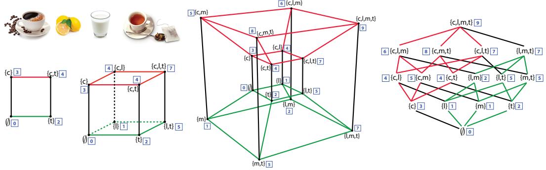
Figure 6.19: The value relationships between co!ee c, lemon l, milk m, and tea t. On the left, we first see a simple square showing the relationships between co!ee and tea and see that they are substitutive (or submodular). In this, and all of the shapes, the vertex label set is indicated in curly braces and the value at that vertex is a blue integer in a box. We next see a three-dimensional cube that adds lemon to the co!ee and tea set. We see that tea and lemon are complementary (supermodular), but co!ee and lemon are additive (modular, or independent). We next see a four-dimensional hypercube (tesseract) showing all of the value relationships described in the text. The four-dimensional hypercube is also shown as a lattice (on the right) showing the same relationships as well as two (red and green, also shown in the tesseract) of the eight three-dimensional cubes contained within.

value since once you have had a cup of co!ee, a cup of tea is less necessary and less desirable. Thus, f(c,t) < f(c) + f(t), which is known as a subadditive relationship, the whole is less than the sum of the parts. On the other hand, some items complement each other. For example, milk and co!ee are better combined together than when both are considered in isolation, or f(m, c) > f(m) + f(c), a superadditive relationship, the whole is more than the sum of the parts. A few of the items do not a!ect each other’s price. For example, lemon and milk cost the same together as apart, so f(l, m) = f(l) + f(m), an additive or modular relationship — such a relationship is perhaps midway between a subadditive and a superadditive relationship and can be seen as a form of independence.

Things become more interesting when we consider three or more items together. For example, once you have tea, lemon becomes less valuable when you acquire milk since there might be those that prefer milk to lemon in their tea. Similarly, milk becomes less valuable once you have acquired lemon since there are those who prefer lemon in their tea to milk. So, once you have tea, lemon and milk are substitutive, you would never use both as the lemon would only curdle the milk. These are submodular relationships, f(l|m,t) < f(l|t) and f(m|l,t) < f(m|t) each of which implies that f(l,t) + f(m,t) > f(l, m,t) + f(t). The value of lemon (respectively milk) with tea decreases in the larger context of having milk (respectively lemon) with tea, typical of submodular relationships.

Not all of the items are in a submodular relationship, as sometimes the presence of an item can increase the value of another item. For example, once you have milk, then tea becomes still more valuable when you also acquire lemon, since tea with the choice of either lemon or milk is more valuable than tea with the option only of milk. Similarly, once you have milk, lemon becomes more valuable when you acquire tea, since lemon with milk alone is not nearly as valuable as lemon with tea, even if milk is at hand. This means that f(t|l, m) > f(t|m) and f(l|t, m) > f(l|m) implying f(l, m) + f(m,t) < f(l, m,t) + f(m). These are known as supermodular relationships, where the value

increases as the context increases.

We have asked for a set of relationships amongst various subsets of the four items V = {c, l, m,t}, Is there a function that o!ers a value to each X ↓ V that satisfies all of the above relationships? Figure 6.19 in fact shows such a function. On the left, we see a two-dimensional square whose vertices indicate the values over subsets of {c,t} and we can quickly verify that the sum of the blue boxes on north-west (corresponding to f({c})) and south-east corners (corresponding to f({t})) is greater than the sum of the north-east and south-west corners, expressing the required submodular relationship. Next on the right is a three-dimensional cube that adds the relationship with lemon. Now we have six squares, and we see that the values at each of the vertices all satisfy the above requirements we verify this by considering the valuations at the four corners of every one of the six faces of the cube. Since |V | = 4, we need a four-dimensional hypercube to show all values, and this may be shown in two ways. It is first shown as a tesseract, a well-known three-dimensional projection of a four-dimensional hypercube. In the figure, all vertices are labeled both with subsets of V as well as the function value f(X) as the blue number in a box. The figure on the right shows a lattice version of the four-dimensional hypercube, where corresponding three-dimensional cubes are shown in green and red.

We thus see that a set function is defined for all subsets of a ground set, and that they correspond to valuations at all vertices of the hypercube. For the particular function over valuations of subsets of co!ee, lemon, milk, and tea, we have seen submodular, supermodular, and modular relationships all in one function. Therefore, the overall function f defined in Figure 6.19 is neither submodular, supermodular, nor modular. For combinatorial auctions, there is often a desire to have a diversity of such manners of relationships [LLN06] — representation of these relationships can be handled by a di!erence of submodular functions [NB05; IB12] or a sum of a submodular and supermodular function [BB18] (further described below). In machine learning, however, most of the time we are interested in functions that are submodular (or modular, or supermodular) everywhere.

6.9.2 Submodular basic definitions

For a function to be submodular, it must satisfy the submodular relationship for all subsets. We arrive at the following definition.

Definition 6.9.1 (Submodular function). A given set function ^f : 2^{V → R} is submodular if for all X, Y ↓ V , we have the following inequality:

\[f(X) + f(Y) \ge f(X \cup Y) + f(X \cap Y) \tag{6.218}\]

There are also many other equivalent definitions of submodularity [Bil22] some of which are more intuitive and easier to understand. For example, submodular functions are those set functions that satisfy the property of diminishing returns. If we think of a function f(X) as measuring the value of a set X that is a subset of a larger set of data items X ↓ V , then the submodular property means that the incremental “value” of adding a data item v to set X decreases as the size of X grows. This gives us a second classic definition of submodularity.

Definition 6.9.2 (Submodular function via diminishing returns). A given set function ^f : 2^{V → R} is submodular if for all X, Y ↓ V , where X ↓ Y and for all v /↑ Y , we have the following inequality:

\[f(X+v) - f(X) \ge f(Y+v) - f(Y) \tag{6.219}\]

The property that the incremental value of lemon with tea is less than the incremental value of lemon once milk is already in the tea is equivalent to Equation 6.218 if we set X = {m,t} and Y = {l,t} (i.e., f(m,t) + f(l,t) > f(l, m,t) + f(t)). It is naturally also equivalent to Equation 6.219 if we set X = {t}, Y = {m,t}, and with v = l (i.e., f(l|m,t) < f(l|t)).

There are many functions that are submodular, one famous one being Shannon entropy seen as a function of subsets of random variables. We first point out that there are non-negative (i.e., f(A) ⇑ 0, AA), monotone non-decreasing (i.e., f(A) ↗ f(B) whenever A ↓ B) submodular functions that are not entropic [Yeu91b; ZY97; ZY98], so submodularity is not just a trivial restatement of the class of entropy functions. When a function is monotone non-decreasing, submodular, and normalized so that f(↔︎)=0, it is often referred to as a polymatroid function. Thus, while the entropy function is a polymatroid function, it does not encompass all polymatroid functions even though all polymatroid functions satisfy the properties Claude Shannon mentioned as being natural for an “information” function (see Section 6.9.7).

A function f is supermodular if and only if ⇐f is submodular. If a function is both submodular and supermodular, it is known as a modular function. It is always the case that a modular function ^m : 2^{V → R} may take the form of a vector-scalar pair. That is, for any ^{A ↓ V} , we have that m(A) = c + # ^v≃^{A mv} where ^c is the scalar, and {mv}^v≃^V can be seen as the elements of a vector indexed by elements of V . If the modular function is normalized, so that m(↔︎)=0, then c = 0 and the modular function can be seen simply as a vector ^{m ↑ RV} . Hence, we sometimes say that the modular function ^{x ↑ RV o}!ers a value for set ^A as the partial sum ^x(A) = # ^v≃^{A x}(v). Many combinatorial problems use modular functions as objectives. For example, the graph cut problem uses a modular function defined over the edges, judges a cut in a graph as the modular function applied to the edges that comprise the cut.

As can be seen from the above, and by considering Figure 6.19, a submodular function, and in fact any set function, ^f : 2^{V → R} can be seen as a function defined only on the vertices of the ⁿ-dimensional unit hypercube [0, 1]ⁿ. Given any set ^{X ↓ V} , we define 1^{X ↑} {0, 1}^V to be the characteristic vector of set X defined as 1X(v)=1 if v ↑ X and 1X(v)=0 otherwise. This gives us a way to map from any set X ↓ V to a binary vector 1X. We also see that 1^X is itself a modular function since ^{1X ↑} {0, ¹}^V △ ^RV .

Submodular functions share a number of properties in common with both convex and concave functions [Lov83], including wide applicability, generality, multiple representations, and closure under a number of common operators (including mixtures, truncation, complementation, and certain convolutions). There is one important submodular closure property that we state here — that if we take non-negative weighted (or conical) combinations of submodular functions, we preserve submodularity. In other words, if we have a set of ^k submodular functions, ^fi : 2^{V → R}, ^{i ↑} [k], and we form f(X) = #^{k i}=1 ωifi(X) where ωⁱ ⇑ 0 for all i, then Definition 6.9.1 immediately implies that f is also submodular. When we consider Definition 6.9.1, we see that submodular functions live in a cone in 2n-dimensional space defined by the intersection of an exponential number of half-spaces each one of which is defined by one of the inequalities of the form f(X) + f(Y ) ⇑ f(X ↘ Y ) + f(X ≃ Y ). Each submodular function is therefore a point in that cone. It is therefore not surprising that taking conical combinations of such points stays within this cone.

6.9.3 Example submodular functions

As mentioned above, there are many functions that are submodular besides entropy. Perhaps the simplest such function is ^f(A) = |A^| which is the composition of the square-root function (which is concave) with the cardinality ^|A^| of the set ^A. The gain function is ^f(^{A + v}) ⇐ ^f(A) = ↖^k + 1 ⇐ ↖ k if |A| = k, which we know to be a decreasing in k, thus establishing the submodularity of f. In fact, if ▷ : R → R is any concave function, then f(A) = ▷(|A|) will be submodular for the same reason.8 Generalizing this slightly further, a function defined as f(A) = ▷( # ^a≃^{A m}(a)) is also submodular, whenever m(a) ⇑ 0 for all a ↑ V . This yields a composition of a concave function with a modular function f(A) = ▷(m(A)) since # ^a≃^{A m}(a) = ^m(A). We may take sums of such functions as well as add a final modular function without losing submodularity, leading to f(A) = # ^u≃^{U ▷}u( # ^a≃^{A m}u(a)) + # ^a≃^{A m}±(a) where ^▷u can be a distinct concave function for each u, mu(a) is a non-negative real value for all u and a, and m±(a) is an arbitrary real number. Therefore, f(A) = # ^u≃^{U ▷}u(mu(A))+m±(A) where ^mu is a ^u-specific non-negative modular function and m^± is an arbitrary modular function. Such functions are sometimes known as feature-based submodular functions [BB17] because U can be a set of non-negative features (in the machine-learning “bag-of-words” sense) and this function measures a form of dispersion over A as determined by the set of features U.

A function such as f(A) = # ^u≃^{U ▷}u(mu(A)) tends to award high diversity to a set ^A that has a high valuation by a distinct set of the features U. The reason is that, due to the concave nature of ▷u, any addition to the argument mu(A) by adding, say, v to A would diminish as A gets larger. In order to produce a set larger than A that has a much larger valuation, one must use a feature u^↔︎ ⇓= u that has not yet diminished as much.

Facility location is another well-known submodular function — perhaps an appropriate nickname would be the “k-means of submodular functions”, due to its applicability, utility, ease-of-use (it needs only an a”nity matrix), and similarity to k-medoids problems. The facility location function is defined using an a”nity matrix as follows: f(A) = # ^v≃^V max^a≃^A sim(a, v) where sim(a, v) is a non-negative measure of the a”nity (or similarity) between element a and v. Here, every element v ↑ V must have a representative within the set A and the representative for each v ↑ V is chosen to be the element a ↑ A most similar to v. This function is also a form of dispersion or diversity function because, in order to maximize it, every element v ↑ V must have some element similar to it in A. The overall score is then the sum of the similarity between each element v ↑ V and v’s representative. This function is monotone (since as A includes more elements to become B N A, it is possible only to find an element in B more similar to a given v than an element in A).

While the facility location looks quite di!erent from a feature-based function, it is possible to precisely represent any facility location function with a feature-based function. Consider just max^a≃^A x^a and, without loss of generality, assume that 0 ↗ x¹ ↗ x² ↗ ··· ↗ xn. Then max^a≃^{A xa =} #^{n i}=1 yⁱ min(|A ≃ {i, i + 1,…,n}|, 1) where yⁱ = xⁱ ⇐ xⁱ↑¹ and we set x⁰ = 0. We note that this is a sum of weighted concave composed with modular functions since min(α, 1) is concave in α, and |A ≃ {i, i + 1,…,n}| is a modular function in A. Thus, the facility location function, a sum of these, is merely a feature-based function.

Feature-based functions, in fact, are quite expressive, and can be used to represent many di!erent submodular functions including set cover and graph-based functions. For example, we can define a set

^8. While we will not be extensively discussing supermodular functions in this section, f(A) = ⇀(|A|) is supermodular for any convex function ⇀.

cover function, given a set of sets {Uv}v≃^V , via ^f(X) = ^D D V ^v≃^{X Uv} D ^D. If ^f(X) = ^|U^| where ^{U = V v}≃^{V Uv} then X indexes a set that fully covers U. This can also be represented as f(X) = # ^u≃^U min(1, mu(X)) where mu(X) is a modular function where mu(v)=1 if and only if u ↑ U^v and otherwise mu(v)=0. We see that this is a feature-based submodular function since min(1, x) is concave in x, and U is a set of features.

This construct can be used to produce the vertex cover function if we set U = V to be the set of vertices in a graph, and set mu(v)=1 if and only if vertices u and v are adjacent in the graph and otherwise set mu(v)=0. Similarly, the edge cover function can be expressed by setting V to be the set of edges in a graph, U to be the set of vertices in the graph, and mu(v)=1 if and only edge v is incident to vertex u.

A generalization of the set cover function is the probabilistic coverage function. Let P [Bu,v = 1] be the probability of the presence of feature (or concept) u within element v. Here, we treat Bu,v as a Bernoulli random variable for each element v and feature u so that P [Bu,v = 1] = 1 ⇐ P [Bu,v = 0]. Then we can define the probabilistic coverage function as f(X) = # ^u≃^{U f}u(X) where, for feature ^u, we have ^fu(X)=1 ⇐ ^v≃^X(1 ⇐ P [Bu,v = 1]) which indicates the degree to which feature ^u is “covered” by X. If we set P [Bu,v = 1] = 1 if and only if u ↑ U^v and otherwise P [Bu,v = 1] = 0, then fu(X) = min(1, mu(X)) and the set cover function can be represented as # ^u≃^{U f}u(X). We can generalize this in two ways. First, to make it softer and more probabilistic we allow P [Bu,v = 1] to be any number between zero and one. We also allow each feature to have a non-negative weight. This yields the general form of the probabilistic coverage function, which is defined by taking a weighted combination over all features: fu(X) = # ^u≃^{U ω}ufu(X) where ^ωu ⇑ 0 is a weight for feature ^u. Observe that ¹ ⇐ ^v≃X(1 ⇐ ^P [Bu,v = 1])=1 ⇐ exp(⇐mu(X)) = ^▷(mu(X)) where ^mu is a modular function with evaluation mu(X) = # ^v≃^X log’ 1/(1⇐P [Bu,v = 1]) ( and for z ↑ R, ▷(z)=1⇐exp(⇐z) is a concave function. Thus, the probabilistic coverage function (and its set cover specialization) is also a feature-based function.

Another common submodular function is the graph cut function. Here, we measure the value of a subset of V by the edges that cross between a set of nodes and all but that set of nodes. We are given an undirected non-negative weighted graph G = (V,E,w) where V is the set of nodes, E ↓ V ∞ V is the set of edges, and ^{w ↑ RE +} are non-negative edge weights corresponding to symmetric matrix (so wi,j = wj,i). For any e ↑ E, we have e = {i, j} for some i, j ↑ V with i ⇓= j, the graph cut function ^f : 2^{V → R} is defined as ^f(X) = # ⁱ≃X,j≃X¯ ^wi,j where ^wi,j ⇑ 0 is the weight of edge ^e = {i, j} (wi,j = 0 if the edge does not exist), and where ^X¯ ^{= V  X} is the complement of set ^X. Notice that we can write the graph cut function as follows:

\[f(X) = \sum\_{i \in X, j \in \bar{X}} w\_{i,j} = \sum\_{i, j \in V} w\_{i,j} \mathbf{1} \{ i \in X, j \in \bar{X} \} \tag{6.220}\]

\[=\frac{1}{2}\sum\_{i,j\in V}w\_{i,j}\min(|X\cap\{i,j\}|,1)+\frac{1}{2}\sum\_{i,j\in V}w\_{i,j}\min(|\{V\nmid X\}\cap\{i,j\}|,1)-\frac{1}{2}\sum\_{i,j\in V}w\_{i,j}\tag{6.221}\]

\[=\ddot{f}(X) + \ddot{f}(V \mid X) - \ddot{f}(V) \tag{6.222}\]

where ˜f(X) = ¹ 2 # i,j≃^{V w}i,j min(|^{X ≃} {i, j}|, 1). Therefore, since min(α, 1) is concave, and since ^mi,j (X) = ^{|X ≃}{i, j}| is modular, ˜f(X) is submodular for all i, j. Also, since ˜f(X) is submodular, so is ˜f(^{V  X}) (in ^X). Therefore, the graph cut function can be expressed as a sum of non-normalized feature-based functions. Note that here the second modular function is not normalized and is

non-increasing, and also we subtract the constant ˜f(V ) to achieve equality.

Another way to view the graph cut function is to consider the non-negative weights as a modular function defined over the edges. That is, we view ^{w ↑ RE +} as a modular function ^w : 2^{E → R+} where for every ^{A ↓ E}, ^w(A) = # ^e≃^{A w}(e) is the weight of the edges ^A where ^w(e) is the weight of edge e. Then the graph cut function becomes f(X) = w({(a, b) ↑ E : a ↑ X, b ↑ X  X}). We view {(a, b) ↑ E : a ↑ X, b ↑ X  X} as a set-to-set mapping function, that maps subsets of nodes to subsets of edges, and the edge weight modular function w measures the weight of the resulting edges. This immediately suggests that other functions can measure the weight of the resulting edges as well, including non-modular functions. One example is to use a polymatroid function itself leading ^h(X) = ^g({(a, b) ^{↑ E} : ^{a ↑} X, b ^{↑ X  X}}) where ^g : 2^{E → R+} is a submodular function defined on subsets of edges. The function h is known as the cooperative cut function, and it is neither submodular nor supermodular in general but there are many useful and practical algorithms that can be used to optimize it [JB16] thanks to its internal yet exposed and thus available to exploit submodular structure.

While feature-based functions are flexible and powerful, there is a strictly broader class of submodular functions, unable to be expressed by feature-based functions, that are related to deep neural networks. Here, we create a recursively nested composition of concave functions with sums of compositions of concave functions. An example is f(A) = ▷( # ^u≃^{U ω}u▷u( # ^a≃^{A m}u(a))), where ^▷ is an outer concave function composed with a feature-based function, with mu(a) ⇑ 0 and ω^u ⇑ 0. This is known as a two-layer deep submodular function (DSF). A three-layer DSF has the form f(A) = ▷( # ^c≃^{C ω}c▷c( # ^u≃^{U ω}u,c▷u( # ^a≃^{A m}u(a)))). DSFs strictly expand the class of submodular functions beyond feature-based functions, meaning that there are feature-based functions that cannot represent deep submodular functions, even simple ones [BB17].

6.9.4 Submodular optimization

Submodular functions, while discrete, would not be very useful if it was not possible to optimize over them e”ciently. There are many natural problems in machine learning that can be cast as submodular optimization and that can be addressed relatively e”ciently.

When one wishes to encourage diversity, information, spread, high complexity, independence, coverage, or dispersion, one usually will maximize a submodular function, in the form of max^A≃^C f(A) where ^{C ↓ 2V} is a constraint set, a set of subsets we are willing to accept as feasible solutions (more on this below).

Why is submodularity, in general, a good model for diversity? Submodular functions are such that once you have some elements, any other elements not in your possession but that are similar to, explained by, or represented by the elements in your possession become less valuable. Thus, in order to maximize the function, one must choose other elements that are dissimilar to, or not well represented by, the ones you already have. That is, the elements similar to the ones you own are diminished in value relative to their original values, while the elements dissimilar to the ones you have do not have diminished value relative to their original values. Thus, maximizing a submodular function successfully involves choosing elements that are jointly dissimilar amongst each other, which is a definition of diversity. Diversity in general is a critically important aspect in machine learning and artificial intelligence. For example, bias in data science and machine learning can often be seen as some lack of diversity somewhere. Submodular functions have the potential to encourage (and even ensure) diversity, enhance balance, and reduce bias in artificial intelligence.

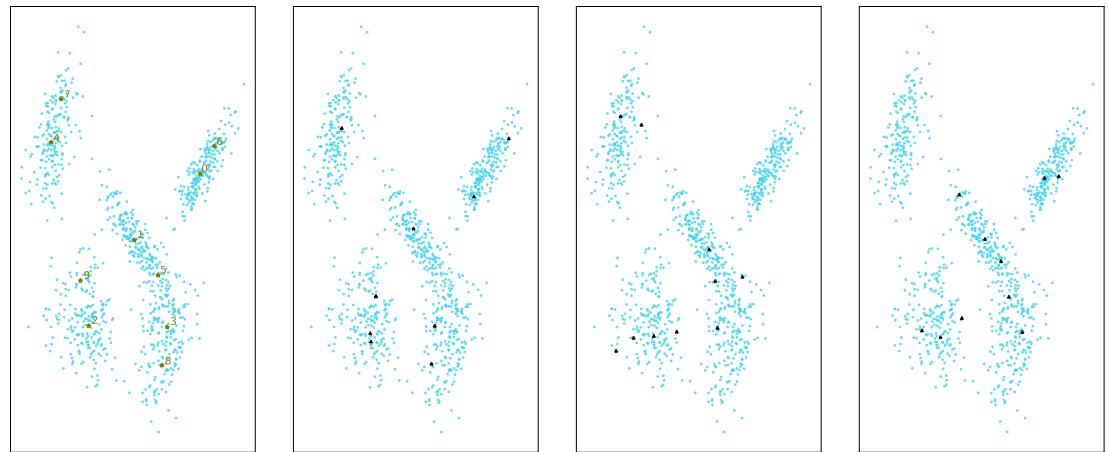
Figure 6.20: Far left: cardinality constrained (to ten) submodular maximization of a facility location function over 1000 points in two dimensions. Similarities are based on a Gaussian kernel sim(a, v) = exp(↓d(a, v)) where d(·, ·) is a distance. Selected points are green stars, and the greedy order is also shown next to each selected point. Right three plots: di!erent uniformly-at-random subsets of size ten.

Note that in order for a submodular function to appropriately model diversity, it is important for it to be instantiated appropriately. Figure 6.20 shows an example in two dimensions. The plot compares the ten points chosen according to a facility location instantiated with a Gaussian kernel, along with the random samples of size ten. We see that the facility location selected points are more diverse and tend to cover the space much better than any of the randomly selected points, each of which miss large regions of the space and/or show cases where points near each other are jointly selected.

When one wishes for homogeneity, conformity, low complexity, coherence, or cooperation, one will usually minimize a submodular function, in the form of min^A≃^C f(A). For example, if V is a set of pixels in an image, one might wish to choose a subset of pixels corresponding to a particular object over which the properties (i.e., color, luminance, texture) are relatively homogeneous. Finding a set X of size k, even if k is large, need not have a large valuation f(X), in fact it could even have the least valuation. Thus, semantic image segmentation could work even if the object being segmented and isolated consists of the majority of image pixels.

6.9.4.1 Submodular maximization

While the cardinality constrained submodular maximization problem is NP complete [Fei98], it was shown in [NWF78; FNW78] that the very simple and e”cient greedy algorithm finds an approximate solution guaranteed to be within 1⇐1/e ¬ 0.63 of the optimal solution. Moreover, the approximation ratio achieved by the simple greedy algorithm is provably the best achievable in polynomial time, assuming P ⇓= NP [Fei98]. The greedy algorithm proceeds as follows: Starting with X⁰ = ↔︎, we

repeat the following greedy step for i = 0 …(k ⇐ 1):

\[X\_{i+1} = X\_i \cup \operatorname\*{argmax}\_{v \in V \backslash X\_i} f(X\_i \cup \{v\}) \tag{6.223}\]

What the above approximation result means is that if ^X↘ ^↑ argmax{f(X) : ^|X^| ↗ ^k}, and if ^X˜ is the result of the greedy procedure, then ^f(X˜) ⇑ (1 ⇐ ¹/e)f(X↘).

The 1 ⇐ 1/e guarantee is a powerful constant factor approximation result since it holds regardless of the size of the initial set V and regardless of which polymatroid function f is being optimized. It is possible to make this algorithm run extremely fast using various acceleration tricks [FNW78; NWF78; Min78].

A minor bit of additional information about a polymatroid function, however, can improve the approximation guarantee. Define the total curvature if the polymatroid function f as ⇀ = 1 ⇐ min^v≃^V f(v|V ⇐ v)/f(v) where we assume f(v) > 0 for all v (if not, we may prune them from the ground set since such elements can never improve a polymatroid function valuation). We thus have ⁰ ↗ ⇀ ↗ ¹, and [CC84] showed that the greedy algorithm gives a guarantee of ^{1 ϑ} (1 ⇐ ^e↑ϑ) ⇑ ¹ ⇐ ¹/e. In fact, this is an equality (and we get the same bound) when ⇀ = 1, which is the fully curved case. As ⇀ gets smaller, the bound improves, until we reach the ⇀ = 0 case and the bound becomes unity. Observe that ⇀ = 0 if and only if the function is modular, in which case the greedy algorithm is optimal for the cardinality constrained maximization problem. In some cases, non-submodular functions can be decomposed into components that each might be more amenable to approximation. We see below that any set function can be written as a di!erence of submodular [NB05; IB12] functions, and sometimes (but not always) a given h can be composed into a monotone submodular plus a monotone supermodular function, or a BP function [BB18], i.e., h = f + g where f is submodular and g is supermodular. g has an easily computed quantity called the supermodular curvature ⇀^g = 1 ⇐ min^v≃^{V g}(v)/g(v|^V ⇐ ^v) that, together with the submodular curvature, can be used to produce an approximation ratio having the form ^{1 ϑ} (1 ⇐ ^e↑ϑ(1↑ϑg) ) for greedy maximization of h.

6.9.4.2 Discrete constraints

There are many other types of constraints one might desire besides a cardinality limitation. The next simplest constraint allows each element v to have a non-negative cost, say m(v) ↑ R+. In fact, this means that the costs are modular, i.e., the cost of any set X is m(X) = # ^v≃^{X m}(v). A submodular maximization problem subject to a knapsack constraint then takes the form max^X⇔^V :m(X)⇒^b f(X) where b is a non-negative budget. While the greedy algorithm does not solve this problem directly, a slightly modified cost-scaled version of the greedy algorithm [Svi04] does solve this problem for any set of knapsack costs. This has been used for various multi-document summarization tasks [LB11; LB12].

There is no single direct analogy for a convex set when one is optimizing over subsets of the set V , but there are a few forms of discrete constraints that are both mathematically interesting and that often occur repeatedly in applications.

The first form is the independent subsets of a matroid. The independent sets of a matroid are useful to represent a constraint set for submodular maximization [Cal+07; LSV09; Lee+10], max^X≃^I f(X), and this can be useful in many ways. We can see this by showing a simple example of what is known as a partition matroid. Consider a partition V = {V1, V2,…,Vm} of V into m mutually disjoint

subsets that we call blocks. Suppose also that for each of the m blocks, there is a positive integer limit ⇁ⁱ for i ↑ [m]. Consider next the set of sets formed by taking all subsets of V such that each subset has intersection with Vⁱ no more than ⇁ⁱ for each i. I.e., consider

\[\mathcal{Z}\_{\mathbf{p}} = \{ X : \forall i \in [m], \left| V\_i \cap X \right| \le \ell\_i \}. \tag{6.224}\]

Then (V, Ip) is a matroid. The corresponding submodular maximization problem is a natural generalization of the cardinality constraint in that, rather than having a fixed number of elements beyond which we are uninterested, the set of elements V is organized into groups, and here we have a fixed per-group limit beyond which we are uninterested. This is useful for fairness applications since the solution must be distributed over the blocks of the matroid. Still, there are many much more powerful types of matroids that one can use [Oxl11; GM12].

Regardless of the matroid, the problem max^X≃^I f(X) can be solved, with a 1/2 approximation factor, using the same greedy algorithm as above [NWF78; FNW78]. Indeed, the greedy algorithm has an intimate relationship with submodularity, a fact that is well studied in some of the seminal works on submodularity [Edm70; Lov83; Sch04]. It is also possible to define constraints consisting of an intersection of matroids, meaning that the solution must be simultaneously independent in multiple distinct matroids. Adding on to this, we might wish a set to be independent in multiple matroids and also satisfy a knapsack constraint. Knapsack constraints are not matroid constraints, since there can be multiple maximal cost solutions that are not the same size (as must be the case in a matroid). It is also possible to define discrete constraints using level sets of another completely di!erent submodular function [IB13] — given two submodular functions f and g, this leads to optimization problems of the form max^X⇔^V :g(X)⇒^ϖ f(X) (the submodular cost submodular knapsack, or SCSK, problem) and min^X⇔^V :g(X)↙^ϖ f(X) (the submodular cost submodular cover, or SCSC, problem). Other examples include covering constraints [IN09], and cut constraints [JB16]. Indeed, the type of constraints on submodular maximization for which good and scalable algorithms exist is quite vast, and still growing.

One last note on submodular maximization. In the above, the function f has been assumed to be a polymatroid function. There are many submodular functions that are not monotone [Buc+12]. One example we saw before, namely the graph cut function. Another example is the log of the determinant (log-determinant) of a submatrix of a positive-definite matrix (which is the Gaussian entropy plus a constant). Suppose that M is an n ∞ n symmetric positive-definite (SPD) matrix, and that M^X is a row-column submatrix (i.e., it is an |X| ∞ |X| matrix consisting of the rows and columns of M consisting of the elements in X). Then the function defined as f(X) = log det(MX) is submodular but not necessarily monotone non-decreasing. In fact, the submodularity of the log-determinant function is one of the reasons that determinantal point processes (DPPs), which instantiate probability distributions over sets in such a way that high probability is given to those subsets that are diverse according to M, are useful for certain tasks where we wish to probabilistically model diversity [KT11]. (See Supplementary Section 31.8.5 for details on DPPs.) Diversity of a set X here is measured by the volume of the parallelepiped which is known to be computed as the determinant of the submatrix M^X and taking the log of this volume makes the function submodular in X. A DPP in fact is an example of a log-submodular probabilistic model (more in Section 6.9.10).

6.9.4.3 Submodular function minimization

In the case of a polymatroid function, unconstrained minimization is again trivial. However, even in the unconstrained case, the minimization of an arbitrary (i.e., not necessarily monotone) submodular function minX⇔^V f(X) might seem hopelessly intractable. Unconstrained submodular maximization is NP-hard (albeit approximable), and this is not surprising given that there are an exponential number of sets needing to be considered. Remarkably, submodular minimization does not require exponential computation, and is not NP-hard; in fact, there are polynomial time algorithms for doing so, something that is not at all obvious. This is one of the important characteristics that submodular functions share with convex functions, their common amenability to minimization. Starting in the very late 1960s and spearheaded by individuals such as Jack Edmonds [Edm70], there was a concerted e!ort in the discrete mathematics community in search of either an algorithm that could minimize a submodular function in polynomial time or a proof that such a problem was NP-hard. The nut was finally cracked in a classic paper [GLS81] on the ellipsoid algorithm that gave a polynomial time algorithm for submodular function minimization (SFM). While the algorithm was polynomial, it was a continuous algorithm, and it was not practical, so the search continued for a purely combinatorial strongly polynomial time algorithm. Queyranne [Que98] then proved that an algorithm [NI92] worked for this problem when the set function also satisfies a symmetry condition (i.e., ^{AX ↓} V,f(X) = ^f(^{V  X})), which only requires ^O(n³) time. The result finally came around the year 2000 using two mostly independent methods [IFF00; Sch00]. These algorithms, however, also were impractical, in that while they are polynomial time, they had unrealistically high polynomial degree (i.e., ^O˜(|^{V | 7 ∋ φ + |V | 8}) for [Sch00] and ^O˜(|^{V | 7 ∋ φ}) for [IFF00]). This led to additional work on combinatorial algorithms for SFM leading to algorithms that could perform SFM in time ^O˜(|^{V | 5φ} + ^{|V | 6}) in [IO09]. Two practical algorithms for SFM include the Fujishige-Wolfe procedure [Fuj05; Wol76] 9 as well as the Frank-Wolfe procedure, each of which minimize the 2-norm on a polyhedron B^f associated with the submodular function f and which is defined below (it should also be noted that the Frank-Wolfe algorithm can also be used to minimize the convex extension of the function, something that is relatively easy to compute via the Lovász extension [Lov83]). More recent work on SFM are also based on continuous relaxations of the problem in some form or another, leading algorithms with strongly polynomial running time [LSW15] of O(|V | ³ log^{2 |V |}) for which it was possible to drop the log factors leading to a complexity of O(|V | ³) in [Jia21], weakly-polynomial running time [LSW15] of ^O˜(|^{V | 2} log ^M) (where M >⁼ max^S⇔^{V |}f(S)|), pseudopolynomial running time [ALS20; Cha+17] of ^O˜(|^{V |}M²), and a ³-approximate minimization with a linear running time [ALS20] of ^O˜(|^{V |}/3²). There have been other e!orts to utilize parallelism to further improve SFM [BS20].

6.9.5 Applications of submodularity in machine learning and AI

Submodularity arises naturally in applications in machine learning and artificial intelligence, but its utility has still not yet been as widely recognized and exploited as other techniques. For example, while information theoretic concepts like entropy and mutual information are extremely widely used in machine learning (e.g., the cross-entropy loss for classification is ubiquitous), the submodularity property of entropy is not nearly as widely explored.

^9. This is the same Wolfe as the Wolfe in Frank-Wolfe but not the same algorithm.

Still, in the last several decades, submodularity has been increasingly studied and utilized in the context of machine learning. In the below we begin to provide only a brief survey of some of the major subareas within machine learning that have been touched by submodularity. The list is not meant to be exhaustive, or even extensive. It is hoped that the below should, at least, o!er a reasonable introduction into how submodularity has been and can continue to be useful in machine learning and artificial intelligence.

6.9.6 Sketching, coresets, distillation, and data subset and feature selection

A summary is a concise representation of a body of data that can be used as an e!ective and e”cient substitute for that data. There are many types of summaries, some being extremely simple. For example, the mean or median of a list of numbers summarizes some property (the central tendency) of that list. A random subset is also a form of summary.

Any given summary, however, is not guaranteed to do a good job serving all purposes. Moreover, a summary usually involves at least some degree of approximation and fidelity loss relative to the original, and di!erent summaries are faithful to the original in di!erent ways and for di!erent tasks. For these and other reasons, the field of summarization is rich and diverse, and summarization procedures are often very specialized.

Several distinct names for summarization have been used over the past few decades, including “sketches”, “coresets”, (in the field of natural language processing) “summaries”, and “distillation”.

Sketches [Cor17; CY20; Cor+12], arose in the field of computer science and was based on the acknowledgment that data is often too large to fit in memory and too large for an algorithm to run on a given machine, something enabled by a much smaller but still representative, and provably approximate, representation of the data.

Coresets are similar to sketches and there are some properties that are more often associated with coresets than with sketches, but sometimes the distinction is a bit vague. The notion of a coreset [BHPI02; AHP+05; BC08] comes from the field of computational geometry where one is interested in solving certain geometric problems based on a set of points in R^d. For any geometric problem and a set of points, a coreset problem typically involves finding the smallest weighted subset of points so that when an algorithm is run on the weighted subset, it produces approximately the same answer as when it is run on the original large dataset. For example, given a set of points, one might wish to find the diameter of a set, or the radius of the smallest enclosing sphere, or finding the narrowest annulus (ring) containing the points, or a subset of points whose k-center clustering is approximately the same as the k-center clustering of the whole [BHPI02].

Document summarization became one of the most important problems in natural language processing (NLP) in the 1990s although the idea of computing a summary of a text goes back much further to the 1950s [Luh58; Edm69], also and coincidentally around the same time that the Cli!sNotes [Wik21] organization began. There are two main forms of document summarization [YWX17]. With extractive summarization [NM12], a set of sentences (or phrases) are extracted from the documents needing to be summarized, and the resulting subset of sentences, perhaps appropriately ordered, comprises the summary.

With abstractive summarization [LN19], on the other hand, the goal is to produce an “abstract” of the documents, where one is not constrained to have any of the sentences in the abstract correspond to any of the sentences in the original documents. With abstractive summarization, therefore, the goal is to synthesize a small set of new pseudo sentences that represent the original documents. Cli!sNotes, for example, are abstractive summaries of the literature being represented.

Another form of summarization that has more recently become popular in the machine learning community is data distillation [SG06b; Wan+20c; Suc+20; BYH20; NCL20; SS21; Ngu+21] or equivalently dataset condensation [ZMB21; ZB21]. With data distillation10, the goal is to produce a small set of synthetic pseudosamples that can be used, for example, to train a model. The key here is that in the reduced dataset, the samples are not compelled to be the same as, or a subset of, the original dataset.

All of the above should be contrasted with data compression, which in some sense is the most extreme data reduction method. With compression, either lossless or lossy, one is no longer under any obligation that the reduced form of the data must be usable, or even recognizable, by any algorithm or entity other than the decoder, or uncompression, algorithm.

6.9.6.1 Summarization Algorithm Design Choices

It is the author’s contention that the notions of summarization, coresets, sketching, and distillation are certainly analogous and quite possibly synonymous, and they are all di!erent from compression. The di!erent names for summarization are simply di!erent nomenclatures for the same language game. What matters is not what you call it but the choices one makes when designing a procedure for summarization. And indeed, there are many choices.

Submodularity o!ers essentially an infinite number of ways to perform data sketching and coresets. When we view the submodular function as an information function (as we discussed in Section 6.9.7), where f(X) is the information contained in set X and f(V ) is the maximum available information, finding the small X that maximizes f(X) (i.e., X↘ ↑ argmax{f(X) : |X| ↗ k}), is a form of coreset computation that is parameterized by the function f which has 2ⁿ parameters since f lives in a 2ⁿ-dimensional cone. Performing this maximization will then minimize the residual information f(V  X|X) about anything not present in the summary V  X since f(V ) = f(X ↘ V  X) = f(V  X|X) + f(X) so maximizing f(X) will minimize f(V  X|X). For every f, moreover, the same algorithm (e.g., the greedy algorithm) can be used to produce the summarization, and in every case, there is an approximation guarantee relative to the current f, as mentioned in earlier sections, as long as f stays submodular. Hence, submodularity provides a universal framework for summarization, coresets, and sketches to the extent that the space of submodular functions itself is su”ciently diverse and spans over di!erent coreset problems.

Overall, the coreset or sketching problem, when using submodular functions, therefore becomes a problem of “submodular design”. That is, how do we construct a submodular function that, for a particular problem, acts as a good coreset producer when the function is maximized. There are three general approaches to produce an f that works well as a summarization objective: (1) a pragmatic approach where the function is constructed by hand and heuristics, (2) a learning approach where all or part of the submodular function is inferred from an optimization procedure, and (3) a mathematical approach where a given submodular function when optimized o!ers a coreset property.

When the primary goal is a practical and scalable algorithm that can produce an extractive summary that works well on a variety of di!erent data types, and if one is comfortable with heuristics that work well in practice, a good option is to specify a submodular function by hand. For example, given a similarity matrix, it is easy to instantiate a facility location function and maximize it to

^10. Data distillation is distinct from the notion of knowledge distillation [HVD14; BC14; BCNM06] or model distillation, where the “knowledge” contained in a large model is distilled or reduced down into a di!erent smaller model.

produce a summary. If there are multiple similarity matrices, one can construct multiple facility location functions and maximize their convex combination. Such an approach is viable and practical and has been used successfully many times in the past for producing good summaries. One of the earliest examples of this is the algorithm presented in [KKT03] that shows how a submodular model can be used to select the most influential nodes in a social network. Perhaps the earliest example of this approach used for data subset selection for machine learning is [LB09] which utilizes a submodular facility location function based on Fisher kernels (gradients wrt parameters of log probabilities) and applies it to unsupervised speech selection to reduce transcription costs. Other examples of this approach includes: [LB10a; LB11] which developed submodular functions for query-focused document summarization; [KB14b] which computes a subset of training data in the context of transductive learning in a statistical machine translation system; [LB10b; Wei+13; Wei+14] which develops submodular functions for speech data subset selection (the former, incidentally, is the first use of a deep submodular function and the latter does this in an unsupervised label-free fashion); [SS18a] which is a form of robust submodularity for producing coresets for training CNNs; [Kau+19] which uses a facility location to facilitate diversity selection in active learning; [Bai+15; CTN17] which develops a mixture of submodular functions for document summarization where the mixture coe”cients are also included in the hyperparameter set; and [Xu+15], which uses a symmetrized submodular function for the purposes of video summarization.

The learnability and identifiability of submodular functions has received a good amount of study from a theoretical perspective. Starting with the strictest learning settings, the problem looks pretty dire. For example, [SF08; Goe+09] shows that if one is restricted to making a polynomial number of queries (i.e., training pairs of the form (S, f(S))) of a monotone submodular function, then it is not possible to approximate f with a multiplicative approximation factor better than !˜( ↖n). In [BH11], goodness is judged multiplicatively, meaning for a set ^{A ↓ V} we wish that ˜f(A) ↗ ^f(A) ↗ ^g(n)f(A) for some function g(n), and this is typically a probabilistic condition (i.e., measured by distribution, or ˜f(A) ↗ ^f(A) ↗ ^g(n)f(A), should happen on a fraction at least ¹ ⇐ ↼ of the points). Alternatively, goodness may also be measured by an additive approximation error, say by a norm. I.e., defining errp(f, ˜f) = ̸^f ⇐ ˜f̸^p = (E^A⇑Pr[|f(A) ⇐ ˜f(A)^| p ])¹/p, we may wish errp(f, ˜f) < 3 for p = 1 or p = 2. In the PAC (probably approximately correct) model, we probably (1 > 0) approximately (3 > 0 or g(n) > 1) learn (↼ = 0) with a sample or algorithmic complexity that depends on 1 and g(n). In the PMAC (probably mostly approximately correct) model [BH11], we also “mostly” (↼ > 0) learn. In some cases, we wish to learn the best submodular approximation to a non-submodular function. In other cases, we are allowed to deviate from submodularity as long as the error is small. Learning special cases includes coverage functions [FK14; FK13a], and low-degree polynomials [FV15], curvature limited functions [IJB13], functions with a limited “goal” [DHK14; Bac+18], functions that are Fourier sparse [Wen+20a], or that are of a family called “juntas” [FV16], or that come from families other than submodular [DFF21], and still others [BRS17; FKV14; FKV17; FKV20; FKV13; YZ19]. Other results include that one cannot minimize a submodular function by learning it first from samples [BS17]. The essential strategy of learning is to attempt to construct a submodular function approximation ˆf from an underlying submodular function f querying the latter only a small number of times. The overall gist of these results is that it is hard to learn everywhere and accurately.

In the machine learning community, learning can be performed extremely e”ciently in practice, although there are not the types of guarantees as one finds above. For example, given a mixture of submodular components of the form f(A) = # ⁱ αifi(A), if each fⁱ is considered fixed, then the learning occurs only over the mixture coe”cients αi. This can be solved as a linear regression problem

where the optimal coe”cients can be computed in a linear regression setting. Alternatively, such functions can be learnt in a max-margin setting where the goal is primarily to adjust αⁱ to ensure that f(A) is large on certain subsets [SSJ12; LB12; Tsc+14]. Even here there are practical challenges, however, since it is in general hard in practice to obtain a training set of pairs {(Si, F(Si))}i. Alternatively, one can also “learn” a submodular function in a reinforcement learning setting [CKK17] by optimizing the implicit function directly from gain vectors queried from an environment. In general, such practical learning algorithms have been used for image summarization [Tsc+14], document summarization [LB12], and video summarization [GGG15; Vas+17a; Gon+14; SGS16; SLG17]. While none of these learning approaches claim to approximate some true underlying submodular function, in practice, they do perform better than the by-hand crafting of a submodular function mentioned above.

By a submodularity based coreset, we mean one where the direct optimization of a submodular function o!ers a theoretical guarantee for some specific problem. This is distinct from above where the submodular function is used as a surrogate heuristic objective function and for which, even if the submodular function is learnt, optimizing it is only a heuristic for the original problem. In some limited cases, it can be shown that the function we wish to approximate is already submodular, e.g., in the case of certain naive Bayes and k-NN classifiers [WIB15] where the training accuracy, as a function of the training data subset, can be shown to be submodular. Hence, maximizing this function o!ers the same guarantee on the training accuracy as it does on the submodular function. Unfortunately, the accuracy for many models is not a submodular function, although they do have a di!erence of submodular [NB05; IB12] decomposition.

In other cases, it can be shown that certain desirable coreset objectives are inherently submodular. For example, in [MBL20], it is shown that the normed di!erence between the overall gradient (from summing over all samples in the training data) and an approximate gradient (from summing over only samples in a summary) can be upper bounded with a supermodular function that, when converted to a submodular facility location function and maximized, will select a set that reduces this di!erence, and will lead to similar convergence rates to an approximate optimum solution in the convex case. A similar example of this in a DPP context is shown in [TBA19]. In other cases, subsets of the training data and training occur simultaneously using a continuous-discrete optimization framework, where the goal is to minimize the loss on diverse and challenging samples measured by a submodular objective [ZB18]. In still other cases, bi-level objectives related to but not guaranteed to be submodular can be formed where a set is selected from a training set with the deliberate purpose of doing well on a validation set [Kil+20; BMK20].

The methods above have focused on reducing the number of samples in a training dataset. Considering the transpose of a design matrix, however, all of the above methods can be used for reducing the features of a machine learning procedure as well. Specifically, any of the extractive summarization, subset selection, or coreset methods can be seen as feature selection while any of the abstract summarization, sketching, or distillation approaches can be seen as dimensionality reduction.

6.9.7 Combinatorial information functions

The entropy function over a set of random variables X1, X2,…,Xⁿ is defined as H(X1, X2,…,Xn) = ⇐# ^x1,x2,…,xⁿ p(x1,…,xn)log p(x1,…,xn). From this we can define three set-argument conditional mutual information functions as IH(A; B|C) = I(XA; XB|X^C ) where the latter is the mutual

information between variables indexed by A and B given variables indexed by C. This mutual information expresses the residual information between X^A and X^B that is not explained by their common information with X^C .

As mentioned above, we may view any polymatroid function as a type of information function over subsets of V . That is, f(A) is the information in set A — to the extent that this is true, this property justifies f’s use as a summarization objective as mentioned above. The reason f may be viewed as an information function stems from f being normalized, f’s non-negativity, f’s monotonicity, and the property that further conditioning reduces valuation (i.e., f(A|B) ⇑ f(A|B,C) which is identical to the submodularity property). These properties were deemed as essential to the entropy function in Shannon’s original work [Sha48] but are true of any polymatroid function as well. Hence, given any polymatroid function f, is it possible to define a combinatorial mutual information function [Iye+21] in a similar way. Specifically, we can define the combinatorial (submodular) conditional mutual information (CCMI) as I^f (A; B|C) = f(A + C) + f(B + C) ⇐ f(C) ⇐ f(A + B + C), which has been known as the connectivity function [Cun83] amongst other names. If f is the entropy function, then this yields the standard entropic mutual information but here the mutual information can be defined for any submodular information measure f. For an arbitrary polymatroid f, therefore, I^f (A; B|C) can be seen as an A, B set-pair similarity score that ignores, neglects, or discounts any common similarity between the A, B pair that is due to C.

Historical use of a special case of CCMI, i.e., I^f (A; B) where C = ↔︎, occurred in a number of circumstances. For example, in [GKS05] the function g(A) = I^f (A; V ) (which, incidentally, is both symmetric (g(A) = g(V ) for all A) and submodular) was optimized using the greedy procedure; this has a guarantee as long as g(A) is monotone up 2k elements whenever one wishes for a summary of size k. This was done for f being the entropy function, but it can be used for any polymatroid function. In similar work, where f is the Shannon entropy function, [KG05] demonstrated that g^C (A) = I^f (A; C) (for a fixed set C) is not submodular in A but if it is the case that the elements of V are independent given C then submodularity is preserved. This can be immediately seen by the consequence of this independence assumption which yields that ^If (A; ^C) = ^f(A) ⇐ ^f(A|C) = ^f(A) ⇐# ^a≃^{A f}(a|C) where the second equality is due to the conditional independence property. In this case, I^f is the di!erence between a submodular and a modular function which preserves submodularity for any polymatroid f.

On the other hand, it would be useful for gB,C (A) = I^f (A; B|C), where B and C are fixed, to be possible to optimize in terms of A. One can view this function as one that, when it is maximized, chooses A to be similar to B in a way that neglects or discounts any common similarity that A and B have with C. One option to optimize this function to utilize di!erence of submodular [NB05; IB12] optimization as mentioned earlier. A more recent result shows that in some cases gB,C (A) is still submodular in A. Define the second-order partial derivative of a submodular function f as follows f(i, j|S) ↭ f(j|S + i) ⇐ f(j|S). Then if it is the case that f(i, j|S) is monotone non-decreasing in S for S ↓ V  {i, j} then I^f (A; B|C) is submodular in A for fixed B and C. It may be thought that only esoteric functions have this property, but in fact [Iye+21] shows that this is true for a number of widely used submodular functions in practice, including the facility location function which results in the form ^If (A; ^B|C) = # ^v≃^V max^K min’# ^a≃^A sim(v, a), max^b≃^B sim(v, b) ( ⇐ max^c≃^C sim(v, c), 0 L . This function was used [Kot+22] to produce summaries A that were particularly relevant to a query given by B but that should neglect information in C that can be considered “private” information to avoid.

There are an almost unlimited number of clustering algorithms and a plethora of reviews on their variants. Any given submodular function can also instantiate a clustering procedure as well, and there are several ways to do this. Here we o!er only a brief outline of the approach. In the last section, we defined I^f (A; V  A) as the CCMI between A and everything but A. When we view this as a function of A, then g(A) = I^f (A; V  A) and g(A) is a symmetric submodular function that can be minimized using Queyranne’s algorithm [Que98; NI92]. Once this is done, the resulting A is such that it is least similar to V  A, according to I^f (A; V  A) and hence forms a 2-clustering. This process can then be recursively applied where we form two new functions gA(B) = I^f (B; A  B) for B ↓ A and g^V (B) = I^f* (B; (V  A)  B) for B ↓ V  A. These are two symmetric submodular functions on di!erent ground sets that also can be minimized using Queyranne’s algorithm. This recursive bisection algorithm then repeats until the desired number of clusters is formed. Hence, the CCMI function can be used as a top-down recursive bisection clustering procedure and has been called Q-clustering [NJB05; NB06]. It should be noted that such forms of clustering often generalize forming a multiway cut in an undirected graph in which case the objective becomes the graph-cut function that, as we saw above, is also submodular. In some cases, the number of clusters need not be specified in advance [NKI10]. Another submodular approach to clustering can be found in [Wei+15b] where the goal is to minimize the maximum valued block in a partitioning which can lead to submodular load balancing or minimum makespan scheduling [HS88; LST90].

Yet another form of clustering can be seen via the simple cardinality constrained submodular maximization process itself which can be compared to a k-medoids process whenever the objective f is the facility location function. Hence, any such submodular function can be seen as a submodularfunction-parameterized form of finding the k “centers” among a set of data items. There have been numerous applications of submodular clustering. For example, using these techniques it is possible to identify parcellations of the human brain [Sal+17a]. Other applications include partitioning data for more e!ective and accurate and lower variance distributed machine learning training [Wei+15a] and also for more ideal mini-batch construction for training deep neural networks [Wan+19b].

6.9.9 Active and semi-supervised learning

Suppose we are given dataset {xi, yi}ⁱ≃^V consisting of |V | = n samples of x, y pairs but where the labels are unknown. Samples are labeled one at a time or one mini-batch at a time, and after each labeling step t each remaining unlabeled sample is given a score st(xi) that indicates the potential benefit of acquiring a label for that sample. Examples include the entropy of the model’s output distribution on xi, or a margin-based score consisting of the di!erence between the top and the second-from-the-top posterior probability. This produces a modular function on the unlabeled samples, mt(A) = # ^a≃^{A s}(xa) where ^{A ↓ V} . It is simple to use this modular function to produce a mini-batch active learning procedure where at each stage we form A^t ↑ argmax^A⇔Ut:|A|=^k mt(A) where U^t is the set of unlabeled samples at stage t. Then A^t is a set of size k that gets labeled, we form U^t = U^t  At, update st(a) for a ↑ Ut, and repeat. This is called active learning.

The reason for using active learning with mini-batches of size greater than one is that it is often ine”cient to ask for a single label at a time. The problem with such a minibatch strategy, however, is that the set A^t can be redundant. The reason is that the uncertainty about every sample in A^t could be owing to the same underlying cause — even though the model is most uncertain about

samples in At, once one sample in A^t is labeled, it may not be optimal to label the remaining samples in A^t due to this redundancy. Utilizing submodularity, therefore, can help reduce this redundancy. Suppose ft(A) is a submodular diversity model over samples at step t. At each stage, choosing the set of samples to label becomes A^t ↑ argmaxA⇔Ut:|A|=^k mt(A) + ft(A) — A^t is selected based on a combination of both uncertainty (via mt(A)) and diversity (via ft(A)). This is precisely the submodular active learning approach taken in [WIB15; Kau+19].

Another quite di!erent approach to a form of submodular “batch” active learning setting where a batch L of labeled samples are selected all at once and then used to label the rest of the unlabeled samples. This also allows the remaining unlabeled samples to be utilized in a semi-supervised framework [GB09; GB11]. In this setting, we start with a graph G = (V,E) where the nodes V need to be given a binary {0, 1}-valued label, ^{y ↑} {0, 1}^V . For any ^{A ↓ V} let ^{yA ↑} {0, 1}^A be the labels just for node set A. We also define V (y) ↓ V as V (y) = {v ↑ V : y^v = 1}. Hence V (y) are the graph nodes labeled 1 by y and V  V (y) are the nodes labeled 0. Given submodular objective f, we form its symmetric CCMI variant I^f (A) ↭ I^f (A; V  A) — note that I^f (A) is always submodular in A. This allows I^f (V (y)) to determine the “smoothness” of a given candidate labeling y. For example, if I^f is the weighted graph cut function where each weight corresponds to an a”nity between the corresponding two nodes, then I^f (V (y)) would be small if V (y) (the 1-labeled nodes) do not have strong a”nity with V  V (y) (the 0-labeled nodes). In general, however, I^f can be any symmetric submodular function. Let L ↓ V be any candidate set of nodes to be labeled, and define ‘(L) ↭ min^{T ⇔}(^V ):T⇐=^∝ I^f* (T)/|T|. Then’(L) measures the “strength” of L in that if ‘(L) is small, an adversary can label nodes other than L without being too unsmooth according to I^f , while if’(L) is large, an adversary can do no such thing. Then [GB11] showed that given a node set L to be queried, and the corresponding correct labels y^L that are completed (in a semi-supervised fashion) according to the following y^↔︎ = argminyˆ≃{0,1}^V :ˆyL=y^L I^f (V (yˆ)), then this results in the following bound on the true labeling ̸y ⇐ y^↔︎ ̸² ↗ 2I^f (^V (y))/’(L) suggesting that we can find a good set to query by maximizing L in ’(L), and this holds for any submodular function. Of course, it is necessary to find an underlying submodular function f that fits a given problem, and this is discussed in Section 6.9.6.

6.9.10 Probabilistic modeling

Graphical models are often used to describe factorization requirements on families of probability distributions. Factorization is not the only way, however, to describe restrictions on such families. In a graphical model, graphs describe only which random variable may directly interact with other random variables. An entirely di!erent strategy for producing families of often-tractable probabilistic models can be produced without requiring any factorization property at all. Considering an energy function E(x) where p(x) ↙ exp(⇐E(x)), factorizations correspond to there being cliques in the graph such that the graph’s tree-width often is limited. On the other hand, finding max^x p(x) is the same as finding min^x E(x), something that can be done if E(x) = f(V (x)) is a submodular function (using the earlier used notation V (x) to map from binary vectors to subsets of V ). Even a submodular function as simple as ^f(A) = |A|⇐m(A) where ^m is modular has tree-width of ⁿ⇐1, and this leads to an energy function E(x) that allows max^x p(x) to be solved in polynomial time using submodular function minimization (see Section 6.9.4.3). Such restrictions to E(x) therefore are not of the form amongst the random variables, who is allowed to directly interact with whom, but rather amongst the random variables, what is the manner that they interact. Such potential function restrictions can

also combine with direct interaction restrictions as well, and this has been widely used in computer vision, leading to cases where graph-cut and graph-cut like “move making” algorithms (such as α ⇐ ↼ swap and α-expansion algorithms) used in attractive models (see Supplementary Section 9.3.4.3). In fact, the culmination of these e!orts [KZ02] lead to a rediscovery of the submodularity (or the “regular” property) as being the essential ingredient for when Markov random fields can be solved using graph cut minimization, which is a special case of submodular function minimization.

The above model can be seen as log-supermodular since log p(x) = ⇐E(x) + log 1/Z is a supermodular function. These are all distributions that put high probability on configurations that yield small valuation by a submodular function. Therefore, these distributions have high probability when x consists of a homogeneous set of assignments to the elements of x. For this reason, they are useful for computer vision segmentation problems (e.g., in a segment of an image, the nearby pixels should roughly be homogeneous as that is often what defines an object). The DPPs we saw above, however, are an example of a log-submodular probability distribution since f(X) = log det(MX) is submodular. These models have high probability for diverse sets.

More generally, E(x) being either a submodular or supermodular function can produce logsubmodular or log-supermodular distributions, covering both cases above where the partition function takes the form Z = # ^A⇔^V exp(f(A)) for objective ^f. Moreover, we often wish to perform tasks much more than just finding the most probable random variable assignments. This includes marginalization, computing the partition function, constrained maximization, and so on. Unfortunately, many of these more general probabilistic inference problems do not have polynomial time solutions even though the objectives are submodular or supermodular. On the other hand, such structure has opened the doors to an assortment of new probabilistic inference procedures that exploit this structure [DK14; DK15a; DTK16; ZDK15; DJK18]. Most of these methods were of the variational sort and o!ered bounds on the partition function Z, sometimes making use of the fact that submodular functions have easily computable semi-gradients [IB15; Fuj05] which are modular upper and lower bounds on a submodular or supermodular function that are tight at one or more subsets. Given a submodular (or supermodular) function f and a set A, it is possible to easily construct (in linear time) a modular function upper bound ^mA : 2^{V → R} and a modular function lower bound ^mA : 2^{V → R} having the properties that ^mA(X) ↗ ^f(X) ↗ ^mA(X) for all ^{X ↓ V} and that is tight at ^X = ^A meaning mA(A) = f(A) = m^A(A) [IB15]. For any modular function m, the probability function for a characteristic vector x = 1^A becomes p(1A)=1/Z exp(E(1A)) = ^a≃^{A ε}(m(a)) a /≃^{A ε}(⇐m(a)) where ε is the logistic function. Thus, a modular approximation of a submodular function is like a mean-field approximation of the distribution and makes the assumption that all random variables are independent. Such an approximation can then be used to compute quantities such as upper and lower bounds on the partition function, and much else.

6.9.11 Structured norms and loss functions

Convex norms are used ubiquitously in machine learning, often as complexity penalizing regularizers (e.g., the ubiquitous p-norms for p ⇑ 1) and also sometimes as losses (e.g., squared error). Identifying new useful structured and possibly learnable sparse norms is an interesting and useful endeavor, and submodularity can help here as well. Firstly, recall the ⇁⁰ or counting norm ̸x̸⁰ simply counts the number of nonzero entries in x. When we wish for a sparse solution, we may wish to regularize using ̸x̸⁰ but it both leads to an intractable combinatorial optimization problem, and it leads to an object that is not di!erentiable. The usual approach is to find the closest convex relaxation of this

norm and that is the one norm or ̸x̸1. This is convex in x and has a sub-gradient structure and hence can be combined with a loss function to produce an optimizable machine learning objective, for example the lasso. On the other hand, ̸x̸¹ has no structure, as each element of x is penalized based on its absolute value irrespective of the state of any of the other elements. There have thus been e!orts to develop group norms that penalize groups or subsets of elements of x together, such as group lasso [HTW15].

It turns out that there is a way to utilize a submodular function as the regularizer. Penalizing x via ̸x̸⁰ is identical to penalizing it via |V (x)| and note that m(A) = |A| is a modular function. Instead, we could penalize x via f(V (x)) for a submodular function f. Here, any element of x being non-zero would allow for a diminishing penalty of other elements of x being zero all according to the submodular function, and such cooperative penalties can be obtained via a submodular parameterization. Like when using the zero-norm ̸x̸0, this leads to the same combinatorial problem due to continuous optimization of x with a penalty term of the form f(V (x)). To address this, we can use the Lovász extension ˘f(x) on a vector x. This function is convex, but it is not a norm, but if we consider the construct defined as ̸x̸^{f =} ˘f(|x|), it can be shown that this satisfies all the properties of a norm for all non-trivial submodular functions [PG98; Bac+13] (i.e., those normalized submodular functions for which f(v) > 0 for all v). In fact, the group lasso mentioned above is a special case for a particularly simple feature-based submodular function (a sum of min-truncated cardinality functions). But in principle, the same submodular design strategies mentioned in Section 6.9.6 can be used to produce a submodular function to instantiate an appropriate convex structured norm for a given machine learning problem.

6.9.12 Conclusions

We have only barely touched the surface of submodularity and how it applies to and can benefit machine learning. For more details, see [Bil22] and the many references contained therein. Considering once again the innocuous looking submodular inequality, then very much like the definition of convexity, we observe something that belies much of its complexity while opening the gates to wide and worthwhile avenues for machine learning exploration.