Probabilistic Machine Learning: An Introduction
Part III
Deep Neural Networks
13 Neural Networks for Tabular Data
13.1 Introduction
In Part II, we discussed linear models for regression and classification. In particular, in Chapter 10, we discussed logistic regression, which, in the binary case, corresponds to the model p(y|x, w) = Ber(y|ω(wTx)), and in the multiclass case corresponds to the model p(y|x,W) = Cat(y|softmax(Wx)). In Chapter 11, we discussed linear regression, which corresponds to the model p(y|x, w) = N (y|wTx, ω2). And in Chapter 12, we discussed generalized linear models, which generalizes these models to other kinds of output distributions, such as Poisson. However, all these models make the strong assumption that the input-output mapping is linear.
A simple way of increasing the flexibility of such models is to perform a feature transformation, by replacing x with ω(x). For example, we can use a polynomial transform, which in 1d is given by ω(x) = [1, x, x2, x3,…], as we discussed in Section 1.2.2.2. This is sometimes called basis function expansion. The model now becomes
\[f(x; \theta) = \mathbf{W}\phi(x) + b\]
This is still linear in the parameters ε = (W, b), which makes model fitting easy (since the negative log-likelihood is convex). However, having to specify the feature transformation by hand is very limiting.
A natural extension is to endow the feature extractor with its own parameters, ε2, to get
\[f(x; \theta) = \mathbf{W}\phi(x; \theta\_2) + \mathbf{b} \tag{13.2}\]
where ε = (ε1, ε2) and ε1 = (W, b). We can obviously repeat this process recursively, to create more and more complex functions. If we compose L functions, we get
\[f(x; \theta) = f\_L(f\_{L-1}(\cdots(f\_1(x))\cdots))\tag{13.3}\]
where fω(x) = f(x; εω) is the function at layer ε. This is the key idea behind deep neural networks or DNNs.
The term “DNN” actually encompasses a larger family of models, in which we compose di!erentiable functions into any kind of DAG (directed acyclic graph), mapping input to output. Equation (13.3) is the simplest example where the DAG is a chain. This is known as a feedforward neural network (FFNN) or multilayer perceptron (MLP).
An MLP assumes that the input is a fixed-dimensional vector, say x → RD. It is common to call such data “structured data” or “tabular data”, since the data is often stored in an N ↑ D design
| x1 | x2 | y |
|---|---|---|
| 0 | 0 | 0 |
| 0 | 1 | 1 |
| 1 | 0 | 1 |
| 1 | 1 | 0 |
Table 13.1: Truth table for the XOR (exclusive OR) function, y = x1 ↭ x2.
matrix, where each column (feature) has a specific meaning, such as height, weight, age, etc. In later chapters, we discuss other kinds of DNNs that are more suited to “unstructured data” such as images and text, where the input data is variable sized, and each individual element (e.g., pixel or word) is often meaningless on its own.1 In particular, in Chapter 14, we discuss convolutional neural networks (CNN), which are designed to work with images; in Chapter 15, we discuss recurrent neural networks (RNN) and transformers, which are designed to work with sequences; and in Chapter 23, we discuss graph neural networks (GNN), which are designed to work with graphs.
Although DNNs can work well, there are often a lot of engineering details that need to be addressed to get good performance. Some of these details are discussed in the supplementary material to this book, available at probml.ai. There are also various other books that cover this topic in more depth (e.g., [Zha+20; Cho21; Gér19; GBC16; Raf22]), as well as a multitude of online courses. For a more theoretical treatment, see e.g., [Ber+21; Cal20; Aro+21; RY21].
13.2 Multilayer perceptrons (MLPs)
In Section 10.2.5, we explained that a perceptron is a deterministic version of logistic regression. Specifically, it is a mapping of the following form:
\[f(\mathbf{z}; \boldsymbol{\theta}) = \mathbb{I}\left(\mathbf{w}^{\mathsf{T}}\mathbf{z} + b \geq 0\right) = H(\mathbf{w}^{\mathsf{T}}\mathbf{z} + b) \tag{13.4}\]
where H(a) is the heaviside step function, also known as a linear threshold function. Since the decision boundaries represented by perceptrons are linear, they are very limited in what they can represent. In 1969, Marvin Minsky and Seymour Papert published a famous book called Perceptrons [MP69] in which they gave numerous examples of pattern recognition problems which perceptrons cannot solve. We give a specific example below, before discussing how to solve the problem.
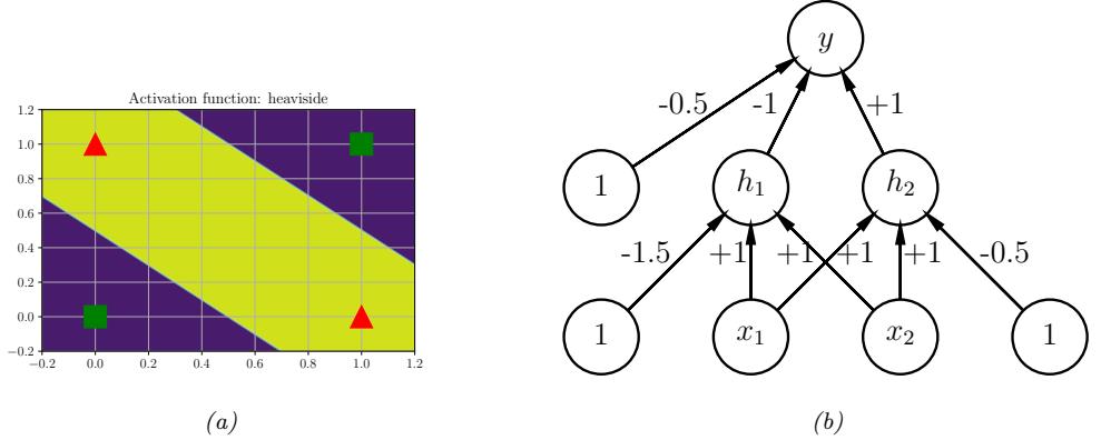
Figure 13.1: (a) Illustration of the fact that the XOR function is not linearly separable, but can be separated by the two layer model using Heaviside activation functions. Adapted from Figure 10.6 of [Gér19]. Generated by xor\_heaviside.ipynb. (b) A neural net with one hidden layer, whose weights have been manually constructed to implement the XOR function. h1 is the AND function and h2 is the OR function. The bias terms are implemented using weights from constant nodes with the value 1.
13.2.1 The XOR problem
One of the most famous examples from the Perceptrons book is the XOR problem. Here the goal is to learn a function that computes the exclusive OR of its two binary inputs. The truth table for this function is given in Table 13.1. We visualize this function in Figure 13.1a. It is clear that the data is not linearly separable, so a perceptron cannot represent this mapping.
However, we can overcome this problem by stacking multiple perceptrons on top of each other. This is called a multilayer perceptron (MLP). For example, to solve the XOR problem, we can use the MLP shown in Figure 13.1b. This consists of 3 perceptrons, denoted h1, h2 and y. The nodes marked x are inputs, and the nodes marked 1 are constant terms. The nodes h1 and h2 are called hidden units, since their values are not observed in the training data.
The first hidden unit computes h1 = x1 ↔︎ x2 by using appropriately set weights. (Here ↔︎ is the AND operation.) In particular, it has inputs from x1 and x2, both weighted by 1.0, but has a bias term of -1.5 (this is implemented by a “wire” with weight -1.5 coming from a dummy node whose value is fixed to 1). Thus h1 will fire i! x1 and x2 are both on, since then
\[\mathbf{w}\_1^\mathsf{T}\mathbf{z} - b\_1 = [1.0, 1.0]^\mathsf{T}[1, 1] - 1.5 = 0.5 > 0\tag{13.5}\]
1. The term “unstructured data” is a bit misleading, since images and text do have structure. For example, neighboring pixels in an image are highly correlated, as are neighboring words in a sentence. Indeed, it is precisely this structure that is exploited (assumed) by CNNs and RNNs. By contrast, MLPs make no assumptions about their inputs. This is useful for applications such as tabular data, where the structure (dependencies between the columns) is usually not obvious, and thus needs to be learned. We can also apply MLPs to images and text, as we will see, but performance will usually be worse compared to specialized models, such as as CNNs and RNNs. (There are some exceptions, such as the MLP-mixer model of [Tol+21], which is an unstructured model that can learn to perform well on image and text data, but such models need massive datasets to overcome their lack of inductive bias.)
Similarly, the second hidden unit computes h2 = x1 ↘ x2, where ↘ is the OR operation, and the third computes the output y = h1 ↔︎ h2, where h = ¬h is the NOT (logical negation) operation. Thus y computes
\[y = f(x\_1, x\_2) = \overline{(x\_1 \land x\_2)} \land (x\_1 \lor x\_2) \tag{13.6}\]
This is equivalent to the XOR function.
By generalizing this example, we can show that an MLP can represent any logical function. However, we obviously want to avoid having to specify the weights and biases by hand. In the rest of this chapter, we discuss ways to learn these parameters from data.
13.2.2 Di!erentiable MLPs
The MLP we discussed in Section 13.2.1 was defined as a stack of perceptrons, each of which involved the non-di!erentiable Heaviside function. This makes such models di”cult to train, which is why they were never widely used. However, suppose we replace the Heaviside function H : R ≃ {0, 1} with a di!erentiable activation function ϑ : R ≃ R. More precisely, we define the hidden units zl at each layer l to be a linear transformation of the hidden units at the previous layer passed elementwise through this activation function:
\[\mathbf{z}\_{l} = f\_{l}(\mathbf{z}\_{l-1}) = \varphi\_{l} \left( \mathbf{b}\_{l} + \mathbf{W}\_{l} \mathbf{z}\_{l-1} \right) \tag{13.7}\]
or, in scalar form,
\[z\_{kl} = \varphi\_l \left( b\_{kl} + \sum\_{j=1}^{K\_{l-1}} w\_{lkj} z\_{jl-1} \right) \tag{13.8}\]
The quantity that is passed to the activation function is called the pre-activations:
\[\mathbf{a}\_l = \mathbf{b}\_l + \mathbf{W}\_l \mathbf{z}\_{l-1} \tag{13.9}\]
so zl = ϑl(al).
If we now compose L of these functions together, as in Equation (13.3), then we can compute the gradient of the output wrt the parameters in each layer using the chain rule, also known as backpropagation, as we explain in Section 13.3. (This is true for any kind of di!erentiable activation function, although some kinds work better than others, as we discuss in Section 13.2.3.) We can then pass the gradient to an optimizer, and thus minimize some training objective, as we discuss in Section 13.4. For this reason, the term “MLP” almost always refers to this di!erentiable form of the model, rather than the historical version with non-di!erentiable linear threshold units.
13.2.3 Activation functions
We are free to use any kind of di!erentiable activation function we like at each layer. However, if we use a linear activation function, ϑω(a) = cωa, then the whole model reduces to a regular linear model. To see this, note that Equation (13.3) becomes
\[f(x; \theta) = \mathbf{W}\_L c\_L(\mathbf{W}\_{L-1} c\_{L-1}(\cdots(\mathbf{W}\_1 x) \cdots)) \propto \mathbf{W}\_L \mathbf{W}\_{L-1} \cdots \mathbf{W}\_1 x = \mathbf{W}' x \tag{13.10}\]
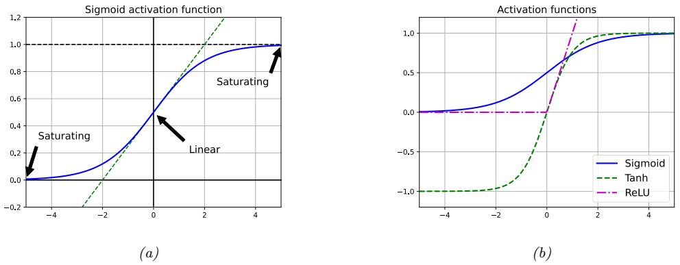
Figure 13.2: (a) Illustration of how the sigmoid function is linear for inputs near 0, but saturates for large positive and negative inputs. Adapted from 11.1 of [Gér19]. (b) Plots of some neural network activation functions. Generated by activation\_fun\_plot.ipynb.
where we dropped the bias terms for notational simplicity. For this reason, it is important to use nonlinear activation functions.
In the early days of neural networks, a common choice was to use a sigmoid (logistic) function, which can be seen as a smooth approximation to the Heaviside function used in a perceptron:
\[ \sigma(a) = \frac{1}{1 + e^{-a}} \tag{13.11} \]
However, as shown in Figure 13.2a, the sigmoid function saturates at 1 for large positive inputs, and at 0 for large negative inputs. Another common choice is the tanh function, which has a similar shape, but saturates at -1 and +1. See Figure 13.2b.
In the saturated regimes, the gradient of the output wrt the input will be close to zero, so any gradient signal from higher layers will not be able to propagate back to earlier layers. This is called the vanishing gradient problem, and it makes it hard to train the model using gradient descent (see Section 13.4.2 for details). One of the keys to being able to train very deep models is to use non-saturating activation functions. Several di!erent functions have been proposed. The most common is rectified linear unit or ReLU, proposed in [GBB11; KSH12]. This is defined as
\[\text{ReLU}(a) = \max(a, 0) = a \mathbb{I}\left(a > 0\right) \tag{13.12}\]
The ReLU function simply “turns o!” negative inputs, and passes positive inputs unchanged: see Figure 13.2b for a plot, and Section 13.4.3 for more details.
When neural networks are used to represent functions defined on a continuous input space such as points in time, f(t), or in 3d space, f(x, y, z) — they are often called neural implicit representations or coordinated based representations of the underlying signal. In such cases, it is often important to capture high frequencies to represent the signal faithfully. Unfortunately MLPs have an intrinsic bias to low frequency functions [Tan+20; RML22]. One simple solution is to use a sine function, sin(a), as the nonlinearity, instead of ReLU, as explained in [Sit+20].2
2. For some simple illustrations of the surprising power of the sine activation function for learning functions
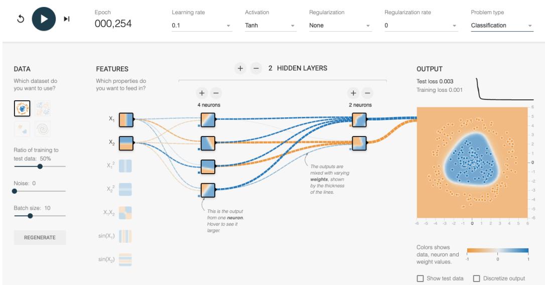
Figure 13.3: An MLP with 2 hidden layers applied to a set of 2d points from 2 classes, shown in the top left corner. The visualizations associated with each hidden unit show the decision boundary at that part of the network. The final output is shown on the right. The input is x → R2, the first layer activations are z1 → R4, the second layer activations are z2 → R2, and the final logit is a3 → R, which is converted to a probability using the sigmoid function. This is a screenshot from the interactive demo at http: // playground. tensorflow. org .
13.2.4 Example models
MLPs can be used to perform classification and regression for many kinds of data. We give some examples below.
13.2.4.1 MLP for classifying 2d data into 2 categories
Figure 13.3 gives an illustration of an MLP with two hidden layers applied to a 2d input vector, corresponding to points in the plane, coming from two concentric circles. This model has the following form:
\[p(y|x; \theta) = \text{Ber}(y|\sigma(a\_3))\tag{13.13}\]
\[a\_3 = w\_3^\top \mathbf{z}\_2 + b\_3 \tag{13.14}\]
\[\mathbf{z}\_2 = \varphi(\mathbf{W}\_2 \mathbf{z}\_1 + \mathbf{b}\_2) \tag{13.15}\]
\[\mathbf{z}\_1 = \varphi(\mathbf{W}\_1 \mathbf{z} + \mathbf{b}\_1) \tag{13.16}\]
Here a3 is the final logit score, which is converted to a probability via the sigmoid (logistic) function. The value a3 is computed by taking a linear combination of the 2 hidden units in layer 2, using
on low dimensional input spaces, see https://nipunbatra.github.io/blog/posts/siren-paper.html and https: //nipunbatra.github.io/blog/posts/siren-paper.html.
| _________________________________________________________________ Layer (type) |
Output Shape | Param # |
|---|---|---|
| ================================================================= flatten (Flatten) |
(None, 784) | 0 |
| _________________________________________________________________ dense (Dense) |
(None, 128) | 100480 |
| _________________________________________________________________ dense_1 (Dense) |
(None, 128) | 16512 |
| _________________________________________________________________ dense_2 (Dense) |
(None, 10) | 1290 |
| ================================================================= Total params: 118,282 Trainable params: 118,282 Non-trainable params: 0 |
Model: “sequential”
Table 13.2: Structure of the MLP used for MNIST classification. Note that 100, 480 = (784 + 1) ↑ 128, and 16, 512 = (128 + 1) ↑ 128. mlp\_mnist\_tf.ipynb.
a3 = wT 3 z2 + b3. In turn, layer 2 is computed by taking a nonlinear combination of the 4 hidden units in layer 1, using z2 = ϑ(W2z1+b2). Finally, layer 1 is computed by taking a nonlinear combination of the 2 input units, using z1 = ϑ(W1x+b1). By adjusting the parameters, ε = (W1, b1,W2, b2, w3, b3), to minimize the negative log likelihood, we can fit the training data very well, despite the highly nonlinear nature of the decision boundary. (You can find an interactive version of this figure at http://playground.tensorflow.org.)
13.2.4.2 MLP for image classification
To apply an MLP to image classification, we need to “flatten” the 2d input into 1d vector. We can then use a feedforward architecture similar to the one described in Section 13.2.4.1. For example, consider building an MLP to classifiy MNIST digits (Section 3.5.2). These are 28 ↑ 28 = 784 dimensional. If we use 2 hidden layers with 128 units each, followed by a final 10 way softmax layer, we get the model shown in Table 13.2.
We show some predictions from this model in Figure 13.4. We train it for just two “epochs” (passes over the dataset), but already the model is doing quite well, with a test set accuracy of 97.1%. Furthermore, the errors seem sensible, e.g., 9 is mistaken as a 3. Training for more epochs can further improve test accuracy.
In Chapter 14 we discuss a di!erent kind of model, called a convolutional neural network, which is better suited to images. This gets even better performance and uses fewer parameters, by exploiting prior knowledge about the spatial structure of images. By contrast, with an MLP, we can randomly shu#e (permute) the pixels without a!ecting the output (assuming we use the same random permutation for all inputs).
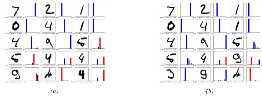
Figure 13.4: Results of applying an MLP (with 2 hidden layers with 128 units and 1 output layer with 10 units) to some MNIST images (cherry picked to include some errors). Red is incorrect, blue is correct. (a) After 1 epoch of training. (b) After 2 epochs. Generated by mlp\_mnist\_tf.ipynb.
13.2.4.3 MLP for text classification
To apply MLPs to text classification, we need to convert the variable-length sequence of words v1,…, vT (where each vt is a one-hot vector of length V , where V is the vocabulary size) into a fixed dimensional vector x. The easiest way to do this is as follows. First we treat the input as an unordered bag of words (Section 1.5.4.1), {vt}. The first layer of the model is a E ↑ V embedding matrix W1, which converts each sparse V -dimensional vector to a dense E-dimensional embedding, et = W1vt (see Section 20.5 for more details on word embeddings). Next we convert this set of T E-dimensional embeddings into a fixed-sized vector using global average pooling, e = 1 T (T t=1 et. This can then be passed as input to an MLP. For example, if we use a single hidden layer, and a logistic output (for binary classification), we get
\[p(y|x; \boldsymbol{\theta}) = \text{Ber}(y|\sigma(\boldsymbol{w}\_3^\mathsf{T}\boldsymbol{h} + b\_3))\tag{13.17}\]
\[h = \varphi(\mathbf{W}\_2 \overline{\mathbf{e}} + \mathbf{b}\_2) \tag{13.18}\]
\[\overline{\mathbf{e}} = \frac{1}{T} \sum\_{t=1}^{T} \mathbf{e}\_t \tag{13.19}\]
\[\mathbf{e}\_t = \mathbf{W}\_1 \mathbf{v}\_t\tag{13.20}\]
If we use a vocabulary size of V = 10, 000, an embedding size of E = 16, and a hidden layer of size 16, we get the model shown in Table 13.3. If we apply this to the IMDB movie review sentiment classification dataset discussed in Section 1.5.2.1, we get 86% on the validation set.
We see from Table 13.3 that the model has a lot of parameters, which can result in overfitting, since the IMDB training set only has 25k examples. However, we also see that most of the parameters are in the embedding matrix, so instead of learning these in a supervised way, we can perform unsupervised pre-training of word embedding models, as we discuss in Section 20.5. If the embedding matrix W1 is fixed, we just have to fine-tune the parameters in layers 2 and 3 for this specific labeled task, which requires much less data. (See also Chapter 19, where we discuss general techniques for training with limited labeled data.)
Model: “sequential”
| _________________________________________________________________ Layer (type) |
Output Shape | Param # |
|---|---|---|
| ================================================================= embedding (Embedding) |
(None, None, 16) | 160000 |
| _________________________________________________________________ global_average_pooling1d (Gl (None, 16) _________________________________________________________________ |
0 | |
| dense (Dense) _________________________________________________________________ |
(None, 16) | 272 |
| dense_1 (Dense) ================================================================= |
(None, 1) | 17 |
| Total params: 160,289 Trainable params: 160,289 Non-trainable params: 0 |
Table 13.3: Structure of the MLP used for IMDB review classification. We use a vocabulary size of V = 10, 000, an embedding size of E = 16, and a hidden layer of size 16. The embedding matrix W1 has size 10, 000 ↑ 16, the hidden layer (labeled “dense”) has a weight matrix W2 of size 16 ↑ 16 and bias b2 of size 16 (note that 16 ↑ 16 + 16 = 272), and the final layer (labeled “dense_1”) has a weight vector w3 of size 16 and a bias b3 of size 1. The global average pooling layer has no free parameters. mlp\_imdb\_tf.ipynb.
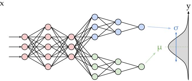
Figure 13.5: Illustration of an MLP with a shared “backbone” and two output “heads”, one for predicting the mean and one for predicting the variance. From https: // brendanhasz. github. io/ 2019/ 07/ 23/ bayesian-density-net. html . Used with kind permission of Brendan Hasz.
13.2.4.4 MLP for heteroskedastic regression
We can also use MLPs for regression. Figure 13.5 shows how we can make a model for heteroskedastic nonlinear regression. (The term “heteroskedastic” just means that the predicted output variance is input-dependent, as discussed in Section 2.6.3.) This function has two outputs which compute fµ(x) = E [y|x, ε] and fε(x) = )V [y|x, ε]. We can share most of the layers (and hence parameters) between these two functions by using a common “backbone” and two output “heads”, as shown in Figure 13.5. For the µ head, we use a linear activation, ϑ(a) = a. For the ω head, we use a softplus
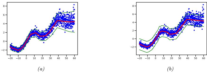
Figure 13.6: Illustration of predictions from an MLP fit using MLE to a 1d regression dataset with growing noise. (a) Output variance is input-dependent, as in Figure 13.5. (b) Mean is computed using same model as in (a), but output variance is treated as a fixed parameter ω2, which is estimated by MLE after training, as in Section 11.2.3.6. Generated by mlp\_1d\_regression\_hetero\_tfp.ipynb.
activation, ϑ(a) = ω+(a) = log(1 + ea). If we use linear heads and a nonlinear backbone, the overall model is given by
\[p(y|\mathbf{z},\boldsymbol{\theta}) = \mathcal{N}\left(y|\mathbf{w}\_{\mu}^{\mathsf{T}}f(\boldsymbol{x};\boldsymbol{w}\_{\text{shared}}), \sigma\_{+}(\boldsymbol{w}\_{\sigma}^{\mathsf{T}}f(\boldsymbol{x};\boldsymbol{w}\_{\text{shared}}))\right) \tag{13.21}\]
Figure 13.6 shows the advantage of this kind of model on a dataset where the mean grows linearly over time, with seasonal oscillations, and the variance increases quadratically. (This is a simple example of a stochastic volatility model; it can be used to model financial data, as well as the global temperature of the earth, which (due to climate change) is increasing in mean and in variance.) We see that a regression model where the output variance ω2 is treated as a fixed (input-independent) parameter will sometimes be underconfident, since it needs to adjust to the overall noise level, and cannot adapt to the noise level at each point in input space.
13.2.5 The importance of depth
One can show that an MLP with one hidden layer is a universal function approximator, meaning it can model any suitably smooth function, given enough hidden units, to any desired level of accuracy [HSW89; Cyb89; Hor91]. Intuitively, the reason for this is that each hidden unit can specify a half plane, and a su”ciently large combination of these can “carve up” any region of space, to which we can associate any response (this is easiest to see when using piecewise linear activation functions, as shown in Figure 13.7).
However, various arguments, both experimental and theoretical (e.g., [Has87; Mon+14; Rag+17; Pog+17]), have shown that deep networks work better than shallow ones. The reason is that later layers can leverage the features that are learned by earlier layers; that is, the function is defined in a compositional or hierarchical way. For example, suppose we want to classify DNA strings, and the positive class is associated with the string *AA??CGCG??AA*, where ? is a wildcard denoting any single character, and * is a wildcard denoting any sequence of characters (possibly of length 0). Although we could fit this with a single hidden layer model, intuitively it will be easier to learn if the model first learns to detect the AA and CG “motifs” using the hidden units in layer 1, and then uses
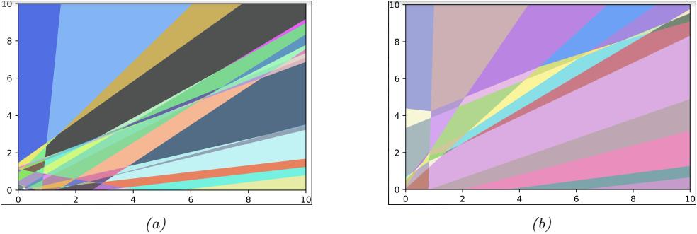
Figure 13.7: A decomposition of R2 into a finite set of linear decision regions produced by an MLP with ReLU activations with (a) one hidden layer of 25 hidden units and (b) two hidden layers. From Figure 1 of [HAB19]. Used with kind permission of Maksym Andriuschenko.
these features to define a simple linear classifier in layer 2, analogously to how we solved the XOR problem in Section 13.2.1.
13.2.6 The “deep learning revolution”
Although the ideas behind DNNs date back several decades, it was not until the 2010s that they started to become very widely used. The first area to adopt these methods was the field of automatic speech recognition (ASR), based on breakthrough results in [Dah+11]. This approach rapidly became the standard paradigm, and was widely adopted in academia and industry [Hin+12].
However, the moment that got the most attention was when [KSH12] showed that deep CNNs could significantly improve performance on the challenging ImageNet image classification benchmark, reducing the error rate from 26% to 16% in a single year (see Figure 1.14b); this was a huge jump compared to the previous rate of progress of about 2% reduction per year.
The “explosion” in the usage of DNNs has several contributing factors. One is the availability of cheap GPUs (graphics processing units); these were originally developed to speed up image rendering for video games, but they can also massively reduce the time it takes to fit large CNNs, which involve similar kinds of matrix-vector computations. Another is the growth in large labeled datasets, which enables us to fit complex function approximators with many parameters without overfitting. (For example, ImageNet has 1.3M labeled images, and is used to fit models that have millions of parameters.) Indeed, if deep learning systems are viewed as “rockets”, then large datasets have been called the fuel.3
Motivated by the outstanding empirical success of DNNs, various companies started to become interested in this technology. This had led to the development of high quality open-source software libraries, such as Tensorflow (made by Google), PyTorch (made by Facebook), and MXNet (made by Amazon). These libraries support automatic di!erentiation (see Section 13.3) and scalable gradient-based optimization (see Section 8.4) of complex di!erentiable functions. We will use some
3. This popular analogy is due to Andrew Ng, who mentioned it in a keynote talk at the GPU Technology Conference (GTC) in 2015. His slides are available at https://bit.ly/38RTxzH.
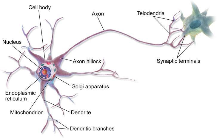
Figure 13.8: Illustration of two neurons connected together in a “circuit”. The output axon of the left neuron makes a synaptic connection with the dendrites of the cell on the right. Electrical charges, in the form of ion flows, allow the cells to communicate. From https: // en. wikipedia. org/ wiki/ Neuron . Used with kind permission of Wikipedia author BruceBlaus.
of these libraries in various places throughout the book to implement a variety of models, not just DNNs.4
More details on the history of the “deep learning revolution” can be found in e.g., [Sej18; Met21].
13.2.7 Connections with biology
In this section, we discuss the connections between the kinds of neural networks we have discussed above, known as artificial neural networks or ANNs, and real neural networks. The details on how real biological brains work are quite complex (see e.g., [Kan+12]), but we can give a simple “cartoon”.
We start by considering a model of a single neuron. To a first approximation, we can say that whether neuron k fires, denoted by hk → {0, 1}, depends on the activity of its inputs, denoted by x → RD, as well as the strength of the incoming connections, which we denote by wk → RD. We can compute a weighted sum of the inputs using ak = wT kx. These weights can be viewed as “wires” connecting the inputs xd to neuron hk; these are analogous to dendrites in a real neuron (see Figure 13.8). This weighted sum is then compared to a threshold, bk, and if the activation exceeds the threshold, the neuron fires; this is analogous to the neuron emitting an electrical output or action potential. Thus we can model the behavior of the neuron using hk(x) = H(wT kx ↗ bk), where H(a) = I(a > 0) is the Heaviside function. This is called the McCulloch-Pitts model of the neuron, and was proposed in 1943 [MP43].
We can combine multiple such neurons together to make an ANN. The result has sometimes been
4. Note, however, that some have argued (see e.g., [BI19]) that current libraries are too inflexible, and put too much emphasis on methods based on dense matrix-vector multiplication, as opposed to more general algorithmic primitives.
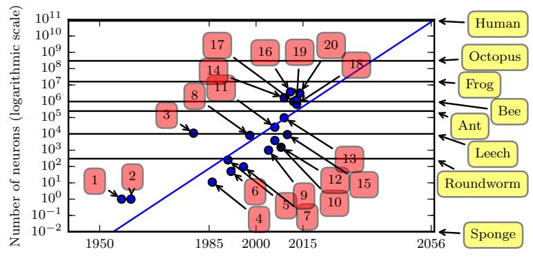
Figure 13.9: Plot of neural network sizes over time. Models 1, 2, 3 and 4 correspond to the perceptron [Ros58], the adaptive linear unit [WH60] the neocognitron [Fuk80], and the first MLP trained by backprop [RHW86]. Approximate number of neurons for some living organisms are shown on the right scale (the sponge has 0 neurons), based on https: // en. wikipedia. org/ wiki/ List\_ of\_ animals\_ by\_ number\_ of\_ neurons . From Figure 1.11 of [GBC16]. Used with kind permission of Ian Goodfellow.
viewed as a model of the brain. However, ANNs di!ers from biological brains in many ways, including the following:
- Most ANNs use backpropagation to modify the strength of their connections (see Section 13.3). However, real brains do not use backprop, since there is no way to send information backwards along an axon [Ben+15b; BS16; KH19]. Instead, they use local update rules for adjusting synaptic strengths.
- Most ANNs are strictly feedforward, but real brains have many feedback connections. It is believed that this feedback acts like a prior, which can be combined with bottom up likelihoods from the sensory system to compute a posterior over hidden states of the world, which can then be used for optimal decision making (see e.g., [Doy+07]).
- Most ANNs use simplified neurons consisting of a weighted sum passed through a nonlinearity, but real biological neurons have complex dendritic tree structures (see Figure 13.8), with complex spatio-temporal dynamics.
- Most ANNs are smaller in size and number of connections than biological brains (see Figure 13.9). Of course, ANNs are getting larger every week, fueled by various new hardware accelerators, such as GPUs and TPUs (tensor processing units), etc. However, even if ANNs match biological brains in terms of number of units, the comparison is misleading since the processing capability of a biological neuron is much higher than an artificial neuron (see point above).
- Most ANNs are designed to model a single function, such as mapping an image to a label, or a sequence of words to another sequence of words. By contrast, biological brains are very complex systems, composed of multiple specialized interacting modules, which implement di!erent kinds of functions or behaviors such as perception, control, memory, language, etc (see e.g., [Sha88; Kan+12]).
Of course, there are e!orts to make realistic models of biological brains (e.g., the Blue Brain Project [Mar06; Yon19]). However, an interesting question is whether studying the brain at this level of detail is useful for “solving AI”. It is commonly believed that the low level details of biological brains do not matter if our goal is to build “intelligent machines”, just as aeroplanes do not flap their wings. However, presumably “AIs” will follow similar “laws of intelligence” to intelligent biological agents, just as planes and birds follow the same laws of aerodynamics.
Unfortunately, we do not yet know what the “laws of intelligence” are, or indeed if there even are such laws. In this book we make the assumption that any intelligent agent should follow the basic principles of information processing and Bayesian decision theory, which is known to be the optimal way to make decisions under uncertainty (see Section 5.1).
In practice, the optimal Bayesian approach is often computationally intractable. In the natural world, biological agents have evolved various algorithmic “shortcuts” to the optimal solution; this can explain many of the heuristics that people use in everyday reasoning [KST82; GTA00; Gri20]. As the tasks we want our machines to solve become harder, we may be able to gain insights from neuroscience and cognitive science for how to solve such tasks in an approximate way (see e.g., [SC16; MWK16; Has+17; Lak+17; HG21]). However, we should also bear in mind that AI/ML systems are increasingly used for safety-critical applications, in which we might want and expect the machine to do better than a human. In such cases, we may want more than just heuristic solutions that often work; instead we may want provably reliable methods, similar to other engineering fields (see Section 1.6.3 for further discussion).
13.3 Backpropagation
13.3.1 Forward vs reverse mode di!erentiation
Consider a mapping of the form o = f(x), where x → Rn and o → Rm. We assume that f is defined as a composition of functions:
\[f = f\_4 \circ f\_3 \circ f\_2 \circ f\_1 \tag{13.22}\]
5. https://en.wikipedia.org/wiki/Backpropagation#History
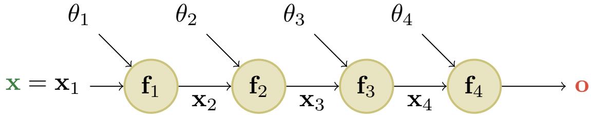
Figure 13.10: A simple linear-chain feedforward model with 4 layers. Here x is the input and o is the output. From [Blo20].
where f1 : Rn ≃ Rm1 , f2 : Rm1 ≃ Rm2 , f3 : Rm2 ≃ Rm3 , and f4 : Rm3 ≃ Rm. The intermediate steps needed to compute o = f(x) are x2 = f1(x), x3 = f2(x2), x4 = f3(x3), and o = f4(x4).
We can compute the Jacobian Jf (x) = ϑo ϑx → Rm↓n using the chain rule:
\[\frac{\partial \mathbf{o}}{\partial x} = \frac{\partial \mathbf{o}}{\partial x\_4} \frac{\partial x\_4}{\partial x\_3} \frac{\partial x\_3}{\partial x\_2} \frac{\partial x\_2}{\partial x} = \frac{\partial f\_4(x\_4)}{\partial x\_4} \frac{\partial f\_3(x\_3)}{\partial x\_3} \frac{\partial f\_2(x\_2)}{\partial x\_2} \frac{\partial f\_1(x)}{\partial x} \tag{13.23}\]
\[\mathbf{J}\_1 = \mathbf{J}\_{f\_4}(x\_4)\mathbf{J}\_{f\_3}(x\_3)\mathbf{J}\_{f\_2}(x\_2)\mathbf{J}\_{f\_1}(x) \tag{13.24}\]
We now discuss how to compute the Jacobian Jf (x) e”ciently. Recall that
\[\mathbf{J}\_f(\mathbf{x}) = \frac{\partial f(\mathbf{x})}{\partial \mathbf{z}} = \begin{pmatrix} \frac{\partial f\_1}{\partial x\_1} & \cdots & \frac{\partial f\_1}{\partial x\_n} \\ \vdots & \ddots & \vdots \\ \frac{\partial f\_m}{\partial x\_1} & \cdots & \frac{\partial f\_m}{\partial x\_n} \end{pmatrix} = \begin{pmatrix} \nabla f\_1(\mathbf{z})^\mathsf{T} \\ \vdots \\ \nabla f\_m(\mathbf{z})^\mathsf{T} \end{pmatrix} = \begin{pmatrix} \frac{\partial f}{\partial x\_1}, \cdots, \frac{\partial f}{\partial x\_n} \end{pmatrix} \in \mathbb{R}^{m \times n} \tag{13.25}\]
where ⇑fi(x) T → R1↓n is the i’th row (for i =1: m) and ϑf ϑxj → Rm is the j’th column (for j =1: n). Note that, in our notation, when m = 1, the gradient, denoted ⇑f(x), has the same shape as x. It is therefore a column vector, while Jf (x) is a row vector. In this case, we therefore technically have ⇑f(x) = Jf (x) T.
We can extract the i’th row from Jf (x) by using a vector Jacobian product (VJP) of the form eT i Jf (x), where ei → Rm is the unit basis vector. Similarly, we can extract the j’th column from Jf (x) by using a Jacobian vector product (JVP) of the form Jf (x)ej , where ej → Rn. This shows that the computation of Jf (x) reduces to either n JVPs or m VJPs.
If n<m, it is more e”cient to compute Jf (x) for each column j =1: n by using JVPs in a right-to-left manner. The right multiplication with a column vector v is
\[\mathbf{J}\_f(x)v = \underbrace{\mathbf{J}\_{f\_4}(x\_4)}\_{m \times m\_3} \underbrace{\mathbf{J}\_{f\_3}(x\_3)}\_{m\_3 \times m\_2} \underbrace{\mathbf{J}\_{f\_2}(x\_2)}\_{m\_2 \times m\_1} \underbrace{v}\_{m \times 1} \tag{13.26}\]
This can be computed using forward mode di!erentiation; see Algorithm 13.1 for the pseudocode. Assuming m = 1 and n = m1 = m2 = m3, the cost of computing Jf (x) is O(n2).
If n>m (e.g., if the output is a scalar), it is more e”cient to compute Jf (x) for each row i =1: m by using VJPs in a left-to-right manner. The left multiplication with a row vector uT is
\[u^{\sf T} \mathbf{J}\_f(x) = \underbrace{u^{\sf T}}\_{1 \times m} \underbrace{\mathbf{J}\_{f\_4}(x\_4)}\_{m \times m\_3} \underbrace{\mathbf{J}\_{f\_3}(x\_3)}\_{m\_3 \times m\_2} \underbrace{\mathbf{J}\_{f\_2}(x\_2)}\_{m\_2 \times m\_1} \mathbf{J}\_{f\_1}(x\_1) \tag{13.27}\]
Algorithm 13.1: Foward mode di!erentiation
1 x1 := x vj := ej → Rn for j =1: n for k =1: K do xk+1 = fk(xk) vj := Jfk (xk)vj for j =1: n Return o = xK+1, [Jf (x)]:,j = vj for j =1: n
This can be done using reverse mode di!erentiation; see Algorithm 13.2 for the pseudocode. Assuming m = 1 and n = m1 = m2 = m3, the cost of computing Jf (x) is O(n2).
Algorithm 13.2: Reverse mode di!erentiation 1 x1 := x 2 for k =1: K do 3 xk+1 = fk(xk) 4 ui := ei → Rm for i =1: m 5 for k = K : 1 do 6 uT i := uT i Jfk (xk) for i =1: m 7 Return o = xK+1, [Jf (x)]i,: = uT i for i =1: m
Both Algorithms 13.1 and 13.2 can be adapted to compute JVPs and VJPs against any collection of input vectors, by accepting {vj}j=1,…,n and {ui}i=1,…,m as respective inputs. Initializing these vectors to the standard basis is useful specifically for producing the complete Jacobian as output.
13.3.2 Reverse mode di!erentiation for multilayer perceptrons
In the previous section, we considered a simple linear-chain feedforward model where each layer does not have any learnable parameters. In this section, each layer can now have (optional) parameters ε1,…, ε4. See Figure 13.10 for an illustration. We focus on the case where the mapping has the form L : Rn ≃ R, so the output is a scalar. For example, consider ε2 loss for a MLP with one hidden layer:
\[\mathcal{L}((x, y), \theta) = \frac{1}{2} ||y - \mathbf{W}\_2 \varphi(\mathbf{W}\_1 x)||\_2^2 \tag{13.28}\]
we can represent this as the following feedforward model:
\[\mathcal{L} = \mathbf{f}\_4 \diamond \mathbf{f}\_3 \diamond \mathbf{f}\_2 \diamond \mathbf{f}\_1 \tag{13.29}\]
\[x\_2 = f\_1(x, \theta\_1) = \mathbf{W}\_1 x \tag{13.30}\]
\[x\_3 = f\_2(x\_2, \emptyset) = \varphi(x\_2) \tag{13.31}\]
\[x\_4 = f\_3(x\_3, \theta\_3) = \mathbf{W}\_2 x\_3 \tag{13.32}\]
\[\mathcal{L} = \mathbf{f}\_4(x\_4, y) = \frac{1}{2}||x\_4 - y||^2 \tag{13.33}\]
We use the notation fk(xk, εk) to denote the function at layer k, where xk is the previous output and εk are the optional parameters for this layer.
In this example, the final layer returns a scalar, since it corresponds to a loss function L → R. Therefore it is more e”cient to use reverse mode di!erentation to compute the gradient vectors.
We first discuss how to compute the gradient of the scalar output wrt the parameters in each layer. We can easily compute the gradient wrt the predictions in the final layer ϑL ϑx4 . For the gradient wrt the parameters in the earlier layers, we can use the chain rule to get
\[\frac{\partial \mathcal{L}}{\partial \mathbf{a}} = \frac{\partial \mathcal{L}}{\partial \mathbf{a}} \frac{\partial \mathbf{x}\_4}{\partial \mathbf{a}} \tag{13.34}\]
\[ \begin{array}{ccccc} \partial\theta\_3 & \partial x\_4 \,\partial\theta\_3 & & & \\ \partial\mathcal{L} & \\_\partial\mathcal{L} & \partial x\_4 \,\partial x\_3 & & \\ & & & & \\ \end{array} \tag{12.25} \]
\[\frac{\partial \mathcal{L}}{\partial \theta\_2} = \frac{\partial \mathcal{L}}{\partial x\_4} \frac{\partial x\_4}{\partial x\_3} \frac{\partial x\_3}{\partial \theta\_2} \tag{13.35}\]
\[\frac{\partial \mathcal{L}}{\partial \boldsymbol{\theta}\_{1}} = \frac{\partial \mathcal{L}}{\partial \boldsymbol{x}\_{4}} \frac{\partial \boldsymbol{x}\_{4}}{\partial \boldsymbol{x}\_{3}} \frac{\partial \boldsymbol{x}\_{3}}{\partial \boldsymbol{x}\_{2}} \frac{\partial \boldsymbol{x}\_{2}}{\partial \boldsymbol{\theta}\_{1}} \tag{13.36}\]
where each ϑL ϑεk = (⇑εk L) T is a dk-dimensional gradient row vector, where dk is the number of parameters in layer k. We see that these can be computed recursively, by multiplying the gradient row vector at layer k by the Jacobian ϑxk ϑxk→1 which is an nk ↑ nk→1 matrix, where nk is the number of hidden units in layer k. See Algorithm 13.3 for the pseudocode.
This algorithm computes the gradient of the loss wrt the parameters at each layer. It also computes the gradient of the loss wrt the input, ⇑xL → Rn, where n is the dimensionality of the input. This latter quantity is not needed for parameter learning, but can be useful for generating inputs to a model (see Section 14.6 for some applications).
All that remains is to specify how to compute the vector Jacobian product (VJP) of all supported layers. The details of this depend on the form of the function at each layer. We discuss some examples below.
13.3.3 Vector-Jacobian product for common layers
Recall that the Jacobian for a layer of the form f : Rn ≃ Rm. is defined by
\[\mathbf{J}\_{f}(\mathbf{z}) = \frac{\partial f(\mathbf{z})}{\partial \mathbf{z}} = \begin{pmatrix} \frac{\partial f\_{1}}{\partial x\_{1}} & \cdots & \frac{\partial f\_{1}}{\partial x\_{n}} \\ \vdots & \ddots & \vdots \\ \frac{\partial f\_{m}}{\partial x\_{1}} & \cdots & \frac{\partial f\_{m}}{\partial x\_{n}} \end{pmatrix} = \begin{pmatrix} \nabla f\_{1}(\mathbf{z})^{\mathsf{T}} \\ \vdots \\ \nabla f\_{m}(\mathbf{z})^{\mathsf{T}} \end{pmatrix} = \begin{pmatrix} \frac{\partial f}{\partial x\_{1}}, \cdots, \frac{\partial f}{\partial x\_{n}} \end{pmatrix} \in \mathbb{R}^{m \times n} \tag{13.37}\]
where ⇑fi(x) T → Rn is the i’th row (for i =1: m) and ϑf ϑxj → Rm is the j’th column (for j =1: n). In this section, we describe how to compute the VJP uTJf (x) for common layers.
Algorithm 13.3: Backpropagation for an MLP with K layers
1 // Forward pass 2 x1 := x 3 for k =1: K do 4 xk+1 = fk(xk, εk) 5 // Backward pass 6 uK+1 := 1 7 for k = K : 1 do 8 gk := uT k+1 ϑfk(xk,εk) ϑεk 9 uT k := uT k+1 ϑfk(xk,εk) ϑxk 10 // Output 11 Return L = xK+1, ⇑xL = u1, {⇑εk L = gk : k =1: K}
13.3.3.1 Cross entropy layer
Consider a cross-entropy loss layer taking logits x and target labels y as input, and returning a scalar:
\[z = f(\mathbf{z}) = \text{CrossEntropyWithLogits}(y, \mathbf{z}) = -\sum\_{c} y\_c \log(\text{softmax}(\mathbf{z})\_c) = -\sum\_{c} y\_c \log p\_c \quad (13.38)\]
where p = softmax(x) = exc !C c↑=1 exc↑ are the predicted class probabilites, and y is the true distribution over labels (often a one-hot vector). The Jacobian wrt the input is
\[\mathbf{J} = \frac{\partial z}{\partial x} = (\mathbf{p} - \mathbf{y})^{\mathsf{T}} \in \mathbb{R}^{1 \times C} \tag{13.39}\]
To see this, assume the target label is class c. We have
\[z = f(x) = -\log(p\_c) = -\log\left(\frac{e^{x\_c}}{\sum\_j e^{x\_j}}\right) = \log\left(\sum\_j e^{x\_j}\right) - x\_c \tag{13.40}\]
Hence
\[\frac{\partial z}{\partial x\_i} = \frac{\partial}{\partial x\_i} \log \sum\_j e^{x\_j} - \frac{\partial}{\partial x\_i} x\_c = \frac{e^{x\_i}}{\sum\_j e^{x\_j}} - \frac{\partial}{\partial x\_i} x\_c = p\_i - \mathbb{I}\left(i = c\right) \tag{13.41}\]
If we define y = [I(i = c)], we recover Equation (13.39). Note that the Jacobian of this layer is a row vector, since the output is a scalar.
13.3.3.2 Elementwise nonlinearity
Consider a layer that applies an elementwise nonlinearity, z = f(x) = ϑ(x), so zi = ϑ(xi). The (i, j) element of the Jacobian is given by
\[\frac{\partial z\_i}{\partial x\_j} = \begin{cases} \varphi'(x\_i) & \text{if } i = j \\ 0 & \text{otherwise} \end{cases} \tag{13.42}\]
where ϑ↑ (a) = d daϑ(a). In other words, the Jacobian wrt the input is
\[\mathbf{J} = \frac{\partial f}{\partial x} = \text{diag}(\varphi'(x))\tag{13.43}\]
For an arbitrary vector u, we can compute uTJ by elementwise multiplication of the diagonal elements of J with u. For example, if
\[ \varphi(a) = \text{ReLU}(a) = \max(a, 0) \tag{13.44} \]
we have
\[\varphi'(a) = \begin{cases} 0 & a < 0 \\ 1 & a > 0 \end{cases} \tag{13.45}\]
The subderivative (Section 8.1.4.1) at a = 0 is any value in [0, 1]. It is often taken to be 0. Hence
\[\text{ReLU}'(a) = H(a) \tag{13.46}\]
where H is the Heaviside step function.
13.3.3.3 Linear layer
Now consider a linear layer, z = f(x,W) = Wx, where W → Rm↓n, so x → Rn and z → Rm. We can compute the Jacobian wrt the input vector, J = ϑz ϑx → Rm↓n, as follows. Note that
\[z\_i = \sum\_{k=1}^{n} W\_{ik} x\_k \tag{13.47}\]
So the (i, j) entry of the Jacobian will be
\[\frac{\partial z\_i}{\partial x\_j} = \frac{\partial}{\partial x\_j} \sum\_{k=1}^n W\_{ik} x\_k = \sum\_{k=1}^n W\_{ik} \frac{\partial}{\partial x\_j} x\_k = W\_{ij} \tag{13.48}\]
since ϑ ϑxj xk = I(k = j). Hence the Jacobian wrt the input is
\[\mathbf{J} = \frac{\partial \mathbf{z}}{\partial x} = \mathbf{W} \tag{13.49}\]
The VJP between uT → R1↓m and J → Rm↓n is
\[\mathbf{u}^{\mathsf{T}} \frac{\partial \mathbf{z}}{\partial x} = \mathbf{u}^{\mathsf{T}} \mathbf{W} \in \mathbb{R}^{1 \times n} \tag{13.50}\]
Now consider the Jacobian wrt the weight matrix, J = ϑz ϑW. This can be represented as a m↑(m↑n) matrix, which is complex to deal with. So instead, let us focus on taking the gradient wrt a single weight, Wij . This is easier to compute, since ϑz ϑWij is a vector. To compute this, note that
\[z\_k = \sum\_{l=1}^{n} W\_{kl} x\_l \tag{13.51}\]
\[\frac{\partial z\_k}{\partial W\_{ij}} = \sum\_{l=1}^n x\_l \frac{\partial}{\partial W\_{ij}} W\_{kl} = \sum\_{l=1}^n x\_l \mathbb{I}\left(i = k \text{ and } j = l\right) \tag{13.52}\]
Hence
\[\frac{\partial \mathbf{z}}{\partial W\_{ij}} = \begin{pmatrix} 0 & \cdots & 0 & x\_j & 0 & \cdots & 0 \end{pmatrix}^{\mathsf{T}} \tag{13.53}\]
where the non-zero entry occurs in location i. The VJP between uT → R1↓m and ϑz ϑW → Rm↓(m↓n) can be represented as a matrix of shape 1 ↑ (m ↑ n). Note that
\[\mathbf{u}^{\mathsf{T}} \frac{\partial \mathbf{z}}{\partial W\_{ij}} = \sum\_{k=1}^{m} u\_k \frac{\partial z\_k}{\partial W\_{ij}} = u\_i x\_j \tag{13.54}\]
Therefore
\[\left[\mathbf{u}^{\mathsf{T}}\frac{\partial\mathbf{z}}{\partial\mathbf{W}}\right]\_{1,:} = \mathbf{u}\mathbf{z}^{\mathsf{T}} \in \mathbb{R}^{m \times n} \tag{13.55}\]
13.3.3.4 Putting it all together
For an exercise that puts this all together, see Exercise 13.1.
13.3.4 Computation graphs
MLPs are a simple kind of DNN in which each layer feeds directly into the next, forming a chain structure, as shown in Figure 13.10. However, modern DNNs can combine di!erentiable components in much more complex ways, to create a computation graph, analogous to how programmers combine elementary functions to make more complex ones. (Indeed, some have suggested that “deep learning” be called “di!erentiable programming”.) The only restriction is that the resulting computation graph corresponds to a directed acyclic graph (DAG), where each node is a di!erentiable function of all its inputs.
For example, consider the function
\[f(x\_1, x\_2) = x\_2 e^{x\_1} \sqrt{x\_1 + x\_2 e^{x\_1}} \tag{13.56}\]
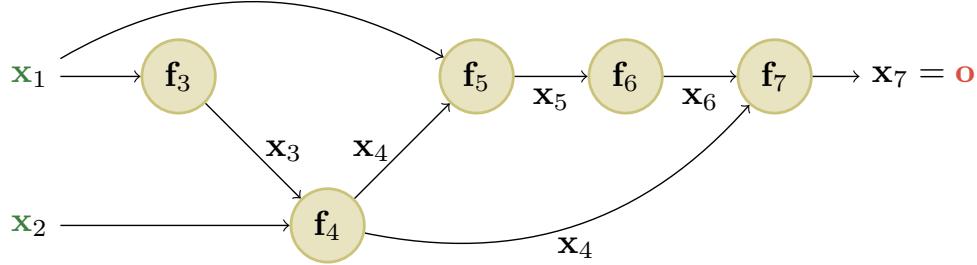
Figure 13.11: An example of a computation graph with 2 (scalar) inputs and 1 (scalar) output. From [Blo20].
We can compute this using the DAG in Figure 13.11, with the following intermediate functions:
\[x\_3 = f\_3(x\_1) = e^{x\_1} \tag{13.57}\]
\[x\_4 = f\_4(x\_2, x\_3) = x\_2 x\_3 \tag{13.58}\]
\[x\_5 = f\_5(x\_1, x\_4) = x\_1 + x\_4 \tag{13.59}\]
\[x\_6 = f\_6(x\_5) = \sqrt{x\_5} \tag{13.60}\]
\[x\_7 = f\_7(x\_4, x\_6) = x\_4 x\_6 \tag{13.61}\]
Note that we have numbered the nodes in topological order (parents before children). During the backward pass, since the graph is no longer a chain, we may need to sum gradients along multiple paths. For example, since x4 influences x5 and x7, we have
\[\frac{\partial \mathbf{o}}{\partial x\_4} = \frac{\partial \mathbf{o}}{\partial x\_5} \frac{\partial x\_5}{\partial x\_4} + \frac{\partial \mathbf{o}}{\partial x\_7} \frac{\partial x\_7}{\partial x\_4} \tag{13.62}\]
We can avoid repeated computation by working in reverse topological order. For example,
\[\frac{\partial \mathbf{o}}{\partial x\_7} = \frac{\partial x\_7}{\partial x\_7} = \mathbf{I}\_m \tag{13.63}\]
\[\frac{\partial \mathbf{o}}{\partial \mathbf{o}} = \frac{\partial \mathbf{o}}{\partial \mathbf{o}} \frac{\partial \mathbf{x}\_7}{\partial \mathbf{x}\_8} \tag{13.64}\]
\[\begin{aligned} \frac{\partial \mathbf{x}\_6}{\partial \mathbf{a}} &= \frac{\partial \mathbf{x}\_7}{\partial \mathbf{a}} \frac{\partial \mathbf{x}\_6}{\partial \mathbf{a}}\\ \frac{\partial \mathbf{a}}{\partial \mathbf{a}} &= \frac{\partial \mathbf{a}}{\partial \mathbf{a}} \frac{\partial \mathbf{x}\_6}{\partial \mathbf{a}} \end{aligned} \tag{13.65}\]
\[\begin{aligned} \frac{\partial \mathbf{\bar{x}}\_5}{\partial \mathbf{z}\_6} &= \frac{\partial \mathbf{x}\_6}{\partial \mathbf{z}\_6} \frac{\partial \mathbf{x}\_5}{\partial \mathbf{z}\_5} \\ \frac{\partial \mathbf{\bar{o}}}{\partial \mathbf{z}\_2} &= \frac{\partial \mathbf{o}}{\partial \mathbf{z}} \frac{\partial \mathbf{x}\_5}{\partial \mathbf{z}} + \frac{\partial \mathbf{o}}{\partial \mathbf{z}} \frac{\partial \mathbf{x}\_7}{\partial \mathbf{z}} \end{aligned} \tag{13.60}\]
\[\frac{\partial \mathbf{U}}{\partial \mathbf{x}\_4} = \frac{\partial \mathbf{x}\_5}{\partial \mathbf{x}\_5} \frac{\partial \mathbf{x}\_4}{\partial \mathbf{x}\_4} + \frac{\partial \mathbf{x}\_5}{\partial \mathbf{x}\_7} \frac{\partial \mathbf{x}\_4}{\partial \mathbf{x}\_4} \tag{13.66}\]
In general, we use
\[\frac{\partial \mathbf{o}}{\partial x\_j} = \sum\_{k \in \text{Ch}(j)} \frac{\partial \mathbf{o}}{\partial x\_k} \frac{\partial \mathbf{x}\_k}{\partial x\_j} \tag{13.67}\]
where the sum is over all children k of node j, as shown in Figure 13.12. The ϑo ϑxk gradient vector has already been computed for each child k; this quantity is called the adjoint. This gets multiplied by the Jacobian ϑxk ϑxj of each child.
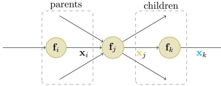
Figure 13.12: Notation for automatic di!erentiation at node j in a computation graph. From [Blo20].
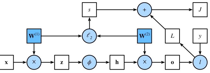
Figure 13.13: Computation graph for an MLP with input x, hidden layer h, output o, loss function L = ε(o, y), an ε2 regularizer s on the weights, and total loss J = L + s. From Figure 4.7.1 of [Zha+20]. Used with kind permission of Aston Zhang.
The computation graph can be computed ahead of time, by using an API to define a static graph. (This is how Tensorflow 1 worked.) Alternatively, the graph can be computed “just in time”, by tracing the execution of the function on an input argument. (This is how Tensorflow eager mode works, as well as JAX and PyTorch.) The latter approach makes it easier to work with a dynamic graph, whose shape can change depending on the values computed by the function.
Figure 13.13 shows a computation graph corresponding to an MLP with one hidden layer with weight decay. More precisely, the model computes the linear pre-activations z = W(1)x, the hidden activations h = ϱ(z), the linear outputs o = W(2)h, the loss L = ε(o, y), the regularizer s = ϖ 2 (||W(1)||2 F + ||W(2)||2 F ), and the total loss J = L + s.
13.4 Training neural networks
In this section, we discuss how to fit DNNs to data. The standard approach is to use maximum likelihood estimation, by minimizing the NLL:
\[\mathcal{L}(\boldsymbol{\theta}) = -\log p(\mathcal{D}|\boldsymbol{\theta}) = -\sum\_{n=1}^{N} \log p(y\_n|\boldsymbol{x}\_n; \boldsymbol{\theta}) \tag{13.68}\]
It is also common to add a regularizer (such as the negative log prior), as we discuss in Section 13.5.
In principle we can just use the backprop algorithm (Section 13.3) to compute the gradient of this loss and pass it to an o!-the-shelf optimizer, such as those discussed in Chapter 8. (The Adam optimizer of Section 8.4.6.3 is a popular choice, due to its ability to scale to large datasets (by virtue of being an SGD-type algorithm), and to converge fairly quickly (by virtue of using diagonal preconditioning and momentum).) However, in practice this may not work well. In this section, we discuss various problems that may arise, as well as some solutions. For more details on the practicalities of training DNNs, see various other books, such as [HG20; Zha+20; Gér19].
In addition to practical issues, there are important theoretical issues. In particular, we note that the DNN loss is not a convex objective, so in general we will not be able to find the global optimum. Nevertheless, SGD can often find suprisingly good solutions. The research into why this is the case is still being conducted; see [Bah+20] for a recent review of some of this work.
13.4.1 Tuning the learning rate
It is important to tune the learning rate (step size), to ensure convergence to a good solution. We discuss this issue in Section 8.4.3.
13.4.2 Vanishing and exploding gradients
When training very deep models, the gradient tends to become either very small (this is called the vanishing gradient problem) or very large (this is called the exploding gradient problem), because the error signal is being passed through a series of layers which either amplify or diminish it [Hoc+01]. (Similar problems arise in RNNs on long sequences, as we explain in Section 15.2.6.)
To explain the problem in more detail, consider the gradient of the loss wrt a node at layer l:
\[\frac{\partial \mathcal{L}}{\partial \mathbf{z}\_{l}} = \frac{\partial \mathcal{L}}{\partial \mathbf{z}\_{l+1}} \frac{\partial \mathbf{z}\_{l+1}}{\partial \mathbf{z}\_{l}} = \mathbf{J}\_{l} g\_{l+1} \tag{13.69}\]
where Jl = ϑzl+1 ϑzl is the Jacobian matrix, and gl+1 = ϑL ϑzl+1 is the gradient at the next layer. If Jl is constant across layers, it is clear that the contribution of the gradient from the final layer, gL, to layer l will be JL→l gL. Thus the behavior of the system depends on the eigenvectors of J.
Although J is a real-valued matrix, it is not (in general) symmetric, so its eigenvalues and eigenvectors can be complex-valued, with the imaginary components corresponding to oscillatory behavior. Let ς be the spectral radius of J, which is the maximum of the absolute values of the eigenvalues. If this is greater than 1, the gradient can explode; if this is less than 1, the gradient can vanish. (Similarly, the spectral radius of W, connecting zl to zl+1, determines the stability of the dynamical system when run in forwards mode.)
The exploding gradient problem can be ameliorated by gradient clipping, in which we cap the magnitude of the gradient if it becomes too large, i.e., we use
\[\mathbf{g}' = \min(1, \frac{c}{||\mathbf{g}||}) \mathbf{g} \tag{13.70}\]
This way, the norm of g↑ can never exceed c, but the vector is always in the same direction as g.
However, the vanishing gradient problem is more di”cult to solve. There are various solutions, such as the following:
| Name | Definition | Range | Reference |
|---|---|---|---|
| Sigmoid | 1 ω(a) = 1+e→a |
[0, 1] |
|
| Hyperbolic tangent |
tanh(a)=2ω(2a) ↗ 1 |
[↗1, 1] |
|
| Softplus | ea) ω+(a) = log(1 + |
[0, ↖] |
[GBB11] |
| Rectified linear unit |
ReLU(a) = max(a, 0) |
[0, ↖] |
[GBB11; KSH12] |
| Leaky ReLU |
max(a, 0) + φ min(a, 0) |
[↗↖, ↖] |
[MHN13] |
| Exponential linear unit |
min(φ(ea ↗ max(a, 0) + 1), 0) |
[↗↖, ↖] |
[CUH16] |
| Swish | aω(a) | [↗↖, ↖] |
[RZL17] |
| GELU | a!(a) | [↗↖, ↖] |
[HG16] |
Table 13.4: List of some popular activation functions for neural networks.
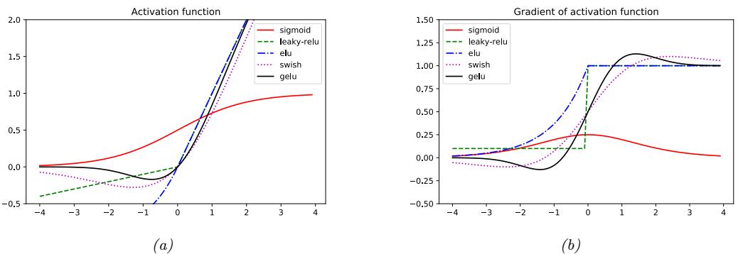
Figure 13.14: (a) Some popular activation functions. (b) Plot of their gradients. Generated by activation\_fun\_deriv\_jax.ipynb.
- Modify the the activation functions at each layer to prevent the gradient from becoming too large or too small; see Section 13.4.3.
- Modify the architecture so that the updates are additive rather than multiplicative; see Section 13.4.4.
- Modify the architecture to standardize the activations at each layer, so that the distribution of activations over the dataset remains constant during training; see Section 14.2.4.1.
- Carefully choose the initial values of the parameters; see Section 13.4.5.
13.4.3 Non-saturating activation functions
In Section 13.2.3, we mentioned that the sigmoid activation function saturates at 0 for large negative inputs, and at 1 for large positive inputs. It turns out that the gradient signal in these regimes is 0, preventing backpropagation from working.
To see why the gradient vanishes, consider a layer which computes z = ω(Wx), where the activation
function is sigmoidal:
\[ \varphi(a) = \sigma(a) = \frac{1}{1 + \exp(-a)}\tag{13.71} \]
If the weights are initialized to be large (positive or negative), then it becomes very easy for a = Wx to take on large values, and hence for z to saturate near 0 or 1, since the sigmoid saturates, as shown in Figure 13.14a.
Now let us consider how gradients propagate through this layer. The derivative of the activation function (elementwise) is given by
\[ \varphi'(a) = \sigma(a)(1 - \sigma(a))\tag{13.72} \]
See Figure 13.14b for a plot. By the chain rule, we can compute the Jacobian for this layer wrt the inputs by multiplying the Jacobian for the sigmoid nonlinearity, z = ω(a), using Equation (13.43), with the Jacobian for the linear layer, a = Wx, using Equation (13.49), to get
\[\frac{\partial \mathbf{z}}{\partial \mathbf{z}} = \text{diag}(\mathbf{z}(1-\mathbf{z})^{\mathsf{T}})\mathbf{W} \tag{13.73}\]
Hence, if z is near 0 or 1, the gradients wrt the inputs will go to 0.
Similarly, the Jacobian of this layer wrt the parameters can be computed by multiplying Equation (13.43) with Equation (13.55) to get
\[\frac{\partial z}{\partial \mathbf{W}} = z(1 - z)\mathbf{z}^{\mathsf{T}} \tag{13.74}\]
Hence, if z is near 0 or 1, the gradients wrt the parameters will go to 0.
One of the keys to being able to train very deep models is to use non-saturating activation functions. Several di!erent functions have been proposed: see Table 13.4 for a summary.
13.4.3.1 ReLU
The most common is rectified linear unit or ReLU, proposed in [GBB11; KSH12]. This is defined as
\[\text{ReLU}(a) = \max(a, 0) = a \mathbb{I}(a > 0) \tag{13.75}\]
The ReLU function simply “turns o!” negative inputs, and passes positive inputs unchanged. The gradient has the following form:
\[\text{ReLU}'(a) = \mathbb{I}\left(a > 0\right) \tag{13.76}\]
Now suppose we use this in a layer to compute z = ReLU(Wx). Using the results from Section 13.3.3, we can show that the Jacobian for this layer wrt the inputs has the form
\[\frac{\partial \mathbf{z}}{\partial \mathbf{z}} = \mathbf{W}^{\mathsf{T}} \mathbb{I}(\mathbf{z} > \mathbf{0}) \tag{13.77}\]
and wrt the parameters has the form
\[\frac{\partial \mathbf{z}}{\partial \mathbf{W}} = \mathbb{I}\left(\mathbf{z} > \mathbf{0}\right)\mathbf{z}^{\mathrm{T}}\tag{13.78}\]
Hence the gradient will not vanish, as long as z is positive.
Unfortunately, when using ReLU, if the weights are initialized to be large and negative, then it becomes very easy for (some components of) a = Wx to take on large negative values, and hence for z to go to 0. This will cause the gradient for the weights to go to 0. The algorithm will never be able to escape this situation, so the hidden units (components of z) will stay permanently o!. This is called the “dead ReLU” problem [Lu+19].
13.4.3.2 Non-saturating ReLU
The problem of dead ReLU’s can be solved by using non-saturating variants of ReLU. One alternate is the leaky ReLU, proposed in [MHN13]. This is defined as
\[\text{LReLU}(a; \alpha) = \max(\alpha a, a) \tag{13.79}\]
where 0 < φ < 1. The slope of this function is 1 for positive inputs, and φ for negative inputs, thus ensuring there is some signal passed back to earlier layers, even when the input is negative. See Figure 13.14b for a plot. If we allow the parameter φ to be learned, rather than fixed, the leaky ReLU is called parametric ReLU [He+15].
Another popular choice is the ELU, proposed in [CUH16]. This is defined by
\[\text{ELU}(a;\alpha) = \begin{cases} \alpha(e^a - 1) & \text{if } a \le 0 \\ a & \text{if } a > 0 \end{cases} \tag{13.80}\]
This has the advantage over leaky ReLU of being a smooth function.6 See Figure 13.14 for plot.
A slight variant of ELU, known as SELU (self-normalizing ELU), was proposed in [Kla+17]. This has the form
\[\text{SELU}(a;\alpha,\lambda) = \lambda \text{ELU}(a;\alpha) \tag{13.81}\]
Surprisingly, they prove that by setting φ and ς to carefully chosen values, this activation function is guaranteed to ensure that the output of each layer is standardized (provided the input is also standardized), even without the use of techniques such as batchnorm (Section 14.2.4.1). This can help with model fitting.
13.4.3.3 Other choices
As an alternative to manually discovering good activation functions, we can use blackbox optimization methods to search over the space of functional forms. Such an approach was used in [RZL17], where they discovered a function they call swish that seems to do well on some image classification benchmarks. It is defined by
\[\text{swish}(a;\beta) = a\sigma(\beta a) \tag{13.82}\]
6. ELU only has a continuous first derivative if ω = 1.
(The same function, under the name SiLU (for Sigmoid Linear Unit), was independently proposed in [HG16].) See Figure 13.14 for plot.
Another popular activation function is GELU, which stands for “Gaussian Error Linear Unit” [HG16]. This is defined as follows:
\[\text{GELU}(a) = a\Phi(a) \tag{13.83}\]
where !(a) is the cdf of a standard normal:
\[\Phi(a) = \Pr(\mathcal{N}(0, 1) \le a) = \frac{1}{2} \left( 1 + \text{erf}(a/\sqrt{2}) \right) \tag{13.84}\]
We see from Figure 13.14 that this is not a convex or monontonic function, unlike most other activation functions.
We can think of GELU as a “soft” version of ReLU, since it replaces the step function I(a > 0) with the Gaussian cdf, !(a). Alternatively, the GELU can be motivated as an adaptive version of dropout (Section 13.5.4), where we multiply the input by a binary scalar mask, m ∝ Ber(!(a)), where the probability of being dropped is given by 1 ↗ !(a). Thus the expected output is
\[\mathbb{E}[a] = \Phi(a) \times a + (1 - \Phi(a)) \times 0 = a\Phi(a) \tag{13.85}\]
We can approximate GELU using swish with a particular parameter setting, namely
\[\text{GELU}(a) \approx a \sigma (1.702a) \tag{13.86}\]
The SmelU activation function proposed in [SLC20] is another smooth version of ReLU but which results in more reproducibility in terms of training runs, due to enhanced robustness to numerical issues.
13.4.4 Residual connections
One solution to the vanishing gradient problem for DNNs is to use a residual network or ResNet [He+16a]. This is a feedforward model in which each layer has the form of a residual block, defined by
\[\mathcal{F}\_l'(x) = \mathcal{F}\_l(x) + x \tag{13.87}\]
where Fl is a standard shallow nonlinear mapping (e.g., linear-activation-linear). The inner Fl function computes the residual term or delta that needs to be added to the input x to generate the desired output; it is often easier to learn to generate a small perturbation to the input than to directly predict the output. (Residual connections are usually used in conjunction with CNNs, as discussed in Section 14.3.4, but can also be used in MLPs.)
A model with residual connections has the same number of parameters as a model without residual connections, but it is easier to train. The reason is that gradients can flow directly from the output to earlier layers, as sketched in Figure 13.15b. To see this, note that the activations at the output layer can be derived in terms of any previous layer l using
\[\mathbf{z}\_{L} = \mathbf{z}\_{l} + \sum\_{i=l}^{L-1} \mathcal{F}\_{i}(\mathbf{z}\_{i}; \boldsymbol{\theta}\_{i}). \tag{13.88}\]
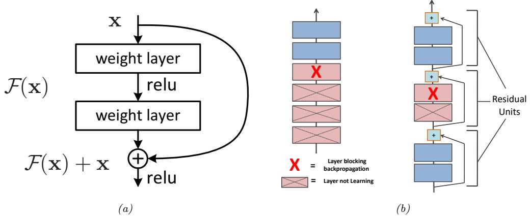
Figure 13.15: (a) Illustration of a residual block. (b) Illustration of why adding residual connections can help when training a very deep model. Adapted from Figure 14.16 of [Gér19].
We can therefore compute the gradient of the loss wrt the parameters of the l’th layer as follows:
\[\frac{\partial \mathcal{L}}{\partial \mathbf{a}} = \frac{\partial \mathbf{z}\_l}{\partial \mathbf{a}} \frac{\partial \mathcal{L}}{\partial \mathbf{a}} \tag{13.89}\]
\[\begin{split} \frac{\partial \boldsymbol{\theta}\_{l}}{\partial \boldsymbol{z}\_{l}} &= \frac{\partial \boldsymbol{\theta}\_{l}}{\partial \boldsymbol{z}\_{l}} \frac{\partial \boldsymbol{z}\_{l}}{\partial \boldsymbol{z}\_{L}} \frac{\partial \boldsymbol{z}\_{L}}{\partial \boldsymbol{z}\_{l}} \\ &= \frac{\partial \boldsymbol{z}\_{l}}{\partial \boldsymbol{\theta}\_{l}} \frac{\partial \mathcal{L}}{\partial \boldsymbol{z}\_{L}} \frac{\partial \boldsymbol{z}\_{L}}{\partial \boldsymbol{z}\_{l}} \end{split} \tag{13.90}\]
\[\mathcal{L} = \frac{\partial \mathbf{z}\_l}{\partial \boldsymbol{\theta}\_l} \frac{\partial \mathcal{L}}{\partial \mathbf{z}\_L} \left( \mathbf{1} + \sum\_{i=l}^{L-1} \frac{\partial \mathcal{F}\_i(\mathbf{z}\_i; \boldsymbol{\theta}\_i)}{\partial \mathbf{z}\_l} \right) \tag{13.91}\]
\[\mathbf{H} = \frac{\partial \mathbf{z}\_l}{\partial \theta\_l} \frac{\partial \mathcal{L}}{\partial \mathbf{z}\_L} + \text{other terms} \tag{13.92}\]
Thus we see that the gradient at layer l depends directly on the gradient at layer L in a way that is independent of the depth of the network.
13.4.5 Parameter initialization
Since the objective function for DNN training is non-convex, the way that we initialize the parameters of a DNN can play a big role on what kind of solution we end up with, as well as how easy the function is to train (i.e., how well information can flow forwards and backwards through the model). In the rest of this section, we present some common heuristic methods that are used for initializing parameters.
13.4.5.1 Heuristic initialization schemes
In [GB10], they show that sampling parameters from a standard normal with fixed variance can result in exploding activations or gradients. To see why, consider a linear unit with no activation
function given by oi = (nin j=1 wijxj ; suppose wij ∝ N (0, ω2), and E [xj ] = 0 and V [xj ] = ↽2, where we assume xj are independent of wij . The mean and variance of the output is given by
\[\mathbb{E}\left[o\_{i}\right] = \sum\_{j=1}^{n\_{\text{in}}} \mathbb{E}\left[w\_{ij}x\_{j}\right] = \sum\_{j=1}^{n\_{\text{in}}} \mathbb{E}\left[w\_{ij}\right] \mathbb{E}\left[x\_{j}\right] = 0 \tag{13.93}\]
\[\mathbb{E}\left[o\_i\right] = \mathbb{E}\left[o\_i^2\right] - \left(\mathbb{E}\left[o\_i\right]\right)^2 = \sum\_{j=1}^{n\_{\text{in}}} \mathbb{E}\left[w\_{ij}^2 x\_j^2\right] - 0 = \sum\_{j=1}^{n\_{\text{in}}} \mathbb{E}\left[w\_{ij}^2\right] \mathbb{E}\left[x\_j^2\right] = n\_{\text{in}} \sigma^2 \gamma^2 \tag{13.94}\]
To keep the output variance from blowing up, we need to ensure ninω2 = 1 (or some other constant), where nin is the fan-in of a unit (number of incoming connections).
Now consider the backwards pass. By analogous reasoning, we see that the variance of the gradients can blow up unless noutω2 = 1, where nout is the fan-out of a unit (number of outgoing connections). To satisfy both requirements at once, we set 1 2 (nin + nout)ω2 = 1, or equivalently
\[ \sigma^2 = \frac{2}{n\_{\rm in} + n\_{\rm out}} \tag{13.95} \]
This is known as Xavier initialization or Glorot initialization, named after the first author of [GB10].
A special case arises if we use ω2 = 1/nin; this is known as LeCun initialization, named after Yann LeCun, who proposed it in the 1990s. This is equivalent to Glorot initialization when nin = nout. If we use ω2 = 2/nin, the method is called He initialization, named after Kaiming He, who proposed it in [He+15].
Note that it is not necessary to use a Gaussian distribution. Indeed, the above derivation just worked in terms of the first two moments (mean and variance), and made no assumptions about Gaussianity. For example, suppose we sample weights from a uniform distribution, wij ∝ Unif(↗a, a). The mean is 0, and the variance is ω2 = a2/3. Hence we should set a = 6 nin+nout .
Although the above derivation assumes a linear output unit, the technique works well empirically even for nonlinear units. The best choice of initialization method depends on which activation function you use. For linear, tanh, logistic, and softmax, Glorot is recommended. For ReLU and variants, He is recommended. For SELU, LeCun is recommended. See e.g., [Gér19] for more heuristics, and e.g., [HDR19] for some theory.
13.4.5.2 Data-driven initializations
We can also adopt a data-driven approach to parameter initialization. For example, [MM16] proposed a simple but e!ective scheme known as layer-sequential unit-variance (LSUV) initialization, which works as follows. First we initialize the weights of each (fully connected or convolutional) layer with orthonormal matrices, as proposed in [SMG14]. (This can be achieved by drawing from w ∝ N (0, I), reshaping to w to a matrix W, and then computing an orthonormal basis using QR or SVD decomposition.) Then, for each layer l, we compute the variance vl of the activations across a minibatch; we then rescale using Wl := Wl/ ⇔vl. This scheme can be viewed as an orthonormal initialization combined with batch normalization performed only on the first mini-batch. This is faster than full batch normalization, but can sometimes work just as well.
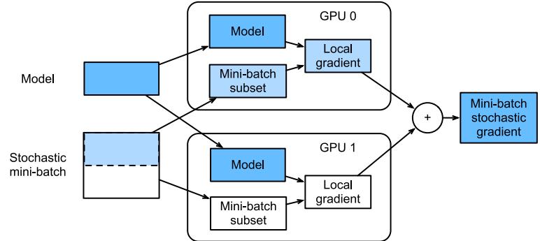
Figure 13.16: Calculation of minibatch stochastic gradient using data parallelism and two GPUs. From Figure 12.5.2 of [Zha+20]. Used with kind permission of Aston Zhang.
13.4.6 Parallel training
It can be quite slow to train large models on large datasets. One way to speed this process up is to use specialized hardware, such as graphics processing units (GPUs) and tensor processing units (TPUs), which are very e”cient at performing matrix-matrix multiplication. If we have multiple GPUs, we can sometimes further speed things up. There are two main approaches: model parallelism, in which we partition the model between machines, and data parallelism, in which each machine has its own copy of the model, and applies it to a di!erent set of data.
Model parallelism can be quite complicated, since it requires tight communication between machines to ensure they compute the correct answer. We will not discuss this further. Data parallelism is generally much simpler, since it is embarassingly parallel. To use this to speed up training, at each training step t, we do the following: 1) we partition the minibatch across the K machines to get Dk t ; 2) each machine k computes its own gradient, gk t = ⇑εL(ε; Dk t ); 3) we collect all the local gradients on a central machine (e.g., device 0) and sum them using gt = (K k=1 gk t ; 4) we broadcast the summed gradient back to all devices, so g˜k t = gt; 5) each machine updates its own copy of the parameters using εk t := εk t ↗ ⇀tg˜k t . See Figure 13.16 for an illustration and multi\_gpu\_training\_jax.ipynb for some sample code.
Note that steps 3 and 4 are usually combined into one atomic step; this is known as an all-reduce operation (where we use sum to reduce the set of (gradient) vectors into one). If each machine blocks until receiving the centrally aggregated gradient, gt, the method is known as synchronous training. This will give the same results as training with one machine (with a larger batchsize), only faster (assuming we ignore any batch normalization layers). If we let each machine update its parameters using its own local gradient estimate, and not wait for the broadcast to/from the other machines, the method is called asynchronous training. This is not guaranteed to work, since the di!erent machines may get out of step, and hence will be updating di!erent versions of the parameters; this approach has therefore been called hogwild training [Niu+11]. However, if the updates are sparse, so each machine “touches” a di!erent part of the parameter vector, one can prove that hogwild training behaves like standard synchronous SGD.
13.5 Regularization
In Section 13.4 we discussed computational issues associated with training (large) neural networks. In this section, we discuss statistical issues. In particular, we focus on ways to avoid overfitting. This is crucial, since large neural networks can easily have millions of parameters.
13.5.1 Early stopping
Perhaps the simplest way to prevent overfitting is called early stopping, which refers to the heuristic of stopping the training procedure when the error on the validation set starts to increase (see Figure 4.8 for an example). This method works because we are restricting the ability of the optimization algorithm to transfer information from the training examples to the parameters, as explained in [AS19].
13.5.2 Weight decay
A common approach to reduce overfitting is to impose a prior on the parameters, and then use MAP estimation. It is standard to use a Gaussian prior for the weights N (w|0, φ2I) and biases, N (b|0, ↼2I). This is equivalent to ε2 regularization of the objective. In the neural networks literature, this is called weight decay, since it encourages small weights, and hence simpler models, as in ridge regression (Section 11.3).
13.5.3 Sparse DNNs
Since there are many weights in a neural network, it is often helpful to encourage sparsity. This allows us to perform model compression, which can save memory and time. To do this, we can use ε1 regularization (as in Section 11.4), or ARD (as in Section 11.7.7), or several other methods (see e.g., [Hoe+21; Bha+20] for recent reviews). As a simple example, Figure 13.17 shows a 5 layer MLP which has been fit to some 1d regression data using an ε1 regularizer on the weights. We see that the resulting graph topology is sparse.
Despite the intuitive appeal of sparse topology, in practice these methods are not widely used, since modern GPUs are optimized for dense matrix multiplication, and there are few computational benefits to sparse weight matrices. However, if we use methods that encourage group sparsity, we can prune out whole layers of the model. This results in block sparse weight matrices, which can result in speedups and memory savings (see e.g., [Sca+17; Wen+16; MAV17; LUW17]).
13.5.4 Dropout
Suppose that we randomly (on a per-example basis) turn o! all the outgoing connections from each neuron with probability p, as illustrated in Figure 13.18. This technique is known as dropout [Sri+14].
Dropout can dramatically reduce overfitting and is very widely used. Intuitively, the reason dropout works well is that it prevents complex co-adaptation of the hidden units. In other words, each unit must learn to perform well even if some of the other units are missing at random. This prevents the
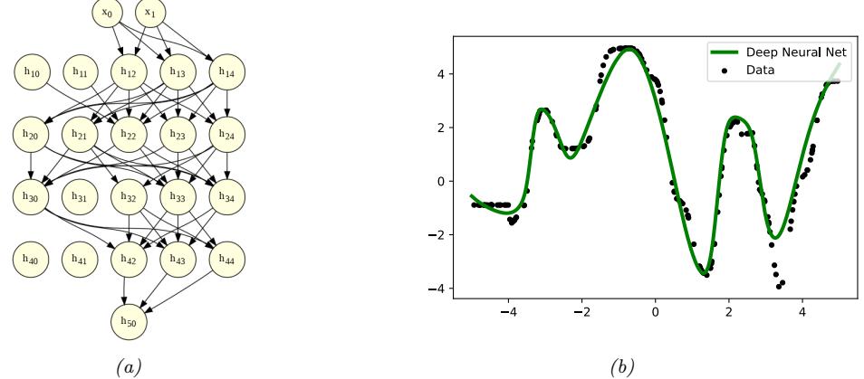
Figure 13.17: (a) A deep but sparse neural network. The connections are pruned using ε1 regularization. At each level, nodes numbered 0 are clamped to 1, so their outgoing weights correspond to the o!set/bias terms. (b) Predictions made by the model on the training set. Generated by sparse\_mlp.ipynb.
Figure 13.18: Illustration of dropout. (a) A standard neural net with 2 hidden layers. (b) An example of a thinned net produced by applying dropout with p0 = 0.5. Units that have been dropped out are marked with an x. From Figure 1 of [Sri+14]. Used with kind permission of Geo! Hinton.
units from learning complex, but fragile, dependencies on each other.7 A more formal explanation, in terms of Gaussian scale mixture priors, can be found in [NHLS19].
We can view dropout as estimating a noisy version of the weights, ⇁lji = wlji,li, where ,li ∝ Ber(1 ↗ p) is a Bernoulli noise term. (So if we sample ,li = 0, then all of the weights going out of unit i in layer l ↗ 1 into any j in layer l will be set to 0.) At test time, we usually turn the noise o!.
7. Geo! Hinton, who invented dropout, said he was inspired by a talk on sexual reproduction, which encourages genes to be individually useful (or at most depend on a small number of other genes), even when combined with random other genes.
To ensure the weights have the same expectation at test time as they did during training (so the input activation to the neurons is the same, on average), at test time we should use wlij = ⇁ljiE [,li]. For Bernoulli noise, we have E [,] = 1 ↗ p, so we should multiply the weights by the keep probability, 1 ↗ p, before making predictions.
We can, however, use dropout at test time if we wish. The result is an ensemble of networks, each with slightly di!erent sparse graph structures. This is called Monte Carlo dropout [GG16; KG17], and has the form
\[p(\mathbf{y}|\mathbf{z}, \mathcal{D}) \approx \frac{1}{S} \sum\_{s=1}^{S} p(\mathbf{y}|\mathbf{z}, \hat{\mathbf{W}}\epsilon^{s} + \hat{\mathbf{b}}) \tag{13.96}\]
where S is the number of samples, and we write Wˆ ,s to indicate that we are multiplying all the estimated weight matrices by a sampled noise vector. This can sometimes provide a good approximation to the Bayesian posterior predictive distribution p(y|x, D), especially if the noise rate is optimized [GHK17].
13.5.5 Bayesian neural networks
Modern DNNs are usually trained using a (penalized) maximum likelihood objective to find a single setting of parameters. However, with large models, there are often many more parameters than data points, so there may be multiple possible models which fit the training data equally well, yet which generalize in di!erent ways. It is often useful to capture the induced uncertainty in the posterior predictive distribution. This can be done by marginalizing out the parameters by computing
\[p(\mathbf{y}|\mathbf{z}, \mathcal{D}) = \int p(\mathbf{y}|\mathbf{z}, \boldsymbol{\theta}) p(\boldsymbol{\theta}|\mathcal{D}) d\boldsymbol{\theta} \tag{13.97}\]
The result is known as a Bayesian neural network or BNN. It can be thought of as an infinite ensemble of di!erently weight neural networks. By marginalizing out the parameters, we can avoid overfitting [Mac95]. Bayesian marginalization is challenging for large neural networks, but also can lead to significant performance gains [WI20]. For more details on the topic of Bayesian deep learning, see the sequel to this book, [Mur23].
13.5.6 Regularization e!ects of (stochastic) gradient descent *
Some optimization methods (in particular, second-order batch methods) are able to find “needles in haystacks”, corresponding to narrow but deep “holes” in the loss landscape, corresponding to parameter settings with very low loss. These are known as sharp minima, see Figure 13.19(right). From the point of view of minimizing the empirical loss, the optimizer has done a good job. However, such solutions generally correspond to a model that has overfit the data. It is better to find points that correspond to flat minima, as shown in Figure 13.19(left); such solutions are more robust and generalize better. To see why, note that flat minima correspond to regions in parameter space where there is a lot of posterior uncertainty, and hence samples from this region are less able to precisely memorize irrelevant details about the training set [AS17]. SGD often finds such flat minima by virtue of the addition of noise, which prevents it from “entering” narrow regions of the loss landscape (see e.g., [SL18]). This is called implicit regularization. It is also possible to explicitly encourage
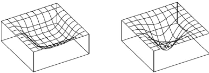
Figure 13.19: Flat vs sharp minima. From Figures 1 and 2 of [HS97a]. Used with kind permission of Jürgen Schmidhuber.
Figure 13.20: Each curve shows how the loss varies across parameter values for a given minibatch. (a) A stable local minimum. (b) An unstable local minimum. Generated by sgd\_minima\_variance.ipynb. Adapted from https: // bit. ly/ 3wTc1L6 .
SGD to find such flat minima, using entropy SGD [Cha+17], sharpness aware minimization [For+21], stochastic weight averaging (SWA) [Izm+18], and other related techniques.
Of course, the loss landscape depends not just on the parameter values, but also on the data. Since we usually cannot a!ord to do full-batch gradient descent, we will get a set of loss curves, one per minibatch. If each one of these curves corresponds to a wide basin, as shown in Figure 13.20a, we are at a point in parameter space that is robust to perturbations, and will likely generalize well. However, if the overall wide basin is the result of averaging over many di!erent narrow basins, as shown in Figure 13.20b, the resulting estimate will likely generalize less well.
This can be formalized using the analysis in [Smi+21; BD21]. Specifically, they consider continuous time gradient flow which approximates the behavior of (S)GD. In [BD21], they consider full-batch GD, and show that the flow has the form w˙ = ↗⇑wL˜GD(w), where
\[\bar{\mathcal{L}}\_{GD}(\boldsymbol{w}) = \mathcal{L}(\boldsymbol{w}) + \frac{\epsilon}{4} ||\nabla \mathcal{L}(\boldsymbol{w})||^2 \tag{13.98}\]
where L(w) is the original loss, , is the learning rate, and the second term is an implicit regularization term that penalizes solutions with large gradients (high curvature).
In [Smi+21], they extend this analysis to the SGD case. They show that the flow has the form w˙ = ↗⇑wL˜SGD(w), where
\[\bar{\mathcal{L}}\_{SGD}(\mathbf{w}) = \mathcal{L}(\mathbf{w}) + \frac{\epsilon}{4m} \sum\_{k=1}^{m} ||\nabla \mathcal{L}\_k(\mathbf{w})||^2 \tag{13.99}\]
where m is the number of minibatches, and Lk(w) is the loss on the k’th such minibatch. Comparing this to the full-batch GD loss, we see
\[\tilde{\mathcal{L}}\_{SGD}(\boldsymbol{w}) = \tilde{\mathcal{L}}\_{GD}(\boldsymbol{w}) + \frac{\epsilon}{4m} \sum\_{k=1}^{m} ||\nabla \mathcal{L}\_k(\boldsymbol{w}) - \nabla \mathcal{L}(\boldsymbol{w})||^2 \tag{13.100}\]
The second term estimates the variance of the minibatch gradients, which is a measure of stability, and hence of generalization ability.
The above analysis shows that SGD not only has computational advantages (since it is faster than full-batch GD or second-order methods), but also statistical advantages.
13.5.7 Over-parameterized models
Modern neural networks use many more parameters P than training examples N. Such models are said to be over-parameterized. As such, they typically achieve zero training loss (at least for classification problems). Despite this, they often generalize better than models where P ∞ N. In particular, it is observed that models where P <N show the usual U-shaped curve, where test error initially decreases with increasing P, and then increases as the model starts to overfit, as predicted by the bias-variance tradeo! discussed in Section 4.7.6.3. However, when P >N, test error starts to decrease again; this is known as the double descent phenomenon [HK92; Bel+19; Nak+19]. Intuitively the reason for this is as follows: when P = N, the model may need to represent a very non-smooth function to interpolate the data (see Figure 1.7c), but when P ∈ N, it can interpolate the data (thus getting zero training error) using a smooth function [BS21]. See [DMB21] for details.
13.6 Other kinds of feedforward networks *
13.6.1 Radial basis function networks
Consider a 1 layer neural net where the hidden layer is given by the feature vector
\[\phi(x) = [\mathbb{K}(x, \mu\_1), \dots, \mathbb{K}(x, \mu\_K)] \tag{13.101}\]
where µk → X are a set of K centroids or exemplars, and K(x, µ) ↓ 0 is a kernel function. We describe kernel functions in detail in Section 17.1. Here we just give an example, namely the Gaussian kernel
\[\mathcal{K}\_{\text{gauss}}(\mathbf{z}, \mathbf{c}) \stackrel{\Delta}{=} \exp\left(-\frac{1}{2\sigma^2}||\mathbf{c} - \mathbf{z}||\_2^2\right) \tag{13.102}\]
The parameter ω is known as the bandwidth of the kernel. Note that this kernel is shift invariant, meaning it is only a function of the distance r = ||x ↗ c||2, so we can equivalently write this as
\[\mathcal{K}\_{\text{gauss}}(r) \stackrel{\Delta}{=} \exp\left(-\frac{1}{2\sigma^2}r^2\right) \tag{13.103}\]
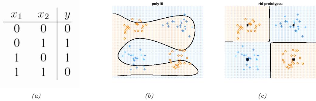
Figure 13.21: (a) xor truth table. (b) Fitting a linear logistic regression classifier using degree 10 polynomial expansion. (c) Same model, but using an RBF kernel with centroids specified by the 4 black crosses. Generated by logregXorDemo.ipynb.
This is therefore called a radial basis function kernel or RBF kernel.
A 1 layer neural net in which we use Equation (13.101) as the hidden layer, with RBF kernels, is called an RBF network [BL88]. This has the form
\[p(y|x; \theta) = p(y|w^\top \phi(x))\tag{13.104}\]
where ε = (µ, w). If the centroids µ are fixed, we can solve for the optimal weights w using (regularized) least squares, as discussed in Chapter 11. If the centroids are unknown, we can estimate them by using an unsupervised clustering method, such as K-means (Section 21.3). Alternatively, we can associate one centroid per data point in the training set, to get µn = xn, where now K = N. This is an example of a non-parametric model, since the number of parameters grows (in this case linearly) with the amount of data, and is not independent of N. If K = N, the model can perfectly interpolate the data, and hence may overfit. However, by ensuring that the output weight vector w is sparse, the model will only use a finite subset of the input examples; this is called a sparse kernel machine, and will be discussed in more detail in Section 17.4.1 and Section 17.3. Another way to avoid overfitting is to adopt a Bayesian approach, by integrating out the weights w; this gives rise to a model called a Gaussian process, which will be discussed in more detail in Section 17.2.
13.6.1.1 RBF network for regression
We can use RBF networks for regression by defining p(y|x, ε) = N (wT ω(x), ω2). For example, Figure 13.22 shows a 1d data set fit with K = 10 uniformly spaced RBF prototypes, but with the bandwidth ranging from small to large. Small values lead to very wiggly functions, since the predicted function value will only be non-zero for points x that are close to one of the prototypes µk. If the bandwidth is very large, the design matrix reduces to a constant matrix of 1’s, since each point is equally close to every prototype; hence the corresponding function is just a straight line.
13.6.1.2 RBF network for classification
We can use RBF networks for binary classification by defining p(y|x, ε) = Ber(ω(wT ω(x))). As an example, consider the data coming from the exclusive or function. This is a binary-valued function
Figure 13.22: Linear regression using 10 equally spaced RBF basis functions in 1d. Left column: fitted function. Middle column: basis functions evaluated on a grid. Right column: design matrix. Top to bottom we show di!erent bandwidths for the kernel function: ω = 0.5, 10, 50. Generated by linregRbfDemo.ipynb.
of two binary inputs. Its truth table is shown in Figure 13.21(a). In Figure 13.21(b), we have shown some data labeled by the xor function, but we have jittered the points to make the picture clearer.8 We see we cannot separate the data even using a degree 10 polynomial. However, using an RBF kernel and just 4 prototypes easily solves the problem as shown in Figure 13.21(c).
13.6.2 Mixtures of experts
When considering regression problems, it is common to assume a unimodal output distribution, such as a Gaussian or Student distribution, where the mean and variance is some function of the input, i.e.,
\[p(\mathbf{y}|\mathbf{z}) = \mathcal{N}(\mathbf{y}|f\_{\mu}(\mathbf{z}), \text{diag}(\sigma\_{+}(f\_{\sigma}(\mathbf{z}))))\tag{13.105}\]
where the f functions may be MLPs (possibly with some shared hidden units, as in Figure 13.5). However, this will not work well for one-to-many functions, in which each input can have multiple possible outputs.
Figure 13.23a gives a simple example of such a function. We see that in the middle of the plot there are certain x values for which there are two equally probable y values. There are many real world problems of this form, e.g., 3d pose prediction of a person from a single image [Bo+08], colorization
8. Jittering is a common visualization trick in statistics, wherein points in a plot/display that would otherwise land on top of each other are dispersed with uniform additive noise.
(a) (b) (c) (d)
Figure 13.23: (a) Some data from a one-to-many function. Horizontal axis is the input x, vertical axis is the target y = f(x). (b) The responsibilities of each expert for the input domain. (c) Prediction of each expert (colored lines) superimposed on the training data. (d) Overall prediction. Mean is red cross, mode is black square. Adapted from Figures 5.20 and 5.21 of [Bis06]. Generated by mixexpDemoOneToMany.ipynb.
of a black and white image [Gua+17], predicting future frames of a video sequence [VT17], etc. Any model which is trained to maximize likelihood using a unimodal output density — even if the model is a flexible nonlinear model, such as neural network — will work poorly on one-to-many functions such as these, since it will just produce a blurry average output.
To prevent this problem of regression to the mean, we can use a conditional mixture model. That is, we assume the output is a weighted mixture of K di!erent outputs, corresponding to di!erent modes of the output distribution for each input x. In the Gaussian case, this becomes
\[p(\mathbf{y}|\mathbf{x}) = \sum\_{k=1}^{K} p(\mathbf{y}|\mathbf{x}, z=k)p(z=k|\mathbf{x})\tag{13.106}\]
\[p(y|x, z=k) = \mathcal{N}(y|f\_{\mu,k}(x), \text{diag}(f\_{\sigma,k}(x)))\tag{13.107}\]
\[p(z=k|\mathbf{x}) = \text{Cat}(z|\text{softmax}(f\_z(\mathbf{x}))) \tag{13.108}\]
Here fµ,k predicts the mean of the k’th Gaussian, fε,k predicts its variance terms, and fz predicts which mixture component to use. This model is called a mixture of experts (MoE) [Jac+91; JJ94; YWG12; ME14]. The idea is that the k’th submodel p(y|x, z = k) is considered to be an “expert” in a certain region of input space. The function p(z = k|x) is called a gating function, and
decides which expert to use, depending on the input values. By picking the most likely expert for a given input x, we can “activate” just a subset of the model. This is an example of conditional computation, since we decide what expert to run based on the results of earlier computations from the gating network [Sha+17].
We can train this model using SGD, or using the EM algorithm (see Section 8.7.3 for details on the latter method).
13.6.2.1 Mixture of linear experts
In this section, we consider a simple example in which we use linear regression experts and a linear classification gating function, i.e., the model has the form:
\[p(y|\mathbf{z}, z=k, \boldsymbol{\theta}) = \mathcal{N}(y|\mathbf{w}\_k^\top \mathbf{z}, \sigma\_k^2) \tag{13.109}\]
\[p(z=k|\mathbf{x}, \theta) = \text{Cat}(z|\text{softmax}\_k(\mathbf{V}\mathbf{x})) \tag{13.110}\]
where softmaxk is the k’th output from the softmax function. The individual weighting term p(z = k|x) is called the responsibility for expert k for input x. In Figure 13.23b, we see how the gating networks softly partitions the input space amongst the K = 3 experts.
Each expert p(y|x, z = k) corresponds to a linear regression model with di!erent parameters. These are shown in Figure 13.23c.
If we take a weighted combination of the experts as our output, we get the red curve in Figure 13.23d, which is clearly is a bad predictor. If instead we only predict using the most active expert (i.e., the one with the highest responsibility), we get the discontinuous black curve, which is a much better predictor.
13.6.2.2 Mixture density networks
The gating function and experts can be any kind of conditional probabilistic model, not just a linear model. If we make them both DNNs, then resulting model is called a mixture density network (MDN) [Bis94; ZS14] or a deep mixture of experts [CGG17]. See Figure 13.24 for a sketch of the model.
13.6.2.3 Hierarchical MOEs
If each expert is itself an MoE model, the resulting model is called a hierarchical mixture of experts [JJ94]. See Figure 13.25 for an illustration of such a model with a two level hierarchy.
An HME with L levels can be thought of as a “soft” decision tree of depth L, where each example is passed through every branch of the tree, and the final prediction is a weighted average. (We discuss decision trees in Section 18.1.)
13.7 Exercises
Exercise 13.1 [Backpropagation for a MLP]
(Based on an exercise by Kevin Clark.)
Figure 13.24: Deep MOE with m experts, represented as a neural network. From Figure 1 of [CGG17]. Used with kind permission of Jacob Goldberger.
Figure 13.25: A 2-level hierarchical mixture of experts as a neural network. The top gating network chooses between the left and right expert, shown by the large boxes; the left and right experts themselves choose between their left and right sub-experts.
Consider the following classification MLP with one hidden layer:
\[\mathbf{x} = \text{input} \in \mathbb{R}^D \tag{13.111}\]
\[\mathbf{z} = \mathbf{W}\mathbf{z} + \mathbf{b}\_1 \in \mathbb{R}^K \tag{13.112}\]
\[h = \text{ReLU}(\mathbf{z}) \in \mathbb{R}^K \tag{13.113}\]
\[a = \mathbf{U}h + b\_2 \in \mathbb{R}^C\tag{13.114}\]
\[\mathcal{L} = \text{CrossEntropy}(\mathbf{y}, \text{softmax}(\mathbf{a})) \in \mathbb{R} \tag{13.115}\]
where x → RD, b1 → RK, W → RK→D, b2 → RC , U → RC→K, where D is the size of the input, K is the number of hidden units, and C is the number of classes. Show that the gradients for the parameters and input are as follows:
\[\nabla \mathbf{v} \mathcal{L} = \left[ \frac{\partial \mathcal{L}}{\partial \mathbf{V}} \right]\_{1,:} = \delta\_1 \boldsymbol{\hbar}^{\mathsf{T}} \in \mathbb{R}^{C \times K} \tag{13.116}\]
\[\nabla\_{\mathbf{b}\_2} \mathcal{L} = \left(\frac{\partial \mathcal{L}}{\partial \mathbf{b}\_2}\right)^{\mathsf{T}} = \boldsymbol{\delta}\_1 \in \mathbb{R}^C \tag{13.117}\]
\[ \nabla\_{\mathbf{W}} \mathcal{L} = \left[ \frac{\partial \mathcal{L}}{\partial \mathbf{W}} \right]\_{1,:} = \mathfrak{G}\_2 \mathbf{z}^\top \in \mathbb{R}^{K \times D} \tag{13.118} \]
\[\nabla \mathbf{b}\_1 \mathcal{L} = \left(\frac{\partial \mathcal{L}}{\partial \mathbf{b}\_1}\right)^\mathsf{T} = \delta\_2 \in \mathbb{R}^K \tag{13.119}\]
\[\nabla\_{\mathbf{z}} \mathcal{L} = \left(\frac{\partial \mathcal{L}}{\partial \mathbf{z}}\right)^{\mathsf{T}} = \mathbf{W}^{\mathsf{T}} \ \mathsf{ } \mathsf{G} \in \mathbb{R}^{D} \tag{13.120}\]
where the gradients of the loss wrt the two layers (logit and hidden) are given by the following:
\[\boldsymbol{\delta}\_{1} = \nabla\_{\mathbf{a}} \mathcal{L} = \left(\frac{\partial \mathcal{L}}{\partial \mathbf{a}}\right)^{\mathsf{T}} = (\mathsf{p} - \mathsf{y}) \in \mathbb{R}^{C} \tag{13.121}\]
\[\boldsymbol{\delta}\_{2} = \nabla\_{\mathbf{z}} \mathcal{L} = \left(\frac{\partial \mathcal{L}}{\partial \mathbf{z}}\right)^{\mathsf{T}} = (\mathbf{V}^{\mathsf{T}} \ \boldsymbol{\delta}\_{1}) \odot \boldsymbol{H}(\mathbf{z}) \in \mathbb{R}^{K} \tag{13.122}\]
where H is the Heaviside function. Note that, in our notation, the gradient (which has the same shape as the variable with respect to which we di!erentiate) is equal to the Jacobian’s transpose when the variable is a vector and to the first slice of the Jacobian when the variable is a matrix.
14 Neural Networks for Images
14.1 Introduction
In Chapter 13, we discussed multilayered perceptrons (MLPs) as a way to learn functions mapping “unstructured” input vectors x → RD to outputs. In this chapter, we extend this to the case where the input x has 2d spatial structure. (Similar ideas apply to 1d temporal structure, or 3d spatio-temporal structure.)
To see why it is not a good idea to apply MLPs directly to image data, recall that the core operation in an MLP at each hidden layer is computing the activations z = ϑ(Wx), where x is the input to a layer, W are the weights, and ϑ() is the nonlinear activation function. Thus the j’th element of the hidden layer has value zj = ϑ(wT j x). We can think of this inner product operation as comparing the input x to a learned template or pattern wj ; if the match is good (large positive inner product), the activation of that unit will be large (assuming a ReLU nonlinearity), signalling that the j’th pattern is present in the input.
However, this does not work well if the input is a variable-sized image, x → RWHC , where W is the width, H is the height, and C is the number of input channels (e.g., C = 3 for RGB color). The problem is that we would need to learn a di!erent-sized weight matrix W for every size of input image. In addition, even if the input was fixed size, the number of parameters needed would be prohibitive for reasonably sized images, since the weight matrix would have size (W ↑ H ↑ C) ↑ D, where D is the number of outputs (hidden units). The final problem is that a pattern that occurs in one location may not be recognized when it occurs in a di!erent location — that is, the model may not exhibit translation invariance — because the weights are not shared across locations (see Figure 14.1).
To solve these problems, we will use convolutional neural networks (CNNs), in which we replace matrix multiplication with a convolution operation. We explain this in detail in Section 14.2, but the basic idea is to divide the input into overlapping 2d image patches, and to compare each patch with a set of small weight matrices, or filters, which represent parts of an object; this is illustrated in Figure 14.2. We can think of this as a form of template matching. We will learn these templates from data, as we explain below. Because the templates are small (often just 3x3 or 5x5), the number of parameters is significantly reduced. And because we use convolution to do the template matching, instead of matrix multiplication, the model will be translationally invariant. This is useful for tasks such as image classification, where the goal is to classify if an object is present, regardless of its location.
CNNs have many other applications besides image classification, as we will discuss later in this chapter. They can also be applied to 1d inputs (see Section 15.3) and 3d inputs; however, we mostly
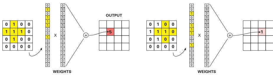
Figure 14.1: Detecting patterns in 2d images using unstructured MLPs does not work well, because the method is not translation invariant. We can design a weight vector to act as a matched filter for detecting the desired cross-shape. This will give a strong response of 5 if the object is on the left, but a weak response of 1 if the object is shifted over to the right. Adapted from Figure 7.16 of [SAV20].
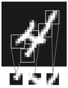
Figure 14.2: We can classify a digit by looking for certain discriminative features (image templates) occuring in the correct (relative) locations. From Figure 5.1 of [Cho17]. Used with kind permission of Francois Chollet.
focus on the 2d case in this chapter.
14.2 Common layers
In this section, we discuss the basics of CNNs.
14.2.1 Convolutional layers
We start by describing the basics of convolution in 1d, and then in 2d, and then describe how they are used as a key component of CNNs.
14.2.1.1 Convolution in 1d
The convolution between two functions, say f,g : RD ≃ R, is defined as
\[f(f\circledast g)(\mathbf{z}) = \int\_{\mathbb{R}^D} f(\mathbf{u})g(\mathbf{z}-\mathbf{u})d\mathbf{u} \tag{14.1}\]
Now suppose we replace the functions with finite-length vectors, which we can think of as functions defined on a finite set of points. For example, suppose f is evaluated at the points {↗L, ↗L +
| - | - | 1 | 2 | 3 | 4 | - | - | |
|---|---|---|---|---|---|---|---|---|
| 7 | 6 | 5 | - | - | - | - | - | z0 = x0w0 = 5 |
| - | 7 | 6 | 5 | - | - | - | - | z1 = x0w1 + x1w0 = 16 |
| - | - | 7 | 6 | 5 | - | - | - | z2 = x0w2 + x1w1 + x2w0 = 34 |
| - | - | - | 7 | 6 | 5 | - | - | z3 = x1w2 + x2w1 + x3w0 = 52 |
| - | - | - | - | 7 | 6 | 5 | - | z4 = x2w2 + x3w1 = 45 |
| - | - | - | - | - | 7 | 6 | 5 | z5 = x3w2 = 28 |
Figure 14.3: Discrete convolution of x = [1, 2, 3, 4] with w = [5, 6, 7] to yield z = [5, 16, 34, 52, 45, 28]. We see that this operation consists of “flipping” w and then “dragging” it over x, multiplying elementwise, and adding up the results.
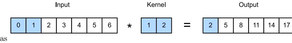
Figure 14.4: 1d cross correlation. From Figure 15.3.2 of [Zha+20]. Used with kind permission of Aston Zhang.
1,…, 0, 1,…,L} to yield the weight vector (also called a filter or kernel) w→L = f(↗L) up to wL = f(L). Now let g be evaluated at points {↗N,…,N} to yield the feature vector x→N = g(↗N) up to xN = g(N). Then the above equation becomes
\[[\mathbf{w} \circledast \mathbf{z}](i) = w\_{-L}x\_{i+L} + \dots + w\_{-1}x\_{i+1} + w\_0x\_i + w\_1x\_{i-1} + \dots + w\_Lx\_{i-L} \tag{14.2}\]
(We discuss boundary conditions (edge e!ects) later on.) We see that we “flip” the weight vector w (since indices of w are reversed), and then “drag” it over the x vector, summing up the local windows at each point, as illustrated in Figure 14.3.
There is a very closely related operation, in which we do not flip w first:
\[[w\*x](i) = w\_{-L}x\_{i-L} + \dots + w\_{-1}x\_{i-1} + w\_0x\_i + w\_1x\_{i+1} + \dots + w\_Lx\_{i+L} \tag{14.3}\]
This is called cross correlation; If the weight vector is symmetric, as is often the case, then cross correlation and convolution are the same. In the deep learning literature, the term “convolution” is usually used to mean cross correlation; we will follow this convention.
We can also evaluate the weights w on domain {0, 1,…,L ↗ 1} and the features x on domain {0, 1,…,N ↗ 1}, to eliminate negative indices. Then the above equation becomes
\[[w \circledast x](i) = \sum\_{u=0}^{L-1} w\_u x\_{i+u} \tag{14.4}\]
See Figure 14.4 for an example.
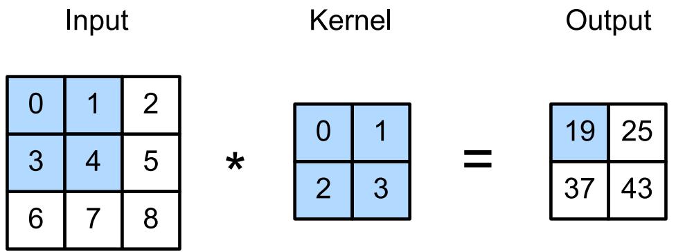
Figure 14.5: Illustration of 2d cross correlation. Generated by conv2d\_jax.ipynb. Adapted from Figure 6.2.1 of [Zha+20].
Figure 14.6: Convolving a 2d image (left) with a 3 ↑ 3 filter (middle) produces a 2d response map (right). The bright spots of the response map correspond to locations in the image which contain diagonal lines sloping down and to the right. From Figure 5.3 of [Cho17]. Used with kind permission of Francois Chollet.
14.2.1.2 Convolution in 2d
In 2d, Equation (14.4) becomes
\[\mathbb{E}\left[\mathbf{W}\oplus\mathbf{X}\right](i,j) = \sum\_{u=0}^{H-1}\sum\_{v=0}^{W-1} w\_{u,v} x\_{i+u,j+v} \tag{14.5}\]
where the 2d filter W has size H ↑ W. For example, consider convolving a 3 ↑ 3 input X with a 2 ↑ 2 kernel W to compute a 2 ↑ 2 output Y:
\[\mathbf{Y} = \begin{pmatrix} w\_1 & w\_2 \\ w\_3 & w\_4 \end{pmatrix} \oplus \begin{pmatrix} x\_1 & x\_2 & x\_3 \\ x\_4 & x\_5 & x\_6 \\ x\_7 & x\_8 & x\_9 \end{pmatrix} \tag{14.6}\]
\[\mathbf{x} = \begin{pmatrix} (w\_1x\_1 + w\_2x\_2 + w\_3x\_4 + w\_4x\_5) & (w\_1x\_2 + w\_2x\_3 + w\_3x\_5 + w\_4x\_6) \\ (w\_1x\_4 + w\_2x\_5 + w\_3x\_7 + w\_4x\_8) & (w\_1x\_5 + w\_2x\_6 + w\_3x\_8 + w\_4x\_9) \end{pmatrix} \tag{14.7}\]
See Figure 14.5 for a visualization of this process.
We can think of 2d convolution as template matching, since the output at a point (i, j) will be large if the corresponding image patch centered on (i, j) is similar to W. If the template W corresponds to an oriented edge, then convolving with it will cause the output heat map to “light up” in regions that contain edges that match that orientation, as shown in Figure 14.6. More generally, we can think of convolution as a form of feature detection. The resulting output Y = W↬ X is therefore called a feature map.
14.2.1.3 Convolution as matrix-vector multiplication
Since convolution is a linear operator, we can represent it by matrix multiplication. For example, consider Equation (14.7). We can rewrite this as matrix-vector mutiplication by flattening the 2d matrix X into a 1d vector x, and multiplying by a Toeplitz-like matrix C derived from the kernel W, as follows:
\[\mathbf{y} = \mathbf{C} \mathbf{x} = \begin{pmatrix} w\_1 & w\_2 & 0 & w\_3 & w\_4 & 0 & 0 & 0 & 0 \\ 0 & w\_1 & w\_2 & 0 & w\_3 & w\_4 & 0 & 0 & 0 \\ 0 & 0 & 0 & 0 & w\_1 & w\_2 & 0 & w\_3 & w\_4 & 0 \\ 0 & 0 & 0 & 0 & 0 & w\_1 & w\_2 & 0 & w\_3 & w\_4 \end{pmatrix} \begin{pmatrix} x\_1 \\ x\_2 \\ x\_3 \\ x\_4 \\ x\_5 \\ x\_6 \\ x\_7 \\ x\_8 \\ x\_9 \end{pmatrix} \tag{14.8}\]
\[= \begin{pmatrix} w\_1 x\_1 + w\_2 x\_2 + w\_3 x\_4 + w\_4 x\_5 \\ w\_1 x\_2 + w\_2 x\_3 + w\_3 x\_5 + w\_4 x\_6 \\ w\_1 x\_4 + w\_2 x\_5 + w\_3 x\_7 + w\_4 x\_8 \end{pmatrix} \tag{14.9}\]
We can recover the 2 ↑ 2 output by reshaping the 4 ↑ 1 vector y back to Y. 1
Thus we see that CNNs are like MLPs where the weight matrices have a special sparse structure, and the elements are tied across spatial locations. This implements the idea of translation invariance, and massively reduces the number of parameters compared to a weight matrix in a standard fully connected or dense layer, as used in MLPs.
14.2.1.4 Boundary conditions and padding
w1x5 + w2x6 + w3x8 + w4x9
In Equation (14.7), we saw that convolving a 3 ↑ 3 image with a 2 ↑ 2 filter resulted in a 2 ↑ 2 output. In general, convolving a fh ↑ fw filter over an image of size xh ↑ xw produces an output of size (xh ↗ fh + 1) ↑ (xw ↗ fw + 1); this is called valid convolution, since we only apply the filter to “valid” parts of the input, i.e., we don’t let it “slide o! the ends”. If we want the output to have the same size as the input, we can use zero-padding, which means we add a border of 0s to the image, as illustrated in Figure 14.7. This is called same convolution.
1. See conv2d\_jax.ipynb for a demo.
Figure 14.7: Same-convolution (using zero-padding) ensures the output is the same size as the input. Adapted from Figure 8.3 of [SAV20].
Figure 14.8: Illustration of padding and strides in 2d convolution. (a) We apply “same convolution” to a ↑ 7 input (with zero padding) using a 3 ↑ 3 filter to create a 5 ↑ 7 output. (b) Now we use a stride of 2, so the output has size 3 ↑ 4. Adapted from Figures 14.3–14.4 of [Gér19].
In general, if the input has size xh ↑ xw, we use a kernel of size fh ↑ fw, we use zero padding on each side of size ph and pw, then the output has the following size [DV16]:
\[(x\_h + 2p\_h - f\_h + 1) \times (x\_w + 2p\_w - f\_w + 1) \tag{14.10}\]
For example, consider Figure 14.8a. We have p = 1, f = 3, xh = 5 and xw = 7, so the output has size
\[(5+2-3+1)\times(7+2-3+1) = 5\times7\tag{14.11}\]
If we set 2p = f ↗ 1, then the output will have the same size as the input.
Figure 14.9: Illustration of 2d convolution applied to an input with 2 channels. Generated by conv2d\_jax.ipynb. Adapted from Figure 6.4.1 of [Zha+20].
14.2.1.5 Strided convolution
Since each output pixel is generated by a weighted combination of inputs in its receptive field (based on the size of the filter), neighboring outputs will be very similar in value, since their inputs are overlapping. We can reduce this redundancy (and speedup computation) by skipping every s’th input. This is called strided convolution. This is illustrated in Figure 14.8b, where we convolve a 5 ↑ 7 image with a 3 ↑ 3 filter with stride 2 to get a 3 ↑ 4 output.
In general, if the input has size xh ↑ xw, we use a kernel of size fh ↑ fw, we use zero padding on each side of size ph and pw, and we use strides of size sh and sw, then the output has the following size [DV16]:
\[\left\lfloor \frac{x\_h + 2p\_h - f\_h + s\_h}{s\_h} \right\rfloor \times \left\lfloor \frac{x\_w + 2p\_w - f\_w + s\_w}{s\_w} \right\rfloor \tag{14.12}\]
For example, consider Figure 14.8b, where we set the stride to s = 2. Now the output is smaller than the input, and has size
\[ \lfloor \frac{5+2-3+2}{2} \rfloor \times \lfloor \frac{7+2-3+2}{2} \rfloor = \lfloor \frac{6}{2} \rfloor \times \lfloor \frac{4}{1} \rfloor = 3 \times 4 \tag{14.13} \]
14.2.1.6 Multiple input and output channels
In Figure 14.6, the input was a gray-scale image. In general, the input will have multiple channels (e.g., RGB, or hyper-spectral bands for satellite images). We can extend the definition of convolution to this case by defining a kernel for each input channel; thus now W is a 3d weight matrix or tensor. We compute the output by convolving channel c of the input with kernel W:,:,c, and then summing over channels:
\[z\_{i,j} = b + \sum\_{u=0}^{H-1} \sum\_{v=0}^{W-1} \sum\_{c=0}^{C-1} x\_{si+u,sj+v,c} w\_{u,v,c} \tag{14.14}\]
Figure 14.10: Illustration of a CNN with 2 convolutional layers. The input has 3 color channels. The feature maps at internal layers have multiple channels. The cylinders correspond to hypercolumns, which are feature vectors at a certain location. Adapted from Figure 14.6 of [Gér19].
where s is the stride (which we assume is the same for both height and width, for simplicity), and b is the bias term. This is illustrated in Figure 14.9.
Each weight matrix can detect a single kind of feature. We typically want to detect multiple kinds of features, as illustrated in Figure 14.2. We can do this by making W into a 4d weight matrix. The filter to detect feature type d in input channel c is stored in W:,:,c,d. We extend the definition of convolution to this case as follows:
\[z\_{i,j,d} = b\_d + \sum\_{u=0}^{H-1} \sum\_{v=0}^{W-1} \sum\_{c=0}^{C-1} x\_{si+u,sj+v,c} w\_{u,v,c,d} \tag{14.15}\]
This is illustrated in Figure 14.10. Each vertical cylindrical column denotes the set of output features at a given location, zi,j,1:D; this is sometimes called a hypercolumn. Each element is a di!erent weighted combination of the C features in the receptive field of each of the feature maps in the layer below.2
14.2.1.7 1 → 1 (pointwise) convolution
Sometimes we just want to take a weighted combination of the features at a given location, rather than across locations. This can be done using 1x1 convolution, also called pointwise convolution.
2. In Tensorflow, a filter for 2d CNNs has shape (H, W, C, D), and a minibatch of feature maps has shape (batch-size, image-height, image-width, image-channels); this is called NHWC format. Other systems use di!erent data layouts.
Figure 14.11: Mapping 3 channels to 2 using convolution with a filter of size 1 ↑ 1 ↑ 3 ↑ 2. Adapted from Figure 6.4.2 of [Zha+20].
Figure 14.12: Illustration of maxpooling with a 2x2 filter and a stride of 1. Adapted from Figure 6.5.1 of [Zha+20].
This changes the number of channels from C to D, without changing the spatial dimensionality:
\[z\_{i,j,d} = b\_d + \sum\_{c=0}^{C-1} x\_{i,j,c} w\_{0,0,c,d} \tag{14.16}\]
This can be thought of as a single layer MLP applied to each feature column in parallel.
14.2.2 Pooling layers
Convolution will preserve information about the location of input features (modulo reduced resolution), a property known as equivariance. In some case we want to be invariant to the location. For example, when performing image classification, we may just want to know if an object of interest (e.g., a face) is present anywhere in the image.
One simple way to achieve this is called max pooling, which just computes the maximum over its incoming values, as illustrated in Figure 14.12. An alternative is to use average pooling, which replaces the max by the mean. In either case, the output neuron has the same response no matter
Figure 14.13: A simple CNN for classifying images. Adapted from https: // blog. floydhub. com/ building-your-first-convnet/ .
where the input pattern occurs within its receptive field. (Note that we apply pooling to each feature channel independently.)
If we average over all the locations in a feature map, the method is called global average pooling. Thus we can convert a H ↑ W ↑ D feature map into a 1 ↑ 1 ↑ D dimensional feature map; this can be reshaped to a D-dimensional vector, which can be passed into a fully connected layer to map it to a C-dimensional vector before passing into a softmax output. The use of global average pooling means we can apply the classifier to an image of any size, since the final feature map will always be converted to a fixed D-dimensional vector before being mapped to a distribution over the C classes.
14.2.3 Putting it all together
A common design pattern is to create a CNN by alternating convolutional layers with max pooling layers, followed by a final linear classification layer at the end. This is illustrated in Figure 14.13. (We omit normalization layers in this example, since the model is quite shallow.) This design pattern first appeared in Fukushima’s neocognitron [Fuk75], and was inspired by Hubel and Wiesel’s model of simple and complex cells in the human visual cortex [HW62]. In 1998 Yann LeCun used a similar design in his eponymous LeNet model [LeC+98], which used backpropagation and SGD to estimate the parameters. This design pattern continues to be popular in neurally-inspired models of visual object recognition [RP99], as well as various practical applications (see Section 14.3 and Section 14.5).
14.2.4 Normalization layers
The basic design in Figure 14.13 works well for shallow CNNs, but it can be di”cult to scale it to deeper models, due to problems with vanishing or exploding gradients, as explained in Section 13.4.2. A common solution to this problem is to add extra layers to the model, to standardize the statistics of the hidden units (i.e., to ensure they are zero mean and unit variance), just like we do to the inputs of many models. We discuss various kinds of normalization layers below.
14.2.4.1 Batch normalization
The most popular normalization layer is called batch normalization (BN) [IS15]. This ensures the distribution of the activations within a layer has zero mean and unit variance, when averaged across the samples in a minibatch. More precisely, we replace the activation vector zn (or sometimes the pre-activation vector an) for example n (in some layer) with z˜n, which is computed as follows:
\[ \hat{\mathbf{z}}\_n = \gamma \odot \hat{\mathbf{z}}\_n + \beta \tag{14.17} \]
\[ \hat{\mathbf{z}}\_n = \frac{\mathbf{z}\_n - \mu\_\mathcal{B}}{\sqrt{\sigma\_\mathcal{B}^2 + \epsilon}} \tag{14.18} \]
\[\mu\_{\mathcal{B}} = \frac{1}{|\mathcal{B}|} \sum\_{z \in \mathcal{B}} z\]
\[ \sigma\_{\mathcal{B}}^2 = \frac{1}{|\mathcal{B}|} \sum\_{\mathbf{z} \in \mathcal{B}} (\mathbf{z} - \mu\_{\mathcal{B}})^2 \tag{14.20} \]
where B is the minibatch containing example n, µB is the mean of the activations for this batch3, ϱ2 B is the corresponding variance, zˆn is the standardized activation vector, z˜n is the shifted and scaled version (the output of the BN layer), ϖ and ϑ are learnable parameters for this layer, and , > 0 is a small constant. Since this transformation is di!erentiable, we can easily pass gradients back to the input of the layer and to the BN parameters ϖ and ϑ.
When applied to the input layer, batch normalization is equivalent to the usual standardization procedure we discussed in Section 10.2.8. Note that the mean and variance for the input layer can be computed once, since the data is static. However, the empirical means and variances of the internal layers keep changing, as the parameters adapt. (This is sometimes called “internal covariate shift”.) This is why we need to recompute µ and ϱ2 on each minibatch.
At test time, we may have a single input, so we cannot compute batch statistics. The standard solution to this is as follows: after training, compute µl and ϱ2 l for layer l across all the examples in the training set (i.e. using the full batch), and then “freeze” these parameters, and add them to the list of other parameters for the layer, namely ϖl and ϑl. At test time, we then use these frozen training values for µl and ϱ2 l , rather than computing statistics from the test batch. Thus when using a model with BN, we need to specify if we are using it for inference or training. (See batchnorm\_jax.ipynb for some sample code.)
For speed, we can combine a frozen batch norm layer with the previous layer. In particular suppose the previous layer computes XW + b; combining this with BN gives ϑ ̸(XW + b ↗ µ)/ϱ + ϖ. If we define W↑ = ϑ ̸W/ϱ and b↑ = ϑ ̸(b ↗ µ)/ϱ + ϖ, then we can write the combined layers as XW↑ + b↑ . This is called fused batchnorm. Similar tricks can be developed to speed up BN during training [Jun+19].
The benefits of batch normalization (in terms of training speed and stability) can be quite dramatic, especially for deep CNNs. The exact reasons for this are still unclear, but BN seems to make the optimization landscape significantly smoother [San+18b]. It also reduces the sensitivity to the learning rate [ALL18]. In addition to computational advantages, it has statistical advantages. In
3. When applied to a convolutional layer, we average across spatial locations and across examples, but not across channels (so the length of µ is the number of channels). When applied to a fully connected layer, we just average across examples (so the length of µ is the width of the layer).
Figure 14.14: Illustration of di!erent activation normalization methods for a CNN. Each subplot shows a feature map tensor, with N as the batch axis, C as the channel axis, and (H, W) as the spatial axes. The pixels in blue are normalized by the same mean and variance, computed by aggregating the values of these pixels. Left to right: batch norm, layer norm, instance norm, and group norm (with 2 groups of 3 channels). From Figure 2 of [WH18]. Used with kind permission of Kaiming He.
particular, BN acts like a regularizer; indeed it can be shown to be equivalent to a form of approximate Bayesian inference [TAS18; Luo+19].
However, the reliance on a minibatch of data causes several problems. In particular, it can result in unstable estimates of the parameters when training with small batch sizes, although a more recent version of the method, known as batch renormalization [Iof17], partially addresses this. We discuss some other alternatives to batch norm below.
14.2.4.2 Other kinds of normalization layer
In Section 14.2.4.1 we discussed batch normalization, which standardizes all the activations within a given feature channel to be zero mean and unit variance. This can significantly help with training, and allow for a larger learning rate. (See batchnorm\_jax.ipynb for some sample code.)
Although batch normalization works well, it struggles when the batch size is small, since the estimated mean and variance parameters can be unreliable. One solution is to compute the mean and variance by pooling statistics across other dimensions of the tensor, but not across examples in the batch. More precisely, let zi refer to the i’th element of a tensor; in the case of 2d images, the index i has 4 components, indicating batch, height, width and channel, i = (iN , iH, iW , iC ). We compute the mean and standard deviation for each index zi as follows:
\[\mu\_i = \frac{1}{|\mathcal{S}\_i|} \sum\_{k \in \mathcal{S}\_i} z\_k, \ \sigma\_i = \sqrt{\frac{1}{|\mathcal{S}\_i|} \sum\_{k \in \mathcal{S}\_i} (z\_k - \mu\_i)^2 + \epsilon} \tag{14.21}\]
where Si is the set of elements we average over. We then compute zˆi = (zi ↗µi)/ωi and z˜i = ↽czˆi +↼c, where c is the channel corresponding to index i.
In batch norm, we pool over batch, height, width, so Si is the set of all location in the tensor that match the channel index of i. To avoid problems with small batches, we can instead pool over channel, height and width, but match on the batch index. This is known as layer normalization [BKH16]. (See layer\_norm\_jax.ipynb for some sample code.) Alternatively, we can have separate normalization parameters for each example in the batch and for each channel. This is known as instance normalization [UVL16].
A natural generalization of the above methods is known as group normalization [WH18], where we pool over all locations whose channel is in the same group as i’s. This is illustrated in Figure 14.14. Layer normalization is a special case in which there is a single group, containing all the channels. Instance normalization is a special case in which there are C groups, one per channel. In [WH18], they show experimentally that it can be better (in terms of training speed, as well as training and test accuracies) to use groups that are larger than individual channels, but smaller than all the channels.
More recently, [SK20] proposed filter response normalization which is an alternative to batch norm that works well even with a minibatch size of 1. The idea is to define each group as all locations with a single channel and batch sample (as in instance normalization), but then to just divide by the mean squared norm instead of standardizing. That is, if the input (for a given channel and batch entry) is z = Zb,:,:,c → RN , we compute zˆ = z/ ⇔ν2 + ,, where ν2 = ( ij z2 bijc/N, and then z˜ = ↽czˆ + ↼c. Since there is no mean centering, the activations can drift away from 0, which can have detrimental e!ects, especially with ReLU activations. To compensate for this, the authors propose to add a thresholded linear unit at the output. This has the form y = max(x, ▷ ), where ▷ is a learnable o!set. The combination of FRN and TLU results in good performance on image classification and object detection even with a batch size of 1.
14.2.4.3 Normalizer-free networks
Recently, [Bro+21] have proposed a method called normalizer-free networks, which is a way to train deep residual networks without using batchnorm or any other form of normalization layer. The key is to replace it with adaptive gradient clipping, as an alternative way to avoid training instabilities. That is, we use Equation (13.70), but adapt the clipping strength dynamically. The resulting model is faster to train, and more accurate, than other competitive models trained with batchnorm.
14.3 Common architectures for image classification
It is common to use CNNs to perform image classification, which is the task of estimating the function f : RH↓W↓K ≃ {0, 1}C , where K is the number of input channels (e.g., K = 3 for RGB images), and C is the number of class labels.
In this section, we briefly review various CNNs that have been developed over the years to solve image classification tasks. See e.g., [Kha+20] for a more extensive review of CNNs, and e.g., https://github.com/rwightman/pytorch-image-models for an up-to-date repository of code and models (in PyTorch).
14.3.1 LeNet
One of the earliest CNNs, created in 1998, is known as LeNet [LeC+98], named after its creator, Yann LeCun. It was designed to classify images of handwritten digits, and was trained on the MNIST dataset introduced in Section 3.5.2. The model is shown in Figure 14.15. (See also Figure 14.16a for a more compact representation of the model.) Some predictions of this model are shown in Figure 14.17. After just 1 epoch, the test accuracy is already 98.8%. By contrast, the MLP in Section 13.2.4.2 had an accuracy of 95.9% after 1 epoch. More rounds of training can further increase accuracy to a point where performance is indistinguishable from label noise. (See lenet\_jax.ipynb for some sample code.)
Figure 14.15: LeNet5, a convolutional neural net for classifying handwritten digits. From Figure 6.6.1 of [Zha+20]. Used with kind permission of Aston Zhang.
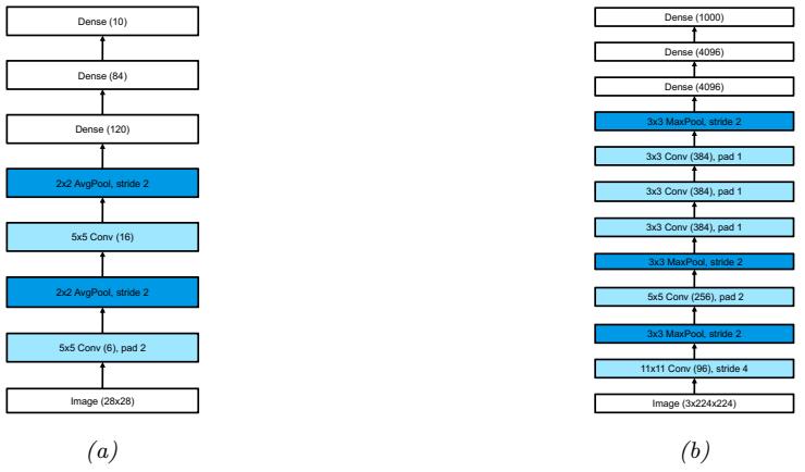
Figure 14.16: (a) LeNet5. We assume the input has size 1 ↑ 28 ↑ 28, as is the case for MNIST. From Figure 6.6.2 of [Zha+20]. Used with kind permission of Aston Zhang. (b) AlexNet. We assume the input has size 3↑224↑224, as is the case for (cropped and rescaled) images from ImageNet. From Figure 7.1.2 of [Zha+20]. Used with kind permission of Aston Zhang.
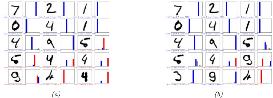
Figure 14.17: Results of applying a CNN to some MNIST images (cherry picked to include some errors). Red is incorrect, blue is correct. (a) After 1 epoch of training. (b) After 2 epochs. Generated by cnn\_mnist\_tf.ipynb.
Of course, classifying isolated digits is of limited applicability: in the real world, people usually write strings of digits or other letters. This requires both segmentation and classification. LeCun and colleagues devised a way to combine convolutional neural networks with a model similar to a conditional random field to solve this problem. The system was deployed by the US postal service. See [LeC+98] for a more detailed account of the system.
14.3.2 AlexNet
Although CNNs have been around for many years, it was not until the paper of [KSH12] in 2012 that mainstream computer vision researchers paid attention to them. In that paper, the authors showed how to reduce the (top 5) error rate on the ImageNet challenge (Section 1.5.1.2) from the previous best of 26% to 15%, which was a dramatic improvement. This model became known as AlexNet model, named after its creator, Alex Krizhevsky.
Figure 14.16b(b) shows the architecture. It is very similar to LeNet, shown in Figure 14.16a, with the following di!erences: it is deeper (8 layers of adjustable parameters (i.e., excluding the pooling layers) instead of 5); it uses ReLU nonlinearities instead of tanh (see Section 13.2.3 for why this is important); it uses dropout (Section 13.5.4) for regularization instead of weight decay; and it stacks several convolutional layers on top of each other, rather than strictly alternating between convolution and pooling. Stacking multiple convolutional layers together has the advantage that the receptive fields become larger as the output of one layer is fed into another (for example, three 3 ↑ 3 filters in a row will have a receptive field size of 7 ↑ 7). This is better than using a single layer with a larger receptive field, since the multiple layers also have nonlinearities in between. Also, three 3 ↑ 3 filters have fewer parameters than one 7 ↑ 7.
Note that AlexNet has 60M free parameters (which is much more than the 1M labeled examples), mostly due to the three fully connected layers at the output. Fitting this model relied on using two GPUs (due to limited memory of GPUs at that time), and is widely considered an engineering tour de force. 4 Figure 1.14a shows some predictions made by the model on some images from ImageNet.
4. The 3 authors of the paper (Alex Krizhevsky, Ilya Sutskever and Geo! Hinton) were subsequently hired by Google, although Ilya left in 2015, and Alex left in 2017. For more historical details, see https://en.wikipedia.org/wiki/ AlexNet. Note that AlexNet was not the first CNN implemented on a GPU; that honor goes to a group at Microsoft
Figure 14.18: Inception module. The 1 ↑ 1 convolutional layers reduce the number of channels, keeping the spatial dimensions the same. The parallel pathways through convolutions of di!erent sizes allows the model to learn which filter size to use for each layer. The final depth concatenation block combines the outputs of all the di!erent pathways (which all have the same spatial size). From Figure 7.4.1 of [Zha+20]. Used with kind permission of Aston Zhang.
Figure 14.19: GoogLeNet (slightly simplified from the original). Input is on the left. From Figure 7.4.2 of [Zha+20]. Used with kind permission of Aston Zhang.
14.3.3 GoogLeNet (Inception)
Google who developed a model known as GoogLeNet [Sze+15a]. (The name is a pun on Google and LeNet.) The main di!erence from earlier models is that GoogLeNet used a new kind of block, known as an inception block5, that employs multiple parallel pathways, each of which has a convolutional filter of a di!erent size. See Figure 14.18 for an illustration. This lets the model learn what the optimal filter size should be at each level. The overall model consists of 9 inception blocks followed by global average pooling. See Figure 14.19 for an illustration. Since this model first came out, various extensions were proposed; details can be found in [IS15; Sze+15b; SIV17].
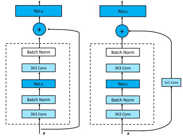
Figure 14.20: A residual block for a CNN. Left: standard version. Right: version with 1x1 convolution, to allow a change in the number of channels between the input to the block and the output. From Figure 7.6.3 of [Zha+20]. Used with kind permission of Aston Zhang.
Figure 14.21: The ResNet-18 architecture. Each dotted module is a residual block shown in Figure 14.20. From Figure 7.6.4 of [Zha+20]. Used with kind permission of Aston Zhang.
14.3.4 ResNet
The winner of the 2015 ImageNet classification challenge was a team at Microsoft, who proposed a model known as ResNet [He+16a]. The key idea is to replace xl+1 = Fl(xl) with
\[x\_{l+1} = \varphi(x\_l + \mathcal{F}\_l(x\_l))\tag{14.22}\]
This is known as a residual block, since Fl only needs to learn the residual, or di!erence, between input and output of this layer, which is a simpler task. In [He+16a], F has the form conv-BN-reluconv-BN, where conv is a convolutional layer, and BN is a batch norm layer (Section 14.2.4.1). See Figure 14.20(left) for an illustration.
[CPS06], who got a 4x speedup over CPUs, and then [Cir+11], who got a 60x speedup.
5. This term comes from the movie Inception, in which the phrase “We need to go deeper” was uttered. This became a popular meme in 2014.
We can ensure the spatial dimensions of the output Fl(xl) of the convolutional layer match those of the input xl by using padding. However, if we want to allow for the output of the convolutional layer to have a di!erent number of channels, we need to add 1 ↑ 1 convolution to the skip connection on xl. See Figure 14.20(right) for an illustration.
The use of residual blocks allows us to train very deep models. The reason this is possible is that gradient can flow directly from the output to earlier layers, via the skip connections, for reasons explained in Section 13.4.4.
In [He+16a] they trained a 152 layer ResNet on ImageNet. However, it is common to use shallower models. For example, Figure 14.21 shows the ResNet-18 architecture, which has 18 trainable layers: there are 2 3x3 conv layers in each residual block, and there are 8 such blocks, with an initial 7x7 conv (stride 2) and a final fully connected layer. Symbolically, we can define the model as follows:
(Conv : BN : Max) : (R : R) : (R' : R) : (R' : R) : (R' : R) : Avg : FCwhere R is a residual block, R’ is a residual block with skip connection (due to the change in the number of channels) with stride 2, FC is fully connected (dense) layer, and : denotes concatenation. Note that the input size gets reduced spatially by a factor of 25 = 32 (factor of 2 for each R’ block, plus the initial Conv-7x7(2) and Max-pool), so a 224x224 images becomes a 7x7 image before going into the global average pooling layer.
Some code to fit these models can be found online.6
In [He+16b], they showed how a small modification of the above scheme allows us to train models with up to 1001 layers. The key insight is that the signal on the skip connections is still being attenuated due to the use of the nonlinear activation function after the addition step, xl+1 = ϑ(xl + F(xl)). They showed that it is better to use
\[x\_{l+1} = x\_l + \varphi(\mathcal{F}\_l(x\_l)) \tag{14.23}\]
This is called a preactivation resnet or PreResnet for short. Now it is very easy for the network to learn the identity function at a given layer: if we use ReLU activations, we just need to ensure that Fl(xl) = 0, which we can do by setting the weights and biases to 0.
An alternative to using a very deep model is to use a very “wide” model, with lots of feature channels per layer. This is the idea behind the wide resnet model [ZK16], which is quite popular.
14.3.5 DenseNet
In a residual net, we add the output of each function to its input. An alternative approach would be to concatenate the output with the input, as illustrated in Figure 14.22a. If we stack a series of such blocks, we can get an architecture similar to Figure 14.22b. This is known as a DenseNets [Hua+17a], since each layer densely depends on all previous layers. Thus the overall model is computing a function of the form
\[x \to [x, f\_1(x), f\_2(x, f\_1(x)), f\_3(x, f\_1(x), f\_2(x, f\_1(x))), \dots] \tag{14.24}\]
6. The notebook resnet\_jax.ipynb fits this model on FashionMNIST. The notebook cifar10\_cnn\_lightning.ipynb fits it on the more challenging CIFAR-10 dataset. The latter code uses various tricks to achieve 89% top-1 accuracy on the CIFAR test set after 20 training epochs. The tricks are data augmentation (Section 19.1), consisting of random crops and horizontal flips, and to use one-cycle learning rate schedule (Section 8.4.3). If you use 50 epochs, and stochastic weight averaging (Section 8.4.4), you can get to → 94% accuracy.
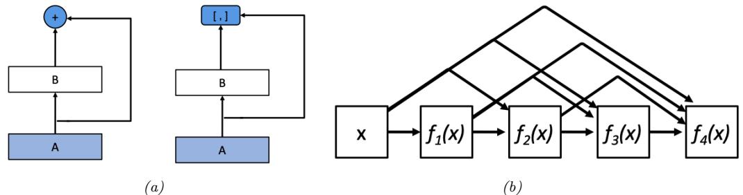
Figure 14.22: (a) Left: a residual block adds the output to the input. Right: a densenet block concatenates the output with the input. (b) Illustration of a densenet. From Figures 7.7.1–7.7.2 of [Zha+20]. Used with kind permission of Aston Zhang.
The dense connectivity increases the number of parameters, since the channels get stacked depthwise. We can compensate for this by adding 1 ↑ 1 convolution layers in between. We can also add pooling layers with a stride of 2 to reduce the spatial resolution. (See densenet\_jax.ipynb for some sample code.)
DenseNets can perform better than ResNets, since all previously computed features are directly accessible to the output layer. However, they can be more computationally expensive.
14.3.6 Neural architecture search
We have seen how many CNNs are fairly similar in their design, and simply rearrange various building blocks (such as convolutional or pooling layers) in di!erent topologies, and adjust various parameter settings (e.g., stride, number of channels, or learning rate). Indeed, the recent ConvNeXt model of [Liu+22] — which, at the time of writing (April 2022) is considered the state of the art CNN architecture for a wide variety of vision tasks — was created by combining multiple such small improvements on top of a standard ResNet architecture.
We can automate this design process using blackbox (derivative free) optimization methods to find architectures that minimize the validation loss. This is called AutoML (see e.g., [HKV19]). In the context of neural nets, it is called neural architecture search or NAS [EMH19].
When performing NAS, we can optimize for multiple objectives at the same time, such as accuracy, model size, training or inference speed, etc (this is how E”cientNetv2 is created [TL21]). The main challenge arises due to the expense of computing the objective (since it requires training each candidate point in model space). One way to reduce the number of calls to the objective function is to use Bayesian optimization (see e.g., [WNS19]). Another approach is to create di!erentiable approximations to the loss (see e.g., [LSY19; Wan+21]), or to convert the architecture into a kernel function (using the neural tangent kernel method, Section 17.2.8), and then to analyze properties of its eigenvalues, which can predict performance without actually training the model [CGW21]. The field of NAS is very large and still growing. See [EMH19] for a more thorough review.
Figure 14.23: Dilated convolution with a 3x3 filter using rate 1, 2 and 3. From Figure 1 of [Cui+19]. Used with kind permission of Ximin Cui.
14.4 Other forms of convolution *
We discussed the basics of convolution in Section 14.2. In this section, we discuss some extensions, which are needed for applications such as image segmentation and image generation.
14.4.1 Dilated convolution
Convolution is an operation that combines the pixel values in a local neighborhood. By using striding, and stacking many layers of convolution together, we can enlarge the receptive field of each neuron, which is the region of input space that each neuron responds to. However, we would need many layers to give each neuron enough context to cover the entire image (unless we used very large filters, which would be slow and require too many parameters).
As an alternative, we can use convolution with holes [Mal99], sometimes known by the French term à trous algorithm, and recently renamed dilated convolution [YK16]. This method simply takes every r’th input element when performing convolution, where r is known as the rate or dilation factor. For example, in 1d, convolving with filter w using rate r = 2 is equivalent to regular convolution using the filter w˜ = [w1, 0, w2, 0, w3], where we have inserted 0s to expand the receptive field (hence the term “convolution with holes”). This allows us to get the benefit of increased receptive fields without increasing the number of parameters or the amount of compute. See Figure 14.23 for an illustration.
More precisely, dilated convolution in 2d is defined as follows:
\[z\_{i,j,d} = b\_d + \sum\_{u=0}^{H-1} \sum\_{v=0}^{W-1} \sum\_{c=0}^{C-1} x\_{i+ru,j+rv,c} w\_{u,v,c,d} \tag{14.25}\]
where we assume the same rate r for both height and width, for simplicity. Compare this to Equation (14.15), where the stride parameter uses xsi+u,sj+v,c.
14.4.2 Transposed convolution
In convolution, we reduce from a large input X to a small output Y by taking a weighted combination of the input pixels and the convolutional kernel K. This is easiest to explain in code:
Figure 14.24: Transposed convolution with 2x2 kernel. From Figure 13.10.1 of [Zha+20]. Used with kind permission of Aston Zhang.
def conv(X, K):
    h, w = K.shape
    Y = zeros((X.shape[0] - h + 1, X.shape[1] - w + 1))
    for i in range(Y.shape[0]):
        for j in range(Y.shape[1]):
            Y[i, j] = (X[i:i + h, j:j + w] * K).sum()
    return Y
In transposed convolution, we do the opposite, in order to produce a larger output from a smaller input:
def trans_conv(X, K):
    h, w = K.shape
    Y = zeros((X.shape[0] + h - 1, X.shape[1] + w - 1))
    for i in range(X.shape[0]):
        for j in range(X.shape[1]):
            Y[i:i + h, j:j + w] += X[i, j] * K
    return Y
This is equivalent to padding the input image with (h ↗ 1, w ↗ 1) 0s (on the bottom right), where (h, w) is the kernel size, then placing a weighted copy of the kernel on each one of the input locations, where the weight is the corresponding pixel value, and then adding up. This process is illustrated in Figure 14.24. We can think of the kernel as a “stencil” that is used to generate the output, modulated by the weights in the input.
The term “transposed convolution” comes from the interpretation of convolution as matrix multiplication, which we discussed in Section 14.2.1.3. If W is the matrix derived from kernel K using the process illustrated in Equation (14.9), then one can show that Y = transposed-conv(X, K) is equivalent to Y = reshape(WTvec(X)). See transposed\_conv\_jax.ipynb for a demo.
Note that transposed convolution is also sometimes called deconvolution, but this is an incorrect usage of the term: deconvolution is the process of “undoing” the e!ect of convolution with a known filter, such as a blur filter, to recover the original input, as illustrated in Figure 14.25.
Figure 14.25: Convolution, deconvolution and transposed convolution. Here s is the stride and p is the padding. From https: // tinyurl. com/ ynxcxsut . Used with kind permission of Aqeel Anwar.
14.4.3 Depthwise separable convolution
Standard convolution uses a filter of size H ↑ W ↑ C ↑ D, which requires a lot of data to learn and a lot of time to compute with. A simplification, known as depthwise separable convolution, first convolves each input channel by a corresponding 2d filter w, and then maps these C channels to D channels using 1 ↑ 1 convolution w↑ :
\[z\_{i,j,d} = b\_d + \sum\_{c=0}^{C-1} w\_{c,d}' \left( \sum\_{u=0}^{H-1} \sum\_{v=0}^{W-1} x\_{i+u,j+v,c} w\_{u,v} \right) \tag{14.26}\]
See Figure 14.26 for an illustration.
To see the advantage of this, let us consider a simple numerical example.7 Regular convolution of a 12 ↑ 12 ↑ 3 input with a 5 ↑ 5 ↑ 3 ↑ 256 filter gives a 8 ↑ 8 ↑ 256 output (assuming valid convolution: 12-5+1=8), as illustrated in Figure 14.13. With separable convolution, we start with 12↑12↑3 input, convolve with a 5 ↑ 5 ↑ 1 ↑ 1 filter (across space but not channels) to get 8 ↑ 8 ↑ 3, then pointwise convolve (across channels but not space) with a 1 ↑ 1 ↑ 3 ↑ 256 filter to get a 8 ↑ 8 ↑ 256 output. So the output has the same size as before, but we used many fewer parameters to define the layer, and used much less compute. For this reason, separable convolution is often used in lightweight CNN models, such as the MobileNet model [How+17; San+18a] and other edge devices.
14.5 Solving other discriminative vision tasks with CNNs *
In this section, we briefly discuss how to tackle various other vision tasks using CNNs. Each task also introduces a new architectural innovation to the library of basic building blocks we have already seen. More details on CNNs for computer vision can be found in e.g., [Bro19].
14.5.1 Image tagging
Image classification associates a single label with the whole image, i.e., the outputs are assumed to be mutually exclusive. In many problems, there may be multiple objects present, and we want to label all of them. This is known as image tagging, and is an application of multi-label prediction. In this case, we define the output space as Y = {0, 1}C , where C is the number of tag types. Since the output bits are independent (given the image), we should replace the final softmax with a set of C logistic units.
7. This example is from https://bit.ly/2Uj64Vo by Chi-Feng Wang.
Figure 14.26: Depthwise separable convolutions: each of the C input channels undergoes a 2d convolution to produce C output channels, which get combined pointwise (via 1x1 convolution) to produce D output channels. From https: // bit. ly/ 2L9fm2o . Used with kind permission of Eugenio Culurciello.
Users of social media sites like Instagram often create hashtags for their images; this therefore provides a “free” way of creating large supervised datasets. Of course, many tags may be quite sparsely used, and their meaning may not be well-defined visually. (For example, someone may take a photo of themselves after they get a COVID test and tag the image “#covid”; however, visually it just looks like any other image of a person.) Thus this kind of user-generated labeling is usually considered quite noisy. However, it can be useful for “pre-training”, as discussed in [Mah+18].
Finally, it is worth noting that image tagging is often a much more sensible objective than image classification, since many images have multiple objects in them, and it can be hard to know which one we should be labeling. Indeed, Andrej Karpathy, who created the “human performance benchmark” on ImageNet, noted the following:8
Both [CNNs] and humans struggle with images that contain multiple ImageNet classes (usually many more than five), with little indication of which object is the focus of the image. This error is only present in the classification setting, since every image is constrained to have exactly one correct label. In total, we attribute 16% of human errors to this category.
14.5.2 Object detection
In some cases, we want to produce a variable number of outputs, corresponding to a variable number of objects of interest that may be present in the image. (This is an example of an open world problem, with an unknown number of objects.)
A canonical example of this is object detection, in which we must return a set of bounding boxes representing the locations of objects of interest, together with their class labels. A special case of this is face detection, where there is only one class of interest. This is illustrated in Figure 14.27a. 9
8. Source: https://bit.ly/3cFbALk
9. Note that face detection is di!erent from face recognition, which is a classification task that tries to predict the
Figure 14.27: (a) Illustration of face detection, a special case of object detection. (Photo of author and his wife Margaret, taken at Filoli in California in Feburary, 2018. Image processed by Jonathan Huang using SSD face model.) (b) Illustration of anchor boxes. Adapted from [Zha+20, Sec 12.5].
The simplest way to tackle such detection problems is to convert it into a closed world problem, in which there is a finite number of possible locations (and orientations) any object can be in. These candidate locations are known as anchor boxes. We can create boxes at multiple locations, scales and aspect ratios, as illustrated in Figure 14.27b. For each box, we train the system to predict what category of object it contains (if any); we can also perform regression to predict the o!set of the object location from the center of the anchor. (These residual regression terms allow sub-grid spatial localization.)
Abstractly, we are learning a function of the form
\[f\_{\theta}: \mathbb{R}^{H \times W \times K} \to [0, 1]^{A \times A} \times \{1, \dots, C\}^{A \times A} \times (\mathbb{R}^4)^{A \times A} \tag{14.27}\]
where K is the number of input channels, A is the number of anchor boxes in each dimension, and C is the number of object types (class labels). For each box location (i, j), we predict three outputs: an object presence probability, pij → [0, 1], an object category, yij → {1,…,C}, and two 2d o!set vectors, ςij → R4, which can be added to the centroid of the box to get the top left and bottom right corners.
Several models of this type have been proposed, including the single shot detector model of [Liu+16], and the YOLO (you only look once) model of [Red+16]. Many other methods for object detection have been proposed over the years. These models make di!erent tradeo!s between speed, accuracy, simplicity, etc. See [Hua+17b] for an empirical comparison, and [Zha+18] for a more recent review.
14.5.3 Instance segmentation
In object detection, we predict a label and bounding box for each object. In instance segmentation, the goal is to predict the label and 2d shape mask of each object instance in the image, as illustrated in Figure 14.28. This can be done by applying a semantic segmentation model to each detected box,
identity of a person from a set or “gallery” of possible people. Face recognition is usually solved by applying the classifier to all the patches that are detected as containing faces.
Figure 14.28: Illustration of object detection and instance segmentation using Mask R-CNN. From https: // github. com/ matterport/ Mask\_ RCNN . Used with kind permission of Waleed Abdulla.
Figure 14.29: Illustration of an encoder-decoder (aka U-net) CNN for semantic segmentation. The encoder uses convolution (which downsamples), and the decoder uses transposed convolution (which upsamples). From Figure 1 of [BKC17]. Used with kind permission of Alex Kendall.
which has to label each pixel as foreground or background. (See Section 14.5.4 for more details on semantic segmentation.)
14.5.4 Semantic segmentation
In semantic segmentation, we have to predict a class label yi → {1,…,C} for each pixel, where the classes may represent things like sky, road, car, etc. In contrast to instance segmentation, which we discussed in Section 14.5.3, all car pixels get the same label, so semantic segmentation does not di!erentiate between objects. We can combine semantic segmentation of “stu!” (like sky, road) and instance segmentation of “things” (like car, person) into a coherent framework called “panoptic segmentation” [Kir+19].
A common way to tackle semantic segmentation is to use an encoder-decoder architecture, as illustrated in Figure 14.29. The encoder uses standard convolution to map the input into a small 2d bottleneck, which captures high level properties of the input at a coarse spatial resolution. (This typically uses a technique called dilated convolution that we explain in Section 14.4.1, to capture a
Figure 14.30: Illustration of the U-Net model for semantic segmentation. Each blue box corresponds to a multi-channel feature map. The number of channels is shown on the top of the box, and the height/width is shown in the bottom left. White boxes denote copied feature maps. The di!erent colored arrows correspond to di!erent operations. From Figure 1 from [RFB15]. Used with kind permission of Olaf Ronenberg.
Figure 14.31: Illustration of a multi-task dense prediction problem. From Figure 1 of [EF15]. Used with kind permission of Rob Fergus.
large field of view, i.e., more context.) The decoder maps the small 2d bottleneck back to a full-sized output image using a technique called transposed convolution that we explain in Section 14.4.2. Since the bottleneck loses information, we can also add skip connections from input layers to output layers. We can redraw this model as shown in Figure 14.30. Since the overall structure resembles the letter U, this is also known as a U-net [RFB15].
A similar encoder-decoder architecture can be used for other dense prediction or image-toimage tasks, such as depth prediction (predict the distance from the camera, zi → R, for each pixel i), surface normal prediction (predict the orientation of the surface, zi → R3, at each image patch), etc. We can of course train one model to solve all of these tasks simultaneously, using multiple output heads, as illustrated in Figure 14.31. (See e.g., [Kok17] for details.)
14.5.5 Human pose estimation
We can train an object detector to detect people, and to predict their 2d shape, as represented by a mask. However, we can also train the model to predict the location of a fixed set of skeletal keypoints,
Figure 14.32: Illustration of keypoint detection for body, hands and face using the OpenPose system. From Figure 8 of [Cao+18]. Used with kind permission of Yaser Sheikh.
e.g., the location of the head or hands. This is called human pose estimation. See Figure 14.32 for an example. There are several techniques for this, e.g., PersonLab [Pap+18] and OpenPose [Cao+18]. See [Bab19] for a recent review.
We can also predict 3d properties of each detected object. The main limitation is the ability to collect enough labeled training data, since it is di”cult for human annotators to label things in 3d. However, we can use computer graphics engines to create simulated images with infinite ground truth 3d annotations (see e.g., [GNK18]).
14.6 Generating images by inverting CNNs *
A CNN trained for image classification is a discriminative model of the form p(y|x), which takes as input an image, and returns as output a probability distribution over C class labels. In this section we discuss how to “invert” this model, by converting it into a (conditional) generative image model of the form p(x|y). This will allow us to generate images that belong to a specific class. (We discuss more principled approaches to creating generative models for images in the sequel to this book, [Mur23].)
14.6.1 Converting a trained classifier into a generative model
We can define a joint distribution over images and labels using p(x, y) = p(x)p(y|x), where p(y|x) is the CNN classifier, and p(x) is some prior over images. If we then clamp the class label to a specific value, we can create a conditional generative model using p(x|y) ⇐ p(x)p(y|x). Note that the discriminative classifier p(y|x) was trained to “throw away” information, so p(y|x) is not an invertible function. Thus the prior term p(x) will play an important role in regularizing this process, as we see in Section 14.6.2.
One way to sample from this model is to use the Metropolis Hastings algorithm (Section 4.6.8.4), treating Ec(x) = log p(y = c|x) + log p(x) as the energy function. Since gradient information is available, we can use a proposal of the form q(x↑ |x) = N (µ(x), ,I), where µ(x) = x + ϱ 2⇑ log Ec(x). This is called the Metropolis-adjusted Langevin algorithm (MALA). As an approximation, we can ignore the rejection step, and accept every proposal. This is called the unadjusted Langevin algorithm, and was used in [Ngu+17] for conditional image generation. In addition, we can scale
the gradient of the log prior and log likelihood independently. Thus we get an update over the space of images that looks like a noisy version of SGD, except we take derivatives wrt the input pixels (using Equation (13.50)), instead of the parameters:
\[x\_{t+1} = x\_t + \epsilon\_1 \frac{\partial \log p(x\_t)}{\partial x\_t} + \epsilon\_2 \frac{\partial \log p(y = c | \mathbf{x}\_t)}{\partial x\_t} + \mathcal{N}(\mathbf{0}, \epsilon\_3^2 \mathbf{I}) \tag{14.28}\]
We can interpret each term in this equation as follows: the ,1 term ensures the image is plausible under the prior, the ,2 term ensures the image is plausible under the likelihood, and the ,3 term is a noise term, in order to generate diverse samples. If we set ,3 = 0, the method becomes a deterministic algorithm to (approximately) generate the “most likely image” for this class.
14.6.2 Image priors
In this section, we discuss various kinds of image priors that we can use to regularize the ill-posed problem of inverting a classifier. These priors, together with the image that we start the optimization from, will determine the kinds of outputs that we generate.
14.6.2.1 Gaussian prior
Just specifying the class label is not enough information to specify the kind of images we want. We also need a prior p(x) over what constitutes a “plausible” image. The prior can have a large e!ect on the quality of the resulting image, as we show below.
Arguably the simplest prior is p(x) = N (x|0, I), as suggested in [SVZ14]. (This assumes the image pixels have been centered.) This can prevent pixels from taking on extreme values. In this case, the update due to the prior term has the form
\[\nabla\_{\mathbf{z}} \nabla\_{\mathbf{z}} \log p(\mathbf{z}\_t) = \nabla\_{\mathbf{z}} \left[ -\frac{1}{2} ||\mathbf{z}\_t - \mathbf{0}||\_2^2 \right] = -\mathbf{z}\_t \tag{14.29}\]
Thus the overall update (assuming ,2 = 1 and ,3 = 0) has the form
\[x\_{t+1} = (1 - \epsilon\_1)x\_t + \frac{\partial \log p(y = c | x\_t)}{\partial x\_t} \tag{14.30}\]
See Figure 14.33 for some samples generated by this method.
14.6.2.2 Total variation (TV) prior
We can generate slightly more realistic looking images if we use additional regularizers. [MV15; MV16] suggested computing the total variation or TV norm of the image. This is equal to the integral of the per-pixel gradients, which can be approximated as follows:
\[\text{TV}(x) = \sum\_{ijk} (x\_{ijk} - x\_{i+1,j,k})^2 + (x\_{ijk} - x\_{i,j+1,k})^2 \tag{14.31}\]
where xijk is the pixel value in row i, column j and channel k (for RGB images). We can rewrite this in terms of the horizontal and vertical Sobel edge detector applied to each channel:
\[\text{TV}(\mathbf{z}) = \sum\_{k} ||\mathbf{H}(\mathbf{z}\_{::,k})||\_F^2 + ||\mathbf{V}(\mathbf{z}\_{::,k})||\_F^2 \tag{14.32}\]
Figure 14.33: Images that maximize the probability of ImageNet classes “goose” and “ostrich” under a simple Gaussian prior. From http: // yosinski. com/ deepvis . Used with kind permission of Je! Clune.
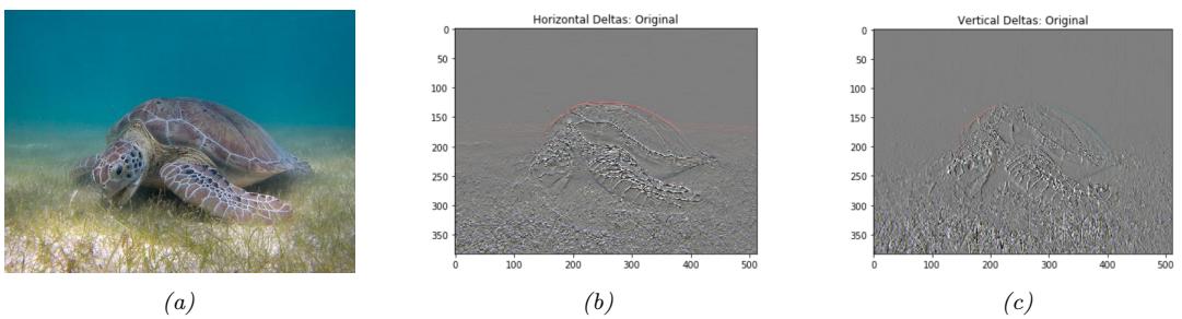
Figure 14.34: Illustration of total variation norm. (a) Input image: a green sea turtle (Used with kind permission of Wikimedia author P. Lindgren). (b) Horizontal deltas. (c) Vertical deltas. Adapted from https: // www. tensorflow. org/ tutorials/ generative/ style\_ transfer .
See Figure 14.34 for an illustration of these edge detectors. Using p(x) ⇐ exp(↗TV(x)) discourages images from having high frequency artefacts. In [Yos+15], they use Gaussian blur instead of TV norm, but this has a similar e!ect.
In Figure 14.35 we show some results of optimizing log p(y = c, x) using a TV prior and a CNN likelihood for di!erent class labels c starting from random noise.
14.6.3 Visualizing the features learned by a CNN
It is interesting to ask what the “neurons” in a CNN are learning. One way to do this is to start with a random image, and then to optimize the input pixels so as to maximize the average activation of a particular neuron. This is called activation maximization (AM), and uses the same technique as in Section 14.6.1 but fixes an internal node to a specific value, rather than clamping the output class label.
Figure 14.36 illustrates the output of this method (with the TV prior) when applied to the AlexNet CNN trained on Imagenet classification. We see that, as the depth increases, neurons are learning to recognize simple edges/blobs, then texture patterns, then object parts, and finally whole objects. This is believed to be roughly similar to the hierarchical structure of the visual cortex (see e.g., [Kan+12]).
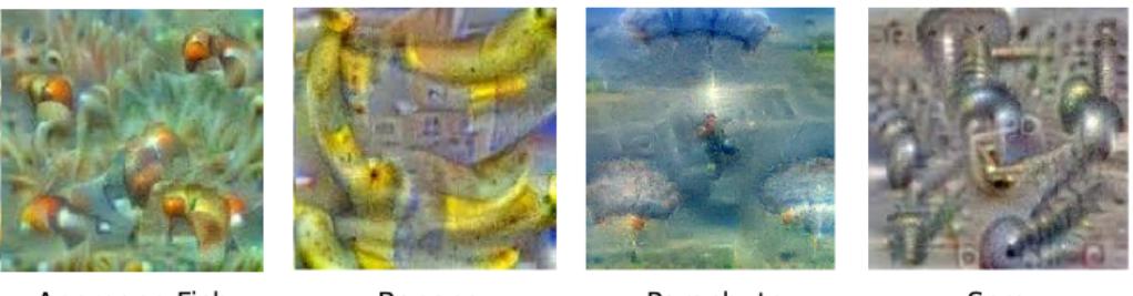
Figure 14.35: Images that maximize the probability of certain ImageNet classes under a TV prior. From https: // research. googleblog. com/ 2015/ 06/ inceptionism-going-deeper-into-neural. html . Used with kind permission of Alexander Mordvintsev.
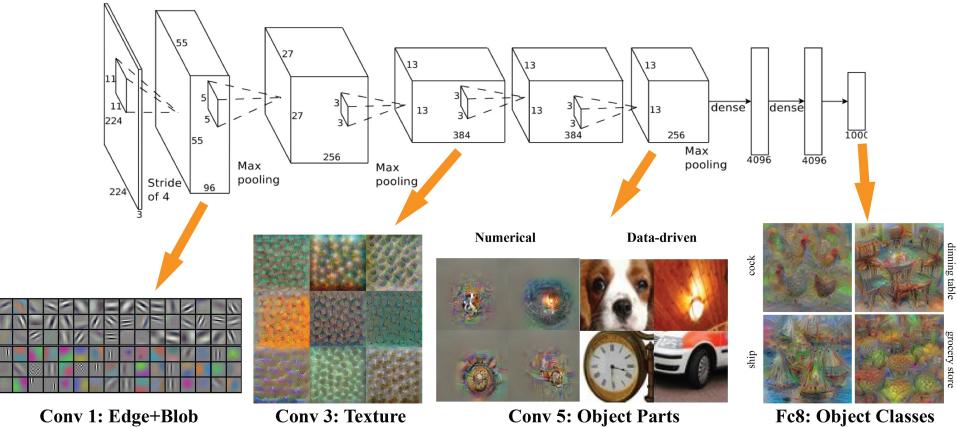
Figure 14.36: We visualize “optimal stimuli” for neurons in layers Conv 1, 3, 5 and fc8 in the AlexNet architecture, trained on the ImageNet dataset. For Conv5, we also show retrieved real images (under the column “data driven”) that produce similar activations. Based on the method in [MV16]. Used with kind permission of Donglai Wei.
An alternative to optimizing in pixel space is to search the training set for images that maximally activate a given neuron. This is illustrated in Figure 14.36 for the Conv5 layer.
For more information on feature visualization see e.g., [OMS17].
14.6.4 Deep Dream
So far we have focused on generating images which maximize the class label or some other neuron of interest. In this section we tackle a more artistic application, in which we want to generate versions of an input image that emphasize certain features.
To do this, we view our pre-trained image classifier as a feature extractor. Based on the results in Section 14.6.3, we know the activity of neurons in di!erent layers correspond to di!erent kinds
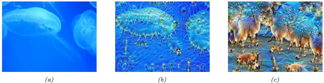
Figure 14.37: Illustration of DeepDream. The CNN is an Inception classifier trained on ImageNet. (a) Starting image of an Aurelia aurita (also called moon jelly). (b) Image generated after 10 iterations. (c) Image generated after 50 iterations. From https: // en. wikipedia. org/ wiki/ DeepDream . Used with kind permission of Wikipedia author Martin Thoma.
of features in the image. Suppose we are interested in “amplifying” features from layers l → L. We can do this by defining an energy or loss function of the form L(x) = ( l↔︎L ωl(x), where ωl = 1 HWC ( hwc ωlhwc(x) is the feature vector for layer l. We can now use gradient descent to optimize this energy. The resulting process is called DeepDream [MOT15], since the model amplifies features that were only hinted at in the original image and then creates images with more and more of them.10
Figure 14.37 shows an example. We start with an image of a jellyfish, which we pass into a CNN that was trained to classify ImageNet images. After several iterations, we generate some image which is a hybrid of the input and the kinds of “hallucinations” we saw in Figure 14.33; these hallucinations involve dog parts, since ImageNet has so many kinds of dogs in its label set. See [Tho16] for details, and https://deepdreamgenerator.com for a fun web-based demo.
14.6.5 Neural style transfer
The DeepDream system in Figure 14.37 shows one way that CNNs can be used to create “art”. However, it is rather creepy. In this section, we discuss a related approach that gives the user more control. In particular, the user has to specify a reference “style image” xs and “content image” xc. The system will then try to generate a new image x that “re-renders” xc in the style of xs. This is called neural style transfer, and is illustrated in Figure 14.38 and Figure 14.39. This technique was first proposed in [GEB16], and there are now many papers on this topic; see [Jin+17] for a recent review.
14.6.5.1 How it works
Style transfer works by optimizing the following energy function:
\[\mathcal{L}(\mathbf{x}|\mathbf{z}\_s, \mathbf{z}\_c) = \lambda\_{\rm TV} \mathcal{L}\_{\rm TV}(\mathbf{z}) + \lambda\_c \mathcal{L}\_{\rm content}(\mathbf{z}, \mathbf{z}\_c) + \lambda\_s \mathcal{L}\_{\rm style}(\mathbf{z}, \mathbf{z}\_s) \tag{14.33}\]
See Figure 14.40 for a high level illustration.
10. The method was originally called Inceptionism, since it uses the inception CNN (Section 14.3.3).
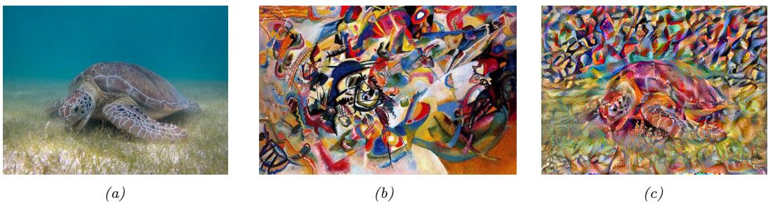
Figure 14.38: Example output from a neural style transfer system. (a) Content image: a green sea turtle (Used with kind permission of Wikimedia author P. Lindgren). (b) Style image: a painting by Wassily Kandinsky called “Composition 7”. (c) Output of neural style generation. Adapted from https: // www. tensorflow. org/ tutorials/ generative/ style\_ transfer .
Figure 14.39: Neural style transfer applied to photos of the “production team”, who helped create code and demos for this book and its sequel. From top to bottom, left to right: Kevin Murphy (the author), Mahmoud Soliman, Aleyna Kara, Srikar Jilugu, Drishti Patel, Ming Liang Ang, Gerardo Durán-Martín, Coco (the team dog). Each content photo used a di!erent artistic style. Adapted from https: // www. tensorflow. org/ tutorials/ generative/ style\_ transfer .
Figure 14.40: Illustration of how neural style transfer works. Adapted from Figure 12.12.2 of [Zha+20].
Figure 14.41: Schematic representation of 3 kinds of feature maps for 3 di!erent input images. Adapted from Figure 5.16 of [Fos19].
The first term in Equation (14.33) is the total variation prior discussed in Section 14.6.2.2. The second term measures how similar x is to xc by comparing feature maps of a pre-trained CNN ω(x) in the relevant “content layer” l:
\[\mathcal{L}\_{\text{content}}(\mathbf{z}, \mathbf{z}\_c) = \frac{1}{C\_\ell H\_\ell W\_\ell} ||\phi\_\ell(\mathbf{z}) - \phi\_\ell(\mathbf{z}\_c)||\_2^2 \tag{14.34}\]
Finally we have to define the style term. We can interpret visual style as the statistical distribution of certain kinds of image features. The location of these features in the image may not matter, but their co-occurence does. This is illustrated in Figure 14.41. It is clear (to a human) that image 1 is more similar in style to image 2 than to image 3. Intuitively this is because both image 1 and image 2 have spiky green patches in them, whereas image 3 has spiky things that are not green.
To capture the co-occurence statistics we compute the Gram matrix for an image using feature maps from a specific layer ε:
\[G\_{\ell}(\mathbf{x})\_{c,d} = \frac{1}{H\_{\ell}W\_{\ell}} \sum\_{h=1}^{H\_{\ell}} \sum\_{w=1}^{W\_{\ell}} \phi\_{\ell}(\mathbf{x})\_{h,w,c} \, \phi\_{\ell}(\mathbf{x})\_{h,w,d} \tag{14.35}\]
The Gram matrix is a Cω ↑ Cω matrix which is proportional to the uncentered covariance of the Cω-dimensional feature vectors sampled over each of the HωWω locations.
Given this, we define the style loss for layer ε as follows:
\[\mathcal{L}\_{\text{style}}^{\ell}(\mathbf{z}, \mathbf{z}\_s) = ||\mathbf{G}\_{\ell}(\mathbf{z}) - \mathbf{G}\_{\ell}(\mathbf{z}\_s)||\_F^2 \tag{14.36}\]
Finally, we define the overall style loss as a sum over the losses for a set S of layers:
\[\mathcal{L}\_{\text{style}}(\mathbf{z}, \mathbf{z}\_s) = \sum\_{\ell \in \mathcal{S}} \mathcal{L}\_{\text{style}}^{\ell}(\mathbf{z}, \mathbf{z}\_s) \tag{14.37}\]
For example, in Figure 14.40, we compute the style loss at layers 1 and 3. (Lower layers will capture visual texture, and higher layers will capture object layout.)
14.6.5.2 Speeding up the method
In [GEB16], they used L-BFGS (Section 8.3.2) to optimize Equation (14.33), starting from white noise. We can get faster results if we use an optimizer such as Adam instead of BFGS, and initialize from the content image instead of white noise. Nevertheless, running an optimizer for every new style and content image is slow. Several papers (see e.g., [JAFF16; Uly+16; UVL16; LW16]) have proposed to train a neural network to directly predict the outcome of this optimization, rather than solving it for each new image pair. (This can be viewed as a form of amortized optimization.) In particular, for every style image xs, we fit a model fs such that fs(xc) = argminx L(x|xs, xc). We can then apply this model to new content images without having to reoptimize.
More recently, [DSK16] has shown how it is possible to train a single network that takes as input both the content and a discrete representation s of the style, and then produces f(xc, s) = argminx L(x|s, xc) as the output. This avoids the need to train a separate network for every style image. The key idea is to standardize the features at a given layer using scale and shift parameters that are style specific. In particular, we use the following conditional instance normalization transformation:
\[\text{CIN}(\phi(\mathbf{z}\_c), s) = \gamma\_s \left( \frac{\phi(\mathbf{z}\_c) - \mu(\phi(\mathbf{z}\_c))}{\sigma(\phi(\mathbf{z}\_c))} \right) + \beta\_s \tag{14.38}\]
where µ(ϱ(xc)) is the mean of the features in a given layer, ω(ϱ(xc)) is the standard deviation, and ↼s and ↽s are parameters for style type s. (See Section 14.2.4.2 for more details on instance normalization.) Surprisingly, this simple trick is enough to capture many kinds of styles.
The drawback of the above technique is that it only works for a fixed number of discrete styles. [HB17] proposed to generalize this by replacing the constants ↼s and ↽s by the output of another CNN, which takes an arbitrary style image xs as input. That is, in Equation (14.38), we set ↼s = fϑ(ϱ(xs))
and ↽s = fϖ(ϱ(xs)), and we learn the parameters ϖ and ϑ along with all the other parameters. The model becomes
\[\text{AIN}(\phi(\mathbf{z}\_c), \phi(\mathbf{z}\_s)) = f\_\gamma(\phi(\mathbf{z}\_s)) \left( \frac{\phi(\mathbf{z}\_c) - \mu(\phi(\mathbf{z}\_c))}{\sigma(\phi(\mathbf{z}\_c))} \right) + f\_\beta(\phi(\mathbf{z}\_s)) \tag{14.39}\]
They call their method adaptive instance normalization.
15 Neural Networks for Sequences
15.1 Introduction
In this chapter, we discuss various kinds of neural networks for sequences. We will consider the case where the input is a sequence, the output is a sequence, or both are sequences. Such models have many applications, such as machine translation, speech recognition, text classification, image captioning, etc. Our presentation borrows from parts of [Zha+20], which should be consulted for more details.
15.2 Recurrent neural networks (RNNs)
A recurrent neural network or RNN is a neural network which maps from an input space of sequences to an output space of sequences in a stateful way. That is, the prediction of output yt depends not only on the input xt, but also on the hidden state of the system, ht, which gets updated over time, as the sequence is processed. Such models can be used for sequence generation, sequence classification, and sequence translation, as we explain below.1
15.2.1 Vec2Seq (sequence generation)
In this section, we discuss how to learn functions of the form fε : RD ≃ RN↓C , where D is the size of the input vector, and the output is an arbitrary-length sequence of vectors, each of size C. (Note that words are discrete tokens, but can be converted to real-valued vectors as we discuss in Section 1.5.4.) We call these vec2seq models, since they map a vector to a sequence.
The output sequence y1:T is generated one token at a time. At each step we sample y˜t from the hidden state ht of the model, and then “feed it back in” to the model to get the new state ht+1 (which also depends on the input x). See Figure 15.1 for an illustration. In this way the model defines a conditional generative model of the form p(y1:T |x), which captures dependencies between the output tokens. We explain this in more detail below.
1. For a more detailed introduction, see http://karpathy.github.io/2015/05/21/rnn-effectiveness/.
Figure 15.1: Recurrent neural network (RNN) for generating a variable length output sequence y1:T given an optional fixed length input vector x.
15.2.1.1 Models
For notational simplicity, let T be the length of the output (with the understanding that this is chosen dynamically). The RNN then corresponds to the following conditional generative model:
\[p(y\_{1:T}|\mathbf{x}) = \sum\_{h\_{1:T}} p(y\_{1:T}, h\_{1:T}|\mathbf{x}) = \sum\_{h\_{1:T}} \prod\_{t=1}^{T} p(y\_t|h\_t) p(h\_t|h\_{t-1}, y\_{t-1}, \mathbf{x}) \tag{15.1}\]
where ht is the hidden state, and where we define p(h1|h0, y0, x) = p(h1|x) as the initial hidden state distribution (often deterministic).
The output distribution is usually given by
\[p(y\_t | h\_t) = \text{Cat}(y\_t | \text{softmax}(\mathbf{W}\_{hy}h\_t + b\_y))\tag{15.2}\]
where Why are the hidden-to-output weights, and by is the bias term. However, for real-valued outputs, we can use
\[p(\mathbf{y}|\boldsymbol{h}\_t) = N(\mathbf{y}\_t|\mathbf{W}\_{hy}\boldsymbol{h}\_t + \mathbf{b}\_y, \sigma^2\mathbf{I})\tag{15.3}\]
We assume the hidden state is computed deterministically as follows:
\[p(h\_t | h\_{t-1}, y\_{t-1}, x) = \mathbb{I}(h\_t = f(h\_{t-1}, y\_{t-1}, x))\tag{15.4}\]
for some deterministic function f. The update function f is usually given by
\[\mathbf{h}\_{t} = \varphi(\mathbf{W}\_{xh}[x; y\_{t-1}] + \mathbf{W}\_{hh}h\_{t-1} + \mathbf{b}\_{h}) \tag{15.5}\]
where Whh are the hidden-to-hidden weights, Wxh are the input-to-hidden weights, and bh are the bias terms. See Figure 15.1 for an illustration, and rnn\_jax.ipynb for some code.
Note that yt depends on ht, which depends on yt→1, which depends on ht→1, and so on. Thus yt implicitly depends on all past observations (as well as the optional fixed input x). Thus an RNN overcomes the limitations of standard Markov models, in that they can have unbounded memory. This makes RNNs theoretically as powerful as a Turing machine [SS95; PMB19]. In practice,
the githa some thong the time traveller held in his hand was a glitteringmetallic framework scarcely larger than a small clock and verydelicately made there was ivory in it and the latter than s bettyre tat howhong s ie time thave ler
simk you a dimensions le ghat dionthat shall travel indi!erently in any direction of space and timeas the driver determinesfilby contented himself with laughterbut i have experimental verification said the time travellerit would be remarkably convenient for the histo
Figure 15.2: Example output of length 500 generated from a character level RNN when given the prefix “the”. We use greedy decoding, in which the most likely character at each step is computed, and then fed back into the model. The model is trained on the book The Time Machine by H. G. Wells. Generated by rnn\_jax.ipynb.
however, the memory length is determined by the size of the latent state and the strength of the parameters; see Section 15.2.7 for further discussion of this point.
When we generate from an RNN, we sample from y˜t ∝ p(yt|ht), and then “feed in” the sampled value into the hidden state, to deterministically compute ht+1 = f(ht, y˜t, x), from which we sample y˜t+1 ∝ p(yt+1|ht+1), etc. Thus the only stochasticity in the system comes from the noise in the observation (output) model, which is fed back to the system in each step. (However, there is a variant, known as a variational RNN [Chu+15], that adds stochasticity to the dynamics of ht independent of the observation noise.)
15.2.1.2 Applications
RNNs can be used to generate sequences unconditionally (by setting x = ⇓) or conditionally on x. Unconditional sequence generation is often called language modeling; this refers to learning joint probability distributions over sequences of discrete tokens, i.e., models of the form p(y1,…,yT ). (See also Section 3.6.1.2, where we discuss using Markov chains for language modeling.)
Figure 15.2 shows a sequence generated from a simple RNN trained on the book The Time Machine by H. G. Wells. (This is a short science fiction book, with just 32,000 words and 170k characters.) We see that the generated sequence looks plausible, even though it is not very meaningful. By using more sophisticated RNN models (such as those that we discuss in Section 15.2.7.1 and Section 15.2.7.2), and by training on more data, we can create RNNs that give state-of-the-art performance on the language modeling task [CNB17]. (In the language modeling community, performance is usually measured by perplexity, which is just the exponential of the average per-token negative log likelihood; see Section 6.1.5 for more information.)
We can also make the generated sequence depend on some kind of input vector x. For example, consider the task of image captioning: in this case, x is some embedding of the image computed by a CNN, as illustrated in Figure 15.3. See e.g., [Hos+19; LXW19] for a review of image captioning methods, and https://bit.ly/2Wvs1GK for a tutorial with code.
It is also possible to use RNNs to generate sequences of real-valued feature vectors, such as pen strokes for hand-written characters [Gra13] and hand-drawn shapes [HE18]. This can also be useful for time series forecasting real-value sequences.
15.2.2 Seq2Vec (sequence classification)
In this section, we assume we have a single fixed-length output vector y we want to predict, given a variable length sequence as input. Thus we want to learn a function of the form fε : RTD ≃ RC . We
Figure 15.3: Illustration of a CNN-RNN model for image captioning. The pink boxes labeled “LSTM” refer to a specific kind of RNN that we discuss in Section 15.2.7.2. The pink boxes labeled Wemb refer to embedding matrices for the (sampled) one-hot tokens, so that the input to the model is a real-valued vector. From https: // bit. ly/ 2FKnqHm . Used with kind permission of Yunjey Choi.
Figure 15.4: (a) RNN for sequence classification. (b) Bi-directional RNN for sequence classification.
call this a seq2vec model. We will focus on the case where the output is a class label, y → {1,…,C}, for notational simplicity.
The simplest approach is to use the final state of the RNN as input to the classifier:
\[p(y|\mathbf{z}\_{1:T}) = \text{Cat}(y|\text{softmax}(\mathbf{W}\hbar\_T))\tag{15.6}\]
See Figure 15.4a for an illustration.
We can often get better results if we let the hidden states of the RNN depend on the past and future context. To do this, we create two RNNs, one which recursively computes hidden states in the forwards direction, and one which recursively computes hidden states in the backwards direction. This is called a bidirectional RNN [SP97].
Figure 15.5: (a) RNN for transforming a sequence to another, aligned sequence. (b) Bi-directional RNN for the same task.
More precisely, the model is defined as follows:
\[\mathbf{h}\_t^{\rightarrow} = \varphi(\mathbf{W}\_{xh}^{\rightarrow}\mathbf{z}\_t + \mathbf{W}\_{hh}^{\rightarrow}h\_{t-1}^{\rightarrow} + \mathbf{b}\_h^{\rightarrow}) \tag{15.7}\]
\[h\_t^{\leftarrow} = \varphi(\mathbf{W}\_{xh}^{\leftarrow}\mathbf{x}\_t + \mathbf{W}\_{hh}^{\leftarrow}h\_{t+1}^{\leftarrow} + \mathbf{b}\_h^{\leftarrow})\tag{15.8}\]
We can then define ht = [h↗ t , h↘ t ] to be the representation of the state at time t, taking into account past and future information. Finally we average pool over these hidden states to get the final classifier:
\[p(y|\mathbf{z}\_{1:T}) = \text{Cat}(y|\text{softmax}(\mathbf{W}\overline{h})) \tag{15.9}\]
\[\overline{h} = \frac{1}{T} \sum\_{t=1}^{T} h\_t \tag{15.10}\]
See Figure 15.4b for an illustration, and rnn\_sentiment\_jax.ipynb for some code. (This is similar to the 1d CNN text classifier1 in Section 15.3.1.)
15.2.3 Seq2Seq (sequence translation)
In this section, we consider learning functions of the form fε : RTD ≃ RT↑ C . We consider two cases: one in which T↑ = T, so the input and output sequences have the same length (and hence are aligned), and one in which T↑ 7= T, so the input and output sequences have di!erent lengths. This is called a seq2seq problem.
15.2.3.1 Aligned case
In this section, we consider the case where the input and output sequences are aligned. We can also think of it as dense sequence labeling, since we predict one label per location. It is straightforward to modify an RNN to solve this task, as shown in Figure 15.5a. This corresponds to
\[p(y\_{1:T}|x\_{1:T}) = \sum\_{h\_{1:T}} \prod\_{t=1}^{T} p(y\_t|h\_t) \mathbb{I}\left(h\_t = f(h\_{t-1}, x\_t)\right) \tag{15.11}\]
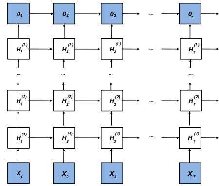
Figure 15.6: Illustration of a deep RNN. Adapted from Figure 9.3.1 of [Zha+20].
Figure 15.7: Encoder-decoder RNN architecture for mapping sequence x1:T to sequence y1:T ↑ .
where we define h1 = f(h0, x1) = f0(x1) to be the initial state.
Note that yt depends on ht which only depends on the past inputs, x1:t. We can get better results if we let the decoder look into the “future” of x as well as the past, by using a bidirectional RNN, as shown in Figure 15.5b.
We can create more expressive models by stacking multiple hidden chains on top of each other, as shown in Figure 15.6. The hidden units for layer l at time t are computed using
\[\mathbf{h}\_t^l = \varphi\_l(\mathbf{W}\_{xh}^l \mathbf{h}\_t^{l-1} + \mathbf{W}\_{hh}^l \mathbf{h}\_{t-1}^l + \mathbf{b}\_h^l) \tag{15.12}\]
The output is given by
\[\mathbf{o}\_{t} = \mathbf{W}\_{ho} \mathbf{h}\_{t}^{L} + \mathbf{b}\_{o} \tag{15.13}\]
15.2.3.2 Unaligned case
In this section, we discuss how to learn a mapping from one sequence of length T to another of length T↑ . We first encode the input sequence to get the context vector c = fe(x1:T ), using the last state of an RNN (or average pooling over a biRNN). We then generate the output sequence using an RNN
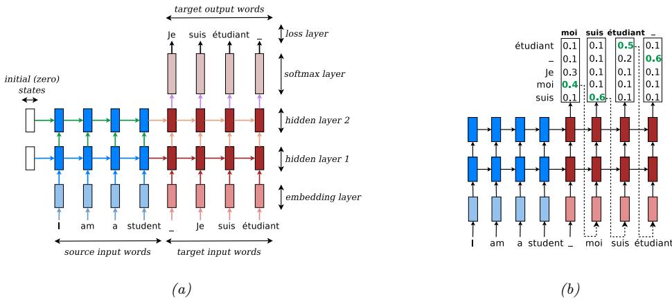
Figure 15.8: (a) Illustration of a seq2seq model for translating English to French. The - character represents the end of a sentence. From Figure 2.4 of [Luo16]. Used with kind permission of Minh-Thang Luong. (b) Illustration of greedy decoding. The most likely French word at each step is highlighted in green, and then fed in as input to the next step of the decoder. From Figure 2.5 of [Luo16]. Used with kind permission of Minh-Thang Luong.
decoder y1:T↑ = fd(c). This is called an encoder-decoder architecture [SVL14; Cho+14a]. See Figure 15.7 for an illustration.
An important application of this is machine translation. When this is tackled using RNNs, it is called neural machine translation (as opposed to the older approach called statistical machine translation, that did not use neural networks). See Figure 15.8a for the basic idea, and nmt\_jax.ipynb for some code which has more details. For a review of the NMT literature, see [Luo16; Neu17].
15.2.4 Teacher forcing
When training a language model, the likelihood of a sequence of words w1, w2,…,wT , is given by
\[p(w\_{1:T}) = \prod\_{t=1}^{T} p(w\_t|w\_{1:t-1}) \tag{15.14}\]
In an RNN, we therefore set the input to xt = wt→1 and the output to yt = wt. Note that we condition on the ground truth labels from the past, w1:t→1, not labels generated from the model. This is called teacher forcing, since the teacher’s values are “force fed” into the model as input at each step (i.e., xt is set to wt→1).
Unfortunately, teacher forcing can sometimes result in models that perform poorly at test time. The reason is that the model has only ever been trained on inputs that are “correct”, so it may not know what to do if, at test time, it encounters an input sequence w1:t→1 generated from the previous step that deviates from what it saw in training.
Figure 15.9: An RNN unrolled (vertically) for 3 time steps, with the target output sequence and loss node shown explicitly. From Figure 8.7.2 of [Zha+20]. Used with kind permission of Aston Zhang.
A common solution to this is known as scheduled sampling [Ben+15a]. This starts o! using teacher forcing, but at random time steps, feeds in samples from the model instead; the fraction of time this happens is gradually increased.
An alternative solution is to use other kinds of models where MLE training works better, such as 1d CNNs (Section 15.3) and transformers (Section 15.5).
15.2.5 Backpropagation through time
We can compute the maximum likelihood estimate of the parameters for an RNN by solving ε≃ = argmaxε p(y1:T |x1:T , ε), where we have assumed a single training sequence for notational simplicity. To compute the MLE, we have to compute gradients of the loss wrt the parameters. To do this, we can unroll the computation graph, as shown in Figure 15.9, and then apply the backpropagation algorithm. This is called backpropagation through time (BPTT) [Wer90].
More precisely, consider the following model:
\[h\_t = \mathbf{W}\_{hx} x\_t + \mathbf{W}\_{hh} h\_{t-1} \tag{15.15}\]
\[\mathbf{o}\_{t} = \mathbf{W}\_{ho} \mathbf{h}\_{t} \tag{15.16}\]
where ot are the output logits, and where we drop the bias terms for notational simplicity. We assume yy are the true target labels for each time step, so we define the loss to be
\[L = \frac{1}{T} \sum\_{t=1}^{T} \ell(y\_t, \mathbf{o}\_t) \tag{15.17}\]
We need to compute the derivatives ϑL ϑWhx , ϑL ϑWhh , and ϑL ϑWho . The latter term is easy, since it is local to each time step. However, the first two terms depend on the hidden state, and thus require working backwards in time.
We simplify the notation by defining
\[h\_t = f(x\_t, h\_{t-1}, w\_h) \tag{15.18}\]
\[\mathbf{o}\_{t} = g(\mathbf{h}\_{t}, \mathbf{w}\_{o}) \tag{15.19}\]
where wh is the flattened version of Whh and Whx stacked together. We focus on computing ϑL ϑwh . By the chain rule, we have
\[\frac{\partial L}{\partial \mathbf{w}\_h} = \frac{1}{T} \sum\_{t=1}^{T} \frac{\partial \ell(y\_t, \mathbf{o}\_t)}{\partial \mathbf{w}\_h} = \frac{1}{T} \sum\_{t=1}^{T} \frac{\partial \ell(y\_t, \mathbf{o}\_t)}{\partial \mathbf{o}\_t} \frac{\partial g(\mathbf{h}\_t, \mathbf{w}\_o)}{\partial \mathbf{h}\_t} \frac{\partial \mathbf{h}\_t}{\partial \mathbf{w}\_h} \tag{15.20}\]
We can expand the last term as follows:
\[\frac{\partial \hbar\_{t}}{\partial \mathbf{w}\_{h}} = \frac{\partial f(\mathbf{x}\_{t}, \mathbf{h}\_{t-1}, \mathbf{w}\_{h})}{\partial \mathbf{w}\_{h}} + \frac{\partial f(\mathbf{x}\_{t}, \mathbf{h}\_{t-1}, \mathbf{w}\_{h})}{\partial \mathbf{h}\_{t-1}} \frac{\partial \hbar\_{t-1}}{\partial \mathbf{w}\_{h}} \tag{15.21}\]
If we expand this recursively, we find the following result (see the derivation in [Zha+20, Sec 8.7]):
\[\frac{\partial \mathbf{h}\_{t}}{\partial \mathbf{w}\_{h}} = \frac{\partial f(\mathbf{x}\_{t}, \mathbf{h}\_{t-1}, \mathbf{w}\_{h})}{\partial \mathbf{w}\_{h}} + \sum\_{i=1}^{t-1} \left( \prod\_{j=i+1}^{t} \frac{\partial f(\mathbf{x}\_{j}, \mathbf{h}\_{j-1}, \mathbf{w}\_{h})}{\partial \mathbf{h}\_{j-1}} \right) \frac{\partial f(\mathbf{x}\_{i}, \mathbf{h}\_{i-1}, \mathbf{w}\_{h})}{\partial \mathbf{w}\_{h}} \tag{15.22}\]
Unfortunately, this takes O(T) time to compute per time step, for a total of O(T2) overall. It is therefore standard to truncate the sum to the most recent K terms. It is possible to adaptively pick a suitable truncation parameter K [AFF19]; however, it is usually set equal to the length of the subsequence in the current minibatch.
When using truncated BPTT, we can train the model with batches of short sequences, usually created by extracting non-overlapping subsequences (windows) from the original sequence. If the previous subsequence ends at time t ↗ 1, and the current subsequence starts at time t, we can “carry over” the hidden state of the RNN across batch updates during training. However, if the subsequences are not ordered, we need to reset the hidden state. See rnn\_jax.ipynb for some sample code that illustrates these details.
15.2.6 Vanishing and exploding gradients
Unfortunately, the activations in an RNN can decay or explode as we go forwards in time, since we multiply by the weight matrix Whh at each time step. Similarly, the gradients in an RNN can decay or explode as we go backwards in time, since we multiply the Jacobians at each time step (see Section 13.4.2 for details). A simple heuristic is to use gradient clipping (Equation (13.70)). More sophisticated methods attempt to control the spectral radius ς of the forward mapping, Whh, as well as the backwards mapping, given by the Jacobian Jhh.
The simplest way to control the spectral radius is to randomly initialize Whh in such a way as to ensure ς ′ 1, and then keep it fixed (i.e., we do not learn Whh). In this case, only the output matrix Who needs to be learned, resulting in a convex optimization problem. This is called an echo state network [JH04]. A closely related approach, known as a liquid state machine [MNM02], uses binary-valued (spiking) neurons instead of real-valued neurons. A generic term for both ESNs
Figure 15.10: Illustration of a GRU. Adapted from Figure 9.1.3 of [Zha+20].
and LSMs is reservoir computing [LJ09]. Another approach to this problem is use constrained optimization to ensure the Whh matrix remains orthogonal [Vor+17].
An alternative to explicitly controlling the spectral radius is to modify the RNN architecture itself, to use additive rather than multiplicative updates to the hidden states, as we discuss in Section 15.2.7. This significantly improves training stability.
15.2.7 Gating and long term memory
RNNs with enough hidden units can in principle remember inputs from long in the past. However, in practice “vanilla” RNNs fail to do this because of the vanishing gradient problem (Section 13.4.2). In this section we give a solution to this in which we update the hidden state in an additive way, similar to a residual net (Section 14.3.4).
15.2.7.1 Gated recurrent units (GRU)
In this section, we discuss models which use gated recurrent units (GRU), as proposed in [Cho+14a]. The key idea is to learn when to update the hidden state, by using a gating unit. This can be used to selectively “remember” important pieces of information when they are first seen. The model can also learn when to reset the hidden state, and thus forget things that are no longer useful.
To explain the model in more detail, we present it in two steps, following the presentation of [Zha+20, Sec 8.8]. We assume Xt is a N ↑ D matrix, where N is the batch size, and D is the vocabulary size. Similarly, Ht is a N ↑ H matrix, where H is the number of hidden units at time t.
The reset gate Rt → RN↓H and update gate Zt → RN↓H are computed using
\[\mathbf{R}\_t = \sigma(\mathbf{X}\_t \mathbf{W}\_{xr} + \mathbf{H}\_{t-1} \mathbf{W}\_{hr} + \mathbf{b}\_r) \tag{15.23}\]
\[\mathbf{Z}\_t = \sigma(\mathbf{X}\_t \mathbf{W}\_{xz} + \mathbf{H}\_{t-1} \mathbf{W}\_{hz} + \mathbf{b}\_z) \tag{15.24}\]
Note that each element of Rt and Zt is in [0, 1], because of the sigmoid function.
Given this, we define a “candidate” next state vector using
\[\tilde{\mathbf{H}}\_t = \tanh(\mathbf{X}\_t \mathbf{W}\_{xh} + (\mathbf{R}\_t \odot \mathbf{H}\_{t-1})\mathbf{W}\_{hh} + \mathbf{b}\_h) \tag{15.25}\]
This combines the old memories that are not reset (computed using Rt ̸ Ht→1) with the new inputs Xt. We pass the resulting linear combination through a tanh function to ensure the hidden units remain in the interval (↗1, 1). If the entries of the reset gate Rt are close to 1, we recover the standard RNN update rule. If the entries are close to 0, the model acts more like an MLP applied to Xt. Thus the reset gate can capture new, short-term information.
Once we have computed the candidate new state, the model computes the actual new state by using the dimensions from the candidate state H˜ t chosen by the update gate, 1 ↗ Zt, and keeping the remaining dimensions at their old values of Ht→1:
\[\mathbf{H}\_t = \mathbf{Z}\_t \odot \mathbf{H}\_{t-1} + (1 - \mathbf{Z}\_t) \odot \hat{\mathbf{H}}\_t \tag{15.26}\]
When Ztd = 1, we pass Ht→1,d through unchanged, and ignore Xt. Thus the update gate can capture long-term dependencies.
See Figure 15.10 for an illustration of the overall architecture, and gru\_jax.ipynb for some sample code.
15.2.7.2 Long short term memory (LSTM)
In this section, we discuss the long short term memory (LSTM) model of [HS97b], which is a more sophisticated version of the GRU (and pre-dates it by almost 20 years). For a more detailed introduction, see https://colah.github.io/posts/2015-08-Understanding-LSTMs.
The basic idea is to augment the hidden state ht with a memory cell ct. We need three gates to control this cell: the output gate Ot determines what gets read out; the input gate It determines what gets read in; and the forget gate Ft determines when we should reset the cell. These gates are computed as follows:
\[\mathbf{O}\_t = \sigma(\mathbf{X}\_t \mathbf{W}\_{xo} + \mathbf{H}\_{t-1} \mathbf{W}\_{ho} + \mathbf{b}\_o) \tag{15.27}\]
\[\mathbf{I}\_{t} = \sigma(\mathbf{X}\_{t}\mathbf{W}\_{xi} + \mathbf{H}\_{t-1}\mathbf{W}\_{hi} + \mathbf{b}\_{i})\tag{15.28}\]
\[\mathbf{F}\_t = \sigma(\mathbf{X}\_t \mathbf{W}\_{xf} + \mathbf{H}\_{t-1} \mathbf{W}\_{hf} + \mathbf{b}\_f) \tag{15.29}\]
We then compute a candidate cell state:
\[\ddot{\mathbf{C}}\_{t} = \tanh(\mathbf{X}\_{t}\mathbf{W}\_{xc} + \mathbf{H}\_{t-1}\mathbf{W}\_{hc} + \mathbf{b}\_{c})\tag{15.30}\]
The actual update to the cell is either the candidate cell (if the input gate is on) or the old cell (if the not-forget gate is on):
\[\mathbf{C}\_{t} = \mathbf{F}\_{t} \odot \mathbf{C}\_{t-1} + \mathbf{I}\_{t} \odot \mathbf{\tilde{C}}\_{t} \tag{15.31}\]
Figure 15.11: Illustration of an LSTM. Adapted from Figure 9.2.4 of [Zha+20].
If Ft = 1 and It = 0, this can remember long term memories.2
Finally, we compute the hidden state to be a transformed version of the cell, provided the output gate is on:
\[\mathbf{H}\_t = \mathbf{O}\_t \odot \tanh(\mathbf{C}\_t) \tag{15.32}\]
Note that Ht is used as the output of the unit as well as the hidden state for the next time step. This lets the model remember what it has just output (short-term memory), whereas the cell Ct acts as a long-term memory. See Figure 15.11 for an illustration of the overall model, and lstm\_jax.ipynb for some sample code.
Sometimes we add peephole connections, where we pass the cell state as an additional input to the gates. Many other variants have been proposed. In fact, [JZS15] used genetic algorithms to test over 10,000 di!erent architectures. Some of these worked better than LSTMs or GRUs, but in general, LSTMs seemed to do consistently well across most tasks. Similar conclusions were reached in [Gre+17]. More recently, [ZL17] used an RNN controller to generate strings which specify RNN architectures, and then trained the controller using reinforcement learning. This resulted in a novel cell structure that outperformed LSTM. However, it is rather complex and has not been adopted by the community.
2. One important detail pointed out in [JZS15] is that we need to initialize the bias term for the forget gate bf to be large, so the sigmoid is close to 1. This ensures that information can easily pass through the C chain over time. Without this trick, performance is often much worse.
Figure 15.12: Conditional probabilities of generating each token at each step for two di!erent sequences. From Figures 9.8.1–9.8.2 of [Zha+20]. Used with kind permission of Aston Zhang.
15.2.8 Beam search
The simplest way to generate from an RNN is to use greedy decoding, in which we compute yˆt = argmaxy p(yt = y|yˆ1:t, x) at each step. We can repeat this process until we generate the end-of-sentence token. See Figure 15.8b for an illustration of this method applied to NMT.
Unfortunately greedy decoding will not generate the MAP sequence, which is defined by y≃ 1:T = argmaxy1:T p(y1:T |x). The reason is that the locally optimal symbol at step t might not be on the globally optimal path.
As an example, consider Figure 15.12a. We greedily pick the MAP symbol at step 1, which is A. Conditional on this, suppose we have p(y2|y1 = A) = [0.1, 0.4, 0.3, 0.2], as shown. We greedily pick the MAP symbol from this, which is B. Conditional on this, suppose we have p(y3|y1 = A, y2 = B) = [0.2, 0.2, 0.4, 0.2], as shown. We greedily pick the MAP symbol from this, which is C. Conditional on this, suppose we have p(y4|y1 = A, y2 = B,y3 = C) = [0.0, 0.2, 0.2, 0.6], as shown. We greedily pick the MAP symbol from this, which is eos (end of sentence), so we stop generating. The overall probability of the generated sequence is 0.5 ↑ 0.4 ↑ 0.4 ↑ 0.6=0.048.
Now consider Figure 15.12b. At step 2, suppose we pick the second most probable token, namely C. Conditional on this, suppose we have p(y3|y1 = A, y2 = C) = [0.1, 0.6, 0.2, 0.1], as shown. We greedily pick the MAP symbol from this, which is B. Conditional on this, suppose we have p(y4|y1 = A, y2 = C, y3 = B) = [0.1, 0.2, 0.1, 0.6], as shown. We greedily pick the MAP symbol from this, which is eos (end of sentence), so we stop generating. The overall probability of the generated sequence is 0.5 ↑ 0.3 ↑ 0.6 ↑ 0.6=0.054. So by being less greedy, we found a sequence with overall higher likelihood.
For hidden Markov models, we can use an algorithm called Viterbi decoding (which is an example of dynamic programming) to compute the globally optimal sequence in O(T V 2) time, where V is the number of words in the vocabulary. (See [Mur23] for details.) But for RNNs, computing the global optimum takes O(V T ), since the hidden state is not a su”cient statistic for the data.
Beam search is a much faster heuristic method. In this approach, we compute the top K candidate outputs at each step; we then expand each one in all V possible ways, to generate V K candidates, from which we pick the top K again. This process is illustrated in Figure 15.13.
It is also possible to extend the algorithm to sample the top K sequences without replacement
Figure 15.13: Illustration of beam search using a beam of size K = 2. The vocabulary is Y = {A, B, C, D, E}, with size V = 5. We assume the top 2 symbols at step 1 are A,C. At step 2, we evaluate p(y1 = A, y2 = y) and p(y1 = C, y2 = y) for each y → Y. This takes O(KV ) time. We then pick the top 2 partial paths, which are (y1 = A, y2 = B) and (y1 = C, y2 = E), and continue in the obvious way. Adapted from Figure 9.8.3 of [Zha+20].
(i.e., pick the top one, renormalize, pick the new top one, etc.), using a method called stochastic beam search. This perturbs the model’s partial probabilities at each step with Gumbel noise. See [KHW19] for details. and [SBS20] for a sequential alternative. These sampling methods can improve diversity of the outputs. (See also the deterministic diverse beam search method of [Vij+18].)
15.3 1d CNNs
Convolutional neural networks (Chapter 14) compute a function of some local neighborhood for each input using tied weights, and return an output. They are usually used for 2d inputs, but can also be applied in the 1d case, as we discuss below. They are an interesting alternative to RNNs that are much easier to train, because they don’t have to maintain long term hidden state.
15.3.1 1d CNNs for sequence classification
In this section, we discuss the use of 1d CNNs for learning a mapping from variable-length sequences to a fixed length output, i.e., a function of the form fε : RDT ≃ RC , where T is the length of the input, D is the number of features per input, and C is the size of the output vector (e.g., class logits).
A basic 1d convolution operation applied to a 1d sequence is shown in Figure 14.4. Typically the input sequence will have D > 1 input channels (feature dimensions). In this case, we can convolve each channel separately and add up the result, using a di!erent 1d filter (kernel) for each input channel to get zi = ( d xT i→k:i+k,dwd, where k is size of the 1d receptive field, and wd is the filter for input channel d. This produces a 1d vector z → RT encoding the input (ignoring boundary e!ects). We can create a vector representation for each location using a di!erent weight vector for each output channel c to get zic = ( d xT i→k:i+k,dwd,c. This implements a mapping from T D to T C. To reduce this to a fixed sized vector, z → RC , we can use max-pooling over time to get zc = maxi zic. We can
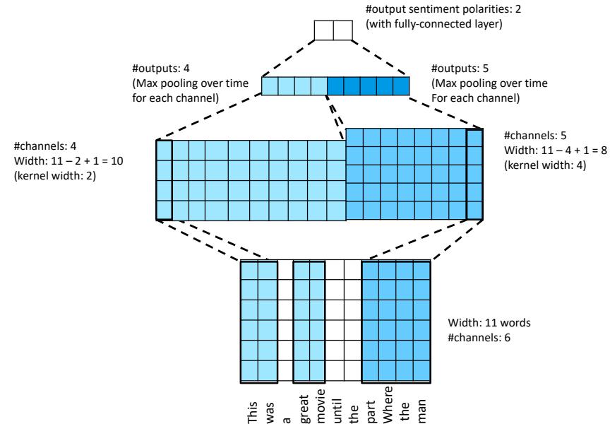
Figure 15.14: Illustration of the TextCNN model for binary sentiment classification. Adapted from Figure 15.3.5 of [Zha+20].
then pass this into a softmax layer.
In [Kim14], they applied this model to sequence classification. The idea is to embed each word using an embedding layer, and then to compute various features using 1d kernels of di!erent widths, to capture patterns of di!erent length scales. We then apply max pooling over time, and concatenate the results, and pass to a fully connected layer. See Figure 15.14 for an illustration, and cnn1d\_sentiment\_jax.ipynb for some code.
15.3.2 Causal 1d CNNs for sequence generation
To use 1d CNNs in a generative setting, we must convert them to a causal CNN, in which each output variable only depends on previously generated variables. (This is also called a convolutional Markov model.) In particular, we define the model as follows:
\[p(\mathbf{y}) = \prod\_{t=1}^{T} p(y\_t | \mathbf{y}\_{1:t-1}) = \prod\_{t=1}^{T} \text{Cat}(y\_t | \text{softmax}(\varphi(\sum\_{\tau=1}^{t-k} w^\top y\_{\tau:\tau+k}))) \tag{15.33}\]
where w is the convolutional filter of size k, and we have assumed a single nonlinearity ϑ and categorical output, for notational simplicity. This is like regular 1d convolution except we “mask out” future inputs, so that yt only depends on the past values, rather than past and future values. This is
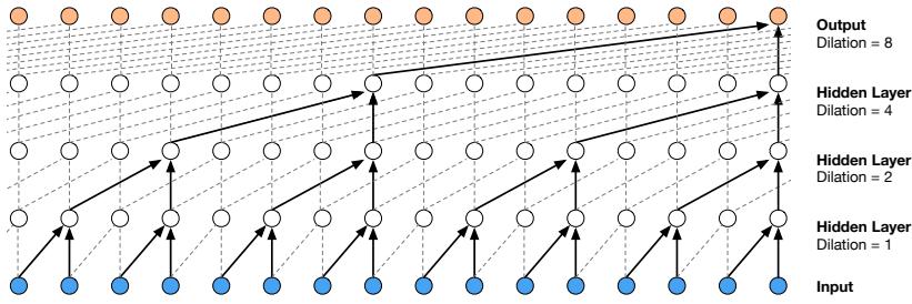
Because models with causal convolutions do not have recurrent connections, they are typically faster to train than RNNs, especially when applied to very long sequences. One of the problems of causal convolutions is that they require many layers, or large filters to increase the receptive field. For example, in Fig. 2 the receptive field is only 5 (= #layers + filter length - 1). In this paper we use dilated convolutions to increase the receptive field by orders of magnitude, without greatly increasing
A dilated convolution (also called a trous ` , or convolution with holes) is a convolution where the filter is applied over an area larger than its length by skipping input values with a certain step. It is equivalent to a convolution with a larger filter derived from the original filter by dilating it with zeros, but is significantly more efficient. A dilated convolution effectively allows the network to operate on a coarser scale than with a normal convolution. This is similar to pooling or strided convolutions, but here the output has the same size as the input. As a special case, dilated convolution with dilation 1 yields the standard convolution. Fig. 3 depicts dilated causal convolutions for dilations 1, 2, 4, and 8. Dilated convolutions have previously been used in various contexts, e.g. signal processing
Figure 3: Visualization of a stack of dilated causal convolutional layers. Stacked dilated convolutions enable networks to have very large receptive fields with just a few lay-Figure 15.15: Illustration of the wavenet model using dilated (atrous) convolutions, with dilation factors of 1, 2, 4 and 8. From Figure 3 of [Oor+16]. Used with kind permission of Aaron van den Oord.
ers, while preserving the input resolution throughout the network as well as computational efficiency.
In this paper, the dilation is doubled for every layer up to a limit and then repeated: e.g. 1, 2, 4,…, 512, 1, 2, 4,…, 512, 1, 2, 4,…, 512. called causal convolution. We can of course use deeper models, and we can condition on input features x.
The intuition behind this configuration is two-fold. First, exponentially increasing the dilation factor results in exponential receptive field growth with depth (Yu & Koltun, 2016). For example each 1, 2, 4,…, 512 block has receptive field of size 1024, and can be seen as a more efficient and discriminative (non-linear) counterpart of a 1⇥1024 convolution. Second, stacking these blocks further increases the model capacity and the receptive field size. 2.2 SOFTMAX DISTRIBUTIONS In order to capture long-range dependencies, we can use dilated convolution (Section 14.4.1), as illustrated in Figure 15.15. This model has been successfully used to create a state of the art text to speech (TTS) synthesis system known as wavenet [Oor+16]. In particular, they stack 10 causal 1d convolutional layers with dilation rates 1, 2, 4,…, 256, 512 to get a convolutional block with an e!ective receptive field of 1024. (They left-padded the input sequences with a number of zeros equal to the dilation rate before every layer, so that every layer has the same length.) They then repeat this block 3 times to compute deeper features.
One approach to modeling the conditional distributions p (xt | x1,…,xt1) over the individual audio samples would be to use a mixture model such as a mixture density network (Bishop, 1994) or mixture of conditional Gaussian scale mixtures (MCGSM) (Theis & Bethge, 2015). However, van den Oord et al. (2016a) showed that a softmax distribution tends to work better, even when the data is implicitly continuous (as is the case for image pixel intensities or audio sample values). One In wavenet, the conditioning information x is a set of linguistic features derived from an input sequence of words; the model then generates raw audio using the above model. It is also possible to create a fully end-to-end approach, which starts with raw words rather than linguistic features (see [Wan+17]).
of the reasons is that a categorical distribution is more flexible and can more easily model arbitrary distributions because it makes no assumptions about their shape. Because raw audio is typically stored as a sequence of 16-bit integer values (one per timestep), a Although wavenet produces high quality speech, it is too slow for use in production systems. However, it can be “distilled” into a parallel generative model [Oor+18]. We discuss these kinds of parallel generative models in the sequel to this book, [Mur23].
softmax layer would need to output 65,536 probabilities per timestep to model all possible values.
To make this more tractable, we first apply a µ-law companding transformation (ITU-T, 1988) to the data, and then quantize it to 256 possible values: 15.4 Attention
f (xt) = sign(xt) ln (1 + µ |xt|) ln (1 + µ) , 3 In all of the neural networks we have considered so far, the hidden activations are a linear combination of the input activations, followed by a nonlinearity: Z = ϑ(XW), where X → Rm↓v are the hidden feature vectors, and W → Rv↓v↑ are a fixed set of weights that are learned on a training set to produce Z → Rm↓v↑ outputs.
However, we can imagine a more flexible model in which the weights depend on the inputs, i.e., Z = ϑ(XW(X)). This kind of multiplicative interaction is called attention. More generally, we can write Z = ϑ(VW(Q, K)), where Q → Rm↓q are a set of queries (derived from X) used to describe what each input is “looking for”, K → Rm↓q are a set of keys (derived from X) used to describe what each input vector contains, and V → Rm↓v are a set of values V → Rm↓v (derived from X) used to describe how each input should be transmitted to the output. (We usually compute these quantities using linear projections of the input, Q = WqX, K = WkX, and V = WvX.)
computational cost.
Koltun, 2016).
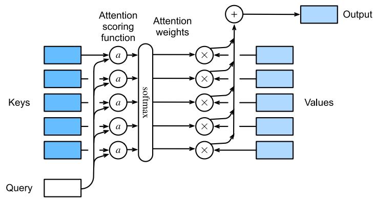
Figure 15.16: Attention computes a weighted average of a set of values, where the weights are derived by comparing the query vector to a set of keys. From Figure 10.3.1 of [Zha+20]. Used with kind permission of Aston Zhang.
When using attention to compute output zj , we use its corresponding query qj and compare it to each key ki to get a similarity score, 0 ↙ φij ↙ 1, where ( i φij = 1; we then set zj = ( i φijvi. (We assume ϑ(u) = u is the identity function.) For example, suppose V = X, and query qj equally matches keys 1 and 2, so φ1j = φ2j = 0.5; then we have zj = 0.5x1 + 0.5x2. Thus the outputs become a dynamic weighted combination of the inputs, rather than a fixed weighted combination. And rather than learning the weight matrix, we learn the projection matrices Wq, Wk and Wv. We explain this in more detail below.
Note that attention was originally developed for natural language sequence models. However, nowadays it is applied to a variety of models, including vision models. Our presentation in the following sections is based on [Zha+20, Chap 10.].
15.4.1 Attention as soft dictionary lookup
We will focus on a single output vector, with corresponding query vector q. We can think of attention as a dictionary lookup, in which we compare the query q to each key ki, and then retrieve the corresponding value vi. To make this lookup operation di!erentiable, instead of retrieving a single value vi, we compute a convex combination of the values, as follows:
\[\text{Attn}(\mathbf{q}, (k\_1, v\_1), \dots, (k\_m, v\_m)) = \text{Attn}(\mathbf{q}, (k\_{1:m}, v\_{1:m})) = \sum\_{i=1}^m \alpha\_i(\mathbf{q}, k\_{1:m}) v\_i \in \mathbb{R}^v \tag{15.34}\]
where φi(q, k1:m) is the i’th attention weight; these weights satisfy 0 ↙ φi(q, k1:m) ↙ 1 for each i and ( i φi(q, k1:m)=1.
The attention weights can be computed from an attention score function a(q, ki) → R, that computes the similarity of query q to key ki. We will discuss several such score function below. Given the scores, we can compute the attention weights using the softmax function:
\[\alpha\_i(\mathbf{q}, k\_{1:m}) = \text{softmax}\_i([a(\mathbf{q}, k\_1), \dots, a(\mathbf{q}, k\_m)]) = \frac{\exp(a(\mathbf{q}, k\_i))}{\sum\_{j=1}^m \exp(a(\mathbf{q}, k\_j))}\tag{15.35}\]
See Figure 15.16 for an illustration.
In some cases, we want to restrict attention to a subset of the dictionary, corresponding to valid entries. For example, we might want to pad sequences to a fixed length (for e”cient minibatching), in which case we should “mask out” the padded locations. This is called masked attention. We can implement this e”ciently by setting the attention score for the masked entries to a large negative number, such as ↗106, so that the corresponding softmax weights will be 0. (This is analogous to causal convolution, discussed in Section 15.3.2.)
15.4.2 Kernel regression as non-parametric attention
We can interpret attention in terms of kernel regression, which is a nonparametric model which we discuss in Section 16.3.5. In brief this a model where the predicted output at query point x is a weighted combination of all the target labels yi, where the weights depend on the similarity of query point x to each training point xi:
\[f(\mathbf{z}) = \sum\_{i=1}^{n} \alpha\_i(\mathbf{z}, \mathbf{z}\_{1:n}) y\_i \tag{15.36}\]
where φi(x, x1:n) ↓ 0 measures the normalized similarity of test input x to training input xi. This similarity measure is usually computed by defining the attention score in terms of a density kernel, such as the Gaussian:
\[\mathcal{K}\_{\sigma}(u) = \frac{1}{\sqrt{2\pi\sigma^2}} e^{-\frac{1}{2\sigma^2}u^2} \tag{15.37}\]
where ω is called the bandwidth. We then define a(x, xi) = Kε(x ↗ xi).
Because the scores are normalized, we can drop the ⇐ 1 2↽ε2 term. In addition, we rewrite the kernel in terms of ↼2 = 1/ω2 to get
\[\mathcal{K}(u;\beta) = \exp(-\frac{\beta^2}{2}u^2) \tag{15.38}\]
Plugging this in to Equation (15.36), we get
\[f(\mathbf{z}) = \sum\_{i=1}^{n} \alpha\_i(\mathbf{z}, \mathbf{z}\_{1:n}) y\_i \tag{15.39}\]
\[\hat{y}\_i = \sum\_{i=1}^n \frac{\exp[-\frac{1}{2}((\mathbf{z} - \mathbf{z}\_i)\beta)^2]}{\sum\_{j=1}^n \exp[-\frac{1}{2}((\mathbf{z} - \mathbf{z}\_j)\beta)^2]} y\_i \tag{15.40}\]
\[y = \sum\_{i=1}^{n} \text{softmax}\_i \left[ -\frac{1}{2} ((x - x\_1)\beta)^2, \dots, -\frac{1}{2} ((x - x\_n)\beta)^2 \right] y\_i \tag{15.41}\]
We can interpret this as a form of nonparametric attention, where the queries are the test points x, the keys are the training inputs xi, and the values are the training labels yi. If we set ↼ = 1, the resulting attention matrix Aji = φi(xj , x1:n) for test input j is shown in Figure 15.17a. The resulting predicted curve is shown in Figure 15.17b.
The size of the diagonal band in Figure 15.17a, and hence the sparsity of the attention mechanism, depends on the parameter ↼. If we increase ↼, corresponding to reducing the kernel bandwidth, the band will get narrower, but the model will start to overfit.
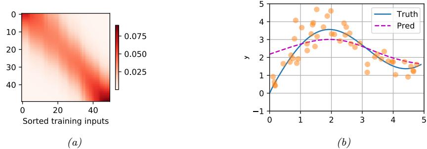
Figure 15.17: Kernel regression in 1d. (a) Kernel weight matrix. (b) Resulting predictions on a dense grid of test points. Generated by kernel\_regression\_attention.ipynb.
15.4.3 Parametric attention
In Section 15.4.2, we defined the attention score in terms of the Gaussian kernel, comparing a query (test point) to each of the values in the training set. However, non-parametric methods do not scale well to large training sets, or high-dimensional inputs. We will therefore turn our attention (no pun intended) to parametric models, where we have a fixed set of keys and values, and where we compare queries and keys in a learned embedding space.
There are several ways to do this. In the general case, the query q → Rq and the key k → Rk may have di!erent sizes. To compare them, we can map them to a common embedding space of size h by computing Wqq and Wkk. where Wq → Rh↓q and Wk → Rh↓k. We can then pass these into an MLP to get the following additive attention scoring function:
\[a(\mathbf{q}, \mathbf{k}) = \mathbf{w}\_v^\mathsf{T} \tanh(\mathbf{W}\_q \mathbf{q} + \mathbf{W}\_k \mathbf{k}) \in \mathbb{R} \tag{15.42}\]
A more computationally e”cient approach is to assume the queries and keys both have length d, so we can compute qTk directly. If we assume these are independent random variables with 0 mean and unit variance, the mean of their inner product is 0, and the variance is d. (This follows from Equation (2.34) and Equation (2.39).) To ensure the variance of the inner product remains 1 regardless of the size of the inputs, it is standard to divide by ⇔ d. This gives rise to the scaled dot-product attention:
\[a(\mathbf{q}, \mathbf{k}) = \mathbf{q}^{\mathsf{T}} \mathbf{k} / \sqrt{d} \in \mathbb{R} \tag{15.43}\]
In practice, we usually deal with minibatches of n vectors at a time. Let the corresponding matrices of queries, keys and values be denoted by Q → Rn↓d, K → Rm↓d, V → Rm↓v. Then we can compute the attention-weighted outputs as follows:
\[\text{Attn}(\mathbf{Q}, \mathbf{K}, \mathbf{V}) = \text{softmax}(\frac{\mathbf{Q}\mathbf{K}^{\mathsf{T}}}{\sqrt{d}})\mathbf{V} \in \mathbb{R}^{n \times v} \tag{15.44}\]
where the softmax function softmax is applied row-wise. See attention\_jax.ipynb for some sample code.
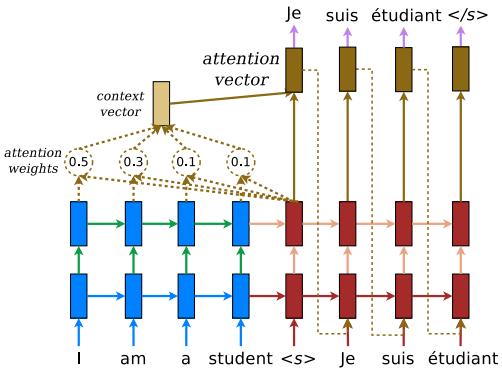
Figure 15.18: Illustration of seq2seq with attention for English to French translation. Used with kind permission of Minh-Thang Luong.
Figure 15.19: Illustration of the attention heatmaps generated while translating two sentences from Spanish to English. (a) Input is “hace mucho frio aqui.”, output is “it is very cold here.”. (b) Input is “¿todavia estan en casa?”, output is “are you still at home?”. Note that when generating the output token “home”, the model should attend to the input token “casa”, but in fact it seems to attend to the input token “?”. Adapted from https: // www. tensorflow. org/ tutorials/ text/ nmt\_ with\_ attention .
15.4.4 Seq2Seq with attention
Recall the seq2seq model from Section 15.2.3. This uses an RNN decoder of the form hd t = fd(hd t→1, yt→1, c), where c is a fixed-length context vector, representing the encoding of the input x1:T . Usually we set c = he T , which is the final state of the encoder RNN (or we use a bidirectional RNN with average pooling). However, for tasks such as machine translation, this can result in poor performance, since the output does not have access to the input words themselves. We can avoid this bottleneck by allowing the output words to directly “look at” the input words. But which inputs should it look at? After all, word order is not always preserved across languages (e.g., German often puts verbs at the end of a sentence), so we need to infer the alignment between source and target.
We can solve this problem (in a di!erentiable way) by using (soft) attention, as first proposed in [BCB15; LPM15]. In particular, we can replace the fixed context vector c in the decoder with a
dynamic context vector ct computed as follows:
\[\mathbf{c}\_t = \sum\_{i=1}^T \alpha\_i (\mathbf{h}\_{t-1}^d, \mathbf{h}\_{1:T}^e) \mathbf{h}\_i^e \tag{15.45}\]
This uses attention where the query is the hidden state of the decoder at the previous step, hd t→1, the keys are all the hidden states from the encoder, and the values are also the hidden states from the encoder. (When the RNN has multiple hidden layers, we usually take the top layer from the encoder, as the keys and values, and the top layer of the decoder as the query.) This context vector is concatenated with the input vector of the decoder, yt→1, and fed into the decoder, along with the previous hidden state hd t→1, to create hd t . See Figure 15.18 for an illustration of the overall model.
We can train this model in the usual way on sentence pairs, and then use it to perform machine translation. (See nmt\_attention\_jax.ipynb for some sample code.) We can also visualize the attention weights computed at each step of decoding, to get an idea of which parts of the input the model thinks are most relevant for generating the corresponding output. Some examples are shown in Figure 15.19.
15.4.5 Seq2vec with attention (text classification)
We can also use attention with sequence classifiers. For example [Raj+18] apply an RNN classifier to the problem of predicting if a patient will die or not. The input is a set of electronic health records, which is a time series containing structured data, as well as unstructured text (clinical notes). Attention is useful for identifying “relevant” parts of the input, as illustrated in Figure 15.20.
15.4.6 Seq+Seq2Vec with attention (text pair classification)
Suppose we see the sentence “A person on a horse jumps over a log” (call this the premise) and then we later read “A person is outdoors on a horse” (call this the hypothesis). We may reasonably say that the premise entails the hypothesis, meaning that the hypothesis is more likely given the premise.3 Now suppose the hypothesis is “A person is at a diner ordering an omelette”. In this case, we would say that the premise contradicts the hypothesis, since the hypothesis is less likely given the premise. Finally, suppose the hypothesis is “A person is training his horse for a competition”. In this case, we see that the relationship between premise and hypothesis is neutral, since the hypothesis may or may not follow from the premise. The task of classifying a sentence pair into these three categories is known as textual entailment or “natural language inference”. A standard benchmark in this area is the Stanford Natural Language Inference or SNLI corpus [Bow+15]. This consists of 550,000 labeled sentence pairs.
An interesting solution to this classification problem was presented in [Par+16a]; at the time, it was the state of the art on the SNLI dataset. The overall approach is sketched in Figure 15.21. Let A = (a1,…, am) be the premise and B = (b1,…, bn) be the hypothesis, where ai, bj → RE are embedding vectors for the words. The model has 3 steps. First, each word in the premise, ai, attends
3. Note that the premise does not logically imply the hypothesis, since the person could be horse-back riding indoors, but generally people ride horses outdoors. Also, we are assuming the phrase “a person” refers to the same person in the two sentences.
Figure 15.20: Example of an electronic health record. In this example, 24h after admission to the hospital, the RNN classifier predicts the risk of death as 19.9%; the patient ultimately died 10 days after admission. The “relevant” keywords from the input clinical notes are shown in red, as identified by an attention mechanism. From Figure 3 of [Raj+18]. Used with kind permission of Alvin Rajkomar.
to each word in the hypothesis, bj , to compute an attention weight
\[e\_{ij} = f(\mathbf{a}\_i)^\top f(\mathbf{b}\_j) \tag{15.46}\]
where f : RE ≃ RD is an MLP; we then compute a weighted average of the matching words in the hypothesis,
\[\beta\_i = \sum\_{j=1}^{n} \frac{\exp(e\_{ij})}{\sum\_{k=1}^{n} \exp(e\_{ik})} \mathbf{b}\_j \tag{15.47}\]
Next, we compare ai with ϖi by mapping their concatenation to a hidden space using an MLP g : R2E ≃ RH:
\[w\_{A,i} = g([\mathbf{a}\_i, \beta\_i]), \ i = 1, \ldots, m \tag{15.48}\]
Figure 15.21: Illustration of sentence pair entailment classification using an MLP with attention to align the premise (“I do need sleep”) with the hypothesis (“I am tired”). White squares denote active attention weights, blue squares are inactive. (We are assuming hard 0/1 attention for simplicity.) From Figure 15.5.2 of [Zha+20]. Used with kind permission of Aston Zhang.
Finally, we aggregate over the comparisons to get an overall similarity of premise to hypothesis:
\[\mathbf{v}\_A = \sum\_{i=1}^m \mathbf{v}\_{A,i} \tag{15.49}\]
We can similarly compare the hypothesis to the premise using
\[\alpha\_j = \sum\_{i=1}^{m} \frac{\exp(e\_{ij})}{\sum\_{k=1}^{m} \exp(e\_{kj})} \mathbf{a}\_i \tag{15.50}\]
\[w\_{B,j} = g([\mathbf{b}\_j, \alpha\_j]), \ j = 1, \ldots, n \tag{15.51}\]
\[\mathbf{v}\_{B} = \sum\_{j=1}^{n} \mathbf{v}\_{B,j} \tag{15.52}\]
At the end, we classify the output using another MLP h : R2H ≃ R3:
\[ \hat{y} = h([\mathbf{v}\_A, \mathbf{v}\_B])\tag{15.53} \]
See entailment\_attention\_mlp\_jax.ipynb for some sample code.
We can modify this model to learn other kinds of mappings from sentence pairs to output labels. For example, in the semantic textual similarity task, the goal is to predict how semantically related two input sentences are. A standard dataset for this is the STS Benchmark [Cer+17], where relatedness ranges from 0 (meaning unrelated) to 5 (meaning maximally related).
15.4.7 Soft vs hard attention
If we force the attention heatmap to be sparse, so that each output can only attend to one input location instead of a weighted combination of all of them, the method is called hard attention. We
Figure 15.22: Image captioning using attention. (a) Soft attention. Generates “a woman is throwing a frisbee in a park”. (b) Hard attention. Generates “a man and a woman playing frisbee in a field”. From Figure 6 of [Xu+15]. Used with kind permission of Kelvin Xu.
compare these two approaches for an image captioning problem in Figure 15.22. Unfortunately, hard attention results in a nondi!erentiable training objective, and requires methods such as reinforcement learning to fit the model. See [Xu+15] for the details.
It seems from the above examples that these attention heatmaps can “explain” why the model generates a given output. However, the interpretability of attention is controversial (see e.g., [JW19; WP19; SS19; Bru+19] for discussion).
15.5 Transformers
The transformer model [Vas+17] is a seq2seq model which uses attention in the encoder as well as the decoder, thus eliminating the need for RNNs, as we explain below. Transformers have been used for many (conditional) sequence generation tasks, such as machine translation [Vas+17], constituency parsing [Vas+17], music generation [Hua+18], protein sequence generation [Mad+20; Cho+20b], abstractive text summarization [Zha+19a], image generation [Par+18] (treating the image as a rasterized 1d sequence), etc.
The transformer is a rather complex model that uses several new kinds of building blocks or layers. We introduce these new blocks below, and then discuss how to put them all together.4
15.5.1 Self-attention
In Section 15.4.4 we showed how the decoder of an RNN could use attention to the input sequence in order to capture contexual embeddings of each input. However, rather than the decoder attending to the encoder, we can modify the model so the encoder attends to itself. This is called self attention [CDL16; Par+16b].
In more detail, given a sequence of input tokens x1,…, xn, where xi → Rd, self-attention can generate a sequence of outputs of the same size using
\[\mathbf{y}\_{i} = \text{Attn}(x\_{i}, (x\_{1}, x\_{1}), \dots, (x\_{n}, x\_{n})) \tag{15.54}\]
4. For a more detailed introduction, see [Tur23] or https://huggingface.co/learn/nlp-course.
Figure 15.23: Illustration of how encoder self-attention for the word “it” di!ers depending on the input context. From https: // ai. googleblog. com/ 2017/ 08/ transformer-novel-neural-network. html . Used with kind permission of Jakob Uszkoreit.
where the query is xi, and the keys and values are all the (valid) inputs x1,…, xn.
To use this in a decoder, we can set xi = yi→1, and n = i ↗ 1, so all the previously generated outputs are available. At training time, all the outputs are already known, so we can evaluate the above function in parallel, overcoming the sequential bottleneck of using RNNs.
In addition to improved speed, self-attention can give improved representations of context. As an example, consider translating the English sentences “The animal didn’t cross the street because it was too tired” and “The animal didn’t cross the street because it was too wide” into French. To generate a pronoun of the correct gender in French, we need to know what “it” refers to (this is called coreference resolution). In the first case, the word “it” refers to the animal. In the second case, the word “it” now refers to the street.
Figure 15.23 illustrates how self attention applied to the English sentence is able to resolve this ambiguity. In the first sentence, the representation for “it” depends on the earlier representations of “animal”, whereas in the latter, it depends on the earlier representations of “street”.
15.5.2 Multi-headed attention
If we think of an attention matrix as like a kernel matrix (as discussed in Section 15.4.2), it is natural to want to use multiple attention matrices, to capture di!erent notions of similarity. This is the basic idea behind multi-headed attention (MHA). In more detail, given a query q → Rdq , keys kj → Rdk , and values vj → Rdv , we define the i’th attention head to be
\[h\_i = \text{Attn}(\mathbf{W}\_i^{(q)} \mathbf{q}, \{\mathbf{W}\_i^{(k)} \mathbf{k}\_j, \mathbf{W}\_i^{(v)} \mathbf{v}\_j\}) \in \mathbb{R}^{p\_v} \tag{15.55}\]
where W(q) i → Rpq↓dq , W(k) i → Rpk↓dk , and W(v) i → Rpv↓dv are projection matrices. We then stack the h heads together, and project to Rpo using
\[\mathbf{h} = \text{MHA}(\mathbf{q}, \{\mathbf{k}\_j, \mathbf{v}\_j\}) = \mathbf{W}\_o \begin{pmatrix} h\_1 \\ \vdots \\ h\_h \end{pmatrix} \in \mathbb{R}^{p\_o} \tag{15.56}\]
where hi is defined in Equation (15.55), and Wo → Rpo↓hpv . If we set pqh = pkh = pvh = po, we can compute all the output heads in parallel. See multi\_head\_attention\_jax.ipynb for some sample
Figure 15.24: Multi-head attention. Adapted from Figure 9.3.3 of [Zha+20].
code.
15.5.3 Positional encoding
The performance of “vanilla” self-attention can be low, since attention is permutation invariant, and hence ignores the input word ordering. To overcome this, we can concatenate the word embeddings with a positional embedding, so that the model knows what order the words occur in.
One way to do this is to represent each position by an integer. However, neural networks cannot natively handle integers. To overcome this, we can encode the integer in binary form. For example, if we assume the sequence length is n = 8, we can use the following sequence of d = 3-dimensional bit vectors for each location: 000, 001, 010, 011, 100, 101, 110, 111. We see that the right most index toggles the fastest (has highest frequency), whereas the left most index (most significant bit) toggles the slowest. (We could of course change this, so that the left most bit toggles fastest.) We can represent this as a position matrix P → Rn↓d.
We can think of the above representation as using a set of basis functions (corresponding to powers of 2), where the coe”cients are 0 or 1. We can obtain a more compact code by using a di!erent set of basis functions, and real-valued weights. [Vas+17] propose to use a sinusoidal basis, as follows:
\[p\_{i,2j} = \sin\left(\frac{i}{C^{2j/d}}\right), \ p\_{i,2j+1} = \cos\left(\frac{i}{C^{2j/d}}\right),\tag{15.57}\]
where C = 10, 000 corresponds to some maximum sequence length. For example, if d = 4, the i’th row is
\[\mathbf{p}\_i = [\sin(\frac{i}{C^{0/4}}), \cos(\frac{i}{C^{0/4}}), \sin(\frac{i}{C^{2/4}}), \cos(\frac{i}{C^{2/4}})] \tag{15.58}\]
Figure 15.25a shows the corresponding position matrix for n = 60 and d = 32. In this case, the left-most columns toggle fastest. We see that each row has a real-valued “fingerprint” representing its location in the sequence. Figure 15.25b shows some of the basis functions (column vectors) for dimensions 6 to 9.
Figure 15.25: (a) Positional encoding matrix for a sequence of length n = 60 and an embedding dimension of size d = 32. (b) Basis functions for columns 6 to 9. Generated by positional\_encoding\_jax.ipynb.
The advantage of this representation is two-fold. First, it can be computed for arbitrary length inputs (up to T ↙ C), unlike a learned mapping from integers to vectors. Second, the representation of one location is linearly predictable from any other, given knowledge of their relative distance. In particular, we have pt+⇀ = f(pt), where f is a linear transformation. To see this, note that
\[ \begin{pmatrix} \sin(\omega\_k(t+\phi)) \\ \cos(\omega\_k(t+\phi)) \end{pmatrix} = \begin{pmatrix} \sin(\omega\_k t)\cos(\omega\_k \phi) + \cos(\omega\_k t)\sin(\omega\_k \phi) \\ \cos(\omega\_k t)\cos(\omega\_k \phi) - \sin(\omega t)\sin(\omega\_k \phi) \end{pmatrix} \tag{15.59} \]
\[\mathbf{x} = \begin{pmatrix} \cos(\omega\_k \phi) & \sin(\omega\_k \phi) \\ -\sin(\omega\_k \phi) & \cos(\omega\_k \phi) \end{pmatrix} \begin{pmatrix} \sin(\omega\_k t) \\ \cos(\omega\_k t) \end{pmatrix} \tag{15.60}\]
So if ϱ is small, then pt+⇀ ′ pt. This provides a useful form of inductive bias.
Once we have computed the positional embeddings P, we need to combine them with the original word embeddings X using the following:5
POS(Embed(X)) = X + P. (15.61)
15.5.4 Putting it all together
A transformer is a seq2seq model that uses self-attention for the encoder and decoder rather than an RNN. The encoder uses a series of encoder blocks, each of which uses multi-headed attention (Section 15.5.2), residual connections (Section 13.4.4), feedforward layers (Section 13.2), and layer normalization (Section 14.2.4.2). More precisely, the encoder block can be defined as follows:
def EncoderBlock(X):
  Z = LayerNorm(MultiHeadAttn(Q=X, K=X, V=X) + X)
  E = LayerNorm(FeedForward(Z) + Z)
return E5. A more obvious combination scheme would be to concatenate, X and P, but adding takes less space. Furthermore, since the X embeddings are learned, the model could emulate concatentation by setting the first K dimensions of X, and the last D ↑ K dimensions of P, to 0, where K is defined implicitly by the sparsity pattern. For more discussion, see https://bit.ly/3rMG1at.
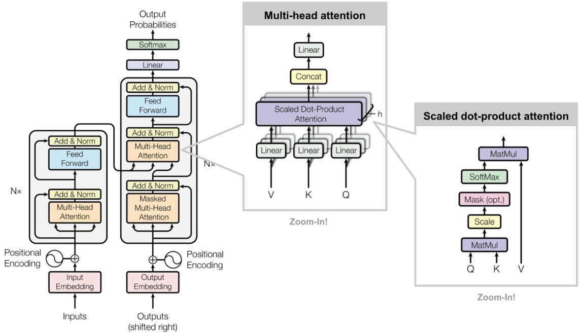
Figure 15.26: The transformer. From [Wen18]. Used with kind permission of Lilian Weng. Adapted from Figures 1–2 of [Vas+17].
Note that the MHA layer combines information across the sequence, and the feedforward layer combines information across the dimensions at each location in parallel. (Most of the parameters of large transformer models are stored inside these MLPs, and it has been conjectured that this is where most of the “world knowledge” lives [Men+22].) The layer norm can either be applied after the module (i.e., z = LN(module(x) + x)) or before (i.e., z = module(LN(x) + x)); these are known as post-norm and pre-norm.
The overall encoder is defined by applying positional encoding to the embedding of the input sequence, following by N copies of the encoder block, where N controls the depth of the block:
def Encoder(X, N):
  E = POS(Embed(X))
  for n in range(N):
     E = EncoderBlock(E)
  return E
See the LHS of Figure 15.26 for an illustration.
The decoder has a somewhat more complex structure. It is given access to the encoder via another multi-head attention block. But it is also given access to previously generated outputs: these are shifted, and then combined with a positional embedding, and then fed into a masked (causal) multi-head attention model. Finally the output distribution over tokens at each location is computed
| Layer type |
Complexity | Sequential ops. |
Max. path length |
|---|---|---|---|
| Self-attention | O(n2d) | O(1) | O(1) |
| Recurrent | O(nd2) | O(n) | O(n) |
| Convolutional | O(knd2) | O(1) | O(logk n) |
Table 15.1: Comparison of the transformer with other neural sequential generative models. n is the sequence length, d is the dimensionality of the input features, and k is the kernel size for convolution. Based on Table 1 of [Vas+17].
in parallel.
In more detail, the decoder block is defined as follows:
def DecoderBlock(Y, E):
  Z = LayerNorm(MultiHeadAttn(Q=Y, K=Y, V=Y) + Y)
  Z' = LayerNorm(MultiHeadAttn(Q=Z, K=E, V=E) + Z)
  D = LayerNorm(FeedForward(Z') + Z')
  return D
The overall decoder is defined by N copies of the decoder block:
def Decoder(Y, E, N):
  D = POS(Embed(Y))
  for n in range(N):
     D = DecoderBlock(D,E)
  return D
See the RHS of Figure 15.26 for an illustration.
During training time, all the inputs Y to the decoder are known in advance, since they are derived from embedding the lagged target output sequence. During inference (test) time, we need to decode sequentially, and use masked attention, where we feed the generated output into the embedding layer, and add it to the set of keys/values that can be attended to. (We initialize by feeding in the start-of-sequence token.) See transformers\_jax.ipynb for some sample code, and [Rus18; Ala18] for a detailed tutorial on this model.
15.5.5 Comparing transformers, CNNs and RNNs
In Figure 15.27, we visually compare three di!erent architectures for mapping a sequence x1:n to another sequence y1:n: a 1d CNN, an RNN, and an attention-based model. Each model makes di!erent tradeo!s in terms of speed and expressive power, where the latter can be quantified in terms of the maximum path length between any two inputs. See Table 15.1 for a summary.
For a 1d CNN with kernel size k and d feature channels, the time to compute the output is O(knd2), which can be done in parallel. We need a stack of n/k layers, or logk(n) if we use dilated convolution, to ensure all pairs can communicate. For example, in Figure 15.27, we see that x1 and x5 are initially 5 apart, and then 3 apart in layer 1, and then connected in layer 2.
For an RNN, the computational complexity is O(nd2), for a hidden state of size d, since we have to perform matrix-vector multiplication at each step. This is an inherently sequential operation. The maximum path length is O(n).
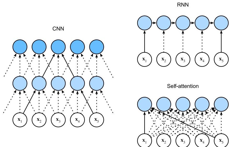
Figure 15.27: Comparison of (1d) CNNs, RNNs and self-attention models. From Figure 10.6.1 of [Zha+20]. Used with kind permission of Aston Zhang.
Finally, for self-attention models, every output is directly connected to every input, so the maximum path length is O(1). However, the computational cost is O(n2d). For short sequences, we typically have n ∞ d, so this is fine. For longer sequences, we discuss various fast versions of attention in Section 15.6.
15.5.6 Transformers for images *
CNNs (Chapter 14) are the most common model type for processing image data, since they have useful built-in inductive bias, such as locality (due to small kernels), equivariance (due to weight tying), and invariance (due to pooling). Suprisingly, it has been found that transformers can also do well at image classification [Rag+21], at least if trained on enough data. (They need a lot of data to overcome their lack of relevant inductive bias.)
The first model of this kind, known as ViT (vision transformer) [Dos+21], chops the input up into 16x16 patches, projects each patch into an embedding space, and then passes this set of embeddings x1:T to a transformer, analogous to the way word embeddings are passed to a transformer. The input is also prepended with a special [CLASS] embedding, x0. The output of the transformer is a set of encodings e0:T ; the model maps e0 to the target class label y, and is trained in a supervised way. See Figure 15.28 for an illustration.
After supervised pretraining, the model is fine-tuned on various downstream classification tasks, an approach known as transfer learning (see Section 19.2 for more details). When trained on “small” datasets such as ImageNet (which has 1k classes and 1.3M images), they find that they cannot outperform a pretrained CNN ResNet model (Section 14.3.4) known as BiT (big transfer) [Kol+20].
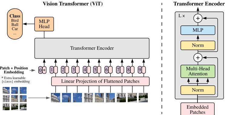
Figure 15.28: The Vision Transformer (ViT) model. This treats an image as a set of input patches. The input is prepended with the special CLASS embedding vector (denoted by *) in location 0. The class label for the image is derived by applying softmax to the final output encoding at location 0. From Figure 1 of [Dos+21]. Used with kind permission of Alexey Dosovitskiy
However, when trained on larger datasets, such as ImageNet-21k (with 21k classes and 14M images), or the Google-internal JFT dataset (with 18k classes and 303M images), they find that ViT does better than BiT at transfer learning.6 ViT is also cheaper to train than ResNet at this scale. (However, training is still expensive: the large ViT model on ImageNet-21k takes 30 days on a Google Cloud TPUv3 with 8 cores!)
15.5.7 Other transformer variants *
Many extensions of transformers have been published in the last few years. For example, the Gshard paper [Lep+21] shows how to scale up transformers to even more parameters by replacing some of the feed forward dense layers with a mixture of experts (Section 13.6.2) regression module. This allows for sparse conditional computation, in which only a subset of the model capacity (chosen by the gating network) is used for any given input.
As another example, the conformer paper [Gul+20] showed how to add convolutional layers inside the transformer architecture, which was shown to be helpful for various speech recognition tasks.
15.6 E!cient transformers *
This section is written by Krzysztof Choromanski.
Regular transformers take O(N2) time and space complexity, for a sequence of length N, which makes them impractical to apply to long sequences. In the past few years, researchers have proposed several more e”cient variants of transformers to bypass this di”culty. In this section, we give a
6. More recent work, specifically the ConvNeXt model of [Liu+22], has shown that CNNs can be made be to outperform ViT.
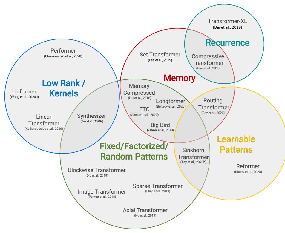
Figure 15.29: Venn diagram presenting the taxonomy of di!erent e”cient transformer architectures. From [Tay+20b]. Used with kind permission of Yi Tay.
brief survey of some of these methods (see Figure 15.29 for a summary). For more details, see e.g., [Tay+20b; Tay+20a; Lin+21].
15.6.1 Fixed non-learnable localized attention patterns
The simplest modification of the attention mechanism is to constrain it to a fixed non-learnable localized window, in other words restrict each token to attend only to a pre-selected set of other tokens. If for instance, each sequence is chunked into K blocks, each of length N K , and attention is conducted only within a block, then space/time complexity is reduced from O(N2) to O(N2/K). For K ∈ 1 this constitutes substantial overall computational improvements. Such an approach is applied in particular in [Qiu+19b; Par+18]. The attention patterns do not need to be in the form of blocks. Other approaches involve strided / dilated windows, or hybrid patterns, where several fixed attention patterns are combined together [Chi+19b; BPC20].
15.6.2 Learnable sparse attention patterns
A natural extension of the above approach is to allow the above compact patterns to be learned. The attention is still restricted to pairs of tokens within a single partition of some partitioning of the set of all the tokens, but now those partitionings are trained. In this class of methods we can distinguish two main approaches: based on hashing and clustering. In the hashing scenario all tokens are hashed and thus di!erent partitions correspond to di!erent hashing-buckets. This is the case for instance for the Reformer architecture [KKL20], where locality sensitive hashing (LSH) is applied. That leads to time complexity O(NM2 log(M)) of the attention module, where M stands for the dimensionality of tokens’ embeddings.
Hashing approaches require the set of queries to be identical to the set of keys. Furthermore, the number of hashes needed for precise partitioning (which in the above expression is treated as a constant) can be a large constant. In the clustering approach, tokens are clustered using standard clustering algorithms such as K-means (Section 21.3); this is known as the “clustering transformer” [Roy+20]. As in the block-case, if K equal-size clusters are used then space complexity of the attention module is reduced to O( N2 K ). In practice K is often taken to be of order K = “( ⇔ N), yet imposing that the clusters be similar in size is in practice di”cult.
15.6.3 Memory and recurrence methods
In some approaches, a side memory module can access several tokens simultaneously. This method is often instantiated in the form of a global memory algorithm as used in [Lee+19; Zah+20].
Another approach is to connect di!erent local blocks via recurrence. A flagship example of this approach is the class of Transformer-XL methods [Dai+19].
15.6.4 Low-rank and kernel methods
In this section, we discuss methods that approximate attention using low rank matrices. In [She+18; Kat+20] they approximate the attention matrix A directly by a low rank matrix, so that
\[A\_{ij} = \phi(q\_i)^{\mathsf{T}} \phi(\mathbf{k}\_j) \tag{15.62}\]
where ω(x) → RM is some finite-dimensional vector with M<D. One can leverage this structure to compute AV in O(N) time. Unfortunately, for softmax attention, the A is not low rank.
In Linformer [Wan+20a], they instead transform the keys and values via random Gaussian projections. They then apply the theory of the Johnson-Lindenstrauss Transform [AL13] to approximate softmax attention in this lower dimensional space.
In Performer [Cho+20a; Cho+20b], they show that the attention matrix can be computed using a (positive definite) kernel function. We define kernel functions in Section 17.1, but the basic idea is that K(q, k) ↓ 0 is some measure of similarity between q → RD and k → RD. For example, the Gaussian kernel, also called the radial basis function kernel, has the form
\[\mathcal{K}\_{\text{gauss}}(\mathbf{q}, \mathbf{k}) = \exp\left(-\frac{1}{2\sigma^2}||\mathbf{q} - \mathbf{k}||\_2^2\right) \tag{15.63}\]
To see how this can be used to compute an attention matrix, note that [Cho+20a] show the following:
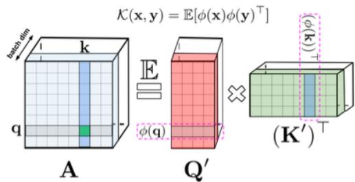
Figure 15.30: Attention matrix A rewritten as a product of two lower rank matrices Q↑ and (K↑ ) T with random feature maps ε(qi) → RM and ε(vk) → RM for the corresponding queries/keys stored in the rows/columns. Used with kind permission of Krzysztof Choromanski.
\[A\_{i,j} = \exp(\frac{\mathbf{q}\_i^\mathsf{T} k\_j}{\sqrt{D}}) = \exp(\frac{-\|\mathbf{q}\_i - \mathbf{k}\_j\|\_2^2}{2\sqrt{D}}) \times \exp(\frac{\|\mathbf{q}\_i\|\_2^2}{2\sqrt{D}}) \times \exp(\frac{\|\mathbf{k}\_j\|\_2^2}{2\sqrt{D}}).\tag{15.64}\]
The first term in the above expression is equal to Kgauss(qiD→1/4, kjD→1/4) with ω = 1, and the other two terms are just independent scaling factors.
So far we have not gained anything computationally. However, we will show in Section 17.2.9.3 that the Gaussian kernel can be written as the expectation of a set of random features:
\[\mathcal{K}\_{\text{gauss}}(x, y) = \mathbb{E}\left[\eta(x)^{\mathsf{T}}\eta(y)\right] \tag{15.65}\]
where ↼(x) → RM is a random feature vector derived from x, either based on trigonometric functions Equation (17.60) or exponential functions Equation (17.61). (The latter has the advantage that all the features are positive, which gives much better results [Cho+20b].) Therefore for the regular softmax attention, Ai,j can be rewritten as
\[A\_{i,j} = \mathbb{E}[\phi(\mathbf{q}\_i)^\mathsf{T}\phi(\mathbf{k}\_j)] \tag{15.66}\]
where ω is defined as:
\[\phi(x) \triangleq \exp\left(\frac{\|x\|\_2^2}{2\sqrt{D}}\right) \eta\left(\frac{x}{D^{\frac{1}{4}}}\right). \tag{15.67}\]
We can write the full attention matrix as follows
\[\mathbf{A} = \mathbb{E}[\mathbf{Q}'(\mathbf{K}')^\top] \tag{15.68}\]
where Q↑ , K↑ → RN↓M have rows encoding random feature maps corresponding to the queries and keys. (Note that we can get better performance if we ensure these random features are orthogonal, see [Cho+20a] for the details.) See Figure 15.30 for an illustration.
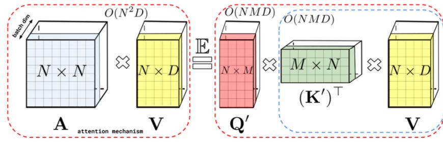
Figure 15.31: Decomposition of the attention matrix A can be leveraged to improve attention computations via matrix associativity property. To compute AV, we first calculate G = (k↑ ) TV and then q↑ G, resulting in linear in N space and time complexity. Used with kind permission of Krzysztof Choromanski.
We can create an approximation to A by using a single sample of the random features ω(qi) and ω(kj ), and using a small value of M, say M = O(D log(D)). We can then approximate the entire attention operator in O(N) time using
\[\text{attention}(\mathbf{Q}, \mathbf{K}, \mathbf{V}) = \text{diag}^{-1}(\mathbf{Q}^{\prime}((\mathbf{K}^{\prime})^{\top}\mathbf{1}\_{N}))(\mathbf{Q}^{\prime}((\mathbf{K}^{\prime})^{\top}\mathbf{V})) \tag{15.69}\]
This can be shown to be an unbiased approximation to the exact softmax attention operator. See Figure 15.31 for an illustration. (For details on how to generalize this to masked (causal) attention, see [Cho+20a].)
15.7 Language models and unsupervised representation learning
We have discussed how RNNs and autoregressive (decoder-only) transformers can be used as language models, which are generative sequence models of the form p(x1,…,xT ) = T t=1 p(xt|x1:t→1), where each xt is a discrete token, such as a word or wordpiece. (See Section 1.5.4 for a discussion of text preprocessing methods.) The latent state of these models can then be used as a continuous vector representation of the text. That is, instead of using the one-hot vector xt, or a learned embedding of it (such as those discussed in Section 20.5), we use the hidden state ht, which depends on all the previous words in the sentence. These vectors can then be used as contextual word embeddings, for purposes such as text classification or seq2seq tasks (see e.g. [LKB20] for a review). The advantage of this approach is that we can pre-train the language model in an unsupervised way, on a large corpus of text, and then we can fine-tune the model in a supervised way on a small labeled task-specific dataset. (This general approach is called transfer learning, see Section 19.2 for details.)
If our primary goal is to compute useful representations for transfer learning, as opposed to generating text, we can replace the generative sequence model with non-causal models that can compute a representation of a sentence, but cannot generate it. These models have the advantage that now the hidden state ht can depend on the past, y1:t→1, present yt, and future, yt+1:T . This can sometimes result in better representations, since it takes into account more context. However, if our goal is to generate textual outputs, we must use a “causal” or generative language model. We discuss both variants below.
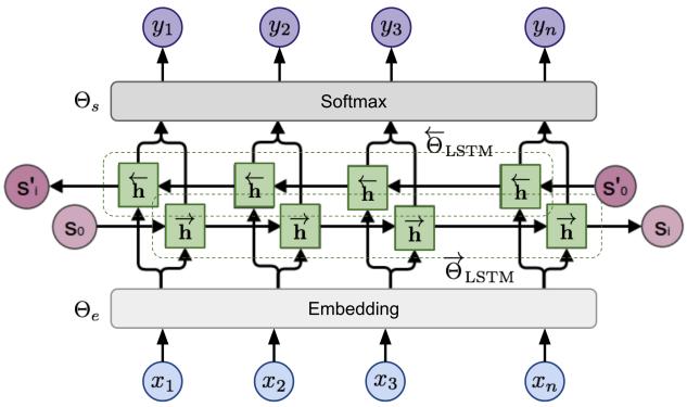
Figure 15.32: Illustration of ELMo bidirectional language model. Here yt = xt+1 when acting as the target for the forwards LSTM, and yt = xt↓1 for the backwards LSTM. (We add bos and eos sentinels to handle the edge cases.) From [Wen19]. Used with kind permission of Lilian Weng.
15.7.1 Non-generative language models
In this section we discuss models for learning representations (embeddings) of text.
15.7.1.1 ELMo
In [Pet+18], they present a method called ELMo, which is short for “Embeddings from Language Model”. The basic idea is to fit two RNN language models, one left-to-right, and one right-to-left, and then to combine their hidden state representations to come up with an embedding for each word. Unlike a biRNN (Section 15.2.2), which needs an input-output pair, ELMo is trained in an unsupervised way, to minimize the negative log likelihood of the input sentence x1:T :
\[\mathcal{L}(\boldsymbol{\theta}) = -\sum\_{t=1}^{T} \left[ \log p(\boldsymbol{x}\_t | \boldsymbol{x}\_{1:t-1}; \boldsymbol{\theta}\_e, \boldsymbol{\theta}^{\rightarrow}, \boldsymbol{\theta}\_s) + \log p(\boldsymbol{x}\_t | \boldsymbol{x}\_{t+1:T}; \boldsymbol{\theta}\_e, \boldsymbol{\theta}^{\leftarrow}, \boldsymbol{\theta}\_s) \right] \tag{15.70}\]
where εe are the shared parameters of the embedding layer, εs are the shared parameters of the softmax output layer, and ε↗ and ε↘ are the parameters of the two RNN models. (They use LSTM RNNs, described in Section 15.2.7.2.) See Figure 15.32 for an illustration.
After training, we define the contextual representation rt = [et, h↗ t,1:L, h↘ t,1:L], where L is the number of layers in the LSTM. We then learn a task-specific set of linear weights to map this to the final context-specific embedding of each token: rj t = rT t wj , where j is the task id. If we are performing a syntactic task like part-of-speech (POS) tagging (i.e., labeling each word as a noun, verb, adjective, etc), then the task will learn to put more weight on lower layers. If we are performing a semantic task like word sense disambiguation (WSD), then the task will learn to put more weight on higher layers. In both cases, we only need a small amount of task-specific labeled data, since we are just learning a single weight vector, to map from r1:T to the target labels y1:T .
15.7.1.2 BERT
In this section, we describe the BERT model (Bidirectional Encoder Representations from Transformers) of [Dev+19]. Like ELMo, this is a non-causal model, that can be used to create representations of text, but not to generate text. In particular, it uses a transformer model to map a modified version of a sequence back to the unmodified form. The modified input at location t omits the t’th, and the task is to predict the missing word given the remaining words. This is called the fill-in-the-blank or cloze task.
15.7.1.3 Masked language model task
More precisely, the model is trained to minimize the negative log pseudo-likelihood:
\[\mathcal{L} = \mathbb{E}\_{\mathbf{z} \sim \mathcal{D}} \mathbb{E}\_{\mathbf{m}} \sum\_{i \in m} -\log p(x\_i | x\_{-m}) \tag{15.71}\]
where m is a random binary mask. For example, if we train the model on transcripts from cooking videos, we might create a training sentence of the form
Let’s make [MASK] chicken! [SEP] It [MASK] great with orange sauce.
where [SEP] is a separator token inserted between two sentences. The desired target labels for the masked words are “some” and “tastes”. (This example is from [Sun+19a].)
The conditional probability is given by applying a softmax to the final layer hidden vector at location i:
\[p(x\_i|\hat{\mathbf{z}}) = \frac{\exp(\hbar(\hat{\mathbf{z}})\_i^{\mathsf{T}}\mathbf{e}(x\_i))}{\sum\_{x'} \exp(\hbar(\hat{\mathbf{z}})\_i^{\mathsf{T}}\mathbf{e}(x'))}\tag{15.72}\]
where xˆ = x→m is the masked input sentence, and e(x) is the embedding for token x. This is used to compute the loss at the masked locations; this is therefore called a masked language model. (This is similar to a denoising autoencoder, Section 20.3.2). See Figure 15.33a for an illustration of the model.
15.7.1.4 Next sentence prediction task
In addition to the masked language model objective, the original BERT paper added an additional objective, in which the model is trained to classify if one sentence follows another. More precisely, the model is fed as input
\[\text{CLS } A\_1 \ A\_2; \dots \ A\_m; \text{SEP } B\_1 \ B\_2; \dots; B\_n \text{SEP} \tag{15.73}\]
where SEP is a special separator token, and CLS is a special token marking the class. If sentence B follows A in the original text, we set the target label to y = 1, but if B is a randomly chosen sentence, we set the target label to y = 0. This is called the next sentence prediction task. This kind of pre-training can be useful for sentence-pair classification tasks, such as textual entailment or textual similarity, which we discussed in Section 15.4.6. (Note that this kind of pre-training is considered unsupervised, or self-supervised, since the target labels are automatically generated.)
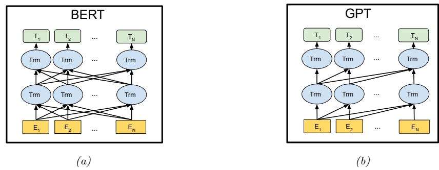
Figure 15.33: Illustration of (a) BERT and (b) GPT. Et is the embedding vector for the input token at location t, and Tt is the output target to be predicted. From Figure 3 of [Dev+19]. Used with kind permission of Ming-Wei Chang.
Figure 15.34: Illustration of how a pair of input sequences, denoted A and B, are encoded before feeding to BERT. From Figure 14.8.2 of [Zha+20]. Used with kind permission of Aston Zhang.
When performing next sentence prediction, the input to the model is specified using 3 di!erent embeddings: one per token, one for each segment label (sentence A or B), and one per location (using a learned positional embedding). These are then added. See Figure 15.34 for an illustration. BERT then uses a transformer encoder to learn a mapping from this input embedding sequence to an output embedding sequence, which gets decoded into word labels (for the masked locations) or a class label (for the CLS location).
15.7.1.5 Fine-tuning BERT for NLP applications
After pre-training BERT in an unsupervised way, we can use it for various downstream tasks by performing supervised fine-tuning. (See Section 19.2 for more background on such transfer learning methods.) Figure 15.35 illustrates how we can modify a BERT model to perform di!erent tasks, by simply adding one or more new output heads to the final hidden layer. See bert\_jax.ipynb for some sample code.
In Figure 15.35(a), we show how we can tackle single sentence classification (e.g., sentiment analysis): we simply take the feature vector associated with the dummy CLS token and feed it into an
Figure 15.35: Illustration of how BERT can be used for di!erent kinds of supervised NLP tasks. (a) Single sentence classification (e.g., sentiment analysis); (b) Sentence-pair classification (e.g., textual entailment); (c) Single sentence tagging (e.g., shallow parsing); (d) Question answering. From Figure 4 of [Dev+19]. Used with kind permission of Ming-Wei Chang.
MLP. Since each output attends to all inputs, this hidden vector will summarize the entire sentence. The MLP then learns to map this to the desired label space.
In Figure 15.35(b), we show how we can tackle sentence-pair classification (e.g., textual entailment, as discussed in Section 15.4.6): we just feed in the two input sentences, formatted as in Equation (15.73), and then classify the CLS token.
In Figure 15.35(c), we show how we can tackle single sentence tagging, in which we associate a label or tag with each word, instead of just the entire sentence. A common application of this is part of speech tagging, in which we annotate each words a noun, verb, adjective, etc. Another application of this is noun phrase chunking, also called shallow parsing, in which we must annotate the span of each noun phrase. The span is encoded using the BIO notation, in which B is the beginning of an entity, I-x is for inside, and O is for outside any entity. For example, consider the following sentence:
B I O O O BI O BII British Airways rose after announcing its withdrawl from the UAI deal
We see that there are 3 noun phrases, “British Airways”, “its withdrawl” and “the UAI deal”. (We require that the B, I and O labels occur in order, so this a prior constraint that can be included in the model.)
We can also associate types with each noun phrase, for example distinguishing person, location,
organization, and other. Thus the label space becomes {B-Per, I-Per, B-Loc, I-Loc, B-Org, I-Org, Outside }. This is called named entity recognition, and is a key step in information extraction. For example, consider the following sentence:
BP IP O O O BL IL BP O O O O Mrs Green spoke today in New York. Green chairs the finance committee.
From this, we infer that the first sentence has two named entities, namely “Mrs Green” (of type Person) and “New York” (of type Location). The second sentence mentions another person, “Green”, that most likely is the same as the first person, although this across-sentence entity resolution is not part of the basic NER task.
Finally, in Figure 15.35(d), we show how we can tackle question answering. Here the first input sentence is the question, the second is the background text, and the output is required to specifying the start and end locations of the relevant part of the background that contains the answer (see Table 1.4). The start location s and end location e are computed by applying 2 di!erent MLPs to a pooled version of the output encodings for the background text; the output of the MLPs is a softmax over all locations. At test time, we can extract the span (i, j) which maximizes the sum of scores si + ej for i ↙ j.
BERT achieves state-of-the-art performance on many NLP tasks. Interestingly, [TDP19] shows that BERT implicitly rediscovers the standard NLP pipeline, in which di!erent layers perform tasks such as part of speech (POS) tagging, parsing, named entity relationship (NER) detection, semantic role labeling (SRL), coreference resolution, etc. More details on NLP can be found in [JM20].
15.7.2 Generative (causal) Large Language Models (LLMs)
In this section, we briefly discuss generative or causal language models based on (decoder-only) transformers. These are generally as large language models (see e.g., [Bur25] for details).
15.7.2.1 GPT
In [Rad+18], they propose a model called GPT, which is short for “Generative Pre-training Transformer”. This is a causal (generative) model, that uses a masked transformer as the decoder. See Figure 15.33b for an illustration.
In the original GPT paper, they jointly optimize on a large unlabeled dataset, and a small labeled dataset. In the classification setting, the loss is given by L = Lcls + ςLLM, where Lcls = ↗( (x,y)↔︎DL log p(y|x) is the classification loss on the labeled data, and LLM = ↗( x↔︎DU ( t log p(xt|x1:t→1) is the language modeling loss on the unlabeled data.
In [Rad+19], they propose GPT-2, which is a larger version of GPT, trained on a large web corpus called WebText. They also eliminate any task-specific training, and instead just train it as a language model. The GPT-3 [Bro+20] and GPT-4 [Ope23] models are even larger version of GPT-2, but based on the same principles.7 More recently, OpenAI released ChatGPT [Ope], which is an improved version of GPT-3 which has been trained to have interactive dialogs by using a technique called reinforcement learning from human feedback or RLHF, a technique first
7. Even though these models are all based on the same principles, it has been found that larger models, with more parameters which are trained on more data, perform significantly better at both next word prediction, and various downstream tasks. This is known as the scaling hypothesis [Kap+20].
Figure 15.36: Illustration of how the T5 model (“Text-to-text Transfer Transformer”) can be used to perform multiple NLP tasks, such as translating English to German; determining if a sentence is linguistic valid or not (CoLA stands for “Corpus of Linguistic Acceptability”); determining the degree of semantic similarity (STSB stands for “Semantic Textual Similarity Benchmark”); and abstractive summarization. From Figure 1 of [Raf+20]. Used with kind permission of Colin Ra!el.
introduced in the InstructGPT paper [Ouy+22]. This uses reinforcement learning techniques to fine tune the model so that it generates responses that are more “aligned” with human intent, as estimated by a ranking model, which is pre-trained on supervised data (see e.g., [Lam25] for more details).
15.7.2.2 Applications of LLMs
LLMs like GPT can generate text given an initial input prompt. The prompt can specify a task; if the generated response fulfills the task “out of the box”, we say the model is performing zero-shot task transfer (see Section 19.6 for details). For example, to perform abstractive summarization of some input text x1:T (as opposed to extractive summarization, which just selects a subset of the input words), we sample from p(xT +1:T +100|[x1:T ; TL;DR]), where TL;DR is a special token added to the end of the input text, which tells the system the user wants a summary. TL;DR stands for “too long; didn’t read” and frequently occurs in webtext followed by a human-created summary. By adding this token to the input, the user hopes to “trigger” the transformer decoder into a state in which it enters summarization mode. (This is an example of “prompt engineering”.) However, an arguably better way to tell the model what task to perform is to train it on input-output pairs, as discussed in Section 15.7.2.3.
LLMs can also be used to create chatbots, such as ChatGPT [Ope], and for code generation (see e.g., [HBK23]).
15.7.2.3 T5
Many models are trained in an unsupervised way, and then fine-tuned on specific tasks. It is also possible to train a single model to perform multiple tasks, by telling the system what task to perform as part of the input sentence, and then training it as a seq2seq model, as illustrated in Figure 15.36. This is the approach used in T5 [Raf+20], which stands for “Text-to-text Transfer Transformer”. The model is a standard seq2seq transformer, that is pretrained on unsupervised (x↑ , x↑↑) pairs, where x↑ is a masked version of x and x↑↑ are the missing tokens that need to be predicted, and then fine-tuned
on multiple supervised (x, y) pairs.
The unsupervised data comes from C4, or the “Colossal Clean Crawled Corpus”, a 750GB corpus of web text. This is used for pretraining using a BERT-like denoising objective. For example, the sentence x =“Thank you for inviting me to your party last week” may get converted to the input x↑ = “Thank you
The supervised datasets are manually created, and are taken from the literature. Recently the FLAN-T5 model [Chu+22] was released, which uses instruction fine-tuning on over 1800 such tasks, including language translation, text classification, and question answering. The resulting model is currently the state-of-the-art on many NLP tasks.
15.7.2.4 Discussion
LLMs, such as GPT, have recently generated a lot of interest, and have even made their way into the mainstream media.8 For more details on how they work, see e.g., [Bur25]. However, there is some doubt about whether such systems “understand” language and reasoning in a robust way, beyond just finding superficial patterns patterns seen in their massive training sets [Dzi+24]. For a healthy dose of skepticism, see e.g., [NK24].
8. See e.g., https://www.nytimes.com/2020/11/24/science/artificial-intelligence-ai-gpt3.html.
Part IV
Nonparametric Models
16 Exemplar-based Methods
So far in this book, we have mostly focused on parametric models, either unconditional p(y|ε) or conditional p(y|x, ε), where ε is a fixed-dimensional vector of parameters. The parameters are estimated from a variable-sized dataset, D = {(xn, yn) : n =1: N}, but after model fitting, the data is thrown away.
In this section we consider various kinds of nonparametric models, that keep the training data around. Thus the e!ective number of parameters of the model can grow with |D|. We focus on models that can be defined in terms of the similarity between a test input, x, and each of the training inputs, xn. Alternatively, we can define the models in terms of a dissimilarity or distance function d(x, xn). Since the models keep the training examples around at test time, we call them exemplar-based models. (This approach is also called instance-based learning [AKA91], or memory-based learning.)
16.1 K nearest neighbor (KNN) classification
In this section, we discuss one of the simplest kind of classifier, known as the K nearest neighbor (KNN) classifier. The idea is as follows: to classify a new input x, we find the K closest examples to x in the training set, denoted NK(x, D), and then look at their labels, to derive a distribution over the outputs for the local region around x. More precisely, we compute
\[p(y = c | \mathbf{z}, \mathcal{D}) = \frac{1}{K} \sum\_{n \in N\_K(\mathfrak{a}, \mathcal{D})} \mathbb{I}\left(y\_n = c\right) \tag{16.1}\]
We can then return this distribution, or the majority label.
The two main parameters in the model are the size of the neighborhood, K, and the distance metric d(x, x↑ ). For the latter, it is common to use the Mahalanobis distance
\[d\_{\mathbf{M}}(x,\mu) = \sqrt{(x-\mu)^{\mathsf{T}}\mathbf{M}(x-\mu)}\tag{16.2}\]
where M is a positive definite matrix. If M = I, this reduces to Euclidean distance. We discuss how to learn the distance metric in Section 16.2.
Despite the simplicity of KNN classifiers, it can be shown that this approach gets within a factor of 2 of the Bayes error (which measures the performance of the best possible classifier) as N ≃ ↖ [CH67; CD14]. (Of course the convergence rate to this optimal performance may be poor in practice, for reasons we discuss in Section 16.1.2.)
Figure 16.1: (a) Illustration of a K-nearest neighbors classifier in 2d for K = 5. The nearest neighbors of test point x have labels {1, 1, 1, 0, 0}, so we predict p(y = 1|x, D)=3/5. (b) Illustration of the Voronoi tessellation induced by 1-NN. Adapted from Figure 4.13 of [DHS01]. Generated by knn\_voronoi\_plot.ipynb.
16.1.1 Example
We illustrate the KNN classifier in 2d in Figure 16.1(a) for K = 5. The test point is marked as an “x”. 3 of the 5 nearest neighbors have label 1, and 2 of the 5 have label 0. Hence we predict p(y = 1|x, D)=3/5=0.6.
If we use K = 1, we just return the label of the nearest neighbor, so the predictive distribution becomes a delta function. A KNN classifier with K = 1 induces a Voronoi tessellation of the points (see Figure 16.1(b)). This is a partition of space which associates a region V (xn) with each point xn in such a way that all points in V (xn) are closer to xn than to any other point. Within each cell, the predicted label is the label of the corresponding training point. Thus the training error will be 0 when K = 1. However, such a model is usually overfitting the training set, as we show below.
Figure 16.2 gives an example of KNN applied to a 2d dataset, in which we have three classes. We see how, with K = 1, the method makes zero errors on the training set. As K increases, the decision boundaries become smoother (since we are averaging over larger neighborhoods), so the training error increases, as we start to underfit. This is shown in Figure 16.2(d). The test error shows the usual U-shaped curve.
16.1.2 The curse of dimensionality
The main statistical problem with KNN classifiers is that they do not work well with high dimensional inputs, due to the curse of dimensionality.
The basic problem is that the volume of space grows exponentially fast with dimension, so you might have to look quite far away in space to find your nearest neighbor. To make this more precise, consider this example from [HTF09, p22]. Suppose we apply a KNN classifier to data where the inputs are uniformly distributed in the D-dimensional unit cube. Suppose we estimate the density of class labels around a test point x by “growing” a hyper-cube around x until it contains a desired fraction p of the data points. The expected edge length of this cube will be eD(s) ↫ p1/D; this function is plotted in Figure 16.3(b). If D = 10, and we want to base our estimate on 10% of the
Figure 16.2: Decision boundaries induced by a KNN classifier. (a) K = 1. (b) K = 2. (c) K = 5. (d) Train and test error vs K. Generated by knn\_classify\_demo.ipynb.
Figure 16.3: Illustration of the curse of dimensionality. (a) We embed a small cube of side s inside a larger unit cube. (b) We plot the edge length of a cube needed to cover a given volume of the unit cube as a function of the number of dimensions. Adapted from Figure 2.6 from [HTF09]. Generated by curse\_dimensionality\_plot.ipynb.
data, we have e10(0.1) = 0.8, so we need to extend the cube 80% along each dimension around x. Even if we only use 1% of the data, we find e10(0.01) = 0.63. Since the range of the data is only 0 to 1 along each dimension, we see that the method is no longer very local, despite the name “nearest neighbor”. The trouble with looking at neighbors that are so far away is that they may not be good predictors about the behavior of the function at a given point.
There are two main solutions to the curse: make some assumptions about the form of the function (i.e., use a parametric model), and/or use a metric that only cares about a subset of the dimensions (see Section 16.2).
16.1.3 Reducing the speed and memory requirements
KNN classifiers store all the training data. This is obviously very wasteful of space. Various heuristic pruning techniques have been proposed to remove points that do not a!ect the decision boundaries, see e.g., [WM00]. In Section 17.4, we discuss a more principled approach based on a sparsity promoting prior; the resulting method is called a sparse kernel machine, and only keeps a subset of the most useful exemplars.
In terms of running time, the challenge is to find the K nearest neighbors in less than O(N) time, where N is the size of the training set. Finding exact nearest neighbors is computationally intractable when the dimensionality of the space goes above about 10 dimensions, so most methods focus on finding the approximate nearest neighbors. There are two main classes of techniques, based on partitioning space into regions, or using hashing.
For partitioning methods, one can either use some kind of k-d tree, which divides space into axis-parallel regions, or some kind of clustering method, which uses anchor points. For hashing methods, locality sensitive hashing (LSH) [GIM99] is widely used, although more recent methods learn the hashing function from data (see e.g., [Wan+15]). See [LRU14] for a good introduction to hashing methods.
An open-source library called FAISS, for e”cient exact and approximate nearest neighbor search (and K-means clustering) of dense vectors, is available at https://github.com/facebookresearch/ faiss, and described in [JDJ17].
16.1.4 Open set recognition
Ask not what this is called, ask what this is like. — Moshe Bar.[Bar09]
In all of the classification problems we have considered so far, we have assumed that the set of classes C is fixed. (This is an example of the closed world assumption, which assumes there is a fixed number of (types of) things.) However, many real world problems involve test samples that come from new categories. This is called open set recognition, as we discuss below.
16.1.4.1 Online learning, OOD detection and open set recognition
For example, suppose we train a face recognition system to predict the identity of a person from a fixed set or gallery of face images. Let Dt = {(xn, yn) : xn → X , yn → Ct, n =1: Nt} be the labeled dataset at time t, where X is the set of (face) images, and Ct = {1,…,Ct} is the set of people known to the system at time t (where Ct ↙ t). At test time, the system may encounter a new person that it has not seen before. Let xt+1 be this new image, and yt+1 = Ct+1 be its new label. The system
needs to recognize that the input is from a new category, and not accidentally classify it with a label from Ct. This is called novelty detection. In this case, the input is being generated from the distribution p(x|y = Ct+1), where Ct+1 7→ Ct is the new “class label”. Detecting that xt+1 is from a novel class may be hard if the appearance of this new image is similar to the appearance of any of the existing images in Dt.
If the system is successful at detecting that xt+1 is novel, then it may ask for the id of this new instance, call it Ct+1. It can then add the labeled pair (xt+1, Ct+1) to the dataset to create Dt+1, and can grow the set of unique classes by adding Ct+1 to Ct (c.f., [JK13]). This is called incremental learning, online learning, life-long learning, or continual learning. At future time points, the system may encounter an image sampled from p(x|y = c), where c is an existing class, or where c is a new class, or the image may be sampled from some entirely di!erent kind of distribution p↑ (x) unrelated to faces (e.g., someone uploads a photo of their dog). (Detecting this latter kind of event is called out-of-distribution or OOD detection.)
In this online setting, we often only get a few (sometimes just one) example of each class. Prediction in this setting is known as few-shot classification, and is discussed in more detail in Section 19.6. KNN classifiers are well-suited to this task. For example, we can just store all the instances of each class in a gallery of examples, as we explained above. At time t + 1, when we get input xt+1, rather than predicting a label for xt+1 by comparing it to some parametric model for each class, we just find the example in the gallery that is nearest (most similar) to xt+1, call it x↑ . We then need to determine if x↑ and xt+1 are su”ciently similar to constitute a match. (In the context of person classification, this is known as person re-identification or face verification, see e.g., [WSH16]).) If there is no match, we can declare the input to be novel or OOD.
The key ingredient for all of the above problems is the (dis)similarity metric between inputs. We discuss ways to learn this in Section 16.2.
16.1.4.2 Other open world problems
The problem of open-set recognition, and incremental learning, are just examples of problems that require the open world assumption c.f., [Rus15]. There are many other examples of such problems.
For example, consider the problem of entity resolution, called entity linking. In this problem, we need to determine if di!erent strings (e.g., “John Smith” and “Jon Smith”) refer to the same entity or not. See e.g. [SHF15] for details.
Another important application is in multi-object tracking. For example, when a radar system detects a new “blip”, is it due to an existing missile that is being tracked, or is it a new objective that has entered the airspace? An elegant mathematical framework for dealing with such problems, known as random finite sets, is described in [Mah07; Mah13; Vo+15].
16.2 Learning distance metrics
Being able to compute the “semantic distance” between a pair of points, d(x, x↑ ) → R+ for x, x↑ → X , or equivalently their similarity s(x, x↑ ) → R+, is of crucial importance to tasks such as nearest neighbor classification (Section 16.1), self-supervised learning (Section 19.2.4.4), similarity-based clustering (Section 21.5), content-based retrieval, visual tracking, etc.
When the input space is X = RD, the most common distance metric is the Mahalanobis distance
\[d\_{\mathbf{M}}(x, x') = \sqrt{(x - x')^{\mathsf{T}} \mathbf{M}(x - x')} \tag{16.3}\]
We discuss some methods to learn the matrix M in Section 16.2.1. For high dimensional inputs, or structured inputs, it is better to first learn an embedding e = f(x), and then to compute distances in embedding space. When f is a DNN, this is called deep metric learning; we discuss this in Section 16.2.2.
16.2.1 Linear and convex methods
In this section, we discuss some methods that try to learn the Mahalanobis distance matrix M, either directly (as a convex problem), or indirectly via a linear projection. For other approaches to metric learning, see e.g., [Kul13; Kim19] for more details.
16.2.1.1 Large margin nearest neighbors
In [WS09], they propose to learn the Mahalanobis matrix M so that the resulting distance metric works well when used by a nearest neighbor classifier. The resulting method is called large margin nearest neighbor or LMNN.
This works as follows. For each example data point i, let Ni be a set of target neighbors; these are usually chosen to be the set of K points with the same class label that are closest in Euclidean distance. We now optimize M so that we minimize the distance between each point i and all of its target neighbors j → Ni:
\[\mathcal{L}\_{\text{pull}}(\mathbf{M}) = \sum\_{i=1}^{N} \sum\_{j \in N\_i} d\_{\mathbf{M}}(\mathbf{z}\_i, \mathbf{z}\_j)^2 \tag{16.4}\]
We also want to ensure that examples with incorrect labels are far away. To do this, we ensure that each example i is closer (by some margin m ↓ 0) to its target neighbors j than to other points l with di!erent labels (so-called impostors). We can do this by minimizing
\[\mathcal{L}\_{\text{push}}(\mathbf{M}) = \sum\_{i=1}^{N} \sum\_{j \in N\_i} \sum\_{l=1}^{N} \mathbb{I}\left(y\_i \neq y\_l\right) [m + d\_{\mathbf{M}}(x\_i, x\_j)^2 - d\_{\mathbf{M}}(x\_i, x\_l)^2]\_+ \tag{16.5}\]
where [z]+ = max(z, 0) is the hinge loss function (Section 4.3.2). The overall objective is L(M) = (1 ↗ ς)Lpull(M) + ςLpush(M), where 0 < ς < 1. This is a convex function defined over a convex set, which can be minimized using semidefinite programming. Alternatively, we can parameterize the problem using M = WTW, and then minimize wrt W using unconstrained gradient methods. This is no longer convex, but allows us to use a low-dimensional mapping W.
For large datasets, we need to tackle the O(N3) cost of computing Equation (16.5). We discuss some speedup tricks in Section 16.2.5.
16.2.1.2 Neighborhood components analysis
Another way to learn a linear mapping W such that M = WTW is known as neighborhood components analysis or NCA [Gol+05]. This defines the probability that sample xi has xj as its
x
Figure 16.4: Illustration of latent coincidence analysis (LCA) as a directed graphical model. The inputs x, x↑ → RD are mapped into Gaussian latent variables z, z↑ → RL via a linear mapping W. If the two latent points coincide (within length scale ϖ) then we set the similarity label to y = 1, otherwise we set it to y = 0. From Figure 1 of [DS12]. Used with kind permission of Lawrence Saul.
nearest neighbor using the linear softmax function
\[p\_{ij}^{\mathbf{W}} = \frac{\exp(-||\mathbf{W}\mathbf{z}\_i - \mathbf{W}\mathbf{z}\_j||\_2^2)}{\sum\_{l \neq i} \exp(-||\mathbf{W}\mathbf{z}\_i - \mathbf{W}\mathbf{z}\_l||\_2^2)}\tag{16.6}\]
(This is a supervised version of stochastic neighborhood embeddings discussed in Section 20.4.10.1.) The expected number of correctly classified examples according for a 1NN classifier using distance W is given by J(W) = (N i=1 ( j⇑=i:yj=yi pW ij . Let L(W)=1 ↗ J(W)/N be the leave one out error. We can minimize L wrt W using gradient methods.
16.2.1.3 Latent coincidence analysis
Yet another way to learn a linear mapping W such that M = WTW is known as latent coincidence analysis or LCA [DS12]. This defines a conditional latent variable model for mapping a pair of inputs, x and x↑ , to a label y → {0, 1}, which specifies if the inputs are similar (e.g., have same class label) or dissimilar. Each input x → RD is mapped to a low dimensional latent point z → RL using a stochastic mapping p(z|x) = N (z|Wx, ω2I), and p(z↑ |x↑ ) = N (z↑ |Wx↑ , ω2I). (Compare this to factor analysis, discussed in Section 20.2.) We then define the probability that the two inputs are similar using p(y = 1|z, z↑ ) = exp(↗ 1 2⇁2 ||z ↗ z↑ ||). See Figure 16.4 for an illustration of the modeling assumptions.
We can maximize the log marginal likelihood ε(W, ω2, 12) = ( n log p(yn|xn, x↑ n) using the EM algorithm (Section 8.7.2). (We can set 1 = 1 WLOG, since it just changes the scale of W.) More precisely, in the E step, we compute the posterior p(z, z↑ |x, x↑ , y) (which can be done in closed form), and in the M step, we solve a weighted least squares problem (c.f., Section 13.6.2). EM will monotonically increase the objective, and does not need step size adjustment, unlike the gradient based methods used in NCA (Section 16.2.1.2). (It is also possible to use variational Bayes (Section 4.6.8.3) to fit this model, as well as various sparse and nonlinear extensions, as discussed in [ZMY19].)
16.2.2 Deep metric learning
When measuring the distance between high-dimensional or structured inputs, it is very useful to first learn an embedding to a lower dimensional “semantic” space, where distances are more meaningful, and less subject to the curse of dimensionality (Section 16.1.2). Let e = f(x; ε) → RL be an embedding of the input that preserves the “relevant” semantic aspects of the input, and let eˆ = e/||e||2 be the ε2-normalized version. This ensures that all points lie on a hyper-sphere. We can then measure the distance between two points using the normalized Euclidean distance
\[d(x\_i, x\_j; \theta) = ||\hat{\mathbf{e}}\_i - \hat{\mathbf{e}}\_j||\_2^2 \tag{16.7}\]
where smaller values means more similar, or the cosine similarity
\[d(x\_i, x\_j; \theta) = \hat{\mathbf{e}}\_i^{\sf T} \hat{\mathbf{e}}\_j \tag{16.8}\]
where larger values means more similar. (Cosine similarity measures the angle between the two vectors, as illustrated in Figure 20.43.) These quantities are related via
\[||\hat{\mathbf{e}}\_{i} - \hat{\mathbf{e}}\_{j}||\_{2}^{2} = (\hat{\mathbf{e}}\_{i} - \hat{\mathbf{e}}\_{j})^{\mathsf{T}}(\hat{\mathbf{e}}\_{i} - \hat{\mathbf{e}}\_{j}) = 2 - 2\hat{\mathbf{e}}\_{i}^{\mathsf{T}}\hat{\mathbf{e}}\_{j} \tag{16.9}\]
This overall approach is called deep metric learning or DML.
The basic idea in DML is to learn the embedding function such that similar examples are closer than dissimilar examples. More precisely, we assume we have a labeled dataset, D = {(xi, yi) : i =1: N}, from which we can derive a set of similar pairs, S = {(i, j) : yi = yj}. If (i, j) → S but (i, k) 7→ S, then we assume that xi and xj should be close in embedding space, whereas xi and xk should be far. We discuss various ways to enforce this property below. Note that these methods also work when we do not have class labels, provided we have some other way of defining similar pairs. For example, in Section 19.2.4.3, we discuss self-supervised approaches to representation learning, that automatically create semantically similar pairs, and learn embeddings to force these pairs to be closer than unrelated pairs.
Before discussing DML in more detail, it is worth mentioning that many recent approaches to DML are not as good as they claim to be, as pointed out in [MBL20; Rot+20]. (The claims in some of these papers are often invalid due to improper experimental comparisons, a common flaw in contemporary ML research, as discussed in e.g., [BLV19; LS19b].) We therefore focus on (slightly) older and simpler methods, that tend to be more robust.
16.2.3 Classification losses
Suppose we have labeled data with C classes. Then we can fit a classification model in O(NC) time, and then reuse the hidden features as an embedding function. (It is common to use the second-to-last layer, since it generalizes better to new classes than the final layer.) This approach is simple and scalable. However, it only learns to embed examples on the correct side of a decision boundary, which does not necessarily result in similar examples being placed close together and dissimilar examples being placed far apart. In addition, this method cannot be used if we do not have labeled training data.
Figure 16.5: Networks for deep metric learning. (a) Siamese network. (b) Triplet network. Adapted from Figure 5 of [KB19].
16.2.4 Ranking losses
In this section, we consider minimizing ranking loss, to ensure that similar examples are closer than dissimilar examples. Most of these methods do not need class labels (although we sometimes assume that labels exist as a notationally simple way to define similarity).
16.2.4.1 Pairwise (contrastive) loss and Siamese networks
One of the earliest approaches to representation learning from similar/dissimilar pairs was based on minimizing the following contrastive loss [CHL05]:
\[\mathcal{L}(\theta; x\_i, x\_j) = \mathbb{I}\left(y\_i = y\_j\right) d(x\_i, x\_j)^2 + \mathbb{I}\left(y\_i \neq y\_j\right) [m - d(x\_i, x\_j)]\_+^2 \tag{16.10}\]
where [z]+ = max(0, z) is the hinge loss and m > 0 is a margin parameter. Intuitively, we want to force positive pairs (with the same label) to be close, and negative pairs (with di!erent labels) to be further apart than some minimal safety margin. We minimize this loss over all pairs of data. Naively this takes O(N2) time; see Section 16.2.5 for some speedups.
Note that we use the same feature extractor f(·; ε) for both inputs, xi and xj . when computing the distance, as illustrated in Figure 16.5a. The resulting network is therefore called a Siamese network (named after Siamese twins).
16.2.4.2 Triplet loss
One disadvantage of pairwise losses is that the optimization of the positive pairs is independent of the negative pairs, which can make their magnitudes incomparable. A solution to this is to use the triplet loss [SKP15]. This is defined as follows. For each example i (known as an anchor), we find a similar (positive) example x+ i and a dissimilar (negative) example x→ i . We then minimize the following loss, averaged overall all triples:
\[\mathcal{L}(\theta; x\_i, x\_i^+, x\_i^-) = [d\_\theta(x\_i, x\_i^+)^2 - d\_\theta(x\_i, x\_i^-)^2 + m]\_+ \tag{16.11}\]
Intuitively this says we want the distance from the anchor to the positive to be less (by some safety margin m) than the distance from the anchor to the negative. We can compute the triplet loss using a triplet network as shown in Figure 16.5b.
Naively minimizing triplet loss takes O(N3) time. In practice we compute the loss on a minibatch (chosen so that there is at least one similar and one dissimilar example for the anchor point, often taken to be the first entry in the minibatch). Nevertheless the method can be slow. We discuss some speedups in Section 16.2.5.
16.2.4.3 N-pairs loss
One problem with the triplet loss is that each anchor is only compared to one negative example at a time. This might not provide a strong enough learning signal. One solution to this is to create a multi-class classification problem in which we create a set of N ↗ 1 negatives and 1 positive for every anchor. This is called the N-pairs loss [Soh16]. More precisely, we define the following loss for each set:
\[\mathcal{L}(\boldsymbol{\theta}; \boldsymbol{x}, \boldsymbol{x}^{+}, \{\boldsymbol{x}\_{k}^{-}\}\_{k=1}^{N-1}) = \log\left(1 + \sum\_{k=1}^{N-1} \exp\left[\hat{\mathbf{e}}\_{\boldsymbol{\theta}}(\boldsymbol{x})^{\mathsf{T}}\hat{\mathbf{e}}\_{\boldsymbol{\theta}}(\boldsymbol{x}\_{k}^{-}) - \hat{\mathbf{e}}\_{\boldsymbol{\theta}}(\boldsymbol{x})^{\mathsf{T}}\hat{\mathbf{e}}\_{\boldsymbol{\theta}}(\boldsymbol{x}^{+})\right]\right) \tag{16.12}\]
\[=-\log\frac{\exp(\hat{\mathbf{e}}\_{\theta}(\mathbf{z})^{\mathsf{T}}\hat{\mathbf{e}}\_{\theta}(\mathbf{z}^{+}))}{\exp(\hat{\mathbf{e}}\_{\theta}(\mathbf{z})^{\mathsf{T}}\hat{\mathbf{e}}\_{\theta}(\mathbf{z}^{+}))+\sum\_{k=1}^{N-1}\exp(\hat{\mathbf{e}}\_{\theta}(\mathbf{z})^{\mathsf{T}}\hat{\mathbf{e}}\_{\theta}(\mathbf{z}\_{k}^{-}))}\tag{16.13}\]
Note that the N-pairs loss is the same as the InfoNCE loss used in the CPC paper [OLV18]. In [Che+20a], they propose a version where they scale the similarities by a temperature term; they call this the NT-Xent (normalized temperature-scaled cross-entropy) loss. We can view the temperature parameter as scaling the radius of the hypersphere on which the data lives.
When N = 2, the loss reduces to the logistic loss
\[\mathcal{L}(\boldsymbol{\theta}; \boldsymbol{x}, \boldsymbol{x}^+, \boldsymbol{x}^-) = \log\left(1 + \exp(\hat{\mathbf{e}}\_{\boldsymbol{\theta}}(\boldsymbol{x})^\mathsf{T}\hat{\mathbf{e}}\_{\boldsymbol{\theta}}(\boldsymbol{x}^-) - \hat{\mathbf{e}}\_{\boldsymbol{\theta}}(\boldsymbol{x})^\mathsf{T}\hat{\mathbf{e}}\_{\boldsymbol{\theta}}(\boldsymbol{x}^+))\right) \tag{16.14}\]
Compare this to the margin loss used by triplet learning (when m = 1):
\[\mathcal{L}(\theta; x, x^+, x^-) = \max\left(0, \hat{\mathbf{e}}(x)^\mathsf{T}\hat{\mathbf{e}}(x^-) - \hat{\mathbf{e}}(x)^\mathsf{T}\hat{\mathbf{e}}(x^+) + 1\right) \tag{16.15}\]
See Figure 4.2 for a comparison of these two functions.
16.2.5 Speeding up ranking loss optimization
The main disadvantage of ranking loss is the O(N2) or O(N3) cost of computing the loss function, due to the need to compare all pairs or triples of examples. In this section, we discuss various speedup tricks.
16.2.5.1 Mining techniques
A key insight is that we don’t need to consider all negative examples for each anchor, since most will be uninformative (i.e., will incur zero loss). Instead we can focus attention on negative examples which are closer to the anchor than its nearest positive example. These are called hard negatives, and are particularly useful for speeding up triplet loss.
Figure 16.6: Speeding up triplet loss minimization. (a) Illustration of hard vs easy negatives. Here a is the anchor point, p is a positive point, and ni are negative points. Adapted from Figure 4 of [KB19]. (b) Standard triplet loss would take 8 ↑ 3 ↑ 4 = 96 calculations, whereas using a proxy loss (with one proxy per class) takes 8 ↑ 2 = 16 calculations. From Figure 1 of [Do+19]. Used with kind permission of Gustavo Cerneiro.
More precisely, if a is an anchor and p is its nearest positive example, we say that n is a hard negative (for a) if d(xa, xn) < d(xa, xp) and yn 7= ya. Sometimes an anchor may not have any hard negatives. We can therefore increase the pool of candidates by considering semi-hard negatives, for which
\[d(\mathbf{x}\_a, \mathbf{x}\_p) < d(\mathbf{x}\_a, \mathbf{x}\_n) < d(\mathbf{x}\_a, \mathbf{x}\_p) + m \tag{16.16}\]
where m > 0 is a margin parameter. See Figure 16.6a for an illustration. This is the technique used by Google’s FaceNet model [SKP15], which learns an embedding function for faces, so it can cluster similar looking faces together, to which the user can attach a name.
In practice, the hard negatives are usually chosen from within the minibatch. This therefore requires large batch sizes to ensure su”cient diversity. Alternatively, we can have a separate process that continually updates the set of candidate hard negatives, as the distance measure evolves during training.
16.2.5.2 Proxy methods
Triplet loss minimization is expensive even with hard negative mining (Section 16.2.5.1). Ideally we can find a method that is O(N) time, just like classification loss.
One such method, proposed in [MA+17], measures the distance between each anchor and a set of P proxies that represent each class, rather than directly measuring distance between examples. These proxies need to be updated online as the distance metric evolves during learning. The overall procedure takes O(NP2) time, where P ∝ C.
More recently, [Qia+19] proposed to represent each class with multiple prototypes, while still achieving linear time complexity, using a soft triple loss.
16.2.5.3 Optimizing an upper bound
[Do+19] proposed a simple and fast method for optimizing the triplet loss. The key idea is to define one fixed proxy or centroid per class, and then to use distance to the proxy as an upper bound on
the triplet loss.
More precisely, consider a simplified form of the triplet loss, without the margin term:
\[\ell\_t(x\_i, x\_j, x\_k) = ||\hat{\mathbf{e}}\_i - \hat{\mathbf{e}}\_j|| - ||\hat{\mathbf{e}}\_i - \hat{\mathbf{e}}\_k||\tag{16.17}\]
where eˆi = eˆε(xi), etc. Using the triangle inequality we have
\[||\hat{\mathbf{e}}\_{i} - \hat{\mathbf{e}}\_{j}|| \le ||\hat{\mathbf{e}}\_{i} - \mathbf{c}\_{y\_{i}}|| + ||\hat{\mathbf{e}}\_{j} - \mathbf{c}\_{y\_{i}}||\tag{16.18}\]
\[||\hat{\mathbf{e}}\_{i} - \hat{\mathbf{e}}\_{k}|| \ge ||\hat{\mathbf{e}}\_{i} - \mathbf{c}\_{yk}|| - ||\hat{\mathbf{e}}\_{k} - \mathbf{c}\_{yk}||\tag{16.19}\]
Hence
\[\ell\_t(\mathbf{z}\_i, \mathbf{z}\_j, \mathbf{z}\_k) \le \ell\_u(\mathbf{z}\_i, \mathbf{z}\_j, \mathbf{z}\_k) \stackrel{\Delta}{=} ||\hat{\mathbf{e}}\_i - \mathbf{c}\_{y\_i}|| - ||\hat{\mathbf{e}}\_i - \mathbf{c}\_{y\_k}|| + ||\hat{\mathbf{e}}\_j - \mathbf{c}\_{y\_i}|| + ||\hat{\mathbf{e}}\_k - \mathbf{c}\_{y\_k}||\tag{16.20}\]
We can use this to derive a tractable upper bound on the triplet loss as follows:
\[\mathcal{L}\_t(\mathcal{D}, \mathcal{S}) = \sum\_{\{i, j\} \in \mathcal{S}, \{i, k\} \notin \mathcal{S}, i, j, k \in \{1, \ldots, N\}} \ell\_i(\mathbf{x}\_i, \mathbf{x}\_j, \mathbf{x}\_k) \le \sum\_{\{i, j\} \in \mathcal{S}, \{i, k\} \notin \mathcal{S}, i, j, k \in \{1, \ldots, N\}} \ell\_u(\mathbf{x}\_i, \mathbf{x}\_j, \mathbf{x}\_k) \tag{16.21}\]
\[\mathbf{x} = C' \sum\_{i=1}^{N} \left( ||\mathbf{x}\_i - \mathbf{c}\_{y\_i}|| - \frac{1}{3(C-1)} \sum\_{m=1, m \neq y\_i}^{C} ||\mathbf{x}\_i - \mathbf{c}\_m|| \right) \stackrel{\Delta}{=} \mathcal{L}\_u(\mathcal{D}, \mathcal{S}) \tag{16.22}\]
where C↑ = 3(C ↗ 1)( N C ↗ 1) N C is a constant, and we assume that (N i=1 I(yi = c) = N/C for each c. It is clear that Lu can be computed in O(NC) time. See Figure 16.6b for an illustration.
In [Do+19], they show that 0 ↙ Lt ↗ Lu ↙ N3 C2 K, where K is some constant that depends on the spread of the centroids. To ensure the bound is tight, the centroids should be as far from each other as possible, and the distances between them should be as similar as possible. An easy way to ensure is to define the cm vectors to be one-hot vectors, one per class. These vectors already have unit norm, and are orthogonal to each other. The distance between each pair of centroids is ⇔2, which ensures the upper bound is fairly tight.
The downside of this approach is that it assumes the embedding layer is L = C dimensional. There are two solutions to this. First, after training, we can add a linear projection layer to map from C to L 7= C, or we can take the second-to-last layer of the embedding network. The second approach is to sample a large number of points on the L-dimensional unit hyper-sphere (which we can do by sampling from the standard normal, and then normalizing [Mar72]), and then running K-means clustering (Section 21.3) with K = C. In the experiments reported in [Do+19], these two approaches give similar results.
Interestingly, in [Rot+20], they show that increasing ◁intra/◁inter results in improved downstream performance on various retrieval tasks, where
\[\pi\_{\text{intra}} = \frac{1}{Z\_{\text{intra}}} \sum\_{c=1}^{C} \sum\_{i \neq j: y\_i = y\_j = c} d(\mathbf{x}\_i, \mathbf{x}\_j) \tag{16.23}\]
is the average intra-class distance, and
\[\pi\_{\text{inter}} = \frac{1}{Z\_{\text{inter}}} \sum\_{c=1}^{C} \sum\_{c'=1}^{C} d(\mu\_c, \mu\_{c'}) \tag{16.24}\]
Figure 16.7: Adding spherical embedding constraint to a deep metric learning method. Used with kind permission of Dingyi Zhang.
is the average inter-class distance, where µc = 1 Zc ( i:yi=c eˆi is the mean embedding for examples from class c. This suggests that we should not only keep the centroids far apart (in order to maximize the numerator), but we should also prevent examples from getting too close to their centroids (in order to minimize the denominator); this latter term is not captured in the method of [Do+19].
16.2.6 Other training tricks for DML
Besides the speedup tricks in Section 16.2.5, there are a lot of other details that are important to get right in order to ensure good DML performance. Many of these details are discussed in [MBL20; Rot+20]. Here we just briefly mention a few.
One important issue is how the minibatches are created. In classification problems (at least with balanced classes), selecting examples at random from the training set is usually su”cient. However, for DML, we need to ensure that each example has some other examples in the minibatch that are similar to it, as well as some others that are dissimilar to it. One approach is to use hard mining techniques (Section 16.2.5.1). Another idea is to use coreset methods applied to previously learned embeddings to select a diverse minibatch at each step [Sin+20]. However, [Rot+20] show that the following simple strategy also works well for creating each batch: pick B/n classes, and then pick Nc examples randomly from each class, where B is the batch size, and Nc = 2 is a tuning parameter.
Another important issue is avoiding overfitting. Since most datasets used in the DML literature are small, it is standard to use an image classifier, such as GoogLeNet (Section 14.3.3) or ResNet (Section 14.3.4), which has been pre-trained on ImageNet, and then to fine-tune the model using the DML loss. (See Section 19.2 for more details on this kind of transfer learning.) In addition, it is standard to use data augmentation (see Section 19.1). (Indeed, with some self-supervised learning methods, data aug is the only way to create similar pairs.)
In [ZLZ20], they propose to add a spherical embedding constraint (SEC), which is an additional batchwise regularization term, which encourages all the examples to have the same norm. That is, the regularizer is just the empirical variance of the norms of the (unnormalized) embeddings in that batch. See Figure 16.7 for an illustration. This regularizer can be added to any of the existing DML losses to modestly improve training speed and stability, as well as final performance, analogously to how batchnorm (Section 14.2.4.1) is used.
16.3 Kernel density estimation (KDE)
In this section, we consider a form of non-parametric density estimation known as kernel density estimation or KDE. This is a form of generative model, since it defines a probability distribution p(x) that can be evaluated pointwise, and which can be sampled from to generate new data.
16.3.1 Density kernels
Before explaining KDE, we must define what we mean by a “kernel”. This term has several di!erent meanings in machine learning and statistics.1 In this section, we use a specific kind of kernel which we refer to as a density kernel. This is a function K : R ≃ R+ such that K(x)dx = 1 and K(↗x) = K(x). This latter symmetry property implies the xK(x)dx = 0, and hence
\[\int x\mathbb{X}(x-x\_n)dx = x\_n\tag{16.25}\]
A simple example of such a kernel is the boxcar kernel, which is the uniform distribution within the unit interval around the origin:
\[\mathcal{K}(x) \triangleq 0.5\mathbb{I}\left(|x| \le 1\right) \tag{16.26}\]
Another example is the Gaussian kernel:
\[\mathcal{K}(x) = \frac{1}{(2\pi)^{\frac{1}{2}}} e^{-x^2/2} \tag{16.27}\]
We can control the width of the kernel by introducing a bandwidth parameter h:
\[ \mathcal{K}\_h(x) \triangleq \frac{1}{h} \mathcal{K}(\frac{x}{h}) \tag{16.28} \]
We can generalize to vector valued inputs by defining a radial basis function or RBF kernel:
\[ \mathcal{K}\_h(x) \propto \mathcal{K}\_h(||x||)\tag{16.29} \]
In the case of the Gaussian kernel, this becomes
\[\mathcal{K}\_h(x) = \frac{1}{h^D (2\pi)^{D/2}} \prod\_{d=1}^D \exp(-\frac{1}{2h^2} x\_d^2) \tag{16.30}\]
Although Gaussian kernels are popular, they have unbounded support. Some alternative kernels, which have compact support (which can be computationally faster), are listed in Table 16.1. See Figure 16.8 for a plot of these kernel functions.
1. For a good blog post on this, see https://francisbach.com/cursed-kernels/.
Figure 16.8: A comparison of some popular normalized kernels. Generated by smoothingKernelPlot.ipynb.
| Name | Definition | Compact | Smooth | Boundaries |
|---|---|---|---|---|
| Gaussian | 2 e→x2/2 (2◁)→ 1 K(x) = |
0 | 1 | 1 |
| Boxcar | 1 K(x) = 2 I( x ↙ 1) |
1 | 0 | 0 |
| Epanechnikov kernel |
3 ↗ x2)I( x K(x) = 4 (1 ↙ 1) |
1 | 1 | 0 |
| Tri-cube kernel |
70 3)3I( x K(x) = 81 (1 ↗ x ↙ 1) |
1 | 1 | 1 |
Table 16.1: List of some popular normalized kernels in 1d. Compact=1 means the function is non-zero for a finite range of inputs. Smooth=1 means the function is di!erentiable over the range of its support. Boundaries=1 means the function is also di!erentiable at the boundaries of its support.
16.3.2 Parzen window density estimator
To explain how to use kernels to define a nonparametric density estimate, recall the form of the Gaussian mixture model from Section 3.5.1. If we assume a fixed spherical Gaussian covariance and uniform mixture weights, we get
\[p(x|\theta) = \frac{1}{K} \sum\_{k=1}^{K} \mathcal{N}(x|\mu\_k, \sigma^2 \mathbf{I}) \tag{16.31}\]
One problem with this model is that it requires specifying the number K of clusters, as well as their locations µk. An alternative to estimating these parameters is to allocate one cluster center per data point. In this case, the model becomes
\[p(\mathbf{z}|\boldsymbol{\theta}) = \frac{1}{N} \sum\_{n=1}^{N} \mathcal{N}(\mathbf{z}|\mathbf{z}\_n, \sigma^2 \mathbf{I}) \tag{16.32}\]
We can generalize Equation (16.32) by writing
\[p(\mathbf{z}|\mathcal{D}) = \frac{1}{N} \sum\_{n=1}^{N} \mathcal{K}\_h \left(\mathbf{z} - \mathbf{z}\_n\right) \tag{16.33}\]
Figure 16.9: A nonparametric (Parzen) density estimator in 1d estimated from 6 data points, denoted by x. Top row: uniform kernel. Bottom row: Gaussian kernel. Left column: bandwidth parameter h = 1. Right column: bandwidth parameter h = 2. Adapted from http: // en. wikipedia. org/ wiki/ Kernel\_ density\_ estimation . Generated by parzen\_window\_demo2.ipynb.
where Kh is a density kernel. This is called a Parzen window density estimator, or kernel density estimator (KDE).
The advantage over a parametric model is that no model fitting is required (except for choosing h, discussed in Section 16.3.3), and there is no need to pick the number of cluster centers. The disadvantage is that the model takes a lot of memory (you need to store all the data) and a lot of time to evaluate.
Figure 16.9 illustrates KDE in 1d for two kinds of kernel. On the top, we use a boxcar kernel; the resulting model just counts how many data points land within an interval of size h around each xn to get a piecewise constant density. On the bottom, we use a Gaussian kernel, which results in a smoother density.
16.3.3 How to choose the bandwidth parameter
We see from Figure 16.9 that the bandwidth parameter h has a large e!ect on the learned distribution. We can view this as controlling the complexity of the model.
In the case of 1d data, where the “true” data generating distribution is assumed to be a Gaussian, one can show [BA97a] that the optimal bandwidth for a Gaussian kernel (from the point of view of
minimizing frequentist risk) is given by h = ω ! 4 3N “1/5 . We can compute a robust approximation to the standard deviation by first computing the median absolute deviation, median(|x ↗ median(x)|), and then using ωˆ = 1.4826 MAD. If we have D dimensions, we can estimate hd separately for each dimension, and then set h = (D d=1 hd)1/D.
16.3.4 From KDE to KNN classification
In Section 16.1, we discussed the K nearest neighbor classifier as a heuristic approach to classification. Interestingly, we can derive it as a generative classifier in which the class conditional densities p(x|y = c) are modeled using KDE. Rather than using a fixed bandwidth and counting how many data points fall within the hyper-cube centered on a datapoint, we will allow the bandwidth or volume to be di!erent for each data point. Specifically, we will “grow” a volume around x until we encounter K data points, regardless of their class label. This is called a balloon kernel density estimator [TS92]. Let the resulting volume have size V (x) (this was previously hD), and let there be Nc(x) examples from class c in this volume. Then we can estimate the class conditional density as follows:
\[p(\mathbf{z}|y=c,\mathcal{D}) = \frac{N\_c(\mathbf{z})}{N\_c V(\mathbf{z})} \tag{16.34}\]
where Nc is the total number of examples in class c in the whole data set. If we take the class prior to be p(y = c) = Nc/N, then the class posterior is given by
\[p(y=c|\mathbf{z}, \mathcal{D}) = \frac{\frac{N\_c(\mathbf{z})}{N\_c V(\mathbf{z})} \frac{N\_c}{N}}{\sum\_{c'} \frac{N\_{c'}(\mathbf{z})}{N\_{c'} V(\mathbf{z})} \frac{N\_{c'}}{N}} = \frac{N\_c(\mathbf{z})}{\sum\_{c'} N\_{c'}(\mathbf{z})} = \frac{N\_c(\mathbf{z})}{K} = \frac{1}{K} \sum\_{\substack{n \in N\_K(\mathbf{z}, \mathcal{D})}} \mathbb{I}\left(y\_n = c\right) \tag{16.35}\]
where we used the fact that ( c Nc(x) = K, since we choose a total of K points (regardless of class) around every point. This matches Equation (16.1).
16.3.5 Kernel regression
Just as KDE can be used for generative classifiers (see Section 16.1), it can also be used for generative models for regression, as we discuss below.
16.3.5.1 Nadaraya-Watson estimator for the mean
In regression, our goal is to compute the conditional expectation
\[\mathbb{E}\left[y|\mathbf{z}, \mathcal{D}\right] = \int y \, p(y|\mathbf{z}, \mathcal{D}) dy = \frac{\int y \, p(\mathbf{z}, y|\mathcal{D}) dy}{\int p(\mathbf{z}, y|\mathcal{D}) dy} \tag{16.36}\]
If we use an MVN for p(y, x|D), we derive a result which is equivalent to linear regression, as we showed in Section 11.2.3.5. However, the assumption that p(y, x|D) is Gaussian is rather limiting. We can use KDE to more accurately approximate the joint density p(x, y|D) as follows:
\[p(y, x | \mathcal{D}) \approx \frac{1}{N} \sum\_{n=1}^{N} \mathcal{K}\_h(x - x\_n) \mathcal{K}\_h(y - y\_n) \tag{16.37}\]

Figure 16.10: An example of kernel regression in 1d using a Gaussian kernel. Generated by kernelRegression-Demo.ipynb.
Hence
\[\mathbb{E}\left[y|\mathbf{z},\mathcal{D}\right] = \frac{\frac{1}{N}\sum\_{n=1}^{N}\mathcal{K}\_{h}(\mathbf{z}-\mathbf{z}\_{n})\int y\mathcal{K}\_{h}(y-y\_{n})dy}{\frac{1}{N}\sum\_{n'=1}^{N}\mathcal{K}\_{h}(\mathbf{z}-\mathbf{z}\_{n'})\int\mathcal{K}\_{h}(y-y\_{n'})dy} \tag{16.38}\]
We can simplify the numerator using the fact that yKh(y↗yn)dy = yn (from Equation (16.25)). We can simplify the denominator using the fact that density kernels integrate to one, i.e., Kh(y↗yn)dy = 1. Thus
\[\mathbb{E}\left[y|\mathbf{z}, \mathcal{D}\right] = \frac{\sum\_{n=1}^{N} \mathcal{K}\_{h}(\mathbf{z} - \mathbf{z}\_{n}) y\_{n}}{\sum\_{n'=1}^{N} \mathcal{K}\_{h}(\mathbf{z} - \mathbf{z}\_{n'})} = \sum\_{n=1}^{N} y\_{n} w\_{n}(\mathbf{z}) \tag{16.39}\]
\[w\_n(\mathbf{z}) \triangleq \frac{\mathcal{K}\_h(\mathbf{z} - \mathbf{z}\_n)}{\sum\_{n'=1}^N \mathcal{K}\_h(\mathbf{z} - \mathbf{z}\_{n'})} \tag{16.40}\]
We see that the prediction is just a weighted sum of the outputs at the training points, where the weights depend on how similar x is to the stored training points. This method is called kernel regression, kernel smoothing, or the Nadaraya-Watson (N-W) model. See Figure 16.10 for an example, where we use a Gaussian kernel.
In Section 17.2.3, we discuss the connection between kernel regression and Gaussian process regression.
16.3.5.2 Estimator for the variance
Sometimes it is useful to compute the predictive variance, as well as the predictive mean. We can do this by noting that
\[\mathbb{V}\left[y|\mathbf{z}, \mathcal{D}\right] = \mathbb{E}\left[y^2|\mathbf{z}, \mathcal{D}\right] - \mu(\mathbf{z})^2\tag{16.41}\]
where µ(x) = E [y|x, D] is the N-W estimate. If we use a Gaussian kernel with variance ω2, we can compute E y2|x, D as follows:
\[\mathbb{E}\left[y^{2}|\mathcal{X},\mathcal{D}\right] = \frac{\sum\_{n=1}^{N} \mathcal{K}\_{h}(\mathbf{z} - \mathbf{z}\_{n}) \int y^{2} \mathcal{K}\_{h}(y - y\_{n}) dy}{\sum\_{n'=1}^{N} \mathcal{K}\_{h}(\mathbf{z} - \mathbf{z}\_{n'}) \int \mathcal{K}\_{h}(y - y\_{n'}) dy} \tag{16.42}\]
\[\hat{\lambda} = \frac{\sum\_{n=1}^{N} \mathcal{K}\_h(\mathbf{z} - \mathbf{z}\_n)(\sigma^2 + y\_n^2)}{\sum\_{n'=1}^{N} \mathcal{K}\_h(\mathbf{z} - \mathbf{z}\_{n'})} \tag{16.43}\]
where we used the fact that
\[\int y^2 N(y|y\_n, \sigma^2) dy = \sigma^2 + y\_n^2 \tag{16.44}\]
Combining Equation (16.43) with Equation (16.41) gives
\[\mathbb{V}\left[y|\mathbf{z}, \mathcal{D}\right] = \sigma^2 + \sum\_{n=1}^{N} w\_n(\mathbf{z}) y\_n^2 - \mu(\mathbf{z})^2 \tag{16.45}\]
This matches Eqn. 8 of [BA10] (modulo the initial ω2 term).
16.3.5.3 Locally weighted regression
We can drop the normalization term from Equation (16.39) to get
\[\mu(\mathbf{z}) = \sum\_{n=1}^{N} y\_n \mathcal{K}\_h(\mathbf{z} - \mathbf{z}\_n) \tag{16.46}\]
This is just a weighted sum of the observed responses, where the weights depend on how similar the test input x is to the training points xn.
Rather than just interpolating the stored responses yn, we can fit a locally linear model around each training point:
\[\mu(\mathbf{z}) = \min\_{\beta} \sum\_{n=1}^{N} \left[ y\_n - \beta^\top \phi(\mathbf{z}\_n) \right]^2 \mathcal{K}\_h(\mathbf{z} - \mathbf{z}\_n) \tag{16.47}\]
where ω(x) = [1, x]. This is called locally linear regression (LRR) or locally-weighted scatterplot smoothing, and is commonly known by the acronym LOWESS or LOESS [CD88]. This is often used when annotating scatter plots with local trend lines.
17 Kernel Methods *
In this chapter, we consider nonparametric methods for regression and classification. Such methods do not assume a fixed parametric form for the prediction function, but instead try to estimate the function itself (rather than the parameters) directly from data. The key idea is that we observe the function value at a fixed set of N points, namely yn = f(xn) for n =1: N, where f is the unknown function, so to predict the function value at a new point, say x≃, we just have to compare how “similar” x≃ is to each of the N training points, {xn}, and then we can predict that f(x≃) is some weighted combination of the {f(xn)} values. Thus we may need to “remember” the entire training set, D = {(xn, yn)}, in order to make predictions at test time — we cannot “compress” D into a fixed-sized parameter vector.
The weights that are used for prediction are determined by the similarity between x≃ and each xn, which is computed using a special kind of function known as kernel function, K(xn, x≃) ↓ 0, which we explain in Section 17.1. This approach is similar to RBF networks (Section 13.6.1), except we use the datapoints {xn} themselves as the “anchors”, rather than learning the RBF centroids {µk}.
In Section 17.2, we discuss an approach called Gaussian processes, which allows us to use the kernel to define a prior over functions, which we can update given data to get a posterior over functions. Alternatively we can use the same kernel with a method called Support Vector Machines to compute a MAP estimate of the function, as we explain in Section 17.3.
17.1 Mercer kernels
The key to nonparametric methods is that we need a way to encode prior knowledge about the similarity of two input vectors. If we know that xi is similar to xj , then we can encourage the model to make the predicted output at both locations (i.e., f(xi) and f(xj )) to be similar.
To define similarity, we introduce the notion of a kernel function. The word “kernel” has many di!erent meanings in mathematics, including density kernels (Section 16.3.1), transition kernels of a Markov chain (Section 3.6.1.2), and convolutional kernels (Section 14.1). Here we consider a Mercer kernel, also called a positive definite kernel. This is any symmetric function K : X ↑ X ≃ R+ such that
\[\sum\_{i=1}^{N} \sum\_{j=1}^{N} \mathcal{K}(\mathbf{x}\_i, \mathbf{x}\_j) c\_i c\_j \ge 0 \tag{17.1}\]
for any set of N (unique) points xi → X , and any choice of numbers ci → R. (We assume K(xi, xj ) > 0, so that we can only achieve equality in the above equation if ci = 0 for all i.)
Another way to understand this condition is the following. Given a set of N datapoints, let us define the Gram matrix as the following N ↑ N similarity matrix:
\[\mathbf{K} = \begin{pmatrix} \mathcal{K}(\mathbf{z}\_1, \mathbf{z}\_1) & \cdots & \mathcal{K}(\mathbf{z}\_1, \mathbf{z}\_N) \\ & \vdots \\ \mathcal{K}(\mathbf{z}\_N, \mathbf{z}\_1) & \cdots & \mathcal{K}(\mathbf{z}\_N, \mathbf{z}\_N) \end{pmatrix} \tag{17.2}\]
We say that K is a Mercer kernel i! the Gram matrix is positive definite for any set of (distinct) inputs {xi}N i=1.
The most widely used kernel for real-valued inputs is the squared exponential kernel (SE), also called the exponentiated quadratic kernel (EQ), Gaussian kernel, or RBF kernel. It is defined by
\[\mathcal{K}(\mathbf{z}, \mathbf{z}') = \exp\left(-\frac{||\mathbf{z} - \mathbf{z}'||^2}{2\ell^2}\right) \tag{17.3}\]
Here ε corresponds to the length scale of the kernel, i.e., the distance over which we expect di!erences to matter. This is known as the bandwidth parameter. The RBF kernel measures similarity between two vectors in RD using (scaled) Euclidean distance. In Section 17.1.2, we will discuss several other kinds of kernel.
In Section 17.2, we show how to use kernels to define priors and posteriors over functions. The basic idea is this: if K(x, x↑ ) is large, meaning the inputs are similar, then we expect the output of the function to be similar as well, so f(x) ′ f(x↑ ). More precisely, information we learn about f(x) will help us predict f(x↑ ) for all x↑ which are correlated with x, and hence for which K(x, x↑ ) is large.
In Section 17.3, we show how to use kernels to generalize from Euclidean distance to a more general notion of distance, so that we can use geometric methods such as linear discriminant analysis in an implicit feature space instead of input space.
17.1.1 Mercer’s theorem
Recall from Section 7.4 that any positive definite matrix K can be represented using an eigendecomposition of the form K = UT!U, where ! is a diagonal matrix of eigenvalues ςi > 0, and U is a matrix containing the eigenvectors. Now consider element (i, j) of K:
\[k\_{ij} = (\mathbf{A}^{\frac{1}{2}} \mathbf{U}\_{:i})^{\mathsf{T}} (\mathbf{A}^{\frac{1}{2}} \mathbf{U}\_{:j}) \tag{17.4}\]
where U:i is the i’th column of U. If we define ω(xi) = !1 2 U:i, then we can write
\[k\_{ij} = \phi(\mathbf{x}\_i)^\mathsf{T}\phi(\mathbf{x}\_j) = \sum\_m \phi\_m(\mathbf{x}\_i)\phi\_m(\mathbf{x}\_j) \tag{17.5}\]
Thus we see that the entries in the kernel matrix can be computed by performing an inner product of some feature vectors that are implicitly defined by the eigenvectors of the kernel matrix. This idea can be generalized to apply to kernel functions, not just kernel matrices; this result is known as Mercer’s theorem.
For example, consider the quadratic kernel K(x, x↑ ) = ∃x, x↑ ¬2. In 2d, we have
\[\mathcal{K}(\mathbf{x}, \mathbf{z}') = (x\_1 x\_1' + x\_2 x\_2')^2 = x\_1^2 (x\_1')^2 + 2x\_1 x\_2 x\_1' x\_2' + x\_2^2 (x\_2')^2 \tag{17.6}\]
Figure 17.1: Function samples from a GP with an ARD kernel. (a) ε1 = ε2 = 1. Both dimensions contribute to the response. (b) ε1 = 1, ε2 = 5. The second dimension is essentially ignored. Adapted from Figure 5.1 of [RW06]. Generated by gprDemoArd.ipynb.
We can write this as K(x, x↑ ) = ω(x) Tω(x) if we define ω(x1, x2)=[x2 1, ⇔2x1x2, x2 2] → R3. So we embed the 2d inputs x into a 3d feature space ω(x).
Now consider the RBF kernel. In this case, the corresponding feature representation is infinite dimensional (see Section 17.2.9.3 for details). However, by working with kernel functions, we can avoid having to deal with infinite dimensional vectors.
17.1.2 Some popular Mercer kernels
In the sections below, we describe some popular Mercer kernels. More details can be found at [Wil14] and https://www.cs.toronto.edu/~duvenaud/cookbook/.
17.1.2.1 Stationary kernels for real-valued vectors
For real-valued inputs, X = RD, it is common to use stationary kernels, which are functions of the form K(x, x↑ ) = K(||x ↗ x↑ ||); thus the value only depends on the elementwise di!erence between the inputs. The RBF kernel is a stationary kernel. We give some other examples below.
ARD kernel
We can generalize the RBF kernel by replacing Euclidean distance with Mahalanobis distance, as follows:
\[\mathcal{K}(\mathbf{r}) = \sigma^2 \exp\left(-\frac{1}{2}\mathbf{r}^\mathsf{T}\Sigma^{-1}\mathbf{r}\right) \tag{17.7}\]
Figure 17.2: Functions sampled from a GP with a Matern kernel. (a) ϱ = 5/2. (b) ϱ = 1/2. Generated by gpKernelPlot.ipynb.
where r = x ↗ x↑ . If ” is diagonal, this can be written as
\[\mathcal{K}(r;\ell,\sigma^2) = \sigma^2 \exp\left(-\frac{1}{2} \sum\_{d=1}^D \frac{1}{\ell\_d^2} r\_d^2\right) = \prod\_{d=1}^D \mathcal{K}(r\_d; \ell\_d, \sigma^{2/D}) \tag{17.8}\]
where
\[\mathcal{K}(r;\ell,\tau^2) = \tau^2 \exp\left(-\frac{1}{2}\frac{1}{\ell^2}r^2\right) \tag{17.9}\]
We can interpret ω2 as the overall variance, and εd as defining the characteristic length scale of dimension d. If d is an irrelevant input dimension, we can set εd = ↖, so the corresponding dimension will be ignored. This is known as automatic relevancy determination or ARD (Section 11.7.7). Hence the corresponding kernel is called the ARD kernel. See Figure 17.1 for an illustration of some 2d functions sampled from a GP using this prior.
Matern kernels
The SE kernel gives rise to functions that are infinitely di!erentiable, and therefore are very smooth. For many applications, it is better to use the Matern kernel, which gives rise to “rougher” functions, which can better model local “wiggles” without having to make the overall length scale very small.
The Matern kernel has the following form:
\[\mathcal{K}(r;\nu,\ell) = \frac{2^{1-\nu}}{\Gamma(\nu)} \left(\frac{\sqrt{2\nu}r}{\ell}\right)^{\nu} K\_{\nu}\left(\frac{\sqrt{2\nu}r}{\ell}\right) \tag{17.10}\]
where Kν is a modified Bessel function and ε is the length scale. Functions sampled from this GP are k-times di!erentiable i! ν > k. As ν ≃ ↖, this approaches the SE kernel.
Figure 17.3: Functions sampled from a GP using various stationary periodic kernels. Generated by gpKernelPlot.ipynb.
For values ν → { 1 2 , 3 2 , 5 2 }, the function simplifies as follows:
\[\mathcal{K}(r; \frac{1}{2}, \ell) = \exp(-\frac{r}{\ell})\tag{17.11}\]
\[\mathcal{K}(r; \frac{3}{2}, \ell) = \left(1 + \frac{\sqrt{3}r}{\ell}\right) \exp\left(-\frac{\sqrt{3}r}{\ell}\right) \tag{17.12}\]
\[\mathcal{K}(r; \frac{5}{2}, \ell) = \left( 1 + \frac{\sqrt{5}r}{\ell} + \frac{5r^2}{3\ell^2} \right) \exp\left( -\frac{\sqrt{5}r}{\ell} \right) \tag{17.13}\]
The value ν = 1 2 corresponds to the Ornstein-Uhlenbeck process, which describes the velocity of a particle undergoing Brownian motion. The corresponding function is continuous but not di!erentiable, and hence is very “jagged”. See Figure 17.2b for an illustration.
Periodic kernels
The periodic kernel captures repeating structure, and has the form
\[\mathcal{K}\_{\text{per}}(r;\ell,p) = \exp\left(-\frac{2}{\ell^2}\sin^2(\pi\frac{r}{p})\right) \tag{17.14}\]
where p is the period. See Figure 17.3a for an illustration.
A related kernel is the cosine kernel:
\[\mathcal{K}(r;p) = \cos\left(2\pi\frac{r}{p}\right) \tag{17.15}\]
See Figure 17.3b for an illustration.
17.1.2.2 Making new kernels from old
Given two valid kernels K1(x, x↑ ) and K2(x, x↑ ), we can create a new kernel using any of the following methods:
\[\mathcal{K}(\mathbf{x}, \mathbf{z}') = c \mathbb{X}\_1(\mathbf{z}, \mathbf{z}'), \text{ for any constant } c > 0 \tag{17.16}\]
\[\mathcal{K}(\mathbf{x}, \mathbf{z}') = f(\mathbf{z}) \mathcal{K}\_1(\mathbf{z}, \mathbf{z}') f(\mathbf{z}'), \text{ for any function } f \tag{17.17}\]
\[\mathcal{K}(\mathbf{x}, \mathbf{z}') = q(\mathcal{K}\_1(\mathbf{x}, \mathbf{z}')) \text{ for any function polynomial } q \text{ with nonnegative. coef.} \tag{17.18}\]
\[\mathcal{K}(\mathbf{z}, \mathbf{z}') = \exp(\mathcal{K}\_1(\mathbf{z}, \mathbf{z}')) \tag{17.19}\]
\[\mathcal{K}(\mathbf{x}, \mathbf{z}') = \mathbf{z}^{\mathsf{T}} \mathbf{A} \mathbf{z}', \text{ for any psd matrix } \mathbf{A} \tag{17.20}\]
For example, suppose we start with the linear kernel K(x, x↑ ) = xTx↑ . We know this is a valid Mercer kernel, since the corresponding Gram matrix is just the (scaled) covariance matrix of the data. From the above rules, we can see that the polynomial kernel K(x, x↑ )=(xTx↑ )M is a valid Mercer kernel. This contains all monomials of order M. For example, if M = 2 and the inputs are 2d, we have
\[(\mathbf{x}^\mathsf{T}\mathbf{z}')^2 = (x\_1x\_1' + x\_2x\_2')^2 = (x\_1x\_1')^2 + (x\_2x\_2)^2 + 2(x\_1x\_1')(x\_2x\_2') \tag{17.21}\]
We can generalize this to contain all terms up to degree M by using the kernel K(x, x↑ )=(xTx↑+c)M. For example, if M = 2 and the inputs are 2d, we have
\[\begin{aligned} \left(x^\top x' + 1\right)^2 &= (x\_1 x\_1')^2 + (x\_1 x\_1')(x\_2 x\_2') + (x\_1 x\_1')\\ &+ (x\_2 x\_2)(x\_1 x\_1') + (x\_2 x\_2')^2 + (x\_2 x\_2')\\ &+ (x\_1 x\_1') + (x\_2 x\_2') + 1 \end{aligned} \tag{17.22}\]
We can also use the above rules to establish that the Gaussian kernel is a valid kernel. To see this, note that
\[||\mathbf{x} - \mathbf{x}'||^2 = \mathbf{x}^\mathsf{T}\mathbf{x} + (\mathbf{x}')^\mathsf{T}\mathbf{x}' - 2\mathbf{x}^\mathsf{T}\mathbf{x}'\tag{17.23}\]
and hence
\[\mathcal{K}(\mathbf{x}, \mathbf{z}') = \exp(-||\mathbf{z} - \mathbf{z}'||^2 / 2\sigma^2) = \exp(-\mathbf{z}^\mathsf{T}\mathbf{z}/2\sigma^2)\exp(\mathbf{z}^\mathsf{T}\mathbf{z}'/\sigma^2)\exp(-(\mathbf{z}')^\mathsf{T}\mathbf{z}'/2\sigma^2) \tag{17.24}\]
is a valid kernel.
17.1.2.3 Combining kernels by addition and multiplication
We can also combine kernels using addition or multiplication:
\[ \mathcal{K}(x, x') = \mathcal{K}\_1(x, x') + \mathcal{K}\_2(x, x') \tag{17.25} \]
\[ \mathcal{K}(\mathbf{x}, \mathbf{z}') = \mathcal{K}\_1(\mathbf{z}, \mathbf{z}') \times \mathcal{K}\_2(\mathbf{z}, \mathbf{z}') \tag{17.26} \]
Multiplying two positive-definite kernels together always results in another positive definite kernel. This is a way to get a conjunction of the individual properties of each kernel, as illustrated in Figure 17.4.
In addition, adding two positive-definite kernels together always results in another positive definite kernel. This is a way to get a disjunction of the individual properties of each kernel, as illustrated in Figure 17.5.
Figure 17.4: Examples of 1d structures obtained by multiplying elementary kernels. Top row shows K(x, x↑ = 1). Bottom row shows some functions sampled from GP(f|0, K). From Figure 2.2 of [Duv14]. Used with kind permission of David Duvenaud.
Figure 17.5: Examples of 1d structures obtained by adding elementary kernels. Here SE(short) and SE(long) are two SE kernels with di!erent length scales. From Figure 2.4 of [Duv14]. Used with kind permission of David Duvenaud.
17.1.2.4 Kernels for structured inputs
Kernels are particularly useful when the inputs are structured objects, such as strings and graphs, since it is often hard to “featurize” variable-sized inputs. For example, we can define a string kernel which compares strings in terms of the number of n-grams they have in common [Lod+02; BC17].
We can also define kernels on graphs [KJM19]. For example, the random walk kernel conceptually performs random walks on two graphs simultaneously, and then counts the number of paths that were produced by both walks. This can be computed e”ciently as discussed in [Vis+10]. For more details on graph kernels, see [KJM19].
For a review of kernels on structured objects, see e.g., [Gär03].
Figure 17.6: A Gaussian process for 2 training points, x1 and x2, and 1 testing point, x↔︎, represented as a graphical model representing p(y, fX|X) = N (fX|m(X), K(X)) % i p(yi|fi). The hidden nodes fi = f(xi) represent the value of the function at each of the data points. These hidden nodes are fully interconnected by undirected edges, forming a Gaussian graphical model; the edge strengths represent the covariance terms !ij = K(xi, xj ). If the test point x↔︎ is similar to the training points x1 and x2, then the value of the hidden function f↔︎ will be similar to f1 and f2, and hence the predicted output y↔︎ will be similar to the training values y1 and y2.
17.2 Gaussian processes
In this section, we discuss Gaussian processes, which is a way to define distributions over functions of the form f : X ≃ R, where X is any domain. The key assumption is that the function values at a set of M > 0 inputs, f = [f(x1),…,f(xM)], is jointly Gaussian, with mean (µ = m(x1),…,m(xM)) and covariance “ij = K(xi, xj ), where m is a mean function and K is a positive definite (Mercer) kernel. Since we assume this holds for any M > 0, this includes the case where M = N + 1, containing N training points xn and 1 test point x≃. Thus we can infer f(x≃) from knowledge of f(x1),…,f(xn) by manipulating the joint Gaussian distribution p(f(x1),…,f(xN ), f(x≃)), as we explain below. We can also extend this to work with the case where we observe noisy functions of f(xn), such as in regression or classification problems.
17.2.1 Noise-free observations
Suppose we observe a training set D = {(xn, yn) : n =1: N}, where yn = f(xn) is the noise-free observation of the function evaluated at xn. If we ask the GP to predict f(x) for a value of x that it has already seen, we want the GP to return the answer f(x) with no uncertainty. In other words, it should act as an interpolator of the training data.
Now we consider the case of predicting the outputs for new inputs that may not be in D. Specifically, given a test set X≃ of size N≃↑D, we want to predict the function outputs f≃ = [f(x≃1),…,f(x≃N↔︎ )]. By definition of the GP, the joint distribution p(fX, f≃|X, X≃) has the following form
\[\begin{pmatrix} f\_X \\ f\_\* \end{pmatrix} \sim \mathcal{N} \left( \begin{pmatrix} \mu\_X \\ \mu\_\* \end{pmatrix}, \begin{pmatrix} \mathbf{K}\_{X,X} & \mathbf{K}\_{X,\*} \\ \mathbf{K}\_{X,\*}^\top & \mathbf{K}\_{\*,\*} \end{pmatrix} \right) \tag{17.27}\]
Figure 17.7: (a) some functions sampled from a GP prior with squared exponential kernel. (b-d) : some samples from a GP posterior, after conditioning on 1,2, and 4 noise-free observations. The shaded area represents E [f(x)] ± 2std [f(x)]. Adapted from Figure 2.2 of [RW06]. Generated by gprDemoNoiseFree.ipynb.
where µX = [m(x1),…,m(xN )], µ≃ = [m(x≃ 1),…,m(x≃ N↔︎ )], KX,X = K(X, X) is N ↑ N, KX,≃ = K(X, X≃) is N ↑ N≃, and K≃,≃ = K(X≃, X≃) is N≃ ↑ N≃. See Figure 17.6 for an illustration. By the standard rules for conditioning Gaussians (Section 3.2.3), the posterior has the following form
\[p(\mathbf{f}\_\*|\mathbf{X}\_\*, \mathcal{D}) = \mathcal{N}(\mathbf{f}\_\*|\boldsymbol{\mu}\_\*, \boldsymbol{\Sigma}\_\*) \tag{17.28}\]
\[\boldsymbol{\mu}\_{\*} = m(\mathbf{X}\_{\*}) + \mathbf{K}\_{X,\*}^{\mathrm{T}} \mathbf{K}\_{X,X}^{-1} (\mathbf{f}\_{X} - m(\mathbf{X})) \tag{17.29}\]
\[\mathbf{E}\_{\*} = \mathbf{K}\_{\*,\*} - \mathbf{K}\_{X,\*}^{\mathsf{T}} \mathbf{K}\_{X,X}^{-1} \mathbf{K}\_{X,\*} \tag{17.30}\]
This process is illustrated in Figure 17.7. On the left we show some samples from the prior, p(f), where we use an RBF kernel (Section 17.1) and a zero mean function. On the right, we show samples from the posterior, p(f|D). We see that the model perfectly interpolates the training data, and that the predictive uncertainty increases as we move further away from the observed data.
17.2.2 Noisy observations
Now let us consider the case where what we observe is a noisy version of the underlying function, yn = f(xn) + ,n, where ,n ∝ N (0, ω2 y). In this case, the model is not required to interpolate the data,
but it must come “close” to the observed data. The covariance of the observed noisy responses is
\[\text{Cov}\left[y\_i, y\_j\right] = \text{Cov}\left[f\_i, f\_j\right] + \text{Cov}\left[\epsilon\_i, \epsilon\_j\right] = \mathcal{K}(\mathbf{x}\_i, \mathbf{x}\_j) + \sigma\_y^2 \delta\_{ij} \tag{17.31}\]
where 2ij = I(i = j). In other words
\[\text{Cov}\left[y|\mathbf{X}\right] = \mathbf{K}\_{X,X} + \sigma\_y^2 \mathbf{I}\_N \stackrel{\Delta}{=} \mathbf{K}\_{\sigma} \tag{17.32}\]
The joint density of the observed data and the latent, noise-free function on the test points is given by
\[N\begin{pmatrix}\boldsymbol{y} \\ \boldsymbol{f}\_{\*}\end{pmatrix} \sim \mathcal{N}\left( \begin{pmatrix} \mu\_{\boldsymbol{X}} \\ \mu\_{\*} \end{pmatrix}, \begin{pmatrix} \mathbf{K}\_{\sigma} & \mathbf{K}\_{\boldsymbol{X},\*} \\ \mathbf{K}\_{\boldsymbol{X},\*}^{\top} & \mathbf{K}\_{\*,\*} \end{pmatrix} \right) \tag{17.33}\]
Hence the posterior predictive density at a set of test points X≃ is
\[p(\mathbf{f}\_\*|\mathcal{D}, \mathbf{X}\_\*) = \mathcal{N}(\mathbf{f}\_\*|\mu\_{\*|X}, \Sigma\_{\*|X}) \tag{17.34}\]
\[ \mu\_{\*\vert X} = \mu\_\* + \mathbf{K}\_{X,\*}^{\mathsf{T}} \mathbf{K}\_{\sigma}^{-1} (y - \mu\_X) \tag{17.35} \]
\[\mathbf{E}\_{\*|X} = \mathbf{K}\_{\*,\*} - \mathbf{K}\_{X,\*}^{\mathrm{T}} \mathbf{K}\_{\sigma}^{-1} \mathbf{K}\_{X,\*} \tag{17.36}\]
In the case of a single test input, this simplifies as follows
\[p(f\_\*|\mathcal{D}, \mathbf{z}\_\*) = \mathcal{N}(f\_\*|m\_\* + \mathbf{k}\_\*^\mathsf{T}\mathbf{K}\_\sigma^{-1}(y - \mu\_X), \, k\_{\*\*} - \mathbf{k}\_\*^\mathsf{T}\mathbf{K}\_\sigma^{-1}\mathbf{k}\_\*) \tag{17.37}\]
where k≃ = [K(x≃, x1),…, K(x≃, xN )] and k≃≃ = K(x≃, x≃). If the mean function is zero, we can write the posterior mean as follows:
\[\mu\_{\*|X} = k\_\*^\top (\mathbf{K}\_\sigma^{-1} y) \stackrel{\Delta}{=} k\_\*^\top \alpha = \sum\_{n=1}^N \mathcal{K}(x\_\*, x\_n) \alpha\_n \tag{17.38}\]
This is identical to the predictions from kernel ridge regression in Equation (17.108).
17.2.3 Comparison to kernel regression
In Section 16.3.5, we discussed kernel regression, which is a generative approach to regression in which we approximate p(y, x) using kernel density estimation. In particular, Equation (16.39) gives us
\[\mathbb{E}\left[y|\mathbf{z}, \mathcal{D}\right] = \frac{\sum\_{n=1}^{N} \mathcal{K}\_h(\mathbf{z} - \mathbf{z}\_n) y\_n}{\sum\_{n'=1}^{N} \mathcal{K}\_h(\mathbf{z} - \mathbf{z}\_{n'})} = \sum\_{n=1}^{N} y\_n w\_n(\mathbf{z}) \tag{17.39}\]
\[w\_n(\mathbf{z}) \triangleq \frac{\mathcal{K}\_h(\mathbf{z} - \mathbf{z}\_n)}{\sum\_{n'=1}^N \mathcal{K}\_h(\mathbf{z} - \mathbf{z}\_{n'})} \tag{17.40}\]
This is very similar to Equation (17.38). However, there are a few important di!erences. Firstly, in a GP, we use a positive definite (Mercer) kernel instead of a density kernel; Mercer kernels can be defined on structured objects, such as strings and graphs, which is harder to do for density kernels.
Second, a GP is an interpolator (at least when ω2 = 0), so E [y|xn, D] = yn. By contrast, kernel regression is not an interpolator (although it can be made into one by iteratively fitting the residuals, as in [KJ16]). Third, a GP is a Bayesian method, which means we can estimate hyperparameters (of the kernel) by maximizing the marginal likelihood; by contrast, in kernel regression we must use cross-validation to estimate the kernel parameters, such as the bandwidth. Fourth, computing the weights wn for kernel regression takes O(N) time, where N = |D|, whereas computing the weights φn for GP regression takes O(N3) time (although there are approximation methods that can reduce this to O(NM2), as we discuss in Section 17.2.9).
17.2.4 Weight space vs function space
In this section, we show how Bayesian linear regression is a special case of a GP.
Consider the linear regression model y = f(x) + ,, where f(x) = wTω(x) and , ∝ N (0, ω2 y). If we use a Gaussian prior p(w) = N (w|0, “w), then the posterior is as follows (see Section 11.7.2 for the derivation):
\[p(\mathbf{w}|\mathcal{D}) = \mathcal{N}(\mathbf{w}|\frac{1}{\sigma\_y^2}\mathbf{A}^{-1}\Phi^T\mathbf{y}, \mathbf{A}^{-1})\tag{17.41}\]
where # is the N ↑ D design matrix, and
\[\mathbf{A} = \sigma\_y^{-2} \Phi^\mathsf{T} \Phi + \Sigma\_w^{-1} \tag{17.42}\]
The posterior predictive distribution for f≃ = f(x≃) is therefore
\[p(f\_\*|\mathcal{D}, \mathbf{x}\_\*) = \mathcal{N}(f\_\*|\frac{1}{\sigma\_y^2} \boldsymbol{\phi}\_\*^\mathsf{T} \mathbf{A}^{-1} \boldsymbol{\Phi}^\mathsf{T} \boldsymbol{y}, \; \boldsymbol{\phi}\_\*^\mathsf{T} \mathbf{A}^{-1} \boldsymbol{\phi}\_\*) \tag{17.43}\]
where ω≃ = ω(x≃). This views the problem of inference and prediction in weight space.
We now show that this is equivalent to the predictions made by a GP using a kernel of the form K(x, x↑ ) = ω(x) T“wω(x↑ ). To see this, let K = #”w#T, k≃ = #“wω≃, and k≃≃ = ωT ≃”wω≃. Using this notation, and the matrix inversion lemma, we can rewrite Equation (17.43) as follows
\[p(f\_\*|\mathcal{D}, \mathbf{x}\_\*) = \mathcal{N}(f\_\*|\mu\_{\*|X}, \Sigma\_{\*|X}) \tag{17.44}\]
\[ \mu\_{\*|X} = \phi\_\*^\mathsf{T} \Sigma\_w \Phi^\mathsf{T} (\mathbf{K} + \sigma\_y^2 \mathbf{I})^{-1} y = k\_\*^\mathsf{T} \mathbf{K}\_\sigma^{-1} y \tag{17.45} \]
\[ \Delta \Sigma\_{\ast \mid X} = \phi\_{\ast}^{\mathsf{T}} \Sigma\_{w} \phi\_{\ast} - \phi\_{\ast}^{\mathsf{T}} \Sigma\_{w} \Phi^{\mathsf{T}} (\mathbf{K} + \sigma\_{y}^{2} \mathbf{I})^{-1} \Phi \Sigma\_{w} \phi\_{\ast} = k\_{\ast \ast} - k\_{\ast}^{\mathsf{T}} \mathbf{K}\_{\sigma}^{-1} k\_{\ast} \tag{17.46} \]
which matches the results in Equation (17.37), assuming m(x)=0. (Non-zero mean can be captured by adding a constant feature with value 1 to ω(x).)
Thus we can derive a GP from Bayesian linear regression. Note, however, that linear regression assumes ω(x) is a finite length vector, whereas a GP allows us to work directly in terms of kernels, which may correspond to infinite length feature vectors (see Section 17.1.1). That is, a GP works in function space.
17.2.5 Numerical issues
In this section, we discuss computational and numerical issues which arise when implementing the above equations. For notational simplicity, we assume the prior mean is zero, m(x)=0.
Figure 17.8: Some 1d GPs with SE kernels but di!erent hyper-parameters fit to 20 noisy observations. The hyper-parameters (ε, ωf , ωy) are as follows: (a) (1,1,0.1) (b) (3.0, 1.16, 0.89). Adapted from Figure 2.5 of [RW06]. Generated by gprDemoChangeHparams.ipynb.
The posterior predictive mean is given by µ≃ = kT ≃K→1 ε y. For reasons of numerical stability, it is unwise to directly invert Kε. A more robust alternative is to compute a Cholesky decomposition, Kε = LLT, which takes O(N3) time. Then we compute φ = LT * (L y), where we have used the backslash operator to represent backsubstitution (Section 7.7.1). Given this, we can compute the posterior mean for each test case in O(N*) time using
\[ \mu\_\* = k\_\*^\mathsf{T} \mathbf{K}\_\sigma^{-1} y = k\_\*^\mathsf{T} \mathbf{L}^{-\mathsf{T}} (\mathbf{L}^{-1} y) = k\_\*^\mathsf{T} \alpha \tag{17.47} \]
We can compute the variance in O(N2) time for each test case using
\[ \sigma\_s^2 = k\_{ss} - \mathbf{k}\_s^\mathsf{T} \mathbf{L}^{-T} \mathbf{L}^{-1} \mathbf{k}\_s = k\_{ss} - \mathbf{v}^\mathsf{T} \mathbf{v} \tag{17.48} \]
where v = L k≃.
Finally, the log marginal likelihood (needed for kernel learning, Section 17.2.6) can be computed using
\[\log p(\mathbf{y}|\mathbf{X}) = -\frac{1}{2}\mathbf{y}^{\mathsf{T}}\boldsymbol{\alpha} - \sum\_{n=1}^{N} \log L\_{nn} - \frac{N}{2}\log(2\pi) \tag{17.49}\]
17.2.6 Estimating the kernel
Most kernels have some free parameters, which can have a large e!ect on the predictions from the model. For example, suppose we are performing 1d regression using a GP with an RBF kernel of the form
\[\mathcal{K}(x\_p, x\_q) = \sigma\_f^2 \exp(-\frac{1}{2\ell^2}(x\_p - x\_q)^2) \tag{17.50}\]
Here ε is the horizontal scale over which the function changes, ω2 f controls the vertical scale of the function. We assume observation noise with variance ω2 y.
We sampled 20 observations from an MVN with a covariance given by ” = K(xi, xj ) for a grid of points {xi}, and added observation noise of value ωy. We then fit this data using a GP with the same kernel, but with a range of hyperparmameters. Figure 17.8 illustrates the e!ects of changing these parameters. In Figure 17.8(a), we use (ε, ωf , ωy) = (1, 1, 0.1), and the result is a good fit. In Figure 17.8(b), we increase the length scale to ε = 3; now the function looks overly smooth.
17.2.6.1 Empirical Bayes
To estimate the kernel parameters ε (sometimes called hyperparameters), we could use exhaustive search over a discrete grid of values, with validation loss as an objective, but this can be quite slow. (This is the approach used by nonprobabilistic methods, such as SVMs (Section 17.3) to tune kernels.) Here we consider an empirical Bayes approach (Section 4.6.5.3), which will allow us to use gradient-based optimization methods, which are much faster. In particular, we will maximize the marginal likelihood
\[p(\mathbf{y}|\mathbf{X},\boldsymbol{\theta}) = \int p(\mathbf{y}|\mathbf{f},\mathbf{X})p(\mathbf{f}|\mathbf{X},\boldsymbol{\theta})d\mathbf{f} \tag{17.51}\]
(The reason it is called the marginal likelihood, rather than just likelihood, is because we have marginalized out the latent Gaussian vector f.)
For notational simplicity, we assume the mean function is 0. Since p(f|X) = N (f|0, K), and p(y|f) = N n=1 N (yn|fn, ω2 y), the marginal likelihood is given by
\[\log p(y|\mathbf{X}, \theta) = \log N(y|0, \mathbf{K}\_{\sigma}) = -\frac{1}{2}y^{\mathsf{T}}\mathbf{K}\_{\sigma}^{-1}y - \frac{1}{2}\log|\mathbf{K}\_{\sigma}| - \frac{N}{2}\log(2\pi) \tag{17.52}\]
where the dependence of Kε = KX,X + ω2 yIN on ε is implicit. The first term is a data fit term, the second term is a model complexity term, and the third term is just a constant. To understand the tradeo! between the first two terms, consider a SE kernel in 1D, as we vary the length scale ε and hold ω2 y fixed. For short length scales, the fit will be good, so yTK→1 ε y will be small. However, the model complexity will be high: K will be almost diagonal, (as in Figure 13.22, top right), since most points will not be considered “near” any others, so the log |Kε| term will be large. For long length scales, the fit will be poor but the model complexity will be low: K will be almost all 1’s, (as in Figure 13.22, bottom right), so log |Kε| will be small.
We now discuss how to maximize the marginal likelihood. One can show that
\[\frac{\partial}{\partial \theta\_j} \log p(\mathbf{y}|\mathbf{X}, \theta) = \frac{1}{2} \mathbf{y}^\mathsf{T} \mathbf{K}\_\sigma^{-1} \frac{\partial \mathbf{K}\_\sigma}{\partial \theta\_j} \mathbf{K}\_\sigma^{-1} \mathbf{y} - \frac{1}{2} \text{tr}(\mathbf{K}\_\sigma^{-1} \frac{\partial \mathbf{K}\_\sigma}{\partial \theta\_j}) \tag{17.53}\]
\[=\frac{1}{2}\text{tr}\left((\boldsymbol{\alpha}\boldsymbol{\alpha}^{\mathsf{T}}-\mathbf{K}\_{\sigma}^{-1})\frac{\partial\mathbf{K}\_{\sigma}}{\partial\theta\_{j}}\right)\tag{17.54}\]
where φ = K→1 ε y. It takes O(N3) time to compute K→1 ε , and then O(N2) time per hyper-parameter to compute the gradient.
The form of ϑKε ϑθj depends on the form of the kernel, and which parameter we are taking derivatives with respect to. Often we have constraints on the hyper-parameters, such as ω2 y ↓ 0. In this case, we can define ⇁ = log(ω2 y), and then use the chain rule.
Figure 17.9: Illustration of local minima in the marginal likelihood surface. (a) We plot the log marginal likelihood vs kernel length scale ε and observation noise ωy, for fixed signal level ωf = 1, using the 7 data points shown in panels b and c. (b) The function corresponding to the lower left local minimum, (ε, ωy) ↘ (1, 0.2). This is quite “wiggly” and has low noise. (c) The function corresponding to the top right local minimum, (ε, ωy) ↘ (10, 0.8). This is quite smooth and has high noise. The data was generated using (ε, ωf , ωy) = (1, 1, 0.1). Adapted from Figure 5.5 of [RW06]. Generated by gpr\_demo\_marglik.ipynb.
Given an expression for the log marginal likelihood and its derivative, we can estimate the kernel parameters using any standard gradient-based optimizer. However, since the objective is not convex, local minima can be a problem, as we illustrate below, so we may need to use multiple restarts.
As an example, consider the RBF in Equation (17.50) with ω2 f = 1. In Figure 17.9(a), we plot log p(y|X, ε, ω2 y) (where X and y are the 7 data points shown in panels b and c) as we vary ε and ω2 y. The two local optima are indicated by +. The bottom left optimum corresponds to a low-noise, short-length scale solution (shown in panel b). The top right optimum corresponds to a high-noise, long-length scale solution (shown in panel c). With only 7 data points, there is not enough evidence to confidently decide which is more reasonable, although the more complex model (panel b) has a marginal likelihood that is about 60% higher than the simpler model (panel c). With more data, the more complex model would become even more preferred.
Figure 17.9 illustrates some other interesting (and typical) features. The region where ω2 y ′ 1 (top of panel a) corresponds to the case where the noise is very high; in this regime, the marginal likelihood is insensitive to the length scale (indicated by the horizontal contours), since all the data is explained as noise. The region where ε ′ 0.5 (left hand side of panel a) corresponds to the case where the length scale is very short; in this regime, the marginal likelihood is insensitive to the noise level (indicated by the vertical contours), since the data is perfectly interpolated. Neither of these regions would be chosen by a good optimizer.
17.2.6.2 Bayesian inference
When we have a small number of datapoints (e.g., when using GPs for Bayesian optimization), using a point estimate of the kernel parameters can give poor results [Bul11; WF14]. In such cases, we may wish to approximate the posterior over the kernel parameters. Several methods can be used. For example, [MA10] shows how to use slice sampling, [Hen+15] shows how to use Hamiltonian Monte Carlo, and [BBV11] shows how to use sequential Monte Carlo.
Figure 17.10: GP classifier for a binary classification problem on Iris flowers (Setosa vs Versicolor) using a single input feature (sepal length). The fat vertical line is the credible interval for the decision boundary. (a) SE kernel. (b) SE plus linear kernel. Adapted from Figures 7.11–7.12 of [Mar18]. Generated by gp\_classify\_iris\_1d\_pymc3.ipynb.
17.2.7 GPs for classification
So far, we have focused on GPs for regression using Gaussian likelihoods. In this case, the posterior is also a GP, and all computation can be performed analytically. However, if the likelihood is non-Gaussian, such as the Bernoulli likelihood for binary classification, we can no longer compute the posterior exactly.
There are various approximations we can make, some of which we discuss in the sequel to this book, [Mur23]. In this section, we use the Hamiltonian Monte Carlo method (Section 4.6.8.4), both for the latent Gaussian function f as well as the kernel hyperparameters ε. The basic idea is to specify the negative log joint
\[-\mathcal{E}(f,\boldsymbol{\theta}) = \log p(\boldsymbol{f},\boldsymbol{\theta}|\mathbf{X},\boldsymbol{y}) = \log \mathcal{N}(f|\mathbf{0},\mathbf{K}(\mathbf{X},\mathbf{X})) + \sum\_{n=1}^{N} \log \text{Ber}(y\_n|f\_n(\mathbf{z}\_n)) + \log p(\boldsymbol{\theta}) \tag{17.55}\]
We then use autograd to compute ⇑f E(f, ε) and ⇑εE(f, ε), and use these gradients as inputs to a Gaussian proposal distribution.
Let us consider a 1d example from [Mar18]. This is similar to the Bayesian logistic regression example from Figure 4.20, where the goal is to classify iris flowers as being Setosa or Versicolor, yn → {0, 1}, given information about the sepal length, xn. We will use an SE kernel with length scale ε. We put a Ga(2, 0.5) prior on ε.
Figure 17.10a shows the results using the SE kernel. This is similar to the results of linear logistic regression (see Figure 4.20), except that at the edges (away from the data), the probability curves towards 0.5. This is because the prior mean function is m(x)=0, and ω(0) = 0.5. We can eliminate this artefact by using a more flexible kernel, which encodes the prior knowledge that we expect the output to be monotonically increasing or decreasing in the input. We can do this using a linear kernel,
\[\mathcal{K}(x, x') = (x - c)(x' - c) \tag{17.56}\]
Figure 17.11: (a) Fictitious “space flu” binary classification problem. (b) Fit from a GP with SE kernel. Adapted from Figures 7.13–7.14 of [Mar18]. Generated by gp\_classify\_spaceflu\_1d\_pymc3.ipynb.
We can scale and add this to the SE kernel to get
\[\mathcal{K}(x, x') = \tau(x - c)(x' - c) + \exp\left[-\frac{(x - x')^2}{2\ell^2}\right] \tag{17.57}\]
The results are shown in Figure 17.10b, and look more reasonable.
One might wonder why we bothered to use a GP, when the results are no better than a simple linear logistic regression model. The reason is that the GP is much more flexible, and makes fewer a priori assumptions, beyond smoothness. For example, suppose the data looked like Figure 17.11a. In this case, a linear logistic regression model could not fit the data. We could in principle use a neural network, but it may not work well since we only have 60 data points. However, GPs are well designed to handle the small sample setting. In Figure 17.11b, we show the results of fitting a GP with an SE kernel to this data. The results look reasonable.
17.2.8 Connections with deep learning
It turns out that there are many interesting connections and similarities between GPs and deep neural networks. For example, one can show that a neural network with a single, infinitely wide layer of RBF units is equivalent to a GP with an RBF kernel. (This follows from the fact that the RBF kernel can be expressed as the inner product of an infinite number of features.) In fact, many kinds of DNNs (in the infinite limit) can be converted to an equivalent GP using a specific kind of kernel known as the neural tangent kernel [JGH18]. See the sequel to this book, [Mur23], for details.
17.2.9 Scaling GPs to large datasets
The main disadvantage of GPs (and other kernel methods, such as SVMs, which we discuss in Section 17.3) is that inverting the N ↑ N kernel matrix takes O(N3) time, making the method too
slow for big datasets. Many di!erent approximate schemes have been proposed to speedup GPs (see e.g., [Liu+18a] for a review). In this section, we briefly mention some of them. For more details, see the sequel to this book, [Mur23].
17.2.9.1 Sparse (inducing-point) approximations
A simple approach to speeding up GP inference is to use less data. A better approach is to try to “summarize” the N training points X into M ∞ N inducing points or pseudo inputs Z. This lets us replace p(f|fX) with p(f|fZ), where fX = {f(x) : x → Z} is the vector of observed function values at the training points, and fZ = {f(x) : x → Z} is the vector of estimated function values at the inducing points. By optimizing (Z, fZ) we can learn to “compress” the training data (X, fX) into a “bottleneck” (Z, fZ), thus speeding up computation from O(N3) to O(M3). This is called a sparse GP. This whole process can be made rigorous using the framework of variational inference. For details, see the sequel to this book, [Mur23].
17.2.9.2 Exploiting parallelization and kernel matrix structure
It takes O(N3) time to compute the Cholesky decomposition of KX,X, which is needed to solve the linear system Kεφ = y and to compute |KX,X|, where Kε = KX,X + ω2IN . An alternative to Cholesky decomposition is to use linear algebra methods, often called Krylov subspace methods, which are based just on matrix vector multiplication or MVM. These approaches are often much faster, since they can naturally exploit structure in the kernel matrix. Moreover, even if the kernel matrix does not have special structure, matrix multiplies are trivial to parallelize, and can thus be greatly accelerated by GPUs, unlike Cholesky based methods which are largely sequential. This is the basis of the popular GPyTorch package [Gar+18]. For more details, see the sequel to this book, [Mur23].
17.2.9.3 Random feature approximation
Although the power of kernels resides in the ability to avoid working with featurized representations of the inputs, such kernelized methods take O(N3) time, in order to invert the Gram matrix K. This can make it di”cult to use such methods on large scale data. Fortunately, we can approximate the feature map for many (shift invariant) kernels using a randomly chosen finite set of M basis functions, thus reducing the cost to O(NM + M3). We briefly discuss this idea below. For more details, see e.g., [Liu+20].
Random features for RBF kernel
We will focus on the case of the Gaussian RBF kernel. One can show that
\[ \mathcal{K}(x, x') \approx \phi(x)^{\mathsf{T}} \phi(x') \tag{17.58} \]
where the (real-valued) feature vector is given by
\[\boldsymbol{\phi}(\boldsymbol{x}) \triangleq \frac{1}{\sqrt{T}} [ (\sin(\boldsymbol{\omega}\_1^\mathsf{T} \boldsymbol{x}), \dots, \sin(\boldsymbol{\omega}\_T^\mathsf{T} \boldsymbol{x}), \cos(\boldsymbol{\omega}\_1^\mathsf{T} \boldsymbol{x}), \dots, \cos(\boldsymbol{\omega}\_T^\mathsf{T} \boldsymbol{x}))] \tag{17.59}\]
\[=\frac{1}{\sqrt{T}}\left[\sin(\Omega x), \cos(\Omega x)\right] \tag{17.60}\]
where T = M/2, and $ → RT ↓D is a random Gaussian matrix, where the entries are sampled iid from N (0, 1/ω2), where ω is the kernel bandwidth. The bias of the approximation decreases as we increase M. In practice, we use a finite M, and compute a single sample Monte Carlo approximation to the expectation by drawing a single random matrix. The features in Equation (17.60) are called random Fourier features (RFF) [RR08] or “weighted sums of random kitchen sinks” [RR09].
We can also use positive random features, rather than trigonometric random features, which can be preferable in some applications, such as models which use attention (see Section 15.6.4). In particular, we can use
\[\phi(\mathbf{x}) \triangleq e^{-||\mathbf{z}||^{2}/2} \frac{1}{\sqrt{M}} \begin{bmatrix} (\exp(\boldsymbol{\omega}\_{1}^{\mathsf{T}} \mathbf{z}), \cdots, (\exp(\boldsymbol{\omega}\_{M}^{\mathsf{T}} \mathbf{z})) \end{bmatrix} \tag{17.61}\]
where ⇀m are sampled as before. For details, see [Cho+20b].
Regardless of whether we use trigonometric or positive features, we can obtain a lower variance estimate by ensuring that the rows of $ are random but orthogonal; these are called orthogonal random features. Such sampling can be conducted e”ciently via Gram-Schmidt orthogonalization of the unstructured Gaussian matrices [Yu+16], or several approximations that are even faster (see [CRW17; Cho+19]).
Fastfood approximation
Unfortunately, storing the random matrix $ takes O(DM) space, and computing $x takes O(DM) time, where D is the input dimensionality, and M is the number of random features. This can be prohibitive if M ∈ D, which it may need to be in order to get any benefits over using the original set of features. Fortunately, we can use the fast Hadamard transform to reduce the memory from O(MD) to O(M), and reduce the time from O(MD) to O(M log D). This approach has been called fastfood [LSS13], a reference to the original term “kitchen sinks”.
Extreme learning machines
We can use the random features approximation to the kernel to convert a GP into a linear model of the form
\[f(x; \theta) = \mathbf{W}\phi(x) = \mathbf{W}h(\Omega x) \tag{17.62}\]
where h(a) = )1/M[sin(a), cos(a)] for RBF kernels. This is equivalent to a one-layer MLP with random (and fixed) input-to-hidden weights. When M>N, this corresponds to an over-parameterized model, which can perfectly interpolate the training data.
In [Cur+17], they apply this method to fit a logistic regression model of the form f(x; ε) = WTh($ˆ x) + b using SGD; they call the resulting method “McKernel”. We can also optimize $ as well as W, as discussed in [Alb+17], although now the problem is no longer convex.
Alternatively, we can use M<N, but stack many such random nonlinear layers together, and just optimize the output weights. This has been called an extreme learning machine or ELM (see e.g., [Hua14]), although this work is controversial.1
1. The controversy has arisen because the inventor Guang-Bin Huang has been accused of not citing related prior work, such as the equivalent approach based on random feature approximations to kernels. For details, see https: //en.wikipedia.org/wiki/Extreme\_learning\_machine#Controversy.
Figure 17.12: Illustration of the large margin principle. Left: a separating hyper-plane with large margin. Right: a separating hyper-plane with small margin.
17.3 Support vector machines (SVMs)
In this section, we discuss a form of (non-probabilistic) predictors for classification and regression problems which have the form
\[f(\mathbf{z}) = \sum\_{i=1}^{N} \alpha\_i \mathcal{K}(\mathbf{z}, \mathbf{z}\_i) \tag{17.63}\]
By adding suitable constraints, we can ensure that many of the φi coe”cients are 0, so that predictions at test time only depend on a subset of the training points, known as “support vectors”. Hence the resulting model is called a support vector machine or SVM. We give a brief summary below. More details, can be found in e.g., [VGS97; SS01].
17.3.1 Large margin classifiers
Consider a binary classifier of the form h(x) = sign(f(x)), where the decision boundary is given by the following linear function:
\[f(\mathbf{x}) = \mathbf{w}^{\mathsf{T}} \mathbf{z} + w\_0 \tag{17.64}\]
(In the SVM literature, it is common to assume the class labels are ↗1 and +1, rather than 0 and 1. To avoid confusion, we denote such target labels by y˜ rather than y.) There may be many lines that separate the data. However, intuitively we would like to pick the one that has maximum margin, which is the distance of the closest point to the decision boundary, since this will give us the most robust solution. This idea is illustrated in Figure 17.12: the solution on the left has larger margin than the one on the right, so it will be less sensitive to perturbations of the data.
How can we compute such a large margin classifier? First we need to derive an expression for the distance of a point to the decision boundary. Referring to Figure 17.13(a), we see that
\[x = x\_{\perp} + r \frac{w}{||w||} \tag{17.65}\]
where r is the distance of x from the decision boundary whose normal vector is w, and x⇓ is the orthogonal projection of x onto this boundary.
Figure 17.13: (a) Illustration of the geometry of a linear decision boundary in 2d. A point x is classified as belonging in decision region R1 if f(x) > 0, otherwise it belongs in decision region R0; w is a vector which is perpendicular to the decision boundary. The term w0 controls the distance of the decision boundary from the origin. x↗ is the orthogonal projection of x onto the boundary. The signed distance of x from the boundary is given by f(x)/||w||. Adapted from Figure 4.1 of [Bis06]. (b) Points with circles around them are support vectors, and have dual variables ςn > 0. In the soft margin case, we associate a slack variable φn with each example. If 0 < φn < 1, the point is inside the margin, but on the correct side of the decision boundary. If φn > 1, the point is on the wrong side of the boundary. Adapted from Figure 7.3 of [Bis06].
We would like to maximize r, so we need to express it as a function of w. First, note that
\[f(\mathbf{x}) = \mathbf{w}^{\mathsf{T}}\mathbf{x} + w\_0 = (\mathbf{w}^{\mathsf{T}}\mathbf{x}\_{\perp} + w\_0) + r\frac{\mathbf{w}^{\mathsf{T}}\mathbf{w}}{||\mathbf{w}||} = (\mathbf{w}^{\mathsf{T}}\mathbf{x}\_{\perp} + w\_0) + r||\mathbf{w}||\tag{17.66}\]
Since 0 = f(x⇓) = wTx⇓ + w0, we have f(x) = r||w|| and hence r = f(x) ||w|| .
Since we want to ensure each point is on the correct side of the boundary, we also require f(xn)y˜n > 0. We want to maximize the distance of the closest point, so our final objective becomes
\[\max\_{\mathbf{w}, w\_0} \frac{1}{||\mathbf{w}||} \min\_{n=1}^{N} \left[ \tilde{y}\_n (\mathbf{w}^T \mathbf{x}\_n + w\_0) \right] \tag{17.67}\]
Note that by rescaling the parameters using w ≃ kw and w0 ≃ kw0, we do not change the distance of any point to the boundary, since the k factor cancels out when we divide by ||w||. Therefore let us define the scale factor such that y˜nfn = 1 for the point that is closest to the decision boundary.
Figure 17.14: Illustration of the benefits of scaling the input features before computing a max margin classifier. Adapted from Figure 5.2 of [Gér19]. Generated by svm\_classifier\_feature\_scaling.ipynb.
Hence we require y˜nfn ↓ 1 for all n. Finally, note that maximizing 1/||w|| is equivalent to minimizing ||w||2. Thus we get the new objective
\[\min\_{\mathbf{w}, w\_0} \frac{1}{2} ||\mathbf{w}||^2 \quad \text{s.t.} \quad \ddot{y}\_n(\mathbf{w}^\mathsf{T} \mathbf{z}\_n + w\_0) \ge 1, n = 1:N \tag{17.68}\]
(The factor of 1 2 is added for convenience and doesn’t a!ect the optimal parameters.) The constraint says that we want all points to be on the correct side of the decision boundary with a margin of at least 1.
Note that it is important to scale the input variables before using an SVM, otherwise the margin measures distance of a point to the boundary using all input dimensions equally. See Figure 17.14 for an illustration.
17.3.2 The dual problem
The objective in Equation (17.68) is a standard quadratic programming problem (Section 8.5.4), since we have a quadratic objective subject to linear constraints. This has N + D + 1 variables subject to N constraints, and is known as a primal problem.
In convex optimization, for every primal problem we can derive a dual problem. Let φ → RN be the dual variables, corresponding to Lagrange multipliers that enforce the N inequality constraints. The generalized Lagrangian is given below (see Section 8.5.2 for relevant background information on constrained optimization):
\[\mathcal{L}(\boldsymbol{w}, \boldsymbol{w}\_0, \boldsymbol{\alpha}) = \frac{1}{2} \boldsymbol{w}^\mathsf{T} \boldsymbol{w} - \sum\_{n=1}^N \alpha\_n (\boldsymbol{\bar{y}}\_n(\boldsymbol{w}^\mathsf{T} \boldsymbol{x}\_n + \boldsymbol{w}\_0) - 1) \tag{17.69}\]
To optimize this, we must find a stationary point that satisfies
\[\mathcal{L}(\hat{\boldsymbol{w}}, \hat{\boldsymbol{w}}\_0, \hat{\boldsymbol{\alpha}}) = \min\_{\mathbf{w}, \mathbf{w}\_0} \max\_{\mathbf{\alpha}} \mathcal{L}(\mathbf{w}, \boldsymbol{w}\_0, \boldsymbol{\alpha}) \tag{17.70}\]
We can do this by computing the partial derivatives wrt w and w0 and setting to zero. We have
\[\nabla\_{\mathbf{w}} \mathcal{L}(w, w\_0, \alpha) = w - \sum\_{n=1}^{N} \alpha\_n \tilde{y}\_n x\_n \tag{17.71}\]
\[\frac{\partial}{\partial w\_0} \mathcal{L}(w, w\_0, \alpha) = -\sum\_{n=1}^{N} \alpha\_n \ddot{y}\_n \tag{17.72}\]
and hence
\[ \hat{w} = \sum\_{n=1}^{N} \hat{\alpha}\_n \hat{y}\_n \mathbf{z}\_n \tag{17.73} \]
\[0 = \sum\_{n=1}^{N} \hat{\alpha}\_n \tilde{y}\_n \tag{17.74}\]
Plugging these into the Lagrangian yields the following
\[\mathcal{L}(\hat{\boldsymbol{w}}, \hat{\boldsymbol{w}}\_0, \boldsymbol{\alpha}) = \frac{1}{2} \hat{\boldsymbol{w}}^{\mathsf{T}} \hat{\boldsymbol{w}} - \sum\_{n=1}^{N} \alpha\_n \tilde{y}\_n \hat{\boldsymbol{w}}^{\mathsf{T}} \boldsymbol{x}\_n - \sum\_{n=1}^{N} \alpha\_n \tilde{y}\_n \boldsymbol{w}\_0 + \sum\_{n=1}^{N} \alpha\_n \tag{17.75}\]
\[=\frac{1}{2}\hat{\boldsymbol{w}}^{\mathsf{T}}\hat{\boldsymbol{w}} - \hat{\boldsymbol{w}}^{\mathsf{T}}\hat{\boldsymbol{w}} - 0 + \sum\_{n=1}^{N} \alpha\_{n} \tag{17.76}\]
\[= -\frac{1}{2} \sum\_{i=1}^{N} \sum\_{j=1}^{N} \alpha\_i \alpha\_j \tilde{y}\_i \tilde{y}\_j \mathbf{z}\_i^\top \mathbf{z}\_j + \sum\_{n=1}^{N} \alpha\_n \tag{17.77}\]
This is called the dual form of the objective. We want to maximize this wrt φ subject to the constraints that (N n=1 φny˜n = 0 and 0 ↙ φn for n =1: N.
The above objective is a quadratic problem in N variables. Standard QP solvers take O(N3) time. However, specialized algorithms, which avoid the use of generic QP solvers, have been developed for this problem, such as the sequential minimal optimization or SMO algorithm [Pla98], which takes O(N) to O(N2) time.
Since this is a convex objective, the solution must satisfy the KKT conditions (Section 8.5.2), which tell us that the following properties hold:
\[ \alpha\_n \ge 0 \tag{17.78} \]
\[ \ddot{y}\_n f(\mathbf{x}\_n) - 1 \ge 0 \tag{17.79} \]
\[ \alpha\_n(\ddot{y}\_n f(x\_n) - 1) = 0 \tag{17.80} \]
Hence either φn = 0 (in which case example n is ignored when computing wˆ ) or the constraint y˜n(wˆ Txn + wˆ0)=1 is active. This latter condition means that example n lies on the decision boundary; these points are known as the support vectors, as shown in Figure 17.13(b). We denote the set of support vectors by S.
To perform prediction, we use
\[f(\mathbf{z}; \hat{w}, \hat{w}\_0) = \hat{w}^\mathsf{T}\mathbf{z} + \hat{w}\_0 = \sum\_{n \in \mathcal{S}} \alpha\_n \tilde{y}\_n \mathbf{z}\_n^\mathsf{T}\mathbf{z} + \hat{w}\_0 \tag{17.81}\]
To solve for wˆ0 we can use the fact that for any support vector, we have y˜nf(x; wˆ , wˆ0)=1. Multiplying both sides by y˜n, and exploiting the fact that y˜2 n = 1, we get wˆ0 = y˜n ↗ wˆ Txn. In practice we get better results by averaging over all the support vectors to get
\[\hat{w}\_0 = \frac{1}{|\mathcal{S}|} \sum\_{n \in \mathcal{S}} (\bar{y}\_n - \hat{w}^\mathsf{T} x\_n) = \frac{1}{|\mathcal{S}|} \sum\_{n \in \mathcal{S}} (\bar{y}\_n - \sum\_{m \in \mathcal{S}} \alpha\_m \bar{y}\_m x\_m^\mathsf{T} x\_n) \tag{17.82}\]
17.3.3 Soft margin classifiers
If the data is not linearly separable, there will be no feasible solution in which y˜nfn ↓ 1 for all n. We therefore introduce slack variables 3n ↓ 0 and replace the hard constraints that y˜nfn ↓ 0 with the soft margin constraints that y˜nfn ↓ 1 ↗ 3n. The new objective becomes
\[\min\_{\mathbf{w}, w\_0, \xi} \frac{1}{2} ||\mathbf{w}||^2 + C \sum\_{n=1}^{N} \xi\_n \text{ s.t. } \xi\_n \ge 0, \ \tilde{y}\_n(\mathbf{z}\_n^\mathsf{T} \mathbf{w} + w\_0) \ge 1 - \xi\_n \tag{17.83}\]
where C ↓ 0 is a hyper parameter controlling how many points we allow to violate the margin constraint. (If C = ↖, we recover the unregularized, hard-margin classifier.)
The corresponding Lagrangian for the soft margin classifier becomes
\[\mathcal{L}(\boldsymbol{w}, \boldsymbol{w}\_{0}, \boldsymbol{\alpha}, \boldsymbol{\xi}, \boldsymbol{\mu}) = \frac{1}{2} \boldsymbol{w}^{\mathsf{T}} \boldsymbol{w} + C \sum\_{n=1}^{N} \xi\_{n} - \sum\_{n=1}^{N} \alpha\_{n} (\boldsymbol{\hat{y}}\_{n} (\boldsymbol{w}^{\mathsf{T}} \boldsymbol{x}\_{n} + \boldsymbol{w}\_{0}) - 1 + \xi\_{n}) - \sum\_{n=1}^{N} \mu\_{n} \xi\_{n} \tag{17.84}\]
where φn ↓ 0 and µn ↓ 0 are the Lagrange multipliers. Optimizing out w, w0 and ⇁ gives the dual form
\[\mathcal{L}(\boldsymbol{\alpha}) = \sum\_{i=1}^{N} \alpha\_i - \frac{1}{2} \sum\_{i=1}^{N} \sum\_{j=1}^{N} \alpha\_i \alpha\_j \tilde{y}\_i \tilde{y}\_j \mathbf{x}\_i^\top \mathbf{x}\_j \tag{17.85}\]
This is identical to the hard margin case; however, the constraints are di!erent. In particular, the KKT conditions imply
\[0 \le \alpha\_n \le C \tag{17.86}\]
\[\sum\_{n=1}^{N} \alpha\_n \ddot{y}\_n = 0\]
\[\tag{17.87}\]
If φn = 0, the point is ignored. If 0 < φn < C then 3n = 0, so the point lies on the margin. If φn = C, the point can lie inside the margin, and can either be correctly classified if 3n ↙ 1, or misclassified if 3n > 1. See Figure 17.13(b) for an illustration. Hence ( n 3n is an upper bound on the number of misclassified points.
As before, the bias term can be computed using
\[ \hat{w}\_0 = \frac{1}{|\mathcal{M}|} \sum\_{n \in \mathcal{M}} (\check{y}\_n - \sum\_{m \in \mathcal{S}} \alpha\_m \check{y}\_m \mathbf{z}\_m^\mathsf{T} \mathbf{z}\_n) \tag{17.88} \]
where M is the set of points having 0 < φn < C.
There is an alternative formulation of the soft margin SVM known as the ν-SVM classifier [Sch+00]. This involves maximizing
\[\mathcal{L}(\boldsymbol{\alpha}) = -\frac{1}{2} \sum\_{i=1}^{N} \sum\_{j=1}^{N} \alpha\_i \alpha\_j \tilde{y}\_i \tilde{y}\_j \mathbf{x}\_i^\top \mathbf{x}\_j \tag{17.89}\]
subject to the constraints that
\[0 \le \alpha\_n \le 1/N \tag{17.90}\]
\[\sum\_{n=1}^{N} \alpha\_n \ddot{y}\_n = 0\]
\[\tag{17.91}\]
\[\sum\_{n=1}^{M} \alpha\_n \ge \nu \tag{17.92}\]
This has the advantage that the parameter ν, which replaces C, can be interpreted as an upper bound on the fraction of margin errors (points for which 3n > 0), as well as a lower bound on the number of support vectors.
17.3.4 The kernel trick
So far we have converted the large margin binary classification problem into a dual problem in N unknowns (φ) which (in general) takes O(N3) time to solve, which can be slow. However, the principal benefit of the dual problem is that we can replace all inner product operations xTx↑ with a call to a positive definite (Mercer) kernel function, K(x, x↑ ). This is called the kernel trick.
In particular, we can rewrite the prediction function in Equation (17.81) as follows:
\[f(\mathbf{x}) = \hat{\mathbf{u}}^{\mathsf{T}}\mathbf{x} + \hat{w}\_0 = \sum\_{n \in \mathcal{S}} \alpha\_n \tilde{y}\_n \mathbf{x}\_n^{\mathsf{T}} \mathbf{z} + \hat{w}\_0 = \sum\_{n \in \mathcal{S}} \alpha\_n \tilde{y}\_n \mathcal{K}(\mathbf{z}\_n, \mathbf{z}) + \hat{w}\_0 \tag{17.93}\]
We also need to kernelize the bias term. This can be done by kernelizing Equation (17.82) as follows:
\[\hat{w}\_0 = \frac{1}{|\mathcal{S}|} \sum\_{i \in \mathcal{S}} \left( \check{y}\_i - (\sum\_{j \in \mathcal{S}} \hat{\alpha}\_j \check{y}\_j \boldsymbol{x}\_j)^\top \boldsymbol{x}\_i \right) = \frac{1}{|\mathcal{S}|} \sum\_{i \in \mathcal{S}} \left( \check{y}\_i - \sum\_{j \in \mathcal{S}} \hat{\alpha}\_j \check{y}\_j \mathcal{K}(\boldsymbol{x}\_j, \boldsymbol{x}\_i) \right) \tag{17.94}\]
The kernel trick allows us to avoid having to deal with an explicit feature representation of our data, and allows us to easily apply classifiers to structured objects, such as strings and graphs.
Figure 17.15: Log-odds vs x for 3 di!erent methods. Adapted from Figure 10 of [Tip01]. Used with kind permission of Mike Tipping.
17.3.5 Converting SVM outputs into probabilities
An SVM classifier produces a hard-labeling, yˆ(x) = sign(f(x)). However, we often want a measure of confidence in our prediction. One heuristic approach is to interpret f(x) as the log-odds ratio, log p(y=1|x) p(y=0|x) . We can then convert the output of an SVM to a probability using
\[p(y=1|x, \theta) = \sigma(af(x) + b) \tag{17.95}\]
where a, b can be estimated by maximum likelihood on a separate validation set. (Using the training set to estimate a and b leads to severe overfitting.) This technique was first proposed in [Pla00], and is known as Platt scaling.
However, the resulting probabilities are not particularly well calibrated, since there is nothing in the SVM training procedure that justifies interpreting f(x) as a log-odds ratio. To illustrate this, consider an example from [Tip01]. Suppose we have 1d data where p(x|y = 0) = Unif(0, 1) and p(x|y = 1) = Unif(0.5, 1.5). Since the class-conditional distributions overlap in the [0.5, 1] range, the log-odds of class 1 over class 0 should be zero in this region, and infinite outside this region. We sampled 1000 points from the model, and then fit a probabilistic kernel classifier (an RVM, described in Section 17.4.1) and an SVM with a Gaussian kernel of width 0.1. Both models can perfectly capture the decision boundary, and achieve a generalization error of 25%, which is Bayes optimal in this problem. The probabilistic output from the RVM is a good approximation to the true log-odds, but this is not the case for the SVM, as shown in Figure 17.15.
17.3.6 Connection with logistic regression
We have seen that data points that are on the correct side of the decision boundary have 3n = 0; for the others, we have 3n = 1 ↗ y˜nf(xn). Therefore we can rewrite the objective in Equation (17.83) as follows:
\[\mathcal{L}(\mathbf{w}) = \sum\_{n=1}^{N} \ell\_{\text{hinge}}(\ddot{y}\_n, f(x\_n)) + \lambda |w|^2 \tag{17.96}\]
where ς = (2C)→1 and εhinge(y, ⇀) is the hinge loss function defined by
\[\ell\_{\text{hinge}}(\ddot{y}, \eta) = \max(0, 1 - \ddot{y}\eta) \tag{17.97}\]
Figure 17.16: (a) The one-versus-rest approach. The green region is predicted to be both class 1 and class 2. (b) The one-versus-one approach. The label of the green region is ambiguous. Adapted from Figure 4.2 of [Bis06].
As we see from Figure 4.2, this is a convex, piecewise di!erentiable upper bound to the 0-1 loss, that has the shape of a partially open door hinge.
By contrast, (penalized) logistic regression optimizes
\[\mathcal{L}(\boldsymbol{w}) = \sum\_{n=1}^{N} \ell\_{ll}(\bar{y}\_n, f(\boldsymbol{x}\_n)) + \lambda |\boldsymbol{w}|^2 \tag{17.98}\]
where the log loss is given by
\[\ell\_{ll}(\ddot{y}, \eta) = -\log p(y|\eta) = \log(1 + e^{-\ddot{y}\eta}) \tag{17.99}\]
This is also plotted in Figure 4.2. We see that it is similar to the hinge loss, but with two important di!erences. First the hinge loss is piecewise linear, so we cannot use regular gradient methods to optimize it. (We can, however, compute the subgradient at y˜⇀ = 1.) Second, the hinge loss has a region where it is strictly 0; this results in sparse estimates.
We see that both functions are convex upper bounds on the 0-1 loss, which is given by
\[\ell\_{01}(\ddot{y}, \hat{y}) = \mathbb{I}\left(\ddot{y} \neq \hat{y}\right) = \mathbb{I}\left(\ddot{y} \,\hat{y} < 0\right) \tag{17.100}\]
These upper bounds are easier to optimize and can be viewed as surrogates for the 0-1 loss. See Section 4.3.2 for details.
17.3.7 Multi-class classification with SVMs
SVMs are inherently a binary classifier. One way to convert them to a multi-class classification model is to train C binary classifiers, where the data from class c is treated as positive, and the data from all the other classes is treated as negative. We then use the rule yˆ(x) = arg maxc fc(x) to
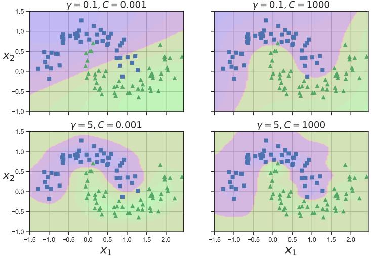
Figure 17.17: SVM classifier with RBF kernel with precision ↼ and regularizer C applied to two moons data. Adapted from Figure 5.9 of [Gér19]. Generated by svm\_classifier\_2d.ipynb.
predict the final label, where fc(x) = log p(c=1|x) p(c=0|x) is the score given by classifier c. This is known as the one-versus-the-rest approach (also called one-vs-all).
Unfortunately, this approach has several problems. First, it can result in regions of input space which are ambiguously labeled. For example, the green region at the top of Figure 17.16(a) is predicted to be both class 2 and class 1. A second problem is that the magnitude of the fc’s scores are not calibrated with each other, so it is hard to compare them. Finally, each binary subproblem is likely to su!er from the class imbalance problem (Section 10.3.8.2). For example, suppose we have 10 equally represented classes. When training f1, we will have 10% positive examples and 90% negative examples, which can hurt performance.
Another approach is to use the one-versus-one or OVO approach, also called all pairs, in which we train C(C ↗ 1)/2 classifiers to discriminate all pairs fc,c↑ . We then classify a point into the class which has the highest number of votes. However, this can also result in ambiguities, as shown in Figure 17.16(b). Also, this requires fitting O(C2) models.
17.3.8 How to choose the regularizer C
SVMs require that you specify the kernel function and the parameter C. Typically C is chosen by cross-validation. Note, however, that C interacts quite strongly with the kernel parameters. For example, suppose we are using an RBF kernel with precision ↽ = 1 2ε2 . If ↽ is large, corresponding to narrow kernels, we may need heavy regularization, and hence small C. If ↽ is small, a larger value of C should be used. So we see that ↽ and C are tightly coupled, as illustrated in Figure 17.17.
The authors of libsvm [HCL03] recommend using CV over a 2d grid with values C → {2→5, 2→3,…, 215}
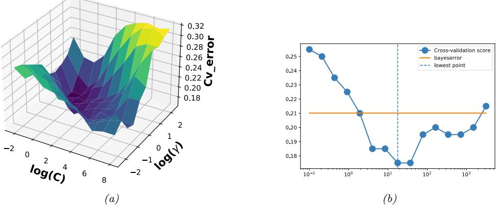
Figure 17.18: (a) A cross validation estimate of the 0-1 error for an SVM classifier with RBF kernel with di!erent precisions ↼ = 1/(2ω2) and di!erent regularizer ↽ = 1/C, applied to a synthetic data set drawn from a mixture of 2 Gaussians. (b) A slice through this surface for ↼ = 5 The red dotted line is the Bayes optimal error, computed using Bayes rule applied to the model used to generate the data. Adapted from Figure 12.6 of [HTF09]. Generated by svmCgammaDemo.ipynb.
and ↽ → {2→15, 2→13,…, 23}. See Figure 17.18 which shows the CV estimate of the 0-1 risk as a function of C and ↽.
To choose C e”ciently, one can develop a path following algorithm in the spirit of lars (Section 11.4.4). The basic idea is to start with C small, so that the margin is wide, and hence all points are inside of it and have φi = 1. By slowly increasing C, a small set of points will move from inside the margin to outside, and their φi values will change from 1 to 0, as they cease to be support vectors. When C is maximal, the margin becomes empty, and no support vectors remain. See [Has+04] for the details.
17.3.9 Kernel ridge regression
Recall the equation for ridge regression from Equation (11.55):
\[\hat{w}\_{\text{map}} = (\mathbf{X}^{\mathsf{T}}\mathbf{X} + \lambda\mathbf{I}\_D)^{-1}\mathbf{X}^{\mathsf{T}}\mathbf{y} = (\sum\_{n} x\_n \mathbf{x}\_n^{\mathsf{T}} + \lambda\mathbf{I}\_D)^{-1}(\sum\_{n} \tilde{y}\_n \mathbf{x}\_n) \tag{17.101}\]
Using the matrix inversion lemma (Section 7.3.3), we can rewrite the ridge estimate as follows
\[\boldsymbol{w} = \mathbf{X}^{\mathsf{T}} (\mathbf{X}\mathbf{X}^{\mathsf{T}} + \lambda\mathbf{I}\_N)^{-1} \mathbf{y} = \sum\_{n} \mathbf{x}\_n ( (\sum\_{n} \mathbf{x}\_n^{\mathsf{T}} \mathbf{x}\_n + \lambda\mathbf{I}\_N)^{-1} \mathbf{y} )\_n \tag{17.102}\]
Let us define the following dual variables:
\[\alpha \triangleq (\mathbf{X}\mathbf{X}^{\mathsf{T}} + \lambda \mathbf{I}\_N)^{-1} \mathbf{y} = (\sum\_{n} x\_n^{\mathsf{T}} x\_n + \lambda \mathbf{I}\_N)^{-1} \mathbf{y} \tag{17.103}\]
Then we can rewrite the primal variables as follows
\[\mathbf{w} = \mathbf{X}^{\mathsf{T}} \boldsymbol{\alpha} = \sum\_{n=1}^{N} \alpha\_{n} \mathbf{z}\_{n} \tag{17.104}\]
This tells us that the solution vector is just a linear sum of the N training vectors. When we plug this in at test time to compute the predictive mean, we get
\[f(\mathbf{z}; \mathbf{w}) = \mathbf{w}^{\mathsf{T}} \mathbf{z} = \sum\_{n=1}^{N} \alpha\_{n} \mathbf{z}\_{n}^{\mathsf{T}} \mathbf{z} \tag{17.105}\]
We can then use the kernel trick to rewrite this as
\[f(x; w) = \sum\_{n=1}^{N} \alpha\_n \mathcal{K}(x\_n, x) \tag{17.106}\]
where
\[\alpha = (\mathbf{K} + \lambda \mathbf{I}\_N)^{-1} \mathbf{y} \tag{17.107}\]
In other words,
\[f(x; w) = k^{\mathsf{T}} (\mathbf{K} + \lambda \mathbf{I}\_N)^{-1} \mathbf{y} \tag{17.108}\]
where k = [K(x, x1),…, K(x, xN )]. This is called kernel ridge regression.
The trouble with the above approach is that the solution vector φ is not sparse, so predictions at test time will take O(N) time. We discuss a solution to this in Section 17.3.10.
17.3.10 SVMs for regression
Consider the following ε2-regularized ERM problem:
\[J(\boldsymbol{w}, \lambda) = \lambda ||\boldsymbol{w}||^2 + \sum\_{n=1}^{N} \ell(\tilde{y}\_n, \hat{y}\_n) \tag{17.109}\]
where yˆn = wTxn + w0. If we use the quadratic loss, ε(y, yˆ)=(y ↗ yˆ)2, where y, yˆ → R, we recover ridge regression (Section 11.3). If we then apply the kernel trick, we recover kernel ridge regression (Section 17.3.9).
The problem with kernel ridge regression is that the solution depends on all N training points, which makes it computationally intractable. However, by changing the loss function, we can make the optimal set of basis function coe”cients, φ≃, be sparse, as we show below.
In particular, consider the following variant of the Huber loss function (Section 5.1.5.3) called the epsilon insensitive loss function:
\[L\_{\epsilon}(y,\hat{y}) \triangleq \begin{cases} 0 & \text{if } |y-\hat{y}| < \epsilon \\ |y-\hat{y}| - \epsilon & \text{otherwise} \end{cases} \tag{17.110}\]
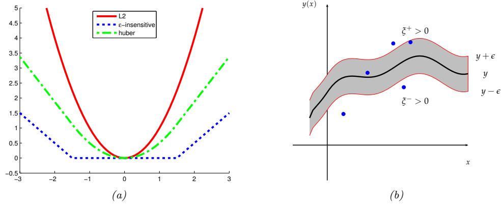
Figure 17.19: (a) Illustration of ε2, Huber and ⇀-insensitive loss functions, where ⇀ = 1.5. Generated by huberLossPlot.ipynb. (b) Illustration of the ⇀-tube used in SVM regression. Points above the tube have φ+ i > 0 and φ↓ i = 0. Points below the tube have φ+ i = 0 and φ↓ i > 0. Points inside the tube have φ+ i = φ↓ i = 0. Adapted from Figure 7.7 of [Bis06].
This means that any point lying inside an ,-tube around the prediction is not penalized, as in Figure 17.19.
The corresponding objective function is usually written in the following form
\[J = \frac{1}{2}||\boldsymbol{w}||^2 + C\sum\_{n=1}^{N} L\_{\epsilon}(\ddot{y}\_n, \hat{y}\_n) \tag{17.111}\]
where yˆn = f(xn) = wTxn + w0 and C = 1/ς is a regularization constant. This objective is convex and unconstrained, but not di!erentiable, because of the absolute value function in the loss term. As in Section 11.4.9, where we discussed the lasso problem, there are several possible algorithms we could use. One popular approach is to formulate the problem as a constrained optimization problem. In particular, we introduce slack variables to represent the degree to which each point lies outside the tube:
\[ \ddot{y}\_n \le f(x\_n) + \epsilon + \xi\_n^+ \tag{17.112} \]
\[ \ddot{y}\_n \ge f(x\_n) - \epsilon - \xi\_n^- \tag{17.113} \]
Given this, we can rewrite the objective as follows:
\[J = \frac{1}{2}||\mathbf{w}||^2 + C\sum\_{n=1}^{N} (\xi\_n^+ + \xi\_n^-) \tag{17.114}\]
This is a quadratic function of w, and must be minimized subject to the linear constraints in Equations 17.112-17.113, as well as the positivity constraints 3+ n ↓ 0 and 3→ n ↓ 0. This is a standard quadratic program in 2N + D + 1 variables.
By forming the Lagrangian and optimizing, as we did above, one can show that the optimal solution has the following form
\[ \hat{\mathbf{w}} = \sum\_{n} \alpha\_{n} \mathbf{z}\_{n} \tag{17.115} \]
where φn ↓ 0 are the dual variables. (See e.g., [SS02] for details.) Fortunately, the φ vector is sparse, meaning that many of its entries are equal to 0. This is because the loss doesn’t care about errors which are smaller than ,. The degree of sparsity is controlled by C and ,.
The xn for which φn > 0 are called the support vectors; these are points for which the errors lie on or outside the , tube. These are the only training examples we need to keep for prediction at test time, since
\[f(\mathbf{x}) = \hat{w}\_0 + \hat{w}^\mathsf{T}\mathbf{x} = \hat{w}\_0 + \sum\_{n:\alpha\_n>0} \alpha\_n \mathbf{z}\_n^\mathsf{T}\mathbf{z} \tag{17.116}\]
Finally, we can use the kernel trick to get
\[\hat{f}(\mathbf{x}) = \hat{w}\_0 + \sum\_{n:\alpha\_n > 0} \alpha\_n \mathcal{K}(\mathbf{x}\_n, \mathbf{z}) \tag{17.117}\]
This overall technique is called support vector machine regression or SVM regression for short, and was first proposed in [VGS97].
In Figure 17.20, we give an example where we use an RBF kernel with ↽ = 1. When C is small, the model is heavily regularized; when C is large, the model is less regularized and can fit the data better. We also see that when , is small, the tube is smaller, so there are more support vectors.
17.4 Sparse vector machines
GPs are very flexible models, but incur an O(N) time cost at prediction time, which can be prohibitive. SVMs solve that problem by estimating a sparse weight vector. However, SVMs do not give calibrated probabilistic outputs.
We can get the best of both worlds by using parametric models, where the feature vector is defined using basis functions centered on each of the training points, as follows:
\[\phi(x) = [\mathcal{K}(x, x\_1), \dots, \mathcal{K}(x, x\_N)] \tag{17.118}\]
where K is any similarity kernel, not necessarily a Mercer kernel. Equation (17.118) maps x → X into ω(x) → RN . We can plug this new feature vector into any discriminative model, such as logistic regression. Since we have D = N parameters, we need to use some kind of regularization, to prevent overfitting. If we fit such a model using ε2 regularization (which we will call L2VM, for ε2-vector machine), the result often has good predictive performance, but the weight vector w will be dense, and will depend on all N training points. A natural solution is to impose a sparsity-promoting prior on w, so that not all the exemplars need to be kept. We call such methods sparse vector machines.
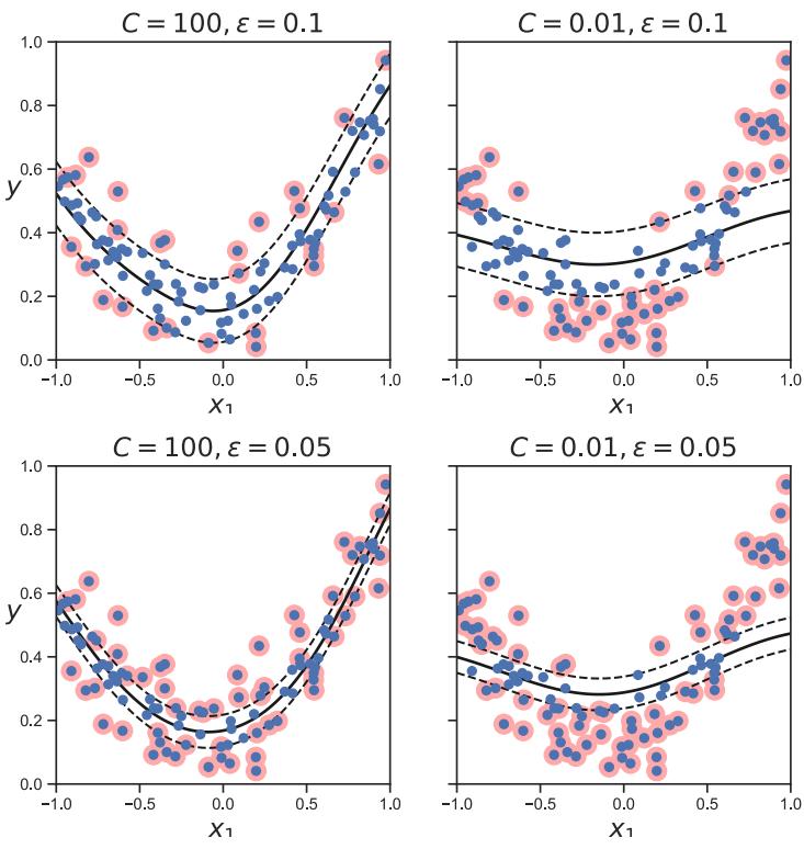
Figure 17.20: Illustration of support vector regression. Adapted from Figure 5.11 of [Gér19]. Generated by svm\_regression\_1d.ipynb.
17.4.1 Relevance vector machines (RVMs)
The simplest way to ensure w is sparse is to use ε1 regularization, as in Section 11.4. We call this L1VM or Laplace vector machine, since this approach is equivalent to using MAP estimation with a Laplace prior for w.
However, sometimes ε1 regularization does not result in a su”cient level of sparsity for a given level of accuracy. An alternative approach is based on the use of ARD or automatic relevancy determination, which uses type II maximum likelihood (aka empirical Bayes) to estimate a sparse weight vector [Mac95; Nea96]. If we apply this technique to a feature vector defined in terms of kernels, as in Equation (17.118), we get a method called the relevance vector machine or RVM [Tip01; TF03].
17.4.2 Comparison of sparse and dense kernel methods
In Figure 17.21, we compare L2VM, L1VM, RVM and an SVM using an RBF kernel on a binary classification problem in 2d. We use cross validation to pick C = 1/ς for the SVM (see Section 17.3.8),
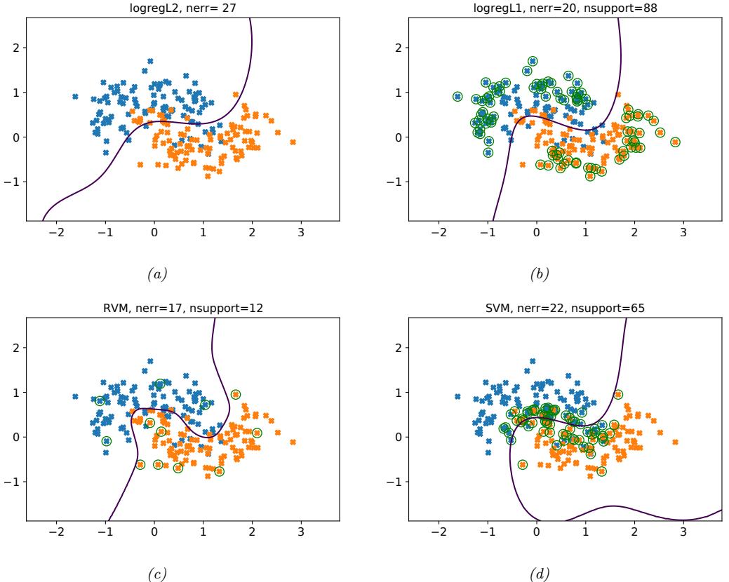
Figure 17.21: Example of non-linear binary classification using an RBF kernel with bandwidth ω = 0.3. (a) L2VM. (b) L1VM. (c) RVM. (d) SVM. Green circles denote the support vectors. Generated by kernelBinaryClassifDemo.ipynb.
and then use the same value of the regularizer for L2VM and L1VM. We see that all the methods give similar predictive performance. However, we see that the RVM is the sparsest model, so it will be the fastest at run time.
In Figure 17.22, we compare L2VM, L1VM, RVM and an SVM using an RBF kernel on a 1d regression problem. Again, we see that predictions are quite similar, but RVM is the sparsest, then L1VM, then SVM. This is further illustrated in Figure 17.23.
Beyond these small empirical examples, we provide a more general summary of the di!erent methods in Table 17.1. The columns of this table have the following meaning:
• Optimize w: a key question is whether the objective L(w) = ↗ log p(D|w) ↗ log p(w) is convex or not. L2VM, L1VM and SVMs have convex objectives. RVMs do not. GPs are Bayesian methods that integrate out the weights w.
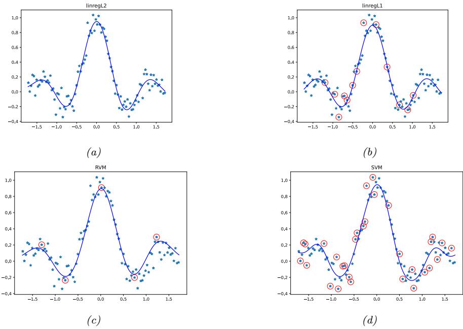
Figure 17.22: Model fits for kernel based regression on the noisy sinc function using an RBF kernel with bandwidth ω = 0.3. (a) L2VM with ↽ = 0.5. (b) L1VM with ↽ = 0.5. (c) RVM. (d) SVM regression with C = 1/↽. chosen by cross validation. Red circles denote the retained training exemplars. Generated by rvm\_regression\_1d.ipynb.
- Optimize kernel: all the methods require that we “tune” the kernel parameters, such as the bandwidth of the RBF kernel, as well as the level of regularization. For methods based on Gaussian priors, including L2VM, RVMs and GPs, we can use e”cient gradient based optimizers to maximize the marginal likelihood. For SVMs and L1VMs, we must use cross validation, which is slower (see Section 17.3.8).
- Sparse: L1VM, RVMs and SVMs are sparse kernel methods, in that they only use a subset of the training examples. GPs and L2VM are not sparse: they use all the training examples. The principle advantage of sparsity is that prediction at test time is usually faster. However, this usually results in overconfidence in the predictions.
- Probabilistic: All the methods except for SVMs produce probabilistic output of the form p(y|x). SVMs produce a “confidence” value that can be converted to a probability, but such probabilities are usually very poorly calibrated (see Section 17.3.5).
- Multiclass: All the methods except for SVMs naturally work in the multiclass setting, by using a categorical distribution instead of a Bernoulli. The SVM can be made into a multiclass classifier, but there are various di”culties with this approach, as discussed in Section 17.3.7.
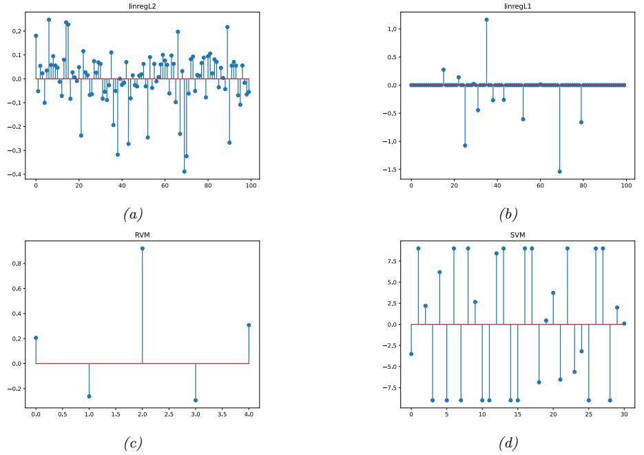
Figure 17.23: Estimated coe”cients for the models in Figure 17.22. Generated by rvm\_regression\_1d.ipynb.
| Method | Opt. w |
Opt. kernel |
Sparse | Prob. | Multiclass | Non-Mercer | Section |
|---|---|---|---|---|---|---|---|
| SVM | Convex | CV | Yes | No | Indirectly | No | 17.3 |
| L2VM | Convex | EB | No | Yes | Yes | Yes | 17.4.1 |
| L1VM | Convex | CV | Yes | Yes | Yes | Yes | 17.4.1 |
| RVM | Not convex |
EB | Yes | Yes | Yes | Yes | 17.4.1 |
| GP | N/A | EB | No | Yes | Yes | No | 17.2.7 |
Table 17.1: Comparison of various kernel based classifiers. EB = empirical Bayes, CV = cross validation. See text for details.
• Mercer kernel: SVMs and GPs require that the kernel is positive definite; the other techniques do not, since the kernel function in Equation (17.118) can be an arbitrary function of two inputs.
17.5 Exercises
Exercise 17.1 [Fitting an SVM classifier by hand † ]
(Source: Jaakkola.) Consider a dataset with 2 points in 1d: x1 = 0 with label y1 = ↔︎1 and x2 = ≃2 with label y2 = 1. Consider mapping each point to 3d using the feature vector ε(x) = [1, ≃2x, x2] T . (This is
equivalent to using a second order polynomial kernel.) The max margin classifier has the form
\[\min \left|| \left\| w \right\|\right|^2 \quad \text{s.t.} \tag{17.119}\]
\[y\_1(\boldsymbol{w}^T \boldsymbol{\phi}(\boldsymbol{x}\_1) + \boldsymbol{w}\_0) \ge 1\tag{17.120}\]
\[\frac{1}{2}\left(w^T\phi(\mathbf{z}\_2) + w\_0\right) \ge 1\tag{17.121}\]
- Write down a vector that is parallel to the optimal vector w. Hint: recall from Figure 17.12(a) that w is perpendicular to the decision boundary between the two points in the 3d feature space.
- What is the value of the margin that is achieved by this w? Hint: recall that the margin is the distance from each support vector to the decision boundary. Hint 2: think about the geometry of 2 points in space, with a line separating one from the other.
- Solve for w, using the fact that the margin is equal to 1/||w||.
- Write down the form of the discriminant function f(x) = w0 + wT ε(x) as an explicit function of x.
18 Trees, Forests, Bagging, and Boosting
18.1 Classification and regression trees (CART)
Classification and regression trees or CART models [BFO84], also called decision trees [Qui86; Qui93], are defined by recursively partitioning the input space, and defining a local model in each resulting region of input space. The overall model can be represented by a tree, with one leaf per region, as we explain below.
18.1.1 Model definition
We start by considering regression trees, where all inputs are real-valued. The tree consists of a set of nested decision rules. At each node i, the feature dimension di of the input vector x is compared to a threshold value ti, and the input is then passed down to the left or right branch, depending on whether it is above or below threshold. At the leaves of the tree, the model specifies the predicted output for any input that falls into that part of the input space.
For example, consider the regression tree in Figure 18.1(a). The first node asks if x1 is less than some threshold t1. If yes, we then ask if x2 is less than some other threshold t2. If yes, we enter the bottom left leaf node. This corresponds to the region of space defined by
\[R\_1 = \{x : x\_1 \le t\_1, x\_2 \le t\_2\} \tag{18.1}\]
We can associate this region with the predicted output, say y = 2. In a similar way, we can partition the entire input space into 5 regions using axis parallel splits, as shown in Figure 18.1(b).1
Formally, a regression tree can be defined by
\[f(x; \theta) = \sum\_{j=1}^{J} w\_j \mathbb{I}\left(x \in R\_j\right) \tag{18.2}\]
where Rj is the region specified by the j’th leaf node, wj is the predicted output for that node,
\[w\_j = \frac{\sum\_{n=1}^{N} y\_n \mathbb{I}(\mathbf{z}\_n \in R\_j)}{\sum\_{n=1}^{N} \mathbb{I}(\mathbf{z}\_n \in R\_j)} \tag{18.3}\]
1. By using enough splits (i.e., deep enough trees), we can make a piecewise linear approximation to decision boundaries with more complex shapes, but it may require a lot of data to fit such a model.
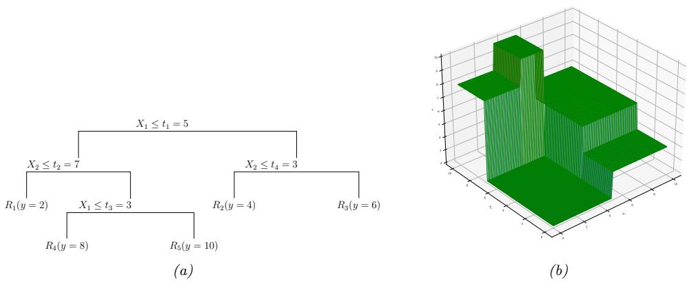
Figure 18.1: (a) A regression tree on two inputs. (b) Corresponding piecewise constant surface, where the regions have heights 2, 4, 6, 8 and 10. Adapted from Figure 9.2 of [HTF09]. Generated by regtreeSurfaceDemo.ipynb.
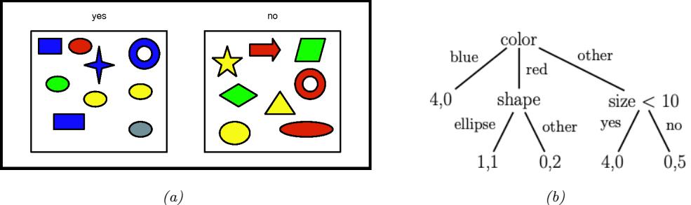
Figure 18.2: (a) A set of shapes with corresponding binary labels. The features are: color (values “blue”, “red”, “other”), shape (values “ellipse”, “other”), and size (real-valued). (b) A hypothetical classification tree fitted to this data. A leaf labeled as (n1, n0) means that there are n1 positive examples that fall into this partition, and n0 negative examples.
and ε = {(Rj , wj ) : j =1: J}, where J is the number of nodes. The regions themselves are defined by the feature dimensions that are used in each split, and the corresponding thresholds, on the path from the root to the leaf. For example, in Figure 18.1(a), we have R1 = [(x1 ↙ t1),(x2 ↙ t2)], R4 = [(x1 ↙ t1),(x2 > t2),(x3 ↙ t3)], etc. (For categorical inputs, we can define the splits based on comparing feature xi to each of the possible values for that feature, rather than comparing to a numeric threshold.) We discuss how to learn these regions in Section 18.1.2.
For classification problems, the leaves contain a distribution over the class labels, rather than just the mean response. See Figure 18.2 for an example of a classification tree.
18.1.2 Model fitting
To fit the model, we need to minimize the following loss:
\[\mathcal{L}(\boldsymbol{\theta}) = \sum\_{n=1}^{N} \ell(y\_n, f(\boldsymbol{x}\_n; \boldsymbol{\theta})) = \sum\_{j=1}^{J} \sum\_{\mathfrak{a}\_n \in R\_j} \ell(y\_n, \boldsymbol{w}\_j) \tag{18.4}\]
Unfortunately, this is not di!erentiable, because of the need to learn the discrete tree structure. Indeed, finding the optimal partitioning of the data is NP-complete [HR76]. The standard practice is to use a greedy procedure, in which we iteratively grow the tree one node at a time. This approach is used by CART [BFO84], C4.5 [Qui93], and ID3 [Qui86], which are three popular implementations of the method.
The idea is as follows. Suppose we are at node i; let Di = {(xn, yn) → Ni} be the set of examples that reach this node. We will consider how to split this node into a left branch and right branch so as to minimize the error in each child subtree.
If the j’th feature is a real-valued scalar, we can partition the data at node i by comparing to a threshold t. The set of possible thresholds Tj for feature j can be obtained by sorting the unique values of {xnj}. For example, if feature 1 has the values {4.5, ↗12, 72, ↗12}, then we set T1 = {↗12, 4.5, 72}. For each possible threshold, we define the left and right splits, DL i (j, t) = {(xn, yn) → Ni : xn,j ↙ t} and DR i (j, t) = {(xn, yn) → Ni : xn,j > t}.
If the j’th feature is categorical, with Kj possible values, then we check if the feature is equal to each of those values or not. This defines a set of Kj possible binary splits: DL i (j, t) = {(xn, yn) → Ni : xn,j = t} and DR i (j, t) = {(xn, yn) → Ni : xn,j 7= t}.) (Alternatively, we could allow for a multi-way split, as in Figure 18.2(b). However, this may cause data fragmentation, in which too little data might “fall” into each subtree, resulting in overfitting. Therefore it is more common to use binary splits.)
Once we have computed DL i (j, t) and DR i (j, t) for each j and t at node i, we choose the best feature ji to split on, and the best value for that feature, ti, as follows:
\[c(j\_i, t\_i) = \arg\min\_{j \in \{1, \ldots, D\}} \min\_{t \in \mathcal{T}\_j} \frac{|\mathcal{D}\_i^L(j, t)|}{|\mathcal{D}\_i|} c(\mathcal{D}\_i^L(j, t)) + \frac{|\mathcal{D}\_i^R(j, t)|}{|\mathcal{D}\_i|} c(\mathcal{D}\_i^R(j, t))\tag{18.5}\]
We now discuss the cost function c(Di) which is used to evaluate the cost of node i. For regression, we can use the mean squared error
\[\text{cost}(\mathcal{D}\_i) = \frac{1}{|\mathcal{D}|} \sum\_{n \in \mathcal{D}\_i} (y\_n - \overline{y})^2 \tag{18.6}\]
where y = 1 |D| ( n↔︎Di yn is the mean of the response variable for examples reaching node i.
For classification, we first compute the empirical distribution over class labels for this node:
\[\hat{\pi}\_{ic} = \frac{1}{|\mathcal{D}\_i|} \sum\_{n \in \mathcal{D}\_i} \mathbb{I}\left(y\_n = c\right) \tag{18.7}\]
Given this, we can then compute the Gini index
\[G\_i = \sum\_{c=1}^{C} \hat{\pi}\_{ic} (1 - \hat{\pi}\_{ic}) = \sum\_{c} \hat{\pi}\_{ic} - \sum\_{c} \hat{\pi}\_{ic}^2 = 1 - \sum\_{c} \hat{\pi}\_{ic}^2 \tag{18.8}\]
This is the expected error rate. To see this, note that ◁ˆic is the probability a random entry in the leaf belongs to class c, and 1 ↗ ◁ˆic is the probability it would be misclassified.
Alternatively we can define cost as the entropy or deviance of the node:
\[H\_i = \mathbb{H}(\hat{\pi}\_i) = -\sum\_{c=1}^{C} \hat{\pi}\_{ic} \log \hat{\pi}\_{ic} \tag{18.9}\]
A node that is pure (i.e., only has examples of one class) will have 0 entropy.
Given one of the above cost functions, we can use Equation (18.5) to pick the best feature, and best threshold at each node. We then partition the data, and call the fitting algorithm recursively on each subset of the data.
In [SL99], they propose to soften the hard split decision at each node by using a binary logistic regression model. This is called a di!erentiable decision tree or soft decision tree. For a fixed tree structure, this allows them to fit the model by gradient-based optimization methods.
18.1.3 Regularization
If we let the tree become deep enough, it can achieve 0 error on the training set (assuming no label noise), by partioning the input space into su”ciently small regions where the output is constant. However, this will typically result in overfitting. To prevent this, there are two main approaches. The first is to stop the tree growing process according to some heuristic, such as having too few examples at a node, or reaching a maximum depth. The second approach is to grow the tree to its maximum depth, where no more splits are possible, and then to prune it back, by merging split subtrees back into their parent (see e.g., [BA97b]). This can partially overcome the greedy nature of top-down tree growing. (For example, consider applying the top-down approach to the xor data in Figure 13.1: the algorithm would never make any splits, since each feature on its own has no predictive power.) However, forward growing and backward pruning is slower than the greedy top-down approach.
18.1.4 Handling missing input features
In general, it is hard for discriminative models, such as neural networks, to handle missing input features, as we discussed in Section 1.5.5. However, for trees, there are some simple heuristics that can work well.
The standard heuristic for handling missing inputs in decision trees is to look for a series of “backup” variables, which can induce a similar partition to the chosen variable at any given split; these can be used in case the chosen variable is unobserved at test time. These are called surrogate splits. This method finds highly correlated features, and can be thought of as learning a local joint model of the input. This has the advantage over a generative model of not modeling the entire joint distribution of inputs, but it has the disadvantage of being entirely ad hoc. A simpler approach, applicable to categorical variables, is to code “missing” as a new value, and then to treat the data as fully observed.
18.1.5 Pros and cons
Tree models are popular for several reasons:
• They are easy to interpret.
Figure 18.3: (a) A decision tree of depth 2 fit to the iris data, using just the petal length and petal width features. Leaf nodes are color coded according to the majority class. The number of training samples that pass from the root to each node is shown inside each box, as well as how many of these values fall into each class. This can be normalized to get a distribution over class labels for each node. (b) Decision surface induced by (a). (c) Fit to data where we omit a single data point (shown by red star). (d) Ensemble of the two models in (b) and (c). Generated by dtree\_sensitivity.ipynb.
- They can easily handle mixed discrete and continuous inputs.
- They are insensitive to monotone transformations of the inputs (because the split points are based on ranking the data points), so there is no need to standardize the data.
- They perform automatic variable selection.
- They are relatively robust to outliers.
- They are fast to fit, and scale well to large data sets.
- They can handle missing input features.
However, tree models also have some disadvantages. The primary one is that they do not predict very accurately compared to other kinds of model. This is in part due to the greedy nature of the tree construction algorithm.
A related problem is that trees are unstable: small changes to the input data can have large e!ects on the structure of the tree, due to the hierarchical nature of the tree-growing process, causing errors at the top to a!ect the rest of the tree. For example, consider the tree in Figure 18.3b. Omitting even a single data point from the training set can result in a dramatically di!erent decision surface, as shown in Figure 18.3c, due to the use of axis parallel splits. (Omitting features can also cause instability.) In Section 18.3 and Section 18.4, we will turn this instability into a virtue.
18.2 Ensemble learning
In Section 18.1, we saw that decision trees can be quite unstable, in the sense that their predictions might vary a lot if the training data is perturbed. In other words, decision trees are a high variance estimator. A simple way to reduce variance is to average multiple models. This is called ensemble learning. The result model has the form
\[f(y|\mathbf{z}) = \frac{1}{|\mathcal{M}|} \sum\_{m \in \mathcal{M}} f\_m(y|\mathbf{z}) \tag{18.10}\]
where fm is the m’th base model. The ensemble will have similar bias to the base models, but lower variance, generally resulting in improved overall performance (see Section 4.7.6.3 for details on the bias-variance tradeo!).
Averaging is a sensible way to combine predictions from regression models. For classifiers, it can sometimes be better to take a majority vote of the outputs. (This is sometimes called a committee method.) To see why this can help, suppose each base model is a binary classifier with an accuracy of ⇁, and suppose class 1 is the correct class. Let Ym → {0, 1} be the prediction for the m’th model, and let S = (M m=1 Ym be the number of votes for class 1. We define the final predictor to be the majority vote, i.e., class 1 if S > M/2 and class 0 otherwise. The probability that the ensemble will pick class 1 is
\[p = \Pr(S > M/2) = 1 - B(M/2, M, \theta) \tag{18.11}\]
where B(x, M, ⇁) is the cdf of the binomial distribution with parameters M and ⇁ evaluated at x. For ⇁ = 0.51 and M = 1000, we get p = 0.73 and with M = 10, 000 we get p = 0.97.
The performance of the voting approach is dramatically improved, because we assumed each predictor made independent errors. In practice, their mistakes may be correlated, but as long as we ensemble su”ciently diverse models, we can still come out ahead.
18.2.1 Stacking
An alternative to using an unweighted average or majority vote is to learn how to combine the base models, by using
\[f(y|\mathbf{z}) = \sum\_{m \in \mathcal{M}} w\_m f\_m(y|\mathbf{z}) \tag{18.12}\]
This is called stacking, which stands for “stacked generalization” [Wol92]. Note that the combination weights used by stacking need to be trained on a separate dataset, otherwise they would put all their mass on the best performing base model.
18.2.2 Ensembling is not Bayes model averaging
It is worth noting that an ensemble of models is not the same as using Bayes model averaging over models (Section 4.6), as pointed out in [Min00]. An ensemble considers a larger hypothesis class of the form
\[p(y|x, w, \theta) = \sum\_{m \in \mathcal{M}} w\_m p(y|x, \theta\_m) \tag{18.13}\]
whereas BMA uses
\[p(y|\mathbf{z}, \mathcal{D}) = \sum\_{m \in \mathcal{M}} p(m|\mathcal{D}) p(y|\mathbf{z}, m, \mathcal{D}) \tag{18.14}\]
The key di!erence is that in the case of BMA, the weights p(m|D) sum to one, and in the limit of infinite data, only a single model will be chosen (namely the MAP model). By contrast, the ensemble weights wm are arbitrary, and don’t collapse in this way to a single model.
18.3 Bagging
In this section, we discuss bagging [Bre96], which stands for “bootstrap aggregating”. This is a simple form of ensemble learning in which we fit M di!erent base models to di!erent randomly sampled versions of the data; this encourages the di!erent models to make diverse predictions. The datasets are sampled with replacement (a technique known as bootstrap sampling, Section 4.7.3), so a given example may appear multiple times, until we have a total of N examples per model (where N is the number of original data points).
The disadvantage of bootstrap is that each base model only sees, on average, 63% of the unique input examples. To see why, note that the chance that a single item will not be selected from a set of size N in any of N draws is (1 ↗ 1/N)N . In the limit of large N, this becomes e→1 ′ 0.37, which means only 1 ↗ 0.37 = 0.63 of the data points will be selected.
The 37% of the training instances that are not used by a given base model are called out-of-bag instances (oob). We can use the predicted performance of the base model on these oob instances as an estimate of test set performance. This provides a useful alternative to cross validation.
The main advantage of bootstrap is that it prevents the ensemble from relying too much on any individual training example, which enhances robustness and generalization [Gra04]. For example, comparing Figure 18.3b and Figure 18.3c, we see that omitting a single example from the training set can have a large impact on the decision tree that we learn (even though the tree growing algorithm is otherwise deterministic). By averaging the predictions from both of these models, we get the more reasonable prediction model in Figure 18.3d. This advantage generally increases with the size of the ensemble, as shown in Figure 18.4. (Of course, larger ensembles take more memory and more time.)
Bagging does not always improve performance. In particular, it relies on the base models being unstable estimators, so that omitting some of the data significantly changes the resulting model fit.
Figure 18.4: (a) A single decision tree. (b-c) Bagging ensemble of 10 and 50 trees. (d) Random forest of 50 trees. Adapted from Figure 7.5 of [Gér19]. Generated by bagging\_trees.ipynb and rf\_demo\_2d.ipynb.
This is the case for decision trees, but not for other models, such as nearest neighbor classifiers. For neural networks, the story is more mixed. They can be unstable wrt their training set. On the other hand, deep networks will underperform if they only see 63% of the data, so bagged DNNs do not usually work well [NTL20].
18.4 Random forests
Bagging relies on the assumption that re-running the same learning algorithm on di!erent subsets of the data will result in su”ciently diverse base models. The technique known as random forests [Bre01] tries to decorrelate the base learners even further by learning trees based on a randomly chosen subset of input variables (at each node of the tree), as well as a randomly chosen subset of data cases. It does this by modifying Equation (18.5) so the the feature split dimension j is optimized over a random subset of the features, Si ∅ {1,…,D}.
For example, consider the email spam dataset [HTF09, p301]. This dataset contains 4601 email messages, each of which is classified as spam (1) or non-spam (0). The data was open sourced by George Forman from Hewlett-Packard (HP) Labs.
There are 57 quantitative (real-valued) features, as follows:
• 48 features corresponding to the percentage of words in the email that match a given word, such as “remove” or “labs”.
Figure 18.5: Preditive accuracy vs size of tree ensemble for bagging, random forests and gradient boosting with log loss. Adapted from Figure 15.1 of [HTF09]. Generated by spam\_tree\_ensemble\_compare.ipynb.
- 6 features corresponding to the percentage of characters in the email that match a given character, namely ;.[!$#
- 3 features corresponding to the average length, max length, and sum of lengths of uninterrupted sequences of capital letters. (These features are called CAPAVE, CAPMAX and CAPTOT.)
Figure 18.5 shows that random forests work much better than bagged decision trees, because many input features are irrelevant. (We also see that a method called “boosting”, discussed in Section 18.5, works even better; however, this requires sequentially fitting trees, whereas random forests can be fit in parallel.)
18.5 Boosting
Ensembles of trees, whether fit by bagging or the random forest algorithm, corresponding to a model of the form
\[f(x; \boldsymbol{\theta}) = \sum\_{m=1}^{M} \beta\_m F\_m(x; \boldsymbol{\theta}\_m) \tag{18.15}\]
where Fm is the m’th tree, and ↼m is the corresponding weight, often set to ↼m = 1/M. We can generalize this by allowing the Fm functions to be general function approximators, such as neural networks, not just trees. The result is called an additive model [HTF09]. We can think of this as a linear model with adaptive basis functions. The goal, as usual, is to minimize the empirical loss (with an optional regularizer):
\[\mathcal{L}(f) = \sum\_{i=1}^{N} \ell(y\_i, f(x\_i)) \tag{18.16}\]
Boosting [Sch90; FS96] is an algorithm for sequentially fitting additive models where each Fm is a binary classifier that returns Fm → {↗1, +1}. In particular, we first fit F1 on the original data,
and then we weight the data samples by the errors made by F1, so misclassified examples get more weight. Next we fit F2 to this weighted data set. We keep repeating this process until we have fit the desired number M of components. (M is a hyper-parameter that controls the complexity of the overall model, and can be chosen by monitoring performance on a validation set, and using early stopping.)
It can be shown that, as long as each Fm has an accuracy that is better than chance (even on the weighted dataset), then the final ensemble of classifiers will have higher accuracy than any given component. That is, if Fm is a weak learner (so its accuracy is only slightly better than 50%), then we can boost its performance using the above procedure so that the final f becomes a strong learner. (See e.g., [SF12] for more details on the learning theory approach to boosting.)
Note that boosting reduces the bias of the strong learner, by fitting trees that depend on each other, whereas bagging and RF reduce the variance by fitting independent trees. In many cases, boosting can work better. See Figure 18.5 for an example.
The original boosting algorithm focused on binary classification with a particular loss function that we will explain in Section 18.5.3, and was derived from the PAC learning theory framework (see Section 5.4.4). In the rest of this section, we focus on a more statistical version of boosting, due to [FHT00; Fri01], which works with arbitrary loss functions, making the method suitable for regression, multi-class classification, ranking, etc. Our presentation is based on [HTF09, ch10] and [BH07], which should be consulted for further details.
18.5.1 Forward stagewise additive modeling
In this section, we discuss forward stagewise additive modeling, in which we sequentially optimize the objective in Equation (18.16) for general (di!erentiable) loss functions, where f is an additive model as in Equation 18.15. That is, at iteration m, we compute
\[\ell(\beta\_m, \theta\_m) = \underset{\beta, \theta}{\text{argmin}} \sum\_{i=1}^{N} \ell(y\_i, f\_{m-1}(x\_i) + \beta F(x\_i; \theta)) \tag{18.17}\]
We then set
\[f\_m(x) = f\_{m-1}(x) + \beta\_m F(x; \theta\_m) = f\_{m-1}(x) + \beta\_m F\_m(x) \tag{18.18}\]
(Note that we do not adjust the parameters of previously added models.) The details on how to perform this optimization step depend on the loss function that we choose, and (in some cases) on the form of the weak learner F, as we discuss below.
18.5.2 Quadratic loss and least squares boosting
Suppose we use squared error loss, ε(y, yˆ)=(y ↗ yˆ)2. In this case, the i’th term in the objective at step m becomes
\[\ell(y\_i, f\_{m-1}(x\_i) + \beta F(x\_i; \theta)) = (y\_i - f\_{m-1}(x\_i) - \beta F(x\_i; \theta))^2 = (r\_{im} - \beta F(x\_i; \theta))^2 \tag{18.19}\]
where rim = yi ↗ fm→1(xi) is the residual of the current model on the i’th observation. We can minimize the above objective by simply setting ↼ = 1, and fitting F to the residual errors. This is called least squares boosting [BY03].
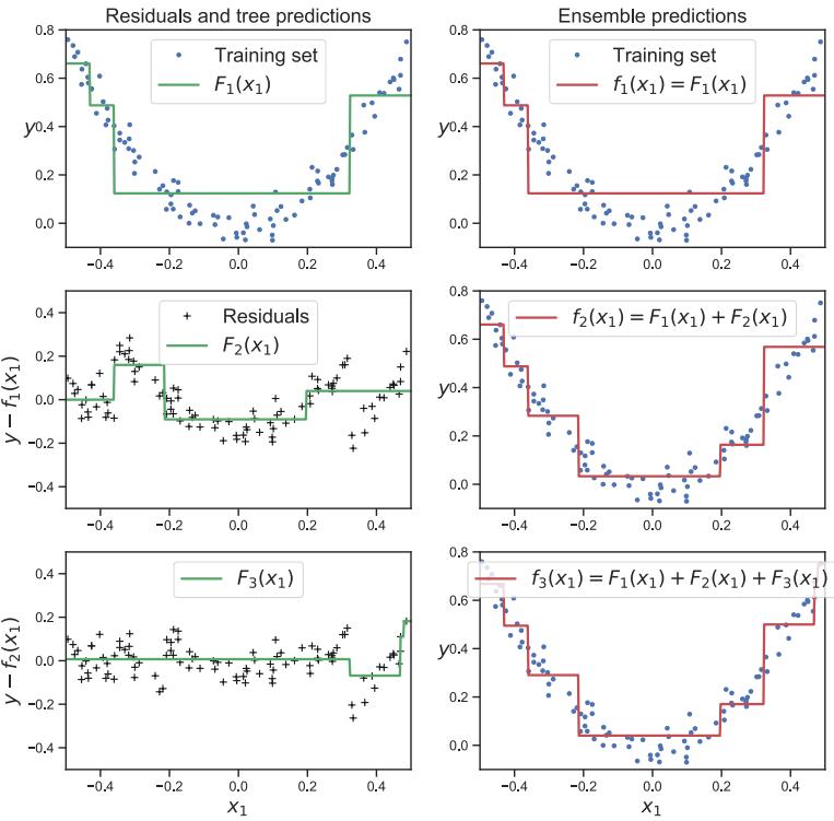
Figure 18.6: Illustration of boosting using a regression tree of depth 2 applied to a 1d dataset. Adapted from Figure 7.9 of [Gér19]. Generated by boosted\_regr\_trees.ipynb.
We give an example of this process in Figure 18.6, where we use a regression tree of depth 2 as the weak learner. On the left, we show the result of fitting the weak learner to the residuals, and on the right, we show the current strong learner. We see how each new weak learner that is added to the ensemble corrects the errors made by earlier versions of the model.
18.5.3 Exponential loss and AdaBoost
Suppose we are interested in binary classification, i.e., predicting y˜i → {↗1, +1}. Let us assume the weak learner computes
\[p(y=1|\mathbf{z}) = \frac{e^{F(\mathbf{z})}}{e^{-F(\mathbf{z})} + e^{F(\mathbf{z})}} = \frac{1}{1 + e^{-2F(\mathbf{z})}} \tag{18.20}\]
so F(x) returns half the log odds. We know from Equation (10.13) that the negative log likelihood is given by
\[\ell(\ddot{y}, F(x)) = \log(1 + e^{-2\tilde{y}F(x)}) \tag{18.21}\]
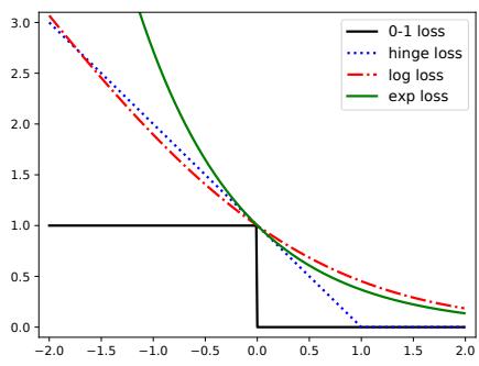
Figure 18.7: Illustration of various loss functions for binary classification. The horizontal axis is the margin m(x) = yF˜ (x), the vertical axis is the loss. The log loss uses log base 2. Generated by hinge\_loss\_plot.ipynb.
We can minimize this by ensuring that the margin m(x) = yF˜ (x) is as large as possible. We see from Figure 18.7 that the log loss is a smooth upper bound on the 0-1 loss. We also see that it penalizes negative margins more heavily than positive ones, as desired (since positive margins are already correctly classified).
However, we can also use other loss functions. In this section, we consider the exponential loss
\[\ell(\ddot{y}, F(x)) = \exp(-\ddot{y}F(x))\tag{18.22}\]
We see from Figure 18.7 that this is also a smooth upper bound on the 0-1 loss. In the population setting (with infinite sample size), the optimal solution to the exponential loss is the same as for log loss. To see this, we can just set the derivative of the expected loss (for each x) to zero:
\[\frac{\partial}{\partial F(\mathbf{z})} \mathbb{E} \left[ e^{-\tilde{y}f(\mathbf{z})} | \mathbf{z} \right] = \frac{\partial}{\partial F(\mathbf{z})} [p(\tilde{y} = 1 | \mathbf{z}) e^{-F(\mathbf{z})} + p(\tilde{y} = -1 | \mathbf{z}) e^{F(\mathbf{z})}] \tag{18.23}\]
\[\dot{y} = -p(\ddot{y} = 1|\mathbf{x})e^{-F(\mathbf{x})} + p(\ddot{y} = -1|\mathbf{x})e^{F(\mathbf{x})} \tag{18.24}\]
\[\tilde{y} = 0 \Rightarrow \frac{p(\tilde{y} = 1 | x)}{p(\tilde{y} = -1 | x)} = e^{2F(\mathfrak{x})} \tag{18.25}\]
However, it turns out that the exponential loss is easier to optimize in the boosting setting, as we show below. (We consider the log loss case in Section 18.5.4.)
We now discuss how to solve for the m’th weak learner, Fm, when we use exponential loss. We will assume that the base classifier Fm returns a binary class label; the resulting algorithm is called discrete AdaBoost [FHT00]. If Fm returns a probability instead, a modified algorithm, known as real AdaBoost, can be used [FHT00].
At step m we have to minimize
\[L\_m(F) = \sum\_{i=1}^{N} \exp[-\ddot{y}\_i(f\_{m-1}(\mathbf{z}\_i) + \beta F(\mathbf{z}\_i))] = \sum\_{i=1}^{N} \omega\_{i,m} \exp(-\beta \ddot{y}\_i F(\mathbf{z}\_i)) \tag{18.26}\]
where 0i,m ↫ exp(↗y˜ifm→1(xi)) is a weight applied to datacase i, and y˜i → {↗1, +1}. We can rewrite this objective as follows:
\[L\_m = e^{-\beta} \sum\_{\tilde{y}\_i = F(\mathfrak{w}\_i)} \omega\_{i,m} + e^{\beta} \sum\_{\tilde{y}\_i \neq F(\mathfrak{w}\_i)} \omega\_{i,m} \tag{18.27}\]
\[\Psi = (e^{\beta} - e^{-\beta}) \sum\_{i=1}^{N} \omega\_{i,m} \mathbb{I} \left( \bar{y}\_i \neq F(\mathbf{z}\_i) \right) + e^{-\beta} \sum\_{i=1}^{N} \omega\_{i,m} \tag{18.28}\]
Consequently the optimal function to add is
\[F\_m = \underset{F}{\text{argmin}} \sum\_{i=1}^{N} \omega\_{i,m} \mathbb{I}\left(\check{y}\_i \neq F(\boldsymbol{x}\_i)\right) \tag{18.29}\]
This can be found by applying the weak learner to a weighted version of the dataset, with weights 0i,m.
All that remains is to solve for the size of the update, ↼. Subsituting Fm into Lm and solving for ↼ we find
\[ \beta\_m = \frac{1}{2} \log \frac{1 - \text{err}\_m}{\text{err}\_m} \tag{18.30} \]
where
\[\text{err}\_m = \frac{\sum\_{i=1}^{N} \omega\_{i,m} \mathbb{I}\left(\ddot{y}\_i \neq F\_m(\mathbf{z}\_i)\right)}{\sum\_{i=1}^{N} \omega\_{i,m}} \tag{18.31}\]
Therefore overall update becomes
\[f\_m(x) = f\_{m-1}(x) + \beta\_m F\_m(x) \tag{18.32}\]
After updating the strong learner, we need to recompute the weights for the next iteration, as follows:
\[ \omega\_{i,m+1} = e^{-\tilde{y}\_i f\_m(\mathbf{z}\_i)} = e^{-\tilde{y}\_i f\_{m-1}(\mathbf{z}\_i) - \tilde{y}\_i \beta\_m F\_m(\mathbf{z}\_i)} = \omega\_{i,m} e^{-\tilde{y}\_i \beta\_m F\_m(\mathbf{z}\_i)} \tag{18.33} \]
If y˜i = Fm(xi), then y˜iFm(xi)=1, and if y˜i 7= Fm(xi), then y˜iFm(xi) = ↗1. Hence ↗y˜iFm(xi) = 2I(˜yi 7= Fm(xo)) ↗ 1, so the update becomes
\[ \omega\_{i,m+1} = \omega\_{i,m} e^{\beta\_m(2\text{I}(\hat{y}\_i \neq F\_m(\mathbf{z}\_i)) - 1)} = \omega\_{i,m} e^{2\beta\_m \text{I}(\hat{y}\_i \neq F\_m(\mathbf{z}\_i))} e^{-\beta\_m} \tag{18.34} \]
Since the e→φm is constant across all examples, it can be dropped. If we then define φm = 2↼m, the update becomes
\[\omega\_{i,m+1} = \begin{cases} \omega\_{i,m} e^{\alpha\_m} & \text{if } \ddot{y}\_i \neq F\_m(x\_i) \\ \omega\_{i,m} & \text{otherwise} \end{cases} \tag{18.35}\]
Thus we see that we exponentially increase weights of misclassified examples. The resulting algorithm shown in Algorithm 18.1, and is known as Adaboost.M1 [FS96].
A multiclass generalization of exponential loss, and an adaboost-like algorithm to minimize it, known as SAMME (stagewise additive modeling using a multiclass exponential loss function), is described in [Has+09]. This is implemented in scikit learn (the AdaBoostClassifier class).
Algorithm 18.1: Adaboost.M1, for binary classification with exponential loss
1 0i = 1/N 2 for m =1: M do 3 Fit a classifier Fm(x) to the training set using weights w 4 Compute errm = !N i=1 0i,mI(˜yi⇑=Fm(xi)) !N i=1 0i,m 5 Compute φm = log[(1 ↗ errm)/errm] 6 Set 0i ℑ 0i exp[φmI(˜yi 7= Fm(xi))] 7 Return f(x) = sgn D(M m=1 φmFm(x) E
18.5.4 LogitBoost
The trouble with exponential loss is that it puts a lot of weight on misclassified examples, as is apparent from the exponential blowup on the left hand side of Figure 18.7. This makes the method very sensitive to outliers (mislabeled examples). In addition, e→yf˜ is not the logarithm of any pmf for binary variables y˜ → {↗1, +1}; consequently we cannot recover probability estimates from f(x).
A natural alternative is to use log loss, as we discussed in Section 18.5.3. This only punishes mistakes linearly, as is clear from Figure 18.7. Furthermore, it means that we will be able to extract probabilities from the final learned function, using
\[p(y=1|\mathbf{z}) = \frac{e^{f(\mathbf{z})}}{e^{-f(\mathbf{z})} + e^{f(\mathbf{z})}} = \frac{1}{1 + e^{-2f(\mathbf{z})}} \tag{18.36}\]
The goal is to minimze the expected log-loss, given by
\[L\_m(F) = \sum\_{i=1}^{N} \log\left[1 + \exp\left(-2\bar{y}\_i(f\_{m-1}(x) + F(x\_i))\right)\right] \tag{18.37}\]
By performing a Newton update on this objective (similar to IRLS), one can derive the algorithm shown in Algorithm 18.2. This is known as logitBoost [FHT00]. The key subroutine is the ability of the weak learner F to solve a weighted least squares problem. This method can be generalized to the multi-class setting, as explained in [FHT00].
18.5.5 Gradient boosting
Rather than deriving new versions of boosting for every di!erent loss function, it is possible to derive a generic version, known as gradient boosting [Fri01; Mas+00]. To explain this, imagine solving fˆ = argminf L(f) by performing gradient descent in the space of functions. Since functions are infinite dimensional objects, we will represent them by their values on the training set, f = (f(x1),…,f(xN )). At step m, let gm be the gradient of L(f) evaluated at f = fm→1:
\[g\_{im} = \left[\frac{\partial \ell(y\_i, f(\mathbf{z}\_i))}{\partial f(\mathbf{z}\_i)}\right]\_{f = f\_{m-1}}\tag{18.38}\]
Algorithm 18.2: LogitBoost, for binary classification with log-loss
1 0i = 1/N, ◁i = 1/2 2 for m =1: M do 3 Compute the working response zi = y↔︎ i →↽i ↽i(1→↽i) 4 Compute the weights 0i = ◁i(1 ↗ ◁i) 5 Fm = argminF (N i=1 0i(zi ↗ F(xi))2 6 Update f(x) ℑ f(x) + 1 2Fm(x) 7 Compute ◁i = 1/(1 + exp(↗2f(xi))); 8 Return f(x) = sgn D(M m=1 Fm(x) E
| Name | Loss | ↗ϖε(yi, f(xi))/ϖf(xi) |
|---|---|---|
| Squared error |
1 ↗ f(xi))2 2 (yi |
yi ↗ f(xi) |
| Absolute error |
yi ↗ f(xi) |
sgn(yi ↗ f(xi)) |
| Exponential loss |
exp(↗y˜if(xi)) | ↗y˜i exp(↗y˜if(xi)) |
| Binary Logloss |
e→y˜ifi ) log(1 + |
yi ↗ ◁i |
| Multiclass logloss |
↗( c yic log ◁ic |
yic ↗ ◁ic |
Table 18.1: Some commonly used loss functions and their gradients. For binary classification problems, we assume y˜i → {↔︎1, +1}, and πi = ω(2f(xi)). For regression problems, we assume yi → R. Adapted from [HTF09, p360] and [BH07, p483].
Gradients of some common loss functions are given in Table 18.1. We then make the update
\[f\_m = f\_{m-1} - \beta\_m g\_m \tag{18.39}\]
where ↼m is the step length, chosen by
\[\beta\_m = \operatorname\*{argmin}\_{\beta} \mathcal{L}(\mathbf{f}\_{m-1} - \beta \mathbf{g}\_m) \tag{18.40}\]
In its current form, this is not much use, since it only optimizes f at a fixed set of N points, so we do not learn a function that can generalize. However, we can modify the algorithm by fitting a weak learner to approximate the negative gradient signal. That is, we use this update
\[F\_m = \underset{F}{\text{argmin}} \sum\_{i=1}^{N} (-g\_{im} - F(x\_i))^2 \tag{18.41}\]
The overall algorithm is summarized in Algorithm 18.3. We have omitted the line search step for ↼m, which is not strictly necessary, as argued in [BH07]. However, we have introduced a learning rate or shrinkage factor 0 < ν ↙ 1, to control the size of the updates, for regularization purposes.
If we apply this algorithm using squared loss, we recover L2Boosting, since ↗gim = yi ↗ fm→1(xi) is just the residual error. We can also apply this algorithm to other loss functions, such as absolute loss or Huber loss (Section 5.1.5.3), which is useful for robust regression problems.
Algorithm 18.3: Gradient boosting
1 Initialize f0(x) = argminF (N i=1 L(yi, F(xi)) 2 for m =1: M do 3 Compute the gradient residual using rim = ↗ D ϑL(yi,f(xi)) ϑf(xi) E f(xi)=fm→1(xi) 4 Use the weak learner to compute Fm = argminF (N i=1(rim ↗ F(xi))2 5 Update fm(x) = fm→1(x) + νFm(x) 6 Return f(x) = fM(x)
For classification, we can use log-loss. In this case, we get an algorithm known as BinomialBoost [BH07]. The advantage of this over LogitBoost is that it does not need to be able to do weighted fitting: it just applies any black-box regression model to the gradient vector. To apply this to multi-class classification, we can fit C separate regression trees, using the pseudo residual of the form
\[-g\_{icm} = \frac{\partial \ell(y\_i, f\_{1m}(x\_i), \dots, f\_{Cm}(x\_i))}{\partial f\_{cm}(x\_i)} = \mathbb{I}\left(y\_i = c\right) - \pi\_{ic} \tag{18.42}\]
Although the trees are fit separately, their predictions are combined via a softmax transform
\[p(y=c|\mathbf{z}) = \frac{e^{f\_c(\mathbf{z})}}{\sum\_{c'=1}^C e^{f\_{c'}(\mathbf{z})}} \tag{18.43}\]
When we have large datasets, we can use a stochastic variant in which we subsample (without replacement) a random fraction of the data to pass to the regression tree at each iteration. This is called stochastic gradient boosting [Fri99]. Not only is it faster, but it can also generalize better, because subsampling the data is a form of regularization.
18.5.5.1 Gradient tree boosting
In practice, gradient boosting nearly always assumes that the weak learner is a regression tree, which is a model of the form
\[F\_m(\mathbf{z}) = \sum\_{j=1}^{J\_m} w\_{jm} \mathbb{I}\left(\mathbf{z} \in R\_{jm}\right) \tag{18.44}\]
where wjm is the predicted output for region Rjm. (In general, wjm could be a vector.) This combination is called gradient boosted regression trees, or gradient tree boosting. (A related version is known as MART, which stands for “multivariate additive regression trees” [FM03].)
To use this in gradient boosting, we first find good regions Rjm for tree m using standard regression tree learning (see Section 18.1) on the residuals; we then (re)solve for the weights of each leaf by solving
\[ \hat{w}\_{jm} = \underset{w}{\text{argmin}} \sum\_{\mathbf{x}\_i \in R\_{jm}} \ell(y\_i, f\_{m-1}(\mathbf{x}\_i) + w) \tag{18.45} \]
For squared error (as used by gradient boosting), the optimal weight wˆjm is the just the mean of the residuals in that leaf.
18.5.5.2 XGBoost
XGBoost (https://github.com/dmlc/xgboost), which stands for “extreme gradient boosting”, is a very e”cient and widely used implementation of gradient boosted trees, that adds a few more improvements beyond the description in Section 18.5.5.1. The details can be found in [CG16], but in brief, the extensions are as follows: it adds a regularizer on the tree complexity, it uses a second order approximation of the loss (from [FHT00]) instead of just a linear approximation, it samples features at internal nodes (as in random forests), and it uses various computer science methods (such as handling out-of-core computation for large datasets) to ensure scalability.2
In more detail, XGBoost optimizes the following regularized objective
\[\mathcal{L}(f) = \sum\_{i=1}^{N} \ell(y\_i, f(x\_i)) + \Omega(f) \tag{18.46}\]
where
\[ \Omega(f) = \gamma J + \frac{1}{2}\lambda \sum\_{j=1}^{J} w\_j^2 \tag{18.47} \]
is the regularizer, where J is the number of leaves, and ↽ ↓ 0 and ς ↓ 0 are regularization coe”cients. At the m’th step, the loss is given by
\[\mathcal{L}\_m(F\_m) = \sum\_{i=1}^N \ell(y\_i, f\_{m-1}(\mathbf{z}\_i) + F\_m(\mathbf{z}\_i)) + \Omega(F\_m) + \text{const} \tag{18.48}\]
We can compute a second order Taylor expansion of this as follows:
\[\mathcal{L}\_m(F\_m) \approx \sum\_{i=1}^N \left[ \ell(y\_i, f\_{m-1}(x\_i)) + g\_{im} F\_m(x\_i) + \frac{1}{2} h\_{im} F\_m^2(x\_i) \right] + \Omega(F\_m) + \text{const} \tag{18.49}\]
where him is the Hessian
\[h\_{im} = \left[\frac{\partial^2 \ell(y\_i, f(x\_i))}{\partial f(x\_i)^2}\right]\_{f = f\_{m-1}}\tag{18.50}\]
In the case of regression trees, we have F(x) = wq(x), where q : RD ≃ {1,…,J} specifies which leaf node x belongs to, and w → RJ are the leaf weights. Hence we can rewrite Equation (18.49) as
2. Some other popular gradient boosted trees packages are CatBoost (https://catboost.ai/) and LightGBM (https://github.com/Microsoft/LightGBM).
follows, dropping terms that are independent of Fm:
\[\mathcal{L}\_m(q, \mathbf{w}) \approx \sum\_{i=1}^N \left[ g\_{im} F\_m(\mathbf{z}\_i) + \frac{1}{2} h\_{im} F\_m^2(\mathbf{z}\_i) \right] + \gamma J + \frac{1}{2} \lambda \sum\_{j=1}^J w\_j^2 \tag{18.51}\]
\[\hat{\lambda} = \sum\_{j=1}^{J} \left[ (\sum\_{i \in I\_j} g\_{im}) w\_j + \frac{1}{2} (\sum\_{i \in I\_j} h\_i + \lambda) w\_j^2 \right] + \gamma J \tag{18.52}\]
where Ij = {i : q(xi) = j} is the set of indices of data points assigned to the j’th leaf.
Let us define Gjm = ( i↔︎Ij gim and Hjm = ( i↔︎Ij him. Then the above simplifies to
\[\mathcal{L}\_m(q, \mathbf{w}) = \sum\_{j=1}^J \left[ G\_{jm} w\_j + \frac{1}{2} (H\_{jm} + \lambda) w\_j^2 \right] + \gamma J \tag{18.53}\]
This is a quadratic in each wj , so the optimal weights are given by
\[w\_j^\* = -\frac{G\_{jm}}{H\_{jm} + \lambda} \tag{18.54}\]
The loss for evaluating di!erent tree structures q then becomes
\[\mathcal{L}\_m(q, w^\*) = -\frac{1}{2} \sum\_{j=1}^J \frac{G\_{jm}^2}{H\_{jm} + \lambda} + \gamma J \tag{18.55}\]
We can greedily optimize this using a recursive node splitting procedure, as in Section 18.1. Specifically, for a given leaf j, we consider splitting it into a left and right half, I = IL ⊤ IR. We can compute the gain (reduction in loss) of such a split as follows:
\[\text{gain} = \frac{1}{2} \left[ \frac{G\_L^2}{H\_L + \lambda} + \frac{G\_R^2}{H\_R + \lambda} - \frac{(G\_L + G\_R)^2}{(H\_L + H\_R) + \lambda} \right] - \gamma \tag{18.56}\]
where GL = ( i↔︎IL gim, GR = ( i↔︎IR gim, HL = ( i↔︎IL him, and HR = ( i↔︎IR him. Thus we see that it is not worth splitting a node if the gain is negative (i.e., the first term is less than ↽).
A fast approximation for evaluating this objective, that does not require sorting the features (for choosing the optimal threshold to split on), is described in [CG16].
18.6 Interpreting tree ensembles
Trees are popular because they are interpretable. Unfortunately, ensembles of trees (whether in the form of bagging, random forests, or boosting) lose that property. Fortunately, there are some simple methods we can use to interpret what function has been learned.
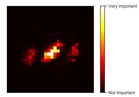
Figure 18.8: Feature importance of a random forest classifier trained to distinguish MNIST digits from classes 0 and 8. Adapted from Figure 7.6 of [Gér19]. Generated by rf\_feature\_importance\_mnist.ipynb.
18.6.1 Feature importance
For a single decision tree T , [BFO84] proposed the following measure for feature importance of feature k:
\[R\_k(T) = \sum\_{j=1}^{J-1} G\_j \mathbb{I}\left(v\_j = k\right) \tag{18.57}\]
where the sum is over all non-leaf (internal) nodes, Gj is the gain in accuracy (reduction in cost) at node j, and vj = k if node j uses feature k. We can get a more reliable estimate by averaging over all trees in the ensemble:
\[R\_k = \frac{1}{M} \sum\_{m=1}^{M} R\_k(T\_m) \tag{18.58}\]
After computing these scores, we can normalize them so the largest value is 100%. We give some examples below.
Figure 18.8 gives an example of estimating feature importance for a classifier trained to distinguish MNIST digits from classes 0 and 8. We see that it focuses on the parts of the image that di!er between these classes.
In Figure 18.9, we plot the relative importance of each of the features for the spam dataset (Section 18.4). Not surprisingly, we find that the most important features are the words “george” (the name of the recipient) and “hp” (the company he worked for), as well as the characters ! and $. (Note it can be the presence or absence of these features that is informative.)
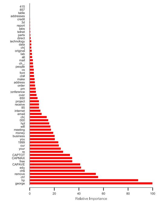
Figure 18.9: Feature importance of a gradient boosted classifier trained to distinguish spam from non-spam email. The dataset has X training examples with Y features, corresponding to token frequency. Adapted from Figure 10.6 of [HTF09]. Generated by spam\_tree\_ensemble\_interpret.ipynb.
Figure 18.10: (a) Partial dependence of log-odds of the spam class for 4 important predictors. The red ticks at the base of the plot are deciles of the empirical distribution for this feature. (b) Joint partial dependence of log-odds on the features hp and !. Adapted from Figure 10.6–10.8 of [HTF09]. Generated by spam\_tree\_ensemble\_interpret.ipynb.
18.6.2 Partial dependency plots
After we have identified the most relevant input features, we can try to assess the impact they have on the output. A partial dependency plot for feature k is a plot of
\[\overline{f}\_k(x\_k) = \frac{1}{N} \sum\_{n=1}^{N} f(x\_{n,-k}, x\_k) \tag{18.59}\]
vs xk. Thus we marginalize out all features except k. In the case of a binary classifier, we can convert this to log odds, log p(y = 1|xk)/p(y = 0|xk), before plotting. We illustrate this for our spam example in Figure 18.10a for 4 di!erent features. We see that as the frequency of ! and “remove” increases, so does the probability of spam. Conversely, as the frequency of “edu” or “hp” increases, the probability of spam decreases.
We can also try to capture interaction e!ects between features j and k by computing
\[\sqrt{f}\_{jk}(x\_j, x\_k) = \frac{1}{N} \sum\_{n=1}^{N} f(x\_{n,-jk}, x\_j, x\_k) \tag{18.60}\]
We illustrate this for our spam example in Figure 18.10b for hp and !. We see that higher frequency of ! makes it more likely to be spam, but much more so if the word “hp” is missing.
Part V
Beyond Supervised Learning
19 Learning with Fewer Labeled Examples
Many ML models, especially neural networks, often have many more parameters than we have labeled training examples. For example, a ResNet CNN (Section 14.3.4) with 50 layers has 23 million parameters. Transformer models (Section 15.5) can be even bigger. Of course these parameters are highly correlated, so they are not independent “degrees of freedom”. Nevertheless, such big models are slow to train and, more importantly, they may easily overfit. This is particularly a problem when you do not have a large labeled training set. In this chapter, we discuss some ways to tackle this issue, beyond the generic regularization techniques we discussed in Section 13.5 such as early stopping, weight decay and dropout.
19.1 Data augmentation
Suppose we just have a single small labeled dataset. In some cases, we may be able to create artificially modified versions of the input vectors, which capture the kinds of variations we expect to see at test time, while keeping the original labels unchanged. This is called data augmentation. 1 We give some examples below, and then discuss why this approach works.
19.1.1 Examples
For image classification tasks, standard data augmentation methods include random crops, zooms, and mirror image flips, as illustrated in Figure 19.1. [GVZ16] gives a more sophisticated example, where they render text characters onto an image in a realistic way, thereby creating a very large dataset of text “in the wild”. They used this to train a state of the art visual text localization and reading system. Other examples of data augmentation include artifically adding background noise to clean speech signals, and artificially replacing characters or words at random in text documents.
If we a!ord to train and test the model many times using di!erent versions of the data, we can learn which augmentations work best, using blackbox optimization methods such as RL (see e.g., [Cub+19]) or Bayesian optimization (see e.g., [Lim+19]); this is called AutoAugment. We can also learn to combine multiple augmentations together; this is called AutoAugment [Cub+19].
For some examples of augmentation in NLP, see e.g., [Fen+21].
1. The term “data augmentation” is also used in statistics to mean the addition of auxiliary latent variables to a model in order to speed up convergence of posterior inference algorithms [DM01].
Figure 19.1: Illustration of random crops and zooms of the image on the left. Generated by image\_augmentation\_jax.ipynb.
19.1.2 Theoretical justification
Data augmentation often significantly improves performance (predictive accuracy, robustness, etc). At first this might seem like we are getting something for nothing, since we have not provided additional data. However, the data augmentation mechanism can be viewed as a way to algorithmically inject prior knowledge.
To see this, recall that in standard ERM training, we minimize the empirical risk
\[R(f) = \int \ell(f(x), y) p^\*(x, y) dx dy \tag{19.1}\]
where we approximate p≃(x, y) by the empirical distribution
\[p\_{\mathcal{D}}(x, y) = \frac{1}{N} \sum\_{n=1}^{N} \delta(x - x\_n) \delta(y - y\_n) \tag{19.2}\]
We can think of data augmentation as replacing the empirical distribution with the following algorithmically smoothed distribution
\[p\_{\mathcal{D}}(\mathbf{z}, \mathbf{y} | A) = \frac{1}{N} \sum\_{n=1}^{N} p(\mathbf{z} | \mathbf{x}\_n, A) \delta(\mathbf{y} - \mathbf{y}\_n) \tag{19.3}\]
where A is the data augmentation algorithm, which generates a sample x from a training point xn, such that the label (“semantics”) is not changed. (A very simple example would be a Gaussian kernel, p(x|xn, A) = N (x|xn, ω2I).) This has been called vicinal risk minimization [Cha+01], since we are minimizing the risk in the vicinity of each training point x. For more details on this perspective, see [Zha+17b; CDL19; Dao+19].
19.2 Transfer learning
This section is coauthored with Colin Ra!el.
Figure 19.2: Illustration of fine-tuning a model on a new dataset. The final output layer is trained from scratch, since it might correspond to a di!erent label set. The other layers are initialized at their previous parameters, and then optionally updated using a small learning rate. From Figure 13.2.1 of [Zha+20]. Used with kind permission of Aston Zhang.
Many data-poor tasks have some high-level structural similarity to other data-rich tasks. For example, consider the task of fine-grained visual classification of endangered bird species. Given that endangered birds are by definition rare, it is unlikely that a large quantity of diverse labeled images of these birds exist. However, birds bear many structural similarities across species - for example, most birds have wings, feathers, beaks, claws, etc. We therefore might expect that first training a model on a large dataset of non-endangered bird species and then continuing to train it on a small dataset of endangered species could produce better performance than training on the small dataset alone.
This is called transfer learning, since we are transferring information from one dataset to another, via a shared set of parameters. More precisely, we first perform a pre-training phase, in which we train a model with parameters ε on a large source dataset Dp; this may be labeled or unlabeled. We then perform a second fine-tuning phase on the small labeled target dataset Dq of interest. We discuss these two phases in more detail below, but for more information, see e.g., [Tan+18; Zhu+21] for recent surveys.
19.2.1 Fine-tuning
Suppose, for now, that we already have a pretrained classifier, p(y|x, εp), such as a CNN, that works well for inputs x → Xp (e.g. natural images) and outputs y → Yp (e.g., ImageNet labels), where the data comes from a distribution p(x, y) similar to the one used in training. Now we want to create a new model q(y|x, εq) that works well for inputs x → Xq (e.g. bird images) and outputs y → Yq (e.g., fine-grained bird labels), where the data comes from a distribution q(x, y) which may be di!erent from p.
We will assume that the set of possible inputs is the same, so Xq ′ Xp (e.g., both are RGB images), or that we can easily transform inputs from domain p to domain q (e.g., we can convert an RGB image to grayscale by dropping the chrominance channels and just keeping luminance). (If this is not
Figure 19.3: (a) Adding adapter layers to a transformer. From Figure 2 of [Hou+19]. Used with kind permission of Neil Houlsby. (b) Adding adapter layers to a resnet. From Figure 2 of [RBV18]. Used with kind permission of Sylvestre-Alvise Rebu”.
the case, then we may need to use a method called domain adaptation, that modifies models to map between modalities, as discussed in Section 19.2.5.)
However, the output domains are usually di!erent, i.e., Yq 7= Yp. For example, Yp might be Imagenet labels and Yq might be medical labels (e.g., types of diabetic retinopathy [Arc+19]). In this case, we need to “translate” the output of the pre-trained model to the new domain. This is easy to do with neural networks: we simply “chop o!” the final layer of the original model, and add a new “head” to model the new class labels, as illustrated in Figure 19.2. For example, suppose p(y|x, εp) = softmax(y|W2h(x; ε1) + b2), where εp = (W2, b2, ε1). Then we can construct q(y|εq) = softmax(y|W3h(x; ε1) + b3), where εq = (W3, b3, ε1) and h(x; ε1) is the shared nonlinear feature extractor.
After performing this “model surgery”, we can fine-tune the new model with parameters εq = (ε1, ε3), where ε1 parameterizes the feature extractor, and ε3 parameterizes the final linear layer that maps features to the new set of labels. If we treat ε1 as “frozen parameters”, then the resulting model q(y|x, εq) is linear in its parameters, so we have a convex optimization problem for which many simple and e”cient fitting methods exist (see Part II). This is particularly helpful in the long-tail setting, where some classes are very rare [Kan+20]. However, a linear “decoder” may be too limiting, so we can also allow ε1 to be fine-tuned as well, but using a lower learning rate, to prevent the values moving too far from the values estimated on Dp.
19.2.2 Adapters
One disadvantage of fine-tuning all the model parameters of a pre-trained model is that it can be slow, since there are often many parameters, and we may need to use a small learning rate to prevent the low-level feature extractors from diverging too far from their prior values. In addition, every new task requires a new model to be trained, making task sharing hard. An alternative approach is to keep the pre-trained model untouched, but to add new parameters to modify its internal behavior to
customize the feature extraction process for each task. This idea is called adapters, and has been explored in several papers (e.g., [RBV17; RBV18; Hou+19]).
Figure 19.3a illustrates adapters for transformer networks (Section 15.5), as proposed in [Hou+19]. The basic idea is to insert two shallow bottleneck MLPs inside each transformer layer, one after the multi-head attention and once after the feed-forward layers. Note that these MLPs have skip connections, so that they can be initialized to implement the identity mapping. If the transformer layer has features of dimensionality D, and the adapter uses a bottleneck of size M, this introduces O(DM) new parameters per layer. These adapter MLPs, as well as the layer norm parameters and final output head, are trained for each new task, but the all remaining parameters are frozen. Empirically on several NLP benchmarks, this is found to give better performance than fine tuning, while only needing about 1-10% of the original parameters.
Figure 19.3b illustrates adapters for residual networks (Section 14.3.4), as proposed in [RBV17; RBV18]. The basic idea is to add a 1x1 convolution layer φ, which is analogous to the MLP adapter in the transformer case, to the internal layers of the CNN. This can be added in series or in parallel, as shown in the diagram. If we denote the adapter layer by 4(x), we can define the series adapter to be
\[\rho(\mathbf{z}) = \mathbf{z} + \text{diag}\_1(\mathbf{a}) \oplus \mathbf{z} = \text{diag}\_1(\mathbf{I} + \mathbf{a}) \oplus \mathbf{z} \tag{19.4}\]
where diag1(φ) → R1↓1↓C↓D reshapes a matrix φ → RC↓D into a matrix that can be applied to each spatial location in parallel. (We have omitted batch normalization for simplicity.) If we insert this after a regular convolution layer f ↬ x we get
\[\mathbf{y} = \rho(\mathbf{f} \circledast \mathbf{z}) = (\text{diag}\_1(\mathbf{I} + \mathbf{a}) \circledast \mathbf{f}) \circledast \mathbf{z} \tag{19.5}\]
This can be interpreted as a low-rank multiplicative perturbation to the original filter f. The parallel adapter can be defined by
\[y = f \circledast x + \text{diag}\_1(\alpha) \circledast x = (f + \text{diag}\_L(\alpha)) \circledast x \tag{19.6}\]
This can be interpreted as a low-rank additive perturbation to the original filter f. In both cases, setting φ = 0 ensures the adapter layers can be initialized to the identity transformation. In addition, both methods required O(C2) parameters per layer.
19.2.3 Supervised pre-training
The pre-training task may be supervised or unsupervised; the main requirements are that it can teach the model basic structure about the problem domain and that it is su”ciently similar to the downstream fine-tuning task. The notion of task similarity is not rigorously defined, but in practice the domain of the pre-training task is often more broad than that of the fine-tuning task (e.g., pre-train on all bird species and fine-tune on endangered ones).
The most straightforward form of transfer learning is the case where a large labeled dataset is suitable for pre-training. For example, it is very common to use the ImageNet dataset (Section 1.5.1.2) to pretrain CNNs, which can then be used for a variety of downstream tasks and datasets (see e.g., [Kol+19]). Imagenet has 1.28 million natural images, each associated with a label from one of 1,000 classes. The classes constitute a wide variety of di!erent concepts, including animals, foods, buildings, musical instruments, clothing, and so on. The images themselves are diverse in the sense
that they contain objects from many angles and in many sizes with a wide variety of backgrounds. This diversity and scale may partially explain why it has become a de-facto pre-training task for transfer learning in computer vision. (See finetune\_cnn\_jax.ipynb for some example code.)
However, Imagenet pre-training has been shown to be less helpful when the domain of the finetuning task is quite di!erent from natural images (e.g. medical images [Rag+19]). And in some cases where it is helpful (e.g., training object detection systems), it seems to be more of a speedup trick (by warm-starting optimization at a good point) rather than something that is essential, in the sense that one can achieve comparable performance on the downstream task when training from scratch, if done for long enough [HGD19].
Supervised pre-training is somewhat less common in non-vision applications. One notable exception is to pre-train on natural language inference data (i.e. whether a sentence implies or contradicts another) to learn vector representations of sentences [Con+17], though this approach has largely been supplanted by unsupervised methods (Section 19.2.4). Another non-vision application of transfer learning is to pre-train a speech recognition on a large English-labeled corpus before fine-tuning on low-resource languages [Ard+20].
19.2.4 Unsupervised pre-training (self-supervised learning)
It is increasingly common to use unsupervised pre-training, because unlabeled data is often easy to acquire, e.g., unlabeled images or text documents from the web.
For a short period of time it was common to pre-train deep neural networks using an unsupervised objective (e.g., reconstruction error, as discussed in Section 20.3) over the labeled dataset (i.e. ignoring the labels) before proceeding with standard supervised training [HOT06; Vin+10b; Erh+10]. While this technique is also called unsupervised pre-training, it di!ers from the form of pre-training for transfer learning we discuss in this section, which uses a (large) unlabeled dataset for pre-training before fine-tuning on a di!erent (smaller) labeled dataset.
Pre-training tasks that use unlabeled data are often called self-supervised rather than unsupervised. This term is used because the labels are created by the algorithm, rather than being provided externally by a human, as in standard supervised learning. Both supervised and self-supervised learning are discriminative tasks, since they require predicting outputs given inputs. By contrast, other unsupervised approaches, such as some of those discussed in Chapter 20, are generative, since they predict outputs unconditionally.
There are many di!erent self-supervised learning heuristics that have been tried (see e.g., [GR18; JT19; Ren19] for a review, and https://github.com/jason718/awesome-self-supervised-learning for an extensive list of papers). We can identify at least three main broad groups, which we discuss below.
19.2.4.1 Imputation tasks
One approach to self-supervised learning is to solve imputation tasks. In this approach, we partition the input vector x into two parts, x = (xh, xv), and then try to predict the hidden part xh given the remaining visible part, xv, using a model of the form xˆh = f(xv, xh = 0). We can think of this as a “fill-in-the-blank” task; in the NLP community, this is called a cloze task. See Figure 19.4 for some visual examples, and Section 15.7.1.2 for some NLP examples.
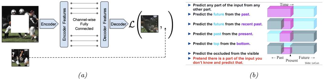
Figure 19.4: (a) Context encoder for self-supervised learning. From [Pat+16]. Used with kind permission of Deepak Pathak. (b) Some other proxy tasks for self-supervised learning. From [LeC18]. Used with kind permission of Yann LeCun.
19.2.4.2 Proxy tasks
Another approach to SSL is to solve proxy tasks, also called pretext tasks. In this setup, we create pairs of inputs, (x1, x2), and then train a Siamese network classifier (Figure 16.5a) of the form p(y|x1, x2) = p(y|r[f(x1), f(x2)]), where f(x) is some function that performs “representation learning” [BCV13], and y is some label that captures the relationship between x1 and x2, which is predicted by r(f1, f2). For example, suppose x1 is an image patch, and x2 = t(x1) is some transformation of x1 that we control, such as a random rotation; then we define y to be the rotation angle that we used [GSK18].
19.2.4.3 Contrastive tasks
The currently most popular approach to self-supervised learning is to use various kinds of contrastive tasks. The basic idea is to create pairs of examples that are semantically similar to each other, using data augmentation methods (Section 19.1), and then to ensure that the distance between their representations is closer (in embedding space) than the distance between two unrelated examples. This is exactly the same idea that is used in deep metric learning (Section 16.2.2) — the only di!erence is that the algorithm creates its own similar pairs, rather than relying on an externally provided measure of similarity, such as labels. We give some examples of this in Section 19.2.4.4 and Section 19.2.4.5.
19.2.4.4 SimCLR
In this section, we discuss SimCLR, which stands for “Simple contrastive learning of visual representations” [Che+20b; Che+20c]. This has shown state of the art performance on transfer learning and semi-supervised learning. The basic idea is as follows. Each input x → RD is converted to two augmented “views’ x1 = t1(x), x2 = t2(x), which are”semantically equivalent” versions of the input generated by some transformations t1, t2. For example, if x is an image, these could be small perturbations to the image, such as random crops, as discussed in Section 19.1. In addition, we sample “negative” examples x→ 1 ,…, x→ n → N(x) from the dataset which represent “semantically di!erent” images (in practice, these are the other examples in the minibatch). Next we define some feature mapping F : RD ≃ RE, where D is the size of the input, and E is the size of the embedding.
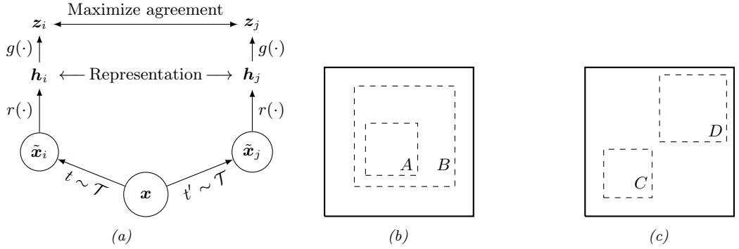
Figure 19.5: (a) Illustration of SimCLR training. T is a set of stochastic semantics-preserving transformations (data augmentations). (b-c) Illustration of the benefit of random crops. Solid rectangles represent the original image, dashed rectangles are random crops. In (b), the model is forced to predict the local view A from the global view B (and vice versa). In (c), the model is forced to predict the appearance of adjacent views (C,D). From Figures 2–3 of [Che+20b]. Used with kind permission of Ting Chen.
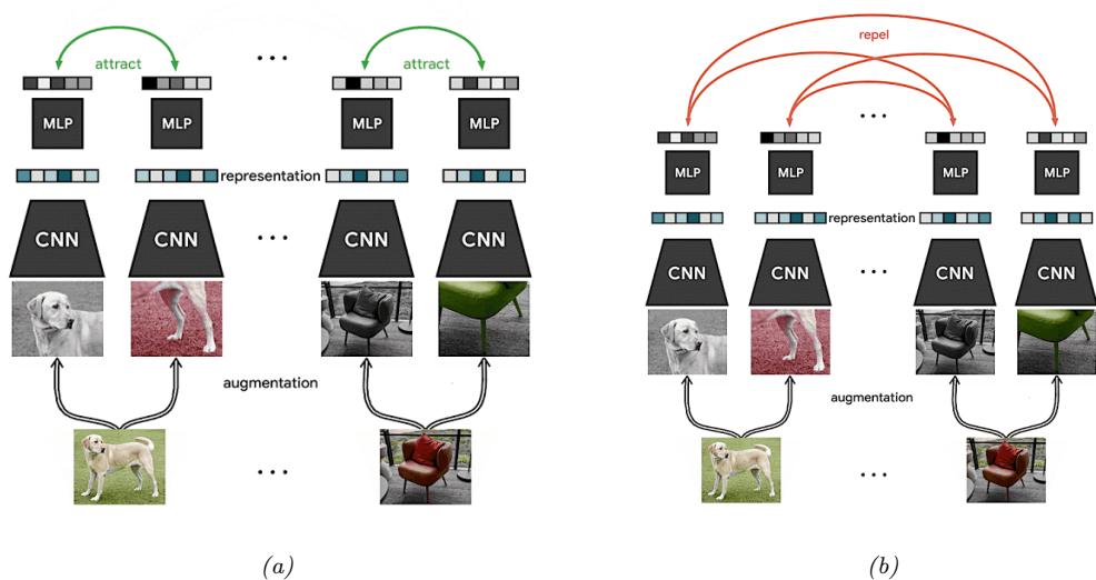
Figure 19.6: Visualization of SimCLR training. Each input image in the minibatch is randomly modified in two di!erent ways (using cropping (followed by resize), flipping, and color distortion), and then fed into a Siamese network. The embeddings (final layer) for each pair derived from the same image is forced to be close, whereas the embeddings for all other pairs are forced to be far. From https: // ai. googleblog. com/ 2020/ 04/ advancing-self-supervised-and-semi. html . Used with kind permission of Ting Chen.
We then try to maximize the similarity of the similar views, while minimizing the similarity of the di!erent views, for each input x:
\[J = F(t\_1(\mathbf{z}))^\top F(t\_2(\mathbf{z})) - \log \sum\_{\mathbf{z}\_i^- \in N(\mathbf{z})} \exp\left[F(\mathbf{z}\_i^-)^\top F(t\_1(\mathbf{z}))\right] \tag{19.7}\]
In practice, we use cosine similarity, so we ε2-normalize the representations produced by F before taking inner products, but this is omitted in the above equation. See Figure 19.5a for an illustration. (In this figure, we assume F(x) = g(r(x)), where the intermediate representation h = r(x) is the one that will be later used for fine-tuning, and g is an additional transformation applied during training.)
Interestingly, we can interpret this as a form of conditional energy based model of the form
\[p(\mathbf{x}\_2|\mathbf{x}\_1) = \frac{\exp[-\mathcal{E}(\mathbf{x}\_2|\mathbf{x}\_1)]}{Z(\mathbf{x}\_1)}\tag{19.8}\]
where E(x2|x1) = ↗F(x2) TF(x1) is the energy, and
\[Z(\mathbf{z}) = \int \exp[-\mathcal{E}(\mathbf{z}^-|\mathbf{z})]d\mathbf{z}^- = \int \exp[F(\mathbf{z}^-)^\mathsf{T}F(\mathbf{z})]d\mathbf{z}^-\tag{19.9}\]
is the normalization constant, known as the partition function. The conditional log likelihood under this model has the form
\[\log p(\mathbf{z}\_2|\mathbf{z}\_1) = F(\mathbf{z}\_2)^\mathsf{T} F(\mathbf{z}\_1) - \log \int \exp[F(\mathbf{z}^-)^\mathsf{T} F(\mathbf{z}\_1)] d\mathbf{z}^- \tag{19.10}\]
The only di!erence from Equation (19.7) is that we replace the integral with a Monte Carlo upper bound derived from the negative samples. Thus we can think of contrastive learning as approximate maximum likelihood estimation of a conditional energy based generative model [Gra+20]. More details on such models can be found in the sequel to this book, [Mur23].
A critical ingredient to the success of SimCLR is the choice of data augmentation methods. By using random cropping, they can force the model to predict local views from global views, as well as to predict adjacent views of the same image (see Figure 19.5). After cropping, all images are resized back to the same size. In addition, they randomly flip the image some fraction of the time.2
SimCLR relies on large batch training, in order to ensure a su”ciently diverse set of negatives. When this is not possible, we can use a memory bank of past (negative) embeddings, which can be updated using exponential moving averaging (Section 4.4.2.2). This is known as momentum contrastive learning or MoCo [He+20].
19.2.4.5 CLIP
In this section, we describe CLIP, which stands for “Contrastive Language-Image Pre-training” [Rad+]. This is a contrastive approach to representation learning which uses a massive corpus of
2. It turns out that distinguishing positive crops (from the same image) from negative crops (from di!erent images) is often easy to do just based on color histograms. To prevent this kind of “cheating”, they also apply a random color distortion, thus cutting o! this “short circuit”. The combination of random cropping and color distortion is found to work better than either method alone.
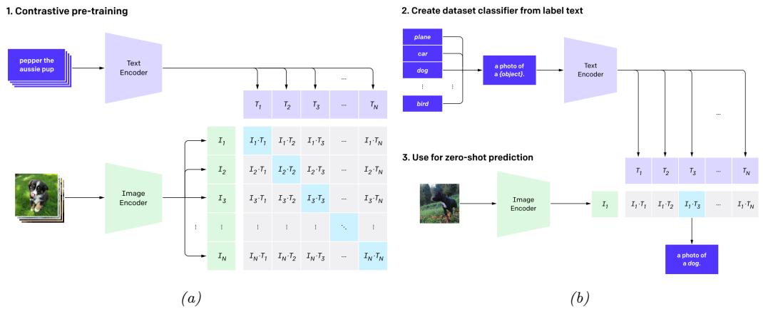
Figure 19.7: Illustration of the CLIP model. From Figure 1 of [Rad+]. Used with kind permission of Alec Radford.
400M (image, text) pairs extracted from the web. Let xi be the i’th image and yi be its matching text. Rather than trying to predict the exact words associated with the image, it is simpler to just determine if yi is more likely to be the correct text compared to yj , for some other text string j in the minibatch. Similarly, the model can try to determine if image xi is more likely to be matched than xj to a given text yi.
More precisely, let fI (xi) be the embedding of the image, fT (yj ) be the embedding of the text, Ii = fI (xi)/||fI (xi)||2 be the unit-norm version of the image embedding, and Tj = fT (yj )/||fT (yj )||2 be the unit-norm version of the text embedding. Define the vector of pairwise logits (similarity scores) to be
\[L\_{ij} = \mathbf{I}\_i^\mathsf{T} \mathbf{T}\_j \tag{19.11}\]
We now train the parameters of the two embedding functions fI and fT to minimize the following loss, averaged over minibatches of size N:
\[J = \frac{1}{2} \left[ \sum\_{i=1}^{N} \text{CE}(\mathbf{L}\_{i,:}, \mathbf{1}\_i) + \sum\_{j=1}^{N} \text{CE}(\mathbf{L}\_{:,j}, \mathbf{1}\_j) \right] \tag{19.12}\]
where CE is the cross entropy loss
\[\text{CE}(\mathbf{p}, \mathbf{q}) = -\sum\_{k=1}^{K} p\_k \log q\_k \tag{19.13}\]
and 1i is a one-hot encoding of label i. See Figure 19.7a for an illustration. (In practice, the normalized embeddings are scaled by a temperature parameter which is also learned; this controls the sharpness of the softmax.)
In their paper, they considered using a ResNet (Section 14.3.4) and a vision transformer (Section 15.5.6) for the function fI , and a text transformer (Section 15.5) for fT . They used a very large minibatch of N ∝ 32k, and trained for many days on 100s of GPUs.
After the model is trained, it can be used for zero-shot classification of an image x as follows. First each of the K possible class labels for a given dataset is converted into a text string yk that might occur on the web. For example, “dog” becomes “a photo of a dog”. Second, we compute the normalized embeddings I ⇐ fI (x) and Tk ⇐ fT (yk). Third, we compute the softmax probabilites
\[p(y = k | \mathbf{x}) = \text{softmax}([\mathbf{I}^{\mathsf{T}} \mathbf{T}\_1, \dots, \mathbf{I}^{\mathsf{T}} \mathbf{T}\_k])\_k \tag{19.14}\]
See Figure 19.7b for an illustration. (A similar approach was adopted in the visual n-grams paper [Li+17].)
Remarkably, this approach can perform as well as standard supervised learning on tasks such as ImageNet classification, without ever being explicitly trained on specific labeled datasets. Of course, the images in ImageNet come from the web, and were found using text-based web-search, so the model has seen similar data before. Nevertheless, its generalization to new tasks, and robustness to distribution shift, are quite impressive (see the paper for examples).
One drawback of the approach, however, is that it is sensitive to how class labels are converted to textual form. For example, to make the model work on food classification, it is necessary to use text strings of the form “a photo of guacamole, a type of food”, “a photo of ceviche, a type of food”, etc. Disambiguating phrases such as “a type of food” are currently added by hand, on a per-dataset basis. This is called prompt engineering, and is needed since the raw class names can be ambiguous across (and sometimes within) a dataset.
19.2.5 Domain adaptation
Consider a problem in which we have inputs from di!erent domains, such as a source domain Xs and target domain Xt, but a common set of output labels, Y. (This is the “dual” of transfer learning, since the input domains are di!erent, but the output domains the same.) For example, the domains might be images from a computer graphics system and real images, or product reviews and movie reviews. We assume we do not have labeled examples from the target domain. Our goal is to fit the model on the source domain, and then modify its parameters so it works on the target domain. This is called (unsupervised) domain adaptation (see e.g., [KL21] for a review).
A common approach to this problem is to train the source classifier in such a way that it cannot distinguish whether the input is coming from the source or target distribution; in this case, it will only be able to use features that are common to both domains. This is called domain adversarial learning [Gan+16]. More formally, let dn → {s, t} be a label that specifies if the data example n comes from domain s or t. We want to optimize
\[\min\_{\boldsymbol{\Phi}} \max\_{\boldsymbol{\Phi}} \frac{1}{N\_s + N\_t} \sum\_{n \in \mathcal{D}\_s, \mathcal{D}\_t} \ell(d\_n, f\_{\boldsymbol{\theta}}(\mathbf{z}\_n)) + \frac{1}{N\_s} \sum\_{m \in \mathcal{D}\_s} \ell(y\_m, g\_{\boldsymbol{\Phi}}(f\_{\boldsymbol{\theta}}(\mathbf{z}\_m))) \tag{19.15}\]
where Ns = |Ds|, Nt = |Dt|, f maps Xs ⊤ Xt ≃ H, and g maps H ≃ Yt. The objective in Equation (19.15) minimizes the loss on the desired task of classifying y, but maximizes the loss on the auxiliary task of classifying the source domain d. This can be implemented by the gradient sign reversal trick, and is related to GANs (generative adversarial networks). See e.g., [Csu17; Wu+19] for some other approaches to domain adaptation.
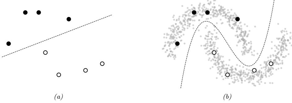
Figure 19.8: Illustration of the benefits of semi-supervised learning for a binary classification problem. Labeled points from each class are shown as black and white circles respectively. (a) Decision boundary we might learn given only labeled data. (b) Decision boundary we might learn if we also had a lot of unlabeled data points, shown as smaller grey circles.
19.3 Semi-supervised learning
19.3.1 Self-training and pseudo-labeling
An early and straightforward approach to semi-supervised learning is self-training [Scu65; Agr70; McL75]. The basic idea behind self-training is to use the model itself to infer predictions on unlabeled
data, and then treat these predictions as labels for subsequent training. Self-training has endured as a semi-supervised learning method because of its simplicity and general applicability; i.e. it is applicable to any model that can generate predictions for the unlabeled data. Recently, it has become common to refer to this approach as “pseudo-labeling” [Lee13] because the inferred labels for unlabeled data are only “pseudo-correct” in comparison with the true, ground-truth targets used in supervised learning.
Algorithmically, self-training typically follows one of the following two procedures. In the first approach, pseudo-labels are first predicted for the entire collection of unlabeled data and the model is re-trained (possibly from scratch) to convergence on the combination of the labeled and (pseudolabeled) unlabeled data. Then, the unlabeled data is re-labeled by the model and the process repeats itself until a suitable solution is found. The second approach instead continually generates predictions on randomly-chosen batches of unlabeled data and immediately trains the model against these pseudo-labels. Both approaches are currently common in practice; the first “o#ine” variant has been shown to be particularly successful when leveraging giant collections of unlabeled data [Yal+19; Xie+20] whereas the “online” approach is often used as one component of more sophisticated semisupervised learning methods [Soh+20]. Neither variant is fundamentally better than the other. O#ine self-training can result in training the model on “stale” pseudo-labels, since they are only updated each time the model converges. However, online pseudo-labeling can incur larger computational costs since it involves constantly “re-labeling” unlabeled data.
Self-training can su!er from an obvious problem: If the model generates incorrect predictions for unlabeled data and then is re-trained on these incorrect predictions, it can become progressively worse and worse at the intended classification task until it eventually learns a totally invalid solution. This issue has been dubbed confirmation bias [TV17] because the model is continually confirming its own (incorrect) bias about the decision rule.
A common way to mitigate confirmation bias is to use a “selection metric” [RHS05] which heuristically tries to only retain pseudo-labels that are correct. For example, assuming that a model outputs probabilities for each possible class, a frequently-used selection metric is to only retain pseudo-labels whose largest class probability is above a threshold [Yar95; RHS05]. If the model’s class probability estimates are well-calibrated, then this selection metric will only retain labels that are highly likely to be correct (according to the model, at least). More sophisticated selection metrics can be designed according to the problem domain.
19.3.2 Entropy minimization
Self-training has the implicit e!ect of encouraging the model to output low-entropy (i.e. highconfidence) predictions. This e!ect is most apparent in the online setting with a cross-entropy loss, where the model minimizes the following loss function L on unlabeled data:
\[\mathcal{L} = -\max\_{c} \log p\_{\theta}(y = c|x) \tag{19.16}\]
where pθ(y|x) is the model’s class probability distribution given input x. This function is minimized when the model assigns all of its class probability to a single class c≃, i.e. p(y = c≃|x)=1 and p(y 7= c≃|x)=0.
A closely-related semi-supervised learning method is entropy minimization [GB05], which
Figure 19.9: Comparison of the entropy minimization, self-training, and “sharpened” entropy minimization loss functions for a binary classification problem.
minimizes the following loss function:
\[\mathcal{L} = -\sum\_{c=1}^{C} p\_{\theta}(y = c|\mathbf{x}) \log p\_{\theta}(y = c|\mathbf{x}) \tag{19.17}\]
Note that this function is also minimized when the model assigns all of its class probability to a single class. We can make the entropy-minimization loss in Equation (19.17) equivalent to the online self-training loss in Equation (19.16) by replacing the first pθ(y = c|x) term with a “one-hot” vector that assigns a probability of 1 for the class that was assigned the highest probability. In other words, online self-training minimizes the cross-entropy between the model’s output and the “hard” target arg max pθ(y|x), whereas entropy minimization uses the the “soft” target pθ(y|x). One way to trade o! between these two extremes is to adjust the “temperature” of the target distribution by raising each probability to the power of 1/T and renormalizing; this is the basis of the mixmatch method of [Ber+19b; Ber+19a; Xie+19]. At T = 1, this is equivalent to entropy minimization; as T ≃ 0, it becomes hard online self-training. A comparison of these loss functions is shown in Figure 19.9.
19.3.2.1 The cluster assumption
Why is entropy minimization a good idea? A basic assumption of many semi-supervised learning methods is that the decision boundary between classes should fall in a low-density region of the data manifold. This e!ectively assumes that the data corresponding to di!erent classes are clustered together. A good decision boundary, therefore, should not pass through clusters; it should simply separate them. Semi-supervised learning methods that make the “cluster assumption” can be thought of as using unlabeled data to estimate the shape of the data manifold and moving the decision boundary away from it.
Entropy minimization is one such method. To see why, first assume that the decision boundary between two classes is “smooth”, i.e. the model does not abruptly change its class prediction anywhere in its domain. This is true in practice for simple and/or regularized models. In this case, if the decision boundary passes through a high-density region of data, it will by necessity produce highentropy predictions for some samples from the data distribution. Entropy minimization will therefore encourage the model to place its decision boundary in low-density regions of the input space to
Figure 19.10: Visualization demonstrating how entropy minimization enforces the cluster assumption. The classifier assigns a higher probability to class 1 (black dots) or 2 (white dots) in red or blue regions respectively. The predicted class probabilities for one particular unlabeled datapoint is shown in the bar plot. In (a), the decision boundary passes through high-density regions of data, so the classifier is forced to output high-entropy predictions. In (b), the classifier avoids high-density regions and is able to assign low-entropy predictions to most of the unlabeled data.
avoid transitioning from one class to another in a region of space where data may be sampled. A visualization of this behavior is shown in Figure 19.10.
19.3.2.2 Input-output mutual information
An alternative justification for the entropy minimization objective was proposed by Bridle, Heading, and MacKay [BHM92], where it was shown that it naturally arises from maximizing the mutual information (Section 6.3) between the data and the label (i.e. the input and output of a model). Denoting x as the input and y as the target, the input-output mutual information can be written as
\[\mathcal{Z}(y;x) = \iint p(y,x) \log \frac{p(y,x)}{p(y)p(x)} dy dx \tag{19.18}\]
\[=\iint p(y|\mathbf{z})p(\mathbf{z})\log\frac{p(y,\mathbf{z})}{p(y)p(\mathbf{z})}dyd\mathbf{z}\tag{19.19}\]
\[\dot{y} = \int p(\mathbf{x}) \int p(y|\mathbf{x}) \log \frac{p(y|\mathbf{x})}{p(y)} dy d\mathbf{x} \tag{19.20}\]
\[=\int p(\mathbf{x})\int p(y|\mathbf{x})\log\frac{p(y|\mathbf{x})}{\int p(\mathbf{x})p(y|\mathbf{x})d\mathbf{x}}dyd\mathbf{x}\tag{19.21}\]
Note that the first integral is equivalent to taking an expectation over x, and the second integral is equivalent to summing over all possible values of the class y. Using these relations, we obtain
\[\mathcal{Z}(y; \boldsymbol{x}) = \mathbb{E}\_{\mathbf{z}} \left[ \sum\_{i=1}^{L} p(y\_i | \boldsymbol{x}) \log \frac{p(y\_i | \boldsymbol{x})}{\mathbb{E}\_{\mathbf{z}}[p(y\_i | \boldsymbol{x})]} \right] \tag{19.22}\]
\[=\mathbb{E}\_{\mathbf{z}}\left[\sum\_{i=1}^{L}p(y\_i|\mathbf{z})\log p(y\_i|\mathbf{z})\right]-\mathbb{E}\_{\mathbf{z}}\left[\sum\_{i=1}^{L}p(y\_i|\mathbf{z})\log\mathbb{E}\_{\mathbf{z}}\left[p(y\_i|\mathbf{z})\right]\right]\tag{19.23}\]
\[\mathbf{E} = \mathbb{E}\_{\mathbf{z}} \left[ \sum\_{i=1}^{L} p(y\_i|\mathbf{z}) \log p(y\_i|\mathbf{z}) \right] - \sum\_{i=1}^{L} \mathbb{E}\_{\mathbf{z}} \left[ p(y\_i|\mathbf{z}) \log \mathbb{E}\_{\mathbf{z}} \left[ p(y\_i|\mathbf{z}) \right] \right] \tag{19.24}\]
Since we had initially sought to maximize the mutual information, and we typically minimize loss functions, we can convert this to a suitable loss function by negating it:
\[\mathcal{L}(y; \boldsymbol{x}) = -\mathbb{E}\_{\mathbf{z}} \left[ \sum\_{i=1}^{L} p(y\_i|\mathbf{z}) \log p(y\_i|\mathbf{z}) \right] + \sum\_{i=1}^{L} \mathbb{E}\_{\mathbf{z}}[p(y\_i|\mathbf{z}) \log \mathbb{E}\_{\mathbf{z}}[p(y\_i|\mathbf{z})]] \tag{19.25}\]
The first term is exactly the entropy minimization objective in expectation. The second term specifies that we should maximize the entropy of the expected class prediction, i.e. the average class prediction over our training set. This encourages the model to predict each possible class with equal probability, which is only appropriate when we know a priori that all classes are equally likely.
19.3.3 Co-training
Co-training [BM98] is also similar to self-training, but makes an additional assumption that there are two complementary “views” (i.e. independent sets of features) of the data, both of which can be used separately to train a reasonable model. After training two models separately on each view, unlabeled data is classified by each model to obtain candidate pseudo-labels. If a particular pseudo-label receives a low-entropy prediction (indicating high confidence) from one model and a high-entropy prediction (indicating low confidence) from the other, then that pseudo-labeled datapoint is added to the training set for the low-confidence model. Then, the process is repeated with the new, larger training datasets. The procedure of only retaining pseudo-labels when one of the models is confident ideally builds up the training sets with correctly-labeled data.
Co-training makes the strong assumption that there are two informative-but-independent views of the data, which may not be true for many problems. The Tri-Training algorithm [ZL05] circumvents this issue by instead using three models that are first trained on independently-sampled (with replacement) subsets of the labeled data. Ideally, initially training on di!erent collections of labeled data results in models that do not always agree on their predictions. Then, pseudo-labels are generated for the unlabeled data independently by each of the three models. For a given unlabeled datapoint, if two of the models agree on the pseudo-label, it is added to the training set for the third model. This can be seen as a selection metric, because it only retains pseudo-labels where two (di!erently initialized) models agree on the correct label. The models are then re-trained on the combination of the labeled data and the new pseudo-labels, and the whole process is repeated iteratively.
19.3.4 Label propagation on graphs
If two datapoints are “similar” in some meaningful way, we might expect that they share a label. This idea has been referred to as the manifold assumption. Label propagation is a semi-supervised learning technique that leverages the manifold assumption to assign labels to unlabeled data. Label propagation first constructs a graph where the nodes are the data examples and the edge weights represent the degree of similarity. The node labels are known for nodes corresponding to labeled data but are unknown for unlabeled data. Label propagation then propagates the known labels across edges of the graph in such a way that there is minimal disagreement in the labels of a given node’s neighbors. This provides label guesses for the unlabeled data, which can then be used in the usual way for supervised training of a model.
More specifically, the basic label propagation algorithm [ZG02] proceeds as follows: First, let wi,j denote a non-negative edge weight between xi and xj that provides a measure of similarity for the two (labeled or unlabeled) datapoints. Assuming that we have M labeled datapoints and N unlabeled datapoints, define the (M + N) ↑ (M + N) transition matrix T as having entries
\[\mathbf{T}\_{i,j} = \frac{w\_{i,j}}{\sum\_{k} w\_{k,j}} \tag{19.26}\]
Ti,j represents the probability of propagating the label for node j to node i. Further, define the (M + N) ↑ C label matrix Y, where C is the number of possible classes. The ith row of Y represents the class probability distribution of datapoint i. Then, repeat the following steps until the values in Y do not change significantly: First, use the transition matrix T to propagate labels in Y by setting Y ℑ TY. Then, re-normalize the rows of Y by setting Yi,c ℑ Yi,c/ ( k Yi,k. Finally, replace the rows of Y corresponding to labeled datapoints with their one-hot representation (i.e. Yi,c = 1 if datapoint i has ground-truth label c and 0 otherwise). After convergence, guessed labels are chosen based on the highest class probability for each datapoint in Y.
This algorithm iteratively uses the similarity of datapoints (encoded in the weights used to construct the transition matrix) to propagate information from the (fixed) labels onto the unlabeled data. At each iteration, the label distribution for a given datapoint is computed as the weighted average of the label distributions for all of its connected datapoints, where the weighting corresponds to the edge weights in T. It can be shown that this procedure converges to a single fixed point, whose computational cost mainly involves the inversion of the matrix of unlabled-to-unlabled transition probabilities [ZG02].
The overall approach can be seen as a form of transductive learning, since it is learning to predict labels for a fixed unlabeled dataset, rather than learning a model that generalizes. However, given the induced labeling. we can perform inductive learning in the usual way.
The success of label propagation depends heavily on the notion of similarity used to construct the weights between di!erent nodes (datapoints). For simple data, measuring the Euclidean distance between datapoints can be su”cient. However, for complex and high-dimensional data the Euclidean distance might not meaningfully reflect the likelihood that two datapoints share the same class. The similarity weights can also be set arbitrarily according to problem-specific knowledge. For a few examples of di!erent ways of constructing the similarity graph, see Zhu [Zhu05, chapter 3]. For some recent papers that use this approach in conjunction with deep learning, see e.g., [BRR18; Isc+19].
19.3.5 Consistency regularization
Consistency regularization leverages the simple idea that perturbing a given datapoint (or the model itself) should not cause the model’s output to change dramatically. Since measuring consistency in this way only makes use of the model’s outputs (and not ground-truth labels), it is readily applicable to unlabeled data and therefore can be used to create appropriate loss functions for semi-supervised learning. This idea was first proposed under the framework of “learning with pseudo-ensembles” [BAP14], with similar variants following soon thereafter [LA16; SJT16].
In its most general form, both the model pθ(y|x) and the transformations applied to the input can be stochastic. For example, in computer vision problems we may transform the input by using data augmentation like randomly rotating or adding noise the input image, and the network may include stochastic components like dropout (Section 13.5.4) or weight noise [Gra11]. A common and simple form of consistency regularization first samples x↑ ∝ q(x↑ |x) (where q(x↑ |x) is the distribution induced by the stochastic input transformations) and then minimizes the loss ∀pθ(y|x) ↗ pθ(y|x↑ )∀2. In practice, the first term pθ(y|x) is typically treated as fixed (i.e. gradients are not propagated through it). In the semi-supervised setting, the combined loss function over a batch of labeled data (x1, y1),(x2, y2),…,(xM, yM) and unlabeled data x1, x2,…, xN is
\[\mathcal{L}(\boldsymbol{\theta}) = -\sum\_{i=1}^{M} \log p\_{\boldsymbol{\theta}}(\boldsymbol{y} = \boldsymbol{y}\_{i}|\boldsymbol{x}\_{i}) + \lambda \sum\_{j=1}^{N} \|p\_{\boldsymbol{\theta}}(\boldsymbol{y}|\boldsymbol{x}\_{j}) - p\_{\boldsymbol{\theta}}(\boldsymbol{y}|\boldsymbol{x}\_{j}^{\prime})\|^{2} \tag{19.27}\]
where ς is a scalar hyperparameter that balances the importance of the loss on unlabeled data and, for simplicity, we write x↑ j to denote a sample drawn from q(x↑ |xj ).
The basic form of consistency regularization in Equation (19.27) reveals many design choices that impact the success of this semi-supervised learning approach. First, the value chosen for the ς hyperparameter is important. If it is too large, then the model may not give enough weight to learning the supervised task and will instead start to reinforce its own bad predictions (as with confirmation bias in self-training). Since the model is often poor at the start of training before it has been trained on much labeled data, it is common in practice to initially set ς to zero and increase its value over the course of training.
A second important consideration are the random transformations applied to the input, i.e., q(x↑ |x). Generally speaking, these transformations should be designed so that they do not change the label of x. As mentioned above, a common choice is to use domain-specific data augmentations. It has recently been shown that using strong data augmentations that heavily corrupt the input (but, arguably, still do not change the label) can produce particularly strong results [Xie+19; Ber+19a; Soh+20].
The use of data augmentation requires expert knowledge to determine what kinds of transformations are label-preserving and appropriate for a given problem. An alternative technique, called virtual adversarial training (VAT), instead transforms the input using an analytically-found perturbation designed to maximally change the model’s output. Specifically, VAT computes a perturbation ς that approximates ς = argmax↼ DKL (pθ(y|x) ∀ pθ(y|x + ς)). The approximation is done by sampling d from a multivariate Gaussian distribution, initializing ς = d, and then setting
\[ \delta \leftarrow \nabla\_{\delta} D\_{\text{KL}} \left( p\_{\theta}(y|x) \parallel p\_{\theta}(y|x + \delta) \right) \vert\_{\delta = \xi d} \tag{19.28} \]
Figure 19.11: Comparison of the squared error and KL divergence losses for a consistency regularization. This visualization is for a binary classification problem where it is assumed that the model’s output for the unperturbed input is 1. The figure plots the loss incurred for a particular value of the logit (i.e. the pre-activation fed into the output sigmoid nonlinearity) for the perturbed input. As the logit grows towards infinity, the model predicts a class label of 1 (in agreement with the prediction for the unperturbed input); as it grows towards negative infinity, the model predicts class 0. The squared error loss saturates (and has zero gradients) when the model predicts one class or the other with high probability, but the KL divergence grows without bound as the model predicts class 0 with more and more confidence.
where 3 is a small constant, typically 10→6. VAT then sets
\[x' = x + \epsilon \frac{\delta}{\|\delta\|\_2} \tag{19.29}\]
and proceeds as usual with consistency regularization (as in Equation (19.27)), where , is a scalar hyperparameter that sets the L2-norm of the perturbation applied to x.
Consistency regularization can also profoundly a!ect the geometry properties of the training objective, and the trajectory of SGD, such that performance can particularly benefit from nonstandard training procedures. For example, the Euclidean distances between weights at di!erent training epochs is significantly larger for objectives that use consistency regularization. Athiwaratkun et al. [Ath+19] show that a variant of stochastic weight averaging (SWA) [Izm+18] can achieve state-of-the-art performance on semi-supervised learning tasks by exploiting the geometric properties of consistency regularization.
A final consideration when using consistency regularization is the function used to measure the di!erence between the network’s output with and without perturbations. Equation (19.27) uses the squared L2 distance (also referred to as the Brier score), which is a common choice [SJT16; TV17; LA16; Ber+19b]. It is also common to use the KL divergence DKL (pθ(y|x) ∀ pθ(y|x↑ ) in analogy with the cross-entropy loss (i.e. KL divergence between ground-truth label and prediction) used for labeled examples [Miy+18; Ber+19a; Xie+19]. The gradient of the squared-error loss approaches zero as the model’s predictions on the perturbed and unperturbed input di!er more and more, assuming the model uses a softmax nonlinearity on its output. Using the squared-error loss therefore has a possible advantage that the model is not updated when its predictions are very unstable. However, the KL divergence has the same scale as the cross-entropy loss used for labeled data, which makes for more intuitive tuning of the unlabeled loss hyperparameter ς. A comparison of the two loss functions is shown in Figure 19.11.
19.3.6 Deep generative models *
Generative models provide a natural way of making use of unlabeled data through learning a model of the marginal distribution by minimizing LU = ↗( n log pε(xn). Various approaches have leveraged generative models for semi-supervised learning by developing ways to use the model of pε(xn) to help produce a better supervised model.
19.3.6.1 Variational autoencoders
In Section 20.3.5, we describe the variational autoencoder (VAE), which defines a probabilistic model of the joint distribution of data x and latent variables z. Data is assumed to be generated by first sampling z ∝ p(z) and then sampling x ∝ p(x|z). For learning, the VAE uses an encoder qϖ(z|x) to approximate the posterior and a decoder pθ(x|z) to approximate the likelihood. The encoder and decoder are typically deep neural networks. The parameters of the encoder and decoder can be jointly trained by maximizing the evidence lower bound (ELBO) of data.
The marginal distribution of latent variables p(z) is often chosen to be a simple distribution like a diagonal-covariance Gaussian. In practice, this can make the latent variables z more amenable to downstream classification thanks to the facts that z is typically lower-dimensional than x, that z is constructed via cascaded nonlinear transformations, and that the dimensions of the latent variables are designed to be independent. In other words, the latent variables can provide a (learned) representation where data may be more easily separable. In [Kin+14], this approach is called M1 and it is indeed shown that the latent variables can be used to train stronger models when labels are scarce. (The general idea of unsupervised learning of representations to help with downstream classification tasks is described further in Section 19.2.4.)
An alternative approach to leveraging VAEs, also proposed in [Kin+14] and called M2, has the form
\[p\_{\theta}(x,y) = p\_{\theta}(y)p\_{\theta}(x|y) = p\_{\theta}(y) \int p\_{\theta}(x|y,z)p\_{\theta}(z)dz\tag{19.30}\]
where z is a latent variable, pε(z) = N (z|µε, “ε) is the latent prior (typically we fix µε = 0 and”ε = I), pε(y) = Cat(y|πε) the label prior, and pε(x|y, z) = p(x|fε(y, z)) is the likelihood, such as a Gaussian, with parameters computed by f (a deep neural network). The main innovation of this approach is to assume that data is generated according to both a latent class variable y as well as the continuous latent variable z. The class variable y is observed for labeled data and unobserved for unlabled data.
To compute the likelihood for the labeled data, pε(x, y), we need to marginalize over z, which we can do by using an inference network of the form
\[q\_{\phi}(\mathbf{z}|y,\mathbf{z}) = \mathcal{N}(\mathbf{z}|\mu\_{\phi}(y,\mathbf{z}), \text{diag}(\sigma\_{\phi}^{2}(\mathbf{z})) \tag{19.31}\]
We then use the following variational lower bound
\[\log p\_{\theta}(\mathbf{z}, y) \ge \mathbb{E}\_{q\_{\phi}(\mathbf{z}|\mathbf{z}, y)} \left[ \log p\_{\theta}(\mathbf{z}|y, \mathbf{z}) + \log p\_{\theta}(y) + \log p\_{\theta}(\mathbf{z}) - \log q\_{\phi}(\mathbf{z}|\mathbf{z}, y) \right] = -\mathcal{L}(\mathbf{z}, y) \tag{19.32}\]
as is standard for VAEs (see Section 20.3.5). The only di!erence is that we observe two kinds of data: x and y.
To compute the likelihood for the unlabeled data, pε(x), we need to marginalize over z and y, which we can do by using an inference network of the form
\[q\_{\phi}(\mathbf{z}, y|\mathbf{z}) = q\_{\phi}(\mathbf{z}|\mathbf{z})q\_{\phi}(y|\mathbf{z})\tag{19.33}\]
\[q\_{\phi}(\mathbf{z}|\mathbf{x}) = \mathcal{N}(\mathbf{z}|\mu\_{\phi}(\mathbf{z}), \text{diag}(\sigma\_{\phi}^{2}(\mathbf{z})) \tag{19.34}\]
\[q\_{\phi}(y|\mathbf{z}) = \text{Cat}(y|\pi\_{\phi}(\mathbf{z})) \tag{19.35}\]
Note that qφ(y|x) acts like a discriminative classifier, that imputes the missing labels. We then use the following variational lower bound:
\[\log p\_{\theta}(\mathbf{z}) \ge \mathbb{E}\_{q\_{\phi}(\mathbf{z}, y|\mathbf{z})} \left[ \log p\_{\theta}(\mathbf{z}|y, \mathbf{z}) + \log p\_{\theta}(y) + \log p\_{\theta}(\mathbf{z}) - \log q\_{\phi}(\mathbf{z}, y|\mathbf{z}) \right] \tag{19.36}\]
\[\mathcal{L} = -\sum\_{y} q\_{\phi}(y|x)\mathcal{L}(x,y) + \mathbb{H}\left(q\_{\phi}(y|x)\right) = -\mathcal{U}(x) \tag{19.37}\]
Note that the discriminative classifier qφ(y|x) is only used to compute the log-likelihood of the unlabeled data, which is undesirable. We can therefore add an extra classification loss on the supervised data, to get the following overall objective function:
\[\mathcal{L}(\boldsymbol{\theta}) = \mathbb{E}\_{(\mathbf{z}, y) \sim \mathcal{D}\_L} \left[ \mathcal{L}(\mathbf{z}, y) \right] + \mathbb{E}\_{\mathbf{z} \sim \mathcal{D}\_U} \left[ \mathcal{U}(\mathbf{z}) \right] + \alpha \mathbb{E}\_{(\mathbf{z}, y) \sim \mathcal{D}\_L} \left[ -\log q\_{\boldsymbol{\phi}}(y|\mathbf{z}) \right] \tag{19.38}\]
where φ is a hyperparameter that controls the relative weight of generative and discriminative learning.
Of course, the probablistic model used in M2 is just one of many ways to decompose the dependencies between the observed data, the class labels, and the continuous latent variables. There are also many ways other than variational inference to perform approximate inference. The best technique will be problem dependent, but overall the main advantage of the generative approach is that we can incorporate domain knowledge. For example, we can model the missing data mechanism, since the absence of a label may be informative about the underlying data (e.g., people may be reluctant to answer a survey question about their health if they are unwell).
19.3.6.2 Generative adversarial networks
Generative adversarial networks (GANs) (described in more detail in the sequel to this book, [Mur23]) are a popular class of generative models that learn an implicit model of the data distribution. They consist of a generator network, which maps samples from a simple latent distribution to the data space, and a critic network, which attempts to distinguish between the outputs of the generator and samples from the true data distribution. The generator is trained to generate samples that the critic classifies as “real”.
Since standard GANs do not produce a learned latent representation of a given datapoint and do not learn an explicit model of the data distribution, we cannot use the same approaches as were used for VAEs. Instead, semi-supervised learning with GANs is typically done by modifying the critic so that it outputs either a class label or “fake” instead of simply classifying real vs. fake [Sal+16; Ode16]. For labeled real data, the critic is trained to output the appropriate class label, and for unlabeled real data, it is trained to raise the probability of any of the class labels. As with standard GAN training, the critic is trained to classify outputs from the generator as fake and the generator is trained to fool the critic.
Figure 19.12: Diagram of the semi-supervised GAN framework. The discriminator is trained to output the class of labeled datapoints (red), a “fake” label for outputs from the generator (yellow), and any label for unlabeled data (green).
In more detail, let pθ(y|x) denote the critic with C + 1 outputs corresponding to C classes plus a “fake” class, and let G(z) denote the generator which takes as input samples from the prior distribution p(z). Let us assume that we are using the standard cross-entropy GAN loss as originally proposed in [Goo+14]. Then the critic’s loss is
\[-\mathbb{E}\_{\mathbf{z},y\sim p(\mathbf{z},y)}\log p\_{\theta}(y|\mathbf{z}) - \mathbb{E}\_{\mathbf{z}\sim p(\mathbf{z})}\log[1 - p\_{\theta}(y = C + 1|\mathbf{z})] - \mathbb{E}\_{\mathbf{z}\sim p(\mathbf{z})}\log p\_{\theta}(y = C + 1|G(\mathbf{z})) \tag{19.39}\]
This tries to maximize the probability of the correct class for the labeled examples, to minimize the probability of the fake class for real unlabeled examples, and to maximize the probability of the fake class for generated examples. The generator’s loss is simpler, namely
\[\mathbb{E}\_{z \sim p(\mathbf{z})} \log p\_{\theta}(y = C + 1 | G(\mathbf{z})) \tag{19.40}\]
A diagram visualizing the semi-supervised GAN framework is shown in Figure 19.12.
19.3.6.3 Normalizing flows
Normalizing flows (described in more detail in the sequel to this book, [Mur23]) are a tractable way to define deep generative models. More precisely, they define an invertible mapping fθ : X ≃ Z, with parameters ⇁, from the data space X to the latent space Z. The density in data space can be written starting from the density in the latent space using the change of variables formula:
\[p(x) = p(f(x)) \cdot \left| \det \left( \frac{\partial f}{\partial x} \right) \right|. \tag{19.41}\]
We can extend this to semi-supervised learning, as proposed in [Izm+20]. For class labels y → {1 … C}, we can specify the latent distribution, conditioned on a label k, as Gaussian with mean µk and covariance %k: p(z|y = k) = N (z|µk, %k). The marginal distribution of z is then a Gaussian mixture. The likelihood for labeled data is then
\[p\_{\mathcal{X}}(x|y=k) = \mathcal{N}\left(f(x)|\mu\_k, \Sigma\_k\right) \cdot \left| \det\left(\frac{\partial f}{\partial x}\right) \right|,\tag{19.42}\]
Figure 19.13: Combining self-supervised learning on unlabeled data (left), supervised fine-tuning (middle), and self-training on pseudo-labeled data (right). From Figure 3 of [Che+20c]. Used with kind permission of Ting Chen.
and the likelihood for data with unknown label is p(x) = ( k p(x|y = k)p(y = k).
For semi-supervised learning we can then maximize the joint likelihood of the labeled Dω and unlabeled data Du:
\[p(\mathcal{D}\_\ell, \mathcal{D}\_u | \theta) = \prod\_{(x\_i, y\_i) \in \mathcal{D}\_\ell} p(x\_i, y\_i) \prod\_{x\_j \in \mathcal{D}\_u} p(x\_j), \tag{19.43}\]
over the parameters ⇁ of the bijective function f, which learns a density model for a Bayes classifier.
Given a test point x, the model predictive distribution is given by
\[p\_X(y=c|x) = \frac{p(x|y=c)p(y=c)}{p(x)} = \frac{p(x|y=c)p(y=c)}{\sum\_{k=1}^C p(x|y=k)p(y=k)} = \frac{\mathcal{N}(f(x)|\mu\_c, \Sigma\_c)}{\sum\_{k=1}^C \mathcal{N}(f(x)|\mu\_k, \Sigma\_k)},\tag{19.44}\]
where we have assumed p(y = c)=1/C. We can make predictions for a test point x with the Bayes decision rule y = arg maxc↔︎{1,…,C} p(y = c|x).
19.3.7 Combining self-supervised and semi-supervised learning
It is possible to combine self-supervised and semi-supervised learning. For example, [Che+20c] use SimCLR (Section 19.2.4.4) to perform self-supervised representation learning on the unlabeled data, they then fine-tune this representation on a small labeled dataset (as in transfer learning, Section 19.2), and finally, they apply the trained model back to the original unlabeled dataset, and distill the predictions from this teacher model T into a student model S. (Knowledge distillation is the name given to the approach of training one model on the predictions of another, as originally proposed in [HVD14].) That is, after fine-tuning T, they train S by minimizing
\[\mathcal{L}(T) = -\sum\_{\mathbf{x}\_i \in \mathcal{D}} \left[ \sum\_y p^T(y|\mathbf{x}\_i; \tau) \log p^S(y|\mathbf{x}\_i; \tau) \right] \tag{19.45}\]
where ▷ > 0 is a temperature parameter applied to the softmax output, which is used to perform label smoothing. If S has the same form as T, this is known as self-training, as discussed in Section 19.3.1. However, normally the student S is smaller than the teacher T. (For example, T might be a high capacity model, and S is a lightweight version that runs on a phone.) See Figure 19.13 for an illustration of the overall approach.
19.4 Active learning
In active learning, the goal is to identify the true predictive mapping y = f(x) by querying as few (x, y) points as possible. There are three main variants. In query synthesis, the algorithm gets to choose any input x, and can ask for its corresponding output y = f(x). In pool-based active learning, there is a large, but fixed, set of unlabeled data points, and the algorithm gets to ask for a label for one or more of these points. Finally, in stream-based active learning, the incoming data is arriving continuously, and the algorithm must choose whether it wants to request a label for the current input or not.
There are various closely related problems. In Bayesian optimization the goal is to estimate the location of the global optimum x≃ = argminx f(x) in as few queries as possible; typically we fit a surrogate (response surface) model to the intermediate (x, y) queries, to decide which question to ask next. In experiment design, the goal is to infer a parameter vector of some model, using carefully chosen data samples D = {x1,…, xN }, i.e. we want to estimate p(ε|D) using as little data as possible. (This can be thought of as an unsupervised, or generalized, form of active learning.)
In this section, we give a brief review of the pool based approach to active learning. For more details, see e.g., [Set12] for a review.
19.4.1 Decision-theoretic approach
In the decision theoretic approach to active learning, proposed in [KHB07; RM01], we define the utility of querying x in terms of the value of information. In particular, we define the utility of issuing query x as
\[U(x) \stackrel{\Delta}{=} \mathbb{E}\_{p(y|x,\mathcal{D})} \left[ \min\_{a} \left( \rho(a|\mathcal{D}) - \rho(a|\mathcal{D}, (x,y)) \right) \right] \tag{19.46}\]
where 4(a|D) = Ep(θ|D) [ε(⇁, a)] is the posterior expected loss of taking some future action a given the data D observed so far. Unfortunately, evaluating U(x) for each x is quite expensive, since for each possible response y we might observe, we have to update our beliefs given (x, y) to see what e!ect it might have on our future decisions (similar to look ahead search technique applied to belief states).
19.4.2 Information-theoretic approach
In the information theoretic approach to active supervised learning, we avoid using task-specific loss functions, and instead focus on learning our model as well as we can. In particular, [Lin56] proposed to define the utility of querying x in terms of information gain about the parameters ε, i.e., the reduction in entropy:
\[U(\mathbf{z}) \triangleq \mathbb{H}\left(p(\boldsymbol{\theta}|\mathcal{D})\right) - \mathbb{E}\_{p(\boldsymbol{y}|\mathbf{z}, \mathcal{D})}\left[\mathbb{H}\left(p(\boldsymbol{\theta}|\mathcal{D}, \mathbf{z}, \boldsymbol{y}\right)\right] \tag{19.47}\]
(Note that the first term is a constant wrt x, but we include it for later convenience.) Exercise 19.1 asks you to show that this objective is identical to the expected change in the posterior over the parameters which is given by
\[U'(\mathbf{z}) \stackrel{\Delta}{=} \mathbb{E}\_{p(y|\mathbf{z}, \mathcal{D})} \left[ D\_{\mathbb{KL}} \left( p(\boldsymbol{\theta} | \mathcal{D}, \mathbf{z}, y) \parallel p(\boldsymbol{\theta} | \mathcal{D}) \right) \right] \tag{19.48}\]
Using symmetry of the mutual information, we can rewrite Equation (19.47) as follows:
\[U(\mathbf{x}) = \mathbb{H}\left(p(\boldsymbol{\theta}|\mathcal{D})\right) - \mathbb{E}\_{p(y|\mathbf{z}, \mathcal{D})}\left[\mathbb{H}\left(p(\boldsymbol{\theta}|\mathcal{D}, \mathbf{z}, y)\right)\right] \tag{19.49}\]
\[= \mathbb{I}(\theta, y | \mathcal{D}, x) \tag{19.50}\]
\[\mathbb{E}\_{\theta} = \mathbb{H}\left(p(y|x,\mathcal{D})\right) - \mathbb{E}\_{p(\theta|\mathcal{D})}\left[\mathbb{H}\left(p(y|x,\theta)\right)\right] \tag{19.51}\]
The advantage of this approach is that we now only have to reason about the uncertainty of the predictive distribution over outputs y, not over the parameters ε.
Equation (19.51) has an interesting interpretation. The first term prefers examples x for which there is uncertainty in the predicted label. Just using this as a selection criterion is called maximum entropy sampling [SW87]. However, this can have problems with examples which are inherently ambiguous or mislabeled. The second term in Equation (19.51) will discourage such behavior, since it prefers examples x for which the predicted label is fairly certain once we know ε; this will avoid picking inherently hard-to-predict examples. In other words, Equation (19.51) will select examples x for which the model makes confident predictions which are highly diverse. This approach has therefore been called Bayesian active learning by disagreement or BALD [Hou+12].
This method can be used to train classifiers for other domains where expert labels are hard to acquire, such as medical images or astronomical images [Wal+20].
19.4.3 Batch active learning
So far, we have assumed a greedy or myopic strategy, in which we select a single example x, as if it were the last datapoint to be selected. But sometimes we have a budget to collect a set of B samples, call them (X, Y). In this case, the information gain criterion becomes U(x) = H (p(ε|D)) ↗ Ep(Y|x,D) [H (p(ε|Y, x, D))]. Unfortunately, optimizing this is NP-hard in the horizon length B [KLQ95; KG05].
Fortunately, under certain conditions, the greedy strategy is near-optimal, as we now explain. Let us fix query x and define f(y) ↫ H (p(ε|D)) ↗ H (p(ε|Y, x, D)) as the information gain function, so U(x) = Ey [f(y, x)]. It is clear that f(⇓)=0, and that f is non-decreasing, meaning f(Y large) ↓ f(Y small), due to the “more information never hurts” principle. Furthermore, [KG05] proved that f is submodular. As a consequence, a sequential greedy approach is within a constant factor of optimal. If we combine this greedy technique with the BALD objective, we get a method called BatchBALD [KAG19].
19.5 Meta-learning
We can think of a learning algorithm as a function A that maps data to a parameter estimate, ⇁ = A(D). The function A usually has its own parameter — call them ϱ — such as the initial values for ⇁, or the learning rate, etc. We denote this by ⇁ = A(D; ϱ). We can imagine learning ϱ itself,
Figure 19.14: Illustration of a hierarchical Bayesian model for meta-learning. Generated by hbayes\_maml.ipynb.
given a collection of datasets D1:J and some meta-learning algorithm M, i.e., ϱ = M(D1:J ). We can then apply A(·; ϱ) to learn the parameters ⇁J+1 on some new dataset DJ+1. There are many techniques for meta-learning — see e.g., [Van18; HRP21] for recent reviews. Below we discuss one particularly popular method. (Note that meta-learning is also called learning to learn [TP97].)
19.5.1 Model-agnostic meta-learning (MAML)
A natural approach to meta learning is to use a hierarchical Bayesian model, as illustrated in Figure 19.14. The parameters for each task εj are assumed to come from a common prior, p(εj |⇁), which can be used to help pool statistical strength from multiple data-poor problems. Meta-learning becomes equivalent to learning the prior ϱ. Rather than performing full Bayesian inference in this model, a more e”cient approach is to use the following empirical Bayes (Section 4.6.5.3) approximation:
\[\boldsymbol{\xi}^\* = \underset{\boldsymbol{\xi}}{\text{argmax}} \frac{1}{J} \sum\_{j=1}^J \log p(\mathcal{D}\_{\text{valid}}^j | \hat{\theta}\_j(\boldsymbol{\xi}, \mathcal{D}\_{\text{train}}^j)) \tag{19.52}\]
where εˆj = εˆ(⇁, Dj train) is a point estimate of the parameters for task j based on Dj train and prior ⇁, and where we use a cross-validation approximation to the marginal likelihood (Section 5.2.4).
To compute the point estimate of the parameters for the target task εˆJ+1, we use K steps of a gradient ascent procedure starting at ⇁ with a learning rate of ⇀. This is known as model-agnostic meta-learning or MAML [FAL17]. This can be shown to be equivalent to an approximate MAP estimate using a Gaussian prior centered at ⇁, where the strength of the prior is controlled by the number of gradient steps [San96; Gra+18]. (This is an example of fast adapation of the task specific weights starting from the shared prior ⇁.)
Figure 19.15: Illustration of meta-learning for few-shot learning. Here, each task is a 3-way-2-shot classification problem because each training task contains a support set with three classes, each with two examples. From https: // bit. ly/ 3rrvSjw . Copyright (2019) Borealis AI. Used with kind permission of Simon Prince and April Cooper.
19.6 Few-shot learning
People can learn to predict from very few labeled examples. This is called few-shot learning. In the extreme in which the person or system learns from a single example of each class, this is called one-shot learning, and if no labeled examples are given, it is called zero-shot learning.
A common way to evaluate methods for FSL is to use C-way N-shot classification, in which the system is expected to learn to classify C classes using just N training examples of each class. Typically N and C are very small, e.g., Figure 19.15 illustrates the case where we have C = 3 classes, each with N = 2 examples. Since the amount of data from the new domain (here, ducks, dolphins and hens) is so small, we cannot expect to learn from scratch. Therefore we turn to meta-learning.
During training, the meta-algorithm M trains on a labeled support set from group j, returns a predictor fj , which is then evaluated on a disjoint query set also from group j. We optimize M over all J groups. Finally we can apply M to our new labeled support set to get ftest, which is applied to the query set from the test domain. This is illustrated in Figure 19.15. We see that there is no overlap between the classes in the two training tasks ({cat, lamb, pig} and {dog, shark, lion}) and those in the test task ({duck, dolphin, hen}). Thus the algorithm M must learn to predict image classes in general rather than any particular set of labels.
There are many approaches to few-shot learning. We discuss one such method in Section 19.6.1. For more methods, see e.g., [Wan+20b].
19.6.1 Matching networks
One approach to few shot learning is to learn a distance metric on some other dataset, and then to use dε(x, x↑ ) inside of a nearest neighbor classifier. Essentially this defines a semi-parametric model of the form pε(y|x, S), where S is the small labeled dataset (known as the support set), and ε are the parameters of the distance function. This approach is widely used for fine-grained classification
Figure 19.16: Illustration of a matching network for one-shot learning. From Figure 1 of [Vin+16]. Used with kind permission of Oriol Vinyals.
tasks, where there are many di!erent visually similar categories, such as face images from a gallery, or product images from a catalog.
An extension of this approach is to learn a function of the form
\[p\_{\theta}(y|\mathbf{x}, \mathcal{S}) = \mathbb{I}\left(y = \sum\_{n \in \mathcal{S}} a\_{\theta}(\mathbf{x}, x\_n; \mathcal{S}) y\_n\right) \tag{19.53}\]
where aε(x, xn; S) → R+ is some kind of adaptive similarity kernel. For example, we can use an attention kernel of the form
\[a(\mathbf{z}, \mathbf{z}\_n; \mathcal{S}) = \frac{\exp(c(f(\mathbf{z}), g(\mathbf{z}\_n)))}{\sum\_{n'=1}^N \exp(c(f(\mathbf{z}), g(\mathbf{z}\_{n'})))} \tag{19.54}\]
where c(u, v) is the cosine distance. (We can make f and g be the same function if we want.) Intuitively, the attention kernel will compare x to xn in the context of all the labeled examples, which provides an implicit signal about which feature dimensions are relevant. (We discuss attention mechanisms in more detail in Section 15.4.) This is called a matching network [Vin+16]. See Figure 19.16 for an illustration.
We can train the f and g functions using multiple small datasets, as in meta-learning (Section 19.5). More precisely, let D be a large labeled dataset (e.g., ImageNet), and let p(L) be a distribution over its labels. We create a task by sampling a small set of labels (say 25), L ∝ p(L), and then sampling a small support set of examples from D with those labels, S ∝ L, and finally sampling a small test set with those same labels, T ∝ L. We then train the model to predict the test labels given the support set, i.e., we optimize the following objective:
\[\mathcal{L}(\boldsymbol{\theta}; \mathcal{D}) = \mathbb{E}\_{\mathcal{L} \sim p(\mathcal{L})} \left[ \mathbb{E}\_{\mathcal{S} \sim \mathcal{L}, \mathcal{T} \sim \mathcal{L}} \left[ \sum\_{(\mathfrak{a}, y) \in \mathcal{T}} \log p\_{\boldsymbol{\theta}}(y|\boldsymbol{x}, \mathcal{S}) \right] \right] \tag{19.55}\]
After training, we freeze ε, and apply Equation (19.53) to a test support set S.
19.7 Weakly supervised learning
The term weakly supervised learning refers to scenarios where we do not have an exact label associated with every feature vector in the training set.
One scenario is when we have a distribution over labels for each case, rather than a single label. Fortunately, we can still do maximum likelihood training: we just have to minimize the cross entropy,
\[\mathcal{L}(\boldsymbol{\theta}) = -\sum\_{n} \sum\_{y} p(y|\boldsymbol{x}\_n) \log q\_{\boldsymbol{\theta}}(y|\boldsymbol{x}\_n) \tag{19.56}\]
where p(y|xn) is the label distribution for case n, and qε(y|xn) is the predicted distribution. Indeed, it is often useful to artificially replace exact labels with a “soft” version, in which we replace the delta function with a distribution that puts, say, 90% of its mass on the observed label, and spreads the remaining mass uniformly over the other choices. This is called label smoothing, and is a useful form of regularization (see e.g., [MKH19]).
Another scenario is when we have a set, or bag, of instances, xn = {xn,1,…, xn,B}, but we only have a label for the entire bag, yn, not for the members of the bag, ynb. We often assume that if any member of the bag is positive, the whole bag is labeled positive, so yn = ↘B b=1ynb, but we do not know which member “caused” the positive outcome. However, if all the members are negative, the entire bag is negative. This is known as multi-instance learning [DLLP97]. (For a recent example of this in the context of COVID-19 risk score learning, see [MKS21].) Various algorthms can be used to solve the MIL problem, depending on what assumptions we make about the correlation between the labels in each bag, and the fraction of positive members we expect to see (see e.g., [KF05]).
Yet another scenario is known as distant supervision [Min+09], which is often used to train information extraction systems. The idea is that we have some fact, such as “Married(B,M)”, that we know to be true (since it is stored in a database). We use this to label every sentence (in our unlabeled training corpus) in which the entities B and M are mentioned as being a positive example of the “Married” relation. For example, the sentence “B and M invited 100 people to their wedding” will be labeled positive. But this heuristic may include false positives, for example “B and M went out to dinner” will also be labeled positive. Thus the resulting labels will be noisy. We discuss some ways to handle label noise in Section 10.4.
19.8 Exercises
Exercise 19.1 [Information gain equations]
Consider the following two objectives for evaluating the utility of querying a datapoint x in an active learning setting:
\[U(\mathbf{z}) \triangleq \mathbb{H}\left(p(\boldsymbol{\theta}|\mathcal{D})\right) - \mathbb{E}\_{p(\boldsymbol{y}|\mathbf{z}, \mathcal{D})}\left[\mathbb{H}\left(p(\boldsymbol{\theta}|\mathcal{D}, \mathbf{z}, \boldsymbol{y}\right)\right] \tag{19.57}\]
\[U'(\mathbf{x}) \triangleq \mathbb{E}\_{p(y|\mathbf{z}, \mathcal{D})} \left[ D\_{\text{KL}} \left( p(\theta | \mathcal{D}, \mathbf{z}, y) \parallel p(\theta | \mathcal{D}) \right) \right] \tag{19.58}\]
Prove that these are equal.
20 Dimensionality Reduction
A common form of unsupervised learning is dimensionality reduction, in which we learn a mapping from the high-dimensional visible space, x → RD, to a low-dimensional latent space, z → RL. This mapping can either be a parametric model z = f(x; ε) which can be applied to any input, or it can be a nonparametric mapping where we compute an embedding zn for each input xn in the data set, but not for any other points. This latter approach is mostly used for data visualization, whereas the former approach can also be used as a preprocessing step for other kinds of learning algorithms. For example, we might first reduce the dimensionality by learning a mapping from x to z, and then learn a simple linear classifier on this embedding, by mapping z to y.
20.1 Principal components analysis (PCA)
The simplest and most widely used form of dimensionality reduction is principal components analysis or PCA. The basic idea is to find a linear and orthogonal projection of the high dimensional data x → RD to a low dimensional subspace z → RL, such that the low dimensional representation is a “good approximation” to the original data, in the following sense: if we project or encode x to get z = WTx, and then unproject or decode z to get xˆ = Wz, then we want xˆ to be close to x in ε2 distance. In particular, we can define the following reconstruction error or distortion:
\[\mathcal{L}(\mathbf{W}) \triangleq \frac{1}{N} \sum\_{n=1}^{N} ||x\_n - \text{decode}(\text{encode}(x\_n; \mathbf{W}); \mathbf{W})||\_2^2 \tag{20.1}\]
where the encode and decoding stages are both linear maps, as we explain below.
In Section 20.1.2, we show that we can minimize this objective by setting Wˆ = UL, where UL contains the L eigenvectors with largest eigenvalues of the empirical covariance matrix
\[\hat{\Delta} = \frac{1}{N} \sum\_{n=1}^{N} (\mathbf{x}\_n - \overline{\mathbf{z}})(\mathbf{x}\_n - \overline{\mathbf{z}})^\top = \frac{1}{N} \mathbf{X}\_c^\top \mathbf{X}\_c \tag{20.2}\]
where Xc is a centered version of the N ↑ D design matrix. In Section 20.2.2, we show that this is equivalent to maximizing the likelihood of a latent linear Gaussian model known as probabilistic PCA.
20.1.1 Examples
Before giving the details, we start by showing some examples.
Figure 20.1: An illustration of PCA where we project from 2d to 1d. Red circles are the original data points, blue circles are the reconstructions. The red dot is the data mean. Generated by pcaDemo2d.ipynb.
Figure 20.2: An illustration of PCA applied to MNIST digits from class 9. Grid points are at the 5, 25, 50, 75, 95 % quantiles of the data distribution along each dimension. The circled points are the closest projected images to the vertices of the grid. Adapted from Figure 14.23 of [HTF09]. Generated by pca\_digits.ipynb.
Figure 20.1 shows a very simple example, where we project 2d data to a 1d line. This direction captures most of the variation in the data.
In Figure 20.2, we show what happens when we project some MNIST images of the digit 9 down to 2d. Although the inputs are high dimensional (specifically 28 ↑ 28 = 784 dimensional), the number of “e!ective degrees of freedom” is much less, since the pixels are correlated, and many digits look similar. Therefore we can represent each image as a point in a low dimensional linear space.
In general, it can be hard to interpret the latent dimensions to which the data is projected. However, by looking at several projected points along a given direction, and the examples from which they are derived, we see that the first principal component (horizontal direction) seems to capture the orientation of the digit, and the second component (vertical direction) seems to capture line thickness.
In Figure 20.3, we show PCA applied to another image dataset, known as the Olivetti face dataset,

Figure 20.3: a) Some randomly chosen 64 ↑ 64 pixel images from the Olivetti face database. (b) The mean and the first three PCA components represented as images. Generated by pcaImageDemo.ipynb.
which is a set of 64 ↑ 64 grayscale images. We project these to a 3d subspace. The resulting basis vectors (columns of the projection matrix W) are shown as images in in Figure 20.3b; these are known as eigenfaces [Tur13], for reasons that will be explained in Section 20.1.2. We see that the main modes of variation in the data are related to overall lighting, and then di!erences in the eyebrow region of the face. If we use enough dimensions (but fewer than the 4096 we started with), we can use the representation z = WTx as input to a nearest-neighbor classifier to perform face recognition; this is faster and more reliable than working in pixel space [MWP98].
20.1.2 Derivation of the algorithm
Suppose we have an (unlabeled) dataset D = {xn : n =1: N}, where xn → RD. We can represent this as an N ↑ D data matrix X. We will assume x = 1 N (N n=1 xn = 0, which we can ensure by centering the data.
We would like to approximate each xn by a low dimensional representation, zn → RL. We assume that each xn can be “explained” in terms of a weighted combination of basis functions w1,…, wL, where each wk → RD, and where the weights are given by zn → RL, i.e., we assume xn ′ (L k=1 znkwk. The vector zn is the low dimensional representation of xn, and is known as the latent vector, since it consists of latent or “hidden” values that are not observed in the data. The collection of these latent variables are called the latent factors.
We can measure the error produced by this approximation as follows:
\[\mathcal{L}(\mathbf{W}, \mathbf{Z}) = \frac{1}{N} ||\mathbf{X} - \mathbf{Z}\mathbf{W}^{\mathrm{T}}||\_{F}^{2} = \frac{1}{N} ||\mathbf{X}^{\mathrm{T}} - \mathbf{W}\mathbf{Z}^{\mathrm{T}}||\_{F}^{2} = \frac{1}{N} \sum\_{n=1}^{N} ||x\_{n} - \mathbf{W}z\_{n}||^{2} \tag{20.3}\]
where the rows of Z contain the low dimension versions of the rows of X. This is known as the (average) reconstruction error, since we are approximating each xn by xˆn = Wzn.
We want to minimize this subject to the constraint that W is an orthogonal matrix. Below we show that the optimal solution is obtained by setting Wˆ = UL, where UL contains the L eigenvectors with largest eigenvalues of the empirical covariance matrix.
20.1.2.1 Base case
Let us start by estimating the best 1d solution, w1 → RD. We will find the remaining basis vectors w2, w3, etc. later.
Let the coe”cients for each of the data points associated with the first basis vector be denoted by ˜z1 = [z11,…,zN1] → RN . The reconstruction error is given by
\[\mathcal{L}(\boldsymbol{w}\_{1}, \tilde{\mathbf{z}}\_{1}) = \frac{1}{N} \sum\_{n=1 \atop n \atop \rm{w}}^{N} ||\boldsymbol{x}\_{n} - \boldsymbol{z}\_{n1}\boldsymbol{w}\_{1}||^{2} = \frac{1}{N} \sum\_{n=1}^{N} (\boldsymbol{x}\_{n} - \boldsymbol{z}\_{n1}\boldsymbol{w}\_{1})^{\mathsf{T}} (\boldsymbol{x}\_{n} - \boldsymbol{z}\_{n1}\boldsymbol{w}\_{1}) \tag{20.4}\]
\[\mathbf{x} = \frac{1}{N} \sum\_{n=1}^{N} [\mathbf{x}\_n^\mathsf{T} \mathbf{x}\_n - 2z\_{n1} \mathbf{w}\_1^\mathsf{T} \mathbf{x}\_n + z\_{n1}^2 \mathbf{w}\_1^\mathsf{T} \mathbf{w}\_1] \tag{20.5}\]
\[=\frac{1}{N}\sum\_{n=1}^{N}[\mathbf{x}\_{n}^{\mathsf{T}}\mathbf{z}\_{n} - 2z\_{n1}\mathbf{w}\_{1}^{\mathsf{T}}\mathbf{z}\_{n} + z\_{n1}^{2}]\tag{20.6}\]
since wT 1w1 = 1 (by the orthonormality assumption). Taking derivatives wrt zn1 and equating to zero gives
\[\frac{\partial}{\partial z\_{n1}}\mathcal{L}(\boldsymbol{w}\_{1},\widetilde{\mathbf{z}}\_{1}) = \frac{1}{N} [-2\boldsymbol{w}\_{1}^{\sf T}\boldsymbol{x}\_{n} + 2z\_{n1}] = 0 \Rightarrow z\_{n1} = \boldsymbol{w}\_{1}^{\sf T}\boldsymbol{x}\_{n} \tag{20.7}\]
So the optimal embedding is obtained by orthogonally projecting the data onto w1 (see Figure 20.1). Plugging this back in gives the loss for the weights:
\[\mathcal{L}(\boldsymbol{w}\_{1}) = \mathcal{L}(\boldsymbol{w}\_{1}, \widetilde{\mathbf{z}}\_{1}^{\*}(\boldsymbol{w}\_{1})) = \frac{1}{N} \sum\_{n=1}^{N} [\boldsymbol{x}\_{n}^{\sf T} \boldsymbol{x}\_{n} - \boldsymbol{z}\_{n1}^{2}] = \text{const} - \frac{1}{N} \sum\_{n=1}^{N} \boldsymbol{z}\_{n1}^{2} \tag{20.8}\]
To solve for w1, note that
\[\mathcal{L}(\boldsymbol{w}\_{1}) = -\frac{1}{N} \sum\_{n=1}^{N} z\_{n1}^{2} = -\frac{1}{N} \sum\_{n=1}^{N} w\_{1}^{\mathsf{T}} \boldsymbol{x}\_{n} \boldsymbol{x}\_{n}^{\mathsf{T}} \boldsymbol{w}\_{1} = -w\_{1}^{\mathsf{T}} \boldsymbol{\Sigma} \boldsymbol{w}\_{1} \tag{20.9}\]
where ” is the empirical covariance matrix (since we assumed the data is centered). We can trivially optimize this by letting ||w1|| ≃ ↖, so we impose the constraint ||w1|| = 1 and instead optimize
\[\tilde{\mathcal{L}}(\boldsymbol{w}\_1) = \boldsymbol{w}\_1^\mathsf{T} \hat{\Sigma} \boldsymbol{w}\_1 - \lambda\_1 (\boldsymbol{w}\_1^\mathsf{T} \boldsymbol{w}\_1 - 1) \tag{20.10}\]
where ς1 is a Lagrange multiplier (see Section 8.5.1). Taking derivatives and equating to zero we have
\[2\frac{\partial}{\partial w\_1}\tilde{\mathcal{L}}(w\_1) = 2\hat{\Sigma}w\_1 - 2\lambda\_1 w\_1 = 0 \tag{20.11}\]
\[ \hat{\Sigma}w\_1 = \lambda\_1 w\_1 \tag{20.12} \]
Hence the optimal direction onto which we should project the data is an eigenvector of the covariance matrix. Left multiplying by wT 1 (and using wT 1w1 = 1) we find
\[ w\_1^T \hat{\Sigma} w\_1 = \lambda\_1 \tag{20.13}\]
Since we want to maximize this quantity (minimize the loss), we pick the eigenvector which corresponds to the largest eigenvalue.
Figure 20.4: Illustration of the variance of the points projected onto di!erent 1d vectors. v1 is the first principal component, which maximizes the variance of the projection. v2 is the second principal component which is direction orthogonal to v1. Finally v↑ is some other vector in between v1 and v2. Adapted from Figure 8.7 of [Gér19]. Generated by pca\_projected\_variance.ipynb
20.1.2.2 Optimal weight vector maximizes the variance of the projected data
Before continuing, we make an interesting observation. Since the data has been centered, we have
\[\mathbb{E}\left[z\_{n1}\right] = \mathbb{E}\left[\mathbf{z}\_{n}^{\mathsf{T}}\mathbf{w}\_{1}\right] = \mathbb{E}\left[\mathbf{z}\_{n}\right]^{\mathsf{T}}\mathbf{w}\_{1} = 0\tag{20.14}\]
Hence variance of the projected data is given by
\[\mathbb{V}\left[\tilde{\mathbf{z}}\_{1}\right] = \mathbb{E}\left[\tilde{\mathbf{z}}\_{1}^{2}\right] - \left(\mathbb{E}\left[\tilde{\mathbf{z}}\_{1}\right]\right)^{2} = \frac{1}{N}\sum\_{n=1}^{N} z\_{n1}^{2} - 0 = -\mathcal{L}(w\_{1}) + \text{const} \tag{20.15}\]
From this, we see that minimizing the reconstruction error is equivalent to maximizing the variance of the projected data:
\[\arg\min\_{\mathbf{w}\_1} \mathcal{L}(\mathbf{w}\_1) = \arg\max\_{\mathbf{w}\_1} \mathbb{V}\left[\tilde{\mathbf{z}}\_1(\mathbf{w}\_1)\right] \tag{20.16}\]
This is why it is often said that PCA finds the directions of maximal variance. (See Figure 20.4 for an illustration.) However, the minimum error formulation is easier to understand and is more general.
20.1.2.3 Induction step
Now let us find another direction w2 to further minimize the reconstruction error, subject to wT 1w2 = 0 and wT 2w2 = 1. The error is
\[\mathcal{L}(\mathbf{w}\_1, \tilde{\mathbf{z}}\_1, \mathbf{w}\_2, \tilde{\mathbf{z}}\_2) = \frac{1}{N} \sum\_{n=1}^{N} ||\mathbf{z}\_n - z\_{n1}\mathbf{w}\_1 - z\_{n2}\mathbf{w}\_2||^2 \tag{20.17}\]
Figure 20.5: E!ect of standardization on PCA applied to the height/weight dataset. (Red=female, blue=male.) Left: PCA of raw data. Right: PCA of standardized data. Generated by pcaStandardization.ipynb.
Optimizing wrt w1 and z1 gives the same solution as before. Exercise 20.3 asks you to show that ϑL ϑz2 = 0 yields zn2 = wT 2xn. Substituting in yields
\[\mathcal{L}(\boldsymbol{w}\_{2}) = \frac{1}{N} \sum\_{n=1}^{N} [\boldsymbol{x}\_{n}^{\mathsf{T}} \boldsymbol{x}\_{n} - \boldsymbol{w}\_{1}^{\mathsf{T}} \boldsymbol{x}\_{n} \boldsymbol{x}\_{n}^{\mathsf{T}} \boldsymbol{w}\_{1} - \boldsymbol{w}\_{2}^{\mathsf{T}} \boldsymbol{x}\_{n} \boldsymbol{x}\_{n}^{\mathsf{T}} \boldsymbol{w}\_{2}] = \text{const} - \boldsymbol{w}\_{2}^{\mathsf{T}} \hat{\Sigma} \boldsymbol{w}\_{2} \tag{20.18}\]
Dropping the constant term, plugging in the optimal w1 and adding the constraints yields
\[\tilde{\mathcal{L}}(\boldsymbol{w}\_2) = -\boldsymbol{w}\_2^\mathsf{T}\hat{\Sigma}\boldsymbol{w}\_2 + \lambda\_2(\boldsymbol{w}\_2^\mathsf{T}\boldsymbol{w}\_2 - 1) + \lambda\_{12}(\boldsymbol{w}\_2^\mathsf{T}\boldsymbol{w}\_1 - 0) \tag{20.19}\]
Exercise 20.3 asks you to show that the solution is given by the eigenvector with the second largest eigenvalue:
\[ \hat{\Sigma}w\_2 = \lambda\_2 w\_2\tag{20.20} \]
The proof continues in this way to show that Wˆ = UL.
20.1.3 Computational issues
In this section, we discuss various practical issues related to using PCA.
20.1.3.1 Covariance matrix vs correlation matrix
We have been working with the eigendecomposition of the covariance matrix. However, it is better to use the correlation matrix instead. The reason is that otherwise PCA can be “misled” by directions in which the variance is high merely because of the measurement scale. Figure 20.5 shows an example of this. On the left, we see that the vertical axis uses a larger range than the horizontal axis. This results in a first principal component that looks somewhat “unnatural”. On the right, we show the results of PCA after standardizing the data (which is equivalent to using the correlation matrix instead of the covariance matrix); the results look much better.
20.1.3.2 Dealing with high-dimensional data
We have presented PCA as the problem of finding the eigenvectors of the D ↑ D covariance matrix XTX. If D>N, it is faster to work with the N ↑ N Gram matrix XXT. We now show how to do this.
First, let U be an orthonormal matrix containing the eigenvectors of XXT with corresponding eigenvalues in !. By definition we have (XXT)U = U!. Pre-multiplying by XT gives
\[(\mathbf{X}^{\mathsf{T}}\mathbf{X})(\mathbf{X}^{\mathsf{T}}\mathbf{U}) = (\mathbf{X}^{\mathsf{T}}\mathbf{U})\mathbf{A} \tag{20.21}\]
from which we see that the eigenvectors of XTX are V = XTU, with eigenvalues given by ! as before. However, these eigenvectors are not normalized, since ||vj ||2 = uT j XXTuj = ςjuT juj = ςj . The normalized eigenvectors are given by
\[\mathbf{V} = \mathbf{X}^{\mathsf{T}} \mathbf{U} \Lambda^{-\frac{1}{2}} \tag{20.22}\]
This provides an alternative way to compute the PCA basis. It also allows us to use the kernel trick, as we discuss in Section 20.4.6.
20.1.3.3 Computing PCA using SVD
In this section, we show the equivalence between PCA as computed using eigenvector methods (Section 20.1) and the truncated SVD.1
Let U!!!UT ! be the top L eigendecomposition of the covariance matrix ” ⇐ XTX (we assume X is centered). Recall from Section 20.1.2 that the optimal estimate of the projection weights W is given by the top L eigenvalues, so W = U!.
Now let UXSXVT X ′ X be the L-truncated SVD approximation to the data matrix X. From Equation (7.184), we know that the right singular vectors of X are the eigenvectors of XTX, so VX = U! = W. (In addition, the eigenvalues of the covariance matrix are related to the singular values of the data matrix via ςk = s2 k/N.)
Now suppose we are interested in the projected points (also called the principal components or PC scores), rather than the projection matrix. We have
\[\mathbf{Z} = \mathbf{X}\mathbf{W} = \mathbf{U}\_X \mathbf{S}\_X \mathbf{V}\_X^\top \mathbf{V}\_X = \mathbf{U}\_X \mathbf{S}\_X \tag{20.23}\]
Finally, if we want to approximately reconstruct the data, we have
\[ \hat{\mathbf{X}} = \mathbf{Z}\mathbf{W}^{\mathsf{T}} = \mathbf{U}\_{X}\mathbf{S}\_{X}\mathbf{V}\_{X}^{\mathsf{T}} \tag{20.24} \]
This is precisely the same as a truncated SVD approximation (Section 7.5.5).
Thus we see that we can perform PCA either using an eigendecomposition of ” or an SVD decomposition of X. The latter is often preferable, for computational reasons. For very high dimensional problems, we can use a randomized SVD algorithm, see e.g., [HMT11; SKT14; DM16]. For example, the randomized solver used by sklearn takes O(NL2) + O(L3) time for N examples and L principal components, whereas exact SVD takes O(ND2) + O(D3) time.
1. A more detailed explanation can be found at https://bit.ly/2I566OK.
Figure 20.6: Reconstruction error on MNIST vs number of latent dimensions used by PCA. (a) Training set. (b) Test set. Generated by pcaOverfitDemo.ipynb.
20.1.4 Choosing the number of latent dimensions
In this section, we discuss how to choose the number of latent dimensions L for PCA.
20.1.4.1 Reconstruction error
Let us define the reconstruction error on some dataset D incurred by the model when using L dimensions:
\[\mathcal{L}\_L = \frac{1}{|\mathcal{D}|} \sum\_{n \in \mathcal{D}} ||x\_n - \hat{x}\_n||^2 \tag{20.25}\]
where the reconstruction is given by xˆn = Wzn + µ, where zn = WT(xn ↗ µ) and µ is the empirical mean, and W is estimated as above. Figure 20.6(a) plots LL vs L on the MNIST training data. We see that it drops o! quite quickly, indicating that we can capture most of the empirical correlation of the pixels with a small number of factors.
Of course, if we use L = rank(X), we get zero reconstruction error on the training set. To avoid overfitting, it is natural to plot reconstruction error on the test set. This is shown in Figure 20.6(b). Here we see that the error continues to go down even as the model becomes more complex! Thus we do not get the usual U-shaped curve that we typically expect to see in supervised learning. The problem is that PCA is not a proper generative model of the data: If you give it more latent dimensions, it will be able to approximate the test data more accurately. (A similar problem arises if we plot reconstruction error on the test set using K-means clustering, as discussed in Section 21.3.7.) We discuss some solutions to this below.
20.1.4.2 Scree plots
A common alternative to plotting reconstruction error vs L is to use something called a scree plot, which is a plot of the eigenvalues ςj vs j in order of decreasing magnitude. One can show
Figure 20.7: (a) Scree plot for training set, corresponding to Figure 20.6(a). (b) Fraction of variance explained. Generated by pcaOverfitDemo.ipynb.
(Exercise 20.4) that
\[\mathcal{L}\_L = \sum\_{j=L+1}^D \lambda\_j \tag{20.26}\]
Thus as the number of dimensions increases, the eigenvalues get smaller, and so does the reconstruction error, as shown in Figure 20.7a. 2 A related quantity is the fraction of variance explained, defined as
\[F\_L = \frac{\sum\_{j=1}^{L} \lambda\_j}{\sum\_{j'=1}^{L} \lambda\_{j'}} \tag{20.27}\]
This captures the same information as the scree plot, but goes up with L (see Figure 20.7b).
20.1.4.3 Profile likelihood
Although there is no U-shape in the reconstruction error plot, there is sometimes a “knee” or “elbow” in the curve, where the error suddenly changes from relatively large errors to relatively small. The idea is that for L<L≃, where L≃ is the “true” latent dimensionality (or number of clusters), the rate of decrease in the error function will be high, whereas for L>L≃, the gains will be smaller, since the model is already su”ciently complex to capture the true distribution.
One way to automate the detection of this change in the gradient of the curve is to compute the profile likelihood, as proposed in [ZG06]. The idea is this. Let ςL be some measure of the error incurred by a model of size L, such that ς1 ↓ ς2 ↓ ··· ↓ ςLmax . In PCA, these are the eigenvalues, but the method can also be applied to the reoconstruction error from K-means clustering (see Section 21.3.7). Now consider partitioning these values into two groups, depending on whether k<L or k>L, where L is some threshold which we will determine. To measure the quality of L,
2. The reason for the term “scree plot” is that “the plot looks like the side of a mountain, and ‘scree’ refers to the debris fallen from a mountain and lying at its base”. (Quotation from Kenneth Janda, https://bit.ly/2kqG1yW.)
Figure 20.8: Profile likelihood corresponding to PCA model in Figure 20.6(a). Generated by pcaOverfit-Demo.ipynb.
we will use a simple change-point model, where ςk ∝ N (µ1, ω2) if k ↙ L, and ςk ∝ N (µ2, ω2) if k>L. (It is important that ω2 be the same in both models, to prevent overfitting in the case where one regime has less data than the other.) Within each of the two regimes, we assume the ςk are iid, which is obviously incorrect, but is adequate for our present purposes. We can fit this model for each L =1: Lmax by partitioning the data and computing the MLEs, using a pooled estimate of the variance:
\[ \mu\_1(L) = \frac{\sum\_{k \le L} \lambda\_k}{L} \tag{20.28} \]
\[\mu\_2(L) = \frac{\sum\_{k>L} \lambda\_k}{L^{\max} - L} \tag{20.29}\]
\[\sigma^2(L) = \frac{\sum\_{k \le L} (\lambda\_k - \mu\_1(L))^2 + \sum\_{k > L} (\lambda\_k - \mu\_2(L))^2}{L^{\text{max}}} \tag{20.30}\]
We can then evaluate the profile log likelihood
\[\ell(L) = \sum\_{k=1}^{L} \log \mathcal{N}(\lambda\_k | \mu\_1(L), \sigma^2(L)) + \sum\_{k=L+1}^{L^{\text{max}}} \log \mathcal{N}(\lambda\_k | \mu\_2(L), \sigma^2(L)) \tag{20.31}\]
This is illustrated in Figure 20.8. We see that the peak L≃ = argmax ε(L) is well determined.
20.2 Factor analysis *
PCA is a simple method for computing a linear low-dimensional representation of data. In this section, we present a generalization of PCA known as factor analysis. This is based on a probabilistic model, which means we can treat it as a building block for more complex models, such as the mixture of FA models in Section 20.2.6, or the nonlinear FA model in Section 20.3.5. We can recover PCA as a special limiting case of FA, as we discuss in Section 20.2.2.
20.2.1 Generative model
Factor analysis corresponds to the following linear-Gaussian latent variable generative model:
\[p(\mathbf{z}) = \mathcal{N}(\mathbf{z}|\mu\_0, \Sigma\_0) \tag{20.32}\]
\[p(\mathbf{z}|\mathbf{z}, \boldsymbol{\theta}) = \mathcal{N}(\mathbf{z}|\mathbf{W}\mathbf{z} + \boldsymbol{\mu}, \boldsymbol{\Psi}) \tag{20.33}\]
where W is a D ↑ L matrix, known as the factor loading matrix, and % is a diagonal D ↑ D covariance matrix.
FA can be thought of as a low-rank version of a Gaussian distribution. To see this, note that the induced marginal distribution p(x|ε) is a Gaussian (see Equation (3.38) for the derivation):
\[p(\mathbf{z}|\boldsymbol{\theta}) = \int \mathcal{N}(\mathbf{z}|\mathbf{W}z + \boldsymbol{\mu}, \boldsymbol{\Psi}) \mathcal{N}(\mathbf{z}|\boldsymbol{\mu}\_0, \boldsymbol{\Sigma}\_0) d\mathbf{z} \tag{20.34}\]
\[\mathbf{W} = \mathcal{N}(x|\mathbf{W}\mu\_0 + \mu, \Psi + \mathbf{W}\Sigma\_0 \mathbf{W}^\top) \tag{20.35}\]
Hence E [x] = Wµ0 + µ and Cov [x] = WCov [z]WT + % = W”0WT + %. From this, we see that we can set µ0 = 0 without loss of generality, since we can always absorb Wµ0 into µ. Similarly, we can set “0 = I without loss of generality, since we can always absorb a correlated prior by using a new weight matrix, W˜ = W”→ 1 2 0 . After these simplifications we have
\[p(\mathbf{z}) = \mathcal{N}(\mathbf{z}|\mathbf{0}, \mathbf{I})\tag{20.36}\]
\[p(x|z) = \mathcal{N}(x|\mathbf{W}z + \mu, \Psi) \tag{20.37}\]
\[p(\mathbf{x}) = N(x|\mu, \mathbf{W}\mathbf{W}^{\top} + \Psi) \tag{20.38}\]
For example, suppose where L = 1, D = 2 and % = ω2I. We illustrate the generative process in this case in Figure 20.9. We can think of this as taking an isotropic Gaussian “spray can”, representing the likelihood p(x|z), and “sliding it along” the 1d line defined by wz + µ as we vary the 1d latent prior z. This induces an elongated (and hence correlated) Gaussian in 2d. That is, the induced distribution has the form p(x) = N (x|µ, wwT + ω2I).
In general, FA approximates the covariance matrix of the visible vector using a low-rank decomposition:
\[\mathbf{C} = \text{Cov}\left[x\right] = \mathbf{W}\mathbf{W}^{\mathsf{T}} + \boldsymbol{\Psi} \tag{20.39}\]
This only uses O(LD) parameters, which allows a flexible compromise between a full covariance Gaussian, with O(D2) parameters, and a diagonal covariance, with O(D) parameters.
From Equation (20.39), we see that we should restrict % to be diagonal, otherwise we could set W = 0, thus ignoring the latent factors, while still being able to model any covariance. The marginal variance of each visible variable is given by V [xd] = (L k=1 w2 dk + 5d, where the first term is the variance due to the common factors, and the second 5d term is called the uniqueness, and is the variance term that is specific to that dimension.
We can estimate the parameters of an FA model using EM (see Section 20.2.3). Once we have fit the model, we can compute probabilistic latent embeddings using p(z|x). Using Bayes rule for Gaussians we have
\[p(\mathbf{z}|\mathbf{z}) = \mathcal{N}(\mathbf{z}|\mathbf{W}^{\mathsf{T}}\mathbf{C}^{-1}(\mathbf{z}-\boldsymbol{\mu}), \mathbf{I}-\mathbf{W}^{\mathsf{T}}\mathbf{C}^{-1}\mathbf{W})\tag{20.40}\]
where C is defined in Equation (20.39).
Figure 20.9: Illustration of the FA generative process, where we have L = 1 latent dimension generating D = 2 observed dimensions; we assume ! = ω2I. The latent factor has value z → R, sampled from p(z); this gets mapped to a 2d o!set ω = zw, where w → R2, which gets added to µ to define a Gaussian p(x|z) = N (x|µ + ω, ω2I). By integrating over z, we “slide” this circular Gaussian “spray can” along the principal component axis w, which induces elliptical Gaussian contours in x space centered on µ. Adapted from Figure 12.9 of [Bis06].
20.2.2 Probabilistic PCA
In this section, we consider a special case of the factor analysis model in which W has orthonormal columns, and % = ω2I. This model is called probabilistic principal components analysis (PPCA) [TB99], or sensible PCA [Row97]. The marginal distribution on the visible variables has the form
\[p(x|\theta) = \int \mathcal{N}(x|\mathbf{W}z, \sigma^2 \mathbf{I}) \mathcal{N}(z|\mathbf{0}, \mathbf{I}) dz = \mathcal{N}(x|\mu, \mathbf{C}) \tag{20.41}\]
where
\[\mathbf{C} = \mathbf{W}\mathbf{W}^{\mathsf{T}} + \sigma^2 \mathbf{I} \tag{20.42}\]
The log likelihood for PPCA is given by
\[\log p(\mathbf{X}|\mu, \mathbf{W}, \sigma^2) = -\frac{ND}{2}\log(2\pi) - \frac{N}{2}\log|\mathbf{C}| - \frac{1}{2}\sum\_{n=1}^{N}(x\_n - \mu)^\mathsf{T}\mathbf{C}^{-1}(x\_n - \mu) \tag{20.43}\]
The MLE for µ is x. Plugging in gives
\[\log p(\mathbf{X}|\mu, \mathbf{W}, \sigma^2) = -\frac{N}{2} \left[ D \log(2\pi) + \log|\mathbf{C}| + \text{tr}(\mathbf{C}^{-1}\mathbf{S}) \right] \tag{20.44}\]
where S = 1 N (N n=1(xn ↗ x)(xn ↗ x) T is the empirical covariance matrix. In [TB99; Row97] they show that the maximum of this objective must satisfy
\[\mathbf{W} = \mathbf{U}\_L (\mathbf{L}\_L - \sigma^2 \mathbf{I})^{\frac{1}{2}} \mathbf{R} \tag{20.45}\]
where UL is a D ↑ L matrix whose columns are given by the L eigenvectors of S with largest eigenvalues, LL is the L ↑ L diagonal matrix of eigenvalues, and R is an arbitrary L ↑ L orthogonal matrix, which (WLOG) we can take to be R = I. In the noise-free limit, where ω2 = 0, we see that Wmle = ULL 1 2 L, which is proportional to the PCA solution.
The MLE for the observation variance is
\[ \sigma^2 = \frac{1}{D - L} \sum\_{i = L + 1}^{D} \lambda\_i \tag{20.46} \]
which is the average distortion associated with the discarded dimensions. If L = D, then the estimated noise is 0, since the model collapses to z = x.
To compute the likelihood p(X|µ,W, ω2), we need to evaluate C→1 and log |C|, where C is a D ↑ D matrix. To do this e”ciently, we can use the matrix inversion lemma to write
\[\mathbf{C}^{-1} = \sigma^{-2} \left[ \mathbf{I} - \mathbf{W} \mathbf{M}^{-1} \mathbf{W}^{\mathrm{T}} \right] \tag{20.47}\]
where the L ↑ L dimensional matrix M is given by
\[\mathbf{M} = \mathbf{W}^{\mathrm{T}} \mathbf{W} + \sigma^{2} \mathbf{I} \tag{20.48}\]
When we plug in the MLE for W from Equation (20.45) (using R = I) we find
\[\mathbf{M} = \mathbf{U}\_L(\mathbf{L}\_L - \sigma^2 \mathbf{I})\mathbf{U}\_L^\top + \sigma^2 \mathbf{I} \tag{20.49}\]
and hence
\[\mathbf{C}^{-1} = \sigma^{-2} \left[ \mathbf{I} - \mathbf{U}\_L (\mathbf{L}\_L - \sigma^2 \mathbf{I}) \mathbf{A}\_L^{-1} \mathbf{U}\_L^T \right] \tag{20.50}\]
\[\log|\mathbf{C}| = (D - L)\log\sigma^2 + \sum\_{j=1}^{L} \log\lambda\_j \tag{20.51}\]
Thus we can avoid all matrix inversions (since !→1 L = diag(1/ςj )).
To use PPCA as an alternative to PCA, we need to compute the posterior mean E [z|x], which is the equivalent of the encoder model. Using Bayes rule for Gaussians we have
\[p(\mathbf{z}|\mathbf{z}) = \mathcal{N}(\mathbf{z}|\mathbf{M}^{-1}\mathbf{W}^{\mathrm{T}}(\mathbf{z}-\boldsymbol{\mu}), \sigma^{2}\mathbf{M}^{-1})\tag{20.52}\]
where M is defined in Equation (20.48). In the ω2 = 0 limit, the posterior mean using the MLE parameters becomes
\[\mathbb{E}\left[z|x\right] = (\mathbf{W}^{\mathsf{T}}\mathbf{W})^{-1}\mathbf{W}^{\mathsf{T}}(x-\overline{x})\tag{20.53}\]
which is the orthogonal projection of the data into the latent space, as in standard PCA.
20.2.3 EM algorithm for FA/PPCA
In this section, we describe one method for computing the MLE for the FA model using the EM algorithm, based on [RT82; GH96].
20.2.3.1 EM for FA
In the E step, we compute the posterior embeddings
\[p(\mathbf{z}\_i|\mathbf{x}\_i, \boldsymbol{\theta}) = \mathcal{N}(\mathbf{z}\_i|\mathbf{m}\_i, \boldsymbol{\Sigma}\_i) \tag{20.54}\]
\[\boldsymbol{\Sigma}\_{i} \stackrel{\scriptstyle \Delta}{=} (\mathbf{I}\_{L} + \mathbf{W}^{\mathrm{T}} \boldsymbol{\Psi}^{-1} \mathbf{W})^{-1} \tag{20.55}\]
\[m\_i \triangleq \Sigma\_i(\mathbf{W}^\mathsf{T}\Psi^{-1}(x\_i - \mu))\tag{20.56}\]
In the M step, it is easiest to estimate µ and W at the same time, by defining W˜ = (W, µ), z˜ = (z, 1), Also, define
\[\mathbf{b}\_{i} \triangleq \mathbb{E}\left[\tilde{\mathbf{z}}|x\_{i}\right] = [m\_{i}; 1] \tag{20.57}\]
\[\mathbf{C}\_{i} \triangleq \mathbb{E}\left[\mathbf{\tilde{z}}\mathbf{\tilde{z}}^{T}|\mathbf{z}\_{i}\right] = \begin{pmatrix} \mathbb{E}\left[\mathbf{z}\mathbf{z}^{T}|\mathbf{x}\_{i}\right] & \mathbb{E}\left[\mathbf{z}|\mathbf{x}\_{i}\right] \\ \mathbb{E}\left[\mathbf{z}|\mathbf{x}\_{i}\right]^{T} & 1 \end{pmatrix} \tag{20.58}\]
Then the M step is as follows:
\[\hat{\mathbf{W}} = \left[\sum\_{i} x\_i \mathbf{b}\_i^{\mathsf{T}}\right] \left[\sum\_{i} \mathbf{C}\_i\right]^{-1} \tag{20.59}\]
\[\hat{\Psi} = \frac{1}{N} \text{diag} \left\{ \sum\_{i} \left( x\_i - \hat{\hat{\mathbf{W}}} \mathbf{b}\_i \right) x\_i^T \right\} \tag{20.60}\]
Note that these updates are for “vanilla” EM. A much faster version of this algorithm, based on ECM, is described in [ZY08].
20.2.3.2 EM for (P)PCA
We can also use EM to fit the PPCA model, which provides a useful alternative to eigenvector methods. This relies on the probabilistic formulation of PCA. However the algorithm continues to work in the zero noise limit, ω2 = 0, as shown by [Row97].
In particular, let Z˜ = ZT be a L ↑ N matrix storing the posterior means (low-dimensional representations) along its columns. Similarly, let X˜ = XT store the original data along its columns. From Equation (20.52), when ω2 = 0, we have
\[\mathbf{Z} = (\mathbf{W}^T \mathbf{W})^{-1} \mathbf{W}^T \mathbf{\tilde{X}} \tag{20.61}\]
This constitutes the E step. Notice that this is just an orthogonal projection of the data.
From Equation 20.59, the M step is given by
\[\hat{\mathbf{W}} = \left[\sum\_{i} \mathbf{z}\_{i} \mathbb{E}\left[\mathbf{z}\_{i}\right]^{T}\right] \left[\sum\_{i} \mathbb{E}\left[\mathbf{z}\_{i}\right] \mathbb{E}\left[\mathbf{z}\_{i}\right]^{T}\right]^{-1} \tag{20.62}\]
where we exploited the fact that ” = Cov [zi|xi, ε]=0I when ω2 = 0.
It is worth comparing this expression to the MLE for multi-output linear regression (Equation 11.2), which has the form W = (( i yixT i )(( i xixT i )→1. Thus we see that the M step is like linear regression where we replace the observed inputs by the expected values of the latent variables.
In summary, here is the entire algorithm:
\[\tilde{\mathbf{Z}} = (\mathbf{W}^T \mathbf{W})^{-1} \mathbf{W}^T \tilde{\mathbf{X}} \text{ (E step)}\tag{20.63}\]
\[\mathbf{W} = \tilde{\mathbf{X}} \tilde{\mathbf{Z}}^T (\tilde{\mathbf{Z}} \tilde{\mathbf{Z}}^T)^{-1} \text{ (M step)} \tag{20.64}\]
[TB99] showed that the only stable fixed point of the EM algorithm is the globally optimal solution. That is, the EM algorithm converges to a solution where W spans the same linear subspace as that defined by the first L eigenvectors. However, if we want W to be orthogonal, and to contain the eigenvectors in descending order of eigenvalue, we have to orthogonalize the resulting matrix (which can be done quite cheaply). Alternatively, we can modify EM to give the principal basis directly [AO03].
This algorithm has a simple physical analogy in the case D = 2 and L = 1 [Row97]. Consider some points in R2 attached by springs to a rigid rod, whose orientation is defined by a vector w. Let zi be the location where the i’th spring attaches to the rod. In the E step, we hold the rod fixed, and let the attachment points slide around so as to minimize the spring energy (which is proportional to the sum of squared residuals). In the M step, we hold the attachment points fixed and let the rod rotate so as to minimize the spring energy. See Figure 20.10 for an illustration.
20.2.3.3 Advantages
EM for PCA has the following advantages over eigenvector methods:
- EM can be faster. In particular, assuming N,D ∈ L, the dominant cost of EM is the projection operation in the E step, so the overall time is O(T LND), where T is the number of iterations. [Row97] showed experimentally that the number of iterations is usually very small (the mean was 3.6), regardless of N or D. (This result depends on the ratio of eigenvalues of the empirical covariance matrix.) This is much faster than the O(min(ND2, DN2)) time required by straightforward eigenvector methods, although more sophisticated eigenvector methods, such as the Lanczos algorithm, have running times comparable to EM.
- EM can be implemented in an online fashion, i.e., we can update our estimate of W as the data streams in.
- EM can handle missing data in a simple way (see e.g., [IR10; DJ15]).
- EM can be extended to handle mixtures of PPCA/ FA models (see Section 20.2.6).
- EM can be modified to variational EM or to variational Bayes EM to fit more complex models (see e.g., Section 20.2.7).
20.2.4 Unidentifiability of the parameters
The parameters of a FA model are unidentifiable. To see this, consider a model with weights W and observation covariance %. We have
\[\text{Cov}\left[\mathbf{z}\right] = \mathbf{W} \mathbb{E}\left[\mathbf{z}\mathbf{z}^{\mathsf{T}}\right] \mathbf{W}^{\mathsf{T}} + \mathbb{E}\left[\epsilon \boldsymbol{\epsilon}^{\mathsf{T}}\right] = \mathbf{W} \mathbf{W}^{\mathsf{T}} + \boldsymbol{\Psi} \tag{20.65}\]
Figure 20.10: Illustration of EM for PCA when D = 2 and L = 1. Green stars are the original data points, black circles are their reconstructions. The weight vector w is represented by blue line. (a) We start with a random initial guess of w. The E step is represented by the orthogonal projections. (b) We update the rod w in the M step, keeping the projections onto the rod (black circles) fixed. (c) Another E step. The black circles can ‘slide’ along the rod, but the rod stays fixed. (d) Another M step. Adapted from Figure 12.12 of [Bis06]. Generated by pcaEmStepByStep.ipynb.
Now consider a di!erent model with weights W˜ = WR, where R is an arbitrary orthogonal rotation matrix, satisfying RRT = I. This has the same likelihood, since
\[\text{Cov}\left[\boldsymbol{x}\right] = \check{\mathbf{W}} \mathbb{E}\left[\boldsymbol{z}\boldsymbol{z}^{\mathsf{T}}\right] \check{\mathbf{W}}^{\mathsf{T}} + \mathbb{E}\left[\boldsymbol{\epsilon}\boldsymbol{\epsilon}^{\mathsf{T}}\right] = \mathbf{W} \mathbf{R} \mathbf{R}^{\mathsf{T}} \mathbf{W}^{\mathsf{T}} + \boldsymbol{\Psi} = \mathbf{W} \mathbf{W}^{\mathsf{T}} + \boldsymbol{\Psi} \tag{20.66}\]
Geometrically, multiplying W by an orthogonal matrix is like rotating z before generating x; but since z is drawn from an isotropic Gaussian, this makes no di!erence to the likelihood. Consequently, we cannot uniquely identify W, and therefore cannot uniquely identify the latent factors, either.
To break this symmetry, several solutions can be used, as we discuss below.
- Forcing W to have orthonormal columns. Perhaps the simplest solution to the identifiability problem is to force W to have orthonormal columns. This is the approach adopted by PCA. The resulting posterior estimate will then be unique, up to permutation of the latent dimensions. (In PCA, this ordering ambiguity is resolved by sorting the dimensions in order of decreasing eigenvalues of W.)
- Forcing W to be lower triangular. One way to resolve permutation unidentifiability, which is popular in the Bayesian community (e.g., [LW04c]), is to ensure that the first visible feature is only generated by the first latent factor, the second visible feature is only generated by the first two latent factors, and so on. For example, if L = 3 and D = 4, the corresponding factor loading matrix is given by
\[\mathbf{W} = \begin{pmatrix} w\_{11} & 0 & 0 \\ w\_{21} & w\_{22} & 0 \\ w\_{31} & w\_{32} & w\_{33} \\ w\_{41} & w\_{42} & w\_{43} \end{pmatrix} \tag{20.67}\]
We also require that wkk > 0 for k =1: L. The total number of parameters in this constrained matrix is D +DL↗L(L↗1)/2, which is equal to the number of uniquely identifiable parameters in FA.3 The disadvantage of this method is that the first L visible variables, known as the founder variables, a!ect the interpretation of the latent factors, and so must be chosen carefully.
- Sparsity promoting priors on the weights. Instead of pre-specifying which entries in W are zero, we can encourage the entries to be zero, using ε1 regularization [ZHT06], ARD [Bis99; AB08], or spike-and-slab priors [Rat+09]. This is called sparse factor analysis. This does not necessarily ensure a unique MAP estimate, but it does encourage interpretable solutions.
- Choosing an informative rotation matrix. There are a variety of heuristic methods that try to find rotation matrices R which can be used to modify W (and hence the latent factors) so as to try to increase the interpretability, typically by encouraging them to be (approximately) sparse. One popular method is known as varimax [Kai58].
- Use of non-Gaussian priors for the latent factors. If we replace the prior on the latent variables, p(z), with a non-Gaussian distribution, we can sometimes uniquely identify W, as well as the latent factors. See e.g., [KKH20] for details.
20.2.5 Nonlinear factor analysis
The FA model assumes the observed data can be modeled as arising from a linear mapping from a low-dimensional set of Gaussian factors. One way to relax this assumption is to let the mapping from z to x be a nonlinear model, such as a neural network. That is, the model becomes
\[p(\mathbf{z}) = \int \mathcal{N}(\mathbf{z}|f(\mathbf{z};\theta), \Psi) \mathcal{N}(\mathbf{z}|\mathbf{0}, \mathbf{I}) d\mathbf{z} \tag{20.68}\]
3. We get D parameters for ! and DL for W, but we need to remove L(L ↑ 1)/2 degrees of freedom coming from R, since that is the dimensionality of the space of orthogonal matrices of size L ↓ L. To see this, note that there are L ↑ 1 free parameters in R in the first column (since the column vector must be normalized to unit length), there are L ↑ 2 free parameters in the second column (which must be orthogonal to the first), and so on.
Figure 20.11: Mixture of factor analyzers as a PGM.
This is called nonlinear factor analysis. Unfortunately we can no longer compute the posterior or the MLE exactly, so we need to use approximate methods. In Section 20.3.5, we discuss variational autoencoders, which is the most common way to approximate a nonlinear FA model.
20.2.6 Mixtures of factor analyzers
The factor analysis model (Section 20.2) assumes the observed data can be modeled as arising from a linear mapping from a low-dimensional set of Gaussian factors. One way to relax this assumption is to assume the model is only locally linear, so the overall model becomes a (weighted) combination of FA models; this is called a mixture of factor analyzers. The overall model for the data is a mixture of linear manifolds, which can be used to approximate an overall curved manifold.
More precisely, let the latent indicator mn → {1,…,K} specify which subspace (cluster) we should use to generate data point n. If mn = k, we sample zn from a Gaussian prior and pass it through the Wk matrix and add noise, where Wk maps from the L-dimensional subspace to the D-dimensional visible space.4 More precisely, the model is as follows:
\[p(\mathbf{z}\_n | \mathbf{z}\_n, m\_n = k, \boldsymbol{\theta}) = \mathcal{N}(\mathbf{z}\_n | \boldsymbol{\mu}\_k + \mathbf{W}\_k \mathbf{z}\_n, \boldsymbol{\Psi}\_k) \tag{20.69}\]
\[p(\mathbf{z}\_n|\boldsymbol{\theta}) = \mathcal{N}(\mathbf{z}\_n|\mathbf{0}, \mathbf{I})\tag{20.70}\]
\[p(m\_n|\theta) = \text{Cat}(m\_n|\pi) \tag{20.71}\]
This is called a mixture of factor analyzers (MFA) [GH96]. The corresponding distribution in the visible space is given by
\[p(\mathbf{z}|\boldsymbol{\theta}) = \sum\_{k} p(\mathbf{c} = k) \int d\mathbf{z} \, p(\mathbf{z}|\mathbf{c}) p(\mathbf{z}|\mathbf{z}, \mathbf{c}) = \sum\_{k} \pi\_{k} \int d\mathbf{z} \, \mathcal{N}(\mathbf{z}|\boldsymbol{\mu}\_{k}, \mathbf{I}) \mathcal{N}(\mathbf{z}|\mathbf{W}\mathbf{z}, \sigma^{2}\mathbf{I}) \tag{20.72}\]
In the special case that %k = ω2I, we get a mixture of PPCA models (although it is di”cult to ensure orthogonality of the Wk in this case). See Figure 20.12 for an example of the method applied to some 2d data.
We can think of this as a low-rank version of a mixture of Gaussians. In particular, this model needs O(KLD) parameters instead of the O(KD2) parameters needed for a mixture of full covariance Gaussians. This can reduce overfitting.
4. If we allow zn to depend on mn, we can let each subspace have a di!erent dimensionality, as suggested in [KS15].
Figure 20.12: Mixture of PPCA models fit to a 2d dataset, using L = 1 latent dimensions. (a) K = 1 mixture components. (b) K = 10 mixture components. Generated by mixPpcaDemo.ipynb.
20.2.7 Exponential family factor analysis
So far we have assumed the observed data is real-valued, so xn → RD. If we want to model other kinds of data (e.g., binary or categorical), we can simply replace the Gaussian output distribution with a suitable member of the exponential family, where the natural parameters are given by a linear function of zn. That is, we use
\[p(\mathbf{z}\_n|\mathbf{z}\_n) = \exp(\mathcal{T}(\mathbf{z})^\mathsf{T}\boldsymbol{\theta} + h(\mathbf{z}) - g(\boldsymbol{\theta})) \tag{20.73}\]
where the N ↑ D matrix of natural parameters is assumed to be given by the low rank decomposition & = ZW, where Z is N ↑ L and W is L ↑ D. The resulting model is called exponential family factor analysis.
Unlike the linear-Gaussian FA, we cannot compute the exact posterior p(zn|xn,W) due to the lack of conjugacy between the expfam likelihood and the Gaussian prior. Furthermore, we cannot compute the exact marginal likelihood either, which prevents us from finding the optimal MLE.
[CDS02] proposed a coordinate ascent method for a deterministic variant of this model, known as exponential family PCA. This alternates between computing a point estimate of zn and W. This can be regarded as a degenerate version of variational EM, where the E step uses a delta function posterior for zn. [GS08] present an improved algorithm that finds the global optimum, and [Ude+16] presents an extension called generalized low rank models, that covers many di!erent kinds of loss function.
However, it is often preferable to use a probabilistic version of the model, rather than computing point estimates of the latent factors. In this case, we must represent the posterior using a nondegenerate distribution to avoid overfitting, since the number of latent variables is proportional to the number of datacases [WCS08]. Fortunately, we can use a non-degenerate posterior, such as a Gaussian, by optimizing the variational lower bound. We give some examples of this below.
20.2.7.1 Example: binary PCA
Consider a factored Bernoulli likelihood:
\[p(\mathbf{z}|\mathbf{z}) = \prod\_{d} \text{Ber}(x\_d | \sigma(\mathbf{w}\_d^\mathsf{T} \mathbf{z})) \tag{20.74}\]
Figure 20.13: (a) 150 synthetic 16 dimensional bit vectors. (b) The 2d embedding learned by binary PCA, fit using variational EM. We have color coded points by the identity of the true “prototype” that generated them. (c) Predicted probability of being on. (d) Thresholded predictions. Generated by binary\_fa\_demo.ipynb.
Suppose we observe N = 150 bit vectors of length D = 16. Each example is generated by choosing one of three binary prototype vectors, and then by flipping bits at random. See Figure 20.13(a) for the data. We can fit this using the variational EM algorithm (see [Tip98] for details). We use L = 2 latent dimensions to allow us to visualize the latent space. In Figure 20.13(b), we plot E D zn|xn,Wˆ E . We see that the projected points group into three distinct clusters, as is to be expected. In Figure 20.13(c), we plot the reconstructed version of the data, which is computed as follows:
\[p(\hat{x}\_{nd} = 1 | \mathbf{z}\_n) = \int d\mathbf{z}\_n \, p(\mathbf{z}\_n | \mathbf{z}\_n) p(\hat{x}\_{nd} | \mathbf{z}\_n) \tag{20.75}\]
If we threshold these probabilities at 0.5 (corresponding to a MAP estimate), we get the “denoised” version of the data in Figure 20.13(d).
Figure 20.14: Gaussian latent factor models for paired data. (a) Supervised PCA. (b) Partial least squares.
20.2.7.2 Example: categorical PCA
We can generalize the model in Section 20.2.7.1 to handle categorical data by using the following likelihood:
\[p(\mathbf{z}|\mathbf{z}) = \prod\_{d} \text{Cat}(x\_d | \text{softmax}(\mathbf{W}\_d \mathbf{z})) \tag{20.76}\]
We call this categorical PCA (CatPCA). A variational EM algorithm for fitting this is described in [Kha+10].
20.2.8 Factor analysis models for paired data
In this section, we discuss linear-Gaussian factor analysis models when we have two kinds of observed variables, x → RDx and y → RDy , which are paired. These often correspond to di!erent sensors or modalities (e.g., images and sound). We follow the presentation of [Vir10].
20.2.8.1 Supervised PCA
In supervised PCA [Yu+06], we model the joint p(x, y) using a shared low-dimensional representation using the following linear Gaussian model:
\[p(\mathbf{z}\_n) = \mathcal{N}(\mathbf{z}\_n|\mathbf{0}, \mathbf{I}\_L) \tag{20.77}\]
\[p(\mathbf{z}\_n|\mathbf{z}\_n, \boldsymbol{\theta}) = \mathcal{N}(\mathbf{z}\_n|\mathbf{W}\_x \mathbf{z}\_n, \sigma\_x^2 \mathbf{I}\_{D\_x}) \tag{20.78}\]
\[p(y\_n|z\_n, \theta) = N(y\_n|\mathbf{W}\_y z\_n, \sigma\_y^2 \mathbf{I}\_{D\_y}) \tag{20.79}\]
This is illustrated as a graphical model in Figure 20.14a. The intuition is that zn is a shared latent subspace, that captures features that xn and yn have in common. The variance terms ωx and ωy control how much emphasis the model puts on the two di!erent signals. If we put a prior on the parameters ε = (Wx,Wy, ωx, ωy), we recover the Bayesian factor regression model of [Wes03].
We can marginalize out zn to get p(yn|xn). If yn is a scalar, this becomes
\[p(y\_n|\mathbf{x}\_n, \theta) = \mathcal{N}(y\_n|\mathbf{x}\_n^\mathsf{T}\mathbf{v}, \mathbf{w}\_y^\mathsf{T}\mathbf{C}\mathbf{w}\_y + \sigma\_y^2) \tag{20.80}\]
\[\mathbf{C} = (\mathbf{I} + \sigma\_x^{-2} \mathbf{W}\_x^\mathsf{T} \mathbf{W}\_x)^{-1} \tag{20.81}\]
\[w = \sigma\_x^{-2} \mathbf{W}\_x \mathbf{C} w\_y \tag{20.82}\]
To apply this to the classification setting, we can use supervised ePCA [Guo09], in which we replace the Gaussian p(y|z) with a logistic regression model.
This model is completely symmetric in x and y. If our goal is to predict y from x via the latent bottleneck z, then we might want to upweight the likelihood term for y, as proposed in [Ris+08]. This gives
\[p(\mathbf{X}, \mathbf{Y}, \mathbf{Z} | \theta) = p(\mathbf{Y} | \mathbf{Z}, \mathbf{W}\_y) p(\mathbf{X} | \mathbf{Z}, \mathbf{W}\_x)^\alpha p(\mathbf{Z}) \tag{20.83}\]
where φ ↙ 1 controls the relative importance of modeling the two sources. The value of φ can be chosen by cross-validation.
20.2.8.2 Partial least squares
Another way to improve the predictive performance in supervised tasks is to allow the inputs x to have their own “private” noise source that is independent on the target variable, since not all variation in x is relevant for predictive purposes. We can do this by introducing an extra latent variable zx n just for the inputs, that is di!erent from zs n that is the shared bottleneck between xn and yn. In the Gaussian case, the overall model has the form
\[p(\mathbf{z}\_n) = \mathcal{N}(\mathbf{z}\_n^s | \mathbf{0}, \mathbf{I}) \mathcal{N}(\mathbf{z}\_n^x | \mathbf{0}, \mathbf{I}) \tag{20.84}\]
\[p(x\_n|z\_n, \theta) = \mathcal{N}(x\_n|\mathbf{W}\_x z\_n^s + \mathbf{B}\_x z\_n^x, \sigma\_x^2 \mathbf{I})\tag{20.85}\]
\[p(y\_n|z\_n, \theta) = N(y\_n|\mathbf{W}\_y z\_n^s, \sigma\_y^2 \mathbf{I})\tag{20.86}\]
See Figure 20.14b. MLE for ε in this model is equivalent to the technique of partial least squares (PLS) [Gus01; Nou+02; Sun+09].
20.2.8.3 Canonical correlation analysis
In some cases, we want to use a fully symmetric model, so we can capture the dependence between x and y, while allowing for domain-specific or “private” noise sources. We can do this by introducing a latent variable zx n just for xn, a latent variable zy n just for yn, and a shared latent variable zs n. In the Gaussian case, the overall model has the form
\[p(\mathbf{z}\_n) = \mathcal{N}(\mathbf{z}\_n^s | \mathbf{0}, \mathbf{I}) \mathcal{N}(\mathbf{z}\_n^x | \mathbf{0}, \mathbf{I}) \mathcal{N}(\mathbf{z}\_n^y | \mathbf{0}, \mathbf{I}) \tag{20.87}\]
(20.88)
\[p(\mathbf{z}\_n|\mathbf{z}\_n, \boldsymbol{\theta}) = N(\mathbf{z}\_n|\mathbf{W}\_x\mathbf{z}\_n^s + \mathbf{B}\_x\mathbf{z}\_n^x, \sigma\_x^2\mathbf{I})\tag{20.89}\]
\[p(y\_n|z\_n, \theta) = \mathcal{N}(y\_n|\mathbf{W}\_y z\_n^s + \mathbf{B}\_y z\_n^y, \sigma\_y^2 \mathbf{I})\tag{20.90}\]
where Wx and Wy are Ls ↑D dimensional, Bx is Lx ↑D dimensional, and By is Ly ↑D dimensional. See Figure 20.15 for the PGM.
Figure 20.15: Canonical correlation analysis as a PGM.
If we marginalize out all the latent variables, we get the following distribution on the visibles (where we assume ωx = ωy = ω):
\[p(\mathbf{z}\_n, y\_n) = \int dz\_n p(z\_n) p(x\_n, y\_n | z\_n) = \mathcal{N}(x\_n, y\_n | \mu, \mathbf{W} \mathbf{W}^\top + \sigma^2 \mathbf{I}) \tag{20.91}\]
where µ = (µx; µy), and W = [Wx;Wy]. Thus the induced covariance is the following low rank matrix:
\[\mathbf{W}\mathbf{W}^{\sf T} = \begin{pmatrix} \mathbf{W}\_x\mathbf{W}\_x^{\sf T} + \mathbf{B}\_x\mathbf{B}\_x^{\sf T} & \mathbf{W}\_x\mathbf{W}\_y^{\sf T} \\ \mathbf{W}\_y\mathbf{W}\_x^{\sf T} & \mathbf{W}\_y\mathbf{W}\_y^{\sf T} + \mathbf{B}\_y\mathbf{B}\_y^{\sf T} \end{pmatrix} \tag{20.92}\]
[BJ05] showed that MLE for this model is equivalent to a classical statistical method known as canonical correlation analysis or CCA [Hot36]. However, the PGM perspective allows us to easily generalize to multiple kinds of observations (this is known as generalized CCA [Hor61]) or to nonlinear models (this is known as deep CCA [WLL16; SNM16]), or exponential family CCA [KVK10]. See [Uur+17] for further discussion of CCA and its extensions.
20.3 Autoencoders
We can think of PCA (Section 20.1) and factor analysis (Section 20.2) as learning a (linear) mapping from x ≃ z, called the encoder, fe, and learning another (linear) mapping z ≃ x , called the decoder, fd. The overall reconstruction function has the form r(x) = fd(fe(x)). The model is trained to minimize L(ε) = ||r(x) ↗ x||2 2. More generally, we can use L(ε) = ↗ log p(x|r(x)).
In this section, we consider the case where the encoder and decoder are nonlinear mappings implemented by neural networks. This is called an autoencoder. If we use an MLP with one hidden layer, we get the model shown Figure 20.16. We can think of the hidden units in the middle as a low-dimensional bottleneck between the input and its reconstruction.
Of course, if the hidden layer is wide enough, there is nothing to stop this model from learning the identity function. To prevent this degenerate solution, we have to restrict the model in some way. The simplest approach is to use a narrow bottleneck layer, with L ∞ D; this is called an undercomplete representation. The other approach is to use L ∈ D, known as an overcomplete representation, but to impose some other kind of regularization, such as adding noise to the inputs,
Figure 20.16: An autoencoder with one hidden layer.
forcing the activations of the hidden units to be sparse, or imposing a penalty on the derivatives of the hidden units. We discuss these options in more detail below.
20.3.1 Bottleneck autoencoders
We start by considering the special case of a linear autoencoder, in which there is one hidden layer, the hidden units are computed using z = W1x, and the output is reconstructed using xˆ = W2z, where W1 is a L ↑ D matrix, W2 is a D ↑ L matrix, and L<D. Hence xˆ = W2W1x = Wx is the output of the model. If we train this model to minimize the squared reconstruction error, L(W) = (N n=1 ||xn ↗ Wxn||2 2, one can show [BH89; KJ95] that Wˆ is an orthogonal projection onto the first L eigenvectors of the empirical covariance matrix of the data. This is therefore equivalent to PCA.
If we introduce nonlinearities into the autoencoder, we get a model that is strictly more powerful than PCA, as proved in [JHG00]. Such methods can learn very useful low dimensional representations of data.
Consider fitting an autoencoder to the Fashion MNIST dataset. We consider both an MLP architecture (with 2 layers and a bottleneck of size 30), and a CNN based architecture (with 3 layers and a 3d bottleneck with 64 channels). We use a Bernoulli likelihood model and binary cross entropy as the loss. Figure 20.17 shows some test images and their reconstructions. We see that the CNN model reconstructs the images more accurately than the MLP model. However, both models are small, and were only trained for 5 epochs; results can be improved by using larger models, and training for longer.
Figure 20.18 visualizes the first 2 (of 30) latent dimensions produced by the MLP-AE. More precisely, we plot the tSNE embeddings (see Section 20.4.10), color coded by class label. We also show some corresponding images from the dataset, from which the embeddings were derived. We see that the method has done a good job of separating the classes in a fully unsupervised way. We also see that the latent space of the MLP and CNN models is very similar (at least when viewed through this 2d projection).
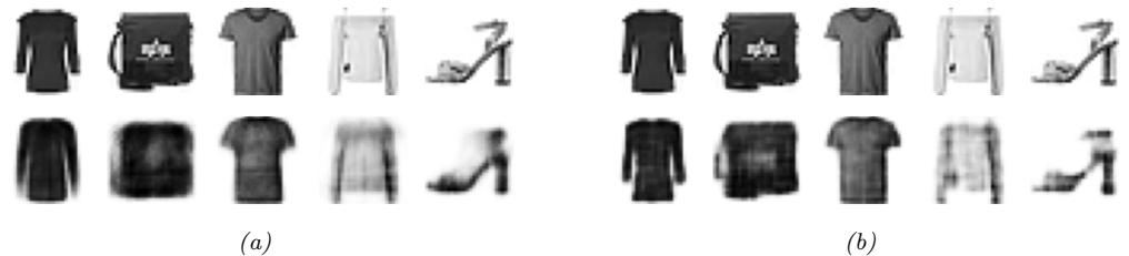
Figure 20.17: Results of applying an autoencoder to the Fashion MNIST data. Top row are first 5 images from validation set. Bottom row are reconstructions. (a) MLP model (trained for 20 epochs). The encoder is an MLP with architecture 784-100-30. The decoder is the mirror image of this. (b) CNN model (trained for 5 epochs). The encoder is a CNN model with architecture Conv2D(16, 3 ↑ 3, same, selu), MaxPool2D(2x2), Conv2D(32, 3 ↑ 3, same, selu), MaxPool2D(2 ↑ 2), Conv2D(64, 3 ↑ 3, same, selu), MaxPool2D(2 ↑ 2). The decoder is the mirror image of this, using transposed convolution and without the max pooling layers. Adapted from Figure 17.4 of [Gér19]. Generated by ae\_mnist\_tf.ipynb.
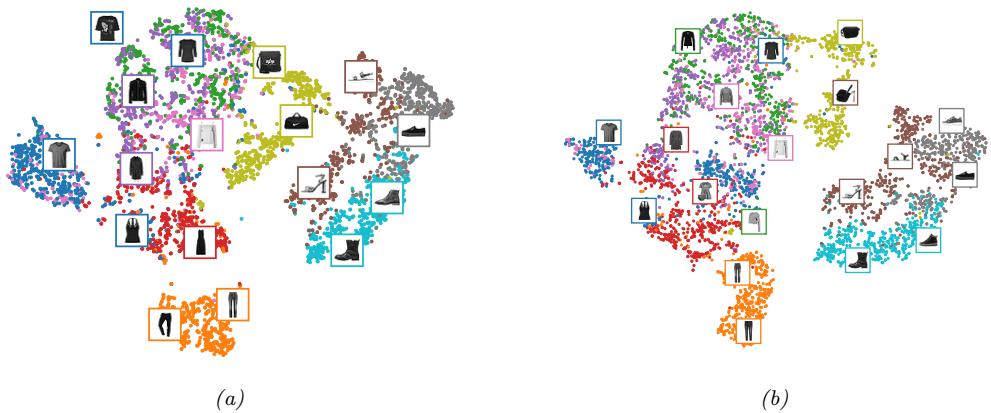
Figure 20.18: tSNE plot of the first 2 latent dimensions of the Fashion MNIST validation set using an autoencoder. (a) MLP. (b) CNN. Adapted from Figure 17.5 of [Gér19]. Generated by ae\_mnist\_tf.ipynb.
20.3.2 Denoising autoencoders
One useful way to control the capacity of an autoencoder is to add noise to its input, and then train the model to reconstruct a clean (uncorrupted) version of the original input. This is called a denoising autoencoder [Vin+10a].
We can implement this by adding Gaussian noise, or using Bernoulli dropout. Figure 20.19 shows some reconstructions of corrupted images computed using a DAE. We see that the model is able to “hallucinate” details that are missing in the input, since it has seen similar images before, and can store this information in the parameters of the model.
Suppose we train a DAE using Gaussian corruption and squared error reconstruction, i.e., we use pc(x˜|x) = N (x˜|x, ω2I) and ε(x, r(x˜)) = ||e||2 2, where e(x) = r(x˜)↗x is the residual error for example
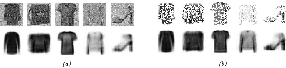
Figure 20.19: Denoising autoencoder (MLP architecture) applied to some noisy Fashion MNIST images from the validation set. (a) Gaussian noise. (b) Bernoulli dropout noise. Top row: input. Bottom row: output. Adapted from Figure 17.9 of [Gér19]. Generated by ae\_mnist\_tf.ipynb.
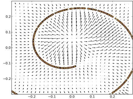
Figure 20.20: The residual error from a DAE, e(x) = r(x˜) ↔︎ x, can learn a vector field corresponding to the score function. Arrows point towards higher probability regions. The length of the arrow is proportional to ||e(x)||, so points near the 1d data manifold (represented by the curved line) have smaller arrows. From Figure 5 of [AB14]. Used with kind permission of Guillaume Alain.
x. Then one can show [AB14] the remarkable result that, as ω ≃ 0 (and with a su”ciently powerful model and enough data), the residuals approximate the score function, which is the log probability of the data, i.e., e(x) ′ ⇑x log p(x). That is, the DAE learns a vector field, corresponding to the gradient of the log data density. Thus points that are close to the data manifold will be projected onto it via the sampling process. See Figure 20.20 for an illustration.
20.3.3 Contractive autoencoders
A di!erent way to regularize autoencoders is by adding the penalty term
\[\Delta \Omega(\mathbf{z}, \mathbf{z}) = \lambda ||\frac{\partial f\_e(\mathbf{z})}{\partial \mathbf{z}}||\_F^2 = \lambda \sum\_k ||\nabla\_\mathbf{z} \ h\_k(\mathbf{z})||\_2^2 \tag{20.93}\]
to the reconstruction loss, where hk is the value of the k’th hidden embedding unit. That is, we penalize the Frobenius norm of the encoder’s Jacobian. This is called a contractive autoencoder
[Rif+11]. (A linear operator with Jacobian J is called a contraction if ||Jx|| ↙ 1 for all unit-norm inputs x.)
To understand why this is useful, consider Figure 20.20. We can approximate the curved lowdimensional manifold by a series of locally linear manifolds. These linear approximations can be computed using the Jacobian of the encoder at each point. By encouraging these to be contractive, we ensure the model “pushes” inputs that are o! the manifold to move back towards it.
Another way to think about CAEs is as follows. To minimize the penalty term, the model would like to ensure the encoder is a constant function. However, if it was completely constant, it would ignore its input, and hence incur high reconstruction cost. Thus the two terms together encourage the model to learn a representation where only a few units change in response to the most significant variations in the input.
One possible degenerate solution is that the encoder simply learns to multiply the input by a small constant , (which scales down the Jacobian), followed by a decoder that divides by , (which reconstructs perfectly). To avoid this, we can tie the weights of the encoder and decoder, by setting the weight matrix for layer ε of fd to be the transpose of the weight matrix for layer ε of fe, but using untied bias terms. Unfortunately CAEs are slow to train, because of the expense of computing the Jacobian.
20.3.4 Sparse autoencoders
Yet another way to regularize autoencoders is to add a sparsity penalty to the latent activations of the form $(z) = ς||z||1. (This is called activity regularization.)
An alternative way to implement sparsity, that often gives better results, is to use logistic units, and then to compute the expected fraction of time each unit k is on within a minibatch (call this qk), and ensure that this is close to a desired target value p, as proposed in [GBB11]. In particular, we use the regularizer $(z1:L,1:N ) = ς( k DKL (p ∀ qk) for latent dimensions 1 : L and examples 1 : N, where p = (p, 1 ↗ p) is the desired target distribution, and qk = (qk, 1 ↗ qk) is the empirical distribution for unit k, computed using qk = 1 N (N n=1 I(zn,k = 1).
Figure 20.21 shows the results when fitting an AE-MLP (with 300 hidden units) to Fashion MNIST. If we set ς = 0 (i.e., if we don’t impose a sparsity penalty), we see that the average activation value is about 0.4, with most neurons being partially activated most of the time. With the ε1 penalty, we see that most units are o! all the time, which means they are not being used at all. With the KL penalty, we see that about 70% of neurons are o! on average, but unlike the ε1 case, we don’t see units being permanently turned o! (the average activation level is 0.1). This latter kind of sparse firing pattern is similar to that observed in biological brains (see e.g., [Bey+19]).
20.3.5 Variational autoencoders
In this section, we discuss the variational autoencoder or VAE [KW14; RMW14; KW19a], which can be thought of as a probabilistic version of a deterministic autoencoder (Section 20.3) The principal advantage is that a VAE is a generative model that can create new samples, whereas an autoencoder just computes embeddings of input vectors.
We discuss VAEs in detail in the sequel to this book, [Mur23]. However, in brief, the VAE combines two key ideas. First we create a non-linear extension of the factor analysis generative model, i.e., we
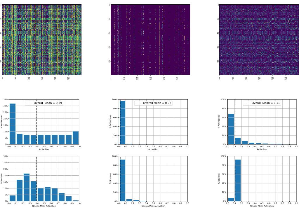
Figure 20.21: Neuron activity (in the bottleneck layer) for an autoencoder applied to Fashion MNIST. We show results for three models, with di!erent kinds of sparsity penalty: no penalty (left column), ε1 penalty (middle column), KL penalty (right column). Top row: Heatmap of 300 neuron activations (columns) across 100 examples (rows). Middle row: Histogram of activation levels derived from this heatmap. Bottom row: Histogram of the mean activation per neuron, averaged over all examples in the validation set. Adapted from Figure 17.11 of [Gér19]. Generated by ae\_mnist\_tf.ipynb.
replace p(x|z) = N (x|Wz, ω2I) with
\[p\_{\theta}(x|\mathbf{z}) = \mathcal{N}(x|f\_d(\mathbf{z};\theta), \sigma^2 \mathbf{I})\tag{20.94}\]
where fd is the decoder. For binary observations we should use a Bernoulli likelihood:
\[p(\mathbf{z}|\mathbf{z}, \boldsymbol{\theta}) = \prod\_{i=1}^{D} \text{Ber}(x\_i | f\_d(\mathbf{z}; \boldsymbol{\theta}), \sigma^2 \mathbf{I}) \tag{20.95}\]
Second, we create another model, q(z|x), called the recognition network or inference network, that is trained simultaneously with the generative model to do approximate posterior inference. If we assume the posterior is Gaussian, with diagonal covariance, we get
\[q\_{\phi}(\mathbf{z}|\mathbf{x}) = N(\mathbf{z}|f\_{e,\mu}(\mathbf{x};\phi), \text{diag}(f\_{e,\sigma}(\mathbf{z};\phi)))\tag{20.96}\]
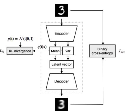
Figure 20.22: Schematic illustration of a VAE. From a figure from http: // krasserm. github. io/ 2018/ 07/ 27/ dfc-vae/ . Used with kind permission of Martin Krasser.
where fe is the encoder. See Figure 20.22 for a sketch.
The idea of training an inference network to “invert” a generative network, rather than running an optimization algorithm to infer the latent code, is called amortized inference. This idea was first proposed in the Helmholtz machine [Day+95]. However, that paper did not present a single unified objective function for inference and generation, but instead used the wake sleep method for training, which alternates between optimizing the generative model and inference model. By contrast, the VAE optimizes a variational lower bound on the log-likelihood, which is more principled, since it is a single unified objective.
20.3.5.1 Training VAEs
We cannot compute the exact marginal likelihood p(x|ε) needed for MLE training, because posterior inference in a nonlinear FA model is intractable. However, we can use the inference network to compute an approximate posterior, q(z|x). We can then use this to compute the evidence lower bound or ELBO. For a single example x, this is given by
\[\mathbb{E}(\theta, \phi | \mathbf{z}) = \mathbb{E}\_{q\_{\phi}(\mathbf{z}|\mathbf{z})} \left[ \log p\_{\theta}(\mathbf{z}, \mathbf{z}) - \log q\_{\phi}(\mathbf{z}|\mathbf{z}) \right] \tag{20.97}\]
\[\mathbf{E}\_{\mathbf{q}} = \mathbb{E}\_{\mathbf{q}(\mathbf{z}|\mathbf{z}, \boldsymbol{\phi})} \left[ \log p(\mathbf{z}|\mathbf{z}, \boldsymbol{\theta}) \right] - D\_{\text{KL}} \left( q(\mathbf{z}|\mathbf{z}, \boldsymbol{\phi}) \parallel p(\mathbf{z}) \right) \tag{20.98}\]
This can be interpreted as the expected log likelihood, plus a regularizer, that penalizes the posterior from deviating too much from the prior. (This is di!erent than the approach in Section 20.3.4, where we applied the KL penalty to the aggregate posterior in each minibatch.)
The ELBO is a lower bound of the log marginal likelihood (aka evidence), as can be seen from Jensen’s inequality:
\[\text{KL}(\theta, \phi | x) = \int q\_{\phi}(z | x) \log \frac{p\_{\theta}(x, z)}{q\_{\phi}(z | x)} dz \tag{20.99}\]
\[\leq \log \int q\_{\boldsymbol{\phi}}(\boldsymbol{z}|\boldsymbol{x}) \frac{p\_{\boldsymbol{\theta}}(\boldsymbol{x},\boldsymbol{z})}{q\_{\boldsymbol{\phi}}(\boldsymbol{z}|\boldsymbol{x})} d\boldsymbol{z} = \log p\_{\boldsymbol{\theta}}(\boldsymbol{x}) \tag{20.100}\]
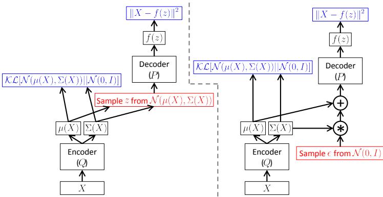
Figure 20.23: Computation graph for VAEs. where p(z) = N (z|0, I), p(x|z, ϑ) = N (x|f(z), ω2I), and q(z|x, ε) = N (z|µ(x), !(x)). Red boxes show sampling operations which are not di!erentiable. Blue boxes show loss layers (we assume Gaussian likelihoods and priors). (Left) Without the reparameterization trick. (Right) With the reparameterization trick. Gradients can flow from the output loss, back through the decoder and into the encoder. From Figure 4 of [Doe16]. Used with kind permission of Carl Doersch.
Thus for fixed inference network parameters ω, increasing the ELBO should increase the log likelihood of the data, similar to EM Section 8.7.2.
20.3.5.2 The reparameterization trick
In this section, we discuss how to compute the ELBO and its gradient. For simplicity, let us suppose that the inference network estimates the parameters of a Gaussian posterior. Since qφ(z|x) is Gaussian, we can write
\[\mathbf{z} = f\_{e,\mu}(x;\phi) + f\_{e,\sigma}(x;\phi) \odot \epsilon \tag{20.101}\]
where - ∝ N (0, I). Hence
\[\operatorname{KL}(\theta,\phi|x) = \mathbb{E}\_{\mathbf{e}\sim\mathcal{N}(\mathbf{0},\mathbf{I})} \left[ \log p\_{\theta}(x|\mathbf{z}=\mu\_{\phi}(x) + \sigma\_{\phi}(x)\odot\mathbf{e}) \right] - D\_{\text{KL}}\left(q\_{\phi}(z|x) \parallel p(z)\right) \tag{20.102}\]
Now the expectation is independent of the parameters of the model, so we can safely push gradients inside and use backpropagation for training in the usual way, by minimizing ↗Ex⇒D [$(ε, ω|x)] wrt ε and ω. This is known as the reparameterization trick. See Figure 20.23 for an illustration.
The first term in the ELBO can be approximated by sampling -, scaling it by the output of the inference network to get z, and then evaluating log p(x|z) using the decoder network.
The second term in the ELBO is the KL of two Gaussians, which has a closed form solution. In particular, inserting p(z) = N (z|0, I) and q(z) = N (z|µ, diag(ϱ)) into Equation (6.33), we get
\[D\_{\mathrm{KL}}(q \parallel p) = \sum\_{k=1}^{K} \left[ \log(\frac{1}{\sigma\_k}) + \frac{\sigma\_k^2 + (\mu\_k - 0)^2}{2 \cdot 1} - \frac{1}{2} \right] = -\frac{1}{2} \sum\_{k=1}^{K} \left[ \log \sigma\_k^2 - \sigma\_k^2 - \mu\_k^2 + 1 \right] \tag{20.103}\]
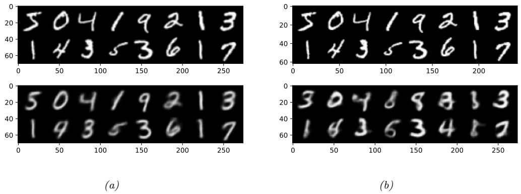
Figure 20.24: Reconstructing MNIST digits using a 20 dimensional latent space. Top row: input images. Bottom row: reconstructions. (a) VAE. Generated by vae\_mnist\_conv\_lightning.ipynb. (b) Deterministic AE. Generated by ae\_mnist\_conv.ipynb.
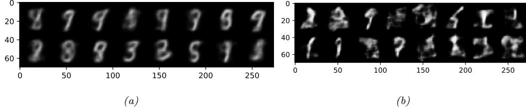
Figure 20.25: Sampling MNIST digits using a 20 dimensional latent space. (a) VAE. Generated by vae\_mnist\_conv\_lightning.ipynb. (b) Deterministic AE. Generated by ae\_mnist\_conv.ipynb.
20.3.5.3 Comparison of VAEs and autoencoders
VAEs are very similar to autoencoders. In particular, the generative model, pε(x|z), acts like the decoder, and the inference network, qφ(z|x), acts like the encoder. The reconstruction abilities of both models are similar, as can be seen by comparing Figure 20.24a with Figure 20.24b.
The primary advantage of the VAE is that it can be used to generate new data from random noise. In particular, we sample z from the Gaussian prior N (z|0, I), and then pass this through the decoder to get E [x|z] = fd(z; ε). The VAE’s decoder is trained to convert random points in the embedding space (generated by perturbing the input encodings) to sensible outputs. By contrast, the decoder for the deterministic autoencoder only ever gets as inputs the exact encodings of the training set, so it does not know what to do with random inputs that are outside what it was trained on. So a standard autoencoder cannot create new samples. This di!erence can be seen by comparing Figure 20.25a with Figure 20.25b.
The reason the VAE is better at sample is that it embeds images into Gaussians in latent space, whereas the AE embeds images into points, which are like delta functions. The advantage of using a
Figure 20.26: tSNE projection of a 20 dimensional latent space. (a) VAE. Generated by vae\_mnist\_conv\_lightning.ipynb. (b) Deterministic AE. Generated by ae\_mnist\_conv.ipynb.
Figure 20.27: Linear interpolation between the left and right images in a 20 dimensional latent space. (a) VAE. (b) Deterministic AE. Generated by vae\_mnist\_conv\_lightning.ipynb.
latent distribution is that it encourages local smoothness, since a given image may map to multiple nearby places, depending on the stochastic sampling. By contrast, in an AE, the latent space is typically not smooth, so images from di!erent classes often end up next to each other. This di!erence can be seen by comparing Figure 20.26a with Figure 20.26b.
We can leverage the smoothness of the latent space to perform image interpolation. Rather than working in pixel space, we can work in the latent space of the model. Specifically, let x1 and x2 be two images, and let z1 = Eq(z|x1) [z] and z2 = Eq(z|x2) [z] be their encodings. We can now generate new images that interpolate between these two anchors by computing z = ςz1 + (1 ↗ ς)z2, where 0 ↙ ς ↙ 1, and then decoding by computing E [x|z]. This is called latent space interpolation. (The justification for taking a linear interpolation is that the learned manifold has approximately zero curvature, as shown in [SKTF18].) A VAE is more useful for latent space interpolation than an AE because its latent space is smoother, and because the model can generate from almost any point in latent space. This di!erence can be seen by comparing Figure 20.27a with Figure 20.27b.
Figure 20.28: Illustration of the tangent space and tangent vectors at two di!erent points on a 2d curved manifold. From Figure 1 of [Bro+17a]. Used with kind permission of Michael Bronstein.
20.4 Manifold learning *
In this section, we discuss the problem of recovering the underlying low-dimensional structure in a high-dimensional dataset. This structure is often assumed to be a curved manifold (explained in Section 20.4.1), so this problem is called manifold learning or nonlinear dimensionality reduction. The key di!erence from methods such as autoencoders (Section 20.3) is that we will focus on non-parametric methods, in which we compute an embedding for each point in the training set, as opposed to learning a generic model that can embed any input vector. That is, the methods we discuss do not (easily) support out-of-sample generalization. However, they can be easier to fit, and are quite flexible. Such methods can be a useful for unsupervised learning (knowledge discovery), data visualization, and as a preprocessing step for supervised learning. See [AAB21] for a recent review of this field.
20.4.1 What are manifolds?
Roughly speaking, a manifold is a topological space which is locally Euclidean. One of the simplest examples is the surface of the earth, which is a curved 2d surface embedded in a 3d space. At each local point on the surface, the earth seems flat.
More formally, a d-dimensional manifold X is a space in which each point x → X has a neighborhood which is topologically equivalent to a d-dimensional Euclidean space, called the tangent space, denoted Tx = TxX . This is illustrated in Figure 20.28.
A Riemannian manifold is a di!erentiable manifold that associates an inner product operator at each point x in tangent space; this is assumed to depend smoothly on the position x. The inner product induces a notion of distance, angles, and volume. The collection of these inner products is called a Riemannian metric. It can be shown that any su”ciently smooth Riemannian manifold can be embedded into a Euclidean space of potentially higher dimension; the Riemannian inner product at a point then becomes Euclidean inner product in that tangent space.
20.4.2 The manifold hypothesis
Most “naturally occuring” high dimensional dataset lie a low dimensional manifold. This is called the manifold hypothesis [FMN16]. For example, consider the case of an image. Figure 20.29a shows a
Figure 20.29: Illustration of the image manifold. (a) An image of the digit 6 from the USPS dataset, of size 64 ↑ 57 = 3, 648. (b) A random sample from the space {0, 1}3648 reshaped as an image. (c) A dataset created by rotating the original image by one degree 360 times. We project this data onto its first two principal components, to reveal the underlying 2d circular manifold. From Figure 1 of [Law12]. Used with kind permission of Neil Lawrence.
single image of size 64 ↑ 57. This is a vector in a 3,648-dimensional space, where each dimension corresponds to a pixel intensity. Suppose we try to generate an image by drawing a random point in this space; it is unlikely to look like the image of a digit, as shown in Figure 20.29b. However, the pixels are not independent of each other, since they are generated by some lower dimensional structure, namely the shape of the digit 6.
As we vary the shape, we will generate di!erent images. We can often characterize the space of shape variations using a low-dimensional manifold. This is illustrated in Figure 20.29c, where we apply PCA (Section 20.1) to project a dataset of 360 images, each one a slightly rotated version of the digit 6, into a 2d space. We see that most of the variation in the data is captured by an underlying curved 2d manifold. We say that the intrinsic dimensionality d of the data is 2, even though the ambient dimensionality D is 3,648.
20.4.3 Approaches to manifold learning
In the rest of this section, we discuss ways to learn manifolds from data. There are many di!erent algorithms that have been proposed, which make di!erent assumptions about the nature of the manifold, and which have di!erent computational properties. We discuss a few of these methods in the following sections. For more details, see e.g., [Bur10].
The methods can be categorized as shown in Table 20.1. The term “nonparametric” refers to methods that learn a low dimensional embedding zi for each datapoint xi, but do not learn a mapping function which can be applied to an out-of-sample datapoint. (However, [Ben+04b] discusses how to extend many of these methods beyond the training set by learning a kernel.)
In the sections below, we compare some of these methods using 2 di!erent datasets: a set of 1000 3d-points sampled from the 2d “Swiss roll” manifold, and a set of 1797 64-dimensional points sampled from the UCI digits dataset. See Figure 20.30 for an illustration of the data. We will learn a 2d manifold, so we can visualize the data.
| Method | Parametric | Convex | Section |
|---|---|---|---|
| PCA / classical MDS |
N | Y (Dense) |
Section 20.1 |
| Kernel PCA |
N | Y (Dense) |
Section 20.4.6 |
| Isomap | N | Y (Dense) |
Section 20.4.5 |
| LLE | N | Y (Sparse) |
Section 20.4.8 |
| Laplacian Eigenmaps |
N | Y (Sparse) |
Section 20.4.9 |
| tSNE | N | N | Section 20.4.10 |
| Autoencoder | Y | N | Section 20.3 |
Table 20.1: A list of some approaches to dimensionality reduction. If a method is convex, we specify in parentheses whether it requires solving a sparse or dense eigenvalue problem.
Figure 20.30: Illustration of some data generated from low-dimensional manifolds. (a) The 2d Swiss-roll manifold embedded into 3d. Generated by manifold\_swiss\_sklearn.ipynb. (b) Sample of some UCI digits, which have size 8 ↑ 8 = 64. Generated by manifold\_digits\_sklearn.ipynb.
20.4.4 Multi-dimensional scaling (MDS)
The simplest approach to manifold learning is multidimensional scaling (MDS). This tries to find a set of low dimensional vectors {zi → RL : i =1: N} such that the pairwise distances between these vectors is as similar as possible to a set of pairwise dissimilarities D = {dij} provided by the user. There are several variants of MDS, one of which turns out to be equivalent to PCA, as we discuss below.
20.4.4.1 Classical MDS
Suppose we start an N ↑ D data matrix X with rows xi. Let us define the centered Gram (similarity) matrix as follows:
\[ \tilde{K}\_{ij} = \langle \mathbf{x}\_i - \overline{\mathbf{x}}, \mathbf{x}\_j - \overline{\mathbf{x}} \rangle \tag{20.104} \]
In matrix notation, we have K˜ = X˜ X˜ T, where X˜ = CN X and CN = IN ↗ 1 N 1N 1T N is the centering matrix.
Now define the strain of a set of embeddings as follows:
\[\mathcal{L}\_{\text{strain}}(\mathbf{Z}) = \sum\_{i,j} (\tilde{K}\_{ij} - \langle \tilde{\mathbf{z}}\_i, \tilde{\mathbf{z}}\_j \rangle)^2 = ||\tilde{\mathbf{K}} - \tilde{\mathbf{Z}}\tilde{\mathbf{Z}}^\top||\_F^2 \tag{20.105}\]
where z˜i = zi ↗ z is the centered embedding vector. Intuitively this measures how well similarities in the high-dimensional data space, K˜ij , are matched by similarities in the low-dimensional embedding space, ∃z˜i, z˜j ¬. Minimizing this loss is called classical MDS.
We know from Section 7.5 that the best rank L approximation to a matrix is its truncated SVD representation, K˜ = USVT. Since K˜ is positive semi definite, we have that V = U. Hence the optimal embedding satisfies
\[\mathbf{^j\bar{Z}\bar{Z}^\mathsf{T} = U\mathbf{S}U^\mathsf{T} = (\mathbf{U}\mathbf{S}^\frac{1}{2})(\mathbf{S}^\frac{1}{2}\mathbf{U}^\mathsf{T})}\tag{20.106}\]
Thus we can set the embedding vectors to be the rows of Z˜ = US 1 2 .
Now we describe how to apply classical MDS to a dataset where we just have Euclidean distances, rather than raw features. First we compute a matrix of squared Euclidean distances, D(2) = D ̸ D, which has the following entries:
\[D\_{ij}^{(2)} = ||\mathbf{x}\_i - \mathbf{x}\_j||^2 = ||\mathbf{x}\_i - \overline{\mathbf{x}}||^2 + ||\mathbf{x}\_j - \overline{\mathbf{x}}||^2 - 2\langle \mathbf{x}\_i - \overline{\mathbf{x}}, \mathbf{x}\_j - \overline{\mathbf{x}} \rangle \tag{20.107}\]
\[\dot{\mathbf{x}} = ||\mathbf{x}\_i - \overline{\mathbf{x}}||^2 + ||\mathbf{x}\_j - \overline{\mathbf{x}}||^2 - 2\tilde{K}\_{ij} \tag{20.108}\]
We see that D(2) only di!ers from K˜ by some row and column constants (and a factor of -2). Hence we can compute K˜ by double centering D(2) using Equation (7.89) to get K˜ = ↗1 2CN D(2)CN . In other words,
\[\tilde{K}\_{ij} = -\frac{1}{2} \left( d\_{ij}^2 - \frac{1}{N} \sum\_{l=1}^{N} d\_{il}^2 - \frac{1}{N} \sum\_{l=1}^{N} d\_{jl}^2 + \frac{1}{N^2} \sum\_{l=1}^{N} \sum\_{m=1}^{N} d\_{lm}^2 \right) \tag{20.109}\]
We can then compute the embeddings as before.
It turns out that classical MDS is equivalent to PCA (Section 20.1). To see this, let K˜ = ULSLUT L be the rank L truncated SVD of the centered kernel matrix. The MDS embedding is given by ZMDS = ULS 1 2 L. Now consider the rank L SVD of the centered data matrix, X˜ = UXSXVT X. The PCA embedding is ZPCA = UXSX. Now
\[\hat{\mathbf{K}} = \hat{\mathbf{X}}\hat{\mathbf{X}}^{\mathsf{T}} = \mathbf{U}\_{X}\mathbf{S}\_{X}\mathbf{V}\_{X}^{\mathsf{T}}\mathbf{V}\_{X}\mathbf{S}\_{X}\mathbf{U}\_{X}^{\mathsf{T}} = \mathbf{U}\_{X}\mathbf{S}\_{X}^{2}\mathbf{U}\_{X}^{\mathsf{T}} = \mathbf{U}\_{L}\mathbf{S}\_{L}\mathbf{U}\_{L}^{\mathsf{T}} \tag{20.110}\]
Hence UX = UL and SX = S2 L, and so ZPCA = ZMDS.
20.4.4.2 Metric MDS
Classical MDS assumes Euclidean distances. We can generalize it to allow for any dissimilarity measure by defining the stress function
\[\mathcal{L}\_{\text{stress}}(\mathbf{Z}) = \sqrt{\frac{\sum\_{i\]
Figure 20.31: Metric MDS applied to (a) Swiss roll. Generated by manifold\_swiss\_sklearn.ipynb. (b) UCI digits. Generated by manifold\_digits\_sklearn.ipynb.
where ˆ dij = ||zi ↗ zj ||. This is called metric MDS. Note that this is a di!erent objective than the one used by classical MDS, so even if dij are Euclidean distances, the results will be di!erent.
We can use gradient descent to solve the optimization problem. However, it is better to use a bound optimization algorithm (Section 8.7) called SMACOF [Lee77], which stands for “Scaling by MAjorizing a COmplication Function”. (This is the method implemented in scikit-learn.) See Figure 20.31 for the results of applying this to our running example.
20.4.4.3 Non-metric MDS
Instead of trying to match the distance between points, we can instead just try to match the ranking of how similar points are. To do this, let f(d) be a monotonic transformation from distances to ranks. Now define the loss
\[\mathcal{L}\_{\rm NM}(\mathbf{Z}) = \sqrt{\frac{\sum\_{i\]
where ˆ dij = ||zi ↗ zj ||. (Note the ˆ d2 ij in the denominator, not d2 ij .) Minimizing this is known as non-metric MDS.
This objective can be optimized iteratively. First the function f is optimized, for a given Z, using isotonic regression; this finds the optimal monotonic transformation of the input distances to match the current embedding distances. Then the embeddings Z are optimized, for a given f, using gradient descent, and the process repeats.
20.4.4.4 Sammon mapping
Metric MDS tries to minimize the sum of squared distances, so it puts the most emphasis on large distances. However, for many embedding methods, small distances matter more, since they capture local structure. One way to capture this is to divide each term of the loss by dij , so small distances
Figure 20.32: (a) If we measure distances along the manifold, we find d(1, 6) > d(1, 4), whereas if we measure in ambient space, we find d(1, 6) < d(1, 4). The plot at the bottom shows the underlying 1d manifold. (b) The K-nearest neighbors graph for some datapoints; the red path is the shortest distance between A and B on this graph. From [Hin13]. Used with kind permission of Geo! Hinton.
get upweighted:
\[\mathcal{L}\_{\text{sammon}}(\mathbf{Z}) = \left(\frac{1}{\sum\_{i\]
(Note the dij in the denominator, not d2 ij .) Minimizing this results in a Sammon mapping. (The coe”cient in front of the sum is just to simplify the gradient of the loss.) Unfortunately this is a non-convex objective, and it arguably puts too much emphasis on getting very small distances exactly right. We will discuss better methods for capturing local structure later on.
20.4.5 Isomap
If the high-dimensional data lies on or near a curved manifold, such as the Swiss roll example, then MDS might consider two points to be close even if their distance along the manifold is large. This is illustrated in Figure 20.32a.
One way to capture this is to create the K-nearest neighbor graph between datapoints5, and then approximate the manifold distance between a pair of points by the shortest distance along this graph; this can be computed e”ciently using Dijkstra’s shortest path algorithm. See Figure 20.32b for an illustration. Once we have computed this new distance metric, we can apply classical MDS (i.e., PCA). This is a way to capture local structure while avoiding local optima. The overall method is called isomap [TSL00].
See Figure 20.33 for the results of this method on our running example. We see that they are quite reasonable. However, if the data is noisy, there can be “false” edges in the nearest neighbor graph, which can result in “short circuits” which significantly distort the embedding, as shown in Figure 20.34. This problem is known as “topological instability” [BS02]. Choosing a very small neighborhood does not solve this problem, since this can fragment the manifold into a large number of disconnected regions. Various other solutions have been proposed, e.g., [CC07].
5. In scikit-learn, you can use the function sklearn.neighbors.kneighbors_graph.
Figure 20.33: Isomap applied to (a) Swiss roll. Generated by manifold\_swiss\_sklearn.ipynb. (b) UCI digits. Generated by manifold\_digits\_sklearn.ipynb.
Figure 20.34: (a) Noisy version of Swiss roll data. We perturb each point by adding N (0, 0.52) noise. (b) Results of Isomap applied to this data. Generated by manifold\_swiss\_sklearn.ipynb.
20.4.6 Kernel PCA
PCA (and classical MDS) finds the best linear projection of the data, so as to preserve pairwise similarities between all the points. In this section, we consider nonlinear projections. The key idea is to solve PCA by finding the eigenvectors of the inner product (Gram) matrix K = XXT, as in Section 20.1.3.2, and then to use the kernel trick (Section 17.3.4), which lets us replace inner products such as xT i xj with a kernel function, Kij = K(xi, xk). This is known as kernel PCA [SSM98].
Recall from Mercer’s theorem that the use of a kernel implies some underlying feature space, so we are implicitly replacing xi with ω(xi) = ωi. Let # be the corresponding (notional) design matrix, and K = XXT be the Gram matrix. Finally, let S⇀ = 1 N ( i ωiωT i be the covariance matrix in feature space. (We are assuming for now the features are centered.) From Equation (20.22), the normalized eigenvectors of S are given by VkPCA = #TU!→ 1 2 , where U and ! contain the eigenvectors and eigenvalues of K. Of course, we can’t actually compute VkPCA, since ωi is potentially infinite dimensional. However, we can compute the projection of a test vector x≃ onto the feature space as
Figure 20.35: Visualization of the first 8 kernel principal component basis functions derived from some 2d data. We use an RBF kernel with ω2 = 0.1. Generated by kpcaScholkopf.ipynb.
follows:
\[ \phi\_\*^{\mathsf{T}} \mathbf{V}\_{\mathrm{kPCA}} = \phi\_\*^{\mathsf{T}} \Phi^{\mathsf{T}} \mathbf{U} \Lambda^{-\frac{1}{2}} = k\_\*^{\mathsf{T}} \mathbf{U} \Lambda^{-\frac{1}{2}} \tag{20.114} \]
where k≃ = [K(x≃, x1),…, K(x≃, xN )].
There is one final detail to worry about. The covariance matrix is only given by S = #T# if the features is zero-mean. Thus we can only use the Gram matrix K = ##T if E [ωi] = 0. Unfortunately, we cannot simply subtract o! the mean in feature space, since it may be infinite dimensional. However, there is a trick we can use. Define the centered feature vector as ω˜i = ω(xi) ↗ 1 N (N j=1 ω(xj ). The Gram matrix of the centered feature vectors is given by K˜ij = ω˜T i ω˜j . Using the double centering trick from Equation (7.89), we can write this in matrix form as K˜ = CN KCN , where CN ↫ IN ↗ 1 N 1N 1T N is the centering matrix.
If we apply kPCA with a linear kernel, we recover regular PCA (classical MDS). This is limited to using L ↙ D embedding dimensions. If we use a non-degenerate kernel, we can use up to N components, since the size of # is N ↑ D≃, where D≃ is the (potentially infinite) dimensionality of embedded feature vectors. Figure 20.35 gives an example of the method applied to some D = 2 dimensional data using an RBF kernel. We project points in the unit grid onto the first 8 components and visualize the corresponding surfaces using a contour plot. We see that the first two components separate the three clusters, and the following components split the clusters.
See Figure 20.36 for some the results on kPCA (with an RBF kernel) on our running example. In this case, the results are arguably not very useful. In fact, it can be shown that kPCA with an RBF kernel expands the feature space instead of reducing it [WSS04], as we saw in Figure 20.35, which
Figure 20.36: Kernel PCA applied to (a) Swiss roll. Generated by manifold\_swiss\_sklearn.ipynb. (b) UCI digits. Generated by manifold\_digits\_sklearn.ipynb.
makes it not very useful as a method for dimensionality reduction. We discuss a solution to this in Section 20.4.7.
20.4.7 Maximum variance unfolding (MVU)
kPCA with certain kernels, such as RBF, might not result in a low dimensional embedding, as discussed in Section 20.4.6. This observation led to the development of the semidefinite embedding algorithm [WSS04], also called maximum variance unfolding, which tries to learn an embedding {zi} such that
\[\max \sum\_{ij} ||\mathbf{z}\_i - \mathbf{z}\_j||\_2^2 \text{ s.t. } ||\mathbf{z}\_i - \mathbf{z}\_j||\_2^2 = ||\mathbf{z}\_i - \mathbf{z}\_j||\_2^2 \text{ for all } (i, j) \in G \tag{20.115}\]
where G is the nearest neighbor graph (as in Isomap). This approach explicitly tries to ‘unfold’ the data manifold while respecting the nearest neighbor constraints.
This can be reformulated as a semidefinite programming (SDP) problem by defining the kernel matrix K = ZZT and then optimizing
\[\max \text{tr}(\mathbf{K}) \quad \text{s.t.} \quad ||\mathbf{z}\_i - \mathbf{z}\_j||\_2^2 = ||\mathbf{x}\_i - \mathbf{x}\_j||\_2^2, \sum\_{ij} K\_{ij} = 0, \ \mathbf{K} \succ 0 \tag{20.116}\]
The resulting kernel is then passed to kPCA, and the resulting eigenvectors give the low dimensional embedding.
20.4.8 Local linear embedding (LLE)
The techniques we have discussed so far all rely on an eigendecomposition of a full matrix of pairwise similarities, either in the ambient space (PCA), in feature space (kPCA), or along the KNN graph (Isomap). In this section, we discuss local linear embedding (LLE) [RS00], a technique that solves a sparse eigenproblem, thus focusing more on local structure in the data.
Figure 20.37: LLE applied to (a) Swiss roll. Generated by manifold\_swiss\_sklearn.ipynb. (b) UCI digits. Generated by manifold\_digits\_sklearn.ipynb.
LLE assumes the data manifold around each point xi is locally linear. The best linear approximation can be found by predicting xi as a linear combination of its K nearest neighbors using reconstruction weights wi. This can be found by solving
\[\hat{\mathbf{W}} = \min\_{\mathbf{W}} \sum\_{i=1}^{N} (\mathbf{x}\_i - \sum\_{j=1}^{N} w\_{ij} \mathbf{x}\_j)^2 \tag{20.117}\]
\[\text{subject to} \begin{cases} w\_{ij} = 0 & \text{if } \mathbf{z}\_j \notin \text{nbr}(\mathbf{z}\_i, K) \\ \sum\_{j=1}^{N} w\_{ij} = 1 & \text{for } i = 1:N \end{cases} \tag{20.118}\]
Note that we need the sum-to-one constraint on the weights to prevent the trivial solution W = 0. The resulting vector of weights wi,: constitute the barycentric coordinates of xi.
Any linear mapping of this hyperplane to a lower dimensional space preserves the reconstruction weights, and thus the local geometry. Thus we can solve for the low-dimensional embeddings for each point by solving
\[\hat{\mathbf{Z}} = \underset{\mathbf{Z}}{\text{argmin}} \sum\_{i} ||\mathbf{z}\_{i} - \sum\_{j=1}^{N} \hat{w}\_{ij} \mathbf{z}\_{j}||\_{2}^{2} \tag{20.119}\]
where wˆij = 0 if j is not one of the K nearest neighbors of i. We can rewrite this loss as
\[\mathcal{L}(\mathbf{Z}) = ||\mathbf{Z} - \mathbf{W}\mathbf{Z}||^2 = \mathbf{Z}^\mathsf{T}(\mathbf{I} - \mathbf{W})^\mathsf{T}(\mathbf{I} - \mathbf{W})\mathbf{Z} \tag{20.120}\]
Thus the solution is given by the eigenvectors of (I ↗ W) T(I ↗ W) corresponding to the smallest nonzero eigenvalues, as shown in Section 7.4.8.
See Figure 20.37 for some the results on LLE on our running example. In this case, the results do not seem as good as those produced by Isomap. However, the method tends to be somewhat less sensitive to short-circuiting (noise).
Figure 20.38: Laplacian eigenmaps applied to (a) Swiss roll. Generated by manifold\_swiss\_sklearn.ipynb. (b) UCI digits. Generated by manifold\_digits\_sklearn.ipynb.
20.4.9 Laplacian eigenmaps
In this section, we describe Laplacian eigenmaps or spectral embedding [BN01]. The idea is to compute a low-dimensional representation of the data in which the weighted distances between a datapoint and its K nearest neighbors are minimized. We put more weight on the first nearest neighbor than the second, etc. We give the details below.
20.4.9.1 Using eigenvectors of the graph Laplacian to compute embeddings
We want to find embeddings which minimize
\[\mathcal{L}(\mathbf{Z}) = \sum\_{(i,j)\in E} W\_{i,j} ||\mathbf{z}\_i - \mathbf{z}\_j||\_2^2 \tag{20.121}\]
where Wij = exp(↗ 1 2ε2 ||xi ↗ xj ||2 2) if i ↗ j are neighbors in the KNN graph and 0 otherwise. We add the constraint ZTDZ = I to avoid the degenerate solution where Z = 0, where D is the diagonal weight matrix storing the degree of each node, Dii = ( j Wi,j .
We can rewrite the above objective as follows:
\[\mathcal{L}(\mathbf{Z}) = \sum\_{ij} W\_{ij} (||\mathbf{z}\_i||^2 + ||\mathbf{z}\_j||^2 - 2\mathbf{z}\_i^\mathsf{T}\mathbf{z}\_j) \tag{20.122}\]
\[I = \sum\_{i} D\_{ii} ||\mathbf{z}\_{i}||^{2} + \sum\_{j} D\_{jj} ||\mathbf{z}\_{j}||^{2} - 2 \sum\_{ij} W\_{ij} \mathbf{z}\_{i} \mathbf{z}\_{j}^{\mathsf{T}} \tag{20.123}\]
\[=2\text{tr}(\mathbf{Z}^{\mathsf{T}}\mathbf{D}\mathbf{Z}) - 2\text{tr}(\mathbf{Z}^{\mathsf{T}}\mathbf{W}\mathbf{Z}) = 2\text{tr}(\mathbf{Z}^{\mathsf{T}}\mathbf{L}\mathbf{Z})\tag{20.124}\]
where L = D ↗ W is the graph Laplacian (see Section 20.4.9.2). One can show that minimizing this is equivalent to solving the (generalized) eigenvalue problem Lzi = ςiDzi for the L smallest nonzero eigenvalues.
See Figure 20.38 for the results of applying this method (with an RBF kernel) to our running example.
| Labelled graph | Degree matrix | Adjacency matrix | Laplacian matrix | ||||||||||||||
|---|---|---|---|---|---|---|---|---|---|---|---|---|---|---|---|---|---|
| O | 2 0 0 3 |
0 0 0 0 2 0 0 3 0 0 0 0 |
0 0 0 0 3 |
0 0 0 0 0 |
0 1 0 0 0 |
1 0 0 0 0 0 |
0 0 0 |
0 11 0 |
1 0 1 0 0 0 |
0 0 0 0 |
2 - 0 0 0 |
- 1 I |
0 2 0 0 0 |
0 l |
l 3 |
0 0 0 - |
Figure 20.39: Illustration of the Laplacian matrix derived from an undirected graph. From https: // en. wikipedia. org/ wiki/ Laplacian\_ matrix . Used with kind permission of Wikipedia author AzaToth.
Figure 20.40: Illustration of a (positive) function defined on a graph. From Figure 1 of [Shu+13]. Used with kind permission of Pascal Frossard.
20.4.9.2 What is the graph Laplacian?
We saw above that we can compute the eigenvectors of the graph Laplacian in order to learn a good embedding of the high dimensional points. In this section, we give some intuition as to why this works.
Let W be a symmetric weight matrix for a graph, where Wij = Wji ↓ 0. Let D = diag(di) be a diagonal matrix containing the weighted degree of each node, di = ( j wij . We define the graph Laplacian as follows:
\[\mathbf{L} \triangleq \mathbf{D} - \mathbf{W} \tag{20.125}\]
Thus the elements of L are given by
\[L\_{ij} = \begin{cases} d\_i & \text{if } i = j \\ -w\_{ij} & \text{if } i \neq j \text{ and } w\_{ij} \neq 0 \\ 0 & \text{otherwise} \end{cases} \tag{20.126}\]
See Figure 20.39 for an example of how to compute this.
Suppose we associate a value fi → R with each node i in the graph (see Figure 20.40 for example). Then we can use the graph Laplacian as a di!erence operator, to compute a discrete derivative of
the function at a point:
\[(\mathbf{L}f)(i) = \sum\_{j \in \text{nbr}\_i} W\_{ij} [f(i) - f(j)] \tag{20.127}\]
where nbri is the set of neighbors of node i. We can also compute an overall measure of “smoothness” of the function f by computing its Dirichlet energy as follows:
\[f^T \mathbf{L}f = f^T \mathbf{D}f - f^T \mathbf{W}f = \sum\_i d\_i f\_i^2 - \sum\_{i,j} f\_i f\_j w\_{ij} \tag{20.128}\]
\[\mathcal{L} = \frac{1}{2} \left( \sum\_{i} d\_i f\_i^2 - 2 \sum\_{i,j} f\_i f\_j w\_{ij} + \sum\_j d\_j f\_j^2 \right) = \frac{1}{2} \sum\_{i,j} w\_{ij} (f\_i - f\_j)^2 \tag{20.129}\]
By studying the eigenvalues and eigenvectors of the Laplacian matrix, we can determine various useful properties of the function. (Applying linear algebra to study the adjacency matrix of a graph, or related matrices, is called spectral graph theory [Chu97].) For example, we see that L is symmetric and positive semi-definite, since we have fTLf ↓ 0 for all f → RN , which follows from Equation (20.129) due to the assumption that wij ↓ 0. Consequently L has N non-negative, real-valued eigenvalues, 0 ↙ ς1 ↙ ς2 ↙ … ↙ ςN . The corresponding eigenvectors form an orthogonal basis for the function f defined on the graph, in order of decreasing smoothness.
In Section 20.4.9.1, we discuss Laplacian eigenmaps, which is a way to learn low dimensional embeddings for high dimensional data vectors. The approach is to let zid = f d i be the d’th embedding dimension for input i, and then to find a basis for these functions (i.e., embedding of the points) that varies smoothly over the graph, thus respecting distance of the points in ambient space.
There are many other applications of the graph Laplacian in ML. For example, in Section 21.5.1, we discuss normalized cuts, which is a way to learn a clustering of high dimensional data vectors based on pairwise similarity; and [WTN19] discusses how to use the eigenvectors of the state transition matrix to learn representations for RL.
20.4.10 t-SNE
In this section, we describe a very popular nonconvex technique for learning low dimensional embeddings called t-SNE [MH08]. This extends the earlier stochastic neighbor embedding method of [HR03], so we first describe SNE, before describing the t-SNE extension.
20.4.10.1 Stochastic neighborhood embedding (SNE)
The basic idea in SNE is to convert high-dimensional Euclidean distances into conditional probabilities that represent similarities. More precisely, we define pj|i to be the probability that point i would pick point j as its neighbor if neighbors were picked in proportion to their probability under a Gaussian centered at xi:
\[p\_{j|i} = \frac{\exp(-\frac{1}{2\sigma\_i^2}||x\_i - x\_j||^2)}{\sum\_{k \neq i} \exp(-\frac{1}{2\sigma\_i^2}||x\_i - x\_k||^2)}\tag{20.130}\]
Here ω2 i is the variance for data point i, which can be used to “magnify” the scale of points in dense regions of input space, and diminish the scale in sparser regions. (We discuss how to estimate the length scales ω2 i shortly).
Let zi be the low dimensional embedding representing xi. We define similarities in the low dimensional space in an analogous way:
\[q\_{j|i} = \frac{\exp(-||\mathbf{z}\_i - \mathbf{z}\_j||^2)}{\sum\_{k \neq i} \exp(-||\mathbf{z}\_i - \mathbf{z}\_k||^2)}\tag{20.131}\]
In this case, the variance is fixed to a constant; changing it would just rescale the learned map, and not change its topology.
If the embedding is a good one, then qj|i should match pj|i. Therefore, SNE defines the objective to be
\[\mathcal{L} = \sum\_{i} D\_{\text{KL}}(P\_i \parallel Q\_i) = \sum\_{i} \sum\_{j} p\_{j|i} \log \frac{p\_{j|i}}{q\_{j|i}} \tag{20.132}\]
where Pi is the conditional distribution over all other data points given xi, Qi is the conditional distribution over all other latent points given zi, and DKL (Pi ∀ Qi) is the KL divergence (Section 6.2) between the distributions.
Note that this is an asymmetric objective. In particular, there is a large cost if a small qj|i is used to model a large pj|i. This objective will prefer to pull distant points together rather than push nearby points apart. We can get a better idea of the geometry by looking at the gradient for each embedding vector, which is given by
\[\nabla\_{\mathbf{z}\_i} \mathcal{L}(\mathbf{Z}) = 2 \sum\_{j} (\mathbf{z}\_i - \mathbf{z}\_j)(p\_{j|i} - q\_{j|i} + p\_{i|j} - q\_{i|j}) \tag{20.133}\]
Thus points are pulled towards each other if the p’s are bigger than the q’s, and repelled if the q’s are bigger than the p’s.
Although this is an intuitively sensible objective, it is not convex. Nevertheless it can be minimized using SGD. In practice, it helps to add Gaussian noise to the embedding points, and to gradually anneal the amount of noise. [Hin13] recommends to “spend a long time at the noise level at which the global structure starts to form from the hot plasma of map points” before reducing it.6
20.4.10.2 Symmetric SNE
There is a slightly simpler version of SNE that minimizes a single KL between the joint distribution P in high dimensional space and Q in low dimensional space:
\[\mathcal{L} = D\_{\text{KL}}\left(P \parallel Q\right) = \sum\_{i\]
This is called symmetric SNE.
6. See [Ros98; WF20] for a discussion of annealing and phase transitions in unsupervised learning. See also [CP10] for a discussion of the elastic embedding algorithm, which uses a homotopy method to more e”ciently optimize a model that is related to both SNE and Laplacian eigenmaps.
The obvious way to define pij is to use
\[p\_{ij} = \frac{\exp\left(-\frac{1}{2\sigma^2}||x\_i - x\_j||^2\right)}{\sum\_{k \neq l} \exp\left(-\frac{1}{2\sigma^2}||x\_k - x\_l||^2\right)}\tag{20.135}\]
We can define qij similarily.
The corresponding gradient becomes
\[\nabla\_{\mathbf{z}\_i} \mathcal{L}(\mathbf{Z}) = 4 \sum\_{j} (\mathbf{z}\_i - \mathbf{z}\_j)(p\_{ij} - q\_{ij}) \tag{20.136}\]
As before, points are pulled towards each other if the p’s are bigger than the q’s, and repelled if the q’s are bigger than the p’s.
Although symmetric SNE is slightly easier to implement, it loses the nice property of regular SNE that the data is its own optimal embedding if the embedding dimension L is set equal to the ambient dimension D. Nevertheless, the methods seems to give similar results in practice on real datasets where L ∞ D.
20.4.10.3 t-distributed SNE
A fundamental problem with SNE and many other embedding techniques is that they tend to squeeze points that are relatively far away in the high dimensional space close together in the low dimensional (usually 2d) embedding space; this is called the crowding problem, and arises due to the use of squared errors (or Gaussian probabilities).
One solution to this is to use a probability distribution in latent space that has heavier tails, which eliminates the unwanted attractive forces between points that are relatively far in the high dimensional space. An obvious choice is the Student-t distribution (Section 2.7.1). In t-SNE, they set the degree of freedom parameter to ν = 1, so the distribution becomes equivalent to a Cauchy:
\[q\_{ij} = \frac{(1 + ||\mathbf{z}\_i - \mathbf{z}\_j||^2)^{-1}}{\sum\_{k\]
We can use the same global KL objective as in Equation (20.134). For t-SNE, the gradient turns out to be
\[\nabla \mathbf{z}\_i \mathcal{L} = 4 \sum\_{j} (p\_{ij} - q\_{ij})(\mathbf{z}\_i - \mathbf{z}\_j)(1 + ||\mathbf{z}\_i - \mathbf{z}\_j||^2)^{-1} \tag{20.138}\]
The gradient for symmetric (Gaussian) SNE is the same, but lacks the (1 + ||zi ↗ zj ||2)→1 term. This term is useful because (1 + ||zi ↗ zj ||2)→1 acts like an inverse square law. This means that points in embedding space act like stars and galaxies, forming many well-separated clusters (galaxies) each of which has many stars tightly packed inside. This can be useful for separating di!erent classes of data in an unsupervised way (see Figure 20.41 for an example).
Figure 20.41: tSNE applied to (a) Swiss roll. Generated by manifold\_swiss\_sklearn.ipynb. (b) UCI digits. Generated by manifold\_digits\_sklearn.ipynb.
Figure 20.42: Illustration of the e!ect of changing the perplexity parameter when t-SNE is applied to some 2d data. From [WVJ16]. See http: // distill. pub/ 2016/ misread-tsne for an animated version of these figures. Used with kind permission of Martin Wattenberg.
20.4.10.4 Choosing the length scale
An important parameter in t-SNE is the local bandwidth ω2 i . This is usually chosen so that Pi has a perplexity chosen by the user.7 This can be interpreted as a smooth measure of the e!ective number of neighbors.
Unfortunately, the results of t-SNE can be quite sensitive to the perplexity parameter, so it is wise to run the algorithm with many di!erent values. This is illustrated in Figure 20.42. The input data is 2d, so there is no distortion generating by mapping to a 2d latent space. If the perplexity is too small, the method tends to find structure within each cluster which is not truly present. At perplexity 30 (the default for scikit-learn), the clusters seem equi-distant in embedding space, even though some are closer than others in the data space. Many other caveats in interpreting t-SNE plots can be found in [WVJ16].
7. The perplexity is defined to be 2H(Pi), where H(Pi) = ↑! j pj|i log2 pj|i is the entropy; see Section 6.1.5 for details. A big radius around each point (large value of εi) will result in a high entropy, and thus high perplexity.
20.4.10.5 Computational issues
The naive implementation of t-SNE takes O(N2) time, as can be seen from the gradient term in Equation (20.138). A faster version can be created by leveraging an analogy to N-body simulation in physics. In particular, the gradient requires computing the force of N points on each of N points. However, points that are far away can be grouped into clusters (computationally speaking), and their e!ective force can be approximated by a few representative points per cluster. We can then approximate the forces using the Barnes-Hut algorithm [BH86], which takes O(N log N) time, as proposed in [Maa14]. Unfortunately, this only works well for low dimensional embeddings, such as L = 2.
20.4.10.6 UMAP
Various extensions of tSNE have been proposed, that try to improve its speed, the quality of the embedding space, or the ability to embed into more than 2 dimensions.
One popular recent extension is called UMAP (which stands for “Uniform Manifold Approximation and Projection”), was proposed in [MHM18]. At a high level, this is similar to tSNE, but it tends to preserve global structure better, and it is much faster. This makes it easier to try multiple values of the hyperparameters. For an interactive tutorial on UMAP, and a comparison to tSNE, see [CP19].
20.5 Word embeddings
Words are categorical random variables, so their corresponding one-hot vector representations are sparse. The problem with this binary representation is that semantically similar words may have very di!erent vector representations. For example, the pair of related words “man” and “woman” will be Hamming distance 1 apart, as will the pair of unrelated words “man” and “banana”.
The standard way to solve this problem is to use word embeddings, in which we map each sparse one-hot vector, sn,t → {0, 1}M, representing the t’th word in document n, to a lower-dimensional dense vector, zn,t → RD, such that semantically similar words are placed close by. This can significantly help with data sparsity. There are many ways to learn such embeddings, as we discuss below.
Before discussing methods, we have to define what we mean by “semantically similar” words. We will assume that two words are semantically similar if they occur in similar contexts. This is known as the distributional hypothesis [Har54], which is often summarized by the phase (originally from [Fir57]) “a word is characterized by the company it keeps”. Thus the methods we discuss will all learn a mapping from a word’s context to an embedding vector for that word.
20.5.1 Latent semantic analysis / indexing
In this section, we discuss a simple way to learn word embeddings based on singular value decomposition (Section 7.5) of a term-frequency count matrix.
20.5.1.1 Latent semantic indexing (LSI)
Let Cij be the number of times “term” i occurs in “context” j. The definition of what we mean by “term” is application-specific. In English, we often take it to be the set of unique tokens that are separated by punctuation or whitespace; for simplicity, we will call these “words”. However, we may
Figure 20.43: Illustration of the cosine similarity between a query vector q and two document vectors d1 and d2. Since angle ς is less than angle θ, we see that the query is more similar to document 1. From https: // en. wikipedia. org/ wiki/ Vector\_ space\_ model . Used with kind permission of Wikipedia author Riclas.
preprocess the text data to remove very frequent or infrequent words, or perform other kinds of preprocessing. as we discuss in Section 1.5.4.1.
The definition of what we mean by “context” is also application-specific. In this section, we count how many times word i occurs in each document j → {1,…,N} from a set or corpus of documents; the resulting matrx C is called a term-document frequency matrix, as in Figure 1.15. (Sometimes we apply the TF-IDF transformation to the counts, as discussed in Section 1.5.4.2.)
Let C → RM↓N be the count matrix, and let Cˆ be the rank K approximation that minimizes the following loss:
\[\mathcal{L}(\hat{\mathbf{C}}) = ||\mathbf{C} - \hat{\mathbf{C}}||\_F = \sum\_{ij} (C\_{ij} - \hat{C}\_{ij})^2 \tag{20.139}\]
One can show that the minimizer of this is given by the rank K truncated SVD approximation, Cˆ = USV. This means we can represent each cij as a bilinear product:
\[c\_{ij} \approx \sum\_{k=1}^{K} u\_{ik} s\_k v\_{kj} \tag{20.140}\]
We define ui to be the embedding for word i, and s ̸ vj to be the embedding for context j.
We can use these embeddings for document retrieval. The idea is to compute an embedding for the query words using ui, and to compare this to the embedding of all the documents or contexts vj . This is known as latent semantic indexing or LSI [Dee+90].
In more detail, suppose the query is a bag of words w1,…,wB; we represent this by the vector q = 1 B (B b=1 uwb , where uwb is the embedding for word wb. Let document j be represented by vj . We then rank documents by the cosine similarity between the query vector and document, defined by
\[\text{sinc}(\mathbf{q}, \mathbf{d}) = \frac{\mathbf{q}^{\mathsf{T}} \mathbf{d}}{||\mathbf{q}|| \,||\mathbf{d}||}\tag{20.141}\]
where ||q|| = )( i q2 i is the ε2-norm of q. This measures the angles between the two vectors, as shown in Figure 20.43. Note that if the vectors are unit norm, cosine similarity is the same as inner
product; it is also equal to the squared Euclidean distance, up to a change of sign and an irrelevant additive constant:
\[||\mathbf{q} - \mathbf{d}||^2 = (\mathbf{q} - \mathbf{d})^\mathsf{T}(\mathbf{q} - \mathbf{d}) = \mathbf{q}^\mathsf{T}\mathbf{q} + \mathbf{d}^\mathsf{T}\mathbf{d} - 2\mathbf{q}^\mathsf{T}\mathbf{d} = 2(1 - \mathrm{sim}(\mathbf{q}, \mathbf{d})) \tag{20.142}\]
20.5.1.2 Latent semantic analysis (LSA)
Now suppose we define context more generally to be some local neighborhood of words j → {1,…,Mh}, where h is the window size. Thus Cij is how many times word i occurs in a neighborhood of type j. We can compute the SVD of this matrix as before, to get cij ′ (K k=1 uikskvjk. We define ui to be the embedding for word i, and s ̸ vj to be the embedding for context j. This is known as latent semantic analysis or LSA [Dee+90].
For example, suppose we compute C on the British National Corpus.8 For each word, let us retrieve the K nearest neighbors in embedding space ranked by cosine similarity (i.e., normalized inner product). If the query word is “dog”, and we use h = 2 or h = 30, the nearest neighbors are as follows:
h=2: cat, horse, fox, pet, rabbit, pig, animal, mongrel, sheep, pigeon h=30: kennel, puppy, pet, bitch, terrier, rottweiler, canine, cat, to bark
The 2-word context window is more sensitive to syntax, while the 30-word window is more sensitive to semantics. The “optimal” value of context size h depends on the application.
20.5.1.3 PMI
In practice LSA (and other similar methods) give much better results if we replace the raw counts Cij with pointwise mutual information (PMI) [CH90], defined as
\[\text{PMI}(i, j) = \log \frac{p(i, j)}{p(i)p(j)} \tag{20.143}\]
If word i is strongly associated with context j, we will have PMI(i, j) > 0. If the PMI is negative, it means i and j co-occur less often that if they were independent; however, such negative correlations can be unreliable, so it is common to use the positive PMI: PPMI(i, j) = max(PMI(i, j), 0). In [BL07b], they show that SVD applied to the PPMI matrix results in word embeddings that perform well on a many tasks related to word meaning. See Section 20.5.5 for a theoretical model that explains this empirical performance.
20.5.2 Word2vec
In this section, we discuss the popular word2vec model from [Mik+13a; Mik+13b], which are “shallow” neural nets for predicting a word given its context. In Section 20.5.5, we will discuss the connections with SVD of the PMI matrix.
There are two versions of the word2vec model. The first is called CBOW, which stands for “continuous bag of words”. The second is called skipgram. We discuss both of these below.
8. This example is taken from [Eis19, p312].
Figure 20.44: Illustration of word2vec model with window size of 2. (a) CBOW version. (b) Skip-gram version.
20.5.2.1 Word2vec CBOW model
In the continuous bag of words (CBOW) model (see Figure 20.44(a)), the log likelihood of a sequence of words is computed using the following model:
\[\log p(\boldsymbol{w}) = \sum\_{t=1}^{T} \log p(\boldsymbol{w}\_t | \boldsymbol{w}\_{t-m:t+m}) = \sum\_{t=1}^{T} \log \frac{\exp(\boldsymbol{v}\_{w\_t}^{\mathsf{T}} \overline{\boldsymbol{v}}\_t)}{\sum\_{i \in \mathcal{V}} \exp(\boldsymbol{v}\_i^{\mathsf{T}} \overline{\boldsymbol{v}}\_t)} \tag{20.144}\]
\[=\sum\_{t=1}^{T} \boldsymbol{v}\_{w\_t}^{\mathsf{T}} \overline{\boldsymbol{v}}\_t - \log \sum\_{i \in \mathcal{V}} \exp(\boldsymbol{v}\_i^{\mathsf{T}} \overline{\boldsymbol{v}}\_t) \tag{20.145}\]
where vwt is the vector for the word at location wt, V is the set of all words, m is the context size, and
\[\overline{v}\_t = \frac{1}{2m} \sum\_{h=1}^{m} (v\_{w\_{t+h}} + v\_{w\_{t-h}}) \tag{20.146}\]
is the average of the word vectors in the window around word wt. Thus we try to predict each word given its context. The model is called CBOW because it uses a bag of words assumption for the context, and represents each word by a continuous embedding.
20.5.2.2 Word2vec Skip-gram model
In CBOW, each word is predicted from its context. A variant of this is to predict the context (surrounding words) given each word. This yields the following objective:
\[-\log p(\boldsymbol{w}) = -\sum\_{t=1}^{T} \left[ \sum\_{j=1}^{m} \log p(w\_{t-j}|w\_t) + \log p(w\_{t+j}|w\_t) \right] \tag{20.147}\]
\[=-\sum\_{t=1}^{T} \sum\_{-m \le j \le m, j \ne 0} \log p(w\_{t+j}|w\_t) \tag{20.148}\]
where m is the context window length. We define the log probability of some other context word wo given the central word wc to be
\[\log p(w\_o|w\_c) = \mathbf{u}\_o^\mathsf{T}\mathbf{v}\_c - \log \left(\sum\_{i \in \mathcal{V}} \exp(\mathbf{u}\_i^\mathsf{T}\mathbf{v}\_c)\right) \tag{20.149}\]
where V is the vocabulary. Here ui is the embedding of a word if used as context, and vi is the embedding of a word if used as the central word. This model is known as the skipgram model. See Figure 20.44(b) for an illustration.
20.5.2.3 Negative sampling
Computing the conditional probability of each word using Equation (20.149) is expensive, due to the need to normalize over all possible words in the vocabulary. This makes it slow to compute the log likelihood and its gradient, for both the CBOW and skip-gram models.
In [Mik+13b], they propose a fast approximation, called skip-gram with negative sampling (SGNS). The basic idea is to create a set of K + 1 context words for each central word wt, and to label the one that actually occurs as positive, and the rest as negative. The negative words are called noise words, and can be sampled from a reweighted unigram distribution, p(w) ⇐ freq(w)3/4, which has the e!ect of redistributing probability mass from common to rare words. The conditional probability is now approximated by
\[p(w\_{t+j}|w\_t) = p(D=1|w\_t, w\_{t+j}) \prod\_{k=1}^{K} p(D=0|w\_t, w\_k) \tag{20.150}\]
where wk ∝ p(w) are noise words, and D = 1 is the event that the word pair actually occurs in the data, and D = 0 is the event that the word pair does not occur. The binary probabilities are given by
\[p(D=1|w\_t, w\_{t+j}) = \sigma(\mathbf{u}\_{w\_{t+j}}^\mathsf{T}, \mathbf{v}\_{w\_t}) \tag{20.151}\]
\[p(D=0|w\_t, w\_k) = 1 - \sigma(\mathbf{u}\_{w\_k}^\mathsf{T} \mathbf{e}\_{w\_t}) \tag{20.152}\]
To train this model, we just need to compute the contexts for each central word, and a set of negative noise words. We associate a label of 1 with the context words, and a label of 0 with the noise words. We can then compute the log probability of the data, and optimize the embedding vectors ui and vi for each word using SGD. See skipgram\_jax.ipynb for some sample code.
20.5.3 GloVE
A popular alternative to Skipgram is the GloVe model of [PSM14a]. (GloVe stands for “global vectors for word representation”.) This method uses a simpler objective, which is much faster to optimize.
To explain the method, recall that in the skipgram model, the predicted conditional probability of word j occuring in the context window of central word i as
\[q\_{ij} = \frac{\exp(\mathbf{u}\_j^\mathsf{T} \mathbf{v}\_i)}{\sum\_{k \in \mathcal{V}} \exp(\mathbf{u}\_k^\mathsf{T} \mathbf{v}\_i)}\tag{20.153}\]
Let xij be the number of times word j occurs in any context window of i. (Note that if word i occurs in the window of j, then j will occur in the window of i, so we have xij = xji.) Then we can rewrite Equation (20.148) as follows:
\[\mathcal{L} = -\sum\_{i \in \mathcal{V}} \sum\_{j \in \mathcal{V}} x\_{ij} \log q\_{ij} \tag{20.154}\]
If we define pij = xij/xi to be the empirical probability of word j occuring in the context window of central word i, we can rewrite the skipgram loss as a cross entropy loss:
\[\mathcal{L} = -\sum\_{i \in \mathcal{V}} x\_i \sum\_{j \in \mathcal{V}} p\_{ij} \log q\_{ij} \tag{20.155}\]
The problem with this objective is that computing qij is expensive, due to the need to normalize over all words. In GloVe, we work with unnormalized probabilities, p↑ ij = xij and q↑ ij = exp(uT j vi +bi +cj ), where bi and cj are bias terms to capture marginal probabilities. In addition, we minimize the squared loss, (log p↑ ij ↗ log q↑ ij )2, which is more robust to errors in estimating small probablities than log loss. Finally, we upweight rare words for which xij < c, where c = 100, by weighting the squared errors by h(xij ), where h(x)=(x/c)0.75 if x<c, and h(x)=1 otherwise. This gives the final GloVe objective:
\[\mathcal{L} = -\sum\_{i \in \mathcal{V}} \sum\_{j \in \mathcal{V}} h(x\_{ij}) (\mathbf{u}\_j^\mathsf{T} \mathbf{v}\_i + b\_i + c\_j - \log x\_{ij})^2 \tag{20.156}\]
We can precompute xij o#ine, and then optimize the above objective using SGD. After training, we define the embedding of word i to be the average of vi and ui.
Empirically GloVe gives similar results to skigram, but it is faster to train. See Section 20.5.5 for a theoretical model that explains why these methods work.
20.5.4 Word analogies
One of the most remarkable properties of word embeddings produced by word2vec, GloVe, and other similar methods is that the learned vector space seems to capture relational semantics in terms of simple vector addition. For example, consider the word analogy problem “man is to woman as king is to queen”, often written as man:woman::king:queen. Suppose we are given the words a=man, b=woman, c=king; how do we find d=queen? Let ς = vb ↗ va be the vector representing the
Figure 20.45: Visualization of arithmetic operations in word2vec embedding space. From https: // www. tensorflow. org/ tutorials/ representation/ word2vec .
concept of “converting the gender from male to female”. Intuitively we can find word d by computing vd = c + ς, and then finding the closest word in the vocabulary to vd. See Figure 20.45 for an illustration of this process, and word\_analogies\_jax.ipynb for some code.
In [PSM14a], they conjecture that a : b :: c : d holds i! for every word w in the vocabulary, we have
\[\frac{p(w|a)}{p(w|b)} \approx \frac{p(w|c)}{p(w|d)}\tag{20.157}\]
In [Aro+16], they show that this follows from the RAND-WALK modeling assumptions in Section 20.5.5. See also [AH19; EDH19] for other explanations of why word analogies work, based on di!erent modeling assumptions.
20.5.5 RAND-WALK model of word embeddings
Word embeddings significantly improve the performance of various kinds of NLP models compared to using one-hot encodings for words. It is natural to wonder why the above word embeddings work so well. In this section, we give a simple generative model for text documents that explains this phenomenon, based on [Aro+16].
Consider a sequence of words w1,…,wT . We assume each word is generated by a latent context or discourse vector zt → RD using the following log bilinear language model, similar to [MH07]:
\[p(w\_t = w | \mathbf{z}\_t) = \frac{\exp(\mathbf{z}\_t^\mathsf{T} \mathbf{v}\_w)}{\sum\_{w'} \exp(\mathbf{z}\_t^\mathsf{T} \mathbf{v}\_{w'})} = \frac{\exp(\mathbf{z}\_t^\mathsf{T} \mathbf{v}\_w)}{Z(\mathbf{z}\_t)}\tag{20.158}\]
where vw → RD is the embedding for word w, and Z(zt) is the partition function. We assume D<M, the number of words in the vocabulary.
Let us further assume the prior for the word embeddings vw is an isotropic Gaussian, and that the latent topic zt undergoes a slow Gaussian random walk. (This is therefore called the RAND-WALK model.) Under this model, one can show that Z(zt) is approximately equal to a fixed constant, Z, independent of the context. This is known as the self-normalization property of log-linear models
[AK15]. Furthermore, one can show that the pointwise mutual information of predictions from the model is given by
\[\mathbb{PMI}(w, w') = \frac{p(w, w')}{p(w)p(w')} \approx \frac{\mathbf{v}\_w^\mathsf{T} \mathbf{v}\_{w'}}{D} \tag{20.159}\]
We can therefore fit the RAND-WALK model by matching the model’s predicted values for PMI with the empirical values, i.e., we minimize
\[\mathcal{L} = \sum\_{w, w'} X\_{w, w'} (\text{PMI}(w, w') - \mathbf{v}\_w^{\mathsf{T}} \mathbf{v}\_{w'})^2 \tag{20.160}\]
where Xw,w↑ is the number of times w and w↑ occur next to each other. This objective can be seen as a frequency-weighted version of the SVD loss in Equation (20.139). (See [LG14] for more connections between word embeddings and SVD.)
Furthermore, some additional approximations can be used to show that the NLL for the RAND-WALK model is equivalent to the CBOW and SGNS word2vec objectives. We can also derive the objective for GloVE from this approach.
20.5.6 Contextual word embeddings
Consider the sentences “I was eating an apple” and “I bought a new phone from Apple”. The meaning of the word “apple” is di!erent in both cases, but a fixed word embedding, of the type discussed in Section 20.5, would not be able to capture this. In Section 15.7, we discuss contextual word embeddings, where the embedding of a word is a function of all the words in its context (usually a sentence). This can give much improved results, and is currently the standard approach to representing natural language data, as a pre-processing step before doing transfer learning (see Section 19.2).
20.6 Exercises
Exercise 20.1 [EM for FA]
Derive the EM updates for the factor analysis model. For simplicity, you can optionally assume µ = 0 is fixed.
Exercise 20.2 [EM for mixFA † ]
Derive the EM updates for a mixture of factor analysers.
Exercise 20.3 [Deriving the second principal component]
- Let
\[J(\boldsymbol{\psi}\_{2}, \boldsymbol{z}\_{2}) = \frac{1}{n} \sum\_{i=1}^{n} \left(\boldsymbol{x}\_{i} - z\_{i1}\boldsymbol{\psi}\_{1} - z\_{i2}\boldsymbol{\psi}\_{2}\right)^{T} \left(\boldsymbol{x}\_{i} - z\_{i1}\boldsymbol{\psi}\_{1} - z\_{i2}\boldsymbol{\psi}\_{2}\right) \tag{20.161}\]
Show that ωJ ωz2 = 0 yields zi2 = vT 2 xi.
- Show that the value of v2 that minimizes
\[\bar{J}(\boldsymbol{\psi}\_{2}) = -\boldsymbol{\psi}\_{2}^{T}\mathbf{C}\boldsymbol{\psi}\_{2} + \lambda\_{2}(\boldsymbol{\psi}\_{2}^{T}\boldsymbol{\psi}\_{2} - 1) + \lambda\_{12}(\boldsymbol{\psi}\_{2}^{T}\boldsymbol{\psi}\_{1} - 0) \tag{20.162}\]
is given by the eigenvector of C with the second largest eigenvalue. Hint: recall that Cv1 = ↽1v1 and ωxT Ax ωx = (A + AT )x.
Exercise 20.4 [Deriving the residual error for PCA † ]
- Prove that
\[\left\|\left|\mathbf{x}\_{i} - \sum\_{j=1}^{K} z\_{ij}\mathbf{v}\_{j}\right\|\right\|^{2} = \mathbf{x}\_{i}^{T}\mathbf{x}\_{i} - \sum\_{j=1}^{K} \mathbf{v}\_{j}^{T}\mathbf{x}\_{i}\mathbf{x}\_{i}^{T}\mathbf{v}\_{j} \tag{20.163}\]
Hint: first consider the case K = 2. Use the fact that vT j vj = 1 and vT j vk = 0 for k ↖= j. Also, recall zij = xT i vj .
- Now show that
\[J\_K \triangleq \frac{1}{n} \sum\_{i=1}^n \left( \mathbf{x}\_i^T \mathbf{x}\_i - \sum\_{j=1}^K \mathbf{v}\_j^T \mathbf{x}\_i \mathbf{x}\_i^T \mathbf{v}\_j \right) = \frac{1}{n} \sum\_{i=1}^n \mathbf{x}\_i^T \mathbf{x}\_i - \sum\_{j=1}^K \lambda\_j \tag{20.164}\]
Hint: recall vT j Cvj = ↽jvT j vj = ↽j .
- If K = d there is no truncation, so Jd = 0. Use this to show that the error from only using K<d terms is given by
\[J\_K = \sum\_{j=K+1}^d \lambda\_j \tag{20.165}\]
Hint: partition the sum )d j=1 ↽j into )K j=1 ↽j and )d j=K+1 ↽j .
Exercise 20.5 [PCA via successive deflation]
Let v1, v2,…, vk be the first k eigenvectors with largest eigenvalues of C = 1 nXT X, where X is the centered N ↑ D design matrix; these are known as the principal basis vectors. These satisfy
\[\boldsymbol{\sigma}\_{j}^{T}\boldsymbol{\sigma}\_{k} = \begin{cases} \begin{array}{c} 0 & \text{if } j \neq k \\ 1 & \text{if } j = k \end{array} \\\\ \end{cases} \tag{20.166}\]
We will construct a method for finding the vj sequentially.
As we showed in class, v1 is the first principal eigenvector of C, and satisfies Cv1 = ↽1v1. Now define x˜i as the orthogonal projection of xi onto the space orthogonal to v1:
\[\bar{x}\_i = \mathbf{P}\_{\perp \cdot v\_1} \ x\_i = (\mathbf{I} - \mathbf{v}\_1 \mathbf{v}\_1^T) x\_i \tag{20.167}\]
Define X˜ = [x˜1; …; x˜n] as the deflated matrix of rank d ↔︎ 1, which is obtained by removing from the d dimensional data the component that lies in the direction of the first principal direction:
\[\dot{\mathbf{X}} = (\mathbf{I} - \boldsymbol{\upsilon}\_1 \boldsymbol{\upsilon}\_1^T)^T \mathbf{X} = (\mathbf{I} - \boldsymbol{\upsilon}\_1 \boldsymbol{\upsilon}\_1^T) \mathbf{X} \tag{20.168}\]
- Using the facts that XT Xv1 = n↽1v1 (and hence vT 1 XT X = n↽1vT 1 ) and vT 1 v1 = 1, show that the covariance of the deflated matrix is given by
\[\bar{\mathbf{C}} \triangleq \frac{1}{n} \bar{\mathbf{X}}^T \bar{\mathbf{X}} = \frac{1}{n} \mathbf{X}^T \mathbf{X} - \lambda\_1 \mathbf{v}\_1 \mathbf{v}\_1^T \tag{20.169}\]
Let u be the principal eigenvector of C˜ . Explain why u = v2. (You may assume u is unit norm.)
Suppose we have a simple method for finding the leading eigenvector and eigenvalue of a pd matrix, denoted by [↽, u] = f(C). Write some pseudo code for finding the first K principal basis vectors of X that only uses the special f function and simple vector arithmetic, i.e., your code should not use SVD or the eig function. Hint: this should be a simple iterative routine that takes 2–3 lines to write. The input is C, K and the function f, the output should be vj and ↽j for j =1: K.
Exercise 20.6 [PPCA variance terms]
Recall that in the PPCA model, C = WWT + ω2I. We will show that this model correctly captures the variance of the data along the principal axes, and approximates the variance in all the remaining directions with a single average value ω2.
Consider the variance of the predictive distribution p(x) along some direction specified by the unit vector v, where vT v = 1, which is given by vT Cv.
- First suppose v is orthogonal to the principal subspace. and hence vT U = 0. Show that vT Cv = ω2.
- Now suppose v is parallel to the principal subspace. and hence v = ui for some eigenvector ui. Show that vT Cv = (↽i ↔︎ ω2) + ω2 = ↽i.
Exercise 20.7 [Posterior inference in PPCA † ]
Derive p(zn|xn) for the PPCA model.
Exercise 20.8 [Imputation in a FA model † ]
Derive an expression for p(xh|xv, ϑ) for a FA model, where x = (xh, xv) is a partition of the data vector.
Exercise 20.9 [E”ciently evaluating the PPCA density]
Derive an expression for p(x|Wˆ , ωˆ2) for the PPCA model based on plugging in the MLEs and using the matrix inversion lemma.
21 Clustering
21.1 Introduction
Clustering is a very common form of unsupervised learning. There are two main kinds of methods. In the first approach, the input is a set of data samples D = {xn : n =1: N}, where xn → X , where typically X = RD. In the second approach, the input is an N ↑ N pairwise dissimilarity metric Dij ↓ 0. In both cases, the goal is to assign similar data points to the same cluster.
As is often the case with unsupervised learning, it is hard to evaluate the quality of a clustering algorithm. If we have labels for some of the data, we can use the similarity (or equality) between the labels of two data points as a metric for determining if the two inputs “should” be assigned to the same cluster or not. If we don’t have labels, but the method is based on a generative model of the data, we can use log likelihood as a metric. We will see examples of both approaches below.
21.1.1 Evaluating the output of clustering methods
The validation of clustering structures is the most di”cult and frustrating part of cluster analysis. Without a strong e!ort in this direction, cluster analysis will remain a black art accessible only to those true believers who have experience and great courage. — Jain and Dubes [JD88]
Clustering is an unsupervised learning technique, so it is hard to evaluate the quality of the output of any given method [Kle02; LWG12]. If we use probabilistic models, we can always evaluate the likelihood of the data, but this has two drawbacks: first, it does not directly assess any clustering that is discovered by the model; and second, it does not apply to non-probabilistic methods. So now we discuss some performance measures not based on likelihood.
Intuitively, the goal of clustering is to assign points that are similar to the same cluster, and to ensure that points that are dissimilar are in di!erent clusters. There are several ways of measuring these quantities e.g., see [JD88; KR90]. However, these internal criteria may be of limited use. An alternative is to rely on some external form of data with which to validate the method. For example, if we have labels for each object, then we can assume that objects with the same label are similar. We can then use the metrics we discuss below to quantify the quality of the clusters. (If we do not have labels, but we have a reference clustering, we can derive labels from that clustering.)
Figure 21.1: Three clusters with labeled objects inside.
21.1.1.1 Purity
Let Nij be the number of objects in cluster i that belong to class j, and let Ni = (C j=1 Nij be the total number of objects in cluster i. Define pij = Nij/Ni; this is the empirical distribution over class labels for cluster i. We define the purity of a cluster as pi ↫ maxj pij , and the overall purity of a clustering as
\[\text{purity} \stackrel{\Delta}{=} \sum\_{i} \frac{N\_i}{N} p\_i \tag{21.1}\]
For example, in Figure 21.1, we have that the purity is
\[\frac{6}{17}\frac{5}{6} + \frac{6}{17}\frac{4}{6} + \frac{5}{17}\frac{3}{5} = \frac{5+4+3}{17} = 0.71\tag{21.2}\]
The purity ranges between 0 (bad) and 1 (good). However, we can trivially achieve a purity of 1 by putting each object into its own cluster, so this measure does not penalize for the number of clusters.
21.1.1.2 Rand index
Let U = {u1,…,uR} and V = {v1,…,vC } be two di!erent partitions of the N data points. For example, U might be the estimated clustering and V is reference clustering derived from the class labels. Now define a 2 ↑ 2 contingency table, containing the following numbers: T P is the number of pairs that are in the same cluster in both U and V (true positives); T N is the number of pairs that are in the di!erent clusters in both U and V (true negatives); F N is the number of pairs that are in the di!erent clusters in U but the same cluster in V (false negatives); and F P is the number of pairs that are in the same cluster in U but di!erent clusters in V (false positives). A common summary statistic is the Rand index:
\[R \stackrel{\Delta}{=} \frac{TP + TN}{TP + FP + FN + TN} \tag{21.3}\]
This can be interpreted as the fraction of clustering decisions that are correct. Clearly 0 ↙ R ↙ 1.
For example, consider Figure 21.1, The three clusters contain 6, 6 and 5 points, so the number of “positives” (i.e., pairs of objects put in the same cluster, regardless of label) is
\[TP + FP = \binom{6}{2} + \binom{6}{2} + \binom{5}{2} = 40\tag{21.4}\]
Of these, the number of true positives is given by
\[TP = \binom{5}{2} + \binom{4}{2} + \binom{3}{2} + \binom{2}{2} = 20\tag{21.5}\]
where the last two terms come from cluster 3: there are 3 2 pairs labeled C and 2 2 pairs labeled A. So F P = 40 ↗ 20 = 20. Similarly, one can show F N = 24 and T N = 72. So the Rand index is (20 + 72)/(20 + 20 + 24 + 72) = 0.68.
The Rand index only achieves its lower bound of 0 if T P = T N = 0, which is a rare event. One can define an adjusted Rand index [HA85] as follows:
\[AR \stackrel{\Delta}{=} \frac{\text{index} - \text{expected index}}{\text{max index} - \text{expected index}} \tag{21.6}\]
Here the model of randomness is based on using the generalized hyper-geometric distribution, i.e., the two partitions are picked at random subject to having the original number of classes and objects in each, and then the expected value of T P + T N is computed. This model can be used to compute the statistical significance of the Rand index.
The Rand index weights false positives and false negatives equally. Various other summary statistics for binary decision problems, such as the F-score (Section 5.1.4), can also be used.
21.1.1.3 Mutual information
Another way to measure cluster quality is to compute the mutual information between two candidate partitions U and V , as proposed in [VD99]. To do this, let pUV (i, j) = |ui↖vj | N be the probability that a randomly chosen object belongs to cluster ui in U and vj in V . Also, let pU (i) = |ui|/N be the be the probability that a randomly chosen object belongs to cluster ui in U; define pV (j) = |vj |/N similarly. Then we have
\[\mathbb{I}(U, V) = \sum\_{i=1}^{R} \sum\_{j=1}^{C} p\_{UV}(i, j) \log \frac{p\_{UV}(i, j)}{p\_U(i) p\_V(j)} \tag{21.7}\]
This lies between 0 and min{H (U), H (V )}. Unfortunately, the maximum value can be achieved by using lots of small clusters, which have low entropy. To compensate for this, we can use the normalized mutual information,
\[NMI(U,V) \triangleq \frac{\mathbb{I}(U,V)}{(\mathbb{H}(U) + \mathbb{H}(V))/2} \tag{21.8}\]
This lies between 0 and 1. A version of this that is adjusted for chance (under a particular random data model) is described in [VEB09]. Another variant, called variation of information, is described in [Mei05].
21.2 Hierarchical agglomerative clustering
A common form of clustering is known as hierarchical agglomerative clustering or HAC. The input to the algorithm is an N ↑ N dissimilarity matrix Dij ↓ 0, and the output is a tree structure in which groups i and j with small disimilarity are grouped together in a hierarchical fashion.
Figure 21.2: (a) An example of single link clustering using city block distance. Pairs (1,3) and (4,5) are both distance 1 apart, so get merged first. (b) The resulting dendrogram. Adapted from Figure 7.5 of [Alp04]. Generated by agglomDemo.ipynb.
Figure 21.3: Illustration of (a) Single linkage. (b) Complete linkage. (c) Average linkage.
For example, consider the set of 5 inputs points in Figure 21.2(a), xn → R2. We will use city block distance between the points to define the dissimilarity, i.e.,
\[d\_{ij} = \sum\_{k=1}^{2} |x\_{ik} - x\_{jk}|\tag{21.9}\]
We start with a tree with N leaves, each corresponding to a cluster with a single data point. Next we compute the pair of points that are closest, and merge them. We see that (1,3) and (4,5) are both distance 1 apart, so they get merged first. We then measure the dissimilarity between the sets {1, 3}, {4, 5} and {2} using some measure (details below), and group them, and repeat. The result is a binary tree known as a dendrogram, as shown in Figure 21.2(b). By cutting this tree at di!erent heights, we can induce a di!erent number of (nested) clusters. We give more details below.
21.2.1 The algorithm
Agglomerative clustering starts with N groups, each initially containing one object, and then at each step it merges the two most similar groups until there is a single group, containing all the data. See Algorithm 21.1 for the pseudocode. Since picking the two most similar clusters to merge takes O(N2) time, and there are O(N) steps in the algorithm, the total running time is O(N3). However, by using a priority queue, this can be reduced to O(N2 log N) (see e.g., [MRS08, ch. 17] for details).
Algorithm 21.1: Agglomerative clustering
Initialize clusters as singletons: for i ℑ 1 to n do Ci ℑ {i} 2 Initialize set of clusters available for merging: S ℑ {1,…,n}; repeat Pick 2 most similar clusters to merge: (j, k) ℑ arg minj,k↔︎S dj,k Create new cluster Cω ℑ Cj ⊤ Ck Mark j and k as unavailable: S ℑ S {j, k} if Cω 7= {1,…,n} then Mark ε as available, S ℑ S ⊤ {ε} foreach i → S do Update dissimilarity matrix d(i, ε) until no more clusters are available for merging
Figure 21.4: Hierarchical clustering of yeast gene expression data. (a) Single linkage. (b) Complete linkage. (c) Average linkage. Generated by hclust\_yeast\_demo.ipynb.
There are actually three variants of agglomerative clustering, depending on how we define the dissimilarity between groups of objects. We give the details below.
21.2.1.1 Single link
In single link clustering, also called nearest neighbor clustering, the distance between two groups G and H is defined as the distance between the two closest members of each group:
\[d\_{SL}(G, H) = \min\_{i \in G, i' \in H} d\_{i, i'} \tag{21.10}\]
See Figure 21.3(a).
The tree built using single link clustering is a minimum spanning tree of the data, which is a tree that connects all the objects in a way that minimizes the sum of the edge weights (distances). To see this, note that when we merge two clusters, we connect together the two closest members of the clusters; this adds an edge between the corresponding nodes, and this is guaranteed to be the
“lightest weight” edge joining these two clusters. And once two clusters have been merged, they will never be considered again, so we cannot create cycles. As a consequence of this, we can actually implement single link clustering in O(N2) time, whereas the other variants take O(N3) time.
21.2.1.2 Complete link
In complete link clustering, also called furthest neighbor clustering, the distance between two groups is defined as the distance between the two most distant pairs:
\[d\_{CL}(G,H) = \max\_{i \in G, i' \in H} d\_{i,i'} \tag{21.11}\]
See Figure 21.3(b).
Single linkage only requires that a single pair of objects be close for the two groups to be considered close together, regardless of the similarity of the other members of the group. Thus clusters can be formed that violate the compactness property, which says that all the observations within a group should be similar to each other. In particular if we define the diameter of a group as the largest dissimilarity of its members, dG = maxi↔︎G,i↑↔︎G di,i↑ , then we can see that single linkage can produce clusters with large diameters. Complete linkage represents the opposite extreme: two groups are considered close only if all of the observations in their union are relatively similar. This will tend to produce clusterings with small diameter, i.e., compact clusters. (Compare Figure 21.4(a) with Figure 21.4(b).)
21.2.1.3 Average link
In practice, the preferred method is average link clustering, which measures the average distance between all pairs:
\[d\_{avg}(G,H) = \frac{1}{n\_G n\_H} \sum\_{i \in G} \sum\_{i' \in H} d\_{i,i'} \tag{21.12}\]
where nG and nH are the number of elements in groups G and H. See Figure 21.3(c).
Average link clustering represents a compromise between single and complete link clustering. It tends to produce relatively compact clusters that are relatively far apart. (See Figure 21.4(c).) However, since it involves averaging of the di,i↑ ’s, any change to the measurement scale can change the result. In contrast, single linkage and complete linkage are invariant to monotonic transformations of di,i↑ , since they leave the relative ordering the same.
21.2.2 Example
Suppose we have a set of time series measurements of the expression levels for N = 300 genes at T = 7 points. Thus each data sample is a vector xn → R7. See Figure 21.5 for a visualization of the data. We see that there are several kinds of genes, such as those whose expression level goes up monotonically over time (in response to a given stimulus), those whose expression level goes down monotonically, and those with more complex response patterns.
Suppose we use Euclidean distance to compute a pairwise dissimilarity matrix, D → R300↓300, and apply HAC using average linkage. We get the dendrogram in Figure 21.6(a). If we cut the tree at
Figure 21.5: (a) Some yeast gene expression data plotted as a heat map. (b) Same data plotted as a time series. Generated by yeast\_data\_viz.ipynb.
Figure 21.6: Hierarchical clustering applied to the yeast gene expression data. (a) The rows are permuted according to a hierarchical clustering scheme (average link agglomerative clustering), in order to bring similar rows close together. (b) 16 clusters induced by cutting the average linkage tree at a certain height. Generated by hclust\_yeast\_demo.ipynb.
a certain height, we get the 16 clusters shown in Figure 21.6(b). The time series assigned to each cluster do indeed “look like” each other.
21.2.3 Extensions
There are many extensions to the basic HAC algorithm. For example, [Mon+21] present a more scalable version of the bottom up algorithm that builds sub-clusters in parallel. And [Mon+19] discusses an online version of the algorithm, that can cluster data as it arrives, while reconsidering
previous clustering decisions (as opposed to only making greedy decisions). Under certain assumptions, this can provably recover the true underlying structure. This can be useful for clustering “mentions” of “entities” (such as people or things) in streaming text data. (This problem is called entity discovery.)
21.3 K means clustering
There are several problems with hierarchical agglomerative clustering (Section 21.2). First, it takes O(N3) time (for the average link method), making it hard to apply to big datasets. Second, it assumes that a dissimilarity matrix has already been computed, whereas the notion of “similarity” is often unclear and needs to be learned. Third, it is just an algorithm, not a model, and so it is hard to evaluate how good it is. That is, there is no clear objective that it is optimizing.
In this section, we discuss the K-means algorithm [Mac67; Llo82], which addresses these issues. First, it runs in O(NKT) time, where T is the number of iterations. Second, it computes similarity in terms of Euclidean distance to learned cluster centers µk → RD, rather than requiring a dissimilarity matrix. Third, it optimizes a well-defined cost function, as we will see.
21.3.1 The algorithm
We assume there are K cluster centers µk → RD, so we can cluster the data by assigning each data point xn → RD to it closest center:
\[z\_n^\* = \arg\min\_k ||x\_n - \mu\_k||\_2^2\tag{21.13}\]
Of course, we don’t know the cluster centers, but we can estimate them by computing the average value of all points assigned to them:
\[ \mu\_k = \frac{1}{N\_k} \sum\_{n: z\_n = k} x\_n \tag{21.14} \]
We can then iterate these steps to convergence.
More formally, we can view this as finding a local minimum of the following cost function, known as the distortion:
\[J(\mathbf{M}, \mathbf{Z}) = \sum\_{n=1}^{N} ||x\_n - \mu\_{z\_n}||^2 = ||\mathbf{X} - \mathbf{Z}\mathbf{M}^\top||\_F^2\tag{21.15}\]
where X → RN↓D, Z → [0, 1]N↓K, and M → RD↓K contains the cluster centers µk in its columns. K-means optimizes this using alternating minimization. (This is closely related to the EM algorithm for GMMs, as we discuss in Section 21.4.1.1.)
21.3.2 Examples
In this section, we give some examples of K-means clustering.
Figure 21.7: Illustration of K-means clustering in 2d. We show the result of using two di!erent random seeds. Adapted from Figure 9.5 of [Gér19]. Generated by kmeans\_voronoi.ipynb.
Figure 21.8: Clustering the yeast data from Figure 21.5 using K-means clustering with K = 16. (a) Visualizing all the time series assigned to each cluster. (b) Visualizing the 16 cluster centers as prototypical time series. Generated by kmeans\_yeast\_demo.ipynb.
21.3.2.1 Clustering points in the 2d plane
Figure 21.7 gives an illustration of K-means clustering applied to some points in the 2d plane. We see that the method induces a Voronoi tessellation of the points. The resulting clustering is sensitive to the initialization. Indeed, we see that the lower quality clustering on the right has higher distortion. By default, sklearn uses 10 random restarts (combined with the K-means++ initialization described in Section 21.3.4) and returns the clustering with lowest distortion. (In sklearn, the distortion is called the “inertia”.)
21.3.2.2 Clustering gene expression time series data from yeast cells
In Figure 21.8, we show the result of applying K-means clustering with K = 16 to the 300 ↑ 7 yeast time series matrix shown in Figure 21.5. We see that time series that “look similar” to each other are
Figure 21.9: An image compressed using vector quantization with a codebook of size K. (a) K = 2. (b) K = 4. (c) Original uncompressed image. Generated by vqDemo.ipynb.
assigned to the same cluster. We also see that the centroid of each cluster is a reasonabe summary all the data points assigned to that cluster. Finally we notice that group 6 was not used, since no points were assigned to it. However, this is just an accident of the initialization process, and we are not guaranteed to get the same clustering, or number of clusters, if we repeat the algorithm. (We discuss good ways to initialize the method in Section 21.3.4, and ways to choose K in Section 21.3.7.)
21.3.3 Vector quantization
Suppose we want to perform lossy compression of some real-valued vectors, xn → RD. A very simple approach to this is to use vector quantization or VQ. The basic idea is to replace each real-valued vector xn → RD with a discrete symbol zn → {1,…,K}, which is an index into a codebook of K prototypes, µk → RD. Each data vector is encoded by using the index of the most similar prototype, where similarity is measured in terms of Euclidean distance:
\[\text{anecode}(\mathbf{z}\_n) = \arg\min\_k ||\mathbf{z}\_n - \mu\_k||^2 \tag{21.16}\]
We can define a cost function that measures the quality of a codebook by computing the reconstruction error or distortion it induces:
\[J \triangleq \frac{1}{N} \sum\_{n=1}^{N} ||\mathbf{x}\_n - \text{decode}(\text{encode}(\mathbf{x}\_n))||^2 = \frac{1}{N} \sum\_{n=1}^{N} ||\mathbf{x}\_n - \boldsymbol{\mu}\_{z\_n}||^2 \tag{21.17}\]
where decode(k) = µk. This is exactly the cost function that is minimized by the K-means algorithm.
Of course, we can achieve zero distortion if we assign one prototype to every data vector, by using K = N and assigning µn = xn. However, this does not compress the data at all. In particular, it takes O(NDB) bits, where N is the number of real-valued data vectors, each of length D, and B is the number of bits needed to represent a real-valued scalar (the quantization accuracy to represent each xn).
We can do better by detecting similar vectors in the data, creating prototypes or centroids for them, and then representing the data as deviations from these prototypes. This reduces the space
requirement to O(N log2 K + KDB) bits. The O(N log2 K) term arises because each of the N data vectors needs to specify which of the K codewords it is using; and the O(KDB) term arises because we have to store each codebook entry, each of which is a D-dimensional vector. When N is large, the first term dominates the second, so we can approximate the rate of the encoding scheme (number of bits needed per object) as O(log2 K), which is typically much less than O(DB).
One application of VQ is to image compression. Consider the 200 ↑ 320 pixel image in Figure 21.9; we will treat this as a set of N = 64, 000 scalars. If we use one byte to represent each pixel (a gray-scale intensity of 0 to 255), then B = 8, so we need NB = 512, 000 bits to represent the image in uncompressed form. For the compressed image, we need O(N log2 K) bits. For K = 4, this is about 128kb, a factor of 4 compression, yet it results in negligible perceptual loss (see Figure 21.9(b)).
Greater compression could be achieved if we modeled spatial correlation between the pixels, e.g., if we encoded 5x5 blocks (as used by JPEG). This is because the residual errors (di!erences from the model’s predictions) would be smaller, and would take fewer bits to encode. This shows the deep connection between data compression and density estimation. See the sequel to this book, [Mur23], for more information.
21.3.4 The K-means++ algorithm
K-means is optimizing a non-convex objective, and hence needs to be initialized carefully. A simple approach is to pick K data points at random, and to use these as the initial values for µk. We can improve on this by using multiple restarts, i.e., we run the algorithm multiple times from di!erent random starting points, and then pick the best solution. However, this can be slow.
A better approach is to pick the centers sequentially so as to try to “cover” the data. That is, we pick the initial point uniformly at random, and then each subsequent point is picked from the remaining points, with probability proportional to its squared distance to the point’s closest cluster center. That is, at iteration t, we pick the next cluster center µt to be xn with probability
\[p(\mu\_t = x\_n) = \frac{D\_{t-1}(x\_n)}{\sum\_{n'=1}^N D\_{t-1}(x\_{n'})} \tag{21.18}\]
where
\[\_1D\_{t-1}(x) = \min\_{k=1}^{t-1} ||x - \mu\_k||\_2^2 \tag{21.19}\]
is the squared distance of x to the closest existing centroid up to time step t ↗ 1. Thus points that are far away from a centroid are more likely to be picked, thus reducing the distortion. This is known as farthest point clustering [Gon85], or K-means++ [AV07; Bah+12; Bac+16; BLK17; LS19a]. Surprisingly, this simple trick can be shown to guarantee that the recontruction error is never more than O(log K) worse than optimal [AV07].
21.3.5 The K-medoids algorithm
There is a variant of K-means called K-medoids algorithm, in which we estimate each cluster center µk by choosing the data example xn → X whose average dissimilarity to all other points in that cluster is minimal; such a point is known as a medoid. By contrast, in K-means, we take averages over points xn → RD assigned to the cluster to compute the center. K-medoids can be more robust to
outliers (although that issue can also be tackled by using mixtures of Student distributions, instead of mixtures of Gaussians). More importantly, K-medoids can be applied to data that does not live in RD, where averaging may not be well defined. In K-medoids, the input to the algorithm is N ↑ N pairwise distance matrix, D(n, n↑ ), not an N ↑ D feature matrix.
The classic algorithm for solving the K-medoids is the partitioning around medoids or PAM method [KR87]. In this approach, at each iteration, we loop over all K medoids. For each medoid m, we consider each non-medoid point o, swap m and o, and recompute the cost (sum of all the distances of points to their medoid). If the cost has decreased, we keep this swap. The running time of this algorithm is O(N2KT), where T is the number of iterations.
There is also a simpler and faster method, known as the Voronoi iteration method due to [PJ09]. In this approach, at each iteration, we have two steps, similar to K-means. First, for each cluster k, look at all the points currently assigned to that cluster, Sk = {n : zn = k}, and then set mk to be the index of the medoid of that set. (To find the medoid requires examining all |Sk| candidate points, and choosing the one that has the smallest sum of distances to all the other points in Sk.) Second, for each point n, assign it to its closest medoid, zn = argmink D(n, k). The pseudo-code is given in Algorithm 21.2.
Algorithm 21.2: K-medoids algorithm
1 Initialize m1:K as a random subset of size K from {1,…,N} 2 repeat 3 zn = argmink d(n, mk) for n =1: N 4 mk = argminn:zn=k ( n↑:zn↑=k d(n, n↑ ) for k =1: K 5 until converged
21.3.6 Speedup tricks
K-means clustering takes O(NKI) time, where I is the number of iterations, but we can reduce the constant factors using various tricks. For example, [Elk03] shows how to use the triangle inequality to keep track of lower and upper bounds for the distances between inputs and the centroids; this can be used to eliminate some redundant computations. Another approach is to use a minibatch approximation, as proposed in [Scu10]. This can be significantly faster, although can result in slightly worse loss (see Figure 21.10).
21.3.7 Choosing the number of clusters K
In this section, we discuss how to choose the number of clusters K in the K-means algorithm and other related methods.
Figure 21.10: Illustration of batch vs mini-batch K-means clustering on the 2d data from Figure 21.7. Left: distortion vs K. Right: Training time vs K. Adapted from Figure 9.6 of [Gér19]. Generated by kmeans\_minibatch.ipynb.
Figure 21.11: Performance of K-means and GMM vs K on the 2d dataset from Figure 21.7. (a) Distortion on validation set vs K. Generated by kmeans\_silhouette.ipynb. (b) BIC vs K. Generated by gmm\_2d.ipynb. (c) Silhouette score vs K. Generated by kmeans\_silhouette.ipynb.
21.3.7.1 Minimizing the distortion
Based on our experience with supervised learning, a natural choice for picking K is to pick the value that minimizes the reconstruction error on a validation set, defined as follows:
\[\text{err}(\mathcal{D}\_{\text{valid}}, K) = \frac{1}{|\mathcal{D}\_{\text{valid}}|} \sum\_{n \in \mathcal{D}\_{\text{valid}}} ||x\_n - \hat{x}\_n||\_2^2 \tag{21.20}\]
where xˆn = decode(encode(xn)) is the reconstruction of xn.
Unfortunately, this technique will not work. Indeed, as we see in Figure 21.11a, the distortion monotonically decreases with K. To see why, note that the K-means model is a degenerate density model which consists of K “spikes” at the µk centers. As we increase K, we “cover” more of the input space. Hence any given input point is more likely to find a close prototype to accurately represent it as K increases, thus decreasing reconstruction error. Thus unlike with supervised learning, we cannot use reconstruction error on a validation set as a way to select the best unsupervised model. (This comment also applies to picking the dimensionality for PCA, see Section 20.1.4.)
21.3.7.2 Maximizing the marginal likelihood
A method that does work is to use a proper probabilistic model, such as a GMM, as we describe in Section 21.4.1. We can then use the log marginal likelihood (LML) of the data to perform model selection.
We can approximate the LML using the BIC score as we discussed in Section 5.2.5.1. From Equation (5.59), we have
\[\text{BIC}(K) = \log p(\mathcal{D}|\hat{\theta}\_k) - \frac{D\_K}{2} \log(N) \tag{21.21}\]
where DK is the number of parameters in a model with K clusters, and εˆK is the MLE. We see from Figure 21.11b that this exhibits the typical U-shaped curve, where the penalty decreases and then increases.
The reason this works is that each cluster is associated with a Gaussian distribution that fills a volume of the input space, rather than being a degenerate spike. Once we have enough clusters to cover the true modes of the distribution, the Bayesian Occam’s razor (Section 5.2.3) kicks in, and starts penalizing the model for being unncessarily complex.
See Section 21.4.1.3 for more discussion of Bayesian model selection for mixture models.
21.3.7.3 Silhouette coe”cient
In this section, we describe a common heuristic method for picking the number of clusters in a K-means clustering model. This is designed to work for spherical (not elongated) clusters. First we define the silhouette coe”cient of an instance i to be sc(i)=(bi ↗ ai)/ max(ai, bi), where ai is the mean distance to the other instances in cluster ki = argmink ||µk ↗ xi||, and bi is the mean distance to the other instances in the next closest cluster, k↑ i = argmink⇑=ki ||µk ↗ xi||. Thus ai is a measure of compactness of i’s cluster, and bi is a measure of distance between the clusters. The silhouette coe”cient varies from -1 to +1. A value of +1 means the instance is close to all the members of its cluster, and far from other clusters; a value of 0 means it is close to a cluster boundary; and a value of -1 means it may be in the wrong cluster. We define the silhouette score of a clustering K to be the mean silhouette coe”cient over all instances.
In Figure 21.11a, we plot the distortion vs K for the data in Figure 21.7. As we explained above, it goes down monotonically with K. There is a slight “kink” or “elbow” in the curve at K = 3, but this is hard to detect. In Figure 21.11c, we plot the silhouette score vs K. Now we see a more prominent peak at K = 3, although it seems K = 7 is almost as good. See Figure 21.12 for a comparison of some of these clusterings.
It can be informative to look at the individual silhouette coe”cients, and not just the mean score. We can plot these in a silhouette diagram, as shown in Figure 21.13, where each colored region corresponds to a di!erent cluster. The dotted vertical line is the average coe”cient. Clusters with many points to the left of this line are likely to be of low quality. We can also use the silhouette diagram to look at the size of each cluster, even if the data is not 2d.
21.3.7.4 Incrementally growing the number of mixture components
An alternative to searching for the best value of K is to incrementally “grow” GMMs. We can start with a small value of K, and after each round of training, we consider splitting the cluster with the
Figure 21.12: Voronoi diagrams for K-means for di!erent K on the 2d dataset from Figure 21.7. Generated by kmeans\_silhouette.ipynb.
highest mixing weight into two, with the new centroids being random perturbations of the original centroid, and the new scores being half of the old scores. If a new cluster has too small a score, or too narrow a variance, it is removed. We continue in this way until the desired number of clusters is reached. See [FJ02] for details.
21.3.7.5 Sparse estimation methods
Another approach is to pick a large value of K, and then to use some kind of sparsity-promoting prior or inference method to “kill o!” unneeded mixture components, such as variational Bayes. See the sequel to this book, [Mur23], for details.
21.4 Clustering using mixture models
We have seen how the K-means algorithm can be used to cluster data vectors in RD. However, this method assumes that all clusters have the same spherical shape, which is a very restrictive assumption. In addition, K-means assumes that all clusters can be described by Gaussians in the input space, so it cannot be applied to discrete data. By using mixture models (Section 3.5), we can overcome both of these problems, as we illustrate below.
Figure 21.13: Silhouette diagrams for K-means for di!erent K on the 2d dataset from Figure 21.7. Generated by kmeans\_silhouette.ipynb.
21.4.1 Mixtures of Gaussians
Recall from Section 3.5.1 that a Gaussian mixture model (GMM) is a model of the form
\[p(x|\theta) = \sum\_{k=1}^{K} \pi\_k \mathcal{N}(x|\mu\_k, \Sigma\_k) \tag{21.22}\]
If we know the model parameters ε = (π, {µk, “k}), we can use Bayes rule to compute the responsibility (posterior membership probability) of cluster k for data point xn:
\[r\_{nk} \triangleq p(z\_n = k | \mathbf{x}\_n, \boldsymbol{\theta}) = \frac{p(z\_n = k | \boldsymbol{\theta}) p(\mathbf{x}\_n | z\_n = k, \boldsymbol{\theta})}{\sum\_{k'=1}^{K} p(z\_n = k' | \boldsymbol{\theta}) p(\mathbf{x}\_n | z\_n = k', \boldsymbol{\theta})} \tag{21.23}\]
Given the responsibilities, we can compute the most probable cluster assignment as follows:
\[\hat{z}\_n = \arg\max\_k r\_{nk} = \arg\max\_k \left[ \log p(\mathbf{z}\_n | z\_n = k, \boldsymbol{\theta}) + \log p(z\_n = k | \boldsymbol{\theta}) \right] \tag{21.24}\]
This is known as hard clustering.
21.4.1.1 K-means is a special case of EM
We can estimate the parameters of a GMM using the EM algorithm (Section 8.7.3). It turns out that the K-means algorithm is a special case of this algorithm, in which we make two approximations:
Figure 21.14: Some data in 2d fit using a GMM with K = 5 components. Left column: marginal distribution p(x). Right column: visualization of each mixture distribution, and the hard assignment of points to their most likely cluster. (a-b) Full covariance. (c-d) Tied full covariance. (e-f) Diagonal covairance, (g-h) Spherical covariance. Color coding is arbitrary. Generated by gmm\_2d.ipynb.
Figure 21.15: Some 1d data, with a kernel density estimate superimposed. Adapted from Figure 6.2 of [Mar18]. Generated by gmm\_identifiability\_pymc3.ipynb.
Figure 21.16: Illustration of the label switching problem when performing posterior inference for the parameters of a GMM. We show a KDE estimate of the posterior marginals derived from 1000 samples from 4 HMC chains. (a) Unconstrained model. Posterior is symmetric. (b) Constrained model, where we add a penalty to ensure µ0 < µ1. Adapted from Figure 6.6-6.7 of [Mar18]. Generated by gmm\_identifiability\_pymc3.ipynb.
we fix “k = I and ◁k = 1/K for all the clusters (so we just have to estimate the means µk), and we approximate the E step, by replacing the soft responsibilities with hard cluster assignments, i.e., we compute z≃ n = argmaxk rnk, and set rnk ′ I(k = z≃ n) instead of using the soft responsibilities, rnk = p(zn = k|xn, ε). With this approximation, the weighted MLE problem in Equation (8.165) of the M step reduces to Equation (21.14), so we recover K-means.
However, the assumption that all the clusters have the same spherical shape is very restrictive. For example, Figure 21.14 shows the marginal density and clustering induced using di!erent shaped covariance matrices for some 2d data. We see that modeling this particular dataset needs the ability to capture o!-diagonal covariance for some clusters (top row).
21.4.1.2 Unidentifiability and label switching
Note that we are free to permute the labels in a mixture model without changing the likelihood. This is called the label switching problem, and is an example of non-identifiability of the parameters.
This can cause problems if we wish to perform posterior inference over the parameters (as opposed to just computing the MLE or a MAP estimate). For example, suppose we fit a GMM with K = 2 components to the data in Figure 21.15 using HMC. The posterior over the means, p(µ1, µ2|D), is shown in Figure 21.16a. We see that the marginal posterior for each component, p(µk|D), is bimodal. This reflects the fact that there are two equally good explanations of the data: either µ1 ′ 47 and µ2 ′ 57, or vice versa.
To break symmetry, we can add an ordering constraint on the centers, so that µ1 < µ2. We can do this by adding a penalty or potential function to the objective if the constraint is violated. More precisely, the penalized log joint becomes
\[\ell'(\theta) = \log p(\mathcal{D}|\theta) + \log p(\theta) + \phi(\mu) \tag{21.25}\]
where
\[\phi(\mu) = \begin{cases} -\infty & \text{if } \mu\_1 < \mu\_0 \\ 0 & \text{otherwise} \end{cases} \tag{21.26}\]
This has the desired e!ect, as shown in Figure 21.16b.
A more general approach is to apply a transformation to the parameters, to ensure identifiability. That is, we sample the parameters ε from a proposal, and then apply an invertible transformation ε↑ = f(ε) to them before computing the log joint, log p(D, ε↑ ). To account for the change of variables (Section 2.8.3), we add the log of the determinant of the Jacobian. In the case of a 1d ordering transformation, which just sorts its inputs, the determinant of the Jacobian is 1, so the log-det-Jacobian term vanishes.
Unfortunately, this approach does not scale to more than 1 dimensional problems, because there is no obvious way to enforce an ordering constraint on the centers µk.
21.4.1.3 Bayesian model selection
Once we have a reliable way to ensure identifiability, we can use Bayesian model selection techniques from Section 5.2.2 to select the number of clusters K. In Figure 21.17, we illustrate the results of fitting a GMM with K = 3 ↗ 6 components to the data in Figure 21.15. We use the ordering transform on the means, and perform inference using HMC. We compare the resulting GMM model fits to the fit of a kernel density estimate (Section 16.3), which often over-smooths the data. We see fairly strong evidence for two bumps, corresponding to di!erent subpopulations.
We can compare these models more quantitatively by computing their WAIC scores (widely applicable information criterion) which is an approximation to the log marginal likelihood (see [Wat10; Wat13; VGG17] for details). The results are shown in Figure 21.18. (This kind of visualization was proposed in [McE20, p228].) We see that the model with K = 6 scores significantly higher than the other models, although K = 5 is a close second. This is consistent with the plot in Figure 21.17.
21.4.2 Mixtures of Bernoullis
As we discussed in Section 3.5.2, we can use a mixtures of Bernoullis to cluster binary data. The model has the form
\[p(\mathbf{y}|z=k,\boldsymbol{\theta}) = \prod\_{d=1}^{D} \text{Ber}(y\_d|\mu\_{dk}) = \prod\_{d=1}^{D} \mu\_{dk}^{y\_d} (1-\mu\_{dk})^{1-y\_d} \tag{21.27}\]
Figure 21.17: Fitting GMMs with di!erent numbers of clusters K to the data in Figure 21.15. Black solid line is KDE fit. Solid blue line is posterior mean; feint blue lines are posterior samples. Dotted lines show the individual Gaussian mixture components, evaluated by plugging in their posterior mean parameters. Adapted from Figure 6.8 of [Mar18]. Generated by gmm\_chooseK\_pymc3.ipynb.
Here µdk is the probability that bit d turns on in cluster k. We can fit this model with EM, SGD, MCMC, etc. See Figure 3.13 for an example, where we cluster some binarized MNIST digits.
21.5 Spectral clustering *
In this section, we discuss an approach to clustering based on eigenvalue analysis of a pairwise similarity matrix. It uses the eigenvectors to derive feature vectors for each datapoint, which are then clustered using a feature-based clustering method, such as K-means (Section 21.3). This is known as spectral clustering [SM00; Lux07].
21.5.1 Normalized cuts
We start by creating a weighted undirected graph W, where each data vector is a node, and the strength of the i ↗ j edge is a measure of similarity. Typically we only connected a node to its most similar neighbors, to ensure the graph is sparse, which speeds computation.
Our goal is to find K clusters of similar points. That is, we want to find a graph partition into S1,…,SK disjoint sets of nodes so as to minimize some kind of cost.
Our first attempt at a cost function is to compute the weight of connections between nodes in each cluster to nodes outside each cluster:
\[\text{cut}(S\_1, \dots, S\_K) \triangleq \frac{1}{2} \sum\_{k=1}^K W(S\_k, \overline{S}\_k) \tag{21.28}\]
where W(A, B) ↫ ( i↔︎A,j↔︎B wij and Sk = V Sk is the complement of Sk, where V = {1,…,N}.
Unfortunately the optimal solution to this often just partitions o! a single node from the rest, since that minimizes the weight of the cut. To prevent this, we can divide by the size of each set, to
Figure 21.18: WAIC scores for the di!erent GMMs. The empty circle is the posterior mean WAIC score for each model, and the black lines represent the standard error of the mean. The solid circle is the in-sample deviance of each model, i.e., the unpenalized log-likelihood. The dashed vertical line corresponds to the maximum WAIC value. The gray triangle is the di!erence in WAIC score for that model compared to the best model. Adapted from Figure 6.10 of [Mar18]. Generated by gmm\_chooseK\_pymc3.ipynb.
get the following objective, known as the normalized cut:
\[\text{Ncut}(S\_1, \dots, S\_K) \triangleq \frac{1}{2} \sum\_{k=1}^K \frac{\text{cut}(S\_k, \overline{S}\_k)}{\text{vol}(S\_k)} \tag{21.29}\]
where vol(A) ↫ ( i↔︎A di is the total weight of set A and di = (N j=1 wij is the weighted degree of node i. This splits the graph into K clusters such that nodes within each cluster are similar to each other, but are di!erent to nodes in other clusters.
We can formulate the Ncut problem in terms of searching for binary vectors ci → {0, 1}N that minimizes the above objective, where cik = 1 i! point i belongs to cluster k. Unfortunately this is NP-hard [WW93]. Below we discuss a continuous relaxation of the problem based on eigenvector methods that is easier to solve.
21.5.2 Eigenvectors of the graph Laplacian encode the clustering
In Section 20.4.9.2, we discussed the graph Laplacian, which is defined as L ↫ D ↗ W, where W is a symmetric weight matrix for the graph, and D = diag(di) is a diagonal matrix containing the weighted degree of each node, di = ( j wij . To get some intuition as to why L might be useful for graph-based clustering, we note the following result.
Theorem 21.5.1. The set of eigenvectors of L with eigenvalue 0 is spanned by the indicator vectors 1S1 ,…, 1SK , where Sk are the K connected components of the graph.
Proof. ( Let us start with the case K = 1. If f is an eigenvector with eigenvalue 0, then 0 = ij wij (fi ↗ fj )2. If two nodes are connected, so wij > 0, we must have that fi = fj . Hence f is constant for all vertices which are connected by a path in the graph. Now suppose K > 1. In this
Figure 21.19: Results of clustering some data. (a) K-means. (b) Spectral clustering. Generated by spectral\_clustering\_demo.ipynb.
case, L will be block diagonal. A similar argument to the above shows that we will have K indicator functions, which “select out” the connected components.
This suggests the following clustering algorithm. Compute the eigenvectors and values of L, and let U be an N ↑ K matrix with the K eigenvectors with smallest eigenvalue in its columns. (Fast methods for computing such “bottom” eigenvectors are discussed in [YHJ09]). Let ui → RK be the i’th row of U. Since these ui will be piecewise constant, we can apply K-means clustering (Section 21.3) to them to recover the connected components. (Note that the vectors ui are the same as those computed by Laplacian eigenmaps discussed in Section 20.4.9.)
Real data may not exhibit such clean block structure, but one can show, using results from perturbation theory, that the eigenvectors of a “perturbed” Laplacian will be close to these ideal indicator functions [NJW01].
In practice, it is important to normalize the graph Laplacian, to account for the fact that some nodes are more highly connected than others. One way to do this (proposed in [NJW01]) is to create a symmetric matrix
\[\mathbf{L}\_{sym} \triangleq \mathbf{D}^{-\frac{1}{2}} \mathbf{L} \mathbf{D}^{-\frac{1}{2}} = \mathbf{I} - \mathbf{D}^{-\frac{1}{2}} \mathbf{W} \mathbf{D}^{-\frac{1}{2}} \tag{21.30}\]
This time the eigenspace of 0 is spanned by D1 2 1Sk . This suggests the following algorithm: find the smallest K eigenvectors of Lsym, stack them into the matrix U, normalize each row to unit norm by creating tij = uij/ )( ( k u2 ik) to make the matrix T, cluster the rows of T using K-means, then infer the partitioning of the original points.
21.5.3 Example
Figure 21.19 illustrates the method in action. In Figure 21.19(a), we see that K-means does a poor job of clustering, since it implicitly assumes each cluster corresponds to a spherical Gaussian. Next we try spectral clustering. We compute a dense similarity matrix W using a Gaussian kernel,
Wij = exp(↗ 1 2ε2 ||xi ↗xj ||2 2). We then compute the first two eigenvectors of the normalized Laplacian Lsym. From this we infer the clustering using K-means, with K = 2; the results are shown in Figure 21.19(b).
21.5.4 Connection with other methods
Spectral clustering is closely related to several other methods for unsupervised learning, some of which we discuss below.
21.5.4.1 Connection with kPCA
Spectral clustering is closely related to kernel PCA (Section 20.4.6). In particular, kPCA uses the largest eigenvectors of W; these are equivalent to the smallest eigenvectors of I ↗ W. This is similar to the above method, which computes the smallest eigenvectors of L = D ↗ W. See [Ben+04a] for details. In practice, spectral clustering tends to give better results than kPCA.
21.5.4.2 Connection with random walk analysis
In practice we get better results by computing the eigenvectors of the normalized graph Laplacian. One way to normalize the graph Laplacian, which is used in [SM00; Mei01], is to define
\[\mathbf{L}\_{rw} \triangleq \mathbf{D}^{-1} \mathbf{L} = \mathbf{I} - \mathbf{D}^{-1} \mathbf{W} \tag{21.31}\]
One can show that for Lrw, the eigenspace of 0 is again spanned by the indicator vectors 1Sk [Lux07], so we can perform clustering directly on the K smallest eigenvectors U.
There is an interesting connection between this approach and random walks on a graph. First note that P = D→1W = I ↗ Lrw is a stochastic matrix, where pij = wij/di can be interpreted as the probability of going from i to j. If the graph is connected and non-bipartite, it possesses a unique stationary distribution π = (π1,…,πN ), where ◁i = di/vol(V ), and vol(V ) = ( i di is the sum of all the node degrees. Furthermore, one can show that for a partition of size 2,
\[\text{Ncut}(S, \overline{S}) = p(\overline{S}|S) + p(S|\overline{S}) \tag{21.32}\]
This means that we are looking for a cut such that a random walk spends more time transitioning to similar points, and rarely makes transitions from S to S or vice versa. This analysis can be extended to K > 2; for details, see [Mei01].
21.6 Biclustering *
In some cases, we have a data matrix X → RNr↓Nc and we want to cluster the rows and the columns; this is known as biclustering or coclustering. This is widely used in bioinformatics, where the rows often represent genes and the columns represent conditions. It can also be used for collaborative filtering, where the rows represent users and the columns represent movies.
A variety of ad hoc methods for biclustering have been proposed; see [MO04] for a review. In Section 21.6.1, we present a simple probabilistic generative model in which we assign a latent cluster id to each row, and a di!ernet latent cluster id to each column. In Section 21.6.2, we extend this to the case where each row can belong to multiple clusters, depending on which groups of features (columns) we choose to use to define the di!erent groups of objects (rows).
Figure 21.20: Illustration of biclustering. We show 5 of the 12 organism clusters, and 6 of the 33 feature clusters. The original data matrix is shown, partitioned according to the discovered clusters. From Figure 3 of [Kem+06]. Used with kind permission of Charles Kemp.
21.6.1 Basic biclustering
Here we present a simple probabilistic generative model for biclustering based on [Kem+06] (see also [SMM03] for a related approach). The idea is to associate each row and each column with a latent indicator, ui → {1,…,Nu}, vj → {1,…,Nv}, where Nu is the number of row clusters, and Nv is the number of column clusters. We then use the following generative model:
\[p(\mathbf{U}) = \prod\_{i=1}^{N\_r} \text{Unif}(u\_i | \{1, \dots, N\_u\}) \tag{21.33}\]
\[p(\mathbf{V}) = \prod\_{j=1}^{N\_c} \text{Cat}(v\_j | \{1, \dots, N\_v\}) \tag{21.34}\]
\[p(\mathbf{X}|\mathbf{U}, \mathbf{V}, \boldsymbol{\theta}) = \prod\_{i=1}^{N\_r} \prod\_{j=1}^{N\_c} p(X\_{ij}|\boldsymbol{\theta}\_{u\_i, v\_j}) \tag{21.35}\]
where εa,b are the parameters for row cluster a and column cluster b.
Figure 21.20 shows a simple example. The data has the form Xij = 1 i! animal i has feature j, where i = 1 : 50 and j = 1 : 85. The animals represent whales, bears, horses, etc. The features represent properties of the habitat (jungle, tree, coastal), or anatomical properties (has teeth, quadripedal), or behavioral properties (swims, eats meat), etc. The method discovered 12 animal clusters and 33 feature clusters. ([Kem+06] use a Bayesian nonparametric method to infer the number of clusters.) For example, the O2 cluster is { antelope, horse, gira!e, zebra, deer }, which is characterized by feature clusters F2 = { hooves, long neck, horns} and F6 = { walks, quadripedal, ground }, whereas the O4 cluster is { hippo, elephant, rhino }, which is characterized by feature clusters F4 = { bulbous body shape, slow, inactive } and F6.
21.6.2 Nested partition models (Crosscat)
The problem with basic biclustering (Section 21.6.1) is that each object (row) can only belong to one cluster. Intuitively, an object can have multiple roles, and can be assigned to di!erent clusters depending on which subset of features you use. For example, in the animal dataset, we may want to group the animals on the basis of anatomical features (e.g., mammals are warm blooded, reptiles are
Figure 21.21: (a) Example of biclustering. Each row is assigned to a unique cluster, and each column is assigned to a unique cluster. (b) Example of multi-clustering using a nested partition model. The rows can belong to di!erent clusters depending on which subset of column features we are looking at.
not), or on the basis of behavioral features (e.g., predators vs prey).
We now present a model that can capture this phenomenon. We illustrate the method with an example. Suppose we have a 6 ↑ 6 matrix, with Nu = 2 row clusters and Nv = 3 column clusters. Furthermore, suppose the latent column assignments are as follows: v = [1, 1, 2, 3, 3, 3]. This means we put columns 1 and 2 into group 1, column 3 into group 2, and columns 4 to 6 into group 3. For the columns that get clustered into group 1, we cluster the rows as follows: u:,1 = [1, 1, 1, 2, 2, 2]; For the columns that get clustered into group 2, we cluster the rows as follows: u:,2 = [1, 1, 2, 2, 2, 2]; and for the columns that get clustered into group 3, we cluster the rows as follows: u:,3 = [1, 1, 1, 1, 1, 2]. The resulting partition is shown in Figure 21.21(b). We see that the clustering of the rows depends on which group of columns we choose to focus on.
Formally, we can define the model as follows:
\[p(\mathbf{U}) = \prod\_{i=1}^{N\_r} \prod\_{l=1}^{N\_v} \text{Unif}(u\_{il} | \{1, \dots, N\_u\}) \tag{21.36}\]
\[p(\mathbf{V}) = \prod\_{j=1}^{N\_c} \text{Unif}(v\_j | \{1, \dots, N\_v\}) \tag{21.37}\]
\[p(\mathbf{Z}|\mathbf{U}, \mathbf{V}) = \prod\_{i=1}^{N\_r} \prod\_{j=1}^{N\_c} \mathbb{I}\left(Z\_{ij} = (u\_{i, v\_j}, v\_j)\right) \tag{21.38}\]
\[p(\mathbf{X}|\mathbf{Z}, \boldsymbol{\theta}) = \prod\_{i=1}^{N\_r} \prod\_{j=1}^{N\_c} p(X\_{ij}|\boldsymbol{\theta}\_{z\_{ij}}) \tag{21.39}\]
where εk,l are the parameters for cocluster k → {1,…,Nu} and l → {1,…,Nv}.
This model was independently proposed in [Sha+06; Man+16] who call it crosscat (for crosscategorization), in [Gua+10; CFD10], who call it multi-clust, and in [RG11], who call it nested partitioning. In all of these papers, the authors propose to use Dirichlet processes, to avoid the problem of estimating the number of clusters. Here we assume the number of clusters is known, and show the parameters explicitly, for notational simplicity.
Figure 21.22 illustrates the model applied to some binary data containing 22 animals and 106 features. The figure shows the (approximate) MAP partition. The first partition of the columns contains taxonomic features, such as “has bones”, “is warm-blooded”, “lays eggs”, etc. This divides the
Figure 21.22: MAP estimate produced by the crosscat system when applied to a binary data matrix of animals (rows) by features (columns). See text for details. From Figure 7 of [Sha+06]. Used with kind permission of Vikash Mansingkha.
animals into birds, reptiles/ amphibians, mammals, and invertebrates. The second partition of the columns contains features that are treated as noise, with no apparent structure (except for the single row labeled “frog”). The third partition of the columns contains ecological features like “dangerous”, “carnivorous”, “lives in water”, etc. This divides the animals into prey, land predators, sea predators and air predators. Thus each animal (row) can belong to a di!erent cluster depending on what set of features are considered.
22 Recommender Systems
Recommender systems are systems which recommend items (such as movies, books, ads) to users based on various information, such as their past viewing/ purchasing behavior (e.g., which movies they rated high or low, which ads they clicked on), as well as optional “side information” such as demographics about the user, or information about the content of the item (e.g., its title, genre or price). Such systems are widely used by various internet companies, such as Facebook, Amazon, Netflix, Google, etc. In this chapter, we give a brief introduction to the topic. More details can be found in e.g., [DKK12; Pat12; Yan+14; AC16; Agg16; Zha+19b]..
22.1 Explicit feedback
In this section, we consider the simplest setting in which the user gives explicit feedback to the system in terms of a rating, such as +1 or -1 (for like/dislike) or a score from 1 to 5. Let Yui → R be the rating that user u gives to item i. We can represent this as an M ↑ N matrix, where M is the number of users, and N is the number of items. Typically this matrix will be very large but very sparse, since most users will not provide any feedback on most items. See Figure 22.1(a) for an example. We can also view this sparse matrix as a bipartite graph, where the weight of the u ↗ i edge is Yui. This reflects the fact that we are dealing with relational data, i.e., the values of u and i have no intrinsic meaning (they are just arbitrary indices), it is the fact that u and i are connected that matters.
If Yui is missing, it could be because user u has not interacted with item i, or it could be that they knew they wouldn’t like it and so they chose not to engage with it. In the former case, some of the data is missing at random; in the latter case, the missingness is informative about the true value of Yui. (See e.g., [Mar+11] for further discussion of this point.) We will assume the data is missing at random, for simplicity.
22.1.1 Datasets
A famous example of an explicit ratings matrix was made available by the movie streaming company Netflix. In 2006, they released a large dataset of 100,480,507 movie ratings (on a scale of 1 to 5) from 480,189 users of 17,770 movies. Despite the large size of the training set, the ratings matrix is still 99% sparse (unknown). Along with the data, they o!ered a prize of $1M, known as the Netflix Prize, to any team that could predict the true ratings of a set of test (user, item) pairs more accurately than their incumbent system. The prize was claimed on September 21, 2009 by a team known as “BellKor’s Pragmatic Chaos”. They used an ensemble of di!erent methods, as described in
Figure 22.1: Example of a relational dataset represented as a sparse matrix (left) or a sparse bipartite graph (right). Values corresponding to empty cells (missing edges) are unknown. Rows 3 and 4 are similar to each other, indicating that users 3 and 4 might have similar preferences, so we can use the data from user 3 to predict user 4’s preferences. However, user 1 seems quite di!erent in their preferences, and seems to give low ratings to all items. For user 2, we have very little observed data, so it is hard to make reliable predictions.
[Kor09; BK07; FHK12]. However, a key component in their ensemble was the method described in Section 22.1.3.
Unfortunately the Netflix data is no longer available due to privacy concerns. Fortunately the MovieLens group at the University of Minnesota have released an anonymized public dataset of movie ratings, on a scale of 1-5, that can be used for research [HK15]. There are also various other public explicit ratings datasets, such as the Jester jokes dataset from [Gol+01] and the BookCrossing dataset from [Zie+05].
22.1.2 Collaborative filtering
The original approach to the recommendation problem is called collaborative filtering [Gol+92]. The idea is that users collaborate on recommending items by sharing their ratings with other users; then if u wants to know if they interact with i, they can see what ratings other users u↑ have given to i, and take a weighted average:
\[\hat{Y}\_{ui} = \sum\_{u': Y\_{u',i} \neq ?} \text{sim}(u, u') \; Y\_{u',i} \tag{22.1}\]
where we assume Yu↑,i =? if the entry is unknown. The traditional approach measured the similarity of two users by comparing the sets Su = {Yu,i 7=? : i → I} and Su↑ = {Yu↑,i 7=? : i → I}, where I is the set of items. However, this can su!er from data sparsity. In Section 22.1.3 we discuss an approach based on learning dense embedding vectors for each item and each user, so we can compute similarity in a low dimensional feature space.
22.1.3 Matrix factorization
We can view the recommender problem as one of matrix completion, in which we wish to predict all the missing entries of Y. We can formulate this as the following optimization problem:
\[\mathcal{L}(\mathbf{Z}) = \sum\_{ij: Y\_{ij} \neq ?} (Z\_{ij} - Y\_{ij})^2 = ||\mathbf{Z} - \mathbf{Y}||\_F^2 \tag{22.2}\]
However, this is an under-specified problem, since there are an infinite number of ways of filling in the missing entries of Z.
We need to add some constraints. Suppose we assume that Y is low rank. Then we can write it in the form Z = UVT ′ Y, where U is an M ↑ K matrix, V is a N ↑ K matrix, K is the rank of the matrix, M is the number of users, and N is the number of items. This corresponds to a prediction of the form by writing
\[ \hat{y}\_{ui} = \mathbf{u}\_u^\mathsf{T} v\_i \tag{22.3} \]
This is called matrix factorization.
If we observe all the Yij entries, we can find the optimal Z using SVD (Section 7.5). However, when Y has missing entries, the corresponding objective is no longer convex, and does not have a unique optimum [SJ03]. We can fit this using alternating least squares (ALS), where we estimate U given V and then estimate V given U (for details, see e.g., [KBV09]). Alternatively we can just use SGD.
In practice, it is important to also allow for user-specific and item-specific baselines, by writing
\[ \hat{y}\_{ui} = \mu + b\_u + c\_i + \mathbf{u}\_u^\top \mathbf{v}\_i \tag{22.4} \]
This can capture the fact that some users might always tend to give low ratings and others may give high ratings; in addition, some items (e.g., very popular movies) might have unusually high ratings.
In addition, we can add some ε2 regularization to the parameters to get the objective
\[\mathcal{L}(\boldsymbol{\theta}) = \sum\_{ij:\boldsymbol{Y}\_{ij}\neq\boldsymbol{?}} (y\_{ij} - \hat{y}\_{ij})^2 + \lambda (b\_u^2 + c\_i^2 + ||\mathbf{u}\_u||^2 + ||\mathbf{v}\_i||^2) \tag{22.5}\]
We can optimize this using SGD by sampling a random (u, i) entry from the set of observed values, and performing the following updates:
\[b\_u = b\_u + \eta(e\_{ui} - \lambda b\_u) \tag{22.6}\]
\[c\_i = c\_i + \eta (e\_{ui} - \lambda c\_i) \tag{22.7}\]
\[\mathbf{u}\_{\mathbf{u}} = \mathbf{u}\_{\mathbf{u}} + \eta (e\_{\mathbf{u}\mathbf{i}} \mathbf{v}\_{\mathbf{i}} - \lambda \mathbf{u}\_{\mathbf{u}}) \tag{22.8}\]
\[ \omega\_i = \mathbf{v}\_i + \eta (e\_{ui}\mathbf{u}\_u - \lambda \mathbf{v}\_i) \tag{22.9} \]
where eui = yui ↗ yˆui is the error term, and ⇀ ↓ 0 is the learning rate. This approach was first proposed by Simon Funk, who was one of the first to do well in the early days of the Netflix competition.1
1. https://sifter.org/~simon/journal/20061211.html.
Figure 22.2: Visualization of the first two latent movie factors estimated from the Netflix challenge data. Each movie j is plotted at the location specified by vj . See text for details. From Figure 3 of [KBV09]. Used with kind permission of Yehuda Koren.
22.1.3.1 Probabilistic matrix factorization (PMF)
We can convert matrix factorization into a probabilistic model by defining
\[p(y\_{ui} = y) = \mathcal{N}(y | \mu + b\_u + c\_i + \mathbf{u}\_u^\mathsf{T} v\_i, \sigma^2) \tag{22.10}\]
This is known as probabilistic matrix factorization (PMF) [SM08]. The NLL of this model is equivalent to the matrix factorization objective in Equation (22.2). However, the probabilistic perspective allows us to generalize the model more easily. For example, we can capture the fact that the ratings are integers (often mostly 0s), and not reals, using a Poisson or negative Binomial likelihood (see e.g., [GOF18]). This is similar to exponential family PCA (Section 20.2.7), except that we view rows and columns symmetrically.
22.1.3.2 Example: Netflix
Suppose we apply PMF to the Netflix dataset using K = 2 latent factors. Figure 22.2 visualizes the learned embedding vectors ui for a few movies. On the left of the plot we have low-brow humor and horror movies (Half Baked, Freddy vs Jason), and on the right we have more serious dramas (Sophie’s Choice, Moonstruck). On the top we have critically acclaimed independent movies (Punch-Drunk Love, I Heart Huckabees), and on the bottom we have mainstream Hollywood blockbusters (Armageddon, Runway Bride). The Wizard of Oz is right in the middle of these axes, since it is in some senses an “average movie”.
Users are embedded into the same spaces as movies. We can then predict the rating for any user-video pair using proximity in the latent embedding space.
Figure 22.3: (a) A fragment of the observed ratings matrix from the MovieLens-1M dataset. (b) Predictions using SVD with 50 latent components. Generated by matrix\_factorization\_recommender.ipynb.
22.1.3.3 Example: MovieLens
Now suppose we apply PMF to the MovieLens-1M dataset with 6040 users, 3706 movies, and 1,000,209 ratings. We will use K = 50 factors. For simplicity, we fit this using SVD applied to the dense ratings matrix, where we replace missing values with 0. (This is just a simple approximation to keep the demo code simple.) In Figure 22.3 we show a snippet of the true and predicted ratings matrix. (We truncate the predictions to lie in the range [1,5].) We see that the model is not particularly accurate, but does capture some structure in the data.
Furthermore, it seems to behave in a qualitatively sensible way. For example, in Figure 22.4 we show the top 10 movies rated by a given user as well as the top 10 predictions for movies they had not seen. The model seems to have “picked up” on the underlying preferences of the user. For example, we see that many of the predicted movies are action or film-noir, and both of these genres feature in the user’s own top-10 list, even though explicit genre information is not used during model training.
22.1.4 Autoencoders
Matrix factorization is a (bi)linear model. We can make a nonlinear version using autoencoders. Let y:,i → RM be the i’th column of the ratings matrix, where unknown ratings are set to 0. We can predict this ratings vector using an autoencoder of the form
\[f(\mathbf{y}\_{:,i}; \boldsymbol{\theta}) = \mathbf{W}^{\mathsf{T}} \boldsymbol{\varphi}(\mathbf{V}\boldsymbol{y}\_{:,i} + \boldsymbol{\mu}) + \mathbf{b} \tag{22.11}\]
where V → RKM maps the ratings to an embedding space, W → RKM maps the embedding space to a distribution over ratings, µ → RK are the biases of the hidden units, and b → RM are the biases of the output units. This is called the (item-based) version of the AutoRec model [Sed+15]. This has 2MK + M + K parameters. There is also a user-based version, that can be derived in a similar manner, which has 2NK + N + K parameters. (On MovieLens and Netflix, the authors find that the item-based method works better.)
| Movie ID | Title | Genres | |
|---|---|---|---|
| 36 | 858 | Godfather, The (1972) | Action Crime Drama |
| 35 | 1387 | Jaws (1975) | Action Horror |
| 65 | 2028 | Saving Private Ryan (1998) | Action Drama War |
| 63 | 1221 | Godfather: Part II, The (1974) | Action Crime Drama |
| 11 | 913 | Maltese Falcon, The (1941) | Film-Noir Mystery |
| 20 | 3417 | Crimson Pirate, The (1952) | Adventure Comedy Sci-Fi |
| 34 | 2186 | Strangers on a Train (1951) | Film-Noir Thriller |
| 55 | 2791 | Airplane! (1980) | Comedy |
| 31 | 1188 | Strictly Ballroom (1992) | Comedy Romance |
| 28 | 1304 | Butch Cassidy and the Sundance Kid (1969) | Action Comedy Western |
(a)
| MovieID | Title | Genres | |
|---|---|---|---|
| 516 | 527 | Schindler’s List (1993) | Drama War |
| 1848 | 1953 | French Connection, The (1971) | Action Crime Drama Thriller |
| 596 | 608 | Fargo (1996) | Crime Drama Thriller |
| 1235 | 1284 | Big Sleep, The (1946) | Film-Noir Mystery |
| 2085 | 2194 | Untouchables, The (1987) | Action Crime Drama |
| 1188 | 1230 | Annie Hall (1977) | Comedy Romance |
| 1198 | 1242 | Glory (1989) | Action Drama War |
| 897 | 922 | Sunset Blvd. (a.k.a. Sunset Boulevard) (1950) | Film-Noir |
| 1849 | 1954 | Rocky (1976) | Action Drama |
| 581 | ਦੇਰੇਤ | Silence of the Lambs, The (1991) | Drama Thriller |
(b)
Figure 22.4: (a) Top 10 movies (from a list of 69) that user “837” has already highly rated. (b) Top 10 predictions (from a list of 3637) from the algorithm. Generated by matrix\_factorization\_recommender.ipynb.
We can fit this by only updating parameters that are associated with the observed entries of y:,i. Furthermore, we can add an ε2 regularizer to the weight matrices to get the objective
\[\mathcal{L}(\boldsymbol{\theta}) = \sum\_{i=1}^{N} \sum\_{\boldsymbol{u} : y\_{\boldsymbol{u} \boldsymbol{i}} \neq \boldsymbol{?}} (y\_{\boldsymbol{u},i} - f(y\_{\boldsymbol{i},i}; \boldsymbol{\theta})\_{\boldsymbol{u}})^2 + \frac{\lambda}{2} (||\mathbf{W}||\_F^2 + ||\mathbf{V}||\_F^2) \tag{22.12}\]
Despite the simplicity of this method, the authors find that this does better than more complex methods such as restricted Boltzmann machines (RBMs, [SMH07]) and local low-rank matrix
approximation (LLORMA, [Lee+13]).
22.2 Implicit feedback
So far, we have assumed that the user gives explicit ratings for each item that they interact with. This is a very restrictive assumption. More generally, we would like to learn from the implicit feedback that users give just by interacting with a system. For example, we can treat the list of movies that user u watches as positives, and regard all the other movies as negatives. Thus we get a sparse, positive-only ratings matrix.
Alternatively, we can view the fact that they watched movie i but did not watch movie j as an implicit signal that they prefer i to j. The resulting data can be represented as a set of tuples of the form yn = (u, i, j), where (u, i) is a positive pair, and (u, j) is a negative (or unlabeled) pair.
22.2.1 Bayesian personalized ranking
To fit a model to data of the form (u, i, j), we need to use a ranking loss, so that the model ranks i ahead of j for user u. A simple way to do this is to use a Bernoulli model of the form
\[p(y\_n = (u, i, j) | \theta) = \sigma(f(u, i; \theta) - f(u, j; \theta))\tag{22.13}\]
If we combine this with a Gaussian prior for ε, we get the following MAP estimation problem:
\[\mathcal{L}(\boldsymbol{\theta}) = \sum\_{\{u,i,j\} \in \mathcal{D}} \log \sigma(f(u,i;\boldsymbol{\theta}) - f(u,j;\boldsymbol{\theta})) - \lambda ||\boldsymbol{\theta}||^2 \tag{22.14}\]
where D = {(u, i, j) : i → I+ u , j → I+ u }, where I+ u* are the set of all items that user u selected, and I+ u* are all the other items (which they may dislike, or simply may not have seen). This is known as Bayesian personalized ranking or BPR [Ren+09].
Let us consider this example from [Zha+20, Sec 16.5]. There are 4 items in total, I = {i1, i2, i3, i4}, and user u chose to interact with I+ u = {i2, i3}. In this case, the implicit item-item preference matrix for user u has the form
\[\mathbf{Y}\_u = \begin{pmatrix} \cdot & + & + & \cdot \\ - & \cdot & ? & - \\ - & ? & \cdot & - \\ ? & + & + & \cdot \end{pmatrix} \tag{22.15}\]
where Yu,i,i↑ = + means user u prefers i ↑ to i, Yu,i,i↑ = ↗ means user u prefers i to i ↑ , and Yu,i,i↑ =? means we cannot tell what the user’s preference is. For example, focusing on the second column, we see that this user rates i2 higher than i1 and i4, since they selected i2 but not i1 or i4; however, we cannot tell if they prefer i2 over i3 or vice versa.
When the set of posssible items is large, the number of negatives in I+ u* can be very large. Fortunately we can approximate the loss by subsampling negatives.
Note that an alternative to the log-loss above is to use a hinge loss, similar to the approach used in SVMs (Section 17.3). This has the form
\[\mathcal{L}(y\_n = (u, i, j), f) = \max\left(m - (f(u, i) - f(u, j)), 0\right) = \max\left(m - f(u, i) + f(u, j), 0\right) \tag{22.16}\]
where m ↓ 0 is the safety margin. This tries to ensure the negative items j never score more than m higher than the positive items i.
22.2.2 Factorization machines
The AutoRec approach of Section 22.1.4 is nonlinear, but treats users and items asymmetrically. In this section, we discuss a more symmetric discriminative modeling approach. We start with a linear version. The basic idea is to predict the output (such as a rating) for any given user-item pair, x = [one-hot(u), one-hot(i)], using
\[f(\mathbf{x}) = \mu + \sum\_{i=1}^{D} w\_i x\_i + \sum\_{i=1}^{D} \sum\_{j=i+1}^{D} (\mathbf{v}\_i^\mathsf{T} \mathbf{v}\_j) x\_i x\_j \tag{22.17}\]
where x → RD where D = (M + N) is the number of inputs, V → RD↓K is a weight matrix, w → RD is a weight vector, and µ → R is a global o!set. This is known as a factorization machine (FM) [Ren12].
The term (vT i vj )xixj measures the interaction between feature i and j in the input. This generalizes the matrix factorization model of Equation (22.4), since it can handle other kinds of information in the input x, beyond just user and item, as we discuss in Section 22.3.
Computing Equation (22.17) takes O(KD2) time, since it considers all possible pairwise interactions between every user and every item. Fortunately we can rewrite this so that we can compute it in O(KD) time as follows:
\[\sum\_{i=1}^{D} \sum\_{j=i+1}^{D} (\boldsymbol{v}\_{i}^{\mathsf{T}} \boldsymbol{v}\_{j}) x\_{i} x\_{j} = \frac{1}{2} \sum\_{i=1}^{D} \sum\_{j=1}^{D} (\boldsymbol{v}\_{i}^{\mathsf{T}} \boldsymbol{v}\_{j}) x\_{i} x\_{j} - \frac{1}{2} \sum\_{i=1}^{D} (\boldsymbol{v}\_{i}^{\mathsf{T}} \boldsymbol{v}\_{i}) x\_{i} x\_{i} \tag{22.18}\]
\[\hat{\lambda} = -\frac{1}{2} \left( \sum\_{i=1}^{D} \sum\_{j=1}^{D} \sum\_{k=1}^{K} v\_{ik} v\_{jk} x\_i x\_j - \sum\_{i=1}^{D} \sum\_{k=1}^{K} v\_{ik} v\_{ik} x\_i x\_i \right) \tag{22.19}\]
\[= -\frac{1}{2} \sum\_{k=1}^{K} \left( (\sum\_{i=1}^{D} v\_{ik} x\_i)^2 - \sum\_{i=1}^{D} v\_{ik}^2 x\_i^2 \right) \tag{22.20}\]
For sparse vectors, the overall complexity is linear in the number of non-zero components. So if we use one-hot encodings of the user and item id, the complexity is just O(K), analogous to the original matrix factorization objective of Equation (22.4).
We can fit this model to minimize any loss we want. For example, if we have explicit feedback, we may choose MSE loss, and if we have implicit feedback, we may choose ranking loss.
In [Guo+17], they propose a model called deep factorization machines, which combines the above method with an MLP applied to a concatenation of the embedding vectors, instead of the inner product. More precisely, it is a model of the form
\[f(x; \theta) = \sigma(\text{FM}(x) + \text{MLP}(x))\tag{22.21}\]
This is closely related to the wide and deep model proposed in [Che+16]. The idea is that the bilinear FM model captures explicit interactions between specific users and items (a form of memorization), whereas the MLP captures implicit interactions between user features and item features, which allows the model to generalize.
Figure 22.5: Illustration of the neural matrix factorization model. From Figure 2 of [He+17]. Used with kind permission of Xiangnan He.
22.2.3 Neural matrix factorization
In this section, we describe the neural matrix factorization model of [He+17]. This is another way to combine bilinear models with deep neural networks. The bilinear part is used to define the following generalized matrix factorization (GMF) pathway, which computes the following feature vector for user u and item i:
\[\mathbf{z}\_{ui}^{1} = \mathbf{P}\_{u,:} \odot \mathbf{Q}\_{i,:} \tag{22.22}\]
where P → RMK is a user embedding matrix, and Q → RNK is an item embedding matrix. The DNN part is just an MLP applied to a concatenation of the embedding vectors (using di!erent embedding matrices):
\[\mathbf{z}\_{ui}^{2} = \text{MLP}([\mathbf{\tilde{U}}\_{u,:}, \mathbf{\tilde{V}}\_{i,:}]) \tag{22.23}\]
Finally, the model combines these to get
\[f(u, i; \theta) = \sigma(w^{\sf T}[\mathbf{z}\_{ui}^{1}, \mathbf{z}\_{ui}^{2}]) \tag{22.24}\]
See Figure 22.5 for an illustration.
In [He+17], the model is trained on implicit feedback, where yui = 1 if the interaction of user u with item i is observed, and yui = 0 otherwise. However, it could be trained to minimize BPR loss.
22.3 Leveraging side information
So far, we have assumed that the only information available to the predictor are the integer id of the user and the integer id of the item. This is an extremely impoverished representation, and will fail to
| Feature vector x | Target y | |||||||||||||||||||
|---|---|---|---|---|---|---|---|---|---|---|---|---|---|---|---|---|---|---|---|---|
| x | 0 | 0 | 1 | 0 | 0 | 0 | 0.3 0.3 0.3 | 0 | 13 |
0 | 0 | 0 | 0 | 5 |
y, | |||||
| X2 | 1 | 0 | 0 | 0 | 1 | 0 | 0 | 0.3 0.3 0.3 | 0 | 14 |
1 | 0 | 0 | 0 | 3 |
y; | ||||
| X3 | 1 | 0 | 0 | 0 | 0 | 1 | 0 | 0.3 0.3 0.3 | 0 | 16 |
0 | 1 | 0 | 0 | y 3 | |||||
| × | 0 | 1 | 0 | 0 | 0 | 1 | 0 | 0 | 0 | 0.5 | 0.5 | 5 |
0 | 0 | 0 | 0 | 4 |
y 4 | ||
| X5 | 0 | 1 | 0 | 0 | 0 | 0 | 1 | 0 | 0 | 0.5 0.5 | 8 |
0 | 0 | 1 | 0 | 5 |
y s | |||
| Xe | 0 | 0 | 1 | 1 | 0 | 0 | 0 | 0.5 | 0 | 0.5 | 0 | 9 |
0 | 0 | 0 | 0 | y 6 | |||
| x | 0 | 0 | 1 | 0 | 0 | 1 | 0 | 0.5 | 0 | 0.5 | 0 | 12 |
1 | 0 | 0 | 0 | 5 |
y- | ||
| A | B | C User |
TI | NH SW Movie |
ST | NH SW | ST | Other Movies rated Time | TI | NH SW Last Movie rated |
ST |
Figure 22.6: Illustration of a design matrix for a movie recommender system, where we show the id of the user and movie, as well as other side information. From Figure 1 of [Ren12]. Used with kind permission of Stefen Rendle.
work if we encounter a new user or new item (the so-called cold start problem). To overcome this, we need to leverage “side information”, beyond just the id of the user/item.
There are many forms of side information we can use. For items, we often have rich meta-data, such as text (e.g., title), images (e.g., cover), high-dimensional categorical variables (e.g., location), or just scalars (eg., price). For users, the side information available depends on the specific form of the interactive system. For search engines, it is the list of queries the user has issued, and (if they are logged in), information derived from websites they have visited (which is tracked via cookies). For online shopping sites, it is the list of searches plus past viewing and purchasing behavior. For social networking sites, there is information about the friendship graph of each user.
It is very easy to capture this side information in the factorization machines framework, by expanding our definition of x beyond the two one-hot vectors, as illustrated in Figure 22.6. The same input encoding can of course be fed into other kinds of models, such as deepFM or neuralMF.
In addition to features about the user and item, there may be other contextual features, such as the time of the interaction (e.g., the day or evening). The order (sequence) of the most recently viewed items is often also a useful signal. The “Convolutional Sequence Embedding Recommendation” or Caser model proposed in [TW18] captures this by embedding the last M items, and then treating the M ↑ K input as an image, by using a convolutional layer as part of the model.
Many other kinds of neural models can be designed for the recommender task. See e.g., [Zha+19b] for a review.
22.4 Exploration-exploitation tradeo”
An interesting “twist” to recommender systems that does not arise in other kinds of prediction problems is the fact that the data that the system is trained on is a consequence of recommendations made by earlier versions of the system. Thus there is a feedback loop [Bot+13]. For example, consider the YouTube video recommendation system [CAS16]. There are millions of videos on the site, so the system must come up with a shortlist, or “slate”, of videos to show the user, to help them find what they want (see e.g., [Ie+19]). If the user watches one of these videos, the system can consider this positive feedback that it made a good recommendation, and it can update the model parameters accordingly. However, maybe there was some other video that the user would have liked even more? It is impossible to answer this counterfactual unless the system takes a chance and shows some items for which the user response is uncertain. This is an example of the exploration-exploitation tradeo!.
In addition to needing to explore, the system may have to wait for a long time until it can detect if a change it made to its recommendation policies was beneficial. It is common to use reinforcement learning to learn policies which optimize long-term reward. See the sequel to this book, [Mur23], for details.
23 Graph Embeddings *
This chapter is coauthored with Bryan Perozzi, Sami Abu-El-Haija and Ines Chami, and is based on [Cha+21].
23.1 Introduction
We now turn our focus to data which has semantic relationships between training samples {xn}N n=1. The relationships (known as edges) connect training samples (nodes) with an application specific meaning (commonly similarity). Graphs provide the mathematical foundations for reasoning about these kind of relationships
Graphs are universal data structures that can represent complex relational data (composed of nodes and edges), and appear in multiple domains such as social networks, computational chemistry [Gil+17], biology [Sta+06], recommendation systems [KSJ09], semi-supervised learning [GB18], and others.
Let A → {0, 1}N↓N be the adjacency matrix, where N is the number of nodes, and let W → RN↓N be a weighted version. In the methods we discuss below, some set W = A while others set W to a transformation of A, such as row-wise normalization. Finally, let X → RN↓D be a matrix of node features.
When designing and training a neural network model over graph data, we desire the designed method to be applicable to nodes which participate in di!erent graph settings (e.g. have di!ering connections and community structure). Contrast this with a neural network model designed for images, where each pixel (node) has the same neighborhood structure. By contrast, an arbitrary graph has no specified alignment of nodes, and further, each node might have a di!erent neighborhood structure. See Figure 23.1 for a comparison. Consequently, operations like Euclidean spatial convolution cannot be directly applied on irregular graphs: Euclidean convolutions strongly rely on geometric priors (such as shift invariance), which don’t generalize to non-Euclidean domains.
These challenges led to the development of Geometric Deep Learning (GDL) research [Bro+17b], which aims at applying deep learning techniques to non-Euclidean data. In particular, given the widespread prevalence of graphs in real-world applications, there has been a surge of interest in applying machine learning methods to graph-structured data. Among these, Graph Representation Learning (GRL) [Cha+21] methods aim at learning low-dimensional continuous vector representations for graph-structured data, also called embeddings.
We divide GRL here into two classes of problems: unsupervised and supervised (or semisupervised) GRL. The first class aims at learning low-dimensional Euclidean representations optimizing
(a) Grid (Euclidean). (b) Arbitrary graph (Non-Euclidean).
Figure 23.1: An illustration of Euclidean vs. non-Euclidean graphs. Used with permission from [Cha+21].
an objective, e.g. one that preserve the structure of an input graph. The second class also learns low-dimensional Euclidean representations but for a specific downstream prediction task such as node or graph classification. Further, the graph structure can be fixed throughout training and testing, which is known as the transductive learning setting (e.g. predicting user properties in a large social network), or alternatively the model is expected to answer questions about graphs not seen during training, known as the inductive learning setting (e.g. classifying molecular structures). Finally, while most supervised and unsupervised methods learn representations in Euclidean vector spaces, there recently has been interest for non-Euclidean representation learning, which aims at learning non-Euclidean embedding spaces such as hyperbolic or spherical spaces. The main motivations for this body of work is to use a continuous embedding space that resembles the underlying discrete structure of the input data it tries to embed (e.g. the hyperbolic space is a continuous version of trees [Sar11]).
23.2 Graph Embedding as an Encoder/Decoder Problem
While there are many approaches to GRL, many methods follow a similar pattern. First, the network input (node features X → RN↓D and graph edges in A or W → RN↓N ) is encoded from the discrete domain of the graph into a continuous representation (embedding), Z → RN↓L. Next, the learned representation Z is used to optimize a particular objective (such as reconstructing the links of the graph). In this section we will use the graph encoder-decoder model (GraphEDM) proposed by Chami et al. [Cha+21] to analyze popular families of GRL methods.
The GraphEDM framework (Figure 23.2, [Cha+21]) provides a general framework that encapsulates a wide variety of supervised and unsupervised graph embedding methods: including ones utilizing the graph as a regularizer (e.g. [ZG02]), positional embeddings(e.g. [PARS14]), and graph neural networks such as ones based on message passing [Gil+17; Sca+09] or graph convolutions
Figure 23.2: Illustration of the GraphEDM framework from Chami et al. [Cha+21]. Based on the supervision available, methods will use some or all of the branches. In particular, unsupervised methods do not leverage label decoding for training and only optimize the similarity decoder (lower branch). On the other hand, semi-supervised and supervised methods leverage the additional supervision to learn models’ parameters (upper branch). Reprinted with permission from [Cha+21].
[Bru+14; KW16a]).
The GraphEDM framework takes as input a weighted graph W → RN↓N , and optional node features X → RN↓D. In (semi-)supervised settings, we assume that we are given training target labels for nodes (denoted N), edges (denoted E), and/or for the entire graph (denoted G). We denote the supervision signal as S → {N,E,G}, as presented below.
The GraphEDM model itself can be decomposed into the following components:
• Graph encoder network ENC”E : RN↓N ↑ RN↓D ≃ RN↓L, parameterized by “E, which combines the graph structure with optional node features to produce a node embedding matrix Z → RN↓L as follows:
\[\mathbf{Z} = \text{ENC}(\mathbf{W}, \mathbf{X}; \Theta^{E}). \tag{23.1}\]
As we shall see next, this node embedding matrix might capture di!erent graph properties depending on the supervision used for training.
• Graph decoder network DEC”D : RN↓L ≃ RN↓N , parameterized by “D, which uses the node embeddings Z to compute similarity scores for all node pairs in matrix WU → RN↓N as follows:
\[ \widehat{\mathbf{W}} = \text{DEC}(\mathbf{Z}; \Theta^D). \tag{23.2} \]
• Classification network DEC”S : RN↓L ≃ RN↓|Y|, where Y is the label space. This network is used in (semi-)supervised settings and parameterized by “S. The output is a distribution over the labels yˆS, using node embeddings, as follows:
\[ \hat{y}^S = \text{DEC}(\mathbf{Z}; \Theta^S). \tag{23.3} \]
Specific choices of the aforementioned (encoder and decoder) networks allows GraphEDM to realize specific graph embedding methods, as we explain in the next subsections.
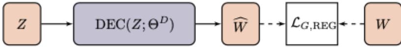
Figure 23.3: Shallow embedding methods. The encoder is a simple embedding look-up and the graph structure is only used in the loss function. Reprinted with permission from [Cha+21].
The output of a model, as described by GraphEDM framework, is a reconstructed graph similarity matrix W U (often used to train unsupervised embedding algorithms), and/or labels yVS for supervised applications. The label output space Y is application dependent. For instance, in node-level classification, yVN → YN , with Y representing the node label space. Alternately, for edge-level labeling, yVE → YN↓N , with Y representing the edge label space. Finally, we note that other kinds of labeling are possible, such as graph-level labeling (where we would say yVG → Y, with Y representing the graph label space).
Finally, a loss must be specified. This can be used to optimize the parameters ” = {”E, “D,”S}. GraphEDM models can be optimized using a combination of three di!erent terms. First, a supervised loss term, LS SUP, compares the predicted labels yˆS to the ground truth labels yS. Next, a graph reconstruction loss term, LG,RECON, may leverage the graph structure to impose regularization constraints on the model parameters. Finally, a weight regularization loss term, LREG, allows representing priors on trainable model parameters for reducing overfitting. Models realizable by GraphEDM framework are trained by minimizing the total loss L defined as:
\[\mathcal{L} = \alpha \mathcal{L}\_{\text{SUP}}^{S}(y^{S}, \hat{y}^{S}; \Theta) + \beta \mathcal{L}\_{\text{G,RECON}}(\mathbf{W}, \widehat{\mathbf{W}}; \Theta) + \gamma \mathcal{L}\_{\text{REG}}(\Theta), \tag{23.4}\]
where φ, ↼ and ↽ are hyper-parameters, that can be tuned or set to zero. Note that graph embedding methods can be trained in a supervised (φ 7= 0) or unsupervised (φ = 0) fashion. Supervised graph embedding approaches leverage an additional source of information to learn embeddings such as node or graph labels. On the other hand, unsupervised network embedding approaches rely on the graph structure only to learn node embeddings.
23.3 Shallow graph embeddings
Shallow embedding methods are transductive graph embedding methods, where the encoder function maps categorical node IDs onto a Euclidean space through an embedding matrix. Each node vi → V has a corresponding low-dimensional learnable embedding vector Zi → RL and the shallow encoder function is
\[\mathbf{Z} = \text{ENC}(\Theta^E) \triangleq \Theta^E \quad \text{where} \quad \Theta^E \in \mathbb{R}^{N \times L}. \tag{23.5}\]
Crucially, the embedding dictionary Z is directly learned as model parameters. In the unsupervised case, embeddings Z are optimized to recover some information about the input graph (e.g., the adjacency matrix W, or some transformation of it). This is somewhat similar to dimensionality reduction methods, such as PCA (Section 20.1), but for graph data structures. In the supervised case, the embeddings are optimized to predict some labels, for nodes, edges and/or the whole graph.
23.3.1 Unsupervised embeddings
In the unsupervised case, we will consider two main types of shallow graph embedding methods: distance-based and outer product-based. Distance-based methods optimize the embedding dictionary Z = “E → RN↓L such that nodes i and j which are close in the graph (as measured by some graph distance function) are embedded in Z such that d2(Zi, Zj ) is small, where d2(., .) is a pairwise distance function between embedding vectors. The distance function d2(·, ·) can be customized, which can lead to Euclidean (Section 23.3.2) or non-Euclidean (Section 23.3.3) embeddings. The decoder outputs a node-to-node matrix WU = DEC(Z;”D), with W Uij = d2(Zi, Zj ).
Alternatively, some methods rely on pairwise dot-products to compute node similarities. The decoder network can be written as: W U = DEC(Z; “D) = ZZ↙.
In both cases, unsupervised embeddings for distance- and product-based methods are learned by minimizing the graph reconstruction loss:
\[\mathcal{L}\_{G, \text{RECON}}(\mathbf{W}, \widehat{\mathbf{W}}; \Theta) = d\_1(s(\mathbf{W}), \widehat{\mathbf{W}}), \tag{23.6}\]
where s(W) is an optional transformation of the adjacency matrix W, and d1 is pairwise distance function between matrices, which does not need to be of the same form as d2. As we shall see, there are many plausible choices for s, d1, d2. For instance, we can let s be the adjacency matrix itself, s(W) = W or a power of it e.g. s(W) = W2. If the input is a weighted binary matrix W = A, we can set s(W)=1 ↗ W, so that connected nodes with Aij = 1 get a weight (distance) of 0.
23.3.2 Distance-based: Euclidean methods
Distance-based methods minimize Euclidean distances between similar (connected) nodes. We give some examples below.
Multi-dimensional scaling (MDS, Section 20.4.4) is equivalent to setting s(W) to some distance matrix measuring the dissimilarity between nodes (e.g. proportional to pairwise shortest distance) and then defining
\[d\_1(s(W), \widehat{W}) = \sum\_{i,j} (s(W)\_{ij} - \widehat{W}\_{ij})^2 = ||s(\mathbf{W}) - \widehat{\mathbf{W}}||\_F^2 \tag{23.7}\]
where W Uij = d2(Zi, Zj ) = ||Zi ↗ Zj || (although other distance metrics are plausible).
Laplacian eigenmaps (Section 20.4.9) learn embeddings by solving the generalized eigenvector problem
\[\min\_{\mathbf{Z}\in\mathbb{R}^{|V|\times d}} \text{tr}(\mathbf{Z}^{\mathsf{T}}\mathbf{L}\,\mathbf{Z}) \text{ s.t. } \mathbf{Z}^{\mathsf{T}}\mathbf{D}\mathbf{Z} = \mathbf{I} \text{ and } \mathbf{Z}^{\mathsf{T}}\mathbf{D}\mathbf{1} = \mathbf{0} \tag{23.8}\]
where L = D ↗ W is the graph Laplacian (Section 20.4.9.2), and D is a diagonal matrix containing the sum across columns for each row. The first constraint removes an arbitrary scaling factor in the embedding and the second one removes trivial solutions corresponding to the constant eigenvector (with eigenvalue zero for connected graphs). Further, note that tr(ZTLZ) = 1 2 ( i,j Wij ||Zi ↗ Zj ||2 2, where Zi is the i’th row of Z; therefore the minimization objective can be equivalently written as a
graph reconstruction term, as follows:
\[d\_1(s(\mathbf{W}), \widehat{\mathbf{W}}) = \sum\_{i,j} \mathbf{W}\_{ij} \times \widehat{\mathbf{W}}\_{ij} \tag{23.9}\]
\[\widehat{\mathbf{W}}\_{ij} = d\_2(\mathbf{Z}\_i, \mathbf{Z}\_j) = ||\mathbf{Z}\_i - \mathbf{Z}\_j||\_2^2 \tag{23.10}\]
where s(W) = W.
23.3.3 Distance-based: non-Euclidean methods
So far, we have discussed methods which assume that embeddings lie in an Euclidean Space. However, recent work has considered hyperbolic geometry for graph embedding. In particular, hyperbolic embeddings are ideal for embedding trees and o!er an exciting alternative to Euclidean geometry for graphs that exhibit hierarchical structures. We give some examples below.
Nickel and Kiela [NK17] learn embeddings of hierarchical graphs using the Poincaré model of hyperbolic space. This is simple to represent in our notation as we only need to change d2(Zi, Zj ) to the Poincaré distance function:
\[d\_2(\mathbf{Z}\_i, \mathbf{Z}\_j) = d\_{\text{Poincar\'e}}(\mathbf{Z}\_i, \mathbf{Z}\_j) = \text{arcosh}\left(1 + 2\frac{||\mathbf{Z}\_i - \mathbf{Z}\_j||\_2^2}{(1 - ||\mathbf{Z}\_i||\_2^2)(1 - ||\mathbf{Z}\_j||\_2^2)}\right). \tag{23.11}\]
The optimization then learns embeddings which minimize distances between connected nodes while maximizing distances between disconnected nodes:
\[d\_1(\mathbf{W}, \widehat{\mathbf{W}}) = \sum\_{i,j} \mathbf{W}\_{ij} \log \frac{e^{-\hat{\mathbf{W}}\_{ij}}}{\sum\_{k \mid \mathbf{W}\_{ik} = 0} e^{-\widehat{\mathbf{W}}\_{ik}}} \tag{23.12}\]
where the denominator is approximated using negative sampling. Note that since the hyperbolic space has a manifold structure, care needs to be taken to ensure that the embeddings remain on the manifold (using Riemannian optimization techniques [Bon13]).
Other variants of these methods have been proposed. Nickel and Kiela [NK18] explore the Lorentz model of hyperbolic space , and show that it provides better numerical stability than the Poincaré model. Another line of work extends non-Euclidean embeddings to mixed-curvature product spaces [Gu+18], which provide more flexibility for other types of graphs (e.g. ring of trees). Finally, work by Chamberlain, Clough, and Deisenroth [CCD17] extends Poincaré embeddings using skip-gram losses with hyperbolic inner products.
23.3.4 Outer product-based: Matrix factorization methods
Matrix factorization approaches learn embeddings that lead to a low rank representation of some similarity matrix s(W), with s : RN↓N ≃ RN↓N . The following are frequent choices: s(W) = W, s(W) = L (Graph Laplacian), or other proximity measure such as the Katz centrality index, Common Neighbors or Adamic/Adar index.
The decoder function in matrix factorization methods is just a dot product:
\[ \hat{\mathbf{W}} = \text{DEC}(\mathbf{Z}; \Theta^D) = \mathbf{Z}\mathbf{Z}^T \tag{23.13} \]
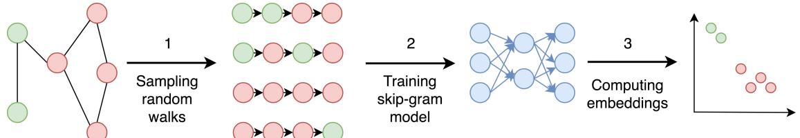
Figure 23.4: An overview of the pipeline for random-walk graph embedding methods. Reprinted with permission from [God18].
Matrix factorization methods learn Z by minimizing a regularization loss LG,RECON(W,WU; “) = ||s(W) ↗ WU||2 F .
The graph factorization method of [Ahm+13] learns a low-rank factorization of a graph by minimizing the graph regularization loss LG,RECON(W,WU; “) = ( (vi,vj )↔︎E(Wij ↗ WUij )2.
Note that if A is the binary adjacency matrix, (Aij = 1 i! (vi, vj ) → E and Aij = 0 otherwise), the graph reconstruction loss can be expressed in terms of the Frobenius norm:
\[\mathcal{L}\_{G, \text{RECON}}(\mathbf{W}, \widehat{\mathbf{W}}; \Theta) = ||\mathbf{A} \odot (\mathbf{W} - \widehat{\mathbf{W}})||\_F^2,\tag{23.14}\]
where ̸ is the element-wise matrix multiplication operator. Therefore, GF also learns a low-rank factorization of the adjacency matrix W measured in Frobenuis norm. We note that this is a sparse operation (summing only over edges which exist in the graph), and so the method has computational complexity O(M).
The methods described so far are all symmetric, that is, they assume that Wij = Wji. This is a limiting assumption when working with directed graphs as some relationships are not reciprocal. The GraRep method of [CLX15] overcomes this limitation by learning two embeddings per node, a source embedding Zs and a target embedding Zt , which capture asymmetric proximity in directed networks. In addition to asymmetry, GraRep learns embeddings that preserve k-hop neighborhoods via powers of the adjacency matrix and minimizes a graph reconstruction loss with:
\[ \widehat{\mathbf{W}}^{(k)} = \mathbf{Z}^{(k),s} \mathbf{Z}^{(k),t} \tag{23.15} \]
\[\mathcal{L}\_{G, \text{RECON}}(\mathbf{W}, \widehat{\mathbf{W}}^{(k)}; \Theta) = ||\mathbf{D}^{-k}\mathbf{W}^{k} - \widehat{\mathbf{W}}^{(k)}||\_F^2,\tag{23.16}\]
for each 1 ↙ k ↙ K. GraRep concatenates all representations to get source embeddings Zs = [Z(1),s| … |Z(K),s] and target embeddings Zt = [Z(1),t| … |Z(K),t]. Unfortunately, GraRep is not very scalable, since it uses a matrix power, D→1W, making it increasingly more dense. This limitation can be circumvented by using implicit matrix factorization [Per+17] as discussed below.
23.3.5 Outer product-based: Skip-gram methods
Skip-gram graph embedding models were inspired by research in natural language processing to model the distributional behavior of words [Mik+13c; PSM14b]. Skip-gram word embeddings are optimized to predict words in their context (the surrounding words) for each target word in a sentence. Given
a sequence of words (w1,…,wT ), skip-gram will minimize the objective:
\[\mathcal{L} = -\sum\_{-K \le i \le K, i \ne 0} \log \mathbb{P}(w\_{k-i}|w\_k),\]
for each target words wk. These conditional probabilities can be e”ciently estimated using neural networks. See Section 20.5.2.2 for details.
This idea has been leveraged for graph embeddings in the DeepWalk framework of [PARS14]. They justified this by showing empirically how the frequency statistics induced by random walks in real graphs follow a distribution similar to that of words used in natural language. In terms of GraphEDM, skip-gram graph embedding methods use an outer product (Equation 23.13) as their decoder function and a graph reconstruction term computed over random walks on the graph.
In more detail, DeepWalk trains node embeddings to maximize the probability of predicting context nodes for each center node. The context nodes are nodes appearing adjacent to the center node, in simulated random walks on A. To train embeddings, DeepWalk generates sequences of nodes using truncated unbiased random walks on the graph — which can be compared to sentences in natural language models — and then maximizes their log-likelihood. Each random walk starts with a node vi1 → V and repeatedly samples the next node uniformly at random: vij+1 → {v → V | (vij , v) → E}. The walk length is a hyperparameter. All generated random-walks can then be encoded by a sequence model. This two-step paradigm introduced by [PARS14] has been followed by many subsequent works, such as node2vec [GL16].
We note that it is common for underlying implementations to use two distinct representations for each node, one for when a node is center of a truncated random walk, and one when it is in the context. The implications of this modeling choice are studied further in [AEHPAR17].
To present DeepWalk in the GraphEDM framework, we can set:
\[s(\mathbf{W}) = \mathbb{E}\_q\left[ \left( \mathbf{D}^{-1} \mathbf{W} \right)^q \right] \text{ with } q \sim P(Q) = \text{Categorical}([1, 2, \dots, T\_{\text{max}}]) \tag{23.17}\]
where P(Q = q) = Tmax→1+q Tmax (see [AEH+18] for the derivation).
Training DeepWalk is equivalent to minimizing:
\[\mathcal{L}\_{G, \text{RECON}}(W, \widehat{W}; \Theta) = \log Z(\mathbf{Z}) - \sum\_{v\_i \in V, v\_j \in V} s(\mathbf{W})\_{ij} \widehat{\mathbf{W}}\_{ij},\tag{23.18}\]
where WU = ZZT, and the partition function Z(Z) = i ( j exp(WUij ) can be approximated in O(N) time via hierarchical softmax (see Section 20.5.2). (It is also common to model WU = ZoutZin T for directed graphs using embedding dictionaries Zout, Zin → RN↓L.)
As noted by [LG14], Skip-gram methods can be viewed as implicit matrix factorization, and the methods discussed here are related to those of Matrix Factorization (see Section 23.3.4). This relationship is discussed in depth by [Qiu+18], who propose a general matrix factorization framework, NetMF, which uses the same underlying graph proximity information as DeepWalk, LINE [Tan+15], and node2vec [GL16]. Casting the node embedding problem as matrix factorization can inherit benefits of e”cient sparse matrix operations [Qiu+19a].
23.3.6 Supervised embeddings
In many applications, we have labeled data in addition to node features and graph structure. While it is possible to tackle a supervised task by first learning unsupervised representations and then using them as features in a secondary model, this is not the ideal workflow. Unsupervised node embeddings might not preserve important properties of graphs (e.g., node neighborhoods or attributes), that are most useful for a downstream supervised task.
In light of this limitation, a number of methods combining these two steps, namely learning embeddings and predicting node or graph labels, have been proposed. Here, we focus on simple shallow methods. We discuss deep, nonlinear embeddings later on.
23.3.6.1 Label propagation
Label propagation (LP) [ZG02] is a very popular algorithm for graph-based semi-supervised node classification. The encoder is a shallow model represented by a lookup table Z. LP uses the label space to represent the node embeddings directly (i.e. the decoder in LP is simply the identity function):
\[ \hat{y}^N = \text{DEC}(\mathbf{Z}; \Theta^C) = \mathbf{Z}. \]
In particular, LP uses the graph structure to smooth the label distribution over the graph by adding a regularization term to the loss function, using the underlying assumption that neighbor nodes should have similar labels (i.e. there exist some label consistency between connected nodes). Laplacian eigenmaps are utilized in the regularization to enforce this smoothness:
\[\mathcal{L}\_{G, \text{RECON}}(\mathbf{W}, \widehat{\mathbf{W}}; \Theta) = \sum\_{i, j} \mathbf{W}\_{ij} ||y\_i^N - \hat{y}\_j^N||\_2^2 \tag{23.19}\]
LP minimizes this energy function over the space of functions that take fixed values on labeled nodes (i.e. yˆN i = yN i ℵi|vi → VL) using an iterative algorithm that updates an unlabeled node’s label distribution via the weighted average of its neighbors’ labels.
Label spreading (LS) [Zho+04] is a variant of label propagation which minimizes the following energy function:
\[\mathcal{L}\_{G, \text{RECON}}(\mathbf{W}, \widehat{\mathbf{W}}; \Theta) = \sum\_{i,j} \mathbf{W}\_{ij} \left| \left| \frac{\hat{y}\_i^N}{\sqrt{D\_i}} - \frac{\hat{y}\_j^N}{\sqrt{D\_j}} \right| \right|\_2^2,\tag{23.20}\]
where Di = ( j Wij is the degree of node vi.
In both methods, the supervised loss is simply the sum of distances between predicted labels and ground truth labels (one-hot vectors):
\[\mathcal{L}\_{\text{SUP}}^{N}(y^{N}, \hat{y}^{N}; \Theta) = \sum\_{i \mid v\_{i} \in V\_{L}} ||y\_{i}^{N} - \hat{y}\_{i}^{N}||\_{2}^{2}. \tag{23.21}\]
Note that while the regularization term is computed over all nodes in the graph, the supervised loss is computed over labeled nodes only. These methods are expected to work well with consistent graphs, that is graphs where node proximity in the graph is positively correlated with label similarity.
23.4 Graph Neural Networks
An extensive area of research focuses on defining convolutions over graph data. In the notation of Chami et al. [Cha+21], these (semi-)supervised neighborhood aggregation methods can be represented by an encoder of the form Z = ENC(X,W; “E), and decoders of the form WU = DEC(Z;”D) and/or yVS = DEC(Z; “S). There are many models in this family; we review some of them below.
23.4.1 Message passing GNNs
The original graph neural network (GNN) model of [GMS05; Sca+09] was the first formulation of deep learning methods for graph-structured data. It views the supervised graph embedding problem as an information di!usion mechanism, where nodes send information to their neighbors until some stable equilibrium state is reached. More concretely, given randomly initialized node embeddings Z0, it applies the following recursion:
\[\mathbf{Z}^{t+1} = \text{ENC}(\mathbf{X}, \mathbf{W}, \mathbf{Z}^t; \Theta^E), \tag{23.22}\]
where parameters “E are reused at every iteration. After convergence (t = T), the node embeddings ZT are used to predict the final output such as node or graph labels:
\[ \hat{y}^S = \text{DEC}(\mathbf{X}, \mathbf{Z}^T; \Theta^S). \tag{23.23} \]
This process is repeated several times and the GNN parameters “E and”D are learned with backpropagation via the Almeda-Pineda algorithm [Alm87; Pin88]. By Banach’s fixed point theorem, this process is guaranteed to converge to a unique solution when the recursion provides a contraction mapping. In light of this, Scarselli et al. [Sca+09] explore maps that can be expressed using message passing networks:
\[\mathbf{Z}\_{i}^{t+1} = \sum\_{j | (v\_i, v\_j) \in E} f(\mathbf{X}\_i, \mathbf{X}\_j, \mathbf{Z}\_j^t; \Theta^E), \tag{23.24}\]
where f(·) is a multi-layer perception (MLP) constrained to be a contraction mapping. The decoder function, however, has no constraints and can be any MLP.
Li et al. [Li+15] propose Gated Graph Sequence Neural Networks (GGSNNs), which remove the contraction mapping requirement from GNNs. In GGSNNs, the recursive algorithm in Equation 23.22 is relaxed by applying mapping functions for a fixed number of steps, where each mapping function is a gated recurrent unit [Cho+14b] with parameters shared for every iteration. The GGSNN model outputs predictions at every step, and so is particularly useful for tasks which have sequential structure (such as temporal graphs).
Gilmer et al. [Gil+17] provide a framework for graph neural networks called message passing neural networks (MPNNs), which encapsulates many recent models. In contrast with the GNN model which runs for an indefinite number of iterations, MPNNs provide an abstraction for modern approaches, which consist of multi-layer neural networks with a fixed number of layers. At every layer ε, message functions fω(.) receive messages from neighbors (based on neighbor’s hidden state), which are then passed to aggregation functions hω(.):
\[\mathbf{m}\_{i}^{\ell+1} = \sum\_{j | \langle v\_{i}, v\_{j} \rangle \in E} f^{\ell}(\mathbf{H}\_{i}^{\ell}, \mathbf{H}\_{j}^{\ell}) \tag{23.25}\]
\[\mathbf{H}\_{i}^{\ell+1} = h^{\ell}(\mathbf{H}\_{i}^{\ell}, \mathbf{m}\_{i}^{\ell+1}),\tag{23.26}\]
where H0 = X. After ε layers of message passing, nodes’ hidden representations encode information within ε-hop neighborhoods.
Battaglia et al. [Bat+18] propose GraphNet, which further extends the MPNN framework to learn representations for edges, nodes and the entire graph using message passing functions. The explicit addition of edge and graph representations adds additional expressivity to the MPNN model, and allows the application of graph models to additional domains.
23.4.2 Spectral Graph Convolutions
Spectral methods define graph convolutions using the spectral domain of the graph Laplacian matrix. These methods broadly fall into two categories: spectrum-based methods, which explicitly compute an eigendecomposition of the Laplacian (e.g., spectral CNNs [Bru+14]) and spectrum-free methods, which are motivated by spectral graph theory but do not actually perform a spectral decomposition (e.g., Graph convolutional networks or GCN [KW16a]).
A major disadvantage of spectrum-based methods is that they rely on the spectrum of the graph Laplacian and are therefore domain-dependent (i.e. cannot generalize to new graphs). Moreover, computing the Laplacian’s spectral decomposition is computationally expensive. Spectrum-free methods overcome these limitations by utilizing approximations of these spectral filters. However, spectrum-free methods require using the whole graph W, and so do not scale well.
For more details on spectral approaches, see e.g., [Bro+17b; Cha+21].
23.4.3 Spatial Graph Convolutions
Spectrum-based methods have an inherent domain dependency which limits the application of a model trained on one graph to a new dataset. Additionally, spectrum-free methods (e.g. GCNs) require using the entire graph A, which can quickly become unfeasible as the size of the graph grows.
To overcome these limitations, another branch of graph convolutions (spatial methods) borrow ideas from standard CNNs – applying convolutions in the spatial domain as defined by the graph topology. For instance, in computer vision, convolutional filters are spatially localized by using fixed rectangular patches around each pixel. Combined with the natural ordering of pixels in images (top, left, bottom, right), it is possible to reuse filters’ weights at every location. This process significantly reduces the total number of parameters needed for a model. While such spatial convolutions cannot directly be applied in graph domains, spatial graph convolutions take inspiration from them. The core idea is to use neighborhood sampling and attention mechanisms to create fixed-size graph patches, overcoming the irregularity of graphs.
23.4.3.1 Sampling-based spatial methods
To overcome the domain dependency and storage limitations of GCNs, Hamilton, Ying, and Leskovec [HYL17] propose GraphSAGE, a framework to learn inductive node embeddings. Instead of
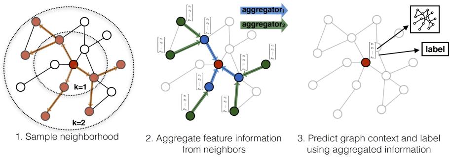
Figure 23.5: Illustration of the GraphSAGE model. Reprinted with permission from [HYL17].
averaging signals from all one-hop neighbors (via multiplications with the Laplacian matrix), SAGE samples fixed neighborhoods (of size q) for each node. This removes the strong dependency on fixed graph structure and allows generalization to new graphs. At every SAGE layer, nodes aggregate information from nodes sampled from their neighborhood (see Figure 23.5). In the GraphEDM notation, the propagation rule can be written as:
\[\mathbf{H}\_{\cdot,i}^{\ell+1} = \sigma(\Theta\_1^{\ell} \mathbf{H}\_{\cdot,i}^{\ell} + \Theta\_2^{\ell} \text{AGG}(\{\mathbf{H}\_{\cdot,j}^{\ell} \mid v\_j \in \text{Sample}(\text{nbr}(v\_i), q)\})),\tag{23.27}\]
where AGG(·) is an aggregation function. This aggregation function can be any permutation invariant operator such as averaging (SAGE-mean) or max-pooling (SAGE-pool). As SAGE works with fixed size neighborhoods (and not the entire adjacency matrix), it also reduces the computational complexity of training GCNs.
23.4.3.2 Attention-based spatial methods
Attention mechanisms (Section 15.4) have been successfully used in language models where they, for example, allow models to identify relevant parts of long sequence inputs. Inspired by their success in language, similar ideas have been proposed for graph convolution networks. Such graph-based attention models learn to focus their attention on important neighbors during the message passing step via parametric patches which are learned on top of node features. This provides more flexibility in inductive settings, compared to methods that rely on fixed weights such as GCNs.
The Graph attention network (GAT) model of [Vel+18] is an attention-based version of GCNs. At every GAT layer, it attends over the neighborhood of each node and learns to selectively pick nodes which lead to the best performance for some downstream task. The intuition behind this is similar to SAGE [HYL17] and makes GAT suitable for inductive and transductive problems. However unlike SAGE, which limits the convolution step to fixed size-neighborhoods, GAT allows each node to attend over the entirety of its neighbors – assigning each of them di!erent weights. The attention parameters are trained through backpropagation, and the attention scores are then row-normalized with a softmax activation.
23.4.3.3 Geometric spatial methods
Monti et al. [Mon+17] propose MoNet, a general framework that works particularly well when the node features lie in a geometric space, such as 3D point clouds or meshes. MoNet learns attention patches using parametric functions in a pre-defined spatial domain (e.g. spatial coordinates), and then applies convolution filters in the resulting graph domain.
MoNet generalizes spatial approaches which introduce constructions for convolutions on manifolds, such as the Geodesic CNN (GCNN) [Mas+15] and the Anisotropic CNN (ACNN) [Bos+16]. Both GCNN and ACNN use fixed patches that are defined on a specific coordinate system and therefore cannot generalize to graph-structured data. However, the MoNet framework is more general; any pseudo-coordinates (i.e. node features) can be used to induce the patches. More formally, if Us are pseudo-coordinates and Hω are features from another domain, the MoNet layer can be expressed in our notation as:
\[\mathbf{H}^{\ell+1} = \sigma \left( \sum\_{k=1}^{K} (\mathbf{W} \odot g\_k(\mathbf{U}^s)) \mathbf{H}^\ell \Theta\_k^\ell \right), \tag{23.28}\]
where gk(Us) are the learned parametric patches, which are N ↑ N matrices. In practice, MoNet uses Gaussian kernels to learn patches, such that:
\[g\_k(\mathbf{U}^s) = \exp\left(-\frac{1}{2}(\mathbf{U}^s - \mu\_k)^\mathsf{T}\Sigma\_k^{-1}(\mathbf{U}^s - \mu\_k)\right),\tag{23.29}\]
where µk and “k are learned parameters, and”k is restricted to be diagonal.
23.4.4 Non-Euclidean Graph Convolutions
As we discussed in Section 23.3.3, hyperbolic geometry enables learning of shallow embeddings of hierarchical graphs which have smaller distortion than Euclidean embeddings. However, one major downside of shallow embeddings is that they do not generalize well (if at all) across graphs. On the other hand, Graph Neural Networks, which leverage node features, have achieved good results on many inductive graph embedding tasks.
It is natural then, that there has been recent interest in extending Graph Neural Networks to learn non-Euclidean embeddings. One major challenge in doing so again revolves around the nature of convolution itself. How should we perform convolutions in a non-Euclidean space, where standard operations such as inner products and matrix multiplications are not defined?
Hyperbolic Graph Convolution Networks (HGCN) [Cha+19a] and Hyperbolic Graph Neural Networks (HGNN) [LNK19] apply graph convolutions in hyperbolic space by leveraging the Euclidean tangent space, which provides a first-order approximation of the hyperbolic manifold at a point. For every graph convolution step, node embeddings are mapped to the Euclidean tangent space at the origin, where convolutions are applied, and then mapped back to the hyperbolic space. These approaches yield significant improvements on graphs that exhibit hierarchical structure (Figure 23.6).
23.5 Deep graph embeddings
In this section, we use graph neural networks to devise graph embeddings in the unsupervised and semi-supervised cases.
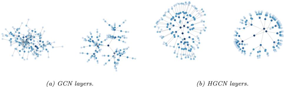
Figure 23.6: Euclidean (left) and hyperbolic (right) embeddings of a tree graph. Hyperbolic embeddings learn natural hierarchies in the embedding space (depth indicated by color). Reprinted with permission from [Cha+19a].
Figure 23.7: Unsupervised graph neural networks. Graph structure and input features are mapped to lowdimensional embeddings using a graph neural network encoder. Embeddings are then decoded to compute a graph regularization loss (unsupervised). Reprinted with permission from [Cha+21].
23.5.1 Unsupervised embeddings
In this section, we discuss unsupervised losses for GNNs, as illustrated in Figure 23.7.
23.5.1.1 Structural deep network embedding
The structural deep network embedding (SDNE) method of [WCZ16] uses auto-encoders which preserve first and second-order node proximity. The SDNE encoder takes a row of the adjacency matrix as input (setting s(W) = W) and produces node embeddings Z = ENC(W; ⇁E). (Note that this ignores any node features.) The SDNE decoder returns WU = DEC(Z; “D), a reconstruction trained to recover the original graph adjacency matrix. SDNE preserves second order node proximity by minimizing the following loss:
\[||(s(\mathbf{W}) - \widehat{\mathbf{W}}) \cdot \mathbb{I}(s(\mathbf{W}) > 0)||\_F^2 + \alpha\_{\text{SDNE}} \sum\_{ij} s(\mathbf{W})\_{ij} ||\mathbf{Z}\_i - \mathbf{Z}\_j||\_2^2 \tag{23.30}\]
The first term is similar to the matrix factorization regularization objective, except that WU is not computed using outer products. The second term is used by distance-based shallow embedding methods.
23.5.1.2 (Variational) graph auto-encoders
Kipf and Welling [KW16b] use graph convolutions (Section 23.4.2) to learn node embeddings Z = GCN(W, X; “E). The decoder is an outer product: DEC(Z;”D) = ZZT. The graph reconstruction term is the sigmoid cross entropy between the true adjacency and the predicted edge similarity scores:
\[\mathcal{L}\_{\text{G,RECON}}(\mathbf{W}, \widehat{\mathbf{W}}; \Theta) = -\left(\sum\_{i,j} (1 - \mathbf{W}\_{ij}) \log(1 - \sigma(\widehat{\mathbf{W}}\_{ij})) + \mathbf{W}\_{ij} \log \sigma(\widehat{\mathbf{W}}\_{ij})\right). \tag{23.31}\]
Computing the regularization term over all possible nodes pairs is computationally challenging in practice, so the Graph Auto Encoders (GAE) model uses negative sampling to overcome this challenge.
Whereas GAE is a deterministic model, the authors also introduce variational graph auto-encoders (VGAE), which rely on variational auto-encoders (as in Section 20.3.5) to encode and decode the graph structure. In VGAE, the embedding Z is modeled as a latent variable with a standard multivariate normal prior p(Z) = N (Z|0, I) and a graph convolution is used as the amortized inference network, q#(Z|W, X). The model is trained by minimizing the corresponding negative evidence lower bound:
\[\text{NELBO}(\mathbf{W}, \mathbf{X}; \Theta) = -\mathbb{E}\_{q\_{\Phi}(\mathbf{Z}|\mathbf{W}, \mathbf{X})}[\log p(\mathbf{W}|\mathbf{Z})] + \text{KL}(q\_{\Phi}(\mathbf{Z}|\mathbf{W}, \mathbf{X})||p(\mathbf{Z})) \tag{23.32}\]
\[=\mathcal{L}\_{G,\text{RECON}}(\mathbf{W},\mathbf{\dot{W}};\Theta) + \text{KL}(q\_{\Phi}(\mathbf{Z}|\mathbf{W},\mathbf{X})||p(\mathbf{Z})).\tag{23.33}\]
23.5.1.3 Iterative generative modelling of graphs (Graphite)
The graphite model of [GZE19] extends GAE and VGAE by introducing a more complex decoder. This decoder iterates between pairwise decoding functions and graph convolutions, as follows:
\[\begin{aligned} \widehat{\mathbf{W}}^{(k)} &= \frac{\mathbf{Z}^{(k)} \mathbf{Z}^{(k)^{\mathsf{T}}}}{||\mathbf{Z}^{(k)}||\_2^2} + \frac{\mathbf{1} \mathbf{1}^{\mathsf{T}}}{N} \\ \mathbf{Z}^{(k+1)} &= \text{GCN}(\widehat{\mathbf{W}}^{(k)}, \mathbf{Z}^{(k)}) \end{aligned}\]
where Z(0) is initialized using the output of the encoder network. This process allows Graphite to learn more expressive decoders. Finally, similar to GAE, Graphite can be deterministic or variational.
23.5.1.4 Methods based on contrastive losses
The deep graph infomax method of [Vel+19] is a GAN-like method for creating graph-level embeddings. Given one or more real (positive) graphs, each with its adjacency matrix W → RN↓N and node features X → RN↓D, this method creates fake (negative) adjacency matrices W→ → RN→↓N→ and their features X→ → RN→↓D. It trains (i) an encoder that processes both real and fake samples, respectively giving Z = ENC(X,W; “E) → RN↓L and Z→ = ENC(X→,W→;”E) → RN→↓L, (ii) a (readout) graph pooling function R : RN↓L ≃ RL, and (iii) a discriminator function D : RL ↑ RL ≃ [0, 1] which is trained to output D(Zi, R(Z)) ′ 1 and D(Z→ j , R(Z→)) ′ 0, respectively, for nodes corresponding to given graph i → V and fake graph j → V →. Specifically, DGI optimizes:
\[\min\_{\boldsymbol{\Theta}} - \underset{\mathbf{X}, \mathbf{W}}{\operatorname{\mathbb{E}}} \sum\_{i=1}^{N} \log \mathcal{D}(\mathbf{Z}\_{i}, \mathcal{R}(\mathbf{Z})) - \underset{\mathbf{X}^{-}, \mathbf{W}^{-}}{\operatorname{\mathbb{E}}} \sum\_{j=1}^{N^{-}} \log \left( 1 - \mathcal{D}(\mathbf{Z}\_{j}^{-}, \mathcal{R}(\mathbf{Z}^{-})) \right), \tag{23.34}\]
where ” contains “E and the parameters of R, D. In the first expectation, DGI samples from the real (positive) graphs. If only one graph is given, it could sample some subgraphs from it (e.g. connected components). The second expectation samples fake (negative) graphs. In DGI, fake samples use the real adjacency W→ := W but fake features X→ are a row-wise random permutation of real X. The ENC used in DGI is a graph convolutional network, though any GNN can be used. The readout R summarizes an entire (variable-size) graph to a single (fixed-dimension) vector. Veli%kovi& et al. [Vel+19] use R as a row-wise mean, though other graph pooling might be used e.g. ones aware of the adjacency.
The optimization of Equation (23.34) is shown by [Vel+19] to maximize a lower-bound on the mutual information between the outputs of the encoder and the graph pooling function, i.e., between individual node representations and the graph representation.
In [Pen+20] they present a variant called Graphical Mutual Information. Rather than maximizing MI of node information and an entire graph, GMI maximizes the MI between the representation of a node and its neighbors.
23.5.2 Semi-supervised embeddings
In this section, we discuss semi-supervised losses for GNNs. We consider the simple special case in which we use a nonlinear encoder of the node features, but ignore the graph structure, i.e., we use Z = ENC(X; “E).
23.5.2.1 SemiEmb
[WRC08] propose an approach called semi-supervised embeddings (SemiEmb) They use an MLP for the encoder of X. For the decoder, we can use a distance-based graph decoder: WUij = DEC(Z; “D)ij = ||Zi ↗ Zj ||2, where || · || can be the L2 or L1 norm.
SemiEmb regularizes intermediate or auxiliary layers in the network using the same regularizer as the label propagation loss in Equation (23.19). SemiEmb uses a feed forward network to predict labels from intermediate embeddings, which are then compared to ground truth labels using the Hinge loss.
23.5.2.2 Planetoid
Unsupervised skip-gram methods like DeepWalk and node2vec learn embeddings in a multi-step pipeline, where random walks are first generated from the graph and then used to learn embeddings. These embeddings are likely not optimal for downstream classification tasks. The Planetoid method of [YCS16] extends such random walk methods to leverage node label information during the embedding algorithm.
Planetoid first maps nodes to embeddings Z = [Zc||ZF ] = ENC(X; “E) using a neural network (again ignoring graph structure). The node embeddings Zc capture structural information while the
node embeddings ZF capture feature information. There are two variants, a transductive version that directly learns Zc (as an embedding lookup), and an inductive model where Zc is computed with parametric mappings that act on input features X. The Planetoid objective contains both a supervised loss and a graph regularization loss. The graph regularization loss measures the ability to predict context using nodes embeddings:
\[\mathcal{L}\_{\text{G,RECON}}(\mathbf{W}, \widehat{\mathbf{W}}; \Theta) = -\mathbb{E}\_{(i, j, \gamma)} \log \sigma \left(\gamma \widehat{\mathbf{W}}\_{ij}\right),\tag{23.35}\]
with WUij = ZiZT j and ↽ → {↗1, 1} with ↽ = 1 if (vi, vj ) → E is a positive pair and ↽ = ↗1 if (vi, vj ) is a negative pair. The distribution under the expectation is directly defined through a sampling process.
The supervised loss in Planetoid is the negative log-likelihood of predicting the correct labels:
\[\mathcal{L}\_{\text{SUP}}^{N}(y^{N}, \widehat{y}^{N}; \Theta) = -\frac{1}{|V\_{L}|} \sum\_{i \mid v\_{i} \in V\_{L}} \sum\_{1 \le k \le C} y\_{ik}^{N} \log \widehat{y}\_{ik}^{N},\tag{23.36}\]
where i is a node’s index while k indicates label classes, and yVN i are computed using a neural network followed by a softmax activation, mapping Zi to predicted labels.
23.6 Applications
There are many applications of graph embeddings, both unsupervised and supervised. We give some examples in the sections below.
23.6.1 Unsupervised applications
In this section, we discuss common unsupervised applications.
23.6.1.1 Graph reconstruction
A popular unsupervised graph application is graph reconstruction. In this setting, the goal is to learn mapping functions (which can be parametric or not) that map nodes onto a manifold which can reconstruct the graph. This is regarded as unsupervised in the sense that there is no supervision beyond the graph structure. Models can be trained by minimizing a reconstruction error, which is the error in recovering the original graph from learned embeddings. Several algorithms were designed specifically for this task, and we refer to Section 23.3.1 and Section 23.5.1 for some examples of reconstruction objectives. At a high level, graph reconstruction is similar to dimensionality reduction in the sense that the main goal is to summarize some input data into a low-dimensional embedding. Instead of compressing high dimensional vectors into low-dimensional ones as standard dimensionality reduction methods (e.g. PCA) do, the goal of graph reconstruction models is to compress data defined on graphs into low-dimensional vectors.
23.6.1.2 Link prediction
The goal in link prediction is to predict missing or unobserved links (e.g., links that may appear in the future for dynamic and temporal networks). Link prediction can also help identify spurious
Figure 23.8: A graph representation of some financial transactions. Adapted from http: // pgql-lang. org/ spec/ 1. 2/ .
links and remove them. It is a major application of graph learning models in industry, and common example of applications include predicting friendships in social networks, predicting user-product interactions in recommendation systems, predicting suspicious links in a fraud detection system (see Figure 23.8), or predicting missing relationships between entities in a knowledge graph (see e.g., [Nic+15]).
A common approach for training link prediction models is to mask some edges in the graph (positive and negative edges), train a model with the remaining edges and then test it on the masked set of edges. Note that link prediction is di!erent from graph reconstruction. In link prediction, we aim at predicting links that are not observed in the original graph while in graph reconstruction, we only want to compute embeddings that preserve the graph structure through reconstruction error minimization.
Finally, while link prediction has similarities with supervised tasks in the sense that we have labels for edges (positive, negative, unobserved), we group it under the unsupervised class of applications since edge labels are usually not used during training, but only used to measure the predictive quality of embeddings.
23.6.1.3 Clustering
Clustering is particularly useful for discovering communities and has many real-world applications. For instance, clusters exist in biological networks (e.g. as groups of proteins with similar properties), or in social networks (e.g. as groups of people with similar interests).
The unsupervised methods introduced in this chapter can be used to solve clustering problems
by applying the clustering algorithm (e.g. k-means) to embeddings that are output by an encoder. Further, clustering can be joined with the learning algorithm while learning a shallow [Roz+19] or Graph Convolution [Chi+19a; CEL19] embedding model.
23.6.1.4 Visualization
There are many o!-the-shelf tools for mapping graph nodes onto two-dimensional manifolds for the purpose of visualization. Visualizations allow network scientists to qualitatively understand graph properties, understand relationships between nodes or visualize node clusters. Among the popular tools are methods based on Force-Directed Layouts, with various web-app Javascript implementations.
Unsupervised graph embedding methods are also used for visualization purposes: by first training an encoder-decoder model (corresponding to a shallow embedding or graph convolution network), and then mapping every node representation onto a two-dimensional space using t-SNE (Section 20.4.10) or PCA (Section 20.1). Such a process (embedding ≃ dimensionality reduction) is commonly used to qualitatively evaluate the performance of graph learning algorithms. If nodes have attributes, one can use these attributes to color the nodes on 2D visualization plots. Good embedding algorithms embed nodes that have similar attributes nearby in the embedding space, as demonstrated in visualizations of various methods [PARS14; KW16a; AEH+18]. Finally, beyond mapping every node to a 2D coordinate, methods which map every graph to a representation [ARZP19] can similarly be projected into two dimensions to visualize and qualitatively analyze graph-level properties.
23.6.2 Supervised applications
In this section, we discuss common supervised applications.
23.6.2.1 Node classification
Node classification is an important supervised graph application, where the goal is to learn node representations that can accurately predict node labels. (This is sometimes called statistical relational learning [GT07].) For instance, node labels could be scientific topics in citation networks, or gender and other attributes in social networks.
Since labeling large graphs can be time-consuming and expensive, semi-supervised node classification is a particularly common application. In semi-supervised settings, only a fraction of nodes are labeled and the goal is to leverage links between nodes to predict attributes of unlabeled nodes. This setting is transductive since there is only one partially labeled fixed graph. It is also possible to do inductive node classification, which corresponds to the task of classifying nodes in multiple graphs.
Note that node features can significantly boost the performance on node classification tasks if these are descriptive for the target label. Indeed, recent methods such as GCN (Section 23.4.2) GraphSAGE (Section 23.4.3.1) have achieved state-of-the-art performance on multiple node classification benchmarks due to their ability to combine structural information and semantics coming from features. On the other hand, other methods such as random walks on graphs fail to leverage feature information and therefore achieve lower performance on these tasks.
Figure 23.9: Structurally similar molecules do not necessarily have similar odor descriptors. (A) Lyral, the reference molecule. (B) Molecules with similar structure can share similar odor descriptors. (C) However, a small structural change can render the molecule odorless. (D) Further, large structural changes can leave the odor of the molecule largely unchanged. From Figure 1 of [SL+19], originally from [OPK12]. Used with kind permission of Benjamin Sanchez-Lengeling.
23.6.2.2 Graph classification
Graph classification is a supervised application where the goal is to predict graph labels. Graph classification problems are inductive and a common example is classifying chemical compounds (e.g. predicting toxicity or odor from a molecule, as shown in Figure 23.9).
Graph classification requires some notion of pooling, in order to aggregate node-level information into graph-level information. As discussed earlier, generalizing this notion of pooling to arbitrary graphs is non trivial because of the lack of regularity in the graph structure making graph pooling an active research area. In addition to the supervised methods discussed above, a number of unsupervised methods for learning graph-level representations have been proposed [Tsi+18; ARZP19; TMP20].
A Notation
A.1 Introduction
It is very di”cult to come up with a single, consistent notation to cover the wide variety of data, models and algorithms that we discuss in this book. Furthermore, conventions di!er between di!erent fields (such as machine learning, statistics and optimization), and between di!erent books and papers within the same field. Nevertheless, we have tried to be as consistent as possible. Below we summarize most of the notation used in this book, although individual sections may introduce new notation. Note also that the same symbol may have di!erent meanings depending on the context, although we try to avoid this where possible.
A.2 Common mathematical symbols
We list some common symbols below.
| Symbol | Meaning |
|---|---|
| ↖ | Infinity |
| ≃ | Tends towards, e.g., n ≃ ↖ |
| ⇐ | Proportional to, so y = ax can be written as y ⇐ x |
| ↫ | Defined as |
| O(·) | Big-O: roughly means order of magnitude |
| Z+ | The positive integers |
| R | The real numbers |
| R+ | The positive reals |
| SK | The K-dimensional probability simplex |
| SD ++ |
Cone of positive definite D ↑ D matrices |
| ′ | Approximately equal to |
| {1,,N} | The finite set {1, 2,,N} |
| 1 : N |
The finite set {1, 2,,N} |
| [ε, u] |
The continuous interval {ε ↙ x ↙ u}. |
A.3 Functions
Generic functions will be denoted by f (and sometimes g or h). We will encounter many named functions, such as tanh(x) or ω(x). A scalar function applied to a vector is assumed to be applied elementwise, e.g., x2 = [x2 1,…,x2 D]. Functionals (functions of a function) are written using “blackboard” font, e.g., H(p) for the entropy of a distribution p. A function parameterized by fixed parameters ε will be denoted by f(x; ε) or sometimes fε(x). We list some common functions (with no free parameters) below.
A.3.1 Common functions of one argument
| Symbol | Meaning |
|---|---|
| △x▽ | Floor of x, i.e., round down to nearest integer |
| AxB | x, Ceiling of i.e., round up to nearest integer |
| ¬a | logical NOT |
| I(x) | I(x)=1 x I(x)=0 Indicator function, if is true, else |
| 2(x) | Dirac delta function, 2(x) = ↖ if x = 0, else 2(x)=0 |
| x | Absolute value |
| S | Size (cardinality) of a set |
| n! | Factorial function |
| log(x) | Natural logarithm of x |
| exp(x) | ex Exponential function |
| #(x) | ∝ ux→1e→udu #(x) = Gamma function, 0 |
| &(x) | d Digamma function, &(x) = dx log #(x) |
| ω(x) | 1 Sigmoid (logistic) function, 1+e→x |
A.3.2 Common functions of two arguments
| Symbol | Meaning |
|---|---|
| a ↔︎ b |
logical AND |
| a ↘ b |
logical OR |
| B(a, b) |
$(a)$(b) Beta function, B(a, b) = $(a+b) |
| ! “ n k |
n choose k, equal to n!/(k!(n ↗ k)!) |
| 2ij | I(i = j) Kronecker delta, equals |
| u ̸ v |
Elementwise product of two vectors |
| u v ↬ |
Convolution of two vectors |
A.3.3 Common functions of > 2 arguments
| Symbol | Meaning |
|---|---|
| B(x) | # k $(xk) Multivariate beta function, ! $( k xk) |
| #(x) | ◁D(D→1)/4 D Multi. gamma function, d=1 # (x + (1 ↗ d)/2) |
\[\text{softmax}(x) \quad \text{Softmax function}, \left[\frac{e^{x\_c}}{\sum\_{c'=1}^C e^{x\_{c'}}}\right]\_{c=1}^C\]
A.4 Linear algebra
In this section, we summarize the notation we use for linear algebra (see Chapter 7 for details).
A.4.1 General notation
Vectors are bold lower case letters such as x, w. Matrices are bold upper case letters, such as X, W. Scalars are non-bold lower case. When creating a vector from a list of N scalars, we write x = [x1,…,xN ]; this may be a column vector or a row vector, depending on the context. (Vectors are assumed to be column vectors, unless noted otherwise.) When creating an M ↑ N matrix from a list of vectors, we write X = [x1,…, xN ] if we stack along the columns, or X = [x1; … ; xM] if we stack along the rows.
A.4.2 Vectors
Here is some standard notation for vectors. (We assume u and v are both N-dimensional vectors.)
| Symbol | Meaning |
|---|---|
| uTv | (N Inner (scalar) product, i=1 uivi |
| uvT | Outer product (N ↑ N matrix) |
| u ̸ v |
Elementwise product, [u1v1,,uN vN ] |
| vT | Transpose of v |
| dim(v) | v N) Dimensionality of (namely |
| diag(v) | Diagonal N ↑ N matrix made from vector v |
| 1 1N or |
N) Vector of ones (of length |
| 0 or 0N |
Vector of zeros (of length N) |
| v = v 2 |
(N i=1 v2 Euclidean or ε2 norm i |
| v 1 | (N ε1 norm i=1 vi |
A.4.3 Matrices
Here is some standard notation for matrices. (We assume S is a square N ↑ N matrix, X and Y are of size M ↑ N, and Z is of size M↑ ↑ N↑ .)
| Symbol | Meaning |
|---|---|
| X:,j | j’th column of matrix |
| Xi,: | i’th row of matrix (treated as a column vector) |
| Xij | Element (i, j) of matrix |
| S ⊥ 0 |
True i! S is a positive definite matrix |
| tr(S) | Trace of a square matrix |
| det(S) | Determinant of a square matrix |
| S | Determinant of a square matrix |
| S→1 | Inverse of a square matrix |
|---|---|
| X† | Pseudo-inverse of a matrix |
| XT | Transpose of a matrix |
| diag(S) | Diagonal vector extracted from square matrix |
| I or IN |
Identity matrix of size N ↑ N |
| X ̸ Y |
Elementwise product |
| X C Z |
Kronecker product (see Section 7.2.5) |
A.4.4 Matrix calculus
In this section, we summarize the notation we use for matrix calculus (see Section 7.8 for details).
Let ε → RN be a vector and f : RN ≃ R be a scalar valued function. The derivative of f wrt its argument is denoted by the following:
\[\nabla\_{\theta} f(\theta) \stackrel{\Delta}{=} \nabla f(\theta) \stackrel{\Delta}{=} \nabla f \stackrel{\Delta}{=} \begin{pmatrix} \frac{\partial f}{\partial \theta\_1} & \cdots & \frac{\partial f}{\partial \theta\_N} \end{pmatrix} \tag{A.1}\]
The gradient is a vector that must be evaluated at a point in space. To emphasize this, we will sometimes write
\[\mathcal{g}\_t \triangleq \mathcal{g}(\boldsymbol{\theta}\_t) \triangleq \nabla f(\boldsymbol{\theta})\Big|\_{\boldsymbol{\theta}\_t} \tag{A.2}\]
We can also compute the (symmetric) N ↑ N matrix of second partial derivatives, known as the Hessian:
\[\nabla^2 f \triangleq \begin{pmatrix} \frac{\partial^2 f}{\partial \theta\_1^2} & \cdots & \frac{\partial^2 f}{\partial \theta\_1 \partial \theta\_N} \\ & \vdots \\ \frac{\partial^2 f}{\partial \theta\_N \theta\_1} & \cdots & \frac{\partial^2 f}{\partial \theta\_N^2} \end{pmatrix} \tag{A.3}\]
The Hessian is a matrix that must be evaluated at a point in space. To emphasize this, we will sometimes write
\[\mathbf{H}\_t \triangleq \mathbf{H}(\boldsymbol{\theta}\_t) \triangleq \nabla^2 f(\boldsymbol{\theta}) \Bigg|\_{\boldsymbol{\theta}\_t} \tag{A.4}\]
A.5 Optimization
In this section, we summarize the notation we use for optimization (see Chapter 8 for details).
We will often write an objective or cost function that we wish to minimize as L(ε), where ε are the variables to be optimized (often thought of as parameters of a statistical model). We denote the parameter value that achieves the minimum as ε≃ = argminε↔︎” L(ε), where ” is the set we are optimizing over. (Note that there may be more than one such optimal value, so we should really write ε≃ → argminε↔︎” L(ε).)
When performing iterative optimization, we use t to index the iteration number. We use ⇀ as a step size (learning rate) parameter. Thus we can write the gradient descent algorithm (explained in Section 8.4) as follows: εt+1 = εt ↗ ⇀tgt.
We often use a hat symbol to denote an estimate or prediction (e.g., εˆ, yˆ), a star subscript or superscript to denote a true (but usually unknown) value (e.g., ε≃ or ε≃), an overline to denote a mean value (e.g., ε).
A.6 Probability
In this section, we summarize the notation we use for probability theory (see Chapter 2 for details).
We denote a probability density function (pdf) or probability mass function (pmf) by p, a cumulative distribution function (cdf) by P, and the probability of a binary event by Pr. We write p(X) for the distribution for random variable X, and p(Y ) for the distribution for random variable Y — these refer to di!erent distributions, even though we use the same p symbol in both cases. (In cases where confusion may arise, we write pX(·) and pY (·).) Approximations to a distribution p will often be represented by q, or sometimes pˆ.
In some cases, we distinguish between a random variable (rv) and the values it can take on. In this case, we denote the variable in upper case (e.g., X), and its value in lower case (e.g., x). However, we often ignore this distinction between variables and values. For example, we sometimes write p(x) to denote either the scalar value (the distribution evaluated at a point) or the distribution itself, depending on whether X is observed or not.
We write X ∝ p to denote that X is distributed according to distribution p. We write X D Y | Z to denote that X is conditionally independent of Y given Z. If X ∝ p, we denote the expected value of f(X) using
\[\mathbb{E}\left[f(X)\right] = \mathbb{E}\_{p(X)}\left[f(X)\right] = \mathbb{E}\_X\left[f(X)\right] = \int\_x f(x)p(x)dx\tag{A.5}\]
If f is the identity function, we write X ↫ E [X]. Similarly, the variance is denoted by
\[\mathbb{V}\left[f(X)\right] = \mathbb{V}\_{p(X)}\left[f(X)\right] = \mathbb{V}\_{X}\left[f(X)\right] = \int\_{x} \left(f(x) - \mathbb{E}\left[f(X)\right]\right)^{2} p(x) dx \tag{A.6}\]
If x is a random vector, the covariance matrix is denoted
\[\text{Cov}\left[\mathbf{z}\right] = \mathbb{E}\left[ (\mathbf{z} - \overline{\mathbf{z}})(\mathbf{z} - \overline{\mathbf{z}})^{\mathsf{T}} \right] \tag{A.7}\]
If X ∝ p, the mode of a distribution is denoted by
\[ \hat{x} = \text{mode}\left[p\right] = \underset{x}{\text{argmax}}\, p(x) \tag{A.8} \]
We denote parametric distributions using p(x|ε), where x are the random variables, ε are the parameters and p is a pdf or pmf. For example, N (x|µ, ω2) is a Gaussian (normal) distribution with mean µ and standard deviation ω.
A.7 Information theory
In this section, we summarize the notation we use for information theory (see Chapter 6 for details).
If X ∝ p, we denote the (di!erential) entropy of the distribution by H (X) or H (p). If Y ∝ q, we denote the KL divergence from distribution p to q by DKL (p ∀ q). If (X, Y ) ∝ p, we denote the mutual information between X and Y by I(X; Y ).
A.8 Statistics and machine learning
We briefly summarize the notation we use for statistical learning.
A.8.1 Supervised learning
For supervised learning, we denote the observed features (also called inputs or covariates) by x → X . Often X = RD, meaning the features are real-valued. (Note that this includes the case of discrete-valued inputs, which can be represented as one-hot vectors.) Sometimes we compute manually-specified features of the input; we denote these by ω(x). We also have outputs (also called targets or response variables) y → Y that we wish to predict. Our task is to learn a conditional probability distribution p(y|x, ε), where ε are the parameters of the model. If Y = {1,…,C}, we call this classification. If Y = RC , we call this regression (often C = 1, so we are just predicting a scalar response).
The parameters ε are estimated from training data, denoted by D = {(xn, yn) : n → {1,…,N}} (so N is the number of training cases). If X = RD, we can store the training inputs in an N ↑ D design matrix denoted by X. If Y = RC , we can store the training outputs in an N ↑ C matrix Y. If Y = {1,…,C}, we can represent each class label as a C-dimensional bit vector, with one element turned on (this is known as a one-hot encoding), so we can store the training outputs in an N ↑ C binary matrix Y.
A.8.2 Unsupervised learning and generative models
Unsupervised learning is usually formalized as the task of unconditional density estimation, namely modeling p(x|ε). In some cases, we want to perform conditional density estimation; we denote the values we are conditioning on by u, so the model becomes p(x|u, ε). This is similar to supervised learning, except that x is usually high dimensional (e.g., an image) and u is usually low dimensional (e.g., a class label or a text description).
In some models, we have latent variables, also called hidden variables, which are never observed in the training data. We call such models latent variable models (LVM). We denote the latent variables for data case n by zn → Z. Sometimes latent variables are known as hidden variables, and are denoted by hn. By contrast, the visible variables will be denoted by vn. Typically the latent variables are continuous or discrete, i.e., Z = RL or Z = {1,…,K}.
Most LVMs have the form p(xn, zn|ε); such models can be used for unsupervised learning. However, LVMs can also be used for supervised learning. In particular, we can either create a generative (unconditional) model of the form p(xn, yn, zn|ε), or a discriminative (conditional) model of the form p(yn, zn|xn, ε).
A.8.3 Bayesian inference
When working with Bayesian inference, we write the prior over the parameters as p(ε|⇁), where ⇁ are the hyperparameters. For conjugate models, the posterior has the same form as the prior (by definition). We can therefore just update the hyperparameters from their prior value, ↭ ⇁, to their posterior value, ↫ ⇁.
In variational inference (Section 4.6.8.3), we use ▷ to represent the parameters of the variational posterior, i.e., p(ε|D) ′ q(ε|▷). We optimize the ELBO wrt ▷ to make this a good approximation.
When performing Monte Carlo sampling, we use a s subscript or superscript to denote a sample (e.g., εs or εs).
A.9 Abbreviations
Here are some of the abbreviations used in the book.
| Abbreviation | Meaning |
|---|---|
| cdf | Cumulative distribution function |
| CNN | Convolutional neural network |
| DAG | Directed acyclic graph |
| DML | Deep metric learning |
| DNN | Deep neural network |
| dof | Degrees of freedom |
| EB | Empirical Bayes |
| EM | Expectation maximization algorithm |
| GLM | Generalized linear model |
| GMM | Gaussian mixture model |
| HMC | Hamiltonian Monte Carlo |
| HMM | Hidden Markov model |
| iid | Independent and identically distributed |
| i’ | If and only if |
| KDE | Kernel density estimation |
| KL | Kullback Leibler divergence |
| KNN | K nearest neighbor |
| LHS | Left hand side (of an equation) |
| LSTM | Long short term memory (a kind of RNN) |
| LVM | Latent variable model |
| MAP | Maximum A Posterior estimate |
| MCMC | Markov chain Monte Carlo |
| MLE | Maximum likelihood estimate |
| MLP | Multilayer perceptron |
| MSE | Mean squared error |
| NLL | Negative log likelihood |
| OLS | Ordinary least squares |
| psd | Positive definite (matrix) |
| Probability density function |
|
| pmf | Probability mass function |
| PNLL | Penalized NLL |
| PGM | Probabilistic graphical model |
| RNN | Recurrent neural network |
| RHS | Right hand side (of an equation) |
| RSS | Residual sum of squares |
| rv | Random variable |
| RVM | Relevance vector machine |
| SGD | Stochastic gradient descent |
|---|---|
| SSE | Sum of squared errors |
| SVI | Stochastic variational inference |
| SVM | Support vector machine |
| VB | Variational Bayes |
| wrt | With respect to |
Index
à trous algorithm, 486 AMSGrad, 301 AdaDelta, 300 AdaGrad, 299 Adam, 300 Padam, 301 RMSProp, 299 RPROP, 299 Yogi, 301 1x1 convolution, 474 abstractive summarization, 543 action potential, 436 actions, 167 activation function, 428 activation maximization, 495 active, 305 active learning, 407, 650 active set, 399 activity regularization, 683 Adaboost.M1, 615 AdaBoostClassifier, 615 Adam, 447 Adamic/Adar, 758 adapters, 631 adaptive basis functions, 611 adaptive instance normalization, 501 adaptive learning rate, 299, 301 add-one smoothing, 122, 132, 335 additive attention, 521 additive model, 611 adjoint, 445 adjusted Rand index, 717 admissible, 192 ADOPT, 301 a!ne function, 8, 8 agent, 17, 167 aggregated gradient, 298 AGI, 28 AI, 28 AI ethics, 28 AI safety, 28 Akaike information criterion, 186 aleatoric uncertainty, 7, 34 AlexNet, 481 alignment, 522 alignment problem, 28 all pairs, 593
all-reduce, 454 ALS, 743 alternating least squares, 743 alternative hypothesis, 179, 198 ambient dimensionality, 690 amortized inference, 685 anchor, 555 anchor boxes, 490 ANN, 436 Anscombe’s quartet, 43, 43 approximate posterior inference, 151 approximation error, 194 ARD, 411, 570, 598 ARD kernel, 570 area under the curve, 173 Armijo backtracking method, 286 Armijo-Goldstein, 286 artificial general intelligence, 28 artificial intelligence, 28 artificial neural networks, 436 associative, 242 asymptotic normality, 155 asymptotically optimal, 160 asynchronous training, 454 atomic bomb, 73 attention, 518, 522 attention kernel, 654 attention score, 519 attention weight, 519 AUC, 173 augmented intelligence, 28 auto-covariance matrix, 79 AutoAugment, 627 autocorrelation matrix, 79 autodi”, 438 autoencoder, 679 automatic di”erentiation, 438 automatic relevancy determination, 411, 570, 598 AutoML, 485 AutoRec, 745 autoregressive model, 101 average link clustering, 720 average pooling, 475 average precision, 175 axis aligned, 82 axis parallel splits, 603 axon, 436
B-splines, 399 backbone, 433 backfitting, 402 backpropagation, 428 backpropagation algorithm, 438 backpropagation through time, 510 backslash operator, 267 backsubstitution, 267, 375 bag, 655 bag of word embeddings, 26 bag of words, 24, 432 bagging, 609 BALD, 651 balloon kernel density estimator, 563 band-diagonal matrix, 239 bandwidth, 459, 560, 568 Barnes-Hut algorithm, 705 barycentric coordinates, 698 base measure, 93 basis, 233 basis function expansion, 425 basis vectors, 243 batch learning, 119 batch normalization, 477, 478 batch renormalization, 478 BatchBALD, 651 Bayes decision rule, 168 Bayes error, 127, 547 Bayes estimator, 168, 191 Bayes factor, 180 Bayes model averaging, 129 Bayes risk, 191 Bayes rule, 45 Bayes rule for Gaussians, 87 Bayes’ rule, 45, 45 Bayes’s rule, 45 Bayesian, 33 Bayesian 22-test, 188 Bayesian active learning by disagreement, 651 Bayesian decision theory, 167 Bayesian deep learning, 457 Bayesian factor regression, 677 Bayesian inference, 44, 46 Bayesian information criterion, 185 Bayesian machine learning, 147 Bayesian model selection, 185 Bayesian network, 100 Bayesian neural network, 457 Bayesian Occam’s razor, 183 Bayesian optimization, 650 Bayesian personalized ranking, 747 Bayesian statistics, 129, 154 Bayesian t-test, 188 BBO, 319 Beam search, 515 belief state, 46 Berkson’s paradox, 102 Bernoulli distribution, 49 Bernoulli mixture model, 98 BERT, 539 Bessel function, 570 beta distribution, 63, 121, 131 beta function, 63 beta-binomial, 135 BFGS, 290 bi-tempered logistic regression, 362 bias, 8, 159, 371
bias-variance tradeo”, 161, 459 BIC, 185 BIC loss, 186 BIC score, 186, 728 biclustering, 737 bidirectional RNN, 506 big data, 3 bigram model, 102, 212 bijector, 67 bilevel optimization, 195 binary classification, 2, 46 binary connect, 311 binary cross entropy, 342 binary entropy function, 208 binary logistic regression, 339 binomial coe!cient, 50 binomial distribution, 50, 50 binomial regression, 416 BinomialBoost, 618 BIO, 541 BiT, 532 bits, 207 bivariate Gaussian, 81 black swan paradox, 122 blackbox, 319 blackbox optimization, 319 block diagonal, 239 block structured matrices, 250 Blue Brain Project, 438 BMA, 129 BMM, 98 BN, 477 BNN, 457 Boltzmann distribution, 55 BookCrossing, 742 Boolean logic, 34 Boosting, 611 bootstrap, 156 bottleneck, 679 bound optimization, 312, 354 bounding boxes, 489 bowl shape, 344 box constraints, 308 box plots, 44 boxcar kernel, 560, 562 branching factor, 212 Brier score, 179, 645 Brier Skill Score, 179 Brownian motion, 571 byte-pair encoding, 26 C-way N-shot classification, 653 C4, 544 C4.5, 605 calculus, 269 calculus of variations, 95 calibration plot, 420 canonical correlation analysis, 679 canonical form, 94 canonical link function, 417 canonical parameters, 93 CART, 603, 605 Cartesian, 68 Caser, 750 CatBoost, 619 categorical, 53 categorical PCA, 677
CatPCA, 677 Cauchy, 63 causal, 80 causal CNN, 517 causal convolution, 518 CBOW, 707, 708, 708 CCA, 679 cdf, 37, 57 center, 408 centering matrix, 113, 247, 696 central interval, 146 central limit theorem, 60, 72 centroids, 459 chain rule for entropy, 211 chain rule for mutual information, 219 chain rule of calculus, 273 chain rule of probability, 39 change of variables, 67 channels, 467, 473 characteristic equation, 254 characteristic length scale, 570 characteristic matrix, 222 chatbots, 543 ChatGPT, 542, 543 Chi-squared distribution, 65 Cholesky decomposition, 382 Cholesky factorization, 266 Chow’s rule, 170 CIFAR, 20 city block distance, 718 class conditional density, 323 class confusion matrix, 172 class imbalance, 173, 359, 593 class-balanced sampling, 359 classes, 2 classical MDS, 692 classical statistics, 154 classification, 2, 778 Classification and regression trees, 603 CLIP, 635 closed world assumption, 550 cloze, 539 cloze task, 632 cluster assumption, 640 Clustering, 715 clustering, 97 clusters, 14 CNN, 3, 426, 467 co-adaptation, 455 Co-training, 642 coclustering, 737 code generation, 543 codebook, 724 coe!cient of determination, 381 CoLA, 543 cold start, 750 collaborative filtering, 737, 742 column rank, 237 column space, 233 column vector, 229 column-major order, 231 committee method, 608 commutative, 242 compactness, 720 comparison of classifiers, 187 complementary log-log, 418 complementary slackness, 305
complete link clustering, 720 completing the square, 88 complexity penalty, 121, 185 composite objective, 282 compositional, 434 compound hypothesis, 199 computation graph, 444 computer graphics, 493 concave, 278 condition number, 123, 238, 286 conditional computation, 463 conditional distribution, 38 conditional entropy, 210 conditional instance normalization, 500 conditional mixture model, 462 conditional mutual information, 219 conditional probability, 35 conditional probability distribution, 7, 50, 100 conditional probability table, 100 conditional variance formula, 42 conditionally independent, 35, 39, 99 confidence interval, 146, 157 confirmation bias, 639 conformer, 533 conjugate function, 279 conjugate gradient, 286, 375 conjugate prior, 87, 130, 130, 131 consensus sequence, 209 conservation of probability mass, 183 Consistency regularization, 644 consistent estimator, 192, 406 constrained optimization, 277 constrained optimization problem, 302 constrained optimization problems, 403 constraints, 277 contextual word embeddings, 26, 537, 712 contingency table, 189 continual learning, 551 continuation method, 398 continuous optimization, 275 continuous random variable, 36 contraction, 683 contractive autoencoder, 682 contradicts, 523 contrastive loss, 555 contrastive tasks, 633 control variate, 297 convex, 344 convex combination, 133 convex function, 278 convex optimization, 277 convex relaxation, 386 convex set, 277 ConvNeXt, 485, 533 convolution, 71, 468 convolution theorem, 71 convolution with holes, 486 convolutional Markov model, 517 convolutional neural network, 3, 21 convolutional neural networks, 12, 426, 467 coordinate descent, 397 coordinate vectors, 233 coordinated based representations, 429 coreference resolution, 527 coreset, 559 corpus, 706 correlation coe!cient, 78, 82
correlation does not imply causation, 79 correlation matrix, 78, 114 cosine kernel, 571 cosine similarity, 706 cost function, 275 covariance, 77 covariance matrix, 77, 81 covariates, 2, 371, 778 COVID-19, 46 CPD, 100 CPT, 100 Cramer-Rao lower bound, 160 credible interval, 143, 146, 146 critical point, 303 cross correlation, 469 cross entropy, 209, 214, 216 cross validation, 126, 196 cross-covariance, 77 cross-entropy, 178 cross-over rate, 173 cross-validated risk, 126, 196 crosscat, 739 crowding problem, 703 cubic splines, 399 cumulants, 95 cumulative distribution function, 37, 57 curse of dimensionality, 548 curve fitting, 14 curved exponential family, 94 CV, 126, 196 cyclic permutation property, 236 cyclical learning rate, 296
DAG, 100, 444 data augmentation, 216, 627 data compression, 16, 725 data fragmentation, 605 Data mining, 27 data parallelism, 454 data processing inequality, 223 Data science, 27 data uncertainty, 7, 34 Datasaurus Dozen, 43, 44 dead ReLU, 450 debiasing, 389 decision boundary, 5, 53, 149, 340 decision making under uncertainty, 1 decision rule, 5 decision surface, 6 decision tree, 6 decision trees, 603 decode, 657 decoder, 679, 687 deconvolution, 487 deduction, 201 deep CCA, 679 deep factorization machines, 748 deep graph infomax, 767 deep metric learning, 552, 554 deep mixture of experts, 463 deep neural networks, 12, 425 DeepDream, 497 DeepWalk, 760 default prior, 145 defender’s fallacy, 75 deflated matrix, 713 deflation, 259
degree of normality, 62 degrees of freedom, 13, 62, 383 delta rule, 294 demonstrations, 18 dendrites, 436 dendrogram, 718 denoising autoencoder, 681 dense prediction, 492 dense sequence labeling, 507 DenseNets, 484 density estimation, 16 density kernel, 520, 560 dependent variable, 371 depth prediction, 492 depthwise separable convolution, 488 derivative, 269 derivative free optimization, 319 descent direction, 283, 284 design matrix, 3, 245, 426, 778 determinant, 237 development set, 124 deviance, 185, 420, 606 DFO, 319 diagonal covariance matrix, 83 diagonal matrix, 239 diagonalizable, 255 diagonally dominant, 240 diameter, 720 di”erentiable decision tree, 606 di”erentiable programming, 444 di”erential entropy, 212 di”erentiating under the integral sign, 71 di”erentiation, 270 di”use prior, 145 dilated convolution, 486, 491 dilation factor, 486 dimensionality reduction, 4, 657 Dirac delta function, 60, 148 directed acyclic graph, 100, 444 directional derivative, 270 Dirichlet distribution, 138, 334 Dirichlet energy, 701 discrete AdaBoost, 614 discrete optimization, 275 discrete random variable, 35 discretize, 213, 220 discriminant function, 324 discriminative classifier, 323, 336 dispersion parameter, 415 distance metric, 213 distant supervision, 655 distortion, 657, 722, 724 distributional hypothesis, 705 distributive, 242 divergence measure, 213 diverse beam search, 516 DNA sequence motifs, 208 DNN, 12, 425 document retrieval, 706 document summarization, 22 domain adaptation, 630, 637 domain adversarial learning, 637 dominates, 192, 200 dot product, 242 double centering trick, 247 double descent, 459 double sided exponential, 63
dropout, 455 dual feasibility, 305 dual form, 588 dual problem, 587 dual variables, 594 dummy encoding, 23, 53 Dutch book theorem, 203 dynamic graph, 446 dynamic programming, 515 E step, 312, 314 early stopping, 126, 455 EB, 145 echo state network, 511 ECM, 670 economy sized QR, 265 economy sized SVD, 260 edge devices, 311, 488 EER, 173 e”ect size, 187 E!cientNetv2, 485 eigenfaces, 659 eigenvalue, 253 eigenvalue decomposition, 253 eigenvalue spectrum, 123 eigenvector, 253 Einstein summation, 248 einsum, 248 elastic embedding, 702 elastic net, 390, 396 ELBO, 153, 314, 685 elbow, 728 electronic health records, 523 ell-2 loss, 9 ELM, 584 ELMo, 538 ELPD, 187 ELU, 450 EM, 85, 312 EMA, 119 email spam classification, 22 embarassingly parallel, 454 embedding, 657 EMNIST, 20 empirical Bayes, 145, 182, 411 empirical distribution, 65, 73, 109, 193, 215 empirical risk, 6, 194 empirical risk minimization, 7, 115, 194, 293 encode, 657 encoder, 679, 687 encoder-decoder, 491 encoder-decoder architecture, 509 endogenous variables, 2 energy based model, 635 energy function, 152 ensemble, 296, 457 ensemble learning, 608 entails, 523 entity discovery, 722 entity linking, 551 entity resolution, 542, 551 entropy, 178, 207, 314, 606 entropy minimization, 639 entropy SGD, 458 Epanechnikov kernel, 561 epigraph, 278 epistemic uncertainty, 7, 34
epistemology, 34 epoch, 293 epsilon insensitive loss function, 595 equal error rate, 173 equality constraints, 277, 302 equitability, 222 equivalent sample size, 131 equivariance, 475 ERM, 115, 194 error function, 57 estimation error, 194 estimator, 154 EVD, 253 event, 34, 34, 35, 35 events, 33 evidence, 135, 182 evidence lower bound, 153, 314, 685 EWMA, 119, 299 exact line search, 286 exchangeable, 102 exclusive KL, 216 exclusive or, 460 exemplar-based models, 547 exemplars, 459 exogenous variables, 2 expectation maximization, 312 expected complete data log likelihood, 315 expected log pointwise predictive density, 187 expected su!cient statistics, 315 expected value, 40, 58 experiment design, 650 explaining away, 102 explanatory variables, 371 explicit feedback, 741 exploding gradient problem, 447 exploration-exploitation tradeo”, 751 exploratory data analysis, 4 exponential dispersion family, 415 Exponential distribution, 65 exponential family, 93, 96, 144 exponential family factor analysis, 675 exponential family PCA, 675 Exponential linear unit, 448 exponential loss, 614 exponential moving average, 119 exponentially weighted moving average, 119 exponentiated cross entropy, 212 exponentiated quadratic kernel, 568 extractive summarization, 543 extreme learning machine, 584
F score, 175 face detection, 489 face recognition, 489 face verification, 551 FaceNet, 557 factor analysis, 16, 666 factor loading matrix, 667 factorization machine, 748 FAISS, 550 false alarm rate, 172 false negative rate, 46 false positive rate, 46, 172 fan-in, 453 fan-out, 453 Fano’s inequality, 225 farthest point clustering, 725
Fashion-MNIST, 20 fast adapation, 652 fast Hadamard transform, 584 fastfood, 584 feasibility, 304 feasibility problem, 277 feasible set, 277 feature crosses, 24 feature detection, 471 feature engineering, 12 feature extraction, 12 feature extractor, 372 feature importance, 621, 621 feature map, 471 feature preprocessing, 12 feature selection, 225, 310, 385 features, 1 featurization, 4 feedforward neural network, 425 few-shot classification, 551 few-shot learning, 653 FFNN, 425 fill in, 27 fill-in-the-blank, 539, 632 filter, 469 filter response normalization, 479 filters, 467 FIM, 155 fine-grained classification, 21, 653 fine-grained visual classification, 629 fine-tune, 537 fine-tuning phase, 629 finite di”erence, 270 finite sum problem, 293 first order, 346 first order Markov condition, 101 first-order, 282, 289 Fisher information matrix, 155, 348 Fisher scoring, 348 Fisher’s linear discriminant analysis, 328 FISTA, 398 FLAN-T5, 544 flat local minimum, 276 flat minima, 457 flat prior, 144 flatten, 431 FLDA, 328 folds, 126, 196 forget gate, 513 forward mode di”erentiation, 439 forward stagewise additive modeling, 612 forwards KL, 216 forwards model, 49 founder variables, 673 fraction of variance explained, 665 fraud detection system, 770 frequentist, 33 frequentist decision theory, 189 frequentist statistics, 154 Frobenius norm, 236 frozen parameters, 630 full covariance matrix, 82 full rank, 237 full-matrix Adagrad, 301 function space, 577 furthest neighbor clustering, 720 fused batchnorm, 477
gallery, 490, 550 GAM, 401 gamma distribution, 64 GANs, 637 Gated Graph Sequence Neural Networks, 762 gated recurrent units, 512 gating function, 462 Gaussian, 9 Gaussian discriminant analysis, 323 Gaussian distribution, 57 Gaussian kernel, 459, 535, 560, 568 Gaussian mixture model, 97 Gaussian process, 460 Gaussian process regression, 401 Gaussian processes, 574 Gaussian scale mixture, 105 GCN, 763 GDA, 323 GELU, 448, 451 generalization error, 197 generalization gap, 13, 194 generalize, 7, 121 generalized additive model, 401 generalized CCA, 679 generalized eigenvalue, 330 generalized Lagrangian, 304, 587 generalized linear models, 415 generalized low rank models, 675 generalized probit approximation, 367 Generative adversarial networks, 647 generative classifier, 323, 336 generative image model, 493 Geometric Deep Learning, 753 geometric series, 120, 287 Gini index, 605 glmnet, 397 GLMs, 415 global average pooling, 432, 476 global optimization, 275 global optimum, 275, 344 globally convergent, 276 Glorot initialization, 453 GloVe, 710 GMM, 97 GMRES, 376 GNN, 426, 762 goodness of fit, 380 GoogLeNet, 482 GPT, 542 GPT-2, 542 GPT-3, 542 GPT-4, 542 GPUs, 435, 454 GPyTorch, 583 gradient, 270, 283 gradient boosted regression trees, 618 gradient boosting, 616 gradient clipping, 447 gradient sign reversal, 637 gradient tree boosting, 618 Gram matrix, 241, 247, 500, 568 Gram Schmidt, 242 Graph attention network, 764 Graph convolutional networks, 763 graph factorization, 759 graph Laplacian, 700, 735 graph neural network, 762
INDEX 787
graph neural networks, 426 graph partition, 734 Graph Representation Learning, 753 graphical models, 40 Graphical Mutual Information, 768 graphics processing units, 454 graphite, 767 GraphNet, 763 GraphSAGE, 763 GraRep, 759 greedy decoding, 515 greedy forward selection, 399 grid approximation, 152 grid search, 125, 320 group lasso, 394 group normalization, 479 group sparsity, 393 grouping e”ect, 396 GRU, 512 Gshard, 533 Gumbel noise, 516
HAC, 717
half Cauchy, 63 half spaces, 340 Hamiltonian Monte Carlo, 154 hard attention, 525 hard clustering, 98, 730 hard negatives, 556 hard thresholding, 388, 391 hardware accelerators, 437 harmonic mean, 175 hat matrix, 375 HDI, 147 He initialization, 453 heads, 433 heat map, 471 Heaviside, 346 Heaviside step function, 443 heaviside step function, 52, 426 heavy ball, 287 heavy tails, 62, 402 Helmholtz machine, 685 Hessian, 344, 776 Hessian matrix, 272 heteroskedastic regression, 59, 376 heuristics, 438 hidden, 45 hidden common cause, 79 hidden units, 427 hidden variables, 102, 312, 778 hierarchical, 434 hierarchical agglomerative clustering, 717 hierarchical Bayesian model, 145 hierarchical mixture of experts, 463 hierarchical softmax, 358 hierarchy, 357 highest density interval, 147 highest posterior density, 147 hinge loss, 116, 320, 591, 747 Hinton diagram, 86 hit rate, 172 HMC, 154 Hoe”ding’s inequality, 197 hogwild training, 454 holdout set, 196 homogeneous, 101
homoscedastic regression, 59 homotopy, 398 HPD, 147 Huber loss, 177, 404, 617 Hu”man encoding, 358 human pose estimation, 493 Hutchinson trace estimator, 236, 237 hyper-parameters, 131, 319 hypercolumn, 474 hypernyms, 358 hyperparameter, 195 hyperparameters, 145 hyperplane, 340 hypothesis, 523 hypothesis space, 194 hypothesis testing, 179 I-projection, 216 IA, 28 ID3, 605 identifiability, 355 identifiable, 192, 355 identity matrix, 239 iid, 72, 108, 130 ill-conditioned, 114, 238 ill-posed, 49 ILP, 307 ILSVRC, 21 image captioning, 505 image classification, 3 image compression, 725 image interpolation, 688 image patches, 467 image tagging, 350, 488 image-to-image, 492 ImageNet, 21, 435, 481 ImageNet-21k, 533 IMDB, 128 IMDB movie review dataset, 22 implicit feedback, 747 implicit regularization, 457 impostors, 552 imputation tasks, 632 inception block, 482 Inceptionism, 497 inclusive KL, 216 incremental learning, 551 indefinite, 240 independent, 35, 39 independent and identically distributed, 72, 130 independent variables, 371 indicator function, 6, 36 induced norm, 235 inducing points, 583 induction, 122, 201 inductive bias, 13, 427, 532 inductive learning, 643 inequality constraints, 277, 302 infeasible, 306 inference, 107, 129 inference network, 684 infinitely wide, 582 InfoNCE, 556 information, 33 information content, 207 information criteria, 185 information diagram, 218
information diagrams, 219 information extraction, 542 information gain, 213, 650 information gathering action, 7 information projection, 216 information retrieval, 173 information theory, 178, 207 inner product, 242 input gate, 513 Instagram, 489 instance normalization, 478 instance segmentation, 490 instance-balanced sampling, 359 instance-based learning, 547 InstructGPT, 543 instruction fine-tuning, 544 Integer linear programming, 307 integrated risk, 191 integrating out, 129 intelligence augmentation, 28 inter-quartile range, 44 interaction e”ects, 23 intercept, 8 interior point method, 306 internal covariate shift, 477 interpolate, 12 interpolated precision, 175 interpolator, 574 interpretable, 17 intrinsic dimensionality, 690 inverse, 249 inverse cdf, 38 inverse document frequency, 25 inverse Gamma distribution, 65 inverse probability, 49 inverse problems, 49 inverse reinforcement learning, 28 inverse Wishart, 122 Iris, 2 Iris dataset, 3 IRLS, 348 isomap, 694 isotropic covariance matrix, 83 ISTA, 398 items, 741 iterate averaging, 297 iterative soft thresholding algorithm, 398 iteratively reweighted least squares, 348
Jacobian, 68, 352 Jacobian formulation, 271 Jacobian matrix, 271 Jacobian vector product, 271 Jensen’s inequality, 214, 314 Jeopardy, 170 Jester, 742 JFT, 533 jittered, 461 joint distribution, 38 joint probability, 34 JPEG, 725 just in time, 446 JVP, 271
K nearest neighbor, 547 k-d tree, 550
K-means algorithm, 722 K-means clustering, 98 K-means++, 725 K-medoids, 725 Kalman filter, 91 Karl Popper, 122 Karush-Kuhn-Tucker, 305 Katz centrality index, 758 KDE, 560, 562 kernel, 469, 560 kernel density estimation, 560 kernel density estimator, 562 kernel function, 459, 567, 567 kernel PCA, 695, 737 kernel regression, 520, 564, 576 kernel ridge regression, 576, 595 kernel smoothing, 564 kernel trick, 590 keys, 518 keywords, 261 kink, 728 KKT, 305 KL divergence, 109, 177, 213, 314 KNN, 547 knots, 399 Knowledge distillation, 649 knowledge graph, 770 Kronecker product, 248 Krylov subspace methods, 583 KSG estimator, 220 Kullback Leibler divergence, 109, 177 Kullback-Leibler divergence, 213, 314 L-BFGS, 291 L0-norm, 385, 386 L1 loss, 176 L1 regularization, 385 L1VM, 598 L2 loss, 176 L2 regularization, 123, 349, 381 L2VM, 597 label, 2 label noise, 360, 655 Label propagation, 643, 761 label smearing, 358 label smoothing, 650, 655 Label spreading, 761 label switching problem, 319, 732 Lagrange multiplier, 303 Lagrange multipliers, 95, 111 Lagrange notation, 270 Lagrangian, 95, 259, 277, 303, 386 Lanczos algorithm, 671 language model, 101 language modeling, 22, 505 language models, 211, 537 Laplace, 385 Laplace approximation, 152, 363 Laplace distribution, 63 Laplace smoothing, 335 Laplace vector machine, 598 Laplace’s rule of succession, 134 Laplacian eigenmaps, 699, 736, 757
LAR, 399 large language models, 542 large margin classifier, 585 large margin nearest neighbor, 552
INDEX 789
LARS, 398 lasso, 307, 385 latent coincidence analysis, 553 latent factors, 15, 659 latent semantic analysis, 707 latent semantic indexing, 706 latent space interpolation, 688 latent variable, 96 latent variable models, 778 latent variables, 778 latent vector, 659 law of iterated expectations, 41 law of total expectation, 41 law of total variance, 42 layer normalization, 478 layer-sequential unit-variance, 453 LCA, 553 LDA, 323, 325 Leaky ReLU, 448 leaky ReLU, 450 learning curve, 127 learning rate, 283 learning rate schedule, 284, 294, 295 learning rate warmup, 296 learning to learn, 652 learning with a critic, 18 learning with a teacher, 18 least angle regression, 399 least favorable prior, 192 least mean squares, 294, 378 least squares boosting, 399, 612 least squares objective, 268 least squares solution, 10 leave-one-out cross-validation, 126, 196 LeCun initialization, 453 left pseudo inverse, 269 Leibniz notation, 270 LeNet, 476, 479 level sets, 82, 83 life-long learning, 551 LightGBM, 619 likelihood, 45 likelihood function, 129 likelihood principle, 202 likelihood ratio, 180, 201 likelihood ratio test, 198 limited memory BFGS, 291, 354 line search, 285 Linear algebra, 229 linear autoencoder, 680 linear combination, 243 linear discriminant analysis, 323, 325 linear function, 8 linear Gaussian system, 86 linear kernel, 581 linear map, 233 linear operator, 376 linear programming, 403 linear rate, 286 linear regression, 59, 371, 415, 425 linear subspace, 243 linear threshold function, 426 linear transformation, 233 linearity of expectation, 40 linearly dependent, 232 linearly independent, 232 linearly separable, 340
Linformer, 535 link function, 415, 417 link prediction, 769 Lipschitz constant, 281 liquid state machine, 511 LMNN, 552 LMS, 294 local linear embedding, 697 local maximum, 276 local minimum, 275 local optimum, 275, 344 locality sensitive hashing, 550 locally linear regression, 565 locally-weighted scatterplot smoothing, 565 LOESS, 565 log bilinear language model, 711 log likelihood, 108 log loss, 178, 592 log odds, 52 log partition function, 93 log-sum-exp trick, 56 logistic, 51 logistic function, 52, 148 Logistic regression, 339 logistic regression, 8, 53, 148, 415 logit, 51, 339, 342 logit adjustment, 359 logit function, 52 logitBoost, 616 logits, 7, 55, 350 long short term memory, 513 long tail, 151, 358 Lorentz, 63 Lorentz model, 758 loss function, 6, 9, 167, 275 lossy compression, 724 lower triangular matrix, 240 LOWESS, 565 LSA, 707 lse, 56 LSH, 550 LSI, 706 LSTM, 513 M step, 312 M’th order Markov model, 101 M-projection, 216 M1, 646 M2, 646 machine learning, 1 machine translation, 22, 509 Mahalanobis distance, 83, 547 Mahalanobis whitening, 258 main e”ects, 23 majorize-minimize, 312 MALA, 493 MAML, 652 manifold, 689, 689 manifold assumption, 643 manifold hypothesis, 689 manifold learning, 689 mAP, 175 MAP estimate, 169 MAP estimation, 121, 195 MAR, 27 margin, 116, 585, 614
margin errors, 590
marginal distribution, 38 marginal likelihood, 45, 129, 135, 137, 145, 182 marginalizing out, 129, 148 marginalizing over, 129 marginally independent, 39 Markov chain, 101 Markov chain Monte Carlo, 153 Markov kernel, 101 Markov model, 101 MART, 618 masked attention, 520 masked language model, 539 matched filter, 468 matching network, 654 Matern kernel, 570 matrix, 229 matrix completion, 743 matrix determinant lemma, 252 matrix factorization, 743 matrix inversion lemma, 251, 594 matrix square root, 235, 245, 266 matrix vector multiplication, 583 max pooling, 475 maxent classifier, 357 maximal information coe!cient, 221 maximum a posterior estimation, 121 maximum a posteriori, 169 maximum entropy, 60, 207 maximum entropy classifer, 357 maximum entropy model, 95 maximum entropy sampling, 651 maximum expected utility principle, 168 maximum likelihood estimate, 8 maximum likelihood estimation, 107 maximum risk, 191 maximum variance unfolding, 697 MCAR, 27 McCulloch-Pitts model, 436 McKernel, 584 MCMC, 153 MDL, 186 MDN, 463 MDS, 691 mean, 40, 58 mean average precision, 175 mean function, 415 mean squared error, 9, 115 mean value imputation, 27 median, 38, 57 median absolute deviation, 563 medoid, 725 memory cell, 513 memory-based learning, 547 Mercer kernel, 567 Mercer’s theorem, 568 message passing neural networks, 762 meta-learning, 652, 654 method of moments, 117 metric MDS, 693 Metropolis-adjusted Langevin algorithm, 493 MICe, 222 min-max scaling, 350 minibatch, 293 minimal, 93 minimal representation, 94 minimal su!cient statistic, 224 minimally informative prior, 145
minimax estimator, 192 minimum description length, 186 minimum mean squared error, 176 minimum message length, 186 minimum spanning tree, 719 minorize-maximize, 312 MIP, 307 misclassification rate, 6, 116 missing at random, 27, 741 missing completely at random, 27 missing data, 26, 312 missing data mechanism, 27, 647 missing value imputation, 85 mixed ILP, 307 mixing weights, 137 mixmatch, 640 mixture density network, 463 mixture model, 96 mixture of Bernoullis, 98 mixture of beta distributions, 136 mixture of experts, 462, 533 mixture of factor analyzers, 674 mixture of Gaussians, 97 ML, 1 MLE, 8, 107 MLP, 425, 427 MLP-mixer, 427 MM, 312 MMSE, 176 MNIST, 19, 479 MobileNet, 488 MoCo, 635 mode, 41, 169 mode-covering, 216 mode-seeking, 217 model compression, 455 model fitting, 7, 107 model parallelism, 454 model selection, 181 model selection consistent, 392 model uncertainty, 7, 34 model-agnostic meta-learning, 652 modus tollens, 201 MoE, 462 MoG, 97 moment projection, 216 momentum, 287 momentum contrastive learning, 635 MoNet, 765 Monte Carlo approximation, 73, 153, 366 Monte Carlo dropout, 457 Monty Hall problem, 47 Moore-Penrose pseudo-inverse, 261 most powerful test, 200 motes, 11 MovieLens, 742 moving average, 119 MSE, 9, 115 multi-class classification, 350 multi-clust, 739 Multi-dimensional scaling, 757 multi-headed attention, 527 multi-instance learning, 655 multi-label classification, 350 multi-label classifier, 358 multi-level model, 145 multi-object tracking, 551
INDEX 791
multiclass logistic regression, 339 multidimensional scaling, 691 multilayer perceptron, 425, 427 multimodal, 41 multinomial coe!cient, 54 multinomial distribution, 53, 54 Multinomial logistic regression, 350 multinomial logistic regression, 55, 339 multinomial logit, 54 multiple imputation, 85 multiple linear regression, 10, 371 multiple restarts, 725 multiplicative interaction, 518 multivariate Bernoulli naive Bayes, 332 multivariate Gaussian, 80 multivariate linear regression, 372 multivariate normal, 80 mutual information, 79, 217 mutually independent, 74 MVM, 583 MVN, 80 myopic, 651 N-pairs loss, 556 Nadaraya-Watson, 564 naive Bayes assumption, 327, 332 naive Bayes classifier, 332 named entity recognition, 542 NAS, 485 nats, 207 natural exponential family, 94 natural language inference, 523 natural language processing, 21, 357 natural language understanding, 49 natural parameters, 93 NBC, 332 NCA, 552 NCM, 328 nearest centroid classifier, 328 nearest class mean classifier, 328, 359 nearest class mean metric learning, 328 nearest neighbor clustering, 719 NEF, 94 negative definite, 240 negative log likelihood, 8, 108 negative semidefinite, 240 neighborhood components analysis, 552 neocognitron, 476 nested optimization, 195 nested partitioning, 739 Nesterov accelerated gradient, 288 Netflix Prize, 741 NetMF, 760 neural architecture search, 485 neural implicit representations, 429 neural language model, 102 neural machine translation, 509 neural matrix factorization, 749 neural style transfer, 497 neural tangent kernel, 582 NeurIPS, 18 neutral, 523 Newton’s method, 289, 347 next sentence prediction, 539 Neyman-Pearson lemma, 200 NHST, 200 NHWC, 474
NIPS, 18 NLL, 108 NLP, 21 NMAR, 27 no free lunch theorem, 13 node2vec, 760 noise floor, 127 non-identifiability, 732 non-identifiable, 410 non-metric MDS, 693 non-parametric bootstrap, 157 non-parametric methods, 689 non-parametric model, 460 non-saturating activation functions, 429, 449 noninformative, 144 nonlinear dimensionality reduction, 689 nonlinear factor analysis, 674 nonparametric methods, 567 nonparametric models, 547 nonsmooth optimization, 281 norm, 234, 238 normal, 9 normal distribution, 57 normal equations, 269, 373 Normal-Inverse-Wishart distribution, 318 normalization layers, 476 normalized, 241 normalized cut, 735 normalized mutual information, 221, 717 normalizer-free networks, 479 Normalizing flows, 648 not missing at random, 27 noun phrase chunking, 541 novelty detection, 551 NT-Xent, 556 nu-SVM classifier, 590 nuclear norm, 235 nucleotide, 208 null hypothesis, 179, 187, 198 null hypothesis significance testing, 200 nullspace, 233 numerator layout, 271 object detection, 489
objective, 144 objective function, 108, 275 observation distribution, 45 Occam factor, 185 Occam’s razor, 183 o”set, 10, 371 Old Faithful, 316 Olivetti face dataset, 658 OLS, 115, 269, 373 one-cycle learning rate schedule, 296 one-hot, 178 one-hot encoding, 23, 352, 778 one-hot vector, 53, 229 one-shot learning, 328, 653 one-sided p-value, 200 one-sided test, 187 one-standard error rule, 126 one-to-many functions, 461 one-versus-one, 593 one-versus-the-rest, 593 one-vs-all, 593 online learning, 119, 311, 551 OOD, 551
OOV, 24, 26 open class, 26 open set recognition, 550 open world, 489 open world assumption, 551 OpenPose, 493 opt-einsum, 249 optimal policy, 168 optimism of the training error, 195 optimization problem, 275 order, 231 order statistics, 118 ordered Markov property, 100 ordering constraint, 733 ordinary least squares, 115, 269, 373 Ornstein-Uhlenbeck process, 571 orthodox statistics, 154 orthogonal, 241, 255 orthogonal projection, 375 orthogonal random features, 584 orthonormal, 241, 255 out of vocabulary, 26 out-of-bag instances, 609 out-of-distribution, 551 out-of-sample generalization, 689 out-of-vocabulary, 24 outer product, 243 outliers, 61, 176, 360, 402 output gate, 513 over-complete representation, 94 over-parameterized, 55, 459 overcomplete representation, 679 overdetermined, 266 overdetermined system, 374 overfitting, 13, 120, 133 p-value, 180, 200 PAC learnable, 197 PageRank, 258 pair plot, 4 paired test, 187 pairwise independent, 74 PAM, 726
panoptic segmentation, 491 parameter space, 275 parameter tying, 101 parameters, 6 parametric bootstrap, 157 parametric models, 547 parametric ReLU, 450 part of speech tagging, 541 part-of-speech, 538 partial dependency plot, 623 partial derivative, 270 partial least squares, 678 partial pivoting, 264 partial regression coe!cient, 377 partially observed, 167 partition function, 56, 93, 635 partitioned inverse formulae, 250 partitioning around medoids, 726 Parzen window density estimator, 562 pathologies, 203 pattern recognition, 2 PCA, 16, 657, 658 PCA whitening, 257 pdf, 37, 58
peephole connections, 514 penalty term, 309 percent point function, 38 perceptron, 346, 426 perceptron learning algorithm, 346 Performer, 535 periodic kernel, 571 permutation test, 201 perplexity, 211, 505 person re-identification, 551 PersonLab, 493 perturbation theory, 736 PGM, 100 Planetoid, 768 plates, 103 Platt scaling, 591 PLS, 678 plug-in approximation, 133, 148 plugin approximation, 366 PMF, 744 pmf, 36 PMI, 707 Poincaré model, 758 point estimate, 107 point null hypothesis, 187 pointwise convolution, 474 pointwise mutual information, 707 Poisson regression, 417 polar, 69 policy, 17 Polyak-Ruppert averaging, 297 polynomial expansion, 372 polynomial regression, 10, 123, 372 polytope, 305 pool-based active learning, 650 population risk, 13, 125, 193 POS, 538 position weight matrix, 208, 209 positional embedding, 528 positive definite, 240 positive definite kernel, 567 positive PMI, 707 positive semidefinite, 240 post-norm, 530 posterior, 129 posterior distribution, 46, 129 posterior expected loss, 167 posterior inference, 46 posterior mean, 176 posterior median, 177 posterior predictive distribution, 129, 134, 148, 366, 406 power, 200 power method, 258 PPCA, 668 ppf, 38 pre-activation, 339 pre-activations, 428 pre-norm, 530 pre-train, 537 pre-trained word embedding, 26 pre-training phase, 629 preactivation resnet, 484 precision, 57, 141, 174, 174 precision at K, 174 precision matrix, 84, 112 precision-recall curve, 174 preconditioned SGD, 298
INDEX 793
preconditioner, 298 preconditioning matrix, 298 predictive analytics, 27 predictors, 2 preferences, 167 premise, 523 PreResnet, 484 pretext tasks, 633 prevalence, 46, 175 primal problem, 587 primal variables, 595 principal components analysis, 16, 657 principal components regression, 384 prior, 121, 129 prior distribution, 45 probabilistic forecasting, 177 probabilistic graphical model, 100 probabilistic inference, 46 probabilistic matrix factorization, 744 probabilistic PCA, 657 probabilistic perspective, 1 probabilistic prediction, 177 probabilistic principal components analysis, 668 probability density function, 37, 58 probability distribution, 177 probability distributions, 1 probability mass function, 36 probability simplex, 138 probability theory, 45 probably approximately correct, 197 probit approximation, 367 probit function, 57, 367 probit link function, 418 product rule, 39 product rule of probability, 45 profile likelihood, 665 profile log likelihood, 666 projected gradient descent, 309, 398 projection, 234 projection matrix, 375 prompt, 543 prompt engineering, 543, 637 proper scoring rule, 179 prosecutor’s fallacy, 75 proxies, 557 proximal gradient descent, 398 proximal gradient method, 308 proximal operator, 308 ProxQuant, 311 proxy tasks, 633 prune, 606 psd, 240 pseudo counts, 131, 334 pseudo inputs, 583 pseudo inverse, 373 pseudo norm, 235 pseudo-labeling, 639 pseudo-likelihood, 539 pure, 606 purity, 716 Pythagoras’s theorem, 268 QALY, 167
QP, 306 quadratic approximation, 152 quadratic discriminant analysis, 324 quadratic form, 240, 256
quadratic kernel, 568 quadratic loss, 9, 176 quadratic program, 306, 386, 596 quality-adjusted life years, 167 quantile, 38, 57 quantile function, 38 quantization, 212 quantize, 213, 220 quantized, 311 quartiles, 38, 57 Quasi-Newton, 290 quasi-Newton, 354 queries, 518 query synthesis, 650 question answering, 22, 542 radial basis function, 560 radial basis function kernel, 460, 535 Rand index, 716 RAND-WALK, 711 random finite sets, 551 random forests, 610 random Fourier features, 584 random number generator, 73 random shu#ing, 293 random variable, 35 random variables, 1 random walk kernel, 573 range, 233 rank, 231, 237 rank deficient, 237 rank one update, 251 rank-nullity theorem, 262 ranking loss, 555, 747 RANSAC, 404 rate, 486, 725 rate of convergence, 286 rating, 741 Rayleigh quotient, 258 RBF, 560 RBF kernel, 460, 568 RBF network, 460 real AdaBoost, 614 recall, 172, 174 receiver operating characteristic, 173 receptive field, 473, 486 recognition network, 684 recommendation systems, 770 Recommender systems, 741 reconstruction error, 657, 659, 724 Rectified linear unit, 448 rectified linear unit, 429, 449 recurrent neural network, 503 recurrent neural networks, 12, 426 recursive update, 119 recursively, 377 reduce-on-plateau, 296 reduced QR, 265 Reformer, 535 region of practical equivalence, 187 regression, 8, 778 regression coe!cient, 377 regression coe!cients, 8, 371 regularization, 121 regularization parameter, 121 regularization path, 384, 389, 398 regularized discriminant analysis, 327
regularized empirical risk, 195 reinforcement learning, 17, 751 reinforcement learning from human feedback, 542 reject option, 170 reject the null hypothesis, 200 relational data, 741 relative entropy, 213 relevance vector machine, 598 ReLU, 429, 449 reparameterization trick, 686 representation learning, 633 reservoir computing, 512 reset gate, 513 reshape, 231 residual block, 451, 483 residual error, 115 residual network, 451 residual plot, 380 residual sum of squares, 115, 373 residuals, 9, 380 ResNet, 451, 483 ResNet-18, 484 response, 2 response variables, 778 responsibility, 98, 315, 463 reverse KL, 216 reverse mode di”erentiation, 440 reward, 18 reward function, 275 reward hacking, 28 RFF, 584 ridge regression, 123, 162, 381, 455 Riemannian manifold, 689 Riemannian metric, 689 right pseudo inverse, 268 risk, 167, 189 risk averse, 169, 170 risk neutral, 169 risk sensitive, 169 RL, 17 RLHF, 542 RMSE, 115, 381 RNN, 426, 503 Robbins-Monro conditions, 295 robust, 9, 61, 176 robust linear regression, 306 robust logistic regression, 360 robustness, 402 ROC, 173 root mean squared error, 115, 381 ROPE, 187 rotation matrix, 241 row rank, 237 row-major order, 231 RSS, 115 rule of iterated expectation, 104 rule of total probability, 38 running sum, 119 rv, 35 RVM, 598 saddle point, 277, 280 SAGA, 298, 346 same convolution, 471 SAMME, 615 Sammon mapping, 694
sample e!ciency, 17
sample mean, 160 sample size, 2, 110, 130 sample space, 35 sample variance, 143 sampling distribution, 154 SARS-CoV-2, 46 saturated model, 420 saturates, 429 scalar field, 270 scalar product, 242 scalars, 232 scale of evidence, 180 scaled dot-product attention, 521 scaling hypothesis, 542 scatter matrix, 113, 246 Schatten p-norm, 235 scheduled sampling, 510 Schur complement, 84, 250 score function, 155, 275, 682 scree plot, 664 second order, 346 Second-order, 289 self attention, 526 self-normalization property, 711 self-supervised, 632 self-supervised learning, 16 self-training, 638, 650 SELU, 450 semantic role labeling, 357 semantic segmentation, 491 semantic textual similarity, 525 semi-hard negatives, 557 semi-supervised embeddings, 768 Semi-supervised learning, 638 semi-supervised learning, 337 semidefinite embedding, 697 semidefinite programming, 552, 697 sensible PCA, 668 sensitivity, 46, 172 sensor fusion, 92 sentiment analysis, 22 seq2seq, 507 seq2seq model, 22 seq2vec, 506 sequence logo, 209 sequence motif, 209 sequential minimal optimization, 588 SGD, 292 SGNS, 709 shaded nodes, 102 shallow parsing, 541 Shampoo, 301 Shannon’s source coding theorem, 209 shared, 325 sharp minima, 457 sharpness aware minimization, 458 Sherman-Morrison formula, 251 Sherman-Morrison-Woodbury formula, 251 shooting, 397 short and fat, 3 shrinkage, 90, 143, 384 shrinkage estimation, 122 shrinkage factor, 390, 617 Siamese network, 555, 633 side information, 750 sifting property, 61, 148 sigmoid, 51, 52, 148, 326
INDEX 795
signal-to-noise ratio, 90 significance, 199 significance level, 200 silhouette coe!cient, 728, 728 silhouette diagram, 728 silhouette score, 728 SiLU, 451 SimCLR, 633 similarity, 547 simple hypothesis, 199 simple linear regression, 9, 371 simplex algorithm, 306 Simpson’s paradox, 80 simulated annealing, 43 single link clustering, 719 single shot detector, 490 singular, 249 singular statistical model, 186 singular value decomposition, 260 singular values, 238, 260 singular vectors, 260 skip connections, 484 skip-gram with negative sampling, 709 skipgram, 707 skipgram model, 709 slack variables, 589, 596 slate, 750 slope, 10 SMACOF, 693 SmelU, 451 SMO, 588 smooth optimization, 281 Smoothing splines, 401 SNLI, 523 Sobel edge detector, 494 social networks, 770 soft clustering, 98 soft decision tree, 606 soft margin constraints, 589 soft thresholding, 388, 391 soft thresholding operator, 310 soft triple, 557 softmax, 54 softmax function, 7 Softplus, 448 softplus, 59 solver, 275 source dataset, 629 source domain, 637 span, 232 sparse, 138, 385 sparse Bayesian learning, 411 sparse factor analysis, 673 sparse GP, 583 sparse kernel machine, 460, 550 sparse linear regression, 307 sparse vector machines, 597 sparsity inducing regularizer, 310 specificity, 46 spectral clustering, 734 spectral CNNs, 763 spectral embedding, 699 spectral graph theory, 701 spectral radius, 447 spherical covariance matrix, 83 spherical embedding constraint, 559 split variable trick, 397
spurious correlation, 79 spurious correlations, 80 spurious features, 337 square, 230 square-root sampling, 359 square-root schedule, 296 squared error, 176 squared exponential kernel, 568 stacking, 609 standard basis, 233 standard deviation, 41, 58 standard error, 133, 156 standard error of the mean, 126, 143 standard form, 305 standard normal, 57, 58 standardization operation, 246 standardize, 350, 376 standardized, 316 standardizing, 256 Stanford Natural Language Inference, 523 state of nature, 167 state space, 35 state transition matrix, 101 static graph, 446 stationary, 101 stationary kernels, 569 stationary point, 276 statistical learning theory, 196 statistical machine translation, 509 statistical relational learning, 771 statistics, 27 steepest descent, 284 Stein’s paradox, 193 step decay, 296 step function, 66 step size, 283 stochastic averaged gradient accelerated, 298 stochastic beam search, 516 stochastic gradient boosting, 618 stochastic gradient descent, 292, 345 stochastic gradient descent with warm restarts, 296 stochastic matrix, 101 stochastic neighbor embedding, 701 stochastic optimization, 292 stochastic variance reduced gradient, 297 stochastic volatility model, 434 Stochastic Weight Averaging, 297 stochastic weight averaging, 458, 645 stop word removal, 24 storks, 80 straight-through estimator, 311 strain, 692 stream-based active learning, 650 stress function, 692 strict, 192 strict local minimum, 276 strictly concave, 278 strictly convex, 278 strided convolution, 473 string kernel, 573 strong learner, 612 strongly convex, 280 structural deep network embedding, 766 structural risk minimization, 195 structured data, 425 STS Benchmark, 525 STSB, 543
Student distribution, 61 Student t distribution, 61 subderivative, 443 subdi”erentiable, 282 subdi”erential, 282 subgradient, 282 submodular, 651 subword units, 26 su!cient statistic, 224 su!cient statistics, 93, 110, 112, 130 sum of squares matrix, 246 sum rule, 38 supervised learning, 1 supervised PCA, 677 support vector machine, 585 support vector machine regression, 597 support vectors, 585, 588, 597 surface normal prediction, 492 surrogate function, 312 surrogate loss function, 116 surrogate splits, 606 suspicious coincidence, 181 SVD, 260, 383 SVM, 307, 585 SVM regression, 597 SVRG, 297 Swish, 448 swish, 450 Swiss roll, 690 symmetric, 230
symmetric SNE, 702 synaptic connection, 436 synchronous training, 454 syntactic sugar, 103 systems of linear equations, 266
t-SNE, 701
T5, 543 tabular data, 3, 425 tall and skinny, 3 tangent space, 689 target, 2, 371 target dataset, 629 target domain, 637 target neighbors, 552 targets, 778 taxonomy, 357 Taylor series, 152 Taylor series expansion, 226 teacher forcing, 509 temperature, 55 tempered cross entropy, 361 tempered softmax, 361 template matching, 467, 471 tensor, 230, 473 tensor processing units, 437, 454 term frequency matrix, 25 term-document frequency matrix, 706 test risk, 13 test set, 13 test statistic, 200 text to speech, 518 textual entailment, 523 TF-IDF, 25 thin SVD, 260 thresholded linear unit, 479 TICe, 222
tied, 325 Tikhonov damping, 292 Tikhonov regularization, 292 time series forecasting, 505 time-invariant, 101 TinyImages, 20 TL;DR, 543 token, 24 topological instability, 694 topological order, 100 total derivative, 271 total di”erential, 271 total variation, 494 TPUs, 437, 454 trace, 236 trace norm, 235 trace trick, 236 tracing, 446 training, 7, 107 training data, 778 training set, 2 transductive learning, 643 transfer learning, 537, 559, 629 transformer, 526 transformers, 426 transition function, 101 transition kernel, 101 translation invariance, 467 transpose, 230 transposed convolution, 487, 492 treewidth, 249 Tri-cube kernel, 561 Tri-Training, 642 triangle inequality, 213 tridiagonal, 239 trigram model, 101 triplet loss, 555 true negative rate, 46 true positive rate, 46, 172 truncate, 511 truncated Gaussian, 61 truncated SVD, 264 trust-region optimization, 292 tube, 596 Turing machine, 504 TV, 494 two-part code, 186 two-sided p-value, 200 two-sided test, 187 type I error, 199 type I error rate, 172 type II error, 199 type II maximum likelihood, 145 typical patterns, 16
U-net, 491, 492 U-shaped curve, 13 UMAP, 705 unadjusted Langevin algorithm, 493 unbiased, 160 uncertainty, 33 unconditionally independent, 39 unconstrained optimization, 277 undercomplete representation, 679 underdetermined, 266 underfitting, 13, 124, 127 unidentifiable, 356
uninformative, 132, 144 uninformative prior, 143 union bound, 197 uniqueness, 667 unit vector, 229 unit vectors, 53 unitary, 241 universal function approximator, 434 UNK, 26 unrolled, 103 unstable, 608 unstructured data, 426 unsupervised learning, 14 unsupervised pre-training, 632 update gate, 513 upper triangular matrix, 240 users, 741 utility function, 168
VAE, 683 valid convolution, 471 validation risk, 125, 196 validation set, 13, 124, 196 value of information, 650 values, 518 vanishing gradient problem, 429, 447 variable metric, 290 variable selection, 392 variance, 40, 58 variation of information, 717 variational autoencoder, 16, 646, 683 variational autoencoders, 674 variational EM, 315 variational inference, 153 variational RNN, 505 varimax, 673 VC dimension, 198 vec2seq, 503 vector, 229 vector addition, 710 vector field, 270, 682 vector Jacobian product, 272 vector quantization, 724 vector space, 232 vector space model, 24 VI, 153 vicinal risk minimization, 628 violin plot, 44 virtual adversarial training, 644 visible variables, 778 visual n-grams, 637 visual scene understanding, 49 ViT, 532 Viterbi decoding, 515 VJP, 272 Voronoi iteration, 726 Voronoi tessellation, 548, 723 VQ, 724
WAIC, 733 wake sleep, 685 Wald interval, 159 Wald statistic, 200 warm start, 384 warm starting, 398 Watanabe–Akaike information criterion, 187 Watson, 170 wavenet, 518 weak learner, 612 weakly supervised learning, 655 WebText, 542 weight decay, 123, 349, 381, 455 weight space, 577 weighted least squares, 376 weighted least squares problem, 347 weighted linear regression, 376 weights, 8, 371 well-conditioned, 238 whiten, 256 wide and deep, 748 wide data, 3 wide format, 24 wide resnet, 484 widely applicable information criterion, 187 Widrow-Ho” rule, 294 winner takes all, 55 WMT dataset, 22 Wolfe conditions, 291 word analogy problem, 710 word embeddings, 26, 705, 705 word sense disambiguation, 538 word stemming, 24 word2vec, 707 wordpieces, 26 working response, 347 World Health Organization, 222 WSD, 538
YOLO, 490
ZCA, 258 zero count, 122 zero-avoiding, 216 zero-forcing, 217 zero-one loss, 6, 169 zero-padding, 471 zero-shot classification, 637 zero-shot learning, 653 zero-shot task transfer, 543 zig-zag, 286
Bibliography
- [AAB21] A. Agrawal, A. Ali, and S. Boyd. “Minimumdistortion embedding”. en. In: Foundations and Trends in Machine Learning 14.3 (2021), pp. 211–378.
- [AB08] C. Archambeau and F. Bach. “Sparse probabilistic projections”. In: NIPS. 2008.
- [AB14] G. Alain and Y. Bengio. “What Regularized Auto-Encoders Learn from the Data-Generating Distribution”. In: JMLR (2014).
- [AC16] D. K. Agarwal and B.-C. Chen. Statistical Methods for Recommender Systems. en. 1st edition. Cambridge University Press, 2016.
- [Ace] “The Turing Test is Bad for Business”. In: (2021).
- [AEH+18] S. Abu-El-Haija, B. Perozzi, R. Al-Rfou, and A. A. Alemi. “Watch your step: Learning node embeddings via graph attention”. In: Advances in Neural Information Processing Systems. 2018, pp. 9180–9190.
- [AEHPAR17] S. Abu-El-Haija, B. Perozzi, and R. Al-Rfou. “Learning Edge Representations via Low-Rank Asymmetric Projections”. In: Proceedings of the 2017 ACM on Conference on Information and Knowledge Management. CIKM ’17. 2017, 1787–1796.
- [AEM18] Ö. D. Akyildiz, V. Elvira, and J. Miguez. “The Incremental Proximal Method: A Probabilistic Perspective”. In: ICASSP. 2018.
- [AFF19] C. Aicher, N. J. Foti, and E. B. Fox. “Adaptively Truncating Backpropagation Through Time to Control Gradient Bias”. In: (2019). arXiv: 1905.07473 [cs.LG].
- [Agg16] C. C. Aggarwal. Recommender Systems: The Textbook. en. 1st ed. 2016 edition. Springer, 2016.
- [Agg20] C. C. Aggarwal. Linear Algebra and Optimization for Machine Learning: A Textbook. en. 1st ed. 2020 edition. Springer, 2020.
- [AGM19] V. Amrhein, S. Greenland, and B. McShane. “Scientists rise up against statistical significance”. In: Nature 567.7748 (2019), p. 305.
- [Agr70] A. Agrawala. “Learning with a probabilistic teacher”. In: IEEE Transactions on Information Theory 16.4 (1970), pp. 373–379.
- [AH19] C. Allen and T. Hospedales. “Analogies Explained: Towards Understanding Word Embeddings”. In: ICML. 2019.
- [AHK12] A. Anandkumar, D. Hsu, and S. M. Kakade. “A Method of Moments for Mixture Models and Hidden Markov Models”. In: COLT. Vol. 23. Proceedings of Machine Learning Research. PMLR, 2012, pp. 33.1–33.34.
- [Ahm+13] A. Ahmed, N. Shervashidze, S. Narayanamurthy, V. Josifovski, and A. J. Smola. “Distributed large-scale natural graph factorization”. In: Proceedings of the 22nd international conference on World Wide Web. ACM. 2013, pp. 37–48.
- [AK15] J. Andreas and D. Klein. “When and why are log-linear models self-normalizing?” In: Proc. ACL. Association for Computational Linguistics, 2015, pp. 244–249.
- [Aka74] H. Akaike. “A new look at the statistical model identification”. In: IEEE Trans. on Automatic Control 19.6 (1974).
- [AKA91] D. W. Aha, D. Kibler, and M. K. Albert. “Instance-based learning algorithms”. In: Mach. Learn. 6.1 (1991), pp. 37–66.
- [Aky+19] Ö. D. Akyildiz, É. Chouzenoux, V. Elvira, and J. Míguez. “A probabilistic incremental proximal gradient method”. In: IEEE Signal Process. Lett. 26.8 (2019).
- [AL13] N. Ailon and E. Liberty. “An Almost Optimal Unrestricted Fast Johnson-Lindenstrauss Transform”. In: ACM Trans. Algorithms 9.3 (2013), 21:1–21:12.
- [Ala18] J. Alammar. Illustrated Transformer. Tech. rep. 2018.
- [Alb+17] M. Alber, P.-J. Kindermans, K. Schütt, K.-R. Müller, and F. Sha. “An Empirical Study on The Properties of Random Bases for Kernel Methods”. In: NIPS. Curran Associates, Inc., 2017, pp. 2763–2774.
- [Alb+18] D. Albanese, S. Riccadonna, C. Donati, and P. Franceschi. “A practical tool for maximal information coe!cient analysis”. en. In: Gigascience 7.4 (2018), pp. 1–8.
- [ALL18] S. Arora, Z. Li, and K. Lyu. “Theoretical Analysis of Auto Rate-Tuning by Batch Normalization”. In: (2018). arXiv: 1812.03981 [cs.LG].
- [Alm87] L. B. Almeida. “A learning rule for asynchronous perceptrons with feedback in a combinatorial environment.” In: Proceedings, 1st First International Conference on Neural Networks. Vol. 2. IEEE. 1987, pp. 609–618.
- [Alo+09] D. Aloise, A. Deshpande, P. Hansen, and P. Popat. “NP-hardness of Euclidean sum-ofsquares clustering”. In: Machine Learning 75 (2009), pp. 245–249.
- [Alp04] E. Alpaydin. Introduction to machine learning. MIT Press, 2004.
- [Ami+19] E. Amid, M. K. Warmuth, R. Anil, and T. Koren. “Robust Bi-Tempered Logistic Loss Based on Bregman Divergences”. In: NIPS. 2019.
- [Amo+16] D. Amodei, C. Olah, J. Steinhardt, P. Christiano, J. Schulman, and D. Mané. “Concrete
Problems in AI Safety”. In: (2016). arXiv: 1606.06565 [cs.AI].
- [Amo17] Amoeba. What is the di!erence between ZCA whitening and PCA whitening. Stackexchange. 2017.
- [And01] C. A. Anderson. “Heat and Violence”. In: Current Directions in Psychological Science 10.1 (2001), pp. 33–38.
- [And+18] R. Anderson, J. Huchette, C. Tjandraatmadja, and J. P. Vielma. “Strong convex relaxations and mixed-integer programming formulations for trained neural networks”. In: (2018). arXiv: 1811.01988 [math.OC].
- [Ani+20] R. Anil, V. Gupta, T. Koren, K. Regan, and Y. Singer. “Scalable Second Order Optimization for Deep Learning”. In: (2020). arXiv: 2002.09018 [cs.LG].
- [Ans73] F. J. Anscombe. “Graphs in Statistical Analysis”. In: Am. Stat. 27.1 (1973), pp. 17–21.
- [AO03] J.-H. Ahn and J.-H. Oh. “A Constrained EM Algorithm for Principal Component Analysis”. In: Neural Computation 15 (2003), pp. 57–65.
- [Arc+19] F. Arcadu, F. Benmansour, A. Maunz, J. Willis, Z. Haskova, and M. Prunotto. “Deep learning algorithm predicts diabetic retinopathy progression in individual patients”. en. In: NPJ Digit Med 2 (2019), p. 92.
- [Ard+20] R. Ardila, M. Branson, K. Davis, M. Kohler, J. Meyer, M. Henretty, R. Morais, L. Saunders, F. Tyers, and G. Weber. “Common Voice: A Massively-Multilingual Speech Corpus”. In: Proceedings of The 12th Language Resources and Evaluation Conference. 2020, pp. 4218– 4222.
- [Arj21] M. Arjovsky. “Out of Distribution Generalization in Machine Learning”. In: (2021). arXiv: 2103.02667 [stat.ML].
- [Arn+19] S. M. R. Arnold, P.-A. Manzagol, R. Babanezhad, I. Mitliagkas, and N. Le Roux. “Reducing the variance in online optimization by transporting past gradients”. In: NIPS. 2019.
- [Aro+16] S. Arora, Y. Li, Y. Liang, T. Ma, and A. Risteski. “A Latent Variable Model Approach to PMI-based Word Embeddings”. In: TACL 4 (2016), pp. 385–399.
- [Aro+19] L. Aroyo, A. Dumitrache, O. Inel, Z. Szlávik, B. Timmermans, and C. Welty. “Crowdsourcing Inclusivity: Dealing with Diversity of Opinions, Perspectives and Ambiguity in Annotated Data”. In: WWW. WWW ’19. Association for Computing Machinery, 2019, pp. 1294– 1295.
- [Aro+21] R. Arora et al. Theory of deep learning. 2021.
- [ARZP19] R. Al-Rfou, D. Zelle, and B. Perozzi. “DDGK: Learning Graph Representations for Deep Divergence Graph Kernels”. In: Proceedings of the 2019 World Wide Web Conference on World Wide Web (2019).
- [AS17] A. Achille and S. Soatto. “On the Emergence of Invariance and Disentangling in Deep Representations”. In: (2017). arXiv: 1706 . 01350 [cs.LG].
- [AS19] A. Achille and S. Soatto. “Where is the Information in a Deep Neural Network?” In: (2019). arXiv: 1905.12213 [cs.LG].
- [Ash18] J. Asher. “A Rise in Murder? Let’s Talk About the Weather”. In: The New York Times (2018).
- [ASR15] A. Ali, S. M. Shamsuddin, and A. L. Ralescu. “Classification with class imbalance problem: A Review”. In: Int. J. Advance Soft Compu. Appl 7.3 (2015).
- [Ath+19] B. Athiwaratkun, M. Finzi, P. Izmailov, and A. G. Wilson. “There Are Many Consistent Explanations of Unlabeled Data: Why You Should Average”. In: ICLR. 2019.
- [AV07] D. Arthur and S. Vassilvitskii. “k-means++: the advantages of careful seeding”. In: Proc. 18th ACM-SIAM symp. on Discrete algorithms. 2007, 1027–1035.
- [AWS19] E. Amid, M. K. Warmuth, and S. Srinivasan. “Two-temperature logistic regression based on the Tsallis divergence”. In: AISTATS. 2019.
- [Axl15] S. Axler. Linear algebra done right. 2015.
- [BA10] R. Bailey and J. Addison. A Smoothed-Distribution Form of Nadaraya-Watson Estimation. Tech. rep. 10-30. Univ. Birmingham, 2010.
- [BA97a] A. Bowman and A. Azzalini. Applied Smoothing Techniques for Data Analysis. Oxford, 1997.
- [BA97b] L. A. Breslow and D. W. Aha. “Simplifying decision trees: A survey”. In: Knowl. Eng. Rev. 12.1 (1997), pp. 1–40.
- [Bab19] S. Babu. A 2019 guide to Human Pose Estimation with Deep Learning. 2019.
- [Bac+16] O. Bachem, M. Lucic, H. Hassani, and A. Krause. “Fast and Provably Good Seedings for k-Means”. In: NIPS. 2016, pp. 55–63.
- [Bah+12] B. Bahmani, B. Moseley, A. Vattani, R. Kumar, and S. Vassilvitskii. “Scalable k-Means++”. In: VLDB. 2012.
- [Bah+20] Y. Bahri, J. Kadmon, J. Pennington, S. Schoenholz, J. Sohl-Dickstein, and S. Ganguli. “Statistical Mechanics of Deep Learning”. In: Annu. Rev. Condens. Matter Phys. (2020).
- [BAP14] P. Bachman, O. Alsharif, and D. Precup. “Learning with pseudo-ensembles”. In: Advances in neural information processing systems. 2014, pp. 3365–3373.
- [Bar09] M. Bar. “The proactive brain: memory for predictions”. en. In: Philos. Trans. R. Soc. Lond. B Biol. Sci. 364.1521 (2009), pp. 1235–1243.
- [Bar19] J. T. Barron. “A General and Adaptive Robust Loss Function”. In: CVPR. 2019.
- [Bat+18] P. W. Battaglia, J. B. Hamrick, V. Bapst, A. Sanchez-Gonzalez, V. Zambaldi, M. Malinowski, A. Tacchetti, D. Raposo, A. Santoro, R. Faulkner, et al. “Relational inductive biases, deep learning, and graph networks”. In: arXiv preprint arXiv:1806.01261 (2018).
- [BB08] O. Bousquet and L. Bottou. “The Tradeo”s of Large Scale Learning”. In: NIPS. 2008, pp. 161–168.
- [BB11] L. Bottou and O. Bousquet. “The Tradeo”s of Large Scale Learning”. In: Optimization for Machine Learning. Ed. by S. Sra, S. Nowozin, and S. J. Wright. MIT Press, 2011, pp. 351– 368.
- [BBV11] R. Benassi, J. Bect, and E. Vazquez. “Bayesian optimization using sequential Monte Carlo”. In: (2011). arXiv: 1111.4802 [math.OC].
- [BC17] D. Beck and T. Cohn. “Learning Kernels over Strings using Gaussian Processes”. In: Proceedings of the Eighth International Joint Conference on Natural Language Processing (Volume 2: Short Papers). Vol. 2. 2017, pp. 67–73.
- [BCB15] D. Bahdanau, K. Cho, and Y. Bengio. “Neural Machine Translation by Jointly Learning to Align and Translate”. In: ICLR. 2015.
- [BCD01] L. Brown, T. Cai, and A. DasGupta. “Interval Estimation for a Binomial Proportion”. In: Statistical Science 16.2 (2001), pp. 101–133.
- [BCN18] L. Bottou, F. E. Curtis, and J. Nocedal. “Optimization Methods for Large-Scale Machine Learning”. In: SIAM Rev. 60.2 (2018), pp. 223–311.
- [BCV13] Y. Bengio, A. Courville, and P. Vincent. “Representation learning: a review and new perspectives”. en. In: IEEE PAMI 35.8 (2013), pp. 1798–1828.
- [BD20] B. Barz and J. Denzler. “Do We Train on Test Data? Purging CIFAR of Near-Duplicates”. In: J. of Imaging 6.6 (2020).
- [BD21] D. G. T. Barrett and B. Dherin. “Implicit Gradient Regularization”. In: ICLR. 2021.
- [BD87] G. Box and N. Draper. Empirical Model-Building and Response Surfaces. Wiley, 1987.
- [BDEL03] S. Ben-David, N. Eiron, and P. M. Long. “On the di!culty of approximately maximizing agreements”. In: J. Comput. System Sci. 66.3 (2003), pp. 496–514.
- [Bel+19] M. Belkin, D. Hsu, S. Ma, and S. Mandal. “Reconciling modern machine-learning practice and the classical bias-variance trade-o”“. en. In: PNAS 116.32 (2019), pp. 15849–15854.
- [Ben+04a] Y. Bengio, O. Delalleau, N. Roux, J. Paiement, P. Vincent, and M. Ouimet. “Learning eigenfunctions links spectral embedding and kernel PCA”. In: Neural Computation 16 (2004), pp. 2197–2219.
- [Ben+04b] Y. Bengio, J.-F. Paiement, P. Vincent, O. Delalleau, N. L. Roux, and M. Ouimet. “Out-of-Sample Extensions for LLE, Isomap, MDS, Eigenmaps, and Spectral Clustering”. In: NIPS. MIT Press, 2004, pp. 177–184.
- [Ben+15a] S. Bengio, O. Vinyals, N. Jaitly, and N. Shazeer. “Scheduled Sampling for Sequence Prediction with Recurrent Neural Networks”. In: NIPS. 2015.
- [Ben+15b] Y. Bengio, D.-H. Lee, J. Bornschein, T. Mesnard, and Z. Lin. “Towards Biologically Plausible Deep Learning”. In: (2015). arXiv: 1502. 04156 [cs.LG].
- [Ben+17] A. Benavoli, G. Corani, J. Demsar, and M. Za”alon. “Time for a change: a tutorial
for comparing multiple classifiers through Bayesian analysis”. In: JMLR (2017).
- [Ber15] D. Bertsekas. Convex Optimization Algorithms. Athena Scientific, 2015.
- [Ber16] D. Bertsekas. Nonlinear Programming. Third. Athena Scientific, 2016.
- [Ber+19a] D. Berthelot, N. Carlini, E. D. Cubuk, A. Kurakin, K. Sohn, H. Zhang, and C. Ra”el. “Remixmatch: Semi-supervised learning with distribution alignment and augmentation anchoring”. In: arXiv preprint arXiv:1911.09785 (2019).
- [Ber+19b] D. Berthelot, N. Carlini, I. Goodfellow, N. Papernot, A. Oliver, and C. Ra”el. “Mixmatch: A holistic approach to semi-supervised learning”. In: Advances in Neural Information Processing Systems. 2019, pp. 5049–5059.
- [Ber+21] J. Berner, P. Grohs, G. Kutyniok, and P. Petersen. “The Modern Mathematics of Deep Learning”. In: (2021). arXiv: 2105 . 04026 [cs.LG].
- [Ber85] J. Berger. “Bayesian Salesmanship”. In: Bayesian Inference and Decision Techniques with Applications: Essays in Honor of Bruno deFinetti. Ed. by P. K. Goel and A. Zellner. North-Holland, 1985.
- [Ber99] D. Bertsekas. Nonlinear Programming. Second. Athena Scientific, 1999.
- [Bey+19] M. Beyeler, E. L. Rounds, K. D. Carlson, N. Dutt, and J. L. Krichmar. “Neural correlates of sparse coding and dimensionality reduction”. en. In: PLoS Comput. Biol. 15.6 (2019), e1006908.
- [Bey+20] L. Beyer, O. J. Héna”, A. Kolesnikov, X. Zhai, and A. van den Oord. “Are we done with ImageNet?” In: (2020). arXiv: 2006.07159 [cs.CV].
- [BFO84] L. Breiman, J. Friedman, and R. Olshen. Classification and regression trees. Wadsworth, 1984.
- [BG11] P. Buhlmann and S. van de Geer. Statistics for High-Dimensional Data: Methodology, Theory and Applications. Springer, 2011.
- [BH07] P. Buhlmann and T. Hothorn. “Boosting Algorithms: Regularization, Prediction and Model Fitting”. In: Statistical Science 22.4 (2007), pp. 477–505.
- [BH69] A. Bryson and Y.-C. Ho. Applied optimal control: optimization, estimation, and control. Blaisdell Publishing Company, 1969.
- [BH86] J. Barnes and P. Hut. “A hierarchical O(N log N) force-calculation algorithm”. In: Nature 324.6096 (1986), pp. 446–449.
- [BH89] P. Baldi and K. Hornik. “Neural networks and principal components analysis: Learning from examples without local minima”. In: Neural Networks 2 (1989), pp. 53–58.
- [Bha+19] A. Bhadra, J. Datta, N. G. Polson, and B. T. Willard. “Lasso Meets Horseshoe: a survey”. In: Bayesian Anal. 34.3 (2019), pp. 405–427.
- [Bha+20] A. Bhadra, J. Datta, Y. Li, and N. Polson. “Horseshoe regularisation for machine learning
in complex and deep models”. en. In: Int. Stat. Rev. 88.2 (2020), pp. 302–320.
- [BHM92] J. S. Bridle, A. J. Heading, and D. J. MacKay. “Unsupervised Classifiers, Mutual Information and’Phantom Targets”. In: Advances in neural information processing systems. 1992, pp. 1096–1101.
- [BI19] P. Barham and M. Isard. “Machine Learning Systems are Stuck in a Rut”. In: Proceedings of the Workshop on Hot Topics in Operating Systems. HotOS ’19. Association for Computing Machinery, 2019, pp. 177–183.
- [Bis06] C. Bishop. Pattern recognition and machine learning. Springer, 2006.
- [Bis94] C. M. Bishop. Mixture Density Networks. Tech. rep. NCRG 4288. Neural Computing Research Group, Department of Computer Science, Aston University, 1994.
- [Bis99] C. Bishop. “Bayesian PCA”. In: NIPS. 1999.
- [BJ05] F. Bach and M. Jordan. A probabilistic interpretation of canonical correlation analysis. Tech. rep. 688. U. C. Berkeley, 2005.
- [BJM06] P. Bartlett, M. Jordan, and J. McAuli”e. “Convexity, Classification, and Risk Bounds”. In: JASA 101.473 (2006), pp. 138–156.
- [BK07] R. M. Bell and Y. Koren. “Lessons from the Netflix Prize Challenge”. In: SIGKDD Explor. Newsl. 9.2 (2007), pp. 75–79.
- [BKC17] V. Badrinarayanan, A. Kendall, and R. Cipolla. “SegNet: A Deep Convolutional Encoder-Decoder Architecture for Image Segmentation”. In: IEEE PAMI 39.12 (2017).
- [BKH16] J. L. Ba, J. R. Kiros, and G. E. Hinton. “Layer Normalization”. In: (2016). arXiv: 1607.06450 [stat.ML].
- [BKL10] S. Bird, E. Klein, and E. Loper. Natural Language Processing with Python: Analyzing Text with the Natural Language Toolkit. 2010.
- [BL04] P. Bickel and E. Levina. “Some theory for Fisher’s linear discriminant function,”Naive Bayes”, and some alternatives when there are many more variables than observations”. In: Bernoulli 10 (2004), pp. 989–1010.
- [BL07a] C. M. Bishop and J. Lasserre. “Generative or discriminative? Getting the best of both worlds”. In: Bayesian Statistics 8. 2007.
- [BL07b] J. A. Bullinaria and J. P. Levy. “Extracting semantic representations from word cooccurrence statistics: a computational study”. en. In: Behav. Res. Methods 39.3 (2007), pp. 510–526.
- [BL12] J. A. Bullinaria and J. P. Levy. “Extracting semantic representations from word cooccurrence statistics: stop-lists, stemming, and SVD”. en. In: Behav. Res. Methods 44.3 (2012), pp. 890–907.
- [BL88] D. S. Broomhead and D Lowe. “Multivariable Functional Interpolation and Adaptive Networks”. In: Complex Systems (1988).
- [BLK17] O. Bachem, M. Lucic, and A. Krause. “Distributed and provably good seedings for k-
means in constant rounds”. In: ICML. 2017, pp. 292–300.
- [Blo20] M. Blondel. Automatic di!erentiation. 2020.
- [BLV19] X. Bouthillier, C. Laurent, and P. Vincent. “Unreproducible Research is Reproducible”. In: ICML. Vol. 97. Proceedings of Machine Learning Research. PMLR, 2019, pp. 725–734.
- [BM98] A. Blum and T. Mitchell. “Combining labeled and unlabeled data with co-training”. In: Proceedings of the eleventh annual conference on Computational learning theory. 1998, pp. 92– 100.
- [BN01] M. Belkin and P. Niyogi. “Laplacian Eigenmaps and Spectral Techniques for Embedding and Clustering”. In: NIPS. 2001, pp. 585–591.
- [BNJ03] D. Blei, A. Ng, and M. Jordan. “Latent Dirichlet allocation”. In: JMLR 3 (2003), pp. 993– 1022.
- [Bo+08] L. Bo, C. Sminchisescu, A. Kanaujia, and D. Metaxas. “Fast Algorithms for Large Scale Conditional 3D Prediction”. In: CVPR. 2008.
- [Boh92] D. Bohning. “Multinomial logistic regression algorithm”. In: Annals of the Inst. of Statistical Math. 44 (1992), pp. 197–200.
- [Bon13] S. Bonnabel. “Stochastic gradient descent on Riemannian manifolds”. In: IEEE Transactions on Automatic Control 58.9 (2013), pp. 2217–2229.
- [Bos+16] D. Boscaini, J. Masci, E. Rodolà, and M. Bronstein. “Learning shape correspondence with anisotropic convolutional neural networks”. In: Advances in Neural Information Processing Systems. 2016, pp. 3189–3197.
- [Bot+13] L. Bottou, J. Peters, J. Quiñonero-Candela, D. X. Charles, D. M. Chickering, E. Portugaly, D. Ray, P. Simard, and E. Snelson. “Counterfactual Reasoning and Learning Systems: The Example of Computational Advertising”. In: JMLR 14 (2013), pp. 3207–3260.
- [Bow+15] S. R. Bowman, G. Angeli, C. Potts, and C. D. Manning. “A large annotated corpus for learning natural language inference”. In: EMNLP. Association for Computational Linguistics, 2015, pp. 632–642.
- [BPC20] I. Beltagy, M. E. Peters, and A. Cohan. “Longformer: The Long-Document Transformer”. In: CoRR abs/2004.05150 (2020). arXiv: 2004 . 05150.
- [Bre01] L. Breiman. “Random Forests”. In: Machine Learning 45.1 (2001), pp. 5–32.
- [Bre96] L. Breiman. “Bagging predictors”. In: Machine Learning 24 (1996), pp. 123–140.
- [Bri50] G. W. Brier. “Verification of forecasts expressed in terms of probability”. In: Monthly Weather Review 78.1 (1950), pp. 1–3.
- [Bri90] J. Bridle. “Probabilistic Interpretation of Feedforward Classification Network Outputs, with Relationships to Statistical Pattern Recognition”. In: Neurocomputing: Algorithms, Ar- chitectures and Applications. Ed. by F. F. Soulie and J. Herault. Springer Verlag, 1990, pp. 227–236.
- [Bro+17a] M. M. Bronstein, J Bruna, Y LeCun, A Szlam, and P Vandergheynst. “Geometric Deep Learning: Going beyond Euclidean data”. In: IEEE Signal Process. Mag. 34.4 (2017), pp. 18–42.
- [Bro+17b] M. M. Bronstein, J. Bruna, Y. LeCun, A. Szlam, and P. Vandergheynst. “Geometric deep learning: going beyond euclidean data”. In: IEEE Signal Processing Magazine 34.4 (2017), pp. 18–42.
- [Bro19] J. Brownlee. Deep Learning for Computer Vision - Machine Learning Mastery. Accessed: 2020-6-30. Machine Learning Mastery, 2019.
- [Bro+20] T. B. Brown et al. “Language Models are Few-Shot Learners”. In: (2020). arXiv: 2005.14165 [cs.CL].
- [Bro+21] A. Brock, S. De, S. L. Smith, and K. Simonyan. “High-Performance Large-Scale Image Recognition Without Normalization”. In: (2021). arXiv: 2102.06171 [cs.CV].
- [BRR18] T. D. Bui, S. Ravi, and V. Ramavajjala. “Neural Graph Machines: Learning Neural Networks Using Graphs”. In: WSDM. 2018.
- [Bru+14] J. Bruna, W. Zaremba, A. Szlam, and Y. Lecun. “Spectral networks and locally connected networks on graphs International Conference on Learning Representations (ICLR2014)”. In: CBLS, April (2014).
- [Bru+19] G. Brunner, Y. Liu, D. Pascual, O. Richter, and R. Wattenhofer. “On the Validity of Self-Attention as Explanation in Transformer Models”. In: (2019). arXiv: 1908.04211 [cs.CL].
- [BS02] M. Balasubramanian and E. L. Schwartz. “The isomap algorithm and topological stability”. en. In: Science 295.5552 (2002), p. 7.
- [BS16] P. Baldi and P. Sadowski. “A Theory of Local Learning, the Learning Channel, and the Optimality of Backpropagation”. In: Neural Netw. 83 (2016), pp. 51–74.
- [BS17] D. M. Blei and P. Smyth. “Science and data science”. en. In: Proc. Natl. Acad. Sci. U. S. A. (2017).
- [BS21] S. Bubeck and M. Sellke. “A Universal Law of Robustness via Isoperimetry”. In: NIPS 34 (Dec. 2021), pp. 28811–28822.
- [BS94] J. Bernardo and A. Smith. Bayesian Theory. John Wiley, 1994.
- [BS97] A. J. Bell and T. J. Sejnowski. “The”independent components” of natural scenes are edge filters”. en. In: Vision Res. 37.23 (1997), pp. 3327–3338.
- [BT04] G. Bouchard and B. Triggs. “The tradeo” between generative and discriminative classifiers”. In: IASC International Symposium on Computational Statistics (COMPSTAT ’04). 2004.
- [BT08] D. Bertsekas and J. Tsitsiklis. Introduction to Probability. 2nd Edition. Athena Scientific, 2008.
- [BT09] A Beck and M Teboulle. “A Fast Iterative Shrinkage-Thresholding Algorithm for Linear
Inverse Problems”. In: SIAM J. Imaging Sci. 2.1 (2009), pp. 183–202.
- [BT73] G. Box and G. Tiao. Bayesian inference in statistical analysis. Addison-Wesley, 1973.
- [Bul11] A. D. Bull. “Convergence rates of e!cient global optimization algorithms”. In: JMLR 12 (2011), 2879–2904.
- [Bur10] C. J. C. Burges. “Dimension Reduction: A Guided Tour”. en. In: Foundations and Trends in Machine Learning (2010).
- [Bur25] A. Burkov. The Hundred-Page Language Models Book. 2025.
- [BV04] S. Boyd and L. Vandenberghe. Convex optimization. Cambridge, 2004.
- [BW08] P. L. Bartlett and M. H. Wegkamp. “Classification with a Reject Option using a Hinge Loss”. In: JMLR 9.Aug (2008), pp. 1823–1840.
- [BW88] J. Berger and R. Wolpert. The Likelihood Principle. 2nd edition. The Institute of Mathematical Statistics, 1988.
- [BWL19] Y. Bai, Y.-X. Wang, and E. Liberty. “Prox-Quant: Quantized Neural Networks via Proximal Operators”. In: ICLR. 2019.
- [BY03] P. Buhlmann and B. Yu. “Boosting with the L2 loss: Regression and classification”. In: JASA 98.462 (2003), pp. 324–339.
- [Byr+16] R Byrd, S Hansen, J Nocedal, and Y Singer. “A Stochastic Quasi-Newton Method for Large-Scale Optimization”. In: SIAM J. Optim. 26.2 (2016), pp. 1008–1031.
- [BZ20] A. Barbu and S.-C. Zhu. Monte Carlo Methods. en. Springer, 2020.
- [Cal20] O. Calin. Deep Learning Architectures: A Mathematical Approach. en. 1st ed. Springer, 2020.
- [Cao+18] Z. Cao, G. Hidalgo, T. Simon, S.-E. Wei, and Y. Sheikh. “OpenPose: Realtime Multi-Person 2D Pose Estimation using Part A!nity Fields”. In: (2018). arXiv: 1812.08008 [cs.CV].
- [CAS16] P. Covington, J. Adams, and E. Sargin. “Deep Neural Networks for YouTube Recommendations”. In: Proceedings of the 10th ACM Conference on Recommender Systems. RecSys ’16. Association for Computing Machinery, 2016, pp. 191–198.
- [CB02] G. Casella and R. Berger. Statistical inference. 2nd edition. Duxbury, 2002.
- [CBD15] M. Courbariaux, Y. Bengio, and J.-P. David. “BinaryConnect: Training Deep Neural Networks with binary weights during propagations”. In: NIPS. 2015.
- [CC07] H. Choi and S. Choi. “Robust kernel Isomap”. In: Pattern Recognit. 40.3 (2007), pp. 853– 862.
- [CCD17] B. P. Chamberlain, J. Clough, and M. P. Deisenroth. “Neural embeddings of graphs in hyperbolic space”. In: arXiv preprint arXiv:1705.10359 (2017).
- [CD14] K. Chaudhuri and S. Dasgupta. “Rates of Convergence for Nearest Neighbor Classification”. In: NIPS. 2014.
- [CD88] W. Cleveland and S. Devlin. “Locally-Weighted Regression: An Approach to Regression Analysis by Local Fitting”. In: JASA 83.403 (1988), pp. 596–610.
- [CDL16] J. Cheng, L. Dong, and M. Lapata. “Long Short-Term Memory-Networks for Machine Reading”. In: EMNLP. Association for Computational Linguistics, 2016, pp. 551–561.
- [CDL19] S. Chen, E. Dobriban, and J. H. Lee. “Invariance reduces Variance: Understanding Data Augmentation in Deep Learning and Beyond”. In: (2019). arXiv: 1907.10905 [stat.ML].
- [CDS02] M. Collins, S. Dasgupta, and R. E. Schapire. “A Generalization of Principal Components Analysis to the Exponential Family”. In: NIPS-14. 2002.
- [CEL19] Z. Chen, J. B. Estrach, and L. Li. “Supervised community detection with line graph neural networks”. In: 7th International Conference on Learning Representations, ICLR 2019. 2019.
- [Cer+17] D. Cer, M. Diab, E. Agirre, I. Lopez-Gazpio, and L. Specia. “SemEval-2017 Task 1: Semantic Textual Similarity Multilingual and Crosslingual Focused Evaluation”. In: Proc. 11th Intl. Workshop on Semantic Evaluation (SemEval-2017). Association for Computational Linguistics, 2017, pp. 1–14.
- [CFD10] Y. Cui, X. Z. Fern, and J. G. Dy. “Learning Multiple Nonredundant Clusterings”. In: ACM Transactions on Knowledge Discovery from Data 4.3 (2010).
- [CG16] T. Chen and C. Guestrin. “XGBoost: A Scalable Tree Boosting System”. In: KDD. ACM, 2016, pp. 785–794.
- [CG18] J. Chen and Q. Gu. “Closing the Generalization Gap of Adaptive Gradient Methods in Training Deep Neural Networks”. In: (2018). arXiv: 1806.06763 [cs.LG].
- [CGG17] S. E. Chazan, J. Goldberger, and S. Gannot. “Speech Enhancement using a Deep Mixture of Experts”. In: (2017). arXiv: 1703 . 09302 [cs.SD].
- [CGW21] W. Chen, X. Gong, and Z. Wang. “Neural Architecture Search on ImageNet in Four GPU Hours: A Theoretically Inspired Perspective”. In: ICLR. 2021.
- [CH67] T. Cover and P. Hart. ” Nearest neighbor pattern classification”. In: IEEE Trans. Inform. Theory 13.1 (1967), pp. 21–27.
- [CH90] K. W. Church and P. Hanks. “Word Association Norms, Mutual Information, and Lexicography”. In: Computational Linguistics (1990).
- [Cha+01] O. Chapelle, J. Weston, L. Bottou, and V. Vapnik. “Vicinal Risk Minimization”. In: NIPS. MIT Press, 2001, pp. 416–422.
- [Cha+17] P. Chaudhari, A. Choromanska, S. Soatto, Y. LeCun, C. Baldassi, C. Borgs, J. Chayes, L. Sagun, and R. Zecchina. “Entropy-SGD: Biasing Gradient Descent Into Wide Valleys”. In: ICLR. 2017.
- [Cha+19a] I. Chami, Z. Ying, C. Ré, and J. Leskovec. “Hyperbolic graph convolutional neural networks”. In: Advances in Neural Information Processing Systems. 2019, pp. 4869–4880.
- [Cha+19b] J. J. Chandler, I. Martinez, M. M. Finucane, J. G. Terziev, and A. M. Resch. “Speaking on Data’s Behalf: What Researchers Say and How Audiences Choose”. en. In: Eval. Rev. (2019), p. 193841X19834968.
- [Cha+21] I. Chami, S. Abu-El-Haija, B. Perozzi, C. Ré, and K. Murphy. “Machine Learning on Graphs: A Model and Comprehensive Taxonomy”. In: JMLR (2021).
- [Cha21] S. H. Chan. Introduction to Probability for Data Science. Michigan Publishing, 2021.
- [Che+16] H.-T. Cheng et al. “Wide & Deep Learning for Recommender Systems”. In: (2016). arXiv: 1606.07792 [cs.LG].
- [Che+20a] T. Chen, S. Kornblith, M. Norouzi, and G. Hinton. “A Simple Framework for Contrastive Learning of Visual Representations”. In: ICML. 2020.
- [Che+20b] T. Chen, S. Kornblith, M. Norouzi, and G. Hinton. “A simple framework for contrastive learning of visual representations”. In: ICML. 2020.
- [Che+20c] T. Chen, S. Kornblith, K. Swersky, M. Norouzi, and G. Hinton. “Big Self-Supervised Models are Strong Semi-Supervised Learners”. In: NIPS. 2020.
- [Chi+19a] W.-L. Chiang, X. Liu, S. Si, Y. Li, S. Bengio, and C.-J. Hsieh. “Cluster-GCN: An E!- cient Algorithm for Training Deep and Large Graph Convolutional Networks”. In: ACM SIGKDD Conference on Knowledge Discovery and Data Mining (KDD). 2019.
- [Chi+19b] R. Child, S. Gray, A. Radford, and I. Sutskever. “Generating Long Sequences with Sparse Transformers”. In: CoRR abs/1904.10509 (2019). arXiv: 1904.10509.
- [CHL05] S. Chopra, R. Hadsell, and Y. LeCun. “Learning a Similarity Metric Discriminatively, with Application to Face Verification”. en. In: CVPR. 2005.
- [Cho+14a] K. Cho, B. van Merrienboer, C. Gulcehre, D. Bahdanau, F. Bougares, H. Schwenk, and Y. Bengio. “Learning Phrase Representations using RNN Encoder-Decoder for Statistical Machine Translation”. In: EMNLP. 2014.
- [Cho+14b] K. Cho, B. Van Merriënboer, D. Bahdanau, and Y. Bengio. “On the properties of neural machine translation: Encoderdecoder approaches”. In: arXiv preprint arXiv:1409.1259 (2014).
- [Cho+15] Y. Chow, A. Tamar, S. Mannor, and M. Pavone. “Risk-Sensitive and Robust Decision-Making: a CVaR Optimization Approach”. In: NIPS. 2015, pp. 1522–1530.
- [Cho17] F. Chollet. Deep learning with Python. Manning, 2017.
- [Cho+19] K. Choromanski, M. Rowland, W. Chen, and A. Weller. “Unifying Orthogonal Monte Carlo Methods”. In: Proceedings of the 36th International Conference on Machine Learning, ICML 2019, 9-15 June 2019, Long Beach,
California, USA. Ed. by K. Chaudhuri and R. Salakhutdinov. Vol. 97. Proceedings of Machine Learning Research. PMLR, 2019, pp. 1203–1212.
- [Cho+20a] K. Choromanski et al. “Masked Language Modeling for Proteins via Linearly Scalable Long-Context Transformers”. In: (2020). arXiv: 2006.03555 [cs.LG].
- [Cho+20b] K. Choromanski et al. “Rethinking Attention with Performers”. In: CoRR abs/2009.14794 (2020). arXiv: 2009.14794.
- [Cho21] F. Chollet. Deep learning with Python (second edition). Manning, 2021.
- [Cho70] C Chow. “On optimum recognition error and reject tradeo”“. en. In: IEEE Trans. Inf. Theory 16.1 (Jan. 1970), pp. 41–46.
- [Chr20] B. Christian. The Alignment Problem: Machine Learning and Human Values. en. 1st ed. W. W. Norton & Company, 2020.
- [Chu+15] J. Chung, K. Kastner, L. Dinh, K. Goel, A. Courville, and Y. Bengio. “A Recurrent Latent Variable Model for Sequential Data”. In: NIPS. 2015.
- [Chu+22] H. W. Chung et al. “Scaling Instruction-Finetuned Language Models”. In: (Oct. 2022). arXiv: 2210.11416 [cs.LG].
- [Chu97] F. Chung. Spectral Graph Theory. AMS, 1997.
- [Cir+10] D. C. Ciresan, U. Meier, L. M. Gambardella, and J. Schmidhuber. “Deep Big Simple Neural Nets For Handwritten Digit Recognition”. In: Neural Computation 22.12 (2010), pp. 3207– 3220.
- [Cir+11] D. C. Ciresan, U. Meier, J. Masci, L. M. Gambardella, and J. Schmidhuber. “Flexible, High Performance Convolutional Neural Networks for Image Classification”. In: IJCAI. 2011.
- [CL96] B. P. Carlin and T. A. Louis. Bayes and Empirical Bayes Methods for Data Analysis. Chapman and Hall, 1996.
- [Cla21] A. Clayton. Bernoulli’s Fallacy: Statistical Illogic and the Crisis of Modern Science. en. Columbia University Press, 2021.
- [CLX15] S. Cao, W. Lu, and Q. Xu. “Grarep: Learning graph representations with global structural information”. In: Proceedings of the 24th ACM International on Conference on Information and Knowledge Management. ACM. 2015, pp. 891–900.
- [CNB17] C. Chelba, M. Norouzi, and S. Bengio. “Ngram Language Modeling using Recurrent Neural Network Estimation”. In: (2017). arXiv: 1703.10724 [cs.CL].
- [Coh+17] G. Cohen, S. Afshar, J. Tapson, and A. van Schaik. “EMNIST: an extension of MNIST to handwritten letters”. In: (2017). arXiv: 1702. 05373 [cs.CV].
- [Coh94] J. Cohen. “The earth is round (p < .05)”. In: American Psychologist 49.12 (1994), pp. 997– 1003.
- [Con+17] A. Conneau, D. Kiela, H. Schwenk, L. Barrault, and A. Bordes. “Supervised learning of universal sentence representations from
natural language inference data”. In: arXiv preprint arXiv:1705.02364 (2017).
- [Coo05] J. Cook. Exact Calculation of Beta Inequalities. Tech. rep. M. D. Anderson Cancer Center, Dept. Biostatistics, 2005.
- [CP10] M. A. Carreira-Perpinan. “The Elastic Embedding Algorithm for Dimensionality Reduction”. In: ICML. 2010.
- [CP19] A. Coenen and A. Pearce. Understanding UMAP. 2019.
- [CPS06] K. Chellapilla, S. Puri, and P. Simard. “High Performance Convolutional Neural Networks for Document Processing”. In: 10th Intl. Workshop on Frontiers in Handwriting Recognition. 2006.
- [CRW17] K. Choromanski, M. Rowland, and A. Weller. “The Unreasonable E”ectiveness of Structured Random Orthogonal Embeddings”. In: NIPS. 2017.
- [CS20] F. E. Curtis and K Scheinberg. “Adaptive Stochastic Optimization: A Framework for Analyzing Stochastic Optimization Algorithms”. In: IEEE Signal Process. Mag. 37.5 (2020), pp. 32–42.
- [Csu17] G. Csurka. “Domain Adaptation for Visual Applications: A Comprehensive Survey”. In: Domain Adaptation in Computer Vision Applications. Ed. by G. Csurka. 2017.
- [CT06] T. M. Cover and J. A. Thomas. Elements of Information Theory. 2nd edition. John Wiley, 2006.
- [CT91] T. M. Cover and J. A. Thomas. Elements of Information Theory. John Wiley, 1991.
- [Cub+19] E. D. Cubuk, B. Zoph, D. Mane, V. Vasudevan, and Q. V. Le. “AutoAugment: Learning Augmentation Policies from Data”. In: CVPR. 2019.
- [CUH16] D.-A. Clevert, T. Unterthiner, and S. Hochreiter. “Fast and Accurate Deep Network Learning by Exponential Linear Units (ELUs)”. In: ICLR. 2016.
- [Cui+19] X. Cui, K. Zheng, L. Gao, B. Zhang, D. Yang, and J. Ren. “Multiscale Spatial-Spectral Convolutional Network with Image-Based Framework for Hyperspectral Imagery Classification”. en. In: Remote Sensing 11.19 (2019), p. 2220.
- [Cur+17] J. D. Curtó, I. C. Zarza, F Yang, A Smola, F Torre, C. W. Ngo, and L Gool. “McKernel: A Library for Approximate Kernel Expansions in Log-linear Time”. In: (2017). arXiv: 1702.08159v14 [cs.LG].
- [Cyb89] G. Cybenko. “Approximation by superpositions of a sigmoidal function”. In: Mathematics of Control, Signals, and Systems 2 (1989), 303–331.
- [D’A+20] A. D’Amour et al. “Underspecification Presents Challenges for Credibility in Modern Machine Learning”. In: (2020). arXiv: 2011 . 03395 [cs.LG].
- [Dah+11] G. E. Dahl, D. Yu, L. Deng, and A. Acero. “Large vocabulary continuous speech recognition with context-dependent DBN-HMMS”. In: ICASSP. IEEE, 2011, pp. 4688–4691.
- [Dai+19] Z. Dai, Z. Yang, Y. Yang, J. G. Carbonell, Q. V. Le, and R. Salakhutdinov. “Transformer-XL: Attentive Language Models beyond a Fixed-Length Context”. In: Proc. ACL. 2019, pp. 2978–2988.
- [Dao+19] T. Dao, A. Gu, A. J. Ratner, V. Smith, C. De Sa, and C. Re. “A Kernel Theory of Modern Data Augmentation”. In: ICML. 2019.
- [Dau17] J. Daunizeau. “Semi-analytical approximations to statistical moments of sigmoid and softmax mappings of normal variables”. In: (2017). arXiv: 1703.00091 [stat.ML].
- [Day+95] P. Dayan, G. Hinton, R. Neal, and R. Zemel. “The Helmholtz machine”. In: Neural Networks 9.8 (1995).
- [DB18] A. Defazio and L. Bottou. “On the Ine”ectiveness of Variance Reduced Optimization for Deep Learning”. In: (2018). arXiv: 1812.04529 [cs.LG].
- [DBLJ14] A. Defazio, F. Bach, and S. Lacoste-Julien. “SAGA: A Fast Incremental Gradient Method With Support for Non-Strongly Convex Composite Objectives”. In: NIPS. Curran Associates, Inc., 2014, pp. 1646–1654.
- [DDDM04] I Daubechies, M Defrise, and C De Mol. “An iterative thresholding algorithm for linear inverse problems with a sparsity constraint”. In: Commun. Pure Appl. Math. Advances in E 57.11 (2004), pp. 1413–1457.
- [Dee+90] S. Deerwester, S. Dumais, G. Furnas, T. Landauer, and R. Harshman. “Indexing by Latent Semantic Analysis”. In: J. of the American Society for Information Science 41.6 (1990), pp. 391–407.
- [DeG70] M. DeGroot. Optimal Statistical Decisions. McGraw-Hill, 1970.
- [Den+12] J. Deng, J Krause, A. C. Berg, and L. Fei-Fei. “Hedging your bets: Optimizing accuracyspecificity trade-o”s in large scale visual recognition”. In: CVPR. 2012, pp. 3450–3457.
- [Den+14] J. Deng, N. Ding, Y. Jia, A. Frome, K. Murphy, S. Bengio, Y. Li, H. Neven, and H. Adam. “Large-Scale Object Classification using Label Relation Graphs”. In: ECCV. 2014.
- [Dev+19] J. Devlin, M.-W. Chang, K. Lee, and K. Toutanova. “BERT: Pre-training of Deep Bidirectional Transformers for Language Understanding”. In: NAACL. 2019.
- [DG06] J. Davis and M. Goadrich. “The Relationship Between Precision-Recall and ROC Curves”. In: ICML. 2006, pp. 233–240.
- [DHM07] P. Diaconis, S. Holmes, and R. Montgomery. “Dynamical Bias in the Coin Toss”. In: SIAM Review 49.2 (2007), pp. 211–235.
- [DHS01] R. O. Duda, P. E. Hart, and D. G. Stork. Pattern Classification. 2nd edition. Wiley Interscience, 2001.
- [DHS11] J. Duchi, E. Hazan, and Y. Singer. “Adaptive Subgradient Methods for Online Learning and Stochastic Optimization”. In: JMLR 12 (2011), pp. 2121–2159.
- [Die98] T. G. Dietterich. “Approximate Statistical Tests for Comparing Supervised Classification
Learning Algorithms”. In: Neural Computation. 10.7 (1998), pp. 1895–1923.
[Din+15] N. Ding, J. Deng, K. Murphy, and H. Neven. “Probabilistic Label Relation Graphs with Ising Models”. In: ICCV. 2015.
[DJ15] S. Dray and J. Josse. “Principal component analysis with missing values: a comparative survey of methods”. In: Plant Ecol. 216.5 (2015), pp. 657–667.
[DKK12] G Dror, N Koenigstein, and Y Koren. “Web-Scale Media Recommendation Systems”. In: Proc. IEEE 100.9 (2012), pp. 2722–2736.
[DKS95] J. Dougherty, R. Kohavi, and M. Sahami. “Supervised and Unsupervised Discretization of Continuous Features”. In: ICML. 1995.
[DLLP97] T. Dietterich, R. Lathrop, and T. Lozano-Perez. “Solving the multiple instance problem with axis-parallel rectangles”. In: Artificial Intelligence 89 (1997), pp. 31–71.
[DLR77] A. P. Dempster, N. M. Laird, and D. B. Rubin. “Maximum likelihood from incomplete data via the EM algorithm”. In: J. of the Royal Statistical Society, Series B 34 (1977), pp. 1– 38.
[DM01] D. van Dyk and X.-L. Meng. “The Art of Data Augmentation”. In: J. Computational and Graphical Statistics 10.1 (2001), pp. 1– 50.
[DM16] P. Drineas and M. W. Mahoney. “RandNLA: Randomized Numerical Linear Algebra”. In: CACM (2016).
[DMB21] Y. Dar, V. Muthukumar, and R. G. Baraniuk. “A Farewell to the Bias-Variance Tradeo”? An Overview of the Theory of Overparameterized Machine Learning”. In: (Sept. 2021). arXiv: 2109.02355 [stat.ML].
[Do+19] T.-T. Do, T. Tran, I. Reid, V. Kumar, T. Hoang, and G. Carneiro. “A Theoretically Sound Upper Bound on the Triplet Loss for Improving the E!ciency of Deep Distance Metric Learning”. In: CVPR. 2019, pp. 10404– 10413.
[Doe16] C. Doersch. “Tutorial on Variational Autoencoders”. In: (2016). arXiv: 1606 . 05908 [stat.ML].
[Don95] D. L. Donoho. “De-noising by softthresholding”. In: IEEE Trans. Inf. Theory 41.3 (1995), pp. 613–627.
[Dos+21] A. Dosovitskiy et al. “An Image is Worth 16x16 Words: Transformers for Image Recognition at Scale”. In: ICLR. 2021.
[Doy+07] K. Doya, S. Ishii, A. Pouget, and R. P. N. Rao, eds. Bayesian Brain: Probabilistic Approaches to Neural Coding. MIT Press, 2007.
[DP97] P. Domingos and M. Pazzani. “On the Optimality of the Simple Bayesian Classifier under Zero-One Loss”. In: Machine Learning 29 (1997), pp. 103–130.
[DR21] H. Duanmu and D. M. Roy. “On extended admissibale procedures and their nonstandard Bayes risk”. In: Annals of Statistics (2021).
[Dri+04] P. Drineas, A. Frieze, R. Kannan, S. Vempala, and V. Vinay. “Clustering Large Graphs via the Singular Value Decomposition”. In: Machine Learning 56 (2004), pp. 9–33.
[DS12] M. Der and L. K. Saul. “Latent Coincidence Analysis: A Hidden Variable Model for Distance Metric Learning”. In: NIPS. Curran Associates, Inc., 2012, pp. 3230–3238.
[DSK16] V. Dumoulin, J. Shlens, and M. Kudlur. “A Learned Representation For Artistic Style”. In: (2016). arXiv: 1610.07629 [cs.CV].
[Dum+18] A. Dumitrache, O. Inel, B. Timmermans, C. Ortiz, R.-J. Sips, L. Aroyo, and C. Welty. “Empirical Methodology for Crowdsourcing Ground Truth”. In: Semantic Web Journal (2018).
[Duv14] D. Duvenaud. “Automatic Model Construction with Gaussian Processes”. PhD thesis. Computational and Biological Learning Laboratory, University of Cambridge, 2014.
[DV16] V. Dumoulin and F. Visin. “A guide to convolution arithmetic for deep learning”. In: (2016). arXiv: 1603.07285 [stat.ML].
[Dwi+23] R. Dwivedi, C. Singh, B. Yu, and M. J. Wainwright. “Revisiting minimum description length complexity in overparameterized models”. In: J. Mach. Learn. Res. (2023).
[Dzi+24] N. Dziri et al. “Faith and Fate: Limits of Transformers on Compositionality”. In: NIPS. 2024.
[EDH19] K. Ethayarajh, D. Duvenaud, and G. Hirst. “Towards Understanding Linear Word Analogies”. In: Proc. ACL. Association for Computational Linguistics, 2019, pp. 3253–3262.
[EF15] D. Eigen and R. Fergus. “Predicting Depth, Surface Normals and Semantic Labels with a Common Multi-Scale Convolutional Architecture”. In: ICCV. 2015.
[Efr+04] B. Efron, I. Johnstone, T. Hastie, and R. Tibshirani. “Least angle regression”. In: Annals of Statistics 32.2 (2004), pp. 407–499.
[Efr86] B. Efron. “Why Isn’t Everyone a Bayesian?” In: The American Statistician 40.1 (1986).
[Efr87] B. Efron. The Jackknife, the Bootstrap, and Other Resampling Plans (CBMS-NSF Regional Conference Series in Applied Mathematics). en. Society for Industrial and Applied Mathematics, 1987.
[EH16] B. Efron and T. Hastie. Computer Age Statistical Inference: Algorithms, Evidence, and Data Science. en. Cambridge University Press, June 2016.
[Ein16] A Einstein. “Die Grundlage der allgemeinen Relativitätstheorie”. In: Ann. Phys. 354.7 (1916), pp. 769–822.
[Eis19] J. Eisenstein. Introduction to Natural Language Processing. 2019.
[Elk03] C. Elkan. “Using the triangle inequality to accelerate k-means”. In: ICML. 2003.
[EMH19] T. Elsken, J. H. Metzen, and F. Hutter. “Neural Architecture Search: A Survey”. In: JMLR 20 (2019), pp. 1–21.
[Erh+10] D. Erhan, Y. Bengio, A. Courville, P.-A. Manzagol, P. Vincent, and S. Bengio. “Why Does Unsupervised Pre-training Help Deep Learning?” In: JMLR 11 (2010), pp. 625–660.
[FAL17] C. Finn, P. Abbeel, and S. Levine. “Model-Agnostic Meta-Learning for Fast Adaptation of Deep Networks”. In: ICML. 2017.
[FB81] M. A. Fischler and R. Bolles. “Random sample concensus: A paradigm for model fitting with applications to image analysis and automated cartography”. In: Comm. ACM 24.6 (1981), pp. 381–395.
[Fen+21] S. Y. Feng, V. Gangal, J. Wei, S. Chandar, S. Vosoughi, T. Mitamura, and E. Hovy. “A Survey of Data Augmentation Approaches for NLP”. In: (2021). arXiv: 2105.03075 [cs.CL].
[Fer+10] D. Ferrucci et al. “Building Watson: An Overview of the DeepQA Project”. In: AI Magazine (2010), pp. 59–79.
[FH20] E. Fong and C. Holmes. “On the marginal likelihood and cross-validation”. In: Biometrika 107.2 (2020).
[FHK12] A. Feuerverger, Y. He, and S. Khatri. “Statistical Significance of the Netflix Challenge”. In: Stat. Sci. 27.2 (2012), pp. 202–231.
[FHT00] J. Friedman, T. Hastie, and R. Tibshirani. “Additive logistic regression: a statistical view of boosting”. In: Annals of statistics 28.2 (2000), pp. 337–374.
[FHT10] J. Friedman, T. Hastie, and R. Tibshirani. “Regularization Paths for Generalized Linear Models via Coordinate Descent”. In: J. of Statistical Software 33.1 (2010).
[Fir57] J. Firth. “A synopsis of linguistic theory 1930- 1955”. In: Studies in Linguistic Analysis. Ed. by F. Palmer. 1957.
[FJ02] M. A. T. Figueiredo and A. K. Jain. “Unsupervised Learning of Finite Mixture Models”. In: IEEE PAMI 24.3 (2002), pp. 381–396.
[FM03] J. H. Friedman and J. J. Meulman. “Multiple additive regression trees with application in epidemiology”. en. In: Stat. Med. 22.9 (2003), pp. 1365–1381.
[FMN16] C. Fe”erman, S. Mitter, and H. Narayanan. “Testing the manifold hypothesis”. In: J. Amer. Math. Soc. 29.4 (2016), pp. 983–1049.
[FNW07] M. Figueiredo, R. Nowak, and S. Wright. “Gradient projection for sparse reconstruction: application to compressed sensing and other inverse problems”. In: IEEE. J. on Selected Topics in Signal Processing (2007).
[For+21] P. Foret, A. Kleiner, H. Mobahi, and B. Neyshabur. “Sharpness-aware Minimization for E!ciently Improving Generalization”. In: ICLR. 2021.
[Fos19] D. Foster. Generative Deep Learning: Teaching Machines to Paint, Write, Compose, and Play. 1 edition. O’Reilly Media, 2019.
[FR07] C. Fraley and A. Raftery. “Bayesian Regularization for Normal Mixture Estimation and Model-Based Clustering”. In: J. of Classification 24 (2007), pp. 155–181.
[Fra+17] L. Franceschi, M. Donini, P. Frasconi, and M. Pontil. “Forward and Reverse Gradient-Based Hyperparameter Optimization”. In: ICML. 2017.
[Fre98] B. Frey. Graphical Models for Machine Learning and Digital Communication. MIT Press, 1998.
[Fri01] J. Friedman. “Greedy Function Approximation: a Gradient Boosting Machine”. In: Annals of Statistics 29 (2001), pp. 1189–1232.
[Fri97a] J. Friedman. “On bias, variance, 0-1 loss and the curse of dimensionality”. In: J. Data Mining and Knowledge Discovery 1 (1997), pp. 55–77.
[Fri97b] J. H. Friedman. “Data mining and statistics: What’s the connection”. In: Proceedings of the 29th Symposium on the Interface Between Computer Science and Statistics. 1997.
[Fri99] J. Friedman. Stochastic Gradient Boosting. Tech. rep. 1999.
[FS96] Y. Freund and R. R. Schapire. “Experiments with a new boosting algorithm”. In: ICML. 1996.
[FT05] M. Fashing and C. Tomasi. “Mean shift is a bound optimization”. en. In: IEEE Trans. Pattern Anal. Mach. Intell. 27.3 (2005), pp. 471–474.
[Fu98] W. Fu. “Penalized regressions: the bridge versus the lasso”. In: J. Computational and graphical statistics 7 (1998), 397– 416.
[Fuk75] K. Fukushima. “Cognitron: a self-organizing multilayered neural network”. In: Biological Cybernetics 20.6 (1975), pp. 121–136.
[Fuk80] K Fukushima. “Neocognitron: a self organizing neural network model for a mechanism of pattern recognition una”ected by shift in position”. en. In: Biol. Cybern. 36.4 (1980), pp. 193–202.
[Fuk90] K. Fukunaga. Introduction to Statistical Pattern Recognition. 2nd edition. Academic Press, 1990.
[Gag94] P. Gage. “A New Algorithm for Data Compression”. In: Dr Dobbs Journal (1994).
[Gan+16] Y Ganin, E Ustinova, H Ajakan, P Germain, and others. “Domain-adversarial training of neural networks”. In: JMLR (2016).
[Gär03] T. Gärtner. “A Survey of Kernels for Structured Data”. In: SIGKDD Explor. Newsl. 5.1 (2003), pp. 49–58.
[Gar+18] J. Gardner, G. Pleiss, K. Q. Weinberger, D. Bindel, and A. G. Wilson. “GPyTorch: Blackbox Matrix-Matrix Gaussian Process Inference with GPU Acceleration”. In: NIPS. Ed. by S Bengio, H Wallach, H Larochelle, K Grauman, N Cesa-Bianchi, and R Garnett. Curran Associates, Inc., 2018, pp. 7576–7586.
[GASG18] D. G. A. Smith and J. Gray. “opt-einsum A Python package for optimizing contraction order for einsum-like expressions”. In: JOSS 3.26 (2018), p. 753.
[GB05] Y. Grandvalet and Y. Bengio. “Semisupervised learning by entropy minimization”.
In: Advances in neural information processing systems. 2005, pp. 529–536.
[GB10] X. Glorot and Y. Bengio. “Understanding the di!culty of training deep feedforward neural networks”. In: AISTATS. 2010, pp. 249–256.
[GB18] V. Garcia and J. Bruna. “Few-shot Learning with Graph Neural Networks”. In: International Conference on Learning Representations (ICLR). 2018.
[GBB11] X. Glorot, A. Bordes, and Y. Bengio. “Deep Sparse Rectifer Neural Networks”. In: AIS-TATS. 2011.
[GBC16] I. Goodfellow, Y. Bengio, and A. Courville. Deep Learning. http://www.deeplearningbook. org. MIT Press, 2016.
[GBD92] S. Geman, E. Bienenstock, and R. Doursat. “Neural networks and the bias-variance dilemma”. In: Neural Computing 4 (1992), pp. 1–58.
[GC20] A. Gelman and B. Carpenter. “Bayesian analysis of tests with unknown specificity and sensitivity”. In: J. of Royal Stat. Soc. Series C medrxiv;2020.05.22.20108944v2 (2020).
[GEB16] L. A. Gatys, A. S. Ecker, and M. Bethge. “Image style transfer using convolutional neural networks”. In: CVPR. 2016, pp. 2414–2423.
[GEH19] T. Gale, E. Elsen, and S. Hooker. “The State of Sparsity in Deep Neural Networks”. In: (2019). arXiv: 1902.09574 [cs.LG].
[Gel+04] A. Gelman, J. Carlin, H. Stern, and D. Rubin. Bayesian data analysis. 2nd edition. Chapman and Hall, 2004.
[Gel+14] A. Gelman, J. B. Carlin, H. S. Stern, D. B. Dunson, A. Vehtari, and D. B. Rubin. Bayesian Data Analysis, Third Edition. Third edition. Chapman and Hall/CRC, 2014.
[Gel16] A. Gelman. “The problems with p-values are not just with p-values”. In: American Statistician (2016).
[Gér17] A. Géron. Hands-On Machine Learning with Scikit-Learn and TensorFlow: Concepts, Tools, and Techniques for Building Intelligent Systems. en. O’Reilly Media, Incorporated, 2017.
[Gér19] A. Géron. Hands-On Machine Learning with Scikit-Learn and TensorFlow: Concepts, Tools, and Techniques for Building Intelligent Systems (2nd edition). en. O’Reilly Media, Incorporated, 2019.
[GEY19] Y. Geifman and R. El-Yaniv. “SelectiveNet: A Deep Neural Network with an Integrated Reject Option”. In: ICML. 2019.
[GG16] Y. Gal and Z. Ghahramani. “Dropout as a Bayesian Approximation: Representing Model Uncertainty in Deep Learning”. In: ICML. 2016.
[GH96] Z. Ghahramani and G. Hinton. The EM Algorithm for Mixtures of Factor Analyzers. Tech. rep. Dept. of Comp. Sci., Uni. Toronto, 1996.
[GHK17] Y. Gal, J. Hron, and A. Kendall. “Concrete Dropout”. In: (2017). arXiv: 1705.07832 [stat.ML].
[GHV14] A. Gelman, J. Hwang, and A. Vehtari. “Understanding predictive information criteria for Bayesian models”. In: Statistics and Computing 24.6 (2014), pp. 997–1016.
[Gib97] M. Gibbs. “Bayesian Gaussian Processes for Regression and Classification”. PhD thesis. U. Cambridge, 1997.
[Gil+17] J. Gilmer, S. S. Schoenholz, P. F. Riley, O. Vinyals, and G. E. Dahl. “Neural message passing for quantum chemistry”. In: ICML. 2017, pp. 1263–1272.
[Gil+21] J. Gilmer, B. Ghorbani, A. Garg, S. Kudugunta, B. Neyshabur, D. Cardoze, G. Dahl, Z. Nado, and O. Firat. “A Loss Curvature Perspective on Training Instability in Deep Learning”. In: (2021). arXiv: 2110.04369 [cs.LG].
[GIM99] A. Gionis, P. Indyk, and R. Motwani. “Similarity Search in High Dimensions via Hashing”. In: Proc. 25th Intl. Conf. on Very Large Data Bases. VLDB ’99. 1999, pp. 518–529.
[GKS18] V. Gupta, T. Koren, and Y. Singer. “Shampoo: Preconditioned Stochastic Tensor Optimization”. In: ICML. 2018.
[GL15] B. Gu and C. Ling. “A New Generalized Error Path Algorithm for Model Selection”. In: ICML. 2015.
[GL16] A. Grover and J. Leskovec. “node2vec: Scalable feature learning for networks”. In: Proceedings of the 22nd ACM SIGKDD international conference on Knowledge discovery and data mining. ACM. 2016, pp. 855–864.
[GMS05] M. Gori, G. Monfardini, and F. Scarselli. “A new model for learning in graph domains”. In: Proceedings. 2005 IEEE International Joint Conference on Neural Networks, 2005. Vol. 2. IEEE. 2005, pp. 729–734.
[GNK18] R. A. Güler, N. Neverova, and I. Kokkinos. “Densepose: Dense human pose estimation in the wild”. In: CVPR. 2018, pp. 7297–7306.
[God18] P. Godec. Graph Embeddings; The Summary. https : / / towardsdatascience . com / graph embeddings-the-summary-cc6075aba007. 2018.
[GOF18] O. Gouvert, T. Oberlin, and C. Févotte. “Negative Binomial Matrix Factorization for Recommender Systems”. In: (2018). arXiv: 1801. 01708 [cs.LG].
[Gol+01] K. Goldberg, T. Roeder, D. Gupta, and C. Perkins. “Eigentaste: A Constant Time Collaborative Filtering Algorithm”. In: Information Retrieval 4.2 (2001), pp. 133–151.
[Gol+05] J. Goldberger, S. Roweis, G. Hinton, and R. Salakhutdinov. “Neighbourhood Components Analysis”. In: NIPS. 2005.
[Gol+92] D. Goldberg, D. Nichols, B. M. Oki, and D. Terry. “Using collaborative filtering to weave an information tapestry”. In: Commun. ACM 35.12 (1992), pp. 61–70.
[Gon85] T. Gonzales. “Clustering to minimize the maximum intercluster distance”. In: Theor. Comp. Sci. 38 (1985), pp. 293–306.
[Goo01] N. Goodman. “Classes for fast maximum entropy training”. In: ICASSP. 2001.
[Goo+14] I. J. Goodfellow, J. Pouget-Abadie, M. Mirza, B. Xu, D. Warde-Farley, S. Ozair, A. Courville, and Y. Bengio. “Generative Adversarial Networks”. In: NIPS. 2014.
[Gor06] P. F. Gorder. “Neural Networks Show New Promise for Machine Vision”. In: Computing in science & engineering 8.6 (2006), pp. 4–8.
[Got+19] A. Gotmare, N. S. Keskar, C. Xiong, and R. Socher. “A Closer Look at Deep Learning Heuristics: Learning rate restarts, Warmup and Distillation”. In: ICLR. 2019.
[GOV18] W Gao, S Oh, and P Viswanath. “Demystifying Fixed k -Nearest Neighbor Information Estimators”. In: IEEE Trans. Inf. Theory 64.8 (2018), pp. 5629–5661.
[GR07] T. Gneiting and A. E. Raftery. “Strictly Proper Scoring Rules, Prediction, and Estimation”. In: JASA 102.477 (2007), pp. 359– 378.
[GR18] A. Graves and M.-A. Ranzato. “Tutorial on unsupervised deep learning: part 2”. In: NIPS. 2018.
[GR19] P. Grünwald and T. Roos. “Minimum description length revisited”. In: Int. J. Math. Ind. 11.01 (Dec. 2019), p. 1930001.
[Gra04] Y. Grandvalet. “Bagging Equalizes Influence”. In: Mach. Learn. 55 (2004), pp. 251–270.
[Gra11] A. Graves. “Practical variational inference for neural networks”. In: Advances in neural information processing systems. 2011, pp. 2348– 2356.
[Gra13] A. Graves. “Generating Sequences With Recurrent Neural Networks”. In: (2013). arXiv: 1308.0850 [cs.NE].
[Gra+17] E. Grave, A. Joulin, M. Cissé, D. Grangier, and H. Jégou. “E!cient softmax approximation for GPUs”. In: ICML. 2017.
[Gra+18] E. Grant, C. Finn, S. Levine, T. Darrell, and T. Gri!ths. “Recasting Gradient-Based Meta-Learning as Hierarchical Bayes”. In: ICLR. 2018.
[Gra+20] W. Grathwohl, K.-C. Wang, J.-H. Jacobsen, D. Duvenaud, M. Norouzi, and K. Swersky. “Your classifier is secretly an energy based model and you should treat it like one”. In: ICLR. 2020.
[Gre+17] K. Gre”, R. K. Srivastava, J. Koutník, B. R. Steunebrink, and J. Schmidhuber. “LSTM: A Search Space Odyssey”. In: IEEE Transactions on Neural Networks and Learning Systems 28.10 (2017).
[Gri20] T. L. Gri!ths. “Understanding Human Intelligence through Human Limitations”. en. In: Trends Cogn. Sci. 24.11 (2020), pp. 873–883.
[Gru07] P. Grunwald. The Minimum Description Length Principle. MIT Press, 2007.
[GS08] Y Guo and D Schuurmans. “E!cient global optimization for exponential family PCA and low-rank matrix factorization”. In: 2008 46th Annual Allerton Conference on Communication, Control, and Computing. 2008, pp. 1100–1107.
[GS97] C. M. Grinstead and J. L. Snell. Introduction to probability (2nd edition). American Mathematical Society, 1997.
[GSK18] S. Gidaris, P. Singh, and N. Komodakis. “Unsupervised Representation Learning by Predicting Image Rotations”. In: ICLR. 2018.
[GT07] L. Getoor and B. Taskar, eds. Introduction to Relational Statistical Learning. MIT Press, 2007.
[GTA00] G. Gigerenzer, P. M. Todd, and ABC Research Group. Simple Heuristics That Make Us Smart. en. Illustrated edition. Oxford University Press, 2000.
[Gu+18] A. Gu, F. Sala, B. Gunel, and C. Ré. “Learning Mixed-Curvature Representations in Product Spaces”. In: International Conference on Learning Representations (2018).
[Gua+10] Y. Guan, J. Dy, D. Niu, and Z. Ghahramani. “Variational Inference for Nonparametric Multiple Clustering”. In: 1st Intl. Workshop on Discovering, Summarizing and Using Multiple Clustering (MultiClust). 2010.
[Gua+17] S. Guadarrama, R. Dahl, D. Bieber, M. Norouzi, J. Shlens, and K. Murphy. “PixColor: Pixel Recursive Colorization”. In: BMVC. 2017.
[Gul+20] A. Gulati et al. “Conformer: Convolutionaugmented Transformer for Speech Recognition”. In: (2020). arXiv: 2005.08100 [eess.AS].
[Guo09] Y. Guo. “Supervised exponential family principal component analysis via convex optimization”. In: NIPS. 2009.
[Guo+17] H. Guo, R. Tang, Y. Ye, Z. Li, and X. He. “DeepFM: a factorization-machine based neural network for CTR prediction”. In: IJCAI. IJCAI’17. AAAI Press, 2017, pp. 1725–1731.
[Gus01] M. Gustafsson. “A probabilistic derivation of the partial least-squares algorithm”. In: Journal of Chemical Information and Modeling 41 (2001), pp. 288–294.
[GVZ16] A. Gupta, A. Vedaldi, and A. Zisserman. “Synthetic Data for Text Localisation in Natural Images”. In: CVPR. 2016.
[GZE19] A. Grover, A. Zweig, and S. Ermon. “Graphite: Iterative Generative Modeling of Graphs”. In: International Conference on Machine Learning. 2019, pp. 2434–2444.
[HA85] L. Hubert and P. Arabie. “Comparing Partitions”. In: J. of Classification 2 (1985), pp. 193–218.
[HAB19] M. Hein, M. Andriushchenko, and J. Bitterwolf. “Why ReLU networks yield highconfidence predictions far away from the training data and how to mitigate the problem”. In: CVPR. 2019.
[Hac75] I. Hacking. The Emergence of Probability: A Philosophical Study of Early Ideas about Probability, Induction and Statistical Inference. Cambridge University Press, 1975.
[Háj08] A. Hájek. “Dutch Book Arguments”. In: The Oxford Handbook of Rational and Social Choice. Ed. by P. Anand, P. Pattanaik, and C. Puppe. Oxford University Press, 2008.
[Han+20] B. Han, Q. Yao, T. Liu, G. Niu, I. W. Tsang, J. T. Kwok, and M. Sugiyama. “A Survey of Label-noise Representation Learning: Past, Present and Future”. In: (2020). arXiv: 2011. 04406 [cs.LG].
[Har54] Z. Harris. “Distributional structure”. In: Word 10.23 (1954), pp. 146–162.
[Has+04] T. Hastie, S. Rosset, R. Tibshirani, and J. Zhu. “The entire regularization path for the support vector machine”. In: JMLR 5 (2004), pp. 1391–1415.
[Has+09] T. Hastie, S. Rosset, J. Zhu, and H. Zou. “Multi-class AdaBoost”. In: Statistics and tis Interface 2.3 (2009), pp. 349–360.
[Has+17] D. Hassabis, D. Kumaran, C. Summerfield, and M. Botvinick. “Neuroscience-Inspired Artificial Intelligence”. en. In: Neuron 95.2 (2017), pp. 245–258.
[Has87] J. Hastad. Computational limits of smalldepth circuits. MIT Press, 1987.
[HB17] X. Huang and S. Belongie. “Arbitrary style transfer in real-time with adaptive instance normalization”. In: ICCV. 2017.
[HBK23] P. Haluptzok, M. Bowers, and A. T. Kalai. “Language Models Can Teach Themselves to Program Better”. In: ICLR. Feb. 2023.
[HCD12] D. Hoiem, Y. Chodpathumwan, and Q. Dai. “Diagnosing Error in Object Detectors”. In: ECCV. 2012.
[HCL03] C.-W. Hsu, C.-C. Chang, and C.-J. Lin. A Practical Guide to Support Vector Classification. Tech. rep. Dept. Comp. Sci., National Taiwan University, 2003.
[HDR19] S. Hayou, A. Doucet, and J. Rousseau. “On the Impact of the Activation Function on Deep Neural Networks Training”. In: (2019). arXiv: 1902.06853 [stat.ML].
[He+15] K. He, X. Zhang, S. Ren, and J. Sun. “Delving Deep into Rectifiers: Surpassing Human-Level Performance on ImageNet Classification”. In: ICCV. 2015.
[He+16a] K. He, X. Zhang, S. Ren, and J. Sun. “Deep Residual Learning for Image Recognition”. In: CVPR. 2016.
[He+16b] K. He, X. Zhang, S. Ren, and J. Sun. “Identity Mappings in Deep Residual Networks”. In: ECCV. 2016.
[He+17] X. He, L. Liao, H. Zhang, L. Nie, X. Hu, and T.-S. Chua. “Neural Collaborative Filtering”. In: WWW. 2017.
[HE18] D. Ha and D. Eck. “A Neural Representation of Sketch Drawings”. In: ICLR. 2018.
[He+20] K. He, H. Fan, Y. Wu, S. Xie, and R. Girshick. “Momentum contrast for unsupervised visual representation learning”. In: CVPR. 2020, pp. 9729–9738.
[Hen+15] J. Hensman, A. Matthews, M. Filippone, and Z. Ghahramani. “MCMC for Variationally Sparse Gaussian Processes”. In: NIPS. 2015, pp. 1648–1656.
[HG16] D. Hendrycks and K. Gimpel. “Gaussian Error Linear Units (GELUs)”. In: arXiv [cs.LG] (2016).
[HG20] J. Howard and S. Gugger. Deep Learning for Coders with Fastai and PyTorch: AI Applications Without a PhD. en. 1st ed. O’Reilly Media, 2020.
[HG21] M. K. Ho and T. L. Gri!ths. “Cognitive science as a source of forward and inverse models of human decisions for robotics and control”. In: Annual Review of Control, Robotics, and Autonomous Systems. 2021.
[HGD19] K. He, R. Girshick, and P. Dollár. “Rethinking ImageNet Pre-training”. In: CVPR. 2019.
[Hin+12] G. E. Hinton et al. “Deep Neural Networks for Acoustic Modeling in Speech Recognition: The Shared Views of Four Research Groups”. In: IEEE Signal Process. Mag. 29.6 (2012), pp. 82–97.
[Hin13] G. Hinton. CSC 2535 Lecture 11: Non-linear dimensionality reduction. 2013.
[Hin14] G. Hinton. Lecture 6e on neural networks (RMSprop: Divide the gradient by a running average of its recent magnitude). 2014.
[HK15] F. M. Harper and J. A. Konstan. “The Movie-Lens Datasets: History and Context”. In: ACM Trans. Interact. Intell. Syst. 5.4 (2015), pp. 1–19.
[HK92] A Hertz and J Krogh. “Generalization in a linear perceptron in the presence of noise”. In: J. Physics A (1992).
[HKV19] F. Hutter, L. Kottho”, and J. Vanschoren, eds. Automated Machine Learning - Methods, Systems, Challenges. Springer, 2019.
[HL04] D. R. Hunter and K. Lange. “A Tutorial on MM Algorithms”. In: The American Statistician 58 (2004), pp. 30–37.
[HMT11] N. Halko, P.-G. Martinsson, and J. A. Tropp. “Finding structure with randomness: Probabilistic algorithms for constructing approximate matrix decompositions”. In: SIAM Rev., Survey and Review section 53.2 (2011), pp. 217–288.
[HN19] C. M. Holmes and I. Nemenman. “Estimation of mutual information for real-valued data with error bars and controlled bias”. en. In: Phys Rev E 100.2-1 (2019), p. 022404.
[Hoc+01] S. Hochreiter, Y. Bengio, P. Frasconi, and J. Schmidhuber. “Gradient flow in recurrent nets: the di!culty of learning long-term dependencies”. In: A Field Guide to Dynamical Recurrent Neural Networks. Ed. by S. C. Kremer and J. F. Kolen. 2001.
[Hoe+14] R. Hoekstra, R. D. Morey, J. N. Rouder, and E.-J. Wagenmakers. “Robust misinterpretation of confidence intervals”. en. In: Psychon. Bull. Rev. 21.5 (2014), pp. 1157–1164.
[Hoe+21] T. Hoefler, D. Alistarh, T. Ben-Nun, N. Dryden, and A. Peste. “Sparsity in Deep Learning: Pruning and growth for e!cient inference and training in neural networks”. In: (2021). arXiv: 2102.00554 [cs.LG].
[Hof09] P. D. Ho”. A First Course in Bayesian Statistical Methods. Springer, 2009.
[Hor61] P Horst. “Generalized canonical correlations and their applications to experimental data”. en. In: J. Clin. Psychol. 17 (1961), pp. 331– 347.
[Hor91] K. Hornik. “Approximation Capabilities of Multilayer Feedforward Networks”. In: Neural Networks 4.2 (1991), pp. 251–257.
[Hos+19] M. Z. Hossain, F. Sohel, M. F. Shiratuddin, and H. Laga. “A Comprehensive Survey of Deep Learning for Image Captioning”. In: ACM Computing Surveys (2019).
[HOT06] G. Hinton, S. Osindero, and Y. Teh. “A fast learning algorithm for deep belief nets”. In: Neural Computation 18 (2006), pp. 1527– 1554.
[Hot36] H. Hotelling. “Relations Between Two Sets of Variates”. In: Biometrika 28.3/4 (1936), pp. 321–377.
[Hou+12] N. Houlsby, F. Huszar, Z. Ghahramani, and J. M. Hernández-lobato. “Collaborative Gaussian Processes for Preference Learning”. In: NIPS. 2012, pp. 2096–2104.
[Hou+19] N. Houlsby, A. Giurgiu, S. Jastrzebski, B. Morrone, Q. de Laroussilhe, A. Gesmundo, M. Attariyan, and S. Gelly. “Parameter-E!cient Transfer Learning for NLP”. In: ICML. 2019.
[How+17] A. G. Howard, M. Zhu, B. Chen, D. Kalenichenko, W. Wang, T. Weyand, M. Andreetto, and H. Adam. “MobileNets: E!cient Convolutional Neural Networks for Mobile Vision Applications”. In: CVPR. 2017.
[HR03] G. E. Hinton and S. T. Roweis. “Stochastic Neighbor Embedding”. In: NIPS. 2003, pp. 857–864.
[HR76] L. Hyafil and R. Rivest. “Constructing Optimal Binary Decision Trees is NP-complete”. In: Information Processing Letters 5.1 (1976), pp. 15–17.
[HRP21] M. Huisman, J. N. van Rijn, and A. Plaat. “A Survey of Deep Meta-Learning”. In: AI Review (2021).
[HS19] J. Haochen and S. Sra. “Random Shu#ing Beats SGD after Finite Epochs”. In: ICML. Vol. 97. Proceedings of Machine Learning Research. PMLR, 2019, pp. 2624–2633.
[HS97a] S Hochreiter and J Schmidhuber. “Flat minima”. en. In: Neural Comput. 9.1 (1997), pp. 1– 42.
[HS97b] S. Hochreiter and J. Schmidhuber. “Long short-term memory”. In: Neural Computation 9.8 (1997), 1735–1780.
[HSW89] K. Hornik, M. Stinchcombe, and H. White. “Multilayer feedforward networks are universal approximators”. In: Neural Networks 2.5 (1989), pp. 359–366.
[HT90] T. Hastie and R. Tibshirani. Generalized additive models. Chapman and Hall, 1990.
[HTF01] T. Hastie, R. Tibshirani, and J. Friedman. The Elements of Statistical Learning. Springer, 2001.
[HTF09] T. Hastie, R. Tibshirani, and J. Friedman. The Elements of Statistical Learning. 2nd edition. Springer, 2009.
[HTW15] T. Hastie, R. Tibshirani, and M. Wainwright. Statistical Learning with Sparsity: The Lasso and Generalizations. CRC Press, 2015.
[Hua14] G.-B. Huang. “An Insight into Extreme Learning Machines: Random Neurons, Random Features and Kernels”. In: Cognit. Comput. 6.3 (2014), pp. 376–390.
[Hua+17a] G. Huang, Z. Liu, K. Q. Weinberger, and L. van der Maaten. “Densely Connected Convolutional Networks”. In: CVPR. 2017.
[Hua+17b] J. Huang et al. “Speed/accuracy trade-o”s for modern convolutional object detectors”. In: CVPR. 2017.
[Hua+18] C.-Z. A. Huang, A. Vaswani, J. Uszkoreit, N. Shazeer, I. Simon, C. Hawthorne, A. M. Dai, M. D. Ho”man, M. Dinculescu, and D. Eck. “Music Transformer”. In: (2018). arXiv: 1809.04281 [cs.LG].
[Hub+08] M. F. Huber, T Bailey, H Durrant-Whyte, and U. D. Hanebeck. “On entropy approximation for Gaussian mixture random vectors”. In: 2008 IEEE International Conference on Multisensor Fusion and Integration for Intelligent Systems. 2008, pp. 181–188.
[Hub64] P. Huber. “Robust Estimation of a Location Parameter”. In: Annals of Statistics 53 (1964), 73–101.
[Hut90] M. F. Hutchinson. “A stochastic estimator of the trace of the influence matrix for laplacian smoothing splines”. In: Communications in Statistics - Simulation and Computation 19.2 (1990), pp. 433–450.
[HVD14] G. Hinton, O. Vinyals, and J. Dean. “Distilling the Knowledge in a Neural Network”. In: NIPS Deep Learning Workshop. 2014.
[HW62] D. Hubel and T. Wiesel. “Receptive fields, binocular interaction, and functional architecture in the cat’s visual cortex”. In: J. Physiology 160 (1962), pp. 106–154.
[HY01a] D. J. Hand and K. Yu. “Idiot’s Bayes: Not So Stupid after All?” In: Int. Stat. Rev. 69.3 (2001), pp. 385–398.
[HY01b] M. Hansen and B. Yu. “Model selection and the principle of minimum description length”. In: JASA (2001).
[HYL17] W. Hamilton, Z. Ying, and J. Leskovec. “Inductive representation learning on large graphs”. In: Advances in Neural Information Processing Systems. 2017, pp. 1024–1034.
[Idr+17] H. Idrees, A. R. Zamir, Y.-G. Jiang, A. Gorban, I. Laptev, R. Sukthankar, and M. Shah. “The THUMOS challenge on action recognition for videos”in the wild”“. In: Comput. Vis. Image Underst. 155 (2017), pp. 1–23.
[Ie+19] E. Ie, V. Jain, J. Wang, S. Narvekar, R. Agarwal, R. Wu, H.-T. Cheng, T. Chandra, and C. Boutilier. “SlateQ: A tractable decomposition for reinforcement learning with recommendation sets”. In: IJCAI. International Joint Conferences on Artificial Intelligence Organization, 2019.
[Iof17] S. Io”e. “Batch Renormalization: Towards Reducing Minibatch Dependence in Batch-Normalized Models”. In: (2017). arXiv: 1702. 03275 [cs.LG].
[Ips09] I. Ipsen. Numerical matrix analysis: Linear systems and least squares. SIAM, 2009.
[IR10] A. Ilin and T. Raiko. “Practical Approaches to Principal Component Analysis in the Presence of Missing Values”. In: JMLR 11 (2010), pp. 1957–2000.
[IS15] S. Io”e and C. Szegedy. “Batch Normalization: Accelerating Deep Network Training by Reducing Internal Covariate Shift”. In: ICML. 2015, pp. 448–456.
[Isc+19] A. Iscen, G. Tolias, Y. Avrithis, and O. Chum. “Label Propagation for Deep Semi-supervised Learning”. In: CVPR. 2019.
[Izm+18] P. Izmailov, D. Podoprikhin, T. Garipov, D. Vetrov, and A. G. Wilson. “Averaging Weights Leads to Wider Optima and Better Generalization”. In: UAI. 2018.
[Izm+20] P. Izmailov, P. Kirichenko, M. Finzi, and A. G. Wilson. “Semi-supervised learning with normalizing flows”. In: ICML. 2020, pp. 4615– 4630.
[Jac+91] R. Jacobs, M. Jordan, S. Nowlan, and G. Hinton. “Adaptive mixtures of local experts”. In: Neural Computation (1991).
[JAFF16] J. Johnson, A. Alahi, and L. Fei-Fei. “Perceptual Losses for Real-Time Style Transfer and Super-Resolution”. In: ECCV. 2016.
[Jan18] E. Jang. Normalizing Flows Tutorial. https://blog.evjang.com/2018/01/nf1.html. 2018.
[Jay03] E. T. Jaynes. Probability theory: the logic of science. Cambridge university press, 2003.
[Jay76] E. T. Jaynes. “Confidence intervals vs Bayesian intervals”. In: Foundations of Probability Theory, Statistical Inference, and Statistical Theories of Science, vol II. Ed. by W. L. Harper and C. A. Hooker. Reidel Publishing Co., 1976.
[JD88] A. Jain and R. Dubes. Algorithms for Clustering Data. Prentice Hall, 1988.
[JDJ17] J. Johnson, M. Douze, and H. Jégou. “Billionscale similarity search with GPUs”. In: (2017). arXiv: 1702.08734 [cs.CV].
[Jef61] H. Je”reys. Theory of Probability. Oxford, 1961.
[Jef73] H. Je”reys. Scientific Inference. Third edition. Cambridge, 1973.
[JGH18] A. Jacot, F. Gabriel, and C. Hongler. “Neural Tangent Kernel: Convergence and Generalization in Neural Networks”. In: NIPS. 2018.
[JH04] H. Jaeger and H. Haas. “Harnessing Nonlinearity: Predicting Chaotic Systems and Saving Energy in Wireless Communication”. In: Science 304.5667 (2004).
[JHG00] N. Japkowicz, S. Hanson, and M. Gluck. “Nonlinear autoassociation is not equivalent to PCA”. In: Neural Computation 12 (2000), pp. 531–545.
[Jia+20] Y. Jiang, B. Neyshabur, H. Mobahi, D. Krishnan, and S. Bengio. “Fantastic Generalization Measures and Where to Find Them”. In: ICLR. 2020.
[Jin+17] Y. Jing, Y. Yang, Z. Feng, J. Ye, Y. Yu, and M. Song. “Neural Style Transfer: A Review”. In: arXiv [cs.CV] (2017).
[JJ94] M. I. Jordan and R. A. Jacobs. “Hierarchical mixtures of experts and the EM algorithm”. In: Neural Computation 6 (1994), pp. 181– 214.
[JK13] A. Jern and C. Kemp. “A probabilistic account of exemplar and category generation”. en. In: Cogn. Psychol. 66.1 (2013), pp. 85–125.
[JM08] D. Jurafsky and J. H. Martin. Speech and language processing: An Introduction to Natural Language Processing, Computational Linguistics, and Speech Recognition. 2nd edition. Prentice-Hall, 2008.
[JM20] D. Jurafsky and J. H. Martin. Speech and language processing: An Introduction to Natural Language Processing, Computational Linguistics, and Speech Recognition (Third Edition). Draft of 3rd edition. 2020.
[Jor19] M. Jordan. “Artificial Intelligence The Revolution Hasn’t Happened Yet”. In: Harvard Data Science Review 1.1 (2019).
[JT19] L. Jing and Y. Tian. “Self-supervised Visual Feature Learning with Deep Neural Networks: A Survey”. In: (2019). arXiv: 1902 . 06162 [cs.CV].
[Jun+19] W. Jung, D. Jung, B. Kim, S. Lee, W. Rhee, and J. Anh. “Restructuring Batch Normalization to Accelerate CNN Training”. In: SysML. 2019.
[JW19] S. Jain and B. C. Wallace. “Attention is not Explanation”. In: NAACL. 2019.
[JZ13] R. Johnson and T. Zhang. “Accelerating Stochastic Gradient Descent using Predictive Variance Reduction”. In: NIPS. Curran Associates, Inc., 2013, pp. 315–323.
[JZS15] R. Jozefowicz, W. Zaremba, and I. Sutskever. “An Empirical Exploration of Recurrent Network Architectures”. In: ICML. 2015, pp. 2342–2350.
[KAG19] A. Kirsch, J. van Amersfoort, and Y. Gal. “BatchBALD: E!cient and Diverse Batch Acquisition for Deep Bayesian Active Learning”. In: NIPS. 2019.
[Kai58] H. Kaiser. “The varimax criterion for analytic rotation in factor analysis”. In: Psychometrika 23.3 (1958).
[Kan+12] E. Kandel, J. Schwartz, T. Jessell, S. Siegelbaum, and A. Hudspeth, eds. Principles of Neural Science. Fifth Edition. 2012.
[Kan+20] B. Kang, S. Xie, M. Rohrbach, Z. Yan, A. Gordo, J. Feng, and Y. Kalantidis. “Decoupling Representation and Classifier for Long-Tailed Recognition”. In: ICLR. 2020.
[Kap16] J. Kaplan. Artificial Intelligence: What Everyone Needs to Know. en. 1st ed. Oxford University Press, 2016.
[Kap+20] J. Kaplan, S. McCandlish, T. Henighan, T. B. Brown, B. Chess, R. Child, S. Gray, A. Radford, J. Wu, and D. Amodei. “Scaling laws for neural language models”. In: arXiv [cs.LG] (Jan. 2020).
[Kat+20] A. Katharopoulos, A. Vyas, N. Pappas, and F. Fleuret. “Transformers are RNNs: Fast Autoregressive Transformers with Linear Attention”. In: ICML. 2020.
[KB15] D. Kingma and J. Ba. “Adam: A Method for Stochastic Optimization”. In: ICLR. 2015.
[KB19] M. Kaya and H. S. Bilge. “Deep Metric Learning: A Survey”. en. In: Symmetry 11.9 (2019), p. 1066.
[KBV09] Y. Koren, R. Bell, and C. Volinsky. “Matrix factorization techniques for recommender systems”. In: IEEE Computer 42.8 (2009), pp. 30–37.
[KD09] A. D. Kiureghian and O. Ditlevsen. “Aleatory or epistemic? Does it matter?” In: Structural Safety 31.2 (2009), pp. 105–112.
[Kem+06] C. Kemp, J. Tenenbaum, T. Y. T. Gri!ths and, and N. Ueda. “Learning systems of concepts with an infinite relational model”. In: AAAI. 2006.
[KF05] H. Kuck and N. de Freitas. “Learning about individuals from group statistics”. In: UAI. 2005.
[KG05] A. Krause and C. Guestrin. “Near-optimal value of information in graphical models”. In: UAI. 2005.
[KG17] A. Kendall and Y. Gal. “What Uncertainties Do We Need in Bayesian Deep Learning for Computer Vision?” In: NIPS. Curran Associates, Inc., 2017, pp. 5574–5584.
[KGS20] J. von Kügelgen, L. Gresele, and B. Schölkopf. “Simpson’s paradox in Covid-19 case fatality rates: a mediation analysis of age-related causal e”ects”. In: (2020). arXiv: 2005.07180 [stat.AP].
[KH09] A Krizhevsky and G Hinton. Learning multiple layers of features from tiny images. Tech. rep. U. Toronto, 2009.
[KH19] D. Krotov and J. J. Hopfield. “Unsupervised learning by competing hidden units”. en. In: PNAS 116.16 (2019), pp. 7723–7731.
[Kha+10] M. E. Khan, B. Marlin, G. Bouchard, and K. P. Murphy. “Variational bounds for mixeddata factor analysis”. In: NIPS. 2010.
[Kha+20] A. Khan, A. Sohail, U. Zahoora, and A. S. Qureshi. “A Survey of the Recent Architectures of Deep Convolutional Neural Networks”. In: AI Review (2020).
[KHB07] A. Kapoor, E. Horvitz, and S. Basu. “Selective Supervision: Guiding Supervised Learning with Decision-Theoretic Active Learning”. In: IJCAI. 2007.
[KHW19] W. Kool, H. van Hoof, and M. Welling. “Stochastic Beams and Where to Find Them: The Gumbel-Top-k Trick for Sampling Sequences Without Replacement”. In: ICML. 2019.
[Kim14] Y. Kim. “Convolutional Neural Networks for Sentence Classification”. In: EMNLP. 2014.
[Kim19] D. H. Kim. Survey of Deep Metric Learning. 2019.
[Kin+14] D. P. Kingma, D. J. Rezende, S. Mohamed, and M. Welling. “Semi-Supervised Learning with Deep Generative Models”. In: NIPS. 2014.
[Kir+19] A. Kirillov, K. He, R. Girshick, C. Rother, and P. Dollár. “Panoptic Segmentation”. In: CVPR. 2019.
[KJ16] L Kang and V Joseph. “Kernel Approximation: From Regression to Interpolation”. In: SIAM/ASA J. Uncertainty Quantification 4.1 (2016), pp. 112–129.
[KJ95] J. Karhunen and J. Joutsensalo. “Generalizations of principal component analysis, optimization problems, and neural networks”. In: Neural Networks 8.4 (1995), pp. 549–562.
[KJM19] N. M. Kriege, F. D. Johansson, and C. Morris. “A Survey on Graph Kernels”. In: (2019). arXiv: 1903.11835 [cs.LG].
[KK06] S. Kotsiantis and D. Kanellopoulos. “Discretization Techniques: A recent survey”. In: GESTS Intl. Trans. on Computer Science and Engineering 31.1 (2006), pp. 47–58.
[KKH20] I. Khemakhem, D. P. Kingma, and A. Hyvärinen. “Variational Autoencoders and Nonlinear ICA: A Unifying Framework”. In: AISTATS. 2020.
[KKL20] N. Kitaev, L. Kaiser, and A. Levskaya. “Reformer: The E!cient Transformer”. In: 8th International Conference on Learning Representations, ICLR 2020, Addis Ababa, Ethiopia, April 26-30, 2020. OpenReview.net, 2020.
[KKS20] F. Kunstner, R. Kumar, and M. Schmidt. “Homeomorphic-Invariance of EM: Non-Asymptotic Convergence in KL Divergence for Exponential Families via Mirror Descent”. In: (2020). arXiv: 2011.01170 [cs.LG].
[KL17] J. K. Kruschke and T. M. Liddell. “The Bayesian New Statistics: Hypothesis testing, estimation, meta-analysis, and power analysis from a Bayesian perspective”. In: Psychon. Bull. Rev. (2017).
[KL21] W. M. Kouw and M. Loog. “A review of domain adaptation without target labels”. en. In: IEEE PAMI (2021).
[Kla+17] G. Klambauer, T. Unterthiner, A. Mayr, and S. Hochreiter. “Self-Normalizing Neural Networks”. In: NIPS. 2017.
[Kle02] J. Kleinberg. “An Impossibility Theorem for Clustering”. In: NIPS. 2002.
[Kle+11] A. Kleiner, A. Talwalkar, P. Sarkar, and M. I. Jordan. A scalable bootstrap for massive data. Tech. rep. UC Berkeley, 2011.
[Kle13] P. N. Klein. Coding the Matrix: Linear Algebra through Applications to Computer Science. en. 1 edition. Newtonian Press, 2013.
[KLQ95] C. Ko, J. Lee, and M. Queyranne. “An exact algorithm for maximum entropy sampling”. In: Operations Research 43 (1995), 684–691.
[Kok17] I. Kokkinos. “UberNet: Training a Universal Convolutional Neural Network for Low-, Mid-, and High-Level Vision Using Diverse Datasets and Limited Memory”. In: CVPR. Vol. 2. 2017, p. 8.
[Kol+19] A. Kolesnikov, L. Beyer, X. Zhai, J. Puigcerver, J. Yung, S. Gelly, and N. Houlsby. “Large Scale Learning of General Visual Representations for Transfer”. In: (2019). arXiv: 1912.11370 [cs.CV].
[Kol+20] A. Kolesnikov, L. Beyer, X. Zhai, J. Puigcerver, J. Yung, S. Gelly, and N. Houlsby. “Large Scale Learning of General Visual Representations for Transfer”. In: ECCV. 2020.
[Kon20] M. Konnikova. The Biggest Blu!: How I Learned to Pay Attention, Master Myself, and Win. en. Penguin Press, 2020.
[Kor09] Y. Koren. The BellKor Solution to the Netflix Grand Prize. Tech. rep. Yahoo! Research, 2009.
[KR19] M. Kearns and A. Roth. The Ethical Algorithm: The Science of Socially Aware Algorithm Design. en. Oxford University Press, 2019.
[KR87] L. Kaufman and P. Rousseeuw. “Clustering by means of Medoids”. In: Statistical Data Analysis Based on the L1-norm and Related Methods. Ed. by Y. Dodge. North-Holland, 1987, 405–416.
[KR90] L. Kaufman and P. Rousseeuw. Finding Groups in Data: An Introduction to Cluster Analysis. Wiley, 1990.
[Kri+05] B. Krishnapuram, L. Carin, M. Figueiredo, and A. Hartemink. “Learning sparse Bayesian classifiers: multi-class formulation, fast algorithms, and generalization bounds”. In: IEEE Transaction on Pattern Analysis and Machine Intelligence (2005).
[Kru13] J. K. Kruschke. “Bayesian estimation supersedes the t test”. In: J. Experimental Psychology: General 142.2 (2013), pp. 573–603.
[Kru15] J. Kruschke. Doing Bayesian Data Analysis: A Tutorial with R, JAGS and STAN. Second edition. Academic Press, 2015.
[KS15] H. Kaya and A. A. Salah. “Adaptive Mixtures of Factor Analyzers”. In: (2015). arXiv: 1507. 02801 [stat.ML].
[KSG04] A. Kraskov, H. Stögbauer, and P. Grassberger. “Estimating mutual information”. en. In: Phys. Rev. E Stat. Nonlin. Soft Matter Phys. 69.6 Pt 2 (2004), p. 066138.
[KSH12] A. Krizhevsky, I. Sutskever, and G. Hinton. “Imagenet classification with deep convolutional neural networks”. In: NIPS. 2012.
[KSJ09] I. Konstas, V. Stathopoulos, and J. M. Jose. “On social networks and collaborative recommendation”. In: Proceedings of the 32nd in- ternational ACM SIGIR conference on Research and development in information retrieval. 2009, pp. 195–202.
[KST82] D. Kahneman, P. Slovic, and A. Tversky, eds. Judgment under uncertainty: Heuristics and biases. Cambridge, 1982.
[KTB11] D. P. Kroese, T. Taimre, and Z. I. Botev. Handbook of Monte Carlo Methods. en. 1 edition. Wiley, 2011.
[Kua+09] P. Kuan, G. Pan, J. A. Thomson, R. Stewart, and S. Keles. A hierarchical semi-Markov model for detecting enrichment with application to ChIP-Seq experiments. Tech. rep. U. Wisconsin, 2009.
[Kul13] B. Kulis. “Metric Learning: A Survey”. In: Foundations and Trends in Machine Learning 5.4 (2013), pp. 287–364.
[KV94] M. J. Kearns and U. V. Vazirani. An Introduction to Computational Learning Theory. MIT Press, 1994.
[KVK10] A. Klami, S. Virtanen, and S. Kaski. “Bayesian exponential family projections for coupled data sources”. In: UAI. 2010.
[KW14] D. P. Kingma and M. Welling. “Auto-encoding variational Bayes”. In: ICLR. 2014.
[KW16a] T. N. Kipf and M. Welling. “Semi-supervised classification with graph convolutional networks”. In: arXiv preprint arXiv:1609.02907 (2016).
[KW16b] T. N. Kipf and M. Welling. “Variational graph auto-encoders”. In: arXiv preprint arXiv:1611.07308 (2016).
[KW19a] D. P. Kingma and M. Welling. “An Introduction to Variational Autoencoders”. In: Foundations and Trends in Machine Learning 12.4 (2019), pp. 307–392.
[KW19b] M. J. Kochenderfer and T. A. Wheeler. Algorithms for Optimization. en. The MIT Press, 2019.
[KWW22] M. J. Kochenderfer, T. A. Wheeler, and K. Wray. Algorithms for Decision Making. The MIT Press, 2022.
[Kyu+10] M. Kyung, J. Gill, M. Ghosh, and G. Casella. “Penalized Regression, Standard Errors and Bayesian Lassos”. In: Bayesian Analysis 5.2 (2010), pp. 369–412.
[LA16] S. Laine and T. Aila. “Temporal ensembling for semi-supervised learning”. In: arXiv preprint arXiv:1610.02242 (2016).
[Lak+17] B. M. Lake, T. D. Ullman, J. B. Tenenbaum, and S. J. Gershman. “Building Machines That Learn and Think Like People”. en. In: Behav. Brain Sci. (2017), pp. 1–101.
[Lam18] B. Lambert. A Student’s Guide to Bayesian Statistics. en. 1st ed. SAGE Publications Ltd, 2018.
[Lam25] N. Lambert. Reinforcement Learning from Human Feedback. 2025.
[Law12] N. D. Lawrence. “A Unifying Probabilistic Perspective for Spectral Dimensionality Reduction: Insights and New Models”. In: JMLR 13.May (2012), pp. 1609–1638.
[LBM06] J. A. Lasserre, C. M. Bishop, and T. P. Minka. “Principled Hybrids of Generative and Discriminative Models”. In: CVPR. Vol. 1. June 2006, pp. 87–94.
[LBS19] Y. Li, J. Bradshaw, and Y. Sharma. “Are Generative Classifiers More Robust to Adversarial Attacks?” In: ICML. Ed. by K. Chaudhuri and R. Salakhutdinov. Vol. 97. Proceedings of Machine Learning Research. PMLR, 2019, pp. 3804–3814.
[LeC18] Y. LeCun. Self-supervised learning: could machines learn like humans? 2018.
[LeC+98] Y. LeCun, L. Bottou, Y. Bengio, and P. Ha”ner. “Gradient-Based Learning Applied to Document Recognition”. In: Proceedings of the IEEE 86.11 (1998), pp. 2278–2324.
[Lee13] D.-H. Lee. “Pseudo-label: The simple and efficient semi-supervised learning method for deep neural networks”. In: ICML Workshop on Challenges in Representation Learning. 2013.
[Lee+13] J. Lee, S. Kim, G. Lebanon, and Y. Singer. “Local Low-Rank Matrix Approximation”. In: ICML. Vol. 28. Proceedings of Machine Learning Research. PMLR, 2013, pp. 82–90.
[Lee+19] J. Lee, Y. Lee, J. Kim, A. R. Kosiorek, S. Choi, and Y. W. Teh. “Set Transformer: A Framework for Attention-based Permutation-Invariant Neural Networks”. In: ICML. 2019.
[Lee77] J. de Leeuw. “Applications of Convex Analysis to Multidimensional Scaling”. In: Recent Developments in Statistics. Ed. by J. R. Barra, F Brodeau, G Romier, and B Van Cutsem. 1977.
[Lep+21] D. Lepikhin, H. Lee, Y. Xu, D. Chen, O. Firat, Y. Huang, M. Krikun, N. Shazeer, and Z. Chen. “GShard: Scaling Giant Models with Conditional Computation and Automatic Sharding”. In: ICLR. 2021.
[LG14] O. Levy and Y. Goldberg. “Neural Word Embedding as Implicit Matrix Factorization”. In: NIPS. 2014.
[LH17] I. Loshchilov and F. Hutter. “SGDR: Stochastic Gradient Descent with Warm Restarts”. In: ICLR. 2017.
[Li+15] Y. Li, D. Tarlow, M. Brockschmidt, and R. Zemel. “Gated graph sequence neural networks”. In: arXiv preprint arXiv:1511.05493 (2015).
[Li+17] A. Li, A. Jabri, A. Joulin, and L. van der Maaten. “Learning Visual N-Grams from Web Data”. In: ICCV. 2017.
[Lia20] S. M. Liao, ed. Ethics of Artificial Intelligence. en. 1st ed. Oxford University Press, 2020.
[Lim+19] S. Lim, I. Kim, T. Kim, C. Kim, and S. Kim. “Fast AutoAugment”. In: (2019). arXiv: 1905. 00397 [cs.LG].
[Lin06] D. Lindley. Understanding Uncertainty. Wiley, 2006.
[Lin+21] T. Lin, Y. Wang, X. Liu, and X. Qiu. “A Survey of Transformers”. In: (2021). arXiv: 2106.04554 [cs.LG].
[Lin56] D. Lindley. “On a measure of the information provided by an experiment”. In: The Annals of Math. Stat. (1956), 986–1005.
[Liu01] J. Liu. Monte Carlo Strategies in Scientific Computation. Springer, 2001.
[Liu+16] W. Liu, D. Anguelov, D. Erhan, C. Szegedy, and S. Reed. “SSD: Single Shot MultiBox Detector”. In: ECCV. 2016.
[Liu+18a] H. Liu, Y.-S. Ong, X. Shen, and J. Cai. “When Gaussian Process Meets Big Data: A Review of Scalable GPs”. In: (2018). arXiv: 1807.01065 [stat.ML].
[Liu+18b] L. Liu, X. Liu, C.-J. Hsieh, and D. Tao. “Stochastic Second-order Methods for Nonconvex Optimization with Inexact Hessian and Gradient”. In: (2018). arXiv: 1809.09853 [math.OC].
[Liu+20] F. Liu, X. Huang, Y. Chen, and J. A. K. Suykens. “Random Features for Kernel Approximation: A Survey on Algorithms, Theory, and Beyond”. In: (2020). arXiv: 2004.11154 [stat.ML].
[Liu+22] Z. Liu, H. Mao, C.-Y. Wu, C. Feichtenhofer, T. Darrell, and S. Xie. “A ConvNet for the 2020s”. In: (2022). arXiv: 2201.03545 [cs.CV].
[LJ09] H. Lukosevicius and H. Jaeger. “Reservoir computing approaches to recurrent neural network training”. In: Computer Science Review 3.3 (2009), 127–149.
[LKB20] Q. Liu, M. J. Kusner, and P. Blunsom. “A Survey on Contextual Embeddings”. In: (2020). arXiv: 2003.07278 [cs.CL].
[LLM14] D. Lay, S. Lay, and J. McConald. Linear algebra and its applications. Pearson, 2014.
[Llo82] S Lloyd. “Least squares quantization in PCM”. In: IEEE Trans. Inf. Theory 28.2 (1982), pp. 129–137.
[LLT89] K. Lange, R. Little, and J. Taylor. “Robust Statistical Modeling Using the T Distribution”. In: JASA 84.408 (1989), pp. 881–896.
[LM04] E. Learned-Miller. Hyperspacings and the estimation of information theoretic quantities. Tech. rep. 04-104. U. Mass. Amherst Comp. Sci. Dept, 2004.
[LM86] R. Larsen and M. Marx. An introduction to mathematical statistics and its applications. Prentice Hall, 1986.
[LN81] D. V. Lindley and M. R. Novick. “The Role of Exchangeability in Inference”. en. In: Annals of Statistics 9.1 (1981), pp. 45–58.
[LNK19] Q. Liu, M. Nickel, and D. Kiela. “Hyperbolic graph neural networks”. In: Advances in Neural Information Processing Systems. 2019, pp. 8228–8239.
[Loa00] C. F. V. Loan. “The ubiquitous Kronecker product”. In: J. Comput. Appl. Math. 123.1 (2000), pp. 85–100.
[Lod+02] H. Lodhi, C. Saunders, J. Shawe-Taylor, N. Cristianini, and C. Watkins. “Text classification using string kernels”. en. In: J. Mach. Learn. Res. (2002).
[LPM15] M.-T. Luong, H. Pham, and C. D. Manning. “E”ective Approaches to Attention-based Neural Machine Translation”. In: EMNLP. 2015.
[LR87] R. J. Little and D. B. Rubin. Statistical Analysis with Missing Data. Wiley and Son, 1987.
[LRU14] J. Leskovec, A. Rajaraman, and J. Ullman. Mining of massive datasets. Cambridge, 2014.
[LS10] P. Long and R. Servedio. “Random classification noise beats all convex potential boosters”. In: JMLR 78.3 (2010), pp. 287–304.
[LS19a] S. Lattanzi and C. Sohler. “A Better kmeans++ Algorithm via Local Search”. In: ICML. Vol. 97. Proceedings of Machine Learning Research. PMLR, 2019, pp. 3662–3671.
[LS19b] Z. C. Lipton and J. Steinhardt. “Troubling Trends in Machine Learning Scholarship: Some ML papers su”er from flaws that could mislead the public and stymie future research”. In: The Queue 17.1 (2019), pp. 45–77.
[LSS13] Q. Le, T. Sarlos, and A. Smola. “Fastfood - Computing Hilbert Space Expansions in loglinear time”. In: ICML. Vol. 28. Proceedings of Machine Learning Research. PMLR, 2013, pp. 244–252.
[LSY19] H. Liu, K. Simonyan, and Y. Yang. “DARTS: Di”erentiable Architecture Search”. In: ICLR. 2019.
[Lu+19] L. Lu, Y. Shin, Y. Su, and G. E. Karniadakis. “Dying ReLU and Initialization: Theory and Numerical Examples”. In: (2019). arXiv: 1903. 06733 [stat.ML].
[Luo16] M.-T. Luong. “Neural machine translation”. PhD thesis. Stanford Dept. Comp. Sci., 2016.
[Luo+19] P. Luo, X. Wang, W. Shao, and Z. Peng. “Towards Understanding Regularization in Batch Normalization”. In: ICLR. 2019.
[LUW17] C. Louizos, K. Ullrich, and M. Welling. “Bayesian Compression for Deep Learning”. In: NIPS. 2017.
[Lux07] U. von Luxburg. “A tutorial on spectral clustering”. In: Statistics and Computing 17.4 (2007), pp. 395–416.
[LW04a] O. Ledoit and M. Wolf. “A Well-Conditioned Estimator for Large-Dimensional Covariance Matrices”. In: J. of Multivariate Analysis 88.2 (2004), pp. 365–411.
[LW04b] O. Ledoit and M. Wolf. “Honey, I Shrunk the Sample Covariance Matrix”. In: J. of Portfolio Management 31.1 (2004).
[LW04c] H. Lopes and M. West. “Bayesian model assessment in factor analysis”. In: Statisica Sinica 14 (2004), pp. 41–67.
[LW16] C. Li and M. Wand. “Precomputed Real-Time Texture Synthesis with Markovian Generative Adversarial Networks”. In: ECCV. 2016.
[LWG12] U. von Luxburg, R. Williamson, and I. Guyon. “Clustering: science or art?” In: Workshop on Unsupervised and Transfer Learning. 2012.
[LXW19] X. Liu, Q. Xu, and N. Wang. “A survey on deep neural network-based image captioning”. In: The Visual Computer 35.3 (2019), pp. 445–470.
[Lyu+20] X.-K. Lyu, Y. Xu, X.-F. Zhao, X.-N. Zuo, and C.-P. Hu. “Beyond psychology: prevalence of p value and confidence interval misinterpretation across di”erent fields”. In: Journal of Pacific Rim Psychology 14 (2020).
[MA10] I. Murray and R. P. Adams. “Slice sampling covariance hyperparameters of latent Gaussian models”. In: NIPS. 2010, pp. 1732–1740.
[MA+17] Y. Movshovitz-Attias, A. Toshev, T. K. Leung, S. Io”e, and S. Singh. “No Fuss Distance Metric Learning using Proxies”. In: ICCV. 2017.
[Maa+11] A. L. Maas, R. E. Daly, P. T. Pham, D. Huang, A. Y. Ng, and C. Potts. “Learning Word Vectors for Sentiment Analysis”. In: Proc. ACL. 2011, pp. 142–150.
[Maa14] L. van der Maaten. “Accelerating t-SNE using Tree-Based Algorithms”. In: JMLR (2014).
[Mac03] D. MacKay. Information Theory, Inference, and Learning Algorithms. Cambridge University Press, 2003.
[Mac09] L. W. Mackey. “Deflation Methods for Sparse PCA”. In: NIPS. 2009.
[Mac67] J MacQueen. “Some methods for classification and analysis of multivariate observations”. en. In: Proceedings of the Fifth Berkeley Symposium on Mathematical Statistics and Probability, Volume 1: Statistics. The Regents of the University of California, 1967.
[Mac95] D. MacKay. “Probable networks and plausible predictions — a review of practical Bayesian methods for supervised neural networks”. In: Network: Computation in Neural Systems 6.3 (1995), pp. 469–505.
[Mad+20] A. Madani, B. McCann, N. Naik, N. S. Keskar, N. Anand, R. R. Eguchi, P.-S. Huang, and R. Socher. “ProGen: Language Modeling for Protein Generation”. en. 2020.
[Mah07] R. P. S. Mahler. Statistical Multisource-Multitarget Information Fusion. Artech House, Inc., 2007.
[Mah13] R Mahler. “Statistics 102 for Multisource-Multitarget Detection and Tracking”. In: IEEE J. Sel. Top. Signal Process. 7.3 (2013), pp. 376–389.
[Mah+18] D. Mahajan, R. Girshick, V. Ramanathan, K. He, M. Paluri, Y. Li, A. Bharambe, and L. van der Maaten. “Exploring the Limits of Weakly Supervised Pretraining”. In: (2018). arXiv: 1805.00932 [cs.CV].
[Mai15] J Mairal. “Incremental Majorization-Minimization Optimization with Application to Large-Scale Machine Learning”. In: SIAM J. Optim. 25.2 (2015), pp. 829–855.
[Mak+19] D. Makowski, M. S. Ben-Shachar, S. H. A. Chen, and D. Lüdecke. “Indices of E”ect Existence and Significance in the Bayesian Framework”. en. In: Front. Psychol. 10 (2019), p. 2767.
[Mal99] S. Mallat. A Wavelet Tour of Signal Processing. Academic Press, 1999.
[Man+16] V. Mansinghka, P. Shafto, E. Jonas, C. Petschulat, M. Gasner, and J. Tenenbaum. “Crosscat: A Fully Bayesian, Nonparametric Method For Analyzing Heterogeneous, Highdimensional Data.” In: JMLR 17 (2016).
[Mar06] H. Markram. “The blue brain project”. en. In: Nat. Rev. Neurosci. 7.2 (2006), pp. 153–160.
[Mar08] B. Marlin. “Missing Data Problems in Machine Learning”. PhD thesis. U. Toronto, 2008.
[Mar+11] B. M. Marlin, R. S. Zemel, S. T. Roweis, and M. Slaney. “Recommender Systems, Missing Data and Statistical Model Estimation”. In: IJCAI. 2011.
[Mar18] O. Martin. Bayesian analysis with Python. Packt, 2018.
[Mar72] G. Marsaglia. “Choosing a Point from the Surface of a Sphere”. en. In: Ann. Math. Stat. 43.2 (1972), pp. 645–646.
[Mas+00] L. Mason, J. Baxter, P. L. Bartlett, and M. R. Frean. “Boosting Algorithms as Gradient Descent”. In: NIPS. 2000, pp. 512–518.
[Mas+15] J. Masci, D. Boscaini, M. Bronstein, and P. Vandergheynst. “Geodesic convolutional neural networks on riemannian manifolds”. In: Proceedings of the IEEE international conference on computer vision workshops. 2015, pp. 37–45.
[Mat00] R. Matthews. “Storks Deliver Babies ( p = 0.008)”. In: Teach. Stat. 22.2 (2000), pp. 36– 38.
[Mat98] R. Matthews. Bayesian Critique of Statistics in Health: The Great Health Hoax. 1998.
[MAV17] D. Molchanov, A. Ashukha, and D. Vetrov. “Variational Dropout Sparsifies Deep Neural Networks”. In: ICML. 2017.
[MB05] F. Morin and Y. Bengio. “Hierarchical Probabilistic Neural Network Language Model”. In: AISTATS. 2005.
[MB06] N. Meinshausen and P. Buhlmann. “High dimensional graphs and variable selection with the lasso”. In: The Annals of Statistics 34 (2006), pp. 1436–1462.
[MBL20] K. Musgrave, S. Belongie, and S.-N. Lim. “A Metric Learning Reality Check”. In: ECCV. 2020.
[McE20] R. McElreath. Statistical Rethinking: A Bayesian Course with Examples in R and Stan (2nd edition). en. Chapman and Hall/CRC, 2020.
[McL75] G. J. McLachlan. “Iterative reclassification procedure for constructing an asymptotically optimal rule of allocation in discriminant analysis”. In: Journal of the American Statistical Association 70.350 (1975), pp. 365–369.
[MD97] X. L. Meng and D. van Dyk. “The EM algorithm — an old folk song sung to a fast new tune (with Discussion)”. In: J. Royal Stat. Soc. B 59 (1997), pp. 511–567.
[ME14] S. Masoudnia and R. Ebrahimpour. “Mixture of experts: a literature survey”. In: Artificial Intelligence Review 42.2 (2014), pp. 275–293.
[Mei01] M. Meila. “A random walks view of spectral segmentation”. In: AISTATS. 2001.
[Mei05] M. Meila. “Comparing clusterings: an axiomatic view”. In: ICML. 2005.
[Men+12] T. Mensink, J. Verbeek, F. Perronnin, and G. Csurka. “Metric Learning for Large Scale Image Classification: Generalizing to
New Classes at Near-Zero Cost”. In: ECCV. Springer Berlin Heidelberg, 2012, pp. 488–501.
- [Men+21] A. K. Menon, S. Jayasumana, A. S. Rawat, H. Jain, A. Veit, and S. Kumar. “Long-tail learning via logit adjustment”. In: ICLR. 2021.
- [Men+22] K. Meng, D. Bau, A. Andonian, and Y. Belinkov. “Locating and Editing Factual Associations in GPT”. In: (Feb. 2022). arXiv: 2202. 05262 [cs.CL].
- [Met21] C. Metz. Genius Makers: The Mavericks Who Brought AI to Google, Facebook, and the World. en. Dutton, 2021.
- [MF17] J. Matejka and G. Fitzmaurice. “Same Stats, Di”erent Graphs: Generating Datasets with Varied Appearance and Identical Statistics through Simulated Annealing”. In: Proceedings of the 2017 CHI Conference on Human Factors in Computing Systems. Association for Computing Machinery, 2017, pp. 1290– 1294.
- [MFR20] G. M. Martin, D. T. Frazier, and C. P. Robert. “Computing Bayes: Bayesian Computation from 1763 to the 21st Century”. In: (2020). arXiv: 2004.06425 [stat.CO].
- [MG05] I. Murray and Z. Ghahramani. A note on the evidence and Bayesian Occam’s razor. Tech. rep. Gatsby, 2005.
- [MH07] A. Mnih and G. Hinton. “Three new graphical models for statistical language modelling”. en. In: ICML. 2007.
- [MH08] L. v. d. Maaten and G. Hinton. “Visualizing Data using t-SNE”. In: JMLR 9.Nov (2008), pp. 2579–2605.
- [MHM18] L. McInnes, J. Healy, and J. Melville. “UMAP: Uniform Manifold Approximation and Projection for Dimension Reduction”. In: (2018). arXiv: 1802.03426 [stat.ML].
- [MHN13] A. L. Maas, A. Y. Hannun, and A. Y. Ng. “Rectifier Nonlinearities Improve Neural Network Acoustic Models”. In: ICML. Vol. 28. 2013.
- [Mik+13a] T. Mikolov, K. Chen, G. Corrado, and J. Dean. “E!cient Estimation of Word Representations in Vector Space”. In: ICLR. 2013.
- [Mik+13b] T. Mikolov, I. Sutskever, K. Chen, G. Corrado, and J. Dean. “Distributed Representations of Words and Phrases and their Compositionality”. In: NIPS. 2013.
- [Mik+13c] T. Mikolov, I. Sutskever, K. Chen, G. S. Corrado, and J. Dean. “Distributed representations of words and phrases and their compositionality”. In: NIPS. 2013, pp. 3111–3119.
- [Min00] T. Minka. Bayesian model averaging is not model combination. Tech. rep. MIT Media Lab, 2000.
- [Min+09] M. Mintz, S. Bills, R. Snow, and D. Jurafksy. “Distant supervision for relation extraction without labeled data”. In: Prof. Conf. Recent Advances in NLP. 2009.
- [Mit97] T. Mitchell. Machine Learning. McGraw Hill, 1997.
- [Miy+18] T. Miyato, S.-I. Maeda, M. Koyama, and S. Ishii. “Virtual Adversarial Training: A Regu-
larization Method for Supervised and Semi-Supervised Learning”. In: IEEE PAMI (2018).
- [MK97] G. J. McLachlan and T. Krishnan. The EM Algorithm and Extensions. Wiley, 1997.
- [MKH19] R. Müller, S. Kornblith, and G. E. Hinton. “When does label smoothing help?” In: NIPS. 2019, pp. 4694–4703.
- [MKL11] O. Martin, R. Kumar, and J. Lao. Bayesian Modeling and Computation in Python. CRC Press, 2011.
- [MKL21] O. A. Martin, R. Kumar, and J. Lao. Bayesian Modeling and Computation in Python. CRC Press, 2021.
- [MKS21] K. Murphy, A. Kumar, and S. Serghiou. “Risk score learning for COVID-19 contact tracing apps”. In: Machine Learning for Healthcare. 2021.
- [MM16] D. Mishkin and J. Matas. “All you need is a good init”. In: ICLR. 2016.
- [MN89] P. McCullagh and J. Nelder. Generalized linear models. 2nd edition. Chapman and Hall, 1989.
- [MNM02] W. Maass, T. Natschlaeger, and H. Markram. “Real-time computing without stable states: A new framework for neural computation based on perturbations”. In: Neural Computation 14.11 (2002), 2531––2560.
- [MO04] S. C. Madeira and A. L. Oliveira. “Biclustering Algorithms for Biological Data Analysis: A Survey”. In: IEEE/ACM Transactions on Computational Biology and Bioinformatics 1.1 (2004), pp. 24–45.
- [Mol04] C. Moler. Numerical Computing with MAT-LAB. SIAM, 2004.
- [Mon+14] G. F. Montufar, R. Pascanu, K. Cho, and Y. Bengio. “On the Number of Linear Regions of Deep Neural Networks”. In: NIPS. 2014.
- [Mon+17] F. Monti, D. Boscaini, J. Masci, E. Rodola, J. Svoboda, and M. M. Bronstein. “Geometric deep learning on graphs and manifolds using mixture model cnns”. In: Proceedings of the IEEE Conference on Computer Vision and Pattern Recognition. 2017, pp. 5115–5124.
- [Mon+19] N. Monath, A. Kobren, A. Krishnamurthy, M. R. Glass, and A. McCallum. “Scalable Hierarchical Clustering with Tree Grafting”. In: KDD. KDD ’19. Association for Computing Machinery, 2019, pp. 1438–1448.
- [Mon+21] N. Monath et al. “Scalable Bottom-Up Hierarchical Clustering”. In: KDD. 2021.
- [Mor+16] R. D. Morey, R. Hoekstra, J. N. Rouder, M. D. Lee, and E.-J. Wagenmakers. “The fallacy of placing confidence in confidence intervals”. en. In: Psychon. Bull. Rev. 23.1 (2016), pp. 103–123.
- [MOT15] A. Mordvintsev, C. Olah, and M. Tyka. Inceptionism: Going Deeper into Neural Networks. https : / / ai . googleblog . com / 2015 / 06/inceptionism- going- deeper- into- neural. html. Accessed: NA-NA-NA. 2015.
- [MP43] W. McCulloch and W. Pitts. “A logical calculus of the ideas immanent in nervous activity”.
In: Bulletin of Mathematical Biophysics 5 (1943), pp. 115–137.
- [MP69] M. Minsky and S. Papert. Perceptrons. MIT Press, 1969.
- [MRS08] C. Manning, P. Raghavan, and H. Schuetze. Introduction to Information Retrieval. Cambridge University Press, 2008.
- [MS11] D. Mayo and A. Spanos. “Error Statistics”. In: Handbook of Philosophy of Science. Ed. by P. S. Bandyopadhyay and M. R. Forster. 2011.
- [Muk+19] B. Mukhoty, G. Gopakumar, P. Jain, and P. Kar. “Globally-convergent Iteratively Reweighted Least Squares for Robust Regression Problems”. In: AISTATS. 2019, pp. 313– 322.
- [Mur23] K. P. Murphy. Probabilistic Machine Learning: Advanced Topics. MIT Press, 2023.
- [MV15] A Mahendran and A Vedaldi. “Understanding deep image representations by inverting them”. In: CVPR. 2015, pp. 5188–5196.
- [MV16] A. Mahendran and A. Vedaldi. “Visualizing Deep Convolutional Neural Networks Using Natural Pre-images”. In: Intl. J. Computer Vision (2016), pp. 1–23.
- [MWK16] A. H. Marblestone, G. Wayne, and K. P. Kording. “Toward an Integration of Deep Learning and Neuroscience”. en. In: Front. Comput. Neurosci. 10 (2016), p. 94.
- [MWP98] B Moghaddam, W Wahid, and A Pentland. “Beyond eigenfaces: probabilistic matching for face recognition”. In: Proceedings Third IEEE International Conference on Automatic Face and Gesture Recognition. 1998, pp. 30–35.
- [Nad+19] S. Naderi, K. He, R. Aghajani, S. Sclaro”, and P. Felzenszwalb. “Generalized Majorization-Minimization”. In: ICML. 2019.
- [Nak+19] P. Nakkiran, G. Kaplun, Y. Bansal, T. Yang, B. Barak, and I. Sutskever. “Deep Double Descent: Where Bigger Models and More Data Hurt”. In: (2019). arXiv: 1912.02292 [cs.LG].
- [NAM21] C. G. Northcutt, A. Athalye, and J. Mueller. “Pervasive Label Errors in Test Sets Destabilize Machine Learning Benchmarks”. In: NeurIPS Track on Datasets and Benchmarks. Mar. 2021.
- [Nar+23] H. Narasimhan, A. K. Menon, W. Jitkrittum, and S. Kumar. “Plugin estimators for selective classification with out-of-distribution detection”. In: arXiv [cs.LG] (Jan. 2023).
- [Nea96] R. Neal. Bayesian learning for neural networks. Springer, 1996.
- [Nes04] Y. Nesterov. Introductory Lectures on Convex Optimization. A basic course. Kluwer, 2004.
- [Neu04] A. Neumaier. “Complete search in continuous global optimization and constraint satisfaction”. In: Acta Numer. 13 (2004), pp. 271– 369.
- [Neu17] G. Neubig. “Neural Machine Translation and Sequence-to-sequence Models: A Tutorial”. In: (2017). arXiv: 1703.01619 [cs.CL].
- [Ngu+17] A. Nguyen, J. Yosinski, Y. Bengio, A. Dosovitskiy, and J. Clune. “Plug & Play Generative Networks: Conditional Iterative Generation of Images in Latent Space”. In: CVPR. 2017.
- [NH98] R. M. Neal and G. E. Hinton. “A View of the EM Algorithm that Justifies Incremental, Sparse, and other Variants”. In: Learning in Graphical Models. Ed. by M. I. Jordan. Springer Netherlands, 1998, pp. 355–368.
- [NHLS19] E. Nalisnick, J. M. Hernández-Lobato, and P. Smyth. “Dropout as a Structured Shrinkage Prior”. In: ICML. 2019.
- [Nic+15] M. Nickel, K. Murphy, V. Tresp, and E. Gabrilovich. “A Review of Relational Machine Learning for Knowledge Graphs”. In: Proc. IEEE (2015).
- [Niu+11] F. Niu, B. Recht, C. Re, and S. J. Wright. “HOGWILD!: A Lock-Free Approach to Parallelizing Stochastic Gradient Descent”. In: NIPS. 2011.
- [NJ02] A. Y. Ng and M. I. Jordan. “On Discriminative vs. Generative Classifiers: A comparison of logistic regression and Naive Bayes”. In: NIPS-14. 2002.
- [NJW01] A. Ng, M. Jordan, and Y. Weiss. “On Spectral Clustering: Analysis and an algorithm”. In: NIPS. 2001.
- [NK17] M. Nickel and D. Kiela. “Poincaré embeddings for learning hierarchical representations”. In: Advances in neural information processing systems. 2017, pp. 6338–6347.
- [NK18] M. Nickel and D. Kiela. “Learning Continuous Hierarchies in the Lorentz Model of Hyperbolic Geometry”. In: International Conference on Machine Learning. 2018, pp. 3779– 3788.
- [NK24] A. Narayanan and S. Kapoor. AI Snake Oil: What Artificial Intelligence Can Do, What It Can’t, and How to Tell the Di!erence. en. 2024.
- [NMC05] A. Niculescu-Mizil and R. Caruana. “Predicting Good Probabilities with Supervised Learning”. In: ICML. 2005.
- [Nou+02] M. N. Nounou, B. R. Bakshi, P. K. Goel, and X. Shen. “Process modeling by Bayesian latent variable regression”. In: Am. Inst. Chemical Engineers Journal 48.8 (2002), pp. 1775– 1793.
- [Nov62] A. Noviko”. “On convergence proofs on perceptrons”. In: Symp. on the Mathematical Theory of Automata 12 (1962), pp. 615–622.
- [NR18] G. Neu and L. Rosasco. “Iterate Averaging as Regularization for Stochastic Gradient Descent”. In: COLT. 2018.
- [NTL20] J. Nixon, D. Tran, and B. Lakshminarayanan. “Why aren’t bootstrapped neural networks better?” In: NIPS Workshop on “I can’t believe it’s not better”. 2020.
- [NW06] J. Nocedal and S. Wright. Numerical Optimization. Springer, 2006.
- [Ode16] A. Odena. “Semi-supervised learning with generative adversarial networks”. In: arXiv preprint arXiv:1606.01583 (2016).
- [OLV18] A. van den Oord, Y. Li, and O. Vinyals. “Representation Learning with Contrastive Predictive Coding”. In: (2018). arXiv: 1807 . 03748 [cs.LG].
- [OMS17] C. Olah, A. Mordvintsev, and L. Schubert. “Feature Visualization”. In: Distill (2017).
- [Oor+16] A. Van den Oord, S. Dieleman, H. Zen, K. Simonyan, O. Vinyals, A. Graves, N. Kalchbrenner, A. Senior, and K. Kavukcuoglu. “WaveNet: A Generative Model for Raw Audio”. In: (2016). arXiv: 1609.03499 [cs.SD].
- [Oor+18] A. van den Oord et al. “Parallel WaveNet: Fast High-Fidelity Speech Synthesis”. In: ICML. Ed. by J. Dy and A. Krause. Vol. 80. Proceedings of Machine Learning Research. PMLR, 2018, pp. 3918–3926.
- [Ope] OpenAI. ChatGPT: Optimizing Language Models for Dialogue. Blog.
- [Ope23] OpenAI. GPT4. Tech. rep. 2023.
- [OPK12] G. Ohlo”, W. Pickenhagen, and P. Kraft. Scent and Chemistry. en. Wiley, 2012.
- [OPT00a] M. R. Osborne, B. Presnell, and B. A. Turlach. “A new approach to variable selection in least squares problems”. In: IMA Journal of Numerical Analysis 20.3 (2000), pp. 389– 403.
- [OPT00b] M. R. Osborne, B. Presnell, and B. A. Turlach. “On the lasso and its dual”. In: J. Computational and graphical statistics 9 (2000), pp. 319–337.
- [Ort+19] P. A. Ortega et al. “Meta-learning of Sequential Strategies”. In: (2019). arXiv: 1905.03030 [cs.LG].
- [Osb16] I. Osband. “Risk versus Uncertainty in Deep Learning: Bayes, Bootstrap and the Dangers of Dropout”. In: NIPS workshop on Bayesian deep learning. 2016.
- [OTJ07] G. Obozinski, B. Taskar, and M. I. Jordan. Joint covariate selection for grouped classification. Tech. rep. UC Berkeley, 2007.
- [Ouy+22] L. Ouyang et al. “Training language models to follow instructions with human feedback”. In: (Mar. 2022). arXiv: 2203.02155 [cs.CL].
- [Pai05] A. Pais. Subtle Is the Lord: The Science and the Life of Albert Einstein. en. Oxford University Press, 2005.
- [Pan+15] V. Panayotov, G. Chen, D. Povey, and S. Khudanpur. “Librispeech: an asr corpus based on public domain audio books”. In: ICASSP. IEEE. 2015, pp. 5206–5210.
- [Pap+18] G. Papandreou, T. Zhu, L.-C. Chen, S. Gidaris, J. Tompson, and K. Murphy. “Person-Lab: Person Pose Estimation and Instance Segmentation with a Bottom-Up, Part-Based, Geometric Embedding Model”. In: ECCV. 2018, pp. 269–286.
- [Par+16a] A. Parikh, O. Täckström, D. Das, and J. Uszkoreit. “A Decomposable Attention Model for Natural Language Inference”. In: EMNLP. Association for Computational Linguistics, 2016, pp. 2249–2255.
- [Par+16b] A. Parikh, O. Täckström, D. Das, and J. Uszkoreit. “A Decomposable Attention Model
for Natural Language Inference”. In: EMNLP. Association for Computational Linguistics, 2016, pp. 2249–2255.
- [Par+18] N. Parmar, A. Vaswani, J. Uszkoreit, $. Kaiser, N. Shazeer, A. Ku, and D. Tran. “Image Transformer”. In: ICLR. 2018.
- [PARS14] B. Perozzi, R. Al-Rfou, and S. Skiena. “Deepwalk: Online learning of social representations”. In: Proceedings of the 20th ACM SIGKDD international conference on Knowledge discovery and data mining. ACM. 2014, pp. 701–710.
- [Pas14] R. Pascanu. “On Recurrent and Deep Neural Networks”. PhD thesis. U. Montreal, 2014.
- [Pat12] A. Paterek. Predicting movie ratings and recommender systems. 2012.
- [Pat+16] D. Pathak, P. Krahenbuhl, J. Donahue, T. Darrell, and A. A. Efros. “Context Encoders: Feature Learning by Inpainting”. In: CVPR. 2016.
- [Pau+20] A. Paullada, I. D. Raji, E. M. Bender, E. Denton, and A. Hanna. “Data and its (dis)contents: A survey of dataset development and use in machine learning research”. In: NeurIPS 2020 Workshop: ML Retrospectives, Surveys & Meta-analyses (ML-RSA). 2020.
- [PB+14] N. Parikh, S. Boyd, et al. “Proximal algorithms”. In: Foundations and Trends in Optimization 1.3 (2014), pp. 127–239.
- [Pea18] J. Pearl. Theoretical Impediments to Machine Learning With Seven Sparks from the Causal Revolution. Tech. rep. UCLA, 2018.
- [Pen+20] Z. Peng, W. Huang, M. Luo, Q. Zheng, Y. Rong, T. Xu, and J. Huang. “Graph Representation Learning via Graphical Mutual Information Maximization”. In: Proceedings of The Web Conference. 2020.
- [Per+17] B. Perozzi, V. Kulkarni, H. Chen, and S. Skiena. “Don’t Walk, Skip! Online Learning of Multi-Scale Network Embeddings”. In: Proceedings of the 2017 IEEE/ACM International Conference on Advances in Social Networks Analysis and Mining 2017. ASONAM ’17. Association for Computing Machinery, 2017, 258–265.
- [Pet13] J. Peters. When Ice Cream Sales Rise, So Do Homicides. Coincidence, or Will Your Next Cone Murder You? https://slate.com/ news - and - politics / 2013 / 07 / warm - weather homicide-rates-when-ice-cream-sales-risehomicides- rise- coincidence.html. Accessed: 2020-5-20. 2013.
- [Pet+18] M. E. Peters, M. Neumann, M. Iyyer, M. Gardner, C. Clark, K. Lee, and L. Zettlemoyer. “Deep contextualized word representations”. In: NAACL. 2018.
- [Pey20] G. Peyre. “Course notes on Optimization for Machine Learning”. 2020.
- [PH18] T. Parr and J. Howard. “The Matrix Calculus You Need For Deep Learning”. In: (2018). arXiv: 1802.01528 [cs.LG].
- [Pin88] F. J. Pineda. “Generalization of back propagation to recurrent and higher order neural
networks”. In: Neural information processing systems. 1988, pp. 602–611.
- [Piz01] Z Pizlo. “Perception viewed as an inverse problem”. en. In: Vision Res. 41.24 (2001), pp. 3145–3161.
- [PJ09] H.-S. Park and C.-H. Jun. “A simple and fast algorithm for K-medoids clustering”. In: Expert Systems with Applciations 36.2, Part 2 (2009), pp. 3336–3341.
- [PJ92] B Polyak and A Juditsky. “Acceleration of Stochastic Approximation by Averaging”. In: SIAM J. Control Optim. 30.4 (1992), pp. 838– 855.
- [Pla00] J. Platt. “Probabilities for SV machines”. In: Advances in Large Margin Classifiers. Ed. by A. Smola, P. Bartlett, B. Schoelkopf, and D. Schuurmans. MIT Press, 2000.
- [Pla98] J. Platt. “Using analytic QP and sparseness to speed training of support vector machines”. In: NIPS. 1998.
- [PM17] D. L. Poole and A. K. Mackworth. Artificial intelligenceL foundations computational agents 2nd edition. Cambridge University Press, 2017.
- [PM18] J. Pearl and D. Mackenzie. The book of why: the new science of cause and e!ect. 2018.
- [PMB19] J. Pérez, J. Marinkovic, and P. Barcelo. “On the Turing Completeness of Modern Neural Network Architectures”. In: ICLR. 2019.
- [Pog+17] T. Poggio, H. Mhaskar, L. Rosasco, B. Miranda, and Q. Liao. “Why and when can deepbut not shallow-networks avoid the curse of dimensionality: A review”. en. In: Int. J. Autom. Comput. (2017), pp. 1–17.
- [PP+20] M. Papadatou-Pastou, E. Ntolka, J. Schmitz, M. Martin, M. R. Munafò, S. Ocklenburg, and S. Paracchini. “Human handedness: A metaanalysis”. en. In: Psychol. Bull. 146.6 (2020), pp. 481–524.
- [PPS18] T. Pierrot, N. Perrin, and O. Sigaud. “Firstorder and second-order variants of the gradient descent in a unified framework”. In: (2018). arXiv: 1810.08102 [cs.LG].
- [Pre21] K. Pretz. “Stop Calling Everything AI, Machine-Learning Pioneer Says”. In: IEEE Spectrum (2021).
- [Pri+23] I. Price, A. Sanchez-Gonzalez, F. Alet, T. Ewalds, A. El-Kadi, J. Stott, S. Mohamed, P. Battaglia, R. Lam, and M. Willson. “Gen-Cast: Di”usion-based ensemble forecasting for medium-range weather”. In: (Dec. 2023). arXiv: 2312.15796 [cs.LG].
- [PSM14a] J. Pennington, R. Socher, and C. Manning. “GloVe: Global vectors for word representation”. In: EMNLP. 2014, pp. 1532–1543.
- [PSM14b] J. Pennington, R. Socher, and C. Manning. “Glove: Global vectors for word representation”. In: Proceedings of the 2014 conference on empirical methods in natural language processing (EMNLP). 2014, pp. 1532–1543.
- [PSW15] N. G. Polson, J. G. Scott, and B. T. Willard. “Proximal Algorithms in Statistics and Machine Learning”. en. In: Stat. Sci. 30.4 (2015), pp. 559–581.
- [QC+06] J. Quiñonero-Candela, C. E. Rasmussen, F. Sinz, O. Bousquet, and B. Schölkopf. “Evaluating Predictive Uncertainty Challenge”. In: Machine Learning Challenges. Evaluating Predictive Uncertainty, Visual Object Classification, and Recognising Tectual Entailment. Lecture Notes in Computer Science. Springer Berlin Heidelberg, 2006, pp. 1–27.
- [Qia+19] Q. Qian, L. Shang, B. Sun, J. Hu, H. Li, and R. Jin. “SoftTriple Loss: Deep Metric Learning Without Triplet Sampling”. In: ICCV. 2019.
- [Qiu+18] J. Qiu, Y. Dong, H. Ma, J. Li, K. Wang, and J. Tang. “Network embedding as matrix factorization: Unifying deepwalk, line, pte, and node2vec”. In: Proceedings of the Eleventh ACM International Conference on Web Search and Data Mining. 2018, pp. 459– 467.
- [Qiu+19a] J. Qiu, Y. Dong, H. Ma, J. Li, C. Wang, K. Wang, and J. Tang. “NetSMF: Large-Scale Network Embedding as Sparse Matrix Factorization”. In: The World Wide Web Confer- ence. WWW ’19. Association for Computing Machinery, 2019, 1509–1520.
- [Qiu+19b] J. Qiu, H. Ma, O. Levy, S. W. Yih, S. Wang, and J. Tang. “Blockwise Self-Attention for Long Document Understanding”. In: CoRR abs/1911.02972 (2019). arXiv: 1911.02972.
- [Qui86] J. R. Quinlan. “Induction of decision trees”. In: Machine Learning 1 (1986), pp. 81–106.
- [Qui93] J. R. Quinlan. C4.5 Programs for Machine Learning. Morgan Kau”man, 1993.
- [Rad+] A. Radford et al. Learning transferable visual models from natural language supervision. Tech. rep. OpenAI.
- [Rad+18] A. Radford, K. Narasimhan, T. Salimans, and I. Sutskever. Improving Language Understanding by Generative Pre-Training. Tech. rep. OpenAI, 2018.
- [Rad+19] A. Radford, J. Wu, R. Child, D. Luan, D. Amodei, and I. Sutskever. Language Models are Unsupervised Multitask Learners. Tech. rep. OpenAI, 2019.
- [Raf+20] C. Ra”el, N. Shazeer, A. Roberts, K. Lee, S. Narang, M. Matena, Y. Zhou, W. Li, and P. J. Liu. “Exploring the Limits of Transfer Learning with a Unified Text-to-Text Transformer”. In: JMLR (2020).
- [Raf22] E. Ra”. Inside Deep Learning: Math, Algorithms, Models. en. Annotated edition. Manning, May 2022.
- [Rag+17] M. Raghu, B. Poole, J. Kleinberg, S. Ganguli, and J. Sohl-Dickstein. “On the Expressive Power of Deep Neural Networks”. In: ICML. 2017.
- [Rag+19] M. Raghu, C. Zhang, J. Kleinberg, and S. Bengio. “Transfusion: Understanding transfer learning for medical imaging”. In: NIPS. 2019, pp. 3347–3357.
- [Rag+21] M. Raghu, T. Unterthiner, S. Kornblith, C. Zhang, and A. Dosovitskiy. “Do Vision Transformers See Like Convolutional Neural Networks?” In: NIPS. 2021.
- [Raj+16] P. Rajpurkar, J. Zhang, K. Lopyrev, and P. Liang. “SQuAD: 100,000+ Questions for Ma-
chine Comprehension of Text”. In: EMNLP. 2016.
- [Raj+18] A. Rajkomar et al. “Scalable and accurate deep learning with electronic health records”. en. In: NPJ Digit Med 1 (2018), p. 18.
- [Rat+09] M. Rattray, O. Stegle, K. Sharp, and J. Winn. “Inference algorithms and learning theory for Bayesian sparse factor analysis”. In: Proc. Intl. Workshop on Statistical-Mechanical Informatics. 2009.
- [RB93] M. Riedmiller and H. Braun. “A direct adaptive method for faster backpropagation learning: The RPROP algorithm”. In: ICNN. IEEE. 1993, pp. 586–591.
- [RBV17] S.-A. Rebu!, H. Bilen, and A. Vedaldi. “Learning multiple visual domains with residual adapters”. In: NIPS. 2017.
- [RBV18] S.-A. Rebu!, H. Bilen, and A. Vedaldi. “Efficient parametrization of multi-domain deep neural networks”. In: CVPR. 2018.
- [RC04] C. Robert and G. Casella. Monte Carlo Statisical Methods. 2nd edition. Springer, 2004.
- [Rec+19] B. Recht, R. Roelofs, L. Schmidt, and V. Shankar. “Do Image Net Classifiers Generalize to Image Net?” In: ICML. 2019.
- [Red+16] J Redmon, S Divvala, R Girshick, and A Farhadi. “You Only Look Once: Unified, Real-Time Object Detection”. In: CVPR. 2016, pp. 779–788.
- [Ren+09] S. Rendle, C. Freudenthaler, Z. Gantner, and L. Schmidt-Thieme. “BPR: Bayesian Personalized Ranking from Implicit Feedback”. In: UAI. 2009.
- [Ren12] S. Rendle. “Factorization Machines with libFM”. In: ACM Trans. Intell. Syst. Technol. 3.3 (2012), pp. 1–22.
- [Ren19] Z. Ren. List of papers on self-supervised learning. 2019.
- [Res+11] D. Reshef, Y. Reshef, H. Finucane, S. Grossman, G. McVean, P. Turnbaugh, E. Lander, M. Mitzenmacher, and P. Sabeti. “Detecting Novel Associations in Large Data Sets”. In: Science 334 (2011), pp. 1518–1524.
- [Res+16] Y. A. Reshef, D. N. Reshef, H. K. Finucane, P. C. Sabeti, and M. Mitzenmacher. “Measuring Dependence Powerfully and Equitably”. In: J. Mach. Learn. Res. 17.211 (2016), pp. 1–63.
- [RF17] J. Redmon and A. Farhadi. “YOLO9000: Better, Faster, Stronger”. In: CVPR. 2017.
- [RFB15] O. Ronneberger, P. Fischer, and T. Brox. “U-Net: Convolutional Networks for Biomedical Image Segmentation”. In: MICCAI (Intl. Conf. on Medical Image Computing and Computer Assisted Interventions). 2015.
- [RG11] A. Rodriguez and K. Ghosh. Modeling relational data through nested partition models. Tech. rep. UC Santa Cruz, 2011.
- [RHS05] C. Rosenberg, M. Hebert, and H. Schneiderman. “Semi-Supervised Self-Training of Object Detection Models”. In: Proceedings of the Seventh IEEE Workshops on Application
of Computer Vision (WACV/MOTION’05)- Volume 1-Volume 01. 2005, pp. 29–36.
- [RHW86] D. Rumelhart, G. Hinton, and R. Williams. “Learning internal representations by error propagation”. In: Parallel Distributed Processing: Explorations in the Microstructure of Cognition. Ed. by D. Rumelhart, J. Mc-Clelland, and the PDD Research Group. MIT Press, 1986.
- [Ric95] J. Rice. Mathematical statistics and data analysis. 2nd edition. Duxbury, 1995.
- [Rif+11] S. Rifai, P. Vincent, X. Muller, X. Glorot, and Y. Bengio. “Contractive Auto-Encoders: Explicit Invariance During Feature Extraction”. In: ICML. 2011.
- [Ris+08] I. Rish, G. Grabarnik, G. Cecchi, F. Pereira, and G. Gordon. “Closed-form supervised dimensionality reduction with generalized linear models”. In: ICML. 2008.
- [RKK18] S. J. Reddi, S. Kale, and S. Kumar. “On the Convergence of Adam and Beyond”. In: ICLR. 2018.
- [RM01] N. Roy and A. McCallum. “Toward optimal active learning through Monte Carlo estimation of error reduction”. In: ICML. 2001.
- [RMC09] H. Rue, S. Martino, and N. Chopin. “Approximate Bayesian Inference for Latent Gaussian Models Using Integrated Nested Laplace Approximations”. In: J. of Royal Stat. Soc. Series B 71 (2009), pp. 319–392.
- [RML22] S. Ramasinghe, L. Macdonald, and S. Lucey. “On the frequency-bias of coordinate-MLPs”. In: NIPS. 2022.
- [RMW14] D. J. Rezende, S. Mohamed, and D. Wierstra. “Stochastic Backpropagation and Approximate Inference in Deep Generative Models”. In: ICML. Ed. by E. P. Xing and T. Jebara. Vol. 32. Proceedings of Machine Learning Research. PMLR, 2014, pp. 1278–1286.
- [RN10] S. Russell and P. Norvig. Artificial Intelligence: A Modern Approach. 3rd edition. Prentice Hall, 2010.
- [Roo+21] F. de Roos, C. Jidling, A. Wills, T. Schön, and P. Hennig. “A Probabilistically Motivated Learning Rate Adaptation for Stochastic Optimization”. In: (2021). arXiv: 2102 . 10880 [cs.LG].
- [Ros58] F. Rosenblatt. “The Perceptron: A Probabilistic Model for Information Storage and Organization in the Brain”. In: Psychological Review 65.6 (1958), pp. 386–408.
- [Ros98] K. Rose. “Deterministic Annealing for Clustering, Compression, Classification, Regression, and Related Optimization Problems”. In: Proc. IEEE 80 (1998), pp. 2210–2239.
- [Rot+18] W. Roth, R. Peharz, S. Tschiatschek, and F. Pernkopf. “Hybrid generative-discriminative training of Gaussian mixture models”. In: Pattern Recognit. Lett. 112 (Sept. 2018), pp. 131– 137.
- [Rot+20] K. Roth, T. Milbich, S. Sinha, P. Gupta, B. Ommer, and J. P. Cohen. “Revisiting Training Strategies and Generalization Performance in Deep Metric Learning”. In: ICML. 2020.
- [Rou+09] J. Rouder, P. Speckman, D. Sun, and R. Morey. “Bayesian t tests for accepting and rejecting the null hypothesis”. In: Psychonomic Bulletin & Review 16.2 (2009), pp. 225–237.
- [Row97] S. Roweis. “EM algorithms for PCA and SPCA”. In: NIPS. 1997.
- [Roy+20] A. Roy, M. Sa”ar, A. Vaswani, and D. Grangier. “E!cient Content-Based Sparse Attention with Routing Transformers”. In: CoRR abs/2003.05997 (2020). arXiv: 2003.05997.
- [Roz+19] B. Rozemberczki, R. Davies, R. Sarkar, and C. Sutton. “GEMSEC: Graph Embedding with Self Clustering”. In: Proceedings of the 2019 IEEE/ACM International Conference on Advances in Social Networks Analysis and Mining. ASONAM ’19. Association for Computing Machinery, 2019, 65–72.
- [RP99] M. Riesenhuber and T. Poggio. “Hierarchical Models of Object Recognition in Cortex”. In: Nature Neuroscience 2 (1999), pp. 1019–1025.
- [RR08] A. Rahimi and B. Recht. “Random Features for Large-Scale Kernel Machines”. In: NIPS. Curran Associates, Inc., 2008, pp. 1177–1184.
- [RR09] A. Rahimi and B. Recht. “Weighted Sums of Random Kitchen Sinks: Replacing minimization with randomization in learning”. In: NIPS. Curran Associates, Inc., 2009, pp. 1313–1320.
- [RS00] S. T. Roweis and L. K. Saul. “Nonlinear dimensionality reduction by locally linear embedding”. en. In: Science 290.5500 (2000), pp. 2323–2326.
- [RT82] D. B. Rubin and D. T. Thayer. “EM algorithms for ML factor analysis”. In: Psychometrika 47.1 (1982), pp. 69–76.
- [RTA18] H. G. Ramaswamy, A. Tewari, and S. Agarwal. “Consistent algorithms for multiclass classification with an abstain option”. en. In: Electron. J. Stat. 12.1 (Jan. 2018), pp. 530–554.
- [Rub84] D. B. Rubin. “Bayesianly Justifiable and Relevant Frequency Calculations for the Applied Statistician”. In: Ann. Stat. 12.4 (1984), pp. 1151–1172.
- [Rup88] D Ruppert. E”cient Estimations from a Slowly Convergent Robbins-Monro Process. Tech. rep. 1988.
- [Rus+15] O. Russakovsky et al. “ImageNet Large Scale Visual Recognition Challenge”. In: Intl. J. Computer Vision (2015), pp. 1–42.
- [Rus15] S. Russell. “Unifying Logic and Probability”. In: Commun. ACM 58.7 (2015), pp. 88–97.
- [Rus18] A. M. Rush. “The Annotated Transformer”. In: Proceedings of ACL Workshop on Open Source Software for NLP. 2018.
- [Rus19] S. Russell. Human Compatible: Artificial Intelligence and the Problem of Control. en. Kindle. Viking, 2019.
- [RW06] C. E. Rasmussen and C. K. I. Williams. Gaussian Processes for Machine Learning. MIT Press, 2006.
- [RY21] D. Roberts and S. Yaida. The Principles of Deep Learning Theory: An E!ective Theory
Approach to Understanding Neural Network. 2021.
- [RZL17] P. Ramachandran, B. Zoph, and Q. V. Le. “Searching for Activation Functions”. In: (2017). arXiv: 1710.05941 [cs.NE].
- [SA93] P Sinha and E Adelson. “Recovering reflectance and illumination in a world of painted polyhedra”. In: ICCV. 1993, pp. 156– 163.
- [Sab21] W. Saba. “Machine Learning Won’t Solve Natural Language Understanding”. In: (2021).
- [Sal+16] T. Salimans, I. Goodfellow, W. Zaremba, V. Cheung, A. Radford, and X. Chen. “Improved Techniques for Training GANs”. In: (2016). arXiv: 1606.03498 [cs.LG].
- [SAM04] D. J. Spiegelhalter, K. R. Abrams, and J. P. Myles. Bayesian Approaches to Clinical Trials and Health-Care Evaluation. Wiley, 2004.
- [San+18a] M. Sandler, A. Howard, M. Zhu, A. Zhmoginov, and L.-C. Chen. “Inverted Residuals and Linear Bottlenecks: Mobile Networks for Classification, Detection and Segmentation”. In: (2018). arXiv: 1801.04381 [cs.CV].
- [San+18b] S. Santurkar, D. Tsipras, A. Ilyas, and A. Madry. “How Does Batch Normalization Help Optimization? (No, It Is Not About Internal Covariate Shift)”. In: NIPS. 2018.
- [San96] R. Santos. “Equivalence of regularization and truncated iteration for general ill-posed problems”. In: Linear Algebra and its Applications 236.15 (1996), pp. 25–33.
- [Sar11] R. Sarkar. “Low distortion delaunay embedding of trees in hyperbolic plane”. In: International Symposium on Graph Drawing. Springer. 2011, pp. 355–366.
- [SAV20] E. Stevens, L. Antiga, and T. Viehmann. Deep Learning with PyTorch. Manning, 2020.
- [SBB01] T. Sellke, M. J. Bayarri, and J. Berger. “Calibration of p Values for Testing Precise Null Hypotheses”. In: The American Statistician 55.1 (2001), pp. 62–71.
- [SBP17] Y Sun, P Babu, and D. P. Palomar. “Majorization-Minimization Algorithms in Signal Processing, Communications, and Machine Learning”. In: IEEE Trans. Signal Process. 65.3 (2017), pp. 794–816.
- [SBS20] K. Shi, D. Bieber, and C. Sutton. “Incremental sampling without replacement for sequence models”. In: ICML. 2020.
- [SC16] A. N. Sanborn and N. Chater. “Bayesian brains without probabilities”. en. In: Trends Cogn. Sci. 20.12 (Dec. 2016), pp. 883–893.
- [Sca+09] F. Scarselli, M. Gori, A. C. Tsoi, M. Hagenbuchner, and G. Monfardini. “The graph neural network model”. In: IEEE Transactions on Neural Networks 20.1 (2009), pp. 61–80.
- [Sca+17] S. Scardapane, D. Comminiello, A. Hussain, and A. Uncini. “Group Sparse Regularization for Deep Neural Networks”. In: Neurocomputing 241 (2017).
- [Sch+00] B Scholkopf, A. J. Smola, R. C. Williamson, and P. L. Bartlett. “New support vector algo-
rithms”. en. In: Neural Comput. 12.5 (2000), pp. 1207–1245.
- [Sch19] B. Schölkopf. “Causality for Machine Learning”. In: (2019). arXiv: 1911.10500 [cs.LG].
- [Sch78] G. Schwarz. “Estimating the dimension of a model”. In: Annals of Statistics 6.2 (1978), pp. 461–464.
- [Sch90] R. E. Schapire. “The strength of weak learnability”. In: Mach. Learn. 5.2 (1990), pp. 197– 227.
- [Sco79] D. Scott. “On optimal and data-based histograms”. In: Biometrika 66.3 (1979), pp. 605– 610.
- [Scu10] D Sculley. “Web-scale k-means clustering”. In: WWW. WWW ’10. Association for Computing Machinery, 2010, pp. 1177–1178.
- [Scu65] H. Scudder. “Probability of error of some adaptive pattern-recognition machines”. In: IEEE Transactions on Information Theory 11.3 (1965), pp. 363–371.
- [Sed+15] S. Sedhain, A. K. Menon, S. Sanner, and L. Xie. “AutoRec: Autoencoders Meet Collaborative Filtering”. In: WWW. WWW ’15 Companion. Association for Computing Machinery, 2015, pp. 111–112.
- [Sej18] T. J. Sejnowski. The Deep Learning Revolution. en. Kindle. The MIT Press, 2018.
- [Set12] B. Settles. “Active learning”. In: Synthesis Lectures on Artificial Intelligence and Machine Learning 6 (2012), 1–114.
- [SF12] R. Schapire and Y. Freund. Boosting: Foundations and Algorithms. MIT Press, 2012.
- [SGJ11] D. Sontag, A. Globerson, and T. Jaakkola. “Introduction to Dual Decomposition for Inference”. In: Optimization for Machine Learning. Ed. by S. Sra, S. Nowozin, and S. J. Wright. MIT Press, 2011.
- [Sha+06] P. Shafto, C. Kemp, V. Mansinghka, M. Gordon, and J. B. Tenenbaum. “Learning crosscutting systems of categories”. In: Cognitive Science Conference. 2006.
- [Sha+17] N. Shazeer, A. Mirhoseini, K. Maziarz, A. Davis, Q. Le, G. Hinton, and J. Dean. “Outrageously Large Neural Networks: The Sparsely-Gated Mixture-of-Experts Layer”. In: ICLR. 2017.
- [Sha88] T. Shallice. From Neuropsychology to Mental Structure. 1988.
- [SHB16] R. Sennrich, B. Haddow, and A. Birch. “Neural Machine Translation of Rare Words with Subword Units”. In: Proc. ACL. 2016.
- [She+18] Z. Shen, M. Zhang, S. Yi, J. Yan, and H. Zhao. “Factorized Attention: Self-Attention with Linear Complexities”. In: CoRR abs/1812.01243 (2018). arXiv: 1812.01243.
- [She94] J. R. Shewchuk. An introduction to the conjugate gradient method without the agonizing pain. Tech. rep. CMU, 1994.
- [SHF15] R. Steorts, R. Hall, and S. Fienberg. “A Bayesian Approach to Graphical Record Linkage and De-duplication”. In: JASA (2015).
- [Shu+13] D. I. Shuman, S. K. Narang, P Frossard, A Ortega, and P Vandergheynst. “The emerging field of signal processing on graphs: Extending high-dimensional data analysis to networks and other irregular domains”. In: IEEE Signal Process. Mag. 30.3 (2013), pp. 83–98.
- [Sin+20] S. Sinha, H. Zhang, A. Goyal, Y. Bengio, H. Larochelle, and A. Odena. “Small-GAN: Speeding up GAN Training using Core-Sets”. In: ICML. Vol. 119. Proceedings of Machine Learning Research. PMLR, 2020, pp. 9005– 9015.
- [Sit+20] V. Sitzmann, J. N. P. Martel, A. W. Bergman, D. B. Lindell, and G. Wetzstein. “Implicit Neural Representations with Periodic Activation Functions”. In: NIPS. https://www.vincentsitzmann.com/siren/. June 2020.
- [SIV17] C. Szegedy, S. Io”e, and V. Vanhoucke. “Inception-v4, Inception-ResNet and the Impact of Residual Connections on Learning”. In: AAAI. 2017.
- [SJ03] N. Srebro and T. Jaakkola. “Weighted lowrank approximations”. In: ICML. 2003.
- [SJT16] M. Sajjadi, M. Javanmardi, and T. Tasdizen. “Regularization with stochastic transformations and perturbations for deep semisupervised learning”. In: Advances in neural information processing systems. 2016, pp. 1163–1171.
- [SK20] S. Singh and S. Krishnan. “Filter Response Normalization Layer: Eliminating Batch Dependence in the Training of Deep Neural Networks”. In: CVPR. 2020.
- [SKP15] F. Schro”, D. Kalenichenko, and J. Philbin. “FaceNet: A Unified Embedding for Face Recognition and Clustering”. In: CVPR. 2015.
- [SKT14] A. Szlam, Y. Kluger, and M. Tygert. “An implementation of a randomized algorithm for principal component analysis”. In: (2014). arXiv: 1412.3510 [stat.CO].
- [SKTF18] H. Shao, A. Kumar, and P Thomas Fletcher. “The Riemannian Geometry of Deep Generative Models”. In: CVPR. 2018, pp. 315–323.
- [SL18] S. L. Smith and Q. V. Le. “A Bayesian Perspective on Generalization and Stochastic Gradient Descent”. In: ICLR. 2018.
- [SL+19] B. Sanchez-Lengeling, J. N. Wei, B. K. Lee, R. C. Gerkin, A. Aspuru-Guzik, and A. B. Wiltschko. “Machine Learning for Scent: Learning Generalizable Perceptual Representations of Small Molecules”. In: (2019). arXiv: 1910.10685 [stat.ML].
- [SL90] D. J. Spiegelhalter and S. L. Lauritzen. “Sequential updating of conditional probabilities on directed graphical structures”. In: Networks 20 (1990).
- [SL99] A Suarez and J. F. Lutsko. “Globally optimal fuzzy decision trees for classification and regression”. en. In: IEEE Trans. Pattern Anal. Mach. Intell. 21.12 (1999), pp. 1297–1311.
- [SLC20] G. I. Shamir, D. Lin, and L. Coviello. “Smooth activations and reproducibility in deep networks”. In: arXiv [cs.LG] (Oct. 2020).
- [SLRB17] M. Schmidt, N. Le Roux, and F. Bach. “Minimizing finite sums with the stochastic average gradient”. In: Mathematical Programming 162.1-2 (2017), pp. 83–112.
- [SM00] J. Shi and J. Malik. “Normalized Cuts and Image Segmentation”. In: IEEE PAMI (2000).
- [SM08] R. Salakhutdinov and A. Mnih. “Probabilistic Matrix Factorization”. In: NIPS. Vol. 20. 2008.
- [SMG14] A. M. Saxe, J. L. McClelland, and S. Ganguli. “Exact solutions to the nonlinear dynamics of learning in deep linear neural networks”. In: ICLR. 2014.
- [SMH07] R. Salakhutdinov, A. Mnih, and G. Hinton. “Restricted Boltzmann machines for collaborative filtering”. In: ICML. ICML ’07. Association for Computing Machinery, 2007, pp. 791– 798.
- [Smi18] L. Smith. “A disciplined approach to neural network hyper-parameters: Part 1 – learning rate, batch size, momentum, and weight decay”. In: (2018). arXiv: 1803.09820.
- [Smi+21] S. L. Smith, B. Dherin, D. Barrett, and S. De. “On the Origin of Implicit Regularization in Stochastic Gradient Descent”. In: ICLR. 2021.
- [SMM03] Q. Sheng, Y. Moreau, and B. D. Moor. “Biclustering Microarray data by Gibbs sampling”. In: Bioinformatics 19 (2003), pp. ii196–ii205.
- [SNM16] M. Suzuki, K. Nakayama, and Y. Matsuo. “Joint Multimodal Learning with Deep Generative Models”. In: (2016). arXiv: 1611.01891 [stat.ML].
- [Soh16] K. Sohn. “Improved Deep Metric Learning with Multi-class N-pair Loss Objective”. In: NIPS. Curran Associates, Inc., 2016, pp. 1857– 1865.
- [Soh+20] K. Sohn, D. Berthelot, C.-L. Li, Z. Zhang, N. Carlini, E. D. Cubuk, A. Kurakin, H. Zhang, and C. Ra”el. “FixMatch: Simplifying Semi-Supervised Learning with Consistency and Confidence”. In: (2020). arXiv: 2001 . 07685 [cs.LG].
- [SP97] M Schuster and K. K. Paliwal. “Bidirectional recurrent neural networks”. In: IEEE. Trans on Signal Processing 45.11 (1997), pp. 2673– 2681.
- [Spe11] T. Speed. “A correlation for the 21st century”. In: Science 334 (2011), pp. 1502–1503.
- [Spe+22] A. Z. Spector, P. Norvig, C. Wiggins, and J. M. Wing. Data Science in Context: Foundations, Challenges, Opportunities. en. New edition. Cambridge University Press, Oct. 2022.
- [SR15] T. Saito and M. Rehmsmeier. “The precisionrecall plot is more informative than the ROC plot when evaluating binary classifiers on imbalanced datasets”. en. In: PLoS One 10.3 (2015), e0118432.
- [SRG03] R. Salakhutdinov, S. T. Roweis, and Z. Ghahramani. “Optimization with EM and Expectation-Conjugate-Gradient”. In: ICML. 2003.
- [Sri+14] N. Srivastava, G. Hinton, A. Krizhevsky, I. Sutskever, and R. Salakhutdinov. “Dropout: A
Simple Way to Prevent Neural Networks from Overfitting”. In: JMLR (2014).
[SS01] B. Schlkopf and A. J. Smola. Learning with Kernels: Support Vector Machines, Regularization, Optimization, and Beyond (Adaptive Computation and Machine Learning). en. 1st edition. The MIT Press, 2001.
[SS02] B. Schoelkopf and A. Smola. Learning with Kernels: Support Vector Machines, Regularization, Optimization, and Beyond. MIT Press, 2002.
[SS05] J. Schaefer and K. Strimmer. “A shrinkage approach to large-scale covariance matrix estimation and implications for functional genomics”. In: Statist. Appl. Genet. Mol. Biol 4.32 (2005).
[SS19] S. Serrano and N. A. Smith. “Is Attention Interpretable?” In: Proc. ACL. 2019.
[SS95] H. T. Siegelmann and E. D. Sontag. “On the Computational Power of Neural Nets”. In: J. Comput. System Sci. 50.1 (1995), pp. 132– 150.
[SSM98] B. Schoelkopf, A. Smola, and K.-R. Mueller. “Nonlinear component analysis as a kernel Eigenvalue problem”. In: Neural Computation 10 (5 1998), pp. 1299 –1319.
[Sta+06] C. Stark, B.-J. Breitkreutz, T. Reguly, L. Boucher, A. Breitkreutz, and M. Tyers. “BioGRID: a general repository for interaction datasets”. In: Nucleic acids research 34.suppl_1 (2006), pp. D535–D539.
[Ste56] C. Stein. “Inadmissibility of the usual estimator for the mean of a multivariate distribution”. In: Proc. 3rd Berkeley Symposium on Mathematical Statistics and Probability (1956), 197–206.
[Str09] G. Strang. Introduction to linear algebra. 4th edition. SIAM Press, 2009.
[Sug+19] A. S. Suggala, K. Bhatia, P. Ravikumar, and P. Jain. “Adaptive Hard Thresholding for Nearoptimal Consistent Robust Regression”. In: Proceedings of the Annual Conference On Learning Theory (COLT). 2019, pp. 2892– 2897.
[Sun+09] L. Sun, S. Ji, S. Yu, and J. Ye. “On the Equivalence Between Canonical Correlation Analysis and Orthonormalized Partial Least Squares”. In: IJCAI. 2009.
[Sun+19a] C. Sun, A. Myers, C. Vondrick, K. Murphy, and C. Schmid. “VideoBERT: A Joint Model for Video and Language Representation Learning”. In: ICCV. 2019.
[Sun+19b] S. Sun, Z. Cao, H. Zhu, and J. Zhao. “A Survey of Optimization Methods from a Machine Learning Perspective”. In: (2019). arXiv: 1906.06821 [cs.LG].
[SVL14] I. Sutskever, O. Vinyals, and Q. V. V. Le. “Sequence to Sequence Learning with Neural Networks”. In: NIPS. 2014.
[SVZ14] K. Simonyan, A. Vedaldi, and A. Zisserman. “Deep Inside Convolutional Networks: Visualising Image Classification Models and Saliency Maps”. In: ICLR. 2014.
[SW87] M. Shewry and H. Wynn. “Maximum entropy sampling”. In: J. Applied Statistics 14 (1987), 165–170.
[SWY75] G Salton, A Wong, and C. S. Yang. “A vector space model for automatic indexing”. In: Commun. ACM 18.11 (1975), pp. 613–620.
[Sze+15a] C. Szegedy, W. Liu, Y. Jia, P. Sermanet, S. Reed, D. Anguelov, D. Erhan, V. Vanhoucke, and A. Rabinovich. “Going Deeper with Convolutions”. In: CVPR. 2015.
[Sze+15b] C. Szegedy, V. Vanhoucke, S. Io”e, J. Shlens, and Z. Wojna. “Rethinking the Inception Architecture for Computer Vision”. In: (2015). arXiv: 1512.00567 [cs.CV].
[Tal07] N. Taleb. The Black Swan: The Impact of the Highly Improbable. Random House, 2007.
[Tan+15] J. Tang, M. Qu, M. Wang, M. Zhang, J. Yan, and Q. Mei. “Line: Large-scale information network embedding”. In: Proceedings of the 24th International Conference on World Wide Web. International World Wide Web Conferences Steering Committee. 2015, pp. 1067– 1077.
[Tan+18] C. Tan, F. Sun, T. Kong, W. Zhang, C. Yang, and C. Liu. “A Survey on Deep Transfer Learning”. In: ICANN. 2018.
[Tan+20] M. Tancik, P. P. Srinivasan, B. Mildenhall, S. Fridovich-Keil, N. Raghavan, U. Singhal, R. Ramamoorthi, J. T. Barron, and R. Ng. “Fourier features let networks learn high frequency functions in low dimensional domains”. In: NIPS. June 2020.
[Tan+24] S. Taniguchi, K. Harada, G. Minegishi, Y. Oshima, S. C. Jeong, G. Nagahara, T. Iiyama, M. Suzuki, Y. Iwasawa, and Y. Matsuo. “ADOPT: Modified Adam can converge with any φ2 with the optimal rate”. In: NIPS. Nov. 2024.
[TAS18] M. Teye, H. Azizpour, and K. Smith. “Bayesian Uncertainty Estimation for Batch Normalized Deep Networks”. In: ICML. 2018.
[Tay+20a] Y. Tay, M. Dehghani, S. Abnar, Y. Shen, D. Bahri, P. Pham, J. Rao, L. Yang, S. Ruder, and D. Metzler. “Long Range Arena: A Benchmark for e!cient Transformers”. In: CoRR (2020).
[Tay+20b] Y. Tay, M. Dehghani, D. Bahri, and D. Metzler. “E!cient Transformers: A Survey”. In: (2020). arXiv: 2009.06732 [cs.LG].
[TB97] L. Trefethen and D. Bau. Numerical Linear Algebra. SIAM, 1997.
[TB99] M. Tipping and C. Bishop. “Probabilistic principal component analysis”. In: J. of Royal Stat. Soc. Series B 21.3 (1999), pp. 611–622.
[TDP19] I. Tenney, D. Das, and E. Pavlick. “BERT Rediscovers the Classical NLP Pipeline”. In: Proc. ACL. 2019.
[TF03] M. Tipping and A. Faul. “Fast marginal likelihood maximisation for sparse Bayesian models”. In: AI/Stats. 2003.
[Tho16] M. Thoma. “Creativity in Machine Learning”. In: (2016). arXiv: 1601.03642 [cs.CV].
[Tho17] R. Thomas. Computational Linear Algebra for Coders. 2017.
[Tib96] R. Tibshirani. “Regression shrinkage and selection via the lasso”. In: J. Royal. Statist. Soc B 58.1 (1996), pp. 267–288.
[Tip01] M. Tipping. “Sparse Bayesian learning and the relevance vector machine”. In: JMLR 1 (2001), pp. 211–244.
[Tip98] M. Tipping. “Probabilistic visualization of high-dimensional binary data”. In: NIPS. 1998.
[Tit16] M. Titsias. “One-vs-Each Approximation to Softmax for Scalable Estimation of Probabilities”. In: NIPS. 2016, pp. 4161–4169.
[TK86] L. Tierney and J. Kadane. “Accurate approximations for posterior moments and marginal densities”. In: JASA 81.393 (1986).
[TL21] M. Tan and Q. V. Le. “E!cientNetV2: Smaller Models and Faster Training”. In: (2021). arXiv: 2104.00298 [cs.CV].
[TM15] D. Trafimow and M. Marks. “Editorial”. In: Basic Appl. Soc. Psych. 37.1 (2015), pp. 1–2.
[TMP20] A. Tsitsulin, M. Munkhoeva, and B. Perozzi. “Just SLaQ When You Approximate: Accurate Spectral Distances for Web-Scale Graphs”. In: Proceedings of The Web Conference 2020. WWW ’20. 2020, 2697–2703.
[TOB16] L. Theis, A. van den Oord, and M. Bethge. “A note on the evaluation of generative models”. In: ICLR. 2016.
[Tol+21] I. Tolstikhin et al. “MLP-Mixer: An all-MLP Architecture for Vision”. In: (2021). arXiv: 2105.01601 [cs.CV].
[TP10] P. D. Turney and P. Pantel. “From Frequency to Meaning: Vector Space Models of Semantics”. In: JAIR 37 (2010), pp. 141–188.
[TP97] S. Thrun and L. Pratt, eds. Learning to learn. Kluwer, 1997.
[TS92] D. G. Terrell and D. W. Scott. “Variable kernel density estimation”. In: Annals of Statistics 20.3 (1992), 1236–1265.
[Tsi+18] A. Tsitsulin, D. Mottin, P. Karras, A. Bronstein, and E. Müller. “NetLSD: Hearing the Shape of a Graph”. In: Proceedings of the 24th ACM SIGKDD International Conference on Knowledge Discovery & Data Mining. KDD ’18. 2018, 2347–2356.
[TSL00] J. Tenenbaum, V. de Silva, and J. Langford. “A global geometric framework for nonlinear dimensionality reduction”. In: Science 290.550 (2000), pp. 2319–2323.
[Tur13] M. Turk. “Over Twenty Years of Eigenfaces”. In: ACM Trans. Multimedia Comput. Commun. Appl. 9.1s (2013), 45:1–45:5.
[Tur23] R. E. Turner. “An Introduction to Transformers”. In: (Apr. 2023). arXiv: 2304.10557 [cs.LG].
[TV17] A. Tarvainen and H. Valpola. “Mean teachers are better role models: Weight-averaged consistency targets improve semi-supervised deep learning results”. In: Advances in neural information processing systems. 2017, pp. 1195– 1204.
[TVW05] B. Turlach, W. Venables, and S. Wright. “Simultaneous Variable Selection”. In: Technometrics 47.3 (2005), pp. 349–363.
[TW18] J. Tang and K. Wang. “Personalized Top-N Sequential Recommendation via Convolutional Sequence Embedding”. In: WSDM. WSDM ’18. Association for Computing Machinery, 2018, pp. 565–573.
[TXT19] V. Tjeng, K. Xiao, and R. Tedrake. “Evaluating Robustness of Neural Networks with Mixed Integer Programming”. In: ICLR. 2019.
[UB05] I. Ulusoy and C. Bishop. “Generative Versus Discriminative Methods for Object Recognition”. In: CVPR. 2005.
[Ude+16] M. Udell, C. Horn, R. Zadeh, and S. Boyd. “Generalized Low Rank Models”. In: Foundations and Trends in Machine Learning 9.1 (2016), pp. 1–118.
[Uly+16] D. Ulyanov, V. Lebedev, Andrea, and V. Lempitsky. “Texture Networks: Feed-forward Synthesis of Textures and Stylized Images”. In: ICML. 2016, pp. 1349–1357.
[Uur+17] V. Uurtio, J. M. Monteiro, J. Kandola, J. Shawe-Taylor, D. Fernandez-Reyes, and J. Rousu. “A Tutorial on Canonical Correlation Methods”. In: ACM Computing Surveys (2017).
[UVL16] D. Ulyanov, A. Vedaldi, and V. Lempitsky. “Instance Normalization: The Missing Ingredient for Fast Stylization”. In: (2016). arXiv: 1607.08022 [cs.CV].
[Van06] L. Vandenberghe. Applied Numerical Computing: Lecture notes. 2006.
[Van14] J. VanderPlas. Frequentism and Bayesianism III: Confidence, Credibility, and why Frequentism and Science do not Mix. Blog post. 2014.
[Van18] J. Vanschoren. “Meta-Learning: A Survey”. In: (2018). arXiv: 1810.03548 [cs.LG].
[Vap98] V. Vapnik. Statistical Learning Theory. Wiley, 1998.
[Vas+17] A. Vaswani, N. Shazeer, N. Parmar, J. Uszkoreit, L. Jones, A. N. Gomez, L. Kaiser, and I. Polosukhin. “Attention Is All You Need”. In: NIPS. 2017.
[Vas+19] S. Vaswani, A. Mishkin, I. Laradji, M. Schmidt, G. Gidel, and S. Lacoste-Julien. “Painless Stochastic Gradient: Interpolation, Line-Search, and Convergence Rates”. In: NIPS. Curran Associates, Inc., 2019, pp. 3727– 3740.
[VD99] S. Vaithyanathan and B. Dom. “Model Selection in Unsupervised Learning With Applications To Document Clustering”. In: ICML. 1999.
[VEB09] N. Vinh, J. Epps, and J. Bailey. “Information Theoretic Measures for Clusterings Comparison: Is a Correction for Chance Necessary?” In: ICML. 2009.
[Vel+18] P. Veli%kovi&, G. Cucurull, A. Casanova, A. Romero, P. Lio, and Y. Bengio. “Graph attention networks”. In: ICLR. 2018.
[Vel+19] P. Veli%kovi&, W. Fedus, W. L. Hamilton, P. Liò, Y. Bengio, and R. D. Hjelm. “Deep Graph
Infomax”. In: International Conference on Learning Representations. 2019.
- [VGG17] A. Vehtari, A. Gelman, and J. Gabry. “Practical Bayesian model evaluation using leaveone-out cross-validation and WAIC”. In: Stat. Comput. 27.5 (2017), pp. 1413–1432.
- [VGS97] V. Vapnik, S. Golowich, and A. Smola. “Support vector method for function approximation, regression estimation, and signal processing”. In: NIPS. 1997.
- [Vig15] T. Vigen. Spurious Correlations. en. Gift edition. Hachette Books, 2015.
- [Vij+18] A. K. Vijayakumar, M. Cogswell, R. R. Selvaraju, Q. Sun, S. Lee, D. Crandall, and D. Batra. “Diverse Beam Search: Decoding Diverse Solutions from Neural Sequence Models”. In: IJCAI. 2018.
- [Vin+10a] P. Vincent, H. Larochelle, I. Lajoie, Y. Bengio, and P.-A. Manzagol. “Stacked Denoising Autoencoders: Learning Useful Representations in a Deep Network with a Local Denoising Criterion”. In: JMLR 11 (2010), pp. 3371– 3408.
- [Vin+10b] P. Vincent, H. Larochelle, I. Lajoie, Y. Bengio, and P.-A. Manzagol. “Stacked denoising autoencoders: Learning useful representations in a deep network with a local denoising criterion”. In: Journal of machine learning research 11.Dec (2010), pp. 3371–3408.
- [Vin+16] O. Vinyals, C. Blundell, T. Lillicrap, K. Kavukcuoglu, and D. Wierstra. “Matching Networks for One Shot Learning”. In: NIPS. 2016.
- [Vir10] S. Virtanen. “Bayesian exponential family projections”. MA thesis. Aalto University, 2010.
- [Vis+10] S. V. N. Vishwanathan, N. N. Schraudolph, R. Kondor, and K. M. Borgward. “Graph Kernels”. In: JMLR 11 (2010), pp. 1201–1242.
- [Vo+15] B.-N. Vo, M. Mallick, Y. Bar-Shalom, S. Coraluppi, R. Osborne, R. Mahler, B. t Vo, and J. Webster. Multitarget tracking. John Wiley and Sons, 2015.
- [Vor+17] E. Vorontsov, C. Trabelsi, S. Kadoury, and C. Pal. “On orthogonality and learning recurrent networks with long term dependencies”. In: ICML. 2017.
- [VT17] C. Vondrick and A. Torralba. “Generating the Future with Adversarial Transformers”. In: CVPR. 2017.
- [VV13] G. Valiant and P. Valiant. “Estimating the unseen: improved estimators for entropy and other properties”. In: NIPS. 2013.
- [Wah+22] O. Wahltinez, A. Cheung, R. Alcantara, D. Cheung, M. Daswani, A. Erlinger, M. Lee, P. Yawalkar, M. P. Brenner, and K. Murphy. “COVID-19 Open-Data: a global-scale, spatially granular meta-dataset for SARS-CoV-2”. In: Nature Scientific Data 9.162 (2022).
- [Wal05] C. S. Wallace. Statistical and Inductive Inference by Minimum Message Length (Information Science and Statistics). en. 2005th ed. Springer, May 2005.
- [Wal+20] M. Walmsley et al. “Galaxy Zoo: probabilistic morphology through Bayesian CNNs and active learning”. In: Monthly Notices Royal
Astronomial Society 491.2 (2020), pp. 1554– 1574.
- [Wal47] A. Wald. “An Essentially Complete Class of Admissible Decision Functions”. en. In: Ann. Math. Stat. 18.4 (1947), pp. 549–555.
- [Wan+15] J. Wang, W. Liu, S. Kumar, and S.-F. Chang. “Learning to Hash for Indexing Big Data - A Survey”. In: Proc. IEEE (2015).
- [Wan+17] Y. Wang et al. “Tacotron: Towards End-to-End Speech Synthesis”. In: Interspeech. 2017.
- [Wan+20a] S. Wang, B. Z. Li, M. Khabsa, H. Fang, and H. Ma. “Linformer: Self-Attention with Linear Complexity”. In: CoRR abs/2006.04768 (2020). arXiv: 2006.04768.
- [Wan+20b] Y. Wang, Q. Yao, J. Kwok, and L. M. Ni. “Generalizing from a Few Examples: A Survey on Few-Shot Learning”. In: ACM Computing Surveys 1.1 (2020).
- [Wan+21] R. Wang, M. Cheng, X. Chen, X. Tang, and C.-J. Hsieh. “Rethinking Architecture Selection in Di”erentiable NAS”. In: ICLR. 2021.
- [Was04] L. Wasserman. All of statistics. A concise course in statistical inference. Springer, 2004.
- [Wat10] S. Watanabe. “Asymptotic Equivalence of Bayes Cross Validation and Widely Applicable Information Criterion in Singular Learning Theory”. In: JMLR 11 (2010), pp. 3571–3594.
- [Wat13] S. Watanabe. “A Widely Applicable Bayesian Information Criterion”. In: JMLR 14 (2013), pp. 867–897.
- [WCS08] M. Welling, C. Chemudugunta, and N. Sutter. “Deterministic Latent Variable Models and their Pitfalls”. In: ICDM. 2008.
- [WCZ16] D. Wang, P. Cui, and W. Zhu. “Structural deep network embedding”. In: Proceedings of the 22nd ACM SIGKDD international conference on Knowledge discovery and data mining. ACM. 2016, pp. 1225–1234.
- [Wei76] J. Weizenbaum. Computer Power and Human Reason: From Judgment to Calculation. en. 1st ed. W H Freeman & Co, 1976.
- [Wen+16] W. Wen, C. Wu, Y. Wang, Y. Chen, and H. Li. “Learning Structured Sparsity in Deep Neural Networks”. In: (2016). arXiv: 1608.03665 [cs.NE].
- [Wen18] L. Weng. “Attention? Attention!” In: lilianweng.github.io/lil-log (2018).
- [Wen19] L. Weng. “Generalized Language Models”. In: lilianweng.github.io/lil-log (2019).
- [Wer74] P. Werbos. “Beyond regression: New Tools for Prediction and Analysis in the Behavioral Sciences”. PhD thesis. Harvard, 1974.
- [Wer90] P. J. Werbos. “Backpropagation Through Time: What It Does and How to Do It”. In: Proc. IEEE 78.10 (1990), pp. 1550–1560.
- [Wes03] M. West. “Bayesian Factor Regression Models in the”Large p, Small n” Paradigm”. In: Bayesian Statistics 7 (2003).
- [WF14] Z. Wang and N. de Freitas. “Theoretical Analysis of Bayesian Optimisation with Un-
known Gaussian Process Hyper-Parameters”. In: (2014). arXiv: 1406.7758 [stat.ML].
- [WF20] T. Wu and I. Fischer. “Phase Transitions for the Information Bottleneck in Representation Learning”. In: ICLR. 2020.
- [WH18] Y. Wu and K. He. “Group Normalization”. In: ECCV. 2018.
- [WH60] B. Widrow and M. E. Ho”. “Adaptive Switching Circuits”. In: 1960 IRE WESCON Convention Record, Part 4. IRE, 1960, pp. 96– 104.
- [WI20] A. G. Wilson and P. Izmailov. “Bayesian Deep Learning and a Probabilistic Perspective of Generalization”. In: NIPS. 2020.
- [Wil14] A. G. Wilson. “Covariance kernels for fast automatic pattern discovery and extrapolation with Gaussian processes”. PhD thesis. University of Cambridge, 2014.
- [Wil20] C. K. I. Williams. “The E”ect of Class Imbalance on Precision-Recall Curves”. In: Neural Comput. (2020).
- [WL08] T. T. Wu and K. Lange. “Coordinate descent algorithms for lasso penalized regression”. In: Ann. Appl. Stat 2.1 (2008), pp. 224–244.
- [WLL16] W. Wang, H. Lee, and K. Livescu. “Deep Variational Canonical Correlation Analysis”. In: arXiv (2016).
- [WM00] D. R. Wilson and T. R. Martinez. “Reduction Techniques for Instance-Based Learning Algorithms”. In: Mach. Learn. 38.3 (2000), pp. 257–286.
- [WNF09] S. Wright, R. Nowak, and M. Figueiredo. “Sparse reconstruction by separable approximation”. In: IEEE Trans. on Signal Processing 57.7 (2009), pp. 2479–2493.
- [WNS19] C. White, W. Neiswanger, and Y. Savani. “BA-NANAS: Bayesian Optimization with Neural Architectures for Neural Architecture Search”. In: (2019). arXiv: 1910.11858 [cs.LG].
- [Wol92] D. Wolpert. “Stacked Generalization”. In: Neural Networks 5.2 (1992), pp. 241–259.
- [Wol96] D. Wolpert. “The lack of a priori distinctions between learning algorithms”. In: Neural Computation 8.7 (1996), pp. 1341–1390.
- [WP19] S. Wiegre”e and Y. Pinter. “Attention is not not Explanation”. In: EMNLP. 2019.
- [WRC08] J. Weston, F. Ratle, and R. Collobert. “Deep learning via semi-supervised embedding”. In: Proceedings of the 25th international conference on Machine learning. ACM. 2008, pp. 1168–1175.
- [WS09] K. Weinberger and L. Saul. “Distance Metric Learning for Large Margin Classification”. In: JMLR 10 (2009), pp. 207–244.
- [WSH16] L. Wu, C. Shen, and A. van den Hengel. “PersonNet: Person Re-identification with Deep Convolutional Neural Networks”. In: (2016). arXiv: 1601.07255 [cs.CV].
- [WSL19] R. L. Wasserstein, A. L. Schirm, and N. A. Lazar. “Moving to a World Beyond”p < 0.05”“.
In: The American Statistician 73.sup1 (2019), pp. 1–19.
- [WSS04] K. Q. Weinberger, F. Sha, and L. K. Saul. “Learning a kernel matrix for nonlinear dimensionality reduction”. In: ICML. 2004.
- [WTN19] Y. Wu, G. Tucker, and O. Nachum. “The Laplacian in RL: Learning Representations with E!cient Approximations”. In: ICLR. 2019.
- [Wu+16] Y. Wu et al. “Google’s Neural Machine Translation System: Bridging the Gap between Human and Machine Translation”. In: (2016). arXiv: 1609.08144 [cs.CL].
- [Wu+19] Y. Wu, E. Winston, D. Kaushik, and Z. Lipton. “Domain Adaptation with Asymmetrically-Relaxed Distribution Alignment”. In: ICML. 2019.
- [WVJ16] M. Wattenberg, F. Viégas, and I. Johnson. “How to Use t-SNE E”ectively”. In: Distill 1.10 (2016).
- [WW93] D. Wagner and F. Wagner. “Between min cut and graph bisection”. In: Proc. 18th Intl. Symp. on Math. Found. of Comp. Sci. 1993, pp. 744–750.
- [Xie+19] Q. Xie, Z. Dai, E. Hovy, M.-T. Luong, and Q. V. Le. “Unsupervised data augmentation for consistency training”. In: arXiv preprint arXiv:1904.12848 (2019).
- [Xie+20] Q. Xie, M.-T. Luong, E. Hovy, and Q. V. Le. “Self-training with noisy student improves imagenet classification”. In: Proceedings of the IEEE/CVF Conference on Computer Vision and Pattern Recognition. 2020, pp. 10687– 10698.
- [XJ96] L. Xu and M. I. Jordan. “On Convergence Properties of the EM Algorithm for Gaussian Mixtures”. In: Neural Computation 8 (1996), pp. 129–151.
- [XRV17] H. Xiao, K. Rasul, and R. Vollgraf. “Fashion-MNIST: a Novel Image Dataset for Benchmarking Machine Learning Algorithms”. In: (2017). arXiv: 1708.07747 [stat.ML].
- [Xu+15] K. Xu, J. L. Ba, R. Kiros, K. Cho, A. Courville, R. Salakhutdinov, R. S. Zemel, and Y. Bengio. “Show, Attend and Tell: Neural Image Caption Generation with Visual Attention”. In: ICML. 2015.
- [Yal+19] I. Z. Yalniz, H. Jégou, K. Chen, M. Paluri, and D. Mahajan. “Billion-scale semi-supervised learning for image classification”. In: arXiv preprint arXiv:1905.00546 (2019).
- [Yan+14] X. Yang, Y. Guo, Y. Liu, and H. Steck. “A Survey of Collaborative Filtering Based Social Recommender Systems”. In: Comput. Commun. 41 (2014), pp. 1–10.
- [Yar95] D. Yarowsky. “Unsupervised word sense disambiguation rivaling supervised methods”. In: 33rd annual meeting of the association for computational linguistics. 1995, pp. 189–196.
- [YB19] C. Yadav and L. Bottou. “Cold Case: The Lost MNIST Digits”. In: arXiv (2019).
- [YCS16] Z. Yang, W. W. Cohen, and R. Salakhutdinov. “Revisiting semi-supervised learning
with graph embeddings”. In: Proceedings of the 33rd International Conference on International Conference on Machine Learning-Volume 48. JMLR. org. 2016, pp. 40–48.
- [Yeu91] R. W. Yeung. “A new outlook on Shannon’s information measures”. In: IEEE Trans. Inf. Theory 37.3 (1991), pp. 466–474.
- [YHJ09] D. Yan, L. Huang, and M. I. Jordan. “Fast approximate spectral clustering”. In: 15th ACM Conf. on Knowledge Discovery and Data Mining. 2009.
- [Yin+19] P. Yin, J. Lyu, S. Zhang, S. Osher, Y. Qi, and J. Xin. “Understanding Straight-Through Estimator in Training Activation Quantized Neural Nets”. In: ICLR. 2019.
- [YK16] F. Yu and V. Koltun. “Multi-Scale Context Aggregation by Dilated Convolutions”. In: ICLR. 2016.
- [YL06] M. Yuan and Y. Lin. “Model Selection and Estimation in Regression with Grouped Variables”. In: J. Royal Statistical Society, Series B 68.1 (2006), pp. 49–67.
- [YL21] A. L. Yuille and C. Liu. “Deep Nets: What have they ever done for Vision?” In: Intl. J. Computer Vision 129 (2021), pp. 781–802.
- [Yon19] E. Yong. “The Human Brain Project Hasn’t Lived Up to Its Promise”. In: The Atlantic (2019).
- [Yos+15] J. Yosinski, J. Clune, A. Nguyen, T. Fuchs, and H. Lipson. “Understanding Neural Networks Through Deep Visualization”. In: ICML Workshop on Deep Learning. 2015.
- [Yu+06] S. Yu, K. Yu, V. Tresp, K. H-P., and M. Wu. “Supervised probabilistic principal component analysis”. In: KDD. 2006.
- [Yu+16] F. X. X. Yu, A. T. Suresh, K. M. Choromanski, D. N. Holtmann-Rice, and S. Kumar. “Orthogonal Random Features”. In: NIPS. Curran Associates, Inc., 2016, pp. 1975–1983.
- [YWG12] S. E. Yuksel, J. N. Wilson, and P. D. Gader. “Twenty Years of Mixture of Experts”. In: IEEE Trans. on neural networks and learning systems (2012).
- [Zah+18] M. Zaheer, S. Reddi, D. Sachan, S. Kale, and S. Kumar. “Adaptive Methods for Nonconvex Optimization”. In: NIPS. Curran Associates, Inc., 2018, pp. 9815–9825.
- [Zah+20] M. Zaheer et al. “Big Bird: Transformers for Longer Sequences”. In: CoRR abs/2007.14062 (2020). arXiv: 2007.14062.
- [Zei12] M. D. Zeiler. “ADADELTA: An Adaptive Learning Rate Method”. In: (2012). arXiv: 1212.5701 [cs.LG].
- [Zel76] A. Zellner. “Bayesian and non-Bayesian analysis of the regression model with multivariate Student-t error terms”. In: JASA 71.354 (1976), pp. 400–405.
- [ZG02] X. Zhu and Z. Ghahramani. Learning from labeled and unlabeled data with label propagation. Tech. rep. CALD tech report CMU-CALD-02-107. CMU, 2002.
- [ZG06] M. Zhu and A. Ghodsi. “Automatic dimensionality selection from the scree plot via the
use of profile likelihood”. In: Computational Statistics & Data Analysis 51 (2006), pp. 918– 930.
- [ZH05] H. Zou and T. Hastie. “Regularization and Variable Selection via the Elastic Net”. In: J. of Royal Stat. Soc. Series B 67.2 (2005), pp. 301–320.
- [Zha+17a] C. Zhang, S. Bengio, M. Hardt, B. Recht, and O. Vinyals. “Understanding deep learning requires rethinking generalization”. In: ICLR. 2017.
- [Zha+17b] H. Zhang, M. Cisse, Y. N. Dauphin, and D. Lopez-Paz. “mixup: Beyond Empirical Risk Minimization”. In: ICLR. 2017.
- [Zha+18] Z.-Q. Zhao, P. Zheng, S.-T. Xu, and X. Wu. “Object Detection with Deep Learning: A Review”. In: (2018). arXiv: 1807.05511 [cs.CV].
- [Zha+19a] J. Zhang, Y. Zhao, M. Saleh, and P. J. Liu. “PEGASUS: Pre-training with Extracted Gapsentences for Abstractive Summarization”. In: (2019). arXiv: 1912.08777 [cs.CL].
- [Zha+19b] S. Zhang, L. Yao, A. Sun, and Y. Tay. “Deep Learning Based Recommender System: A Survey and New Perspectives”. In: ACM Comput. Surv. 52.1 (2019), pp. 1–38.
- [Zha+20] A. Zhang, Z. Lipton, M. Li, and A. Smola. Dive into deep learning. 2020.
- [Zha+22] Y. Zhang, C. Chen, N. Shi, R. Sun, and Z.-Q. Luo. “Adam Can Converge Without Any Modification On Update Rules”. In: (Aug. 2022). arXiv: 2208.09632 [cs.LG].
- [Zho+04] D. Zhou, O. Bousquet, T. N. Lal, J. Weston, and B. Schölkopf. “Learning with local and global consistency”. In: Advances in neural information processing systems. 2004, pp. 321– 328.
- [Zho+18] D. Zhou, Y. Tang, Z. Yang, Y. Cao, and Q. Gu. “On the Convergence of Adaptive Gradient Methods for Nonconvex Optimization”. In: (2018). arXiv: 1808.05671 [cs.LG].
- [Zho+21] C. Zhou, X. Ma, P. Michel, and G. Neubig. “Examining and Combating Spurious Features under Distribution Shift”. In: ICML. 2021.
- [ZHT06] H. Zou, T. Hastie, and R. Tibshirani. “Sparse principal component analysis”. In: JCGS 15.2 (2006), pp. 262–286.
- [Zhu05] X. Zhu. “Semi-supervised learning with graphs”. PhD thesis. Carnegie Mellon University, 2005.
- [Zhu+21] F. Zhuang, Z. Qi, K. Duan, D. Xi, Y. Zhu, H. Zhu, H. Xiong, and Q. He. “A Comprehensive Survey on Transfer Learning”. In: Proc. IEEE 109.1 (2021).
- [Zie+05] C.-N. Ziegler, S. M. McNee, J. A. Konstan, and G. Lausen. “Improving recommendation lists through topic diversification”. In: WWW. WWW ’05. Association for Computing Machinery, 2005, pp. 22–32.
- [ZK16] S. Zagoruyko and N. Komodakis. “Wide Residual Networks”. In: BMVC. 2016.
- [ZL05] Z.-H. Zhou and M. Li. “Tri-training: Exploiting unlabeled data using three classifiers”. In: IEEE Transactions on knowledge and Data Engineering 17.11 (2005), pp. 1529–1541.
- [ZL17] B. Zoph and Q. V. Le. “Neural Architecture Search with Reinforcement Learning”. In: ICLR. 2017.
- [ZLZ20] D. Zhang, Y. Li, and Z. Zhang. “Deep metric learning with spherical embedding”. In: NIPS. 2020.
- [ZMY19] D. Zabihzadeh, R. Monsefi, and H. S. Yazdi. “Sparse Bayesian approach for metric learning in latent space”. In: Knowledge-Based Systems 178 (2019), pp. 11–24.
- [ZRY05] P. Zhao, G. Rocha, and B. Yu. Grouped and Hierarchical Model Selection through Composite Absolute Penalties. Tech. rep. UC Berkeley, 2005.
- [ZS14] H. Zen and A Senior. “Deep mixture density networks for acoustic modeling in statistical parametric speech synthesis”. In: ICASSP. 2014, pp. 3844–3848.
- [ZY08] J.-H. Zhao and P. L. H. Yu. “Fast ML Estimation for the Mixture of Factor Analyzers via an ECM Algorithm”. In: IEEE. Trans. on Neural Networks 19.11 (2008).